Steady-state 1D electrothermal modeling of an electrothermal transducer

INSTITUTE OF PHYSICS PUBLISHING JOURNAL OF MICROMECHANICS AND MICROENGINEERING

J. Micromech. Microeng. 15 (2005) 2264–2276 doi:10.1088/0960-1317/15/12/008

Steady-state 1D electrothermal modelingof an electrothermal transducerShane T Todd1 and Huikai Xie

Department of Electrical and Computer Engineering, University of Florida,136 Larsen Building, PO Box 116200, Gainesville, FL 32611-6200, USA

E-mail: [email protected]

Received 23 June 2005, in final form 10 October 2005Published 28 October 2005Online at stacks.iop.org/JMM/15/2264

AbstractElectrothermal models that describe the steady-state electrothermal behaviorof a general electrothermal transducer have been developed using theone-dimensional heat transport equation. Compared to previously reportedelectrothermal transducer models, these models produce simpler equationsfor the temperature change versus an electrical input. Models of thetransducer temperature distribution are derived using various thermalconditions such as surface convection and temperature-dependent electricalresistivity. The models are made for a general electrothermal transducer byassuming that the transducer is attached to arbitrary thermal resistances at itsboundaries. Critical thermal parameters of the transducer—such as theposition of maximum temperature, maximum temperature change andaverage temperature change—are derived from the models. It is shown thatthe average temperature change versus applied power and voltagerelationships of the simpler models always agree with the more accuratemodel within factors of 12/π2 and 2

√3/π respectively. It is also shown that

the temperature change of an electrothermal transducer is approximatelylinear with respect to applied voltage when actuated in a certain voltagerange. The models are compared to FEM simulations and experimentalresults of an electrothermal micromirror.

1. Introduction

Electrothermal transducers are common in MEMS devicesand have been used in applications such as micro-opticaldevices, gas and pressure sensors and read–write cantileversfor data storage [1–6]. Modeling the electrothermal behaviorof these devices can be challenging if the thermal distributionof the device varies over more than one dimension and/orif the thermal properties and conditions (such as thermalconductivity, electrical resistivity, convection and radiation)are temperature dependent. Temperature dependenceis especially true for polysilicon-based electrothermaltransducers because the electrical resistivity and thermalconductivity of polysilicon are strongly temperature dependent[7]. In such cases numerical techniques, such as finite elementmethod (FEM), are commonly used to model electrothermal

1 Current address: Department of Electrical and Computer Engineering,University of California, Santa Barbara, CA 93106, USA. E-mail:[email protected].

transducers with complex geometry and/or nonlinear thermalbehavior. Geisberger et al used FEM to model the behaviorof polysilicon thermal transducers [7]. Another way tonumerically model electrothermal behavior is to use a lumpedelement model (LEM) in a circuit simulator such as SPICE.Manginell et al developed an LEM to simulate the behavior ofa polysilicon-based microbridge gas sensor [4]. LEMs offer anadvantage over FEMs in that optimal designs can be obtainedby sweeping parameters of LEMs. However, the most efficientway to optimize a design is to develop an analytical model thatgives direct relationships between input parameters, physicalproperties and dimensions and output parameters.

Many analytical models have been developed forelectrothermal transducers using the heat transport equation.A common type of electrothermal transducer is a microbridgewhere the boundaries of the transducer are attached to contactpads. Tai et al developed an analytical model to describe theelectrothermal behavior of a polysilicon microbridge [8] anda detailed description of this model was given by Mastrangelo

0960-1317/05/122264+13$30.00 © 2005 IOP Publishing Ltd Printed in the UK 2264

Steady-state 1D electrothermal modeling of an electrothermal transducer

[9]. Models for similar devices were reported by Fedderand Howe [10] and Lin and Chiao [11]. The electrothermalmodels described in [8–11] are applicable to electrothermaltransducers that have identical boundary conditions at thetransducer boundaries, i.e., either each boundary is held to aconstant temperature, or the boundaries are attached to contactpads of identical thermal resistance.

However, many electrothermal transducers have morecomplex structures that require different types of boundaryconditions. For instance, in a common type of hotarm/cold arm electrothermal transducer design, the transduceris composed of regions of different cross-sectional areas,resulting in a non-symmetric temperature distribution uponactuation. Temperature and heat continuity boundaryconditions must be applied at the region interfaces. Analyticalmodels for hot arm/cold arm electrothermal transducers havebeen reported by Huang and Lee [12], Hickey et al [13]and Yan et al [14]. Another example of an electrothermaltransducer that required interface boundary conditions was anelectrothermally actuated micromirror shown by Lammel et al[15]. The problem with obtaining an analytical electrothermalmodel for a device with multiple regions is that matrixequations are required to solve for constants of integration.These matrix equations can be large and tedious to solveanalytically. Therefore, it would be beneficial to derivea general model for an electrothermal transducer that canrepresent the constants of integration without the need to solvelarge matrix equations.

In this paper we develop general electrothermal analyticalmodels that can be used for electrothermal transducers witharbitrary material properties and arbitrary thermal resistancesat the transducer boundaries. These general models wereoriginally developed for an electrothermal micromirror (themirror design was previously reported by Xie et al [2]) andcan be applied to many types of electrothermal transducers. Insection 2.1, we define the properties of a general electrothermaltransducer that are used to develop the models. In section 2.2,specific models of the transducer electrothermal behavior aredeveloped using the one-dimensional heat transport equationfor three cases that give results that vary in simplicity andaccuracy. In section 2.3, the derived analytical models arecompared to each other using normalized parameters to showhow close the simplified models can predict the electrothermalbehavior compared to the more accurate model. Finally, insection 3 the models are compared to FEM simulations andexperimental results of the electrothermal micromirror device[2] to test their validity.

2. Electrothermal models developed from heattransport theory

In this section we will develop analytical models of anelectrothermal transducer behavior upon actuation using theheat transport equation. First, we will define the parametersof the electrothermal transducer. Second, we will developelectrothermal models of the transducer using three cases.Finally, we will compare the results of the case models usingnormalized parameters.

( 0)Tq x =

( )Tq x L=

L

C

A

TRR

0T

0T

TLR

V II

xy

z

( )( ) T

T

q xq x dx

x

∂+∂

( )Gq x

( )Gq x

( )Cq x

( )Cq x

( )Tq x

( )Tq x

(a)

(b)

Electrothermal Transducer

Differential slice

Conduction Heat FluxConvection Heat FluxGenerated Power Density

Differential Slice

Figure 1. (a) Schematic of the electrothermal transducer dimensionsand external thermal resistances. (b) Differential slice illustratingthe heat flow at a position along the length of the transducer.

2.1. General electrothermal transducer definition

Here we give the properties of the electrothermal transducerthat are used to develop the electrothermal models. We aremodeling an electrothermal transducer, shown in figure 1(a),which is actuated by applying a voltage across or currentthrough an electrical resistor embedded in the transducer. Thetransducer has the following properties.

(a) The transducer is made of an arbitrary shape that has afinite length (L), cross-sectional area (A) and perimeterlength (C). The cross-sectional area (A) and perimeterlength (C) are constant along the length of the transducer.

(b) The temperature distribution is assumed to be uniformabout the cross-sectional area in the y and z directionsand the temperature varies only along the length in the x

direction denoted as T (x). The temperature change at aposition x is defined as

�T (x) = T (x) − T0 (1)

where T0 is the substrate and ambient temperature.(c) The transducer has a thermal conductivity (κ) that stays

constant with changes in temperature. If the transduceris a composite structure of different materials, then κ isgiven by the average of the thermal conductivities of thematerials in the transducer.

(d) Embedded in the transducer is an electrical resistor whichis used to generate heat upon actuation. The transducerelectrical resistivity (ρ) varies linearly with temperature.

2265

S T Todd and H Xie

The electrical resistivity at a position x is represented by

ρ(x) = ρ0(1 + ξ�T (x)), (2)

where ρ0 is the electrical resistivity at the ambienttemperature, and ξ is the temperature coefficient ofelectrical resistance (TCR).

(e) The transducer is attached to two arbitrary thermalresistances at its boundaries. RTL represents theequivalent thermal resistance seen to the left of thetransducer base (x = 0) and RTR represents the thermalresistance seen to the right of the transducer end (x = L).

By summing the heat flow through a differential slice ofthe electrothermal transducer shown in figure 1(b), the steady-state heat transport equation for a 1D temperature distributioncan be shown to be

∂2�T (x)

∂x2− hC

κA�T (x) = −qG(x)

κ, (3)

where h is the convection coefficient on the surface of thetransducer, and qG(x) is the power density generated by theelectrical resistor at a position x.

We will solve the heat transport equation for three casesthat consider different thermal conditions on the transducerwhich are given below.

(1) Case 1. The power density generated by the electricalresistance is assumed to be uniform about the transducervolume (i.e. qG(x) is constant). Surface convection on thetransducer is ignored (i.e. h = 0). This case provides thesimplest and least accurate solution. Parameters of thecase 1 model will be denoted by subscript ‘1’.

(2) Case 2. The power density generated by the electricalresistance is assumed to be uniform about the transducervolume. Surface convection on the transducer isconsidered (i.e. h is constant). Parameters of the case 2model will be denoted by subscript ‘2’.

(3) Case 3. The power density generated by the electricalresistance at a position x along the length of the transducerdepends on the temperature change �T (x) and is givenby

qG(x) = J 2ρ0(1 + ξ�T (x)), (4)

where J is the current density. Surface convection onthe transducer is considered. This case provides the mostcomplex and most accurate solution. Parameters of thecase 3 model will be denoted by subscript ‘3’.

In the next section, we use the parameters of theelectrothermal transducer and the heat transport equationto develop models for the electrothermal behavior of thetransducer.

2.2. Development of the electrothermal models

In this section, we develop electrothermal models of thetransducer using the heat transport equation. We willdevelop equations for the temperature distribution, positionof maximum temperature, maximum temperature change andaverage temperature change for each case model. Two thermalresistance terms will be used frequently in the followingequations. The first term is the thermal resistance of theelectrothermal transducer due to conduction given by RTA =L/κA. The second term is the thermal resistance due toconvection given by RCA = 1/hCL.

2.2.1. Boundary conditions. Once the particular solution ofthe heat transport equation is found for each case, boundaryconditions are applied at the base and end of the transducerto obtain general solutions. We consider the possibility thatthe transducer can be arbitrarily attached at its boundariesto materials that dissipate heat through conduction and/orconvection. The boundary conditions at the transducer base(x = 0) and end (x = L) are respectively given by

�T (x = 0) = κA∂�T

∂x(x = 0)RTL

= ∂�T

∂x(x = 0)L

RTL

RTA(5)

�T (x = L) = −κA∂�T

∂x(x = L)RTR

= −∂�T

∂x(x = L)L

RTR

RTA(6)

where RTL is the thermal resistance seen externally to theleft of the transducer base and RTR is the thermal resistanceseen externally to the right of the transducer end. Theseboundary conditions are represented in figure 1(a) wherethe boundaries of the transducer are attached to the thermalresistances described above. When the models are appliedto a specific electrothermal transducer, the external thermalresistances can be obtained using the properties of the specificdesign. In section 3, we apply the models to an electrothermalmicromirror design and show equations for the externalthermal resistances of the design.

2.2.2. Temperature distributions. The temperaturedistribution equation for each case can be readily obtainedby applying the boundary conditions and were derived in [16].The case 1 temperature distribution is given by

�T1(x) = P1

[RTA

(− x2

2L2+ f

x

L

)+ f RTL

], (7)

where P1 is the total power dissipated by the electrical resistorand f is called the balancing factor and is given by

f = RTA/2 + RTR

RTL + RTA + RTR. (8)

The balancing factor is a unitless parameter that variesfrom 0 to 1. The case 1 model was previously reported in [17].Solving for the case 2 temperature distribution yields

�T2(x) = P2RTC

×[

[e−a(1−arR)−(1+arL)] ea xL +[(1−arL)−ea(1+arR)] e−a x

L

2[a(rL+rR) cosh a+(1+a2rLrR) sinh a] + 1],

(9)

where P2 is the total power dissipated by the electricalresistor, a = √

RTA/RCA is the square root of the ratio ofthe conduction thermal resistance to the convection thermalresistance, rL = RTL/RTA is the left-side external thermalresistance normalized by the conduction thermal resistanceand rR = RTR/RTA is the right-side external thermal resistancenormalized by the conduction thermal resistance. The case 2model is the same as the case 1 model except that it considersconvection on the surface of the transducer. As the surfaceconvection becomes insignificant (or as the convection thermal

2266

Steady-state 1D electrothermal modeling of an electrothermal transducer

resistance approaches infinity), the case 2 model approachesthe case 1 model (i.e. RTC → ∞,�T2(x) → �T1(x)). Thecase 2 model is similar to a model reported in [15].

The case 3 temperature distribution can be readily derivedas

�T3(x) = c2

ξb2

×[

[brL+sin b+brR cos b] cos(b xL )+[1−cos b+brR sin b] sin(b x

L )b(rL+rR) cos b+(1−b2rLrR) sin b

− 1](10)

where c = √R0ξRTAI is the current normalized by the TCR,

electrical resistance and conduction thermal resistance andb = √

c2 − a2. The case 3 temperature distribution is similarto models reported in [9, 11].

2.2.3. Position of maximum temperature, maximumtemperature change and average temperature change. Theposition of maximum temperature, x̂, can be obtained byevaluating ∂�T

∂x(x = x̂) = 0, which for all cases yields

x̂1 = f L (11)

x̂2 = L

2aln

[(1 − arL) − ea(1 + arR)

e−a(1 − arR) − (1 + arL)

](12)

x̂3 = L

btan−1

[1 − cos b + brR sin b

brL + brR cos b + sin b

]. (13)

The maximum temperature change upon actuation, �T̂ ,can be obtained by evaluating �T̂ = �T (x = x̂), which forall cases yields

�T̂1 = P1(f2RTA/2 + f RTL) (14)

�T̂2 = P2RTC

×[

1 −√

a2(r2L+r2

R)+2[(1+a2rLrR) cosh a+a(rL+rR) sinh a−1]a(rL+rR) cosh a+(1+a2rLrR) sinh a

](15)

�T̂3 = c2

ξb2

×[√

b2(r2L+r2

R)+2[1−(1−b2rLrR) cos b+b(rL+rR) sin b]b(rL+rR) cos b+(1−b2rLrR) sin b

− 1

].

(16)

The average temperature change upon actuation, �T̄ , canbe obtained by evaluating �T̄ = 1

L

∫ L

0 �T (x) dx, which forall cases yields

�T̄ 1 = P1[(f − 1/3)RTA/2 + f RTL] (17)

�T̄ 2

= P2RTC

[2[1 − cosh a] − a(rL + rR) sinh a

a2(rL + rR) cosh a + a(1 + a2rLrR) sinh a+ 1

](18)

�T̄ 3 = c2

ξb2

[2[1 − cos b] + b(rL + rR) sin b

b2(rL + rR) cos b + b(1 − b2rLrR) sin b− 1

].

(19)

2.2.4. Equivalent average thermal resistance. For the case 1and case 2 models, the relationships between the averagetemperature change and total power are linear, so an equivalentaverage thermal resistance can be found by taking the ratioof the average temperature change to the total power. Theequivalent average thermal resistance can be used to test thenonlinearity of the case 3 model. From equations (17) and(18) we find the case 1 and case 2 equivalent average thermalresistances as

R̄T1 = (f − 1/3)RTA/2 + f RTL (20)

R̄T2 = RTC

[2[1 − cosh a] − a(rL + rR) sinh a

a2(rL + rR) cosh a + a(1 + a2rLrR) sinh a+ 1

].

(21)

For the case 3 model, the power is not uniformlydistributed about the transducer volume. In this case, currentis used as the input argument and therefore we need to findthe total power as a function of current. This can be easilydone by multiplying the total electrical resistance across thelength of the transducer by the input current squared. The totalelectrical resistance is given by

RE = ρ0

A

∫ L

0(1 + ξ�T (x)) dx = R0(1 + ξ�T̄ ), (22)

where R0 is the initial total electrical resistance at the ambienttemperature. Thus, the case 3 total power is given by

P3 = I 2R0(1 + ξ�T̄ 3). (23)

Similarly, the case 3 voltage across the transducer can be foundby multiplying the total resistance by the current, yielding

V3 = IR0(1 + ξ�T̄ 3). (24)

So the case 3 total power and voltage are functions ofthe current and average temperature change, and the case 3total power is not linearly related to the average temperaturechange. This means that the slope of the case 3 averagetemperature change versus applied power is not constant overthe actuation range. The equivalent average thermal resistancefor case 3 is therefore non-constant and can be derived bytaking the partial derivative of the average temperature changewith respect to the applied power. Since both the averagetemperature change and total power are functions of currentwe can find the case 3 equivalent average thermal resistanceby evaluating R̄T3 = ∂�T̄ 3/∂P3 = ∂�T̄ 3/∂I(∂P3/∂I)−1,which yields

R̄T3 = ∂�T̄ 3/∂I

I 2R0ξ∂�T̄ 3/∂I + 2IR0(1 + ξ�T̄ 3). (25)

2.2.5. Case 1 and case 2 total power, critical voltage andcritical current. If we want to compare the models to eachother we must make them in terms of the same input variables.The case 1 and case 2 models are in terms of power whereasthe case 3 model is in terms of current. So we would liketo obtain expressions for the case 1 and case 2 total power asfunctions of current. Since the total power is linearly related tothe average temperature change for cases 1 and 2, we can alsoderive the total power for both cases as functions of voltage.By using the transducer TCR and equivalent average thermal

2267

S T Todd and H Xie

resistances of the case 1 and case 2 models, it can be shownthat the case 1 or case 2 total power as functions of current andvoltage is respectively given by

P1,2(I ) = I 2R0

1 − I 2R0ξR̄T1,2(26)

P1,2(V ) = 1

2ξR̄T1,2

√4ξR̄T1,2

R0V 2 + 1 − 1

(27)

where P1,2 is the total power for case 1 or case 2 and R̄T1,2 isthe equivalent average thermal resistance for case 1 or case 2.One of the advantages of the case 1 and case 2 models overthe case 3 model is that they can explicitly represent thetemperature change in terms of voltage. The case 3 modelcannot directly represent the temperature change in terms ofvoltage because the case 3 voltage is a function of current.

In the case 1 and case 2 models, both the averagetemperature change and applied power are approximatelylinear with respect to voltage when a certain voltage is passed.We define the critical voltage of the case 1 and case 2 modelsto be

VC1,2 =√

R0/ξR̄T1,2. (28)

The case 1 and case 2 average temperature change andpower become linear with voltage when the voltage is greaterthan half the critical voltage represented respectively by

�T̄ 1,2(V � VC1,2/2) ≈√

R̄T1,2/R0ξV (29)

P1,2(V � VC1,2/2) ≈√

1/R0ξR̄T1,2V. (30)

Therefore, an electrothermal transducer can be linearlycontrolled with applied voltage when operating in a certainrange. We can also define the critical current where thetemperature change approaches infinity. For both case 1 andcase 2, the critical current is found by setting the denominatorof equation (26) equal to zero, yielding

IC1,2 =√

1/R0ξR̄T1,2. (31)

The critical current for case 3 can be determined byfinding the current which makes the denominator in the secondterm of equation (10) equal to zero (i.e. bC3(rL + rR) cos bC3 +(1 − b2

C3rLrR)

sin bC3 = 0), which leads to

tan bC3 = bC3(rL + rR)

b2C3rLrR − 1

. (32)

The case 3 critical current cannot be explicitly solved forin general, except for two special instances. The first instanceis where both external thermal resistances are equal to zero (i.e.rL = rR = 0). For this instance the normalized critical currentbecomes

√R0ξRTAIC3 =

√π2 + a2 and its minimum value

is√

R0ξRTAIC3 = π when a = 0. This is the same resultreported in [9]. The corresponding case 1 normalized criticalcurrent for this instance is given by

√R0ξRTAIC1 = 2

√3 and

the ratio between the case 1 and case 3 critical currents isIC1/IC3 = 2

√3/π .

The second instance is where one external thermalresistance is equal to zero and the other is equal to infinity(i.e. rL, rR = 0, rR, rL = ∞). For this instance the normalizedcritical current becomes

√R0ξRTAIC3 =

√π2/4 + a2 and

Normalized Position (x/L)

Nor

mal

ized

Tem

pera

ture

Cha

nge

(ξ·∆

T)

Case 1 (a = 0)Case 3 (a = 0)Case 2 (a = 2/3)Case 3 (a = 2/3)

rL = 0, rR = ∞

rL = 0, rR = 1

rL = 0, rR = 0

0 0.1 0.2 0.3 0.4 0.5 0.6 0.7 0.8 0.9 10

0.1

0.2

0.3

0.4

0.5

0.6

0.7

0.8

0.9

Figure 2. Plots of the normalized temperature change versus thenormalized position along the length of the transducer for differentsets of convection and external thermal resistance values.

its minimum value is√

R0ξRTAIC3 = π/2 when a = 0.The corresponding case 1 normalized critical current for thisinstance can be found to be

√R0ξRTAIC1 = √

3 and the ratiobetween the case 1 and case 3 critical currents is the same asthe previous instance IC1/IC3 = 2

√3/π . This ratio will prove

to be useful when we examine the equivalent average thermalresistance of each case. Now that we have forms for the case 1,case 2 and case 3 models, we will compare the results of eachmodel in the next section.

2.3. Model comparison using normalized parameters

We can compare the results of the case 1, case 2 andcase 3 models by plotting output variables of each modelagainst sets of different input variables. We can makethis comparison general by using the following normalizedvariables: temperature change (ξ�T ), position (x/L), inputcurrent (c = √

R0ξRTAI ), input voltage (v = √ξRTA/R0V ),

total power (p = ξRTAP ), surface convection (a =√RTA/RCA) and external thermal resistances (rL = RTL/RTA

and rR = RTR/RTA).

2.3.1. Temperature distribution. The first comparisonis given in figure 2 which shows a representation of thetemperature distribution along the length of the transducer fora normalized input current of c = 1, and different ranges ofconvection and external thermal resistance values. Convectionvalues of a = 0, 2/3 are considered. The left-side externalresistance is set to zero (rL = 0) and the right-side externalresistance is set to values of rR = 0, 1,∞. This representsthe full range of external thermal resistance values when oneside of the transducer is set to the ambient temperature, andthe other side is either connected to the ambient temperature(rR = 0), or thermally insulated (rR = ∞), or connected to athermal resistance between these extremes.

Figure 2 shows that for all values of external thermalresistance, convection lowers the temperature at any position.Note that when both sides of the transducer are connectedto the ambient temperature (i.e. when rL = 0 and rR = 0),

2268

Steady-state 1D electrothermal modeling of an electrothermal transducerE

xter

nalT

herm

alR

esis

tanc

eR

atio

(RTR/R

TL)

Relative Position of Maximum Temperature (x̂/L)

Ext

erna

lT

herm

alR

esis

tanc

eR

atio

(RTL/R

TR)

Case 1Case 2 (a = 1)Case 3 (b = 1)

RTA/RTL = 0 RTA/RTR = 0

RTA/RTL = 1 RTA/RTR = 1

RTA/RTL = ∞ RTA/RTR = ∞

0 0.1 0.2 0.3 0.4 0.5 0.6 0.7 0.8 0.9 10

0.2

0.4

0.6

0.8

1

0

0.2

0.4

0.6

0.8

1

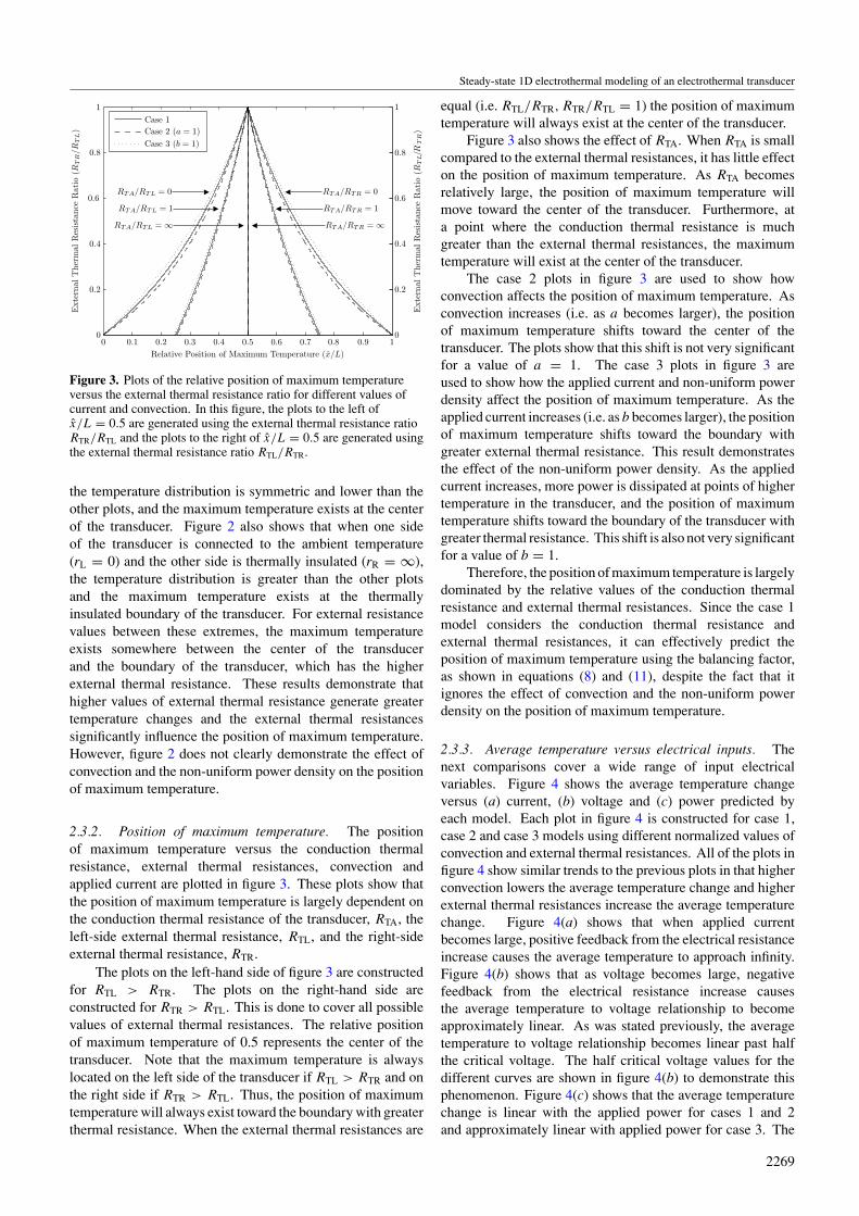
Figure 3. Plots of the relative position of maximum temperatureversus the external thermal resistance ratio for different values ofcurrent and convection. In this figure, the plots to the left ofx̂/L = 0.5 are generated using the external thermal resistance ratioRTR/RTL and the plots to the right of x̂/L = 0.5 are generated usingthe external thermal resistance ratio RTL/RTR.

the temperature distribution is symmetric and lower than theother plots, and the maximum temperature exists at the centerof the transducer. Figure 2 also shows that when one sideof the transducer is connected to the ambient temperature(rL = 0) and the other side is thermally insulated (rR = ∞),the temperature distribution is greater than the other plotsand the maximum temperature exists at the thermallyinsulated boundary of the transducer. For external resistancevalues between these extremes, the maximum temperatureexists somewhere between the center of the transducerand the boundary of the transducer, which has the higherexternal thermal resistance. These results demonstrate thathigher values of external thermal resistance generate greatertemperature changes and the external thermal resistancessignificantly influence the position of maximum temperature.However, figure 2 does not clearly demonstrate the effect ofconvection and the non-uniform power density on the positionof maximum temperature.

2.3.2. Position of maximum temperature. The positionof maximum temperature versus the conduction thermalresistance, external thermal resistances, convection andapplied current are plotted in figure 3. These plots show thatthe position of maximum temperature is largely dependent onthe conduction thermal resistance of the transducer, RTA, theleft-side external thermal resistance, RTL, and the right-sideexternal thermal resistance, RTR.

The plots on the left-hand side of figure 3 are constructedfor RTL > RTR. The plots on the right-hand side areconstructed for RTR > RTL. This is done to cover all possiblevalues of external thermal resistances. The relative positionof maximum temperature of 0.5 represents the center of thetransducer. Note that the maximum temperature is alwayslocated on the left side of the transducer if RTL > RTR and onthe right side if RTR > RTL. Thus, the position of maximumtemperature will always exist toward the boundary with greaterthermal resistance. When the external thermal resistances are

equal (i.e. RTL/RTR, RTR/RTL = 1) the position of maximumtemperature will always exist at the center of the transducer.

Figure 3 also shows the effect of RTA. When RTA is smallcompared to the external thermal resistances, it has little effecton the position of maximum temperature. As RTA becomesrelatively large, the position of maximum temperature willmove toward the center of the transducer. Furthermore, ata point where the conduction thermal resistance is muchgreater than the external thermal resistances, the maximumtemperature will exist at the center of the transducer.

The case 2 plots in figure 3 are used to show howconvection affects the position of maximum temperature. Asconvection increases (i.e. as a becomes larger), the positionof maximum temperature shifts toward the center of thetransducer. The plots show that this shift is not very significantfor a value of a = 1. The case 3 plots in figure 3 areused to show how the applied current and non-uniform powerdensity affect the position of maximum temperature. As theapplied current increases (i.e. as b becomes larger), the positionof maximum temperature shifts toward the boundary withgreater external thermal resistance. This result demonstratesthe effect of the non-uniform power density. As the appliedcurrent increases, more power is dissipated at points of highertemperature in the transducer, and the position of maximumtemperature shifts toward the boundary of the transducer withgreater thermal resistance. This shift is also not very significantfor a value of b = 1.

Therefore, the position of maximum temperature is largelydominated by the relative values of the conduction thermalresistance and external thermal resistances. Since the case 1model considers the conduction thermal resistance andexternal thermal resistances, it can effectively predict theposition of maximum temperature using the balancing factor,as shown in equations (8) and (11), despite the fact that itignores the effect of convection and the non-uniform powerdensity on the position of maximum temperature.

2.3.3. Average temperature versus electrical inputs. Thenext comparisons cover a wide range of input electricalvariables. Figure 4 shows the average temperature changeversus (a) current, (b) voltage and (c) power predicted byeach model. Each plot in figure 4 is constructed for case 1,case 2 and case 3 models using different normalized values ofconvection and external thermal resistances. All of the plots infigure 4 show similar trends to the previous plots in that higherconvection lowers the average temperature change and higherexternal thermal resistances increase the average temperaturechange. Figure 4(a) shows that when applied currentbecomes large, positive feedback from the electrical resistanceincrease causes the average temperature to approach infinity.Figure 4(b) shows that as voltage becomes large, negativefeedback from the electrical resistance increase causesthe average temperature to voltage relationship to becomeapproximately linear. As was stated previously, the averagetemperature to voltage relationship becomes linear past halfthe critical voltage. The half critical voltage values for thedifferent curves are shown in figure 4(b) to demonstrate thisphenomenon. Figure 4(c) shows that the average temperaturechange is linear with the applied power for cases 1 and 2and approximately linear with applied power for case 3. The

2269

S T Todd and H Xie

Normalized Total Power (ξRTA P )

Nor

mal

ized

Ave

rage

Tem

pera

ture

Cha

nge

(ξ·∆

T̄)

Case 1 (a = 0)Case 3 (a = 0)Case 2 (a = 2/3)Case 3 (a = 2/3)

rL = 0, rR = ∞rL = 0, rR = 1

rL = 0, rR = 0

0 1 2 3 4 5 6 70

0.1

0.2

0.3

0.4

0.5

0.6

0.7

Normalized Voltage (√

ξRTA/R0 · V )

Nor

mal

ized

Ave

rage

Tem

pera

ture

Cha

nge

(ξ·∆

T̄)

Case 1 (a = 0)Case 3 (a = 0)Case 2 (a = 2/3)Case 3 (a = 2/3)

rL = 0, rR = ∞rL = 0, rR = 1

rL = 0, rR = 0

V = VC/2

0 0.5 1 1.5 2 2.5 30

0.2

0.4

0.6

0.8

1

1.2

1.4

Normalized Current (√R0ξRTA · I)

Nor

mal

ized

Ave

rage

Tem

pera

ture

Cha

nge

(ξ·∆

T̄)

Case 1 (a = 0)Case 3 (a = 0)Case 2 (a = 2/3)Case 3 (a = 2/3)

rL = 0, rR = 0

rL = 0, rR = 1

rL = 0, rR = ∞

0 0.2 0.4 0.6 0.8 1 1.2 1.4 1.6 1.80

0.05

0.1

0.15

0.2

0.25

0.3

0.35(a)

(b)

(c)

Figure 4. Plots of the normalized average temperature changeversus normalized ranges of (a) current, (b) voltage and (c) totalpower. The plots are constructed for all case models using differentvalues of normalized convection and normalized external thermalresistances.

slopes of the case 3 curves increase gradually as the powerincreases due to the non-uniform power density generatedby the electrical resistor. This means that as the appliedpower becomes greater, the case 3 model predicts highertemperatures.

To examine the extent of the increase of the slope weplot the ratio of the case 3 to case 1 equivalent averagethermal resistances for zero convection, and the ratio of thecase 3 to case 2 equivalent average thermal resistances fora normalized convection of a = 1, for different values of

Normalized Current (√R0ξRTA I)

Ave

rage

The

rmal

Res

ista

nce

Rat

io(R̄

T3/R̄

T1,2

)

No Convection (a = 0)Convection (a = 1)

12/π2

rL = 0, rR = ∞rL = 0, rR = 1

rL = 0, rR = 0

Critical Current Ratio Squared: (IC1/IC3)2 (IC2/IC3)2

0 0.5 1 1.5 2 2.5 3 3.51

1.05

1.1

1.15

1.2

1.25

Figure 5. Plots of the ratio between the case 3 to case 1 and case 3to case 2 equivalent average thermal resistance versus current fordifferent values of external thermal resistance. The case 3 to case 2ratio curves are plotted using a normalized convection of a = 1.

external thermal resistance in figure 5. Figure 5 demonstratesthe significance of the nonlinearity of the average temperaturechange versus total power of the case 3 model. As the appliedcurrent becomes close to zero, the equivalent average thermalresistance ratio approaches 1. This means that the averagetemperature change versus total power of the case 3 model isapproximately the same as the case 1 or the case 2 model forsmall currents. As the current increases, the equivalent averagethermal resistance ratio increases. This increase representsthe nonlinear behavior of the case 3 model. As the currentincreases toward the critical current, the equivalent averagethermal resistance ratio increases and approaches a constantvalue at the critical current.

By examining the plots, it can be seen that the maximumvalue of the equivalent average thermal resistance ratio occursat the critical current. At the critical current, the equivalentaverage thermal resistance ratio is equal to the reciprocalof the ratio between the square of the case 3 and case 1or case 2 critical currents. The envelopes of the squareof the critical current ratios are plotted in figure 5 and themaximum value of the equivalent average thermal resistanceratio always lies along these envelopes. This is an importantresult because it gives the maximum difference between theaverage temperature change to total power relationship of thecase 3 model compared to the case 1 and case 2 models. Thisrelationship can also be proven by examining equation (25). Itcan be shown that as the applied current approaches the criticalcurrent, the case 3 equivalent average thermal resistance willbe maximum and given by

max(R̄T3) = 1/I 2

C3R0ξ . (33)

By taking the ratio of the maximum case 3 equivalentaverage thermal resistance to the case 1 or case 2 equivalentaverage thermal resistance we have

max(R̄T3/R̄T1,2) = (IC1,2/IC3)2. (34)

This proves that the maximum value of the equivalentaverage thermal resistance ratio is equal to the reciprocal ofthe critical current ratio squared. In the following paragraph,

2270

Steady-state 1D electrothermal modeling of an electrothermal transducer

1V

0V

Figure 6. Top-view schematic of the 1D electrothermal micromirror design.

we will show how this result gives us mathematical insight intohow well the case 1 and case 2 models agree with the case 3model.

The maximum value of the equivalent average thermalresistance ratio of all curves occurs when no convection ispresent (a = 0) and the external thermal resistances are equalto either rL = 0 and rR = 0 or rL = 0 and rR = ∞. This valueis equal to 12/π2 as shown in the top line of figure 5. This isa very useful result because it gives us a direct measurementof how accurate the case 1 and case 2 models can agree withthe case 3 model for any values of external thermal resistance.From this result we know that the slope of the case 3 averagetemperature change versus total power will never exceed theslope of the case 1 or case 2 average temperature change versustotal power by more than a factor of 12/π2. Therefore, weconclude that the difference between the average temperaturechange to total power relationship of the case 3 and case 1or case 2 models will always be less than or equal to a factorof 12/π2 ≈ 1.216. Similarly, the difference between theaverage temperature to voltage relationship of the case 3 andcase 1 or case 2 models will always be less than or equal tothe square root of this factor or 2

√3/π ≈ 1.103. Thus, the

average temperature versus power and voltage relationships ofthe case 1 or case 2 will always agree with the case 3 modelwithin these factors and provide a reasonable approximationof the electrothermal behavior of the transducer.

2.3.4. Summary of model results. We have developed threemodels to predict the behavior of an electrothermal transducer.Below is a summary of the important characteristics of anelectrothermal transducer predicted by the models.

• The position of maximum temperature is largelydetermined by the conduction thermal resistance of thetransducer and the external thermal resistances attachedat the boundaries and can be predicted using the case 1balancing factor. Surface convection and the non-uniformpower density do not significantly affect the position ofmaximum temperature.

• Higher external thermal resistances raise the temperaturechange for a given electrical input. Higher surfaceconvection lowers the temperature change for a givenelectrical input.

• The case 1 and case 2 models give a linear relationshipbetween the temperature change and total power and canexplicitly represent the temperature change in terms ofvoltage.

• The temperature dependence of the electrical resistivitycauses the temperature change of the transducer to beapproximately linear with respect to applied voltage whenoperated past half the critical voltage.

• The non-uniform power density causes the case 3 averagetemperature change to be nonlinearly related to thetotal power. The significance of the nonlinearity ofthe case 3 model was determined by comparing theequivalent average thermal resistances of the models. Thiscomparison shows that the average temperature changeversus total power and voltage relationships of the case1 and case 2 models always agree with the case 3 modelwithin factors of 12/π2 ≈ 1.216 and 2

√3/π ≈ 1.103

respectively.

In the next section, we will apply the models to anelectrothermal micromirror and compare the model results toFEM simulations and experimental measurements.

3. Model verification using FEM and experimentalmeasurements

The electrothermal transducer models have been used to modelthe behavior of a 1D electrothermal micromirror design thatwas previously reported by Xie et al [2]. The micromirrordesign consists of four regions—-an electrothermal bimorphactuator region, a mirror plate region, a substrate thermalisolation region and a mirror thermal isolation region asshown in figure 6. The mirror is actuated when a voltageis applied to polysilicon resistors embedded in the bimorphactuator array. The power dissipated by the resistors raises thetemperature of the bimorph actuator array and the difference

2271

S T Todd and H Xie

Table 1. Geometric and material parameters of one two-beam section of the 1D micromirror device.

Parameters Symbol Value

GeometricBimorph actuator length L 170.1 µmSubstrate thermal isolation length Lis 31.7 µmMirror thermal isolation length Lim 56.7 µmMirror plate length Lm 1 mmBimorph actuator width w 2 × 8.6 µmPolysilicon width wpoly 2 × 7 µmSubstrate thermal isolation width wis 2 × 8.6 µmMirror thermal isolation width wim 2 × 8.6 µmMirror plate width wm 2 × 15.6 µmAluminum thickness tAl 0.5 µmSiO2 thickness tOx 1.25 µmSilicon thickness tSi 15 µmPolysilicon thickness tpoly 0.2 µmBimorph actuator thickness t 1.75 µm

ElectricalPolysilicon electrical resistivity at 25 ◦C ρpoly 0.527 × 10−6 � mActuator equivalent electrical resistivity at 25 ◦C ρ0 5.66 × 10−6 � mPolysilicon TCR ξ 5.85 × 10−3 K−1

ThermalAluminum thermal conductivity κAl 237 W K−1 m−1

SiO2 thermal conductivity κOx 1.1 WK−1 m−1

Silicon thermal conductivity κSi 170 WK−1 m−1

Polysilicon thermal conductivity κpoly 29 W K−1 m−1

Actuator equivalent thermal conductivity κ 71.2 W K−1 m−1

Substrate thermal isolation equivalent thermal conductivity κ is 38.6 W K−1 m−1

Mirror thermal isolation equivalent thermal conductivity κ im 56.2 W K−1 m−1

Mirror plate equivalent thermal conductivity κm 164.4 W K−1 m−1

in the coefficients of thermal expansion (CTEs) of the bimorphmaterials cause the bimorph beams to change curvature androtate the mirror surface. The thermal parameter that affectsthe mechanical rotation angle is the average temperaturechange of the bimorph beams [16]. Thus, in order to modelthe electrothermomechanical behavior of the device, we mustextract the average temperature versus current or voltagerelationships from electrothermal modeling.

3.1. Description of the electrothermal micromirror device

The electrothermal transducer models described previouslycan be applied to the micromirror design [2]. As shown infigure 6, there are 72 bimorph beams in the actuator array.The polysilicon electrical resistors of two adjacent bimorphbeams are attached in parallel yielding a total of 36 electricalresistors in the actuator array attached in series. Since thedevice is symmetric about the width of the actuator array, thetemperature will be approximately uniform about the widthof the actuator array. Therefore, the actuator region canbe cut into one two-beam section for thermal analysis. Across-section slice of one two-beam section of the micromirrordevice is shown in figure 7. Since resistors in the actuator arrayare attached in series, the voltage and electrical resistance ofone two-beam section must be multiplied by a factor of 36to find the total voltage and electrical resistance across theentire array. An SEM of the micromirror device is shownin figure 8. The material and geometric parameters of all ofthe micromirror regions for a two-beam section are given intable 1.

0x =x

TLR TRR

isL imLL mL

Figure 7. Side-view schematic of one two-beam section slice of themicromirror device for thermal analysis.

Figure 8. SEM of the micromirror device used in the electrothermaltransducer model.

2272

Steady-state 1D electrothermal modeling of an electrothermal transducer

The transducer thermal parameters are extracted from thematerial and geometric properties of the bimorph actuatorregion. The bimorph actuator is composed of an SiO2 bottomlayer, an Al top layer and a polysilicon layer embedded inthe SiO2 layer. The left-side external thermal resistance isthe thermal resistance due to the conduction and convectionin the substrate thermal isolation region. The right-sideexternal thermal resistance is a combination of the thermalresistance due to conduction and convection in the mirrorthermal isolation and mirror plate regions. The thermalisolation regions are composite structures of Al and SiO2

layers. The mirror plate region is composed of a thick singlecrystal silicon (SCS) bottom layer, an Al top layer and an SiO2

layer in between both layers.

3.1.1. External thermal resistance equations. To find theleft-side and right-side external thermal resistances for themicromirror device, we use an equation for the equivalentthermal resistance seen looking into a convecting region whichwas derived in [16] and is given by

Rcr =√

RTcrRCcr

[acrrex cosh acr + sinh acr

cosh acr + acrrex sinh acr

](35)

where RTcr is the conduction thermal resistance of the region,RCcr is the convection thermal resistance of the region, Rex isthe external thermal resistance seen at the end of the region,acr = √

RTcr/RCcr, and rex = Rex/RTcr. We can applyequation (35) to the substrate isolation region to find theexternal thermal resistance seen to the left of the bimorphactuator, RTL. The substrate thermal isolation region isattached to the substrate at its end; thus, the external thermalresistance at the end of the substrate thermal isolation regionis zero. Therefore, the external thermal resistance seen to theleft of the bimorph actuator is given by

RTL =√

RTisRCis tanh ais ≈ 2RTisRCis

RTis + 2RCis(36)

where RTis is the conduction thermal resistance of the substratethermal isolation region, RCis is the convection thermalresistance of the substrate thermal isolation region and ais =√

RTis/RCis. The length of the substrate thermal isolationregion is relatively small, so the equivalent thermal resistancewill be dominated by the conduction thermal resistance.

We can also apply equation (35) to the mirror isolationregion to find the external thermal resistance seen to theright of the bimorph actuator, RTR. The mirror isolationregion is attached to the mirror plate at its end and thus theexternal thermal resistance seen at the end of the mirror thermalisolation region will be due to conduction and convection ofthe mirror plate. This equivalent thermal resistance can befound by applying equation (35) to the mirror plate region.Since the mirror plate region is free at its end, we assume thatthe end of the mirror is thermally insulated. Thus, the externalthermal resistance seen at the end of the mirror plate is infinite.The equivalent thermal resistance of the mirror plate region istherefore given by

Rm =√

RTmRCm coth am ≈ RTm/2 + RCm (37)

where RTm is the conduction thermal resistance of the mirrorplate region, RCm is the convection thermal resistance of themirror plate region and am = √

RTm/RCm. The mirror plate

region is relatively long, so convection on the surface of themirror could dissipate a significant amount of heat. Usingthe equivalent thermal resistance of the mirror plate region,the equivalent thermal resistance to the right of the bimorphactuator region becomes

RTR =√

RTimRCim

[aimrm cosh aim + sinh aim

cosh aim + aimrm sinh aim

](38)

where RTim is the conduction thermal resistance of the mirrorthermal isolation region, RCim is the convection thermalresistance of the mirror thermal isolation region, aim =√

RTim/RCim, and rm = Rm/RTim. These equations forthe external thermal resistances complete the electrothermalmodels of the micromirror. In the next sections, we willcompare the results of the models and FEM simulations toexperimental results.

3.2. Experimental results

Two types of characterization experiments were conductedon the micromirror device. The first was a dc characterizationexperiment where the current through the device was measuredfrom a range of applied voltages. The average temperaturechange cannot be measured directly, but is related to theelectrical resistance as shown by equation (22). Thereforethe average temperature change was extracted by measuringthe electrical resistance at a given actuation point and thenusing the polysilicon TCR with equation (22) to calculatethe average temperature change at that actuation point. Thepolysilicon TCR was determined to be 5.85 × 10−3 K−1 froma previous experiment [16]. The dc characterization dataprovided the extracted average temperature change versuscurrent, voltage and power. The second characterizationexperiment was a thermal imaging experiment which revealedthe temperature distribution of the device over a rangeof applied voltages. FEM simulations were conductedusing CoventorWare2. The characterization data and FEMsimulations were used in comparison with the modelpredictions to test the validity of the models.

3.2.1. DC characterization experiments. The dccharacterization experiments were conducted in a vacuumchamber and open air to test the thermal behavior ofthe device without and with the presence of convection,respectively. Experimental results of the average temperaturechange versus current, voltage and power are respectivelyshown in figures 9(a), (b) and (c). For both vacuumchamber and open air experiments, the experimental averagetemperature change was nonlinear with respect to the appliedpower as shown in figure 9(c). The slope of the averagetemperature change versus power was found to decrease asthe power increased. This nonlinear behavior could be dueto radiation, the Thompson effect [9] and/or temperature-dependent thermal conductivities. In the open air experiment,the nonlinear behavior could also be due to a temperature-dependent convection coefficient that changes as the powerincreases. The open air experiments produce a loweraverage temperature change compared to the vacuum chamberexperiments for all actuation ranges as shown in all plots

2 CoventorWare, Cary, NC, www.conventor.com.

2273

S T Todd and H Xie

Voltage (V)

Ave

rage

Tem

pera

ture

Cha

nge

(◦C

)

Case 1 ModelCase 2 ModelCase 3 ModelFEM SimulationExperimental

Half Critical Voltage = 5.74 V

Half Critical Voltage = 7.42 V

Vacuum h = 0 W/Km2

Open Air h = 193 W/Km2

0 2 4 6 8 10 12 14 160

20

40

60

80

100

120

140

Current (mA)

Ave

rage

Tem

pera

ture

Cha

nge

(◦C

)

Case 1 ModelCase 2 ModelCase 3 ModelFEM SimulationExperimental

Vacuum h = 0 W/Km2

Open Air h = 193 W/Km2

0 1 2 3 4 5 6 7 8 90

20

40

60

80

100

120

140

Power (mW)

Ave

rage

Tem

pera

ture

Cha

nge

(◦C

)

Case 1 ModelCase 2 ModelCase 3 ModelFEM SimulationExperimental

Vacuum h = 0 W/Km2

Open Air h = 193 W/Km2

0 20 40 60 80 100 120 1400

20

40

60

80

100

120

140

(a)

(b)

(c)

Figure 9. Plots from dc characterization in vacuum and open air foranalytical, FEM simulation and experimental data showing theaverage temperature change versus (a) current, (b) voltage and(c) power.

in figure 9. This result demonstrates that the presence ofconvection lowers the average temperature change. Whenthe device was characterized in open air, the convectioncoefficient was unknown. To estimate the convectioncoefficient, the experimental data were fitted using a quadraticequation, and the convection coefficient used in the case 2model was adjusted until the equivalent average thermalresistance of the case 2 model matched the linear term of thequadratic experimental fit. This approach yielded a convectioncoefficient of approximately 193 W K−1 m−2 on the surface ofthe device.

The plots of the average temperature change versuscurrent and voltage shown respectively in figures 9(a) and(b) demonstrate the effect of the polysilicon TCR on thethermal behavior of the device. The plots in figure 9(a) showthat the average temperature change increases exponentiallyas the current increases toward the critical current. Theplots in figure 9(b) show that the average temperature changebecomes approximately linear with voltage when the voltageis increased past half the critical voltage. These results agreewith the model predictions, and the linear actuation range isdesirable for many applications.

The case 1, case 2 and case 3 model predictions of thedc behavior agree with each other within 2% for all actuationranges. This result reiterates that the simple case 1 and case 2models can be effectively used to predict the behavior of anelectrothermal transducer. The analytical model predictionsagree with the FEM simulations within 5% for all actuationranges. This is perhaps the best validation of the modelsbecause the geometric and material parameters used in themodels and FEM simulations are identical. The experimentaldata matched the FEM simulations and analytical modelpredictions within 10% for all actuation ranges. The analyticalmodel predictions and FEM simulations were based on theassumptions that the material parameters of the device wereknown and equal to published data, and that the geometricparameters of the device were known. Sources of errorinclude inaccurate representation of the material and geometricproperties of the device and nonlinear thermal effects.

3.2.2. Thermal imaging experiment. Thermal imagingexperiments were conducted using a QFI Infrascope II thermalimaging system3. The micromirror was actuated in a 0–15 Vrange and thermal images were taken at each step within theactuation range. The substrate temperature of the devicewas held constant at 25 ◦C using a liquid nitrogen cooler.Figure 10(a) shows a thermal image of the device at an appliedvoltage of 15 V. The temperature distribution across the lengthof the device at 15 V is shown in figure 10(b). The thermalimaging system is not able to accurately resolve temperaturesbelow 60 ◦C. This is why the thermal imaging producedtemperatures close to the substrate are higher than 25 ◦C.

To estimate the convection coefficient in each deviceregion, the convection coefficient used in the case 3 modelwas iterated to fit the model distribution to the thermalimaging data. Using this approach, a convection coefficient of122 W K−1 m−2 was determined on the surface of the device.An FEM simulation of the temperature distribution at 15 Vusing the described convection coefficient is also shown infigure 10(b). The convection coefficient determined by thethermal imaging experiment is different than the convectioncoefficient determined by the open-air dc characterizationexperiment. The open-air dc characterization experimentwas conducted in a different environment than the thermalimaging experiment. The difference between the determinedconvection coefficients could be due to different conditionsin the environments such as air currents that lead to forcedconvection.

From the thermal imaging data, the position of maximumtemperature (shown in figure 10(b)) was found at 124.6 µm.

3 Quantum Focus Instruments, Vista, CA, www.quantumfocus.com.

2274

Steady-state 1D electrothermal modeling of an electrothermal transducer

Distance from Bimorph Actuator Base (µm)

Tem

pera

ture

(◦C

)

Case 3 ModelFEM SimulationThermal Imaging Data

Maximum Temperature

Mirror Thermal Isolation Region

Mirror Region

Substrate Thermal Isolation Region

Bimorph Actuator Region

0 50 100 150 200 250 30020

40

60

80

100

120

140

160

180

200

(a)

(b)

Figure 10. (a) Thermal image of the micromirror at 15 V. (b) Plots of the temperature distribution for analytical model, FEM simulation andthermal imaging data.

The experimentally determined relative position of maximumtemperature is found by taking the ratio of the position ofmaximum temperature to the total actuator length yielding124.6/170.1 ≈ 0.73. Using the convection coefficient tocalculate the external thermal resistances in equation (8) yieldsa case 1 balancing factor of 0.75. As was described previously,the case 1 balancing factor is equivalent to the relative positionof maximum temperature. The case 1 balancing factor predictsthe experimentally determined relative position of maximumtemperature within 3% compared to the thermal imagingdata. The temperature distributions produced by the thermalimaging data, case 3 model and FEM simulation agree within7% for all positions along the length of the device.

4. Conclusion

Analytical models of the electrothermal behavior of anelectrothermal transducer have been presented in this paper.The models are developed from the heat transport equationwith different considerations of surface convection and thepower density. It was shown that the simpler case 1 andcase 2 models can effectively predict the average temperaturechange within a factor of 12/π2 ≈ 1.216 for all actuationranges compared to the more accurate and complex case 3model. It is analytically and experimentally verified that

an electrothermal transducer can be linearly actuated withrespect to voltage when operated above half the critical voltage.A balancing factor has been derived and can be used tocalculate the relative position of maximum temperature andmatches the thermal imaging data within 3%. The analyticalmodels agreed with all FEM simulations and experimentalresults within 10%. Future work includes determining thecause of the nonlinear relationship between the averagetemperature change and applied power and conducting morecontrolled experiments to estimate the convection coefficient.

Acknowledgments

The authors would like to thank Ankur Jain for help with dccharacterization experiments and Grant Albright at QuantumFocus Instruments for use of the Infrascope II thermal imagingsystem. This project is supported by the National ScienceFoundation under award number BES-0423557.

References

[1] Xie H, Pan Y and Fedder G K 2003 Endoscopic opticalcoherence tomographic imaging with a CMOS-MEMSmicromirror Sensors Actuators A 103 237–41

[2] Xie H, Jain A, Xie T, Pan Y and Fedder G K 2003 Asingle-crystal silicon-based micromirror with large

2275

S T Todd and H Xie

scanning angle for biomedical applications Technical DigestCLEO 2003 (Baltimore, MD)

[3] Jain A and Xie H 2005 A tunable microlens scanner withlarge-vertical-displacement actuation 18th IEEE Int. Conf.on Micro Electro Mechanical Systems (MEMS 2005)(Miami Beach, FL, January) pp 92–5

[4] Manginell R P, Smith J H, Ricco A J, Hughes R C, Moreno D Jand Huber R J 1997 Electro-thermal modeling of amicrobridge gas sensor SPIE Symp. on Micromachining andMicrofabrication (Austin, TX) pp 360–71

[5] Robert P, Saias D, Billard C, Boret S, Sillon N,Maeder-Pachurka C, Charvet P L, Bouche G, Ancey P andBerruyer P 2003 Integrated RF-MEMS switch based on acombination of thermal and electrostatic actuation 12th Int.Conf. on Solid-State Sensors, Actuators and Microsystems(Transducers 2003) pp 1714–7

[6] Vettiger P et al 2002 The Millepede-nanotechnology enteringdata storage IEEE Trans. Nanotechnol. 1 39–55

[7] Geisberger A A, Sarkar N, Ellis M and Skidmore G D 2003Electrothermal properties and modeling of polysiliconmicrothermal transducers J. Microelectromech. Syst.12 513–22

[8] Tai Y C, Mastrangelo C H and Muller R S 1998 Thermalconductivity of heavily doped low-pressure chemical vapordeposited polycrystalline silicon films J. Appl. Phys.63 1442–7

[9] Mastrangelo C H 1991 Thermal applications of microbridgesPhD Dissertation University of California, Berkeley

[10] Fedder G K and Howe R T 1991 Thermal assembly ofpolysilicon microstructures IEEE Micro Electro MechanicalSystems Workshop 1991 pp 63–8

[11] Lin L and Chiao M 1996 Electrothermal responses oflineshape microstructures Sensors Actuators A 55 35–41

[12] Huang Q-A and Lee N K S 1999 Analysis and design ofpolysilicon thermal flexure actuator J. Micromech.Microeng. 9 64–70

[13] Hickey R, Kujath M and Hubbard T 2002 Heat transferanalysis and optimization of two-beammicroelectromechanical thermal actuators J. Vacuum Sci.Technol. A 20 971–4

[14] Yan D, Khajepour A and Mansour R 2004 Design andmodeling of a MEMS bidirectional vertical thermaltransducer J. Micromech. Microeng. 14 841–50

[15] Lammel G, Schweizer S and Renaud P 2002 OpticalMicroscanners and Microspectrometers Using ThermalBimorph Transducers (Boston, MA: Kluwer)

[16] Todd S T 2005 Electrothermomechanical modeling of a 1-Delectrothermal MEMS micromirror MS Thesis University ofFlorida

[17] Todd S T and Xie H 2004 An analytical electrothermal modelof a 1-D electrothermal MEMS micromirror Proc. SPIE5649 344–53

2276