Steady bubble rise and deformation in Newtonian and viscoplastic fluids and conditions for bubble entrapment

J. Fluid Mech. (2008), vol. 601, pp. 123–164. c© 2008 Cambridge University Press

doi:10.1017/S0022112008000517 Printed in the United Kingdom

123

Steady bubble rise and deformation inNewtonian and viscoplastic fluids andconditions for bubble entrapment

J. TSAMOPOULOS, Y. DIMAKOPOULOS, N. CHATZIDAI,G. KARAPETSAS AND M. PAVLIDIS

Laboratory of Computational Fluid Dynamics, Department of Chemical EngineeringUniversity of Patras, Patras 26500, Greece

(Received 7 December 2006 and in revised form 28 November 2007)

We examine the buoyancy-driven rise of a bubble in a Newtonian or a viscoplasticfluid assuming axial symmetry and steady flow. Bubble pressure and rise velocityare determined, respectively, by requiring that its volume remains constant and itscentre of mass remains fixed at the centre of the coordinate system. The continuousconstitutive model suggested by Papanastasiou is used to describe the viscoplasticbehaviour of the material. The flow equations are solved numerically using the mixedfinite-element/Galerkin method. The nodal points of the computational mesh aredetermined by solving a set of elliptic differential equations to follow the often largedeformations of the bubble surface. The accuracy of solutions is ascertained by meshrefinement and predictions are in very good agreement with previous experimentaland theoretical results for Newtonian fluids. We determine the bubble shape andvelocity and the shape of the yield surfaces for a wide range of material properties,expressed in terms of the Bingham Bn= τ ∗

y /ρ∗g∗R∗b , Bond Bo = ρ∗g∗R∗2

b /γ ∗ and

Archimedes Ar = ρ∗2g∗R∗3b /µ∗2

o numbers, where ρ∗ is the density, µ∗o the viscosity,

γ ∗ the surface tension and τ ∗y the yield stress of the material, g∗ the gravitational

acceleration and R∗b the radius of a spherical bubble of the same volume. If the fluid

is viscoplastic, the material will not be deforming outside a finite region around thebubble and, under certain conditions, it will not be deforming either behind it oraround its equatorial plane in contact with the bubble. As Bn increases, the yieldsurfaces at the bubble equatorial plane and away from the bubble merge and thebubble becomes entrapped. When Bo is small and the bubble cannot deform from thespherical shape the critical Bn is 0.143, i.e. it is a factor of 3/2 higher than the criticalBn for the entrapment of a solid sphere in a Bingham fluid, in direct correspondencewith the 3/2 higher terminal velocity of a bubble over that of a sphere under thesame buoyancy force in Stokes flow. As Bo increases allowing the bubble to squeezethrough the material more easily, the critical Bingham number increases as well, buteventually it reaches an asymptotic value. Ar affects the critical Bn value much less.

1. IntroductionThe motion of bubbles in viscous liquids has attracted the interest of many

researchers because of its numerous practical applications and scientific challenges.Over many years people have examined the flow and deformation of a singleor multiple bubbles theoretically, experimentally and numerically in various flow

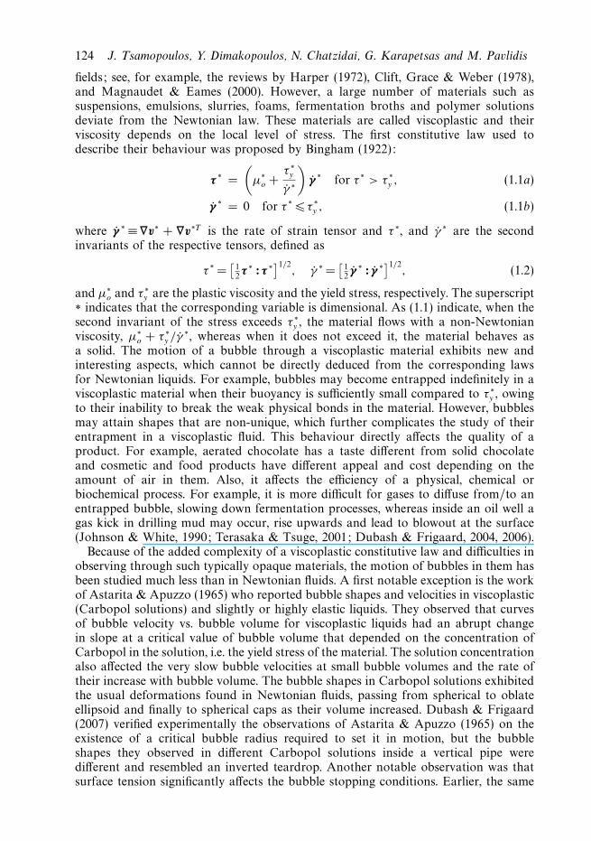
124 J. Tsamopoulos, Y. Dimakopoulos, N. Chatzidai, G. Karapetsas and M. Pavlidis

fields; see, for example, the reviews by Harper (1972), Clift, Grace & Weber (1978),and Magnaudet & Eames (2000). However, a large number of materials such assuspensions, emulsions, slurries, foams, fermentation broths and polymer solutionsdeviate from the Newtonian law. These materials are called viscoplastic and theirviscosity depends on the local level of stress. The first constitutive law used todescribe their behaviour was proposed by Bingham (1922):

τ ∗ =

(µ∗

o +τ ∗y

γ ∗

)γ ∗ for τ ∗ > τ ∗

y , (1.1a)

γ ∗ = 0 for τ ∗ τ ∗y , (1.1b)

where γ ∗ ≡ ∇v∗ + ∇v∗T is the rate of strain tensor and τ ∗, and γ ∗ are the secondinvariants of the respective tensors, defined as

τ ∗ =[

12τ ∗ : τ ∗]1/2

, γ ∗ =[

12γ ∗ : γ ∗]1/2

, (1.2)

and µ∗o and τ ∗

y are the plastic viscosity and the yield stress, respectively. The superscript∗ indicates that the corresponding variable is dimensional. As (1.1) indicate, when thesecond invariant of the stress exceeds τ ∗

y , the material flows with a non-Newtonianviscosity, µ∗

o + τ ∗y /γ ∗, whereas when it does not exceed it, the material behaves as

a solid. The motion of a bubble through a viscoplastic material exhibits new andinteresting aspects, which cannot be directly deduced from the corresponding lawsfor Newtonian liquids. For example, bubbles may become entrapped indefinitely in aviscoplastic material when their buoyancy is sufficiently small compared to τ ∗

y , owingto their inability to break the weak physical bonds in the material. However, bubblesmay attain shapes that are non-unique, which further complicates the study of theirentrapment in a viscoplastic fluid. This behaviour directly affects the quality of aproduct. For example, aerated chocolate has a taste different from solid chocolateand cosmetic and food products have different appeal and cost depending on theamount of air in them. Also, it affects the efficiency of a physical, chemical orbiochemical process. For example, it is more difficult for gases to diffuse from/to anentrapped bubble, slowing down fermentation processes, whereas inside an oil well agas kick in drilling mud may occur, rise upwards and lead to blowout at the surface(Johnson & White, 1990; Terasaka & Tsuge, 2001; Dubash & Frigaard, 2004, 2006).

Because of the added complexity of a viscoplastic constitutive law and difficulties inobserving through such typically opaque materials, the motion of bubbles in them hasbeen studied much less than in Newtonian fluids. A first notable exception is the workof Astarita & Apuzzo (1965) who reported bubble shapes and velocities in viscoplastic(Carbopol solutions) and slightly or highly elastic liquids. They observed that curvesof bubble velocity vs. bubble volume for viscoplastic liquids had an abrupt changein slope at a critical value of bubble volume that depended on the concentration ofCarbopol in the solution, i.e. the yield stress of the material. The solution concentrationalso affected the very slow bubble velocities at small bubble volumes and the rate oftheir increase with bubble volume. The bubble shapes in Carbopol solutions exhibitedthe usual deformations found in Newtonian fluids, passing from spherical to oblateellipsoid and finally to spherical caps as their volume increased. Dubash & Frigaard(2007) verified experimentally the observations of Astarita & Apuzzo (1965) on theexistence of a critical bubble radius required to set it in motion, but the bubbleshapes they observed in different Carbopol solutions inside a vertical pipe weredifferent and resembled an inverted teardrop. Another notable observation was thatsurface tension significantly affects the bubble stopping conditions. Earlier, the same

Bubble rise and deformation in Newtonian and viscoplastic fluids 125

authors estimated the conditions under which bubbles should remain static usingvariational principles (Dubash & Frigaard 2004). The bounds they obtained basedon either strain minimization or stress maximization for any type of viscoplastic fluidwere characterized as conservative, in the sense that they provide a sufficient but notnecessary condition. However, they concluded that in general “if a big bubble doesnot move nor will a small one”. The mobilization of bubbles in a yield-stress fluid bysetting them into pulsation was the subject of Stein & Buggish’s (2000) research, whopresented analytical solutions and experimental data to support them. Apparentlylarger bubbles rose faster than smaller ones at similar pressure amplitudes. Finally,Terasaka & Tsuge (2001) presented shapes developed by a bubble forming at a nozzlein a yield-stress fluid and provided an approximate model for bubble growth. On theother hand, Dimakopoulos & Tsamopoulos (2003a, 2006) simulated the formationand expansion of a long ‘open’ bubble during the displacement of viscoplastic liquidsby pressurised air from straight, suddenly constricing and expanding cylindrical tubesfor a wide range of Bingham (i.e. the dimensionless yield stress) and Reynoldsnumbers, providing details about the topology of the unyielded regions and theireffect on the shape of the long bubble.

The corresponding problem of a solid sphere translating in a Bingham fluid hasbeen studied more extensively. Beris et al. (1985) verified earlier estimations, basedon variational inequalities, of the dependence of the drag force on the sphere inan unbounded medium as on the yield stress. They solved the governing equationswith (1.1) as a constitutive model under creeping flow conditions using an algebraicmapping of the yield surfaces to fixed spherical ones and finite elements. They foundthat the sphere falls within an envelope of fluid, the shape and location of whichdepends on the yield stress and that unyielded material arises around the stagnationpoints of flow at the poles of the sphere. Finally, they obtained the critical yield-stressvalue beyond which the sphere is immobilized by combining asymptotic scalingsderived from the plastic boundary-layer theory with numerical calculations. Similarresults have been reported by Liu, Muller & Denn (2002). Blackery & Mitsoulis (1997)extended this study, including the effect of the tube diameter to the sphere diameterratio when the sphere is moving inside a cylindrical tube, using Papanastasiou’s (1987)viscoplastic model. This model holds in both the yielded and unyielded materialregions:

τ ∗ =

[µ∗

o + τ ∗y

1 − e−nγ ∗

γ ∗

]γ ∗, (1.3)

where the stress growth exponent, n, must assume large enough values, dependingon the particular flow, in order that the original Bingham model is approached;see Dimakopoulos & Tsamopoulos (2003a, 2006) and Burgos, Alexandrou & Entov(1999).

Out of the very extensive literature on bubble motion in viscous liquids, we willmention here only papers that are more relevant to the present work or will beused to compare our predictions to established experimental and theoretical dataand demonstrate ways in which the viscoplastic fluids deviate from Newtonian ones.Early on, Haberman & Morton (1954) measured bubble rise velocities as a functionof bubble size for various liquids and introduced a new dimensionless number forthe description of their results, the Morton number, Mo, which depended on theliquid properties only. Hnat & Buckmaster (1976) experimentally determined thephysical conditions under which either spherical caps arise or bubbles develop verythin, long and rounded ‘skirts’ from their sides. Bhaga & Weber (1981) carried

126 J. Tsamopoulos, Y. Dimakopoulos, N. Chatzidai, G. Karapetsas and M. Pavlidis

out extensive experiments to determine the physical conditions under which bubblesassume spherical, oblate ellipsoidal, deformed ellipsoidal, spherical cap or skirtedshapes, steady or unsteady. They presented these conditions in a map of bubble shapeswith the Reynolds vs. Eotvos numbers as parameters. In their photographs of bubblemotion in aqueous sugar solutions, they quite clearly visualized the streamlines aroundand in the wake of these bubbles. Aware of the importance of surface impurities whilecarrying out experiments with water, Duineveld (1995) used ‘hyper clean’ water andvery accurately determined the velocity and the shape of bubbles, with an equivalentradius of 0.33–1.00 mm or Reynolds numbers in the range 100 Re 700. Finally,Maxworthy et al. (1996) extended such experiments using clean mixtures of triple-distilled water and pure, reagent grade, glycerine. Hence, they covered a wider rangeof the relevant parameters and provided plots of the drag coefficient Cd and thebubble terminal velocity versus the diameter of an equal spherical bubble.

The early theoretical studies assumed that the bubble remained spherical in aninfinite medium and predicted its drag coefficient under creeping flow conditions(Rybczynski 1911; Hadamard 1911). The corresponding analysis for large but finiteReynolds numbers was first attempted by Levich (1949) who argued that the velocityfield around the spherical bubble differed only slightly from the inviscid solution. Heevaluated the drag force from energy dissipation based on the irrotational solution,to find that the drag coefficient based on the bubble diameter is Cd = 48/Re. LaterMoore (1963) performed a very elegant boundary layer analysis to determine thestructure of the flow around the bubble and the wake behind it and calculatedthe next-order correction to this formula. Small bubble deformations in creepingflow were examined by Taylor & Acrivos (1964), who studied the importance ofsurface tension. Deformation at high Reynolds numbers was examined by Moore(1965), who assumed that the bubble had an oblate spheroidal shape and derived theboundary layer solution for it. Since then, the high-Reynolds-number flow aroundoblate ellipsoidal bubbles has been examined to investigate among other things therange of Reynolds numbers in which recirculation arises behind the bubble (Blanco &Magnaudet 1995).

Solution of the general problem, depending solely on fluid properties and bubblesize and dropping any a priori assumption about bubble shape or range of theReynolds number, demands the use of advanced numerical methods, because of thelarge and complicated bubble deformations and flow structure around them. Thisbecame possible in the middle 1980s. First, Miksis, Vanden-Broeck & Keller (1982)assumed potential flow, included only viscous forces in the normal force balanceand calculated shapes of rising bubbles using boundary elements, but inherentlyflow separation could not be predicted. Then Ryskin & Leal (1984) used finitedifferences and an orthogonal two-dimensional transformation, to solve the Navier–Stokes equations and obtained bubble shapes for Reynolds numbers up to 200 andWeber numbers up to 18. They also predicted accurately the flow recirculation behindthe bubble and suggested that the mechanism of eddy formation behind the bubbleis the competition between the rate of vorticity production on the free surface andthe rate of vorticity convection downstream. Subsequently, Christov & Volkov (1985)used finite differences with a quite restrictive one-dimensional mapping to obtain suchsolutions in a narrower parameter range. Numerical methods that do not solve forthe bubble shape simultaneously with the flow field, but calculate it a posteriori bydefining an appropriate function, such as volume tracking and level set, have alsobeen used. Their disadvantage of decreased accuracy can be counterbalanced by theirability to predict more complicated bubble shapes and bubble breakup. Some notable

Bubble rise and deformation in Newtonian and viscoplastic fluids 127

examples are the papers by Unverdi & Trygvasson (1992), Bonometti & Magnaudet(2006, 2007) and Hua & Lou (2007).

We will solve this free-boundary problem, assuming axial symmetry and steadystate, with the very accurate and versatile numerical algorithm that we developedrecently for such problems (Dimakopoulos & Tsamopoulos 2003b). It is based on aquasi-elliptic set of equations for generating a discretization mesh that conforms to theentire fluid domain outside the bubble. Key ideas for the success of the transformationare limiting the orthogonality requirements on the mesh and employing an improvednode distribution function along the deforming boundary through a penalty method.A non-orthogonal mesh is allowed since we will solve the entire equation set by finiteelements. The retained orthogonal term eliminates the discontinuous slopes of thecoordinate lines that are normal to the free surface. These usually arise owing to theharmonic transformation around highly deforming surfaces. This procedure producesmeshes of higher density where necessary: stagnation points of flow, equatorialplane and wake behind the bubble. We have applied this method to a numberof free- or moving-boundary steady or transient problems, such as displacementof a Newtonian or viscoelastic fluid from a tube (Dimakopoulos & Tsamopoulos2003c, 2004), transient squeezing of a viscoplastic material between parallel disks(Karapetsas & Tsamopoulos 2006) and deformation of several bubbles during filamentstretching (Foteinopoulou et al. 2006).

In § 2 we present the governing equations and boundary conditions of this problem.In § 3 we give some basic ideas of our body-fitted coordinate transformation andthe key features to implement the finite-element algorithm for solving this problem.We present our results in terms of bubble shapes, yield surfaces, flow structure andconditions for bubble entrapment depending on fluid parameters and bubble size in§ 4. Conclusions are drawn in § 5.

2. Problem formulationWe consider the flow of a bubble of volume V ∗

b rising at a constant velocityU ∗

b through a viscoplastic fluid, with a constant yield stress τ ∗y , and upon yielding

a constant dynamic viscosity µ∗o. We assume axial symmetry and that the fluid is

incompressible with constant density ρ∗ and a constant interfacial tension with thegas in the bubble γ ∗, whereas the viscosity and density of the gas in the bubbleare assumed to be zero. Figure 1 illustrates the flow geometry examined herein. Themotion of the bubble is driven by gravity which is aligned with the z-axis. We selecta reference frame moving with the bubble and locate the origin of the sphericalcoordinate system at the centre of mass of the bubble. Hence, the bubble becomesstationary and the surrounding fluid moves downwards with velocity U ∗

f = −U ∗b .

Henceforth, we will denote by U ∗ the magnitude of these velocities.We scale all lengths with the equivalent radius, R∗

b , of a spherical bubble with thesame volume, V ∗

b , as the bubble under study: R∗b = (3V ∗

b /4π)1/3. We scale velocitiesby balancing buoyancy and viscous forces, i.e. with ρ∗g∗R∗2

b /µ∗o, where g∗ is the

gravitational acceleration, because: (i) we would like to follow as closely as possibletypical experimental procedures which are carried out using the same fluid whilevarying the bubble size, while the steady rise velocity is measured a posteriori and(ii) we would like to determine conditions under which the bubble velocity canapproach zero resulting in an entrapped bubble. Then the bubble velocity will becalculated as part of the solution, not imposed beforehand, and will be followedby determination of the values of the dynamic parameters, such as the Reynolds

128 J. Tsamopoulos, Y. Dimakopoulos, N. Chatzidai, G. Karapetsas and M. Pavlidis

Viscoplastic fluid

Bubble

g

z

U

rθ

Figure 1. Schematic of the flow geometry and coordinate system.

number, Re= 2R∗bρ

∗U ∗/µ∗o and the Weber number, We= 2R∗

bρ∗U ∗2/γ ∗. Pressure and

stresses are scaled with ρ∗g∗R∗b . Thus, the dimensionless groups that arise are the

Archimedes number, Ar = ρ∗2g∗R∗3b /µ∗2

o , which is related to the Galileo number; theBond number, Bo = ρ∗g∗R∗2

b /γ ∗, often called the Eotvos number and the Binghamnumber, Bn = τ ∗

y /ρ∗g∗R∗b , which is the dimensionless yield stress.

The flow is governed by the momentum and mass conservation equations, which indimensionless form are

Ar v · ∇v − ∇ · σ + ez = 0, (2.1)

∇ · v = 0, (2.2)

where σ is the total stress tensor,

σ = −P I + τ , (2.3)

v and P are the axisymmetric velocity vector and the pressure respectively, while ∇denotes the gradient operator. To complete the description, a constitutive equationthat describes the rheology of the fluid is required. In the present study we employthe continuous constitutive equation proposed by Papanastasiou (1987) which wasmentioned in the introduction and in dimensionless form is

τ =

[1 + Bn

1 − e−Nγ

γ

]γ , (2.4)

where N is the dimensionless stress growth exponent given by N = nρ∗g∗R∗b/µ

∗o. In the

simulations to be presented in this paper and after careful evaluation, we have chosenthe value of N up to 5 × 104 in order to neither affect the yield surface by overlydecreasing N nor produce numerical instabilities or stiff equations by increasing it.

Along the free surface of the bubble, the velocity field should satisfy a local forcebalance between capillary forces, viscous stresses in the liquid and pressure inside the

Bubble rise and deformation in Newtonian and viscoplastic fluids 129

bubble:

n · σ = −Pbn +2H

Bon, (2.5)

where Pb is the pressure inside the bubble, n is the outward unit normal to the freesurface and 2H is its mean curvature which is defined as

2H = −∇s · n, ∇s = (I − nn) · ∇. (2.6)

We cannot define simultaneously both the volume of the bubble and its pressure.Thus, the latter is calculated as part of the solution by imposing that the dimensionlessbubble volume remains constant irrespective of bubble deformation and velocity:∫ π

0

R3f sin θ dθ = 2, (2.7)

where Rf (θ) is the radial position of the bubble interface.On the axis of symmetry (θ =0 and θ = π) we apply the usual symmetry conditions:

vθ = 0, (2.8)

∂vr

∂θ= 0. (2.9)

Very far from the bubble, theoretically at infinite distance, the fluid moves inthe gravity direction with respect to the stationary bubble and with a uniformdimensionless velocity, U :

vθ = −U sin θ, (2.10)

vr = U cos θ. (2.11)

In our numerical implementation of this condition we will truncate the region aroundthe bubble by a spherical surface at a distance r =R∞. The value of R∞ will bedetermined so that it does not affect the solution. As we will see, this is more crucialfor a Newtonian fluid than a viscoplastic one, where the material behaves as a solidat a finite distance from the bubble. The magnitude of the far-field velocity, U , isunknown, but is determined as part of the solution by requiring that the bubblecentre of mass remains at the origin of the spherical coordinate system:∫ π

0

R4f sin θ cos θ dθ =0. (2.12)

The model is completed by setting the datum pressure of the fluid far from the bubbleat the equatorial plane (r =R∞, θ = π/2) equal to zero.

3. Numerical implementationIn order to solve numerically the above set of equations we have chosen the mixed

finite element method to discretize the velocity and pressure fields, combined with anelliptic grid generation scheme for the discretization of the deformed physical domain.

3.1. Elliptic grid generation

The grid generation scheme that has been employed consists of a system ofquasi-elliptic partial differential equations, capable of generating a boundary-fitteddiscretization of the deforming domain occupied by the liquid; see Dimakopoulos &Tsamopoulos (2003b). There it was shown that this scheme is superior to previousones, since it takes into consideration all the intrinsic features of the developing

130 J. Tsamopoulos, Y. Dimakopoulos, N. Chatzidai, G. Karapetsas and M. Pavlidis

surface and the deforming control volume. Here we will only present our adaptationof its essential features to the current problem. The interested reader may referto Dimakopoulos & Tsamopoulos (2003b) for further details on all the importantissues of the method. With this scheme the physical domain (r, θ) is mapped ontoa computational one (ξ, η). A fixed computational mesh is generated in the latterdomain while, through the mapping, the corresponding mesh in the physical domainfollows its deformations. As computational domain we choose here the volume thatwould be occupied by the liquid if the bubble remained spherical. This mappingis based on the solution of the following system of quasi-elliptic partial differentialequations:

∇ ·(

ε1

√r2η + r2θ2

η

r2ξ + r2θ2

ξ

+ (1 − ε1)

)∇η

=0, (3.1)

∇ · ∇ξ =0, (3.2)

where the subscripts denote differentiation with respect to the variable and ε1 isa parameter that controls the smoothness of the mapping relative to the degreeof orthogonality of the mesh lines. This is adjusted by trial and error; here it isset to 0.1. In order to solve the above system of differential equations, appropriateboundary conditions must be imposed. On the fixed boundaries, we impose theequations that define their position, and the remaining degrees of freedom are usedfor optimally distributing the nodes along these boundaries with the assistance of thepenalty method. In addition, along the bubble interface we impose the no-penetrationcondition:

n · v = 0, (3.3)

together with a condition that imposes the desired distribution of nodes along thefree surface.

The computational domain is discretized using triangular elements by appropriatelysplitting into two triangular elements each rectangular element generated by our meshgeneration method. This splitting is preferred, because triangles conform better tolarge deformations of the physical domain and can sustain larger distortions than therectangular ones. In order to illustrate the quality of the mesh produced followingour method we present in figure 2a a blowup of the physical domain close to thebubble, along with the entire mesh around the bubble in figure 2b. For clarity in thisfigure, we show the nearly rectangular elements before splitting them into triangularones in a case with only 80 radial and 90 azimuthal elements. As we can see, the meshbecomes smoothly denser where this is most needed, around the bubble surface andnear its equatorial plane and its poles, because unyielded regions or flow recirculationare expected to arise there. In order to compute accurately the large deformations ofthe physical domain, even under the axial symmetry assumption, we used, in mostcases, the type of mesh shown in figure 2b, but with 120 elements on the ξ -direction(radial) and 100 elements on the η-direction (azimuthal), resulting in 24 000 triangularelements and 205 985 unknowns including the two coordinates of each grid point. Analternative mesh that was employed in order to use the highest value of the stressgrowth exponent (5 × 104), without running into numerical problems, is shown infigure 2c. Here we started with 70 radial and 50 azimuthal equidistant elements faraway from the bubble, but for 2 ξ 3 we split each rectangle into four rectanglesusing a strip of rectangle elements around the bubble that were split to three transitiontriangular elements to connect the two regions. In this way we quadruple the elements

Bubble rise and deformation in Newtonian and viscoplastic fluids 131

(a) (b) (c)

Figure 2. Typical mesh, always conforming to the bubble boundary, for Bn = 0.1, Ar= 500,Bo = 50. For clarity we show rectangular elements only and (a) a region near the bubble and(b) the entire physical domain which in this case extends to R∞ =10. (c) Alternative mesh forthe highest value of the stress growth component, showing triangular elements.

in both ξ - and η-directions. We perform another similar refinement through elementsplitting in the region 1 ξ 2. In this way we achieved a much finer mesh nearthe bubble where it is most needed as we will see shortly, while we actually reducedthe computational time and computer memory requirements. For example, at thebubble surface this approach results in 200 elements in the azimuthal direction, whilethe total number of unknowns has now decreased to 185 223, although the meshis denser near and all around the bubble and in both directions. With both meshgeneration methods, we ensured that there were at least two mesh nodes in any thinboundary layer that could arise at the bubble surface at large Reynolds numbers, asdiscussed by Blanco & Magnaudet (1995).

3.2. Mixed finite element method

We approximate the velocity vector as well as the position vector with 6-nodeLagrangian basis functions, φi , and the pressure with 3-node Lagrangian basisfunctions, ψi . We employ the finite element/Galerkin method, which after applyingthe divergence theorem results in the following weak forms of the momentum andmass balances:∫

Ω

[Ar v · ∇vφi + ∇φi · σ + φiez] dΩ −∫

Γ

[n · σ ]φi dΓ = 0, (3.4)∫Ω

ψi∇ · v dΩ = 0, (3.5)

where dΩ and dΓ are the differential volume and surface area respectively. Thesurface integral that appears in the momentum equation is split into four parts, eachone corresponding to a boundary of the physical domain, and the relevant boundary

132 J. Tsamopoulos, Y. Dimakopoulos, N. Chatzidai, G. Karapetsas and M. Pavlidis

condition is applied. In order to avoid dealing with the second-order derivatives thatarise in the boundary integral of the interface, through the definition of the meancurvature, H , we use the following equivalent form:

2H n =dtds

− nR2

, (3.6)

where the first term describes the change of the tangential vector along the free surface,

t , and R2 is the second principal radius of curvature, R2 = r√

r2θ2η + r2

η/(rθη − rη cot θ ).

The weak form of the mesh generation equations is derived similarly by applying thedivergence theorem:∫

Ω

(ε1

√r2η + r2θ2

η

r2ξ + r2θ2

ξ

+ (1 − ε1)

)∇η · ∇φi dΩ + L

∫Γ

∂φi

∂η

√r2η + r2θ2

η dη = 0, (3.7)

∫Ω

∇ξ · ∇φi dΩ = 0, (3.8)

where the penalty parameter, L, is in the range 103–105 and the line integral is alongthe free surface.

The resulting set of algebraic equations is solved simultaneously for all variablesusing the Newton–Raphson method. The Jacobian matrix that results after eachNewton iteration is stored in Compressed Sparse Row (CSR) format and the linearizedsystem is solved by Gaussian elimination using PARDISO, a robust, direct, sparse-matrix solver, Schenk & Gartner (2004, 2006). The iterations of the Newton–Raphsonmethod are terminated using a tolerance for the absolute error of the residual vector,which is set at 10−9. The code was written in Fortran 90 and was run on a workstationwith dual-core Xeon CPU at 2.8 GHz in the laboratory of Computational FluidDynamics, Patras. Each calculation typically required 2–5 hours to complete.

3.3. Yield surface determination

There are two criteria that have been employed by several researchers in the past fordetermining the location of the yield surface: the first as the location where γ ∗ =0,and the second as the location where τ ∗ = τ ∗

y . Although these criteria are equivalentaccording to the Bingham model, they are not equivalent when the Papanastasioumodel is used. In fact, only the second criterion may be used, i.e. that the materialflows when the second invariant of the extra stress tensor exceeds the yield stress.This criterion in its dimensionless form becomes

yielded material: τ > Bn, (3.9)

unyielded material: τ Bn. (3.10)

Near the yield surface, i.e. for small γ , this is equivalent to

γ ≈ Bn

1 + NBn→ 1

N,

for large N values, which should substitute the first criterion as shown byDimakopoulos & Tsamopoulos (2003a).

Consequently, in order to determine the yield surface, the second invariant of thestress tensor must be calculated and this includes the computation of the velocitygradient tensor. As mentioned earlier however, the velocity field is discretized usingLagrangian basis functions, which means that the velocity gradient tensor is not

Bubble rise and deformation in Newtonian and viscoplastic fluids 133

ρ∗(kg m−3) η∗o(N s m−2) σ ∗(N m−1) Mo

a 1000 10−3 0.0727 2.722 × 10−11

b 1153.8 9.45 × 10−3 0.06782 2.174 × 10−7

c 1208.5 0.0601 0.0655 3.769 × 10−4

Table 1. Physical properties of experimental data by Maxworthy et al. (1996).

continuous on the element sides and, hence, direct computation at the nodes ofthe stress tensor is not possible. The most appropriate way to do this is to find acontinuous approximation of the extra stress tensor by using the Galerkin projectionmethod, that is ∫

Ω

φi (T − τ ) dΩ = 0, (3.11)

where T denotes the continuous approximation of the extra stress tensor τ . Havingcalculated the nodal values of the extra stress tensor, the position of the yield surfacecan be easily determined. A similar procedure is followed to obtain contour linesof γ .

4. Results and discussionFirst we will demonstrate that our numerical algorithm predicts accurately bubble

shapes and velocities and flow field structure of earlier studies. Such detailed studiesexist only for Newtonian fluids. In the process, we will show that our algorithm canextend the parameter values for which converged and accurate solutions have beenobtained even for Newtonian fluids. Then, we will present results for bubble risevelocity, deformation and entrapment in a viscoplastic fluid depending on the fluidparameters and bubble volume. All our results are based on the assumptions of axialsymmetry and steady state. Clearly, obtaining such a solution does not assure that itis stable; this would require a separate stability analysis. Conversely, not obtainingsuch a solution does not imply that a non-axisymmetric or time-dependent solutiondoes not exist, for the same parameter values.

4.1. Comparison with previous experimental and numerical results for Newtonian fluids

First, we compare our results with the experimental observations by Duineveld (1995)who measured bubble rise velocities as a function of bubble size in ‘hyper clean’water and by Maxworthy et al. (1996) who conducted the same experiments usingmixtures of distilled water with glycerin to produce more viscous liquids. The physicalproperties of these liquids are shown in table 1. The Morton number, which is givenalso in table 1, depends only on physical properties of each liquid and is defined as:

Mo =g∗µ∗4

o

ρ∗γ ∗3=

Bo3

Ar2. (4.1)

Figure 3 compares our predictions for the rise velocity as a function of bubblediameter with three sets of experimental data, each one related to three values of Mo,which cover what are typically called fluids with ‘very low’ Mo values of order 10−11

up to fluids with ‘high’ Mo values of order 10−4. In figure 3, d is the diameter in mmof a corresponding spherical bubble of the same volume and U ∗ is the magnitudeof the dimensional rise velocity of the bubble in mm s−1. For the two higher values

134 J. Tsamopoulos, Y. Dimakopoulos, N. Chatzidai, G. Karapetsas and M. Pavlidis

400Mo = 2.722 × 10–11 Mo = 2.174 × 10–7

350

300

250

200

U∗

(mm

s–1

)

150

100

50

01

d (mm)10

Present workMaxworthy et al.

Present workMaxworthy et al.

Mo = 3.769 × 10–4

Present workMaxworthy et al.

DuineveldMoore

Figure 3. Comparison of our predictions for the dimensional bubble rise velocity vs. bubblediameter in a Newtonian liquid for three selected values of Mo with experiments reported byDuineveld (1995), Maxworthy et al. (1996) and theory by Moore (1965).

of Mo, which correspond to more viscous fluids, we observe very good agreementbetween our predictions and the data of Maxworthy et al. (1996). For the lowest value,Mo= 2.722 × 10−11, attained using pure water, we have excellent agreement betweenour predictions and the experimental data of Duineveld (1995). Even Moore’s (1965)analytical predictions, based on the assumptions that the bubble retains an oblatespheroidal shape and that non-separated flow takes place that can be calculated usingboundary layer analysis, are in excellent agreement, except for the largest bubbleswhere bubble shapes deviate from the assumed symmetric shape and flow separationbecomes possible. On the other hand, bubble velocities measured by Maxworthyet al. (1996) are consistently lower, especially for the smaller bubbles. This has beenattributed by Maxworthy et al. (1996) to a very small amount of impurities that is stillpresent in their fluids, which is known to affect the smaller bubbles more substantially.For all values of Mo we observe that, as the size of the bubble increases from itssmallest value, its rise velocity increases, owing to the increased buoyancy. The lessviscous the liquid, the higher the rise velocity is, as the resistance to flow decreases.Moreover, the rate of increase of U ∗ is larger for the fluid with the smallest Mo. In thesame fluid with Mo =2.7 × 10−11, a maximum velocity is achieved at a certain bubblesize, beyond which the velocity decreases and, then, it increases again. The interplayof the forces on the bubble for different sections of this curve has been analysed byMaxworthy et al. (1996). The maximum in the bubble velocity vs. bubble diametercorresponds to the minimum in a drag coefficient vs. Reynolds number curve thathas been reported for these and other low-Mo fluids in the literature. The shape ofthis curve becomes for large Mo, exactly as we predict in figure 3. For the lowerbubble diameters for all three curves the bubbles are nearly spherical. As the bubblediameter increases, they first become oblate spheroidal and then asymmetric havinga flatter front side in the two curves with lower Mo or a flatter rear side for the curvewith the highest Mo.

In figure 4 we compare the predictions of our simulations to the experimentalobservations of Duineveld (1995) for the Weber number dependence of the bubble

Bubble rise and deformation in Newtonian and viscoplastic fluids 135

3.5

3.0

2.5

2.0

We

1.5

1.0

0.5

1.0 1.2 1.4 1.6χ

Duineveld (1995)

Moore (1965)

Present work

1.8 2.0 2.20

Figure 4. Comparison of our predictions for We vs. bubble aspect ratio, χ , in pure waterwith results by Duinevelt (1995) and Moore (1965).

deformation expressed by the ratio between the longer and smaller axes of the bubble,χ . In both the experiments and our study, We can be obtained after computing themagnitude of the bubble rise velocity, U , since it is related to it and the dimensionlessnumbers we have defined by the expression

We=2R∗

bρ∗U ∗2

γ ∗ = 2Ar BoU 2. (4.2)

Clearly, numerical and experimental results are in excellent agreement. In the samefigure, we include Moore’s predictions, which require a consistently larger bubbledeformation for a given We (i.e. bubble rise velocity) owing to their inability topredict flow separation.

To further validate our new algorithm we compared the predicted drag coefficientfor a steadily rising bubble with that calculated by Ryskin & Leal (1984, referred toherein as RL) for different values of Re and We. The Reynolds number and the dragcoefficient are defined as

Re =2R∗

bρ∗U ∗

µ∗o

= 2Ar U, (4.3)

Cd =2F ∗

ρ∗U ∗2πR∗2b

=2F

πAr U 2, (4.4)

where F is the dimensionless drag force, defined in terms of τ and the dynamicpressure, Pdyn:

F = 2π

∫ π

0

n · (−PdynI + τ ) · ezR2f sin θ dθ, (4.5)

where Pdyn includes the gravitational potential. Having calculated the magnitude ofthe bubble velocity, U , we readily determine the values of Cd , Re and We. However,it is not obvious how to obtain the same parameter values for Re and We as thosereported by RL. To this end, we had to rely on trial and error, choosing values

136 J. Tsamopoulos, Y. Dimakopoulos, N. Chatzidai, G. Karapetsas and M. Pavlidis

Re We Cd (Present work) Cd (Ryskin & Leal)

1 0.003 17.43 17.3510 0.02 2.39 2.3820 15 3.53 3.57

100 2.1 0.53 0.54101 0.14 0.37 0.39

Table 2. Comparison of the drag coefficient calculated herein to that calculated in RL.

Bo\Ar 0.01 0.1 1 5 10 20 40 50

1 10−6 10−3 1 125 103 8 × 103 6.4 × 104 1.25 × 105

5 4 × 10−8 4 × 10−5 0.04 1 40 320 2.56 × 103 5 × 103

50 4 × 10−10 4 × 10−6 4 × 10−4 2 × 10−3 0.4 3.2 25.6 50500 4 × 10−12 4 × 10−9 4 × 10−6 5 × 10−4 4 × 10−3 0.032 0.256 0.5

5000 4 × 10−14 4 × 10−11 4 × 10−8 5 × 10−6 4 × 10−5 3.2 × 10−4 2.56 × 10−3 5 × 10−3

Table 3. Morton number for the values of Archimedes and Bond numbers shown in figures 5and 10.

Ar 0.01

(0.617, 0.002) (0.616, 0.019) (0.608, 0.185) (0.591, 0.874) (0.586, 1.719) (0.584, 3.412) (0.584, 6.814) (0.584, 8.517)

(2.725, 0.007) (2.712, 0.074) (2.598, 0.675) (2.387, 2.848) (2.332, 5.437) (2.312, 10.69) (2.308, 21.30)

(19.04, 0.036) (18.57, 0.345) (15.62, 2.441) (12.26, 7.519) (11.65, 13.56) (11.48, 26.34)

(133.9, 0.179) (133.9, 1.298) (64.49, 4.691)

(984.4, 0.969) (541.6, 2.933) (260.9, 6.806) (172.6, 29.81) (160.4, 51.43) (160.2, 102.2) (160.3, 128.6)

(45.06, 10.15) (42.95, 18.44) (42.74, 36.53)

(11.46, 52.51)

(2.316, 26.50)

0.1 1 5 10 20 40 50

Bo

1

5

50

500

5000

Figure 5. Map of bubble shapes in a Newtonian fluid as a function of the Bond andArchimedes numbers. Underneath each figure we give the corresponding Reynolds and Webernumbers (Re, We).

of Ar and Bo, to prepare table 2, which demonstrates that the drag coefficients wecalculated are in very good agreement with those of RL and, in this range of Re, theydecrease with it.

To set the stage for the presentation of bubble shapes in viscoplastic fluids, it isuseful to examine first the effect of fluid properties and bubble size on the shape ofthe bubble when it is steadily rising in a Newtonian fluid. In figure 5 we show a mapof bubble shapes as a function of Bo and Ar. The corresponding Mo is given in table 3and remains the same in the similar shape maps of bubbles in Bingham fluids, to be

Bubble rise and deformation in Newtonian and viscoplastic fluids 137

presented in § 4.2. For easy reference and comparison to previous studies, underneatheach shape we give the corresponding Re and We. We have obtained steady solutionsfor 4 × 10−14 Mo 1.25 × 105 which is a much wider range of Mo than has beenavailable up to now, and for Bo as high as 50. Results for Ar = 0 and any Bo are notshown, because according to (4.2) and (4.3), this leads to Re= We= 0 and, of course,to a perfectly spherical bubble in a Newtonian fluid; see also RL. However, as Ar andBo increase, the importance of gravitational and inertia forces increases and affectsthe shape of the bubble. For Ar 500, on increasing Bo, the shape of the gas bubblechanges from spherical to oblate-spheroid and to more complicated ‘oblate’ shapeswith an indentation and/or flattening of their rear side. For Bo 20, it seems that forthe same Ar the overall shapes do not change much, except that they become morepointed at their rim. It is known that for even higher values of Bo, skirted bubblesdevelop, which demand a much finer discretization. For Ar = 5000, on increasingBo, the bubble first flattens at its top side, then for 3.7 Bo 8.8 steady solutionscould not be obtained with this procedure. The shape we managed to compute forBo = 10 is obtained by parameter continuation in Ar, not by increasing Bo. It requiredspecial attention to be captured accurately. In particular, we had to remove the outerboundary very far away from the bubble in order not to affect the flow in anyway, R∞ = 100, and we had to increase the radial elements to 180, while keeping theazimuthal elements at 100 with the mesh shown in figure 2(b). This steady shapeis qualitatively different from all others reported heretofore, exhibiting an upwardindentation of the bubble outer edge and flatter rear side, resembling a hat. As westart to increase Bo, the bubble becomes a spherical cap again. Comparing our bubbleshapes for various Re and We when such shapes are also available in RL we find verygood agreement. We should mention that we managed to compute steady bubbleshapes for larger Re and We than in RL. For example, Ar= 5000 and Bo = 0.01correspond to Re= 984 and We= 0.97, while Ar = 50 and Bo= 20 correspond toRe = 43 and We= 36.5. We had no difficulty in reaching even higher values of Ar,but it is known that, beyond critical values of Re and We, time-dependent solutionsprevail.

We have captured accurately not only the bubble shapes, but also the details ofthe flow around them and the recirculation behind them, as shown in figure 6, whichcompares the experimental observations in Hnat & Buckmaster (1796, referred toherein as HB), left-hand side of each plot, to our predictions, right-hand side, forthree cases given in that reference. In all three cases of spherical-cap shapes, theseshapes and the streamline pattern including flow separation and wake formationcompare extremely well. This flow separation from a smooth fluid/fluid interface hasnow been reported in numerous theoretical and numerical studies, e.g. RL and HB.The indentation in the rear of the bubble is not visible in the photograph by HB,but can be visualized by the dotted line we have drawn from the bubble tip towardsthe axis of symmetry in our results. A larger indentation in the rear of the bubbleappears in figure 7, which compares our predictions to the experimental observationsby Bhaga & Weber (1981, referred to herein as BW), who unfortunately did not showstreamlines. Again the agreement is extremely good. The excellent agreement holdsfor 5 × 10−3 Mo 103 and Re up to ∼100, which is the entire range reported by BW.This is shown in figure 8 where we compare some of the geometric characteristics ofthe flow concerning bubble and wake shapes to our predictions. These characteristicswere introduced and measured by BW and are defined in figure 8(a). In figure 8(b),we clearly see that increasing Re increases the bubble width and in figure 8(c) that itdecreses the bubble height for the entire range of Morton numbers shown. Moreover,

138 J. Tsamopoulos, Y. Dimakopoulos, N. Chatzidai, G. Karapetsas and M. Pavlidis

(a) (b) (c)

Figure 6. Comparison of bubble shapes and flow streamlines observed by HB (left half)with our predictions (right half): (a) Re = 19.62, We = 15.64, (b) Re = 32.69, We = 31.72 and(c) Re =50.18, We = 58.04.

(a)

(b)

Figure 7. Comparison of bubble shapes observed by BW on the left with our predictions onthe right: (a) Re = 2.44, We = 16.11 and (b) Re = 3.78, We = 21.69.

increasing Re increases both the width (figure 8d) and length (figure 8e) of the wakeand moves its centre behind the bubble further away from the bubble (figure 8f ).

4.2. Bubble shapes in Bingham fluids

First, we will present some of the convergence tests we have performed to verifythat our results have converged with the exponent N of the Papanastasiou model.We have also undertaken the usual convergence tests with just mesh refinement,but we will not report them here for conciseness. The issue of convergence of

Bubble rise and deformation in Newtonian and viscoplastic fluids 139

w

hshw

ws

ww

(a)

(b)

(c)

(d)

(e)

(f )

3.6

3.2

2.8w

h

ww

hw

hs

2.4

2.0

2.0

1.6

1.2

0.8

3

2

1

0

8

6

4

2

0

4

3

2

10–1 100 101 102

1

0

h

Figure 8. Geometric characteristics of the bubble and the vortex behind it as observedin the experiments by BW (open symbols) and predicted by our code (filled symbols) asa function of Re: (a) definitions of bubble characteristics, (b) dimensionless width of thebubble, (c) dimensionless height of the bubble, (d) dimensionless width of the vortex, ww ,(e) dimensionless height of the vortex, hw , and (f ) dimensionless location of the stagnation ringof the vortex, hs . (BW: , Mo =711; , Mo = 55.5; , Mo = 4.17; , Mo = 1.03; , Mo = 0.108;, Mo = 5.48 × 10−3. Present work: , Mo = 2.5 × 10−3 − 5 × 10−3; , Mo = 3.2 × 10−2; ,Mo = 0.4; , Mo = 1, 3.2; , Mo =25.6, 40; , Mo = 125, 320, Mo = 103 − 1.25 × 105).

140 J. Tsamopoulos, Y. Dimakopoulos, N. Chatzidai, G. Karapetsas and M. Pavlidis

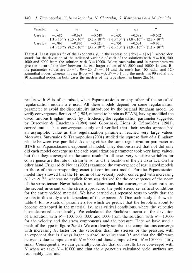
Variable vr vθ τrr τrθ τθθ P

Case B1 −0.685 −0.689 −0.648 −0.635 −0.598 −0.502(1.3 × 10−5) (1.5 × 10−5) (5.2 × 10−5) (3.6 × 10−5) (3.0 × 10−5) (2.3 × 10−5)

Case B2 −0.867 −0.870 −0.721 −0.751 −0.584 −0.701(7.4 × 10−6) (8.2 × 10−6) (3.9 × 10−5) (3.0 × 10−5) (1.9 × 10−5) (1.1 × 10−4)

Table 4. Least squares fit of the exponents, β , in the expression ‖dev‖ = A‖N‖β , where ‘dev’stands for the deviation of the indicated variable of each of the solutions with N = 100, 500,1000 and 5000 from the solution with N = 10000. Below each value and in parentheses wegive the norm of the ‘dev’ between the two larger values of N , 5000 and 10000. In case B1,the parameter values are Ar = 1, Bo =20, Bn = 0.14 and the mesh has 100 radial and 120azimuthal nodes, whereas in case B2 Ar =1, Bo = 5, Bn = 0.1 and the mesh has 90 radial and80 azimuthal nodes. In both cases the mesh is of the type shown in figure 2(a, b).

results with N is often raised, when Papanastasiou’s or any other of the so-calledregularization models are used. All these models depend on some regularizationparameter to avoid the discontinuity introduced by the original Bingham model. Toverify convergence, Beris et al. (1985, referred to herein as BTAB), having modified thediscontinuous Bingham model by introducing the regularization parameter suggestedby Bercovier & Engelman (1980) and Glowinski, Lions & Tremolieres (1981),carried out such a convergence study and verified that their results approachedan asymptotic value as this regularization parameter reached very large values.Moreover, Smyrnaios & Tsamopoulos (2001) studied the squeeze flow of a Binghamplastic between two parallel disks using either the same regularization parameter asBTAB or Papanastasiou’s exponential model. They demonstrated that not did onlydid each model converge as the each regularization parameter took very large values,but that they converged to the same result. In all cases very sensitive variables forconvergence are the rate of strain tensor and the location of the yield surface. On theother hand, Frigaard & Nouar (2005) examined the convergence of regularized modelsto those of the corresponding exact (discontinuous) model. For the Papanastasioumodel they showed that the H1 norm of the velocity vector converged with increasingN like N−0.5, whereas no explicit form was derived for the convergence of the normof the stress tensor. Nevertheless, it was determined that convergence deteriorated asthe second invariant of the stress approached the yield stress, i.e. critical conditionsfor the entire yielded material. We have carried out repeated tests to verify that theresults in this study are independent of the exponent N . One such study is shown intable 4, for two sets of parameters for which we predict that the bubble is about tobecome entrapped in the material, i.e. near critical conditions, where the velocitieshave decreased considerably. We calculated the Euclidean norm of the deviationof a solution with N = 100, 500, 1000 and 5000 from the solution with N =10 000for the velocity and the stress components and the pressure. Here we have used amesh of the type in figure 2(a, b). We can clearly see that the computations convergewith increasing N , faster for the velocities than the stresses or the pressure, withan exponent that is always larger in absolute value than 0.5 and that the differencebetween values computed with N = 5000 and those computed with N =10 000 is fairlysmall. Consequently, we can generally consider that our results have converged withN when we take N = 10 000 and that the a posteriori calculated yield surfaces arereasonably accurate.

Bubble rise and deformation in Newtonian and viscoplastic fluids 141

(a)

(b)

Bn = 0.01 0.05 0.14 0.19

Bn = 0.01 0.05 0.14 0.19

Figure 9. Dependence of the bubble shape and the yielded (white) and unyielded (grey)domains on Bn for N = 104 and (a) Ar= 1, Bo = 50, (b) Ar = 50, Bo = 10, for Bn = 0.01, 0.05,0.14, and 0.19; R∞ = 10 in all cases except for the first one in (b) where R∞ = 15.

Next we will discuss the effect of increasing the Bingham number on bubble shapesand yield surfaces. Figure 9 shows the dependence of the bubble shape and theyielded (white) and unyielded regions (grey) on Bn for two quite distinct cases of Arand Bo. The dimensionless distance of the outer boundary from the bubble centreis always R∞ =10, except for the first case in figure 9(b) where R∞ =15, in order toinclude the outer yield surface in each case. In the first set of bubbles (Figure 9a),where the gravitational forces balance viscous forces (Ar = 1) and capillarity is ratherweak (Bo = 50) we see that inside the indentation that exists at the rear of thebubble, even for a Newtonian fluid, the stresses fall below the yield stress and avery small region of unyielded material is formed for Bn = 0.01. Of course, stressesmonotonically decrease away from the bubble and unyielded material exists therealso. The yield surface is nearly symmetric around the bubble, but slightly closerto it around the poles. A similar shape of the yield surface was obtained for thecreeping flow of a sphere in a Bingham fluid in BTAB. At higher Bn, Bn = 0.05, thematerial around the bubble ‘freezes’ closer to the bubble surface and the yield surfaceretains the previously described shape. The bubble elongates a little, and the size ofthe rear indentation decreases and does not provide enough space for slow enoughflow there. Hence the unyielded region at the rear of the bubble disappears. At even

142 J. Tsamopoulos, Y. Dimakopoulos, N. Chatzidai, G. Karapetsas and M. Pavlidis

higher Bn (Bn = 0.14), the bubble elongates further and unyielded material arises incontact with it around its equatorial plane. BTAB have shown that unyielded materialarises around the poles of a solid sphere in a region that increases with Bn. On thecontrary in a bubble, the zero-shear-stress condition applied on its entire surfaceforces it to move with the surrounding liquid. Moreover, bubble deformability makesit elongated-developing a small region around its equatorial plane that is parallelto the z-axis with a locally uniform azimuthal velocity. Around this portion of thebubble surface velocity variations decrease and the material can become unyielded.As Bn increases further, Bn =0.19, the area of the unyielded material at the equatorialplane increases and the unyielded material away from the bubble comes closer to it.Eventually these two unyielded areas will merge, the velocity all around the bubblewill drastically decrease and the bubble will be entrapped in the material. We willdiscuss this further in § 4.4.

In the second case (figure 9b) where the gravitational forces are more importantcompared to viscous forces (Ar =50) and capillarity is not as weak (Bo = 10), weobserve some distinct changes at small Bn, Bn =0.01 and Bn= 0.05, but nearly thesame bubble shapes at the larger Bn. At Bn = 0.01, the bubble has an oblate ellipsoidalshape with a flatter rear side, not very different from its Newtonian counterpart, butcompletely different from that in case (a). Unyielded material exists at the rear surfaceof the bubble as in (a), but more importantly the rising bubble generates a vortexbehind it and enhances the rate of strain there so that unyielded material appearsfurther away from the bubble at its rear than at its front side. Thus, the unyieldedsurface around the bubble does not have a fore–aft symmetry any longer. At Bn = 0.05the shape of the bubble is still different from that in case (a), being flatter underneath,and the unyielded region around the bubble tends to become symmetric. At evenhigher Bn, both the shape of the bubble and the unyielded areas are much like thosein case (a).

In figure 10 we show how the map of bubble shapes, given in figure 5, evolves asBn increases. The corresponding Morton numbers are given in table 3 and the Re andWe values underneath each bubble shape. The bubble rise velocity decreases with theBingham number and that is reflected in the decreasing Reynolds and Weber numbers.We show the unyielded material in grey. For Bn 0.1 we show only the unyieldedmaterial, when it arises, on the bubble surface, because unyielded regions around thebubble are too far away to be included in this figure. For larger Bn we also show theunyielded material around the bubble. Even a small Bn introduces qualitative changesin certain bubble shapes. For example, when Ar = 0, Bn= 0.01 (figure 10a) and Bois high enough, the bubble is no longer spherical because a small indentation at itsrear side has been formed, while when Bn =0.05 (figure 10b) and Bo 5, the shapeis again not spherical, but slightly elongated and at its rear side flatter or with asmall indentation. Papanastasiou’s (and every other) viscoplastic model is nonlinear.This, for finite Bond numbers, i.e. deformable bubbles, the characteristic Newtonianproperty at Ar → 0 of fore-aft symmetry in the bubble shapes and the flow fieldis broken. The break-up of the flow fore–aft symmetry in inelastic non-Newtonianfluids has been also experimentally observed in the case of the flow around a settlingsphere even at small Reynolds numbers (Gueslin et al. 2006). Moreover, the measuredrate of strain near the bubble and at the equatorial plane has very small values andconsequently the effective viscosity of the material is high there. On the contrary, nearthe poles the measured rate of strain is higher and the effective viscosity is smaller. Asa result, the bubble tends to deform preferentially in the direction of its poles, takingan elongated shape. The elongation of the bubble becomes more prominent as the

Bubble rise and deformation in Newtonian and viscoplastic fluids 143

Ar

Bo (a) Bn = 0.01

Ar

Bo (b) Bn = 0.05

0

1

5

50

500

5000

0.01

(0.000, 0.000) (0.000, 0.000) (0.000, 0.000) (0.000, 0.000) (0.000, 0.000) (0.000, 0.000) (0.000, 0.000) (0.000, 0.000)

(0.000, 0.000) (0.000, 0.000) (0.000, 0.000) (0.000, 0.000) (0.000, 0.000) (0.000, 0.000) (0.000, 0.000) (0.000, 0.000)

(575.6, 0.331) (395.3, 1.563) (181.2, 3.285) (99.53, 4.953) (100.8, 10.16) (100.6, 20.26) (100.8, 40.61) (100.8, 50.79)

(9.036, 0.008) (8.900, 0.079) (7.941, 0.630) (6.976, 2.433) (6.834, 4.670) (6.743, 9.095) (6.691, 17.91) (6.680, 22.31)

(74.42, 0.055) (68.26, 0.466) (44.86, 0.013) (29.18,4.256) (27.35, 7.478) (26.61, 14.17) (26.28, 27.62) (26.22, 34.36)

(0.931, 8.7×10–4) (0.930, 0.009) (0.927, 0.086) (0.993, 0.493) (1.022, 1.044) (1.035, 2.144) (1.042, 4.341) (1.043, 5.440)

(0.186, 1.7×10–4) (0.186, 0.002) (0.188, 0.018) (0.208, 0.108) (0.216, 0.234) (0.221, 0.487) (0.223, 0.992) (0.223, 1.244)

(2.113, 0.004) (2.105, 0.044) (2.032, 0.413) (1.916, 1.836) (1.893, 3.584) (1.886, 7.116) (1.886,14.23)

(17.03, 0.029) (16.63, 0.227) (14.09, 1.984) (11.10, 6.161) (10.58, 11.19) (10.41, 21.68) (10.37, 43.05)

(122.0, 0.149) (105.7, 1.117) (64.69, 4.185)

(904.9, 0.819) (518.1, 2.684) (234.6, 5.503)

(42.04, 8.838) (40.01, 16.01) (39.64, 31.43) (39.58, 62.66)

(138.9, 19.20) (133.2, 35.48) (132.7, 70.48) (132.7, 88.10)

(1.887, 17.80)

(0.430, 9.2×10–4) (0.429, 0.009) (0. 427, 0.091) (0.427, 0.455) (0.428, 0.915) (0.429, 1.839) (0.430, 3.692) (0.430, 4.619)

0.1 1 5 10 20 40 50

0

1

5

50

500

5000

0.01 0.1 1 5 10 20 40 50

Figure 10. For legend see page 145.

yield stress over the capillary forces increase and the bubble has to squeeze throughthe material. In certain cases in which Newtonian fluid recirculates very slowly at therear of the bubble, the stress in a viscoplastic fluid is small, with ‖τ‖ τy , and so the

144 J. Tsamopoulos, Y. Dimakopoulos, N. Chatzidai, G. Karapetsas and M. Pavlidis

Ar

Bo (c) Bn = 0.01

0

1

50

500

5000

0.01

(0.000, 0.000) (0.000, 0.000) (0.000, 0.000) (0.000, 0.000) (0.000, 0.000) (0.000, 0.000) (0.000, 0.000) (0.000, 0.000)

(0.000, 0.000) (0.000, 0.000) (0.000, 0.000) (0.000, 0.000) (0.000, 0.000) (0.000, 0.000) (0.000, 0.000) (0.000, 0.000)

(22.59, 0.005) (21.92, 0.048) (18.21, 0.331) (16.28, 1.352) (15.79, 2.494) (14.92, 4.452) (14.09, 7.940) (13.87, 9.615)

(180.9, 0.033) (158.7, 0.252) (93.45, 0.873) (65.13, 2.121) (61.70, 3.806) (57.99, 6.725) (54.93, 12.07 (54.20, 14.69)

(2.325, 5.4×10–4)(2.318, 0.005) (2.336, 0.054) (2.953, 0.436) (3.150, 0.992) (3.171, 2.0120) (3.139, 3.942) (3.128, 4.893)

0.1 1 5 10 20 40 50

Ar

Bo(d ) Bn = 0.14

0

1

50

500

5000

0.01 0.1 1 5 10 20 40 50

(0.046, 1.1×10–5)(0.046, 1.1×10–4)(0.049, 0.001)(0.070, 0.012) (0.079, 0.031) (0.082, 0.068) (0.084, 0.140) (0.084, 0.175)

(0.002, 1.8×10–8)(0.002, 1.8×10–7)(0.002, 2.6×10–6)(0.011, 3.2×10–5) (0.018, 0.001) (0.020, 0.004)(0.019, 0.007) (0.019, 0.009)

(0.096, 9.2×10–7) (0.096, 9.2×10–6)(0.113, 1.3×10–4) (0.561, 0.016) (0.858, 0.073) (0.938, 0.176) (0.900, 0.324) (0.879, 0.387)

(0.962, 9.2×10–6)(0.963, 9.3×10–5) (5.079, 0.129)(1.131, 0.001) (6.934, 0.481) (7.198, 1.036) (6.824, 1.862) (6.671, 2.225)

(9.620, 9.2×10–5)(9.631, 9.3×10–4) (35.33, 0.624)(11.23, 0.013) (41.42, 1.715) (41.78, 3.491) (40.39, 6.525) (39.90, 7.962)

Figure 10. For legend see facing page.

material in this region is unyielded. One such case is shown in figure 10(a), but suchcases populate the entire corner of the shape map with large Bond and Archimedesnumbers as Bn increases to 0.05 (figure 10b) and the effective viscosity increases. Herethe unyielded area behind the bubble increases and the bubble deformation fromspherical decreases compared to that for a Newtonian fluid. A shape with flatterfront side does not arise in the map of bubble shapes with Bn = 0.05, in which everylocation is occupied by a converged solution.

Dubash & Frigaard (2007) have studied experimentally the motion of air bubblesrising under gravity in a column filled with Carbopol solutions. The yield stress ofthe material they used was τ ∗

y = 2.2–2.3 Pa and its other properties and bubble sizeswere such that Bn =0.0104 − 0.022, Ar = 0.466 − 4.31 and Bo =15 − 66. This rangeof parameter values is covered in figure 10(a, b). Unlike our predictions, the bubble

Bubble rise and deformation in Newtonian and viscoplastic fluids 145

Ar

Bo (e) Bn = 0.19

10

0

1

50

500

5000

(0.000, 0.000)

(0.005, 1.2×10–4) (0.006, 4.2×10–4)

(0.000, 0.000) (0.000, 0.000) (0.000, 0.000)

(0.250, 0.006) (0.325, 0.021) (0.361, 0.052) (0.367, 0.067)

(2.488, 0.062) (3.206, 0.205) (3.548, 0.205) (3.607, 0.651)

(29.09, 1.692) (31.40, 3.943) (31.77, 5.048)

(0.007, 0.001) (0.007, 0.001)

20 40 50

Figure 10. Map of bubble shapes in a Bingham fluid as a function of the Bond andArchimedes numbers. Underneath each figure we give the corresponding Reynolds and Webernumbers (Re, We): (a) Bn = 0.01, (b) Bn = 0.05, (c) Bn = 0.1, (d) Bn =0.14 and (e) Bn = 0.19.Unyielded material is shown black, and always when it arises in contact with the bubble, butaway from the bubble only when it is close enough, Bn 0.14.

shapes they observed resembled an inverted teardrop. We tried to reproduce theseshapes numerically, first using the Papanastasiou model and then using the Herschel–Bulkley model which is more appropriate for the Carbopol solutions used in theseexperiments, by assuming either shapes closer to the experimental ones as initialbubble shapes to start the Newton–Raphson iterations or higher Bn. Our iterationsnever converged to such shapes, but to the shapes given in figure 10(a, b). We couldattribute the inverted teardrop shape to a number of reasons: (i) Carbopol solutionshave a small elasticity which may be important at the rear of the bubble where slowerflow takes place and closer to the axis of symmetry the flow is elongational. It is well-known that bubbles assume inverted teardrop shapes in viscoelastic fluids: Astarista& Apuzzo (1965), Pilz & Benn (2007), Malaga & Rallison (2007). (ii) Another reasoncould be that Carbopol is thixotropic, which could introduce phenomena that cannotbe predicted by viscoplastic models, Gueslin et al. (2006). (iii) A third reason could bethat, in the experiments by Dubash & Frigaard (2007), the bubbles were rising in atube with diameter not much larger than a typical bubble diameter. In such a narrowtube the fluid must flow downwards closer to the bubble surface giving it a prolateshape. If this deformation is large enough for a liquid drop in creeping flow, Koh &Leal (1989) have shown that the drop shape becomes time-dependent, forming a tailthat may constantly elongate and even break. They have also shown that the largerthe initial deformation, the smaller the capillary number required for this instability

146 J. Tsamopoulos, Y. Dimakopoulos, N. Chatzidai, G. Karapetsas and M. Pavlidis

to arise and that this occurs for a wide range of viscosity ratios between the drop andthe host liquid. Presumably this could also take place in a rising bubble and, whenthe host liquid is viscoplastic, the tail can be ‘frozen’, so that a stationary shape isobtained. Moreover, Terasaka & Tsuge (2001) have observed that the bubble assumesinverted teardrop shapes when it is formed at a nozzle and this shape is ‘frozen’owing to the material’s yield stress. Finally, we should mention that experiments withdifferent Carbopol solutions have also been reported by Astarita & Apuzzo (1965)who observed shapes of unconfined bubbles similar to the ones we predict, whereasthey observed teardrop shapes in other fluids which were clearly viscoelastic.

As Bn increases to Bn = 0.1 (figure 10c), the shape of the bubble has changed inall cases for Bo 0.1, for reasons that we have mentioned already. For small Bondnumbers the bubble remains almost spherical, as surface tension is very important.For Bo 5 gravitational forces become dominant over surface tension, the effectiveviscosity around the equatorial plane is higher than that at the poles and the bubblestarts to take a bullet-like shape. The bubble retains a flatter rear side than the frontside and an indentation for large Bond and Archimedes numbers. As the rate ofstrain is low enough around the equatorial plane, unyielded material exists there. Thesizes of the two unyielded regions, the one far from the bubble and the other aroundthe equatorial plane, increase as Bn increases to 0.14 (figure 10d). For Bo < 5 wherethe bubble is nearly spherical the two unyielded regions are considerably larger thanfor Bo 5. At Bn greater than 0.14 and depending on the value of the Bond number,the two regions will start merging, and then the bubble is immobilized and all thematerial becomes unyielded. For this reason, in figure 10(e), where Bn = 0.19, we showcases with Bo 10 only, so that, although Bn approaches its critical value, the moredeformable bubble can take a nearly symmetric prolate shape or a bullet-like shapewhile rising in the material, irrespective of the values of the other parameters. Anenvelope of yielded material still completely surrounds the bubble and flow continueto take place. For Bo < 10 the flow has stopped and the bubble has been immobilized.

Figure 11 quantifies the bubble shapes by showing their aspect ratio χ ≡ h/w,where h and w are defined in figure 8(a), as a function of Bo for the entire range ofAr we studied and Bn = 0.01, 0.1, 0.14. At the smallest Bn and for Ar= 1, the aspectratio remains very close to unity as Bo increases, since for such materials the bubbleremains almost spherical. For larger Ar, the aspect ratio decreases from unity, more soat a larger Ar, until it reaches a plateau, as the bubble assumes an oblate spheroidalshape. In the line with-largest Archimedes number, Ar =5000, and for 4.5 Bo 9there is a discontinuity in the curve of the aspect ratio because stationary bubbleshapes could not be calculated there but the bubble shapes changed abruptly there,see figure 10(a). For Bn= 0.1 and as Bo increases, the aspect ratio decreases below1 for Ar 500 and increases above 1 for Ar 50 as the bubble assumes a prolatespheroidal shape. For the highest Bn, changes in Ar have a small effect on the aspectratio as long as Bo 1. Beyond this Bo value the aspect ratio increases and, above aparticular value of Bo which is in the range 10 Bo 20, it decreases, more so forthe larger Ar, trends which are opposite to those for Bn = 0.01. Summarizing, bubbleswith small Bn will be either spherical or oblate, but with large Bn they will be eitherspherical or prolate.

Figure 12 gives the definitions of the width and the height of the unyielded regionat the rear side of the bubble and shows that they increase monotonically with theBond number, the width more so. Such regions arise mainly when Bn= 0.05 and theyincrease with Ar, which generally produces spherical cap shapes, and with Bo, whichincreases bubble deformability. Given a Bo value, larger inertia produces a flatter

Bubble rise and deformation in Newtonian and viscoplastic fluids 147

1.0(a)

0.9

0.8

0.7A

spec

t rat

io, h

/w

0.6

0.5

0.4 Ar = 1Ar = 5Ar = 50Ar = 500Ar = 5000

0.3

0.2

10–1 100 101 1020.1

1.2(b)

1.1

1.0

0.9

Asp

ect r

atio

, h/w

0.8

0.7

Ar = 1Ar = 50Ar = 500Ar = 5000

10–1 100 101 102

1.30(c)

1.25

1.20

1.15

Asp

ect r

atio

, h/w

1.10

1.05

1.00

Ar = 1Ar = 50Ar = 500Ar = 5000

10–1 100 101 102

Bo

Figure 11. Bubble aspect ratio vs. Bo, for various Ar values and (a) Bn = 0.01, (b) Bn =0.1and (c) Bn = 0.14.

148 J. Tsamopoulos, Y. Dimakopoulos, N. Chatzidai, G. Karapetsas and M. Pavlidis

1.2

1.0wu

wu

hu

hu0.8

Hei

ght o

f th

e un

yiel

ded

regi

on, h

u

Wid

th o

f th

e un

yiel

ded

regi

on, w

u

0.6

0.4

0.2

0

1.2

1.0

0.8

0.6

0.4

0.2

00 5 10 15 20 25

Bo

30 35 40 45 50 55 60

Ar = 5000

Ar = 500

Ar = 50

Figure 12. Dimensionless width (dashed line) and height (solid line) of the unyielded regionbehind the bubble vs. Bo, for various Ar values and Bn = 0.05. In an inset we show thedefinitions of these geometric characteristics.

bubble shape which provides a larger shield behind it for unyielded material to existthere. As soon as unyielded material is formed, its size first increases abruptly withBo, but then both its height and width reach an asymptote which usually do notexceed the radius of the equivalent spherical bubble.

4.3. Flow field in Bingham fluids

Figure 13 illustrates the flow field around the bubble in a viscoplastic fluid. Capillaryforces are rather weak, Bo = 30, while the gravitational forces balance the viscousforces, Ar = 1. We show contour plots of radial velocity, on the left half, and azimuthalvelocity on the right half of each figure, for low Bn = 0.01 (figure 13a) and for highBn= 0.19 (figure 13c). The total number of equidistant contour lines in this and allother similar plots is 20, unless otherwise mentioned. The outer boundary has beenchosen at such a distance that it does not affect the results in any way. For these twocases we have used R∞ = 10, but for clarity in the figures we present a square of sidelength 10 only. The radial velocity takes its lowest and negative values at the upperside far from the bubble, as the fluid flows downwards, and its highest and positivevalues at the far lower side of the bubble, while it is zero at the equatorial plane.As mentioned earlier, a boundary condition sets the radial and azimuthal velocitiesfar from the bubble to vary like cos(θ) and sin(θ), respectively. Our computationsshow that this dependence remains throughout the unyielded material but not in theyielded material and especially as the bubble surface is approached and Bn increases(see § 4.4), indicating that the far-field unyielded material behaves as a solid. Thevalues of the radial velocity are quite large for small Bn, Bn =0.01 (left side offigure 13a) where the fluid still behaves similarly to a Newtonian one. As a reminder,the dimensionless far-field (r → ∞) velocity of a spherical bubble in a Newtonianfluid for Re= 0 is U = 1/3. However, we can see in figure 13(a) that even for this small

Bubble rise and deformation in Newtonian and viscoplastic fluids 149

(a) (b)

(c) (d )

–0.213 –5.580

–5.588

0

0

0

0

0.213

0.224

0

5.580

5.588

0.499

3.969 × 10–4

–3.478 × 10–3

2.003 × 10–2

3.492 × 10–63.958 × 10–3

3.478 × 10–30

Figure 13. (a, c) Contour plots of the radial, left side, and azimuthal, right side, velocity,and (b, d) contour plots of the pressure field, left side, and second invariant of the rate ofstrain tensor, right side, for Ar= 1, Bo = 30, R∞ = 10, N =104 and (a, b) Bn = 0.01 and (c, d)Bn = 0.19. The range of the respective variable is divided into 20 equal intervals.

Bn the far-field (r = 10) velocity has decreased to U = 0.224. This is a consequenceof the viscoplasticity of the fluid and of the shape of the bubble. At higher Bn,Bn = 0.19, viscoplasticity will further decrease the velocity field around the bubble.Indeed, in figure 13(c) the radial velocity is two orders of magnitude smaller, but stillvaries away from the bubble, following the cosine function. The shape of the bubbleis very different in these two cases, as discussed in § 4.2. The azimuthal velocity, forboth values of Bn, is zero at the axis of symmetry as it should be, while it has itslargest values at the equatorial plane. The azimuthal velocity is almost zero inside theindentation that arises at the rear of the bubble for Bn = 0.01. Increasing the Bn to0.19, the magnitude of the azimuthal velocity also decreases by 2 orders of magnitude.Here an area of nearly uniform azimuthal velocity arises at the equatorial plane and

150 J. Tsamopoulos, Y. Dimakopoulos, N. Chatzidai, G. Karapetsas and M. Pavlidis

in contact with the bubble surface. Indeed, the contour lines of the azimuthal velocityclearly demonstrate that its gradient is much larger at the poles while it decreasesto zero at the equatorial plane, where the bubble surface is nearly flat. Figures 13(b)and 13(d) show the pressure field (left side) and the second invariant of the rate ofstrain tensor (right side), respectively. For both Bn values, the pressure field varieslinearly with the axial distance from the bubble, with negative values above it andpositive values below it, as expected. The presence of the bubble affects the pressurefield only locally and around it. The rate of strain has a local maximum at the poles,a local minimum around the equatorial plane near the bubble and tends to zero atinfinity. Calculating γ for a spherical bubble moving in a Newtonian fluid, where theanalytical solution is known, we find that at (θ = π/2, r = 1), γ =0, whereas γ = 0 atθ = 0 and θ = π. The existence of even one point on the bubble surface where γ = 0forces the material to become unyielded there; this slows down the flow field anddecreases γ around it. This eventually leads to the creation of a finite domain in thematerial that is unyielded. In figure 13(b), we observe that γ has a local maximum atthe bubble tip at the rear of the bubble and abruptly decreases as we move towardsthe south pole of the bubble. However, it does not become small enough to allowunyielded material to form inside the small indentation which exists there. This occursfor other parameter values as seen in figures 10(a, b). On the contrary, in figure 13(d),the larger Bn reduces the values that γ takes and gives the bubble a prolate shapewithout a tip or an indentation. Hence, γ varies smoothly around the bubble surfaceand is symmetric with respect to the equatorial plane of the bubble. For both valuesof Bn the values of γ where unyielded material exists are smaller by over three ordersof magnitude than those in the rest of the material.

In figure 14, we show corresponding contours for the same four variables andthe same Bo, but larger buoyancy with respect to dynamic viscosity, Ar = 50. ForBn= 0.01 (figure 14a, b), the bubble has the shape of a spherical cap with a tip inits rear side. For Bn= 0.19 (figure 14c, d), the bubble takes a prolate shape and isnearly flat at its equatorial plane. In the smaller Bn case, the radial velocity is larger,but quite asymmetric before and after the bubble because of the large vortex thatis formed in the bubble wake. The pressure contours remain straight and horizontalaway from the bubble and are slightly affected by it and only in its vicinity. The rateof strain has a local sharp maximum at the bubble tip and becomes very low in itswake, but unyielded material does not arise there. On the contrary, for Bn= 0.19, thevelocity components are much smaller, have a plane of symmetry and the azimuthalvelocity is very small at the equatorial plane near the bubble. At this same location,the rate of strain takes its lowest values (smaller by 4 orders of magnitude than itsmaximum at the poles) giving rise to unyielded material in contact with the bubble.

Selected cases of bubble shapes and streamlines are shown in figure 15. Theparticular values of the stream function are given in each figure. For the lowestBingham number we examined, Bn = 0.01, the streamlines do not deviate appreciablyfrom the corresponding ones for a Newtonian fluid and no unyielded material arises incontact with the bubble. In particular, for Ar= 1, Bo= 50 (figure 15a) an indentationis formed behind the bubble and the streamfunction assumes very small and negativevalues in this region, indicating flow separation. As the Archimedes number increasesto 500 (figure 15b), a vortex is formed behind the bubble, which takes an oblate shapewith rounded edge for Bo = 10 or more pointed edge at higher Bond numbers, Bo = 40(figure 15c). At even higher Bond numbers it is possible that skirted bubbles couldbe formed in analogy to those in Newtonian fluids. Figure 15(d) shows a particularbubble shape that arises for Ar = 5000 and Bo =4.5 just before the region in which

Bubble rise and deformation in Newtonian and viscoplastic fluids 151

(a) (b)

(c) (d )

–0.102–5.275

0.111

0

0

0

0

5.275

–5.274

5.274

0.783

9.115 × 10–2

3.950 × 10–3

3.476 × 10–3

1.971 × 10–4

1.998 × 10–2

3.591 × 10–6

–3.078 × 10–3

–3.476 × 10–3

Figure 14. As figure 13 but for Ar = 50.

steady bubble shapes could not be computed for this Bingham number or for aNewtonian fluid; see figures 5 and 10a. Here the bubble edge is smooth but tilted inthe upstream direction, the bubble resembles a hat and the vortex behind it is fairlylarge. A slight increase of the Bingham number to 0.05 eliminates flow separationand the vortex behind the bubble, see figure 15(e), which is a common feature ingeneral for Bn 0.05. Increasing the Bingham number further to 0.1 (figure 15f ) or0.14 (figure 15g) produces more rounded bubbles with a prolate shape and, hence,streamlines that are less curved around the bubble.

We have measured and depict in figure 16 the size and the location of thevortex behind the bubble in a Bingham fluid only for Bn= 0.01. These geometriccharacteristics were defined in figure 8(a). Figure 16(a) clearly shows that the vortexlength and width increases with both the Archimedes and the Bond numbers. Similarly

152 J. Tsamopoulos, Y. Dimakopoulos, N. Chatzidai, G. Karapetsas and M. Pavlidis

–1.2 × 10–4

–1.45 × 10–4

–1.7 × 10–3

–1.3 × 10–3

–4.5 × 10–4

–1.5 × 10–3

2.5 × 10–3

–1 × 10–3

–5 × 10–4–1 × 10–45 × 10–45 × 10–3

2 × 10–2

1 × 10–2

5 × 102

2 × 102

1 × 10–3

–4.5 × 10–4

–3 × 10–3

–2 × 10–3

–2 × 10–3

–1 × 10–3

–1 × 10–4–5 × 10–4–1 × 10–51 × 10–3

2 × 10–2

1 × 10–3

1 × 10–3

–2.7 × 10–5

3 × 10–5

3 × 10–3

1 × 10–3 5 × 10–5

1 × 10–3

1.8 × 10–2

1.8 × 10–3

–1 × 10–3

(a)

(b)

(c)

(d)

(e)

(g)

( f )

Figure 15. Bubble shapes and streamlines for (a) Ar= 1, Bo = 50, Bn = 0.01, (b) Ar =500,Bo = 10, Bn = 0.01, (c) Ar= 500, Bo = 40, Bn =0.01, (d) Ar= 5000, Bo = 4.5, Bn = 0.01,(e) Ar = 500, Bo = 10, Bn = 0.05, (f ) Ar= 50, Bo = 50, Bn = 0.1, (g) Ar= 50, Bo = 20, Bn = 0.14.

Bubble rise and deformation in Newtonian and viscoplastic fluids 153

2.0(a)

(b)

1.6

1.2ww

hw

ws

hs

0.8

0.4

1.4

1.2

1.0

0.8

0.6

0.4

0.2

1.6

1.2

0.8

0.4

0

4

3

2

1

0 5 10 15 20 25 30 35 40 45 50 55

5 10 15 20 25

Bo

30 35 40 45 50 55

Figure 16. (a) Length and width of the vortex behind the bubble and (b) distance of itscentre from the bubble centre and the axis of symmetry for Bn = 0.01. (, Ar= 5; , Ar =50;, Ar = 500; , Ar = 5000).

figure 16(b), shows that its centre becomes further away from the bubble back sideand the axis of symmetry as these dimensionless parameters increase.

4.4. Dynamic parameters of flow and critical Bingham number for bubble entrapment

The magnitude of the bubble rise velocities or equivalently the magnitude of thefar-field velocities in a frame moving with the bubble is given in terms of the

154 J. Tsamopoulos, Y. Dimakopoulos, N. Chatzidai, G. Karapetsas and M. Pavlidis

18(a)

(b)

16

14

12

Re

We

10

8

6

4

2

0

0 0.02

3.0

2.5

2.0

1.5

1.0

0.5

0

0.04 0.06 0.08 0.10 0.12 0.14 0.16 0.18 0.20

0 0.02 0.04 0.06 0.08 0.10

Bn

0.12 0.14 0.16 0.18 0.20

Ar = 1Ar = 5Ar = 50

Ar = 100

Bo = 1

Bo = 10

Bo = 20

Bo = 30

Figure 17. Dependence of (a) Re on Bn for Bo = 10 and (b) We on Bn for Ar =1.

corresponding Reynolds or Weber number as a function of the Bingham number infigure 17. Both these dynamic parameters are post-calculated based on the bubblevelocity according to (4.2) and (4.3). The Bond number is fixed in figure 17(a) atBo= 10. As Ar increases, Re increases as well, more so for small Bingham numbers.Moreover, as Bn increases Re decreases because the bubble rise velocity decreasesand at a critical Bn the bubble stops moving, irrespective of the value of Ar and Bobecause all the material becomes unyielded. The dependence of We on Bn is similarto that of Re, as shown in figure 17(b), for Ar = 1 and for different values of Bo. TheWeber number increases monotonically with Bo and decreases with Bn. Apparently,lines of different Bo approach zero for different values of Bn, indicating that capillary

Bubble rise and deformation in Newtonian and viscoplastic fluids 155

1.5Bn = 0.09

1.4

1.3

1.2

1.1Vθ

1.0

0.9

0.8

0.7

0.60 1 2 3 4 5

r6 7 8 9 10

0.11

0.07

0.135

0.04

0.02

Newtonian

Figure 18. Radial profiles of the azimuthal velocity at θ = π/2 for different values of Bn andRe = 0.04, Bo = 0.01.

forces will affect the critical level of yield stress in a material that will cause bubbleentrapment. The exact condition for bubble entrapment is not easy to determinefrom this figure or from plotting the drag force on the bubble as a function of Bn,because Papanastasiou’s constitutive equation does not discriminate between yieldedand unyielded domains a priori and allows some residual flow even where unyieldedmaterial is found a posteriori. So a clear asymptote in the drag force, like the oneproduced in figure 6 of BTAB, should not be expected.

A first possible determining the conditions for bubble entrapment in a viscoplasticfluid is to perform a plastic boundary layer analysis assuming that the bubbleremains spherical, i.e. the Bond and Archimedes numbers are fairly small, parallel tothe analysis in BTAB for a solid sphere. Under this assumption, we first examinedwhether a boundary layer is formed around a bubble and whether the Papanastasioumodel can capture it by plotting the radial profile of the azimuthal velocity at thebubble equatorial plane with Bn as a parameter. Unlike the analysis in BTAB, herethe bubble rise velocity is determined as part of the solution and decreases withBn, whereas on the bubble surface it is not zero, owing to the zero-shear boundarycondition applied there. In order to compare the various profiles with each othermore easily, we normalized the azimuthal velocity so that it is equal to 1 away fromthe bubble. The computed profiles are shown in figure 18, where we have kept thesame low value for the Reynolds number, Re = 0.04, in analogy with the creepingflow conditions in BTAB. We observe that the azimuthal velocity for a Newtonianfluid approaches its far-field value monotonically. On the contrary, in a Binghamfluid it exhibits a maximum, which moves closer to the bubble and becomes sharperas the Bingham number increases. This occurs because the outer yield surface movescloser to the bubble decreasing the width of the path through which material canstill flow through the equatorial plane. This approach of the velocity maximum tothe bubble surface indicates the formation of a boundary layer. At r = 1, the locationof the bubble surface at the equatorial plane, the azimuthal velocity is not zero as

156 J. Tsamopoulos, Y. Dimakopoulos, N. Chatzidai, G. Karapetsas and M. Pavlidis

2.468 × 10–31.537 × 10–2

6.094 × 10–6

5.011 × 10–6

1.618 × 10–2

4.334 × 10–6

(a)

(c)

(b)

Figure 19. Yielded (white) and unyielded (grey) domains, left half, and contour plots ofthe second invariant of the rate of strain, right half, near the critical Bingham number forN = 104, R∞ =10, and (a) Bn = 0.142, Ar = 1, Bo =0.1, (b) Bn = 0.198, Ar = 50, Bo = 15, and(c) Bn = 0.201, Ar = 5000, Bo = 30.

in the case of a solid sphere (see figure 10 in BTAB), but equals the bubble surfacevelocity there because of the zero-shear condition. As Bn increases, this velocity firstincreases above its far-field value, 0.04 Bn 0.11, but then it decreases towardsit as critical conditions are approached and the two yield surfaces tend to merge,Bn= 0.135. Unfortunately, the inevitable formation of unyielded material around thebubble equator, the shape and size of which depends on Bn, makes the necessaryscaling arguments very complicated and the outcome of this semi-analytical approachquestionable.

Instead, it is reasonable to consider that the bubble motion stops and that Bn hasreached its critical value when the unyielded area away from the bubble merges withthe one around its equatorial plane. Such a situation just before the two yield surfacesmerge is shown in figure 19 for three different sets of material parameters. If the thirddecimal place of Bn increases by even one unit in each of the three cases the two yieldsurfaces will merge. On the left half of each figure we show the bubble and the yielded

Bubble rise and deformation in Newtonian and viscoplastic fluids 157

10–1

100

10–1

10–2

10–3

0.10 0.11

du

du

0.12 0.13 0.14 0.15 0.16

Bn

0.17 0.18 0.19 0.20 0.21 0.22

Bo = 0.1Bo = 5

Ar = 1

Bo = 10Bo = 50

Figure 20. Variation of the distance between the two yield surfaces at the equatorial plane,du vs. Bn for various Bo. In an insert we show the definition of this distance.

domains in white and the unyielded domains in grey, while on the right half of eachfigure we show the second invariant of the rate of strain tensor. In all cases, we seethat although the two unyielded regions are about to merge, γ is nowhere equal tozero, but where unyielded material is predicted it takes values that are smaller by 3–4orders of magnitude than in the rest of the material and certainly below the criticalvalue N−1 for the Papanastasiou model as explained in § 3.3. So even when the tworegions have merged, finite motion of the material is predicted, albeit with very largeviscosity and, hence, very small velocity. Figure 19 also demonstrates that the criticalBn at which the bubble will stop moving is distinct for the three cases and dependsmostly on the shape of the bubble. The higher the Bond number is, the more thebubble is deformed, becoming elongated in order to squeeze through the materialas the critical condition approaches. This concurs with the conclusion of Dubash &Frigaard (2007) who, based on scaling arguments, mentioned that larger and moredeformable bubbles are more difficult to immobilize. The variation of the distancebetween these two surfaces at the equatorial plane, du, is shown in figure 20. Itdecreases slowly with Bn up to a critical point, after which it decreases exponentiallyand meets the x-axis at increasing values of Bn as Bo increases. We call the pointof intersection with the x-axis the critical Bingham number, Bnc. Its values, shownin figure 21, are independent of the Archimedes number, when Ar < 100, and onlyslightly dependent on it at higher Ar values. The Bond number does not affect Bnc,if it is so small that surface tension does not allow the bubble to deform from itsspherical shape, i.e. Bo 0.1, or so large that bubble deformation is restricted by theouter yield surface, the shape of which does not vary much with the surface tensionof the bubble, i.e. Bo 50. In these calculations of the critical conditions we useda mesh of the type given in figure 2(b) with N = 104. We repeated this calculationwith a mesh of the type given in figure 2(c) with an even larger value N = 5 × 104.The results are given in table 5 and demonstrate that neither the value of N northe structure and density of the mesh affect them. It is noteworthy that the Binghamnumber used so far in this work is related to the so-called yield stress parameter, Yg ,

158 J. Tsamopoulos, Y. Dimakopoulos, N. Chatzidai, G. Karapetsas and M. Pavlidis

Mesh, N/Bo 0.1 5 10 50M1, 104 0.143 0.175 0.192 0.212

M2, 5 × 104 0.142 0.174 0.192 0.214

Table 5. Critical Bn values as a function of Bo for two meshes (figures 2a and 2c) and valuesof N 104 and 5 × 104 at Ar = 1.

0.24Bo = 0.01Bo = 0.1Bo = 1

Bo = 5Bo = 10Bo = 15

Bo = 20 Bo = 50Bo = 30Bo = 400.22

0.20

Cri

tica

l Bn

0.18

0.16

0.14

0.12100 101 102

Ar103 104

Figure 21. Dependence of critical Bingham number on Bond and Archimedes numbers. Thecurves with Bo = 0.01 and 0.1 are indistinguishable.

of BTAB by

Yg = 32Bn. (4.6)

The critical value for entrapment of a sphere in a Bingham fluid under creepingflow conditions was found in BTAB to be Yg = 0.143, i.e. it is smaller by a factor of2/3 than that for a non-deformable bubble under the same conditions. This is thesame ratio as the ratio of the terminal velocity of a solid sphere to that of a sphericalbubble under the same buoyancy force. Clearly, the more retarding no-slip conditionon the solid sphere requires a smaller yield stress to entrap it in a Bingham fluid thanthe shear free condition on a bubble surface.

As the two yield surfaces tend to merge, the magnitudes of the velocity and rate ofstrain fields decrease everywhere in the domain that is still yielded. We stopped ourcomputations at the value of Bn for which they have just merged, because beyondthat value the numerical error in computing such small variables becomes significant.In any case, it reasonable to monitor the bubble rise velocity as the Bingham numberincreases. This is shown in figure 22, for just the first case given in figure 20, whereAr= 1 and Bo= 0.1. We observe that as the Bingham number increases the logarithmof the terminal velocity decreases, but for Bn > 0.13 the slope of the curve decreasesabruptly and then increases again. We attribute the sharp decrease in the slope to theapproach of critical conditions, but the subsequent increase to the numerical errorwe described above. We have taken the slope of this curve at its inflection pointand we can clearly see that it intersects the abscissa at Bn ≈ 0.142. In other words,

Bubble rise and deformation in Newtonian and viscoplastic fluids 159

100

10–1

10–2

U

10–3

10–4

10–5

0 0.02 0.04 0.06 0.08Bn

0.10 0.12 0.14 0.16

Figure 22. Dimensionless bubble rise velocity vs. Bn for Ar =1 and Bo = 0.1.

monitoring the terminal velocity results in the same critical Bingham number. Theoutcome similar is for all other cases we examined. This abrupt change in slopecorresponds to the abrupt change in slope of the terminal velocity vs. bubble volumeexperimentally measured by Astarista & Apuzzo (1965). Unfortunately, these authorsdid not report the value of the material’s yield stress, so we cannot convert theirbubble volumes to our Bingham numbers and directly compare our predictions totheir measurements.

Dubash & Frigaard (2007) experimentally determined the critical Bingham numberfor bubble rise in a Bingham fluid and found that, depending on bubble aspectratio, it varied between 0.01 and 0.15. Their upper limit falls within our predictions,although it should be recalled that the experimental bubble shapes resembled invertedteardrops and this should affect their mobility. On the contrary, the prediction of Bnc,using variational principles and a Newtonian flow field around a spherical bubble bythe same authors (Dubash & Frigaard 2004) grossly overestimates it, since it places itin the range of 0.7–2. We examined the predictions of two inequalities resulting fromthese variational principles (Theorem 3) using the flow field and the bubble shapewe have predicted in this work. Starting with very small Bn values the predicted Bnc

values are about 0.7, as reported by Dubash & Frigaard (2004). Increasing the Bnof the material affects not only the bubble shape but also the flow field qualitativelyas mentioned previously. This results in a continued decrease of the Bnc value upto Bn ≈ 0.12, for which Bnc ≈ 0.25. However, for larger values of Bn, Bnc startedto increase. This is probably caused by the very small values of γ that arise in thedenominator of the inequality (35) in Dubash & Frigaard (2004). The situation didnot change when inequality (51) was used.

Figure 23 shows the dependence of the bubble velocity (in mm s−1) on the equivalentbubble radius (in mm) with the material’s yield stress as a parameter, keeping theother material properties close to those reported by Maxworthy et al. (1996) forthe mixture of 80 % glycerin in water. For small bubbles, their rise velocity is zero

160 J. Tsamopoulos, Y. Dimakopoulos, N. Chatzidai, G. Karapetsas and M. Pavlidis

200 τy = 0 Pa

τy = 0.1 Pa

τy = 0.5 Pa

τy = 1 Pa

τy = 2 Pa

τy = 3 Pa

τy = 5 Pa

160

U*

(mm

s–1

)

Rb* (mm)

120

80

40

0

0 0.5 1.0 1.5 2.0 2.5 3.0 3.5

Figure 23. Dimensional bubble rise velocity vs. dimensional bubble radius for variousviscoplastic fluids with surface tension, γ ∗ = 0.0655N m−1, density, ρ∗ =1008 kg m−3, andviscosity, µ∗

o = 0.0601N sm−2.

irrespective of the yield stress, but it smoothly increases as the bubble size increases.This is understandable, given that an increase in bubble radius decreases Bn. Bubblemobilization occurs earlier and higher velocities are attained for materials with asmaller yield stress. For easier comparison we have also included in the same figurethe bubble terminal velocity in a Newtonian fluid. Finally the drag coefficient isshown as a function of the Bingham number for a given value of Ar (figure 24a) orfor a given value of Bo (figure 24b). In all cases, increasing Bn from zero increasesCd by several orders of magnitude and more abruptly as the critical conditions areapproached, and for all practical cases the bubble is immobilized. The values of Cd

and its increase are larger for a less deformable bubble (Bo =0.01) with less inertia(Ar = 1). As expected, given a value of Ar, increasing Bo decreases the drag coefficientas the bubble deformability increases. Furthermore, given a value of Bo, increasing Ardecreases the drag coefficient. This should be expected also, since according to (4.4)Cd is inversely proportional to Ar. The same dependence is observed for a Newtonianfluid with Bn = 0, which concurs with the fact that here Cd is inversely proportionalto Re. However, instead of approaching a vertical asymptote, as in the case of a solidsphere (see BTAB), at some value of Bn, all curves attain a smaller slope. In thesingle case of a non-deformable bubble this is attributed to numerical error at theseextreme values of Cd ≈ 108, while in all other cases the change of slope is associatedwith a change in the shape of a deformable bubble. Indeed, in figure 25 we plot thebubble height, h, and the axial distance of the outer yielded surface at the axis ofsymmetry, Su, as a function of the Bingham number. We observe that for small valuesof Bn, h does not change for Bo= 0.1 and slightly increases for 5 Bo 50, whereasSu decreases as the outer yield surface approaches the bubble, more so at the axis ofsymmetry; see figure 9(a). Above a characteristic value of Bn, h increases significantlyand almost linearly, whereas Su either decreases with a larger slope and tends tointersect the h curve (Bo = 0.1), decreases with a smaller slope (Bo = 5) or increasesfor the remaining Bond numbers. In other words, at these characteristic Bn values

Bubble rise and deformation in Newtonian and viscoplastic fluids 161

108

(a)

(b)

107

106

105

104

Cd

Cd

103

102

101

100

108

107

106

105

104

103

102

101

100

0 0.04 0.08 0.12 0.16 0.20 0.24

Ar = 1Ar = 50Ar = 500Ar = 5000

Bo = 0.01

Bo = 5

Bo = 10

Bo = 20

Bo = 50

0.28

0 0.04 0.08 0.12Bn

0.16 0.20 0.24 0.28

Figure 24. The drag coefficient as a function of the Bingham number, for various values of(a) Ar and (b) Bo.

either (i) the outer yield surface approaches the bubble surface very rapidly and thebubble is entrapped (Bo = 0.1), or (ii) the bubble elongates forcing the outer yieldsurface to decrease its rate of approach to it, delaying bubble entrapment to higher Bnvalues (Bo = 5, 10), or (iii) the bubble is slightly squeezed by the approaching yieldsurface and then elongates as in (ii) (Bo = 50). The values of Bn at which the bubblestarts to elongate correspond to the inflection points in the drag force in figure 24(b).

5. ConclusionsWe simulated the rise of a bubble in a viscoplastic material for a wide range of

material parameters. The simulation is based on the mixed finite element methodfor the discretization of the governing equations coupled with a quasi-elliptic meshgeneration scheme in order to follow the large deformations of the physical domain.

162 J. Tsamopoulos, Y. Dimakopoulos, N. Chatzidai, G. Karapetsas and M. Pavlidis

6.0

Bo = 0.1Bo = 5

Bo = 10Bo = 50

5.5

5.0

4.5

Su

Su

4.0

3.5

3.0

2.50.10 0.12 0.14 0.16

Bn0.18 0.20 0.22

1.8

2.0

2.2

2.4

2.6 h

2.8

3.0

3.2

3.4

Figure 25. Bubble height, h, and axial distance of the outer yield surfaces, Su, at the axis ofsymmetry vs. Bn.

Our results allow us to determine the evolution of (a) the velocity and pressure fieldsin the fluid, (b) the shape of the liquid/air interface, (c) the domain of the unyieldedmaterial, (d) the critical Bingham number for bubble entrapment and (e) the dynamicparameters of the flow including the drag coefficient.

We examined the effect of the yield stress and the capillary, viscous and gravityforces. First, we verified the accuracy of our new code by comparing our results withprevious theoretical and experimental ones for a Newtonian fluid. Where possible,we extended earlier results to larger values of Reynolds and Weber numbers. In aviscoplastic fluid, the bubble rise velocity and, hence, both the Reynolds and Webernumbers decrease as the yield stress increases. Unyielded material exists at the rear ofthe bubble at low Bingham numbers and large Bond and Archimedes numbers, whenthe bubble has a distorted oblate spheroidal shape. This unyielded area disappears athigher Bingham numbers as the shape of the bubble changes to a bullet-like shapeallowing it to squeeze through the material. Unyielded material also arises around andfar from the bubble and around the equatorial plane for Bn 0.1. The size of thesedomains increases with the Bingham number and when they merge the bubble stopsmoving. As this critical Bingham number is approached the bubble tends to take abullet-like shape owing to the higher effective viscosity at its equatorial plane and thelower viscosity at its poles. The critical Bingham number has strong dependence onthe Bond number, an increase of which allows the bubble to deform more. Finallythe drag coefficient decreases with the Bond and Archimedes numbers and increaseswith the Bingham number.

The predicted bubble shapes and the drag coefficient can be used to determinethe material parameters, µ∗

o and τ ∗y . The numerical approach presented here can be

extended to calculate mass transfer coefficients from/to a bubble in a yield-stressfluid, which are unavailable today, despite being extremely important in determiningoptimal operating conditions for various chemical and physical processes.

Bubble rise and deformation in Newtonian and viscoplastic fluids 163

We thank the European Social Fund (ESF) and the Operational Program forEducational and Vocational Training II (EPEAEK II) and particularly the PythagorasII program for funding the above work. N.C. acknowledges the financial support ofthe PENED 2001 research program of the GSRT of Greece. We appreciate verymuch the very constructive comments made by the referees.

REFERENCES

Astarista, G. & Apuzzo, G. 1965 Motion of gas bubbles in non–Newtonian liquids. AIChE J. 11,815–820.

Bercovier, M. & Engelman, M. 1980 A finite element method for the incompressible non-Newtonian flows. J. Comput. Phys. 36, 313–326.

Beris, A. N., Tsamopoulos, J. A., Armstrong, R. C. & Brown, R. A. 1985 Creeping motion of asphere through a Bingham plastic. J. Fluid Mech. 158, 219–244.

Bhaga, D. & Weber, M. E. 1981 Bubbles in viscous liquids: shapes, wakes and velocities. J. FluidMech. 105, 61–85.

Bingham, E. C. 1922 Fluidity and Plasticity. McGraw-Hill.

Blackery, J. & Mitsoulis E. 1997 Creeping motion of a sphere in tubes filled with a Binghamplastic material. J. Non-Newtonian Fluid Mech. 70, 59–77.

Blanco, A. & Magnaudet, J. 1995 The structure of the axisymmetric high-Reynolds number flowaround an ellipsoidal bubble of fixed shape. Phys. Fluids 7, 1265–1274.

Bonometti, T. & Magnaudet, J. 2006 Transition from spherical cap to toroidal bubbles. Phys.Fluids 18, 052102 1–12.

Bonometti, T. & Magnaudet J. 2007 An interface capturing method for incompressible two phaseflows validation and application to bubble dynamics. Intl. J. Multiphase Flow 33, 109–133.

Burgos, G. R., Alexandrou, A. N. & Entov, N. M. 1999 On the determination of yield surfacesin Herschel-Bulkley fluids. J. Rheol. 43, 463–483.

Christov, C. I. & Volkov, P. K. 1985 Numerical investigation of the steady viscous flow past astationary deformable bubble. J. Fluid Mech. 158, 341–364.

Clift, R., Grace, J. R. & Weber, M. E. 1978 Bubbles, Drops and Particles. Academic.

Dimakopoulos, Y. & Tsamopoulos, J. 2003a Transient displacement of a viscoplastic material byair in straight and suddenly constricted tubes. J. Non-Newtonian Fluid Mech. 112, 43–75.

Dimakopoulos, Y. & Tsamopoulos, J. 2003b A quasi-elliptic transformation for moving boundaryproblems with large anisotropic deformations. J. Comput. Phys. 192, 494–522.

Dimakopoulos, Y. & Tsamopoulos, J. 2003c Transient displacement of a Newtonian fluid by airin straight or suddenly constricted tubes. Phys. Fluids 15, 1973–1991.

Dimakopoulos, Y. & Tsamopoulos, J. 2004 On the gas-penetration in straight tubes completelyfilled with a viscoelastic fluid. J. Non-Newtonian Fluid Mech. 117, 117–139.

Dimakopoulos, Y. & Tsamopoulos, J. 2006 Transient displacement of Newtonian and viscoplasticliquid by air in complex tubes. J. Non-Newtonian Fluid Mech. doi:10.1016/j.jnnfm.2006.08.002.

Dubash, N. & Frigaard, I. 2004 Conditions for static bubbles in viscoplastic fluids. Phys. Fluids16, 4319–4330.

Dubash, N. & Frigaard, I. 2007 Propagation and stopping of air bubbles in Carbopol solutions.J. Non-Newtonian Fluid Mech. 142, 123–134.

Duineveld, P. 1995 The rise velocity and shape of bubbles in pure water at high Reynolds number.J. Fluid Mech. 292, 325–332.

Foteinopoulou, K., Mavrantzas, V., Dimakopoulos, Y. & Tsamopoulos, J. 2006 Numericalsimulation of multiple bubbles growing in a Newtonian liquid filament undergoing stretching.Phys. Fluids 18, 042106.

Frigaard, I. & Nouar, C. 2005 On the usage of viscosity regularization methods for visco-plasticfluid flow computation. J. Non-Newtonian Fluid Mech. 127, 1–26.

Glowinski, R., Lions, J. & Tremolieres, R. 1981 Numerical Analysis of Variational Inequalities,North-Holland.

Gueslin, B., Talini, L., Herzhaft, B., Peysson, Y. & Allain, C. 2006 Flow induced by a spheresettling in an aging yield-stress fluid. Phys. Fluids 18, 103101.

164 J. Tsamopoulos, Y. Dimakopoulos, N. Chatzidai, G. Karapetsas and M. Pavlidis

Haberman, W. L. & Morton, R. K. 1953 An experimental investigation of the drag and shape ofair bubbles rising in various liquids. Report 802, Navy Dept., David W. Taylor Model Basin.68 Washington, DC.

Hadamard, J. S. 1911 Mouvement permanent lent d’une sphere liquide et visqueuse dans un liquidevisqueux. C. R. l’Acad. Sci. Paris 152, 1735–1738.

Harper, J. F. 1972 The motion of bubbles and drops through liquids. Adv. Appl. Mech. 12, 59–129.

Hnat, J. G. & Buckmaster, J. D. 1976 Spherical cap bubbles and skirt formation. Phys. Fluids 19,182–194.

Hua, J. & Lou J. 2007 Numerical simulation of bubble rising in viscous liquid. J. Comput. Phys.222, 769–795.

Johnson, A. & White, D. B. 1991 Gas-rise velocities during kicks. SPE Drilling Engineering, 6,257–263, and Society of Petroleum Engineers Paper 20431.

Karapetsas, G. & Tsamopoulos, J. 2006 Transient squeeze flow of viscoplastic materials. J. Non-Newtonian Fluid Mech. 133, 35–56.

Koh, C. & Leal, L. G. 1989 The stability of drop shapes for transition at zero Reynolds numberthrough a quiescent fluid. Phys. Fluids A 1, 1309–1313.

Levich, V. G. 1949 The motion of bubbles at high Reynolds numbers. Zh. Eksper. Teor. Fiz. 19,18–24.

Liu, B. T., Muller, S. & Denn, M. M. 2002 Convergence of a regularization method for creepingflow of a Bingham material about a rigid sphere, J. Non-Newtonian Fluid Mech. 102, 179–191.

Magnaudet, J. & Eames, I. 2000 The motion of high-Reynolds-number bubbles in inhomogeneousflows. Annu. Rev. Fluid Mech. 32, 659–708.

Malaga, C. & Rallison, J. M. 2007 A rising bubble in a polymer solution. J. Non-Newtonian FluidMech. 141, 59–78.

Maxworthy, T., Gnann, C., Kurten, M. & Durst, F. 1996 Experiments on the rise of air bubblesin clean viscous liquids. J. Fluid Mech. 321, 421–441.

Miksis, M. J., Vanden-Broeck, J. M. & Keller, J. B. 1982 Rising bubbles. J. Fluid Mech. 123,31–41.

Moore, D. W. 1963 The boundary layer on a spherical gas bubble. J. Fluid Mech. 16, 161–176.

Moore, D. W. 1965 The velocity of rise of distorted gas bubbles in a liquid of small viscosity.J. Fluid Mech. 23, 749–766.

Papanastasiou, T. C. 1987 Flows of materials with yield. J. Rheol. 31, 385–404.

Pilz, C. & Benn, G. 2007 On the critical bubble volume at the rise velocity jump discontinuity inviscoelastic liquids. J. Non-Newtonian Fluid Mech. 145, 124–138.

Rybczynski, W. 1911 On the translatory motion of fluid sphere in a viscous medium. Bull. Intl l’Acad. Polonaise Scie. Lett. Classe des Sciences Mathematiques et Naturelles A, 40–46.

Ryskin, G. & Leal, L. G. 1984 Numerical solution of free-boundary problems in fluid mechanics.Part 2. Buoyancy-driven motion of a gas bubble through a quiescent liquid. J. Fluid Mech.148, 19–35.

Schenk, O. & Gartner, K. 2004 Solving unsymmetric sparse systems of linear equations withPARDISO. J. Future Generations Computer Systems 20, 475–487.

Schenk, O. & Gartner, K. 2006 On fast factorization pivoting methods for symmetric indefinitesystems. Elec. Trans. Numer. Anal. 23, 158–179.

Smyrnaios, D. & Tsamopoulos, J. 2001 Squeeze flow of Bingham plastics. J. Non-Newtonian FluidMech. 100, 165–190.

Stein, S. & Buggisch, H. 2000 Rise of pulsating bubble in fluids with a yield stress. Z. Angew.Math. Mech. 11–12, 827–834.

Taylor, T. & Acrivos, A. 1964 On the deformation and drag of a falling drop at low Reynoldsnumber. J. Fluid Mech. 18, 466–476.

Terasaka, K. & Tsuge, H. 2001 Bubble formation at a nozzle submerged in viscous liquids havingyield stress. Chem. Engng Sci. 56, 3237–3245.

Unverdi, S. O. & Tryggvason, G. 1992 A front tracking method for viscous, incompressible,multi-fluid flows. J. Comput. Phys. 100, 25–37.