ste43901 ch05.qxd 5/1/01 12:45 PM Page 172highered.mheducation.com/.../21708/ste43901_ch05qxd.pdfste43901_ch05.qxd 5/1/01 12:45 PM Page 176 Thus, compared with the effective capacity

ste43901_ch05.qxd 5/1/01 12:45 PM Page 172

CHAPTER OUTLINE

Introduction, 000

Importance of CapacityDecisions, 000

Defining and MeasuringCapacity, 000

Determinants of EffectiveCapacity, 000Facilities Factors, 000Product/Service Factors, 000Process Factors, 000Human Factors, 000Operational Factors, 000External Factors, 000

Determining CapacityRequirements, 000

Planning Service Capacity, 000

Developing CapacityAlternatives, 000

Evaluating Alternatives, 000

Calculating ProcessingRequirements, 000

Cost–Volume Analysis, 000Financial Analysis, 000Decision Theory, 000Waiting-Line Analysis, 000

Operations Strategy, 000

Summary, 000

Key Terms, 000

Solved Problems, 000

Discussion and ReviewQuestions, 000

Memo Writing Exercises, 000

Problems, 000

Operations Tour: High AcresLandfill, 000

Selected Bibliography and FurtherReading, 000

Supplement: Decision Theory, 000

LEARNING OBJECTIVES

After completing this chapter, youshould be able to:

1 Explain the importance ofcapacity planning.

2 Discuss ways of defining andmeasuring capacity.

3 Describe the factors thatdetermine effective capacityalternatives.

4 Discuss the major considerationsrelated to developing capacityalternatives.

5 Briefly describe approaches thatare useful for evaluating capacityalternatives.

CHAPTER FIVE

Capacity Planning

173

ste43901_ch05.qxd 5/1/01 12:45 PM Page 173

C apacity planning encompasses many basic decisions with long-term consequences forthe organization. In this chapter, you will learn about the importance of capacity de-

cisions, the measurement of capacity, how capacity requirements are determined, and thedevelopment and evaluation of capacity alternatives.

IntroductionCapacity issues are important for all organizations, and at all levels of an organization.Capacity refers to an upper limit or ceiling on the load that an operating unit can handle.The operating unit might be a plant, department, machine, store, or worker.

The capacity of an operating unit is an important piece of information for planning pur-poses: It enables managers to quantify production capability in terms of inputs or outputs,and thereby make other decisions or plans related to those quantities. The basic questionsin capacity planning are the following:

1. What kind of capacity is needed?

2. How much is needed?

3. When is it needed?

The question of what kind of capacity is needed depends on the products and services thatmanagement intends to produce or provide. Hence, in a very real sense, capacity planningis governed by those choices.

The most fundamental decisions in any organization concern the products and/or ser-vices it will offer. Virtually all other decisions pertaining to capacity, facilities, location,and the like are governed by product and service choices.

In some instances, capacity choices are made very infrequently; in others, they aremade regularly, as part of an ongoing process. Generally, the factors that influence thisfrequency are the stability of demand, the rate of technological change in equipment andproduct design, and competitive factors. Other factors relate to the type of product or ser-vice and whether style changes are important (e.g., automobiles and clothing). In anycase, management must review product and service choices periodically to ensure that thecompany makes capacity changes when they are needed for cost, competitive effective-ness, or other reasons.

174 PART THREE DESIGN OF PRODUCTION SYSTEMS

capacity The upper limit orceiling on the load that an op-erating unit can handle.

N ot too long ago, dire predictions were made about thelack of landfill capacity to handle the growing amounts

of trash companies and residences were generating. Now,some landfills around the country are not getting the trash(and the fees) they need to survive. What was once regardedas undercapacity has now turned into overcapacity.

The reasons for this turnaround can be found in strong ef-forts by the general public to recycle—stronger than most ex-

perts had predicted. Companies, too, are recycling more, a re-sult of government regulations and cost-saving measures.They are also incorporating more recyclable and reusableparts and materials in their products, and they are reducing theamount of materials used to package their products.

But landfills, like many other kinds of operations, are de-signed to operate at a certain level. It is difficult (and in somestates illegal) for them to operate above their design capacity,and it is inefficient to operate at levels much below design ca-pacity. The shortfall that some landfills are experiencing un-derscores the risks involved in long-term capacity planningand the importance of good forecasts of future demand.

Source: Based on “Riga Landfill Strains to Survive,” MichaelCaputo, Rochester Democrat and Chronicle, July 28, 1997, p. 1A.

N E W S C L I P

Less Trash LeavesLandfills in a Bindwww.gm.com

Vol. 5, Seg. 1Tri-State

Importance of Capacity DecisionsFor a number of reasons, capacity decisions are among the most fundamental of all thedesign decisions that managers must make.

ste43901_ch05.qxd 5/1/01 12:45 PM Page 174

1. Capacity decisions have a real impact on the ability of the organization to meet futuredemands for products and services; capacity essentially limits the rate of output possi-ble. Having capacity to satisfy demand can allow a company to take advantage oftremendous opportunities. When the Quigley (www.quigleyco.com) Corporation’szinc gluconate lozenges, sold under the name Cold-Eze™, attracted the public’s inter-est during the height of the cold and flu season in 1997, drugstores and supermarketsquickly sold out. The product was so popular that the company couldn’t keep up withdemand. Because of this, the company was unable to take full advantage of the strongdemand.

2. Capacity decisions affect operating costs. Ideally, capacity and demand requirementswill be matched, which will tend to minimize operating costs. In practice, this is notalways achieved because actual demand either differs from expected demand or tendsto vary (e.g., cyclically). In such cases, a decision might be made to attempt to balancethe costs of over- and undercapacity.

3. Capacity is usually a major determinant of initial cost. Typically, the greater the ca-pacity of a productive unit, the greater its cost. This does not necessarily imply a one-for-one relationship; larger units tend to cost proportionately less than smaller units.

4. Capacity decisions often involve long-term commitment of resources and the fact that,once they are implemented, it may be difficult or impossible to modify those decisionswithout incurring major costs.

5. Capacity decisions can affect competitiveness. If a firm has excess capacity, or canquickly add capacity, that fact may serve as a barrier to entry by other firms. Then too,capacity can affect delivery speed, which can be a competitive advantage.

6. Capacity affects the ease of management; having appropriate capacity makes manage-ment easier than when capacity is mismatched.

Defining and Measuring CapacityCapacity often refers to an upper limit on the rate of output. Even though this seems sim-ple enough, there are subtle difficulties in actually measuring capacity in certain cases.These difficulties arise because of different interpretations of the term capacity and prob-lems with identifying suitable measures for a specific situation.

In selecting a measure of capacity, it is important to choose one that does not requireupdating. For example, dollar amounts are often a poor measure of capacity (e.g., capac-ity of $30 million a year) because price changes necessitate updating of that measure.

Where only one product or service is involved, the capacity of the productive unit maybe expressed in terms of that item. However, when multiple products or services are in-volved, as is often the case, using a simple measure of capacity based on units of outputcan be misleading. An appliance manufacturer may produce both refrigerators and freez-ers. If the output rates for these two products are different, it would not make sense tosimply state capacity in units without reference to either refrigerators or freezers. Theproblem is compounded if the firm has other products. One possible solution is to statecapacities in terms of each product. Thus, the firm may be able to produce 100 refrigera-tors per day or 80 freezers per day. Sometimes this approach is helpful, sometimes not.For instance, if an organization has many different products or services, it may not bepractical to list all of the relevant capacities. This is especially true if there are frequentchanges in the mix of output, because this would necessitate a frequently changing com-posite index of capacity. The preferred alternative in such cases is to use a measure of ca-pacity that refers to availability of inputs. Thus, a hospital has a certain number of beds, afactory has a certain number of machine hours available, and a bus has a certain numberof seats and a certain amount of standing room.

No single measure of capacity will be appropriate in every situation. Rather, the mea-sure of capacity must be tailored to the situation. Table 5–1 provides some examples ofcommonly used measures of capacity.

CHAPTER FIVE CAPACITY PLANNING 175

ste43901_ch05.qxd 5/1/01 12:45 PM Page 175

Up to this point, we have been using a working definition of capacity. Although it isfunctional, it can be refined into two useful definitions of capacity:

1. Design capacity: the maximum output that can possibly be attained.

2. Effective capacity: the maximum possible output given a product mix, scheduling dif-ficulties, machine maintenance, quality factors, and so on.

Design capacity is the maximum rate of output achieved under ideal conditions. Effectivecapacity is usually less than design capacity (it cannot exceed design capacity) owing torealities of changing product mix, the need for periodic maintenance of equipment, lunchbreaks, coffee breaks, problems in scheduling and balancing operations, and similar cir-cumstances. Actual output cannot exceed effective capacity and is often less because ofmachine breakdowns, absenteeism, shortages of materials, and quality problems, as wellas factors that are outside the control of the operations managers.

These different measures of capacity are useful in defining two measures of system ef-fectiveness: efficiency and utilization. Efficiency is the ratio of actual output to effectivecapacity. Utilization is the ratio of actual output to design capacity.

(5–1)

(5–2)

It is common for managers to focus exclusively on efficiency, but in many instances, thisemphasis can be misleading. This happens when effective capacity is low compared withdesign capacity. In those cases, high efficiency would seem to indicate effective use of re-sources when it does not. The following example illustrates this point.

Given the information below, compute the efficiency and the utilization of the vehicle re-pair department:

Design capacity � 50 trucks per day

Effective capacity � 40 trucks per day

Actual output � 36 trucks per day

Utilization �Actual output

Design capacity�

36 trucks per day

50 trucks per day� 72%

Efficiency �Actual output

Effective capacity�

36 trucks per day

40 trucks per day� 90%

Utilization �Actual output

Design capacity

Efficiency �Actual output

Effective capacity


Business Inputs Outputs

Auto manufacturing Labor hours, machine hours Number of cars per shiftSteel mill Furnace size Tons of steel per dayOil refinery Refinery size Gallons of fuel per dayFarming Number of acres, number Bushels of grain per acre per year, gallons

of cows of milk per dayRestaurant Number of tables, seating Number of meals served per day

capacityTheater Number of seats Number of tickets sold per performanceRetail sales Square feet of floor space Revenue generated per day

TABLE 5–1

Measures of capacity

Example 1

Solution

ste43901_ch05.qxd 5/1/01 12:45 PM Page 176

Thus, compared with the effective capacity of 40 units per day, 36 units per day lookspretty good. However, compared with the design capacity of 50 units per day, 36 units perday is much less impressive although probably more meaningful.

Because effective capacity acts as a lid on actual output, the real key to improving ca-pacity utilization is to increase effective capacity by correcting quality problems, main-taining equipment in good operating condition, fully training employees, and fullyutilizing bottleneck equipment.

Hence, increasing utilization depends on being able to increase effective capacity, andthis requires a knowledge of what is constraining effective capacity.

The following section explores some of the main determinants of effective capacity. Itis important to recognize that the benefits of high utilization are realized only in instanceswhere there is demand for the output. When demand is not there, focusing exclusively onutilization can be counterproductive, because the excess output not only results in addi-tional variable costs; it also generates the costs of having to carry the output as inventory.Another disadvantage of high utilization is that operating costs may increase because ofincreasing waiting time due to bottleneck conditions.

Determinants of Effective CapacityMany decisions about system design have an impact on capacity. The same is true formany operating decisions. This section briefly describes some of these factors, which arethen elaborated on elsewhere in the book. The main factors relate to the following:

1. Facilities

2. Products or services

3. Processes

4. Human considerations

5. Operations

6. External forces

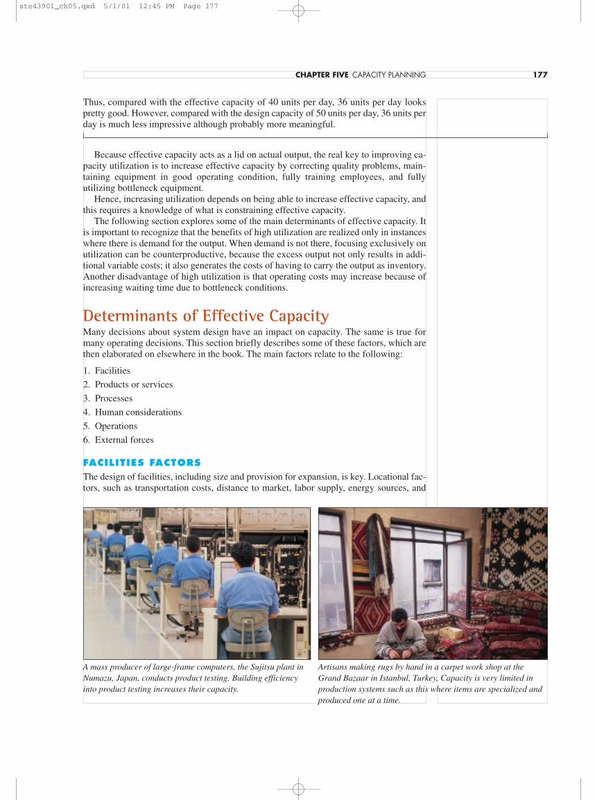
FACILITIES FACTORSThe design of facilities, including size and provision for expansion, is key. Locational fac-tors, such as transportation costs, distance to market, labor supply, energy sources, and


A mass producer of large-frame computers, the Sujitsu plant inNumazu, Japan, conducts product testing. Building efficiencyinto product testing increases their capacity.

Artisans making rugs by hand in a carpet work shop at theGrand Bazaar in Istanbul, Turkey, Capacity is very limited inproduction systems such as this where items are specialized andproduced one at a time.

ste43901_ch05.qxd 5/1/01 12:45 PM Page 177

room for expansion, are also important. Likewise, layout of the work area often determineshow smoothly work can be performed, and environmental factors such as heating, lighting,and ventilation also play a significant role in determining whether personnel can performeffectively or whether they must struggle to overcome poor design characteristics.

PRODUCT/SERVICE FACTORSProduct or service design can have a tremendous influence on capacity. For example,when items are similar, the ability of the system to produce those items is generally muchgreater than when successive items differ. Thus, a restaurant that offers a limited menucan usually prepare and serve meals at a faster rate than a restaurant with an extensivemenu. Generally speaking, the more uniform the output, the more opportunities there arefor standardization of methods and materials, which leads to greater capacity. The partic-ular mix of products or services rendered must also be considered since different itemswill have different rates of output.

PROCESS FACTORSThe quantity capability of a process is an obvious determinant of capacity. A more subtle de-terminant is the influence of output quality. For instance, if quality of output does not meetstandards, the rate of output will be slowed by the need for inspection and rework activities.

HUMAN FACTORSThe tasks that make up a job, the variety of activities involved, and the training, skill, andexperience required to perform a job all have an impact on the potential and actual out-put. In addition, employee motivation has a very basic relationship to capacity, as do ab-senteeism and labor turnover.

OPERATIONAL FACTORSScheduling problems may occur when an organization has differences in equipment capa-bilities among alternative pieces of equipment or differences in job requirements. Inven-tory stocking decisions, late deliveries, acceptability of purchased materials and parts, andquality inspection and control procedures also can have an impact on effective capacity.

Inventory shortages of even one component of an assembled item (e.g., computers, re-frigerators, automobiles) can cause a temporary halt to assembly operations until newcomponents become available. This can have a major impact on effective capacity. Thus,insufficient capacity in one area can affect overall capacity.

EXTERNAL FACTORSProduct standards, especially minimum quality and performance standards, can restrictmanagement’s options for increasing and using capacity. Thus, pollution standards onproducts and equipment often reduce effective capacity, as does paperwork required bygovernment regulatory agencies by engaging employees in nonproductive activities. Asimilar effect occurs when a union contract limits the number of hours and type of workan employee may do.

Table 5–2 summarizes these factors. In general, inadequate planning is a major limit-ing determinant of effective capacity.

Determining Capacity RequirementsCapacity planning decisions involve both long-term and short-term considerations. Long-term considerations relate to overall level of capacity, such as facility size; short-term con-siderations relate to probable variations in capacity requirements created by such thingsas seasonal, random, and irregular fluctuations in demand. Because the time intervals


ste43901_ch05.qxd 5/1/01 12:45 PM Page 178

covered by each of these categories can vary significantly from industry to industry, itwould be misleading to put times on the intervals. However, the distinction will serve asa framework within which to discuss capacity planning.

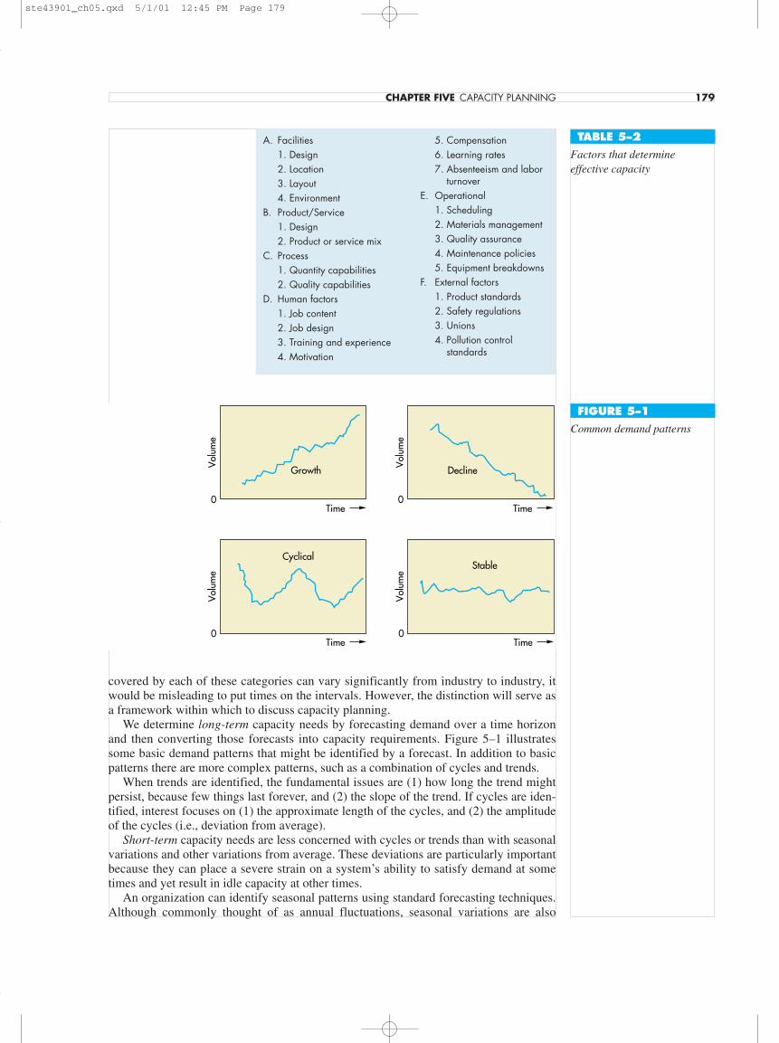
We determine long-term capacity needs by forecasting demand over a time horizonand then converting those forecasts into capacity requirements. Figure 5–1 illustratessome basic demand patterns that might be identified by a forecast. In addition to basicpatterns there are more complex patterns, such as a combination of cycles and trends.

When trends are identified, the fundamental issues are (1) how long the trend mightpersist, because few things last forever, and (2) the slope of the trend. If cycles are iden-tified, interest focuses on (1) the approximate length of the cycles, and (2) the amplitudeof the cycles (i.e., deviation from average).

Short-term capacity needs are less concerned with cycles or trends than with seasonalvariations and other variations from average. These deviations are particularly importantbecause they can place a severe strain on a system’s ability to satisfy demand at sometimes and yet result in idle capacity at other times.

An organization can identify seasonal patterns using standard forecasting techniques.Although commonly thought of as annual fluctuations, seasonal variations are also


A. Facilities1. Design2. Location3. Layout4. Environment

B. Product/Service1. Design2. Product or service mix

C. Process1. Quantity capabilities2. Quality capabilities

D. Human factors1. Job content2. Job design3. Training and experience4. Motivation

5. Compensation6. Learning rates7. Absenteeism and labor

turnoverE. Operational

1. Scheduling2. Materials management3. Quality assurance4. Maintenance policies5. Equipment breakdowns

F. External factors1. Product standards2. Safety regulations3. Unions4. Pollution control

standards

TABLE 5–2

Factors that determineeffective capacity

Time

Time

Time

Time

Volu

me

Volu

me

Volu

me

Volu

me

0

0

0

0

Growth Decline

CyclicalStable

FIGURE 5–1

Common demand patterns

ste43901_ch05.qxd 5/1/01 12:45 PM Page 179

reflected in monthly, weekly, and even daily capacity requirements. Table 5–3 providessome examples of items that tend to exhibit seasonal demand patterns.

When time intervals are too short to have seasonal variations in demand, the analysiscan often describe the variations by probability distributions such as a normal, uniform,or Poisson distribution. For example, we might describe the amount of coffee served dur-ing the midday meal at a luncheonette by a normal distribution with a certain mean andstandard deviation. The number of customers who enter a bank branch on Monday morn-ings might be described by a Poisson distribution with a certain mean. It does not follow,however, that every instance of random variability will lend itself to description by a stan-dard statistical distribution. Service systems in particular may experience a considerableamount of variability in capacity requirements unless requests for service can be sched-uled. Manufacturing systems, because of their typical isolation from customers and themore uniform nature of production, are less likely to experience variations. Waiting-linemodels and simulation models can be useful when analyzing service systems. These mod-els are described in Chapter 19.

Irregular variations are perhaps the most troublesome: They are virtually impossible topredict. They are created by such diverse forces as major equipment breakdowns, freakstorms that disrupt normal routines, foreign political turmoil that causes oil shortages, dis-covery of health hazards (nuclear accidents, unsafe chemical dumping grounds, carcino-gens in food and drink), and so on.

The link between marketing and operations is crucial to realistic determination of ca-pacity requirements. Through customer contracts, demographic analyses, and forecasts,marketing can supply vital information to operations for ascertaining capacity needs forboth the long term and the short term.

Developing Capacity AlternativesAside from the general considerations about the development of alternatives (i.e., conducta reasonable search for possible alternatives, consider doing nothing, take care not tooverlook nonquantitative factors), there are other things that can be done to enhance ca-pacity management:

1. Design flexibility into systems. The long-term nature of many capacity decisionsand the risks inherent in long-term forecasts suggest potential benefits from designingflexible systems. For example, provision for future expansion in the original design of astructure frequently can be obtained at a small price compared to what it would cost to re-model an existing structure that did not have such a provision. Hence, if future expansionof a restaurant seems likely, water lines, power hookups, and waste disposal lines can beput in place initially so that if expansion becomes a reality, modification to the existingstructure can be minimized. Similarly, a new golf course may start as a nine-hole opera-tion, but if provision is made for future expansion by obtaining options on adjacent land,it may progress to a larger (18-hole) course. Other considerations in flexible design in-volve layout of equipment, location, equipment selection, production planning, schedul-ing, and inventory policies, which will be discussed in later chapters.

2. Differentiate between new and mature products or services. Mature products orservices tend to be more predictable in terms of capacity requirements, and they may have


Period Items

Year . . . . . . Beer sales, toy sales, airline traffic, clothing, vacations, tourism, power usage, gasolineconsumption, sports and recreation, education

Month . . . . Welfare and social security checks, bank transactionsWeek . . . . . Retail sales, restaurant meals, automobile traffic, automotive rentals, hotel registrationsDay . . . . . . Telephone calls, power usage, automobile traffic, public transportation, classroom

utilization, retail sales, restaurant meals

TABLE 5–3

Examples of seasonal demandpatterns

Vol. 3, Seg. 3Shouldice Hospital

Vol. 5, Seg. 2TriState

ste43901_ch05.qxd 5/1/01 12:45 PM Page 180

limited life spans. The predictable demand pattern means less risk of choosing an incor-rect capacity, but the possible limited life span of the product or service may necessitatefinding an alternative use for the additional capacity at the end of the life span. New prod-ucts tend to carry higher risk because of the uncertainty often associated with predictingthe quantity and duration of demand. That makes flexibility appealing to managers.

3. Take a “big picture” approach to capacity changes. When developing capacityalternatives, it is important to consider how parts of the system interrelate. For example,when making a decision to increase the number of rooms in a motel, one should also takeinto account probable increased demands for parking, entertainment and food, and house-keeping. This is a “big picture” approach.

4. Prepare to deal with capacity “chunks.” Capacity increases are often acquired infairly large chunks rather than smooth increments, making it difficult to achieve a matchbetween desired capacity and feasible capacity. For instance, the desired capacity of a cer-tain operation may be 55 units per hour; but suppose that machines used for this operationare able to produce 40 units per hour each. One machine by itself would cause capacity tobe 15 units per hour short of what is needed, but two machines would result in an excesscapacity of 25 units per hour. The illustration becomes even more extreme if we shift thetopic—to open-hearth furnaces or to the number of airplanes needed to provide a desiredlevel of capacity.

5. Attempt to smooth out capacity requirements. Unevenness in capacity require-ments also can create certain problems. For instance, during periods of inclement weather,public transportation ridership tends to increase substantially relative to periods of pleas-ant weather. Consequently, the system tends to alternate between underutilization andoverutilization. Increasing the number of buses or subway cars will reduce the burdenduring periods of heavy demand, but this will aggravate the problem of overcapacity atother times and certainly add to the cost of operating the system.

We can trace the unevenness in demand for products and services to a variety ofsources. The bus ridership problem is weather related to a certain extent, but demandcould be considered to be partly random (i.e., varying because of chance factors). Still an-other source of varying demand is seasonality. Seasonal variations are generally easier tocope with than random variations because they are predictable. Consequently, manage-ment can make allowances in planning and scheduling activities and inventories. How-ever, seasonal variations can still pose problems because of their uneven demands on thesystem: At certain times the system will tend to be overloaded, while at other times it willtend to be underloaded. One possible approach to this problem is to identify products orservices that have complementary demand patterns, that is, patterns that tend to offseteach other. For instance, demand for snow skis and demand for water skis might comple-ment each other: Demand for water skis is greater in the spring and summer months, anddemand for snow skis is greater in the fall and winter months. The same might apply toheating and air-conditioning equipment. The ideal case is one in which products or ser-vices with complementary demand patterns involve the use of the same resources but atdifferent times, so that overall capacity requirements remain fairly stable. Figure 5–2 il-lustrates complementary demand patterns.

Variability in demand can pose a problem for managers. Simply adding capacity by in-creasing the size of the operation (e.g., increasing the size of the facility, the workforce,or the amount of processing equipment) is not always the best approach, because that re-duces flexibility and adds to fixed costs. Consequently, managers often choose to respondto higher than normal demand in other ways. One way is through the use of overtimework. Another way is to subcontract some of the work. A third way is to draw down fin-ished goods inventories during periods of high demand and replenish them during periodsof slow demand. These options and others are discussed in detail in the chapter on aggre-gate planning.

6. Identify the optimal operating level. Production units typically have an ideal oroptimal level of operation in terms of unit cost of output. At the ideal level, cost per unitis the lowest for that production unit; larger or smaller rates of output will result in a


ste43901_ch05.qxd 5/1/01 12:45 PM Page 181

higher unit cost. Figure 5–3 illustrates this concept. Notice how unit costs rise as the rateof output varies from the optimal level.

The explanation for the shape of the cost curve is that at low levels of output, the costsof facilities and equipment must be absorbed (paid for) by very few units. Hence, the costper unit is high. As output is increased, there are more units to absorb the “fixed” cost offacilities and equipment, so unit costs decrease. However, beyond a certain point, unitcosts will start to rise. To be sure, the fixed costs are spread over even more units, so thatdoes not account for the increase, but other factors now become important: worker fa-tigue; equipment breakdowns; the loss of flexibility, which leaves less of a margin for er-ror; and, generally, greater difficulty in coordinating operations.

Both optimal operating rate and the amount of the minimum cost tend to be a functionof the general capacity of the operating unit. For example, as the general capacity of aplant increases, the optimal output rate increases and the minimum cost for the optimalrate decreases. Thus, larger plants tend to have higher optimal output rates and lower min-imum costs than smaller plants. Figure 5–4 illustrates these points.

In choosing the capacity of an operating unit, management must take these relation-ships into account along with the availability of financial and other resources and fore-casts of expected demand. To do this, it is necessary to determine enough points for eachsize facility to be able to make a comparison among different sizes. In some instances, fa-cility sizes are givens, whereas in others, facility size is a continuous variable (i.e., anysize can be selected). In the latter case, an ideal facility size can be selected. Usually, man-agement must make a choice from given sizes, and none may have a minimum at the de-sired rate of output.


Time

Dem

and

0

A + B

A

B

FIGURE 5–2

A and B have complementarydemand patterns

Ave

rage

cos

t per

uni

t

0Rate of output

Minimumcost

Optimalrate

FIGURE 5–3

Production units have anoptimal rate of output forminimum cost

ste43901_ch05.qxd 5/1/01 12:45 PM Page 182

Planning Service CapacityThree very important factors in planning service capacity are (1) the need to be near cus-tomers, (2) the inability to store services, and (3) the degree of volatility of demand.

Convenience for customers is often an important aspect of service. Generally, a servicemust be located near customers. For example hotel rooms must be where customers wantto stay; having a vacant room in another city won’t help. Thus, capacity and location areclosely tied.

Capacity must also be matched with the timing of demand. Unlike goods, services can-not be produced in one period and stored for use in a later period. Thus, an unsold seat onan airplane, train, or bus cannot be stored for use on a later trip. Similarly, inventories ofgoods allow customers to immediately satisfy wants, whereas a customer who wants aservice may have to wait. This can result in a variety of negatives for an organization thatprovides the service. Thus, speed of delivery, or customer waiting time, becomes a majorconcern in service capacity planning. For example, deciding on the number of police of-ficers and fire trucks to have on duty at any given time affects the speed of response andbrings into issue the cost of maintaining that capacity. Some of these issues are addressedin the chapter on waiting lines.

Demand volatility presents problems for capacity planners. Demand volatility tends tobe higher for services than for goods, not only in timing of demand, but also in the time


Output rate

Ave

rage

cos

t per

uni

t

0

Smallplant

Mediumplant

Largeplant

FIGURE 5–4

Minimum cost and optimaloperating rate are functions ofsize of a production unit

For routine service needs that come in frequently and in high volume, employees at a call center may provide customer service mostefficiently. For more specialized customer service needs, individualized service may provide the best result.

Vol. 8, Tape 2, Seg. 1McDonald’s

ste43901_ch05.qxd 5/1/01 12:45 PM Page 183

required to service individual customers. For example, banks tend to experience highervolumes of demand on certain days of the week, and the number and nature of transac-tions tend to vary substantially for different individuals. Then, too, a wide range of social,cultural, and even weather factors can cause major peaks and valleys in demand. The factthat services can’t be stored means service systems cannot turn to inventory to smooth de-mand requirements on the system the way goods-producing systems are able to. Instead,service planners have to devise other methods of coping with demand volatility. For ex-ample, to cope with peak demand periods, planners might consider hiring extra workers,outsourcing some or all of a service, or using pricing and promotion to shift some demandto slower periods.

In some instances, demand management is a strategy that can be used to offset capac-ity limitations. Pricing, promotions, discounts, and similar tactics can help to shift somedemand away from peak periods and into slow periods, allowing organizations to achievea closer match in supply and demand.

Evaluating AlternativesAn organization needs to examine alternatives for future capacity from a number of dif-ferent perspectives. Most obvious are economic considerations: Will an alternative beeconomically feasible? How much will it cost? How soon can we have it? What willoperating and maintenance costs be? What will its useful life be? Will it be compatiblewith present personnel and present operations?

Less obvious, but nonetheless important, is possible negative public opinion. For in-stance, the decision to build a new power plant is almost sure to stir up reaction, whetherthe plant is coal-fired, hydroelectric, or nuclear. Any option that could disrupt lives andproperty is bound to generate hostile reactions. Construction of new facilities may neces-sitate moving personnel to a new location. Embracing a new technology may mean re-training some people and terminating some jobs. Relocation can cause unfavorablereactions, particularly if a town is about to lose a major employer. Conversely, commu-nity pressure in a new location may arise if the presence of the company is viewed unfa-vorably (noise, traffic, pollution).

A number of techniques are useful for evaluating capacity alternatives from an eco-nomic standpoint. Some of the more common are cost–volume analysis, financial analy-sis, decision theory, and waiting-line analysis. Cost–volume analysis is described in thischapter. Financial analysis is mentioned briefly; decision analysis is described in thechapter supplement and waiting-line analysis are described in chapter 19.

CALCULATING PROCESSING REQUIREMENTSWhen evaluating capacity alternatives, a necessary piece of information is the capacityrequirements of products that will be processed with a given alternative. To get this in-formation, one must have reasonably accurate demand forecasts for each product, andknow the standard processing time per unit for each product on each alternative machine,the number of workdays per year, and the number of shifts that will be used.

A department works one eight-hour shift, 250 days a year, and has these figures for usageof a machine that is currently being considered:

Annual Standard Processing Processing TimeProduct Demand Time per Unit (Hr) Needed (Hr)

#1 400 5.0 2,000#2 300 8.0 2,400#3 700 2.0 1,400

5,800


Vol. 3, Seg. 4Toyota

Example 2

ste43901_ch05.qxd 5/1/01 12:45 PM Page 184

Working one eight-hour shift, 250 days a year provides an annual capacity of 8 � 250� 2,000 hours per year. We can see that three of these machines would be needed to han-dle the required volume:

COST–VOLUME ANALYSISCost–volume analysis focuses on relationships between cost, revenue, and volume of out-put. The purpose of cost–volume analysis is to estimate the income of an organization un-der different operating conditions. It is particularly useful as a tool for comparing capacityalternatives.

Use of the technique requires identification of all costs related to the production of agiven product. These costs are then designated as fixed costs or variable costs. Fixed coststend to remain constant regardless of volume of output. Examples include rental costs,property taxes, equipment costs, heating and cooling expenses, and certain administrativecosts. Variable costs vary directly with volume of output. The major components of vari-able costs are generally materials and labor costs. We will assume that variable cost perunit remains the same regardless of volume of output.

Table 5–4 summarizes the symbols used in the cost–volume formulas.The total cost associated with a given volume of output is equal to the sum of the fixed

cost and the variable cost per unit times volume:

TC � FC � VC (5–3)

VC � Q � v (5–4)

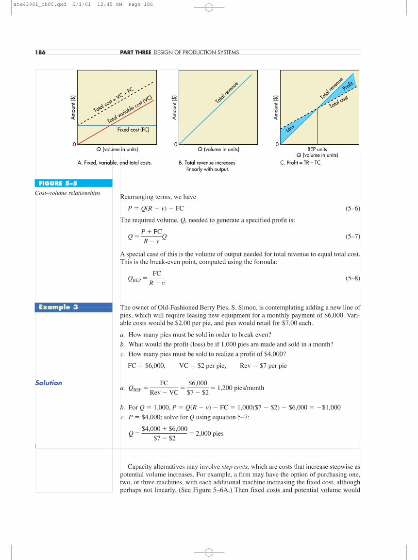
where v � variable cost per unit. Figure 5–5A shows the relationship between volume ofoutput and fixed costs, total variable costs, and total (fixed plus variable) costs.

Revenue per unit, like variable cost per unit, is assumed to be the same regardless ofquantity of output. Total revenue will have a linear relationship to output, as illustrated inFigure 5–5B. Assume that all output can be sold. The total revenue associated with agiven quantity of output, Q, is:

TR � R � Q (5–5)

Figure 5–5C describes the relationship between profit—which is the difference be-tween total revenue and total (i.e., fixed plus variable) cost—and volume of output. Thevolume at which total cost and total revenue are equal is referred to as the break-evenpoint (BEP). When volume is less than the break-even point, there is a loss; when vol-ume is greater than the break-even point, there is a profit. The greater the deviation fromthis point, the greater the profit or loss. Total profit can be computed using the formula:

P � TR � TC � R � Q � (FC � v � Q)

5,800 hours

2,000 hour/machine� 2.90 machines


FC � Fixed costVC � Total variable costv � Variable cost per unitTC � Total costTR � Total revenueR � Revenue per unitQ � Quantity or volume of outputQBEP � Break-even quantityP � Profit

TABLE 5–4

Cost–volume symbols

break-even point (BEP) Thevolume of output at which totalcost and total revenue areequal.

ste43901_ch05.qxd 5/1/01 12:45 PM Page 185

Rearranging terms, we have

P � Q(R � v) � FC (5–6)

The required volume, Q, needed to generate a specified profit is:

Q (5–7)

A special case of this is the volume of output needed for total revenue to equal total cost.This is the break-even point, computed using the formula:

QBEP (5–8)

The owner of Old-Fashioned Berry Pies, S. Simon, is contemplating adding a new line ofpies, which will require leasing new equipment for a monthly payment of $6,000. Vari-able costs would be $2.00 per pie, and pies would retail for $7.00 each.

a. How many pies must be sold in order to break even?

b. What would the profit (loss) be if 1,000 pies are made and sold in a month?

c. How many pies must be sold to realize a profit of $4,000?

FC � $6,000, VC � $2 per pie, Rev � $7 per pie

a. QBEP

b. For Q � 1,000, P � Q(R � v) � FC � 1,000($7 � $2) � $6,000 � �$1,000

c. P � $4,000; solve for Q using equation 5–7:

Capacity alternatives may involve step costs, which are costs that increase stepwise aspotential volume increases. For example, a firm may have the option of purchasing one,two, or three machines, with each additional machine increasing the fixed cost, althoughperhaps not linearly. (See Figure 5–6A.) Then fixed costs and potential volume would

Q �$4,000 � $6,000

$7 � $2� 2,000 pies

�FC

Rev � VC�

$6,000

$7 � $2� 1,200 pies/month

�FC

R � v

Q �P � FC

R � v


Q (volume in units)

Am

ount

($)

0

A. Fixed, variable, and total costs.

Q (volume in units)

Am

ount

($)

0

B. Total revenue increases linearly with output.

BEP unitsQ (volume in units)

Am

ount

($)

0

C. Profit = TR – TC.

Total cost =

VC + FC

Total variable c

ost (VC)

Fixed cost (FC)

Total

reve

nue

Total

reve

nue

Total cost

Profit

Loss

FIGURE 5–5

Cost–volume relationships

Example 3

Solution

ste43901_ch05.qxd 5/1/01 12:45 PM Page 186

depend on the number of machines purchased. The implication is that multiple break-evenquantities may occur, possibly one for each range. Note, however, that the total revenueline might not intersect the fixed-cost line in a particular range, meaning that there wouldbe no break-even point in that range. This possibility is illustrated in Figure 5–6B, wherethere is no break-even point in the first range. In order to decide how many machines topurchase, a manager must consider projected annual demand (volume) relative to themultiple break-even points and choose the most appropriate number of machines, as Ex-ample 4 shows.

A manager has the option of purchasing one, two, or three machines. Fixed costs and po-tential volumes are as follows:

Number of Total Annual Corresponding Machines Fixed Costs Range of Output

1 $ 9,600 0 to 3002 15,000 301 to 6003 $20,000 601 to 900

Variable cost is $10 per unit, and revenue is $40 per unit.

a. Determine the break-even point for each range.

b. If projected annual demand is between 580 and 660 units, how many machines shouldthe manager purchase?

a. Compute the break-even point for each range using the formula QBEP � FC/R � v.

For one machine

QBEP

For two machines QBEP

For three machines QBEP

b. Comparing the projected range of demand to the two ranges for which a break-evenpoint occurs, you can see that the break-even point is 500, which is in the range 301 to600. This means that even if demand is at the low end of the range, it would be above thebreak-even point and thus yield a profit. That is not true of range 601 to 900. At the top

�$20,000

$40/unit � $10/unit� 666.67 units

�$15,000

$40/unit � $10/unit� 500 units

�$9,600

$40/unit � $10/unit� 320 units [not in range, so there is no BEP]


Quantity

A. Step fixed costs and variable costs.

FC + VC = TC

FC1 machine

FC + VC = TC

FC2 machines

FC + VC = TC

FC3 machines

Quantity

B. Multiple break-even points.

1

2

3

BEP3

BEP2

TC

TC

TC

TR

$ FIGURE 5–6

Break-even problem with stepfixed costs

Example 4

Solution

ste43901_ch05.qxd 5/1/01 12:45 PM Page 187

end of projected demand, the volume would still be less than the break-even point forthat range, so there would be no profit. Hence, the manager should choose two machines.

Cost–volume analysis can be a valuable tool for comparing capacity alternatives if cer-tain assumptions are satisfied:

1. One product is involved.

2. Everything produced can be sold.

3. The variable cost per unit is the same regardless of the volume.

4. Fixed costs do not change with volume changes, or they are step changes.

5. The revenue per unit is the same regardless of volume.

6. Revenue per unit exceeds variable cost per unit.

As with any quantitative tool, it is important to verify that the assumptions on whichthe technique is based are reasonably satisfied for a particular situation. For example, rev-enue per unit or variable cost per unit are not always constant. In addition, fixed costs maynot be constant over the range of possible output. If demand is subject to random varia-tions, one must take that into account in the analysis. Also, cost–volume analysis requiresthat fixed and variable costs can be separated, and this is sometimes exceedingly difficultto accomplish.

Cost–volume analysis works best with one product or a few products that have thesame cost characteristics. Nevertheless, a notable benefit of cost–volume considerationsis the conceptual framework it provides for integrating cost, revenue, and profit estimatesinto capacity decisions. If a proposal looks attractive using cost–volume analysis, the nextstep would be to develop cash flow models to see how it fares with the addition of timeand more flexible cost functions.

FINANCIAL ANALYSISA problem that is universally encountered by managers is how to allocate scarce funds. Acommon approach is to use financial analysis to rank investment proposals.

Two important terms in financial analysis are cash flow and present value:

Cash flow refers to the difference between the cash received from sales (of goods or ser-vices) and other sources (e.g., sale of old equipment) and the cash outflow for labor, ma-terials, overhead, and taxes.

Present value expresses in current value the sum of all future cash flows of an investmentproposal.

The three most commonly used methods of financial analysis are payback, presentvalue, and internal rate of return.

Payback is a crude but widely used method that focuses on the length of time it willtake for an investment to return its original cost. For example, an investment with an orig-inal cost of $6,000 and a monthly net cash flow of $1,000 has a payback period of sixmonths. Payback ignores the time value of money. Its use is easier to rationalize for short-term than for long-term projects.

The present value (PV) method summarizes the initial cost of an investment, its esti-mated annual cash flows, and any expected salvage value in a single value called theequivalent current value, taking into account the time value of money (i.e., interest rates).

The internal rate of return (IRR) summarizes the initial cost, expected annual cashflows, and estimated future salvage value of an investment proposal in an equivalent in-terest rate. In other words, this method identifies the rate of return that equates the esti-mated future returns and the initial cost.

These techniques are appropriate when there is a high degree of certainty associatedwith estimates of future cash flows. In many instances, however, operations managers and


cash flow Difference betweencash received from sales andother sources, and cash out-flow for labor, material, over-head, and taxes.

present value The sum, incurrent value, of all future cashflows of an investmentproposal.

ste43901_ch05.qxd 5/1/01 12:45 PM Page 188

other managers must deal with situations better described as risky or uncertain. Whenconditions of risk or uncertainty are present, decision theory is often applied.

DECISION THEORYDecision theory is a helpful tool for financial comparison of alternatives under conditionsof risk or uncertainty. It is suited to capacity decisions and to a wide range of other deci-sions managers must make. Decision theory is described in the supplement to this chapter.

WAITING-LINE ANALYSISAnalysis of lines is often useful for designing service systems. Waiting lines have a ten-dency to form in a wide variety of service systems (e.g., airport ticket counters, telephonecalls to a cable television company, hospital emergency rooms). The lines are symptomsof bottleneck operations. Analysis is useful in helping managers choose a capacity levelthat will be cost-effective through balancing the cost of having customers wait with thecost of providing additional capacity. It can aid in the determination of expected costs forvarious levels of service capacity.

This topic is described in Chapter 19.

Operations StrategyThe strategic implications of capacity decisions can be enormous for an organization, im-pacting all areas of the organization. From an operations management standpoint, capac-ity decisions establish a set of conditions within which operations will be required tofunction. Hence, it is extremely important to include input from operations managementpeople in making capacity decisions.

Flexibility can be a key issue in capacity decisions, although flexibility is not alwaysan option, particularly in capital-intensive industries. However, where possible, flexibil-ity allows an organization to be responsive (agile) to changes in the marketplace. Also, itreduces to a certain extent the dependence on long-range forecasts to accurately predictdemand. And flexibility makes it easier for organizations to take advantage of technolog-ical and other innovations.

Bottleneck management can be a way to increase effective capacity, by schedulingnon–bottleneck operations to achieve maximum utilization of bottleneck operations.

Summary

Capacity refers to a system’s potential for producing goods or delivering services over a specifiedtime interval. Capacity decisions are important because capacity is a ceiling on output and a majordeterminant of operating costs.

The capacity planning decision is one of the most important decisions that managers make. Thecapacity decision is strategic and long-term in nature, often involving a significant initial invest-ment of capital. Capacity planning is particularly difficult in cases where returns will accrue overa lengthy period and risk is a major consideration.

A variety of factors can interfere with capacity utilization, so effective capacity is usually some-what less than design capacity. These factors include facilities design and layout, human factors,product/service design, equipment failures, scheduling problems, and quality considerations.

Capacity planning involves long-term and short-term considerations. Long-term considerationsrelate to the overall level of capacity; short-term considerations relate to variations in capacityrequirements due to seasonal, random, and irregular fluctuations in demand. Ideally, capacity willmatch demand. Thus, there is a close link between forecasting and capacity planning, particularly inthe long term. In the short term, emphasis shifts to describing and coping with variations in demand.

Development of capacity alternatives is enhanced by taking a systems approach to planning, byrecognizing that capacity increments are often acquired in chunks, by designing flexible systems,and by considering product/service complements as a way of dealing with various patterns ofdemand.


Summary

Special service help whenneeded by transfers at the air-port can help keep lines mov-ing at the ticket counter.

Vol. 6, Seg. 3ABT Co

ste43901_ch05.qxd 5/1/01 12:45 PM Page 189


Solved Problems

In evaluating capacity alternatives. a manager must consider both quantitative and qualitativeaspects. Quantitative analysis usually reflects economic factors, and qualitative considerations in-clude intangibles such as public opinion and personal preferences of managers. Cost–volumeanalysis can be useful for analyzing alternatives.

A firm’s manager must decide whether to make or buy a certain item used in the production ofvending machines. Cost and volume estimates are as follows:

Make Buy

Annual fixed cost $150,000 NoneVariable cost/unit $60 $80Annual volume (units) 12,000 12,000

a. Given these numbers, should the firm buy or make this item?b. There is a possibility that volume could change in the future. At what volume would the

manager be indifferent between making and buying?

a. Determine the annual cost of each alternative:

Total cost � Fixed cost � Volume � Variable cost

Make: $150,000 � 12,000($60) � $870,000Buy: 0 � 12,000($80) � $960,000

Because the annual cost of making the item is less than the annual cost of buying it, the man-ager would reasonably choose to make the item.

b. To determine the volume at which the two choices would be equivalent, set the two totalcosts equal to each other, and solve for volume: TCmake � TCbuy. Thus, $150,000 � Q($60)� 0 � Q($80). Solving, Q � 7,500 units. Therefore, at a volume of 7,500 units a year, themanager would be indifferent between making and buying. For lower volumes, the choicewould be to buy, and for higher volumes, the choice would be to make.

A small firm produces and sells novelty items in a five-state area. The firm expects to consoli-date assembly of its electric turtle line at a single location. Currently, operations are in threewidely scattered locations. The leading candidate for location will have a monthly fixed cost of$42,000 and variable costs of $3 per turtle. Turtles sell for $7 each. Prepare a table that showstotal profits, fixed costs, variable costs, and revenues for monthly volumes of 10,000, 12,000,and 15,000 units. What is the break-even point?

Revenue � $7 per unitVariable cost � $3 per unit

? Units(Indifferent

volume)

$

$150,000

0

TCmake

FCmake

TC buy

Key Terms break-even point (BEP), 000capacity, 000

cash flow, 000present value, 000

Problem 1

Solution

Solution

Problem 2

ste43901_ch05.qxd 5/1/01 12:45 PM Page 190


Fixed cost � $42,000 per monthProfit � Q(R � v) � FC

Total cost � FC � v � Q

Total Total Fixed Total Total Volume Revenue VC Cost Cost Profit

10,000 . . . . . . . . . $ 70,000 $30,000 $42,000 $72,000 $(2,000)12,000 . . . . . . . . . 84,000 36,000 42,000 78,000 6,00015,000 . . . . . . . . . 105,000 45,000 42,000 87,000 18,000

QBEP

Refer to Problem 2. Develop an equation that can be used to compute profit for any volume. Usethat equation to determine profit when volume equals 22,000 units.

Profit � Q(R � v) � FC � Q($7 � $3) � $42,000 � $4Q � $42,000For Q � 22,000, profit is$4(22,000) � $42,000 � $46,000

A manager must decide which type of equipment to buy, Type A or Type B. Type A equipmentcosts $15,000 each, and Type B costs $11,000 each. The equipment can be operated 8 hours aday, 250 days a year.

Either machine can be used to perform two types of chemical analysis, C1 and C2. Annualservice requirements and processing times are shown in the following table. Which type ofequipment should be purchased, and how many of that type will be needed? The goal is to min-imize total purchase cost.

PROCESSING TIME PER ANALYSIS (HR)

Analysis Type Annual Volume C1 C2

C1 1,200 1 2C2 900 3 2

Total processing time (annual volume � processing time per analysis) needed by type of equip-ment:

Analysis Type A B

C1 1,200 2,400C2 2,700 1,800

Total 3,900 4,200

Total processing time available per piece of equipment is 8 hours/day � 250 days/year � 2,000.Hence, one piece can handle 2,000 hours of analysis, two pieces of equipment can handle 4,000hours, etc.

Given the total processing requirements, two of Type A would be needed, for a total cost of2 � $15,000 � $30,000, or three of Type B, for a total cost of 3 � $11,000 � $33,000. Thus,two pieces of Type A would have sufficient capacity to handle the load at a lower cost than threeof Type B.

�FC

R � v�

$42,000

$7 � $3� 10,500 units per month

Problem 3

Solution

Problem 4

Solution

Discussion and Review Questions

1. Contrast design capacity and effective capacity.2. List and briefly explain three factors that may inhibit capacity utilization.3. How do long-term and short-term capacity considerations differ?4. Give an example of a good and a service that exhibit these seasonal demand patterns:

a. Annualb. Monthly

ste43901_ch05.qxd 5/1/01 12:45 PM Page 191

c. Weeklyd. Daily

5. Give some examples of building flexibility into system design.6. Why is it important to adopt a “big picture” approach to capacity planning?7. What is meant by “capacity in chunks,” and why is that a factor in capacity planning?8. What kinds of capacity problems do many elementary and secondary schools periodically ex-

perience? What are some alternatives to deal with those problems?9. How can a systems approach to capacity planning be useful?

10. How do capacity decisions influence productivity?11. Why is it important to match process capabilities with product requirements?12. Briefly discuss how uncertainty affects capacity decisions.13. Discuss the importance of capacity planning in deciding on the number of police officers or

fire trucks to have on duty at a given time.


1. Write a short memo to your boss, Al Thomas, outlining the general impact on break-even quan-tities of an increase in the proportion of automation in a process.

2. Write a one-page memo to Don Jones, a production supervisor. Don has questioned your prac-tice of sometimes scheduling production that is below capacity, resulting in less than full uti-lization of personnel and equipment.

Memo Writing Exercises

1. A producer of pottery is considering the addition of a new plant to absorb the backlog of de-mand that now exists. The primary location being considered will have fixed costs of $9,200per month and variable costs of 70 cents per unit produced. Each item is sold to retailers at aprice that averages 90 cents.a. What volume per month is required in order to break even?b. What profit would be realized on a monthly volume of 61,000 units? 87,000 units?c. What volume is needed to obtain a profit of $16,000 per month?d. What volume is needed to provide a revenue of $23,000 per month?e. Plot the total cost and total revenue lines.

2. A small firm intends to increase the capacity of a bottleneck operation by adding a new ma-chine. Two alternatives, A and B, have been identified, and the associated costs and revenueshave been estimated. Annual fixed costs would be $40,000 for A and $30,000 for B; variablecosts per unit would be $10 for A and $12 for B; and revenue per unit would be $15 for A and$16 for B.a. Determine each alternative’s break-even point in units.b. At what volume of output would the two alternatives yield the same profit?c. If expected annual demand is 12,000 units, which alternative would yield the higher profit?

3. A producer of felt-tip pens has received a forecast of demand of 30,000 pens for the comingmonth from its marketing department. Fixed costs of $25,000 per month are allocated to thefelt-tip operation, and variable costs are 37 cents per pen.a. Find the break-even quantity if pens sell for $1 each.b. At what price must pens be sold to obtain a monthly profit of $15,000, assuming that esti-

mated demand materializes?4. A real estate agent is considering installing a cellular telephone in her car. There are three

billing plans to choose from, all of which involve a weekly charge of $20. Plan A has a cost of$0.45 a minute for daytime calls and $0.20 a minute for evening calls. Plan B has a charge of$0.55 a minute for daytime calls and a charge of $0.15 a minute for evening calls. Plan C hasa flat rate of $80 with 200 minutes of calls allowed per week and a cost of $0.40 per minutebeyond that, day or evening.a. Determine the total charge under each plan for this case: 120 minutes of day calls and 40

minutes of evening calls in a week.b. Prepare a graph that shows total weekly cost for each plan versus daytime call minutes.

Problems

a. 46,000 unitsb. (1) $3,000

(2) $8,200c. 126,000 unitsd. 25,556 unitse. Graph in IM

a. (A) 8,000 units(B) 7,500 units

b. 10,000 unitsc. PA � $20,000

PB � $18,000

a. 39,683 unitsb. $1.71

a. (A) $82(B) $92(C) $100

b. Graph in IM

ste43901_ch05.qxd 5/1/01 12:45 PM Page 192

c. If the agent will use the service for daytime calls, over what range of call minutes will eachplan be optimal?

5. Refer to Problem 4. Suppose that the agent expects both daytime and evening calls. At whatpoint (i.e., percentage of call minutes for daytime calls) would she be indifferent between plansA and B?

6. A firm plans to begin production of a new small appliance. The manager must decide whetherto purchase the motors for the appliance from a vendor at $7 each or to produce them in-house.Either of two processes could be used for in-house production; one would have an annual fixedcost of $160,000 and a variable cost of $5 per unit, and the other would have an annual fixedcost of $190,000 and a variable cost of $4 per unit. Determine the range of annual volume forwhich each of the alternatives would be best.

7. A manager is trying to decide whether to purchase a certain part or to have it produced inter-nally. Internal production could use either of two processes. One would entail a variable cost of$17 per unit and an annual fixed cost of $200,000; the other would entail a variable cost of $14per unit and an annual fixed cost of $240,000. Three vendors are willing to provide the part.Vendor A has a price of $20 per unit for any volume up to 30,000 units. Vendor B has a price of$22 per unit for demand of 1,000 units or less, and $18 per unit for larger quantities. Vendor Coffers a price of $21 per unit for the first 1,000 units, and $19 per unit for additional units.a. If the manager anticipates an annual volume of 10,000 units, which alternative would be

best from a cost standpoint? For 20,000 units, which alternative would be best?b. Determine the range for which each alternative is best. Are there any alternatives that are

never best? Which?8. A company manufactures a product using two machine cells. Each cell has a design capacity

of 250 units per day and an effective capacity of 230 units per day. At present, actual outputaverages 200 units per cell, but the manager estimates that productivity improvements soonwill increase output to 225 units per day. Annual demand is currently 50,000 units. It is fore-casted that within two years, annual demand will triple. The company could produce at the rateof 400 per day using available capacity. How many cells should the company plan to produceto satisfy predicted demand under these conditions? Assume 240 workdays per year.

9. A manager must decide which type of machine to buy, A, B, or C. Machine costs are:

Machine Cost

A $40,000B $30,000C $80,000

Product forecasts and processing times on the machines are as follows:

PROCESSING TIME PER UNIT

(MINUTES)DemandProduct Annual A B C

1 16,000 3 4 22 12,000 4 4 33 6,000 5 6 44 30,000 2 2 1

Assume that only purchasing costs are being considered. Which machine would have the low-est total cost, and how many of that machine would be needed? Machines operate 10 hours aday, 250 days a year.

10. Refer to Problem 9. Consider this additional information: The machines differ in terms ofhourly operating costs: The A machines have an hourly operating cost of $10 each, B machineshave an hourly operating cost of $11 each, and C machines have an hourly operating cost of$12 each. Which alternative would be selected, and how many machines, in order to minimizetotal cost while satisfying capacity processing requirements?

11. A manager must decide how many machines of a certain type to purchase. Each machine canprocess 100 customers per hour. One machine will result in a fixed cost of $2,000 per day,


c. A is optimal for 0 to < 178minutes. C is optimal for 178 ormore.

33 percent daytime minutes

For Q less than 63,333, vendor isbest. For larger quantities, best toproduce in-house at $4 per unit.

a. For 10,000 units:Int. 1: $370,000Int. 2: $380,000Vend. A: $200,000Vend. B: $180,000Vend. C: $192,000For 20,000 units:Int. 1: $540,000Int. 2: $520,000Vend. A: $400,000Vend. B: $360,000Vend. C: S382,000

b. Range Best Alt.

1 to 999 A1,000 to 59,999 B60,000 or more Int. 2

3 cells

Total processing time per machine:A: 186,000B: 208,000C: 122,000

Number of each machine neededand total cost:

A: 2, $80,000B: 2, $60,000C: 1, $80,000Buy 2 Bs

A. 111,000B. 98,133C. 104,400Buy 2 machine B

a. 80,152b. 2

ste43901_ch05.qxd 5/1/01 12:45 PM Page 193

while two machines will result in a fixed cost of $3,800 per day. Variable costs will be $20 percustomer, and revenue will be $45 per customer.a. Determine the break-even point for each range.b. If estimated demand is 90 to 120 customers per hour, how many machines should be

purchased?12. The manager of a car wash must decide whether to have one or two wash lines. One line will

mean a fixed cost of $6,000 a month, and two lines will mean a fixed cost of $10,500 a month.Each line would be able to process 15 cars an hour. Variable costs will be $3 per car, and rev-enue will be $5.95 per car. The manager projects an average demand of between 14 and 18 carsan hour. Would you recommend one or two lines? The car wash is open 300 hours a month.


one line

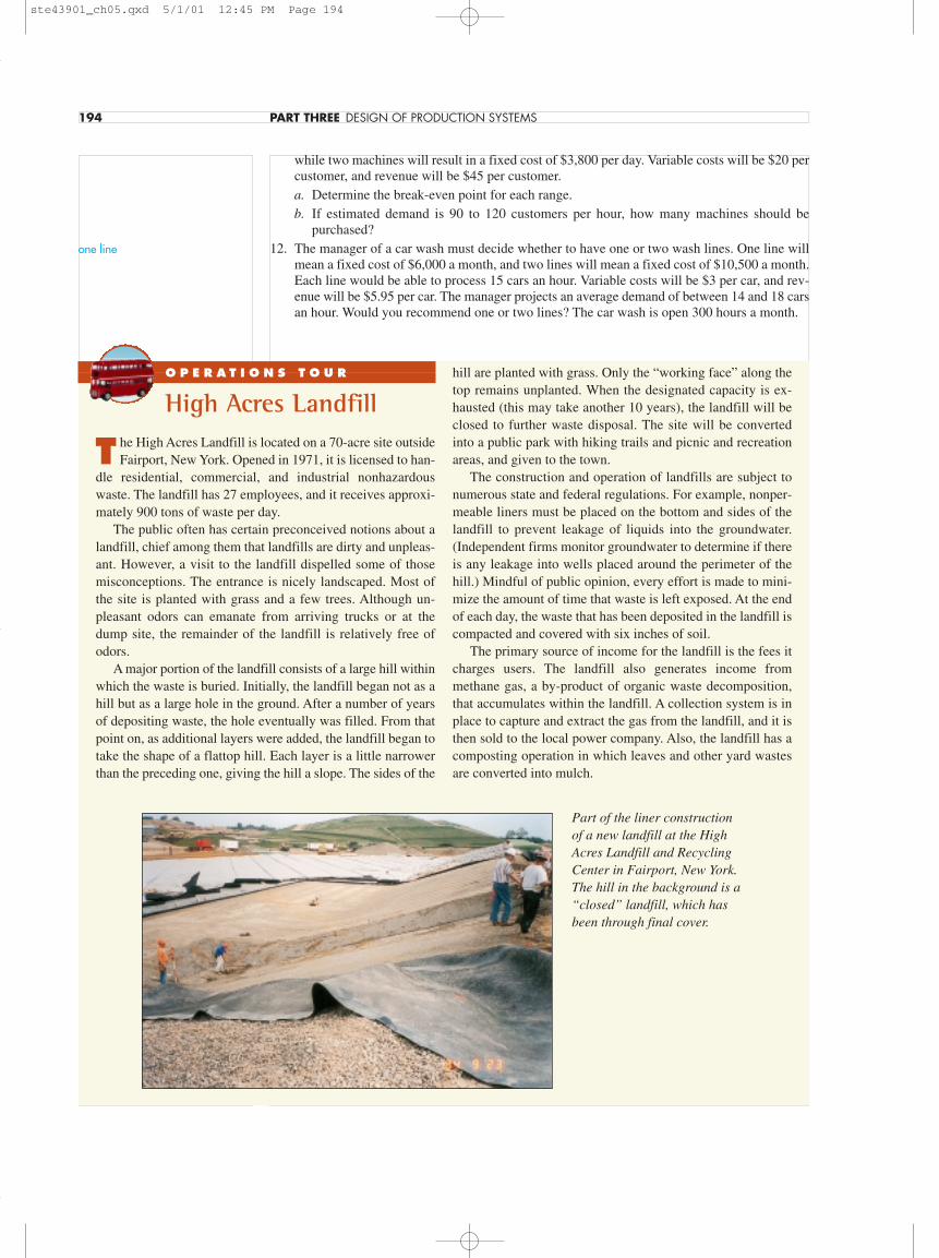
T he High Acres Landfill is located on a 70-acre site outsideFairport, New York. Opened in 1971, it is licensed to han-

dle residential, commercial, and industrial nonhazardouswaste. The landfill has 27 employees, and it receives approxi-mately 900 tons of waste per day.

The public often has certain preconceived notions about alandfill, chief among them that landfills are dirty and unpleas-ant. However, a visit to the landfill dispelled some of thosemisconceptions. The entrance is nicely landscaped. Most ofthe site is planted with grass and a few trees. Although un-pleasant odors can emanate from arriving trucks or at thedump site, the remainder of the landfill is relatively free ofodors.

A major portion of the landfill consists of a large hill withinwhich the waste is buried. Initially, the landfill began not as ahill but as a large hole in the ground. After a number of yearsof depositing waste, the hole eventually was filled. From thatpoint on, as additional layers were added, the landfill began totake the shape of a flattop hill. Each layer is a little narrowerthan the preceding one, giving the hill a slope. The sides of the

hill are planted with grass. Only the “working face” along thetop remains unplanted. When the designated capacity is ex-hausted (this may take another 10 years), the landfill will beclosed to further waste disposal. The site will be convertedinto a public park with hiking trails and picnic and recreationareas, and given to the town.

The construction and operation of landfills are subject tonumerous state and federal regulations. For example, nonper-meable liners must be placed on the bottom and sides of thelandfill to prevent leakage of liquids into the groundwater.(Independent firms monitor groundwater to determine if thereis any leakage into wells placed around the perimeter of thehill.) Mindful of public opinion, every effort is made to mini-mize the amount of time that waste is left exposed. At the endof each day, the waste that has been deposited in the landfill iscompacted and covered with six inches of soil.

The primary source of income for the landfill is the fees itcharges users. The landfill also generates income frommethane gas, a by-product of organic waste decomposition,that accumulates within the landfill. A collection system is inplace to capture and extract the gas from the landfill, and it isthen sold to the local power company. Also, the landfill has acomposting operation in which leaves and other yard wastesare converted into mulch.

O P E R A T I O N S T O U R

High Acres Landfill

Part of the liner constructionof a new landfill at the HighAcres Landfill and RecyclingCenter in Fairport, New York.The hill in the background is a“closed” landfill, which hasbeen through final cover.

ste43901_ch05.qxd 5/1/01 12:45 PM Page 194


SelectedBibliography andFurther Reading

Bolwijn, P. T., and T. Kumpe. “Manufacturing in the1990’s—Productivity, Flexibility, and Innovation.” LongRange Planning 23, no. 4 (1990), pp. 44–57.

Cohen, Morris, and Uday M. Apte. Manufacturing Automa-tion. Burr Ridge, IL: Richard D. Irwin, 1997.

Ettlie, John, and Henry Stoll, Managing the Design-Manu-facturing Process. New York: McGraw-Hill, 1990.

Hill, Terry. Manufacturing Strategy. 2nd ed. Burr Ridge, IL:Richard D. Irwin, 1994.

Monroe, Joseph. “Strategic Use of Technology.” CaliforniaManagement Review, Summer 1989, pp. 91–110.

Moore, Franklin, and Thomas E. Hendrick. Production/Op-erations Management. 9th ed. Burr Ridge, IL: RichardD. Irwin, 1985.

Upton, David. “The Management of Manufacturing Flexi-bility.” California Management Review 36, no. 2, 1994,pp. 72–89.

Upton, David. “What Really Makes Factories Flexible.”Harvard Business Review, July–August 1995, pp. 74–84.

ste43901_ch05.qxd 5/1/01 12:45 PM Page 195

SUPPLEMENT OUTLINE

Introduction, 000

Causes of Poor Decisions, 000

Decision Environments, 000

Decision Making underCertainty, 000

Decision Making underUncertainty, 000

Decision Making under Risk, 000

Decision Trees, 000

Expected Value of PerfectInformation, 000

Sensitivity Analysis, 000

Summary, 000

Key Terms, 000

Solved Problems, 000

Discussion and ReviewQuestions, 000

Problems, 000

Selected Bibliography and FurtherReading, 000

LEARNING OBJECTIVES

After completing this supplement,you should be able to:

1 Describe the differentenvironments under whichoperations decisions are made.

2 Describe and use techniques thatapply to decision making underuncertainty.

3 Describe and use the expected-value approach.

4 Construct a decision tree and useit to analyze a problem.

5 Compute the expected value ofperfect information.

6 Conduct sensitivity analysis on asimple decision problem.

SUPPLEMENT TO CHAPTER 5

Decision Theory

196

ste43901_ch05.qxd 5/1/01 12:45 PM Page 196

IntroductionDecision theory represents a general approach to decision making. It is suitable for a widerange of operations management decisions. Among them are capacity planning, productand service design, equipment selection, and location planning. Decisions that lend them-selves to a decision theory approach tend to be characterized by these elements:

1. A set of possible future conditions exists that will have a bearing on the results of thedecision.

2. A list of alternatives for the manager to choose from.

3. A known payoff for each alternative under each possible future condition.

To use this approach, a decision maker would employ this process:

1. Identify the possible future conditions (e.g., demand will be low, medium, or high; thenumber of contracts awarded will be one, two, or three; the competitor will or will notintroduce a new product). These are called states of nature.

2. Develop a list of possible alternatives, one of which may be to do nothing.

3. Determine or estimate the payoff associated with each alternative for every possiblefuture condition.

4. If possible, estimate the likelihood of each possible future condition.

5. Evaluate alternatives according to some decision criterion (e.g., maximize expectedprofit), and select the best alternative.

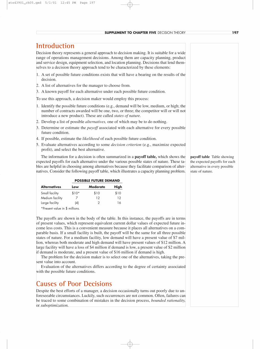
The information for a decision is often summarized in a payoff table, which shows theexpected payoffs for each alternative under the various possible states of nature. These ta-bles are helpful in choosing among alternatives because they facilitate comparison of alter-natives. Consider the following payoff table, which illustrates a capacity planning problem.

POSSIBLE FUTURE DEMAND

Alternatives Low Moderate High

Small facility $10* $10 $10Medium facility 7 12 12Large facility (4) 2 16

*Present value in $ millions.

The payoffs are shown in the body of the table. In this instance, the payoffs are in termsof present values, which represent equivalent current dollar values of expected future in-come less costs. This is a convenient measure because it places all alternatives on a com-parable basis. If a small facility is built, the payoff will be the same for all three possiblestates of nature. For a medium facility, low demand will have a present value of $7 mil-lion, whereas both moderate and high demand will have present values of $12 million. Alarge facility will have a loss of $4 million if demand is low, a present value of $2 millionif demand is moderate, and a present value of $16 million if demand is high.

The problem for the decision maker is to select one of the alternatives, taking the pre-sent value into account.

Evaluation of the alternatives differs according to the degree of certainty associatedwith the possible future conditions.

Causes of Poor DecisionsDespite the best efforts of a manager, a decision occasionally turns out poorly due to un-foreseeable circumstances. Luckily, such occurrences are not common. Often, failures canbe traced to some combination of mistakes in the decision process, bounded rationality,or suboptimization.

SUPPLEMENT TO CHAPTER FIVE DECISION THEORY 197

payoff table Table showingthe expected payoffs for eachalternative in every possiblestate of nature.

ste43901_ch05.qxd 5/1/01 12:45 PM Page 197

In many cases, managers fail to appreciate the importance of each step in the decision-making process. They may skip a step or not devote enough effort to completing it beforejumping to the next step. Sometimes this happens owing to a manager’s style of makingquick decisions or a failure to recognize the consequences of a poor decision. The man-ager’s ego can be a factor. This sometimes happens when the manager has experienced aseries of successes—important decisions that turned out right. Some managers then getthe impression that they can do no wrong. But they soon run into trouble, which is usu-ally enough to bring them back down to earth. Other managers seem oblivious to negativeresults and continue the process they associate with their previous successes, not recog-nizing that some of that success may have been due more to luck than to any special abil-ities of their own. A part of the problem may be the manager’s unwillingness to admit amistake. Yet other managers demonstrate an inability to make a decision; they stall longpast the time when the decision should have been rendered.

Of course, not all managers fall into these traps—it seems safe to say that the majority donot. Even so, this does not necessarily mean that every decision works out as expected. An-other factor with which managers must contend is bounded rationality, or the limits im-posed on decision making by costs, human abilities, time, technology, and the availabilityof information. Because of these limitations, managers cannot always expect to reach deci-sions that are optimal in the sense of providing the best possible outcome (e.g., highestprofit, least cost). Instead, they must often resort to achieving a satisfactory solution.

Still another cause of poor decisions is that organizations typically departmentalize de-cisions. Naturally, there is a great deal of justification for the use of departments in termsof overcoming span-of-control problems and human limitations. However, suboptimiza-tion can occur. This is a result of different departments attempting to reach a solution thatis optimum for each. Unfortunately, what is optimal for one department may not be opti-mal for the organization as a whole.

Decision EnvironmentsOperations management decision environments are classified according to the degree ofcertainty present. There are three basic categories: certainty, risk, and uncertainty.

Certainty means that relevant parameters such as costs, capacity, and demand haveknown values.

Risk means that certain parameters have probabilistic outcomes.

Uncertainty means that it is impossible to assess the likelihood of various possible futureevents.

Consider these situations:

1. Profit per unit is $5. You have an order for 200 units. How much profit will you make?(This is an example of certainty since unit profits and total demand are known.)

2. Profit is $5 per unit. Based on previous experience, there is a 50 percent chance of anorder for 100 units and a 50 percent chance of an order for 200 units. What is expectedprofit? (This is an example of risk since demand outcomes are probabilistic.)

3. Profit is $5 per unit. The probabilities of potential demands are unknown. (This is anexample of uncertainty.)

The importance of these different decision environments is that they require differentanalysis techniques. Some techniques are better suited for one category than for others.You should make note of the environments for which each technique is appropriate.

Decision Making under CertaintyWhen it is known for certain which of the possible future conditions will actually happen,the decision is usually relatively straightforward: Simply choose the alternative that hasthe best payoff under that state of nature. Example S-1 illustrates this.


bounded rationality The lim-itations on decision makingcaused by costs, human abili-ties, time, technology, andavailability of information.

suboptimization The result ofdifferent departments each at-tempting to reach a solutionthat is optimum for thatdepartment.

certainty Environment inwhich relevant parametershave known values.

risk Environment in whichcertain future events haveprobable outcomes.

uncertainty Environment inwhich it is impossible to assessthe likelihood of various futureevents.

ste43901_ch05.qxd 5/1/01 12:45 PM Page 198

Determine the best alternative in the preceding payoff table for each of the cases: It isknown with certainty that demand will be: (a) low, (b) moderate, (c) high.

Choose the alternative with the highest payoff. Thus, if we know demand will be low, wewould elect to build the small facility and realize a payoff of $10 million. If we know de-mand will be moderate, a medium factory would yield the highest payoff ($12 millionversus either $10 or $2 million). For high demand, a large facility would provide the high-est payoff.

Although complete certainty is rare in such situations, this kind of exercise providessome perspective on the analysis. Moreover, in some instances, there may be an opportu-nity to consider allocation of funds to research efforts, which may reduce or remove someof the uncertainty surrounding the states of nature.

Decision Making under UncertaintyAt the opposite extreme is complete uncertainty: no information is available on howlikely the various states of nature are. Under those conditions, four possible decision cri-teria are maximin, maximax, Laplace, and minimax regret. These approaches can be de-fined as follows:

Maximin—Determine the worst possible payoff for each alternative, and choose the al-ternative that has the “best worst.” The maximin approach is essentially a pessimistic onebecause it takes into account only the worst possible outcome for each alternative. The ac-tual outcome may not be as bad as that, but this approach establishes a “guaranteedminimum.”

Maximax—Determine the best possible payoff, and choose the alternative with that pay-off. The maximax approach is an optimistic, “go for it” strategy; it does not take into ac-count any payoff other than the best.

Laplace—Determine the average payoff for each alternative, and choose the alternativewith the best average. The Laplace approach treats the states of nature as equally likely.

Minimax regret—Determine the worst regret for each alternative, and choose the alter-native with the “best worst.” This approach seeks to minimize the difference between thepayoff that is realized and the best payoff for each state of nature.

The next two examples illustrate these decision criteria.

Referring to the preceding payoff table, determine which alternative would be chosen un-der each of these strategies:

a. Maximin

b. Maximax

c. Laplace

a. Using maximin, the worst payoffs for the alternatives are:

Small facility: $10 million

Medium facility: 7 million

Large facility: �4 million

Hence, since $10 million is the best, choose to build the small facility using themaximin strategy.

b. Using maximax, the best payoffs are:


Example S-1

Solution

maximin Choose the alterna-tive with the best of the worstpossible payoffs.

maximax Choose the alterna-tive with the best possible payoff.

Laplace Choose the alterna-tive with the best average pay-off of any of the alternatives.

minimax regret Choose thealternative that has the least ofthe worst regrets.

Example S-2

Solution

ste43901_ch05.qxd 5/1/01 12:45 PM Page 199

Small facility: $10 million

Medium facility: 12 million

Large facility: 16 million

The best overall payoff is the $16 million in the third row. Hence, the maximax crite-rion leads to building a large facility.

c. For the Laplace criterion, first find the row totals, and then divide each of thoseamounts by the number of states of nature (three in this case). Thus, we have:

Row Total Row Average (in $ millions) (in $ millions)

Small facility $30 $10.00Medium facility 31 10.33Large facility 14 4.67

Because the medium facility has the highest average, it would be chosen under theLaplace criterion.

Determine which alternative would be chosen using a minimax regret approach to the ca-pacity planning program.

The first step in this approach is to prepare a table of opportunity losses, or regrets. Todo this, subtract every payoff in each column from the best payoff in that column. Forinstance, in the first column, the best payoff is 10, so each of the three numbers in thatcolumn must be subtracted from 10. Going down the column, the regrets will be 10 � 10� 0, 10 � 7 � 3, and 10 � (� 4) � 14. In the second column, the best payoff is 12. Sub-tracting each payoff from 12 yields 2, 0, and 10. In the third column, 16 is the best pay-off. The regrets are 6, 4, and 0. These results are summarized in a regret table:

REGRETS (in $ millions)

Alternatives Low Moderate High Worst

Small facility $0 $2 $6 $6Medium facility 3 0 4 4Large facility 14 10 0 14

The second step is to identify the worst regret for each alternative. For the first alter-native, the worst is 6; for the second, the worst is 4; and for the third, the worst is 14.

The best of these worst regrets would be chosen using minimax regret. The lowest re-gret is 4, which is for a medium facility. Hence, that alternative would be chosen.

Solved Problem 6 at the end of this supplement illustrates decision making under un-certainty when the payoffs represent costs.

The main weakness of these approaches (except for Laplace) is that they do not takeinto account all of the payoffs. Instead, they focus on the worst or best, and so they losesome information. Still, for a given set of circumstances, each has certain merits that canbe helpful to a decision maker.

Decision Making under RiskBetween the two extremes of certainty and uncertainty lies the case of risk: The probabil-ity of occurrence for each state of nature is known. (Note that because the states are mu-tually exclusive and collectively exhaustive, these probabilities must add to 1.00.) Awidely used approach under such circumstances is the expected monetary value criterion.


Example S-3

Solution

regret The difference betweena given payoff and the bestpayoff for a state of nature.

ste43901_ch05.qxd 5/1/01 12:45 PM Page 200

The expected value is computed for each alternative, and the one with the highest ex-pected value is selected. The expected value is the sum of the payoffs for an alternativewhere each payoff is weighted by the probability for the relevant state of nature. Thus, theapproach is:

Expected monetary value (EMV) criterion—Determine the expected payoff of each al-ternative, and choose the alternative that has the best expected payoff.

Using the expected monetary value criterion, identify the best alternative for the previouspayoff table for these probabilities: low � .30, moderate � .50, and high � .20.

Find the expected value of each alternative by multiplying the probability of occurrencefor each state of nature by the payoff for that state of nature and summing them:

EVsmall � .30($10) � .50($10) � .20($10) � $10

EVmedium � .30($7) � .50($12) � .20($12) � $10.5

EVlarge � .30(–4) � .50($2) � .20($16) � $3

Hence, choose the medium facility because it has the highest expected value.

The expected monetary value approach is most appropriate when a decision maker isneither risk averse nor risk seeking, but is risk neutral. Typically, well-established organi-zations with numerous decisions of this nature tend to use expected value because it pro-vides an indication of the long-run, average payoff. That is, the expected-value amount(e.g., $10.5 million in the last example) is not an actual payoff but an expected or averageamount that would be approximated if a large number of identical decisions were to bemade. Hence, if a decision maker applies this criterion to a large number of similar deci-sions, the expected payoff for the total will approximate the sum of the individual ex-pected payoffs.

Decision TreesA decision tree is a schematic representation of the alternatives available to a decisionmaker and their possible consequences. The term gets its name from the treelike appearanceof the diagram (see Figure 5S–1). Although tree diagrams can be used in place of a payofftable, they are particularly useful for analyzing situations that involve sequential decisions.


expected monetary value(EMV) criterion The bestexpected value among thealternatives.

decision tree A schematic rep-resentation of the available al-ternatives and their possibleconsequences.

Example S-4

Solution

State of nature 1

State of nature 2

State of nature 1

State of nature 2

Payoff 1

Payoff 2

Payoff 3

Payoff 4

Payoff 5

Payoff 6

2

2

Choose A'1

Choose A'2

1

Choose A1

Choose A2

Initialdecision

Possibleseconddecisions

Choose A'3

Choose A'4

Decision point Chance event

FIGURE 5S–1

Format of a decision tree

ste43901_ch05.qxd 5/1/01 12:45 PM Page 201

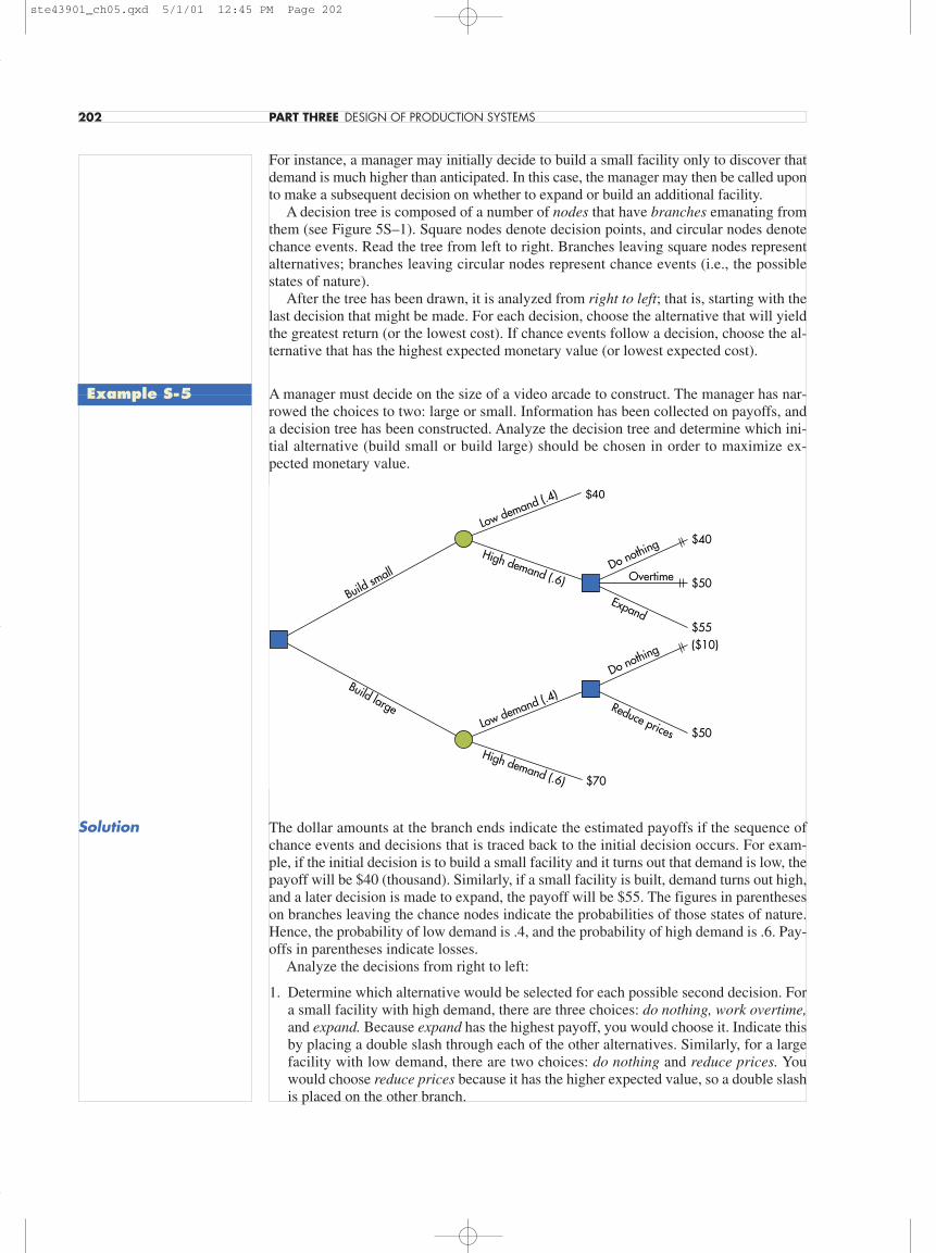
For instance, a manager may initially decide to build a small facility only to discover thatdemand is much higher than anticipated. In this case, the manager may then be called uponto make a subsequent decision on whether to expand or build an additional facility.

A decision tree is composed of a number of nodes that have branches emanating fromthem (see Figure 5S–1). Square nodes denote decision points, and circular nodes denotechance events. Read the tree from left to right. Branches leaving square nodes representalternatives; branches leaving circular nodes represent chance events (i.e., the possiblestates of nature).

After the tree has been drawn, it is analyzed from right to left; that is, starting with thelast decision that might be made. For each decision, choose the alternative that will yieldthe greatest return (or the lowest cost). If chance events follow a decision, choose the al-ternative that has the highest expected monetary value (or lowest expected cost).

A manager must decide on the size of a video arcade to construct. The manager has nar-rowed the choices to two: large or small. Information has been collected on payoffs, anda decision tree has been constructed. Analyze the decision tree and determine which ini-tial alternative (build small or build large) should be chosen in order to maximize ex-pected monetary value.

The dollar amounts at the branch ends indicate the estimated payoffs if the sequence ofchance events and decisions that is traced back to the initial decision occurs. For exam-ple, if the initial decision is to build a small facility and it turns out that demand is low, thepayoff will be $40 (thousand). Similarly, if a small facility is built, demand turns out high,and a later decision is made to expand, the payoff will be $55. The figures in parentheseson branches leaving the chance nodes indicate the probabilities of those states of nature.Hence, the probability of low demand is .4, and the probability of high demand is .6. Pay-offs in parentheses indicate losses.

Analyze the decisions from right to left:

1. Determine which alternative would be selected for each possible second decision. Fora small facility with high demand, there are three choices: do nothing, work overtime,and expand. Because expand has the highest payoff, you would choose it. Indicate thisby placing a double slash through each of the other alternatives. Similarly, for a largefacility with low demand, there are two choices: do nothing and reduce prices. Youwould choose reduce prices because it has the higher expected value, so a double slashis placed on the other branch.

Low demand (.4)

High demand (.6)

$40

Do nothing

Expand

Build small

Build large

Overtime

Do nothing

Reduce pricesLow demand (.4)

High demand (.6)

$50

$55($10)

$50

$40

$70


Example S-5

Solution

ste43901_ch05.qxd 5/1/01 12:45 PM Page 202

2. Determine the product of the chance probabilities and their respective payoffs for theremaining branches:

Build small

Low demand .4($40) � $16

High demand .6($55) � 33

Build large

Low demand .4($50) � 20

High demand .6($70) � 42

3. Determine the expected value of each initial alternative:

Build small $16 � $33 � $49

Build large $20 � $42 � $62

Hence, the choice should be to build the large facility because it has a larger expectedvalue than the small facility.

Expected Value of Perfect InformationIn certain situations, it is possible to ascertain which state of nature will actually occur inthe future. For instance, the choice of location for a restaurant may weigh heavily onwhether a new highway will be constructed or whether a zoning permit will be issued. Adecision maker may have probabilities for these states of nature; however, it may be pos-sible to delay a decision until it is clear which state of nature will occur. This might in-volve taking an option to buy the land. If the state of nature is favorable, the option canbe exercised; if it is unfavorable, the option can be allowed to expire. The question to con-sider is whether the cost of the option will be less than the expected gain due to delayingthe decision (i.e., the expected payoff above the expected value). The expected gain is theexpected value of perfect information, or EVPI.

Expected value of perfect information (EVPI)—the difference between the expectedpayoff with perfect information and the expected payoff under risk.

Other possible ways of obtaining perfect information depend somewhat on the nature ofthe decision being made. Information about consumer preferences might come from mar-ket research, additional information about a product could come from product testing, orlegal experts might be called on.

There are two ways to determine the EVPI. One is to compute the expected payoff un-der certainty and subtract the expected payoff under risk. That is,

Expected value of Expected payoff Expected payoff � � (5S–1)perfect information under certainty under risk

Using the information from Example S-4, determine the expected value of perfect infor-mation using Formula 5S–1.

First, compute the expected payoff under certainty. To do this, identify the best payoff un-der each state of nature. Then combine these by weighting each payoff by the probabilityof that state of nature and adding the amounts. Thus, the best payoff under low demand is$10, the best under moderate demand is $12, and the best under high demand is $16. Theexpected payoff under certainty is, then:

.30($10) � .50($12) � .20($16) � $12.2


expected value of perfect in-formation (EVPI) The differ-ence between the expectedpayoff with perfect informationand the expected payoff underrisk.

Example S-6

Solution

ste43901_ch05.qxd 5/1/01 12:45 PM Page 203

The expected payoff under risk, as computed in Example 4, is $10.5. The EVPI is the dif-ference between these:

EVPI � $12.2 � $10.5 � $1.7

This figure indicates the upper limit on the amount the decision maker should be willingto spend to obtain perfect information in this case. Thus, if the cost equals or exceeds thisamount, the decision maker would be better off not spending additional money and sim-ply going with the alternative that has the highest expected payoff.

A second approach is to use the regret table to compute the EVPI. To do this, find theexpected regret for each alternative. The minimum expected regret is equal to the EVPI.

Determine the expected value of perfect information for the capacity-planning problemusing the expected regret approach.

Using information from Examples 2, 3, and 4, we can compute the expected regret foreach alternative. Thus:

Small facility .30(0) � .50(2) � .20(6) � 2.2

Medium facility .30(3) � .50(0) � .20(4) � 1.7 [minimum]

Large facility .30(14) � .50(10) � .20(0) � 9.2

The lowest expected regret is 1.7, which is associated with the second alternative. Hence,the EVPI is $1.7 million, which agrees with the previous example using the otherapproach.

Sensitivity AnalysisGenerally speaking, both the payoffs and the probabilities in this kind of a decision prob-lem are estimated values. Consequently, it can be useful for the decision maker to havesome indication of how sensitive the choice of an alternative is to changes in one or moreof these values. Unfortunately, it is impossible to consider all possible combinations ofevery variable in a typical problem. Nevertheless, there are certain things a decisionmaker can do to judge the sensitivity of probability estimates.

Sensitivity analysis provides a range of probability over which the choice of alternativewould remain the same. The approach illustrated here is useful when there are two states ofnature. It involves constructing a graph and then using algebra to determine a range of prob-abilities for which a given solution is best. In effect, the graph provides a visual indicationof the range of probability over which the various alternatives are optimal, and the algebraprovides exact values of the endpoints of the ranges. Example 8 illustrates the procedure.

Given the following table, determine the range of probability for state of nature #2, thatis, P(2), for which each alternative is optimal under the expected-value approach.

STATE OFNATURE

#1 #2

A 4 12Alternative B 16 2

C 12 8

First, plot each alternative relative to P(2). To do this, plot the #1 value on the left side ofthe graph and the #2 value on the right side. For instance, for alternative A, plot 4 on the


Example S-7

Solution

sensitivity analysisDetermining the range ofprobability for which analternative has the bestexpected payoff.

Example S-8

Solution

ste43901_ch05.qxd 5/1/01 12:45 PM Page 204

left side of the graph and 12 on the right side. Then connect these two points with astraight line. The three alternatives are plotted on the graph as shown below.

The graph shows the range of values of P(2) over which each alternative is optimal.Thus, for low values of P(2) [and thus high values of P(1), since P(1) � P(2) � 1.0], al-ternative B will have the highest expected value; for intermediate values of P(2), alterna-tive C is best; and for higher values of P(2), alternative A is best.

To find exact values of the ranges, determine where the upper parts of the lines intersect.Note that at the intersections, the two alternatives represented by the lines would be equiv-alent in terms of expected value. Hence, the decision maker would be indifferent betweenthe two at that point. To determine the intersections, you must obtain the equation of eachline. This is relatively simple to do. Because these are straight lines, they have the form y� a � bx, where a is the y-intercept value at the left axis, b is the slope of the line, and xis P(2). Slope is defined as the change in y for a one-unit change in x. In this type of prob-lem, the distance between the two vertical axes is 1.0. Consequently, the slope of each lineis equal to the right-hand value minus the left-hand value. The slopes and equations are:

#1 #2 Slope Equation

A 4 12 12 � 4 � � 8 4 � 8P(2)B 16 2 2 � 16 � �14 16 � 14P(2)C 12 8 8 � 12 � � 4 12 � 4P(2)

From the graph, we can see that alternative B is best from P(2) � 0 to the point wherethat straight line intersects the straight line of alternative C, and that begins the regionwhere C is better. To find that point, solve for the value of P(2) at their intersection. Thisrequires setting the two equations equal to each other and solving for P(2). Thus,

16 � 14P(2) � 12 � 4P(2)

Rearranging terms yields

4 � 10P(2)

Solving yields P(2) � .40. Thus, alternative B is best from P(2) � 0 up to P(2) � .40.B and C are equivalent at P(2) � .40.

Alternative C is best from that point until its line intersects alternative A’s line. To findthat intersection, set those two equations equal and solve for P(2). Thus,

4 � 8P(2) � 12 � 4P(2)

Rearranging terms results in

12P(2) � 8

16

14

12

10

8

6

4

2

0 1.0.8.6.4.2

#1Payoff

16

14

12

10

8

6

4

2

#2Payoff

B

CA

P (2)

B best A bestC best


ste43901_ch05.qxd 5/1/01 12:45 PM Page 205

Solving yields P(2) � .67. Thus, alternative C is best from P(2) � .40 up to P(2) � .67,where A and C are equivalent. For values of P(2) greater than .67 up to P(2) � 1.0, A isbest.

Note: If a problem calls for ranges with respect to P(1), find the P(2) ranges as above,and then subtract each P(2) from 1.00 (e.g., .40 becomes .60, and .67 becomes .33).

Summary

Decision making is an integral part of operations management.Decision theory is a general approach to decision making that is useful in many different aspects

of operations management. Decision theory provides a framework for the analysis of decisions. Itincludes a number of techniques that can be classified according to the degree of uncertainty asso-ciated with a particular decision problem. Two visual tools useful for analyzing some decisionproblems are decision trees and graphical sensitivity analysis.


Key Terms bounded rationality, 000certainty, 000decision tree, 000expected monetary value (EMV) criterion, 000expected value of perfect information

(EVPI), 000Laplace, 000maximax, 000maximin, 000

minimax regret, 000opportunity losses, 000payoff table, 000regret, 000risk, 000sensitivity analysis, 000suboptimization, 000uncertainty, 000

Solved Problems The following solved problems refer to this payoff table:

New No Bridge NewBuilt Bridge

Alternative capacity A 1 14for new store B 2 10

C 4 6where A � small, B � medium, and C � large.

Assume the payoffs represent profits. Determine the alternative that would be chosen undereach of these decision criteria:

a. Maximin.b. Maximax.c. Laplace.

New No New Maximin Maximax Laplace Bridge Bridge (worst) (best) (average)

A 1 14 1 14 [best] 15 � 2 � 7.5 [best]B 2 10 2 10 12 � 2 � 6C 4 6 4 [best] 6 10 � 2 � 5

Thus, the alternatives chosen would be C under maximin, A under maximax, and A under Laplace.

Using graphical sensitivity analysis, determine the probability for no new bridge for which eachalternative would be optimal.

Problem 1

Solution

Problem 2

Summary

ste43901_ch05.qxd 5/1/01 12:45 PM Page 206


Plot a straight line for each alternative. Do this by plotting the payoff for new bridge on the leftaxis and the payoff for no new bridge on the right axis and then connecting the two points. Eachline represents the expected profit for an alternative for the entire range of probability of no newbridge. Because the lines represent expected profit, the line that is highest for a given value ofP (no new bridge) is optimal. Thus, from the graph, you can see that for low values of this prob-ability, alternative C is best, and for higher values, alternative A is best (B is never the highestline, so it is never optimal).

The dividing line between the ranges where C and A are optimal occurs where the two linesintersect. To find that probability, first formulate the equation for each line. To do this, let the in-tersection with the left axis be the y intercept; the slope equals the right-side payoff minus theleft-side payoff. Thus, for C you have 4 � (6 � 4)P, which is 4 � 2P. For A, 1 � (14 � 1)P,which is 1 � 13P. Setting these two equal to each other, you can solve for P:

4 � 2P � 1 � 13P

Solving, P � .27. Therefore, the ranges for P(no new bridge) are:

A: .27 � P 1.00B: never optimalC: 0 P � .27

Using the information in the payoff table, develop a table of regrets, and then:

a. Determine the alternative that would be chosen under minimax regret.b. Determine the expected value of perfect information using the regret table, assuming that the

probability of a new bridge being built is .60.

To obtain the regrets, subtract all payoffs in each column from the best payoff in the column.The regrets are:

New No New Bridge Bridge

A 3 0B 2 4C 0 8

a. Minimax regret involves finding the worst regret for each alternative and then choosing thealternative that has the “best” worst. Thus, you would choose A:

4

21

0 1.0

Payoff fornew bridge 14

10

6

0

Payoff forno newbridge

A

A bestC best

B

C

.27P (no new bridge)


Solution

Solution

Problem 3

ste43901_ch05.qxd 5/1/01 12:45 PM Page 207


Worst

A 3 [best]B 4C 8

b. Once the regret table has been developed, you can compute the EVPI as the smallest ex-pected regret. Since the probability of a new bridge is given as .60, we can deduce that theprobability of no new bridge is 1.00 � .60 � .40. The expected regrets are:

A: .60(3) � .40(0) � 1.80B: .60(2) � .40(4) � 2.80C: .60(0) � .40(8) � 3.20

Hence, the EVPI is 1.80.

Using the probabilities of .60 for a new bridge and .40 for no new bridge, compute the expectedvalue of each alternative in the payoff table, and identify the alternative that would be selectedunder the expected-value approach.

A: .60(1) � .40(14) � 6.20 [best]B: .60(2) � .40(10) � 5.20C: .60(4) � .40(6) � 4.80

Compute the EVPI using the information from the previous problem.

Using formula (5S–1), the EVPI is the expected payoff under certainty minus the maximum ex-pected value. The expected payoff under certainty involves multiplying the best payoff in eachcolumn by the column probability and then summing those amounts. The best payoff in the firstcolumn is 4, and the best in the second is 14. Thus,

Expected payoff under certainty � .60(4) � .40(14) � 8.00

Then

EVPI � 8.00 � 6.20 � 1.80

(This agrees with the result obtained in Solved Problem 3b.)

Excel solution:

Problem 4

Solution

Problem 5

Solution

ste43901_ch05.qxd 5/1/01 12:45 PM Page 208


Placing the problem data in the cell positions shown, the expected monetary value (EMV) foreach alternative is shown in column J.

Then, the overall EMV is obtained in column J as the maximum of the values in J6, J7, and J8.The EVPI is obtained using the Opportunity Loss Table by summing the product of the max-

imum in column C4 and the probability in C4, and the product of the maximum in column Dand the probability in D4.

Suppose that the values in the payoff table represent costs instead of profits.a. Determine the choice that you would make under each of these strategies: maximin, min-

imin, and Laplace.b. Develop the regret table, and identify the alternative chosen using minimax regret. Then find

the EVPI if P(new bridge) � .60.c. Using sensitivity analysis, determine the range of P(no new bridge) for which each alterna-

tive would be optimal.d. If P(new bridge) � .60 and P(no new bridge) � .40, find the alternative chosen to minimize

expected cost.

a. Note: Minimin is the reverse of maximax; for costs minimin identifies the lowest (best) cost.

New No New Maximin Minimin Laplace Bridge Bridge (worst) (best) (average)

A 1 14 14 1 [best] 15 � 2 � 7.5B 2 10 10 2 12 � 2 � 6C 4 6 6 [best] 4 10 � 2 � 5 [best]

b. Develop the regret table by subtracting the lowest cost in each column from each of the val-ues in the column. (Note that none of the values is negative.)

New No NewBridge Bridge Worst

A 0 8 8B 1 4 4C 3 0 3 [best]

EVPI � .60(3) � .40(0) � 1.80

c. The graph is identical to that shown in Solved Problem 2. However, the lines now representexpected costs, so the best alternative for a given value of P(no new bridge) is the lowestline. Hence, for very low values of P(no new bridge), A is best; for intermediate values, B isbest; and for high values, C is best. You can set the equations of A and B, and B and C, equalto each other in order to determine the values of P(no new bridge) at their intersections.Thus,

A � B: 1 � 13P � 2 � 8P; solving, P � .20B � C: 2 � 8P � 4 � 2P; solving, P � .33

Hence, the ranges are:

A best: 0 P � .20B best: .20 � P � .33C best: .33 � P 1.00

d. Expected-value computations are the same whether the values represent costs or profits.Hence, the expected payoffs for costs are the same as the expected payoffs for profits thatwere computed in Solved Problem 4. However, now you want the alternative that has thelowest expected payoff rather than the one with the highest payoff. Consequently, alternativeC is the best because its expected payoff is the lowest of the three.

Solution

Problem 6

ste43901_ch05.qxd 5/1/01 12:46 PM Page 209


1. What is the chief role of the operations manager?

4

21

0 1.0

Cost withnew bridge 14

10

6

0

Cost withno newbridge

A

C best

B

C

.20P (no new bridge)

.33

Bbest

Abest

Discussion and Review Questions

2. List the steps in the decision-making process.3. Explain the term bounded rationality.4. Explain the term suboptimization.5. What are some of the reasons for poor decisions?6. What information is contained in a payoff table?7. What is sensitivity analysis, and how can it be useful to a decision maker?8. Contrast maximax and maximin decision strategies. Under what circumstances is each

appropriate?9. Under what circumstances is expected monetary value appropriate as a decision criterion?

When isn’t it appropriate?10. Explain or define each of these terms:

a. Laplace criterion.b. Minimax regret.c. Expected value.d. Expected value of perfect information.

11. What information does a decision maker need in order to perform an expected-value analysis ofa problem? What options are available to the decision maker if the probabilities of the states ofnature are unknown? Can you think of a way you might use sensitivity analysis in such a case?

12. Suppose a manager is using maximum EMV as a basis for making a capacity decision and, inthe process, obtains a result in which there is a virtual tie between two of the seven alterna-tives. How is the manager to make a decision?

Problems 1. A small building contractor has recently experienced two successive years in which work op-portunities exceeded the firm’s capacity. The contractor must now make a decision on capac-ity for next year. Estimated profits under each of the two possible states of nature are as shownin the table below. Which alternative should be selected if the decision criterion is:

ste43901_ch05.qxd 5/1/01 12:46 PM Page 210

a. Maximax?b. Maximin?c. Laplace?d. Minimax regret?

NEXT YEAR’S DEMAND

Alternative Low High

Do nothing $50* $60Expand 20 80Subcontract 40 70

*Profit in $ thousands.

2. Refer to Problem 1. Suppose after a certain amount of discussion, the contractor is able to sub-jectively assess the probabilities of low and high demand: P(low) � .3 and P(high) � .7.a. Determine the expected profit of each alternative. Which alternative is best? Why?b. Analyze the problem using a decision tree. Show the expected profit of each alternative on

the tree.c. Compute the expected value of perfect information. How could the contractor use this

knowledge?3. Refer to Problems 1 and 2. Construct a graph that will enable you to perform sensitivity analy-

sis on the problem. Over what range of P(high) would the alternative of doing nothing be best?Expand? Subcontract?

4. A firm that plans to expand its product line must decide whether to build a small or a large fa-cility to produce the new products. If it builds a small facility and demand is low, the net pre-sent value after deducting for building costs will be $400,000. If demand is high, the firm caneither maintain the small facility or expand it. Expansion would have a net present value of$450,000, and maintaining the small facility would have a net present value of $50,000.

If a large facility is built and demand is high, the estimated net present value is $800,000.If demand turns out to be low, the net present value will be �$10,000.

The probability that demand will be high is estimated to be .60, and the probability of lowdemand is estimated to be .40.a. Analyze using a tree diagram.b. Compute the EVPI. How could this information be used?c. Determine the range over which each alternative would be best in terms of the value of

P(demand low).5. Determine the course of action that has the highest expected payoff for the following decision

tree.6. The lease of Theme Park, Inc., is about to expire. Management must decide whether to renew

the lease for another 10 years or to relocate near the site of a proposed motel. The town plan-ning board is currently debating the merits of granting approval to the motel. A consultant hasestimated the net present value of Theme Park’s two alternatives under each state of nature asshown below. What course of action would you recommend using:a. Maximax?b. Maximin?c. Laplace?d. Minimax regret?

Motel MotelOptions Approved Rejected

Renew $ 500,000 $4,000,000Relocate 5,000,000 100,000


a. Expand ($80 is best payoff)b. Do nothing 50

Expand 20Subcontract 40

c. Do nothing 55Expand 50Subcontract 55

d.Low High Worst

Do nothing 0 20 20Expand 30 0 30Sub-contract 10 10 10

a. Expected profitDo nothing 57Expand 62Subcontract 61

c. EPC: 71Expected profit 62

EVPI: 9

Do nothing 0 to � .50Expand � .67 to 1.00Subcontract � .50 to .67

a. Graph in IMLarge $476,000Small $430,000

b. EPC $640,000EPR 476,000

EVPI $164,000c. Graph in IM

small: 0 to .46large: .46 to 1

Subcontract $1.23Expand $1.57Build $1.35

a. Renew $4,000,000Relocate $5,000,000*

b. Renew $500,000*Relocate $100,000

c. Renew $2,250,000Relocate $2,550,000*

d. Renew $4,500,000Relocate $3,900,000*

ste43901_ch05.qxd 5/1/01 12:46 PM Page 211

7. Refer to Problem 6. Suppose that the management of Theme Park, Inc., has decided that thereis a .35 probability that the motel’s application will be approved.a. If management uses maximum expected monetary value as the decision criterion, which al-

ternative should it choose?b. Represent this problem in the form of a decision tree.c. If management has been offered the option of a temporary lease while the town planning

board considers the motel’s application, would you advise management to sign the lease?The lease will cost $24,000.

8. Construct a graph that can be used for sensitivity analysis for the preceding problem.a. How sensitive is the solution to the problem in terms of the probability estimate of .35?b. Suppose that, after consulting with a member of the town planning board, management de-

cides that an estimate of approval is approximately .45. How sensitive is the solution to thisrevised estimate? Explain.

c. Suppose the management is confident of all the estimated payoffs except for $4 million. Ifthe probability of approval is .35, for what range of payoff for renew/rejected will the al-ternative selected using maximum expected value remain the same?

Subc

ontra

ct

ExpandSmall demand (.4)

Large demand (.1)

Small demand (.4)

Medium demand (.5) Large demand (.1)

Medium demand (.5)

Medium demand (.5)

Large demand (.1)

Do nothing

* Net present value in millions

Other use #2

Do nothing

Other use #1

Other use #2

Do nothing

Subcontract

Build

Do nothing

Other use #1

Other use #2

Do nothing

Expand

Build

Do nothing

Expand

$1.0*

$1.3

$1.3

$1.5

$1.6

$1.8

$0.7

$1.5

$1.0

$1.6

$1.6

$1.5

$1.7

($0.9)

$1.4

$1.0

$1.0

$1.1

$0.9

$2.4

Build

Other use #1

Small

deman

d (.4)


ffff yyyy iiii ttttoooo PPPPRRRR////CCCCllll iiii eeeennnntttt ::::For problem 5, theart will not fit imme-diately after the text.Please advise. Fornow I put it at top offollowing page, butif it stays here thetext should refer toit.

COMP

a. Renew $2,775,000Relocate $1,815,000Decision: Renew lease

b. Graph in IMc. EVPI � $1,575,000

Sign lease

a, b: Break-even probability of46%

c. Range is $2,523,077 or more

ste43901_ch05.qxd 5/1/01 12:46 PM Page 212

9. A firm must decide whether to construct a small, medium, or large stamping plant. A consul-tant’s report indicates a .20 probability that demand will be low and an .80 probability that de-mand will be high.

If the firm builds a small facility and demand turns out to be low, the net present value willbe $42 million. If demand turns out to be high, the firm can either subcontract and realize thenet present value of $42 million or expand greatly for a net present value of $48 million.

The firm could build a medium-size facility as a hedge: If demand turns out to be low, itsnet present value is estimated at $22 million; if demand turns out to be high, the firm could donothing and realize a net present value of $46 million, or it could expand and realize a net pre-sent value of $50 million.

If the firm builds a large facility and demand is low, the net present value will be �$20 mil-lion, whereas high demand will result in a net present value of $72 million.a. Analyze this problem using a decision tree.b. What is the maximin alternative?c. Compute the EVPI and interpret it.d. Perform sensitivity analysis on P(high).

10. A manager must decide how many machines of a certain type to buy. The machines will beused to manufacture a new gear for which there is increased demand. The manager has nar-rowed the decision to two alternatives: buy one machine or buy two. If only one machine ispurchased and demand is more than it can handle, a second machine can be purchased at a latertime. However, the cost per machine would be lower if the two machines were purchased atthe same time.

The estimated probability of low demand is .30, and the estimated probability of high de-mand is .70.

The net present value associated with the purchase of two machines initially is $75,000 ifdemand is low and $130,000 if demand is high.

The net present value for one machine and low demand is $90,000. If demand is high, thereare three options. One option is to do nothing, which would have a net present value of $90,000.A second option is to subcontract; that would have a net present value of $110,000. The third op-tion is to purchase a second machine. This option would have a net present value of $100,000.

How many machines should the manager purchase initially? Use a decision tree to analyzethis problem.

11. Determine the course of action that has the highest EMV for the accompanying tree diagram.

45(45)

99

4 0

50

30

1/31/31/3

40

50

1/2

1/2

.30

.20

.50

.30

.20

.50

600

90

4 0

4 4

60

1/31/31/3

AlternativeA

Alternative B


a. Figure in IMb. Build large: $53.6 million

Build small: $42 millionc. EPC � $66.0

EVPI � $12.4d. P(high) � x

Small: 42 � 6xMedium: 22 � 28xLarge: �20 � 92xSmall and large EVSame for x � 0.7209

Graph in IM

Buy 2 machines$113,500

Alt. A: 22Alt. B: 25Choose Alt. B

ste43901_ch05.qxd 5/1/01 12:46 PM Page 213

12. A firm that plans to expand its product line must decide whether to build a small or a largefacility to produce the new products. If it builds a small facility and demand is low, the netpresent value after deducting for building costs will be $400,000. If demand is high, the firmcan either maintain the small facility or expand it. Expansion would have a net present valueof $450,000, and maintaining the small facility would have a net present value of $50,000.

If a large facility is built and demand is high, the estimated net present value is $800,000.If demand turns out to be low, the net present value will be �$10,000.

The probability that demand will be high is estimated to be .60, and the probability of lowdemand is estimated to be .40.

Analyze using a tree diagram.13. The director of social services of a county has learned that the state has mandated additional

information requirements. This will place an additional burden on the agency. The director hasidentified three acceptable alternatives to handle the increased workload. One alternative is toreassign present staff members, the second is to hire and train two new workers, and the thirdis to redesign current practice so that workers can readily collect the information with little ad-ditional effort. An unknown factor is the caseload for the coming year when the new data willbe collected on a trial basis. The estimated costs for various options and caseloads are shownin the following table:

CASELOAD

Moderate High Very High

Reassign staff $50* 60 85New staff 60 60 60Redesign collection 40 50 90

*Cost in $ thousands.

Assuming that past experience has shown the probabilities of various caseloads to be unreli-able, what decision would be appropriate using each of the following criteria?a. Maximin.b. Maximax.c. Minimax regret.d. Laplace.

14. After contemplating the caseload question (see previous problem), the director of social ser-vices has decided that reasonable caseload probabilities are .10 for moderate, .30 for high, and.60 for very high.a. Which alternative will yield the minimum expected cost?b. Construct a decision tree for this problem. Indicate the expected costs for the three decision

branches.c. Determine the expected value of perfect information using an opportunity loss table.

15. Suppose the director of social services has the option of hiring an additional staff member ifone staff member is hired initially and the caseload turns out to be high or very high. Underthat plan, the first entry in row 2 of the cost table (see Problem 13) will be 40 instead of 60, thesecond entry will be 75, and the last entry will be 80. Assume the caseload probabilities are asnoted in Problem 14. Construct a decision tree that shows the sequential nature of this deci-sion, and determine which alternative will minimize expected cost.

16. A manager has compiled estimated profits for various capacity alternatives but is reluctant toassign probabilities to the states of nature. The payoff table is:

STATE OF NATURE

#1 #2

A $ 20* 140Alternative B 120 80

C 100 40



Graph in IMLarge $476,000Small $430,000

Worst Best Avg.

Reassign 85 50 65New staff 60 60 60Redesign 90 40 60

a. New staffb. Redesignc. Table in IM

New staffd. (tie) New staff or redesign

a. Reassign $74New staff $60Redesign $73

b. Figure in IMc. EOL

Reassign 19New staff 5Redesign 18

Figure in IM

ste43901_ch05.qxd 5/1/01 12:46 PM Page 214

a. Plot the expected-value lines on a graph.b. Is there any alternative that would never be appropriate in terms of maximizing expected

profit? Explain on the basis of your graph.c. For what range of P(2) would alternative A be the best choice if the goal is to maximize

expected profit?d. For what range of P(1) would alternative A be the best choice if the goal is to maximize

expected profit?

17. Repeat all parts of Problem 16, assuming the values in the payoff table are estimated costs andthe goal is to minimize expected costs.

18. The research staff of a marketing agency has assembled the following payoff table of estimatedprofits:

Receive Not Receive Contract Contract

#1 $10* �2

Proposal #2 8 3#3 5 5#4 0 7


Relative to the probability of not receiving the contract, determine the range of probability forwhich each of the proposals would maximize expected profit.

19. Given this payoff table:

STATE OF NATURE

#1 #2

A $120* 20

Alternative B 60 40C 10 110D 90 90


a. Determine the range of P(1) for which each alternative would be best, treating the payoffsas profits.

b. Answer part a treating the payoffs as costs.


a. Figure in IMb. C is always lower than B.

C is never appropriate.c. P (2) � .625d. P (1) � .375

b. B is not appropriatec. P(2) � .444d. P(1) � .556

EV1 � 10 � 12PEV2 � 8 � 5PEV3 � 5 � 0PEV4 � 0 � 7P1: 0 P (2) � .2862: .286 � P (2) � .603: .60 � P (2) � .7144: .714 � P (2) 1.0

a. A: .70 � P (1) 1.00B: neverC: 0 P (1) � .20D: .20 � P (1) � .70

b. A: 0 P (1) � .25B: .25 � P (1) � .583C: .583 � P (1) 1.00D: never

Bierman, Harold, Charles P. Bonini, and Warren H. Haus-man. Quantitative Analysis for Business Decisions. 8thed. Burr Ridge, IL: Richard D. Irwin, 1991.

Eppen, G. D., F. J. Gould, C. P. Schmidt, Jeffrey H. Moore,and Larry R. Weatherford. Introductory ManagementScience. 5th ed. Upper Saddle River, NJ: Prentice Hall,1998.

Stevenson, William J. Introduction to Management Science.3rd ed. Burr Ridge, IL: Richard D. Irwin, 1998.

Taylor, Bernard W. Introduction to Management Science. 6thed. Dubuque, Iowa: William C. Brown, 1999.

Turban, Efraim, and Jack Meredith. Fundamentals of Man-agement Science. New York: McGraw-Hill, 1998

Selected Bibliography andFurther Reading

ste43901_ch05.qxd 5/1/01 12:46 PM Page 215


ste43901_ch05.qxd 5/1/01 12:46 PM Page 216

ste43901 ch05.qxd 5/1/01 12:45 PM Page 172highered.mheducation.com/.../21708/ste43901_ch05qxd.pdfste43901_ch05.qxd 5/1/01 12:45 PM Page 176 Thus, compared with the effective capacity

Documents