ANL/LWRS-13/3 Status Report on Assessment of Environmentally Assisted Fatigue for LWR Extended Service Conditions Nuclear Engineering Division

Welcome message from author
This document is posted to help you gain knowledge. Please leave a comment to let me know what you think about it! Share it to your friends and learn new things together.
Transcript
ANL/LWRS-13/3
Status Report on Assessment of Environmentally
Assisted Fatigue for LWR Extended Service
Conditions
Nuclear Engineering Division
About Argonne National Laboratory Argonne is a U.S. Department of Energy laboratory managed by UChicago Argonne, LLC under contract DE-AC02-06CH11357. The Laboratory’s main facility is outside Chicago, at 9700 South Cass Avenue, Argonne, Illinois 60439. For information about Argonne and its pioneering science and technology programs, see www.anl.gov.
DOCUMENT AVAILABILITY
Online Access: U.S. Department of Energy (DOE) reports produced after 1991 and a growing number of pre-1991 documents are available free via DOE’s SciTech Connect (http://www.osti.gov/scitech/)
Reports not in digital format may be purchased by the public from the National Technical Information Service (NTIS):
U.S. Department of Commerce National Technical Information Service 5301 Shawnee Rd Alexandria, VA 22312 www.ntis.gov Phone: (800) 553-NTIS (6847) or (703) 605-6000 Fax: (703) 605-6900 Email: [email protected]
Reports not in digital format are available to DOE and DOE contractors from the Office of Scientific and Technical Information (OSTI):
U.S. Department of Energy Office of Scientific and Technical Information P.O. Box 62 Oak Ridge, TN 37831-0062 www.osti.gov Phone: (865) 576-8401 Fax: (865) 576-5728 Email: [email protected]
Disclaimer
This report was prepared as an account of work sponsored by an agency of the United States Government. Neither the United States
Government nor any agency thereof, nor UChicago Argonne, LLC, nor any of their employees or officers, makes any warranty, express
or implied, or assumes any legal liability or responsibility for the accuracy, completeness, or usefulness of any information, apparatus,
product, or process disclosed, or represents that its use would not infringe privately owned rights. Reference herein to any specific
commercial product, process, or service by trade name, trademark, manufacturer, or otherwise, does not necessarily constitute or imply
its endorsement, recommendation, or favoring by the United States Government or any agency thereof. The views and opinions of
document authors expressed herein do not necessarily state or reflect those of the United States Government or any agency thereof,
Argonne National Laboratory, or UChicago Argonne, LLC.

ANL/LWRS-13/3
Status Report on Assessment of Environmentally Assisted Fatigue for LWR Extended Service Conditions
by
S. Mohanty, W. K. Soppet, S. Majumdar, and K. Natesan
Nuclear Engineering Division Argonne National Laboratory
September 2013

Status Report on Assessment of Environmentally Assisted Fatigue for LWR Extended Service Conditions
September 2013
This page intentionally left blank

Status Report on Assessment of Environmentally Assisted Fatigue for LWR Extended Service Conditions
September 2013
i
ABSTRACT
This report provides an update on an earlier assessment of environmentally assisted fatigue
for light water reactor (LWR) materials under extended service conditions. This report is a
deliverable in September 2013, under the work package for environmentally assisted fatigue in
the Light Water Reactor Sustainability (LWRS) program. The overall objective of this LWRS
project is to assess the degradation by environmentally assisted cracking/fatigue of LWR
materials, such as various alloy base metals and their welds used in reactor coolant system
piping. This effort is to support the U.S. Department of Energy LWRS program for developing
tools to predict the aging/failure mechanism and to correspondingly predict the remaining life of
LWR components for anticipated 60-80 year operation. The Argonne National Laboratory work
package can broadly be divided into the following tasks:
1. Development of mechanistic-based predictive model for life estimation of LWR reactor
coolant system piping material (base and weld metals) subjected to stress corrosion
cracking and/or corrosion fatigue
2. Performance of environmentally assisted cracking/fatigue experiments to validate and/or
complement the activities on mechanistic model development.
The specific accomplishments include
Tensile testing of 316 SS base metal specimens under room and elevated temperature.
Tensile testing of 316 SS-316 SS similar metal weld metal specimens under room and
elevated temperature.
Fatigue testing of 316 SS base metal specimens under room temperature.
Mechanistic modeling: Evaluation of extended finite element method for dynamic crack
initiation and propagation modeling.

Status Report on Assessment of Environmentally Assisted Fatigue for LWR Extended Service Conditions
September 2013
ii
This page intentionally left blank

Status Report on Assessment of Environmentally Assisted Fatigue for LWR Extended Service Conditions
September 2013
iii
TABLE OF CONTENTS
Abstract ........................................................................................................................................i
List of Figures ..............................................................................................................................v
List of Tables ...............................................................................................................................x
Abbreviations ...............................................................................................................................xi
Acknowledgements ......................................................................................................................xii
1 Introduction ............................................................................................................................1
1.1 Planned mechanistic modeling activities: ........................................................................2
1.2 Planned testing activities: ................................................................................................3
1.3 Organization of this report ...............................................................................................4
2 Fabrication of 316 SS base and 316 SS-316 SS similar metal weld specimens .....................5
2.1 316 SS base metal specimen ............................................................................................5
2.2 316 SS-316 SS similar metal weld specimen ..................................................................9
3 In-air room & elevated temperature tensile/fatigue test set up ...............................................10
3.1 In-air room temperature test set up ..................................................................................10
3.2 In-air elevated temperature test set up .............................................................................11
4 Room temperature tensile test of 316 SS base metal specimens .............................................13
4.1 Introduction ......................................................................................................................13 4.2 Room temperature tensile test results for 316 SS base metal specimens ........................13
4.2.1 .. Estimated phase-1 (up to 2%) stress-strain curve .................................................13 4.2.2 Estimated full (both phase-1 and 2) stress-strain curve ........................................14
4.3 Summary ..........................................................................................................................19
5 Room temperature fatigue test of 316 SS base metal specimens ............................................20
5.1 Introduction ......................................................................................................................20 5.2 Fatigue testing of 316 SS base metal specimens and resulting data analysis ..................20
5.2.1 Hysteresis behavior of 316SS base metal ..............................................................21
5.2.2 Evolution of cyclic elastic modulus ......................................................................24
5.2.3 Evolution of cyclic maximum ( ) and minimum ( ) peak stress .............26
5.2.4 Evolution of cyclic elastic strain range ( ) and plastic strain range ( ).....27
5.2.5 Evolution of cyclic back stress ( ) .....................................................................31
5.2.6 Evolution of damage state ( ) ............................................................................33
5.3 Constitutive model for cyclic plasticity ...........................................................................34 5.3.1 Detailed evolutionary cyclic plasticity model .......................................................34 5.3.2 Stabilized or half-life based approximate cyclic plasticity model ........................36
max
n min
ne
np
n
t
td

Status Report on Assessment of Environmentally Assisted Fatigue for LWR Extended Service Conditions
September 2013
iv
5.4 Summary ..........................................................................................................................37
6 Room temperature tensile test of 316 SS -316 SS similar metal weld specimen ....................38 6.1 Introduction ......................................................................................................................38
6.2 Estimated stress-strain curve and associated tensile test material properties ..................38 6.2.1 Phase-1 (up to 2%) stress-strain curve of 316 SS -316 SS weld specimen ...........38 6.2.2 Full (phase 1 and 2) stress-strain curve of 316 SS -316 SS weld specimen and
associated tensile test material properties ........................................................................39 6.3 Summary ..........................................................................................................................43
7 Elevated temperature tensile test of 316 SS base metal specimen ..........................................44 7.1 Introduction ......................................................................................................................44
7.2 Pretest heating up the specimen .......................................................................................44 7.3 Summary of tensile test results and estimated stress-strain curve ...................................45
7.3.1 Estimated phase-1 (up to 2%) stress-strain curve .................................................45
7.3.2 Estimated full (both phase-1 and 2) stress-strain curve ........................................47 7.4 Summary ..........................................................................................................................52
8 Elevated temperature tensile test of 316 SS -316 SS similar metal weld specimen ...............53 8.1 Introduction ......................................................................................................................53
8.2 Pretest heating up the specimen .......................................................................................53 8.3 Summary of tensile test results and estimated stress-strain curve ...................................54
8.3.1 Estimated phase-1 (up to 2%) stress-strain curve .................................................54 8.3.2 Estimated full (both phase-1 and 2) stress-strain curve ........................................56
8.4 Summary ..........................................................................................................................60
9 Estimation of the contribution of thermal strain and estimation of CTE for base and similar
metal weld materials ................................................................................................................61 9.1 Introduction ......................................................................................................................61
9.2 Estimation of thermal strain and CTE due to thermal transient .......................................61 9.3 Summary ..........................................................................................................................65
10 Mechanistic modeling: Evaluation of extended finite element method for dynamic crack
initiation and propagation modeling through steam generator tube rupture simulation .........66 10.1 Introduction ......................................................................................................................66 10.2 Theoretical background ...................................................................................................66
10.2.1 Extended finite element method: Generic theoretical background 10.2.2 XFEM modeling through ABAQUS .....................................................................68
10.3 Results and analysis .........................................................................................................71 10.3.1 SG tube model with single initial crack ................................................................72
10.3.2 SG tube model with two initial cracks for crack coalescence simulation .............78 10.4 Summary ..........................................................................................................................82
References ....................................................................................................................................83

Status Report on Assessment of Environmentally Assisted Fatigue for LWR Extended Service Conditions
September 2013
v
LIST OF FIGURES
Figure 1.1 Schematic of a generic usages factor and fatigue life predictive model
framework 1
Figure 1.2 Schematic of parameters those affect environmental fatigue in reactor
coolant system components 2
Figure 1.3 Schematic showing steps involved in a typical environmental fatigue
modeling of RCS components 3
Figure 2.1 Cutting plane with respect to plate rolling direction for hourglass specimen 5
Figure 2.2 Geometry of the 316 SS tensile/fatigue specimen 6
Figure 2.3 Fabricated 316 SS tensile/fatigue specimen 6
Figure 2.4 Weld sequence of 316 SS-316 SS similar metal weld plate 7
Figure 2.5 a) Two types of welded plates with respect to rolling direction, b) Weld
shape after first weld pass (the root side is facing up) 8
Figure 2.6 Schematic of along the weld specimen 8
Figure 2.7 Schematic of across the weld specimen 8
Figure 3.1 In-air room temperature tensile/fatigue test frame with specimen and
various instruments 11
Figure 3.2 a) Test section with induction heating coil b) LEPEL induction heating
system c) Close view of induction heating coil and specimen 12
Figure 3.3 a) Location of thermocouples on pull rod and specimen b) Close view of
the specimen with spot welded thermocouples 12
Figure 4.1 Stress-strain curve estimated from measurements of extensometer and load
cell outputs. 14
Figure 4.2 Crosshead displacement (stroke) versus stress 15
Figure 4.3 Actuator position versus stress 15
Figure 4.4 Crosshead displacement (stroke) with respect to known strain 16
Figure 4.5 Actuator position with respect to known strain 17
Figure 4.6 Stress-strain curves estimated from crosshead displacement (stroke)
measurements for 316 SS base metal specimens tensile tested under room
temperature 18
Figure 4.7 Stress-strain curves estimated from actuator position measurements for
316 SS base metal specimens tensile tested under room temperature 18
Figure 5.1 The applied strain wave form used for the fatigue test. 20
Figure 5.2 Overlapped hysteresis plot for 21
Figure 5.3 Magnified image of Figure 5.2 22
Figure 5.4 Overlapped hysteresis plot for 22
Figure 5.5 Magnified image of Figure 5.4 23
Figure 5.6 Overlapped hysteresis plot for 23
Figure 5.7 Magnified image of Figure 5.6 24
Figure 5.8 Estimated upward and downward elastic modulus for 25
Figure 5.9 Estimated upward and downward elastic modulus for 25

Status Report on Assessment of Environmentally Assisted Fatigue for LWR Extended Service Conditions
September 2013
vi
Figure 5.10 Estimated upward and downward elastic modulus for 26
Figure 5.11 Evolution of maximum and minimum peak stress with respect to number
of fatigue cycles for test cases 27
Figure 5.12 Evolution of elastic strain range for test case 28
Figure 5.13 Evolution of plastic strain range for test case 28
Figure 5.14 Evolution of elastic strain range for test case 29
Figure 5.15 Evolution of plastic strain range for test case 29
Figure 5.16 Evolution of elastic strain range for test case 30
Figure 5.17 Evolution of plastic strain range for test case .30
Figure 5.18 Evolution of mean back stress for individual cycle (n) for test case 32
Figure 5.19 Evolution of mean back stress for individual cycle (n) for test case 32
Figure 5.20 Evolution of mean back stress for individual cycle (n) for test case 33
Figure 5.21 Evolution of plastic path travel based damage states ( ) for test cases 34
Figure 5.22 Schematic showing relation between and with respect to applied strain
cycle 35
Figure 5.23 Overlapping half-life hysteresis curves for test cases and associated
monotonic stress-strain curve 37
Figure 6.1 Up to 2 % strain room temperature strain-versus-stress curve for 316 SS-
316 SS weld specimen 38
Figure 6.2 Crosshead displacement (stroke) versus stress for 316 SS-316 SS weld
specimen under room temperature tensile testing 39
Figure 6.3 Actuator positions versus stress for 316 SS-316 SS weld specimen under
room temperature tensile testing 40
Figure 6.4 Crosshead displacement (stroke) with respect to phase-1 (known
extensometer measurements) strain for 316 SS-316 SS weld specimen
under room temperature tensile testing 40
Figure 6.5 Actuator positions with respect to phase-1 (known extensometer
measurements) for 316 SS-316 SS weld specimen under room temperature
tensile testing 41
Figure 6.6 Combined phase-1 and 2 stress-strain curves estimated using crosshead
displacement (stroke) measurements for 316 SS base metal and 316 SS-
316 SS weld specimens under room temperature tensile testing 41
Figure 6.7 Combined phase-1 and 2 (full) stress-strain curves estimated using
actuator displacement (position) measurements for 316 SS base metal and
316 SS-316 SS weld specimens under room temperature tensile testing 42
Figure 7.1 a) Locations of thermocouples on specimen and pull rod b) Temperature
history at different locations of the specimen and pull rod up to the start of
tensile test for 316 SS base metal specimen 44
Figure 7.2 Temperature distributions at different locations of the specimen and pull
rod at the start of tensile test for 316 SS base metal specimen 45
Figure 7.3 Phase-1 (up to 2% strain) elevated temperature (300 oC) stress-strain
curve for 316 SS base metal specimen 46
Figure 7.4 Temperature profile at start and end of the phase-1 tensile test of 316 SS
base metal specimen 46
Status Report on Assessment of Environmentally Assisted Fatigue for LWR Extended Service Conditions
September 2013
vii
Figure 7.5 Crosshead displacement (stroke) versus stress for 316 SS base metal
specimen tensile tested under elevated temperature 48
Figure 7.6 Actuator positions versus stress for 316 SS base metal specimen tensile
tested under elevated temperature 48
Figure 7.7 Crosshead displacement (stroke) with respect to phase-1 (known
extensometer measurements) strain for 316 SS base metal specimen
tensile tested under elevated temperature 49
Figure 7.8 Actuator positions with respect to phase-1 (known extensometer
measurements) for 316 SS base metal specimen tensile tested under
elevated temperature 49
Figure 7.9 Combined phase-1 and 2 stress-strain curves estimated using crosshead
displacement (stroke) measurements for 316 SS base metal specimen
tensile tested under elevated temperature 50
Figure 7.10 Combined phase-1 and 2 (full) stress-strain curves estimated using
actuator displacement (position) measurements for 316 SS base metal
specimen tensile tested under elevated temperature 50
Figure 7.11 Snap shot of the temperature history recorder after the end of phase-2
tensile test. The phase-2 duration was approximately from 4.5-4.65 hour
with gage center temperature of 285 oC at the end 4.65 hour. 51
Figure 7.12 Specimen location with respect to the fixed coil location after the end of
phase-2 test 51
Figure 8.1 Temperature histories at different locations of the specimen and pull rod
up to the start of tensile test for 316 SS-316 SS weld metal specimen 53
Figure 8.2 Temperature distributions at different locations of the specimen and pull
rod just before the start of tensile test for 316 SS-316 SS weld metal
specimen 54
Figure 8.3 Phase-1 (up to 2% strain) elevated temperature (300 oC) stress-strain
curve for 316 SS-316 SS weld metal specimen 55
Figure 8.4 Temperature profile at start and end of the phase-1 tensile test of 316 SS-
316 SS weld metal specimen 55
Figure 8.5 Crosshead displacement (stroke) versus stress for 316 SS-316 SS weld
metal specimen tensile tested under elevated temperature 56
Figure 8.6 Actuator positions versus stress for 316 SS-316 SS weld metal specimen
tensile tested under elevated temperature 57
Figure 8.7 Crosshead displacement (stroke) with respect to phase-1 (known
extensometer measurements) strain for 316 SS-316 SS weld metal
specimen tensile tested under elevated temperature 57
Figure 8.8 Actuator positions with respect to phase-1 (known extensometer
measurements) for 316 SS-316 SS weld metal specimen tensile tested
under elevated temperature 58
Figure 8.9 Combined phase-1 and 2 stress-strain curves estimated using crosshead
displacement (stroke) measurements for 316 SS-316 SS weld metal
specimen tensile tested under elevated temperature 58
Status Report on Assessment of Environmentally Assisted Fatigue for LWR Extended Service Conditions
September 2013
viii
Figure 8.10 Combined phase-1 and 2 (full) stress-strain curves estimated using
actuator displacement (position) measurements for 316 SS-316 SS weld
metal specimen tensile tested under elevated temperature 59
Figure 8. 11 Snap shot of the temperature history recorder after the end of phase-2
tensile test for 316 SS-316 SS weld metal specimen. The phase-2 duration
was approximately from 4.55-4.7 hour with gage center temperature of
290 oC at the end 4.7 hour. 59
Figure 9.1 Comparison of base and weld metal tensile test temperature profile at
specimen gage area 62
Figure 9.2 Comparison of base and weld metal tensile test stress profile at specimen
gage area 62
Figure 9.3 a) Schematic showing the location of thermocouples b) Comparison of
base and weld metal pre tensile test stabilized temperature profile at
specimen gage area 63
Figure 9.4 Specimen gage area temperature versus extensometer measurements for
base and weld metals 63
Figure 9.5 Specimen gage area temperature versus estimated thermal strain for base
and weld metals 64
Figure 9.6 Specimen gage area temperature versus estimated coefficient of thermal
expansion for base and weld metals 64
Figure 10.1 Schematic of (a) cracked and uncracked mesh showing real and phantom
nodes and (b) cracked element as sum of two virtual or phantom elements 69
Figure 10.2 Schematic showing the orthogonal level set fields that describe the crack
tip 70
Figure 10.3 Schematic of traction separation curve 71
Figure 10.4 Room-temperature stress-strain curves for Alloy 600 73
Figure 10.5 Typical FEM model of a 22.2-mm (7/8-in.) OD tube with an initial crack
length of 6.35 mm and crack depth to wall thickness ratio of 75%: (a) OD
surface and (b) cut section of the cross section 73
Figure 10.6 Maximum principal stress distribution upon exceeding the critical
principal stress just before the crack initiation or cracking of the crack-tip
element in front of initial crack in radial direction 75
Figure 10.7 Shape of the OD surface and maximum principal stress distribution for the
22.2-mm OD tube at (a) ID ligament rupture pressure (37.5 MPa) and (b)
final burst pressure (40.01 MPa) 75
Figure 10.8 After burst shape of a typical 22.2-mm diameter tube with 6.35 mm initial
notch: (a) top view and (b) side view 76
Figure 10.9 Estimated COD with respect to applied pressure at the OD and ID surface
of the 22.2-mm OD tube 76
Figure 10.10 Estimated equivalent plastic strain with respect to applied pressure at
radial crack-tip element (in front of the initial crack) and central ID
ligament element of the 22.2-mm OD tube 77
Figure 10.11 Radial crack initiation pressure and ID ligament rupture pressure with
respect to different ratios of initial crack depth to wall thickness 77

Status Report on Assessment of Environmentally Assisted Fatigue for LWR Extended Service Conditions
September 2013
ix
Figure 10.12 Radial or wall thickness crack initiation pressure and ID ligament rupture
pressure with respect to different initial crack length 78
Figure 10.13 FEM model of 22.2-mm (7/8-in.) OD tube with two interacting initial
cracks 79
Figure 10.14 Shape of the OD surface and maximum principal stress distribution for
case 1 at (a) ID ligament rupture pressure (30.97 MPa) and (b) final burst
pressure (31.2 80
Figure 10.15 Estimated COD with respect to applied pressure at the OD and ID surface
for case-1 tube (see Table 10.2) with 2c + b = 12.7 mm, a/h = 72, and b =
0.25 mm 80
Figure 10.16 Estimated equivalent plastic strain with respect to applied pressure at the
OD and ID surface for case-1 tube (see Table 10.2) with 2c + b = 12.7
mm, a/h = 72, and b = 0.25 mm 81
Figure 10.17 Distribution of equivalent plastic strain at 30.97 MPa (radial ligament
rupture pressure) for case-1 tube (see Table 10.2) with 2c + b = 12.7 mm,
a/h = 72, and b = 0.25 mm 81

Status Report on Assessment of Environmentally Assisted Fatigue for LWR Extended Service Conditions
September 2013
x
LIST OF TABLES
Table 1.1 Tentative test matrix for the ANL lead environmental tensile/fatigue
testing program 3
Table 2.1 Chemical composition of Type 316 SS base metal (heat P91576) 5
Table 2.2 Chemical composition of E316-16 grade filler metal (heat 06814) 6
Table 2.3 Different parameters used for the fabrication of weld plates 7
Table 4.1 Estimated effective and nominal gage length of 316 SS base metal
specimen tensile tested under room temperature 17
Table 4.2 Estimated tensile material properties of 316 SS base metal specimens
tested under room temperature 19
Table 6.1 Estimated effective and nominal gage length of 316 SS-316 SS similar
metal weld specimen tensile tested under room temperature 43
Table 6.2 Estimated tensile material properties of 316 SS-316 SS similar metal weld
specimen tested under room temperature 43
Table 7.1 Estimated effective and nominal gage length of 316 SS base metal
specimen tensile tested under elevated (300 oC) temperature 52
Table 7.2 Estimated tensile material properties of 316 SS base metal specimen tested
under elevated (300 oC) temperature 52
Table 8.1 Estimated effective and nominal gage length of 316 SS-316 SS similar
metal weld specimen tensile tested under elevated (300 oC) temperature 60
Table 8.2 Estimated tensile material properties of 316 SS-316 SS similar metal weld
specimen tested under elevated (300 oC) temperature 60
Table 10.1 Room-temperature material properties for Alloy 600 73
Table 10.2 XFEM and experimental results for three cases of crack coalescence
model 83

Status Report on Assessment of Environmentally Assisted Fatigue for LWR Extended Service Conditions
September 2013
xi
ABBREVIATIONS
ANL Argonne National Laboratory
CF Corrosion Fatigue
CTE Coefficient of Thermal Expansion
DOE Department of Energy
EAF Environmental Assisted Fatigue
FEM Finite Element Method
LWR Light Water Reactor
LWRS Light Water Reactor Sustainability
NPP Nuclear Power Plant
NRC Nuclear Regulatory Commission
RT Room Temperature
SCC Stress Corrosion Cracking
SS Stainless Steel
XFEM Extended Finite Element Method

Status Report on Assessment of Environmentally Assisted Fatigue for LWR Extended Service Conditions
September 2013
xii
ACKNOWLEDGMENTS
This research was sponsored by the U.S. Department of Energy, Office of Nuclear Energy,
for the Light Water Reactor Sustainability Research and Development effort.
Status Report on Assessment of Environmentally Assisted Fatigue for LWR Extended Service Conditions
September 2013
1
1 Introduction
Currently, no mechaniism-based modeling framework is available for developing models for
environmental fatigue damage that can be used to compute usages factors and remaining lives of
components operating in light-water reactor (LWR) environments. Accurate estimation of
usages factors and remaining life estimation of safety-critical NPP components will help to
schedule their maintenance or replacement so that the risk of catastrophic failure can be
minimized. Currently, usages factors and remaining fatigue lives of reactor components are
calculated using empirical equations which cannot be extrapolated reliably beyond the range of
database from which they were derived. Mechanisms and mechanics-based computer models
will help reduce our current dependence on test-based empirical methods and improve our
understanding of environmental damage and ageing phenomena.
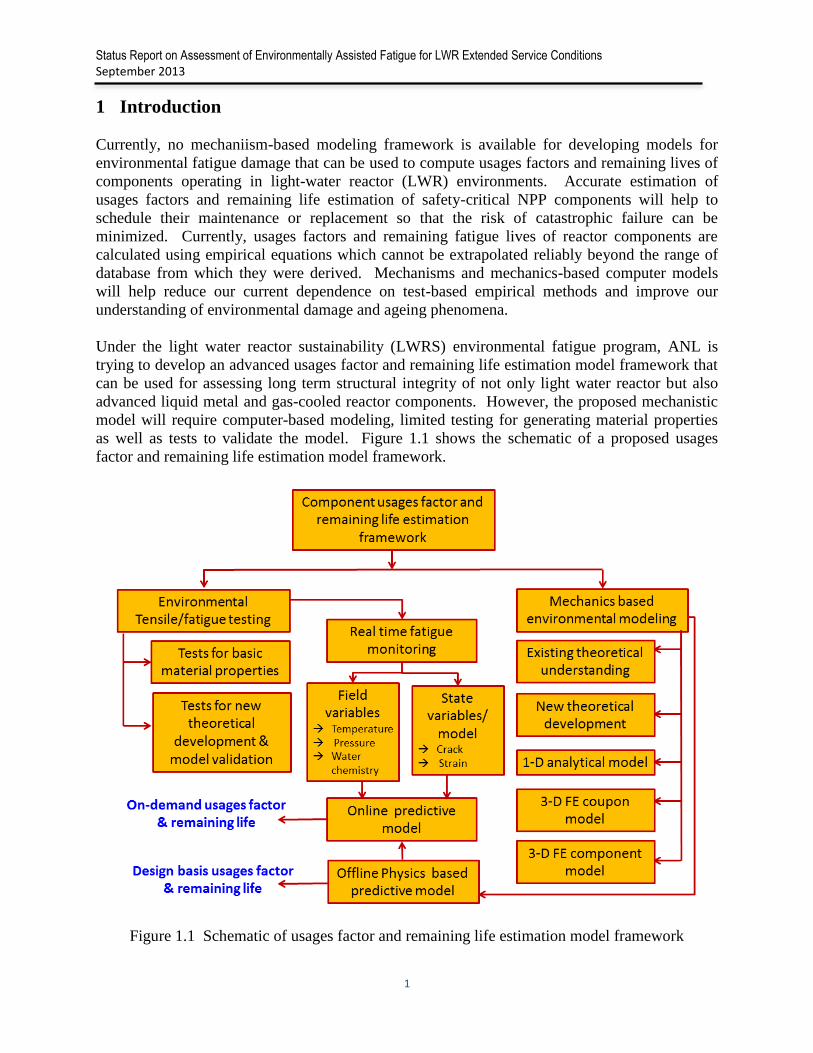
Under the light water reactor sustainability (LWRS) environmental fatigue program, ANL is
trying to develop an advanced usages factor and remaining life estimation model framework that
can be used for assessing long term structural integrity of not only light water reactor but also
advanced liquid metal and gas-cooled reactor components. However, the proposed mechanistic
model will require computer-based modeling, limited testing for generating material properties
as well as tests to validate the model. Figure 1.1 shows the schematic of a proposed usages
factor and remaining life estimation model framework.
Figure 1.1 Schematic of usages factor and remaining life estimation model framework
Status Report on Assessment of Environmentally Assisted Fatigue for LWR Extended Service Conditions
September 2013
2
Under the LWRS program, the following two major activities are currently in progress at
Argonne National Laboratory:
a) Mechanistic modeling of environmental fatigue damage in LWR reactor coolant system
(RCS) piping materials
b) Environmental tensile and/or fatigue testing of RCS pipe base, similar and dissimilar metal
welds.
The tentative mechanistic modeling and experiment plans are as follows:
1.1 Planned mechanistic modeling activities:
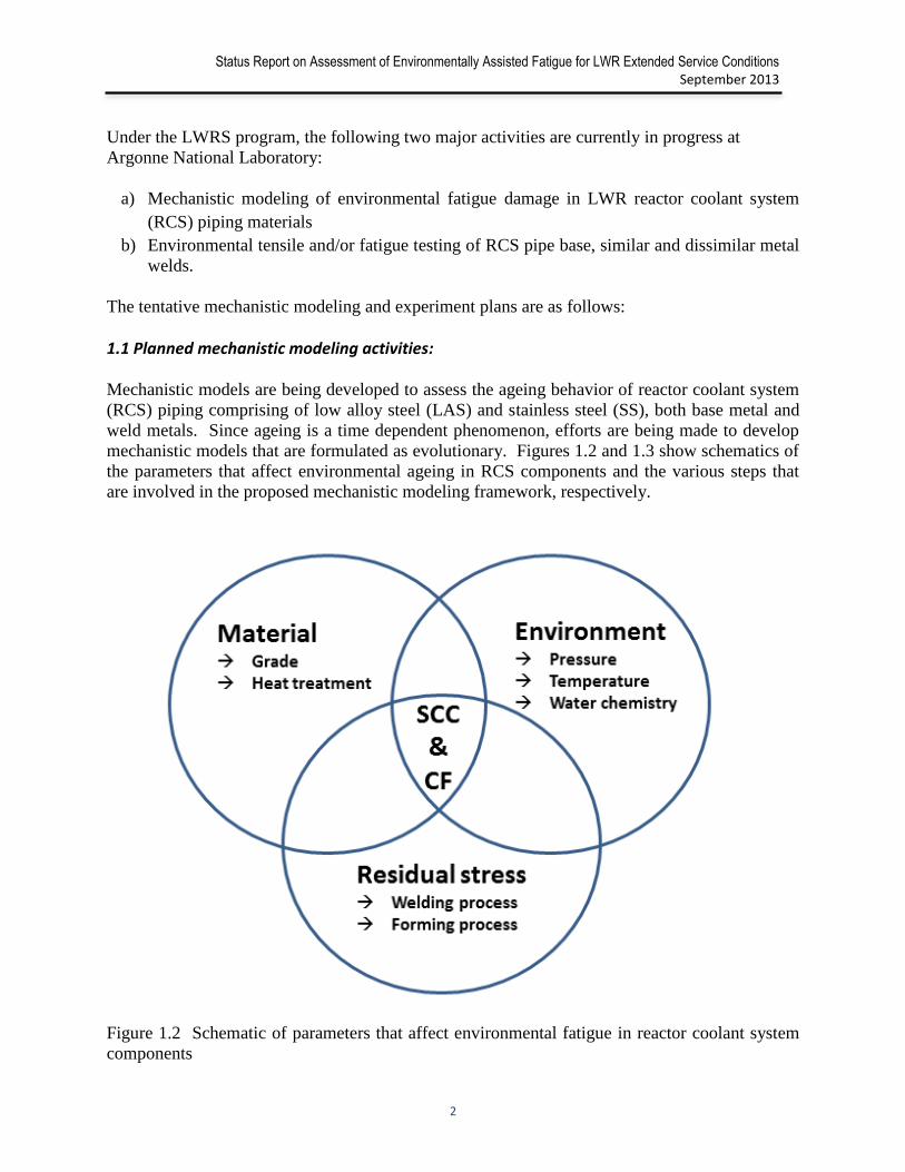
Mechanistic models are being developed to assess the ageing behavior of reactor coolant system
(RCS) piping comprising of low alloy steel (LAS) and stainless steel (SS), both base metal and
weld metals. Since ageing is a time dependent phenomenon, efforts are being made to develop
mechanistic models that are formulated as evolutionary. Figures 1.2 and 1.3 show schematics of
the parameters that affect environmental ageing in RCS components and the various steps that
are involved in the proposed mechanistic modeling framework, respectively.
Figure 1.2 Schematic of parameters that affect environmental fatigue in reactor coolant system
components

Status Report on Assessment of Environmentally Assisted Fatigue for LWR Extended Service Conditions
September 2013
3
Figure 1.3 Schematic of mechanistic modeling framework for reactor coolant system component
environmental fatigue and usages factor estimation
1.2 Planned testing activities:
Limited laboratory tests will be performed to extract the material properties required for the
above mentioned mechanistic model, to understand the ageing behavior and to flesh out different
independent variables that affect the ageing mechanism. Tensile and fatigue experiments of hour
glass type specimens are planned at room temperature, elevated LWR temperature and under in-
air and LWR coolant water chemistry conditions. At present, testing activities are limited to the
material grades used in a typical US PWR type reactor coolant system (RCS) piping. For
example, A533 B low alloy steel (LAS) and 316 stainless steel (SS) grades, which are often used
for reactor pressure vessel (and nozzle) and RCS piping, respectively, are being considered.
Both base metal and weldment (316 SS-316 SS similar metal weld and 316 SS-533B LAS
dissimilar metal weld) specimens will be tested under tensile and/or fatigue loading. Table 1.1
shows the tentative test matrix.
Table 1. 1316 SS-316 SS similar metal weld fabrication parameters
Test conditions
(→)
Specimen type (↓)
In-air room temperature In-air LWR
temperature
LWR water &
temperature
Tensile Fatigue Tensile Fatigue Fatigue
316 SS base
533 B LAS base
316 SS-316 SS
(along the weld)
316 SS-316 SS
(across the weld)
316 SS-533 B LAS
(along the weld)
316 SS-533 B LAS
(across the weld)
Status Report on Assessment of Environmentally Assisted Fatigue for LWR Extended Service Conditions
September 2013
4
1.3 Organization of this report
The report summarizes some of the work conducted during FY 2012-2013. The
accomplishments are described through the following sections.
Section 1: Introduction
Section 2: 316 SS base and 316 SS -316 SS similar weld metal specimen fabrication
Section 3: Room & elevated temperature Fatigue test set-up
Section 4: Room temperature tensile test of 316 SS base metal specimens
Section 5: Room temperature fatigue test of 316 SS base metal specimens
Section 6: Room temperature tensile test of 316 SS -316 SS similar metal weld specimen
Section 7: Elevated temperature tensile test of 316 SS base metal specimens
Section 8: Elevated temperature tensile test of 316 SS -316 SS similar metal weld specimen
Section 9: Estimation of effect of thermal strain and coefficient of thermal expansion in 316
SS base and 316 SS -316 SS similar metal weld material
Section 10: Mechanistic modeling: Evaluation of extended finite element method for dynamic
crack initiation and propagation modeling through steam generator tube rupture
simulation
Status Report on Assessment of Environmentally Assisted Fatigue for LWR Extended Service Conditions
September 2013
5
2 316 SS-316 SS Similar Metal Weld and Specimen Fabrication
During the initial phase of the work, it was decided to start tensile/fatigue testing of 316 SS
base metal and 316 SS-316 SS similar metal weld specimens. The material and geometry
information are briefly discussed below.
2.1 316 SS base metal specimen
The 316 SS specimens used in the current work were fabricated from 316 SS plate. As
described by the manufacturer, the plate was water quenched and mill annealed at 1900°F. The
heat number for the material is P91576 and its chemical composition is given in Table 2.1.
Hourglass specimens conforming to ASTM standard E8/E8M [1] and E606 [2] were fabricated
for both tensile and fatigue testing of the base metal. The specimens were fabricated along the
rolling direction of the 316 SS plate, as shown in Figure 2.1. The dimensions of the specimen
are given in Figure 2.2. Figure 2.3 shows a photograph of the as-fabricated specimen.
Table 2. 1 Chemical composition of Type 316 SS base metal (Heat P91576)
Chemical composition (in wt%)
C Cr Cu Mn Mo N Ni P S Si
0.21 17.37 0.2 1.6 2.12 0.067 10.77 0.018 0.010 0.46
Figure 2.1 Cutting plane with respect to plate rolling direction for hourglass specimen
Status Report on Assessment of Environmentally Assisted Fatigue for LWR Extended Service Conditions
September 2013
6
Figure 2.2 Geometry of 316 SS tensile/fatigue specimen
Figure 2.3 Fabrication drawing of 316 SS tensile/fatigue specimen
2.2 316 SS-316 SS similar metal weld specimen
The 316 SS-316 SS similar metal weld specimens are fabricated from 316 SS-316 SS similar
metal welded plates. The weld plates were fabricated using the above-mentioned 316 SS plates
and shielded metal arc welding (SMAW) process. The plates were joined with a multi-pass
double V-weld using E316-16 grade filler material. Table 2.2 shows the material composition of
the filler material. Figure 2.4 shows the schematic of weld sequences and Table 2.3 shows the
details of the weld sequence fabrication parameters.
Table 2.2 Chemical composition of E316-16 grade filler metal (Heat 06814)
Chemical composition (wt%)
C Cr Cu Mn Mo N Ni P S Si
0.05 18.96 - 0.94 2.49 - 11.88 0.028 0.017 0.31

Status Report on Assessment of Environmentally Assisted Fatigue for LWR Extended Service Conditions
September 2013
7
Figure 2.4 Weld sequence 316 SS-316 SS similar metal weld plate
Table 2.3 316 SS-316 SS similar metal weld fabrication parameters
Pass number
Filler metal wire
diameter (in)
Current
(A)
Voltage
(V)
Torch travel
speed (in/min)
1 3/32 60-90 21-25 6-7
2 1/8 90-120 24-28 7-8
3 1/8 90-120 24-28 7-8
4 1/8 90-120 24-28 7-8
5-18 5/32 120-160 27-30 7-8
Two type of weld plates were fabricated, weld along the rolling direction and weld perpendicular
to the rolling direction of original 316 SS plate. Figure 2.5a shows the two types fabricated weld
plates with respect to rolling direction. Figure 2.5b shows the image of weld plate after first
weld pass. From each type of weld plate two types of specimens were fabricated, one along the
weld fusion zone and the other across the weld fusion zone. Figures 2.6 and 2.7 show
schematics of specimen geometry with respect to along and across the weld fusion zone,
respectively. The specimens aligned along the fusion zone will be tensile/fatigue tested for
generating material properties to be used in the mechanistic model. On the other hand,
specimens aligned across the weld zone will be tensile/fatigue tested for validation of coupon
level mechanistic model, as mentioned earlier (see Figure 1.1). The geometry of all of the
above-mentioned weld specimens are kept the same as the geometry of the base metal specimens
shown in Figure 2.2.
Status Report on Assessment of Environmentally Assisted Fatigue for LWR Extended Service Conditions
September 2013
8
Figure 2.5 a) Two types of weld plate with respect to rolling direction, b) Weld shape after first
weld pass (the root side is facing up)
Figure 2.6 Schematic of along the
weld specimen
Figure 2.7 Schematic of across
the weld specimen

Status Report on Assessment of Environmentally Assisted Fatigue for LWR Extended Service Conditions
September 2013
9
2.1 Summary
This section briefly described the specimen geometry material specifications for 316 SS base
metal and 316 SS-316 SS similar metal specimens. This section also described the welding
processes used for fabricating the 316 SS-316 SS similar metal weld plates from which the weld
specimens were fabricated.

Status Report on Assessment of Environmentally Assisted Fatigue for LWR Extended Service Conditions
September 2013
10
3 In-air Room & elevated temperature Fatigue test set-up
At ANL for the requirement of LWRS program two test frames are being configured/updated.
One test frame will specifically be used for in-air condition tensile and fatigue testing, while the
other one will specifically be used for the LWR water condition testing. The in-air test frame
can handle both room and elevated temperature tensile and fatigue testing.
In the present report in-air test results (both under room and elevated temperature conditions) are
discussed. Following subsections briefly describes the in-air room and elevated temperature test
set up.
3.1 In-air room temperature test setup
A hydraulically controlled MTS test frame was used for the tensile and fatigue tests described in
this report. The test set up (frame with the installed specimen) for the room temperature
tensile/fatigue tests can be seen in Fig. 3.1. In general, measurements were collected by the
following built-in or added-on sensors:
a) Built-in test frame load cell
b) Built-in test frame actuator position sensor for actuator position measurement
c) Added-on displacement (stroke) sensor for crosshead position measurement
d) Added-on extensometer for strain measurement
e) Added-on ultrasonic sensor system in-house built for online/real-time fatigue crack
monitoring
For the current in-air tests, an extensometer-based strain signal is used as feedback to control the
axial strain of the test specimens. However, for environmental testing it may not be feasible to
insert the extensometer into the test chamber, and the controller feedback has to be obtained from
either the actuator position sensor built into the test frame or the added-on crosshead
displacement sensor, which can be mounted outside the environmental chamber. A different test
frame with the environmental chamber is being configured at ANL’s low cycle fatigue
laboratory for future use in the LWRS-related environmental fatigue tests.

Status Report on Assessment of Environmentally Assisted Fatigue for LWR Extended Service Conditions
September 2013
11
Figure 3.1 In-air room temperature tensile/fatigue test frame with specimen and various
instruments
3.2 Fatigue testing of 316 SS base metal specimens and resulting data analysis
For elevated temperature tensile/fatigue testing the test setup shown in Fig. 3.1 is augmented
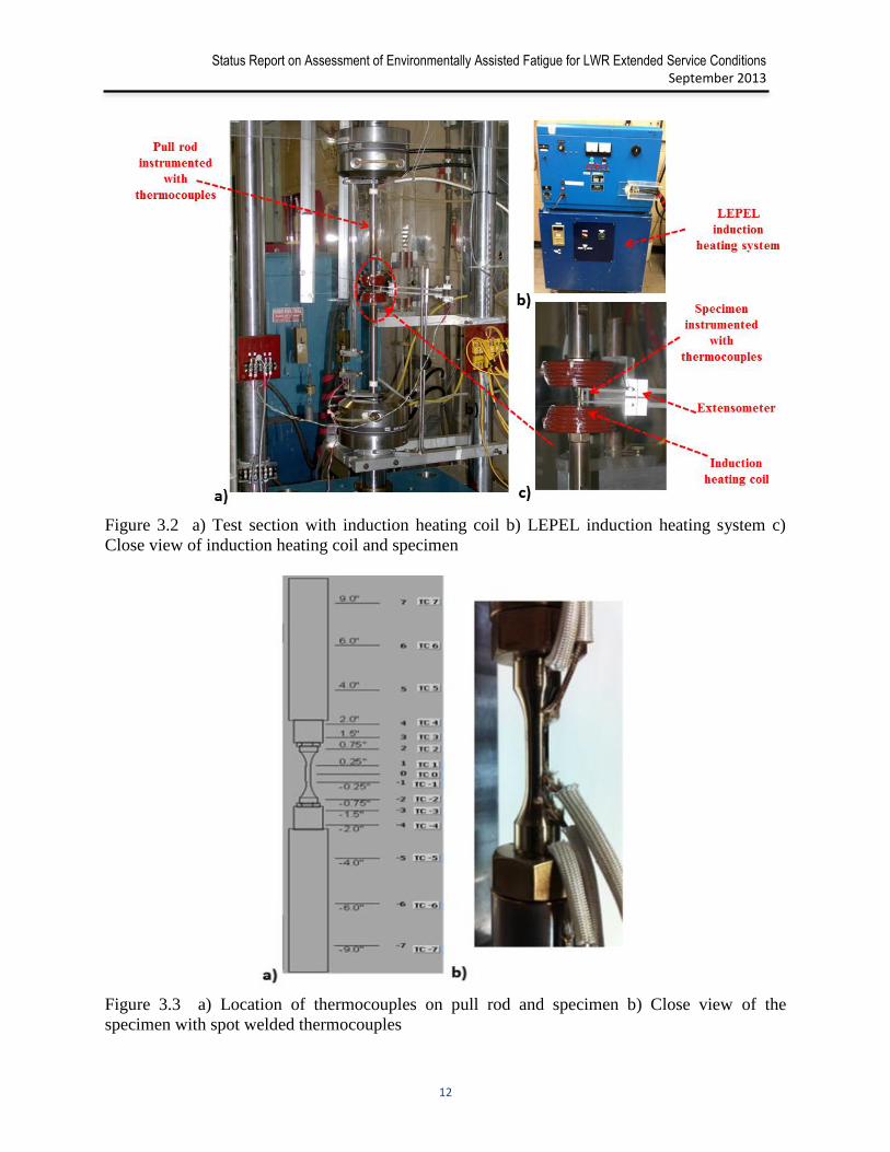
with heating element. Induction type heating is used to locally heat the specimen. Figure 3.2
shows the augmented test section for elevated temperature testing. A LEPEL induction heating
system was used for the purpose. Specific coil shape (diameter and number of turn) designed to
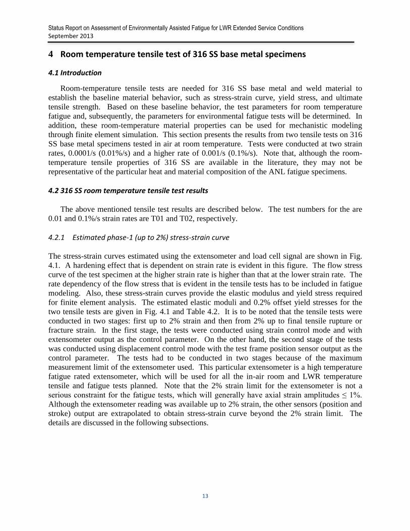
achieve the required temperature in the test specimen. There are total 15 thermocouples spot
welded onto pull rod and specimen (9 on the specimen and 6 on the pull rod) to monitor and
control the temperature. Figure 3.3a shows the schematic of locations of these thermocouples,
whereas Fig. 3.3b shows a magnified view of instrumented specimen.
Status Report on Assessment of Environmentally Assisted Fatigue for LWR Extended Service Conditions
September 2013
12
Figure 3.2 a) Test section with induction heating coil b) LEPEL induction heating system c)
Close view of induction heating coil and specimen
Figure 3.3 a) Location of thermocouples on pull rod and specimen b) Close view of the
specimen with spot welded thermocouples
Status Report on Assessment of Environmentally Assisted Fatigue for LWR Extended Service Conditions
September 2013
13
4 Room temperature tensile test of 316 SS base metal specimens
4.1 Introduction
Room-temperature tensile tests are needed for 316 SS base metal and weld material to
establish the baseline material behavior, such as stress-strain curve, yield stress, and ultimate
tensile strength. Based on these baseline behavior, the test parameters for room temperature
fatigue and, subsequently, the parameters for environmental fatigue tests will be determined. In
addition, these room-temperature material properties can be used for mechanistic modeling
through finite element simulation. This section presents the results from two tensile tests on 316
SS base metal specimens tested in air at room temperature. Tests were conducted at two strain
rates, 0.0001/s (0.01%/s) and a higher rate of 0.001/s (0.1%/s). Note that, although the room-
temperature tensile properties of 316 SS are available in the literature, they may not be
representative of the particular heat and material composition of the ANL fatigue specimens.
4.2 316 SS room temperature tensile test results
The above mentioned tensile test results are described below. The test numbers for the are
0.01 and 0.1%/s strain rates are T01 and T02, respectively.
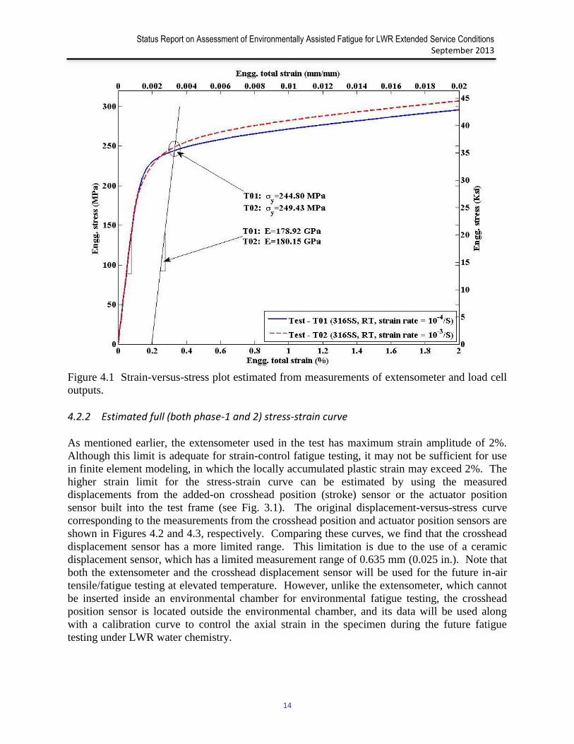
4.2.1 Estimated phase-1 (up to 2%) stress-strain curve
The stress-strain curves estimated using the extensometer and load cell signal are shown in Fig.
4.1. A hardening effect that is dependent on strain rate is evident in this figure. The flow stress
curve of the test specimen at the higher strain rate is higher than that at the lower strain rate. The
rate dependency of the flow stress that is evident in the tensile tests has to be included in fatigue
modeling. Also, these stress-strain curves provide the elastic modulus and yield stress required
for finite element analysis. The estimated elastic moduli and 0.2% offset yield stresses for the
two tensile tests are given in Fig. 4.1 and Table 4.2. It is to be noted that the tensile tests were
conducted in two stages: first up to 2% strain and then from 2% up to final tensile rupture or
fracture strain. In the first stage, the tests were conducted using strain control mode and with
extensometer output as the control parameter. On the other hand, the second stage of the tests
was conducted using displacement control mode with the test frame position sensor output as the
control parameter. The tests had to be conducted in two stages because of the maximum
measurement limit of the extensometer used. This particular extensometer is a high temperature
fatigue rated extensometer, which will be used for all the in-air room and LWR temperature
tensile and fatigue tests planned. Note that the 2% strain limit for the extensometer is not a
serious constraint for the fatigue tests, which will generally have axial strain amplitudes ≤ 1%.
Although the extensometer reading was available up to 2% strain, the other sensors (position and
stroke) output are extrapolated to obtain stress-strain curve beyond the 2% strain limit. The
details are discussed in the following subsections.
Status Report on Assessment of Environmentally Assisted Fatigue for LWR Extended Service Conditions
September 2013
14
Figure 4.1 Strain-versus-stress plot estimated from measurements of extensometer and load cell
outputs.
4.2.2 Estimated full (both phase-1 and 2) stress-strain curve
As mentioned earlier, the extensometer used in the test has maximum strain amplitude of 2%.
Although this limit is adequate for strain-control fatigue testing, it may not be sufficient for use
in finite element modeling, in which the locally accumulated plastic strain may exceed 2%. The
higher strain limit for the stress-strain curve can be estimated by using the measured
displacements from the added-on crosshead position (stroke) sensor or the actuator position
sensor built into the test frame (see Fig. 3.1). The original displacement-versus-stress curve
corresponding to the measurements from the crosshead position and actuator position sensors are
shown in Figures 4.2 and 4.3, respectively. Comparing these curves, we find that the crosshead
displacement sensor has a more limited range. This limitation is due to the use of a ceramic
displacement sensor, which has a limited measurement range of 0.635 mm (0.025 in.). Note that
both the extensometer and the crosshead displacement sensor will be used for the future in-air
tensile/fatigue testing at elevated temperature. However, unlike the extensometer, which cannot
be inserted inside an environmental chamber for environmental fatigue testing, the crosshead
position sensor is located outside the environmental chamber, and its data will be used along
with a calibration curve to control the axial strain in the specimen during the future fatigue
testing under LWR water chemistry.

Status Report on Assessment of Environmentally Assisted Fatigue for LWR Extended Service Conditions
September 2013
15
Figure 4.2 Crosshead displacement (stroke) versus stress
Figure 4.3 Actuator position versus stress

Status Report on Assessment of Environmentally Assisted Fatigue for LWR Extended Service Conditions
September 2013
16
Figures 4.2 and 4.3 show the measured stress as a function of displacement. For input to finite
element analysis, it is necessary to convert these load-displacement curves to equivalent stress-
strain curves. It is also necessary to estimate the equivalent strain from the measured
displacements so that approximate strain-controlled fatigue test could be conducted in situations
where extensometers cannot be used. This estimation could be performed by mapping known
displacement to known strain and then, predicting unknown strains from the known
displacements. For simplicity, a mapping function can be established between known
displacements with known strain through least squares fitting. Using the estimated parameters of
the mapping function, we can estimate the unknown strain from the known or measured
displacements. The known strain at a given instant of time can be expressed as
(4.1)
where is the known or measured displacement at time , is the initial displacement, is
the effective gauge length, and and are the unknown parameters that can be estimated
through least squares fitting. The crosshead displacement (stroke) and actuator position are
plotted with respect to known strain in Figures 4.4 and 4.5, respectively.
Figure 4.4 Crosshead displacement (stroke) with respect to known strain
t
)()1
(eff
ot
effeff
ott
L
ll
LL
ll
tl t 0l effL
effL
1
eff
o
L
l

Status Report on Assessment of Environmentally Assisted Fatigue for LWR Extended Service Conditions
September 2013
17
Figure 4.5 Actuator position with respect to known strain
Using Eq. 2.1 and the known crosshead and actuator position data in Figures 4.2 and 4.3, we
estimated the effective length . Note that, for estimating the least squares fit, we only
considered the straight portions of the curves in Figures 4.4 and 4.5, i.e., the data beyond the
yield strain. The estimated and the physical gage length are given in Table 4.1 for the two
strain rates. The corresponding estimated strain-versus-stress curves with respect to crosshead
and actuator position measurements are shown in Figures 4.6 and 4.7, respectively. In addition,
the scalar material properties estimated from the above-mentioned tensile test data can be found
in Table 4.2.
Table 4.1 Estimated effective gage length (or calibration factor) and specimen nominal gage
length for 316 SS base metal specimen under room temperature tensile testing
Strain rate
estimate in mm (in.) Specimen gage length in mm (in.)
Based on
crosshead
displacement
(stroke)
Based on
actuator
displacement
(position)
Nominal
length
Measured length
0.0001/s 16.507 (0.649) 17.272 (0.68) 14.25 (0.561) 13.233 (0.521)
0.001/s 16.842 (0.663) 17.628 (0.694) 14.25 (0.561) 14.224 (0.560)
effL
effL
effL
Status Report on Assessment of Environmentally Assisted Fatigue for LWR Extended Service Conditions
September 2013
18
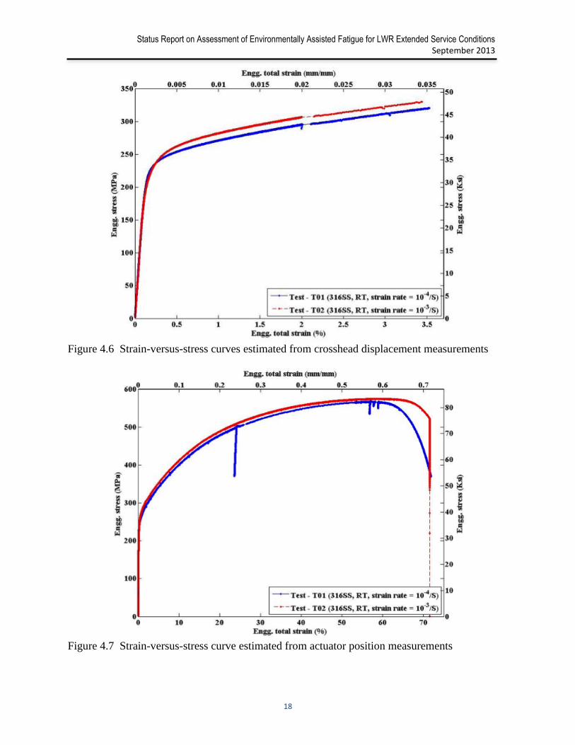
Figure 4.6 Strain-versus-stress curves estimated from crosshead displacement measurements
Figure 4.7 Strain-versus-stress curve estimated from actuator position measurements
Status Report on Assessment of Environmentally Assisted Fatigue for LWR Extended Service Conditions
September 2013
19
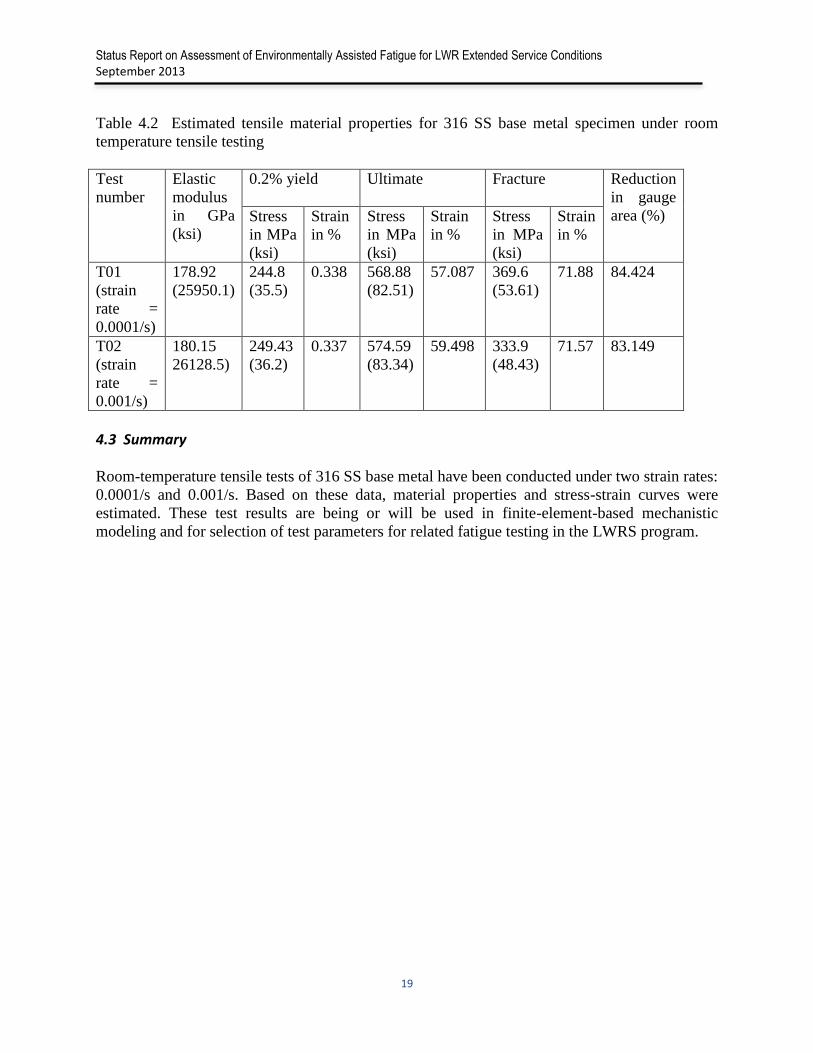
Table 4.2 Estimated tensile material properties for 316 SS base metal specimen under room
temperature tensile testing
Test
number
Elastic
modulus
in GPa
(ksi)
0.2% yield
Ultimate Fracture
Reduction
in gauge
area (%) Stress
in MPa
(ksi)
Strain
in %
Stress
in MPa
(ksi)
Strain
in %
Stress
in MPa
(ksi)
Strain
in %
T01
(strain
rate =
0.0001/s)
178.92
(25950.1)
244.8
(35.5)
0.338 568.88
(82.51)
57.087 369.6
(53.61)
71.88 84.424
T02
(strain
rate =
0.001/s)
180.15
26128.5)
249.43
(36.2)
0.337 574.59
(83.34)
59.498 333.9
(48.43)
71.57 83.149
4.3 Summary
Room-temperature tensile tests of 316 SS base metal have been conducted under two strain rates:
0.0001/s and 0.001/s. Based on these data, material properties and stress-strain curves were
estimated. These test results are being or will be used in finite-element-based mechanistic
modeling and for selection of test parameters for related fatigue testing in the LWRS program.
Status Report on Assessment of Environmentally Assisted Fatigue for LWR Extended Service Conditions
September 2013
20
5 Room Temperature Fatigue Test of 316 SS Base Metal Specimens
5.1 Introduction
Mechanistic modeling of environmental fatigue requires developing cyclic plasticity modeling.
The cyclic plasticity modeling requires cyclic plasticity constitutive relations and related material
properties. For the purpose first four room temperature fatigue tests using 316 SS base metal
specimens were conducted at the ANL’s in-air fatigue test frame. In the present sections, efforts
were made to analyze these fatigue test data. Based on these data analysis, different types of
cyclic plasticity models can be developed. The data analysis results and a proposed cyclic
plasticity model are discussed below.
5.2 Fatigue testing of 316 SS base metal specimens and resulting data analysis
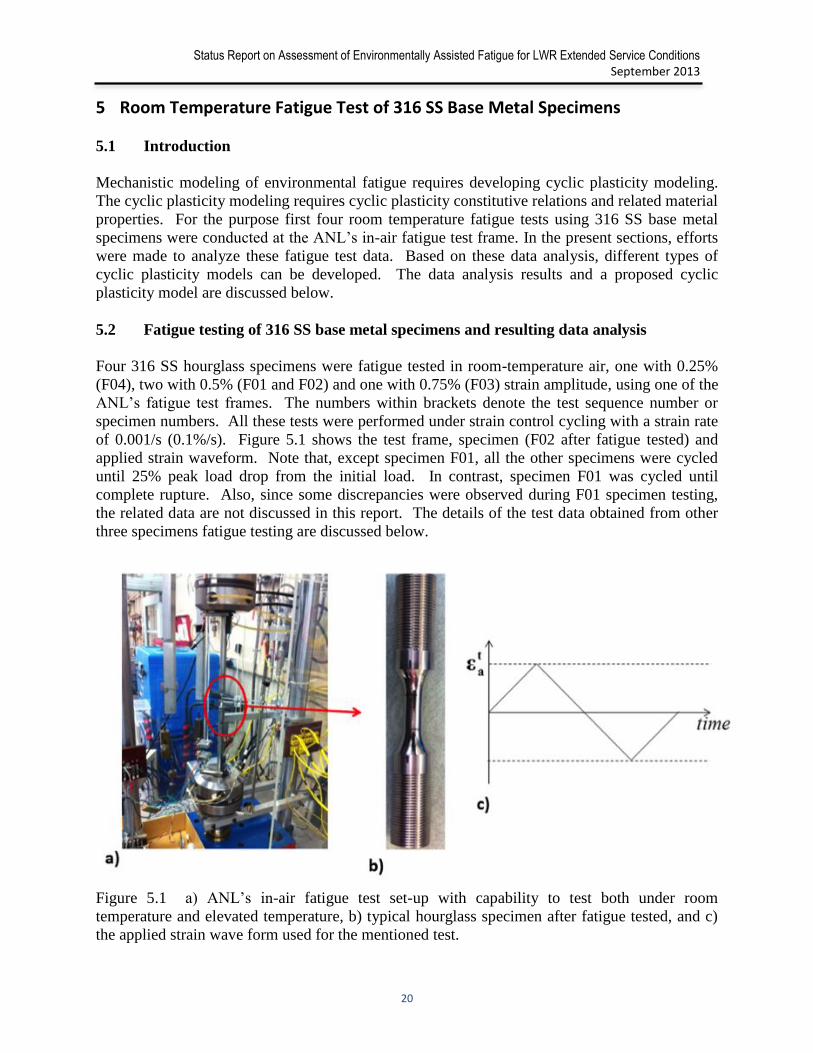
Four 316 SS hourglass specimens were fatigue tested in room-temperature air, one with 0.25%
(F04), two with 0.5% (F01 and F02) and one with 0.75% (F03) strain amplitude, using one of the
ANL’s fatigue test frames. The numbers within brackets denote the test sequence number or
specimen numbers. All these tests were performed under strain control cycling with a strain rate
of 0.001/s (0.1%/s). Figure 5.1 shows the test frame, specimen (F02 after fatigue tested) and
applied strain waveform. Note that, except specimen F01, all the other specimens were cycled
until 25% peak load drop from the initial load. In contrast, specimen F01 was cycled until
complete rupture. Also, since some discrepancies were observed during F01 specimen testing,
the related data are not discussed in this report. The details of the test data obtained from other
three specimens fatigue testing are discussed below.
Figure 5.1 a) ANL’s in-air fatigue test set-up with capability to test both under room
temperature and elevated temperature, b) typical hourglass specimen after fatigue tested, and c)
the applied strain wave form used for the mentioned test.
Status Report on Assessment of Environmentally Assisted Fatigue for LWR Extended Service Conditions
September 2013
21
5.2.1 Hysteresis behavior of 316SS base metal
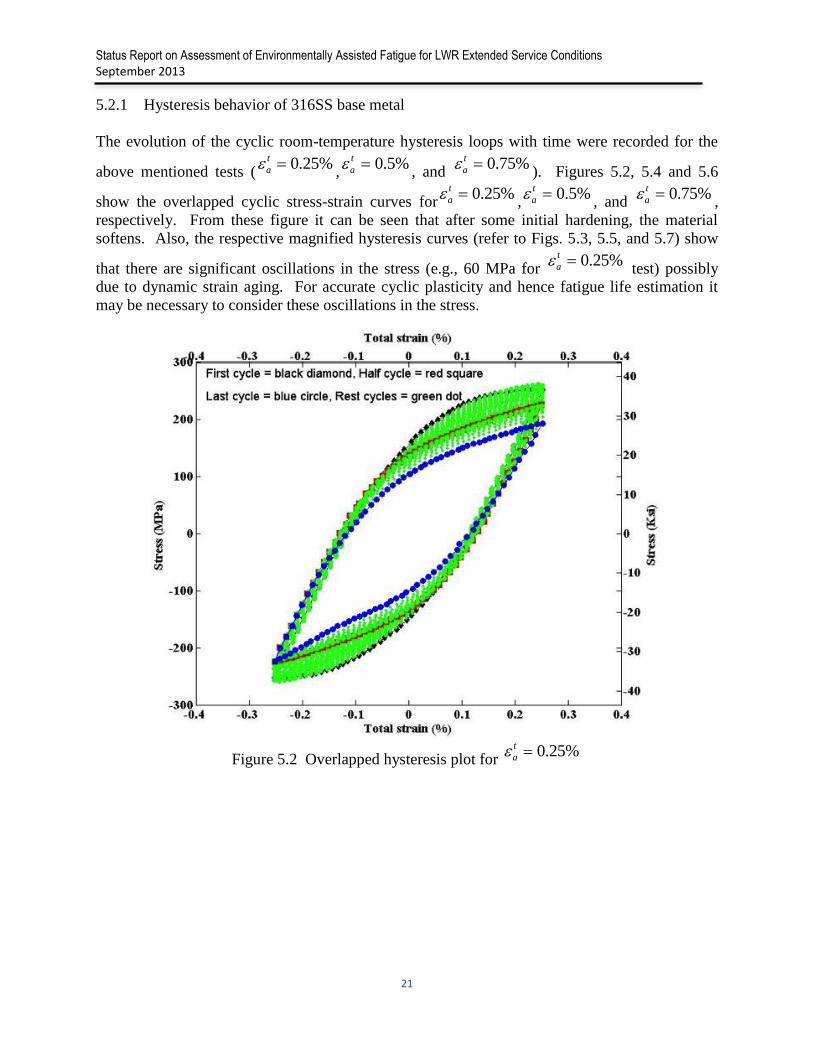
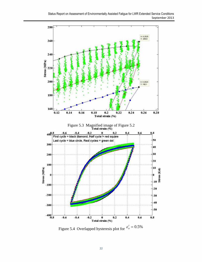
The evolution of the cyclic room-temperature hysteresis loops with time were recorded for the
above mentioned tests ( , , and ). Figures 5.2, 5.4 and 5.6
show the overlapped cyclic stress-strain curves for , , and ,
respectively. From these figure it can be seen that after some initial hardening, the material
softens. Also, the respective magnified hysteresis curves (refer to Figs. 5.3, 5.5, and 5.7) show
that there are significant oscillations in the stress (e.g., 60 MPa for test) possibly
due to dynamic strain aging. For accurate cyclic plasticity and hence fatigue life estimation it
may be necessary to consider these oscillations in the stress.
Figure 5.2 Overlapped hysteresis plot for
%25.0t
a %5.0t
a %75.0t
a
%25.0t
a %5.0t
a %75.0t
a
%25.0t
a
%25.0t
a
Status Report on Assessment of Environmentally Assisted Fatigue for LWR Extended Service Conditions
September 2013
22
Figure 5.3 Magnified image of Figure 5.2
Figure 5.4 Overlapped hysteresis plot for
%5.0t
a

Status Report on Assessment of Environmentally Assisted Fatigue for LWR Extended Service Conditions
September 2013
23
Figure 5.5 Magnified image of Figure 5.4
Figure 5.6 Overlapped hysteresis plot for
%75.0t
a

Status Report on Assessment of Environmentally Assisted Fatigue for LWR Extended Service Conditions
September 2013
24
Figure 5.7 Magnified image of Figure 5.6
5.2.2 Evolution of cyclic elastic modulus
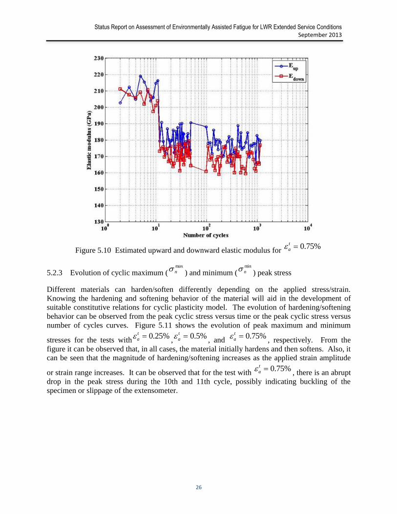
To model cyclic plasticity, it is also necessary to estimate cyclic elastic modulus and its
evolution over time. For the current tests, we have also estimated both the upward and
downward elastic modulus for individual cycles. Figures 5.8, 5.9, and 5.10 show the evolution
of upward ( ) and downward ( ) moduli for the tests with , , and
, respectively. From Fig. 5.8 it can be seen that for the test with , except
during the end of the test, both elastic moduli vary between 180 to 190 GPa, with maximum
variation within the range of 5-6%. It is to be noted that the monotonic elastic modulus for 316
SS estimated under similar conditions (e.g., at room temperature and with a strain rate of
0.1%/Sec.) was 180.15 GPa (see Table 4.2). Similarly, from Fig. 5.9 it can be seen that for the
test with , the elastic moduli vary in the range of 165-185MPa (10-12%). However,
for , (see Fig. 5.10) the elastic moduli varied in the range of 160-220 MPa, which is
more than 25-35%.
upEdownE %25.0t
a %5.0t
a
%75.0t
a %25.0t
a
%5.0t
a
%75.0t
a

Status Report on Assessment of Environmentally Assisted Fatigue for LWR Extended Service Conditions
September 2013
25
Figure 5.8 Estimated upward and downward elastic modulus for
Figure 5.9 Estimated upward and downward elastic modulus for
%25.0t
a
%5.0t
a
Status Report on Assessment of Environmentally Assisted Fatigue for LWR Extended Service Conditions
September 2013
26
Figure 5.10 Estimated upward and downward elastic modulus for
5.2.3 Evolution of cyclic maximum ( ) and minimum ( ) peak stress
Different materials can harden/soften differently depending on the applied stress/strain.
Knowing the hardening and softening behavior of the material will aid in the development of
suitable constitutive relations for cyclic plasticity model. The evolution of hardening/softening
behavior can be observed from the peak cyclic stress versus time or the peak cyclic stress versus
number of cycles curves. Figure 5.11 shows the evolution of peak maximum and minimum
stresses for the tests with , , and , respectively. From the
figure it can be observed that, in all cases, the material initially hardens and then softens. Also, it
can be seen that the magnitude of hardening/softening increases as the applied strain amplitude
or strain range increases. It can be observed that for the test with , there is an abrupt
drop in the peak stress during the 10th and 11th cycle, possibly indicating buckling of the
specimen or slippage of the extensometer.
%75.0t
a
max
n min
n
%25.0t
a %5.0t
a %75.0t
a
%75.0t
a

Status Report on Assessment of Environmentally Assisted Fatigue for LWR Extended Service Conditions
September 2013
27
Figure 5.11 Evolution of maximum and minimum peak stress with respect to number of fatigue
cycles for test cases , , and
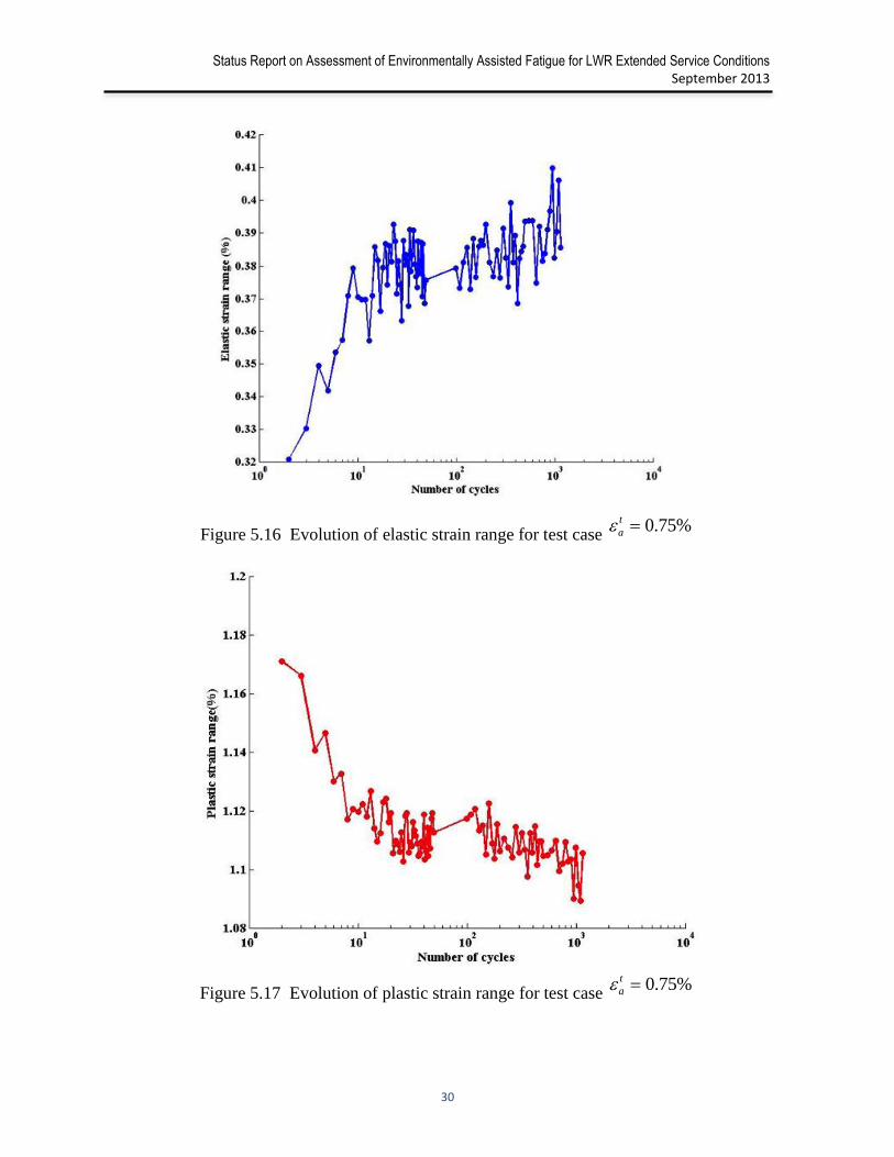
5.2.4 Evolution of cyclic elastic strain range ( ) and plastic strain range ( )
The variations of the elastic strain range ( ) and plastic strain range ( ) with number of
fatigue cycle ( ) are needed for development of the cyclic plasticity model. These
trends can be linked to the cycle-dependent hardening and softening behavior of material, and
will enable to develop a suitable constitutive relation that can be incorporated in to the
mechanics-based evolutionary cyclic plasticity model. Figures 5.12 and 5.13 show the variations
of the elastic and plastic strain ranges with cycles for the test with , respectively.
Figures 5.14 and 5.15 show the corresponding evolutions for the test with and Figs.
5.16 and 5.17 show the evolutions for the test with , respectively. From these
figures it can be observed that, except for the test with (Figs. 5.16 and 5.17), similar
trends in elastic and plastic strain range evolution are observed for tests with and
. For example, Fig. 5.12 shows that the elastic strain range ( ) initially increases
and then decreases, which indicates initial hardening followed by softening. Figure 5.13 shows
that the plastic strain range ( ) initially decreases and then increases, which also indicates
initial hardening and then softening. The continuous hardening with cycle in the case of
%25.0t
a %5.0t
a %75.0t
a
e
np
n
e
np
n
Nn ,1
%25.0t
a
%5.0t
a
%75.0t
a
%75.0t
a
%25.0t
a
%5.0t
ae
n
p
n

Status Report on Assessment of Environmentally Assisted Fatigue for LWR Extended Service Conditions
September 2013
28
is possibly due to the large applied strain amplitude indicating a trend towards stress
saturation and a stable hysteresis loop. However, the possibility of buckling makes this test
questionable.
Figure 5.12 Evolution of elastic strain range for test case
Figure 5.13 Evolution of plastic strain range for test case
%75.0t
a
%25.0t
a
%25.0t
a
Status Report on Assessment of Environmentally Assisted Fatigue for LWR Extended Service Conditions
September 2013
29
Figure 5.14 Evolution of elastic strain range for test case
Figure 5.15 Evolution of plastic strain range for test case
%5.0t
a
%5.0t
a
Status Report on Assessment of Environmentally Assisted Fatigue for LWR Extended Service Conditions
September 2013
30
Figure 5.16 Evolution of elastic strain range for test case
Figure 5.17 Evolution of plastic strain range for test case
%75.0t
a
%75.0t
a

Status Report on Assessment of Environmentally Assisted Fatigue for LWR Extended Service Conditions
September 2013
31
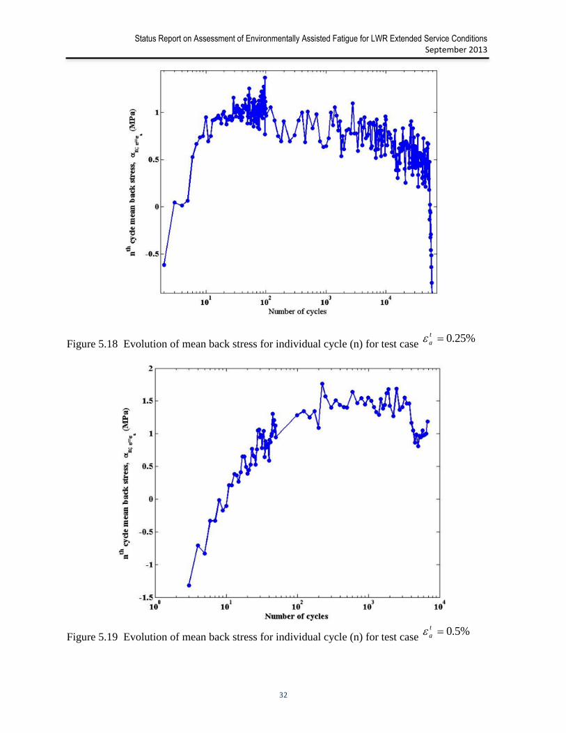
5.2.5 Evolution of cyclic back stress ( )
When there is a stress reversal, the hysteresis loop moves up or down from its original position
depending on the material and applied stress/strain. This is due to strain hardening/softening and
associated Bauschinger effect. This shift in stress space can be represented by a back stress ( ).
The estimation of evolution of back stress with respect to time is necessary for modeling cyclic
plasticity. The evolution of back stress at any given instant of time can be expressed as:
(5.1)
Where, is the mean shift of hysteresis loop in stress space and can be expressed as
(5.2)
and is the back stress at strain within an individual hysteresis loop and can be expressed as
(5.3)
In Eq. 5.2 and denote the fatigue cycle maximum tensile stress at
and maximum compressive stress at , respectively. For the tests with ,
, and , the mean back stresses were estimated and their evolutions are
plotted in Figs 5.18, 5.19, and 5.20, respectively.
t
t
t
εnt ααα
n
)(2
1minmax ;;
c
n
t
nnα
ten
n max;
com
n min; thn max
min %25.0t
a
%5.0t
a %75.0t
a n
Status Report on Assessment of Environmentally Assisted Fatigue for LWR Extended Service Conditions
September 2013
32
Figure 5.18 Evolution of mean back stress for individual cycle (n) for test case
Figure 5.19 Evolution of mean back stress for individual cycle (n) for test case
%25.0t
a
%5.0t
a
Status Report on Assessment of Environmentally Assisted Fatigue for LWR Extended Service Conditions
September 2013
33
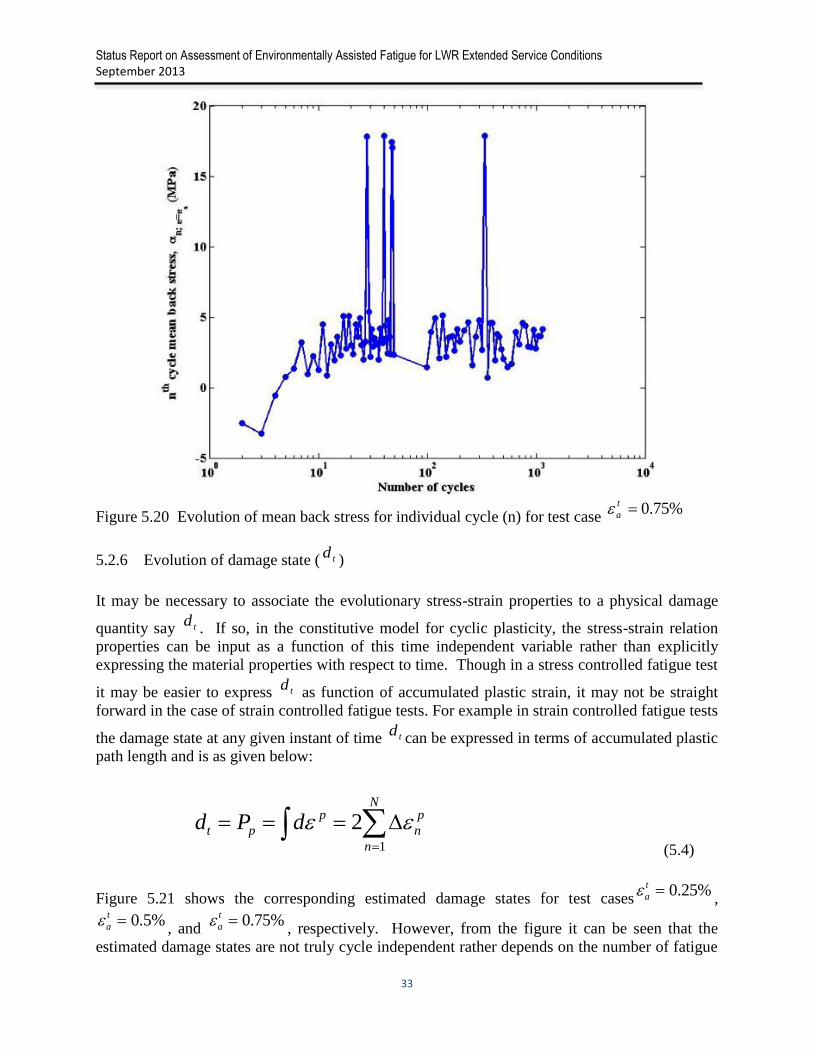
Figure 5.20 Evolution of mean back stress for individual cycle (n) for test case
5.2.6 Evolution of damage state ( )
It may be necessary to associate the evolutionary stress-strain properties to a physical damage
quantity say . If so, in the constitutive model for cyclic plasticity, the stress-strain relation
properties can be input as a function of this time independent variable rather than explicitly
expressing the material properties with respect to time. Though in a stress controlled fatigue test
it may be easier to express as function of accumulated plastic strain, it may not be straight
forward in the case of strain controlled fatigue tests. For example in strain controlled fatigue tests
the damage state at any given instant of time can be expressed in terms of accumulated plastic
path length and is as given below:
(5.4)
Figure 5.21 shows the corresponding estimated damage states for test cases ,
, and , respectively. However, from the figure it can be seen that the
estimated damage states are not truly cycle independent rather depends on the number of fatigue
%75.0t
a
td
td
td
td
N
n
p
n
p
pt dPd1
2
%25.0t
a
%5.0t
a %75.0t
a

Status Report on Assessment of Environmentally Assisted Fatigue for LWR Extended Service Conditions
September 2013
34
cycles the specimen experienced. This drawback may necessitate the need of performing few
stress controlled fatigue tests at least for developing evolutionary plasticity and hence the
evolutionary fatigue model.
Figure 5.21 Evolution of plastic path travel based damage states ( ) for test cases ,
, and
5.3 Constitutive model for cyclic plasticity
The constitutive relation for the cyclic plasticity model can be developed based on the above
discussed test results. The constitutive relation can be of two types such as evolutionary cyclic
plasticity model and stabilized or half-life based cyclic plasticity model. Both these models are
discussed briefly below.
5.3.1 Detailed evolutionary cyclic plasticity model
The evolutionary plasticity model captures the evolution of material parameters over the entire
fatigue life. To apply this model, the material parameters such as elastic modulus, yield stress,
elastic strain range, plastic strain range, back stress, hardening constants, etc. have to be
described as functions of time independent parameter(s) describing the physical damage state of
the structure. For example, the stress state at time can be expressed as
(5.5)
td %25.0t
a
%5.0t
a %75.0t
a
tt
)(:: pltoel
ttt
CC
Status Report on Assessment of Environmentally Assisted Fatigue for LWR Extended Service Conditions
September 2013
35
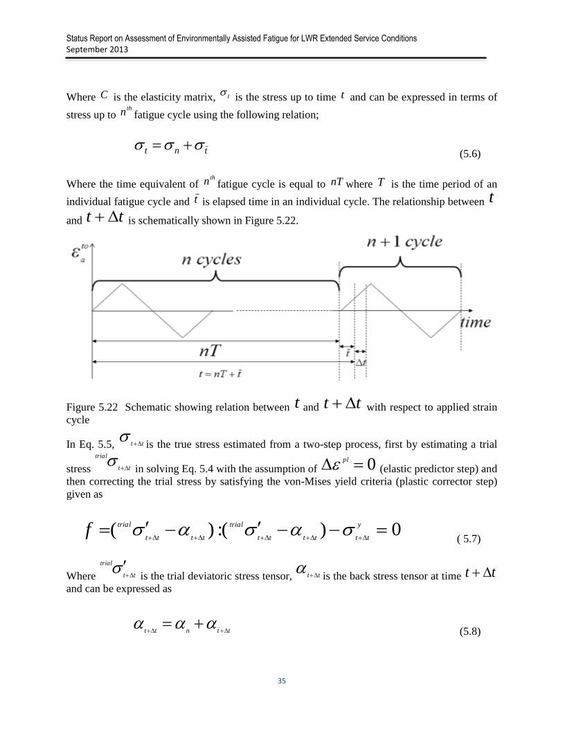
Where is the elasticity matrix, is the stress up to time and can be expressed in terms of
stress up to fatigue cycle using the following relation;
(5.6)
Where the time equivalent of fatigue cycle is equal to where is the time period of an
individual fatigue cycle and is elapsed time in an individual cycle. The relationship between
and is schematically shown in Figure 5.22.
Figure 5.22 Schematic showing relation between and with respect to applied strain
cycle
In Eq. 5.5, is the true stress estimated from a two-step process, first by estimating a trial
stress in solving Eq. 5.4 with the assumption of (elastic predictor step) and
then correcting the trial stress by satisfying the von-Mises yield criteria (plastic corrector step)
given as
( 5.7)
Where is the trial deviatoric stress tensor, is the back stress tensor at time
and can be expressed as
(5.8)
C t tthn
tnt
thn nT T
t t
tt
t tt
tt
tt
trial
0 pl
0):()(
y
tttttt
trial
tttt
trialf
tt
trial
tt tt
ttntt

Status Report on Assessment of Environmentally Assisted Fatigue for LWR Extended Service Conditions
September 2013
36
Where, is the evolutionary contribution expressed as a function of cycles and is the c
contribution within a particular cycle expressed as a function of time. The evolutionary
contribution corrects the by considering the evolutionary effect of stress hardening and
softening. Similarly in Eq.5.7, the yield stress can also be expressed in terms of a
correction part ( ) which is a function of cycles and a yield stress ( ) within an
individual cycle which is a function of time as follows:
(5.9)
The cycle-dependent correction for back stress and for yield stress have to be related to
a time or cycle independent physical parameters (e.g., accumulated plastic strain in a stress
controlled test).
5.3.2 Stabilized or half-life based approximate cyclic plasticity model
Typically estimating the evolutionary correction terms described through Eq. 5.8 and 5.9 are
complex to model with other independent variables unless these independent variables are not
linked to a time or cycle independent physical parameters (e.g accumulated plastic strain in a
stress controlled test). Hence for simplicity in many available cyclic plasticity models the
stabilized or half-cycle stress-strain behavior is assumed constant over the entire fatigue life.
This subsection describes the estimation of some of the stabilized cycle material properties that
can be used in a simplified cyclic plasticity model.
For example, to estimate the hardening and yield parameter only the half-life hysteresis curves of
all the three tests with , , and are considered. An equivalent
monotonic stress-strain curve is estimated by connecting the peak maximum stress point of the
individual plastic strain versus stress hysteresis curves. Figure 5.23 shows the half-life hysteresis
curve of the individual test cases and the associated tensile half of the cyclic stress-strain curve.
In a similar fashion, the compressive half of the cyclic stress-strain curve can be estimated by
connecting the peak minimum stress point of the individual plastic strain versus stress hysteresis
curves. From Fig. 5.23 it can be seen that both the tensile and compressive halves of the cyclic
stress-strain curve follow a linear pattern and the corresponding hardening parameter are
estimated by directly estimating the slopes of these linear stress-strain curves and the yield stress
as the corresponding y-intercepts. Because of lack of data, the usual 0.2% offset strain is not
determined in this case. A stabilized or half-life cyclic stress-strain curve can be constructed by
performing a number of strain-controlled fatigue tests at different strain amplitudes. The same
information can be obtained by performing a single strain controlled fatigue tests with a
sequence of different strain amplitudes, which are repeated at certain regular intervals. The
hardening parameters can be estimated from the estimated cyclic stress-strain curve. For
example, the tensile hardening constant is estimated as 24.426 GPa and the corresponding yield
n
tt
tt
y
tt
y
n y
tt
y
tt
y
n
y
tt
n y
n
%25.0t
a %5.0t
a %75.0t
a
Status Report on Assessment of Environmentally Assisted Fatigue for LWR Extended Service Conditions
September 2013
37
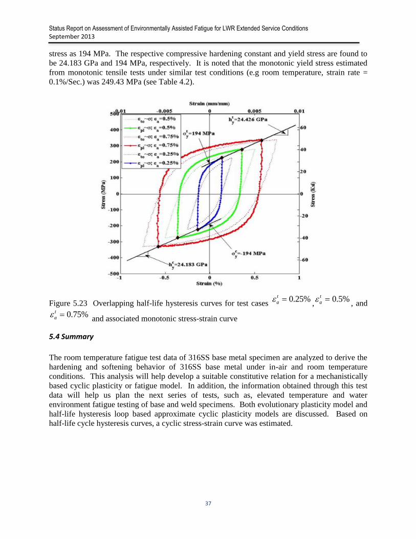
stress as 194 MPa. The respective compressive hardening constant and yield stress are found to
be 24.183 GPa and 194 MPa, respectively. It is noted that the monotonic yield stress estimated
from monotonic tensile tests under similar test conditions (e.g room temperature, strain rate =
0.1%/Sec.) was 249.43 MPa (see Table 4.2).
Figure 5.23 Overlapping half-life hysteresis curves for test cases , , and
and associated monotonic stress-strain curve
5.4 Summary
The room temperature fatigue test data of 316SS base metal specimen are analyzed to derive the
hardening and softening behavior of 316SS base metal under in-air and room temperature
conditions. This analysis will help develop a suitable constitutive relation for a mechanistically
based cyclic plasticity or fatigue model. In addition, the information obtained through this test
data will help us plan the next series of tests, such as, elevated temperature and water
environment fatigue testing of base and weld specimens. Both evolutionary plasticity model and
half-life hysteresis loop based approximate cyclic plasticity models are discussed. Based on
half-life cycle hysteresis curves, a cyclic stress-strain curve was estimated.
%25.0t
a %5.0t
a
%75.0t
a
Status Report on Assessment of Environmentally Assisted Fatigue for LWR Extended Service Conditions
September 2013
38
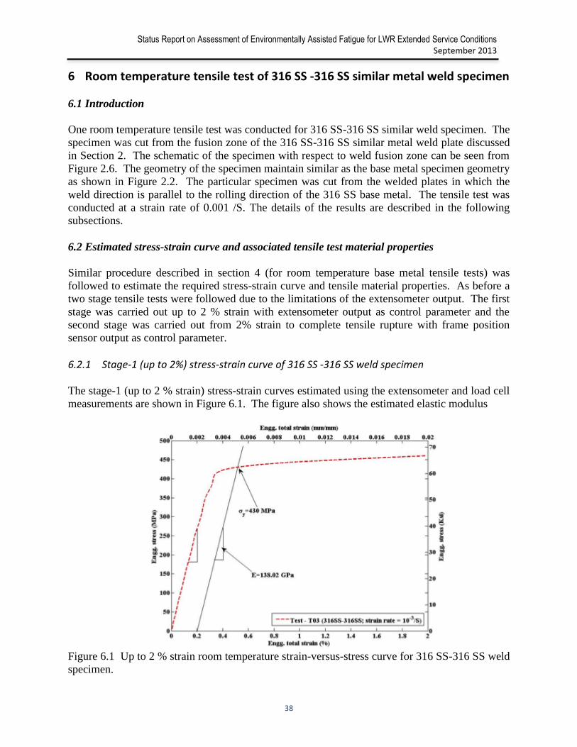
6 Room temperature tensile test of 316 SS -316 SS similar metal weld specimen
6.1 Introduction
One room temperature tensile test was conducted for 316 SS-316 SS similar weld specimen. The
specimen was cut from the fusion zone of the 316 SS-316 SS similar metal weld plate discussed
in Section 2. The schematic of the specimen with respect to weld fusion zone can be seen from
Figure 2.6. The geometry of the specimen maintain similar as the base metal specimen geometry
as shown in Figure 2.2. The particular specimen was cut from the welded plates in which the
weld direction is parallel to the rolling direction of the 316 SS base metal. The tensile test was
conducted at a strain rate of 0.001 /S. The details of the results are described in the following
subsections.
6.2 Estimated stress-strain curve and associated tensile test material properties
Similar procedure described in section 4 (for room temperature base metal tensile tests) was
followed to estimate the required stress-strain curve and tensile material properties. As before a
two stage tensile tests were followed due to the limitations of the extensometer output. The first
stage was carried out up to 2 % strain with extensometer output as control parameter and the
second stage was carried out from 2% strain to complete tensile rupture with frame position
sensor output as control parameter.
6.2.1 Stage-1 (up to 2%) stress-strain curve of 316 SS -316 SS weld specimen
The stage-1 (up to 2 % strain) stress-strain curves estimated using the extensometer and load cell
measurements are shown in Figure 6.1. The figure also shows the estimated elastic modulus
Figure 6.1 Up to 2 % strain room temperature strain-versus-stress curve for 316 SS-316 SS weld
specimen.
Status Report on Assessment of Environmentally Assisted Fatigue for LWR Extended Service Conditions
September 2013
39
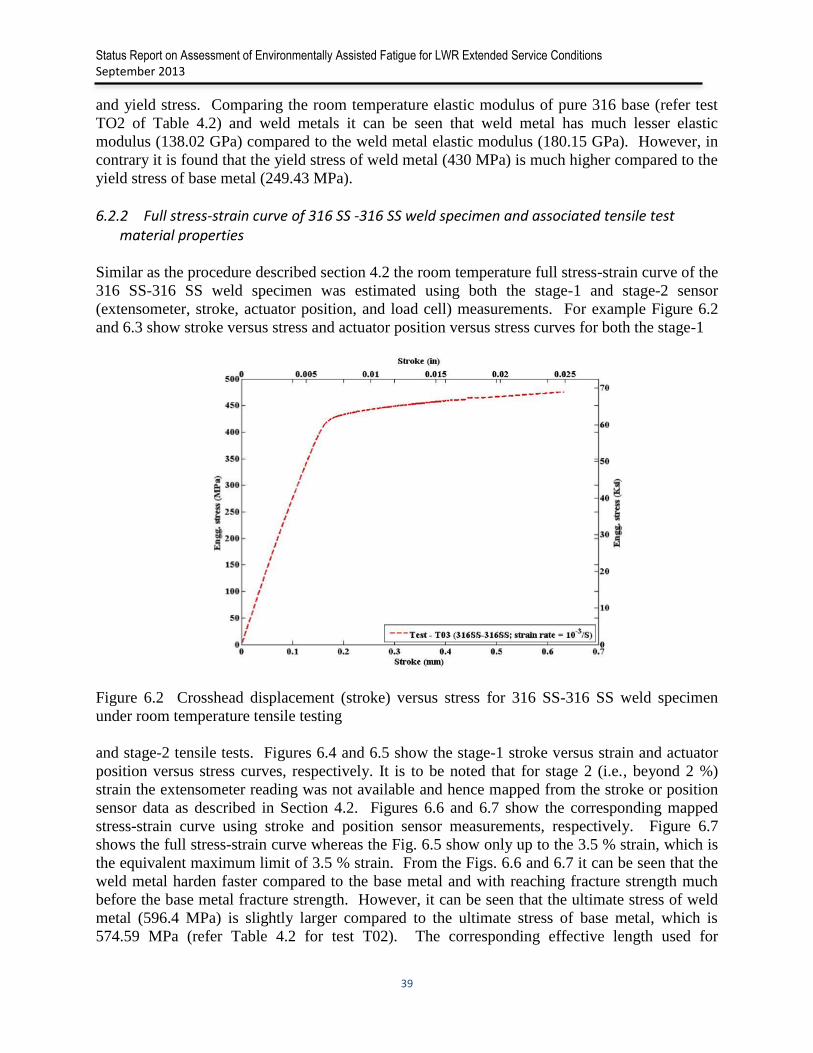
and yield stress. Comparing the room temperature elastic modulus of pure 316 base (refer test
TO2 of Table 4.2) and weld metals it can be seen that weld metal has much lesser elastic
modulus (138.02 GPa) compared to the weld metal elastic modulus (180.15 GPa). However, in
contrary it is found that the yield stress of weld metal (430 MPa) is much higher compared to the
yield stress of base metal (249.43 MPa).
6.2.2 Full stress-strain curve of 316 SS -316 SS weld specimen and associated tensile test material properties
Similar as the procedure described section 4.2 the room temperature full stress-strain curve of the
316 SS-316 SS weld specimen was estimated using both the stage-1 and stage-2 sensor
(extensometer, stroke, actuator position, and load cell) measurements. For example Figure 6.2
and 6.3 show stroke versus stress and actuator position versus stress curves for both the stage-1
Figure 6.2 Crosshead displacement (stroke) versus stress for 316 SS-316 SS weld specimen
under room temperature tensile testing
and stage-2 tensile tests. Figures 6.4 and 6.5 show the stage-1 stroke versus strain and actuator
position versus stress curves, respectively. It is to be noted that for stage 2 (i.e., beyond 2 %)
strain the extensometer reading was not available and hence mapped from the stroke or position
sensor data as described in Section 4.2. Figures 6.6 and 6.7 show the corresponding mapped
stress-strain curve using stroke and position sensor measurements, respectively. Figure 6.7
shows the full stress-strain curve whereas the Fig. 6.5 show only up to the 3.5 % strain, which is
the equivalent maximum limit of 3.5 % strain. From the Figs. 6.6 and 6.7 it can be seen that the
weld metal harden faster compared to the base metal and with reaching fracture strength much
before the base metal fracture strength. However, it can be seen that the ultimate stress of weld
metal (596.4 MPa) is slightly larger compared to the ultimate stress of base metal, which is
574.59 MPa (refer Table 4.2 for test T02). The corresponding effective length used for

Status Report on Assessment of Environmentally Assisted Fatigue for LWR Extended Service Conditions
September 2013
40
converting the stroke and position measurements to equivalent strain can be found from Table
6.1. Also all the estimated room temperature tensile properties of 316 SS-316 SS weld specimen
are summarized in Table 6.2.
Figure 6.3 Actuator positions versus stress for 316 SS-316 SS weld specimen under room
temperature tensile testing
Figure 6.4 Crosshead displacement (stroke) with respect to stage-1 (known extensometer
measurements) strain for 316 SS-316 SS weld specimen under room temperature tensile testing
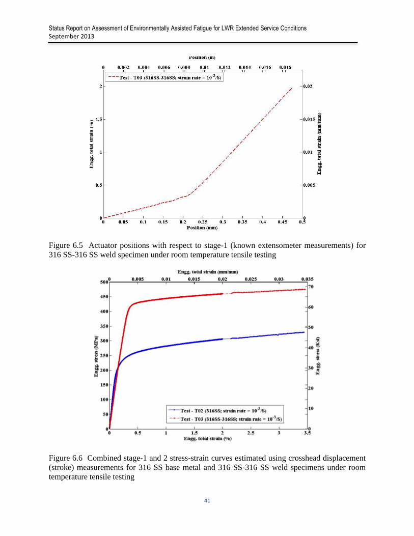
Status Report on Assessment of Environmentally Assisted Fatigue for LWR Extended Service Conditions
September 2013
41
Figure 6.5 Actuator positions with respect to stage-1 (known extensometer measurements) for
316 SS-316 SS weld specimen under room temperature tensile testing
Figure 6.6 Combined stage-1 and 2 stress-strain curves estimated using crosshead displacement
(stroke) measurements for 316 SS base metal and 316 SS-316 SS weld specimens under room
temperature tensile testing

Status Report on Assessment of Environmentally Assisted Fatigue for LWR Extended Service Conditions
September 2013
42
Figure 6.7 Combined stage-1 and 2 (full) stress-strain curves estimated using actuator
displacement (position) measurements for 316 SS base metal and 316 SS-316 SS weld
specimens under room temperature tensile testing
Table 6.1 Estimated effective gage length (or calibration factor) and specimen nominal gage
length for 316 SS-316 SS weld specimen under room temperature tensile testing
Test number (Strain
rate)
estimate in mm (in.) Specimen gage length in mm (in.)
Based on
crosshead
displacement
(stroke)
Based on
actuator
displacement
(position)
Nominal
length
Measured length
T03 (0.001/s) 14.977 (0.589) 15.488 (0.609) 14.25 (0.561) 14.072 (0.554)
Table 6.2 Estimated tensile material properties for 316 SS-316 SS weld specimen under room
temperature tensile testing
Test
number
(Strain
rate)
Elastic
modulus
in GPa
(ksi)
0.2% yield
Ultimate Fracture
Reduction
in gauge
area (%) Stress
in MPa
(ksi)
Strain
in %
Stress
in MPa
(ksi)
Strain in
%
Stress
in MPa
(ksi)
Strain
in %
T03
(strain rate
= 0.001/s)
138.02
(20018.1)
430
(62.36)
0.513 596.4
(86.50)
36.305 476.2
(69.07)
55.94 62.207
effL

Status Report on Assessment of Environmentally Assisted Fatigue for LWR Extended Service Conditions
September 2013
43
6.3 Summary
One room-temperature tensile test of 316 SS-316 SS weld metal was conducted under strain
rates 0.001/s. Based on the test data, tensile material properties and stress-strain curves were
estimated. The estimated results show that the weld metal has higher yield strength and lower
elastic modulus compared to the corresponding base metal. The results also show that the weld
metal fracture well before the base metal although both have the similar ultimate strength.
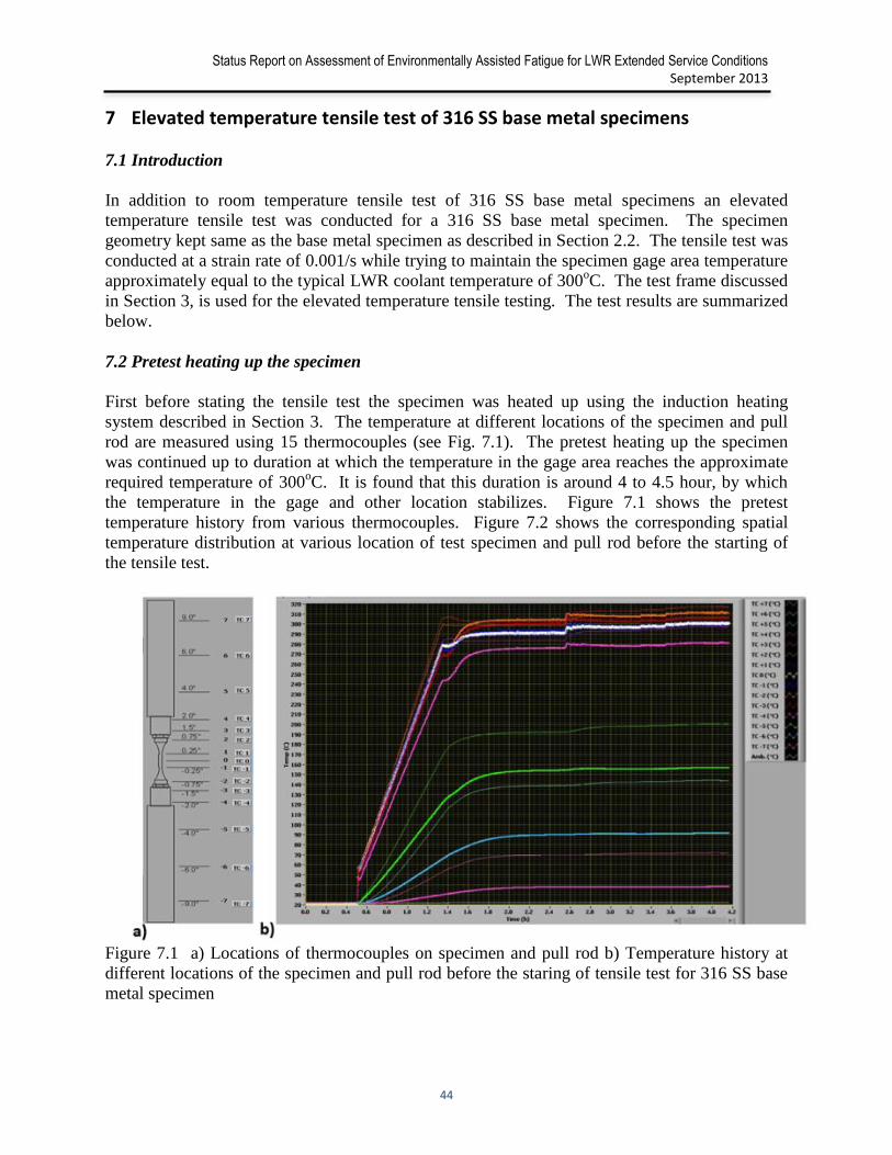
Status Report on Assessment of Environmentally Assisted Fatigue for LWR Extended Service Conditions
September 2013
44
7 Elevated temperature tensile test of 316 SS base metal specimens
7.1 Introduction
In addition to room temperature tensile test of 316 SS base metal specimens an elevated
temperature tensile test was conducted for a 316 SS base metal specimen. The specimen
geometry kept same as the base metal specimen as described in Section 2.2. The tensile test was
conducted at a strain rate of 0.001/s while trying to maintain the specimen gage area temperature
approximately equal to the typical LWR coolant temperature of 300oC. The test frame discussed
in Section 3, is used for the elevated temperature tensile testing. The test results are summarized
below.
7.2 Pretest heating up the specimen
First before stating the tensile test the specimen was heated up using the induction heating
system described in Section 3. The temperature at different locations of the specimen and pull
rod are measured using 15 thermocouples (see Fig. 7.1). The pretest heating up the specimen
was continued up to duration at which the temperature in the gage area reaches the approximate
required temperature of 300oC. It is found that this duration is around 4 to 4.5 hour, by which
the temperature in the gage and other location stabilizes. Figure 7.1 shows the pretest
temperature history from various thermocouples. Figure 7.2 shows the corresponding spatial
temperature distribution at various location of test specimen and pull rod before the starting of
the tensile test.
Figure 7.1 a) Locations of thermocouples on specimen and pull rod b) Temperature history at
different locations of the specimen and pull rod before the staring of tensile test for 316 SS base
metal specimen

Status Report on Assessment of Environmentally Assisted Fatigue for LWR Extended Service Conditions
September 2013
45
Figure 7.2 Temperature distributions at different locations of the specimen and pull rod before
the staring of tensile test for 316 SS base metal specimen
7.3 Summary of tensile test results and estimated stress-strain curve
Except the heating up the specimen, an ssimilar procedure described in section 4 (for room
temperature base metal tensile tests) was followed to conduct the mentioned tensile test and to
estimate the required stress-strain curve and tensile material properties from the test data. As
before mentioned due to the limitation in extensometer measurement range a two phase tensile
test procedure was followed with first phase was carried out up to 2 % strain with extensometer
output as control parameter and the second phase was carried out from 2% strain to complete
tensile rupture with frame position sensor output as control parameter.
7.3.1 Estimated phase-1 (up to 2%) stress-strain curve
The estimated stress-strain curve during the first phase of the tensile test is shown in Fig. 7.3.
The figure also shows the estimated elastic modulus of 157.21 GPa and yield stress of 156.07
MPa, respectively. Comparing the room temperature test results of base metal tensile test (refer
Table 4.2 test TO2) it can be found that the elevated temperature elastic modulus and yield stress
are much lesser compared to the corresponding room temperature elastic modulus (of 180.15
GPa) and yield stress (of 249.43 MPa), respectively. Also from the temperature history data it is
found that the temperature in the gage area relatively remains constant over the phase-1 tensile
test durations. Figure 7.4 shows the comparison of temperature profile at different locations of
specimen at start and end of the phase-1 tensile test.

Status Report on Assessment of Environmentally Assisted Fatigue for LWR Extended Service Conditions
September 2013
46
Figure 7.3 Up to 2 % strain elevated temperature (300 oC) strain-versus-stress curve for 316 SS
base metal specimen
Figure 7.4 Temperature profile at start and end of the phase-1 tensile test

Status Report on Assessment of Environmentally Assisted Fatigue for LWR Extended Service Conditions
September 2013
47
7.3.2 Estimated full (both phase-1 and 2) stress-strain curve
Similar as the procedure described Section 4.2 the full stress-strain curve of the 316 SS base
metal specimen under elevated temperature was estimated using both the phase-1 and phase-2
sensor (extensometer, stroke, actuator position, and load cell) measurements. For example
Figures 7.5 and 7.6 show stroke versus stress and actuator position versus stress curves estimated
from both the phase-1 and 2 tensile test data, respectively. Whereas Figs. 7.7 and 7.8 show the
phase-1 stroke and actuator displacement with respect to stress generated in the gage area. Using
the above-mentioned data and the procedure described in section 4.2 the combined phase-1 and 2
stress-strain curves are estimated. Figures 7.9 and 7.10 show the corresponding estimated stress-
strain curves with respect to stroke and actuator position measurements, respectively. Also the
Figures 7.9 and 7.10 show the comparison of stress-strain curve with respect to the
corresponding room temperature stress-strain curve (refer section 4 for details). From these
figures it can be found the elevated temperature curve harden slower compared to the room
temperature tensile curves. Also it can be found that the ultimate stress and fracture strain of
elevated temperature case are much lesser compared to the corresponding room temperature
case. However, care should be taken while using the above mentioned full stress-strain curve
particularly using the stress-strain data during the end of the test. This is because as the strain
(hence the pull rod displacement) increases, the specimen gage area slowly goes out of the
induction heater coil boundary. This leads to the change in temperature profile in gage area
compared to the original intended temperature profile.
Figure 7.11 show the snap shot of the temperature recorder after the end of phase-2 test. It is to
be noted that the phase-2 test duration was approximately from 4.5-4.65 h and at 4.65 h the
temperature at the center of the gage was approximately 285oC. As can be seen from Fig. 7.11
during the end of the tests the temperature in the lower half the specimen drops, whereas the
temperature of the upper half of the specimen rises. This is due to the specimen pulled
downward from the original position based on the location of the test frame actuator. This can
also be evident from Fig. 7.12, which shows the specimen location with respect to coil location
at the end of test. The estimated effective gage lengths used for converting the stroke and
actuator position sensor measurements to strain are given in Table 7.1. Whereas Table 7.2
summarizes the relevant tensile test properties estimated through above-mentioned data.

Status Report on Assessment of Environmentally Assisted Fatigue for LWR Extended Service Conditions
September 2013
48
Figure 7.5 Crosshead displacement (stroke) versus stress for 316 SS base metal specimen under
elevated temperature tensile testing
Figure 7.6 Actuator positions versus stress for 316 SS base metal specimen under elevated
temperature tensile testing
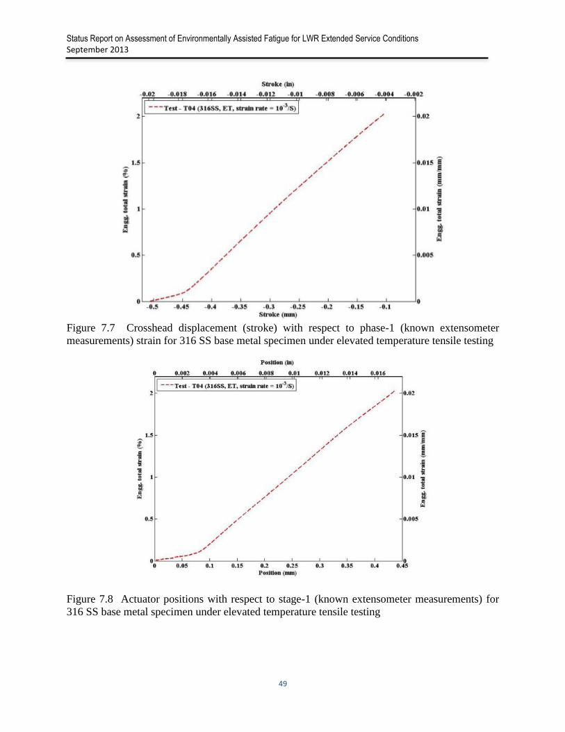
Status Report on Assessment of Environmentally Assisted Fatigue for LWR Extended Service Conditions
September 2013
49
Figure 7.7 Crosshead displacement (stroke) with respect to phase-1 (known extensometer
measurements) strain for 316 SS base metal specimen under elevated temperature tensile testing
Figure 7.8 Actuator positions with respect to stage-1 (known extensometer measurements) for
316 SS base metal specimen under elevated temperature tensile testing
Status Report on Assessment of Environmentally Assisted Fatigue for LWR Extended Service Conditions
September 2013
50
Figure 7.9 Combined phase-1 and 2 stress-strain curves estimated using crosshead displacement
(stroke) measurements for 316 SS base metal specimen under elevated temperature tensile
testing
Figure 7.10 Combined stage-1 and 2 (full) stress-strain curves estimated using actuator
displacement (position) measurements for 316 SS base metal specimen under elevated
temperature tensile testing
Status Report on Assessment of Environmentally Assisted Fatigue for LWR Extended Service Conditions
September 2013
51
Figure 7.11 Snap shot of the temperature history recorder after the end of phase-2 tensile test.
The phase-2 duration was approximately from 4.5-4.65 hour with gage center temperature of 285
oC at the end 4.65 hour.
Figure 7.12 The specimen location with respect to the fixed coil location after the end of phase-2
test
Status Report on Assessment of Environmentally Assisted Fatigue for LWR Extended Service Conditions
September 2013
52
Table 7.1 Estimated effective gage length (or calibration factor) and specimen nominal gage
length for 316 SS base metal specimen under elevated temperature tensile testing
Test number (Strain
rate)
estimate in mm (in.) Specimen gage length in mm (in.)
Based on
crosshead
displacement
(stroke)
Based on actuator
displacement
(position)
Nominal length
Measured length
T04 (0.001/s) 17.748 (0.699) 18.672 (0.735) 14.25 (0.561) 13.487 (0.531)
Table 7.2 Estimated tensile material properties for 316 SS base metal specimen under elevated
temperature tensile testing
Test
number
(Strain
rate)
Elastic
modulus
in GPa
(ksi)
0.2% yield
Ultimate Fracture
Reduction
in gauge
area (%) Stress
in MPa
(ksi)
Strain
in %
Stress
in MPa
(ksi)
Strain in
%
Stress
in MPa
(ksi)
Strain
in %
T04
(strain rate
= 0.001/s)
157.212
(22801.67)
156.067
(22.64)
0.2996 418.717
(60.73)
31.301 275.7
(39.99)
41.24 69.474
7.4 Summary
One elevated-temperature tensile test of 316 SS base metal specimen was conducted under strain
rates 0.001/s and approximately at the typical LWR coolant temperature of 300oC. Based on the
test data, tensile material properties and stress-strain curves were estimated. The estimated
results show that the elevated temperature shows lower yield stress, ultimate stress and fracture
strain compared to the corresponding room temperature tensile test data. This shows that at
300oC the 316 SS base metal has softer tensile properties compared to its room temperature
conditions.
effL

Status Report on Assessment of Environmentally Assisted Fatigue for LWR Extended Service Conditions
September 2013
53
8 Elevated temperature tensile test of 316 SS -316 SS similar metal weld specimen
8.1 Introduction
To obtain the elevated temperature tensile properties and stress-strain curve of 316 SS-316 SS
similar metal weld specimen one elevated temperature tensile test was performed. The tensile
test was conducted at a strain rate of 0.001/s while trying to maintain the specimen gage area
temperature approximately equal to the typical LWR coolant temperature of 300oC. The
geometry of the specimen maintained same as the corresponding room temperature test
specimen. Similar procedure, discussed in Sections 4, 6, and 7, was used to conduct the test and
estimating the relevant material properties and stress-strain curve. The procedure and results are
highlighted below.
8.2 Pretest heating up the specimen
Similar procedure discussed in Section 7.2 was used to initial heating up the specimen until
achieving a stable temperature of 300oC at specimen gage area. Figure 8.1 shows the pretest
temperature history from various thermocouples. Figure 8.2 shows the corresponding spatial
temperature distribution at various location of test specimen and pull rod before the starting of
the tensile test.
Figure 8.1 Temperature history at different locations of the specimen and pull rod before the
starting of tensile test for 316 SS-316 SS weld metal specimen
Status Report on Assessment of Environmentally Assisted Fatigue for LWR Extended Service Conditions
September 2013
54
Figure 8.2 Temperature distributions at different locations of the specimen and pull rod before
the staring of tensile test for 316 SS-316 SS weld metal specimen
8.3 Summary of tensile test results and estimated stress-strain curve
Similar as before a two phase tensile test was performed due to the limitation in extensometer
measurement range with first phase was carried out up to 2 % strain with extensometer output as
control parameter and the second phase was carried out from 2% strain to complete tensile
rupture with frame position sensor output as control parameter.
8.3.1 Estimated phase-1 (up to 2%) stress-strain curve
The estimated stress-strain curve during the first phase of the tensile test is shown in Fig. 8.3.
The figure also shows the estimated elastic modulus of 136.42 GPa and yield stress of 354.25
MPa, respectively. The corresponding room temperature test values are 138.02 GPa and 430
MPa (see Table 6.2) respectively. This says under the mentioned elevated temperature the
material harden lesser compared to its room temperature condition. During the phase 1 test it is
found that the temperature at the gage area had not change much due to the actuator
displacement. Figure 8.4 shows the comparison of temperature distribution on specimen at start
and end of phase-1 test.

Status Report on Assessment of Environmentally Assisted Fatigue for LWR Extended Service Conditions
September 2013
55
Figure 8.3 Up to 2 % strain elevated temperature (300°C) strain-versus-stress curve for 316 SS-
316 SS weld metal specimen
Figure 8.4 Temperature profile at start and end of the phase-1 tensile test
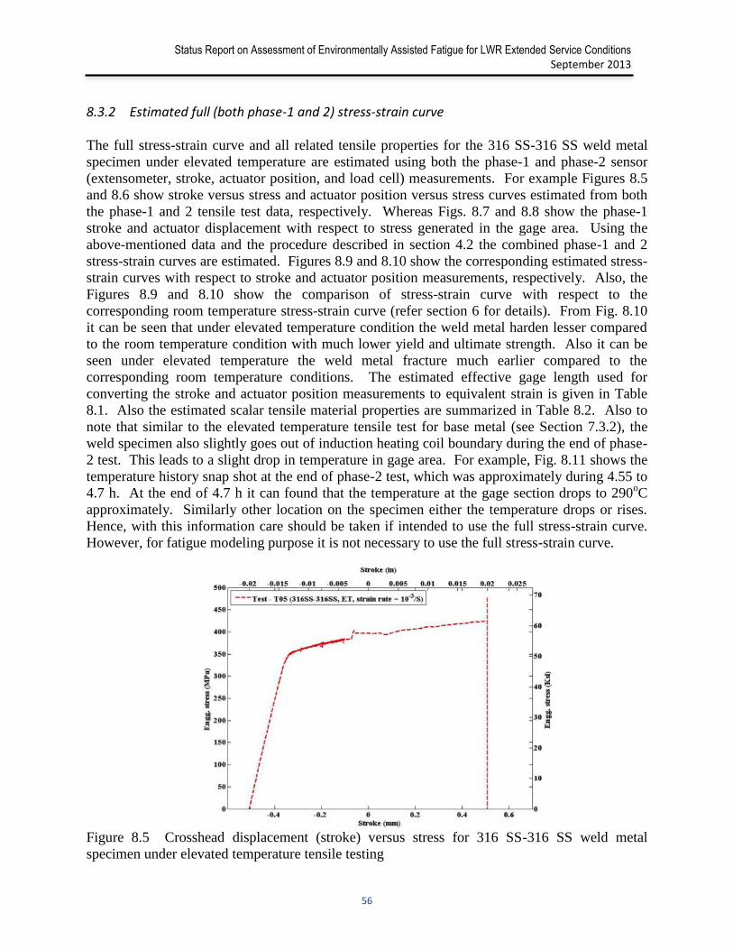
Status Report on Assessment of Environmentally Assisted Fatigue for LWR Extended Service Conditions
September 2013
56
8.3.2 Estimated full (both phase-1 and 2) stress-strain curve
The full stress-strain curve and all related tensile properties for the 316 SS-316 SS weld metal
specimen under elevated temperature are estimated using both the phase-1 and phase-2 sensor
(extensometer, stroke, actuator position, and load cell) measurements. For example Figures 8.5
and 8.6 show stroke versus stress and actuator position versus stress curves estimated from both
the phase-1 and 2 tensile test data, respectively. Whereas Figs. 8.7 and 8.8 show the phase-1
stroke and actuator displacement with respect to stress generated in the gage area. Using the
above-mentioned data and the procedure described in section 4.2 the combined phase-1 and 2
stress-strain curves are estimated. Figures 8.9 and 8.10 show the corresponding estimated stress-
strain curves with respect to stroke and actuator position measurements, respectively. Also, the
Figures 8.9 and 8.10 show the comparison of stress-strain curve with respect to the
corresponding room temperature stress-strain curve (refer section 6 for details). From Fig. 8.10
it can be seen that under elevated temperature condition the weld metal harden lesser compared
to the room temperature condition with much lower yield and ultimate strength. Also it can be
seen under elevated temperature the weld metal fracture much earlier compared to the
corresponding room temperature conditions. The estimated effective gage length used for
converting the stroke and actuator position measurements to equivalent strain is given in Table
8.1. Also the estimated scalar tensile material properties are summarized in Table 8.2. Also to
note that similar to the elevated temperature tensile test for base metal (see Section 7.3.2), the
weld specimen also slightly goes out of induction heating coil boundary during the end of phase-
2 test. This leads to a slight drop in temperature in gage area. For example, Fig. 8.11 shows the
temperature history snap shot at the end of phase-2 test, which was approximately during 4.55 to
4.7 h. At the end of 4.7 h it can found that the temperature at the gage section drops to 290oC
approximately. Similarly other location on the specimen either the temperature drops or rises.
Hence, with this information care should be taken if intended to use the full stress-strain curve.
However, for fatigue modeling purpose it is not necessary to use the full stress-strain curve.
Figure 8.5 Crosshead displacement (stroke) versus stress for 316 SS-316 SS weld metal
specimen under elevated temperature tensile testing

Status Report on Assessment of Environmentally Assisted Fatigue for LWR Extended Service Conditions
September 2013
57
Figure 8.6 Actuator positions versus stress for 316 SS-316 SS weld metal specimen under
elevated temperature tensile testing
Figure 8.7 Crosshead displacement (stroke) with respect to phase-1 (known extensometer
measurements) strain for 316 SS-316 SS weld metal specimen
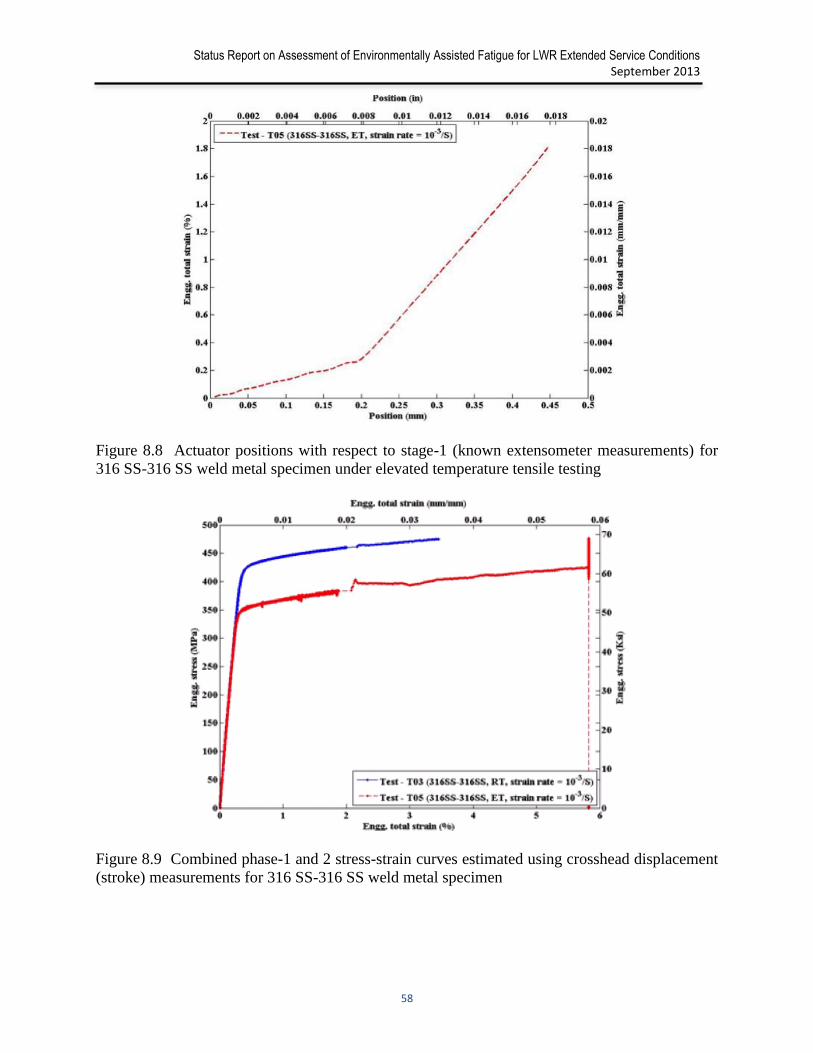
Status Report on Assessment of Environmentally Assisted Fatigue for LWR Extended Service Conditions
September 2013
58
Figure 8.8 Actuator positions with respect to stage-1 (known extensometer measurements) for
316 SS-316 SS weld metal specimen under elevated temperature tensile testing
Figure 8.9 Combined phase-1 and 2 stress-strain curves estimated using crosshead displacement
(stroke) measurements for 316 SS-316 SS weld metal specimen
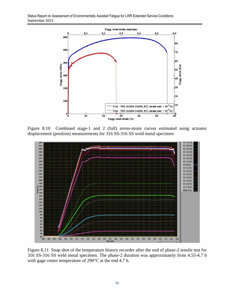
Status Report on Assessment of Environmentally Assisted Fatigue for LWR Extended Service Conditions
September 2013
59
Figure 8.10 Combined stage-1 and 2 (full) stress-strain curves estimated using actuator
displacement (position) measurements for 316 SS-316 SS weld metal specimen
Figure 8.11 Snap shot of the temperature history recorder after the end of phase-2 tensile test for
316 SS-316 SS weld metal specimen. The phase-2 duration was approximately from 4.55-4.7 h
with gage center temperature of 290°C at the end 4.7 h.
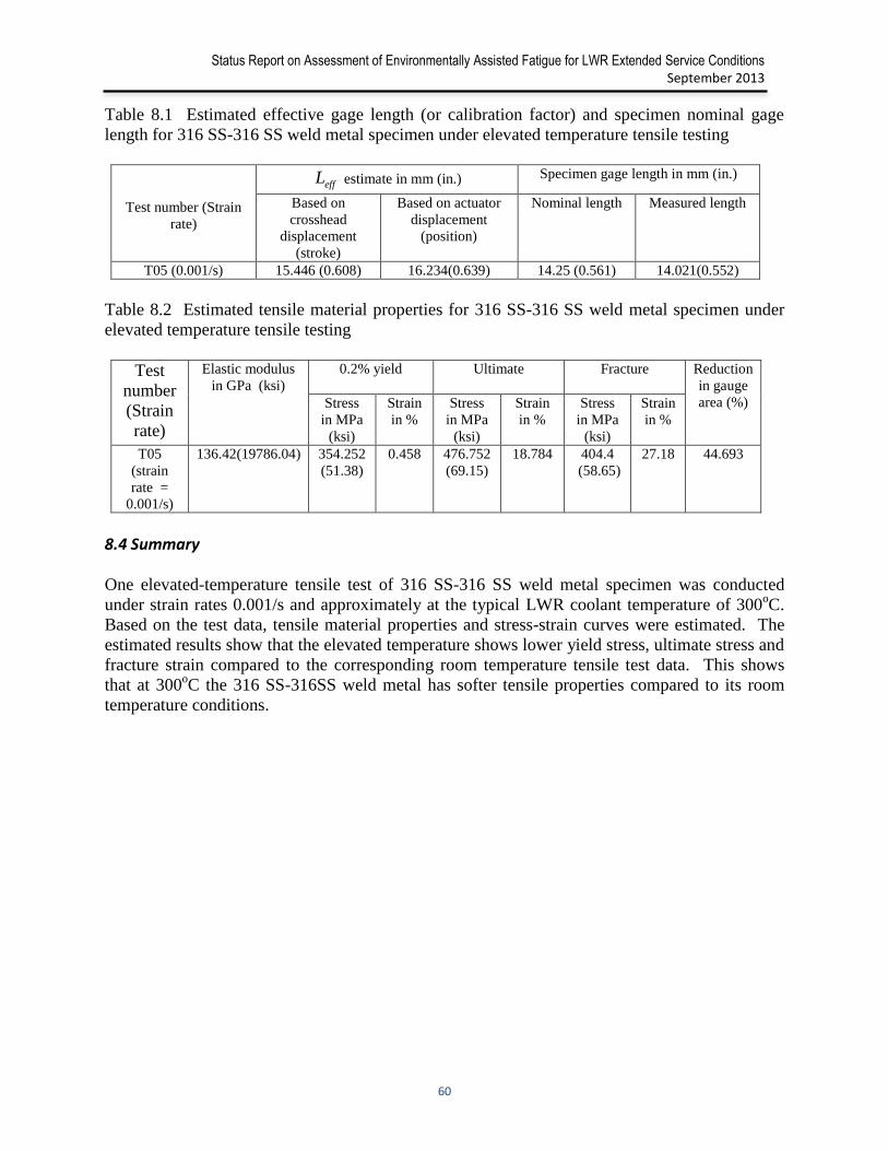
Status Report on Assessment of Environmentally Assisted Fatigue for LWR Extended Service Conditions
September 2013
60
Table 8.1 Estimated effective gage length (or calibration factor) and specimen nominal gage
length for 316 SS-316 SS weld metal specimen under elevated temperature tensile testing
Test number (Strain
rate)
estimate in mm (in.) Specimen gage length in mm (in.)
Based on
crosshead
displacement
(stroke)
Based on actuator
displacement
(position)
Nominal length Measured length
T05 (0.001/s) 15.446 (0.608) 16.234(0.639) 14.25 (0.561) 14.021(0.552)
Table 8.2 Estimated tensile material properties for 316 SS-316 SS weld metal specimen under
elevated temperature tensile testing
Test
number
(Strain
rate)
Elastic modulus
in GPa (ksi)
0.2% yield
Ultimate Fracture
Reduction
in gauge
area (%) Stress
in MPa
(ksi)
Strain
in %
Stress
in MPa
(ksi)
Strain
in %
Stress
in MPa
(ksi)
Strain
in %
T05
(strain
rate =
0.001/s)
136.42(19786.04) 354.252
(51.38)
0.458 476.752
(69.15)
18.784 404.4
(58.65)
27.18 44.693
8.4 Summary
One elevated-temperature tensile test of 316 SS-316 SS weld metal specimen was conducted
under strain rates 0.001/s and approximately at the typical LWR coolant temperature of 300oC.
Based on the test data, tensile material properties and stress-strain curves were estimated. The
estimated results show that the elevated temperature shows lower yield stress, ultimate stress and
fracture strain compared to the corresponding room temperature tensile test data. This shows
that at 300oC the 316 SS-316SS weld metal has softer tensile properties compared to its room
temperature conditions.
effL

Status Report on Assessment of Environmentally Assisted Fatigue for LWR Extended Service Conditions
September 2013
61
9 Estimation of effect of thermal strain and coefficient of thermal expansion in 316 SS base and 316 SS -316 SS similar metal weld material
9.1 Introduction
LWR components may experience significant thermal strains during the heat up and cool down
of the reactor. Since thermal strain by itself does not produce any stress, it is necessary to assess
the contribution of thermal strain to the total strain. The previously discussed elevated
temperature tensile test data for 316 SS base (see Section 7) and 316 SS-316 SS weld (see
Section 8) metal specimens are further analyzed to estimate the magnitude of the purely thermal
strain which has to be deducted from the total strain measured in order to obtain the mechanical
strain that produces stress and to estimate the values of coefficient of thermal expansion (CTE)
of base and weld metal. The results are briefly described below.
9.2 Effect of free thermal straining
The pretest data discussed in Sections 7.2 and 8.2 are used to assess the effect of thermal strain.
Figure 9.1 shows the overall temperature history during the elevated temperature tensile tests
conducted for base and weld metals. The pre-tensile test specimen heat up data are used to
estimate the thermal expansion strain. Particularly, data up to temperature stabilization is
considered. It is to be noted that during pretest heat up period the specimen was kept under load
control with zero load set point and with no other applied mechanical strain. However, the
specimen was allowed to expand freely due to thermal transient strain. Figure 9.2 shows the
measured stress history for both the test cases. Figure 9.3 shows stabilized temperature profile in
the gage area of base and weld specimens. Figure 9.4 shows the gage area temperature build up
versus change in gage area length that was measured by the extensometer. Figure 9.5 shows the
estimated thermal strain for base and weld metal. From the figure it can be seen that weld metal
experienced lower thermal strain compared to the base metal.
Figures 9.4 and 9.5 show that the extensometer recorded a spike in the weld strain during initial
heat up. This is a test related anomaly (may be due to instantaneous slippage of extensometer)
which should be ignored. Also, from Fig. 9.5 it can be seen that the strain increases to 0.5 %
during the temperature build up from room temperature to typical LWR temperature of 300oC.
This thermally-induced strain could lead to significant thermal stress had the specimen been
constrained. In addition, from Fig. 9.1 it can be seen that during start of the pretest heating up,
there is a 50°C jump in the temperature beyond which the temperature increase steadily up to the
stabilized temperature. This is a test related anomaly, which is most likely caused by large
electromagnetic interference when the induction heater was switched on. For the purpose of
estimating the CTE, only the thermal strain data above 50oC was considered. The estimated
variations of the CTEs of both materials with temperature are shown in Fig. 9.6. From the figure
it can be seen that the CTE for both base and weld metals increase with temperature, although
the magnitude is smaller for weld metal. This smaller CTE magnitude for weld metal compared
to base metal is due to smaller thermal strain as can be seen from Fig. 9.4. This preliminary CTE
test data can be used for the mechanistic modeling while considering thermal transient and cyclic
loading. However, the above-discussed approach to estimate the CTE does not follow the
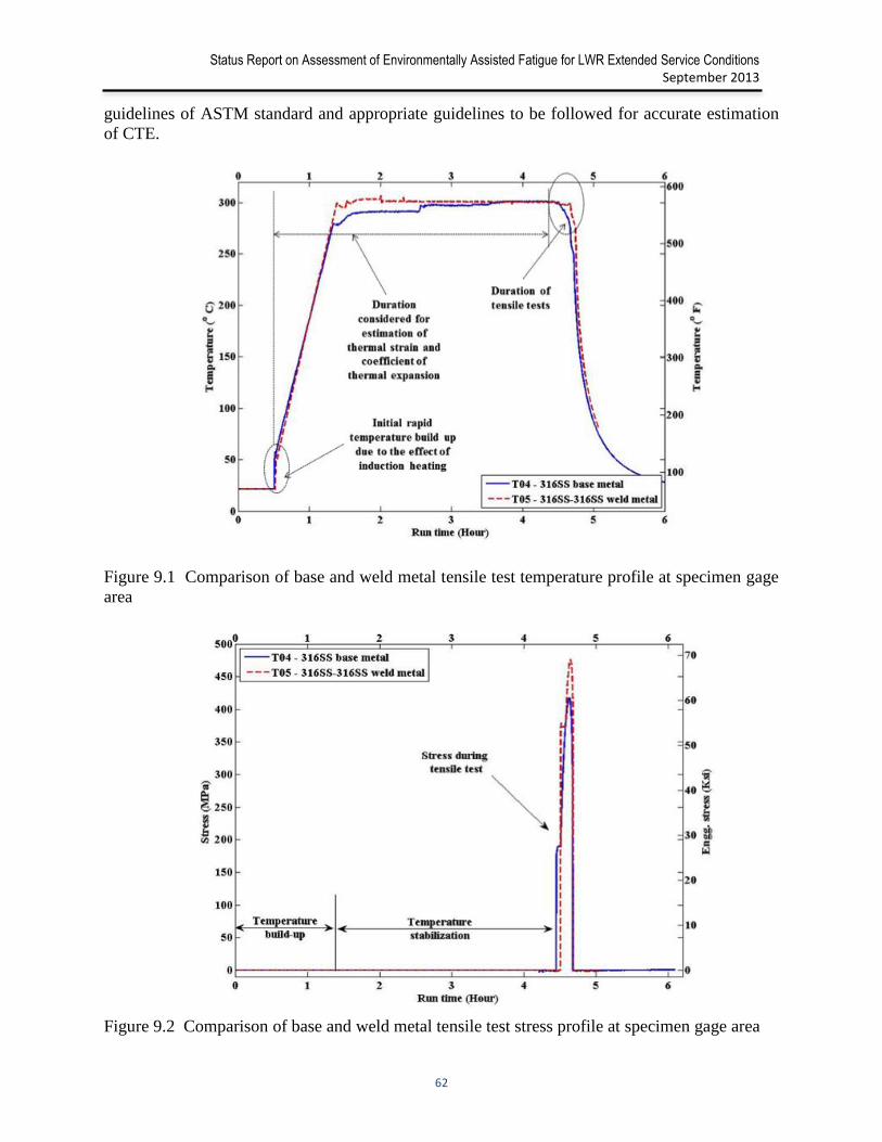
Status Report on Assessment of Environmentally Assisted Fatigue for LWR Extended Service Conditions
September 2013
62
guidelines of ASTM standard and appropriate guidelines to be followed for accurate estimation
of CTE.
Figure 9.1 Comparison of base and weld metal tensile test temperature profile at specimen gage
area
Figure 9.2 Comparison of base and weld metal tensile test stress profile at specimen gage area

Status Report on Assessment of Environmentally Assisted Fatigue for LWR Extended Service Conditions
September 2013
63
Figure 9.3 a) Schematic showing the location of thermocouples b) Comparison of base and weld
metal pre tensile test, stabilized temperature profile at specimen gage area
Figure 9.4 Specimen gage area temperature versus extensometer measurements for base and
weld metals
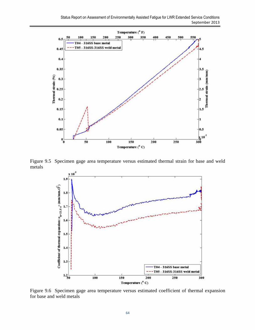
Status Report on Assessment of Environmentally Assisted Fatigue for LWR Extended Service Conditions
September 2013
64
Figure 9.5 Specimen gage area temperature versus estimated thermal strain for base and weld
metals
Figure 9.6 Specimen gage area temperature versus estimated coefficient of thermal expansion
for base and weld metals

Status Report on Assessment of Environmentally Assisted Fatigue for LWR Extended Service Conditions
September 2013
65
9.3 Summary
The effects of thermal transient in 316 SS base and 316 SS-316 SS weld metals are
estimated. This is evaluated using the pretest data during the heat up of the corresponding tensile
specimens. From the results it is found that the thermal strain can reach 0.5 % during the
temperature build up from room temperature to typical LWR temperature of 300oC. This strain,
if constrained, could lead to significant thermal stress if the specimen were constrained.. These
types of data suggest the need for pure thermal cycling test to model the effect of pure thermal
cyclic stress during reactor heat up and cool down. Also using the above-mentioned pre tensile
test data, approximate CTEs for both the base and weld metals were estimated, which can be
used for the future mechanistic model development.
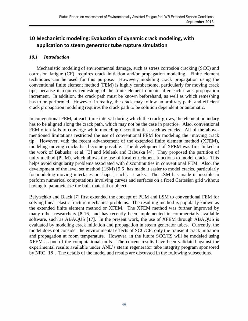
Status Report on Assessment of Environmentally Assisted Fatigue for LWR Extended Service Conditions
September 2013
66
10 Mechanistic modeling: Evaluation of dynamic crack modeling, with application to steam generator tube rupture simulation
10.1 Introduction
Mechanistic modeling of environmental damage, such as stress corrosion cracking (SCC) and
corrosion fatigue (CF), requires crack initiation and/or propagation modeling. Finite element
techniques can be used for this purpose. However, modeling crack propagation using the
conventional finite element method (FEM) is highly cumbersome, particularly for moving crack
tips, because it requires remeshing of the finite element domain after each crack propagation
increment. In addition, the crack path must be known beforehand, as well as which remeshing
has to be performed. However, in reality, the crack may follow an arbitrary path, and efficient
crack propagation modeling requires the crack path to be solution dependent or automatic.
In conventional FEM, at each time interval during which the crack grows, the element boundary
has to be aligned along the crack path, which may not be the case in practice. Also, conventional
FEM often fails to converge while modeling discontinuities, such as cracks. All of the above-
mentioned limitations restricted the use of conventional FEM for modeling the moving crack
tip. However, with the recent advancement of the extended finite element method (XFEM),
modeling moving cracks has become possible. The development of XFEM was first linked to
the work of Babuska, et al. [3] and Melenk and Babuska [4]. They proposed the partition of
unity method (PUM), which allows the use of local enrichment functions to model cracks. This
helps avoid singularity problems associated with discontinuities in conventional FEM. Also, the
development of the level set method (LSM) [5,6] has made it easier to model cracks, particularly
for modeling moving interfaces or shapes, such as cracks. The LSM has made it possible to
perform numerical computations involving curves and surfaces on a fixed Cartesian grid without
having to parameterize the bulk material or object.
Belytschko and Black [7] first extended the concept of PUM and LSM to conventional FEM for
solving linear elastic fracture mechanics problems. The resulting method is popularly known as
the extended finite element method or XFEM. The XFEM method was further improved by
many other researchers [8-16] and has recently been implemented in commercially available
software, such as ABAQUS [17]. In the present work, the use of XFEM through ABAQUS is
evaluated by modeling crack initiation and propagation in steam generator tubes. Currently, the
model does not consider the environmental effects of SCC/CF, only the transient crack initiation
and propagation at room temperature. However, in the future SCC/CS will be modeled using
XFEM as one of the computational tools. The current results have been validated against the
experimental results available under ANL’s steam regenerator tube integrity program sponsored
by NRC [18]. The details of the model and results are discussed in the following subsections.
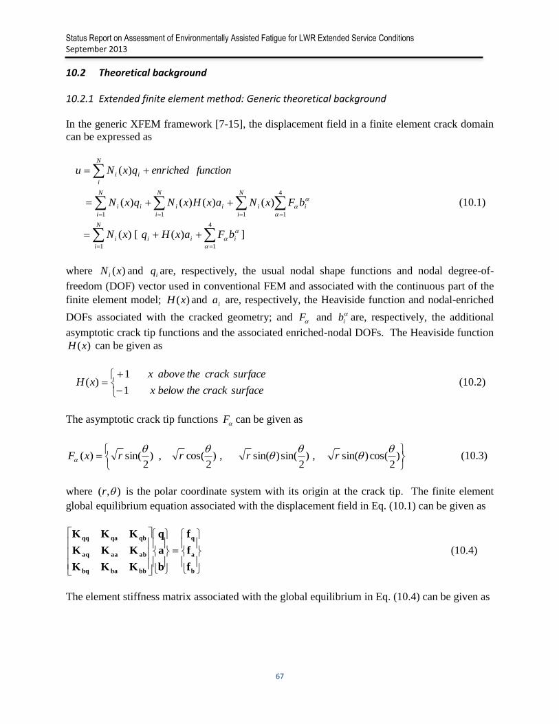
Status Report on Assessment of Environmentally Assisted Fatigue for LWR Extended Service Conditions
September 2013
67
10.2 Theoretical background
10.2.1 Extended finite element method: Generic theoretical background
In the generic XFEM framework [7-15], the displacement field in a finite element crack domain
can be expressed as
])([)(
)()()()(
)(
4
11
4
1111
iii
N
i
i
i
N
i
ii
N
i
ii
N
i
i
i
N
i
i
bFaxHqxN
bFxNaxHxNqxN
functionenrichedqxNu
(10.1)
where )(xN i and iq are, respectively, the usual nodal shape functions and nodal degree-of-
freedom (DOF) vector used in conventional FEM and associated with the continuous part of the
finite element model; )(xH and ia are, respectively, the Heaviside function and nodal-enriched
DOFs associated with the cracked geometry; and F and
ib are, respectively, the additional
asymptotic crack tip functions and the associated enriched-nodal DOFs. The Heaviside function
)(xH can be given as
surfacecrackthebelowx
surfacecracktheabovexxH
1
1)(
(10.2)
The asymptotic crack tip functions F can be given as
)2
cos()sin(,)2
sin()sin(,)2
cos(,)2
sin()(
rrrrxF
(10.3)
where ),( r is the polar coordinate system with its origin at the crack tip. The finite element
global equilibrium equation associated with the displacement field in Eq. (10.1) can be given as
b
a
q
bbbabq
abaaaq
qbqaqq
f
f
f
b
a
q
KKK
KKK
KKK
(10.4)
The element stiffness matrix associated with the global equilibrium in Eq. (10.4) can be given as

Status Report on Assessment of Environmentally Assisted Fatigue for LWR Extended Service Conditions
September 2013
68
e
Ae
bb
e
ba
e
bq
e
ab
e
aa
e
aq
e
qb
e
qa
e
dA
e
a
T
aa
T
bq
T
b
b
T
aa
T
aq
T
a
b
T
qa
T
T
q
DBBDBBDBB
DBBDBBDBB
DBBDBBDBB
KKK
KKK
KKK
(10.5)
In Eq. (10.5), D is the material property matrix, and B stands for the respective strain-
displacement matrix associated with the conventional finite element nodal DOFs (subscript q ),
crack domain enriched-nodal DOFs (subscript a ), and crack tip-enriched nodal DOFs
(subscript b ).
10.2.2 XFEM modeling through ABAQUS
In the present work, commercially available ABAQUS based extended finite element
technique is used to model the initiation and propagation of moving cracks in steam generator
tubes. To note that for simplicity the current version of ABAQUS does not allow considering
the displacement field associated with the asymptotic crack tip functions given in Eq. (10.1),
particularly for modeling moving cracks. The total displacement field considered for modeling a
moving crack in the present work can then be as follows:
])([)()()()(
)(
111
ii
N
i
ii
N
i
ii
N
i
i
i
N
i
i
axHqxNaxHxNqxN
functionenrichedqxNu
(10.6)
In addition to the techniques common to conventional FEM, the XFEM procedure in
ABAQUS has additional techniques, such as phantom node modeling, level set methods, and
cohesive zone modeling. A brief discussion of these techniques is given below. The details of
these techniques can be found in the ABAQUS user manual [17] and elsewhere in the literature
[5-16] related to these topics.
Phantom node modeling approach
In the phantom node approach, additional nodes are created surrounding the crack. These
nodes remain even after the crack has passed through that element. These nodes are introduced
to represent the discontinuity associated with the cracked elements. These phantom nodes are
associated with the Heaviside function )(xH in Eq. (10.6). The location of the phantom nodes
with respect to real nodes and the cracked element is schematically shown in Fig. 10.1. Phantom
nodes are automatically created in the crack tip element of the uncracked mesh. These nodes are
superimposed on the real nodes of the element, and when the element is intact these phantom
nodes are fully constrained to the real nodes. When the crack passes through the element, the
element gets separated into two superimposed elements, consisting of a combination of real
nodes and phantom nodes, as shown in Fig. 10.1b. In the new elements, the cracked surfaces are
separated according to traction separation techniques, which are described in the following
subsection. Unlike the uncracked finite elements, the time-dependent stiffness matrix of the new
cracked element is computed by integrating over the area from the side of the real nodes up to

Status Report on Assessment of Environmentally Assisted Fatigue for LWR Extended Service Conditions
September 2013
69
the crack surface only. For example, the stiffness matrix of the cracked element shown in Figure
10.1 can be expressed as below:
b
A
T
t
A
T
e
A
T dADBBdADBBdADBB
bte
)()()( (10.7)
where tA and bA are the real area of the top and bottom portion of the cracked element,
respectively.
Figure 10.1 Schematic of (a) cracked and uncracked mesh showing real and phantom nodes and
(b) cracked element as sum of two virtual or phantom elements
Level set method
In the XFEM framework it is essential to automatically track the crack surface and crack
front. This tracking is made possible by the level set representation, in which the crack plane
surface and crack tip surface are represented by two level set functions or fields. Figure 10.2
schematically shows the level set fields for the crack plane surface and crack tip surface
represented by 0 and 0 , respectively [15]. These surfaces are assumed orthogonal, such
that 0. . The values of these fields are time or solution dependent. These functions are
computed on a narrow band of grid points surrounding the crack surface and tip. These field
values can be used not only to obtain the geometric information regarding the location of the
crack but also the local coordinate system that can be used to generate the enrichment function
)(xH in Eq. (10.6). The LSM does not require explicit representations of the crack
boundary/interface because they are defined entirely by the solution-dependent surfaces, 0
and 0 .

Status Report on Assessment of Environmentally Assisted Fatigue for LWR Extended Service Conditions
September 2013
70
Figure 10.2 Schematic showing the orthogonal level set fields that describe the crack tip
Crack initiation criteria
A crack, to be initiated in any element, has to satisfy certain criteria. Different initiation criteria
can be defined in terms of solution-dependent stress, strain, etc., and respective critical values. In
the present work, the maximum principal stress criterion is used for the initiation of the crack.
The maximum principal stress initiation criterion is given below:
initiatenotwillcrackf
initiatewillcrackff
tol
tol
p
cr
p
1
1max
(10.8)
where p
max is the solution-dependent maximum principal stress, and p
cr is the critical principal
stress that has to be provided as an input material property. In Eq. (10.8), the symbol
represents Macaulay brackets with 0max p if 0max p , i.e., when the maximum principal
stress is purely compressive.
Crack evolution through traction separation criteria
Crack evolution criteria describe the rate at which traction is applied to the cracked surface of the
cracked element following initiation. The traction in a cracked element is shown schematically
in Fig. 10.1b. The three-dimensional traction in a cracked element can be found by using the
following expression:
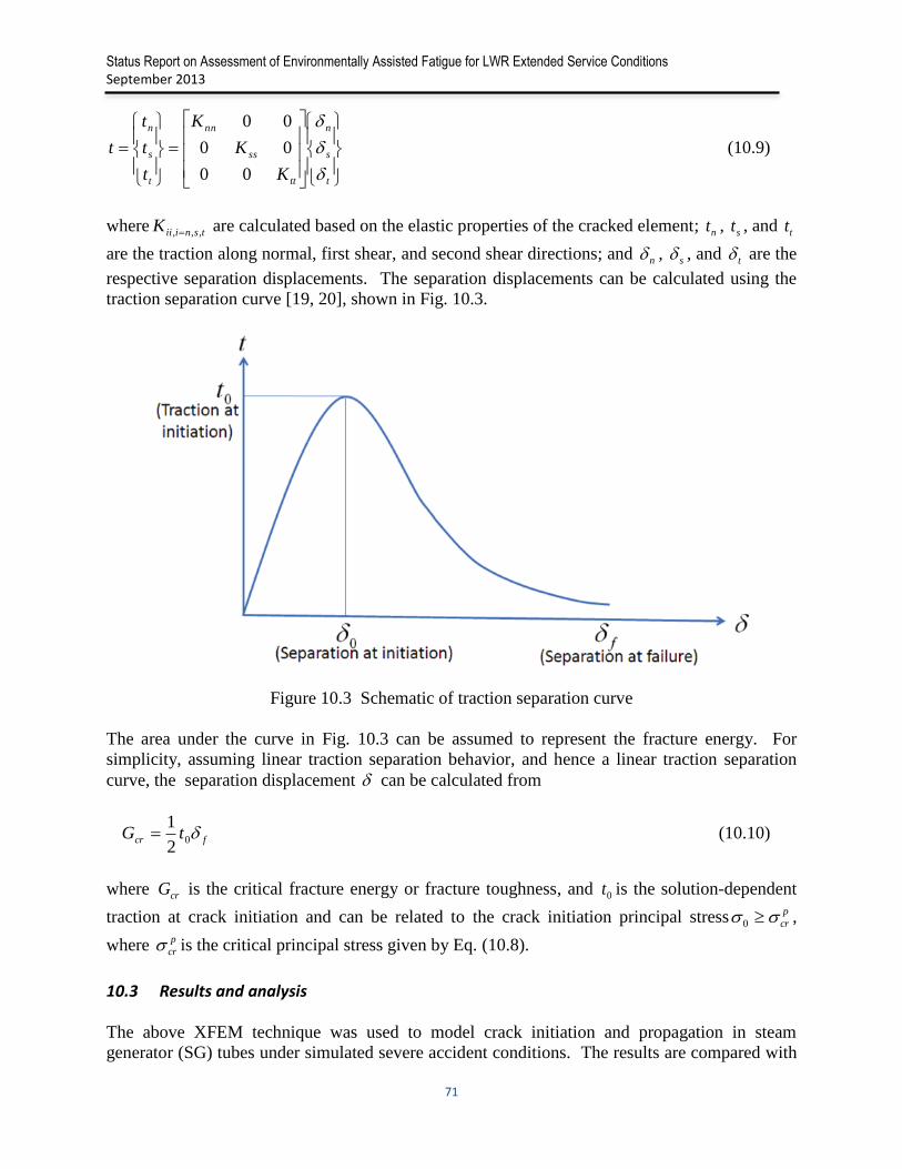
Status Report on Assessment of Environmentally Assisted Fatigue for LWR Extended Service Conditions
September 2013
71
t
s
n
tt
ss
nn
t
s
n
K
K
K
t
t
t
t
00
00
00
(10.9)
where tsniiiK ,,, are calculated based on the elastic properties of the cracked element; nt , st , and tt
are the traction along normal, first shear, and second shear directions; and n , s , and t are the
respective separation displacements. The separation displacements can be calculated using the
traction separation curve [19, 20], shown in Fig. 10.3.
Figure 10.3 Schematic of traction separation curve
The area under the curve in Fig. 10.3 can be assumed to represent the fracture energy. For
simplicity, assuming linear traction separation behavior, and hence a linear traction separation
curve, the separation displacement can be calculated from
fcr tG 02
1 (10.10)
where crG is the critical fracture energy or fracture toughness, and 0t is the solution-dependent
traction at crack initiation and can be related to the crack initiation principal stress p
cr 0 ,
where p
cr is the critical principal stress given by Eq. (10.8).
10.3 Results and analysis
The above XFEM technique was used to model crack initiation and propagation in steam
generator (SG) tubes under simulated severe accident conditions. The results are compared with
Status Report on Assessment of Environmentally Assisted Fatigue for LWR Extended Service Conditions
September 2013
72
the experimental data obtained through the NRC-sponsored SG tube integrity experiments
conducted at ANL. Several Alloy 600 SG tubes were tested under different pressure conditions,
and the details of these tests can be found in NUREG/CR-6804 [18]. In the present report, only a
few prototypical cases are considered to verify the capability of the XFEM modeling techniques.
The details of the model and results are discussed below.
10.3.1 SG tube model with single initial crack
In the first case, SG tube models were developed with a single preexisting part-through-wall
axial crack from the outer diameter (OD) surface. The tubes had an OD of 22.2 mm (7/8 in.),
and a thickness of 1.27 mm and were made from Alloy 600 material. The material properties
considered for the present FEM are given in Table 10.1, and the stress-strain curve is shown in
Fig. 10.4. Three-dimensional brick elements were used to model the tube. The initial crack was
modeled as a shell or planar geometry and assembled to the tube geometry. A typical FEM
model of an SG tube is shown in Fig. 10.5. The model also included a part-through-wall OD
axial crack with length of 6.35 mm and a ratio for the crack depth to tube wall thickness (a/h) of
75%. In the FEM model the geometric and force boundary conditions are applied such that it
can equivalently represent the experimental boundary conditions. In the NRC-sponsored SG
tube integrity experiments, one end of the SG tube was fixed to the compressed air flow path,
whereas the other end was plugged to help build up the pressure inside the tube. As in the
experiment conditions, the FEM model inner surface was subjected to an increasing pressure. In
addition, an equivalent longitudinal pressure applied to the end plug was used to simulate the far-
field biaxial stress field. Crack initiation and propagation were simulated for an increasing
applied internal pressure. Note that the propagation of the initial crack does not occur
immediately after the pressurization starts. The crack may start growing only after a critical
pressure is reached.
Table 10.1 Room-temperature material properties for Alloy 600
Elastic modulus (GPa) 200
Poisson’s ratio 0.3
Yield strength y (MPa) 296
Ultimate strength u (MPa) 684
Critical principal stress in Eq. (10.8)
)(5.0 uy
p
cr
490
Critical fracture energy crG ( kJ/m2) in Eq. (10.10) 415

Status Report on Assessment of Environmentally Assisted Fatigue for LWR Extended Service Conditions
September 2013
73
Figure 10.4 Room-temperature stress-strain curves for Alloy 600
Figure 10.5 Typical FEM model of a 22.2-mm (7/8-in.) OD tube with an initial crack length of
6.35 mm and crack depth to wall thickness ratio of 75%: (a) OD surface and (b) cut section of
the cross section
In real nuclear plants, SG tubes containing preexisting SCC cracks may start to grow due to a
pressure transient when the internal pressure reaches a critical value. Such case may occur
during a design-basis accident. In the XFEM model, this critical pressure can be estimated when
the solution-dependent maximum principal stress equals or exceeds the limiting critical principal
stress p
cr , as given by Eq. (10.8). In all the XFEM models discussed in this work, p
cr is
assumed to be represented mathematically by )(5.0 uy
p
cr , which is approximately the
Status Report on Assessment of Environmentally Assisted Fatigue for LWR Extended Service Conditions
September 2013
74
flow stress of the material. The predicted ligament rupture and final burst pressures based on
this assumption match the corresponding experimental values reasonably well. Note that in the
experiment, the crack after initiation did not arrest but continued to propagate unstably until full
ligament rupture (but before burst). The details of the findings are discussed further below.
For the FEM model shown in Fig. 10.5, the maximum principal stress distribution at an applied
pressure of 24.66 MPa is shown in Fig. 10.6. The simulation results indicate that the crack starts
and begins to propagate along the radial or wall thickness direction at this pressure. also indicate
that the maximum principal stress at the crack tip element exceeds the limiting principal stress,p
cr , of 490 MPa (Table 10.1). After initiation, the crack grows further in the radial direction
(along the thickness) and ruptures the last ligament in the inner diameter (ID) surface. The
corresponding applied pressure is referred to here as “ligament rupture pressure.” After the ID
ligament ruptures, the crack grows further in the axial direction unstably with increasing pressure
until the FEM calculation fails to converge because of issues associated with large plastic
deformation. The corresponding applied internal pressure is referred to as the “burst pressure.”
For the FEM model shown in Fig. 10.5, the estimated ID ligament rupture and burst pressure
were found to be 37.73 MPa and 40.01 MPa, respectively. The corresponding experimental
values were reported as 36.5 and 41.2 MPa, respectively, showing a good correlation between
the XFEM model and experimental results. Figures 10.7a and 10.7b show the corresponding OD
surface shape at the ligament rupture pressure and burst pressure, respectively. The experimental
specimen after bursting, shown in Fig. 10.8, has a remarkably similar geometry to the FEM-
predicted shape (Fig. 10.7b).
Figure 10.9 shows the time-dependent (or with respect to applied pressure) crack opening
displacement (COD) at the OD and ID surface. It shows that, although the OD COD is larger
than the ID COD, both increase unstably after the ID ligament rupture. Figure 10.10 shows the
estimated equivalent plastic strain with respect to applied pressure at a radial crack-tip element
(in front of the initial crack) and at a central ID ligament element. Figures 10.9 and 10.10 both
show that the COD and the maximum equivalent plastic strain behave in a similar manner with
increasing pressure. In addition to the above-mentioned model, additional tube models were
developed with different initial crack lengths and crack depth to wall thickness ratios (a/h). In a
parametric study, some of these results are depicted in Figures 10.11 and 12. For example, Fig.
10.11 shows the radial crack initiation pressure and ID ligament rupture pressure as functions of
a/h. As a/h increases, the corresponding radial crack initiation and ID ligament rupture pressures
decrease non-linearly. Similar trends can also be seen with increasing initial crack length, as
shown in Fig. 10.12.

Status Report on Assessment of Environmentally Assisted Fatigue for LWR Extended Service Conditions
September 2013
75
Figure 10.6 Maximum principal stress distribution upon exceeding the critical principal stress p
crjust before the crack initiation or cracking of the crack-tip element in front of initial crack in
radial direction
Figure 10.7 Shape of the OD surface and maximum principal stress distribution for the 22.2-mm
OD tube at (a) ID ligament rupture pressure (37.5 MPa) and (b) final burst pressure (40.01 MPa)

Status Report on Assessment of Environmentally Assisted Fatigue for LWR Extended Service Conditions
September 2013
76
Figure 10.8 After burst shape of a typical 22.2-mm diameter tube with 6.35 mm initial notch: (a)
top view and (b) side view
Figure 10.9 Estimated COD with respect to applied pressure at the OD and ID surface of the
22.2-mm OD tube
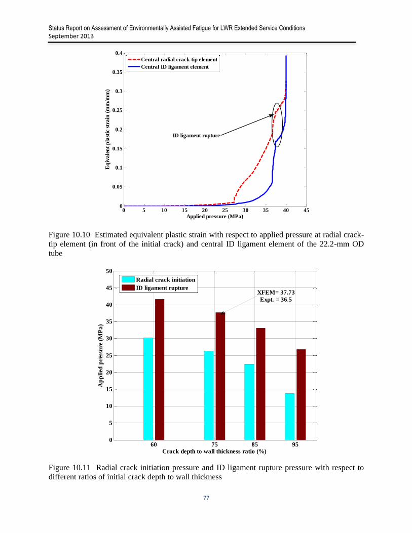
Status Report on Assessment of Environmentally Assisted Fatigue for LWR Extended Service Conditions
September 2013
77
Figure 10.10 Estimated equivalent plastic strain with respect to applied pressure at radial crack-
tip element (in front of the initial crack) and central ID ligament element of the 22.2-mm OD
tube
Figure 10.11 Radial crack initiation pressure and ID ligament rupture pressure with respect to
different ratios of initial crack depth to wall thickness
0 5 10 15 20 25 30 35 40 450
0.05
0.1
0.15
0.2
0.25
0.3
0.35
0.4
Applied pressure (MPa)
Eq
iva
len
t p
last
ic s
tra
in (
mm
/mm
)
Central radial crack tip element
Central ID ligament element
ID ligament rupture
60 75 85 950
5
10
15
20
25
30
35
40
45
50
Crack depth to wall thickness ratio (%)
Ap
pli
ed p
ress
ure
(M
Pa
)
Radial crack initiation
ID ligament ruptureXFEM= 37.73
Expt. = 36.5
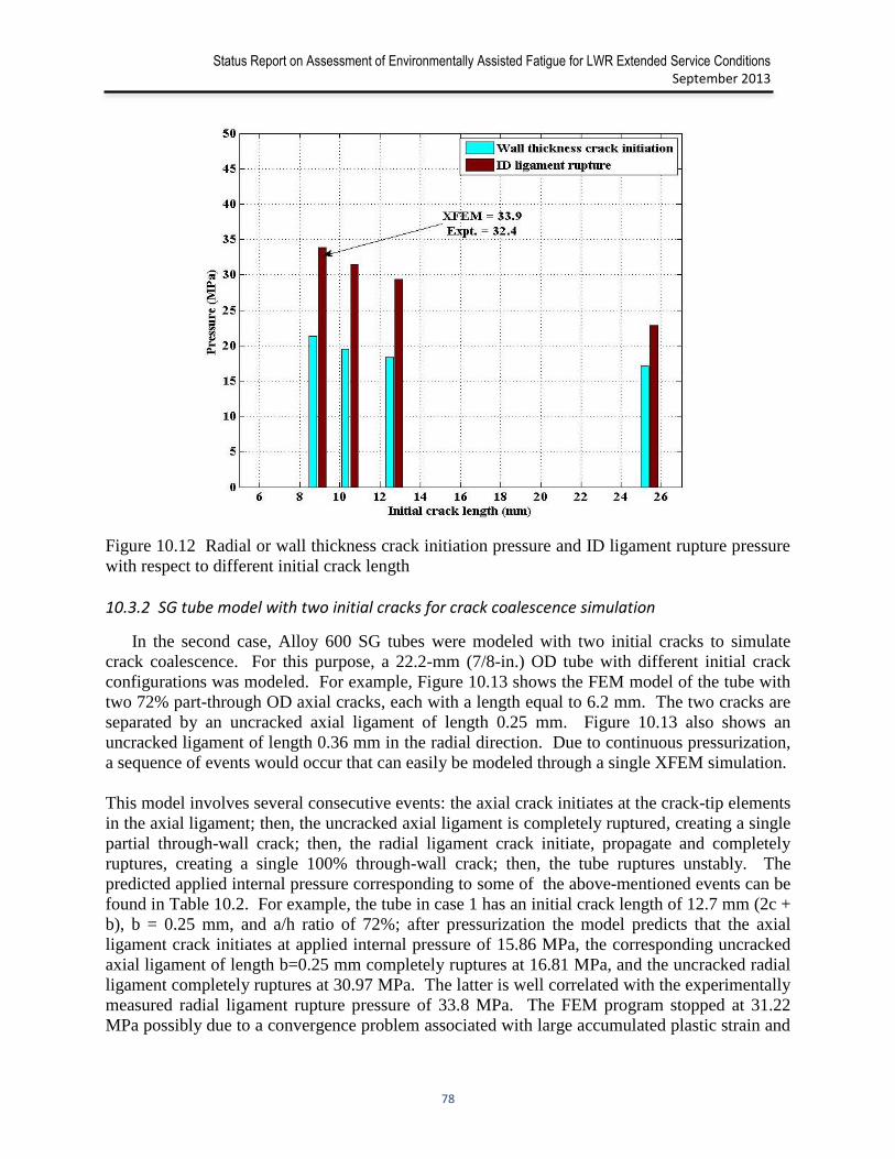
Status Report on Assessment of Environmentally Assisted Fatigue for LWR Extended Service Conditions
September 2013
78
Figure 10.12 Radial or wall thickness crack initiation pressure and ID ligament rupture pressure
with respect to different initial crack length
10.3.2 SG tube model with two initial cracks for crack coalescence simulation
In the second case, Alloy 600 SG tubes were modeled with two initial cracks to simulate
crack coalescence. For this purpose, a 22.2-mm (7/8-in.) OD tube with different initial crack
configurations was modeled. For example, Figure 10.13 shows the FEM model of the tube with
two 72% part-through OD axial cracks, each with a length equal to 6.2 mm. The two cracks are
separated by an uncracked axial ligament of length 0.25 mm. Figure 10.13 also shows an
uncracked ligament of length 0.36 mm in the radial direction. Due to continuous pressurization,
a sequence of events would occur that can easily be modeled through a single XFEM simulation.
This model involves several consecutive events: the axial crack initiates at the crack-tip elements
in the axial ligament; then, the uncracked axial ligament is completely ruptured, creating a single
partial through-wall crack; then, the radial ligament crack initiate, propagate and completely
ruptures, creating a single 100% through-wall crack; then, the tube ruptures unstably. The
predicted applied internal pressure corresponding to some of the above-mentioned events can be
found in Table 10.2. For example, the tube in case 1 has an initial crack length of 12.7 mm (2c +
b), b = 0.25 mm, and a/h ratio of 72%; after pressurization the model predicts that the axial
ligament crack initiates at applied internal pressure of 15.86 MPa, the corresponding uncracked
axial ligament of length b=0.25 mm completely ruptures at 16.81 MPa, and the uncracked radial
ligament completely ruptures at 30.97 MPa. The latter is well correlated with the experimentally
measured radial ligament rupture pressure of 33.8 MPa. The FEM program stopped at 31.22
MPa possibly due to a convergence problem associated with large accumulated plastic strain and
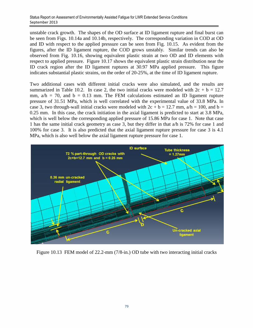
Status Report on Assessment of Environmentally Assisted Fatigue for LWR Extended Service Conditions
September 2013
79
unstable crack growth. The shapes of the OD surface at ID ligament rupture and final burst can
be seen from Figs. 10.14a and 10.14b, respectively. The corresponding variation in COD at OD
and ID with respect to the applied pressure can be seen from Fig. 10.15. As evident from the
figures, after the ID ligament rupture, the COD grows unstably. Similar trends can also be
observed from Fig. 10.16, showing equivalent plastic strain at two OD and ID elements with
respect to applied pressure. Figure 10.17 shows the equivalent plastic strain distribution near the
ID crack region after the ID ligament ruptures at 30.97 MPa applied pressure. This figure
indicates substantial plastic strains, on the order of 20-25%, at the time of ID ligament rupture.
Two additional cases with different initial cracks were also simulated, and the results are
summarized in Table 10.2. In case 2, the two initial cracks were modeled with 2c + b = 12.7
mm, a/h = 70, and b = 0.13 mm. The FEM calculations estimated an ID ligament rupture
pressure of 31.51 MPa, which is well correlated with the experimental value of 33.8 MPa. In
case 3, two through-wall initial cracks were modeled with 2c + b = 12.7 mm, a/h = 100, and b =
0.25 mm. In this case, the crack initiation in the axial ligament is predicted to start at 3.8 MPa,
which is well below the corresponding applied pressure of 15.86 MPa for case 1. Note that case
1 has the same initial crack geometry as case 3, but they differ in that a/h is 72% for case 1 and
100% for case 3. It is also predicted that the axial ligament rupture pressure for case 3 is 4.1
MPa, which is also well below the axial ligament rupture pressure for case 1.
Figure 10.13 FEM model of 22.2-mm (7/8-in.) OD tube with two interacting initial cracks

Status Report on Assessment of Environmentally Assisted Fatigue for LWR Extended Service Conditions
September 2013
80
Figure 10.14 Shape of the OD surface and maximum principal stress distribution for case 1 at
(a) ID ligament rupture pressure (30.97 MPa) and (b) final burst pressure (31.22 MPa)
Figure 10.15 Estimated COD with respect to applied pressure at the OD and ID surface for case-
1 tube (see Table 10.2) with 2c + b = 12.7 mm, a/h = 72, and b = 0.25 mm
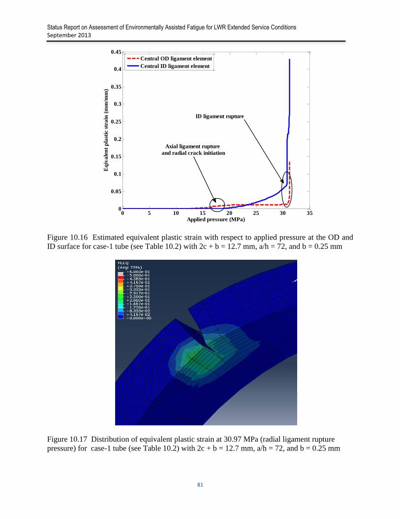
Status Report on Assessment of Environmentally Assisted Fatigue for LWR Extended Service Conditions
September 2013
81
Figure 10.16 Estimated equivalent plastic strain with respect to applied pressure at the OD and
ID surface for case-1 tube (see Table 10.2) with 2c + b = 12.7 mm, a/h = 72, and b = 0.25 mm
Figure 10.17 Distribution of equivalent plastic strain at 30.97 MPa (radial ligament rupture
pressure) for case-1 tube (see Table 10.2) with 2c + b = 12.7 mm, a/h = 72, and b = 0.25 mm
0 5 10 15 20 25 30 350
0.05
0.1
0.15
0.2
0.25
0.3
0.35
0.4
0.45
Applied pressure (MPa)
Eq
iva
len
t p
last
ic s
tra
in (
mm
/mm
)
Central OD ligament element
Central ID ligament element
Axial ligament rupture
and radial crack initiation
ID ligament rupture
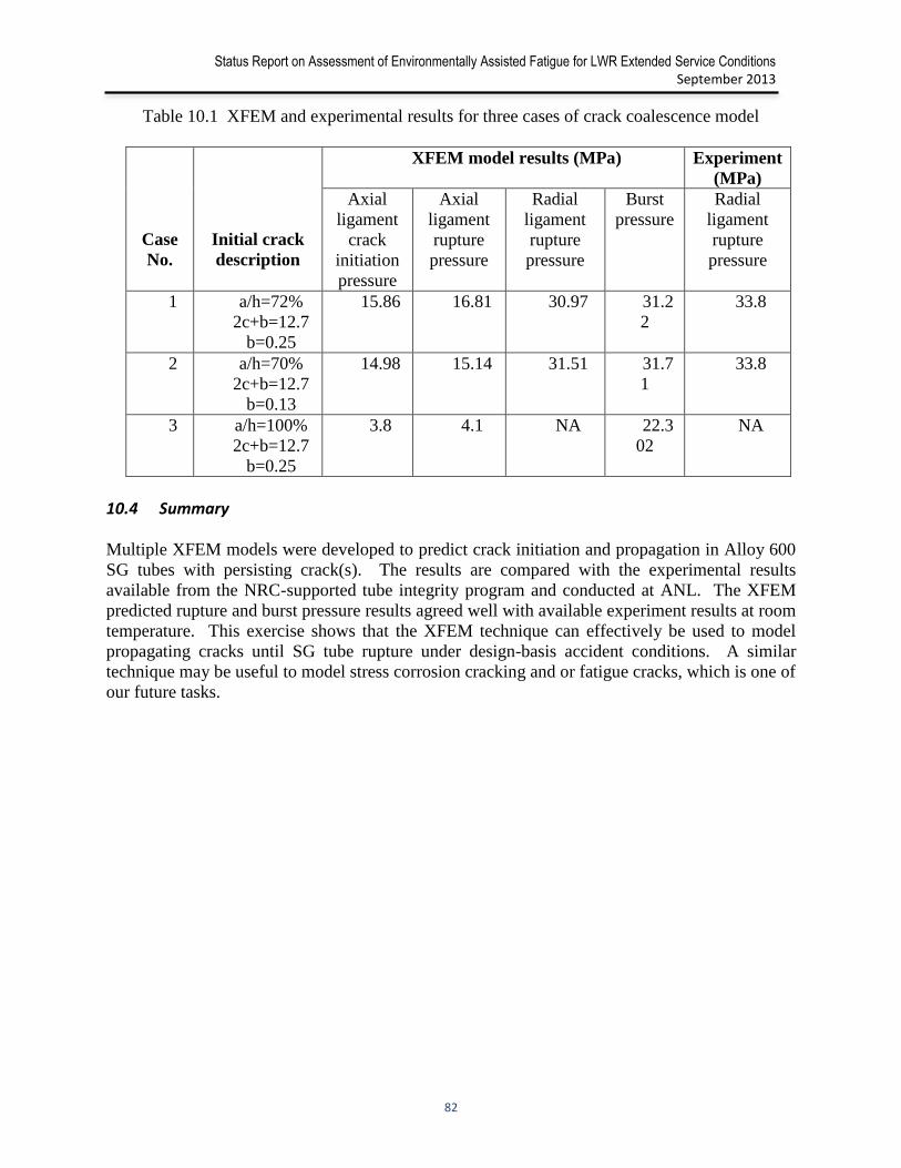
Status Report on Assessment of Environmentally Assisted Fatigue for LWR Extended Service Conditions
September 2013
82
Table 10.1 XFEM and experimental results for three cases of crack coalescence model
Case
No.
Initial crack
description
XFEM model results (MPa) Experiment
(MPa)
Axial
ligament
crack
initiation
pressure
Axial
ligament
rupture
pressure
Radial
ligament
rupture
pressure
Burst
pressure
Radial
ligament
rupture
pressure
1 a/h=72%
2c+b=12.7
b=0.25
15.86 16.81 30.97 31.2
2
33.8
2 a/h=70%
2c+b=12.7
b=0.13
14.98 15.14 31.51 31.7
1
33.8
3 a/h=100%
2c+b=12.7
b=0.25
3.8 4.1 NA 22.3
02
NA
10.4 Summary
Multiple XFEM models were developed to predict crack initiation and propagation in Alloy 600
SG tubes with persisting crack(s). The results are compared with the experimental results
available from the NRC-supported tube integrity program and conducted at ANL. The XFEM
predicted rupture and burst pressure results agreed well with available experiment results at room
temperature. This exercise shows that the XFEM technique can effectively be used to model
propagating cracks until SG tube rupture under design-basis accident conditions. A similar
technique may be useful to model stress corrosion cracking and or fatigue cracks, which is one of
our future tasks.
Status Report on Assessment of Environmentally Assisted Fatigue for LWR Extended Service Conditions
September 2013
83
References
1. American Society for Testing and Materials, “Standard test methods for tensile testing of
metallic materials,” ASTM, E8/E8M-11 (2012).
2. American Society for Testing and Materials, “Standard practice for strain-controlled
fatigue testing,”, ASTM, E606-04 (2012).
3. Babuska, I., Caloz, G., and Osborn, J., “Special finite element methods for a class of
second order elliptic problems with rough coefficients.” SIAM Journal on Numerical
Analysis 31: 945–981 (1994).
4. Melenk, J., and Babuska, I., “The partition of unity finite element method: Basic theory
and applications,” Computer Methods in Applied Mechanics and Engineering, 39: 289-314 (1996).
5. Osher, S., and Sethian, J. A., "Fronts propagating with curvature-dependent speed:
Algorithms based on Hamilton–Jacobi formulations," Journal of Computational Physics
79: 12–49 (1988).
6. Sethian, James A., Level Set Methods and Fast Marching Methods : Evolving Interfaces
in Computational Geometry, Fluid Mechanics, Computer Vision, and Materials Science,
Cambridge: Cambridge University Press (1999).
7. Belytschko, T., and T. Black, “Elastic crack growth in finite elements with minimal
remeshing,” International Journal for Numerical Methods in Engineering, 45: 601-620
(1999).
8. Sukumar, N., Moes, N., Moran, B., and Belytschko, T., “Extended finite element method
for three-dimensional crack modeling,” International Journal for Numerical Methods in
Engineering 48 (11), 1549–1570 (2000).
9. Sukumar, N., Chopp, D. L., Moes, N., Belytschko, T., “Modeling holes and inclusions by
level sets in the extended finite-element method,” Computer Methods in Applied
Mechanics and Engineering 190(46–47): 6183–6200 (2001).
10. Sukumar, N., Chopp, D. L., Moran, B., “Extended finite element method and fast
marching method for three dimensional fatigue crack propagation,” Engineering Fracture
Mechanics 70(1): 29–48 (2003).
11. Chessa J., “The extended finite element method for free surface and two phase flow
problems,” Ph.D. Thesis, Northwestern University, (2002).
12. Chessa, J., Belytschko, T., “An enriched finite element method for axisymmetric two-
phase flow with surface tension,” Journal of Computational Physics 58: 2041-2064
(2003).

Status Report on Assessment of Environmentally Assisted Fatigue for LWR Extended Service Conditions
September 2013
84
13. Chopp, D., Sukumar, N., “Fatigue crack propagation of multiple coplanar cracks with the
coupled extended finite element/fast marching method,” International Journal of
Engineering Science 41(8): 845–869 (2003).
14. Sukumar, N., Chopp, D. L., Bechet, E., Moes, N., “Three-dimensional non-planar crack
growth by a coupled extended finite element and fast marching method,” International
Journal for Numerical Methods in Engineering, 76(5): 727-748 (2008).
15. Shi, J., Chopp, D., Lua, J., Sukumar, N., Belytschko. T., “ABAQUS implementation of
extended finite element method using a level set representation for three-dimensional
fatigue crack growth and life predictions,” Engineering Fracture Mechanics 77: 2840-
2863 (2010).
16. Bordas, S. P. A., Natarajan, S., Kerfriden, P.,, Augarde, C. E., Mahapatra, D. R.,
Rabczuk, T., Dal Pont, S., “On the performance of strain smoothing for quadratic and
enriched finite element approximations (XFEM/GFEM/PUFEM),” International Journal
for Numerical Methods in Engineering 86: 637–666 (2011).
17. Dassault Systèmes Simulia Corp., ABAQUS 6.11 User Manual (2011).
18. Bakhtiari, S., Kasza, K. E., Kupperman, D. S., Majumdar, S., Park, J. Y., Shack, W. J.,
Diercks, D. R.,Second U.S. Nuclear Regulatory Commission International Steam
Generator Tube Integrity Research Program – Final Project Summary Report,
NUREG/CR-6804 (ANL-02/28) (2003).
19. Elices, M., Guinea, G. V., Gomez, J., Planas, J., “The cohesive zone model: Advantages,
limitations and challenges,” Engineering Fracture Mechanics 69: 137-163 (2002).
20. Bonifaz, E. A., “Cohesive zone modeling to predict failure processes,” Canadian Journal
on Mechanical Science and Engineering 2: 42-53 (2011).
21. Lambda Technologies, http://www.lambdatechs.com/index.html.

Status Report on Assessment of Environmentally Assisted Fatigue for LWR Extended Service Conditions
September 2013
85
This page intentionally left blank


Argonne National Laboratory is a U.S. Department of Energy laboratory managed by UChicago Argonne, LLC
Nuclear Engineering Division Argonne National Laboratory
9700 South Cass Avenue, Bldg. 208
Argonne, IL 60439
www.anl.gov
Related Documents