STATUS OF DELAYED-NEUTRON PRECURSOR DATA: HALF-LIVES AND NEUTRON EMISSION PROBABILITIES Bernd Pfeiffer 1 and Karl-Ludwig Kratz Institut f¨ ur Kernchemie, Universit¨at Mainz, Germany PeterM¨oller Theoretical Division, Los Alamos National Laboratory, Los Alamos, NM 87545 Abstract: – We present in this paper a compilation of the present status of experimen- tal delayed-neutron precursor data; i.e. β -decay half-lives (T 1/2 ) and neutron emission probabilities (P n ) in the fission-product region (27 ≤ Z ≤ 57). These data are com- pared to two model predictions of substantially different sophistication: (i) an update of the empirical Kratz–Herrmann formula (KHF), and (ii) a unified macroscopic- microscopic model within the quasi-particle random-phase approximation (QRPA). Both models are also used to calculate so far unknown T 1/2 and P n values up to Z = 63. A number of possible refinements in the microscopic calculations are sug- gested to further improve the nuclear-physics foundation of these data for reactor and astrophysical applications. INTRODUCTION Half-lives (T 1/2 ) and delayed-neutron emission probabilities (P n ) are among the easiest measurable gross β -decay properties of neutron-rich nuclei far from stability. They are not only of importance for reactor applications, but also in the context of studying nuclear- structure features and astrophysical scenarios. Therefore, most of our recent experiments performed at international facilities such as CERN-ISOLDE, GANIL-LISE and GSI-FRS were primarily motivated by our current work on r-process nucleosynthesis. However, it is a pleasure for us to recognize that these data still today may be of interest for applications in reactor physics, a field which we practically left shortly after the ”Specialists’ Meeting on Delayed Neutrons” held at Birmingham in 1986. Our motivation to put together this new compilation of β -decay half-lives and β -delayed neutron-emission came from recent discussions with T.R. England and W.B. Wilson from LANL about our activities in compiling and steadily updating experimental delayed-neutron data as well as various theoretical model predictions (Pfeiffer et al., 2000). They pointed out to us, that their recent summation calculations of aggregate fission-product delayed-neutron production using basic nuclear data from the early 1990’s (Brady, 1989; Brady and England, 1989, Rudstam 1993) show, in general, that a greater fraction of delayed neutrons is emitted at earlier times following fission than measured. As a consequence, the reactor response to a reference reactivity change is enhanced compared to that calculated with pulse functions derived from measurements (Wilson and England, 2000). Therefore, the use of updated P n and T 1/2 values is expected to improve the physics foundation of the basic input data used and to increase the accuracy of aggregate results obtained in summation calculations. Since the tabulation of Brady (1989) and Rudstam (1993), about 40 new P n values have been measured in the fission-product region (27 ≤ Z ≤ 57), a number of delayed-neutron 1 E-mail address: Bernd.Pfeiff[email protected]

Welcome message from author
This document is posted to help you gain knowledge. Please leave a comment to let me know what you think about it! Share it to your friends and learn new things together.
Transcript
STATUS OF DELAYED-NEUTRON PRECURSOR DATA:
HALF-LIVES AND NEUTRON EMISSION
PROBABILITIES
Bernd Pfeiffer1 and Karl-Ludwig KratzInstitut fur Kernchemie, Universitat Mainz, Germany
Peter MollerTheoretical Division, Los Alamos National Laboratory, Los Alamos, NM 87545
Abstract: – We present in this paper a compilation of the present status of experimen-tal delayed-neutron precursor data; i.e. β-decay half-lives (T1/2) and neutron emissionprobabilities (Pn) in the fission-product region (27 ≤ Z ≤ 57). These data are com-pared to two model predictions of substantially different sophistication: (i) an updateof the empirical Kratz–Herrmann formula (KHF), and (ii) a unified macroscopic-microscopic model within the quasi-particle random-phase approximation (QRPA).Both models are also used to calculate so far unknown T1/2 and Pn values up toZ = 63. A number of possible refinements in the microscopic calculations are sug-gested to further improve the nuclear-physics foundation of these data for reactor andastrophysical applications.
INTRODUCTION
Half-lives (T1/2) and delayed-neutron emission probabilities (Pn) are among the easiestmeasurable gross β-decay properties of neutron-rich nuclei far from stability. They are notonly of importance for reactor applications, but also in the context of studying nuclear-structure features and astrophysical scenarios. Therefore, most of our recent experimentsperformed at international facilities such as CERN-ISOLDE, GANIL-LISE and GSI-FRSwere primarily motivated by our current work on r-process nucleosynthesis. However, it isa pleasure for us to recognize that these data still today may be of interest for applicationsin reactor physics, a field which we practically left shortly after the ”Specialists’ Meetingon Delayed Neutrons” held at Birmingham in 1986.
Our motivation to put together this new compilation of β-decay half-lives and β-delayedneutron-emission came from recent discussions with T.R. England and W.B. Wilson fromLANL about our activities in compiling and steadily updating experimental delayed-neutrondata as well as various theoretical model predictions (Pfeiffer et al., 2000). They pointed outto us, that their recent summation calculations of aggregate fission-product delayed-neutronproduction using basic nuclear data from the early 1990’s (Brady, 1989; Brady and England,1989, Rudstam 1993) show, in general, that a greater fraction of delayed neutrons is emittedat earlier times following fission than measured. As a consequence, the reactor response toa reference reactivity change is enhanced compared to that calculated with pulse functionsderived from measurements (Wilson and England, 2000). Therefore, the use of updated Pnand T1/2 values is expected to improve the physics foundation of the basic input data usedand to increase the accuracy of aggregate results obtained in summation calculations.
Since the tabulation of Brady (1989) and Rudstam (1993), about 40 new Pn values havebeen measured in the fission-product region (27 ≤ Z ≤ 57), a number of delayed-neutron
1E-mail address: [email protected]

B. Pfeiffer, K.-L. Kratz, P. Moller, Delayed Neutron-Emission Probabilities . . . 2
β-stableCalculated data Experimental data: New Old Overlap New/Old
Delayed-Neutron Data
40 50 60 70 80 90 100Neutron Number N
30
40
50
60
Pro
ton
Num
ber
Z
Figure 1: Chart illustrating the data available in the fission-product region. The new dataevaluation represents a significant extension of measured Pn values. Some data in the olddata set are not present in the new data set.
branching ratios have also been determined with higher precision, and a similar number ofground-state and isomer decay half-lives of new delayed-neutron precursors have been ob-tained. These data are contained in our compilation (Table 1), and are compared with twoof our model predictions: (i) an update of the empirical Kratz-Herrmann formula (KHF)for β-delayed neutron emission probabilities Pn and β-decay half-lives T1/2 (Kratz andHerrmann, 1973; Pfeiffer, 2000), and an improved version of the macroscopic-microscopicQRPA model (Moller and Randrup, 1990) which can be used to calculate a large number ofnuclear properties consistently (Moller et al., 1997). These two models, with quite differentnuclear-structure basis, are also used to predict so far unknown T1/2 and Pn values in thefission-product region (see Table 1).
EXPERIMENTAL DATA
Most of the new β-decay half-lives of the very neutron-rich delayed-neutron precursorisotopes included in Table 1 have been determined from growth-and-decay curves of neu-trons detected with standard neutron-longcounter set-ups. As an example, the presently

B. Pfeiffer, K.-L. Kratz, P. Moller, Delayed Neutron-Emission Probabilities . . . 3
Table 1: Experimental β-decay half-lives T1/2 and β-delayed neutron-emission probabilitiesPn compared to three calculations.
T1/2 (ms) Pn (%)
Isotope Exp. KHF QRPA-1 QRPA-2 Exp. KHF QRPA-1 QRPA-26627Co 180 10 432 260 260 0.013 0.000 0.0006727Co 425 20 400 76 120 1.132 0.156 0.0616827Co 230 30 168 72 82 2.395 0.812 0.768
68m27Co 1600 3006927Co 216 9 238 64 99 6.585 1.250 0.9057027Co 120 30 101 43 60 7.469 3.213 2.154
70m27Co 500 1807127Co 270 50 109 42 60 16.650 3.468 2.6667227Co 100 50 58 29 52 13.350 5.810 3.7217327Co 63 27 33 28.230 6.153 3.4417427Co 35 17 25 20.700 9.858 5.9627527Co 34 15 20 37.920 8.027 7.4077627Co 21 11 17 29.690 11.034 24.6777727Co 20 10 15 52.810 39.341 78.079
7228Ni 1570 50 859 8141 8141 0.000 0.000 0.0007328Ni 840 30 251 2358 2025 0.097 0.193 0.2267428Ni 500 200 271 2056 1508 0.632 3.098 2.8537528Ni 700 400 114 890 696 1.477 8.967 9.1277628Ni 440 400 126 920 593 4.108 26.207 23.9527728Ni 61 372 323 4.859 36.401 38.7247828Ni 66 332 326 10.810 40.662 55.7477928Ni 26 126 48 14.330 92.135 81.490
7329Cu 3900 300 1936 4092 2726 0.029 6 0.045 0.018 0.0117429Cu 1594 10 393 1308 957 0.075 16 0.117 0.306 0.1587529Cu 1224 3 458 1345 844 2.6 5 3.982 5.840 2.9467629Cu 641 6 153 657 428 2.4 5 2.880 6.706 3.252
76m29Cu 1270 3007729Cu 469 8 155 764 405 15 +10
−5 11.730 26.228 12.3807829Cu 342 11 77 351 268 15 +10
−5 11.990 37.899 13.8657929Cu 188 25 76 358 212 55 17 21.830 33.698 27.8618029Cu 26 97 149 22.530 62.342 76.8008129Cu 28 90 170 72.270 99.985 100.0008229Cu 18 40 40 61.680 98.931 98.931
7730Zn 2080 50 689 8888 8888 0.000 0.000 0.000
77m30Zn 1050 1007830Zn 1470 150 419 5022 15694 0.001 0.027 0.0007930Zn 995 19 225 3925 3098 1.3 4 0.238 0.958 0.364

B. Pfeiffer, K.-L. Kratz, P. Moller, Delayed Neutron-Emission Probabilities . . . 4
Table 1: Continued
T1/2 (ms) Pn (%)
Isotope Exp. KHF QRPA-1 QRPA-2 Exp. KHF QRPA-1 QRPA-28030Zn 545 16 255 3025 2033 1.0 5 0.668 10.889 9.9808130Zn 290 50 64 646 2401 7.5 30 2.343 21.952 60.5058230Zn 52 211 734 17.170 35.281 99.9728330Zn 43 22 818 23.300 9.816 99.9828430Zn 43 65 387 25.480 33.273 100.000
7931Ga 2847 3 999 3463 2062 0.080 14 0.119 0.110 0.0558031Ga 1697 11 301 1575 2413 0.85 6 0.468 0.865 0.6268131Ga 1217 5 404 1684 1852 12.1 4 3.776 6.666 6.9568231Ga 599 2 96 496 1817 22.3 22 5.548 13.248 24.2358331Ga 308 1 82 202 891 38.7 98 33.790 76.668 98.3598431Ga 85 10 56 22 1644 70 15 28.150 15.387 99.9828531Ga 48 71 686 60.390 99.953 100.0008631Ga 29 22 409 42.400 67.188 99.9948731Ga 29 24 118 73.540 99.930 100.000
8332Ge 1850 60 249 2115 70415 0.019 0.109 2.1988432Ge 954 14 207 1046 16208 10.2 9 1.747 8.565 76.2058532Ge 540 50 131 40 9900 14 3 4.297 1.615 99.0888632Ge 95 184 2168 6.044 6.647 65.5668732Ge 64 44 1356 11.430 5.104 93.9318832Ge 66 46 256 17.480 5.595 65.7408932Ge 39 17 20 19.090 15.824 9.194
8433As 4020 30 392 3548 16635 0.18 10 0.026 0.302 0.373
84m33As 650 1508533As 2022 9 280 2485 9431 55 14 7.935 17.599 48.9908633As 945 8 191 187 5023 26 7 9.290 10.392 92.5928733As 560 110 137 269 2458 17.5 25 17.890 32.629 100.0008833As 112 61 2263 23.060 35.870 99.9248933As 59 66 374 29.690 90.576 100.0009033As 43 23 21 30.830 41.952 22.7869133As 44 36 73 58.130 99.784 100.0009233As 27 36 36 40.550 90.468 90.468
8634Se 15300 900 1063 12602 12602 0.000 0.000 0.0008734Se 5500 140 657 677 1885875 0.36 8 0.020 0.012 3.1098834Se 1520 30 327 403 12312 0.67 30 0.193 0.231 0.9868934Se 410 40 232 114 9050 7.8 25 1.198 0.519 9.1879034Se 161 134 1127 2.991 0.859 0.9239134Se 270 50 104 34 40 21 10 8.353 1.524 3.045

B. Pfeiffer, K.-L. Kratz, P. Moller, Delayed Neutron-Emission Probabilities . . . 5
Table 1: Continued
T1/2 (ms) Pn (%)
Isotope Exp. KHF QRPA-1 QRPA-2 Exp. KHF QRPA-1 QRPA-29234Se 93 59 164 11.770 2.187 1.3129334Se 62 87 24 10.910 24.270 9.3429434Se 59 52 43 13.830 19.996 1.712
8735Br 55600 150 1059 12315 37254 2.52 7 0.146 0.277 1.1298835Br 16360 70 685 1386 104991 6.55 18 0.466 0.194 28.5998935Br 4400 30 429 203 10758 13.7 4 2.445 0.255 41.7469035Br 1910 10 283 108 17328 24.9 10 5.622 1.818 99.8009135Br 541 5 172 55 762 31.3 60 12.050 3.319 73.3659235Br 343 15 111 36 54 33.7 12 19.710 13.032 8.4589335Br 102 10 97 46 221 65 8 33.730 21.507 100.0009435Br 70 20 69 133 34 68 16 29.120 48.680 14.2219535Br 66 77 57 34.000 70.822 100.0009635Br 42 42 19 27.600 52.064 33.5739735Br 40 49 49 46.800 95.558 95.558
9136Kr 8570 40 1213 500 500 0.000 0.000 0.0009236Kr 1840 8 560 396 1934 0.033 3 0.010 0.012 0.0519336Kr 1286 10 282 516 78 1.95 11 0.799 1.079 0.0129436Kr 200 10 239 548 559 5.7 22 2.084 0.953 0.0909536Kr 780 30 150 373 61 4.144 4.942 0.7259636Kr 161 196 118 6.118 5.945 0.3229736Kr 111 81 32 6.214 6.104 2.4859836Kr 87 106 38 7.633 9.143 1.0889936Kr 52 72 72 11.600 33.873 33.873
10036Kr 51 48 48 16.610 25.386 25.386
9137Rb 58400 400 2363 19066 408587 0.000 0.000 0.0019237Rb 4492 20 1265 279 723153 0.011 1 0.015 0.001 4.1429337Rb 5840 20 661 184 5735 1.44 10 0.830 0.116 5.2599437Rb 2702 5 285 158 119 9.1 11 2.755 1.414 1.6289537Rb 377.5 8 221 78 386 8.73 31 10.740 2.989 37.9329637Rb 203 3 135 71 57 13.3 7 13.220 10.634 10.5469737Rb 169.9 7 126 46 46 26.0 19 20.530 12.529 12.5299837Rb 96 3 103 52 52 14.6 18 15.070 16.598 16.598
98m37Rb 114 59937Rb 50.3 7 86 43 43 17.3 25 29.310 26.876 26.876
10037Rb 51 8 63 38 38 12 7 15.900 26.153 26.153
100m37Rb
10137Rb 32 4 70 39 39 25 5 36.800 33.729 33.729

B. Pfeiffer, K.-L. Kratz, P. Moller, Delayed Neutron-Emission Probabilities . . . 6
Table 1: Continued
T1/2 (ms) Pn (%)
Isotope Exp. KHF QRPA-1 QRPA-2 Exp. KHF QRPA-1 QRPA-210237Rb 37 5 36 13 13 18 8 25.270 20.312 20.312
10337Rb 39 17 17 48.740 52.410 52.410
10437Rb 27 13 13 37.980 58.332 58.332
10537Rb 28 12 12 55.730 73.481 73.481
9638Sr 1070 10 854 1079 817 0.000 0.000 0.0009738Sr 429 5 556 1179 119 0.02 1 0.109 0.232 0.0019838Sr 653 2 626 724 724 0.40 17 0.161 0.380 0.3809938Sr 269 1 373 359 359 0.25 10 0.504 0.227 0.227
10038Sr 202 3 289 495 495 1.11 34 0.168 0.437 0.437
10138Sr 118 3 171 375 375 2.75 35 2.346 3.944 3.944
10238Sr 69 6 120 142 142 5.5 15 1.450 3.026 3.026
10338Sr 79 35 35 9.952 2.153 2.153
10438Sr 68 79 79 8.340 7.477 7.477
10538Sr 61 49 49 10.420 14.502 14.502
9639Y 5340 50 3009 1439 1413 0.000 0.000 0.000
96m39Y 9600 2009739Y 3750 30 1148 288 5030 0.045 20 0.066 0.014 0.015
97m139Y 1170 30 ≤0.08
97m239Y 142 89839Y 548 2 696 305 302 0.295 33 1.469 0.375 1.253
98m39Y 2000 200 3.4 109939Y 1470 7 602 167 167 2.2 5 3.385 0.492 0.492
10039Y 735 7 496 318 318 1.16 32 0.951 0.309 0.309
100m39Y 940 30
10139Y 426 20 325 149 149 2.3 8 3.936 1.212 1.212
10239Y 360 40 352 189 189 5.0 12 3.689 1.191 1.191
102m39Y 300 10
10339Y 224 19 181 89 89 8.3 30 8.487 3.519 3.519
10439Y 180 60 127 30 30 11.560 3.241 3.241
10539Y 88 48 48 20.420 14.012 14.012
10639Y 66 35 35 24.010 16.345 16.345
10739Y 74 31 31 31.730 32.062 32.062
10839Y 48 23 23 25.540 36.014 36.014
10340Zr 1300 100 779 1866 1866 0.000 0.000 0.000
10440Zr 1200 300 598 1839 1839 0.012 0.023 0.023
10540Zr 600 100 289 100 100 0.127 0.029 0.029
10640Zr 270 367 367 1.476 0.614 0.614

B. Pfeiffer, K.-L. Kratz, P. Moller, Delayed Neutron-Emission Probabilities . . . 7
Table 1: Continued
T1/2 (ms) Pn (%)
Isotope Exp. KHF QRPA-1 QRPA-2 Exp. KHF QRPA-1 QRPA-210740Zr 144 197 197 1.727 1.457 1.457
10840Zr 130 181 181 5.820 1.796 1.796
10940Zr 117 122 122 3.968 4.007 4.007
11040Zr 98 86 86 7.114 5.979 5.979
10341Nb 1500 200 3192 9535 9535 0.000 0.000 0.000
10441Nb 4900 300 1145 2790 2790 0.06 3 0.002 0.003 0.003
104m41Nb 920 40 0.05 3
10541Nb 2950 60 1319 3864 3864 1.7 9 0.241 0.273 0.273
10641Nb 920 40 461 166 166 4.5 3 0.823 0.178 0.178
10741Nb 300 9 440 657 657 6.0 15 3.473 2.994 2.994
10841Nb 193 17 218 365 365 6.2 5 5.720 15.732 15.732
10941Nb 190 30 229 377 377 31 5 12.180 15.499 15.499
11041Nb 170 20 109 253 253 40 8 9.959 17.144 17.144
11141Nb 113 184 184 22.060 59.599 59.599
11241Nb 69 85 85 21.090 64.316 64.316
11341Nb 65 56 56 55.760 90.942 90.942
10942Mo 530 60 484 1802 1802 0.002 0.000 0.000
11042Mo 300 40 594 1832 1832 0.074 0.000 0.000
11142Mo 237 978 978 0.313 0.025 0.025
11242Mo 287 672 672 1.233 0.308 0.308
11342Mo 133 133 133 1.806 3.030 3.030
11442Mo 144 113 113 4.255 3.881 3.881
11542Mo 92 52 52 5.330 4.984 4.984
10843Tc 5170 70 1515 702 702 0.000 0.000 0.000
10943Tc 870 40 2010 378 378 0.08 2 0.017 0.008 0.008
11043Tc 920 30 663 274 274 0.04 2 0.110 0.067 0.067
11143Tc 290 20 886 195 195 0.85 20 1.367 0.327 0.327
11243Tc 290 20 312 142 142 1.5 2 1.135 0.797 0.797
11343Tc 170 20 392 115 115 2.1 3 6.418 4.536 4.536
11443Tc 150 30 172 82 82 1.3 4 4.423 7.233 7.233
11543Tc 210 74 74 13.330 19.044 19.044
11643Tc 96 46 46 11.740 16.381 16.381
11743Tc 94 42 42 22.990 24.361 24.361
11843Tc 66 36 36 17.170 25.068 25.068
11344Ru 800 50 950 2200 2200 0.000 0.000 0.000
11444Ru 530 60 1354 491 491 0.000 0.009 0.009
11544Ru 740 80 47 753 753 0.003 1.021 1.021

B. Pfeiffer, K.-L. Kratz, P. Moller, Delayed Neutron-Emission Probabilities . . . 8
Table 1: Continued
T1/2 (ms) Pn (%)
Isotope Exp. KHF QRPA-1 QRPA-2 Exp. KHF QRPA-1 QRPA-211644Ru 556 612 612 0.053 0.002 0.002
11744Ru 237 175 175 0.287 0.369 0.369
11844Ru 287 233 233 1.029 1.120 1.120
11944Ru 162 185 185 1.712 2.616 2.616
12044Ru 149 118 118 2.599 2.945 2.945
11445Rh 1850 50 1244 2730 2730 0.000 0.000 0.000
114m45Rh 1850 50
11545Rh 990 50 476 682 682 0.083 0.016 0.016
11645Rh 680 60 589 686 686 0.057 0.000 0.000
116m45Rh 900 400
11745Rh 440 40 857 245 245 1.614 0.940 0.940
11845Rh 346 125 125 1.102 0.924 0.924
11945Rh 411 111 111 4.196 3.203 3.203
12045Rh 177 87 87 3.586 3.547 3.547
12145Rh 215 65 65 11.300 7.620 7.620
12245Rh 108 56 56 9.057 8.540 8.540
12046Pd 500 100 1267 2686 2686 0.000 0.000 0.000
12146Pd 428 1632 1632 0.002 0.002 0.002
12246Pd 541 1123 1123 0.039 0.044 0.044
12346Pd 244 476 476 0.224 0.313 0.313
12446Pd 257 328 328 0.552 0.656 0.656
11947Ag 2100 100 3567 985 985 0.000 0.000 0.000
119m47Ag 6000 500
12047Ag 1230 30 865 490 490 ≤0.003 0.000 0.000 0.000
120m47Ag 370 40
12147Ag 780 10 1337 412 412 0.076 5 0.135 0.040 0.040
12247Ag 550 50 488 190 190 0.186 10 0.120 0.175 0.175
122m47Ag 200 50
12347Ag 296 6 652 219 219 0.55 5 1.683 0.642 0.642
12447Ag 172 5 267 117 117 ≥0.1 0.741 0.989 0.989
124m47Ag
12547Ag 166 7 288 116 116 5.088 3.389 3.389
12647Ag 107 12 145 118 118 3.341 3.435 3.435
126m47Ag
12747Ag 79 3 164 84 84 12.210 5.785 5.785
12847Ag 58 5 107 86 86 5.079 6.417 6.417
12947Ag 46† +5
−9 84 33 33 11.760 8.990 8.990
†This experimental data point was added after the manuscript was completed and is therefore not taken
into account elsewhere in figures and tables.

B. Pfeiffer, K.-L. Kratz, P. Moller, Delayed Neutron-Emission Probabilities . . . 9
Table 1: Continued
T1/2 (ms) Pn (%)
Isotope Exp. KHF QRPA-1 QRPA-2 Exp. KHF QRPA-1 QRPA-2129m
47Ag13047Ag 30 36 36 19.240 67.219 67.219
13147Ag 28 40 40 68.150 100.000 100.000
13247Ag 20 34 34 61.090 100.000 100.000
12648Cd 506 15 798 5146 5146 0.000 0.000 0.000
12748Cd 370 70 280 2329 2329 0.019 0.223 0.223
12848Cd 340 30 289 924 924 0.079 0.752 0.752
12948Cd 270 40 135 2284 2284 0.766 0.944 0.944
13048Cd 162 7 138 655 655 3.6 10 1.083 2.883 2.883
13148Cd 68 3 65 545 545 3.5 10 3.855 61.210 61.210
13248Cd 97 10 56 563 563 60 15 20.210 99.976 99.976
13348Cd 38 446 446 26.530 99.025 99.025
13448Cd 38 313 313 37.150 100.000 100.000
13548Cd 28 253 253 36.370 99.407 99.407
13648Cd 30 132 132 44.050 100.000 100.000
12549In 2360 40 3247 857 857 0.000 0.000 0.000
125m49In 12200 200
12649In 1600 100 909 552 552 0.000 0.000 0.000
126m49In 1640 50
12749In 1090 10 1192 567 567 ≤0.03 0.035 0.019 0.019
127m149In 3670 40 0.69 4
127m249In
12849In 776 24 527 480 480 0.038 3 0.023 0.027 0.027
128m49In 776 24
12949In 611 4 525 312 312 0.23 7 0.792 0.670 0.670
129m149In 1230 30 3.6 4
129m249In
13049In 278 3 246 216 216 1.01 22 0.551 0.985 0.985
130m149In 538 5
130m249In 550 10 1.65 18
13149In 280 30 216 146 146 2.2 3 3.685 3.817 3.817
131m149In 350 50
131m249In 320 60
13249In 206 4 45 95 95 5.2 12 7.627 9.237 9.237
13349In 180 15 35 139 139 87 9 56.760 100.000 100.000
13449In 138 8 32 97 97 >17 56.700 100.000 100.000
13549In 41 90 90 70.890 100.000 100.000

B. Pfeiffer, K.-L. Kratz, P. Moller, Delayed Neutron-Emission Probabilities . . . 10
Table 1: Continued
T1/2 (ms) Pn (%)
Isotope Exp. KHF QRPA-1 QRPA-2 Exp. KHF QRPA-1 QRPA-213649In 30 69 69 56.880 100.000 100.000
13749In 31 48 48 79.100 100.000 100.000
13350Sn 1450 30 362 9479 9479 0.0294 24 0.002 0.040 0.040
13450Sn 1120 80 245 2196 2196 17 14 6.000 93.128 93.128
13550Sn 450 50 215 2789 2789 22 7 12.650 98.591 98.591
13650Sn 169 904 904 25 7 9.478 88.334 88.334
13750Sn 140 733 733 16.100 99.360 99.360
13850Sn 143 460 460 32.410 100.000 100.000
13950Sn 81 338 338 18.710 99.303 99.303
14050Sn 86 119 119 27.800 99.997 99.997
13451Sb 780 60 765 88293 973552 0.014 2.032 14.190
134m51Sb 10220 90 0.088 17
13551Sb 1680 15 385 33748 36889 22.0 27 15.210 97.980 99.948
13651Sb 923 14 302 2261 27082 23.2 68 19.440 53.683 99.789
13751Sb 199 970 4727 25.710 96.361 99.998
13851Sb 168 41 1599 28.350 26.302 99.982
13951Sb 127 176 876 35.210 99.766 100.000
14051Sb 80 38 645 36.270 58.560 99.992
14151Sb 86 84 84 65.230 99.378 99.378
14251Sb 46 45 45 40.790 95.947 95.947
14351Sb 50 29 29 62.860 99.999 99.999
13652Te 17630 80 1079 49938 49938 1.26 20 0.128 10.451 10.451
13752Te 2490 50 711 119887 151542 2.86 24 0.440 54.228 69.222
13852Te 1400 400 438 25690 25690 6.3 21 0.978 3.683 3.683
13952Te 347 269 5329 3.304 2.295 52.042
14052Te 304 282 1138 3.880 2.947 7.825
14152Te 213 122 632 4.876 8.355 44.492
14252Te 200 108 108 7.381 10.457 10.457
14352Te 105 67 67 10.320 16.262 16.262
14452Te 117 63 63 14.790 22.622 22.622
14552Te 77 30 30 14.670 21.510 21.510
14652Te 75 38 38 18.540 35.513 35.513
13753I 24130 120 1995 1894022 3365424 7.02 54 1.426 72.004 98.980
13853I 6490 70 1152 2254 9020949 5.17 36 1.092 0.858 69.824
13953I 2282 10 920 2338 58145 10.8 12 7.645 15.749 99.988
14053I 860 40 518 302 17216 14.4 63 5.825 10.850 99.728
14153I 430 20 521 351 2347 30 9 14.190 42.231 100.000

B. Pfeiffer, K.-L. Kratz, P. Moller, Delayed Neutron-Emission Probabilities . . . 11
Table 1: Continued
T1/2 (ms) Pn (%)
Isotope Exp. KHF QRPA-1 QRPA-2 Exp. KHF QRPA-1 QRPA-214253I 308 182 1400 10.750 46.997 99.952
14353I 296 150 150 21.460 77.120 77.120
14453I 194 58 58 17.370 29.379 29.379
14553I 127 57 57 38.580 46.359 46.359
14653I 80 29 29 24.200 27.584 27.584
14753I 75 33 33 41.940 59.854 59.854
14853I 55 30 30 35.650 81.555 81.555
14953I 55 39 39 53.140 97.687 97.687
14154Xe 1730 10 1290 725 83645 0.046 4 0.006 0.004 0.168
14254Xe 1220 20 1113 841 6634 0.42 3 0.027 0.020 0.113
14354Xe 300 30 654 464 4155 0.334 0.450 0.743
14454Xe 1150 200 647 291 291 0.651 0.693 0.693
14554Xe 900 300 417 233 233 1.510 3.805 3.805
14654Xe 369 292 292 1.973 3.397 3.397
14754Xe 260 93 93 4.300 5.438 5.438
14854Xe 176 126 126 6.168 9.592 9.592
14954Xe 119 94 94 9.234 22.899 22.899
15054Xe 112 71 71 11.440 25.968 25.968
15154Xe 83 33 33 14.180 24.373 24.373
15354Xe 0 27 27 0.000 52.705 52.705
14155Cs 24940 60 3636 9279 807516 0.038 8 0.035 0.026 4.653
14255Cs 1689 11 1731 1261 882522 0.091 8 0.121 0.031 39.801
14355Cs 1791 8 1411 1750 21384 1.59 15 1.588 1.067 30.965
14455Cs 993 13 692 1243 18073 3.41 40 1.871 3.754 66.359
14555Cs 582 6 436 412 932 13.1 7 4.884 8.146 17.980
14655Cs 323 6 381 784 784 13.4 10 10.240 36.444 36.444
14755Cs 225 5 206 234 234 27.5 21 8.264 16.383 16.383
14855Cs 158 7 207 165 165 25.0 43 21.700 34.467 34.467
14955Cs 112 3 172 219 219 19.130 64.646 64.646
15055Cs 82 7 123 158 158 20 10 18.110 71.808 71.808
15155Cs 109 101 101 27.690 82.526 82.526
15255Cs 82 30 30 27.290 47.453 47.453
15355Cs 77 56 56 38.830 89.391 89.391
15455Cs 58 43 43 33.580 83.477 83.477
14656Ba 2220 70 2538 2457 2457 0.000 0.000 0.000
14756Ba 893 1 1785 3559 3559 0.000 0.000 0.000
14856Ba 602 25 1054 603 603 0.12 6 0.062 0.076 0.076

B. Pfeiffer, K.-L. Kratz, P. Moller, Delayed Neutron-Emission Probabilities . . . 12
Table 1: Continued
T1/2 (ms) Pn (%)
Isotope Exp. KHF QRPA-1 QRPA-2 Exp. KHF QRPA-1 QRPA-214956Ba 344 7 467 300 300 0.79 39 0.092 0.123 0.123
15056Ba 300 389 438 438 1.0 5 0.700 0.806 0.806
15156Ba 259 310 310 1.757 4.174 4.174
15256Ba 228 205 205 2.763 4.534 4.534
15356Ba 158 69 69 4.732 4.634 4.634
15456Ba 157 94 94 6.361 9.117 9.117
14657La 6270 100 3572 1212 1212 0.000 0.000 0.000
146m57La 10000 100
14757La 4015 8 5033 13458 13458 0.032 11 0.004 0.008 0.008
14857La 1050 10 1731 15129 15129 0.153 43 0.052 0.003 0.003
14957La 1050 30 2342 2255 2255 1.46 29 0.249 1.229 1.229
15057La 510 30 1130 570 570 2.69 34 0.277 0.796 0.796
15157La 778 874 874 1.856 12.933 12.933
15257La 451 612 612 3.104 28.109 28.109
15357La 342 345 345 7.539 50.360 50.360
15457La 228 96 96 9.276 20.237 20.237
15557La 184 142 142 17.560 59.075 59.075
15657La 112 103 103 18.900 60.043 60.043
15258Ce 1100 300 1831 3169 3169 0.000 0.000 0.000
15358Ce 979 1814 1814 0.000 0.018 0.018
15458Ce 775 870 870 0.019 0.095 0.095
15558Ce 471 174 174 0.257 0.180 0.180
15658Ce 369 306 306 0.697 0.734 0.734
15259Pr 3630 120 3746 965 965 0.000 0.000 0.000
15359Pr 4300 200 2607 863 863 0.000 0.001 0.001
15459Pr 2300 100 1539 542 542 0.048 0.169 0.169
15559Pr 852 359 359 0.367 0.150 0.150
15659Pr 733 144 144 2.325 1.336 1.336
15759Pr 598 165 165 3.776 7.694 7.694
15660Nd 5470 110 3229 7086 7086 0.000 0.000 0.000
15760Nd 1906 508 508 0.000 0.000 0.000
15860Nd 1331 1313 1313 0.000 0.000 0.000
15960Nd 773 772 772 0.021 0.026 0.026
15761Pm 10560 100 8084 2101 2101 0.000 0.000 0.000
15861Pm 4800 500 4496 488 488 0.000 0.000 0.000
15961Pm 2623 642 642 0.002 0.006 0.006
16061Pm 1561 493 493 0.073 0.049 0.049

B. Pfeiffer, K.-L. Kratz, P. Moller, Delayed Neutron-Emission Probabilities . . . 13
Table 1: Continued
T1/2 (ms) Pn (%)
Isotope Exp. KHF QRPA-1 QRPA-2 Exp. KHF QRPA-1 QRPA-216161Pm 1065 331 331 0.803 0.361 0.361
16062Sm 9600 300 9440 26147 26147 0.000 0.000 0.000
16162Sm 4800 4442 11207 11207 0.000 0.000 0.000
16262Sm 3099 6821 6821 0.000 0.000 0.000
16362Sm 1748 3580 3580 0.000 0.000 0.000
16462Sm 1226 2527 2527 0.001 0.000 0.000
16562Sm 764 701 701 0.066 0.020 0.020
16662Sm 570 624 624 0.288 0.469 0.469
16263Eu 10600 1000 9218 40430 40430 0.000 0.000 0.000
16363Eu 5219 23562 23562 0.000 0.000 0.000
16463Eu 2844 12047 12047 0.001 0.000 0.000
16563Eu 1794 7521 7521 0.117 0.144 0.144
used Mainz 4π neutron detector consists of 64 3He proportional counters arranged in threeconcentric rings in a large, well-shielded paraffin matrix (Bohmer, 1998) with a total effi-ciency of about 45 %. The majority of the new Pn values were deduced from the ratios ofsimultaneously measured β- and delayed-neutron activities. It was only in a few cases thatγ-spectroscopic data were used to determine the one or other decay property (e.g. indepen-dent Pn determinations for 93Br, 100Rb and 135Sn). Most of the new data were obtainedat the on-line mass-separator facility ISOLDE at CERN (see, e.g. Fedoseyev et al., 1995;Kratz et al., 2000; Hannawald et al., 2000; Koster, 2000; Shergur et al., 2000). Data inthe Fe-group region were obtained at the fragment separators LISE at GANIL (Dorfler et
al., 1996; Sorlin et al., 2000) and FRS at GSI (Ameil et al., 1998; Bernas et al., 1998), andat the LISOL separator at Louvain-la-Neuve (Franchoo et al., 1998; Weissman et al., 1999;Mueller et al., 2000). Data in the refractory-element region were measured at the ion-guideseparator IGISOL at Jyvaskyla (Mehren et al., 1996; Wang et al., 1999). Finally, some newdata in the 132Sn region came from the OSIRIS mass-separator group at Studsvik (Korgulet al., 2000; Mach et al., 2000).
In a number of cases, “old” Pn values from the 1970’s deduced from measured delayed-neutron yields and (questionable) fission yields not yet containing the later well establishedodd-even effects, were – as far as possible – corrected, as was also done by Rudstam inhis 1993 compilation (Rudstam, 1993). In those cases, where later publications explicitlystated that the new data supersede earlier ones, the latter were no longer taken into account.Multiple determinations of the same isotopes performed with the same method at the samefacility by the same authors (e.g. for Rb and Cs precursors) were treated differently fromthe common practice to calculate weighted averages of experimental values, when a latermeasurement was more reliable than earlier ones. Finally, a number of “questionable” Pnvalues, in particular those where no modern mass model would predict the (Qβ - Sn) windowfor neutron emission to be positive (e.g. 146,147Ba and 146La), are still cited in our Table,

B. Pfeiffer, K.-L. Kratz, P. Moller, Delayed Neutron-Emission Probabilities . . . 14
but should in fact be neglected in any application, hence also in reactor calculations.
MODELS
Theoretically, both integral β-decay quantities, T1/2 and Pn, are interrelated via theirusual definition in terms of the so-called β-strength function (Sβ(E)) (see, e.g. Duke et al.
(1970)).
1/T1/2 =
Ei≤Qβ∑
Ei≥0
Sβ(Ei)× f(Z,Qβ −Ei); (1)
whereQβ is the maximum β-decay energy (or the isobaric mass difference) and f(Z,Qβ−Ei)the Fermi function. With this definition, T1/2 may yield information on the average β-feeding of a nucleus. However, since the low-energy part of its excitation spectrum isstrongly weighted by the energy factor of β-decay, f ∼ (Qβ−Ei)
5, T1/2 is dominated by thelowest-energy resonances in Sβ(Ei); i.e. by the (near-) ground-state allowed (Gamow-Teller,GT) or first-forbidden (ff) transitions.
The β-delayed neutron emission probability (Pn) is schematically given by
Pn =
∑Qβ
BnSβ(Ei)f(Z,Qβ −Ei)
∑Qβ
0 Sβ(Ei)f(Z,Qβ −Ei)(2)
thus defining Pn as the ratio of the integral β-strength to states above the neutron separationenergy Sn. As done in nearly all Pn calculations, in the above equation, the ratio of the par-tial widths for l-wave neutron emission (Γjn(En)) and the total width (Γtot = Γj
n(En) + Γγ)is set equal to 1; i.e. possible γ-decay from neutron-unbound levels is neglected. As wewill discuss later, this simplification is justified in most but not all delayed-neutron decay(precursor – emitter – final nucleus) systems. In any case, again because of the (Qβ −E)5
dependence of the Fermi function, the physical significance of the Pn quantity is limited,too. It mainly reflects the β-feeding to the energy region just beyond Sn. Taken together,however, the two gross decay properties, T1/2 and Pn, may well provide some first informa-tion about the nuclear structure determining β-decay. Generally speaking, for a given Qβvalue a short half-life usually correlates with a small Pn value, and vice versa. This is actu-ally more that a rule of thumb since it can be used to check the consistency of experimentalnumbers. Sometimes even global plots of double-ratios of experimental to theoretical Pnto T1/2 relations are used to show systematic trends (see, e.g. Tachibana et al. (1998)).Concerning the identification of special nuclear-structure features only from T1/2 and Pn,there are several impressive examples in literature. Among them are: (i) the development ofsingle-particle (SP) structures and related ground-state shape changes in the 50 ≤ N ≤ 60region of the Sr isotopes (Kratz, 1984), (ii) the at that time totally unexpected predictionof collectivity of neutron-magic (N=28) 44S situated two proton-pairs below the doubly-magic 48Ca (Sorlin et al., 1993), and (iii) the very recent interpretation of the surprisingdecay properties of 131,132Cd just above N = 82 (Kratz et al., 2000; Hannawald et al., 2000).
Today, in studies of nuclear-structure features, even of gross properties such as the T1/2and Pn values considered here, a substantial number of different theoretical approaches areused. The significance and sophistication of these models and their relation to each other

B. Pfeiffer, K.-L. Kratz, P. Moller, Delayed Neutron-Emission Probabilities . . . 15
should, however, be clear before they are applied. Therefore, in the following we assign thenuclear models used to calculate the above two decay properties to different groups:
1. Models where the physical quantity of interest is given by an expression such as a
polynomial or an algebraic expression.Normally, the parameters are determined by adjustments to experimental data anddescribe only a single nuclear property. No nuclear wave functions are obtained inthese models. Examples of theories of this type are purely empirical approaches thatassume a specific shape of Sβ(E) (either constant or proportional to level density),such as the Kratz-Hermann formula (Kratz and Herrmann, 1973) or the statistical”gross theory” of β-decay (Takahashi, 1972; Takahashi et al., 1973). These modelscan be considered to be analogous to the liquid-drop model of nuclear masses, and are—again— appropriate for dealing with average properties of β-decay, however takinginto account the Ikeda sum-rule to quantitatively define the total strength. In bothtypes of approaches, model-inherently no insight into the underlying single-particle(SP) structure is possible.
2. Models that use an effective nuclear interaction and usually solve the microscopic
quantum-mechanical Schrodinger or Dirac equation.The approaches that actually solve the Schrodinger equation provide nuclear wavefunctions which allow a variety of nuclear properties (e.g. ground-state shapes, levelenergies, spins and parities, transition rates, T1/2, Pxn, etc.) to be modeled withina single framework. Most theories of this type that are currently used in large-scalecalculations, such as e.g. the FRDM+QRPA model used here (Moller et al., 1997) orthe ETFSI+cQRPA approach (Aboussir et al., 1995; Borzov et al., 1996), in principlefall into two subgroups, depending on the type of microscopic interaction used. An-other aspect of these models is, whether they are restricted to spherical shapes, or toeven-even isotopes, or whether they can describe all nuclear shapes and all types ofnuclei:
(a) SP approaches that use a simple central potential with additional residual in-teractions. The Schrodinger equation is solved in a SP approximation and ad-ditional two-body interactions are treated in the BCS, Lipkin-Nogami, or RPAapproximations, for example. To obtain the nuclear potential energy as a func-tion of shape, one combines the SP model with a macroscopic model, which thenleads to the macroscopic-microscopic model. Within this approach, the nuclearground-state energy is calculated as a sum of a microscopic correction obtainedfrom the SP levels by use of the Strutinsky method and a macroscopic energy.
(b) Hartree-Fock-type models, in which the postulated effective interaction is of atwo-body type. If the microscopic Schrodinger equation is solved then the wavefunctions obtained are antisymmetrized Slater determinants. In such models,it is possible to obtain the nuclear ground-state energy as E =< Ψ0|H|Ψ0 >,otherwise the HF have many similarities to those in category 2a but have fewerparameters.
In principle, models in group 2b are expected to be more accurate, because the wave func-tions and effective interactions can in principle be more realistic. However, two problems

B. Pfeiffer, K.-L. Kratz, P. Moller, Delayed Neutron-Emission Probabilities . . . 16
still remain today: what effective interaction is sufficiently realistic to yield more accurateresults, and what are the optimized parameter values for such a two-body interaction?
Some models in category 2 have been overparameterized, which means that their micro-scopic origins have been lost and the results are just paramerizations of the experimentaldata. Examples of such models are the calculations of Hirsch et al. (1992, 1996) wherethe strength of the residual GT interaction has been fitted for each element (Z-number) inorder to obtain optimum reproduction of known T1/2 and Pn values in each isotopic chain.
To conclude this section, let us emphasize that there is no “correct” model in nuclearphysics. Any modeling of nuclear-structure properties involves approximations of the trueforces and equations with the goal to obtain a formulation that can be solved in practice,but that “retains the essential features” of the true system under study, so that one canstill learn something. What we mean by this, depends on the actual circumstances. It maywell turn out that when proceeding from a simplistic, macroscopic approach to a more mi-croscopic model, the first overall result may be “worse” just in terms of agreement betweencalcujlated and measured data. However, the disagreements may now be understood moreeasily, and further nuclear-structure-based, realistic improvements will become possible.
PREDICTION OF Pn AND T1/2 VALUES FROM KHF
As outlined above, Kratz and Herrmann in 1972 (Kratz and Herrmann, 1973) applied theconcept of the β-strength function to the integral quantity of the delayed-neutron emissionprobability, and derived a simple phenomenological expression for Pn values, later commonlyreferred to as the ”Kratz-Hermann Formula”
Pn ≃ a[(Qβ − Sn)/(Qβ − C)]b [%] (3)
where a and b are free parameters to be determined by a log-log fit, and C is the cut-offparameter (corresponding to the pairing-gap according to the even and odd character ofthe β-decay daughter, i.e. the neutron-emitter nucleus).
This KHF has been used in evaluations and in generation of data files (e.g. the ENDF/Bversions) for nuclear applications up to present. The above free parameters a and b werefrom time to time redetermined (Mann et al., 1984; Mann, 1986; England et al., 1986) asmore experimental data became available. These values are summarized in Table 2. Usingthe present data set presented in Table 1, we now again obtain new a and b parametersfrom (i) a linear regression, and (ii) a weighted non-linear least-squares fit to about 110measured Pn values in the fission-product region. For the present fits, the mass excesses tocalculate Qβ and Sn were taken from the compilation of Audi and Wapstra (1995), other-wise from the FRDM model predictions (Moller et al., 1995). The cut-off parameter C wascalculated according to the expressions given by of Madland and Nix (1988). With the con-siderably larger database available today, apart from global fits of the whole 27 ≤ Z ≤ 57fission-product region, also separate fits of the light and heavy mass regions may for thefirst time be of some significance. The corresponding fits to the experimental Pn values inthe different mass regions are shown in Figs. 1–3, and the resulting values of the quantitiesa and b are given in Table 3. It is quite evident from both the Figures and the Tables, thatthe new fit parameters differ significantly from the earlier ones; however, no clear trend

B. Pfeiffer, K.-L. Kratz, P. Moller, Delayed Neutron-Emission Probabilities . . . 17
Range: 29Cu − 43Tc
10 − 1 100 (Qβ − Sn)/(Qβ − C)
10 − 2
10 − 1
100
101
102
Bet
a-D
elay
ed N
eutr
on-E
mis
sion
Pro
babi
lity
Pn
(%)
Figure 2: Fits to the Kratz-Herrmann-Formula in the region of “light” fission products.The measured Pn values (dots) are displayed as functions of the reduced energy windowfor delayed neutron emission. The dotted line is derived from a linear regression, whereasthe full line is obtained by a weighted non–linear least–squares procedure. For the fitparameters, see Table 3.
with the increasing number of experimental data over the years is visible. With respect tothe present fits, one can state that – within the given uncertainties – parameter a does notchange very much, neither as a function of mass region, nor between the linear regressionand the non-linear least-squares fit. However, for the slope-parameter b there is a difference.Here, the least-squares fit consistently results in a somewhat steeper slope (by about oneunit) than does the linear regression.
Based on the new non-linear least-squares fit parameters, the KHF was used to predictso far unknown Pn values between 27Co and 63Eu in the relevant mass ranges for each iso-topic chain. These theoretical values are listed in Table 1.
In analogy with the Pn values, the β-decay half-lives T1/2 are to be regarded as “gross”

B. Pfeiffer, K.-L. Kratz, P. Moller, Delayed Neutron-Emission Probabilities . . . 18
Table 2: Parameters from fits to the Kratz–Herrmann–Formula from literature. The twosets from Kratz and Herrmann (1973) derive from different atomic mass evaluations.
Reference Parameters
a [%] b
Kratz and Herrmann (1973) 25. 2.1 ±0.2
Kratz and Herrmann (1973) 51. 3.6 ±0.3
Mann (1984) 123.4 4.34
Mann (1986) 54.0 +31/-20 3.44 ±0.51
England (1986) 44.08 4.119
properties. Therefore, one can assume that the statistical concepts underlying the Kratz–Herrmann-formula for Pn values can be applied for the description of T1/2.
Range: 47Ag − 57La
10 − 1 100 (Qβ − Sn)/(Qβ − C)
10 − 2
10 − 1
100
101
102
Bet
a-D
elay
ed N
eutr
on-E
mis
sion
Pro
babi
lity
Pn
(%)
Figure 3: Fits to the Kratz-Herrmann-Formula in the region of “heavy” fission products.For an explanation of symbols, see Fig. 2.
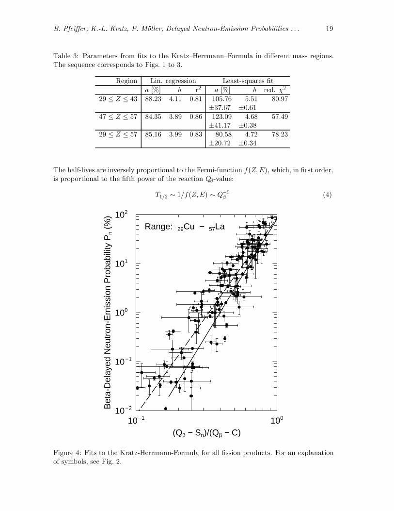
B. Pfeiffer, K.-L. Kratz, P. Moller, Delayed Neutron-Emission Probabilities . . . 19
Table 3: Parameters from fits to the Kratz–Herrmann–Formula in different mass regions.The sequence corresponds to Figs. 1 to 3.
Region Lin. regression Least-squares fit
a [%] b r2 a [%] b red. χ2
29 ≤ Z ≤ 43 88.23 4.11 0.81 105.76 5.51 80.97±37.67 ±0.61
47 ≤ Z ≤ 57 84.35 3.89 0.86 123.09 4.68 57.49±41.17 ±0.38
29 ≤ Z ≤ 57 85.16 3.99 0.83 80.58 4.72 78.23±20.72 ±0.34
The half-lives are inversely proportional to the Fermi-function f(Z,E), which, in first order,is proportional to the fifth power of the reaction Qβ-value:
T1/2 ∼ 1/f(Z,E) ∼ Q−5β (4)
Range: 29Cu − 57La
10 − 1 100 (Qβ − Sn)/(Qβ − C)
10 − 2
10 − 1
100
101
102
Bet
a-D
elay
ed N
eutr
on-E
mis
sion
Pro
babi
lity
Pn
(%)
Figure 4: Fits to the Kratz-Herrmann-Formula for all fission products. For an explanationof symbols, see Fig. 2.

B. Pfeiffer, K.-L. Kratz, P. Moller, Delayed Neutron-Emission Probabilities . . . 20
Table 4: Parameters from fits to T1/2 of neutron–rich nuclides.
lin. regression least-squares fita [ms] b r2 a [ms] b red. χ2
2.74E06 4.5 0.72 7.07E05 4.0 1.1E04±5.33E05 ±0.4
Therefore, in a log-log plot of T1/2 versus Qβ one expects the data points to be scatteredaround a line with a slope of about -(1/5).
Pfeiffer et al. (2000) suggested to fit the T1/2 of neutron-rich nuclides according to thefollowing expression:
T1/2 ≃ a× (Qβ −C)−b (5)
where the cut-off parameter C is calculated according to the fit of Madland and Nix (1988),and the parameters a and b are listed in Table 4.
The gross theory has, basically, the same functional dependence on the Qβ-value, but
underestimates the β-strength to low-lying states, which results in too long half-lives. We
here compensate for this deficiency by treating the coefficient a as a free parameter to be
determined by a fitting procedure. The values obtained are listed in Table 1.
PREDICTION OF T1/2 AND Pn VALUES FROM FRDM-QRPA
The formalism we use to calculate Gamow-Teller (GT) β-strength functions isfairly lengthy, since it involves adding pairing and Gamow-Teller residual interac-tions to the folded-Yukawa single-particle Hamiltonian and solving the resultingSchrodinger equation in the quasi-particle random-phase approximation (QRPA). Be-cause this model has been completely described in two previous papers (Krumlindeet al., 1984; Moller et al., 1990), we refer to those two publications for a full modelspecification and for a definition of notation used. We restrict the discussion here toan overview of features that are particularly relevant to the results discussed in thispaper.
It is well known that wave functions and transition matrix elements are more af-fected by small perturbations to the Hamiltonian than are the eigenvalues. Whentransition rates are calculated it is therefore necessary to add residual interactionsto the folded-Yukawa single-particle Hamiltonian in addition to the pairing interac-tion that is included in the mass model. Fortunately, the residual interaction maybe restricted to a term specific to the particular type of decay considered. To ob-tain reasonably accurate half-lives it is also very important to include ground-statedeformations. Originally the QRPA formalism was developed for and applied onlyto spherical nuclei (Hamamoto, 1965; Halbleib et al., 1967). The extension to de-formed nuclei, which is necessary in global calculations of β-decay properties, wasfirst described in 1984 (Krumlinde et al., 1984).
To treat Gamow-Teller β decay we therefore add the Gamow-Teller force
VGT = 2χGT : β1− � β1+ : (6)

B. Pfeiffer, K.-L. Kratz, P. Moller, Delayed Neutron-Emission Probabilities . . . 21
to the folded-Yukawa single-particle Hamiltonian, after pairing has already been in-corporated, with the standard choice χGT = 23 MeV/A (Hamamoto, 1965; Halbleibet al., 1967; Krumlinde et al., 1984; Moller et al., 1990). Here β1±=
∑
iσit±
i are theGamow-Teller β±-transition operators.
The process of β decay occurs from an initial ground state or excited state ina mother nucleus to a final state in the daughter nucleus. For β− decay, the finalconfiguration is a nucleus in some excited state or its ground state, an electron (withenergy Ee), and an anti-neutrino (with energy Eν). The decay rate wfi to one nuclearstate f is
wfi =m0c
2
h
Γ2
2π3|Mfi|
2f(Z,R, ǫ0) (7)
where R is the nuclear radius and ǫ0 = E0/m0c2, withm0 the electron mass. Moreover,
|Mfi|2 is the nuclear matrix element, which is also the β-strength function. The
dimensionless constant Γ is defined by
Γ ≡g
m0c2
(
m0c
h
)3
(8)
where g is the Gamow-Teller coupling constant. The quantity f(Z,R, ǫ0) has beenextensively discussed and tabulated elsewhere (Preston, 1962; Gove and Martin, 1971;deShalit and Feshbach, 1974).
For the special case in which the two-neutron separation energy S2n in the daughternucleus is greater than Qβ, the energy released in ground-state to ground-state βdecay, the probability for β-delayed one-neutron emission, in percent, is given by
P1n = 100
∑
S1n<Ef<Qβ
wfi
∑
0<Ef<Qβ
wfi
(9)
where Ef = Qβ − E0 is the excitation energy in the daughter nucleus and S1n is theone-neutron separation energy in the daughter nucleus. We assume that decays toenergies above S1n always lead to delayed neutron emission.
To obtain the half-life with respect to β decay one sums up the decay rates wfi
to the individual nuclear states in the allowed energy window. The half-life is thenrelated to the total decay rate by
Tβ =ln 2
∑
0<Ef<Qβ
wfi
(10)
The above equation may be rewritten as
Tβ =h
m0c22π3 ln 2
Γ2
1∑
0<Ef<Qβ
|Mfi|2f(Z,R, ǫ0)
=B
∑
0<Ef<Qβ
|Mfi|2f(Z,R, ǫ0)
(11)
with
B =h
m0c22π3 ln 2
Γ2(12)
B. Pfeiffer, K.-L. Kratz, P. Moller, Delayed Neutron-Emission Probabilities . . . 22
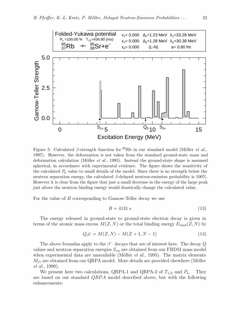
ε2= 0.000
ε4= 0.000
ε6= 0.000
Pn =100.00 % T1/2=434.80 (ms) Folded-Yukawa potential λn=33.28 MeV
λp=30.38 MeV
a= 0.80 fm
∆n=1.23 MeV
∆p=1.28 MeV
(L-N) Rb Sr+e− 37 95 95 38
S1n Qβ S2n 0 5 10 15
0.0
2.5
5.0
Excitation Energy (MeV)
Gam
ow-T
elle
r S
tren
gth
Figure 5: Calculated β-strength function for 95Rb in our standard model (Moller et al.,1997). However, the deformation is not taken from the standard ground-state mass anddeformation calculation (Moller et al., 1995). Instead the ground-state shape is assumedspherical, in accordance with experimental evidence. The figure shows the sensitivity ofthe calculated Pn value to small details of the model. Since there is no strength below theneutron separation energy, the calculated β-delayed neutron-emission probability is 100%.However it is clear from the figure that just a small decrease in the energy of the large peakjust above the neutron binding energy would drastically change the calculated value.
For the value of B corresponding to Gamow-Teller decay we use
B = 4131 s (13)
The energy released in ground-state to ground-state electron decay is given interms of the atomic mass excess M(Z,N) or the total binding energy Ebind(Z,N) by
QβΓ = M(Z,N)−M(Z + 1, N − 1) (14)
The above formulas apply to the β− decays that are of interest here. The decay Qvalues and neutron separation energies Sνn are obtained from our FRDM mass modelwhen experimental data are unavailable (Moller et al., 1995). The matrix elementsMfi are obtained from our QRPA model. More details are provided elsewhere (Molleret al., 1990).
We present here two calculations, QRPA-1 and QRPA-2 of T1/2 and Pn. Theyare based on our standard QRPA model described above, but with the followingenhancements:

B. Pfeiffer, K.-L. Kratz, P. Moller, Delayed Neutron-Emission Probabilities . . . 23
ε2= 0.300
ε4= 0.000
ε6=-0.018
Pn = 2.99 % T1/2= 78.71 (ms) Folded-Yukawa potential λn=33.28 MeV
λp=30.38 MeV
a= 0.80 fm
∆n=0.99 MeV
∆p=1.08 MeV
(L-N) Rb Sr+e− 37 95 95 38
S1n Qβ S2n0 5 10 15
0
1
2
Excitation Energy (MeV)
Gam
ow-T
elle
r S
tren
gth
Figure 6: This calculation corresponds to the QRPA-1 model specification. However, thisnucleus is known to be spherical although a deformed shape was obtained in the ground-state mass-and-deformation calculation (Moller et al., 1995). Therefore, in our QRPA-2
calculation in Fig. 7, this nucleus is treated as spherical in accordance with experiment.
For QRPA-1:
1. To calculate β-decay Q-values and neutron separation energies Sνn weuse experimental ground-state masses where available, otherwise calculatedmasses (Moller et al., 1995). In our previous recent calculations we used the1989 mass evaluation (Audi 1989); here we use the 1995 mass evaluation(Audi et al., 1995).
2. It is known that at higher excitation energies additional residual interac-tions result in a spreading of the transition strength. In our 1997 calculationeach transition goes to a precise, well-specified energy in the daughter nu-cleus. This can result in very large changes in the calculated Pn valuesfor minute changes in, for example S1n, depending on whether an intense,sharp transition is located just below or just above the neutron separationenergy (Moller et al., 1990). To remove this unphysical feature we intro-duce an empirical spreading width that sets in above 2 MeV. Specifically,each transition strength “spike” above 2 MeV is transformed to a Gaussianof width
∆sw =8.62
A0.57(15)
This choice is equal to the error in the mass model. Thus, it accountsapproximately for the uncertainty in calculated neutron separation energies

B. Pfeiffer, K.-L. Kratz, P. Moller, Delayed Neutron-Emission Probabilities . . . 24
ε2= 0.000
ε4= 0.000
ε6= 0.000
Pn = 37.93 % T1/2=386.79 (ms) Folded-Yukawa potential λn=33.28 MeV
λp=30.38 MeV
a= 0.80 fm
∆n=1.23 MeV
∆p=1.28 MeV
(L-N) Rb Sr+e− 37 95 95 38
S1n Qβ S2n0 5 10 15
0.0
0.5
1.0
Excitation Energy (MeV)
Gam
ow-T
elle
r S
tren
gth
Figure 7: This calculation corresponds to theQRPA-2model specification. The calculationis identical to the calculation in Fig. 6 except that the ground-state shape here is spherical.
and at the same time it roughly corresponds to the observed spreading oftransition strengths in the energy range 2–10 MeV, which is the range ofinterest here.
For QRPA-2:
1. In this calculation we retain all of the features of the QRPA-1 calcula-tion and in addition account more accurately for the ground-state deforma-tions which affect the energy levels and wave-functions that are obtained inthe single-particle model. The ground-state deformations calculated in theFRDM mass model (Moller et al., 1992), generally agree with experimentalobservations, but in transition regions between spherical and deformed nu-clei discrepancies do occur. In the QRPA-2 calculation we therefore replacecalculated deformations with spherical shape, when experimental data soindicate. This has been done for the following nuclei:67−78Fe, 67−79Co, 73−80Ni, 73−81Cu, 78−84Zn, 79−87Ga, 83−90Ge, 84−91As, 87−94Se,87−96Br, 92−98Kr, 91−96Rb, 96−97Sr, 96−98Y, 134−140Sb, 136−141Te, 137−142I,141−143Xe, and 141−145Cs.
To illustrate some typical features of β-strength functions we present the strengthfunction of 95Rb calculated in three different ways in Figs. 5–7.
It is not our aim here to make a detailed analysis of each individual nucleus,but instead to present an overview of the model performance in a calculation of

B. Pfeiffer, K.-L. Kratz, P. Moller, Delayed Neutron-Emission Probabilities . . . 25
β− decay (Theory: QRPA-2)
10 − 2 10 − 1 100 101 102 Experimental β-Decay Half-life Tβ,exp (s)
10 − 2
10 − 1
100
101
102
103
Tβ,
calc
/Tβ,
exp
β− decay (Theory: QRPA-1)
10 − 1
100
101
102
T
β,ca
lc /T
β,ex
p
β− decay (Theory: KHF)
10 − 1
100
101
Tβ,
calc
/Tβ,
exp
Figure 8: Ratio of calculated to experimental β-decay half-lives for nuclei in the fission-product region in three different models.
a large number of β-decay half-lives. In Figs. 8 and 9 we compare measured andcalculated β-decay half-lives and β-delayed neutron emission probabilities for thenuclei considered here. To address the reliability in various regions of nuclei and versusdistance from stability, we present the ratios Tβ,calc/Tβ,exp Pn,calc/Pn,exp versus thequantity Tβ,exp. Because the relative error in the calculated half-lives is more sensitiveto small shifts in the positions of the calculated single-particle levels for decays withsmall energy releases, where long half-lives are expected, one can anticipate thathalf-life calculations are more reliable far from stability than close to β-stable nuclei.
Before we make a quantitative analysis of the agreement between calculated andexperimental half-lives we briefly discuss what conclusions can be drawn from a simple

B. Pfeiffer, K.-L. Kratz, P. Moller, Delayed Neutron-Emission Probabilities . . . 26
Theory: QRPA-2
10 − 2 10 − 1 100 101 102 Experimental β-Decay Half-life Tβ,exp (s)
10 − 3
10 − 2
10 − 1
100
101
102
Pn,
calc
/Pn,
exp
Theory: QRPA-1
10 − 2
10 − 1
100
101
P
n,ca
lc /P
n,ex
p
Theory: KHF
10 − 2
10 − 1
100
101
Pn,
calc
/Pn,
exp
Figure 9: Ratio of calculated to experimental β-delayed neutron-emission probabilities fornuclei in the fission-product region in three different models.
visual inspection of Figs. 8 and 9. As functions of Tβ,exp one would expect the averageerror to increase as Tβ,exp increases. This is indeed the case. In addition one is leftwith the impression that the errors in our calculation are fairly large. However, thisis partly a fallacy, since for small errors there are many more points than for largeerrors. This is not clearly seen in the figures, since for small errors many points aresuperimposed on one another. To obtain a more exact understanding of the error inthe calculation we therefore perform a more detailed analysis.
One often analyzes the error in a calculation by studying a root-mean-squaredeviation, which in this case would be
σrms2 =
1
n
n∑
i=1
(Tβ,exp − Tβ,calc)2 (16)

B. Pfeiffer, K.-L. Kratz, P. Moller, Delayed Neutron-Emission Probabilities . . . 27
Table 5: Analysis of the discrepancy between calculated and measured β−-decay half-livesshown in Fig. 8.
Model n Mrl M10rl
σrl σ10rl
Tmaxβ,exp
(s)
KHF 115 −0.11 0.77 0.33 2.15 1QRPA-1 115 −0.02 0.95 0.50 3.14 1QRPA-2 115 0.13 1.37 0.61 4.04 1
KHF 187 −0.40 0.58 0.41 2.56 allQRPA-1 187 −0.06 0.87 0.59 3.88 allQRPA-2 187 0.22 1.67 0.75 5.75 all
However, such an error analysis is unsuitable here, for two reasons. First, the quan-tities studied vary by many orders of magnitude. Second, the calculated and mea-sured quantities may differ by orders of magnitude. We therefore study the quantitylog(Tβ,calc/Tβ,exp), which is plotted in Fig. 8, instead of (Tβ,exp − Tβ,calc)
2. We presentthe formalism here for the half-life, but the formalism is also used to study the errorof our calculated Pn values.
To facilitate the interpretation of the error plots we consider two hypotheticalcases. As the first example, suppose that all the points were grouped on the lineTβ,calc/Tβ,exp = 10. It is immediately clear that an error of this type could be entirelyremoved by introducing a renormalization factor, which is a common practice in thecalculation of β-decay half-lives. We shall see below that in our model the half-livescorresponding to our calculated strength functions have about zero average deviationfrom the calculated half-lives, so no renormalization factor is necessary.
In another extreme, suppose half the points were located on the line Tβ,calc/Tβ,exp =
Table 6: Analysis of the discrepancy between calculated and measured β-delayed neutron-emission probabilities Pn values shown in Fig. 9.
Model n Mrl M10rl
σrl σ10rl
Pminn,exp
(%)
KHF 86 −0.31 0.49 0.36 2.31 1QRPA-1 86 −0.12 0.76 0.60 4.02 1QRPA-2 86 0.12 1.34 0.65 4.51 1
KHF 118 −0.29 0.51 0.44 2.76 allQRPA-1 118 −0.18 0.66 0.62 4.14 allQRPA-2 118 0.11 1.28 0.75 5.62 all

B. Pfeiffer, K.-L. Kratz, P. Moller, Delayed Neutron-Emission Probabilities . . . 28
10 and the other half on the line Tβ,calc/Tβ,exp = 0.1. In this case the average oflog(Tβ,calc/Tβ,exp) would be zero. We are therefore led to the conclusion that thereare two types of errors that are of interest to study, namely the average position ofthe points in Fig. 8, which is just the average of the quantity log(Tβ,calc/Tβ,exp), andthe spread of the points around this average. To analyze the error along these ideas,we introduce the quantities
r = Tβ,calc/Tβ,exp
rl = log10(r)
Mrl =1
n
n∑
i=1
ril
M10rl
= 10Mrl
σrl =
[
1
n
n∑
i=1
(
ril −Mrl
)2]1/2
σ10rl
= 10σrl (17)
where Mrl is the average position of the points and σrl is the spread around this av-erage. The spread σrl can be expected to be related to uncertainties in the positionsof the levels in the underlying single-particle model. The use of a logarithm in thedefinition of rl implies that these two quantities correspond directly to distances asseen by the eye in Figs. 8–9, in units where one order of magnitude is 1. After theerror analysis has been carried out we want to discuss its result in terms like “on theaverage the calculated half-lives are ‘a factor of two’ too long.” To be able to do thiswe must convert back from the logarithmic scale. Thus, we realize that the quantitiesM10
rland σ10
rlare conversions back to “factor of” units of the quantities Mrl and σrl ,
which are expressed in distance or logarithmic units.
DISCUSSION AND SUMMARY
In Tables 5 and 6 we show the results of an evaluation of the quantities in Eq. (17)for T1/2 and Pn corresponding to β decay of the nuclei in table 1. In the QRPAcalculations the ratio between calculated and measured decay half-lives is close to 1.0.This shows, as pointed out earlier (Moller and Randrup, 1990) that no renormalizationof the calculated strength is necessary. The mean deviation between calculated andexperimental half-lives is a factor of 2–5 depending on model and half-life cutoff. Alsothe calculated Pn values agree on the average with the experimental data. Here themean deviation between calculated and experimental data is a factor of 3–6, againdepending on model and half-life cutoff. All half-life calculations agree better withdata for shorter half-lives, cf. Fig. 8 and Table 5. Therefore one can expect themodels to perform better far from stability than what is indicated by the table. Theβ-delayed neutron emission rates are also better calculated in the region of short half-lives and high Pn values, cf. Fig. 9 and Table 6. Again, this suggests calculated Pn
values are more reliable far from stability than indicated by Table 6.

B. Pfeiffer, K.-L. Kratz, P. Moller, Delayed Neutron-Emission Probabilities . . . 29
The KHF results appear more reliable than the QRPA results. This may seemsurprising at first, because the KHF has minimal microscopic content compared to theQRPA. However, an advantage of the QRPA is that it provides so much more detailabout β-decay than does the KHF, namely the ft values of the individual decays, andthe transition energies associated with those decays. A very detailed discussion of thepossible sources of discrepancies between our QRPA results and experimental data ispresented in Ref. (Moller and Randrup, 1990). One difficulty the calculations face isthat the calculated half-lives depend on the energy of the transitions as (Qβ − E)5.As an example we note that calculated half-lives for 95Rb, for which Qβ = 9.28 MeV,change by a factor 1.5 for a change in transition energies by only 0.4 MeV. It is verydifficult to reproduce transition energies to this accuracy in a global nuclear-structuremodel.
For the QRPA-2 calculation we observe that the average of Tβ,calc/Tβ,exp is consid-erably larger than 1, which corresponds to a correct average. One would have a priori
assumed that this calculation would be in better agreement with experiment sincewe substitute calculated deformations for spherical deformations when so indicatedby experimental data. However, since we do not include β-strength due to forbiddentransitions in our model, one would indeed expect that calculated half-lives be toolow on the average. The non-spherical deformations that occur, contrary to experi-mental observations, in the QRPA-1 calculations in some sense simulate the missinglow-lying forbidden β-strength. However, a much more satisfying description wouldbe to use correct ground-state deformations and develop some model to account forthe strength related to forbidden transitions.
The Pn values calculated in the QRPA-1 are on the average too low. At presentwe have no clear explanation for this result. An obvious correction to the model isto take competition with γ emission into account, in particular for emission of l n ≥ 3neutrons. However, such a correction would further lower the ratio Tn,calc/Tn,exp.One may speculate that an accounting for both this effect and forbidden transitionstrength in QRPA-2 would bring about satisfactory agreement. This possibility needto be investigated.
We feel strongly that in a global, unified nuclear-structure model a single set ofconstants must be used over the entire chart of the nuclides, otherwise the basicfoundation of the model is violated. However, for the purpose of generating the bestpossible data bases of half-lives and β-delayed neutron-emission probabilities a com-plementary approach is reasonable. Just as we feel it is appropriate to use experimen-tal ground-state deformations, experimental single-particle levels, when known, couldalso be used as the starting point for the QRPA calculations. In practice the situationwould be that in some regions, such as near the doubly magic 132Sn, many half-livesand Pn values would be unknown, but considerable information on single-particle levelorder and energies would be available. This experimental information could then betaken into account by locally adjusting the single-particle model proton and neutronspin-orbit strengths and the diffuseness of the single-particle well to obtain optimumagreement with the observed single-particle data such as the observed neutron single-particle sequence f7/2, p3/2, p1/2, and h9/2 near 132Sn. The hope would be that thelocal agreement would be retained in some limited extrapolation away from the knownregion. Such a fairly limited extrapolation would be all that is required to reach the

B. Pfeiffer, K.-L. Kratz, P. Moller, Delayed Neutron-Emission Probabilities . . . 30
isotopes in the fission-product region where experimental data are not yet available,cf. Fig. 1. Limited studies along these lines have been undertaken by, for example,Hannawald et al. (2000). Other highly desirable enhancements to the calculationswould be to include first-forbidden strength, perhaps first in a gross-theory approachand later from a new microscopic model. The cut-off parameter C in the KHF for-mula could be taken from the Lipkin-Nogami microscopic calculation instead of fromthe Madland-Nix macroscopic expression. The energy window (Qβ − Sn) could bereduced by 150 to max 500 keV to account for the angular-momentum barrier foremission of l ≥ 3 neutrons in for example 137I.
In conclusion we note that we now have available about 40 new experimental T1/2
and Pn values in the fission-product region. Data for additional nuclei in this regionthat are required as input in reactor criticality, astrophysical and other applicationsare provided from theoretical calculations. The substantial increase in available exper-imental data since the compilations by Brady (1989) and Rudstam (1993) is expectedto have a significant impact on applied calculations.
REFERENCES
Aboussir Y.et al. (1995). Atomic Data and Nucl. Data Tables 61, 127.Ameil F.et al. (1998). Eur. Phys. J. A1, 275.Audi, G. (1989). “Midstream atomic mass evaluation, private communication, withfour revisions”Audi G. and Wapstra A.H. (1995). Nucl.Phys. A595, 409.Bernas M. et al. (1998). Nucl. Phys. A630, 41c.Bohmer W. (1998). PhD Thesis, Univ. Mainz, unpublished.Borzov I.N. et al. (1996). Z. Phys. A335, 127.Brady M.C. (1989). “Evaluation and Application of Delayed Neutron PrecursorData”, LANL Thesis Report LA-11534-T.Brady M.C. and England T.R. (1989). Nucl. Sci. Eng. 103, 129.Dorfler T. et al. (1996). Phys. Rev. C54, 2894.Duke C.L., Hansen P.G., Nielsen O.B. and Rudstam G.(1970). Nucl. Phys. A151,609.England T.R. et al. (1986). Specialists’ Meeting on Delayed Neutron PropertiesISBN 070044 0926 7, p.117. Birmingham, Sep. 1986.Fedoseyev V.N. et al. (1995). Z. Physik A353, 9.Franchoo S. et al. (1998). Phys. Rev. Lett. 81, 3100.Gove N.B. and Martin M.J. (1971). Nucl. Data Tables 10, 205.Halbleib Sr J.A. and Sorensen R. A. (1967). Nucl. Phys. A98, 592.Hamamoto I. (1965). Nucl. Phys. 62, 49.Hannawald M. et al. (2000). Phys. Rev. C62, 054301.Hirsch M., Staudt A., Klapdor-Kleingrothaus H.-V. (1992). Atomic and Nucl. Data
Tables 51, 244.Hirsch M., Staudt A., Klapdor-Kleingrothaus H.-V. (1996). Phys. Rev. C54, 2972.Koster U. (2000). PhD Thesis, TU Munchen, unpublished.Korgul A. et al. (2000). Eur. Phys. J. A3, 167.Kratz K.-L. and Herrmann G. (1973). Z. Physik 263, 435.Kratz K.-L. (1984). Nucl.Phys. A417, 447.

B. Pfeiffer, K.-L. Kratz, P. Moller, Delayed Neutron-Emission Probabilities . . . 31
Kratz K.-L. et al. (2000). AIP Conf. Proc. 529 295.Krumlinde J. and Moller P. (1984). Nucl. Phys. A417, 419.Madland D.M. and Nix J.R. (1988). Nucl. Phys. A476, 1.Mach H., Fogelberg B. and Urban W. (2000). priv. comm. and to be published.Mann F.M. et al. (1984). Nucl. Sci. Eng. 87, 418.Mann F.M. (1986). Specialists’ Meeting on Delayed Neutron Properties ISBN 0700440926 7, p.21. Birmingham, September.Mehren T. et al. (1996). Phys. Rev. Lett. 77, 458.Moller P. and Randrup J. (1990). Nucl. Phys. A514, 1.Moller P. et al. (1992). Nucl. Phys. A536, 61.Moller P. et al. (1995). Atomic Data and Nucl. Data Tables 59, 185.Moller P., Nix J.R. and Kratz K.-L. (1997). Atomic Data and Nucl. Data Tables 66,131.Mueller W.F. et al. (2000). Phys. Rev. C61, 054308.Preston M.A. (1962). “Physics of the Nucleus”, Addison-Wesley, Reading.Pfeiffer B., Kratz K.-L., Moller P. (2000). “Predictions of T1/2 and Pn Values”; In-ternal Report, Inst. fur Kernchemie, Univ. Mainz (2000).URL: www.kernchemie.uni-mainz.de/∼pfeiffer/khf/Rudstam G. (1993). Atomic Data and Nucl. Data Tables 53, 1.deShalit A. and Feshbach H. (1974). “Theoretical Nuclear Physics, vol. I: NuclearStructure”, Wiley, New YorkShergur J. (2000). Proc. Conf. on Nuclear Structure 2000 - NS2000, MSU August2000; Nucl. Phys. A, in print.Sorlin O. et al. (1993). Phys.Rev. C47, 2941.Sorlin O. et al. (2000). Nucl. Phys. A669, 351.Tachibana T., Nakata H., Yamada M. (1998). AIP Conf. Proc. 425, 495.Takahashi K. (1972). Prog. Theoret. Phys. 47, 1500.Takahashi K. et al. (1973). Atomic Data and Nucl. Data Tables 12, 101.Wang J.C. et al. (1999). Phys. Lett. B454, 1.Weissman L. et al. (1999). Phys. Rev. C59, 2004.Wilson W.B. and England T.R. (1993). Prog. Nucl. Energy, this volume.
Related Documents