Statoil´s Exposure to Oil Price Fluctuations - UiS Brage

University of Stavanger

Stavanger, spring 2015

Statoil´s Exposure to Oil Price Fluctuations: An

Analysis on Investment Level and Stock Price

Synne Nåmdal and Kristine Meling

Master in Business Administration, University of Stavanger

Applied Finance

II

DET SAMFUNNSVITENSKAPELIGE FAKULTET,

HANDELSHØGSKOLEN VED UIS

MASTEROPPGAVE STUDIEPROGRAM:

Økonomi og administrasjon, master

OPPGAVEN ER SKREVET INNEN FØLGENDE

SPESIALISERINGSRETNING:

Anvendt finans / Applied Finance

ER OPPGAVEN KONFIDENSIELL?

(NB! Bruk rødt skjema ved konfidensiell oppgave)

TITTEL: Statoils eksponering til fluktuasjoner i oljeprisen: En analyse av investeringsnivå og aksjepris

ENGELSK TITTEL: Statoil´s exposure to oil price fluctuations: An analysis on investment level and stock price

FORFATTER(E)

VEILEDER:

Mads Holm

Studentnummer:

211855

…………………

203260

…………………

Navn:

Kristine Meling

…………………………………….

Synne Meling Nåmdal

…………………………………….

OPPGAVEN ER MOTTATT I TO – 2 – INNBUNDNE EKSEMPLARER

Stavanger, ……/…… 2015 Underskrift administrasjon:……………………………

III

Summary

In this thesis an econometric analysis of Statoil’s investment level and stock return has been

performed, with purpose of examine the affect that fluctuations in the price of crude oil has on

these variables. The results revealed that crude oil prices have a significant impact on Statoil´s

stock returns, due to the direct impact the crude oil price has on Statoil’s cash flows. The

investment level does not seem to be affected by either of the variables in the analysis, and

this could indicate that the company has long-term commitments, and that capex has a lagged

reaction to the crude oil price. Further, an investigation showed what strategies Statoil

practice when the crude oil price drops, and it seems that compered to 2008, company are

now investing in technology to open new renewable energy opportunities. As the demand for

renewable energy and the supply for oil increases, Statoil is focusing on creating value and

growth to the company and at the same time looking into utilizing oil and gas expertise and

technology to open new renewable energy opportunities.

Historically OPEC has had a lot of power in the oil industry, due to their large share of the oil

production. As early as 1973, (OAPEC) decided to cut supply until Israeli forces pulled out of

Arab territory. This made the prices increase dramatically. In 2014, OPEC decided not to

reduce their supply of oil when demand declined, which resulted in an oil price decrease that

went from $80bbl in October down to $65bbl in November. During the writing of this thesis,

the oil price has gone from approximately $45bbl in January to $64bbl in June, and there have

been a reduction of field and modification costs in the sector.

The thesis concludes that the investments level is held more or less unaffected, while the

return of the company´s stock decreases with drops in the price of crude oil. Statoil´s financial

reports show that the company has a stable economy, allowing them to invest even when

crude oil price is low.

IV

Preface

This thesis has been written as the final work of our Masters degree within Business

Administration, with a specialisation in applied finance, at the University of Stavanger (UiS).

The motivation behind this research has been the large changes that the petroleum industry

has experienced recently. The future of this industry is more uncertain now than ever before,

and the energy analysts are divided in their outlook for the future price of crude oil. Due to

Statoil´s strong position in the Norwegian crude oil market, we found it interesting to

investigate the company´s exposure to fluctuation of this much discussed commodity. The

process of working with this thesis has been both challenging and time consuming, but at the

same time highly educational a benefiting. We hope the thesis will arise interest also among

others, and contribute to up-to-date debates.

A great thank you is directed to our advisor, Mads Holm, for his support and all his helpful

advice through this whole process. Thank you for taking the time out of your day to listen,

understand and guide us. We value it highly. Further we would like to thank William Gilje

Gjerdem and Marius Sikveland at the University of Stavanger for helpful advice going into

this process. We would also like to thank Mirza Koristovic, senior analyst at Statoil for his

time and insight.

Last, but definitely not least, we would like to express our unlimited gratitude to our families

and friends. Thank you for your understanding and patience, and for your encouragement and

uplifting words through this challenging process. We could not have done it without your

support. Thank you.

Stavanger, June 15th 2015

___________________ ___________________

Synne Meling Nåmdal Kristine Meling

V

Table of contents

Summary.................................................................................................................................III

Preface.....................................................................................................................................IV

1. Introduction..........................................................................................................................1

1.1 Background information...........................................................................................1

1.2 Purpose of thesis.......................................................................................................2

1.3 Problem Statement....................................................................................................3

1.4 Structure....................................................................................................................4

2. Theoretical Framework........................................................................................................5

2.1 What is Petroleum?...................................................................................................5

2.1.1 Crude Oil....................................................................................................5

2.1.2 Gas..............................................................................................................6

2.1.3 Petroleum Reserves....................................................................................6

2.2 Investment Behaviour...............................................................................................7

2.3 Market Theory………...............................................................................................9

2.3.1 Efficient Market Hypothesis......................................................................9

2.3.2 Stock Price Theory...................................................................................10

2.4 Valuation Models....................................................................................................11

2.4.1 The Discounted Free Cash Flow Model...................................................11

2.4.2 The Dividend-Discount Model.................................................................12

2.4.3 The Capital Asset Pricing Model (CAPM) .............................................13

2.4.4 Multifactor Models...................................................................................14

2.5 Previous Research...................................................................................................15

3. The Petroleum Industry and Statoil ASA........................................................................18

VI

3.1 The Petroleum Industry...........................................................................................18

3.1.1 Crude Oil Demand ..................................................................................19

3.1.2 Crude Oil Supply ....................................................................................20

3.1.3 Crude Oil Market Development ...............................................................21

3.1.4 Crude Oil Price Development ..................................................................22

3.1.4.1 Long-Term Price Development ..................................................24

3.1.4.2 Short-Term Price Development ..................................................25

3.1.5 The Peak Oil Theory.................................................................................25

3.1 Statoil ASA..............................................................................................................26

3.2.2 Investment Strategy...................................................................................28

3.2.3 Present situation.........................................................................................28

3.2.4 Current Production and Consumption of Crude Oil..................................31

3.2.4 Future Aspects...........................................................................................32

4. Econometric Analysis.........................................................................................................34

4.1 Data…………….....................................................................................................34

4.1.1 Data Statistics………...............................................................................35

4.1.2 Data Credibility........................................................................................35

4.2 Regression Model...................................................................................................36

4.2.1 OLS Assumptions....................................................................................37

4.2.2 Parameter Statement................................................................................38

4.2.3 Analytical Interpretation..........................................................................38

4.3 Macroeconomic Influential Factors........................................................................39

4.3.1 Interest Rate.............................................................................................39

4.3.2 Market Index............................................................................................40

4.4 Hypothesis Testing..................................................................................................42

VII

4.5 Residual Analysis....................................................................................................43

4.5.1 Homoscedasticity.....................................................................................43

4.5.2 Autocorrelation.........................................................................................44

4.5.3 Non-Stochastic Explanatory Variables....................................................45

4.5.4 Normality.................................................................................................45

4.6 Correlation Analysis...............................................................................................46

4.7 Implementation of Regression Analysis.................................................................47

4.7.1 Model 1....................................................................................................47

4.7.2 Model 2....................................................................................................48

4.7.3 Model 3....................................................................................................48

4.8 Results.....................................................................................................................49

4.8.1 Presentation of Model 1...........................................................................49

4.8.2 Presentation of Model 2...........................................................................50

4.8.3 Presentation of Model 3...........................................................................51

5. Conclusion...........................................................................................................................52

5.1 Analytical Weaknesses...........................................................................................52

5.2 Conclusion...............................................................................................................53

5.2 Suggestions for further work...................................................................................54

6. References............................................................................................................................55

7. Appendix..............................................................................................................................59

VIII

List of figures

Figure 1 Distribution of Global Proven Reserves.......................................................................6

Figure 2 Value Chain for the Oil and Gas Industry..................................................................18

Figure 3 Brent Crude Oil Price….............................................................................................24

Figure 4 Distribution of Statoil`s shareholders.........................................................................26

Figure 5 Statoil`s Stock Return……………………………………………….........................27

Figure 6 Correlation between Statoil`s Stock Return and Brent Crude Oil Price....................27

Figure 7 Oil Investments and Labor Cost.................................................................................30

Figure 8 World Liquide Fuel Production..................................................................................32

Figure 9 Correlation between OSEAX and S&P 500...............................................................41

List of tables

Table 1 Data Statistics Quarterly Data......................................................................................35

Table 2 Data Statistics Monthly Data.......................................................................................35

Table 3 Hypothesis...................................................................................................................42

Table 4 Durbin-Watson Values................................................................................................44

Table 5 Normality Quarterly Data ...........................................................................................45

Table 6 Normality Monthly Data .............................................................................................45

Table 7 Correlation Analysis....................................................................................................46

Table 8 Regression Model 1.....................................................................................................49

Table 9 Regression Model 2…….............................................................................................50

Table 10 Regression Model 3...................................................................................................51

1

1. Introduction

This study aims to investigate the affect crude oil return fluctuations have on Statoil, the

larges oil and gas company in Norway, measured by changes in the company´s investment

level and stock return. In this chapter, a presentation of the background and motivation

writing this detailed comparative study will be given. The problems addressed will be

carefully considered and formulated. The relevance of the issue to be addressed will further

be argued, and linked to the current situation of the oil and gas market. Finally, the structure

of the thesis will be presented to provide the reader with a general overview.

1.1 Background information

Statoil ASA is an international energy company, which focuses on oil- and gas production.

The company is based in Norway, and has been one of the main actors in the Norwegian

petroleum industry since the beginning of the 70´s. With about 70% of the total production

on the Norwegian continental shelf, Statoil is the largest operator here (Snl, 2015).

In April 2001, the company was made public, as it was listed on NYSE and Oslo Stock

Exchange. Today, the Norwegian State owns 67% of Statoil´s shares, which are managed by

the Ministry of Petroleum and Energy. Consequently, Statoil’s investment decisions do not

only affect the company’s immediate investors, but also the Norwegian society in general. In

Norway the oil- and gas investments plays an important role, to for the industry and the

general economy as well. Because of Statoil’s dominating role in the Norwegian economy,

the company has been central to the discussion of oil investments for several decades.

Companies in the Oil- and Gas industry has been known to have a complex process tied to its

investments, Statoil is no exception. The recovery of a oil- and gas field requires numerous

decisions during several years, from the first assessment of exploration fields, to the last

measurements to expand production at the end of the exploration time. Because of the length

of the investment horizon for petroleum companies, such as Statoil, there is great uncertainty

and risk associated with several underlying factors, like the price of oil.

2

Significant changes in the price of oil tend to have large impact on companies where income

and the commodity price have direct correlation. It can for example be shown that an

upstream oil and gas company, such as Statoil, would perform different as to income if the

price of crude oil where $150 per barrel versus if the price where $30 per barrel.

A low crude oil price can lead to a cease in the exploration for oil and gas, and put large

projects on hold. For companies that are low on cash and dependent on a high crude oil price

to maintain a positive cash flow, a situation where crude oil price is low could in the worst-

case scenario lead to bankruptcy. Fluctuations in the level of oil price may, because of these

concerns, influence the investment behaviour of oil- and gas companies, and cause different

investment behaviour within such firms during periods of recession and growth.

During the last half of 2014, and continuing into the present year of 2015, Norway along with

the rest of the world experienced a sudden, but relatively prolonged drop in the price of crude

oil. The drop of crude oil price has lead to great unrest and uncertainty concerning the future

within the petroleum industry. Today the industry is characterized by large layoffs and

restructuring, something that is having a ripple effect on both the highly oil affected

Norwegian general industry, as well as society. Due to this, and the company´s central role,

Statoil´s decisions are currently in the spotlight, not only within the petroleum industry, but

also to the Norwegian business sector in general.

1.2 Purpose of thesis

The purpose of this thesis is to evaluate and measure Statoil’s exposure to oil price dynamics,

by analysing how changes in the price of crude oil affect the company´s investment level. The

thesis further intends to investigate how this affects the company´s stock return, and hence the

company´s investors. The information emerged from the thesis can be used to better

understand the extent of which the effect changes in the price of crude oil have on two of

Statoil´s key factors, investment level and stock return. This information can further be used

to give an indication of the extent to which Statoil takes their investors into account when

making investment decisions.

3

An in-depth analysis of the affect of oil price dynamics on Statoil´s investment decisions and

stock return can be useful to anyone who are interested in investing in the company´s stock,

or who for other reasons wish to gain better understanding of the subject.

1.3 Problem Statement

Looking back at the previous decades, periods of recession have revealed themselves to

provide both opportunities and restraints for investments within companies. Such periods

have proven that changes in economic risk factors of a market, might influence both the

investment behaviour and the stock return of a company. For these reasons, Statoil´s

investments and stock return has been found interesting to include in this examination of oil

price fluctuations on the company.

The problem to examine in this thesis can be stated as: “Does oil price fluctuations have

an explainable affect on Statoil´s investment level and stock return?”

To simplify the process, and ensure it being as constructive as possible, two different null

hypotheses, and consequently two alternative hypotheses have been developed. This has been

done to refine the problem of the thesis. The first null hypothesis, and accompanying

alternative is stated as:

H0: The effect of oil price on Statoil´s investment level = 0

H1: The effect of oil price on Statoil´s investment level ≠ 0

Further, the second null and alternative hypotheses are stated as:

H0: The effect of oil price on Statoil´s stock return = 0

H1: The effect of oil price on Statoil´s stock return ≠ 0

4

1.4 Structure

When working with complex and challenging hypothesis, it is critical that the thesis is based

on a structural approach, providing the goals and objectives from start to finish. In this

section, an overview of the thesis fundamental structure will be presented.

In chapter 1, an introduction to the subject and the framework of the thesis has been given.

The thesis relevance to the current economic situation has been explained, the main problem

to be further addressed in the thesis has been formulated and stated.

In chapter 2, the general theory and empirical research that the thesis is built upon will be

presented and explained. In short the theory presented involves fundamental investment

behaviour, as well as various acknowledged valuation methods for company stock. Further

commonly used methods for calculations of expected return will be described, before

previous empirical research and related results will be presented.

In chapter 3, a presentation of the petroleum industry, as well as an overview of the

development of crude oil price will be given. Further, the peak oil theory will be explained

before Statoil´s current and previous investment strategy will be described. Finally, the future

aspects for Statoil and the crude oil price will be discussed.

In chapter 4, the econometric analysis will be presented and carefully explained. The data

collected and their characteristics will be presented. Based on econometric theory, a multiple

regression model and hypothesis suitable to the problem statement will be formulated. The

validly of the model will be carefully tested, before the analytical results will be presented and

discussed.

In chapter 5, analytical weaknesses will be pointed out, before the results will be summarized

and a final conclusion will be drawn. Last, suggestions of possible angles for further research

on the subject will be given.

5

2. Theoretical Frameworks

In the following chapter, academic theory relevant for the thesis will be carefully presented.

First. a short introduction will be given on petroleum, to ensure fundamental understanding of

the commodities, oil and gas. Next, fundamental theory on investment behaviour will be

given to emphasize the importance of this field in the further work with the thesis. It exists a

multitude of research and theories within the field of investment behaviour, and reviewing it

all would be impossible. Nevertheless, an understanding comprehensive enough to ensure the

thesis root in literature is critical. Further, as the thesis aims to include the relationship

between Statoil´s stock price and oil price, market theory and a selection of the most

commonly used valuation models will be presented. Last, previous research on the topic will

be reviewed as a foundation for the thesis further development.

2.1 What is petroleum?

Petroleum was discovered and used by mankind as early as the 16th century, but the petroleum

geology as we know it today today, started at the beginning of the 20th century. Several

hundred million years ago, remnants of dead plants and animals were, without aeration,

exposed to a huge pressure and transformed into coal, oil and gas. These resources are by

photosynthesis, altered solar energy, but it is considered as a non-renewable energy source

because the conversion takes several million years. Coal, oil and gas consist mostly of carbon

and hydrogen, which makes them highly useable as a resource. However, oil contains more

energy than coal (per ton) because it contains more hydrogen and small amounts of oxygen,

nitrogen and sulfur.

2.1.1 Crude Oil

Crude oil is the liquid hydrocarbon structures that is left when the water and gas content is

removed. The chemical composition of crude oils varies greatly between different instances,

6

and it is this combination that determines the quality of the oil. Crude Oil is measured in

barrels, which is equivalent to 159 liters.

2.1.2 Gas

Natural Gas instances consist mainly of methane, but also butane, ethane and propane. One

can compare oil- and gas by converting gas into barrels of oil equivalent based on energy

released by combustion of the two commodity resources. Gas is originally measured in

standard cubic foot- or cubic meters. A barrel of oil equivalent is approximately 5800 cubic

feet gas. Gas exists in either pure gas fields or oil- and coalfields.

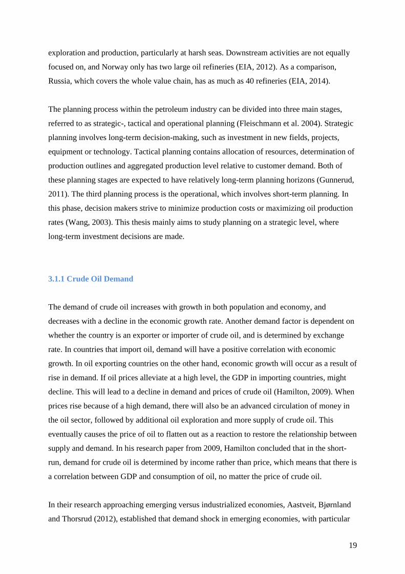
2.1.3 Petroleum reserves

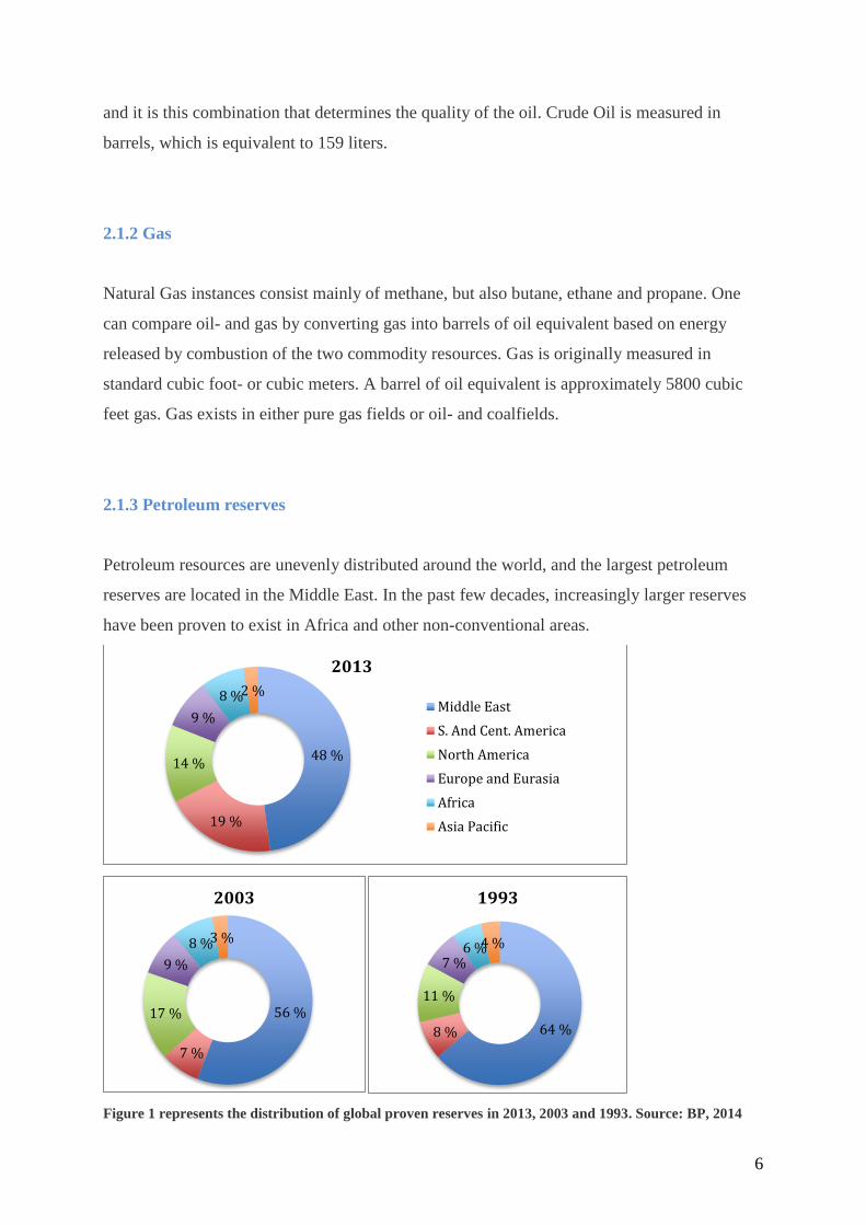
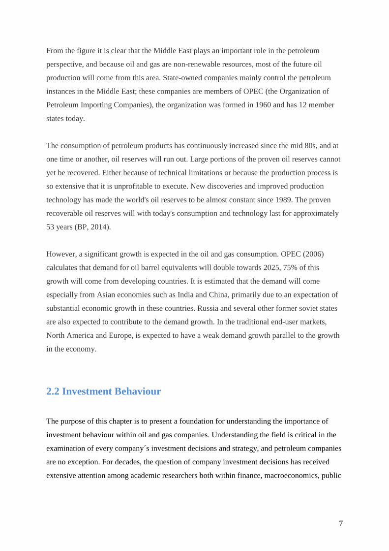
Petroleum resources are unevenly distributed around the world, and the largest petroleum

reserves are located in the Middle East. In the past few decades, increasingly larger reserves

have been proven to exist in Africa and other non-conventional areas.

Figure 1 represents the distribution of global proven reserves in 2013, 2003 and 1993. Source: BP, 2014

48 %

19 %

14 %

9 %

8 %2 %

2013

Middle East

S. And Cent. America

North America

Europe and Eurasia

Africa

Asia Pacific

56 %

7 %

17 %

9 %

8 %3 %

2003

64 %8 %

11 %

7 %6 %4 %

1993

7

From the figure it is clear that the Middle East plays an important role in the petroleum

perspective, and because oil and gas are non-renewable resources, most of the future oil

production will come from this area. State-owned companies mainly control the petroleum

instances in the Middle East; these companies are members of OPEC (the Organization of

Petroleum Importing Companies), the organization was formed in 1960 and has 12 member

states today.

The consumption of petroleum products has continuously increased since the mid 80s, and at

one time or another, oil reserves will run out. Large portions of the proven oil reserves cannot

yet be recovered. Either because of technical limitations or because the production process is

so extensive that it is unprofitable to execute. New discoveries and improved production

technology has made the world's oil reserves to be almost constant since 1989. The proven

recoverable oil reserves will with today's consumption and technology last for approximately

53 years (BP, 2014).

However, a significant growth is expected in the oil and gas consumption. OPEC (2006)

calculates that demand for oil barrel equivalents will double towards 2025, 75% of this

growth will come from developing countries. It is estimated that the demand will come

especially from Asian economies such as India and China, primarily due to an expectation of

substantial economic growth in these countries. Russia and several other former soviet states

are also expected to contribute to the demand growth. In the traditional end-user markets,

North America and Europe, is expected to have a weak demand growth parallel to the growth

in the economy.

2.2 Investment Behaviour

The purpose of this chapter is to present a foundation for understanding the importance of

investment behaviour within oil and gas companies. Understanding the field is critical in the

examination of every company´s investment decisions and strategy, and petroleum companies

are no exception. For decades, the question of company investment decisions has received

extensive attention among academic researchers both within finance, macroeconomics, public

8

economics and industrial organisations. As early as in 1936 Keynes wrote in his General

Theory:

“Most, probably, of our decision to do something positive, the full consequences of which will

be drawn out over many days to come, can only be taken as the result of animal spirits – a

spontaneous urge to action rather than inaction, and not as the outcome of weighted average

of quantitative benefits multiplied by quantitative probabilities”.

The process of accumulation of capital is recognized as genuinely dynamic (Fedvang, 2000).

As a result of new investments, the capital in the companies increases over time. At the same

time, the companies are losing value through economic and technologic depreciation. As for

most industries, the main behavioural assumption for oil and gas companies is profit

maximization (Mohn, K., 2008). This is an assumption that, not unexpectedly, also most

general economic models are based upon. Chirinko (1993) provides a comprehensive survey

of modelling strategies and results up to the early 1990s. This recapitulation displays a clear

separation between two distinct modelling strategies. (Mohn, K., 2008). The first direction

involves neo-classical applied models, which involves direct derivations from the first-order

conditions of companies’ maximization problems. Second, there is the accelerator models

based on general autoregressive lag forms, without any direct connection to theoretical

maximizing behaviour (Bond et al., 2003). The classical models are usually preferable, but

have the weakness that they often provide inferior description of empirical data compared to

the accelerator models.

A great many investments are unalterable, which involves that once an investment decision is

made, there is no way of reversing it. Because of this, the opportunity to invest itself can be

considered valuable. This value is commonly called a real option. In their theories concerning

irreversible investments, Dixit and Pindyck (1994) gives an overview of real options. A key

issue to be highlighted from these theories is that an incensement in risk of investment

decisions further will increase real option value, a statement that implies a negative

correlation between investments and risk. This hypothesis finds broad support among most

empirical studies (Mohn, K., 2007).

Investment behaviour in oil and gas companies possesses many of the same characteristics as

in general companies. However, some influential factors of investment behaviour within

9

petroleum companies are distinctive for this exact type of firms. Examples of such might be

large undividable projects, investments with heavy lags, political attention and cyclical

investment. Further, the exploration activity and its associated costs, as well as reserves

replacement rate are also unique factors that affect investment behaviour within oil and gas

companies.

2.3 Market theory

The central theory behind crude oil market and stock return is important to get an

understanding of how Statoil is directly affected by the fluctuations in crude oil prices. First

the general theory, important for regression analysis, that stock return does not have a delayed

reaction to changes in crude oil price will be presented, and secondly the model which

displays the direct link between Statoil´s cash flows and the crude oil price.

2.3.1 Efficient Market Hypothesis

A central financial theory is the Efficient Market Hypothesis (EMH). Fama, (1970) defines it

as “A market in which prices always fully reflect available information is called efficient”.

Which means that the market prices reflects the information in the market, and current share

price will then be a correct expectation for fair value of a stock. According to EMH there will

not occur delayed reactions in share prices due to changes in oil prices, because oil prices are

public and accessible information. When a market is efficient, the stock price moves as a

“random walk”, the change in value of shares will then be independent of the previous

events because these conditions will already be reflected in the price. However, only new

knowledge will determine whether the stock drops or increases (Fama, 1970).

10

2.3.2 Stock price theory

In the financial world the stock market is a submarket of capital market, and it is available on

different stock exchanges around the world where they work as a marketplace for actors who

are interested to buy and sell shares in listed companies. By issuing shares in the company

through stock exchanges, the companies has the opportunity to obtain venture capital from

investors, which have the right to company earnings and profits through dividend earnings on

company shares. (Bodie Thoene novel as et al., 2011)

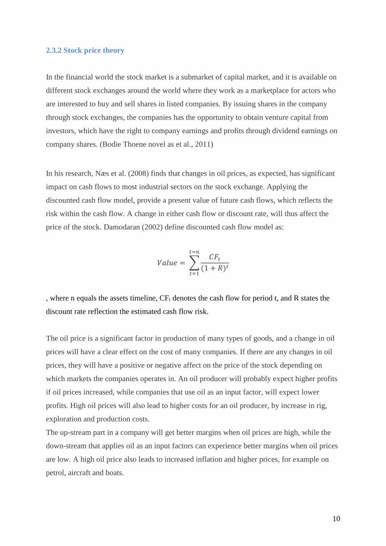
In his research, Næs et al. (2008) finds that changes in oil prices, as expected, has significant

impact on cash flows to most industrial sectors on the stock exchange. Applying the

discounted cash flow model, provide a present value of future cash flows, which reflects the

risk within the cash flow. A change in either cash flow or discount rate, will thus affect the

price of the stock. Damodaran (2002) define discounted cash flow model as:

𝑉𝑎𝑙𝑢𝑒 = ∑𝐶𝐹𝑡

(1 + 𝑅)𝑡

𝑡=𝑛

𝑡=1

, where n equals the assets timeline, CFt denotes the cash flow for period t, and R states the

discount rate reflection the estimated cash flow risk.

The oil price is a significant factor in production of many types of goods, and a change in oil

prices will have a clear effect on the cost of many companies. If there are any changes in oil

prices, they will have a positive or negative affect on the price of the stock depending on

which markets the companies operates in. An oil producer will probably expect higher profits

if oil prices increased, while companies that use oil as an input factor, will expect lower

profits. High oil prices will also lead to higher costs for an oil producer, by increase in rig,

exploration and production costs.

The up-stream part in a company will get better margins when oil prices are high, while the

down-stream that applies oil as an input factors can experience better margins when oil prices

are low. A high oil price also leads to increased inflation and higher prices, for example on

petrol, aircraft and boats.

11

The Norwegian equity market has historically been characterized by fluctuations in oil prices,

which is natural since Statoil alone covers about 20% of Oslo Stock exchange.

2.4 Valuation Models

As Statoil’s stock price has a central part in the thesis it would be natural to include the basic

theorems and methods used in the determination of stock price, as well as calculation used to

find the expected return of an investment. First, some of the most commonly used valuation

methods will be presented, before recognized models used in the calculations of expected

return will be described. These models and methods will be included to give a fundamental

understanding of the formation of company stock.

2.4.1 The Discounted Free Cash Flow Model

Due to the law of one price, to value any security, one must determine the expected cash

flows an investor will receive from owning it (Berk, J. & DeMarzo P., 2014). The discounted

free cash flow model (DCF) is a recognized, and widely used approach in valuation of firms

and company stock. According to Damodaran (2002) the DCF is the fundamental method on

which all other valuation approaches are built upon. In application of the model, future cash

flows are estimated and discounted to determine the present value of a company. Such models

are thereby based on that the value of a company´s share is equal to the present value (PV) of

the cash flow that shareholders are expected to receive from holding it (Elton, et al., 2010).

In the application of the discounted free cash flow model, a key difference from other

valuation models is that this model can be applied to determine the value of a company to all

investors, both equity and debt holders. As a consequence, also the discount rate will be

different from other valuation models (Berk, J., & DeMarzo, P., 2014). Because this model

discounts free cash flow also paid to debt holders, and not only equity holders, the average

cost of capital the firm has to pay to all its investors, also called the weighted average cost of

capital (WACC) will be applied as discount rate. WACC is denoted as rwacc. If a firm has no

debt, rwacc = rE. If the firm has debt, rwacc is the average of the company´s debt and equity cost

12

of capital. As debt generally is considered less risky than equity, rwacc is normally smaller than

rE.

2.4.2 The Dividend-Discount Model

For a company which stock pays dividends, the dividend-discount model can be applied to

find appropriate company value, and thereby stock price (Berk, J. & DeMarzo, P., 2014). The

method discounts all future expected dividends to their present value, and this way finds the

price of the stock. In simple terms, the dividend model can be stated as:

𝑃0 = ∑𝐷𝑖𝑣1

(1 + 𝑟𝐸)𝑁

∞

𝑁=1

where P0 denotes the stocks present value, Div1 is the expected dividends paid in period N,

and rE denotes the equity cost of capital for the stock, which is the expected return of other

investments available the market with equivalent risk to the company´s stock (Berk, J. &

DeMarzo, P., 2014). The above equation holds for any horizon N, hence all investors with the

same beliefs will allocate the stock an equal value, independent of the individual investors

horizon of investment. The above equation shows that the stock price is highly sensitive to

changes in the expected dividends or in the expected rate of return. As predicting dividends

for all future can be highly complicated, various simplified versions of the dividend model

has been developed. An example of such is the constant dividend growth model, which

simplifies estimation of future dividends by assuming constant growth (Berk, J. & DeMarzo

P., 2014). The constant dividend growth model can be illustrated as:

𝑃0 = 𝐷𝑖𝑣1

𝑟𝐸 − 𝑔

where the added denotation g represent the growth rate of the dividends. From the equation it

can be seen that the value of the company in this approach is based on the dividend for the

upcoming year, divided by the equity cost of capital adjusted for the dividends estimated

growth rate.

13

2.4.3 The Capital Asset Pricing Model

The Capital Asset Pricing Model, also know as CAPM, is a single-factor model, and a well-

recognized method for calculation of required rate of return. The model was developed by

Black, Lintner and Sharpe (Black, 1972; Lintner, 1965; Sharpe, 1964), and many consider it

to be the most important measurement for the relationship between risks and return (Berk J. &

DeMarzo P., 2014). As the model is a relative simple one, it is based on fundamental

assumptions. Three main assumptions underlie the model, which are 1) the markets are

assumed to be competitive, 2) investors are assumed to choose efficient portfolios, and 3)

investors are assumed to have homogeneous expectations.

When purchasing company stock, investors will require compensation for exposure to

financial risk. Hence, the expected return (r) has to exceed the return of a risk-free investment

(rf). Excess return of the market index that goes beyond risk free rate is usually referred to as

market risk premium (Brealey et al., 2008). The CAPM, which illustrates the relationship

between risk and expected return, can be stated as,

𝐸(𝑟𝑖) = 𝑟𝑓 + 𝛽𝑖(𝐸(𝑟𝑚) − 𝑟𝑓),

where E(ri) describes the expected rate of return on stock i, and rf is the risk free interest rate.

The expression βi(E(rm) – rf) describes the risk premium. In other words, the above equation

shows that the expected return is equal to the risk free interest rate, plus the risk premium.

The risk premium can be decomposed to beta value, βi, which represents systematic risk, and

the equity risk premium, (E(rm) – rf), where rm denotes expected return on the market index.

The beta value (βi) can further be decomposed to

𝛽𝑖 = 𝐶𝑜𝑣(𝑟𝑖, 𝑟𝑚)

𝑉𝑎𝑟(𝑟𝑚).

The above equation states that the beta-coefficient is determined by the variance of the return

on the market index, and the covariance between expected return of the asset and the expected

market return.

14

Although the capital asset pricing model gives an important insight on the relationship

between risk and returns of a stock, it should be pointed out that the model has its limitations.

In a real-world perspective, the stock price will also be affected by elements to advance for

the CAPM to explain. Further, there could be several difference risk factors influencing the

price of a stock. Fama and French (1992) provided research that criticized CAPM, as they

discovered that the model, for certain periods, were not sufficient to explain risk exposure as a

result of changes in stock return. Due to this criticism, it seems relevant to include theory on

the various multifactor models that have been developed.

2.4.4 Multifactor Models

To better demonstrate the criticism of CAPM, and expansion of the model adding more

influential factors were conducted (Fama & French, 1993). Fama and French developed a

three-factor model, in which they added two new variables to the explanation of expected

stock return. The tree risk factors included in the model were market, size and value, and is

built on that an investor undertaking an investment which is influenced by more than one

risky variable will get a higher expected return (Bodie et al. 2011).

Another widely recognized multifactor model is the Arbitrage Pricing Theory (APT),

developed by Stephen Ross (1976). Similar to the previous explained models, also APT can

be applied to examine the relationship between risk and return (Brealey et al., 2008). The

APT model can be stated as.

𝐸(𝑟𝑖) = 𝑟𝑓 + 𝛽𝑖1(𝑟𝑝1) + 𝛽𝑖2(𝑟𝑝2) + ⋯ + 𝛽𝑖𝑛(𝑟𝑝𝑛)

where E(ri) denotes expected return, rf represents the risk free rate, the risk premium of factor

n are represented by rpn, and the sensitivity of stock i in relation to n is explained by the

variable βin.

The APT model states that stocks bearing the same risk should also have the same price.

Because of the possibility of using the model to detect arbitrage opportunities, by discovering

mispriced stock, this model is commonly used among investors who wish to profit by make

use of such opportunities.

15

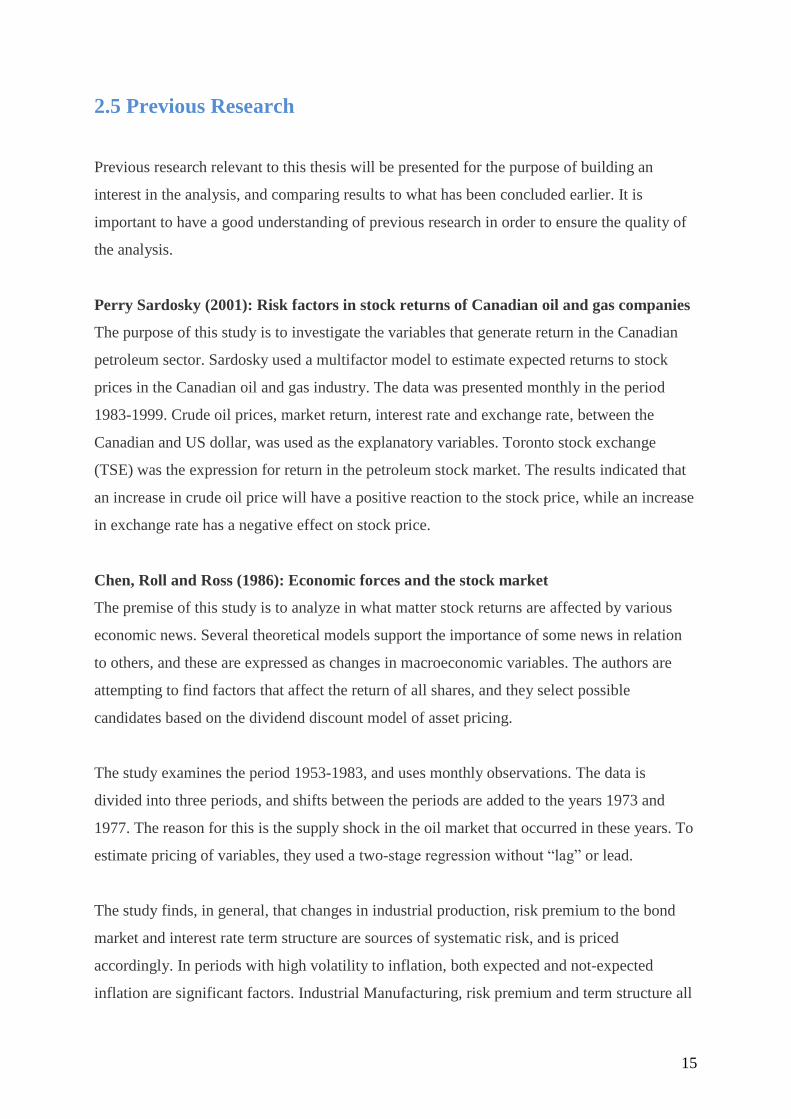
2.5 Previous Research

Previous research relevant to this thesis will be presented for the purpose of building an

interest in the analysis, and comparing results to what has been concluded earlier. It is

important to have a good understanding of previous research in order to ensure the quality of

the analysis.

Perry Sardosky (2001): Risk factors in stock returns of Canadian oil and gas companies

The purpose of this study is to investigate the variables that generate return in the Canadian

petroleum sector. Sardosky used a multifactor model to estimate expected returns to stock

prices in the Canadian oil and gas industry. The data was presented monthly in the period

1983-1999. Crude oil prices, market return, interest rate and exchange rate, between the

Canadian and US dollar, was used as the explanatory variables. Toronto stock exchange

(TSE) was the expression for return in the petroleum stock market. The results indicated that

an increase in crude oil price will have a positive reaction to the stock price, while an increase

in exchange rate has a negative effect on stock price.

Chen, Roll and Ross (1986): Economic forces and the stock market

The premise of this study is to analyze in what matter stock returns are affected by various

economic news. Several theoretical models support the importance of some news in relation

to others, and these are expressed as changes in macroeconomic variables. The authors are

attempting to find factors that affect the return of all shares, and they select possible

candidates based on the dividend discount model of asset pricing.

The study examines the period 1953-1983, and uses monthly observations. The data is

divided into three periods, and shifts between the periods are added to the years 1973 and

1977. The reason for this is the supply shock in the oil market that occurred in these years. To

estimate pricing of variables, they used a two-stage regression without “lag” or lead.

The study finds, in general, that changes in industrial production, risk premium to the bond

market and interest rate term structure are sources of systematic risk, and is priced

accordingly. In periods with high volatility to inflation, both expected and not-expected

inflation are significant factors. Industrial Manufacturing, risk premium and term structure all

16

had positive coefficients to the stock return, while the inflation variables had negative

coefficients

The authors found that the variables for market return, consumption or oil prices were not

significantly priced in some of the periods. Further, the analytic results were consistent in the

three different periods, although the last period, 1978-1983, gave lower absolute values on the

coefficients.

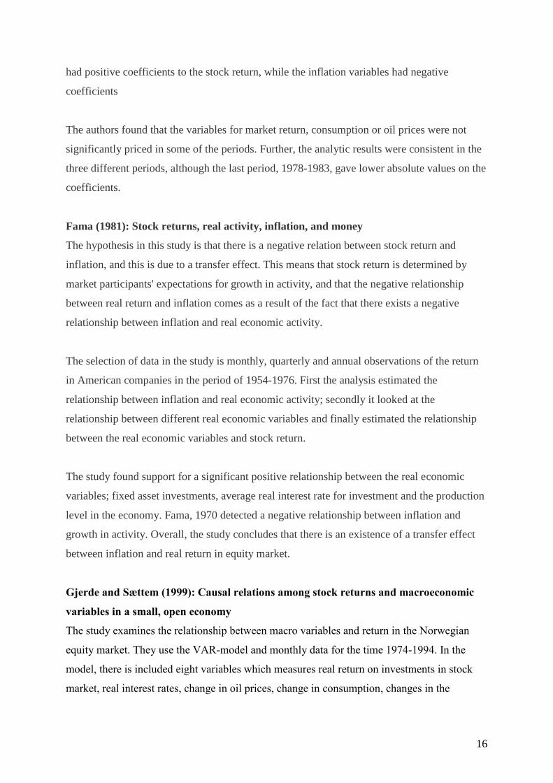
Fama (1981): Stock returns, real activity, inflation, and money

The hypothesis in this study is that there is a negative relation between stock return and

inflation, and this is due to a transfer effect. This means that stock return is determined by

market participants' expectations for growth in activity, and that the negative relationship

between real return and inflation comes as a result of the fact that there exists a negative

relationship between inflation and real economic activity.

The selection of data in the study is monthly, quarterly and annual observations of the return

in American companies in the period of 1954-1976. First the analysis estimated the

relationship between inflation and real economic activity; secondly it looked at the

relationship between different real economic variables and finally estimated the relationship

between the real economic variables and stock return.

The study found support for a significant positive relationship between the real economic

variables; fixed asset investments, average real interest rate for investment and the production

level in the economy. Fama, 1970 detected a negative relationship between inflation and

growth in activity. Overall, the study concludes that there is an existence of a transfer effect

between inflation and real return in equity market.

Gjerde and Sættem (1999): Causal relations among stock returns and macroeconomic

variables in a small, open economy

The study examines the relationship between macro variables and return in the Norwegian

equity market. They use the VAR-model and monthly data for the time 1974-1994. In the

model, there is included eight variables which measures real return on investments in stock

market, real interest rates, change in oil prices, change in consumption, changes in the

17

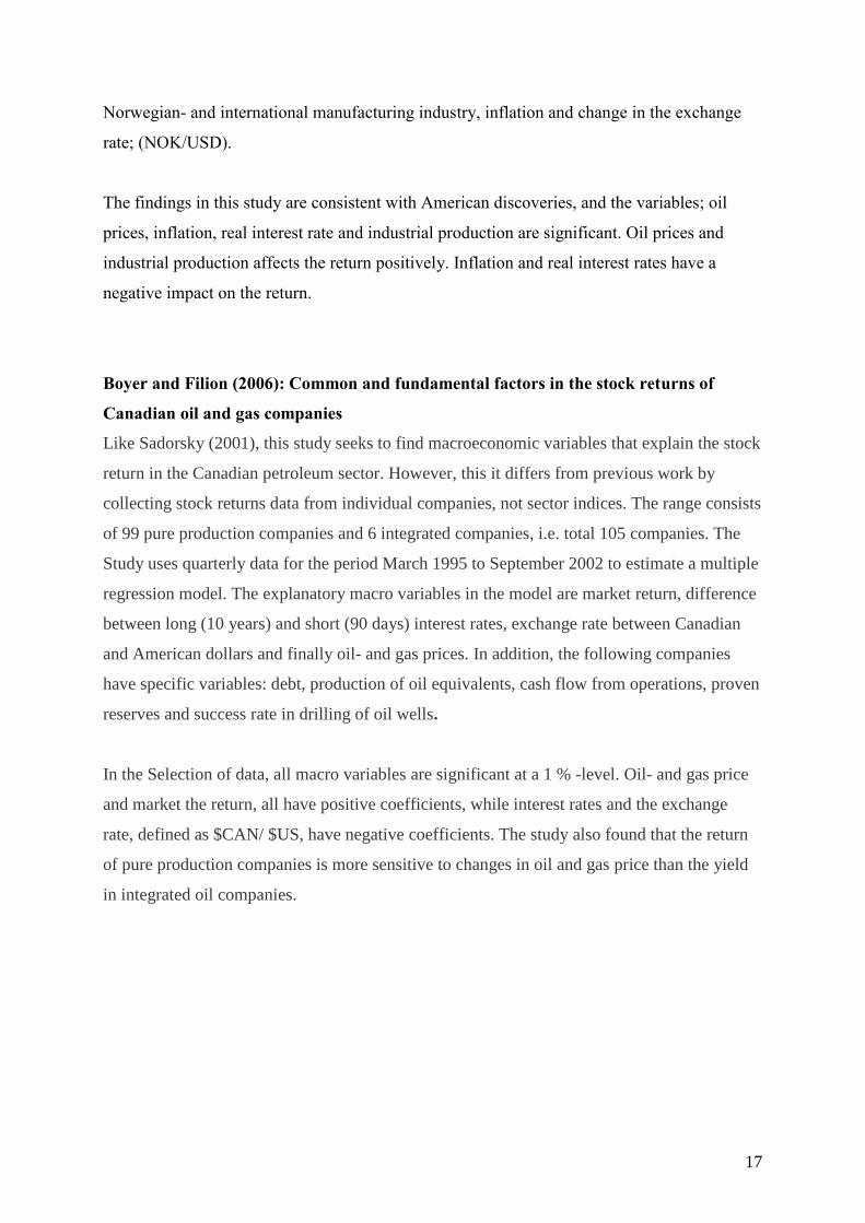
Norwegian- and international manufacturing industry, inflation and change in the exchange

rate; (NOK/USD).

The findings in this study are consistent with American discoveries, and the variables; oil

prices, inflation, real interest rate and industrial production are significant. Oil prices and

industrial production affects the return positively. Inflation and real interest rates have a

negative impact on the return.

Boyer and Filion (2006): Common and fundamental factors in the stock returns of

Canadian oil and gas companies

Like Sadorsky (2001), this study seeks to find macroeconomic variables that explain the stock

return in the Canadian petroleum sector. However, this it differs from previous work by

collecting stock returns data from individual companies, not sector indices. The range consists

of 99 pure production companies and 6 integrated companies, i.e. total 105 companies. The

Study uses quarterly data for the period March 1995 to September 2002 to estimate a multiple

regression model. The explanatory macro variables in the model are market return, difference

between long (10 years) and short (90 days) interest rates, exchange rate between Canadian

and American dollars and finally oil- and gas prices. In addition, the following companies

have specific variables: debt, production of oil equivalents, cash flow from operations, proven

reserves and success rate in drilling of oil wells.

In the Selection of data, all macro variables are significant at a 1 % -level. Oil- and gas price

and market the return, all have positive coefficients, while interest rates and the exchange

rate, defined as $CAN/ $US, have negative coefficients. The study also found that the return

of pure production companies is more sensitive to changes in oil and gas price than the yield

in integrated oil companies.

18

3. The Petroleum Industry and Statoil ASA

In this chapter, fundamental theory relevant to the thesis will be presented. First to be

addressed is the oil and gas industry. Further, the relationship between global supply- and

demand. Thereafter the crude oil market- and price development will be carefully explained,

before Statoil and their investment strategy, will be presented a long with the company´s

current situation.

3.1 Petroleum Industry

The Petroleum industry is exposed to high investments as well as high uncertainties. Projects

in this sector tend to involve long time horizons, as well as heavy investment and negative

cash flows in early phases. Positive cash flows usually first occur after the development of the

projects is finalized, and production is initiated. This structure makes oil and gas companies

exposed to the risk of changes in market conditions. Even though the market conditions are

good in the initial phase, they can easily change before the production phase of the project.

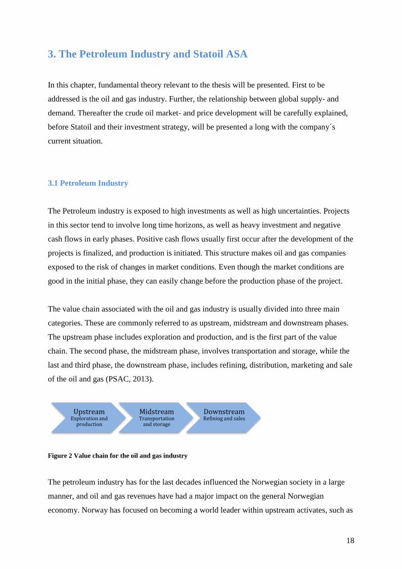
The value chain associated with the oil and gas industry is usually divided into three main

categories. These are commonly referred to as upstream, midstream and downstream phases.

The upstream phase includes exploration and production, and is the first part of the value

chain. The second phase, the midstream phase, involves transportation and storage, while the

last and third phase, the downstream phase, includes refining, distribution, marketing and sale

of the oil and gas (PSAC, 2013).

Figure 2 Value chain for the oil and gas industry

The petroleum industry has for the last decades influenced the Norwegian society in a large

manner, and oil and gas revenues have had a major impact on the general Norwegian

economy. Norway has focused on becoming a world leader within upstream activates, such as

UpstreamExploration and

production

MidstreamTransportation

and storage

DownstreamRefining and sales

19

exploration and production, particularly at harsh seas. Downstream activities are not equally

focused on, and Norway only has two large oil refineries (EIA, 2012). As a comparison,

Russia, which covers the whole value chain, has as much as 40 refineries (EIA, 2014).

The planning process within the petroleum industry can be divided into three main stages,

referred to as strategic-, tactical and operational planning (Fleischmann et al. 2004). Strategic

planning involves long-term decision-making, such as investment in new fields, projects,

equipment or technology. Tactical planning contains allocation of resources, determination of

production outlines and aggregated production level relative to customer demand. Both of

these planning stages are expected to have relatively long-term planning horizons (Gunnerud,

2011). The third planning process is the operational, which involves short-term planning. In

this phase, decision makers strive to minimize production costs or maximizing oil production

rates (Wang, 2003). This thesis mainly aims to study planning on a strategic level, where

long-term investment decisions are made.

3.1.1 Crude Oil Demand

The demand of crude oil increases with growth in both population and economy, and

decreases with a decline in the economic growth rate. Another demand factor is dependent on

whether the country is an exporter or importer of crude oil, and is determined by exchange

rate. In countries that import oil, demand will have a positive correlation with economic

growth. In oil exporting countries on the other hand, economic growth will occur as a result of

rise in demand. If oil prices alleviate at a high level, the GDP in importing countries, might

decline. This will lead to a decline in demand and prices of crude oil (Hamilton, 2009). When

prices rise because of a high demand, there will also be an advanced circulation of money in

the oil sector, followed by additional oil exploration and more supply of crude oil. This

eventually causes the price of oil to flatten out as a reaction to restore the relationship between

supply and demand. In his research paper from 2009, Hamilton concluded that in the short-

run, demand for crude oil is determined by income rather than price, which means that there is

a correlation between GDP and consumption of oil, no matter the price of crude oil.

In their research approaching emerging versus industrialized economies, Aastveit, Bjørnland

and Thorsrud (2012), established that demand shock in emerging economies, with particular

20

emphasis on Asia and China, are significantly more important than demand shock from

industrialized countries. They also concluded that the total demand shock from emerging and

industrialized economies yields up to 60% of random fluctuations in the real price of oil in the

last 20 years.

Traditionally, in markets where oil refineries demand crude oil, they also determine the oil

price. The price has then been settled by the margins and demand for the oil refineries end

product. During the last few years, trading of oil futures has exponentially increased because

more and more financial actors want to be directly exposed to oil speculations. Trading in the

securities market gives actors an opportunity to profit from price changes in the oil market,

creating a demand pressure and contributing to more volatile oil prices (OED, 2011).

3.1.2 Crude Oil Supply

Whether or not the world’s oil resources are sufficient to meet the increased demand for oil in

the future is difficult to predict. It is impossible to estimate precisely the amount of resources

remaining, and to which extent these resources are technically and economically possible to

recover. The amount of available financial resources will play a vital role in the future of the

oil industry. Hence, why high oil prices are important. OPEC (Organization of Petroleum

Exporting to Countries) has historically had a sizeable share of the production in the oil

market. Large, often state-owned companies manage the petroleum activities in these

countries, with a primarily focuses on upstream activities. Their goal as an alliance is to

administrate the oil supplied in the world market. To avoid rapid fluctuations, which can

affect economy in both exporting and importing countries, the OPEC countries attempt to

price the crude oil based on their power in the market (EIA, 2014).

OPEC still has a very strong position in the market, and is currently delivering approximately

40% of the world’s total oil production (BP, 2014). At the same time, two thirds of the worlds

remaining oil resources is assumed to be allocated within the organization’s member states

(OED, 2011). This future resource provides the foundation for a significant increase in

production, way beyond the current level, and represents OPECs excess capacity. Further, this

will give them an even greater opportunity to affect the oil market through price and volume

regulations. Historically, this rich natural resource has not been a guarantee of stable growth

21

for OPEC, when several of the nations have been characterized by political instability (OED,

2011).

In non-OPEC countries, considerable parts of the oil production take place in large private,

multinational companies with origins in industrialized countries. OPEC on the other hand, has

for most part operated within large state-owned oil companies. Both Russia and Norway are

experiencing an even stronger government involvement than in many other western oil-

producing countries. The petroleum industry in Russia was rebuilt through private national

companies, after the dissolution of the Soviet Union in 1991, but in the past few years,

increasingly larger holdings have been added under state control. The worlds largest non-

OPEC oil company is a Russian state-owned company, Gazprom, while the second-largest

owner of oil reserves and manufacturer are privately owned Lukoil (EIA, 2013). Through its

large ownership in Statoil, the Norwegian government owns 67% of the company´s shares.

The petroleum industry has experienced a significant inflation of costs, which includes

increasing costs of both exploration and development. This inflation has made a substantial

impact on the development of crude oil prices, and will most likely continue to do so in the

years to come. In the course of the last 5-10 years, costs associated with the production of oil

have almost doubled, and still continues to rise. Two of the reasons are the major challenges

associated with recovery of the remaining resources in cumulative challenging areas both on

land and at sea, combined with increasing prices of other input factors such as skilled labor

(OED, 2011).

OPEC is currently not willing to reduce their production of oil, even though the demand for

crude oil declined in fall of 2014. (Statoil’s annual report, 2014)

3.1.3 Crude oil market development

Through the 1900s, dominant actors have characterized the oil market. Until the end of the

1950s, there were seven large, multinational oil companies called the seven-sisters1. These

companies had an overall market power by regulating oil reserves, exploration and

productions, as well as transportation and marketing. The seven-sisters controlled most

branches in the oil supply chain. In addition to this, they had co-ownership of companies in

22

different countries of the world to be able to surveillance the amount and price of the crude oil

supplied globally (Mabro, 2006).

At this time, OPEC (The organization of the Petroleum Exporting to Countries) was too frail

to change the seven-sisters´ market control. The OPEC countries did not cooperate nor had

they a noteworthy proportion of supply quotations in the market. In the end of the 1950s,

many of the OPEC countries gained access to new crude oil areas, which resulted in a

growing crude oil supply- and demand outside of the seven sisters control. When the global

demand for crude oil noticeably increased from 1970-1973, it was mainly OPEC who could

produce at this scale. And at the beginning of the 1970s, OPEC had been given a predominant

role in the oil market. In the fall of 1970, the OPEC countries officially united, which gave

them a considerable power as well as a resilient bargaining position. For example, certain

members decided to reduce supply of oil in the fall of 1973. This was in association with the

war between the Arab countries and Israel, which lasted from 1973 to 1974 and led to a global

oil price shock. The Organization for Arabic Petroleum exporting countries (OAPEC), except

Iran, reduced supply by 5% from September 1973, and announced that this would continue

each month until Israeli forces were pulled out of Arab territory (Mabro 2006).

In the course of 1973, oil prices increased dramatically. OPECs export prices, represented by

Arabian Light crude, increased from a level at $3.65 in the beginning of October 1973 to

$11.651 in December 1973. This illustrates that OPEC had an important role in the price

development (Mabro 2006).

3.1.4 Oil price development

In the 1980s, OPEC had monopoly in the crude oil market, and therefore had the opportunity

to set the price of oil as they pleased. Today, the market develops a reference price in which

the price will be set according to. The relationship between the reference price and local price

is determined by a given function. In 1988, this was the primary method for determining the

price of crude oil, and has been ever since. However, the crude oil market developed to be

1 The Seven-Sisters is a tern used to describe Anglo-Persian Oil Company (now BP), Gulf Oil, Standard Oil of California, Texaco, Royal

Dutch Shell, Standard Oil of New Jersey and Standard Oil Company of New York.

23

relatively complex subsequently to the introduction of the system. There is also trading of for

example futures contracts, options, swap and spot contracts based on speculations in the

pricing system (Mabro 2006). When unforeseen events affecting the crude oil price occur,

they often impact the supply-side of the marked. As the production of oil decreases, it leads to

an upswing in the crude oil prices.

Following 9/11, the global economy experienced a situation of uncertainty, portrayed by fear

of unrest, problems within supply and low growth, which led to a decrease in the price of oil.

In December 2002 Venezuelan rebels protested against president Hugo Chavez, something

that affected the industry and manufacturing in the country. As these events occurred almost

simultaneously with the US invasion of Iraq 2003, it resulted in an increase in oil prices due

to the uncertainty associated with procurement. Because the Iraq war was short-lived, prices

quickly settled at the level previous to 9/11 (Hamilton, 2011).

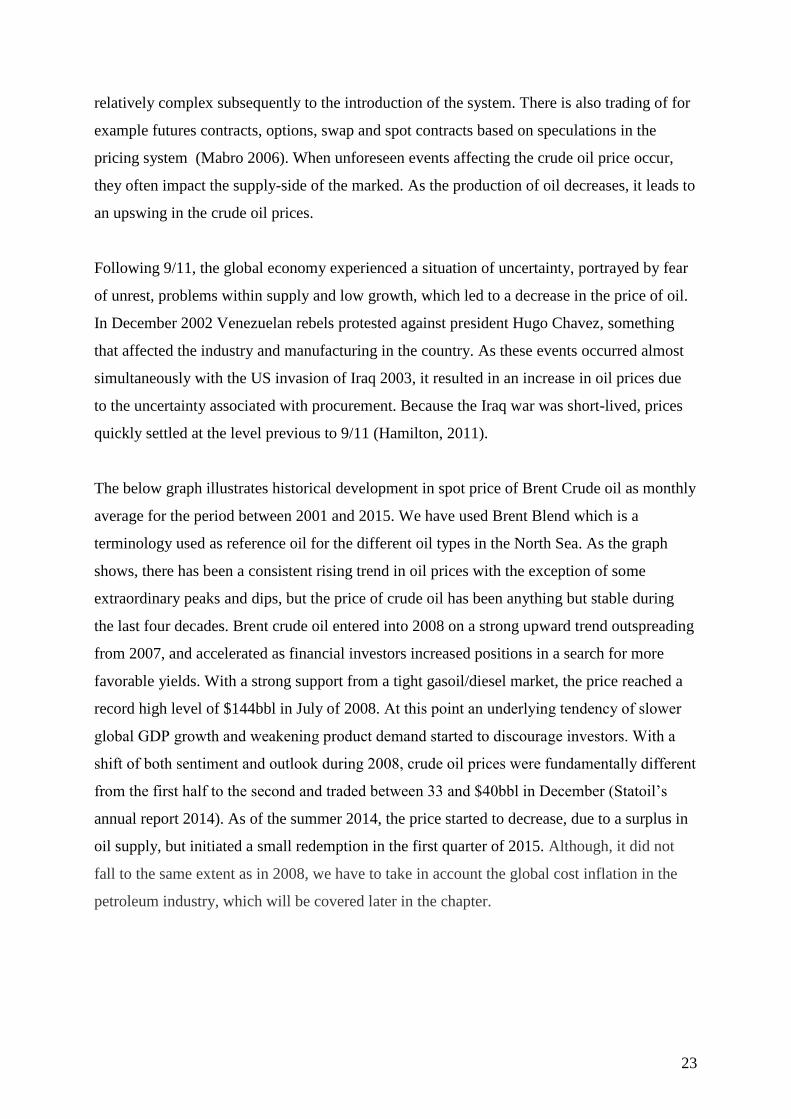
The below graph illustrates historical development in spot price of Brent Crude oil as monthly

average for the period between 2001 and 2015. We have used Brent Blend which is a

terminology used as reference oil for the different oil types in the North Sea. As the graph

shows, there has been a consistent rising trend in oil prices with the exception of some

extraordinary peaks and dips, but the price of crude oil has been anything but stable during

the last four decades. Brent crude oil entered into 2008 on a strong upward trend outspreading

from 2007, and accelerated as financial investors increased positions in a search for more

favorable yields. With a strong support from a tight gasoil/diesel market, the price reached a

record high level of $144bbl in July of 2008. At this point an underlying tendency of slower

global GDP growth and weakening product demand started to discourage investors. With a

shift of both sentiment and outlook during 2008, crude oil prices were fundamentally different

from the first half to the second and traded between 33 and $40bbl in December (Statoil’s

annual report 2014). As of the summer 2014, the price started to decrease, due to a surplus in

oil supply, but initiated a small redemption in the first quarter of 2015. Although, it did not

fall to the same extent as in 2008, we have to take in account the global cost inflation in the

petroleum industry, which will be covered later in the chapter.

24

Figure 3 denotes Brent Crude Oil Price measured in US dollar. The data are monthly range from June

2001 to March 2015.

3.1.4.1 Long-term price development

In the long-term, there are other aspects that have a large influence on price development in

the oil market. The demand curve is influenced by macroeconomic variables such as

development of the GDP, currency rates, interest rates and employment. As oil is traded in

American dollars (USD) on the international market, a country who´s exchange rate has

depreciated against the US dollar, experience oil to be more expensive and can lead to a

reduction in demand, if this persists over time.

With an expansion of supply in the oil market, oil prices will theoretically fall and become

less volatile than if amount of oil offered is uncertain. Vice versa, but opposite, is the case for

oil demand. With an increase in demand, customers will desire and demand larger amounts of

oil, which will thrust the price of upwards. Traditionally, the world’s leading consumers of oil

have been North America and the western countries, but after the recession caused by the

financial crisis, consumption in these countries dropped. However, the falling demand in the

west has been outweighed by the major emerging economies such as the BRICS2 countries

(OED, 2011).

2 The BRICS-countries involves Brazil, Russia, India, China and South-Africa

0

20

40

60

80

100

120

140

160

25

3.1.4.2 Short-term price developments

Price Elasticity is a measure of how responsive an economic variable is for change in price. It

is defined as the percentage change in quantity as a result of a one per cent change in price.

Both supply and demand can be elastic with respect to price, but in the short-term demand for

oil has, as earlier mentioned, very little price elasticity (IMF, 2011). Oil refined products are

necessary goods which households and companies are dependent on in everyday life. It is

characterized by that when there is an increase in income, there is not an equally high increase

in consumption. A necessary good is defined by lower price elasticity when the necessity of

the good is large (Nechyba, 2011). In the current situation, oil is essential in the global and

local transportation, agriculture, energy and production of plastic. There is yet to be a

competitive source of energy or substitute that can be applied in the same scale as oil.

3.1.5 The Peak Oil Theory

The peak oil theory involves the concept of oil as an exhaustible resource, which means that

at some point in the future crude oil will run out. As (Mabro, 2006, page 1) defines it “ The

peak story tells us, indeed, that after rising over years, decades or centuries, production will

enter a phase of decline.” Historically, authors and promoters of this theory, has claimed on

several occasions that the time of the peak (before decline) has been reached, but world oil

production is still rising. However, it is of great importance to have a prediction about the

volume in the remaining oil reserves. BP, 2014 has estimated the proven oil reserves in the

world to be 1687 billion barrels, which is sufficient to meet 53,3 years of global production.

Where OPEC holds the majority of the estimated reserves at 71,9%. This is also one of the

reasons why OPEC can be predicted to have market dominance in the future.

Mabro, 2006 however, is critical to this estimation, and has four reasons in which it does not

hold; When proven reserves is estimated, they are only required to be recoverable under

current operational and economic conditions. Secondly, they are estimated from reserves

where the companies have to negotiate agreements for production with a host country.

Thirdly, some countries have very strict criteria in terms of what they can report to the

authorities as a proven reserve, something that would make the result underestimated. And

finally, remaining recoverable reserves are the relevant expression for determining peak oil

26

production and ultimate exhaustion, not proven reserves (Mabro, 2006). Mabro, 2006 agrees

that peak oil theorists are right about the fact that there has been a significant decline in oil

discoveries since 1961, and that there are not enough discoveries to replace the full amount of

oil produced in the long run.

3.2 Statoil ASA

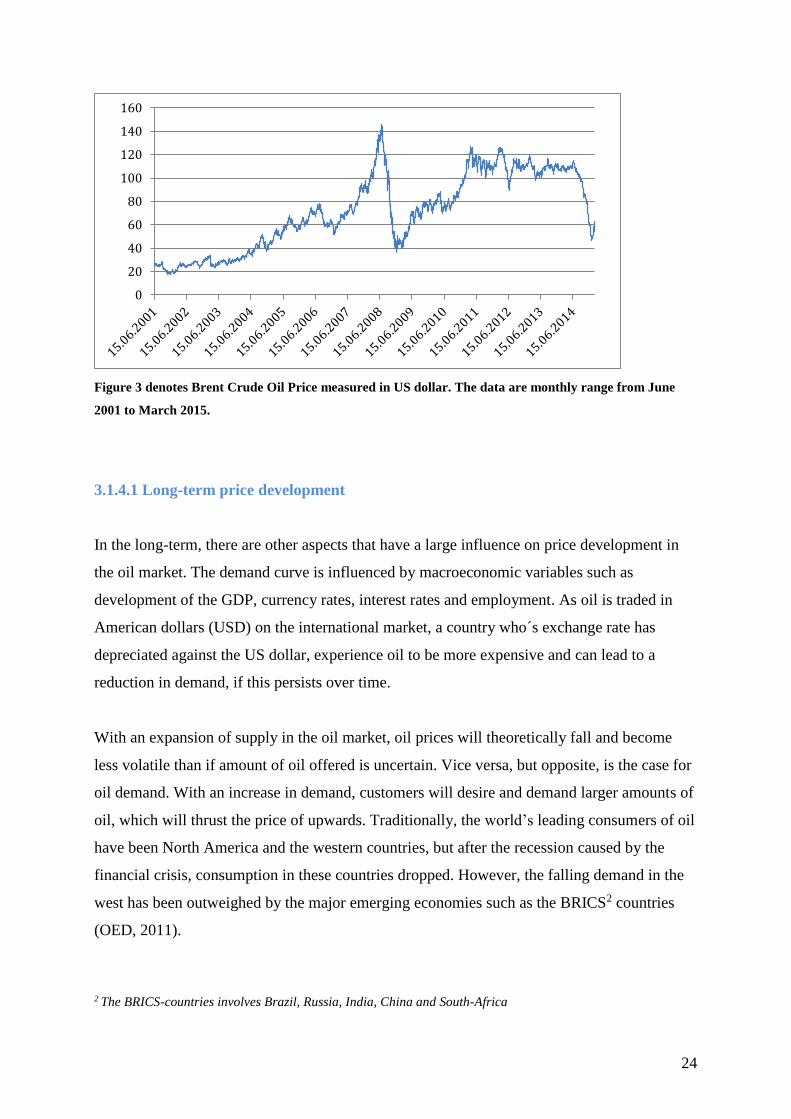
Statoil´s largest shareholder is, as earlier mentioned, the Norwegian government who owns

67% of the company´s stock. The below chart illustrates that as much as 75% of Statoil´s

ownership remains within Norway, were Statoil also has its main office. The largest foreign

investors are the United Kingdom and USA, which combined owns 14% of the shares. Statoil

is without a doubt the largest operator on the Norwegian continental shelf, as the company is

responsible for 70% of the production (Snl, 2015). The company also operates internationally,

and is actively present in approximately 30 other countries around the world (EIA, 2012).

Figure 4 represents a map of Statoil’s shareholders. Source: Statoil’s annual report, 2014.

Below, the historical development of Statoil´s stock price from year 2001 to 2015 is

illustrated. When comparing the company´s stock price to the price of crude oil, one can see

there was a large increase in the price in the course of 2007, followed by a huge drop at the

end of 2008. After the financial crisis there are only small fluctuations in the stock return,

until the end of 2014, where the price again fell.

0

0,1

0,2

0,3

0,4

0,5

0,6

0,7

0,8

Distribution of shareholders at year end 2014

27

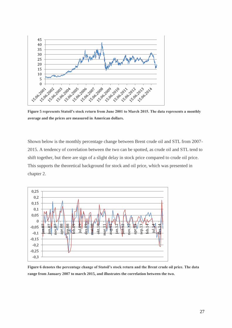
Figure 5 represents Statoil’s stock return from June 2001 to March 2015. The data represents a monthly

average and the prices are measured in American dollars.

Shown below is the monthly percentage change between Brent crude oil and STL from 2007-

2015. A tendency of correlation between the two can be spotted, as crude oil and STL tend to

shift together, but there are sign of a slight delay in stock price compared to crude oil price.

This supports the theoretical background for stock and oil price, which was presented in

chapter 2.

Figure 6 denotes the percentage change of Statoil’s stock return and the Brent crude oil price. The data

range from January 2007 to march 2015, and illustrates the correlation between the two.

0

5

10

15

20

25

30

35

40

45

-0,3

-0,25

-0,2

-0,15

-0,1

-0,05

0

0,05

0,1

0,15

0,2

0,25

jan

.07

jun

.07

no

v.0

7

apr.

08

sep

.08

feb

.09

jul.0

9

des

.09

mai

.10

ok

t.1

0

mar

.11

aug.

11

jan

.12

jun

.12

no

v.1

2

apr.

13

sep

.13

feb

.14

jul.1

4

des

.14

28

3.2.2 Investment Strategy

Statoil’s overall strategy in 2015 is to create value and long-term growth. In the year of 2014,

they experienced challenges involving profitability, which is still applicable in 2015 even

though the oil price has had a small increase in the course of this year. Statoil is proceeding

with stricter project prioritization, which will improve cash flows and profitability. Further,

they are looking into utilizing oil and gas expertise and technology to open new renewable

energy opportunities, which can help the company sustain in times where oil is not profitable

or when it eventually run out (Statoil’s annual report, 2014).

From their annual report in 2008, Statoil stated that over time, energy demand is expected to

pick up and energy prices are expected to increase. A far more positive outlook than Statoil’s

current prediction; in their annual report from 2014, Statoil predicts that oil prices are

acquiring a higher volatility and a more uncertain future.

3.2.3 Present situation

The OPEC meeting held on 27 November 2014 got a lot of attention. The decision not to cut

OPEC production made the prices drop, and they ended on a 5 year low of $54,98bbl in the

end of December.

The growth in US shale oil production came as a surprise to the market in 2014. During the

third quarter of 2014, it became clear that there was a growing supply of oil. The paper

market of crude oil experienced that investors were leaving in an attempt secure profit, and

the pressure then transmitted to the physical market Refinery maintenance in most regions of

the world conceded in the same quarter, reducing demand for oil. Europe still had a slow

growth rate from the financial crisis, and some were close to a recession. In order to stabilize

the price, oil producing and exporting countries were looking to OPEC to cut their production,

but OPEC upheld their current production and prices continued to fall. This was a change of

30-year-old price regime that let the market set the price of crude oil, and may lead to greater

volatility in the future (Statoil’s annual report, 2014).

29

The oil sectors, both internationally and in Norway, are using a lot of resources to increase

profitability. The oil price has been rising steadily during the past few years, and costs in the

oil industry are at a very high level. When internal costs and expensive projects now must be

supported by an oil price that has settled on a much lower level, it creates pressure in the

general ledger. Statoil is one of the companies to have introduced a number of new measures

to conserve and improve resources. It has already been deflected in layoffs and cuts for both

Statoil and its suppliers.

In 2015, Statoil decided to develop for a value of approximately 175 billion on the Norwegian

continental shelf, which means that Statoil's investments in the Stavanger region are expected

to remain close to the same level as in 2013. Johan Sverdrup is Statoil´s largest investment

projects the next few years, and the first phase of development between 215 and 2019, is

expected to cost 120 billion (Statoil. com, 2015). Johan Sverdrup is an oilfield in the North

Sea and was located in 2010. It is the fifth largest discovery in the Norwegian history. The

reserve was found in a mature area in the North Sea, and it most likely consists of 95%

recoverable oil. The field has an estimated break-even price of 40-50 dollars per barrel, which

can be considered a sustainable cost, and most likely a good investment for the uncertain

times ahead (statoil.com, 2015).

The annual reports from 2013, shows that operational income was 155.5 billion, which is a set

back of 25% compared to 2012. Due to reduced production, lower prices measured in

Norwegian kroner (NOK), higher operating costs and lower real value on derivatives. Statoil

stated already in 2013 that the industry was facing future challenges in demand, something

that indicates that Statoil was prepared for the recession the following year. In 2014, operating

income declined even further to 109,5 billion, because of lower prices, impairment losses and

exploration cost (Statoil’s annual report, 2014).

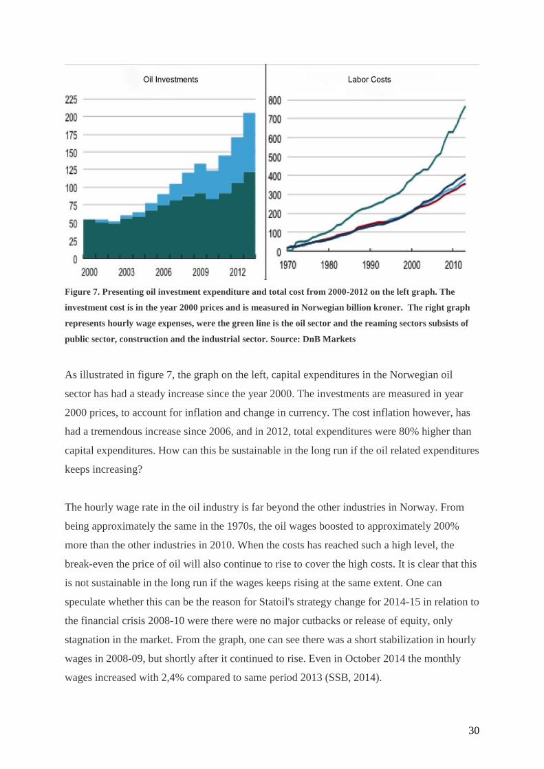
30

Figure 7. Presenting oil investment expenditure and total cost from 2000-2012 on the left graph. The

investment cost is in the year 2000 prices and is measured in Norwegian billion kroner. The right graph

represents hourly wage expenses, were the green line is the oil sector and the reaming sectors subsists of

public sector, construction and the industrial sector. Source: DnB Markets

As illustrated in figure 7, the graph on the left, capital expenditures in the Norwegian oil

sector has had a steady increase since the year 2000. The investments are measured in year

2000 prices, to account for inflation and change in currency. The cost inflation however, has

had a tremendous increase since 2006, and in 2012, total expenditures were 80% higher than

capital expenditures. How can this be sustainable in the long run if the oil related expenditures

keeps increasing?

The hourly wage rate in the oil industry is far beyond the other industries in Norway. From

being approximately the same in the 1970s, the oil wages boosted to approximately 200%

more than the other industries in 2010. When the costs has reached such a high level, the

break-even the price of oil will also continue to rise to cover the high costs. It is clear that this

is not sustainable in the long run if the wages keeps rising at the same extent. One can

speculate whether this can be the reason for Statoil's strategy change for 2014-15 in relation to

the financial crisis 2008-10 were there were no major cutbacks or release of equity, only

stagnation in the market. From the graph, one can see there was a short stabilization in hourly

wages in 2008-09, but shortly after it continued to rise. Even in October 2014 the monthly

wages increased with 2,4% compared to same period 2013 (SSB, 2014).

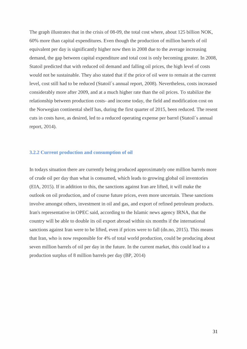
31

The graph illustrates that in the crisis of 08-09, the total cost where, about 125 billion NOK,

60% more than capital expenditures. Even though the production of million barrels of oil

equivalent per day is significantly higher now then in 2008 due to the average increasing

demand, the gap between capital expenditure and total cost is only becoming greater. In 2008,

Statoil predicted that with reduced oil demand and falling oil prices, the high level of costs

would not be sustainable. They also stated that if the price of oil were to remain at the current

level, cost still had to be reduced (Statoil´s annual report, 2008). Nevertheless, costs increased

considerably more after 2009, and at a much higher rate than the oil prices. To stabilize the

relationship between production costs- and income today, the field and modification cost on

the Norwegian continental shelf has, during the first quarter of 2015, been reduced. The resent

cuts in costs have, as desired, led to a reduced operating expense per barrel (Statoil´s annual

report, 2014).

3.2.2 Current production and consumption of oil

In todays situation there are currently being produced approximately one million barrels more

of crude oil per day than what is consumed, which leads to growing global oil inventories

(EIA, 2015). If in addition to this, the sanctions against Iran are lifted, it will make the

outlook on oil production, and of course future prices, even more uncertain. These sanctions

involve amongst others, investment in oil and gas, and export of refined petroleum products.

Iran's representative in OPEC said, according to the Islamic news agency IRNA, that the

country will be able to double its oil export abroad within six months if the international

sanctions against Iran were to be lifted, even if prices were to fall (dn.no, 2015). This means

that Iran, who is now responsible for 4% of total world production, could be producing about

seven million barrels of oil per day in the future. In the current market, this could lead to a

production surplus of 8 million barrels per day (BP, 2014)

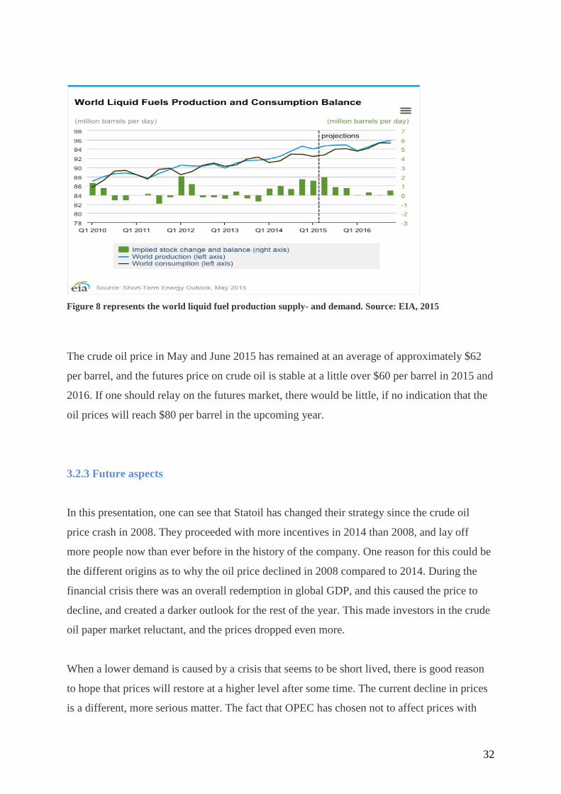
32

Figure 8 represents the world liquid fuel production supply- and demand. Source: EIA, 2015

The crude oil price in May and June 2015 has remained at an average of approximately $62

per barrel, and the futures price on crude oil is stable at a little over $60 per barrel in 2015 and

2016. If one should relay on the futures market, there would be little, if no indication that the

oil prices will reach $80 per barrel in the upcoming year.

3.2.3 Future aspects

In this presentation, one can see that Statoil has changed their strategy since the crude oil

price crash in 2008. They proceeded with more incentives in 2014 than 2008, and lay off

more people now than ever before in the history of the company. One reason for this could be

the different origins as to why the oil price declined in 2008 compared to 2014. During the

financial crisis there was an overall redemption in global GDP, and this caused the price to

decline, and created a darker outlook for the rest of the year. This made investors in the crude

oil paper market reluctant, and the prices dropped even more.

When a lower demand is caused by a crisis that seems to be short lived, there is good reason

to hope that prices will restore at a higher level after some time. The current decline in prices

is a different, more serious matter. The fact that OPEC has chosen not to affect prices with

33

their supply means there will be a change in the dynamics of future crude oil prices, which

also will be hard to predict. According to Bloomberg business, the energy analysts are more

divided in their outlook now than at any time in the last eight years (Bloomberg, 2015). As

mentioned earlier, OPEC´s mission has been to administrate supply to control oil price

fluctuations in the market. Is there a reason for this sudden change of strategy? One can

speculate that their purpose is to bankrupt companies who have a higher marginal cost, and

therefore cannot sustain the same break-even prices as OPEC. At this point, their decision

yields a much lower return for a large amount companies in the petroleum industry. If OPEC

had cut supply in November 2015, prices would probably have restored to their previous level

before the decline in the summer of 2014.

From Statoil’s annual reports, it is interesting to see that development costs is not decreasing,

simultaneously with a decline in operational income in both 2013 and 2014. This can be

speculated as evidence of a growing investment level that hopefully will lead to a positive

cash flow in the future, but it also means that Statoil is experiencing a higher risk, given the

fact that the development investments from 2014 were implemented before the crude oil price

dropped.

The information and strategic measures from this chapter, places the background for the

fundament and theory behind the econometric analysis in chapter 4.

34

4. Econometric Analysis

Econometrics involves summarizing relevant information by using analytical models (Heij, de

Boer, Franses, Kloek & van Dijk, 2004). Statistical methods can be developed to estimate

economic relationships, test economic theories and evaluate business policies. Econometric

models have been developed to investigate the relationship between the variables in question.

In this chapter, the models and their components will be explained and discussed, and

possible challenges in their implantation will be carefully examined and considered.

4.1 Data

The data used in this thesis has been collected primarily from Bloomberg. Relevant

information not obtainable from this source has been manually collected from Statoil´s annual

reports. To account for interest, data for NIBOR has been collected from the Norwegian

Central Banks statistics. Capital Expenditures (CAPEX) have been selected as the best-fit unit

for measure of Statoil´s investment level. To obtain CAPEX, data has been gathered from

Statoil´s consolidated statement of cash flows. These data include (1) additions to property,

plant and equipment (PPE), (2) capitalized interest paid, and (3) Exploration expenditures

capitalized and additions to other intangibles.

Because the purpose of this thesis is to measure general economic relationships between oil

price fluctuations, Statoil´s level of investment and the stock price, quarterly data has been

used in implementation of the analysis. Compared to daily data, these contain significantly

less noise. To avoid autocorrelation, all observation has been transformed into their

logarithmic form. As well as avoiding autocorrelation, this transformation will simplify the

estimation of the coefficients in the model, as observations will be measured in the same

proportion. Consequently, coefficients can be interpreted as the percentage change in the

explained variable, by a 1% change in the explanatory variables. All data has been processed

in Excel, and the regression analysis has been developed using the statistics software SPSS.

Data used has been collected from the period from 2001 to 2015.

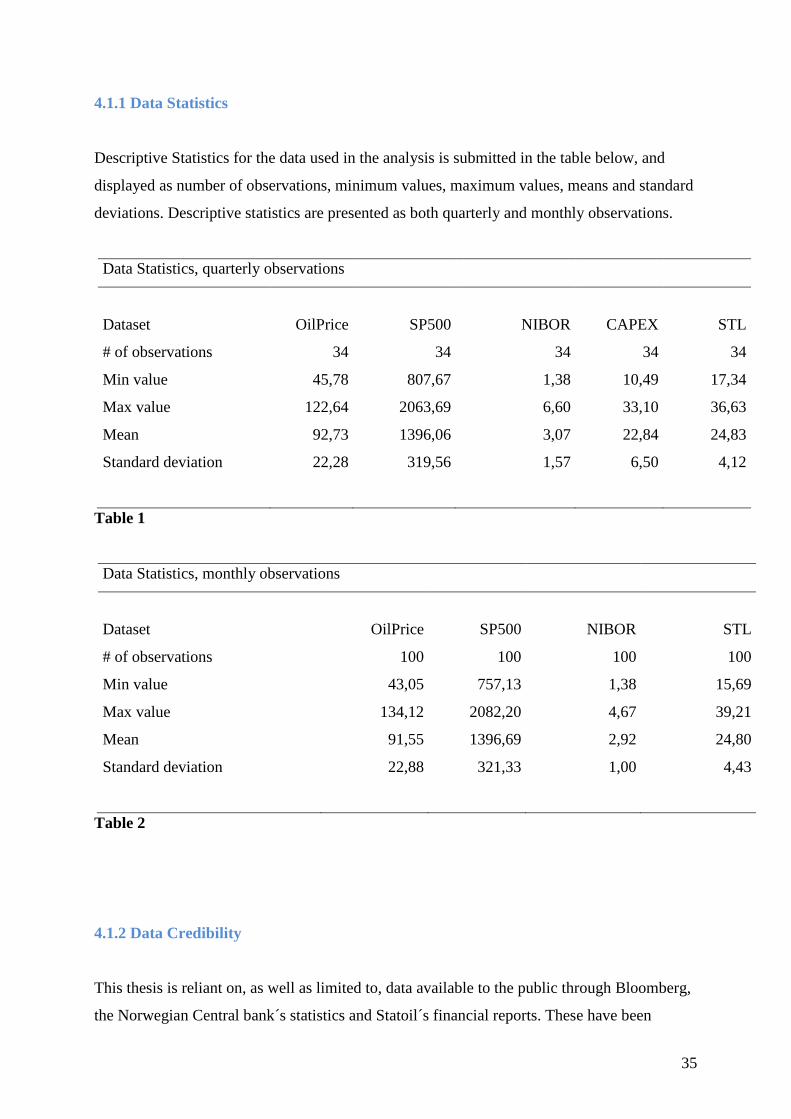
35

4.1.1 Data Statistics

Descriptive Statistics for the data used in the analysis is submitted in the table below, and

displayed as number of observations, minimum values, maximum values, means and standard

deviations. Descriptive statistics are presented as both quarterly and monthly observations.

Data Statistics, quarterly observations

Dataset OilPrice SP500 NIBOR CAPEX STL

# of observations 34 34 34 34 34

Min value 45,78 807,67 1,38 10,49 17,34

Max value 122,64 2063,69 6,60 33,10 36,63

Mean 92,73 1396,06 3,07 22,84 24,83

Standard deviation 22,28 319,56 1,57 6,50 4,12

Table 1

Data Statistics, monthly observations

Dataset OilPrice SP500 NIBOR STL

# of observations 100 100 100 100

Min value 43,05 757,13 1,38 15,69

Max value 134,12 2082,20 4,67 39,21

Mean 91,55 1396,69 2,92 24,80

Standard deviation 22,88 321,33 1,00 4,43

Table 2

4.1.2 Data Credibility

This thesis is reliant on, as well as limited to, data available to the public through Bloomberg,

the Norwegian Central bank´s statistics and Statoil´s financial reports. These have been

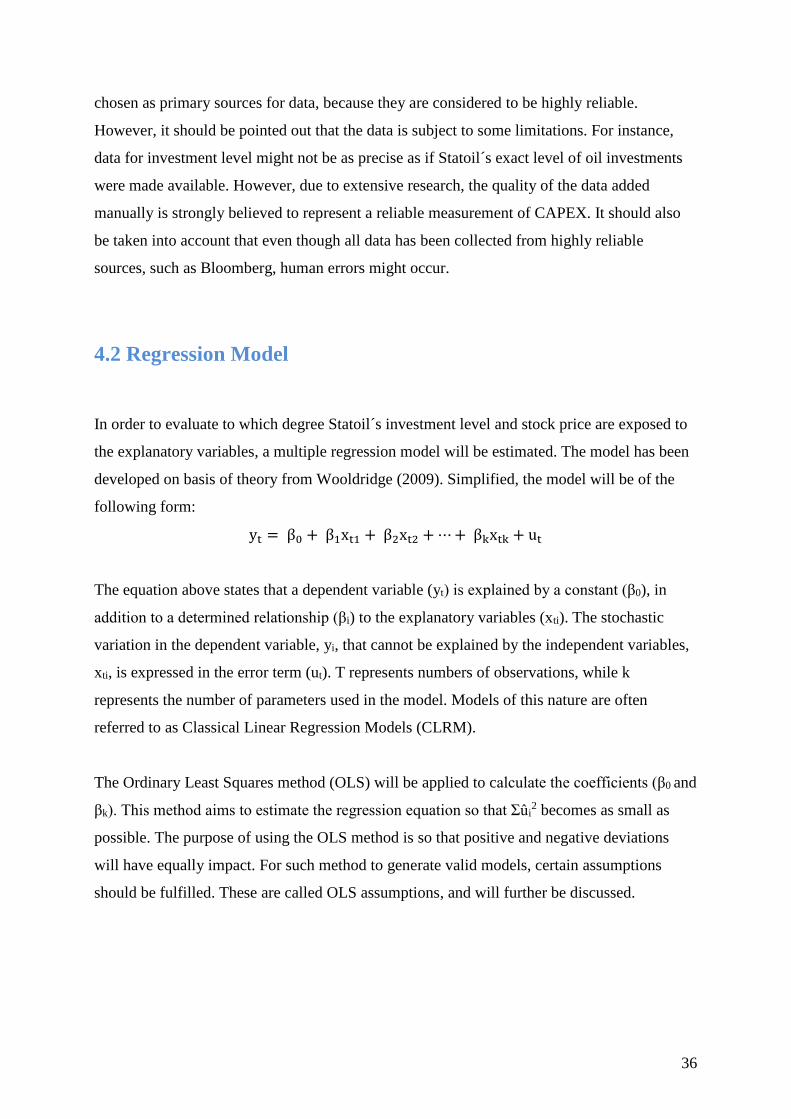
36

chosen as primary sources for data, because they are considered to be highly reliable.

However, it should be pointed out that the data is subject to some limitations. For instance,

data for investment level might not be as precise as if Statoil´s exact level of oil investments

were made available. However, due to extensive research, the quality of the data added

manually is strongly believed to represent a reliable measurement of CAPEX. It should also

be taken into account that even though all data has been collected from highly reliable

sources, such as Bloomberg, human errors might occur.

4.2 Regression Model

In order to evaluate to which degree Statoil´s investment level and stock price are exposed to

the explanatory variables, a multiple regression model will be estimated. The model has been

developed on basis of theory from Wooldridge (2009). Simplified, the model will be of the

following form:

yt = β0 + β1xt1 + β2xt2 + ⋯ + βkxtk + ut

The equation above states that a dependent variable (yt) is explained by a constant (β0), in

addition to a determined relationship (βi) to the explanatory variables (xti). The stochastic

variation in the dependent variable, yi, that cannot be explained by the independent variables,

xti, is expressed in the error term (ut). T represents numbers of observations, while k

represents the number of parameters used in the model. Models of this nature are often

referred to as Classical Linear Regression Models (CLRM).

The Ordinary Least Squares method (OLS) will be applied to calculate the coefficients (β0 and

βk). This method aims to estimate the regression equation so that Σûi2 becomes as small as

possible. The purpose of using the OLS method is so that positive and negative deviations

will have equally impact. For such method to generate valid models, certain assumptions

should be fulfilled. These are called OLS assumptions, and will further be discussed.

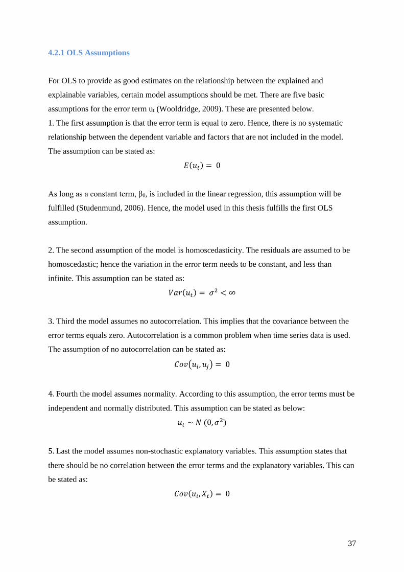
37

4.2.1 OLS Assumptions

For OLS to provide as good estimates on the relationship between the explained and

explainable variables, certain model assumptions should be met. There are five basic

assumptions for the error term ut (Wooldridge, 2009). These are presented below.

1. The first assumption is that the error term is equal to zero. Hence, there is no systematic

relationship between the dependent variable and factors that are not included in the model.

The assumption can be stated as:

𝐸(𝑢𝑡) = 0

As long as a constant term, β0, is included in the linear regression, this assumption will be

fulfilled (Studenmund, 2006). Hence, the model used in this thesis fulfills the first OLS

assumption.

2. The second assumption of the model is homoscedasticity. The residuals are assumed to be

homoscedastic; hence the variation in the error term needs to be constant, and less than

infinite. This assumption can be stated as:

𝑉𝑎𝑟(𝑢𝑡) = 𝜎2 < ∞

3. Third the model assumes no autocorrelation. This implies that the covariance between the

error terms equals zero. Autocorrelation is a common problem when time series data is used.

The assumption of no autocorrelation can be stated as:

𝐶𝑜𝑣(𝑢𝑖 , 𝑢𝑗) = 0

4. Fourth the model assumes normality. According to this assumption, the error terms must be

independent and normally distributed. This assumption can be stated as below:

𝑢𝑡 ∼ 𝑁 (0, 𝜎2)

5. Last the model assumes non-stochastic explanatory variables. This assumption states that

there should be no correlation between the error terms and the explanatory variables. This can

be stated as:

𝐶𝑜𝑣(𝑢𝑖, 𝑋𝑡) = 0

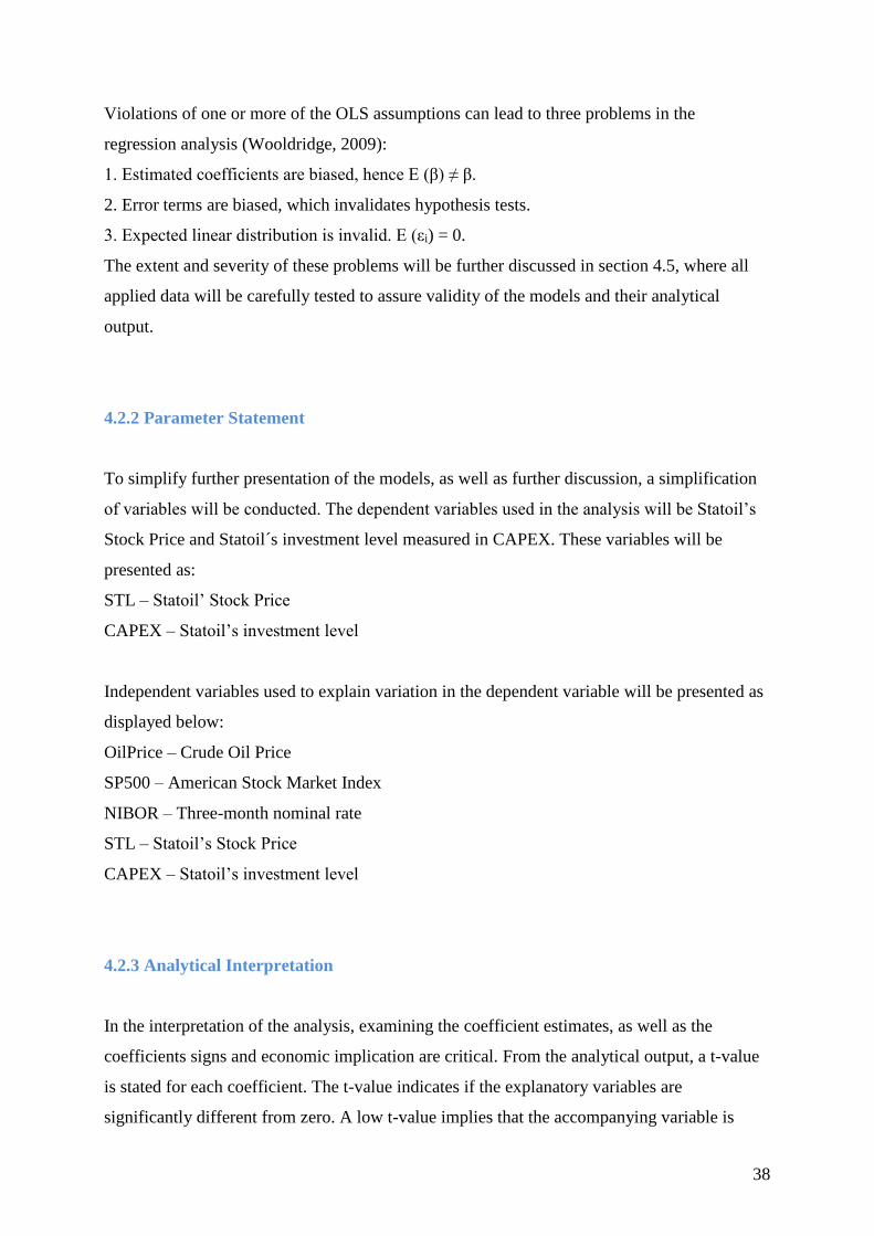
38

Violations of one or more of the OLS assumptions can lead to three problems in the

regression analysis (Wooldridge, 2009):

1. Estimated coefficients are biased, hence E (β) ≠ β.

2. Error terms are biased, which invalidates hypothesis tests.

3. Expected linear distribution is invalid. E (εi) = 0.

The extent and severity of these problems will be further discussed in section 4.5, where all

applied data will be carefully tested to assure validity of the models and their analytical

output.

4.2.2 Parameter Statement

To simplify further presentation of the models, as well as further discussion, a simplification

of variables will be conducted. The dependent variables used in the analysis will be Statoil’s

Stock Price and Statoil´s investment level measured in CAPEX. These variables will be

presented as:

STL – Statoil’ Stock Price

CAPEX – Statoil’s investment level

Independent variables used to explain variation in the dependent variable will be presented as

displayed below:

OilPrice – Crude Oil Price

SP500 – American Stock Market Index

NIBOR – Three-month nominal rate

STL – Statoil’s Stock Price

CAPEX – Statoil’s investment level

4.2.3 Analytical Interpretation

In the interpretation of the analysis, examining the coefficient estimates, as well as the

coefficients signs and economic implication are critical. From the analytical output, a t-value

is stated for each coefficient. The t-value indicates if the explanatory variables are

significantly different from zero. A low t-value implies that the accompanying variable is

39

insignificant. To determine the significance of the total multiple regression model, a F-test is

used.

How much of the variation in the dependent variable that can be explained by the independent

variables are given by R2. R2 will be displayed as a value between 0 and 1. The closer R2 is to

one, the more of the variation is explained by the explanatory variables (Studenmund, A. H,

2011). When parameters are added to the model, R2 as a consequence will change, and is

therefore not a suitable measurement for the variables in multiple regression models. In

application of such models, adjusted R2 should be used to determine whether a variable

should be included. Adding additional variables causes degrees of freedom to be lost;

something adjusted R2 takes into account. If adjusted R2 increases when a variable is added, it

is an indication that this variable in fact should be included in the model (Studenmund, A. H,

2011).

4.3 Influential Factors

As this thesis primarily aims to investigate the relationship between Crude Oil Price and

Statoil’s Investment level and Stock Price, the development of a simple model with oil price

as the only independent variable could be tempting. Still, this could lead to serious errors in

the estimations due to Omitted Variable Bias (OVB). The Omitted Variable Bias occurs in the

OLS estimators when variables relevant to the regression are omitted (Wooldridge, 2009). By

not including the relevant variables, the relationship desired estimated will in fact be

overvalued. Other economic factors relevant to include in the model will therefore be

discussed during this section, as well as expected impact of each variable.

4.3.1 Interest rate

Previous studies indicates that a change in the real interest rate will have a significant effect

on the prices in both the US and Norwegian stock market (Fama, 1981) and (Gjerde &

Sættem, 1999). Gjerde & Sættem’s analysis, which uses monthly data from the period of 1974

to 1994, concludes that a change in real interest rate has an immediate negative effect on

40

stock price. Due to this, interest rate will be included as a variable when developing the

models. The rate applied in the analysis will be a three month nominal NIBOR-rate

(Norwegian Inter Bank Offered Rate). Data for the NIBOR-rate is quarterly and collected

from the Norwegian Central Banks rate statistics.

Expected impact: An increase in interest rates entails higher cost for banks lending money,

which causes banks to increase their lending rates offered to private households and firms. In

many cases, such event would make firms delay projects and investments till lending rate

decreases, and borrowing costs are reduced. Reducing investments would entail decreased

cash flows in the future, and a cohesive lower stock returns. On this basis, an increase in

interest rate is expected to have a negative effect on both investments and stock price.

4.3.2 Market Index

On the basis of previous research, it would be reasonable to include a market index when

looking at the relationship between the price of oil and Statoil´s stock price. Driesprong,

Jacobsen and Maat (2005) showed that a reduced oil price affects stock markets negatively,

while an increased stock price affects the markets positively. Their research finds a broad

support among numerous studies, for example such as Sadorsky (1999). As the Statoil stock

is listed on both the Norwegian and the US stock market, the aggregated returns for both

markets could seem appropriate to include in the analysis. Still, when comparing Oslo Stock

Exchange All Share Index (OSEAX) and Standard and Poor´s 500 index measured as

percentage change over time, (OSEAX) is found to be much less stable than the (S&P 500).

This is illustrated in the below graph, where the blue line indicates OSEAX, while the red

indicated S&P 500.

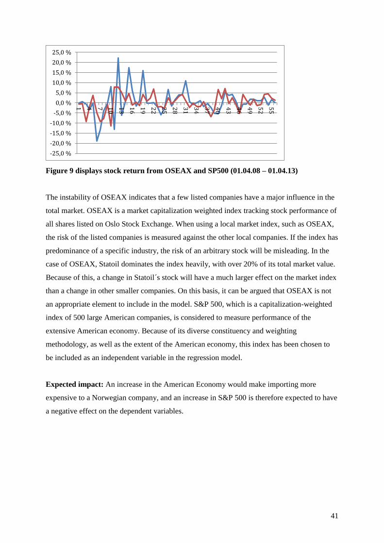
41

Figure 9 displays stock return from OSEAX and SP500 (01.04.08 – 01.04.13)

The instability of OSEAX indicates that a few listed companies have a major influence in the

total market. OSEAX is a market capitalization weighted index tracking stock performance of

all shares listed on Oslo Stock Exchange. When using a local market index, such as OSEAX,

the risk of the listed companies is measured against the other local companies. If the index has

predominance of a specific industry, the risk of an arbitrary stock will be misleading. In the

case of OSEAX, Statoil dominates the index heavily, with over 20% of its total market value.

Because of this, a change in Statoil´s stock will have a much larger effect on the market index

than a change in other smaller companies. On this basis, it can be argued that OSEAX is not

an appropriate element to include in the model. S&P 500, which is a capitalization-weighted

index of 500 large American companies, is considered to measure performance of the

extensive American economy. Because of its diverse constituency and weighting

methodology, as well as the extent of the American economy, this index has been chosen to

be included as an independent variable in the regression model.

Expected impact: An increase in the American Economy would make importing more

expensive to a Norwegian company, and an increase in S&P 500 is therefore expected to have

a negative effect on the dependent variables.

-25,0 %

-20,0 %

-15,0 %

-10,0 %

-5,0 %

0,0 %

5,0 %

10,0 %

15,0 %

20,0 %

25,0 %

1 4 7 10

13

16

19

22

25

28

31

34

37

40

43

46

49

52

55

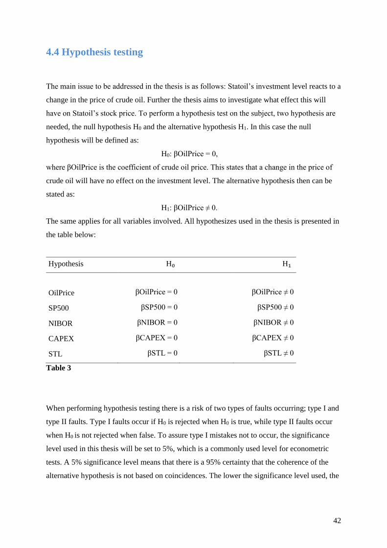
42

4.4 Hypothesis testing

The main issue to be addressed in the thesis is as follows: Statoil’s investment level reacts to a

change in the price of crude oil. Further the thesis aims to investigate what effect this will

have on Statoil’s stock price. To perform a hypothesis test on the subject, two hypothesis are

needed, the null hypothesis H0 and the alternative hypothesis H1. In this case the null

hypothesis will be defined as:

H0: βOilPrice = 0,

where βOilPrice is the coefficient of crude oil price. This states that a change in the price of

crude oil will have no effect on the investment level. The alternative hypothesis then can be

stated as:

H1: βOilPrice ≠ 0.

The same applies for all variables involved. All hypothesizes used in the thesis is presented in

the table below:

Hypothesis H₀ H₁

OilPrice βOilPrice = 0 βOilPrice ≠ 0

SP500 βSP500 = 0 βSP500 ≠ 0

NIBOR βNIBOR = 0 βNIBOR ≠ 0

CAPEX βCAPEX = 0 βCAPEX ≠ 0

STL βSTL = 0 βSTL ≠ 0

Table 3

When performing hypothesis testing there is a risk of two types of faults occurring; type I and

type II faults. Type I faults occur if H0 is rejected when H0 is true, while type II faults occur

when H0 is not rejected when false. To assure type I mistakes not to occur, the significance

level used in this thesis will be set to 5%, which is a commonly used level for econometric

tests. A 5% significance level means that there is a 95% certainty that the coherence of the

alternative hypothesis is not based on coincidences. The lower the significance level used, the

43

less the probability is of making type I mistakes. Initially, there is no other way to prevent

type II mistakes from occurring, than to increase numbers of observations.

However, it is important to be aware of that even if the hypothesis is found to be statistically

significant, it does not necessarily mean that there is a theoretical basis to prove the

relationship. Applying a wide enough selection will in most cases provide statistically

significant relationships (Studenmund, 2006). On this basis, one should always be critical

when evaluating analytical results and their significance.

4.5 Residual Analysis

Violation of the basic assumption stated in 4.2.1 could lead to misinterpretation of test results,

or in worst-case scenario, invalidity of the regression model. To assure the validity of the

model used in the thesis, the basic OLS assumptions will be carefully tested. Result from the

robustness testing will in this section be presented.

4.5.1 Homoscedasticity

If the assumption of homoscedasticity is not fulfilled, heteroscedasticity is present in the

model. Heteroscedasticity can be determined in a spreadsheet between predicted dependent

variable and residuals. If heteroscedasticity is suspected on basis of the scatterplots, a statistic

tests, such as Whites test should be applied. Violation of the assumption of homoscedasticity

causes standard deviation to be biased. In such case, t-tests are no longer reliable, and the

linear regression model is no longer valid.

To avoid heteroscedasticity, all data used in the thesis has been transformed into logarithmic

form, as this rescales and reduces the impact of extreme observations. From scatter plots on

the dependent variables submitted in the appendix, it can be pointed out that there are no

indications of strongly increasing or decreasing variance in the data. Data used in the thesis is

therefore assumed to be homoscedastic.

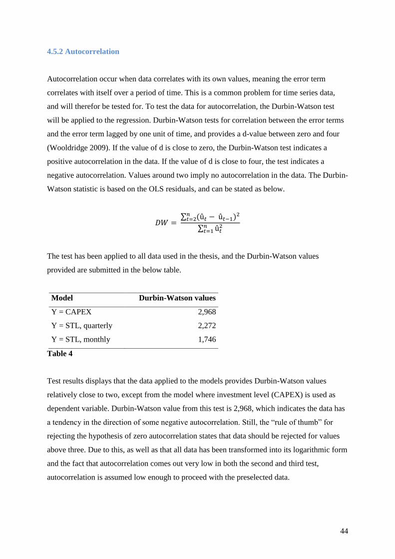
44

4.5.2 Autocorrelation

Autocorrelation occur when data correlates with its own values, meaning the error term

correlates with itself over a period of time. This is a common problem for time series data,

and will therefor be tested for. To test the data for autocorrelation, the Durbin-Watson test

will be applied to the regression. Durbin-Watson tests for correlation between the error terms

and the error term lagged by one unit of time, and provides a d-value between zero and four

(Wooldridge 2009). If the value of d is close to zero, the Durbin-Watson test indicates a

positive autocorrelation in the data. If the value of d is close to four, the test indicates a

negative autocorrelation. Values around two imply no autocorrelation in the data. The Durbin-

Watson statistic is based on the OLS residuals, and can be stated as below.

𝐷𝑊 = ∑ (û𝑡 − û𝑡−1)2𝑛

𝑡=2

∑ û𝑡2𝑛

𝑡=1

The test has been applied to all data used in the thesis, and the Durbin-Watson values

provided are submitted in the below table.

Model Durbin-Watson values

Y = CAPEX 2,968

Y = STL, quarterly 2,272

Y = STL, monthly 1,746

Table 4

Test results displays that the data applied to the models provides Durbin-Watson values

relatively close to two, except from the model where investment level (CAPEX) is used as

dependent variable. Durbin-Watson value from this test is 2,968, which indicates the data has

a tendency in the direction of some negative autocorrelation. Still, the “rule of thumb” for

rejecting the hypothesis of zero autocorrelation states that data should be rejected for values

above three. Due to this, as well as that all data has been transformed into its logarithmic form

and the fact that autocorrelation comes out very low in both the second and third test,

autocorrelation is assumed low enough to proceed with the preselected data.

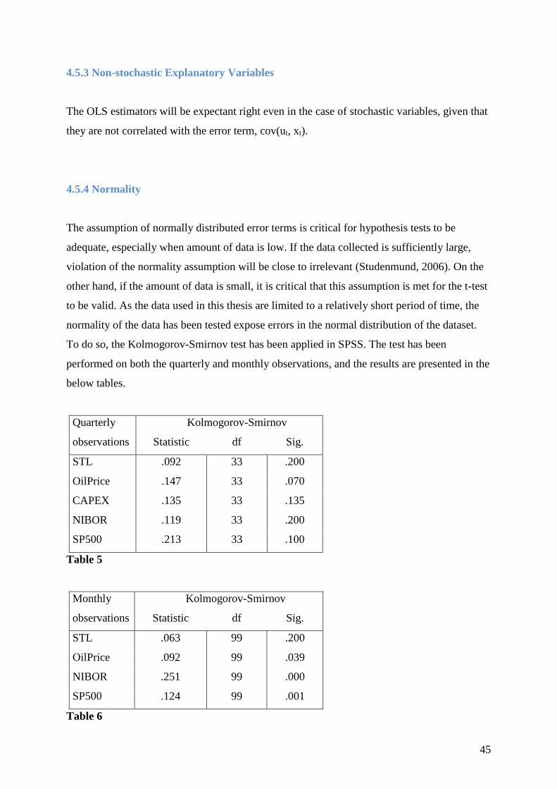
45

4.5.3 Non-stochastic Explanatory Variables

The OLS estimators will be expectant right even in the case of stochastic variables, given that

they are not correlated with the error term, cov(ut, xt).

4.5.4 Normality

The assumption of normally distributed error terms is critical for hypothesis tests to be

adequate, especially when amount of data is low. If the data collected is sufficiently large,

violation of the normality assumption will be close to irrelevant (Studenmund, 2006). On the

other hand, if the amount of data is small, it is critical that this assumption is met for the t-test

to be valid. As the data used in this thesis are limited to a relatively short period of time, the

normality of the data has been tested expose errors in the normal distribution of the dataset.

To do so, the Kolmogorov-Smirnov test has been applied in SPSS. The test has been

performed on both the quarterly and monthly observations, and the results are presented in the

below tables.

Quarterly Kolmogorov-Smirnov

observations Statistic df Sig.

STL .092 33 .200

OilPrice .147 33 .070

CAPEX .135 33 .135

NIBOR .119 33 .200

SP500 .213 33 .100

Table 5

Monthly Kolmogorov-Smirnov

observations Statistic df Sig.

STL .063 99 .200

OilPrice .092 99 .039

NIBOR .251 99 .000

SP500 .124 99 .001

Table 6

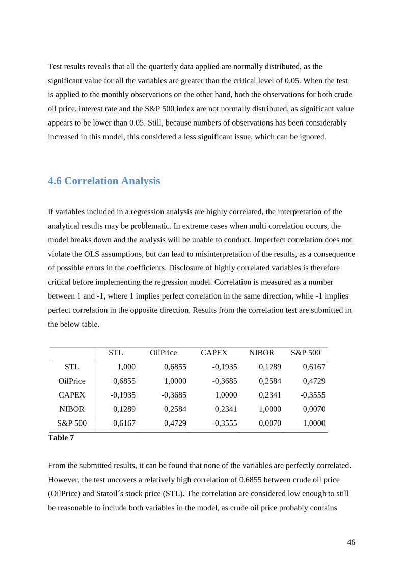
46

Test results reveals that all the quarterly data applied are normally distributed, as the

significant value for all the variables are greater than the critical level of 0.05. When the test

is applied to the monthly observations on the other hand, both the observations for both crude

oil price, interest rate and the S&P 500 index are not normally distributed, as significant value

appears to be lower than 0.05. Still, because numbers of observations has been considerably

increased in this model, this considered a less significant issue, which can be ignored.

4.6 Correlation Analysis

If variables included in a regression analysis are highly correlated, the interpretation of the

analytical results may be problematic. In extreme cases when multi correlation occurs, the

model breaks down and the analysis will be unable to conduct. Imperfect correlation does not

violate the OLS assumptions, but can lead to misinterpretation of the results, as a consequence

of possible errors in the coefficients. Disclosure of highly correlated variables is therefore

critical before implementing the regression model. Correlation is measured as a number

between 1 and -1, where 1 implies perfect correlation in the same direction, while -1 implies

perfect correlation in the opposite direction. Results from the correlation test are submitted in

the below table.

STL OilPrice CAPEX NIBOR S&P 500

STL 1,000 0,6855 -0,1935 0,1289 0,6167

OilPrice 0,6855 1,0000 -0,3685 0,2584 0,4729

CAPEX -0,1935 -0,3685 1,0000 0,2341 -0,3555

NIBOR 0,1289 0,2584 0,2341 1,0000 0,0070

S&P 500 0,6167 0,4729 -0,3555 0,0070 1,0000

Table 7

From the submitted results, it can be found that none of the variables are perfectly correlated.

However, the test uncovers a relatively high correlation of 0.6855 between crude oil price

(OilPrice) and Statoil´s stock price (STL). The correlation are considered low enough to still

be reasonable to include both variables in the model, as crude oil price probably contains

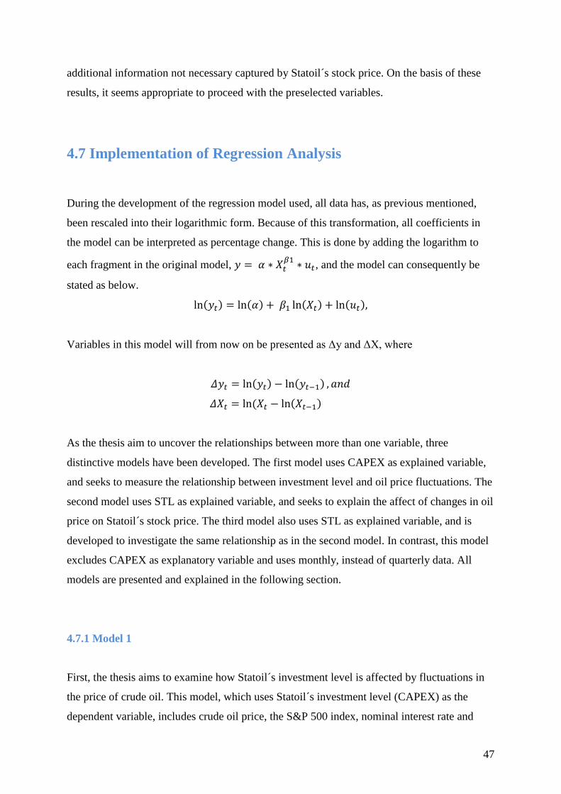
47

additional information not necessary captured by Statoil´s stock price. On the basis of these

results, it seems appropriate to proceed with the preselected variables.

4.7 Implementation of Regression Analysis

During the development of the regression model used, all data has, as previous mentioned,

been rescaled into their logarithmic form. Because of this transformation, all coefficients in

the model can be interpreted as percentage change. This is done by adding the logarithm to

each fragment in the original model, 𝑦 = 𝛼 ∗ 𝑋𝑡𝛽1

∗ 𝑢𝑡, and the model can consequently be

stated as below.

ln(𝑦𝑡) = ln(𝛼) + 𝛽1 ln(𝑋𝑡) + ln(𝑢𝑡),

Variables in this model will from now on be presented as Δy and ΔX, where

𝛥𝑦𝑡 = ln(𝑦𝑡) − ln(𝑦𝑡−1) , 𝑎𝑛𝑑

𝛥𝑋𝑡 = ln (𝑋𝑡 − ln(𝑋𝑡−1)

As the thesis aim to uncover the relationships between more than one variable, three

distinctive models have been developed. The first model uses CAPEX as explained variable,

and seeks to measure the relationship between investment level and oil price fluctuations. The

second model uses STL as explained variable, and seeks to explain the affect of changes in oil

price on Statoil´s stock price. The third model also uses STL as explained variable, and is

developed to investigate the same relationship as in the second model. In contrast, this model

excludes CAPEX as explanatory variable and uses monthly, instead of quarterly data. All

models are presented and explained in the following section.

4.7.1 Model 1

First, the thesis aims to examine how Statoil´s investment level is affected by fluctuations in

the price of crude oil. This model, which uses Statoil´s investment level (CAPEX) as the

dependent variable, includes crude oil price, the S&P 500 index, nominal interest rate and

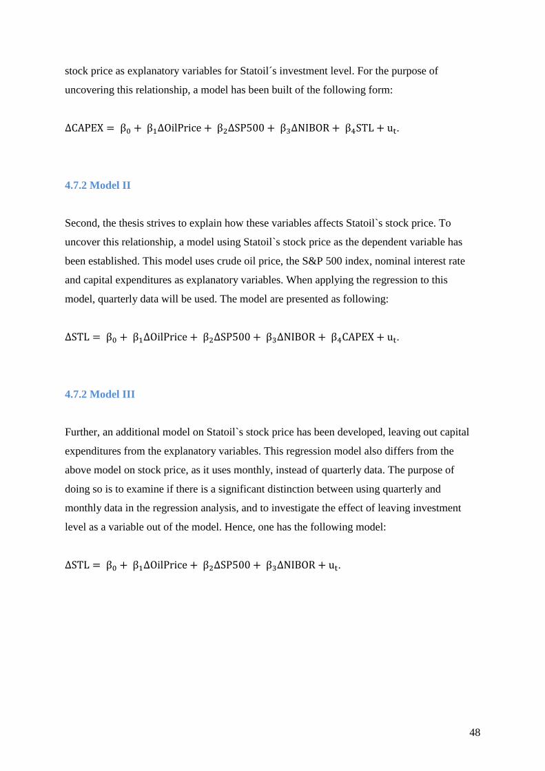
48

stock price as explanatory variables for Statoil´s investment level. For the purpose of

uncovering this relationship, a model has been built of the following form:

ΔCAPEX = β0 + β1ΔOilPrice + β2ΔSP500 + β3ΔNIBOR + β4STL + ut.

4.7.2 Model II

Second, the thesis strives to explain how these variables affects Statoil`s stock price. To

uncover this relationship, a model using Statoil`s stock price as the dependent variable has

been established. This model uses crude oil price, the S&P 500 index, nominal interest rate

and capital expenditures as explanatory variables. When applying the regression to this

model, quarterly data will be used. The model are presented as following:

ΔSTL = β0 + β1ΔOilPrice + β2ΔSP500 + β3ΔNIBOR + β4CAPEX + ut.

4.7.2 Model III

Further, an additional model on Statoil`s stock price has been developed, leaving out capital

expenditures from the explanatory variables. This regression model also differs from the

above model on stock price, as it uses monthly, instead of quarterly data. The purpose of

doing so is to examine if there is a significant distinction between using quarterly and

monthly data in the regression analysis, and to investigate the effect of leaving investment

level as a variable out of the model. Hence, one has the following model:

ΔSTL = β0 + β1ΔOilPrice + β2ΔSP500 + β3ΔNIBOR + ut.

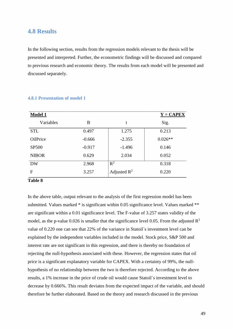
49

4.8 Results

In the following section, results from the regression models relevant to the thesis will be

presented and interpreted. Further, the econometric findings will be discussed and compared

to previous research and economic theory. The results from each model will be presented and

discussed separately.

4.8.1 Presentation of model 1

Model 1 Y = CAPEX

Variables B t Sig.

STL 0.497 1.275 0.213

OilPrice -0.666 -2.355 0.026**

SP500 -0.917 -1.496 0.146

NIBOR 0.629 2.034 0.052

DW 2.968 R2 0.318

F 3.257 Adjusted R2 0.220

Table 8

In the above table, output relevant to the analysis of the first regression model has been

submitted. Values marked * is significant within 0.05 significance level. Values marked **

are significant within a 0.01 significance level. The F-value of 3.257 states validity of the

model, as the p-value 0.026 is smaller that the significance level 0.05. From the adjusted R2

value of 0.220 one can see that 22% of the variance in Statoil´s investment level can be

explained by the independent variables included in the model. Stock price, S&P 500 and

interest rate are not significant in this regression, and there is thereby no foundation of

rejecting the null-hypothesis associated with these. However, the regression states that oil

price is a significant explanatory variable for CAPEX. With a certainty of 99%, the null-

hypothesis of no relationship between the two is therefore rejected. According to the above

results, a 1% increase in the price of crude oil would cause Statoil´s investment level to

decrease by 0.666%. This result deviates from the expected impact of the variable, and should

therefore be further elaborated. Based on the theory and research discussed in the previous

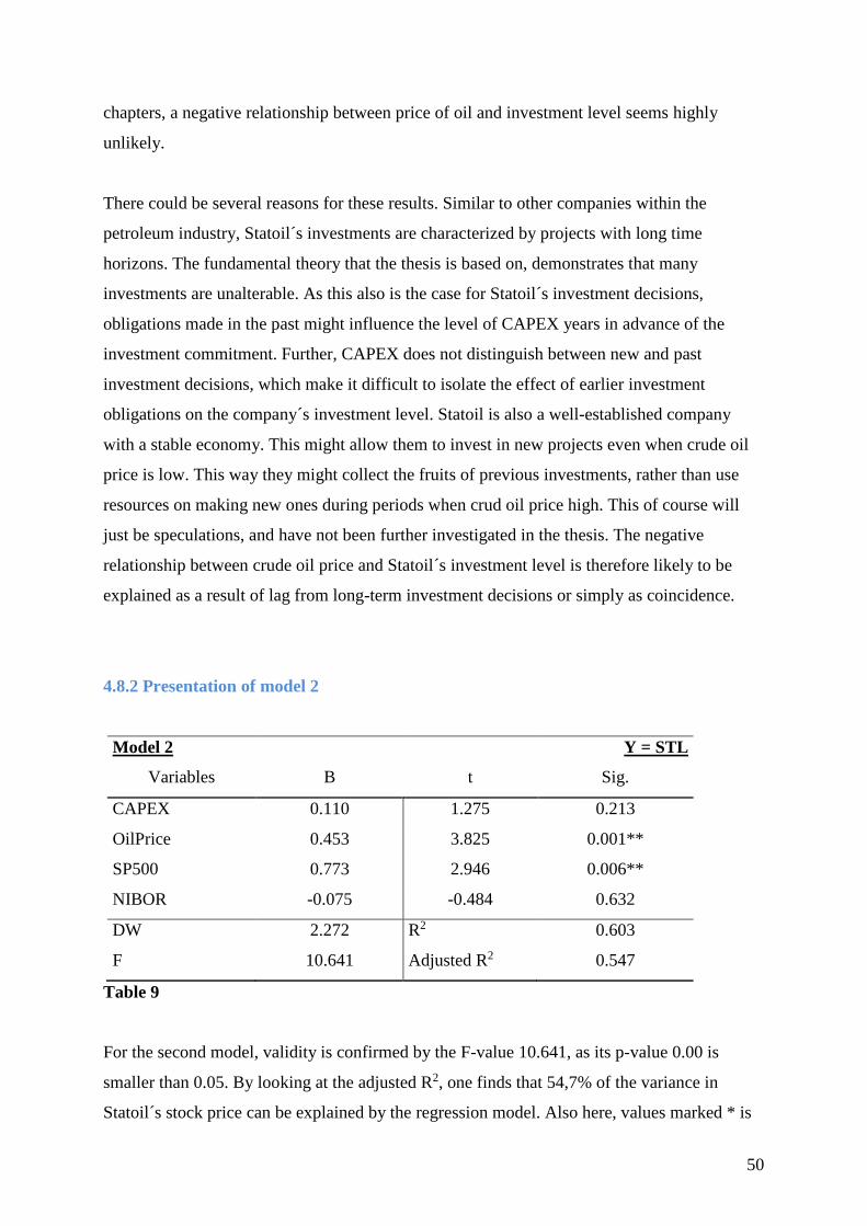
50

chapters, a negative relationship between price of oil and investment level seems highly

unlikely.

There could be several reasons for these results. Similar to other companies within the

petroleum industry, Statoil´s investments are characterized by projects with long time

horizons. The fundamental theory that the thesis is based on, demonstrates that many

investments are unalterable. As this also is the case for Statoil´s investment decisions,

obligations made in the past might influence the level of CAPEX years in advance of the

investment commitment. Further, CAPEX does not distinguish between new and past

investment decisions, which make it difficult to isolate the effect of earlier investment

obligations on the company´s investment level. Statoil is also a well-established company

with a stable economy. This might allow them to invest in new projects even when crude oil

price is low. This way they might collect the fruits of previous investments, rather than use

resources on making new ones during periods when crud oil price high. This of course will

just be speculations, and have not been further investigated in the thesis. The negative

relationship between crude oil price and Statoil´s investment level is therefore likely to be

explained as a result of lag from long-term investment decisions or simply as coincidence.

4.8.2 Presentation of model 2

Model 2 Y = STL

Variables B t Sig.

CAPEX 0.110 1.275 0.213

OilPrice 0.453 3.825 0.001**

SP500 0.773 2.946 0.006**

NIBOR -0.075 -0.484 0.632

DW 2.272 R2 0.603

F 10.641 Adjusted R2 0.547

Table 9

For the second model, validity is confirmed by the F-value 10.641, as its p-value 0.00 is

smaller than 0.05. By looking at the adjusted R2, one finds that 54,7% of the variance in

Statoil´s stock price can be explained by the regression model. Also here, values marked * is

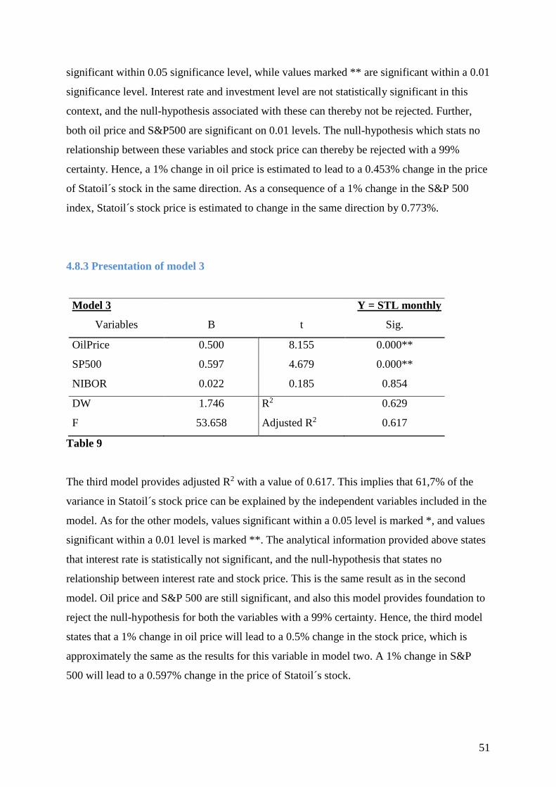
51

significant within 0.05 significance level, while values marked ** are significant within a 0.01

significance level. Interest rate and investment level are not statistically significant in this

context, and the null-hypothesis associated with these can thereby not be rejected. Further,

both oil price and S&P500 are significant on 0.01 levels. The null-hypothesis which stats no

relationship between these variables and stock price can thereby be rejected with a 99%

certainty. Hence, a 1% change in oil price is estimated to lead to a 0.453% change in the price

of Statoil´s stock in the same direction. As a consequence of a 1% change in the S&P 500

index, Statoil´s stock price is estimated to change in the same direction by 0.773%.

4.8.3 Presentation of model 3

Model 3 Y = STL monthly

Variables B t Sig.

OilPrice 0.500 8.155 0.000**

SP500 0.597 4.679 0.000**

NIBOR 0.022 0.185 0.854

DW 1.746 R2 0.629

F 53.658 Adjusted R2 0.617

Table 9

The third model provides adjusted R2 with a value of 0.617. This implies that 61,7% of the

variance in Statoil´s stock price can be explained by the independent variables included in the

model. As for the other models, values significant within a 0.05 level is marked *, and values

significant within a 0.01 level is marked **. The analytical information provided above states

that interest rate is statistically not significant, and the null-hypothesis that states no

relationship between interest rate and stock price. This is the same result as in the second

model. Oil price and S&P 500 are still significant, and also this model provides foundation to

reject the null-hypothesis for both the variables with a 99% certainty. Hence, the third model

states that a 1% change in oil price will lead to a 0.5% change in the stock price, which is

approximately the same as the results for this variable in model two. A 1% change in S&P

500 will lead to a 0.597% change in the price of Statoil´s stock.

52

5. Conclusion

5.1 Analytical weaknesses

In such a context, it is important to point out that economic relationships are highly complex

in nature. Due to this, before stating a final conclusion, it seems relevant to highlight the

weaknesses and challenges associated with the thesis.

A general weakness for econometric analysis is that the results are highly sensitive, even to

small changes in datasets and model specification. As the limited access to CAPEX

observation, monthly, or for some daily, observations for all other variables applied has been

transformed into quarterly data. This transformation is likely to have a distinct impact on the

regression model. It should also be pointed out that, even though processing of data has been

treated with caution and awareness, human errors may occur. To increase the strength of the

econometric models, more variables could have been added. Other variables such as for

example inflation, unemployment, industrial production and exchange rate might have been

interesting to include.

Another analytical weakness is the relative small sample size applied in the thesis. If sample

size is small, detecting violations of the assumptions might be difficult. It would have been

preferable to increase sample size by using monthly observation for Statoil´s capital

expenditures, but this data could not be obtained. An increase of numbers of observations in

the data sets would also reduce the chance of making type II errors. An obvious weakness of

the analysis is therefore the limited access to observations for CAPEX, as these only were

made available through Statoil´s financial reports as quarterly data. Further, Statoil´s CAPEX

contains of various elements, which makes it difficult to determine how accurate a

measurement this is for Statoil´s investment level.

53

5.2 Conclusion

The objective of this thesis has been to measure Statoil´s investment level and stock return´s

exposure to fluctuations in crude oil price. For this purpose, observations for changes in crude

oil price, Statoil´s investments levels and stock return has been carefully studied and

analysed. To obtain trustworthy analytical results, observations over a considerable period of

time have been collected for each of the variables from highly reliable sources. As the thesis

aims to investigate both the exposure of the investment level and the stock return, two main

conclusions can be drawn.

First, analytical results imply a negative relationship between Statoil´s investment level and

the price of crude oil. Due to Statoil´s investment strategies and fundamental theory of

investment behaviour, this relationship is most likely to be determined by coincidence, and

the first main conclusion of the thesis is therefore that there are other factors, and not the price

of crude oil, that effects Statoil´s investment level measured in capital expenditures. This

implies that Statoil has a long-term investment perspective, which is consistent with the

company´s investment strategy.

Secondly, the analysis implies that oil price fluctuations do have a positive influence on the

return of Statoil´s stock. This result finds support in Boye and Filion (2006) who, trough their

research involving pure production companies, found that oil price has a positive beta

coefficient on stock return at a 1% level. Næs et al. (2008) finds that changes in oil price have

significant influence on cash flows in the industrial sectors. Previously discussed valuation

models shows that the return of company´s stock can be determined by looking at discounted

cash flows. Therefore, this is not a surprising conclusion, as a shift in oil price will have a

direct affect on Statoil´s cash flows, in terms of reduced or increased incomes.

An additional conclusion can be drawn from the fact that the investments level is held more or

less unaffected, while the return of the company´s stock decreases with drops in the price of

crude oil. Statoil´s financial reports show that the company has a stable economy, allowing

them to invest even when crude oil price is low. Due to this, it can be concluded that the

company has the financial possibility to consider their long-term investors when determining

their investment strategies.

54

5.3 Suggestion of Further Work

As the subject of this thesis is comprehensive and highly complex, it could open for extensive

further research. Due to this, a last section has been included to the thesis, involving

directions that might be interesting for further study.

As discussed in the presentation of analytical weaknesses, CAPEX is a measurement that

contains various elements, making it difficult to determine how accurate it is for measuring

Statoil´s investment level. It could therefore have been interested divide capex into

subcomponents to examine the isolated effect of each of these. Components which could be

interesting to look closer at is for example investments in exploration, …

It could also be interesting to compare the analytical results to other similar companies, for

example such as Conoco Philips, BP Energy, Total Energy, etc. This could be done both to

support the thesis results, but also to examine if the results are unique for Statoil, or if these

apply to the industry in general.

Further, Statoil is a well-established company with a stable economy. This might allow them

to invest in new projects even when crude oil price is low. This is not necessary the case for

smaller companies operating within the petroleum industry, as these often has smaller

economic margins. It could therefore also be interesting to compare the results to other

smaller companies in attempt to find if smaller companies´ investments might be more

affected be fluctuations in the oil price than large companies such as Statoil.

55

6. References

6.1 Articles and reports

Aastveit, K, A., Bjørnland, H, C. & Thorsrud, L, A., (2012) What drives oil prices?

Emerging versus developed economies, CAMP Working Paper Series. Vol.2

Barkindo, Mohammed, (2006), Oil outlook to 2025, (OPEC)

http://www.opec.org/opec_web/en/1091.htm

Berk, J. & DeMarzo P., (2014): Corporate Finance, 3rd edition, Pearson Education Limited,

page 272-277, 284-285, 351, 379.

Bodie, Z., Kane, A. & Marcus, A. (2011). Investments and Portfolio Management. New

York, USA. McGraw-Hill/Irwin.

Bond, S., Elston, J. A., Meiresse, J. and B. Mulkay (2003): Financial factors and

investment in Belgium, France, Germany and the UK: a comparison using company panel

data. The Review of Economics and Statistics 85(1), page 153-165.

Boyer, M. M. and Filion, D. (2006), “Common and fundamental factors in the stock returns

of Canadian oil and gas companies”, Energy Economics, Vol. 29, pages428-453

BP (2014): BP Statistical Review of World Energy June 2014.

http://www.bp.com/content/dam/bp/pdf/Energy-economics/statistical-review-2014/BP-

statistical-review-of-world-energy-2014-full-report.pdf Collected 07.04.2015

Brealey, R. A., Myers, S. C., & Allen, F. (2008): Principles of Corporate Finance, 9th

edition, New York: McGraw-Hill Irwin.

Chen, Roll and Ross (1986), “Economic forces and the stock market”, The University of

Chicago Press, Vol. 59, pages 383-403

Dagens Næringsliv, “Oljeprisen synker mandag” Collected:08.06.2015

http://www.dn.no/nyheter/energi/2015/06/08/0809/oljeprisen-synker-mandag

Damodaran, A., (2002): Investment valuation: Tools and techniques for determining the

value of any asset, 2nd edition, Ed. New York: John Wiley & Sons, Inc., page 14

Det Kongelige Olje- og Energidepartement (OED) (2011) “En næring for framtida – om

petroleumsvirksomheten”, Meld. St. 28(2010-2011).

Driesprong G., Jacobsen B. & Maat B. (2005): Striking Oil: Another Puzzle? EFA 2005:

Moscow Meetings Paper. http://ssrn.com/abstract=460500

56

Elton, Gruber, Brown and Goetzmann (2010): Modern Portfolio Theory and Investment

Analysis, 8th Edition. John Wiley & Sons, Inc. Page 440.

Fama, E. F. (1970). Efficient Capital Markets: A Review of Theory and Empirical Work.

The Journal of Finance, 25, 383-417.

Fama, E. F. (1981): Stock Returns, Real Activity, Inflation and Money. American Economic

Review 71, September 1981, page 545-565

Fama, E. F., & French, K. R., (1992): The Cross-Section of Expected Stock Returns.

Journal of Finance, 2, page 427-465.

Fama, E. F., & French, K. R., (1993): Common risk factors in the returns of stocks and

bonds. Journal of Financial Economics, 33, page 3-56.

Fleischmann, B., Meier, H. & Wagner, M. (2004): Supply Chain Management and

Advanced Planning. Volume 4, Springer, p. 71-96

Gjerde Ø. & Sættem F. (1999): Causal relations among stock returns and macroeconomic

variables in a small, open economy. Journal of International Financial Markets, Institutions

and Money 9, 1999, pages 65-74

Gunnerud, V. (2011): On Decomposition and Piecewise Linearization in Petroleum

Production Optimization, PhD thesis, The Norwegian University of Science and Technology,

Trondheim, Norway.

Hamilton, J. D. (2009) "Causes and Consequences of the Oil Shock of 2007-08," Brookings

Papers on Economic Activity, Economic Studies Program, The Brookings Institution, vol.

40(1 (Spring), pages 215-283.

Hamilton, J. (2011) Historical Oil Shocks. Kap. 5. 1997-2010: A new industrial age.

Department of Economics: University of California, San Diego, pages 17-23

Heij, de Boer, Franses, Kloek & van Dijk (2004): Econometric Methods with applications

in business and economics. New York: Oxford University Press Inc.

Huang, R., Masulis, R.W. & Stoll, H.R. (1998). Energy Shocks and International Monetary

Fund (IMF) (2011) World Economic Outlook April 2011: Chapter 3.Oil Scarcity, Growth,

and Global Imbalances, pages 97-99

Keynes, J. M., (1936): The general theory of unemployment, interest and money. London:

MacMillan

Mabro, Robert (2006), The Peak Oil Theory, Oxford Energy Comment, pages, 1-6.

Collected: 08.03.2015 http://www.oxfordenergy.org/wpcms/wp-

content/uploads/2011/01/Sept2006-PeakOilTheory-RobertMabro.pdf

57

Mabro, Robert (2006), “Oil in the 21st Century: Issues, Challenges and Opportunities”,

1.Utg., Oxford University Press

Mohn, K. (2008): Investment Behaviour in the International Oil and Gas Industry, Essay in

empirical petroleum economics, PhD thesis, University of Stavanger.

Nechyba, T (2011), Microeconomics: An Intuitive Approach with Calculus International

Edition, SouthWestern Cengage Learning, pages 636-652

Næs, R., Skjeltorp, J.A. og Ødegaard, B.A. (2008). Hvilke faktorer driver kursutviklingen

på Oslo Børs?. Norsk Økonomisk Tidskrift, Vol. 122, 36-81.

Næs, R., Skjeltorp, J.A. og Ødegaard, B.A. (2008). Bransjesammensetningen på Oslo Børs.

Praktisk Økonomi og Finans 4/2008, 65-73.

Petroleum Services Association of Canada (PSAC)(2013) Business: Industry Overview.

Collected 15.03.15 http://www.psac.ca/business/industry-overview/

Sadorsky, Perry (2001) “Risk Factors in Stock Return of Canadian Oil and Gas Companies”,

Energy Economics, Vol. 23, pages 17-28.

Statistisk Sentralbyrå Collected: 23.02.2015

https://www.ssb.no/arbeid-og-lonn/statistikker/lonnolje/aar/2014-12-12#content

Statoil (2015): Key Financials, Collected in the period from 01.02.15 to 01.04.15,

http://www.statoil.com/en/investorcentre/analyticalinformation/financialaccounts/Pages/defau

lt.aspx

Statoil (2015), Johan Sverdrup- en gigantisk verdiskaper

Collected: 06.04.15 http://www.statoil.com/no/Johan-Sverdrup/Pages/Johan-Sverdrup-

Feltet.aspx

Statoil´s annual report (2008), Collected:03.03.2015

http://www.statoil.com/en/InvestorCentre/AnnualReport/Downloads/AR2008DownloadCentr

e/0%20Key%20Downloads/Annual%20report%20on%20Form%2020F/Annual_Report_on_F

orm_20-F.pdf

Statoil´s annual report (2013), Collected: 03.03.2015

http://www.statoil.com/no/investorcentre/annualreport/annualreport2013/pages/default.aspx

Statoil´s annual report (2014), Collected 03.03.2015

http://www.statoil.com/en/investorcentre/annualreport/annualreport2014/pages/default.aspx

Statoil´s quarterly report (2015), Collected: 10.04.2015

http://www.statoil.com/en/InvestorCentre/QuarterlyResults/2015/Downloads/Financial%20st

atements%20and%20review%201Q%202015.pdf

Store Norske Leksikon(2015):https://snl.no/Statoil_ASA Collected 03.02.2015

58

Studenmund, A. H. (2011): Using econometrics, a practical guide, 6th edition. Boston

Pearson.

Tuttle, Robert, Bloomberg business (2015), Oil Price Outlook – Analysts predictions all over

the map. Collected: 21.04.2015 http://www.bloomberg.com/news/articles/2015-04-02/oil-

price-outlook-analyst-predictions-all-over-the-map

US Energy Information Administration (EIA) (2012) What are the products and uses of

petroleum? Collected: 20.02.2015 http://www.eia.gov/tools/faqs/faq.cfm?id=41&t=6

US Energy Information Administration (2012): Country report: Norway. Collected

15.03.14 http://www.eia.gov/beta/international/analysis.cfm?iso=NOR

US Energy Information Administration (2012): Country report: Russia. Collected

15.03.14http://www.eia.gov/beta/international/analysis.cfm?iso=RUS

Wang, P. (2003): Development and Applications of Production Optimization Techniques for

Petroleum Fields, PhD thesis, Stanford University.

US Energy Information Administration (EIA) (2013) AEO2014 Early Release Overview:

Petroleum and other liquids Collected: 26.02.2015

http://www.eia.gov/forecasts/aeo/er/early_production.cfm

US Energy Information Administration (EIA) (2014) Energy & Financial Markets: What

Drives Crude Oil Prices? Collected: 10.03.2015 http://www.eia.gov/finance/markets/

US Energy Information Administration (EIA, 2015) Short-Term Energy Outlook

Collected: 24.05.2015 file://localhost/Users/synnemeling/Pictures/Short-

Term%20Energy%20Outlook%20-

%20U.S.%20Energy%20Information%20Administration%20(EIA).html

Wooldridge, M. Jeffrey (2009): Introductory Econometrics, a modern approach, Issue 4,

page 1, 8, 415.

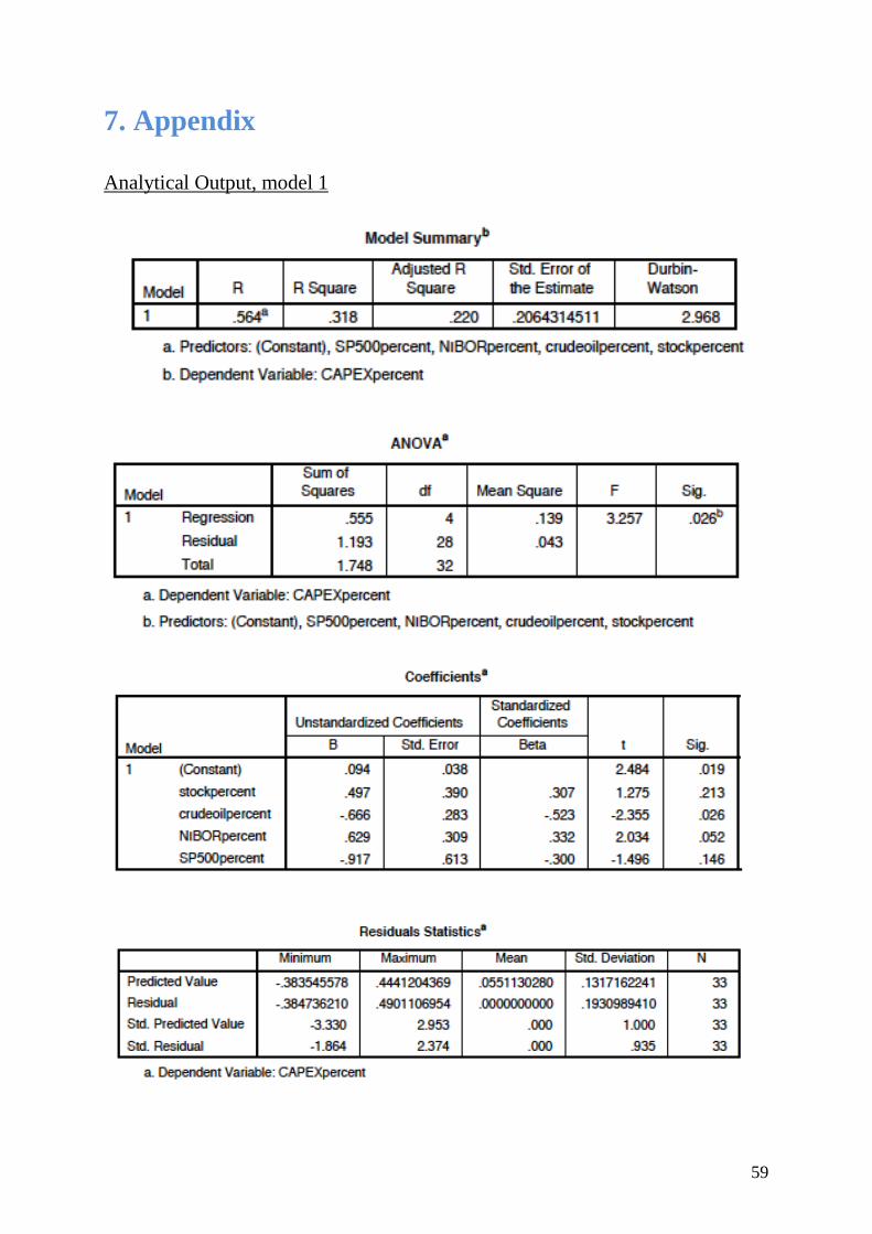
59

7. Appendix

Analytical Output, model 1

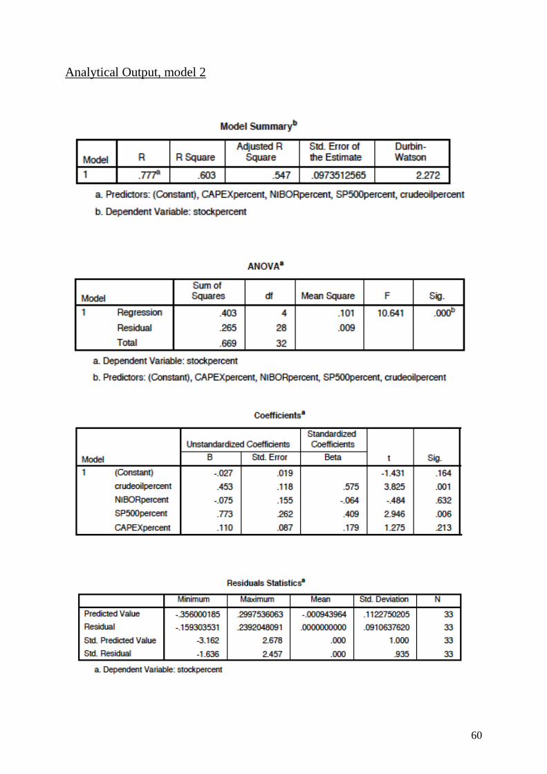
60

Analytical Output, model 2

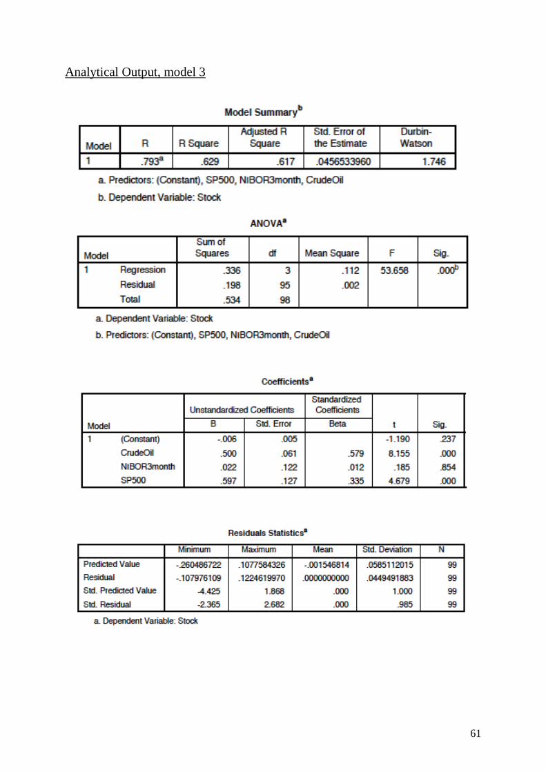
61

Analytical Output, model 3

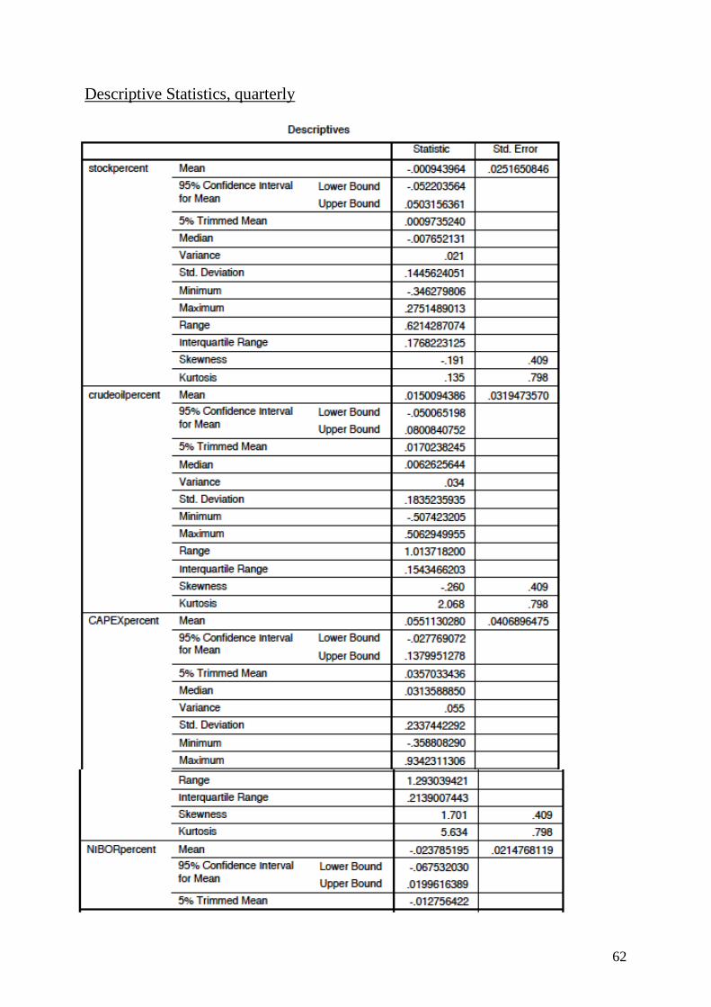
62

Descriptive Statistics, quarterly

63

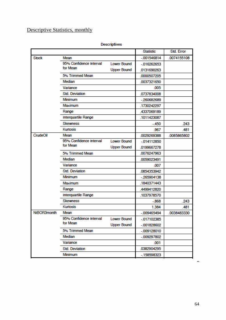
64

Descriptive Statistics, monthly

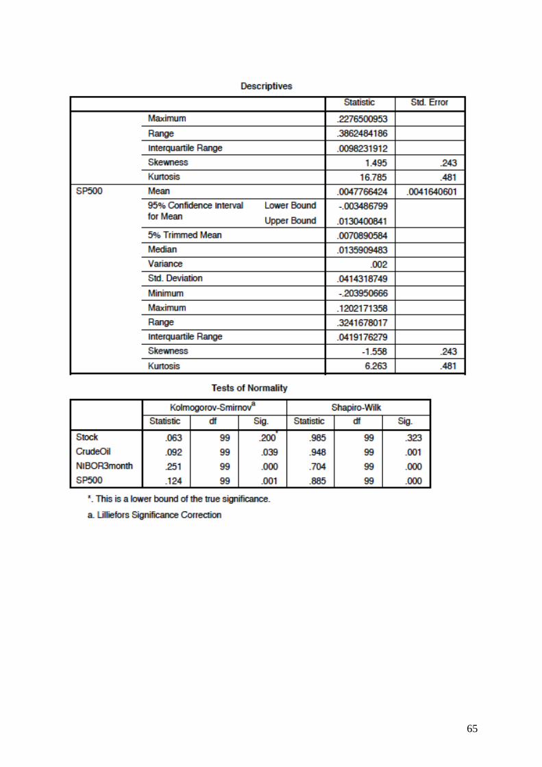
65

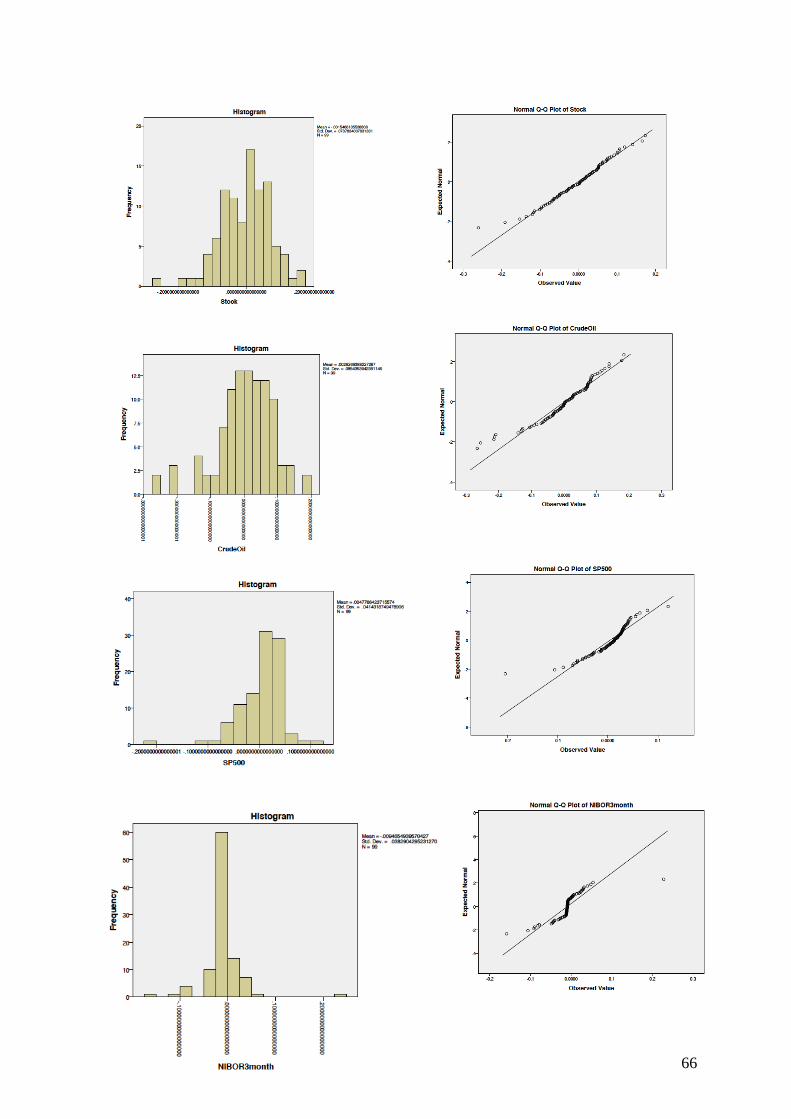
66