
Welcome message from author
This document is posted to help you gain knowledge. Please leave a comment to let me know what you think about it! Share it to your friends and learn new things together.
Transcript

Statistical Mechanics
Dr Alfred Huan

Contents
1 What is Statistical Mechanics? 3
1.1 Key Ideas in the module . . . . . . . . . . . . . . . . . . . . . . . . . . . . 3
1.2 Why do we study Statistical Mechanics? . . . . . . . . . . . . . . . . . . . 4
1.3 Denitions . . . . . . . . . . . . . . . . . . . . . . . . . . . . . . . . . . . . 4
1.3.1 Microstate . . . . . . . . . . . . . . . . . . . . . . . . . . . . . . . . 4
1.3.2 Macrostate . . . . . . . . . . . . . . . . . . . . . . . . . . . . . . . 5
2 Distribution Law 6
2.1 Distribution Law & Ensemble Approaches . . . . . . . . . . . . . . . . . . 6
2.2 Computation of Most Probable Macrostate Distribution, nj . . . . . . . . . 7
2.3 Problems in Derivation of Maxwell-Boltzmann Distribution . . . . . . . . . 11
2.3.1 nj not being always large . . . . . . . . . . . . . . . . . . . . . . . . 11
2.3.2 What about the other macrostates? . . . . . . . . . . . . . . . . . . 11
2.3.3 What happens when we have many energy levels? . . . . . . . . . . 14
2.4 Time Evolution of system of microstates . . . . . . . . . . . . . . . . . . . 15
2.5 Alternative Derivation for Maxwell-Boltzmann Distribution . . . . . . . . . 16
2.6 Examples of Counting in Statistical Mechanics . . . . . . . . . . . . . . . . 17
3 Indistinguishable Particles 20
3.1 Introduction . . . . . . . . . . . . . . . . . . . . . . . . . . . . . . . . . . . 20
3.2 Bose-Einstein Distribution for Bosons . . . . . . . . . . . . . . . . . . . . . 21
3.3 Fermi-Dirac Distribution for Fermions . . . . . . . . . . . . . . . . . . . . 23
3.4 Alternative Derivation for Bose-Einstein and Fermi-Dirac Statistics . . . . 24
4 Statistical Mechanics and Thermodynamic Laws 26
4.1 First Law . . . . . . . . . . . . . . . . . . . . . . . . . . . . . . . . . . . . 26
4.2 Second Law . . . . . . . . . . . . . . . . . . . . . . . . . . . . . . . . . . . 27
4.3 Third Law . . . . . . . . . . . . . . . . . . . . . . . . . . . . . . . . . . . . 29
4.4 Calculation of Other Thermodynamic Variables . . . . . . . . . . . . . . . 30
5 Applications of Maxwell-Boltzmann Statistics 33
5.1 Classical Perfect Gas . . . . . . . . . . . . . . . . . . . . . . . . . . . . . . 33
5.2 Harmonic Oscillator . . . . . . . . . . . . . . . . . . . . . . . . . . . . . . . 39
5.3 Equipartition Theorem . . . . . . . . . . . . . . . . . . . . . . . . . . . . . 40
6 Paramagnetic Systems 42
6.1 Introduction . . . . . . . . . . . . . . . . . . . . . . . . . . . . . . . . . . . 42
6.2 Spin 12Quantum System . . . . . . . . . . . . . . . . . . . . . . . . . . . . 43
6.3 Spin J Quantum System . . . . . . . . . . . . . . . . . . . . . . . . . . . . 45
1

CONTENTS 2
6.4 Adiabatic Cooling . . . . . . . . . . . . . . . . . . . . . . . . . . . . . . . . 49
7 Applications of Fermi-Dirac Statistics 51
7.1 Fermi-Dirac Distribution . . . . . . . . . . . . . . . . . . . . . . . . . . . . 51
7.2 Free Electron Model of Metals . . . . . . . . . . . . . . . . . . . . . . . . . 53
8 Applications of Bose-Einstein Statistics 59
8.1 Introduction to Black Body Radiation . . . . . . . . . . . . . . . . . . . . 59
8.2 Bose-Einstein Distribution . . . . . . . . . . . . . . . . . . . . . . . . . . . 60
8.3 Planck's Radiation Formula . . . . . . . . . . . . . . . . . . . . . . . . . . 61
8.4 Radiation emitted by blackbody . . . . . . . . . . . . . . . . . . . . . . . . 63
9 The Classical Limit 66
9.1 The Classical Regime . . . . . . . . . . . . . . . . . . . . . . . . . . . . . . 66
9.2 Monatomic Gas . . . . . . . . . . . . . . . . . . . . . . . . . . . . . . . . . 67
9.3 Gibbs Paradox . . . . . . . . . . . . . . . . . . . . . . . . . . . . . . . . . 69
10 Kinetic Theory of Gases 71
10.1 Introduction . . . . . . . . . . . . . . . . . . . . . . . . . . . . . . . . . . . 71
10.2 Number of impacts on Area A of a wall . . . . . . . . . . . . . . . . . . . . 73
10.3 Eusion of molecules . . . . . . . . . . . . . . . . . . . . . . . . . . . . . . 74
10.4 Mean Free Path, . . . . . . . . . . . . . . . . . . . . . . . . . . . . . . . 75
10.5 Collision cross-section, . . . . . . . . . . . . . . . . . . . . . . . . . . . . 76

Chapter 1
What is Statistical Mechanics?
1.1 Key Ideas in the module
We begin with the introduction of some important ideas which are fundamental in our
understanding of statistical mechanics. The list of important terms are as follows :
1. Microstate
2. Macrostate
3. Partition Function
4. Derivation of Thermodynamic laws by Statistical Mechanics
5. The idea of interaction
(a) particle (system) - external environment
(b) particle (within a system of many particles)
6. Entropy : Disorder Number
7. Equipartition Theorem : the energies are distributed equally in dierent degrees of
freedom.
8. Temperature
9. Distributions : Maxwell-Boltzmann, Fermi-Dirac, Bose-Einstein
In the 3rd year course, we shall restrict to equilibrium distributions, and static macro-
scopic variables. We will deal with single particle states and no ensembles, weakly inter-
acting particles and the behaviour for distinguishable (degeneracies) and indistinguishable
particles.
3

CHAPTER 1. WHAT IS STATISTICAL MECHANICS? 4
1.2 Why do we study Statistical Mechanics?
We apply statistical mechanics to solve for real systems (a system for many particles).
We can easily solve the Schrodinger's equation for 1 particle/atom/molecule. For many
particles, the solution will take the form :
total = linear combination of a(1) b(2) c(3):::
where a means a particle in state a with an energy Ea.
For example, we consider particles conned in a cubic box of length L. From quantum
mechanics, the possible energies for each particle is :
E =~2
2m
2
L2(n2x + n2y + n2z)
For example in an ideal gas, We assume that the molecules are non-interacting, i.e.
they do not aect each other's energy levels. Each particle contains a certain energy. At T
> 0, the system possesses a total energy,E. So, how is E distributed among the particles?
Another question would be, how the particles are distributed over the energy levels. We
apply statistical mechanics to provide the answer and thermodynamics demands that the
entropy be maximum at equilibrium.
Thermodynamics is concerned about heat and the direction of heat ow, whereas
statistical mechanics gives a microscopic perspective of heat in terms of the structure
of matter and provides a way of evaluating the thermal properties of matter, for e.g., heat
capacity.
1.3 Denitions
1.3.1 Microstate
A Microstate is dened as a state of the system where all the parameters of the con-
stituents (particles) are specied
Many microstates exist for each state of the system specied in macroscopic variables
(E, V, N, ...) and there are many parameters for each state. We have 2 perspectives to
approach in looking at a microstate :
1. Classical Mechanics
The position (x,y,z) and momentum (Px, Py, Pz) will give 6N degrees of freedom
and this is put in a phase space representation.
2. Quantum Mechanics
The energy levels and the state of particles in terms of quantum numbers are used
to specify the parameters of a microstate.

CHAPTER 1. WHAT IS STATISTICAL MECHANICS? 5
1.3.2 Macrostate
A Macrostate is dened as a state of the system where the distribution of particles over
the energy levels is specied..
The macrostate includes what are the dierent energy levels and the number of parti-
cles having particular energies. It contains many microstates.
In the equilibrium thermodynamic state, we only need to specify 3 macroscopic vari-
ables (P,V,T) or (P,V,N) or (E,V,N), where P : pressure, V : Volume, T : Temperature,
N : Number of particles and E : Energy. The equation of state for the system relates the
3 variables to a fourth, for e.g. for an ideal gas.
PV = NkT
We also have examples of other systems like magnetic systems (where we include M, the
magnetization). However, the equilibrium macrostate is unknown from thermodynamics.
In statistical mechanics, the equilibrium tends towards a macrostate which is the most
stable. The stability of the macrostate depends on the perspective of microstates. We
adopt the a priori assumption which states the macrostate that is the most stable con-
tains the overwhelming majority of microstates. This also gives the probabilistic approach
in physics.

Chapter 2
Distribution Law
2.1 Distribution Law & Ensemble Approaches
The distribution law is dependent on how we dene the system. There are three ap-
proaches in dening the system and we adopt the three ensemble approaches.
1. Microcanonical Ensemble : Isolated system with xed energy, E and number of
particles, N.
2. Canonical Ensemble : The system is in a heat bath,at constant temperature with
xed N.
3. Grand Canonical Ensemble : Nothing is xed.
The disorder number, is dened as the number of microstates available to a
macrostate, and is very large for the equilibrium macrostate. The disorder number is
related to entropy, which is maximum at equilibrium.
To enumerate , we need to decide whether the particles are distinguishable or indis-
tinguishable. If they are indistinguishable, every microstate is a macrostate.
Let us now consider independent particles, with energy levels xed and the particles
don't in uence each other's occupation. The energy levels are xed by each particle's in-
teraction with its surroundings but not particle-particle interactions. Mutual interaction
exist only for energy exchange (during collisions).
Each level j has energy "j, degeneracy gj, and occupation nj.
Distinguishability : small and identical particles cannot be distinguished during col-
lisions, i.e. non-localised. However, localised particles are distinguishable because they
are xed in space, the sites being distinguishable e.g. in a paramagnetic solid.
For an isolated system, the volume V, energy E and total number of particles, N are
xed.
6

CHAPTER 2. DISTRIBUTION LAW 7
N =Xj
nj
Total E =Xj
nj"j
The A Priori assumption states that all microstates of a given E are equally probable
thus the equilibrium macrostate must have overwhelming .
Ω
Equilibriumstate
Macrostates
Ω
Equilibriumstate
Macrostates
The disorder number is proportional to thermodynamic probability, i.e. how probable
for a particular macrostate to be the one corresponding to equilibrium.
2.2 Computation of Most Probable Macrostate Dis-
tribution, nj
To nd the nj at equilibrium, i.e. we must nd the most probable macrostate distribution.
Considering the case for distinguishable particles :
1. Enumerate . We distribute N particles over the energy levels: For example,
For the rst level,
The number of ways to assign n1 particles =N !
n1!(N n1)!(2.1)
For the second level,
The number of ways to assign n2 particles =N n1!
n2!(N n1 n2)!(2.2)

CHAPTER 2. DISTRIBUTION LAW 8
Number of ways =N !
n1!(N n1!) N n1!
n2!(N n1 n2)! ::::::
=N !
n1!n2!::::nj !:::::
=N !Qj nj!
(2.3)
Level j has degeneracy gj so any of the nj particles can enter into any of the gj levels.
Number of ways = gnjj (2.4)
For all levels,
Number of ways =Yj
gnjj (2.5)
Total = N !Yj
gnjj
nj!(2.6)
2. Maximise by keeping xed E, N. These constraints are introduced through La-
grange multipliers.
For a xed V, it means that the energy levels,"j are unchanged.
Maximise subject to
Xnj = N
and
Xnj"j = E
At maximum,
d = 0 (2.7)
) d(ln) =1
d
= 0(2.8)
Hence we can choose to maximise ln instead of
ln = lnN ! +Xj
nj ln gj Xj
lnnj! (2.9)
By Stirling's approximation for large N :
lnN ! = N lnN N (2.10)

CHAPTER 2. DISTRIBUTION LAW 9
Proof :
lnN ! =
NX1
lnn
=
Z N
1
lnndn
= [n lnn n]N1
= N lnN N + 1
(2.11)
Or
NX1
lnn4 n =
Z 1
1N
(N lnn
N+N lnN)d(
n
N)
= N [x lnx x]11N
+N lnN(1 1
N)
= N + lnN + 1 +N lnN lnN
= N lnN N + 1
(2.12)
where 4n = d( nN) = dx.
Now we come back to ln
ln N lnN N +Xj
(nj ln gj nj lnnj + nj)
= N lnN +Xj
(nj ln gj njlnnj)
= N lnN +Xj
nj ln(gj
nj)
(2.13)
by assuming large nj also, which is not always true.
d(ln) =Xj
(lngj
njdnj dnj) = 0 (2.14)
It is subjected to the constraints :
Xj
dnj = 0 (for xed N)
Xj
"jdnj = 0 (for xed E)
Note "j does not vary. Therefore
Xj
ln(gj
nj)dnj = 0 (2.15)

CHAPTER 2. DISTRIBUTION LAW 10
Now we introduce the constraints :
Xj
dnj = 0
Xj
"jdnj = 0
so we get Xj
(ln(gj
nj) + "j)dnj = 0 (2.16)
We choose and such that
ln(gj
nj) + "j = 0 (2.17)
The equilibrium macrostate becomes :
nj = gjee"j
=NgjPj gje
"je"j
=Ngj
Ze"j (Maxwell-Boltzmann Distribution)
(2.18)
where z is the partition function
We will prove later that is equal to 1kT
where k is the Boltzmann constant (k =
1:38 1023JK1mol1 ) and T is the temperature.
For "j > "i, we get nj < ni for gj = gi and T > 0
For T = 0, nj = 0, except for n1, i.e. all the particles are at ground state. For T > 0,
the upper levels get piled by particles provided
4" kT (2.19)
Otherwise, the population of upper levels remain small.
In lasers, population inversion leads to negative temperature,
n2
n1=g2e
"2kT
g1e
"1kT
=e
"2kT
e"1kT
> 1
(2.20)
for g1 = g2,
) e"2kT > e
"1kT
"2
kT> "1
kT
"2
T> "1
T
(2.21)
because k > 0.
Since "2 > "1, then T < 0

CHAPTER 2. DISTRIBUTION LAW 11
2.3 Problems in Derivation of Maxwell-Boltzmann
Distribution
There are 2 inherent problems present in the derivation of Maxwell-Boltzmann distribu-
tion :
1. nj is not always large.
2. The other macrostates of the same xed energy E. What are their s? Are they
small enough to be neglected?
The equilibrium distribution ~nj should be weighted against of all possible macrostates
i, so
~nj =
Pj nji(nj)Pji(nj)
(2.22)
The most probable nj (Maxwell-Boltzmann Distribution)
nj =Ngje
"j
kTPgje
"j
kT
(2.23)
2.3.1 nj not being always large
If the total number of levelsP
j 1 is small and T is large enough, then every level j has
many particles so that for large nj. Stirling's approximation can be used.
If many levels exist, the lower levels will have large nj but higher levels will have small
nj. Many of the higher levels will give lnnj! 0. (Note that 0! = 1! = 1).
However, the higher levels contribute very negligibly toP
lnnj! so that we can ap-
proximate again byP(nj lnnj nj) because many of the lower levels have large nj.
2.3.2 What about the other macrostates?
How does the change when we consider other macrostates?
Consider the changes from the most probable macrostate nj to another distribution
nj.
nj = nj + nj (2.24)
Since
ln(nj) = N lnN N Xj
(nj lnnj nj)
= N lnN Xj
nj lnnj(2.25)

CHAPTER 2. DISTRIBUTION LAW 12
Expand about nj,
ln(nj) = N lnN Xj
( nj + nj) ln( nj + nj)
= N lnN Xj
( nj + nj)(ln nj + ln(1 +nj
nj)
= N lnN Xj
( nj + nj)(ln nj +nj
nj 1
2((nj)
2
nj) + ::::)
= N lnN Xj
nj ln nj + nj + nj ln nj +1
2((nj)
2
nj) + :::
= ln( nj)Xj
nj Xj
nj lnnj 1
2
Xj
(nj)2
nj+ ::::
(2.26)
where
nj =N
Ze"jkT
neglecting gj for the purpose of simplifying the discusion.
Now as before,
Xj
nj = 0
andXj
nj"j = 0
Thus,
ln(nj) = ln( nj)Xj
nj(lnN
Z "j
kT) 1
2
Xj
(nj)2
nj+ :::
= ln( nj) lnN
Z
Xj
nj +1
kT
Xj
"jnj 1
2
Xj
(nj)2
nj+ :::
= ln( nj)1
2
Xj
(nj)2
nj+ ::::::
(2.27)
It follows that
(nj) = ( nj)e12
P (nj)2
nj (2.28)
(nj) will be small, if nj pnj.
Since nj are large, the uctuations allowed are very small, by comparison, e.g. if
nj 1020, nj . 1010 for (nj) to be large. Thus nj nj, so the uctuation is minor..
Ultimately, in deriving properties of the system, minor uctuations will not matter very
much.

CHAPTER 2. DISTRIBUTION LAW 13
(i)
(ii)(ii)
Ω
Macrostates
where (i) represents nj nj and (ii) nj large.
Alternatively, we can also argue the problem out by the choice of a fractional deviation
=j(nj)
2j
nj, and we assume is the same for all j. Then,
Xj
(nj)2
nj=Xj
2 nj
= 2N
(2.29)
Hence
(nj) = ( nj)e2N (2.30)
which is small unless 2 . 1N, i.e,
jnjj .njpN< 1 (2.31)
so nj needs to be small in order for (nj) to be signicantly large. In either case, we see
that (nj) will be small when the uctuation nj is large
Now we come back to the total number of macrostates :
The total number of macrostates consistent with constraints :
X ( nj)
Zen21n1 dn1
Zen22n2 dn2:::::::
= ( nj)Yj
( nj)12
(2.32)

CHAPTER 2. DISTRIBUTION LAW 14
Stopping the product when nj = 1
If total number of energy levels, G is very much less than N, then nj NGand j = 1,2,
....., G.
X ( nj)(
N
G)G2 (2.33)
lnX
ln( nj) +G
2lnN G
2lnG (2.34)
Now
ln( nj) N lnN lnN lnG (2.35)
so
lnX
ln( nj) (2.36)
so the most probable microstate has overwhelming .
2.3.3 What happens when we have many energy levels?
If nj 1 for most levels, then we have many energy levels G N . This means that all
macrostates look roughly the same.
The total number of microstates are not mainly due to the maximum term ( nj), i.e.P 6= ( ~nj). Hence Stirling's approximation is invalid in this case.
We resort to the following trick : Energy levels are closely spaced in groups because
G is large. They are grouped into bunches of gi with mi occupation. gi and mi can be
made large in this case.
The energy levelsare so closely spaced such that they aregrouped into bundlesof g levelsi
i = 1
i = 2
firstbundle1 of g1
2nd bundleof g2bundles
bundles
Using the previous derivation by counting ( mi energy states),
mi =Ngie
"ikTP
i gie"jkT
=Ngie
"ikTP
e"j
kT
(2.37)

CHAPTER 2. DISTRIBUTION LAW 15
We take the time average value of nj over a large number of dierent macrostates.
mi =mi
gi
=Ne
"j
kTPj e
"j
kT
(2.38)
( mi) = N !Yi
gmi
i
mi!(2.39)
ln( nj) = lnX
(2.40)
By grouping closely spaced levels, the time-averaged variations are small and the
Maxwell-Boltzmann distribution describes nj very well. Otherwise with nj 1, the
variation at each j level appears large. The treatment tries to obtain the average ni over
many dierent but similar macrostates.
After a series of attack on our fundamental assumptions, we come to establish the ba-
sis of statistical mechanics : All macrostates of signicant probability (i.e. large
) have roughly the same properties and distribution close to the Maxwell-
Boltzmann distribution ignoring minor changes.
2.4 Time Evolution of system of microstates
How many microstates does the system explore within the time for the experiment?
For example, we consider paramagnetic system (where the atomic spins interact with
the external magnetic eld - Zeeman Eect). The particles inside this system (= 1023
particles) are assumed to be non-interacting, and each electron have a spin of 12. We
also x E and T for a xed macrostate i.e. nj. Note in Quantum Mechanics, the energy
levels are discretized. Xk
k:Bk E f(T ) k - each atom
The change in microstates will mean that the spin energy of the electron is exchanged
between neighbouring atoms so the atoms interchange energy levels. The typical time for
spin ip is 1012s. So for 1023 electrons :
The Transition Speed = 1012 1023 = 1035s1
Now, the number of microstates :
eN lnN > e1035
o 1035
So it takes forever to go through all the microstates. Hence, for every experiment, one
can only explore a small proportion of microstates. So we need a statistical assumption
that what we observe corresponds to the real average over all microstates.

CHAPTER 2. DISTRIBUTION LAW 16
2.5 Alternative Derivation for Maxwell-Boltzmann
Distribution
We present an alternative method to derive Maxwell-Boltzmann distribution from the
perspective of equilibrium.
Suppose we change from 1 macrostate to another macrostate, keeping E, V and N
xed. We need a transition from i to k to be accompanied by another transition from j
to l.
k
E
l
Both the transitions from j to l or i to k requires the same amount of energy.
j
E
i
Therefore, the rate
Rij!kl = NiNjTij!kl (2.41)
where Tij!kl is the transition probability.
The total rate out from level i :
Ri out = Ni
Xj;k;l
NjTij!kl (2.42)
The total rate in to level i :
Ri in =Xj;k;l
NkNlTkl!ij (2.43)
At equilibrium,
Ri out = Ri in (2.44)
Therefore it follows that :
Ni
Xj;k;l
NjTij!kl =Xj;k;l
NkNlTkl!ij (2.45)
Now we invoke the time-reversal invariance, which is true for almost all transitions,
Tkl!ij = Tij!kl (2.46)

CHAPTER 2. DISTRIBUTION LAW 17
Thus for every combination i, j, k and l, we require
NiNj = NkNl (Principle of Detailed Balancing) (2.47)
or
lnNi + lnNj = lnNk + lnNl (2.48)
and
"i + "j = "k + "l (2.49)
is required for energy conservation.
Since Ni N("i), both equations will lead to
lnNi = "i + (2.50)
Ni = ee"i (2.51)
which is the Maxwell-Boltzmann Distribution.
2.6 Examples of Counting in Statistical Mechanics
Problem 1 :
Given 6 distinguishable particles, 2 energy levels (one with a degeneracy of 2 and the
other degeneracy of 5). We want to calculate the number of macrostates and microstates
in this system.
First of all, we present a diagramatic scheme of the problem :
g2 = 5
g1 = 2 6 particles
We also note importantly that there are no equilibrium macrostate in this problem be-
cause all the macrostates have dierent total energies.
There are 7 macrostates namely : (6,0), (5,1), (4,2), (3,3), (2,4), (1,5) and (0,6).
Now we come to calculate the microstates :
For (6,0) macrostate,
= 26 ways

CHAPTER 2. DISTRIBUTION LAW 18
For (5,1) macrostate,
=N !
n1!n2!gn11 g
n22
=6!
5!1! 25 5 ways
Subsequently, we can calculate for the remaining macrostates, using the example above.
Problem 2 :
Given 5 energy levels, each separated by E. We consider the particles to be weakly
interacting, i.e. they exchange energy but do not aect each other's energy levels. Let us
look at the rst 3 levels : (i) a particle moves from the 3rd level down to the 2nd level
and (ii) a particle moves from 1st level to the 2nd level. In this case, the change in energy
is balanced by exchange of particles for the 2 processes. Hence we can talk about a xed
macrostate. Now we try to calculate
Now we consider the schematic picture of this problem :
E
E
E
E
Macrostate (5,0,1,0,0), 1 =6 C5 1 C0 1 C1 0 C0 0 C0
= 6 ways
Macrostate (4,2,0,0,0), 2 =6 C4 2 C2 0 C0 0 C0 0 C0
= 15 ways
At equilibrium, we apply the weighted average for microstates, because the number of
microstates in either macrostate is not overwhelming enough.
~nj =
Pnji(nj)P
i
(2.52)
Therefore,
~n1 =5 6 + 4 15
6 + 15
=90
21

CHAPTER 2. DISTRIBUTION LAW 19
~n2 =0 6 + 2 15
6 + 15
=30
21
~n3 =1 6 + 0 15
6 + 15
=6
21
~n4 = 0
~n5 = 0
Note :
Xj
~nj = 6
which is the same asPnj for any macrostate.

Chapter 3
Indistinguishable Particles
3.1 Introduction
Why are particles indistinguishable?
This is a quantum mechanical eect. The exchange of quantum particles cannot be
detected. The 's of the individual particles combine to form a total , and they are
non-localised.
We can write a many particle wavefunction as a linear combination of a(1) b(2)::::::
plus all the possible permutations. For example, for three particle permutations, we get
six possibilities :
a(2) b(1) c(3):::::
a(2) b(3) c(1):::::
a(1) b(3) c(2):::::
etc.
All particles are identical so all permutations are solutions to Schrodinger's equations,
and so are all linear combination of the permutations.
There are two physically meaningful solutions.
1. Symmetric :
s =Xp
P [ (1; 2; ::::; N)] (3.1)
E.g. for 3 particles, we get
s = a(1) b(2) c(3) + a(2) b(1) c(3) + a(3) b(2) c(1)
+ a(1) b(3) c(2) + a(2) b(3) c(1) + a(3) b(1) c(2)
2. Antisymmetric
a =Xp
(1)pP [ (1; 2; :::::; N)] (3.2)
20

CHAPTER 3. INDISTINGUISHABLE PARTICLES 21
where P is the permutation operator; (1)P means (1) every time we exchange
two particle states.
E.g., for 3 particles, we get
s = a(1) b(2) c(3) a(2) b(1) c(3) a(3) b(2) c(1)
a(1) b(3) c(2) + a(2) b(3) c(1) + a(3) b(1) c(2)
If we exchange 1 and 2, then a(2; 1; 3) = a(1; 2; 3)
There are two kinds of quantum particles in nature:
1. Bosons : Symmetric wavefunctions with integral spins.
2. Fermions : Anti-symmetric wavefunctions with half-integral spins.
Note when 2 fermions are in the same state, total is zero. For example, a = b, mean-
ing all permutations cancel in pairs, and hence we obtain Pauli's Exclusion Principle.
3.2 Bose-Einstein Distribution for Bosons
There is no limit to the occupation number at each level of quantum state. In fact, the
more the better. Note that = 1 for all macrostates because of the indistinguishability
of particles. (Macrostates Microstates)
Unless g >> 1 for some levels, for example, by the clumping of levels together to make gilarge. We can then count microstates ( >> 1) because the states in i are distinguishable.
To put mi particles in gi states, imagine arranging mi particles into gi states, by ar-
ranging mi identical particles and gi1 identical barriers on a straight line.
etc.
The number of ways =(mi + gi 1)!
mi!(gi 1)!(3.3)
Therefore,
=(mi + gi 1)!
mi!(gi 1)!(3.4)
To maximise subject to the constraints :
Xi
mi = N
Xi
mi"i = E

CHAPTER 3. INDISTINGUISHABLE PARTICLES 22
Therefore,
ln =Xi
[ln(mi + gi 1)! lnmi! ln(gi 1)!]
Xi
[(mi + gi 1) ln(mi + gi 1) (mi + gi 1)mi lnmi +mi (gi 1) ln(gi 1) (gi 1)
Xi
[(mi + gi) ln(mi + gi)mi lnmi gi ln gi]
(3.5)
for gi; mi 1
d(ln) =Xi
dmi ln(mi + gi) + dmi dmi lnmi dmi = 0 (3.6)
Xi
(lnmi + gi
mi
)dmi = 0 (3.7)
Add in :
Xi
dmi = 0
Xi
"idmi = 0
So
Xi
(ln(mi + gi
mi
) + "i)dmi = 0 (3.8)
Then,
mi + gi
mi
= ee"i (3.9)
Therefore,
mi =gi
ee"i 1(3.10)
where = 1kT
(to be proved later).
Averaging over the gi levels in each clump,
nj =1
ee"j 1(3.11)
which is the Bose-Einstein Distribution.
We will nd later that =
kTwhere is the chemical potential. Two systems at ther-
modynamic equilibrium have the same temperature T. The systems at chemical (particle
number) equilibrium have the same .

CHAPTER 3. INDISTINGUISHABLE PARTICLES 23
3.3 Fermi-Dirac Distribution for Fermions
In this case, we allow 0 or 1 particle to each quantum state.
Now we clump the energy levels to produce gi states and mi (<< gi).
etc...
Either there is a particle or no particle in each quantum state.
Number of ways to ll mi boxes out of gi =gi
mi!(gi mi)!(3.12)
Therefore
=Yi
gi
mi!(gi mi)!(3.13)
To maximise subject to the constraints :Xi
mi = N
Xi
mi"i = E
Therefore,
ln Xi
gi ln gi mi lnmi (gi mi) ln(gi mi) (3.14)
where gi >> mi >> 1
d ln =Xi
dmilnmi dmi + dmi ln(gi mi) + dmi
=Xi
ln(gi mi
mi
)dmi
= 0
(3.15)
Now we add in :
Xi
dmi = 0
Xi
"idmi = 0
So Xi
(ln(gi mi
mi
) + "i)dmi = 0 (3.16)

CHAPTER 3. INDISTINGUISHABLE PARTICLES 24
Then,
gi mi
mi
= ee"i (3.17)
Therefore,
mi =gi
ee"i + 1(3.18)
Averaging over the gi levels in each clump,
nj =1
ee"j + 1(3.19)
which is the Fermi-Dirac Distribution.
Note :
1) The positive sign in Fermi-Dirac distribution implies that nj 1 which is Pauli
Exclusion principle (which states that no 2 fermions can share the same quantum state).
2) IfPnj = N is not a constraint, is zero and this is true for open systems. For
isolated systems with xed N, has a value.
3.4 Alternative Derivation for Bose-Einstein and Fermi-
Dirac Statistics
For equilibrium consideration, Tij!kl is the transition rate from i ! k accompanied by
j ! l to maintain energy conservation.
Suppose the rate depends on the occupation at k and l,
Riout = Ni
Xj;k;l
NjTij!kl(1Nk)(1Nl) (3.20)
Riin =Xj;k;l
NkNlTkl!ij(1Ni)(1Nj)
= (1Ni)Xj;k;l
NkNlTkl!ij(1Nj)(3.21)
At equilibrium,
Ni
Xj;k;l
NjTij!kl(1Nk)(1Nl) = (1Ni)Xj;k;l
NkNlTkl!ij(1Nj) (3.22)
Applying time-reversal invariance,
Tij!kl = Tkl!ij (3.23)

CHAPTER 3. INDISTINGUISHABLE PARTICLES 25
Then for every combination i, j, k, l, we need
NiNj(1Nk)(1Nl) = NkNl(1Ni)(1Nj) (3.24)
So
Ni
1Ni
Nj
1Nj
=Nk
1Nk
Nl
1Nl
(3.25)
lnNi
1Ni
+ lnNj
1Nj
= lnNk
1Nk
+ lnNl
1Nl
(3.26)
with
"i + "j = "k + "l (3.27)
which is the conservation of energy. Therefore
lnNi
1Ni
= "i (3.28)
then,
Ni
1Ni
= ee"i (3.29)
Ni Niee"i = ee"i (3.30)
Ni =1
ee"i 1(3.31)
So starting with the positive (+) sign, we obtain
Ni =1
ee"i + 1Fermi-Dirac Distribution (3.32)
and with the negative (-) sign, we obtain
Ni =1
ee"i 1Bose-Einstein Distribution (3.33)
For fermions, the rate Riout / (1 Nk)(1 Nl) which demostrates Pauli's Exclusion
Principle, and for bosons, the rate Riout / (1 +Nk)(1Nl), i.e. the more particles in k
and l, the more likely the transition. (The more you have, the more you receive).

Chapter 4
Statistical Mechanics and
Thermodynamic Laws
4.1 First Law
The First law of Thermodynamics :
dU = dQ+ dW (4.1)
In Statistical Mechanics :
Total Energy; E = U =Xj
nj"j (4.2)
Therefore
dU =Xj
"jdnj +Xj
njd"j (4.3)
Now, we have dW = PdV or 0Hdm etc. This occurs when there is a change in the
boundary conditions (V, M, etc). When the boundary conditions change, the energy lev-
els change.
For example : particle in a box
"j =~22
2m
1
V23
(n2x + n2y + n2z) (4.4)
Hence
dW =Xj
njd"j (4.5)
So, e.g.
P =Xj
nj@"j
@V(4.6)
or
0H =Xj
nj@"j
@m(4.7)
26

CHAPTER 4. STATISTICAL MECHANICS AND THERMODYNAMIC LAWS 27
dW Original dQ
Then dQ=P"jdnj which takes place by rearrangement in the distribution.
In kinetic theory, the particles may collide with the chamber walls and acquire more
energy where the walls are hotter (with more heat added).
4.2 Second Law
We now search for a microscopic explanation for S in terms of . We start from the TdS
equation :
TdS = dU + PdV dN (4.8)
so
S f(E; V;N) (4.9)
Also
g(E; V;N) (4.10)
Note : In adiabatic changes, for example, volume increase with no heat added (dQ = 0).
dS = 0 i.e. S is constant.Also dnj = 0 so is also constant.
During irreversible changes, the total S in the Universe increases. The total of the
Universe also increases because the equilibrium macrostate must be the maximum .
Now we consider 2 systems with entropy S1 and S2 and disorder number 1 and 2,
Total entropy,S = S1 + S2 (4.11)
Total = 12 (4.12)
Now
S f() (4.13)
so S1 = f(1) and S2 = f(2), Now
f(12) = f(1) + f(2) (4.14)

CHAPTER 4. STATISTICAL MECHANICS AND THERMODYNAMIC LAWS 28
Then
@f(12)
@1
=@f(12)
@(12)2 =
@f(1)
@1
(4.15)
So
@f()
@2 =
@f(1)
@1
(4.16)
Also
@f(12)
@2
=@f()
@1 =
@f(2)
@2
(4.17)
Then
1
2
@f(1)
@1
=1
1
@f(2)
@2
(4.18)
1
@f(1)
@1
= 2
@f(2)
@2
= k (4.19)
where k is a constant by separation of variables.
So
S1 = f(1) = k ln1 + C (4.20)
S2 = f(2) = k ln2 + C (4.21)
S = k ln1 + k ln2 + C
= S1 + S2(4.22)
which implies that C = 0.
Therefore
S = k ln (4.23)
where k is the Boltzmann constant RNA
. (To be proven later)
Hence we have a microscopic meaning of entropy. The system is perfectly ordered when
= 1 and S = k ln = 0. When more microstates are availiable > 1 so S > 0. The
lesser the knowledge about a system, the more disordered it gets.
From the formula which we obtained for the relation of entropy with , we are unable
to deduce the value of k. The value of k comes out from the ideal gas equation.

CHAPTER 4. STATISTICAL MECHANICS AND THERMODYNAMIC LAWS 29
4.3 Third Law
As the temperature T tends to zero, the contribution to the entropy S from the system
components also tend to zero. When all the particles take the ground state, (E0) =
1. When the macrostate has only one microstate, it implies that there are no further
permutations for the Maxwell-Boltzmann distribution.
S = k log(E0) = 0
Practically, some small interactions (e.g. nuclear paramagnetism) may lift the ground
state degeneracy. If kT > "int, then S 6= 0 at a given T. Hence we can only say S ! S0as T ! 0 where S0 is the entropy associated with the remaining small interactions for
which "int < kT and independent of all the entropy for all the other interactions (degrees
of freedom).
The atoms occupyingin the ground stateare placed in fixed positionin a lattice like this.
Note that it is meaningless to talk about the exchange of particles in the same state
because they do not exchange their positions.
We know from the 2nd law of thermodynamics that heat passes from hot (high temper-
ature) to cold (low temperature) if no work is done. The internal energy U(T) increases
when T increases. Now we come to the formulation of the third law :
The Third Law of Thermodynamics states that as the temperature T ! 0, the
entropy S ! 0, it is approaching ground state as U(T) also approaches 0, ) that the
disorder number tends to 1.
From the third law, T=0 is a theoretically correct statement, but it is an impossibility.
Why is this so?
The answer :
There exists very small interactions in the nucleus, made up of magnetic moments,
quadrapole moments and octapole moments etc. In order to make T = 0, the magnetic
moments are required to point in the same direction. However, experimentally, this is not
achievable.
The third law of thermodynamics can also be understood in a quantum mechanical

CHAPTER 4. STATISTICAL MECHANICS AND THERMODYNAMIC LAWS 30
perspective as the freezing out of interactions. By the Schrodinger equation :
~2
2m
@2
@x2+ V () = H
The V() consists of many interaction terms. Hence we can approach the total entropy,
S as a combination of entropies of many sub-systems :
S = Stotal 1 + Stotal 2 + Stotal 3
4.4 Calculation of Other Thermodynamic Variables
From chapter 2, the Partition function Z is dened as :
Z =Xj
gje"j
kT (4.24)
where j represents all levels.
Now we try to nd the relation between P and T, when 2 systems are in thermal equilib-
rium, where will be the same. The depends on the nature of the particles and volume
V etc. For the system of same identical particles, free exchange of particles will allow
to reach the same value. Now we proceed to calculate the other thermodynamic variables.
@Z
@jV;N =
Xj
"jgje"j (4.25)
where
=1
kT
which is proven in tutorial.
We also dene the internal energy, U (or E)
U =Xj
nj"j
=N
Z
Xj
gje"j"j
= NZ
@Z
@jV;N
(4.26)
Since,
d
dT= 1
kT 2

CHAPTER 4. STATISTICAL MECHANICS AND THERMODYNAMIC LAWS 31
and
1
Z@Z = @(lnZ)
therefore,
U = N @ lnZ
@jV;N
= NkT 2@ lnZ
@TjV;N
(4.27)
We know that
nj =N
Zgje
"j
) gj
nj=Z
Ne"j
Then we work out ln ,
ln = N lnN ! +Xj
(nj ln gj lnnj!)
= N lnN N +Xj
(nj ln(gj
nj) + nj)
= N lnN + (Xj
nj"j) +N lnZ N lnN
= U +N lnZ
(4.28)
Therefore
S = k ln
= kU +Nk lnZ
=U
T+Nk lnZ
(4.29)
The Helmholtz free energy, F is dened as :
F = U TS (4.30)
Therefore
F = NkT lnZ (4.31)
Since
dF = dU TdS SdT
= TdS PdV TdS SdT
= SdT PdV
(4.32)

CHAPTER 4. STATISTICAL MECHANICS AND THERMODYNAMIC LAWS 32
From the chain rule
dF = (@F
@V)TdV + (
@F
@T)V dT
Therefore, we can calculate :
Pressure :
P = (@F@V
)T
= NkT (@ lnZ
@V)T
(4.33)
Entropy :
S = (@F@T
)V
= Nk lnZ +NkT
Z
@Z
@T
= Nk lnZ +U
T
(4.34)
Then we can use the results above to compute the heat capacity at constant volume :
Cv = (@U
@T)V (4.35)

Chapter 5
Applications of Maxwell-Boltzmann
Statistics
5.1 Classical Perfect Gas
To apply the Maxwell-Boltzmann Statistics to the classical perfect gas, we require a few
conditions :
1. The gas is monatomic, hence we consider only the translational kinetic energy (KE).
2. There is no internal structure for the particles, i.e. no excited electronic states and
the paricles are treated as single particles.
3. There is no interaction with external elds, e.g. gravity, magnetic elds.
4. The energy is quantized as in the case of particle in a box (in QM).
5. There is a weak mutual interaction - only for exchanging energy between particles
and establishing thermal equilibrium, but there is no interference on each other's
"j.
6. The discrete levels can be replaced by a continuous one if the spacing is small as
compared to T, i.e. " kT which is the classical limit.
7. The atoms are pointlike - occupying no volume.
From quantum mechanics,
"j =~22
2mL2(n2x + n2y + n2z)
for V = L3 and where nx, ny and nz are integers.
33

CHAPTER 5. APPLICATIONS OF MAXWELL-BOLTZMANN STATISTICS 34
Now we compute the partition function, Z and in this case gj = 1, because all the
states are summed over.
Z =Xj
e"j
kT
=Xnx
Xny
Xnz
e~22
2mkTL2(n2x+n
2y+n
2z)
=Xnx
e~
22
2mkTL2n2xXny
e~
22
2mkTL2n2yXnz
e~
22
2mkTL2n2z
=
Z 1
0
dnxe~
22
2mkTL2n2x
Z 1
0
dnye~
22
2mkTL2n2y
Z 1
0
dnze~
22
2mkTL2n2z
(5.1)
To evaluate the integral :
Let x = (~222mL2kT
)12nx
Z 1
0
e~22n2x
2mL2kT dnx = (2mL2kT
~22)121
2
Z 1
1
ex2
dx
= L(2mkT
h2)12
Z 1
1
ex2
dx
(5.2)
where Z 1
1
ex2
dx = (
Z 1
1
ex2
dx
Z 1
1
ey2
dy)12
= (
Z 1
1
Z 1
1
e(x2+y2)dxdy)
12
= (
Z 1
0
rdr
Z 2
0
der2
)12
= (1
22)
12
=p
(5.3)
Therefore
Z = L3(2mkT
h2)32
= V (2mkT
h2)32
(5.4)
lnZ = lnV +3
2lnT +
3
2ln2mk
h2(5.5)
So,
P = NkT (@ lnZ
@V)T
=NkT
V
(5.6)

CHAPTER 5. APPLICATIONS OF MAXWELL-BOLTZMANN STATISTICS 35
i.e. PV = NkT
since
PV = nRT
Nk = nR
k =n
NR
k =R
NA
(5.7)
because Nn= NA molecules per mole
U = NkT 2(@ lnZ
@T)V
= NkT 2 3
2
1
T
=3
2NkT
(5.8)
For each atom,
U =3
2kT
Also the entropy is given by :
S =U
T+Nk lnZ
=3
2Nk +
3
2Nk ln(
2mk
h2) +Nk(lnV +
3
2lnT )
(5.9)
Therefore, the distribution becomes :
nj =N
Ze"j
kT
=Nh3
V (2mkT )32
e"j
kT
(5.10)
where j represent all nx, ny and nz states.
The number of particles having energies between " and "+" :
n =Nh3
V (2mkT )32
e"kTdn
d"" (5.11)
where dn
d"is the density of states, i.e degeneracy dn
d"".
To calculate the density of states, we consider the quantum numbers nx, ny and nzmaking up the grid points with each grid point representing one state.

CHAPTER 5. APPLICATIONS OF MAXWELL-BOLTZMANN STATISTICS 36
By writing
R2 = n2x + n2y + n2z
The number of points (states) with energy up to "R lie within a sphere of volume 43R3.
Only positive n's are allowed so we take the positive octant.
The number of states lying between energy " and "+" will become :
dn
d"" =
1
8(4R2)R
=1
8(4R2)
dR
d""
(5.12)
Using
" =~22
2mL2R2
we obtain,
d"
dR=
~22
mL2R
Therefore,
dn
d"" =
2RmL2
~22"
=
4
(2m)32L3
~33"12"
= 2V(2m
32
)
h3"12"
(5.13)
Therefore,
n =V Nh3e
"kT
(2mkT )32
2v(2m)
32
h3"12"
=N"
12 e
"kTp
4(kT )
32
"
(5.14)
For the momentum distribution, we use :
" =p2
2m
and
d"
dp=
p
m

CHAPTER 5. APPLICATIONS OF MAXWELL-BOLTZMANN STATISTICS 37
So, the number of particles have momentum between p and p + p is :
n =Np
4(kT )
32
pp2m
ep2
2mkTd"
dpp
=N
(2mkT )32
4ep2
2mkT p2p
(5.15)
Note that ZZZall p space
dpxdpydpz =
Z 2
0
dp
Z
0
sin pdp
Z 1
0
p2dp
=
Z 1
0
4p2dp
(5.16)
Therefore we can also express in px, py and pz as
n =N
(2mkT )32
ep2
2mkT pxpypz
=N
(2mkT )32
ep2x+p
2y+p
2z
2mkT pxpypz
=N
(2mkT )32
ep2x
2mkT pxe
p2y
2mkT pye
p2z2mkT pz
(5.17)
For velocity distribution, we use p = mv,
n = f(vx; vy; vz)dvxdvydvz
=Nm3
(2mkT )32
em(v2x+v
2y+v
2z)
2kT vxvyvz
= g(v)dv
=Nm34
(2mkT )32
em(v2)
2kT v2dv
(5.18)
which are the Maxwell distribution laws for velocities and speeds.
We invoke a few integral identities :
In =
Z 1
0
ex2
xndx
I0 =
p
2
I1 =1
2
I2 =1
2I0
I3 = I1
I4 =3
2I2

CHAPTER 5. APPLICATIONS OF MAXWELL-BOLTZMANN STATISTICS 38
So,
Z 1
0
g(v)dv =Nm34
(2mkT )32
(2kT
m)32
Z 1
0
ex2
x2dx
= N
(5.19)
The mean speed, v
v =1
N
Z 1
0
vg(v)dv
=m34
(2mkT )32
(2kT
m)2Z 1
0
ex2
x3dx
=
r8kT
m
(5.20)
and mean square speed is
v2 =1
N
Z 1
0
v2g(v)dv
=m34
(2mkT )52
Z 1
0
ex2
x4dx
=3kT
m
(5.21)
Average energy,1
2m v2 =
3
2kT (5.22)
Root mean square (RMS) speed,p
v2 =
r3kT
m> v (5.23)
The most probable speed :
dg(v)
dv= 0) 2vpe
mv2
2kT mv3p
kTemv2
2kT = 0
) vp =
r2kT
m
(5.24)

CHAPTER 5. APPLICATIONS OF MAXWELL-BOLTZMANN STATISTICS 39
V
TVp V
Maxwell Distribution of Molecular Speeds
V2
vp < v <p
v2
5.2 Harmonic Oscillator
We now consider the simple 1-D harmonic oscillator in equilibrium at T, with the
Hamiltonian, H =p2
2m+1
2k0x
2
"j = (j +1
2)~!
where j = 0,1,2,.....
! =
rk0
m
Assume the oscillators are independent and distinguishable,
nj =N
Ze"jkT
Z =
1Xj=0
e(j+1
2)~!
kT
= e~!2kT
1Xj=0
ej~!
kT
= e~!2kT
1
1 e~!kT
= e~!
21
1 e~!
(5.25)

CHAPTER 5. APPLICATIONS OF MAXWELL-BOLTZMANN STATISTICS 40
Note : for a series of a, ar, ar2,.......
1Xn=0
arn =a
1 r
lnZ = 1
2~! ln(1 e~!) (5.26)
U = N @lnZ
@
=1
2N~! +
N
1 e~!~!e~!
= N~![1
2+
1
e~! 1]
= N~![1
2+
1
e~!kT 1
]
(5.27)
At low T, U 12N~!, it means that the oscillators are in ground state.
At high T,
U = N~![1
2+
1
1 + ~!
kT+ ::: 1
]
= N~![1
2+kT
~!]
= NkT
(5.28)
which is the classical result.
The high energy states are occupied. Quantization is not important for kT >> "(=
~!)
5.3 Equipartition Theorem
The Equipartition theorem states that all terms in the Hamiltonian with squared co-
ordinates (x or px etc) will contribute 12kT to the average energy, provided quantization
is not important. This is re ected in the classical regime at high T (where kT >> "int.
Example 1 : Ideal Gas,
H = kinetic energy only
=p2x2m
+p2y
2m+
p2z2m
Therefore
U =3
2kT N atoms
=3
2NkT

CHAPTER 5. APPLICATIONS OF MAXWELL-BOLTZMANN STATISTICS 41
Example 2 : 1-D Harmonic Oscillator,
H = Kinetic energy + Potential energy
=p2x2m
+1
2k0x
2
Therefore
U = kT N atoms
= NkT
With quantization setting in at low T, the Hamiltonian is frozen out and the contribution
is not 12kT.
Example 3 : Diatomic gas,
For translational motion,
Htrans =p2x2m
+p2y
2m+
p2z2m
For rotational motion,
Hrot =1
2
L2x
Ix+1
2
L2y
Iy
neglecting rotation about z-axis.
For vibrational motion,
Hvib =p02z
2m+1
2k0z
02
where z' is the relative coordinate between the 2 atoms.
Therefore, the total internal energy, U should be 72NkT. However, the experimental
results show that U = 52NkT.
The reason is because the vibrational motion is frozen out, i.e. ~!vib >> kT. So in
terms of Hvib, the atoms are in ground state, i.e. atoms don't appear to vibrate much at
normal temperature.
Total H = Hvib +Htrans +Hrot (5.29)

Chapter 6
Paramagnetic Systems
6.1 Introduction
For a paramagnetic spin system, the atoms have unpaired electrons or partially lled
orbitals. The net angular momentum ~J for each atom is equal to both the linear orbital
angular momentum, ~L and spin, ~S. It also acts like the magnetic moment.
J = gJBJ (6.1)
When the system interacts with an external magnetic eld,
Hamiltonian, H = ~ ~B= gJB ~B ~J= gJBBzJz (Quantization)
(6.2)
The Jz and J are observed from atomic physics.
B =e~
2mc(Bohr Magneton)
In a solid, the outer electrons are involved in valency for chemical bonds, which are ulti-
mately paired up so that the net J of outer electrons is zero. The inner core, particularly
3d, 4d and 4f orbitals of many elements are not involved in valency, so magnetism arises
from their S, L and J.
In many solids of transition elements (3d), the orbital quenching occurs, so that the
net L = 0 for atoms in the ground electronic state. Note that the excited electronic states
are unoccupied at room temperature because " >> kT .
Hence in the ground electronic state of 3d elements, there is a degeneracy of (2S + 1)
states. Note that J = S.
42

CHAPTER 6. PARAMAGNETIC SYSTEMS 43
Applying B-eld to a spin 32system :
3
1
-1
-3
2
2
2
2
B 0
For example,
S = 3/2 system
Hamiltonian, H = gsBBSz (6.3)
and gs 2 for electron spin.
The distribution in the spin states is associated with the spin temperature TS which
may not be the same as the lattice temperature TL. A mechanism must exist for TS and
TL to establish thermal equilibrium - spin-phonon interaction. This is important in spin
resonance experiments such as electron spin resonance and nuclear magnetic resonance,
and determines the relaxation time .
6.2 Spin 12Quantum System
We consider the system of N magnetic atoms of spin 12due to 1 unpaired electron.
The magnetic moment, = gsBSz
= 1
2gsB
(6.4)
The Zeeman interaction with external eld gives energy levels
gsBBzSz = 1
2gsBB (6.5)
where gs 2 and B is the Bohr magneton.
The energies correspond to spin # ( antiparallel to B) or spin " ( parallel to B).

CHAPTER 6. PARAMAGNETIC SYSTEMS 44
So
"" = 1
2gsBB (6.6)
"# = +1
2gsBB (6.7)
Using the Maxwell-Boltzmann distribution,
n" =N
Ze+
gsBB
2kT (6.8)
n# =N
Ze
gsBB
2kT (6.9)
where
Z = e+gsBB
2kT + egsBB
2kT
= 2 cosh(gsBB
2kT)
(6.10)
Therefore, the total energy, E :
E =N
Z(1
2gsBBe
+gsBB
2kT +1
2gsBBe
gsBB
2kT )
= NgsBBZ
(sinh(gsBB
2kT))
= NgsBBZ
(tanh(gsBB
2kT))
(6.11)
The entropy S :
S =U
T+Nk lnZ
= NgsBBT
(tanh(gsBB
2kT)) +Nk ln(2 cosh(
gsBB
2kT))
(6.12)
The magnetization M :
M =1
V
Xj
njj
=N
V Z
Xje
+jB
kT
=N
V Z[1
2gsBe
gsBB
2kT 1
2gsBe
gsBB
2kT
=N
V ZgsB sinh(
gsBB
2kT)
=1
2
N
VgsB tanh(
gsBB
2kT)
= E
BV
(6.13)
where " = B

CHAPTER 6. PARAMAGNETIC SYSTEMS 45
6.3 Spin J Quantum System
Now we consider a system with total angular momentum J in an external B-eld.
0
B=0 B
+J
+(J-1)
-(J-1)
-J
mJ = J;(J 1); ::::::; 0; 1; ::::; (J 1); J
Therefore there are (2J + 1) states.
"J = gJBBmJ (6.14)
where gJ is the Lande g-factor (an experimental quantity).
Let
y = gJBB
Therefore, the partition function,
Z =
JXmJ=J
egJBB
=
JXmJ=J
eymJ
= eyJ2JX
mJ=0
eymJ
= (eyJ)e(2J+1)y 1
ey 1(G.P sum =
a(rn 1)
r 1)
=e(J+1)y eJy
ey 1
=e(J+
12)y e(J+
12)y
e12y e
12y
=sinh(J + 1
2)y
sinh y
2
(6.15)

CHAPTER 6. PARAMAGNETIC SYSTEMS 46
Therefore,
nJ =N
Ze"J
=N
ZegJBBmJ
(6.16)
Then
Magnetization, M =N
V Z
XgJBmJe
gJBBmJ
=N
V Z
1
@Z
@B
=N
V Z
1
@Z
@y
@y
@B
=N
V ZgJB
@Z
@y
=N
VgJB
@ lnZ
@y
(6.17)
lnZ = ln(sinh(J +1
2)y) ln(sinh
y
2) (6.18)
M =N
VgJB(
(J + 12) cosh(J + 1
2)y
sinh(J + 12)y
12cosh y
2
sinh y
2
)
=N
VgJB((J +
1
2) coth(J +
1
2)y 1
2coth
y
2)
=N
VgJBJBJ(y)
(6.19)
where
BJ(y) =1
J[(J +
1
2) coth(J +
1
2)y 1
2coth
y
2] Brillouin function (6.20)
We proceed to evaluate other thermodynamic quantities :
Helmholtz free energy, F = NkT lnZ
= NkT [ln(sinh(J +1
2)y) ln(sinh
y
2)]
(6.21)
Internal energy, U = N @ lnZ
@
= N @ lnZ
@y
@y
@
= NgJBBJBJ(y)
(6.22)

CHAPTER 6. PARAMAGNETIC SYSTEMS 47
Entropy, S =U
T+NK lnZ
= NgJBBJBJ(y)
T+Nk[ln(sinh(J +
1
2)y) ln(sinh
y
2)]
(6.23)
At high T, y << 1, and for small x,
coth x =ex + ex
ex ex
=e2x + 1
e2x 1
= (1 + 2x+4x2
2+ :::: + 1)(1 + 2x +
4x2
2+8x3
3!+ ::::: 1)1
=1
2x(2 + 2x + 2x2 + ::::)(1 + x+
2x2
3+ :::)
=1
x(1 + x + x2 + :::)(1 (x+
2x2
3+ :::) + (x +
2x2
3:::::)2::::)
=1
x(1 + x x+ x2 x2 x2
3+ 2::::)
=1
x(1 +
x2
3+ :::::)
=1
x+x
3
(6.24)
So,
BJ(y) =1
J[(J +
1
2)(
1
(J + 12)y
+(J + 1
2)y
3) 1
2(1y
2
+y
2
3)]
=1
J[1
y+(J + 1
2)2y
3 1
y y
12]
=1
3J[(J2 + J)y]
=y
3(J + 1)
(6.25)
Therefore,
M =N
VgJBJ(J + 1)
y
3
=N
V
g2J2BJ(J + 1)B
3kT
(6.26)
so,
= 0(@
@B)T
=N
V
g2J2B0J(J + 1)
3kT
/ 1
T(Curie's law)
(6.27)

CHAPTER 6. PARAMAGNETIC SYSTEMS 48
Since,
U = NgJBBJ(J + 1)y
3! 0
Since,
lnZ ln(2J + 1) (6.28)
Proof :
lnZ = lne(J+
12)y e(J+
12)y
2
= ln[e(J+12)y e
(J+ 12)2y 1
2 ln[e
y
2ey 1
2]
= (J +1
2)y + ln(
1 + (J + 12)2y + ::: 1
2) +
y
2 ln(
1 + y + :::: 1
2
= Jy + ln[(J +1
2)y + ::::] ln[
y
2+ ::]
= Jy + ln(2J + 1)
ln(2J + 1)
(6.29)
or
lnZ = ln[(1 + (J + 1
2)y + ::::) (1 (J + 1
2+ :::)
2] ln[
(1 + y
2+ :::) (1 y
2+ :::)
2]
= ln(J +1
2)y ln
y
2= ln(2J + 1)
(6.30)
Then
S = Nk ln(2J + 1) (6.31)
for (2J + 1) levels.
At low T, y >> 1, and for large x,
coth x =ex + ex
ex ex= 1
So,
BJ(y) =1
J[J +
1
2 1
2] = 1 (6.32)
Therefore
M =N
VgJBJ (6.33)
where all spins are align in the same direction (parallel to B), hence ! 0.

CHAPTER 6. PARAMAGNETIC SYSTEMS 49
lnZ = ln(e(J+
12)y e(J+
12)y
2) ln(
ey
2 ey
2
2)
= (J +1
2)y + ln
1
2 y
2 ln
1
2= Jy
(6.34)
Internal energy, U = NgJBBJ (6.35)
Entropy, S =NgJBBJ
T+NkJy = 0 (6.36)
6.4 Adiabatic Cooling
From the third law, S ! 0 as T ! 0, so cooling reduces the entropy of system, so we
need magnetic dipoles to align in one direction.
But alignment can also be produced with a B-eld, so we need the alignment to stay
as we reduce the B-eld to zero.
So adiabatic cooling is two-staged.
1. Reduce the entropy by turning on the B-eld isothermally.
The paramagnetic system is in contact with the lattice and the heat bath. As B-eld
increases, dipoles align more and energy and entropy is taken out from the system.
Ts
Spin System
T L
LatticeHeat Bath
at constant T
Heat flow
dQTsEntropy passed to lattice and heat bath =
2. Reduce the temperature by turning o the B-eld adiabatically, i.e. isolated from
heat bath.
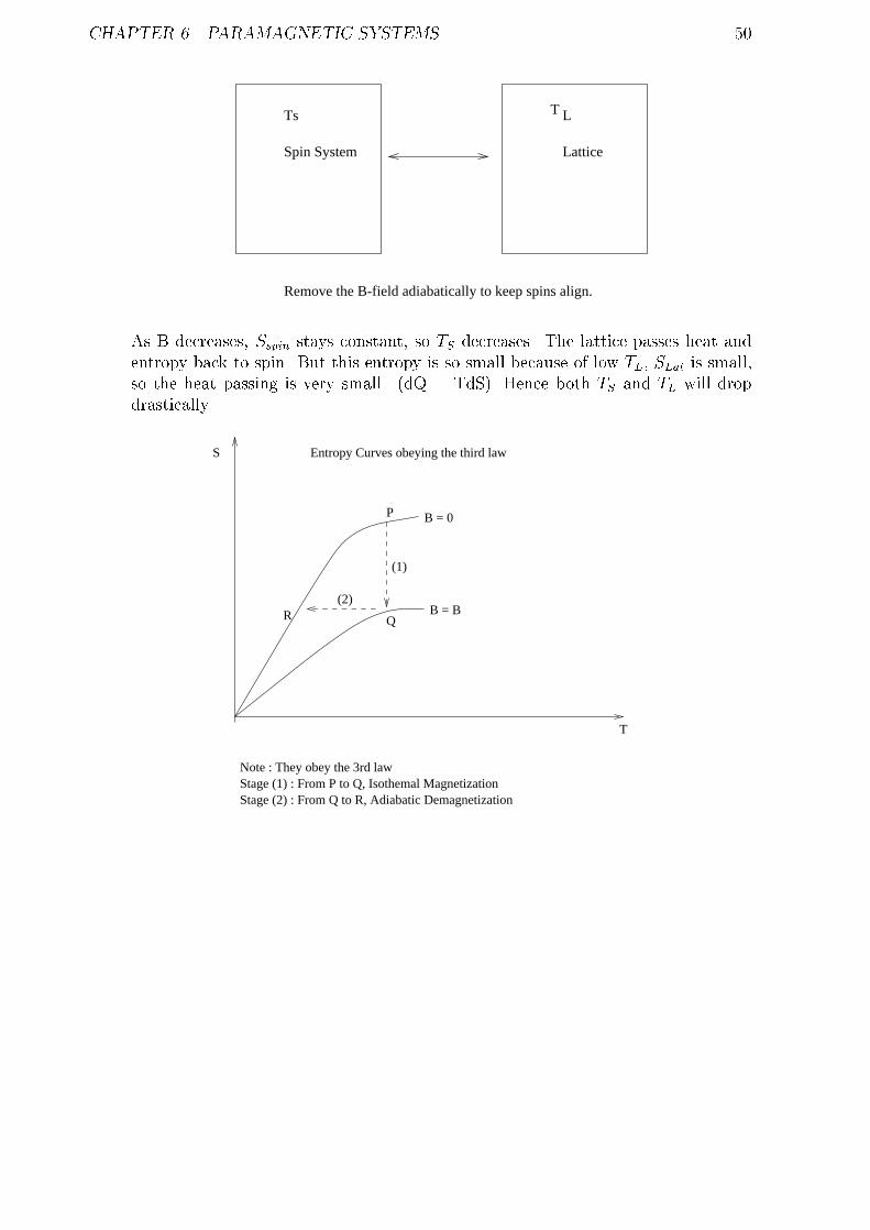
CHAPTER 6. PARAMAGNETIC SYSTEMS 50
Ts
Spin System
T L
Lattice
Remove the B-field adiabatically to keep spins align.
As B decreases, Sspin stays constant, so TS decreases. The lattice passes heat and
entropy back to spin. But this entropy is so small because of low TL, SLat is small,
so the heat passing is very small. (dQ = TdS). Hence both TS and TL will drop
drastically.
S
T
B = 0
B = B
Note : They obey the 3rd law
P
R
Entropy Curves obeying the third law
Q
(2)
(1)
Stage (1) : From P to Q, Isothemal MagnetizationStage (2) : From Q to R, Adiabatic Demagnetization

Chapter 7
Applications of Fermi-Dirac
Statistics
7.1 Fermi-Dirac Distribution
From chapter 3, we obtain two quantum distributions :
1. Fermi-Dirac Distribution
nj =gj
ee" + 1(7.1)
2. Bose-Einstein Distribution
nj =gj
ee" 1(7.2)
For either systems, = 1kT. This can be proven by having the quantum system in
contact with a classical perfect gas where = 1kT. The two s will reach equilibrium at
same temperature.
Now to identify for Fermi-Dirac distribution, we consider 2 fermion systems in ther-
mal and diusive contact so to allow particle exchange. We also assume that the same
type of fermions for both systems.
With the same constraints :
Xni +
Xnj = NX
ni"i + nj"j = E
= ij
=Yi
gi
ni!(gi ni)!
Yj
gj
nj!(gj nj)!(7.3)
51

CHAPTER 7. APPLICATIONS OF FERMI-DIRAC STATISTICS 52
ln =Xi
gi ln gi gi (gi ni) ln(gi ni) + (gi ni) ni lnni + ni
+Xj
gj ln gj gj (gj nj) ln(gj nj) + (gj nj) nj lnnj + nj
=Xi
gi ln gi (gi ni) ln(gi ni) ni lnni +Xj
gj ln gj (gj nj) ln(gj nj) nj lnnj
(7.4)
dln =Xi
ln(gi ni)dni + dni lnnidni dni +Xj
ln(gj nj)dnj + dnj lnnjdnj dnj
=Xi
(lngi ni
ni)dni +
Xj
(lngj nj
nj)dnj
= 0
(7.5)
Using the method of Lagrange multipliers,
(Xi
dni +Xj
dnj) = 0
(Xi
"idni +Xj
"jdnj) = 0
So,
Xi
(lngi ni
ni + "i)dni +
Xj
(lngj nj
nj + "j)dnj = 0 (7.6)
Then Choose and , so that
lngi ni
ni + "i = 0
lngj nj
nj + "j = 0
Then
ni =gi
ee"i + 1
nj =gj
ee"j + 1
So the two systems in thermal contact have the same and the two systems in diusive
contact will have the same , which is related to .
The diusive contact gives rise to chemical equilibrium, so
i = j = (chemical potential)
Suppose we take one of the systems :
Sj = k lnj
=Xj
gj ln gj (gj nj) ln(gj nj) nj lnnj(7.7)

CHAPTER 7. APPLICATIONS OF FERMI-DIRAC STATISTICS 53
Then
dS = kXj
ln(gj nj)dnj + dnj nj lnnj dnj
= kXj
lngj nj
njdnj
= kXj
( + "j)dnj
= kXj
dnj + kXj
[d(nj"j) njd"j]
= kdN + kdU kdW
(7.8)
TdS = kTdN + dU dW
= dN + dU dW(7.9)
because
dU = TdS + dW + dN
Therefore
=
kT(same derivation for bosons) (7.10)
So
nj =gj
e"j
kT + 1(7.11)
where dN is the work done in moving the fermions from one place to another, e.g elec-
trical work.
7.2 Free Electron Model of Metals
The valence electrons (in the outermost shell) are loosely bound, i.e. takes little energy
to detach them, hence they have low ionisation potential.
In metal, the weakly attached conducting electrons are \free" to move in the lattice.
The electrons interact with the electrostatic potential of the positive ions in the lattice. If
we consider the periodicity of the potential, we will obtain the solution to the Schrodinger
equation in the form of Bloch waves. The energy will form a band.
For perfect stationary lattice, there is free propagation and innite conductivity of
electrons. However lattice imperfections, lattice vibrations (phonons) and the scattering
by the other electrons leads to resistance in the lattice.
In the free electron model, we apply Fermi-Dirac Statistics - electrons of spin 12and
= 12. We neglect the lattice potential, the electrons are conned in a box (body of

CHAPTER 7. APPLICATIONS OF FERMI-DIRAC STATISTICS 54
metal) and we neglect the mutual interactions(electron-electron scattering).
For single particle state (nx, ny, nz, ), the energy is given by :
"nx;ny;nz; =~22
2mL2(n2x + n2y + n2z)
=~2
2mk2
(7.12)
where k is the wavevector 2and is dened by the following relation :
k2 =2
L2(n2x + n2y + n2z) (7.13)
nz
nx
ny
nR
Number of states from k=0 to k=k =1
8 4
3n3R 2 (7.14)
(Note : we multiply the relation by 2 because of the 2 spin states and 18because we
only take the positive octant, i.e. nx, ny and nz are all positive integers.)
Number of states between k and k+dk =1
8 4k2dk 2 (
L
)3
=V
2k2dk
(7.15)
Number of states between " and "+d" is g(")d" =V
22m"
~2
dk
d"d"
=V
22m"
~2
m
~2kd"
=V
22m2"
~4
r~2
2m"d"
=V
22(2m)
32
~3"12d"
= V C"12d"
(7.16)

CHAPTER 7. APPLICATIONS OF FERMI-DIRAC STATISTICS 55
where
C =1
22(2m)
32
~3
Therefore,
N =Xj
nj
=Xj
gj
e("j + 1
=
Z 1
0
g(")d"
e("j) + 1
(7.17)
E =Xj
nj"j
=Xj
"jgj
e("j) + 1
=
Z 1
0
"g(")d"
e("j) + 1
(7.18)
We solve equation (7.17) for (N; T; V ) and use in (7.18) to obtain ". This is dicult
to evaluate except at low T. We shall try to evaluate this in 2 cases
1. At T = 0
Probability of occupation of state of energy is fFD(") =1
e("j) + 1(7.19)
EF
f
E
1
0
F-D (E)
For
(T = 0) = "F Fermi energy (7.20)
and
fFD(") = 0 " > "F
fFD(") = 1 " < "F

CHAPTER 7. APPLICATIONS OF FERMI-DIRAC STATISTICS 56
Hence
N =
Z 1
0
g(")fFD(")d"
=
Z "F
0
g(")d"
= V C
Z "F
0
"12d"
= V C2
3"32
F
(7.21)
and
"F = [3N
2V
22~3
(2m)32
]23
= (3N2
V)23~2
2m
=~2
2mk2F
(7.22)
kF = (3N2
V)13 (7.23)
The meaning of Fermi energy is that all states below "F are occupied and all states
above "F are unoccupied at T = 0.
At T=0, all electrons occupy the lowest possible state subject to the Exclusion
Principle, so the states are lled until "F .
Total Energy, E =
Z 1
0
g(")fFD(")d"
= V C
Z "F
0
"32d"
= V C2
5"52
=3
5N"F
(7.24)
2. At low T, kT"F
<< 1, we want to nd Cv and we know that the experimental value
is proportional to T.
N =
Z 1
0
g(")fFD(")d"
Therefore,
U =
Z 1
0
"g(")d"
e(") + 1
=
Z 1
0
(" "F )g(")d"
e(") + 1+
"Fg(")d"
e("j) + 1
=
Z 1
0
(" "F )g(")d"
e(") + 1+N"F
(7.25)

CHAPTER 7. APPLICATIONS OF FERMI-DIRAC STATISTICS 57
Then
Cv = (@U
@T)V
= Z 1
0
(" "F )g(")e(")
(e("j) + 1)2 [(" )( 1
kT 2 1
kT
@
@T)]d"
(7.26)
Since does not change much, so we assume @
@T= 0 and = "F ,
Cv =1
kT 2
Z 1
0
(" "F )2e(""F )V C"
12d"
(e(""F ) + 1)2(7.27)
Now,
e(""F )
(e(""F ) + 1)2= @fFD(")
@"(7.28)
The maximum occurs at " = "F . The value drops to1eof the maximum value when
" "F kT . So the function is sharp for small kT (<< "F ).
kT
EFE
dfF-D (E)
dE
The contribution to the Cv integral comes mainly from values of " near "F , i.e.
" "F
Cv =1
kT 2V C"
12
F
Z 1
0
(" "F )e(""F )d"d"
(e(""F ) + 1)2
= V C"12
Fk2T
Z 1
"F
x2exdx
(ex + 1)2where x = (" "F )
(7.29)
The lower limit can be extended to 1 because kT<< "F .Z 1
1
x2exdx
(ex + 1)2=2
3(7.30)
Therefore
Cv =2
3k2Tg("F ) (7.31)
where g("F ) is the density of states of Fermi level.
The physical picture :

CHAPTER 7. APPLICATIONS OF FERMI-DIRAC STATISTICS 58
T = 0
T>0
E EF
g(E)f F-D (E)
For T = 0 : All states are occupied within " = "F is a truncated parabola.
For T> 0 : We will expect electrons to gain energy kT. However, most electrons
cannot gain kT because the states above them are already occupied. Only those
electrons near "F can gain kT to move into unoccupied states. This results in a
rounded-o cli at "F .
An alternative estimate :
Number of electrons involved is g("F )kT and they gain kT. Therefore
Energy of excitation = g("F )k2T 2 (7.32)
Contribution to Cv, heat capacity =The number of electrons participating energy
T
=g("F )kT kT
T
= f("F )k2T
(7.33)
Experimental result : Cv / T for a fermi gas. The theory is in agreement but does
not give the right constant of proportionality, and need to include eective mass of
electron me > me because electrons are not completely free but the lattice potential
constrains them.

Chapter 8
Applications of Bose-Einstein
Statistics
8.1 Introduction to Black Body Radiation
First, we discuss radiation in thermal equilibrium. The radiation is enclosed in vessel, and
all the walls are at temperature T. The atoms in the wall will absorb and emit electromag-
netic radiation. At equilibrium, the distribution of photons will follow the temperature T.
Second, in order to study the radiation, we assume a hole is cut in the chamber wall to
emit some radiation. The hole is very small so that the equilibrium is not disturbed. This
will approximate to a blackbody. The black body will also absorb all radiation falling on
it. The radiation bounces inside the chamber until nally being absorbed.
In this chapter, we will study black body radiation using statistical mechanics. We
note that the photons have the following characteristics :
1. The photons have spin 1 (bosons) and they obey Bose-Einstein statistics.
2. The photons do not interact with one another.
3. The photons have zero rest mass and travel at c, the speed of light.
4. The photons satisfy the dispersion relation, ! = ck, so,
" = ~! = ~ck
59
CHAPTER 8. APPLICATIONS OF BOSE-EINSTEIN STATISTICS 60
8.2 Bose-Einstein Distribution
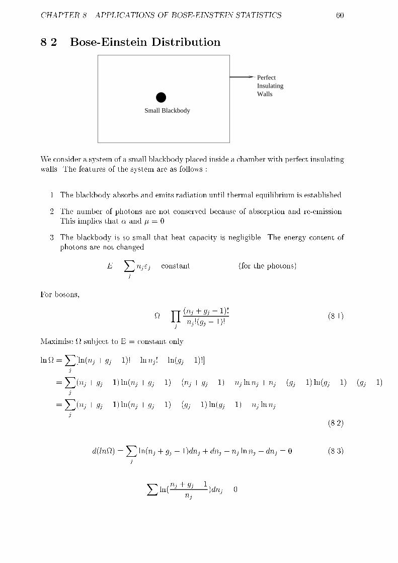
Small Blackbody
Perfect Insulating Walls
We consider a system of a small blackbody placed inside a chamber with perfect insulating
walls. The features of the system are as follows :
1. The blackbody absorbs and emits radiation until thermal equilibrium is established.
2. The number of photons are not conserved because of absorption and re-emission.
This implies that and = 0.
3. The blackbody is so small that heat capacity is negligible. The energy content of
photons are not changed.
E =Xj
nj"j = constant (for the photons)
For bosons,
=Yj
(nj + gj 1)!
nj!(gj 1)!(8.1)
Maximise subject to E = constant only.
ln =Xj
[ln(nj + gj 1)! lnnj! ln(gj 1)!]
=Xj
(nj + gj 1) ln(nj + gj 1) (nj + gj 1) nj lnnj + nj (gj 1) ln(gj 1) + (gj 1)
=Xj
(nj + gj 1) ln(nj + gj 1) (gj 1) ln(gj 1) nj lnnj
(8.2)
d(ln) =Xj
ln(nj + gj 1)dnj + dnj nj lnnj dnj = 0 (8.3)
Xln(
nj + gj 1
nj)dnj = 0

CHAPTER 8. APPLICATIONS OF BOSE-EINSTEIN STATISTICS 61
Xj
dnj"j = 0
Therefore X[ln(
nj + gj 1
nj) "j]dnj = 0 (8.4)
So,
nj =gj
e"j 1(8.5)
for large gj and nj.
Bose-Einstein function =1
e"j 1(8.6)
Prove = 1kT
by having the photon system in thermal contact with another system at
temperature T and use walls that can exchange energy.
8.3 Planck's Radiation Formula
Consider photons enclosed in a box L3, standing electromagnetic waves result such that
n
2 = L
Therefore
kx =2
x=nx
L
ky =2
y=ny
L
kz =2
z=nz
L
For any photon with ~k = (kx, ky, kz),
!2
c2= k2 = k2x + k2y + k2z (8.7)
For any ~k, there are 2 polarizations - 2 linear or 2 circular.
nz
nx
ny
nR

CHAPTER 8. APPLICATIONS OF BOSE-EINSTEIN STATISTICS 62
Therefore,
Number of photon states for k=0 to k=k =1
8 4
3n3R 2
=
3
L3
3k3
(8.8)
since
n2R =L2
2k2
Number of photon states between k and k+dk =V
2k2dk (8.9)
Number of photon states between frequency range ! and !+d! =V
2!2
c2d!
c
=V !2d!
2c3
(8.10)
The number of photons in frequency range ! and !+d! is
N(!)d! = (Density of states) (Bose-Einstein function)
=V !2d!
2c3(e~! 1)
(8.11)
Thus the energy of the photons in the frequency range ! and !+d! is
~!N(!)d! =V ~
2c3!3d!
e~! 1(8.12)
The energy density (per unit volume) in the frequency range is
u(!; T )d! =~
2c3!3d!
e~! 1(Planck's formula) (8.13)
u(w, T)
w
T
T1
2T2>T1
For T2 > T1, the maximum of u(!, T) is given by :
e~!3!2 !2~e~!
(e~! 1)2= 0

CHAPTER 8. APPLICATIONS OF BOSE-EINSTEIN STATISTICS 63
) 3(e~! 1) = ~e~!
) 3(ex 1) = xex
where x = ~!
Solving numerically, x 3, by neglecting (-1), or more accurately, x = 2.822.
Therefore,
~!max
kT= 2:822 (8.14)
!max =2:822k
~T (Wien's displacement law) (8.15)
or
2c
max
=2:822k
~T (8.16)
max =~c
2:822k
1
T(8.17)
So, as T rises, the colour of the blackbody changes from red to blue :
Total Energy Intensity, u(T) =
Z 1
0
u(!; T )d!
=~
2c3
Z 1
0
!3d!
e~! 1
=~
c31
4~4
Z 1
0
x3dx
ex 1
=k4T 4
2c3~34
15
(8.18)
Therefore
u(T ) = aT 4 (Stefan-Boltzmann law) (8.19)
where
a =2k4
15c3~3
8.4 Radiation emitted by blackbody
Consider a tiny hole, A, with photons coming from direction (! + d, ! + d),
with a subtended solid angle d, where
d =r sin drd
r2
= sin dd

CHAPTER 8. APPLICATIONS OF BOSE-EINSTEIN STATISTICS 64
The total solid angle = 4.
The photons that will pass through in time t are located in a parallelpiped of length
ct.
The volume of the parallelpied is dA ct cos .
θθ
θ
dA
c t
Therefore,
No. of photons passing per unit time from direction ( ! + d, ! + d) with a
frequency range ! to ! + d!
=Volume of Parallelpiped
t Fractional solid angle Number density in frequency interval
= dAc cos d
4 N(!)d!
V
Therefore, the total energy radiated per unit time in frequency interval ! to ! + d!
=
Z 2
0
d
Z 2
0
sin ddAc cos
4 ~!
N(!)d!
V
=1
4c~!dA
N(!)d!
V
=1
4cu(!; T )dAd!
Therefore
Power radiated per unit area in frequency interval from ! to ! + d!
=1
4cu(!; T )d!
CHAPTER 8. APPLICATIONS OF BOSE-EINSTEIN STATISTICS 65
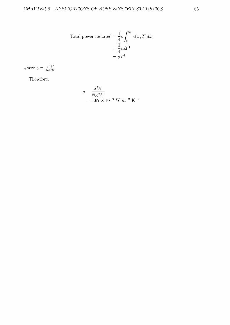
Total power radiated =1
4c
Z 1
0
u(!; T )d!
=1
4caT 4
= T 4
where a = 2k4
15c3~3.
Therefore,
=2k4
60c2~3
= 5:67 108 W m2 K4
Chapter 9
The Classical Limit
9.1 The Classical Regime
In the classical regime, there is a lack of discreteness, we consider the continuous variable
" rather than the discrete energy "r.
The energy spacing is " << kT, and < nr > <<1 which means that there are many
unoccupied states, which are averaged over time.
In the Fermi-Dirac or Bose Einstein statistics, the classical regime is only satised if
1
e("r) 1<< 1
i.e.
e("r) >> 1
so that
< nr >F-D,B-E e("r)
= ee"r M-B distribution
So all the 3 distributions(Maxwell-Boltzmann, Fermi-Dirac and Bose-Einstein) distri-
butions approximate to Maxwell-Boltzmann distributions in the classical regime.
According to the Maxwell-Boltzmann statistics,
< nr >M-B=N
Ze"r << 1 (9.1)
for all r, including r = 0.
So we require N
Z<< 1, since "0 ! 0 for ground state.
66

CHAPTER 9. THE CLASSICAL LIMIT 67
9.2 Monatomic Gas
For monatomic gas,
Z =V
h3
2mkT
32
so,
Nh3
V
1
2mkT
32
<< 1
T >>
N
V
23 h2
2mk
The conditions are high temperature, T and low density N
V, and high mass, m.
Assume the energy is equipartitioned,
" =3
2kT (for each atom)
=p2
2m
So,
p =p2m" =
h
dB(in QM terms) (9.2)
Then
1
2mkT
32
=
1
43m"
32
=
3
2
32 1
p3
=
3
2
32dB
h
3
(9.3)
and
N
V
3
2
32
3dB << 1
i.e.
dB <<
2
3
12V
N
13
=
2
3
12
l0
where l0 is the average seperation between atoms.
Examples :

CHAPTER 9. THE CLASSICAL LIMIT 68
1. He gas :
N
V= 1020 per cm3
so l0 = 2 107cm
At T = 273 K, and
m =4
6 1023g
so dB = 8 109 cm << l0. Hence Maxwell-Boltzmann distribution is applicable.
For liquid He at T = 4 K,
N
V= 2 1022 per cm3
so l0 = 4 108cm.
Since dB > l0, so Bose Einstein statistics apply.
2. For conduction electrons :
Assume 1 electron per atom,
N
V 1023 per cm3
hence
l0 2 108cm
For m = 9:1 1031 kg and T = 273 K, dB > l0, so Fermi-Dirac statistics apply.
T = 0
T>0
E EF
g(E)f F-D (E)
ApproximatelyM-B
EF
f
E
1
0
F-D (E)
T=0
T>0

CHAPTER 9. THE CLASSICAL LIMIT 69
Note that
n(") / "12 e"
for M-B distributions.
9.3 Gibbs Paradox
For classical ideal gas, we assume the atoms to be distinguishable. Now we mix the vol-
umes of identical atoms.
VNTS
VNTS
S =U
T+Nk lnZ
=3
2Nk +Nk
lnV +
3
2lnT +
3
2ln
2mk
h2
(9.4)
Suppose now N ! 2N, V ! 2V, we expect S!2S.
However,
S =3
2(2N)k + (2N)k
ln 2V +
3
2lnT +
3
2ln
2mk
h2
= 2Sold + 2Nk ln 2
(9.5)
The problem lies with distinguishability and overcounting. Hence we use a corrected .
Corrected =old
N !
=Yj
gnjj
nj!
(9.6)
Therefore,
Corrected S = k lnCorrected k(N lnN N)
=5
2Nk +Nk
ln
V
N
+3
2lnT +
3
2ln
2mk
h2
(9.7)

CHAPTER 9. THE CLASSICAL LIMIT 70
Then for N ! 2N, V ! 2V,
S =5
2(2N)k + 2Nk
ln
2V
2N
+3
2lnT +
3
2ln
2mk
h2
= 2Sold
(9.8)

Chapter 10
Kinetic Theory of Gases
10.1 Introduction
Consider the distribution (for e.g. velocity, momentum, position, energy, etc) of system
of gas molecules in thermal equilibrium.
At thermal equilibrium, the momentum and spatial coordinates are independent of
each other, i.e. a molecule in any position (x,y,z) can have any momentum (px, py, pz).
For the Hamiltonian :
1. The kinetic energy (KE) terms are determined by px, py and pz.
2. The potential energy (PE) terms are determined by x, y and z.
The Boltzmann law applies to every coordinate in the Hamiltonian.
For example,
1. The probability that x-momentum which lies between px and px+dpx is :
P [px]dpx = Aep2x2mkT dpx (10.1)
where
A
Z 1
1
ep2x2mkT dpx = 1 (10.2)
2. The probability that x-velocity lies between vx and vx+dvx is :
P [vx]dvx = A0emv2x2kT dvx (10.3)
where
A0
Z 1
1
emv2x2kT dvx = 1 (10.4)
71

CHAPTER 10. KINETIC THEORY OF GASES 72
3. The probability that the molecule is found between and x and x+dx is :
P [x]dx = BeV (x)
kT dx (10.5)
where
B
Z 1
1
eV (x)
kT dx = 1 (10.6)
We concentrate on the momentum and velocity distributions, hence we do not require
the interaction potential except for establishing thermal equilibrium.
For graphs of P[px] or P[vx] : the gaussian curves centred at zero.
p , v
x ]
x
P[p ], P[vx
x
For speed distribution : P[c] dc where c2 = v2x + v2y + v2z .
dc
dθ
φd
P [vx; vy; vz]dvxdvydvz = P [vx]dvxP [vy]dvyP [vz]dvz
=
m
2kT
32
emv2x2kT e
mv2y
2kT emv2z2kT dvxdvydvz
=
m
2kT
32
emc2
2kT dc(cd)(csind)
(10.7)
Integrating over all angles :
P [c]dc = 4
m
2kT
32
emc2
2kT c2dc (10.8)
Hence, we can calculate :

CHAPTER 10. KINETIC THEORY OF GASES 73
1. Most probable speed, cmax :
For cmax, put
dP [c]
dc= 0) cmax =
2kT
m
12
(10.9)
2. Mean speed c :
c =
Z 1
0
cP [c]dc =
8kT
m
12
(10.10)
3. Mean square speed, c2 :
c2 =
Z 1
0
c2P [c]dc =3kT
m(10.11)
4. Root mean square speed,pc2 :
pc2 =
3kT
m
12
(10.12)
5. Mean kinetic energy (KE) :
Mean KE =1
2m c2 =
3
2kT (10.13)
Note :c2 = v2x + v2y + v2z
= 3 v2x(10.14)
so
v2x =kT
m(10.15)
10.2 Number of impacts on Area A of a wall
θ A

CHAPTER 10. KINETIC THEORY OF GASES 74
The distribution of speeds : P[c] dc
The fraction of molecules travelling in direction ( ! + d, ! + d) is
cdcsind
4c2=sindd
4(10.16)
The fraction that will reach A in time t for above direction
=Ac cos t
V(10.17)
where V is the volume of the gas.
Therefore,
Number of impacts on area A in time t
=
ZZZNP [c]dc
sindd
4
Ac cos t
V(10.18)
Number of impacts on unit area per unit time
=N
4V
Z 1
0
cP [c]dc
Z 2
0
sin cos d
Z 2
0
d
=N
4Vc1
2(2)
=1
4nc
(10.19)
where the number density, n = N
V.
10.3 Eusion of molecules
The number of molecules with speeds c!c+dc from direction ( ! + d, ! + d)
imping a area in time t is
N
4VcP [c]dcsinddAt
The distribution is proportional to c P[c] dc.
The mean speed of escape, ce :
ce =
Rc2P [c]dcRcP [c]dc
=3kTm
(8kTm
)12
=
9kT
8m
12
(10.20)

CHAPTER 10. KINETIC THEORY OF GASES 75
Number of molecules escaping per unit time per unit area
1
4mc =
p
kT
8kT
m
12
/ 1
m12
(10.21)
So, the smaller molecules escapes(euses) faster.
10.4 Mean Free Path,
The free path is dened as the distance between collisions. It is not all equal, for some
are longer and some are shorter. The more probable the collision, the shorter is the free
path.
The distribution of free path :
Probability that free path in between x and x+dx / exdx
.
We can prove this by a self consistent argument :
Probablity that collision occurs between x and x+dx
= (Probability of no collision from 0 to x) (Probability of collisions in dx)
Comparing with the above equation, we write
Probability of no collision in dx = edx (10.22)
Probability of collision in dx =dx
(10.23)
According to (10.22),
the probability of no collision in dx = edx (10.24)
Then,
Probability of collision in dx = 1 edx
= 11 dx
+ ::::
dx
(10.25)
which agrees with (10.23).

CHAPTER 10. KINETIC THEORY OF GASES 76
So the argument is self consistent. Also, we see that
Z 1
0
exdx
= 1 (10.26)
which is as required for probability.
Therefore,
Mean free path =
Z 1
0
xexdx
= [xe x ]10 +
Z 1
0
exdx
= [e x ]10
=
(10.27)
10.5 Collision cross-section,
d
d
The moving gas molecules sweeps out a cylinder of cross section :
= d2 (10.28)
where d is the diameter of the each molecule.
Average volume occupied by each molecule =V
N=
1
n(10.29)
So,
Mean free path, =V
N 1
d2
=1
nd2
(10.30)
Taking in account of the motion of gas molecules,
=1p2
1
n(10.31)
At stp, 7 108m. At 106 mbar, 5 m.