Welcome message from author
This document is posted to help you gain knowledge. Please leave a comment to let me know what you think about it! Share it to your friends and learn new things together.
Transcript

OXFORD MASTER SERIES IN STATISTICAL,COMPUTATIONAL, AND THEORETICAL PHYSICS
OXFORD MASTER SERIES IN PHYSICS
The Oxford Master Series is designed for final year undergraduate andbeginning graduate students in physics and related disciplines. It hasbeen driven by a perceived gap in the literature today. While basicundergraduate physics texts often show little or no connection with thehuge explosion of research over the last two decades, more advancedand specialized texts tend to be rather daunting for students. In thisseries, all topics and their consequences are treated at a simple level,while pointers to recent developments are provided at various stages.The emphasis in on clear physical principles like symmetry, quantummechanics, and electromagnetism which underlie the whole of physics.At the same time, the subjects are related to real measurements and tothe experimental techniques and devices currently used by physicists inacademe and industry. Books in this series are written as course books,and include ample tutorial material, examples, illustrations, revisionpoints, and problem sets. They can likewise be used as preparation forstudents starting a doctorate in physics and related fields, or for recentgraduates starting research in one of these fields in industry.
CONDENSED MATTER PHYSICS1. M.T. Dove: Structure and dynamics: an atomic view of materials2. J. Singleton: Band theory and electronic properties of solids3. A.M. Fox: Optical properties of solids4. S.J. Blundell: Magnetism in condensed matter5. J.F. Annett: Superconductivity, superfluids, and condensates6. R.A.L. Jones: Soft condensed matter
ATOMIC, OPTICAL, AND LASER PHYSICS7. C.J. Foot: Atomic physics8. G.A. Brooker: Modern classical optics9. S.M. Hooker, C.E. Webb: Laser physics
15. A.M. Fox: Quantum optics: an introduction
PARTICLE PHYSICS, ASTROPHYSICS, AND COSMOLOGY10. D.H. Perkins: Particle astrophysics11. Ta-Pei Cheng: Relativity, gravitation and cosmology
STATISTICAL, COMPUTATIONAL, AND THEORETICALPHYSICS12. M. Maggiore: A modern introduction to quantum field theory13. W. Krauth: Statistical mechanics: algorithms and computations14. J.P. Sethna: Statistical mechanics: entropy, order parameters, and
complexity
Statistical MechanicsAlgorithms and Computations
Werner Krauth
Laboratoire de Physique Statistique, Ecole NormaleSuperieure, Paris
1
3Great Clarendon Street, Oxford OX2 6DPOxford University Press is a department of the University of Oxford.It furthers the University’s objective of excellence in research, scholarship,and education by publishing worldwide in
Oxford New YorkAuckland Cape Town Dar es Salaam Hong Kong KarachiKuala Lumpur Madrid Melbourne Mexico City NairobiNew Delhi Shanghai Taipei Toronto
With offices inArgentina Austria Brazil Chile Czech Republic France GreeceGuatemala Hungary Italy Japan Poland Portugal SingaporeSouth Korea Switzerland Thailand Turkey Ukraine Vietnam
Oxford is a registered trade mark of Oxford University Pressin the UK and in certain other countries
Published in the United Statesby Oxford University Press Inc., New York
c© Oxford University Press 2006
The moral rights of the author have been assertedDatabase right Oxford University Press (maker)
First published 2006
All rights reserved. No part of this publication may be reproduced,stored in a retrieval system, or transmitted, in any form or by any means,without the prior permission in writing of Oxford University Press,or as expressly permitted by law, or under terms agreed with the appropriatereprographics rights organization. Enquiries concerning reproductionoutside the scope of the above should be sent to the Rights Department,Oxford University Press, at the address above
You must not circulate this book in any other binding or coverand you must impose the same condition on any acquirer
British Library Cataloguing in Publication DataData available
Library of Congress Cataloging in Publication DataData available
Printed in Great Britainon acid-free paper byCPI Antony Rowe, Chippenham, Wilts.
ISBN 0–19–851535–9 (Hbk) 978–0–19–851535–7ISBN 0–19–851536–7 (Pbk) 978–0–19–851536–4
10 9 8 7 6 5 4 3 2 1

Fur Silvia, Alban und Felix

This page intentionally left blank
Preface
This book is meant for students and researchers ready to plunge intostatistical physics, or into computing, or both. It has grown out of myresearch experience, and out of courses that I have had the good fortuneto give, over the years, to beginning graduate students at the Ecole Nor-male Superieure and the Universities of Paris VI and VII, and also tosummer school students in Drakensberg, South Africa, undergraduatesin Salem, Germany, theorists and experimentalists in Lausanne, Switzer-land, young physicists in Shanghai, China, among others. Hundreds ofstudents from many different walks of life, with quite different back-grounds, listened to lectures and tried to understand, made comments,corrected me, and in short helped shape what has now been writtenup, for their benefit, and for the benefit of new readers that I hope toattract to this exciting, interdisciplinary field. Many of the students satdown afterwards, by themselves or in groups, to implement short pro-grams, or to solve other problems. With programming assignments, lackof experience with computers was rarely a problem: there were alwaysmore knowledgeable students around who would help others with thefirst steps in computer programming. Mastering technical coding prob-lems should also only be a secondary problem for readers of this book:all programs here have been stripped to the bare minimum. None exceeda few dozen lines of code.
We shall focus on the concepts of classical and quantum statisticalphysics and of computing: the meaning of sampling, random variables,ergodicity, equidistribution, pressure, temperature, quantum statisticalmechanics, the path integral, enumerations, cluster algorithms, and theconnections between algorithmic complexity and analytic solutions, toname but a few. These concepts built the backbone of my courses, andnow form the tissue of the book. I hope that the simple language andthe concrete settings chosen throughout the chapters take away none ofthe beauty, and only add to the clarity, of the difficult and profoundsubject of statistical physics.
I also hope that readers will feel challenged to implement many ofthe programs. Writing and debugging computer code, even for the naiveprograms, remains a difficult task, especially in the beginning, but it iscertainly a successful strategy for learning, and for approaching the deepunderstanding that we must reach before we can translate the lessons ofthe past into our own research ideas.
This book is accompanied by a compact disc containing more than onehundred pseudocode programs and close to 300 figures, line drawings,
viii Preface
and tables contained in the book. Readers are free to use this mate-rial for lectures and presentations, but must ask for permission if theywant to include it in their own publications. For all questions, pleasecontact me at www.lps.ens.fr/˜krauth. (This website will also keep alist of misprints.) Readers of the book may want to get in contact witheach other, and some may feel challenged to translate the pseudocodeprograms into one of the popular computer languages; I will be happyto assist initiatives in this direction, and to announce them on the abovewebsite.
Contents
1 Monte Carlo methods 11.1 Popular games in Monaco 3
1.1.1 Direct sampling 31.1.2 Markov-chain sampling 41.1.3 Historical origins 91.1.4 Detailed balance 151.1.5 The Metropolis algorithm 211.1.6 A priori probabilities, triangle algorithm 221.1.7 Perfect sampling with Markov chains 24
1.2 Basic sampling 271.2.1 Real random numbers 271.2.2 Random integers, permutations, and combinations 291.2.3 Finite distributions 331.2.4 Continuous distributions and sample transformation 351.2.5 Gaussians 371.2.6 Random points in/on a sphere 39
1.3 Statistical data analysis 441.3.1 Sum of random variables, convolution 441.3.2 Mean value and variance 481.3.3 The central limit theorem 521.3.4 Data analysis for independent variables 551.3.5 Error estimates for Markov chains 59
1.4 Computing 621.4.1 Ergodicity 621.4.2 Importance sampling 631.4.3 Monte Carlo quality control 681.4.4 Stable distributions 701.4.5 Minimum number of samples 76
Exercises 77References 79
2 Hard disks and spheres 812.1 Newtonian deterministic mechanics 83
2.1.1 Pair collisions and wall collisions 832.1.2 Chaotic dynamics 862.1.3 Observables 872.1.4 Periodic boundary conditions 90
2.2 Boltzmann’s statistical mechanics 922.2.1 Direct disk sampling 95
x Contents
2.2.2 Partition function for hard disks 972.2.3 Markov-chain hard-sphere algorithm 1002.2.4 Velocities: the Maxwell distribution 1032.2.5 Hydrodynamics: long-time tails 105
2.3 Pressure and the Boltzmann distribution 1082.3.1 Bath-and-plate system 1092.3.2 Piston-and-plate system 1112.3.3 Ideal gas at constant pressure 1132.3.4 Constant-pressure simulation of hard spheres 115
2.4 Large hard-sphere systems 1192.4.1 Grid/cell schemes 1192.4.2 Liquid–solid transitions 120
2.5 Cluster algorithms 1222.5.1 Avalanches and independent sets 1232.5.2 Hard-sphere cluster algorithm 125
Exercises 128References 130
3 Density matrices and path integrals 1313.1 Density matrices 133
3.1.1 The quantum harmonic oscillator 1333.1.2 Free density matrix 1353.1.3 Density matrices for a box 1373.1.4 Density matrix in a rotating box 139
3.2 Matrix squaring 1433.2.1 High-temperature limit, convolution 1433.2.2 Harmonic oscillator (exact solution) 1453.2.3 Infinitesimal matrix products 148
3.3 The Feynman path integral 1493.3.1 Naive path sampling 1503.3.2 Direct path sampling and the Levy construction 1523.3.3 Periodic boundary conditions, paths in a box 155
3.4 Pair density matrices 1593.4.1 Two quantum hard spheres 1603.4.2 Perfect pair action 1623.4.3 Many-particle density matrix 167
3.5 Geometry of paths 1683.5.1 Paths in Fourier space 1693.5.2 Path maxima, correlation functions 1743.5.3 Classical random paths 177
Exercises 182References 184
4 Bosons 1854.1 Ideal bosons (energy levels) 187
4.1.1 Single-particle density of states 1874.1.2 Trapped bosons (canonical ensemble) 1904.1.3 Trapped bosons (grand canonical ensemble) 196
Contents xi
4.1.4 Large-N limit in the grand canonical ensemble 2004.1.5 Differences between ensembles—fluctuations 2054.1.6 Homogeneous Bose gas 206
4.2 The ideal Bose gas (density matrices) 2094.2.1 Bosonic density matrix 2094.2.2 Recursive counting of permutations 2124.2.3 Canonical partition function of ideal bosons 2134.2.4 Cycle-length distribution, condensate fraction 2174.2.5 Direct-sampling algorithm for ideal bosons 2194.2.6 Homogeneous Bose gas, winding numbers 2214.2.7 Interacting bosons 224
Exercises 225References 227
5 Order and disorder in spin systems 2295.1 The Ising model—exact computations 231
5.1.1 Listing spin configurations 2325.1.2 Thermodynamics, specific heat capacity, and mag-
netization 2345.1.3 Listing loop configurations 2365.1.4 Counting (not listing) loops in two dimensions 2405.1.5 Density of states from thermodynamics 247
5.2 The Ising model—Monte Carlo algorithms 2495.2.1 Local sampling methods 2495.2.2 Heat bath and perfect sampling 2525.2.3 Cluster algorithms 254
5.3 Generalized Ising models 2595.3.1 The two-dimensional spin glass 2595.3.2 Liquids as Ising-spin-glass models 262
Exercises 264References 266
6 Entropic forces 2676.1 Entropic continuum models and mixtures 269
6.1.1 Random clothes-pins 2696.1.2 The Asakura–Oosawa depletion interaction 2736.1.3 Binary mixtures 277
6.2 Entropic lattice model: dimers 2816.2.1 Basic enumeration 2816.2.2 Breadth-first and depth-first enumeration 2846.2.3 Pfaffian dimer enumerations 2886.2.4 Monte Carlo algorithms for the monomer–dimer
problem 2966.2.5 Monomer–dimer partition function 299
Exercises 303References 305
7 Dynamic Monte Carlo methods 307
xii Contents
7.1 Random sequential deposition 3097.1.1 Faster-than-the-clock algorithms 310
7.2 Dynamic spin algorithms 3137.2.1 Spin-flips and dice throws 3147.2.2 Accelerated algorithms for discrete systems 3177.2.3 Futility 319
7.3 Disks on the unit sphere 3217.3.1 Simulated annealing 3247.3.2 Asymptotic densities and paper-cutting 3277.3.3 Polydisperse disks and the glass transition 3307.3.4 Jamming and planar graphs 331
Exercises 333References 335
Acknowledgements 337
Index 339
Monte Carlo methods 11.1 Popular games in Monaco 3
1.2 Basic sampling 27
1.3 Statistical data analysis 44
1.4 Computing 62
Exercises 77
References 79
Starting with this chapter, we embark on a journey into the fascinatingrealms of statistical mechanics and computational physics. We set out tostudy a host of classical and quantum problems, all of value as modelsand with numerous applications and generalizations. Many computa-tional methods will be visited, by choice or by necessity. Not all of thesemethods are, however, properly speaking, computer algorithms. Never-theless, they often help us tackle, and understand, properties of physicalsystems. Sometimes we can even say that computational methods givenumerically exact solutions, because few questions remain unanswered.
Among all the computational techniques in this book, one stands out:the Monte Carlo method. It stems from the same roots as statisticalphysics itself, it is increasingly becoming part of the discipline it is meantto study, and it is widely applied in the natural sciences, mathematics,engineering, and even the social sciences. The Monte Carlo method isthe first essential stop on our journey.
In the most general terms, the Monte Carlo method is a statistical—almost experimental—approach to computing integrals using random1
positions, called samples,1 whose distribution is carefully chosen. In thischapter, we concentrate on how to obtain these samples, how to processthem in order to approximately evaluate the integral in question, andhow to get good results with as few samples as possible. Starting withvery simple example, we shall introduce to the basic sampling techniquesfor continuous and discrete variables, and discuss the specific problemsof high-dimensional integrals. We shall also discuss the basic principlesof statistical data analysis: how to extract results from well-behavedsimulations. We shall also spend much time discussing the simulationswhere something goes wrong.
The Monte Carlo method is extremely general, and the basic recipesallow us—in principle—to solve any problem in statistical physics. Inpractice, however, much effort has to be spent in designing algorithmsspecifically geared to the problem at hand. The design principles areintroduced in the present chapter; they will come up time and again inthe real-world settings of later parts of this book.
1“Random” comes from the old French word randon (to run around); “sample” isderived from the Latin exemplum (example).
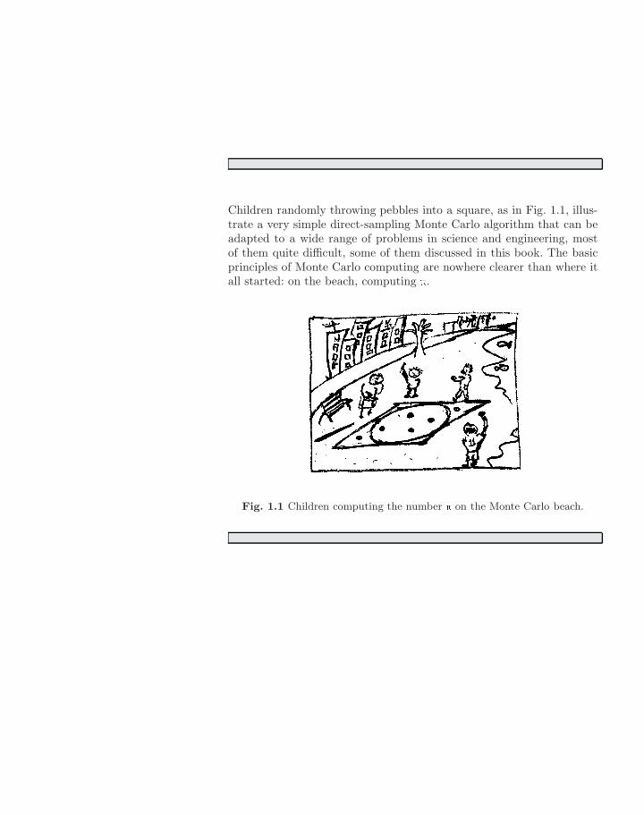
Children randomly throwing pebbles into a square, as in Fig. 1.1, illus-trate a very simple direct-sampling Monte Carlo algorithm that can beadapted to a wide range of problems in science and engineering, mostof them quite difficult, some of them discussed in this book. The basicprinciples of Monte Carlo computing are nowhere clearer than where itall started: on the beach, computing .
Fig. 1.1 Children computing the number on the Monte Carlo beach.
1.1 Popular games in Monaco 3
1.1 Popular games in Monaco
The concept of sampling (obtaining the random positions) is truly com-plex, and we had better get a grasp of the idea in a simplified setting be-fore applying it in its full power and versatility to the complicated casesof later chapters. We must clearly distinguish between two fundamen-tally different sampling approaches: direct sampling and Markov-chainsampling.
1.1.1 Direct sampling
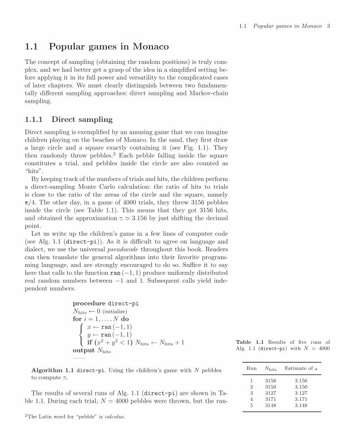
Direct sampling is exemplified by an amusing game that we can imaginechildren playing on the beaches of Monaco. In the sand, they first drawa large circle and a square exactly containing it (see Fig. 1.1). Theythen randomly throw pebbles.2 Each pebble falling inside the squareconstitutes a trial, and pebbles inside the circle are also counted as“hits”.
By keeping track of the numbers of trials and hits, the children performa direct-sampling Monte Carlo calculation: the ratio of hits to trialsis close to the ratio of the areas of the circle and the square, namely/4. The other day, in a game of 4000 trials, they threw 3156 pebblesinside the circle (see Table 1.1). This means that they got 3156 hits,and obtained the approximation 3.156 by just shifting the decimalpoint.
Let us write up the children’s game in a few lines of computer code(see Alg. 1.1 (direct-pi)). As it is difficult to agree on language anddialect, we use the universal pseudocode throughout this book. Readerscan then translate the general algorithms into their favorite program-ming language, and are strongly encouraged to do so. Suffice it to sayhere that calls to the function ran (−1, 1) produce uniformly distributedreal random numbers between −1 and 1. Subsequent calls yield inde-pendent numbers.
procedure direct-pi
Nhits ← 0 (initialize)for i = 1, . . . , N do⎧⎨⎩
x ← ran (−1, 1)y ← ran (−1, 1)if (x2 + y2 < 1) Nhits ← Nhits + 1
output Nhits
——
Algorithm 1.1 direct-pi. Using the children’s game with N pebblesto compute .
Table 1.1 Results of five runs ofAlg. 1.1 (direct-pi) with N = 4000
Run Nhits Estimate of
1 3156 3.1562 3150 3.1503 3127 3.1274 3171 3.1715 3148 3.148
The results of several runs of Alg. 1.1 (direct-pi) are shown in Ta-ble 1.1. During each trial, N = 4000 pebbles were thrown, but the ran-
2The Latin word for “pebble” is calculus.
4 Monte Carlo methods
dom numbers differed, i.e. the pebbles landed at different locations ineach run.
We shall return later to this table when computing the statistical er-rors to be expected from Monte Carlo calculations. In the meantime, weintend to show that the Monte Carlo method is a powerful approach forthe calculation of integrals (in mathematics, physics, and other fields).But let us not get carried away: none of the results in Table 1.1 hasfallen within the tight error bounds already known since Archimedesfrom comparing a circle with regular n-gons:
3.141 31071
< < 317 3.143. (1.1)
The children’s value for is very approximate, but improves and finallybecomes exact in the limit of an infinite number of trials. This is JacobBernoulli’s weak law of large numbers (see Subsection 1.3.2). The chil-dren also adopt a very sensible rule: they decide on the total number ofthrows before starting the game. The other day, in a game of “N=4000”,they had at some point 355 hits for 452 trials—this gives a very nice ap-
355452
=355
4 × 113= 1
4× 3.14159292 . . .
/4 = 14× 3.14159265 . . .
proximation to the book value of . Without hesitation, they went onuntil the 4000th pebble was cast. They understand that one must notstop a stochastic calculation simply because the result is just right, norshould one continue to play because the result is not close enough towhat we think the answer should be.
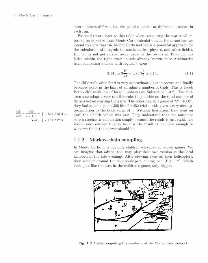
1.1.2 Markov-chain sampling
In Monte Carlo, it is not only children who play at pebble games. Wecan imagine that adults, too, may play their own version at the localheliport, in the late evenings. After stowing away all their helicopters,they wander around the square-shaped landing pad (Fig. 1.2), whichlooks just like the area in the children’s game, only bigger.
Fig. 1.2 Adults computing the number at the Monte Carlo heliport.
1.1 Popular games in Monaco 5
The playing field is much wider than before. Therefore, the game mustbe modified. Each player starts at the clubhouse, with their expensivedesigner handbags filled with pebbles. With closed eyes, they throw thefirst little stone in a random direction, and then they walk to where thisstone has landed. At that position, a new pebble is fetched from thehandbag, and a new throw follows. As before, the aim of the game is tosweep out the heliport square evenly in order to compute the number ,but the distance players can cover from where they stand is much smallerthan the dimensions of the field. A problem arises whenever there is arejection, as in the case of a lady with closed eyes at a point c near theboundary of the square-shaped domain, who has just thrown a pebble toa position outside the landing pad. It is not easy to understand whethershe should simply move on, or climb the fence and continue until, byaccident, she returns to the heliport.
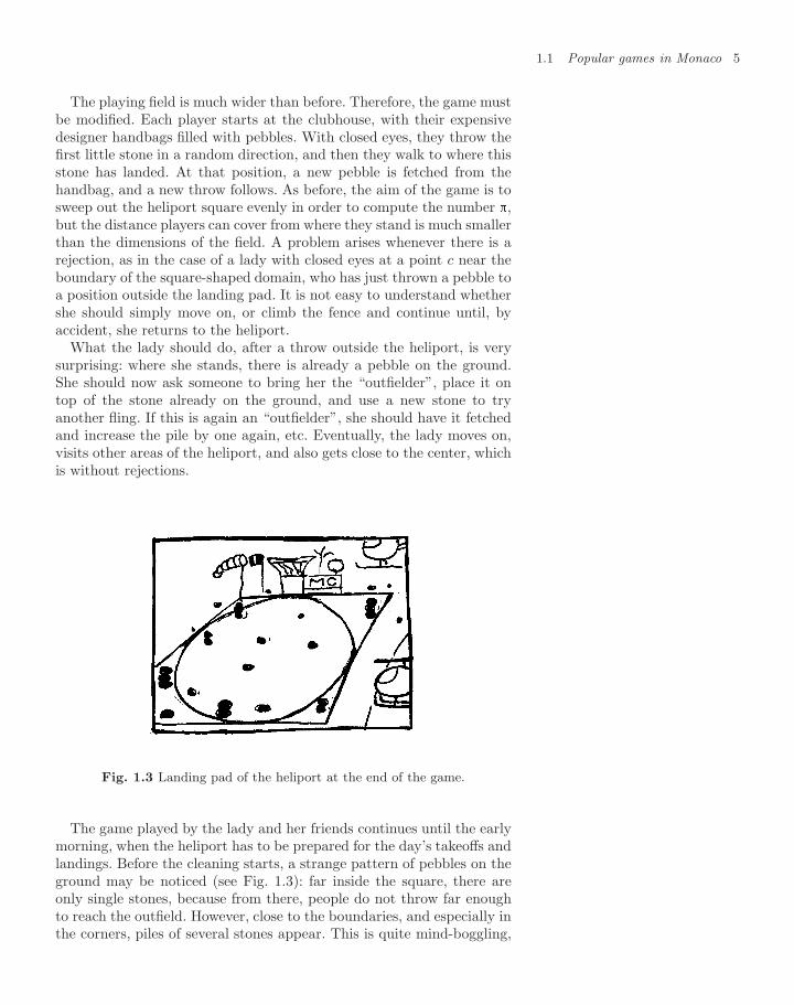
What the lady should do, after a throw outside the heliport, is verysurprising: where she stands, there is already a pebble on the ground.She should now ask someone to bring her the “outfielder”, place it ontop of the stone already on the ground, and use a new stone to tryanother fling. If this is again an “outfielder”, she should have it fetchedand increase the pile by one again, etc. Eventually, the lady moves on,visits other areas of the heliport, and also gets close to the center, whichis without rejections.
Fig. 1.3 Landing pad of the heliport at the end of the game.
The game played by the lady and her friends continues until the earlymorning, when the heliport has to be prepared for the day’s takeoffs andlandings. Before the cleaning starts, a strange pattern of pebbles on theground may be noticed (see Fig. 1.3): far inside the square, there areonly single stones, because from there, people do not throw far enoughto reach the outfield. However, close to the boundaries, and especially inthe corners, piles of several stones appear. This is quite mind-boggling,
6 Monte Carlo methods
but does not change the fact that comes out as four times the ratio ofhits to trials.
Those who hear this story for the first time often find it dubious. Theyobserve that perhaps one should not pile up stones, as in Fig. 1.3, if theaim is to spread them out evenly. This objection places these moderncritics in the illustrious company of prominent physicists and mathe-maticians who questioned the validity of this method when it was firstpublished in 1953 (it was applied to the hard-disk system of Chapter 2).Letters were written, arguments were exchanged, and the issue was set-tled only after several months. Of course, at the time, helicopters andheliports were much less common than they are today.
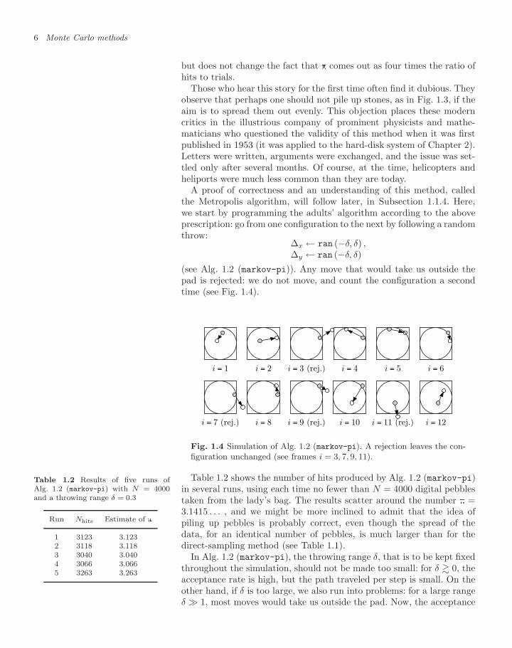
A proof of correctness and an understanding of this method, calledthe Metropolis algorithm, will follow later, in Subsection 1.1.4. Here,we start by programming the adults’ algorithm according to the aboveprescription: go from one configuration to the next by following a randomthrow:
∆x ← ran (−δ, δ) ,∆y ← ran (−δ, δ)
(see Alg. 1.2 (markov-pi)). Any move that would take us outside thepad is rejected: we do not move, and count the configuration a secondtime (see Fig. 1.4).
i = 1 i = 2 i = 3 (rej.) i = 4 i = 5 i = 6
i = 7 (rej.) i = 8 i = 9 (rej.) i = 10 i = 11 (rej.) i = 12
Fig. 1.4 Simulation of Alg. 1.2 (markov-pi). A rejection leaves the con-figuration unchanged (see frames i = 3, 7, 9, 11).
Table 1.2 shows the number of hits produced by Alg. 1.2 (markov-pi)in several runs, using each time no fewer than N = 4000 digital pebblestaken from the lady’s bag. The results scatter around the number =3.1415 . . . , and we might be more inclined to admit that the idea ofpiling up pebbles is probably correct, even though the spread of thedata, for an identical number of pebbles, is much larger than for thedirect-sampling method (see Table 1.1).
Table 1.2 Results of five runs ofAlg. 1.2 (markov-pi) with N = 4000and a throwing range δ = 0.3
Run Nhits Estimate of
1 3123 3.1232 3118 3.1183 3040 3.0404 3066 3.0665 3263 3.263
In Alg. 1.2 (markov-pi), the throwing range δ, that is to be kept fixedthroughout the simulation, should not be made too small: for δ 0, theacceptance rate is high, but the path traveled per step is small. On theother hand, if δ is too large, we also run into problems: for a large rangeδ 1, most moves would take us outside the pad. Now, the acceptance
1.1 Popular games in Monaco 7
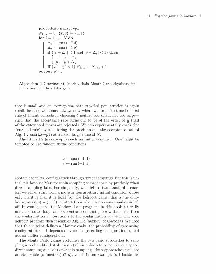
procedure markov-pi
Nhits ← 0; x, y ← 1, 1for i = 1, . . . , N do⎧⎪⎪⎪⎪⎪⎪⎨⎪⎪⎪⎪⎪⎪⎩
∆x ← ran (−δ, δ)∆y ← ran (−δ, δ)if (|x + ∆x| < 1 and |y + ∆y| < 1) then
x ← x + ∆x
y ← y + ∆y
if (x2 + y2 < 1) Nhits ← Nhits + 1output Nhits
——
Algorithm 1.2 markov-pi. Markov-chain Monte Carlo algorithm forcomputing in the adults’ game.
rate is small and on average the path traveled per iteration is againsmall, because we almost always stay where we are. The time-honoredrule of thumb consists in choosing δ neither too small, nor too large—such that the acceptance rate turns out to be of the order of 1
2 (halfof the attempted moves are rejected). We can experimentally check this“one-half rule” by monitoring the precision and the acceptance rate ofAlg. 1.2 (markov-pi) at a fixed, large value of N .
Algorithm 1.2 (markov-pi) needs an initial condition. One might betempted to use random initial conditions
x ← ran (−1, 1) ,y ← ran (−1, 1)
(obtain the initial configuration through direct sampling), but this is un-realistic because Markov-chain sampling comes into play precisely whendirect sampling fails. For simplicity, we stick to two standard scenar-ios: we either start from a more or less arbitrary initial condition whoseonly merit is that it is legal (for the heliport game, this is the club-house, at (x, y) = (1, 1)), or start from where a previous simulation leftoff. In consequence, the Markov-chain programs in this book generallyomit the outer loop, and concentrate on that piece which leads fromthe configuration at iteration i to the configuration at i + 1. The coreheliport program then resembles Alg. 1.3 (markov-pi(patch)). We notethat this is what defines a Markov chain: the probability of generatingconfiguration i + 1 depends only on the preceding configuration, i, andnot on earlier configurations.
The Monte Carlo games epitomize the two basic approaches to sam-pling a probability distribution π(x) on a discrete or continuous space:direct sampling and Markov-chain sampling. Both approaches evaluatean observable (a function) O(x), which in our example is 1 inside the
8 Monte Carlo methods
procedure markov-pi(patch)
input x, y (configuration i)∆x ← . . .∆y ← . . ....output x, y (configuration i + 1)
Algorithm 1.3 markov-pi(patch). Going from one configuration to thenext, in the Markov-chain Monte Carlo algorithm.
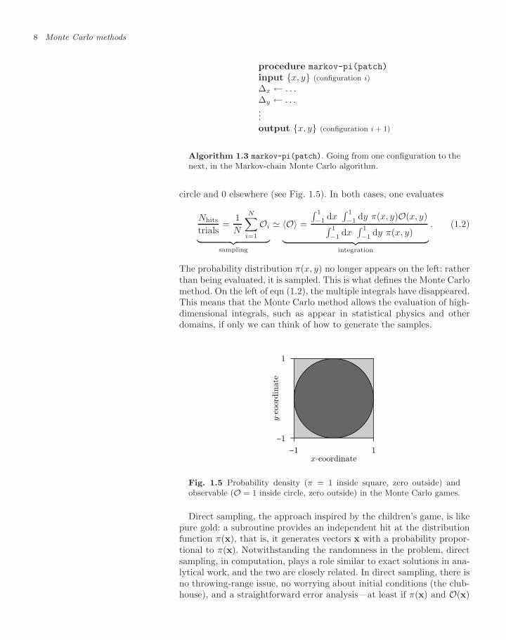
circle and 0 elsewhere (see Fig. 1.5). In both cases, one evaluates
Nhits
trials=
1N
N∑i=1
Oi︸ ︷︷ ︸sampling
〈O〉 =
∫ 1
−1 dx∫ 1
−1 dy π(x, y)O(x, y)∫ 1
−1dx∫ 1
−1dy π(x, y)︸ ︷︷ ︸
integration
. (1.2)
The probability distribution π(x, y) no longer appears on the left: ratherthan being evaluated, it is sampled. This is what defines the Monte Carlomethod. On the left of eqn (1.2), the multiple integrals have disappeared.This means that the Monte Carlo method allows the evaluation of high-dimensional integrals, such as appear in statistical physics and otherdomains, if only we can think of how to generate the samples.
−1 1x-coordinate
−1
1
y-co
ordin
ate
Fig. 1.5 Probability density (π = 1 inside square, zero outside) andobservable (O = 1 inside circle, zero outside) in the Monte Carlo games.
Direct sampling, the approach inspired by the children’s game, is likepure gold: a subroutine provides an independent hit at the distributionfunction π(x), that is, it generates vectors x with a probability propor-tional to π(x). Notwithstanding the randomness in the problem, directsampling, in computation, plays a role similar to exact solutions in ana-lytical work, and the two are closely related. In direct sampling, there isno throwing-range issue, no worrying about initial conditions (the club-house), and a straightforward error analysis—at least if π(x) and O(x)
1.1 Popular games in Monaco 9
are well behaved. Many successful Monte Carlo algorithms contain exactsampling as a key ingredient.
Markov-chain sampling, on the other hand, forces us to be much morecareful with all aspects of our calculation. The critical issue here is thecorrelation time, during which the pebble keeps a memory of the startingconfiguration, the clubhouse. This time can become astronomical. In theusual applications, one is often satisfied with a handful of independentsamples, obtained through week-long calculations, but it can requiremuch thought and experience to ensure that even this modest goal isachieved. We shall continue our discussion of Markov-chain Monte Carlomethods in Subsection 1.1.4, but want to first take a brief look at thehistory of stochastic computing.
1.1.3 Historical origins
The idea of direct sampling was introduced into modern science in thelate 1940s by the mathematician Ulam, not without pride, as one canfind out from his autobiography Adventures of a Mathematician (Ulam(1991)). Much earlier, in 1777, the French naturalist Buffon (1707–1788)imagined a legendary needle-throwing experiment, and analyzed it com-pletely. All through the eighteenth and nineteenth centuries, royal courtsand learned circles were intrigued by this game, and the theory was de-veloped further. After a basic treatment of the Buffon needle problem,we shall describe the particularly brilliant idea of Barbier (1860), whichforeshadows modern techniques of variance reduction.
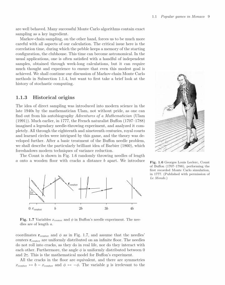
Fig. 1.6 Georges Louis Leclerc, Countof Buffon (1707–1788), performing thefirst recorded Monte Carlo simulation,in 1777. (Published with permission ofLe Monde.)
The Count is shown in Fig. 1.6 randomly throwing needles of lengtha onto a wooden floor with cracks a distance b apart. We introduce
φ
xcenter0 b 2b 3b 4b
rcenter
Fig. 1.7 Variables xcenter and φ in Buffon’s needle experiment. The nee-dles are of length a.
coordinates rcenter and φ as in Fig. 1.7, and assume that the needles’centers rcenter are uniformly distributed on an infinite floor. The needlesdo not roll into cracks, as they do in real life, nor do they interact witheach other. Furthermore, the angle φ is uniformly distributed between 0and 2. This is the mathematical model for Buffon’s experiment.
All the cracks in the floor are equivalent, and there are symmetriesxcenter ↔ b − xcenter and φ ↔ −φ. The variable y is irrelevant to the
10 Monte Carlo methods
problem. We may thus consider a reduced “landing pad”, in which
0 < φ <
2, (1.3)
0 < xcenter <b
2. (1.4)
The tip of each needle is at an x-coordinate xtip = xcenter − (a/2) cos φ;and every xtip < 0 signals a hit on a crack. More precisely, the observableto be evaluated on this landing pad is (writing x for xcenter)
Nhits(x, φ) =
# of hits of needle centered at x,with orientation φ
=
1 for x < a/2 and |φ| < arccos [x/(a/2)]0 otherwise
.
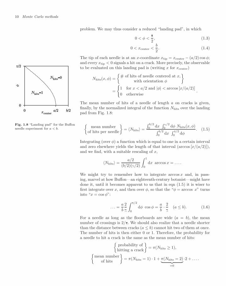
The mean number of hits of a needle of length a on cracks is given,finally, by the normalized integral of the function Nhits over the landingpad from Fig. 1.8:
π/2
0
b/2a/20
φ
xcenter
Nhits=1
Nhits=0
π/2
0
b/2a/20
φ
xcenter
Nhits=1
Nhits=0
Fig. 1.8 “Landing pad” for the Buffonneedle experiment for a < b.
mean number
of hits per needle
= 〈Nhits〉 =
∫ b/2
0 dx∫/2
0 dφ Nhits(x, φ)∫ b/2
0 dx∫/2
0 dφ. (1.5)
Integrating (over φ) a function which is equal to one in a certain intervaland zero elsewhere yields the length of that interval (arccos [x/(a/2)]),and we find, with a suitable rescaling of x,
〈Nhits〉 =a/2
(b/2)(/2)
∫ 1
0
dx arccos x = . . . .
We might try to remember how to integrate arccos x and, in pass-ing, marvel at how Buffon—an eighteenth-century botanist—might havedone it, until it becomes apparent to us that in eqn (1.5) it is wiser tofirst integrate over x, and then over φ, so that the “φ = arccos x” turnsinto “x = cos φ”:
. . . =a
b
2
∫/2
0
dφ cos φ =a
b· 2
(a ≤ b). (1.6)
For a needle as long as the floorboards are wide (a = b), the meannumber of crossings is 2/. We should also realize that a needle shorterthan the distance between cracks (a ≤ b) cannot hit two of them at once.The number of hits is then either 0 or 1. Therefore, the probability fora needle to hit a crack is the same as the mean number of hits:
probability ofhitting a crack
= π(Nhits ≥ 1),
mean numberof hits
= π(Nhits = 1) · 1 + π(Nhits = 2)︸ ︷︷ ︸
=0
·2 + . . . .
1.1 Popular games in Monaco 11
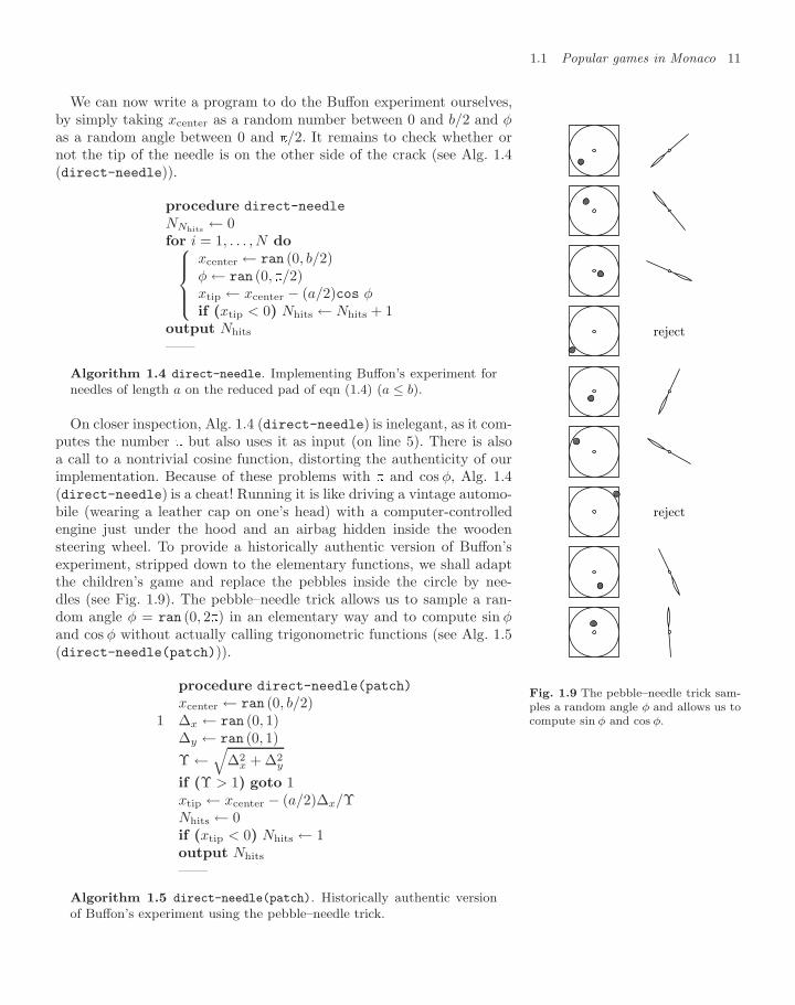
We can now write a program to do the Buffon experiment ourselves,by simply taking xcenter as a random number between 0 and b/2 and φas a random angle between 0 and /2. It remains to check whether ornot the tip of the needle is on the other side of the crack (see Alg. 1.4(direct-needle)).
procedure direct-needle
NNhits← 0
for i = 1, . . . , N do⎧⎪⎪⎨⎪⎪⎩xcenter ← ran (0, b/2)φ ← ran (0, /2)xtip ← xcenter − (a/2)cos φif (xtip < 0) Nhits ← Nhits + 1
output Nhits
——
Algorithm 1.4 direct-needle. Implementing Buffon’s experiment forneedles of length a on the reduced pad of eqn (1.4) (a ≤ b).
On closer inspection, Alg. 1.4 (direct-needle) is inelegant, as it com-putes the number but also uses it as input (on line 5). There is alsoa call to a nontrivial cosine function, distorting the authenticity of ourimplementation. Because of these problems with and cos φ, Alg. 1.4(direct-needle) is a cheat! Running it is like driving a vintage automo-bile (wearing a leather cap on one’s head) with a computer-controlledengine just under the hood and an airbag hidden inside the woodensteering wheel. To provide a historically authentic version of Buffon’sexperiment, stripped down to the elementary functions, we shall adaptthe children’s game and replace the pebbles inside the circle by nee-dles (see Fig. 1.9). The pebble–needle trick allows us to sample a ran-dom angle φ = ran (0, 2) in an elementary way and to compute sin φand cos φ without actually calling trigonometric functions (see Alg. 1.5(direct-needle(patch))).
reject
reject
Fig. 1.9 The pebble–needle trick sam-ples a random angle φ and allows us tocompute sin φ and cos φ.
procedure direct-needle(patch)
xcenter ← ran (0, b/2)1 ∆x ← ran (0, 1)
∆y ← ran (0, 1)Υ ←
√∆2
x + ∆2y
if (Υ > 1) goto 1xtip ← xcenter − (a/2)∆x/ΥNhits ← 0if (xtip < 0) Nhits ← 1output Nhits
——
Algorithm 1.5 direct-needle(patch). Historically authentic versionof Buffon’s experiment using the pebble–needle trick.
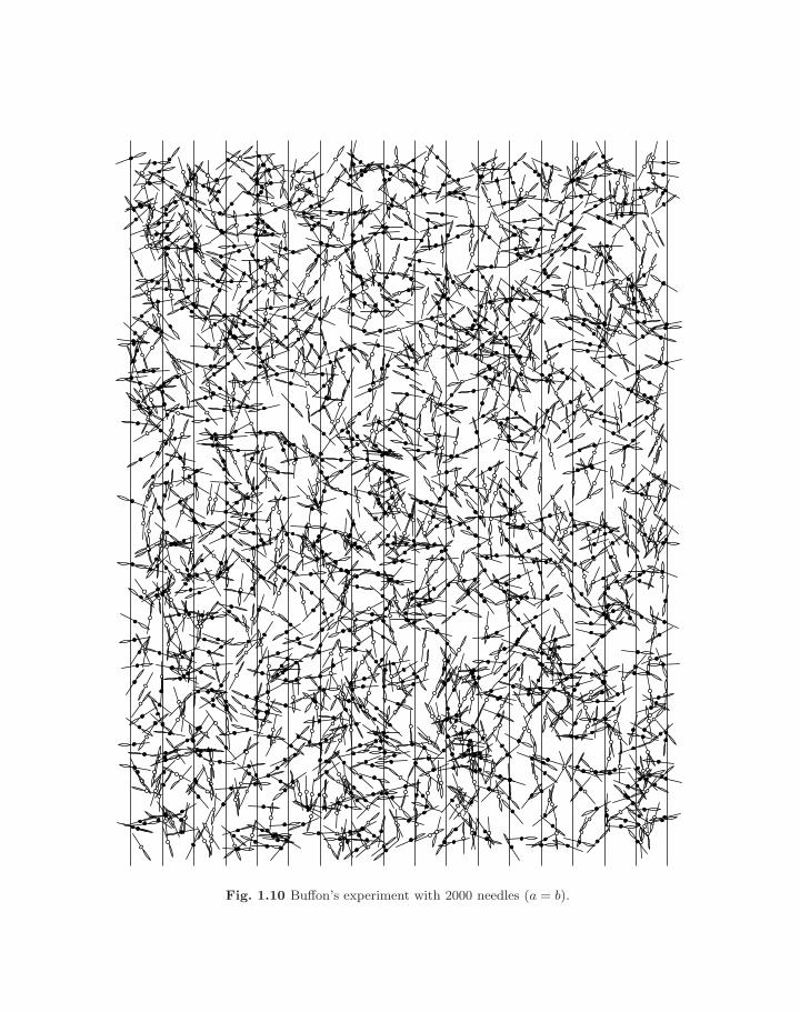
Fig. 1.10 Buffon’s experiment with 2000 needles (a = b).
1.1 Popular games in Monaco 13
The pebble–needle trick is really quite clever, and we shall revisit itseveral times, in discussions of isotropic samplings in higher-dimensionalhyperspheres, Gaussian random numbers, and the Maxwell distributionof particle velocities in a gas.
We can now follow in Count Buffon’s footsteps, and perform our ownneedle-throwing experiments. One of these, with 2000 samples, is shownin Fig. 1.10.
Looking at this figure makes us wonder whether needles are morelikely to intersect a crack at their tip, their center, or their eye. The fullanswer to this question, the subject of the present subsection, allows usto understand the factor 2/ in eqn (1.6) without any calculation.
Mathematically formulated, the question is the following: a needlehitting a crack does so at a certain value l of its interior coordinate0 ≤ l ≤ a (where, say, l = 0 at the tip, and l = a at the end of the eye).The mean number of hits, Nhits, can be written as
〈Nhits〉 =∫ a
0
dl 〈Nhits(l)〉 .
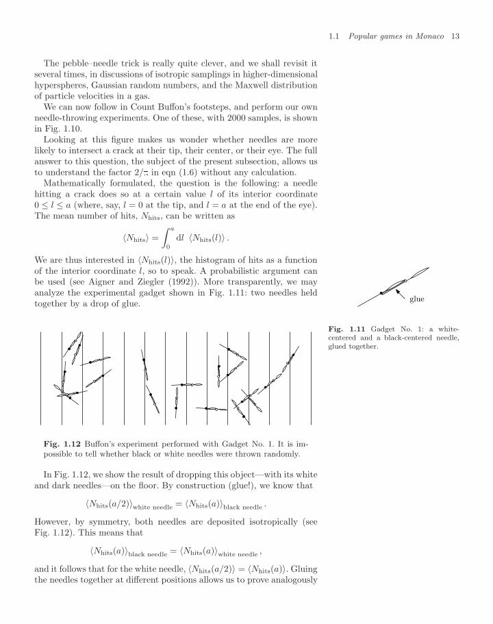
We are thus interested in 〈Nhits(l)〉, the histogram of hits as a functionof the interior coordinate l, so to speak. A probabilistic argument canbe used (see Aigner and Ziegler (1992)). More transparently, we mayanalyze the experimental gadget shown in Fig. 1.11: two needles heldtogether by a drop of glue. glue
Fig. 1.11 Gadget No. 1: a white-centered and a black-centered needle,glued together.
Fig. 1.12 Buffon’s experiment performed with Gadget No. 1. It is im-possible to tell whether black or white needles were thrown randomly.
In Fig. 1.12, we show the result of dropping this object—with its whiteand dark needles—on the floor. By construction (glue!), we know that
〈Nhits(a/2)〉white needle = 〈Nhits(a)〉black needle .
However, by symmetry, both needles are deposited isotropically (seeFig. 1.12). This means that
〈Nhits(a)〉black needle = 〈Nhits(a)〉white needle ,
and it follows that for the white needle, 〈Nhits(a/2)〉 = 〈Nhits(a)〉. Gluingthe needles together at different positions allows us to prove analogously
14 Monte Carlo methods
that 〈Nhits(l)〉 is independent of l. The argument can be carried evenfurther: clearly, the total number of hits for the gadget in Fig. 1.12 is3/2 times that for a single needle, or, more generally,
mean numberof hits
= Υ · length of needle
. (1.7)
The constant Υ (Upsilon) is the same for needles of any length, smalleror larger than the distance between the cracks in the floor (we havecomputed it already in eqn (1.6)).
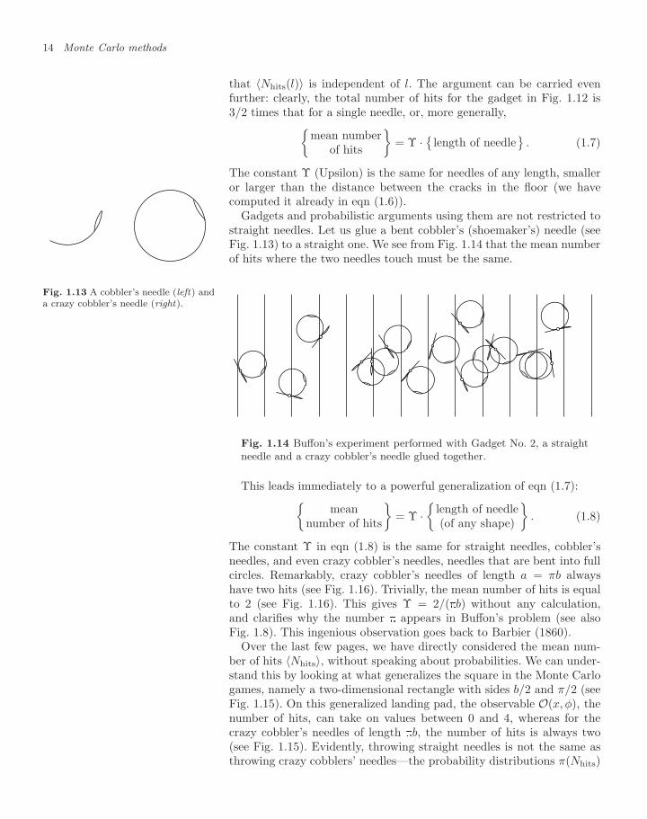
Gadgets and probabilistic arguments using them are not restricted tostraight needles. Let us glue a bent cobbler’s (shoemaker’s) needle (seeFig. 1.13) to a straight one. We see from Fig. 1.14 that the mean numberof hits where the two needles touch must be the same.
Fig. 1.13 A cobbler’s needle (left) anda crazy cobbler’s needle (right).
Fig. 1.14 Buffon’s experiment performed with Gadget No. 2, a straightneedle and a crazy cobbler’s needle glued together.
This leads immediately to a powerful generalization of eqn (1.7):mean
number of hits
= Υ ·
length of needle(of any shape)
. (1.8)
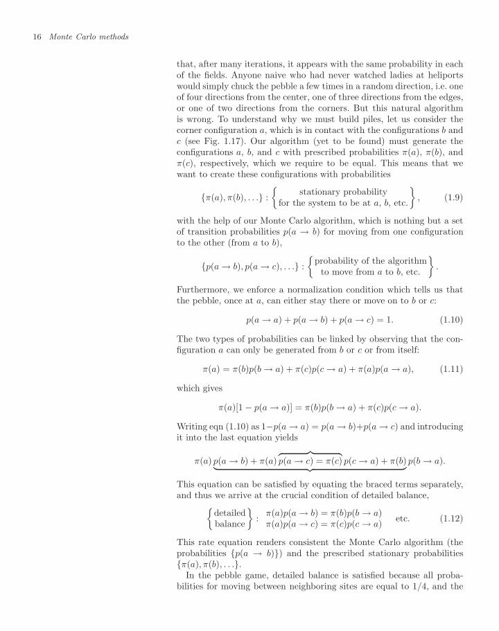
The constant Υ in eqn (1.8) is the same for straight needles, cobbler’sneedles, and even crazy cobbler’s needles, needles that are bent into fullcircles. Remarkably, crazy cobbler’s needles of length a = πb alwayshave two hits (see Fig. 1.16). Trivially, the mean number of hits is equalto 2 (see Fig. 1.16). This gives Υ = 2/(b) without any calculation,and clarifies why the number appears in Buffon’s problem (see alsoFig. 1.8). This ingenious observation goes back to Barbier (1860).
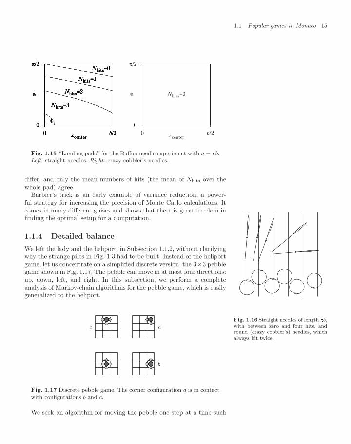
Over the last few pages, we have directly considered the mean num-ber of hits 〈Nhits〉, without speaking about probabilities. We can under-stand this by looking at what generalizes the square in the Monte Carlogames, namely a two-dimensional rectangle with sides b/2 and π/2 (seeFig. 1.15). On this generalized landing pad, the observable O(x, φ), thenumber of hits, can take on values between 0 and 4, whereas for thecrazy cobbler’s needles of length b, the number of hits is always two(see Fig. 1.15). Evidently, throwing straight needles is not the same asthrowing crazy cobblers’ needles—the probability distributions π(Nhits)
1.1 Popular games in Monaco 15
π/2
0
b/20
φ
xcenter
Nhits=0
Nhits=1
Nhits=2
Nhits=3
=4
π/2
0
b/20
φ
xcenter
Nhits=0
Nhits=1
Nhits=2
Nhits=3
=4
π/2
0
b/20
φ
xcenter
Nhits=0
Nhits=1
Nhits=2
Nhits=3
=4
π/2
0
b/20
φ
xcenter
Nhits=0
Nhits=1
Nhits=2
Nhits=3
=4
π/2
0
b/20
φ
xcenter
Nhits=0
Nhits=1
Nhits=2
Nhits=3
=4
π/2
0
b/20φ
xcenter
Nhits=2
Fig. 1.15 “Landing pads” for the Buffon needle experiment with a = b.Left : straight needles. Right : crazy cobbler’s needles.
differ, and only the mean numbers of hits (the mean of Nhits over thewhole pad) agree.
Fig. 1.16 Straight needles of length b,with between zero and four hits, andround (crazy cobbler’s) needles, whichalways hit twice.
Barbier’s trick is an early example of variance reduction, a power-ful strategy for increasing the precision of Monte Carlo calculations. Itcomes in many different guises and shows that there is great freedom infinding the optimal setup for a computation.
1.1.4 Detailed balance
We left the lady and the heliport, in Subsection 1.1.2, without clarifyingwhy the strange piles in Fig. 1.3 had to be built. Instead of the heliportgame, let us concentrate on a simplified discrete version, the 3×3 pebblegame shown in Fig. 1.17. The pebble can move in at most four directions:up, down, left, and right. In this subsection, we perform a completeanalysis of Markov-chain algorithms for the pebble game, which is easilygeneralized to the heliport.
c a
b
Fig. 1.17 Discrete pebble game. The corner configuration a is in contactwith configurations b and c.
We seek an algorithm for moving the pebble one step at a time such
16 Monte Carlo methods
that, after many iterations, it appears with the same probability in eachof the fields. Anyone naive who had never watched ladies at heliportswould simply chuck the pebble a few times in a random direction, i.e. oneof four directions from the center, one of three directions from the edges,or one of two directions from the corners. But this natural algorithmis wrong. To understand why we must build piles, let us consider thecorner configuration a, which is in contact with the configurations b andc (see Fig. 1.17). Our algorithm (yet to be found) must generate theconfigurations a, b, and c with prescribed probabilities π(a), π(b), andπ(c), respectively, which we require to be equal. This means that wewant to create these configurations with probabilities
π(a), π(b), . . . :
stationary probabilityfor the system to be at a, b, etc.
, (1.9)
with the help of our Monte Carlo algorithm, which is nothing but a setof transition probabilities p(a → b) for moving from one configurationto the other (from a to b),
p(a → b), p(a → c), . . . :
probability of the algorithmto move from a to b, etc.
.
Furthermore, we enforce a normalization condition which tells us thatthe pebble, once at a, can either stay there or move on to b or c:
p(a → a) + p(a → b) + p(a → c) = 1. (1.10)
The two types of probabilities can be linked by observing that the con-figuration a can only be generated from b or c or from itself:
π(a) = π(b)p(b → a) + π(c)p(c → a) + π(a)p(a → a), (1.11)
which gives
π(a)[1 − p(a → a)] = π(b)p(b → a) + π(c)p(c → a).
Writing eqn (1.10) as 1−p(a → a) = p(a → b)+p(a → c) and introducingit into the last equation yields
π(a) p(a → b) + π(a)︷ ︸︸ ︷p(a → c) = π(c) p(c → a) + π(b)︸ ︷︷ ︸ p(b → a).
This equation can be satisfied by equating the braced terms separately,and thus we arrive at the crucial condition of detailed balance,
detailedbalance
: π(a)p(a → b) = π(b)p(b → a)
π(a)p(a → c) = π(c)p(c → a) etc. (1.12)
This rate equation renders consistent the Monte Carlo algorithm (theprobabilities p(a → b)) and the prescribed stationary probabilitiesπ(a), π(b), . . ..
In the pebble game, detailed balance is satisfied because all proba-bilities for moving between neighboring sites are equal to 1/4, and the
1.1 Popular games in Monaco 17
probabilities p(a → b) and the return probabilities p(b → a) are triviallyidentical. Now we see why the pebbles have to pile up on the sides andin the corners: all the transition probabilities to neighbors have to beequal to 1/4. But a corner has only two neighbors, which means thathalf of the time we can leave the site, and half of the time we must stay,building up a pile.
Of course, there are more complicated choices for the transition prob-abilities which also satisfy the detailed-balance condition. In addition,this condition is sufficient but not necessary for arriving at π(a) = π(b)for all neighboring sites a and b. On both counts, it is the quest forsimplicity that guides our choice.
To implement the pebble game, we could simply modify Alg. 1.2(markov-pi) using integer variables kx, ky, and installing the movesof Fig. 1.17 with a few lines of code. Uniform integer random numbersnran (−1, 1) (that is, random integers taking values −1, 0, 1, see Sub-section 1.2.2) would replace the real random numbers. With variableskx, ky, kz and another contraption to select the moves, such a programcan also simulate three-dimensional pebble games.
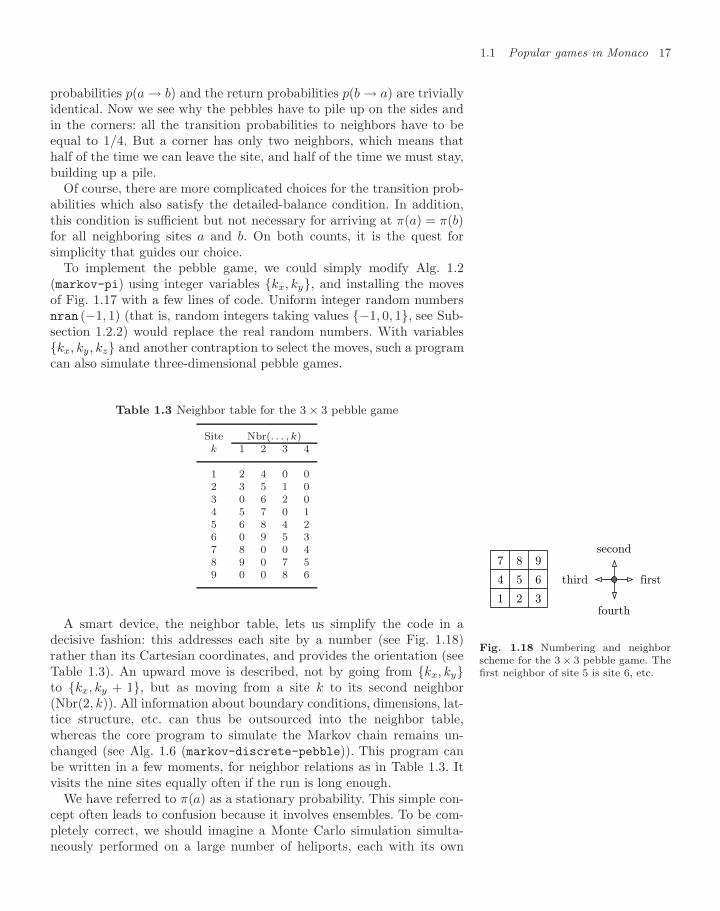
Table 1.3 Neighbor table for the 3 × 3 pebble game
Site Nbr(. . . , k)k 1 2 3 4
1 2 4 0 02 3 5 1 03 0 6 2 04 5 7 0 15 6 8 4 26 0 9 5 37 8 0 0 48 9 0 7 59 0 0 8 6
1 2 3
4 5 6
7 8 9
first
second
third
fourth
Fig. 1.18 Numbering and neighborscheme for the 3 × 3 pebble game. Thefirst neighbor of site 5 is site 6, etc.
A smart device, the neighbor table, lets us simplify the code in adecisive fashion: this addresses each site by a number (see Fig. 1.18)rather than its Cartesian coordinates, and provides the orientation (seeTable 1.3). An upward move is described, not by going from kx, kyto kx, ky + 1, but as moving from a site k to its second neighbor(Nbr(2, k)). All information about boundary conditions, dimensions, lat-tice structure, etc. can thus be outsourced into the neighbor table,whereas the core program to simulate the Markov chain remains un-changed (see Alg. 1.6 (markov-discrete-pebble)). This program canbe written in a few moments, for neighbor relations as in Table 1.3. Itvisits the nine sites equally often if the run is long enough.
We have referred to π(a) as a stationary probability. This simple con-cept often leads to confusion because it involves ensembles. To be com-pletely correct, we should imagine a Monte Carlo simulation simulta-neously performed on a large number of heliports, each with its own
18 Monte Carlo methods
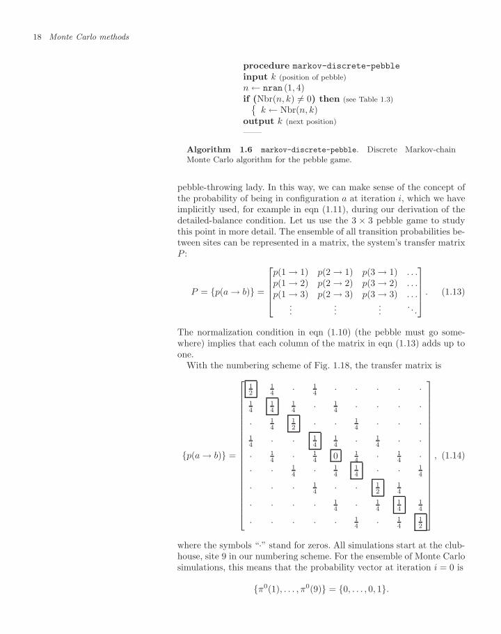
procedure markov-discrete-pebble
input k (position of pebble)n ← nran (1, 4)if (Nbr(n, k) = 0) then (see Table 1.3)
k ← Nbr(n, k)output k (next position)——
Algorithm 1.6 markov-discrete-pebble. Discrete Markov-chainMonte Carlo algorithm for the pebble game.
pebble-throwing lady. In this way, we can make sense of the concept ofthe probability of being in configuration a at iteration i, which we haveimplicitly used, for example in eqn (1.11), during our derivation of thedetailed-balance condition. Let us use the 3 × 3 pebble game to studythis point in more detail. The ensemble of all transition probabilities be-tween sites can be represented in a matrix, the system’s transfer matrixP :
P = p(a → b) =
⎡⎢⎢⎢⎣p(1 → 1) p(2 → 1) p(3 → 1) . . .p(1 → 2) p(2 → 2) p(3 → 2) . . .p(1 → 3) p(2 → 3) p(3 → 3) . . .
......
.... . .
⎤⎥⎥⎥⎦ . (1.13)
The normalization condition in eqn (1.10) (the pebble must go some-where) implies that each column of the matrix in eqn (1.13) adds up toone.
With the numbering scheme of Fig. 1.18, the transfer matrix is
p(a → b) =
⎡⎢⎢⎢⎢⎢⎢⎢⎢⎢⎢⎢⎢⎢⎢⎢⎢⎢⎢⎢⎢⎢⎣
12
14 · 1
4 · · · · ·14
14
14 · 1
4 · · · ·· 1
412 · · 1
4 · · ·14 · · 1
414 · 1
4 · ·· 1
4 · 14 0 1
4 · 14 ·
· · 14 · 1
414 · · 1
4
· · · 14 · · 1
214
· · · · 14 · 1
414
14
· · · · · 14 · 1
412
⎤⎥⎥⎥⎥⎥⎥⎥⎥⎥⎥⎥⎥⎥⎥⎥⎥⎥⎥⎥⎥⎥⎦
, (1.14)
where the symbols “·” stand for zeros. All simulations start at the club-house, site 9 in our numbering scheme. For the ensemble of Monte Carlosimulations, this means that the probability vector at iteration i = 0 is
π0(1), . . . , π0(9) = 0, . . . , 0, 1.
1.1 Popular games in Monaco 19
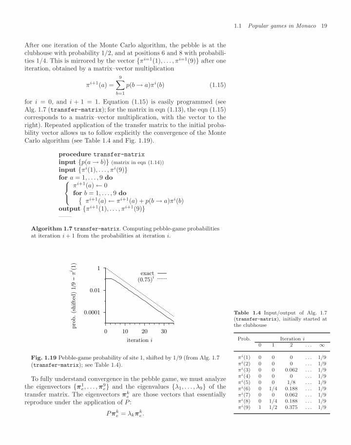
After one iteration of the Monte Carlo algorithm, the pebble is at theclubhouse with probability 1/2, and at positions 6 and 8 with probabili-ties 1/4. This is mirrored by the vector πi=1(1), . . . , πi=1(9) after oneiteration, obtained by a matrix–vector multiplication
πi+1(a) =9∑
b=1
p(b → a)πi(b) (1.15)
for i = 0, and i + 1 = 1. Equation (1.15) is easily programmed (seeAlg. 1.7 (transfer-matrix); for the matrix in eqn (1.13), the eqn (1.15)corresponds to a matrix–vector multiplication, with the vector to theright). Repeated application of the transfer matrix to the initial proba-bility vector allows us to follow explicitly the convergence of the MonteCarlo algorithm (see Table 1.4 and Fig. 1.19).
procedure transfer-matrix
input p(a → b) (matrix in eqn (1.14))input πi(1), . . . , πi(9)for a = 1, . . . , 9 do⎧⎨⎩
πi+1(a) ← 0for b = 1, . . . , 9 do
πi+1(a) ← πi+1(a) + p(b → a)πi(b)output πi+1(1), . . . , πi+1(9)——
Algorithm 1.7 transfer-matrix. Computing pebble-game probabilitiesat iteration i + 1 from the probabilities at iteration i.
0.0001
0.01
1
0 10 20 30
pro
b. (s
hifte
d)
1/9
− π
i (1)
iteration i
exact(0.75)i
Fig. 1.19 Pebble-game probability of site 1, shifted by 1/9 (from Alg. 1.7(transfer-matrix); see Table 1.4).
Table 1.4 Input/output of Alg. 1.7(transfer-matrix), initially started atthe clubhouse
Prob. Iteration i0 1 2 . . . ∞
πi(1) 0 0 0 . . . 1/9πi(2) 0 0 0 . . . 1/9πi(3) 0 0 0.062 . . . 1/9πi(4) 0 0 0 . . . 1/9πi(5) 0 0 1/8 . . . 1/9πi(6) 0 1/4 0.188 . . . 1/9πi(7) 0 0 0.062 . . . 1/9πi(8) 0 1/4 0.188 . . . 1/9πi(9) 1 1/2 0.375 . . . 1/9
To fully understand convergence in the pebble game, we must analyzethe eigenvectors π1
e, . . . ,π9e and the eigenvalues λ1, . . . , λ9 of the
transfer matrix. The eigenvectors πke are those vectors that essentially
reproduce under the application of P :
Pπke = λkπ
ke .
20 Monte Carlo methods
Writing a probability vector π = π(1), . . . , π(9) in terms of the eigen-vectors, i.e.
π = α1π1e + α2π
2e + · · · + α9π
9e =
9∑k=1
αkπke ,
allows us to see how it is transformed after one iteration,
Pπ = α1Pπ1e + α2Pπ
2e + · · · + α9Pπ
9e =
9∑k=1
αkPπke
= α1λ1π1e + α2λ2π
2e + · · · + α9λ9π
9e =
9∑k=1
αkλkπke ,
or after i iterations,
P iπ = α1λ
i1π
1e + α2λ
i2π
2e + · · · + α9λ
i9π
9e =
9∑k=1
αk(λk)iπ
ke .
Only one eigenvector has components that are all nonnegative, so thatit can be a vector of probabilities. This vector must have the largesteigenvalue λ1 (the matrix P being positive). Because of eqn (1.10), wehave λ1 = 1. Other eigenvectors and eigenvalues can be computed ex-plicitly, at least in the 3 × 3 pebble game. Besides the dominant eigen-value λ1, there are two eigenvalues equal to 0.75, one equal to 0.5, etc.This allows us to follow the precise convergence towards the asymptoticequilibrium solution:
πi(1), . . . , πi(9)= 1
9 , . . . , 19︸ ︷︷ ︸
first eigenvectoreigenvalue λ1 = 1
+α2 · (0.75)i −0.21, . . . , 0.21︸ ︷︷ ︸second eigenvector
eigenvalue λ2 = 0.75
+ · · · .
In the limit i → ∞, the contributions of the subdominant eigenvectorsdisappear and the first eigenvector, the vector of stationary probabilitiesin eqn (1.9), exactly reproduces under multiplication by the transfermatrix. The two are connected through the detailed-balance condition,as discussed in simpler terms at the beginning of this subsection.
The difference between πi(1), . . . , πi(9) and the asymptotic solutionis determined by the second largest eigenvalue of the transfer matrix andis proportional to
(0.75)i = ei·log 0.75 = exp(− i
3.476
). (1.16)
The data in Fig. 1.19 clearly show the (0.75)i behavior, which is equiv-alent to an exponential ∝ e−i/∆i where ∆i = 3.476. ∆i is a timescale,and allows us to define short times and long times: a short simulation
1.1 Popular games in Monaco 21
has fewer than ∆i iterations, and a long simulation has many more thanthat.
In conclusion, we see that transfer matrix iterations and Monte Carlocalculations reach equilibrium only after an infinite number of itera-tions. This is not a very serious restriction, because of the existence of atimescale for convergence, which is set by the second largest eigenvalueof the transfer matrix. To all intents and purposes, the asymptotic equi-librium solution is reached after the convergence time has passed a fewtimes. For example, the pebble game converges to equilibrium after afew times 3.476 iterations (see eqn (1.16)). The concept of equilibriumis far-reaching, and the interest in Monte Carlo calculations is rightlystrong because of this timescale, which separates fast and slow processesand leads to exponential convergence.
1.1.5 The Metropolis algorithm
In Subsection 1.1.4, direct inspection of the detailed-balance conditionin eqn (1.12) allowed us to derive Markov-chain algorithms for simplegames where the probability of each configuration was either zero or one.This is not the most general case, even for pebbles, which may be lesslikely to be at a position a on a hilltop than at another position b locatedin a valley (so that π(a) < π(b)). Moves between positions a and b witharbitrary probabilities π(a) and π(b), respecting the detailed-balancecondition in eqn (1.12), are generated by the Metropolis algorithm (seeMetropolis et al. (1953)), which accepts a move a → b with probability
p(a → b) = min[1,
π(b)π(a)
]. (1.17)
In the heliport game, we have unknowingly used eqn (1.17): for a andb both inside the square, the move was accepted without further tests(π(b)/π(a) = 1, p(a → b) = 1). In contrast, for a inside but b outsidethe square, the move was rejected (π(b)/π(a) = 0, p(a → b) = 0).
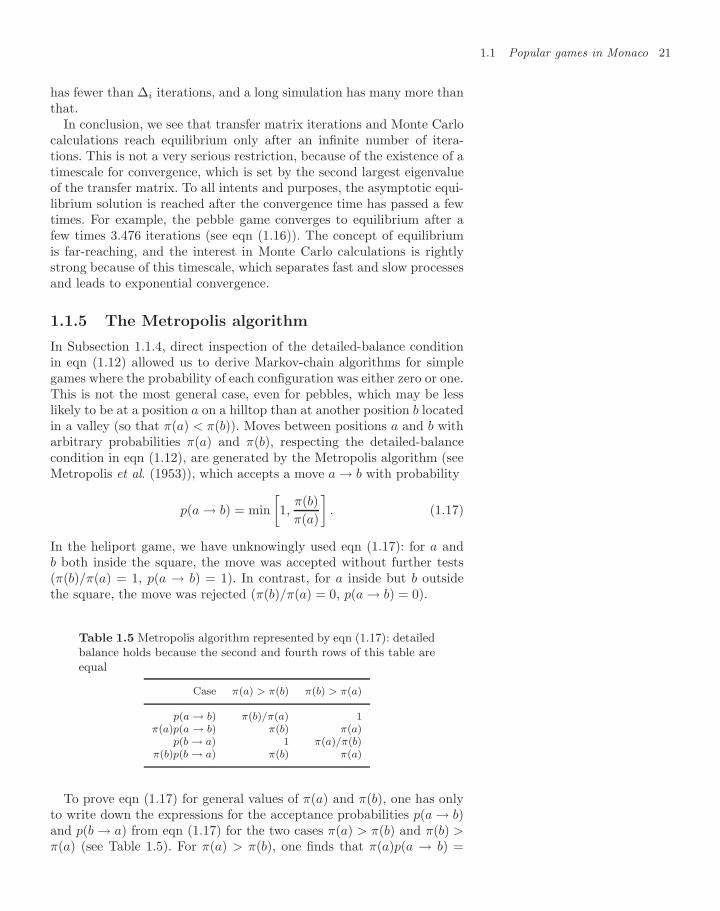
Table 1.5 Metropolis algorithm represented by eqn (1.17): detailedbalance holds because the second and fourth rows of this table areequal
Case π(a) > π(b) π(b) > π(a)
p(a → b) π(b)/π(a) 1π(a)p(a → b) π(b) π(a)
p(b → a) 1 π(a)/π(b)π(b)p(b → a) π(b) π(a)
To prove eqn (1.17) for general values of π(a) and π(b), one has onlyto write down the expressions for the acceptance probabilities p(a → b)and p(b → a) from eqn (1.17) for the two cases π(a) > π(b) and π(b) >π(a) (see Table 1.5). For π(a) > π(b), one finds that π(a)p(a → b) =
22 Monte Carlo methods
π(b)p(b → a) = π(b). In this case, and likewise for π(b) > π(a), detailedbalance is satisfied. This is all there is to the Metropolis algorithm.
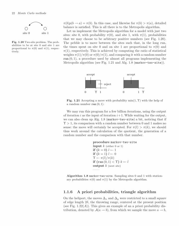
site 0 site 1
Fig. 1.20 Two-site problem. The prob-abilities to be at site 0 and site 1 areproportional to π(0) and π(1), respec-tively.
Let us implement the Metropolis algorithm for a model with just twosites: site 0, with probability π(0), and site 1, with π(1), probabilitiesthat we may choose to be arbitrary positive numbers (see Fig. 1.20).The pebble is to move between the sites such that, in the long run,the times spent on site 0 and on site 1 are proportional to π(0) andπ(1), respectively. This is achieved by computing the ratio of statisticalweights π(1)/π(0) or π(0)/π(1), and comparing it with a random numberran (0, 1), a procedure used by almost all programs implementing theMetropolis algorithm (see Fig. 1.21 and Alg. 1.8 (markov-two-site)).
0 Υ 1
accept
reject
0 Υ1
accept
Fig. 1.21 Accepting a move with probability min(1, Υ) with the help ofa random number ran (0, 1).
We may run this program for a few billion iterations, using the outputof iteration i as the input of iteration i+1. While waiting for the output,we can also clean up Alg. 1.8 (markov-two-site) a bit, noticing that ifΥ > 1, its comparison with a random number between 0 and 1 makes nosense: the move will certainly be accepted. For π(l) > π(k), we shouldthus work around the calculation of the quotient, the generation of arandom number and the comparison with that number.
procedure markov-two-site
input k (either 0 or 1)if (k = 0) l ← 1if (k = 1) l ← 0Υ ← π(l)/π(k)if (ran (0, 1) < Υ) k ← loutput k (next site)——
Algorithm 1.8 markov-two-site. Sampling sites 0 and 1 with station-ary probabilities π(0) and π(1) by the Metropolis algorithm.
1.1.6 A priori probabilities, triangle algorithm
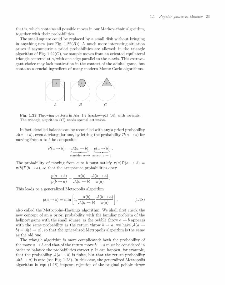
On the heliport, the moves ∆x and ∆y were restricted to a small squareof edge length 2δ, the throwing range, centered at the present position(see Fig. 1.22(A)). This gives an example of an a priori probability dis-tribution, denoted by A(a → b), from which we sample the move a → b,
1.1 Popular games in Monaco 23
that is, which contains all possible moves in our Markov-chain algorithm,together with their probabilities.
The small square could be replaced by a small disk without bringingin anything new (see Fig. 1.22(B)). A much more interesting situationarises if asymmetric a priori probabilities are allowed: in the trianglealgorithm of Fig. 1.22(C), we sample moves from an oriented equilateraltriangle centered at a, with one edge parallel to the x-axis. This extrava-gant choice may lack motivation in the context of the adults’ game, butcontains a crucial ingredient of many modern Monte Carlo algorithms.
A B C
Fig. 1.22 Throwing pattern in Alg. 1.2 (markov-pi) (A), with variants.The triangle algorithm (C ) needs special attention.
In fact, detailed balance can be reconciled with any a priori probabilityA(a → b), even a triangular one, by letting the probability P(a → b) formoving from a to b be composite:
P(a → b) = A(a → b)︸ ︷︷ ︸consider a→b
· p(a → b)︸ ︷︷ ︸accept a → b
.
The probability of moving from a to b must satisfy π(a)P(a → b) =π(b)P(b → a), so that the acceptance probabilities obey
p(a → b)p(b → a)
=π(b)
A(a → b)A(b → a)
π(a).
This leads to a generalized Metropolis algorithm
p(a → b) = min[1,
π(b)A(a → b)
A(b → a)π(a)
], (1.18)
also called the Metropolis–Hastings algorithm. We shall first check thenew concept of an a priori probability with the familiar problem of theheliport game with the small square: as the pebble throw a → b appearswith the same probability as the return throw b → a, we have A(a →b) = A(b → a), so that the generalized Metropolis algorithm is the sameas the old one.
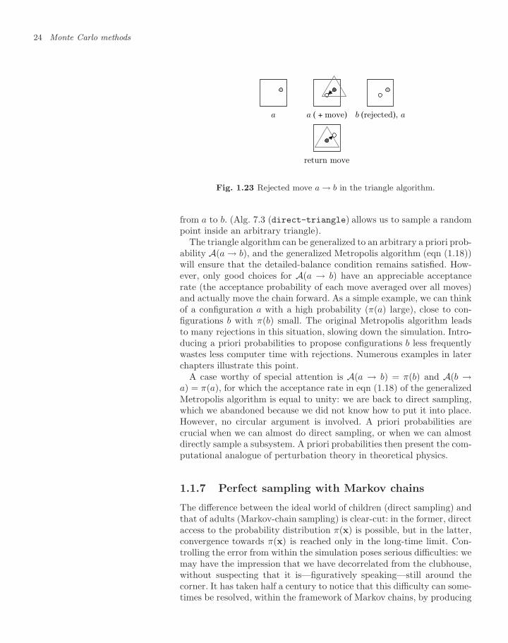
The triangle algorithm is more complicated: both the probability ofthe move a → b and that of the return move b → a must be considered inorder to balance the probabilities correctly. It can happen, for example,that the probability A(a → b) is finite, but that the return probabilityA(b → a) is zero (see Fig. 1.23). In this case, the generalized Metropolisalgorithm in eqn (1.18) imposes rejection of the original pebble throw
24 Monte Carlo methods
a a ( + move) b (rejected), a
return move
Fig. 1.23 Rejected move a → b in the triangle algorithm.
from a to b. (Alg. 7.3 (direct-triangle) allows us to sample a randompoint inside an arbitrary triangle).
The triangle algorithm can be generalized to an arbitrary a priori prob-ability A(a → b), and the generalized Metropolis algorithm (eqn (1.18))will ensure that the detailed-balance condition remains satisfied. How-ever, only good choices for A(a → b) have an appreciable acceptancerate (the acceptance probability of each move averaged over all moves)and actually move the chain forward. As a simple example, we can thinkof a configuration a with a high probability (π(a) large), close to con-figurations b with π(b) small. The original Metropolis algorithm leadsto many rejections in this situation, slowing down the simulation. Intro-ducing a priori probabilities to propose configurations b less frequentlywastes less computer time with rejections. Numerous examples in laterchapters illustrate this point.
A case worthy of special attention is A(a → b) = π(b) and A(b →a) = π(a), for which the acceptance rate in eqn (1.18) of the generalizedMetropolis algorithm is equal to unity: we are back to direct sampling,which we abandoned because we did not know how to put it into place.However, no circular argument is involved. A priori probabilities arecrucial when we can almost do direct sampling, or when we can almostdirectly sample a subsystem. A priori probabilities then present the com-putational analogue of perturbation theory in theoretical physics.
1.1.7 Perfect sampling with Markov chains
The difference between the ideal world of children (direct sampling) andthat of adults (Markov-chain sampling) is clear-cut: in the former, directaccess to the probability distribution π(x) is possible, but in the latter,convergence towards π(x) is reached only in the long-time limit. Con-trolling the error from within the simulation poses serious difficulties: wemay have the impression that we have decorrelated from the clubhouse,without suspecting that it is—figuratively speaking—still around thecorner. It has taken half a century to notice that this difficulty can some-times be resolved, within the framework of Markov chains, by producing
1.1 Popular games in Monaco 25
perfect chain samples, which are equivalent to the children’s throws andguaranteed to be totally decorrelated from the initial condition.
i = − 17
club house
i = − 16 i = − 15 i = − 14 i = − 13 i = − 12
i = − 11 i = − 10 i = − 9 i = − 8 i = − 7 i = − 6
i = − 5 i = − 4 i = − 3 i = − 2 i = − 1 i = 0 (now)
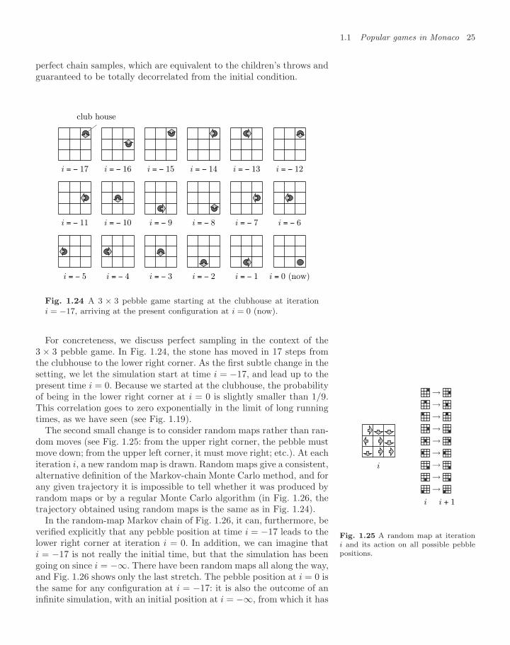
Fig. 1.24 A 3 × 3 pebble game starting at the clubhouse at iterationi = −17, arriving at the present configuration at i = 0 (now).
For concreteness, we discuss perfect sampling in the context of the3 × 3 pebble game. In Fig. 1.24, the stone has moved in 17 steps fromthe clubhouse to the lower right corner. As the first subtle change in thesetting, we let the simulation start at time i = −17, and lead up to thepresent time i = 0. Because we started at the clubhouse, the probabilityof being in the lower right corner at i = 0 is slightly smaller than 1/9.This correlation goes to zero exponentially in the limit of long runningtimes, as we have seen (see Fig. 1.19).
The second small change is to consider random maps rather than ran-dom moves (see Fig. 1.25: from the upper right corner, the pebble mustmove down; from the upper left corner, it must move right; etc.). At eachiteration i, a new random map is drawn. Random maps give a consistent,alternative definition of the Markov-chain Monte Carlo method, and forany given trajectory it is impossible to tell whether it was produced byrandom maps or by a regular Monte Carlo algorithm (in Fig. 1.26, thetrajectory obtained using random maps is the same as in Fig. 1.24).
i
i
→i + 1
→→→→→→→→
Fig. 1.25 A random map at iterationi and its action on all possible pebblepositions.
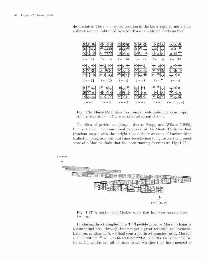
In the random-map Markov chain of Fig. 1.26, it can, furthermore, beverified explicitly that any pebble position at time i = −17 leads to thelower right corner at iteration i = 0. In addition, we can imagine thati = −17 is not really the initial time, but that the simulation has beengoing on since i = −∞. There have been random maps all along the way,and Fig. 1.26 shows only the last stretch. The pebble position at i = 0 isthe same for any configuration at i = −17: it is also the outcome of aninfinite simulation, with an initial position at i = −∞, from which it has
26 Monte Carlo methods
decorrelated. The i = 0 pebble position in the lower right corner is thusa direct sample—obtained by a Markov-chain Monte Carlo method.
i = − 17 i = − 16 i = − 15 i = − 14 i = − 13 i = − 12
i = − 11 i = − 10 i = − 9 i = − 8 i = − 7 i = − 6
i = − 5 i = − 4 i = − 3 i = − 2 i = − 1 i = 0 (now)
Fig. 1.26 Monte Carlo dynamics using time-dependent random maps.All positions at i = −17 give an identical output at i = 0.
The idea of perfect sampling is due to Propp and Wilson (1996).It mixes a minimal conceptual extension of the Monte Carlo method(random maps) with the insight that a finite amount of backtracking(called coupling from the past) may be sufficient to figure out the presentstate of a Markov chain that has been running forever (see Fig. 1.27).
i = 0 (now)
i = − ∞
Fig. 1.27 A random-map Markov chain that has been running sincei = −∞.
Producing direct samples for a 3×3 pebble game by Markov chains isa conceptual breakthrough, but not yet a great technical achievement.Later on, in Chapter 5, we shall construct direct samples (using Markovchains) with 2100 = 1 267 650 600 228 229 401 496 703 205 376 configura-tions. Going through all of them to see whether they have merged is
1.2 Basic sampling 27
out of the question, but we shall see that it is sometimes possible tosqueeze all configurations in between two extremal ones: if those twoconfigurations have come together, all others have merged, too.
Understanding and running a coupling-from-the-past program is theultimate in Monte Carlo style—much more elegant than walking arounda heliport, well dressed and with a fancy handbag over one’s shoulder,waiting for the memory of the clubhouse to more or less fade away.
1.2 Basic sampling
On several occasions already, we have informally used uniform randomnumbers x generated through a call x ← ran (a, b). We now discuss thetwo principal aspects of random numbers. First we must understandhow random numbers enter a computer, a fundamentally deterministicmachine. In this first part, we need little operational understanding, aswe shall always use routines written by experts in the field. We merelyhave to be aware of what can go wrong with those routines. Second,we shall learn how to reshape the basic building block of randomness—ran (0, 1)—into various distributions of random integers and real num-bers, permutations and combinations, N -dimensional random vectors,random coordinate systems, etc. Later chapters will take this programmuch further: ran (0, 1) will be remodeled into random configurations ofliquids and solids, boson condensates, and mixtures, among other things.
1.2.1 Real random numbers
Random number generators (more precisely, pseudorandom number gen-erators), the subroutines which produce ran (0, 1), are intricate deter-ministic algorithms that condense into a few dozen lines a lot of clevernumber theory and probabilities, all rigorously tested. The output ofthese algorithms looks random, but is not: when run a second time, un-der exactly the same initial conditions, they always produce an identicaloutput. Generators that run in the same way on different computers arecalled “portable”. They are generally to be preferred. Random numbershave many uses besides Monte Carlo calculations, and rely on a solidtheoretical and empirical basis. Routines are widely available, and theirwriting is a mature branch of science. Progress has been fostered byessential commercial applications in coding and cryptography. We cer-tainly do not have to conceive such algorithms ourselves and, in essence,only need to understand how to test them for our specific applications.
Every modern, good ran (0, 1) routine has a flat probability distribu-tion. It has passed a battery of standard statistical tests which wouldhave detected unusual correlations between certain values xi, . . . , xi+kand other values xj , . . . , xj+k′ later down the sequence. Last but notleast, the standard routines have been successfully used by many peoplebefore us. However, all the meticulous care taken and all the endorse-ment by others do not insure us against the small risk that the particularrandom number generator we are using may in fact fail in our particular
28 Monte Carlo methods
problem. To truly convince ourselves of the quality of a complicated cal-culation that uses a given random number generator, it remains for us(as end users) to replace the random number generator in the very sim-ulation program we are using by a second, different algorithm. By thedefinition of what constitutes randomness, this change of routine shouldhave no influence on the results (inside the error bars). Therefore, ifchanging the random number generator in our simulation program leadsto no systematic variations, then the two generators are almost certainlyOK for our application. There is nothing more we can do and nothingless we should do to calm our anxiety about this crucial ingredient ofMonte Carlo programs.
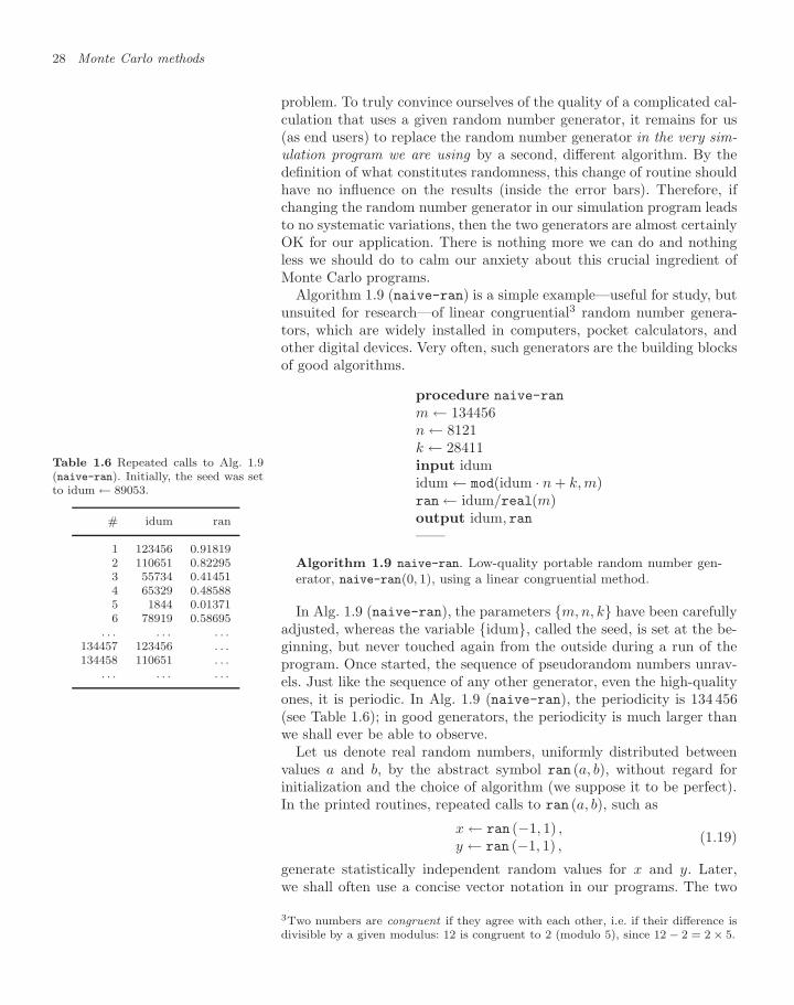
Algorithm 1.9 (naive-ran) is a simple example—useful for study, butunsuited for research—of linear congruential3 random number genera-tors, which are widely installed in computers, pocket calculators, andother digital devices. Very often, such generators are the building blocksof good algorithms.
procedure naive-ran
m ← 134456n ← 8121k ← 28411input idumidum ← mod(idum · n + k, m)ran ← idum/real(m)output idum, ran——
Algorithm 1.9 naive-ran. Low-quality portable random number gen-erator, naive-ran(0, 1), using a linear congruential method.
Table 1.6 Repeated calls to Alg. 1.9(naive-ran). Initially, the seed was setto idum ← 89053.
# idum ran
1 123456 0.918192 110651 0.822953 55734 0.414514 65329 0.485885 1844 0.013716 78919 0.58695
. . . . . . . . .134457 123456 . . .134458 110651 . . .
. . . . . . . . .
In Alg. 1.9 (naive-ran), the parameters m, n, k have been carefullyadjusted, whereas the variable idum, called the seed, is set at the be-ginning, but never touched again from the outside during a run of theprogram. Once started, the sequence of pseudorandom numbers unrav-els. Just like the sequence of any other generator, even the high-qualityones, it is periodic. In Alg. 1.9 (naive-ran), the periodicity is 134 456(see Table 1.6); in good generators, the periodicity is much larger thanwe shall ever be able to observe.
Let us denote real random numbers, uniformly distributed betweenvalues a and b, by the abstract symbol ran (a, b), without regard forinitialization and the choice of algorithm (we suppose it to be perfect).In the printed routines, repeated calls to ran (a, b), such as
x ← ran (−1, 1) ,y ← ran (−1, 1) ,
(1.19)
generate statistically independent random values for x and y. Later,we shall often use a concise vector notation in our programs. The two
3Two numbers are congruent if they agree with each other, i.e. if their difference isdivisible by a given modulus: 12 is congruent to 2 (modulo 5), since 12 − 2 = 2 × 5.
1.2 Basic sampling 29
variables x, y in eqn (1.19), for example, may be part of a vector x,and we may assign independent random values to the components ofthis vector by the call
x ← ran (−1, 1) , ran (−1, 1).(For a discussion of possible conflicts between vectors and random num-bers, see Subsection 1.2.6.)
Depending on the context, random numbers may need a little care.For example, the logarithm of a random number between 0 and 1, x ←log ran (0, 1), may have to be replaced by
1 Υ ← ran (0, 1)if (Υ = 0) goto 1 (reject number)x ← log Υ
to avoid overflow (Υ = 0, x = −∞) and a crash of the program after afew hours of running. To avoid this problem, we might define the randomnumber ran (0, 1) to be always larger than 0 and smaller than 1. Howeverthis does not get us out of trouble: a well-implemented random numbergenerator between 0 and 1, always satisfying
0 < ran (0, 1) < 1,
might be used to implement a routine ran (1, 2). The errors of finite-precision arithmetic could lead to an inconsistent implementation where,owing to rounding, 1 + ran (0, 1) could turn out to be exactly equal toone, even though we want ran (1, 2) to satisfy
1 < ran (1, 2) < 2.
Clearly, great care is called for, in this special case but also in gen-eral: Monte Carlo programs, notwithstanding their random nature, areextremely sensitive to small bugs and irregularities. They have to bemeticulously written: under no circumstance should we accept routinesthat need an occasional manual restart after a crash, or that sometimesproduce data which has to be eliminated by hand. Rare problems, forexample logarithms of zero or random numbers that are equal to 1 butshould be strictly larger, quickly get out of control, lead to a loss of trustin the output, and, in short, leave us with a big mess . . . .
1.2.2 Random integers, permutations, andcombinations
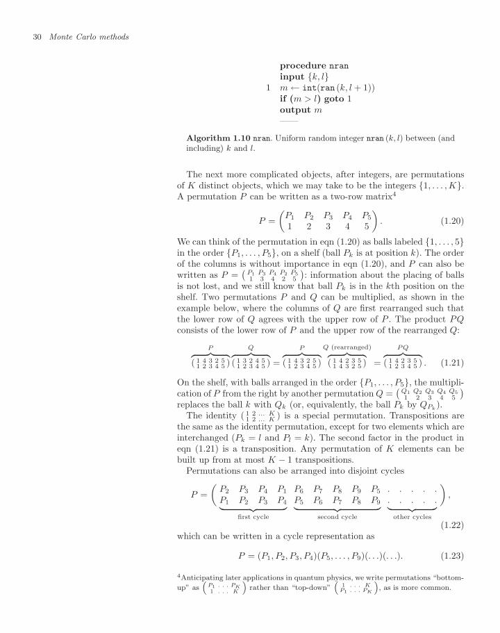
Random variables in a Monte Carlo calculation are not necessarily real-valued. Very often, we need uniformly distributed random integers m,between (and including) k and l. In this book, such a random integer isgenerated by the call m ← nran (k, l). In the implementation in Alg. 1.10(nran), the if ( ) statement (on line 4) provides extra protection againstrounding problems in the underlying ran (k, l + 1) routine.
30 Monte Carlo methods
procedure nran
input k, l1 m ← int(ran (k, l + 1))
if (m > l) goto 1output m——
Algorithm 1.10 nran. Uniform random integer nran (k, l) between (andincluding) k and l.
The next more complicated objects, after integers, are permutationsof K distinct objects, which we may take to be the integers 1, . . . , K.A permutation P can be written as a two-row matrix4
P =(
P1 P2 P3 P4 P5
1 2 3 4 5
). (1.20)
We can think of the permutation in eqn (1.20) as balls labeled 1, . . . , 5in the order P1, . . . , P5, on a shelf (ball Pk is at position k). The orderof the columns is without importance in eqn (1.20), and P can also bewritten as P =
(P1 P3 P4 P2 P51 3 4 2 5
): information about the placing of balls
is not lost, and we still know that ball Pk is in the kth position on theshelf. Two permutations P and Q can be multiplied, as shown in theexample below, where the columns of Q are first rearranged such thatthe lower row of Q agrees with the upper row of P . The product PQconsists of the lower row of P and the upper row of the rearranged Q:
P︷ ︸︸ ︷( 1 4 3 2 5
1 2 3 4 5 )
Q︷ ︸︸ ︷( 1 3 2 4 5
1 2 3 4 5 ) =
P︷ ︸︸ ︷( 1 4 3 2 5
1 2 3 4 5 )
Q (rearranged)︷ ︸︸ ︷( 1 4 2 3 5
1 4 3 2 5 ) =
PQ︷ ︸︸ ︷( 1 4 2 3 5
1 2 3 4 5 ) . (1.21)
On the shelf, with balls arranged in the order P1, . . . , P5, the multipli-cation of P from the right by another permutation Q =
(Q1 Q2 Q3 Q4 Q5
1 2 3 4 5
)replaces the ball k with Qk (or, equivalently, the ball Pk by QPk
).The identity ( 1 2 ... K
1 2 ... K ) is a special permutation. Transpositions arethe same as the identity permutation, except for two elements which areinterchanged (Pk = l and Pl = k). The second factor in the product ineqn (1.21) is a transposition. Any permutation of K elements can bebuilt up from at most K − 1 transpositions.
Permutations can also be arranged into disjoint cycles
P =(
P2 P3 P4 P1
P1 P2 P3 P4︸ ︷︷ ︸first cycle
P6 P7 P8 P9 P5
P5 P6 P7 P8 P9︸ ︷︷ ︸second cycle
. . . . .
. . . . .︸ ︷︷ ︸other cycles
),
(1.22)which can be written in a cycle representation as
P = (P1, P2, P3, P4)(P5, . . . , P9)(. . .)(. . .). (1.23)
4Anticipating later applications in quantum physics, we write permutations “bottom-up” as
“P1 . . . PK1 . . . K
”rather than “top-down”
“1 . . . K
P1 . . . PK
”, as is more common.
1.2 Basic sampling 31
In this representation, we simply record in one pair of parentheses thatP1 is followed by P2, which is in turn followed by P3, etc., until we comeback to P1. The order of writing the cycles is without importance. Inaddition, each cycle of length k has k equivalent representations. Wecould, for example, write the permutation P of eqn (1.23) as
P = (P5, . . . , P9)(P4, P1, P2, P3)(. . .)(. . .).
Cycle representations will be of central importance in later chapters;in particular, the fact that every cycle of k elements can be reachedfrom the identity by means of k − 1 transpositions. As an example, wecan see that multiplying the identity permutation ( 1 2 3 4
1 2 3 4 ) by the threetranspositions of (1, 2), (1, 3), and (1, 4) gives
( 1 2 3 41 2 3 4 )︸ ︷︷ ︸identity
( 2 1 3 41 2 3 4 )︸ ︷︷ ︸1↔2
( 2 3 1 42 1 3 4 )︸ ︷︷ ︸1↔3
( 2 3 4 12 3 1 4 )︸ ︷︷ ︸1↔4
= ( 2 3 4 11 2 3 4 ) = (1, 2, 3, 4),
a cycle of four elements. More generally, we can now consider a permu-tation P of K elements containing n cycles, with k1, . . . , kn elements.The first cycle, which has k1 elements, is generated from the identity byk1 − 1 transpositions, the second cycle by k2 − 1, etc. The total numberof transpositions needed to reach P is (k1 − 1) + · · · + (kn − 1), butsince K = k1 + · · ·+ kn, we can see that the number of transpositions isK − n. The sign of a permutation is positive if the number of transpo-sitions from the identity is even, and odd otherwise (we then speak ofeven and odd permutations). We see that
sign P = (−1)K−n = (−1)K+n = (−1)# of transpositions. (1.24)
We can always add extra transpositions and undo them later, but thesign of the permutation remains the same. Let us illustrate the crucialrelation between the number of cycles and the sign of a permutation byan example:
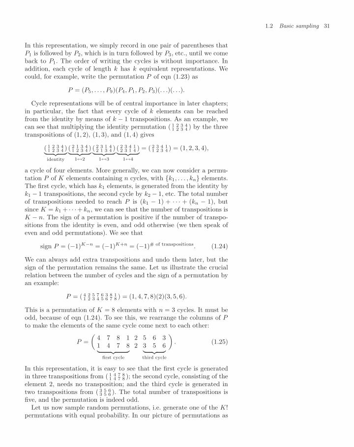
P = ( 4 2 5 7 6 3 8 11 2 3 4 5 6 7 8 ) = (1, 4, 7, 8)(2)(3, 5, 6).
This is a permutation of K = 8 elements with n = 3 cycles. It must beodd, because of eqn (1.24). To see this, we rearrange the columns of Pto make the elements of the same cycle come next to each other:
P =(
4 7 8 11 4 7 8︸ ︷︷ ︸
first cycle
22
5 6 33 5 6︸ ︷︷ ︸third cycle
). (1.25)
In this representation, it is easy to see that the first cycle is generatedin three transpositions from ( 1 4 7 8
1 4 7 8 ); the second cycle, consisting of theelement 2, needs no transposition; and the third cycle is generated intwo transpositions from ( 3 5 6
3 5 6 ). The total number of transpositions isfive, and the permutation is indeed odd.
Let us now sample random permutations, i.e. generate one of the K!permutations with equal probability. In our picture of permutations as
32 Monte Carlo methods
balls on a shelf, it is clear that a random permutation can be createdby placing all K balls into a bucket, and randomly picking out one afterthe other and putting them on the shelf, in their order of appearance.Remarkably, one can implement this procedure with a single vector oflength K, which serves both as the bucket and as the shelf (see Alg. 1.11(ran-perm); for an example, see Table 1.7). We may instead stop the
procedure ran-perm
P1, . . . , PK ← 1, . . . , Kfor k = 1, . . . , K − 1 do
l ← nran (k, K)Pl ↔ Pk
output P1, . . . , PK——
Algorithm 1.11 ran-perm. Generating a uniformly distributed randompermutation of K elements.
process after M steps, rather than K (M < K), to sample a randomcombination (see Alg. 1.12 (ran-combination)).
procedure ran-combination
P1, . . . , PK ← 1, . . . , Kfor k = 1, . . . , M do
l ← nran (k, K)Pl ↔ Pk
output P1, . . . , PM——
Algorithm 1.12 ran-combination. Generating a uniformly distributedrandom combination of M elements from K.
Table 1.7 Example run of Alg. 1.11(ran-perm). In each step k, the numbersk and l are underlined.
# P1 P2 P3 P4 P5
1 2 3 4 51
4 2 3 1 52
4 3 2 1 53
4 3 2 1 54
4 3 2 5 1
These two programs are the most basic examples of random combi-natorics, a mature branch of mathematics, where natural, easy-to-provealgorithms are right next to tough ones. For illustration, we consider aclosely related problem of (a few) black dots and many white dots(• • • ) ,which we want to mix, as in( • • • ) .The fastest algorithm for mixing the three black dots with the white onesis a slightly adapted version of Alg. 1.12 (ran-combination): first swapthe black dot at position 1 with the element at position j = nran (1, 18),then exchange whatever is at position 2 with the element at nran (2, 18),and finally swap the contents of the positions 3 and nran (3, 18). Theresulting configuration of dots is indeed a random mixture, but it takesa bit of thought to prove this.
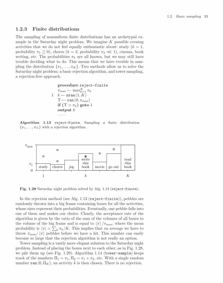
1.2 Basic sampling 33
1.2.3 Finite distributions
The sampling of nonuniform finite distributions has an archetypal ex-ample in the Saturday night problem. We imagine K possible eveningactivities that we do not feel equally enthusiastic about: study (k = 1,probability π1 0), chores (k = 2, probability π2 ≪ 1), cinema, bookwriting, etc. The probabilities πk are all known, but we may still havetrouble deciding what to do. This means that we have trouble in sam-pling the distribution π1, . . . , πK. Two methods allow us to solve theSaturday night problem: a basic rejection algorithm, and tower sampling,a rejection-free approach.
procedure reject-finite
πmax ← maxKk=1 πk
1 k ← nran (1, K)Υ ← ran (0, πmax)if (Υ > πk) goto 1output k——
Algorithm 1.13 reject-finite. Sampling a finite distributionπ1, . . . , πK with a rejection algorithm.
study chores jog bookthiswrite
movie go out bookthisread
Kk1
0
π1
πmax
Fig. 1.28 Saturday night problem solved by Alg. 1.13 (reject-finite).
In the rejection method (see Alg. 1.13 (reject-finite)), pebbles arerandomly thrown into a big frame containing boxes for all the activities,whose sizes represent their probabilities. Eventually, one pebble falls intoone of them and makes our choice. Clearly, the acceptance rate of thealgorithm is given by the ratio of the sum of the volumes of all boxes tothe volume of the big frame and is equal to 〈π〉 /πmax, where the meanprobability is 〈π〉 =
∑k πk/K. This implies that on average we have to
throw πmax/ 〈π〉 pebbles before we have a hit. This number can easilybecome so large that the rejection algorithm is not really an option.
Tower sampling is a vastly more elegant solution to the Saturday nightproblem. Instead of placing the boxes next to each other, as in Fig. 1.28,we pile them up (see Fig. 1.29). Algorithm 1.14 (tower-sample) keepstrack of the numbers Π1 = π1, Π2 = π1 + π2, etc. With a single randomnumber ran (0, ΠK), an activity k is then chosen. There is no rejection.
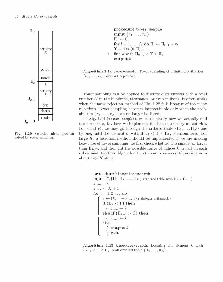
34 Monte Carlo methods
procedure tower-sample
input π1, . . . , πKΠ0 ← 0for l = 1, . . . , K do Πl ← Πl−1 + πl
Υ ← ran (0, ΠK)∗ find k with Πk−1 < Υ < Πk
output k——
Algorithm 1.14 tower-sample. Tower sampling of a finite distributionπ1, . . . , πK without rejections.
Tower sampling can be applied to discrete distributions with a totalnumber K in the hundreds, thousands, or even millions. It often workswhen the naive rejection method of Fig. 1.28 fails because of too manyrejections. Tower sampling becomes impracticable only when the prob-abilities π1, . . . , πK can no longer be listed.
Π0 = 0study
chores
jog
kactivity
Πk−1
Πk
movie
go out
Kactivity
ΠK
Fig. 1.29 Saturday night problemsolved by tower sampling.
In Alg. 1.14 (tower-sample), we must clarify how we actually findthe element k, i.e. how we implement the line marked by an asterisk.For small K, we may go through the ordered table Π0, . . . , ΠK oneby one, until the element k, with Πk−1 < Υ ≤ Πk, is encountered. Forlarge K, a bisection method should be implemented if we are makingheavy use of tower sampling: we first check whether Υ is smaller or largerthan ΠK/2, and then cut the possible range of indices k in half on eachsubsequent iteration. Algorithm 1.15 (bisection-search) terminates inabout log2 K steps.
procedure bisection-search
input Υ, Π0, Π1, . . . , ΠK (ordered table with Πk ≥ Πk−1)kmin ← 0kmax ← K + 1for i = 1, 2, . . . do⎧⎪⎪⎪⎪⎪⎪⎪⎪⎪⎪⎨⎪⎪⎪⎪⎪⎪⎪⎪⎪⎪⎩
k ← (kmin + kmax)/2 (integer arithmetic)if (Πk < Υ) then
kmin ← kelse if (Πk−1 > Υ) then
kmax ← kelse
output kexit
——
Algorithm 1.15 bisection-search. Locating the element k withΠk−1 < Υ < Πk in an ordered table Π0, . . . , ΠK.
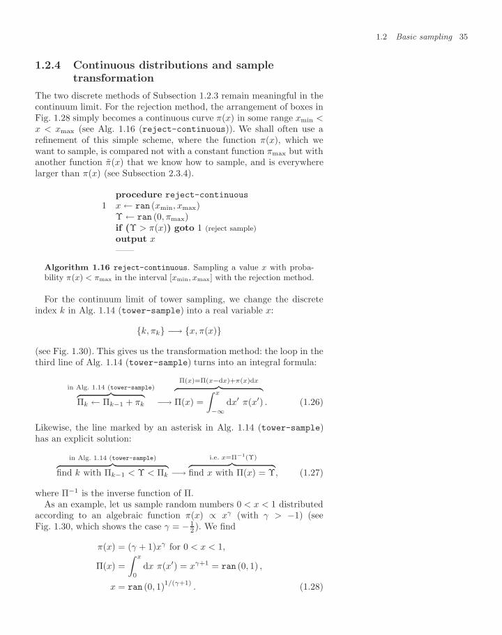
1.2 Basic sampling 35
1.2.4 Continuous distributions and sampletransformation
The two discrete methods of Subsection 1.2.3 remain meaningful in thecontinuum limit. For the rejection method, the arrangement of boxes inFig. 1.28 simply becomes a continuous curve π(x) in some range xmin <x < xmax (see Alg. 1.16 (reject-continuous)). We shall often use arefinement of this simple scheme, where the function π(x), which wewant to sample, is compared not with a constant function πmax but withanother function π(x) that we know how to sample, and is everywherelarger than π(x) (see Subsection 2.3.4).
procedure reject-continuous
1 x ← ran (xmin, xmax)Υ ← ran (0, πmax)if (Υ > π(x)) goto 1 (reject sample)output x——
Algorithm 1.16 reject-continuous. Sampling a value x with proba-bility π(x) < πmax in the interval [xmin, xmax] with the rejection method.
For the continuum limit of tower sampling, we change the discreteindex k in Alg. 1.14 (tower-sample) into a real variable x:
k, πk −→ x, π(x)
(see Fig. 1.30). This gives us the transformation method: the loop in thethird line of Alg. 1.14 (tower-sample) turns into an integral formula:
in Alg. 1.14 (tower-sample)︷ ︸︸ ︷Πk ← Πk−1 + πk −→
Π(x)=Π(x−dx)+π(x)dx︷ ︸︸ ︷Π(x) =
∫ x
−∞dx′ π(x′) . (1.26)
Likewise, the line marked by an asterisk in Alg. 1.14 (tower-sample)has an explicit solution:
in Alg. 1.14 (tower-sample)︷ ︸︸ ︷find k with Πk−1 < Υ < Πk −→
i.e. x=Π−1(Υ)︷ ︸︸ ︷find x with Π(x) = Υ, (1.27)
where Π−1 is the inverse function of Π.As an example, let us sample random numbers 0 < x < 1 distributed
according to an algebraic function π(x) ∝ xγ (with γ > −1) (seeFig. 1.30, which shows the case γ = − 1
2 ). We find
π(x) = (γ + 1)xγ for 0 < x < 1,
Π(x) =∫ x
0
dx π(x′) = xγ+1 = ran (0, 1) ,
x = ran (0, 1)1/(γ+1). (1.28)
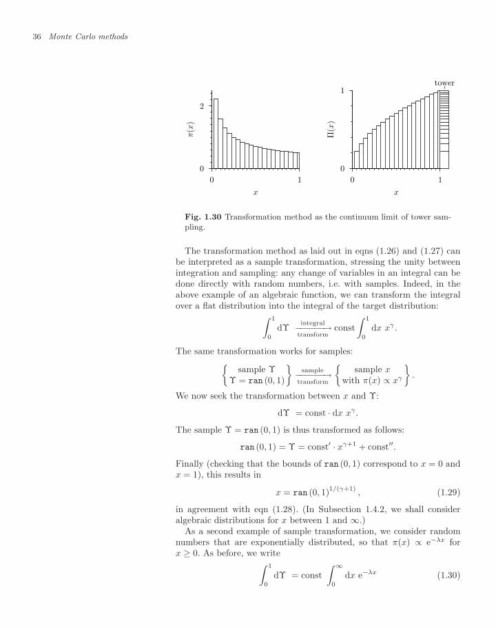
36 Monte Carlo methods
0
2
0 1
π(x
)x
0
1
0 1
Π(x
)
x
tower
Fig. 1.30 Transformation method as the continuum limit of tower sam-pling.
The transformation method as laid out in eqns (1.26) and (1.27) canbe interpreted as a sample transformation, stressing the unity betweenintegration and sampling: any change of variables in an integral can bedone directly with random numbers, i.e. with samples. Indeed, in theabove example of an algebraic function, we can transform the integralover a flat distribution into the integral of the target distribution:∫ 1
0
dΥintegral−−−−−−→
transformconst
∫ 1
0
dx xγ .
The same transformation works for samples:sample Υ
Υ = ran (0, 1)
sample−−−−−−→
transform
sample x
with π(x) ∝ xγ
.
We now seek the transformation between x and Υ:
dΥ = const · dx xγ .
The sample Υ = ran (0, 1) is thus transformed as follows:
ran (0, 1) = Υ = const′ · xγ+1 + const′′.
Finally (checking that the bounds of ran (0, 1) correspond to x = 0 andx = 1), this results in
x = ran (0, 1)1/(γ+1), (1.29)
in agreement with eqn (1.28). (In Subsection 1.4.2, we shall consideralgebraic distributions for x between 1 and ∞.)
As a second example of sample transformation, we consider randomnumbers that are exponentially distributed, so that π(x) ∝ e−λx forx ≥ 0. As before, we write∫ 1
0
dΥ = const∫ ∞
0
dx e−λx (1.30)
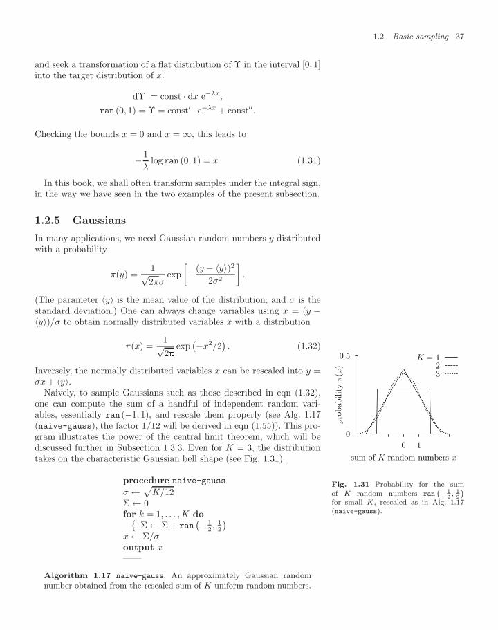
1.2 Basic sampling 37
and seek a transformation of a flat distribution of Υ in the interval [0, 1]into the target distribution of x:
dΥ = const · dx e−λx,
ran (0, 1) = Υ = const′ · e−λx + const′′.
Checking the bounds x = 0 and x = ∞, this leads to
− 1λ
log ran (0, 1) = x. (1.31)
In this book, we shall often transform samples under the integral sign,in the way we have seen in the two examples of the present subsection.
1.2.5 Gaussians
In many applications, we need Gaussian random numbers y distributedwith a probability
π(y) =1√2πσ
exp[− (y − 〈y〉)2
2σ2
].
(The parameter 〈y〉 is the mean value of the distribution, and σ is thestandard deviation.) One can always change variables using x = (y −〈y〉)/σ to obtain normally distributed variables x with a distribution
π(x) =1√2
exp(−x2/2
). (1.32)
Inversely, the normally distributed variables x can be rescaled into y =σx + 〈y〉.
Naively, to sample Gaussians such as those described in eqn (1.32),one can compute the sum of a handful of independent random vari-ables, essentially ran (−1, 1), and rescale them properly (see Alg. 1.17(naive-gauss), the factor 1/12 will be derived in eqn (1.55)). This pro-gram illustrates the power of the central limit theorem, which will bediscussed further in Subsection 1.3.3. Even for K = 3, the distributiontakes on the characteristic Gaussian bell shape (see Fig. 1.31).
0.5
0
10
pro
babilit
y π
(x)
sum of K random numbers x
K = 123
Fig. 1.31 Probability for the sumof K random numbers ran
`− 12, 1
2
´for small K, rescaled as in Alg. 1.17(naive-gauss).
procedure naive-gauss
σ ←√K/12Σ ← 0for k = 1, . . . , K do
Σ ← Σ + ran(− 1
2 , 12
)x ← Σ/σoutput x——
Algorithm 1.17 naive-gauss. An approximately Gaussian randomnumber obtained from the rescaled sum of K uniform random numbers.
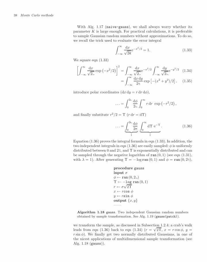
38 Monte Carlo methods
With Alg. 1.17 (naive-gauss), we shall always worry whether itsparameter K is large enough. For practical calculations, it is preferableto sample Gaussian random numbers without approximations. To do so,we recall the trick used to evaluate the error integral∫ ∞
−∞
dx√2
e−x2/2 = 1. (1.33)
We square eqn (1.33)[∫ ∞
−∞
dx√2
exp(−x2/2
)]2=∫ ∞
−∞
dx√2
e−x2/2
∫ ∞
−∞
dy√2
e−y2/2 (1.34)
=∫ ∞
−∞
dx dy
2exp[−(x2 + y2)/2
], (1.35)
introduce polar coordinates (dx dy = r dr dφ),
. . . =∫ 2
0
dφ
2
∫ ∞
0
r dr exp(−r2/2
),
and finally substitute r2/2 = Υ (r dr = dΥ)
. . . =∫ 2
0
dφ
2︸ ︷︷ ︸1
∫ ∞
0
dΥ e−Υ︸ ︷︷ ︸1
. (1.36)
Equation (1.36) proves the integral formula in eqn (1.33). In addition, thetwo independent integrals in eqn (1.36) are easily sampled: φ is uniformlydistributed between 0 and 2, and Υ is exponentially distributed and canbe sampled through the negative logarithm of ran (0, 1) (see eqn (1.31),with λ = 1). After generating Υ = − log ran (0, 1) and φ = ran (0, 2),
procedure gauss
input σφ ← ran (0, 2)Υ ← −log ran (0, 1)r ← σ
√2Υ
x ← rcos φy ← rsin φoutput x, y——
Algorithm 1.18 gauss. Two independent Gaussian random numbersobtained by sample transformation. See Alg. 1.19 (gauss(patch)).
we transform the sample, as discussed in Subsection 1.2.4: a crab’s walkleads from eqn (1.36) back to eqn (1.34) (r =
√2Υ, x = r cos φ, y =
r sin φ). We finally get two normally distributed Gaussians, in one ofthe nicest applications of multidimensional sample transformation (seeAlg. 1.18 (gauss)).
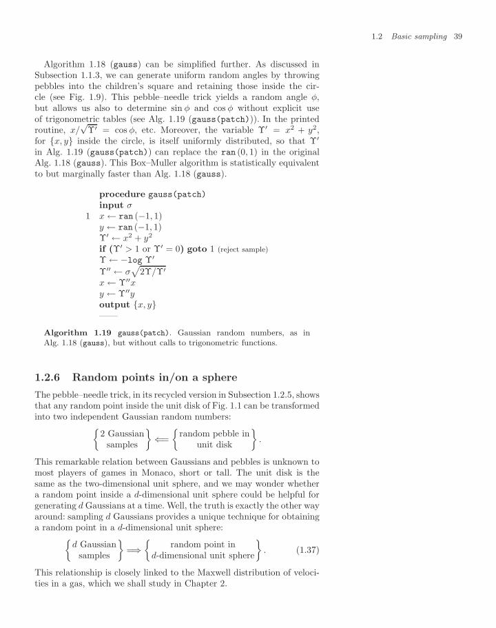
1.2 Basic sampling 39
Algorithm 1.18 (gauss) can be simplified further. As discussed inSubsection 1.1.3, we can generate uniform random angles by throwingpebbles into the children’s square and retaining those inside the cir-cle (see Fig. 1.9). This pebble–needle trick yields a random angle φ,but allows us also to determine sin φ and cos φ without explicit useof trigonometric tables (see Alg. 1.19 (gauss(patch))). In the printedroutine, x/
√Υ′ = cos φ, etc. Moreover, the variable Υ′ = x2 + y2,
for x, y inside the circle, is itself uniformly distributed, so that Υ′
in Alg. 1.19 (gauss(patch)) can replace the ran (0, 1) in the originalAlg. 1.18 (gauss). This Box–Muller algorithm is statistically equivalentto but marginally faster than Alg. 1.18 (gauss).
procedure gauss(patch)
input σ1 x ← ran (−1, 1)
y ← ran (−1, 1)Υ′ ← x2 + y2
if (Υ′ > 1 or Υ′ = 0) goto 1 (reject sample)Υ ← −log Υ′
Υ′′ ← σ√
2Υ/Υ′x ← Υ′′xy ← Υ′′youtput x, y——
Algorithm 1.19 gauss(patch). Gaussian random numbers, as inAlg. 1.18 (gauss), but without calls to trigonometric functions.
1.2.6 Random points in/on a sphere
The pebble–needle trick, in its recycled version in Subsection 1.2.5, showsthat any random point inside the unit disk of Fig. 1.1 can be transformedinto two independent Gaussian random numbers:
2 Gaussiansamples
⇐=
random pebble inunit disk
.
This remarkable relation between Gaussians and pebbles is unknown tomost players of games in Monaco, short or tall. The unit disk is thesame as the two-dimensional unit sphere, and we may wonder whethera random point inside a d-dimensional unit sphere could be helpful forgenerating d Gaussians at a time. Well, the truth is exactly the other wayaround: sampling d Gaussians provides a unique technique for obtaininga random point in a d-dimensional unit sphere:
d Gaussiansamples
=⇒
random point ind-dimensional unit sphere
. (1.37)
This relationship is closely linked to the Maxwell distribution of veloci-ties in a gas, which we shall study in Chapter 2.
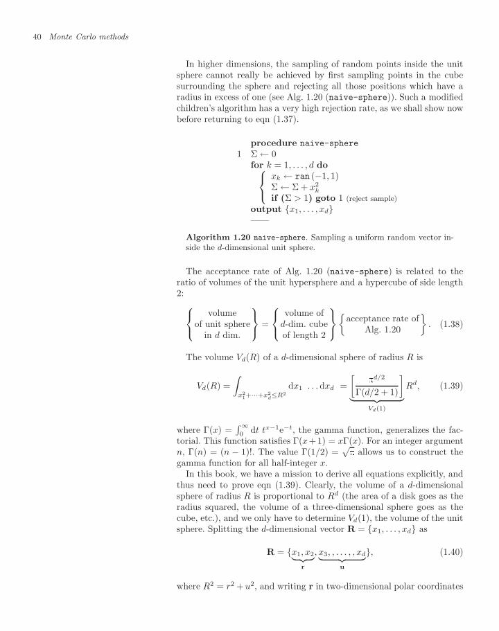
40 Monte Carlo methods
In higher dimensions, the sampling of random points inside the unitsphere cannot really be achieved by first sampling points in the cubesurrounding the sphere and rejecting all those positions which have aradius in excess of one (see Alg. 1.20 (naive-sphere)). Such a modifiedchildren’s algorithm has a very high rejection rate, as we shall show nowbefore returning to eqn (1.37).
procedure naive-sphere
1 Σ ← 0for k = 1, . . . , d do⎧⎨⎩
xk ← ran (−1, 1)Σ ← Σ + x2
k
if (Σ > 1) goto 1 (reject sample)output x1, . . . , xd——
Algorithm 1.20 naive-sphere. Sampling a uniform random vector in-side the d-dimensional unit sphere.
The acceptance rate of Alg. 1.20 (naive-sphere) is related to theratio of volumes of the unit hypersphere and a hypercube of side length2:⎧⎨⎩
volumeof unit sphere
in d dim.
⎫⎬⎭ =
⎧⎨⎩volume of
d-dim. cubeof length 2
⎫⎬⎭
acceptance rate ofAlg. 1.20
. (1.38)
The volume Vd(R) of a d-dimensional sphere of radius R is
Vd(R) =∫
x21+···+x2
d≤R2
dx1 . . . dxd =[
d/2
Γ(d/2 + 1)
]︸ ︷︷ ︸
Vd(1)
Rd, (1.39)
where Γ(x) =∫∞0 dt tx−1e−t, the gamma function, generalizes the fac-
torial. This function satisfies Γ(x+1) = xΓ(x). For an integer argumentn, Γ(n) = (n − 1)!. The value Γ(1/2) =
√ allows us to construct the
gamma function for all half-integer x.In this book, we have a mission to derive all equations explicitly, and
thus need to prove eqn (1.39). Clearly, the volume of a d-dimensionalsphere of radius R is proportional to Rd (the area of a disk goes as theradius squared, the volume of a three-dimensional sphere goes as thecube, etc.), and we only have to determine Vd(1), the volume of the unitsphere. Splitting the d-dimensional vector R = x1, . . . , xd as
R = x1, x2︸ ︷︷ ︸r
, x3, , . . . , , xd︸ ︷︷ ︸u
, (1.40)
where R2 = r2 + u2, and writing r in two-dimensional polar coordinates
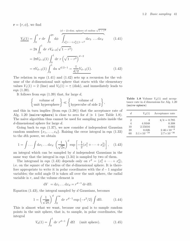
1.2 Basic sampling 41
r = r, φ, we find
Vd(1) =∫ 1
0
r dr
∫ 2
0
dφ
(d − 2)-dim. sphere of radius√
1 − r2︷ ︸︸ ︷∫x23+···+x2
d≤1−r2
dx3 . . . dxd (1.41)
= 2∫ 1
0
dr rVd−2(√
1 − r2)
= 2Vd−2(1)∫ 1
0
dr r(√
1 − r2)d−2
= Vd−2(1)∫ 1
0
du ud/2−1 =
d/2Vd−2(1). (1.42)
The relation in eqns (1.41) and (1.42) sets up a recursion for the vol-ume of the d-dimensional unit sphere that starts with the elementaryvalues V1(1) = 2 (line) and V2(1) = (disk), and immediately leads toeqn (1.39).
It follows from eqn (1.39) that, for large d,volume of
unit hypersphere
volume ofhypercube of side 2
,
and this in turn implies (from eqn (1.38)) that the acceptance rate ofAlg. 1.20 (naive-sphere) is close to zero for d 1 (see Table 1.8).The naive algorithm thus cannot be used for sampling points inside thed-dimensional sphere for large d.
Table 1.8 Volume Vd(1) and accep-tance rate in d dimensions for Alg. 1.20(naive-sphere)
d Vd(1) Acceptance rate
2 /4 = 0.7854 4.9348 0.308
10 2.55016 0.00220 0.026 2.46×10⁻⁸
60 3.1×10⁻¹⁸ 2.7×10−36
Going back to eqn (1.37), we now consider d independent Gaussianrandom numbers x1, . . . , xd. Raising the error integral in eqn (1.33)to the dth power, we obtain
1 =∫
. . .
∫dx1 . . .dxd
(1√2
)d
exp[−1
2(x2
1 + · · · + x2d)]
, (1.43)
an integral which can be sampled by d independent Gaussians in thesame way that the integral in eqn (1.34) is sampled by two of them.
The integrand in eqn (1.43) depends only on r2 = (x21 + · · · + x2
d),i.e. on the square of the radius of the d-dimensional sphere. It is there-fore appropriate to write it in polar coordinates with the d − 1 angularvariables; the solid angle Ω is taken all over the unit sphere, the radialvariable is r, and the volume element is
dV = dx1 . . .dxd = rd−1 dr dΩ.
Equation (1.43), the integral sampled by d Gaussians, becomes
1 =(
1√2
)d ∫ ∞
0
dr rd−1 exp(−r2/2
)∫dΩ. (1.44)
This is almost what we want, because our goal is to sample randompoints in the unit sphere, that is, to sample, in polar coordinates, theintegral
Vd(1) =∫ 1
0
dr rd−1
∫dΩ (unit sphere). (1.45)
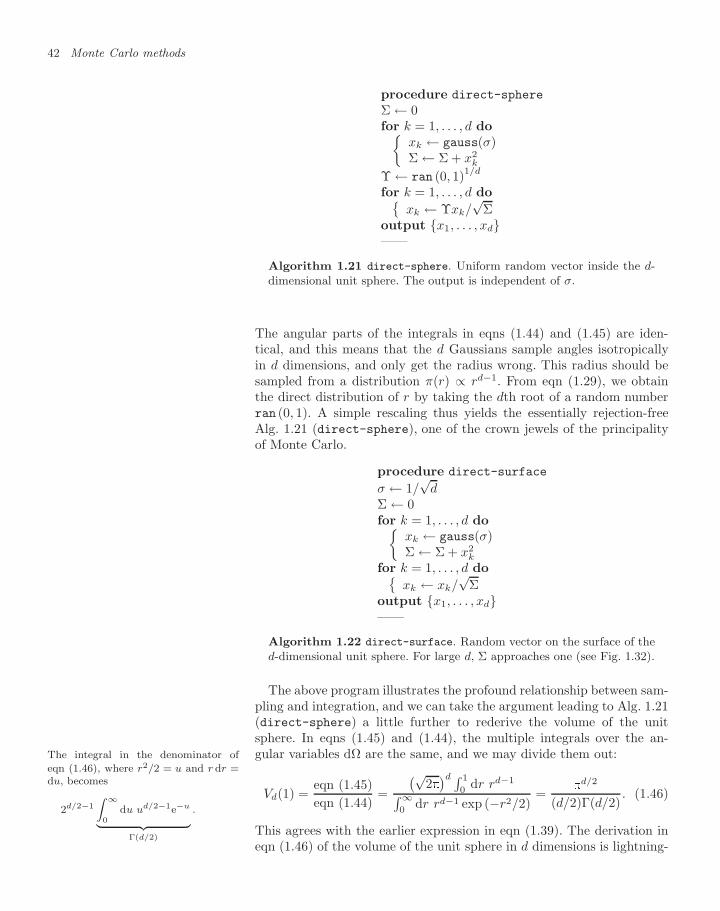
42 Monte Carlo methods
procedure direct-sphere
Σ ← 0for k = 1, . . . , d do
xk ← gauss(σ)Σ ← Σ + x2
k
Υ ← ran (0, 1)1/d
for k = 1, . . . , d doxk ← Υxk/
√Σ
output x1, . . . , xd——
Algorithm 1.21 direct-sphere. Uniform random vector inside the d-dimensional unit sphere. The output is independent of σ.
The angular parts of the integrals in eqns (1.44) and (1.45) are iden-tical, and this means that the d Gaussians sample angles isotropicallyin d dimensions, and only get the radius wrong. This radius should besampled from a distribution π(r) ∝ rd−1. From eqn (1.29), we obtainthe direct distribution of r by taking the dth root of a random numberran (0, 1). A simple rescaling thus yields the essentially rejection-freeAlg. 1.21 (direct-sphere), one of the crown jewels of the principalityof Monte Carlo.
procedure direct-surface
σ ← 1/√
dΣ ← 0for k = 1, . . . , d do
xk ← gauss(σ)Σ ← Σ + x2
k
for k = 1, . . . , d doxk ← xk/
√Σ
output x1, . . . , xd——
Algorithm 1.22 direct-surface. Random vector on the surface of thed-dimensional unit sphere. For large d, Σ approaches one (see Fig. 1.32).
The above program illustrates the profound relationship between sam-pling and integration, and we can take the argument leading to Alg. 1.21(direct-sphere) a little further to rederive the volume of the unitsphere. In eqns (1.45) and (1.44), the multiple integrals over the an-gular variables dΩ are the same, and we may divide them out:The integral in the denominator of
eqn (1.46), where r2/2 = u and r dr =du, becomes
2d/2−1
Z ∞
0du ud/2−1e−u
| z Γ(d/2)
.
Vd(1) =eqn (1.45)eqn (1.44)
=
(√2)d ∫ 1
0dr rd−1∫∞
0dr rd−1 exp (−r2/2)
=
d/2
(d/2)Γ(d/2). (1.46)
This agrees with the earlier expression in eqn (1.39). The derivation ineqn (1.46) of the volume of the unit sphere in d dimensions is lightning-
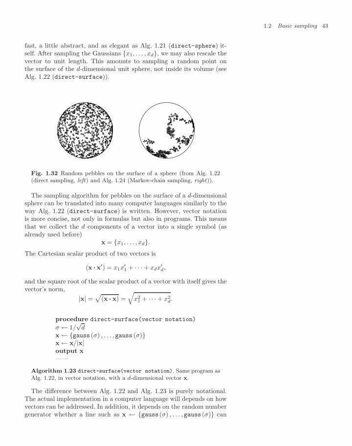
1.2 Basic sampling 43
fast, a little abstract, and as elegant as Alg. 1.21 (direct-sphere) it-self. After sampling the Gaussians x1, . . . , xd, we may also rescale thevector to unit length. This amounts to sampling a random point onthe surface of the d-dimensional unit sphere, not inside its volume (seeAlg. 1.22 (direct-surface)).
Fig. 1.32 Random pebbles on the surface of a sphere (from Alg. 1.22(direct sampling, left) and Alg. 1.24 (Markov-chain sampling, right)).
The sampling algorithm for pebbles on the surface of a d-dimensionalsphere can be translated into many computer languages similarly to theway Alg. 1.22 (direct-surface) is written. However, vector notationis more concise, not only in formulas but also in programs. This meansthat we collect the d components of a vector into a single symbol (asalready used before)
x = x1, . . . , xd.The Cartesian scalar product of two vectors is
(x ··· x′) = x1x′1 + · · · + xdx
′d,
and the square root of the scalar product of a vector with itself gives thevector’s norm,
|x| =√
(x ··· x) =√
x21 + · · · + x2
d.
procedure direct-surface(vector notation)
σ ← 1/√
dx ← gauss (σ) , . . . , gauss (σ)x ← x/|x|output x——
Algorithm 1.23 direct-surface(vector notation). Same program asAlg. 1.22, in vector notation, with a d-dimensional vector x.
The difference between Alg. 1.22 and Alg. 1.23 is purely notational.The actual implementation in a computer language will depends on howvectors can be addressed. In addition, it depends on the random numbergenerator whether a line such as x ← gauss (σ) , . . . , gauss (σ) can
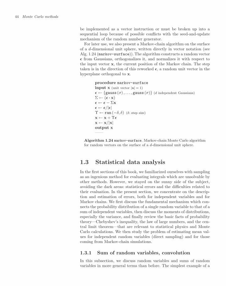
44 Monte Carlo methods
be implemented as a vector instruction or must be broken up into asequential loop because of possible conflicts with the seed-and-updatemechanism of the random number generator.
For later use, we also present a Markov-chain algorithm on the surfaceof a d-dimensional unit sphere, written directly in vector notation (seeAlg. 1.24 (markov-surface)). The algorithm constructs a random vectorε from Gaussians, orthogonalizes it, and normalizes it with respect tothe input vector x, the current position of the Markov chain. The steptaken is in the direction of this reworked ε, a random unit vector in thehyperplane orthogonal to x.
procedure markov-surface
input x (unit vector |x| = 1)ε ← gauss (σ) , . . . , gauss (σ) (d independent Gaussians)Σ ← (ε ··· x)ε ← ε − Σxε ← ε/|ε|Υ ← ran (−δ, δ) (δ: step size)x ← x + Υε
x ← x/|x|output x——
Algorithm 1.24 markov-surface. Markov-chain Monte Carlo algorithmfor random vectors on the surface of a d-dimensional unit sphere.
1.3 Statistical data analysis
In the first sections of this book, we familiarized ourselves with samplingas an ingenious method for evaluating integrals which are unsolvable byother methods. However, we stayed on the sunny side of the subject,avoiding the dark areas: statistical errors and the difficulties related totheir evaluation. In the present section, we concentrate on the descrip-tion and estimation of errors, both for independent variables and forMarkov chains. We first discuss the fundamental mechanism which con-nects the probability distribution of a single random variable to that of asum of independent variables, then discuss the moments of distributions,especially the variance, and finally review the basic facts of probabilitytheory—Chebyshev’s inequality, the law of large numbers, and the cen-tral limit theorem—that are relevant to statistical physics and MonteCarlo calculations. We then study the problem of estimating mean val-ues for independent random variables (direct sampling) and for thosecoming from Markov-chain simulations.
1.3.1 Sum of random variables, convolution
In this subsection, we discuss random variables and sums of randomvariables in more general terms than before. The simplest example of a
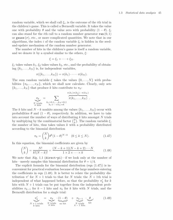
1.3 Statistical data analysis 45
random variable, which we shall call ξi, is the outcome of the ith trial inthe children’s game. This is called a Bernoulli variable. It takes the valueone with probability θ and the value zero with probability (1 − θ). ξi
can also stand for the ith call to a random number generator ran (0, 1)or gauss (σ), etc., or more complicated quantities. We note that in ouralgorithms, the index i of the random variable ξi is hidden in the seed-and-update mechanism of the random number generator.
The number of hits in the children’s game is itself a random variable,and we denote it by a symbol similar to the others, ξ:
ξ = ξ1 + · · · + ξN .
ξ1 takes values k1, ξ2 takes values k2, etc., and the probability of obtain-ing k1, . . . , kN is, for independent variables,
π(k1, . . . , kN) = π(k1) · · · · · π(kN ).
The sum random variable ξ takes the values 0, . . . , N with proba-bilities π0, . . . , πN, which we shall now calculate. Clearly, only setsk1, . . . , kN that produce k hits contribute to πk:
πk︸︷︷︸N trialsk hits
=∑
k1=0,1,...,kN=0,1k1+···+kN =k
π(k1)π(k2)···π(kN )︷ ︸︸ ︷π(k1, . . . , kN ) .
The k hits and N −k nonhits among the values k1, . . . , kN occur withprobabilities θ and (1 − θ), respectively. In addition, we have to takeinto account the number of ways of distributing k hits amongst N trialsby multiplying by the combinatorial factor
(Nk
). The random variable ξ,
the number of hits, thus takes values k with a probability distributedaccording to the binomial distribution
πk =(
N
k
)θk(1 − θ)N−k (0 ≤ k ≤ N). (1.47)
In this equation, the binomial coefficients are given by(N
k
)=
N !k!(N − k)!
=(N − k + 1)(N − k + 2) · · ·N
1 × 2 × · · · × k. (1.48)
We note that Alg. 1.1 (direct-pi)—if we look only at the number ofhits—merely samples this binomial distribution for θ = /4.
The explicit formula for the binomial distribution (eqn (1.47)) is in-convenient for practical evaluation because of the large numbers enteringthe coefficients in eqn (1.48). It is better to relate the probability dis-tribution π′ for N + 1 trials to that for N trials: the N + 1th trial isindependent of what happened before, so that the probability π′
k for khits with N + 1 trials can be put together from the independent prob-abilities πk−1 for k − 1 hits and πk for k hits with N trials, and theBernoulli distribution for a single trial:
π′k︸︷︷︸
N + 1 trialsk hits
= πk︸︷︷︸N trialsk hits
· (1 − θ)︸ ︷︷ ︸no hit
+ πk−1︸ ︷︷ ︸N trials
k − 1 hits
· θ︸︷︷︸hit
, (1.49)
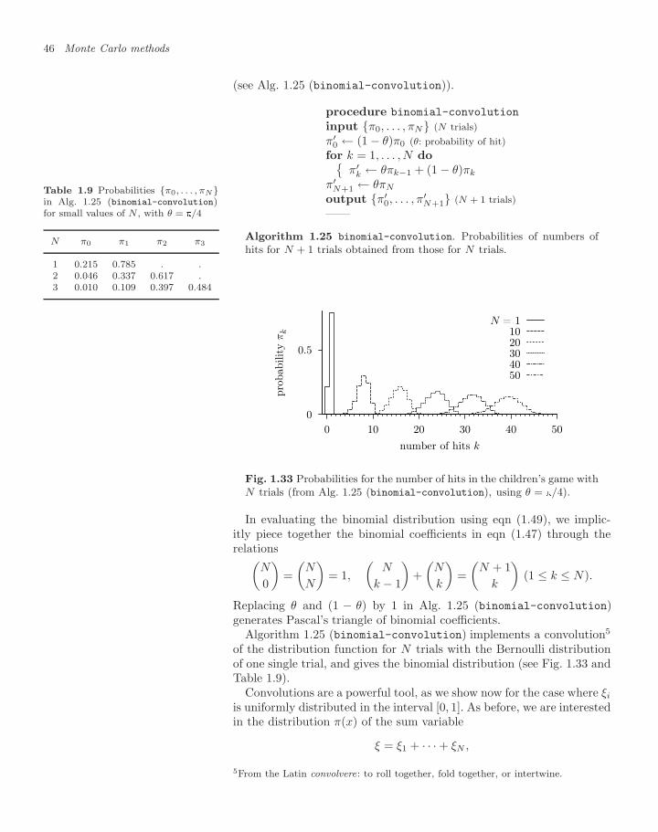
46 Monte Carlo methods
(see Alg. 1.25 (binomial-convolution)).
procedure binomial-convolution
input π0, . . . , πN (N trials)π′
0 ← (1 − θ)π0 (θ: probability of hit)for k = 1, . . . , N do
π′k ← θπk−1 + (1 − θ)πk
π′N+1 ← θπN
output π′0, . . . , π
′N+1 (N + 1 trials)
——
Algorithm 1.25 binomial-convolution. Probabilities of numbers ofhits for N + 1 trials obtained from those for N trials.
Table 1.9 Probabilities π0, . . . , πNin Alg. 1.25 (binomial-convolution)for small values of N , with θ = /4
N π0 π1 π2 π3
1 0.215 0.785 . .2 0.046 0.337 0.617 .3 0.010 0.109 0.397 0.484
0
0.5
0 10 20 30 40 50
pro
babilit
y π
k
number of hits k
N = 11020304050
Fig. 1.33 Probabilities for the number of hits in the children’s game withN trials (from Alg. 1.25 (binomial-convolution), using θ = /4).
In evaluating the binomial distribution using eqn (1.49), we implic-itly piece together the binomial coefficients in eqn (1.47) through therelations(
N
0
)=(
N
N
)= 1,
(N
k − 1
)+(
N
k
)=(
N + 1k
)(1 ≤ k ≤ N).
Replacing θ and (1 − θ) by 1 in Alg. 1.25 (binomial-convolution)generates Pascal’s triangle of binomial coefficients.
Algorithm 1.25 (binomial-convolution) implements a convolution5
of the distribution function for N trials with the Bernoulli distributionof one single trial, and gives the binomial distribution (see Fig. 1.33 andTable 1.9).
Convolutions are a powerful tool, as we show now for the case where ξi
is uniformly distributed in the interval [0, 1]. As before, we are interestedin the distribution π(x) of the sum variable
ξ = ξ1 + · · · + ξN ,
5From the Latin convolvere: to roll together, fold together, or intertwine.
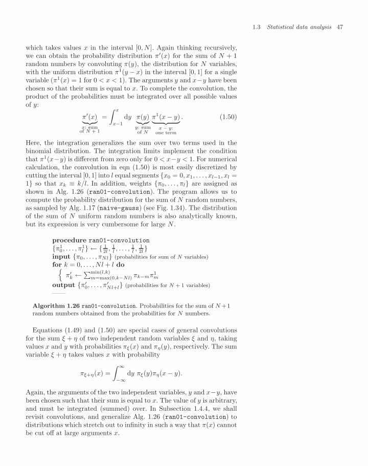
1.3 Statistical data analysis 47
which takes values x in the interval [0, N ]. Again thinking recursively,we can obtain the probability distribution π′(x) for the sum of N + 1random numbers by convoluting π(y), the distribution for N variables,with the uniform distribution π1(y − x) in the interval [0, 1] for a singlevariable (π1(x) = 1 for 0 < x < 1). The arguments y and x−y have beenchosen so that their sum is equal to x. To complete the convolution, theproduct of the probabilities must be integrated over all possible valuesof y:
π′(x)︸ ︷︷ ︸x: sum
of N + 1
=∫ x
x−1
dy π(y)︸︷︷︸y: sumof N
π1(x − y)︸ ︷︷ ︸x − y:
one term
. (1.50)
Here, the integration generalizes the sum over two terms used in thebinomial distribution. The integration limits implement the conditionthat π1(x−y) is different from zero only for 0 < x−y < 1. For numericalcalculation, the convolution in eqn (1.50) is most easily discretized bycutting the interval [0, 1] into l equal segments x0 = 0, x1, . . . , xl−1, xl =1 so that xk ≡ k/l. In addition, weights π0, . . . , πl are assigned asshown in Alg. 1.26 (ran01-convolution). The program allows us tocompute the probability distribution for the sum of N random numbers,as sampled by Alg. 1.17 (naive-gauss) (see Fig. 1.34). The distributionof the sum of N uniform random numbers is also analytically known,but its expression is very cumbersome for large N .
procedure ran01-convolution
π10 , . . . , π
1l ← 1
2l ,1l , . . . ,
1l ,
12l
input π0, . . . , πNl (probabilities for sum of N variables)for k = 0, . . . , Nl + l do
π′k ←∑min(l,k)
m=max(0,k−Nl) πk−mπ1m
output π′0, . . . , π
′Nl+l (probabilities for N + 1 variables)
——
Algorithm 1.26 ran01-convolution. Probabilities for the sum of N +1random numbers obtained from the probabilities for N numbers.
Equations (1.49) and (1.50) are special cases of general convolutionsfor the sum ξ + η of two independent random variables ξ and η, takingvalues x and y with probabilities πξ(x) and πη(y), respectively. The sumvariable ξ + η takes values x with probability
πξ+η(x) =∫ ∞
−∞dy πξ(y)πη(x − y).
Again, the arguments of the two independent variables, y and x−y, havebeen chosen such that their sum is equal to x. The value of y is arbitrary,and must be integrated (summed) over. In Subsection 1.4.4, we shallrevisit convolutions, and generalize Alg. 1.26 (ran01-convolution) todistributions which stretch out to infinity in such a way that π(x) cannotbe cut off at large arguments x.
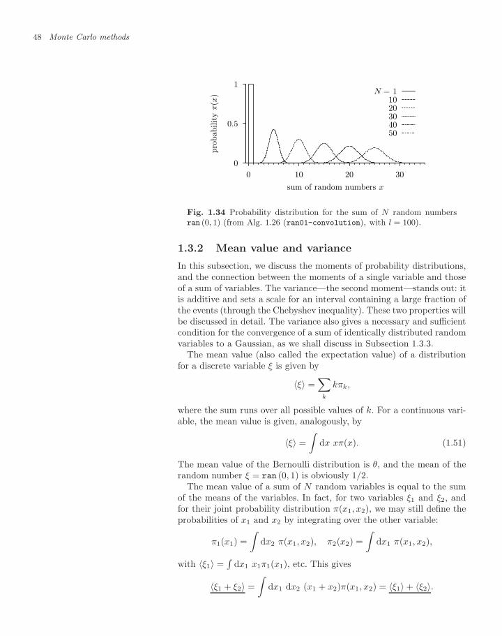
48 Monte Carlo methods
0
0.5
1
0 10 20 30
pro
babilit
y π
(x)
sum of random numbers x
N = 11020304050
Fig. 1.34 Probability distribution for the sum of N random numbersran (0, 1) (from Alg. 1.26 (ran01-convolution), with l = 100).
1.3.2 Mean value and variance
In this subsection, we discuss the moments of probability distributions,and the connection between the moments of a single variable and thoseof a sum of variables. The variance—the second moment—stands out: itis additive and sets a scale for an interval containing a large fraction ofthe events (through the Chebyshev inequality). These two properties willbe discussed in detail. The variance also gives a necessary and sufficientcondition for the convergence of a sum of identically distributed randomvariables to a Gaussian, as we shall discuss in Subsection 1.3.3.
The mean value (also called the expectation value) of a distributionfor a discrete variable ξ is given by
〈ξ〉 =∑
k
kπk,
where the sum runs over all possible values of k. For a continuous vari-able, the mean value is given, analogously, by
〈ξ〉 =∫
dx xπ(x). (1.51)
The mean value of the Bernoulli distribution is θ, and the mean of therandom number ξ = ran (0, 1) is obviously 1/2.
The mean value of a sum of N random variables is equal to the sumof the means of the variables. In fact, for two variables ξ1 and ξ2, andfor their joint probability distribution π(x1, x2), we may still define theprobabilities of x1 and x2 by integrating over the other variable:
π1(x1) =∫
dx2 π(x1, x2), π2(x2) =∫
dx1 π(x1, x2),
with 〈ξ1〉 =∫
dx1 x1π1(x1), etc. This gives
〈ξ1 + ξ2〉 =∫
dx1 dx2 (x1 + x2)π(x1, x2) = 〈ξ1〉 + 〈ξ2〉.
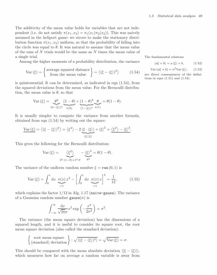
1.3 Statistical data analysis 49
The additivity of the mean value holds for variables that are not inde-pendent (i.e. do not satisfy π(x1, x2) = π1(x1)π2(x2)). This was naivelyassumed in the heliport game: we strove to make the stationary distri-bution function π(x1, x2) uniform, so that the probability of falling intothe circle was equal to θ. It was natural to assume that the mean valueof the sum of N trials would be the same as N times the mean value ofa single trial. The fundamental relations
〈aξ + b〉 = a 〈ξ〉 + b, (1.52)
Var (aξ + b) = a2Var (ξ) , (1.53)
are direct consequences of the defini-tions in eqns (1.51) and (1.54).
Among the higher moments of a probability distribution, the variance
Var (ξ) =
average squared distancefrom the mean value
=⟨(ξ − 〈ξ〉)2⟩ (1.54)
is quintessential. It can be determined, as indicated in eqn (1.54), fromthe squared deviations from the mean value. For the Bernoulli distribu-tion, the mean value is θ, so that
Var (ξ) = θ2︸︷︷︸(0−〈ξ〉)2
(1 − θ)︸ ︷︷ ︸π(0)
+ (1 − θ)2︸ ︷︷ ︸(1−〈ξ〉)2
θ︸︷︷︸π(1)
= θ(1 − θ).
It is usually simpler to compute the variance from another formula,obtained from eqn (1.54) by writing out the square:
Var (ξ) =⟨(ξ − 〈ξ〉)2⟩ =
⟨ξ2⟩− 2 〈ξ · 〈ξ〉〉︸ ︷︷ ︸
〈ξ〉〈ξ〉
+ 〈ξ〉2 =⟨ξ2⟩− 〈ξ〉2.
This gives the following for the Bernoulli distribution:
Var (ξ) =⟨ξ2⟩︸︷︷︸
02·(1−θ)+12·θ
− 〈ξ〉2︸︷︷︸θ2
= θ(1 − θ).
The variance of the uniform random number ξ = ran (0, 1) is
Var (ξ) =∫ 1
0
dx π(x)︸︷︷︸=1
x2 −[∫ 1
0
dx π(x)︸︷︷︸=1
x
]2=
112
, (1.55)
which explains the factor 1/12 in Alg. 1.17 (naive-gauss). The varianceof a Gaussian random number gauss(σ) is∫ ∞
−∞
dx√2σ
x2 exp(− x2
2σ2
)= σ2.
The variance (the mean square deviation) has the dimensions of asquared length, and it is useful to consider its square root, the rootmean square deviation (also called the standard deviation):
root mean square(standard) deviation
:√〈(ξ − 〈ξ〉)2〉 =
√Var (ξ) = σ.
This should be compared with the mean absolute deviation 〈|ξ − 〈ξ〉|〉,which measures how far on average a random variable is away from
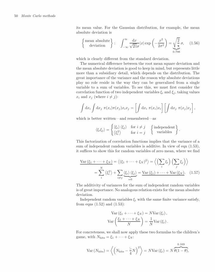
50 Monte Carlo methods
its mean value. For the Gaussian distribution, for example, the meanabsolute deviation is
mean absolutedeviation
:∫ ∞
−∞
dx√2σ
|x| exp(− x2
2σ2
)=
√2︸︷︷︸
0.798
σ, (1.56)
which is clearly different from the standard deviation.The numerical difference between the root mean square deviation and
the mean absolute deviation is good to keep in mind, but represents littlemore than a subsidiary detail, which depends on the distribution. Thegreat importance of the variance and the reason why absolute deviationsplay no role reside in the way they can be generalized from a singlevariable to a sum of variables. To see this, we must first consider thecorrelation function of two independent variables ξi and ξj , taking valuesxi and xj (where i = j):∫
dxi
∫dxj π(xi)π(xj)xixj =
[∫dxi π(xi)xi
] [∫dxj π(xj)xj
],
which is better written—and remembered—as
〈ξiξj〉 =
〈ξi〉 〈ξj〉 for i = j⟨ξ2i
⟩for i = j
independent
variables
.
This factorization of correlation functions implies that the variance of asum of independent random variables is additive. In view of eqn (1.53),it suffices to show this for random variables of zero mean, where we find
Var (ξ1 + · · · + ξN ) =⟨(ξ1 + · · · + ξN )2
⟩=⟨(∑
i
ξi
)(∑j
ξj
)⟩=
N∑i
⟨ξ2i
⟩+∑i=j
〈ξi〉 〈ξj〉︸ ︷︷ ︸=0
= Var (ξ1) + · · · + Var (ξN ). (1.57)
The additivity of variances for the sum of independent random variablesis of great importance. No analogous relation exists for the mean absolutedeviation.
Independent random variables ξi with the same finite variance satisfy,from eqns (1.52) and (1.53):
Var (ξ1 + · · · + ξN ) = NVar (ξi) ,
Var(
ξ1 + · · · + ξN
N
)=
1N
Var (ξi) .
For concreteness, we shall now apply these two formulas to the children’sgame, with Nhits = ξ1 + · · · + ξN :
Var (Nhits) =⟨(
Nhits −
4N)2⟩
= NVar (ξi) = N
0.169︷ ︸︸ ︷θ(1 − θ),
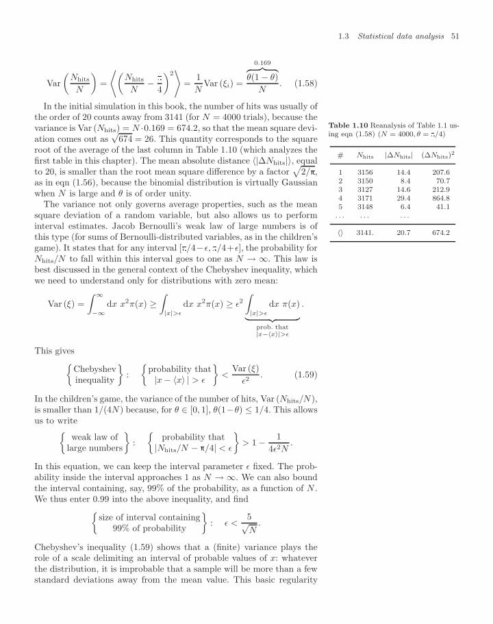
1.3 Statistical data analysis 51
Var(
Nhits
N
)=
⟨(Nhits
N−
4
)2⟩
=1N
Var (ξi) =
0.169︷ ︸︸ ︷θ(1 − θ)
N. (1.58)
In the initial simulation in this book, the number of hits was usually ofthe order of 20 counts away from 3141 (for N = 4000 trials), because thevariance is Var (Nhits) = N ·0.169 = 674.2, so that the mean square devi-ation comes out as
√674 = 26. This quantity corresponds to the square
root of the average of the last column in Table 1.10 (which analyzes thefirst table in this chapter). The mean absolute distance 〈|∆Nhits|〉, equalto 20, is smaller than the root mean square difference by a factor
√2/,
as in eqn (1.56), because the binomial distribution is virtually Gaussianwhen N is large and θ is of order unity.
Table 1.10 Reanalysis of Table 1.1 us-ing eqn (1.58) (N = 4000, θ = /4)
# Nhits |∆Nhits| (∆Nhits)2
1 3156 14.4 207.62 3150 8.4 70.73 3127 14.6 212.94 3171 29.4 864.85 3148 6.4 41.1
. . . . . . . . .
〈〉 3141. 20.7 674.2
The variance not only governs average properties, such as the meansquare deviation of a random variable, but also allows us to performinterval estimates. Jacob Bernoulli’s weak law of large numbers is ofthis type (for sums of Bernoulli-distributed variables, as in the children’sgame). It states that for any interval [/4−ε, /4+ε], the probability forNhits/N to fall within this interval goes to one as N → ∞. This law isbest discussed in the general context of the Chebyshev inequality, whichwe need to understand only for distributions with zero mean:
Var (ξ) =∫ ∞
−∞dx x2π(x) ≥
∫|x|>ε
dx x2π(x) ≥ ε2∫|x|>ε
dx π(x)︸ ︷︷ ︸prob. that|x−〈x〉|>ε
.
This givesChebyshevinequality
:
probability that|x − 〈x〉 | > ε
<
Var (ξ)ε2
. (1.59)
In the children’s game, the variance of the number of hits, Var (Nhits/N),is smaller than 1/(4N) because, for θ ∈ [0, 1], θ(1−θ) ≤ 1/4. This allowsus to write
weak law oflarge numbers
:
probability that|Nhits/N − /4| < ε
> 1 − 1
4ε2N.
In this equation, we can keep the interval parameter ε fixed. The prob-ability inside the interval approaches 1 as N → ∞. We can also boundthe interval containing, say, 99% of the probability, as a function of N .We thus enter 0.99 into the above inequality, and find
size of interval containing99% of probability
: ε <
5√N
.
Chebyshev’s inequality (1.59) shows that a (finite) variance plays therole of a scale delimiting an interval of probable values of x: whateverthe distribution, it is improbable that a sample will be more than a fewstandard deviations away from the mean value. This basic regularity
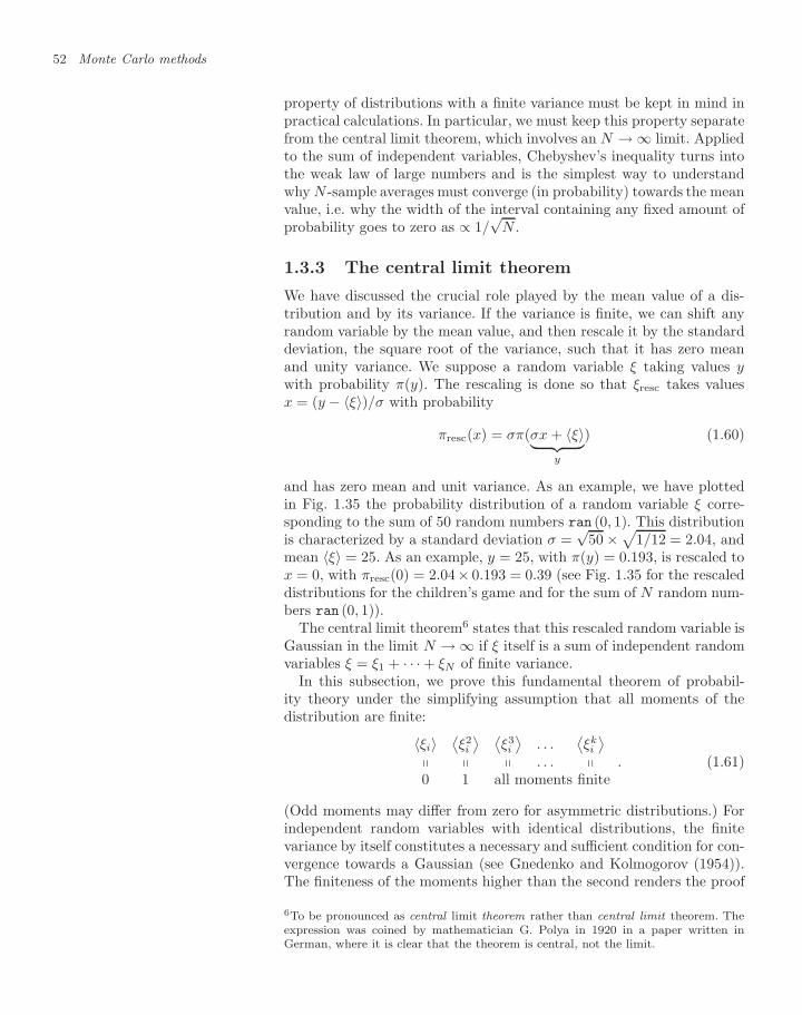
52 Monte Carlo methods
property of distributions with a finite variance must be kept in mind inpractical calculations. In particular, we must keep this property separatefrom the central limit theorem, which involves an N → ∞ limit. Appliedto the sum of independent variables, Chebyshev’s inequality turns intothe weak law of large numbers and is the simplest way to understandwhy N -sample averages must converge (in probability) towards the meanvalue, i.e. why the width of the interval containing any fixed amount ofprobability goes to zero as ∝ 1/
√N .
1.3.3 The central limit theorem
We have discussed the crucial role played by the mean value of a dis-tribution and by its variance. If the variance is finite, we can shift anyrandom variable by the mean value, and then rescale it by the standarddeviation, the square root of the variance, such that it has zero meanand unity variance. We suppose a random variable ξ taking values ywith probability π(y). The rescaling is done so that ξresc takes valuesx = (y − 〈ξ〉)/σ with probability
πresc(x) = σπ(σx + 〈ξ〉︸ ︷︷ ︸y
) (1.60)
and has zero mean and unit variance. As an example, we have plottedin Fig. 1.35 the probability distribution of a random variable ξ corre-sponding to the sum of 50 random numbers ran (0, 1). This distributionis characterized by a standard deviation σ =
√50 ×√1/12 = 2.04, and
mean 〈ξ〉 = 25. As an example, y = 25, with π(y) = 0.193, is rescaled tox = 0, with πresc(0) = 2.04× 0.193 = 0.39 (see Fig. 1.35 for the rescaleddistributions for the children’s game and for the sum of N random num-bers ran (0, 1)).
The central limit theorem6 states that this rescaled random variable isGaussian in the limit N → ∞ if ξ itself is a sum of independent randomvariables ξ = ξ1 + · · · + ξN of finite variance.
In this subsection, we prove this fundamental theorem of probabil-ity theory under the simplifying assumption that all moments of thedistribution are finite:
〈ξi〉⟨ξ2i
⟩ ⟨ξ3i
⟩. . .
⟨ξki
⟩ . . .
0 1 all moments finite. (1.61)
(Odd moments may differ from zero for asymmetric distributions.) Forindependent random variables with identical distributions, the finitevariance by itself constitutes a necessary and sufficient condition for con-vergence towards a Gaussian (see Gnedenko and Kolmogorov (1954)).The finiteness of the moments higher than the second renders the proof
6To be pronounced as central limit theorem rather than central limit theorem. Theexpression was coined by mathematician G. Polya in 1920 in a paper written inGerman, where it is clear that the theorem is central, not the limit.
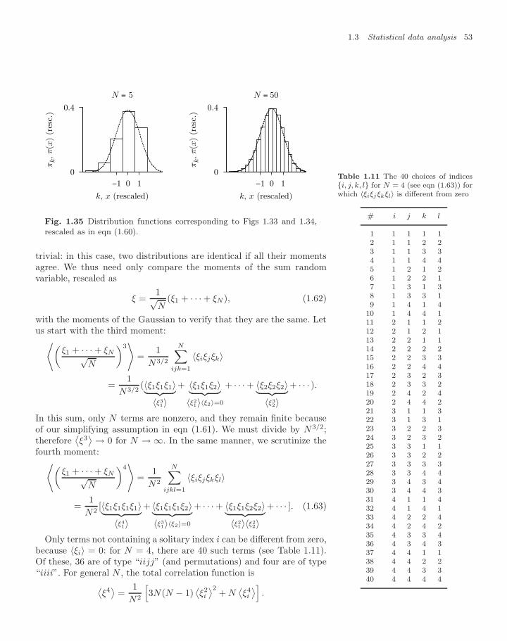
1.3 Statistical data analysis 53
0
0.4
10−1
πk, π(x
) (r
esc.
)
k, x (rescaled)
N = 5
0
0.4
10−1π
k, π(x
) (r
esc.
)k, x (rescaled)
N = 50
Fig. 1.35 Distribution functions corresponding to Figs 1.33 and 1.34,rescaled as in eqn (1.60).
trivial: in this case, two distributions are identical if all their momentsagree. We thus need only compare the moments of the sum randomvariable, rescaled as
ξ =1√N
(ξ1 + · · · + ξN ), (1.62)
with the moments of the Gaussian to verify that they are the same. Letus start with the third moment:⟨(
ξ1 + · · · + ξN√N
)3⟩
=1
N3/2
N∑ijk=1
〈ξiξjξk〉
=1
N3/2(〈ξ1ξ1ξ1〉︸ ︷︷ ︸
〈ξ31〉
+ 〈ξ1ξ1ξ2〉︸ ︷︷ ︸〈ξ2
1〉〈ξ2〉=0
+ · · · + 〈ξ2ξ2ξ2〉︸ ︷︷ ︸〈ξ3
2〉+ · · · ).
In this sum, only N terms are nonzero, and they remain finite becauseof our simplifying assumption in eqn (1.61). We must divide by N3/2;therefore
⟨ξ3⟩ → 0 for N → ∞. In the same manner, we scrutinize the
fourth moment:⟨(ξ1 + · · · + ξN√
N
)4⟩
=1
N2
N∑ijkl=1
〈ξiξjξkξl〉
=1
N2[〈ξ1ξ1ξ1ξ1〉︸ ︷︷ ︸
〈ξ41〉
+ 〈ξ1ξ1ξ1ξ2〉︸ ︷︷ ︸〈ξ3
1〉〈ξ2〉=0
+ · · · + 〈ξ1ξ1ξ2ξ2〉︸ ︷︷ ︸〈ξ2
1〉〈ξ22〉
+ · · · ]. (1.63)
Table 1.11 The 40 choices of indicesi, j, k, l for N = 4 (see eqn (1.63)) forwhich 〈ξiξjξkξl〉 is different from zero
# i j k l
1 1 1 1 12 1 1 2 23 1 1 3 34 1 1 4 45 1 2 1 26 1 2 2 17 1 3 1 38 1 3 3 19 1 4 1 4
10 1 4 4 111 2 1 1 212 2 1 2 113 2 2 1 114 2 2 2 215 2 2 3 316 2 2 4 417 2 3 2 318 2 3 3 219 2 4 2 420 2 4 4 221 3 1 1 322 3 1 3 123 3 2 2 324 3 2 3 225 3 3 1 126 3 3 2 227 3 3 3 328 3 3 4 429 3 4 3 430 3 4 4 331 4 1 1 432 4 1 4 133 4 2 2 434 4 2 4 235 4 3 3 436 4 3 4 337 4 4 1 138 4 4 2 239 4 4 3 340 4 4 4 4
Only terms not containing a solitary index i can be different from zero,because 〈ξi〉 = 0: for N = 4, there are 40 such terms (see Table 1.11).Of these, 36 are of type “iijj” (and permutations) and four are of type“iiii”. For general N , the total correlation function is⟨
ξ4⟩
=1
N2
[3N(N − 1)
⟨ξ2i
⟩2+ N
⟨ξ4i
⟩].
54 Monte Carlo methods
In the limit of large N , where N N − 1, we have⟨ξ4⟩
= 3.In the same way, we can compute higher moments of ξ. Odd moments
approach zero in the large-N limit. For example, the fifth moment is puttogether from const·N2 terms of type “iijjj”, in addition to the N termsof type “iiiii”. Dividing by N5/2 indeed gives zero. The even momentsare finite, and the dominant contributions for large N come, for the sixthmoment, from terms of type “iijjkk” and their permutations. The totalnumber of these terms, for large N is N3 · 6!/3!/23 = N3 × 1 × 3 × 5.For arbitrary k, the number of ways is
momentsin eqn (1.62)
⟨ξ2k⟩→ 1 × 3 ×· · ·× (2k − 1)⟨
x2k−1⟩→ 0
for N → ∞. (1.64)
We now check that the Gaussian distribution also has the momentsgiven by eqn (1.64). This follows trivially for the odd moments, as theGaussian is a symmetric function. The even moments can be computedfrom∫ ∞
−∞
dx√2
exp(−x2
2+ xh
)= exp
(h2
2
)︸ ︷︷ ︸
becauseR
dx√2
expˆ−(x − h)2/2
˜= 1
= 1 +h2
2+
(h2/2)2
2!+ · · · .
We may differentiate this equation 2k times (under the integral on theleft, as it is absolutely convergent) and then set h = 0. On the left, thisgives the (2k)th moment of the Gaussian distribution. On the right, weobtain an explicit expression:
⟨x2k⟩
=∂2k
∂h2k
∫ ∞
−∞
dx√2
exp(−x2
2+ xh
)∣∣∣∣h=0
=∂2k
∂h2k
[1 +
h2
2+
(h2/2)2
2!+
(h2/2)3
3!+ · · ·
]h=0
=∂2k
∂h2k
(h2k
k!2k
)=
(2k)!k!2k
= 1 × 3 × · · · × (2k − 1).
This is the same as eqn (1.64), and the distribution function of thesum of N random variables, in the limit N → ∞, has no choice butto converge to a Gaussian, so that we have proven the central limittheorem (for the simplified case that all the moments of the distributionare finite). The Gaussian has 68% of its weight concentrated withinthe interval [−σ, σ] and 95% of its weight within the interval [−2σ, 2σ](see Fig. 1.36). These numbers are of prime importance for statisticalcalculations in general, and for Monte Carlo error analysis in particular.The probability of being more than a few standard deviations awayfrom the mean value drops precipitously (see Table 1.12, where the errorfunction is erf(x) = (2/
√)∫ t
0 dt exp(−t2
)).
In practical calculations, we are sometimes confronted with a few ex-ceptional sample averages that are many (estimated) standard devia-tions away from our (estimated) mean value. We may, for example,
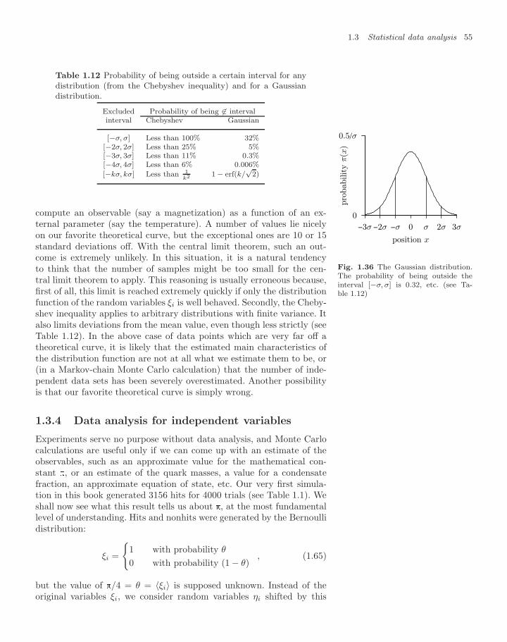
1.3 Statistical data analysis 55
Table 1.12 Probability of being outside a certain interval for anydistribution (from the Chebyshev inequality) and for a Gaussiandistribution.
Excluded Probability of being ∈ intervalinterval Chebyshev Gaussian
[−σ, σ] Less than 100% 32%[−2σ, 2σ] Less than 25% 5%[−3σ, 3σ] Less than 11% 0.3%[−4σ, 4σ] Less than 6% 0.006%[−kσ, kσ] Less than 1
k2 1 − erf(k/√
2)
compute an observable (say a magnetization) as a function of an ex-ternal parameter (say the temperature). A number of values lie nicelyon our favorite theoretical curve, but the exceptional ones are 10 or 15standard deviations off. With the central limit theorem, such an out-come is extremely unlikely. In this situation, it is a natural tendencyto think that the number of samples might be too small for the cen-tral limit theorem to apply. This reasoning is usually erroneous because,first of all, this limit is reached extremely quickly if only the distributionfunction of the random variables ξi is well behaved. Secondly, the Cheby-shev inequality applies to arbitrary distributions with finite variance. Italso limits deviations from the mean value, even though less strictly (seeTable 1.12). In the above case of data points which are very far off atheoretical curve, it is likely that the estimated main characteristics ofthe distribution function are not at all what we estimate them to be, or(in a Markov-chain Monte Carlo calculation) that the number of inde-pendent data sets has been severely overestimated. Another possibilityis that our favorite theoretical curve is simply wrong.
0.5/σ
0
−3σ −2σ −σ 3σ2σσ0
pro
babilit
y π
(x)
position x
Fig. 1.36 The Gaussian distribution.The probability of being outside theinterval [−σ, σ] is 0.32, etc. (see Ta-ble 1.12)
1.3.4 Data analysis for independent variables
Experiments serve no purpose without data analysis, and Monte Carlocalculations are useful only if we can come up with an estimate of theobservables, such as an approximate value for the mathematical con-stant , or an estimate of the quark masses, a value for a condensatefraction, an approximate equation of state, etc. Our very first simula-tion in this book generated 3156 hits for 4000 trials (see Table 1.1). Weshall now see what this result tells us about , at the most fundamentallevel of understanding. Hits and nonhits were generated by the Bernoullidistribution:
ξi =
1 with probability θ
0 with probability (1 − θ), (1.65)
but the value of /4 = θ = 〈ξi〉 is supposed unknown. Instead of theoriginal variables ξi, we consider random variables ηi shifted by this
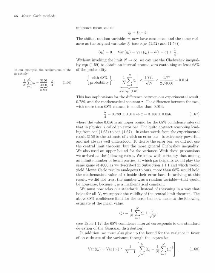
56 Monte Carlo methods
unknown mean value:ηi = ξi − θ.
The shifted random variables ηi now have zero mean and the same vari-ance as the original variables ξi (see eqns (1.52) and (1.53)):
〈ηi〉 = 0, Var (ηi) = Var (ξi) = θ(1 − θ) ≤ 14.
Without invoking the limit N → ∞, we can use the Chebyshev inequal-ity eqn (1.59) to obtain an interval around zero containing at least 68%of the probability:In our example, the realizations of the
ηi satisfy
1N
NXi=1
ηi =31564000| z 0.789
−π
4. (1.66)
with 68%
probability
:
∣∣∣∣∣ 1N
N∑i=1
ηi
∣∣∣∣∣︸ ︷︷ ︸see eqn (1.66)
<1.77σ√
N<
1.772√
4000= 0.014.
This has implications for the difference between our experimental result,0.789, and the mathematical constant . The difference between the two,with more than 68% chance, is smaller than 0.014:
4= 0.789 ± 0.014 ⇔ = 3.156 ± 0.056, (1.67)
where the value 0.056 is an upper bound for the 68% confidence intervalthat in physics is called an error bar. The quite abstract reasoning lead-ing from eqn (1.65) to eqn (1.67)—in other words from the experimentalresult 3156 to the estimate of with an error bar—is extremely powerful,and not always well understood. To derive the error bar, we did not usethe central limit theorem, but the more general Chebyshev inequality.We also used an upper bound for the variance. With these precautionswe arrived at the following result. We know with certainty that amongan infinite number of beach parties, at which participants would play thesame game of 4000 as we described in Subsection 1.1.1 and which wouldyield Monte Carlo results analogous to ours, more than 68% would holdthe mathematical value of inside their error bars. In arriving at thisresult, we did not treat the number as a random variable—that wouldbe nonsense, because is a mathematical constant.
We must now relax our standards. Instead of reasoning in a way thatholds for all N , we suppose the validity of the central limit theorem. Theabove 68% confidence limit for the error bar now leads to the followingestimate of the mean value:
〈ξ〉 =1N
N∑i=1
ξi ± σ√N
(see Table 1.12; the 68% confidence interval corresponds to one standarddeviation of the Gaussian distribution).
In addition, we must also give up the bound for the variance in favorof an estimate of the variance, through the expression
Var (ξi) = Var (ηi) 1N − 1
⎡⎣ N∑j=1
(ξj − 1N
N∑i=1
ξi)2
⎤⎦ . (1.68)
1.3 Statistical data analysis 57
The mean value on the right side of eqn (1.68) is equal to the variancefor all N (and one therefore speaks of an unbiased estimator). With thereplacement ξj → ηj , we obtain
⟨1
N − 1
⎡⎣ N∑j=1
(ηj − 1
N
N∑i=1
ηi
)2⎤⎦⟩
=1
N − 1
⎡⎢⎣ N∑jk
〈ηjηk〉︸ ︷︷ ︸Var(ηj)δjk
− 2N
N∑ij=1
〈ηiηj〉 +1
N2
∑ijk
〈ηiηk〉
⎤⎥⎦ = Var (ηi)
(a more detailed analysis is possible under the conditions of the centrallimit theorem). In practice, we always replace the denominator 1
N−1 → We note that
NXj=1
ξj − 1
N
NXi=1
ξi
!2
=
NXj=1
ξ2j −
2N
(NX
j=1
ξj)(NX
i=1
ξi)+1N
(NX
i=1
ξi)2
=X
j
ξ2j − N
0@ 1
N
Xj
ξj
1A2
. (1.69)
1N in eqn (1.68) (the slight difference plays no role at all). We arrive, witheqn (1.69), at the standard formulas for the data analysis of independentrandom variables:
〈ξ〉 =1N
N∑i=1
ξi ± error,
where
error =1√N
√1N
∑i
ξ2i −(
1N
∑i
ξi
)2
.
The error has a prefactor 1/√
N and not 1/N , because it goes as thestandard deviation, itself the square root of the variance. It should benoted that the replacement of the variance by an estimate is far frominnocent. This replacement can lead to very serious problems, as weshall discuss in an example, namely the γ-integral of Section 1.4. InMarkov-chain Monte Carlo applications, another problem arises becausethe number of samples, N , must be replaced by an effective number ofindependent samples, which must itself be estimated with care. This willbe taken up in Subsection 1.3.5.
We now briefly discuss the Bayesian approach to statistics, not becausewe need it for computing error bars, but because of its close connectionswith statistical physics (see Section 2.2). We stay in the imagery of thechildren’s game. Bayesian statistics attempts to determine the probabil-ity that our experimental result (3156 hits) was the result of a certainvalue test. If test was very large (test 4, so that θ 1), and alsoif test 0, the experimental result, 3156 hits for 4000 trials, would bevery unlikely. Let us make this argument more quantitative and supposethat the test values of are drawn from an a priori probability distribu-tion (not to be confused with the a priori probability of the generalizedMetropolis algorithm). The test values give hits and nonhits with the ap-propriate Bernoulli distribution and values of Nhits with their binomialdistribution (with parameters θ = test/4 and N = 4000), but there is agreat difference between those test values that give 3156 hits, and thosethat do not. To illustrate this point, let us sample the values of test
that yield 3156 hits with a program, Alg. 1.27 (naive-bayes-pi). Like
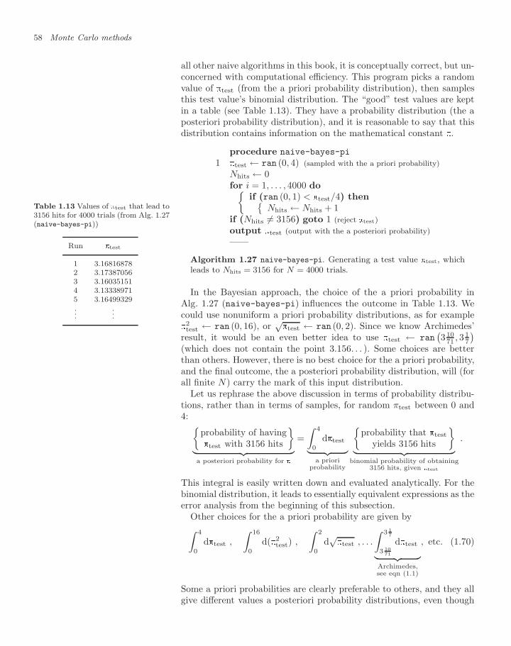
58 Monte Carlo methods
all other naive algorithms in this book, it is conceptually correct, but un-concerned with computational efficiency. This program picks a randomvalue of test (from the a priori probability distribution), then samplesthis test value’s binomial distribution. The “good” test values are keptin a table (see Table 1.13). They have a probability distribution (the aposteriori probability distribution), and it is reasonable to say that thisdistribution contains information on the mathematical constant .
Table 1.13 Values of test that lead to3156 hits for 4000 trials (from Alg. 1.27(naive-bayes-pi))
Run test
1 3.168168782 3.173870563 3.160351514 3.133389715 3.16499329...
...
procedure naive-bayes-pi
1 test ← ran (0, 4) (sampled with the a priori probability)Nhits ← 0for i = 1, . . . , 4000 do
if (ran (0, 1) < test/4) thenNhits ← Nhits + 1
if (Nhits = 3156) goto 1 (reject test)output test (output with the a posteriori probability)——
Algorithm 1.27 naive-bayes-pi. Generating a test value test, whichleads to Nhits = 3156 for N = 4000 trials.
In the Bayesian approach, the choice of the a priori probability inAlg. 1.27 (naive-bayes-pi) influences the outcome in Table 1.13. Wecould use nonuniform a priori probability distributions, as for example2test ← ran (0, 16), or
√test ← ran (0, 2). Since we know Archimedes’
result, it would be an even better idea to use test ← ran(3 10
71 , 3 17
)(which does not contain the point 3.156. . . ). Some choices are betterthan others. However, there is no best choice for the a priori probability,and the final outcome, the a posteriori probability distribution, will (forall finite N) carry the mark of this input distribution.
Let us rephrase the above discussion in terms of probability distribu-tions, rather than in terms of samples, for random πtest between 0 and4:
probability of havingtest with 3156 hits
︸ ︷︷ ︸a posteriori probability for
=∫ 4
0
dtest︸ ︷︷ ︸a priori
probability
probability that test
yields 3156 hits
︸ ︷︷ ︸
binomial probability of obtaining3156 hits, given test
.
This integral is easily written down and evaluated analytically. For thebinomial distribution, it leads to essentially equivalent expressions as theerror analysis from the beginning of this subsection.
Other choices for the a priori probability are given by∫ 4
0
dtest ,
∫ 16
0
d(2test) ,
∫ 2
0
d√test , . . .
∫ 3 17
3 1071
dtest︸ ︷︷ ︸Archimedes,see eqn (1.1)
, etc. (1.70)
Some a priori probabilities are clearly preferable to others, and they allgive different values a posteriori probability distributions, even though
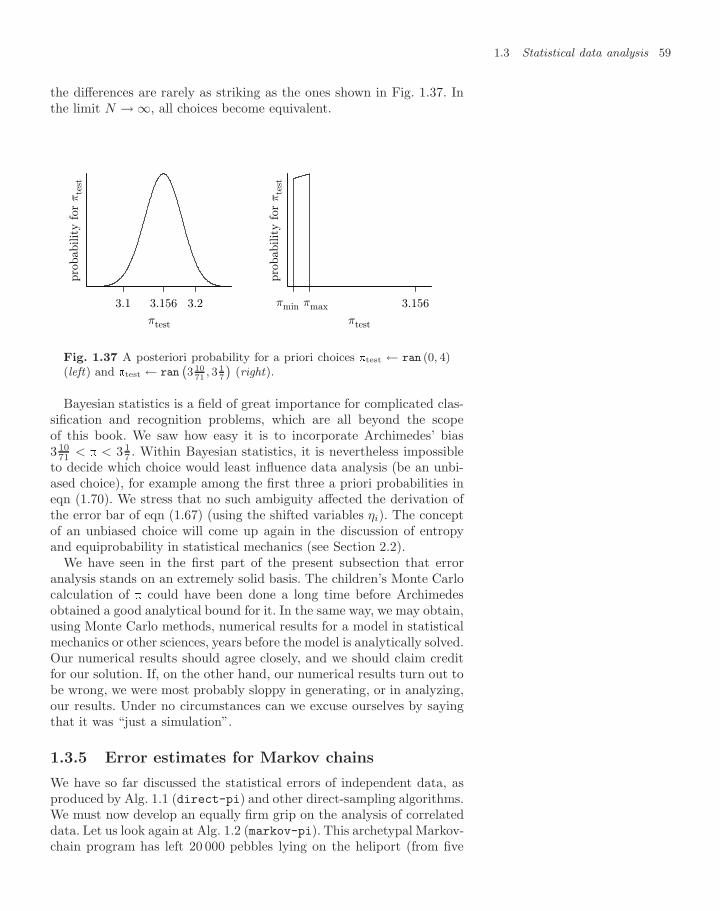
1.3 Statistical data analysis 59
the differences are rarely as striking as the ones shown in Fig. 1.37. Inthe limit N → ∞, all choices become equivalent.
3.23.1563.1
pro
babilit
y for
πte
st
πtest
3.156 πmaxπmin
pro
babilit
y for
πte
st
πtest
Fig. 1.37 A posteriori probability for a priori choices test ← ran (0, 4)(left) and test ← ran
`3 10
71, 3 1
7
´(right).
Bayesian statistics is a field of great importance for complicated clas-sification and recognition problems, which are all beyond the scopeof this book. We saw how easy it is to incorporate Archimedes’ bias3 10
71 < < 3 17 . Within Bayesian statistics, it is nevertheless impossible
to decide which choice would least influence data analysis (be an unbi-ased choice), for example among the first three a priori probabilities ineqn (1.70). We stress that no such ambiguity affected the derivation ofthe error bar of eqn (1.67) (using the shifted variables ηi). The conceptof an unbiased choice will come up again in the discussion of entropyand equiprobability in statistical mechanics (see Section 2.2).
We have seen in the first part of the present subsection that erroranalysis stands on an extremely solid basis. The children’s Monte Carlocalculation of could have been done a long time before Archimedesobtained a good analytical bound for it. In the same way, we may obtain,using Monte Carlo methods, numerical results for a model in statisticalmechanics or other sciences, years before the model is analytically solved.Our numerical results should agree closely, and we should claim creditfor our solution. If, on the other hand, our numerical results turn out tobe wrong, we were most probably sloppy in generating, or in analyzing,our results. Under no circumstances can we excuse ourselves by sayingthat it was “just a simulation”.
1.3.5 Error estimates for Markov chains
We have so far discussed the statistical errors of independent data, asproduced by Alg. 1.1 (direct-pi) and other direct-sampling algorithms.We must now develop an equally firm grip on the analysis of correlateddata. Let us look again at Alg. 1.2 (markov-pi). This archetypal Markov-chain program has left 20 000 pebbles lying on the heliport (from five
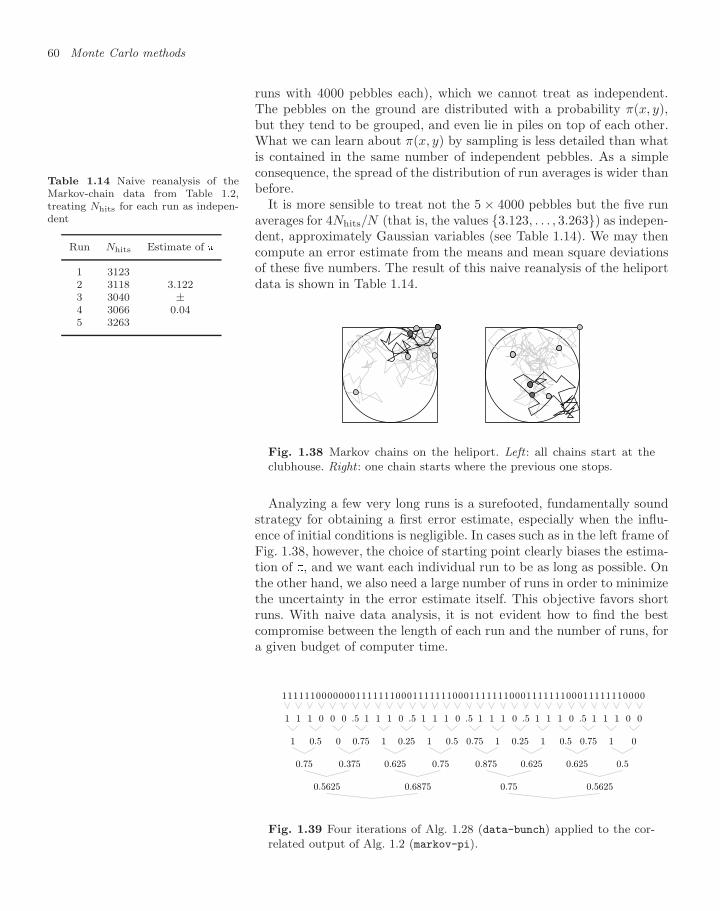
60 Monte Carlo methods
runs with 4000 pebbles each), which we cannot treat as independent.The pebbles on the ground are distributed with a probability π(x, y),but they tend to be grouped, and even lie in piles on top of each other.What we can learn about π(x, y) by sampling is less detailed than whatis contained in the same number of independent pebbles. As a simpleconsequence, the spread of the distribution of run averages is wider thanbefore.
It is more sensible to treat not the 5 × 4000 pebbles but the five runaverages for 4Nhits/N (that is, the values 3.123, . . . , 3.263) as indepen-dent, approximately Gaussian variables (see Table 1.14). We may thencompute an error estimate from the means and mean square deviationsof these five numbers. The result of this naive reanalysis of the heliportdata is shown in Table 1.14.
Table 1.14 Naive reanalysis of theMarkov-chain data from Table 1.2,treating Nhits for each run as indepen-dent
Run Nhits Estimate of
1 31232 3118 3.1223 3040 ±4 3066 0.045 3263
Fig. 1.38 Markov chains on the heliport. Left : all chains start at theclubhouse. Right : one chain starts where the previous one stops.
Analyzing a few very long runs is a surefooted, fundamentally soundstrategy for obtaining a first error estimate, especially when the influ-ence of initial conditions is negligible. In cases such as in the left frame ofFig. 1.38, however, the choice of starting point clearly biases the estima-tion of , and we want each individual run to be as long as possible. Onthe other hand, we also need a large number of runs in order to minimizethe uncertainty in the error estimate itself. This objective favors shortruns. With naive data analysis, it is not evident how to find the bestcompromise between the length of each run and the number of runs, fora given budget of computer time.
1111110000000111111100011111110001111111000111111100011111110000
1 1 1 0 0 0 .5 1 1 1 0 .5 1 1 1 0 .5 1 1 1 0 .5 1 1 1 0 .5 1 1 1 0 0
1 0.5 0 0.75 1 0.25 1 0.5 0.75 1 0.25 1 0.5 0.75 1 0
0.75 0.375 0.625 0.75 0.875 0.625 0.625 0.5
0.5625 0.6875 0.75 0.5625
Fig. 1.39 Four iterations of Alg. 1.28 (data-bunch) applied to the cor-related output of Alg. 1.2 (markov-pi).
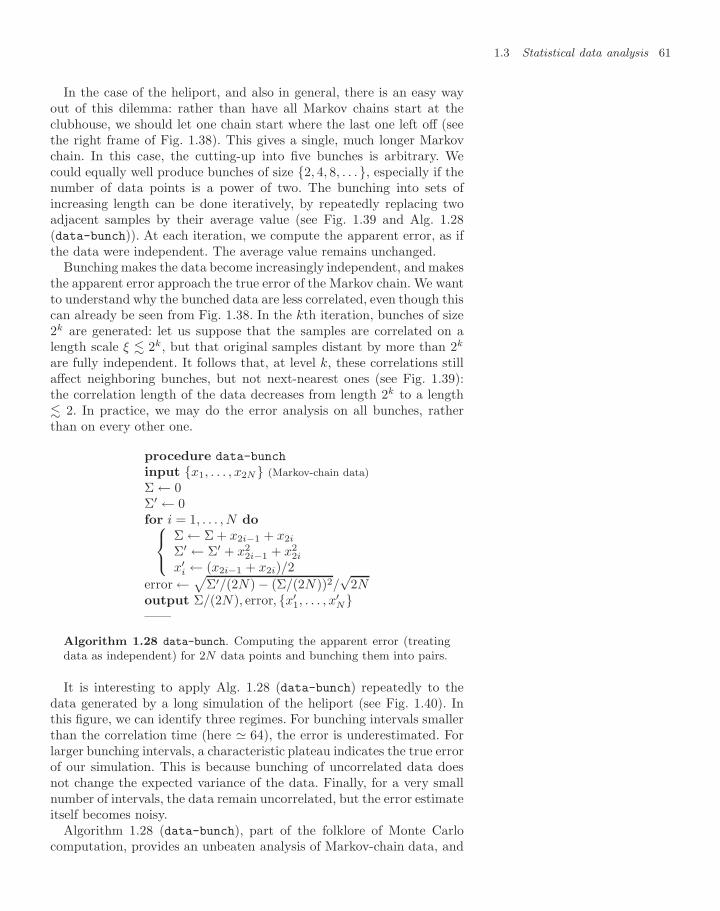
1.3 Statistical data analysis 61
In the case of the heliport, and also in general, there is an easy wayout of this dilemma: rather than have all Markov chains start at theclubhouse, we should let one chain start where the last one left off (seethe right frame of Fig. 1.38). This gives a single, much longer Markovchain. In this case, the cutting-up into five bunches is arbitrary. Wecould equally well produce bunches of size 2, 4, 8, . . ., especially if thenumber of data points is a power of two. The bunching into sets ofincreasing length can be done iteratively, by repeatedly replacing twoadjacent samples by their average value (see Fig. 1.39 and Alg. 1.28(data-bunch)). At each iteration, we compute the apparent error, as ifthe data were independent. The average value remains unchanged.
Bunching makes the data become increasingly independent, and makesthe apparent error approach the true error of the Markov chain. We wantto understand why the bunched data are less correlated, even though thiscan already be seen from Fig. 1.38. In the kth iteration, bunches of size2k are generated: let us suppose that the samples are correlated on alength scale ξ 2k, but that original samples distant by more than 2k
are fully independent. It follows that, at level k, these correlations stillaffect neighboring bunches, but not next-nearest ones (see Fig. 1.39):the correlation length of the data decreases from length 2k to a length 2. In practice, we may do the error analysis on all bunches, ratherthan on every other one.
procedure data-bunch
input x1, . . . , x2N (Markov-chain data)Σ ← 0Σ′ ← 0for i = 1, . . . , N do⎧⎨⎩
Σ ← Σ + x2i−1 + x2i
Σ′ ← Σ′ + x22i−1 + x2
2i
x′i ← (x2i−1 + x2i)/2
error ←√Σ′/(2N) − (Σ/(2N))2/√
2Noutput Σ/(2N), error, x′
1, . . . , x′N
——
Algorithm 1.28 data-bunch. Computing the apparent error (treatingdata as independent) for 2N data points and bunching them into pairs.
It is interesting to apply Alg. 1.28 (data-bunch) repeatedly to thedata generated by a long simulation of the heliport (see Fig. 1.40). Inthis figure, we can identify three regimes. For bunching intervals smallerthan the correlation time (here 64), the error is underestimated. Forlarger bunching intervals, a characteristic plateau indicates the true errorof our simulation. This is because bunching of uncorrelated data doesnot change the expected variance of the data. Finally, for a very smallnumber of intervals, the data remain uncorrelated, but the error estimateitself becomes noisy.
Algorithm 1.28 (data-bunch), part of the folklore of Monte Carlocomputation, provides an unbeaten analysis of Markov-chain data, and
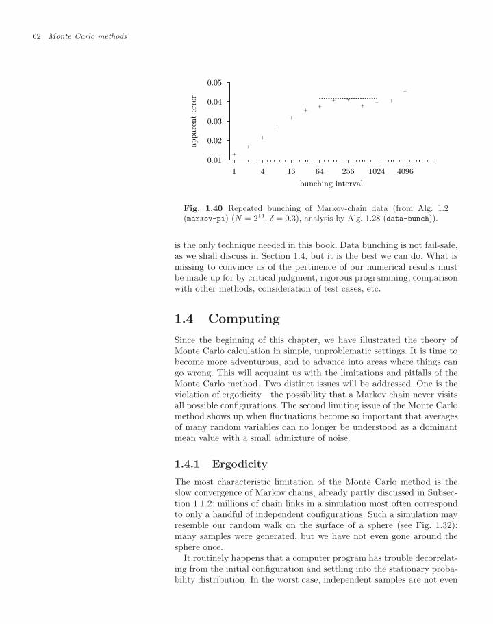
62 Monte Carlo methods
0.01
0.02
0.03
0.04
0.05
1 4 16 64 256 1024 4096
appar
ent
erro
rbunching interval
Fig. 1.40 Repeated bunching of Markov-chain data (from Alg. 1.2(markov-pi) (N = 214, δ = 0.3), analysis by Alg. 1.28 (data-bunch)).
is the only technique needed in this book. Data bunching is not fail-safe,as we shall discuss in Section 1.4, but it is the best we can do. What ismissing to convince us of the pertinence of our numerical results mustbe made up for by critical judgment, rigorous programming, comparisonwith other methods, consideration of test cases, etc.
1.4 Computing
Since the beginning of this chapter, we have illustrated the theory ofMonte Carlo calculation in simple, unproblematic settings. It is time tobecome more adventurous, and to advance into areas where things cango wrong. This will acquaint us with the limitations and pitfalls of theMonte Carlo method. Two distinct issues will be addressed. One is theviolation of ergodicity—the possibility that a Markov chain never visitsall possible configurations. The second limiting issue of the Monte Carlomethod shows up when fluctuations become so important that averagesof many random variables can no longer be understood as a dominantmean value with a small admixture of noise.
1.4.1 Ergodicity
The most characteristic limitation of the Monte Carlo method is theslow convergence of Markov chains, already partly discussed in Subsec-tion 1.1.2: millions of chain links in a simulation most often correspondto only a handful of independent configurations. Such a simulation mayresemble our random walk on the surface of a sphere (see Fig. 1.32):many samples were generated, but we have not even gone around thesphere once.
It routinely happens that a computer program has trouble decorrelat-ing from the initial configuration and settling into the stationary proba-bility distribution. In the worst case, independent samples are not even
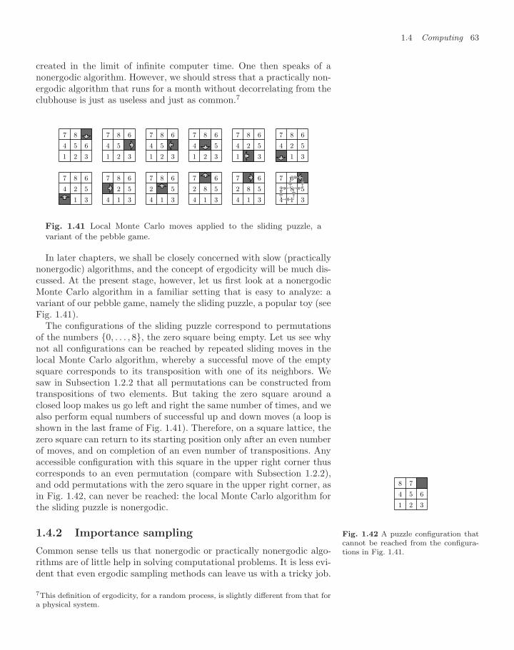
1.4 Computing 63
created in the limit of infinite computer time. One then speaks of anonergodic algorithm. However, we should stress that a practically non-ergodic algorithm that runs for a month without decorrelating from theclubhouse is just as useless and just as common.7
1 2 3
4 5 6
7 8 0
1 2 3
4 5 0
7 8 6
1 2 3
4 5 0
7 8 6
1 2 3
4 0 5
7 8 6
1 0 3
4 2 5
7 8 6
0 1 3
4 2 5
7 8 6
0 1 3
4 2 5
7 8 6
4 1 3
0 2 5
7 8 6
4 1 3
2 0 5
7 8 6
4 1 3
2 8 5
7 0 6
4 1 3
2 8 5
7 0 6
4 1 3
2 8 5
7 6 0
Fig. 1.41 Local Monte Carlo moves applied to the sliding puzzle, avariant of the pebble game.
In later chapters, we shall be closely concerned with slow (practicallynonergodic) algorithms, and the concept of ergodicity will be much dis-cussed. At the present stage, however, let us first look at a nonergodicMonte Carlo algorithm in a familiar setting that is easy to analyze: avariant of our pebble game, namely the sliding puzzle, a popular toy (seeFig. 1.41).
The configurations of the sliding puzzle correspond to permutationsof the numbers 0, . . . , 8, the zero square being empty. Let us see whynot all configurations can be reached by repeated sliding moves in thelocal Monte Carlo algorithm, whereby a successful move of the emptysquare corresponds to its transposition with one of its neighbors. Wesaw in Subsection 1.2.2 that all permutations can be constructed fromtranspositions of two elements. But taking the zero square around aclosed loop makes us go left and right the same number of times, and wealso perform equal numbers of successful up and down moves (a loop isshown in the last frame of Fig. 1.41). Therefore, on a square lattice, thezero square can return to its starting position only after an even numberof moves, and on completion of an even number of transpositions. Anyaccessible configuration with this square in the upper right corner thuscorresponds to an even permutation (compare with Subsection 1.2.2),and odd permutations with the zero square in the upper right corner, asin Fig. 1.42, can never be reached: the local Monte Carlo algorithm forthe sliding puzzle is nonergodic. 1 2 3
4 5 6
8 7 0
Fig. 1.42 A puzzle configuration thatcannot be reached from the configura-tions in Fig. 1.41.
1.4.2 Importance sampling
Common sense tells us that nonergodic or practically nonergodic algo-rithms are of little help in solving computational problems. It is less evi-dent that even ergodic sampling methods can leave us with a tricky job.
7This definition of ergodicity, for a random process, is slightly different from that fora physical system.
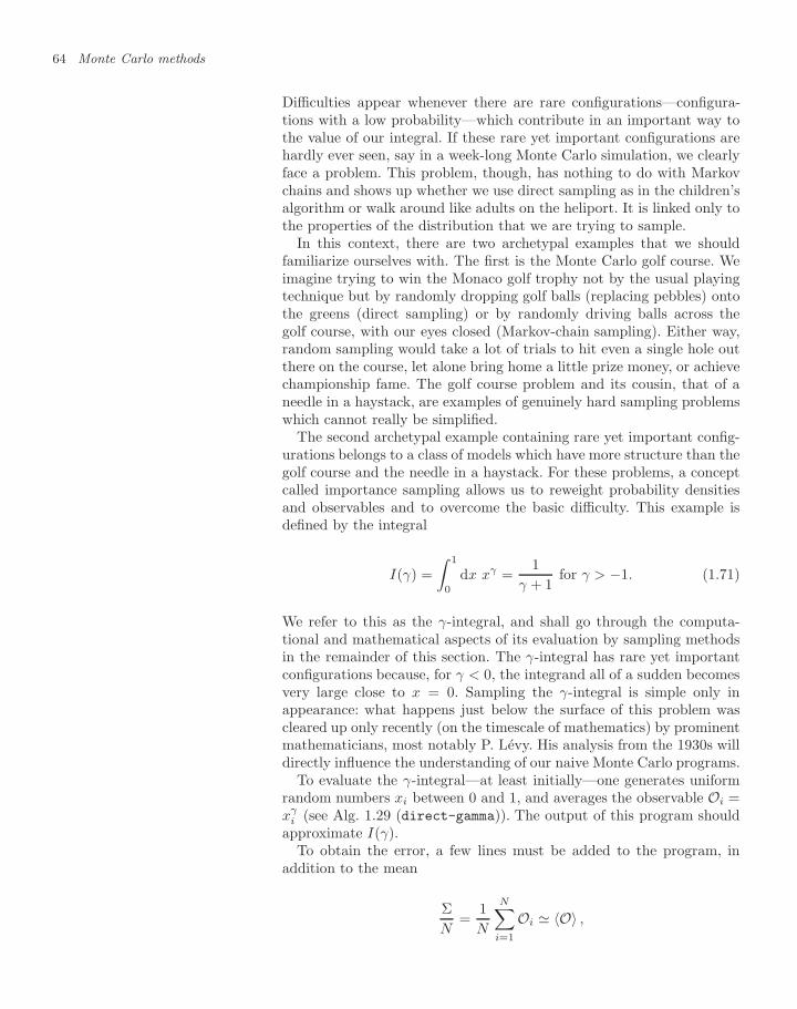
64 Monte Carlo methods
Difficulties appear whenever there are rare configurations—configura-tions with a low probability—which contribute in an important way tothe value of our integral. If these rare yet important configurations arehardly ever seen, say in a week-long Monte Carlo simulation, we clearlyface a problem. This problem, though, has nothing to do with Markovchains and shows up whether we use direct sampling as in the children’salgorithm or walk around like adults on the heliport. It is linked only tothe properties of the distribution that we are trying to sample.
In this context, there are two archetypal examples that we shouldfamiliarize ourselves with. The first is the Monte Carlo golf course. Weimagine trying to win the Monaco golf trophy not by the usual playingtechnique but by randomly dropping golf balls (replacing pebbles) ontothe greens (direct sampling) or by randomly driving balls across thegolf course, with our eyes closed (Markov-chain sampling). Either way,random sampling would take a lot of trials to hit even a single hole outthere on the course, let alone bring home a little prize money, or achievechampionship fame. The golf course problem and its cousin, that of aneedle in a haystack, are examples of genuinely hard sampling problemswhich cannot really be simplified.
The second archetypal example containing rare yet important config-urations belongs to a class of models which have more structure than thegolf course and the needle in a haystack. For these problems, a conceptcalled importance sampling allows us to reweight probability densitiesand observables and to overcome the basic difficulty. This example isdefined by the integral
I(γ) =∫ 1
0
dx xγ =1
γ + 1for γ > −1. (1.71)
We refer to this as the γ-integral, and shall go through the computa-tional and mathematical aspects of its evaluation by sampling methodsin the remainder of this section. The γ-integral has rare yet importantconfigurations because, for γ < 0, the integrand all of a sudden becomesvery large close to x = 0. Sampling the γ-integral is simple only inappearance: what happens just below the surface of this problem wascleared up only recently (on the timescale of mathematics) by prominentmathematicians, most notably P. Levy. His analysis from the 1930s willdirectly influence the understanding of our naive Monte Carlo programs.
To evaluate the γ-integral—at least initially—one generates uniformrandom numbers xi between 0 and 1, and averages the observable Oi =xγ
i (see Alg. 1.29 (direct-gamma)). The output of this program shouldapproximate I(γ).
To obtain the error, a few lines must be added to the program, inaddition to the mean
ΣN
=1N
N∑i=1
Oi 〈O〉 ,
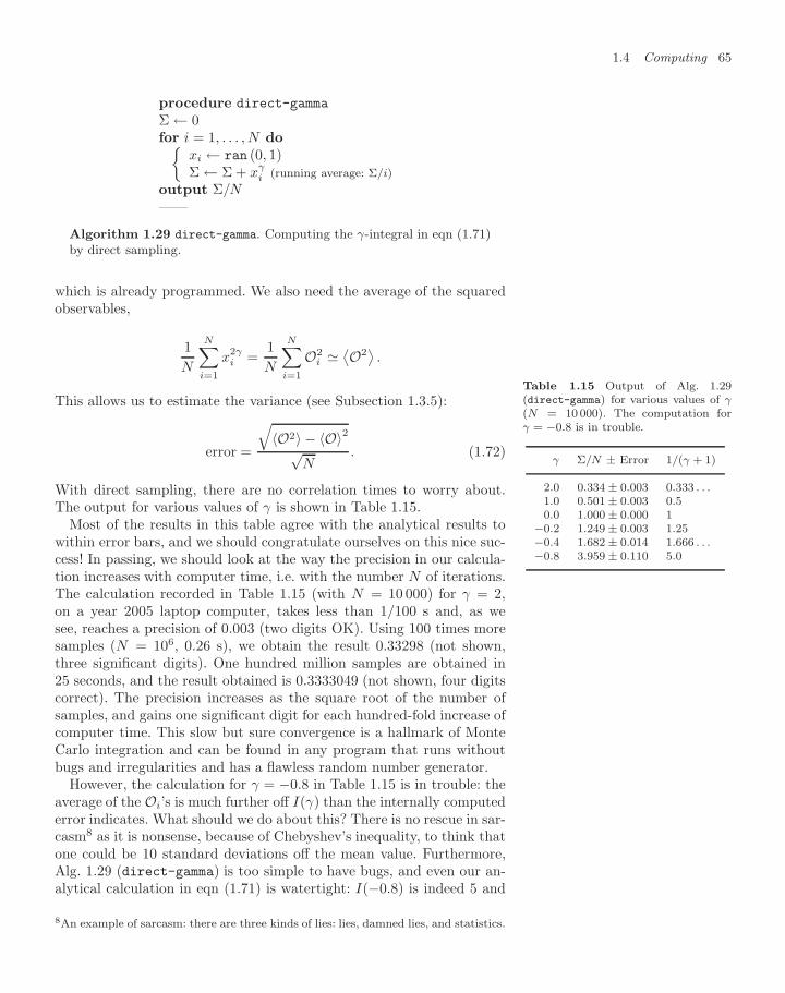
1.4 Computing 65
procedure direct-gamma
Σ ← 0for i = 1, . . . , N do
xi ← ran (0, 1)Σ ← Σ + xγ
i (running average: Σ/i)output Σ/N——
Algorithm 1.29 direct-gamma. Computing the γ-integral in eqn (1.71)by direct sampling.
which is already programmed. We also need the average of the squaredobservables,
1N
N∑i=1
x2γi =
1N
N∑i=1
O2i ⟨O2
⟩.
This allows us to estimate the variance (see Subsection 1.3.5):
error =
√〈O2〉 − 〈O〉2√
N. (1.72)
With direct sampling, there are no correlation times to worry about.The output for various values of γ is shown in Table 1.15.
Table 1.15 Output of Alg. 1.29(direct-gamma) for various values of γ(N = 10 000). The computation forγ = −0.8 is in trouble.
γ Σ/N ± Error 1/(γ + 1)
2.0 0.334 ± 0.003 0.333 . . .1.0 0.501 ± 0.003 0.50.0 1.000 ± 0.000 1
−0.2 1.249 ± 0.003 1.25−0.4 1.682 ± 0.014 1.666 . . .−0.8 3.959 ± 0.110 5.0
Most of the results in this table agree with the analytical results towithin error bars, and we should congratulate ourselves on this nice suc-cess! In passing, we should look at the way the precision in our calcula-tion increases with computer time, i.e. with the number N of iterations.The calculation recorded in Table 1.15 (with N = 10 000) for γ = 2,on a year 2005 laptop computer, takes less than 1/100 s and, as wesee, reaches a precision of 0.003 (two digits OK). Using 100 times moresamples (N = 106, 0.26 s), we obtain the result 0.33298 (not shown,three significant digits). One hundred million samples are obtained in25 seconds, and the result obtained is 0.3333049 (not shown, four digitscorrect). The precision increases as the square root of the number ofsamples, and gains one significant digit for each hundred-fold increase ofcomputer time. This slow but sure convergence is a hallmark of MonteCarlo integration and can be found in any program that runs withoutbugs and irregularities and has a flawless random number generator.
However, the calculation for γ = −0.8 in Table 1.15 is in trouble: theaverage of the Oi’s is much further off I(γ) than the internally computederror indicates. What should we do about this? There is no rescue in sar-casm8 as it is nonsense, because of Chebyshev’s inequality, to think thatone could be 10 standard deviations off the mean value. Furthermore,Alg. 1.29 (direct-gamma) is too simple to have bugs, and even our an-alytical calculation in eqn (1.71) is watertight: I(−0.8) is indeed 5 and
8An example of sarcasm: there are three kinds of lies: lies, damned lies, and statistics.
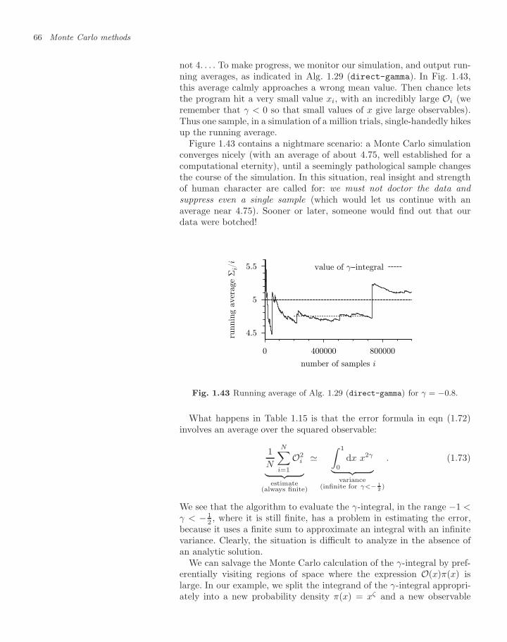
66 Monte Carlo methods
not 4. . . . To make progress, we monitor our simulation, and output run-ning averages, as indicated in Alg. 1.29 (direct-gamma). In Fig. 1.43,this average calmly approaches a wrong mean value. Then chance letsthe program hit a very small value xi, with an incredibly large Oi (weremember that γ < 0 so that small values of x give large observables).Thus one sample, in a simulation of a million trials, single-handedly hikesup the running average.
Figure 1.43 contains a nightmare scenario: a Monte Carlo simulationconverges nicely (with an average of about 4.75, well established for acomputational eternity), until a seemingly pathological sample changesthe course of the simulation. In this situation, real insight and strengthof human character are called for: we must not doctor the data andsuppress even a single sample (which would let us continue with anaverage near 4.75). Sooner or later, someone would find out that ourdata were botched!
4.5
5
5.5
0 400000 800000
runnin
g av
erag
e Σ
i/i
number of samples i
value of γ−integral
Fig. 1.43 Running average of Alg. 1.29 (direct-gamma) for γ = −0.8.
What happens in Table 1.15 is that the error formula in eqn (1.72)involves an average over the squared observable:
1N
N∑i=1
O2i︸ ︷︷ ︸
estimate(always finite)
∫ 1
0
dx x2γ︸ ︷︷ ︸variance
(infinite for γ<− 12 )
. (1.73)
We see that the algorithm to evaluate the γ-integral, in the range −1 <γ < − 1
2 , where it is still finite, has a problem in estimating the error,because it uses a finite sum to approximate an integral with an infinitevariance. Clearly, the situation is difficult to analyze in the absence ofan analytic solution.
We can salvage the Monte Carlo calculation of the γ-integral by pref-erentially visiting regions of space where the expression O(x)π(x) islarge. In our example, we split the integrand of the γ-integral appropri-ately into a new probability density π(x) = xζ and a new observable
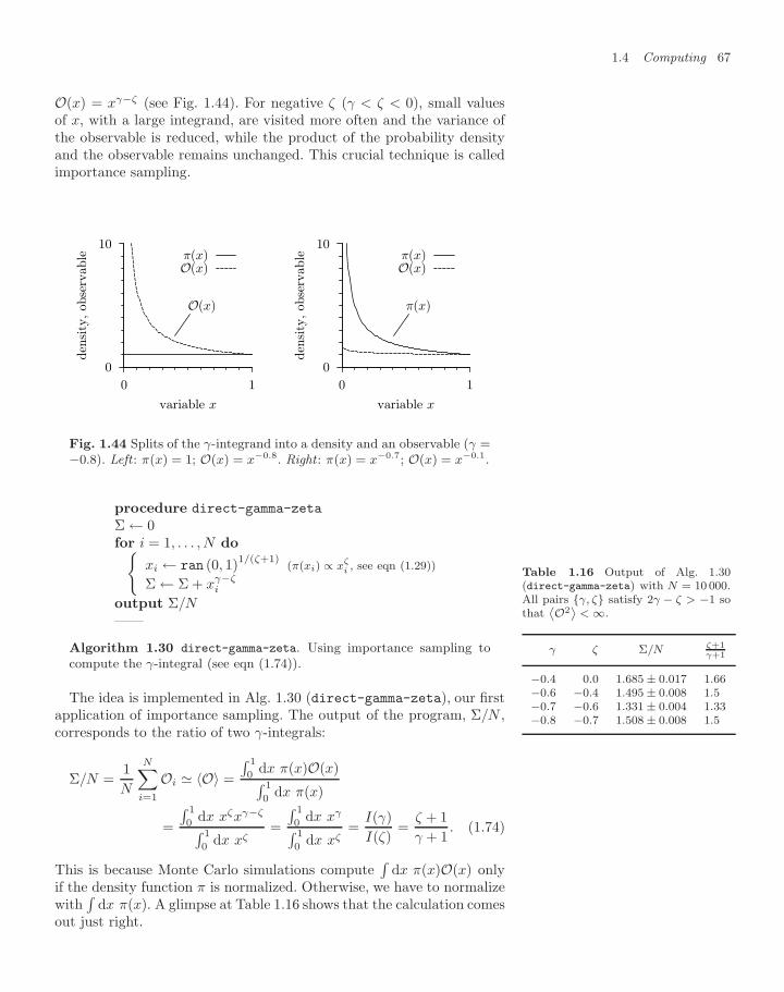
1.4 Computing 67
O(x) = xγ−ζ (see Fig. 1.44). For negative ζ (γ < ζ < 0), small valuesof x, with a large integrand, are visited more often and the variance ofthe observable is reduced, while the product of the probability densityand the observable remains unchanged. This crucial technique is calledimportance sampling.
0
10
0 1
den
sity
, ob
serv
able
variable x
O(x)
π(x)O(x)
0
10
0 1
den
sity
, ob
serv
able
variable x
π(x)
π(x)O(x)
Fig. 1.44 Splits of the γ-integrand into a density and an observable (γ =−0.8). Left : π(x) = 1; O(x) = x−0.8. Right : π(x) = x−0.7; O(x) = x−0.1.
procedure direct-gamma-zeta
Σ ← 0for i = 1, . . . , N do
xi ← ran (0, 1)1/(ζ+1)(π(xi) ∝ xζ
i , see eqn (1.29))
Σ ← Σ + xγ−ζi
output Σ/N——
Algorithm 1.30 direct-gamma-zeta. Using importance sampling tocompute the γ-integral (see eqn (1.74)).
Table 1.16 Output of Alg. 1.30(direct-gamma-zeta) with N = 10 000.All pairs γ, ζ satisfy 2γ − ζ > −1 sothat
˙O2¸
< ∞.
γ ζ Σ/N ζ+1γ+1
−0.4 0.0 1.685 ± 0.017 1.66−0.6 −0.4 1.495 ± 0.008 1.5−0.7 −0.6 1.331 ± 0.004 1.33−0.8 −0.7 1.508 ± 0.008 1.5
The idea is implemented in Alg. 1.30 (direct-gamma-zeta), our firstapplication of importance sampling. The output of the program, Σ/N ,corresponds to the ratio of two γ-integrals:
Σ/N =1N
N∑i=1
Oi 〈O〉 =
∫ 1
0 dx π(x)O(x)∫ 1
0dx π(x)
=
∫ 1
0 dx xζxγ−ζ∫ 1
0dx xζ
=
∫ 1
0 dx xγ∫ 1
0dx xζ
=I(γ)I(ζ)
=ζ + 1γ + 1
. (1.74)
This is because Monte Carlo simulations compute∫
dx π(x)O(x) onlyif the density function π is normalized. Otherwise, we have to normalizewith
∫dx π(x). A glimpse at Table 1.16 shows that the calculation comes
out just right.
68 Monte Carlo methods
We must understand how to compute the error, and why reweightingis useful. The error formula eqn (1.72) remains valid for the observableO(x) = xγ−ζ (a few lines of code have to be added to the program). Thevariance of O is finite under the following condition:
1N
N∑i=1
O2i ⟨O2
⟩=
∫ 1
0 dx π(x)O2(x)∫ 1
0dx π(x)
=∫ 1
0
dx xζx2γ−2ζ < ∞ ⇔ γ > −12
+ ζ/2. (1.75)
This gives a much larger range of possible γ values than does eqn (1.73)for negative values of ζ. All pairs γ, ζ in Table 1.16 satisfy the inequal-ity (1.75). Together, the five different pairs in the table give a productof all the ratios equal to∫ 1
0dx x−0.8∫ 1
0 dx x−0.7︸ ︷︷ ︸γ=−0.8,ζ=−0.7
∫ 1
0dx x−0.7∫ 1
0 dx x−0.6
∫ 1
0dx x−0.6∫ 1
0 dx x−0.4
∫ 1
0dx x−0.4∫ 1
0 dx x0.0= I(−0.8),
with the numerical result
〈O〉 1 × 1.685 × 1.495× 1.331 × 1.508 = 5.057.
Using the rules of Gaussian error propagation, the variance is
Var (O) =
[(0.0171.685
)2
+(
0.0081.495
)2
+(
0.0041.331
)2
+(
0.0081.508
)2]×5.0572.
From the above expression, the final result for the γ-integral is
I(γ = −0.8) = 5.057± 0.06,
obtained entirely by a controlled Monte Carlo calculation.
1.4.3 Monte Carlo quality control
In Subsection 1.4.2, the Monte Carlo evaluation of the γ-integral pro-ceeded on quite shaky ground, because the output was sometimes correctand sometimes wrong. Distressingly, neither the run nor the data anal-ysis produced any warning signals of coming trouble. We relied on ananalytical quality control provided by the inequalities
if γ >
⎧⎪⎨⎪⎩−1 : integral exists− 1
2 : variance exists− 1
2 + ζ/2 : variance exists (importance sampling). (1.76)
To have analytical control over a calculation is very nice, but thiscannot always be achieved. Often, we simply do not completely under-stand the structure of high-dimensional integrals. We are then forced to
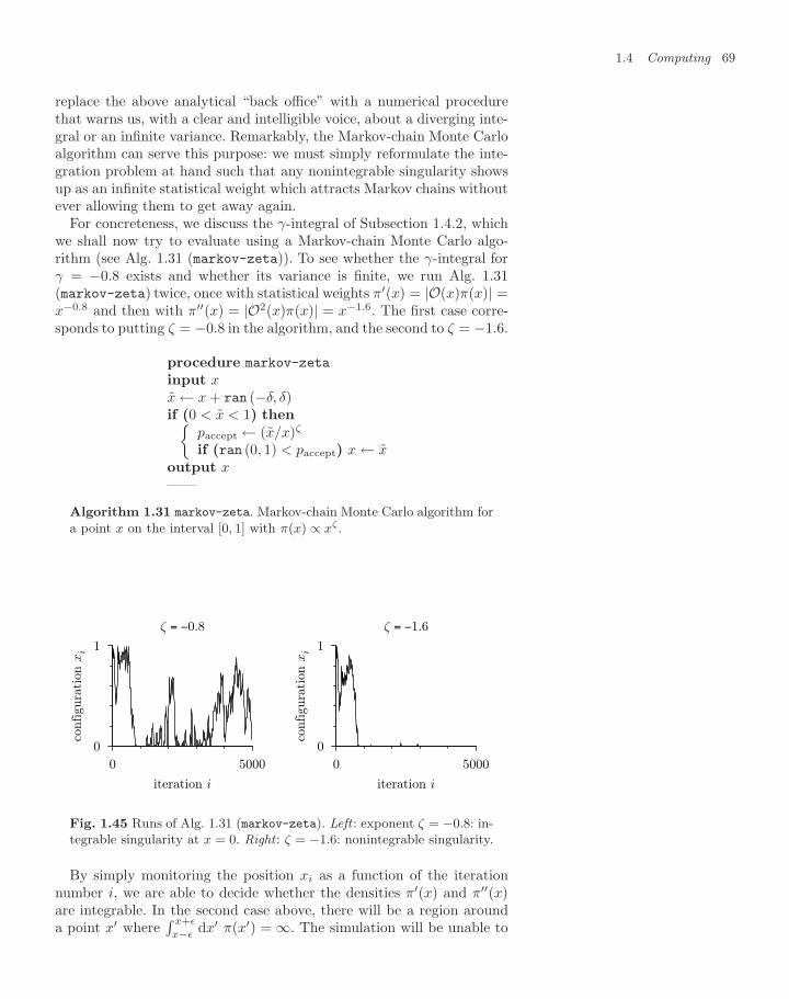
1.4 Computing 69
replace the above analytical “back office” with a numerical procedurethat warns us, with a clear and intelligible voice, about a diverging inte-gral or an infinite variance. Remarkably, the Markov-chain Monte Carloalgorithm can serve this purpose: we must simply reformulate the inte-gration problem at hand such that any nonintegrable singularity showsup as an infinite statistical weight which attracts Markov chains withoutever allowing them to get away again.
For concreteness, we discuss the γ-integral of Subsection 1.4.2, whichwe shall now try to evaluate using a Markov-chain Monte Carlo algo-rithm (see Alg. 1.31 (markov-zeta)). To see whether the γ-integral forγ = −0.8 exists and whether its variance is finite, we run Alg. 1.31(markov-zeta) twice, once with statistical weights π′(x) = |O(x)π(x)| =x−0.8 and then with π′′(x) = |O2(x)π(x)| = x−1.6. The first case corre-sponds to putting ζ = −0.8 in the algorithm, and the second to ζ = −1.6.
procedure markov-zeta
input xx ← x + ran (−δ, δ)if (0 < x < 1) then
paccept ← (x/x)ζ
if (ran (0, 1) < paccept) x ← xoutput x——
Algorithm 1.31 markov-zeta. Markov-chain Monte Carlo algorithm for
a point x on the interval [0, 1] with π(x) ∝ xζ .
0
1
0 5000
configu
rati
on x
i
iteration i
ζ = −0.8
0
1
0 5000
configu
rati
on x
i
iteration i
ζ = −1.6
Fig. 1.45 Runs of Alg. 1.31 (markov-zeta). Left : exponent ζ = −0.8: in-tegrable singularity at x = 0. Right : ζ = −1.6: nonintegrable singularity.
By simply monitoring the position xi as a function of the iterationnumber i, we are able to decide whether the densities π′(x) and π′′(x)are integrable. In the second case above, there will be a region arounda point x′ where
∫ x+ε
x−εdx′ π(x′) = ∞. The simulation will be unable to
70 Monte Carlo methods
escape from the vicinity of this point. On the other hand, an integrablesingularity at x (π(x) → ∞ but
∫ x+ε
x−εdx′ π(x′) is finite) does not trap
the simulation. Data for the two cases, π′(x) and π′′(x), are shown inFig. 1.45. We can correctly infer from the numerical evidence that the γ-integral exists for γ = −0.8 (〈O〉 is finite) but not for γ = −1.6 (
⟨O2⟩
isinfinite). In the present context, the Metropolis algorithm is purely qual-itative, as no observables are computed. This qualitative method allowsus to learn about the analytic properties of high-dimensional integralswhen analytical information analogous to eqn (1.76) is unavailable (seeKrauth and Staudacher (1999)).
1.4.4 Stable distributions
Many problems in the natural and social sciences, economics, engineer-ing, etc. involve probability distributions which are governed by rare yetimportant events. For a geologist, the running-average plot in Fig. 1.43might represent seismic activity over time. Likewise, a financial analystmight have to deal with similar data (with inverted y-axis) in a recordof stock-exchange prices: much small-scale activity, an occasional BlackMonday, and a cataclysmic crash on Wall Street. Neither the geologistnor the financial analyst can choose the easy way out provided by im-portance sampling, because earthquakes and stock crashes cannot bemade to go away through a clever change of variables. It must be un-derstood how often accidents like the ones shown in the running averagein Fig. 1.43 happen. Both the geologist and the financial analyst muststudy the probability distribution of running averages outside the regimeγ > − 1
2 , that is, when the variance is infinite and Monte Carlo calcula-tions are impossible to do without importance sampling. The subject ofsuch distributions with infinite variances was pioneered by Levy in the1930s. He showed that highly erratic sums of N random variables suchas that in Fig. 1.43 tend towards universal distributions, analogously tothe way that sums of random variables with a finite variance tend to-wards the Gaussian, as dictated by the central limit theorem. The limitdistributions depend on the power (the parameter γ) and on the preciseasymptotic behavior for x → ±∞.
We shall first generate these limit distributions from rescaled outputsof Alg. 1.29 (direct-gamma), similarly to what was done for uniformbounded random numbers in Alg. 1.17 (naive-gauss). Secondly, weshall numerically convolute distributions in much the same way as we didfor the bounded uniform distribution in Alg. 1.26 (ran01-convolution).Finally, we shall explicitly construct the limiting distributions usingcharacteristic functions, i.e. the Fourier transforms of the distributionfunctions.
We run Alg. 1.29 (direct-gamma), not once, as for the initial running-average plot of Fig. 1.43, but a few million times, in order to producehistograms of the sample average Σ/N at fixed N (see Fig. 1.46, for γ =−0.8). The mean value of all the histograms is equal to 5, the value of theγ-integral, but this is not a very probable outcome of a single run: from
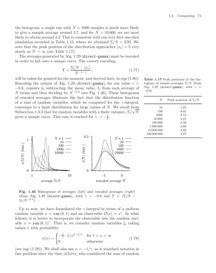
1.4 Computing 71
the histogram, a single run with N = 1000 samples is much more likelyto give a sample average around 3.7, and for N = 10 000, we are mostlikely to obtain around 4.2. This is consistent with our very first one-shotsimulation recorded in Table 1.15, where we obtained Σ/N = 3.95. Wenote that the peak position of the distribution approaches 〈xi〉 = 5 veryslowly as N → ∞ (see Table 1.17).
The averages generated by Alg. 1.29 (direct-gamma) must be rescaledin order to fall onto a unique curve. The correct rescaling,
Υ =Σ/N − 〈xi〉
N−1−γ, (1.77)
will be taken for granted for the moment, and derived later, in eqn (1.80).Rescaling the output of Alg. 1.29 (direct-gamma), for our value γ =−0.8, consists in subtracting the mean value, 5, from each average ofN terms and then dividing by N−0.2 (see Fig. 1.46). These histogramsof rescaled averages illustrate the fact that the distribution functionof a sum of random variables, which we computed for the γ-integral,converges to a limit distribution for large values of N . We recall fromSubsection 1.3.3 that for random variables with a finite variance, Σ/
√N
gives a unique curve. This case is reached for γ → − 12 .
Table 1.17 Peak positions of the his-togram of sample averages Σ/N (fromAlg. 1.29 (direct-gamma), with γ =−0.8)
N Peak position of Σ/N
10 1.85100 3.01
1000 3.7410 000 4.21
100 000 4.501 000 000 4.68
10 000 000 4.80100 000 000 4.87
0
1
1 10
π(Σ
/N)
(his
t.)
average Σ/N
N = 110
1001000
10000
0
0.3
−5 0
π(Υ
) (h
ist.
)
rescaled average Υ
N = 110
1001000
10000
Fig. 1.46 Histograms of averages (left) and rescaled averages (right)(from Alg. 1.29 (direct-gamma), with γ = −0.8 and Υ = (Σ/N −5)/N−0.2).
Up to now, we have formulated the γ-integral in terms of a uniformrandom variable x = ran (0, 1) and an observable O(x) = xγ . In whatfollows, it is better to incorporate the observable into the random vari-able x = ran (0, 1)γ . That is, we consider random variables ξi takingvalues x with probability
π(x) =
− 1
γ · 1/x1−1/γ for 1 < x < ∞0 otherwise
(1.78)
(see eqn (1.29)). We shall also use α = −1/γ, as is standard notation inthis problem since the time of Levy, who considered the sum of random
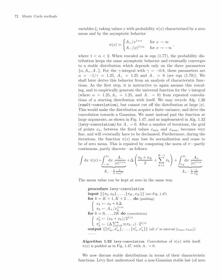
72 Monte Carlo methods
variables ξi taking values x with probability π(x) characterized by a zeromean and by the asymptotic behavior
π(x)
A+/x1+α for x → ∞A−/|x|1+α for x → −∞ ,
where 1 < α < 2. When rescaled as in eqn (1.77), the probability dis-tribution keeps the same asymptotic behavior and eventually convergesto a stable distribution which depends only on the three parametersα, A+, A−. For the γ-integral with γ = −0.8, these parameters areα = −1/γ = 1.25, A+ = 1.25 and A− = 0 (see eqn (1.78)). Weshall later derive this behavior from an analysis of characteristic func-tions. As the first step, it is instructive to again assume this rescal-ing, and to empirically generate the universal function for the γ-integral(where α = 1.25, A+ = 1.25, and A− = 0) from repeated convolu-tions of a starting distribution with itself. We may recycle Alg. 1.26(ran01-convolution), but cannot cut off the distribution at large |x|.This would make the distribution acquire a finite variance, and drive theconvolution towards a Gaussian. We must instead pad the function atlarge arguments, as shown in Fig. 1.47, and as implemented in Alg. 1.32(levy-convolution) for A− = 0. After a number of iterations, the gridof points xk, between the fixed values xmin and xmax, becomes veryfine, and will eventually have to be decimated. Furthermore, during theiterations, the function π(x) may lose its normalization and cease tobe of zero mean. This is repaired by computing the norm of π—partlycontinuous, partly discrete—as follows:∫
dx π(x)=∫ x0
−∞dx
A−|x|1+α︸ ︷︷ ︸
A− · 1α
1|x0|α
+∆
(π0 + πK
2+
K−1∑k=1
πk
)+∫ ∞
xK
dxA+
|x|1+α︸ ︷︷ ︸A+ · 1
α1
xαK
.
The mean value can be kept at zero in the same way.
procedure levy-convolution
input π0, x0, . . . , πK , xK (see Fig. 1.47)for k = K + 1, K + 2 . . . do (padding)
xk ← x0 + k∆πk ← A+/x1+α
k
for k = 0, . . . , 2K do (convolution)x′
k ← (x0 + xk)/21/α
π′k ← (∆
∑kl=0 πlπk−l) · 21/α
output π′m, x′
m, . . . , π′n, x′
n (all x′ in interval [xmin, xmax])——
Algorithm 1.32 levy-convolution. Convolution of π(x) with itself.π(x) is padded as in Fig. 1.47, with A− = 0.
We now discuss stable distributions in terms of their characteristicfunctions. Levy first understood that a non-Gaussian stable law (of zero
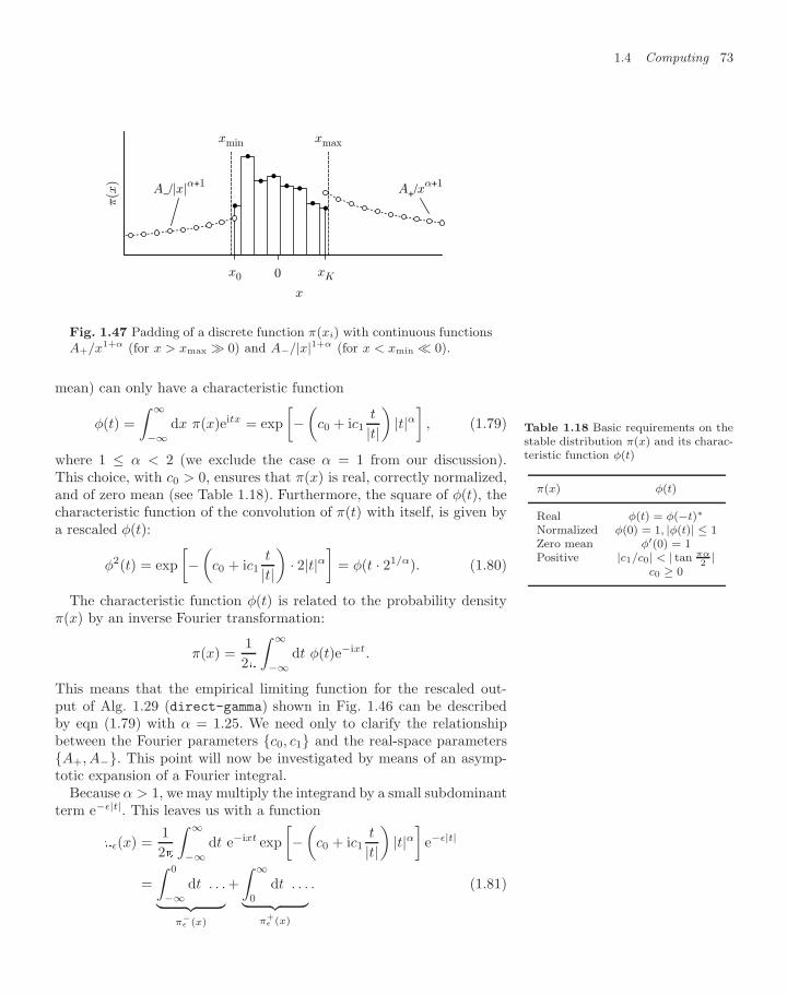
1.4 Computing 73
xK0x0
π(x
)
x
A+/xα+1A−/|x|α+1
xmin xmax
Fig. 1.47 Padding of a discrete function π(xi) with continuous functionsA+/x1+α (for x > xmax 0) and A−/|x|1+α (for x < xmin 0).
mean) can only have a characteristic function
φ(t) =∫ ∞
−∞dx π(x)eitx = exp
[−(
c0 + ic1t
|t|)|t|α]
, (1.79)
where 1 ≤ α < 2 (we exclude the case α = 1 from our discussion).This choice, with c0 > 0, ensures that π(x) is real, correctly normalized,and of zero mean (see Table 1.18). Furthermore, the square of φ(t), thecharacteristic function of the convolution of π(t) with itself, is given bya rescaled φ(t):
Table 1.18 Basic requirements on thestable distribution π(x) and its charac-teristic function φ(t)
π(x) φ(t)
Real φ(t) = φ(−t)∗
Normalized φ(0) = 1, |φ(t)| ≤ 1Zero mean φ′(0) = 1Positive |c1/c0| < | tan πα
2|
c0 ≥ 0φ2(t) = exp[−(
c0 + ic1t
|t|)· 2|t|α
]= φ(t · 21/α). (1.80)
The characteristic function φ(t) is related to the probability densityπ(x) by an inverse Fourier transformation:
π(x) =12
∫ ∞
−∞dt φ(t)e−ixt.
This means that the empirical limiting function for the rescaled out-put of Alg. 1.29 (direct-gamma) shown in Fig. 1.46 can be describedby eqn (1.79) with α = 1.25. We need only to clarify the relationshipbetween the Fourier parameters c0, c1 and the real-space parametersA+, A−. This point will now be investigated by means of an asymp-totic expansion of a Fourier integral.
Because α > 1, we may multiply the integrand by a small subdominantterm e−ε|t|. This leaves us with a function
ε(x) =12
∫ ∞
−∞dt e−ixt exp
[−(
c0 + ic1t
|t|)|t|α]
e−ε|t|
=∫ 0
−∞dt . . .︸ ︷︷ ︸
π−ε (x)
+∫ ∞
0
dt . . .︸ ︷︷ ︸π+
ε (x)
. (1.81)
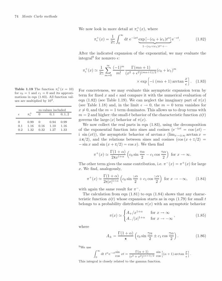
74 Monte Carlo methods
We now look in more detail at π+ε (x), where
π+ε (x) =
12
∫ ∞
0
dt e−ixt exp [−(c0 + ic1)tα]︸ ︷︷ ︸1−(c0+ic1)tα+···
e−εt. (1.82)
After the indicated expansion of the exponential, we may evaluate theintegral9 for nonzero ε:
π+ε (x) 1
2
∞∑m=0
(−1)m
m!Γ(mα + 1)
(x2 + ε2)(mα+1)/2(c0 + ic1)m
× exp[−i (mα + 1) arctan
x
ε
]. (1.83)
For concreteness, we may evaluate this asymptotic expansion term byterm for fixed x and ε and compare it with the numerical evaluation ofeqn (1.82) (see Table 1.19). We can neglect the imaginary part of π(x)(see Table 1.18) and, in the limit ε → 0, the m = 0 term vanishes forx = 0, and the m = 1 term dominates. This allows us to drop terms withm = 2 and higher: the small-t behavior of the characteristic function φ(t)governs the large-|x| behavior of π(x).
Table 1.19 The function π+ε (x = 10)
for c0 = 1 and c1 = 0 and its approxi-mations in eqn (1.83). All function val-ues are multiplied by 103.
m-values includedε π+
ε 0 0, 1 0, 1, 2
0 0.99 0 0.94 0.990.1 1.16 0.16 1.10 1.160.2 1.32 0.32 1.27 1.33
We now collect the real parts in eqn (1.83), using the decompositionof the exponential function into sines and cosines (e−ixt = cos (xt) −i sin (xt)), the asymptotic behavior of arctan x (limx→±∞ arctan x =±/2), and the relations between sines and cosines (cos (x + /2) =− sin x and sin (x + /2) = cos x). We then find
π+(x) Γ(1 + α)2x1+α
(c0 sin
α
2− c1 cos
α
2
)for x → ∞.
The other term gives the same contribution, i.e. π−(x) = π+(x) for largex. We find, analogously,
π+(x) Γ(1 + α)2|x|1+α
(c0 sin
α
2+ c1 cos
α
2
)for x → −∞, (1.84)
with again the same result for π−.The calculation from eqn (1.81) to eqn (1.84) shows that any charac-
teristic function φ(t) whose expansion starts as in eqn (1.79) for small tbelongs to a probability distribution π(x) with an asymptotic behavior
π(x)
A+/x1+α for x → ∞A−/|x|1+α for x → −∞ , (1.85)
where
A± =Γ(1 + α)
(c0 sin
α
2± c1 cos
α
2
). (1.86)
9We use Z ∞
0dt tαe−εtsin
cos xt =Γ(α + 1)
(ε2 + x2)(α+1)/2
sincos
h(α + 1) arctan
x
ε
i.
This integral is closely related to the gamma function.
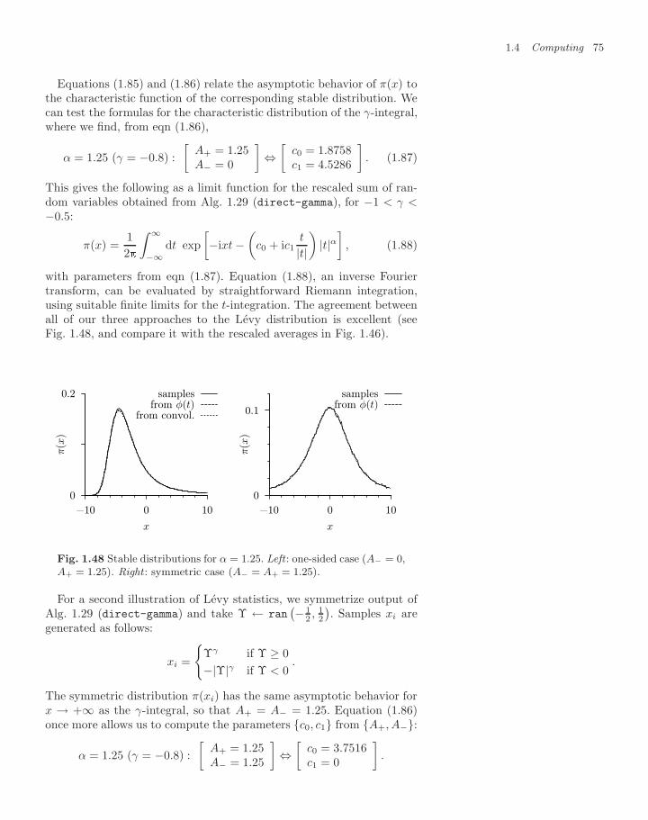
1.4 Computing 75
Equations (1.85) and (1.86) relate the asymptotic behavior of π(x) tothe characteristic function of the corresponding stable distribution. Wecan test the formulas for the characteristic distribution of the γ-integral,where we find, from eqn (1.86),
α = 1.25 (γ = −0.8) :[
A+ = 1.25A− = 0
]⇔[
c0 = 1.8758c1 = 4.5286
]. (1.87)
This gives the following as a limit function for the rescaled sum of ran-dom variables obtained from Alg. 1.29 (direct-gamma), for −1 < γ <−0.5:
π(x) =12
∫ ∞
−∞dt exp
[−ixt −
(c0 + ic1
t
|t|)|t|α]
, (1.88)
with parameters from eqn (1.87). Equation (1.88), an inverse Fouriertransform, can be evaluated by straightforward Riemann integration,using suitable finite limits for the t-integration. The agreement betweenall of our three approaches to the Levy distribution is excellent (seeFig. 1.48, and compare it with the rescaled averages in Fig. 1.46).
0.2
0
−10 0 10
π(x
)
x
samplesfrom φ(t)
from convol.
0
0.1
−10 0 10
π(x
)
x
samplesfrom φ(t)
Fig. 1.48 Stable distributions for α = 1.25. Left : one-sided case (A− = 0,A+ = 1.25). Right : symmetric case (A− = A+ = 1.25).
For a second illustration of Levy statistics, we symmetrize output ofAlg. 1.29 (direct-gamma) and take Υ ← ran
(− 12 , 1
2
). Samples xi are
generated as follows:
xi =
Υγ if Υ ≥ 0−|Υ|γ if Υ < 0
.
The symmetric distribution π(xi) has the same asymptotic behavior forx → +∞ as the γ-integral, so that A+ = A− = 1.25. Equation (1.86)once more allows us to compute the parameters c0, c1 from A+, A−:
α = 1.25 (γ = −0.8) :[
A+ = 1.25A− = 1.25
]⇔[
c0 = 3.7516c1 = 0
].
76 Monte Carlo methods
The parameters α, c0, c1 can again be entered into the inverse Fouriertransform of eqn (1.88), and the result can be compared with the rescaledsimulation data (see Fig. 1.48).
In conclusion, we have progressed in this subsection from a naive casestudy of Alg. 1.29 (direct-gamma) to a systematic analysis of distribu-tions with a finite mean and infinite variance. The mathematical law andorder in these very erratic random processes is expressed through thescaling in eqn (1.77), which fixes the speed of convergence towards themean value, and through the parameters α, A+, A− or, equivalently,α, c0, c1, which are related to each other by eqn (1.86).
1.4.5 Minimum number of samples
In this chapter, we have witnessed Monte Carlo calculations from allwalks of life, and with vastly different convergence properties. With oneexception, when we used Alg. 1.31 (markov-zeta) to sniff out singu-larities, all these programs attempted to estimate an observable mean〈O〉 from a sample average. The success could be outstanding, most pro-nouncedly in the simulation related to the crazy cobbler’s needle, wherea single sample gave complete information about the mean number ofhits. The situation was least glamorous in the case of the γ-integral.There, typical sample averages remained different from the mean of theobservable even after millions of iterations. Practical simulations aresomewhere in between these extremes, even if the variance is finite: it alldepends on how different the original distribution is from a Gaussian,how asymmetric it is, and how quickly it falls to zero for large abso-lute values of its arguments. In a quite difficult case, we saw how thesituation could be saved through importance sampling.
In many problems in physics, importance sampling is incredibly effi-cient. This technique counterbalances the inherent slowness of Markov-chain methods, which are often the only ones available and which, inbillions of iterations and months of computer time, generate only a hand-ful of independent samples. In most cases, though, this relatively smallamount of data allows one to make firm statements about the physicalproperties of the system studied. We can thus often get away with justa few independent samples: this is the main reason why the equilibriumMonte Carlo method is so firmly established in statistical physics.
Exercises 77
Exercises
(Section 1.1)
(1.1) Implement Alg. 1.1 (direct-pi). Run it twentytimes each for N = 10, 100, . . . , 1×10⁸. Convinceyourself that Nhits/N converges towards /4. Esti-mate the mean square deviation
˙(Nhits/N −
4)2
¸from the runs and plot it as a function of N . Howdoes the mean square deviation scale with N?
(1.2) Implement and run Alg. 1.2 (markov-pi), startingfrom the clubhouse. Convince yourself, choosing athrowing range δ = 0.3, that Nhits/N again con-verges towards /4. Next, study the precision ob-tained as a function of δ and check the validity ofthe one-half rule. Plot the mean square deviation˙(Nhits/N −
4)2
¸, for fixed large N , as a function
of δ in the range δ ∈ [0, 3]. Plot the rejection rateof this algorithm as a function of δ. Which value ofthe rejection rate yields the highest precision?
(1.3) Find out whether your programming language al-lows you to check for the presence of a file. If so,improve handling of initial conditions in Alg. 1.2(markov-pi) by including the following code frag-ment:
. . .if (∃ initfile) then˘
input x, y (from initfile)else
x, y ← 1, 1 (legal initial condition). . .
Between runs of the modified program, the outputshould be transferred to initfile, to get new initialconditions. This method for using initial conditionscan be adapted to many Markov-chain programs inthis book.
(1.4) Implement Alg. 1.6 (markov-discrete-pebble), us-ing a subroutine for the numbering scheme andneighbor table. The algorithm should run on arbi-trary rectangular pads without modification of themain program. Check that, during long runs, allsites of the pebble game are visited equally often.
(1.5) For the 3×3 pebble game, find a rejection-free localMonte Carlo algorithm (only moving up, down, leftor right). If you do not succeed for the 3×3 system,consider n × m pebble games.
(1.6) Implement Alg. 1.4 (direct-needle), and Alg. 1.5(direct-needle(patch)). Modify both programs
to allow you to simulate needles that are longerthan the floorboards are wide (a > b). Check thatthe program indeed computes the number . Whichprecision can be reached with this program?
(1.7) Check by an analytic calculation that the relation-ship between the mean number of hits and thelength of the needle (eqn (1.8)) is valid for round(cobbler’s) needles of any size. Analytically calcu-late the function Nhits(x, φ) for semicircular nee-dles, that is, for cobblers’ needles broken into twoequal pieces.
(1.8) Determine all eigenvalues and eigenvectors of thetransfer matrix of the 3 × 3 pebble game ineqn (1.14) (use a standard linear algebra routine).Analogously compute the eigenvalues of n× n peb-ble games. How does the correlation time ∆i dependon the pad size n?
(Section 1.2)
(1.9) Sample permutations using Alg. 1.11 (ran-perm)and check that this algorithm generates all 120 per-mutations of five elements equally often. Determinethe cycle representation of each permutation thatis generated. For permutations of K elements, de-termine the histogram of the probability for be-ing in a cycle of length l (see Subsection 4.2.2).Consider an alternative algorithm for generatingrandom permutations of K elements. Sort randomnumbers x1, . . . , xK = ran (0, 1) , . . . , ran (0, 1)in ascending order xP1 < · · · < xPK
. Show thatP1, . . . , PK is a random permutation.
(1.10) Consider the following algorithm which combinestransformation and rejection techniques:
1 x ← −log ran (0, 1)
Υ ← exph− (x−1)2
2
iif (ran (0, 1) ≥ Υ) goto 1 (reject sample)output x——
Analytically calculate the distribution functionπ(x) sampled by this program, and its rejectionrate. Implement the algorithm and generate a his-togram to check your answers.
(1.11) Consider the following code fragment, which is partof Alg. 1.19 (gauss(patch)):
78 Exercises
x ← ran (−1, 1)y ← ran (−1, 1)Υ ← x2 + y2
output Υ
Compute the distribution function π(Υ) using ele-mentary geometric considerations. Is it true that Υis uniformly distributed in the interval Υ ∈ [0, 1]?Implement the algorithm and generate a histogramto check your answers.
(1.12) Implement both the naive Alg. 1.17 (naive-gauss)with arbitrary K and the Box–Muller algorithm,Alg. 1.18 (gauss). For which value of K can youstill detect statistically significant differences be-tween the two programs?
(1.13) Generate uniformly distributed vectors x1, . . . , xdinside a d-dimensional unit sphere. Next, incorpo-rate the following code fragment:
. . .xd+1 ← ran (−1, 1)
if (Pd+1
k=1 x2k > 1) then˘
output “reject”. . .
Show that the acceptance rate of the modified pro-gram yields the ratio of unit-sphere volumes in (d+1) and in d dimensions. Determine V252(1)/V250(1),and compare with eqn (1.39).
(1.14) Sample random vectors x1, . . . , xd on the surfaceof the d-dimensional unit sphere, using Alg. 1.22(direct-surface). Compute histograms of the vari-able I12 = x2
1 + x22. Discuss the special case of
four dimensions (d = 4). Determine the distribu-tion π(I12) analytically.
(1.15) Generate three-dimensional orthonormal coordi-nate systems with axes ex, ey, ez randomly ori-ented in space, using Alg. 1.22 (direct-surface).Test your program by computing the average scalarproducts 〈(ex ··· e′
x)〉, ˙(ey ··· e′
y)¸, and 〈(ez ··· e′
z)〉 forpairs of random coordinate systems.
(1.16) Implement Alg. 1.13 (reject-finite) for K =10 000 and probabilities πk = 1/kα, where 1 <α < 2. Implement Alg. 1.14 (tower-sample) for thesame problem. Compare the sampling efficiencies.NB: Do not recompute πmax for each sample in therejection method; avoid recomputing Π0, . . . , ΠKfor each sample in the tower-sampling algorithm.
(1.17) Use a sample transformation to derive how to gener-ate random numbers φ distributed as π(φ) = 1
2sin φ
for φ ∈ [0, ]. Likewise, determine the distributionfunction π(x) for x = cos [ran (0, /2)]. Test youranswers with histograms.
(Section 1.3)
(1.18) Implement Alg. 1.25 (binomial-convolution).Compare the probability distribution π(Nhits) forN = 1000, with histograms generated from manyruns of Alg. 1.1 (direct-pi). Plot the probabilitydistributions for the rescaled variables x = Nhits/Nand x = (x − /4)/σ, where σ2 = (/4)(1 − /4).
(1.19) Modify Alg. 1.26 (ran01-convolution) to allow youto handle more general probability distributions,which are nonzero on an arbitrary interval x ∈ [a, b].Follow the convergence of various distributions withzero mean their convergence towards a Gaussian.
(1.20) Implement Alg. 1.28 (data-bunch). Test it fora single, very long, simulation of Alg. 1.2(markov-pi) with throwing ranges δ ∈0.03, 0.1, 0.3. Test it also for output of Alg. 1.6(markov-discrete-pebble) (compute the proba-bility to be at site 1). If possible, compare withthe correlation times for the n × n pebble gameobtained from the second largest eigenvalue of thetransfer matrix (see Exerc. 1.8).
(Section 1.4)
(1.21) Determine the mean value of O = xγ−ζ in a sim-ple implementation of Alg. 1.31 (markov-zeta) forζ > − 1
2. Monitor the rejection rate of the algo-
rithm as a function of the step size δ, and computethe mean square deviation of O. Is the most precisevalue of 〈O〉 obtained with a step size satisfying theone-half rule?
(1.22) Implement Alg. 1.29 (direct-gamma), subtract themean value 1/(γ +1) for each sample, and generatehistograms of the average of N samples, and also ofthe rescaled averages, as in Fig. 1.46.
(1.23) Implement a variant of Alg. 1.29 (direct-gamma),in order to sample the distribution
π(x) ∝(
(x − a)γ if x > a
−c|x − a|γ if x < a.
For concreteness, determine the mean of the dis-tribution analytically as a function of a, c, γ,and subtract it for each sample. Compute the his-tograms of the distribution function for the rescaledsum of random variables distributed as π(x). Com-pute the parameters A±, c1,2 of the Levy distri-bution as a function of a, c, γ, and compare thehistograms of rescaled averages to the analytic limitdistribution of eqn (1.86).
References 79
References
Aigner M., Ziegler G. M. (1992) Proofs from THE BOOK (2nd edn),Springer, Berlin, Heidelberg, New York
Barbier E. (1860) Note sur le probleme de l’aiguille et le jeu du jointcouvert [in French], Journal de Mathematiques Pures et Appliquees (2)5, 273–286
Gnedenko B. V., Kolmogorov A. N. (1954) Limit Distributions for Sumsof Independent Variables, Addison-Wesley, Cambridge, MA
Krauth W., Staudacher M. (1999) Eigenvalue distributions in Yang–Mills integrals, Physics Letters B 453, 253–257
Metropolis N., Rosenbluth A. W., Rosenbluth M. N., Teller A. H., TellerE. (1953) Equation of state calculations by fast computing machines,Journal of Chemical Physics 21, 1087–1092
Propp J. G., Wilson D. B. (1996) Exact sampling with coupled Markovchains and applications to statistical mechanics, Random Structures &Algorithms 9, 223–252
Ulam S. M. (1991) Adventures of a Mathematician, University of Cali-fornia Press, Berkeley, Los Angeles, London

This page intentionally left blank
Hard disks and spheres 22.1 Newtonian deterministic
mechanics 83
2.2 Boltzmann’s statisticalmechanics 92
2.3 Pressure and theBoltzmann distribution 108
2.4 Large hard-spheresystems 119
2.5 Cluster algorithms 122
Exercises 128
References 130
In the first chapter of this book, we considered simple problems in statis-tics: pebbles on the beach, needles falling but never rolling, and peoplestrolling on heliports by night. We now move on to study model systemsin physics—particles with positions, velocities, and interactions—thatobey classical equations of motion. To understand how physical systemscan be treated with the tools of statistics and simulated with MonteCarlo methods, we shall consider the hard-sphere model, which lies atthe heart of statistical mechanics. Hard spheres, which are idealizationsof billiard balls, in free space or in a box, behave as free particles when-ever they are not in contact with other particles or with walls, and obeysimple reflection rules on contact.
The hard-sphere model played a crucial role in the genesis of sta-tistical mechanics. Since the early days of machine computing, in the1950s, and up to the present day, the hard-sphere model has spurredthe development of computer algorithms, and both the explicit numeri-cal integration of Newton’s equations and the Markov-chain Monte Carloalgorithm were first tried out on this model. We shall use such algorithmsto illustrate mechanics and statistical mechanics, and to introduce thefundamental concepts of statistical mechanics: the equiprobability prin-ciple, the Boltzmann distribution, the thermodynamic temperature, andthe pressure. We shall also be concerned with the practical aspects ofcomputations and witness the problems of Markov-chain algorithms athigh densities. We shall conclude the chapter with a first discussion ofsophisticated cluster algorithms which are common to many fields ofcomputational physics.
In the hard-sphere model, all configurations have the same potentialenergy and there is no energetic reason to prefer any configuration overany other. Only entropic effects come into play. In spite of this restric-tion, hard spheres and disks show a rich phenomenology and exhibitphase transitions from the liquid to the solid state. These “entropictransitions” were once quite unsuspected, and then hotly debated, be-fore they ended up poorly understood, especially in two dimensions.The physics of entropy will appear in several places in this chapter, tobe taken up again in earnest in Chapter 6.
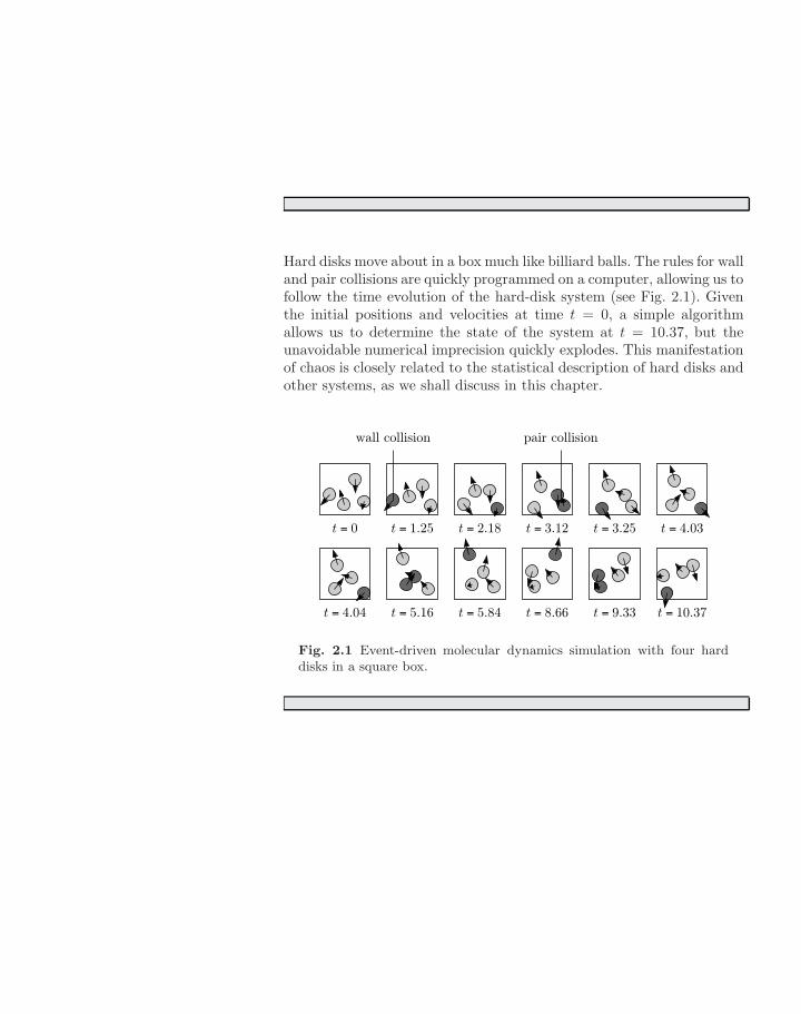
Hard disks move about in a box much like billiard balls. The rules for walland pair collisions are quickly programmed on a computer, allowing us tofollow the time evolution of the hard-disk system (see Fig. 2.1). Giventhe initial positions and velocities at time t = 0, a simple algorithmallows us to determine the state of the system at t = 10.37, but theunavoidable numerical imprecision quickly explodes. This manifestationof chaos is closely related to the statistical description of hard disks andother systems, as we shall discuss in this chapter.
t = 0 t = 1.25
wall collision
t = 2.18 t = 3.12
pair collision
t = 3.25 t = 4.03
t = 4.04 t = 5.16 t = 5.84 t = 8.66 t = 9.33 t = 10.37
Fig. 2.1 Event-driven molecular dynamics simulation with four harddisks in a square box.
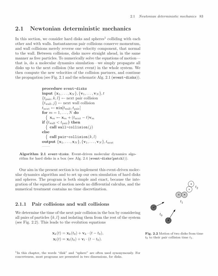
2.1 Newtonian deterministic mechanics 83
2.1 Newtonian deterministic mechanics
In this section, we consider hard disks and spheres1 colliding with eachother and with walls. Instantaneous pair collisions conserve momentum,and wall collisions merely reverse one velocity component, that normalto the wall. Between collisions, disks move straight ahead, in the samemanner as free particles. To numerically solve the equations of motion—that is, do a molecular dynamics simulation—we simply propagate alldisks up to the next collision (the next event) in the whole system. Wethen compute the new velocities of the collision partners, and continuethe propagation (see Fig. 2.1 and the schematic Alg. 2.1 (event-disks)).
procedure event-disks
input x1, . . . ,xN, v1, . . . ,vN, ttpair, k, l ← next pair collisiontwall, j ← next wall collisiontnext ← min[twall, tpair]for m = 1, . . . , N do
xm ← xm + (tnext − t)vm
if (twall < tpair) thencall wall-collision(j)
elsecall pair-collision(k, l)
output x1, . . . ,xN, v1, . . . ,vN, tnext
——
Algorithm 2.1 event-disks. Event-driven molecular dynamics algo-rithm for hard disks in a box (see Alg. 2.4 (event-disks(patch))).
Our aim in the present section is to implement this event-driven molec-ular dynamics algorithm and to set up our own simulation of hard disksand spheres. The program is both simple and exact, because the inte-gration of the equations of motion needs no differential calculus, and thenumerical treatment contains no time discretization.
2.1.1 Pair collisions and wall collisions
We determine the time of the next pair collision in the box by consideringall pairs of particles k, l and isolating them from the rest of the system(see Fig. 2.2). This leads to the evolution equations
t1
t2
t0
Fig. 2.2 Motion of two disks from timet0 to their pair collision time t1.
xk(t) = xk(t0) + vk · (t − t0),xl(t) = xl(t0) + vl · (t − t0).
1In this chapter, the words “disk” and “sphere” are often used synonymously. Forconcreteness, most programs are presented in two dimensions, for disks.
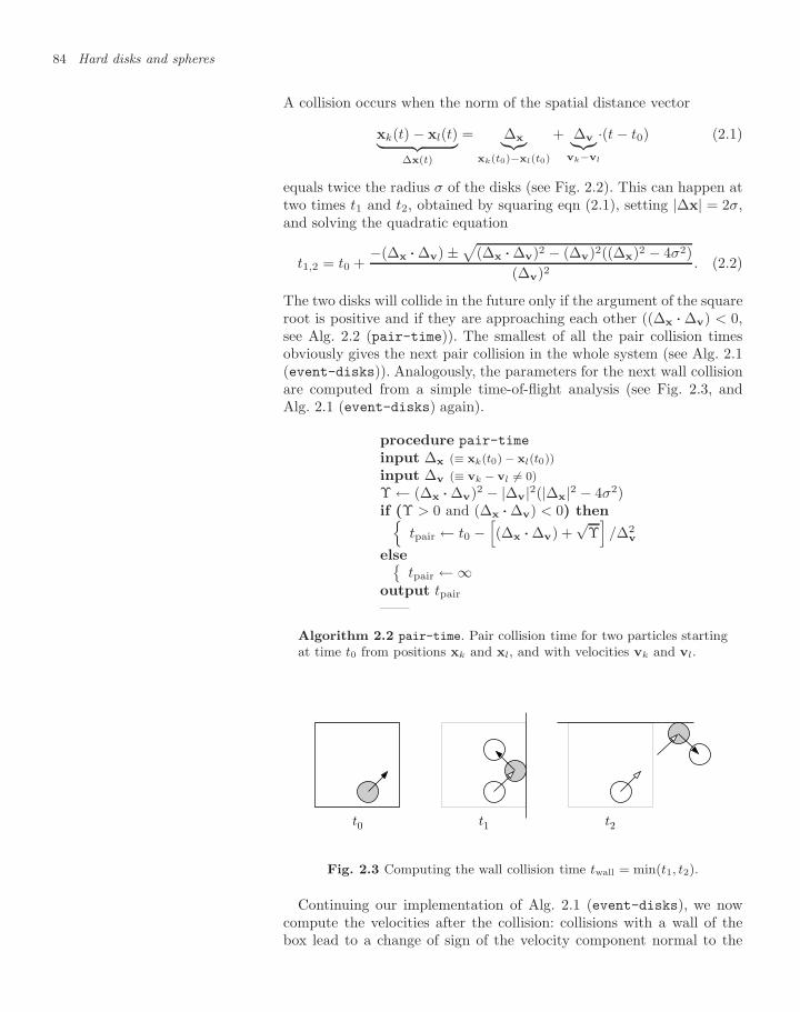
84 Hard disks and spheres
A collision occurs when the norm of the spatial distance vector
xk(t) − xl(t)︸ ︷︷ ︸∆x(t)
= ∆x︸︷︷︸xk(t0)−xl(t0)
+ ∆v︸︷︷︸vk−vl
·(t − t0) (2.1)
equals twice the radius σ of the disks (see Fig. 2.2). This can happen attwo times t1 and t2, obtained by squaring eqn (2.1), setting |∆x| = 2σ,and solving the quadratic equation
t1,2 = t0 +−(∆x ··· ∆v) ±√(∆x ··· ∆v)2 − (∆v)2((∆x)2 − 4σ2)
(∆v)2. (2.2)
The two disks will collide in the future only if the argument of the squareroot is positive and if they are approaching each other ((∆x ··· ∆v) < 0,see Alg. 2.2 (pair-time)). The smallest of all the pair collision timesobviously gives the next pair collision in the whole system (see Alg. 2.1(event-disks)). Analogously, the parameters for the next wall collisionare computed from a simple time-of-flight analysis (see Fig. 2.3, andAlg. 2.1 (event-disks) again).
procedure pair-time
input ∆x (≡ xk(t0) − xl(t0))input ∆v (≡ vk − vl = 0)Υ ← (∆x ··· ∆v)2 − |∆v|2(|∆x|2 − 4σ2)if (Υ > 0 and (∆x ··· ∆v) < 0) then
tpair ← t0 −[(∆x ··· ∆v) +
√Υ]/∆2
v
elsetpair ← ∞
output tpair
——
Algorithm 2.2 pair-time. Pair collision time for two particles startingat time t0 from positions xk and xl, and with velocities vk and vl.
t0 t1 t2
Fig. 2.3 Computing the wall collision time twall = min(t1, t2).
Continuing our implementation of Alg. 2.1 (event-disks), we nowcompute the velocities after the collision: collisions with a wall of thebox lead to a change of sign of the velocity component normal to the
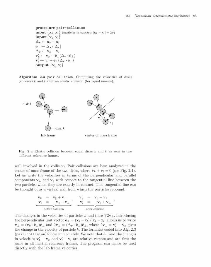
2.1 Newtonian deterministic mechanics 85
procedure pair-collision
input xk,xl (particles in contact: |xk − xl| = 2σ)input vk,vl∆x ← xk − xl
e⊥ ← ∆x/|∆x|∆v ← vk − vl
v′k ← vk − e⊥(∆v ··· e⊥)
v′l ← vl + e⊥(∆v ··· e⊥)
output v′k,v′
l——
Algorithm 2.3 pair-collision. Computing the velocities of disks(spheres) k and l after an elastic collision (for equal masses).
lab frame
disk k
disk l
center of mass frame
v⊥v‖
Fig. 2.4 Elastic collision between equal disks k and l, as seen in twodifferent reference frames.
wall involved in the collision. Pair collisions are best analyzed in thecenter-of-mass frame of the two disks, where vk + vl = 0 (see Fig. 2.4).Let us write the velocities in terms of the perpendicular and parallelcomponents v⊥ and v‖ with respect to the tangential line between thetwo particles when they are exactly in contact. This tangential line canbe thought of as a virtual wall from which the particles rebound:
vk = v‖ + v⊥vl = −v‖ − v⊥︸ ︷︷ ︸
before collision
,v′
k = v‖ − v⊥v′
l = −v‖ + v⊥︸ ︷︷ ︸after collision
.
The changes in the velocities of particles k and l are ∓2v⊥. Introducingthe perpendicular unit vector e⊥ = (xk −xl)/|xk −xl| allows us to writev⊥ = (vk ··· e⊥)e⊥ and 2v⊥ = (∆v ··· e⊥)e⊥, where 2v⊥ = v′
k − vk givesthe change in the velocity of particle k. The formulas coded into Alg. 2.3(pair-collision) follow immediately. We note that e⊥ and the changesin velocities v′
k − vk and v′l − vl are relative vectors and are thus the
same in all inertial reference frames. The program can hence be useddirectly with the lab frame velocities.
86 Hard disks and spheres
Algorithm 2.1 (event-disks) is rigorous, but naive in that it com-putes collision times even for pairs that are far apart and also recom-putes all pair collision times from scratch after each event, although theychange only for pairs involving a collision partner. Improvements couldeasily be worked into the program, but we shall not need them. How-ever, even our basic code can be accepted only if it runs through manybillions of collisions (several hours of CPU time) without crashing. Wemust care about code stability. In addition, we should invest in simpli-fying input–output: it is a good strategy to let the program search for afile containing the initial configuration (velocities, positions, and time),possibly the final configuration of a previous calculation. If no such fileis found, a legal initial configuration should be automatically generatedby the program. Finally, we should plot the results in the natural unitsof time for the simulation, such that during a unit time interval eachparticle undergoes about one pair collision (and the whole system hasN/2 pair collisions). In this way, the results become independent of thescale of the initial velocities.
Our molecular dynamics algorithm moves from one collision to thenext with an essentially fixed number of arithmetic operations, requir-ing on the order of a microsecond for a few disks on a year 2005 laptopcomputer. Each collision drives the system further in physical time. Solv-ing Newton’s dynamics thus appears to be a mere question of computerbudget.
2.1.2 Chaotic dynamics
Algorithm 2.1 (event-disks) solves the hard-sphere equations of mo-tion on the assumption that the calculation of collision times, positions,velocity changes, etc. is done with infinite precision. This cannot re-ally be achieved on a computer, but the question arises of whether itmatters that numbers are truncated after 8 or 16 decimal digits. It iseasiest to answer this question by pitting different versions of the sameevent-driven algorithm against each other, starting from identical ini-tial conditions, but with all calculations performed at different precisionlevels: in one case in short format (single precision), and in the othercase in long format (double precision). The standard encoding of 32-bitfloating-point numbers ±a×10b uses one bit for the sign, eight bits forthe exponent b, and 23 bits for the fraction a, so that the precision—theratio of neighboring numbers that can be represented on the computer—is approximately ε = 2−23 1.2×10⁻⁷. For a 64-bit floating point num-ber, the precision is about ε = 1×10⁻¹⁶. Most computer languages allowone to switch precision levels without any significant rewriting of code.
The two versions of the four-disk molecular dynamics calculation,started off from identical initial conditions (as in Fig. 2.1), get out ofstep after as few as 25 pair collisions (see Fig. 2.5), an extremely smallnumber compared with the million or so collisions which we can handleper second on a year 2005 laptop computer.
This situation is quite uncomfortable: our computational results, for
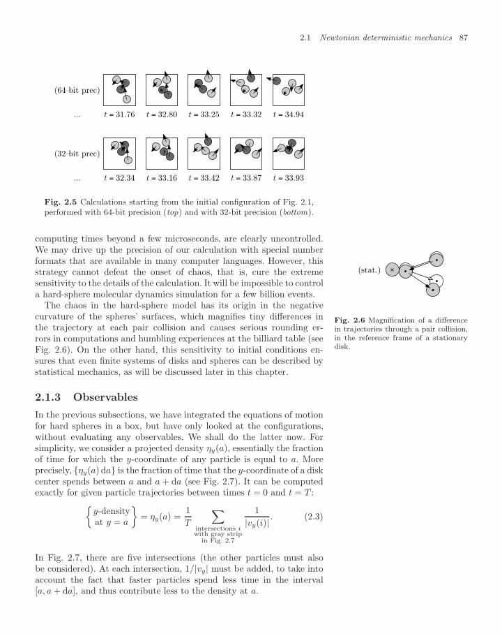
2.1 Newtonian deterministic mechanics 87
(64-bit prec)
... t = 31.76 t = 32.80 t = 33.25 t = 33.32 t = 34.94
(32-bit prec)
... t = 32.34 t = 33.16 t = 33.42 t = 33.87 t = 33.93
Fig. 2.5 Calculations starting from the initial configuration of Fig. 2.1,performed with 64-bit precision (top) and with 32-bit precision (bottom).
computing times beyond a few microseconds, are clearly uncontrolled.We may drive up the precision of our calculation with special numberformats that are available in many computer languages. However, thisstrategy cannot defeat the onset of chaos, that is, cure the extremesensitivity to the details of the calculation. It will be impossible to controla hard-sphere molecular dynamics simulation for a few billion events.
(stat.)
Fig. 2.6 Magnification of a differencein trajectories through a pair collision,in the reference frame of a stationarydisk.
The chaos in the hard-sphere model has its origin in the negativecurvature of the spheres’ surfaces, which magnifies tiny differences inthe trajectory at each pair collision and causes serious rounding er-rors in computations and humbling experiences at the billiard table (seeFig. 2.6). On the other hand, this sensitivity to initial conditions en-sures that even finite systems of disks and spheres can be described bystatistical mechanics, as will be discussed later in this chapter.
2.1.3 Observables
In the previous subsections, we have integrated the equations of motionfor hard spheres in a box, but have only looked at the configurations,without evaluating any observables. We shall do the latter now. Forsimplicity, we consider a projected density ηy(a), essentially the fractionof time for which the y-coordinate of any particle is equal to a. Moreprecisely, ηy(a) da is the fraction of time that the y-coordinate of a diskcenter spends between a and a + da (see Fig. 2.7). It can be computedexactly for given particle trajectories between times t = 0 and t = T :
y-densityat y = a
= ηy(a) =
1T
∑intersections iwith gray strip
in Fig. 2.7
1|vy(i)| . (2.3)
In Fig. 2.7, there are five intersections (the other particles must alsobe considered). At each intersection, 1/|vy| must be added, to take intoaccount the fact that faster particles spend less time in the interval[a, a + da], and thus contribute less to the density at a.
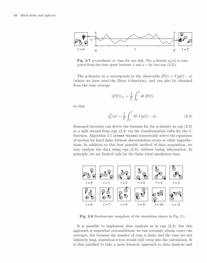
88 Hard disks and spheres
t = 0
a
0 Tt t = T
Fig. 2.7 y-coordinate vs. time for one disk. The y-density ηy(a) is com-puted from the time spent between a and a + da (see eqn (2.3)).
The y-density at a corresponds to the observable O(t) = δ [y(t) − a](where we have used the Dirac δ-function), and can also be obtainedfrom the time average
〈O(t)〉T =1T
∫ T
0
dt O(t),
so that
ηTy (a) =
1T
∫ T
0
dt δ [y(t) − a] . (2.4)
Seasoned theorists can derive the formula for the y-density in eqn (2.3)in a split second from eqn (2.4) via the transformation rules for the δ-function. Algorithm 2.1 (event-disks) numerically solves the equationsof motion for hard disks without discretization errors or other imperfec-tions. In addition to this best possible method of data acquisition, wemay analyze the data using eqn (2.3), without losing information. Inprinciple, we are limited only by the finite total simulation time.
t = 0 t = 1 t = 2 t = 3 t = 4 t = 5
t = 6 t = 7 t = 8 t = 9 t = 10 t = 11
Fig. 2.8 Stroboscopic snapshots of the simulation shown in Fig. 2.1.
It is possible to implement data analysis as in eqn (2.3), but thisapproach is somewhat overambitious: we can certainly obtain exact runaverages, but because the number of runs is finite and the runs are notinfinitely long, statistical errors would still creep into the calculation. Itis thus justified to take a more leisurely approach to data analysis and
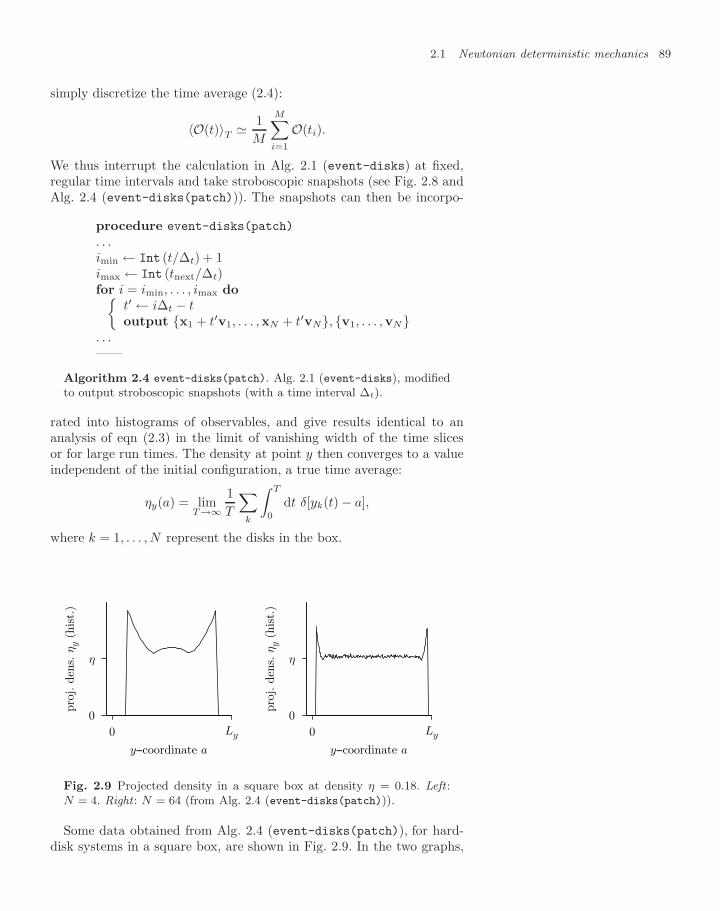
2.1 Newtonian deterministic mechanics 89
simply discretize the time average (2.4):
〈O(t)〉T 1M
M∑i=1
O(ti).
We thus interrupt the calculation in Alg. 2.1 (event-disks) at fixed,regular time intervals and take stroboscopic snapshots (see Fig. 2.8 andAlg. 2.4 (event-disks(patch))). The snapshots can then be incorpo-
procedure event-disks(patch)
. . .imin ← Int (t/∆t) + 1imax ← Int (tnext/∆t)for i = imin, . . . , imax do
t′ ← i∆t − toutput x1 + t′v1, . . . ,xN + t′vN, v1, . . . ,vN
. . .——
Algorithm 2.4 event-disks(patch). Alg. 2.1 (event-disks), modifiedto output stroboscopic snapshots (with a time interval ∆t).
rated into histograms of observables, and give results identical to ananalysis of eqn (2.3) in the limit of vanishing width of the time slicesor for large run times. The density at point y then converges to a valueindependent of the initial configuration, a true time average:
ηy(a) = limT→∞
1T
∑k
∫ T
0
dt δ[yk(t) − a],
where k = 1, . . . , N represent the disks in the box.
η
0Ly0
pro
j. d
ens.
ηy
(his
t.)
y−coordinate a
η
0Ly0
pro
j. d
ens.
ηy
(his
t.)
y−coordinate a
Fig. 2.9 Projected density in a square box at density η = 0.18. Left :N = 4. Right : N = 64 (from Alg. 2.4 (event-disks(patch))).
Some data obtained from Alg. 2.4 (event-disks(patch)), for hard-disk systems in a square box, are shown in Fig. 2.9. In the two graphs,
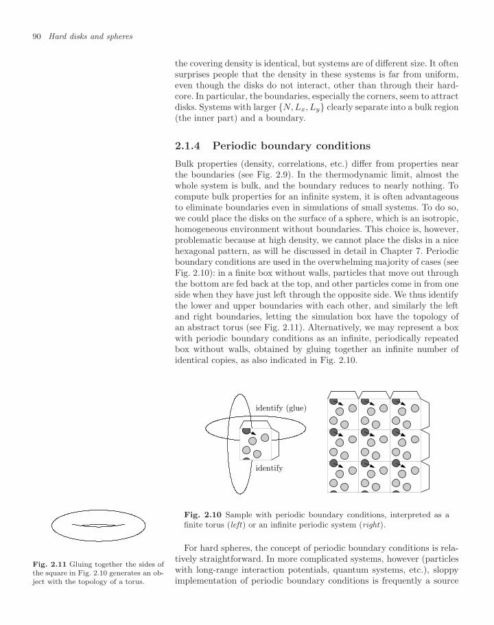
90 Hard disks and spheres
the covering density is identical, but systems are of different size. It oftensurprises people that the density in these systems is far from uniform,even though the disks do not interact, other than through their hard-core. In particular, the boundaries, especially the corners, seem to attractdisks. Systems with larger N, Lx, Ly clearly separate into a bulk region(the inner part) and a boundary.
2.1.4 Periodic boundary conditions
Bulk properties (density, correlations, etc.) differ from properties nearthe boundaries (see Fig. 2.9). In the thermodynamic limit, almost thewhole system is bulk, and the boundary reduces to nearly nothing. Tocompute bulk properties for an infinite system, it is often advantageousto eliminate boundaries even in simulations of small systems. To do so,we could place the disks on the surface of a sphere, which is an isotropic,homogeneous environment without boundaries. This choice is, however,problematic because at high density, we cannot place the disks in a nicehexagonal pattern, as will be discussed in detail in Chapter 7. Periodicboundary conditions are used in the overwhelming majority of cases (seeFig. 2.10): in a finite box without walls, particles that move out throughthe bottom are fed back at the top, and other particles come in from oneside when they have just left through the opposite side. We thus identifythe lower and upper boundaries with each other, and similarly the leftand right boundaries, letting the simulation box have the topology ofan abstract torus (see Fig. 2.11). Alternatively, we may represent a boxwith periodic boundary conditions as an infinite, periodically repeatedbox without walls, obtained by gluing together an infinite number ofidentical copies, as also indicated in Fig. 2.10.
identify (glue)
identify
Fig. 2.10 Sample with periodic boundary conditions, interpreted as afinite torus (left) or an infinite periodic system (right).
Fig. 2.11 Gluing together the sides ofthe square in Fig. 2.10 generates an ob-ject with the topology of a torus.
For hard spheres, the concept of periodic boundary conditions is rela-tively straightforward. In more complicated systems, however (particleswith long-range interaction potentials, quantum systems, etc.), sloppyimplementation of periodic boundary conditions is frequently a source
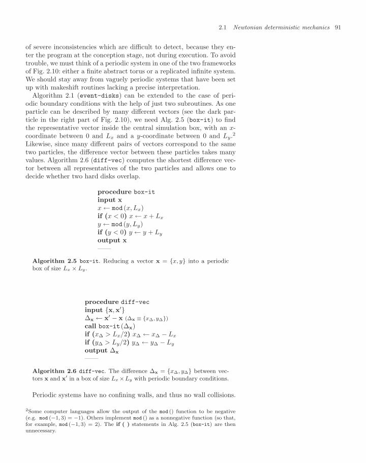
2.1 Newtonian deterministic mechanics 91
of severe inconsistencies which are difficult to detect, because they en-ter the program at the conception stage, not during execution. To avoidtrouble, we must think of a periodic system in one of the two frameworksof Fig. 2.10: either a finite abstract torus or a replicated infinite system.We should stay away from vaguely periodic systems that have been setup with makeshift routines lacking a precise interpretation.
Algorithm 2.1 (event-disks) can be extended to the case of peri-odic boundary conditions with the help of just two subroutines. As oneparticle can be described by many different vectors (see the dark par-ticle in the right part of Fig. 2.10), we need Alg. 2.5 (box-it) to findthe representative vector inside the central simulation box, with an x-coordinate between 0 and Lx and a y-coordinate between 0 and Ly.2
Likewise, since many different pairs of vectors correspond to the sametwo particles, the difference vector between these particles takes manyvalues. Algorithm 2.6 (diff-vec) computes the shortest difference vec-tor between all representatives of the two particles and allows one todecide whether two hard disks overlap.
procedure box-it
input xx ← mod (x, Lx)if (x < 0) x ← x + Lx
y ← mod (y, Ly)if (y < 0) y ← y + Ly
output x——
Algorithm 2.5 box-it. Reducing a vector x = x, y into a periodicbox of size Lx × Ly .
procedure diff-vec
input x,x′∆x ← x′ − x (∆x ≡ x∆, y∆)call box-it (∆x)if (x∆ > Lx/2) x∆ ← x∆ − Lx
if (y∆ > Ly/2) y∆ ← y∆ − Ly
output ∆x
——
Algorithm 2.6 diff-vec. The difference ∆x = x∆, y∆ between vec-tors x and x′ in a box of size Lx ×Ly with periodic boundary conditions.
Periodic systems have no confining walls, and thus no wall collisions.
2Some computer languages allow the output of the mod () function to be negative(e.g. mod (−1, 3) = −1). Others implement mod () as a nonnegative function (so that,for example, mod (−1, 3) = 2). The if ( ) statements in Alg. 2.5 (box-it) are thenunnecessary.
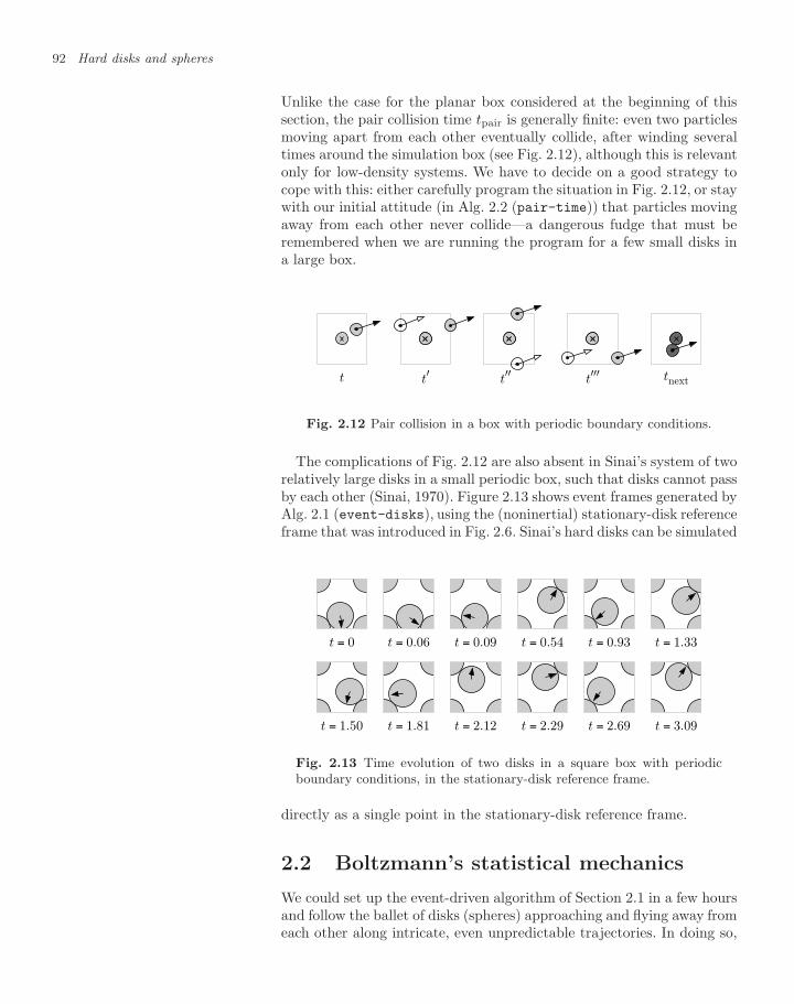
92 Hard disks and spheres
Unlike the case for the planar box considered at the beginning of thissection, the pair collision time tpair is generally finite: even two particlesmoving apart from each other eventually collide, after winding severaltimes around the simulation box (see Fig. 2.12), although this is relevantonly for low-density systems. We have to decide on a good strategy tocope with this: either carefully program the situation in Fig. 2.12, or staywith our initial attitude (in Alg. 2.2 (pair-time)) that particles movingaway from each other never collide—a dangerous fudge that must beremembered when we are running the program for a few small disks ina large box.
t t′ t′′ t′′′ tnext
Fig. 2.12 Pair collision in a box with periodic boundary conditions.
The complications of Fig. 2.12 are also absent in Sinai’s system of tworelatively large disks in a small periodic box, such that disks cannot passby each other (Sinai, 1970). Figure 2.13 shows event frames generated byAlg. 2.1 (event-disks), using the (noninertial) stationary-disk referenceframe that was introduced in Fig. 2.6. Sinai’s hard disks can be simulated
t = 0 t = 0.06 t = 0.09 t = 0.54 t = 0.93 t = 1.33
t = 1.50 t = 1.81 t = 2.12 t = 2.29 t = 2.69 t = 3.09
Fig. 2.13 Time evolution of two disks in a square box with periodicboundary conditions, in the stationary-disk reference frame.
directly as a single point in the stationary-disk reference frame.
2.2 Boltzmann’s statistical mechanics
We could set up the event-driven algorithm of Section 2.1 in a few hoursand follow the ballet of disks (spheres) approaching and flying away fromeach other along intricate, even unpredictable trajectories. In doing so,
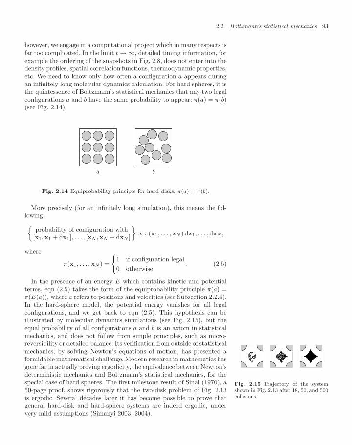
2.2 Boltzmann’s statistical mechanics 93
however, we engage in a computational project which in many respects isfar too complicated. In the limit t → ∞, detailed timing information, forexample the ordering of the snapshots in Fig. 2.8, does not enter into thedensity profiles, spatial correlation functions, thermodynamic properties,etc. We need to know only how often a configuration a appears duringan infinitely long molecular dynamics calculation. For hard spheres, it isthe quintessence of Boltzmann’s statistical mechanics that any two legalconfigurations a and b have the same probability to appear: π(a) = π(b)(see Fig. 2.14).
a b
Fig. 2.14 Equiprobability principle for hard disks: π(a) = π(b).
More precisely (for an infinitely long simulation), this means the fol-lowing:
probability of configuration with[x1,x1 + dx1], . . . , [xN ,xN + dxN ]
∝ π(x1, . . . ,xN ) dx1, . . . , dxN ,
where
π(x1, . . . ,xN ) =
1 if configuration legal0 otherwise
. (2.5)
In the presence of an energy E which contains kinetic and potentialterms, eqn (2.5) takes the form of the equiprobability principle π(a) =π(E(a)), where a refers to positions and velocities (see Subsection 2.2.4).In the hard-sphere model, the potential energy vanishes for all legalconfigurations, and we get back to eqn (2.5). This hypothesis can beillustrated by molecular dynamics simulations (see Fig. 2.15), but theequal probability of all configurations a and b is an axiom in statisticalmechanics, and does not follow from simple principles, such as micro-reversibility or detailed balance. Its verification from outside of statisticalmechanics, by solving Newton’s equations of motion, has presented aformidable mathematical challenge. Modern research in mathematics hasgone far in actually proving ergodicity, the equivalence between Newton’sdeterministic mechanics and Boltzmann’s statistical mechanics, for thespecial case of hard spheres. The first milestone result of Sinai (1970), a50-page proof, shows rigorously that the two-disk problem of Fig. 2.13is ergodic. Several decades later it has become possible to prove thatgeneral hard-disk and hard-sphere systems are indeed ergodic, undervery mild assumptions (Simanyi 2003, 2004).
Fig. 2.15 Trajectory of the systemshown in Fig. 2.13 after 18, 50, and 500collisions.
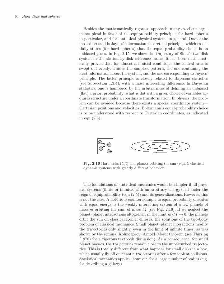
94 Hard disks and spheres
Besides the mathematically rigorous approach, many excellent argu-ments plead in favor of the equiprobability principle, for hard spheresin particular, and for statistical physical systems in general. One of themost discussed is Jaynes’ information-theoretical principle, which essen-tially states (for hard spheres) that the equal-probability choice is anunbiased guess. In Fig. 2.15, we show the trajectory of Sinai’s two-disksystem in the stationary-disk reference frame. It has been mathemat-ically proven that for almost all initial conditions, the central area isswept out evenly. This is the simplest pattern, the one containing theleast information about the system, and the one corresponding to Jaynes’principle. The latter principle is closely related to Bayesian statistics(see Subsection 1.3.4), with a most interesting difference. In Bayesianstatistics, one is hampered by the arbitrariness of defining an unbiased(flat) a priori probability: what is flat with a given choice of variables ac-quires structure under a coordinate transformation. In physics, the prob-lem can be avoided because there exists a special coordinate system—Cartesian positions and velocities. Boltzmann’s equal-probability choiceis to be understood with respect to Cartesian coordinates, as indicatedin eqn (2.5).
Fig. 2.16 Hard disks (left) and planets orbiting the sun (right): classicaldynamic systems with greatly different behavior.
The foundations of statistical mechanics would be simpler if all phys-ical systems (finite or infinite, with an arbitrary energy) fell under thereign of equiprobability (eqn (2.5)) and its generalizations. However, thisis not the case. A notorious counterexample to equal probability of stateswith equal energy is the weakly interacting system of a few planets ofmass m orbiting the sun, of mass M (see Fig. 2.16). If we neglect theplanet–planet interactions altogether, in the limit m/M → 0, the planetsorbit the sun on classical Kepler ellipses, the solutions of the two-bodyproblem of classical mechanics. Small planet–planet interactions modifythe trajectories only slightly, even in the limit of infinite times, as wasshown by the seminal Kolmogorov–Arnold–Moser theorem (see Thirring(1978) for a rigorous textbook discussion). As a consequence, for smallplanet masses, the trajectories remain close to the unperturbed trajecto-ries. This is totally different from what happens for small disks in a box,which usually fly off on chaotic trajectories after a few violent collisions.Statistical mechanics applies, however, for a large number of bodies (e.g.for describing a galaxy).
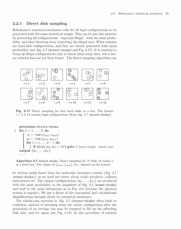
2.2 Boltzmann’s statistical mechanics 95
2.2.1 Direct disk sampling
Boltzmann’s statistical mechanics calls for all legal configurations to begenerated with the same statistical weight. This can be put into practiceby generating all configurations—legal and illegal—with the same proba-bility, and then throwing away (rejecting) the illegal ones. What remainsare hard-disk configurations, and they are clearly generated with equalprobability (see Alg. 2.7 (direct-disks) and Fig. 2.17). It is wasteful tobring up illegal configurations only to throw them away later, but a bet-ter solution has not yet been found. The direct-sampling algorithm can
i = 1 i = 2 i = 3 i = 4 i = 5 i = 6
i = 7 i = 8 i = 9 i = 10 i = 11 i = 12
Fig. 2.17 Direct sampling for four hard disks in a box. The framesi = 4, 9, 12 contain legal configurations (from Alg. 2.7 (direct-disks)).
procedure direct-disks
1 for k = 1, . . . , N do⎧⎪⎪⎨⎪⎪⎩xk ← ran (xmin, xmax)yk ← ran (ymin, ymax)for l = 1, . . . , k − 1 do
if (dist (xk,xl) < 2σ) goto 1 (reject sample—tabula rasa)output x1, . . . ,xN——
Algorithm 2.7 direct-disks. Direct sampling for N disks of radius σin a fixed box. The values of xmin, xmax, etc., depend on the system.
be written much faster than the molecular dynamics routine (Alg. 2.1(event-disks)), as we need not worry about scalar products, collisionsubroutines etc. The output configurations x1, . . . ,xN are producedwith the same probability as the snapshots of Alg. 2.1 (event-disks)and lead to the same histograms as in Fig. 2.9 (because the physicalsystem is ergodic). We get a flavor of the conceptual and calculationalsimplifications brought about by statistical mechanics.
The tabula-rasa rejection in Alg. 2.7 (direct-disks) often leads toconfusion: instead of sweeping away the whole configuration after thegeneration of an overlap, one may be tempted to lift up the offendingdisk only, and try again (see Fig. 2.18). In this procedure of random
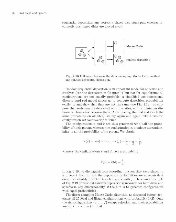
96 Hard disks and spheres
sequential deposition, any correctly placed disk stays put, whereas in-correctly positioned disks are moved away.
Monte Carlo
random deposition
Fig. 2.18 Difference between the direct-sampling Monte Carlo methodand random sequential deposition.
Random sequential deposition is an important model for adhesion andcatalysis (see the discussion in Chapter 7) but not for equilibrium: allconfigurations are not equally probable. A simplified one-dimensionaldiscrete hard-rod model allows us to compute deposition probabilitiesexplicitly and show that they are not the same (see Fig. 2.19): we sup-pose that rods may be deposited onto five sites, with a minimum dis-tance of three sites between them. After placing the first rod (with thesame probability on all sites), we try again and again until a two-rodconfiguration without overlap is found.
The configurations a and b are thus generated with half the proba-bility of their parent, whereas the configuration c, a unique descendant,inherits all the probability of its parent. We obtain
π(a) = π(b) = π(e) = π(f) =14× 1
2=
18,
whereas the configurations c and d have a probability
π(c) = π(d) =14.
In Fig. 2.19, we distinguish rods according to when they were placed (ais different from d), but the deposition probabilities are nonequivalenteven if we identify a with d, b with e, and c with f . The counterexampleof Fig. 2.19 proves that random deposition is incorrect for hard disks andspheres in any dimensionality, if the aim is to generate configurationswith equal probabilities.
The direct-sampling Monte Carlo algorithm, as discussed before, gen-erates all 25 legal and illegal configurations with probability 1/25. Onlythe six configurations a, . . . , f escape rejection, and their probabilitiesare π(a) = · · · = π(f) = 1/6.
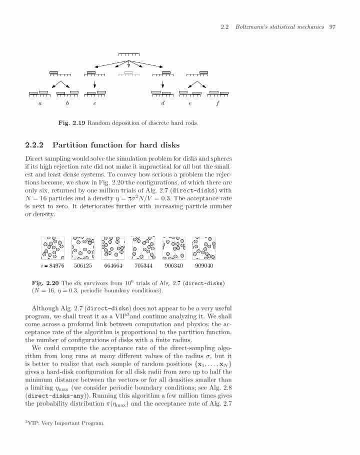
2.2 Boltzmann’s statistical mechanics 97
a b c d e f
Fig. 2.19 Random deposition of discrete hard rods.
2.2.2 Partition function for hard disks
Direct sampling would solve the simulation problem for disks and spheresif its high rejection rate did not make it impractical for all but the small-est and least dense systems. To convey how serious a problem the rejec-tions become, we show in Fig. 2.20 the configurations, of which there areonly six, returned by one million trials of Alg. 2.7 (direct-disks) withN = 16 particles and a density η = σ2N/V = 0.3. The acceptance rateis next to zero. It deteriorates further with increasing particle numberor density.
i = 84976 506125 664664 705344 906340 909040
Fig. 2.20 The six survivors from 106 trials of Alg. 2.7 (direct-disks)(N = 16, η = 0.3, periodic boundary conditions).
Although Alg. 2.7 (direct-disks) does not appear to be a very usefulprogram, we shall treat it as a VIP3and continue analyzing it. We shallcome across a profound link between computation and physics: the ac-ceptance rate of the algorithm is proportional to the partition function,the number of configurations of disks with a finite radius.
We could compute the acceptance rate of the direct-sampling algo-rithm from long runs at many different values of the radius σ, but itis better to realize that each sample of random positions x1, . . . ,xNgives a hard-disk configuration for all disk radii from zero up to half theminimum distance between the vectors or for all densities smaller thana limiting ηmax (we consider periodic boundary conditions; see Alg. 2.8(direct-disks-any)). Running this algorithm a few million times givesthe probability distribution π(ηmax) and the acceptance rate of Alg. 2.7
3VIP: Very Important Program.
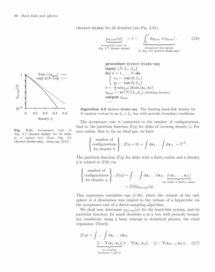
98 Hard disks and spheres
(direct-disks) for all densities (see Fig. 2.21):
paccept(η)︸ ︷︷ ︸acceptance rate of
Alg. 2.7 (direct-disks)
= 1 −∫ η
0
dηmax π(ηmax)︸ ︷︷ ︸integrated histogram
of Alg. 2.8 (direct-disks-any)
. (2.6)
procedure direct-disks-any
input N, Lx, Lyfor k = 1, . . . , N do
xk ← ran (0, Lx)yk ← ran (0, Ly)
σ ← 12 mink =l [dist (xk,xl)]
ηmax ← σ2N/(LxLy) (limiting density)output ηmax
——
Algorithm 2.8 direct-disks-any. The limiting hard-disk density forN random vectors in an Lx ×Ly box with periodic boundary conditions.
1
10−6
0 0.1 0.2 0.3 0.4
pac
cept(
η)
density η
from π(ηmax)exp[−2(N−1)η]
Fig. 2.21 Acceptance rate ofAlg. 2.7 (direct-disks) for 16 disksin a square box (from Alg. 2.8(direct-disks-any), using eqn (2.6)).
The acceptance rate is connected to the number of configurations,that is, the partition function Z(η) for disks of covering density η. Forzero radius, that is, for an ideal gas, we have⎧⎨⎩
number ofconfigurationsfor density 0
⎫⎬⎭ : Z(η = 0) =∫
dx1 . . .
∫dxN = V N .
The partition function Z(η) for disks with a finite radius and a densityη is related to Z(0) via⎧⎨⎩
number ofconfigurationsfor density η
⎫⎬⎭ : Z(η) =∫
. . .
∫dx1 . . . dxN π(x1, . . . ,xN )︸ ︷︷ ︸
for disks of finite radius
= Z(0)paccept(η).
This expression resembles eqn (1.38), where the volume of the unitsphere in d dimensions was related to the volume of a hypercube viathe acceptance rate of a direct-sampling algorithm.
We shall now determine paccept(η) for the hard-disk system, and itspartition function, for small densities η in a box with periodic bound-ary conditions, using a basic concept in statistical physics, the virialexpansion. Clearly,
Z(η) =∫
. . .
∫dx1 . . .dxN
[1 − Υ(x1,x2)]︸ ︷︷ ︸no overlap
between 1 and 2
[1 − Υ(x1,x3)] · · · [1 − Υ(xN−1,xN )] , (2.7)
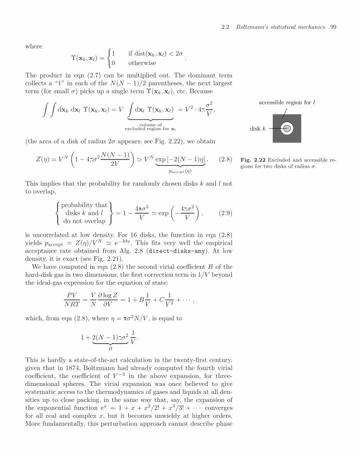
2.2 Boltzmann’s statistical mechanics 99
where
Υ(xk,xl) =
1 if dist(xk,xl) < 2σ
0 otherwise.
The product in eqn (2.7) can be multiplied out. The dominant termcollects a “1” in each of the N(N − 1)/2 parentheses, the next largestterm (for small σ) picks up a single term Υ(xk,xl), etc. Because∫ ∫
dxk dxl Υ(xk,xl) = V
∫dxl Υ(xk,xl)︸ ︷︷ ︸
volume ofexcluded region for xl
= V 2 · 4σ2
V,
(the area of a disk of radius 2σ appears; see Fig. 2.22), we obtain
accessible region for l
disk k
Fig. 2.22 Excluded and accessible re-gions for two disks of radius σ.
Z(η) = V N
(1 − 4σ2 N(N − 1)
2V
) V N exp [−2(N − 1)η]︸ ︷︷ ︸
paccept(η)
. (2.8)
This implies that the probability for randomly chosen disks k and l notto overlap,⎧⎨⎩
probability thatdisks k and l
do not overlap
⎫⎬⎭ = 1 − 4σ2
V exp
(−4σ2
V
), (2.9)
is uncorrelated at low density. For 16 disks, the function in eqn (2.8)yields paccept = Z(η)/V N e−30η. This fits very well the empiricalacceptance rate obtained from Alg. 2.8 (direct-disks-any). At lowdensity, it is exact (see Fig. 2.21).
We have computed in eqn (2.8) the second virial coefficient B of thehard-disk gas in two dimensions, the first correction term in 1/V beyondthe ideal-gas expression for the equation of state:
PV
NRT=
V
N
∂ log Z
∂V= 1 + B
1V
+ C1
V 2+ · · · ,
which, from eqn (2.8), where η = σ2N/V , is equal to
1 + 2(N − 1)σ2︸ ︷︷ ︸B
1V
.
This is hardly a state-of-the-art calculation in the twenty-first century,given that in 1874, Boltzmann had already computed the fourth virialcoefficient, the coefficient of V −3 in the above expansion, for three-dimensional spheres. The virial expansion was once believed to givesystematic access to the thermodynamics of gases and liquids at all den-sities up to close packing, in the same way that, say, the expansion ofthe exponential function ex = 1 + x + x2/2! + x3/3! + · · · convergesfor all real and complex x, but it becomes unwieldy at higher orders.More fundamentally, this perturbation approach cannot describe phase
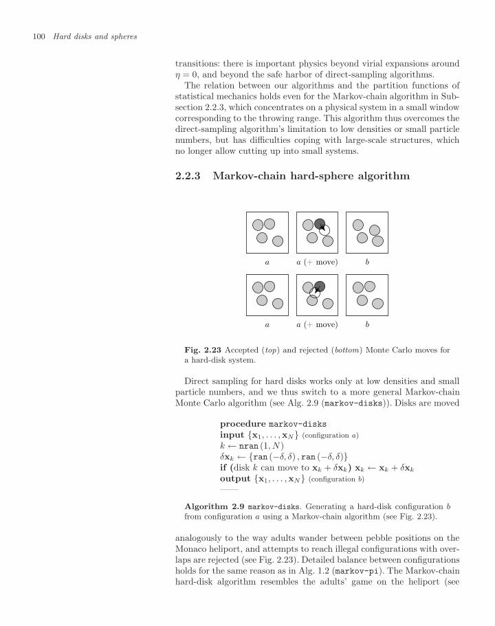
100 Hard disks and spheres
transitions: there is important physics beyond virial expansions aroundη = 0, and beyond the safe harbor of direct-sampling algorithms.
The relation between our algorithms and the partition functions ofstatistical mechanics holds even for the Markov-chain algorithm in Sub-section 2.2.3, which concentrates on a physical system in a small windowcorresponding to the throwing range. This algorithm thus overcomes thedirect-sampling algorithm’s limitation to low densities or small particlenumbers, but has difficulties coping with large-scale structures, whichno longer allow cutting up into small systems.
2.2.3 Markov-chain hard-sphere algorithm
a a (+ move) b
a a (+ move) b
Fig. 2.23 Accepted (top) and rejected (bottom) Monte Carlo moves fora hard-disk system.
Direct sampling for hard disks works only at low densities and smallparticle numbers, and we thus switch to a more general Markov-chainMonte Carlo algorithm (see Alg. 2.9 (markov-disks)). Disks are moved
procedure markov-disks
input x1, . . . ,xN (configuration a)k ← nran (1, N)δxk ← ran (−δ, δ) , ran (−δ, δ)if (disk k can move to xk + δxk) xk ← xk + δxk
output x1, . . . ,xN (configuration b)——
Algorithm 2.9 markov-disks. Generating a hard-disk configuration bfrom configuration a using a Markov-chain algorithm (see Fig. 2.23).
analogously to the way adults wander between pebble positions on theMonaco heliport, and attempts to reach illegal configurations with over-laps are rejected (see Fig. 2.23). Detailed balance between configurationsholds for the same reason as in Alg. 1.2 (markov-pi). The Markov-chainhard-disk algorithm resembles the adults’ game on the heliport (see
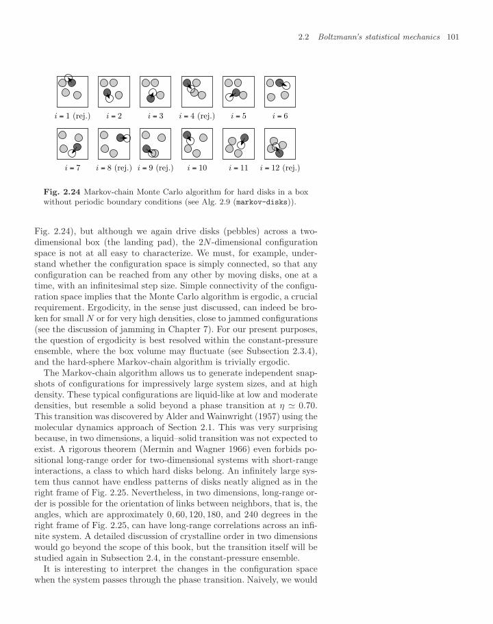
2.2 Boltzmann’s statistical mechanics 101
i = 1 (rej.) i = 2 i = 3 i = 4 (rej.) i = 5 i = 6
i = 7 i = 8 (rej.) i = 9 (rej.) i = 10 i = 11 i = 12 (rej.)
Fig. 2.24 Markov-chain Monte Carlo algorithm for hard disks in a boxwithout periodic boundary conditions (see Alg. 2.9 (markov-disks)).
Fig. 2.24), but although we again drive disks (pebbles) across a two-dimensional box (the landing pad), the 2N -dimensional configurationspace is not at all easy to characterize. We must, for example, under-stand whether the configuration space is simply connected, so that anyconfiguration can be reached from any other by moving disks, one at atime, with an infinitesimal step size. Simple connectivity of the configu-ration space implies that the Monte Carlo algorithm is ergodic, a crucialrequirement. Ergodicity, in the sense just discussed, can indeed be bro-ken for small N or for very high densities, close to jammed configurations(see the discussion of jamming in Chapter 7). For our present purposes,the question of ergodicity is best resolved within the constant-pressureensemble, where the box volume may fluctuate (see Subsection 2.3.4),and the hard-sphere Markov-chain algorithm is trivially ergodic.
The Markov-chain algorithm allows us to generate independent snap-shots of configurations for impressively large system sizes, and at highdensity. These typical configurations are liquid-like at low and moderatedensities, but resemble a solid beyond a phase transition at η 0.70.This transition was discovered by Alder and Wainwright (1957) using themolecular dynamics approach of Section 2.1. This was very surprisingbecause, in two dimensions, a liquid–solid transition was not expected toexist. A rigorous theorem (Mermin and Wagner 1966) even forbids po-sitional long-range order for two-dimensional systems with short-rangeinteractions, a class to which hard disks belong. An infinitely large sys-tem thus cannot have endless patterns of disks neatly aligned as in theright frame of Fig. 2.25. Nevertheless, in two dimensions, long-range or-der is possible for the orientation of links between neighbors, that is, theangles, which are approximately 0, 60, 120, 180, and 240 degrees in theright frame of Fig. 2.25, can have long-range correlations across an infi-nite system. A detailed discussion of crystalline order in two dimensionswould go beyond the scope of this book, but the transition itself will bestudied again in Subsection 2.4, in the constant-pressure ensemble.
It is interesting to interpret the changes in the configuration spacewhen the system passes through the phase transition. Naively, we would
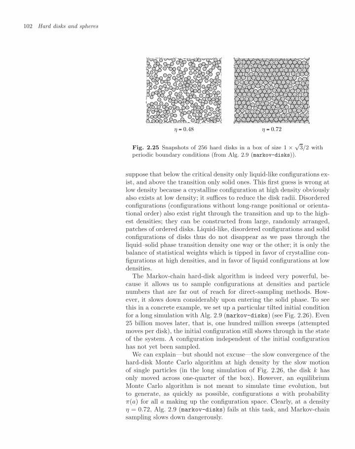
102 Hard disks and spheres
η = 0.48 η = 0.72
Fig. 2.25 Snapshots of 256 hard disks in a box of size 1 × √3/2 with
periodic boundary conditions (from Alg. 2.9 (markov-disks)).
suppose that below the critical density only liquid-like configurations ex-ist, and above the transition only solid ones. This first guess is wrong atlow density because a crystalline configuration at high density obviouslyalso exists at low density; it suffices to reduce the disk radii. Disorderedconfigurations (configurations without long-range positional or orienta-tional order) also exist right through the transition and up to the high-est densities; they can be constructed from large, randomly arranged,patches of ordered disks. Liquid-like, disordered configurations and solidconfigurations of disks thus do not disappear as we pass through theliquid–solid phase transition density one way or the other; it is only thebalance of statistical weights which is tipped in favor of crystalline con-figurations at high densities, and in favor of liquid configurations at lowdensities.
The Markov-chain hard-disk algorithm is indeed very powerful, be-cause it allows us to sample configurations at densities and particlenumbers that are far out of reach for direct-sampling methods. How-ever, it slows down considerably upon entering the solid phase. To seethis in a concrete example, we set up a particular tilted initial conditionfor a long simulation with Alg. 2.9 (markov-disks) (see Fig. 2.26). Even25 billion moves later, that is, one hundred million sweeps (attemptedmoves per disk), the initial configuration still shows through in the stateof the system. A configuration independent of the initial configurationhas not yet been sampled.
We can explain—but should not excuse—the slow convergence of thehard-disk Monte Carlo algorithm at high density by the slow motionof single particles (in the long simulation of Fig. 2.26, the disk k hasonly moved across one-quarter of the box). However, an equilibriumMonte Carlo algorithm is not meant to simulate time evolution, butto generate, as quickly as possible, configurations a with probabilityπ(a) for all a making up the configuration space. Clearly, at a densityη = 0.72, Alg. 2.9 (markov-disks) fails at this task, and Markov-chainsampling slows down dangerously.
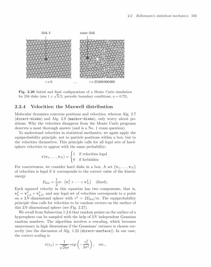
2.2 Boltzmann’s statistical mechanics 103
i = 0
disk k
... i = 25600000000
same disk
Fig. 2.26 Initial and final configurations of a Monte Carlo simulation
for 256 disks (size 1 ×√3/2, periodic boundary conditions, η = 0.72).
2.2.4 Velocities: the Maxwell distribution
Molecular dynamics concerns positions and velocities, whereas Alg. 2.7(direct-disks) and Alg. 2.9 (markov-disks), only worry about po-sitions. Why the velocities disappear from the Monte Carlo programsdeserves a most thorough answer (and is a No. 1 exam question).
To understand velocities in statistical mechanics, we again apply theequiprobability principle, not to particle positions within a box, but tothe velocities themselves. This principle calls for all legal sets of hard-sphere velocities to appear with the same probability:
π(v1, . . . ,vN ) =
1 if velocities legal0 if forbidden
.
For concreteness, we consider hard disks in a box. A set v1, . . . ,vNof velocities is legal if it corresponds to the correct value of the kineticenergy
Ekin =12m · (v2
1 + · · · + v2N
)(fixed).
Each squared velocity in this equation has two components, that is,v2
k = v2x,k + v2
y,k, and any legal set of velocities corresponds to a pointon a 2N -dimensional sphere with r2 = 2Ekin/m. The equiprobabilityprinciple thus calls for velocities to be random vectors on the surface ofthis 2N -dimensional sphere (see Fig. 2.27).
We recall from Subsection 1.2.6 that random points on the surface of ahypersphere can be sampled with the help of 2N independent Gaussianrandom numbers. The algorithm involves a rescaling, which becomesunnecessary in high dimensions if the Gaussians’ variance is chosen cor-rectly (see the discussion of Alg. 1.22 (direct-surface)). In our case,the correct scaling is
π(vx) =1√2σ
exp(− v2
x
2σ2
), etc.,
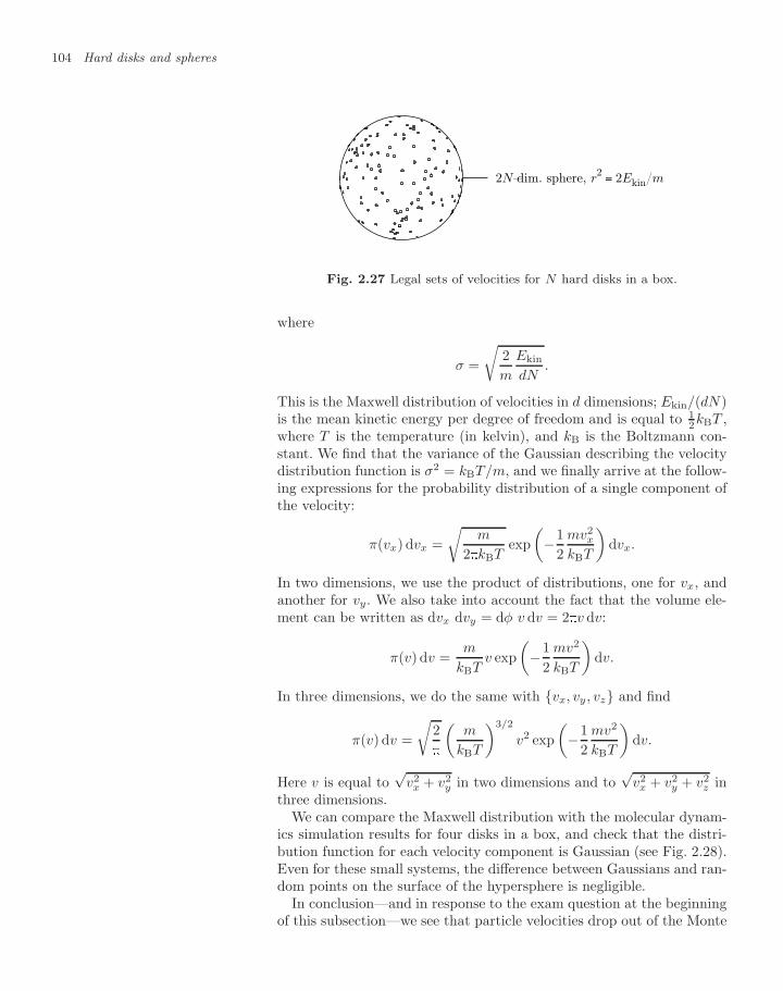
104 Hard disks and spheres
2N-dim. sphere, r2 = 2Ekin/m
Fig. 2.27 Legal sets of velocities for N hard disks in a box.
where
σ =
√2m
Ekin
dN.
This is the Maxwell distribution of velocities in d dimensions; Ekin/(dN)is the mean kinetic energy per degree of freedom and is equal to 1
2kBT ,where T is the temperature (in kelvin), and kB is the Boltzmann con-stant. We find that the variance of the Gaussian describing the velocitydistribution function is σ2 = kBT/m, and we finally arrive at the follow-ing expressions for the probability distribution of a single component ofthe velocity:
π(vx) dvx =√
m
2kBTexp(−1
2mv2
x
kBT
)dvx.
In two dimensions, we use the product of distributions, one for vx, andanother for vy. We also take into account the fact that the volume ele-ment can be written as dvx dvy = dφ v dv = 2v dv:
π(v) dv =m
kBTv exp
(−1
2mv2
kBT
)dv.
In three dimensions, we do the same with vx, vy, vz and find
π(v) dv =
√2
(m
kBT
)3/2
v2 exp(−1
2mv2
kBT
)dv.
Here v is equal to√
v2x + v2
y in two dimensions and to√
v2x + v2
y + v2z in
three dimensions.We can compare the Maxwell distribution with the molecular dynam-
ics simulation results for four disks in a box, and check that the distri-bution function for each velocity component is Gaussian (see Fig. 2.28).Even for these small systems, the difference between Gaussians and ran-dom points on the surface of the hypersphere is negligible.
In conclusion—and in response to the exam question at the beginningof this subsection—we see that particle velocities drop out of the Monte
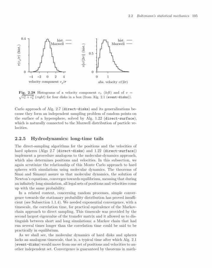
2.2 Boltzmann’s statistical mechanics 105
0
0.4
420−2−4
π(v
x/σ
) (h
ist.
)
velocity component vx/σ
hist.Maxwell
0
0.5
0 1
π[v
/(2σ
)] (
his
t.)
abs. velocity v/(2σ)
hist.Maxwell
Fig. 2.28 Histograms of a velocity component vx (left) and of v =pv2
x + v2y (right) for four disks in a box (from Alg. 2.1 (event-disks)).
Carlo approach of Alg. 2.7 (direct-disks) and its generalizations be-cause they form an independent sampling problem of random points onthe surface of a hypersphere, solved by Alg. 1.22 (direct-surface),which is naturally connected to the Maxwell distribution of particle ve-locities.
2.2.5 Hydrodynamics: long-time tails
The direct-sampling algorithms for the positions and the velocities ofhard spheres (Algs 2.7 (direct-disks) and 1.22 (direct-surface))implement a procedure analogous to the molecular-dynamics approach,which also determines positions and velocities. In this subsection, weagain scrutinize the relationship of this Monte Carlo approach to hardspheres with simulations using molecular dynamics. The theorems ofSinai and Simanyi assure us that molecular dynamics, the solution ofNewton’s equations, converges towards equilibrium, meaning that duringan infinitely long simulation, all legal sets of positions and velocities comeup with the same probability.
In a related context, concerning random processes, simple conver-gence towards the stationary probability distribution has proved insuffi-cient (see Subsection 1.1.4). We needed exponential convergence, with atimescale, the correlation time, for practical equivalence of the Markov-chain approach to direct sampling. This timescale was provided by thesecond largest eigenvalue of the transfer matrix and it allowed us to dis-tinguish between short and long simulations: a Markov chain that hadrun several times longer than the correlation time could be said to bepractically in equilibrium.
As we shall see, the molecular dynamics of hard disks and sphereslacks an analogous timescale, that is, a typical time after which Alg. 2.1(event-disks) would move from one set of positions and velocities to an-other independent set. Convergence is guaranteed by theorems in math-
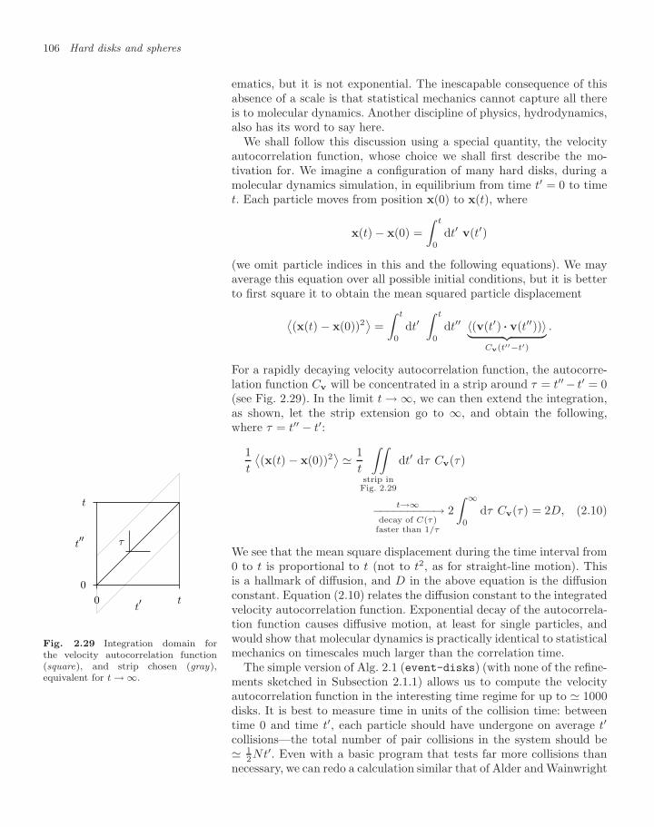
106 Hard disks and spheres
ematics, but it is not exponential. The inescapable consequence of thisabsence of a scale is that statistical mechanics cannot capture all thereis to molecular dynamics. Another discipline of physics, hydrodynamics,also has its word to say here.
We shall follow this discussion using a special quantity, the velocityautocorrelation function, whose choice we shall first describe the mo-tivation for. We imagine a configuration of many hard disks, during amolecular dynamics simulation, in equilibrium from time t′ = 0 to timet. Each particle moves from position x(0) to x(t), where
x(t) − x(0) =∫ t
0
dt′ v(t′)
(we omit particle indices in this and the following equations). We mayaverage this equation over all possible initial conditions, but it is betterto first square it to obtain the mean squared particle displacement
⟨(x(t) − x(0))2
⟩=∫ t
0
dt′∫ t
0
dt′′ 〈(v(t′) ··· v(t′′))〉︸ ︷︷ ︸Cv(t′′−t′)
.
For a rapidly decaying velocity autocorrelation function, the autocorre-lation function Cv will be concentrated in a strip around τ = t′′− t′ = 0(see Fig. 2.29). In the limit t → ∞, we can then extend the integration,as shown, let the strip extension go to ∞, and obtain the following,where τ = t′′ − t′:
1t
⟨(x(t) − x(0))2
⟩ 1t
∫∫strip inFig. 2.29
dt′ dτ Cv(τ)
t→∞−−−−−−−−−→decay of C(τ)faster than 1/τ
2∫ ∞
0
dτ Cv(τ) = 2D, (2.10)
We see that the mean square displacement during the time interval from0 to t is proportional to t (not to t2, as for straight-line motion). Thisis a hallmark of diffusion, and D in the above equation is the diffusionconstant. Equation (2.10) relates the diffusion constant to the integratedvelocity autocorrelation function. Exponential decay of the autocorrela-
t
0
0
t
t′
t′′ τ
Fig. 2.29 Integration domain forthe velocity autocorrelation function(square), and strip chosen (gray),equivalent for t → ∞.
tion function causes diffusive motion, at least for single particles, andwould show that molecular dynamics is practically identical to statisticalmechanics on timescales much larger than the correlation time.
The simple version of Alg. 2.1 (event-disks) (with none of the refine-ments sketched in Subsection 2.1.1) allows us to compute the velocityautocorrelation function in the interesting time regime for up to 1000disks. It is best to measure time in units of the collision time: betweentime 0 and time t′, each particle should have undergone on average t′
collisions—the total number of pair collisions in the system should be 1
2Nt′. Even with a basic program that tests far more collisions thannecessary, we can redo a calculation similar that of Alder and Wainwright
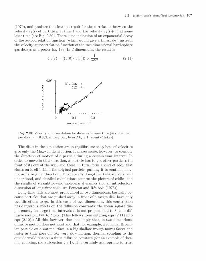
2.2 Boltzmann’s statistical mechanics 107
(1970), and produce the clear-cut result for the correlation between thevelocity vk(t) of particle k at time t and the velocity vk(t + τ) at somelater time (see Fig. 2.30). There is no indication of an exponential decayof the autocorrelation function (which would give a timescale); instead,the velocity autocorrelation function of the two-dimensional hard-spheregas decays as a power law 1/τ . In d dimensions, the result is
Cv(τ) = 〈(v(0) ··· v(τ))〉 ∝ 1τd/2
. (2.11)
0
0.05
0 0.1 0.2
vel
oci
ty a
uto
corr
.
inverse time τ−1
N = 256512
Fig. 2.30 Velocity autocorrelation for disks vs. inverse time (in collisionsper disk; η = 0.302, square box, from Alg. 2.1 (event-disks)).
The disks in the simulation are in equilibrium: snapshots of velocitiesgive only the Maxwell distribution. It makes sense, however, to considerthe direction of motion of a particle during a certain time interval. Inorder to move in that direction, a particle has to get other particles (infront of it) out of the way, and these, in turn, form a kind of eddy thatcloses on itself behind the original particle, pushing it to continue mov-ing in its original direction. Theoretically, long-time tails are very wellunderstood, and detailed calculations confirm the picture of eddies andthe results of straightforward molecular dynamics (for an introductorydiscussion of long-time tails, see Pomeau and Resibois (1975)).
Long-time tails are most pronounced in two dimensions, basically be-cause particles that are pushed away in front of a target disk have onlytwo directions to go. In this case, of two dimensions, this constrictionhas dangerous effects on the diffusion constants: the mean square dis-placement, for large time intervals t, is not proportional to t as in dif-fusive motion, but to t log t. (This follows from entering eqn (2.11) intoeqn (2.10).) All this, however, does not imply that, in two dimensions,diffusive motion does not exist and that, for example, a colloidal Brown-ian particle on a water surface in a big shallow trough moves faster andfaster as time goes on. For very slow motion, thermal coupling to theoutside world restores a finite diffusion constant (for an example of ther-mal coupling, see Subsection 2.3.1). It is certainly appropriate to treat
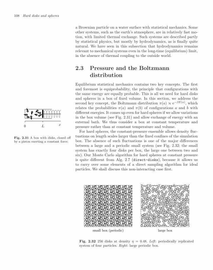
108 Hard disks and spheres
a Brownian particle on a water surface with statistical mechanics. Someother systems, such as the earth’s atmosphere, are in relatively fast mo-tion, with limited thermal exchange. Such systems are described partlyby statistical physics, but mostly by hydrodynamics, as is finally quitenatural. We have seen in this subsection that hydrodynamics remainsrelevant to mechanical systems even in the long-time (equilibrium) limit,in the absence of thermal coupling to the outside world.
2.3 Pressure and the Boltzmanndistribution
Equilibrium statistical mechanics contains two key concepts. The firstand foremost is equiprobability, the principle that configurations withthe same energy are equally probable. This is all we need for hard disksand spheres in a box of fixed volume. In this section, we address thesecond key concept, the Boltzmann distribution π(a) ∝ e−βE(a), whichrelates the probabilities π(a) and π(b) of configurations a and b withdifferent energies. It comes up even for hard spheres if we allow variationsin the box volume (see Fig. 2.31) and allow exchange of energy with anexternal bath. We thus consider a box at constant temperature andpressure rather than at constant temperature and volume.0 L x
Fig. 2.31 A box with disks, closed offby a piston exerting a constant force.
For hard spheres, the constant-pressure ensemble allows density fluc-tuations on length scales larger than the fixed confines of the simulationbox. The absence of such fluctuations is one of the major differencesbetween a large and a periodic small system (see Fig. 2.32; the smallsystem has exactly four disks per box, the large one between two andsix). Our Monte Carlo algorithm for hard spheres at constant pressureis quite different from Alg. 2.7 (direct-disks), because it allows usto carry over some elements of a direct sampling algorithm for idealparticles. We shall discuss this non-interacting case first.
small box (periodic) large box
Fig. 2.32 256 disks at density η = 0.48. Left : periodically replicatedsystem of four particles. Right : large periodic box.
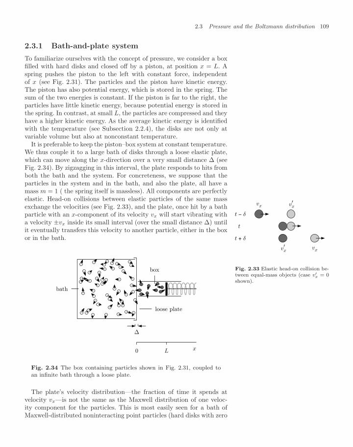
2.3 Pressure and the Boltzmann distribution 109
2.3.1 Bath-and-plate system
To familiarize ourselves with the concept of pressure, we consider a boxfilled with hard disks and closed off by a piston, at position x = L. Aspring pushes the piston to the left with constant force, independentof x (see Fig. 2.31). The particles and the piston have kinetic energy.The piston has also potential energy, which is stored in the spring. Thesum of the two energies is constant. If the piston is far to the right, theparticles have little kinetic energy, because potential energy is stored inthe spring. In contrast, at small L, the particles are compressed and theyhave a higher kinetic energy. As the average kinetic energy is identifiedwith the temperature (see Subsection 2.2.4), the disks are not only atvariable volume but also at nonconstant temperature.
It is preferable to keep the piston–box system at constant temperature.We thus couple it to a large bath of disks through a loose elastic plate,which can move along the x-direction over a very small distance ∆ (seeFig. 2.34). By zigzagging in this interval, the plate responds to hits fromboth the bath and the system. For concreteness, we suppose that theparticles in the system and in the bath, and also the plate, all have amass m = 1 ( the spring itself is massless). All components are perfectlyelastic. Head-on collisions between elastic particles of the same mass
vx vx′
t − δ
t
t + δ
vxvx′
Fig. 2.33 Elastic head-on collision be-tween equal-mass objects (case v′x = 0shown).
exchange the velocities (see Fig. 2.33), and the plate, once hit by a bathparticle with an x-component of its velocity vx will start vibrating witha velocity ±vx inside its small interval (over the small distance ∆) untilit eventually transfers this velocity to another particle, either in the boxor in the bath.
∆
bath
box
loose plate
0 L x
Fig. 2.34 The box containing particles shown in Fig. 2.31, coupled toan infinite bath through a loose plate.
The plate’s velocity distribution—the fraction of time it spends atvelocity vx—is not the same as the Maxwell distribution of one veloc-ity component for the particles. This is most easily seen for a bath ofMaxwell-distributed noninteracting point particles (hard disks with zero
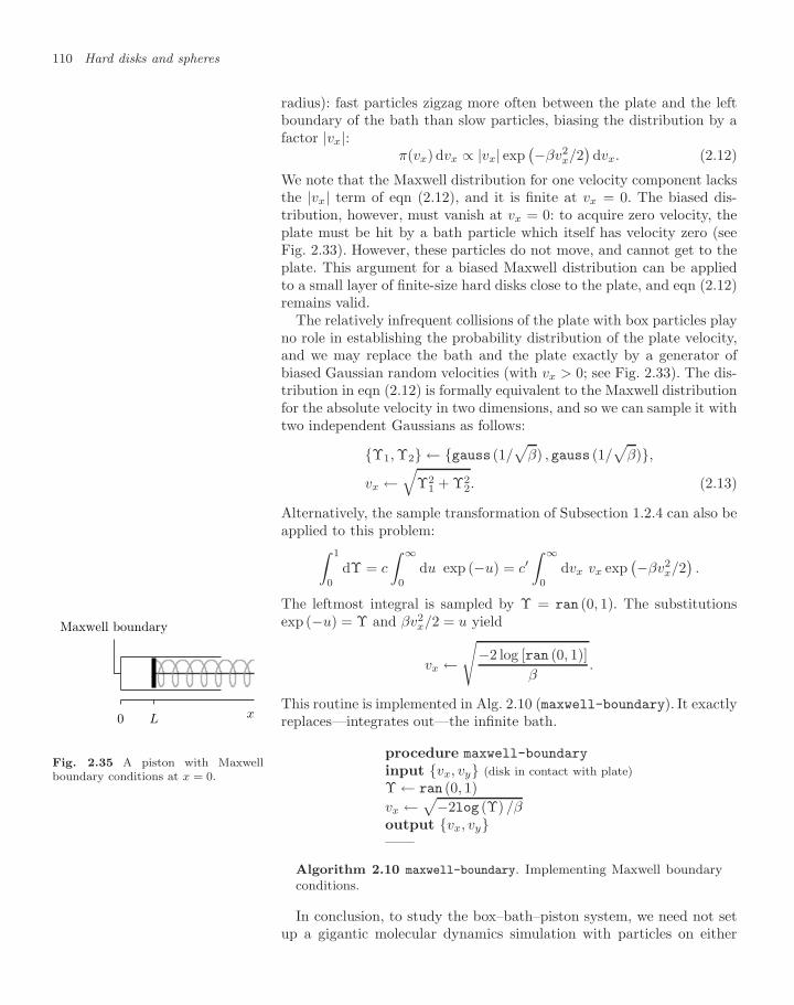
110 Hard disks and spheres
radius): fast particles zigzag more often between the plate and the leftboundary of the bath than slow particles, biasing the distribution by afactor |vx|:
π(vx) dvx ∝ |vx| exp(−βv2
x/2)
dvx. (2.12)
We note that the Maxwell distribution for one velocity component lacksthe |vx| term of eqn (2.12), and it is finite at vx = 0. The biased dis-tribution, however, must vanish at vx = 0: to acquire zero velocity, theplate must be hit by a bath particle which itself has velocity zero (seeFig. 2.33). However, these particles do not move, and cannot get to theplate. This argument for a biased Maxwell distribution can be appliedto a small layer of finite-size hard disks close to the plate, and eqn (2.12)remains valid.
The relatively infrequent collisions of the plate with box particles playno role in establishing the probability distribution of the plate velocity,and we may replace the bath and the plate exactly by a generator ofbiased Gaussian random velocities (with vx > 0; see Fig. 2.33). The dis-tribution in eqn (2.12) is formally equivalent to the Maxwell distributionfor the absolute velocity in two dimensions, and so we can sample it withtwo independent Gaussians as follows:
Υ1, Υ2 ← gauss (1/√
β) , gauss (1/√
β),vx ←
√Υ2
1 + Υ22. (2.13)
Alternatively, the sample transformation of Subsection 1.2.4 can also beapplied to this problem:∫ 1
0
dΥ = c
∫ ∞
0
du exp (−u) = c′∫ ∞
0
dvx vx exp(−βv2
x/2).
The leftmost integral is sampled by Υ = ran (0, 1). The substitutionsexp (−u) = Υ and βv2
x/2 = u yield
vx ←√
−2 log [ran (0, 1)]β
.
This routine is implemented in Alg. 2.10 (maxwell-boundary). It exactlyreplaces—integrates out—the infinite bath.0 L x
Maxwell boundary
Fig. 2.35 A piston with Maxwellboundary conditions at x = 0.
procedure maxwell-boundary
input vx, vy (disk in contact with plate)Υ ← ran (0, 1)vx ←√−2log (Υ) /βoutput vx, vy——
Algorithm 2.10 maxwell-boundary. Implementing Maxwell boundaryconditions.
In conclusion, to study the box–bath–piston system, we need not setup a gigantic molecular dynamics simulation with particles on either
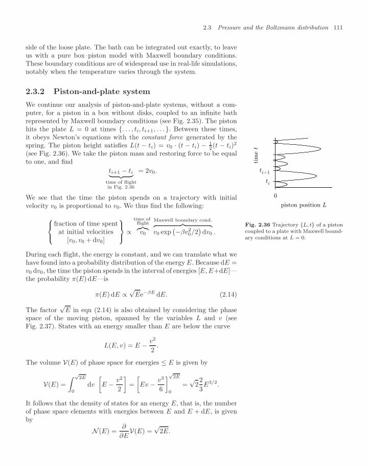
2.3 Pressure and the Boltzmann distribution 111
side of the loose plate. The bath can be integrated out exactly, to leaveus with a pure box–piston model with Maxwell boundary conditions.These boundary conditions are of widespread use in real-life simulations,notably when the temperature varies through the system.
2.3.2 Piston-and-plate system
We continue our analysis of piston-and-plate systems, without a com-puter, for a piston in a box without disks, coupled to an infinite bathrepresented by Maxwell boundary conditions (see Fig. 2.35). The pistonhits the plate L = 0 at times . . . , ti, ti+1, . . . . Between these times,it obeys Newton’s equations with the constant force generated by thespring. The piston height satisfies L(t − ti) = v0 · (t − ti) − 1
2 (t − ti)2
(see Fig. 2.36). We take the piston mass and restoring force to be equalto one, and find
ti+1 − ti︸ ︷︷ ︸time of flightin Fig. 2.36
= 2v0.
We see that the time the piston spends on a trajectory with initialvelocity v0 is proportional to v0. We thus find the following:
ti+1
ti
0
tim
e t
piston position L
Fig. 2.36 Trajectory L, t of a pistoncoupled to a plate with Maxwell bound-ary conditions at L = 0.
⎧⎨⎩fraction of time spent
at initial velocities[v0, v0 + dv0]
⎫⎬⎭ ∝time offlight︷︸︸︷v0
Maxwell boundary cond.︷ ︸︸ ︷v0 exp
(−βv20/2)dv0 .
During each flight, the energy is constant, and we can translate what wehave found into a probability distribution of the energy E. Because dE =v0 dv0, the time the piston spends in the interval of energies [E, E+dE]—the probability π(E) dE—is
π(E) dE ∝√
Ee−βE dE. (2.14)
The factor√
E in eqn (2.14) is also obtained by considering the phasespace of the moving piston, spanned by the variables L and v (seeFig. 2.37). States with an energy smaller than E are below the curve
L(E, v) = E − v2
2.
The volume V(E) of phase space for energies ≤ E is given by
V(E) =∫ √
2E
0
dv
[E − v2
2
]=[Ev − v3
6
]√2E
0
=√
223E3/2.
It follows that the density of states for an energy E, that is, the numberof phase space elements with energies between E and E + dE, is givenby
N (E) =∂
∂EV(E) =
√2E.
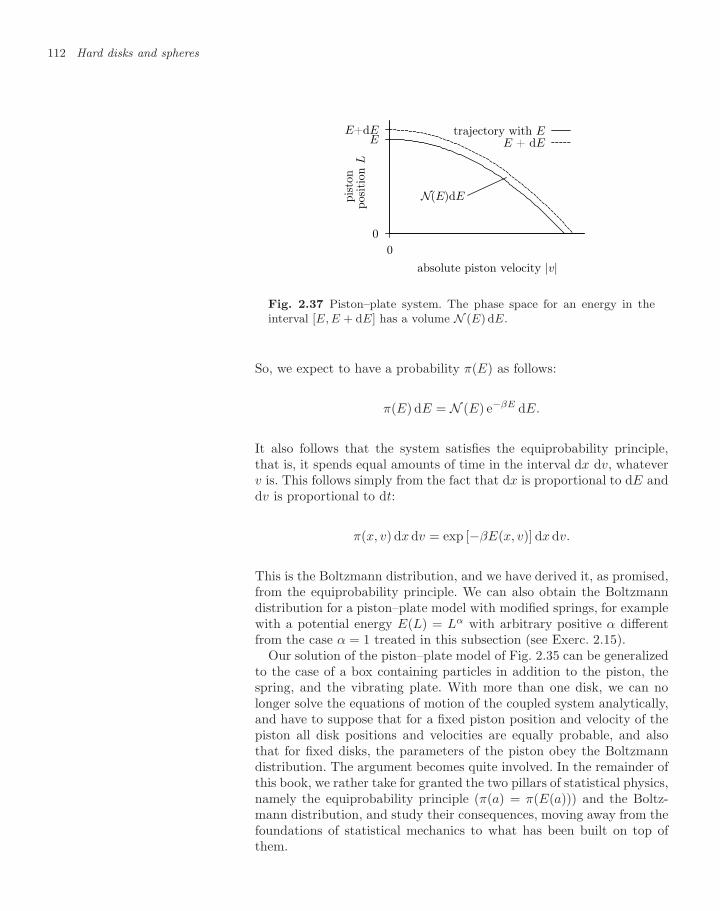
112 Hard disks and spheres
E+dEE
0
0
pis
ton
pos
itio
n L
absolute piston velocity |v|
N(E)dE
trajectory with EE + dE
Fig. 2.37 Piston–plate system. The phase space for an energy in theinterval [E, E + dE] has a volume N (E) dE.
So, we expect to have a probability π(E) as follows:
π(E) dE = N (E) e−βE dE.
It also follows that the system satisfies the equiprobability principle,that is, it spends equal amounts of time in the interval dx dv, whateverv is. This follows simply from the fact that dx is proportional to dE anddv is proportional to dt:
π(x, v) dx dv = exp [−βE(x, v)] dx dv.
This is the Boltzmann distribution, and we have derived it, as promised,from the equiprobability principle. We can also obtain the Boltzmanndistribution for a piston–plate model with modified springs, for examplewith a potential energy E(L) = Lα with arbitrary positive α differentfrom the case α = 1 treated in this subsection (see Exerc. 2.15).
Our solution of the piston–plate model of Fig. 2.35 can be generalizedto the case of a box containing particles in addition to the piston, thespring, and the vibrating plate. With more than one disk, we can nolonger solve the equations of motion of the coupled system analytically,and have to suppose that for a fixed piston position and velocity of thepiston all disk positions and velocities are equally probable, and alsothat for fixed disks, the parameters of the piston obey the Boltzmanndistribution. The argument becomes quite involved. In the remainder ofthis book, we rather take for granted the two pillars of statistical physics,namely the equiprobability principle (π(a) = π(E(a))) and the Boltz-mann distribution, and study their consequences, moving away from thefoundations of statistical mechanics to what has been built on top ofthem.
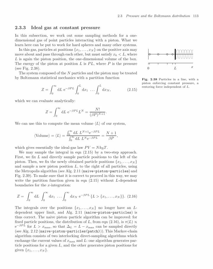
2.3 Pressure and the Boltzmann distribution 113
2.3.3 Ideal gas at constant pressure
In this subsection, we work out some sampling methods for a one-dimensional gas of point particles interacting with a piston. What welearn here can be put to work for hard spheres and many other systems.
In this gas, particles at positions x1, . . . , xN on the positive axis maymove about and pass through each other, but must satisfy xk < L, whereL is again the piston position, the one-dimensional volume of the box.The energy of the piston at position L is PL, where P is the pressure(see Fig. 2.38). L x0
Fig. 2.38 Particles in a line, with apiston enforcing constant pressure, arestoring force independent of L.
The system composed of the N particles and the piston may be treatedby Boltzmann statistical mechanics with a partition function
Z =∫ ∞
0
dL e−βPL
∫ L
0
dx1 . . .
∫ L
0
dxN , (2.15)
which we can evaluate analytically:
Z =∫ ∞
0
dL e−βPLLN =N !
(βP )N+1.
We can use this to compute the mean volume 〈L〉 of our system,
〈Volume〉 = 〈L〉 =
∫∞0 dL LN+1e−βPL∫∞0 dL LNe−βPL
=N + 1βP
,
which gives essentially the ideal-gas law PV = NkBT .We may sample the integral in eqn (2.15) by a two-step approach.
First, we fix L and directly sample particle positions to the left of thepiston. Then, we fix the newly obtained particle positions x1, . . . , xNand sample a new piston position L, to the right of all particles, usingthe Metropolis algorithm (see Alg. 2.11 (naive-piston-particles) andFig. 2.39). To make sure that it is correct to proceed in this way, we maywrite the partition function given in eqn (2.15) without L-dependentboundaries for the x-integration:
Z =∫ ∞
0
dL
∫ ∞
0
dx1 . . .
∫ ∞
0
dxN e−βPL L > x1, . . . , xN. (2.16)
The integrals over the positions x1, . . . , xN no longer have an L-dependent upper limit, and Alg. 2.11 (naive-piston-particles) isthus correct. The naive piston–particle algorithm can be improved: forfixed particle positions, the distribution of L, from eqn (2.16), is π(L) ∝e−βPL for L > xmax, so that ∆L = L − xmax can be sampled directly(see Alg. 2.12 (naive-piston-particles(patch))). This Markov-chainalgorithm consists of two interlocking direct-sampling algorithms whichexchange the current values of xmax and L: one algorithm generates par-ticle positions for a given L, and the other generates piston positions forgiven x1, . . . , xN.
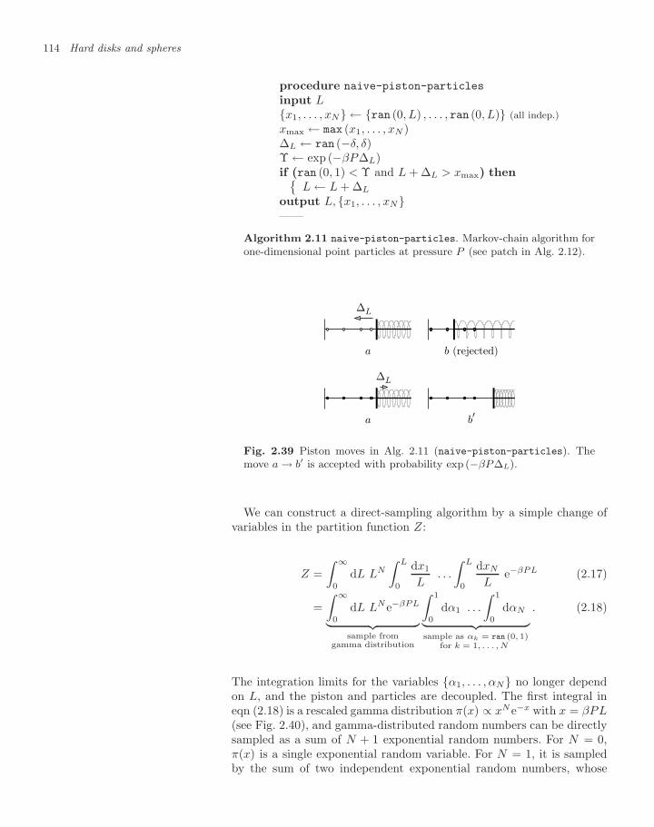
114 Hard disks and spheres
procedure naive-piston-particles
input Lx1, . . . , xN ← ran (0, L) , . . . , ran (0, L) (all indep.)xmax ← max (x1, . . . , xN )∆L ← ran (−δ, δ)Υ ← exp (−βP∆L)if (ran (0, 1) < Υ and L + ∆L > xmax) then
L ← L + ∆L
output L, x1, . . . , xN——
Algorithm 2.11 naive-piston-particles. Markov-chain algorithm forone-dimensional point particles at pressure P (see patch in Alg. 2.12).
a
∆L
b (rejected)
a
∆L
b′
Fig. 2.39 Piston moves in Alg. 2.11 (naive-piston-particles). Themove a → b′ is accepted with probability exp (−βP∆L).
We can construct a direct-sampling algorithm by a simple change ofvariables in the partition function Z:
Z =∫ ∞
0
dL LN
∫ L
0
dx1
L. . .
∫ L
0
dxN
Le−βPL (2.17)
=∫ ∞
0
dL LNe−βPL︸ ︷︷ ︸sample from
gamma distribution
∫ 1
0
dα1 . . .
∫ 1
0
dαN︸ ︷︷ ︸sample as αk = ran (0, 1)
for k = 1, . . . , N
. (2.18)
The integration limits for the variables α1, . . . , αN no longer dependon L, and the piston and particles are decoupled. The first integral ineqn (2.18) is a rescaled gamma distribution π(x) ∝ xN e−x with x = βPL(see Fig. 2.40), and gamma-distributed random numbers can be directlysampled as a sum of N + 1 exponential random numbers. For N = 0,π(x) is a single exponential random variable. For N = 1, it is sampledby the sum of two independent exponential random numbers, whose
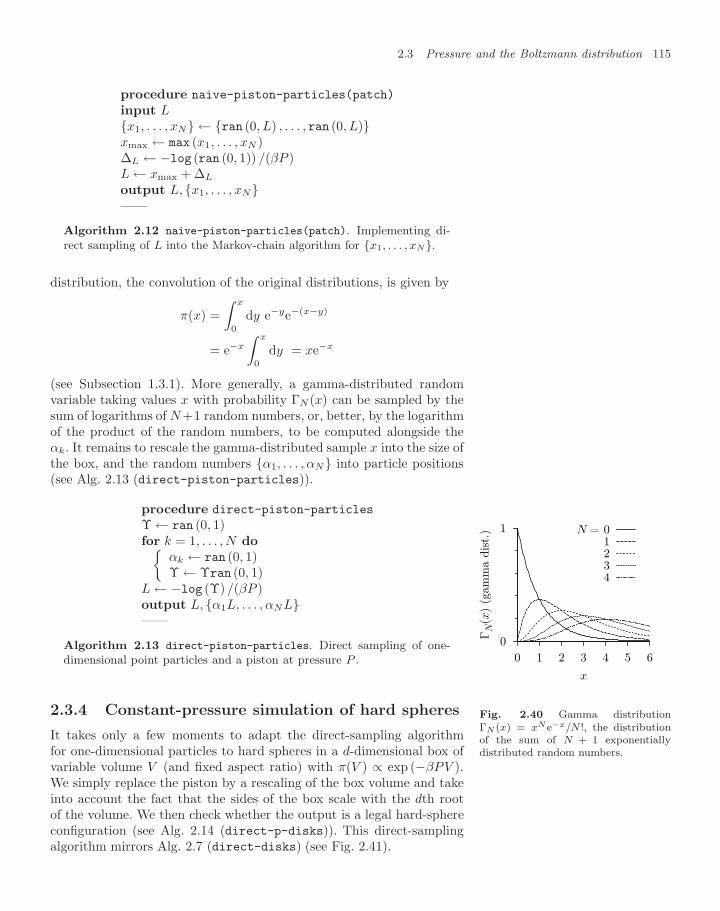
2.3 Pressure and the Boltzmann distribution 115
procedure naive-piston-particles(patch)
input Lx1, . . . , xN ← ran (0, L) , . . . , ran (0, L)xmax ← max (x1, . . . , xN )∆L ← −log (ran (0, 1)) /(βP )L ← xmax + ∆L
output L, x1, . . . , xN——
Algorithm 2.12 naive-piston-particles(patch). Implementing di-rect sampling of L into the Markov-chain algorithm for x1, . . . , xN.
distribution, the convolution of the original distributions, is given by
π(x) =∫ x
0
dy e−ye−(x−y)
= e−x
∫ x
0
dy = xe−x
(see Subsection 1.3.1). More generally, a gamma-distributed randomvariable taking values x with probability ΓN (x) can be sampled by thesum of logarithms of N +1 random numbers, or, better, by the logarithmof the product of the random numbers, to be computed alongside theαk. It remains to rescale the gamma-distributed sample x into the size ofthe box, and the random numbers α1, . . . , αN into particle positions(see Alg. 2.13 (direct-piston-particles)).
procedure direct-piston-particles
Υ ← ran (0, 1)for k = 1, . . . , N do
αk ← ran (0, 1)Υ ← Υran (0, 1)
L ← −log (Υ) /(βP )output L, α1L, . . . , αNL——
Algorithm 2.13 direct-piston-particles. Direct sampling of one-dimensional point particles and a piston at pressure P .
0
1
0 1 2 3 4 5 6
ΓN(x
) (g
am
ma d
ist.
)
x
N = 01234
Fig. 2.40 Gamma distributionΓN (x) = xNe−x/N !, the distributionof the sum of N + 1 exponentiallydistributed random numbers.
2.3.4 Constant-pressure simulation of hard spheres
It takes only a few moments to adapt the direct-sampling algorithmfor one-dimensional particles to hard spheres in a d-dimensional box ofvariable volume V (and fixed aspect ratio) with π(V ) ∝ exp (−βPV ).We simply replace the piston by a rescaling of the box volume and takeinto account the fact that the sides of the box scale with the dth rootof the volume. We then check whether the output is a legal hard-sphereconfiguration (see Alg. 2.14 (direct-p-disks)). This direct-samplingalgorithm mirrors Alg. 2.7 (direct-disks) (see Fig. 2.41).
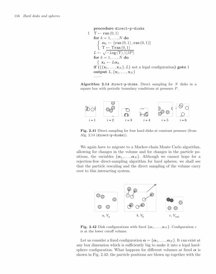
116 Hard disks and spheres
procedure direct-p-disks
1 Υ ← ran (0, 1)for k = 1, . . . , N do
αk ← ran (0, 1) , ran (0, 1)Υ ← Υran (0, 1)
L ←√−log (Υ) /(βP )for k = 1, . . . , N do
xk ← Lαk
if (x1, . . . ,xN, L not a legal configuration) goto 1output L, x1, . . . ,xN——
Algorithm 2.14 direct-p-disks. Direct sampling for N disks in asquare box with periodic boundary conditions at pressure P .
i = 1 i = 2 i = 3 i = 4 i = 5 i = 6
Fig. 2.41 Direct sampling for four hard disks at constant pressure (fromAlg. 2.14 (direct-p-disks)).
We again have to migrate to a Markov-chain Monte Carlo algorithm,allowing for changes in the volume and for changes in the particle po-sitions, the variables α1, . . . ,αN. Although we cannot hope for arejection-free direct-sampling algorithm for hard spheres, we shall seethat the particle rescaling and the direct sampling of the volume carryover to this interacting system.
a, Va b, Vb c, Vcut
Fig. 2.42 Disk configurations with fixed α1, . . . , αN. Configuration cis at the lower cutoff volume.
Let us consider a fixed configuration α = α1, . . . ,αN. It can exist atany box dimension which is sufficiently big to make it into a legal hard-sphere configuration. What happens for different volumes at fixed α isshown in Fig. 2.42: the particle positions are blown up together with the
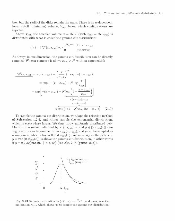
2.3 Pressure and the Boltzmann distribution 117
box, but the radii of the disks remain the same. There is an α-dependentlower cutoff (minimum) volume, Vcut, below which configurations arerejected.
Above Vcut, the rescaled volume x = βPV (with xcut = βPVcut) isdistributed with what is called the gamma-cut distribution:
π(x) = ΓcutN (x, xcut) ∝
xN e−x for x > xcut
0 otherwise.
As always in one dimension, the gamma-cut distribution can be directlysampled. We can compare it above xcut > N with an exponential:
ΓcutN (x, xcut) ∝ πΓ(x, xcut) =
(x
xcut
)N
exp [−(x − xcut)]
= exp[−(x − xcut) + N log
x
xcut
]= exp
[−(x − xcut) + N log
(1 +
x − xcut
xcut
)︸ ︷︷ ︸
<(x−xcut)/xcut
]
<
πexp(x,xcut)︷ ︸︸ ︷exp [−(1 − N/xcut)(x − xcut)] . (2.19)
To sample the gamma-cut distribution, we adapt the rejection methodof Subsection 1.2.4, and rather sample the exponential distribution,which is everywhere larger. We thus throw uniformly distributed peb-bles into the region delimited by x ∈ [xcut,∞] and y ∈ [0, πexp(x)] (seeFig. 2.43). x can be sampled from πexp(x, xcut), and y can be sampled asa random number between 0 and πexp(x). We must reject the pebble ify = ran (0, πexp(x)) is above the gamma-cut distribution, in other wordsif y = πexp(x)ran (0, 1) > πΓ(x) (see Alg. 2.15 (gamma-cut)).
0
N xcut0
πΓ(x
), π
exp(x
)
x
πΓ (gamma)πexp (maj.)
Fig. 2.43 Gamma distribution ΓN (x) ∝ πΓ = xNe−x, and its exponentialmajoration πexp, which allows us to sample the gamma-cut distribution.
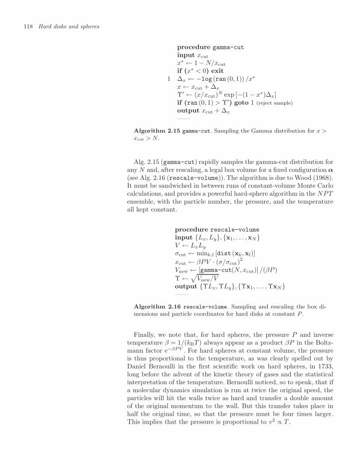
118 Hard disks and spheres
procedure gamma-cut
input xcut
x∗ ← 1 − N/xcut
if (x∗ < 0) exit1 ∆x ← −log (ran (0, 1)) /x∗
x ← xcut + ∆x
Υ′ ← (x/xcut)N exp [−(1 − x∗)∆x]if (ran (0, 1) > Υ′) goto 1 (reject sample)output xcut + ∆x
——
Algorithm 2.15 gamma-cut. Sampling the Gamma distribution for x >xcut > N .
Alg. 2.15 (gamma-cut) rapidly samples the gamma-cut distribution forany N and, after rescaling, a legal box volume for a fixed configuration α
(see Alg. 2.16 (rescale-volume)). The algorithm is due to Wood (1968).It must be sandwiched in between runs of constant-volume Monte Carlocalculations, and provides a powerful hard-sphere algorithm in the NPTensemble, with the particle number, the pressure, and the temperatureall kept constant.
procedure rescale-volume
input Lx, Ly, x1, . . . ,xNV ← LxLy
σcut ← mink,l [dist (xk,xl)]xcut ← βPV · (σ/σcut)
2
Vnew ← [gamma-cut(N, xcut)] /(βP )Υ ←√Vnew/Voutput ΥLx, ΥLy, Υx1, . . . , ΥxN——
Algorithm 2.16 rescale-volume. Sampling and rescaling the box di-mensions and particle coordinates for hard disks at constant P .
Finally, we note that, for hard spheres, the pressure P and inversetemperature β = 1/(kBT ) always appear as a product βP in the Boltz-mann factor e−βPV . For hard spheres at constant volume, the pressureis thus proportional to the temperature, as was clearly spelled out byDaniel Bernoulli in the first scientific work on hard spheres, in 1733,long before the advent of the kinetic theory of gases and the statisticalinterpretation of the temperature. Bernoulli noticed, so to speak, that ifa molecular dynamics simulation is run at twice the original speed, theparticles will hit the walls twice as hard and transfer a double amountof the original momentum to the wall. But this transfer takes place inhalf the original time, so that the pressure must be four times larger.This implies that the pressure is proportional to v2 ∝ T .
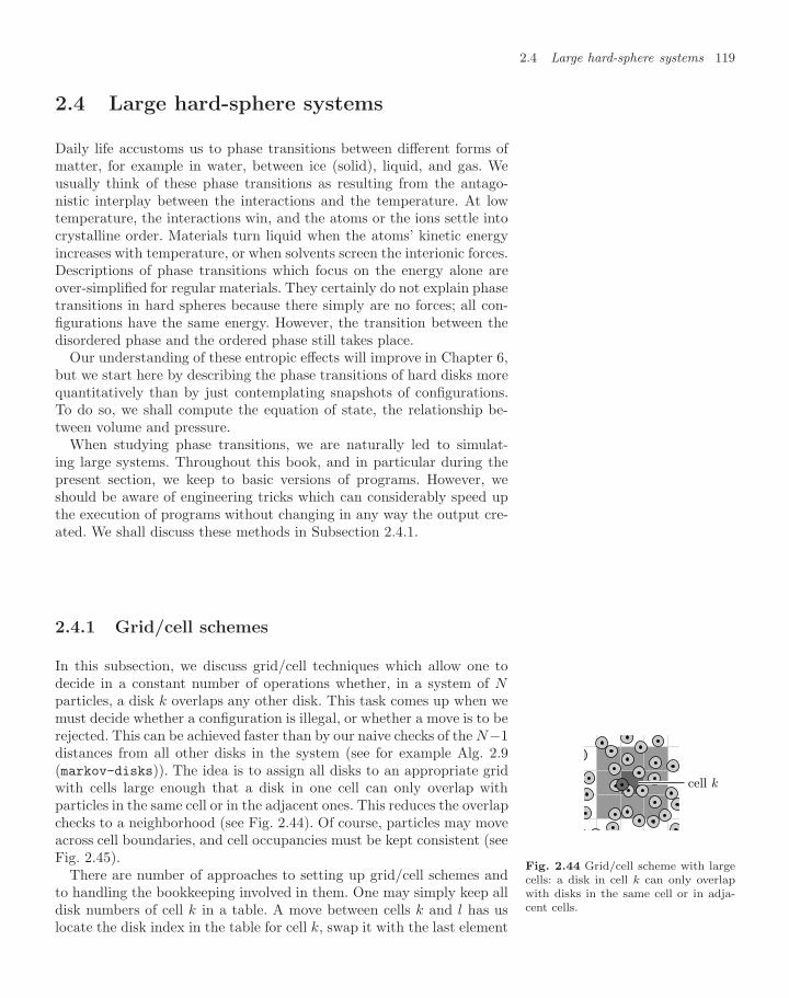
2.4 Large hard-sphere systems 119
2.4 Large hard-sphere systems
Daily life accustoms us to phase transitions between different forms ofmatter, for example in water, between ice (solid), liquid, and gas. Weusually think of these phase transitions as resulting from the antago-nistic interplay between the interactions and the temperature. At lowtemperature, the interactions win, and the atoms or the ions settle intocrystalline order. Materials turn liquid when the atoms’ kinetic energyincreases with temperature, or when solvents screen the interionic forces.Descriptions of phase transitions which focus on the energy alone areover-simplified for regular materials. They certainly do not explain phasetransitions in hard spheres because there simply are no forces; all con-figurations have the same energy. However, the transition between thedisordered phase and the ordered phase still takes place.
Our understanding of these entropic effects will improve in Chapter 6,but we start here by describing the phase transitions of hard disks morequantitatively than by just contemplating snapshots of configurations.To do so, we shall compute the equation of state, the relationship be-tween volume and pressure.
When studying phase transitions, we are naturally led to simulat-ing large systems. Throughout this book, and in particular during thepresent section, we keep to basic versions of programs. However, weshould be aware of engineering tricks which can considerably speed upthe execution of programs without changing in any way the output cre-ated. We shall discuss these methods in Subsection 2.4.1.
2.4.1 Grid/cell schemes
In this subsection, we discuss grid/cell techniques which allow one todecide in a constant number of operations whether, in a system of Nparticles, a disk k overlaps any other disk. This task comes up when wemust decide whether a configuration is illegal, or whether a move is to berejected. This can be achieved faster than by our naive checks of the N−1distances from all other disks in the system (see for example Alg. 2.9(markov-disks)). The idea is to assign all disks to an appropriate gridwith cells large enough that a disk in one cell can only overlap withparticles in the same cell or in the adjacent ones. This reduces the overlapchecks to a neighborhood (see Fig. 2.44). Of course, particles may moveacross cell boundaries, and cell occupancies must be kept consistent (seeFig. 2.45).
cell k
Fig. 2.44 Grid/cell scheme with largecells: a disk in cell k can only overlapwith disks in the same cell or in adja-cent cells.
There are number of approaches to setting up grid/cell schemes andto handling the bookkeeping involved in them. One may simply keep alldisk numbers of cell k in a table. A move between cells k and l has uslocate the disk index in the table for cell k, swap it with the last element
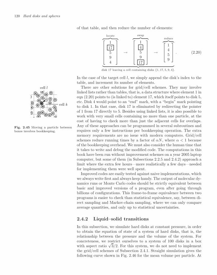
120 Hard disks and spheres
of that table, and then reduce the number of elements:
locate︷ ︸︸ ︷⎡⎢⎢⎢⎢⎣117594
⎤⎥⎥⎥⎥⎦ →
swap︷ ︸︸ ︷⎡⎢⎢⎢⎢⎣145917
⎤⎥⎥⎥⎥⎦ →
reduce︷ ︸︸ ︷⎡⎢⎢⎣1459
⎤⎥⎥⎦︸ ︷︷ ︸disk 17 leaving a cell containing disks 1, 17, 5, 9, 4.
. (2.20)
In the case of the target cell l, we simply append the disk’s index to thetable, and increment its number of elements.
There are other solutions for grid/cell schemes. They may involvelinked lists rather than tables, that is, a data structure where element 1 ineqn (2.20) points to (is linked to) element 17, which itself points to disk 5,etc. Disk 4 would point to an “end” mark, with a “begin” mark pointingto disk 1. In that case, disk 17 is eliminated by redirecting the pointerof 1 from 17 directly to 5. Besides using linked lists, it is also possible towork with very small cells containing no more than one particle, at the
cell k
cell l
Fig. 2.45 Moving a particle betweenboxes involves bookkeeping.
cost of having to check more than just the adjacent cells for overlaps.Any of these approaches can be programmed in several subroutines andrequires only a few instructions per bookkeeping operation. The extramemory requirements are no issue with modern computers. Grid/cellschemes reduce running times by a factor of αN , where α < 1 becauseof the bookkeeping overhead. We must also consider the human time thatit takes to write and debug the modified code. The computations in thisbook have been run without improvement schemes on a year 2005 laptopcomputer, but some of them (in Subsections 2.2.5 and 2.4.2) approach alimit where the extra few hours—more realistically a few days—neededfor implementing them were well spent.
Improved codes are easily tested against naive implementations, whichwe always write first and always keep handy. The output of molecular dy-namics runs or Monte Carlo codes should be strictly equivalent betweenbasic and improved versions of a program, even after going throughbillions of configurations. This frame-to-frame equivalence between twoprograms is easier to check than statistical equivalence, say, between di-rect sampling and Markov-chain sampling, where we can only compareaverage quantities, and only up to statistical uncertainties.
2.4.2 Liquid–solid transitions
In this subsection, we simulate hard disks at constant pressure, in orderto obtain the equation of state of a system of hard disks, that is, therelationship between the pressure and the volume of the system. Forconcreteness, we restrict ourselves to a system of 100 disks in a boxwith aspect ratio
√3/2. For this system, we do not need to implement
the grid/cell schemes of Subsection 2.4.1. Straight simulation gives thefollowing curve shown in Fig. 2.46 for the mean volume per particle. At
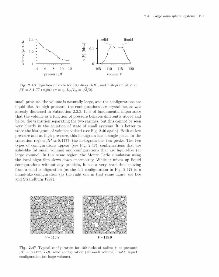
2.4 Large hard-sphere systems 121
1
1.2
1.4
4 6 8 10 12
vol
um
e/par
ticl
e
pressure βP
0
0.1
105 110 115 120
π(V
) (h
ist.
)
volume V
solid liquid
Fig. 2.46 Equation of state for 100 disks (left), and histogram of V at
βP = 8.4177 (right) (σ = 12, Lx/Ly =
√3/2).
small pressure, the volume is naturally large, and the configurations areliquid-like. At high pressure, the configurations are crystalline, as wasalready discussed in Subsection 2.2.3. It is of fundamental importancethat the volume as a function of pressure behaves differently above andbelow the transition separating the two regimes, but this cannot be seenvery clearly in the equation of state of small systems. It is better totrace the histogram of volumes visited (see Fig. 2.46 again). Both at lowpressure and at high pressure, this histogram has a single peak. In thetransition region βP 8.4177, the histogram has two peaks. The twotypes of configurations appear (see Fig. 2.47), configurations that aresolid-like (at small volume) and configurations that are liquid-like (atlarge volume). In this same region, the Monte Carlo simulation usingthe local algorithm slows down enormously. While it mixes up liquidconfigurations without any problem, it has a very hard time movingfrom a solid configuration (as the left configuration in Fig. 2.47) to aliquid-like configuration (as the right one in that same figure, see Leeand Strandburg 1992).
V = 110.8 V = 115.9
Fig. 2.47 Typical configuration for 100 disks of radius 12
at pressureβP = 8.4177. Left : solid configuration (at small volume); right : liquidconfiguration (at large volume).
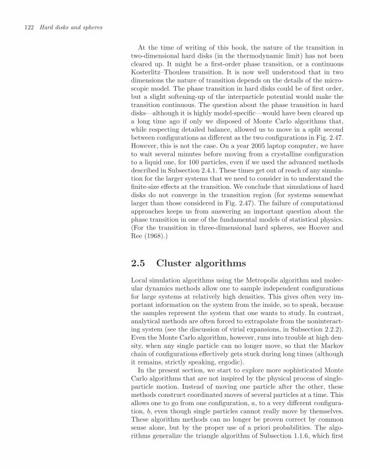
122 Hard disks and spheres
At the time of writing of this book, the nature of the transition intwo-dimensional hard disks (in the thermodynamic limit) has not beencleared up. It might be a first-order phase transition, or a continuousKosterlitz–Thouless transition. It is now well understood that in twodimensions the nature of transition depends on the details of the micro-scopic model. The phase transition in hard disks could be of first order,but a slight softening-up of the interparticle potential would make thetransition continuous. The question about the phase transition in harddisks—although it is highly model-specific—would have been cleared upa long time ago if only we disposed of Monte Carlo algorithms that,while respecting detailed balance, allowed us to move in a split secondbetween configurations as different as the two configurations in Fig. 2.47.However, this is not the case. On a year 2005 laptop computer, we haveto wait several minutes before moving from a crystalline configurationto a liquid one, for 100 particles, even if we used the advanced methodsdescribed in Subsection 2.4.1. These times get out of reach of any simula-tion for the larger systems that we need to consider in to understand thefinite-size effects at the transition. We conclude that simulations of harddisks do not converge in the transition region (for systems somewhatlarger than those considered in Fig. 2.47). The failure of computationalapproaches keeps us from answering an important question about thephase transition in one of the fundamental models of statistical physics.(For the transition in three-dimensional hard spheres, see Hoover andRee (1968).)
2.5 Cluster algorithms
Local simulation algorithms using the Metropolis algorithm and molec-ular dynamics methods allow one to sample independent configurationsfor large systems at relatively high densities. This gives often very im-portant information on the system from the inside, so to speak, becausethe samples represent the system that one wants to study. In contrast,analytical methods are often forced to extrapolate from the noninteract-ing system (see the discussion of virial expansions, in Subsection 2.2.2).Even the Monte Carlo algorithm, however, runs into trouble at high den-sity, when any single particle can no longer move, so that the Markovchain of configurations effectively gets stuck during long times (althoughit remains, strictly speaking, ergodic).
In the present section, we start to explore more sophisticated MonteCarlo algorithms that are not inspired by the physical process of single-particle motion. Instead of moving one particle after the other, thesemethods construct coordinated moves of several particles at a time. Thisallows one to go from one configuration, a, to a very different configura-tion, b, even though single particles cannot really move by themselves.These algorithm methods can no longer be proven correct by commonsense alone, but by the proper use of a priori probabilities. The algo-rithms generalize the triangle algorithm of Subsection 1.1.6, which first
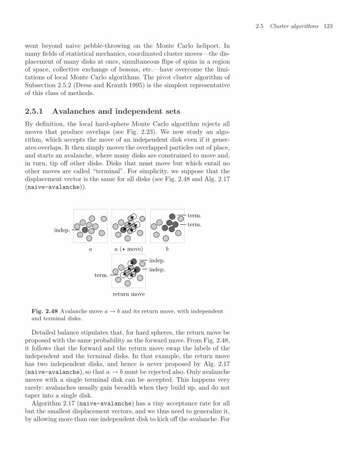
2.5 Cluster algorithms 123
went beyond naive pebble-throwing on the Monte Carlo heliport. Inmany fields of statistical mechanics, coordinated cluster moves—the dis-placement of many disks at once, simultaneous flips of spins in a regionof space, collective exchange of bosons, etc.—have overcome the limi-tations of local Monte Carlo algorithms. The pivot cluster algorithm ofSubsection 2.5.2 (Dress and Krauth 1995) is the simplest representativeof this class of methods.
2.5.1 Avalanches and independent sets
By definition, the local hard-sphere Monte Carlo algorithm rejects allmoves that produce overlaps (see Fig. 2.23). We now study an algo-rithm, which accepts the move of an independent disk even if it gener-ates overlaps. It then simply moves the overlapped particles out of place,and starts an avalanche, where many disks are constrained to move and,in turn, tip off other disks. Disks that must move but which entail noother moves are called “terminal”. For simplicity, we suppose that thedisplacement vector is the same for all disks (see Fig. 2.48 and Alg. 2.17(naive-avalanche)).
a
indep.
a (+ move) b
term.
term.
return move
indep.
indep.
term.
Fig. 2.48 Avalanche move a → b and its return move, with independentand terminal disks.
Detailed balance stipulates that, for hard spheres, the return move beproposed with the same probability as the forward move. From Fig. 2.48,it follows that the forward and the return move swap the labels of theindependent and the terminal disks. In that example, the return movehas two independent disks, and hence is never proposed by Alg. 2.17(naive-avalanche), so that a → b must be rejected also. Only avalanchemoves with a single terminal disk can be accepted. This happens veryrarely: avalanches usually gain breadth when they build up, and do nottaper into a single disk.
Algorithm 2.17 (naive-avalanche) has a tiny acceptance rate for allbut the smallest displacement vectors, and we thus need to generalize it,by allowing more than one independent disk to kick off the avalanche. For
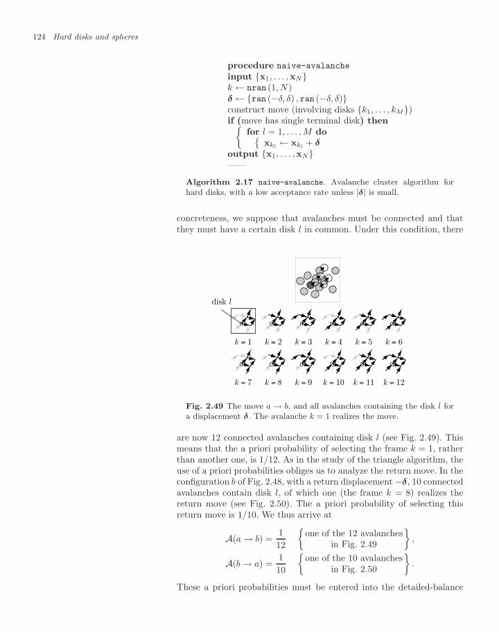
124 Hard disks and spheres
procedure naive-avalanche
input x1, . . . ,xNk ← nran (1, N)δ ← ran (−δ, δ) , ran (−δ, δ)construct move (involving disks k1, . . . , kM)if (move has single terminal disk) then
for l = 1, . . . , M doxkl
← xkl+ δ
output x1, . . . ,xN——
Algorithm 2.17 naive-avalanche. Avalanche cluster algorithm forhard disks, with a low acceptance rate unless |δ| is small.
concreteness, we suppose that avalanches must be connected and thatthey must have a certain disk l in common. Under this condition, there
disk l
k = 1 k = 2 k = 3 k = 4 k = 5 k = 6
k = 7 k = 8 k = 9 k = 10 k = 11 k = 12
Fig. 2.49 The move a → b, and all avalanches containing the disk l fora displacement δ. The avalanche k = 1 realizes the move.
are now 12 connected avalanches containing disk l (see Fig. 2.49). Thismeans that the a priori probability of selecting the frame k = 1, ratherthan another one, is 1/12. As in the study of the triangle algorithm, theuse of a priori probabilities obliges us to analyze the return move. In theconfiguration b of Fig. 2.48, with a return displacement −δ, 10 connectedavalanches contain disk l, of which one (the frame k = 8) realizes thereturn move (see Fig. 2.50). The a priori probability of selecting thisreturn move is 1/10. We thus arrive at
A(a → b) =112
one of the 12 avalanches
in Fig. 2.49
,
A(b → a) =110
one of the 10 avalanches
in Fig. 2.50
.
These a priori probabilities must be entered into the detailed-balance
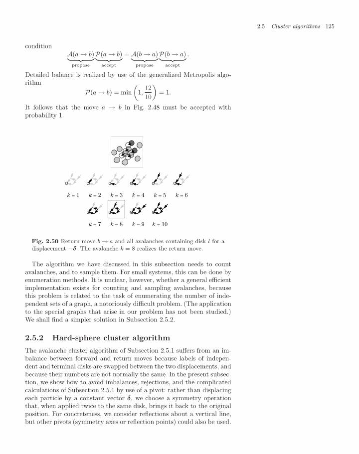
2.5 Cluster algorithms 125
conditionA(a → b)︸ ︷︷ ︸
propose
P(a → b)︸ ︷︷ ︸accept
= A(b → a)︸ ︷︷ ︸propose
P(b → a)︸ ︷︷ ︸accept
.
Detailed balance is realized by use of the generalized Metropolis algo-rithm
P(a → b) = min(
1,1210
)= 1.
It follows that the move a → b in Fig. 2.48 must be accepted withprobability 1.
k = 1 k = 2 k = 3 k = 4 k = 5 k = 6
k = 7 k = 8 k = 9 k = 10
Fig. 2.50 Return move b → a and all avalanches containing disk l for adisplacement −δ. The avalanche k = 8 realizes the return move.
The algorithm we have discussed in this subsection needs to countavalanches, and to sample them. For small systems, this can be done byenumeration methods. It is unclear, however, whether a general efficientimplementation exists for counting and sampling avalanches, becausethis problem is related to the task of enumerating the number of inde-pendent sets of a graph, a notoriously difficult problem. (The applicationto the special graphs that arise in our problem has not been studied.)We shall find a simpler solution in Subsection 2.5.2.
2.5.2 Hard-sphere cluster algorithm
The avalanche cluster algorithm of Subsection 2.5.1 suffers from an im-balance between forward and return moves because labels of indepen-dent and terminal disks are swapped between the two displacements, andbecause their numbers are not normally the same. In the present subsec-tion, we show how to avoid imbalances, rejections, and the complicatedcalculations of Subsection 2.5.1 by use of a pivot: rather than displacingeach particle by a constant vector δ, we choose a symmetry operationthat, when applied twice to the same disk, brings it back to the originalposition. For concreteness, we consider reflections about a vertical line,but other pivots (symmetry axes or reflection points) could also be used.
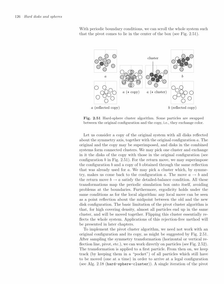
126 Hard disks and spheres
With periodic boundary conditions, we can scroll the whole system suchthat the pivot comes to lie in the center of the box (see Fig. 2.51).
a
a (+ copy) a (+ cluster)
cluster
b
a (reflected copy) b (reflected copy)
Fig. 2.51 Hard-sphere cluster algorithm. Some particles are swappedbetween the original configuration and the copy, i.e., they exchange color.
Let us consider a copy of the original system with all disks reflectedabout the symmetry axis, together with the original configuration a. Theoriginal and the copy may be superimposed, and disks in the combinedsystems form connected clusters. We may pick one cluster and exchangein it the disks of the copy with those in the original configuration (seeconfiguration b in Fig. 2.51). For the return move, we may superimposethe configuration b and a copy of b obtained through the same reflectionthat was already used for a. We may pick a cluster which, by symme-try, makes us come back to the configuration a. The move a → b andthe return move b → a satisfy the detailed-balance condition. All thesetransformations map the periodic simulation box onto itself, avoidingproblems at the boundaries. Furthermore, ergodicity holds under thesame conditions as for the local algorithm: any local move can be seenas a point reflection about the midpoint between the old and the newdisk configuration. The basic limitation of the pivot cluster algorithm isthat, for high covering density, almost all particles end up in the samecluster, and will be moved together. Flipping this cluster essentially re-flects the whole system. Applications of this rejection-free method willbe presented in later chapters.
To implement the pivot cluster algorithm, we need not work with anoriginal configuration and its copy, as might be suggested by Fig. 2.51.After sampling the symmetry transformation (horizontal or vertical re-flection line, pivot, etc.), we can work directly on particles (see Fig. 2.52).The transformation is applied to a first particle. From then on, we keeptrack (by keeping them in a “pocket”) of all particles which still haveto be moved (one at a time) in order to arrive at a legal configuration(see Alg. 2.18 (hard-sphere-cluster)). A single iteration of the pivot
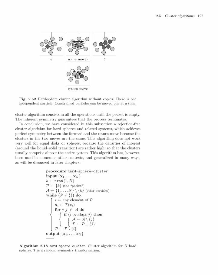
2.5 Cluster algorithms 127
a a ( + move) b
return move
Fig. 2.52 Hard-sphere cluster algorithm without copies. There is oneindependent particle. Constrained particles can be moved one at a time.
cluster algorithm consists in all the operations until the pocket is empty.The inherent symmetry guarantees that the process terminates.
In conclusion, we have considered in this subsection a rejection-freecluster algorithm for hard spheres and related systems, which achievesperfect symmetry between the forward and the return move because theclusters in the two moves are the same. This algorithm does not workvery well for equal disks or spheres, because the densities of interest(around the liquid–solid transition) are rather high, so that the clustersusually comprise almost the entire system. This algorithm has, however,been used in numerous other contexts, and generalized in many ways,as will be discussed in later chapters.
procedure hard-sphere-cluster
input x1, . . . ,xNk ← nran (1, N)P ← k (the “pocket”)A ← 1, . . . , N \ k (other particles)while (P = ) do⎧⎪⎪⎪⎪⎪⎪⎪⎪⎨⎪⎪⎪⎪⎪⎪⎪⎪⎩
i ← any element of Pxi ← T (xi)for ∀ j ∈ A do⎧⎨⎩
if (i overlaps j) then A ← A \ jP ← P ∪ j
P ← P \ ioutput x1, . . . ,xN——
Algorithm 2.18 hard-sphere-cluster. Cluster algorithm for N hardspheres. T is a random symmetry transformation.
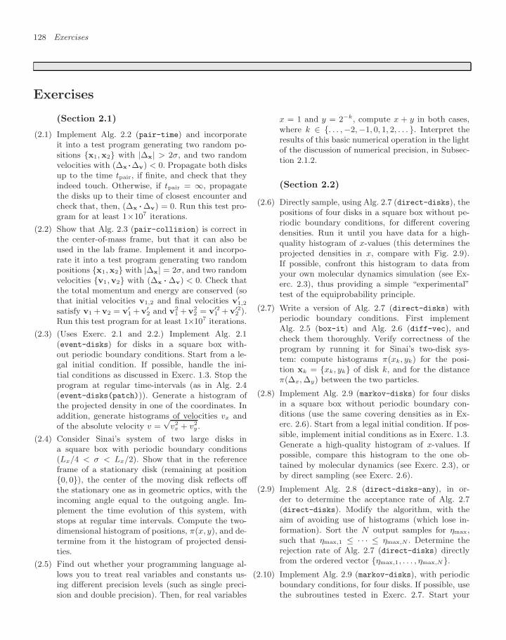
128 Exercises
Exercises
(Section 2.1)
(2.1) Implement Alg. 2.2 (pair-time) and incorporateit into a test program generating two random po-sitions x1, x2 with |∆x| > 2σ, and two randomvelocities with (∆x ···∆v) < 0. Propagate both disksup to the time tpair, if finite, and check that theyindeed touch. Otherwise, if tpair = ∞, propagatethe disks up to their time of closest encounter andcheck that, then, (∆x ···∆v) = 0. Run this test pro-gram for at least 1×10⁷ iterations.
(2.2) Show that Alg. 2.3 (pair-collision) is correct inthe center-of-mass frame, but that it can also beused in the lab frame. Implement it and incorpo-rate it into a test program generating two randompositions x1,x2 with |∆x| = 2σ, and two randomvelocities v1,v2 with (∆x ··· ∆v) < 0. Check thatthe total momentum and energy are conserved (sothat initial velocities v1,2 and final velocities v′
1,2
satisfy v1 +v2 = v′1 +v′
2 and v21 +v2
2 = v′21 +v′2
2 ).Run this test program for at least 1×10⁷ iterations.
(2.3) (Uses Exerc. 2.1 and 2.2.) Implement Alg. 2.1(event-disks) for disks in a square box with-out periodic boundary conditions. Start from a le-gal initial condition. If possible, handle the ini-tial conditions as discussed in Exerc. 1.3. Stop theprogram at regular time-intervals (as in Alg. 2.4(event-disks(patch))). Generate a histogram ofthe projected density in one of the coordinates. Inaddition, generate histograms of velocities vx andof the absolute velocity v =
√v2
x + v2y .
(2.4) Consider Sinai’s system of two large disks ina square box with periodic boundary conditions(Lx/4 < σ < Lx/2). Show that in the referenceframe of a stationary disk (remaining at position0, 0), the center of the moving disk reflects offthe stationary one as in geometric optics, with theincoming angle equal to the outgoing angle. Im-plement the time evolution of this system, withstops at regular time intervals. Compute the two-dimensional histogram of positions, π(x, y), and de-termine from it the histogram of projected densi-ties.
(2.5) Find out whether your programming language al-lows you to treat real variables and constants us-ing different precision levels (such as single preci-sion and double precision). Then, for real variables
x = 1 and y = 2−k, compute x + y in both cases,where k ∈ . . . ,−2,−1, 0, 1, 2, . . . . Interpret theresults of this basic numerical operation in the lightof the discussion of numerical precision, in Subsec-tion 2.1.2.
(Section 2.2)
(2.6) Directly sample, using Alg. 2.7 (direct-disks), thepositions of four disks in a square box without pe-riodic boundary conditions, for different coveringdensities. Run it until you have data for a high-quality histogram of x-values (this determines theprojected densities in x, compare with Fig. 2.9).If possible, confront this histogram to data fromyour own molecular dynamics simulation (see Ex-erc. 2.3), thus providing a simple “experimental”test of the equiprobability principle.
(2.7) Write a version of Alg. 2.7 (direct-disks) withperiodic boundary conditions. First implementAlg. 2.5 (box-it) and Alg. 2.6 (diff-vec), andcheck them thoroughly. Verify correctness of theprogram by running it for Sinai’s two-disk sys-tem: compute histograms π(xk, yk) for the posi-tion xk = xk, yk of disk k, and for the distanceπ(∆x, ∆y) between the two particles.
(2.8) Implement Alg. 2.9 (markov-disks) for four disksin a square box without periodic boundary con-ditions (use the same covering densities as in Ex-erc. 2.6). Start from a legal initial condition. If pos-sible, implement initial conditions as in Exerc. 1.3.Generate a high-quality histogram of x-values. Ifpossible, compare this histogram to the one ob-tained by molecular dynamics (see Exerc. 2.3), orby direct sampling (see Exerc. 2.6).
(2.9) Implement Alg. 2.8 (direct-disks-any), in or-der to determine the acceptance rate of Alg. 2.7(direct-disks). Modify the algorithm, with theaim of avoiding use of histograms (which lose in-formation). Sort the N output samples for ηmax,such that ηmax,1 ≤ · · · ≤ ηmax,N . Determine therejection rate of Alg. 2.7 (direct-disks) directlyfrom the ordered vector ηmax,1, . . . , ηmax,N.
(2.10) Implement Alg. 2.9 (markov-disks), with periodicboundary conditions, for four disks. If possible, usethe subroutines tested in Exerc. 2.7. Start your
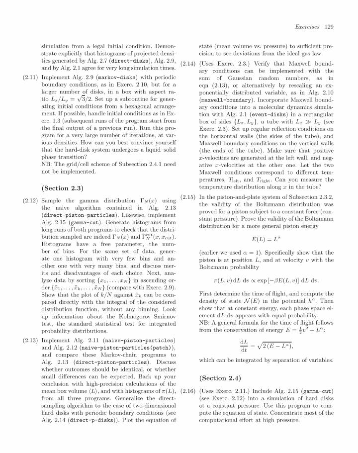
Exercises 129
simulation from a legal initial condition. Demon-strate explicitly that histograms of projected densi-ties generated by Alg. 2.7 (direct-disks), Alg. 2.9,and by Alg. 2.1 agree for very long simulation times.
(2.11) Implement Alg. 2.9 (markov-disks) with periodicboundary conditions, as in Exerc. 2.10, but for alarger number of disks, in a box with aspect ra-tio Lx/Ly =
√3/2. Set up a subroutine for gener-
ating initial conditions from a hexagonal arrange-ment. If possible, handle initial conditions as in Ex-erc. 1.3 (subsequent runs of the program start fromthe final output of a previous run). Run this pro-gram for a very large number of iterations, at var-ious densities. How can you best convince yourselfthat the hard-disk system undergoes a liquid–solidphase transition?NB: The grid/cell scheme of Subsection 2.4.1 neednot be implemented.
(Section 2.3)
(2.12) Sample the gamma distribution ΓN(x) usingthe naive algorithm contained in Alg. 2.13(direct-piston-particles). Likewise, implementAlg. 2.15 (gamma-cut). Generate histograms fromlong runs of both programs to check that the distri-bution sampled are indeed ΓN (x) and Γcut
N (x, xcut).Histograms have a free parameter, the num-ber of bins. For the same set of data, gener-ate one histogram with very few bins and an-other one with very many bins, and discuss mer-its and disadvantages of each choice. Next, ana-lyze data by sorting x1, . . . , xN in ascending or-der x1, . . . , xk, . . . , xN (compare with Exerc. 2.9).Show that the plot of k/N against xk can be com-pared directly with the integral of the considereddistribution function, without any binning. Lookup information about the Kolmogorov–Smirnovtest, the standard statistical test for integratedprobability distributions.
(2.13) Implement Alg. 2.11 (naive-piston-particles)and Alg. 2.12 (naive-piston-particles(patch)),and compare these Markov-chain programs toAlg. 2.13 (direct-piston-particles). Discusswhether outcomes should be identical, or whethersmall differences can be expected. Back up yourconclusion with high-precision calculations of themean box volume 〈L〉, and with histograms of π(L),from all three programs. Generalize the direct-sampling algorithm to the case of two-dimensionalhard disks with periodic boundary conditions (seeAlg. 2.14 (direct-p-disks)). Plot the equation of
state (mean volume vs. pressure) to sufficient pre-cision to see deviations from the ideal gas law.
(2.14) (Uses Exerc. 2.3.) Verify that Maxwell bound-ary conditions can be implemented with thesum of Gaussian random numbers, as ineqn (2.13), or alternatively by rescaling an ex-ponentially distributed variable, as in Alg. 2.10(maxwell-boundary). Incorporate Maxwell bound-ary conditions into a molecular dynamics simula-tion with Alg. 2.1 (event-disks) in a rectangularbox of sides Lx, Ly, a tube with Lx Ly (seeExerc. 2.3). Set up regular reflection conditions onthe horizontal walls (the sides of the tube), andMaxwell boundary conditions on the vertical walls(the ends of the tube). Make sure that positivex-velocities are generated at the left wall, and neg-ative x-velocities at the other one. Let the twoMaxwell conditions correspond to different tem-peratures, Tleft, and Tright. Can you measure thetemperature distribution along x in the tube?
(2.15) In the piston-and-plate system of Subsection 2.3.2,the validity of the Boltzmann distribution wasproved for a piston subject to a constant force (con-stant pressure). Prove the validity of the Boltzmanndistribution for a more general piston energy
E(L) = Lα
(earlier we used α = 1). Specifically show that thepiston is at position L, and at velocity v with theBoltzmann probability
π(L, v) dL dv ∝ exp [−βE(L, v)] dL dv.
First determine the time of flight, and compute thedensity of state N (E) in the potential hα. Thenshow that at constant energy, each phase space el-ement dL dv appears with equal probability.NB: A general formula for the time of flight followsfrom the conservation of energy E = 1
2v2 + Lα:
dL
dt=
p2 (E − Lα),
which can be integrated by separation of variables.
(Section 2.4)
(2.16) (Uses Exerc. 2.11.) Include Alg. 2.15 (gamma-cut)(see Exerc. 2.12) into a simulation of hard disksat a constant pressure. Use this program to com-pute the equation of state. Concentrate most of thecomputational effort at high pressure.
130 References
References
Alder B., Wainwright T. E. (1957) Phase transition for a hard spheresystem, Journal of Chemical Physics 27, 1208–1209
Alder B. J., Wainwright T. E. (1962) Phase transition in elastic disks,Physical Review 127, 359–361
Alder B. J., Wainwright T. E. (1970) Decay of the velocity autocor-relation function, Physical Review A 1, 18–21
Dress C., Krauth W. (1995) Cluster algorithm for hard spheres andrelated systems, Journal of Physics A 28, L597–L601
Hoover W. G., Ree F. H. (1968) Melting transition and communal en-tropy for hard spheres, Journal of Chemical Physics 49, 3609–3617
Lee J. Y., Strandburg K. J. (1992) 1st-order melting transition of thehard-disk system, Physical Review B 46, 11190–11193
Mermin N. D., Wagner H. (1966) Absence of ferromagnetism or anti-ferromagnetism in one- or two-dimensional isotropic Heisenberg models,Physical Review Letters 17, 1133–1136
Metropolis N., Rosenbluth A. W., Rosenbluth M. N., Teller A. H., TellerE. (1953) Equation of state calculations by fast computing machines,Journal of Chemical Physics 21, 1087–1092
Pomeau Y., Resibois P. (1975) Time dependent correlation functionsand mode–mode coupling theory, Physics Reports 19, 63–139
Simanyi N. (2003) Proof of the Boltzmann–Sinai ergodic hypothesis fortypical hard disk systems, Inventiones Mathematicae 154, 123–178
Simanyi N. (2004) Proof of the ergodic hypothesis for typical hard ballsystems, Annales de l’Institut Henri Poincare 5, 203–233
Sinai Y. G. (1970) Dynamical systems with elastic reflections, RussianMathematical Surveys 25, 137–189
Thirring W. (1978) A Course in Mathematical Physics. 1. Classical Dy-namical Systems, Springer, New York
Wood W. W. (1968) Monte Carlo calculations for hard disks in theisothermal–isobaric ensemble, Journal of Chemical Physics 48, 415–434
Density matrices and pathintegrals 3
3.1 Density matrices 133
3.2 Matrix squaring 143
3.3 The Feynmanpath integral 149
3.4 Pair density matrices 159
3.5 Geometry of paths 168
Exercises 182
References 184
In this chapter, we continue our parallel exploration of statistical andcomputational physics, but now move to the field of quantum mechanics,where the density matrix generalizes the classical Boltzmann distribu-tion. The density matrix constructs the quantum statistical probabilitiesfrom their two origins: the quantum mechanical wave functions and theBoltzmann probabilities of the energy levels. The density matrix canthus be defined in terms of the complete solution of the quantum prob-lem (wave functions, energies), but all this information is available onlyin simple examples, such as the free particle or the harmonic oscillator.
A simple general expression exists for the density matrix only at hightemperature. However, a systematic convolution procedure allows us tocompute the density matrix at any given temperature from a productof two density matrices at higher temperature. By iteration, we reachthe density matrix at any temperature from the high-temperature limit.We shall use this procedure, matrix squaring, to compute the quantum-statistical probabilities for particles in an external potential.
The convolution procedure, and the connection it establishes betweenclassical and quantum systems, is the basis of the Feynman path integral,which really opens up the field of finite-temperature quantum statisticsto computation. We shall learn about path integrals in more and morecomplicated settings. As an example of interacting particles, we shallcome back to the case of hard spheres, which model quantum gases andquantum liquids equally well. The path integral allows us to conceive ofsimulations in interacting quantum systems with great ease. This will bestudied in the present chapter for the case of two hard spheres, beforetaking up the many-body problem in Chapter 4.
Classical particles are related to points, the pebbles of our first chap-ter. Analogously, quantum particles are related to one-dimensional ob-jects, the aforementioned paths, which have important geometric prop-erties. Path integrals, like other concepts of statistical mechanics, havespread to areas outside their field of origin, and even beyond physics.They are for example used to describe stock indices in financial math-ematics. The final section of this chapter introduces the geometry ofpaths and related objects. This external look at our subject will fosterour understanding of quantum physics and of the path integral. We shallreach analytical and algorithmic insights complementing those of earliersections of the chapter.
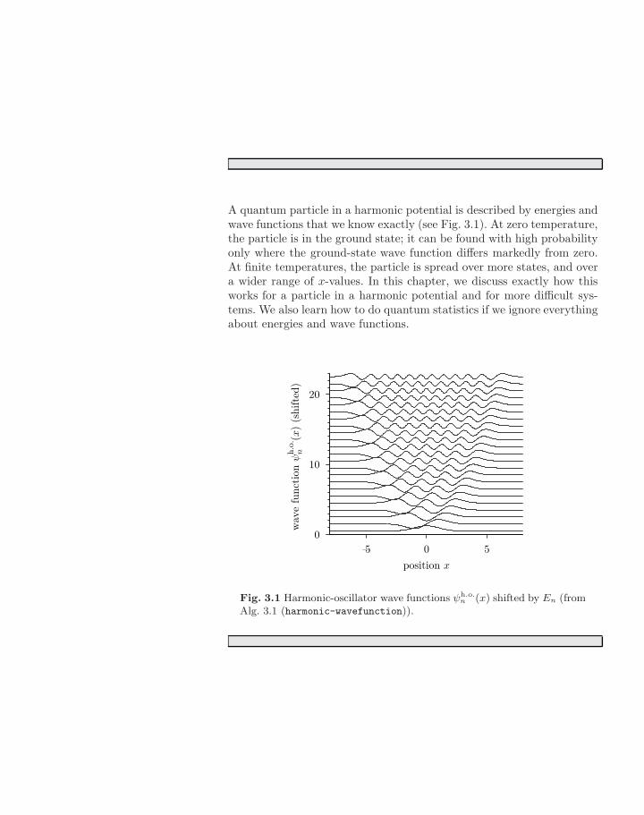
A quantum particle in a harmonic potential is described by energies andwave functions that we know exactly (see Fig. 3.1). At zero temperature,the particle is in the ground state; it can be found with high probabilityonly where the ground-state wave function differs markedly from zero.At finite temperatures, the particle is spread over more states, and overa wider range of x-values. In this chapter, we discuss exactly how thisworks for a particle in a harmonic potential and for more difficult sys-tems. We also learn how to do quantum statistics if we ignore everythingabout energies and wave functions.
0
10
20
-5 0 5
wav
e fu
nct
ion ψ
nh.o
. (x)
(shifte
d)
position x
Fig. 3.1 Harmonic-oscillator wave functions ψh.o.n (x) shifted by En (from
Alg. 3.1 (harmonic-wavefunction)).
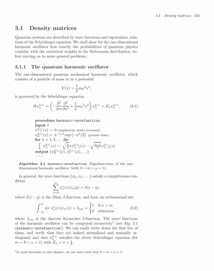
3.1 Density matrices 133
3.1 Density matrices
Quantum systems are described by wave functions and eigenvalues, solu-tions of the Schrodinger equation. We shall show for the one-dimensionalharmonic oscillator how exactly the probabilities of quantum physicscombine with the statistical weights in the Boltzmann distribution, be-fore moving on to more general problems.
3.1.1 The quantum harmonic oscillator
The one-dimensional quantum mechanical harmonic oscillator, whichconsists of a particle of mass m in a potential
V (x) =12mω2x2,
is governed by the Schrodinger equation
Hψh.o.n =
(−
2
2m
∂2
∂x2+
12mω2x2
)ψh.o.
n = Enψh.o.n . (3.1)
procedure harmonic-wavefunction
input xψh.o.−1 (x) ← 0 (unphysical, starts recursion)
ψh.o.0 (x) ←
−1/4 exp(−x2/2
)(ground state)
for n = 1, 2, . . . doψh.o.
n (x) ←√
2nxψh.o.
n−1(x) −√
n−1n ψh.o.
n−2(x)output ψh.o.
0 (x), ψh.o.1 (x), . . .
——
Algorithm 3.1 harmonic-wavefunction. Eigenfunctions of the one-dimensional harmonic oscillator (with = m = ω = 1).
In general, the wave functions ψ0, ψ1, . . . satisfy a completeness con-dition ∞∑
n=0
ψ∗n(x)ψn(y) = δ(x − y),
where δ(x − y) is the Dirac δ-function, and form an orthonormal set:∫ ∞
−∞dx ψ∗
n(x)ψm(x) = δnm =
1 if n = m
0 otherwise, (3.2)
where δnm is the discrete Kronecker δ-function. The wave functionsof the harmonic oscillator can be computed recursively1 (see Alg. 3.1(harmonic-wavefunction)). We can easily write down the first few ofthem, and verify that they are indeed normalized and mutually or-thogonal, and that ψh.o.
n satisfies the above Schrodinger equation (form = = ω = 1) with En = n + 1
2 .
1In most formulas in this chapter, we use units such that = m = ω = 1.
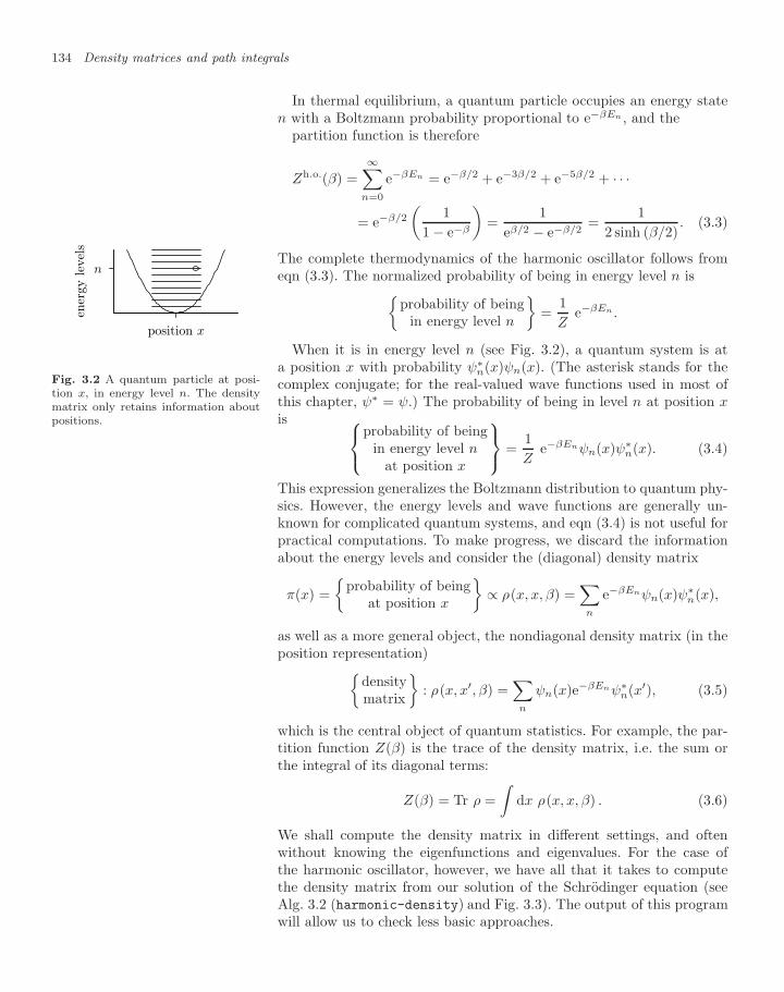
134 Density matrices and path integrals
In thermal equilibrium, a quantum particle occupies an energy staten with a Boltzmann probability proportional to e−βEn , and the
partition function is therefore
Zh.o.(β) =∞∑
n=0
e−βEn = e−β/2 + e−3β/2 + e−5β/2 + · · ·
= e−β/2
(1
1 − e−β
)=
1eβ/2 − e−β/2
=1
2 sinh (β/2). (3.3)
The complete thermodynamics of the harmonic oscillator follows fromeqn (3.3). The normalized probability of being in energy level n is
probability of beingin energy level n
=
1Z
e−βEn .
n
position x
ener
gy lev
els
Fig. 3.2 A quantum particle at posi-tion x, in energy level n. The densitymatrix only retains information aboutpositions.
When it is in energy level n (see Fig. 3.2), a quantum system is ata position x with probability ψ∗
n(x)ψn(x). (The asterisk stands for thecomplex conjugate; for the real-valued wave functions used in most ofthis chapter, ψ∗ = ψ.) The probability of being in level n at position xis ⎧⎨⎩
probability of beingin energy level n
at position x
⎫⎬⎭ =1Z
e−βEnψn(x)ψ∗n(x). (3.4)
This expression generalizes the Boltzmann distribution to quantum phy-sics. However, the energy levels and wave functions are generally un-known for complicated quantum systems, and eqn (3.4) is not useful forpractical computations. To make progress, we discard the informationabout the energy levels and consider the (diagonal) density matrix
π(x) =
probability of beingat position x
∝ ρ(x, x, β) =
∑n
e−βEnψn(x)ψ∗n(x),
as well as a more general object, the nondiagonal density matrix (in theposition representation)
densitymatrix
: ρ(x, x′, β) =
∑n
ψn(x)e−βEnψ∗n(x′), (3.5)
which is the central object of quantum statistics. For example, the par-tition function Z(β) is the trace of the density matrix, i.e. the sum orthe integral of its diagonal terms:
Z(β) = Tr ρ =∫
dx ρ(x, x, β) . (3.6)
We shall compute the density matrix in different settings, and oftenwithout knowing the eigenfunctions and eigenvalues. For the case ofthe harmonic oscillator, however, we have all that it takes to computethe density matrix from our solution of the Schrodinger equation (seeAlg. 3.2 (harmonic-density) and Fig. 3.3). The output of this programwill allow us to check less basic approaches.
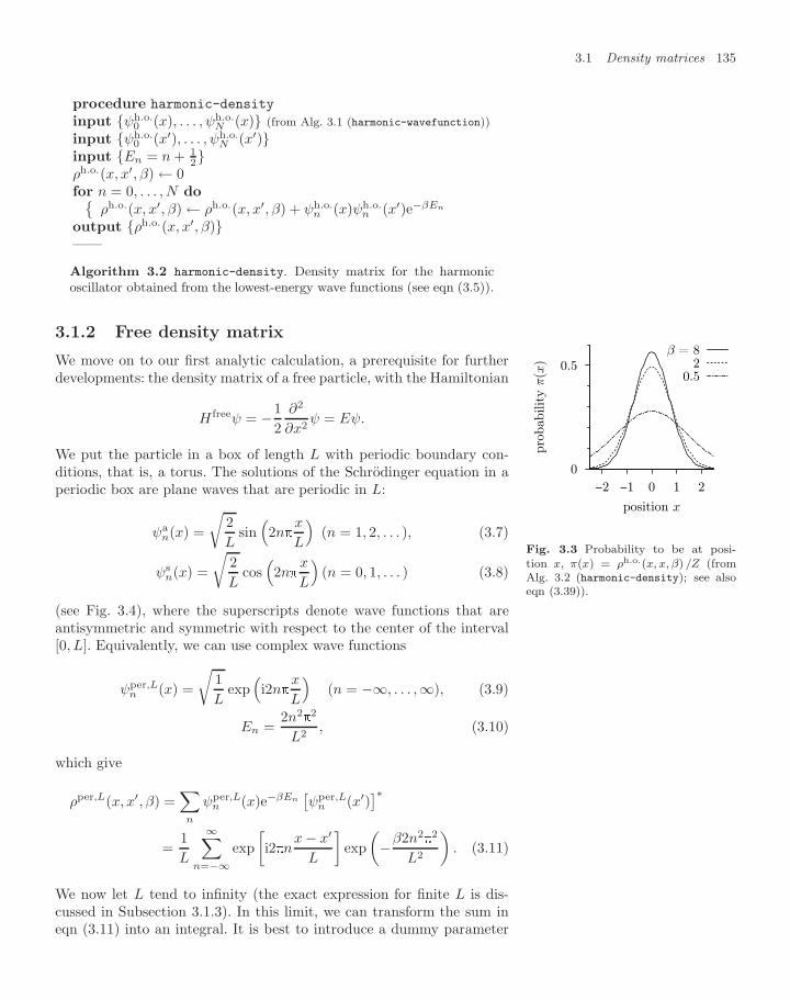
3.1 Density matrices 135
procedure harmonic-density
input ψh.o.0 (x), . . . , ψh.o.
N (x) (from Alg. 3.1 (harmonic-wavefunction))input ψh.o.
0 (x′), . . . , ψh.o.N (x′)
input En = n + 12
ρh.o.(x, x′, β) ← 0for n = 0, . . . , N do
ρh.o.(x, x′, β) ← ρh.o.(x, x′, β) + ψh.o.n (x)ψh.o.
n (x′)e−βEn
output ρh.o.(x, x′, β)——
Algorithm 3.2 harmonic-density. Density matrix for the harmonicoscillator obtained from the lowest-energy wave functions (see eqn (3.5)).
3.1.2 Free density matrix
We move on to our first analytic calculation, a prerequisite for furtherdevelopments: the density matrix of a free particle, with the Hamiltonian
H freeψ = −12
∂2
∂x2ψ = Eψ.
We put the particle in a box of length L with periodic boundary con-0
0.5
210−1−2
pro
babilit
y π
(x)
position x
β = 82
0.5
Fig. 3.3 Probability to be at posi-tion x, π(x) = ρh.o.(x, x, β) /Z (fromAlg. 3.2 (harmonic-density); see alsoeqn (3.39)).
ditions, that is, a torus. The solutions of the Schrodinger equation in aperiodic box are plane waves that are periodic in L:
ψan(x) =
√2L
sin(2n
x
L
)(n = 1, 2, . . . ), (3.7)
ψsn(x) =
√2L
cos(2n
x
L
)(n = 0, 1, . . . ) (3.8)
(see Fig. 3.4), where the superscripts denote wave functions that areantisymmetric and symmetric with respect to the center of the interval[0, L]. Equivalently, we can use complex wave functions
ψper,Ln (x) =
√1L
exp(i2n
x
L
)(n = −∞, . . . ,∞), (3.9)
En =2n2
2
L2, (3.10)
which give
ρper,L(x, x′, β) =∑
n
ψper,Ln (x)e−βEn
[ψper,L
n (x′)]∗
=1L
∞∑n=−∞
exp[i2n
x − x′
L
]exp(−β2n2
2
L2
). (3.11)
We now let L tend to infinity (the exact expression for finite L is dis-cussed in Subsection 3.1.3). In this limit, we can transform the sum ineqn (3.11) into an integral. It is best to introduce a dummy parameter
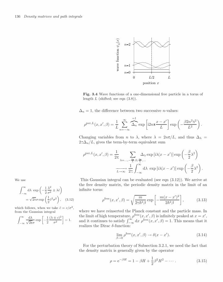
136 Density matrices and path integrals
n=2
n=1
n=0
LL/20
wav
e fu
nct
ion ψ
n(x
)
position x
Fig. 3.4 Wave functions of a one-dimensional free particle in a torus oflength L (shifted; see eqn (3.8)).
∆n = 1, the difference between two successive n-values:
ρper,L(x, x′, β) =1L
∞∑n=−∞
=1︷︸︸︷∆n exp
[i2n
x − x′
L
]exp(−β2n2
2
L2
).
Changing variables from n to λ, where λ = 2n/L, and thus ∆λ =2∆n/L, gives the term-by-term equivalent sum
ρper,L(x, x′, β) =12
∑λ=...,− 2
L,0, 2
L,...
∆λ exp [iλ(x − x′)] exp(−β
2λ2
)
−−−−→L→∞
12
∫ ∞
−∞dλ exp [iλ(x − x′)] exp
(−β
2λ2
).
This Gaussian integral can be evaluated (see eqn (3.12)). We arrive atWe use
Z ∞
−∞
dλ exp„−1
2λ2
σ2± λc
«
=√
2σ exp„
12
c2σ2
«, (3.12)
which follows, when we take c = c/σ2,from the Gaussian integralZ ∞
−∞
dλ√2σ
exp»−1
2(λ ± c)2
σ2
–= 1.
the free density matrix, the periodic density matrix in the limit of aninfinite torus:
ρfree(x, x′, β) =√
m
22βexp[−m(x − x′)2
22β
], (3.13)
where we have reinserted the Planck constant and the particle mass. Inthe limit of high temperature, ρfree(x, x′, β) is infinitely peaked at x = x′,and it continues to satisfy
∫∞−∞ dx ρfree(x, x′, β) = 1. This means that it
realizes the Dirac δ-function:
limβ→0
ρfree(x, x′, β) → δ(x − x′). (3.14)
For the perturbation theory of Subsection 3.2.1, we need the fact thatthe density matrix is generally given by the operator
ρ = e−βH = 1 − βH +12β2H2 − · · · . (3.15)
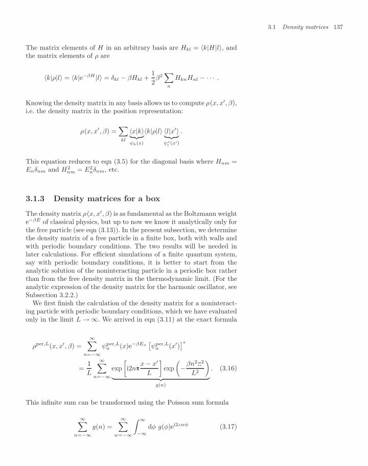
3.1 Density matrices 137
The matrix elements of H in an arbitrary basis are Hkl = 〈k|H |l〉, andthe matrix elements of ρ are
〈k|ρ|l〉 = 〈k|e−βH |l〉 = δkl − βHkl +12β2∑
n
HknHnl − · · · .
Knowing the density matrix in any basis allows us to compute ρ(x, x′, β),i.e. the density matrix in the position representation:
ρ(x, x′, β) =∑kl
〈x|k〉︸ ︷︷ ︸ψk(x)
〈k|ρ|l〉 〈l|x′〉︸ ︷︷ ︸ψ∗
l(x′)
.
This equation reduces to eqn (3.5) for the diagonal basis where Hnm =Enδnm and H2
nm = E2nδnm, etc.
3.1.3 Density matrices for a box
The density matrix ρ(x, x′, β) is as fundamental as the Boltzmann weighte−βE of classical physics, but up to now we know it analytically only forthe free particle (see eqn (3.13)). In the present subsection, we determinethe density matrix of a free particle in a finite box, both with walls andwith periodic boundary conditions. The two results will be needed inlater calculations. For efficient simulations of a finite quantum system,say with periodic boundary conditions, it is better to start from theanalytic solution of the noninteracting particle in a periodic box ratherthan from the free density matrix in the thermodynamic limit. (For theanalytic expression of the density matrix for the harmonic oscillator, seeSubsection 3.2.2.)
We first finish the calculation of the density matrix for a noninteract-ing particle with periodic boundary conditions, which we have evaluatedonly in the limit L → ∞. We arrived in eqn (3.11) at the exact formula
ρper,L(x, x′, β) =∞∑
n=−∞ψper,L
n (x)e−βEn[ψper,L
n (x′)]∗
=1L
∞∑n=−∞
exp[i2n
x − x′
L
]exp(−βn2
2
L2
)︸ ︷︷ ︸
g(n)
. (3.16)
This infinite sum can be transformed using the Poisson sum formula
∞∑n=−∞
g(n) =∞∑
w=−∞
∫ ∞
−∞dφ g(φ)ei2wφ (3.17)
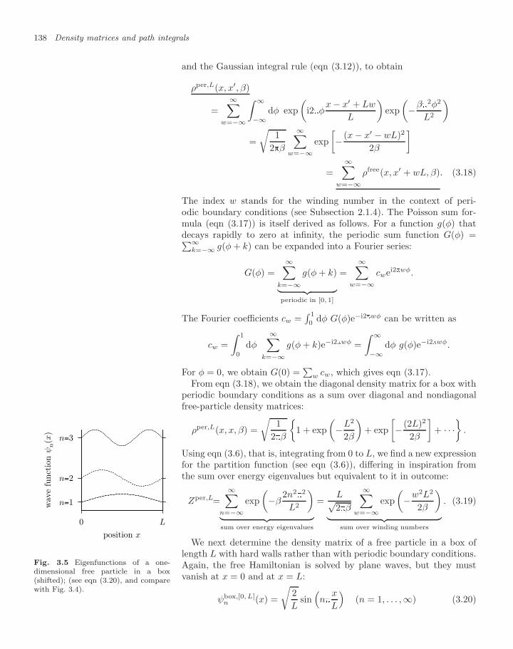
138 Density matrices and path integrals
and the Gaussian integral rule (eqn (3.12)), to obtain
ρper,L(x, x′, β)
=∞∑
w=−∞
∫ ∞
−∞dφ exp
(i2φ
x − x′ + Lw
L
)exp(−β2φ2
L2
)
=√
12β
∞∑w=−∞
exp[− (x − x′ − wL)2
2β
]
=∞∑
w=−∞ρfree(x, x′ + wL, β). (3.18)
The index w stands for the winding number in the context of peri-odic boundary conditions (see Subsection 2.1.4). The Poisson sum for-mula (eqn (3.17)) is itself derived as follows. For a function g(φ) thatdecays rapidly to zero at infinity, the periodic sum function G(φ) =∑∞
k=−∞ g(φ + k) can be expanded into a Fourier series:
G(φ) =∞∑
k=−∞g(φ + k)︸ ︷︷ ︸
periodic in [0, 1]
=∞∑
w=−∞cwei2wφ.
The Fourier coefficients cw =∫ 1
0dφ G(φ)e−i2wφ can be written as
cw =∫ 1
0
dφ∞∑
k=−∞g(φ + k)e−i2wφ =
∫ ∞
−∞dφ g(φ)e−i2wφ.
For φ = 0, we obtain G(0) =∑
w cw, which gives eqn (3.17).From eqn (3.18), we obtain the diagonal density matrix for a box with
periodic boundary conditions as a sum over diagonal and nondiagonalfree-particle density matrices:
ρper,L(x, x, β) =√
12β
1 + exp
(−L2
2β
)+ exp
[− (2L)2
2β
]+ · · ·
.
Using eqn (3.6), that is, integrating from 0 to L, we find a new expressionfor the partition function (see eqn (3.6)), differing in inspiration fromthe sum over energy eigenvalues but equivalent to it in outcome:
Zper,L=∞∑
n=−∞exp(−β
2n22
L2
)︸ ︷︷ ︸sum over energy eigenvalues
=L√2β
∞∑w=−∞
exp(−w2L2
2β
)︸ ︷︷ ︸
sum over winding numbers
. (3.19)
n=3
n=2
n=1
L0
wav
e fu
nct
ion ψ
n(x
)
position x
Fig. 3.5 Eigenfunctions of a one-dimensional free particle in a box(shifted); (see eqn (3.20), and comparewith Fig. 3.4).
We next determine the density matrix of a free particle in a box oflength L with hard walls rather than with periodic boundary conditions.Again, the free Hamiltonian is solved by plane waves, but they mustvanish at x = 0 and at x = L:
ψbox,[0, L]n (x) =
√2L
sin(n
x
L
)(n = 1, . . . ,∞) (3.20)
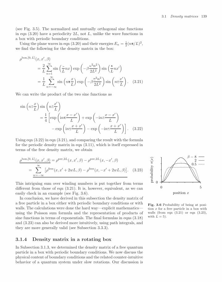
3.1 Density matrices 139
(see Fig. 3.5). The normalized and mutually orthogonal sine functionsin eqn (3.20) have a periodicity 2L, not L, unlike the wave functions ina box with periodic boundary conditions.
Using the plane waves in eqn (3.20) and their energies En = 12 (n/L)2,
we find the following for the density matrix in the box:
ρbox,[0, L](x, x′, β)
=2L
∞∑n=1
sin(
Lnx)
exp(−β
2n2
2L2
)sin(
Lnx′)
=1L
∞∑n=−∞
sin(n
x
L
)exp(−β
2n2
2L2
)sin(
nx′
L
). (3.21)
We can write the product of the two sine functions as
sin(n
x
L
)sin(
nx′
L
)=
14
[exp(
inx − x′
L
)+ exp
(−in
x − x′
L
)− exp
(in
x + x′
L
)− exp
(−in
x + x′
L
)]. (3.22)
Using eqn (3.22) in eqn (3.21), and comparing the result with the formulafor the periodic density matrix in eqn (3.11), which is itself expressed interms of the free density matrix, we obtain
ρbox,[0, L](x, x′, β) = ρper,2L(x, x′, β) − ρper,2L(x,−x′, β)
=∞∑
w=−∞
[ρfree(x, x′ + 2wL, β) − ρfree(x,−x′ + 2wL, β)
]. (3.23)
This intriguing sum over winding numbers is put together from termsdifferent from those of eqn (3.21). It is, however, equivalent, as we caneasily check in an example (see Fig. 3.6).
0
0 5
pro
babilit
y π
(x)
position x
β = 82
0.5
Fig. 3.6 Probability of being at posi-tion x for a free particle in a box withwalls (from eqn (3.21) or eqn (3.23),with L = 5).
In conclusion, we have derived in this subsection the density matrix ofa free particle in a box either with periodic boundary conditions or withwalls. The calculations were done the hard way—explicit mathematics—using the Poisson sum formula and the representation of products ofsine functions in terms of exponentials. The final formulas in eqns (3.18)and (3.23) can also be derived more intuitively, using path integrals, andthey are more generally valid (see Subsection 3.3.3).
3.1.4 Density matrix in a rotating box
In Subsection 3.1.3, we determined the density matrix of a free quantumparticle in a box with periodic boundary conditions. We now discuss thephysical content of boundary conditions and the related counter-intuitivebehavior of a quantum system under slow rotations. Our discussion is
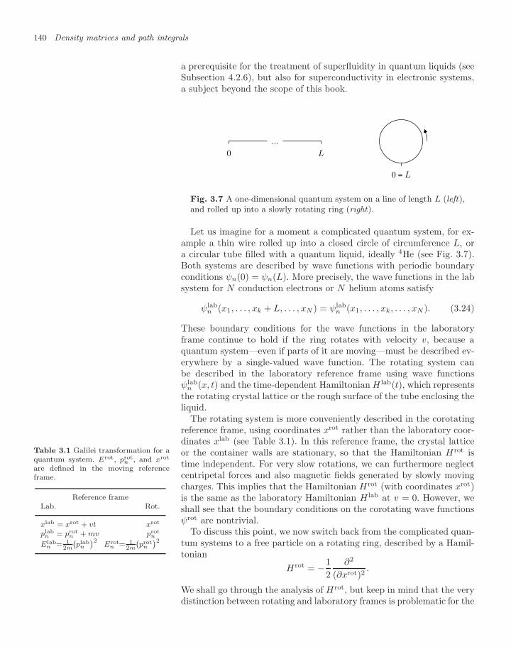
140 Density matrices and path integrals
a prerequisite for the treatment of superfluidity in quantum liquids (seeSubsection 4.2.6), but also for superconductivity in electronic systems,a subject beyond the scope of this book.
...
0 L
0 = L
Fig. 3.7 A one-dimensional quantum system on a line of length L (left),and rolled up into a slowly rotating ring (right).
Let us imagine for a moment a complicated quantum system, for ex-ample a thin wire rolled up into a closed circle of circumference L, ora circular tube filled with a quantum liquid, ideally 4He (see Fig. 3.7).Both systems are described by wave functions with periodic boundaryconditions ψn(0) = ψn(L). More precisely, the wave functions in the labsystem for N conduction electrons or N helium atoms satisfy
ψlabn (x1, . . . , xk + L, . . . , xN ) = ψlab
n (x1, . . . , xk, . . . , xN ). (3.24)
These boundary conditions for the wave functions in the laboratoryframe continue to hold if the ring rotates with velocity v, because aquantum system—even if parts of it are moving—must be described ev-erywhere by a single-valued wave function. The rotating system canbe described in the laboratory reference frame using wave functionsψlab
n (x, t) and the time-dependent Hamiltonian H lab(t), which representsthe rotating crystal lattice or the rough surface of the tube enclosing theliquid.
The rotating system is more conveniently described in the corotatingreference frame, using coordinates xrot rather than the laboratory coor-dinates xlab (see Table 3.1). In this reference frame, the crystal latticeor the container walls are stationary, so that the Hamiltonian Hrot istime independent. For very slow rotations, we can furthermore neglectcentripetal forces and also magnetic fields generated by slowly movingcharges. This implies that the Hamiltonian Hrot (with coordinates xrot)is the same as the laboratory Hamiltonian H lab at v = 0. However, weshall see that the boundary conditions on the corotating wave functionsψrot are nontrivial.
Table 3.1 Galilei transformation for aquantum system. Erot, prot
n , and xrot
are defined in the moving referenceframe.
Reference frameLab. Rot.
xlab = xrot + vt xrot
plabn = prot
n + mv protn
Elabn = 1
2m
`plab
n
´2Erot
n = 12m
`prot
n
´2 To discuss this point, we now switch back from the complicated quan-tum systems to a free particle on a rotating ring, described by a Hamil-tonian
Hrot = −12
∂2
(∂xrot)2.
We shall go through the analysis of Hrot, but keep in mind that the verydistinction between rotating and laboratory frames is problematic for the
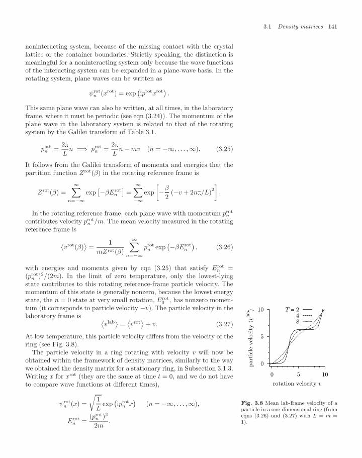
3.1 Density matrices 141
noninteracting system, because of the missing contact with the crystallattice or the container boundaries. Strictly speaking, the distinction ismeaningful for a noninteracting system only because the wave functionsof the interacting system can be expanded in a plane-wave basis. In therotating system, plane waves can be written as
ψrotn (xrot) = exp
(iprotxrot
).
This same plane wave can also be written, at all times, in the laboratoryframe, where it must be periodic (see eqn (3.24)). The momentum of theplane wave in the laboratory system is related to that of the rotatingsystem by the Galilei transform of Table 3.1.
plabn =
2L
n =⇒ protn =
2L
n − mv (n = −∞, . . . ,∞). (3.25)
It follows from the Galilei transform of momenta and energies that thepartition function Zrot(β) in the rotating reference frame is
Zrot(β) =∞∑
n=−∞exp[−βErot
n
]=
∞∑−∞
exp[−β
2(−v + 2n/L)2
].
In the rotating reference frame, each plane wave with momentum protn
contributes velocity protn /m. The mean velocity measured in the rotating
reference frame is
⟨vrot(β)
⟩=
1mZrot(β)
∞∑n=−∞
protn exp
(−βErotn
), (3.26)
with energies and momenta given by eqn (3.25) that satisfy Erotn =
(protn )2/(2m). In the limit of zero temperature, only the lowest-lying
state contributes to this rotating reference-frame particle velocity. Themomentum of this state is generally nonzero, because the lowest energystate, the n = 0 state at very small rotation, Erot
0 , has nonzero momen-tum (it corresponds to particle velocity −v). The particle velocity in thelaboratory frame is ⟨
vlab⟩
=⟨vrot⟩
+ v. (3.27)
At low temperature, this particle velocity differs from the velocity of thering (see Fig. 3.8).
The particle velocity in a ring rotating with velocity v will now beobtained within the framework of density matrices, similarly to the waywe obtained the density matrix for a stationary ring, in Subsection 3.1.3.Writing x for xrot (they are the same at time t = 0, and we do not haveto compare wave functions at different times),
0
5
10
0 5 10
par
ticl
e vel
ocit
y 〈v
lab〉
rotation velocity v
T = 248
Fig. 3.8 Mean lab-frame velocity of aparticle in a one-dimensional ring (fromeqns (3.26) and (3.27) with L = m =1).
ψrotn (x) =
√1L
exp(iprot
n x)
(n = −∞, . . . ,∞),
Erotn =
(protn )2
2m.
142 Density matrices and path integrals
The density matrix at positions x and x′ in the rotating system is:
ρrot(x, x′, β) =∞∑
n=−∞e−βErot
n ψrotn (x)
[ψrot
n (x′)]∗
=1L
∞∑n=−∞
exp[−β
2(prot
n
)2] exp[iprot
n (x − x′)]
︸ ︷︷ ︸g(n), compare with eqn (3.16)
=∞∑
w=−∞
∫dφ
Lexp
[−β
2
(2φL
− v
)2
+ i(
2φL
− v
)(x − x′) + i2wφ
],
where we have again used the Poisson sum formula (eqn (3.17)). Settingφ′ = 2φ/L − v and changing w into −w, we reach
ρrot(x, x′, β) =∞∑
w=−∞e−iLwv
∫ ∞
−∞
dφ
2exp[−β
2φ′2 + iφ′(x − x′ − Lw)
]
=∞∑
w=−∞e−iLwvρfree(x, x′ + Lw, β) .
Integrating the diagonal density matrix over all the positions x, from 0to L, yields the partition function in the rotating system:
Zrot(β) = Tr ρrot(x, x, β)
=∞∑
w=−∞e−iLvw
∫ L
0
dx ρfree(x, x + wL, β) (3.28)
(see eqn (3.6)). For small velocities, we expand the exponential in theabove equation. The zeroth-order term gives the partition function inthe stationary system, and the first-order term vanishes because of asymmetry for the winding number w → −w. The term proportional tow2 is nontrivial. We multiply and divide by the laboratory partitionfunction at rest, Z lab
v=0, and obtain
Zrot(β) =∞∑
w=−∞
∫ L
0
dx ρfree(x, x + wL, β)︸ ︷︷ ︸Zlab
v=0, see eqn (3.18)
− 12v2L2
∞∑w=−∞
w2ρfree(x, x + wL, β)Z lab
v=0︸ ︷︷ ︸〈w2〉v=0
Z labv=0 + · · ·
= Z labv=0
(1 − 1
2v2L2
⟨w2⟩
v=0
).
Noting that the free energy is F = − log (Z) /β, we obtain the followingfundamental formula:
F rot = F labv=0 +
v2L2⟨w2⟩
v=0
2β+ · · · . (3.29)
3.2 Matrix squaring 143
This is counter-intuitive because we would naively expect the slowlyrotating system to rotate along with the reference system and have thesame free energy as the laboratory system at rest, in the same way asa bucket of water, under very slow rotation, simply rotates with thewalls and satisfies F rot = F lab
v=0. However, we saw the same effect in theprevious calculation, using wave functions and eigenvalues. Part of thesystem simply does not rotate with the bucket. It remains stationary inthe laboratory system.
The relation between the mean squared winding number and thechange of free energies upon rotation is due to Pollock and Ceperley(1986). Equation (3.29) contains no more quantities specific to nonin-teracting particles; it therefore holds also in an interacting system, atleast for small velocities. We shall understand this more clearly by rep-resenting the density matrix as a sum of paths, which do not changewith interactions, and only get reweighted. Equation (3.29) is very con-venient for evaluating the superfluid fraction of a liquid, that part of avery slowly rotating system which remains stationary in the laboratoryframe.
In conclusion, we have computed in this subsection the density ma-trix for a free particle in a rotating box. As mentioned several times, thiscalculation has far-reaching consequences for quantum liquids and su-perconductors. Hess and Fairbank (1967) demonstrated experimentallythat a quantum liquid in a slowly rotating container rotates more slowlythan the container, or even stops to rest. The reader is urged to studythe experiment, and Leggett’s classic discussion (Leggett 1973).
3.2 Matrix squaring
A classical equilibrium system is at coordinates x with a probability π(x)given by the Boltzmann distribution. In contrast, a quantum statisticalsystem is governed by the diagonal density matrix, defined through wavefunctions and energy eigenvalues. The problem is that we usually do notknow the solutions of the Schrodinger equation, so that we need othermethods to compute the density matrix. In this section, we discuss ma-trix squaring, an immensely practical approach to computing the densitymatrix at any temperature from a high-temperature limit with the helpof a convolution principle, which yields the density matrix at low tem-perature once we know it at high temperature.
Convolutions of probability distributions have already been discussedin Chapter 1. Their relation to convolutions of density matrices willbecome evident in the context of the Feynman path integral (see Sec-tion 3.3).
3.2.1 High-temperature limit, convolution
In the limit of high temperature, the density matrix of a quantum sys-tem described by a Hamiltonian H = H free + V is given by a general
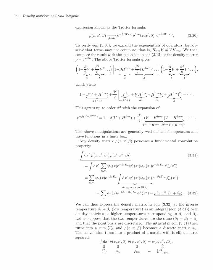
144 Density matrices and path integrals
expression known as the Trotter formula:
ρ(x, x′, β) −−−→β→0
e−12 βV (x)ρfree(x, x′, β) e−
12 βV (x′). (3.30)
To verify eqn (3.30), we expand the exponentials of operators, but ob-serve that terms may not commute, that is, HfreeV = V Hfree. We thencompare the result with the expansion in eqn (3.15) of the density matrixρ = e−βH . The above Trotter formula gives(
1− β
2V︸︷︷︸
a
+β2
8V 2︸ ︷︷ ︸b
. . .
)[1−βH free︸ ︷︷ ︸
c
+β2
2(H free)2︸ ︷︷ ︸
d
. . .
](1− β
2V︸︷︷︸e
+β2
8V 2︸ ︷︷ ︸
f
. . .
),
which yields
1 − β(V + H free)︸ ︷︷ ︸a+e+c
+β2
2
[V 2︸︷︷︸
ae+b+f
+ V H free︸ ︷︷ ︸ac
+ H freeV︸ ︷︷ ︸ce
+ (H free)2︸ ︷︷ ︸d
]− · · · .
This agrees up to order β2 with the expansion of
e−β(V +Hfree) = 1 − β(V + H free) +β2
2(V + H free)(V + H free)︸ ︷︷ ︸
V 2+V Hfree+HfreeV +(Hfree)2
+ · · · .
The above manipulations are generally well defined for operators andwave functions in a finite box.
Any density matrix ρ(x, x′, β) possesses a fundamental convolutionproperty:∫
dx′ ρ(x, x′, β1) ρ(x′, x′′, β2) (3.31)
=∫
dx′ ∑n,m
ψn(x)e−β1Enψ∗n(x′)ψm(x′)e−β2Emψ∗
m(x′′)
=∑n,m
ψn(x)e−β1En
∫dx′ ψ∗
n(x′)ψm(x′)︸ ︷︷ ︸δnm, see eqn (3.2)
e−β2Emψ∗m(x′′)
=∑
n
ψn(x)e−(β1+β2)Enψ∗n(x′′) = ρ(x, x′′, β1 + β2). (3.32)
We can thus express the density matrix in eqn (3.32) at the inversetemperature β1 + β2 (low temperature) as an integral (eqn (3.31)) overdensity matrices at higher temperatures corresponding to β1 and β2.Let us suppose that the two temperatures are the same (β1 = β2 = β)and that the positions x are discretized. The integral in eqn (3.31) thenturns into a sum
∑l, and ρ(x, x′, β) becomes a discrete matrix ρkl.
The convolution turns into a product of a matrix with itself, a matrixsquared: ∫
dx′
∑l
ρ(x, x′, β)ρkl
ρ(x′, x′′, β)
ρlm
=
=
ρ(x, x′′, 2β) .(
ρ2)km
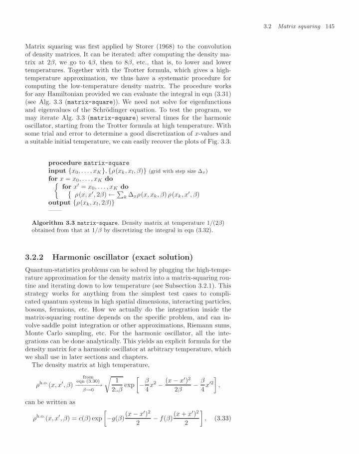
3.2 Matrix squaring 145
Matrix squaring was first applied by Storer (1968) to the convolutionof density matrices. It can be iterated: after computing the density ma-trix at 2β, we go to 4β, then to 8β, etc., that is, to lower and lowertemperatures. Together with the Trotter formula, which gives a high-temperature approximation, we thus have a systematic procedure forcomputing the low-temperature density matrix. The procedure worksfor any Hamiltonian provided we can evaluate the integral in eqn (3.31)(see Alg. 3.3 (matrix-square)). We need not solve for eigenfunctionsand eigenvalues of the Schrodinger equation. To test the program, wemay iterate Alg. 3.3 (matrix-square) several times for the harmonicoscillator, starting from the Trotter formula at high temperature. Withsome trial and error to determine a good discretization of x-values anda suitable initial temperature, we can easily recover the plots of Fig. 3.3.
procedure matrix-square
input x0, . . . , xK, ρ(xk, xl, β) (grid with step size ∆x)for x = x0, . . . , xK do
for x′ = x0, . . . , xK doρ(x, x′, 2β) ←∑k ∆xρ(x, xk, β) ρ(xk, x′, β)
output ρ(xk, xl, 2β)——
Algorithm 3.3 matrix-square. Density matrix at temperature 1/(2β)obtained from that at 1/β by discretizing the integral in eqn (3.32).
3.2.2 Harmonic oscillator (exact solution)
Quantum-statistics problems can be solved by plugging the high-tempe-rature approximation for the density matrix into a matrix-squaring rou-tine and iterating down to low temperature (see Subsection 3.2.1). Thisstrategy works for anything from the simplest test cases to compli-cated quantum systems in high spatial dimensions, interacting particles,bosons, fermions, etc. How we actually do the integration inside thematrix-squaring routine depends on the specific problem, and can in-volve saddle point integration or other approximations, Riemann sums,Monte Carlo sampling, etc. For the harmonic oscillator, all the inte-grations can be done analytically. This yields an explicit formula for thedensity matrix for a harmonic oscillator at arbitrary temperature, whichwe shall use in later sections and chapters.
The density matrix at high temperature,
ρh.o.(x, x′, β)from
eqn (3.30)−−−−−−→β→0
√1
2βexp[−β
4x2 − (x − x′)2
2β− β
4x′2]
,
can be written as
ρh.o.(x, x′, β) = c(β) exp[−g(β)
(x − x′)2
2− f(β)
(x + x′)2
2
], (3.33)
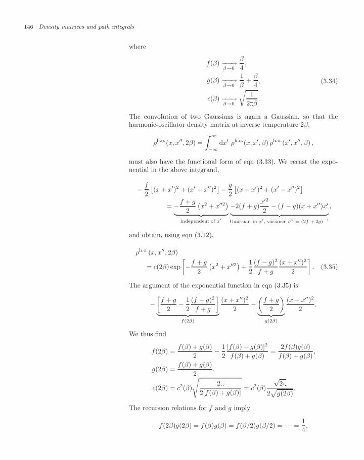
146 Density matrices and path integrals
where
f(β) −−−→β→0
β
4,
g(β) −−−→β→0
1β
+β
4,
c(β) −−−→β→0
√1
2β.
(3.34)
The convolution of two Gaussians is again a Gaussian, so that theharmonic-oscillator density matrix at inverse temperature 2β,
ρh.o.(x, x′′, 2β) =∫ ∞
−∞dx′ ρh.o.(x, x′, β) ρh.o.(x′, x′′, β) ,
must also have the functional form of eqn (3.33). We recast the expo-nential in the above integrand,
− f
2[(x + x′)2 + (x′ + x′′)2
]− g
2[(x − x′)2 + (x′ − x′′)2
]= −f + g
2(x2 + x′′2)︸ ︷︷ ︸
independent of x′
−2(f + g)x′2
2− (f − g)(x + x′′)x′︸ ︷︷ ︸
Gaussian in x′, variance σ2 = (2f + 2g)−1
,
and obtain, using eqn (3.12),
ρh.o.(x, x′′, 2β)
= c(2β) exp[−f + g
2(x2 + x′′2)+
12
(f − g)2
f + g
(x + x′′)2
2
]. (3.35)
The argument of the exponential function in eqn (3.35) is
−[f + g
2− 1
2(f − g)2
f + g
]︸ ︷︷ ︸
f(2β)
(x + x′′)2
2−(
f + g
2
)︸ ︷︷ ︸
g(2β)
(x − x′′)2
2.
We thus find
f(2β) =f(β) + g(β)
2− 1
2[f(β) − g(β)]2
f(β) + g(β)=
2f(β)g(β)f(β) + g(β)
,
g(2β) =f(β) + g(β)
2,
c(2β) = c2(β)
√2
2[f(β) + g(β)]= c2(β)
√2
2√
g(2β).
The recursion relations for f and g imply
f(2β)g(2β) = f(β)g(β) = f(β/2)g(β/2) = · · · =14,
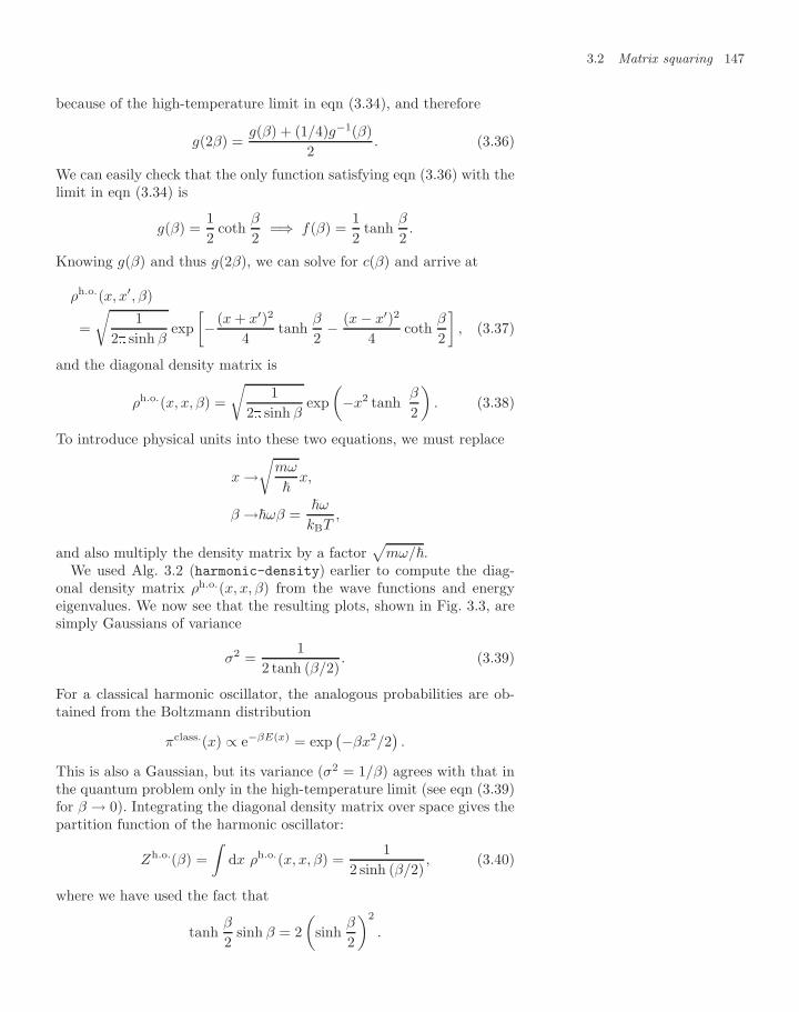
3.2 Matrix squaring 147
because of the high-temperature limit in eqn (3.34), and therefore
g(2β) =g(β) + (1/4)g−1(β)
2. (3.36)
We can easily check that the only function satisfying eqn (3.36) with thelimit in eqn (3.34) is
g(β) =12
cothβ
2=⇒ f(β) =
12
tanhβ
2.
Knowing g(β) and thus g(2β), we can solve for c(β) and arrive at
ρh.o.(x, x′, β)
=√
12 sinh β
exp[− (x + x′)2
4tanh
β
2− (x − x′)2
4coth
β
2
], (3.37)
and the diagonal density matrix is
ρh.o.(x, x, β) =√
12 sinh β
exp(−x2 tanh
β
2
). (3.38)
To introduce physical units into these two equations, we must replace
x →√
mω
x,
β →ωβ =ω
kBT,
and also multiply the density matrix by a factor√
mω/.We used Alg. 3.2 (harmonic-density) earlier to compute the diag-
onal density matrix ρh.o.(x, x, β) from the wave functions and energyeigenvalues. We now see that the resulting plots, shown in Fig. 3.3, aresimply Gaussians of variance
σ2 =1
2 tanh (β/2). (3.39)
For a classical harmonic oscillator, the analogous probabilities are ob-tained from the Boltzmann distribution
πclass.(x) ∝ e−βE(x) = exp(−βx2/2
).
This is also a Gaussian, but its variance (σ2 = 1/β) agrees with that inthe quantum problem only in the high-temperature limit (see eqn (3.39)for β → 0). Integrating the diagonal density matrix over space gives thepartition function of the harmonic oscillator:
Zh.o.(β) =∫
dx ρh.o.(x, x, β) =1
2 sinh (β/2), (3.40)
where we have used the fact that
tanhβ
2sinh β = 2
(sinh
β
2
)2
.
148 Density matrices and path integrals
This way of computing the partition function agrees with what weobtained from the sum of energies in eqn (3.3). Matrix squaring alsoallows us to compute the ground-state wave function without solvingthe Schrodinger equation because, in the limit of zero temperature,eqn (3.38) becomes ρh.o.(x, x, β) ∝ exp
(−x2) ∝ ψh.o.
0 (x)2 (see Alg. 3.1(harmonic-wavefunction)).
In conclusion, we have obtained in this subsection an analytic expres-sion for the density matrix of a harmonic oscillator, not from the energyeigenvalues and eigenfunctions, but using matrix squaring down fromhigh temperature. We shall need this expression several times in thischapter and in Chapter 4.
3.2.3 Infinitesimal matrix products
The density matrix at low temperature (inverse temperature β1 + β2)ρ(x, x′, β1 + β2) is already contained in the density matrices at β1 andβ2. We can also formulate this relation between density matrices at twodifferent temperatures in terms of a differential relation, by taking oneof the temperatures to be infinitesimally small:
ρ(∆β)ρ(β) = ρ(β + ∆β).
Because of ρ(∆β) = e−∆βH 1 − ∆βH , this is equivalent to
−Hρ ρ(β + ∆β) − ρ(β)∆β
=∂
∂βρ. (3.41)
The effect of the hamiltonian on the density matrix is best clarified inthe position representation, where one finds, either by inserting completesets of states into eqn (3.41) or from the definition of the density matrix:
∂
∂βρ(x, x′, β) = −
∑n
Enψn(x)︸ ︷︷ ︸Hψn(x)
e−βEnψ∗n(x′) = −Hxρ(x, x′, β) , (3.42)
where Hx means that the Hamiltonian acts on x, not on x′, in the densitymatrix ρ(x, x′, β). Equation (3.42) is the differential version of matrixsquaring, and has the same initial condition at infinite temperature:ρ(x, x′, β → 0) → δ(x − x′) (see eqn (3.14)).
We shall not need the differential equation (3.42) in the further courseof this book and shall simply check in passing that it is satisfied byρfree(x, x′, β). We have
∂
∂βρfree(x, x′, β) =
∂
∂β
1√2β
exp[− (x − x′)2
2β
]=
−β + (x − x′)2
2β2ρfree(x, x′, β) .
On the other hand, we can explicitly check that:
∂2
∂x2ρfree(x, x′, β) = ρfree(x, x′, β)
(x − x′)2
β2− ρfree(x, x′, β) /β,
3.3 The Feynman path integral 149
so that the free density matrix solves the differential equation (3.42).In this book, we shall be interested only in the density matrix in sta-
tistical mechanics, shown in eqn (3.41), which is related to the evolutionoperator in real time, e−itH . Formally, we can pass from real time t toinverse temperature β through the replacement
β = it,
and β is often referred to as an “imaginary” time. The quantum MonteCarlo methods in this chapter and in Chapter 4 usually do not carry overto real-time quantum dynamics, because the weights would become com-plex numbers, and could then no longer be interpreted as probabilities.
3.3 The Feynman path integral
In matrix squaring, one of the subjects of Section 3.2, we convolute twodensity matrices at temperature T to produce the density matrix at tem-perature T/2. By iterating this process, we can obtain the density ma-trix at any temperature from the quasi-classical high-temperature limit.Most often, however, it is impossible to convolute two density matricesanalytically. With increasing numbers of particles and in high dimen-sionality, the available computer memory soon becomes insufficient evento store a reasonably discretized matrix ρ(x,x′, β), so that one cannotrun Alg. 3.3 (matrix-square) on a discretized approximation of thedensity matrix. Monte Carlo methods are able to resolve this problem.They naturally lead to the Feynman path integral for quantum systemsand to the idea of path sampling, as we shall see in the present section.
Instead of evaluating the convolution integrals one after the other, asis done in matrix squaring, we can write them out all together:
ρ(x, x′, β) =∫
dx′′ ρ(x, x′′, β/2) ρ(x′′, x′, β/2)
=∫∫∫
dx′′dx′′′dx′′′′ρ(x, x′′′,β
4) ρ(x′′′, x′′,
β
4) ρ(x′′, x′′′′,
β
4) ρ(x′′′′, x′,
β
4)
= . . . .
This equation continues to increasingly deeper levels, with the kth appli-cations of the matrix-squaring algorithm corresponding to 2k integra-tions. Writing x0, x1, . . . instead of the cumbersome x, x′, x′′, . . . ,this gives
ρ(x0, xN , β) =∫
· · ·∫
dx1 . . .dxN−1
× ρ
(x0, x1,
β
N
). . . ρ
(xN−1, xN ,
β
N
), (3.43)
where we note that, for the density matrix ρ(x0, xN , β), the variables x0
and xN are fixed on both sides of eqn (3.43). For the partition function,
150 Density matrices and path integrals
there is one more integration, over the variable x0, which is identifiedwith xN :
Z =∫
dx0 ρ(x0, x0, β) =∫
· · ·∫
dx0 . . .dxN−1
× ρ
(x0, x1,
β
N
). . . ρ
(xN−1, x0,
β
N
). (3.44)
The sequence x0, . . . , xN in eqns (3.43) and (3.44) is called a path, andwe can imagine the variable xk at the value kβ/N of the imaginary-timevariable τ , which goes from 0 to β in steps of ∆τ = β/N (see Feynman(1972)). Density matrices and partition functions are thus representedas multiple integrals over paths, called path integrals, both at finite Nand in the limit N → ∞. The motivation for this representation is againthat for large N , the density matrices under the multiple integral signsare at small ∆τ = β/N (high temperature) and can thus be replacedby their quasi-classical high-temperature approximations. To distinguishbetween the density matrix with fixed positions x0 and xN and the par-tition function, where one integrates over x0 = xN , we shall refer to thepaths in eqn (3.43) as contributing to the density matrix ρ(x0, xN , β),and to the paths in eqn (3.44) as contributing to the partition function.
After presenting a naive sampling approach in Subsection 3.3.1, wediscuss direct path sampling using the Levy construction, in Subsec-tion 3.3.2. The closely related later Subsection 3.5.1 introduces pathsampling in Fourier space.
3.3.1 Naive path sampling
The Feynman path integral describes a single quantum particle in termsof paths x0, . . . , xN (often referred to as world lines), with weightsgiven by the high-temperature density matrix or another suitable ap-proximation:
Z =∫ ∫
dx0, . . . , dxN−1︸ ︷︷ ︸sum of paths
ρ(x0, x1, ∆τ ) · · · · · ρ(xN−1, x0, ∆τ )︸ ︷︷ ︸weight π of path
.
More generally, any variable xk can represent a d-dimensional quantumsystem. The full path then lies in d + 1 dimensions.
Let us first sample the paths contributing to the partition function of aharmonic oscillator using a local Markov-chain algorithm (see Fig. 3.9).We implement the Trotter formula, as we would for an arbitrary poten-tial. Each path comes with a weight containing terms as the following:
. . . ρfree(xk−1, xk, ∆τ ) e−12 ∆τV (xk)︸ ︷︷ ︸
ρ(xk−1, xk, ∆τ ) in Trotter formula
e−12 ∆τV (xk)ρfree(xk, xk+1, ∆τ ) . . .︸ ︷︷ ︸ρ(xk, xk+1, ∆τ ) in Trotter formula
.
As shown, each argument xk appears twice, and any two contributionsexp[− 1
2∆τV (xk)], where V (x) = 1
2x2, can be combined into a single
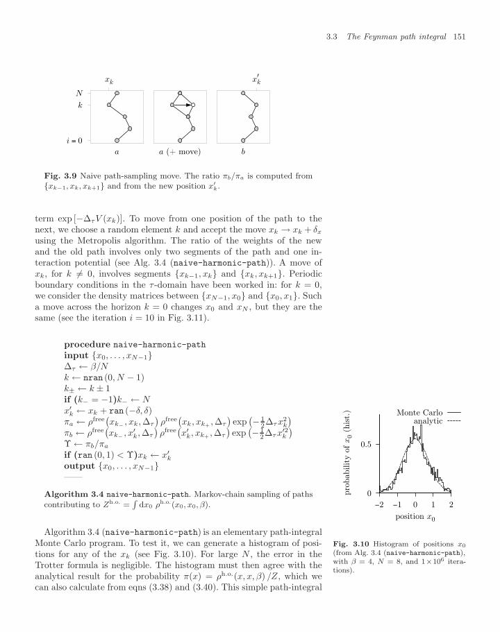
3.3 The Feynman path integral 151
a
i = 0
xk
k
N
a (+ move) b
x′k
Fig. 3.9 Naive path-sampling move. The ratio πb/πa is computed fromxk−1, xk, xk+1 and from the new position x′
k.
term exp [−∆τV (xk)]. To move from one position of the path to thenext, we choose a random element k and accept the move xk → xk + δx
using the Metropolis algorithm. The ratio of the weights of the newand the old path involves only two segments of the path and one in-teraction potential (see Alg. 3.4 (naive-harmonic-path)). A move ofxk, for k = 0, involves segments xk−1, xk and xk, xk+1. Periodicboundary conditions in the τ -domain have been worked in: for k = 0,we consider the density matrices between xN−1, x0 and x0, x1. Sucha move across the horizon k = 0 changes x0 and xN , but they are thesame (see the iteration i = 10 in Fig. 3.11).
0
0.5
210−1−2
pro
bab
ilit
y o
f x
0 (h
ist.
)
position x0
Monte Carloanalytic
Fig. 3.10 Histogram of positions x0
(from Alg. 3.4 (naive-harmonic-path),with β = 4, N = 8, and 1×10⁶ itera-tions).
procedure naive-harmonic-path
input x0, . . . , xN−1∆τ ← β/Nk ← nran (0, N − 1)k± ← k ± 1if (k− = −1)k− ← Nx′
k ← xk + ran (−δ, δ)πa ← ρfree
(xk− , xk, ∆τ
)ρfree(xk, xk+ , ∆τ
)exp(− 1
2∆τx2k
)πb ← ρfree
(xk− , x′
k, ∆τ
)ρfree(x′
k, xk+ , ∆τ
)exp(− 1
2∆τx′2k
)Υ ← πb/πa
if (ran (0, 1) < Υ)xk ← x′k
output x0, . . . , xN−1——
Algorithm 3.4 naive-harmonic-path. Markov-chain sampling of paths
contributing to Zh.o. =R
dx0 ρh.o.(x0, x0, β).
Algorithm 3.4 (naive-harmonic-path) is an elementary path-integralMonte Carlo program. To test it, we can generate a histogram of posi-tions for any of the xk (see Fig. 3.10). For large N , the error in theTrotter formula is negligible. The histogram must then agree with theanalytical result for the probability π(x) = ρh.o.(x, x, β) /Z, which wecan also calculate from eqns (3.38) and (3.40). This simple path-integral
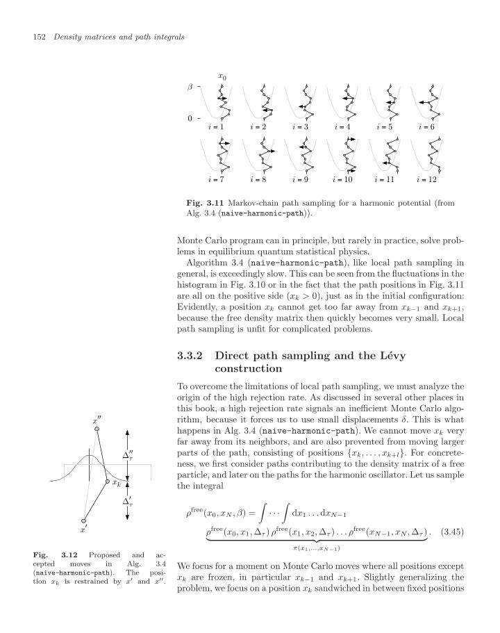
152 Density matrices and path integrals
0
β
x0
i = 1 i = 2 i = 3 i = 4 i = 5 i = 6
i = 7 i = 8 i = 9 i = 10 i = 11 i = 12
Fig. 3.11 Markov-chain path sampling for a harmonic potential (fromAlg. 3.4 (naive-harmonic-path)).
Monte Carlo program can in principle, but rarely in practice, solve prob-lems in equilibrium quantum statistical physics.
Algorithm 3.4 (naive-harmonic-path), like local path sampling ingeneral, is exceedingly slow. This can be seen from the fluctuations in thehistogram in Fig. 3.10 or in the fact that the path positions in Fig. 3.11are all on the positive side (xk > 0), just as in the initial configuration:Evidently, a position xk cannot get too far away from xk−1 and xk+1,because the free density matrix then quickly becomes very small. Localpath sampling is unfit for complicated problems.
3.3.2 Direct path sampling and the Levyconstruction
To overcome the limitations of local path sampling, we must analyze theorigin of the high rejection rate. As discussed in several other places inthis book, a high rejection rate signals an inefficient Monte Carlo algo-rithm, because it forces us to use small displacements δ. This is whathappens in Alg. 3.4 (naive-harmonic-path). We cannot move xk veryfar away from its neighbors, and are also prevented from moving largerparts of the path, consisting of positions xk, . . . , xk+l. For concrete-ness, we first consider paths contributing to the density matrix of a freeparticle, and later on the paths for the harmonic oscillator. Let us samplethe integral
ρfree(x0, xN , β) =∫
· · ·∫
dx1 . . . dxN−1
ρfree(x0, x1, ∆τ ) ρfree(x1, x2, ∆τ ) . . . ρfree(xN−1, xN , ∆τ )︸ ︷︷ ︸π(x1,...,xN−1)
. (3.45)
We focus for a moment on Monte Carlo moves where all positions except
x′
x′′
xk
∆′τ
∆′′τ
Fig. 3.12 Proposed and ac-cepted moves in Alg. 3.4(naive-harmonic-path). The posi-tion xk is restrained by x′ and x′′. xk are frozen, in particular xk−1 and xk+1. Slightly generalizing the
problem, we focus on a position xk sandwiched in between fixed positions
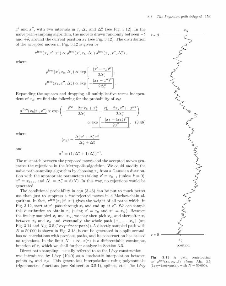
3.3 The Feynman path integral 153
x′ and x′′, with two intervals in τ , ∆′τ and ∆′′
τ (see Fig. 3.12). In thenaive path-sampling algorithm, the move is drawn randomly between −δand +δ, around the current position xk (see Fig. 3.12). The distributionof the accepted moves in Fig. 3.12 is given by
πfree(xk|x′, x′′) ∝ ρfree(x′, xk, ∆′τ ) ρfree(xk, x′′, ∆′′
τ ) ,
where
ρfree(x′, xk, ∆′τ ) ∝ exp
[− (x′ − xk)2
2∆′τ
],
ρfree(xk, x′′, ∆′′τ ) ∝ exp
[− (xk − x′′)2
2∆′′τ
].
Expanding the squares and dropping all multiplicative terms indepen-dent of xk, we find the following for the probability of xk:
πfree(xk|x′, x′′) ∝ exp(− x′2 − 2x′xk + x2
k
2∆′τ
− x2k − 2xkx′′+ x′′2
2∆′′τ
)∝ exp
[− (xk − 〈xk〉)2
2σ2
], (3.46)
where〈xk〉 =
∆′′τ x′ + ∆′
τx′′
∆′τ + ∆′′
τ
andσ2 = (1/∆′′
τ + 1/∆′τ )−1.
The mismatch between the proposed moves and the accepted moves gen-erates the rejections in the Metropolis algorithm. We could modify thenaive path-sampling algorithm by choosing xk from a Gaussian distribu-tion with the appropriate parameters (taking x′ ≡ xk−1 (unless k = 0),x′′ ≡ xk+1, and ∆′
τ = ∆′′τ = β/N). In this way, no rejections would be
generated.The conditional probability in eqn (3.46) can be put to much better
use than just to suppress a few rejected moves in a Markov-chain al-gorithm. In fact, πfree(xk|x′, x′′) gives the weight of all paths which, inFig. 3.12, start at x′, pass through xk and end up at x′′. We can samplethis distribution to obtain x1 (using x′ = x0 and x′′ = xN ). Betweenthe freshly sampled x1 and xN , we may then pick x2, and thereafter x3
between x2 and xN and, eventually, the whole path x1, . . . , xN (seeFig. 3.14 and Alg. 3.5 (levy-free-path)). A directly sampled path withN = 50 000 is shown in Fig. 3.13; it can be generated in a split second,has no correlations with previous paths, and its construction has causedno rejections. In the limit N → ∞, x(τ) is a differentiable continuousfunction of τ , which we shall further analyze in Section 3.5.
τ = β
τ = 0x0
xN
position
Fig. 3.13 A path contributingto ρfree(x0, xN , β) (from Alg. 3.5(levy-free-path), with N = 50 000).
Direct path sampling—usually referred to as the Levy construction—was introduced by Levy (1940) as a stochastic interpolation betweenpoints x0 and xN . This generalizes interpolations using polynomials,trigonometric functions (see Subsection 3.5.1), splines, etc. The Levy
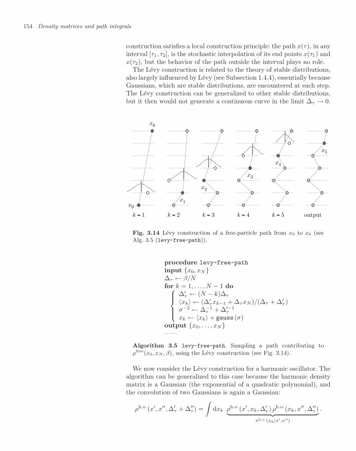
154 Density matrices and path integrals
construction satisfies a local construction principle: the path x(τ), in anyinterval [τ1, τ2], is the stochastic interpolation of its end points x(τ1) andx(τ2), but the behavior of the path outside the interval plays no role.
The Levy construction is related to the theory of stable distributions,also largely influenced by Levy (see Subsection 1.4.4), essentially becauseGaussians, which are stable distributions, are encountered at each step.The Levy construction can be generalized to other stable distributions,but it then would not generate a continuous curve in the limit ∆τ → 0.
x0
x6
k = 1
x1
k = 2
x2
k = 3
x3
k = 4
x4
k = 5
x5
output
Fig. 3.14 Levy construction of a free-particle path from x0 to x6 (seeAlg. 3.5 (levy-free-path)).
procedure levy-free-path
input x0, xN∆τ ← β/Nfor k = 1, . . . , N − 1 do⎧⎪⎪⎨⎪⎪⎩
∆′τ ← (N − k)∆τ
〈xk〉 ← (∆′τxk−1 + ∆τxN )/(∆τ + ∆′
τ )σ−2 ← ∆−1
τ + ∆′−1τ
xk ← 〈xk〉 + gauss (σ)output x0, . . . , xN——
Algorithm 3.5 levy-free-path. Sampling a path contributing to
ρfree(x0, xN , β), using the Levy construction (see Fig. 3.14).
We now consider the Levy construction for a harmonic oscillator. Thealgorithm can be generalized to this case because the harmonic densitymatrix is a Gaussian (the exponential of a quadratic polynomial), andthe convolution of two Gaussians is again a Gaussian:
ρh.o.(x′, x′′, ∆′τ + ∆′′
τ ) =∫
dxk ρh.o.(x′, xk, ∆′τ ) ρh.o.(xk, x′′, ∆′′
τ )︸ ︷︷ ︸πh.o.(xk|x′,x′′)
.
3.3 The Feynman path integral 155
Because of the external potential, the mean value 〈xk〉 no longer lieson the straight line between x′ and x′′. From the nondiagonal harmonicdensity matrix in eqn (3.37), and proceeding as in eqn (3.46), we findthe following:
πh.o.(xk|x′, x′′) ∝ exp[− 1
2σ2(xk − 〈xk〉)2
],
with parameters
〈xk〉 =Υ2
Υ1,
σ =Υ−1/21 ,
Υ1 = coth ∆′τ + coth ∆′′
τ ,
Υ2 =x′
sinh ∆′τ
+x′′
sinh ∆′′τ
,
as already used in the analytic matrix squaring for the harmonic oscil-lator. We can thus directly sample paths contributing to the harmonicdensity matrix ρh.o.(x0, xN , β) (see Alg. 3.6 (levy-harmonic-path)),and also paths contributing to Zh.o. =
∫dx0 ρh.o.(x0, x0, β), if we first
sample x0 from the Gaussian diagonal density matrix in eqn (3.38).
procedure levy-harmonic-path
input x0, xN∆τ ← β/Nfor k = 1, . . . , N − 1 do⎧⎪⎪⎪⎪⎨⎪⎪⎪⎪⎩
Υ1 ← coth ∆τ + coth [(N − k)∆τ ]Υ2 ← xk−1/ sinh ∆τ + xN/ sinh [(N − k)∆τ ]〈xk〉 ← Υ2/Υ1
σ ← 1/√
Υ1
xk ← 〈xk〉 + gauss (σ)output x0, . . . , xN——
Algorithm 3.6 levy-harmonic-path. Sampling a path contributing to
ρh.o.(x0, xN , β), using the Levy construction (see Fig. 3.15).
In Alg. 3.5 (levy-free-path), we were not obliged to sample thepath in chronological order (first x0, then x1, then x2, etc.). After fixingx0 and xN , we could have chosen to sample the midpoint xN/2, thenthe midpoint between x0 and xN/2 and between xN/2 and xN , etc. (seeAlg. 3.8 (naive-box-path) and Fig. 3.19 later). We finally note thatfree paths can also be directly sampled using Fourier-transformationmethods (see Subsection 3.5.1).
3.3.3 Periodic boundary conditions, paths in a box
We now turn to free paths in a box, first with periodic boundary con-ditions, and then with hard walls. A path contributing to the density
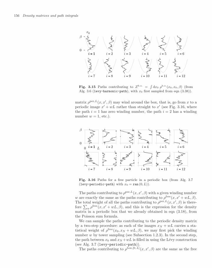
156 Density matrices and path integrals
0
β
i = 1
x0
i = 1 i = 2 i = 3 i = 4 i = 5 i = 6
i = 7 i = 8 i = 9 i = 10 i = 11 i = 12
Fig. 3.15 Paths contributing to Zh.o. =R
dx0 ρh.o.(x0, x0, β) (fromAlg. 3.6 (levy-harmonic-path), with x0 first sampled from eqn (3.38)).
matrix ρper,L(x, x′, β) may wind around the box, that is, go from x to aperiodic image x′ + wL rather than straight to x′ (see Fig. 3.16, wherethe path i = 1 has zero winding number, the path i = 2 has a windingnumber w = 1, etc.).
0
β
0 Li = 1i = 1 i = 2 i = 3 i = 4 i = 5 i = 6
i = 7 i = 8 i = 9 i = 10 i = 11 i = 12
Fig. 3.16 Paths for a free particle in a periodic box (from Alg. 3.7(levy-periodic-path) with x0 = ran (0, L)).
The paths contributing to ρper,L(x, x′, β) with a given winding numberw are exactly the same as the paths contributing to ρfree(x, x′ + wL, β).The total weight of all the paths contributing to ρper,L(x, x′, β) is there-fore
∑w ρfree(x, x′ + wL, β), and this is the expression for the density
matrix in a periodic box that we already obtained in eqn (3.18), fromthe Poisson sum formula.
We can sample the paths contributing to the periodic density matrixby a two-step procedure: as each of the images xN + wL carries a sta-tistical weight of ρfree(x0, xN + wL, β), we may first pick the windingnumber w by tower sampling (see Subsection 1.2.3). In the second step,the path between x0 and xN +wL is filled in using the Levy construction(see Alg. 3.7 (levy-periodic-path)).
The paths contributing to ρbox,[0, L](x, x′, β) are the same as the free
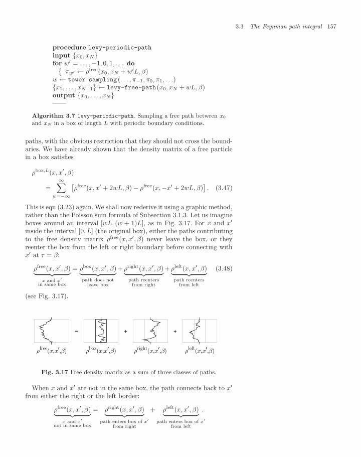
3.3 The Feynman path integral 157
procedure levy-periodic-path
input x0, xNfor w′ = . . . ,−1, 0, 1, . . . do
πw′ ← ρfree(x0, xN + w′L, β)w ← tower sampling (. . . , π−1, π0, π1, . . .)x1, . . . , xN−1 ← levy-free-path(x0, xN + wL, β)output x0, . . . , xN——
Algorithm 3.7 levy-periodic-path. Sampling a free path between x0
and xN in a box of length L with periodic boundary conditions.
paths, with the obvious restriction that they should not cross the bound-aries. We have already shown that the density matrix of a free particlein a box satisfies
ρbox,L(x, x′, β)
=∞∑
w=−∞
[ρfree(x, x′ + 2wL, β) − ρfree(x,−x′ + 2wL, β)
]. (3.47)
This is eqn (3.23) again. We shall now rederive it using a graphic method,rather than the Poisson sum formula of Subsection 3.1.3. Let us imagineboxes around an interval [wL, (w + 1)L], as in Fig. 3.17. For x and x′
inside the interval [0, L] (the original box), either the paths contributingto the free density matrix ρfree(x, x′, β) never leave the box, or theyreenter the box from the left or right boundary before connecting withx′ at τ = β:
ρfree(x, x′, β)︸ ︷︷ ︸x and x′
in same box
= ρbox(x, x′, β)︸ ︷︷ ︸path does not
leave box
+ ρright(x, x′, β)︸ ︷︷ ︸path reentersfrom right
+ ρleft(x, x′, β)︸ ︷︷ ︸path reenters
from left
(3.48)
(see Fig. 3.17).
ρfree(x,x′,β)
=
ρbox(x,x′,β)
+
ρright(x,x′,β)
+
ρleft(x,x′,β)
Fig. 3.17 Free density matrix as a sum of three classes of paths.
When x and x′ are not in the same box, the path connects back to x′
from either the right or the left border:
ρfree(x, x′, β)︸ ︷︷ ︸x and x′
not in same box
= ρright(x, x′, β)︸ ︷︷ ︸path enters box of x′
from right
+ ρleft(x, x′, β)︸ ︷︷ ︸path enters box of x′
from left
.
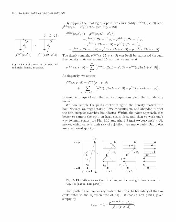
158 Density matrices and path integrals
By flipping the final leg of a path, we can identify ρright(x, x′, β) withρleft(x, 2L − x′, β) etc., (see Fig. 3.18):
ρright(x, x′, β) = ρleft(x, 2L − x′, β)
= ρfree(x, 2L − x′, β) − ρright(x, 2L − x′, β)
= ρfree(x, 2L − x′, β) − ρleft(x, 2L + x′, β)
= ρfree(x, 2L − x′, β) − ρfree(x, 2L + x′, β) + ρright(x, 2L + x′, β).
The density matrix ρright(x, 2L + x′, β) can itself be expressed throughρright(x,x′,β)
=
0 L 2L
ρleft(x,2L−x′,β)
Fig. 3.18 A flip relation between leftand right density matrices.
free density matrices around 4L, so that we arrive at
ρright(x, x′, β) =∞∑
w=1
[ρfree(x, 2wL − x′, β) − ρfree(x, 2wL + x′, β)
].
Analogously, we obtain
ρleft(x, x′, β) = ρfree(x,−x′, β)
+∑
w=−1,−2,...
[ρfree(x, 2wL − x′, β) − ρfree(x, 2wL + x′, β)
].
Entered into eqn (3.48), the last two equations yield the box densitymatrix.
We now sample the paths contributing to the density matrix in abox. Naively, we might start a Levy construction, and abandon it afterthe first trespass over box boundaries. Within the naive approach, it isbetter to sample the path on large scales first, and then to work one’sway to small scales (see Fig. 3.19 and Alg. 3.8 (naive-box-path)). Bigmoves, which carry a high risk of rejection, are made early. Bad pathsare abandoned quickly.
x4
x0
x8
k = 1τ = 0
τ = β
0 L
x2
x6
k = 2
x1
x3
x5
x7
k = 3 ...
Fig. 3.19 Path construction in a box, on increasingly finer scales (inAlg. 3.8 (naive-box-path)).
Each path of the free density matrix that hits the boundary of the boxcontributes to the rejection rate of Alg. 3.8 (naive-box-path), givensimply by
preject = 1 − ρbox,[0, L](x, x′, β)ρfree(x, x′, β)
.
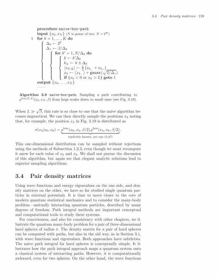
3.4 Pair density matrices 159
procedure naive-box-path
input x0, xN (N is power of two: N = 2K)1 for k = 1, . . . , K do⎧⎪⎪⎪⎪⎪⎪⎪⎪⎪⎪⎨⎪⎪⎪⎪⎪⎪⎪⎪⎪⎪⎩
∆k ← 2k
∆τ ← β/∆k⎧⎪⎪⎪⎪⎪⎪⎨⎪⎪⎪⎪⎪⎪⎩
for k′ = 1, N/∆k do⎧⎪⎪⎪⎪⎨⎪⎪⎪⎪⎩k ← k′∆k
k± ← k ± ∆k
〈xk′∆〉 ← 12
(xk− + xk+
)xk ← ⟨xk−
⟩+ gauss (
√2/∆τ)
if (xk < 0 or xk > L) goto 1output x0, . . . , xN——
Algorithm 3.8 naive-box-path. Sampling a path contributing to
ρbox,[0, L](x0, xN , β) from large scales down to small ones (see Fig. 3.19).
When L √β, this rate is so close to one that the naive algorithm be-
comes impractical. We can then directly sample the positions xk notingthat, for example, the position x4 in Fig. 3.19 is distributed as
π(x4|x0, x8) = ρbox(x0, x4, β/2)ρbox(x4, x8, β/2)︸ ︷︷ ︸explicitly known, see eqn (3.47)
.
This one-dimensional distribution can be sampled without rejectionsusing the methods of Subsection 1.2.3, even though we must recomputeit anew for each value of x0 and x8. We shall not pursue the discussionof this algorithm, but again see that elegant analytic solutions lead tosuperior sampling algorithms.
3.4 Pair density matrices
Using wave functions and energy eigenvalues on the one side, and den-sity matrices on the other, we have so far studied single quantum par-ticles in external potentials. It is time to move closer to the core ofmodern quantum statistical mechanics and to consider the many-bodyproblem—mutually interacting quantum particles, described by manydegrees of freedom. Path integral methods are important conceptualand computational tools to study these systems.
For concreteness, and also for consistency with other chapters, we il-lustrate the quantum many-body problem for a pair of three-dimensionalhard spheres of radius σ. The density matrix for a pair of hard spherescan be computed with paths, but also in the old way, as in Section 3.1,with wave functions and eigenvalues. Both approaches have subtleties.The naive path integral for hard spheres is conceptually simple. It il-lustrates how the path integral approach maps a quantum system ontoa classical system of interacting paths. However, it is computationallyawkward, even for two spheres. On the other hand, the wave functions
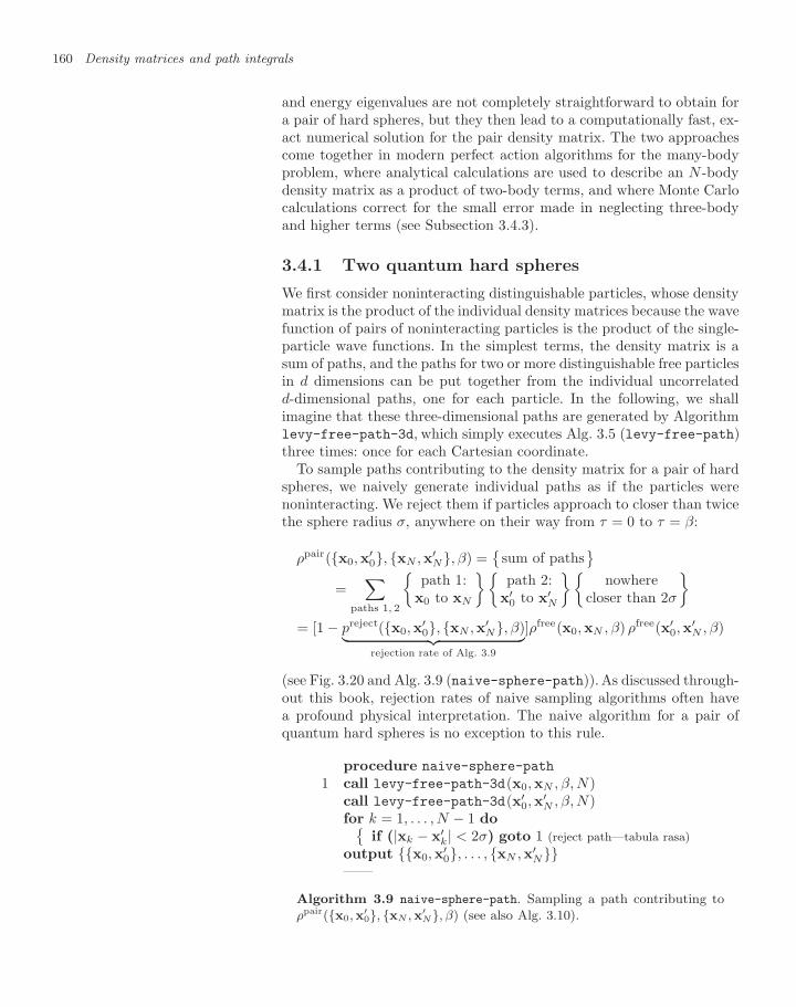
160 Density matrices and path integrals
and energy eigenvalues are not completely straightforward to obtain fora pair of hard spheres, but they then lead to a computationally fast, ex-act numerical solution for the pair density matrix. The two approachescome together in modern perfect action algorithms for the many-bodyproblem, where analytical calculations are used to describe an N -bodydensity matrix as a product of two-body terms, and where Monte Carlocalculations correct for the small error made in neglecting three-bodyand higher terms (see Subsection 3.4.3).
3.4.1 Two quantum hard spheres
We first consider noninteracting distinguishable particles, whose densitymatrix is the product of the individual density matrices because the wavefunction of pairs of noninteracting particles is the product of the single-particle wave functions. In the simplest terms, the density matrix is asum of paths, and the paths for two or more distinguishable free particlesin d dimensions can be put together from the individual uncorrelatedd-dimensional paths, one for each particle. In the following, we shallimagine that these three-dimensional paths are generated by Algorithmlevy-free-path-3d, which simply executes Alg. 3.5 (levy-free-path)three times: once for each Cartesian coordinate.
To sample paths contributing to the density matrix for a pair of hardspheres, we naively generate individual paths as if the particles werenoninteracting. We reject them if particles approach to closer than twicethe sphere radius σ, anywhere on their way from τ = 0 to τ = β:
ρpair(x0,x′0, xN ,x′
N, β) =
sum of paths
=∑
paths 1, 2
path 1:
x0 to xN
path 2:
x′0 to x′
N
nowhere
closer than 2σ
= [1 − preject(x0,x
′0, xN ,x′
N, β)︸ ︷︷ ︸rejection rate of Alg. 3.9
]ρfree(x0,xN , β) ρfree(x′0,x
′N , β)
(see Fig. 3.20 and Alg. 3.9 (naive-sphere-path)). As discussed through-out this book, rejection rates of naive sampling algorithms often havea profound physical interpretation. The naive algorithm for a pair ofquantum hard spheres is no exception to this rule.
procedure naive-sphere-path
1 call levy-free-path-3d(x0,xN , β, N)call levy-free-path-3d(x′
0,x′N , β, N)
for k = 1, . . . , N − 1 doif (|xk − x′
k| < 2σ) goto 1 (reject path—tabula rasa)output x0,x
′0, . . . , xN ,x′
N——
Algorithm 3.9 naive-sphere-path. Sampling a path contributing toρpair(x0,x
′0, xN , x′
N, β) (see also Alg. 3.10).
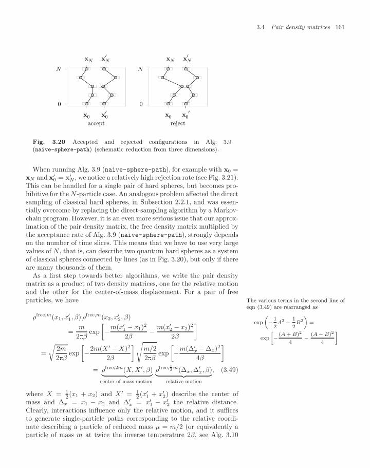
3.4 Pair density matrices 161
accept
0
N
xN
x0
xN′
x0′
reject
0
N
xN
x0
xN′
x0′
Fig. 3.20 Accepted and rejected configurations in Alg. 3.9(naive-sphere-path) (schematic reduction from three dimensions).
When running Alg. 3.9 (naive-sphere-path), for example with x0 =xN and x′
0 = x′N , we notice a relatively high rejection rate (see Fig. 3.21).
This can be handled for a single pair of hard spheres, but becomes pro-hibitive for the N -particle case. An analogous problem affected the directsampling of classical hard spheres, in Subsection 2.2.1, and was essen-tially overcome by replacing the direct-sampling algorithm by a Markov-chain program. However, it is an even more serious issue that our approx-imation of the pair density matrix, the free density matrix multiplied bythe acceptance rate of Alg. 3.9 (naive-sphere-path), strongly dependson the number of time slices. This means that we have to use very largevalues of N , that is, can describe two quantum hard spheres as a systemof classical spheres connected by lines (as in Fig. 3.20), but only if thereare many thousands of them.
As a first step towards better algorithms, we write the pair densitymatrix as a product of two density matrices, one for the relative motionand the other for the center-of-mass displacement. For a pair of freeparticles, we have The various terms in the second line of
eqn (3.49) are rearranged as
exp„−1
2A2 − 1
2B2
«=
exp»− (A + B)2
4− (A − B)2
4
–ρfree,m(x1, x
′1, β) ρfree,m(x2, x
′2, β)
=m
2βexp[−m(x′
1 − x1)2
2β− m(x′
2 − x2)2
2β
]=√
2m
2βexp[−2m(X ′ − X)2
2β
]√m/22β
exp[−m(∆′
x − ∆x)2
4β
]= ρfree,2m(X, X ′, β)︸ ︷︷ ︸
center of mass motion
ρfree,12 m(∆x, ∆′x, β)︸ ︷︷ ︸
relative motion
, (3.49)
where X = 12 (x1 + x2) and X ′ = 1
2 (x′1 + x′
2) describe the center ofmass and ∆x = x1 − x2 and ∆′
x = x′1 − x′
2 the relative distance.Clearly, interactions influence only the relative motion, and it sufficesto generate single-particle paths corresponding to the relative coordi-nate describing a particle of reduced mass µ = m/2 (or equivalently aparticle of mass m at twice the inverse temperature 2β, see Alg. 3.10
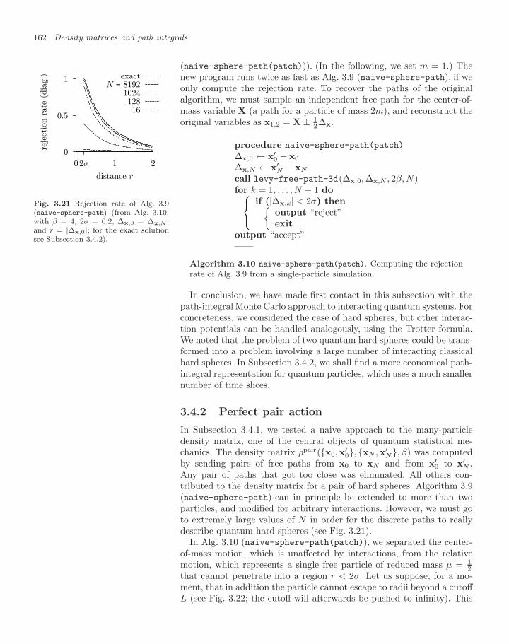
162 Density matrices and path integrals
(naive-sphere-path(patch))). (In the following, we set m = 1.) Thenew program runs twice as fast as Alg. 3.9 (naive-sphere-path), if weonly compute the rejection rate. To recover the paths of the originalalgorithm, we must sample an independent free path for the center-of-mass variable X (a path for a particle of mass 2m), and reconstruct theoriginal variables as x1,2 = X ± 1
2∆x.
0
0.5
1
212σ0
reje
ctio
n r
ate
(dia
g.)
distance r
exactN = 8192
102412816
Fig. 3.21 Rejection rate of Alg. 3.9(naive-sphere-path) (from Alg. 3.10,with β = 4, 2σ = 0.2, ∆x,0 = ∆x,N ,and r = |∆x,0|; for the exact solutionsee Subsection 3.4.2).
procedure naive-sphere-path(patch)
∆x,0 ← x′0 − x0
∆x,N ← x′N − xN
call levy-free-path-3d(∆x,0, ∆x,N , 2β, N)for k = 1, . . . , N − 1 do⎧⎨⎩
if (|∆x,k| < 2σ) thenoutput “reject”exit
output “accept”——
Algorithm 3.10 naive-sphere-path(patch). Computing the rejectionrate of Alg. 3.9 from a single-particle simulation.
In conclusion, we have made first contact in this subsection with thepath-integral Monte Carlo approach to interacting quantum systems. Forconcreteness, we considered the case of hard spheres, but other interac-tion potentials can be handled analogously, using the Trotter formula.We noted that the problem of two quantum hard spheres could be trans-formed into a problem involving a large number of interacting classicalhard spheres. In Subsection 3.4.2, we shall find a more economical path-integral representation for quantum particles, which uses a much smallernumber of time slices.
3.4.2 Perfect pair action
In Subsection 3.4.1, we tested a naive approach to the many-particledensity matrix, one of the central objects of quantum statistical me-chanics. The density matrix ρpair(x0,x
′0, xN ,x′
N, β) was computedby sending pairs of free paths from x0 to xN and from x′
0 to x′N .
Any pair of paths that got too close was eliminated. All others con-tributed to the density matrix for a pair of hard spheres. Algorithm 3.9(naive-sphere-path) can in principle be extended to more than twoparticles, and modified for arbitrary interactions. However, we must goto extremely large values of N in order for the discrete paths to reallydescribe quantum hard spheres (see Fig. 3.21).
In Alg. 3.10 (naive-sphere-path(patch)), we separated the center-of-mass motion, which is unaffected by interactions, from the relativemotion, which represents a single free particle of reduced mass µ = 1
2that cannot penetrate into a region r < 2σ. Let us suppose, for a mo-ment, that in addition the particle cannot escape to radii beyond a cutoffL (see Fig. 3.22; the cutoff will afterwards be pushed to infinity). This
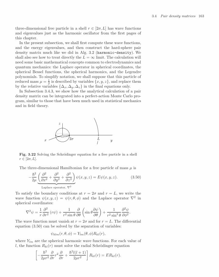
3.4 Pair density matrices 163
three-dimensional free particle in a shell r ∈ [2σ, L] has wave functionsand eigenvalues just as the harmonic oscillator from the first pages ofthis chapter.
In the present subsection, we shall first compute these wave functions,and the energy eigenvalues, and then construct the hard-sphere pairdensity matrix much like we did in Alg. 3.2 (harmonic-density). Weshall also see how to treat directly the L = ∞ limit. The calculation willneed some basic mathematical concepts common to electrodynamics andquantum mechanics: the Laplace operator in spherical coordinates, thespherical Bessel functions, the spherical harmonics, and the Legendrepolynomials. To simplify notation, we shall suppose that this particle ofreduced mass µ = 1
2 is described by variables x, y, z, and replace themby the relative variables ∆x, ∆y, ∆z in the final equations only.
In Subsection 3.4.3, we show how the analytical calculation of a pairdensity matrix can be integrated into a perfect-action Monte Carlo pro-gram, similar to those that have been much used in statistical mechanicsand in field theory.
L y
z
x 2σ
Fig. 3.22 Solving the Schrodinger equation for a free particle in a shellr ∈ [2σ, L].
The three-dimensional Hamiltonian for a free particle of mass µ is
− 2
2µ
(∂2
∂x2+
∂2
∂y2+
∂2
∂z2
)︸ ︷︷ ︸
Laplace operator, ∇2
ψ(x, y, z) = Eψ(x, y, z). (3.50)
To satisfy the boundary conditions at r = 2σ and r = L, we write thewave function ψ(x, y, z) = ψ(r, θ, φ) and the Laplace operator ∇2 inspherical coordinates:
∇2ψ =1r
∂2
∂r2(rψ) +
1r2 sin θ
∂
∂θ
(sin θ
∂ψ
∂θ
)+
1r2 sin2 θ
∂2ψ
∂φ2.
The wave function must vanish at r = 2σ and for r = L. The differentialequation (3.50) can be solved by the separation of variables:
ψklm(r, θ, φ) = Ylm(θ, φ)Rkl(r),
where Ylm are the spherical harmonic wave functions. For each value ofl, the function Rkl(r) must solve the radial Schrodinger equation[
− 2
2µr2
∂
∂rr2 ∂
∂r+
2l(l + 1)2µr2
]Rkl(r) = ERkl(r).
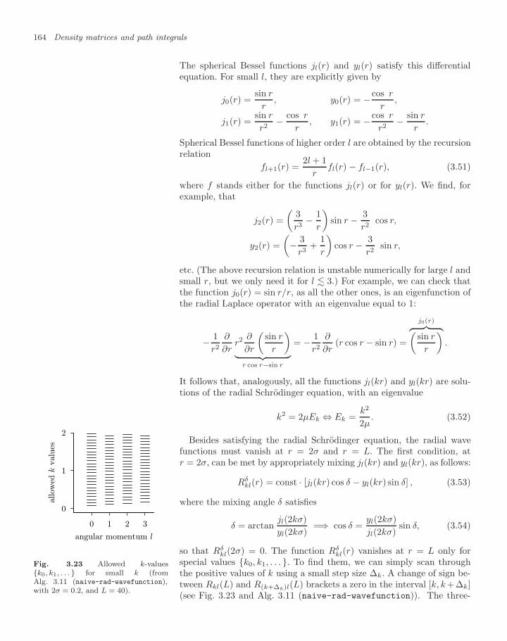
164 Density matrices and path integrals
The spherical Bessel functions jl(r) and yl(r) satisfy this differentialequation. For small l, they are explicitly given by
j0(r) =sin r
r, y0(r) = −cos r
r,
j1(r) =sin r
r2− cos r
r, y1(r) = −cos r
r2− sin r
r.
Spherical Bessel functions of higher order l are obtained by the recursionrelation
fl+1(r) =2l + 1
rfl(r) − fl−1(r), (3.51)
where f stands either for the functions jl(r) or for yl(r). We find, forexample, that
j2(r) =(
3r3
− 1r
)sin r − 3
r2cos r,
y2(r) =(− 3
r3+
1r
)cos r − 3
r2sin r,
etc. (The above recursion relation is unstable numerically for large l andsmall r, but we only need it for l 3.) For example, we can check thatthe function j0(r) = sin r/r, as all the other ones, is an eigenfunction ofthe radial Laplace operator with an eigenvalue equal to 1:
− 1r2
∂
∂rr2 ∂
∂r
(sin r
r
)︸ ︷︷ ︸
r cos r−sin r
= − 1r2
∂
∂r(r cos r − sin r) =
j0(r)︷ ︸︸ ︷(sin r
r
).
It follows that, analogously, all the functions jl(kr) and yl(kr) are solu-tions of the radial Schrodinger equation, with an eigenvalue
k2 = 2µEk ⇔ Ek =k2
2µ. (3.52)
Besides satisfying the radial Schrodinger equation, the radial wavefunctions must vanish at r = 2σ and r = L. The first condition, atr = 2σ, can be met by appropriately mixing jl(kr) and yl(kr), as follows:
Rδkl(r) = const · [jl(kr) cos δ − yl(kr) sin δ] , (3.53)
where the mixing angle δ satisfies
δ = arctanjl(2kσ)yl(2kσ)
=⇒ cos δ =yl(2kσ)jl(2kσ)
sin δ, (3.54)
so that Rδkl(2σ) = 0. The function Rδ
kl(r) vanishes at r = L only forspecial values k0, k1, . . . . To find them, we can simply scan throughthe positive values of k using a small step size ∆k. A change of sign be-tween Rkl(L) and R(k+∆k)l(L) brackets a zero in the interval [k, k +∆k](see Fig. 3.23 and Alg. 3.11 (naive-rad-wavefunction)). The three-
0
1
2
3210
allo
wed
k v
alues
angular momentum l
Fig. 3.23 Allowed k-valuesk0, k1, . . . for small k (fromAlg. 3.11 (naive-rad-wavefunction),with 2σ = 0.2, and L = 40).
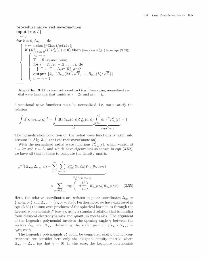
3.4 Pair density matrices 165
procedure naive-rad-wavefunction
input r, σ, Ln ← 0for k = 0, ∆k, . . . do⎧⎪⎪⎪⎪⎪⎪⎪⎪⎪⎪⎨⎪⎪⎪⎪⎪⎪⎪⎪⎪⎪⎩
δ ← arctan [jl(2kσ)/yl(2kσ)]if (Rδ
(k+∆k)l(L)Rδkl(L) < 0) then (function Rδ
kl(r) from eqn (3.53))⎧⎪⎪⎪⎪⎪⎪⎨⎪⎪⎪⎪⎪⎪⎩
kn ← kΥ ← 0 (squared norm)for r = 2σ, 2σ + ∆r, . . . , L do
Υ ← Υ + ∆rr2[Rδ
knl(r)]2
output kn, Rknl(2σ)/√
Υ, . . . , Rknl(L)/√
Υn ← n + 1
——
Algorithm 3.11 naive-rad-wavefunction. Computing normalized ra-dial wave functions that vanish at r = 2σ and at r = L.
dimensional wave functions must be normalized, i.e. must satisfy therelation∫
d3x |ψklm(x)|2 =∫
dΩ Ylm(θ, φ)Y ∗lm(θ, φ)︸ ︷︷ ︸
=1
∫ L
2σ
dr r2R2kl(r)︸ ︷︷ ︸
must be 1
= 1.
The normalization condition on the radial wave functions is taken intoaccount in Alg. 3.11 (naive-rad-wavefunction).
With the normalized radial wave functions Rδknl(r), which vanish at
r = 2σ and r = L, and which have eigenvalues as shown in eqn (3.52),we have all that it takes to compute the density matrix
ρrel(∆x0 , ∆xN, β) =
∞∑l=0
l∑m=−l
Y ∗lm(θ0, φ0)Ylm(θN , φN )︸ ︷︷ ︸
2l+14 Pl(cos γ)
×∑
n=0,1,...
exp(−β
k2n
2µ
)Rknl(r0)Rknl(rN ). (3.55)
Here, the relative coordinates are written in polar coordinates ∆x0 =r0, θ0, φ0 and ∆xN
= rN , θN , φN. Furthermore, we have expressed ineqn (3.55) the sum over products of the spherical harmonics through theLegendre polynomials Pl(cos γ), using a standard relation that is familiarfrom classical electrodynamics and quantum mechanics. The argumentof the Legendre polynomial involves the opening angle γ between thevectors ∆x0 and ∆xN
, defined by the scalar product (∆x0 ··· ∆xN) =
r0rN cos γ.The Legendre polynomials Pl could be computed easily, but for con-
creteness, we consider here only the diagonal density matrix, where∆x0 = ∆xN
(so that γ = 0). In this case, the Legendre polynomials
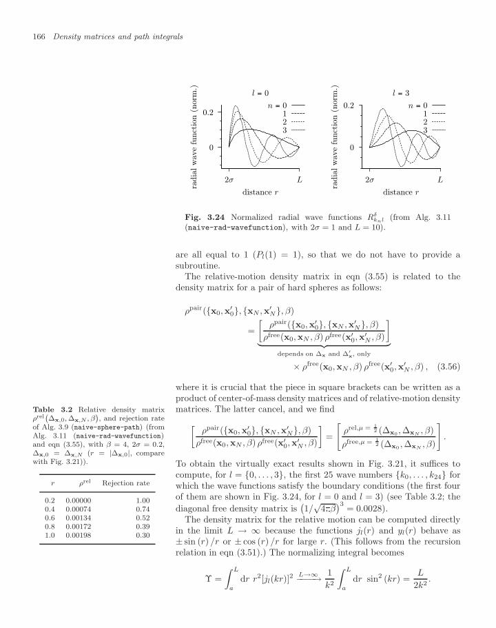
166 Density matrices and path integrals
0
0.2
L2σ
radia
l w
ave
funct
ion (
nor
m.)
distance r
l = 0
n = 0123
0
0.2
L2σ
radia
l w
ave
funct
ion (
nor
m.)
distance r
l = 3
n = 0123
Fig. 3.24 Normalized radial wave functions Rδknl (from Alg. 3.11
(naive-rad-wavefunction), with 2σ = 1 and L = 10).
are all equal to 1 (Pl(1) = 1), so that we do not have to provide asubroutine.
The relative-motion density matrix in eqn (3.55) is related to thedensity matrix for a pair of hard spheres as follows:
ρpair(x0,x′0, xN ,x′
N, β)
=[
ρpair(x0,x′0, xN ,x′
N, β)ρfree(x0,xN , β) ρfree(x′
0,x′N , β)
]︸ ︷︷ ︸
depends on ∆x and ∆′x, only
× ρfree(x0,xN , β) ρfree(x′0,x
′N , β) , (3.56)
where it is crucial that the piece in square brackets can be written as aproduct of center-of-mass density matrices and of relative-motion densitymatrices. The latter cancel, and we find[
ρpair(x0,x′0, xN ,x′
N, β)ρfree(x0,xN , β) ρfree(x′
0,x′N , β)
]=
[ρrel,µ = 1
2 (∆x0 , ∆xN, β)
ρfree,µ = 12 (∆x0 , ∆xN
, β)
].
To obtain the virtually exact results shown in Fig. 3.21, it suffices tocompute, for l = 0, . . . , 3, the first 25 wave numbers k0, . . . , k24 forwhich the wave functions satisfy the boundary conditions (the first fourof them are shown in Fig. 3.24, for l = 0 and l = 3) (see Table 3.2; thediagonal free density matrix is
(1/
√4β)3 = 0.0028).
Table 3.2 Relative density matrixρrel`∆x,0, ∆x,N , β
´, and rejection rate
of Alg. 3.9 (naive-sphere-path) (fromAlg. 3.11 (naive-rad-wavefunction)and eqn (3.55), with β = 4, 2σ = 0.2,∆x,0 = ∆x,N (r = |∆x,0|, comparewith Fig. 3.21)).
r ρrel Rejection rate
0.2 0.00000 1.000.4 0.00074 0.740.6 0.00134 0.520.8 0.00172 0.391.0 0.00198 0.30
The density matrix for the relative motion can be computed directlyin the limit L → ∞ because the functions jl(r) and yl(r) behave as± sin (r) /r or ± cos (r) /r for large r. (This follows from the recursionrelation in eqn (3.51).) The normalizing integral becomes
Υ =∫ L
a
dr r2[jl(kr)]2 L→∞−−−−→ 1k2
∫ L
a
dr sin2 (kr) =L
2k2.
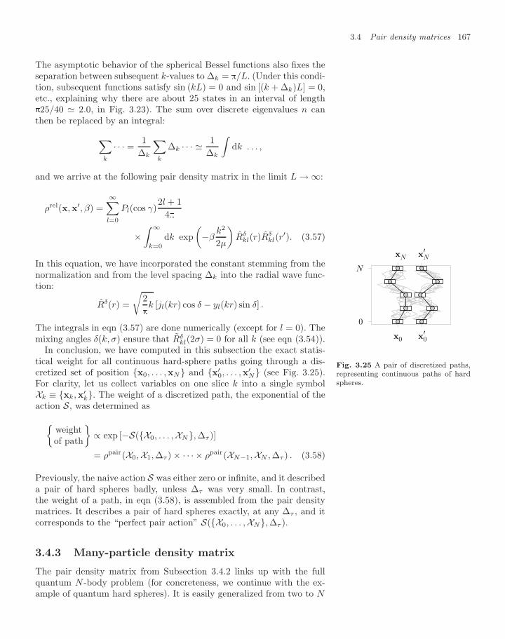
3.4 Pair density matrices 167
The asymptotic behavior of the spherical Bessel functions also fixes theseparation between subsequent k-values to ∆k = /L. (Under this condi-tion, subsequent functions satisfy sin (kL) = 0 and sin [(k + ∆k)L] = 0,etc., explaining why there are about 25 states in an interval of length25/40 2.0, in Fig. 3.23). The sum over discrete eigenvalues n canthen be replaced by an integral:
∑k
· · · =1
∆k
∑k
∆k · · · 1∆k
∫dk . . . ,
and we arrive at the following pair density matrix in the limit L → ∞:
ρrel(x,x′, β) =∞∑
l=0
Pl(cos γ)2l + 1
4
×∫ ∞
k=0
dk exp(−β
k2
2µ
)Rδ
kl(r)Rδkl(r
′). (3.57)
In this equation, we have incorporated the constant stemming from thenormalization and from the level spacing ∆k into the radial wave func-tion:
Rδ(r) =
√2
k [jl(kr) cos δ − yl(kr) sin δ] .
The integrals in eqn (3.57) are done numerically (except for l = 0). Themixing angles δ(k, σ) ensure that Rδ
kl(2σ) = 0 for all k (see eqn (3.54)).
0
N
xN
x0
xN′
x0′
Fig. 3.25 A pair of discretized paths,representing continuous paths of hardspheres.
In conclusion, we have computed in this subsection the exact statis-tical weight for all continuous hard-sphere paths going through a dis-cretized set of position x0, . . . ,xN and x′
0, . . . ,x′N (see Fig. 3.25).
For clarity, let us collect variables on one slice k into a single symbolXk ≡ xk,x′
k. The weight of a discretized path, the exponential of theaction S, was determined as
weightof path
∝ exp [−S(X0, . . . ,XN, ∆τ )]
= ρpair(X0,X1, ∆τ ) × · · · × ρpair(XN−1,XN , ∆τ ) . (3.58)
Previously, the naive action S was either zero or infinite, and it describeda pair of hard spheres badly, unless ∆τ was very small. In contrast,the weight of a path, in eqn (3.58), is assembled from the pair densitymatrices. It describes a pair of hard spheres exactly, at any ∆τ , and itcorresponds to the “perfect pair action” S(X0, . . . ,XN, ∆τ ).
3.4.3 Many-particle density matrix
The pair density matrix from Subsection 3.4.2 links up with the fullquantum N -body problem (for concreteness, we continue with the ex-ample of quantum hard spheres). It is easily generalized from two to N
168 Density matrices and path integrals
particles:
ρN-part(x1, . . . ,xN, x′1, . . . ,x
′N, ∆τ )
N∏k=1
ρfree(xk,x′k, ∆τ )
∏k<l
ρpair(xk,xl, x′k,x′
l, ∆τ )ρfree(xk,x′
k, ∆τ ) ρfree(xl,x′l, ∆τ )︸ ︷︷ ︸
prob. that paths k and l do not collide
. (3.59)
For two particles, this is the same as eqn (3.56), and it is exact. ForN particles, eqn (3.59) remains correct under the condition that we cantreat the collision probabilities for any pair of particles as independent ofthose for other pairs. This condition was already discussed in the contextof the virial expansion for classical hard spheres (see Subsection 2.2.2).It is justified at low density or at high temperature. In the first case (lowdensity) paths rarely collide, so that the paths interfere very little. In thesecond case (∆τ corresponding to high temperature), the path of particlek does not move away far from the position xk x′
k, and the interferenceof paths is again limited. Because of the relation ∆τ = β/N , we canalways find an appropriate value of N for which the N -density matrix ineqn (3.59) is essentially exact. The representation of the density matrixin eqn (3.59) combines elements of a high-temperature expansion andof a low-density expansion. It is sometimes called a Wigner–Kirkwoodexpansion.
In all practical cases, the values of N that must be used are muchsmaller than the number of time slices needed in the naive approach ofSubsection 3.4.1 (see Pollock and Ceperley (1984), Krauth (1996)).
3.5 Geometry of paths
Quantum statistical mechanics can be formulated in terms of randompaths in space and imaginary time. This is the path-integral approachthat we started to discuss in Sections 3.3 and 3.4, and for which wehave barely scratched the surface. Rather than continue with quantumstatistics as it is shaped by path integrals, we analyze in this section theshapes of the paths themselves. This will lead us to new sampling al-gorithms using Fourier transformation methods. The geometry of pathsalso provides an example of the profound connections between classicalstatistical mechanics and quantum physics, because random paths donot appear in quantum physics alone. They can describe cracks in ho-mogeneous media (such as a wall), interfaces between different media(such as between air and oil in a suspension) or else between differentphases of the same medium (such as the regions of a magnet with differ-ent magnetizations). These interfaces are often very rough. They thenresemble the paths of quantum physics, and can be described by verysimilar methods. This will be the subject of Subsection 3.5.3.
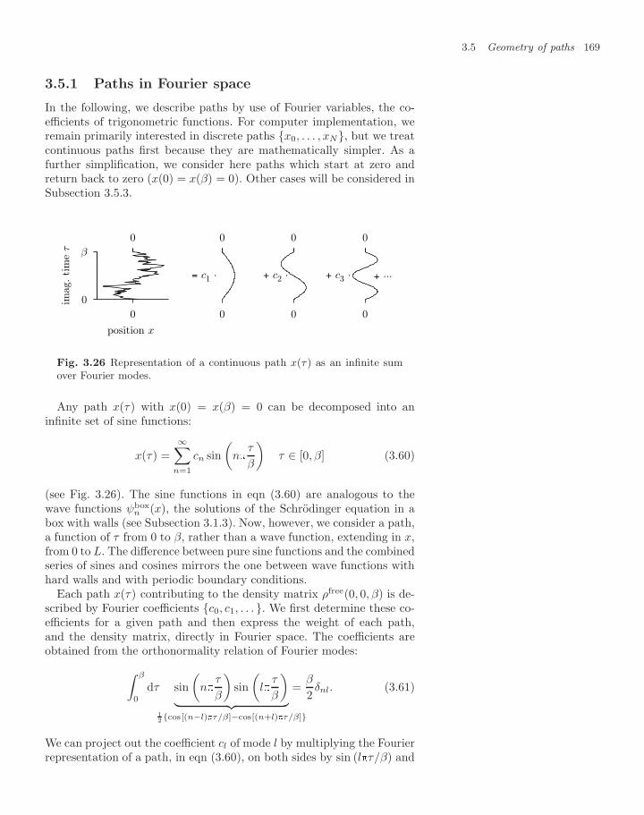
3.5 Geometry of paths 169
3.5.1 Paths in Fourier space
In the following, we describe paths by use of Fourier variables, the co-efficients of trigonometric functions. For computer implementation, weremain primarily interested in discrete paths x0, . . . , xN, but we treatcontinuous paths first because they are mathematically simpler. As afurther simplification, we consider here paths which start at zero andreturn back to zero (x(0) = x(β) = 0). Other cases will be considered inSubsection 3.5.3.
β
0
0000
0000
imag. ti
me
τ
position x
= c1 · + c2 · + c3 · + ···
Fig. 3.26 Representation of a continuous path x(τ ) as an infinite sumover Fourier modes.
Any path x(τ) with x(0) = x(β) = 0 can be decomposed into aninfinite set of sine functions:
x(τ) =∞∑
n=1
cn sin(
nτ
β
)τ ∈ [0, β] (3.60)
(see Fig. 3.26). The sine functions in eqn (3.60) are analogous to thewave functions ψbox
n (x), the solutions of the Schrodinger equation in abox with walls (see Subsection 3.1.3). Now, however, we consider a path,a function of τ from 0 to β, rather than a wave function, extending in x,from 0 to L. The difference between pure sine functions and the combinedseries of sines and cosines mirrors the one between wave functions withhard walls and with periodic boundary conditions.
Each path x(τ) contributing to the density matrix ρfree(0, 0, β) is de-scribed by Fourier coefficients c0, c1, . . . . We first determine these co-efficients for a given path and then express the weight of each path,and the density matrix, directly in Fourier space. The coefficients areobtained from the orthonormality relation of Fourier modes:∫ β
0
dτ sin(
nτ
β
)sin(
lτ
β
)︸ ︷︷ ︸
12cos[(n−l)τ/β]−cos[(n+l)τ/β]
=β
2δnl. (3.61)
We can project out the coefficient cl of mode l by multiplying the Fourierrepresentation of a path, in eqn (3.60), on both sides by sin (lτ/β) and
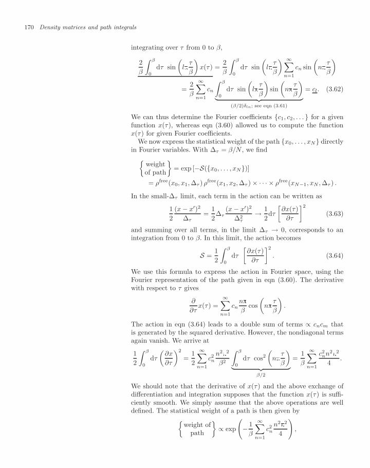
170 Density matrices and path integrals
integrating over τ from 0 to β,
2β
∫ β
0
dτ sin(
lτ
β
)x(τ) =
2β
∫ β
0
dτ sin(
lτ
β
) ∞∑n=1
cn sin(
nτ
β
)
=2β
∞∑n=1
cn
∫ β
0
dτ sin(
lτ
β
)sin(
nτ
β
)︸ ︷︷ ︸
(β/2)δln; see eqn (3.61)
= cl. (3.62)
We can thus determine the Fourier coefficients c1, c2, . . . for a givenfunction x(τ), whereas eqn (3.60) allowed us to compute the functionx(τ) for given Fourier coefficients.
We now express the statistical weight of the path x0, . . . , xN directlyin Fourier variables. With ∆τ = β/N , we find
weightof path
= exp [−S(x0, . . . , xN)]
= ρfree(x0, x1, ∆τ ) ρfree(x1, x2, ∆τ ) × · · · × ρfree(xN−1, xN , ∆τ ) .
In the small-∆τ limit, each term in the action can be written as
12
(x − x′)2
∆τ=
12
∆τ(x − x′)2
∆2τ
→ 12
dτ
[∂x(τ)
∂τ
]2(3.63)
and summing over all terms, in the limit ∆τ → 0, corresponds to anintegration from 0 to β. In this limit, the action becomes
S =12
∫ β
0
dτ
[∂x(τ)
∂τ
]2. (3.64)
We use this formula to express the action in Fourier space, using theFourier representation of the path given in eqn (3.60). The derivativewith respect to τ gives
∂
∂τx(τ) =
∞∑n=1
cnn
βcos(
nτ
β
).
The action in eqn (3.64) leads to a double sum of terms ∝ cncm thatis generated by the squared derivative. However, the nondiagonal termsagain vanish. We arrive at
12
∫ β
0
dτ
(∂x
∂τ
)2
=12
∞∑n=1
c2n
n22
β2
∫ β
0
dτ cos2(
nτ
β
)︸ ︷︷ ︸
β/2
=1β
∞∑n=1
c2nn2
2
4.
We should note that the derivative of x(τ) and the above exchange ofdifferentiation and integration supposes that the function x(τ) is suffi-ciently smooth. We simply assume that the above operations are welldefined. The statistical weight of a path is then given by
weight ofpath
∝ exp
(− 1
β
∞∑n=1
c2n
n22
4
),
3.5 Geometry of paths 171
and the density matrix, written in terms of Fourier variables, is an infi-nite product of integrals:
ρfree(0, 0, β) ∝∞∏
n=1
[∫ ∞
−∞
dcnn√4β
exp
(− 1
β
∞∑n=1
c2n
n22
4
)].
The Fourier transform of a continuous path is operationally quite sim-ple but, as mentioned, hides mathematical subtleties. These difficultiesare absent for the Fourier transformation of discrete paths x0, . . . , xN,a subject we now turn to.
A discrete function x0, . . . , xN can be represented by a finite numberN of Fourier modes:
xk =N−1∑n=1
cn sin(
nk
N
)k = 0, . . . , N (3.65)
(see Fig. 3.27). Remarkably, the discrete sine functions remain mutuallyorthogonal if we simply replace the integral over τ in the orthogonalitycondition in eqn (3.61) by the sum over a discrete index k: In the following, k and j are discretized
τ indices, and n and l describe Fouriermodes.
β
0
0000
0000
imag. ti
me
τ
position x
= c1 · + c2 · + c3 ·
Fig. 3.27 Representation of a discrete path x0, . . . , x4 as a finite sumover Fourier modes.
N−1∑k=1
sin(
nk
N
)sin(
lk
N
)︸ ︷︷ ︸
12cos[(n−l)k/N ]−cos[(n+l)k/N ]
=N
2δnl. (3.66)
Equation (3.66) can be checked in exponential notation (cos x = Re(eix))by summing the geometric series for noninteger M/N :
N−1∑k=0
cos M
k
N= Re
N−1∑k=0
exp(
iM
N
)k
= Re
[1 − eiM
1 − exp(iMN
)] . (3.67)
In eqn (3.66), (n − l) and (n + l) are either both even or odd. In thefirst case, the sum in eqn (3.67) is zero. In the second, the two sums areeasily seen to be equal. They thus cancel.
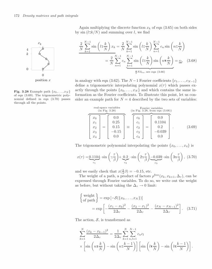
172 Density matrices and path integrals
Again multiplying the discrete function xk of eqn (3.65) on both sidesby sin (lk/N) and summing over l, we find
2N
N−1∑k=1
sin(
lk
N
)xk =
2N
N−1∑k=1
sin(
lk
N
)N−1∑n=1
cn sin(
nk
N
)
=2N
N−1∑n=1
cn
N−1∑k=1
sin(
lk
N
)sin(
nk
N
)︸ ︷︷ ︸
12 Nδln, see eqn (3.66)
= cl, (3.68)
in analogy with eqn (3.62). The N −1 Fourier coefficients c1, . . . , cN−1
0
xk
k
4
0
position x
Fig. 3.28 Example path x0, . . . , xNof eqn (3.69). The trigonometric poly-nomial defined in eqn (3.70) passesthrough all the points.
define a trigonometric interpolating polynomial x(τ) which passes ex-actly through the points x0, . . . , xN and which contains the same in-formation as the Fourier coefficients. To illustrate this point, let us con-sider an example path for N = 4 described by the two sets of variables:
real-space variables(in Fig. 3.28)︷ ︸︸ ︷⎡⎢⎢⎢⎢⎣
x0
x1
x2
x3
x4
⎤⎥⎥⎥⎥⎦ =
⎡⎢⎢⎢⎢⎣0.00.250.15−0.15
0.0
⎤⎥⎥⎥⎥⎦ ≡
Fourier variables(in Fig. 3.28, from eqn (3.68))︷ ︸︸ ︷⎡⎢⎢⎢⎢⎣
c0
c1
c2
c3
c4
⎤⎥⎥⎥⎥⎦ =
⎡⎢⎢⎢⎢⎣0.0
0.11040.2
−0.0390.0
⎤⎥⎥⎥⎥⎦ . (3.69)
The trigonometric polynomial interpolating the points x0, . . . , x4 is
x(τ) =0.1104︸ ︷︷ ︸c1
· sin(
τ
β
)+ 0.2︸︷︷︸
c2
· sin(
2τ
β
)−0.039︸ ︷︷ ︸
c3
· sin(
3τ
β
), (3.70)
and we easily check that x(34β) = −0.15, etc.
The weight of a path, a product of factors ρfree(xk, xk+1, ∆τ ), can beexpressed through Fourier variables. To do so, we write out the weightas before, but without taking the ∆τ → 0 limit:
weightof path
= exp [−S(x0, . . . , xN)]
= exp[− (x1 − x0)2
2∆τ− (x2 − x1)2
2∆τ− (xN − xN−1)2
2∆τ
]. (3.71)
The action, S, is transformed as
N∑k=1
(xk − xk−1)2
2∆τ=
12∆τ
N∑k=1
N−1∑n,l=1
cncl
×[sin(
nk
N
)− sin
(n
k − 1N
)][sin(
lk
N
)− sin
(l
k − 1N
)].
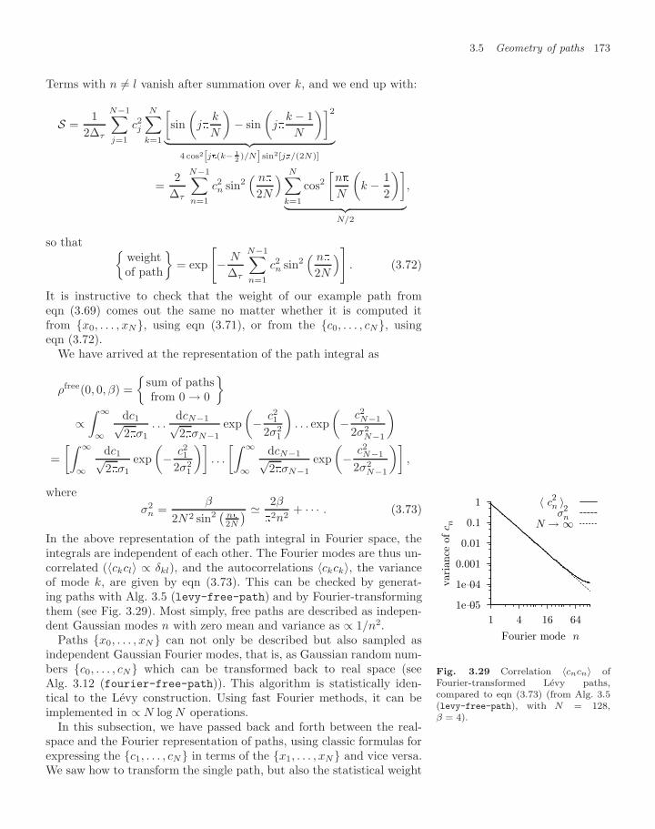
3.5 Geometry of paths 173
Terms with n = l vanish after summation over k, and we end up with:
S =1
2∆τ
N−1∑j=1
c2j
N∑k=1
[sin(
jk
N
)− sin
(j
k − 1N
)]2︸ ︷︷ ︸
4 cos2[j(k− 12 )/N] sin2[j/(2N)]
=2
∆τ
N−1∑n=1
c2n sin2
( n
2N
) N∑k=1
cos2[n
N
(k − 1
2
)]︸ ︷︷ ︸
N/2
,
so that weightof path
= exp
[− N
∆τ
N−1∑n=1
c2n sin2
( n
2N
)]. (3.72)
It is instructive to check that the weight of our example path fromeqn (3.69) comes out the same no matter whether it is computed itfrom x0, . . . , xN, using eqn (3.71), or from the c0, . . . , cN, usingeqn (3.72).
We have arrived at the representation of the path integral as
ρfree(0, 0, β) =
sum of pathsfrom 0 → 0
∝∫ ∞
∞
dc1√2σ1
. . .dcN−1√2σN−1
exp(− c2
1
2σ21
). . . exp
(− c2
N−1
2σ2N−1
)=[∫ ∞
∞
dc1√2σ1
exp(− c2
1
2σ21
)]. . .
[∫ ∞
∞
dcN−1√2σN−1
exp(− c2
N−1
2σ2N−1
)],
whereσ2
n =β
2N2 sin2(
n2N
) 2β
2n2
+ · · · . (3.73)
In the above representation of the path integral in Fourier space, theintegrals are independent of each other. The Fourier modes are thus un-correlated (〈ckcl〉 ∝ δkl), and the autocorrelations 〈ckck〉, the varianceof mode k, are given by eqn (3.73). This can be checked by generat-ing paths with Alg. 3.5 (levy-free-path) and by Fourier-transformingthem (see Fig. 3.29). Most simply, free paths are described as indepen-dent Gaussian modes n with zero mean and variance as ∝ 1/n2.
Paths x0, . . . , xN can not only be described but also sampled asindependent Gaussian Fourier modes, that is, as Gaussian random num-bers c0, . . . , cN which can be transformed back to real space (seeAlg. 3.12 (fourier-free-path)). This algorithm is statistically iden-tical to the Levy construction. Using fast Fourier methods, it can beimplemented in ∝ N log N operations.
1e-05
1e-04
0.001
0.01
0.1
1
1 4 16 64
var
iance
of c n
Fourier mode n
〈 cn2 〉 σn
2
N → ∞
Fig. 3.29 Correlation 〈cncn〉 ofFourier-transformed Levy paths,compared to eqn (3.73) (from Alg. 3.5(levy-free-path), with N = 128,β = 4).
In this subsection, we have passed back and forth between the real-space and the Fourier representation of paths, using classic formulas forexpressing the c1, . . . , cN in terms of the x1, . . . , xN and vice versa.We saw how to transform the single path, but also the statistical weight
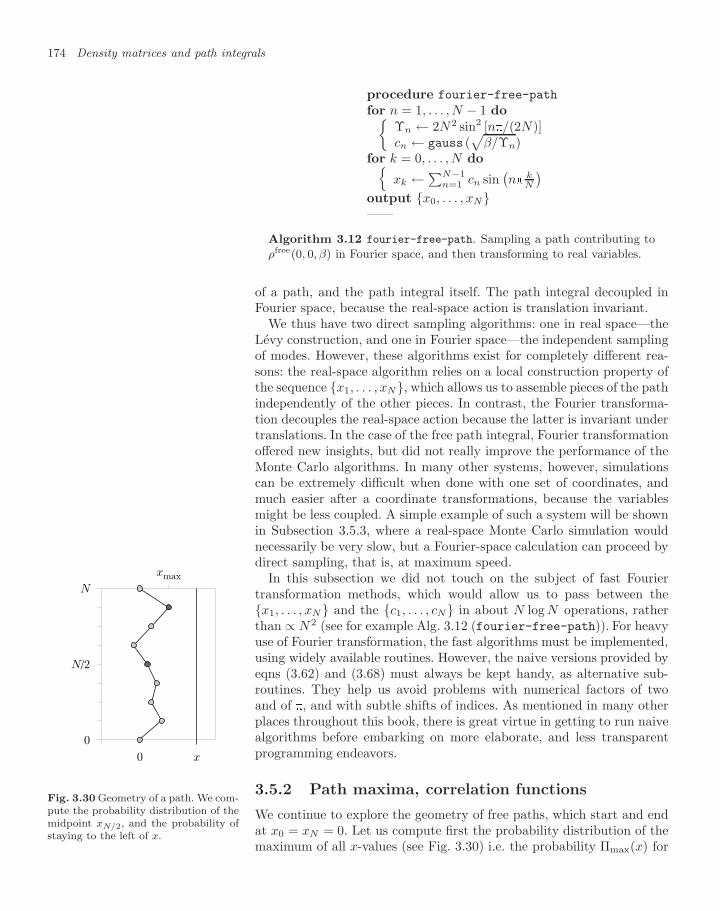
174 Density matrices and path integrals
procedure fourier-free-path
for n = 1, . . . , N − 1 doΥn ← 2N2 sin2 [n/(2N)]cn ← gauss (
√β/Υn)
for k = 0, . . . , N doxk ←∑N−1
n=1 cn sin(n k
N
)output x0, . . . , xN——
Algorithm 3.12 fourier-free-path. Sampling a path contributing to
ρfree(0, 0, β) in Fourier space, and then transforming to real variables.
of a path, and the path integral itself. The path integral decoupled inFourier space, because the real-space action is translation invariant.
We thus have two direct sampling algorithms: one in real space—theLevy construction, and one in Fourier space—the independent samplingof modes. However, these algorithms exist for completely different rea-sons: the real-space algorithm relies on a local construction property ofthe sequence x1, . . . , xN, which allows us to assemble pieces of the pathindependently of the other pieces. In contrast, the Fourier transforma-tion decouples the real-space action because the latter is invariant undertranslations. In the case of the free path integral, Fourier transformationoffered new insights, but did not really improve the performance of theMonte Carlo algorithms. In many other systems, however, simulationscan be extremely difficult when done with one set of coordinates, andmuch easier after a coordinate transformations, because the variablesmight be less coupled. A simple example of such a system will be shownin Subsection 3.5.3, where a real-space Monte Carlo simulation wouldnecessarily be very slow, but a Fourier-space calculation can proceed bydirect sampling, that is, at maximum speed.
In this subsection we did not touch on the subject of fast Fouriertransformation methods, which would allow us to pass between thex1, . . . , xN and the c1, . . . , cN in about N log N operations, ratherthan ∝ N2 (see for example Alg. 3.12 (fourier-free-path)). For heavyuse of Fourier transformation, the fast algorithms must be implemented,using widely available routines. However, the naive versions provided byeqns (3.62) and (3.68) must always be kept handy, as alternative sub-routines. They help us avoid problems with numerical factors of twoand of , and with subtle shifts of indices. As mentioned in many otherplaces throughout this book, there is great virtue in getting to run naivealgorithms before embarking on more elaborate, and less transparentprogramming endeavors.
3.5.2 Path maxima, correlation functions
0
N/2
N
x
xmax
0
Fig. 3.30 Geometry of a path. We com-pute the probability distribution of themidpoint xN/2, and the probability ofstaying to the left of x.
We continue to explore the geometry of free paths, which start and endat x0 = xN = 0. Let us compute first the probability distribution of themaximum of all x-values (see Fig. 3.30) i.e. the probability Πmax(x) for
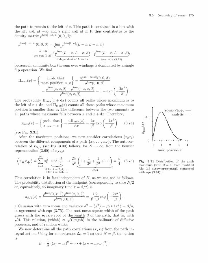
3.5 Geometry of paths 175
the path to remain to the left of x. This path is contained in a box withthe left wall at −∞ and a right wall at x. It thus contributes to thedensity matrix ρbox[−∞, x](0, 0, β):
ρbox[−∞, x](0, 0, β) = limL→∞
ρbox[0, L](L − x, L − x, β)
L→∞−−−−−−−−−→see eqn (3.23)
ρfree(L − x, L − x, β)︸ ︷︷ ︸independent of L and x
− ρfree(L − x, L + x, β)︸ ︷︷ ︸from eqn (3.23)
,
because in an infinite box the sum over windings is dominated by a singleflip operation. We find
Πmax(x) =
prob. thatmax. position < x
=
ρbox[−∞, x](0, 0, β)ρfree(0, 0, β)
=ρfree(x, x, β) − ρfree(−x, x, β)
ρfree(x, x, β)= 1 − exp
(−2x2
β
).
The probability Πmax(x + dx) counts all paths whose maximum is tothe left of x + dx, and Πmax(x) counts all those paths whose maximumposition is smaller than x. The difference between the two amounts toall paths whose maximum falls between x and x + dx. Therefore,
πmax(x) =
prob. thatxmax = x
=
dΠmax(x)dx
=4x
βexp(−2x2
β
)(3.74)
(see Fig. 3.31).After the maximum positions, we now consider correlations 〈xkxl〉
between the different components of a path x0, . . . , xN. The autocor-relation of xN/2 (see Fig. 3.30) follows, for N → ∞, from the Fourierrepresentation (3.60) of xN/2:
0
0.5
0 1 2 3 4π
max
(x)
max. position x
Monte Carloanalytic
Fig. 3.31 Distribution of the pathmaximum (with β = 4, from modifiedAlg. 3.5 (levy-free-path), comparedwith eqn (3.74)).
⟨xN
2xN
2
⟩=
∞∑k=1
σ2k sin2 k
2︸ ︷︷ ︸0 for k = 2, 4, . . .1 for k = 1, 3, . . .
→ 2β
2
(1 +
132
+152
+ · · ·)
︸ ︷︷ ︸2/8
=β
4. (3.75)
This correlation is in fact independent of N , as we can see as follows.The probability distribution of the midpoint (corresponding to slice N/2or, equivalently, to imaginary time τ = β/2) is
πβ/2(x) =ρfree(0, x, β
2 ) ρfree(x, 0, β2 )
ρfree(0, 0, β)=√
2β
exp(−2x2
β
),
a Gaussian with zero mean and variance σ2 =⟨x2⟩
= β/4⟨x2⟩
= β/4,in agreement with eqn (3.75). The root mean square width of the pathgrows with the square root of the length β of the path, that is, with√
β. This relation, (width) ∝ √(length), is the hallmark of diffusiveprocesses, and of random walks.
We now determine all the path correlations 〈xkxl〉 from the path in-tegral action. Using for concreteness ∆τ = 1 so that N = β, the actionis
S =12[(x1 − x0)2 + · · · + (xN − xN−1)2
].
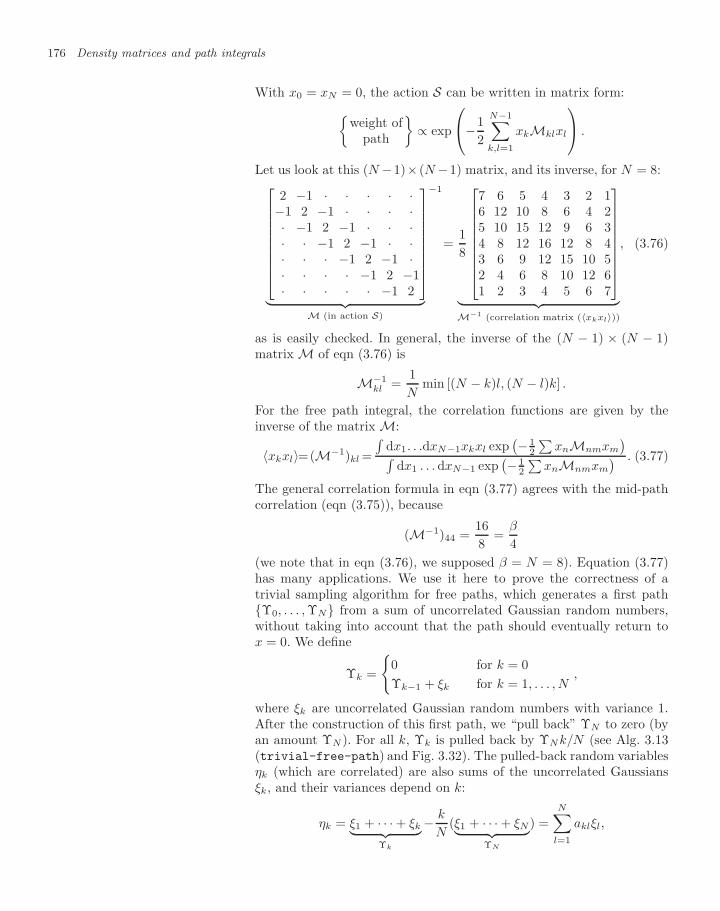
176 Density matrices and path integrals
With x0 = xN = 0, the action S can be written in matrix form:weight of
path
∝ exp
⎛⎝−12
N−1∑k,l=1
xkMklxl
⎞⎠ .
Let us look at this (N −1)× (N −1) matrix, and its inverse, for N = 8:⎡⎢⎢⎢⎢⎢⎢⎢⎢⎣
2 −1 · · · · ·−1 2 −1 · · · ·· −1 2 −1 · · ·· · −1 2 −1 · ·· · · −1 2 −1 ·· · · · −1 2 −1· · · · · −1 2
⎤⎥⎥⎥⎥⎥⎥⎥⎥⎦
−1
︸ ︷︷ ︸M (in action S)
=18
⎡⎢⎢⎢⎢⎢⎢⎢⎢⎣
7 6 5 4 3 2 16 12 10 8 6 4 25 10 15 12 9 6 34 8 12 16 12 8 43 6 9 12 15 10 52 4 6 8 10 12 61 2 3 4 5 6 7
⎤⎥⎥⎥⎥⎥⎥⎥⎥⎦︸ ︷︷ ︸M−1 (correlation matrix (〈xkxl〉))
, (3.76)
as is easily checked. In general, the inverse of the (N − 1) × (N − 1)matrix M of eqn (3.76) is
M−1kl =
1N
min [(N − k)l, (N − l)k] .
For the free path integral, the correlation functions are given by theinverse of the matrix M:
〈xkxl〉=(M−1)kl =
∫dx1. . .dxN−1xkxl exp
(− 12
∑xnMnmxm
)∫dx1 . . . dxN−1 exp
(− 12
∑xnMnmxm
) . (3.77)
The general correlation formula in eqn (3.77) agrees with the mid-pathcorrelation (eqn (3.75)), because
(M−1)44 =168
=β
4(we note that in eqn (3.76), we supposed β = N = 8). Equation (3.77)has many applications. We use it here to prove the correctness of atrivial sampling algorithm for free paths, which generates a first pathΥ0, . . . , ΥN from a sum of uncorrelated Gaussian random numbers,without taking into account that the path should eventually return tox = 0. We define
Υk =
0 for k = 0Υk−1 + ξk for k = 1, . . . , N
,
where ξk are uncorrelated Gaussian random numbers with variance 1.After the construction of this first path, we “pull back” ΥN to zero (byan amount ΥN ). For all k, Υk is pulled back by ΥNk/N (see Alg. 3.13(trivial-free-path) and Fig. 3.32). The pulled-back random variablesηk (which are correlated) are also sums of the uncorrelated Gaussiansξk, and their variances depend on k:
ηk = ξ1 + · · · + ξk︸ ︷︷ ︸Υk
− k
N(ξ1 + · · · + ξN︸ ︷︷ ︸
ΥN
) =N∑
l=1
aklξl,
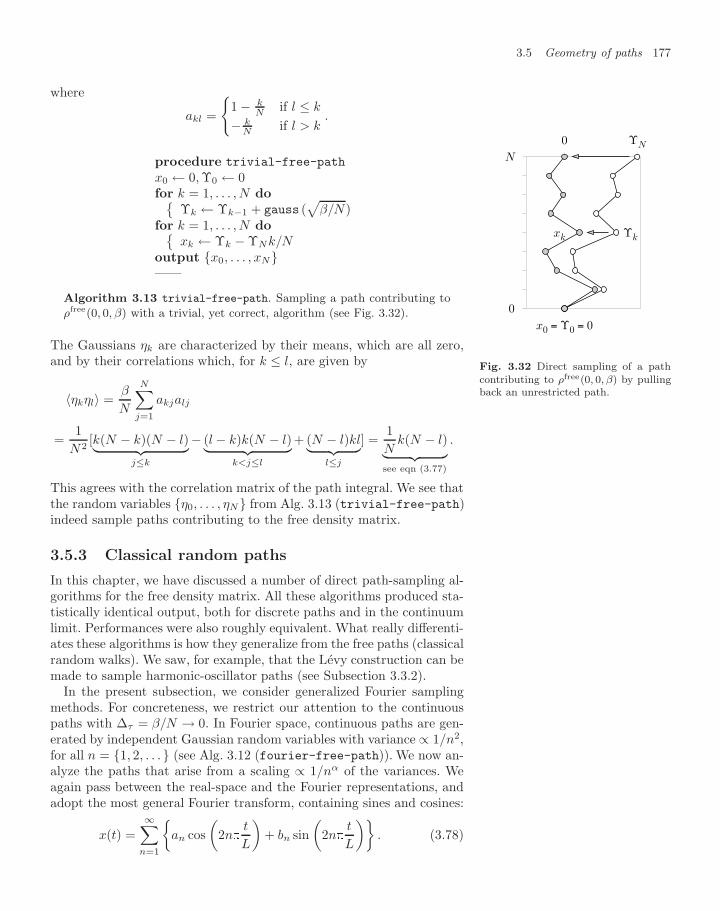
3.5 Geometry of paths 177
where
akl =
1 − k
N if l ≤ k
− kN if l > k
.
procedure trivial-free-path
x0 ← 0, Υ0 ← 0for k = 1, . . . , N do
Υk ← Υk−1 + gauss (√
β/N)for k = 1, . . . , N do
xk ← Υk − ΥNk/Noutput x0, . . . , xN——
Algorithm 3.13 trivial-free-path. Sampling a path contributing to
ρfree(0, 0, β) with a trivial, yet correct, algorithm (see Fig. 3.32). 0
Υkxk
ΥN0
N
x0 = Υ0 = 0
Fig. 3.32 Direct sampling of a pathcontributing to ρfree(0, 0, β) by pullingback an unrestricted path.
The Gaussians ηk are characterized by their means, which are all zero,and by their correlations which, for k ≤ l, are given by
〈ηkηl〉 =β
N
N∑j=1
akjalj
=1
N2[k(N − k)(N − l)︸ ︷︷ ︸
j≤k
− (l − k)k(N − l)︸ ︷︷ ︸k<j≤l
+ (N − l)kl︸ ︷︷ ︸l≤j
] =1N
k(N − l)︸ ︷︷ ︸see eqn (3.77)
.
This agrees with the correlation matrix of the path integral. We see thatthe random variables η0, . . . , ηN from Alg. 3.13 (trivial-free-path)indeed sample paths contributing to the free density matrix.
3.5.3 Classical random paths
In this chapter, we have discussed a number of direct path-sampling al-gorithms for the free density matrix. All these algorithms produced sta-tistically identical output, both for discrete paths and in the continuumlimit. Performances were also roughly equivalent. What really differenti-ates these algorithms is how they generalize from the free paths (classicalrandom walks). We saw, for example, that the Levy construction can bemade to sample harmonic-oscillator paths (see Subsection 3.3.2).
In the present subsection, we consider generalized Fourier samplingmethods. For concreteness, we restrict our attention to the continuouspaths with ∆τ = β/N → 0. In Fourier space, continuous paths are gen-erated by independent Gaussian random variables with variance ∝ 1/n2,for all n = 1, 2, . . . (see Alg. 3.12 (fourier-free-path)). We now an-alyze the paths that arise from a scaling ∝ 1/nα of the variances. Weagain pass between the real-space and the Fourier representations, andadopt the most general Fourier transform, containing sines and cosines:
x(t) =∞∑
n=1
an cos
(2n
t
L
)+ bn sin
(2n
t
L
). (3.78)
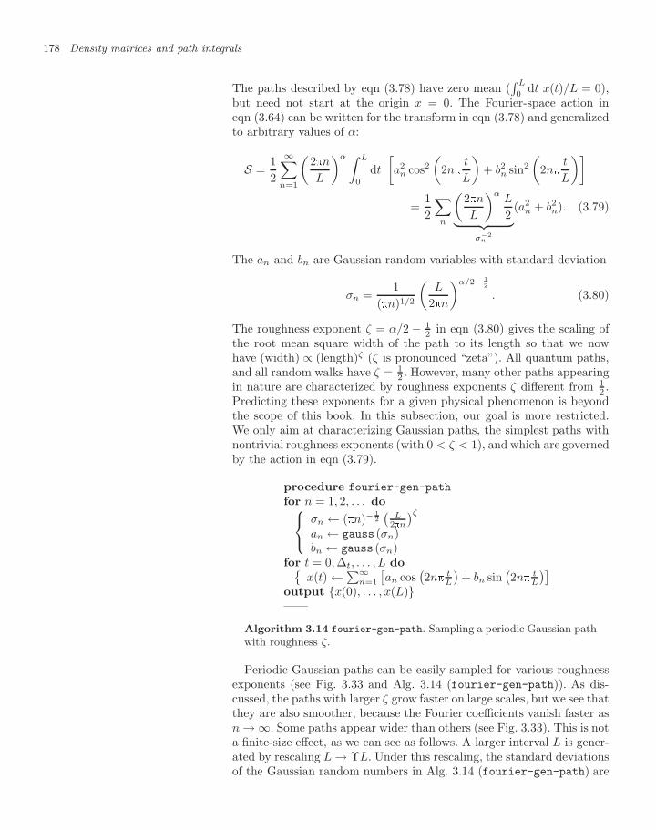
178 Density matrices and path integrals
The paths described by eqn (3.78) have zero mean (∫ L
0dt x(t)/L = 0),
but need not start at the origin x = 0. The Fourier-space action ineqn (3.64) can be written for the transform in eqn (3.78) and generalizedto arbitrary values of α:
S =12
∞∑n=1
(2nL
)α ∫ L
0
dt
[a2
n cos2(
2nt
L
)+ b2
n sin2
(2n
t
L
)]=
12
∑n
(2nL
)αL
2︸ ︷︷ ︸σ−2
n
(a2n + b2
n). (3.79)
The an and bn are Gaussian random variables with standard deviation
σn =1
(n)1/2
(L
2n
)α/2− 12
. (3.80)
The roughness exponent ζ = α/2 − 12 in eqn (3.80) gives the scaling of
the root mean square width of the path to its length so that we nowhave (width) ∝ (length)ζ (ζ is pronounced “zeta”). All quantum paths,and all random walks have ζ = 1
2 . However, many other paths appearingin nature are characterized by roughness exponents ζ different from 1
2 .Predicting these exponents for a given physical phenomenon is beyondthe scope of this book. In this subsection, our goal is more restricted.We only aim at characterizing Gaussian paths, the simplest paths withnontrivial roughness exponents (with 0 < ζ < 1), and which are governedby the action in eqn (3.79).
procedure fourier-gen-path
for n = 1, 2, . . . do⎧⎨⎩ σn ← (n)−12
(L
2n
)ζan ← gauss (σn)bn ← gauss (σn)
for t = 0, ∆t, . . . , L dox(t) ←∑∞
n=1
[an cos
(2n t
L
)+ bn sin
(2n t
L
)]output x(0), . . . , x(L)——
Algorithm 3.14 fourier-gen-path. Sampling a periodic Gaussian pathwith roughness ζ.
Periodic Gaussian paths can be easily sampled for various roughnessexponents (see Fig. 3.33 and Alg. 3.14 (fourier-gen-path)). As dis-cussed, the paths with larger ζ grow faster on large scales, but we see thatthey are also smoother, because the Fourier coefficients vanish faster asn → ∞. Some paths appear wider than others (see Fig. 3.33). This is nota finite-size effect, as we can see as follows. A larger interval L is gener-ated by rescaling L → ΥL. Under this rescaling, the standard deviationsof the Gaussian random numbers in Alg. 3.14 (fourier-gen-path) are
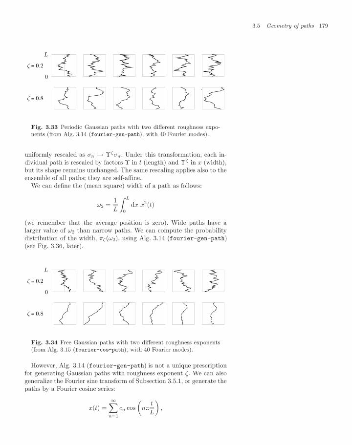
3.5 Geometry of paths 179
ζ = 0.2
0
L
ζ = 0.8
Fig. 3.33 Periodic Gaussian paths with two different roughness expo-nents (from Alg. 3.14 (fourier-gen-path), with 40 Fourier modes).
uniformly rescaled as σn → Υζσn. Under this transformation, each in-dividual path is rescaled by factors Υ in t (length) and Υζ in x (width),but its shape remains unchanged. The same rescaling applies also to theensemble of all paths; they are self-affine.
We can define the (mean square) width of a path as follows:
ω2 =1L
∫ L
0
dx x2(t)
(we remember that the average position is zero). Wide paths have alarger value of ω2 than narrow paths. We can compute the probabilitydistribution of the width, πζ(ω2), using Alg. 3.14 (fourier-gen-path)(see Fig. 3.36, later).
ζ = 0.2
0
L
ζ = 0.8
Fig. 3.34 Free Gaussian paths with two different roughness exponents(from Alg. 3.15 (fourier-cos-path), with 40 Fourier modes).
However, Alg. 3.14 (fourier-gen-path) is not a unique prescriptionfor generating Gaussian paths with roughness exponent ζ. We can alsogeneralize the Fourier sine transform of Subsection 3.5.1, or generate thepaths by a Fourier cosine series:
x(t) =∞∑
n=1
cn cos(
nt
L
),
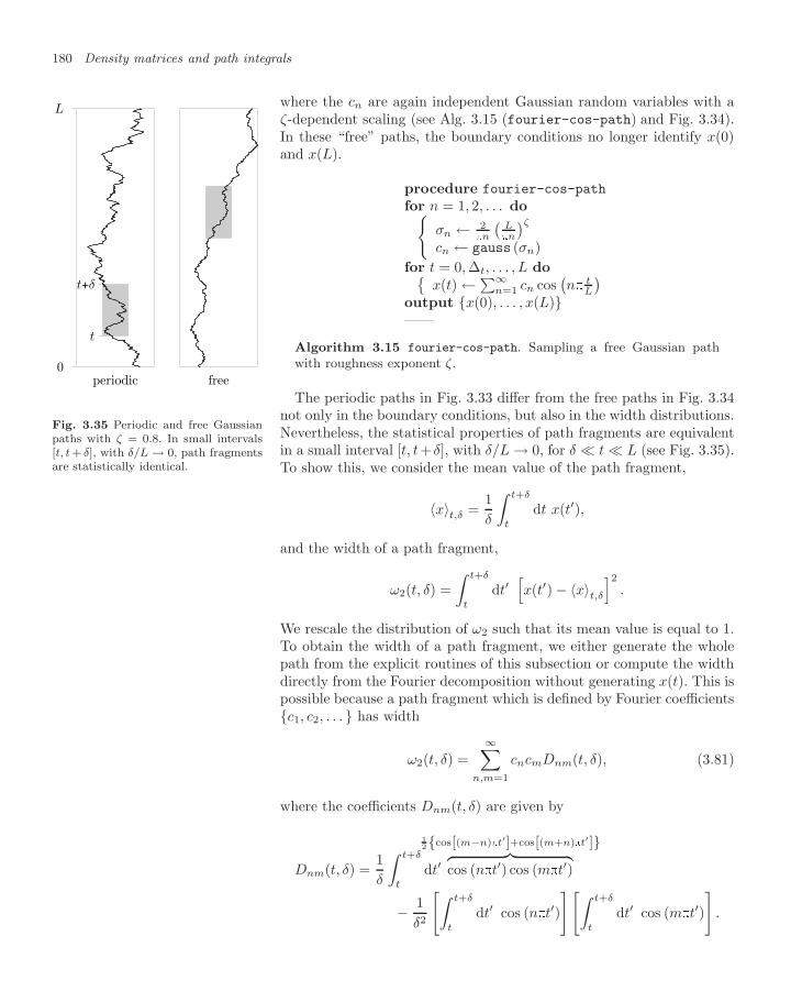
180 Density matrices and path integrals
where the cn are again independent Gaussian random variables with aζ-dependent scaling (see Alg. 3.15 (fourier-cos-path) and Fig. 3.34).In these “free” paths, the boundary conditions no longer identify x(0)and x(L).
procedure fourier-cos-path
for n = 1, 2, . . . doσn ← 2
n
(Ln
)ζcn ← gauss (σn)
for t = 0, ∆t, . . . , L dox(t) ←∑∞
n=1 cn cos(n t
L
)output x(0), . . . , x(L)——
Algorithm 3.15 fourier-cos-path. Sampling a free Gaussian pathwith roughness exponent ζ.0
L
t
t+δ
periodic free
Fig. 3.35 Periodic and free Gaussianpaths with ζ = 0.8. In small intervals[t, t + δ], with δ/L → 0, path fragmentsare statistically identical.
The periodic paths in Fig. 3.33 differ from the free paths in Fig. 3.34not only in the boundary conditions, but also in the width distributions.Nevertheless, the statistical properties of path fragments are equivalentin a small interval [t, t+ δ], with δ/L → 0, for δ t L (see Fig. 3.35).To show this, we consider the mean value of the path fragment,
〈x〉t,δ =1δ
∫ t+δ
t
dt x(t′),
and the width of a path fragment,
ω2(t, δ) =∫ t+δ
t
dt′[x(t′) − 〈x〉t,δ
]2.
We rescale the distribution of ω2 such that its mean value is equal to 1.To obtain the width of a path fragment, we either generate the wholepath from the explicit routines of this subsection or compute the widthdirectly from the Fourier decomposition without generating x(t). This ispossible because a path fragment which is defined by Fourier coefficientsc1, c2, . . . has width
ω2(t, δ) =∞∑
n,m=1
cncmDnm(t, δ), (3.81)
where the coefficients Dnm(t, δ) are given by
Dnm(t, δ) =1δ
∫ t+δ
t
dt′
12cos[(m−n)t′]+cos[(m+n)t′]︷ ︸︸ ︷
cos (nt′) cos (mt′)
− 1δ2
[∫ t+δ
t
dt′ cos (nt′)
][∫ t+δ
t
dt′ cos (mt′)
].
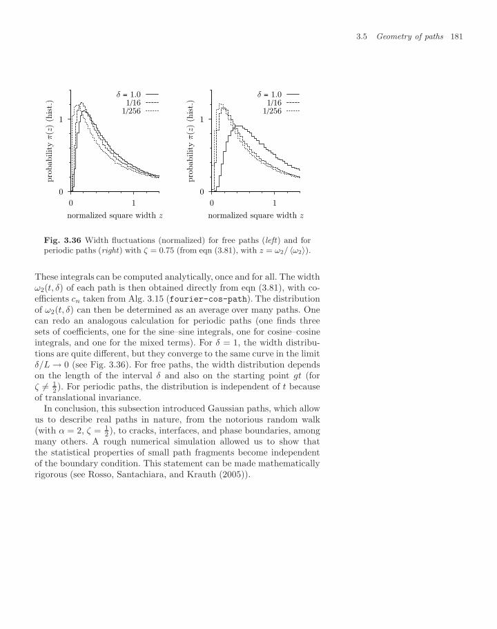
3.5 Geometry of paths 181
0
1
0 1
pro
babilit
y π
(z)
(his
t.)
normalized square width z
δ = 1.0 1/161/256
0
1
0 1
pro
babilit
y π
(z)
(his
t.)
normalized square width z
δ = 1.0 1/161/256
Fig. 3.36 Width fluctuations (normalized) for free paths (left) and forperiodic paths (right) with ζ = 0.75 (from eqn (3.81), with z = ω2/ 〈ω2〉).
These integrals can be computed analytically, once and for all. The widthω2(t, δ) of each path is then obtained directly from eqn (3.81), with co-efficients cn taken from Alg. 3.15 (fourier-cos-path). The distributionof ω2(t, δ) can then be determined as an average over many paths. Onecan redo an analogous calculation for periodic paths (one finds threesets of coefficients, one for the sine–sine integrals, one for cosine–cosineintegrals, and one for the mixed terms). For δ = 1, the width distribu-tions are quite different, but they converge to the same curve in the limitδ/L → 0 (see Fig. 3.36). For free paths, the width distribution dependson the length of the interval δ and also on the starting point gt (forζ = 1
2 ). For periodic paths, the distribution is independent of t becauseof translational invariance.
In conclusion, this subsection introduced Gaussian paths, which allowus to describe real paths in nature, from the notorious random walk(with α = 2, ζ = 1
2 ), to cracks, interfaces, and phase boundaries, amongmany others. A rough numerical simulation allowed us to show thatthe statistical properties of small path fragments become independentof the boundary condition. This statement can be made mathematicallyrigorous (see Rosso, Santachiara, and Krauth (2005)).
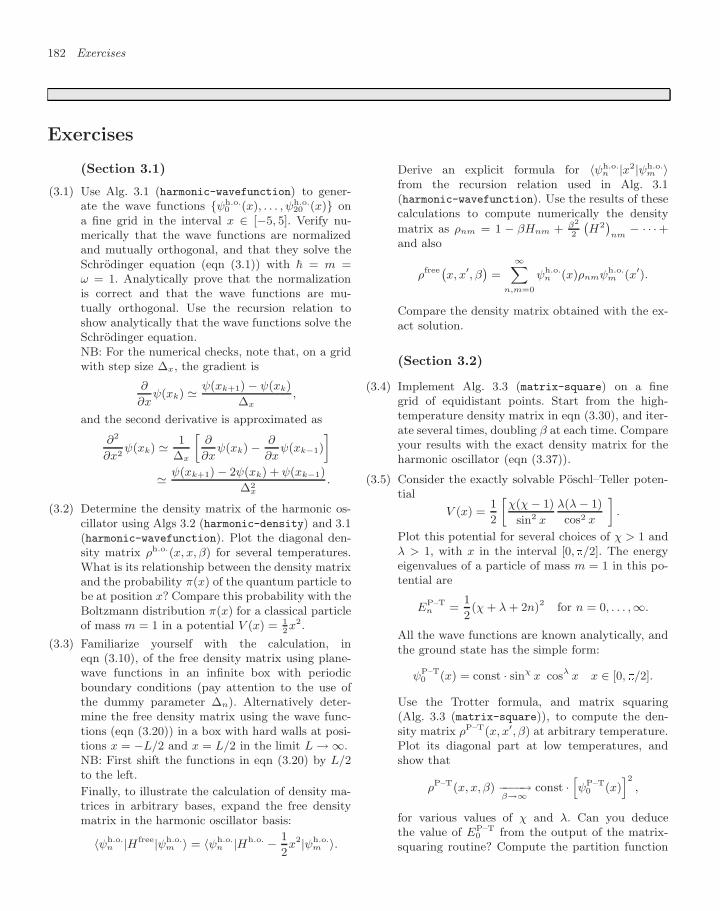
182 Exercises
Exercises
(Section 3.1)
(3.1) Use Alg. 3.1 (harmonic-wavefunction) to gener-ate the wave functions ψh.o.
0 (x), . . . , ψh.o.20 (x) on
a fine grid in the interval x ∈ [−5, 5]. Verify nu-merically that the wave functions are normalizedand mutually orthogonal, and that they solve theSchrodinger equation (eqn (3.1)) with = m =ω = 1. Analytically prove that the normalizationis correct and that the wave functions are mu-tually orthogonal. Use the recursion relation toshow analytically that the wave functions solve theSchrodinger equation.NB: For the numerical checks, note that, on a gridwith step size ∆x, the gradient is
∂
∂xψ(xk) ψ(xk+1) − ψ(xk)
∆x,
and the second derivative is approximated as
∂2
∂x2ψ(xk) 1
∆x
»∂
∂xψ(xk) − ∂
∂xψ(xk−1)
–
ψ(xk+1) − 2ψ(xk) + ψ(xk−1)
∆2x
.
(3.2) Determine the density matrix of the harmonic os-cillator using Algs 3.2 (harmonic-density) and 3.1(harmonic-wavefunction). Plot the diagonal den-sity matrix ρh.o.(x, x, β) for several temperatures.What is its relationship between the density matrixand the probability π(x) of the quantum particle tobe at position x? Compare this probability with theBoltzmann distribution π(x) for a classical particleof mass m = 1 in a potential V (x) = 1
2x2.
(3.3) Familiarize yourself with the calculation, ineqn (3.10), of the free density matrix using plane-wave functions in an infinite box with periodicboundary conditions (pay attention to the use ofthe dummy parameter ∆n). Alternatively deter-mine the free density matrix using the wave func-tions (eqn (3.20)) in a box with hard walls at posi-tions x = −L/2 and x = L/2 in the limit L → ∞.NB: First shift the functions in eqn (3.20) by L/2to the left.
Finally, to illustrate the calculation of density ma-trices in arbitrary bases, expand the free densitymatrix in the harmonic oscillator basis:
〈ψh.o.n |H free|ψh.o.
m 〉 = 〈ψh.o.n |Hh.o. − 1
2x2|ψh.o.
m 〉.
Derive an explicit formula for 〈ψh.o.n |x2|ψh.o.
m 〉from the recursion relation used in Alg. 3.1(harmonic-wavefunction). Use the results of thesecalculations to compute numerically the density
matrix as ρnm = 1 − βHnm + β2
2
`H2
´nm
− · · ·+and also
ρfree`x, x′, β
´=
∞Xn,m=0
ψh.o.n (x)ρnmψh.o.
m (x′).
Compare the density matrix obtained with the ex-act solution.
(Section 3.2)
(3.4) Implement Alg. 3.3 (matrix-square) on a finegrid of equidistant points. Start from the high-temperature density matrix in eqn (3.30), and iter-ate several times, doubling β at each time. Compareyour results with the exact density matrix for theharmonic oscillator (eqn (3.37)).
(3.5) Consider the exactly solvable Poschl–Teller poten-tial
V (x) =1
2
»χ(χ − 1)
sin2 x
λ(λ − 1)
cos2 x
–.
Plot this potential for several choices of χ > 1 andλ > 1, with x in the interval [0, /2]. The energyeigenvalues of a particle of mass m = 1 in this po-tential are
EP–Tn =
1
2(χ + λ + 2n)2 for n = 0, . . . ,∞.
All the wave functions are known analytically, andthe ground state has the simple form:
ψP–T0 (x) = const · sinχ x cosλ x x ∈ [0, /2].
Use the Trotter formula, and matrix squaring(Alg. 3.3 (matrix-square)), to compute the den-sity matrix ρP–T(x, x′, β) at arbitrary temperature.Plot its diagonal part at low temperatures, andshow that
ρP–T(x, x, β) −−−−→β→∞
const ·hψP–T
0 (x)i2
,
for various values of χ and λ. Can you deducethe value of EP–T
0 from the output of the matrix-squaring routine? Compute the partition function
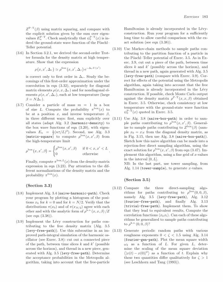
Exercises 183
ZP–T(β) using matrix squaring, and compare withthe explicit solution given by the sum over eigen-values EP–T
n . Check analytically that ψP–T0 (x) is in-
deed the ground-state wave function of the Poschl–Teller potential.
(3.6) In Section 3.2.1, we derived the second-order Trot-ter formula for the density matrix at high temper-ature. Show that the expression
ρ`x, x′, ∆τ
´ ρfree`x, x′, ∆τ
´e−∆τ V (x′)
is correct only to first order in ∆τ . Study the be-comings of this first-order approximation under theconvolution in eqn (3.32), separately for diagonalmatrix elements ρ(x, x, ∆τ ) and for nondiagonal el-ements ρ(x, x′, ∆τ ), each at low temperature (largeβ = N∆τ ).
(3.7) Consider a particle of mass m = 1 in a boxof size L. Compute the probability πbox(x) tobe at a position x, and inverse temperature β,in three different ways: first, sum explicitly overall states (adapt Alg. 3.2 (harmonic-density) tothe box wave functions of eqn (3.20), with eigen-values En = 1
2(n/L)2). Second, use Alg. 3.3
(matrix-square) to compute ρbox(x, x′, β) fromthe high-temperature limit
ρbox`x, x′, β
´=
(ρfree(x, x′, β) if 0 < x, x′ < L
0 otherwise.
Finally, compute πbox,L(x) from the density-matrixexpression in eqn (3.23). Pay attention to the dif-ferent normalizations of the density matrix and theprobability πbox(x).
(Section 3.3)
(3.8) Implement Alg. 3.4 (naive-harmonic-path). Checkyour program by plotting a histogram of the posi-tions xk for k = 0 and for k = N/2. Verify that thedistributions π(x0) and of π(xN/2) agree with eachother and with the analytic form of ρh.o.(x, x, β) /Z(see eqn (3.38)).
(3.9) Implement the Levy construction for paths con-tributing to the free density matrix (Alg. 3.5(levy-free-path)). Use this subroutine in an im-proved path-integral simulation of the harmonic os-cillator (see Exerc. 3.8): cut out a connected pieceof the path, between time slices k and k′ (possibleacross the horizon), and thread in a new piece, gen-erated with Alg. 3.5 (levy-free-path). Determinethe acceptance probabilities in the Metropolis al-gorithm, taking into account that the free-particle
Hamiltonian is already incorporated in the Levy-construction. Run your program for a sufficientlylong time to allow careful comparison with the ex-act solution (see eqn (3.38)).
(3.10) Use Markov-chain methods to sample paths con-tributing to the partition function of a particle inthe Poschl–Teller potential of Exerc. 3.5. As in Ex-erc. 3.9, cut out a piece of the path, between timeslices k and k′ (possibly across the horizon), andthread in a new path, again generated with Alg. 3.5(levy-free-path) (compare with Exerc. 3.9). Cor-rect for effects of the potential using the Metropolisalgorithm, again taking into account that the freeHamiltonian is already incorporated in the Levyconstruction. If possible, check Monte Carlo outputagainst the density matrix ρP–T(x, x, β) obtainedin Exerc. 3.5. Otherwise, check consistency at lowtemperature with the ground-state wave functionψP–T
0 (x) quoted in Exerc. 3.5.
(3.11) Use Alg. 3.8 (naive-box-path) in order to sam-ple paths contributing to ρbox(x, x′, β). General-ize to sample paths contributing to Zbox(β) (sam-ple x0 = xN from the diagonal density matrix, asin Fig. 3.15, then use Alg. 3.8 (naive-box-path)).Sketch how this naive algorithm can be made into arejection-free direct sampling algorithm, using theexact solution for ρbox(x, x′, β) from eqn (3.47). Im-plement this algorithm, using a fine grid of x-valuesin the interval [0, L].NB: In the last part, use tower sampling, fromAlg. 1.14 (tower-sample), to generate x-values.
(Section 3.5)
(3.12) Compare the three direct-sampling algo-rithms for paths contributing to ρfree(0, 0, β),namely Alg. 3.5 (levy-free-path), Alg. 3.12(fourier-free-path), and finally Alg. 3.13(trivial-free-path). Implement them. To showthat they lead to equivalent results, Compute thecorrelation functions 〈xkxl〉. Can each of these algo-rithms be generalized to sample paths contributingto ρh.o.(0, 0, β)?
(3.13) Generate periodic random paths with variousroughness exponents 0 < ζ < 1.5 using Alg. 3.14(fourier-gen-path). Plot the mean square widthω2 as a function of L. For given L, deter-mine the scaling of the mean square deviation˙|x(t) − x(0)|2¸
as a function of t. Explain whythese two quantities differ qualitatively for ζ > 1(see Leschhorn and Tang (1993)).
184 References
References
Feynman R. P. (1972) Statistical Mechanics: A Set of Lectures, Benja-min/Cummings, Reading, Massachusetts
Hess G. B., Fairbank W. M. (1967) Measurement of angular momen-tum in superfluid helium, Physical Review Letters 19, 216–218
Krauth W. (1996) Quantum Monte Carlo calculations for a large num-ber of bosons in a harmonic trap, Physical Review Letters 77, 3695–3699
Leggett A. J. (1973) Topics in the theory of helium, Physica Fennica8, 125–170
Leschhorn H., Tang L. H. (1993) Elastic string in a random potential–comment, Physical Review Letters 70, 2973
Levy P., (1940) Sur certains processus stochastiques homogenes [inFrench], Composition Mathematica 7, 283–339
Pollock E. L., Ceperley D. M. (1984) Simulation of quantum many-bodysystems by path-integral methods, Physical Review B 30, 2555–2568
Pollock E. L., Ceperley D. M. (1987) Path-integral computation of su-perfluid densities, Physical Review B 36, 8343–8352
Rosso A., Santachiara R., Krauth W. (2005) Geometry of Gaussian sig-nals, Journal of Statistical Mechanics: Theory and Experiment, L08001
Storer R. G. (1968) Path-integral calculation of quantum-statistical den-sity matrix for attractive Coulomb forces, Journal of Mathematical Phy-sics 9, 964–970
Bosons 44.1 Ideal bosons
(energy levels) 187
4.2 The ideal Bose gas(density matrices) 209
Exercises 225
References 227
The present chapter introduces the statistical mechanics and computa-tional physics of identical bosons. Thus, after studying, in Chapter 3, themanifestation of Heisenberg’s uncertainty principle at finite temperaturefor a single quantum particle or several distinguishable quantum parti-cles, we now follow identical particles to low temperature, where theylose their individual characters and enter a collective state of mattercharacterized by Bose condensation and superfluidity.
We mostly focus in this chapter on the modeling of noninteracting(ideal) bosons. Our scope is thus restricted, by necessity, because quan-tum systems are more complex than the classical models of earlier chap-ters. However, ideal bosons are of considerably greater interest thanother noninteracting systems because they can have a phase transition.In fact, a statistical interaction originates here from the indistinguisha-bility of the particles, and can best be studied in the model of idealbosons, where it is not masked by other interactions. This chapter’s re-striction to ideal bosons—leaving aside the case of interacting bosons—isthus, at least partly, a matter of choice.
Ideal bosons are looked at from two technically and conceptually dif-ferent perspectives. First, we focus on the energy-level description ofthe ideal Bose gas. This means that particles are distributed amongsingle-particle energy levels following the laws of bosonic statistics. Asin other chapters, we stress concrete calculations with a finite numberof particles.
The chapter’s second viewpoint is density matrices and path integrals,which are important tools in computational quantum physics. We give arather complete treatment of the ideal Bose gas in this framework, lead-ing up to a direct-sampling algorithm for ideal bosons at finite temper-ature. We have already discussed in Chapter 3 the fact that interactionsare very easily incorporated into the path-integral formalism. Our ideal-boson simulation lets us picture real simulations of interacting bosonsin three-dimensional traps and homogeneous periodic boxes.
Our main example system, bosons in a harmonic trap, has providedthe setting for groundbreaking experiments in atomic physics, whereBose–Einstein condensation has actually been achieved and studied ina way very close to what we shall do in our simulations using path-integral Monte Carlo methods. Path-integral Monte Carlo methods havebecome a standard approach to interacting quantum systems, from 4He,to interacting fermions and bosons in condensed matter physics, and toatomic gases.
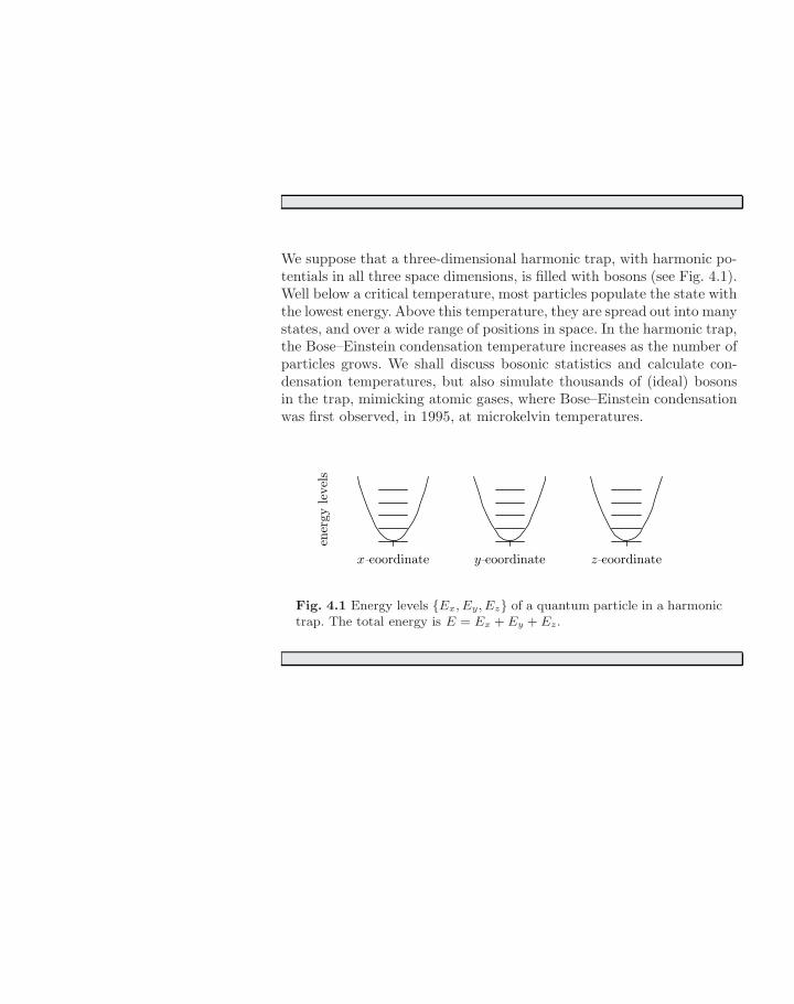
We suppose that a three-dimensional harmonic trap, with harmonic po-tentials in all three space dimensions, is filled with bosons (see Fig. 4.1).Well below a critical temperature, most particles populate the state withthe lowest energy. Above this temperature, they are spread out into manystates, and over a wide range of positions in space. In the harmonic trap,the Bose–Einstein condensation temperature increases as the number ofparticles grows. We shall discuss bosonic statistics and calculate con-densation temperatures, but also simulate thousands of (ideal) bosonsin the trap, mimicking atomic gases, where Bose–Einstein condensationwas first observed, in 1995, at microkelvin temperatures.
z-coordinatey-coordinatex-coordinate
ener
gy lev
els
Fig. 4.1 Energy levels Ex, Ey, Ez of a quantum particle in a harmonictrap. The total energy is E = Ex + Ey + Ez.
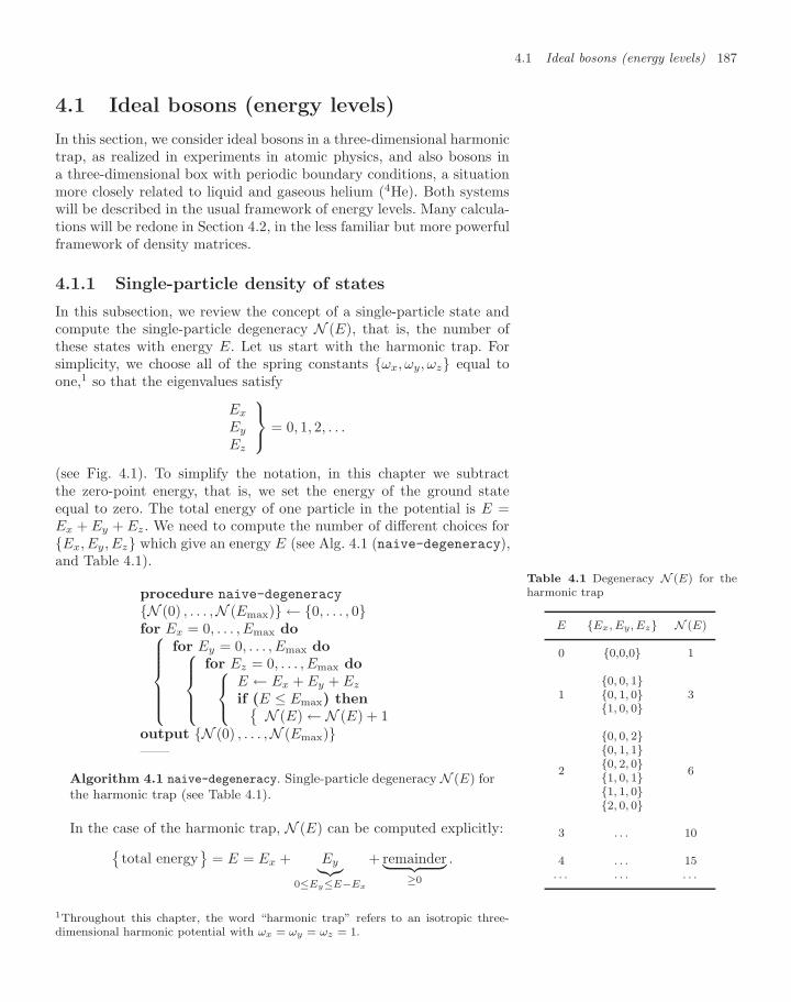
4.1 Ideal bosons (energy levels) 187
4.1 Ideal bosons (energy levels)
In this section, we consider ideal bosons in a three-dimensional harmonictrap, as realized in experiments in atomic physics, and also bosons ina three-dimensional box with periodic boundary conditions, a situationmore closely related to liquid and gaseous helium (4He). Both systemswill be described in the usual framework of energy levels. Many calcula-tions will be redone in Section 4.2, in the less familiar but more powerfulframework of density matrices.
4.1.1 Single-particle density of states
In this subsection, we review the concept of a single-particle state andcompute the single-particle degeneracy N (E), that is, the number ofthese states with energy E. Let us start with the harmonic trap. Forsimplicity, we choose all of the spring constants ωx, ωy, ωz equal toone,1 so that the eigenvalues satisfy
Ex
Ey
Ez
⎫⎬⎭ = 0, 1, 2, . . .
(see Fig. 4.1). To simplify the notation, in this chapter we subtractthe zero-point energy, that is, we set the energy of the ground stateequal to zero. The total energy of one particle in the potential is E =Ex + Ey + Ez . We need to compute the number of different choices forEx, Ey, Ez which give an energy E (see Alg. 4.1 (naive-degeneracy),and Table 4.1).
procedure naive-degeneracy
N (0) , . . . ,N (Emax) ← 0, . . . , 0for Ex = 0, . . . , Emax do⎧⎪⎪⎪⎪⎨⎪⎪⎪⎪⎩
for Ey = 0, . . . , Emax do⎧⎪⎪⎨⎪⎪⎩for Ez = 0, . . . , Emax do⎧⎨⎩
E ← Ex + Ey + Ez
if (E ≤ Emax) then N (E) ← N (E) + 1output N (0) , . . . ,N (Emax)——
Algorithm 4.1 naive-degeneracy. Single-particle degeneracy N (E) forthe harmonic trap (see Table 4.1).
Table 4.1 Degeneracy N (E) for theharmonic trap
E Ex, Ey, Ez N (E)
0 0,0,0 1
10, 0, 10, 1, 01, 0, 0
3
2
0, 0, 20, 1, 10, 2, 01, 0, 11, 1, 02, 0, 0
6
3 . . . 10
4 . . . 15. . . . . . . . .
In the case of the harmonic trap, N (E) can be computed explicitly:total energy
= E = Ex + Ey︸︷︷︸
0≤Ey≤E−Ex
+ remainder︸ ︷︷ ︸≥0
.
1Throughout this chapter, the word “harmonic trap” refers to an isotropic three-dimensional harmonic potential with ωx = ωy = ωz = 1.
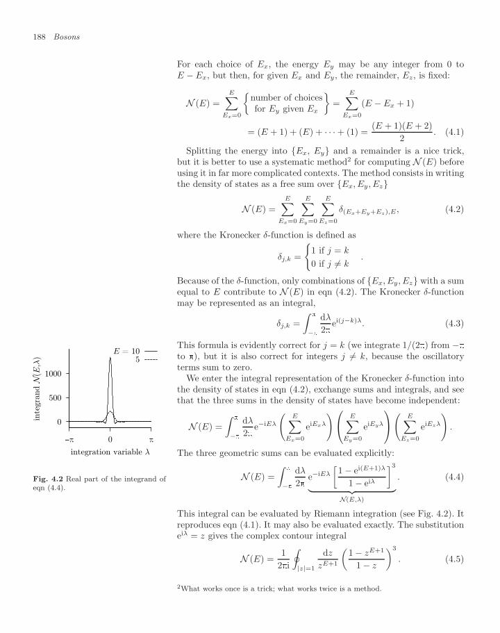
188 Bosons
For each choice of Ex, the energy Ey may be any integer from 0 toE − Ex, but then, for given Ex and Ey , the remainder, Ez, is fixed:
N (E) =E∑
Ex=0
number of choicesfor Ey given Ex
=
E∑Ex=0
(E − Ex + 1)
= (E + 1) + (E) + · · · + (1) =(E + 1)(E + 2)
2. (4.1)
Splitting the energy into Ex, Ey and a remainder is a nice trick,but it is better to use a systematic method2 for computing N (E) beforeusing it in far more complicated contexts. The method consists in writingthe density of states as a free sum over Ex, Ey, Ez
N (E) =E∑
Ex=0
E∑Ey=0
E∑Ez=0
δ(Ex+Ey+Ez),E , (4.2)
where the Kronecker δ-function is defined as
δj,k =
1 if j = k
0 if j = k.
Because of the δ-function, only combinations of Ex, Ey, Ez with a sumequal to E contribute to N (E) in eqn (4.2). The Kronecker δ-functionmay be represented as an integral,
δj,k =∫
−
dλ
2ei(j−k)λ. (4.3)
This formula is evidently correct for j = k (we integrate 1/(2) from −
to ), but it is also correct for integers j = k, because the oscillatoryterms sum to zero.
We enter the integral representation of the Kronecker δ-function intothe density of states in eqn (4.2), exchange sums and integrals, and seethat the three sums in the density of states have become independent:
N (E) =∫
−
dλ
2e−iEλ
(E∑
Ex=0
eiExλ
)⎛⎝ E∑Ey=0
eiEyλ
⎞⎠( E∑Ez=0
eiEzλ
).
The three geometric sums can be evaluated explicitly:
1000
500
0
π0−π
inte
gran
d N
(E,λ
)
integration variable λ
E = 105
Fig. 4.2 Real part of the integrand ofeqn (4.4).
N (E) =∫
−
dλ
2e−iEλ
[1 − ei(E+1)λ
1 − eiλ
]3︸ ︷︷ ︸
N(E,λ)
. (4.4)
This integral can be evaluated by Riemann integration (see Fig. 4.2). Itreproduces eqn (4.1). It may also be evaluated exactly. The substitutioneiλ = z gives the complex contour integral
N (E) =1
2i
∮|z|=1
dz
zE+1
(1 − zE+1
1 − z
)3
. (4.5)
2What works once is a trick; what works twice is a method.
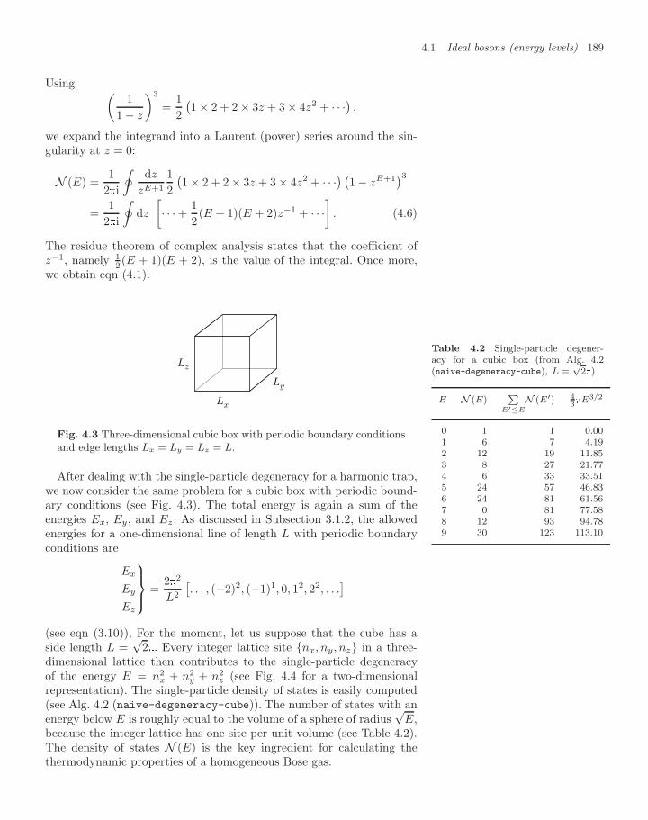
4.1 Ideal bosons (energy levels) 189
Using (1
1 − z
)3
=12(1 × 2 + 2 × 3z + 3 × 4z2 + · · ·) ,
we expand the integrand into a Laurent (power) series around the sin-gularity at z = 0:
N (E) =1
2i
∮dz
zE+1
12(1 × 2 + 2 × 3z + 3 × 4z2 + · · ·) (1 − zE+1
)3=
12i
∮dz
[· · · + 1
2(E + 1)(E + 2)z−1 + · · ·
]. (4.6)
The residue theorem of complex analysis states that the coefficient ofz−1, namely 1
2 (E + 1)(E + 2), is the value of the integral. Once more,we obtain eqn (4.1).
Lx
Lz
Ly
Fig. 4.3 Three-dimensional cubic box with periodic boundary conditionsand edge lengths Lx = Ly = Lz = L.
Table 4.2 Single-particle degener-acy for a cubic box (from Alg. 4.2(naive-degeneracy-cube), L =
√2)
E N (E)P
E′≤E
N (E′) 43E3/2
0 1 1 0.001 6 7 4.192 12 19 11.853 8 27 21.774 6 33 33.515 24 57 46.836 24 81 61.567 0 81 77.588 12 93 94.789 30 123 113.10
After dealing with the single-particle degeneracy for a harmonic trap,we now consider the same problem for a cubic box with periodic bound-ary conditions (see Fig. 4.3). The total energy is again a sum of theenergies Ex, Ey, and Ez . As discussed in Subsection 3.1.2, the allowedenergies for a one-dimensional line of length L with periodic boundaryconditions are
Ex
Ey
Ez
⎫⎪⎬⎪⎭ =22
L2
[. . . , (−2)2, (−1)1, 0, 12, 22, . . .
](see eqn (3.10)), For the moment, let us suppose that the cube has aside length L =
√2. Every integer lattice site nx, ny, nz in a three-
dimensional lattice then contributes to the single-particle degeneracyof the energy E = n2
x + n2y + n2
z (see Fig. 4.4 for a two-dimensionalrepresentation). The single-particle density of states is easily computed(see Alg. 4.2 (naive-degeneracy-cube)). The number of states with anenergy below E is roughly equal to the volume of a sphere of radius
√E,
because the integer lattice has one site per unit volume (see Table 4.2).The density of states N (E) is the key ingredient for calculating thethermodynamic properties of a homogeneous Bose gas.
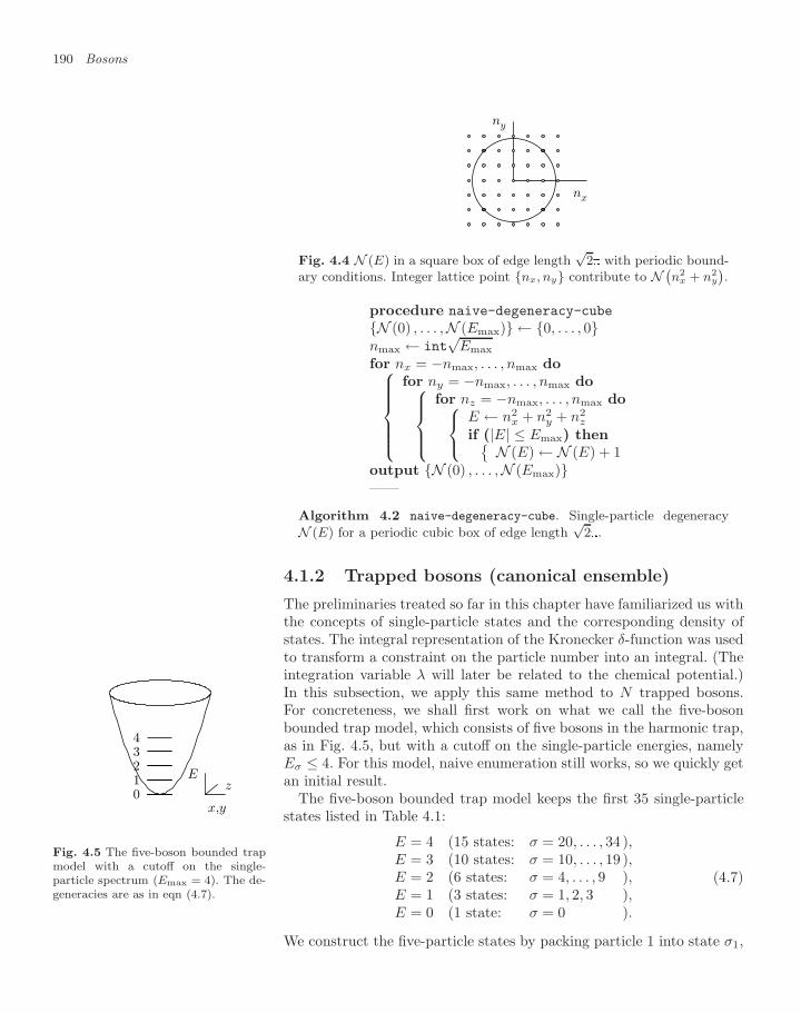
190 Bosons
nx
ny
Fig. 4.4 N (E) in a square box of edge length√
2 with periodic bound-ary conditions. Integer lattice point nx, ny contribute to N `
n2x + n2
y
´.
procedure naive-degeneracy-cube
N (0) , . . . ,N (Emax) ← 0, . . . , 0nmax ← int
√Emax
for nx = −nmax, . . . , nmax do⎧⎪⎪⎪⎪⎨⎪⎪⎪⎪⎩for ny = −nmax, . . . , nmax do⎧⎪⎪⎨⎪⎪⎩
for nz = −nmax, . . . , nmax do⎧⎨⎩E ← n2
x + n2y + n2
z
if (|E| ≤ Emax) then N (E) ← N (E) + 1output N (0) , . . . ,N (Emax)——
Algorithm 4.2 naive-degeneracy-cube. Single-particle degeneracy
N (E) for a periodic cubic box of edge length√
2.
4.1.2 Trapped bosons (canonical ensemble)
The preliminaries treated so far in this chapter have familiarized us withthe concepts of single-particle states and the corresponding density ofstates. The integral representation of the Kronecker δ-function was usedto transform a constraint on the particle number into an integral. (Theintegration variable λ will later be related to the chemical potential.)
x,y
zE
01234
Fig. 4.5 The five-boson bounded trapmodel with a cutoff on the single-particle spectrum (Emax = 4). The de-generacies are as in eqn (4.7).
In this subsection, we apply this same method to N trapped bosons.For concreteness, we shall first work on what we call the five-bosonbounded trap model, which consists of five bosons in the harmonic trap,as in Fig. 4.5, but with a cutoff on the single-particle energies, namelyEσ ≤ 4. For this model, naive enumeration still works, so we quickly getan initial result.
The five-boson bounded trap model keeps the first 35 single-particlestates listed in Table 4.1:
E = 4 (15 states: σ = 20, . . . , 34 ),E = 3 (10 states: σ = 10, . . . , 19 ),E = 2 (6 states: σ = 4, . . . , 9 ),E = 1 (3 states: σ = 1, 2, 3 ),E = 0 (1 state: σ = 0 ).
(4.7)
We construct the five-particle states by packing particle 1 into state σ1,
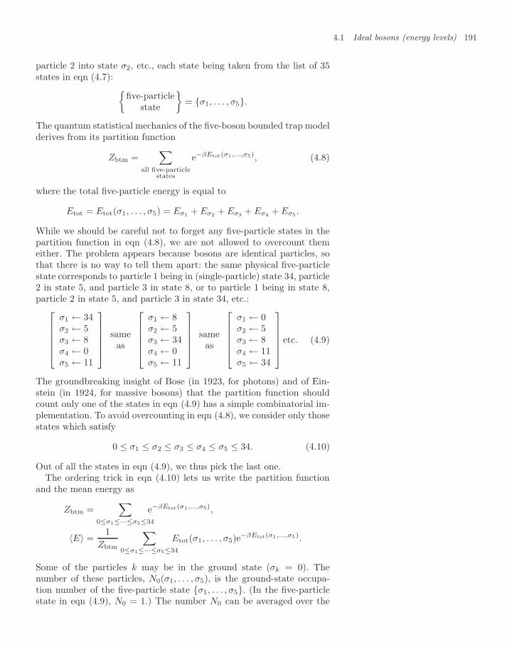
4.1 Ideal bosons (energy levels) 191
particle 2 into state σ2, etc., each state being taken from the list of 35states in eqn (4.7):
five-particlestate
= σ1, . . . , σ5.
The quantum statistical mechanics of the five-boson bounded trap modelderives from its partition function
Zbtm =∑
all five-particlestates
e−βEtot(σ1,...,σ5), (4.8)
where the total five-particle energy is equal to
Etot = Etot(σ1, . . . , σ5) = Eσ1 + Eσ2 + Eσ3 + Eσ4 + Eσ5 .
While we should be careful not to forget any five-particle states in thepartition function in eqn (4.8), we are not allowed to overcount themeither. The problem appears because bosons are identical particles, sothat there is no way to tell them apart: the same physical five-particlestate corresponds to particle 1 being in (single-particle) state 34, particle2 in state 5, and particle 3 in state 8, or to particle 1 being in state 8,particle 2 in state 5, and particle 3 in state 34, etc.:⎡⎢⎢⎢⎢⎣
σ1 ← 34σ2 ← 5σ3 ← 8σ4 ← 0σ5 ← 11
⎤⎥⎥⎥⎥⎦ sameas
⎡⎢⎢⎢⎢⎣σ1 ← 8σ2 ← 5σ3 ← 34σ4 ← 0σ5 ← 11
⎤⎥⎥⎥⎥⎦ sameas
⎡⎢⎢⎢⎢⎣σ1 ← 0σ2 ← 5σ3 ← 8σ4 ← 11σ5 ← 34
⎤⎥⎥⎥⎥⎦ etc. (4.9)
The groundbreaking insight of Bose (in 1923, for photons) and of Ein-stein (in 1924, for massive bosons) that the partition function shouldcount only one of the states in eqn (4.9) has a simple combinatorial im-plementation. To avoid overcounting in eqn (4.8), we consider only thosestates which satisfy
0 ≤ σ1 ≤ σ2 ≤ σ3 ≤ σ4 ≤ σ5 ≤ 34. (4.10)
Out of all the states in eqn (4.9), we thus pick the last one.The ordering trick in eqn (4.10) lets us write the partition function
and the mean energy as
Zbtm =∑
0≤σ1≤···≤σ5≤34
e−βEtot(σ1,...,σ5),
〈E〉 =1
Zbtm
∑0≤σ1≤···≤σ5≤34
Etot(σ1, . . . , σ5)e−βEtot(σ1,...,σ5).
Some of the particles k may be in the ground state (σk = 0). Thenumber of these particles, N0(σ1, . . . , σ5), is the ground-state occupa-tion number of the five-particle state σ1, . . . , σ5. (In the five-particlestate in eqn (4.9), N0 = 1.) The number N0 can be averaged over the
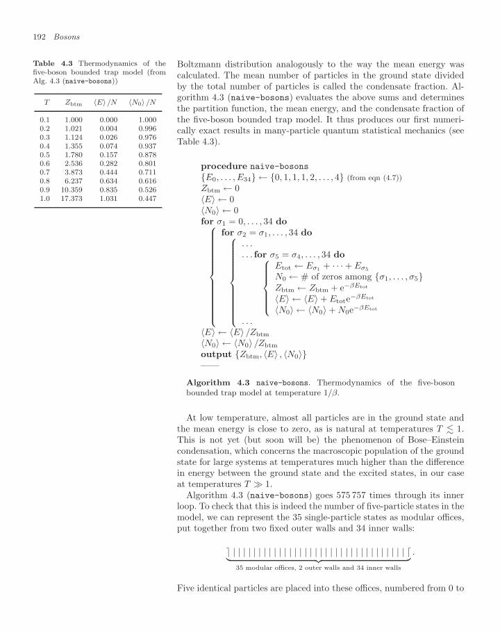
192 Bosons
Boltzmann distribution analogously to the way the mean energy wascalculated. The mean number of particles in the ground state dividedby the total number of particles is called the condensate fraction. Al-gorithm 4.3 (naive-bosons) evaluates the above sums and determinesthe partition function, the mean energy, and the condensate fraction ofthe five-boson bounded trap model. It thus produces our first numeri-cally exact results in many-particle quantum statistical mechanics (seeTable 4.3).
Table 4.3 Thermodynamics of thefive-boson bounded trap model (fromAlg. 4.3 (naive-bosons))
T Zbtm 〈E〉/N 〈N0〉 /N
0.1 1.000 0.000 1.0000.2 1.021 0.004 0.9960.3 1.124 0.026 0.9760.4 1.355 0.074 0.9370.5 1.780 0.157 0.8780.6 2.536 0.282 0.8010.7 3.873 0.444 0.7110.8 6.237 0.634 0.6160.9 10.359 0.835 0.5261.0 17.373 1.031 0.447
procedure naive-bosons
E0, . . . , E34 ← 0, 1, 1, 1, 2, . . . , 4 (from eqn (4.7))Zbtm ← 0〈E〉 ← 0〈N0〉 ← 0for σ1 = 0, . . . , 34 do⎧⎪⎪⎪⎪⎪⎪⎪⎪⎪⎪⎪⎪⎨⎪⎪⎪⎪⎪⎪⎪⎪⎪⎪⎪⎪⎩
for σ2 = σ1, . . . , 34 do⎧⎪⎪⎪⎪⎪⎪⎪⎪⎪⎪⎨⎪⎪⎪⎪⎪⎪⎪⎪⎪⎪⎩
. . .
. . . for σ5 = σ4, . . . , 34 do⎧⎪⎪⎪⎪⎨⎪⎪⎪⎪⎩Etot ← Eσ1 + · · · + Eσ5
N0 ← # of zeros among σ1, . . . , σ5Zbtm ← Zbtm + e−βEtot
〈E〉 ← 〈E〉 + Etote−βEtot
〈N0〉 ← 〈N0〉 + N0e−βEtot
. . .〈E〉 ← 〈E〉 /Zbtm
〈N0〉 ← 〈N0〉 /Zbtm
output Zbtm, 〈E〉 , 〈N0〉——
Algorithm 4.3 naive-bosons. Thermodynamics of the five-bosonbounded trap model at temperature 1/β.
At low temperature, almost all particles are in the ground state andthe mean energy is close to zero, as is natural at temperatures T 1.This is not yet (but soon will be) the phenomenon of Bose–Einsteincondensation, which concerns the macroscopic population of the groundstate for large systems at temperatures much higher than the differencein energy between the ground state and the excited states, in our caseat temperatures T 1.
Algorithm 4.3 (naive-bosons) goes 575 757 times through its innerloop. To check that this is indeed the number of five-particle states in themodel, we can represent the 35 single-particle states as modular offices,put together from two fixed outer walls and 34 inner walls:
| | | | | | | | | | | | | | | | | | | | | | | | | | | | | | | | | | ︸ ︷︷ ︸35 modular offices, 2 outer walls and 34 inner walls
.
Five identical particles are placed into these offices, numbered from 0 to
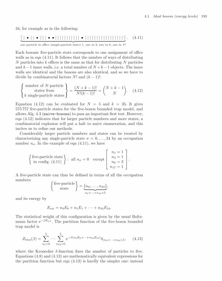
4.1 Ideal bosons (energy levels) 193
34, for example as in the following:
| • | | • | | | • • | | | | | | | | | | | • | | | | | | | | | | | | | | | | | ︸ ︷︷ ︸one particle in office (single-particle state) 1, one in 3, two in 6, one in 17
. (4.11)
Each bosonic five-particle state corresponds to one assignment of officewalls as in eqn (4.11). It follows that the number of ways of distributingN particles into k offices is the same as that for distributing N particlesand k−1 inner walls, i.e. a total number of N +k−1 objects. The innerwalls are identical and the bosons are also identical, and so we have todivide by combinatorial factors N ! and (k − 1)!:⎧⎨⎩
number of N -particlestates from
k single-particle states
⎫⎬⎭ =(N + k − 1)!N !(k − 1)!
=(
N + k − 1N
). (4.12)
Equation (4.12) can be evaluated for N = 5 and k = 35. It gives575 757 five-particle states for the five-boson bounded trap model, andallows Alg. 4.3 (naive-bosons) to pass an important first test. However,eqn (4.12) indicates that for larger particle numbers and more states, acombinatorial explosion will put a halt to naive enumeration, and thisincites us to refine our methods.
Considerably larger particle numbers and states can be treated bycharacterizing any single-particle state σ = 0, . . . , 34 by an occupationnumber nσ. In the example of eqn (4.11), we have
five-particle statein config. (4.11)
: all nσ = 0 except
⎡⎢⎢⎣n1 = 1n3 = 1n6 = 2
n17 = 1
⎤⎥⎥⎦ .
A five-particle state can thus be defined in terms of all the occupationnumbers
five-particlestate
= n0, . . . , n34︸ ︷︷ ︸
n0+···+n34=5
,
and its energy by
Etot = n0E0 + n1E1 + · · · + n34E34.
The statistical weight of this configuration is given by the usual Boltz-mann factor e−βEtot . The partition function of the five-boson boundedtrap model is
Zbtm(β) =5∑
n0=0
· · ·5∑
n34=0
e−β(n0E0+···+n34E34)δ(n0+···+n34),5, (4.13)
where the Kronecker δ-function fixes the number of particles to five.Equations (4.8) and (4.13) are mathematically equivalent expressions forthe partition function but eqn (4.13) is hardly the simpler one: instead
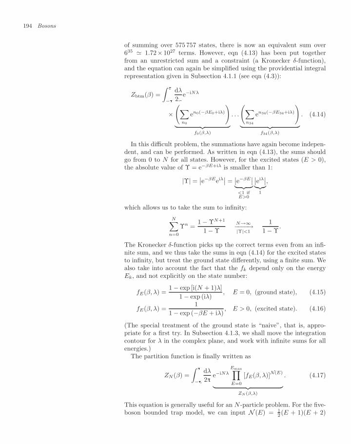
194 Bosons
of summing over 575 757 states, there is now an equivalent sum over635 1.72× 1027 terms. However, eqn (4.13) has been put togetherfrom an unrestricted sum and a constraint (a Kronecker δ-function),and the equation can again be simplified using the providential integralrepresentation given in Subsection 4.1.1 (see eqn (4.3)):
Zbtm(β) =∫
−
dλ
2e−iNλ
×(∑
n0
en0(−βE0+iλ)
)︸ ︷︷ ︸
f0(β,λ)
. . .
(∑n34
en34(−βE34+iλ)
)︸ ︷︷ ︸
f34(β,λ)
. (4.14)
In this difficult problem, the summations have again become indepen-dent, and can be performed. As written in eqn (4.13), the sums shouldgo from 0 to N for all states. However, for the excited states (E > 0),the absolute value of Υ = e−βE+iλ is smaller than 1:
|Υ| =∣∣e−βEeiλ
∣∣ = ∣∣e−βE∣∣︸ ︷︷ ︸
<1 ifE>0
∣∣eiλ∣∣︸︷︷︸
1
,
which allows us to take the sum to infinity:
N∑n=0
Υn =1 − ΥN+1
1 − ΥN→∞−−−−→|Υ|<1
11 − Υ
.
The Kronecker δ-function picks up the correct terms even from an infi-nite sum, and we thus take the sums in eqn (4.14) for the excited statesto infinity, but treat the ground state differently, using a finite sum. Wealso take into account the fact that the fk depend only on the energyEk, and not explicitly on the state number:
fE(β, λ) =1 − exp [i(N + 1)λ]
1 − exp (iλ), E = 0, (ground state), (4.15)
fE(β, λ) =1
1 − exp (−βE + iλ), E > 0, (excited state). (4.16)
(The special treatment of the ground state is “naive”, that is, appro-priate for a first try. In Subsection 4.1.3, we shall move the integrationcontour for λ in the complex plane, and work with infinite sums for allenergies.)
The partition function is finally written as
ZN (β) =∫
−
dλ
2e−iNλ
Emax∏E=0
[fE(β, λ)]N(E)
︸ ︷︷ ︸ZN (β,λ)
. (4.17)
This equation is generally useful for an N -particle problem. For the five-boson bounded trap model, we can input N (E) = 1
2 (E + 1)(E + 2)
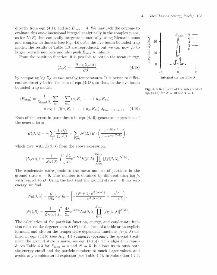
4.1 Ideal bosons (energy levels) 195
directly from eqn (4.1), and set Emax = 4. We may lack the courage toevaluate this one-dimensional integral analytically in the complex plane,as for N (E), but can easily integrate numerically, using Riemann sumsand complex arithmetic (see Fig. 4.6). For the five-boson bounded trapmodel, the results of Table 4.3 are reproduced, but we can now go tolarger particle numbers and also push Emax to infinity.
From the partition function, it is possible to obtain the mean energy,
〈EN 〉 = −∂ log ZN (β)∂β
, (4.18)
by comparing log ZN at two nearby temperatures. It is better to differ-
40
20
0
π0−π
inte
gran
d Z
N(β
,λ)
integration variable λ
Emax = 86420
Fig. 4.6 Real part of the integrand ofeqn (4.17) for N = 10 and T = 1.
entiate directly inside the sum of eqn (4.13), so that, in the five-bosonbounded trap model:
〈Ebtm〉 =1
Zbtm(β)
∑n0
· · ·∑n34
(n0E0 + · · · + n34E34)
× exp [−β(n0E0 + · · · + n34E34)] δ(n0+···+n34),5. (4.19)
Each of the terms in parentheses in eqn (4.19) generates expressions ofthe general form
E(β, λ) = −∑
k
1fk
∂fk
∂β=∑E =0
N (E) E ·(
e−βE+iλ
1 − e−βE+iλ
),
which give, with E(β, λ) from the above expression,
〈EN (β)〉 =1
ZN (β)
∫
−
dλ
2e−iNλE(β, λ)
Emax∏E=0
[fE(β, λ)]N(E).
The condensate corresponds to the mean number of particles in theground state σ = 0. This number is obtained by differentiating log f0
with respect to iλ. Using the fact that the ground state σ = 0 has zeroenergy, we find
N0(β, λ) =∂
i∂λlog f0 =
[− (N + 1) eiλ(N+1)
1 − eiλ(N+1)+
eiλ
1 − eiλ
],
〈N0(β)〉 =1
ZN (β)
∫
−
dλ
2e−iNλN0(β, λ)
Emax∏E=0
[fE(β, λ)]N(E).
The calculation of the partition function, energy, and condensate frac-tion relies on the degeneracies N (E) in the form of a table or an explicitformula, and also on the temperature-dependent functions fE(β, λ) de-fined in eqn (4.16) (see Alg. 4.4 (canonic-bosons); the special treat-ment the ground state is naive, see eqn (4.15)). This algorithm repro-duces Table 4.3 for Emax = 4 and N = 5. It allows us to push boththe energy cutoff and the particle numbers to much larger values, andavoids any combinatorial explosion (see Table 4.4). In Subsection 4.2.3,
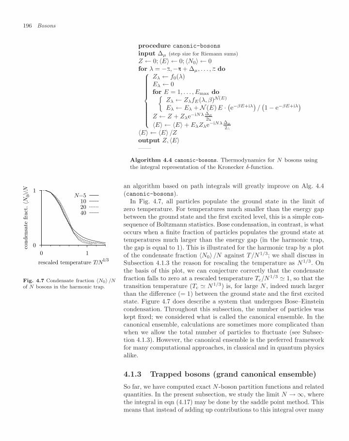
196 Bosons
procedure canonic-bosons
input ∆µ (step size for Riemann sums)Z ← 0; 〈E〉 ← 0; 〈N0〉 ← 0for λ = −,−+ ∆µ, . . . , do⎧⎪⎪⎪⎪⎪⎪⎪⎪⎨⎪⎪⎪⎪⎪⎪⎪⎪⎩
Zλ ← f0(λ)Eλ ← 0for E = 1, . . . , Emax do
Zλ ← ZλfE(λ, β)N(E)
Eλ ← Eλ + N (E) E · (e−βE+iλ)/(1 − e−βE+iλ
)Z ← Z + Zλe−iNλ ∆µ
2
〈E〉 ← 〈E〉 + EλZλe−iNλ ∆µ
2〈E〉 ← 〈E〉 /Zoutput Z, 〈E〉——
Algorithm 4.4 canonic-bosons. Thermodynamics for N bosons usingthe integral representation of the Kronecker δ-function.
an algorithm based on path integrals will greatly improve on Alg. 4.4(canonic-bosons).
In Fig. 4.7, all particles populate the ground state in the limit ofzero temperature. For temperatures much smaller than the energy gapbetween the ground state and the first excited level, this is a simple con-sequence of Boltzmann statistics. Bose condensation, in contrast, is whatoccurs when a finite fraction of particles populates the ground state attemperatures much larger than the energy gap (in the harmonic trap,
0
1
0 1
conden
sate
fra
ct. 〈N
0〉/N
rescaled temperature T/N1/3
N=5102040
Fig. 4.7 Condensate fraction 〈N0〉 /Nof N bosons in the harmonic trap.
the gap is equal to 1). This is illustrated for the harmonic trap by a plotof the condensate fraction 〈N0〉 /N against T/N1/3; we shall discuss inSubsection 4.1.3 the reason for rescaling the temperature as N1/3. Onthe basis of this plot, we can conjecture correctly that the condensatefraction falls to zero at a rescaled temperature Tc/N
1/3 1, so that thetransition temperature (Tc N1/3) is, for large N , indeed much largerthan the difference (= 1) between the ground state and the first excitedstate. Figure 4.7 does describe a system that undergoes Bose–Einsteincondensation. Throughout this subsection, the number of particles waskept fixed; we considered what is called the canonical ensemble. In thecanonical ensemble, calculations are sometimes more complicated thanwhen we allow the total number of particles to fluctuate (see Subsec-tion 4.1.3). However, the canonical ensemble is the preferred frameworkfor many computational approaches, in classical and in quantum physicsalike.
4.1.3 Trapped bosons (grand canonical ensemble)
So far, we have computed exact N -boson partition functions and relatedquantities. In the present subsection, we study the limit N → ∞, wherethe integral in eqn (4.17) may be done by the saddle point method. Thismeans that instead of adding up contributions to this integral over many
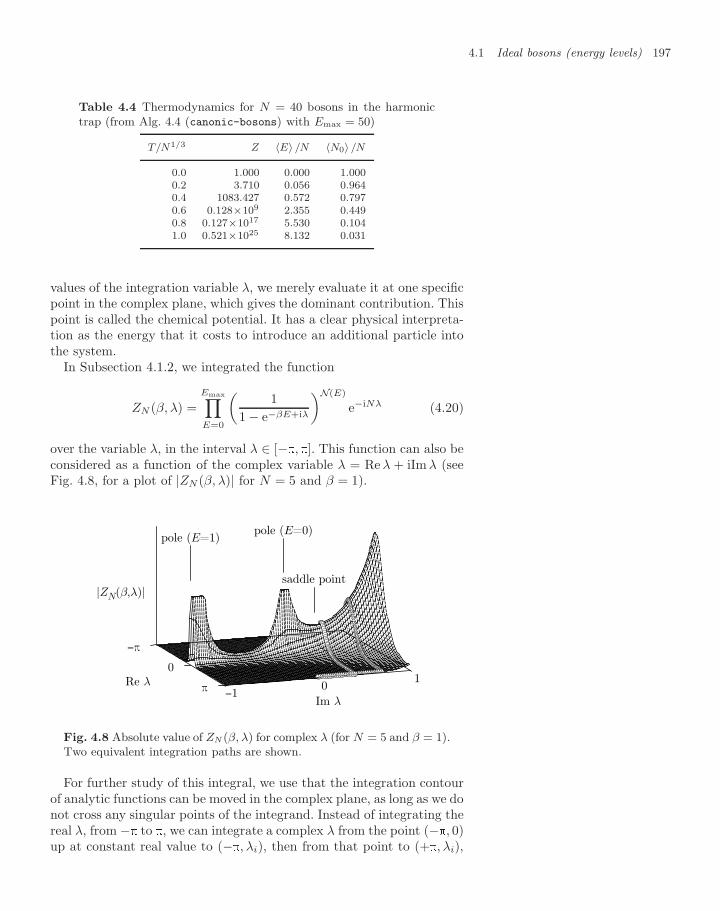
4.1 Ideal bosons (energy levels) 197
Table 4.4 Thermodynamics for N = 40 bosons in the harmonictrap (from Alg. 4.4 (canonic-bosons) with Emax = 50)
T/N1/3 Z 〈E〉 /N 〈N0〉 /N
0.0 1.000 0.000 1.0000.2 3.710 0.056 0.9640.4 1083.427 0.572 0.7970.6 0.128×10⁹ 2.355 0.4490.8 0.127×10¹⁷ 5.530 0.1041.0 0.521×1025 8.132 0.031
values of the integration variable λ, we merely evaluate it at one specificpoint in the complex plane, which gives the dominant contribution. Thispoint is called the chemical potential. It has a clear physical interpreta-tion as the energy that it costs to introduce an additional particle intothe system.
In Subsection 4.1.2, we integrated the function
ZN (β, λ) =Emax∏E=0
(1
1 − e−βE+iλ
)N(E)
e−iNλ (4.20)
over the variable λ, in the interval λ ∈ [−, ]. This function can also beconsidered as a function of the complex variable λ = Re λ + iIm λ (seeFig. 4.8, for a plot of |ZN (β, λ)| for N = 5 and β = 1).
pole (E=1)pole (E=0)
saddle point
−10
1π
0
−π
Re λ
Im λ
|ZN(β,λ)|
Fig. 4.8 Absolute value of ZN (β, λ) for complex λ (for N = 5 and β = 1).Two equivalent integration paths are shown.
For further study of this integral, we use that the integration contourof analytic functions can be moved in the complex plane, as long as we donot cross any singular points of the integrand. Instead of integrating thereal λ, from − to , we can integrate a complex λ from the point (−, 0)up at constant real value to (−, λi), then from that point to (+, λi),
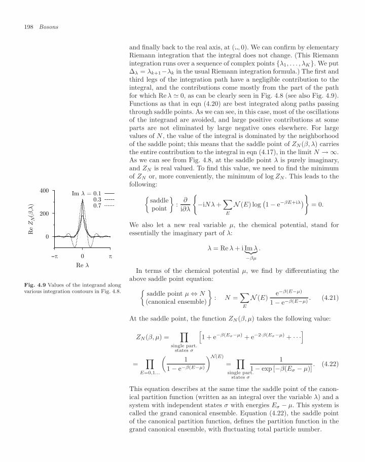
198 Bosons
and finally back to the real axis, at (, 0). We can confirm by elementaryRiemann integration that the integral does not change. (This Riemannintegration runs over a sequence of complex points λ1, . . . , λK. We put∆λ = λk+1−λk in the usual Riemann integration formula.) The first andthird legs of the integration path have a negligible contribution to theintegral, and the contributions come mostly from the part of the pathfor which Re λ 0, as can be clearly seen in Fig. 4.8 (see also Fig. 4.9).Functions as that in eqn (4.20) are best integrated along paths passingthrough saddle points. As we can see, in this case, most of the oscillationsof the integrand are avoided, and large positive contributions at someparts are not eliminated by large negative ones elsewhere. For largevalues of N , the value of the integral is dominated by the neighborhoodof the saddle point; this means that the saddle point of ZN(β, λ) carriesthe entire contribution to the integral in eqn (4.17), in the limit N → ∞.As we can see from Fig. 4.8, at the saddle point λ is purely imaginary,and ZN is real valued. To find this value, we need to find the minimumof ZN or, more conveniently, the minimum of log ZN . This leads to thefollowing:
saddlepoint
:
∂
i∂λ
−iNλ +
∑E
N (E) log(1 − e−βE+iλ
)= 0.
We also let a new real variable µ, the chemical potential, stand foressentially the imaginary part of λ:
λ = Re λ + i Im λ︸︷︷︸−βµ
.
0
200
400
π0−π
Re
ZN(β
,λ)
Re λ
Im λ = 0.10.30.7
Fig. 4.9 Values of the integrand alongvarious integration contours in Fig. 4.8.
In terms of the chemical potential µ, we find by differentiating theabove saddle point equation:
saddle point µ ⇔ N(canonical ensemble)
: N =
∑E
N (E)e−β(E−µ)
1 − e−β(E−µ). (4.21)
At the saddle point, the function ZN(β, µ) takes the following value:
ZN(β, µ) =∏
single part.states σ
[1 + e−β(Eσ−µ) + e−2·β(Eσ−µ) + · · ·
]
=∏
E=0,1...
(1
1 − e−β(E−µ)
)N(E)
=∏
single part.states σ
11 − exp [−β(Eσ − µ)]
. (4.22)
This equation describes at the same time the saddle point of the canon-ical partition function (written as an integral over the variable λ) and asystem with independent states σ with energies Eσ − µ. This system iscalled the grand canonical ensemble. Equation (4.22), the saddle pointof the canonical partition function, defines the partition function in thegrand canonical ensemble, with fluctuating total particle number.
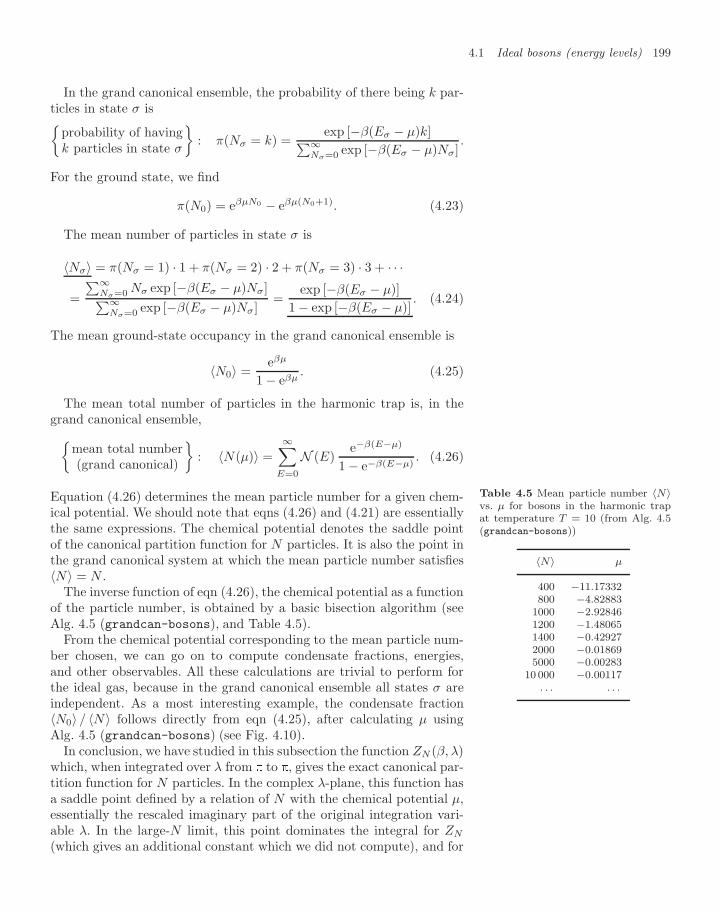
4.1 Ideal bosons (energy levels) 199
In the grand canonical ensemble, the probability of there being k par-ticles in state σ is
probability of havingk particles in state σ
: π(Nσ = k) =
exp [−β(Eσ − µ)k]∑∞Nσ=0 exp [−β(Eσ − µ)Nσ]
.
For the ground state, we find
π(N0) = eβµN0 − eβµ(N0+1). (4.23)
The mean number of particles in state σ is
〈Nσ〉 = π(Nσ = 1) · 1 + π(Nσ = 2) · 2 + π(Nσ = 3) · 3 + · · ·
=
∑∞Nσ=0 Nσ exp [−β(Eσ − µ)Nσ]∑∞
Nσ=0 exp [−β(Eσ − µ)Nσ]=
exp [−β(Eσ − µ)]1 − exp [−β(Eσ − µ)]
. (4.24)
The mean ground-state occupancy in the grand canonical ensemble is
〈N0〉 =eβµ
1 − eβµ. (4.25)
The mean total number of particles in the harmonic trap is, in thegrand canonical ensemble,
mean total number(grand canonical)
: 〈N(µ)〉 =
∞∑E=0
N (E)e−β(E−µ)
1 − e−β(E−µ). (4.26)
Equation (4.26) determines the mean particle number for a given chem-ical potential. We should note that eqns (4.26) and (4.21) are essentiallythe same expressions. The chemical potential denotes the saddle pointof the canonical partition function for N particles. It is also the point inthe grand canonical system at which the mean particle number satisfies〈N〉 = N .
The inverse function of eqn (4.26), the chemical potential as a functionof the particle number, is obtained by a basic bisection algorithm (seeAlg. 4.5 (grandcan-bosons), and Table 4.5).
Table 4.5 Mean particle number 〈N〉vs. µ for bosons in the harmonic trapat temperature T = 10 (from Alg. 4.5(grandcan-bosons))
〈N〉 µ
400 −11.17332800 −4.82883
1000 −2.928461200 −1.480651400 −0.429272000 −0.018695000 −0.00283
10 000 −0.00117. . . . . .
From the chemical potential corresponding to the mean particle num-ber chosen, we can go on to compute condensate fractions, energies,and other observables. All these calculations are trivial to perform forthe ideal gas, because in the grand canonical ensemble all states σ areindependent. As a most interesting example, the condensate fraction〈N0〉 / 〈N〉 follows directly from eqn (4.25), after calculating µ usingAlg. 4.5 (grandcan-bosons) (see Fig. 4.10).
In conclusion, we have studied in this subsection the function ZN (β, λ)which, when integrated over λ from to , gives the exact canonical par-tition function for N particles. In the complex λ-plane, this function hasa saddle point defined by a relation of N with the chemical potential µ,essentially the rescaled imaginary part of the original integration vari-able λ. In the large-N limit, this point dominates the integral for ZN
(which gives an additional constant which we did not compute), and for
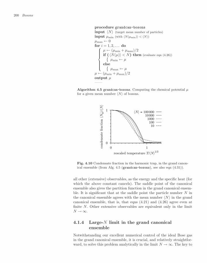
200 Bosons
procedure grandcan-bosons
input 〈N〉 (target mean number of particles)input µmin (with 〈N(µmin)〉 < 〈N〉)µmax ← 0for i = 1, 2, . . . do⎧⎪⎪⎪⎪⎨⎪⎪⎪⎪⎩
µ ← (µmin + µmax)/2if ( 〈N(µ)〉 < N) then (evaluate eqn (4.26))
µmin ← µelse
µmax ← µµ ← (µmin + µmax)/2output µ——
Algorithm 4.5 grandcan-bosons. Computing the chemical potential µfor a given mean number 〈N〉 of bosons.
0
1
0 1conden
sate
fra
ctio
n 〈N
0〉/〈N
〉
rescaled temperature T/〈N〉1/3
〈N〉 = 10000010000100010010
Fig. 4.10 Condensate fraction in the harmonic trap, in the grand canon-ical ensemble (from Alg. 4.5 (grandcan-bosons), see also eqn (4.31)).
all other (extensive) observables, as the energy and the specific heat (forwhich the above constant cancels). The saddle point of the canonicalensemble also gives the partition function in the grand canonical ensem-ble. It is significant that at the saddle point the particle number N inthe canonical ensemble agrees with the mean number 〈N〉 in the grandcanonical ensemble, that is, that eqns (4.21) and (4.26) agree even atfinite N . Other extensive observables are equivalent only in the limitN → ∞.
4.1.4 Large-N limit in the grand canonicalensemble
Notwithstanding our excellent numerical control of the ideal Bose gasin the grand canonical ensemble, it is crucial, and relatively straightfor-ward, to solve this problem analytically in the limit N → ∞. The key to
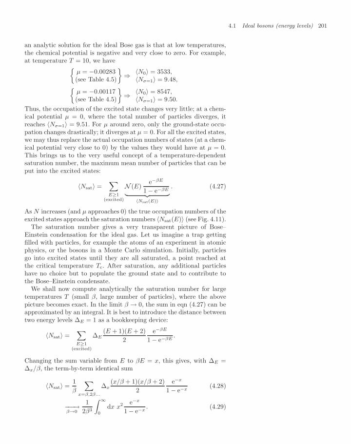
4.1 Ideal bosons (energy levels) 201
an analytic solution for the ideal Bose gas is that at low temperatures,the chemical potential is negative and very close to zero. For example,at temperature T = 10, we have
µ = −0.00283(see Table 4.5)
⇒ 〈N0〉 = 3533,
〈Nσ=1〉 = 9.48,µ = −0.00117(see Table 4.5)
⇒ 〈N0〉 = 8547,
〈Nσ=1〉 = 9.50.
Thus, the occupation of the excited state changes very little; at a chem-ical potential µ = 0, where the total number of particles diverges, itreaches 〈Nσ=1〉 = 9.51. For µ around zero, only the ground-state occu-pation changes drastically; it diverges at µ = 0. For all the excited states,we may thus replace the actual occupation numbers of states (at a chem-ical potential very close to 0) by the values they would have at µ = 0.This brings us to the very useful concept of a temperature-dependentsaturation number, the maximum mean number of particles that can beput into the excited states:
〈Nsat〉 =∑E≥1
(excited)
N (E)e−βE
1 − e−βE︸ ︷︷ ︸〈Nsat(E)〉
. (4.27)
As N increases (and µ approaches 0) the true occupation numbers of theexcited states approach the saturation numbers 〈Nsat(E)〉 (see Fig. 4.11).
The saturation number gives a very transparent picture of Bose–Einstein condensation for the ideal gas. Let us imagine a trap gettingfilled with particles, for example the atoms of an experiment in atomicphysics, or the bosons in a Monte Carlo simulation. Initially, particlesgo into excited states until they are all saturated, a point reached atthe critical temperature Tc. After saturation, any additional particleshave no choice but to populate the ground state and to contribute tothe Bose–Einstein condensate.
We shall now compute analytically the saturation number for largetemperatures T (small β, large number of particles), where the abovepicture becomes exact. In the limit β → 0, the sum in eqn (4.27) can beapproximated by an integral. It is best to introduce the distance betweentwo energy levels ∆E = 1 as a bookkeeping device:
〈Nsat〉 =∑E≥1
(excited)
∆E(E + 1)(E + 2)
2e−βE
1 − e−βE.
Changing the sum variable from E to βE = x, this gives, with ∆E =∆x/β, the term-by-term identical sum
〈Nsat〉 =1β
∑x=β,2β...
∆x(x/β + 1)(x/β + 2)
2e−x
1 − e−x(4.28)
−−−→β→0
12β3
∫ ∞
0
dx x2 e−x
1 − e−x. (4.29)
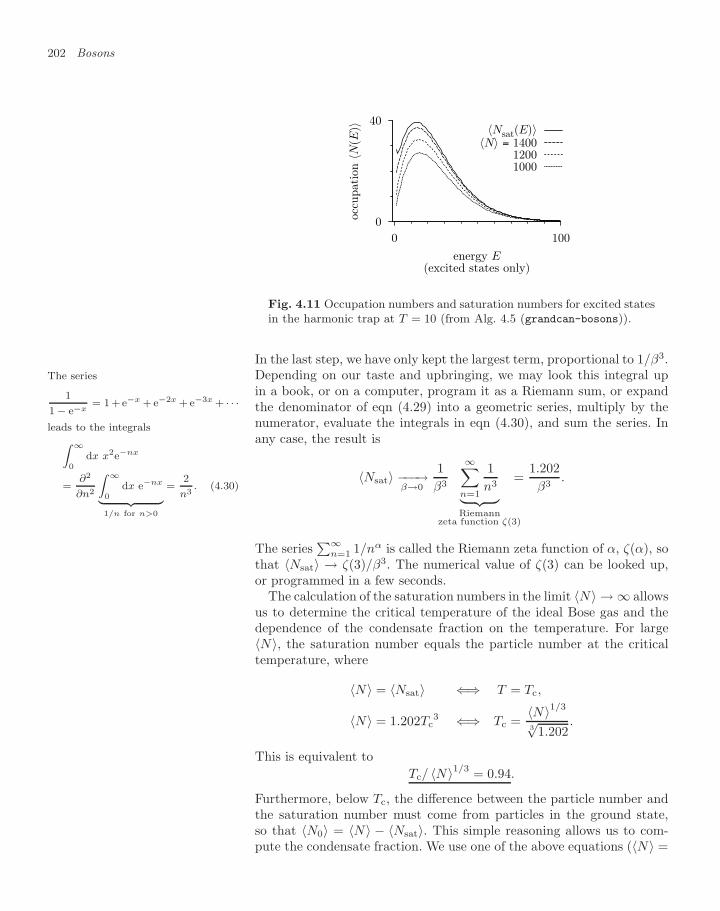
202 Bosons
0
40
0 100
occu
pat
ion 〈N
(E)〉
energy E(excited states only)
〈Nsat(E)〉〈N〉 = 1400
12001000
Fig. 4.11 Occupation numbers and saturation numbers for excited statesin the harmonic trap at T = 10 (from Alg. 4.5 (grandcan-bosons)).
In the last step, we have only kept the largest term, proportional to 1/β3.Depending on our taste and upbringing, we may look this integral upThe series
11 − e−x
= 1 + e−x + e−2x + e−3x + · · ·
leads to the integralsZ ∞
0dx x2e−nx
=∂2
∂n2
Z ∞
0dx e−nx
| z 1/n for n>0
=2n3
. (4.30)
in a book, or on a computer, program it as a Riemann sum, or expandthe denominator of eqn (4.29) into a geometric series, multiply by thenumerator, evaluate the integrals in eqn (4.30), and sum the series. Inany case, the result is
〈Nsat〉 −−−→β→0
1β3
∞∑n=1
1n3︸ ︷︷ ︸
Riemannzeta function ζ(3)
=1.202β3
.
The series∑∞
n=1 1/nα is called the Riemann zeta function of α, ζ(α), sothat 〈Nsat〉 → ζ(3)/β3. The numerical value of ζ(3) can be looked up,or programmed in a few seconds.
The calculation of the saturation numbers in the limit 〈N〉 → ∞ allowsus to determine the critical temperature of the ideal Bose gas and thedependence of the condensate fraction on the temperature. For large〈N〉, the saturation number equals the particle number at the criticaltemperature, where
〈N〉 = 〈Nsat〉 ⇐⇒ T = Tc,
〈N〉 = 1.202Tc3 ⇐⇒ Tc =
〈N〉1/3
3√
1.202.
This is equivalent toTc/ 〈N〉1/3 = 0.94.
Furthermore, below Tc, the difference between the particle number andthe saturation number must come from particles in the ground state,so that 〈N0〉 = 〈N〉 − 〈Nsat〉. This simple reasoning allows us to com-pute the condensate fraction. We use one of the above equations (〈N〉 =
4.1 Ideal bosons (energy levels) 203
1.202Tc3), and also the dependence of the saturation number on tem-
perature (〈Nsat(T )〉 = 1.202T 3), to arrive at
〈N0〉〈N〉 = 1 − T 3
Tc3 . (4.31)
The critical temperature Tc increases with the cube root of the meanparticle number. This justifies the scaling used for representing our datafor the five-boson bounded trap model (see Fig. 4.7).
After the thermodynamics, we now turn to structural properties. Wecompute the density distribution in the gas, in the grand canonicalensemble. The grand canonical density is obtained by multiplying thesquared wave functions in the harmonic trap by the occupation numbersNσ of eqn (4.24):
density at pointr = x, y, z
≡ η(x, y, z) =
∑σ
ψ2σ(x, y, z) 〈Nσ〉 . (4.32)
The states σ, indexed by the energies Ex, Ey, Ez, run through the listin Table 4.1, where
ψσ(x, y, z) = ψh.o.Ex
(x)ψh.o.Ey
(y)ψh.o.Ez
(z).
The wave functions of the harmonic oscillator can be computed byAlg. 3.1 (harmonic-wavefunction). The naive summation in eqn (4.32)is awkward because to implement it, we would have to program theharmonic-oscillator wave functions. It is better to reduce the density atpoint x, y, z into a sum of one-particle terms. This allows us to expressη(x, y, z) in terms of the single-particle density matrix of the harmonicoscillator, which we determined in Subsection 3.2.2. We expand the de-nominator of the explicit expression for 〈Nσ〉 back into a geometric sumand multiply by the numerator:
〈Nσ〉 =exp [−β(Eσ − µ)]
1 − exp [−β(Eσ − µ)]=
∞∑k=1
exp [−kβ(Eσ − µ)]
=∞∑
k=1
exp [−kβ(Ex + Ey + Ez − µ)] .
The density in eqn (4.32) at the point x, y, z turns into
η(x, y, z) =∞∑
k=1
ekβµ
×∞∑
Ex=0
e−kβExψ2Ex
(x)︸ ︷︷ ︸ρh.o.(x,x,kβ)
∞∑Ey=0
e−kβEyψ2Ey
(y)
︸ ︷︷ ︸ρh.o.(y,y,kβ)
∞∑Ez=0
e−kβEzψ2Ez
(z)︸ ︷︷ ︸ρh.o.(z,z,kβ)
.
Each of the sums in this equation contains a diagonal one-particle harmo-nic-oscillator density matrix at temperature 1/(kβ), as determined ana-lytically in Subsection 3.2.2, but for a different choice of the ground-state
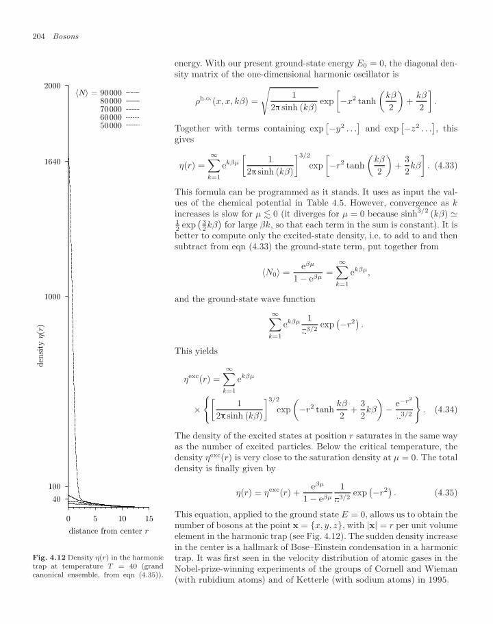
204 Bosons
energy. With our present ground-state energy E0 = 0, the diagonal den-sity matrix of the one-dimensional harmonic oscillator is
ρh.o.(x, x, kβ) =
√1
2 sinh (kβ)exp[−x2 tanh
(kβ
2
)+
kβ
2
].
Together with terms containing exp[−y2 . . .
]and exp
[−z2 . . .], this
gives
η(r) =∞∑
k=1
ekβµ
[1
2 sinh (kβ)
]3/2
exp[−r2 tanh
(kβ
2
)+
32kβ
]. (4.33)
This formula can be programmed as it stands. It uses as input the val-ues of the chemical potential in Table 4.5. However, convergence as kincreases is slow for µ 0 (it diverges for µ = 0 because sinh3/2 (kβ) 12 exp
(32kβ)
for large βk, so that each term in the sum is constant). It isbetter to compute only the excited-state density, i.e. to add to and thensubtract from eqn (4.33) the ground-state term, put together from
〈N0〉 =eβµ
1 − eβµ=
∞∑k=1
ekβµ,
and the ground-state wave function
∞∑k=1
ekβµ 13/2
exp(−r2
).
This yields
ηexc(r) =∞∑
k=1
ekβµ
×[
12 sinh (kβ)
]3/2
exp(−r2 tanh
kβ
2+
32kβ
)− e−r2
3/2
. (4.34)
The density of the excited states at position r saturates in the same wayas the number of excited particles. Below the critical temperature, thedensity ηexc(r) is very close to the saturation density at µ = 0. The totaldensity is finally given by
η(r) = ηexc(r) +eβµ
1 − eβµ
13/2
exp(−r2
). (4.35)
This equation, applied to the ground state E = 0, allows us to obtain thenumber of bosons at the point x = x, y, z, with |x| = r per unit volumeelement in the harmonic trap (see Fig. 4.12). The sudden density increasein the center is a hallmark of Bose–Einstein condensation in a harmonictrap. It was first seen in the velocity distribution of atomic gases in theNobel-prize-winning experiments of the groups of Cornell and Wieman(with rubidium atoms) and of Ketterle (with sodium atoms) in 1995.
2000
1640
1000
100
40
0 5 10 15
den
sity
η(r
)
distance from center r
〈N〉 = 9000080000700006000050000
Fig. 4.12 Density η(r) in the harmonictrap at temperature T = 40 (grandcanonical ensemble, from eqn (4.35)).
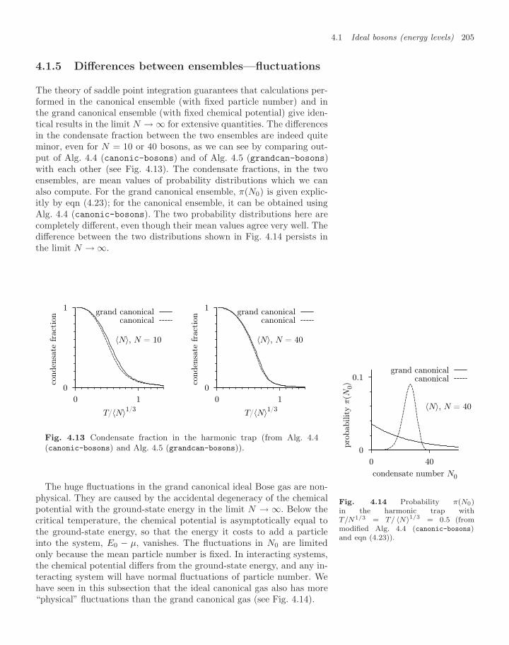
4.1 Ideal bosons (energy levels) 205
4.1.5 Differences between ensembles—fluctuations
The theory of saddle point integration guarantees that calculations per-formed in the canonical ensemble (with fixed particle number) and inthe grand canonical ensemble (with fixed chemical potential) give iden-tical results in the limit N → ∞ for extensive quantities. The differencesin the condensate fraction between the two ensembles are indeed quiteminor, even for N = 10 or 40 bosons, as we can see by comparing out-put of Alg. 4.4 (canonic-bosons) and of Alg. 4.5 (grandcan-bosons)with each other (see Fig. 4.13). The condensate fractions, in the twoensembles, are mean values of probability distributions which we canalso compute. For the grand canonical ensemble, π(N0) is given explic-itly by eqn (4.23); for the canonical ensemble, it can be obtained usingAlg. 4.4 (canonic-bosons). The two probability distributions here arecompletely different, even though their mean values agree very well. Thedifference between the two distributions shown in Fig. 4.14 persists inthe limit N → ∞.
0
1
0 1
conden
sate
fra
ctio
n
T/〈N〉1/3
〈N〉, N = 10
grand canonicalcanonical
0
1
0 1
conden
sate
fra
ctio
n
T/〈N〉1/3
〈N〉, N = 40
grand canonicalcanonical
Fig. 4.13 Condensate fraction in the harmonic trap (from Alg. 4.4(canonic-bosons) and Alg. 4.5 (grandcan-bosons)). 0
0.1
400
pro
babilit
y π
(N0)
condensate number N0
〈N〉, N = 40
grand canonicalcanonical
Fig. 4.14 Probability π(N0)in the harmonic trap withT/N1/3 = T/ 〈N〉1/3 = 0.5 (frommodified Alg. 4.4 (canonic-bosons)and eqn (4.23)).
The huge fluctuations in the grand canonical ideal Bose gas are non-physical. They are caused by the accidental degeneracy of the chemicalpotential with the ground-state energy in the limit N → ∞. Below thecritical temperature, the chemical potential is asymptotically equal tothe ground-state energy, so that the energy it costs to add a particleinto the system, E0 − µ, vanishes. The fluctuations in N0 are limitedonly because the mean particle number is fixed. In interacting systems,the chemical potential differs from the ground-state energy, and any in-teracting system will have normal fluctuations of particle number. Wehave seen in this subsection that the ideal canonical gas also has more“physical” fluctuations than the grand canonical gas (see Fig. 4.14).
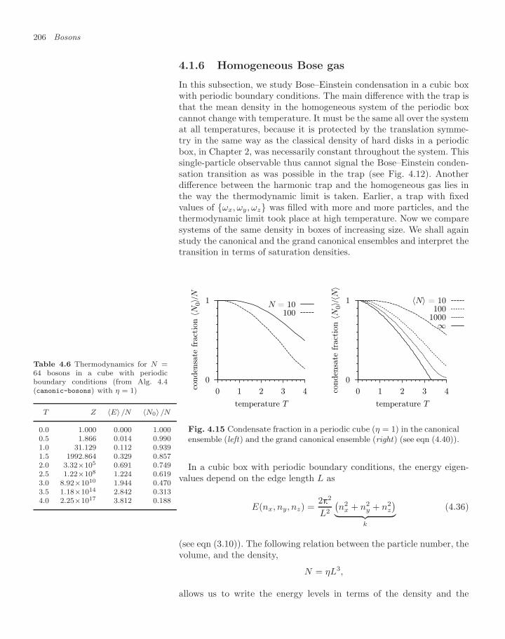
206 Bosons
4.1.6 Homogeneous Bose gas
In this subsection, we study Bose–Einstein condensation in a cubic boxwith periodic boundary conditions. The main difference with the trap isthat the mean density in the homogeneous system of the periodic boxcannot change with temperature. It must be the same all over the systemat all temperatures, because it is protected by the translation symme-try in the same way as the classical density of hard disks in a periodicbox, in Chapter 2, was necessarily constant throughout the system. Thissingle-particle observable thus cannot signal the Bose–Einstein conden-sation transition as was possible in the trap (see Fig. 4.12). Anotherdifference between the harmonic trap and the homogeneous gas lies inthe way the thermodynamic limit is taken. Earlier, a trap with fixedvalues of ωx, ωy, ωz was filled with more and more particles, and thethermodynamic limit took place at high temperature. Now we comparesystems of the same density in boxes of increasing size. We shall againstudy the canonical and the grand canonical ensembles and interpret thetransition in terms of saturation densities.
0
1
0 1 2 3 4conden
sate
fra
ctio
n 〈N
0〉/N
temperature T
N = 10100
0
1
0 1 2 3 4conden
sate
fra
ctio
n 〈N
0〉/〈N
〉
temperature T
〈N〉 = 10100
1000∞
Fig. 4.15 Condensate fraction in a periodic cube (η = 1) in the canonicalensemble (left) and the grand canonical ensemble (right) (see eqn (4.40)).
Table 4.6 Thermodynamics for N =64 bosons in a cube with periodicboundary conditions (from Alg. 4.4(canonic-bosons) with η = 1)
T Z 〈E〉/N 〈N0〉 /N
0.0 1.000 0.000 1.0000.5 1.866 0.014 0.9901.0 31.129 0.112 0.9391.5 1992.864 0.329 0.8572.0 3.32×10⁵ 0.691 0.7492.5 1.22×10⁸ 1.224 0.6193.0 8.92×10¹⁰ 1.944 0.4703.5 1.18×10¹⁴ 2.842 0.3134.0 2.25×10¹⁷ 3.812 0.188
In a cubic box with periodic boundary conditions, the energy eigen-values depend on the edge length L as
E(nx, ny, nz) =22
L2
(n2
x + n2y + n2
z
)︸ ︷︷ ︸k
(4.36)
(see eqn (3.10)). The following relation between the particle number, thevolume, and the density,
N = ηL3,
allows us to write the energy levels in terms of the density and the
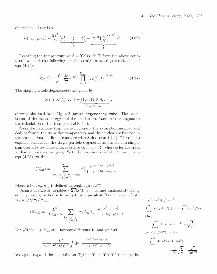
4.1 Ideal bosons (energy levels) 207
dimensions of the box:
E(nx, ny, nz) =22
L2
(n2
x + n2y + n2
z
)︸ ︷︷ ︸E
=[22( η
N
)2/3]
︸ ︷︷ ︸Υ
E. (4.37)
Rescaling the temperature as β = Υβ (with Υ from the above equa-tion), we find the following, in the straightforward generalization ofeqn (4.17):
ZN(β) =∫
−
dλ
2e−iNλ
Emax∏E=0
[fE(β, λ)
]N(E)
. (4.38)
The single-particle degeneracies are given by
N (0) ,N (1) , . . . = 1, 6, 12, 8, 4, . . .︸ ︷︷ ︸from Table 4.2
,
directly obtained from Alg. 4.2 (naive-degeneracy-cube). The calcu-lation of the mean energy and the condensate fraction is analogous tothe calculation in the trap (see Table 4.6).
As in the harmonic trap, we can compute the saturation number anddeduce from it the transition temperature and the condensate fraction inthe thermodynamic limit (compare with Subsection 4.1.4). There is noexplicit formula for the single-particle degeneracies, but we can simplysum over all sites of the integer lattice nx, ny, nz (whereas for the trap,we had a sum over energies). With dummy sum variables ∆n = 1, as ineqn (4.28), we find
〈Nsat〉 =nmax∑
nx,ny,nz=−nmax
=0,0,0
∆3n
e−βE(nx,ny,nz)
1 − e−βE(nx,ny,nz),
where E(nx, ny, nz) is defined through eqn (4.37).Using a change of variables
√2β(/L)nx = x, and analogously for ny
and nz, we again find a term-by-term equivalent Riemann sum (with∆x =
√2β/L∆n): If r2 = x2 + y2 + z2,Z ∞
−∞
dx dy dz f(r) = 4Z ∞
0dr r2f(r).
Also,Z ∞
−∞
dµ exp`−nµ2
´=r
n
(see eqn (3.12)) impliesZ ∞
−∞
du u2 exp`−nu2
´= − ∂
∂n
r
n=
√
2n3/2.
〈Nsat〉 =L3
3(2β)3/2
∑xi,yi,zi=0,0,0
∆x∆y∆ze−(x2
i +y2i +z2
i )
1 − e−(x2i+y2
i+z2
i).
For√
β/L → 0, ∆x, etc., become differentials, and we find
−−−→β→0
L3
3(2β)3/2
∫dV
e−(x2+y2+z2)
1 − e−(x2+y2+z2).
We again expand the denominator Υ/(1 − Υ) = Υ + Υ2 + · · · (as for
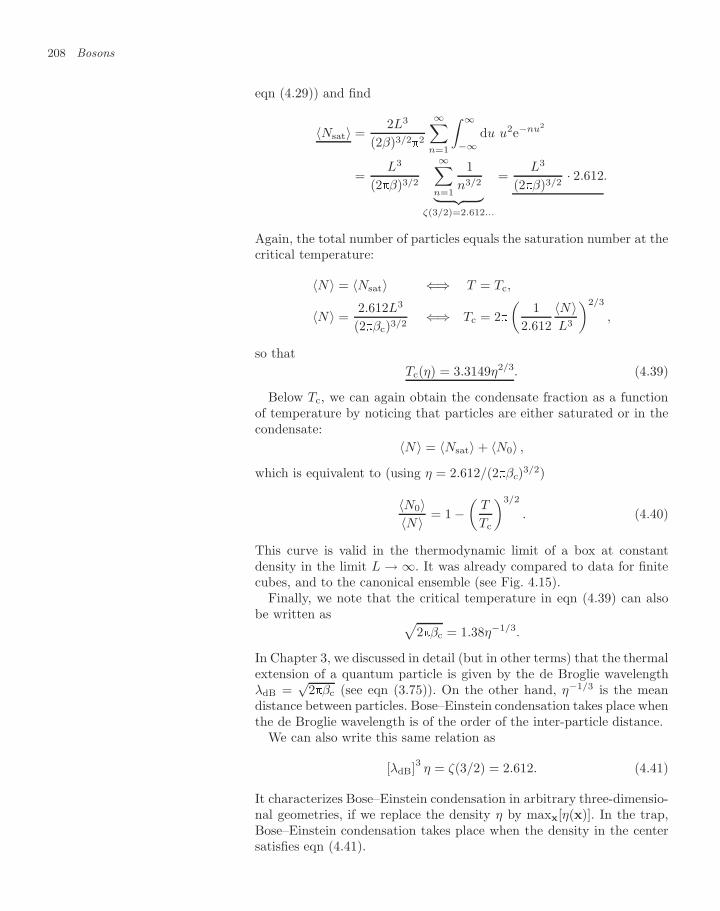
208 Bosons
eqn (4.29)) and find
〈Nsat〉 =2L3
(2β)3/22
∞∑n=1
∫ ∞
−∞du u2e−nu2
=L3
(2β)3/2
∞∑n=1
1n3/2︸ ︷︷ ︸
ζ(3/2)=2.612...
=L3
(2β)3/2· 2.612.
Again, the total number of particles equals the saturation number at thecritical temperature:
〈N〉 = 〈Nsat〉 ⇐⇒ T = Tc,
〈N〉 =2.612L3
(2βc)3/2⇐⇒ Tc = 2
(1
2.612〈N〉L3
)2/3
,
so thatTc(η) = 3.3149η2/3. (4.39)
Below Tc, we can again obtain the condensate fraction as a functionof temperature by noticing that particles are either saturated or in thecondensate:
〈N〉 = 〈Nsat〉 + 〈N0〉 ,
which is equivalent to (using η = 2.612/(2βc)3/2)
〈N0〉〈N〉 = 1 −
(T
Tc
)3/2
. (4.40)
This curve is valid in the thermodynamic limit of a box at constantdensity in the limit L → ∞. It was already compared to data for finitecubes, and to the canonical ensemble (see Fig. 4.15).
Finally, we note that the critical temperature in eqn (4.39) can alsobe written as √
2βc = 1.38η−1/3.
In Chapter 3, we discussed in detail (but in other terms) that the thermalextension of a quantum particle is given by the de Broglie wavelengthλdB =
√2βc (see eqn (3.75)). On the other hand, η−1/3 is the mean
distance between particles. Bose–Einstein condensation takes place whenthe de Broglie wavelength is of the order of the inter-particle distance.
We can also write this same relation as
[λdB]3 η = ζ(3/2) = 2.612. (4.41)
It characterizes Bose–Einstein condensation in arbitrary three-dimensio-nal geometries, if we replace the density η by maxx[η(x)]. In the trap,Bose–Einstein condensation takes place when the density in the centersatisfies eqn (4.41).
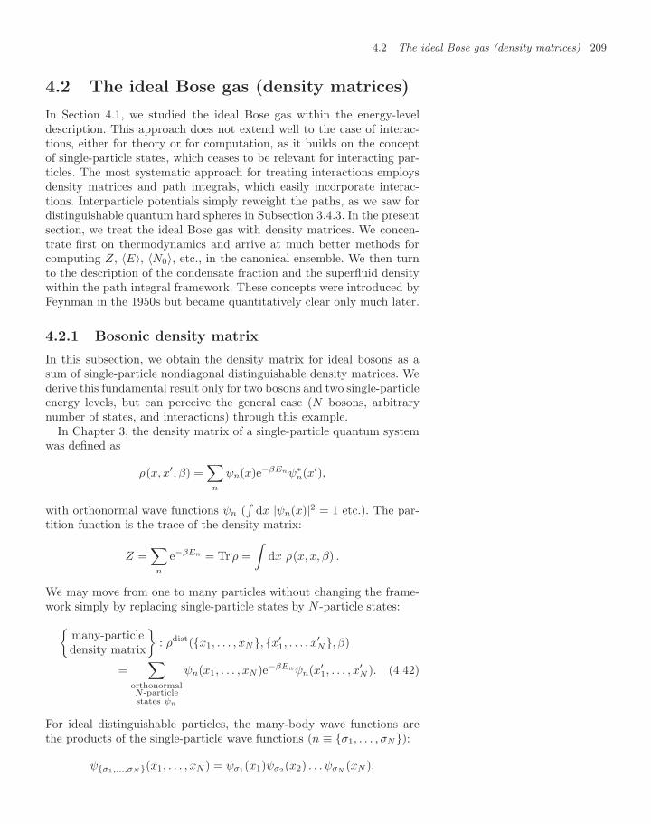
4.2 The ideal Bose gas (density matrices) 209
4.2 The ideal Bose gas (density matrices)
In Section 4.1, we studied the ideal Bose gas within the energy-leveldescription. This approach does not extend well to the case of interac-tions, either for theory or for computation, as it builds on the conceptof single-particle states, which ceases to be relevant for interacting par-ticles. The most systematic approach for treating interactions employsdensity matrices and path integrals, which easily incorporate interac-tions. Interparticle potentials simply reweight the paths, as we saw fordistinguishable quantum hard spheres in Subsection 3.4.3. In the presentsection, we treat the ideal Bose gas with density matrices. We concen-trate first on thermodynamics and arrive at much better methods forcomputing Z, 〈E〉, 〈N0〉, etc., in the canonical ensemble. We then turnto the description of the condensate fraction and the superfluid densitywithin the path integral framework. These concepts were introduced byFeynman in the 1950s but became quantitatively clear only much later.
4.2.1 Bosonic density matrix
In this subsection, we obtain the density matrix for ideal bosons as asum of single-particle nondiagonal distinguishable density matrices. Wederive this fundamental result only for two bosons and two single-particleenergy levels, but can perceive the general case (N bosons, arbitrarynumber of states, and interactions) through this example.
In Chapter 3, the density matrix of a single-particle quantum systemwas defined as
ρ(x, x′, β) =∑
n
ψn(x)e−βEnψ∗n(x′),
with orthonormal wave functions ψn (∫
dx |ψn(x)|2 = 1 etc.). The par-tition function is the trace of the density matrix:
Z =∑
n
e−βEn = Tr ρ =∫
dx ρ(x, x, β) .
We may move from one to many particles without changing the frame-work simply by replacing single-particle states by N -particle states:
many-particledensity matrix
: ρdist(x1, . . . , xN, x′
1, . . . , x′N, β)
=∑
orthonormalN-particlestates ψn
ψn(x1, . . . , xN )e−βEnψn(x′1, . . . , x
′N ). (4.42)
For ideal distinguishable particles, the many-body wave functions arethe products of the single-particle wave functions (n ≡ σ1, . . . , σN):
ψσ1,...,σN(x1, . . . , xN ) = ψσ1(x1)ψσ2 (x2) . . . ψσN(xN ).
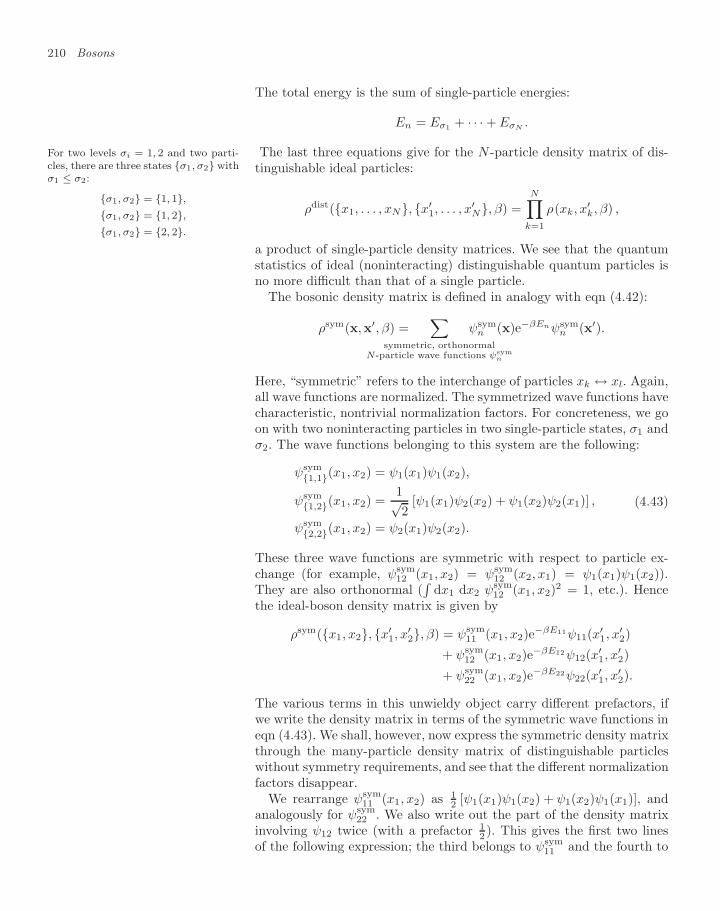
210 Bosons
The total energy is the sum of single-particle energies:
En = Eσ1 + · · · + EσN.
The last three equations give for the N -particle density matrix of dis-For two levels σi = 1, 2 and two parti-cles, there are three states σ1, σ2 withσ1 ≤ σ2:
σ1, σ2 = 1, 1,σ1, σ2 = 1, 2,σ1, σ2 = 2, 2.
tinguishable ideal particles:
ρdist(x1, . . . , xN, x′1, . . . , x
′N, β) =
N∏k=1
ρ(xk, x′k, β) ,
a product of single-particle density matrices. We see that the quantumstatistics of ideal (noninteracting) distinguishable quantum particles isno more difficult than that of a single particle.
The bosonic density matrix is defined in analogy with eqn (4.42):
ρsym(x,x′, β) =∑
symmetric, orthonormalN-particle wave functions ψsym
n
ψsymn (x)e−βEnψsym
n (x′).
Here, “symmetric” refers to the interchange of particles xk ↔ xl. Again,all wave functions are normalized. The symmetrized wave functions havecharacteristic, nontrivial normalization factors. For concreteness, we goon with two noninteracting particles in two single-particle states, σ1 andσ2. The wave functions belonging to this system are the following:
ψsym1,1(x1, x2) = ψ1(x1)ψ1(x2),
ψsym1,2(x1, x2) =
1√2
[ψ1(x1)ψ2(x2) + ψ1(x2)ψ2(x1)] ,
ψsym2,2(x1, x2) = ψ2(x1)ψ2(x2).
(4.43)
These three wave functions are symmetric with respect to particle ex-change (for example, ψsym
12 (x1, x2) = ψsym12 (x2, x1) = ψ1(x1)ψ1(x2)).
They are also orthonormal (∫
dx1 dx2 ψsym12 (x1, x2)2 = 1, etc.). Hence
the ideal-boson density matrix is given by
ρsym(x1, x2, x′1, x
′2, β) = ψsym
11 (x1, x2)e−βE11ψ11(x′1, x
′2)
+ ψsym12 (x1, x2)e−βE12ψ12(x′
1, x′2)
+ ψsym22 (x1, x2)e−βE22ψ22(x′
1, x′2).
The various terms in this unwieldy object carry different prefactors, ifwe write the density matrix in terms of the symmetric wave functions ineqn (4.43). We shall, however, now express the symmetric density matrixthrough the many-particle density matrix of distinguishable particleswithout symmetry requirements, and see that the different normalizationfactors disappear.
We rearrange ψsym11 (x1, x2) as 1
2 [ψ1(x1)ψ1(x2) + ψ1(x2)ψ1(x1)], andanalogously for ψsym
22 . We also write out the part of the density matrixinvolving ψ12 twice (with a prefactor 1
2 ). This gives the first two linesof the following expression; the third belongs to ψsym
11 and the fourth to
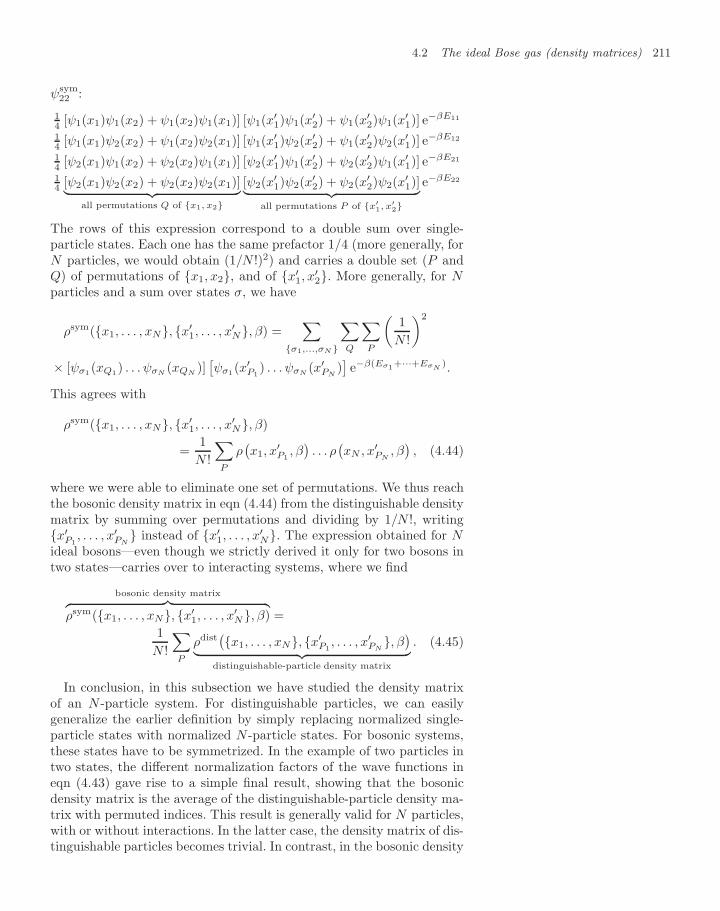
4.2 The ideal Bose gas (density matrices) 211
ψsym22 :
14 [ψ1(x1)ψ1(x2) + ψ1(x2)ψ1(x1)] [ψ1(x′
1)ψ1(x′2) + ψ1(x′
2)ψ1(x′1)] e−βE11
14 [ψ1(x1)ψ2(x2) + ψ1(x2)ψ2(x1)] [ψ1(x′
1)ψ2(x′2) + ψ1(x′
2)ψ2(x′1)] e−βE12
14 [ψ2(x1)ψ1(x2) + ψ2(x2)ψ1(x1)] [ψ2(x′
1)ψ1(x′2) + ψ2(x′
2)ψ1(x′1)] e−βE21
14 [ψ2(x1)ψ2(x2) + ψ2(x2)ψ2(x1)]︸ ︷︷ ︸
all permutations Q of x1, x2
[ψ2(x′1)ψ2(x′
2) + ψ2(x′2)ψ2(x′
1)]︸ ︷︷ ︸all permutations P of x′
1, x′2
e−βE22
The rows of this expression correspond to a double sum over single-particle states. Each one has the same prefactor 1/4 (more generally, forN particles, we would obtain (1/N !)2) and carries a double set (P andQ) of permutations of x1, x2, and of x′
1, x′2. More generally, for N
particles and a sum over states σ, we have
ρsym(x1, . . . , xN, x′1, . . . , x
′N, β) =
∑σ1,...,σN
∑Q
∑P
(1
N !
)2
× [ψσ1 (xQ1) . . . ψσN(xQN
)][ψσ1(x′
P1) . . . ψσN
(x′PN
)]e−β(Eσ1+···+EσN
).
This agrees with
ρsym(x1, . . . , xN, x′1, . . . , x
′N, β)
=1
N !
∑P
ρ(x1, x
′P1
, β). . . ρ(xN , x′
PN, β), (4.44)
where we were able to eliminate one set of permutations. We thus reachthe bosonic density matrix in eqn (4.44) from the distinguishable densitymatrix by summing over permutations and dividing by 1/N !, writingx′
P1, . . . , x′
PN instead of x′
1, . . . , x′N. The expression obtained for N
ideal bosons—even though we strictly derived it only for two bosons intwo states—carries over to interacting systems, where we find
bosonic density matrix︷ ︸︸ ︷ρsym(x1, . . . , xN, x′
1, . . . , x′N, β) =
1N !
∑P
ρdist(x1, . . . , xN, x′
P1, . . . , x′
PN, β)︸ ︷︷ ︸
distinguishable-particle density matrix
. (4.45)
In conclusion, in this subsection we have studied the density matrixof an N -particle system. For distinguishable particles, we can easilygeneralize the earlier definition by simply replacing normalized single-particle states with normalized N -particle states. For bosonic systems,these states have to be symmetrized. In the example of two particles intwo states, the different normalization factors of the wave functions ineqn (4.43) gave rise to a simple final result, showing that the bosonicdensity matrix is the average of the distinguishable-particle density ma-trix with permuted indices. This result is generally valid for N particles,with or without interactions. In the latter case, the density matrix of dis-tinguishable particles becomes trivial. In contrast, in the bosonic density
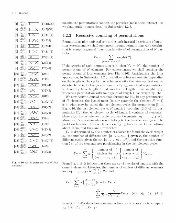
212 Bosons
matrix, the permutations connect the particles (make them interact), aswe shall study in more detail in Subsection 4.2.3.
4.2.2 Recursive counting of permutations
[1] (12341234) (1)(2)(3)(4)
[2] (12431234) (1)(2)(34)
[3] (13241234) (1)(23)(4)
[4] (13421234) (1)(234)
[5] (14231234) (1)(243)
[6] (14321234) (1)(24)(3)
[7] (21341234) (12)(3)(4)
[8] (21431234) (12)(34)
[9] (23141234) (123)(4)
[10] (23411234) (1234)
[11] (24131234) (1243)
[12] (24311234) (124)(3)
[13] (31241234) (132)(4)
[14] (31421234) (1342)
[15] (32141234) (13)(2)(4)
[16] (32411234) (134)(2)
[17] (34121234) (13)(24)
[18] (34211234) (1324)
[19] (41231234) (1432)
[20] (41321234) (142)(3)
[21] (42131234) (143)(2)
[22] (42311234) (14)(2)(3)
[23] (43121234) (1423)
[24] (43211234) (14)(23)
Fig. 4.16 All 24 permutations of fourelements.
Permutations play a pivotal role in the path-integral description of quan-tum systems, and we shall soon need to count permutations with weights,that is, compute general “partition functions” of permutations of N par-ticles
YN =∑
permutations P
weight(P ).
If the weight of each permutation is 1, then YN = N !, the number ofpermutations of N elements. For concreteness, we shall consider thepermutations of four elements (see Fig. 4.16). Anticipating the laterapplication, in Subsection 4.2.3, we allow arbitrary weights dependingon the length of the cycles. For coherence with the later application, wedenote the weight of a cycle of length k by zk, such that a permutationwith one cycle of length 3 and another of length 1 has weight z3z1,whereas a permutation with four cycles of length 1 has weight z4
1 , etc.We now derive a crucial recursion formula for YN . In any permutation
of N elements, the last element (in our example the element N = 4)is in what may be called the last-element cycle. (In permutation [5] inFig. 4.16, the last-element cycle, of length 3, contains 2, 3, 4. In per-mutation [23], the last-element cycle, of length 4, contains all elements).Generally, this last-element cycle involves k elements n1, . . . , nk−1, N.Moreover, N − k elements do not belong to the last-element cycle. Thepartition function of these elements is YN−k, because we know nothingabout them, and they are unrestricted.
YN is determined by the number of choices for k and the cycle weightzk, the number of different sets n1, . . . , nk−1 given k, the number ofdifferent cycles given the set n1, . . . , nk−1, N, and the partition func-tion YM of the elements not participating in the last-element cycle:
YN =N∑
k=1
zk
⎧⎨⎩number ofchoices for
n1, . . . , nk−1
⎫⎬⎭⎧⎨⎩
number ofcycles withn1, . . . , nk
⎫⎬⎭YN−k.
From Fig. 4.16, it follows that there are (k−1)! cycles of length k with thesame k elements. Likewise, the number of choices of different elementsfor n1, . . . , nk−1 is
(N−1k−1
). We find
YN =N∑
k=1
zk
(N − 1k − 1
)(k − 1)! YN−k
=N∑
k=1
1N
zkN !
(N − k)!YN−k (with Y0 = 1). (4.46)
Equation (4.46) describes a recursion because it allows us to computeYN from Y0, . . . , YN−1.
4.2 The ideal Bose gas (density matrices) 213
We now use the recursion formula in eqn (4.46) to count permutationsof N elements for various choices of cycle weights z1, . . . , zN. Let usstart with the simplest case, z1, . . . , zN = 1, . . . , 1, where each cyclelength has the same weight, and every permutation has unit weight. Weexpect to find that YN = N !, and this is indeed what results from therecursion relation, as we may prove by induction. It follows, for this caseof equal cycle weights, that the weight of all permutations with a last-element cycle of length k is the same for all k (as is zkYN−k/(N − k)!in eqn (4.46)). This is a nontrivial theorem. To illustrate it, let us countlast-element cycles in Fig. 4.16:
in Fig. 4.16,element 4 is
⎧⎪⎪⎪⎨⎪⎪⎪⎩in 6 cycles of length 4in 6 cycles of length 3in 6 cycles of length 2in 6 cycles of length 1
.
The element 4 is in no way special, and this implies that any elementamong 1, . . . , N is equally likely to be in a cycle of length 1, . . . , N.As a consequence, in a random permutation (for example generated withAlg. 1.11 (ran-perm)), the probability of having a cycle of length k is∝ 1/k. We need more cycles of shorter length to come up with the sameprobability. Concretely, we find
in Fig. 4.16,
there are
⎧⎪⎪⎪⎨⎪⎪⎪⎩6 cycles of length 48 cycles of length 312 cycles of length 224 cycles of length 1
.
The number of cycles of length k is indeed inversely proportional to k.As a second application of the recursion relation, let us count permuta-tions containing only cycles of length 1 and 2. Now z1, z2, z3, . . . , zN =1, 1, 0, . . . , 0 (every permutation has the same weight, under the con-dition that it contains no cycles of length 3 or longer). We find Y0 = 1and Y1 = 1, and from eqn (4.46) the recursion relation
YN = YN−1 + (N − 1) YN−2,
so that Y0, Y1, Y2, Y3, Y4, . . . = 1, 1, 2, 4, 10, . . .. Indeed, for N = 4,we find 10 such permutations in Fig. 4.16 ([1], [2], [3], [6], [7], [8], [15],[17], [22], and [24]).
In conclusion, we have described in this subsection a recursion formulafor counting permutations that lets us handle arbitrary cycle weights.We shall apply it, in Subsection 4.2.3, to ideal bosons.
4.2.3 Canonical partition function of ideal bosons
In Subsection 4.2.1, we expressed the partition function of a bosonicsystem as a sum over diagonal and nondiagonal density matrices for
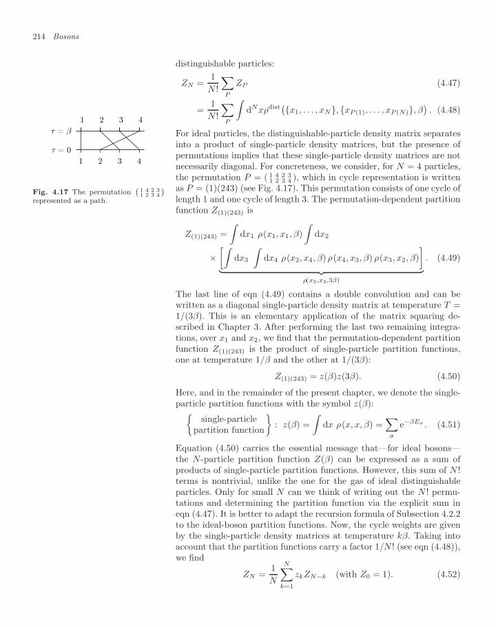
214 Bosons
distinguishable particles:
ZN =1
N !
∑P
ZP (4.47)
=1
N !
∑P
∫dNxρdist
(x1, . . . , xN, xP (1), . . . , xP (N), β). (4.48)
For ideal particles, the distinguishable-particle density matrix separatesinto a product of single-particle density matrices, but the presence ofpermutations implies that these single-particle density matrices are notnecessarily diagonal. For concreteness, we consider, for N = 4 particles,
τ = β
τ = 0
4321
4 3 2 1
Fig. 4.17 The permutation`
1 4 2 31 2 3 4
´represented as a path.
the permutation P = ( 1 4 2 31 2 3 4 ), which in cycle representation is written
as P = (1)(243) (see Fig. 4.17). This permutation consists of one cycle oflength 1 and one cycle of length 3. The permutation-dependent partitionfunction Z(1)(243) is
Z(1)(243) =∫
dx1 ρ(x1, x1, β)∫
dx2
×[∫
dx3
∫dx4 ρ(x2, x4, β) ρ(x4, x3, β) ρ(x3, x2, β)
]︸ ︷︷ ︸
ρ(x2,x2,3β)
. (4.49)
The last line of eqn (4.49) contains a double convolution and can bewritten as a diagonal single-particle density matrix at temperature T =1/(3β). This is an elementary application of the matrix squaring de-scribed in Chapter 3. After performing the last two remaining integra-tions, over x1 and x2, we find that the permutation-dependent partitionfunction Z(1)(243) is the product of single-particle partition functions,one at temperature 1/β and the other at 1/(3β):
Z(1)(243) = z(β)z(3β). (4.50)
Here, and in the remainder of the present chapter, we denote the single-particle partition functions with the symbol z(β):
single-particlepartition function
: z(β) =
∫dx ρ(x, x, β) =
∑σ
e−βEσ . (4.51)
Equation (4.50) carries the essential message that—for ideal bosons—the N -particle partition function Z(β) can be expressed as a sum ofproducts of single-particle partition functions. However, this sum of N !terms is nontrivial, unlike the one for the gas of ideal distinguishableparticles. Only for small N can we think of writing out the N ! permu-tations and determining the partition function via the explicit sum ineqn (4.47). It is better to adapt the recursion formula of Subsection 4.2.2to the ideal-boson partition functions. Now, the cycle weights are givenby the single-particle density matrices at temperature kβ. Taking intoaccount that the partition functions carry a factor 1/N ! (see eqn (4.48)),we find
ZN =1N
N∑k=1
zkZN−k (with Z0 = 1). (4.52)
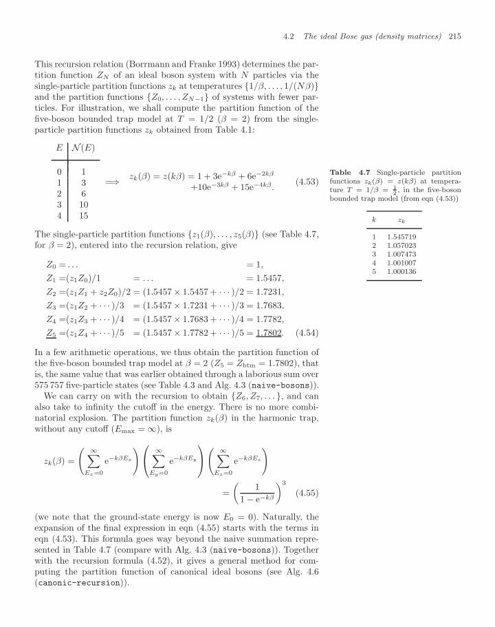
4.2 The ideal Bose gas (density matrices) 215
This recursion relation (Borrmann and Franke 1993) determines the par-tition function ZN of an ideal boson system with N particles via thesingle-particle partition functions zk at temperatures 1/β, . . . , 1/(Nβ)and the partition functions Z0, . . . , ZN−1 of systems with fewer par-ticles. For illustration, we shall compute the partition function of thefive-boson bounded trap model at T = 1/2 (β = 2) from the single-particle partition functions zk obtained from Table 4.1:
E N (E)
0 11 32 63 104 15
=⇒ zk(β) = z(kβ) = 1 + 3e−kβ + 6e−2kβ
+10e−3kβ + 15e−4kβ.(4.53)
The single-particle partition functions z1(β), . . . , z5(β) (see Table 4.7,for β = 2), entered into the recursion relation, give
Table 4.7 Single-particle partitionfunctions zk(β) = z(kβ) at tempera-ture T = 1/β = 1
2, in the five-boson
bounded trap model (from eqn (4.53))
k zk
1 1.5457192 1.0570233 1.0074734 1.0010075 1.000136
Z0 = . . . = 1,
Z1 =(z1Z0)/1 = . . . = 1.5457,
Z2 =(z1Z1 + z2Z0)/2 = (1.5457× 1.5457 + · · · )/2 = 1.7231,
Z3 =(z1Z2 + · · · )/3 = (1.5457× 1.7231 + · · · )/3 = 1.7683,
Z4 =(z1Z3 + · · · )/4 = (1.5457× 1.7683 + · · · )/4 = 1.7782,
Z5 =(z1Z4 + · · · )/5 = (1.5457× 1.7782 + · · · )/5 = 1.7802. (4.54)
In a few arithmetic operations, we thus obtain the partition function ofthe five-boson bounded trap model at β = 2 (Z5 = Zbtm = 1.7802), thatis, the same value that was earlier obtained through a laborious sum over575 757 five-particle states (see Table 4.3 and Alg. 4.3 (naive-bosons)).
We can carry on with the recursion to obtain Z6, Z7, . . . , and canalso take to infinity the cutoff in the energy. There is no more combi-natorial explosion. The partition function zk(β) in the harmonic trap,without any cutoff (Emax = ∞), is
zk(β) =
( ∞∑Ex=0
e−kβEx
)⎛⎝ ∞∑Ey=0
e−kβEy
⎞⎠( ∞∑Ez=0
e−kβEz
)
=(
11 − e−kβ
)3
(4.55)
(we note that the ground-state energy is now E0 = 0). Naturally, theexpansion of the final expression in eqn (4.55) starts with the terms ineqn (4.53). This formula goes way beyond the naive summation repre-sented in Table 4.7 (compare with Alg. 4.3 (naive-bosons)). Togetherwith the recursion formula (4.52), it gives a general method for com-puting the partition function of canonical ideal bosons (see Alg. 4.6(canonic-recursion)).
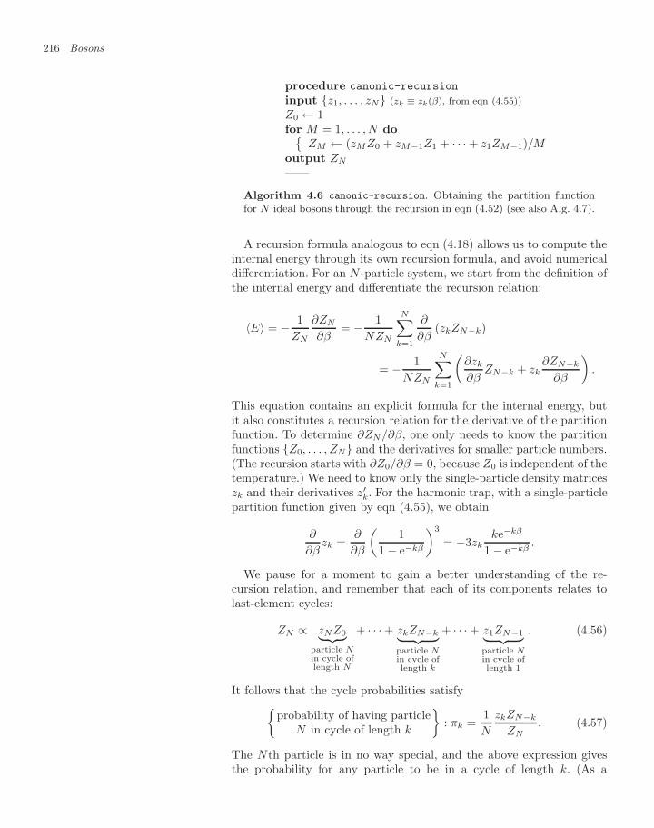
216 Bosons
procedure canonic-recursion
input z1, . . . , zN (zk ≡ zk(β), from eqn (4.55))Z0 ← 1for M = 1, . . . , N do
ZM ← (zMZ0 + zM−1Z1 + · · · + z1ZM−1)/Moutput ZN
——
Algorithm 4.6 canonic-recursion. Obtaining the partition functionfor N ideal bosons through the recursion in eqn (4.52) (see also Alg. 4.7).
A recursion formula analogous to eqn (4.18) allows us to compute theinternal energy through its own recursion formula, and avoid numericaldifferentiation. For an N -particle system, we start from the definition ofthe internal energy and differentiate the recursion relation:
〈E〉 = − 1ZN
∂ZN
∂β= − 1
NZN
N∑k=1
∂
∂β(zkZN−k)
= − 1NZN
N∑k=1
(∂zk
∂βZN−k + zk
∂ZN−k
∂β
).
This equation contains an explicit formula for the internal energy, butit also constitutes a recursion relation for the derivative of the partitionfunction. To determine ∂ZN/∂β, one only needs to know the partitionfunctions Z0, . . . , ZN and the derivatives for smaller particle numbers.(The recursion starts with ∂Z0/∂β = 0, because Z0 is independent of thetemperature.) We need to know only the single-particle density matriceszk and their derivatives z′k. For the harmonic trap, with a single-particlepartition function given by eqn (4.55), we obtain
∂
∂βzk =
∂
∂β
(1
1 − e−kβ
)3
= −3zkke−kβ
1 − e−kβ.
We pause for a moment to gain a better understanding of the re-cursion relation, and remember that each of its components relates tolast-element cycles:
ZN ∝ zNZ0︸ ︷︷ ︸particle Nin cycle oflength N
+ · · · + zkZN−k︸ ︷︷ ︸particle Nin cycle oflength k
+ · · · + z1ZN−1︸ ︷︷ ︸particle Nin cycle oflength 1
. (4.56)
It follows that the cycle probabilities satisfyprobability of having particle
N in cycle of length k
: πk =
1N
zkZN−k
ZN. (4.57)
The Nth particle is in no way special, and the above expression givesthe probability for any particle to be in a cycle of length k. (As a
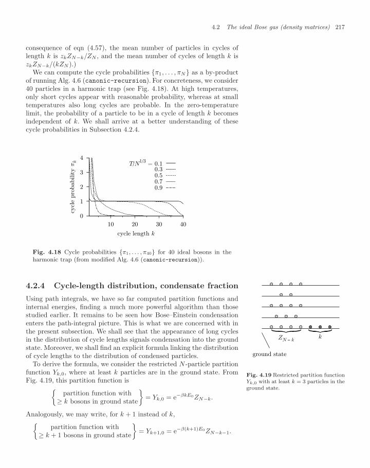
4.2 The ideal Bose gas (density matrices) 217
consequence of eqn (4.57), the mean number of particles in cycles oflength k is zkZN−k/ZN , and the mean number of cycles of length k iszkZN−k/(kZN ).)
We can compute the cycle probabilities π1, . . . , πN as a by-productof running Alg. 4.6 (canonic-recursion). For concreteness, we consider40 particles in a harmonic trap (see Fig. 4.18). At high temperatures,only short cycles appear with reasonable probability, whereas at smalltemperatures also long cycles are probable. In the zero-temperaturelimit, the probability of a particle to be in a cycle of length k becomesindependent of k. We shall arrive at a better understanding of thesecycle probabilities in Subsection 4.2.4.
0
1
2
3
4
10 20 30 40
cycl
e pro
bab
ilit
y π
k
cycle length k
T/N1/3 = 0.10.30.50.70.9
Fig. 4.18 Cycle probabilities π1, . . . , π40 for 40 ideal bosons in theharmonic trap (from modified Alg. 4.6 (canonic-recursion)).
4.2.4 Cycle-length distribution, condensate fraction
Using path integrals, we have so far computed partition functions andinternal energies, finding a much more powerful algorithm than thosestudied earlier. It remains to be seen how Bose–Einstein condensationenters the path-integral picture. This is what we are concerned with inthe present subsection. We shall see that the appearance of long cyclesin the distribution of cycle lengths signals condensation into the groundstate. Moreover, we shall find an explicit formula linking the distributionof cycle lengths to the distribution of condensed particles.
ZN − kk
ground state
Fig. 4.19 Restricted partition functionYk,0 with at least k = 3 particles in theground state.
To derive the formula, we consider the restricted N -particle partitionfunction Yk,0, where at least k particles are in the ground state. FromFig. 4.19, this partition function is
partition function with≥ k bosons in ground state
= Yk,0 = e−βkE0ZN−k.
Analogously, we may write, for k + 1 instead of k,partition function with
≥ k + 1 bosons in ground state
= Yk+1,0 = e−β(k+1)E0ZN−k−1.
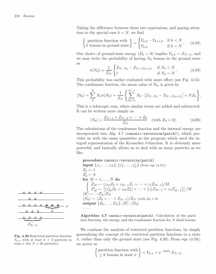
218 Bosons
Taking the difference between these two expressions, and paying atten-tion to the special case k = N , we find
partition function withk bosons in ground state
=
Yk,0 − Yk+1,0 if k < N
Yk,0 if k = N. (4.58)
Our choice of ground-state energy (E0 = 0) implies Yk,0 = ZN−k, andwe may write the probability of having N0 bosons in the ground stateas
π(N0) =1
ZN
ZN−N0 − ZN−(N0+1) if N0 < N
1 if N0 = N. (4.59)
This probability was earlier evaluated with more effort (see Fig. 4.14).The condensate fraction, the mean value of N0, is given by
〈N0〉 =N∑0
N0π(N0) =1
ZN
N−1∑N0=1
N0 ·[ZN−N0 − ZN−(N0+1)
]+ NZ0
.
This is a telescopic sum, where similar terms are added and subtracted.It can be written more simply as
〈N0〉 =ZN−1 + ZN−2 + · · · + Z0
ZN(with E0 = 0). (4.60)
The calculations of the condensate fraction and the internal energy areincorporated into Alg. 4.7 (canonic-recursion(patch)), which pro-vides us with the same quantities as the program which used the in-tegral representation of the Kronecker δ-function. It is obviously morepowerful, and basically allows us to deal with as many particles as welike.
procedure canonic-recursion(patch)
input z1, . . . , zN, z′1, . . . , z′N (from eqn (4.51))Z0 ← 1Z ′
0 ← 0for M = 1, . . . , N do
ZM ← (zMZ0 + zM−1Z1 + · · · + z1ZM−1)/MZ ′
M ← [(z′MZ0 + zMZ ′0) + · · · + (z′1ZM−1 + z1Z
′M−1
)]/M
〈E〉 ← −Z ′N/ZN
〈N0〉 ← (Z0 + · · · + ZN−1)/ZN (with E0 = 0)output Z0, . . . , ZN, 〈E〉 , 〈N0〉——
Algorithm 4.7 canonic-recursion(patch). Calculation of the parti-tion function, the energy, and the condensate fraction for N ideal bosons.
ZN − k
k
σ
Fig. 4.20 Restricted partition functionYk,σ with at least k = 3 particles instate σ (for N = 20 particles).
We continue the analysis of restricted partition functions, by simplygeneralizing the concept of the restricted partition functions to a stateσ, rather than only the ground state (see Fig. 4.20). From eqn (4.58),we arrive at
partition function with≥ k bosons in state σ
= Yk,σ = e−βkEσZN−k.
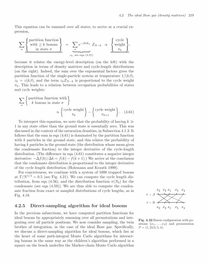
4.2 The ideal Bose gas (density matrices) 219
This equation can be summed over all states, to arrive at a crucial ex-pression,
∑σ
⎧⎨⎩partition functionwith ≥ k bosons
in state σ
⎫⎬⎭ =∑
σ
e−βkEσ
︸ ︷︷ ︸zk, see eqn (4.51)
ZN−k ∝⎧⎨⎩
cycleweight
πk
⎫⎬⎭,
because it relates the energy-level description (on the left) with thedescription in terms of density matrices and cycle-length distributions(on the right). Indeed, the sum over the exponential factors gives thepartition function of the single-particle system at temperature 1/(kβ),zk = z(kβ), and the term zkZN−k is proportional to the cycle weightπk. This leads to a relation between occupation probabilities of statesand cycle weights:
∑σ
partition function with
k bosons in state σ
∝
cycle weightπk
−
cycle weightπk+1
. (4.61)
To interpret this equation, we note that the probability of having k 1 in any state other than the ground state is essentially zero. This wasdiscussed in the context of the saturation densities, in Subsection 4.1.3. Itfollows that the sum in eqn (4.61) is dominated by the partition functionwith k particles in the ground state, and this relates the probability ofhaving k particles in the ground state (the distribution whose mean givesthe condensate fraction) to the integer derivative of the cycle-lengthdistribution. (The difference in eqn (4.61) constitutes a negative integerderivative: −∆f(k)/∆k = f(k)− f(k + 1).) We arrive at the conclusionthat the condensate distribution is proportional to the integer derivativeof the cycle length distribution (Holzmann and Krauth 1999).
For concreteness, we continue with a system of 1000 trapped bosonsat T/N1/3 = 0.5 (see Fig. 4.21). We can compute the cycle length dis-tribution, from eqn (4.56), and the distribution function π(N0) for thecondensate (see eqn (4.59)). We are thus able to compute the conden-sate fraction from exact or sampled distributions of cycle lengths, as inFig. 4.18.
4.2.5 Direct-sampling algorithm for ideal bosons
τ = β
τ = 0x5 x4x3x2 x1
x5 x4x3x2 x1
Fig. 4.22 Boson configuration with po-sitions x1, . . . , x5 and permutationP = (1, 2)(3, 5, 4).
In the previous subsections, we have computed partition functions forideal bosons by appropriately summing over all permutations and inte-grating over all particle positions. We now consider sampling, the twinbrother of integration, in the case of the ideal Bose gas. Specifically,we discuss a direct-sampling algorithm for ideal bosons, which lies atthe heart of some path-integral Monte Carlo algorithms for interact-ing bosons in the same way as the children’s algorithm performed in asquare on the beach underlies the Markov-chain Monte Carlo algorithm
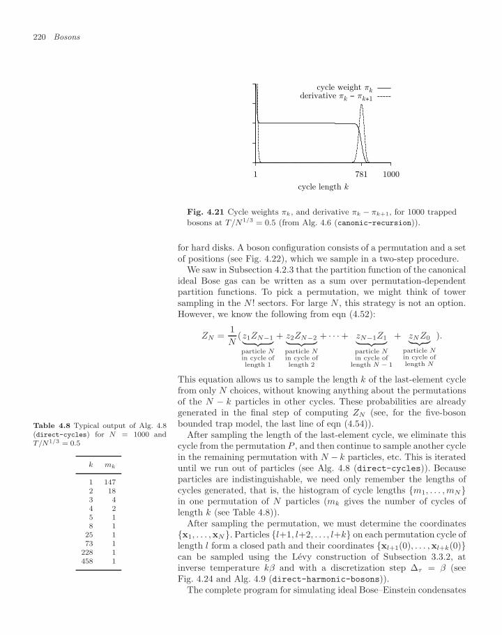
220 Bosons
10007811
cycle length k
cycle weight πkderivative πk − πk+1
Fig. 4.21 Cycle weights πk, and derivative πk − πk+1, for 1000 trapped
bosons at T/N1/3 = 0.5 (from Alg. 4.6 (canonic-recursion)).
for hard disks. A boson configuration consists of a permutation and a setof positions (see Fig. 4.22), which we sample in a two-step procedure.
We saw in Subsection 4.2.3 that the partition function of the canonicalideal Bose gas can be written as a sum over permutation-dependentpartition functions. To pick a permutation, we might think of towersampling in the N ! sectors. For large N , this strategy is not an option.However, we know the following from eqn (4.52):
ZN =1N
(z1ZN−1︸ ︷︷ ︸particle Nin cycle oflength 1
+ z2ZN−2︸ ︷︷ ︸particle Nin cycle oflength 2
+ · · · + zN−1Z1︸ ︷︷ ︸particle Nin cycle of
length N − 1
+ zNZ0︸ ︷︷ ︸particle Nin cycle oflength N
).
This equation allows us to sample the length k of the last-element cyclefrom only N choices, without knowing anything about the permutationsof the N − k particles in other cycles. These probabilities are alreadygenerated in the final step of computing ZN (see, for the five-bosonbounded trap model, the last line of eqn (4.54)).
After sampling the length of the last-element cycle, we eliminate thiscycle from the permutation P , and then continue to sample another cyclein the remaining permutation with N − k particles, etc. This is iterateduntil we run out of particles (see Alg. 4.8 (direct-cycles)). Becauseparticles are indistinguishable, we need only remember the lengths ofcycles generated, that is, the histogram of cycle lengths m1, . . . , mNin one permutation of N particles (mk gives the number of cycles oflength k (see Table 4.8)).
Table 4.8 Typical output of Alg. 4.8(direct-cycles) for N = 1000 andT/N1/3 = 0.5
k mk
1 1472 183 44 25 18 1
25 173 1
228 1458 1
After sampling the permutation, we must determine the coordinatesx1, . . . ,xN. Particles l+1, l+2, . . . , l+k on each permutation cycle oflength l form a closed path and their coordinates xl+1(0), . . . ,xl+k(0)can be sampled using the Levy construction of Subsection 3.3.2, atinverse temperature kβ and with a discretization step ∆τ = β (seeFig. 4.24 and Alg. 4.9 (direct-harmonic-bosons)).
The complete program for simulating ideal Bose–Einstein condensates
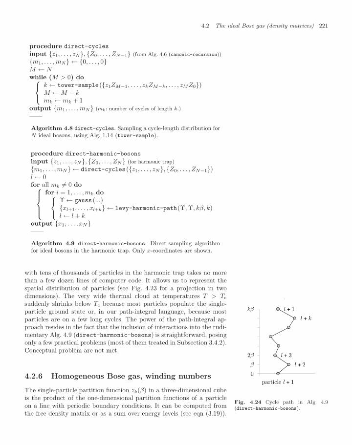
4.2 The ideal Bose gas (density matrices) 221
procedure direct-cycles
input z1, . . . , zN, Z0, . . . , ZN−1 (from Alg. 4.6 (canonic-recursion))m1, . . . , mN ← 0, . . . , 0M ← Nwhile (M > 0) do⎧⎨⎩
k ← tower-sample(z1ZM−1, . . . , zkZM−k, . . . , zMZ0)M ← M − kmk ← mk + 1
output m1, . . . , mN (mk : number of cycles of length k.)——
Algorithm 4.8 direct-cycles. Sampling a cycle-length distribution forN ideal bosons, using Alg. 1.14 (tower-sample).
procedure direct-harmonic-bosons
input z1, . . . , zN, Z0, . . . , ZN (for harmonic trap)m1, . . . , mN ← direct-cycles(z1, . . . , zN, Z0, . . . , ZN−1)l ← 0for all mk = 0 do⎧⎪⎪⎨⎪⎪⎩
for i = 1, . . . , mk do⎧⎨⎩Υ ← gauss (...)xl+1, . . . , xl+k ← levy-harmonic-path(Υ, Υ, kβ, k)l ← l + k
output x1, . . . , xN——
Algorithm 4.9 direct-harmonic-bosons. Direct-sampling algorithmfor ideal bosons in the harmonic trap. Only x-coordinates are shown.
with tens of thousands of particles in the harmonic trap takes no morethan a few dozen lines of computer code. It allows us to represent thespatial distribution of particles (see Fig. 4.23 for a projection in twodimensions). The very wide thermal cloud at temperatures T > Tc
suddenly shrinks below Tc because most particles populate the single-particle ground state or, in our path-integral language, because mostparticles are on a few long cycles. The power of the path-integral ap-proach resides in the fact that the inclusion of interactions into the rudi-mentary Alg. 4.9 (direct-harmonic-bosons) is straightforward, posingonly a few practical problems (most of them treated in Subsection 3.4.2).Conceptual problem are not met.
4.2.6 Homogeneous Bose gas, winding numbers 0
particle l + 1
β l + 2
l + 3
l + k
l + 1
2β
kβ
Fig. 4.24 Cycle path in Alg. 4.9(direct-harmonic-bosons).
The single-particle partition function zk(β) in a three-dimensional cubeis the product of the one-dimensional partition functions of a particleon a line with periodic boundary conditions. It can be computed fromthe free density matrix or as a sum over energy levels (see eqn (3.19)).
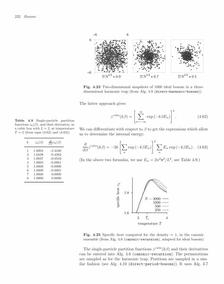
222 Bosons
−6
−6
6
6
T/N1/3 = 0.9 T/N1/3 = 0.7 T/N1/3 = 0.5
Fig. 4.23 Two-dimensional snapshots of 1000 ideal bosons in a three-dimensional harmonic trap (from Alg. 4.9 (direct-harmonic-bosons)).
The latter approach gives
zcube(kβ) =
[ ∞∑n=−∞
exp (−kβEn)
]3. (4.62)
We can differentiate with respect to β to get the expressions which allowus to determine the internal energy:
∂
∂βzcube(kβ) = −3k
[∑n
exp (−kβEn)
]2∑n
En exp (−kβEn) . (4.63)
(In the above two formulas, we use En = 2n22/L2, see Table 4.9.)
Table 4.9 Single-particle partitionfunctions zk(β), and their derivative, ina cubic box with L = 2, at temperatureT = 2 (from eqns (4.62) and (4.63))
k zk(β) ∂∂β
zk(β)
1 1.6004 -3.44402 1.0438 -0.43823 1.0037 -0.05434 1.0003 -0.00615 1.0000 -0.00066 1.0000 -0.00017 1.0000 0.00008 1.0000 0.0000
1.6
1.8
43 Tc
spec
ific
hea
t c V
temperature T
N = 20001000500250
Fig. 4.25 Specific heat computed for the density = 1, in the canonicensemble (from Alg. 4.6 (canonic-recursion), adapted for ideal bosons)
The single-particle partition functions zcube(kβ) and their derivativescan be entered into Alg. 4.6 (canonic-recursion). The permutationsare sampled as for the harmonic trap. Positions are sampled in a sim-ilar fashion (see Alg. 4.10 (direct-period-bosons)). It uses Alg. 3.7
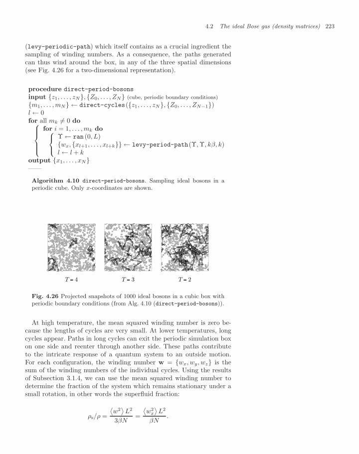
4.2 The ideal Bose gas (density matrices) 223
(levy-periodic-path) which itself contains as a crucial ingredient thesampling of winding numbers. As a consequence, the paths generatedcan thus wind around the box, in any of the three spatial dimensions(see Fig. 4.26 for a two-dimensional representation).
procedure direct-period-bosons
input z1, . . . , zN, Z0, . . . , ZN (cube, periodic boundary conditions)m1, . . . , mN ← direct-cycles(z1, . . . , zN, Z0, . . . , ZN−1)l ← 0for all mk = 0 do⎧⎪⎪⎨⎪⎪⎩
for i = 1, . . . , mk do⎧⎨⎩Υ ← ran (0, L)wx, xl+1, . . . , xl+k ← levy-period-path(Υ, Υ, kβ, k)l ← l + k
output x1, . . . , xN——
Algorithm 4.10 direct-period-bosons. Sampling ideal bosons in aperiodic cube. Only x-coordinates are shown.
T = 4 T = 3 T = 2
Fig. 4.26 Projected snapshots of 1000 ideal bosons in a cubic box withperiodic boundary conditions (from Alg. 4.10 (direct-period-bosons)).
At high temperature, the mean squared winding number is zero be-cause the lengths of cycles are very small. At lower temperatures, longcycles appear. Paths in long cycles can exit the periodic simulation boxon one side and reenter through another side. These paths contributeto the intricate response of a quantum system to an outside motion.For each configuration, the winding number w = wx, wy, wz is thesum of the winding numbers of the individual cycles. Using the resultsof Subsection 3.1.4, we can use the mean squared winding number todetermine the fraction of the system which remains stationary under asmall rotation, in other words the superfluid fraction:
ρs/ρ =
⟨w2⟩L2
3βN=
⟨w2
x
⟩L2
βN.
224 Bosons
4.2.7 Interacting bosons
The structure of general path-integral Monte Carlo algorithms for inter-acting bosons is virtually unchanged with respect to the two samplingalgorithms for ideal bosons, Algs 4.9 (direct-harmonic-bosons) and4.10 (direct-period-bosons). Their detailed presentation and the dis-cussion of results that can be obtained with them are beyond the scopeof this book. An interacting system has the same path configurations asthe noninteracting system, but the configurations must be reweighted.This can be done using the perfect pair actions discussed in Chapter 3(see eqn (3.59)). Markov-chain sampling methods must be employed forchanging both the permutation state and the spatial configurations. Theresulting approach has been useful in precision simulations for liquid he-lium (see Pollock and Ceperley (1987), and Ceperley (1998)), and manyother systems in condensed matter physics. It can also be used for sim-ulations of weakly interacting bosons in atomic physics (Krauth, 1996).Cluster algorithms, which are discussed in several other chapter of thisbook, can also be adapted to path-integral simulations of bosons on alattice (see Prokof’ev, Svistunov, and Tupitsyn (1998)). This is also be-yond the present scope of this book, but a discussion of these methodswill certainly be included in subsequent editions.
Exercises 225
Exercises
(Section 4.1)
(4.1) Generalize eqn (4.1), the single-particle densityof states N (E) in the homogeneous trap, to thecase of an inhomogeneous trap with frequenciesωx, ωy , ωz = 5, 1, 1. Test your result with amodified version of Alg. 4.1 (naive-degeneracy).Use the Kronecker δ-function to generalize the in-tegral representation of N (E) to arbitrary inte-ger values of ωx, ωy, ωz. For frequencies of yourchoice, evaluate this integral as a discrete Riemannsum (generalizing eqn (4.4)). Also determine thediscrete Riemann sum in the complex plane, gener-alizing eqn (4.5), then, determine an analytic for-mula for the density of states, valid in the limit oflarge energies.NB: Address the isotropic trap first and recover Ta-ble 4.1. The complex Riemann sum might incorpo-rate the following fragment, with complex variablesz, zold, ∆z,
. . .zold ← 1, 0for φ = ∆φ, 2∆φ, . . . , 2 do8>><
>>:z ← eiφ
∆z ← z − zold
. . .zold ← z
. . .
(4.2) Implement Alg. 4.3 (naive-bosons). Compare itsoutput with the data in Table 4.3. Test the re-sults for Z(β) against a numerical integration ofeqns (4.17) and (4.16). Are the two calculations ofthe partition function equivalent (in the limit of in-tegration step size ∆x → 0) or should you expectsmall differences? Include the calculation of the dis-tribution function π(N0) in the five-boson boundedtrap model. Implement Alg. 4.4 (canonic-bosons).Test it for the case of the five-boson bounded trapmodel. Finally, choose larger values for Emax andincrease the number of particles.
(4.3) Calculate the ideal-boson chemical potential µ vs.mean particle number in the grand canonical en-semble (Alg. 4.5 (grandcan-bosons)), for the har-monic trap. Plot the condensate fraction againstthe rescaled temperature, as in Fig. 4.7. Discusswhy the macroscopic occupation of the ground
state in the T → 0 limit does not constitute Bose–Einstein condensation and that a more subtle limitis involved. Compute saturation numbers for theexcited states.
(4.4) Familiarize yourself with the calculations of thecritical temperature for Bose–Einstein condensa-tion, and of the saturation densities, for theisotropic harmonic trap. Then, compute the criticaltemperature for an anisotropic harmonic trap withfrequencies ωx, ωy, ωz. In that trap, the energyEx can take on values 0, ωx, 2ωx, 3ωx . . . , etc.
(4.5) Compute the specific heat capacity in the grandcanonical ensemble for N ideal bosons at densityρ = 1 in a box with periodic boundary condi-tions. First determine the chemical potential µ for agiven mean number 〈N〉 of bosons (adapt Alg. 4.5(grandcan-bosons) to the case of a cubic box—you may obtain the density of states from Alg. 4.2(naive-degeneracy-cube)). Then compute the en-ergy and the specific heat capacity. Compare yourdata, at finite N , with the results valid in the ther-modynamic limit.
(4.6) Implement the first thirty wave functionsψh.o.
0 , . . . , ψh.o.29 of the harmonic oscillator using
Alg. 3.1 (harmonic-wavefunction) (see Subsec-tion 3.1.1). Use these wave functions to naivelycalculate the density of N bosons in the harmonictrap (see eqn (4.32)). (Either implement Alg. 4.5(grandcan-bosons) for determining the chemicalpotential as a function of mean particle number,or use data from Table 4.5.) Is it possible to speakof a saturation density ηsat(x, y, z) of all the parti-cles in excited states (analogous to the saturationnumbers discussed in Subsection 4.1.3)?
(4.7) Redo the calculation of the critical temperaturesTc for Bose–Einstein condensation of the idealBose gas, in the harmonic trap and in the cubewith periodic boundary conditions, but use physicalunits (containing particle masses, the Boltzmannand Planck constants, and the harmonic oscilla-tor strengths ω), rather than natural units (where = m = ω = 1).
What is the Bose–Einstein condensation temper-ature, in kelvin, of a gas of N = 1×10⁶ Sodiumatoms (atomic weight 23) in a harmonic trap ofω 1991 Hz? Likewise, compute the critical tem-
226 Exercises
perature of a gas of ideal bosons of the same mass as4He (atomic weight 4), and the same molar volume(59.3 cm3/mole at atmospheric pressure). Is thistransition temperature close to the critical temper-ature for the normal–superfluid transition in liquid4He (2.17 kelvin)?
(Section 4.2)
(4.8) (See also Exerc. 1.9). Implement Alg. 1.11(ran-perm), as discussed in Subsection 1.2.2. Useit to generate 1×10⁶ random permutations withN = 1000 elements. Write any of them in cycle-representation, using a simple subroutine. Generatehistograms for the cycle length distribution, andshow that the probability of finding a cycle is in-versely proportional to its length. Likewise, gener-ate a histogram of the length of the cycle containingan arbitrary element say k = 1000. Convince your-self that it is flat (see Subsection 4.2.2). Next, usethe recursion relation of eqn (4.46) to determinethe number of permutations of 1000 elements con-taining only cycles of length l ≤ 5 (construct analgorithm from eqn (4.46), test it with smaller per-mutations). Write a program to sample these per-mutations (again test this program for smaller N).In addition, compute the number of permutationsof 1000 elements with cycles only of length 5. De-termine the number of permutations of N elementswith a cycle of length l = 1000.
(4.9) Enumerate the 120 permutations of five elements.Write each of them in cycle representation, usinga simple subroutine, and generate the cycle lengthdistribution m1, . . . , m5. Use this information tocompute nonrecursively the partition function ofthe five-boson bounded trap model as a sum over120 permutation partition functions ZP , each ofthem written as a product of single-particle par-tition functions (see eqns (4.47) and (4.50)).NB: Repeatedly use the fragment
. . .input P1, . . . , PNfor k = N, N − 1, . . . , 0 do˘
output P1, . . . , Pk, N + 1, Pk+1, . . . , PN. . .
to generate all permutations of N+1 elements froma list of permutations of N elements. It generatesthe following permutations of four elements fromone permutation of three elements, P = ( 3 1 2
1 2 3 ):
312 →
8>><>>:
3124314234124312
(4.10) Compute the single-particle partition function in acubic box with periodic boundary conditions, andenter it in the recursion relations for the internalenergy and the specific heat capacity of the idealBose gas in the canonical ensemble. Implement re-cursions for Z(β) and for the derivative ∂Z(β)/∂β,and compute the mean energy as a function of tem-perature. Determine the specific heat capacity ofthe ideal Bose gas, as in Fig. 4.25, from the numer-ical derivative of the energy with respect to tem-perature. Determine the condensate fraction fromeqn (4.60) for various temperatures and tempera-tures. Compare your results with those obtained inthe grand canonical ensemble.
(4.11) Perform a quantum Monte Carlo simulation ofN ideal bosons in the harmonic trap. First im-plement Alg. 4.6 (canonic-recursion) and thensample permutations for the N-particle system,using Alg. 4.8 (direct-cycles). Finally, sam-ple positions of particles on each cycle withthe Levy algorithm in a harmonic potential (seeAlg. 3.6 (levy-harmonic-path)). At various tem-peratures, reproduce snapshots of configurations asin Fig. 4.23. Which is the largest particle numberthat you can handle?
(4.12) (Compare with Exerc. 4.11.) Set up a quantumMonte Carlo simulation of N ideal bosons in athree-dimensional cubic box with periodic bound-ary conditions. The algorithm is similar to thatin Exerc. 4.11, however, positions must be sam-pled using Alg. 3.7 (levy-periodic-path). (Usea naive subroutine for sampling the winding num-bers.) Show that below the transition temperaturenonzero winding numbers become relevant. Plotpaths of particles on a cycle, as in Fig. 4.26, forseveral system sizes and temperatures. Next, usethis program to study quantum effects at high tem-peratures. Sample configurations at temperatureT/Tc = 3; compute the pair correlation functionbetween particles k and l, using the periodicallycorrected distance, r, between them (see Alg. 2.6(diff-vec)). Generate a histogram of this pair cor-relation as a function of distance, to obtain π(r).The function π(r)/(4r2) shows a characteristic in-crease at small distance, in the region of close en-counter. Interpret this effect in terms of cycle lengthdistributions. What is its length scale? Discuss thismanifestation of the quantum nature of the Bosegas at high temperature.
References 227
References
Borrmann P., Franke G. (1993) Recursion formulas for quantum statis-tical partition functions, Journal of Chemical Physics 98, 2484–2485
Ceperley D. M. (1995) Path-integrals in the theory of condensed he-lium, Reviews of Modern Physics 67, 279–355
Feynman R. P. (1972) Statistical Mechanics: A Set of Lectures, Benja-min/Cummings, Reading, Massachusetts
Holzmann M., Krauth W. (1999) Transition temperature of the homo-geneous, weakly interacting Bose gas, Physical Review Letters 83, 2687–2690
Krauth W. (1996) Quantum Monte Carlo calculations for a large num-ber of bosons in a harmonic trap, Physical Review Letters 77, 3695–3699
Pollock E. L., Ceperley D. M. (1987) Path-integral computation of su-perfluid densities, Physical Review B 36, 8343–8352
Prokof’ev N. V., Svistunov B. V., Tupitsyn I. S. (1998) “Worm” al-gorithm in quantum Monte Carlo simulations, Physics Letters A 238,253–257

This page intentionally left blank
Order and disorder in spinsystems 5
5.1 The Ising model(exact computations) 231
5.2 The Ising model(Monte Carlo algorithms) 249
5.3 Generalized Ising models 259
Exercises 264
References 266
In this chapter, we approach the statistical mechanics and computationalphysics of the Ising model, which has inspired generations of physicists.This archetypal physical system undergoes an order–disorder phase tran-sition. The Ising model shares this transition and many other propertieswith more complicated models which cannot be analyzed so well.
The first focus of this chapter is on enumeration, which applies to theIsing model because of its finite number of configurations, even thoughthis number grows exponentially with the lattice size. We shall enu-merate the spin configurations, and also the loop configurations of theIsing model’s high-temperature expansion, which can be summed forvery large and even infinite lattices, leading to Onsager’s analytic solu-tion in two dimensions. This chapter’s second focus is on Monte Carloalgorithms. We shall start with a simple local implementation of theMetropolis sampling algorithm and move on to nontrivial realizationsof the perfect-sampling approach described in Subsection 1.1.7 and tomodern cluster algorithms. Cluster algorithms originated from the Isingmodel. They have revolutionized computation in many fields of classicaland quantum statistical mechanics.
Theoretical and computational approaches to the Ising model havemet with outstanding success. However, it suffices to modify a few pa-rameters in the model, for example to let the sign of the interaction besometimes positive and sometimes negative, to cause all combined ap-proaches to get into trouble. The two-dimensional spin glass (where theinteractions are randomly positive and negative) illustrates the difficul-ties faced by Monte Carlo algorithms. Remarkably, the above-mentionedenumeration of loop configurations still works. Onsager’s analytic solu-tion of the Ising model thus turns into a powerful algorithm for two-dimensional spin glasses.
In this chapter, we witness many close connections between theoryand computation across widely different fields. This unity of physics isillustrated further in the final section through a relation between spinsystems and classical liquids: we shall see that a liquid with pair inter-actions is in some sense equivalent to an Ising spin glass and can besimulated with exactly the same methods. This far-reaching equivalencemakes it difficult to tell whether we are simulating a liquid (with parti-cles moving around in a continuous space) or spins that are sometimesup and sometimes down.
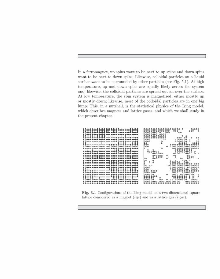
In a ferromagnet, up spins want to be next to up spins and down spinswant to be next to down spins. Likewise, colloidal particles on a liquidsurface want to be surrounded by other particles (see Fig. 5.1). At hightemperature, up and down spins are equally likely across the systemand, likewise, the colloidal particles are spread out all over the surface.At low temperature, the spin system is magnetized, either mostly upor mostly down; likewise, most of the colloidal particles are in one biglump. This, in a nutshell, is the statistical physics of the Ising model,which describes magnets and lattice gases, and which we shall study inthe present chapter.
Fig. 5.1 Configurations of the Ising model on a two-dimensional squarelattice considered as a magnet (left) and as a lattice gas (right).
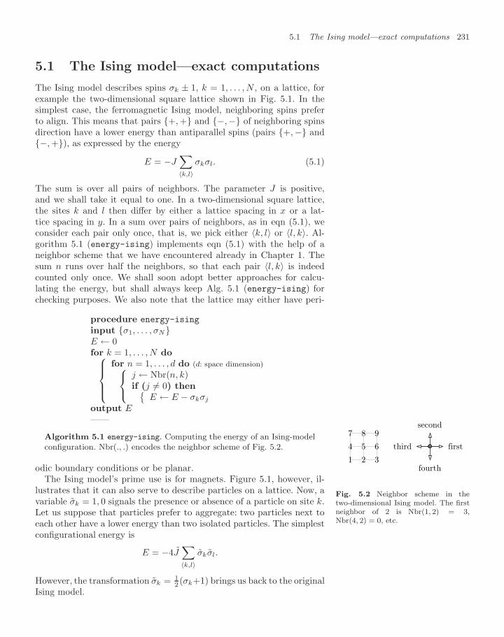
5.1 The Ising model—exact computations 231
5.1 The Ising model—exact computations
The Ising model describes spins σk ± 1, k = 1, . . . , N , on a lattice, forexample the two-dimensional square lattice shown in Fig. 5.1. In thesimplest case, the ferromagnetic Ising model, neighboring spins preferto align. This means that pairs +, + and −,− of neighboring spinsdirection have a lower energy than antiparallel spins (pairs +,− and−, +), as expressed by the energy
E = −J∑〈k,l〉
σkσl. (5.1)
The sum is over all pairs of neighbors. The parameter J is positive,and we shall take it equal to one. In a two-dimensional square lattice,the sites k and l then differ by either a lattice spacing in x or a lat-tice spacing in y. In a sum over pairs of neighbors, as in eqn (5.1), weconsider each pair only once, that is, we pick either 〈k, l〉 or 〈l, k〉. Al-gorithm 5.1 (energy-ising) implements eqn (5.1) with the help of aneighbor scheme that we have encountered already in Chapter 1. Thesum n runs over half the neighbors, so that each pair 〈l, k〉 is indeedcounted only once. We shall soon adopt better approaches for calcu-lating the energy, but shall always keep Alg. 5.1 (energy-ising) forchecking purposes. We also note that the lattice may either have peri-
procedure energy-ising
input σ1, . . . , σNE ← 0for k = 1, . . . , N do⎧⎪⎪⎨⎪⎪⎩
for n = 1, . . . , d do (d: space dimension)⎧⎨⎩j ← Nbr(n, k)if (j = 0) then
E ← E − σkσj
output E——
Algorithm 5.1 energy-ising. Computing the energy of an Ising-modelconfiguration. Nbr(., .) encodes the neighbor scheme of Fig. 5.2.
odic boundary conditions or be planar.1 2 3
4 5 6
7 8 9
first
second
third
fourth
Fig. 5.2 Neighbor scheme in thetwo-dimensional Ising model. The firstneighbor of 2 is Nbr(1, 2) = 3,Nbr(4, 2) = 0, etc.
The Ising model’s prime use is for magnets. Figure 5.1, however, il-lustrates that it can also serve to describe particles on a lattice. Now, avariable σk = 1, 0 signals the presence or absence of a particle on site k.Let us suppose that particles prefer to aggregate: two particles next toeach other have a lower energy than two isolated particles. The simplestconfigurational energy is
E = −4J∑〈k,l〉
σkσl.
However, the transformation σk = 12 (σk+1) brings us back to the original
Ising model.
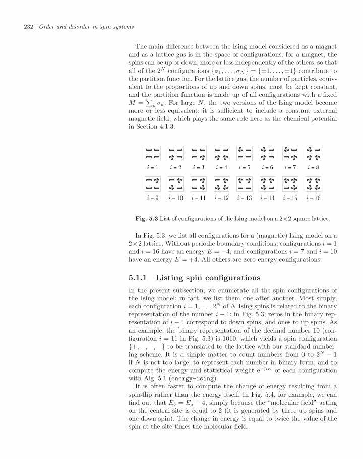
232 Order and disorder in spin systems
The main difference between the Ising model considered as a magnetand as a lattice gas is in the space of configurations: for a magnet, thespins can be up or down, more or less independently of the others, so thatall of the 2N configurations σ1, . . . , σN = ±1, . . . ,±1 contribute tothe partition function. For the lattice gas, the number of particles, equiv-alent to the proportions of up and down spins, must be kept constant,and the partition function is made up of all configurations with a fixedM =
∑k σk. For large N , the two versions of the Ising model become
more or less equivalent: it is sufficient to include a constant externalmagnetic field, which plays the same role here as the chemical potentialin Section 4.1.3.
i = 1 i = 2 i = 3 i = 4 i = 5 i = 6 i = 7 i = 8
i = 9 i = 10 i = 11 i = 12 i = 13 i = 14 i = 15 i = 16
Fig. 5.3 List of configurations of the Ising model on a 2×2 square lattice.
In Fig. 5.3, we list all configurations for a (magnetic) Ising model on a2×2 lattice. Without periodic boundary conditions, configurations i = 1and i = 16 have an energy E = −4, and configurations i = 7 and i = 10have an energy E = +4. All others are zero-energy configurations.
5.1.1 Listing spin configurations
In the present subsection, we enumerate all the spin configurations ofthe Ising model; in fact, we list them one after another. Most simply,each configuration i = 1, . . . , 2N of N Ising spins is related to the binaryrepresentation of the number i − 1: in Fig. 5.3, zeros in the binary rep-resentation of i − 1 correspond to down spins, and ones to up spins. Asan example, the binary representation of the decimal number 10 (con-figuration i = 11 in Fig. 5.3) is 1010, which yields a spin configuration+,−, +,− to be translated to the lattice with our standard number-ing scheme. It is a simple matter to count numbers from 0 to 2N − 1if N is not too large, to represent each number in binary form, and tocompute the energy and statistical weight e−βE of each configurationwith Alg. 5.1 (energy-ising).
It is often faster to compute the change of energy resulting from aspin-flip rather than the energy itself. In Fig. 5.4, for example, we canfind out that Eb = Ea − 4, simply because the “molecular field” actingon the central site is equal to 2 (it is generated by three up spins andone down spin). The change in energy is equal to twice the value of thespin at the site times the molecular field.
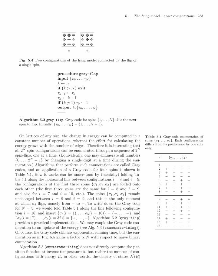
5.1 The Ising model—exact computations 233
a b
Fig. 5.4 Two configurations of the Ising model connected by the flip ofa single spin.
procedure gray-flip
input τ0, . . . , τNk ← τ0
if (k > N) exitτk−1 ← τk
τk ← k + 1if (k = 1) τ0 ← 1output k, τ0, . . . , τN——
Algorithm 5.2 gray-flip. Gray code for spins 1, . . . , N. k is the nextspin to flip. Initially, τ0, . . . , τN = 1, . . . , N + 1.
On lattices of any size, the change in energy can be computed in aconstant number of operations, whereas the effort for calculating theenergy grows with the number of edges. Therefore it is interesting thatall 2N spin configurations can be enumerated through a sequence of 2N
spin-flips, one at a time. (Equivalently, one may enumerate all numbers0, . . . , 2N − 1 by changing a single digit at a time during the enu-meration.) Algorithms that perform such enumerations are called Graycodes, and an application of a Gray code for four spins is shown inTable 5.1. How it works can be understood by (mentally) folding Ta-ble 5.1 along the horizontal line between configurations i = 8 and i = 9:the configurations of the first three spins σ1, σ2, σ3 are folded ontoeach other (the first three spins are the same for i = 8 and i = 9,and also for i = 7 and i = 10, etc.). The spins σ1, σ2, σ3 remainunchanged between i = 8 and i = 9, and this is the only momentat which σ4 flips, namely from − to +. To write down the Gray codefor N = 5, we would fold Table 5.1 along the line following configura-tion i = 16, and insert σ5(i = 1), . . . , σ5(i = 16) = −, . . . ,−, andσ5(i = 17), . . . , σ5(i = 32) = +, . . . , +. Algorithm 5.2 (gray-flip)provides a practical implementation. We may couple the Gray code enu-meration to an update of the energy (see Alg. 5.3 (enumerate-ising)).Of course, the Gray code still has exponential running time, but the enu-meration as in Fig. 5.5 gains a factor ∝ N with respect to naive binaryenumeration.
Table 5.1 Gray-code enumeration ofspins σ1, . . . , σ4. Each configurationdiffers from its predecessor by one spinonly.
i σ1, . . . , σ4
1 − − − −2 + − − −3 + + − −4 − + − −5 − + + −6 + + + −7 + − + −8 − − + −
9 − − + +10 + − + +11 + + + +12 − + + +13 − + − +14 + + − +15 + − − +16 − − − +
Algorithm 5.3 (enumerate-ising) does not directly compute the par-tition function at inverse temperature β, but rather the number of con-figurations with energy E, in other words, the density of states N (E)
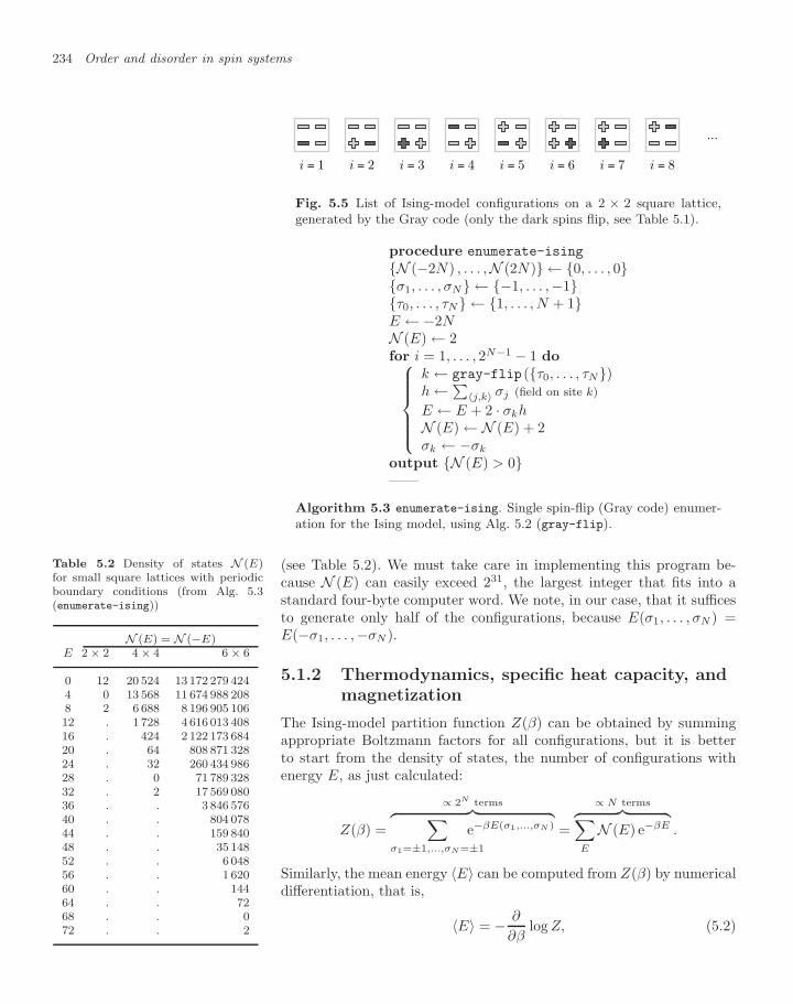
234 Order and disorder in spin systems
i = 1 i = 2 i = 3 i = 4 i = 5 i = 6 i = 7 i = 8
...
Fig. 5.5 List of Ising-model configurations on a 2 × 2 square lattice,generated by the Gray code (only the dark spins flip, see Table 5.1).
procedure enumerate-ising
N (−2N) , . . . ,N (2N) ← 0, . . . , 0σ1, . . . , σN ← −1, . . . ,−1τ0, . . . , τN ← 1, . . . , N + 1E ← −2NN (E) ← 2for i = 1, . . . , 2N−1 − 1 do⎧⎪⎪⎪⎪⎨⎪⎪⎪⎪⎩
k ← gray-flip (τ0, . . . , τN)h ←∑〈j,k〉 σj (field on site k)
E ← E + 2 · σkhN (E) ← N (E) + 2σk ← −σk
output N (E) > 0——
Algorithm 5.3 enumerate-ising. Single spin-flip (Gray code) enumer-ation for the Ising model, using Alg. 5.2 (gray-flip).
(see Table 5.2). We must take care in implementing this program be-cause N (E) can easily exceed 231, the largest integer that fits into astandard four-byte computer word. We note, in our case, that it sufficesto generate only half of the configurations, because E(σ1, . . . , σN ) =E(−σ1, . . . ,−σN ).
Table 5.2 Density of states N (E)for small square lattices with periodicboundary conditions (from Alg. 5.3(enumerate-ising))
N (E) = N (−E)E 2 × 2 4 × 4 6 × 6
0 12 20 524 13 172 279 4244 0 13 568 11 674 988 2088 2 6 688 8 196 905 10612 . 1 728 4 616 013 40816 . 424 2 122 173 68420 . 64 808 871 32824 . 32 260 434 98628 . 0 71 789 32832 . 2 17 569 08036 . . 3 846 57640 . . 804 07844 . . 159 84048 . . 35 14852 . . 6 04856 . . 1 62060 . . 14464 . . 7268 . . 072 . . 2
5.1.2 Thermodynamics, specific heat capacity, andmagnetization
The Ising-model partition function Z(β) can be obtained by summingappropriate Boltzmann factors for all configurations, but it is betterto start from the density of states, the number of configurations withenergy E, as just calculated:
Z(β) =
∝ 2N terms︷ ︸︸ ︷∑σ1=±1,...,σN=±1
e−βE(σ1,...,σN ) =
∝ N terms︷ ︸︸ ︷∑E
N (E) e−βE .
Similarly, the mean energy 〈E〉 can be computed from Z(β) by numericaldifferentiation, that is,
〈E〉 = − ∂
∂βlog Z, (5.2)
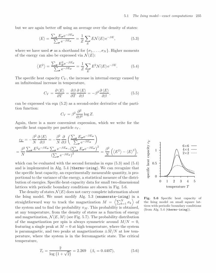
5.1 The Ising model—exact computations 235
but we are again better off using an average over the density of states:
〈E〉 =∑
σEσe−βEσ∑σ
e−βEσ
=1Z
∑E
EN (E) e−βE , (5.3)
where we have used σ as a shorthand for σ1, . . . , σN. Higher momentsof the energy can also be expressed via N (E):
⟨E2⟩
=∑
σE2
σe−βEσ∑
σe−βEσ
=1Z
∑E
E2N (E) e−βE. (5.4)
The specific heat capacity CV , the increase in internal energy caused byan infinitesimal increase in temperature,
CV =∂ 〈E〉∂T
=∂β
∂T
∂ 〈E〉∂β
= −β2 ∂ 〈E〉∂β
, (5.5)
can be expressed via eqn (5.2) as a second-order derivative of the parti-tion function:
CV = β2 ∂2
∂β2log Z.
Again, there is a more convenient expression, which we write for thespecific heat capacity per particle cV ,
cV = −β2
N
∂ 〈E〉∂β
= −β2
N
∂
∂β
(∑σ
Eσe−βEσ∑σ
e−βEσ
)=
β2
N
∑σ
E2e−βEσ
∑σ
e−βEσ−(∑σ
Eσe−βEσ
)2(∑
σe−βEσ)2
=β2
N
(⟨E2⟩− 〈E〉2
),
which can be evaluated with the second formulas in eqns (5.3) and (5.4)and is implemented in Alg. 5.4 (thermo-ising). We can recognize thatthe specific heat capacity, an experimentally measurable quantity, is pro-portional to the variance of the energy, a statistical measure of the distri-bution of energies. Specific-heat-capacity data for small two-dimensionallattices with periodic boundary conditions are shown in Fig. 5.6.
0
0.5
1
0 1 2 3 4 5
spec
ific
hea
t ca
pac
ity c
V
temperature T
6×64×42×2
Fig. 5.6 Specific heat capacity ofthe Ising model on small square lat-tices with periodic boundary conditions(from Alg. 5.4 (thermo-ising)).
The density of states N (E) does not carry complete information aboutthe Ising model. We must modify Alg. 5.3 (enumerate-ising) in astraightforward way to track the magnetization M =
⟨∑Nk=1 σk
⟩of
the system and to find the probability πM . This probability is obtained,at any temperature, from the density of states as a function of energyand magnetization, N (E, M) (see Fig. 5.7). The probability distributionof the magnetization per spin is always symmetric around M/N = 0,featuring a single peak at M = 0 at high temperature, where the systemis paramagnetic, and two peaks at magnetizations ±M/N at low tem-perature, where the system is in the ferromagnetic state. The criticaltemperature,
Tc =2
log(1 +
√2) = 2.269 (βc = 0.4407), (5.6)
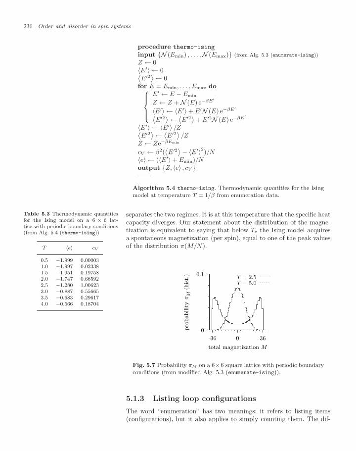
236 Order and disorder in spin systems
procedure thermo-ising
input N (Emin) , . . . ,N (Emax) (from Alg. 5.3 (enumerate-ising))Z ← 0〈E′〉 ← 0⟨E′2⟩← 0
for E = Emin, . . . , Emax do⎧⎪⎪⎨⎪⎪⎩E′ ← E − Emin
Z ← Z + N (E) e−βE′
〈E′〉 ← 〈E′〉 + E′N (E) e−βE′⟨E′2⟩← ⟨E′2⟩+ E′2N (E) e−βE′
〈E′〉 ← 〈E′〉 /Z⟨E′2⟩← ⟨E′2⟩ /Z
Z ← Ze−βEmin
cV ← β2(⟨E′2⟩− 〈E′〉2)/N
〈e〉 ← (〈E′〉 + Emin)/Noutput Z, 〈e〉 , cV ——
Algorithm 5.4 thermo-ising. Thermodynamic quantities for the Isingmodel at temperature T = 1/β from enumeration data.
separates the two regimes. It is at this temperature that the specific heatcapacity diverges. Our statement about the distribution of the magne-tization is equivalent to saying that below Tc the Ising model acquiresa spontaneous magnetization (per spin), equal to one of the peak valuesof the distribution π(M/N).
Table 5.3 Thermodynamic quantitiesfor the Ising model on a 6 × 6 lat-tice with periodic boundary conditions(from Alg. 5.4 (thermo-ising))
T 〈e〉 cV
0.5 −1.999 0.000031.0 −1.997 0.023381.5 −1.951 0.197582.0 −1.747 0.685922.5 −1.280 1.006233.0 −0.887 0.556653.5 −0.683 0.296174.0 −0.566 0.18704
0
0.1
-36 0 36
pro
babilit
y π
M (
his
t.)
total magnetization M
T = 2.5T = 5.0
Fig. 5.7 Probability πM on a 6×6 square lattice with periodic boundaryconditions (from modified Alg. 5.3 (enumerate-ising)).
5.1.3 Listing loop configurations
The word “enumeration” has two meanings: it refers to listing items(configurations), but it also applies to simply counting them. The dif-
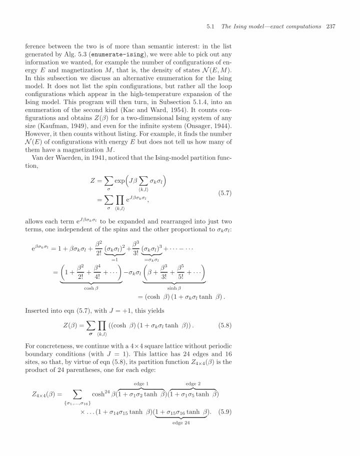
5.1 The Ising model—exact computations 237
ference between the two is of more than semantic interest: in the listgenerated by Alg. 5.3 (enumerate-ising), we were able to pick out anyinformation we wanted, for example the number of configurations of en-ergy E and magnetization M , that is, the density of states N (E, M).In this subsection we discuss an alternative enumeration for the Isingmodel. It does not list the spin configurations, but rather all the loopconfigurations which appear in the high-temperature expansion of theIsing model. This program will then turn, in Subsection 5.1.4, into anenumeration of the second kind (Kac and Ward, 1954). It counts con-figurations and obtains Z(β) for a two-dimensional Ising system of anysize (Kaufman, 1949), and even for the infinite system (Onsager, 1944).However, it then counts without listing. For example, it finds the numberN (E) of configurations with energy E but does not tell us how many ofthem have a magnetization M .
Van der Waerden, in 1941, noticed that the Ising-model partition func-tion,
Z =∑
σ
exp(Jβ∑〈k,l〉
σkσl
)=∑
σ
∏〈k,l〉
eJβσkσl ,(5.7)
allows each term eJβσkσl to be expanded and rearranged into just twoterms, one independent of the spins and the other proportional to σkσl:
eβσkσl = 1 + βσkσl +β2
2!(σkσl)2︸ ︷︷ ︸
=1
+β3
3!(σkσl)3︸ ︷︷ ︸=σkσl
+ · · · − · · ·
=(
1 +β2
2!+
β4
4!+ · · ·
)︸ ︷︷ ︸
cosh β
−σkσl
(β +
β3
3!+
β5
5!+ · · ·
)︸ ︷︷ ︸
sinhβ
= (cosh β) (1 + σkσl tanh β) .
Inserted into eqn (5.7), with J = +1, this yields
Z(β) =∑σ
∏〈k,l〉
((cosh β) (1 + σkσl tanh β)) . (5.8)
For concreteness, we continue with a 4×4 square lattice without periodicboundary conditions (with J = 1). This lattice has 24 edges and 16sites, so that, by virtue of eqn (5.8), its partition function Z4×4(β) is theproduct of 24 parentheses, one for each edge:
Z4×4(β) =∑
σ1,...,σ16cosh24 β(
edge 1︷ ︸︸ ︷1 + σ1σ2 tanh β)(
edge 2︷ ︸︸ ︷1 + σ1σ5 tanh β)
× . . . (1 + σ14σ15 tanh β)(1 + σ15σ16 tanh β︸ ︷︷ ︸edge 24
). (5.9)
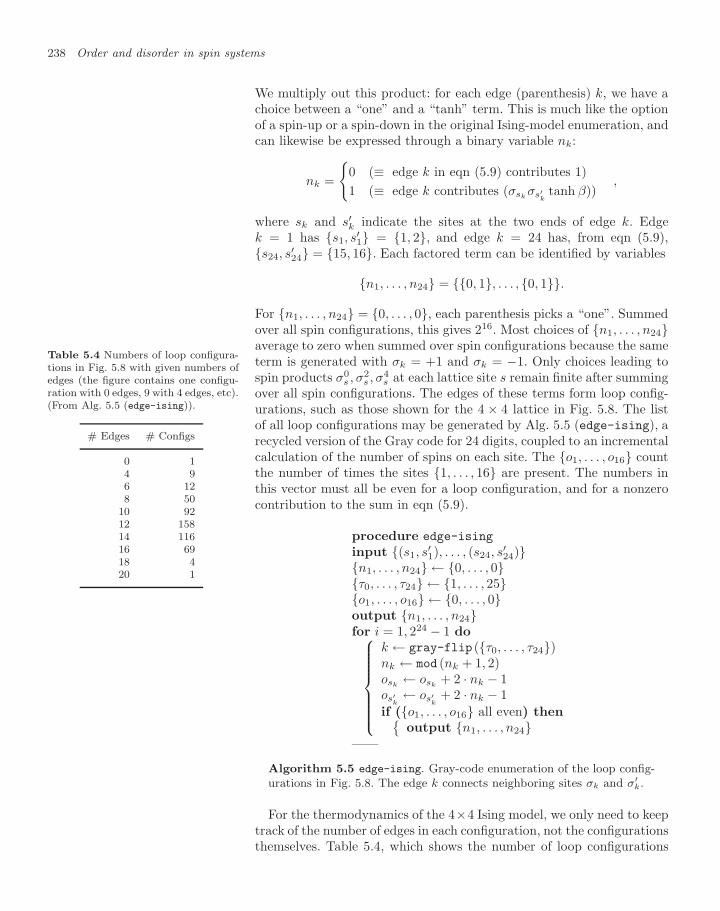
238 Order and disorder in spin systems
We multiply out this product: for each edge (parenthesis) k, we have achoice between a “one” and a “tanh” term. This is much like the optionof a spin-up or a spin-down in the original Ising-model enumeration, andcan likewise be expressed through a binary variable nk:
nk =
0 (≡ edge k in eqn (5.9) contributes 1)1 (≡ edge k contributes (σsk
σs′k
tanh β)),
where sk and s′k indicate the sites at the two ends of edge k. Edgek = 1 has s1, s
′1 = 1, 2, and edge k = 24 has, from eqn (5.9),
s24, s′24 = 15, 16. Each factored term can be identified by variables
n1, . . . , n24 = 0, 1, . . . , 0, 1.
For n1, . . . , n24 = 0, . . . , 0, each parenthesis picks a “one”. Summedover all spin configurations, this gives 216. Most choices of n1, . . . , n24average to zero when summed over spin configurations because the sameterm is generated with σk = +1 and σk = −1. Only choices leading tospin products σ0
s , σ2s , σ4
s at each lattice site s remain finite after summingover all spin configurations. The edges of these terms form loop config-urations, such as those shown for the 4 × 4 lattice in Fig. 5.8. The listof all loop configurations may be generated by Alg. 5.5 (edge-ising), arecycled version of the Gray code for 24 digits, coupled to an incrementalcalculation of the number of spins on each site. The o1, . . . , o16 countthe number of times the sites 1, . . . , 16 are present. The numbers inthis vector must all be even for a loop configuration, and for a nonzerocontribution to the sum in eqn (5.9).
Table 5.4 Numbers of loop configura-tions in Fig. 5.8 with given numbers ofedges (the figure contains one configu-ration with 0 edges, 9 with 4 edges, etc).(From Alg. 5.5 (edge-ising)).
# Edges # Configs
0 14 96 128 50
10 9212 15814 11616 6918 420 1
procedure edge-ising
input (s1, s′1), . . . , (s24, s
′24)
n1, . . . , n24 ← 0, . . . , 0τ0, . . . , τ24 ← 1, . . . , 25o1, . . . , o16 ← 0, . . . , 0output n1, . . . , n24for i = 1, 224 − 1 do⎧⎪⎪⎪⎪⎪⎪⎨⎪⎪⎪⎪⎪⎪⎩
k ← gray-flip (τ0, . . . , τ24)nk ← mod (nk + 1, 2)osk
← osk+ 2 · nk − 1
os′k← os′
k+ 2 · nk − 1
if (o1, . . . , o16 all even) thenoutput n1, . . . , n24
——
Algorithm 5.5 edge-ising. Gray-code enumeration of the loop config-urations in Fig. 5.8. The edge k connects neighboring sites σk and σ′
k.
For the thermodynamics of the 4×4 Ising model, we only need to keeptrack of the number of edges in each configuration, not the configurationsthemselves. Table 5.4, which shows the number of loop configurations
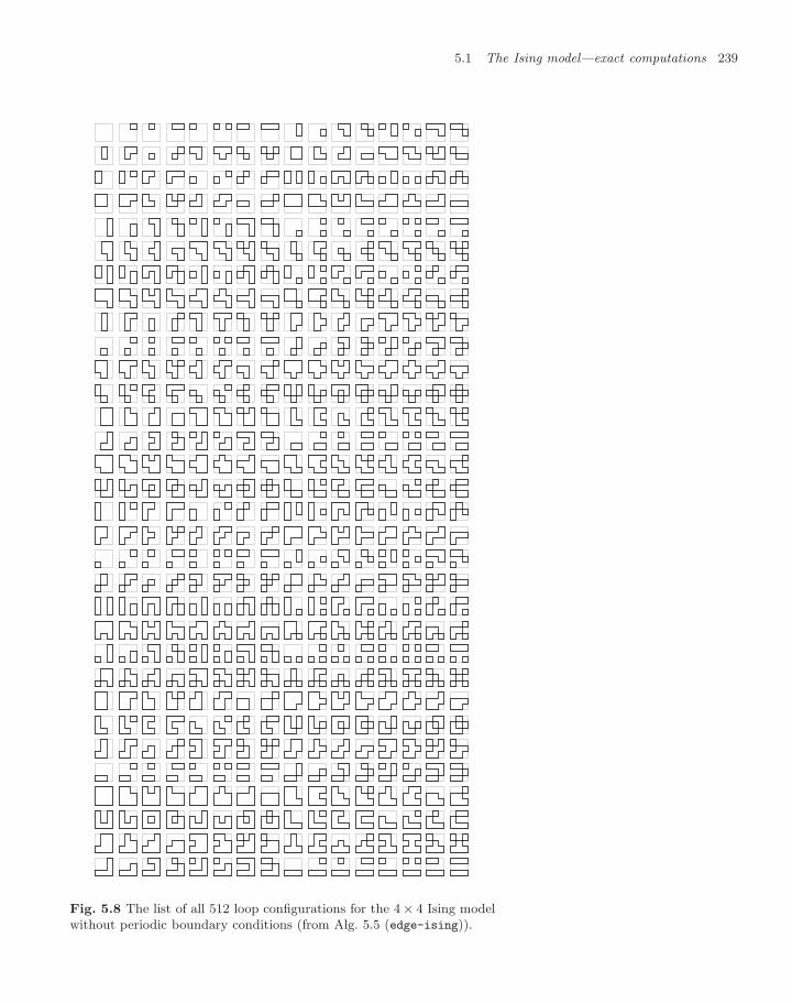
5.1 The Ising model—exact computations 239
Fig. 5.8 The list of all 512 loop configurations for the 4× 4 Ising modelwithout periodic boundary conditions (from Alg. 5.5 (edge-ising)).
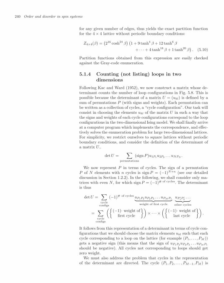
240 Order and disorder in spin systems
for any given number of edges, thus yields the exact partition functionfor the 4 × 4 lattice without periodic boundary conditions:
Z4×4(β) =(216 cosh24 β
) (1 + 9 tanh4 β + 12 tanh6 β
+ · · · + 4 tanh18 β + 1 tanh20 β). (5.10)
Partition functions obtained from this expression are easily checkedagainst the Gray-code enumeration.
5.1.4 Counting (not listing) loops in twodimensions
Following Kac and Ward (1952), we now construct a matrix whose de-terminant counts the number of loop configurations in Fig. 5.8. This ispossible because the determinant of a matrix U = (ukl) is defined by asum of permutations P (with signs and weights). Each permutation canbe written as a collection of cycles, a “cycle configuration”. Our task willconsist in choosing the elements ukl of the matrix U in such a way thatthe signs and weights of each cycle configurations correspond to the loopconfigurations in the two-dimensional Ising model. We shall finally arriveat a computer program which implements the correspondence, and effec-tively solves the enumeration problem for large two-dimensional lattices.For simplicity, we restrict ourselves to square lattices without periodicboundary conditions, and consider the definition of the determinant ofa matrix U ,
det U =∑
permutations
(sign P )u1P1u2P2 . . . uNPN.
We now represent P in terms of cycles. The sign of a permutationP of N elements with n cycles is signP = (−1)N+n (see our detaileddiscussion in Section 1.2.2). In the following, we shall consider only ma-trices with even N , for which signP = (−1)# of cycles. The determinantis thus
det U =∑cycle
configs
(−1)# of cycles uP1P2uP2P3 . . . uPM P1︸ ︷︷ ︸weight of first cycle
uP ′1P ′
2. . .︸ ︷︷ ︸
other cycles
=∑cycle
configs
((−1)· weight of
first cycle
)× · · · ×
((−1)· weight of
last cycle
).
It follows from this representation of a determinant in terms of cycle con-figurations that we should choose the matrix elements ukl such that eachcycle corresponding to a loop on the lattice (for example (P1, . . . , PM ))gets a negative sign (this means that the sign of uP1P2uP2P3 . . . uPM P1
should be negative). All cycles not corresponding to loops should getzero weight.
We must also address the problem that cycles in the representationof the determinant are directed. The cycle (P1, P2, . . . , PM−1, PM ) is
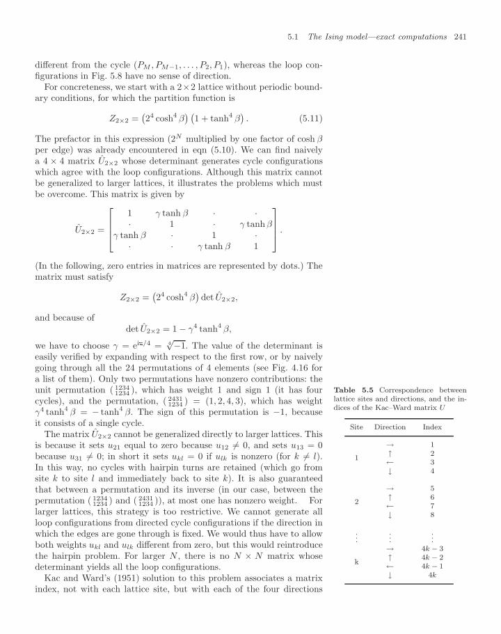
5.1 The Ising model—exact computations 241
different from the cycle (PM , PM−1, . . . , P2, P1), whereas the loop con-figurations in Fig. 5.8 have no sense of direction.
For concreteness, we start with a 2×2 lattice without periodic bound-ary conditions, for which the partition function is
Z2×2 =(24 cosh4 β
) (1 + tanh4 β
). (5.11)
The prefactor in this expression (2N multiplied by one factor of cosh βper edge) was already encountered in eqn (5.10). We can find naivelya 4 × 4 matrix U2×2 whose determinant generates cycle configurationswhich agree with the loop configurations. Although this matrix cannotbe generalized to larger lattices, it illustrates the problems which mustbe overcome. This matrix is given by
U2×2 =
⎡⎢⎢⎣1 γ tanh β · ·· 1 · γ tanh β
γ tanh β · 1 ·· · γ tanh β 1
⎤⎥⎥⎦ .
(In the following, zero entries in matrices are represented by dots.) Thematrix must satisfy
Z2×2 =(24 cosh4 β
)det U2×2,
and because ofdet U2×2 = 1 − γ4 tanh4 β,
we have to choose γ = ei/4 = 4√−1. The value of the determinant is
easily verified by expanding with respect to the first row, or by naivelygoing through all the 24 permutations of 4 elements (see Fig. 4.16 fora list of them). Only two permutations have nonzero contributions: theunit permutation ( 1234
1234 ), which has weight 1 and sign 1 (it has fourcycles), and the permutation, ( 2431
1234 ) = (1, 2, 4, 3), which has weightγ4 tanh4 β = − tanh4 β. The sign of this permutation is −1, becauseit consists of a single cycle.
The matrix U2×2 cannot be generalized directly to larger lattices. Thisis because it sets u21 equal to zero because u12 = 0, and sets u13 = 0because u31 = 0; in short it sets ukl = 0 if ulk is nonzero (for k = l).In this way, no cycles with hairpin turns are retained (which go fromsite k to site l and immediately back to site k). It is also guaranteedthat between a permutation and its inverse (in our case, between thepermutation ( 1234
1234 ) and ( 24311234 )), at most one has nonzero weight. For
Table 5.5 Correspondence betweenlattice sites and directions, and the in-dices of the Kac–Ward matrix U
Site Direction Index
1
→↑←↓
1234
2
→↑←↓
5678
......
...
k
→↑←↓
4k − 34k − 24k − 1
4k
larger lattices, this strategy is too restrictive. We cannot generate allloop configurations from directed cycle configurations if the direction inwhich the edges are gone through is fixed. We would thus have to allowboth weights ukl and ulk different from zero, but this would reintroducethe hairpin problem. For larger N , there is no N × N matrix whosedeterminant yields all the loop configurations.
Kac and Ward’s (1951) solution to this problem associates a matrixindex, not with each lattice site, but with each of the four directions
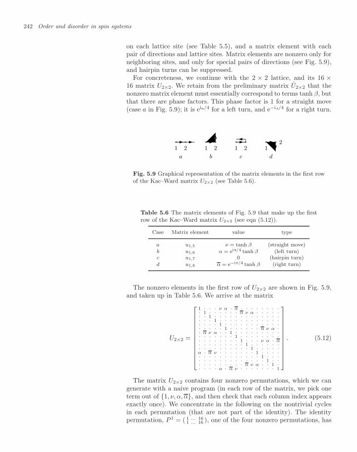
242 Order and disorder in spin systems
on each lattice site (see Table 5.5), and a matrix element with eachpair of directions and lattice sites. Matrix elements are nonzero only forneighboring sites, and only for special pairs of directions (see Fig. 5.9),and hairpin turns can be suppressed.
For concreteness, we continue with the 2 × 2 lattice, and its 16 ×16 matrix U2×2. We retain from the preliminary matrix U2×2 that thenonzero matrix element must essentially correspond to terms tanh β, butthat there are phase factors. This phase factor is 1 for a straight move(case a in Fig. 5.9); it is ei/4 for a left turn, and e−i/4 for a right turn.
1 2
a
1 2
b
1 2
c
12
d
Fig. 5.9 Graphical representation of the matrix elements in the first rowof the Kac–Ward matrix U2×2 (see Table 5.6).
Table 5.6 The matrix elements of Fig. 5.9 that make up the firstrow of the Kac–Ward matrix U2×2 (see eqn (5.12)).
Case Matrix element value type
a u1,5 ν = tanh β (straight move)b u1,6 α = ei/4 tanh β (left turn)c u1,7 0 (hairpin turn)d u1,8 α = e−i/4 tanh β (right turn)
The nonzero elements in the first row of U2×2 are shown in Fig. 5.9,and taken up in Table 5.6. We arrive at the matrix
U2×2 =
⎡⎢⎢⎢⎢⎢⎢⎢⎢⎢⎢⎣
1 · · · ν α · α · · · · · · · ·· 1 · · · · · · α ν α · · · · ·· · 1 · · · · · · · · · · · · ·· · · 1 · · · · · · · · · · · ·· · · · 1 · · · · · · · · · · ·· · · · · 1 · · · · · · α ν α ·· α ν α · · 1 · · · · · · · · ·· · · · · · · 1 · · · · · · · ·· · · · · · · · 1 · · · ν α · α· · · · · · · · · 1 · · · · · ·· · · · · · · · · · 1 · · · · ·α · α ν · · · · · · · 1 · · · ·· · · · · · · · · · · · 1 · · ·· · · · · · · · · · · · · 1 · ·· · · · · · · · · α ν α · · 1 ·· · · · α · α ν · · · · · · · 1
⎤⎥⎥⎥⎥⎥⎥⎥⎥⎥⎥⎦. (5.12)
The matrix U2×2 contains four nonzero permutations, which we cangenerate with a naive program (in each row of the matrix, we pick oneterm out of 1, ν, α, α, and then check that each column index appearsexactly once). We concentrate in the following on the nontrivial cyclesin each permutation (that are not part of the identity). The identitypermutation, P 1 = ( 1 ... 16
1 ... 16 ), one of the four nonzero permutations, has
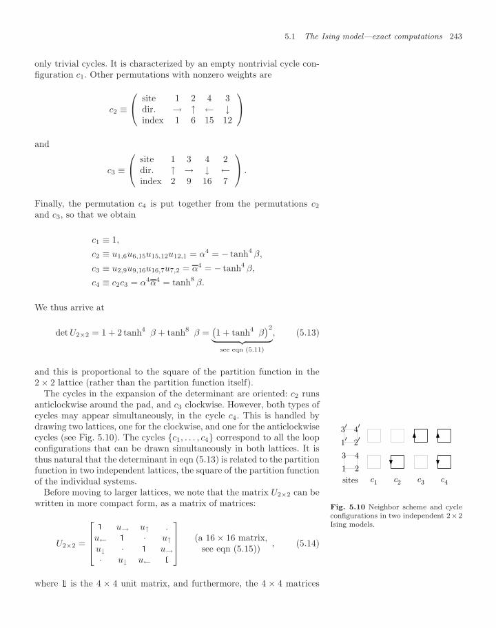
5.1 The Ising model—exact computations 243
only trivial cycles. It is characterized by an empty nontrivial cycle con-figuration c1. Other permutations with nonzero weights are
c2 ≡⎛⎝ site 1 2 4 3
dir. → ↑ ← ↓index 1 6 15 12
⎞⎠and
c3 ≡⎛⎝ site 1 3 4 2
dir. ↑ → ↓ ←index 2 9 16 7
⎞⎠ .
Finally, the permutation c4 is put together from the permutations c2
and c3, so that we obtain
c1 ≡ 1,
c2 ≡ u1,6u6,15u15,12u12,1 = α4 = − tanh4 β,
c3 ≡ u2,9u9,16u16,7u7,2 = α4 = − tanh4 β,
c4 ≡ c2c3 = α4α4 = tanh8 β.
We thus arrive at
det U2×2 = 1 + 2 tanh4 β + tanh8 β =(1 + tanh4 β
)2︸ ︷︷ ︸see eqn (5.11)
, (5.13)
and this is proportional to the square of the partition function in the2 × 2 lattice (rather than the partition function itself).
The cycles in the expansion of the determinant are oriented: c2 runsanticlockwise around the pad, and c3 clockwise. However, both types ofcycles may appear simultaneously, in the cycle c4. This is handled bydrawing two lattices, one for the clockwise, and one for the anticlockwisecycles (see Fig. 5.10). The cycles c1, . . . , c4 correspond to all the loopconfigurations that can be drawn simultaneously in both lattices. It isthus natural that the determinant in eqn (5.13) is related to the partitionfunction in two independent lattices, the square of the partition functionof the individual systems.
1 2
3 4
1′ 2′3′ 4′
sites c1 c2 c3 c4
Fig. 5.10 Neighbor scheme and cycleconfigurations in two independent 2×2Ising models.
Before moving to larger lattices, we note that the matrix U2×2 can bewritten in more compact form, as a matrix of matrices:
U2×2 =
⎡⎢⎢⎣ u→ u↑ .
u← · u↑u↓ · u→· u↓ u←
⎤⎥⎥⎦ (a 16 × 16 matrix,see eqn (5.15)) , (5.14)
where is the 4 × 4 unit matrix, and furthermore, the 4 × 4 matrices
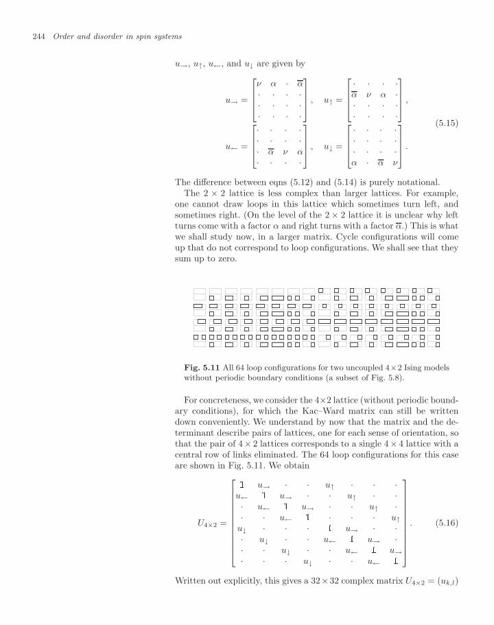
244 Order and disorder in spin systems
u→, u↑, u←, and u↓ are given by
u→ =
⎡⎢⎢⎣ν α · α· · · ·· · · ·· · · ·
⎤⎥⎥⎦ , u↑ =
⎡⎢⎢⎣· · · ·α ν α ·· · · ·· · · ·
⎤⎥⎥⎦ ,
u← =
⎡⎢⎢⎣· · · ·· · · ·· α ν α· · · ·
⎤⎥⎥⎦ , u↓ =
⎡⎢⎢⎣· · · ·· · · ·· · · ·α · α ν
⎤⎥⎥⎦ .
(5.15)
The difference between eqns (5.12) and (5.14) is purely notational.The 2 × 2 lattice is less complex than larger lattices. For example,
one cannot draw loops in this lattice which sometimes turn left, andsometimes right. (On the level of the 2 × 2 lattice it is unclear why leftturns come with a factor α and right turns with a factor α.) This is whatwe shall study now, in a larger matrix. Cycle configurations will comeup that do not correspond to loop configurations. We shall see that theysum up to zero.
Fig. 5.11 All 64 loop configurations for two uncoupled 4×2 Ising modelswithout periodic boundary conditions (a subset of Fig. 5.8).
For concreteness, we consider the 4×2 lattice (without periodic bound-ary conditions), for which the Kac–Ward matrix can still be writtendown conveniently. We understand by now that the matrix and the de-terminant describe pairs of lattices, one for each sense of orientation, sothat the pair of 4× 2 lattices corresponds to a single 4× 4 lattice with acentral row of links eliminated. The 64 loop configurations for this caseare shown in Fig. 5.11. We obtain
U4×2 =
⎡⎢⎢⎢⎢⎢⎢⎢⎢⎢⎢⎣
u→ · · u↑ · · ·u← u→ · · u↑ · ·· u← u→ · · u↑ ·· · u← · · · u↑
u↓ · · · u→ · ·· u↓ · · u← u→ ·· · u↓ · · u← u→· · · u↓ · · u←
⎤⎥⎥⎥⎥⎥⎥⎥⎥⎥⎥⎦. (5.16)
Written out explicitly, this gives a 32×32 complex matrix U4×2 = (uk,l)
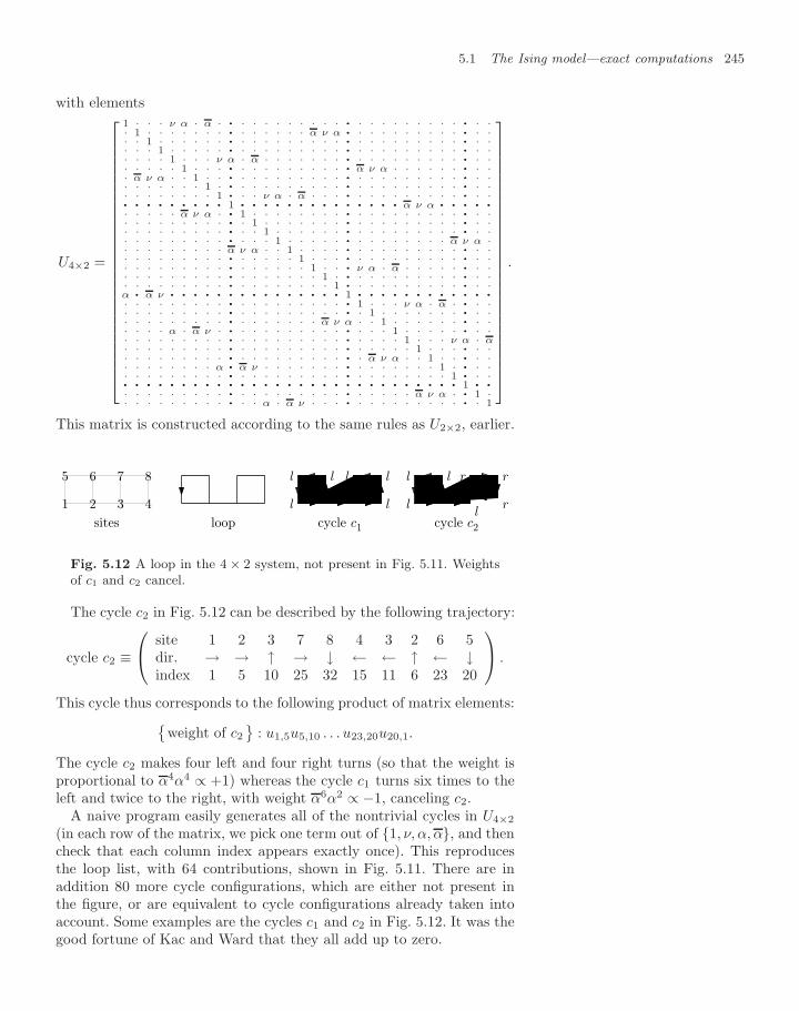
5.1 The Ising model—exact computations 245
with elements
U4×2 =
⎡⎢⎢⎢⎢⎢⎢⎢⎢⎢⎢⎢⎢⎢⎢⎢⎢⎢⎢⎢⎢⎢⎢⎢⎢⎢⎢⎣
1 · · · ν α · α · ········· · · · · · · · · · ········· · · · · · · · · · ········· · ·· 1 · · · · · · · ········· · · · · · · α ν α ········· · · · · · · · · · ········· · ·· · 1 · · · · · · ········· · · · · · · · · · ········· · · · · · · · · · ········· · ·· · · 1 · · · · · ········· · · · · · · · · · ········· · · · · · · · · · ········· · ·· · · · 1 · · · ν α · α · · · · · · · ········· · · · · · · · · · ········· · ·· · · · · 1 · · · ········· · · · · · · · · · ········· α ν α · · · · · · ········· · ·· α ν α · · 1 · · ········· · · · · · · · · · ········· · · · · · · · · · ········· · ·· · · · · · · 1 · ········· · · · · · · · · · ········· · · · · · · · · · ········· · ·· · · · · · · · 1 ········· · · ν α · α · · · ········· · · · · · · · · · ········· · ·········· ········· ········· ········· ········· ········· ········· ········· ········· 1 ········· ········· ········· ········· ········· ········· ········· ········· ········· ········· ········· ········· ········· ········· α ν α ········· ········· ········· ········· ·········· · · · · α ν α · ········· 1 · · · · · · · · ········· · · · · · · · · · ········· · ·· · · · · · · · · ········· · 1 · · · · · · · ········· · · · · · · · · · ········· · ·· · · · · · · · · ········· · · 1 · · · · · · ········· · · · · · · · · · ········· · ·· · · · · · · · · ········· · · · 1 · · · · · ········· · · · · · · · · α ν α ·· · · · · · · · · α ν α · · 1 · · · · ········· · · · · · · · · · ········· · ·· · · · · · · · · ········· · · · · · 1 · · · ········· · · · · · · · · · ········· · ·· · · · · · · · · ········· · · · · · · 1 · · ········· ν α · α · · · · · ········· · ·· · · · · · · · · ········· · · · · · · · 1 · ········· · · · · · · · · · ········· · ·· · · · · · · · · ········· · · · · · · · · 1 ········· · · · · · · · · · ········· · ·α ········· α ν ········· ········· ········· ········· ········· ········· ········· ········· ········· ········· ········· ········· ········· ········· ········· 1 ········· ········· ········· ········· ········· ········· ········· ········· ········· ········· ········· ·········· · · · · · · · · ········· · · · · · · · · · ········· 1 · · · ν α · α · ········· · ·· · · · · · · · · ········· · · · · · · · · · ········· · 1 · · · · · · · ········· · ·· · · · · · · · · ········· · · · · · · · α ν α · · 1 · · · · · · ········· · ·· · · · α · α ν · ········· · · · · · · · · · ········· · · · 1 · · · · · ········· · ·· · · · · · · · · ········· · · · · · · · · · ········· · · · · 1 · · · ν α · α· · · · · · · · · ········· · · · · · · · · · ········· · · · · · 1 · · · ········· · ·· · · · · · · · · ········· · · · · · · · · · ········· · α ν α · · 1 · · ········· · ·· · · · · · · · α ········· α ν · · · · · · · ········· · · · · · · · 1 · ········· · ·· · · · · · · · · ········· · · · · · · · · · ········· · · · · · · · · 1 ········· · ·········· ········· ········· ········· ········· ········· ········· ········· ········· ········· ········· ········· ········· ········· ········· ········· ········· ········· ········· ········· ········· ········· ········· ········· ········· ········· ········· ········· ········· 1 ········· ·········· · · · · · · · · ········· · · · · · · · · · ········· · · · · · α ν α · ········· 1 ·· · · · · · · · · ········· · · α · α ν · · · ········· · · · · · · · · · ········· · 1
⎤⎥⎥⎥⎥⎥⎥⎥⎥⎥⎥⎥⎥⎥⎥⎥⎥⎥⎥⎥⎥⎥⎥⎥⎥⎥⎥⎦
.
This matrix is constructed according to the same rules as U2×2, earlier.
1 2 3 4
5 6 7 8
sites loop cycle c1
l l
llll
r r
cycle c2
ll
r r
r
ll
r
Fig. 5.12 A loop in the 4 × 2 system, not present in Fig. 5.11. Weightsof c1 and c2 cancel.
The cycle c2 in Fig. 5.12 can be described by the following trajectory:
cycle c2 ≡⎛⎝ site 1 2 3 7 8 4 3 2 6 5
dir. → → ↑ → ↓ ← ← ↑ ← ↓index 1 5 10 25 32 15 11 6 23 20
⎞⎠ .
This cycle thus corresponds to the following product of matrix elements:weight of c2
: u1,5u5,10 . . . u23,20u20,1.
The cycle c2 makes four left and four right turns (so that the weight isproportional to α4α4 ∝ +1) whereas the cycle c1 turns six times to theleft and twice to the right, with weight α6α2 ∝ −1, canceling c2.
A naive program easily generates all of the nontrivial cycles in U4×2
(in each row of the matrix, we pick one term out of 1, ν, α, α, and thencheck that each column index appears exactly once). This reproducesthe loop list, with 64 contributions, shown in Fig. 5.11. There are inaddition 80 more cycle configurations, which are either not present inthe figure, or are equivalent to cycle configurations already taken intoaccount. Some examples are the cycles c1 and c2 in Fig. 5.12. It was thegood fortune of Kac and Ward that they all add up to zero.
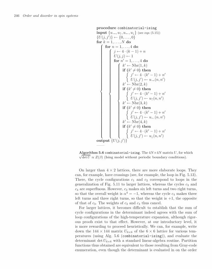
246 Order and disorder in spin systems
procedure combinatorial-ising
input u→, u↑, u←, u↓ (see eqn (5.15))U(j, j′) ← 0, . . . , 0for k = 1, . . . , N do⎧⎪⎪⎪⎪⎪⎪⎪⎪⎪⎪⎪⎪⎪⎪⎪⎪⎪⎪⎪⎪⎪⎪⎪⎪⎪⎪⎪⎪⎪⎪⎪⎪⎪⎪⎨⎪⎪⎪⎪⎪⎪⎪⎪⎪⎪⎪⎪⎪⎪⎪⎪⎪⎪⎪⎪⎪⎪⎪⎪⎪⎪⎪⎪⎪⎪⎪⎪⎪⎪⎩
for n = 1, . . . , 4 do⎧⎪⎪⎪⎪⎪⎪⎪⎪⎪⎪⎪⎪⎪⎪⎪⎪⎪⎪⎪⎪⎪⎪⎪⎪⎪⎪⎪⎪⎪⎪⎪⎪⎨⎪⎪⎪⎪⎪⎪⎪⎪⎪⎪⎪⎪⎪⎪⎪⎪⎪⎪⎪⎪⎪⎪⎪⎪⎪⎪⎪⎪⎪⎪⎪⎪⎩
j ← 4 · (k − 1) + nU(j, j) ← 1for n′ = 1, . . . , 4 do⎧⎪⎪⎪⎪⎪⎪⎪⎪⎪⎪⎪⎪⎪⎪⎪⎪⎪⎪⎪⎪⎪⎪⎪⎪⎪⎪⎨⎪⎪⎪⎪⎪⎪⎪⎪⎪⎪⎪⎪⎪⎪⎪⎪⎪⎪⎪⎪⎪⎪⎪⎪⎪⎪⎩
k′ ← Nbr(1, k)if (k′ = 0) then
j′ ← 4 · (k′ − 1) + n′
U(j, j′) ← u→(n, n′)k′ ← Nbr(2, k)if (k′ = 0) then
j′ ← 4 · (k′ − 1) + n′
U(j, j′) ← u↑(n, n′)k′ ← Nbr(3, k)if (k′ = 0) then
j′ ← 4 · (k′ − 1) + n′
U(j, j′) ← u←(n, n′)k′ ← Nbr(4, k)if (k′ = 0) then
j′ ← 4 · (k′ − 1) + n′
U(j, j′) ← u↓(n, n′)output U(j, j′)——
Algorithm 5.6 combinatorial-ising. The 4N×4N matrix U , for which√detU ∝ Z(β) (Ising model without periodic boundary conditions).
On larger than 4 × 2 lattices, there are more elaborate loops. Theycan, for example, have crossings (see, for example, the loop in Fig. 5.13).There, the cycle configurations c1 and c2 correspond to loops in thegeneralization of Fig. 5.11 to larger lattices, whereas the cycles c3 andc4 are superfluous. However, c3 makes six left turns and two right turns,so that the overall weight is α4 = −1, whereas the cycle c4 makes threeleft turns and three right turns, so that the weight is +1, the oppositeof that of c3. The weights of c3 and c4 thus cancel.
For larger lattices, it becomes difficult to establish that the sum ofcycle configurations in the determinant indeed agrees with the sum ofloop configurations of the high-temperature expansion, although rigor-ous proofs exist to that effect. However, at our introductory level, itis more rewarding to proceed heuristically. We can, for example, writedown the 144 × 144 matrix U6×6 of the 6 × 6 lattice for various tem-peratures (using Alg. 5.6 (combinatorial-ising)), and evaluate thedeterminant det U6×6 with a standard linear-algebra routine. Partitionfunctions thus obtained are equivalent to those resulting from Gray-codeenumeration, even though the determinant is evaluated in on the order
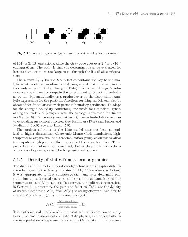
5.1 The Ising model—exact computations 247
loop c1 c2 c3
l lr
l
llr
l
c4
l l
r
rr
l
Fig. 5.13 Loop and cycle configurations. The weights of c3 and c4 cancel.
of 1443 3×10⁶ operations, while the Gray code goes over 235 3×10¹⁰
configurations. The point is that the determinant can be evaluated forlattices that are much too large to go through the list of all configura-tions.
The matrix UL×L for the L × L lattice contains the key to the ana-lytic solution of the two-dimensional Ising model first obtained, in thethermodynamic limit, by Onsager (1944). To recover Onsager’s solu-tion, we would have to compute the determinant of U , not numericallyas we did, but analytically, as a product over all the eigenvalues. Ana-lytic expressions for the partition functions for Ising models can also beobtained for finite lattices with periodic boundary conditions. To adaptfor the changed boundary conditions, one needs four matrices, gener-alizing the matrix U (compare with the analogous situation for dimersin Chapter 6). Remarkably, evaluating Z(β) on a finite lattice reducesto evaluating an explicit function (see Kaufman (1949) and Fisher andFerdinand (1969); see also Exerc. 5.9).
The analytic solutions of the Ising model have not been general-ized to higher dimensions, where only Monte Carlo simulations, high-temperature expansions, and renormalization-group calculations allowto compute to high precision the properties of the phase transition. Theseproperties, as mentioned, are universal, that is, they are the same for awide class of systems, called the Ising universality class.
5.1.5 Density of states from thermodynamics
The direct and indirect enumeration algorithms in this chapter differ inthe role played by the density of states. In Alg. 5.3 (enumerate-ising),it was appropriate to first compute N (E), and later determine par-tition functions, internal energies, and specific heat capacities at anytemperature, in ∝ N operations. In contrast, the indirect enumerationsin Section 5.1.4 determine the partition function Z(β), not the densityof states. Computing Z(β) from N (E) is straightforward, but how torecover N (E) from Z(β) requires some thought:
N (E)Subsection 5.1.2−−−−−−−−−−→←−−−−−−−−−this subsection
Z(β).
The mathematical problem of the present section is common to manybasic problems in statistical and solid state physics, and appears also inthe interpretation of experimental or Monte Carlo data. In the presence
248 Order and disorder in spin systems
of statistical uncertainties, it is very difficult to solve, and may often beill-defined. This means, in our case, that algorithms exist for computingN (E) if the partition functions were computed exactly. If, however, Z(β)is known only to limited precision, the output generated by the slightlyperturbed input can be drastically different from the exact output.
For a two-dimensional Ising model on a finite lattice, the exact par-tition function Z(β) can be obtained from the matrix U of Alg. 5.6(combinatorial-ising), or better from Kaufman’s explicit formula (seeExerc. 5.9). For concreteness, we consider the case of periodic boundaryconditions, where the ∆E = 4, and where there are N levels of excitedstates. In this case, the Boltzmann weight of the kth excited state isxke−βE0 , where x = e−4β . The partition function can be expressed as apolynomial in x, where the prefactors are the densities of state,
Z(x) =Z(β)e−βE0
= N (0) + N (1)x + N (2) x2 + · · · + N (N) xN .
It now suffices to compute the partition functions of the Ising model atN +1 different temperatures, x0 = e−4β0 , . . . , xN = e−4βN , to arrive at amatrix equation relating the partition functions to the densities of state:⎡⎢⎢⎢⎣
1 x0 x20 . . . xN
0
1 x1 x21 . . . xN
1...
......
...1 xN x2
N . . . xNN
⎤⎥⎥⎥⎦︸ ︷︷ ︸
A (Vandermonde matrix)
⎡⎢⎢⎢⎣N (0)N (1)
...N (N)
⎤⎥⎥⎥⎦ =
⎡⎢⎢⎢⎣Z0
Z1
...ZN
⎤⎥⎥⎥⎦ . (5.17)
In principle, we can multiply both sides of eqn (5.17) (from the left)by A−1 to obtain the densities of states. ( The special type of matrix ineqn (5.17) is called a Vandermonde matrix.)
As an alternative to matrix inversion, we could also obtain the den-sities of state N (0) , . . . ,N (N) from repeated interpolations of thepartition function to zero temperature, where only the ground statecontributes to the partition function:
Z(x) N (E0) e−βE0 for x → 0.
Extrapolating Z(β) to zero temperature thus gives the energy and thedegeneracy of the ground state. We can now go further and, so to speak,peel off the result of this interpolation from our original problem, thatis, interpolate (Zk −N (0))/xk through a polynomial of order N − 1, inorder to determine N (1), etc.
For lattices beyond 4 × 4 or 6 × 6, the matrix inversion in eqn (5.17)and the naive interpolation scheme both run into numerical instabili-ties, unless we increase the precision of our calculation much beyondthe standard 32- or 64-bit floating-point formats discussed in Subsec-tion 2.1.2. Overall, we may be better off using symbolic rather thannumerical computations, and relying on commercial software packages,which are beyond the scope of this book. A compact procedure by Beale(1996) allows one to obtain the exact density of states of the Ising modelfor systems of size up to 100 × 100.
5.2 The Ising model—Monte Carlo algorithms 249
5.2 The Ising model—Monte Carlo
algorithms
Gray-code enumerations, as discussed in Subsection 5.1.1, succeed onlyfor relatively small systems, and high-temperature expansions, the sub-ject of Subsection 5.1.4, must usually be stopped after a limited numberof terms, before they get too complicated. Only under exceptional cir-cumstances, as in the two-dimensional Ising model, can these methodsbe pushed much further. Often, Monte Carlo methods alone are able toobtain exact results for large sizes. The price to be paid is that config-urations are sampled rather than enumerated, so that statistical errorsare inevitable. The Ising model has been a major test bed for MonteCarlo simulations and algorithms, methods and recipes.
Roughly speaking, there have been two crucial periods in Ising-modelcomputations, since it was realized that local Monte Carlo calculationsare rather imprecise in the neighborhood of the critical point. It tooka long time to appreciate that the lack of precision has two origins:First, spins are spatially correlated on a certain length scale, called thecorrelation length ξ. On this length scale, spins mostly point in the samedirection. It is difficult to turn a spin around, or to turn a small patchof correlated spins, embedded in a larger region, where the spins arethemselves correlated. This large-scale correlation of spins is directlyresponsible for the “critical slowing down” of simulations close to Tc.Large correlation times are the first origin of the lack of precision. Inthe infinite system, ξ diverges at the critical temperature, but in a finitelattice, this correlation length cannot exceed the system size, so thatthe simulation has a typical length scale which depends on system size.This is the second origin of the lack of precision. In summary, we findthat, on the one hand, observables are difficult to evaluate close to Tc
because of critical slowing down. On the other hand, the observablesof the infinite lattice are difficult to evaluate, because they differ fromthose computed for a finite system if we are close to the critical point.Extrapolation to an infinite system size is thus nontrivial. The criticalslowing down of Monte Carlo algorithms is a natural consequence of adiverging correlation length, and it can also be seen in many experiments,in liquids, magnets, etc.
The second crucial period of simulations of the Ising model startedin the late 1980s, when it was finally understood that critical slowingdown is not an inescapable curse of simulation, as it is for experiments.It was overcome through the construction of cluster algorithms whichenforce the detailed-balance condition with nonintuitive rules which areunrelated to the flipping of single spins. These methods have spread fromthe Ising model to many other fields of statistical physics.
5.2.1 Local sampling methods
A basic task in statistical physics is to write a local Metropolis algo-rithm for the Ising model. This program is even simpler than a basic
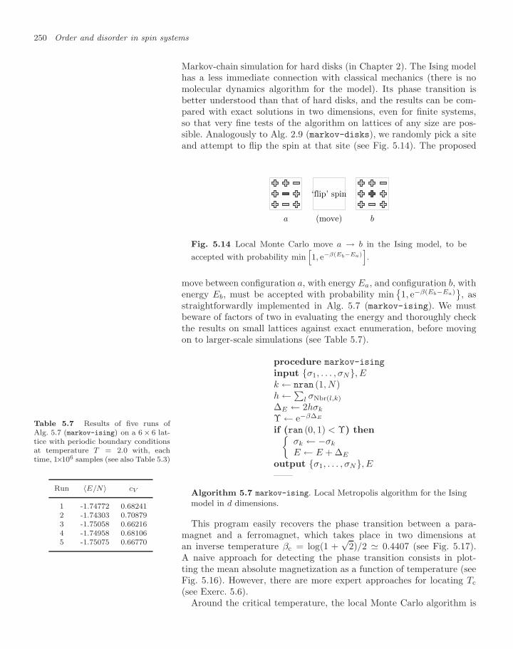
250 Order and disorder in spin systems
Markov-chain simulation for hard disks (in Chapter 2). The Ising modelhas a less immediate connection with classical mechanics (there is nomolecular dynamics algorithm for the model). Its phase transition isbetter understood than that of hard disks, and the results can be com-pared with exact solutions in two dimensions, even for finite systems,so that very fine tests of the algorithm on lattices of any size are pos-sible. Analogously to Alg. 2.9 (markov-disks), we randomly pick a siteand attempt to flip the spin at that site (see Fig. 5.14). The proposed
a
‘flip’ spin
(move) b
Fig. 5.14 Local Monte Carlo move a → b in the Ising model, to be
accepted with probability minh1, e−β(Eb−Ea)
i.
move between configuration a, with energy Ea, and configuration b, withenergy Eb, must be accepted with probability min
1, e−β(Eb−Ea)
, as
straightforwardly implemented in Alg. 5.7 (markov-ising). We mustbeware of factors of two in evaluating the energy and thoroughly checkthe results on small lattices against exact enumeration, before movingon to larger-scale simulations (see Table 5.7).
procedure markov-ising
input σ1, . . . , σN, Ek ← nran (1, N)h ←∑l σNbr(l,k)
∆E ← 2hσk
Υ ← e−β∆E
if (ran (0, 1) < Υ) thenσk ← −σk
E ← E + ∆E
output σ1, . . . , σN, E——
Algorithm 5.7 markov-ising. Local Metropolis algorithm for the Isingmodel in d dimensions.
Table 5.7 Results of five runs ofAlg. 5.7 (markov-ising) on a 6 × 6 lat-tice with periodic boundary conditionsat temperature T = 2.0 with, eachtime, 1×10⁶ samples (see also Table 5.3)
Run 〈E/N〉 cV
1 -1.74772 0.682412 -1.74303 0.708793 -1.75058 0.662164 -1.74958 0.681065 -1.75075 0.66770
This program easily recovers the phase transition between a para-magnet and a ferromagnet, which takes place in two dimensions atan inverse temperature βc = log(1 +
√2)/2 0.4407 (see Fig. 5.17).
A naive approach for detecting the phase transition consists in plot-ting the mean absolute magnetization as a function of temperature (seeFig. 5.16). However, there are more expert approaches for locating Tc
(see Exerc. 5.6).Around the critical temperature, the local Monte Carlo algorithm is
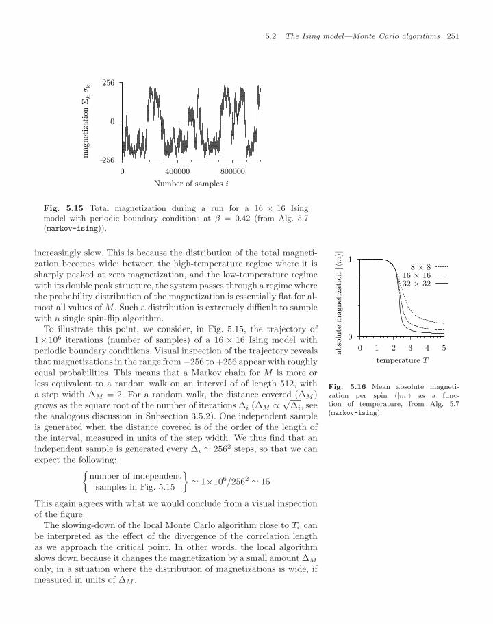
5.2 The Ising model—Monte Carlo algorithms 251
-256
0
256
0 400000 800000
mag
net
izat
ion Σ
k σ
k
Number of samples i
Fig. 5.15 Total magnetization during a run for a 16 × 16 Isingmodel with periodic boundary conditions at β = 0.42 (from Alg. 5.7(markov-ising)).
increasingly slow. This is because the distribution of the total magneti-zation becomes wide: between the high-temperature regime where it issharply peaked at zero magnetization, and the low-temperature regimewith its double peak structure, the system passes through a regime wherethe probability distribution of the magnetization is essentially flat for al-most all values of M . Such a distribution is extremely difficult to samplewith a single spin-flip algorithm.
0
1
0 1 2 3 4 5ab
solu
te m
agnet
izat
ion |〈m
〉|
temperature T
8 × 816 × 1632 × 32
Fig. 5.16 Mean absolute magneti-zation per spin 〈|m|〉 as a func-tion of temperature, from Alg. 5.7(markov-ising).
To illustrate this point, we consider, in Fig. 5.15, the trajectory of1×106 iterations (number of samples) of a 16 × 16 Ising model withperiodic boundary conditions. Visual inspection of the trajectory revealsthat magnetizations in the range from −256 to +256 appear with roughlyequal probabilities. This means that a Markov chain for M is more orless equivalent to a random walk on an interval of of length 512, witha step width ∆M = 2. For a random walk, the distance covered (∆M )grows as the square root of the number of iterations ∆i (∆M ∝ √
∆i, seethe analogous discussion in Subsection 3.5.2). One independent sampleis generated when the distance covered is of the order of the length ofthe interval, measured in units of the step width. We thus find that anindependent sample is generated every ∆i 2562 steps, so that we canexpect the following:
number of independentsamples in Fig. 5.15
1×10⁶/2562 15
This again agrees with what we would conclude from a visual inspectionof the figure.
The slowing-down of the local Monte Carlo algorithm close to Tc canbe interpreted as the effect of the divergence of the correlation lengthas we approach the critical point. In other words, the local algorithmslows down because it changes the magnetization by a small amount ∆M
only, in a situation where the distribution of magnetizations is wide, ifmeasured in units of ∆M .
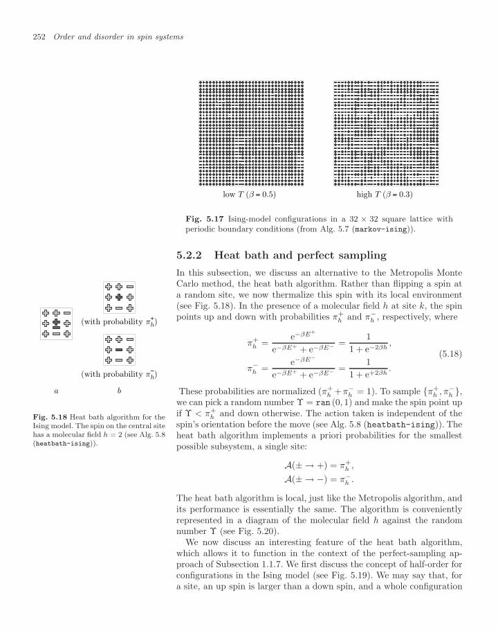
252 Order and disorder in spin systems
low T (β = 0.5) high T (β = 0.3)
Fig. 5.17 Ising-model configurations in a 32 × 32 square lattice withperiodic boundary conditions (from Alg. 5.7 (markov-ising)).
5.2.2 Heat bath and perfect sampling
In this subsection, we discuss an alternative to the Metropolis MonteCarlo method, the heat bath algorithm. Rather than flipping a spin ata random site, we now thermalize this spin with its local environment(see Fig. 5.18). In the presence of a molecular field h at site k, the spinpoints up and down with probabilities π+
h and π−h , respectively, where
π+h =
e−βE+
e−βE+ + e−βE− =1
1 + e−2βh,
π−h =
e−βE−
e−βE+ + e−βE− =1
1 + e+2βh.
(5.18)
These probabilities are normalized (π+h +π−
h = 1). To sample π+h , π−
h ,
(with probability π+h)
a
(with probability π−h)
b
Fig. 5.18 Heat bath algorithm for theIsing model. The spin on the central sitehas a molecular field h = 2 (see Alg. 5.8(heatbath-ising)).
we can pick a random number Υ = ran (0, 1) and make the spin point upif Υ < π+
h and down otherwise. The action taken is independent of thespin’s orientation before the move (see Alg. 5.8 (heatbath-ising)). Theheat bath algorithm implements a priori probabilities for the smallestpossible subsystem, a single site:
A(± → +) = π+h ,
A(± → −) = π−h .
The heat bath algorithm is local, just like the Metropolis algorithm, andits performance is essentially the same. The algorithm is convenientlyrepresented in a diagram of the molecular field h against the randomnumber Υ (see Fig. 5.20).
We now discuss an interesting feature of the heat bath algorithm,which allows it to function in the context of the perfect-sampling ap-proach of Subsection 1.1.7. We first discuss the concept of half-order forconfigurations in the Ising model (see Fig. 5.19). We may say that, fora site, an up spin is larger than a down spin, and a whole configuration
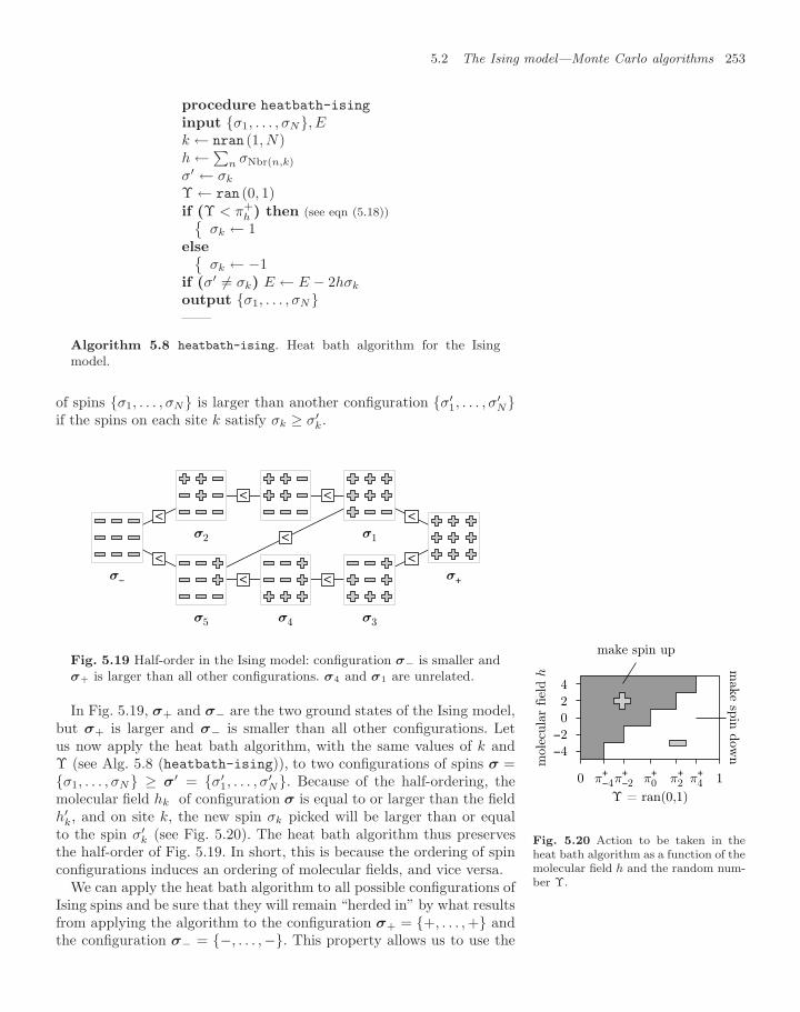
5.2 The Ising model—Monte Carlo algorithms 253
procedure heatbath-ising
input σ1, . . . , σN, Ek ← nran (1, N)h ←∑n σNbr(n,k)
σ′ ← σk
Υ ← ran (0, 1)if (Υ < π+
h ) then (see eqn (5.18))σk ← 1
elseσk ← −1
if (σ′ = σk) E ← E − 2hσk
output σ1, . . . , σN——
Algorithm 5.8 heatbath-ising. Heat bath algorithm for the Isingmodel.
of spins σ1, . . . , σN is larger than another configuration σ′1, . . . , σ
′N
if the spins on each site k satisfy σk ≥ σ′k.
<
<σ2
<
<
< σ1
<σ−
<σ+<
σ5
<
σ4 σ3
Fig. 5.19 Half-order in the Ising model: configuration σ− is smaller andσ+ is larger than all other configurations. σ4 and σ1 are unrelated.
In Fig. 5.19, σ+ and σ− are the two ground states of the Ising model,but σ+ is larger and σ− is smaller than all other configurations. Letus now apply the heat bath algorithm, with the same values of k andΥ (see Alg. 5.8 (heatbath-ising)), to two configurations of spins σ =σ1, . . . , σN ≥ σ′ = σ′
1, . . . , σ′N. Because of the half-ordering, the
molecular field hk of configuration σ is equal to or larger than the field
−4
−2
0
2
4
0 1
Υ = ran(0,1)
mol
ecula
r fiel
d h
π+−4π
+−2 π+
0 π+2 π+
4
mak
e spin
dow
n
make spin up
Fig. 5.20 Action to be taken in theheat bath algorithm as a function of themolecular field h and the random num-ber Υ.
h′k, and on site k, the new spin σk picked will be larger than or equal
to the spin σ′k (see Fig. 5.20). The heat bath algorithm thus preserves
the half-order of Fig. 5.19. In short, this is because the ordering of spinconfigurations induces an ordering of molecular fields, and vice versa.
We can apply the heat bath algorithm to all possible configurations ofIsing spins and be sure that they will remain “herded in” by what resultsfrom applying the algorithm to the configuration σ+ = +, . . . , + andthe configuration σ− = −, . . . ,−. This property allows us to use the
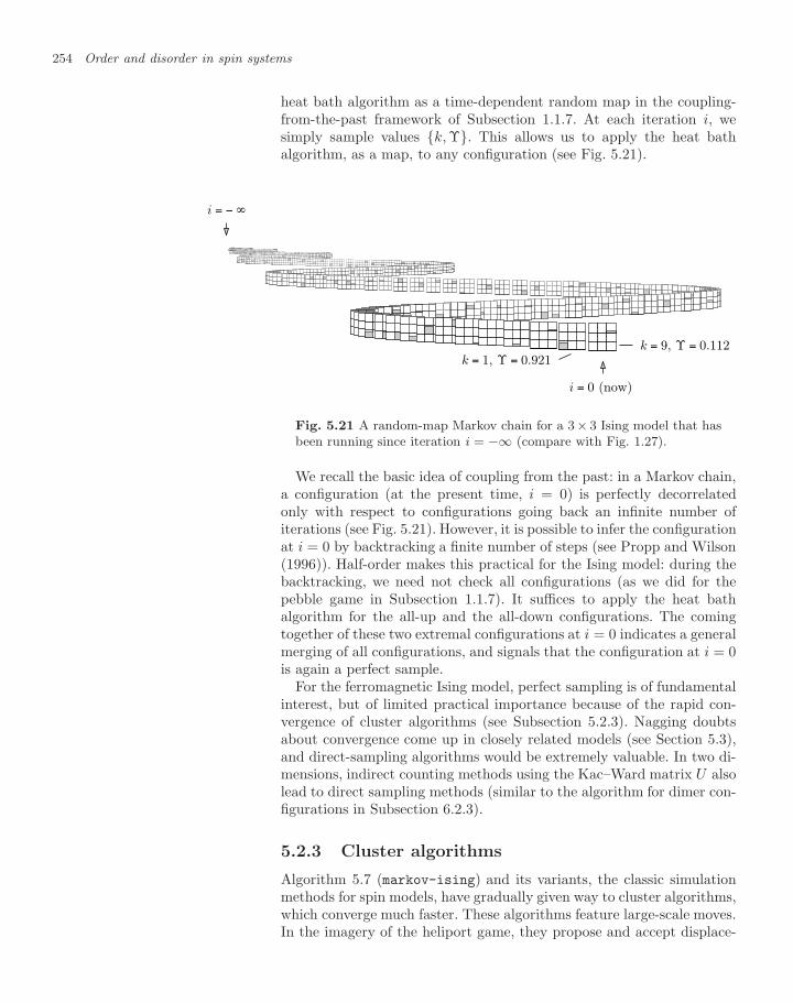
254 Order and disorder in spin systems
heat bath algorithm as a time-dependent random map in the coupling-from-the-past framework of Subsection 1.1.7. At each iteration i, wesimply sample values k, Υ. This allows us to apply the heat bathalgorithm, as a map, to any configuration (see Fig. 5.21).
i = 0 (now)
i = − ∞
k = 9, Υ = 0.112k = 1, Υ = 0.921
Fig. 5.21 A random-map Markov chain for a 3× 3 Ising model that hasbeen running since iteration i = −∞ (compare with Fig. 1.27).
We recall the basic idea of coupling from the past: in a Markov chain,a configuration (at the present time, i = 0) is perfectly decorrelatedonly with respect to configurations going back an infinite number ofiterations (see Fig. 5.21). However, it is possible to infer the configurationat i = 0 by backtracking a finite number of steps (see Propp and Wilson(1996)). Half-order makes this practical for the Ising model: during thebacktracking, we need not check all configurations (as we did for thepebble game in Subsection 1.1.7). It suffices to apply the heat bathalgorithm for the all-up and the all-down configurations. The comingtogether of these two extremal configurations at i = 0 indicates a generalmerging of all configurations, and signals that the configuration at i = 0is again a perfect sample.
For the ferromagnetic Ising model, perfect sampling is of fundamentalinterest, but of limited practical importance because of the rapid con-vergence of cluster algorithms (see Subsection 5.2.3). Nagging doubtsabout convergence come up in closely related models (see Section 5.3),and direct-sampling algorithms would be extremely valuable. In two di-mensions, indirect counting methods using the Kac–Ward matrix U alsolead to direct sampling methods (similar to the algorithm for dimer con-figurations in Subsection 6.2.3).
5.2.3 Cluster algorithms
Algorithm 5.7 (markov-ising) and its variants, the classic simulationmethods for spin models, have gradually given way to cluster algorithms,which converge much faster. These algorithms feature large-scale moves.In the imagery of the heliport game, they propose and accept displace-
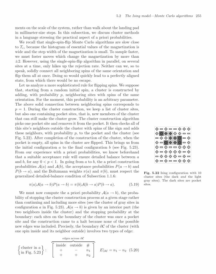
5.2 The Ising model—Monte Carlo algorithms 255
ments on the scale of the system, rather than walk about the landing padin millimeter-size steps. In this subsection, we discuss cluster methodsin a language stressing the practical aspect of a priori probabilities.
We recall that single-spin-flip Monte Carlo algorithms are slow closeto Tc, because the histogram of essential values of the magnetization iswide and the step width of the magnetization is small. To sample faster,we must foster moves which change the magnetization by more than±2. However, using the single-spin-flip algorithm in parallel, on severalsites at a time, only hikes up the rejection rate. Neither can we, so tospeak, solidly connect all neighboring spins of the same orientation andflip them all at once. Doing so would quickly lead to a perfectly alignedstate, from which there would be no escape.
Let us analyze a more sophisticated rule for flipping spins. We supposethat, starting from a random initial spin, a cluster is constructed byadding, with probability p, neighboring sites with spins of the sameorientation. For the moment, this probability is an arbitrary parameter.The above solid connection between neighboring spins corresponds top = 1. During the cluster construction, we keep a list of cluster sites,but also one containing pocket sites, that is, new members of the clusterthat can still make the cluster grow. The cluster construction algorithmpicks one pocket site and removes it from the pocket. It then checks all ofthis site’s neighbors outside the cluster with spins of like sign and addsthese neighbors, with probability p, to the pocket and the cluster (seeFig. 5.22). After completion of the construction of the cluster, when thepocket is empty, all spins in the cluster are flipped. This brings us fromthe initial configuration a to the final configuration b (see Fig. 5.23).From our experience with a priori probabilities, we know beforehandthat a suitable acceptance rule will ensure detailed balance between aand b, for any 0 < p < 1. In going from a to b, the a priori construction
Fig. 5.22 Ising configuration with 10cluster sites (the dark and the lightgray sites). The dark sites are pocketsites.
probabilities A(a) and A(b), the acceptance probabilities P (a → b) andP (b → a), and the Boltzmann weights π(a) and π(b), must respect thegeneralized detailed-balance condition of Subsection 1.1.6:
π(a)A(a → b)P (a → b) = π(b)A(b → a)P (b → a). (5.19)
We must now compute the a priori probability A(a → b), the proba-bility of stopping the cluster construction process at a given stage ratherthan continuing and including more sites (see the cluster of gray sites inconfiguration a in Fig. 5.23). A(a → b) is given by an interior part (thetwo neighbors inside the cluster) and the stopping probability at theboundary: each sites on the boundary of the cluster was once a pocketsite and the construction came to a halt because none of the possiblenew edges was included. Precisely, the boundary ∂C of the cluster (withone spin inside and its neighbor outside) involves two types of edge:
cluster in ain Fig. 5.23
:
edges across ∂C︷ ︸︸ ︷⎡⎣ inside outside #+ − n1
+ + n2
⎤⎦ E|∂C = n1 − n2 (5.20)
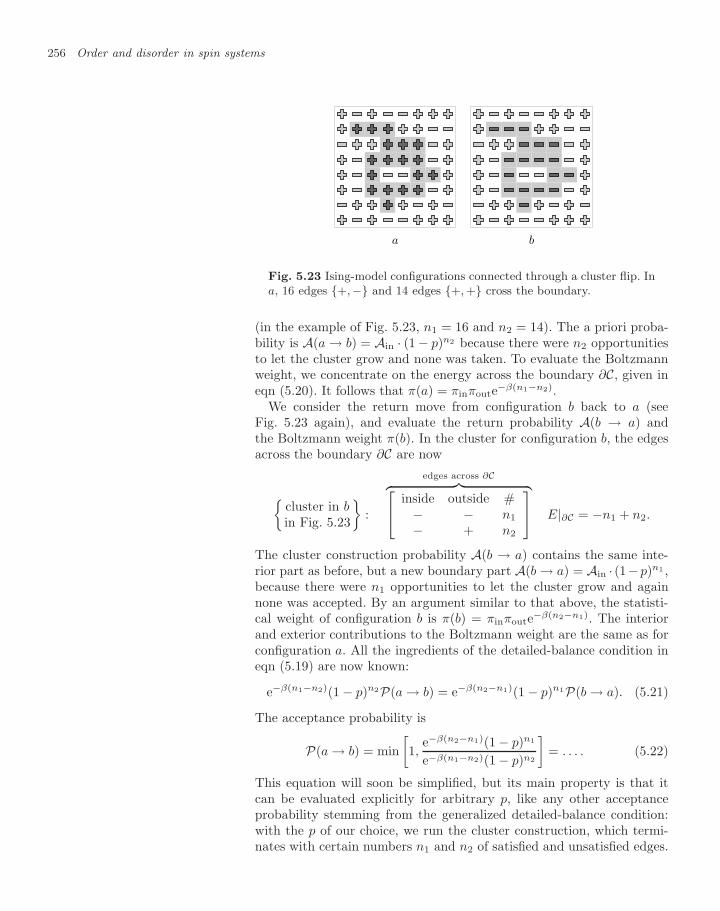
256 Order and disorder in spin systems
a b
Fig. 5.23 Ising-model configurations connected through a cluster flip. Ina, 16 edges +,− and 14 edges +, + cross the boundary.
(in the example of Fig. 5.23, n1 = 16 and n2 = 14). The a priori proba-bility is A(a → b) = Ain · (1 − p)n2 because there were n2 opportunitiesto let the cluster grow and none was taken. To evaluate the Boltzmannweight, we concentrate on the energy across the boundary ∂C, given ineqn (5.20). It follows that π(a) = πinπoute−β(n1−n2).
We consider the return move from configuration b back to a (seeFig. 5.23 again), and evaluate the return probability A(b → a) andthe Boltzmann weight π(b). In the cluster for configuration b, the edgesacross the boundary ∂C are now
cluster in bin Fig. 5.23
:
edges across ∂C︷ ︸︸ ︷⎡⎣ inside outside #− − n1
− + n2
⎤⎦ E|∂C = −n1 + n2.
The cluster construction probability A(b → a) contains the same inte-rior part as before, but a new boundary part A(b → a) = Ain · (1−p)n1 ,because there were n1 opportunities to let the cluster grow and againnone was accepted. By an argument similar to that above, the statisti-cal weight of configuration b is π(b) = πinπoute−β(n2−n1). The interiorand exterior contributions to the Boltzmann weight are the same as forconfiguration a. All the ingredients of the detailed-balance condition ineqn (5.19) are now known:
e−β(n1−n2)(1 − p)n2P(a → b) = e−β(n2−n1)(1 − p)n1P(b → a). (5.21)
The acceptance probability is
P(a → b) = min[1,
e−β(n2−n1)(1 − p)n1
e−β(n1−n2)(1 − p)n2
]= . . . . (5.22)
This equation will soon be simplified, but its main property is that itcan be evaluated explicitly for arbitrary p, like any other acceptanceprobability stemming from the generalized detailed-balance condition:with the p of our choice, we run the cluster construction, which termi-nates with certain numbers n1 and n2 of satisfied and unsatisfied edges.
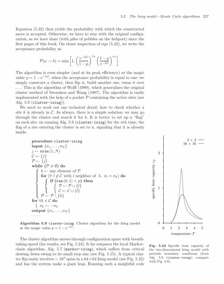
5.2 The Ising model—Monte Carlo algorithms 257
Equation (5.22) then yields the probability with which the constructedmove is accepted. Otherwise, we have to stay with the original configu-ration, as we have done (with piles of pebbles on the heliport) since thefirst pages of this book. On closer inspection of eqn (5.22), we write theacceptance probability as
P(a → b) = min[1,
(e−2β
1 − p
)n2 (1 − p
e−2β
)n1]
.
The algorithm is even simpler (and at its peak efficiency) at the magicvalue p = 1− e−2β , when the acceptance probability is equal to one: wesimply construct a cluster, then flip it, build another one, turns it over. . . . This is the algorithm of Wolff (1989), which generalizes the originalcluster method of Swendsen and Wang (1987). The algorithm is easilyimplemented with the help of a pocket P containing the active sites (seeAlg. 5.9 (cluster-ising)).
We need to work out one technical detail: how to check whether asite k is already in C. As always, there is a simple solution: we may gothrough the cluster and search it for k. It is better to set up a “flag”on each site: on running Alg. 5.9 (cluster-ising) for the nth time, theflag of a site entering the cluster is set to n, signaling that it is alreadyinside.
procedure cluster-ising
input σ1, . . . , σNj ← nran (1, N)C ← jP ← jwhile (P = ∅) do⎧⎪⎪⎪⎪⎪⎪⎨⎪⎪⎪⎪⎪⎪⎩
k ← any element of Pfor (∀ l ∈ C with l neighbor of k, σl = σk) do⎧⎨⎩
if (ran (0, 1) < p) then P ← P ∪ lC ← C ∪ l
P ← P \ kfor ∀k ∈ C do
σk ← −σk
output σ1, . . . , σN——
Algorithm 5.9 cluster-ising. Cluster algorithm for the Ising model
at the magic value p = 1 − e−2β .
0
1
2
0 1 2 3 4 5
spec
ific
hea
t ca
pac
ity c
V
temperature T
4 × 416 × 16
Fig. 5.24 Specific heat capacity ofthe two-dimensional Ising model withperiodic boundary conditions (fromAlg. 5.9 (cluster-ising); comparewith Fig. 5.6).
The cluster algorithm moves through configuration space with breath-taking speed (for results, see Fig. 5.24). It far outpaces the local Markov-chain algorithm, Alg. 5.7 (markov-ising), which suffers from criticalslowing down owing to its small step size (see Fig. 5.15). A typical clus-ter flip easily involves ∼ 103 spins in a 64×64 Ising model (see Fig. 5.25)and has the system make a giant leap. Running such a insightful code
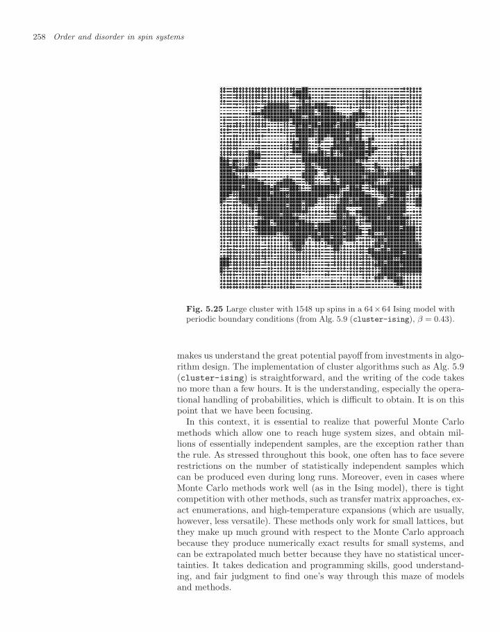
258 Order and disorder in spin systems
Fig. 5.25 Large cluster with 1548 up spins in a 64×64 Ising model withperiodic boundary conditions (from Alg. 5.9 (cluster-ising), β = 0.43).
makes us understand the great potential payoff from investments in algo-rithm design. The implementation of cluster algorithms such as Alg. 5.9(cluster-ising) is straightforward, and the writing of the code takesno more than a few hours. It is the understanding, especially the opera-tional handling of probabilities, which is difficult to obtain. It is on thispoint that we have been focusing.
In this context, it is essential to realize that powerful Monte Carlomethods which allow one to reach huge system sizes, and obtain mil-lions of essentially independent samples, are the exception rather thanthe rule. As stressed throughout this book, one often has to face severerestrictions on the number of statistically independent samples whichcan be produced even during long runs. Moreover, even in cases whereMonte Carlo methods work well (as in the Ising model), there is tightcompetition with other methods, such as transfer matrix approaches, ex-act enumerations, and high-temperature expansions (which are usually,however, less versatile). These methods only work for small lattices, butthey make up much ground with respect to the Monte Carlo approachbecause they produce numerically exact results for small systems, andcan be extrapolated much better because they have no statistical uncer-tainties. It takes dedication and programming skills, good understand-ing, and fair judgment to find one’s way through this maze of modelsand methods.
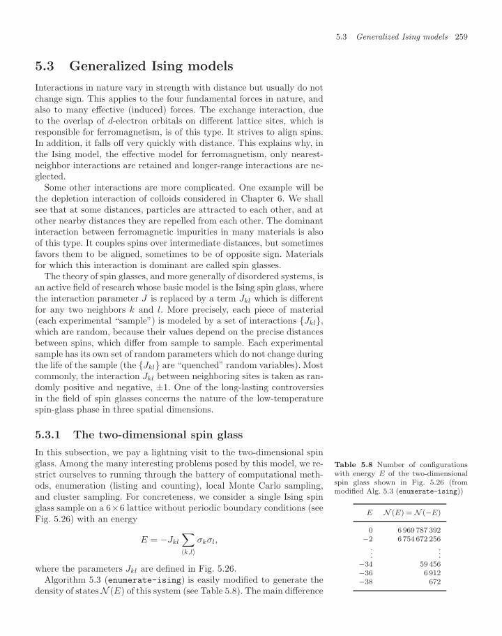
5.3 Generalized Ising models 259
5.3 Generalized Ising models
Interactions in nature vary in strength with distance but usually do notchange sign. This applies to the four fundamental forces in nature, andalso to many effective (induced) forces. The exchange interaction, dueto the overlap of d-electron orbitals on different lattice sites, which isresponsible for ferromagnetism, is of this type. It strives to align spins.In addition, it falls off very quickly with distance. This explains why, inthe Ising model, the effective model for ferromagnetism, only nearest-neighbor interactions are retained and longer-range interactions are ne-glected.
Some other interactions are more complicated. One example will bethe depletion interaction of colloids considered in Chapter 6. We shallsee that at some distances, particles are attracted to each other, and atother nearby distances they are repelled from each other. The dominantinteraction between ferromagnetic impurities in many materials is alsoof this type. It couples spins over intermediate distances, but sometimesfavors them to be aligned, sometimes to be of opposite sign. Materialsfor which this interaction is dominant are called spin glasses.
The theory of spin glasses, and more generally of disordered systems, isan active field of research whose basic model is the Ising spin glass, wherethe interaction parameter J is replaced by a term Jkl which is differentfor any two neighbors k and l. More precisely, each piece of material(each experimental “sample”) is modeled by a set of interactions Jkl,which are random, because their values depend on the precise distancesbetween spins, which differ from sample to sample. Each experimentalsample has its own set of random parameters which do not change duringthe life of the sample (the Jkl are “quenched” random variables). Mostcommonly, the interaction Jkl between neighboring sites is taken as ran-domly positive and negative, ±1. One of the long-lasting controversiesin the field of spin glasses concerns the nature of the low-temperaturespin-glass phase in three spatial dimensions.
5.3.1 The two-dimensional spin glass
In this subsection, we pay a lightning visit to the two-dimensional spinglass. Among the many interesting problems posed by this model, we re-strict ourselves to running through the battery of computational meth-ods, enumeration (listing and counting), local Monte Carlo sampling,and cluster sampling. For concreteness, we consider a single Ising spinglass sample on a 6×6 lattice without periodic boundary conditions (seeFig. 5.26) with an energy
E = −Jkl
∑〈k,l〉
σkσl,
where the parameters Jkl are defined in Fig. 5.26.
Table 5.8 Number of configurationswith energy E of the two-dimensionalspin glass shown in Fig. 5.26 (frommodified Alg. 5.3 (enumerate-ising))
E N (E) = N (−E)
0 6 969 787 392−2 6 754 672 256
......
−34 59 456−36 6 912−38 672Algorithm 5.3 (enumerate-ising) is easily modified to generate the
density of states N (E) of this system (see Table 5.8). The main difference
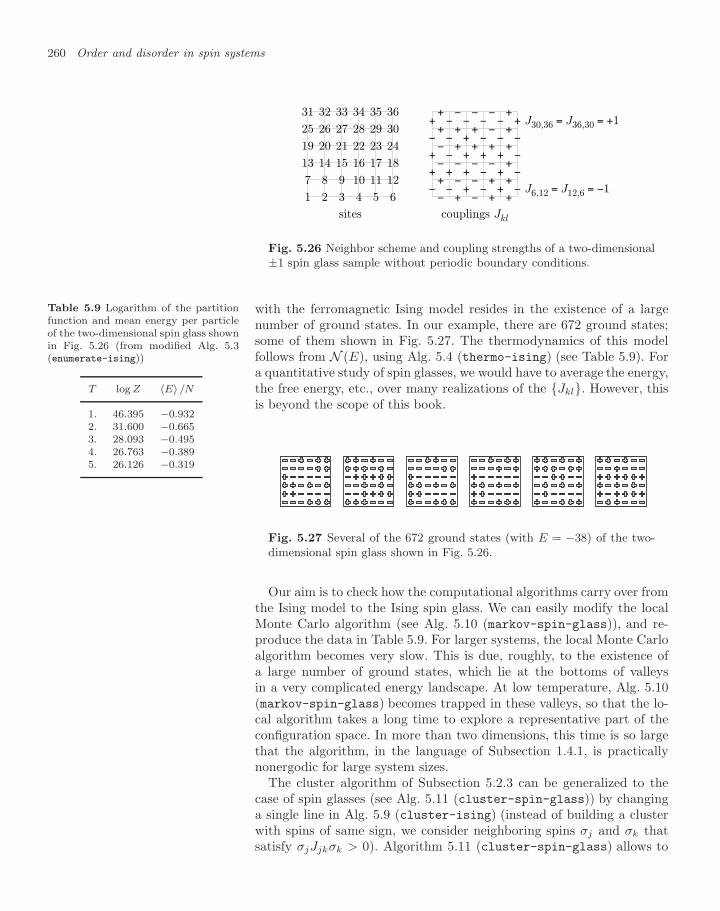
260 Order and disorder in spin systems
1 2 3 4 5 6
7 8 9 10 11 12
13 14 15 16 17 18
19 20 21 22 23 24
25 26 27 28 29 30
31 32 33 34 35 36
sites
− + − + +
+ − − + +
− − − − +
− + + + +
+ + + − +
+ − − − +
− − + − + −
+ + + − + −
+ − + + + −
− − + − − −
+ − − − − +
J6,12 = J12,6 = −1
J30,36 = J36,30 = +1
couplings Jkl
Fig. 5.26 Neighbor scheme and coupling strengths of a two-dimensional±1 spin glass sample without periodic boundary conditions.
with the ferromagnetic Ising model resides in the existence of a largenumber of ground states. In our example, there are 672 ground states;some of them shown in Fig. 5.27. The thermodynamics of this modelfollows from N (E), using Alg. 5.4 (thermo-ising) (see Table 5.9). Fora quantitative study of spin glasses, we would have to average the energy,the free energy, etc., over many realizations of the Jkl. However, thisis beyond the scope of this book.
Table 5.9 Logarithm of the partitionfunction and mean energy per particleof the two-dimensional spin glass shownin Fig. 5.26 (from modified Alg. 5.3(enumerate-ising))
T log Z 〈E〉/N
1. 46.395 −0.9322. 31.600 −0.6653. 28.093 −0.4954. 26.763 −0.3895. 26.126 −0.319
Fig. 5.27 Several of the 672 ground states (with E = −38) of the two-dimensional spin glass shown in Fig. 5.26.
Our aim is to check how the computational algorithms carry over fromthe Ising model to the Ising spin glass. We can easily modify the localMonte Carlo algorithm (see Alg. 5.10 (markov-spin-glass)), and re-produce the data in Table 5.9. For larger systems, the local Monte Carloalgorithm becomes very slow. This is due, roughly, to the existence ofa large number of ground states, which lie at the bottoms of valleysin a very complicated energy landscape. At low temperature, Alg. 5.10(markov-spin-glass) becomes trapped in these valleys, so that the lo-cal algorithm takes a long time to explore a representative part of theconfiguration space. In more than two dimensions, this time is so largethat the algorithm, in the language of Subsection 1.4.1, is practicallynonergodic for large system sizes.
The cluster algorithm of Subsection 5.2.3 can be generalized to thecase of spin glasses (see Alg. 5.11 (cluster-spin-glass)) by changinga single line in Alg. 5.9 (cluster-ising) (instead of building a clusterwith spins of same sign, we consider neighboring spins σj and σk thatsatisfy σjJjkσk > 0). Algorithm 5.11 (cluster-spin-glass) allows to
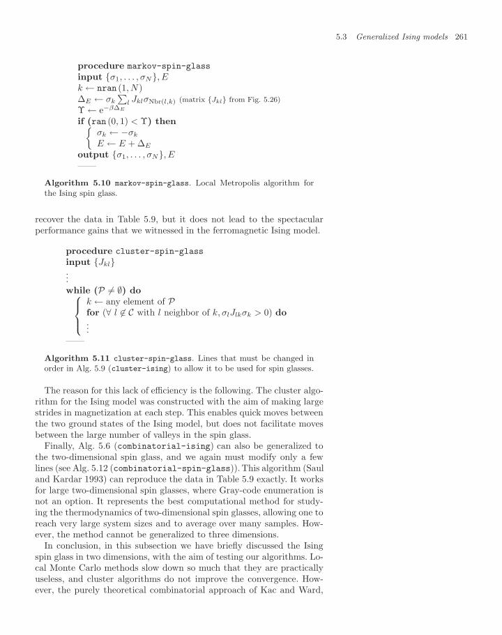
5.3 Generalized Ising models 261
procedure markov-spin-glass
input σ1, . . . , σN, Ek ← nran (1, N)∆E ← σk
∑l JklσNbr(l,k) (matrix Jkl from Fig. 5.26)
Υ ← e−β∆E
if (ran (0, 1) < Υ) thenσk ← −σk
E ← E + ∆E
output σ1, . . . , σN, E——
Algorithm 5.10 markov-spin-glass. Local Metropolis algorithm forthe Ising spin glass.
recover the data in Table 5.9, but it does not lead to the spectacularperformance gains that we witnessed in the ferromagnetic Ising model.
procedure cluster-spin-glass
input Jkl...while (P = ∅) do⎧⎪⎨⎪⎩
k ← any element of Pfor (∀ l ∈ C with l neighbor of k, σlJlkσk > 0) do...
——
Algorithm 5.11 cluster-spin-glass. Lines that must be changed inorder in Alg. 5.9 (cluster-ising) to allow it to be used for spin glasses.
The reason for this lack of efficiency is the following. The cluster algo-rithm for the Ising model was constructed with the aim of making largestrides in magnetization at each step. This enables quick moves betweenthe two ground states of the Ising model, but does not facilitate movesbetween the large number of valleys in the spin glass.
Finally, Alg. 5.6 (combinatorial-ising) can also be generalized tothe two-dimensional spin glass, and we again must modify only a fewlines (see Alg. 5.12 (combinatorial-spin-glass)). This algorithm (Sauland Kardar 1993) can reproduce the data in Table 5.9 exactly. It worksfor large two-dimensional spin glasses, where Gray-code enumeration isnot an option. It represents the best computational method for study-ing the thermodynamics of two-dimensional spin glasses, allowing one toreach very large system sizes and to average over many samples. How-ever, the method cannot be generalized to three dimensions.
In conclusion, in this subsection we have briefly discussed the Isingspin glass in two dimensions, with the aim of testing our algorithms. Lo-cal Monte Carlo methods slow down so much that they are practicallyuseless, and cluster algorithms do not improve the convergence. How-ever, the purely theoretical combinatorial approach of Kac and Ward,
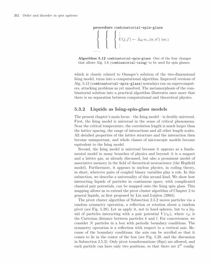
262 Order and disorder in spin systems
procedure combinatorial-spin-glass⎧⎪⎪⎨⎪⎪⎩⎧⎪⎪⎨⎪⎪⎩
⎧⎪⎪⎨⎪⎪⎩...U(j, j′) ← Jkk′u→(n, n′) (etc.)...
——
Algorithm 5.12 combinatorial-spin-glass. One of the four changesthat allows Alg. 5.6 (combinatorial-ising) to be used for spin glasses.
which is closely related to Onsager’s solution of the two-dimensionalIsing model, turns into a computational algorithm. Improved versions ofAlg. 5.12 (combinatorial-spin-glass) nowadays run on supercomput-ers, attacking problems as yet unsolved. The metamorphosis of the com-binatorial solution into a practical algorithm illustrates once more thatthere is no separation between computational and theoretical physics.
5.3.2 Liquids as Ising-spin-glass models
The present chapter’s main focus—the Ising model—is doubly universal.First, the Ising model is universal in the sense of critical phenomena.Near the critical temperature, the correlation length is much larger thanthe lattice spacing, the range of interactions and all other length scales.All detailed properties of the lattice structure and the interaction thenbecome unimportant, and whole classes of microscopic models becomeequivalent to the Ising model.
Second, the Ising model is universal because it appears as a funda-mental model in many branches of physics and beyond: it is a magnetand a lattice gas, as already discussed, but also a prominent model ofassociative memory in the field of theoretical neuroscience (the Hopfieldmodel). Furthermore, it appears in nuclear physics, in coding theory,in short, wherever pairs of coupled binary variables play a role. In thissubsection, we describe a universality of this second kind. We show howinteracting liquids of particles in continuous space, with complicatedclassical pair potentials, can be mapped onto the Ising spin glass. Thismapping allows us to extend the pivot cluster algorithm of Chapter 2 togeneral liquids, as first proposed by Liu and Luijten (2004).
The pivot cluster algorithm of Subsection 2.5.2 moves particles via arandom symmetry operation, a reflection or rotation about a randompivot (see Fig. 5.28). Let us apply it, not to hard spheres, but to a liq-uid of particles interacting with a pair potential V (rkl), where rkl isthe Cartesian distance between particles k and l. For concreteness, weconsider N particles in a box with periodic boundary conditions. Thesymmetry operation is a reflection with respect to a vertical axis. Be-cause of the boundary conditions, the axis can be scrolled so that itcomes to lie in the center of the box (see Fig. 5.28, and the discussionin Subsection 2.5.2). Only pivot transformations (flips) are allowed, andeach particle can have only two positions, so that there are 2N config-
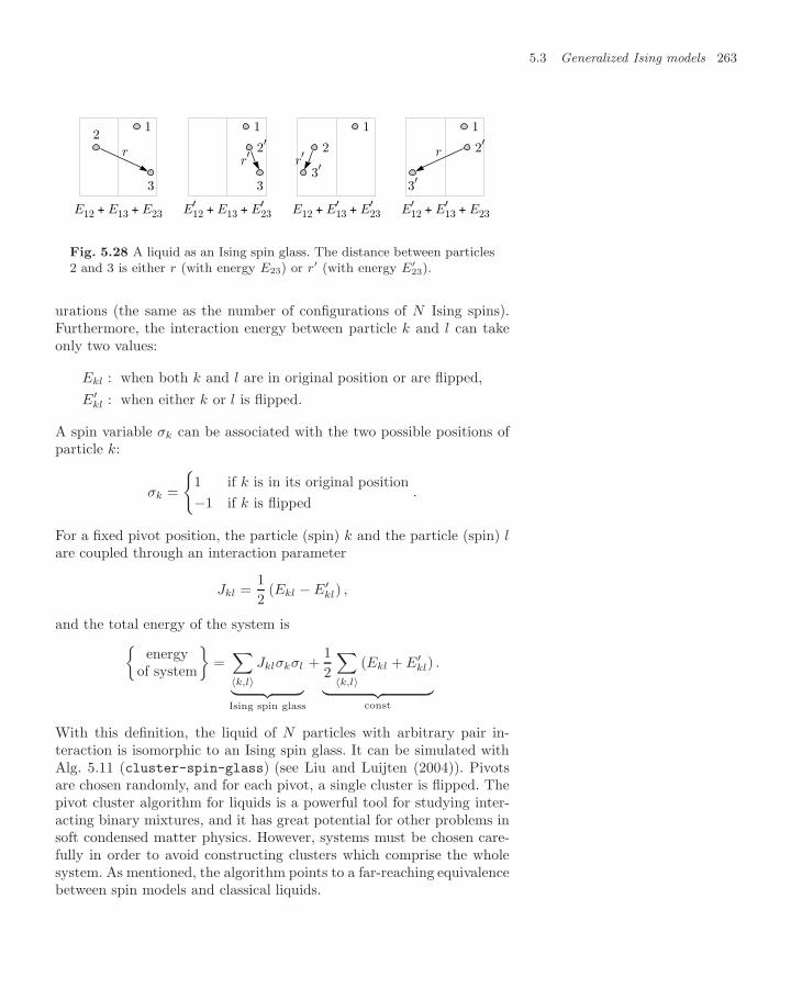
5.3 Generalized Ising models 263
12
3
E12 + E13 + E23
r
1
2′
3
E′12 + E13 + E′
23
r′
1
2
3′
E12 + E′13 + E′
23
r′
1
2′
3′
E′12 + E′
13 + E23
r
Fig. 5.28 A liquid as an Ising spin glass. The distance between particles2 and 3 is either r (with energy E23) or r′ (with energy E′
23).
urations (the same as the number of configurations of N Ising spins).Furthermore, the interaction energy between particle k and l can takeonly two values:
Ekl : when both k and l are in original position or are flipped,E′
kl : when either k or l is flipped.
A spin variable σk can be associated with the two possible positions ofparticle k:
σk =
1 if k is in its original position−1 if k is flipped
.
For a fixed pivot position, the particle (spin) k and the particle (spin) lare coupled through an interaction parameter
Jkl =12
(Ekl − E′kl) ,
and the total energy of the system isenergy
of system
=∑〈k,l〉
Jklσkσl︸ ︷︷ ︸Ising spin glass
+12
∑〈k,l〉
(Ekl + E′kl)︸ ︷︷ ︸
const
.
With this definition, the liquid of N particles with arbitrary pair in-teraction is isomorphic to an Ising spin glass. It can be simulated withAlg. 5.11 (cluster-spin-glass) (see Liu and Luijten (2004)). Pivotsare chosen randomly, and for each pivot, a single cluster is flipped. Thepivot cluster algorithm for liquids is a powerful tool for studying inter-acting binary mixtures, and it has great potential for other problems insoft condensed matter physics. However, systems must be chosen care-fully in order to avoid constructing clusters which comprise the wholesystem. As mentioned, the algorithm points to a far-reaching equivalencebetween spin models and classical liquids.
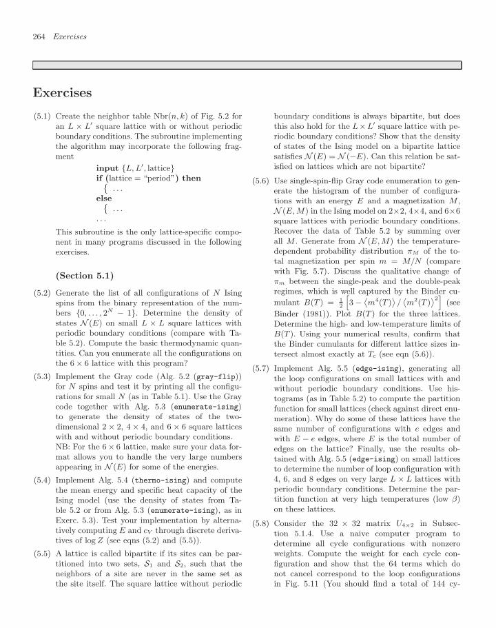
264 Exercises
Exercises
(5.1) Create the neighbor table Nbr(n, k) of Fig. 5.2 foran L × L′ square lattice with or without periodicboundary conditions. The subroutine implementingthe algorithm may incorporate the following frag-ment
input L, L′, latticeif (lattice = “period”) then˘
. . .else
. . .. . .
This subroutine is the only lattice-specific compo-nent in many programs discussed in the followingexercises.
(Section 5.1)
(5.2) Generate the list of all configurations of N Isingspins from the binary representation of the num-bers 0, . . . , 2N − 1. Determine the density ofstates N (E) on small L × L square lattices withperiodic boundary conditions (compare with Ta-ble 5.2). Compute the basic thermodynamic quan-tities. Can you enumerate all the configurations onthe 6 × 6 lattice with this program?
(5.3) Implement the Gray code (Alg. 5.2 (gray-flip))for N spins and test it by printing all the configu-rations for small N (as in Table 5.1). Use the Graycode together with Alg. 5.3 (enumerate-ising)to generate the density of states of the two-dimensional 2 × 2, 4 × 4, and 6 × 6 square latticeswith and without periodic boundary conditions.NB: For the 6× 6 lattice, make sure your data for-mat allows you to handle the very large numbersappearing in N (E) for some of the energies.
(5.4) Implement Alg. 5.4 (thermo-ising) and computethe mean energy and specific heat capacity of theIsing model (use the density of states from Ta-ble 5.2 or from Alg. 5.3 (enumerate-ising), as inExerc. 5.3). Test your implementation by alterna-tively computing E and cV through discrete deriva-tives of log Z (see eqns (5.2) and (5.5)).
(5.5) A lattice is called bipartite if its sites can be par-titioned into two sets, S1 and S2, such that theneighbors of a site are never in the same set asthe site itself. The square lattice without periodic
boundary conditions is always bipartite, but doesthis also hold for the L×L′ square lattice with pe-riodic boundary conditions? Show that the densityof states of the Ising model on a bipartite latticesatisfies N (E) = N (−E). Can this relation be sat-isfied on lattices which are not bipartite?
(5.6) Use single-spin-flip Gray code enumeration to gen-erate the histogram of the number of configura-tions with an energy E and a magnetization M ,N (E, M) in the Ising model on 2×2, 4×4, and 6×6square lattices with periodic boundary conditions.Recover the data of Table 5.2 by summing overall M . Generate from N (E, M) the temperature-dependent probability distribution πM of the to-tal magnetization per spin m = M/N (comparewith Fig. 5.7). Discuss the qualitative change ofπm between the single-peak and the double-peakregimes, which is well captured by the Binder cu-
mulant B(T ) = 12
h3 − ˙
m4(T )¸/
˙m2(T )
¸2i
(see
Binder (1981)). Plot B(T ) for the three lattices.Determine the high- and low-temperature limits ofB(T ). Using your numerical results, confirm thatthe Binder cumulants for different lattice sizes in-tersect almost exactly at Tc (see eqn (5.6)).
(5.7) Implement Alg. 5.5 (edge-ising), generating allthe loop configurations on small lattices with andwithout periodic boundary conditions. Use his-tograms (as in Table 5.2) to compute the partitionfunction for small lattices (check against direct enu-meration). Why do some of these lattices have thesame number of configurations with e edges andwith E − e edges, where E is the total number ofedges on the lattice? Finally, use the results ob-tained with Alg. 5.5 (edge-ising) on small latticesto determine the number of loop configuration with4, 6, and 8 edges on very large L × L lattices withperiodic boundary conditions. Determine the par-tition function at very high temperatures (low β)on these lattices.
(5.8) Consider the 32 × 32 matrix U4×2 in Subsec-tion 5.1.4. Use a naive computer program todetermine all cycle configurations with nonzeroweights. Compute the weight for each cycle con-figuration and show that the 64 terms which donot cancel correspond to the loop configurationsin Fig. 5.11 (You should find a total of 144 cy-
Exercises 265
cle configurations with nonzero weights.) Generatethe matrix UL×L on larger lattices using Alg. 5.6(combinatorial-ising). Compute det UL×L usinga standard numerical linear-algebra routine. Com-pare with the results of Gray-code enumerations forsmall lattices.NB: To simplify the enumeration of cycle config-urations in the naive program, note that a rowvectoruk,1, . . . , uk,16 which differs from zero onlyon the diagonal contributes to trivial cycles only.
(5.9) Implement Kaufman’s formula (Kaufman 1949) forthe partition function of the Ising model on a L×Llattice with periodic boundary conditions from thefollowing fragment:
. . .γ0 ← log
`e2β tanh β
´for k = 1, . . . , 2L − 1 doj
Υ ← cosh2 (2β) / sinh (2β) − cos (k/L)
γk ← log`Υ +
√Υ2 − 1
´Υ ← sinhL2/2 (2β)Y1, . . . , Y4 ← Υ, . . . , Υfor k = 0, . . . , L − 1 do8>><
>>:Y1 ← 2Y1 cosh (γ2k+1L/2)Y2 ← 2Y2 sinh (γ2k+1L/2)Y3 ← 2Y3 cosh (γ2kL/2)Y4 ← 2Y4 sinh (γ2kL/2)
Z ← 2L2/2−1 (Y1 + Y2 + Y3 + Y4). . .
Test output of this program against exact enumer-ation data, from your own Gray-code enumerationon the lattice with periodic boundary conditions,or from Table 5.3. Then consult Kaufman’s originalpaper. For a practical application of these formulas,see, for example, Beale (1996).
(Section 5.2)
(5.10) Implement Alg. 5.7 (markov-ising) (localMetropolis algorithm for the Ising model) and testit against the specific heat capacity and the energyfor small lattices from exact enumeration to at leastfour significant digits (see Table 5.3). Improve yourprogram as follows. The exponential function eval-uating the Boltzmann weight may take on only afew values: replace it by a table to avoid repeatedfunction evaluations. Also, a variable Υ > 1 willnever be smaller than a random number ran (0, 1):avoid the superfluous generation of a random num-ber and comparison in this case. Again test theimproved program against exact results. Generateplots of the average absolute magnetization against
temperature for lattices of different sizes (comparewith Fig. 5.16).
(5.11) Implement Alg. 5.9 (cluster-ising) with setsC,Fold, and Fnew simply programmed as vec-tors. Check for cluster membership through sim-ple look-up. Test your program against specific-heat-capacity and mean-energy data obtained byexact enumeration on small lattices. Improvementsof this program depend on the way your computerlanguage treats vectors and lists. If possible, han-dle the initial conditions as follows (compare withExerc. 1.3): at each temperature T , let the pro-gram search for an initial configuration generatedat that same temperature (choose file names whichencode T ). If such a file does not exist, choose ran-dom initial spins. The final configuration of eachrun should be made into an initial configuration forthe next run. Use this improved program to com-pute histograms of the magnetization and to plotthe Binder cumulant as a function of T (comparewith Exerc. 5.6). Reconfirm that Binder cumulants,at different lattice sizes, intersect almost exactly atTc.
(Section 5.3)
(5.12) Implement the local Monte Carlo algorithm for thetwo-dimensional ±1 spin glass. Thoroughly test itin the specific case of Fig. 5.26 (compare the meanenergies per particle with Table 5.9, for the choiceof Jkl given). Compute the specific heat capacity,and average over many samples. Study the behav-ior of the ensemble-averaged specific heat capacityfor square lattices of sizes between 2×2 and 32×32.
(5.13) Consider N particles, constrained onto a unit circle,with positions x1, . . . ,xN, satisfying |xk| = 1.Particles interact with a Lennard-Jones potential
Ekl = |∆x|12 − |∆x|6,
where ∆x = xk−xl is the two-dimensional distancevector. Implement the spin-glass cluster algorithmof Liu and Luijten (2004) for this problem. To testyour program, compute the mean energy per par-ticle, and compare it, for N ≤ 6, with the exactvalue obtained by Riemann integration. (You mayalso compare with the results of a local Monte Carlosimulation.)NB: If Alg. 5.11 (cluster-spin-glass) exists,adapt it for the particle simulation. Otherwise,write a naive version of the cluster algorithm fora few particles.
266 References
References
Beale P. D. (1996) Exact distribution of energies in the two-dimensionalIsing model, Physical Review Letters 76, 78–81
Binder K. (1981) Finite size scaling analysis of Ising-model block distri-bution-functions, Zeitschrift fur Physik B–Condensed Matter 43, 119–140
Ferdinand A. E., Fisher M. E. (1969) Bounded and inhomogeneous Isingmodels. I. specific-heat anomaly of a finite lattice, Physical Review 185,832–846
Kac M., Ward J. C. (1952) A combinatorial solution of the two-dimensio-nal Ising model, Physical Review 88, 1332–1337
Kaufman B. (1949) Crystal Statistics. II. Partition function evaluatedby spinor analysis, Physical Review 76, 1232–1243
Liu J. W., Luijten E. (2004) Rejection-free geometric cluster algorithmfor complex fluids, Physical Review Letters 92, 035504
Onsager L. (1944) Crystal Statistics. I. A two-dimensional model withan order-disorder transition, Physical Review 65, 117–149
Propp J. G., Wilson D. B. (1996) Exact sampling with coupled Markovchains and applications to statistical mechanics, Random Structures &Algorithms 9, 223–252
Saul L., Kardar M. (1993) Exact integer algorithm for the two-dimen-sional ±J Ising spin glass, Physical Review E 48, R3221–R3224
Swendsen R. H., Wang J. S. (1987) Nonuniversal critical-dynamics inMonte-Carlo simulations, Physical Review Letters 58, 86–88
Wolff U. (1989) Collective Monte-Carlo updating for spin systems, Phys-ical Review Letters 62, 361–364
Entropic forces 66.1 Entropic continuum
models and mixtures 269
6.2 Entropic lattice model:dimers 281
Exercises 303
References 305
In the present chapter, we revisit classical entropic models, where allconfigurations have the same probability. This sight is familiar from thehard-core systems of Chapter 2, where we struggled with the foundationsof statistical mechanics, and reached a basic understanding of molecu-lar dynamics and Monte Carlo algorithms. At present, we are more in-terested in describing entropic forces, which dominate many effects insoft condensed matter (the physics of biological systems, colloids, andpolymers) and are also of fundamental interest in the context of order–disorder transitions in quantum mechanical electronic systems.
The chapter begins with a complete mathematical and algorithmicsolution of the problem of one-dimensional hard spheres (the “randomclothes-pins” model) and leads us to a discussion of the Asakura–Oosawadepletion interaction, one of the fundamental forces in nature, at leastin the realm of biological systems, colloids, and polymers. This multi-faceted, mysterious interaction is at its strongest in binary systems oflarge and small particles, where interesting effects and phase transitionsappear even at low density for no other reason than the presence of con-stituents of different sizes. Binary oriented squares in two dimensionsprovide the simplest model for colloids where the depletion interactionis sufficiently strong to induce a demixing (flocculation) transition. Thisextremely constrained model has not been solved analytically, and re-sists attacks by standard local Monte Carlo simulation. However, a sim-ple cluster algorithm—set up in a few dozen lines—samples the binary-squares model without any problems.
In the second part of this chapter, we consider dimers on a lattice, thearchetypal model of a discrete entropic system where orientation effectsdominate. This lattice system has profound connections with the Isingmodel of a magnet (see Chapter 5). Ever since Pauling’s theory of thebenzene molecule in terms of resonating singlets (dimers), the theoryof dimers has had important applications and extensions in molecularphysics and condensed matter theory.
From a computational point of view, dimers lead us to revisit theissue of enumeration, as in Chapter 5, but here with the chance to as-similate systematic “breadth-first” and “depth-first” techniques, whichare of general use. These tree-based methods are second only to theextremely powerful enumeration method based on Pfaffians, which weshall go through in detail. Again, we discuss Monte Carlo methods, andconclude with discussions of order and disorder in the monomer–dimermodel.
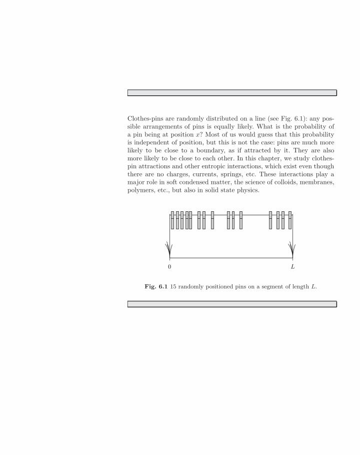
Clothes-pins are randomly distributed on a line (see Fig. 6.1): any pos-sible arrangements of pins is equally likely. What is the probability ofa pin being at position x? Most of us would guess that this probabilityis independent of position, but this is not the case: pins are much morelikely to be close to a boundary, as if attracted by it. They are alsomore likely to be close to each other. In this chapter, we study clothes-pin attractions and other entropic interactions, which exist even thoughthere are no charges, currents, springs, etc. These interactions play amajor role in soft condensed matter, the science of colloids, membranes,polymers, etc., but also in solid state physics.
0 L
Fig. 6.1 15 randomly positioned pins on a segment of length L.
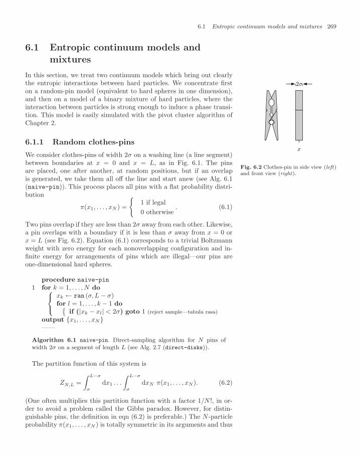
6.1 Entropic continuum models and mixtures 269
6.1 Entropic continuum models and
mixtures
In this section, we treat two continuum models which bring out clearlythe entropic interactions between hard particles. We concentrate firston a random-pin model (equivalent to hard spheres in one dimension),and then on a model of a binary mixture of hard particles, where theinteraction between particles is strong enough to induce a phase transi-tion. This model is easily simulated with the pivot cluster algorithm ofChapter 2.
6.1.1 Random clothes-pins
2σ
x
Fig. 6.2 Clothes-pin in side view (left)and front view (right).
We consider clothes-pins of width 2σ on a washing line (a line segment)between boundaries at x = 0 and x = L, as in Fig. 6.1. The pinsare placed, one after another, at random positions, but if an overlapis generated, we take them all off the line and start anew (see Alg. 6.1(naive-pin)). This process places all pins with a flat probability distri-bution
π(x1, . . . , xN ) =
1 if legal0 otherwise
. (6.1)
Two pins overlap if they are less than 2σ away from each other. Likewise,a pin overlaps with a boundary if it is less than σ away from x = 0 orx = L (see Fig. 6.2). Equation (6.1) corresponds to a trivial Boltzmannweight with zero energy for each nonoverlapping configuration and in-finite energy for arrangements of pins which are illegal—our pins areone-dimensional hard spheres.
procedure naive-pin
1 for k = 1, . . . , N do⎧⎨⎩xk ← ran (σ, L − σ)for l = 1, . . . , k − 1 do
if (|xk − xl| < 2σ) goto 1 (reject sample—tabula rasa)output x1, . . . , xN——
Algorithm 6.1 naive-pin. Direct-sampling algorithm for N pins ofwidth 2σ on a segment of length L (see Alg. 2.7 (direct-disks)).
The partition function of this system is
ZN,L =∫ L−σ
σ
dx1 . . .
∫ L−σ
σ
dxN π(x1, . . . , xN ). (6.2)
(One often multiplies this partition function with a factor 1/N !, in or-der to avoid a problem called the Gibbs paradox. However, for distin-guishable pins, the definition in eqn (6.2) is preferable.) The N -particleprobability π(x1, . . . , xN ) is totally symmetric in its arguments and thus
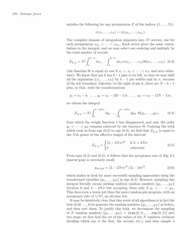
270 Entropic forces
satisfies the following for any permutation P of the indices 1, . . . , N:
π(x1, . . . , xN ) = π(xP1 , . . . , xPN).
The complete domain of integration separates into N ! sectors, one foreach permutation xP1 < · · · < xPN
. Each sector gives the same contri-bution to the integral, and we may select one ordering and multiply bythe total number of sectors:
ZN,L = N !∫ L−σ
σ
dx1 . . .
∫ L−σ
σ
dxNπ(x1, . . . , xN )Θ(x1, . . . , xN ) (6.3)
(the function Θ is equal to one if x1 < x2 < · · · < xN and zero other-wise). We know that pin k has k−1 pins to its left, so that we may shiftall the arguments x1, . . . , xN by k − 1 pin widths and by σ, becauseof the left boundary. Likewise, to the right of pin k, there are N − k − 1pins, so that, with the transformations
y1 = x1 − σ, . . . , yk = xk − (2k − 1)σ, . . . , yN = xN − (2N − 1)σ,
we obtain the integral
ZN,L = N !∫ L−2Nσ
0
dy1 . . .
∫ L−2Nσ
0
dyN Θ(y1, . . . , yN), (6.4)
from which the weight function π has disappeared, and only the ordery1 < · · · < yN remains enforced by the function Θ. Undoing the trickwhich took us from eqn (6.2) to eqn (6.3), we find that ZN,L is equal tothe Nth power of the effective length of the interval:
ZN,L =
(L − 2Nσ)N if L > 2Nσ
0 otherwise. (6.5)
From eqns (6.2) and (6.5), it follows that the acceptance rate of Alg. 6.1(naive-pin) is extremely small:
paccept = (L − 2Nσ)N/(L − 2σ)N , (6.6)
which makes us look for more successful sampling approaches using thetransformed variables y1, . . . , yN in eqn (6.4). However, sampling thisintegral literally means picking uniform random numbers y1, . . . , yNbetween 0 and L − 2Nσ but accepting them only if y1 < · · · < yN .This does even a worse job than the naive random-pin program, with anacceptance rate of 1/N !, an all-time low.
It may be intuitively clear that this worst of all algorithms is in fact thebest of all . . . , if we generate the random numbers y1, . . . , yN as before,and then sort them. To justify this trick, we decompose the samplingof N random numbers y1, . . . , yN = ran (0, 1) , . . . , ran (0, 1) intotwo steps: we first find the set of the values of the N numbers (withoutdeciding which one is the first, the second, etc.), and then sample a
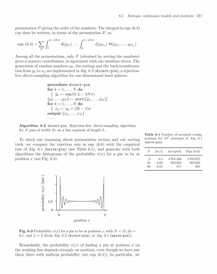
6.1 Entropic continuum models and mixtures 271
permutation P giving the order of the numbers. The integral in eqn (6.4)can then be written, in terms of the permutation P , as
eqn (6.4) =∑P
∫ L−2Nσ
0
d(yP1) . . .
∫ L−2Nσ
0
d(yPN) Θ(yP1 , . . . , yPN
).
Among all the permutations, only P (obtained by sorting the numbers)gives a nonzero contribution, in agreement with our intuition above. Thegeneration of random numbers yk, the sorting and the back-transforma-tion from yk to xk are implemented in Alg. 6.2 (direct-pin), a rejection-free direct-sampling algorithm for one-dimensional hard spheres.
procedure direct-pin
for k = 1, . . . , N doyk ← ran (0, L − 2Nσ)
y1, . . . , yN ← sort[y1, . . . , yN]for k = 1, . . . , N do
xk ← yk + (2k − 1)σoutput x1, . . . , xN——
Algorithm 6.2 direct-pin. Rejection-free direct-sampling algorithmfor N pins of width 2σ on a line segment of length L.
To check our reasoning about permutation sectors and our sortingtrick, we compare the rejection rate in eqn (6.6) with the empiricalrate of Alg. 6.1 (naive-pin) (see Table 6.1), and generate with bothalgorithms the histograms of the probability π(x) for a pin to be atposition x (see Fig. 6.3).
Table 6.1 Number of accepted config-urations for 107 attempts of Alg. 6.1(naive-pin)
N 2σ/L Accepted Eqn (6.6)
3 0.1 4 705 436 4 705 07510 0.03 383 056 383 05630 0.01 311 305
1/L
0
L0
pro
babilit
y π
(x)
(his
t.)
position x
Fig. 6.3 Probability π(x) for a pin to be at position x, with N = 15, 2σ =0.1, and L = 2 (from Alg. 6.2 (direct-pin), or Alg. 6.1 (naive-pin)).
Remarkably, the probability π(x) of finding a pin at position x onthe washing line depends strongly on position, even though we have putthem there with uniform probability (see eqn (6.1)). In particular, we
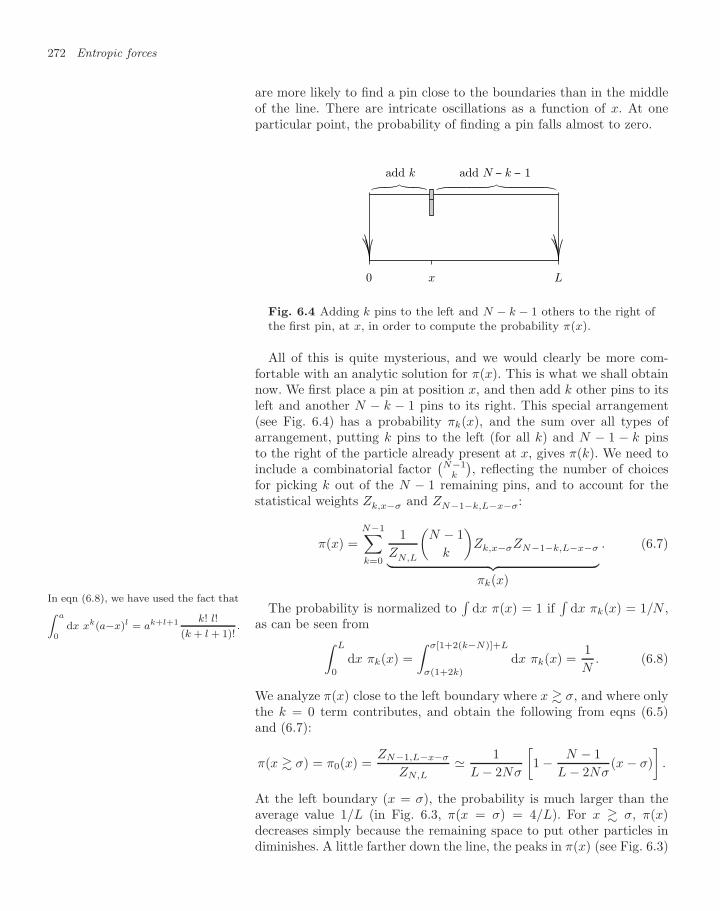
272 Entropic forces
are more likely to find a pin close to the boundaries than in the middleof the line. There are intricate oscillations as a function of x. At oneparticular point, the probability of finding a pin falls almost to zero.
0 Lx
add k add N − k − 1
Fig. 6.4 Adding k pins to the left and N − k − 1 others to the right ofthe first pin, at x, in order to compute the probability π(x).
All of this is quite mysterious, and we would clearly be more com-fortable with an analytic solution for π(x). This is what we shall obtainnow. We first place a pin at position x, and then add k other pins to itsleft and another N − k − 1 pins to its right. This special arrangement(see Fig. 6.4) has a probability πk(x), and the sum over all types ofarrangement, putting k pins to the left (for all k) and N − 1 − k pinsto the right of the particle already present at x, gives π(k). We need toinclude a combinatorial factor
(N−1
k
), reflecting the number of choices
for picking k out of the N − 1 remaining pins, and to account for thestatistical weights Zk,x−σ and ZN−1−k,L−x−σ:
π(x) =N−1∑k=0
1ZN,L
(N − 1
k
)Zk,x−σZN−1−k,L−x−σ︸ ︷︷ ︸πk(x)
. (6.7)
In eqn (6.8), we have used the fact thatZ a
0dx xk(a−x)l = ak+l+1 k! l!
(k + l + 1)!.
The probability is normalized to∫
dx π(x) = 1 if∫
dx πk(x) = 1/N ,as can be seen from∫ L
0
dx πk(x) =∫ σ[1+2(k−N)]+L
σ(1+2k)
dx πk(x) =1N
. (6.8)
We analyze π(x) close to the left boundary where x σ, and where onlythe k = 0 term contributes, and obtain the following from eqns (6.5)and (6.7):
π(x σ) = π0(x) =ZN−1,L−x−σ
ZN,L 1
L − 2Nσ
[1 − N − 1
L − 2Nσ(x − σ)
].
At the left boundary (x = σ), the probability is much larger than theaverage value 1/L (in Fig. 6.3, π(x = σ) = 4/L). For x σ, π(x)decreases simply because the remaining space to put other particles indiminishes. A little farther down the line, the peaks in π(x) (see Fig. 6.3)
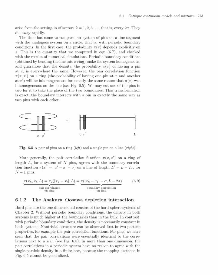
6.1 Entropic continuum models and mixtures 273
arise from the setting-in of sectors k = 1, 2, 3 . . . , that is, every 2σ. Theydie away rapidly.
The time has come to compare our system of pins on a line segmentwith the analogous system on a circle, that is, with periodic boundaryconditions. In the first case, the probability π(x) depends explicitly onx. This is the quantity that we computed in eqn (6.7), and checkedwith the results of numerical simulations. Periodic boundary conditions(obtained by bending the line into a ring) make the system homogeneous,and guarantee that the density, the probability π(x) of having a pinat x, is everywhere the same. However, the pair correlation functionπ(x, x′) on a ring (the probability of having one pin at x and anotherat x′) will be inhomogeneous, for exactly the same reason that π(x) wasinhomogeneous on the line (see Fig. 6.5). We may cut one of the pins intwo for it to take the place of the two boundaries. This transformationis exact: the boundary interacts with a pin in exactly the same way astwo pins with each other.
x x′
≡
0 x′′ L′
Fig. 6.5 A pair of pins on a ring (left) and a single pin on a line (right).
More generally, the pair correlation function π(x, x′) on a ring oflength L, for a system of N pins, agrees with the boundary correla-tion function π(x′′ = |x′ − x| − σ) on a line of length L′ = L − 2σ, forN − 1 pins:
π(xk, xl, L) = π2(|xk − xl|, L)︸ ︷︷ ︸pair correlation
on ring
= π(|xk − xl| − σ, L − 2σ)︸ ︷︷ ︸boundary correlation
on line
. (6.9)
6.1.2 The Asakura–Oosawa depletion interaction
Hard pins are the one-dimensional cousins of the hard-sphere systems ofChapter 2. Without periodic boundary conditions, the density in bothsystems is much higher at the boundaries than in the bulk. In contrast,with periodic boundary conditions, the density is necessarily constant inboth systems. Nontrivial structure can be observed first in two-particleproperties, for example the pair correlation functions. For pins, we haveseen that the pair correlations were essentially identical to the corre-lations next to a wall (see Fig. 6.5). In more than one dimension, thepair correlations in a periodic system have no reason to agree with thesingle-particle density in a finite box, because the mapping sketched inFig. 6.5 cannot be generalized.
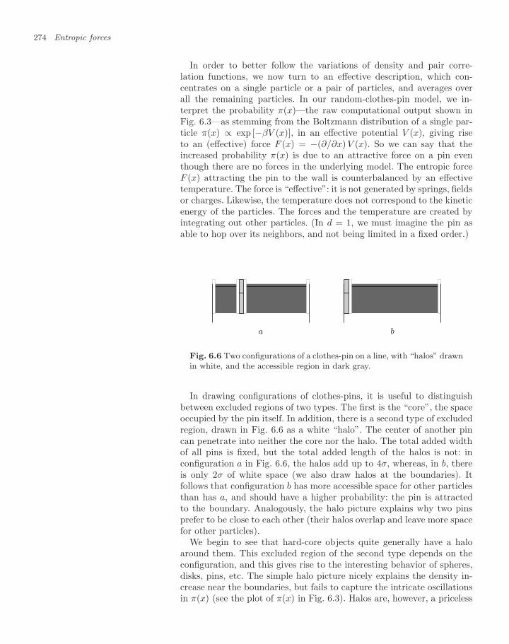
274 Entropic forces
In order to better follow the variations of density and pair corre-lation functions, we now turn to an effective description, which con-centrates on a single particle or a pair of particles, and averages overall the remaining particles. In our random-clothes-pin model, we in-terpret the probability π(x)—the raw computational output shown inFig. 6.3—as stemming from the Boltzmann distribution of a single par-ticle π(x) ∝ exp [−βV (x)], in an effective potential V (x), giving riseto an (effective) force F (x) = −(∂/∂x) V (x). So we can say that theincreased probability π(x) is due to an attractive force on a pin eventhough there are no forces in the underlying model. The entropic forceF (x) attracting the pin to the wall is counterbalanced by an effectivetemperature. The force is “effective”: it is not generated by springs, fieldsor charges. Likewise, the temperature does not correspond to the kineticenergy of the particles. The forces and the temperature are created byintegrating out other particles. (In d = 1, we must imagine the pin asable to hop over its neighbors, and not being limited in a fixed order.)
a b
Fig. 6.6 Two configurations of a clothes-pin on a line, with “halos” drawnin white, and the accessible region in dark gray.
In drawing configurations of clothes-pins, it is useful to distinguishbetween excluded regions of two types. The first is the “core”, the spaceoccupied by the pin itself. In addition, there is a second type of excludedregion, drawn in Fig. 6.6 as a white “halo”. The center of another pincan penetrate into neither the core nor the halo. The total added widthof all pins is fixed, but the total added length of the halos is not: inconfiguration a in Fig. 6.6, the halos add up to 4σ, whereas, in b, thereis only 2σ of white space (we also draw halos at the boundaries). Itfollows that configuration b has more accessible space for other particlesthan has a, and should have a higher probability: the pin is attractedto the boundary. Analogously, the halo picture explains why two pinsprefer to be close to each other (their halos overlap and leave more spacefor other particles).
We begin to see that hard-core objects quite generally have a haloaround them. This excluded region of the second type depends on theconfiguration, and this gives rise to the interesting behavior of spheres,disks, pins, etc. The simple halo picture nicely explains the density in-crease near the boundaries, but fails to capture the intricate oscillationsin π(x) (see the plot of π(x) in Fig. 6.3). Halos are, however, a priceless
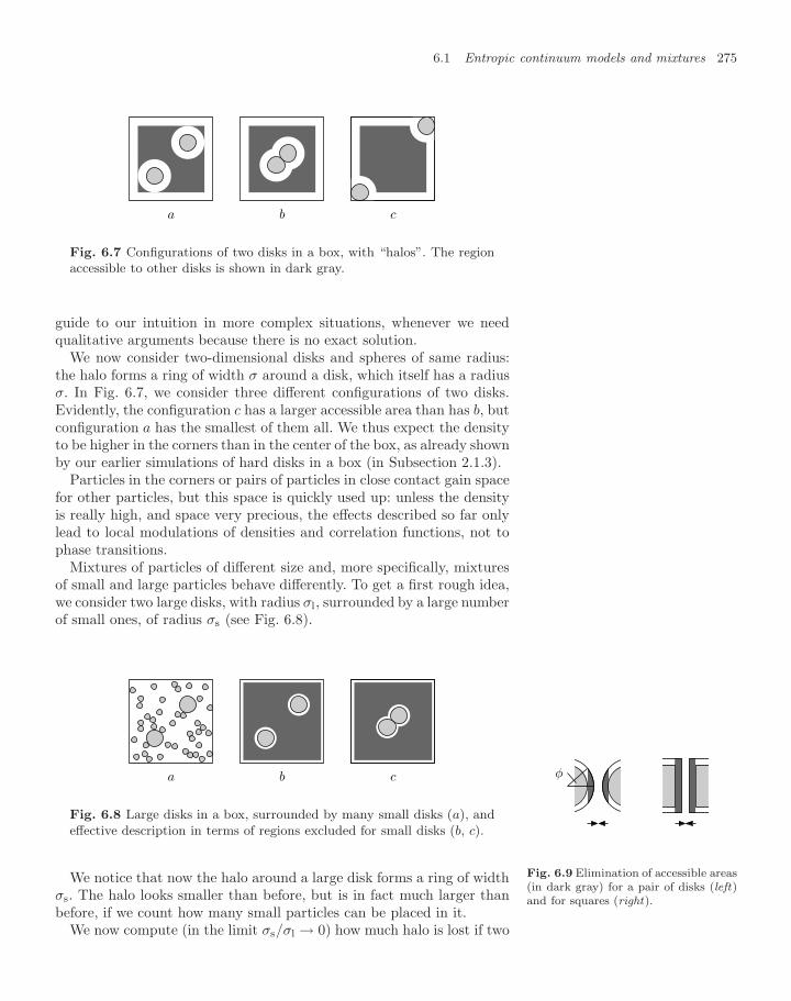
6.1 Entropic continuum models and mixtures 275
a b c
Fig. 6.7 Configurations of two disks in a box, with “halos”. The regionaccessible to other disks is shown in dark gray.
guide to our intuition in more complex situations, whenever we needqualitative arguments because there is no exact solution.
We now consider two-dimensional disks and spheres of same radius:the halo forms a ring of width σ around a disk, which itself has a radiusσ. In Fig. 6.7, we consider three different configurations of two disks.Evidently, the configuration c has a larger accessible area than has b, butconfiguration a has the smallest of them all. We thus expect the densityto be higher in the corners than in the center of the box, as already shownby our earlier simulations of hard disks in a box (in Subsection 2.1.3).
Particles in the corners or pairs of particles in close contact gain spacefor other particles, but this space is quickly used up: unless the densityis really high, and space very precious, the effects described so far onlylead to local modulations of densities and correlation functions, not tophase transitions.
Mixtures of particles of different size and, more specifically, mixturesof small and large particles behave differently. To get a first rough idea,we consider two large disks, with radius σl, surrounded by a large numberof small ones, of radius σs (see Fig. 6.8).
a b c
Fig. 6.8 Large disks in a box, surrounded by many small disks (a), andeffective description in terms of regions excluded for small disks (b, c).
We notice that now the halo around a large disk forms a ring of widthσs. The halo looks smaller than before, but is in fact much larger thanbefore, if we count how many small particles can be placed in it.
φ
Fig. 6.9 Elimination of accessible areas(in dark gray) for a pair of disks (left)and for squares (right).
We now compute (in the limit σs/σl → 0) how much halo is lost if two
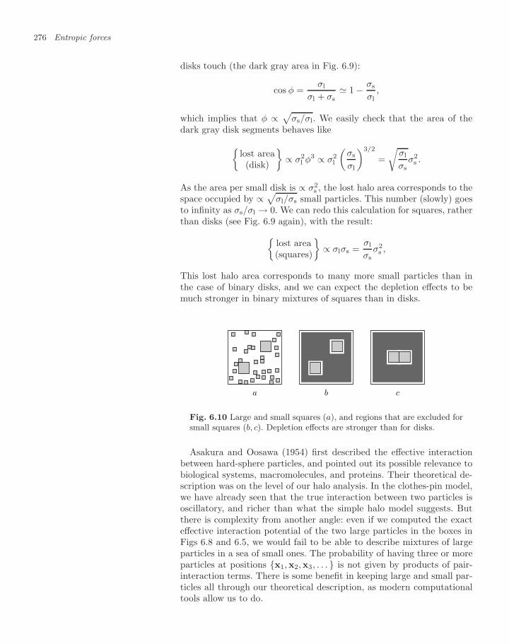
276 Entropic forces
disks touch (the dark gray area in Fig. 6.9):
cos φ =σl
σl + σs 1 − σs
σl,
which implies that φ ∝ √σs/σl. We easily check that the area of thedark gray disk segments behaves like
lost area(disk)
∝ σ2
l φ3 ∝ σ2l
(σs
σl
)3/2
=√
σl
σsσ2
s .
As the area per small disk is ∝ σ2s , the lost halo area corresponds to the
space occupied by ∝√σl/σs small particles. This number (slowly) goesto infinity as σs/σl → 0. We can redo this calculation for squares, ratherthan disks (see Fig. 6.9 again), with the result:
lost area(squares)
∝ σlσs =
σl
σsσ2
s ,
This lost halo area corresponds to many more small particles than inthe case of binary disks, and we can expect the depletion effects to bemuch stronger in binary mixtures of squares than in disks.
a b c
Fig. 6.10 Large and small squares (a), and regions that are excluded forsmall squares (b, c). Depletion effects are stronger than for disks.
Asakura and Oosawa (1954) first described the effective interactionbetween hard-sphere particles, and pointed out its possible relevance tobiological systems, macromolecules, and proteins. Their theoretical de-scription was on the level of our halo analysis. In the clothes-pin model,we have already seen that the true interaction between two particles isoscillatory, and richer than what the simple halo model suggests. Butthere is complexity from another angle: even if we computed the exacteffective interaction potential of the two large particles in the boxes inFigs 6.8 and 6.5, we would fail to be able to describe mixtures of largeparticles in a sea of small ones. The probability of having three or moreparticles at positions x1,x2,x3, . . . is not given by products of pair-interaction terms. There is some benefit in keeping large and small par-ticles all through our theoretical description, as modern computationaltools allow us to do.
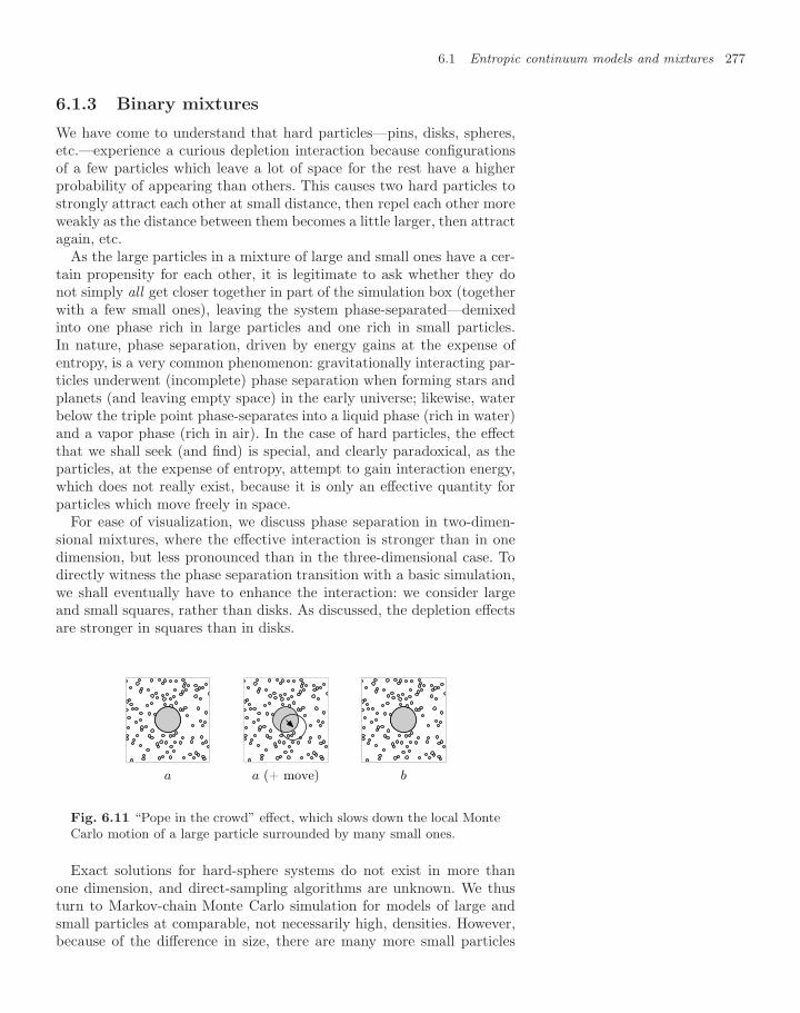
6.1 Entropic continuum models and mixtures 277
6.1.3 Binary mixtures
We have come to understand that hard particles—pins, disks, spheres,etc.—experience a curious depletion interaction because configurationsof a few particles which leave a lot of space for the rest have a higherprobability of appearing than others. This causes two hard particles tostrongly attract each other at small distance, then repel each other moreweakly as the distance between them becomes a little larger, then attractagain, etc.
As the large particles in a mixture of large and small ones have a cer-tain propensity for each other, it is legitimate to ask whether they donot simply all get closer together in part of the simulation box (togetherwith a few small ones), leaving the system phase-separated—demixedinto one phase rich in large particles and one rich in small particles.In nature, phase separation, driven by energy gains at the expense ofentropy, is a very common phenomenon: gravitationally interacting par-ticles underwent (incomplete) phase separation when forming stars andplanets (and leaving empty space) in the early universe; likewise, waterbelow the triple point phase-separates into a liquid phase (rich in water)and a vapor phase (rich in air). In the case of hard particles, the effectthat we shall seek (and find) is special, and clearly paradoxical, as theparticles, at the expense of entropy, attempt to gain interaction energy,which does not really exist, because it is only an effective quantity forparticles which move freely in space.
For ease of visualization, we discuss phase separation in two-dimen-sional mixtures, where the effective interaction is stronger than in onedimension, but less pronounced than in the three-dimensional case. Todirectly witness the phase separation transition with a basic simulation,we shall eventually have to enhance the interaction: we consider largeand small squares, rather than disks. As discussed, the depletion effectsare stronger in squares than in disks.
a a (+ move) b
Fig. 6.11 “Pope in the crowd” effect, which slows down the local MonteCarlo motion of a large particle surrounded by many small ones.
Exact solutions for hard-sphere systems do not exist in more thanone dimension, and direct-sampling algorithms are unknown. We thusturn to Markov-chain Monte Carlo simulation for models of large andsmall particles at comparable, not necessarily high, densities. However,because of the difference in size, there are many more small particles
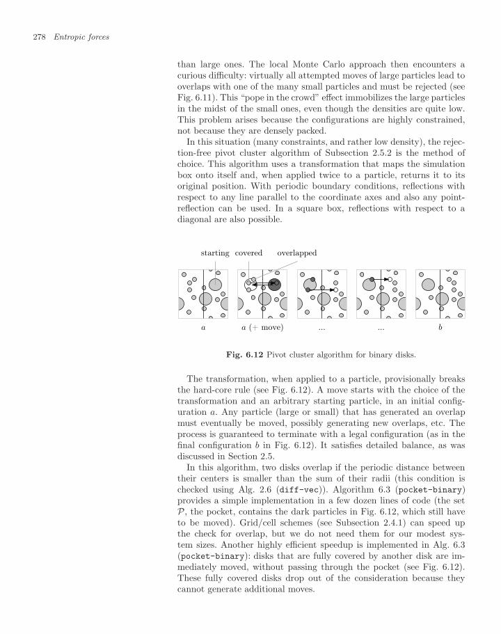
278 Entropic forces
than large ones. The local Monte Carlo approach then encounters acurious difficulty: virtually all attempted moves of large particles lead tooverlaps with one of the many small particles and must be rejected (seeFig. 6.11). This “pope in the crowd” effect immobilizes the large particlesin the midst of the small ones, even though the densities are quite low.This problem arises because the configurations are highly constrained,not because they are densely packed.
In this situation (many constraints, and rather low density), the rejec-tion-free pivot cluster algorithm of Subsection 2.5.2 is the method ofchoice. This algorithm uses a transformation that maps the simulationbox onto itself and, when applied twice to a particle, returns it to itsoriginal position. With periodic boundary conditions, reflections withrespect to any line parallel to the coordinate axes and also any point-reflection can be used. In a square box, reflections with respect to adiagonal are also possible.
a
starting
a (+ move)
covered overlapped
... ... b
Fig. 6.12 Pivot cluster algorithm for binary disks.
The transformation, when applied to a particle, provisionally breaksthe hard-core rule (see Fig. 6.12). A move starts with the choice of thetransformation and an arbitrary starting particle, in an initial config-uration a. Any particle (large or small) that has generated an overlapmust eventually be moved, possibly generating new overlaps, etc. Theprocess is guaranteed to terminate with a legal configuration (as in thefinal configuration b in Fig. 6.12). It satisfies detailed balance, as wasdiscussed in Section 2.5.
In this algorithm, two disks overlap if the periodic distance betweentheir centers is smaller than the sum of their radii (this condition ischecked using Alg. 2.6 (diff-vec)). Algorithm 6.3 (pocket-binary)provides a simple implementation in a few dozen lines of code (the setP , the pocket, contains the dark particles in Fig. 6.12, which still haveto be moved). Grid/cell schemes (see Subsection 2.4.1) can speed upthe check for overlap, but we do not need them for our modest sys-tem sizes. Another highly efficient speedup is implemented in Alg. 6.3(pocket-binary): disks that are fully covered by another disk are im-mediately moved, without passing through the pocket (see Fig. 6.12).These fully covered disks drop out of the consideration because theycannot generate additional moves.
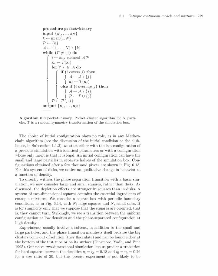
6.1 Entropic continuum models and mixtures 279
procedure pocket-binary
input x1, . . . ,xNk ← nran (1, N)P ← kA ← 1, . . . , N \ kwhile (P = ) do⎧⎪⎪⎪⎪⎪⎪⎪⎪⎪⎪⎪⎪⎪⎪⎨⎪⎪⎪⎪⎪⎪⎪⎪⎪⎪⎪⎪⎪⎪⎩
i ← any element of Pxi ← T (xi)for ∀ j ∈ A do⎧⎪⎪⎪⎪⎪⎪⎨⎪⎪⎪⎪⎪⎪⎩
if (i covers j) then A ← A \ jxj ← T (xj)
else if (i overlaps j) then A ← A \ jP ← P ∪ j
P ← P \ ioutput x1, . . . ,xN——
Algorithm 6.3 pocket-binary. Pocket–cluster algorithm for N parti-cles. T is a random symmetry transformation of the simulation box.
The choice of initial configuration plays no role, as in any Markov-chain algorithm (see the discussion of the initial condition at the club-house, in Subsection 1.1.2): we start either with the last configuration ofa previous simulation with identical parameters or with a configurationwhose only merit is that it is legal. An initial configuration can have thesmall and large particles in separate halves of the simulation box. Con-figurations obtained after a few thousand pivots are shown in Fig. 6.13.For this system of disks, we notice no qualitative change in behavior asa function of density.
To directly witness the phase separation transition with a basic sim-ulation, we now consider large and small squares, rather than disks. Asdiscussed, the depletion effects are stronger in squares than in disks. Asystem of two-dimensional squares contains the essential ingredients ofentropic mixtures. We consider a square box with periodic boundaryconditions, as in Fig. 6.14, with Nl large squares and Ns small ones. Itis for simplicity only that we suppose that the squares are oriented, thatis, they cannot turn. Strikingly, we see a transition between the uniformconfiguration at low densities and the phase-separated configuration athigh density.
Experiments usually involve a solvent, in addition to the small andlarge particles, and the phase transition manifests itself because the bigclusters come out of solution (they flocculate) and can be found either atthe bottom of the test tube or on its surface (Dinsmore, Yodh, and Pine1995). Our naive two-dimensional simulation lets us predict a transitionfor hard squares between the densities ηl = ηs = 0.18 and ηl = ηs = 0.26for a size ratio of 20, but this precise experiment is not likely to be
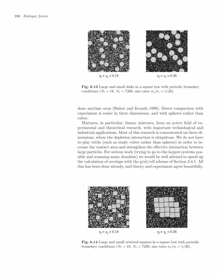
280 Entropic forces
ηl = ηs = 0.18 ηl = ηs = 0.26
Fig. 6.13 Large and small disks in a square box with periodic boundaryconditions (Nl = 18, Ns = 7200, size ratio σs/σl = 1/20).
done anytime soon (Buhot and Krauth 1999). Direct comparison withexperiment is easier in three dimensions, and with spheres rather thancubes.
Mixtures, in particular, binary mixtures, form an active field of ex-perimental and theoretical research, with important technological andindustrial applications. Most of this research is concentrated on three di-mensions, where the depletion interaction is ubiquitous. We do not haveto play tricks (such as study cubes rather than spheres) in order to in-crease the contact area and strengthen the effective interaction betweenlarge particles. For serious work (trying to go to the largest systems pos-sible and scanning many densities) we would be well advised to speed upthe calculation of overlaps with the grid/cell scheme of Section 2.4.1. Allthis has been done already, and theory and experiment agree beautifully.
ηl = ηs = 0.18 ηl = ηs = 0.26
Fig. 6.14 Large and small oriented squares in a square box with periodicboundary conditions (Nl = 18, Ns = 7200, size ratio σs/σl = 1/20).
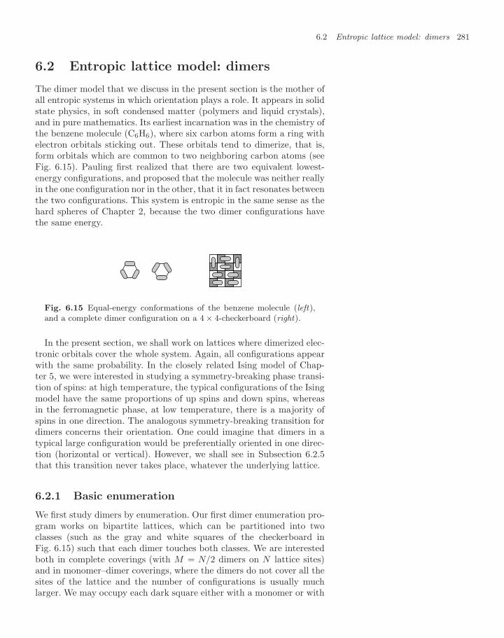
6.2 Entropic lattice model: dimers 281
6.2 Entropic lattice model: dimers
The dimer model that we discuss in the present section is the mother ofall entropic systems in which orientation plays a role. It appears in solidstate physics, in soft condensed matter (polymers and liquid crystals),and in pure mathematics. Its earliest incarnation was in the chemistry ofthe benzene molecule (C6H6), where six carbon atoms form a ring withelectron orbitals sticking out. These orbitals tend to dimerize, that is,form orbitals which are common to two neighboring carbon atoms (seeFig. 6.15). Pauling first realized that there are two equivalent lowest-energy configurations, and proposed that the molecule was neither reallyin the one configuration nor in the other, that it in fact resonates betweenthe two configurations. This system is entropic in the same sense as thehard spheres of Chapter 2, because the two dimer configurations havethe same energy.
Fig. 6.15 Equal-energy conformations of the benzene molecule (left),and a complete dimer configuration on a 4 × 4-checkerboard (right).
In the present section, we shall work on lattices where dimerized elec-tronic orbitals cover the whole system. Again, all configurations appearwith the same probability. In the closely related Ising model of Chap-ter 5, we were interested in studying a symmetry-breaking phase transi-tion of spins: at high temperature, the typical configurations of the Isingmodel have the same proportions of up spins and down spins, whereasin the ferromagnetic phase, at low temperature, there is a majority ofspins in one direction. The analogous symmetry-breaking transition fordimers concerns their orientation. One could imagine that dimers in atypical large configuration would be preferentially oriented in one direc-tion (horizontal or vertical). However, we shall see in Subsection 6.2.5that this transition never takes place, whatever the underlying lattice.
6.2.1 Basic enumeration
We first study dimers by enumeration. Our first dimer enumeration pro-gram works on bipartite lattices, which can be partitioned into twoclasses (such as the gray and white squares of the checkerboard inFig. 6.15) such that each dimer touches both classes. We are interestedboth in complete coverings (with M = N/2 dimers on N lattice sites)and in monomer–dimer coverings, where the dimers do not cover all thesites of the lattice and the number of configurations is usually muchlarger. We may occupy each dark square either with a monomer or with
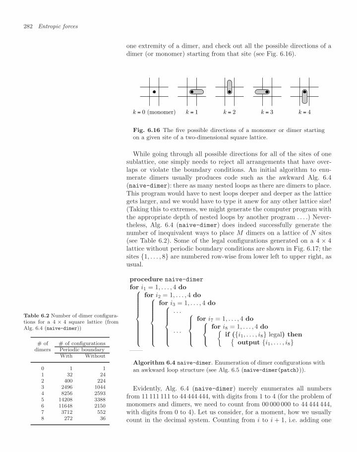
282 Entropic forces
one extremity of a dimer, and check out all the possible directions of adimer (or monomer) starting from that site (see Fig. 6.16).
k = 0 (monomer) k = 1 k = 2 k = 3 k = 4
Fig. 6.16 The five possible directions of a monomer or dimer startingon a given site of a two-dimensional square lattice.
While going through all possible directions for all of the sites of onesublattice, one simply needs to reject all arrangements that have over-laps or violate the boundary conditions. An initial algorithm to enu-merate dimers usually produces code such as the awkward Alg. 6.4(naive-dimer): there as many nested loops as there are dimers to place.This program would have to nest loops deeper and deeper as the latticegets larger, and we would have to type it anew for any other lattice size!(Taking this to extremes, we might generate the computer program withthe appropriate depth of nested loops by another program . . . .) Never-theless, Alg. 6.4 (naive-dimer) does indeed successfully generate thenumber of inequivalent ways to place M dimers on a lattice of N sites(see Table 6.2). Some of the legal configurations generated on a 4 × 4lattice without periodic boundary conditions are shown in Fig. 6.17; thesites 1, . . . , 8 are numbered row-wise from lower left to upper right, asusual.
procedure naive-dimer
for i1 = 1, . . . , 4 do⎧⎪⎪⎪⎪⎪⎪⎪⎪⎨⎪⎪⎪⎪⎪⎪⎪⎪⎩
for i2 = 1, . . . , 4 do⎧⎪⎪⎪⎪⎪⎪⎨⎪⎪⎪⎪⎪⎪⎩
for i3 = 1, . . . , 4 do⎧⎪⎪⎪⎪⎨⎪⎪⎪⎪⎩. . .
. . .
⎧⎪⎪⎨⎪⎪⎩for i7 = 1, . . . , 4 do⎧⎨⎩
for i8 = 1, . . . , 4 doif (i1, . . . , i8 legal) then
output i1, . . . , i8——
Algorithm 6.4 naive-dimer. Enumeration of dimer configurations withan awkward loop structure (see Alg. 6.5 (naive-dimer(patch))).
Table 6.2 Number of dimer configura-tions for a 4 × 4 square lattice (fromAlg. 6.4 (naive-dimer))
# of # of configurationsdimers Periodic boundary
With Without
0 1 11 32 242 400 2243 2496 10444 8256 25935 14208 33886 11648 21507 3712 5528 272 36
Evidently, Alg. 6.4 (naive-dimer) merely enumerates all numbersfrom 11 111 111 to 44 444 444, with digits from 1 to 4 (for the problem ofmonomers and dimers, we need to count from 00 000 000 to 44 444 444,with digits from 0 to 4). Let us consider, for a moment, how we usuallycount in the decimal system. Counting from i to i + 1, i.e. adding one
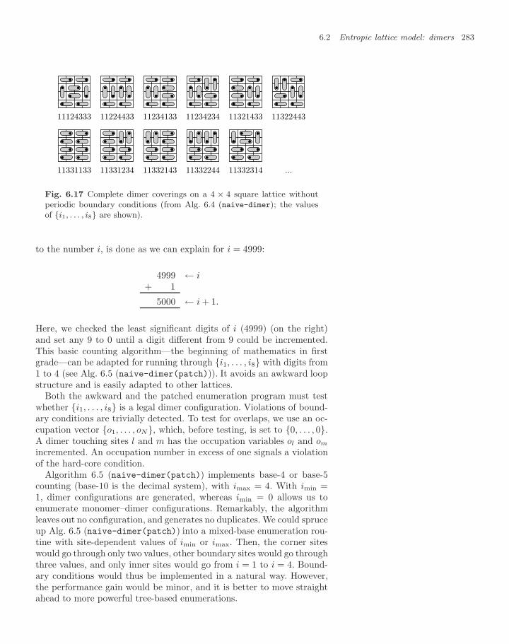
6.2 Entropic lattice model: dimers 283
11124333 11224433 11234133 11234234 11321433 11322443
11331133 11331234 11332143 11332244 11332314 ...
Fig. 6.17 Complete dimer coverings on a 4 × 4 square lattice withoutperiodic boundary conditions (from Alg. 6.4 (naive-dimer); the valuesof i1, . . . , i8 are shown).
to the number i, is done as we can explain for i = 4999:
4999 ← i+ 1
5000 ← i + 1.
Here, we checked the least significant digits of i (4999) (on the right)and set any 9 to 0 until a digit different from 9 could be incremented.This basic counting algorithm—the beginning of mathematics in firstgrade—can be adapted for running through i1, . . . , i8 with digits from1 to 4 (see Alg. 6.5 (naive-dimer(patch))). It avoids an awkward loopstructure and is easily adapted to other lattices.
Both the awkward and the patched enumeration program must testwhether i1, . . . , i8 is a legal dimer configuration. Violations of bound-ary conditions are trivially detected. To test for overlaps, we use an oc-cupation vector o1, . . . , oN, which, before testing, is set to 0, . . . , 0.A dimer touching sites l and m has the occupation variables ol and om
incremented. An occupation number in excess of one signals a violationof the hard-core condition.
Algorithm 6.5 (naive-dimer(patch)) implements base-4 or base-5counting (base-10 is the decimal system), with imax = 4. With imin =1, dimer configurations are generated, whereas imin = 0 allows us toenumerate monomer–dimer configurations. Remarkably, the algorithmleaves out no configuration, and generates no duplicates. We could spruceup Alg. 6.5 (naive-dimer(patch)) into a mixed-base enumeration rou-tine with site-dependent values of imin or imax. Then, the corner siteswould go through only two values, other boundary sites would go throughthree values, and only inner sites would go from i = 1 to i = 4. Bound-ary conditions would thus be implemented in a natural way. However,the performance gain would be minor, and it is better to move straightahead to more powerful tree-based enumerations.
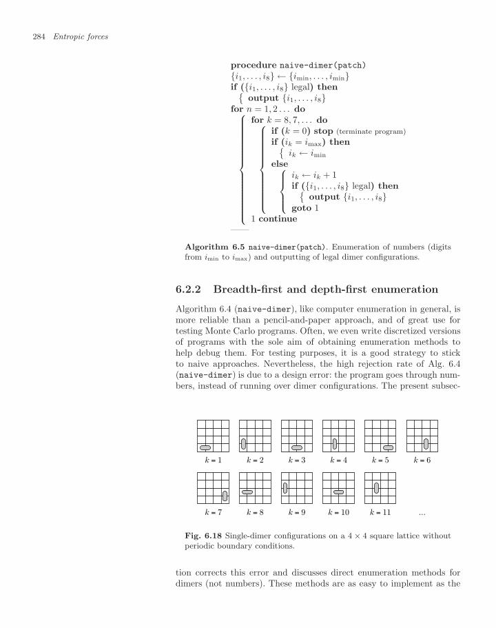
284 Entropic forces
procedure naive-dimer(patch)
i1, . . . , i8 ← imin, . . . , iminif (i1, . . . , i8 legal) then
output i1, . . . , i8for n = 1, 2 . . . do⎧⎪⎪⎪⎪⎪⎪⎪⎪⎪⎪⎪⎪⎪⎪⎨⎪⎪⎪⎪⎪⎪⎪⎪⎪⎪⎪⎪⎪⎪⎩
for k = 8, 7, . . . do⎧⎪⎪⎪⎪⎪⎪⎪⎪⎪⎪⎨⎪⎪⎪⎪⎪⎪⎪⎪⎪⎪⎩
if (k = 0) stop (terminate program)if (ik = imax) then
ik ← imin
else⎧⎪⎪⎨⎪⎪⎩ik ← ik + 1if (i1, . . . , i8 legal) then
output i1, . . . , i8goto 1
1 continue——
Algorithm 6.5 naive-dimer(patch). Enumeration of numbers (digitsfrom imin to imax) and outputting of legal dimer configurations.
6.2.2 Breadth-first and depth-first enumeration
Algorithm 6.4 (naive-dimer), like computer enumeration in general, ismore reliable than a pencil-and-paper approach, and of great use fortesting Monte Carlo programs. Often, we even write discretized versionsof programs with the sole aim of obtaining enumeration methods tohelp debug them. For testing purposes, it is a good strategy to stickto naive approaches. Nevertheless, the high rejection rate of Alg. 6.4(naive-dimer) is due to a design error: the program goes through num-bers, instead of running over dimer configurations. The present subsec-
k = 1 k = 2 k = 3 k = 4 k = 5 k = 6
k = 7 k = 8 k = 9 k = 10 k = 11 ...
Fig. 6.18 Single-dimer configurations on a 4 × 4 square lattice withoutperiodic boundary conditions.
tion corrects this error and discusses direct enumeration methods fordimers (not numbers). These methods are as easy to implement as the
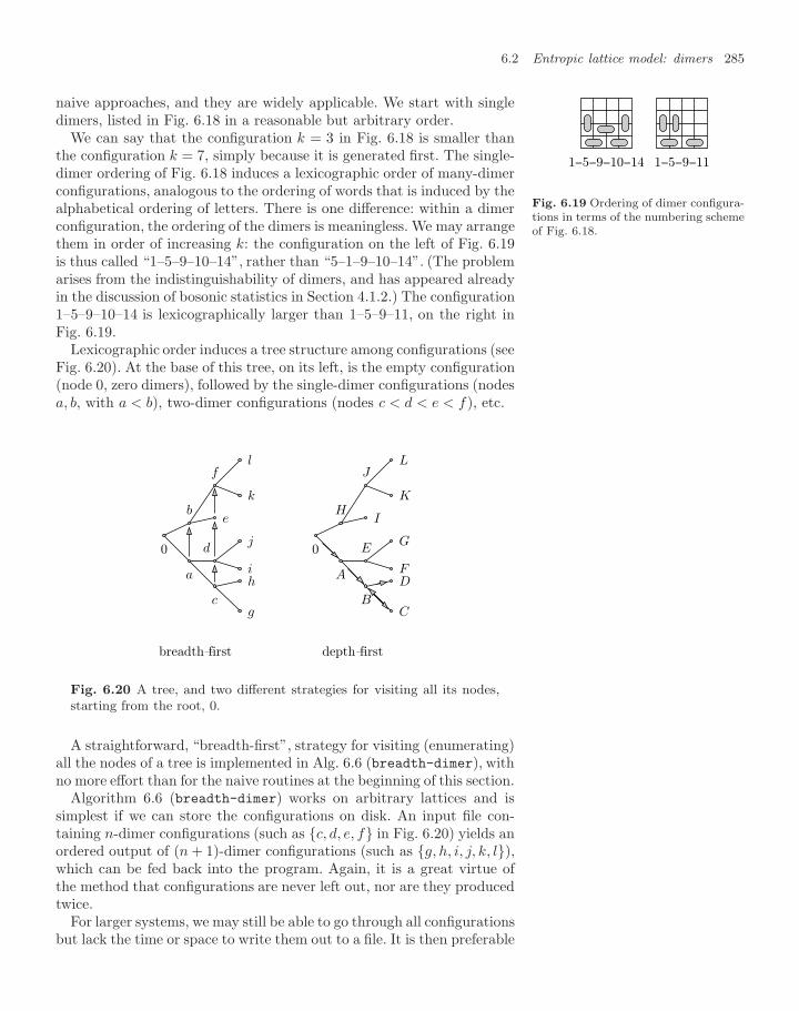
6.2 Entropic lattice model: dimers 285
naive approaches, and they are widely applicable. We start with singledimers, listed in Fig. 6.18 in a reasonable but arbitrary order.
1−5−9−10−14 1−5−9−11
Fig. 6.19 Ordering of dimer configura-tions in terms of the numbering schemeof Fig. 6.18.
We can say that the configuration k = 3 in Fig. 6.18 is smaller thanthe configuration k = 7, simply because it is generated first. The single-dimer ordering of Fig. 6.18 induces a lexicographic order of many-dimerconfigurations, analogous to the ordering of words that is induced by thealphabetical ordering of letters. There is one difference: within a dimerconfiguration, the ordering of the dimers is meaningless. We may arrangethem in order of increasing k: the configuration on the left of Fig. 6.19is thus called “1–5–9–10–14”, rather than “5–1–9–10–14”. (The problemarises from the indistinguishability of dimers, and has appeared alreadyin the discussion of bosonic statistics in Section 4.1.2.) The configuration1–5–9–10–14 is lexicographically larger than 1–5–9–11, on the right inFig. 6.19.
Lexicographic order induces a tree structure among configurations (seeFig. 6.20). At the base of this tree, on its left, is the empty configuration(node 0, zero dimers), followed by the single-dimer configurations (nodesa, b, with a < b), two-dimer configurations (nodes c < d < e < f), etc.
0
a
cg
h
d
i
j
be
f
k
l
breadth-first
0
A
BC
D
E
F
G
HI
J
K
L
depth-first
Fig. 6.20 A tree, and two different strategies for visiting all its nodes,starting from the root, 0.
A straightforward, “breadth-first”, strategy for visiting (enumerating)all the nodes of a tree is implemented in Alg. 6.6 (breadth-dimer), withno more effort than for the naive routines at the beginning of this section.
Algorithm 6.6 (breadth-dimer) works on arbitrary lattices and issimplest if we can store the configurations on disk. An input file con-taining n-dimer configurations (such as c, d, e, f in Fig. 6.20) yields anordered output of (n + 1)-dimer configurations (such as g, h, i, j, k, l),which can be fed back into the program. Again, it is a great virtue ofthe method that configurations are never left out, nor are they producedtwice.
For larger systems, we may still be able to go through all configurationsbut lack the time or space to write them out to a file. It is then preferable
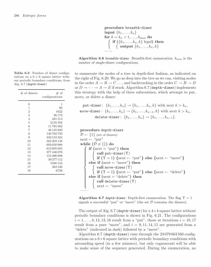
286 Entropic forces
procedure breadth-dimer
input k1, . . . , knfor k = kn + 1, . . . , kmax do
if (k1, . . . , kn, k legal) thenoutput k1, . . . , kn, k
——
Algorithm 6.6 breadth-dimer. Breadth-first enumeration. kmax is thenumber of single-dimer configurations.
to enumerate the nodes of a tree in depth-first fashion, as indicated onthe right of Fig. 6.20. We go as deep into the tree as we can, visiting nodesin the order A → B → C . . . , and backtracking in the order C → B → Dor D → · · · → A → E if stuck. Algorithm 6.7 (depth-dimer) implementsthis strategy with the help of three subroutines, which attempt to put,move, or delete a dimer:
put-dimer : k1, . . . , kn → k1, . . . , kn, k with next k > kn,
move-dimer : k1, . . . , kn → k1, . . . , kn−1, k with next k > kn,
delete-dimer : k1, . . . , kn → k1, . . . , kn−1.
Table 6.3 Number of dimer configu-rations on a 6 × 6 square lattice with-out periodic boundary conditions, fromAlg. 6.7 (depth-dimer)
# of dimers # ofconfigurations
0 11 602 16223 26 1724 281 5145 2135 3566 11 785 3827 48 145 8208 146 702 7939 333 518 32410 562 203 14811 693 650 98812 613 605 04513 377 446 07614 154 396 89815 39 277 11216 5580 15217 363 53618 6728
procedure depth-dimer
D ← 1 (set of dimers)next ← “put”while (D = ) do⎧⎪⎪⎪⎪⎪⎪⎪⎪⎪⎪⎪⎪⎨⎪⎪⎪⎪⎪⎪⎪⎪⎪⎪⎪⎪⎩
if (next = “put”) thencall put-dimer (Υ)if (Υ = 1) next ← “put” else next ← “move”
else if (next = “move”) thencall move-dimer(Υ)if (Υ = 1) next ← “put” else next ← “delete”
else if (next = “delete”) thencall delete-dimer(Υ)next ← “move”
——
Algorithm 6.7 depth-dimer. Depth-first enumeration. The flag Υ = 1signals a successful “put” or “move” (the set D contains the dimers).
The output of Alg. 6.7 (depth-dimer) for a 4×4 square lattice withoutperiodic boundary conditions is shown in Fig. 6.21. The configurationsi = 1, . . . , 8, 12, 13, 16 result from a “put”, those at iterations i = 10, 17result from a pure “move”, and i = 9, 11, 14, 15 are generated from a“delete” (indicated in dark) followed by a “move”.
Algorithm 6.7 (depth-dimer) runs through the 23 079 663 560 config-urations on a 6×6 square lattice with periodic boundary conditions withastounding speed (in a few minutes), but only cognoscenti will be ableto make sense of the sequence generated. During the enumeration, no
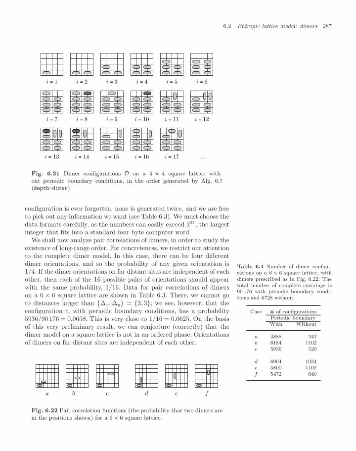
6.2 Entropic lattice model: dimers 287
i = 1 i = 2 i = 3 i = 4 i = 5 i = 6
i = 7 i = 8 i = 9 i = 10 i = 11 i = 12
i = 13 i = 14 i = 15 i = 16 i = 17 ...
Fig. 6.21 Dimer configurations D on a 4 × 4 square lattice with-out periodic boundary conditions, in the order generated by Alg. 6.7(depth-dimer).
configuration is ever forgotten, none is generated twice, and we are freeto pick out any information we want (see Table 6.3). We must choose thedata formats carefully, as the numbers can easily exceed 231, the largestinteger that fits into a standard four-byte computer word.
We shall now analyze pair correlations of dimers, in order to study theexistence of long-range order. For concreteness, we restrict our attentionto the complete dimer model. In this case, there can be four differentdimer orientations, and so the probability of any given orientation is1/4. If the dimer orientations on far distant sites are independent of eachother, then each of the 16 possible pairs of orientations should appearwith the same probability, 1/16. Data for pair correlations of dimerson a 6 × 6 square lattice are shown in Table 6.3. There, we cannot goto distances larger than ∆x, ∆y = 3, 3; we see, however, that theconfiguration c, with periodic boundary conditions, has a probability5936/90 176 = 0.0658. This is very close to 1/16 = 0.0625. On the basisof this very preliminary result, we can conjecture (correctly) that thedimer model on a square lattice is not in an ordered phase. Orientationsof dimers on far distant sites are independent of each other.
Table 6.4 Number of dimer configu-rations on a 6 × 6 square lattice, withdimers prescribed as in Fig. 6.22. Thetotal number of complete coverings is90 176 with periodic boundary condi-tions and 6728 without.
Case # of configurationsPeriodic boundaryWith Without
a 4888 242b 6184 1102c 5936 520
d 6904 1034e 5800 1102f 5472 640
a b c d e f
Fig. 6.22 Pair correlation functions (the probability that two dimers arein the positions shown) for a 6 × 6 square lattice.
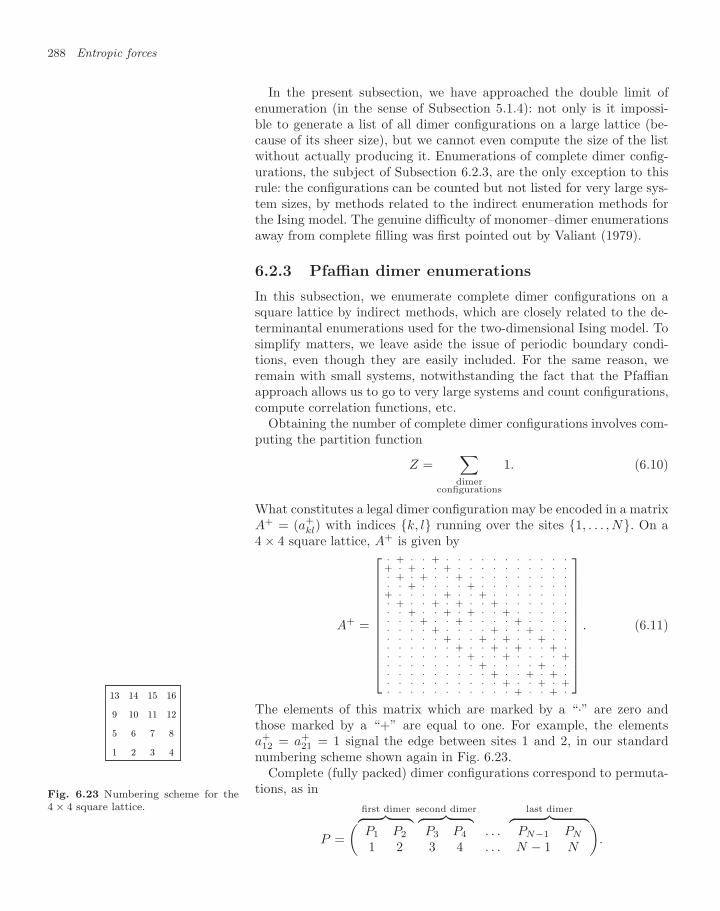
288 Entropic forces
In the present subsection, we have approached the double limit ofenumeration (in the sense of Subsection 5.1.4): not only is it impossi-ble to generate a list of all dimer configurations on a large lattice (be-cause of its sheer size), but we cannot even compute the size of the listwithout actually producing it. Enumerations of complete dimer config-urations, the subject of Subsection 6.2.3, are the only exception to thisrule: the configurations can be counted but not listed for very large sys-tem sizes, by methods related to the indirect enumeration methods forthe Ising model. The genuine difficulty of monomer–dimer enumerationsaway from complete filling was first pointed out by Valiant (1979).
6.2.3 Pfaffian dimer enumerations
In this subsection, we enumerate complete dimer configurations on asquare lattice by indirect methods, which are closely related to the de-terminantal enumerations used for the two-dimensional Ising model. Tosimplify matters, we leave aside the issue of periodic boundary condi-tions, even though they are easily included. For the same reason, weremain with small systems, notwithstanding the fact that the Pfaffianapproach allows us to go to very large systems and count configurations,compute correlation functions, etc.
Obtaining the number of complete dimer configurations involves com-puting the partition function
Z =∑dimer
configurations
1. (6.10)
What constitutes a legal dimer configuration may be encoded in a matrixA+ = (a+
kl) with indices k, l running over the sites 1, . . . , N. On a4 × 4 square lattice, A+ is given by
A+ =
⎡⎢⎢⎢⎢⎢⎢⎢⎢⎢⎢⎢⎣
· + · · + · · · · · · · · · · ·+ · + · · + · · · · · · · · · ·· + · + · · + · · · · · · · · ·· · + · · · · + · · · · · · · ·+ · · · · + · · + · · · · · · ·· + · · + · + · · + · · · · · ·· · + · · + · + · · + · · · · ·· · · + · · + · · · · + · · · ·· · · · + · · · · + · · + · · ·· · · · · + · · + · + · · + · ·· · · · · · + · · + · + · · + ·· · · · · · · + · · + · · · · +· · · · · · · · + · · · · + · ·· · · · · · · · · + · · + · + ·· · · · · · · · · · + · · + · +· · · · · · · · · · · + · · + ·
⎤⎥⎥⎥⎥⎥⎥⎥⎥⎥⎥⎥⎦. (6.11)
The elements of this matrix which are marked by a “·” are zero andthose marked by a “+” are equal to one. For example, the elementsa+12 = a+
21 = 1 signal the edge between sites 1 and 2, in our standardnumbering scheme shown again in Fig. 6.23.1 2 3 4
5 6 7 8
9 10 11 12
13 14 15 16
Fig. 6.23 Numbering scheme for the4 × 4 square lattice.
Complete (fully packed) dimer configurations correspond to permuta-tions, as in
P =( first dimer︷ ︸︸ ︷
P1 P2
1 2
second dimer︷ ︸︸ ︷P3 P4
3 4. . .. . .
last dimer︷ ︸︸ ︷PN−1 PN
N − 1 N
).
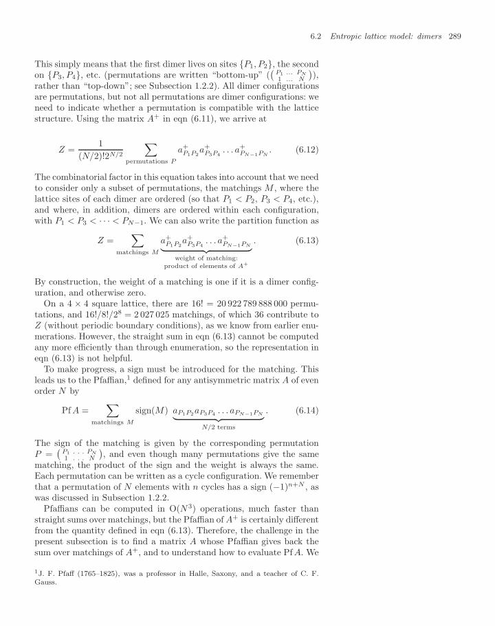
6.2 Entropic lattice model: dimers 289
This simply means that the first dimer lives on sites P1, P2, the secondon P3, P4, etc. (permutations are written “bottom-up” (
(P1 ... PN
1 ... N
)),
rather than “top-down”; see Subsection 1.2.2). All dimer configurationsare permutations, but not all permutations are dimer configurations: weneed to indicate whether a permutation is compatible with the latticestructure. Using the matrix A+ in eqn (6.11), we arrive at
Z =1
(N/2)!2N/2
∑permutations P
a+P1P2
a+P3P4
. . . a+PN−1PN
. (6.12)
The combinatorial factor in this equation takes into account that we needto consider only a subset of permutations, the matchings M , where thelattice sites of each dimer are ordered (so that P1 < P2, P3 < P4, etc.),and where, in addition, dimers are ordered within each configuration,with P1 < P3 < · · · < PN−1. We can also write the partition function as
Z =∑
matchings M
a+P1P2
a+P3P4
. . . a+PN−1PN︸ ︷︷ ︸
weight of matching:product of elements of A+
. (6.13)
By construction, the weight of a matching is one if it is a dimer config-uration, and otherwise zero.
On a 4 × 4 square lattice, there are 16! = 20 922 789 888 000 permu-tations, and 16!/8!/28 = 2 027 025 matchings, of which 36 contribute toZ (without periodic boundary conditions), as we know from earlier enu-merations. However, the straight sum in eqn (6.13) cannot be computedany more efficiently than through enumeration, so the representation ineqn (6.13) is not helpful.
To make progress, a sign must be introduced for the matching. Thisleads us to the Pfaffian,1 defined for any antisymmetric matrix A of evenorder N by
Pf A =∑
matchings M
sign(M) aP1P2aP3P4 . . . aPN−1PN︸ ︷︷ ︸N/2 terms
. (6.14)
The sign of the matching is given by the corresponding permutationP =
(P1 . . . PN
1 . . . N
), and even though many permutations give the same
matching, the product of the sign and the weight is always the same.Each permutation can be written as a cycle configuration. We rememberthat a permutation of N elements with n cycles has a sign (−1)n+N , aswas discussed in Subsection 1.2.2.
Pfaffians can be computed in O(N3) operations, much faster thanstraight sums over matchings, but the Pfaffian of A+ is certainly differentfrom the quantity defined in eqn (6.13). Therefore, the challenge in thepresent subsection is to find a matrix A whose Pfaffian gives back thesum over matchings of A+, and to understand how to evaluate Pf A. We
1J. F. Pfaff (1765–1825), was a professor in Halle, Saxony, and a teacher of C. F.Gauss.
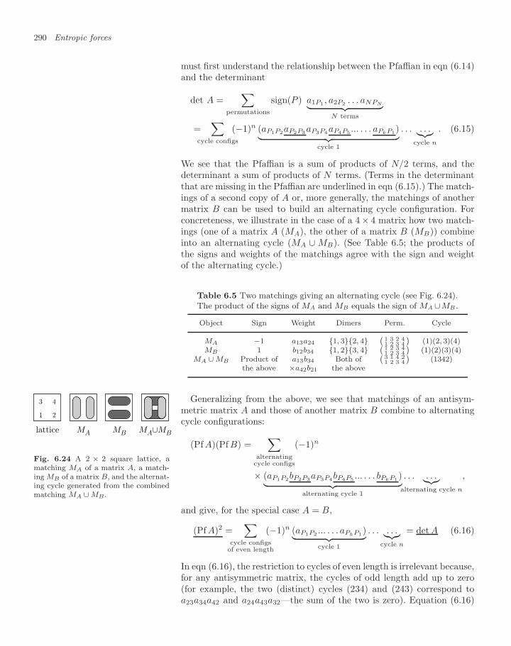
290 Entropic forces
must first understand the relationship between the Pfaffian in eqn (6.14)and the determinant
det A =∑
permutations
sign(P ) a1P1 , a2P2 . . . aNPN︸ ︷︷ ︸N terms
=∑
cycle configs
(−1)n (aP1P2aP2P3aP3P4aP4P5 ... . . . aPkP1)︸ ︷︷ ︸cycle 1
. . . . . .︸︷︷︸cycle n
. (6.15)
We see that the Pfaffian is a sum of products of N/2 terms, and thedeterminant a sum of products of N terms. (Terms in the determinantthat are missing in the Pfaffian are underlined in eqn (6.15).) The match-ings of a second copy of A or, more generally, the matchings of anothermatrix B can be used to build an alternating cycle configuration. Forconcreteness, we illustrate in the case of a 4× 4 matrix how two match-ings (one of a matrix A (MA), the other of a matrix B (MB)) combineinto an alternating cycle (MA ∪ MB). (See Table 6.5; the products ofthe signs and weights of the matchings agree with the sign and weightof the alternating cycle.)
Table 6.5 Two matchings giving an alternating cycle (see Fig. 6.24).The product of the signs of MA and MB equals the sign of MA ∪MB .
Object Sign Weight Dimers Perm. Cycle
MA −1 a13a24 1, 32, 4 `1 3 2 41 2 3 4
´(1)(2, 3)(4)
MB 1 b12b34 1, 23, 4 `1 2 3 41 2 3 4
´(1)(2)(3)(4)
MA ∪ MB Product of a13b34 Both of`
3 1 4 21 2 3 4
´(1342)
the above ×a42b21 the above
1 2
3 4
lattice MA MB MA∪MB
Fig. 6.24 A 2 × 2 square lattice, amatching MA of a matrix A, a match-ing MB of a matrix B, and the alternat-ing cycle generated from the combinedmatching MA ∪ MB .
Generalizing from the above, we see that matchings of an antisym-metric matrix A and those of another matrix B combine to alternatingcycle configurations:
(Pf A)(Pf B) =∑
alternatingcycle configs
(−1)n
× (aP1P2bP2P3aP3P4bP4P5 ... . . . bPkP1)︸ ︷︷ ︸alternating cycle 1
. . . . . .︸︷︷︸alternating cycle n
,
and give, for the special case A = B,
(Pf A)2 =∑
cycle configsof even length
(−1)n (aP1P2 ... . . . aPkP1)︸ ︷︷ ︸cycle 1
. . . . . .︸︷︷︸cycle n
= det A (6.16)
In eqn (6.16), the restriction to cycles of even length is irrelevant because,for any antisymmetric matrix, the cycles of odd length add up to zero(for example, the two (distinct) cycles (234) and (243) correspond toa23a34a42 and a24a43a32—the sum of the two is zero). Equation (6.16)
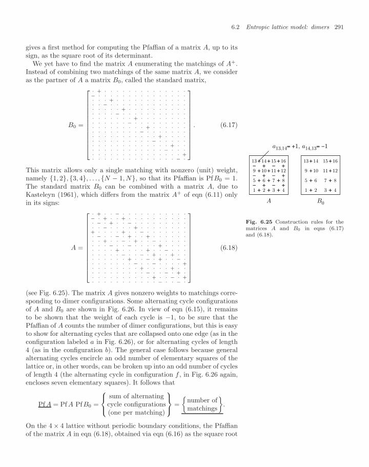
6.2 Entropic lattice model: dimers 291
gives a first method for computing the Pfaffian of a matrix A, up to itssign, as the square root of its determinant.
We yet have to find the matrix A enumerating the matchings of A+.Instead of combining two matchings of the same matrix A, we consideras the partner of A a matrix B0, called the standard matrix,
B0 =
⎡⎢⎢⎢⎢⎢⎢⎢⎢⎢⎢⎢⎣
· + · · · · · · · · · · · · · ·− · · · · · · · · · · · · · · ·· · · + · · · · · · · · · · · ·· · − · · · · · · · · · · · · ·· · · · · + · · · · · · · · · ·· · · · − · · · · · · · · · · ·· · · · · · · + · · · · · · · ·· · · · · · − · · · · · · · · ·· · · · · · · · · + · · · · · ·· · · · · · · · − · · · · · · ·· · · · · · · · · · · + · · · ·· · · · · · · · · · − · · · · ·· · · · · · · · · · · · · + · ·· · · · · · · · · · · · − · · ·· · · · · · · · · · · · · · · +· · · · · · · · · · · · · · − ·
⎤⎥⎥⎥⎥⎥⎥⎥⎥⎥⎥⎥⎦. (6.17)
This matrix allows only a single matching with nonzero (unit) weight,namely 1, 2, 3, 4, . . . , N − 1, N, so that its Pfaffian is PfB0 = 1.The standard matrix B0 can be combined with a matrix A, due toKasteleyn (1961), which differs from the matrix A+ of eqn (6.11) onlyin its signs:
1 2 3 4
5 6 7 8
9 10 11 12
13 14 15 16
+ + +
+ + +
+ + +
+ + +
−
−
−
+
+
+
−
−
−
+
+
+
A
a13,14= +1, a14,13= −1
1 2 3 4
5 6 7 8
9 10 11 12
13 14 15 16
+ +
+ +
+ +
+ +
B0
Fig. 6.25 Construction rules for thematrices A and B0 in eqns (6.17)and (6.18).
A =
⎡⎢⎢⎢⎢⎢⎢⎢⎢⎢⎢⎢⎣
· + · · − · · · · · · · · · · ·− · + · · + · · · · · · · · · ·· − · + · · − · · · · · · · · ·· · − · · · · + · · · · · · · ·+ · · · · + · · − · · · · · · ·· − · · − · + · · + · · · · · ·· · + · · − · + · · − · · · · ·· · · − · · − · · · · + · · · ·· · · · + · · · · + · · − · · ·· · · · · − · · − · + · · + · ·· · · · · · + · · − · + · · − ·· · · · · · · − · · − · · · · +· · · · · · · · + · · · · + · ·· · · · · · · · · − · · − · + ·· · · · · · · · · · + · · − · +· · · · · · · · · · · − · · − ·
⎤⎥⎥⎥⎥⎥⎥⎥⎥⎥⎥⎥⎦(6.18)
(see Fig. 6.25). The matrix A gives nonzero weights to matchings corre-sponding to dimer configurations. Some alternating cycle configurationsof A and B0 are shown in Fig. 6.26. In view of eqn (6.15), it remainsto be shown that the weight of each cycle is −1, to be sure that thePfaffian of A counts the number of dimer configurations, but this is easyto show for alternating cycles that are collapsed onto one edge (as in theconfiguration labeled a in Fig. 6.26), or for alternating cycles of length4 (as in the configuration b). The general case follows because generalalternating cycles encircle an odd number of elementary squares of thelattice or, in other words, can be broken up into an odd number of cyclesof length 4 (the alternating cycle in configuration f , in Fig. 6.26 again,encloses seven elementary squares). It follows that
Pf A = Pf A PfB0 =
⎧⎨⎩sum of alternatingcycle configurations(one per matching)
⎫⎬⎭ =
number ofmatchings
.
On the 4 × 4 lattice without periodic boundary conditions, the Pfaffianof the matrix A in eqn (6.18), obtained via eqn (6.16) as the square root
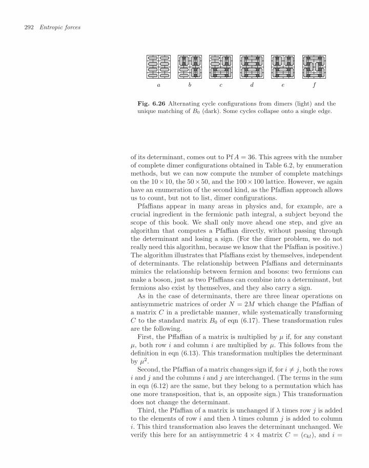
292 Entropic forces
a b c d e f
Fig. 6.26 Alternating cycle configurations from dimers (light) and theunique matching of B0 (dark). Some cycles collapse onto a single edge.
of its determinant, comes out to Pf A = 36. This agrees with the numberof complete dimer configurations obtained in Table 6.2, by enumerationmethods, but we can now compute the number of complete matchingson the 10×10, the 50×50, and the 100×100 lattice. However, we againhave an enumeration of the second kind, as the Pfaffian approach allowsus to count, but not to list, dimer configurations.
Pfaffians appear in many areas in physics and, for example, are acrucial ingredient in the fermionic path integral, a subject beyond thescope of this book. We shall only move ahead one step, and give analgorithm that computes a Pfaffian directly, without passing throughthe determinant and losing a sign. (For the dimer problem, we do notreally need this algorithm, because we know that the Pfaffian is positive.)The algorithm illustrates that Pfaffians exist by themselves, independentof determinants. The relationship between Pfaffians and determinantsmimics the relationship between fermion and bosons: two fermions canmake a boson, just as two Pfaffians can combine into a determinant, butfermions also exist by themselves, and they also carry a sign.
As in the case of determinants, there are three linear operations onantisymmetric matrices of order N = 2M which change the Pfaffian ofa matrix C in a predictable manner, while systematically transformingC to the standard matrix B0 of eqn (6.17). These transformation rulesare the following.
First, the Pffaffian of a matrix is multiplied by µ if, for any constantµ, both row i and column i are multiplied by µ. This follows from thedefinition in eqn (6.13). This transformation multiplies the determinantby µ2.
Second, the Pfaffian of a matrix changes sign if, for i = j, both the rowsi and j and the columns i and j are interchanged. (The terms in the sumin eqn (6.12) are the same, but they belong to a permutation which hasone more transposition, that is, an opposite sign.) This transformationdoes not change the determinant.
Third, the Pfaffian of a matrix is unchanged if λ times row j is addedto the elements of row i and then λ times column j is added to columni. This third transformation also leaves the determinant unchanged. Weverify this here for an antisymmetric 4 × 4 matrix C = (ckl), and i =
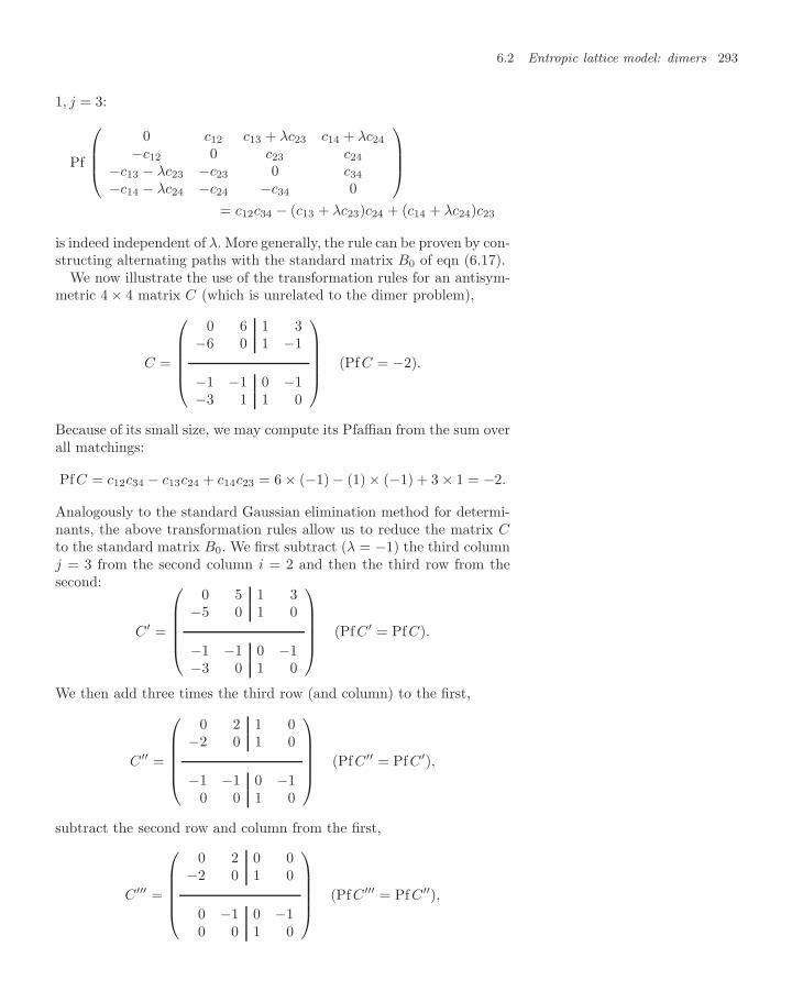
6.2 Entropic lattice model: dimers 293
1, j = 3:
Pf
⎛⎜⎜⎝0 c12 c13 + λc23 c14 + λc24
−c12 0 c23 c24
−c13 − λc23 −c23 0 c34
−c14 − λc24 −c24 −c34 0
⎞⎟⎟⎠= c12c34 − (c13 + λc23)c24 + (c14 + λc24)c23
is indeed independent of λ. More generally, the rule can be proven by con-structing alternating paths with the standard matrix B0 of eqn (6.17).
We now illustrate the use of the transformation rules for an antisym-metric 4 × 4 matrix C (which is unrelated to the dimer problem),
C =
⎛⎜⎜⎜⎜⎝0 6 1 3
−6 0 1 −1
−1 −1 0 −1−3 1 1 0
⎞⎟⎟⎟⎟⎠ (Pf C = −2).
Because of its small size, we may compute its Pfaffian from the sum overall matchings:
PfC = c12c34 − c13c24 + c14c23 = 6 × (−1) − (1) × (−1) + 3 × 1 = −2.
Analogously to the standard Gaussian elimination method for determi-nants, the above transformation rules allow us to reduce the matrix Cto the standard matrix B0. We first subtract (λ = −1) the third columnj = 3 from the second column i = 2 and then the third row from thesecond:
C′ =
⎛⎜⎜⎜⎜⎝0 5 1 3
−5 0 1 0
−1 −1 0 −1−3 0 1 0
⎞⎟⎟⎟⎟⎠ (Pf C′ = Pf C).
We then add three times the third row (and column) to the first,
C′′ =
⎛⎜⎜⎜⎜⎝0 2 1 0
−2 0 1 0
−1 −1 0 −10 0 1 0
⎞⎟⎟⎟⎟⎠ (Pf C′′ = Pf C′),
subtract the second row and column from the first,
C′′′ =
⎛⎜⎜⎜⎜⎝0 2 0 0
−2 0 1 0
0 −1 0 −10 0 1 0
⎞⎟⎟⎟⎟⎠ (Pf C′′′ = Pf C′′),
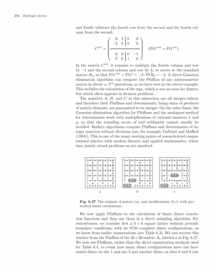
294 Entropic forces
and finally subtract the fourth row from the second and the fourth col-umn from the second,
C′′′′ =
⎛⎜⎜⎜⎜⎝0 2 0 0
−2 0 0 0
0 0 0 −10 0 1 0
⎞⎟⎟⎟⎟⎠ (Pf C′′′′ = Pf C′′′).
In the matrix C′′′′, it remains to multiply the fourth column and rowby −1 and the second column and row by 1
2 , to arrive at the standardmatrix B0, so that Pf C′′′′ = Pf C = −2 ·PfB0 = −2. A direct Gaussianelimination algorithm can compute the Pfaffian of any antisymmetricmatrix in about ∝ N3 operations, as we have seen in the above example.This includes the calculation of the sign, which is not an issue for dimers,but which often appears in fermion problems.
The matrices A, B, and C in this subsection are all integer-valued,and therefore their Pfaffians and determinants, being sums of productsof matrix elements, are guaranteed to be integer. On the other hand, theGaussian elimination algorithm for Pfaffians and the analogous methodfor determinants work with multiplications of rational numbers λ andµ, so that the rounding errors of real arithmetic cannot usually beavoided. Modern algorithms compute Pfaffians and determinants of in-teger matrices without divisions (see, for example, Galbiati and Maffioli(1994)). This is one of the many meeting points of research-level compu-tational physics with modern discrete and applied mathematics, wherethey jointly attack problems as yet unsolved.
1 2 3 4 5 6
7 8 9 10 11 12
13 14 15 16 17 18
19 20 21 22 23 24
25 26 27 28 29 30
31 32 33 34 35 36
+ + + + +
+ + + + +
+ + + + +
+ + + + +
+ + + + +
+ + + + +
−
−
−
−
−
−
−
−
−
−
−
−
−
−
−
+
+
+
+
+
+
+
+
+
+
+
+
+
+
+
a
1 2 3 4 5 6
7 8 9 10 11 12
13 14 15 16 17 18
19 20 21 22 23 24
25 26 27 28 29 30
31 32 33 34 35 36
+ + + +
+ + +
+ + + + +
+ + + + +
+ + + + +
+ + + + +
−
−
−
−
−
−
−
−
−
−
−
−
+
+
+
+
+
+
+
+
+
+
+
+
+
b
1 2 3 4 5 6
7 8 9 10 11 12
13 14 15 16 17 18
19 20 21 22 23 24
25 26 27 28 29 30
31 32 33 34 35 36
+ + + +
+ + + + +
+ + +
+ + + + +
+ + + + +
+ + + + +
−
−
−
−
−
−
−
−
−
−
−
−
+
+
+
+
+
+
+
+
+
+
+
+
c
Fig. 6.27 The original A-matrix (a), and modifications (b, c) with pre-scribed dimer orientations.
We now apply Pfaffians to the calculation of dimer–dimer correla-tion functions and then use them in a direct sampling algorithm. Forconcreteness, we consider first a 6 × 6 square lattice without periodicboundary conditions, with its 6728 complete dimer configurations, aswe know from earlier enumerations (see Table 6.3). We can recover thisnumber from the Pfaffian of the 36×36 matrix Aa labeled a in Fig. 6.27.We now use Pfaffians, rather than the direct enumeration methods usedfor Table 6.4, to count how many dimer configurations have one hori-zontal dimer on site 1 and site 2 and another dimer on sites 8 and 9 (see
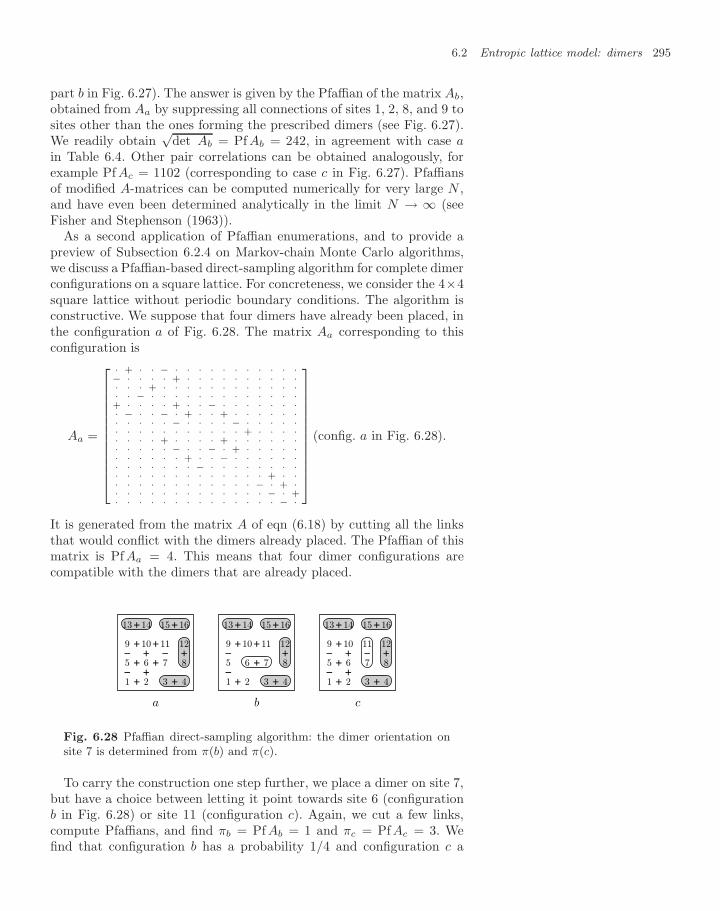
6.2 Entropic lattice model: dimers 295
part b in Fig. 6.27). The answer is given by the Pfaffian of the matrix Ab,obtained from Aa by suppressing all connections of sites 1, 2, 8, and 9 tosites other than the ones forming the prescribed dimers (see Fig. 6.27).We readily obtain
√det Ab = Pf Ab = 242, in agreement with case a
in Table 6.4. Other pair correlations can be obtained analogously, forexample Pf Ac = 1102 (corresponding to case c in Fig. 6.27). Pfaffiansof modified A-matrices can be computed numerically for very large N ,and have even been determined analytically in the limit N → ∞ (seeFisher and Stephenson (1963)).
As a second application of Pfaffian enumerations, and to provide apreview of Subsection 6.2.4 on Markov-chain Monte Carlo algorithms,we discuss a Pfaffian-based direct-sampling algorithm for complete dimerconfigurations on a square lattice. For concreteness, we consider the 4×4square lattice without periodic boundary conditions. The algorithm isconstructive. We suppose that four dimers have already been placed, inthe configuration a of Fig. 6.28. The matrix Aa corresponding to thisconfiguration is
Aa =
⎡⎢⎢⎢⎢⎢⎢⎢⎢⎢⎢⎢⎣
· + · · − · · · · · · · · · · ·− · · · · + · · · · · · · · · ·· · · + · · · · · · · · · · · ·· · − · · · · · · · · · · · · ·+ · · · · + · · − · · · · · · ·· − · · − · + · · + · · · · · ·· · · · · − · · · · − · · · · ·· · · · · · · · · · · + · · · ·· · · · + · · · · + · · · · · ·· · · · · − · · − · + · · · · ·· · · · · · + · · − · · · · · ·· · · · · · · − · · · · · · · ·· · · · · · · · · · · · · + · ·· · · · · · · · · · · · − · + ·· · · · · · · · · · · · · − · +· · · · · · · · · · · · · · − ·
⎤⎥⎥⎥⎥⎥⎥⎥⎥⎥⎥⎥⎦(config. a in Fig. 6.28).
It is generated from the matrix A of eqn (6.18) by cutting all the linksthat would conflict with the dimers already placed. The Pfaffian of thismatrix is PfAa = 4. This means that four dimer configurations arecompatible with the dimers that are already placed.
1 2 3 4
5 6 7 8
9 10 11 12
13 14 15 16
+ +
+ +
+ +
+ +
−
−
+
+ − +
a
1 2 3 4
5 6 7 8
9 10 11 12
13 14 15 16
+ +
+
+ +
+ +
−
− +
b
1 2 3 4
5 6 7 8
9 10 11 12
13 14 15 16
+ +
+
+
+ +
−
−
+
+ − +
c
Fig. 6.28 Pfaffian direct-sampling algorithm: the dimer orientation onsite 7 is determined from π(b) and π(c).
To carry the construction one step further, we place a dimer on site 7,but have a choice between letting it point towards site 6 (configurationb in Fig. 6.28) or site 11 (configuration c). Again, we cut a few links,compute Pfaffians, and find πb = Pf Ab = 1 and πc = PfAc = 3. Wefind that configuration b has a probability 1/4 and configuration c a
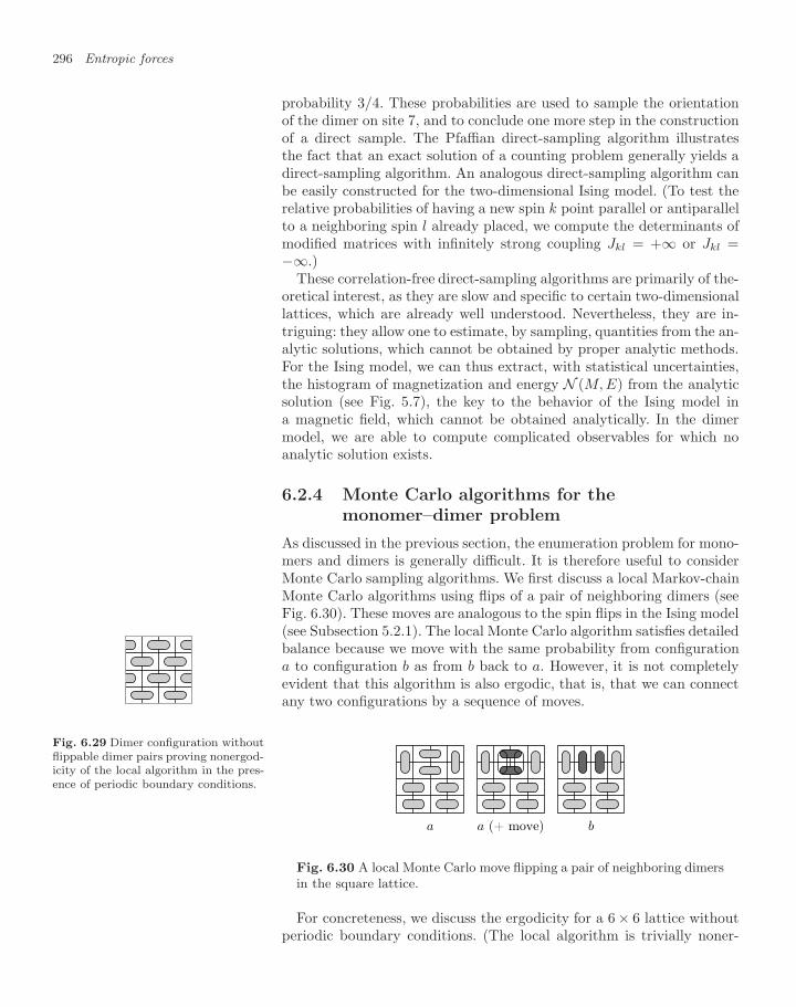
296 Entropic forces
probability 3/4. These probabilities are used to sample the orientationof the dimer on site 7, and to conclude one more step in the constructionof a direct sample. The Pfaffian direct-sampling algorithm illustratesthe fact that an exact solution of a counting problem generally yields adirect-sampling algorithm. An analogous direct-sampling algorithm canbe easily constructed for the two-dimensional Ising model. (To test therelative probabilities of having a new spin k point parallel or antiparallelto a neighboring spin l already placed, we compute the determinants ofmodified matrices with infinitely strong coupling Jkl = +∞ or Jkl =−∞.)
These correlation-free direct-sampling algorithms are primarily of the-oretical interest, as they are slow and specific to certain two-dimensionallattices, which are already well understood. Nevertheless, they are in-triguing: they allow one to estimate, by sampling, quantities from the an-alytic solutions, which cannot be obtained by proper analytic methods.For the Ising model, we can thus extract, with statistical uncertainties,the histogram of magnetization and energy N (M, E) from the analyticsolution (see Fig. 5.7), the key to the behavior of the Ising model ina magnetic field, which cannot be obtained analytically. In the dimermodel, we are able to compute complicated observables for which noanalytic solution exists.
6.2.4 Monte Carlo algorithms for themonomer–dimer problem
As discussed in the previous section, the enumeration problem for mono-mers and dimers is generally difficult. It is therefore useful to considerMonte Carlo sampling algorithms. We first discuss a local Markov-chainMonte Carlo algorithms using flips of a pair of neighboring dimers (seeFig. 6.30). These moves are analogous to the spin flips in the Ising model(see Subsection 5.2.1). The local Monte Carlo algorithm satisfies detailedbalance because we move with the same probability from configurationa to configuration b as from b back to a. However, it is not completelyevident that this algorithm is also ergodic, that is, that we can connectany two configurations by a sequence of moves.
Fig. 6.29 Dimer configuration withoutflippable dimer pairs proving nonergod-icity of the local algorithm in the pres-ence of periodic boundary conditions.
a a (+ move) b
Fig. 6.30 A local Monte Carlo move flipping a pair of neighboring dimersin the square lattice.
For concreteness, we discuss the ergodicity for a 6× 6 lattice withoutperiodic boundary conditions. (The local algorithm is trivially noner-
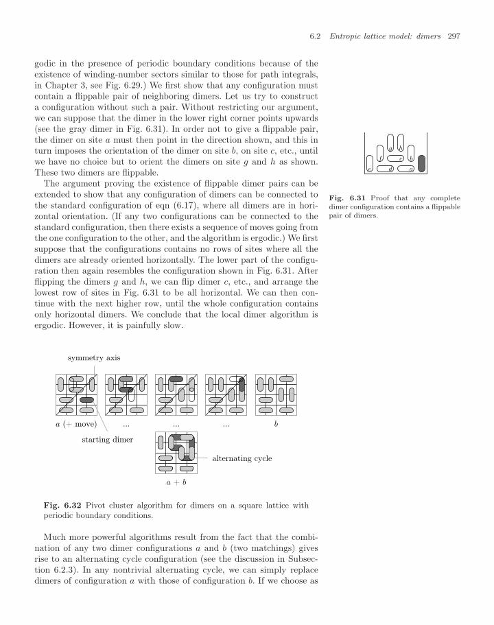
6.2 Entropic lattice model: dimers 297
godic in the presence of periodic boundary conditions because of theexistence of winding-number sectors similar to those for path integrals,in Chapter 3, see Fig. 6.29.) We first show that any configuration mustcontain a flippable pair of neighboring dimers. Let us try to constructa configuration without such a pair. Without restricting our argument,we can suppose that the dimer in the lower right corner points upwards(see the gray dimer in Fig. 6.31). In order not to give a flippable pair,the dimer on site a must then point in the direction shown, and this inturn imposes the orientation of the dimer on site b, on site c, etc., untilwe have no choice but to orient the dimers on site g and h as shown.These two dimers are flippable. a
bc
de
f
g h
Fig. 6.31 Proof that any completedimer configuration contains a flippablepair of dimers.
The argument proving the existence of flippable dimer pairs can beextended to show that any configuration of dimers can be connected tothe standard configuration of eqn (6.17), where all dimers are in hori-zontal orientation. (If any two configurations can be connected to thestandard configuration, then there exists a sequence of moves going fromthe one configuration to the other, and the algorithm is ergodic.) We firstsuppose that the configurations contains no rows of sites where all thedimers are already oriented horizontally. The lower part of the configu-ration then again resembles the configuration shown in Fig. 6.31. Afterflipping the dimers g and h, we can flip dimer c, etc., and arrange thelowest row of sites in Fig. 6.31 to be all horizontal. We can then con-tinue with the next higher row, until the whole configuration containsonly horizontal dimers. We conclude that the local dimer algorithm isergodic. However, it is painfully slow.
a (+ move)
symmetry axis
starting dimer
... ... ... b
a + b
alternating cycle
Fig. 6.32 Pivot cluster algorithm for dimers on a square lattice withperiodic boundary conditions.
Much more powerful algorithms result from the fact that the combi-nation of any two dimer configurations a and b (two matchings) givesrise to an alternating cycle configuration (see the discussion in Subsec-tion 6.2.3). In any nontrivial alternating cycle, we can simply replacedimers of configuration a with those of configuration b. If we choose as
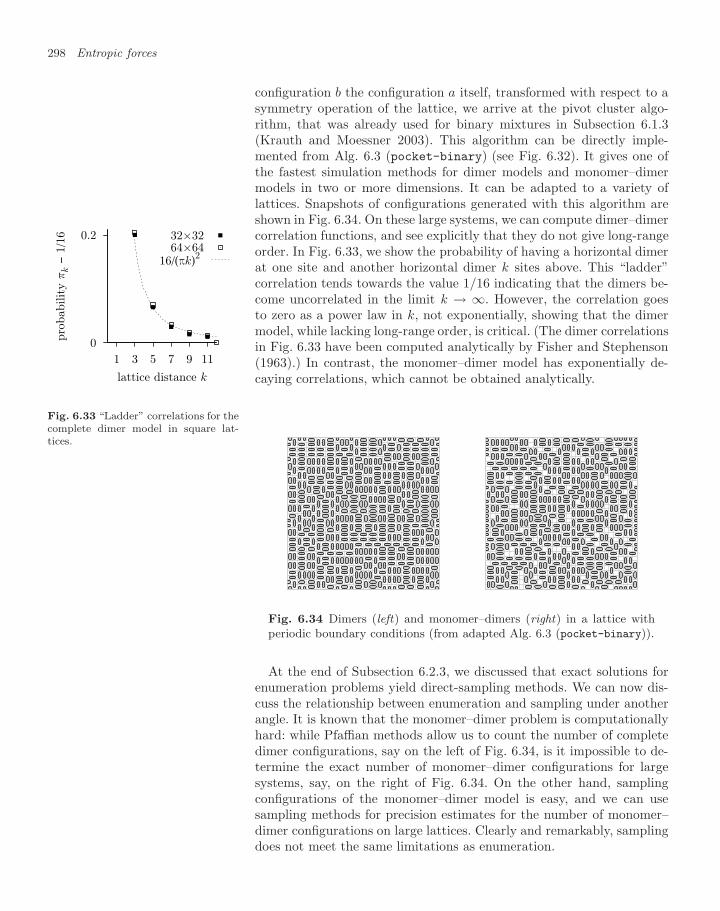
298 Entropic forces
configuration b the configuration a itself, transformed with respect to asymmetry operation of the lattice, we arrive at the pivot cluster algo-rithm, that was already used for binary mixtures in Subsection 6.1.3(Krauth and Moessner 2003). This algorithm can be directly imple-mented from Alg. 6.3 (pocket-binary) (see Fig. 6.32). It gives one ofthe fastest simulation methods for dimer models and monomer–dimermodels in two or more dimensions. It can be adapted to a variety oflattices. Snapshots of configurations generated with this algorithm areshown in Fig. 6.34. On these large systems, we can compute dimer–dimercorrelation functions, and see explicitly that they do not give long-rangeorder. In Fig. 6.33, we show the probability of having a horizontal dimerat one site and another horizontal dimer k sites above. This “ladder”correlation tends towards the value 1/16 indicating that the dimers be-come uncorrelated in the limit k → ∞. However, the correlation goesto zero as a power law in k, not exponentially, showing that the dimermodel, while lacking long-range order, is critical. (The dimer correlationsin Fig. 6.33 have been computed analytically by Fisher and Stephenson(1963).) In contrast, the monomer–dimer model has exponentially de-caying correlations, which cannot be obtained analytically.
0.2
0
1 3 5 7 9 11
pro
babilit
y π
k −
1/1
6
lattice distance k
32×3264×64
16/(πk)2
Fig. 6.33 “Ladder” correlations for thecomplete dimer model in square lat-tices.
Fig. 6.34 Dimers (left) and monomer–dimers (right) in a lattice withperiodic boundary conditions (from adapted Alg. 6.3 (pocket-binary)).
At the end of Subsection 6.2.3, we discussed that exact solutions forenumeration problems yield direct-sampling methods. We can now dis-cuss the relationship between enumeration and sampling under anotherangle. It is known that the monomer–dimer problem is computationallyhard: while Pfaffian methods allow us to count the number of completedimer configurations, say on the left of Fig. 6.34, is it impossible to de-termine the exact number of monomer–dimer configurations for largesystems, say, on the right of Fig. 6.34. On the other hand, samplingconfigurations of the monomer–dimer model is easy, and we can usesampling methods for precision estimates for the number of monomer–dimer configurations on large lattices. Clearly and remarkably, samplingdoes not meet the same limitations as enumeration.
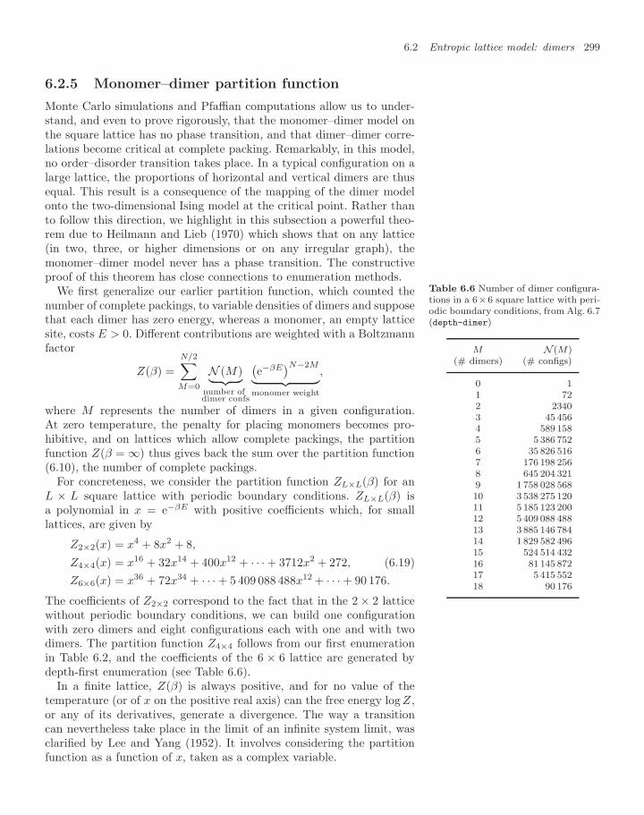
6.2 Entropic lattice model: dimers 299
6.2.5 Monomer–dimer partition function
Monte Carlo simulations and Pfaffian computations allow us to under-stand, and even to prove rigorously, that the monomer–dimer model onthe square lattice has no phase transition, and that dimer–dimer corre-lations become critical at complete packing. Remarkably, in this model,no order–disorder transition takes place. In a typical configuration on alarge lattice, the proportions of horizontal and vertical dimers are thusequal. This result is a consequence of the mapping of the dimer modelonto the two-dimensional Ising model at the critical point. Rather thanto follow this direction, we highlight in this subsection a powerful theo-rem due to Heilmann and Lieb (1970) which shows that on any lattice(in two, three, or higher dimensions or on any irregular graph), themonomer–dimer model never has a phase transition. The constructiveproof of this theorem has close connections to enumeration methods.
We first generalize our earlier partition function, which counted thenumber of complete packings, to variable densities of dimers and supposethat each dimer has zero energy, whereas a monomer, an empty latticesite, costs E > 0. Different contributions are weighted with a Boltzmannfactor
Z(β) =N/2∑M=0
N (M)︸ ︷︷ ︸number ofdimer confs
(e−βE
)N−2M︸ ︷︷ ︸monomer weight
,
where M represents the number of dimers in a given configuration.At zero temperature, the penalty for placing monomers becomes pro-hibitive, and on lattices which allow complete packings, the partitionfunction Z(β = ∞) thus gives back the sum over the partition function(6.10), the number of complete packings.
Table 6.6 Number of dimer configura-tions in a 6×6 square lattice with peri-odic boundary conditions, from Alg. 6.7(depth-dimer)
M N (M)(# dimers) (# configs)
0 11 722 23403 45 4564 589 1585 5 386 7526 35 826 5167 176 198 2568 645 204 3219 1 758 028 56810 3 538 275 12011 5 185 123 20012 5 409 088 48813 3 885 146 78414 1 829 582 49615 524 514 43216 81 145 87217 5 415 55218 90 176
For concreteness, we consider the partition function ZL×L(β) for anL × L square lattice with periodic boundary conditions. ZL×L(β) isa polynomial in x = e−βE with positive coefficients which, for smalllattices, are given by
Z2×2(x) = x4 + 8x2 + 8,
Z4×4(x) = x16 + 32x14 + 400x12 + · · · + 3712x2 + 272, (6.19)Z6×6(x) = x36 + 72x34 + · · · + 5 409 088 488x12 + · · · + 90 176.
The coefficients of Z2×2 correspond to the fact that in the 2 × 2 latticewithout periodic boundary conditions, we can build one configurationwith zero dimers and eight configurations each with one and with twodimers. The partition function Z4×4 follows from our first enumerationin Table 6.2, and the coefficients of the 6 × 6 lattice are generated bydepth-first enumeration (see Table 6.6).
In a finite lattice, Z(β) is always positive, and for no value of thetemperature (or of x on the positive real axis) can the free energy log Z,or any of its derivatives, generate a divergence. The way a transitioncan nevertheless take place in the limit of an infinite system limit, wasclarified by Lee and Yang (1952). It involves considering the partitionfunction as a function of x, taken as a complex variable.
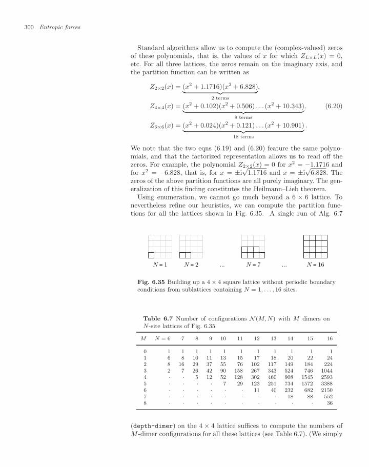
300 Entropic forces
Standard algorithms allow us to compute the (complex-valued) zerosof these polynomials, that is, the values of x for which ZL×L(x) = 0,etc. For all three lattices, the zeros remain on the imaginary axis, andthe partition function can be written as
Z2×2(x) = (x2 + 1.1716)(x2 + 6.828)︸ ︷︷ ︸2 terms
,
Z4×4(x) = (x2 + 0.102)(x2 + 0.506) . . . (x2 + 10.343)︸ ︷︷ ︸8 terms
, (6.20)
Z6×6(x) = (x2 + 0.024)(x2 + 0.121) . . . (x2 + 10.901)︸ ︷︷ ︸18 terms
.
We note that the two eqns (6.19) and (6.20) feature the same polyno-mials, and that the factorized representation allows us to read off thezeros. For example, the polynomial Z2×2(x) = 0 for x2 = −1.1716 andfor x2 = −6.828, that is, for x = ±i
√1.1716 and x = ±i
√6.828. The
zeros of the above partition functions are all purely imaginary. The gen-eralization of this finding constitutes the Heilmann–Lieb theorem.
Using enumeration, we cannot go much beyond a 6 × 6 lattice. Tonevertheless refine our heuristics, we can compute the partition func-tions for all the lattices shown in Fig. 6.35. A single run of Alg. 6.7
N = 1 N = 2 ... N = 7 ... N = 16
Fig. 6.35 Building up a 4 × 4 square lattice without periodic boundaryconditions from sublattices containing N = 1, . . . , 16 sites.
Table 6.7 Number of configurations N (M, N) with M dimers onN-site lattices of Fig. 6.35
M N = 6 7 8 9 10 11 12 13 14 15 16
0 1 1 1 1 1 1 1 1 1 1 11 6 8 10 11 13 15 17 18 20 22 242 8 16 29 37 55 76 102 117 149 184 2243 2 7 26 42 90 158 267 343 524 746 10444 · · 5 12 52 128 302 460 908 1545 25935 · · · · 7 29 123 251 734 1572 33886 · · · · · · 11 40 232 682 21507 · · · · · · · · 18 88 5528 · · · · · · · · · · 36
(depth-dimer) on the 4 × 4 lattice suffices to compute the numbers ofM -dimer configurations for all these lattices (see Table 6.7). (We simply
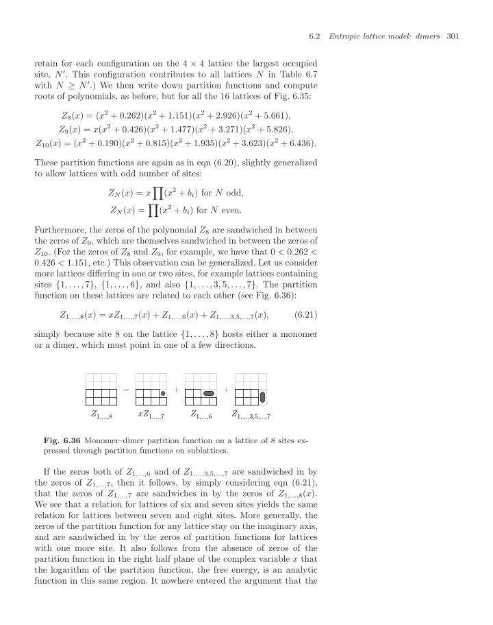
6.2 Entropic lattice model: dimers 301
retain for each configuration on the 4 × 4 lattice the largest occupiedsite, N ′. This configuration contributes to all lattices N in Table 6.7with N ≥ N ′.) We then write down partition functions and computeroots of polynomials, as before, but for all the 16 lattices of Fig. 6.35:
Z8(x) = (x2 + 0.262)(x2 + 1.151)(x2 + 2.926)(x2 + 5.661),
Z9(x) = x(x2 + 0.426)(x2 + 1.477)(x2 + 3.271)(x2 + 5.826),Z10(x) = (x2 + 0.190)(x2 + 0.815)(x2 + 1.935)(x2 + 3.623)(x2 + 6.436).
These partition functions are again as in eqn (6.20), slightly generalizedto allow lattices with odd number of sites:
ZN (x) = x∏
(x2 + bi) for N odd,
ZN (x) =∏
(x2 + bi) for N even.
Furthermore, the zeros of the polynomial Z8 are sandwiched in betweenthe zeros of Z9, which are themselves sandwiched in between the zeros ofZ10. (For the zeros of Z8 and Z9, for example, we have that 0 < 0.262 <0.426 < 1.151, etc.) This observation can be generalized. Let us considermore lattices differing in one or two sites, for example lattices containingsites 1, . . . , 7, 1, . . . , 6, and also 1, . . . , 3, 5, . . . , 7. The partitionfunction on these lattices are related to each other (see Fig. 6.36):
Z1,...,8(x) = xZ1,...,7(x) + Z1,...,6(x) + Z1,...,3,5,...,7(x), (6.21)
simply because site 8 on the lattice 1, . . . , 8 hosts either a monomeror a dimer, which must point in one of a few directions.
Z1,...,8
=
xZ1,...,7
+
Z1,...,6
+
Z1,...,3,5,...,7
Fig. 6.36 Monomer–dimer partition function on a lattice of 8 sites ex-pressed through partition functions on sublattices.
If the zeros both of Z1,...,6 and of Z1,...,3,5,...,7 are sandwiched in bythe zeros of Z1,...,7, then it follows, by simply considering eqn (6.21),that the zeros of Z1,...,7 are sandwiches in by the zeros of Z1,...,8(x).We see that a relation for lattices of six and seven sites yields the samerelation for lattices between seven and eight sites. More generally, thezeros of the partition function for any lattice stay on the imaginary axis,and are sandwiched in by the zeros of partition functions for latticeswith one more site. It also follows from the absence of zeros of thepartition function in the right half plane of the complex variable x thatthe logarithm of the partition function, the free energy, is an analyticfunction in this same region. It nowhere entered the argument that the

302 Entropic forces
lattice was planar, or the sublattices of the special form used in ourexample. Whatever the lattice (2-dimensional lattice, three-dimensional,an irregular graph, etc.), there can thus never be a phase transition inthe monomer–dimer model.
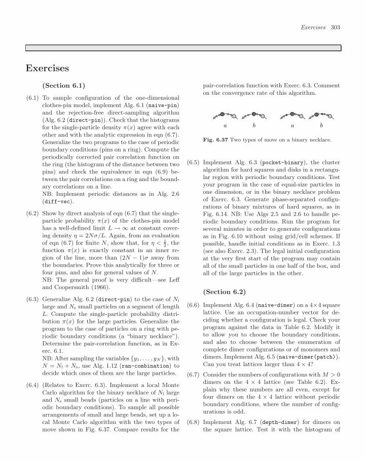
Exercises 303
Exercises
(Section 6.1)
(6.1) To sample configuration of the one-dimensionalclothes-pin model, implement Alg. 6.1 (naive-pin)and the rejection-free direct-sampling algorithm(Alg. 6.2 (direct-pin)). Check that the histogramsfor the single-particle density π(x) agree with eachother and with the analytic expression in eqn (6.7).Generalize the two programs to the case of periodicboundary conditions (pins on a ring). Compute theperiodically corrected pair correlation function onthe ring (the histogram of the distance between twopins) and check the equivalence in eqn (6.9) be-tween the pair correlations on a ring and the bound-ary correlations on a line.NB: Implement periodic distances as in Alg. 2.6(diff-vec).
(6.2) Show by direct analysis of eqn (6.7) that the single-particle probability π(x) of the clothes-pin modelhas a well-defined limit L → ∞ at constant cover-ing density η = 2Nσ/L. Again, from an evaluationof eqn (6.7) for finite N , show that, for η < 1
2, the
function π(x) is exactly constant in an inner re-gion of the line, more than (2N − 1)σ away fromthe boundaries. Prove this analytically for three orfour pins, and also for general values of N .NB: The general proof is very difficult—see Leffand Coopersmith (1966).
(6.3) Generalize Alg. 6.2 (direct-pin) to the case of Nl
large and Ns small particles on a segment of lengthL. Compute the single-particle probability distri-bution π(x) for the large particles. Generalize theprogram to the case of particles on a ring with pe-riodic boundary conditions (a “binary necklace”).Determine the pair-correlation function, as in Ex-erc. 6.1.NB: After sampling the variables y1, . . . , yN, withN = Nl + Ns, use Alg. 1.12 (ran-combination) todecide which ones of them are the large particles.
(6.4) (Relates to Exerc. 6.3). Implement a local MonteCarlo algorithm for the binary necklace of Nl largeand Ns small beads (particles on a line with peri-odic boundary conditions). To sample all possiblearrangements of small and large beads, set up a lo-cal Monte Carlo algorithm with the two types ofmove shown in Fig. 6.37. Compare results for the
pair-correlation function with Exerc. 6.3. Commenton the convergence rate of this algorithm.
a b a b
Fig. 6.37 Two types of move on a binary necklace.
(6.5) Implement Alg. 6.3 (pocket-binary), the clusteralgorithm for hard squares and disks in a rectangu-lar region with periodic boundary conditions. Testyour program in the case of equal-size particles inone dimension, or in the binary necklace problemof Exerc. 6.3. Generate phase-separated configu-rations of binary mixtures of hard squares, as inFig. 6.14. NB: Use Algs 2.5 and 2.6 to handle pe-riodic boundary conditions. Run the program forseveral minutes in order to generate configurationsas in Fig. 6.10 without using grid/cell schemes. Ifpossible, handle initial conditions as in Exerc. 1.3(see also Exerc. 2.3). The legal initial configurationat the very first start of the program may containall of the small particles in one half of the box, andall of the large particles in the other.
(Section 6.2)
(6.6) Implement Alg. 6.4 (naive-dimer) on a 4×4 squarelattice. Use an occupation-number vector for de-ciding whether a configuration is legal. Check yourprogram against the data in Table 6.2. Modify itto allow you to choose the boundary conditions,and also to choose between the enumeration ofcomplete dimer configurations or of monomers anddimers. Implement Alg. 6.5 (naive-dimer(patch)).Can you treat lattices larger than 4 × 4?
(6.7) Consider the numbers of configurations with M > 0dimers on the 4 × 4 lattice (see Table 6.2). Ex-plain why these numbers are all even, except forfour dimers on the 4 × 4 lattice without periodicboundary conditions, where the number of config-urations is odd.
(6.8) Implement Alg. 6.7 (depth-dimer) for dimers onthe square lattice. Test it with the histogram of
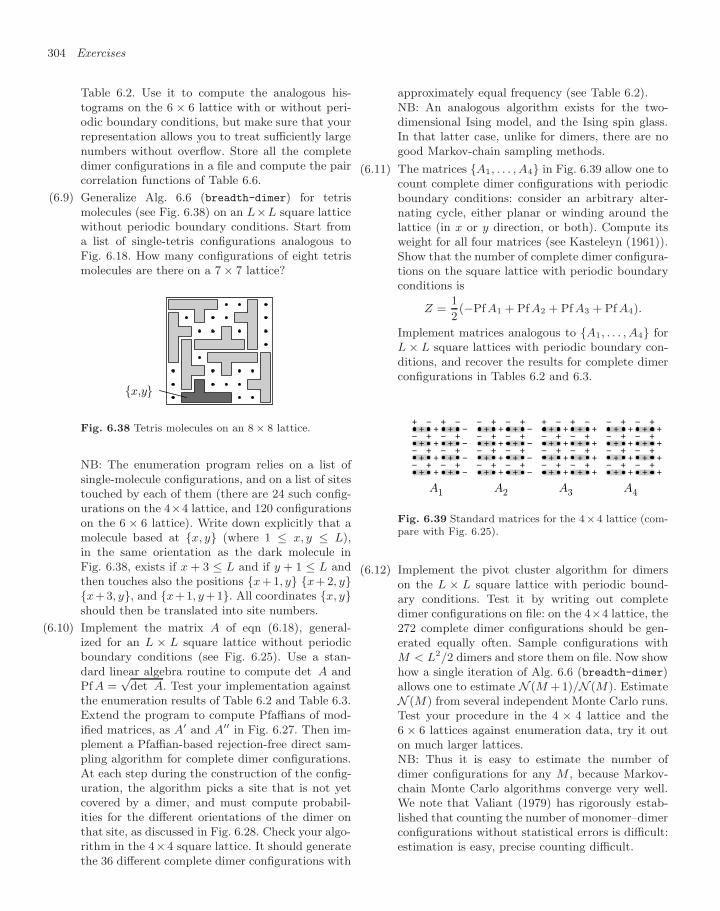
304 Exercises
Table 6.2. Use it to compute the analogous his-tograms on the 6 × 6 lattice with or without peri-odic boundary conditions, but make sure that yourrepresentation allows you to treat sufficiently largenumbers without overflow. Store all the completedimer configurations in a file and compute the paircorrelation functions of Table 6.6.
(6.9) Generalize Alg. 6.6 (breadth-dimer) for tetrismolecules (see Fig. 6.38) on an L×L square latticewithout periodic boundary conditions. Start froma list of single-tetris configurations analogous toFig. 6.18. How many configurations of eight tetrismolecules are there on a 7 × 7 lattice?
x,y
Fig. 6.38 Tetris molecules on an 8 × 8 lattice.
NB: The enumeration program relies on a list ofsingle-molecule configurations, and on a list of sitestouched by each of them (there are 24 such config-urations on the 4×4 lattice, and 120 configurationson the 6 × 6 lattice). Write down explicitly that amolecule based at x, y (where 1 ≤ x, y ≤ L),in the same orientation as the dark molecule inFig. 6.38, exists if x + 3 ≤ L and if y + 1 ≤ L andthen touches also the positions x+1, y x+2, yx+3, y, and x+1, y+1. All coordinates x, yshould then be translated into site numbers.
(6.10) Implement the matrix A of eqn (6.18), general-ized for an L × L square lattice without periodicboundary conditions (see Fig. 6.25). Use a stan-dard linear algebra routine to compute det A andPfA =
√det A. Test your implementation against
the enumeration results of Table 6.2 and Table 6.3.Extend the program to compute Pfaffians of mod-ified matrices, as A′ and A′′ in Fig. 6.27. Then im-plement a Pfaffian-based rejection-free direct sam-pling algorithm for complete dimer configurations.At each step during the construction of the config-uration, the algorithm picks a site that is not yetcovered by a dimer, and must compute probabil-ities for the different orientations of the dimer onthat site, as discussed in Fig. 6.28. Check your algo-rithm in the 4×4 square lattice. It should generatethe 36 different complete dimer configurations with
approximately equal frequency (see Table 6.2).NB: An analogous algorithm exists for the two-dimensional Ising model, and the Ising spin glass.In that latter case, unlike for dimers, there are nogood Markov-chain sampling methods.
(6.11) The matrices A1, . . . , A4 in Fig. 6.39 allow one tocount complete dimer configurations with periodicboundary conditions: consider an arbitrary alter-nating cycle, either planar or winding around thelattice (in x or y direction, or both). Compute itsweight for all four matrices (see Kasteleyn (1961)).Show that the number of complete dimer configura-tions on the square lattice with periodic boundaryconditions is
Z =1
2(−PfA1 + Pf A2 + Pf A3 + Pf A4).
Implement matrices analogous to A1, . . . , A4 forL × L square lattices with periodic boundary con-ditions, and recover the results for complete dimerconfigurations in Tables 6.2 and 6.3.
+
+
+
+
+
+
+ + +
+ + +
+ + +
+ + +
−
−
−
−
−
−
−
−
−
−+ − + −
A1
+
+
+
+
+
+
+ + +
+ + +
+ + +
+ + +
−
−
−
−
−
−
−
−
−
−− + − +
A2
+
+
+
+
+
+
+ + +
+ + +
+ + +
+ + +
−
−
−
−
−
−
+ − + −
+
+
+
+
A3
+
+
+
+
+
+
+ + +
+ + +
+ + +
+ + +
−
−
−
−
−
−
− + − +
+
+
+
+
A4
Fig. 6.39 Standard matrices for the 4× 4 lattice (com-pare with Fig. 6.25).
(6.12) Implement the pivot cluster algorithm for dimerson the L × L square lattice with periodic bound-ary conditions. Test it by writing out completedimer configurations on file: on the 4×4 lattice, the272 complete dimer configurations should be gen-erated equally often. Sample configurations withM < L2/2 dimers and store them on file. Now showhow a single iteration of Alg. 6.6 (breadth-dimer)allows one to estimate N (M +1)/N (M). EstimateN (M) from several independent Monte Carlo runs.Test your procedure in the 4 × 4 lattice and the6 × 6 lattices against enumeration data, try it outon much larger lattices.NB: Thus it is easy to estimate the number ofdimer configurations for any M , because Markov-chain Monte Carlo algorithms converge very well.We note that Valiant (1979) has rigorously estab-lished that counting the number of monomer–dimerconfigurations without statistical errors is difficult:estimation is easy, precise counting difficult.
References 305
References
Asakura S., Oosawa F. (1954) On interaction between 2 bodies immersedin a solution of macromolecules, Journal of Chemical Physics 22, 1255–1256
Buhot A., Krauth W. (1999) Phase separation in two-dimensional addi-tive mixtures, Physical Review E 59, 2939–2941
Dinsmore A. D., Yodh A. G., Pine D. J. (1995) Phase-diagrams of nearlyhard-sphere binary colloids, Physical Review E 52, 4045–4057
Fisher M. E., Stephenson J. (1963) Statistical mechanics of dimers ona plane lattice. II. Dimer correlations and monomers, Physical Review132, 1411–1431
Galbiati G., Maffioli F. (1994) On the computation of Pfaffians, Dis-crete Applied Mathematics 51, 269–275
Heilmann O. J., Lieb E. H. (1970) Monomers and dimers, Physical Re-view Letters 24, 1412–1414
Kasteleyn P. W. (1961) The statistics of dimers on a lattice I. The num-ber of dimer arrangements on a quadratic lattice, Physica 27, 1209–1225
Krauth W., Moessner R. (2003) Pocket Monte Carlo algorithm for clas-sical doped dimer models, Physical Review B 67, 064503
Lee T. D., Yang C. N. (1952) Statistical theory of equations of stateand phase transitions. 2. Lattice gas and Ising model, Physical Review87, 410–419
Leff H. S., Coopersmith M. H. (1966) Translational invariance proper-ties of a finite one-dimensional hard-core fluid, Journal of MathematicalPhysics 8, 306–314
Valiant L. G. (1979) Complexity of enumeration and reliability prob-lems, SIAM Journal on Computing 8, 410–421

This page intentionally left blank
Dynamic Monte Carlomethods 7
7.1 Random sequentialdeposition 309
7.2 Dynamic spin algorithms 313
7.3 Disks on the unit sphere 321
Exercises 333
References 335
In the first six chapters of this book, we have concentrated on equilibriumstatistical mechanics and related computational-physics approaches, no-tably the equilibrium Monte Carlo method. These and other approachesallowed us to determine partition functions, energies, superfluid densi-ties, etc. Physical time played a minor role, as the observables were gen-erally time-independent. Likewise, Monte Carlo “time” was treated as ofsecondary interest, if not a nuisance: we strove only to make things hap-pen as quickly as possible, that is, to have algorithms converge rapidly.
The moment has come to reach beyond equilibrium statistical mechan-ics, and to explore time-dependent phenomena such as the crystallizationof hard spheres after a sudden increase in pressure or the magnetic re-sponse of Ising spins to an external field switched on at some initial time.The local Monte Carlo algorithm often provides an excellent frameworkfor studying dynamical phenomena.
The conceptual difference between equilibrium and dynamic MonteCarlo methods cannot be overemphasized. In the first case, we have anessentially unrestricted choice of a priori probabilities, since we only wantto generate independent configurations x distributed with a probabilityπ(x), in whatever way we choose, but as fast as possible. In dynamiccalculations, the time dependence becomes the main object of our study.We first look at this difference between equilibrium and dynamics in thecase of the random-sequential-deposition problem of Chapter 2, wherea powerful dynamic algorithm perfectly implements the faster-than-the-clock paradigm. We then discuss dynamic Monte Carlo methods for theIsing model and encounter the main limitation of the faster-than-the-clock approach, the futility problem.
In the final section of this chapter, we apply a Monte Carlo methodcalled simulated annealing, an important tool for solving difficult opti-mization problems, mostly without any relation to physics. In this ap-proach, a discrete or continuous optimization problem is mapped ontoan artificial physical system whose ground state (at zero temperature orinfinite pressure) contains the solution to the original task. This groundstate is slowly approached through simulation. Simulated annealing willbe discussed for monodisperse and polydisperse hard disks on the surfaceof a sphere, under increasing pressure. It works prodigiously in one case,where the disks end up crystallizing, but fails in another case, wherethey settle into a glassy state.
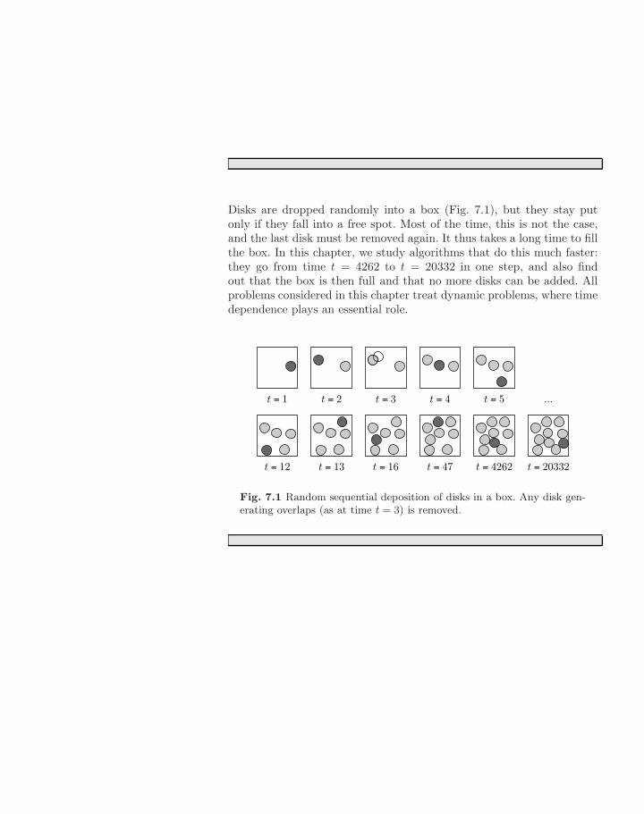
Disks are dropped randomly into a box (Fig. 7.1), but they stay putonly if they fall into a free spot. Most of the time, this is not the case,and the last disk must be removed again. It thus takes a long time to fillthe box. In this chapter, we study algorithms that do this much faster:they go from time t = 4262 to t = 20332 in one step, and also findout that the box is then full and that no more disks can be added. Allproblems considered in this chapter treat dynamic problems, where timedependence plays an essential role.
t = 1 t = 2 t = 3 t = 4 t = 5 ...
t = 12 t = 13 t = 16 t = 47 t = 4262 t = 20332
Fig. 7.1 Random sequential deposition of disks in a box. Any disk gen-erating overlaps (as at time t = 3) is removed.
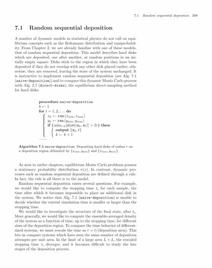
7.1 Random sequential deposition 309
7.1 Random sequential deposition
A number of dynamic models in statistical physics do not call on equi-librium concepts such as the Boltzmann distribution and equiprobabil-ity. From Chapter 2, we are already familiar with one of these models,that of random sequential deposition. This model describes hard diskswhich are deposited, one after another, at random positions in an ini-tially empty square. Disks stick to the region in which they have beendeposited if they do not overlap with any other disk placed earlier; oth-erwise, they are removed, leaving the state of the system unchanged. Itis instructive to implement random sequential deposition (see Alg. 7.1(naive-deposition)) and to compare this dynamic Monte Carlo processwith Alg. 2.7 (direct-disks), the equilibrium direct-sampling methodfor hard disks.
procedure naive-deposition
k ← 1for t = 1, 2, . . . do⎧⎪⎪⎪⎪⎨⎪⎪⎪⎪⎩
xk ← ran (xmin, xmax)yk ← ran (ymin, ymax)if (minl<k[dist(xk,xl)] > 2r) then
output xk, tk ← k + 1
——
Algorithm 7.1 naive-deposition. Depositing hard disks of radius r ona deposition region delimited by xmin, ymin and xmax, ymax.
As seen in earlier chapters, equilibrium Monte Carlo problems possessa stationary probability distribution π(x). In contrast, dynamic pro-cesses such as random sequential deposition are defined through a rule.In fact, the rule is all there is to the model.
Random sequential deposition raises several questions. For example,we would like to compute the stopping time ts for each sample, thetime after which it becomes impossible to place an additional disk inthe system. We notice that Alg. 7.1 (naive-deposition) is unable todecide whether the current simulation time is smaller or larger than thestopping time.
We would like to investigate the structure of the final state, after ts.More generally, we would like to compute the ensemble-averaged densityof the system as a function of time, up to the stopping time, for differentsizes of the deposition region. To compare the time behavior of different-sized systems, we must rescale the time as τ = t/(deposition area). Thislets us compare systems which have seen the same number of depositionattempts per unit area. In the limit of a large area L × L, the rescaledstopping time τs diverges, and it becomes difficult to study the latestages of the deposition process.
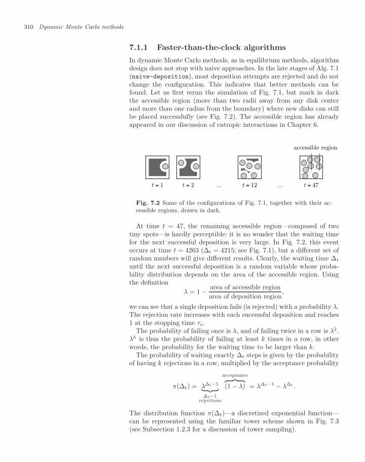
310 Dynamic Monte Carlo methods
7.1.1 Faster-than-the-clock algorithms
In dynamic Monte Carlo methods, as in equilibrium methods, algorithmdesign does not stop with naive approaches. In the late stages of Alg. 7.1(naive-deposition), most deposition attempts are rejected and do notchange the configuration. This indicates that better methods can befound. Let us first rerun the simulation of Fig. 7.1, but mark in darkthe accessible region (more than two radii away from any disk centerand more than one radius from the boundary) where new disks can stillbe placed successfully (see Fig. 7.2). The accessible region has alreadyappeared in our discussion of entropic interactions in Chapter 6.
t = 1 t = 2 ... t = 12 ... t = 47
accessible region
Fig. 7.2 Some of the configurations of Fig. 7.1, together with their ac-cessible regions, drawn in dark.
At time t = 47, the remaining accessible region—composed of twotiny spots—is hardly perceptible: it is no wonder that the waiting timefor the next successful deposition is very large. In Fig. 7.2, this eventoccurs at time t = 4263 (∆t = 4215; see Fig. 7.1), but a different set ofrandom numbers will give different results. Clearly, the waiting time ∆t
until the next successful deposition is a random variable whose proba-bility distribution depends on the area of the accessible region. Usingthe definition
λ = 1 − area of accessible regionarea of deposition region
,
we can see that a single deposition fails (is rejected) with a probability λ.The rejection rate increases with each successful deposition and reaches1 at the stopping time τs.
The probability of failing once is λ, and of failing twice in a row is λ2.λk is thus the probability of failing at least k times in a row, in otherwords, the probability for the waiting time to be larger than k.
The probability of waiting exactly ∆t steps is given by the probabilityof having k rejections in a row, multiplied by the acceptance probability
π(∆t) = λ∆t−1︸ ︷︷ ︸∆t−1
rejections
acceptance︷ ︸︸ ︷(1 − λ) = λ∆t−1 − λ∆t .
The distribution function π(∆t)—a discretized exponential function—can be represented using the familiar tower scheme shown in Fig. 7.3(see Subsection 1.2.3 for a discussion of tower sampling).
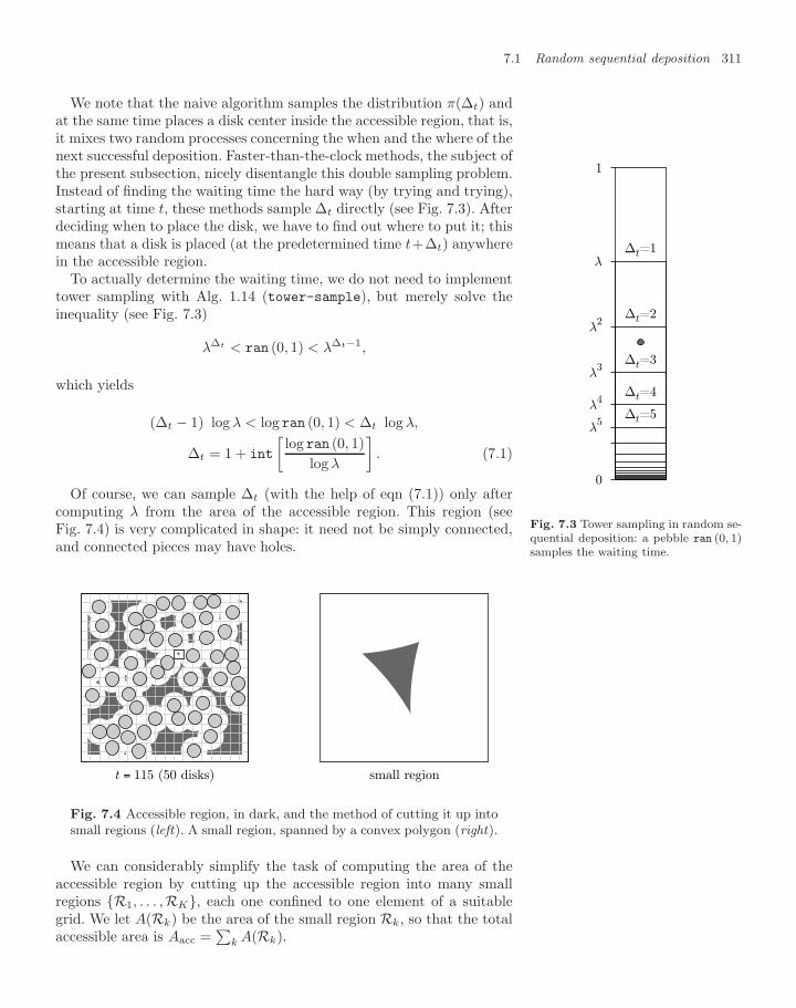
7.1 Random sequential deposition 311
We note that the naive algorithm samples the distribution π(∆t) andat the same time places a disk center inside the accessible region, that is,it mixes two random processes concerning the when and the where of thenext successful deposition. Faster-than-the-clock methods, the subject ofthe present subsection, nicely disentangle this double sampling problem.Instead of finding the waiting time the hard way (by trying and trying),starting at time t, these methods sample ∆t directly (see Fig. 7.3). Afterdeciding when to place the disk, we have to find out where to put it; thismeans that a disk is placed (at the predetermined time t+∆t) anywherein the accessible region.
To actually determine the waiting time, we do not need to implementtower sampling with Alg. 1.14 (tower-sample), but merely solve theinequality (see Fig. 7.3)
λ∆t < ran (0, 1) < λ∆t−1,
which yields
(∆t − 1) log λ < log ran (0, 1) < ∆t log λ,
∆t = 1 + int
[log ran (0, 1)
log λ
]. (7.1)
0
1
∆t=1λ
∆t=2λ2
∆t=3λ3
∆t=4λ4
∆t=5λ5
Fig. 7.3 Tower sampling in random se-quential deposition: a pebble ran (0, 1)samples the waiting time.
Of course, we can sample ∆t (with the help of eqn (7.1)) only aftercomputing λ from the area of the accessible region. This region (seeFig. 7.4) is very complicated in shape: it need not be simply connected,and connected pieces may have holes.
t = 115 (50 disks) small region
Fig. 7.4 Accessible region, in dark, and the method of cutting it up intosmall regions (left). A small region, spanned by a convex polygon (right).
We can considerably simplify the task of computing the area of theaccessible region by cutting up the accessible region into many smallregions R1, . . . ,RK, each one confined to one element of a suitablegrid. We let A(Rk) be the area of the small region Rk, so that the totalaccessible area is Aacc =
∑k A(Rk).
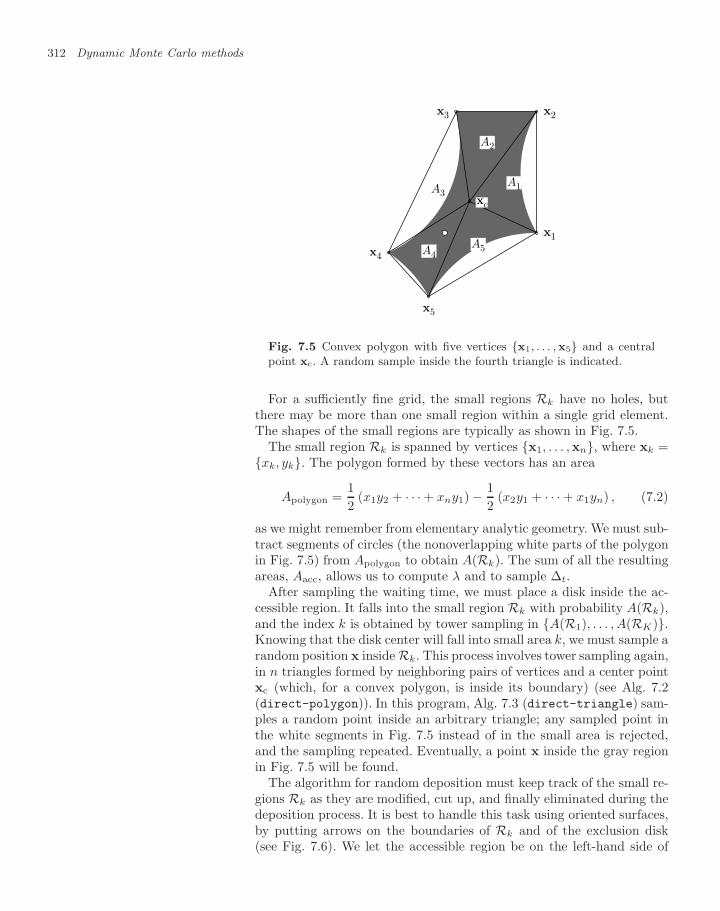
312 Dynamic Monte Carlo methods
x1
x2x3
x4
x5
xc
A1
A2
A3
A4A5
Fig. 7.5 Convex polygon with five vertices x1, . . . ,x5 and a centralpoint xc. A random sample inside the fourth triangle is indicated.
For a sufficiently fine grid, the small regions Rk have no holes, butthere may be more than one small region within a single grid element.The shapes of the small regions are typically as shown in Fig. 7.5.
The small region Rk is spanned by vertices x1, . . . ,xn, where xk =xk, yk. The polygon formed by these vectors has an area
Apolygon =12
(x1y2 + · · · + xny1) − 12
(x2y1 + · · · + x1yn) , (7.2)
as we might remember from elementary analytic geometry. We must sub-tract segments of circles (the nonoverlapping white parts of the polygonin Fig. 7.5) from Apolygon to obtain A(Rk). The sum of all the resultingareas, Aacc, allows us to compute λ and to sample ∆t.
After sampling the waiting time, we must place a disk inside the ac-cessible region. It falls into the small region Rk with probability A(Rk),and the index k is obtained by tower sampling in A(R1), . . . , A(RK).Knowing that the disk center will fall into small area k, we must sample arandom position x inside Rk. This process involves tower sampling again,in n triangles formed by neighboring pairs of vertices and a center pointxc (which, for a convex polygon, is inside its boundary) (see Alg. 7.2(direct-polygon)). In this program, Alg. 7.3 (direct-triangle) sam-ples a random point inside an arbitrary triangle; any sampled point inthe white segments in Fig. 7.5 instead of in the small area is rejected,and the sampling repeated. Eventually, a point x inside the gray regionin Fig. 7.5 will be found.
The algorithm for random deposition must keep track of the small re-gions Rk as they are modified, cut up, and finally eliminated during thedeposition process. It is best to handle this task using oriented surfaces,by putting arrows on the boundaries of Rk and of the exclusion disk(see Fig. 7.6). We let the accessible region be on the left-hand side of
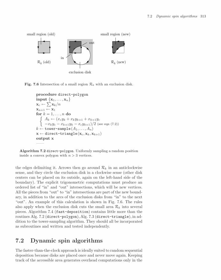
7.2 Dynamic spin algorithms 313
Rk (old)
small region (old)
out
in
exclusion disk
Rk (new)
small region (new)
Fig. 7.6 Intersection of a small region Rk with an exclusion disk.
procedure direct-polygon
input x1, . . . ,xnxc ←
∑xk/n
xn+1 ← x1
for k = 1, . . . , n doAk ← (xcyk + xkyk+1 + xk+1yc
−xkyc − xk+1yk − xcyk+1)/2 (see eqn (7.2))k ← tower-sample(A1, . . . , An)x ← direct-triangle(xc,xk,xk+1)output x——
Algorithm 7.2 direct-polygon. Uniformly sampling a random positioninside a convex polygon with n > 3 vertices.
the edges delimiting it. Arrows then go around Rk in an anticlockwisesense, and they circle the exclusion disk in a clockwise sense (other diskcenters can be placed on its outside, again on the left-hand side of theboundary). The explicit trigonometric computations must produce anordered list of “in” and “out” intersections, which will be new vertices.All the pieces from “out” to “in” intersections are part of the new bound-ary, in addition to the arcs of the exclusion disks from “in” to the next“out”. An example of this calculation is shown in Fig. 7.6. The rulesalso apply when the exclusion disk cuts the small area Rk into severalpieces. Algorithm 7.4 (fast-deposition) contains little more than theroutines Alg. 7.2 (direct-polygon), Alg. 7.3 (direct-triangle), in ad-dition to the tower-sampling algorithm. They should all be incorporatedas subroutines and written and tested independently.
7.2 Dynamic spin algorithms
The faster-than-the-clock approach is ideally suited to random sequentialdeposition because disks are placed once and never move again. Keepingtrack of the accessible area generates overhead computations only in the
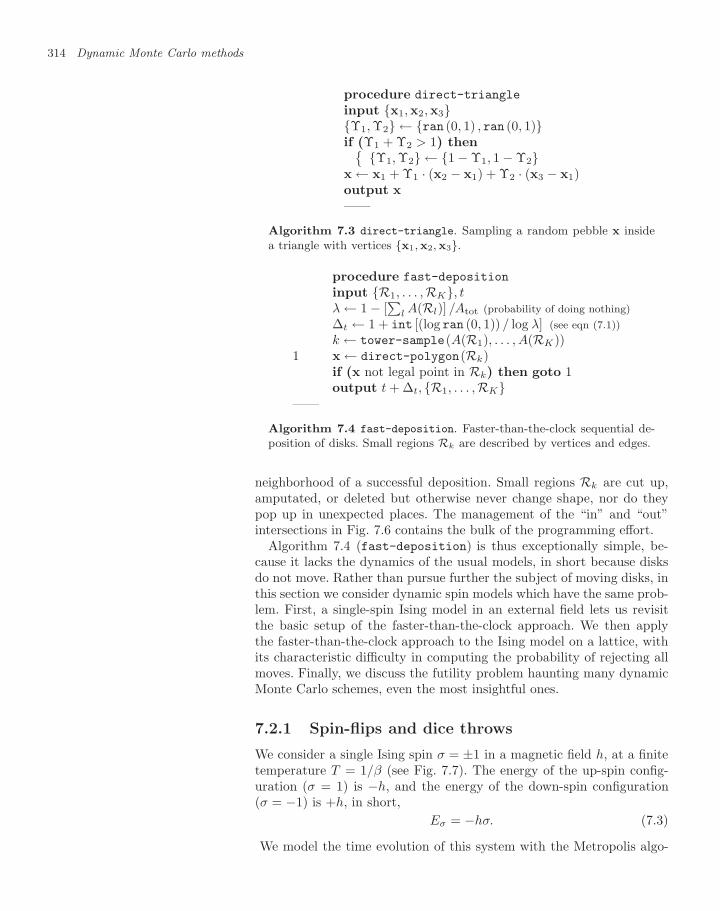
314 Dynamic Monte Carlo methods
procedure direct-triangle
input x1,x2,x3Υ1, Υ2 ← ran (0, 1) , ran (0, 1)if (Υ1 + Υ2 > 1) then Υ1, Υ2 ← 1 − Υ1, 1 − Υ2x ← x1 + Υ1 · (x2 − x1) + Υ2 · (x3 − x1)output x——
Algorithm 7.3 direct-triangle. Sampling a random pebble x insidea triangle with vertices x1,x2, x3.
procedure fast-deposition
input R1, . . . ,RK, tλ ← 1 − [
∑l A(Rl)] /Atot (probability of doing nothing)
∆t ← 1 + int [(log ran (0, 1)) / log λ] (see eqn (7.1))k ← tower-sample(A(R1), . . . , A(RK))
1 x ← direct-polygon(Rk)if (x not legal point in Rk) then goto 1output t + ∆t, R1, . . . ,RK
——
Algorithm 7.4 fast-deposition. Faster-than-the-clock sequential de-position of disks. Small regions Rk are described by vertices and edges.
neighborhood of a successful deposition. Small regions Rk are cut up,amputated, or deleted but otherwise never change shape, nor do theypop up in unexpected places. The management of the “in” and “out”intersections in Fig. 7.6 contains the bulk of the programming effort.
Algorithm 7.4 (fast-deposition) is thus exceptionally simple, be-cause it lacks the dynamics of the usual models, in short because disksdo not move. Rather than pursue further the subject of moving disks, inthis section we consider dynamic spin models which have the same prob-lem. First, a single-spin Ising model in an external field lets us revisitthe basic setup of the faster-than-the-clock approach. We then applythe faster-than-the-clock approach to the Ising model on a lattice, withits characteristic difficulty in computing the probability of rejecting allmoves. Finally, we discuss the futility problem haunting many dynamicMonte Carlo schemes, even the most insightful ones.
7.2.1 Spin-flips and dice throws
We consider a single Ising spin σ = ±1 in a magnetic field h, at a finitetemperature T = 1/β (see Fig. 7.7). The energy of the up-spin config-uration (σ = 1) is −h, and the energy of the down-spin configuration(σ = −1) is +h, in short,
Eσ = −hσ. (7.3)
We model the time evolution of this system with the Metropolis algo-
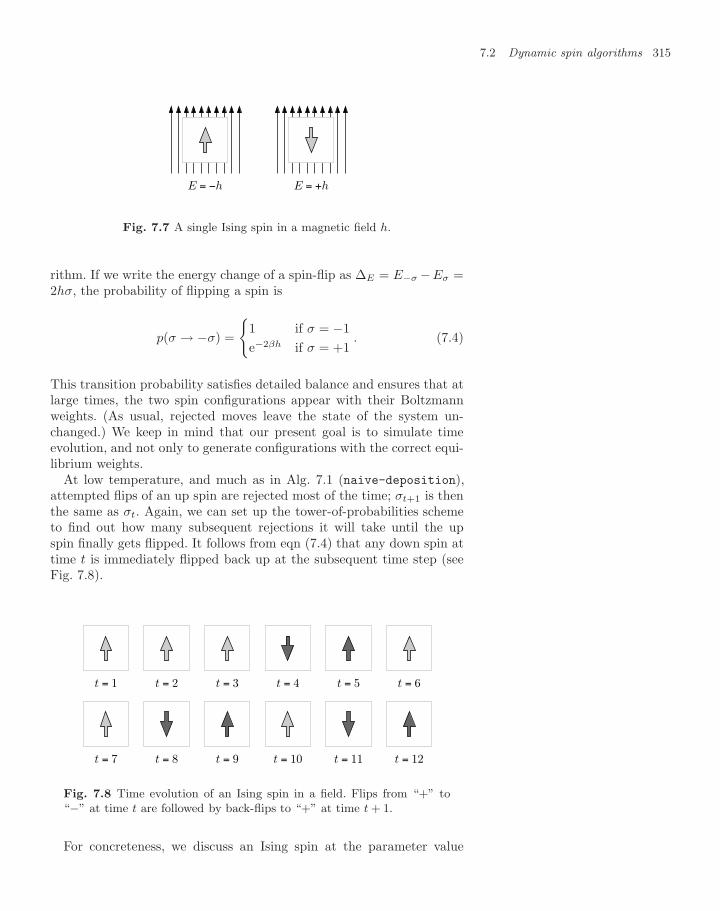
7.2 Dynamic spin algorithms 315
E = −h E = +h
Fig. 7.7 A single Ising spin in a magnetic field h.
rithm. If we write the energy change of a spin-flip as ∆E = E−σ −Eσ =2hσ, the probability of flipping a spin is
p(σ → −σ) =
1 if σ = −1e−2βh if σ = +1
. (7.4)
This transition probability satisfies detailed balance and ensures that atlarge times, the two spin configurations appear with their Boltzmannweights. (As usual, rejected moves leave the state of the system un-changed.) We keep in mind that our present goal is to simulate timeevolution, and not only to generate configurations with the correct equi-librium weights.
At low temperature, and much as in Alg. 7.1 (naive-deposition),attempted flips of an up spin are rejected most of the time; σt+1 is thenthe same as σt. Again, we can set up the tower-of-probabilities schemeto find out how many subsequent rejections it will take until the upspin finally gets flipped. It follows from eqn (7.4) that any down spin attime t is immediately flipped back up at the subsequent time step (seeFig. 7.8).
t = 1 t = 2 t = 3 t = 4 t = 5 t = 6
t = 7 t = 8 t = 9 t = 10 t = 11 t = 12
Fig. 7.8 Time evolution of an Ising spin in a field. Flips from “+” to“−” at time t are followed by back-flips to “+” at time t + 1.
For concreteness, we discuss an Ising spin at the parameter value
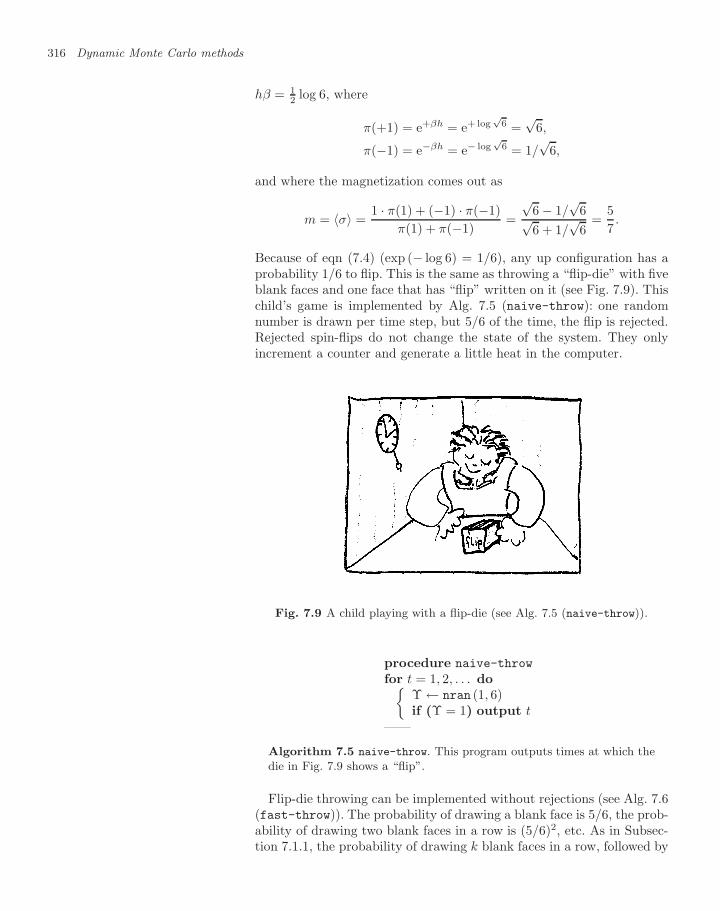
316 Dynamic Monte Carlo methods
hβ = 12 log 6, where
π(+1) = e+βh = e+ log√
6 =√
6,
π(−1) = e−βh = e− log√
6 = 1/√
6,
and where the magnetization comes out as
m = 〈σ〉 =1 · π(1) + (−1) · π(−1)
π(1) + π(−1)=
√6 − 1/
√6√
6 + 1/√
6=
57.
Because of eqn (7.4) (exp (− log 6) = 1/6), any up configuration has aprobability 1/6 to flip. This is the same as throwing a “flip-die” with fiveblank faces and one face that has “flip” written on it (see Fig. 7.9). Thischild’s game is implemented by Alg. 7.5 (naive-throw): one randomnumber is drawn per time step, but 5/6 of the time, the flip is rejected.Rejected spin-flips do not change the state of the system. They onlyincrement a counter and generate a little heat in the computer.
Fig. 7.9 A child playing with a flip-die (see Alg. 7.5 (naive-throw)).
procedure naive-throw
for t = 1, 2, . . . doΥ ← nran (1, 6)if (Υ = 1) output t
——
Algorithm 7.5 naive-throw. This program outputs times at which thedie in Fig. 7.9 shows a “flip”.
Flip-die throwing can be implemented without rejections (see Alg. 7.6(fast-throw)). The probability of drawing a blank face is 5/6, the prob-ability of drawing two blank faces in a row is (5/6)2, etc. As in Subsec-tion 7.1.1, the probability of drawing k blank faces in a row, followed by
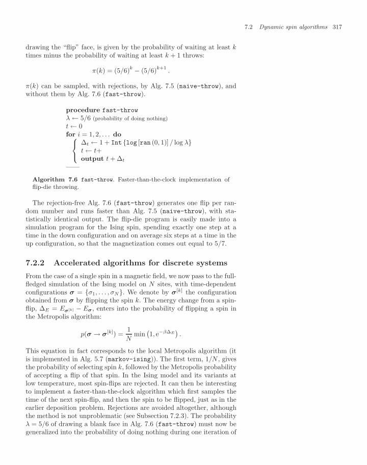
7.2 Dynamic spin algorithms 317
drawing the “flip” face, is given by the probability of waiting at least ktimes minus the probability of waiting at least k + 1 throws:
π(k) = (5/6)k − (5/6)k+1.
π(k) can be sampled, with rejections, by Alg. 7.5 (naive-throw), andwithout them by Alg. 7.6 (fast-throw).
procedure fast-throw
λ ← 5/6 (probability of doing nothing)t ← 0for i = 1, 2, . . . do⎧⎨⎩
∆t ← 1 + Int log [ran (0, 1)] / log λt ← t+output t + ∆t
——
Algorithm 7.6 fast-throw. Faster-than-the-clock implementation offlip-die throwing.
The rejection-free Alg. 7.6 (fast-throw) generates one flip per ran-dom number and runs faster than Alg. 7.5 (naive-throw), with sta-tistically identical output. The flip-die program is easily made into asimulation program for the Ising spin, spending exactly one step at atime in the down configuration and on average six steps at a time in theup configuration, so that the magnetization comes out equal to 5/7.
7.2.2 Accelerated algorithms for discrete systems
From the case of a single spin in a magnetic field, we now pass to the full-fledged simulation of the Ising model on N sites, with time-dependentconfigurations σ = σ1, . . . , σN. We denote by σ[k] the configurationobtained from σ by flipping the spin k. The energy change from a spin-flip, ∆E = E
σ[k] − Eσ , enters into the probability of flipping a spin in
the Metropolis algorithm:
p(σ → σ[k]) =
1N
min(1, e−β∆E
).
This equation in fact corresponds to the local Metropolis algorithm (itis implemented in Alg. 5.7 (markov-ising)). The first term, 1/N , givesthe probability of selecting spin k, followed by the Metropolis probabilityof accepting a flip of that spin. In the Ising model and its variants atlow temperature, most spin-flips are rejected. It can then be interestingto implement a faster-than-the-clock algorithm which first samples thetime of the next spin-flip, and then the spin to be flipped, just as in theearlier deposition problem. Rejections are avoided altogether, althoughthe method is not unproblematic (see Subsection 7.2.3). The probabilityλ = 5/6 of drawing a blank face in Alg. 7.6 (fast-throw) must now begeneralized into the probability of doing nothing during one iteration of
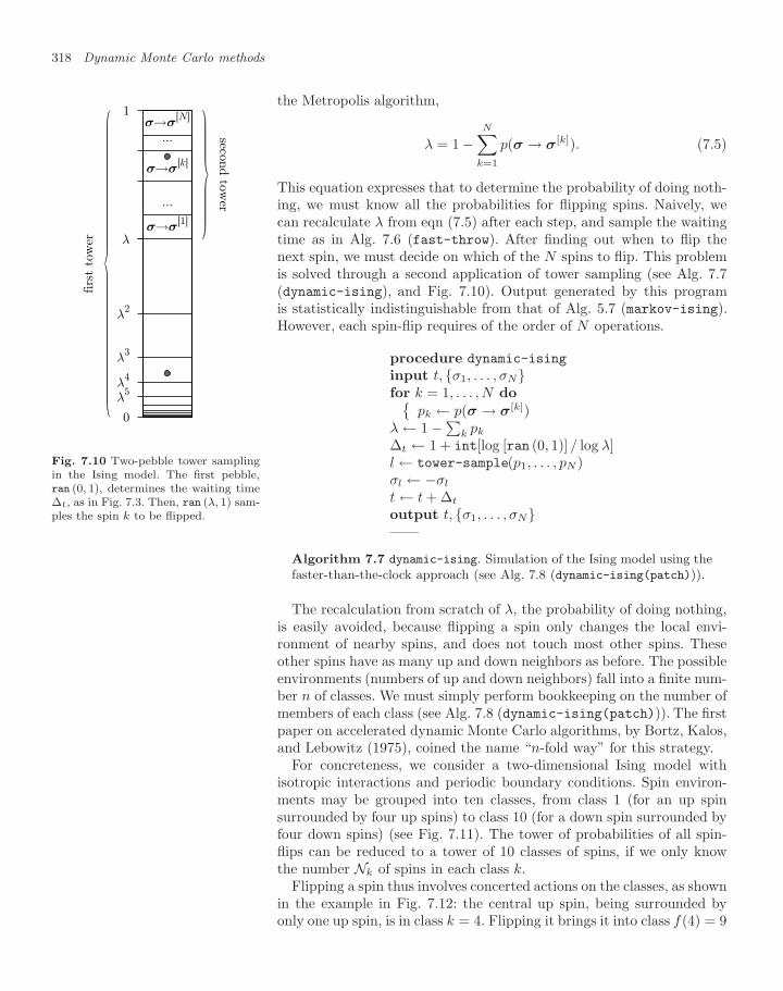
318 Dynamic Monte Carlo methods
the Metropolis algorithm,
λ = 1 −N∑
k=1
p(σ → σ[k]). (7.5)
This equation expresses that to determine the probability of doing noth-ing, we must know all the probabilities for flipping spins. Naively, wecan recalculate λ from eqn (7.5) after each step, and sample the waitingtime as in Alg. 7.6 (fast-throw). After finding out when to flip thenext spin, we must decide on which of the N spins to flip. This problemis solved through a second application of tower sampling (see Alg. 7.7(dynamic-ising), and Fig. 7.10). Output generated by this programis statistically indistinguishable from that of Alg. 5.7 (markov-ising).However, each spin-flip requires of the order of N operations.
0
1
λσ→σ
[1]
λ2
λ3
λ4
λ5
...
σ→σ[k]
...σ→σ
[N]
firs
t to
wer
second tow
er
Fig. 7.10 Two-pebble tower samplingin the Ising model. The first pebble,ran (0, 1), determines the waiting time∆t, as in Fig. 7.3. Then, ran (λ, 1) sam-ples the spin k to be flipped.
procedure dynamic-ising
input t, σ1, . . . , σNfor k = 1, . . . , N do
pk ← p(σ → σ[k])λ ← 1 −∑k pk
∆t ← 1 + int[log [ran (0, 1)] / log λ]l ← tower-sample(p1, . . . , pN )σl ← −σl
t ← t + ∆t
output t, σ1, . . . , σN——
Algorithm 7.7 dynamic-ising. Simulation of the Ising model using thefaster-than-the-clock approach (see Alg. 7.8 (dynamic-ising(patch))).
The recalculation from scratch of λ, the probability of doing nothing,is easily avoided, because flipping a spin only changes the local envi-ronment of nearby spins, and does not touch most other spins. Theseother spins have as many up and down neighbors as before. The possibleenvironments (numbers of up and down neighbors) fall into a finite num-ber n of classes. We must simply perform bookkeeping on the number ofmembers of each class (see Alg. 7.8 (dynamic-ising(patch))). The firstpaper on accelerated dynamic Monte Carlo algorithms, by Bortz, Kalos,and Lebowitz (1975), coined the name “n-fold way” for this strategy.
For concreteness, we consider a two-dimensional Ising model withisotropic interactions and periodic boundary conditions. Spin environ-ments may be grouped into ten classes, from class 1 (for an up spinsurrounded by four up spins) to class 10 (for a down spin surrounded byfour down spins) (see Fig. 7.11). The tower of probabilities of all spin-flips can be reduced to a tower of 10 classes of spins, if we only knowthe number Nk of spins in each class k.
Flipping a spin thus involves concerted actions on the classes, as shownin the example in Fig. 7.12: the central up spin, being surrounded byonly one up spin, is in class k = 4. Flipping it brings it into class f(4) = 9
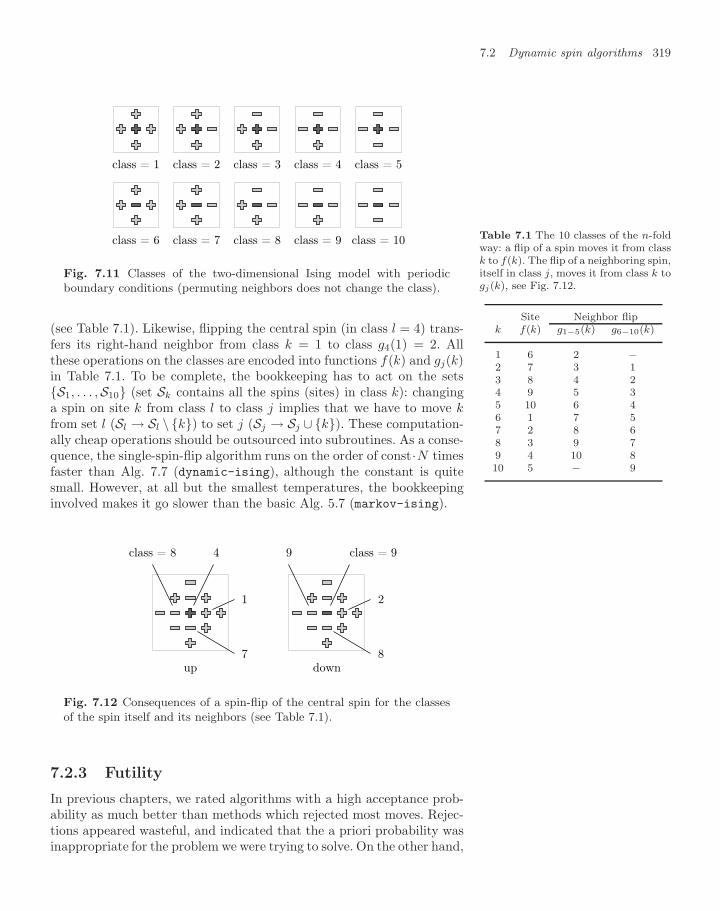
7.2 Dynamic spin algorithms 319
class = 1 class = 2 class = 3 class = 4 class = 5
class = 6 class = 7 class = 8 class = 9 class = 10
Fig. 7.11 Classes of the two-dimensional Ising model with periodicboundary conditions (permuting neighbors does not change the class).
(see Table 7.1). Likewise, flipping the central spin (in class l = 4) trans-fers its right-hand neighbor from class k = 1 to class g4(1) = 2. Allthese operations on the classes are encoded into functions f(k) and gj(k)in Table 7.1. To be complete, the bookkeeping has to act on the setsS1, . . . ,S10 (set Sk contains all the spins (sites) in class k): changinga spin on site k from class l to class j implies that we have to move kfrom set l (Sl → Sl \ k) to set j (Sj → Sj ∪ k). These computation-ally cheap operations should be outsourced into subroutines. As a conse-quence, the single-spin-flip algorithm runs on the order of const·N timesfaster than Alg. 7.7 (dynamic-ising), although the constant is quitesmall. However, at all but the smallest temperatures, the bookkeepinginvolved makes it go slower than the basic Alg. 5.7 (markov-ising).
Table 7.1 The 10 classes of the n-foldway: a flip of a spin moves it from classk to f(k). The flip of a neighboring spin,itself in class j, moves it from class k togj(k), see Fig. 7.12.
Site Neighbor flipk f(k) g1−5(k) g6−10(k)
1 6 2 −2 7 3 13 8 4 24 9 5 35 10 6 46 1 7 57 2 8 68 3 9 79 4 10 810 5 − 9
up
4
1
7
class = 8
down
class = 9
2
8
9
Fig. 7.12 Consequences of a spin-flip of the central spin for the classesof the spin itself and its neighbors (see Table 7.1).
7.2.3 Futility
In previous chapters, we rated algorithms with a high acceptance prob-ability as much better than methods which rejected most moves. Rejec-tions appeared wasteful, and indicated that the a priori probability wasinappropriate for the problem we were trying to solve. On the other hand,
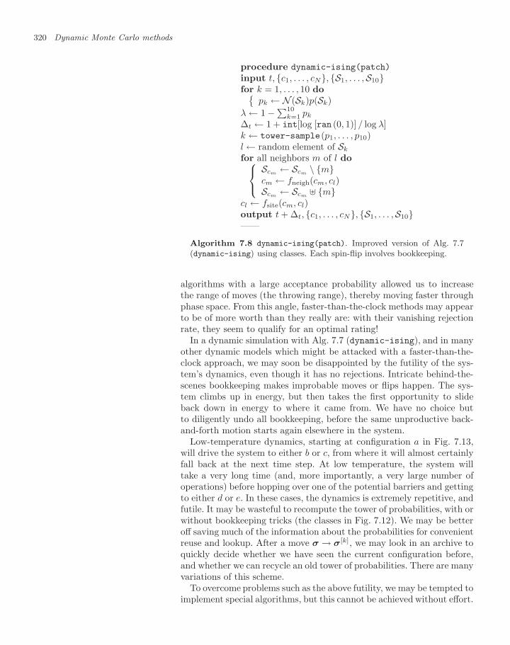
320 Dynamic Monte Carlo methods
procedure dynamic-ising(patch)
input t, c1, . . . , cN, S1, . . . ,S10for k = 1, . . . , 10 do
pk ← N (Sk)p(Sk)λ ← 1 −∑10
k=1 pk
∆t ← 1 + int[log [ran (0, 1)] / log λ]k ← tower-sample(p1, . . . , p10)l ← random element of Sk
for all neighbors m of l do⎧⎨⎩Scm
← Scm\ m
cm ← fneigh(cm, cl)Scm
← Scm$ m
cl ← fsite(cm, cl)output t + ∆t, c1, . . . , cN, S1, . . . ,S10——
Algorithm 7.8 dynamic-ising(patch). Improved version of Alg. 7.7(dynamic-ising) using classes. Each spin-flip involves bookkeeping.
algorithms with a large acceptance probability allowed us to increasethe range of moves (the throwing range), thereby moving faster throughphase space. From this angle, faster-than-the-clock methods may appearto be of more worth than they really are: with their vanishing rejectionrate, they seem to qualify for an optimal rating!
In a dynamic simulation with Alg. 7.7 (dynamic-ising), and in manyother dynamic models which might be attacked with a faster-than-the-clock approach, we may soon be disappointed by the futility of the sys-tem’s dynamics, even though it has no rejections. Intricate behind-the-scenes bookkeeping makes improbable moves or flips happen. The sys-tem climbs up in energy, but then takes the first opportunity to slideback down in energy to where it came from. We have no choice butto diligently undo all bookkeeping, before the same unproductive back-and-forth motion starts again elsewhere in the system.
Low-temperature dynamics, starting at configuration a in Fig. 7.13,will drive the system to either b or c, from where it will almost certainlyfall back at the next time step. At low temperature, the system willtake a very long time (and, more importantly, a very large number ofoperations) before hopping over one of the potential barriers and gettingto either d or e. In these cases, the dynamics is extremely repetitive, andfutile. It may be wasteful to recompute the tower of probabilities, with orwithout bookkeeping tricks (the classes in Fig. 7.12). We may be betteroff saving much of the information about the probabilities for convenientreuse and lookup. After a move σ → σ[k], we may look in an archive toquickly decide whether we have seen the current configuration before,and whether we can recycle an old tower of probabilities. There are manyvariations of this scheme.
To overcome problems such as the above futility, we may be tempted toimplement special algorithms, but this cannot be achieved without effort.
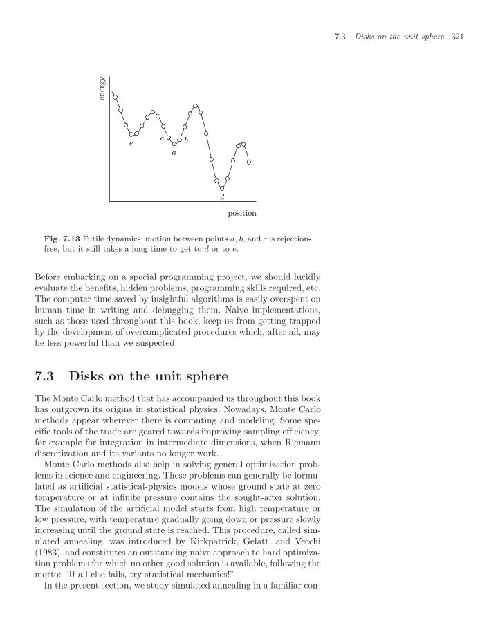
7.3 Disks on the unit sphere 321
a
bc
d
e
ener
gy
position
Fig. 7.13 Futile dynamics: motion between points a, b, and c is rejection-free, but it still takes a long time to get to d or to e.
Before embarking on a special programming project, we should lucidlyevaluate the benefits, hidden problems, programming skills required, etc.The computer time saved by insightful algorithms is easily overspent onhuman time in writing and debugging them. Naive implementations,such as those used throughout this book, keep us from getting trappedby the development of overcomplicated procedures which, after all, maybe less powerful than we suspected.
7.3 Disks on the unit sphere
The Monte Carlo method that has accompanied us throughout this bookhas outgrown its origins in statistical physics. Nowadays, Monte Carlomethods appear wherever there is computing and modeling. Some spe-cific tools of the trade are geared towards improving sampling efficiency,for example for integration in intermediate dimensions, when Riemanndiscretization and its variants no longer work.
Monte Carlo methods also help in solving general optimization prob-lems in science and engineering. These problems can generally be formu-lated as artificial statistical-physics models whose ground state at zerotemperature or at infinite pressure contains the sought-after solution.The simulation of the artificial model starts from high temperature orlow pressure, with temperature gradually going down or pressure slowlyincreasing until the ground state is reached. This procedure, called sim-ulated annealing, was introduced by Kirkpatrick, Gelatt, and Vecchi(1983), and constitutes an outstanding naive approach to hard optimiza-tion problems for which no other good solution is available, following themotto: “If all else fails, try statistical mechanics!”
In the present section, we study simulated annealing in a familiar con-
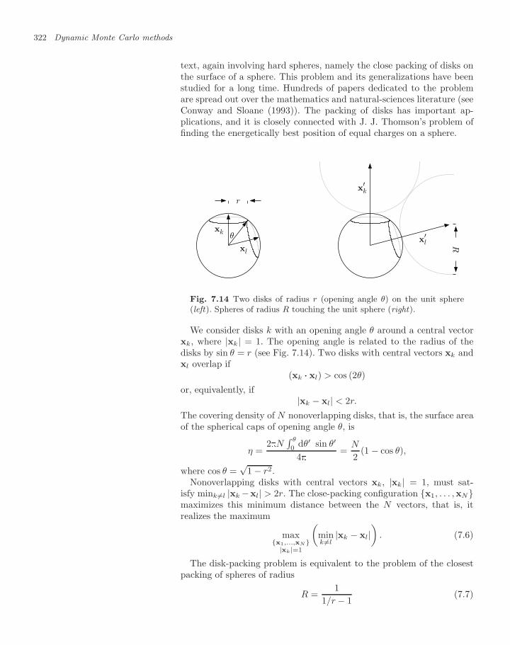
322 Dynamic Monte Carlo methods
text, again involving hard spheres, namely the close packing of disks onthe surface of a sphere. This problem and its generalizations have beenstudied for a long time. Hundreds of papers dedicated to the problemare spread out over the mathematics and natural-sciences literature (seeConway and Sloane (1993)). The packing of disks has important ap-plications, and it is closely connected with J. J. Thomson’s problem offinding the energetically best position of equal charges on a sphere.
xk
xl
r
θ
xk′
xl′
R
Fig. 7.14 Two disks of radius r (opening angle θ) on the unit sphere(left). Spheres of radius R touching the unit sphere (right).
We consider disks k with an opening angle θ around a central vectorxk, where |xk| = 1. The opening angle is related to the radius of thedisks by sin θ = r (see Fig. 7.14). Two disks with central vectors xk andxl overlap if
(xk ··· xl) > cos (2θ)
or, equivalently, if|xk − xl| < 2r.
The covering density of N nonoverlapping disks, that is, the surface areaof the spherical caps of opening angle θ, is
η =2N
∫ θ
0dθ′ sin θ′
4=
N
2(1 − cos θ),
where cos θ =√
1 − r2.Nonoverlapping disks with central vectors xk, |xk| = 1, must sat-
isfy mink =l |xk −xl| > 2r. The close-packing configuration x1, . . . ,xNmaximizes this minimum distance between the N vectors, that is, itrealizes the maximum
maxx1,...,xN
|xk|=1
(mink =l
|xk − xl|)
. (7.6)
The disk-packing problem is equivalent to the problem of the closestpacking of spheres of radius
R =1
1/r − 1(7.7)
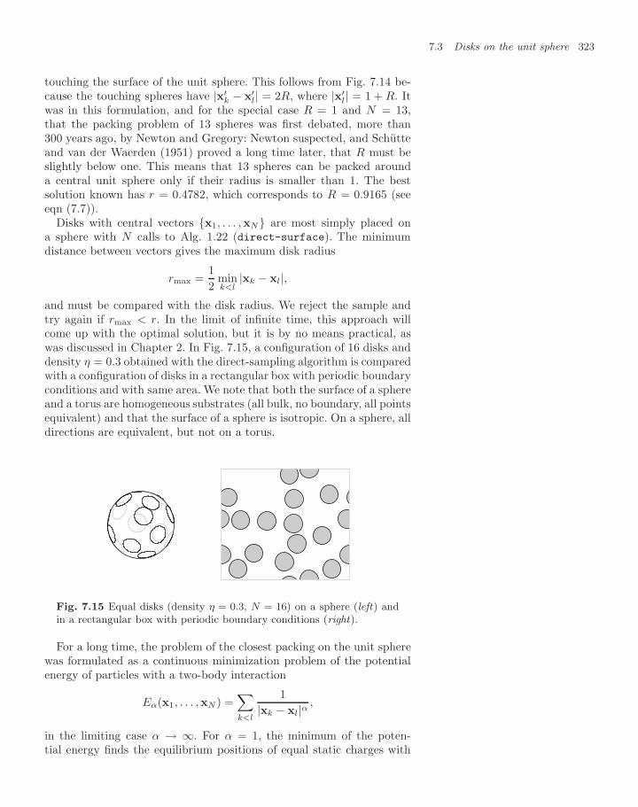
7.3 Disks on the unit sphere 323
touching the surface of the unit sphere. This follows from Fig. 7.14 be-cause the touching spheres have |x′
k − x′l| = 2R, where |x′
l| = 1 + R. Itwas in this formulation, and for the special case R = 1 and N = 13,that the packing problem of 13 spheres was first debated, more than300 years ago, by Newton and Gregory: Newton suspected, and Schutteand van der Waerden (1951) proved a long time later, that R must beslightly below one. This means that 13 spheres can be packed arounda central unit sphere only if their radius is smaller than 1. The bestsolution known has r = 0.4782, which corresponds to R = 0.9165 (seeeqn (7.7)).
Disks with central vectors x1, . . . ,xN are most simply placed ona sphere with N calls to Alg. 1.22 (direct-surface). The minimumdistance between vectors gives the maximum disk radius
rmax =12
mink<l
|xk − xl|,
and must be compared with the disk radius. We reject the sample andtry again if rmax < r. In the limit of infinite time, this approach willcome up with the optimal solution, but it is by no means practical, aswas discussed in Chapter 2. In Fig. 7.15, a configuration of 16 disks anddensity η = 0.3 obtained with the direct-sampling algorithm is comparedwith a configuration of disks in a rectangular box with periodic boundaryconditions and with same area. We note that both the surface of a sphereand a torus are homogeneous substrates (all bulk, no boundary, all pointsequivalent) and that the surface of a sphere is isotropic. On a sphere, alldirections are equivalent, but not on a torus.
Fig. 7.15 Equal disks (density η = 0.3, N = 16) on a sphere (left) andin a rectangular box with periodic boundary conditions (right).
For a long time, the problem of the closest packing on the unit spherewas formulated as a continuous minimization problem of the potentialenergy of particles with a two-body interaction
Eα(x1, . . . ,xN ) =∑k<l
1|xk − xl|α ,
in the limiting case α → ∞. For α = 1, the minimum of the poten-tial energy finds the equilibrium positions of equal static charges with
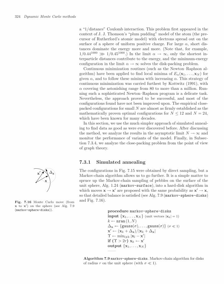
324 Dynamic Monte Carlo methods
a “1/distance” Coulomb interaction. This problem first appeared in thecontext of J. J. Thomson’s “plum pudding” model of the atom (the pre-cursor of Rutherford’s atomic model) with electrons spread out on thesurface of a sphere of uniform positive charge. For large α, short dis-tances dominate the energy more and more. (Note that, for example,1/0.441000 ≫ 1/0.451000.) In the limit α → ∞, only the shortest in-terparticle distances contribute to the energy, and the minimum-energyconfiguration in the limit α → ∞ solves the disk-packing problem.
Continuous minimization routines (such as the Newton–Raphson al-gorithm) have been applied to find local minima of Eα(x1, . . . ,xN ) forgiven α, and to follow these minima with increasing α. This strategy ofcontinuous minimization was carried furthest by Kottwitz (1991), withα covering the astonishing range from 80 to more than a million. Run-ning such a sophisticated Newton–Raphson program is a delicate task.Nevertheless, the approach proved to be successful, and most of theconfigurations found have not been improved upon. The empirical close-packed configurations for small N are almost as firmly established as themathematically proven optimal configurations for N ≤ 12 and N = 24,which have been known for many decades.
In this section, we use the much simpler approach of simulated anneal-ing to find data as good as were ever discovered before. After discussingthe method, we analyze the results in the asymptotic limit N → ∞ andmonitor the performance of variants of the model. Finally, in Subsec-tion 7.3.4, we analyze the close-packing problem from the point of viewof graph theory.
7.3.1 Simulated annealing
The configurations in Fig. 7.15 were obtained by direct sampling, but aMarkov-chain algorithm allows us to go further. It is a simple matter tospruce up the Markov-chain sampling of pebbles on the surface of theunit sphere, Alg. 1.24 (markov-surface), into a hard-disk algorithm inwhich moves x → x′ are proposed with the same probability as x′ → x,
x′
x
∆x
Fig. 7.16 Monte Carlo move (fromx to x′) on the sphere (see Alg. 7.9(markov-sphere-disks)).
so that detailed balance is satisfied (see Alg. 7.9 (markov-sphere-disks)and Fig. 7.16).
procedure markov-sphere-disks
input x1, . . . ,xN (unit vectors |xk| = 1)k ← nran (1, N)∆x ← gauss(σ), . . . , gauss(σ) (σ 1)x′ ← (xk + ∆x)/|xk + ∆x|Υ ← minl =k |xl − x′|if (Υ > 2r) xk ← x′
output x1, . . . ,xN——
Algorithm 7.9 markov-sphere-disks. Markov-chain algorithm for disksof radius r on the unit sphere (with σ 1).
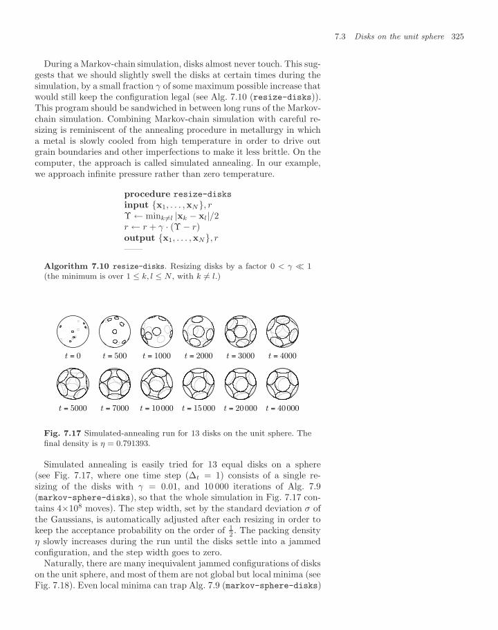
7.3 Disks on the unit sphere 325
During a Markov-chain simulation, disks almost never touch. This sug-gests that we should slightly swell the disks at certain times during thesimulation, by a small fraction γ of some maximum possible increase thatwould still keep the configuration legal (see Alg. 7.10 (resize-disks)).This program should be sandwiched in between long runs of the Markov-chain simulation. Combining Markov-chain simulation with careful re-sizing is reminiscent of the annealing procedure in metallurgy in whicha metal is slowly cooled from high temperature in order to drive outgrain boundaries and other imperfections to make it less brittle. On thecomputer, the approach is called simulated annealing. In our example,we approach infinite pressure rather than zero temperature.
procedure resize-disks
input x1, . . . ,xN, rΥ ← mink =l |xk − xl|/2r ← r + γ · (Υ − r)output x1, . . . ,xN, r——
Algorithm 7.10 resize-disks. Resizing disks by a factor 0 < γ 1(the minimum is over 1 ≤ k, l ≤ N , with k = l.)
t = 0 t = 500 t = 1000 t = 2000 t = 3000 t = 4000
t = 5000 t = 7000 t = 10000 t = 15000 t = 20000 t = 40000
Fig. 7.17 Simulated-annealing run for 13 disks on the unit sphere. Thefinal density is η = 0.791393.
Simulated annealing is easily tried for 13 equal disks on a sphere(see Fig. 7.17, where one time step (∆t = 1) consists of a single re-sizing of the disks with γ = 0.01, and 10 000 iterations of Alg. 7.9(markov-sphere-disks), so that the whole simulation in Fig. 7.17 con-tains 4×10⁸ moves). The step width, set by the standard deviation σ ofthe Gaussians, is automatically adjusted after each resizing in order tokeep the acceptance probability on the order of 1
2 . The packing densityη slowly increases during the run until the disks settle into a jammedconfiguration, and the step width goes to zero.
Naturally, there are many inequivalent jammed configurations of diskson the unit sphere, and most of them are not global but local minima (seeFig. 7.18). Even local minima can trap Alg. 7.9 (markov-sphere-disks)
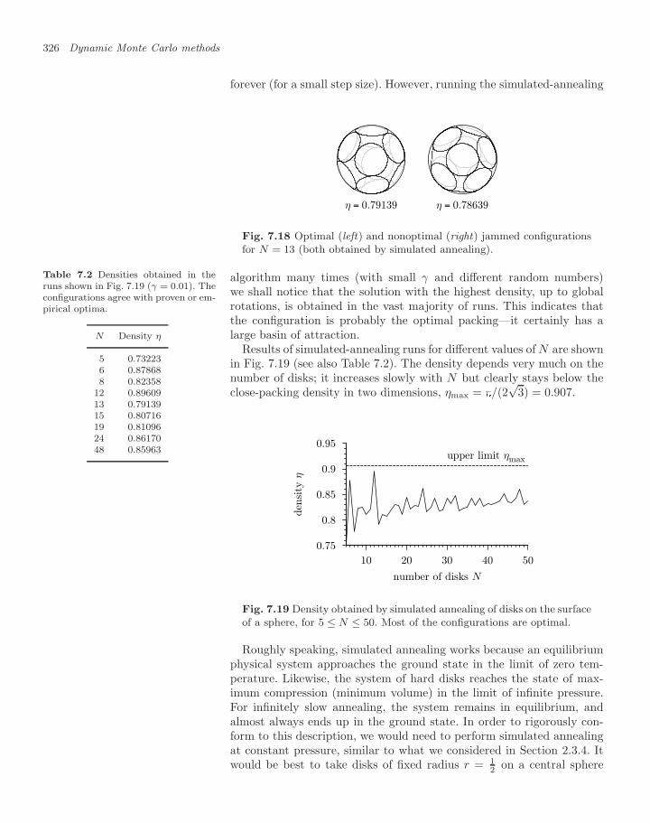
326 Dynamic Monte Carlo methods
forever (for a small step size). However, running the simulated-annealing
η = 0.79139 η = 0.78639
Fig. 7.18 Optimal (left) and nonoptimal (right) jammed configurationsfor N = 13 (both obtained by simulated annealing).
algorithm many times (with small γ and different random numbers)we shall notice that the solution with the highest density, up to globalrotations, is obtained in the vast majority of runs. This indicates thatthe configuration is probably the optimal packing—it certainly has alarge basin of attraction.
Results of simulated-annealing runs for different values of N are shownin Fig. 7.19 (see also Table 7.2). The density depends very much on thenumber of disks; it increases slowly with N but clearly stays below theclose-packing density in two dimensions, ηmax = /(2
√3) = 0.907.
Table 7.2 Densities obtained in theruns shown in Fig. 7.19 (γ = 0.01). Theconfigurations agree with proven or em-pirical optima.
N Density η
5 0.732236 0.878688 0.82358
12 0.8960913 0.7913915 0.8071619 0.8109624 0.8617048 0.85963
0.75
0.8
0.85
0.9
0.95
10 20 30 40 50
den
sity
η
number of disks N
upper limit ηmax
Fig. 7.19 Density obtained by simulated annealing of disks on the surfaceof a sphere, for 5 ≤ N ≤ 50. Most of the configurations are optimal.
Roughly speaking, simulated annealing works because an equilibriumphysical system approaches the ground state in the limit of zero tem-perature. Likewise, the system of hard disks reaches the state of max-imum compression (minimum volume) in the limit of infinite pressure.For infinitely slow annealing, the system remains in equilibrium, andalmost always ends up in the ground state. In order to rigorously con-form to this description, we would need to perform simulated annealingat constant pressure, similar to what we considered in Section 2.3.4. Itwould be best to take disks of fixed radius r = 1
2 on a central sphere
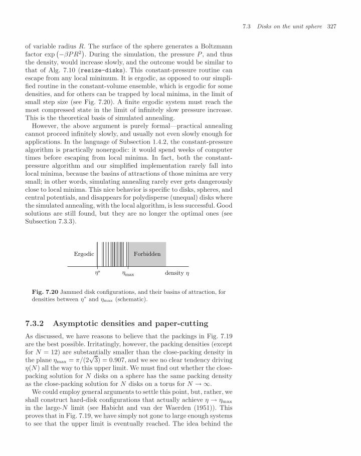
7.3 Disks on the unit sphere 327
of variable radius R. The surface of the sphere generates a Boltzmannfactor exp
(−βPR2). During the simulation, the pressure P , and thus
the density, would increase slowly, and the outcome would be similar tothat of Alg. 7.10 (resize-disks). This constant-pressure routine canescape from any local minimum. It is ergodic, as opposed to our simpli-fied routine in the constant-volume ensemble, which is ergodic for somedensities, and for others can be trapped by local minima, in the limit ofsmall step size (see Fig. 7.20). A finite ergodic system must reach themost compressed state in the limit of infinitely slow pressure increase.This is the theoretical basis of simulated annealing.
However, the above argument is purely formal—practical annealingcannot proceed infinitely slowly, and usually not even slowly enough forapplications. In the language of Subsection 1.4.2, the constant-pressurealgorithm is practically nonergodic: it would spend weeks of computertimes before escaping from local minima. In fact, both the constant-pressure algorithm and our simplified implementation rarely fall intolocal minima, because the basins of attractions of those minima are verysmall; in other words, simulating annealing rarely ever gets dangerouslyclose to local minima. This nice behavior is specific to disks, spheres, andcentral potentials, and disappears for polydisperse (unequal) disks wherethe simulated annealing, with the local algorithm, is less successful. Goodsolutions are still found, but they are no longer the optimal ones (seeSubsection 7.3.3).
Ergodic
η* ηmax
Forbidden
density η
Fig. 7.20 Jammed disk configurations, and their basins of attraction, fordensities between η∗ and ηmax (schematic).
7.3.2 Asymptotic densities and paper-cutting
As discussed, we have reasons to believe that the packings in Fig. 7.19are the best possible. Irritatingly, however, the packing densities (exceptfor N = 12) are substantially smaller than the close-packing density inthe plane ηmax = π/(2
√3) = 0.907, and we see no clear tendency driving
η(N) all the way to this upper limit. We must find out whether the close-packing solution for N disks on a sphere has the same packing densityas the close-packing solution for N disks on a torus for N → ∞.
We could employ general arguments to settle this point, but, rather, weshall construct hard-disk configurations that actually achieve η → ηmax
in the large-N limit (see Habicht and van der Waerden (1951)). Thisproves that in Fig. 7.19, we have simply not gone to large enough systemsto see that the upper limit is eventually reached. The idea behind the
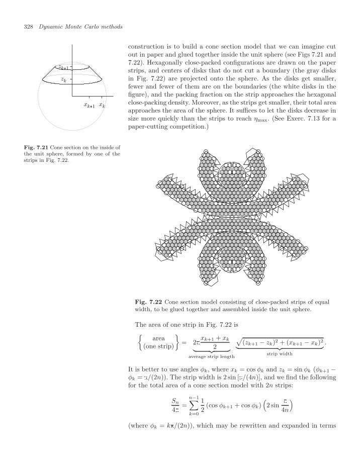
328 Dynamic Monte Carlo methods
construction is to build a cone section model that we can imagine cutout in paper and glued together inside the unit sphere (see Figs 7.21 and7.22). Hexagonally close-packed configurations are drawn on the paperstrips, and centers of disks that do not cut a boundary (the gray disksin Fig. 7.22) are projected onto the sphere. As the disks get smaller,fewer and fewer of them are on the boundaries (the white disks in thefigure), and the packing fraction on the strip approaches the hexagonalclose-packing density. Moreover, as the strips get smaller, their total areaapproaches the area of the sphere. It suffices to let the disks decrease insize more quickly than the strips to reach ηmax. (See Exerc. 7.13 for apaper-cutting competition.)
xkxk+1
zk
zk+1
Fig. 7.21 Cone section on the inside ofthe unit sphere, formed by one of thestrips in Fig. 7.22.
Fig. 7.22 Cone section model consisting of close-packed strips of equalwidth, to be glued together and assembled inside the unit sphere.
The area of one strip in Fig. 7.22 isarea
(one strip)
= 2
xk+1 + xk
2︸ ︷︷ ︸average strip length
√(zk+1 − zk)2 + (xk+1 − xk)2︸ ︷︷ ︸
strip width
.
It is better to use angles φk, where xk = cos φk and zk = sin φk (φk+1 −φk = /(2n)). The strip width is 2 sin [/(4n)], and we find the followingfor the total area of a cone section model with 2n strips:
Sn
4=
n−1∑k=0
12
(cos φk+1 + cos φk)(2 sin
4n
)(where φk = k/(2n)), which may be rewritten and expanded in terms
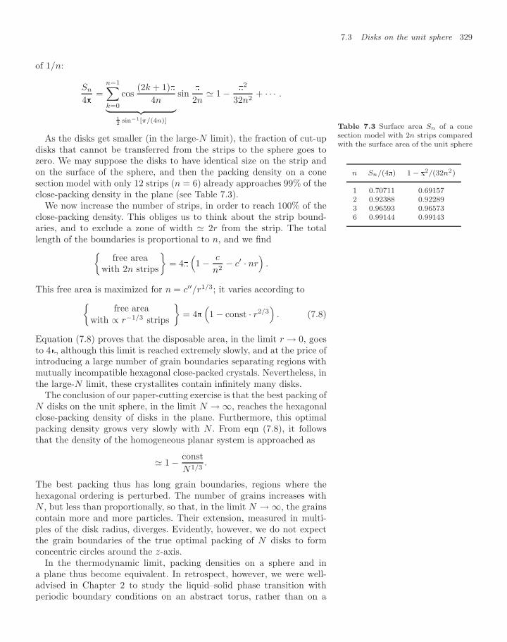
7.3 Disks on the unit sphere 329
of 1/n:
Sn
4=
n−1∑k=0
cos(2k + 1)
4n︸ ︷︷ ︸12 sin−1[π/(4n)]
sin
2n 1 −
2
32n2+ · · · .
As the disks get smaller (in the large-N limit), the fraction of cut-updisks that cannot be transferred from the strips to the sphere goes tozero. We may suppose the disks to have identical size on the strip andon the surface of the sphere, and then the packing density on a conesection model with only 12 strips (n = 6) already approaches 99% of theclose-packing density in the plane (see Table 7.3).
Table 7.3 Surface area Sn of a conesection model with 2n strips comparedwith the surface area of the unit sphere
n Sn/(4) 1 − 2/(32n2)
1 0.70711 0.691572 0.92388 0.922893 0.96593 0.965736 0.99144 0.99143
We now increase the number of strips, in order to reach 100% of theclose-packing density. This obliges us to think about the strip bound-aries, and to exclude a zone of width 2r from the strip. The totallength of the boundaries is proportional to n, and we find
free areawith 2n strips
= 4
(1 − c
n2− c′ · nr
).
This free area is maximized for n = c′′/r1/3; it varies according tofree area
with ∝ r−1/3 strips
= 4
(1 − const · r2/3
). (7.8)
Equation (7.8) proves that the disposable area, in the limit r → 0, goesto 4, although this limit is reached extremely slowly, and at the price ofintroducing a large number of grain boundaries separating regions withmutually incompatible hexagonal close-packed crystals. Nevertheless, inthe large-N limit, these crystallites contain infinitely many disks.
The conclusion of our paper-cutting exercise is that the best packing ofN disks on the unit sphere, in the limit N → ∞, reaches the hexagonalclose-packing density of disks in the plane. Furthermore, this optimalpacking density grows very slowly with N . From eqn (7.8), it followsthat the density of the homogeneous planar system is approached as
1 − constN1/3
.
The best packing thus has long grain boundaries, regions where thehexagonal ordering is perturbed. The number of grains increases withN , but less than proportionally, so that, in the limit N → ∞, the grainscontain more and more particles. Their extension, measured in multi-ples of the disk radius, diverges. Evidently, however, we do not expectthe grain boundaries of the true optimal packing of N disks to formconcentric circles around the z-axis.
In the thermodynamic limit, packing densities on a sphere and ina plane thus become equivalent. In retrospect, however, we were well-advised in Chapter 2 to study the liquid–solid phase transition withperiodic boundary conditions on an abstract torus, rather than on a
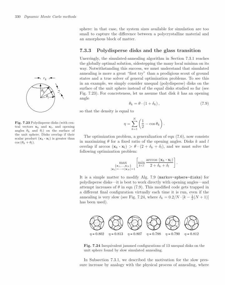
330 Dynamic Monte Carlo methods
sphere: in that case, the system sizes available for simulation are toosmall to capture the difference between a polycrystalline material andan amorphous block of matter.
7.3.3 Polydisperse disks and the glass transition
Unerringly, the simulated-annealing algorithm in Section 7.3.1 reachesthe globally optimal solution, sidestepping the many local minima on itsway. Notwithstanding this success, we must understand that simulatedannealing is more a great “first try” than a prodigious scout of groundstates and a true solver of general optimization problems. To see thisin an example, we simply consider unequal (polydisperse) disks on thesurface of the unit sphere instead of the equal disks studied so far (seeFig. 7.23). For concreteness, let us assume that disk k has an openingangle
θk = θ · (1 + δk) , (7.9)
so that the density is equal to
rk
rlθk
θl
Fig. 7.23 Polydisperse disks (with cen-tral vectors xk and xl, and openingangles θk and θl) on the surface ofthe unit sphere. Disks overlap if theirscalar product (xk ··· xl) is greater thancos (θk + θl).
η =N∑
k=1
(12− cos θk
).
The optimization problem, a generalization of eqn (7.6), now consistsin maximizing θ for a fixed ratio of the opening angles. Disks k and loverlap if arccos (xk ··· xl) > θ · (2 + δk + δl), and we must solve thefollowing optimization problem:
maxx1,...,xN
|x1|=···=|xN |=1
[mink<l
arccos (xk ··· xl)2 + δk + δl
].
It is a simple matter to modify Alg. 7.9 (markov-sphere-disks) forpolydisperse disks—it is best to work directly with opening angles—andattempt increases of θ in eqn (7.9). This modified code gets trapped ina different final configuration virtually each time it is run, even if theannealing is very slow (see Fig. 7.24, where δk = 0.2/N · [k − 1
2 (N + 1)]has been used).
η = 0.802 η = 0.813 η = 0.807 η = 0.788 η = 0.790 η = 0.812
Fig. 7.24 Inequivalent jammed configurations of 13 unequal disks on theunit sphere found by slow simulated annealing.
In Subsection 7.3.1, we described the motivation for the slow pres-sure increase by analogy with the physical process of annealing, where
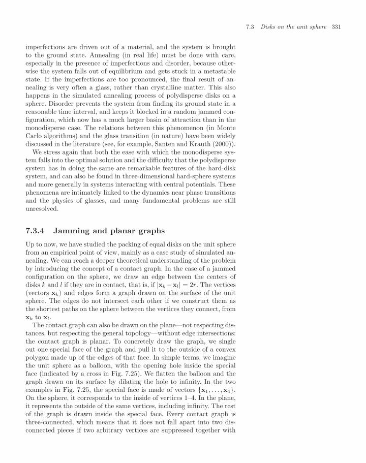
7.3 Disks on the unit sphere 331
imperfections are driven out of a material, and the system is broughtto the ground state. Annealing (in real life) must be done with care,especially in the presence of imperfections and disorder, because other-wise the system falls out of equilibrium and gets stuck in a metastablestate. If the imperfections are too pronounced, the final result of an-nealing is very often a glass, rather than crystalline matter. This alsohappens in the simulated annealing process of polydisperse disks on asphere. Disorder prevents the system from finding its ground state in areasonable time interval, and keeps it blocked in a random jammed con-figuration, which now has a much larger basin of attraction than in themonodisperse case. The relations between this phenomenon (in MonteCarlo algorithms) and the glass transition (in nature) have been widelydiscussed in the literature (see, for example, Santen and Krauth (2000)).
We stress again that both the ease with which the monodisperse sys-tem falls into the optimal solution and the difficulty that the polydispersesystem has in doing the same are remarkable features of the hard-disksystem, and can also be found in three-dimensional hard-sphere systemsand more generally in systems interacting with central potentials. Thesephenomena are intimately linked to the dynamics near phase transitionsand the physics of glasses, and many fundamental problems are stillunresolved.
7.3.4 Jamming and planar graphs
Up to now, we have studied the packing of equal disks on the unit spherefrom an empirical point of view, mainly as a case study of simulated an-nealing. We can reach a deeper theoretical understanding of the problemby introducing the concept of a contact graph. In the case of a jammedconfiguration on the sphere, we draw an edge between the centers ofdisks k and l if they are in contact, that is, if |xk −xl| = 2r. The vertices(vectors xk) and edges form a graph drawn on the surface of the unitsphere. The edges do not intersect each other if we construct them asthe shortest paths on the sphere between the vertices they connect, fromxk to xl.
The contact graph can also be drawn on the plane—not respecting dis-tances, but respecting the general topology—without edge intersections:the contact graph is planar. To concretely draw the graph, we singleout one special face of the graph and pull it to the outside of a convexpolygon made up of the edges of that face. In simple terms, we imaginethe unit sphere as a balloon, with the opening hole inside the specialface (indicated by a cross in Fig. 7.25). We flatten the balloon and thegraph drawn on its surface by dilating the hole to infinity. In the twoexamples in Fig. 7.25, the special face is made of vectors x1, . . . ,x4.On the sphere, it corresponds to the inside of vertices 1–4. In the plane,it represents the outside of the same vertices, including infinity. The restof the graph is drawn inside the special face. Every contact graph isthree-connected, which means that it does not fall apart into two dis-connected pieces if two arbitrary vertices are suppressed together with
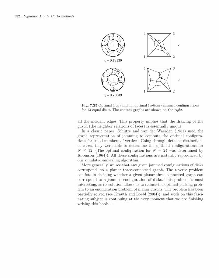
332 Dynamic Monte Carlo methods
η = 0.79139
1
2
3
4×
1 2
34
×
η = 0.78639
1
2 3
4×
1 2
34
×
Fig. 7.25 Optimal (top) and nonoptimal (bottom) jammed configurationsfor 13 equal disks. The contact graphs are shown on the right.
all the incident edges. This property implies that the drawing of thegraph (the neighbor relations of faces) is essentially unique.
In a classic paper, Schutte and van der Waerden (1951) used thegraph representation of jamming to compute the optimal configura-tions for small numbers of vertices. Going through detailed distinctionsof cases, they were able to determine the optimal configurations forN ≤ 12. (The optimal configuration for N = 24 was determined byRobinson (1964)). All these configurations are instantly reproduced byour simulated-annealing algorithm.
More generally, we see that any given jammed configurations of diskscorresponds to a planar three-connected graph. The reverse problemconsists in deciding whether a given planar three-connected graph cancorrespond to a jammed configuration of disks. This problem is mostinteresting, as its solution allows us to reduce the optimal-packing prob-lem to an enumeration problem of planar graphs. The problem has beenpartially solved (see Krauth and Loebl (2004)), and work on this fasci-nating subject is continuing at the very moment that we are finishingwriting this book. . . .
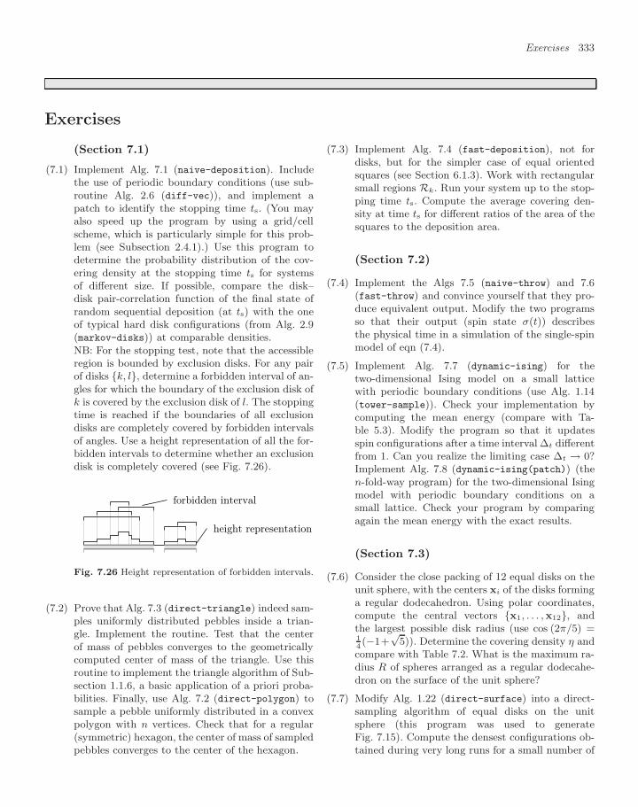
Exercises 333
Exercises
(Section 7.1)
(7.1) Implement Alg. 7.1 (naive-deposition). Includethe use of periodic boundary conditions (use sub-routine Alg. 2.6 (diff-vec)), and implement apatch to identify the stopping time ts. (You mayalso speed up the program by using a grid/cellscheme, which is particularly simple for this prob-lem (see Subsection 2.4.1).) Use this program todetermine the probability distribution of the cov-ering density at the stopping time ts for systemsof different size. If possible, compare the disk–disk pair-correlation function of the final state ofrandom sequential deposition (at ts) with the oneof typical hard disk configurations (from Alg. 2.9(markov-disks)) at comparable densities.NB: For the stopping test, note that the accessibleregion is bounded by exclusion disks. For any pairof disks k, l, determine a forbidden interval of an-gles for which the boundary of the exclusion disk ofk is covered by the exclusion disk of l. The stoppingtime is reached if the boundaries of all exclusiondisks are completely covered by forbidden intervalsof angles. Use a height representation of all the for-bidden intervals to determine whether an exclusiondisk is completely covered (see Fig. 7.26).
forbidden interval
height representation
Fig. 7.26 Height representation of forbidden intervals.
(7.2) Prove that Alg. 7.3 (direct-triangle) indeed sam-ples uniformly distributed pebbles inside a trian-gle. Implement the routine. Test that the centerof mass of pebbles converges to the geometricallycomputed center of mass of the triangle. Use thisroutine to implement the triangle algorithm of Sub-section 1.1.6, a basic application of a priori proba-bilities. Finally, use Alg. 7.2 (direct-polygon) tosample a pebble uniformly distributed in a convexpolygon with n vertices. Check that for a regular(symmetric) hexagon, the center of mass of sampledpebbles converges to the center of the hexagon.
(7.3) Implement Alg. 7.4 (fast-deposition), not fordisks, but for the simpler case of equal orientedsquares (see Section 6.1.3). Work with rectangularsmall regions Rk. Run your system up to the stop-ping time ts. Compute the average covering den-sity at time ts for different ratios of the area of thesquares to the deposition area.
(Section 7.2)
(7.4) Implement the Algs 7.5 (naive-throw) and 7.6(fast-throw) and convince yourself that they pro-duce equivalent output. Modify the two programsso that their output (spin state σ(t)) describesthe physical time in a simulation of the single-spinmodel of eqn (7.4).
(7.5) Implement Alg. 7.7 (dynamic-ising) for thetwo-dimensional Ising model on a small latticewith periodic boundary conditions (use Alg. 1.14(tower-sample)). Check your implementation bycomputing the mean energy (compare with Ta-ble 5.3). Modify the program so that it updatesspin configurations after a time interval ∆t differentfrom 1. Can you realize the limiting case ∆t → 0?Implement Alg. 7.8 (dynamic-ising(patch)) (then-fold-way program) for the two-dimensional Isingmodel with periodic boundary conditions on asmall lattice. Check your program by comparingagain the mean energy with the exact results.
(Section 7.3)
(7.6) Consider the close packing of 12 equal disks on theunit sphere, with the centers xi of the disks forminga regular dodecahedron. Using polar coordinates,compute the central vectors x1, . . . ,x12, andthe largest possible disk radius (use cos (2π/5) =14(−1+
√5)). Determine the covering density η and
compare with Table 7.2. What is the maximum ra-dius R of spheres arranged as a regular dodecahe-dron on the surface of the unit sphere?
(7.7) Modify Alg. 1.22 (direct-surface) into a direct-sampling algorithm of equal disks on the unitsphere (this program was used to generateFig. 7.15). Compute the densest configurations ob-tained during very long runs for a small number of
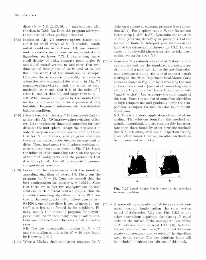
334 Exercises
disks (N = 5, 8, 12, 13, 16, . . . ) and compare withthe data in Table 7.2. Does this program allow youto estimate the close packing densities?
(7.8) Implement Alg. 7.9 (markov-sphere-disks) andrun it for small values of N . If possible, handleinitial conditions as in Exerc. 1.3; use Gaussianunit random vectors for constructing an initial con-figuration (see Exerc. 7.7). During a long run atsmall density of disks, compute polar angles θk
and φk of central vectors xk and check that two-dimensional histograms of cos θk and of φk areflat. This shows that the simulation is isotropic.Compute the acceptance probability of moves asa function of the standard deviation σ in Alg. 7.9(markov-sphere-disks), and find a rule to auto-matically set σ such that it is of the order of 1
2
(that is, smaller than 0.9, and larger than 0.1).NB: When sampling integrals by the Monte Carlomethod, adaptive choice of the step-size is strictlyforbidden, because it interferes with the detailed-balance condition.
(7.9) (Uses Exerc. 7.8.) Use Alg. 7.10 (resize-disks) to-gether with Alg. 7.9 (markov-sphere-disks) of Ex-erc. 7.8 to implement simulated annealing for harddisks on the unit sphere. Adapt the step-size σ inorder to keep an acceptance rate of order 1
2. Check
that for N = 12 disks, your program convergestowards the perfect dodecahedron arrangement ofdisks. Then, implement the 13-sphere problem: re-cover the configurations shown in Fig. 7.18. Studythe influence of the annealing rate γ on the qualityof the final configuration (on the probability thatit is not optimal). List all nonequivalent jammedconfigurations generated.
(7.10) Perform further experiments with the simulatedannealing algorithm of Exerc. 7.9. First, run theprogram for N = 15. Convince yourself that thebest configuration has density η = 0.80731. Showthat there are in fact two nonequivalent optimalsolutions, with different contact graphs. Run thesimulated annealing algorithm for N = 19. Showthat in the configuration with highest density (η =0.81096), one of the disks is free to move. It “rat-tles” in a free spot formed by its neighbors. Fi-nally, modify the annealing program for polydis-perse disks. Show that many nonequivalent solu-tions are obtained even for very small annealingrates.NB: The two nonequivalent minima for N = 15and the rattling solutions for N = 19 were foundby Kottwitz (1991).
(7.11) Write a Markov-chain simulation program for N
disks on a sphere at constant pressure (see Subsec-tion 2.3.4). For a sphere radius R, the Boltzmannfactor is exp
`−βP · 4R2´. Determine the equation
of state (covering density η vs. pressure P ) of thesystem for finite N . Interpret your findings in thelight of the discussion of Subsection 7.3.2. Do youexpect a liquid–solid phase transition to take placein this system for large N?
(7.12) Generate N randomly distributed “cities” in theunit square and use the simulated annealing algo-rithm to find a good solution to the traveling sales-man problem: a round-trip tour of shortest lengthvisiting all the cities. Implement local Monte Carlomoves as shown in Fig. 7.27 by rearranging the tourat two cities k and l (instead of connecting city kwith city k′ and city l with city l′, connect k withl and k′ with l′). Use as energy the total length ofthe tour. Start the simulated annealing algorithmat high temperature and gradually lower the tem-perature. Compare the final solution found for dif-ferent runs.NB: This is a historic application of simulated an-nealing. The solutions found by this method areusually nonoptimal, and are considerably less accu-rate than those found by other heuristic methods(for N 100 cities, even visual inspection usuallygives better tours). However, no other method canbe implemented as quickly.
k
k′
l
l′
a
k
k′
l
l′
b
Fig. 7.27 Local Monte Carlo move in the travelingsalesman problem.
(7.13) (Paper-cutting competition.) Write a portable com-puter program implementing the cone sectionmodel of Subsection 7.3.2 (see Fig. 7.22) or anyother nonrandom algorithm for placing N equaldisks on the surface of the unit sphere (use valuesof N between 12 and at least 1 000 000). Note thehighest covering densities η(N) obtained. Commu-nicate your program, and a sketch of the algorithmused, to the author. The best solutions found willbe included in subsequent editions of this book.
References 335
References
Bortz A. B., Kalos M. H., Lebowitz J. L. (1975) A new algorithmfor Monte Carlo simulation of Ising spin systems, Journal of Chemi-cal Physics 17, 10–18
Conway J. H., Sloane N. J. A. (1993) Sphere Packings, Lattices, andGroups, 2nd edn, Springer, New York
Habicht W., van der Waerden B. L. (1951) Lagerung von Punkten aufder Kugel [in German], Mathematische Annalen 96, 223–234
Kirkpatrick S., Gelatt C. D., Vecchi M. P. (1983) Optimization by sim-ulated annealing, Science 220, 671–680
Kottwitz D. A. (1991) The densest packing of equal circles on a sphere,Acta Crystallographica A47, 158–165
Krauth W. (2002) Disks on a sphere and two-dimensional glasses, Mar-kov Processes and Related Fields 8, 215–219
Krauth W., Loebl M. (2004) Jamming and geometric representationsof graphs, preprint, math.CO/0406166
Robinson R. M. (1961) Arrangement of 24 points on a sphere, Math-ematische Annalen 144, 17–48
Santen L., Krauth W. (2000) Absence of thermodynamic phase tran-sition in a model glass former, Nature 405, 550–551
Schutte K., van der Waerden B. L. (1951) Auf welcher Kugel haben5, 6, 7, 8 oder 9 Punkte mit Mindestabstand Eins Platz? [in German],Mathematische Annalen 123, 96

This page intentionally left blank
Acknowledgements
The cover illustration, taken from a work by Robert Filliou (1923–1987),is used with kind permission of Marianne Filliou. I thank FrancoiseNinghetto for making the cover project possible.
The illustration of Count Buffon (Fig. 1.6) first appeared in an articleLes mathematiciens jouent a la roulette pour comprendre le hasard, in LeMonde (Paris), edition of 13 december 1996. Used with kind permissionof Le Monde.
Figures 1.1, 1.2, 1.3, and 7.9 were first published as Figures 1, 2, 7,and 16; in Krauth, W. “Introduction to Monte Carlo Algorithms” in Ad-vances in Computer Simulation, Lectures Held at the Eotvos SummerSchool in Budapest, Hungary, 16–20 July 1996, Springer Lecture Notesin Physics, Vol. 501, Kertesz J., Kondor I. (Eds.), Copyright Springer1998. With kind permission of Springer Science and Business Media.
Material in this book was shaped through essential discussions andcollaborations with C. Bouchiat, A. Buhot, M. Caffarel, D. M. Ceperley,C. Dress, O. Duemmer, S. Grossmann, M. Holzmann, J. L. Lebowitz,P. Le Doussal, M. Loebl, M. Mezard, R. Moessner, A. Rosso, L. Santen,and M. Staudacher.
I thank P. Zoller for the initial suggestion that it was time to startwriting, M. Staudacher for encouragement throughout the project, andP. M. Goldbart for help.
I am indebted to A. Barrat, O. Duemmer, J.-G. Malherbe, R. Moess-ner, and A. Rosso for reading through many versions of the text, gen-erously offering advice and suggesting improvements in the content andthe presentation of the material. I thank C. T. Pham for expert helpwith many technical questions.
It was a pleasure working with S. Adlung, E. Robottom, and theeditorial team at OUP.

This page intentionally left blank

Index
a priori probability, 22–24and dynamic Monte Carlo algorithms,
307and heat bath algorithm, 252and rejection rates, 319and triangle algorithm, 23in Bayesian statistics, 57in cluster algorithms, 255
acceptance probabilityin avalanche cluster algorithm, 123in Ising cluster algorithm, 255in Metropolis algorithm, 21
generalized, 23acceptance rate
and acceptance probability, 24and one-half rule, 6, 77as ratio of partition functions, 33, 78,
97, 128of direct sampling algorithm, 97of local Monte Carlo algorithm, 255of local path sampling, 152physical interpretation of, 160
action, 167Aigner M., 13Alder B. J., 101, 106algorithmbinomial-convolution (Alg. 1.25), 46bisection-search (Alg. 1.15), 34box-it (Alg. 2.5), 91breadth-dimer (Alg. 6.6), 285canonic-bosons (Alg. 4.4), 195canonic-recursion (Alg. 4.6), 215canonic-recursion(patch) (Alg. 4.7),
218cluster-ising (Alg. 5.9), 257cluster-spin-glass (Alg. 5.11), 260combinatorial-ising (Alg. 5.6), 246combinatorial-spin-glass (Alg.
5.12), 261data-bunch (Alg. 1.28), 61depth-dimer (Alg. 6.7), 286diff-vec (Alg. 2.6), 91direct-cycles (Alg. 4.8), 220direct-disks (Alg. 2.7), 95direct-disks-any (Alg. 2.8), 97direct-gamma (Alg. 1.29), 64direct-gamma-zeta (Alg. 1.30), 67direct-harmonic-bosons (Alg. 4.9),
220direct-needle (Alg. 1.4), 11
direct-needle(patch) (Alg. 1.5), 11direct-p-disks (Alg. 2.14), 115direct-period-bosons (Alg. 4.10), 222direct-pi (Alg. 1.1), 3direct-pin (Alg. 6.2), 271direct-piston-particles (Alg. 2.13),
115direct-polygon (Alg. 7.2), 312direct-sphere (Alg. 1.21), 42direct-surface (Alg. 1.22), 43
in vector notation, 43direct-triangle (Alg. 7.3), 312dynamic-ising (Alg. 7.7), 318dynamic-ising(patch) (Alg. 7.8), 318edge-ising (Alg. 5.5), 238energy-ising (Alg. 5.1), 231enumerate-ising (Alg. 5.3), 233event-disks (Alg. 2.1), 83event-disks(patch) (Alg. 2.4), 89fast-deposition (Alg. 7.4), 313fast-throw (Alg. 7.6), 316fourier-cos-path (Alg. 3.15), 180fourier-free-path (Alg. 3.12), 173fourier-gen-path (Alg. 3.14), 178gamma-cut (Alg. 2.15), 117gauss (Alg. 1.18), 38gauss(patch) (Alg. 1.19), 39grandcan-bosons (Alg. 4.5), 199gray-flip (Alg. 5.2), 233hard-sphere-cluster (Alg. 2.18), 126harmonic-density (Alg. 3.2), 134harmonic-wavefunction (Alg. 3.1), 133heatbath-ising (Alg. 5.8), 252levy-convolution (Alg. 1.32), 72levy-free-path (Alg. 3.5), 153levy-free-path-3d, 160levy-harmonic-path (Alg. 3.6), 155levy-periodic-path (Alg. 3.7), 156markov-discrete-pebble (Alg. 1.6), 17markov-disks (Alg. 2.9), 100markov-ising (Alg. 5.7), 250markov-pi (Alg. 1.2), 6markov-pi(patch) (Alg. 1.3), 7markov-sphere-disks (Alg. 7.9), 324markov-spin-glass (Alg. 5.10), 260markov-surface (Alg. 1.24), 44markov-two-site (Alg. 1.8), 22markov-zeta (Alg. 1.31), 69matrix-square (Alg. 3.3), 145maxwell-boundary (Alg. 2.10), 110
naive-avalanche (Alg. 2.17), 123naive-bayes-pi (Alg. 1.27), 57naive-bosons (Alg. 4.3), 192naive-box-path (Alg. 3.8), 158naive-degeneracy (Alg. 4.1), 187naive-degeneracy-cube (Alg. 4.2), 189naive-deposition (Alg. 7.1), 309naive-dimer (Alg. 6.4), 282naive-dimer(patch) (Alg. 6.5), 283naive-gauss (Alg. 1.17), 37naive-harmonic-path (Alg. 3.4), 151naive-pin (Alg. 6.1), 269naive-piston-particles (Alg. 2.11),
113naive-piston-particles(patch) (Alg.
2.12), 113naive-rad-wavefunction (Alg. 3.11),
164naive-ran (Alg. 1.9), 28naive-sphere (Alg. 1.20), 40naive-sphere-path (Alg. 3.9), 160naive-sphere-path(patch) (Alg.
3.10), 161naive-throw (Alg. 7.5), 316nran (Alg. 1.10), 29pair-collision (Alg. 2.3), 85pair-time (Alg. 2.2), 84pocket-binary (Alg. 6.3), 278ran-combination (Alg. 1.12), 32ran-perm (Alg. 1.11), 32ran01-convolution (Alg. 1.26), 47reject-continuous (Alg. 1.16), 35reject-finite (Alg. 1.13), 33rescale-volume (Alg. 2.16), 118resize-disks (Alg. 7.10), 325thermo-ising (Alg. 5.4), 235tower-sample (Alg. 1.14), 33transfer-matrix (Alg. 1.7), 19trivial-free-path (Alg. 3.13), 176
annealing, simulated, 307, 334disks on sphere, 321–325traveling salesman problem, 334
Archimedes, 4, 58Asakura S., 267, 276
Barbier E., 9, 14, 15Bayesian statistics, 57
and Jaynes’ principle, 94Beale P. D., 248, 265Bernoulli D., 118
340 Index
Bernoulli J., 4Bernoulli variable, 45Binder K., 264, 265Boltzmann distribution, 81, 108–112Boltzmann L., 94, 99Borrmann P., 215Bortz A. B., 318Bose–Einstein condensation, 192
and saturation numbers, 201critical temperature
homogeneous gas, 208trap, 202
boundary conditions, periodic, 90Buffon G. L. L., 9Buffon needle problem, 9Buhot A., 280
central limit theorem, 37, 44and Chebyshev inequality, 52and data analysis, 56and Levy distribution, 70simplified proof of, 52
Ceperley D. M., 143, 168, 224characteristic function, 73Chebyshev inequality, 51, 55–56, 65cluster algorithm, 81, 123
avalanche, 123for bosons, 224for Ising spin glasses, 260Ising model, 229, 254–258pivot, 123, 126, 262
for binary mixtures, 267, 278for liquids, 262
convolutionof density matrix, 131, 143–145, 149of probability distributions, 46–47, 72,
73, 115, 146Conway J. H., 322Coopersmith M. H., 303coupling from the past, see perfect
sampling
de Broglie wavelength, 208δ-function, 88
Dirac, 133, 136Kronecker, 133, 188
integral representation, 188, 193density matrix, 131–149
bosons, 211box
hard walls, 139, 157periodic, 138, 155rotating, 142
distinguishable particles, 210free particle, 136pair of hard spheres, 167
density of statesfrom partition function, 247–248Ising model, 234, 235single-particle, 187, 189
deposition, random sequential, 95, 309detailed balance, 16Dinsmore A. D., 279direct sampling, 3
and a priori probabilities, 24and analytic solution, 8, 159dimer configuration, 295, 304γ integral, 65historical origin, 9ideal bosons, 185, 219
in periodic box, 222, 226in trap, 220, 226
path, 150Fourier method, 173free particle, 153harmonic oscillator, 155in box, 159, 183in periodic box, 155trivial algorithm, 176
pebblein sphere, 39in square, 7in triangle, 312on surface of sphere, 43
pebble in sphere, 42permutation
general distribution, 220uniform, 31
pins (one-dimensional hard spheres),271
two-dimensional Ising model, 254, 304two-dimensional Ising spin glass, 304
Dress C., 123
ensemblecanonical, 196, 205constant-pressure, 101, 108, 326constant-volume, 118, 327grand canonical, 198, 199, 205grand canonical (for ideal bosons)
limit N → ∞, 200, 203enumeration
awkward, 282breadth-first, 285depth-first, 286Gray code, 233in the five-boson bounded trap model,
193independent sets, 125loop configurations, 229pencil-and-paper, 284permutations, 226spin configurations, 229, 232tetris configurations, 304tree-based, 267two meanings of, 236using Pfaffians, 288, 304
ergodicityof Monte Carlo algorithm, 63, 101,
296–297, 327
of physical system, 93, 95error bar, 56
Fairbank W. M., 143Ferdinand A. E., 247Feynman R. P., 150Fisher M. E., 247, 295, 298Franke G., 215
Galbiati G., 294Gaussian integral formula, 136Gelatt C. D., 321Gnedenko B. V., 52
Habicht W., 327haystack
needle in, 64heat bath algorithm, 252Heilmann O. J., 299Hess G. B., 143Holzmann M., 219Hoover W. G., 122
imaginary time, 149importance sampling, 67initial condition, 7
good implementation of, 77, 128, 265,303, 334
legal, 7, 128, 303integration
contour, in complex plane, 188relation with sampling, 8, 36Riemann
complex, 198, 225real-valued, 188
Jaynes’ principle, 94
Kac M., 237Kalos M. H., 318Kardar M., 261Kasteleyn P. W., 291, 304Kaufman B., 237, 247, 248, 265Kirkpatrick S., 321Kolmogorov A. N., 52Kottwitz D. A., 324, 334
Lebowitz J. L., 318Lee J. Y., 121Lee T. D., 299Leff H. S., 303Leggett A. J., 143Leschhorn H., 183Levy construction, 153, 220Levy P., 64, 70, 72, 78, 153Lieb E. H., 299Liu J. W., 262Loebl M., 332long-time tails, 105Luijten E., 262
Index 341
Maffioli F., 294Markov chain, definition of, 7Markov-chain sampling, 7Maxwell distribution, 13, 39, 104Mermin N. D., 101Metropolis algorithm, 6, 21
analysis of inefficiency, 122, 153and heat bath algorithm, 252for path sampling, 151for piston–particle problem, 113generalized, 23, 125Ising model, 249
Metropolis N., 21Metropolis–Hastings algorithm, 23Moessner R., 298molecular dynamics, 83molecular field, 232
naivemeaning of word, 58, 194
one-half rule, 7Onsager L., 229, 237, 247, 262Oosawa F., 267, 276
paper-cutting competition, 334partition function, 97
and acceptance rate, 98and density of states, 234and Gibbs paradox, 269and path integral, 149and virial expansion, 99dimers, 288ideal bosons, 191
canonical, 194grand canonical, 198recursion relation, 215
in complex plane, 299Ising model, 234
high-temperature expansion, 237,240
Kaufman’s formula, 247, 265monomer–dimer, 299permutation-dependent (for bosons),
214permutations, 212pins, 269Poschl–Teller potential, 182quantum harmonic oscillator, 134, 147quantum system
rotating, 141sum of energies, 134trace of density matrix, 138
restricted (bosons), 217single-particle, 214trace of density matrix, 209
path integral, 150path-integral Monte Carlo, 151pebble–needle trick
and Maxwell distribution, 13
for generating Gaussians, 39in Buffon needle problem, 11
perfect action, 160, 167, 224perfect sampling, 26
Ising model, 252–254pebble game, 25
permutationand bosonic density matrix, 211and dimer configuration, 289and matching, 289basic properties of, 30cycle representation, 30, 240, 289enumeration of, 226in matrix determinant, 240in puzzle game, 63list of, with four elements, 212partition function as sum over, 213random
cycle structure of, 213recursive counting of, 212sampling, with cycle-dependent
weight, 220sign of, 31, 289uniform random
sampling of, 31Pfaff J. F., 289Pfaffian, 288
and alternating cycle configurations,290
and direct sampling of dimers, 295definition, 289dimer–dimer correlation through, 294Gaussian elimination algorithm, 292of integer matrix, 294relation with determinant, 290–292
Pine D. J., 279pivot cluster algorithm, see cluster
algorithmPoisson sum formula, 137Pollock E. L., 143, 168, 224Pomeau Y., 107Prokof’ev N. V., 224Propp J. G., 26pseudocode, 3pseudorandom number generator, see
random number generator
random number generator, 27–28random numbers
algebraic distribution, 35exponentially distributed, 36gamma-cut-distributed, 117gamma-distributed, 114Gaussian, 37–39general distribution
by rejection method, 33by tower sampling, 33
uniformly distributedinteger, 29real, 3, 27–29
random permutation, see permutationrandom variable
correlated, 59independent, 45
Ree F. H., 122rejection rate, see acceptance rateResibois P., 107Riemann ζ function, 202Robinson R. M., 332Rosenbluth A. W., 21Rosenbluth M. N., 21Rosso A., 181
sample transformation, 36samples, 1sampling
direct, see direct samplingMarkov-chain, see Markov-chain
samplingrelation with integration, 8, 42
Santachiara R., 181Santen L., 331Saul L., 261Schutte K., 323, 332seed, of random number generator, 45Simanyi N., 93, 105Sinai Y. G., 92, 93, 105Sloane N. J. A., 322sphere
d-dimensionalsampling points in, 41sampling points on surface, 43volume of, 40
disks on surface of, 322Staudacher M., 70Stephenson J., 295, 298Storer R. G., 145Strandburg K. J., 121Svistunov B. V., 224Swendsen R. H., 257
Tang L. H., 183Teller A. H., 21Teller E., 21Thirring W., 94tower sampling, 33
for permutations, 220in n-fold-way algorithm, 318in dynamic Monte Carlo, 311–315, 318periodic density matrix, 156
trace, of matrix, 134, 209transfer matrix, 18–20, 77triangle algorithm, 23, 333Trotter formula, 144
and matrix squaring, 145and path integral, 150
Tupitsyn I. S., 224
Ulam S. M., 9
Valiant L. G., 288, 304
342 Index
van der Waerden B. L., 237, 323, 327, 332variance
and Chebyshev inequality, 51definition, 49estimation of, 56infinite, difficulty to detect, 66
variance reduction, 9, 15and importance sampling, 67
Vecchi M. P., 321vector notation, in algorithms, 28
virial expansion, 98–100
Wagner H., 101Wainwright T. E., 101, 106Wang J. S., 257Ward J. C., 237Wilson D. B., 26winding number
and rotations, 143and superfluid density, 223of periodic density matrix, 138
sampling of, 156, 223, 226Wolff U., 257Wood W. W., 118world line, 150
Yang C. N., 299Yodh A. G., 279
ζ function, 202Ziegler G. M., 13
Related Documents