STATISTICS I COURSE INSTRUCTOR: TEHSEEN IMRAAN. CHAPTER 4 DESCRIBING DATA.

STATISTICS I

COURSE INSTRUCTOR: TEHSEEN IMRAAN

CHAPTER 4

DESCRIBING DATA

INTRODUCTION

We continue our study of descriptive statistics with measures of dispersion, such as dot plots, stem and leaf displays, quartiles, percentiles, and box plots. Dot plots, a stem-and-leaf display, and box plots give additional insight into where the values are concentrated and dispersed and the general shape of the data. Finally we consider bivariate data where we observe two variables for each individual or observation selected.

DOT PLOTS

• A graph for displaying a set of data. Each numerical value is represented by a dot placed above a horizontal number line.

• To develop a dot plot we display a dot for each observation along a horizontal number line indicating the value of each piece of data. For multiple observations we pile the dots on top of each other.

STEPS TO CONSTRUCT DOT PLOT

• Sort the data from smallest to largest. • Draw and label a number line. • Place a dot . for each observation.

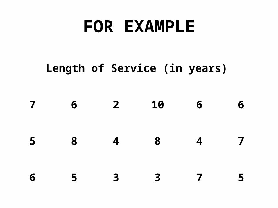
FOR EXAMPLE

Length of Service (in years)

7 6 2 10 6 6

5 8 4 8 4 7

6 5 3 3 7 5

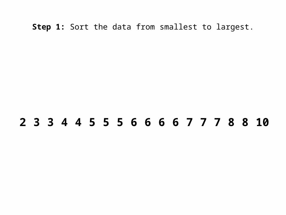
Step 1: Sort the data from smallest to largest.

2 3 3 4 4 5 5 5 6 6 6 6 7 7 7 8 8 10

Step 2: Draw the number line and label it as shown.

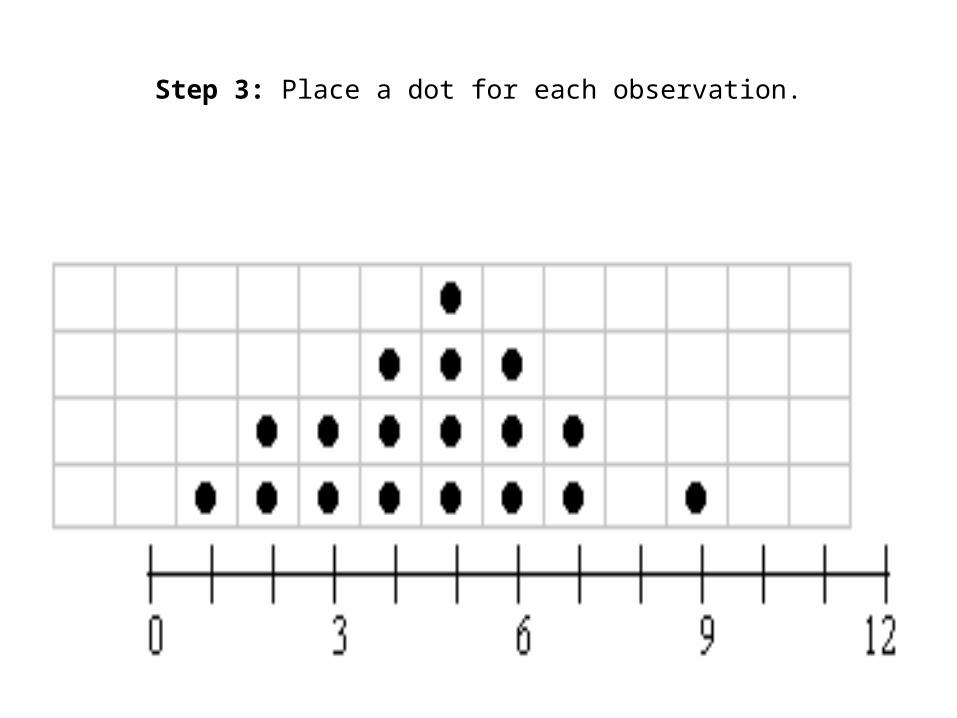
Step 3: Place a dot for each observation.

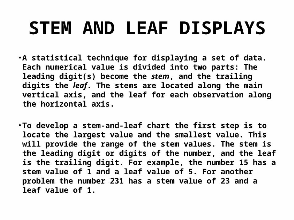
STEM AND LEAF DISPLAYS• A statistical technique for displaying a set of data. Each numerical

value is divided into two parts: The leading digit(s) become the stem, and the trailing digits the leaf. The stems are located along the main vertical axis, and the leaf for each observation along the horizontal axis.

• To develop a stem-and-leaf chart the first step is to locate the largest value and the smallest value. This will provide the range of the stem values. The stem is the leading digit or digits of the number, and the leaf is the trailing digit. For example, the number 15 has a stem value of 1 and a leaf value of 5. For another problem the number 231 has a stem value of 23 and a leaf value of 1.

FOR EXAMPLE

$12 $28 $32 $24 $17 $6

$34 $18 $22 $42 $36 $26

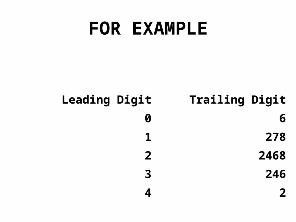
FOR EXAMPLE

Leading Digit Trailing Digit

0 6

1 278

2 2468

3 246

4 2

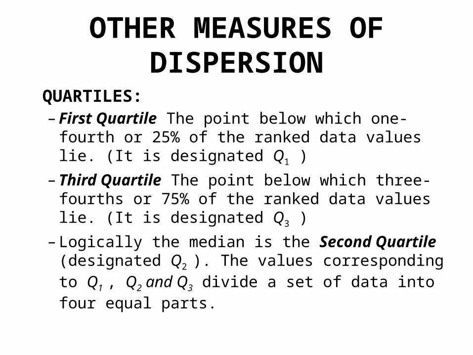
OTHER MEASURES OF DISPERSION

QUARTILES:– First Quartile The point below which one-fourth or

25% of the ranked data values lie. (It is designated Q1 )

– Third Quartile The point below which three-fourths or 75% of the ranked data values lie. (It is designated Q3 )

– Logically the median is the Second Quartile (designated Q2 ). The values corresponding to Q1 , Q2 and Q3 divide a set of data into four equal parts.

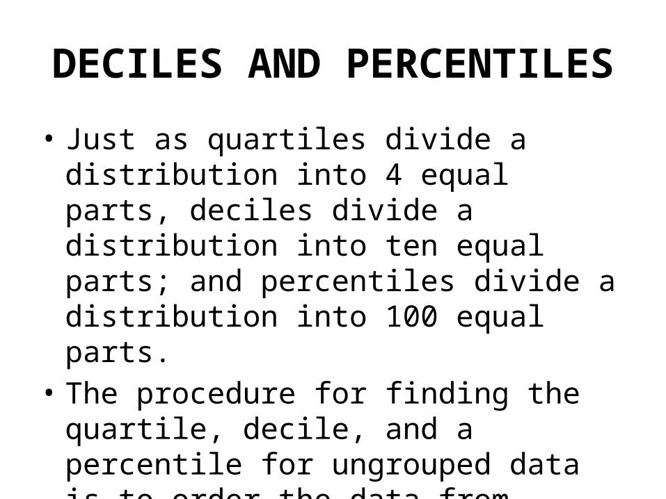
DECILES AND PERCENTILES

• Just as quartiles divide a distribution into 4 equal parts, deciles divide a distribution into ten equal parts; and percentiles divide a distribution into 100 equal parts.

• The procedure for finding the quartile, decile, and a percentile for ungrouped data is to order the data from smallest to largest. Then use text formula [4-1].

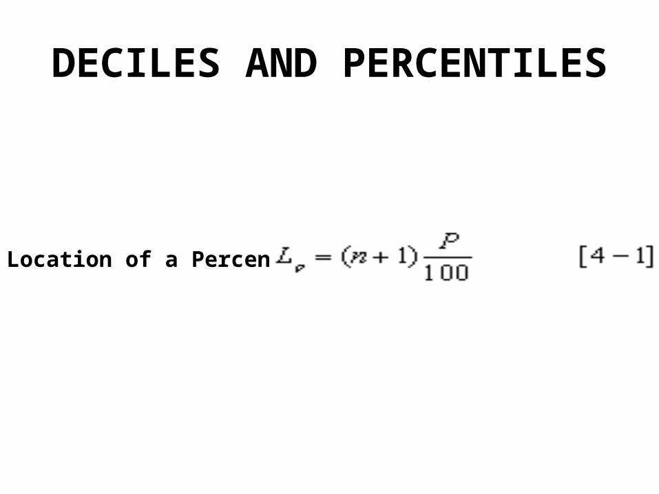
DECILES AND PERCENTILES

Location of a Percentile,

BOX PLOTS

• A graphical display based on five statistics: the minimum value, Q1 (the first quartile), Q2 the median, Q3 (the third quartile) and the maximum value.

• To construct a box plot we need five pieces of information. We need the minimum value, Q1 (the first quartile), Q2 the median, Q3 (the third quartile) and the maximum value.

RELATIVE DISPERSION

• Coefficient of variation: The ratio of the standard deviation to the arithmetic mean, expressed as a percent.

FORMULA FOR CV

Coefficient of Variation,

Multiplying by 100 converts the decimal to a percent

[4-2]

COEFFICIENT OF VARIATION

• Characteristics of the coefficient of variation are:– It reports the variation relative to the mean. – It is useful for comparing distributions with

different units.

SKEWNESS

• Four shapes of distribution

• Coefficient of skewness: A measure to describe the degree of skewness. How the distribution is skewed?

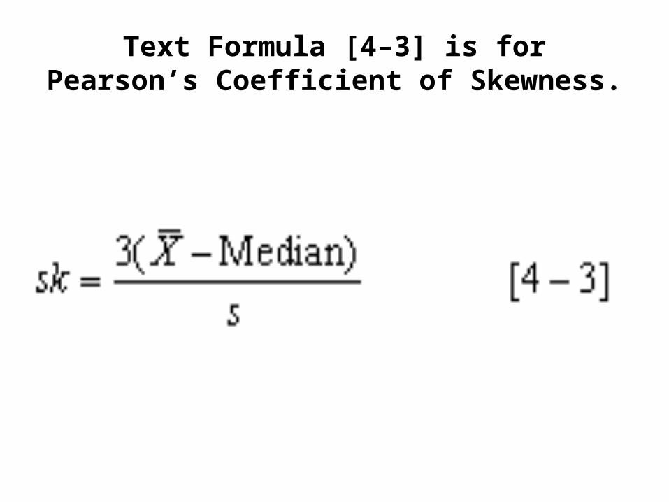
Text Formula [4–3] is for Pearson’s Coefficient of Skewness.

Characteristics of the coefficient of skewness are:

• The coefficient of skewness, designated sk, measures the amount of skewness and may range from -3.0 to +3.0.

• A value near -3, such as -2.57, indicates considerable negative skewness.

• A value such as 1.63 indicates moderate positive skewness.

• A value of 0, which will occur when the mean and median are equal, indicates the distribution is symmetrical and that there is no skewness.

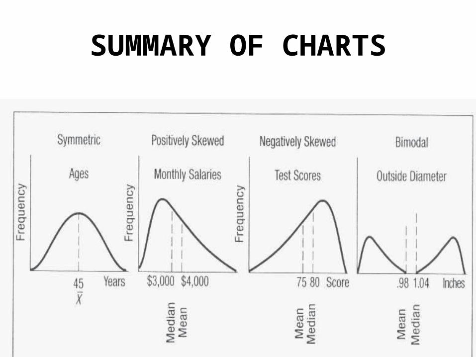
SUMMARY OF CHARTS

RELATIONSHIP BETWEEN TWO VARIABLES

• Bivariate data: A collection of paired data values. • Scatter diagram: A graph in which paired data

values are plotted on an X,Y Axis.• The steps to follow in developing a scatter diagram

are:– We need two variables. – We scale one variable (x) along the horizontal axis (X –

Axis) of a graph and the corresponding variable (y) along the vertical axis (Y – Axis).

– Place a dot for each (x, y) pair of observations.

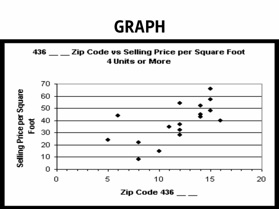
GRAPH

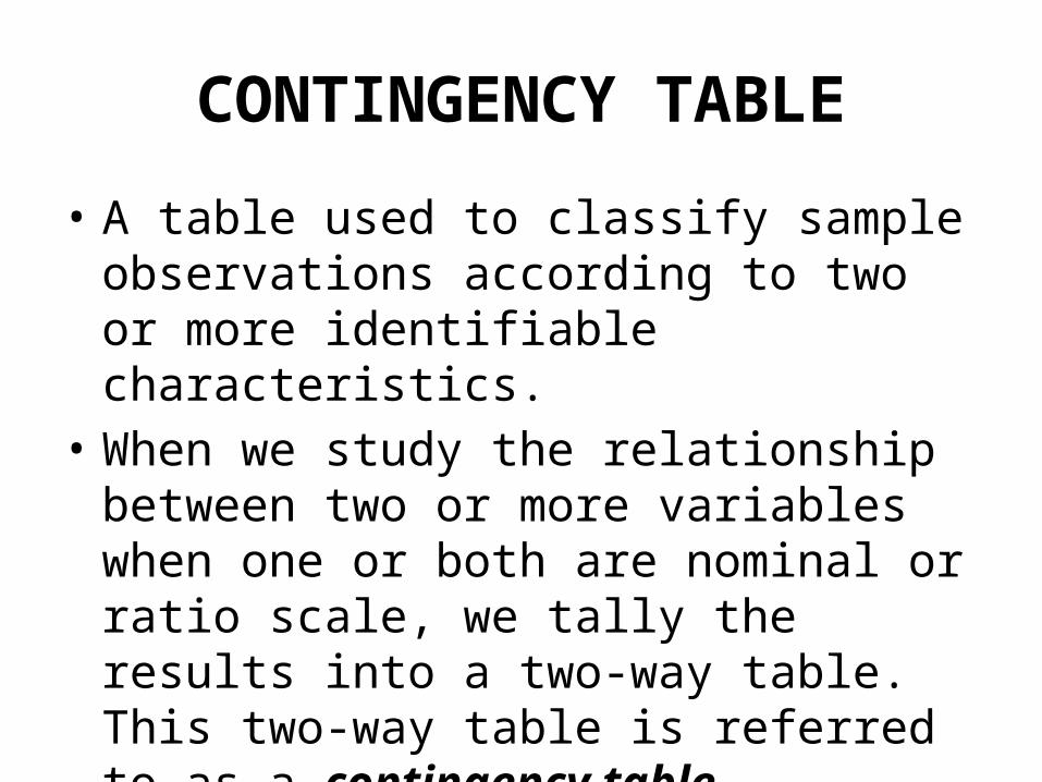
CONTINGENCY TABLE

• A table used to classify sample observations according to two or more identifiable characteristics.

• When we study the relationship between two or more variables when one or both are nominal or ratio scale, we tally the results into a two-way table. This two-way table is referred to as a contingency table.

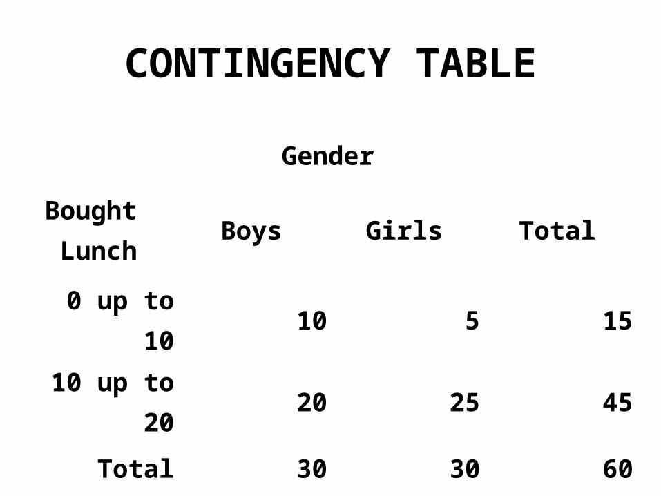
CONTINGENCY TABLE

  Gender  

Bought Lunch

Boys Girls Total

0 up to 10 10 5 15

10 up to 20 20 25 45

Total 30 30 60

CONTINGENCY TABLE

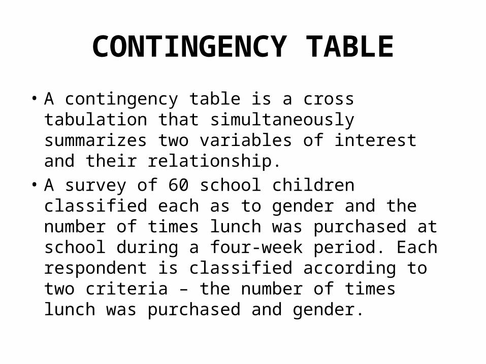
• A contingency table is a cross tabulation that simultaneously summarizes two variables of interest and their relationship.

• A survey of 60 school children classified each as to gender and the number of times lunch was purchased at school during a four-week period. Each respondent is classified according to two criteria – the number of times lunch was purchased and gender.