Welcome message from author
This document is posted to help you gain knowledge. Please leave a comment to let me know what you think about it! Share it to your friends and learn new things together.
Transcript


La fameuse pipe, me l’a-t-on assez reprochée ! Et pourtant, pouvez-vous la bourrer ma pipe ?Non, n’est-ce pas, elle n’est qu’une représentation.
Donc si j’avais écrit sous mon tableau « Ceci est une pipe », j’aurais menti !
- René Magritte
The famous pipe, how people reproached me for it! And yet, can you stuff my pipe? No, it is just a representation,is it not? So had I written on my picture « This is a pipe », I would have lied!
- René Magritte

SIKS Dissertation Series No. 2019-01The research reported in this thesis has been carried out under the auspices of SIKS, the Dutch ResearchSchool for Information and Knowledge Systems.
© 2019 Emmanuelle M.A.L. Beauxis-AussaletAll rights reserved
ISBN-13 978-90-393-7084-1
Cover images:L’interpretation des rêves, René Magritte, 1927 (front).La clé des songes, René Magritte, 1930 (back).These paintings, contemporary with La trahison des images (The treachery of images, 1929), discussthe limitations of all forms of representation, as these fail to convey reality itself. There is moreto reality than what our senses, languages or arts may represent. Magritte aimed at preservingthis complexity through surrealism. "Le Surréalisme, c’est la connaissance immédiate du réel"("Surrealism is the immediate knowledge of reality"). Similarly, there is more to reality than whatour datasets and artificial intelligence models may represent. These technological limitationsare the matter of this dissertation. May the art of Magritte bring to the reader’s attentiondeep underlying problems that this dissertation humbly aims at addressing. "Le monde et sonmystère ne se refait jamais, il n’est pas un modèle qu’il suffit de copier" ("The world and its mysterynever remakes itself, it is not a model which copying suffices").

Statistics and Visualizationsfor Assessing
Class Size Uncertainty
Statistiek en Visualisaties voor het Vaststellen vanOnzekerheid in Klassenfrequenties
(met een samenvatting in het Nederlands)
Proefschrift
ter verkrijging van de graad van doctoraan de Universiteit Utrecht op gezag vande rector magnificus, prof.dr. H.R.B.M.Kummeling, ingevolge het besluit van hetcollege voor promoties in het openbaar teverdedigen op maandag 28 januari 2019des ochtends te 10.30 uur
door
Emmanuelle Morgane Aude Lucie Beauxis-Aussalet
geboren op 1 augustus 1983 te Parijs, Frankrijk

Promotor: Prof.dr. H.L. Hardman
This thesis was partly accomplished with financial support from the NWO institute Centrum Wiskunde& Informatica (CWI), the European Union Seventh Framework Programme (FP7), and Amsterdam DataScience (ADS).

Contents
1 Introduction 11.1 The Fish4Knowledge project . . . . . . . . . . . . . . . . . . . . . . . . . . . . . . . . . . . . . 21.2 Interpreting computer vision results . . . . . . . . . . . . . . . . . . . . . . . . . . . . . . . . 31.3 Analysing class sizes . . . . . . . . . . . . . . . . . . . . . . . . . . . . . . . . . . . . . . . . . 51.4 Research questions . . . . . . . . . . . . . . . . . . . . . . . . . . . . . . . . . . . . . . . . . . 61.5 Scope . . . . . . . . . . . . . . . . . . . . . . . . . . . . . . . . . . . . . . . . . . . . . . . . . . 81.6 Thesis overview . . . . . . . . . . . . . . . . . . . . . . . . . . . . . . . . . . . . . . . . . . . . 91.7 Thesis contributions . . . . . . . . . . . . . . . . . . . . . . . . . . . . . . . . . . . . . . . . . 111.8 Publications . . . . . . . . . . . . . . . . . . . . . . . . . . . . . . . . . . . . . . . . . . . . . . 14
2 User Information Requirements 172.1 Interviews with stakeholders . . . . . . . . . . . . . . . . . . . . . . . . . . . . . . . . . . . . 182.2 Population monitoring use cases . . . . . . . . . . . . . . . . . . . . . . . . . . . . . . . . . . 192.3 High-level information needs . . . . . . . . . . . . . . . . . . . . . . . . . . . . . . . . . . . . 222.4 Data collection techniques . . . . . . . . . . . . . . . . . . . . . . . . . . . . . . . . . . . . . . 25
2.4.1 Well-established data collection methods . . . . . . . . . . . . . . . . . . . . . . . . . 262.4.2 Sampling methods . . . . . . . . . . . . . . . . . . . . . . . . . . . . . . . . . . . . . . 272.4.3 Impact of video technologies on sampling methods . . . . . . . . . . . . . . . . . . . 282.4.4 Choice of data collection and sampling method . . . . . . . . . . . . . . . . . . . . . 28
2.5 Biases of data collection techniques . . . . . . . . . . . . . . . . . . . . . . . . . . . . . . . . . 292.6 Implications for the Fish4Knowledge system . . . . . . . . . . . . . . . . . . . . . . . . . . . 312.7 Requirements for accountable classification systems . . . . . . . . . . . . . . . . . . . . . . . 32
2.7.1 Identify the application conditions . . . . . . . . . . . . . . . . . . . . . . . . . . . . . 322.7.2 Identify the uncertainty factors . . . . . . . . . . . . . . . . . . . . . . . . . . . . . . . 332.7.3 Identify the uncertainty measurements . . . . . . . . . . . . . . . . . . . . . . . . . . 342.7.4 Estimate uncertainty in end-results . . . . . . . . . . . . . . . . . . . . . . . . . . . . . 35
2.8 Conclusion . . . . . . . . . . . . . . . . . . . . . . . . . . . . . . . . . . . . . . . . . . . . . . . 37
3 Establishing Informed Trust 393.1 Errors in binary classification . . . . . . . . . . . . . . . . . . . . . . . . . . . . . . . . . . . . 403.2 Experimental setup . . . . . . . . . . . . . . . . . . . . . . . . . . . . . . . . . . . . . . . . . . 403.3 Trust, acceptance, understanding & information needs . . . . . . . . . . . . . . . . . . . . . . 453.4 Impact of introducing classification error assessments . . . . . . . . . . . . . . . . . . . . . . 46
3.4.1 Trust and Acceptance . . . . . . . . . . . . . . . . . . . . . . . . . . . . . . . . . . . . 463.4.2 Understanding and Information Needs . . . . . . . . . . . . . . . . . . . . . . . . . . 48
3.5 Unadressed information needs . . . . . . . . . . . . . . . . . . . . . . . . . . . . . . . . . . . 493.5.1 Information on classification errors . . . . . . . . . . . . . . . . . . . . . . . . . . . . . 503.5.2 Information on other uncertainty factors . . . . . . . . . . . . . . . . . . . . . . . . . 53
3.6 Conclusion . . . . . . . . . . . . . . . . . . . . . . . . . . . . . . . . . . . . . . . . . . . . . . . 54
4 Uncertainty Factors and Assessment Methods 57
v
vi Contents
4.1 Sources of uncertainty . . . . . . . . . . . . . . . . . . . . . . . . . . . . . . . . . . . . . . . . 584.1.1 Computer vision system . . . . . . . . . . . . . . . . . . . . . . . . . . . . . . . . . . . 594.1.2 In-situ system deployment . . . . . . . . . . . . . . . . . . . . . . . . . . . . . . . . . 60
4.2 Uncertainty factors . . . . . . . . . . . . . . . . . . . . . . . . . . . . . . . . . . . . . . . . . . 614.2.1 Uncertainty factors from the computer vision system . . . . . . . . . . . . . . . . . . 614.2.2 Uncertainty factors from the in-situ system deployment . . . . . . . . . . . . . . . . 624.2.3 Uncertainty factors from both system and in-situ deployment . . . . . . . . . . . . . 63
4.3 Uncertainty propagation . . . . . . . . . . . . . . . . . . . . . . . . . . . . . . . . . . . . . . . 644.3.1 Interactions between uncertainty factors . . . . . . . . . . . . . . . . . . . . . . . . . 644.3.2 High-level impact . . . . . . . . . . . . . . . . . . . . . . . . . . . . . . . . . . . . . . . 66
4.4 Uncertainty assessment methods . . . . . . . . . . . . . . . . . . . . . . . . . . . . . . . . . . 674.4.1 Measuring computer vision errors . . . . . . . . . . . . . . . . . . . . . . . . . . . . . 674.4.2 Measuring the impact of deployment conditions . . . . . . . . . . . . . . . . . . . . . 69
4.5 Conclusion . . . . . . . . . . . . . . . . . . . . . . . . . . . . . . . . . . . . . . . . . . . . . . . 724.5.1 Impacts of uncertainty factors . . . . . . . . . . . . . . . . . . . . . . . . . . . . . . . . 724.5.2 User-oriented assessment methods . . . . . . . . . . . . . . . . . . . . . . . . . . . . . 73
5 Estimating Classification Errors 755.1 Introduction . . . . . . . . . . . . . . . . . . . . . . . . . . . . . . . . . . . . . . . . . . . . . . 765.2 Existing bias correction methods . . . . . . . . . . . . . . . . . . . . . . . . . . . . . . . . . . 77
5.2.1 Reclassification method . . . . . . . . . . . . . . . . . . . . . . . . . . . . . . . . . . . 785.2.2 Misclassification method . . . . . . . . . . . . . . . . . . . . . . . . . . . . . . . . . . 795.2.3 Application . . . . . . . . . . . . . . . . . . . . . . . . . . . . . . . . . . . . . . . . . . 795.2.4 Discussion . . . . . . . . . . . . . . . . . . . . . . . . . . . . . . . . . . . . . . . . . . . 80
5.3 Error composition . . . . . . . . . . . . . . . . . . . . . . . . . . . . . . . . . . . . . . . . . . . 825.3.1 Ratio-to-TP method . . . . . . . . . . . . . . . . . . . . . . . . . . . . . . . . . . . . . 825.3.2 Application . . . . . . . . . . . . . . . . . . . . . . . . . . . . . . . . . . . . . . . . . . 835.3.3 Discussion . . . . . . . . . . . . . . . . . . . . . . . . . . . . . . . . . . . . . . . . . . . 83
5.4 Sample-to-Sample method . . . . . . . . . . . . . . . . . . . . . . . . . . . . . . . . . . . . . . 855.4.1 Error rate estimator . . . . . . . . . . . . . . . . . . . . . . . . . . . . . . . . . . . . . . 865.4.2 Evaluation of error rate estimator . . . . . . . . . . . . . . . . . . . . . . . . . . . . . 865.4.3 Application to estimating class sizes . . . . . . . . . . . . . . . . . . . . . . . . . . . . 895.4.4 Application to estimating error composition . . . . . . . . . . . . . . . . . . . . . . . 915.4.5 Discussion . . . . . . . . . . . . . . . . . . . . . . . . . . . . . . . . . . . . . . . . . . . 91
5.5 Maximum Determinant method . . . . . . . . . . . . . . . . . . . . . . . . . . . . . . . . . . . 955.5.1 Determinants as variance predictors . . . . . . . . . . . . . . . . . . . . . . . . . . . . 955.5.2 Application . . . . . . . . . . . . . . . . . . . . . . . . . . . . . . . . . . . . . . . . . . 965.5.3 Discussion . . . . . . . . . . . . . . . . . . . . . . . . . . . . . . . . . . . . . . . . . . . 98
5.6 Applicability issues . . . . . . . . . . . . . . . . . . . . . . . . . . . . . . . . . . . . . . . . . . 995.6.1 Impractical cases . . . . . . . . . . . . . . . . . . . . . . . . . . . . . . . . . . . . . . . 1005.6.2 Test set representativity . . . . . . . . . . . . . . . . . . . . . . . . . . . . . . . . . . . 1015.6.3 Varying feature distributions . . . . . . . . . . . . . . . . . . . . . . . . . . . . . . . . 103
5.7 Future work . . . . . . . . . . . . . . . . . . . . . . . . . . . . . . . . . . . . . . . . . . . . . . 1055.7.1 Discrete approaches . . . . . . . . . . . . . . . . . . . . . . . . . . . . . . . . . . . . . 1055.7.2 Continuous approaches . . . . . . . . . . . . . . . . . . . . . . . . . . . . . . . . . . . 1055.7.3 Identify the misclassified items . . . . . . . . . . . . . . . . . . . . . . . . . . . . . . . 107
5.8 Conclusion . . . . . . . . . . . . . . . . . . . . . . . . . . . . . . . . . . . . . . . . . . . . . . . 1085.9 Additional materials . . . . . . . . . . . . . . . . . . . . . . . . . . . . . . . . . . . . . . . . . 110
5.9.1 Code . . . . . . . . . . . . . . . . . . . . . . . . . . . . . . . . . . . . . . . . . . . . . . 1105.9.2 Application of Fieller’s theorem . . . . . . . . . . . . . . . . . . . . . . . . . . . . . . 1105.9.3 Tutorials explaining the Logistic Regression method . . . . . . . . . . . . . . . . . . . 111
6 Visualization of Classification Errors 1156.1 End-user requirements . . . . . . . . . . . . . . . . . . . . . . . . . . . . . . . . . . . . . . . . 1166.2 Information needs . . . . . . . . . . . . . . . . . . . . . . . . . . . . . . . . . . . . . . . . . . . 118

Contents vii
6.3 Related work . . . . . . . . . . . . . . . . . . . . . . . . . . . . . . . . . . . . . . . . . . . . . . 1186.4 Classee visualization . . . . . . . . . . . . . . . . . . . . . . . . . . . . . . . . . . . . . . . . . 1206.5 User experiment . . . . . . . . . . . . . . . . . . . . . . . . . . . . . . . . . . . . . . . . . . . . 1256.6 Quantitative results . . . . . . . . . . . . . . . . . . . . . . . . . . . . . . . . . . . . . . . . . . 1296.7 Qualitative analysis . . . . . . . . . . . . . . . . . . . . . . . . . . . . . . . . . . . . . . . . . . 1346.8 Conclusion . . . . . . . . . . . . . . . . . . . . . . . . . . . . . . . . . . . . . . . . . . . . . . . 139
7 Visualization Tool for Exploring Uncertain Class Sizes 1437.1 Related work . . . . . . . . . . . . . . . . . . . . . . . . . . . . . . . . . . . . . . . . . . . . . . 144
7.1.1 Visualizing multidimensional and uncertain data . . . . . . . . . . . . . . . . . . . . 1447.1.2 Usability issues . . . . . . . . . . . . . . . . . . . . . . . . . . . . . . . . . . . . . . . . 1457.1.3 Situation awareness . . . . . . . . . . . . . . . . . . . . . . . . . . . . . . . . . . . . . 145
7.2 User interface . . . . . . . . . . . . . . . . . . . . . . . . . . . . . . . . . . . . . . . . . . . . . 1467.2.1 Design rationale . . . . . . . . . . . . . . . . . . . . . . . . . . . . . . . . . . . . . . . 1477.2.2 Interface design . . . . . . . . . . . . . . . . . . . . . . . . . . . . . . . . . . . . . . . . 1507.2.3 Usage scenario . . . . . . . . . . . . . . . . . . . . . . . . . . . . . . . . . . . . . . . . 160
7.3 Evaluation . . . . . . . . . . . . . . . . . . . . . . . . . . . . . . . . . . . . . . . . . . . . . . . 1637.3.1 Experimental setup . . . . . . . . . . . . . . . . . . . . . . . . . . . . . . . . . . . . . . 1647.3.2 Experiment results . . . . . . . . . . . . . . . . . . . . . . . . . . . . . . . . . . . . . . 1687.3.3 Interpretation and recommendations . . . . . . . . . . . . . . . . . . . . . . . . . . . 171
7.4 Conclusion . . . . . . . . . . . . . . . . . . . . . . . . . . . . . . . . . . . . . . . . . . . . . . . 174
8 Conclusion 1778.1 Practical challenges with end-users’ requirements . . . . . . . . . . . . . . . . . . . . . . . . 177
8.1.1 Challenges with assessing error propagation . . . . . . . . . . . . . . . . . . . . . . . 1788.1.2 Challenges with assessing the errors in specific end-results . . . . . . . . . . . . . . . 179
8.2 Unified classification assessment framework . . . . . . . . . . . . . . . . . . . . . . . . . . . 1808.2.1 Tuning classifiers in collaboration with end-users . . . . . . . . . . . . . . . . . . . . 1818.2.2 Mapping error rates and feature distributions . . . . . . . . . . . . . . . . . . . . . . 1828.2.3 Uncovering variance issues . . . . . . . . . . . . . . . . . . . . . . . . . . . . . . . . . 183
8.3 Developing classification literacy . . . . . . . . . . . . . . . . . . . . . . . . . . . . . . . . . . 1848.4 Epilogue . . . . . . . . . . . . . . . . . . . . . . . . . . . . . . . . . . . . . . . . . . . . . . . . 186
A Study of User Trust and Acceptance 187A.1 Questionnaire . . . . . . . . . . . . . . . . . . . . . . . . . . . . . . . . . . . . . . . . . . . . . 187A.2 Interpretation of participant responses . . . . . . . . . . . . . . . . . . . . . . . . . . . . . . . 197
Bibliography 201
Summary 215
Samenvatting 217
Curriculum Vitae 221
Acknowledgements 223


Chapter 1Introduction
Classification technologies are increasingly pervasive in our societies and impact ourprofessional and personal lives. For instance, classification systems are used in do-mains such as medical diagnosis, information retrieval, fraud detection, loan defaultprediction, or natural language processing. Handling classification uncertainty is acrucial challenge for supporting efficient and ethical systems. For instance, providingunderstandable uncertainty assessments to stakeholders is necessary for conductingresponsible data science, i.e., for controlling accuracy and fairness, and achievingtransparency1.
This thesis addresses uncertainty issues that pertain to estimating class sizes.We focus on the perspective of end-users with little or no expertise in machinelearning, who are interested in numbers of objects per class, i.e., class sizes. Suchusers may analyse the patterns in class sizes, but may not seek to retrieve individualobjects of particular classes. We aim at enabling end-users of classification systemsto conduct uncertainty-aware and scientifically-valid analysis of class sizes.
Our research is motivated by a practical use case of computer vision for monitor-ing fish populations, implemented within the Fish4Knowledge project2. Monitoringanimals in their natural habitats allows scientists to study population sizes and be-haviors, and phenomena such as reproduction or migration. It also provides evidenceon how environmental conditions and human activities impact animal populations,whether in positive or negative ways. In our era facing major environmental chal-lenges, monitoring wild animal populations provides key information to assess theneeds for protecting natural habitats.
1Dutch initiative for Responsible Data Science: www.responsibledatascience.org (van der Aalst et al.2017)
2Website of the Fish4Knowledge project: www.fish4knowledge.eu
1

2 Chapter 1
Deploying human observers to study animals in their natural environment in-volves significant costs that limit the extent of such studies. Human observers mayalso disturb animals and interfere with their natural behaviors, so that observationscan be biased (e.g., animals may avoid areas where observers are present). In con-trast, deploying cameras instead of human observers offers opportunities to reducesuch costs and biases.
Computer vision systems can classify animals’ species or behaviors, and the classsizes provide a means to monitor the sizes of animal populations. However, suchapplication requires rigorous assessments of the uncertainty issues that impact theclassification results. Without assessing the uncertainty, no scientific conclusions canbe drawn on the animal populations. This is a challenge we aim to address in thisthesis.
Hence we investigate how to support end-users’ understanding of class sizeuncertainty, in the context of in-situ video monitoring of animal populations. Fromthe specific use case within the Fish4Knowledge project, we derive generalizablemethods for:
• Assessing the uncertainty factors and the uncertainty propagation that resultin high-level errors and biases in class size estimates.
• Visualizing classification uncertainty when evaluating classification systems,and interpreting class size estimates.
• Estimating the magnitude of classification errors in class size estimates.
1.1 The Fish4Knowledge project
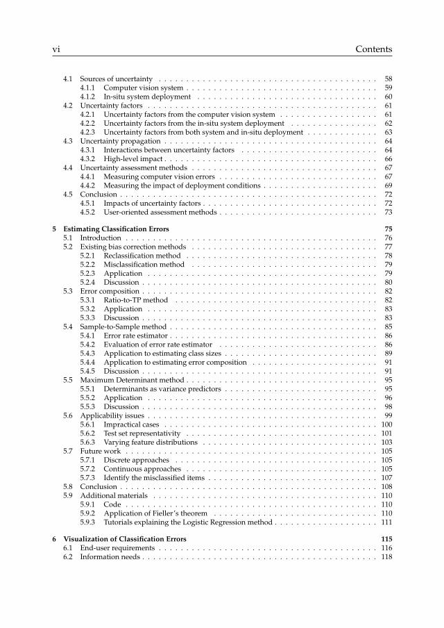
The Fish4Knowledge project3 delivered computer vision tools for studying fish pop-ulations (Figure 1.1). The project used 9 fixed underwater cameras (Figures 1.2and 1.3) to continuously monitor Taiwanese coral reef ecosystems during 3 years.It produced 87 thousand hours of video, in which 1.4 billion fish were detected.Observations were collected over continuous periods of time (e.g., observing popu-lations over complete days, seasons and years) and with limited disturbance fromthe data collection devices. The resulting dataset is highly valuable for studying fishpopulations in their natural environment.
The project delivered computer vision software able to differentiate fish and non-fish objects in individual video frames (Figure 1.4), track individual fish across videoframes, and recognize up to 23 fish species (Figures 1.5 and 1.6). Our research con-tributed to developing visualization tools for exploring the computer vision resultsand their uncertainties. Our results provided tools and methods for conductinguncertainty-aware analyses of the fish populations.
3 Book: R. B. Fisher et. al, Fish4Knowledge: Collecting and Analyzing Massive Coral Reef Fish VideoData. Springer (2016). Teaser: https://www.youtube.com/watch?v=AFV-FiKUFyI (Boom et al. 2012).
Introduction 3
Figure 1.1: Example fish species monitored within the Fish4Knowledge project.
Figure 1.2: Locations of the Fish4Knowledge cameras in southern Taiwan.
The Fish4Knowledge project was funded by the European Union Seventh Frame-work Programme FP7 (grant 257024) and lasted 3 years from 2012 to 2015. It includedresearch teams from Edinburgh University (United Kingdoms), Catania University(Italy), National Centre for High Performance Computing (Taiwan), Academia Sinica(Taiwan), and CWI (the Netherlands).
1.2 Interpreting computer vision results
Computer vision technologies contrast with traditional practices, such as experimen-tal fishing or diving observations, as the information collected and the uncertaintyissues are different. Computer vision is based on visual information, such as contour,

4 Chapter 1
contrast, colour histograms or textures, while ecology research is based on biologicalcharacteristics, such as species, size, age or behavior. It is challenging to derive thebiological information from the visual information: the high-level information needsof ecologists may not be fully addressed, or may not be addressed with the requiredreliability.
Figure 1.3: Views from the cameras deployed within the Fish4Knowledge project.
Figure 1.4: Classification of fish and non-fish objects.
Figure 1.5: Description of the visual features (e.g., contour, orientation, body parts)

Introduction 5
Figure 1.6: Classification of fish species (e.g., into classes C1, C7, or C9) using all imagesalong fish trajectories.
The classification of objects appearing in the videos is inherently imperfect. Manyunderlying factors can impact the magnitude of classification errors. For example,video images of poor quality yield more errors than high-quality images (Figure 1.7).Computer vision systems typically use pipelines of classifiers, and uncertainty canpropagate from one classifier to another. For example, if fish are not detectedin all video frames, their trajectories are misidentified (Figure 1.8 and 1.9). If fishtrajectories are discontinued, individual fish are counted as two separate fish and theresulting class sizes are over-estimated. If fish trajectories contain non-fish objectsmisclassified as fish, the classification of such fish into species has increased chancesof errors. Ultimately, the classification errors impact the high-level informationprovided to ecologists. For example, the population sizes can be over- or under-estimated (e.g., if fish are not detected, if non-fish objects are classified as fish, or iffish species are misclassified).
It is crucial to communicate the uncertainties that computer vision results cancarry. As scientists, ecologists are required to investigate and disclose the potentialsources of uncertainty and, where possible, to estimate the resulting errors and biases.These are prerequisites for drawing scientifically valid interpretations of computervision and classification data. Hence the perspective of ecologists is particularlyrelevant for researching the means to assess and communicate class size uncertainty,and to enable accountable classification systems.
1.3 Analysing class sizes
Our use case concerns users of classification systems who study population sizesestimated as class sizes. The users have no technical expertise in classification tech-nologies, yet need to assess the uncertainty issues. They need to assess whether theclass sizes are representative of the actual populations. Within the Fish4Knowledgeproject, for instance, ecologists use computer vision to classify fish into species.They need to draw scientific conclusions on the class sizes, yet have no expertise inthe biases that classification and computer vision entail. From this particular use

6 Chapter 1
case, this thesis develops generalizable methods and tools for supporting end-userunderstanding of computer vision and classification uncertainty, and enablinguncertainty-aware and scientifically-valid analyses of class sizes.
Analysing class sizes is a common task in domains other than ecology. For exam-ple, geologists can analyse land coverage from satellite images, e.g., by classifyingimage pixels into forest, sand, urban areas or other types of land. In this case, thenumbers of pixels per class, i.e., the class sizes, evaluate areas of types of land. Inthe medical domain, when classifying the pixels of images of cancerous tissues, classsizes estimate the sizes of tumors.
Analysing class sizes is also common with technologies other than computervision. For instance, when classifying the topics of texts, class sizes measure thefrequency at which topics are discussed. Within the financial sector, when classifyingborrowers’ potential defaults, class sizes estimate the risks associated with loanportfolios.
Hence, our generic use case concerns the analysis of class sizes and their uncer-tainties. For this use case, the high-level uncertainty concerns how class sizes drawnfrom classification systems may differ from the actual class sizes in the real world.
1.4 Research questions
We first explore the specific topic of monitoring animal populations using computervision, before addressing the more generic topic of assessing class size uncertainty.
Question 1: What high-level information needs and uncertainty requirements inmarine ecology research can be addressed with computer vision systems?
As computer vision technologies are relatively new in marine ecology, we need toestablish which high-level tasks and information needs can or cannot be addressed,and which types of uncertainty are acceptable. This is the topic of our first researchquestion, addressed in Chapter 2 - User Information Requirements.
Figure 1.7: Example of low quality images collected within the Fish4Knowledge project.From left to right: encoding error, murky water, dirt on the lens.

Introduction 7
Figure 1.8: Example of objects that are difficult to classify into fish or non-fish objects.
Figure 1.9: Uncertainty propagation yielding tracking error. One fish was not detected in avideo frame. This fish trajectory was misinterpreted (green line). The missing fish image wasreplaced with one from the nearby fish.
Question 2: What information on classification errors is required for end-users toestablish informed trust in classification results?
Providing information on classification errors may improve users’ trust and ac-ceptance of classification systems. Without sufficient information on classificationerrors, users’ trust or mistrust of classification results may be uninformed. We needto establish the information that support user understanding of uncertainty issues,and informed decision when interpreting classification results. This is the topic ofour second research question, addressed in Chapter 3 - Establishing Informed Trust.
Question 3: When applying computer vision systems for population monitoring,what uncertainty factors can arise from computer vision systems, and from theenvironment in which systems are deployed?Question 4: How uncertainty assessment methods address the combined effect ofuncertainty factors?
With the insights from our initial research questions, we can develop a comprehen-sive overview of the underlying factors that contribute to the high-level uncertaintywhen estimating population sizes. To enable transparent and accountable computervision systems for population monitoring, we must consider how uncertainty prop-agates within the pipeline of classification algorithms. We must also consider theuncertainty that arises from the conditions under which the computer vision systemis deployed. This is the topics of our third and fourth research question, addressedin Chapter 4 - Uncertainty Factors and Assessment Methods.

8 Chapter 1
Question 5: How can we estimate the magnitudes of classification errors in end-results?
Key uncertainty factors are not fully addressed by existing assessment methods.In particular, we identify missing methods for estimating the magnitudes of clas-sification errors that can be expected in classification results. Test sets are used tomeasure the rates of classification errors. Such error rates intend to represent theclassification errors to expect in future applications. However, end-users are notprovided with formal methods to estimate the magnitude of errors in classificationresults, using error rates measured with test sets. This is the topic of our fifth researchquestion, addressed in Chapter 5 - Estimating Classification Errors.
Question 6: How can visualization support non-expert users in understandingclassification errors?
It is not trivial to understand how the magnitudes of classification errors canbias class size estimates. The end-users who must assess such classification errorsmay have no expertise in classification. Without understanding the implications ofclassification errors, end-users cannot perform uncertainty-aware interpretations ofclass sizes. Hence we focus on the means to support non-experts’ understandingof classification errors. We investigate simplified visualization designs that enablenon-experts to choose classifiers, use simple tuning parameters, and understand themagnitude of errors to expect in future classification results. This is the topic of oursixth research question, addressed in Chapter 6 - Visualization of Classification Errors.
Question 7: How can interactive visualization tools support the exploration ofcomputer vision results and their multifactorial uncertainties?
Conducting uncertainty-aware class size analyses does not only involve classifi-cation errors. Other uncertainty factors must be considered, such as those identifiedthrough our research question 3. Hence we investigates comprehensive user in-terfaces that provide complete information on computer vision results and theiruncertainties. This is the topic of our last research question, addressed in Chapter 7 -Visualization for Monitoring Uncertain Population Sizes.
With these research questions, we address the needs of scientists dealing withthe multiple uncertainty factors of computer vision systems for population moni-tor. Beyond this specific use case, our research questions investigate fundamentalvisualization and statistical methods for tackling classification uncertainty.
1.5 Scope
The computer vision technologies included in our scope are those developed withinthe Fish4Knowledge project. These technologies did not include measurements

Introduction 9
of fish body size, or other numerical data such as speed. The Fish4Knowledgesystem provides classification data (i.e., categorical data) that describe the typesand sizes of fish populations. Hence, our scope concerns uncertainty issues relatedto classification problems, such as estimating the misclassifications that can occurbetween each class. Uncertainty issues inherent to computer vision are consideredfrom the perspective of their impact on classification results provided to end-users.
Our research does not concern the development or improvement of computervision or classification technologies. We do not aim at reducing the uncertainty incomputer vision or classification results. Instead we aim at enabling end-users tounderstand the uncertainty, to account for the uncertainty when analysing computervision and classification data, and to draw uncertainty-aware conclusions.
Our scope does not concern uncertainty related to sampling methods, e.g., re-lated to the number and locations of the video samples, and cameras deployedin the ecosystem. Handling such uncertainty is highly dependent on the specificstudies conducted by ecologists, who have the domain knowledge to elicit the ap-propriate methods for handling issues with sampling the ecosystem. However, ourscope includes sampling issues that are related to computer vision and classifica-tion technologies, i.e., regarding the sampling of groundtruth sets used to train andtest classifiers and computer vision algorithms. As we do not aim at improvingthe computer vision and classification technologies, we do not investigate methodsfor sampling or selecting the groundtruth training sets (used to train classifiers andcomputer vision algorithms).
However, we are concerned with the groundtruth test sets that are used to estimatethe classification errors. Test sets intend to represent the errors to expect in futureapplications, and are crucial for assessing classification uncertainty. Thus we considersampling issues such as representativity, scarcity and error rate variance.
1.6 Thesis overview
Our preliminary user studies elicit the user information needs (Chapter 2) with aparticular focus on information needs w.r.t. classification uncertainty (Chapter 3).From these studies, we derive the uncertainty issues of concern to end-users, and therelated uncertainty assessment methods (Chapter 4). We then introduce new meth-ods for estimating the numbers of errors in classification results, and for correctingthe ensuing biases in class size estimates (Chapter 5). Finally, we investigate newvisualization tools for assessing classification errors (Chapter 6) and for analysingpopulation sizes and their uncertainties (Chapter 7). We conclude by discussing theimplications of our results (Chapter 8).
Chapter 2 - User Information Requirements
We establish the scope of high-level information that can be provided by computervision systems for the scientific study of animal populations. We study the applica-

10 Chapter 1
tion domain by interviewing marine ecologists. Typical data collection techniquesare compared to derive generic information needs. After interviewing computer vi-sion experts, we identify the information needs that can or cannot be addressed byvideo monitoring techniques. Finally, the uncertainty issues inherent to each datacollection technique are discussed, and high-level requirements for uncertaintyassessment are identified.
Chapter 3 - Establishing Informed Trust
We investigate the information on uncertainty issues that support end-users in de-veloping informed uncertainty assessments. Our second user study explores howinformation about classification errors impacts users’ understanding, trust and ac-ceptance of the computer vision system. We collect users’ feedback on uncertaintyfactors other than classification errors, and discuss the relationships between user(mis)understanding of uncertainty, trust and acceptance of the system. Our conclu-sions highlight unfulfilled information needs requiring additional uncertainty as-sessments, and high-level user-oriented information that uncertainty assessmentsmust provide.
Chapter 4 - Uncertainty Factors
We identify key uncertainty factors that must be considered for enabling scientifi-cally valid analyses of computer vision results. We focus on in-situ video monitoringtechnologies such as those implemented within the Fish4Knowledge system, whichprovides counts of individuals per class of species, and uses fixed underwater cam-eras without stereoscopic vision. Our scope includes uncertainty factors beyond thecomputer vision system, arising from the in-situ environment in which the systemis deployed (e.g., camera placement and fields of view). After specifying the typi-cal computer vision system and deployment conditions, the uncertainty factors areelicited from interviews of marine ecologists and computer experts. We then identifythe interactions between uncertainty factors, and how uncertainties propagates tohigh-level information. Finally, we identify the uncertainty assessment methodsthat are applicable or that are missing.
Chapter 5 - Estimating Classification Errors
We identify methods for estimating the numbers of errors in classification results,using error measurements performed with test sets. These methods can provideunbiased estimates of class sizes and do not primarily aim at identifying which spe-cific items are misclassified. Class sizes can be corrected to account for the potentialFalse Positives and False Negatives in each class. We review existing bias correc-tion methods from statistics and epidemiology, and investigate their applicability forcomputer vision classifiers. We then extend the bias correction methods to estimatingthe number of errors between specific classes. We identify the unaddressed case of

Introduction 11
disjoint test and target sets, which impacts the variance of bias correction and errorestimation results. We introduce 3 new methods:
• The Sample-to-Sample method estimates the variance of bias correction anderror estimation results for disjoint test and target sets.
• The Ratio-to-TP method uses atypical error rates that have properties ofinterest for estimating the variance of error estimation results.
• The Maximum Determinant method uses the determinant of error rates,encoded as a confusion matrix, as a predictor of the variance of error estimationresults, prior to applying the classifier to target sets.
Chapter 6 - Visualization of Classification Errors
We introduce a simplified design for visualizing classification errors, i.e., the errorsmeasured on a groundtruth test set and typically encoded in confusion matrices. Weavoid the display of error rates which can be misinterpreted. Our design rationalesselect raw numbers of errors as a basic yet complete metric, and simple barchartswhere several visual features distinguish the actual and assigned classes. Wepresent a user study that compares our simplified visualization to well-establishedvisualizations (ROC curve and confusion matrix with heatmap). We identify themain difficulties that users encountered with the visualizations and with under-standing classification errors, depending on user’s background knowledge.
Chapter 7 - Visualization Tool for Exploring Uncertain Class Sizes
We introduce a comprehensive visualization tool that enables end-users to monitorpopulation sizes, and to investigate uncertainties in specific subsets of the data.We introduce an interaction design for exploring population sizes, as well as theunderlying uncertainty factors (e.g., quality of video footage, classification errors ofcomputer vision algorithms). We present a user study that investigates the interfacedesign, and how it supports user awareness of uncertainty. We highlight the factorsthat facilitated or complicated the exploration of the data and its uncertainties,and in particular, how users may be unaware of important uncertainty factors. Weconclude with recommendations for improving the design of such interfaces.
1.7 Thesis contributions
Our research results contribute to enabling the scientific study of animal populationsbased on computer vision. Our results contribute to a broader range of applicationsdealing with uncertain computer vision and classification data. They inform thedesign of comprehensive uncertainty assessment methods and tools.

12 Chapter 1
Empirical contributions
Ü Domain analysis of computer vision for video monitoring animal popula-tions (Chapter 2).q Typical use cases are synthesized (Section 2.2), establishing key high-levelinformation needs (Section 2.3), data collection methods (Section 2.4) and un-certainty concerns (Section 2.5).q The synthesis highlights high-level information needs that can be addressedwith computer vision (Table 2.5) and uncertainty issues they entail (Table 2.6).
Ü User behaviors towards trust, acceptance, information needs, and under-standing of uncertainty (Chapter 3).q Mechanisms underlying the development of informed trust and acceptanceof classification systems are reported (Section 3.4).q Information needs about uncertainty issues are identified (Section 3.5).
Ü Applicability of methods for estimating classification errors and biases inclass size estimates (Chapter 5).q Error estimation methods from statistics and epidemiology domains are suc-cessfully applied to the domain of machine learning classification (Section 5.2).q Issues with existing error estimation methods are demonstrated (Section 5.2.4):sensitivity to stable or varying class proportions, and limited sample sizes (e.g.,small datasets yield high error rate variance).q Applicability to estimating the error composition in class size estimates isdemonstrated, i.e., detailing the numbers of errors between all possible combi-nation of classes (Section 5.3).
Ü Applicability of methods for estimating the variance of classification errorestimates (Chapter 5).q The variance estimation solution provided by our Sample-to-Sample methodis empirically validated.Its compatibility with error estimation methods, and applicability to disjoint testand target sets are demonstrated (Section 5.4).q Existing methods for estimating the variance of error estimation results areshown to be inapplicable if test and target sets are disjoint (Section 5.4.5). Suchcase is common in machine learning, but did not concern the initial applicationdomains of error estimation methods.
Ü Factors impacting user understanding of classification errors and their visu-alization (Chapter 6).q Users’ issues when interpreting classification errors using visualization sup-ports are reported. The influence of users’ prior knowledge is considered(Section 6.7).q The report establishes issues with the complexity of technical concepts andterminology, and how visualization features address or aggravate them.

Introduction 13
Ü Factors impacting user understanding of uncertainty issues when exploringcomputer vision results with interactive visualization (Chapter 7).q Usability issues with the Fish4Knowledge user interface are reported (Sec-tion 7.3.1).q Issues with visual features and dataset features are distinguished, e.g., choiceof metrics to display, and style of display (Section 7.3.2).q Recommendations are elicited for improving the interface’s support of user-awareness of uncertainty (Section 7.3.3).
Theoretical contributions
Ü Model of uncertainty factors pertaining to computer vision for monitoringanimal populations (Chapter 4).q The model comprehends uncertainty factors arising from computer visionand classification systems, or from the environment in which systems are de-ployed (Section 4.1).q Uncertainty issues are synthesized as a combination of uncertainty factors(Section 4.2).q The interactions between uncertainty factors are described (Section 4.3).
Ü Sample-to-Sample variance estimation (Chapter 5).q The distribution of rate estimators is specified for the case of disjoint datasets,i.e., for rates measured in one dataset and used as estimators of rates in disjointdatasets. Datasets are disjoint but sampled from the same population. Forinstance, such estimators can represent rates of classification errors in targetsets using error rates measured in disjoint test sets (Section 5.4.1).
Ü Maximum Determinant variance prediction (Chapter 5).q The hypothesis that the determinants of error rate matrices are predictors ofclassification errors’ variance is conjectured. (Section 5.5).q The type of error rate (e.g., FP Rate or Ratio-to-TP) and numbers of classesare shown to influence the predictive power (Table 5.3).q Future work is required for establishing theory and validating the predictionmethod (Section 5.6).
Methodological contributions
Ü Guidelines for comprehensive and user-oriented uncertainty assessments(Chapter 2).q Methodological steps are proposed for establishing the uncertainty fac-tors and uncertainty assessment methods that address end-users’ needs (Sec-tion 2.7).
Ü Methods for estimating classification errors in end-results (Chapter 5).q Error estimation method are established for binary problems, combining the

14 Chapter 1
Misclassification method, Sample-to-Sample method, and Fieller’s theorem(Sections 5.4.3 and 5.4.4).
Ü Metric for estimating classification errors in end-results, and for normalizingthe visualization of classification errors (Chapters 5 and 6).q Ratio-to-TP error rates (FN/TP) support alternative methods for estimating andpredicting classification errors in end-results (i.e., in target sets). Predictionmethods require future work for establishing theory (Section 5.3.1).q Ratio-to-TP error rates supports normalized visualization of classificationerrors. Such normalization is of interest for illustrating the impact of varyingclass proportions, and for facilitating the comparisons of False Positives andFalse Negatives (Section 6.4, Figure 6.8).
Artifact contributions
Ü Visualization of classification errors for non-expert end-users (Chapter 6).q The visualization of confusion matrices is simplified with Classee barcharts,designed to facilitate non-experts’ understanding of classification error (Sec-tion 6.4).q The design is applicable to binary and multiclass problems.q The design provides alternative to ROC and Precision/Recall curves, andincludes additional information of interest to end-users (Section 6.2, Table 6.2).q Open source visualization components and web interface are delivered(http://classee.project.cwi.nl).
Ü User interface for exploring computer vision results and their uncertainties(Chapter 7).q The Fish4Knowledge user interface is delivered to ecologists and the generalpublic. It provides access to the computer vision results collected within theFish4Knowledge project (Section 7.2).q The interface supports the exploration of fish population sizes and key un-certainty factors (Table 7.1).q The interface design is applicable to multidimensional data exploration, andmultifactorial uncertainty assessment. Reuse has been experimented with theSightCorp emotion recognition system (Section 7.4, Figure 7.28).
1.8 Publications
The research presented in this PhD thesis is based on the following publications:
Bastiaan J. Boom, Phoenix X. Huang, Cigdem Beyan, Concetto Spampinato, Si-mone Palazzo, Jiyin He, Emma Beauxis-Aussalet, Sun-In Lin, Hsiu-Mei Chou, Gay-athri Nadarajan, Yun-Heh Chen-Burger, Jacco van Ossenbruggen, Daniela Giordano,Lynda Hardman, Fang-Pang Lin, Robert B. Fisher. Long-Term Underwater CameraSurveillance for Monitoring and Analysis of Fish Populations. Workshop on Visual

Introduction 15
observation and Analysis of Animal and Insect Behavior (VAIB) at ACM MultimediaConference. 2012. Mentioned in Chapter 1.
Emma Beauxis-Aussalet, Lynda Hardman. User Information Needs. Fish4Knowledge:Collecting and Analyzing Massive Coral Reef Fish Video Data. Springer. 2016. Re-ported in Chapter 2.
Concetto Spampinato, Emma Beauxis-Aussalet, Simone Palazzo, Cigdem Beyan,Jacco van Ossenbruggen, Jiyin He, Bas Boom, Phoenix X. Huang. A Rule-BasedEvent Detection System for Real-Life Underwater Domain. Machine Vision andApplications 25(1). 2014. Mentioned in Chapter 2.
Emma Beauxis-Aussalet, Lynda Hardman: Understanding Uncertainty Issuesin the Exploration of Fish Counts. Fish4Knowledge: Collecting and AnalyzingMassive Coral Reef Fish Video Data. Springer. 2016. Reported in Chapter 3.
Emma Beauxis-Aussalet, Elvira Arslanova, Lynda Hardman, Jacco van Ossen-bruggen. A Case Study of Trust Issues in Scientific Video Collections. InternationalWorkshop on Multimedia Analysis for Ecological Data (MAED) at ACM MultimediaConference. 2013. Reported in Chapter 3.
Emma Beauxis-Aussalet, Lynda Hardman. Multifactorial Uncertainty Assess-ment for Monitoring Population Abundance using Computer Vision. IEEE Confer-ence on Data Science and Advanced Analytics (DSAA). 2015. Reported in Chapter 4.
Emma Beauxis-Aussalet, Lynda Hardman. Extended Methods to Handle Classi-fication Biases. IEEE Conference on Data Science and Advanced Analytics (DSAA).2017. Reported in Chapter 5.
Bastiaan J. Boom, Emma Beauxis-Aussalet, Lynda Hardman, Robert B. Fisher.Uncer-tainty-Aware Estimation of Population Abundance using Machine Learn-ing. Multimedia Systems 22(6). 2016. Mentioned in Chapter 5.
Emma Beauxis-Aussalet, Elvira Arslanova, Lynda Hardman. Supporting UserUnderstanding of Classification Errors. ACM European Conference on CognitiveErgonomics (ECCE). 2018. Reported in Chapter 6.
Emma Beauxis-Aussalet, Elvira Arslanova, Lynda Hardman. Supporting UserUnderstanding of Classification Errors (Extended Versions). CWI Technical ReportNo. IA-1801. 2018. Reported in Chapter 6.
Emma Beauxis-Aussalet, Lynda Hardman. Simplifying the Visualization ofConfusion Matrix. Belgian-Dutch Conference on Artificial Intelligence (BNAIC).2014. Reported in Chapter 6.
Medha Katehara, Emma Beauxis-Aussalet, Bilal Alsallakh. Prediction Scores asa Window into Classifier Behavior. NIPS Symposium on Interpretable MachineLearning. 2017. Mentioned in Chapter 6.
Emma Beauxis-Aussalet, Elvira Arslanova, Lynda Hardman. Supporting Non-Experts’ Awareness of Uncertainty: Negative Effects of Simple Visualizations in

16 Chapter 1
Multiple Views. ACM European Conference on Cognitive Ergonomics (ECCE).2015. Reported in Chapter 7.
Emma Beauxis-Aussalet, Lynda Hardman. Multi-Purpose Exploration of Un-certain Data for the Video Monitoring of Ecosystems. EuroGraphics Workshopon Visualization in Environmental Sciences (EnvirVis) at EuroVis Conference. 2015.Reported in Chapter 7.
Emma Beauxis-Aussalet, Lynda Hardman: Appendix I: User Interface and Us-age Scenario. Fish4Knowledge: Collecting and Analyzing Massive Coral Reef FishVideo Data. Springer. 2016. Reported in Chapter 7.
Sabine Theis, Christina Brohl, Matthias Wille, Peter Rasche, Alexander Mertens,Emma Beauxis-Aussalet, Lynda Hardman, Christopher M. Schlick: Ergonomic Con-siderations for the Design and the Evaluation of Uncertain Data Visualizations.Springer Conference HCI International. 2016. Mentioned in Chapter 7.
Emma Beauxis-Aussalet, Simone Palazzo, Gayathri Nadarajan, Elvira Arslanova,Concetto Spampinato, Lynda Hardman. A Video Processing and Data RetrievalFramework for Fish Population Monitoring. International Workshop on Multime-dia Analysis for Ecological Data (MAED) at ACM Multimedia Conference. 2013.Mentioned in Chapter 7.
Project deliverables by the author are:
Emma Beauxis-Aussalet, Lynda Hardman, Jacco van Ossenbruggen. D2.1 UserInformation Needs. 2011. Reported in Chapter 2.URL: http://groups.inf.ed.ac.uk/f4k/DELIVERABLES/Del21.pdf
Emma Beauxis-Aussalet, Lynda Hardman. D2.2 User Scenarios and Implemen-tation Plan. 2012. Reported in Chapter 7.URL: http://groups.inf.ed.ac.uk/f4k/DELIVERABLES/F4K_Del2-2_v3-9.pdf
Emma Beauxis-Aussalet, Jiyin He, Concetto Spampinato, Baastian J. Boom, Jaccovan Ossenbruggen, Lynda Hardman. D2.3 Component-based prototypes and eval-uation criteria. 2013. Reported in Chapter 7.URL: http://groups.inf.ed.ac.uk/f4k/DELIVERABLES/F4KDel23.pdf
Emma Beauxis-Aussalet, Elvira Arslanova, Jacco van Ossenbruggen, Lynda Hard-man. D2.4 Advanced User Interface and component-based evaluation. 2013. Re-ported in Chapter 7.URL: http://groups.inf.ed.ac.uk/f4k/DELIVERABLES/D2.4.pdf
Emma Beauxis-Aussalet, Tiziano Perrucci, Lynda Hardman. D2.5 UI compo-nents integrated into end-to-end system. 2013. Reported in Chapter 7.URL: http://groups.inf.ed.ac.uk/f4k/DELIVERABLES/D2.5.pdf
Emma Beauxis-Aussalet, Elvira Arslanova, Lynda Hardman. D6.6 Public QueryInterface. 2013. Reported in Chapter 7.URL: http://groups.inf.ed.ac.uk/f4k/DELIVERABLES/F4KDel66.pdf
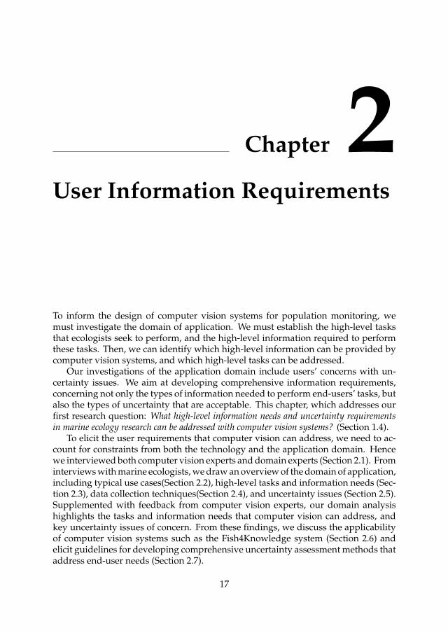
Chapter 2User Information Requirements
To inform the design of computer vision systems for population monitoring, wemust investigate the domain of application. We must establish the high-level tasksthat ecologists seek to perform, and the high-level information required to performthese tasks. Then, we can identify which high-level information can be provided bycomputer vision systems, and which high-level tasks can be addressed.
Our investigations of the application domain include users’ concerns with un-certainty issues. We aim at developing comprehensive information requirements,concerning not only the types of information needed to perform end-users’ tasks, butalso the types of uncertainty that are acceptable. This chapter, which addresses ourfirst research question: What high-level information needs and uncertainty requirementsin marine ecology research can be addressed with computer vision systems? (Section 1.4).
To elicit the user requirements that computer vision can address, we need to ac-count for constraints from both the technology and the application domain. Hencewe interviewed both computer vision experts and domain experts (Section 2.1). Frominterviews with marine ecologists, we draw an overview of the domain of application,including typical use cases(Section 2.2), high-level tasks and information needs (Sec-tion 2.3), data collection techniques(Section 2.4), and uncertainty issues (Section 2.5).Supplemented with feedback from computer vision experts, our domain analysishighlights the tasks and information needs that computer vision can address, andkey uncertainty issues of concern. From these findings, we discuss the applicabilityof computer vision systems such as the Fish4Knowledge system (Section 2.6) andelicit guidelines for developing comprehensive uncertainty assessment methods thataddress end-user needs (Section 2.7).
17
18 Chapter 2
2.1 Interviews with stakeholders
We investigated the domain of application, and the potential use cases for computervision systems, through series of interviews with marine ecologists and computervision experts. This iterative process us allowed to develop a comprehensive un-derstanding of user needs and technical issues. Conducting the interviews itera-tively allow unforeseen information requirements and uncertainty issues to emerge.Including feedback from computer vision experts was crucial to complement theinterviews of marine ecology experts. Ecologists were not acquainted with the tech-nical constraints of computer vision, and therefore could not envision all potentiallimitations and uncertainty issues. Computer vision experts were able to indicateuncertainties related to specific high-level information needs, and low-level technicalfeatures of computer vision technologies. To help ecologists familiarize themselveswith computer vision technologies, we used user interface and visualization proto-types that provided tangible examples of the computer vision capabilities.
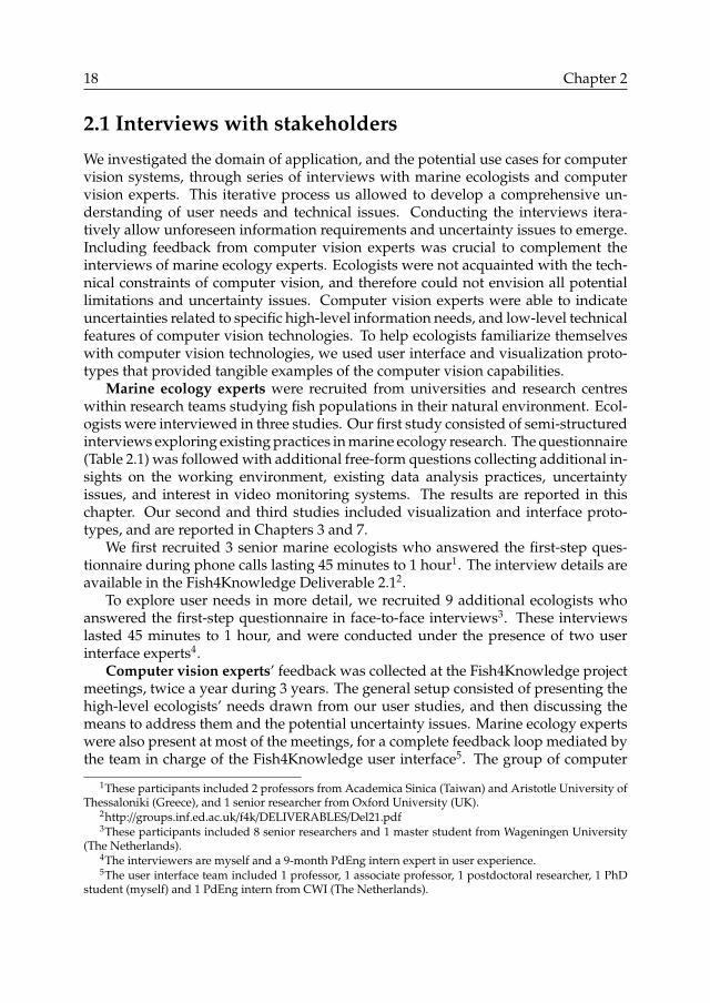
Marine ecology experts were recruited from universities and research centreswithin research teams studying fish populations in their natural environment. Ecol-ogists were interviewed in three studies. Our first study consisted of semi-structuredinterviews exploring existing practices in marine ecology research. The questionnaire(Table 2.1) was followed with additional free-form questions collecting additional in-sights on the working environment, existing data analysis practices, uncertaintyissues, and interest in video monitoring systems. The results are reported in thischapter. Our second and third studies included visualization and interface proto-types, and are reported in Chapters 3 and 7.
We first recruited 3 senior marine ecologists who answered the first-step ques-tionnaire during phone calls lasting 45 minutes to 1 hour1. The interview details areavailable in the Fish4Knowledge Deliverable 2.12.
To explore user needs in more detail, we recruited 9 additional ecologists whoanswered the first-step questionnaire in face-to-face interviews3. These interviewslasted 45 minutes to 1 hour, and were conducted under the presence of two userinterface experts4.
Computer vision experts’ feedback was collected at the Fish4Knowledge projectmeetings, twice a year during 3 years. The general setup consisted of presenting thehigh-level ecologists’ needs drawn from our user studies, and then discussing themeans to address them and the potential uncertainty issues. Marine ecology expertswere also present at most of the meetings, for a complete feedback loop mediated bythe team in charge of the Fish4Knowledge user interface5. The group of computer
1These participants included 2 professors from Academica Sinica (Taiwan) and Aristotle University ofThessaloniki (Greece), and 1 senior researcher from Oxford University (UK).
2http://groups.inf.ed.ac.uk/f4k/DELIVERABLES/Del21.pdf3These participants included 8 senior researchers and 1 master student from Wageningen University
(The Netherlands).4The interviewers are myself and a 9-month PdEng intern expert in user experience.5The user interface team included 1 professor, 1 associate professor, 1 postdoctoral researcher, 1 PhD
student (myself) and 1 PdEng intern from CWI (The Netherlands).
User Information Requirements 19
vision experts included 9 researchers from Catania University (Italy) and EdinburghUniversity (UK)6. The marine ecology experts attending the meetings included atleast one Professor from Academia Sinica in Taiwan, with decades of experience inresearching the marine ecosystem targeted by the Fish4Knowledge project.
The Fish4Knowledge project description:This project aims at realizing a video analysis tool dedicated to the study of undersea ecosystems. Fixedunderwater cameras continuously record videos that are automatically analysed to detect fish speciesand behaviours.1. Briefly, what are your scientific research goals and topics of interest?(if relevant, please name biological patterns, processes or models implied)2. What information, data or measures do you need to fulfil your goals?3. How do you collect relevant data (manual methods as well as automated)? What trust or reliabilityissues do you encounter?4. What tools do you use to process and analyse those data? What issues do you encounter whileusing those tools?5. What would be the 20 most important questions you would ask the Fish4Knowledge tool?
Table 2.1: Questions of the semi-structured interview of marine ecology experts (Section 2.1).
2.2 Population monitoring use cases
From the interviews with ecologists, we identify typical use cases of data collectionpractices for fish population monitoring, and the uncertainty issues they entail (Ta-ble 2.2). The use cases are drawn from 11 out of the 12 interviews we conducted, as 1interview did not provide sufficient information about the data collection practices ofthe participant. The use cases are synthesized by grouping together ecologists whoshare the same high-level topics of study and data collection methods. The use casessummarize ecologists’ usual practices, uncertainty issues, and potential applicationsof computer vision systems, as mentioned during the interviews.
-Case 1 - Video at single point (1 participant). The team based in The Nether-lands studies Caribbean reef fish, e.g., the distribution of specific species and theirvariations over time (e.g., population dynamics and migrations). They use baitedstereoscopic cameras to count fish, identify their species and evaluate their size. Theyuse vessels to collect video samples at single-point locations that cover the areas andperiods of interest. They manually identify single fish, without duplicates, by ana-lyzing only one frame per video sample. They select the frame with the most fish.The uncertainties caused by occlusions are resolved by browsing other video frames.Their existing method is satisfactory, but the manual image analysis is time-consum-ing. They would potentially use video analysis tools for automatically counting fish
6The computer vision experts included 1 professor, 1 associate professor, 2 senior researchers and 5PhD students.

20 Chapter 2
and identifying species, with the same sampling method using the most dense frame.The uncertainty issues introduced by video analysis are easily accepted because thecost reduction is important.
Case 2 - Video in transects (3 participants). The team based in The Netherlandsstudies North Sea deep-water corals and seabed ecosystems, e.g., the distribution ofspecies in the various deep sea habitats, and the related trophic systems (i.e., foodchain). They use cameras held by a line just above the seabed, and moved in transects(lines) within the areas of interest. A laser measures the exact distance between thecamera and the seabed. It serves to calibrate the measurement of fish size. Theymanually identify each organism and habitat features (e.g., rocks), and measure theirsize. The organisms are very sparse and noticeable on the empty seabed surface, butthey encounter uncertainties with respect to species identification and cryptic (hid-den or camouflaged) organisms. A video browsing tool allows them to manuallyextract object size by using the size measured in pixels and the camera to seabeddistance. The observations and measures are manually collected in spreadsheet files.Their existing method is satisfactory, but the manual image analysis is extremelytime-consuming and the vessel is very expensive. They would potentially use avideo analysis tool for automatically identifying objects in their video collection, orfor designing cheaper data collection techniques.
Case 3 - Diving along transects (1 participant). The team based in The Nether-lands focuses on commercial fisheries. They study the abundance, distribution, andtrophic systems of the Philippines’ coral reef fish, and their vulnerability to fishing.They collect diving observations along transects at varying depth. Video cameras areused for backup purposes and occasional refinements of the live observations. Theanalysis of the diving notes and videos is entirely manual. They encounter uncer-tainty issues with the missed detection, since many organisms occur simultaneously.They usually approximate the number of fish in dense fish groups with many over-laps. The observable species are different depending on the depth, and it requiresan extensive taxonomic knowledge and sample collection to cover their diversity.The data collection technique is satisfactory but costly and time-consuming, whichlimits the quantity of samples. They would potentially use video analysis tools forbrowsing the video collection, or for designing new data collection techniques.
Case 4 - Experimental fishery (1 participant). The team based in Greece studiespopulation dynamics, trophic systems, reproduction and physiology of pelagic fishliving in the Aegan Sea. They sample and dissect fish from experimental fisheries, ascommonly practiced in the marine biology domain. They collect fish at single-pointlocations or following a stratified sampling method. Fish dissection provides preciseidentification of look-alike species, and precise measurements of age, fertility andfeeding habits. They encounter uncertainty regarding the replicability of fish catch.Fish catches performed under the same conditions (e.g., one after the other, releasingand re-catching fish) provide highly variable results. This issue is difficult overcome,

User Information Requirements 21
and may require collecting large numbers of samples. This data collection techniqueis costly but satisfactory. Their acceptance of our tool is low because: i) video analysiscannot supply all the data they need, ii) they need a different sampling of the areasof interest, and iii) video analysis introduces uncertainties they can avoid with theirexisting method.
Case 5 - Commercial fishery (2 participants). Their separate teams, based inThe Netherlands, conduct similar studies of population dynamics in the North Sea.They collect fish counts from commercial fisheries, as practiced for decades in themarine biology domain. The large amount of available data supports the study ofpopulation dynamics, migration and reproduction. Commercial fisheries target onlyspecific species, and onboard fisherman may not report the bycatches of not commer-cialized fish species and often misidentify unusual species. Thus uncertainty issuesarise due to the uneven or biased sampling of species, areas, depths and environ-mental conditions. However, the large amount of collected data allows statisticalmethods to overcome the uncertainty issues. This data collection technique is sat-isfactory, but could be complemented by video analysis tools for compensating thesampling biases.
Case 6 - Diving at single points and transects (2 participants). Their separate teams,based in Taiwan and The Netherlands, conduct similar studies of coral reef ecosys-tems. They study population dynamics, interactions between species (trophic sys-tems, reproduction), migration patterns, and vulnerability to environmental changes.They collect fish counts, species identification and approximate fish size from divingobservations. They collect data at single-point locations or in transects. They en-counter uncertainty issues regarding missed detections, multiple detection of singlefish, species misidentification, and some species are likely to avoid divers, thus bias-ing the collected data. These issues are tackled by statistical methods (e.g., ANOVA)and by comparing data from different sources. They would potentially use videoanalysis tools to reduce data collection costs, and for collecting larger numbers ofsamples.
Case 7 - Video and commercial fishery (1 participant). The team based in TheNetherlands studies population dynamics and the vulnerability of the Wadden Seafish to fisheries. They collect data from industrial waste of commercial fisheries. Thisdata collection technique is its early stage of development. It uses common CCTVcameras to record individuals falling out of the nets, or being discarded during in-dustrial fish sorting. They manually count fish and identify species, while they aredeveloping video analysis software to address this task. With their video analysistool, they encounter uncertainty issues regarding the misidentification of species andnon-fish objects. This is due to the speed at which fish pass by the camera duringindustrial processes.

22 Chapter 2
Data Collection Technique SamplingMethod
Uncertainty Issues Interest inComputer Vision
Case 1 Video Images: baited stereo-scopic camera, manual imageanalysis
Single-pointlocations
Avoid detecting the same fish mul-tiple times. Few overlaps in fishgroups.
To avoid manual imageanalysis.
Case 2 Video Images: lighted cameraheld close to deep sea floor, ata constant calibrated distancefrom seabed, and manual im-age analysis
Transects (i.e.,along a virtualline)
Rare misidentification of species.Cryptic organisms may remainundetected.
To avoid manual imageanalysis. To reduce ex-pensive use of scientificvessels.
Case 3 Diving Observations withhandheld camera for backuppurposes
Transects (atvarying depths)
Species misidentification. Somespecies hide from divers. Over-laps in fish groups.
To analyze existingvideos. To avoid diving.
Case 4 Experimental Fishery withfish dissection
Single-pointlocations ortransects
Variability of fish catch albeit iden-tical experimental conditions.
Excluded, due to un-supported measurementsand uncertainty issues
Case 5 Commercial Fishery: datafrom the North-Sea fishmarket
Dependent oncommercialfisheries
Variability of fish catch. Tar-gets only commercial species.Misidentifies uncommon species.
To compensate the biasesin the market-dependentsampling conditions
Case 6 Diving Observations Single-pointlocations ortransects
Species misidentification. Somespecies are hiding from divers.Overlaps in fish groups.
To avoid diving.
Case 7 Video Images & CommercialFishery: onboard video moni-toring of fish discarded duringfish processing
Dependent onequipmentavailableonboard
Misidentification of species andnon-fish objects.
Experimented in 2013,needs improvement.
Table 2.2: Summary of 7 typical use cases of fish population monitoring for ecology research.
Research Topic Information NeedPopulationDynamics
Migration Reproduction TrophicSystems
FishCount
SpeciesRecognition
BodySize
Other
Case 1 x x x x xCase 2 x x x x x Other organismsCase 3 x x x x xCase 4 x x x x x x x Weight, Bone size,
Stomach content,Chemicals
Case 5 x x x x x x WeightCase 6 x x x x x x BehaviorCase 7 x x x
Table 2.3: High-level information needs drawn from the use cases in Section 2.2 and Table 2.2.
2.3 High-level information needs
We aim at identifying widespread information needs that concern a broad range ofresearch topics in marine ecology. Identifying the most essential user needs informsthe design of computer vision systems that address a broad range of applicationswithin marine ecology. Thus we report the information needs and research topicsthat are most common amongst the ecologists we interviewed. We analyze the 7 usecases introduced in Section 2.2 (Table 2.3) and examples of information seeking taskscollected from ecologists (Table 2.4). We identify 4 key research topics (populationdynamics, migration, reproduction, trophic systems) and 4 key information needs(fish counts, species recognition, behavior recognition, body size).

User Information Requirements 23
fishcount
speciesrecog.
behaviorrecog.
bodysize
1 How many species appear and their abundance and body size in day and nightincluding sunrise and sunset period.
x x x
2 How many species appear and their abundance and body size in certain periodof time (day, week, month, season or year). Species composition [set of species andrelative population sizes] change within one period.
x x x
3 Give the rank of above species, i.e., list them according to their abundance ordominance. How many percent are dominant (abundant), common, occasional andrare species.
x x
4 Fish colour pattern change and fish behaviour in the night for diurnal fish and indaytime for nocturnal fishes.
x x x
5 Fish activity within one day (24 hours). x x x6 Feeding, predator-prey, territorial, reproduction (mating, spawning or nursing) or
other social or interaction behavior of various species.x x x
7 Growth rate of certain species for a certain colony or group of observed fish. x x x8 Population size change for certain species within a single period of time. x x9 The relationship of above population size change or species composition change
with environmental factors, such as turbidity, current velocity, water temperature,salinity, typhoon, surge or wave, pollution or other human impact or disturbance.
x x
10 Immigration or emigration rate of one group of fish inside one monitoring stationor one coral head.
x x
11 Solitary, pairing or schooling behavior of fishes. [these behavior have different meaningsdepending on species]
x x x
12 Settle down time or recruitment season [when species stop migrating and start repro-ducing], body size and abundance for various fish.
x x x
13 In certain area or geographical region, how many species could be identifiedor recognized easily and how many species are difficult. The most importantdiagnostic characteristics to distinguish some similar or sibling species [specieswhich look-alike].
x
14 Association [co-occurrence] among different fish species or fish-invertebrates. x x15 Short term, mid-term or long term fish assemblage [co-occurrence] fluctuation at
one monitoring station or comparison between experimental and control stations inMAP. [MPA: Marine Protected Area]
x x
16 Comparison of the different study result between using diving observation orunderwater real time video monitoring techniques. Or the advantage and disad-vantage of using this new technique.
x x x x
17 The difference of using different camera lens and different angle width. x x x x18 Is it possible to do the same monitoring in the evening time. x x x x19 How to clean the lens and solve the biofouling problem.20 Hardware and information technique problem and the possible improvement
based on current technology development and how much cost they are.21 What is the average body size for species X? How many percent of fish are small,
normal or big?x x x
22 What is the number of fish in area X for indicative species related to pollution? [forspecies which absence is likely due to pollution]
x x
23 What is the distribution and number of fish for indicative species of factor X? [forspecies which presence or absence is likely due to the factor of interest (e.g., water acidity)]
x x
24 What is the analysis of factor X impact, using pattern of indicative data Y? [Indicativedata include fish counts and behavior observations for indicative species, i.e., species that areknown to react to factor X]
x x x
25 What are the areas and periods of time of species X migrations? x x26 What are the areas and periods of time of species X SPAGS? [SPAGS:Spawning
Agregation Sites, where fish gather to reproduce]x x x
27 What are the SPAGS periods in area Y? x x x x
Table 2.4: Information seeking tasks that ecologists would perform with the Fish4Knowledgesystem. The tasks are reported using participants’ own words, in the order they were mentioned, when answeringquestion 5 in Table 2.1. The texts in [...] explain the concepts from the marine ecology domain. The tasks inbold refer to uncertainty or technical issues. The last 4 columns identify high-level information needs (discussed inSection 2.3). The tasks were collected from one participant of Case 6 (tasks 1-20) and from the participant who wasnot included in the use cases (tasks 21-27).

24 Chapter 2
All the use cases and information seeking tasks require information on fish countsand species recognition (e.g., fish count per species) except tasks 13, 19 and 20which concern uncertainty issues (Table 2.4). With this information, ecologists caninvestigate how many fish occur in specific time periods and locations (i.e., fishabundance), what are their species, what is the species distribution and density overareas, what is the proportion of each species in the overall population (i.e., speciescomposition), or what is the total number of species (i.e., species richness).
Ecologists are also interested in information on fish body size and behaviorrecognition (9 and 10 tasks in Table 2.4, respectively). From fish body size, ecolo-gists derive fish age and maturity, as well as reproductive cycles (e.g., presence ofoffspring). From fish behavior (e.g., mating, feeding, nursing, aggression), ecolo-gists derive fish maturity and reproductive cycles too, but also seasonal cycles andtrophic systems. Few mentions of behavior recognition occurred when ecologistswere asked to describe their current data collection practices, and behaviors cannotbe directly observed from fishery data (Cases 4, 5 and 7). Ecologists’ interest in be-haviors emerged when asked what would be the most important tasks they wouldperform with the Fish4Knowledge system (Table 2.4). Such computer vision systemwas deemed promising for observing behaviors without disturbance from divers.
From information on fish counts, species, behaviors and body size, ecologists canstudy population dynamics, i.e., how species distributions evolve over time, loca-tions or environmental conditions. For instance, monitoring population dynamicscan support the study of ecosystems’ typology (e.g., types of habitat, distributionsof animal and plant species, food chains and predator/prey relationships), the studyof differences between ecosystem (e.g., before and after seasonal changes, or eventssuch as typhoons, pollutions or construction works), or the study of species life cycles(e.g., daily routines, reproduction, migration and maturity phases). With informa-tion on fish counts, species, behaviors and body size, ecologists can also study threemain phenomena influencing population dynamics: migration, reproduction, andtrophic systems (i.e., food chains describing which species feed on which species).
Each topic of study requires specific information (Tables 2.3 and 2.5) but all requireat least information on fish counts per species. For instance, population dynamicsconcerns the relative sizes of species populations over time periods and locations(i.e., species distributions). Migrations, reproduction and trophic systems requirethe recognition of fish species, as these phenomena are species-dependent (e.g., eachspecies has specific time periods or locations for migrations, reproductions or feedingbehaviors).
Additional information is of interest for studying underlying phenomenom thatimpact migrations. For example, information on fish age (estimated from bodysize, or otolith bone size) supports investigations of relationships between migrationand reproduction. Chemicals in fish bodies or surrounding waters, or other envi-ronmental information such as temperature or pressure, support investigations ofrelationships between migration and environmental conditions.
The topic of reproduction can be studied using only fish counts and speciesidentification, given that ecologists can rely on prior knowledge of the typical repro-

User Information Requirements 25
duction sites and periods. For example, changes in fish population sizes occurring atthese known sites and locations can be assumed to be related to reproduction. How-ever, information on fish body size and behavior provides more reliable evidence ofreproduction cycles (e.g., time period and locations) and more information on thedemographic characteristics of fish populations.
The topic of trophic systems is more difficult to study using only fish counts andspecies identification. Provided with the species composition, i.e., the distribution offish per species, ecologists can infer the potential food chains. However, such infer-ence must rely on prior knowledge of typical feeding behaviors of each fish species,and of other available nutrients (e.g., sea weed or plankton species). Information onfish behaviors and on stomach contents are of particular interest for providing evi-dence of the food chains in the ecosystems. While observing fish behaviors informsecologists on predator-prey and foraging mechanisms, analysing stomach contentsinforms ecologists on actual diets resulting from these behaviors.
Fish Count SpeciesRecognition
BehaviorRecognition
Body Size
Research TopicPopulation Dynamics mandatory mandatory optional importantMigration mandatory mandatory optional optionalReproduction mandatory mandatory important importantTrophic Systems mandatory mandatory important important
Data Collection Technique
Experimental Fishery (Case 4) + +/++1 - +Commercial Fishery (Cases 5, 7) + + - +Diving Observation (Cases 3, 6) + + ++ +
Manual Image Analysis (Cases 1, 2, 3, 7) + + + -/+ 2
Computer Vision + + -/+3 -/+ 2
The signs indicate whether data collection techniques: - cannot supply the information, + can supply the information,++ can supply the most precise information.1 Fish dissection, sometimes performed after experimental fishing, is the most accurate technique for differentiatingfish species that are visually similar.2 Information supplied if stereoscopic vision or calibrated distance camera-background are available.3 The state-of-the-art does not fully address the wide scope of fish behavior variety.
Table 2.5: Information required for the main topics of study, and ability of data collectiontechniques to provide this information.
2.4 Data collection techniques
From the 7 use cases of ecology research on fish populations (Section 2.2), we identify4 well-established data collection techniques: experimental fishery (i.e., samplingfish stock), commercial fishery data, diving observations, and manual image analysis(Section 2.4.1, Table 2.5). To provide reliable information, data collection techniquesmust be applied with appropriate sampling methods. We outline sampling methodsthat are usually applied by ecologists (Section 2.4.2) and discuss sampling strategiesfor video data collection (Section 2.4.3). Finally, we outline ecologists’ rationales forselecting appropriate data collection and sampling methods (Section 2.4.4).

26 Chapter 2
2.4.1 Well-established data collection methods
Experimental fishery - Scientific vessels are used to catch fish at specific samplinglocations and time periods, with calibrated nets or fish traps (Case 4). Ecologistscan then perform measurements (e.g., from fish dissection) that include informationunavailable with other data collection techniques, such as fish weight, bone size (e.g.,otolith precisely indicating fish age), stomach content (e.g., to study trophic systems),traces of chemicals (e.g., from pollution), or the presence of fish eggs (e.g., to studyreproduction cycles).
Commercial fishery - Data can be collected onboard commercial vessels, by ecologists(Case 7) or by non-scientific personnels of fishery companies (Case 5). The latterinvolves trust issues and potential biases due to the person in charge of collecting thedata, e.g., lack of expertise with rare species, inconsistent practices between observers(Kraan et al. 2013). Commercial fishery data have the advantage of offering largecoverage of marine areas, but at the disadvantage of targeting only commercialspecies.
Diving observation - Divers can collect information on fish counts and species recog-nition, and can observe a variety of fish behaviors (Cases 3 and 6). Data can becollected by individual divers, or in teams who compare their observations to limithuman biases. Observations are collected within fixed areas (e.g., delimited withframes or ropes) or along transects (i.e., predetermined path on the sea floor coveringa representative part of the ecosystem). Cryptic and benthic species (camouflaged orliving on the seabed) are better sampled as they are unlikely to be caught in fishingnets. However, diving observations carries uncertainty as human observers disturbnatural fish behaviors and can make mistakes, e.g., depending on their diving ex-perience, or difficulties with the fish species or ecosystems (e.g., fast or small fish,overlaps in fish groups, fish fleeing divers, inaccessible locations). Such human bi-ases are difficult to quantify. To address them, ecologists collect data repeatedly anduse well-specified consistent protocols.
Manual image analysis - Images are widely used as a means of observation. Camerascan be used at fixed or moving locations, with or without baits attracting fish (Case 1).They can be oriented toward the open sea, or toward the sea floor for observingbenthic ecosystems. For the latter, calibrating a fixed distance between cameras andsea floor allows the measurement of fish body size (Cases 2 and 7). Stereoscopicvision (i.e., the use of pairs of cameras) is another technique for estimating fishbody size. Body size is derived by classifying image pixels as inside or outsidea fish contour (a classification task called segmentation). Divers also use handheldcameras, at fixed locations or moved along transects (Case 3). Otherwise, cameras canbe dragged by boats or embarked on remote controlled vehicles (e.g., BRUV, BaitedRemote Underwater Video systems). Image analysis is mainly performed manually,as automatic image analysis with computer vision are not supported with well-established methods for handling uncertainty and technological issues. However,computer vision has raised interest as a promising cost-effective technique (Harvey

User Information Requirements 27
et al. 2001, Cappo et al. 2004, Hetrick et al. 2004, Langlois et al. 2006, Lowry et al.2012, Shafait et al. 2016).
2.4.2 Sampling methods
Sampling error is a crucial source of uncertainty. Only subsets of ecosystems areactually observed, and conclusions drawn on overall ecosystems based on limitedsets of samples are inherently uncertain. In the case of computer vision system,collecting video samples caries specific uncertainty and may require specific samplingmethods. To inform the design of sampling methods applicable to computer visionsystems, we discuss the methods usually applied by the ecologists we interviewed.
Sampling methods are designed to target specific conditions: ecosystems, habi-tats, environmental conditions, time periods, locations, species or behaviors of inter-est. The choice of sampling methods depends on the topic of study and the scientificrequirements of the research. For instance, to study migration it can be necessary tocollect samples over large areas and time periods (e.g., multiple years).
Samples are collected within subsets of the locations and time periods of interests.In the marine ecology domain, the observable populations can greatly vary depend-ing on the time periods and locations. To remain representative of the ecosystem ofinterest, the sampling methods must account for natural cycles and habitat topolo-gies. For instance, the sampled time periods need to account for the hours of theday (e.g., some species appear in morning, evening or at night, for feeding) and theseasons of the year (e.g., some species migrate or reproduce in spring). The sampledlocations can be fixed points (i.e., single-point locations in Table 2.2) or predeterminedpath covering a representative part of the ecosystem (i.e., transects in Table 2.2). Thesampled locations must represent ecosystems’ components, e.g., the types of habitatsand their proportional land coverage. Samples are often collected in each part of theecosystems, proportionally to their geographical coverage, and aggregated using thestratified sampling method (Cochran 2007).
Sampling methods provide repeated measurements to account for their variance.Estimating sample variance (i.e., the variance between measurements collected in eachsample) contributes to the interpretation of the patterns observed in the collecteddata. Well-founded statistical methods (e.g., ANOVA) account for sample varianceto compute the probability that the patterns observed in the data occurred by chance,and may not be representative of the actual fish populations. For example, popu-lation sizes can differ between two time periods or two species, but the differencemay not be significant due to high sample variance. Such statistical methods areessential for ecology research, as they support the scientific validity of conclusionsdrawn on fish populations. Statistical methods can also be applied to estimate theoverall population sizes in the overall ecosystem, and the variance of such estimate.However, the relative trends in fish populations often provide sufficient informationfor assessing population dynamics, without needing to estimate overall populationsizes for specific areas.

28 Chapter 2
2.4.3 Impact of video technologies on sampling methods
Special attention must be paid to the spatio-temporal coverage of video samples. Thespatial coverage depends on the placement and orientation of cameras, on the typelens, and on the image resolution. The placement and orientation of cameras targetspecific habitats, and impact the species that are likely to be observed. The type of lensand the image resolution impact the depth and width of fields of view. These modifythe areas and volumes within which fish populations can be observed, as well as thequality of observations (e.g., small fish in the background can be unrecognizable).
Estimating the spatial coverage of video samples is essential to the design ofsampling methods, and to the analysis of the collected data (e.g., to study fish density).But estimating the spatial coverage of a camera is a difficult task. For instance, itrequires controlling the distance within which information collection is possible, or isreliable enough (e.g., for detecting small fish). The information quality depends notonly on the depth of field of view (i.e., on camera lens) but also on other environmentalfactors (e.g., lighting, water turbidity) and on the capabilities of the computer visionsoftware (e.g., how the software performs with low image quality). Finally, whenbaits are used, estimating the area covered by cameras is more subtle. The strengthand direction of currents modify the areas in which animals can sense the bait, andthus the spatial coverage of video samples (Taylor et al. 2013).
Regarding the temporal coverage of video samples, the use of fixed camerasthat continuously monitor fish populations is an important paradigm shift. It con-trasts with common data collection techniques that perform measurements duringlimited time periods. Their temporal coverage concerns a small set of preselectedtime periods, and the measurements performed within a time period are intendedto represent of all the species living in the environment. With video monitoringsystems such as Fish4Knowledge, the temporal coverage is very large, covering alltime periods when there is sunlight. Ecologists do not need to extrapolate the fishpopulations that would occur in time periods for which no sample is available. In-stead, the can assume that the fish populations occur in the videos samples at theirnatural frequency.
2.4.4 Choice of data collection and sampling method
Each data collection technique has its own advantages and disadvantages, and no sin-gle method fits all types of ecology research. The most important information needsare addressed by a choice of data collection techniques, as summarized in Table 2.5.The requirements for selecting a data collection technique comprise constraints onthe types of ecosystem to access, the time periods for performing the study, the hu-man and material resources available, the funding for acquiring and maintainingequipments, the information that needs to be collected, the measurements’ potentialerrors and biases, and on the uncertainties that are acceptable. Uncertainty issuesare crucial for choosing a data collection technique. Given alternative methods thatcan collect the information of interest, analysing uncertainty issues allow stakehold-

User Information Requirements 29
ers to understand the tradeoffs of each data collection technique. For example, amethod may be faster or cheaper but entails unacceptable uncertainty. In other cases,a method may limit uncertainty but entails additional costs that are not worthwhilecompared to alternatives.
ExperimentalFishery
CommercialFishery
DivingObservation
Manual ImageAnalysis
Computer .Vision
Benthic species -1 -1 = = =
Sedentary species -1 -1 = =/+2 =/+2
Schooling species = = -/+ -/+ -/+2
Small fish -/=3 -/=3 -/=4 -/=4 -/=4
Shy species - - -/=5 -/=6 -/=6
Cryptic species - - = - -Look-alike species = = -/+ -/+ -/+Rare species = - = = -/=7
Herbivorous orcarnivorous species
-/=8 = = -/=8 -/=8
The signs indicate whether parts of ecosystems are likely to be + over-represented, = neither under- norover-represented, - under-represented.1 Considering that the destructive use of trawl nets is not an option.2 Species living in coral heads often swim in and out of the camera field of view, which may yield over-estimated fish counts.3 Large granularity of nets’ and fish traps’ mesh can let small fish slip through.4 Small fish may not be visually detectable from a large distance.5 Cloaking procedures can allow the observation of shy fish.6 With handheld cameras, some species flee from divers.7 The recognition of all rare species may not be possible due to lack of ground-truth images.8 Baits, if used, can attract either herbivorous or carnivorous species.
Table 2.6: Main biases with species that are potentially under- or over-estimated by datacollection techniques.
2.5 Biases of data collection techniques
All data collection techniques carry uncertainty issues and can yield errors andbiases in the collected data, e.g., some species are potentially over- and under-represented. For example, cryptic species camouflaged amongst corals are typicallyunder-represented because they are more difficult to detect. Data collection tech-niques are thus always selective, i.e., specific parts of ecosystems and specific speciescan entail a different magnitude of errors than the the rest of the data, while otherparts are measured with lower and consistent levels of errors.
From comparative studies of data collection techniques (Trevor et al. 2000, Harveyet al. 2001, Cappo et al. 2004, Lowry et al. 2012)) and from our interviews withecologists, we identified nine types of fish species that are particularly susceptible tobiases depending on the data collection technique. Table 2.6 summarizes the potentialbiases entailed by the common data collection techniques discussed in Section 2.4.
30 Chapter 2
Benthic species - Organisms living on the seafloor are under-estimated in experi-mental or commercial fishery data. Fish nets are usually cast in the open sea (i.e.,pelagic zone) where the species usually living in the seafloor (i.e., the benthic zone)are rarely found. Trawl nets dragging the seafloor can collect samples of benthicspecies, but this fishing technique dramatically destroys benthic ecosystems andthus is usually excluded for scientific purposes.
Sedentary species - Sedentary species living in the same rocks or coral heads, ratherthan circulating across larger areas, are less likely to swim in the open sea and thus tobe sampled through fishery. Computer vision potentially over-estimates sedentaryspecies because they are likely to repeatedly swim in and out of the camera fieldof view. Hence single individuals may be repeatedly counted. For instance, withthe Fish4Knowledge system, we observed over-estimation of the sedentary speciesDascyllus reticulatus.
Schooling species - Species living in groups can be under- or over-estimated throughdiving observation, manual image analysis and computer vision. Fish in a school(i.e., school) occlude each other, and individual fish are likely to swim in and outof cameras’ field of view. With computer vision, the number of fish in a schoolcan be either under-estimated due to occlusion, or over-estimated due to repeatedoccurrences of the same individuals. With diving observations and manual imageanalysis, humans need to interpret the overall size of the school and can subjectivelyover- or under-estimate the number of fish.
Note: To overcome biases with sedentary and schooling species, the ecologists fromthe Case 1 of our first user study (Section 2.2) count the fish appearing in only oneframe of the video footage. However, this method is likely to further under-estimaterare species, since the chance they appear in one single frame is lower than thechance they appear in the complete set of frames. Further, this method disablesthe analysis of visual features over several frames (e.g., fish trajectories) which canbe necessary for recognizing fish behavior, and for identifying species for whichswimming behavior is more discriminative than visual appearance.
Small fish - Detecting small species or offspring is difficult for all data collectiontechniques in Table 2.5. Small fish are difficult to detect and recognize if they aretoo far away from divers or cameras (e.g., depending on visual acuity and fish bodysizes). In the case of diving observations, manual image analysis and computervision, this type of bias is limited if observations are performed within small depthsof field of view. With large depths of field of view (e.g., observing the open sea),ecologists need to consider that small fish are sampled only in a limited range aroundcameras or divers.
Shy species - Some species flee boats and divers as they detect their sounds, move-ments (especially that of bubbles from divers), and sometimes their chemicals (sens-ing underwater chemicals is comparable to sensing smells). Ecologists overcome withcloaking procedures, such as using no-bubble diving equipment (e.g., rebreather) and
User Information Requirements 31
allowing time for shy species to come back after divers settled in. Cameras are non-intrusive and are well-suited for observing shy species, unless divers or boats are toonearby.
Cryptic species - Cryptic species (e.g., camouflaged) are difficult to detect for bothcomputer vision software and human observers. Cryptic species are very likely to beunder-estimated, and ecologists need to apply specific methods for studying them.For instance, divers carefully scrutinize sea floors or coral heads, or use of toxicantsforcing the fish to leave their camouflaged position. Data collection based on imageryis not suitable for their study. Cryptic species are often benthic species, and are thuslikely to be under-estimated by commercial and experimental fisheries.
Look-alike species - Species that look-alike are difficult to detect for both computervision software and human observers. Ecologists may rely on specific expertise todifferentiate look-alike species. For instance, the species behaviors or body sizes maydiffer.
Rare species - Ecologists are trained to target and recognize rare species, so theycan collect unbiased measurements from experimental fisheries, diving observationsand manual image analysis. Commercial fishery and computer vision potentiallyunder-estimate rare species. Computer vision software may not recognize speciesfor which there are insufficient image samples to train the recognition algorithm.Uncommon species may not be recognized and recorded in commercial fishery data.But these uncommon species may be frequent enough for collecting sufficient imagesamples to train computer vision algorithms to recognize them.
Herbivorous or carnivorous species - Baits attract only the species that feed on thematerials used as baits. Thus specific types of bait attract specific species, whichmay be over-estimated while other species are under-estimated. Baits may, however,be of particular interest for sampling species that would otherwise remain largelyunobserved (e.g., rare, shy or crptic species), or for limiting the duration, thus thecosts, of data collection.
2.6 Implications for the Fish4Knowledge system
Computer vision systems can address essential user information needs with twobasic functionalities: detecting fish in video images, and classifying their species.Such information supports the study of four key topics in ecology research: pop-ulation dynamics, migration, reproduction and trophic systems (Section 2.3). TheFish4Knowledge system was able to provide information on fish counts and species.Other information needs (e.g., behavior recognition, body size) could not be ad-dressed due to technical limitations (e.g., no stereoscopic vision, or ground-truthcollection issues) and were excluded from the scope of our research. The lack ofinformation on fish behavior particularly impacts the study of trophic systems. Clas-sification software can be developed to recognize fish behaviors (Spampinato et al.
32 Chapter 2
2014). However, it is challenging to differentiate the large variety of fish behaviors,and collect sufficient groundtruth data for each behavior of interest.
Computer vision systems entail uncertainty issues due software components (e.g.,errors from the classification software), hardware components (e.g., camera settings),and ecosystems in which computer vision systems are deployed (e.g., light condi-tions, visibility). End-users require that these uncertainty issues are assessed (e.g.,information seeking tasks in bold in Table 2.4, Section 2.2). Furthermore, biases canarise due the characteristics of fish species (Section 2.5). The Fish4Knowledge systemuses cameras without bait, at fixed positions, not held by divers, and that can be po-sitioned to observe benthic zones and coral heads. These settings can limit potentialbiases with benthic, sedentary, shy, herbivorous and carnivorous species. Yet, biasesare still at stake with sedentary, schooling, cryptic, look-alike and rare species, aswell as small fish.
2.7 Requirements for accountable classification systems
Our study of the marine ecology domain provide insights on the uncertainty issuespertaining to computer vision systems for monitoring animal populations. Furtherinvestigations are required to elicit comprehensive scopes of uncertainty factors (e.g.,depending on specific system features and application conditions) and to identifythe high-level impacts of uncertainty. Such uncertainty assessments must eventuallyprovide end-users with practical information on the uncertainty that pertains to thespecific datasets they are using. This section draws guidelines for conducting suchuncertainty assessment that specifically address end-users needs (e.g., rather thanthe needs of technology experts who seek to improve computer vision systems).
The Fish4Knowledge computer vision system delivers classification data whereclass sizes represents population sizes, e.g., from specific species or behaviors. Hencewe focus on classification systems, beyond the domains of computer vision and ecol-ogy. We thus draw high-level user requirements for supporting uncertainty-awareanalysis of class sizes. We do not intend to provide fully exhaustive requirements,however, we aim at providing essential guidelines for enabling accountable classifi-cation systems for monitoring class sizes.
2.7.1 Identify the application conditions
Uncertainty arises from the interactions between the classification system and itsapplication conditions, e.g., how the system is deployed and in which ecosystem. Toidentify the uncertainty issues pertaining to specific applications, it is necessary tofirst specify the internal characteristics of the classification system, and the externalcharacteristics of the environment in which the system is deployed.
Requirement 1-a - Specify the components underlying classification system: Thepipeline of interoperating components within the classification system must be specified.

User Information Requirements 33
For describing the pipeline of components (e.g., classification software), the spec-ifications must include i) the execution sequence of the components; ii) the datainputted and outputted by each component, describing how uncertainty can propa-gate along the pipeline of components.
Requirement 1-b - Specify the application conditions: The external environment inwhich the system is deployed, and the material characteristics of the system implementationmust be specified.
In the case of computer vision systems, the specifications must include i) the cam-eras and their technical features (e.g., lens, frame rate, resolution); ii) the real-worldenvironment observed through the cameras, including the kind of events that are ex-pected to occur, whether desirable (e.g., fish populations of interest) or undesirable(e.g., dirt on the lens or occlusions by floating object). The Human-Computer systemthat enables end-users to process the classification data must also be specified, assupporting uncertainty-aware data analyses cannot be achieved if end-users haveno access to complete and understandable information on uncertainty. The specifi-cations must include i) the end-users prior knowledge and skills, their goals, theirhigh-level information needs, and the data analysis tasks they intend to perform; ii)the working environment of end-users, the interface used to access the classificationdata, and other information sources used to perform the high-level tasks, includinghuman collaborators or other information systems.
These requirements are consistent with prior work considering that uncertaintyarises from three information processing steps (Pang et al. 1997): data collection (e.g.,the conditions in which systems are deployed to collect data, requirement 1-b), dataprocessing (e.g., the pipeline of software components, requirement 1-a), and datainterpretation (e.g., the Human-Computer system, requirement 1-b).
We address these requirements in Chapter 4 for population monitoring systemssuch as the Fish4Knowledge system. The application conditions at the data interpreta-tion level, i.e., regarding the Human-Computer system, are investigated in Chapters 3,6 and 7.
2.7.2 Identify the uncertainty factors
A large variety of issues can arise depending on systems’ technical features andapplication conditions. Uncertainty can arise from low-level factors (e.g., imagefeatures and quality) but needs to be described in terms of the high-level impactson the data analysed by end-users. To identify the relevant lower-level factors ofuncertainty, it is necessary to relate the low-level factors to the higher-level impactson user tasks.
Requirement 2-a - Identify the high-level impacts: The misinterpretations that canoccur if uncertainty is not considered when interpreting classification data must be identified.

34 Chapter 2
In the case of population monitoring, the misinterpretations include, e.g., consid-ering that the class sizes are representative of the true population sizes, while theclass sizes can under- or over-estimate the actual populations (e.g., due to randomor systematic classification errors); or considering that the trends observed in classsizes (e.g., over time periods or locations) are representative of the actual trends inpopulation sizes, while the observed and actual trends can differ (e.g., due to biasesarising from varying image quality).
Requirement 2-b - Identify the uncertainty factors: The chain of phenomenon that canyield discrepancies between facts and information provided to end-users must be identified.
The factors of uncertainty arise from technical issues within the classification sys-tem, and from the environment in which the system is deployed. Thus addressingrequirement 2-b must rely on the specifications provided by requirements 1-a and1-b. In the case of fish population monitoring, the uncertainty factors from the classi-fication system include, e.g., errors in detecting fish and non-fish objects, or errors inrecognizing species and behaviour. The uncertainty factors from the in-situ deploy-ment conditions include, e.g., lens biofouling, water turbidity or low light, whichincrease the chances of errors from the classification system. The uncertainty prop-agation, i.e., the uncertainty accumulated though interactions between uncertaintyfactors, must also be specified. For example, fish detection errors are propagated tospecies recognition algorithms, and increase the chances that species are misclassi-fied. Finally, uncertainty factors also arise from the way information is provided toend-users, e.g., if key information are difficult to access or understand.
We address these requirements in Chapter 4 for population monitoring systemssuch as the Fish4Knowledge system. The uncertainty factors at the end-user level,i.e., when end-users interpret the classification data, are investigated in Chapters 3,6 and 7.
2.7.3 Identify the uncertainty measurements
Given the scope of uncertainty factors (Requirement 2-a), end-users need to es-timate the resulting uncertainty in high-level information (Requirement 2-b). Thecharacteristics of uncertainty factors can be measured for each factor separately.However, end-users are particularly concerned with measuring their combined im-pact resulting from uncertainty propagation. To deal with the high-level impacts ofmultiple uncertainty factors, it is necessary to identify i) how each uncertainty factorcan impact other uncertainty factors; ii) the metrics and methods that can specifyeach component’s uncertainty; and iii) the methods that can estimate the combineduncertainty resulting from the interactions between uncertainty factors.
Requirement 3-a - Identify factor-specific measurements: The characteristics of eachuncertainty factor’s impact on high-level information or on other uncertainty factors, and themeans to measure these characteristics, must be identified.

User Information Requirements 35
Factor-specific measurements aim, for example, at describing the characteristics ofimage quality that impact the classification errors. Image features that do not impactthe classification uncertainty or the end-results are of no concern.
Requirement 3-b - Identify uncertainty propagation measurements: The means toestimate the combined uncertainty in high-level information, resulting from interactionsbetween uncertainty factors, must be identified.
Uncertainty propagation measurements aim, for example, at describing the mag-nitude of classification errors as a function of image quality features. In the case ofpopulation monitoring, uncertainty propagation measurements eventually describethe potential noise and bias in class sizes (i.e., random or systematic discrepanciesbetween class sizes and true population sizes). Uncertain propagation measurementsmust match the high-level information that users are analysing. For example, if usersare analysing trends in class sizes, e.g. populations’ growth rates, then the uncer-tainty propagation measurements must express uncertainty in terms of growth rates(e.g., providing confidence intervals for growth rates rather than population sizes).
We address these requirements in Chapter 4 where we identify existing andmissing uncertainty assessment methods for computer vision systems such as theFish4Knowledge system, and in Chapter 5 where we introduce factor-specific mea-surements addressing classification uncertainty.
2.7.4 Estimate uncertainty in end-results
End-users need to interpret the uncertainty in the specific datasets they are analysing.Each dataset has specific characteristics which can vary across datasets and impactthe uncertainty. For instance, datasets can be drawn from videos with different imagequality. To estimate the uncertainty in specific datasets in particular, it is necessaryto i) identify the datasets’ characteristics that can impact the uncertainty factors; ii)measure uncertainty in controlled conditions, with datasets whose characteristicsare representative of the potential end-usage datasets; and ii) estimate uncertainty inspecific data subsets by accounting for their specific characteristics.
Requirement 4-a - Identify the typical characteristics of end-usage datasets: Thepossible characteristics of end-usage datasets, e.g., the range of feature values, must beidentified.
The uncertainty measurements must cover the potential conditions that can beencountered in practice when applying the classification system. Thus the possiblevalues of datasets characteristics must be identified. For instance, the range of imagequality features must be identified. The datasets characteristics to consider are thoseimpacting the uncertainty factors, identified by requirements 3-a.
Requirement 4-b - Measure uncertainty in controlled conditions: Uncertainty mea-surements must be performed for the most typical characteristics of uncertainty factors.

36 Chapter 2
Given the uncertainty measurement methods identified through requirements 3-aand 3-b, uncertainty measurement must be performed in controlled conditions thatrepresent the potential end-usage conditions identified through requirement 4-a. Forexample, classification errors must be measured for the typical characteristics ofimage quality, e.g., for the potential values of contrast and luminosity.
Requirement 4-c - Assess uncertainty in specific datasets: Uncertainty in specific setsof classification data must be estimated using the uncertainty measurements in controlledconditions, and the specific characteristics of the dataset.
Uncertainty in specific sets of end-results must be estimated using the uncertaintymeasurements performed in controlled conditions, provided by requirement 4-a. Forexample, classification errors can be estimated using groundtruth evaluations per-formed on test sets. However, the uncertainty measurements in controlled conditionsmay not exactly match those of other datasets. For instance, the rates of classificationerrors can randomly vary across datasets. Hence, estimating uncertainty in end-results using test set samples also carries uncertainty, e.g., due to sample variance,which must also be estimated. For instance, error rate variance must be estimated.
Requirement 4-d - Communicate uncertainty to end-users: The uncertainty in clas-sification results must be communicated to end-users, in an comprehensive, understandableand accessible manner.
Uncertainty assessment can only be achieved if end-users are provided with rel-evant and understandable information, that enable end-users to comprehend theimpact of uncertainty factors on their data analysis task. "Data science can only beeffective if people trust the results and are able to correctly interpret the outcomes." (van derAalst et al. 2017). End-users who are not experts in classification or computer visionmay require specific visualization and user interface support.
In this thesis, we do not address requirements 4-a to 4-b as we do not aim at describ-ing the particular characteristics of a single classification system. Requirement 4-c isaddress in Chapter 5, which methods for estimating numbers of classification errorsin specific end-usage datasets. Requirement 4-d is addressed in:
• Chapter 3 where we investigating the uncertainty information of interest toend-users, and its impact on users’ trust,
• Chapter 6 where we investigate visualizations that communicate classificationerrors,
• Chapter 7 where we investigate the Fish4Knowledge interface design that con-veys comprehensive information on multifactorial uncertainty.

User Information Requirements 37
2.8 Conclusion
This chapter provides an overview of the domain of population monitoring formarine ecology research. Our analysis outlines the potential applications of computervision for this domain, and answers our first research question: What high-levelinformation needs and uncertainty requirements in marine ecology research can be addressedwith computer vision systems?
Key high-level information needs are identified: fish counts, species recognition,behavior recognition, fish body size. They address four main topics of research:population dynamics, migration, reproduction and trophic systems. The most es-sential information needs are fish counts and species recognitions. This informationsupports all four topics of study (Table 2.5). Information on fish behaviors and bodysizes are important for studying reproduction and trophic systems. Fish body size isalso of interest for describing the age groups underlying population dynamics.
Information on fish count and species recognition can be provided by computer vi-sion systems that integrate classification software, e.g., for detecting fish and non-fishobjects (binary classification) and recognizing fish species (multiclass classification).Computer vision systems can estimate fish body size if appropriate hardware is im-plemented, e.g., stereoscopic vision, or calibrated fields of view. Recognizing fishbehaviors does not required specific hardware, as classification software can addressthis problem. However, it is challenging to address the variety of fish behaviors: theircharacteristics differ depending on each species, and collecting groundtruth datasetsfor each behavior of interest is tedious and costly.
We outline uncertainty issues that are inherent to marine ecology research, andthat computer vision systems compound. Uncertainty issues include sampling errors(Section 2.4.3) and biases arising from the characteristics of fish species (Table 2.5).Further investigations are required for establishing more comprehensive uncertaintyassessments and related user information needs. We thus proposed a set of high-level requirements that provide guidelines for addressing the information needsof end-users dealing with the multiple uncertainty issues of computer vision andclassification systems (Section 2.7). These requirements provided directions for theremainder of the research presented in this thesis.
The user needs and domain requirements we present in this chapter inform thedesign of computer vision systems for a broad range of applications within marineecology research. We provide insights for eliciting functionalities that address impor-tant user requirements, depending on the topics of research and the characteristicsof ecosystems and species of interest. These findings informed the design of theFish4Knowledge system and its user interface.


Chapter 3Establishing Informed Trust
To support informed trust and acceptance of classification systems, end-users mustbe provided with sufficient information on the classification errors that such systemsentail. End-users must be aware of the types of errors (e.g., False Positives and FalseNegatives), their magnitudes, and their impact on classification results. Withoutsuch information, end-users may mistrust or misinterpret classification results.
This chapter investigates users’ understanding of classification errors, and itsimpact on users’ trust and acceptance of classification systems. We highlight mech-anisms that underlie informed or uninformed trust and acceptance. Our findingsinform the design of methods and tools for supporting user awareness of classifi-cation uncertainty, and answer our second research question: What information onclassification errors is required for end-users to establish informed trust in classificationresults? (Section 1.4).
Our investigations are conducted within the context of the Fish4Knowledgeproject, where classification techniques are used to detect fish and recognize theirspecies. We investigate how information about classification errors (Section 3.1) de-livered with different levels of detail (Section 3.2) can impact users’ understanding,trust and acceptance of classification systems (Section 3.3). We also investigate whichinformation needs about classification uncertainty remain unfulfilled.
We observe that users’ trust and acceptance can remain relatively high regardlessof the information delivered on classification errors, or the actual understanding ofthis information (Section 3.4). Detailing the types and magnitudes of classificationerrors can increase users’ trust and acceptance, unless users’ skepticism increasetogether with their understanding of the classification errors. User information needson classification uncertainty are broader and additional uncertainty assessments arerequired, regarding classification errors and other uncertainty factors (Section 3.5).
39

40 Chapter 3
3.1 Errors in binary classification
Our study introduced users to a basic classification algorithm: the Fish Detectionalgorithm that identifies fish occurring in video images. Fish detection is an inter-esting classification task for our investigations because it is in-between lower- andhigher-level tasks of the computer vision system:
• It is impacted by lower-level uncertainty factors (e.g., image quality, segmen-tation errors) which users may also wish to investigate.
• It serves as the basis for higher-level computer vision algorithms (e.g., theSpecies Recognition algorithm that classifies fish into species). Thus understand-ing Fish Detection uncertainty is required for understanding how uncertaintypropagates to higher-level information.
• It is simpler to evaluate for users with no technical expertise because it dealswith only two classes (i.e., binary classification of fish or non-fish objects) whileother classification algorithms may involve numerous classes (e.g., 23 classesfor the Species Recognition algorithm of the Fish4Knowledge project).
3.2 Experimental setup
We recruited 15 marine ecology experts as described in Chapter 2 (Section 2.1 p.18).Six participants, who also completed our first study, performed the experiment attheir workplace while monitored by two user interface experts (Elvira Arslanova andmyself). The other 9 participants performed the same experiment remotely throughan online interface, without being observed by the experimenters. The experimentalinterface was the same for all participants.
The interface presented short tutorials that gradually explained the Fish Detectionalgorithm and the method used to measure its classification errors (i.e., groundtruthevaluation with test sets). The tutorials were organized in three tabs:
• The introduction tab described the video collection and the groundtruth testset and training set (Fig. 3.1).
• The video analysis tab presented an evaluation of the Fish Detection algorithm(Fig. 3.2 left).
• The application tab presented an example of the Fish Detection results, usingsynthetic data representing fish counts and seasonal trends over one full year(Fig. 3.2 right).
The technical concepts were gradually introduced in 3 steps, with dedicatedtutorials. At each step, the video analysis and application tabs introduced additionalinformation and technical concepts, while the introduction tab remained identical.The tutorials provided examples of Fish Detection results and errors which were all

Establishing Informed Trust 41
drawn from simulated data. Using simulated data allowed us to control the errormagnitudes, which were relatively high in order to expose participants to significantlevels of uncertainty. The technical concepts were explained as follows:
• Explanations at Step 1 - Errors in fish counts: The Fish Detection algorithmlearns the fish appearance using a groundtruth training set, i.e., a set of videosin which fish are manually detected. The number of fish detected by the FishDetection algorithm may not match the actual number of fish appearing in thevideos, i.e., fish counts can be over- or under-estimated. The difference betweenactual and automatic fish counts can be measured using a groundtruth test setdistinct from the training set.The video analysis tab compared fish counts from Fish Detection software and testset. The application tab presented an example of Fish Detection results, showingfish counts and seasonal trends over one full year. It provided an extrapolationof the errors to expect, assuming the magnitude of errors remains as in the testset.
• Explanations at Step 2 - Types of errors: There are two types of errors. FalseNegatives are fish that were not detected, and False Positives are non-fish objectsthat were detected as fish.The video analysis tab detailed the comparison of actual fish counts and FishDetection results by showing the numbers of False Positives, True Positives andFalse Negatives. The application tab extended the extrapolation of errors in thedata example by adding estimates for the False Positives.
• Explanations at Step 3 - Balancing the types of errors: The tradeoff betweenFalse Negatives and False Positives can be controlled using a threshold parameter,e.g., increasing the threshold decreases the False Positives but increases theFalse Negatives.The video analysis tab showed the numbers of False Positives, True Positives andFalse Negatives for 4 different values of the threshold parameter. The applicationtab extended the simulated example of the Fish Detection results by showingthe different fish counts that would be obtained if using the threshold valuespresented in the video analysis tab.
At each step, a questionnaire evaluated the impact of the information that wasintroduced (Table 3.1). At each question, participants could provide feedback infree form text. The questionnaire investigated which information needs regardinguncertainty remained unfulfilled, and measured user understanding of the infor-mation presented in the tutorial, user trust in the computer vision system, and useracceptance of the system and its uncertainty.
With this experimental setup, we observed how the technical information, andits understanding by users, impacted the trust and acceptance of the fish detectionalgorithm, and the fulfilment of information needs. In the next Section 3.3, we specifythe concepts of trust, acceptance, understanding and information needs, and the methodused to measure them with our questionnaire.

42 Chapter 3
Figure 3.1: Interface tab introducing the Fish Detection software (Steps 1, 2, 3).

Establishing Informed Trust 43
Step 1:
Step 2:
Step 3:
Figure 3.2: Interface tabs showing the Fish Detection errors measured with a test set (left),corresponding levels of errors for the complete dataset (right, top and middle), or alternativeresults obtained using different parameter settings (bottom right).

44 Chapter 3
Step 1 - Information on Uncertainty: Errors in fish countsQ1 What is this trend? How likely is it to be the same in reality? [asked 4 times with 4 different trends, Appendix A,
Figure A.3 p.190]T
Q2 Can this explain the difference between manual and automatic counts:i) The automatic fish count is likely to contain non-fish objects (e.g., rocks) that are incorrectly considered asbeing a fish.ii) When one single fish swims in and out of the camera’s field of view, it is counted several times by the videoanalysis software. It is also counted several times by the experts that manually count the fish.iii) The automatic fish count is likely to miss some fish that are not detected at all.
U
Q3 i) Some videos may be missing due to errors during the recording of the video.ii) Some videos may be of very poor quality due to video encoding errors.iii) Some videos may be of very poor quality due to dirt or algae on the camera lens.iv) Some videos may not be analyzed at all due to video processing errors.v) The camera’s field of view may have changed (e.g., due to strong current).vi) For the large collection of videos for the year 2011, some fish counts may include more non-fishobjects, in a much greater proportion than for the videos used for evaluation.vii) For the large collection of videos for 2011 some fish counts may miss more non-detected fish,in a much greater proportion than for the videos used for evaluation.
Can we en-counter theseerrors?
U
Do you wantto evaluatethe impor-tance of theseerrors?
I
Q4 Which is the most accurate version of the software? [asked twice with different datasets, Appendix A, Fig. A.1 p.189] UQ5 Which fish count would you choose to use for studying the variations of fish counts over time? [with or without
extrapolation of classification errors]I
Q6A-i) This software is suitable for counting fish.A-ii) The automatic fish counts produced by the software are as good as the fish counts that marine biologyexperts could produce.A-iii) The accuracy of the software is good enough to be used for the scientific study of trends in fish abundance.A-iv) I would like to use the video analysis software to count fish.
A
T-i) The software uses an appropriate method for analyzing the videos and counting fish.T-ii) The system correctly handles the errors it produces.T-iii) The automatic fish counts are trustworthy.
T
U-i) I fully understood the explanations given about the video analysis software.U-ii) I fully understand how the video analysis software works.U-iii) I know how the errors produced by the video analysis software can influence the results of my scientificstudy of fish counts.U-iv) I understand how to handle the errors that were produced by the video analysis software and minimizetheir influence on my scientific research.
U
I-i) The software is transparent about its possible errors.I-ii) The given explanations contained enough information for understanding how the video analysis softwareworks.I-iii) I would need more explanations about how the software works.I-iv) It is easy to understand how the video analysis software works.I-v) I was interested in the explanations given about how the video analysis software works.
I
Step 2 - Information on Uncertainty: Types of Errors (FP, FN)Q2 Does it influence the number of False Positives (FP), True Positives (TP), and/or False Negatives (FN):
i) Some versions of the software are more likely to detect non-fish objects (e.g., seaweed) as being a fish.ii) Some versions of the software are more likely to correctly detect the fish in the videos.iii) Some versions of the software are more likely to miss the detection of some fish in the videos.
U
Is it possible that A>B, A=B and/or A<B:iv) We compare A) the number of False Positives (FP); and B) the number of False Negatives (FN).v) We compare A) the manual fish count; and B) the sum of True Positives (TP) and False Negatives (FN).vi) We compare A) the manual fish count; and B) the automatic fish count.
U
Q1 and Q4-5: Same as Step 1, Q4 asked thrice (Appendix A, Figure A.2 p.189)Step 3 - Information on Uncertainty: Balancing the Types of Errors (FP, FN)Q2 Does it influence the number of False Positives (FP), True Positives (TP), and/or False Negatives (FN):
i) Some thresholds are more likely to discard non-fish objects (e.g., seaweed) that were detected as being a fish.ii) Some thresholds are more likely to include non-fish objects in the fish counts.iii) Some thresholds are more likely to incorrectly discard fish that were correctly detected.
U
Is it possible that A>B, A=B and/or A<B:iv) We compare the number of True Positives (TP) for A) a threshold = 0.2; and B) a threshold = 0.6.v) We compare the number of False Positives (FP) for A) a threshold = 0.2; and B) a threshold = 0.6.vi) We compare the number of False Negatives (FN) for A) a threshold = 0.2; and B) a threshold = 0.6.
U
Q1 and Q6: Same as Step 1
Table 3.1: Questionnaire investigating the relationships between user Trust (T, last column)in the video system, Acceptance (A) of the system and its uncertainty, Understanding (U) ofthe technical features and sources of uncertainty, and the satisfaction of Information Needs(I) on uncertainty issues.
Establishing Informed Trust 45
3.3 Trust, acceptance, understanding & information needs
We investigate user information needs w.r.t. uncertainty issues in order to supportinformed trust and acceptance of classification systems such as the Fish4Knowledgesystem. This section provides definitions for the concepts of Trust, Acceptance, Un-derstanding and Information Needs, and introduces the means we used to measurethem.
The definition of trust from (Madsen and Gregor 2000) and (McAllister 1995,p.25) can be adapted to our context as: "The extent to which a user is confident in, andwilling to [use] the [video analysis system]". We define Trust as the confidence in thevideo analysis system, and Acceptance as the willingness to use the video analysissystem.
Both (Madsen and Gregor 2000) and (McAllister 1995) consider that trust is basedon affect-based and cognition-based components. Understanding is a cognition-basedcomponent defined as "the [user] can form a mental model and predict future system behav-ior" (Madsen and Gregor 2000, p.11) with a focus on the perceived user understanding(i.e., users self-appraisal of their understanding). We retain this approach and alsoconsider the actual user understanding (i.e., the correct understanding of the techni-cal concepts).
User understanding may be correct but incomplete, as crucial information maybe unknown (e.g., information on classification errors or other uncertainty issues).Fulfilling the Information Needs on uncertainty issues is necessary to assess thesystem’s Reliability (e.g., "the system [may not] provide the advice required to make [a]decision") and Technical Competence (e.g., "the advice the system produces [may not be]as good as that which a highly competent person could produce") which are the two othercognition-based components of trust.
Affect-based components of trust (Faith and Personal Attachment) are excludedfrom this study because classification and computer vision systems are new to ourtarget users. Such systems are not part of our users’ practices, thus these users couldnot develop Personal Attachment to the system nor rely on Faith when using it.
A number of models and scales are used to measure trust in different compu-tational systems (Artz and Gil 2007). However, they concern decision aid systemsrather than computer vision systems. Hence we designed a questionnaire (Table 3.1)that addressed our context, and included 5 questions adapted from (Madsen andGregor 2000) (Q6-A-ii and -iv, Q6-T-iii, Q6-I-vii and -viii).
Some questions were identical at each step of the experiment and others werespecific to each step. The step-specific questions (Q2-4) evaluated the Actual Under-standing of the tutorials. Quantitative measurements were derived from the numbersof correct and incorrect answers. The step-invariant questions (Q1, Q6) evaluatedusers’ Acceptance, Trust, Perceived Understanding and Information Needs. Quantitativemeasurements were derived from participants’ agreement to statements about thesystem. The levels of agreement were indicated using Likert-scales with gradualvalues, where the neutral answer "Neither agree or disagree" scored 0.

46 Chapter 3
Questions Q3 and Q5 collected qualitative feedback and did not contribute to thequantitative measurements. Participants’ oral and written feedback complementedour interpretation of the quantitative measurements. For instance, the feedbackshowed that some participants had a generally good understanding of the uncertaintyissues, but gave wrong answers to questions which concepts or terminology weremisinterpreted. The detailed participants’ answers are given in Appendix A.
3.4 Impact of introducing classification error assessments
We analyse the evolution of users’ Trust and Acceptance over the steps of the ex-periment (Section 3.4.1) and how it relate to users’ Understanding of the system andunfulfilled Information Needs (Section 3.4.2).
3.4.1 Trust and Acceptance
At the first step of the experiment, 9 participants had Trust in the system, i.e., aboveneutral (Fig. 3.3 top). Other participants remained rather neutral, e.g., neither trustingor distrusting the system. Participants’ Acceptance of the system did not necessarilymatch their Trust. Of the 9 trusting participants, 3 expressed neutral or negativeAcceptance of the system. Of the 6 more skeptical participants, 2 expressed ratherpositive Acceptance of the system.
Low Acceptance was related to participants’ need for further information on theuncertainty factors1 and on the variability of classification errors2 before the systemmay be deemed suitable for scientific research. High Acceptance despite limitedTrust was related to users’ acknowledgement that uncertainty is unavoidable withany data collection technique3 and that computer vision has high potential (e.g., tolower the costs of data collection).
Along the next steps of the experiment, participants’ Acceptance of the systemremained relatively unchanged for most participants, increasing for 2 participantsand decreasing for 1 participant. It indicates that Acceptance may rely on factorsother than the information provided on classification errors (e.g., on other unful-filled Information Needs4). However, providing details on the classification errorsimproved some participants’ Trust and Acceptance, especially when detailing theerrors to expect in the classifier’s output 5. Although all participants were willing to
1 Participant P4, Step 1, Question Q5: "I think I will be to understand why we lost 27% [of the fish to detect,due to classification errors]".
2 Participant P5, Step 1, Question Q4: "Maybe data on several runs and standard deviation of those runs willhelp to really see which [classifier] is better", "The important is to see how good are the methods giving consistentcounts".
3 Participant P3, Step 1, Question Q4: "Experts might have missed fish too".4 Participant P5, Step 2, Question Q1: "The new information don’t really solve the doubts expressed before".5 Participant P12, Step 1, Question Q1: I’m very convinced about the new line added to the graph with the
fish count with estimated non-fish object".

Establishing Informed Trust 47Trust
−20
−10
010
20
Step 1Step 2Step 3
P1 P2 P3 P4 P5 P6 P7 P8 P9 P10 P11 P12 P13 P14 P15
Acceptance
−15
−10
−50
510
15
Step 1Step 2Step 3
P1 P2 P3 P4 P5 P6 P7 P8 P9 P10 P11 P12 P13 P14 P15
Actual Understanding
−6
−4
−2
02
46
Step 1Step 2Step 3
P1 P2 P3 P4 P5 P6 P7 P8 P9 P10 P11 P12 P13 P14 P15
Perceived Understanding
−15
−10
−50
510
15
Step 1Step 2Step 3
P1 P2 P3 P4 P5 P6 P7 P8 P9 P10 P11 P12 P13 P14 P15
Information Needs
−20
−10
010
20
Step 1Step 2Step 3
P1 P2 P3 P4 P5 P6 P7 P8 P9 P10 P11 P12 P13 P14 P15
Figure 3.3: Measurements collected for participants P1 to P15. Measurements are expressed asthe sum of Likert-scale values for all questions related to the same concepts (Trust, Acceptance, ActualUnderstanding, Perceived Understanding, Information Needs). Dashed lines indicate the highest andlowest possible scores. Actual Understanding was measured from different numbers of questions at eachstep. To support comparisons, the scores were normalized to range from -5 to 5.

48 Chapter 3
5.0
2.5
0.0
2.5
5.0
5.0
2.5
0.0
2.5
5.0
5.0
2.5
0.0
2.5
5.0
S1 S2 S3 S1 S2 S3 S1 S2 S3 S1 S2 S3 S1 S2 S3
ConstructTRUSTACCEPT.UND actualUND perc.INFO perc.
P1 P2 P3 P4 P5
P6 P7 P8 P9 P10
P11 P12 P13 P14 P15
Figure 3.4: Comparison of measurements for participants P1 to P15 at step S1 to S3. Measure-ments are expressed as the sum of Likert-scale values for all questions related to the same concepts (Trust,Acceptance, Actual Understanding, Perceived Understanding, Information Needs) and normalized torange from -5 to 5 (to support comparisons).
use such estimations of errors in classification end-results, they expressed concernsregarding the variability of the underlying error rates6.
The evolution of participants’ Trust was consistent with the evolution of theirAcceptance, except for participant P4. For most participants, the trends followed thesame direction (i.e., gradual increase or decrease, or relative stability). However someparticipants’ Trust has first decreased then increased, especially participant P4. Thispattern can be explained by analysing participants’ Understanding and InformationNeeds.
3.4.2 Understanding and Information Needs
Participants’ Trust and Acceptance decreased due to either good or poor under-standing of the information provided on the classification errors. With a good un-derstanding, participants gained awareness of the uncertainty issues, and were thusmore skeptical about using or trusting the system. On the contrary, with a poorunderstanding, participants struggled to comprehend the classification errors, or the
6 Participant P5, Step 2, Question Q4: "The error seems constant all over the trend. But that may not be thecase and I want to know when that happens". Participant P7, Step 2, Question Q4: "It is always better to havean estimate of possible error margins".
Establishing Informed Trust 49
breadth of other issues, and were less confident in the system. However, after de-veloping an understanding of the uncertainty issues and their impact on their dataanalysis goals, some participants envisioned methods to further address these is-sues. Their Acceptance increased accordingly, despite their initial skepticism, as theywere willing to use the system to conduct more experiments on methods to handleuncertainty.
Participants’ Perceived Understanding did not necessarily match their Actual Un-derstanding. Participants were not always aware that they misunderstood some of thetechnical concepts about classification errors. For example, participants often misun-derstood the test set as being drawn from diving observation (instead of the manualanalysis of video footage). In many cases, participants’ Perceived Understandingremained low because their Information Needs were largely unfulfilled. Participantsneeded more information on the classification algorithm, and the impact of otheruncertainty factors (e.g., image quality, small or occluded objects, fish camouflage).Without such information, some participants considered that their understanding ofthe system and its classification errors was critically incomplete.
For 8 participants, the levels Actual Understanding did not match those of othermeasures. Their Actual Understanding decreased while their Trust, Acceptance andPerceived Understanding increased or remained relatively unchanged. It indicatesthat participants’ assessment of the system can rely on factors other than the infor-mation provided on the classification errors.
Despite the misunderstandings of the information provided on classification er-rors, participants’ written feedback show that they seek to build informed Trust andAcceptance, and that they developed an understanding of other uncertainty factors.
We conclude that further Information Needs regarding uncertainty must befulfilled for users to build informed Trust in the system. High Acceptance of thesystem may not entail that users Understand the uncertainty issues, nor that theInformation Needs about uncertainty are fulfilled. Users can be willing to use thesystem despite its uncertainty as:
• Dealing with uncertainty is at the core of users’ common practices.• The system’s potential benefits is worth developing the necessary uncertainty
assessment methods.• Using the system is necessary to experiment with the uncertainty assessment
methods.
3.5 Unadressed information needs
This section describes participants’ unaddressed information needs w.r.t. uncer-tainty issues. These information needs were derived from users’ written feedback(Appendix A, Tables A.5 to A.7). They concern classification errors (Section 3.5.1)and other uncertainty factors (Section 3.5.2). The information needs we identifiedare synthesized in Table 3.2.

50 Chapter 3
P1 P2 P3 P4 P5 P6 P7 P8 P9 P10 P11 P12 P13 P14 P15
Classification errorsExplanation of Terminology x x x x x x x x x x x x x xCauses of Errors x x xErrors for Each Species x x x x x xHuman Errors & Groundtruth Quality x x x x xError Rate Variability x x x x xClassification Errors in End-Results x x x x x x x x x x x x x x x
Other uncertainty factorsDomain Knowledge x x x x xDuplicated Individuals x x x xImage Quality x x xMissing Videos x x x x x x xField of View & Sampling Validity x x x x x x x x
Table 3.2: Information needs on uncertainty, derived from ecologists’ feedback.
3.5.1 Information on classification errors
—-Explanation of terminology: Classification errors must be explained carefully.The technical concepts are likely to be overwhelming and misunderstood by userswho have no prior knowledge of classification. Further, the classification terminol-ogy may conflict with the terminology in the domain of application. For example,the terms accuracy and precision have different definitions in the classification andecology domains (Fig. 3.5).—-We assumed that the terms groundtruth test set, True Positive, False Positive andFalse Negative are confusing for non-experts. Hence our questions often replaced thetechnical terms with common terms (e.g., "missed fish" instead of False Negatives).However, such simplified terminology did not ensure that answers were correct (e.g.,answers to questions Q2-i to -iii were mostly incorrect). For example, the term "man-ual fish count", used instead of "fish count from the test set", was often misunderstoodas fish counts from diving observations instead of counts from the manual analysisof video footage (e.g., question Q2-ii at Step 1, which answers were thus excluded).—-The terminology issues may limit user understanding of the classification uncer-tainty. At Step 1, only 5 participants correctly answered all the questions evaluatingthe Actual Understanding of the tutorials (Q2-3). However, all participants under-stood the visualization of classification errors (Fig. 3.2) and correctly answered all thequestions where the information was visualized (Q3). At Step 2, only 1 participantcorrectly answered all the questions measuring the Actual Understanding, but 10participants correctly answered all the questions where the information was visual-ized. Hence visualization may facilitate user understanding of classification errorsand help overcoming the terminology issues.—-We conclude that terminology issues must not be overlooked. Replacing technicalterms by common terms does not ensure a solution to terminology issues. How-ever, visualization is a promising solution to support user understanding, which isinvestigated further in Chapter 6.

Establishing Informed Trust 51
Figure 3.5: Meaning of the terms Accuracy and Precision for marine ecologists. These differ fromtheir meaning in the classification domain where Accuracy = TP+TN
TP+TN+FP+FN and Precision = TPTP+FP .
Illustration from the National Oceanic and Atmospheric Administration website, http://www.noaa.gov.
—-Causes of errors: Several participants sought to understand what causes thesystem to misclassify the fish and non-fish objects. Participants needed to understandwhich application conditions (e.g., kinds of fish, camera settings) can yield highuncertainty7. Hence explaining the causes of errors should include explanations ofthe ecosystem’s characteristics that can interfere with the classification algorithms(e.g., lens biofouling, occlusions due to rocks or dense groups of fish).
—-Errors for each species: Several participants required that classification errors aremeasured at the species level, i.e., for the species recognition classifier. Participantsalso required that fish detection errors are estimated for each species separately,in order to assess whether some species yield more errors than others8 and howfish detection errors may vary as species composition vary (i.e., the relative speciespopulation sizes). Without such information, the fish detection errors were of limitedinterest. However, most participants were interested in the classification errors atthe fish detection level. Some participants were even willing to balance the FalsePositives and False Negatives using the tuning parameter introduced at Step 39.—-We conclude that assessing uncertainty propagation is a key information need.Users need to assess what variations of objects’ features (e.g., their species) affectthe classification errors, and how errors from one classifier can impact the errors ofanother classifier (e.g., how Fish Detection error impact Species Recognition errors).
—-Human errors & groundtruth quality: Several participants mentioned that hu-mans too make errors when classifying fish, and may produce different manual fishcounts10. It impacts the quality of the groundtruth which is produced by differenthumans. Some participants requested that the human errors in the groundtruth be
7 Participant P4, Step 1, Question Q5: "Why we lost 27% [of the fish to detect]". Participant P11,Step 1, Question Q6: "You don’t explain how the software is counting the fish. Does it react on movement?".Participant P3, Step 1, Question Q3: "Video blocked by an object". Participant P11, Step 1, Question Q2:"Some fishes if they swim too far away from the camera and could not be detected by software especially when thewater visibility is not good [...] especially when camera lens has biofouling problem".
8 Participant P11, Step 1, Question Q2: "Smaller body size fish or cryptic fish may not be detected". Partici-pant P2, Step 1, Question Q3: "Benthic fish can be missed".
9 Participant P10, Step 2, Question Q4: "Rather have the non-fish selections removed from my data-set [lessFP] then have more fish in my count [less FN]" .
10 Participant P4, Step 1, Question Q2: "Different experts’ count will be different". Participant P13, Step 1,Question Q3: "Inter-observer differences". Participant P3, Step 1, Question Q4: "Experts might have missedfish too". Participant P11, Step 1, Question Q2: "Certainly different divers may have different results. That is abias by different observers".

52 Chapter 3
evaluated11 or that the magnitudes of classification errors be compared with the vari-ability of human observations12.—-We conclude that users need information on i) the human errors and disagree-ments when producing the groundtruth; and ii) the impact that such groundtruthuncertainty can have on classification errors and their measurement.
—-Image quality: Questions Q3-ii and -iii investigated the issue of poor image qual-ity due to dirt accumulating on camera lenses (Q3-ii) and encoding errors that canerase sections of the images (Q3-ii). These image quality issue may increase thenumber of classification errors. Almost all participants acknowledged this issue, butonly 3 participants requested more information about it. Participants may considerthat low image quality occurs randomly or rarely and are thus negligible. However,lens fouling may consistently lower image quality for long periods of time (i.e., untillenses are cleaned) and encoding errors can significantly increase the classification er-rors (e.g., we observed extreme peaks of False Positives). Other image quality issuesmay systematically modify the error rates (e.g., water turbidity due to environmentalevents such as typhoon, low light at dawn and dusk, colour bias due to algae bloom).—-We conclude that users need explanations to understand the importance imagequality. For example, users need to know which image quality issues can impact theerror rates, the magnitudes at which error rate may differ, and how frequently, ran-domly or systematically the image quality issues can occur. Further, when analysingclassification results, users should be provided with information on the quality of theimages from which the results were drawn.
—-Error rate variability: Questions Q3-vi and -vii investigated users’ concerns forerror rate variability: the rates of False Positives (Q3-vi) or False Negatives (Q3-vii)may vary across datasets, thus the error rates measured from the test set may differfrom the error rates in other datasets. Almost all participants acknowledged thisissue but only one participant requested more information about it. However, in thetext feedback 4 other participants requested information on error rate variability butusing a different terminology (e.g., "standard deviation", "error margin")13.—-We conclude that providing estimates of error rate variability is a relevant infor-mation need to address. This issue is investigated in Chapter 5.
—-Classification errors in end-results: Question Q5 at Step 1 and 2 investigatedusers’ need for estimating the number of classification errors in the end-results. Suchestimation can be performed using the error rates measured for the groundtruth test
11 Participant P10, Step 1, Question Q4: "We have to take human as well as computer errors into account".12 Participant P11, Step 1, Question Q3: "We should have both data, one from software count and another from
divers count, and then make a comparison study".13 Participant P5, Step 1, Question Q4: "Maybe data on several runs and standard deviation of those runs
will help to really see which [classifier] is better". Participant P5, Step 2, Question Q5: "The error seemsconstant all over the trend. But that may not be the case and I want to know when that happens". Participant P7,Step 2, Question Q5: "It is always better to have an estimate of possible error margins". Participant P4, Step 1,Question Q4: "Because of interference [there] may not [be] much difference [between the classifiers’ results]","interference" concerned the variability of error rates (e.g., random variations due to sample variance, andsystematic variations due to biasing factors such as species composition or image quality).
Establishing Informed Trust 53
set, assuming they are representative of the error rates in the end-results. Such es-timation is particularly relevant for assessing the trends in population sizess14. Forexample, a class size may increase due to an increase of classification errors, whilein reality this class size is not increasing. All participants but one required such esti-mation of errors in end-results, sometimes with a focus on either False Negatives orFalse Positives15. The remaining participant was skeptical because the extrapolationmethod must be verified, e.g., to account for the error rate variability 16.—-We conclude that estimating the classification errors in end-results is a key in-formation needs that must be addressed for providing accountable classificationsystems. This information need is related to the need for estimating error rate vari-ability. The error estimation relies on the assumption that error rates in the test setsare similar to error rates in the end-results. If error rates differ, the error estimationis inaccurate. This problem is investigated in Chapter 5.
3.5.2 Information on other uncertainty factors
—-Domain knowledge: Several participants stated that their trust in the system’sresults needs to be rooted in prior knowledge of the ecosystem, its species, and theusual trends in fish populations17. Participants also needed to compare the classifi-cation results with results obtained from a well-accepted and trusted technique, suchas diving observations18. The need for prior knowledge requires information beyondthe scope of what classification and computer vision systems can provide. Thus wedid not include this information need in the scope of user needs we address in thisthesis.
—-Duplicated individuals: Question Q2-ii at Step 1 investigated the issue of indi-vidual fish that swim in and out of the field of view, and are thus detected severaltimes by the classification system. The text feedback showed that ecologists usu-ally try to identify unique individuals, and avoid counting them several times19.Further feedback from ecologists indicated that the chances of repeatedly countingindividuals depend on the species’ swimming behaviors. For example, the chances
14 Participant P4, Step 2, Questions Q4-5: "The trend is the focus, not the numbers".15 Participant P10, Step 1, Question Q5: "It’s relevant to know how much errors in the estimates you have,
especially if you want to use the data for further analysis!". Participant P12, Step 2, Question Q1: "I’m veryconvince about the new line [...] with estimated non-fish objects".
16 Participant P11, Step 1, Question Q5: "First of all, I should know how you estimate the missing fish andwhether it is reasonable or not" . Participant P11, Step 2, Question Q5: "We should do some evaluation on theaccuracy [Fig. 3.5] of video analysis" .
17 Participant P5, Step 1, Question Q1: "Can I say that this likely to be what is happening there? No I can’twithout background information on location, species composition, etc.".
18 Participant P11, Step 1, Question Q3: "We should have both data, one from software count and another fromdivers count, and then make a comparison".
19 Participant P4, Step 1, Question Q2: "The expert will not repeat count for the same fish". Participant P11,Step 1, Question Q2: "Diver can judge whether the fish swim out and in the camera field is the same or differentindividual". Participant P12, Step 1, Question Q2: "When doing the fish count manually it is more likely thatthe same fish has not been recorded several times".

54 Chapter 3
of individuals swimming in and out of the field of view are higher for schoolingspecies and sedentary species living in coral heads.—-We conclude that estimating the chances of duplicates for each species is a keyinformation need. This information allow users to assess potential biases in the clas-sification results. For example, sedentary species may have the largest populationsize in the classification results, while in reality they represent a small number ofindividuals that live in the coral heads in front of the camera.
—-Missing videos: Questions Q3-i and -iv investigated the issue of video footagesthat are missing or unusable due to issues when encoding or processing the videos.Missing videos reduce the number of video samples used to monitor which fishpopulations, and thus reduce the external validity of the conclusion drawn fromcomputer vision data. It also impacts the comparisons of fish counts drawn fromdifferent sets of videos: the more videos the more fish, and the more representativethe trends. Almost all participants acknowledged this issue, but only half of themrequested further information about it. Participants may consider that missing videosoccurs randomly or rarely, and are thus negligible. However, technical incidents mayinterrupt the monitoring of significant time periods or locations.—-We conclude that the number of available videos needs to be provided to end-users, with information on their location and time periods. This information allowusers to estimate the sample size, and the uncertainty that may result from small orunequal samples.
—-Field of view and sampling validity: Questions Q3-v investigated issues withstatic cameras’ field of view that can shift over time, e.g., due to strong currentor lens cleaning operations. Almost all participants acknowledged this issue, and7 participants requested more information about it. The feedback also mentionedfurther issues with the fields of view, e.g., accidental occlusions, parts of the ecosystemthat are over- or under-represented, or the size of the areas within the field of view20.We conclude that the cameras’ field of view is a key uncertainty issue, as it stronglyimpacts the validity and consistency of the sampling method. Users need informationon the parts of ecosystems that are observed or not. Users also need information ofhow the fields of view of static cameras have shifted over time. These shifts can beinspected manually, by browsing the video footages. The shifts can also be detectedautomatically by developing dedicated computer vision algorithms.
3.6 Conclusion
This chapter reports mechanisms underlying the development of informed trust andacceptance of classification systems. We identify information needs that support thedevelopment informed trust and acceptance of classification systems, and answer
20 Participant P12, :"The range of view.. especially if you want to compare the videos. For instance, when coralis blocking the view of the cameras. Also, the position of the cameras, because you can miss certain reef associatedfish species when the cameras are pointing a bit upwards".

Establishing Informed Trust 55
our second research question: What information on classification errors is required forend-users to establish informed trust in classification results?.
Users’ trust and acceptance of classification systems may not be supported bytheir actual understanding of classification errors. Users may not be aware that theydo not fully understand the types of classification errors, or their impact on end-results (i.e., users’ perceived and actual understanding may not match). To supportuser understanding, particular attention must be paid to the technical terminologyused to describe the classification errors. The visualizations used in our experimentoffered promising support for improving user understanding of classification errors.This finding motivates the development of simplified visualizations that address theneeds of non-expert end-users, presented in Chapter 6.
Users may accept classification systems without trusting them nor understandingtheir errors. This behavior arises from users’ interest in the opportunities that suchsystems provide, e.g., for collecting information that would otherwise be unavail-able or costly. Users may also accept uncertain classification systems for experimentalpurposes, e.g. to develop uncertainty assessment methods that fit their requirements.In contrast, users may correctly understand the classification errors, deem their mag-nitudes acceptable, and yet not trust or accept classification systems. This behavioris due to information needs on uncertainty issues that remain largely unfulfilled.
Several uncertainty factors must be considered to develop informed trust andacceptance of classification systems (Table 3.2). Providing measurements of classi-fication errors drawn from test sets does not address all these uncertainty factors.For instance, underlying factors can impact the magnitudes of classification errors,e.g., the image quality. Test sets can contain human errors and misrepresent theapplications conditions, e.g., the image quality. Error rates may systematically orrandomly vary between datasets, e.g., depending on image quality or sample vari-ance. Hence error measurements drawn from test sets may not represent the errorsin end-usage datasets. However, end-users require such estimation of classificationerrors in end-results. Thus statistical methods are required to assess the reliabil-ity of such classification errors estimates, e.g., accounting for error rates’ variabilitybetween test sets and end-usage datasets.
These findings inform our model of uncertainty factors pertaining to computervision systems for population monitoring, presented in Chapter 4. They also motivatethe development of methods for estimating the classification errors in end-results,presented in Chapter 5.


Chapter 4Uncertainty Factors andAssessment Methods
In Chapters 2 and 3 we identified ecologists’ concerns for uncertainty issues aris-ing from the computer vision system and its deployment conditions. From theseinsights, this chapter synthesizes key uncertainty factors of concerns to end-users ofcomputer vision systems for population monitoring. A model of interactions amonguncertainty factors, and ensuing uncertainty propagation, is derived. The modelprovides guidelines for reviewing how uncertainty assessment methods address theuncertainty factors and uncertainty propagation of concern to end-users.
Uncertainty factors are identified from the perspective of a core task in ecologyresearch, identified in Chapter 2: the analysis of population sizes, e.g. populationsfrom specific species or exhibiting specific behaviors. For instance, analysing pop-ulation sizes over time periods and locations supports the study of migration orreproduction (Section 2.3).
We consider computer vision systems that classify individuals occurring in videofootage into classes representing the populations of interest, e.g., a class can representa species or a behavior. Ecologists can then analyze the numbers of individuals perclass, i.e., the class sizes. For instance, within the Fish4Knowledge system, class sizesrepresent population sizes of different fish species.
To assess the validity of video-based estimations of population sizes, we mustconsider how uncertainty propagates through the computer vision system and itscomponents (e.g., the pipeline of classification components). We must also considerthe uncertainty that arises from the application conditions (e.g., from the environmentin which the system is deployed). These requirements are identified in Chapter 2(requirements 1-a and 1-b, Section 2.7.1, p.32).
57

58 Chapter 4
We first specify the typical computer vision system and application conditionswe consider (Section 4.1). We then describe the uncertainty factors arising from thecomputer vision system, the deployment conditions, or both (Section 4.2). Finally,we analyse the interactions between uncertainty factors and how uncertainty prop-agates into high-level information (Section 4.3). This model of uncertainty factorsaddresses requirements 2-a and 2-b in Chapter 2 (Section 2.7.2, p.33) and our thirdresearch question: When applying computer vision systems for population monitoring,what uncertainty factors can arise from computer vision systems, and from the environmentin which systems are deployed?
We conclude our analysis of uncertainty factors by discussing the applicableuncertainty assessment methods (Section 4.4) and discuss uncertainty factors unad-dressed in the literature (highlighted in Figure 4.2, p.65). This overview of uncertaintyassessment methods addresses requirements 3-a and 3-b in Chapter 2 (Section 2.7.3,p.34) and partially addresses our fourth research question: How uncertainty assessmentmethods address the combined effect of uncertainty factors?
Our model of uncertainty factors, and overview of uncertainty assessment meth-ods, synthesize the insights we collected in Chapters 2 and 3. These insights aredrawn from interviews with marine ecology experts and computer vision experts(introduced in Chapter 2, Section 2.1, p.18). Involving experts from both system andapplication domains limited the issue of "framing problems such that the context fits thetacit values of the experts and/or fits the tools, which experts can use to provide a solution tothe problem" (Walker et al. 2003) as the locations of uncertainty may lie beyond thoseconsidered by a single domain of expertise (i.e., computer vision or marine ecology).
4.1 Sources of uncertainty
Uncertainty arises from the interactions of different factors, depending on the tech-nologies employed by the system and the conditions in which the system is deployed."Different forms of uncertainty are introduced into the pipeline as data are acquired, trans-formed, and visualized" (Pang et al. 1997) and "uncertainty gets transformed as data movesthrough the analytics process" (Correa et al. 2009). We thus consider sources of un-certainty from both 1) the computer vision system, i.e., arising at the data processingstep and 2) the deployment conditions, i.e., arising at the data collection step (Panget al. 1997). The context of the system (e.g., the deployment conditions) is of partic-ular concern since "external driving forces [can] have an influence on the system and itsperformance" (Walker et al. 2003).
Hence this section describes the main elements of the computer vision system(Section 4.1.1) and its deployment conditions (Section 4.1.2). Defining such "logicalstructure of a generic system model within which it is possible to pinpoint the various sourcesof uncertainty" is essential for identifying the locations of uncertainty (Walker et al.2003). For instance, uncertainty can be located in each component of the computervision system.

Uncertainty Factors and Assessment Methods 59
4.1.1 Computer vision system
We consider a computer vision system that uses classification algorithms to monitorthe sizes of different classes of animal populations. The classes can represent animalspecies (e.g., fish species in the Fish4Knowledge project) or behaviors (e.g., prey-ing, mating). Our scope does not include other measurements such as body sizes,requiring other technologies than those used in the Fish4Knowledge project.
Computer vision systems may apply different kinds of algorithm (e.g., SVM,Bayes, GMM) and low-level feature extraction methods (e.g., Fourier descriptor, Ga-bor filter, Histogram of Oriented Gradients, Moment Invariants). Regardless of thekind of algorithms and feature descriptors, the computer vision systems we considerperform 3 main high-level tasks: binary classification (e.g., detect individuals), track-ing (e.g., follow individuals across video frames), and multiclass classification (e.g.,recognize species or behaviors). We focus on a typical pipeline of algorithms thatperforms such classification and tracking tasks (Figure 4.1). This pipeline was, forexample, deployed within the Fish4Knowledge project (Fisher et al. 2016, Beauxis-Aussalet et al. 2013).
DetectIndividualsin each image
TrackIndividuals
over images
Recognize Species
Recognize Behaviors
Video Samples
Contour and Features Trajectory
Behavior Labels
ClassifyImage Quality
for each video
Image Quality Labels
Species Labels
Individual Objects
Groundtruth Evaluations (Confusion Matrices)
Legend:
Task performed by algorithms
Task performed by users
Low-level data (accessed by algorithms only) High-level data (accessed by users & algorithms)
Data flow
Task flow
of IndividualsAnalyse Counts
over conditions of interests
Figure 4.1: Typical pipeline of computer vision components, each introducing potential un-certainty (BPMN notation).
Our scope of algorithms excludes low-level sub-processing algorithms that are notdirectly related to the end-user’s task of analysing class sizes. For instance, algorithmswhich Detect Individuals use lower-level segmentation algorithms that classify eachpixel as being within or outside an object contour. Imperfect segmentation influencesthe uncertainty of higher-level algorithms, but measuring segmentation errors does

60 Chapter 4
not directly contribute to assessing the errors in the class size estimates. However,other use cases may require the estimation of such segmentation errors (e.g., landcoverage estimated from satellite images, where segmentation detects types of lands,and class sizes represent area sizes).
The use cases captured by the computer vision system in Figure 4.1 may havechosen alternative implementation strategies. For instance, Recognize Species maybe performed before Track Individuals, as species labels can be used by the trackingalgorithm. This would impact how uncertainty propagates in the system. Thekey uncertainty factors would remain unchanged, but their interactions and relateduncertainty propagation would differ.
Our pipeline of algorithms relies on two important conditions that, if inapplicable,can introduce additional uncertainty factors.
1. The system processes continuous video streams that are sequenced in videoclips of equal duration, called video samples. For instance in the Fish4knowledgeproject, the video streams are split into 10-minute samples. Considering videosamples of equal duration simplifies the uncertainty assessment.
2. Image quality is assessed for each video sample, and classified into several cate-gories. The next classification algorithms use this information to apply differentparameters depending on the image quality (e.g., correcting exaggerated greencolors in case of algae bloom, or low contrasts at dawn and dusk). Image qualitycould be measured with continuous values (e.g., blur score) or within parts ofeach image (segmentation). Opportunities of such approaches are worth beinginvestigated in future work.
In the system we consider, after classifying the image quality of video samples,individuals are detected in each video frame (binary classification). Object features(e.g., contour, texture) are extracted, normalized depending on image quality, andmade available to other algorithms. The tracking algorithm identifies the trajectoryof individuals over each video frame. The species recognition algorithm classifieseach individual into a species (multiclass classification) considering all images alongthe individual’s trajectory. Finally, the trajectory, species and features of individualsare used to classify their behaviors (multiclass classification, although multi-labelapproaches are relevant but not considered here).
4.1.2 In-situ system deployment
In-situ video monitoring involves dispatching cameras in the ecosystem of interest,as well as setting servers to host the computer vision system and process the videos.The computations executed on the servers may fail, resulting in missing data orvideo samples. The ecosystems’ environment is subject to changes of light (e.g., lowcontrast and skewed colors at dawn and dusk) or weather conditions (e.g., stormsyielding murky waters). These can impact the image quality and degrade the camerasetup (e.g., dirt on the lens, camera breakdown, camera displacement).

Uncertainty Factors and Assessment Methods 61
The cameras’ features (e.g., frame rates, resolution, lenses) also impact the imagequality, as well as the breadth and depth of the field of view. Their placement inthe ecosystem, and the coverage of their field of view, can also impact the imagequality. For instance, cameras with large depths of view can observe distant thusfuzzy objects.
The geographical or topological locations of the cameras are crucial for imple-menting a correct sampling of ecosystems and populations of interest: the monitoredecosystems’ components (e.g., habitats, sources of food or shelter) greatly impact thespecies and behaviors that can be observed. The monitored time periods are alsocrucial: seasonal and daily cycles greatly impact the species and behaviors that canoccur at specific locations (e.g., nocturnal species, seasonal behaviors like mating).
Depending on the sampling strategy, and the types of species or behaviors ofinterest, end-users can choose between static or moving cameras (e.g., handheld bydivers, or trawled by boats), operating a different depth, altitudes or habitats, withdistinct or overlapping fields of view (e.g., stereoscopic vision), oriented towards anopen view or a specific ecosystem element (e.g., rocks or coral heads), with or withoutdevices designed to attract or repel individuals of interests (e.g., bait, light, noise).The cameras can also be deployed in artificial, experimental environment (e.g., fishtanks, zoos).
Amongst the variety of potential application setups, we focus on setups thatconsist of static cameras, with fixed and distinct fields of views (e.g., no stereoscopicvision) that continuously record videos in long-term time periods (e.g., several years),and that are deployed in natural habitats without any device to attract or repel specificpopulations (e.g., no bait). The types of camera may vary (e.g., lenses, frame rates)and we consider their impacts in terms of fields of view and image quality.
4.2 Uncertainty factors
This section describes key uncertainty factors that arise from i) the computer visionsystem (Section 4.2.1); ii) the system’s deployment conditions (Section 4.2.2); andiii) both the computer vision system and its deployment conditions (Section 4.2.3).Overall, 12 key uncertainty factors are identified, as summarized in Table 4.1.
4.2.1 Uncertainty factors from the computer vision system
Within the computer vision domain, uncertainty factors are often investigated fromthe perspective of the underlying algorithms, focusing on uncertainties specific toparticular machine learning techniques (Csurka et al. 1997, Zhu and Wu 2004, Spamp-inato et al. 2012, Senge et al. 2014). Here we consider the algorithms as black boxesand focus on higher-level uncertainty, i.e., the uncertainty in the class sizes providedto end-users.

62 Chapter 4
The computer vision system may produce 4 types of high-level errors:
• Object Detection Errors concern the erroneous detections of individuals in eachvideo frame, i.e., undetected individuals (False Negatives) and other objectsidentified as individuals of interest (False Positives).
• Tracking Errors concern the misidentification of individuals’ trajectories acrossmultiple frames, i.e., splitting, merging or intertwining trajectories of differentindividuals (Spampinato et al. 2012).
• Species Recognition Errors concern individuals that are classified into a speciesthey do not actually belong to.
• Behavior Recognition Errors concern individuals that are classified into a be-havior they are not actually exhibiting.
The image quality of video samples impacts the appearance of objects, and thusthe visual features extracted by computer vision algorithms and used to recognizeanimals, species and behaviors. Hence Image Quality has a direct impact on the 4types of computer vision errors we consider.
Computer vision algorithms use groundtruth training sets to learn to detect in-dividuals, species or behaviors, but also to track individuals and to detect imagequality. Groundtruth is typically manually annotated by experts, but is often crowd-sourced by non-experts (He et al. 2013). Hence Groundtruth Quality is essentialto control the errors in computer vision results. Scarcity, unrepresentative views ofobjects, unrepresentative image quality, or labelling errors in groundtruth may yielderror-prone computer vision software.
4.2.2 Uncertainty factors from the in-situ system deployment
This source of uncertainty is usually not in the scope of evaluations performed inthe computer vision and classification domains. Evaluations of computer visionand classification algorithms are intended to be valid for most applications, and areabstracted from case-specific application conditions. However, errors and biases inthe algorithms’ results can be significantly influenced by several uncertainty factorsarising from the application conditions.
Time-varying environmental conditions (e.g., lighting, turbidity, biofouling) orcamera features (e.g., lens, resolution) can lower the Image Quality. The placementof cameras and their Field of View can target specific habitats. Thus the Fields ofView can under-represent species living in other habitats, or over-represent animalbehaviors occurring in these habitats. The Fields of view can also modify the chancesof Duplicated Individuals (e.g., targeting a feeding zone may increase the numberof individuals moving back and forth, thus in and out the field of view), and thechances of obtaining low Image Quality (e.g., in shade- or turbidity-prone locations).The numbers of cameras may not provide sufficient Sampling Coverage. Finally,computational issues with the servers executing the computer vision algorithms canyield Fragmentary Processing (e.g., missing videos).

Uncertainty Factors and Assessment Methods 63
Factor DescriptionUncertainty factors due to computer vision system (Section 4.2.1)GroundtruthQuality
Groundtruth items may be scarce, represent the wrong animals,odd animal appearances (i.e., odd feature distributions).
Object Detec-tion Errors
Some individuals may be undetected, and other objects may beerroneously detected as individuals of interest.
Tracking Errors Trajectories of individuals tracked over video frames may be split,merged or intertwined.
Species Recog-nition Errors
Some species may not be recognized, or confused with another.
Behavior Recog-nition Errors
Some behaviors may not be recognized, or confused with another.
Uncertainty factors due to in-situ system deployment (Section 4.2.2)Field of View Cameras may observe heterogeneous ecosystems, and over- or
under-represent species, behaviors or objects features. Fields ofview may be partially or totally occluded, cover heterogeneousarea sizes, and shift from their intended position.
FragmentaryProcessing
Some videos may be yet unprocessed, missing, or unusable (e.g.,encoding errors).
DuplicatedIndividuals
Individuals moving back and forth are repeatedly recorded. Ratesof duplication vary among species behaviors and Fields of view.
SamplingCoverage
The numbers of video samples may not suffice for end-results to bestatistically representative.
Uncertainty factor due to both system and in-situ system deployment (Section 4.2.3)Image Quality Lighting, water turbidity, contrast, resolution or fuzziness may
impact the magnitude of computer vision errors.Noise & Bias Computer vision errors may be random (noise) or systematic (bias).
Biases may emerge from a combination of factors (Image Quality,Field of View, Duplicated Individuals, Object Detection Errors, Species &Behavior Recognition Errors). Additional biases arise from DuplicatedIndividuals and heterogeneous Fields of View.
Uncertainty inSpecificDatasets
Uncertainty in specific sets of computer vision results depend onthe specific characteristics of the datasets (e.g., distribution of imagequality) which impact the magnitude of Noise and Bias.
Table 4.1: Key uncertainty factors in computer vision systems for population monitoring.
4.2.3 Uncertainty factors from both system and in-situ deploymentImage Quality is a factor of uncertainty that impacts the computer vision algorithms,and that is impacted by the in-situ deployment conditions. Beside image quality, weidentified two other uncertainty factors arising from both the computer vision systemand the deployment conditions. Assessing these high-level uncertainty factors isnecessary for conveying the uncertainty propagation to end-users.

64 Chapter 4
When analysing class sizes, ecologists are concerned with differentiating stochas-tic errors (noise) from systematic errors (bias). Such Noise and Bias arise from acombination of factors that may yield class size estimates that are lower or higherthan their true values. Errors from the computer vision algorithms (Object Detection,Tacking, Species Recognition and Behavior Recognition Errors) may yield class sizes thatover- or under-estimate specific populations. For example, two similar species canbe often confused for one another. Species appearing at dawn and dusk, where dimnatural light degrades the image quality, have higher chances of being misclassified.Such under- or over-estimation of class sizes may be random (yielding noise) orsystematic (yielding biases).
The levels of Noise and Bias may differ depending on the specific subsets of com-puter vision data. The chances of computer vision errors may vary, e.g., dependingon the image quality or the object features in the data subset. The placement ofcameras may create additional biases. The Fields of View, Duplicated Individuals andSampling Coverage modify the chances that specific species or behaviors appear onthe videos. For example, Fields of View observing the open sea, with no foregroundcoral head, are not likely to collect samples of species or behaviors that usually occuron specific coral heads. Hence the specific cameras from which the data subset iscollect impact the chances of over- or under-estimating the population sizes.
Thus for deriving the Uncertainty in Specific Datasets, end-users must accountfor the specific characteristics of each dataset. They need to assess:• The proportion of Image Quality in the dataset, e.g., to infer the magnitude of
computer vision errors given the errors measured with groundtruth test setsfrom each image quality.
• How the Fields of View impact the chances of Duplicated Individuals and thecompleteness of Sampling Coverage, as these potentially under- or over-estimatesome species or behaviors.
• How Fragmentary Processing of the video samples impact the Sampling Coverage.
4.3 Uncertainty propagation
The uncertainty factors interact with each other, yielding a complex scheme of un-certainty propagation (Figure 4.2). We describe these interactions (Section 4.3.1)and discuss their impact on the high-level information provided to end-users (Sec-tion 4.3.2).
4.3.1 Interactions between uncertainty factors
Each computer vision algorithm is impacted by the errors of the algorithms pre-viously applied. In systems such as the Fish4Knowledge system (Figure 4.1) Ob-ject Detection Errors impact Tracking Errors as missing individuals (False Negatives)and other objects (False Positives) can yield erroneous interpretations of trajectories.

Uncertainty Factors and Assessment Methods 65
Species Recognition Errors are impacted by both Object Detection and Tracking Errors,as False Positives (e.g., non-fish objects) may be attributed a species, and speciesrecognition suffers from intertwined trajectories merging individuals from differentspecies. Behavior Recognition Errors are impacted by Species Recognition Errors as be-havior features are species-specific (e.g., one speed indicates predator/prey behaviorsfor one species, but is a neutral movement for another).
The Fields of View impact the kind of ecosystems observed by each camera. Italso impacts the chances of Duplicated Individuals, e.g., observing coral heads is morelikely to yield overestimation of sedentary species than observing the open sea. Thedepth of Field of View impacts the size of the monitored areas, hence the SamplingCoverage. The initial Sampling Coverage of the set of cameras can be reduced by theFragmentary Processing of the videos, i.e., due to unprocessed or missing videos.
The depth of Field of View further impacts the Image Quality as resolution andfuzziness are poorer for distant backgrounds than foregrounds. Image Quality isfurther impacted by the Field of View as some cameras may be placed in area wherelow light, turbidity or bio-fouling are more likely to occur. Different types of ImageQuality can yield different levels of Object Detection Errors, Species Recognition Errorsand Behavior Recognition Errors, and thus potential Noise and Biases. Hence the Fieldsof View can under- or over-represent species, behaviors and ranges of image quality,thus influencing the potential Noise and Biases.
Fragmentary Processing
Field of View Duplicated Individuals
Sampling Coverage
Tracking Errors
Species Recognition Errors
Noise and Bias
Uncertainty inSpecific Datasets
over- or under-represent species or behaviors
modify chances of duplicates
modify chances of errors
Behavior Recognition Errors
Image Quality
Groundtruth Quality
calibrate the estimation of specific errors depending on species, behaviors, image quality and dataset features
Object Detection Errors
modify the potential image quality
modify spatial coverage
modify groundtruth representativity
Source of Uncertainty:
Computer Vision System
In-Situ System Deployment
Both Computer Vision System & In-Situ System Deployment
Uncertainty Assessment:
Assessment Method Exists
Assessment Method is Missing
over- or under-represent environmental conditions
Figure 4.2: Interactions among the uncertainty factors in Table 4.1

66 Chapter 4
The Groundtruth Quality depends on how image samples are representative ofthe possible Image Quality. The groundtruth needs to contain samples of the pos-sible object appearances (e.g., different angles), but also samples that represent thevariations of object appearances depending on image quality and low-level imagefeatures (e.g., variability of shapes or colors).
4.3.2 High-level impact
The interactions between uncertainty factors propagates uncertainty to the high-level information provided to end-users, i.e., the class size estimates. The class sizeestimates may not be representative of the actual population sizes in the ecosystem.We discuss how the sampling method (Section A) or the computer vision errors(Section B) can both yield unrepresentative class sizes.
A. Sampling validity
Inappropriate sampling methods can yield class sizes that are not representative ofthe ecosystem of interest, even if the computer vision system makes no error. Forexample, ecologists might seek to study the relative species distribution (e.g., whichspecies are dominant or rare) while the cameras observe habitats where some speciesare not likely to occur. Further, the videos may be sampled in time periods wheresome species or behaviors are likely to occur, and others are not (e.g., dependingon daily cycles of species behaviors). Such inappropriate spatio-temporal coveragecan under- or over-estimate specific populations. Additionally, individuals fromsedentary species may be repeatedly observed as they swim in and out of the fieldsof view (i.e., over-estimation). Finally, too few video samples impact the statisticalvalidity of the observed class sizes, e.g., the findings on population sizes may not begeneralizable.
B. Computer vision errors
Computer vision errors can yield class size estimates that differ from the actual con-tent of the videos. Species and behaviors can be over- or under-estimated, randomlyor systematically, as the propagation of computer vision errors result in Noise andBias in class size estimates.
For example, for a particular class, the magnitude of computer vision errors canbe random, yielding noisy class sizes misestimated by +/- 10% with average numberof errors close to 0. For another class, the magnitude of of computer vision errors canbe systematic, yielding biased class sizes over-estimated by +10% on average.
The magnitude of biases depends on the classes of objects that co-occur in thevideos (e.g., class A is over-estimated when class B also occurs, as class B objects areoften misclassified as class A) and on the quality of images and object appearances(e.g., class sizes are under-estimated due to unrecognised blurry or occluded objects).Hence uncertainty due to the Fields of View and Duplicated Individuals propagates to
Uncertainty Factors and Assessment Methods 67
higher-level Noise and Bias in class sizes, as they modify the chances of observingspecific species, behaviors, image quality, and object viewpoints such as occludedobjects.
Finally, the Noise and Biases due to computer vision errors propagates to theUncertainty in Specific Datasets. The magnitudes of noise and bias is specific to eachset of video samples, as it depends on the species, behaviors and and image qualityoccurring in the videos.
4.4 Uncertainty assessment methods
We investigate how to assess the combined impact of uncertainty factors on thehigh-level population sizes estimated by computer vision systems. We review howuncertainty assessment methods address the uncertainty factors and uncertaintypropagation of concern to end-users. This review, synthesized in Figure 4.2, allowsto identify uncertainty issues unaddressed in the literature and requiring future re-search. For instance, uncertainty assessment methods may address system engineers’concerns rather than end-users’ concerns, e.g., by assessing individual system com-ponents in isolation, thus not addressing the uncertainty propagating to and fromthe components.
We focus on uncertainty related to the information processing techniques of com-puter vision systems. Uncertainty related to sampling techniques is excluded becauseit depends on the specificity of ecosystems (e.g., the 3-dimensional land topology)and on the related sampling strategies (e.g., stratification may be required). We dis-cuss how to measure computer vision errors (Section 4.4.1) and how to measure theimpact of in-situ deployment conditions, i.e., how camera setup modifies the chancesof computer vision errors (Section 4.4.2).
4.4.1 Measuring computer vision errors
We review uncertainty assessment methods that can assess the computer vision er-rors in end-results. We highlight that assessment methods do not directly addressthe uncertainty propagation in pipelines of classification components, nor the impactof groundtruth uncertainty.
Tacking errors - The computer vision algorithms we consider are primarily clas-sification algorithms except for tracking algorithms that identify single individualsacross several video frames. Tracking algorithms have specific error metrics, such asrates of correct tracking from one frame to another, or rates of incorrect individualswithin single trajectories (Spampinato et al. 2012). These metrics are excluded fromour scope because the user task of analysing class sizes does not directly concernanalysing trajectories. The impact of tracking errors on class sizes must be consid-ered, but in terms of classification errors and numbers of errors in class sizes, ratherthan numbers of errors within individual trajectories.

68 Chapter 4
Groundtruth quality - Classification errors are typically measured by usinggroundtruth test sets, e.g., sets of items that are manually classified. Manual andautomatic classifications are compared, typically by using confusion matrices. Eachclassifier is usually evaluated separately, using a specific test set independent of otherclassifiers’ test sets.
This well-established approach relies on the assumption that groundtruth test setsdo not contain any errors. However, in practice groundtruth datasets are manuallyclassified and humans can make errors, ambiguous objects may not be identifiablewith full certainty (e.g., in fuzzy images). Existing assessment methods, such asCohen’s kappa, can measure the agreement between the humans that produced thegroundtruth (e.g., agreement occur when humans classify the same item in the sameclass). The lower the agreement, the higher the chances of error in the groundtruth.Such approach assesses the Groundtruth Quality, however, it does not estimate thenumber of errors in the groundtruth.
Future work is needed to estimate the number of errors in groundtruth datasets,e.g., using the agreement measures. Such error estimation is required to refine the mea-surements of classification errors, and account for the potential errors in groundtruthtest sets. For example, an object classification may be correct but evaluated as anerror because the groundtruth test set contains an error, and assigns the wrong classto that object.
Uncertainty propagation - Class sizes obtained through a pipeline of classificationalgorithms are impacted by the combined errors of each classifier. For measuringthe classification errors that propagate in the pipeline of classifiers into the class sizeestimates, the test sets used to evaluate each classifier must be must be representativeof the potential errors of the previous classifiers. For example, Object DetectionErrors can be measured after tracking is performed, rather than before. Errors canbe measured for each object trajectory, rather than for each object occurrence inindividual video frames. Such Object Detection Errors should be measured withtest sets that consists of the results of the previous algorithms that segment, detectand track individuals in each video frame. The test sets should include examplesof segmentation and tracking errors. However, some object trajectories may beambiguous, e.g., if half of trajectory’s images are fish and the other half are non-fish. Such example of tracking errors should be included in the test set, but they aredifficult to label as error or not. Ideally such ambiguous trajectories must remainvery rare in the tracking results.
To continue assessing uncertainty propagation with a consistent test set, theSpecies Recognition Errors should be measured with a test set that is representative ofthe Object Detection Errors. For example, such test set should include examples ofFalse Positives objects (e.g., trajectories of non-fish objects detected as fish), trajecto-ries containing False Positives, and trajectories containing individuals from differentspecies.
Test sets that represent the errors of previous classifiers can be difficult to col-lect. Examples of computer vision errors can be difficult to label, e.g., low-quality
Uncertainty Factors and Assessment Methods 69
images are also difficult for human to recognize, and trajectories containing manytracking errors may warrant no clear species label. Furthermore, measuring theerrors that propagate from the previous algorithms’ errors can require additionalclasses that represent the errors from previous algorithms.
For example, estimating Species Recognition Errors would require only one addi-tional class to represent the False Positives from Object Detection Errors (e.g., non-fishobjects). This additional class allows to measures the Species Recognition Errors arisingfrom the False Positives in Object Detection Errors. Estimating Behavior RecognitionErrors would require many additional classes: one class for each possible speciesmisclassifications (e.g., items can be from Species A and misclassified as Species B,thus increasing the chances of misclassifying the behaviours).
On top of representing the combined classification errors, the test sets should alsorepresent the potential Image Quality. It is difficult to collect examples of all possiblecombinations of classification errors and image quality, and the resulting confusionmatrices can be difficult to analyse by end-users.
Classification noise and bias - Confusion matrices do not easily convey theuncertainty in specific class size estimates. Confusion matrices can have many cells(i.e., n2 cells for classifications into n classes). End-users need to analysis all cells, andassociate them row-wise and column-wise, which can be tedious and error-prone.For example, to derive the errors in a class size, end-users need to read the n cellswithin the same row or column, and sum them to derive the total number of errors.It is thus complex to estimate the Noise and Bias due to classification errors, e.g., toassess how class sizes are over- or under-estimated. Simplified visualization tools forassessing the potential Noise and Biases due to classification errors are thus addressedin Chapter 6.
Resulting class size uncertainty - It is complex to derive the Uncertainty in SpecificDatasets, i.e., the classification errors in specific class size estimates. For instance, theuncertainty in specific class size estimates is not directly conveyed by confusionmatrices.
The errors measured in test sets can differ from the errors in specific end-usagedatasets, called target sets. For instance, the class distribution, i.e., the relative classsizes, can differ between test and target sets. This impacts the magnitude of clas-sification biases. For example, if Species A is more prevalent in the target set, ityields more misclassifications between Species A and other species, thus differentmagnitudes of biases. Methods for assessing Errors in Specific Datasets, arising fromNoise and Biases due to classification errors, are addressed in Chapter 5.
4.4.2 Measuring the impact of deployment conditions
The literature does not offer well-established methods for assessing the impact ofuncertainty arising from the conditions in which computer vision systems are de-ployed. Computer vision research usually focuses on generic uncertainty assessmentabstracted from specific application conditions. We highlight that methods for assess-
70 Chapter 4
ing the biases arising from Duplicated Individuals and heterogeneous Fields of View arelargely unaddressed. However, we identify methods for dealing with FragmentaryProcessing.
Duplicated individuals - Future work is needed to develop methods for measur-ing Duplicated Individuals, e.g., depending on species, behaviors and Fields of View.Such measurements are required for assessing over-estimations of species that oftenmove in and out certain fields of view. Such measurements should also account forschooling behaviors (i.e., swimming in group) where individuals can be duplicatedas well as occluded.
It can be difficult to collect groundtruth data to assess Duplicated Individuals. Itis difficult for humans to identify single individuals swimming in and out of thefields of view, and to estimate the total number of individuals in a group. Divingobservations on cameras’ site may provide groundtruth data, as the total sizes offish groups can be estimated by experienced divers. However, divers can makemistake, and they interfere with the natural environment thus observing differentfish behaviors.
Fields of view - Uncertainty assessment methods are also missing for issues withshifting Fields of View. For systems using fixed cameras, the fields of view maygradually vary over time, e.g., due to typhoons, strong currents, or maintenanceoperations such as lens cleaning. Detecting and measuring the shifts of fields of viewis not sufficient to estimate the resulting uncertainty: the changes in the SamplingCoverage must also be measured (e.g., the sizes and types of areas within the fields ofview).
Fragmentary processing - Assessments methods for handling uncertainty dueto Fragmentary Processing (e.g., missing videos) are easier to establish given thatvideo samples are of equal duration. Such assessment methods can rely on countingthe numbers of video samples, and estimating the class sizes per video sample.We recommend using video samples of equal duration, and of duration that is longenough to avoid too many split trajectories at the beginnings and ends of the samples(e.g., 10 minutes for the Fish4Knowledge project). Otherwise, handling FragmentaryProcessing is more complicated.
Class sizes can be drawn from different numbers of video samples, making com-parisons difficult (e.g., increasing class sizes can be due to increasing numbers ofsamples, or to actual increases of population sizes). To compare class sizes drawnfrom different numbers of video samples, we first consider the case of video samplescollected from the same camera. We propose to use mean class sizes per video sampleestimated with equation (4.1). Mean class sizes can be compared, e.g., over time pe-riods, even if drawn from different numbers of video samples. However, mean classsizes drawn from scarce samples are less representative of actual population sizes.Such uncertainty with the temporal Sampling Coverage can be assessed by computingthe variance of mean class sizes with equation (4.2).

Uncertainty Factors and Assessment Methods 71
Ck =Ck
Nk
Ck : Mean class size per video sample for class c observed from camera kCk : Number of individuals classified in class c (class size)
observed from camera kNk : Number of video samples collected from camera k (4.1)
V(
Ck
)=
Vk∑i=1
(Ck − Ckt
)2
Nk
V(
Ck
): Variance of mean class size Ck (4.1) for class c
observed from camera k.Nk : Number of video samples collected from camera kCkt : Number of individuals classified in class c
observed from camera k in a single video sample t(i.e., representing time unit t)
(4.2)
To analyse class sizes drawn from different cameras, mean class sizes per videosample must be estimated with equation (4.3). It would be incorret to divide theclass sizes by the total number of video samples for all cameras, i.e.,
∑k Ck/∑k Nk. For
example, with 2 video samples recorded simultaneously from different cameras, andobserving 100 and 50 fish, the total number of fish that occurred during this timeperiod is 150, not 150/2. This approach assumes that cameras have no overlappingfields of view, and are placed sufficiently far away from each others, so that the sameindividuals are not recorded several times by different cameras. If these assumptionsare violated, a different approach must be considered.
C =∑
k
CkC : Mean class size per video sample for class c observed from all cameras
Ck : Mean class size per video sample (4.1) for class cobserved from camera k (4.3)
Estimating the variance of mean class sizes over several cameras (4.3) can bedifficult. As sums of random variables, their variance is given by equations (4.4).It requires estimating the covariance between mean class sizes Ck (4.2) drawn fromdifferent cameras k. We consider that mean class sizes Ck and Ck′ covary alongindividual time units t, and specify their covariances in equation (4.5).
V(
C)
=∑
k V(
Ck
)+
∑k∑
k′,k Cov(
Ck ,Ck′)
V(C)
: Variance of mean class size C (4.3)for class c observed from all cameras
V(
Ck
): Variance of mean class size Ck (4.2)
for class c observed from camera kCov
(Ck ,Ck′
): Covariance of mean class sizes Ck, Ck
for class c observed from cameras k, k′
(4.4)

72 Chapter 4
Cov(
Ck ,Ck′)
=∑
t
(Ck − Ckt
)(Ck′ − Ck′t
)Nt
Ck : Mean class size (4.2) for camera kCk′ : Mean class size (4.2) for camera k′
Ckt : Class size for camera k and time unit tCk′t : Class size for camera k′ and time unit t
(i.e., from the video sample correspon-ding to time unit t)
Nt : Number of time units t from whichclass sizes are drawn
(4.5)
Such approach assumes that all video samples are recorded simultaneously overtime units t of equal duration, and available for all cameras k and all time units t.For example, the Fish4Knowledge system uses 10-minute time units, and all videosamples are recorded over the same time units. For instance, video samples are allrecorded from 08:00 to 08:10, then 08:10 to 08:20, and so on. No video sample isrecorded from 08:05 to 08:15. If one cameras provides a video sample for a time unit t(e.g., 08:00 to 08:10 on Jan. 1st 2012) then all cameras must provide a video samplefor that time unit. Otherwise, equation (4.5) cannot be computed.
Such issues with missing video samples can be addressed with imputation meth-ods. Alternative methods exist and must be chosen depending on the applicationrequirements (Little and Rubin 2014). However, these methods do not address het-erogeneous time units, i.e., video samples having differemt beginning and end times(e.g., some videos are recorded from 08:00 to 08:10, and others from 08:05 to 08:15).
4.5 Conclusion
This chapter synthesized uncertainty issues of concerns to end-users, which we iden-tified in Chapters 2 and 3. The remainder of this thesis addresses uncertainty factorsthat are introduced in this chapter: methods to estimates numbers of classificationerrors in specific datasets (Uncertainty in Specific Datasets, Chapter 5), simplified visu-alizations for communicating classification errors and biases to non-expert end-users(classification Noise and Bias, Chapter 6), and user interface for assessing the multipleuncertainty factors (Chapter 7).
We conclude this chapter by highlighting how uncertainty factors impact end-users’ tasks (Section 4.5.1) and the uncertainty assessment methods of interest toend-users (Section 4.5.2).
4.5.1 Impacts of uncertainty factors
We introduced a model of key uncertainty factors pertaining to computer vision sys-tem for population monitoring. The model provides foundations for assessing classsize uncertainty from the perspective of end-users, and answers our third research
Uncertainty Factors and Assessment Methods 73
question: When applying computer vision systems for population monitoring, what uncer-tainty factors can arise from computer vision systems, and from the environment in whichsystems are deployed?
Uncertainty factors arising from the computer vision system result in classi-fication errors that can be random (yielding noise) or systematic (yielding biases).Classification bias threatens the validity of the resulting estimations of populationsizes, and trends in population sizes. Classification biases may misrepresent the pro-portions of the different populations (e.g., species composition) and yield deceptiveincreases or decreases of population sizes.
Image quality (e.g., blurry images yield more errors) and groundtruth quality(e.g., unrepresentative groundtruth yield more errors) are also of concern. For in-stance, within the Fish4Knowledge project, the low contrast of images recorded atdusk can increase the number of Species Recognition Errors as fish colors are not distin-guishable while being an important discrimination factor between species of similarbody shapes.
Uncertainty factors arising from the deployment conditions can have significantimpacts on the population estimates. Besides impacting the sampling validity, andthe statistical validity of class size estimates, the deployment conditions can signifi-cantly impact the noise and biases in class size estimates. For instance, the cameras’fields of view modify the chances that class sizes are over- or under-estimated. Thefields of view impact the image quality, thus the magnitudes of computer visionerrors. The fields of view also impact the chances to repeatedly detect the sameindividuals, thus the over-estimation of specific species (e.g., living or feeding withinthe fields of view).
4.5.2 User-oriented assessment methods
End-users require assessments of the uncertainty that results from the multiple uncer-tainty factors. This chapter briefly reviewed the applicable assessment methods, andpartially answered our fourth research question: How uncertainty assessment methodsaddress the combined effect of uncertainty factors?
Unaddressed factors - Three key uncertainty factors are not addressed in theliterature: the heterogeneity and shifts of camera’s fields of view (e.g., impacting thesampling validity), the impact of duplicates (e.g., individuals that are repeatedly de-tected can greatly over-estimate specific populations depending on their behaviors),and the errors in groundtruth datasets. Methods to assess groundtruth quality areavailable but do assess the uncertainty propagating to the classification results, e.g.,to the class size estimates.
Existing methods - Classification errors can be assessed with well-establish as-sessment methods. However, these methods do not assess the uncertainty that prop-

74 Chapter 4
agates along pipelines of classifiers. Nor do they estimate the errors in classificationend-results, but in test sets only. Methods to infer the numbers of classification errorsin end-results are developed in Chapter 5. To assess uncertainty propagation alongpipelines of classifiers, we propose to use test sets that represent the errors of the pre-vious classifiers, and include additional classes to represent the propagated errors.However such an approach can be challenging in practice, as extensive groundtruthand many additional classes may be needed.
Finally, assessing the impact of varying numbers of video samples (e.g., frag-mentary processing) can rely on computing averages and variances of populationsizes, as in equations (4.1)-(4.5). This approach is compatible with the methods in-troduced in Chapter 5, which can refine the population sizes that are averaged inequations (4.1)-(4.5).
Chapter 5Estimating Classification Errors
Classification errors can yield biased class sizes, and threaten the validity of classsize estimates. For instance, class size estimates can be systematically over- or under-estimated due to systematic confusions of specific classes (Chapter 4, Section 4.2.3,p.63). Well-established methods can assess classification errors by using groundtruthtest sets, and measuring error rates such as Precision, TP Rate, Accuracy, or F-measures. These methods do not estimate classification errors in end-results but intest sets only (Chapter 4, Section 4.4.1, p.69). However, end-users require estimationsof classification errors in end-results, as estimating potential classification errors andbiases is required to establish informed interpretation of classification data (Chapter 3,Section 3.5.1, p.52).
This chapter investigates methods for estimating classification errors in end-results by using error measurements from test sets. Our results address require-ment 4-c in Chapter 2 (Assess uncertainty in specific datasets, p.36) and answer ourfifth research question: How can we estimate the magnitudes of classification errors inend-results?
After introducing the problems we address (Section 5.2), we review existingmethods for estimating unbiased class sizes (Section 5.2). We then provide additionalmethods for:• Estimating the number of errors between specific classes (Section 5.3)• Estimating the variance of error estimation results (Section 5.4)• Predicting the variance of error estimation results, i.e., before classifiers are
applied (Section 5.5)We discuss the applicability of these error estimation methods (Section 5.6) andresearch directions to refine them (Section 5.7). Finally, we underline higher-levelimplications of our findings (Section 5.8). For instance, variance and bias issues inerror estimation problems also concern classifier assessment problems. If estimatingclassification errors is uncertain, so is assessing classifiers’ suitability for end-users’task.
75

76 Chapter 5
5.1 Introduction
The statistics and epidemiology domains devised bias correction methods that can es-timate classification biases in specific sets of end-results (Tenenbein 1972, Grassia andSundberg 1982, Shieh 2009, Buonaccorsi 2010). Given estimates of the classificationerrors, i.e., drawn from test sets, unbiased class sizes can be derived. This approachdoes not identify which individual items are misclassified.
These bias correction methods are applicable to machine learning classifiers, butare seldom considered except for land coverage estimation (Card 1982, Hay 1988,van Deusen 1996, Foody 2002). However, bias correction methods are of interestfor a large range of use cases, e.g., for analysing class sizes, class probabilities andclass distributions. Without estimating potential classification biases, e.g., with biascorrection methods, no scientific conclusion can be drawn from classification data.
We investigate the application of existing bias correction methods to classificationproblems with machine learning software (i.e., to assess the Uncertainty in SpecificDatasets, Chapter 4, p.69). We show that these methods can reduce biases in classsize estimates. However, we highlight cases where the bias correction methods canyield high result variance or increased biases (Section 5.2).
We extend the application of bias correction methods to estimating numbersof errors in classification results, i.e., detailing the error composition, for instance,within the items misclassified as class y how many truly belong to class x. Estimatingthe error composition describes the quality of classification data beyond accuracy orprecision. We introduce an alternative method for estimating the error composition,called Ratio-to-TP method. It provides exactly the same result as one extended biascorrection method, but has properties of interest (Section 5.3).
We show that the variance of error estimation results can be critical and is crucialto estimate. For instance, with small datasets the variance magnitude can exceedthe bias magnitude, thus applying error estimation methods may worsen the initialbiases.
Variance estimation methods exist for uses cases where test sets are randomly sam-pled within classification end-results (Tenenbein 1972). However, machine learningclassifiers are usually evaluated using test sets that are distinct from the end-usagedatasets to which classifiers are applied, called target sets. For instance, all poten-tial target sets may not be known when classifiers are evaluated. For disjoint testand target sets, existing variance estimation methods describe the overall populationfrom which test and target sets are sampled (Grassia and Sundberg 1982, Shieh 2009,Buonaccorsi 2010, van Deusen 1996). If applied to describing the target set itself, theyprovide biased estimates.
We thus introduce the Sample-to-Sample method that addresses the case ofdisjoint test and target sets, and estimates the variance of error estimation results thatpertain to specific target sets. The Sample-to-Sample method estimates the varianceat the level of the error rate estimator, which must account for the class sizes in bothtest and target sets. From error rates’ variance estimates, we derive well-boundedconfidence intervals for the error estimation results in binary problems. Multiclass

Estimating Classification Errors 77
problems are more complex to formalize algebraically, but may be addressed withbootstrapping or simulation (Section 5.4).
End-users may prefer classifiers that minimize the variance of error estimationresults. However, predicting the variance of error estimation results is difficultwhen the characteristics of potential target sets are unknown (e.g., the class sizes). Toaddress this case, we postulate that the determinant of error rate matrices can predictthe variance of error estimation results. We derive the Maximum Determinantmethod for predicting which classifier yields the least variance when applying errorestimation methods, without knowledge of the potential target sets. Initial resultsare promising but future research is needed to establish theory, e.g., to specify theeffects of class sizes and proportions, number of classes, and error rate magnitudes(Section 5.5).
The methods presented in this chapter rely on the assumption that error ratesdo not vary systematically between test and target sets, but may vary randomly. Iffeature distributions (e.g., class models) differ between test and target sets, biasensues. We illustrate this domain adaption problem and its critical impact on errorestimation results. However, domain adaptation problems that concern shifts inclass prior probability can be addressed with the methods presented in this chapter(Section 5.6).
The methods presented in this chapter are demonstrated empirically, with realand synthetic data. We discuss the need for establishing theory and guidelines forchoosing the methods to apply depending on the characteristics of test and targetsets (Section 5.8).
5.2 Existing bias correction methods
As introduced in Section , the statistics and epidemiology domains devised bias cor-rection methods that can estimate unbiased class sizes (Tenenbein 1972, Grassia andSundberg 1982, Shieh 2009, Buonaccorsi 2010). Unbiased class sizes, or class propor-tions1, can be estimated without identifying which individual items are misclassified.These bias correction methods address end-users’ need for assessing the Uncertaintyin specific datasets due to classification Noise and Bias (Chapter 4, Section 4.4.1, p.69).
Bias correction methods are based on error rates measured in test sets, i.e., sets ofitems whose actual class is known (also called groundtruth, gold standard, validationor calibration set). The error rates are assumed to be the same in target sets, i.e., for thedatasets to which classifiers are applied in practice (also called unlabelled, real-lifeor end-usage data).
Two bias correction methods exist:
• The Reclassification method (Buonaccorsi 2010), also called inverse calibration(Katila 2006), ratio method (Hay 1988) or double sampling (Tenenbein 1972). Itrequires equal class proportions in test and target sets (Section 5.2.1).
1Class size divided by total number of items to classify, also considered as class probability.

78 Chapter 5
• The Misclassification method (Buonaccorsi 2010), also called classical calibra-tion (Katila 2006), matrix inversion method (Hay 1989), or PERLE (Beauxis-Aussalet and Hardman 2015)2. It is robust to varying class proportions (Sec-tion 5.2.2).
The Misclassification method yields a larger results variance than the Reclassifi-cation method, as noted by Shieh (2009) and shown in Figure 5.1 (p.81). Thus, whenpossible, it is preferable to use the Reclassification method, using test sets which classproportions are similar to the target set. However, this is often impossible in machinelearning problems, as class proportions may vary over target sets or are unknownwhen test sets are collected.
We specify the two error estimation methods using the notation in Table 5.1 andthe following variables:nxy : Number of items that actually belong to class x and are classified as class ynx. : Actual class size for class x (i.e., number of items that actually belong to class x)n.x : Output class size for class x (i.e., class size estimated by the classifier)n.. : Total number of items in the dataset
Actual Class EstimatedClass Sizeclass 1 class 2 ... class x
OutputClass
class 1 n11 n21 ... nx1 n.1class 2 n12 n22 ... nx2 n.2
... ... ... ... ... ...class x n1x n2x ... nxx n.x
Actual Class Size n1. n2. ... nx. Total n..
Table 5.1: Confusion matrix and notation.
The variables for the target set are denoted with the prime symbol, to distinguishthem from the variable related to the test set. With prime symbol, n′ concerns thetarget set. Without prime, n concerns the test set. For example, n1. is the actual sizeof class1 in the test set, and n′1. the actual class size in the target set.
The existing error estimation methods estimate actual class sizes n′x. in target sets,given the known output class sizes n′.x and numbers of error nxy measured in thetest set. We present the error estimation methods in terms of class size estimates n′x.rather than class proportions n′x./n′.. as in the literature, the latter being easily derivedfrom the former.
5.2.1 Reclassification method
The Reclassification method is based on error rates that use output class sizes n.y asdenominators, e.g., precision in binary problems. Assuming equal error rates in test
2We introduced the PERLE method in this former publication, at a time we had without prior knowledgeof similar prior work. Hence the PERLE method was incorrectly introduced as a new method.

Estimating Classification Errors 79
and target sets (i.e., e′xy = exy), actual class sizes are estimated with equation (5.1).This assumption is violated, and the method is not applicable, if class proportionsdiffer between test and target sets (Section 5.2.4).
exy =nxy
n.yn′xy = exyn′.y n′x. =
∑y
exyn′.y (5.1)
Variance estimates V(n′x.
)are provided by Tenenbein (1972) for test sets randomly
sampled within target sets, using a weighted sum to account for the sample size ofboth test and target sets.
5.2.2 Misclassification method
The Misclassification method is based on error rates that use actual class size nx. asdenominator, e.g., recall in binary problems (5.2). Assuming equal error rates in testand target sets (i.e., θ′xy = θxy), actual class sizes are estimated with equation (5.2),i.e., solving a system of linear equations (Beauxis-Aussalet and Hardman 2015).
θxy =nxy
nx.
n′1.
n′2....
n′x.
=
θ11 θ21 . . . θx1
θ12 θ22 . . . θx2...
.... . .
...θ1x θ2x . . . θxx
−1 n′.1
n′.2...
n′.x
(5.2)
Variance estimates V(n′x.
)are provided by Grassia and Sundberg (1982) for test
sets that are randomly sampled within target sets, and with similar class proportionsnx./n..'n′x./n′... The case of disjoint test and target sets with different class proportionsis addressed by Shieh (2009) and Buonaccorsi (2010) for estimating the characteristicsof the overall populations from which both test and target sets are sampled.
5.2.3 Application
We demonstrate the applicability of bias correction methods to classification problemsin the machine learning domain. We apply Reclassification and Misclassificationmethods to open-source datasets from the UCI repository. To demonstrate issueswith results variance (Shieh 2009), we select datasets with smaller to larger classsizes. To demonstrate issues with class proportions Buonaccorsi (2010), we split thedatasets into test and target sets of different class proportions (Table 5.2).
We randomly sample test sets of predefined sizes (Table 5.2), and consider theremaining items as target sets. We draw 100 random splits to show the variance andbias in the initial classification results, and in the error estimation results (Figure 5.1).To maximize the sizes of test and target sets, we do not select distinct training sets

80 Chapter 5
but use 10-fold cross validation. We applied a common classification technique: aNaive Bayes classifier (from the Weka platform).
Dataset Test Set Size nx. Target Set Size n′x.Iris n1.=25 n2.=20 n3.=30 n′1.=25 n′2.=30 n′3.=20Ionosphere n1.=63 n0.=150 n′1.=63 n′0.=75Segment n1.,3.,5.,7.=210 n2.,4.,6.=110 n′1.,3.,5.,7.=120 n′2.,4.,6.=220
Ohscaln0.=471 n1.=433 n2.=124 n3.=125 n4.=275n5.=205 n6.=738 n7.=339 n8.=490 n9.=613 n′0.-n
′
9.=400
Waveform n1.=600 n2.=900 n3.=1200 n′1.=1092 n′2.=753 n′3.=455Chess n1.=1000 n0.=500 n′1.=669 n′0.=1027
Table 5.2: Datasets used for experiments in Figure 5.1 Source: UCI Repository(https://archive.ics.uci.edu/ml/datasets.html).
The Reclassification method yields biased results (i.e., median results differ fromactual class sizes) because class proportions differ between test and target sets. TheMisclassification method is unbiased but yields larger variance than the Reclassifica-tion method.
5.2.4 Discussion
The Misclassification method is unaffected by changes in class proportions becauseits error rates θxy involve items belonging to the same true class, unlike the errorrates exy of the Reclassification method, as shown in equations (5.3)- (5.4).
Class proportions in binary problems:n′x.n′..
=αnx.
n..
n′y.n′..
=βny.
n..α, β∈R<0
Assuming proportional errors: n′xy =αnxy and n′yy =βnyy
With unequal class proportions α,β: n′.y = n′xy + n′yy = αnxy + βnyy , αn.y
θ′xy =αnxy
αnx.= θxy e′xy =
αnxy
αnxy + βnyy, exy (5.3)
Class proportions in multiclass problems:n′z.n′..
=αznz.
n..n′zy =αz nzy αz∈R<0
If ∃ classes ζx, ζz with αx,αz then: n′.y =∑
z n′zy =∑
z αznzy , αxn.y
θ′xy =αxnxy
αxnx.= θxy e′xy =
αxnxy∑z αznzy
, exy (5.4)

Estimating Classification Errors 81
C3
010
2030
4050
60
C1 C2 C1
010
2030
4050
60
C2 C3C1 C2 C3
010
2030
4050
60
a) Iris b) Ionosphere
Reclass. Meth.
N P
4050
6070
8090
100
Classifier Results
N P
4050
6070
8090
100
Misclass. Meth.
N P
4050
6070
8090
100
c) Segment
d) Ohscal
Reclassification Method
5010
015
020
025
0C1 C2 C3 C4 C5 C6 C7
Classifier Results
5010
015
020
025
0
C1 C2 C3 C4 C5 C6 C7
Misclassification Method
5010
015
020
025
0
C1 C2 C3 C4 C5 C6 C7
C0 C1 C2 C3 C4 C5 C6 C7 C8 C9
Misclassification Method
C0 C1 C2 C3 C4 C5 C6 C7 C8 C9
Reclassification Method
C0 C1 C2 C3 C4 C5 C6 C7 C8 C9
Classifier Results
Misclassification Method Reclassification MethodClassifier Results
C1 C2 C3
200
600
1000
1400
Reclassification Method
C1 C2 C3
200
600
1000
1400
Misclassification Method
C1 C2 C3
200
600
1000
1400
Classifier Results
e) Waveform f) ChessN P
400
600
800
1000
1200
N P
400
600
800
1000
1200
N P
400
600
800
1000
1200
Reclass. Meth.Classifier Results Misclass. Meth.
100
200
300
400
500
600
700
Figure 5.1: Class sizes provided by the raw classifier output (left graphs), error estimation withthe Misclassification method (middle graphs) and Reclassification method (right graphs). Box-plots show the median, 50%, 95% quartiles for 100 randomly sampled test and target sets. Horizontaldashed lines indicate actual class sizes, and colors indicate the related class (e.g., green boxplots withmedian values on green dashed lines indicate unbiased results).

82 Chapter 5
The Misclassification method yields significantly higher variance than the Reclas-sification method. The latter uses a simple linear sum of random variable n′.y exy whilethe former uses a matrix inversion. Cramer’s rule (Kosinski 2001) shows that therandom variables θxy are involved several times in the denominator and numeratorof a fraction, hence the higher variance (e.g., as the estimator is not linear).
If the test or target sets are small, or changes in class proportions are not signifi-cant, the variance of the Misclassification method may introduce more bias than theReclassification method or the initial classification results (Figure 5.1-a to -d). Com-bining both methods does not reduce the variance (e.g., estimate n′x. with the Misclas-sification method, subsample the test set with similar class proportions nx.=αn′x.∀x,and apply Reclassification method using the resampled test set). Demonstration isomitted for brevity but reproducible with code in Section 5.9.
We conclude that existing bias corrections methods are applicable to machinelearning classification problems. However, these applications must consider issueswith results variance and changes in class proportions. If class proportions differbetween test and target sets, the Misclassification method must be applied and theReclassification method is inappropriate. If class sizes are relatively small, andclass proportions do not differ, the Reclassification method is preferable. With theMisclassification method, variance issues have significant impact even when classsizes are not scarce (e.g., even with class sizes of several hundreds items, Figure 5.1-dto -f). Future work must investigate the guidelines for choosing the bias correctionmethod to apply (or not) depending on test and target sizes, magnitude of changesin class proportions, and magnitude of classification biases.
5.3 Error composition
The methods presented in Section 5.2 can refine class size estimates. However,end-users may require more details on the errors between specific classes, e.g., inan output of n′.y items classified as class y, how many items n′xy actually belong toclass x. Such estimates of the error composition are of interest for describing thequality of classification results. We thus apply the methods presented in Section 5.2to estimating the number of errors n′xy between all possible combination of classes.
The Reclassification and Misclassification methods are easily extended to estimaten′xy as in equation (5.5), using the error rates and class size estimates specified inequations (5.1)-(5.2).
n′xy = exy n′.y n′xy = θxyn′x. (5.5)
5.3.1 Ratio-to-TP method
We introduce an alternative method called Ratio-to-TP (Section 5.3.1). It providesexactly the same estimates as the Misclassification method, and is impacted by the
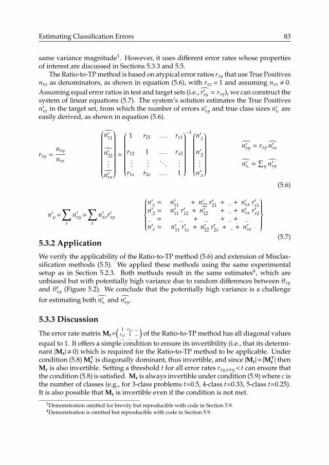
Estimating Classification Errors 83
same variance magnitude3. However, it uses different error rates whose propertiesof interest are discussed in Sections 5.3.3 and 5.5.
The Ratio-to-TP method is based on atypical error ratios rxy that use True Positivesnxx as denominators, as shown in equation (5.6), with rxx = 1 and assuming nxx , 0.Assuming equal error ratios in test and target sets (i.e., r′xy = rxy), we can construct thesystem of linear equations (5.7). The system’s solution estimates the True Positivesn′xx in the target set, from which the number of errors n′xy and true class sizes n′x. areeasily derived, as shown in equation (5.6).
rxy =nxy
nxx
n′11
n′22...
n′xx
=
1 r21 . . . rx1
r12 1 . . . rx2...
.... . .
...r1x r2x . . . 1
−1 n′.1
n′.2...
n′.x
n′xy = rxy n′xx
n′x. =∑
y n′xy
(5.6)
n′.y =∑
x
n′xy =∑
x
n′xxr′xy
n′.1 = n′11 + n′22 r′21 + ... + n′xx r′x1n′.2 = n′11 r′12 + n′22 + ... + n′xx r′x2... = ... + ... + ... + ...
n′.x = n′11 r′1x + n′22 r′2x + ... + n′xx
(5.7)
5.3.2 Application
We verify the applicability of the Ratio-to-TP method (5.6) and extension of Misclas-sification methods (5.5). We applied these methods using the same experimentalsetup as in Section 5.2.3. Both methods result in the same estimates4, which areunbiased but with potentially high variance due to random differences between θxyand θ′xy (Figure 5.2). We conclude that the potentially high variance is a challenge
for estimating both n′x. and n′xy.
5.3.3 Discussion
The error rate matrix Mr=( 1 r2x ...
rx2 1 ...... ... ...
)of the Ratio-to-TP method has all diagonal values
equal to 1. It offers a simple condition to ensure its invertibility (i.e., that its determi-nant |Mr|, 0) which is required for the Ratio-to-TP method to be applicable. Undercondition (5.8) Mᵀ
r is diagonally dominant, thus invertible, and since |Mr|= |Mᵀr | then
Mr is also invertible. Setting a threshold t for all error rates rxy,x,y< t can ensure thatthe condition (5.8) is satisfied. Mr is always invertible under condition (5.9) where c isthe number of classes (e.g., for 3-class problems t=0.5, 4-class t=0.33, 5-class t=0.25).It is also possible that Mr is invertible even if the condition is not met.
3Demonstration omitted for brevity but reproducible with code in Section 5.9.4Demonstration is omitted but reproducible with code in Section 5.9.

84 Chapter 5
n’11 n’12 n’13 n’21 n’22 n’23 n’31 n’32 n’33
−50
050
a) Iris
c) Segment
b) Ionospheren’11 n’12 n’21 n’22
−30
−20
−10
010
2030
n’11 n’14 n’17 n’23 n’26 n’32 n’35 n’41 n’44 n’47 n’53 n’56 n’62 n’65 n’71 n’74 n’77
−100
−50
050
100
d) Ohscaln’01 n’06 n’11 n’16 n’21 n’26 n’31 n’36 n’41 n’46 n’51 n’56 n’61 n’66 n’71 n’76 n’81 n’86 n’91 n’97
−100
−50
050
100
f) Chessn’11 n’12 n’21 n’22
−100
−50
050
100
e) Waveformn’11 n’12 n’13 n’21 n’22 n’23 n’31 n’32 n’33
−200
0200
Err
or
n’xy
- n’
xyE
rror
n’
xy -
n’xy
Err
or
n’xy
- n’
xyE
rror
n’
xy -
n’xy
Figure 5.2: Evaluation of estimated n′xy, showing the absolute error n′xy − n′xy for 104 pairs testand target sets sampled as in Section 5.2.3.
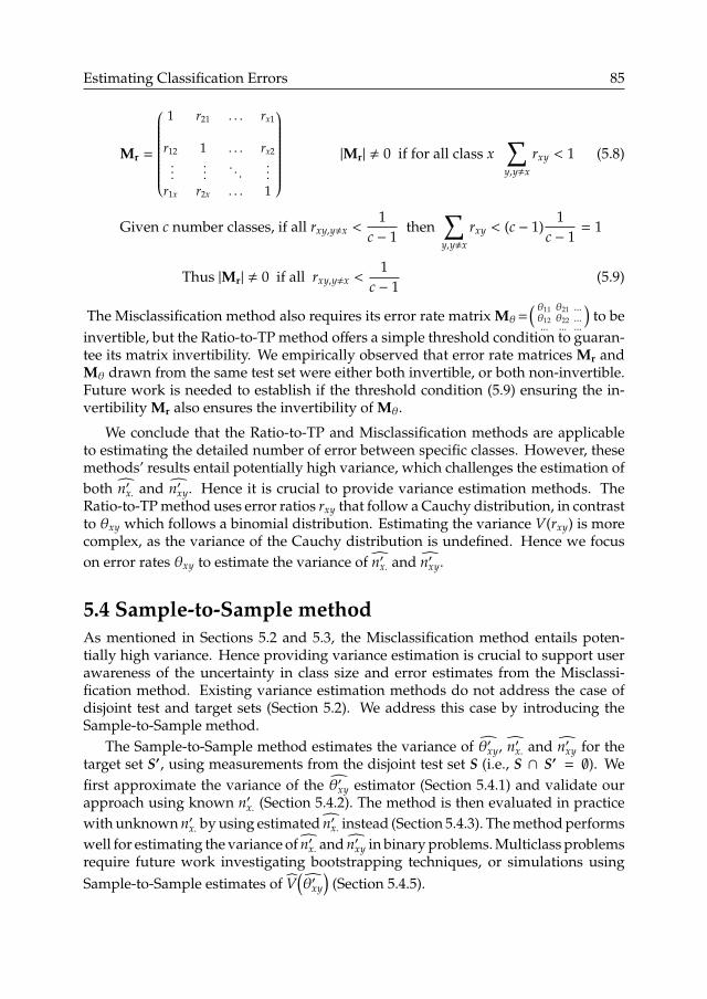
Estimating Classification Errors 85
Mr =
1 r21 . . . rx1
r12 1 . . . rx2...
.... . .
...r1x r2x . . . 1
|Mr| , 0 if for all class x∑y,y,x
rxy < 1 (5.8)
Given c number classes, if all rxy,y,x <1
c − 1then
∑y,y,x
rxy < (c − 1)1
c − 1= 1
Thus |Mr| , 0 if all rxy,y,x <1
c − 1(5.9)
The Misclassification method also requires its error rate matrix Mθ=( θ11 θ21 ...θ12 θ22 ...... ... ...
)to be
invertible, but the Ratio-to-TP method offers a simple threshold condition to guaran-tee its matrix invertibility. We empirically observed that error rate matrices Mr andMθ drawn from the same test set were either both invertible, or both non-invertible.Future work is needed to establish if the threshold condition (5.9) ensuring the in-vertibility Mr also ensures the invertibility of Mθ.
We conclude that the Ratio-to-TP and Misclassification methods are applicableto estimating the detailed number of error between specific classes. However, thesemethods’ results entail potentially high variance, which challenges the estimation ofboth n′x. and n′xy. Hence it is crucial to provide variance estimation methods. TheRatio-to-TP method uses error ratios rxy that follow a Cauchy distribution, in contrastto θxy which follows a binomial distribution. Estimating the variance V(rxy) is morecomplex, as the variance of the Cauchy distribution is undefined. Hence we focuson error rates θxy to estimate the variance of n′x. and n′xy.
5.4 Sample-to-Sample methodAs mentioned in Sections 5.2 and 5.3, the Misclassification method entails poten-tially high variance. Hence providing variance estimation is crucial to support userawareness of the uncertainty in class size and error estimates from the Misclassi-fication method. Existing variance estimation methods do not address the case ofdisjoint test and target sets (Section 5.2). We address this case by introducing theSample-to-Sample method.
The Sample-to-Sample method estimates the variance of θ′xy, n′x. and n′xy for thetarget set S′, using measurements from the disjoint test set S (i.e., S ∩ S′ = ∅). Wefirst approximate the variance of the θ′xy estimator (Section 5.4.1) and validate ourapproach using known n′x. (Section 5.4.2). The method is then evaluated in practicewith unknown n′x. by using estimated n′x. instead (Section 5.4.3). The method performswell for estimating the variance of n′x. and n′xy in binary problems. Multiclass problemsrequire future work investigating bootstrapping techniques, or simulations usingSample-to-Sample estimates of V
(θ′xy
)(Section 5.4.5).
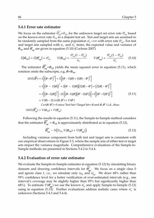
86 Chapter 5
5.4.1 Error rate estimator
We focus on the estimator θ′xy=θxy for the unknown target set error rate θ′xy basedon the known error rate θxy in a disjoint test set. Test and target sets are assumed tobe randomly sampled from the same population n∗x.→∞ with error rate θ∗xy. For testand target sets sampled with nx. and n′x. items, the expected value and variance ofθxy and θ′xy are given in equation (5.10) (Cochran 2007).
E[θxy] = E[θ′xy] = θ∗xy V(θxy) =θ∗xy(1 − θ∗xy)
nx.V(θ′xy) =
θ∗xy(1 − θ∗xy)
n′x.(5.10)
The estimator θ′xy=θxy yields the mean squared error in equation (5.11), whichnotation omits the subscripts, e.g, θ=θxy.
MSE(θ′) = E[(θ−θ′
)2]
= E[(θ − E[θ] + E[θ] − θ′
)2]
= E[(θ − E[θ]
)2+ 2
(θ − E[θ]
)(E[θ] − θ′
)+
(E[θ] − θ′
)2]
= E[(θ−E[θ]
)2]−2E
[(θ−E[θ]
)(θ′−E[θ′]
)]+E
[(θ′−E[θ′]
)2]
= V(θ) − 2Cov(θ,θ′) + V(θ′)
Cov(θ,θ′)=0 since Test Set∩Target Set=∅ and θ,θ′ i.i.d., thus:
MSE(θ′xy) = V(θxy) + V(θ′xy)
(5.11)
Following the results in equation (5.11), the Sample-to-Sample method considersthat the estimator θ′xy = θxy is approximately distributed as in equation (5.12).
θ′xy ∼ N(θxy,V(θxy) + V(θ′xy)
)(5.12)
Including variance component from both test and target sets is consistent withour empirical observations in Figure 5.3, where the sample size of either test or targetsets impact the variance magnitude. Comprehensive evaluations of the Sample-to-Sample methods are presented in Sections 5.4.2 to 5.4.4.
5.4.2 Evaluation of error rate estimator
We evaluate the Sample-to-Sample estimates in equation (5.12) by simulating binarydatasets and drawing confidence intervals for θ′
01. We focus on a single class 0
and ignore class 1, i.e., we simulate only n0y and n′0y. We draw 68% rather than95% confidence level for a better verification of over-estimated intervals (e.g., oneinterval’s coverage may be slightly higher than 95% but significantly higher than68%). To estimate V(θ′
01) we use the known n′0. and apply Sample-to-Sample (5.12)
using in equation (5.13). Further evaluations address realistic cases where n′x. isunknown (Sections 5.4.3 and 5.4.4).

Estimating Classification Errors 87
●●●●●●●●●●●●●●●●●●
●●●●●●●●●●●●●●●
●●●●●●●●●●●●●●
●●●●●●●●●●●●●●●●
●●●●●●●●●●●
●
●
●
●
●
●●●●●●●●●●●●●●●●●●●●●●
100
200
300
●●●●●●●●●●●●●●●
●●●●●●●●●●●●●●●●●●●●●●●●●●●●●●
●●●●●●●●●●●●●●●●●●●●
●●●●●●●●●●●●
●
●
●
●
●
●●●●●●●●●●●●●●●●●●● ●●●●●●
●●●●●●●
●●●●●●●●●●●
●●●●●●●
●●●●●●●●●●●●●●●●●●●●●●●●●●●●●●●●●●●●●●●●●●●●●●●●●
●
●
●
●
●
●●●●●●●●●●●●●●●● ●●●
●●●●●●●
●●●●●●●●●●●●●●●●●●●
●●●●●●●●●●●●●●●●●●●●●●●●●●●●●●●●●●●●●●●●●●●●●●
●●●●
●●●
●
●
●
●
●
●●●●●●●●●●●●●● ●●●●●
●●●●●
●
●●●●●●●
●●●●●●●●●●●●●●●●●●●●●●●●●●●●●●●●●●●●●●●●●●●●●●●●●●●●●●●●●●●
●●●●●
●●
●
●●
●
●
●
●●
●●●●●●●●●
●●●●●●●●●●●●●●●●●●●●●●●●●●●●●●●
●●●●●●●●●●●
●●●●●●●●●●●●●●●●●●●●●●●●●
●
●●
●●●●●
●
●
●●●●●●●●●●●●●●●●●●●●●●●●
200
400
600
●●●●●●●●●●●●●●●●●
●
●●●●●●●●●●
●●●●●●●●●●●●●●●●●●●●●●●●●●●●●●●●
●●●●●●●●●●●●●●●
●
●●
●
●
●
●
●●●●●●●●●●●●●●●●●●● ●●●●●●●
●●●●●●●●
●
●●●●●●●●●●●●●●●●●●●●●●●●●●●●●●●
●●●●●●●●●●●●●●●●●●●●●●●●●●●●●●●
●●●
●
●
●
●
●●●●●●●●●●●●●●●● ●●●●●●●
●●●
●●●●●●●●●●●●
●●●●●●●●●●●●●●●●●●●●●●●●●●●●●●●●●●●●●●●●●●●●●●●●●●●
●●●●●●●
●●
●
●
●●
●●●●●●●●●●●●●●● ●●●●
●●●●
●●●●
●●●●●●●●●●●●●●●●●●●●●●●●●●●●●●●●●●●●●●●●●●●●●●●●●●●●●●●●●●●●●●●●●●●●●
●●●●●
●
●●
●
●●●●●●●●●●●
●●●●●●●●●●●●●●●●●●●●●●●●●●●●●●●
●●●●●●●●●
●●●●●●●●●●●●●●●●●●●●
●●●●●●●
●●●
●●●
●
●
●
●●
●●●●●●●●●●●●●●●●●●●●●●●
50
100
150
●●●●●●●●
●
●●
●
●●●
●
●●●●●●●●
●●●●●●●●●●●●●●●●●●●●●●●●●●●●●●●●●●●●●●●●●●●●●●●●●●●●●●●●●●●●●●
●
●●
●
●
●●●●●●●●●●●●●●●●
●●●●●
●●
●●●●●
●●●●●●●●●
●●●●●●●●●●●●●●●●●●●●●●●●●●●●●●●●●●●●●●●●●●●
●●●●●●●●●●●●●
●
●
●●●●
●●●●●●●●●●●●●●●●●●●●●●●●●
●●
●
●●●●●●●●●●●●●●●●●●●●●●●●●●●●●●●●
●●●●●●●●●●●●●●●●●●●●●●●●●●●●●●●●●
●
●
●
●●●●●●●●●●●●●●●●●●●●●●●●●●●
●●●●
●●
●●●●●●●●●●●●●●●●●●●●●●●●●●●●●●●●●
●●●●●●●●●●●●●●●●●●●●●●●●●●●●
●
●
●
●●
●●●●●●●●●●●●●●●●●●●
●●●●●●●●
●
●●
●●●●●●●●●●●●●●●●●●●●●●●●●●●●●●●●●●●●●●●●●
●●●●●●●●●●●●●●●●●●●●●●●●●●●●●
●
●●
●●●●
●
●
●●●
●●●●●●●●
●●●●●●●●●●
●●●●●●
●
●●●
●●●●●●●●●●●●●●●●●●●●●●
●●●●●●●●●●●●●●●●●●●●●●●●●●●●●●●●●●●●●●●●●
●
●
●●
●●●●●●●●●●●●●●●●●●●●●
●●●●●
●●●●●●
●●●●●●●●●●●●
●●●●●●●●●●●●●●●●●●●●●●●●●●●●●●●●●
●●●●●●●●●●●●●●●●
●
●●
●
●
●
●
●●●●●●●●●●●●●●●●●●●●●●●●
●●●●●●●●●●●●●●●●●
●●●●●●●●●●
●●●●●●●●●●●●●●●●●●●●●●●●
●●●●●●●●●●●●●●●
●●●●
●
●
●●
●●●●●●●●●●●●●●●●●●
20
40
60
●●●●●●●●●●●●●●●●●●●●●●●●●●●●●●●●
●●●●●●●●●●●●●●●●●●●●●●●●●
●●●●●●●●●●●●●●●
●
●
●
●
●
●●●●●●●●●●●●●●●●●●●●●●●●
●●●●●
●●●●●
●
●●●●●●●
●●●●●●●●●●●●●●●●●●●●●●●●●●●●●●●●●●●●●●●●●●●●●●●●●●●●●●●●●●●
●●●●●●●●●●
●
●
●
●
●●●●●●●●●●●●●●●●●●●●
●●●●●●
●●●●●●●●●●●●●●●●●●●●●●●●●●●●●●●●●●●●●●●●●●●●●
●●●●●●●●●●●●●●●●●●●●●
●
●●
●
●
●
●●●●●●●●●●●●●●●●●●●
●●●●●●
●●
●●
●●●●●●●●●●●●●●●●●●●●
●●●●●●●●●●●●●●●●●●●●●●●●●●●●●●●●●●●●
●●●●●●●
●
●
●
●
●
●●
●●●●●●●●●●●●●●●●●●●●●●●●●●●●●●●●
●●●●●●●●●●●●●●●●●●●●●●●●●●●●●●●●●●●●●●●●●●●●●●
●●●●●●●●●●●●●●●
●
●
●
●
●
●●●●●●●●●●●●●●●●●●●●●●●●●●●●●●
●●●●●●●●●●●●●●●●●●●●●●●●●●●●●●●●●●●●
●●●●●●●●●●●●●●●●●●
●●●●●●
●●●
●
●
●
●●●●●●●●●●●●●●●●●●●●●●●0
500
1000
1500
0 0.25 0.50 0.75 1 0 0.25 0.50 0.75 1 0 0.25 0.50 0.75 1 0 0.25 0.50 0.75 1 0 0.25 0.50 0.75 1 Score ThresholdScore ThresholdScore ThresholdScore ThresholdScore Threshold
True
Estimated
n0. = 200 n0. = 400 n0. = 1000n0. = 100n0. = 40
n’0.
= 4
0n’
0. =
100
n’0.
= 2
00n’
0. =
400
n’0.
= 1
000
Figure 5.3: Results of Misclassification method for simulated data, showing results variancefor different sample sizes of test and target sets. Score thresholds (x axis) are used to assign class 0or 1, and simulate different magnitudes of error rate, as explained in Figure 5.4. Class sizes n′0. (y axis)are estimated for 104 pairs of test and target sets randomly sampled with score probability and classproportions in Figure 5.4, and for thresholds selected with granularity 0.01. We randomly sampled 100test sets, and then randomly sampled 100 distinct target sets for each test set. This approach is realistic,as in practice one test set is used for several target sets. Unbiased means n′0. (black line) are close to truen′0. (red line) unless test sets are too small and error rate too close to 0 or 1 (e.g., when extreme thresholdsyield few observations with nxy ≈ a few items).
Score0 1
Num
ber o
f ite
ms
n’1.
Var(θ’01)
Var(θ’10)
Var(θ01)Var(θ10)
n’0.
Mean Score
sd = 0.1 sd = 0.1
Threshold
Score0 1
Num
ber o
f ite
ms
Score Threshold0 1Erro
r Rat
e Va
rianc
e
n’10 n’01
0 1
Num
ber o
f ite
ms
n1. forClass C1
n0. forClass C0
Test
Set
Targ
et S
et
mean = 0.6mean = 0.4
Score Variance
Score Variance
Threshold
0 1
Num
ber o
f ite
ms
0 1Erro
r Rat
e Va
rianc
e
n10 n01
Figure 5.4: Specification of classification problem in Figure 5.3. Left: score distribution withmeans µ0=µ′0=0.4 for class 0, µ1=µ′1=0.6 for class 1, and σx=σ′x=0.1. Middle: example of score thresholdand related errors n01, n10. Right: error rate variance over thresholds. V(θ′01)<V(θ′10) because we usen′0.=2n′1.and n0.=n1. to obtain different class proportions in test and target sets.
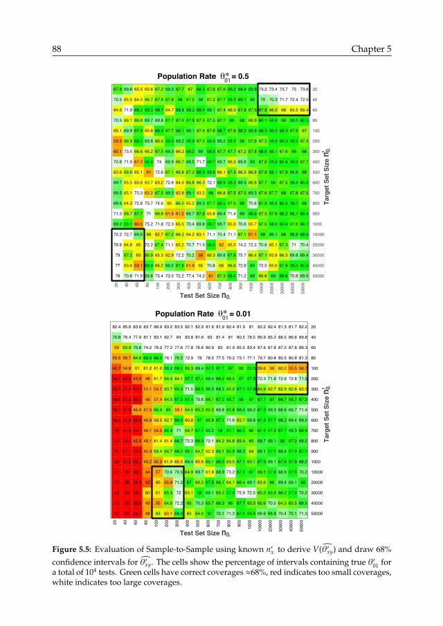
88 Chapter 5
20 40 60 80 100
200
300
400
500
600
700
800
900
1000
1000
0
2000
0
3000
0
4000
0
5000
0
50000
40000
30000
20000
10000
1000
900
800
700
600
500
400
300
200
100
80
60
40
20
Test Set Size n0.
Targ
et S
et S
ize
n 0.
Test Set Size n0.
Targ
et S
et S
ize
n 0.
Population Rate θ∗ = 0.501
’’
78 70.8 71.9 69.8 73.4 73.5 72.2 77.4 74.3 61 67.3 68.4 71.2 69 66.6 69 68.6 70.8 69.9
77 63.6 59.1 68.9 66.2 69.5 67.8 61.9 65 70.8 66 66.6 72.8 69 72.5 65.6 67.9 68.5 68.3
79 67.2 63 66.9 65.3 62.9 72.2 70.2 58 66.3 69.8 67.8 75.7 66.4 67.1 63.8 66.3 69.8 69.4
78.8 64.8 65 72.2 67.4 71.1 65.2 70.7 71.9 68.5 62 65.5 74.2 72.2 70.6 65.1 67.3 71 70.4
75.2 72.7 69.6 66 62.7 67.2 66.2 64.2 63.1 71.1 70.4 71.1 67.1 61.1 68 69.1 68 68.9 68.6
69.2 68.1 60.5 75.2 71.8 72.3 65.5 70.4 69.8 68.7 69.7 65.6 70.6 65.7 67.5 68.9 68.6 67.8 68.1
71.3 66.7 67.7 71 66.8 61.5 61.2 69.7 67.8 65.8 69.4 71.4 69 68.6 67.3 67.9 68.2 68.1 68.4
69.6 64.3 72.8 73.7 74.6 65 66.5 65.2 69.3 67.7 68.5 67.5 68 70.8 67.9 68.8 68.4 68.3 68
69.5 65.1 73.3 62.2 67.5 69.3 62.8 69.1 63.5 68 66.8 67.5 67.5 69.3 67.6 67.7 68 67.8 67.5
69.7 65.5 63.8 63.7 63.2 72.8 64.6 66.8 66.3 72.1 68.9 68.2 69.3 66.8 67.7 68 67.5 68.9 68.2
63.8 66.6 65.1 61 72.6 67.1 66.8 67.2 68.3 68.8 66.1 67.5 66.5 66.8 67.8 68.1 67.9 68.8 68
70.8 71.9 61.3 68.4 74 69.9 66.7 69.5 71.7 68.7 69.7 66.3 69.8 69 67.8 68.6 68.4 68.6 67.7
60.1 73.5 66.6 66.2 67.5 69.3 66.2 68.2 69 68.5 67.7 67.7 67.2 67.8 68.6 68.1 67.6 68 68
59.9 66.9 68.5 69.8 66.8 68.3 69.2 68.9 67.5 68.8 69.2 68.2 68 67.6 67.3 68.6 68.3 68.5 67.3
65.1 69.9 67.9 65.8 68.5 67.7 68.1 69.1 67.4 67.6 68.7 67.8 68.2 68.9 68.3 68.3 68.3 67.9 67
70.5 66.1 66.8 69.7 69.8 67.7 67.8 67.9 67.5 67.5 67.7 68 68 66.9 68.1 68.6 68 68.8 68.5
64.6 71.9 68.2 68.3 68.7 64.7 68.8 68.2 68.4 69.1 67.4 66.5 67.8 67.5 67.8 66.5 66 65.5 65.4
70.5 65.5 64.5 66.7 67.4 67.6 68 67.5 69 67.2 67.7 68.2 68.1 69 70 70.3 71.7 72.4 72.5
67.8 69.8 65.5 65.6 67.2 69.3 67.7 67 68.5 67.6 67.6 68.2 68.9 68.8 73.2 73.4 73.7 75 73.6
20 40 60 80 100
200
300
400
500
600
700
800
900
1000
1000
0
2000
0
3000
0
4000
0
5000
0
50000
40000
30000
20000
10000
1000
900
800
700
600
500
400
300
200
100
80
60
40
20
Population Rate θ∗ = 0.0101
12 26 33.2 48 63 60.1 68.6 63 64.6 67 70.1 71.3 67.6 66.6 69.8 68.8 70.4 70.1 71.3
19 30 38.8 49 55 64.6 72.2 65 70.3 65.7 66.3 66 67.7 65.5 65.6 70.5 64.3 65.5 68.5
18 22 29.8 60 61 65.3 72 63.1 68 69.1 65.3 67.5 75.9 72.5 65.3 65.9 66.2 67.9 70.2
17 28 35.8 43 60 55.8 71.2 67 64.2 67.5 66.1 64.1 66.4 69.1 63.6 66 69.4 69.1 68
22 30 30.2 44 57 70.6 70.5 64.9 69.7 61.8 68.9 73.2 67.9 67 66.3 67.8 68.9 67.6 70.2
19 30.3 29.1 45.2 50.2 61.9 60.5 69.4 60.6 65.1 66.8 63.5 67.1 65.1 67.9 69.1 67.6 67.9 68.2
15 23.1 35.4 45.3 63.4 64.7 66.2 68.1 64.7 62.3 65.1 65.9 68.3 64 68.1 67.7 68.4 67.9 67.3
22 26.4 42.5 48.1 61.4 61.4 68.7 72.3 66.9 72.1 64.2 64.8 65.4 65 68.7 68.1 68 67.2 68.2
16 23.3 34.3 48.1 54.6 66.4 71 64.7 67.5 68.2 68 67.1 66.5 66 67.9 67.2 67.7 68.3 66.9
18.2 24.6 39.8 46.8 59.5 62.7 66.6 60.8 67 65.9 67.1 71.6 63.7 68.8 67.8 67.7 68.2 69.4 69.5
19.5 26.9 45.4 47.5 65.4 65 59.1 64.5 65.3 65.5 69.8 65.8 68.6 69.2 67.8 69.3 68.9 69.7 71.4
19.8 30.2 35.1 45 57.4 64.5 67.9 67.4 70.6 66.1 67.2 66.7 68 67 67.7 67 66.7 66.7 67.2
20.2 33.4 35.9 51.1 54.1 63.7 65.9 71.5 66.8 68.3 68.5 65.2 67.5 67.8 64.8 62.7 62.9 62.6 62.3
26.1 35.6 43.6 46 61.7 64.4 64.1 67.7 67.1 68.4 66.9 66.4 67 67.5 72.3 71.8 72.6 72.8 71.9
42.7 54.8 61 61.2 61.8 68.2 66.9 65.3 69.4 67.5 67.7 67 66 66.5 59.6 59 60.2 55.5 56.7
55.5 56.7 64.8 66.5 66.6 76.1 70.2 72.9 78 78.5 77.5 79.2 73.1 77.1 79.7 80.8 80.5 80.8 81.3
59 63.9 70.6 74.2 76.2 77.2 77.6 77.8 76.6 80.9 83 81.9 85.5 83.4 87.6 87.8 87.5 87.8 88.3
70.8 76.4 77.9 81.1 83.1 82.7 84 83.8 81.6 83 81.4 81 80.5 78.5 86.9 85.2 88.5 86.6 89.8
82.4 85.6 83.8 83.7 86.9 83.2 83.5 82.1 82.9 81.6 81.9 82.4 81.9 81 82.2 82.4 81.5 81.7 82.2
Figure 5.5: Evaluation of Sample-to-Sample using known n′x. to derive V(θ′xy) and draw 68%
confidence intervals for θ′xy. The cells show the percentage of intervals containing true θ′01 fora total of 104 tests. Green cells have correct coverages ≈68%, red indicates too small coverages,white indicates too large coverages.

Estimating Classification Errors 89
We sample 100 test sets of sizes n0.∈{20, ..., 50 000} randomly drawn from an in-finite population with θ∗01∈{0.01, 0.5}. For each test set, we measured θ01 and useequations (5.12-5.13) to draw confidence intervals for θ′01 in target sets of sizesn′0.∈{20, ..., 50 000}. For each interval, we randomly sample 100 target sets with thesame population rate θ∗01.
V(θ′
01
)=θ01(1−θ01)
n0.+θ01(1−θ01)
n′0.(5.13)
The graph cells in Figure 5.5 show the percentage of θ′xy contained in confidenceintervals derived using the Sample-to-Sample method. The confidence intervalsachieve the desired confidence level, except when sample sizes nx. and n′x. are toosmall w.r.t. error rates θ∗xy (in bottom graph only, e.g., nxy≈1 item, same as thebiases observed in Figure 5.3), or w.r.t. each other (nx. � or � n′x., black contours).The interval coverage varies more if nx.<n′x. (lower left triangle of graphs) but meancoverage is correct (e.g., forθ∗xy=0.5, in lower left triangleµ=68.1% andσ=4, otherwiseµ=68.3% and σ=1.5).
5.4.3 Application to estimating class sizes
We evaluate the Sample-to-Sample method applied to estimating confidence intervalsfor the target class sizes n′x. resulting from the Misclassification method in binaryproblems. As in Section 5.4.2, we simulate 100 test sets and 100 target sets for eachtest set, with sizes nx.,n′x.∈{300, 500, 1000, 2000}, drawn from populations with θ∗xyspecified in equation (5.14).θ
∗
00 θ∗10
θ∗01 θ∗11
∈{ (.9 0.1 1
),
(.9 .1.1 .9
),
(.9 .2.1 .8
),
(.8 .2.2 .8
) }(5.14)
Confidence intervals are estimated using Fieller’s theorem, as by Shieh (2009).We express the results of the Misclassification method as ratios in equation (5.15),assuming 1−θ′01−θ
′
10 , 0. Fieller’s theorem applies to ratios of correlated randomvariables A/B, e.g., A=n′.0− θ
′
10n′.. and B=1− θ′
01− θ′
10. The variance and covariance
of A and B are detailed in Section 5.9. For the estimator θ′xy=θxy, we use the varianceestimate in equation (5.16), derived from the Sample-to-Sample method, and usingthe results of the Misclassification method n′x. as estimates of the unknown n′x..
n′0. =n′.0 − θ′10 n′..
1 − θ′01 − θ′10
n′1. =n′.1 − θ′01 n′..
1 − θ′01 − θ′10
(5.15)
V(θ′xy
)=θxy(1−θxy)
nx.+θxy(1−θxy)
n′x.(5.16)

90 Chapter 5
The results in Figure 5.6 show that the Sample-to-Sample method provides ac-curate confidence intervals for n′x.. For each model in equation (5.14), the meanand variance of intervals’ coverage are respectively: µ=68.1% σ=0.7, µ=68.2% σ=0.7,µ=68.2% σ=0.7, µ=68.2% σ=0.7.
These results are obtained without rounding the estimated n′x. nor the confidencelimits. If these are rounded, the intervals are slightly biased and over-estimated. Forinstance, with our experiment setup, the coverage approximatively varied by ±3%for 68% intervals with µ=69.1%, and ±1% for 95% intervals with µ=95.6%.
.8.2
.2.8
θ* 00
θ* 10
θ* 01
θ* 11=
θ* 00
θ* 10
θ* 01
θ* 11=.
90
.11
θ* 00
θ* 10
θ* 01
θ* 11=.9
.1.1
.9θ* 0
0θ* 1
0
θ* 01
θ* 11=.
9.2
.1.8
68 68 68 68 68 68 69 68 68 68 68 69 68 69 69 68
68 68 68 68 68 68 68 68 67 68 68 69 68 68 68 68
68 68 68 68 68 68 68 68 69 68 68 68 69 68 69 68
68 68 68 68 69 68 68 68 67 68 67 68 68 69 69 68
68 68 68 68 68 69 68 68 68 68 67 69 68 69 69 67
69 68 69 68 68 68 68 68 69 68 68 68 69 70 66 69
68 68 68 68 69 68 67 68 68 68 68 68 67 68 68 68
68 68 68 68 69 68 68 68 69 68 68 69 69 67 68 68
67 67 68 67 67 69 68 69 68 68 68 68 68 69 68 68
67 68 68 68 70 68 68 68 69 70 69 68 68 69 67 67
68 68 67 67 68 68 69 67 67 67 68 69 68 68 68 67
68 68 67 67 68 69 68 68 68 69 67 68 68 67 70 68
69 68 68 68 67 68 67 68 68 69 69 69 67 69 68 67
68 68 68 67 68 68 69 68 67 68 66 68 67 69 69 70
68 68 68 68 67 68 67 67 69 67 69 68 67 68 69 68
68 68 68 69 67 68 69 68 66 68 68 68 69 68 70 67
68 69 68 68 69 68 69 68 68 68 68 69 68 67 68 68
69 68 69 69 69 68 69 68 68 68 68 69 69 70 68 68
68 68 68 67 69 69 68 67 68 69 68 68 68 67 68 69
68 68 68 69 67 69 69 68 68 68 67 69 69 68 69 69
68 69 68 68 69 68 69 68 69 68 69 68 69 69 69 68
68 68 68 67 69 68 68 68 68 68 69 69 69 68 68 68
68 68 68 68 68 68 68 69 67 69 69 68 69 68 69 68
68 68 68 69 68 67 69 68 68 69 67 69 68 68 70 68
68 68 69 70 68 68 68 68 69 68 68 68 69 68 68 70
69 69 68 67 69 68 69 68 68 68 69 67 69 70 68 66
68 69 69 68 68 67 69 68 68 68 70 68 68 68 71 68
68 68 67 68 67 68 68 69 67 68 68 69 68 69 68 69
68 69 69 68 69 68 69 68 68 67 68 68 68 68 67 67
68 69 68 67 69 68 68 68 67 69 69 69 67 68 67 68
68 68 67 68 67 69 68 69 69 69 67 68 69 68 68 68
69 68 68 70 68 67 70 68 68 69 70 67 68 67 68 68
69 68 68 69 68 69 69 68 68 68 68 68 67 69 68 69
68 68 68 67 69 68 69 68 68 68 68 68 68 68 67 67
68 68 68 68 69 69 68 69 70 68 68 68 68 67 68 68
69 68 68 69 68 68 68 67 68 68 68 67 68 69 68 70
68 68 68 69 68 68 68 68 68 68 67 68 68 69 69 67
69 68 67 70 68 68 68 69 68 69 68 67 69 69 68 70
68 68 69 70 69 69 69 69 69 69 68 69 68 69 66 69
68 68 68 70 68 69 68 68 68 68 68 69 68 68 67 70
68 68 68 68 68 69 68 69 69 68 68 69 67 68 68 67
68 68 68 69 68 68 68 68 68 69 69 67 69 68 69 68
69 69 68 65 68 68 67 69 69 67 69 67 69 69 68 67
69 68 67 69 69 69 68 68 68 69 68 68 68 69 67 67
68 68 68 68 68 68 69 69 68 68 70 68 67 69 68 68
68 69 68 67 69 68 68 70 69 68 69 68 67 68 69 68
69 69 70 69 68 69 68 68 69 68 67 69 67 69 69 69
68 68 69 67 68 67 68 68 68 68 69 70 66 68 68 67
68 68 68 69 69 68 68 69 68 68 68 68 69 68 68 68
69 69 68 69 68 68 69 70 68 69 68 69 68 68 68 67
68 68 68 69 68 68 68 68 68 68 69 68 68 69 67 68
69 68 67 67 68 66 68 67 68 69 69 67 68 68 68 68
69 68 68 68 68 68 69 69 68 67 68 68 68 68 69 68
69 68 69 69 69 68 68 69 68 68 69 67 69 68 70 67
68 69 68 70 69 68 68 66 68 69 67 68 69 67 67 67
69 68 68 69 68 68 68 68 68 68 68 70 68 68 68 69
68 69 68 69 69 68 68 68 69 69 68 67 67 69 69 71
68 68 68 68 68 69 67 68 68 68 68 68 69 68 69 67
68 68 67 68 68 69 67 68 68 69 68 68 68 70 68 68
69 68 67 66 69 68 69 67 68 67 69 69 69 69 68 69
68 68 68 68 68 69 68 69 67 68 67 68 69 67 68 69
68 68 67 69 67 68 68 68 69 68 67 68 70 67 68 68
69 69 68 68 68 68 68 70 69 69 68 69 69 69 68 68
69 69 69 68 68 68 69 68 68 68 69 67 69 67 70 68
Figure 5.6: Results of Sample-to-Sample applied to estimating confidence intervals for n′x.. Theintervals accurately include the desired percentage of actual class size n′x. (68%, green cells).Test and target datasets are randomly sampled with sizes on columns and rows. The cellsshow the % of intervals that contained n′0. for a total of 104 tests (the % are rounded for clarity).

Estimating Classification Errors 91
5.4.4 Application to estimating error composition
We evaluate the Sample-to-Sample method applied to estimating confidence inter-vals for the results n′xy of the extended Misclassification method (Section 5.3). Asin Section 5.4.3, Fieller’s theorem is applied with the same experimental setup, toderive confidence intervals for n′01 instead of n′0.. In this case, using the result of
equation (5.5), A=θ′01
(n′.0− θ
′
10n′..
)in equation (5.15). The variance and covariance of
A and B are detailed in Section 5.9.Instead of drawing a graph as Figure 5.6, we report the mean and variance of
interval coverage for each model in (5.14), respectively: µ=68.0% σ=0.7, µ=68.1%σ=0.8, µ=68.2% σ=0.7, µ=68.3% σ=0.7. It shows that the Sample-to-Sample methodprovides accurate confidence intervals for n′xy.
5.4.5 Discussion
In this section, we discuss how the Sample-to-Sample method contributes to priorwork focusing on class proportions, and applications of the Reclassification methods(p.92). We then introduce future work of interest for addressing multiclass problems(p.94), and investigating the potential impact of number of classes (p.94) on variancemagnitude.
Prior work - The Sample-to-Sample approach is applicable to prior work focusingon estimating class proportions, e.g., π′x=n′x./n′.. (Shieh 2009, Buonaccorsi 2010). Thisprior method is restated for class 0 in equation (5.17) using our notation.
The main difference with the Sample-to-Sample approach is how test and targetset sizes nx., n′x. are considered for the variance estimation. The Sample-to-Sampleapproach accounts for test and target sets’ class sizes nx., n′x. to estimate the error ratevariance V
(θ′xy
). The prior method uses only test sets’ class sizes nx. to estimate the
error rate variance V(θ′xy
). Target sets’ class sizes n′x. are used only for estimating the
variance of class proportions n′.y/n′.. from the classifier output (i.e., prior to applyingthe Misclassification method).
With the prior approach from Shieh (2009) and Buonaccorsi (2010), the variance ofthe numerator and denominator in equation (5.17) is estimated with equation (5.18).Then, Fieller’s theorem can be applied as detailed in additional materials (Section 5.9).
π0 =n′0.n′..
=n′.0/n
′.. − θ10
1 − θ01 − θ10(5.17)
V(n′.0/n
′
.. − θ10
)=
n′.0/n′..
(1 − n′.0/n
′..
)n′..
+θ10(1 − θ10)
n1.
V(1 − θ01 − θ10
)=θ01(1 − θ01)
n0.+θ10(1 − θ10)
n1.
(5.18)

92 Chapter 5
The results of equations (5.17)-(5.18) are reproduced in Figure 5.7, using variablessimilar to prior evaluation (Shieh 2009): nx.∈{25, 50, 125, 250}, n′x.∈{50, 125, 250, 500},θ01=0.1, θ10=0.2. When used for estimating target sets’ class proportions π′x = n′x./n′..,the prior method is biased for many values of nx. and n′x..
The prior method was designed for estimating the class proportions π∗x = n∗x. /n∗..in the overall population from which test and target sets are randomly sampled. Weshow that this prior variance estimation method is not applicable for estimating theclass sizes or proportions of target sets, i.e., n′x. or π′x = n′x./n′.. as in Figure 5.7.
The bias in Figure 5.7 can be corrected with the Sample-to-Sample method, con-sidering no variance for the initial class proportion n′.y/n′.. as shown in equation (5.19).The corrected results in Figure 5.8 have a small bias when sample sizes nx. and n′x.are small w.r.t. the error rates (i.e., yielding small numbers of errors nxy, n′xy wherevariations of ±1 item can yield significant error rate variations, as mentioned in Fig-ure 5.3). Estimates drawn using the larger sample sizes in Figure 5.6 are unbiasedwith mean coverage µ=68.2%, σ=0.7. These results show that the Sample-to-Samplemethod is suitable for estimating target sets’ class proportions π′x=n′x./n′...
Vcorrected
(n′.0/n
′
.. − θ10
)=θ10(1 − θ10)
n1.+θ10(1 − θ10)
n′1.(5.19)
250
125
50
25
250
125
50
25
250
125
50
25
250
125
50
25
2550
125
250
50 100
250
500 50 100
250
500 50 100
250
500 50 100
250
500
50025010050
θ* 00
θ* 10
θ* 01
θ* 11=.
9.2
.1.8
82 79 73 71 82 80 76 72 77 79 77 74 71 74 76 75
81 78 73 70 81 79 74 70 75 77 75 72 72 73 76 73
78 74 69 67 79 75 71 69 75 76 73 69 72 73 71 72
76 72 67 69 77 72 68 67 74 73 70 69 72 72 70 68
82 79 73 70 80 80 76 74 73 76 77 73 70 70 73 74
80 78 71 69 79 78 74 71 73 76 74 73 69 71 73 72
78 73 70 67 78 76 71 67 72 74 72 68 70 70 71 68
75 71 66 65 76 74 68 66 73 72 70 70 69 70 71 70
80 79 73 69 77 79 75 72 72 72 74 74 68 69 72 73
79 77 71 68 76 78 73 70 70 73 74 69 67 71 70 69
78 74 69 66 75 76 72 69 71 72 72 67 69 70 70 70
75 71 66 67 75 73 69 68 70 70 69 66 67 67 68 68
79 76 72 69 72 74 75 72 68 69 70 70 63 65 69 70
77 76 71 71 73 72 72 70 67 69 71 70 62 66 68 69
75 72 68 68 72 73 71 69 68 66 70 68 63 67 66 68
74 71 67 68 73 72 68 67 67 68 70 68 64 67 67 67
Figure 5.7: Confidence intervals drawn using prior work by Shieh (2009) and Buonaccorsi(2010). The intervals are biased and tend to include a too large percentage of actual class sizesn′x. (too large intervals, white to grey cells). Test and target datasets are randomly sampledwith sizes on columns and rows. The cells show the percentage of intervals that containedπ′0=n′0./n
′
.. for a total of 104 tests per cell (percentages are rounded for clarity).

Estimating Classification Errors 93
250
125
50
25
250
125
50
25
250
125
50
25
250
125
50
25
2550
125
250
50 100
250
500 50 100
250
500 50 100
250
500 50 100
250
500
50025010050
θ* 00
θ* 10
θ* 01
θ* 11=.
9.2
.1.8
69 68 67 69 68 68 69 67 68 68 67 69 70 69 68 69
68 68 68 67 69 68 68 68 68 69 66 67 69 68 69 67
68 68 68 65 68 68 68 68 67 67 68 66 68 67 67 67
68 66 64 67 66 68 63 68 69 67 66 66 68 68 67 64
68 68 69 68 68 68 69 68 69 69 68 68 68 68 67 68
67 68 68 68 68 69 68 68 67 69 66 68 68 67 69 67
68 68 68 68 68 68 67 68 67 67 67 66 68 67 68 68
67 68 68 65 67 67 65 64 68 65 64 68 69 68 67 68
68 67 68 69 66 67 68 68 69 67 67 68 68 68 66 68
68 68 67 67 66 67 67 69 67 66 67 68 70 67 66 70
67 69 68 66 67 67 68 68 65 66 67 69 66 65 67 69
67 65 69 67 67 67 65 66 67 68 68 67 67 68 70 66
66 67 68 68 65 67 67 67 66 64 67 68 64 63 64 67
66 67 69 68 64 65 68 68 67 65 66 67 63 65 65 65
66 67 68 68 67 66 69 68 66 65 66 69 65 64 67 68
67 67 67 67 64 66 70 65 67 64 66 68 64 64 66 67
Figure 5.8: Results of Sample-to-Sample method used to correct the bias in Figure 5.7. Theintervals accurately include the desired percentage of actual class size n′x. (68%, green cells).However, bias may occur if class sizes are scarce (e.g., around 25 items, yellow cells) asvariations of a few errors can have significant impacts on the resulting error rates.
Reclassification method - The Sample-to-Sample approach is not always appli-cable to the Reclassification method, i.e., to the error rate estimator e′xy = exy (equa-tion (5.1) p.79). Equations (5.10) and (5.11) do not apply when class proportions differbetween test and target sets, as e′xy and exy are not identically distributed. As shownin equations (5.3)-(5.4) p.80, their denominators depend on the class proportions. Ifclass proportions differ between test and target sets, the denominators differ andare not proportional to the numerators, yielding different distributions. Thus theirexpected values differ E[exy] , E[e′xy] and equations (5.10) and (5.11) do not apply.
However, stable class proportions is a prerequisite for the reclassification tobe applicable, as otherwise bias ensues (Section 5.2.4). With equal class propor-tions, the Sample-to-Sample approach can be applied with equations (5.20)-(5.22)(equation (5.21) omits the subscripts, e.g, e=exy). However, class proportions mayvary randomly due to sample variance. Thus error rate variance should considerthe variance of its denominator (i.e., V(n.y) =
∑x V(nxy) with Cov(nxy,nzy)=0 since
Class x∩Class z=∅) which is ignored in equation (5.20).
iif ∀x, E[
nx.
n..
]= E
[n′x.n′..
]:
E[exy] = E[e′xy] = e∗xy V(exy) =e∗xy(1 − e∗xy)
n.yV(e′xy) =
e∗xy(1 − e∗xy)
n′.y(5.20)

94 Chapter 5
MSE(e′) = E[(
e−e′)2]
= V(e) − 2Cov(e, e′) + V(e′)
Cov(e, e′)=0 since Test Set∩Target Set=∅ and e, e′ independent, thus:
MSE(e′xy) = V(exy) + V(e′xy)
(5.21)
e′xy ∼ N(exy,V(exy)+V(e′xy)
)V(exy) =
exy(1 − exy)n.y
V(e′xy) =exy(1 − exy)
n′.y(5.22)
Multiclass problems - Classification problems with more than 3 classes are noteasily solved as fractions of random variables using Cramer’s rule, as in equa-tion (5.15) p.89. Thus Fieller’s theorem is not easy to apply. Sarrus’ rule applies to3-class problems, providing a solution that can be expressed as ratios using Cramer’srule. However, applying Fieller’s theorem to the resulting ratios remains complex.
Bootstrapping methods are thus recommended for multiclass problems (Buonac-corsi 2010). Monte Carlo simulations are also of interest. Datasets can be simulatedusing error rate variance from the Sample-to-Sample method, using equation (5.12).Future work should investigate Monte Carlo simulations, and compare their resultsto bootstrapping methods.
Number of classes - Future work could investigate whether the number of classesimpacts the variance of the Misclassification method. For instance, problems withlarger numbers of classes may entail larger magnitudes of variance (for problemswith similar error rates and class size magnitudes).
According to Cramer’s rule, the results of the Misclassification method are frac-tions of two matrix determinants (Kosinski 2001), as shown in equation (5.23) for4-class problems. The matrices are composed of random variables θxy and outputclass sizes n′.y.
The Laplace expansion shows that matrices’ determinants are weighted sums ofsub-matrices’ determinant, as shown in equation (5.24) for 4-class problems. Thevariables θxy are used several times in these sub-matrices. As the variables θxy areduplicated in the sub-matrices, their variances V(θxy) may have increased impacton the variance of the determinants, and thus on the results of the Misclassificationmethod (as mentioned in Section 5.2.4). Problems with larger numbers of classesinvolve more sub-matrices, and thus more duplicated variables θxy. Thus we canexpect that the larger the number of classes, the higher the variance of the Misclassi-fication method’s results.
n′1. =
∣∣∣∣∣∣∣∣∣∣n′.1 θ21 θ31 θ41n′.2 θ22 θ32 θ43n′.3 θ23 θ33 θ43n′.4 θ24 θ34 θ44
∣∣∣∣∣∣∣∣∣∣∣∣∣∣∣∣∣∣∣∣θ11 θ21 θ31 θ41θ12 θ22 θ32 θ43θ13 θ23 θ33 θ43θ14 θ24 θ34 θ44
∣∣∣∣∣∣∣∣∣∣n′2. =
∣∣∣∣∣∣∣∣∣∣θ11 n′.1 θ31 θ41θ12 n′.2 θ32 θ43θ13 n′.3 θ33 θ43θ14 n′.4 θ34 θ44
∣∣∣∣∣∣∣∣∣∣∣∣∣∣∣∣∣∣∣∣θ11 θ21 θ31 θ41θ12 θ22 θ32 θ43θ13 θ23 θ33 θ43θ14 θ24 θ34 θ44
∣∣∣∣∣∣∣∣∣∣. . . (5.23)

Estimating Classification Errors 95
∣∣∣∣∣∣∣∣∣∣θ11 θ21 θ31 θ41θ12 θ22 θ32 θ43θ13 θ23 θ33 θ43θ14 θ24 θ34 θ44
∣∣∣∣∣∣∣∣∣∣ = θ11
∣∣∣∣∣∣∣∣θ22 θ32 θ43θ23 θ33 θ43θ24 θ34 θ44
∣∣∣∣∣∣∣∣ − θ12
∣∣∣∣∣∣∣∣θ21 θ31 θ41θ23 θ33 θ43θ24 θ34 θ44
∣∣∣∣∣∣∣∣+ θ13
∣∣∣∣∣∣∣∣θ21 θ31 θ41θ22 θ32 θ43θ24 θ34 θ44
∣∣∣∣∣∣∣∣ − θ14
∣∣∣∣∣∣∣∣θ21 θ31 θ41θ22 θ32 θ43θ23 θ33 θ43
∣∣∣∣∣∣∣∣(5.24)
5.5 Maximum Determinant method
The Sample-to-Sample method introduced in Section 5.4 can assess the variance ofclassification error estimates for specific datasets. However, when comparing clas-sifiers to select the optimal classifier for their tasks, end-users are not interested inclassifiers’ performance for one specific dataset but for a variety of potential datasets(e.g., unknown target sets). The characteristics of the target sets (e.g., target classsizes) may be unknown when comparing classifiers. In this case, the Sample-to-Sample method cannot be applied, and end-users cannot assess which classifier mayyield the smallest variance when estimating class sizes and numbers of errors.
To address this issue, the Maximum Determinant method is a promising approach.The method aims at predicting which classifier may yield the smallest variancewhen applying the error estimation methods, without requiring information on thepotential target sets.
5.5.1 Determinants as variance predictors
The Maximum Determinant method focuses on the determinant |M| of error rate ma-trices, i.e., |Mθ|=
∣∣∣∣ θ11 θ21 ...θ12 θ22 ...... ... ...
∣∣∣∣ for the Misclassification method, or |Mr|=∣∣∣∣ 1 r21 ...
r12 1 ...... ... ...
∣∣∣∣ for theRatio-to-TP method. According to Cramer’s rule, the results of the misclassificationand Ratio-to-TP methods are fractions of two matrix determinants n′x. = |A|
|M| (Kosinski2001). The fraction’s denominator is the determinant of the error rate matrix |Mθ| or|Mr|. If the determinant |M|→0 then n′x.→∞.
For a small determinant |M|→0, a variation |M+|=|M|+δ can yield a large variation
in n′x. as n′x.→∞. For a larger determinant |M|�0, the same variation |M+|=|M|+δ
yields a smaller variation in n′x..Hence the Maximum Determinant method postulates that the larger the difference
||M| − 0| the smaller the variance V(n′x.). This approach allows to compare classifiers’error rate matrices to predict which classifier may yield the least variance whenestimating the classification errors in target sets. However, this approach is onlyapplicable if the error rate matrices to compare are drawn from the same test set.
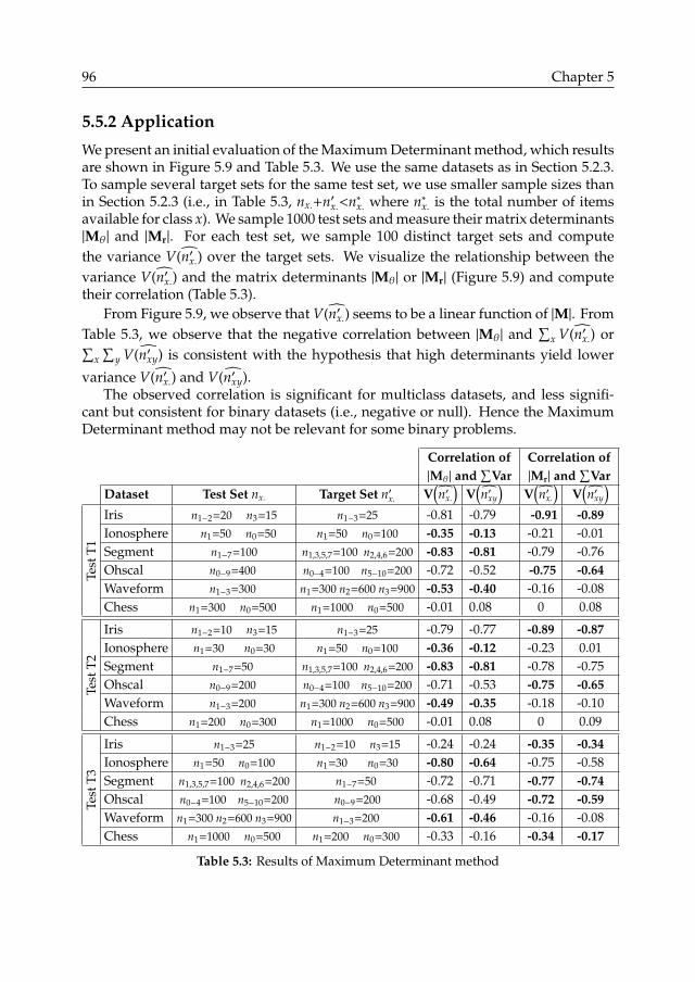
96 Chapter 5
5.5.2 Application
We present an initial evaluation of the Maximum Determinant method, which resultsare shown in Figure 5.9 and Table 5.3. We use the same datasets as in Section 5.2.3.To sample several target sets for the same test set, we use smaller sample sizes thanin Section 5.2.3 (i.e., in Table 5.3, nx.+n′x.<n∗x. where n∗x. is the total number of itemsavailable for class x). We sample 1000 test sets and measure their matrix determinants|Mθ| and |Mr|. For each test set, we sample 100 distinct target sets and computethe variance V(n′x.) over the target sets. We visualize the relationship between thevariance V(n′x.) and the matrix determinants |Mθ| or |Mr| (Figure 5.9) and computetheir correlation (Table 5.3).
From Figure 5.9, we observe that V(n′x.) seems to be a linear function of |M|. FromTable 5.3, we observe that the negative correlation between |Mθ| and
∑x V(n′x.) or∑
x∑
y V(n′xy) is consistent with the hypothesis that high determinants yield lower
variance V(n′x.) and V(n′xy).The observed correlation is significant for multiclass datasets, and less signifi-
cant but consistent for binary datasets (i.e., negative or null). Hence the MaximumDeterminant method may not be relevant for some binary problems.
Correlation of|Mθ| and
∑Var
Correlation of|Mr| and
∑Var
Dataset Test Set nx. Target Set n′x. V(n′x.
)V(n′xy
)V(n′x.
)V(n′xy
)
Test
T1
Iris n1−2=20 n3=15 n1−3=25 -0.81 -0.79 -0.91 -0.89Ionosphere n1=50 n0=50 n1=50 n0=100 -0.35 -0.13 -0.21 -0.01Segment n1−7=100 n1,3,5,7=100 n2,4,6=200 -0.83 -0.81 -0.79 -0.76Ohscal n0−9=400 n0−4=100 n5−10=200 -0.72 -0.52 -0.75 -0.64Waveform n1−3=300 n1=300 n2=600 n3=900 -0.53 -0.40 -0.16 -0.08Chess n1=300 n0=500 n1=1000 n0=500 -0.01 0.08 0 0.08
Test
T2
Iris n1−2=10 n3=15 n1−3=25 -0.79 -0.77 -0.89 -0.87Ionosphere n1=30 n0=30 n1=50 n0=100 -0.36 -0.12 -0.23 0.01Segment n1−7=50 n1,3,5,7=100 n2,4,6=200 -0.83 -0.81 -0.78 -0.75Ohscal n0−9=200 n0−4=100 n5−10=200 -0.71 -0.53 -0.75 -0.65Waveform n1−3=200 n1=300 n2=600 n3=900 -0.49 -0.35 -0.18 -0.10Chess n1=200 n0=300 n1=1000 n0=500 -0.01 0.08 0 0.09
Test
T3
Iris n1−3=25 n1−2=10 n3=15 -0.24 -0.24 -0.35 -0.34Ionosphere n1=50 n0=100 n1=30 n0=30 -0.80 -0.64 -0.75 -0.58Segment n1,3,5,7=100 n2,4,6=200 n1−7=50 -0.72 -0.71 -0.77 -0.74Ohscal n0−4=100 n5−10=200 n0−9=200 -0.68 -0.49 -0.72 -0.59Waveform n1=300 n2=600 n3=900 n1−3=200 -0.61 -0.46 -0.16 -0.08Chess n1=1000 n0=500 n1=200 n0=300 -0.33 -0.16 -0.34 -0.17
Table 5.3: Results of Maximum Determinant method
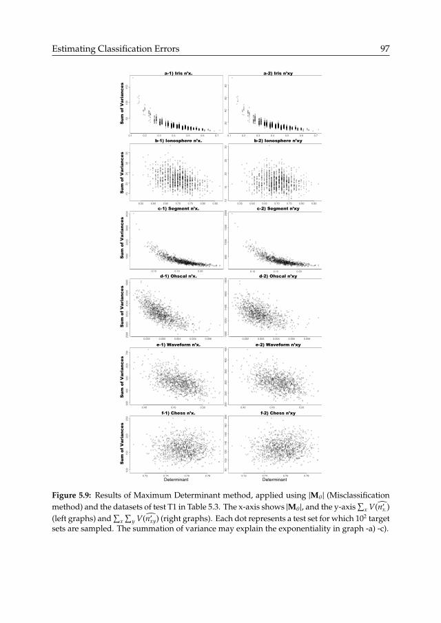
Estimating Classification Errors 97
0.1 0.2 0.3 0.4 0.5 0.6 0.7
5010
015
0S
um o
f V
aria
nces
Sum
of
Var
ianc
esS
um o
f V
aria
nces
Sum
of
Var
ianc
es
0.1 0.2 0.3 0.4 0.5 0.6 0.7
2040
6080
0.55 0.60 0.65 0.70 0.75 0.80 0.85
1520
2530
35
a-2) Iris n’xy
0.55 0.60 0.65 0.70 0.75 0.80 0.85
1015
2025
30
Determinant Determinant
a-1) Iris n’x.
b-2) Ionosphere n’xyb-1) Ionosphere n’x.
c-2) Segment n’xyc-1) Segment n’x.
d-2) Ohscal n’xyd-1) Ohscal n’x.
e-2) Waveform n’xye-1) Waveform n’x.
f-2) Chess n’xyf-1) Chess n’x.
0.10 0.15 0.20
1000
2000
3000
4000
0.10 0.15 0.20
500
1000
1500
2000
0.002 0.003 0.004 0.005 0.0062500
3000
3500
4000
4500
5000
0.002 0.003 0.004 0.005 0.006
1000
1200
1400
1600
1800
0.40 0.45 0.50
300
400
500
600
700
0.72 0.74 0.76 0.78
100
150
200
250
0.72 0.74 0.76 0.78
8010
012
014
016
018
020
0
0.40 0.45 0.50200
250
300
350
400
450
Sum
of
Var
ianc
esS
um o
f V
aria
nces
Figure 5.9: Results of Maximum Determinant method, applied using |Mθ| (Misclassificationmethod) and the datasets of test T1 in Table 5.3. The x-axis shows |Mθ|, and the y-axis
∑x V(n′x.)
(left graphs) and∑
x∑
y V(n′xy) (right graphs). Each dot represents a test set for which 102 targetsets are sampled. The summation of variance may explain the exponentiality in graph -a) -c).

98 Chapter 5
5.5.3 Discussion
The initial results are promising for multiclass problems. Error rate matrices fromeither the Misclassification method |Mθ| or Ratio-to-TP method |Mr| are shown tocorrelate with the variance of the error estimation methods, e.g., correlation coeffi-cients between -0.49 to -0.91 for
∑x V(n′x.). However, the observed correlations may
not hold for cases unaddressed in our initial evaluation.Future work is required for establishing theory and identifying the problem’s
variables and impacts, e.g., to answer questions such as:
• What are the parameters of the functions f (|Mθ|)=V(n′x.) and f (|Mr|)=V(n′x.)?
• Are there binary problems for which the Maximum Determinant method isirrelevant?
• In which cases is |Mθ| or |Mr| a better predictor?
• Given error rate matrices for alternative classifiers c1 and c2, and their determi-nant |Mr,c1|, |Mr,c2|, |Mθ,c1|, |Mθ,c2|. Are the determinants’ order of magnitudeconsistent whether using error rate θ or r, i.e., does |Mθ,c1| < |Mθ,c2| imply that|Mr,c1| < |Mr,c2| ?
• Do smaller test sets with a higher matrix determinant yield less variance thanlarger test sets with a lower determinant?
• Is it recommend to draw alternative split of the groundtruth into test andtraining sets, and select the split yielding the highest matrix determinant? Thisapproach requires training classifications models several times, i.e., with eachalternative training set to draw the corresponding error rate matrices.
• How to refine the Maximum Determinant prediction by using include infor-mation on the potential target set, e.g. ranges of potential class sizes or featuredistributions?
The Maximum Determinant method is based on a postulate that is not establishedat this stage. However, inspecting the determinant of error rate matrices is nonethe-less of interest to assess how error estimation results may vary. For instance, withdeterminants close to zero, the Misclassification method may not be recommendedand the Reclassification method may be preferred (if class proportions remain un-changed between test and target sets).

Estimating Classification Errors 99
5.6 Applicability issues
The methods presented in this chapter are applicable under specific conditions. Forinstance, if class proportions differ between test and target sets, the Reclassificationmethod is biased. However, the Misclassification method yields potentially highresult variance. The variance is higher when the class sizes are smaller, either in testor target sets. Thus if datasets are small with limited variations of class proportions,the Reclassification method may be preferable to the Misclassification method.
Future work is required to establish guidelines for choosing appropriate errorestimation methods. Examples of issues to consider when assessing a method’s ap-plicability are given in Table 5.4. Impractical cases can be identified, e.g., when errorestimation results are unrealistic (Section 5.6.1). Otherwise, test set representativitymust be assessed (Section 5.6.2) as impractical cases ensue with small test sets orvarying feature distributions (Section 5.6.3).
Test and target sets characteristicsErrorratesdiffer
Classproportions
differ
Featuredistributions
differ
Smallclasssize
OverlapTest∩Target, ∅
Applicability w.r.t.: Bias issues Variance issuesReclassificationmethodSection 5.2.1, p.78
No No No Noif nx.<∼100
Yes
MisclassificationmethodSection 5.2.2, p.79
No Yes No Noif nx.<∼500
Yes
Ratio-to-TP methodSection 5.3.1, p.82
No Yes No Noif nx.<∼500
Yes
Sample-to-SamplemethodSection 5.4, p.85
No Yes No ? No
MaximumDeterminantmethodSection 5.5, p.95
No Yes No ? ?
LogisticRegression methodSection 5.7.2.A, p.106
Yes No Yes ? Yes
Bayesian methodSection 5.7.2.B, p.106
No Yes Yes ? Yes
Table 5.4: Method applicability depending on dataset characteristics (the last two methodsare introduced in Section 5.7, p.105)

100 Chapter 5
5.6.1 Impractical cases
We identify practical issues that may arise when applying error estimation methods,and that indicate that the methods may not be applicable:
• The methods may provide negative estimates of n′x. and n′xy (p.100)
• The methods use error rate matrices that require matrix invertibility (p.100)
• The methods may have negative effects and worsen the initial classificationbias (p.100)
• The methods may yield critical result variance if applied to small class sizes(p.101)
Negative estimates n′x. or n′xy
The Misclassification and Ratio-to-TP methods can yield negative estimates n′x. < 0or n′xy < 0, and the Sample-to-Sample method can yield confidence intervals withnegative lower bounds. However, it happened rarely in our experiments, usuallywith scarce class sizes or extreme error rates (e.g., θ→ 0 or 1).
Negative estimates are easily handled for binary problems, i.e., if n′0.<0, set n′1.to n′1. + n′0., and n′0. to 0. Future research is required to handle negative estimates inmulticlass problems, e.g., by using the linear combination (5.25). More importantly,negative estimates indicate that the methods may not be applicable.
Matrix invertibility
The Misclassification method is not applicable when the determinant of the errorrate matrix is zero. For instance, in binary problems, the determinant is zero iffθ01 + θ10 = 1. Such cases occur with random classifiers (i.e., θ01 = θ10 = 0.5), or withclassifiers performing worse than random for one class and inversely proportionalfor the other class (e.g., θ01 = 0.8 and θ10 = 0.2). Such cases imply classifiersperforming very poorly, and are thus impractical. For multiclass problems, futurework is required to specify the cases where the determinant of the error rate matrixis zero, and their practical implications (e.g., poorly performing classifiers).
Negative effect
Random error rate variations can worsen the initial classification bias when applyingerror estimation methods, especially with the Misclassification method. This issue isaddressed by Shieh (2009) with a method balancing the uncorrected classifier outputn′.y and estimated n′x. in a linear combination, e.g., fitting the α parameter in (5.25).This approach is of interest for future work.
n′x.,combined = α n′x. + (1 − α) n′.y (5.25)

Estimating Classification Errors 101
Small datasets
High variance is particularly critical for small datasets (Figure 5.1). Furthermore,biases may occur if class sizes are scarce, e.g., if nx.,n′x.,nxy or n′xy are less than a fewitems (Figure 5.3, p.87 and Section 5.4.2, p.89). Further research is needed to identifythe data sizes for which error estimation methods are not recommended, or linearcombinations (5.25) are preferable (e.g., depending on error rate magnitudes). Caseswhere small nxy yield error rate θxy → 0 or 1 should also be investigated (e.g., highererror rates may be preferable).
From the evaluation in Figure 5.1 (p.81), we observe that variance issues are criticalwhen class sizes contain less than 500 items for the Misclassification method, or lessthan 100 items for the Reclassification method. Many applications cannot afford thecosts of collecting extensive test sets, e.g., with more than 500 items per class. Henceapplying error estimation methods may not be practical in many cases.
These issues with variance and insufficient test set sizes question the applicabilityof error estimation methods. More importantly, they question the representativity ofclassifier evaluation in general. If error measurements from test sets are not reliableenough to estimate the numbers of errors in target sets (i.e., due to high variancewhen applying error estimation methods), then the test sets do not provide reliabledescriptions of the errors to expect when applying classifiers. We stress that errorrate variance significantly impacts the reliability of classifier assessments and is,however, largely overlooked when assessing classifiers.
5.6.2 Test set representativity
The error estimation methods presented in this chapter rely on the assumption thattest sets are representative of the target sets5. We discuss key test set characteristicsthat impact their representativity:
• Test set size, as random differences between test and target set error ratesincrease as test set size decreases (p.101)
• Sampling method, as test sets must represent the feature distributions andmust be disjoint from target sets (p.102)
Test set size
Test set size is critical for test sets to be representative of classifier error rates. If testset size decreases, the test set error rates may differ further from the target set errorrates, and the variance of error estimation results increases (Section 5.4). Small testsets are especially critical with extreme error rates (e.g., θ→0 or 1) as small variationsof ± 1 error can greatly impact the resulting error rates.
5In particular, the methods assume that test and target set error rates converge asymptotically to thesame value as test and target set sizes increase.

102 Chapter 5
Hence it is recommended to maximize test set sizes, e.g., by using cross-validation,unsupervised classification, or reduced training set sizes. Future work is required toestablish strategies for maximizing the test set size, e.g., depending on the availabilityof groundtruth, and classifier characteristics.
For instance, reducing training set sizes may increase the classifier’s error rates,e.g., as class models may become imprecise. However, increasing classifier’s errorrates may reduce the variance of error estimation results, as the numerator increases
in V(θ) =θ(1−θ)
n , and the risk of extreme error rates (e.g., θ→0 or 1).Although unintuitive, these results suggest that classifiers with higher error rates
but tested with a larger test set (which yields lower variance), may be preferableto classifiers with lower error rates but tested with a smaller test set (which yieldshigher variance). However, increased error rates may yield classifiers approachingrandom classifiers, which may worsen variance issues (i.e., as determinants of errorrate matrices tend to zero |M|→0, Section 5.5 p.95).
Test set sampling
The sampling methods used to collect test sets must be carefully designed to ensurethat test sets are representative of the potential target sets. Prior work dealt withtest sets that are randomly sampled within the target set (i.e., for classifiers appliedto a single target set) which ensures test sets’ representativity. However, in machinelearning problems, test sets are often disjoint from the target sets. Several issues ariseif test sets are not sampled within a single target set, beside variance issues addressedin Section 5.4. For instance, class proportions may differ between test and target sets,and the Reclassification method may be inapplicable. Otherwise, error rates maysystematically vary between test and target sets when:
• Training sets are used as test sets. The resulting error estimations may be biased,as in Saerens et al. (2001) with the Misclassification method. Our experimentsin Sections 5.2, 5.3 and 5.5 use cross-validation where test and training setsare not strictly separated. No bias was observed in our experiments, howeverfuture work is required to investigate the impact of using cross validation, orstrictly separated test and training sets.
• Quality improvement methods designed for training sets (e.g., reducing noiseor excluding outliers) are applied to test sets.
• Test and target sets have different feature distributions, e.g., if target sets are oflower data quality (e.g., low image quality in computer vision).
For example, with the Fish4Knowledge system, varying feature distributions canoccur if target sets contain many low quality images, while test set image quality ismore balanced. The feature distributions of each class may systematically differ, e.g.,different colors and contours due to lower contrast or fuzziness. Target sets withlower image quality may have higher error rates than test sets with higher imagequality.

Estimating Classification Errors 103
If feature distributions systematically vary between test and target sets, theassumption of equal error rates may be violated, and none of the error estimationmethods we presented may be applicable. The critical impact of varying featuredistributions is demonstrated in Section 5.6.3, and potential solutions are discussedin Section 5.7.
5.6.3 Varying feature distributions
Classifiers typically use feature distributions to build models of each class, i.e., de-scribing the characteristics of the objects to classify. If feature distributions differbetween test and target sets, error rates may differ too (e.g., if a target set hasmore low-contrast images, more images may be misclassified). This may worsenthe classification biases when applying the bias correction methods introduced inSection 5.2. Figure 5.10 shows examples where a single feature is used, a score as inFigure 5.3 (p.87). Small variations of the feature distribution have created significantbiases.
Hence varying feature distributions are critical and must be assessed prior toapplying bias correction (Section 5.2) and error estimation methods (Section 5.3).For instance, the differences between the feature distributions of test and target setsmay be assessed using distance metrics such as Mallows distance (Levina and Bickel2001).
If test and target sets have similar class proportions, their joint feature distribu-tions can be directly compared (i.e., their global feature distributions joining togetheritem sets from all classes). If test and target sets have different class proportions,their joint feature distributions differ even if feature distributions are identical at thelevel of each class (e.g., even if all items from the same class have the same features).In this case, feature distributions must be compared for each class separately, i.e.,comparing the feature distributions of the nx. and n′x. items that actually belong tothe same class.
However, the actual classes of target set items are unknown. Hence, selecting then′x. items actually belonging to class x is impossible, and only the n′.x items classifiedinto class x are known. The n′.x items classified into class x may be used to approximatethe feature distribution for class x. However, this feature estimator may be biasedsince the n′.x items classified as class x may include items that actually belong to otherclasses and exhibit different feature distributions. To address this issue, methods canbe developed to identify the misclassified items (as discussed in Section 5.7.3) andexclude them when comparing class-specific feature distributions.
In addition to impacting the applicability of error estimation methods, issues withvarying feature distributions question the representativity of classifiers’ evalua-tion in general. If test set feature distributions do not support the estimation of thenumbers of errors in target sets, then the test sets do not provide reliable descriptionsof the errors to expect when applying classifiers.

104 Chapter 5
n0. = 200n0. = 100 n0. = 200n0. = 100 n0. = 200n0. = 100
score threshold score threshold●●●●●●●●●●●●●●●●●●●●●●●●
●●●●●●●●●●●●●●●●●●●●●●●●●●●●●●●●●●●●●●●
●●●●●●●●●●●●●●●
●●●●●●●●●●●●
●●●●●●●●●●● ●●●●●●●●●●●●●●●●●●●●●●●
●●●●●●●●●●●●●●●●●●●●●●●●●●●●●●●●●●●●●●●●●●●●●●●●●●●●●●
●
●●●●
●●
●●●
●
●●●●●●●●●●●●●
●●●●●●●●●
●●●●●●●●●
●
●●
●●●●●●●●●●●●●●●●●●●●●●●●●●●
●●●●●●●●●●●●●●●●●●●●
●●●
●●●
●
●
●
●
●●●●●●●●●●●●●●●●● ●●
●●●●●
●●●●●●●
● ●
●●●●●●●●●●●●●●●●●●●●●●●●
●●●●●●●●●●●●●●●●●●●
●●●●●●●●●●
●●●
●
●
●
●●
●
●●●●●●●●●●●●●
score threshold score threshold
●●●●●●●●●●
●●●●●
●
●●●●
●●
●●●●●●●●●●●●●●●●●●●●●●●●●●●●●●●●●●●●●●●●●●●●●●●●●●●
●●●●●
●
●●
●●●●●●
●●●●●●●●●●●●●●
●●●●●●●●●●●●
●●●
●
●
●
●●
●●●●●●●●●●●
●●●●●●●●●●●●●●●●●●●●●●●●●●●●●●●●●●●●●●●●●●
●●●●●●
●
●●
●●
●
●●
●●●●●●●●●●●●●●
●●●●●●●●
●●●
●●
●
●●
●●●●●●●
●●●●●●●●●●●●●●●●●●●●●●●●●●●●●●●●●●●●●●●●●●●●
●●●●●●●●●●
●
●●
●●
●
●
●
●●
●●●●●●●●●●●●●●
●●●●●●●●●●
●●●
●
●●●●
●●●●●●●●●●●●●●●●●●●●●●●●●●●●●●●●●●●●●●●●●●●●●●●●●●●●●●●●●●●
●
●●
●●
●
●●
●
●●
●
●●●●●●●●●●●●
●●●●●●
●●●●●●●●
●●
●●●●●●●●●●●●●●●●●●●●●●●●●●●●●●●●●●●●●●●●●●●●●●●●●●●●●●
●●●●●●●●●●●●●●●●●●●●●●●
●●●●●●●●●●●●●●●●●●●●
●●●●
●
●●●●●●●●●●●●
●●●●●●●●●●●●●●●●●●●●●●●●●●●●●●●●●●●●●●●●
●●●●●●●●●●●●●●●●●●●
●●●●●●●●●●●
●
●●●
●●
●
●●●●●●●●●●●●●●●●●●●●●●●●●●●●●●●●●●●●●●●●●●●●●●●●●●
●●●●●●
●●●●●●●●●●●●●●●●●●
●●●●●●●●●
●●●
●●
●●●●●●●●●●●●●●●●●●●●●●●●●●●●●●●●●●●●●●●●●●●●●●●●●●●●●●●●●●●
●●●
●●●●●●●●●●●●●●●●
score threshold score threshold
●●●●●●●●●●●●●●●●●●●●●●●●●
●●●
●
●
●●●●●●●●●●●●●●●●●●●●
●●●●●●●●●●
●
●●
●
●
●●●●●●●●●●●●●●●●●●●●●●●●● ●●●●●●●●●●●●●●●●●●●●●●
●●●●
●
●●●
●●●●●●●●●●●●●●●●●●●●●
●●●●●●●
●
●
●
●
●
●●●●●●●●●●●●●●●●●●●●●●●●●
●●●●●●●●●●●●●
●
●●
●●●●●●
●●
●●●●●●●●●●●●
●●●●●●●●●●●●●●
●●●●●●●●●●●●●●●●●
●
●●●
●
●
●
●●
●●●●●●●●●●●●● ●
●●●●●●●
●●●●●
●
●●●●
●
●●●●●●●●●●●●●●●●●●●●●●●●●●●●●
●●●●●●●●●●●●●●●●●●●●●●●●
●
●
●
●
●
●●●●●●●●●● ●●●●●
●●●●●●●●●●●
●
●●
●
●●●●●●●●●●●●●●●●●●●●●●●●●●●●●
●●●●●●●●●●●●●●●●●●●●
●
●
●
●
●●●●●●●●●●●●●
●●●●●●
●●●●●●●
●
●●●
●●●
●●●●●●●●●●●●●●●●●●●●●●●●●●●●●●●
●●●●●●●●●●●●●●●●●●
●●
●
●
●●
●●●●●●●●●●●●●●
●●●●●●●●●
●●
●●
●●●●
●●●●●●●●
●●●●●●●●●●●●●●●●●●●●●●●●●●●●●●●●●●●●●●●●●●●●●●●●
●
●
●
●
●●
●●●●
●●●●●●●
●●●●●●●●
●●●●
●
●
●
●
●●●●●●●●●●●●●●●●●●●●●●●●●●●●●●●●●●●●
●●●●●●●●●●●●●●●●●●
●●
●
●
●●●●●●●●●●
●●●●●●●●●●●
●
●
●
●●
●●
●
●●
●
●●●●●●●●●●●●●●●●●●●●
●●●●●●●●●●●●
●
●
●
●●●
●●●●●●●●●●●● ●●●●●●
●●●●
●
●
●
●
●
●●●●●●●●●●●●●●●●●●●●●●●●●●
●●●●●●●●●
●
●
●●●●
●●●●●●●
●
●●●
●
●●
●
●●●●●●●●●●●●●●●●●●●●●●●●●●●●●●●●●●●●●●●●●●●●●●●●●
●●●●●●●●●●●●●●●●●●●●●●
●●
●
●●
●●
●●● ●
●●
●●
●
●
●●●●●●●●●●●●●●●●●●●●●●●●●●●●●●●●●●●●●●●●●●●●●●●●●●●●
●●●●●●●●●●●●●●●●●●●●●●●
●
●
●
●
●
●●●●●●●●●
●●●●●●
●●●●●●●
●
●●●●●●●●●●●●●●●●●●●●●●●●●●●●●●●●●●●●●●●●●●●●●●●●●●
●●●●
●
●●●●●●●●●●●●●●●●●●●●●●●
●●●●●●●●●●●
●
●
●●●●
●●●●●
●●●●●●●●●●●●●●●●●●●●●●●●●●●●●●●●●●●●●●●●●●●●●●●●●●●●●
●●●
●●●
●●●●●●●●●●●●●●●●●●●●
●●●●●●●●●●●●●●
●
●
●●
●●●●●●●●●●●●●●●●●●●●●●●●●●●●●●●●●●●●●●●●●●●●●●●●●●●●●●●●●●
●●●●●●●●●
●●●●●●●●●●●●●●●●
●●●●●●●●
●
●
●
●●●
●●●
●
●●●
●
●
●●●●●●●●●●●●●●●●●●●●●●●●●●●●●●●●●●●●●●●●●●●●●●●●●●●●●●●●
●●●●●●●●●●●●●●●●●●●●●●
score threshold score threshold0
200
4000
100
200
0 0.5 1 0 0.5 10
200
4000
100
200
0 0.5 1 0 0.5 10
200
4000
100
200
0 0.5 1 0 0.5 1
0
200
4000
100
200
0 0.5 1 0 0.5 10
200
4000
100
200
0 0.5 1 0 0.5 10
200
4000
100
200
0 0.5 1 0 0.5 1
0
200
4000
100
200
0 0.5 1 0 0.5 1
n’0.
= 1
00n’
0. =
200
n’0.
= 1
00n’
0. =
200
n’0.
= 1
00n’
0. =
200
score threshold score threshold0
200
4000
100
200
0 0.5 1 0 0.5 1
score threshold score threshold score threshold score threshold
score threshold score thresholdscore threshold score threshold
●●●●●●●●●●●●●
●●●●
●●
●●●●●●●●●●●●●●●●●●●●●●●●●●●●●●●●●●●●●●●●●●●●
●
●
●
●
●
●●
●●●●●●●●●●●● ●●●●●●●●●
●●
●●●●
●
●
●●●●●●●●●●●●●●●●●●●●●●●●●●●●●●●●●●●●●●●●●●●●●●●●●
●
●
●
●●
●●●●●●●●●●●
●●
●●●●
●●● ●
●●●●●●●●●●●●●●●●●●●●●●●●●●●●●
●●●●●●●●●●●●●●●●●●●●●●●●●●●●●●●●●● ●
●
●
●●
●●●
●●
●
●●●
●
●●●
●
●●●●●●●●●●●●●●●●●●●●●●●●
●●●●●●●●●●●●●●●
●●●●●●●●●●●●●●●●●●●●●●●●●●●
●
●
●
●
0
200
4000
100
200
0 0.5 1 0 0.5 1
b) Score ’0 = 0 - 0.05
g) Score ’0 = 0 - 0.05
e) Score ’0 = 0 + 0.05
a) Score ’1 = 1 - 0.05 ’x = 0.05 (bottom) ’x = 0.1 (top)
’x = 0.05 (bottom) ’x = 0.1 (top)
’x = 0.1
’x = 0.1 ’x = 0.1
’x = 0.1
c) Score ’x = x - 0.05
d) Score ’1 = 1 + 0.05
’1 = 1 + 0.05 h) Score ’0 = 4.05 ’1 = 5.95 (top)
’0 = 3.05 ’1 = 6.95 (bottom) ’x = 0.1 ’0 = 3.05 ’1 = 7.05 (bottom)
’x = 0.1
i) Score ’x = x +0.05 n’1 = 2n’0 (top)
f) Score ’x = x + 0.05 ’x = 0.1
True
Estimated
Figure 5.10: Results of Misclassification method for simulated data with varying featuredistribution. As in Figure 5.3, a score threshold (x axis) is used to assign class 0 or class 1 tothe items to classify. Class sizes n′0. (y axis) are estimated for 104 pairs of test and target sets.Test sets are randomly sampled with class proportions n0.=n1., mean scores µ0=0.4 for class 0,µ1=0.6 for class 1, and score variance σx=0.1. Target sets are sampled from score distributionsthat differ from the test sets, with µ′x=µx ± 0.05 and variance σ′x∈{0.05, 0.1}, and with classproportions n′0.=2n′1.. Lower graphs -h) and -i) illustrate additional cases where µ′x=µx ± 0.1.

Estimating Classification Errors 105
Further work is required to develop methods for handling varying feature distri-butions. For binary classifiers providing threshold parameters, for example, the re-sults in Figure 5.10 suggest that thresholds averaging the mean scores (i.e., (µ0 +µ1)/2in our simulations) may minimise the biases due to varying feature distributions (andthe variance in any case, as suggested in Figure 5.3, p.87). Future work may developmethods to derive optimal thresholds that are specifically adapted to the target sets,depending on their feature distributions.
Furthermore, information on test and target set feature distributions can be usedto develop refined error estimation methods. This can be done with discrete orcontinuous approaches, as discussed in Section 5.7.
5.7 Future work
The methods discussed in the chapter are relatively unexplored within the machinelearning domain. Thus our work opens several perspectives for future work, ad-dressing problems such as:• Correcting critical biases due to varying feature distributions (mentioned in
Section 5.6.3) using discrete or continuous approaches (Sections 5.7.1 and 5.7.2)• Identifying which individual items are misclassified, i.e., to refine the class
assigned to individual items (Section 5.7.3).
5.7.1 Discrete approaches
As discussed in Section 5.6.3, and shown in Figure 5.10, if feature distributions differbetween test and target sets (e.g., if the target set has lower image quality), errorestimation methods may not be applicable as the equal error rate assumption maybe violated.
Within the Fish4Knowledge project, this issue was addressed with a discreteapproach. Discrete types of image quality are identified, and error rates are estimatedfor each type of image quality. Error estimation methods can then be applied usingerror rates measured for each image quality (Beauxis-Aussalet and Hardman 2015).
This discrete approach implies that test sets must be collected for each type ofimage quality. However, it may be difficult to collect sufficiently large test sets, e.g.,containing examples for each species observed with each image quality. If test sets aresmall for each combination of species and image quality, the variance of error ratesand error estimation results may increase significantly, and applying error estimationmethods may not be appropriate.
5.7.2 Continuous approaches
Continuous approaches should be investigated in future work. They may improvethe error estimation results, and address the issues identified in Section 5.6.3, withoutrequiring to partition test sets into many discrete combinations of classes and features.

106 Chapter 5
Instead, for example, linear models can be fitted to represent error rates as a functionof feature distribution. This approach is discussed in Section B.
A. Logistic Regression method
We developed a continuous approach for handling varying feature distributions byfitting logistic regression models that represent error rates as a function of similaritymeasures (Boom et al. 2016). Similarity measures represent how similar an item isto a class model. They can be provided by certain classifiers, for each item and eachclass model. This Logistic Regression method is explained in the tutorials providedin additional materials (Section 5.9.3, Figures 5.11-5.12).
This prior work requires equal class proportions between test and target set, i.e.,extending the Reclassification method. Future work is needed to develop methodsfor the case where class proportions differ between test and target sets, e.g., extendingthe Misclassification method.
B. Bayesian statistics method
Bayesian statistics may offer solutions for developing continuous approach compati-ble with the Misclassification method. Within the Bayesian framework, varying classproportions are equivalent to varying in class prior probabilities. The Misclassificationmethod can estimate target sets’ class prior probabilities, while Bayesian statistics canrefine each item’s class probabilities using its feature distributions. Hence Misclassi-fication and Bayesian methods can be combined to address issues with varying classproportions (Section 5.6.3).
This approach is illustrated in equations (5.26)-(5.28), with variables defined inTables 5.5). The Misclassification method is used to estimate class prior probabilities,providing the estimates in equation (5.28).
A similar approach is introduced (Saerens et al. 2001) without investigating the re-sults’ variance. Future work could investigate applications of the Sample-to-Samplemethod for estimating the results’ variance of equation (5.28).
P(ζx|Fi) =1
P(Fi)P(Fi|ζx) P(ζx) thus
P(ζ1|Fi)P(ζ2|Fi)
...
P(ζx|Fi)
=1
P(Fi)
P(Fi|ζ1)P(Fi|ζ2)
...
P(Fi|ζx)
P(ζ1)P(ζ2)...
P(ζx)
(5.26)
P′(ζ1)P′(ζ2)
...
P′(ζx)
=
P(ζ1→1|ζ1) P(ζ2→1|ζ2) ... P(ζx→1|ζx)P(ζ1→2|ζ1) P(ζ2→2|ζ2) ... P(ζx→2|ζx)
... ... ... ...
P(ζ1→x|ζ1) P(ζ2→x|ζ2) ... P(ζx→x|ζx)
−1
P′(ζ→1)P′(ζ→2)
...
P′(ζ→x)
(5.27)

Estimating Classification Errors 107
P′(ζ1|Fi)P′(ζ2|Fi)
...
P′(ζx|Fi)
=1
P′(Fi)
P(Fi|ζ1)P(Fi|ζ2)
...
P(Fi|ζx)
P(ζ1→1|ζ1) P(ζ2→1|ζ2) ... P(ζx→1|ζx)P(ζ1→2|ζ1) P(ζ2→2|ζ2) ... P(ζx→2|ζx)
... ... ... ...
P(ζ1→x|ζ1) P(ζ2→x|ζ2) ... P(ζx→x|ζx)
−1
P′(ζ→1)P′(ζ→2)
...
P′(ζ→x)
(5.28)
P(ζx) Probability that an item truly belongs to class x (prior probability)P(ζ→y) Probability that an item is classified into class yP(ζx→y|ζx) Probability that an item is classified into class y, given that it truly belongs to class xP(Fi) Probability that an item exhibits the set of features Fi
P(Fi|ζx) Probability that an item exhibits the set of features Fi, given that it truly belongs to class xP(ζx|Fi) Probability that an item truly belongs to class x, given its set of features Fi (posterior probability)
nxy,i Number of items truly belonging to class x, classified into class y, and exhibiting the set of features Fi
nxy,. Number of items truly belonging to class x, classified into class y, and exhibiting any kind of features
nx.,. Number of items truly belonging to class x, classified into any class, and exhibiting any kind offeatures
n..,. Number of items truly belonging to any class, classified into any class, and exhibiting any kind offeatures (i.e., total number of items)
P(ζx) =nx.,.
n..,.P(ζ→y) =
n.y,.n..,.
P(ζx→y|ζx) =nxy,.
nx.,.
P(Fi) =n..,in..,.
P(ζx|Fi) =nx.,i
n..,iP(Fi|ζx) =
nx.,i
nx.,.
Table 5.5: Definitions of variables used in equations (5.26)-(5.28). Variables using prime sym-bols, e.g., P′(ζx), refer to target sets. Without prime symbols, variables refer to the test set.
The feature probabilities P(Fi) and P(Fi|ζx) may not be drawn from the discretebut impractical approach in Table 5.5. This discrete approach requires collecting testset items that represent all the possible sets of features Fi. Instead, linear models canbe fit on the features measured in test and target sets, to derive continuous featureprobabilities.
5.7.3 Identify the misclassified items
Given the estimated error composition (Section 5.3), i.e., the numbers of errors n′xy,methods can be derived for identifying the misclassified items individually, andcorrecting their assigned class. Probabilistic classifiers such as Bayesian classifiersare of interest to address this problem. Classifiers providing similarity measures, i.e.,representing how items are similar to classes’ model, are also of interest.
For example, lets consider the error estimation results estimating that n′xy itemsare misclassified into class y while belonging to class x, and items’ probabilities ofclass membership, e.g., P′(ζx|Fi) in equation (5.28). Within the items classified as classy, we can select the nxy items with the highest probability of belonging to class x.

108 Chapter 5
Alternatively, provided with similarity measures, we can select items with the highestsimilarity to class x model.
However, the problem is not as simple as it may seems from this example becausea single item can have a high probability of class membership (or similarity) forseveral classes. For example, when selecting the nxy and nzy items with the highestchances of belonging to classes x and z, the same items may be selected for bothclasses x and z.
5.8 Conclusion
We demonstrated the applicability of existing error estimation methods to machinelearning classification problems (Section 5.2). We extend existing methods, designedto estimate unbiased class sizes, to estimating numbers of errors in target sets, andintroduce an alternative method called Ratio-to-TP (Section 5.3). Given the n′.y itemsclassified as class y, the extended methods estimate how many n′xy items truly be-long to class x. Such estimation of the error composition describes classificationuncertainty beyond accuracy and metrics such as precision or False Positive rate(Section 5.3).
The results of error estimation methods are subject to potentially high variancedue to random error rate variations. For small datasets, the variance magnitudeis critical and applying error estimation methods may worsen the initial biases.To address such issues, we introduced a novel variance estimation method calledSample-to-Sample. We demonstrate that for disjoint test and target sets, varianceestimation must account for the class sizes in both test and target sets. The Sample-to-Sample method provides accurate confidence intervals describing the variance oferror estimation results (Section 5.4).
Finally, we introduce a promising method for predicting the variance of errorestimations without prior knowledge of the potential target sets. We observe cor-relations between the determinant of error rate matrices and the variance of errorestimation results. We thus postulate that determinants of error rate matrices arepredictors of error estimation variance. If validated in future work, this predictorcan be used to compare and choose classifiers that minimize the error estimationvariance (Section 5.5).
This chapter addressed requirement 4-c in Chapter 2 (extrapolate uncertainty inspecific datasets, p.36) and answered our fifth research question: How can we estimatethe magnitudes of classification errors in end-results?.
The methods we introduced can assess the Noise and Bias due to classificationerrors, and the Uncertainty in Specific Datasets which are key uncertainty factors iden-tified in Chapter 4. They are compatible with the methods we developed to handleFragmentary Processing, another key uncertainty factor identified in Chapter 4 (i.e.,they provide class size estimates that can be used within the metrics in equations (4.1)-(4.5), p.71).

Estimating Classification Errors 109
We identified conditions that can impact the applicability of error estimationmethods, i.e., class sizes (in both test and target sets), error rate magnitudes, numberof classes, and random or systematic variations of error rates, class proportions andfeature distributions. These findings inform the choice of methods depending on theuse case at hand.
However, future work is required to formally identify inapplicable cases andquantify the test and target set characteristics that invalidate error estimation methods(Section 5.6). The most critical applicability issues concern small test or target setsand varying feature distributions. To address the latter, directions for future workare identified (Section 5.7).
We underline that issues with the applicability of error estimation methodsquestion the representativity of classifier evaluation in general. If test sets do notsupport the estimation of the numbers of errors in target sets, then the test sets donot provide reliable descriptions of the errors to expect when applying classifiers.For instance, variance issues are critical with small datasets. However, error ratevariance is seldom considered when assessing classifiers.

110 Chapter 5
5.9 Additional materials
5.9.1 Code
The R code used to apply and evaluate the methods described in this paper is availableonline, free of use: https://github.com/emma-cwi/classification_error
5.9.2 Application of Fieller’s theorem
Fieller’s theorem (Fieller 1954) defines the confidence intervals limits [`−, `+] for aratio of correlated random variables A/B as (5.29), with z=1 for 68% confidence level.
`± =(µAµB − z2σA,B) ±
√(µAµB − z2σA,B)2 − (µ2
A − z2σ2A)(µ2
B − z2σ2B)
µ2B − z2σ2
B
(5.29)
In Section 5.4.3, for estimating n′0., A=n′.0− θ′
10n′.. and B=1− θ′
01− θ′
10(equation
(5.15) p.89). The mean, variance, covariance of A,B are detailed below, knowing thatθ′
01and θ′
10are independent with null covariance.
µB = E[1 − θ′
01−θ′
10
]µB = 1 − θ01 − θ10
σ2B = V
(1 − θ′
01−θ′
10
)= V
(θ′
01
)+V
(θ′
10
)σ2
B =θ01(1−θ01)
n0.+θ01(1−θ01)
n′0.+θ10(1−θ10)
n1.+θ10(1−θ10)
n′1.
µA = E[n′.0−θ
′
10n′..
]µA = n′.0−θ10 n′..
σ2A = V
(n′.0−θ
′
10n′..
)= n′..
2 V(θ′
10
)σ2
A = n′..2
(θ10(1−θ10)
n1.+θ10(1−θ10)
n′1.
)σA,B = Cov
(n′.0−θ
′
10n′.., 1−θ′
01−θ′
10
)= n′..V
(θ′
10
)σA,B = n′..
(θ10(1−θ10)
n1.+θ10(1−θ10)
n′1.
)
In Section 5.4.4, for estimating n′01, A=θ′01
(n′.0− θ
′
10n′..
). B remains unchanged.
Their mean, variance, covariance are detailed below. The covariance of products ofrandom variables is drawn from Bohrnstedt and Goldberger (1969).
µA = E[θ′
01
(n′.0−θ
′
10n′..
)]µA = θ01
(n′.0−θ10 n′..
)

Estimating Classification Errors 111
σ2A = E
[θ′
01
]2 V
(n′.0−θ
′
10n′..
)+ E
[n′.0−θ
′
10n′..
]2 V
(θ′
01
)+ V
(θ′
01
)V(n′.0−θ
′
10n′..
)σ2
A = θ201n′..
2 V(θ′
10
)+
(n′.0−θ10 n′..
)2 V
(θ′
01
)+ n′..
2V(θ′
01
)V(θ′
10
)σA,B = n′..
(Cov
(θ′
01θ′
10, θ′
01
)+ Cov
(θ′
01θ′
10, θ′
10
))− n′.0V
(θ′
10
)Cov
(θ′xyθ
′
yx, θ′
xy
)= E
[θ′xy
]Cov
(θ′yx, θ
′
xy
)+ E
[θ′yx
]Cov
(θ′xy, θ
′
xy
)= E
[θ′yx
]V(θ′xy
)σA,B = n′..
(θ10V
(θ′
01
)+ θ01V
(θ′
10
))− n′.0V
(θ′
01
)With V
(θ′xy
)=θxy(1−θxy)
nx.+θxy(1−θxy)
n′x.(Sample-to-Sample)
In Section 5.4.5, for estimating π0=n′0./n′.. by Shieh (2009) and Buonaccorsi (2010),
A = n′.0/n′.. − θ
′
10(equation (5.17) p.91). B remains unchanged. The mean, variance,
covariance used by Shieh (2009) and Buonaccorsi (2010) are restated below.
µA = n′.0/n′
.. − θ10
σ2A =
n′.0/n′
..
(1 − n′.0/n
′
..
)n′..
+θ10(1 − θ10)
n1.
σ2B =
θ01(1−θ01)n0.
+θ10(1−θ10)
n1.
σA,B =θ10(1−θ10)
n1.
5.9.3 Tutorials explaining the Logistic Regression method
As discussed in Section 5.7.2, error estimation methods can be refined using thefeature distributions of the items to classify. The Logistic Regression method uses alinear model (i.e., logistic regression) to represent error rate distributions as a functionof similarity measures provided by the classifiers. Similarity measures represent howsimilar an item is to a class model, i.e., how an item’s features are similar to the classmodel’s features. The Logistic Regression method is explained in Boom et al. (2016)and in the tutorials shown in Figures 5.11 and 5.12.

112 Chapter 5
Fish I
mage
s
Non-
Fish I
mage
s
Step
1: C
ollec
t exa
mples
of fis
h and
non-
fish
(the G
roun
d-Tr
uth)
Fish M
odel
Step
3: U
se im
ages
for m
odeli
ng to
cons
truct
a mod
el of
fish a
ppea
ranc
e
Imag
es fo
r Mod
eling Fis
hFis
hFis
hFis
h
Non-
Fish
Non-
Fish
Non-
Fish
Non-
Fish
Imag
es fo
r Cali
bratio
n
Fish M
odel
Step
4: E
valua
te the
simi
larity
betw
een t
he fis
h mod
el an
d the
Imag
es fo
r Cali
bratio
n
9.5
78%
69%
51%
9.5
7.8 6.9
5.1
Simila
rity w
ith
the m
odel
(max
=10)
Step
2: S
plit t
he G
roun
d-Tr
uth in
2 gr
oups
Imag
es fo
r Mod
eling
Fish
Fish
Fish
Fish
Non-
Fish
Non-
Fish
Non-
Fish
Non-
Fish
Fish
Fish
Imag
es fo
r Cali
bratio
n
Fish
Fish
Non-
Fish
Non-
Fish
Non-
Fish
Non-
Fish
How
to Im
prov
eAu
tomat
ic Fis
h Cou
ntwit
h Log
istic
Regr
essio
n?
Step
5: P
lot th
e dist
ributi
on of
fish &
non-
fish
over
their
simi
larity
with
the m
odel
Simi
larity
with
th
e fish
mod
el
0
100%
>9[6
-7]
[3-4
]<1
Proportions ofFish & Non-Fish
Non-
Fish
Non-
Fish
Fish
Fish
Step
7: U
se th
e cur
ve to
evalu
ate th
e pro
babil
ity
of ne
w im
ages
being
fish
0.2
0.61.0
100
Probability of Images being a Fish
8.1
Simila
rity Sc
ore: 8
.1New I
mage
s
5.6
8.1
5.6
Simila
rity Sc
ore: 5
.6
Prob
abilit
y of F
ish: 0
.6
Prob
abilit
y of F
ish: 0
.85
0
100%
>9[6
-7]
[3-4
]<1
Step
6: F
it a cu
rve d
escr
ibing
the f
ish/n
on-fi
sh pr
opor
tions
(the “
Logis
tic R
egres
sion”
func
tion)
Simi
larity
with
th
e fish
mod
elProportions of
Fish & Non-Fish
Y
X
Y =
1 +
e- (a
+ b
X)1
Simi
larity
with
th
e fish
mod
el
Step
9: D
erive
the p
roba
bility
of ne
w im
ages
being
fish
(e.g.,
Simi
larity
Scor
e = 4
-> P
roba
bility
= 0.
25)
100
300
500
100
Number of Images
Simi
larity
with
the f
ish m
odel
Number of Images 100
300
500
1.00 Pr
obab
ility o
f bein
g a fi
sh
Simi
larity
Probability 01.0
100%
0%
Step
8: E
valua
te the
simi
larity
of ne
w im
ages
with
the f
ish m
odel
New I
mage
s
100
300
500
Number of Images
Simi
larity
with
th
e fish
mod
el10
0
Step
10: D
erive
the p
roba
ble nu
mber
of fis
h (e.
g., 10
0 Im
ages
with
0.2
5 Pr
obab
ility -
> 25
Fish a
nd 7
5 No
n-Fis
h)
Probable number of Fish Images
0
100
200
300
400
1.0
Prob
abilit
y of b
eing a
fish
200
-100
00
Non-
Fish
Non-
Fish
Fish
Fish
0.85
Number of Images
0
100
200
300
40050
0 Prob
abilit
y of b
eing a
fish1.0
0
Fish
Fish
Non-
Fish
Non-
Fish
Figure 5.11: Logistic regression methods for binary problems, designed by the author of thisthesis (Boom et al. 2016).
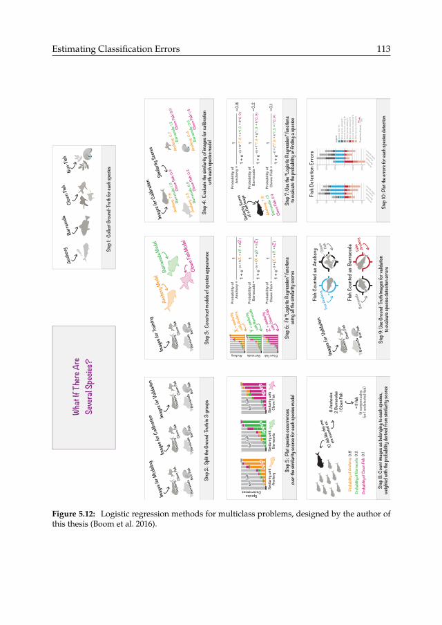
Estimating Classification Errors 113
What
If T
here
Are
Seve
ral S
pecie
s?
Step
3: C
onst
ruct
mode
ls of
spec
ies ap
pear
ance
Prob
abili
ty o
f A
ncho
vy =
Prob
abili
ty o
f B
arra
cuda
=
Prob
abili
ty o
f C
low
n Fi
sh =
Step
4: E
valua
te the
simi
larity
of im
ages
for c
alibra
tion
with
each
spec
ies m
odel
Step
5: P
lot sp
ecies
occu
rrenc
es
over
the s
imila
rity s
cores
for e
ach s
pecie
s mod
elSt
ep 7
: Use
the “
Logis
tic R
egres
sion”
func
tions
to
evalu
ate th
e pro
babil
ity of
findin
g a sp
ecies
Simila
rity Sc
ores
of a F
ish Im
age
Step
6: F
it “Lo
gistic
Reg
ressio
n” fu
nctio
ns
using
all th
e sim
ilarit
y sco
res
X = si
milar
ity
with A
ncho
vy
Y = si
milar
ity
with B
arrac
uda
Z = s
imila
rity
with C
lown F
ish
Step
9: U
se G
roun
d-Tr
uth im
ages
for v
alida
tion
to ev
aluate
spec
ies de
tectio
n erro
rsSt
ep 8
: Cou
nt im
ages
as be
longin
g to e
ach s
pecie
s, we
ighted
with
the p
roba
bility
deriv
ed fr
om si
milar
ity sc
ores
Step
10: P
lot th
e erro
rs fo
r eac
h spe
cies d
etecti
on
Clow
n Fish
Barra
cuda
Anch
ovy
Non-
Fish
Step
1: C
ollec
t Gro
und-
Truth
for e
ach s
pecie
s
Imag
es fo
r Trai
ning
Clow
n Fish
Clow
n Fish
Anch
ovy
Anch
ovy
Barra
cuda
Barra
cuda
Non-
Fish
Non-
Fish
Imag
es fo
r Cali
bratio
n
Simila
rity Sc
ores
Clow
n Fish
Mod
el
Barra
cuda
Mod
el
Anch
ovy M
odel
7.8
7.8
Anch
ovy:
Anch
ovy:
1.3Ba
rracu
da:
0.9
Clow
n Fish
:
7.8
2.5
Anch
ovy:
Anch
ovy:
6.9
Barra
cuda
:0.
2Cl
own F
ish:
7.8
0.7
Anch
ovy:
Anch
ovy:
1.2Ba
rracu
da:
8.9
Clow
n Fish
:
7.8
0.4
Anch
ovy:
Anch
ovy:
0.6
Barra
cuda
:1.4
Clow
n Fish
:
Simi
larity
with
Anch
ovy
SpeciesOccurrences
Simi
larity
with
Barra
cuda
Simi
larity
with
Clow
n Fish
Anchovy Barracuda Clown Fish
1 +
e- (a
+ b
X +
c Y +
dZ
)
1
1 +
e- (e
+ f X
+ g
Y +
hZ
)
1
1 +
e- (i +
j X +
k Y +
l Z)
1
Prob
abili
ty o
f A
ncho
vy =
Prob
abili
ty o
f B
arra
cuda
=
Prob
abili
ty o
f C
low
n Fi
sh =
= 0.8
= 0.2
= 0.1
1 +
e- (a
+ b
* 7.8
+ c
* 1.3
+ d
* 0.9
)
1
1 +
e- (e
+ f*
7.8
+ g
* 1.3
+ h
* 0.9
)
1
1 +
e- (i +
j*7.
8 +
k* 1
.3 +
l*0
.9)
1An
chov
yAn
chov
yBa
rracu
daBa
rracu
daCl
own F
ishCl
own F
ish
Non-
Fish
Non-
Fish
Non-
Fish
Non-
Fish
Non-
Fish
Non-
Fish
7.8
7.8
Anch
ovy:
Anch
ovy:
1.3Ba
rracu
da: 0.
9Cl
own F
ish:
10 fis
h like
this o
ne
are c
ounte
d as:
= 11 f
ish
(it co
mpen
sates
for 1
unde
tected
fish)
8 An
chov
ies2
Barra
cuda
s1 C
lown F
ish
0.8
0.2
Prob
abilit
y of A
ncho
vy:
Prob
abilit
y of B
arra
cuda
: 0.1
Prob
abilit
y of C
lown F
ish:
True A
ncho
vy
Barra
cuda
Miss
edAn
chov
yFa
lse Anch
ovy
Clow
n Fis
h
Clow
n Fish
Clow
n Fish
Anch
ovy
Anch
ovy
Barra
cuda
Barra
cuda
Non-
Fish
Non-
Fish
Imag
es fo
r Vali
datio
nFis
h Cou
nted
as A
ncho
vyFi
sh D
etec
tion E
rror
s
Fish C
ount
ed as
Bar
racu
da
Step
2: S
plit t
he G
roun
d-Tr
uth in
3 gr
oups
Imag
es fo
r Cali
bratio
n
Imag
es fo
r Mod
eling
Clow
n Fish
Clow
n Fish
Anch
ovy
Anch
ovy
Barra
cuda
Barra
cuda
Non-
Fish
Non-
Fish
Clow
n Fish
Clow
n Fish
Anch
ovy
Anch
ovy
Barra
cuda
Barra
cuda
Non-
Fish
Non-
Fish
Clow
n Fish
Clow
n Fish
Anch
ovy
Anch
ovy
Barra
cuda
Barra
cuda
Non-
Fish
Non-
Fish
Imag
es fo
r Vali
datio
n
Barracu
da
Anchovy
Clown Fish
Other S
pecies
100%
200%
300%
-200
%
-100
%
Barracu
da
Anchovy
Clown Fish
Other S
pecies
50100
150
-100-5
0M
ain
Spec
ies
draw
ing
FNSe
cond
Spe
cies
dra
win
g FN
Oth
er S
peci
es d
raw
ing
FN
Seco
nd S
peci
es a
ddin
g FP
Corr
ect F
ish
(TP)
Lege
nd:
Prop
ortio
n of
err
ors:
Mai
n Sp
ecie
s ad
ding
FP
Oth
er S
peci
es a
ddin
g FP
FNa
bTP
a
Figure 5.12: Logistic regression methods for multiclass problems, designed by the author ofthis thesis (Boom et al. 2016).


Chapter 6Visualization of ClassificationErrors
Classifiers are applied in many domains where errors have significant implications,e.g., medicine, security, eScience. However, end-users may not always understandclassification errors and their impact (Chapter 3, Section 3.4.2, p.48). Existing er-ror visualizations primarily address the needs of classification experts who aim atimproving classifiers. These visualizations may not address the specific needs of end-users, especially those with limited expertise in classification technologies. We thusinvestigate visualizations that address the needs of non-expert end-users, and an-swer our sixth question: How can visualization support non-expert users in understandingclassification errors? (Section 1.4).
We first introduce end-users requirements (Section 6.1) and identify informationneeds that pertain to either end-users or developers (Section 6.2). We then discussexisting visualizations of classification errors and the end-users’ or developers’ needsthey address (Section 6.3). We introduce a visualization design named Classee (Fig-ures 6.1-6.4), that aims at addressing specific needs of end-users (Section 6.4). Weevaluate this design with users from three levels of expertise, and compare it to ROCcurves and confusion matrices (Section 6.5). From the quantitative results, we dis-cuss users’ performance w.r.t. the type of visualization and users’ level of expertise(Section 6.6). From the qualitative results, we identify key difficulties with under-standing the classification errors, and how visualizations address or aggravate them(Section 6.7).
115
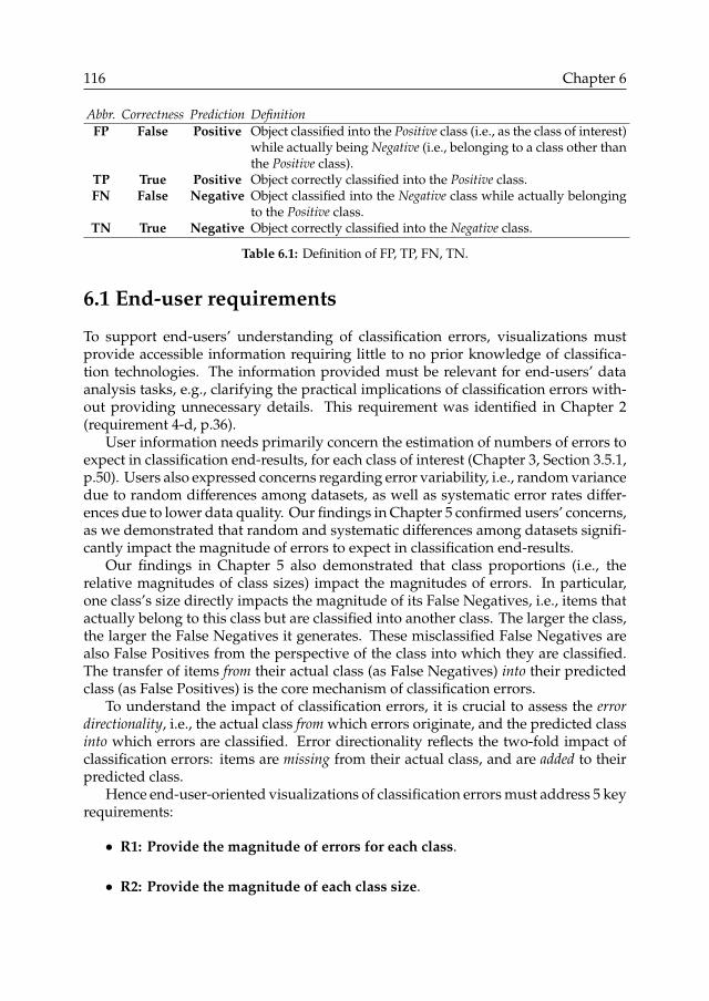
116 Chapter 6
Abbr. Correctness Prediction DefinitionFP False Positive Object classified into the Positive class (i.e., as the class of interest)
while actually being Negative (i.e., belonging to a class other thanthe Positive class).
TP True Positive Object correctly classified into the Positive class.FN False Negative Object classified into the Negative class while actually belonging
to the Positive class.TN True Negative Object correctly classified into the Negative class.
Table 6.1: Definition of FP, TP, FN, TN.
6.1 End-user requirements
To support end-users’ understanding of classification errors, visualizations mustprovide accessible information requiring little to no prior knowledge of classifica-tion technologies. The information provided must be relevant for end-users’ dataanalysis tasks, e.g., clarifying the practical implications of classification errors with-out providing unnecessary details. This requirement was identified in Chapter 2(requirement 4-d, p.36).
User information needs primarily concern the estimation of numbers of errors toexpect in classification end-results, for each class of interest (Chapter 3, Section 3.5.1,p.50). Users also expressed concerns regarding error variability, i.e., random variancedue to random differences among datasets, as well as systematic error rates differ-ences due to lower data quality. Our findings in Chapter 5 confirmed users’ concerns,as we demonstrated that random and systematic differences among datasets signifi-cantly impact the magnitude of errors to expect in classification end-results.
Our findings in Chapter 5 also demonstrated that class proportions (i.e., therelative magnitudes of class sizes) impact the magnitudes of errors. In particular,one class’s size directly impacts the magnitude of its False Negatives, i.e., items thatactually belong to this class but are classified into another class. The larger the class,the larger the False Negatives it generates. These misclassified False Negatives arealso False Positives from the perspective of the class into which they are classified.The transfer of items from their actual class (as False Negatives) into their predictedclass (as False Positives) is the core mechanism of classification errors.
To understand the impact of classification errors, it is crucial to assess the errordirectionality, i.e., the actual class from which errors originate, and the predicted classinto which errors are classified. Error directionality reflects the two-fold impact ofclassification errors: items are missing from their actual class, and are added to theirpredicted class.
Hence end-user-oriented visualizations of classification errors must address 5 keyrequirements:
• R1: Provide the magnitude of errors for each class.
• R2: Provide the magnitude of each class size.

Visualization of Classification Errors 117
• R3: Detail the error directionality, i.e., errors’ true and predicted classes, andthe magnitude of errors for all combinations of true and predicted classes.
• R4: Estimate how the errors measured in test sets may differ from the er-rors that actually occur when applying the classifier to another dataset, e.g.,considering random error rate variance, and bias due to lower data quality orvarying feature distributions.
• R5: Omit unnecessary technical details, e.g., about the underlying classifi-cation technologies, especially details not related to estimating the errors inclassification end-results.
Task VisualizationImprove
Model andAlgorithm
TuneClassifier
EstimateErrors in
End-Results
ConfusionMatrix
Precision-Recall and
ROC curvesClassee
Target AudienceEnd-Users X X XDevelopers X X X X X
Low-Level MetricRaw Numbers X X X X XROC-likeError Ratesin Equation (6.1)
X X X X X
Precision-likeError Ratesin Equation (6.2)
X X X1 X X
Accuracy (6.3) X X XAUC X X X2
High-Level InformationTotal Numberof Errors X X X X X
Errors overTuning Parameter X X X X
Errors overObject Features X X3 X4
Error Composition X X X X X XClass Proportions X X X XClass Sizes X X X X
1 If class proportions are equal (Chapter 5).2 Barcharts’ areas show information similar to AUC.3 Features distributions can be used to tune error estimates (Boom et al. 2016), and verify issues with
varying distributions (Chapter 5).4 Objects’ features can be used as the x-axis dimension.
Table 6.2: Relationships among users, tasks, information needs, metrics and visualizations

118 Chapter 6
6.2 Information needs
We identified key information needs through interviews of machine learning expertsand end-users, reported in Chapters 2 and 3, and synthesized in Chapter 4. Wefound that the needs of developers and end-users have key differences and overlaps(Table 6.2).
Developers often seek to optimise classifiers on all classes and all types of error(e.g., limiting both FP and FN). They often use metrics that summarize the errorsover all classes, e.g., accuracy shown in equation (6.3). For example, they measurethe Area Under the Curve (AUC) (Fawcett 2006) to summarise all types of errors (FNand FP) over all possible values of a tuning parameter. This approach is irrelevant forend-users who apply classifiers that are already tuned with fixed parameter values(Requirement R5, Section 6.1).
Metrics that summarize all types of errors for all classes (e.g., AUC, Accuracy) failto convey "the circumstances under which one classifier outperforms another" (Drummondand Holte 2006), e.g., for which classes, class proportions (e.g., rare or large classes,Requirement R2), error directions (e.g., the composition of errors between all possibleclasses, Requirement R3) and values of the tuning parameters. These characteristicsare crucial for end-users: specific classes and types of errors can be more importantthan others; class proportions may vary in end-usage datasets; and optimal tuningparameters depend on the classes and errors of interest, and on the class proportionsin the datasets to classify.
End-users are also interested in extrapolating the errors in their end-usage datasets(e.g., within the objects classified as class Y how many truly belong to class X?). Suchextrapolation depends on class sizes, class proportions and error directions, and canbe refined depending on the features of classified objects as discussed in Chapter 5(Requirement R4).
6.3 Related work
Existing visualizations - Recent work developed visualizations to improve classifi-cation models (Liu et al. 2017, Krause et al. 2017, Elzen and Wijk 2011), e.g., usingbarcharts (Ren et al. 2017, Alsallakh et al. 2014). They are algorithm-specific (e.g.,applicable only to probabilistic classifiers or decision trees) but end-users may needto compare classifiers based on different algorithms. These comparisons are easierwith algorithm-agnostic visualizations, i.e., using the same representations for allalgorithms, and limiting complex and unnecessary information on the underlyingalgorithms (Requirement R5, Section 6.1).
Confusion matrices, ROC curves and Precision-Recall curves are well-establishedalgorithm-agnostic visualizations (Fawcett 2006) but they are intended for machinelearning experts and simplifications may be needed for non-experts (e.g., under-standing ROC curve’s error rates may be difficult, especially for multiclass data).Furthermore, ROC curves and Precison-Recall curves omit the class sizes although
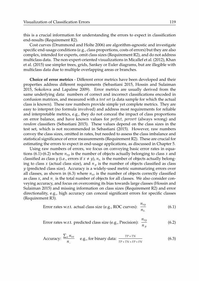
Visualization of Classification Errors 119
this is a crucial information for understanding the errors to expect in classificationend-results (Requirement R2).
Cost curves (Drummond and Holte 2006) are algorithm-agnostic and investigatespecific end-usage conditions (e.g., class proportions, costs of errors) but they are alsocomplex, intended for experts, omit class sizes (Requirement R2), and do not addressmulticlass data. The non-expert-oriented visualizations in Micallef et al. (2012), Khanet al. (2015) use simpler trees, grids, Sankey or Euler diagrams, but are illegible withmulticlass data due to multiple overlapping areas or branches.
Choice of error metrics - Different error metrics have been developed and theirproperties address different requirements (Sebastiani 2015, Hossin and Sulaiman2015, Sokolova and Lapalme 2009). Error metrics are usually derived from thesame underlying data: numbers of correct and incorrect classifications encoded inconfusion matrices, and measured with a test set (a data sample for which the actualclass is known). These raw numbers provide simple yet complete metrics. They areeasy to interpret (no formula involved) and address most requirements for reliableand interpretable metrics, e.g., they do not conceal the impact of class proportionson error balance, and have known values for perfect, pervert (always wrong) andrandom classifiers (Sebastiani 2015). These values depend on the class sizes in thetest set, which is not recommended in Sebastiani (2015). However, raw numbersconvey the class sizes, omitted in rates, but needed to assess the class imbalance andstatistical significance of error measurements (Requirement R2). These are crucial forestimating the errors to expect in end-usage applications, as discussed in Chapter 5.
Using raw numbers of errors, we focus on conveying basic error rates in equa-tions (6.1)-(6.2) where nxy is the number of objects actually belonging to class x andclassified as class y (i.e., errors if x , y), nx. is the number of objects actually belong-ing to class x (actual class size), and n.y is the number of objects classified as classy (predicted class size). Accuracy is a widely-used metric summarizing errors overall classes, as shown in (6.3) where nxx is the number of objects correctly classifiedas class x, and n.. is the total number of objects for all classes. We also consider con-veying accuracy, and focus on overcoming its bias towards large classes (Hossin andSulaiman 2015) and missing information on class sizes (Requirement R2) and errordirectionality, e.g., high accuracy can conceal significant errors for specific classes(Requirement R3).
Error rates w.r.t. actual class size (e.g., ROC curves):nxy
nx.(6.1)
Error rates w.r.t. predicted class size (e.g., Precision):nxy
n.y(6.2)
Accuracy:∑
x nxx
n..e.g., for binary data:
TP + TN
TP + TN + FP + FN(6.3)

120 Chapter 6
Figure 6.1: Classee visualization of classification errors for binary data.
6.4 Classee visualization
The Classee project simplified the visualization of classification errors by using or-dinary barcharts and raw numbers of errors (Figure 6.1-6.4). The actual class andthe error types are differentiated with color codes: vivid colors if the actual class ispositive (blue for TP, red for FN), desaturated colors if the actual class is negative(grey for TN, black for FP). The bars’ positions reinforces the perception of the actualclass, as bars representing items from the same actual class are staked on each otherinto a continuous bar: TP above FN, and FP above TN (Figure 6.2 left). The zero linedistinguishes the predicted class: TP and FP are above the zero line, FN and TN arebelow (Figure 6.2 right).
100
100
200
300
400
0
Number of
classified items
Actual Class Predicted
Class
Figure 6.2: Bars representing the actual and predicted classes.
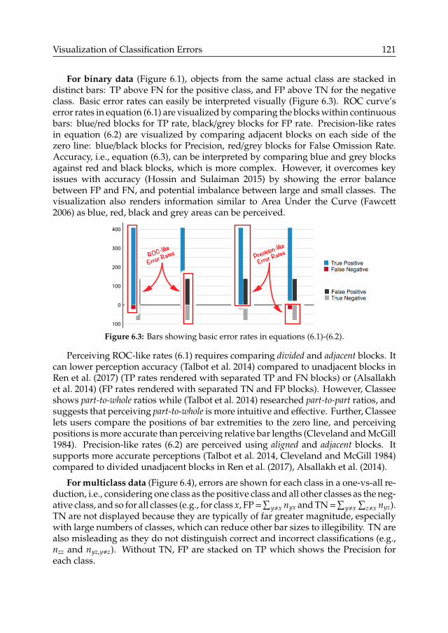
Visualization of Classification Errors 121
For binary data (Figure 6.1), objects from the same actual class are stacked indistinct bars: TP above FN for the positive class, and FP above TN for the negativeclass. Basic error rates can easily be interpreted visually (Figure 6.3). ROC curve’serror rates in equation (6.1) are visualized by comparing the blocks within continuousbars: blue/red blocks for TP rate, black/grey blocks for FP rate. Precision-like ratesin equation (6.2) are visualized by comparing adjacent blocks on each side of thezero line: blue/black blocks for Precision, red/grey blocks for False Omission Rate.Accuracy, i.e., equation (6.3), can be interpreted by comparing blue and grey blocksagainst red and black blocks, which is more complex. However, it overcomes keyissues with accuracy (Hossin and Sulaiman 2015) by showing the error balancebetween FP and FN, and potential imbalance between large and small classes. Thevisualization also renders information similar to Area Under the Curve (Fawcett2006) as blue, red, black and grey areas can be perceived.
100
100
200
300
400
0
ROC-like
Error Rates Precision-like
Error Rates
Figure 6.3: Bars showing basic error rates in equations (6.1)-(6.2).
Perceiving ROC-like rates (6.1) requires comparing divided and adjacent blocks. Itcan lower perception accuracy (Talbot et al. 2014) compared to unadjacent blocks inRen et al. (2017) (TP rates rendered with separated TP and FN blocks) or (Alsallakhet al. 2014) (FP rates rendered with separated TN and FP blocks). However, Classeeshows part-to-whole ratios while (Talbot et al. 2014) researched part-to-part ratios, andsuggests that perceiving part-to-whole is more intuitive and effective. Further, Classeelets users compare the positions of bar extremities to the zero line, and perceivingpositions is more accurate than perceiving relative bar lengths (Cleveland and McGill1984). Precision-like rates (6.2) are perceived using aligned and adjacent blocks. Itsupports more accurate perceptions (Talbot et al. 2014, Cleveland and McGill 1984)compared to divided unadjacent blocks in Ren et al. (2017), Alsallakh et al. (2014).
For multiclass data (Figure 6.4), errors are shown for each class in a one-vs-all re-duction, i.e., considering one class as the positive class and all other classes as the neg-ative class, and so for all classes (e.g., for class x, FP =
∑y,x nyx and TN =
∑y,x
∑z,x nyz).
TN are not displayed because they are typically of far greater magnitude, especiallywith large numbers of classes, which can reduce other bar sizes to illegibility. TN arealso misleading as they do not distinguish correct and incorrect classifications (e.g.,nzz and nyz,y,z). Without TN, FP are stacked on TP which shows the Precision foreach class.
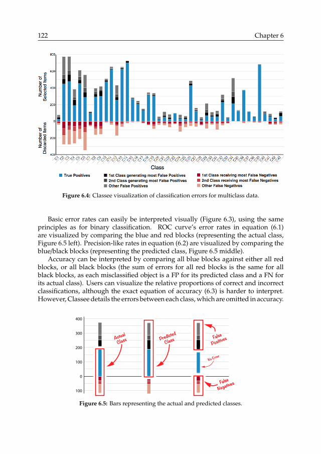
122 Chapter 6
Figure 6.4: Classee visualization of classification errors for multiclass data.
Basic error rates can easily be interpreted visually (Figure 6.3), using the sameprinciples as for binary classification. ROC curve’s error rates in equation (6.1)are visualized by comparing the blue and red blocks (representing the actual class,Figure 6.5 left). Precision-like rates in equation (6.2) are visualized by comparing theblue/black blocks (representing the predicted class, Figure 6.5 middle).
Accuracy can be interpreted by comparing all blue blocks against either all redblocks, or all black blocks (the sum of errors for all red blocks is the same for allblack blocks, as each misclassified object is a FP for its predicted class and a FN forits actual class). Users can visualize the relative proportions of correct and incorrectclassifications, although the exact equation of accuracy (6.3) is harder to interpret.However, Classee details the errors between each class, which are omitted in accuracy.
100
100
200
300
400
0
Actual Class Predicted
Class FalsePositives
FalseNegatives
No Error
Figure 6.5: Bars representing the actual and predicted classes.
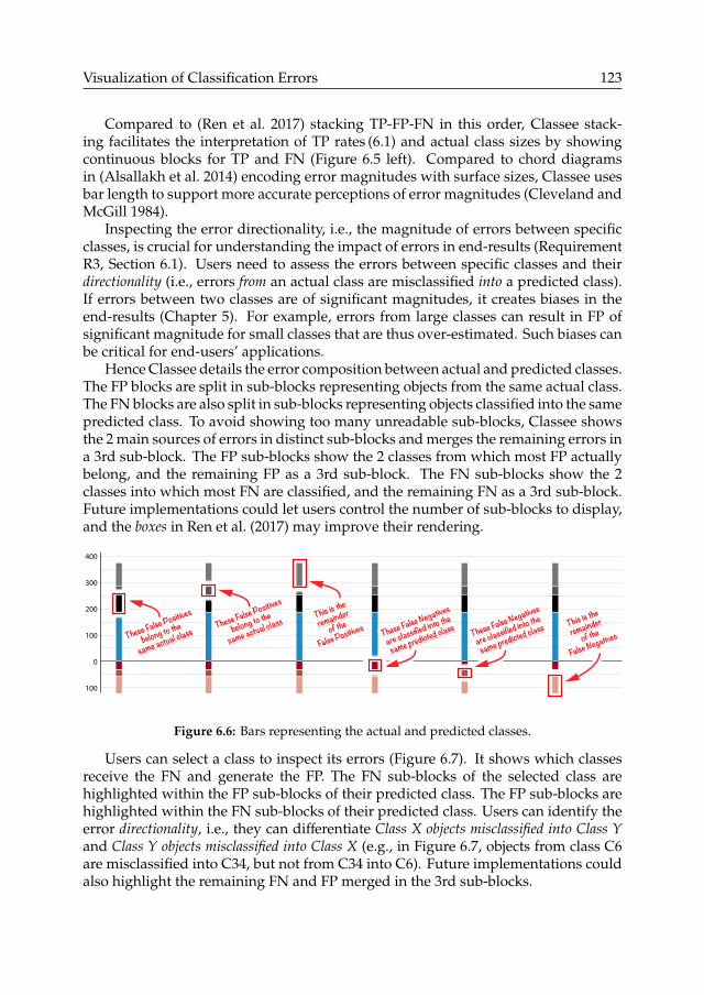
Visualization of Classification Errors 123
Compared to (Ren et al. 2017) stacking TP-FP-FN in this order, Classee stack-ing facilitates the interpretation of TP rates (6.1) and actual class sizes by showingcontinuous blocks for TP and FN (Figure 6.5 left). Compared to chord diagramsin (Alsallakh et al. 2014) encoding error magnitudes with surface sizes, Classee usesbar length to support more accurate perceptions of error magnitudes (Cleveland andMcGill 1984).
Inspecting the error directionality, i.e., the magnitude of errors between specificclasses, is crucial for understanding the impact of errors in end-results (RequirementR3, Section 6.1). Users need to assess the errors between specific classes and theirdirectionality (i.e., errors from an actual class are misclassified into a predicted class).If errors between two classes are of significant magnitudes, it creates biases in theend-results (Chapter 5). For example, errors from large classes can result in FP ofsignificant magnitude for small classes that are thus over-estimated. Such biases canbe critical for end-users’ applications.
Hence Classee details the error composition between actual and predicted classes.The FP blocks are split in sub-blocks representing objects from the same actual class.The FN blocks are also split in sub-blocks representing objects classified into the samepredicted class. To avoid showing too many unreadable sub-blocks, Classee showsthe 2 main sources of errors in distinct sub-blocks and merges the remaining errors ina 3rd sub-block. The FP sub-blocks show the 2 classes from which most FP actuallybelong, and the remaining FP as a 3rd sub-block. The FN sub-blocks show the 2classes into which most FN are classified, and the remaining FN as a 3rd sub-block.Future implementations could let users control the number of sub-blocks to display,and the boxes in Ren et al. (2017) may improve their rendering.
100
100
200
300
400
0
These False Negatives
are classified into the
same predicted class These False Negatives
are classified into the
same predicted class This is the
remainder
of the
False NegativesThese False Positives
belong to the
same actual classThese False Positives
belong to the
same actual classThis is the
remainder
of the
False Positives
Figure 6.6: Bars representing the actual and predicted classes.
Users can select a class to inspect its errors (Figure 6.7). It shows which classesreceive the FN and generate the FP. The FN sub-blocks of the selected class arehighlighted within the FP sub-blocks of their predicted class. The FP sub-blocks arehighlighted within the FN sub-blocks of their predicted class. Users can identify theerror directionality, i.e., they can differentiate Class X objects misclassified into Class Yand Class Y objects misclassified into Class X (e.g., in Figure 6.7, objects from class C6are misclassified into C34, but not from C34 into C6). Future implementations couldalso highlight the remaining FN and FP merged in the 3rd sub-blocks.

124 Chapter 6
Figure 6.7: Rollover detailing the errors for a specific class.
Large classes (with long bars) can hinder the perception of smaller classes (withsmall bars). Thus we propose a normalised view that balances the visual spaceof each class (Figure 6.8). Errors are normalised on the TP of their actual class asnxy/nxx (i.e., dividing FN/TP and reconstructing the FP blocks using the normalisederrors FN/TP). Although unusual, this approach aligns all FP and FN blocks to supporteasy and accurate visual perception (Talbot et al. 2014, Cleveland and McGill 1984).It also reminds users of the impact of varying class proportions: the magnitudeof errors change between normalised and regular views, as they would change ifclass proportions differ between test datasets (from which errors were measured)and end-usage datasets (to which classifiers are applied). It is also the basis of theRatio-to-TP method that estimate the numbers of errors to expect in classificationresults (Chapter 5, Section 5.3, p.82).
Color choices - Classee uses blue rather than green as in Alsallakh et al. (2014)to address colorblindness (Tidwell 2010) while maintaining a high contrast opposingwarm and cold colors. Compared to class-specific colors in Ren et al. (2017) whichcan clutters the visualization to illegibility, e.g., with more than 7 classes (Murch1984), Classee colors can handle large numbers of classes.
Following the Few Hues, Many Values design pattern (Tidwell 2010), sub-blocksof FN and FP use the same shades of red and black. The shades of grey for FP mayconflict with the grey used for TN in binary classification. The multiclass barchartdoes not display TN and its shades of grey remain darker. Thus color consistencyissues are limited, and we deemed that Classee colors are a better tradeoff thanadding a color for FP (e.g., yellow in Alsallakh et al. (2014)).
As a result, the identification of actual and predicted classes is reinforced by theinterplay of three visual features: position (below or above the zero line for the

Visualization of Classification Errors 125
predicted class, left or right bar for the actual class), color hues (blue/red if the actualclass is positive), and color (de)saturation (black/grey if the actual class is negative).
Figure 6.8: Normalized view with errors proportional to True Positives
6.5 User experiment
We evaluated Classee and investigated the factors supporting or impeding the un-derstanding of classification errors. We conducted in-situ semi-structured interviewswith a think-aloud protocol to observe users’ "activity patterns" and "isolate impor-tant factors in the analysis process" (Lam et al. 2012). We focused on evaluating theVisual Data Analysis and Reasoning rather than User Performance (Lam et al. 2012) asour primary goal is to ensure a correct understanding of classification errors andtheir implications. We conducted a qualitative study that informs the design of end-user-oriented visualization, and is preparatory to potential quantitative studies. Weincluded a user group of mathematicians to investigate how mathematical thinkingimpacts the understanding of ROC curves and error metrics. Such prior knowledgeis a component of the Demographic Complexity interacting with the Data Complexity,and thus impacting user cognitive load (Huang et al. 2009).
The 3 user groups represented three types of expertise: 1) practitioners of ma-chine learning (4 developers, 2 researchers), 2) practitioners of mathematics but notmachine learning (5 researchers, 1 medical doctor), and 3) practitioners of neithermachine learning, mathematics nor computer science (including 1 researcher). Atotal of 18 users and 2 users per condition (3 groups x 3 visualizations x 2 users) wassufficient to yield significant observations, as we repeatedly identified key factorsimpacting user understanding.

126 Chapter 6
The 3 experimental visualizations compared the simplified barcharts to twowell-established alternatives: ROC curve and confusion matrix (Figure 6.9-6.11).ROC curves are preferred to Precision-Recall curves which exclude TN and do notconvey the same information as the barcharts. All visualizations used the samedata and users interacted only with one kind of visualization. This between-subjectstudy accounts for the learning curve. After interacting with a first visualization,non-experts gain expertise that would bias the results with a second visualization.
Figure 6.9: ROC curves used for binary and multiclass data.
Figure 6.10: Confusion table for binary data.
Figure 6.11: Confusion matrices used for tasks T2-7 to T2-9.

Visualization of Classification Errors 127
For binary data, classification errors were shown for 5 values of a tuning parametercalled a selection threshold. Confusion matrices for each threshold were shown as atable (Fig. 6.10) with rows representing the thresholds, and columns representing TP,FN, TN, FP. The table included heatmaps reusing the color coding of the barcharts.The color gradients form the default heatmap template from D3 library were mappedon the entire table cells’ values, which is not optimal. Each column’s values haveranges that largely differ. Thus the color gradients may not render the variations ofvalues within each column, as the variations are much smaller than the variationswithin the entire table. Hence color gradient should be mapped within each columnseparately.
For multiclass data, the confusion matrix also included a heatmap with the samecolor coding. The diagonal showed TP in blue scale. A rollover on a class showedthe FP in dark grey scale and the FN in red scale (Figure 6.11 right). If no classwas selected, red was the default color for errors (Figure 6.11 left). The ROC curvesto multiclass data displayed a single dot per class, rather than complex multiclasscurves. The option to normalize barchart (Figure 6.8) was not included, to focus onevaluating the basic barchart using raw numbers of errors.
The 15 user tasks were in two parts, for binary and multiclass data (Table 6.3).Each part started with a tutorial explaining the visualization and the technical con-cepts. This could be displayed anytime during the tasks. For binary problems, itexplained TP, FN, FP, TN and the threshold parameter to balance FN and FP. Formulticlass problems, it explained class-specific TP, FN, FP, TN in one-vs-all reduc-tions, and that FN for one class (the actual class) are FP for another (the predictedclass). The explanations of the technical concepts were the same for all users andvisualizations. Only the explanations of the visualization differed.
The tasks used synthetic data that predefined the right answers. To assess userawareness of uncertainty, users had to indicate their confidence in their answers.User confidence should match the answer correctness (e.g., low confidence in wronganswers). The response time was measured, but without informing users to avoidTime Complexity and stress impacting user cognitive load (Huang et al. 2009). The taskcomplexity targeted 3 levels of data interpretation, drawn from Situation Awareness(Endsley 1995). Level 1 concerned the understanding of individual data (e.g., anumber of FP). Level 2 concerned the integration of several data elements (e.g.,comparing FP and FN). Level 3 concerned the projection of current data to predictfuture situations (e.g., the potential errors in end-usage applications). To facilitateusers’ learning process, the tasks were performed from Level 1 to 3.
Compared to the 3 levels of Task Complexity in Huang et al. (2009), our level 1introduces a lower level of complexity. Our level 2 has less granularity and encom-passes all 3 levels in Huang et al. (2009). Our level 3 introduces a higher level ofcomplexity related to extrapolating unknown information (e.g., the errors to expectwhen applying classifiers to end-usage datasets). Our level 3 also introduces DomainComplexity, e.g., it concerns different application domains in tasks T1-4 to -6. Thedomain at hand can influence user answers. To channel this influence, tasks T2-5
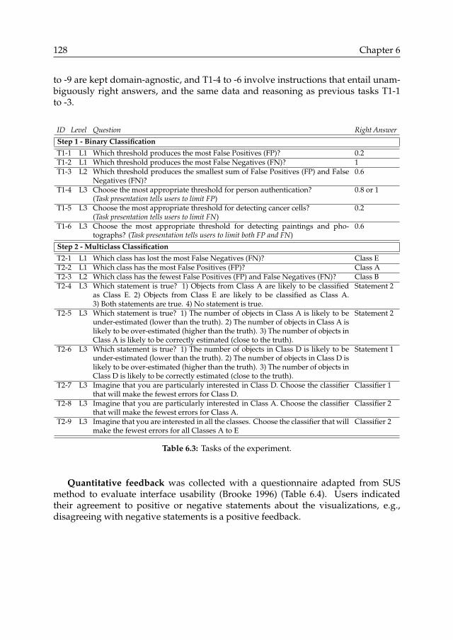
128 Chapter 6
to -9 are kept domain-agnostic, and T1-4 to -6 involve instructions that entail unam-biguously right answers, and the same data and reasoning as previous tasks T1-1to -3.
ID Level Question Right AnswerStep 1 - Binary ClassificationT1-1 L1 Which threshold produces the most False Positives (FP)? 0.2T1-2 L1 Which threshold produces the most False Negatives (FN)? 1T1-3 L2 Which threshold produces the smallest sum of False Positives (FP) and False
Negatives (FN)?0.6
T1-4 L3 Choose the most appropriate threshold for person authentication?(Task presentation tells users to limit FP)
0.8 or 1
T1-5 L3 Choose the most appropriate threshold for detecting cancer cells?(Task presentation tells users to limit FN)
0.2
T1-6 L3 Choose the most appropriate threshold for detecting paintings and pho-tographs? (Task presentation tells users to limit both FP and FN)
0.6
Step 2 - Multiclass ClassificationT2-1 L1 Which class has lost the most False Negatives (FN)? Class ET2-2 L1 Which class has the most False Positives (FP)? Class AT2-3 L2 Which class has the fewest False Positives (FP) and False Negatives (FN)? Class BT2-4 L3 Which statement is true? 1) Objects from Class A are likely to be classified
as Class E. 2) Objects from Class E are likely to be classified as Class A.3) Both statements are true. 4) No statement is true.
Statement 2
T2-5 L3 Which statement is true? 1) The number of objects in Class A is likely to beunder-estimated (lower than the truth). 2) The number of objects in Class A islikely to be over-estimated (higher than the truth). 3) The number of objects inClass A is likely to be correctly estimated (close to the truth).
Statement 2
T2-6 L3 Which statement is true? 1) The number of objects in Class D is likely to beunder-estimated (lower than the truth). 2) The number of objects in Class D islikely to be over-estimated (higher than the truth). 3) The number of objects inClass D is likely to be correctly estimated (close to the truth).
Statement 1
T2-7 L3 Imagine that you are particularly interested in Class D. Choose the classifierthat will make the fewest errors for Class D.
Classifier 1
T2-8 L3 Imagine that you are particularly interested in Class A. Choose the classifierthat will make the fewest errors for Class A.
Classifier 2
T2-9 L3 Imagine that you are interested in all the classes. Choose the classifier that willmake the fewest errors for all Classes A to E
Classifier 2
Table 6.3: Tasks of the experiment.
Quantitative feedback was collected with a questionnaire adapted from SUSmethod to evaluate interface usability (Brooke 1996) (Table 6.4). Users indicatedtheir agreement to positive or negative statements about the visualizations, e.g.,disagreeing with negative statements is a positive feedback.

Visualization of Classification Errors 129
F1-1, F2-1 I would like to use the visualization frequently.F1-2, F2-2 The visualization is unnecessarily complex.F1-3, F2-3 The visualization was easy to use.F1-4, F2-4 I would need the support of an expert to be able to use the visualization.F1-5, F2-5 Most people would learn to use the visualization quickly.F1-6, F2-6 I felt very confident using the visualization.F1-7, F2-7 I would need to learn a lot more before being able to use the visualization.
Table 6.4: Feedback questionnaire
6.6 Quantitative results
We discuss user prior knowledge (Figure 6.12), user performance between visualiza-tions (Figure 6.13) and user groups (Figure 6.14). User performance is consideredimproved if i) wrong answers are limited; ii) confidence is lower for wrong answersand higher for right answers; and iii) user response time is reduced. Finally, wereview the quantitative feedback (Figure 6.15). The detailed participants’ answersare given in Figure 6.20 (p.141).
ML Expert Math Expert Non−Expert
0 2 4 6 0 2 4 6 0 2 4 6
Confusion MatrixGround−TruthML Classifier
PR CurveROC Curve
TP FN FP TN
Number of Users
Tech
nica
l Ter
ms
PriorKnowledge
GoodVagueNone
Highest Degree
PhDMasterBachelor
Education
●● ● ●● ● ●●● ●● ● ● ●●● ●●
ML Expert Math Non−Expert
25 30 35 25 30 35 25 30 35 Age
Figure 6.12: Profiles of study participants.
The prior knowledge of math experts often included TP, FN, FP, TN as theseare involved in statistical hypothesis testing (Figure 6.12). Machine learning expertsknew the technical concepts well, except a self-taught practitioner who was onlyfamiliar to terms related to his daily tasks, e.g., Accuracy but not ROC Curve orConfusion Matrix. This participant, who was in charge of implementing, integratingand testing classifiers, mentioned "Clients only ask for accuracy" but did not recall itsformula. Two other machine learning experts were unfamiliar with either Precision-Recall or ROC curves, and related formulas, because their daily tasks involved onlyone of these.
Machine learning practitioners use different approaches for assessing classifica-tion errors, using specific metrics or visualizations. They may not recall the meaningand formulae of unused metrics, or even metrics used regularly. Some metrics are

130 Chapter 6
not part of their routine, but may be relevant for specific use cases or end-users.Hence experts too can benefit from Classee since i) Remembering error rate formulaeis not needed as rates are visually reconstructed; ii) Both ROC-like or Precision-likerates can be visualized, i.e., equations (6.1)-(6.2); and iii) Accuracy can also be inter-preted, i.e., by comparing the relative proportions of errors (FP and FN in red andblack bars) and correct classifications (TP in blue bars, TN in grey bars for binarydata). Classee also shows the error composition (i.e., which specific classes are oftenconfused) and class sizes. It supports machine learning experts tasks of tuning andimproving classifiers (Table 6.2).
Barchart ROC Table
0 2 4 6 0 2 4 6 0 2 4 6T2−9T2−8T2−7T2−6T2−5T2−4T2−3T2−2T2−1T1−6T1−5T1−4T1−3T1−2T1−1
Number of Answers
Mul
ticla
ss T
asks
Bin
ary
Task
sM
ultic
lass
Tas
ksB
inar
y Ta
sks
0 2 4 6 0 2 4 6 0 2 4 6T2−9T2−8T2−7T2−6T2−5T2−4T2−3T2−2T2−1T1−6T1−5T1−4T1−3T1−2T1−1
0 20 40 60 0 20 40 60 0 20 40 60
RightWrong
Cor
rect
.
Correctnessof Answers
RightWrong
Confidencein Answers
+ + ++ ++−− −− − −
Figure 6.13: Task performance per visualization.

Visualization of Classification Errors 131
ML Expert Math Expert Non−Expert
0 5 10 15 0 5 10 15 0 5 10 15
Bar. Mul.Table Mul.ROC Mul.
Bar. Bin.Table Bin.ROC Bin.
Visu
aliz
atio
n Correctnessof Answers
RightWrong
0 5 10 15 0 5 10 15 0 5 10 15
Bar. Mul.Table Mul.ROC Mul.
Bar. Bin.Table Bin.ROC Bin.
Visu
aliz
atio
n Confidencein Answers
+ + ++ ++−− −− − −
0 20 40 60 80 0 20 40 60 80 0 20 40 60 80
RightWrong
Number of AnswersCor
rect
ness
Ans
wer
ML Expert Math Non Expert
Right Answers
Wrong Answers
0 200 400 600 0 200 400 600 0 200 400 600
Bar. Mul.
Table Mul.
ROC Mul.
Bar. Bin.
Table Bin.
ROC Bin.
Bar. Mul.
Table Mul.
ROC Mul.
Bar. Bin.
Table Bin.
ROC Bin.
Response Time (in seconds) each dot represents an answer
Visu
aliz
atio
n
+1 outlier
+1 outlier
+1 outlier
Figure 6.14: Task performance per user group.

132 Chapter 6
With binary data, the number of wrong answers differed between tasks T1-1to -3 and T1-4 to -6 while both sets of tasks entail the same answers and use thesame dataset (Figure 6.13 top). Tasks T1-4 to -6 involved extrapolations for end-usage applications. These tasks introduced Domain Complexity (Huang et al. 2009)and the tasks’ description had increased task discretion (less detailed instructionsprovided to users) thus increasing the cognitive load (Gill and Hicks 2006). Theincreased task discretion had an important impact as users spent significant effortsrelating the terms TP, FN, FP, TN to the real objects they represent (e.g., intruders areFP). With barcharts, user confidence better matched answer correctness (lower forwrong answers, higher for right answers) and so for all user profiles (Figure 6.14).Machine learning and math experts gave almost no wrong answers regardless ofthe visualization, but were more confident with barcharts than ROC curves (andthan tables for machine learning experts). Non-experts gave more wrong answersand were over-confident with tables, but with barcharts and ROC curves their lowerconfidence indicates a better awareness of their uncertainty.
User response time was lower with barcharts (Figure 6.14 bottom) except formachine learning experts. Their response time was equivalent for all visualizationsbut varied less with ROC curves, possibly because this graph was most familiar.
With multiclass data, wrong answers were limited until task T2-4 (Figure 6.13top). Answers were mostly wrong from task T2-4 onwards, as task complexity in-creased to concern extrapolations of errors in end-results. With barcharts, wronganswers were scarce after T2-4, e.g., after users have familiarized with the graph, butremained high with other graphs. Machine learning and math experts were moreconfident with barcharts (Figure 6.14 middle) but non-experts were under-confident.Yet their response time decreased with barcharts, and was as fast as machine learningand math experts (Figure 6.14 bottom).
User feedback was collected twice, after the tasks for binary and multiclass data,with the same questionnaire (Table 6.4). At the user profile level (Figure 6.15 top),for binary data, non-experts and machine learning experts had the most negativefeedback for ROC curves. Math experts had equivalent feedback for all visual-izations. For multiclass data, confusion matrices had the most negative feedbackfrom non-experts and math experts. ROC-like visualizations had the most positivefeedback from all profiles. At the question level (Figure 6.15 middle), for binarydata, barcharts had the most positive feedback on the design complexity (F1-2). ROCcurves had the most negative feedback for frequent use and need for support (F1-1, -4).For multiclass data, confusion matrices received negative feedback at all questions,especially for confidence and need for training (F2-6, -7).
One barchart user gave the lowest possible feedback to almost all questions. Thisuser disliked math and any form of graph ("Ah! I hate graphs!", "I hate looking atgraphs, it’s too abstract for me") and was particularly reluctant to frequently using thegraphs (F1-1, F2-1). However, this user’s performance was excellent with barchartsfor binary data: only right answers with high confidence, and positive feedbackespecially on the learnability (F1-2, "The graph is easy, even I can use it").

Visualization of Classification Errors 133
Besides this participant, barcharts had the most positive feedback for frequentuse, usability and need for training (F2-1, -3, -7). ROC curves had the most positivefeedback on complexity and learnability (F2-2, -5) but its apparent simplicity (only 5dots on a grid) may conceal underlying data complexity, leading to wrong answers(Figure 6.13).
Over all questions (Figure 6.15 bottom), for binary data the most negative feed-back was observed for ROC curves. The feedback was equivalently positive forbarcharts and tables. For multiclass data, the most negative feedback was observedfor confusion matrices. The feedback was equivalently positive for barcharts andROC visualizations, excluding the barchart user especially averse to any data visu-alization.
Users wondered if the feedback also concerned the explanations, hence the resultsmay not represent only the visualization. Other limitations concern the small numberof users, and user tendency to avoid either average or extreme feedback ("I’m not thekind of person having strong opinions"). More detailed and generalizable insights onthe usability are elicited from our qualitative analysis of user interviews.
ML Expert Math Expert Non−Expert
0 5 10 0 5 10 0 5 10
Bar. Mul.Table Mul.ROC Mul.
Bar. Bin.Table Bin.ROC Bin.
Visu
aliz
atio
n
Feedback+ +++ / −−− −
0 2 4 6 0 2 4 6 0 2 4 6
F2−7F2−6F2−5F2−4F2−3F2−2F2−1
F1−7F1−6F1−5F1−4F1−3F1−2F1−1
Number of Answers
Feed
back
Que
stio
nsO
vera
ll
Barchart ROC Table
0 10 20 30 40 0 10 20 30 40 0 10 20 30 40
Multi.
Binary
Figure 6.15: User feedback.

134 Chapter 6
6.7 Qualitative analysis
To identify the factors influencing user understanding of classification errors, weanalysed user comments and behaviours by transcribing written notes of the inter-views. To let the factors emerge from our observations, we first proceeded withgrounded coding (no predefined codes). We then organized our insights into themesand proceeded to a priori coding (predefined codes). We identified 3 key difficultiesthat are independent of the visualizations:• The terminology (e.g., TP, FN, FP, TN are confusing terms);• The error directionality (e.g., considering both FN and FP);• The extrapolation of error impact on end-usage application (e.g., a class may
be over-estimated).We report these difficulties and how the visualizations aggravated or addressed them.
Terminology - The basic terms TP, FN, FP, TN were difficult to understand and re-member ("In 30 minutes I’ll have completely forgotten"). Twelve users (66%) mentioneddifficulties with these terms, including machine learning experts. The terms Posi-tive/Negative were often misunderstood as the actual class (instead of the predictedclass) especially when not matching their applied meaning ("Cancer is the positiveclass, that’s difficult semantically"). Users were also confused by the unusual syntax("Positive and Negative are usually adjectives but here they are nouns, it’s confusing") andthe association of antonyms (e.g., False and Positive in FP, "False is for somethingnegative") and synonyms (e.g., "The words are so close" with True and Positive in TP, "Iunderstand that FN are not errors" because Negative and False is a logical association).Users misinterpreted the terms True and False as representing the actual or predictedclass, and both are incorrect. Some users suggested adverbs to avoid such confusion("Falsely", "Wrongly"). To cope with the semantic issues, users translated the tech-nical terms into more tangible terms, using concrete examples ("Falsely Discarded","False face"). A machine learning expert requested short acronyms (e.g., TP for TruePositive). A non-expert suggested icons as another form of abbreviation ("like a smi-ley" Figure 6.16). This user preferred labels mentioning the actual class first (usingNegative/Positive) then the errors (using True/False).
Figure 6.16: User-suggested icons for TP, FN, FP, TN. Drawn by the interviewer following user’sinstructions in post-experiment discussions. User-suggested labels are below the icons. Usual labelswere later added above.

Visualization of Classification Errors 135
The terminology of legends and explanations can yield difficulties ("You couldmake the text more clear"). The terms Select and Discard in our tutorials and legendscan be at odds with their application ("Discarding objects may be confusing if bothclasses are equally important"). The term true in its common meaning ("true class","truly belong to [class x]") conflicts with its meaning in TP, TN and must be avoided.
Math experts were often familiar with TP, FN, FP, TN as these are involved instatistical hypothesis testing. Machine learning experts knew the technical termswell, except a self-taught practitioner who was only familiar to terms used in dailytasks, e.g., Accuracy but not ROC Curve or Confusion Matrix. This user mentioned"Clients only ask for accuracy" but did not recall its formula. Two other machinelearning experts were unfamiliar with either Precision-Recall or ROC curves, as theirdaily tasks involved only one of these. Hence machine learning practitioners may notrecall the meaning and formula of unused metrics, or even metrics used regularly.Some metrics are not part of their routines, but may be relevant for specific usecases or end-users. Hence experts too can benefit from Classee since i) rememberingerror rate formulae is not needed as rates are visually reconstructed; ii) both ROC-like or Precision-like rates can be visualized (6.1)-(6.2); and iii) accuracy can also beinterpreted.
Error Directionality - Users need to distinguish the actual and predicted classesof errors, and the direction of errors from an actual class classified into a predictedclass. Ten users (56%) from all profiles had difficulties with error directions, e.g.,confusing FP and FN ("Oh my FP were FN, why did I switch!"). With binary data, usersmay not understand how the tuning parameter influence errors in both directions,e.g., decreasing FN but increasing FP ("I put a high threshold so that there’s no error[FP, FN] in the results", "High threshold means high TP and TN"). With multiclass data,users may not understand that FN for one class are FP for another, and that errorsfor class x concern both errors with predicted class x and actual class x (e.g., notconsidering both FN and FP).
Terminology issues complicated user understanding of error directionality, e.g.,the terms Positive/Negative could mean both the actual or predicted class. Someusers intuitively interpreted these terms as the predicted class, others as the actualclass. Users often used metaphors and more tangible terms to clarify the errordirectionality ("The destination class", "We steal [the FP] from another class"). The termsSelected and Discarded, although using a tangible metaphor, can be misunderstood asthe actual class ("The class that must be selected") yielding misinterpretations of errordirectionality.
Extrapolation of Errors in End-Usage Applications - Users needed additionalinformation to extrapolate the classification errors in end-usage applications ("It’simpossible to deduce a generality", "How can I say anything about the rest of the data?").More information on the consequences of error was needed to decide which errorsare tolerable ("There can be risks in allowing FP, additional tests have further health risks","No guidance on how to make the tradeoff"). Users questioned whether the error mea-surements are representative of end-usage conditions, regarding potential changes

136 Chapter 6
in class sizes and error magnitudes ("Assuming class proportions are equal", "This isa sample data, another sample could have some variations"). They also wondered aboutadditional sources of uncertainty, such as changes in object features or the presenceof other classes ("Will it contain only paintings and photographs?") and their impacton the algorithm ("How does the classifier compute the problem"). The lack of contextinformation decreased user confidence, e.g., when assessing if a class is likely to beover- or under-estimated.
ROC Curve - It is unusual to visualize line charts where both x- and y-axesrepresent a rate, and where thresholds are a third variable encoded on the line. Itis more intuitive to represent thresholds on the x-axis and rates on the y-axis, withdistinct lines for each rate (as a user suggested). Non-experts primarily relied on textexplanations to perform the tasks (e.g., reading that low thresholds reduce FP, thenchecking each dot’s threshold to find the lowest). Only machine learning and mathexperts were comfortable with interpreting the data visually ("My background makesme fluent in reading ROC curves visually", "I don’t use formulas, I compare the dots witheach other without reading the values").
Error rate formulae were difficult to understand and remember, even for experts("Formulas are still confusing, and still require a lot of thinking"). All users but oneneeded to reexamine the equations and their meaning many times during the tasks.It increased their response time and impacted their confidence ("To be sure I’ll need toread it again"). Some users interpreted the rates as numbers of errors, for a simplersurrogate metric. Otherwise, without the numbers of errors, class sizes and potentialimbalance are unknown, and it aggravates the difficulties with extrapolating theerrors in end-results, e.g., it is impossible to assess the balance of errors between largeand small classes ("Unknown ratio of Positive/Negative","Assuming class proportions areequal"). The error composition (how many objects from class X are confused withclass Y) is unavailable for multiclass data. Some users noticed the lack of information("There’s not enough information, errors can come from one class or another", "Assumingthe destination class is random") but others failed to notice, even for one task that wasimpossible to answer without knowing the error composition.
Error rates’ ambiguous labels aggravated the terminology issues. The rates haveactual class sizes as denominators (6.1) but the term Positive in TP and FP rate refers tothe predicted class. It misled users in considering that both rates have the predictedclass size as denominator, e.g., misinterpreting TP rate (6.1) as Precision (6.2). This isconsistent with (Khan et al. 2015) where misinterpretations were more frequent withdenominators than numerators, and with (Hoffrage et al. 2015) where a terminologyspecifying the denominator of probabilistic metrics improved user understanding.A user suggested to replace TP rate by the opposite FN rate (1 - TP rate). It is more in-tuitive that both rates focus on errors (rather than on correct TP), and by mentioningboth Positive and Negative labels, it may indicate that the denominators differ. Yet theterminology remains confusing as it fails to indicate the rate’s denominator. Longerlabels could clear ambiguities but may be tedious to read.
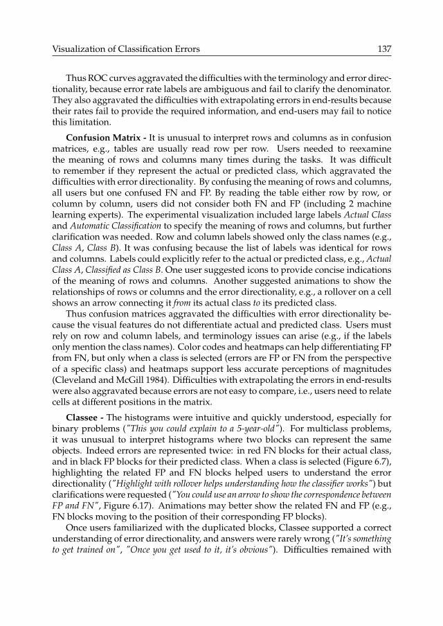
Visualization of Classification Errors 137
Thus ROC curves aggravated the difficulties with the terminology and error direc-tionality, because error rate labels are ambiguous and fail to clarify the denominator.They also aggravated the difficulties with extrapolating errors in end-results becausetheir rates fail to provide the required information, and end-users may fail to noticethis limitation.
Confusion Matrix - It is unusual to interpret rows and columns as in confusionmatrices, e.g., tables are usually read row per row. Users needed to reexaminethe meaning of rows and columns many times during the tasks. It was difficultto remember if they represent the actual or predicted class, which aggravated thedifficulties with error directionality. By confusing the meaning of rows and columns,all users but one confused FN and FP. By reading the table either row by row, orcolumn by column, users did not consider both FN and FP (including 2 machinelearning experts). The experimental visualization included large labels Actual Classand Automatic Classification to specify the meaning of rows and columns, but furtherclarification was needed. Row and column labels showed only the class names (e.g.,Class A, Class B). It was confusing because the list of labels was identical for rowsand columns. Labels could explicitly refer to the actual or predicted class, e.g., ActualClass A, Classified as Class B. One user suggested icons to provide concise indicationsof the meaning of rows and columns. Another suggested animations to show therelationships of rows or columns and the error directionality, e.g., a rollover on a cellshows an arrow connecting it from its actual class to its predicted class.
Thus confusion matrices aggravated the difficulties with error directionality be-cause the visual features do not differentiate actual and predicted class. Users mustrely on row and column labels, and terminology issues can arise (e.g., if the labelsonly mention the class names). Color codes and heatmaps can help differentiating FPfrom FN, but only when a class is selected (errors are FP or FN from the perspectiveof a specific class) and heatmaps support less accurate perceptions of magnitudes(Cleveland and McGill 1984). Difficulties with extrapolating the errors in end-resultswere also aggravated because errors are not easy to compare, i.e., users need to relatecells at different positions in the matrix.
Classee - The histograms were intuitive and quickly understood, especially forbinary problems ("This you could explain to a 5-year-old"). For multiclass problems,it was unusual to interpret histograms where two blocks can represent the sameobjects. Indeed errors are represented twice: in red FN blocks for their actual class,and in black FP blocks for their predicted class. When a class is selected (Figure 6.7),highlighting the related FP and FN blocks helped users to understand the errordirectionality ("Highlight with rollover helps understanding how the classifier works") butclarifications were requested ("You could use an arrow to show the correspondence betweenFP and FN", Figure 6.17). Animations may better show the related FN and FP (e.g.,FN blocks moving to the position of their corresponding FP blocks).
Once users familiarized with the duplicated blocks, Classee supported a correctunderstanding of error directionality, and answers were rarely wrong ("It’s somethingto get trained on", "Once you get used to it, it’s obvious"). Difficulties remained with

138 Chapter 6
confusion matrices and ROC curves, as misunderstandings of FP and FN remainedfrequent. Classee better clarified the error directionality with visual features thatclearly distinguish actual and predicted classes ("I like the zero line, it makes it morevisual"). These also reduced the difficulties with the technical terminology and itsexplanation ("Explanations are more difficult to understand than the graph", "We usuallysay it’s easier said than done, but here it’s the opposite: when you look at the graph it’sobvious") even though multiclass legends were unclear ("What do you mean with 1stclass and 2nd class?"). Classee was more tangible and self-explanatory ("I see an objectthat contains things") and non-experts were more confident than they expected ("I amabsolutely sure but I should be wrong somewhere, I’m not meant for this kind of exercise","It sounds so logical that I’m sure it’s wrong").
Figure 6.17: User-suggested animation with arrows
Extrapolating the errors in end-results was also easier with Classee. Using num-bers of errors provides complete information while ROC curves conceal the classsizes ("You get more insights from the barchart"). Confusion matrices also use num-bers of errors, but are more difficult to interpret (cell values are difficult to compare,rows or columns can be omitted or misinterpreted). Class sizes and error balancewere easier to visualize with Classee ("Here the grey part is more important than here","Histograms are more intuitive").
Thus Classee limited the difficulties with extrapolating errors in end-results be-cause its metrics and visual features are more tangible and intuitive, and they providecomplete information (including class sizes and error balance). Classee also limitedthe difficulties with the terminology and error directionality by using visual featuresthat clearly distinguish actual and predicted classes. Yet error directionality can befurther clarified for multiclass data by adding interactive features to reinforce thecorrespondence of FP and FN (e.g., animations) and choose the details to display(e.g., error composition for more than 2 classes, or for specific classes).
After the experiment, we introduced the alternative visualizations. Most userspreferred Classee, especially after using the other graphs ("It’s easier, I can see whatI was trying to do", "This is what I did in my mind to understand the threshold"). Twomachine learning experts preferred Classee, others preferred the familiar confusionmatrix or ROC curve ("You get more insights from the barchart, but ROC curve I read itin a glimpse") or would use both confusion matrix and Classee as they complementeach other with overview and details.

Visualization of Classification Errors 139
6.8 Conclusion
We identified issues with the terminology, the error directionality (objects from anactual class are misclassified into a predicted class) and the extrapolation of errorimpacts in end-usage applications. To address these issues, labels and visual featuresmust reinforce the identification of actual and predicted classes, e.g., using domainterminology and tangible representations (animations, icons).
Error metrics have crucial impacts on user cognitive load. With error rates, usersmay overlook missing information (e.g., class sizes) and misinterpret the denomina-tors, which is worsened by terminology issues. Raw numbers of errors are simplerto understand, but are difficult to analyse with confusion matrices.
Classee successfully addressed these issues. Its use of numbers of errors encodedin histograms is more tangible and self-explanatory, and supports accurate percep-tions of error magnitudes and class sizes (Requirement R1-3, Section 6.1). The com-bination of 3 visual features that distinguish the actual and predicted class (position,color hue, color saturation) clarified the error directionality. It helped overcome theterminology issues while providing complete information for choosing and tuningclassifiers, and for extrapolating errors in end-usage applications.
Multiclass problems remain particularly difficult to visualize. All three experi-mental visualizations involve unusual representations in otherwise common graphs.ROC curves have rates on both axes, confusion matrices are read both column- androw-wise, and Classee has duplicated blocks representing the same errors (as FN orFP). In our evaluation, Classee was the easiest to learn and familiarize with, but itslegends and interactions should be improved (e.g., with animations highlighting theerror directionality).
Our findings inform the design of visualization tools that support end-users’understanding of classification errors, and answer our sixth question: How can visu-alization support non-expert users in understanding classification errors?
We identified factors that support or hinder the assessment of Noise and Bias dueto classification errors, the resulting Uncertainty in Specific Datasets. These are keyuncertainty factors identified in Chapter 4. The Classee visualizations we introducedaddress the assessment of classification biases. Future work must investigate themeans to assess noise, i.e., how errors may randomly vary among datasets to whichclassifiers are applied (Requirement R4, Section 6.1). Random error variance canbe estimated with the Sample-to-Sample method introduced in Chapter 5. Classeevisualizations can be used to display variance, e.g., as in Figures 6.18-6.19.
Variance visualization partially addresses the assessment of the Uncertainty inSpecific Datasets, i.e., estimating the errors to expect in classification end-results (Re-quirement R4).As identified in Chapter 4 and demonstrated in Chapter 5, the classi-fication errors may largely vary depending on changes in feature distributions (e.g.,lower data quality). Hence assessing the Uncertainty in Specific Datasets requiresthe visualization of non-random error variations, depending on datasets’ featuredistributions.
Visualizing classification errors as a function of varying feature distributions is
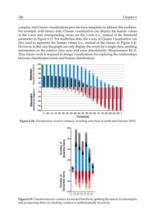
140 Chapter 6
complex, but Classee visualizations provide basic templates to address this problem.For example, with binary data, Classee visualization can display the feature valuesas the x-axis and corresponding errors are the y-axis (i.e., instead of the thresholdparameter in Figure 6.1). For multiclass data, the x-axis of Classee visualization canalso used to represent the feature values (i.e., instead of the classes in Figure 6.4).However, in this case the graph can only display the errors for a single class, omittinginformation on the relative class sizes and error directionality (Requirement R2-3).Thus future work is required to design visualizations for exploring the relationshipsbetween classification errors and feature distributions.
Figure 6.18: Visualization of error variance, avoiding error bars (Correll and Gleicher 2014)
Figure 6.19: Visualization for variance for stacked barcharts, splitting the data in 10 subsamplesand juxtaposing them (as stacking variance is mathematically incorrect).

Visualization of Classification Errors 141
1a 1b 1c 2a 2b 2c 3a 3b 3c 4a 4b 4c 5a 5b 5c 6a 6b 6c
Q2−9
Q2−8
Q2−7
Q2−6
Q2−5
Q2−4
Q2−3
Q2−2
Q2−1
Q1−6
Q1−5
Q1−4
Q1−3
Q1−2
Q1−1
Participants (a: ROC, b:Table, c:Classee, 1−2: ML, 3−4: Math, 5−6:None)
Task
s
Answer Right Wrong
1a 1b 1c 2a 2b 2c 3a 3b 3c 4a 4b 4c 5a 5b 5c 6a 6b 6c
Q2−9
Q2−8
Q2−7
Q2−6
Q2−5
Q2−4
Q2−3
Q2−2
Q2−1
Q1−6
Q1−5
Q1−4
Q1−3
Q1−2
Q1−1
Participants (a: ROC, b:Table, c:Classee, 1−2: ML, 3−4: Math, 5−6:None)
Task
s
Confidence +++ ++ + − −− −−−
Figure 6.20: Answers’ correctness and confidence for each participant


Chapter 7Visualization Tool for ExploringUncertain Class Sizes
End-users of computer vision systems for population monitoring are provided withclassification results, where class sizes represent population sizes. To draw validconclusions on the population sizes (e.g., whether population sizes actually increaseor decrease as their surrogate class sizes), end-users have to deal with several un-certainty factors. These uncertainty factors arise from computer vision systems andtheir classification components, and from the environment in which systems are de-ployed, as identified in Chapters 2 and 3, and synthesized in Chapter 4. End-usersmust be aware of the uncertainty factors, and their impact on the computer visionresults, as identified in Chapter 2 (requirement 4-d, p.36). The information providedon uncertainty factors must be accessible and understandable, as end-users mayhave little to no expertise in computer vision and classification technologies. As aconsequence, it is challenging to enable end-users to make informed decisions whenanalysing computer vision results. The impact of uncertainty may be misunderstood,uncertainty factors may be overlooked, and end-users may not ever be aware of theirlack of information or misunderstanding, as identified in Chapters 3 and 6.
This chapter investigates an interface for visualizing computer vision results andtheir multiple uncertainty factors, and addressing the needs of non-expert end-users.The interface supports the exploration of multidimensional computer vision results(e.g., exploring the distribution of population sizes over multiple dimensions suchas time periods or locations) and multifactorial uncertainty issues (e.g., exploringuncertainty arising from classification errors or from image quality). The interfacewas developed within the Fish4Knowledge project (Section 1.1, p.2). It providesaccess to the end-results of the Fish4Knowledge system1.
1Fish4Knowledge user interface: http://f4k.project.cwi.nl.
143

144 Chapter 7
We first discuss related work on uncertainty visualization, and on assessing userawareness of uncertainty (Section 7.1) before describing the interface design (Sec-tion 7.2). Then, we describe the user experiment we conducted (Section 7.3). Theexperiment evaluated user awareness of uncertainty, and correctness of data inter-pretation. We analyze the usability issues that users encountered, and the factorsimpacting the perception of uncertainty. We compare how users’ perception of un-certainty was impacted by the data features (e.g., the level of uncertainty) or thevisualization features.
Our user study answers our seventh research question: How can interactive vi-sualization tools support the exploration of computer vision results and their multifactorialuncertainties? We identify factors that impact user understanding of uncertaintywhen exploring computer vision results with interactive visualization. We identifysuccessful interaction principles, and design issues requiring improvement. We pro-vide recommendations for improving the interface design, and for prioritizing theinformation that must be most salient to end-users.
7.1 Related work
We identify insights from the visualization literature that guided the design of ourinterface (Section 7.1.1). Then, we discuss usability issues identified in the literatureand that are relevant from our use case of non-experts dealing with complex anduncertain information (Section 7.1.2). Finally, we discuss insights from the situationawareness domain, as its considerations of users’ information processing issues andawareness of uncertainty provided guidelines for designing our user study (Sec-tion 7.1.3).
7.1.1 Visualizing multidimensional and uncertain data
Visualizations of multidimensional data often rely on multiple views (Wang Bal-donado et al. 2000). Uncertainty is itself multidimensional: it is of various typesdepending on the sources of uncertainty (Correa et al. 2009, Thomson et al. 2005)and techniques for uncertainty visualization represent uncertainty as extra dimen-sions of canonical graphical representations (Griethe and Schumann 2006, Pang et al.1997). Hence multiple views offer solutions for visualizing the multiple dimensionsof computer vision results and their complex multifactorial uncertainty.
Non-expert users need contextual information that explain the visualized data(Heer et al. 2008). For instance, the applied data filters should be displayed atall times, and propagated to all views of the interface (Elias and Bezerianos 2011).Propagating the filters constrains interfaces to display views of the same dataset, andlimits the expressibility of multiple views. However, it increases the usability as ithelps manipulating data attributes. Limiting expressibility in favour of usability isreasonable for our audience of non-expert users (Tang et al. 2004). Thus we applied
Source code: https://sourceforge.net/projects/fish4knowledgesourcecode/files/User%20Interface/

Visualization Tool for Exploring Uncertain Class Sizes 145
the recommendation from Elias and Bezerianos (2011), i.e., data filters are displayedat all times and propagated to all views.
7.1.2 Usability issues
is a major challenge for our audience of users who are not experts in classification andcomputer vision. Several issues with non-experts’ understanding of visualizationhave been identified by Grammel et al. (2010):• Translating questions into data attributes (e.g., selecting data filters of interest).• Constructing visualizations (e.g., mapping data attributes into visual tem-
plates).• Interpreting visualizations.
The core difficulty for users is converting concepts of different natures:• The concepts involved in data attributes (e.g., categorical or numerical data).• The concepts involved in a user’s mental model (e.g., the meaning and impli-
cations of data attributes).• The concepts involved in visual features (e.g., the geometry of the graphical
representations).
Issues with converting concepts of different natures relates to issues with:• Manipulating data attributes (Grammel et al. 2010).• Identifying the visualizations that are most relevant to users’ specific tasks
(Griethe and Schumann 2006).• Locating pieces of information and characterizing their relationships (Amar
et al. 2005, Wang Baldonado et al. 2000, Shneiderman 1996).
Misinterpretations are frequently caused by information overload, memory lossand users’ limited working memory (Wickens and Carswell 1997). Memory-loss (i.e.,forgetting information that was previously perceived) is related to the delays betweenreceiving the information and using it. Such delays can be due to intermediateinteractions with the system, or confusing layouts where locating information istedious or involves trial and error. Working memory and memory loss are crucial inour case.
Our users are not familiar with computer vision systems and their uncertainties.The systems’ end-results (e.g., class sizes) and the information on uncertainty issuesare unusual. It is challenging to combine and interpret such unusual information. Itmay overload users’ working memory and yield memory loss, which can be wors-ened by issues with manipulating the visualization interface. We took these issuesinto account when designing the Fish4Knowledge interface, and investigated theoccurrence of these issues during our user study.
7.1.3 Situation awareness
Within the Situation Awareness domain, Endsley (1988a) distinguishes 3 levels ofend-users’ information processing tasks that are similar to the tasks involved with

146 Chapter 7
interpreting visualizations:
1. Perception of cues: occurs when information is simply read without furtherinterpretation or correlation.
2. Comprehension: concerns the integration and assessment of multiple piecesof information.
3. Projection: concerns the forecast of unknown situations (e.g., future events,interpretations of uncertain data).
The first two levels echo the visual analytic tasks of locating and associating informa-tion (Amar et al. 2005, Shneiderman 1996, Wang Baldonado et al. 2000). The thirdlevel is particularly relevant for uncertain information, as it concerns unknown situ-ations. For example, the unknown situations may concern the exact population sizesfor which only uncertain estimates are available.
Methods for evaluating Situation Awareness rely on the usage of probes (i.e., pre-defined states of the system in which users are emerged) and consider the uncertaintyin users’ knowledge of a situation (Jousselme et al. 2003, McGuinness 2004). Probescan be used to expose users to specific interface layouts, prior to letting users in-teract with the system. Probes allow to evaluate separately the layout design andthe interaction design. The tasks to perform while immersed in a probe can targeta specific level of information processing (Perception, Comprehension, Projection).These levels can be introduced gradually to allow users to familiarize themselveswith the interface and the information on classification results and uncertainty.
7.2 User interface
This section discusses the design of the user interface (Figure 7.3, p.150) that wasdeveloped within the Fish4Knowledge project. The interface addresses two high-level user information needs identified in Chapter 2:
• Estimating the sizes of fish populations for specific species, time periods andlocations. Populations sizes are estimated by a computer vision system usinga pipeline of classification components, described in Chapter 4 (Section 4.1.1,p.59). The resulting classification data represents each species with a class. Thenumbers of items per class (i.e., the class size) represents the population sizes.
• Assessing the uncertainty of the population size estimates. The interfaceaddresses 7 of the uncertainty factors identified in Chapter 4 and shown inTable 7.1.
We first discuss the design rationale (Section 7.2.1) before describing the interface(Section 7.2.2) and its usage scenario (Section 7.2.3).
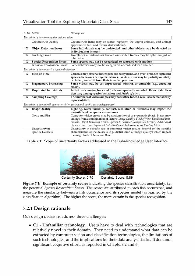
Visualization Tool for Exploring Uncertain Class Sizes 147
In UI Factor DescriptionUncertainty due to computer vision system
Groundtruth Quality Groundtruth items may be scarce, represent the wrong animals, odd animalappearances (i.e., odd feature distributions).
X Object Detection Errors Some individuals may be undetected, and other objects may be detected asindividuals of interest.
X Tracking Errors Trajectories of individuals tracked over video frames may be split, merged orintertwined.
X Species Recognition Errors Some species may not be recognized, or confused with another.Behavior Recognition Errors Some behaviors may not be recognized, or confused with another.
Uncertainty due to in-situ system deploymentX Field of View Cameras may observe heterogeneous ecosystems, and over- or under-represent
species, behaviors or objects features. Fields of view may be partially or totallyoccluded, and shift from their intended position.
X Fragmentary Processing Some videos may be yet unprocessed, missing, or unusable (e.g., encodingerrors).
X Duplicated Individuals Individuals moving back and forth are repeatedly recorded. Rates of duplica-tion vary among species behaviors and Fields of view.
X Sampling Coverage The numbers of video samples may not suffice for end-results to be statisticallyrepresentative.
Uncertainty due to both computer vision system and in-situ system deploymentX Image Quality Lighting, water turbidity, contrast, resolution or fuzziness may impact the
magnitude of computer vision errors.Noise and Bias Computer vision errors may be random (noise) or systematic (bias). Biases may
emerge from a combination of factors (Image Quality, Field of View, Duplicated Indi-viduals, Object Detection Errors, Species & Behavior Recognition Errors). Additionalbiases arise from Duplicated Individuals and heterogeneous Fields of View.
Uncertainty inSpecific Datasets
Uncertainty in specific sets of computer vision results depend on the specificcharacteristics of the datasets (e.g., distribution of image quality) which impactthe magnitude of Noise and Bias.
Table 7.1: Scope of uncertainty factors addressed in the Fish4Knowledge User Interface.
Figure 7.1: Example of certainty scores indicating the species classification uncertainty, i.e.,the potential Species Recognition Errors. The scores are attributed to each fish occurrence, andmeasure the similarity between a fish occurrence and its species model (as learned by theclassification algorithm). The higher the score, the more certain is the species recognition.
7.2.1 Design rationale
Our design decisions address three challenges:
• C1 - Unfamiliar technology. Users have to deal with technologies that arerelatively novel in their domain. They need to understand what data can beextracted by computer vision and classification technologies, the limitations ofsuch technologies, and the implications for their data analysis tasks. It demandssignificant cognitive effort, as reported in Chapters 2 and 6.

148 Chapter 7
• C2 - Multifactorial uncertainty. Users have to deal with multiple factors ofuncertainty, occurring at different information processing steps (Table 7.1). Theresulting complexity is a major challenge.
• C3 - Heterogeneous goals. Users have a variety of research goals, introduced inChapter 2. Users may need to apply specialized data analysis and visualizationmethods, which may not be addressed with a one-size-fits-all visualization tool.
To address these challenges, we aim at providing a generic user interface thatallows users to familiarize themselves with the data and its uncertainty (C1). We aimat supporting the exploration of the multidimensional data and uncertainty, whilelimiting visual and cognitive complexity. We thus use simple graphs and handlemultidimensionality with multiple views (C2). We target generic data analysis tasks,e.g., Retrieve, Filter, Determine Range, Correlate Information (Amar et al. 2005), andexclude advanced data mining and statistical methods (C3).
General layout - To explore the uncertainty factors at each information process-ing step, we organize information in tabs that represent the information processingsteps (e.g., from video collection, to video analysis, to data visualization and inter-pretation). The tabs guide users through the information processing technologies(C1, C2) and provide contextual information about the data, as recommended fornon-expert users (Heer et al. 2008). The rule of Diversity, i.e., separate different typesof information, inspired the organization of information into tabs (Wang Baldonadoet al. 2000).
Data filtering - As recommended by Elias and Bezerianos (2011), data filters aredisplayed at all times and propagated to all views and tabs of the interface (whenrelevant as some tabs do not display data). Propagating filters to all tabs and viewsfollows the rule of Consistency, i.e., make the interface consistent (filters are displayedthe same way) and the state of the interface consistent (same filters are applied, samedata subsets are displayed) (Wang Baldonado et al. 2000).
Data filters are selected using widgets, where each widget represents a specificdata dimension. The organization of multidimensional filters into widgets followsthe rule of Decomposition, i.e., create manageable chunks (Wang Baldonado et al.2000). The widgets are displayed on-demand to avoid information overload andcluttered interface. A textual summary of the selected filters is always displayed.
Data visualization - The interface provides interactive data visualizations in adedicated tab (the Visualization tab) and within the filter widgets. The widgets displaysmall histograms (Figure 7.2). The filter values are discrete, and each selectable valueis displayed on the histogram x-axis. Users can click on a histogram to select the datasubset represented by the histogram, and filter out the remaining data.
Widgets’ y-axis represent the same dimension as the y-axis of the main graph inthe Visualization tab. Users can select the dimension to display on the y-axis, forexample, a species’ population size. In this case, the widget to filter data from specificcameras shows the species distribution over the cameras, i.e., over the cameras’geographical locations.

Visualization Tool for Exploring Uncertain Class Sizes 149
Figure 7.2: The filter widgets that let users select the dataset of interest, e.g.., the timeperiods, camera locations, or fish species. The histograms provide an overview of the datadistributions. The y-axis represents the same dimension as the main graph of the Visualizationtab (Figure 7.3).
Using the same dimension on all y-axes (i.e., widgets and main visualization)follows the rules of Consistency and Complementarity (Wang Baldonado et al. 2000),i.e., expose the relationships between the data dimensions while limiting the interfacecomplexity (C1, C2). The interface can display data distributions on all differentdimensions (i.e., using the widgets) thus showing the relationships between datadimensions. For instance, a population size (y-axis dimension) is influenced by thepopulation distributions over species or camera locations (x-axis dimensions).
In the Visualization tab (Figure 7.3), users can select the dimensions displayed inthe x- and y-axes. Users can also change the type of graph, while keeping the sameaxes’ dimensions. Two graphs offer a third dimension: stacked charts (Figures 7.11-7.12) and boxplots (Figure 7.15) which use a third dimension to break down datainto stacked subsets, or subsamples for boxplots. Users can select visualizationvariants by swapping the graph axes and the type of graph. This navigation designsynthesizes features from ManyEyes (Viegas et al. 2007) (swap axes) and Tableau 2
(swap graph templates).As visualizations are modified (e.g., users select x-axis, then the y-axes, then the
data filters) and each modification is propagated to all graphs of the interface. Thefilters and y-axis are also propagated to the Video tab, i.e., the widgets remain the
2Tableau Software, http://www.tableausoftware.com
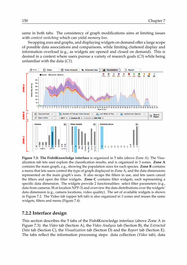
150 Chapter 7
same in both tabs. The consistency of graph modifications aims at limiting issueswith context switching which can yield memory loss.
Swapping axes and graphs, and displaying widgets on demand offer a large scopeof possible data associations and comparisons, while limiting cluttered display andinformation overload (e.g., as widgets are opened and closed on demand). This isdesired in a context where users pursue a variety of research goals (C3) while beingunfamiliar with the data (C1).
Figure 7.3: The Fish4Knowledge interface is organized in 5 tabs (above Zone A). The Visu-alization tab lets user explore the classification results, and is organized in 3 zones. Zone Acontains the main graph, e.g., showing the population sizes for each species. Zone B containsa menu that lets users control the type of graph displayed in Zone A, and the data dimensionsrepresented on the main graph’s axes. It also recaps the filters in use, and lets users cancelthe filters and open the filter widgets. Zone C contains filter widgets, each representing aspecific data dimension. The widgets provide 2 functionalities: select filter parameters (e.g.,data from cameras 38 at location NPP-3) and overview the data distributions over the widgets’data dimension (e.g., camera locations, video quality). The set of available widgets is shownin Figure 7.2. The Video tab (upper left tab) is also organized in 3 zones and reuses the samewidgets, filters and menu (Figure 7.4).
7.2.2 Interface design
This section describes the 5 tabs of the Fish4Knowledge interface (above Zone A inFigure 7.3): the Video tab (Section A), the Video Analysis tab (Section B), the ExtractedData tab (Section C), the Visualization tab (Section D) and the Report tab (Section E).The tabs reflect the information processing steps: data collection (Video tab), data

Visualization Tool for Exploring Uncertain Class Sizes 151
processing (Video Analysis tab), and data interpretation (Extracted Data, Visualizationand Report tabs). The first three tabs guide users through the computer vision systemcomponents, and the uncertainty factors they entail. The other two provide tools forinterpreting the computer vision results.
Figure 7.4: The Video Tab lets users explore the video footage (Zone A) and the numbers ofvideo samples over different dimensions (Zone C). Users can display numbers of video as they-axis of the widgets’ histograms, and open the widgets of interest (using menus in Zone B)
A. The Video tab
The Video tab supports direct browsing of the 10-minute video footages that wereprocessed by the computer vision system (Figure 7.4). It contains filter widgets forselecting the set of videos of interest (e.g., collected at specific locations and timeperiods). With this tab users can inspect the video data collection conditions: whichecosystems are observed, with which field of view and image quality (e.g., blurryimages, algae bloom yield green and murky water). Videos of the same image qualitycan be filtered by using the Video Quality widget.
This tab partially supports the assessment of uncertainty issues with Fields of View,Duplicated Individuals, Sampling Coverage and Image Quality (Table 7.1). Although noquantitative measurement of the uncertainty is provided, browsing the video footageoffers valuable means to visually assess these uncertainty factors. Users can visuallyassess biases due to low Image Quality and inadequate or shifting Fields of View. Thelatter impacts the chances of Duplicated Individuals and the geographical Sampling

152 Chapter 7
Coverage. Uncertainty can be further assessed by exploring the number of videosamples, i.e., if displayed as y-axis of filter widgets, per Image Quality, camera (i.e.,Field of Views) or time period (i.e., temporal Sampling Coverage), e.g., using the widgetsin Figure 7.4.
B. The Video Analysis tab
The Video Analysis tab provides explanations of the video processing steps, andvisualizations of computer vision errors. It explains basic technical concepts neededfor understanding computer vision uncertainty. The Overview sub-tab providesexplanations of the main video processing steps (Figure 7.5). The Fish Detection,and Species Recognition sub-tabs provide visualizations of the classification errorswhen detecting fish and non fish objects (Figure 7.6) and when classifying the fishspecies (Figure 7.7). The prototypes developed for the Fish4Knowledge project canbe improved by including the visualization introduced in Chapter 6, and the menuused in the Video and Visualization tabs (Figure 7.8).
The Workflow sub-tab provides on-demand video processing (Figure 7.9). Userscan request the analysis of specific videos (e.g., from time periods and camerasof interest) with specific component versions (e.g., with the fewest classificationerrors for the species of interest). It serves either for processing videos that werenot yet analyzed, or for experimenting with different versions of the video analysiscomponents (e.g., to check the robustness of observations).
Figure 7.5: The Video Analysis Tab - Overview sub-tab explains the video processing steps.

Visualization Tool for Exploring Uncertain Class Sizes 153
Figure 7.6: The Video Analysis Tab - Fish Detection sub-tab provides simplified visual-izations of classification errors for the Fish Detection algorithm (detecting fish and non-fishobjects). Errors are detailed for each type of video quality, and each version of the FishDetection algorithm.
Figure 7.7: The Video Analysis Tab - Species Recognition sub-tab provides clear and simplevisualizations of classification errors for the Species Recognition components. Errors aredetailed for each species, and each version of the Species Recognition algorithm. The algorithmversion R52 can recognize fewer species than the R51 version, as the R52 algorithm focuses onrecognising the most important species (from ecologists’ point of view), hence excluding therecognition of less important species (which are rare species in the environment studied byecologists).

154 Chapter 7
Figure 7.8: Alternative for the Video Analysis Tab - Species Recognition sub-tab usingClassee visualization (Chapter 6) and menus from the Video and Visualization tabs (Zone B inFigures 7.3 and 7.4).
Figure 7.9: The Video Analysis Tab - Workflow sub-tab supports user requests for specificvideo processing tasks to be executed by the computer vision system. The interface shows theclassification errors of the component versions that users plan to use.

Visualization Tool for Exploring Uncertain Class Sizes 155
The Video Analysis tab supports the assessment of uncertainty issues with ObjectDetection Errors and Species Recognition Errors (Figures 7.6 to 7.7). Future work isrequired to enable the assessment of Object Tracking Errors, Groundtruth Quality, asno well-established method are available for assessing these uncertainty factors, andtheir high-level impact on the Noise and Bias in the classification results (Chapter 4,Section 4.4.1, p.67).
Assessing Groundtruth Quality can be enabled by letting users display numbers ofgroundtruth items as the y-axis of widgets and main graph in the Visualization tab.However, each classification component (e.g., object detection, tracking and speciesrecognition) may be evaluated with their own groundtruth. In this case, the numbersof groundtruth items must be displayed for each groundtruth set. This requires addingseveral dimensions that can be displayed as y-axes, which increases user cognitiveload. By visualizing the groundtruth size, groundtruth scarcity and imbalance maybe assessed. However, the uncertainty propagation to the classification end-resultsis not addressed and requires future work.
C. The Extracted Data tab
The Extracted Data tab specifies the characteristics of the information extracted fromthe video footage, i.e., the data dimensions. It explains 4 metrics provided fordescribing fish populations, and that can be displayed as the y-axis of the widgetsand main graph in the Visualization tab:
• Number of Fish• Number of Video Samples (e.g., to check for missing videos and assess Frag-
mentary Processing )• Mean Number of Fish per Video Sample (e.g., to compensate for missing videos,
introduced in Chapter 4, Section 4.4.2, equation (4.1) p.71)• Number of Species (e.g., for studying species richness, a user information need
identified in Chapter 2, Section 2.3, p.22).
This tab shows the aspects of fish populations that can be monitored with thecomputer vision system. The overview of the data dimensions helps identify theinformation that is relevant for users’ research goals (Challenge C3, Section 7.2.1) andthe functionalities for filtering and visualizing datasets of interest. Future work caninvestigate more elaborate tutorials, e.g., improved textual and visual explanations(e.g., animations, or comic book style tutorials as in Figures 5.11-5.12, p.112).
D. The Visualization tab
The Visualization tab, shown in Figure 7.3 p.150, provides a means of exploring thecomputer vision results, e.g., the class sizes representing fish population sizes. Thelayout is organized in 3 zones. Zone A contains the main graph, Zone B provideswidgets for filtering data, and Zone C controls the widget display and the adaptationof the main graph to specific user needs.

156 Chapter 7
Figure 7.10: The Extracted Data tab provides a schema of the data dimensions, and explana-tions of the y-axis metrics.
In Zone B, users can specify what the axes of the main graph represent. Forinstance, while the y-axis represents numbers of fish, the x-axis can represent theirdistribution over weeks of the year (Figure 7.3) or hours of the day (Figures 7.11-7.12).Users can also select other types of graph, e.g., stacked chart or boxplot, leading tothe display of dedicated menus for adapting the visualization further. For instancefish counts can be stacked by species (Figure 7.11) or by camera (Figures 7.12).
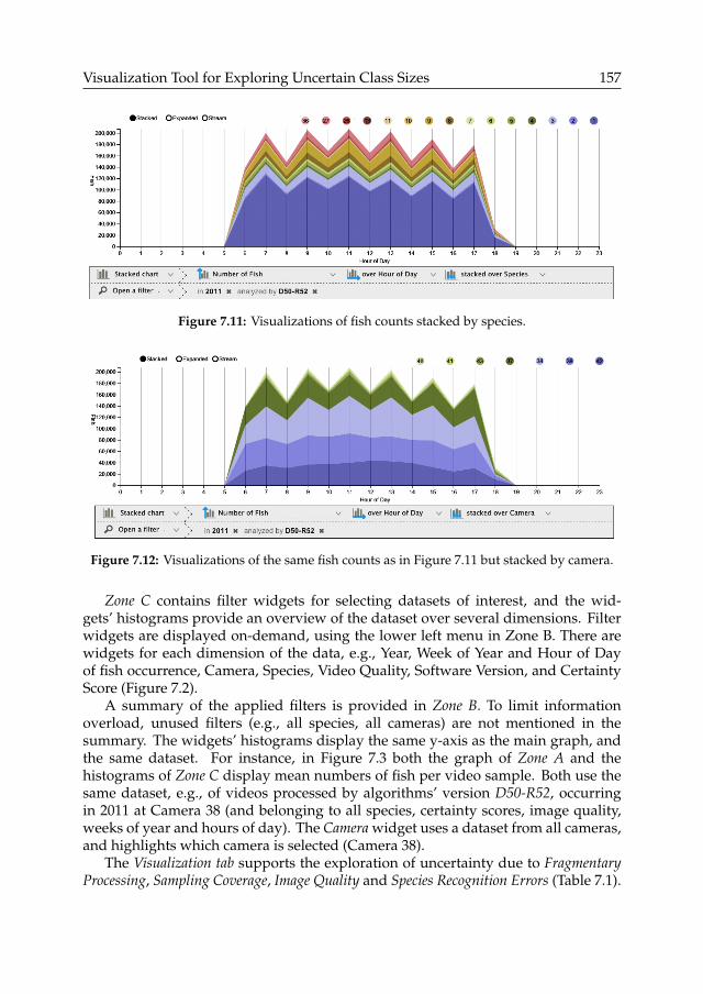
Visualization Tool for Exploring Uncertain Class Sizes 157
Figure 7.11: Visualizations of fish counts stacked by species.
Figure 7.12: Visualizations of the same fish counts as in Figure 7.11 but stacked by camera.
Zone C contains filter widgets for selecting datasets of interest, and the wid-gets’ histograms provide an overview of the dataset over several dimensions. Filterwidgets are displayed on-demand, using the lower left menu in Zone B. There arewidgets for each dimension of the data, e.g., Year, Week of Year and Hour of Dayof fish occurrence, Camera, Species, Video Quality, Software Version, and CertaintyScore (Figure 7.2).
A summary of the applied filters is provided in Zone B. To limit informationoverload, unused filters (e.g., all species, all cameras) are not mentioned in thesummary. The widgets’ histograms display the same y-axis as the main graph, andthe same dataset. For instance, in Figure 7.3 both the graph of Zone A and thehistograms of Zone C display mean numbers of fish per video sample. Both use thesame dataset, e.g., of videos processed by algorithms’ version D50-R52, occurringin 2011 at Camera 38 (and belonging to all species, certainty scores, image quality,weeks of year and hours of day). The Camera widget uses a dataset from all cameras,and highlights which camera is selected (Camera 38).
The Visualization tab supports the exploration of uncertainty due to FragmentaryProcessing, Sampling Coverage, Image Quality and Species Recognition Errors (Table 7.1).

158 Chapter 7
The type of Image Quality is detected for each video sample during pre-processing(i.e., before recognizing the objects occurring in the videos). This uncertainty factorcan be assessed by visualizing the distribution of video samples over the types ofimage quality. Species Recognition Errors can be assessed using the Certainty Scorewidget. Certainty scores and types of image quality are data dimension that can bedisplayed as the main graph’s x-axis, and filtered using dedicated widgets. However,filtering by certainty scores must be used with care as it can introduce biases. Forexample, when filter out low certainty scores, most fish may be filtered out and theselected data may not represent the actual fish populations.
Fragmentary Processing, i.e., missing videos, impacts the temporal and geograph-ical Sampling Coverage. Videos can be missing due to camera maintenance, encodingerrors, or unfinished processing queues. Users can explore the number of videosamples available for each data dimension, i.e., by selecting number of videos asy-axis, and opening widgets or modifying the main graph’s x-axis (Figures 7.13).Users can also explore how variations in numbers of video impact the class sizes,i.e., by switching the y-axis between numbers of fish and numbers of videos. Finallyusers can explore normalized population sizes, abstracted from variations in videonumbers, i.e., by displaying the mean number of fish per video as the graph’s y-axis(Figure 7.14 using equation (4.1) from Chapter 4, p.71).
Figure 7.13: Visualization of the number of videos from which fish counts in Figures 7.11-7.12were extracted. The number of videos has a direct impact on the absolute fish counts: themore the videos, the higher the fish counts. The results shown in this Figure are an example ofFragmentary Processing issues (Table 7.1). The variations in numbers of videos shown in this Figureare due to the batch processing strategy. To process videos over an entire year, and obtain preliminaryresults, batches of videos are processed for every uneven hour of the year (e.g., all videos recorded at07:10, 09:10, 11:10 etc..) and then other batches of videos for every even hour. This process is repeateduntil the entire video collection is processed.

Visualization Tool for Exploring Uncertain Class Sizes 159
Figure 7.14: Visualization of the mean number of fish per video. It balances the impact ofheterogeneous numbers of videos on absolute fish counts shown in Figures 7.11-7.12.
Figure 7.15: Visualization showing the variance of mean number of fish per video. The datasetselected in Figure 7.14 is sub-sampled each week of the year. The boxplot shows how fishcounts for each hour of the day vary over the weeks of the year.
E. The Report tab
The Report tab supports manual grouping and annotation of graphs created in theVisualization tab (Figure 7.16). Visualizations can be added to and removed from areport, and their interpretation can be described with free-form text. Using the Down-load button, users can save the report they are currently working on. Downloadedreports consist of a text file containing a list of parameters. They can be stored orshared with other users as any kind of text file. To visualize a downloaded report,users can upload the parameter files with the Upload button of the Report tab. Withthis tab, users can document their data exploration and interpretation process, andtheir findings.

160 Chapter 7
Figure 7.16: The Report tab showing two visualizations (i.e., Figures 7.11-7.12) that are saved ina report, together with their specifications (i.e., filters and displayed dimensions are recappedabove the graphs). Users can comment their findings in free-form text (i.e., using the text fieldson the right of the graphs).
7.2.3 Usage scenario
This section describes typical interactions involved in the analysis of population sizes(i.e., the analysis of class sizes) and two uncertainty issues: Species Recognition Errorsand Fragmentary Processing (Table 7.1). More detailed usage scenarios are given inAppendix 1 of the Fish4Knowledge book (Beauxis-Aussalet and Hardman 2016).
The usage scenario described in this section focuses on the interaction and layoutdesign evaluated in Section 7.3. The usage scenario is illustrated with screenshots ofthe user interface prototype that was used to conduct the user study. The prototypewas later refined, based partially on the results of this evaluation, which explains thesmall differences with the interface presented in Section 7.2.2.
A. Exploring issues with Fragmentary Processing
When analyzing the fish populations in Figure 7.17, users may wonder if the popula-tion sizes drop in weeks 35 and 45 due to missing videos. Using the Y Axis menu inZone B, they can display the numbers of videos from which fish counts were extracted(Figure 7.18). As no videos were processed for Week 45, no insight can be drawn onfish populations in this period. Considering the high variability of video numbers,visualizing mean numbers of fish per video is preferable to visualizing absolute fishcounts. The Y Axis menu provides this visualization (Figure 7.19).
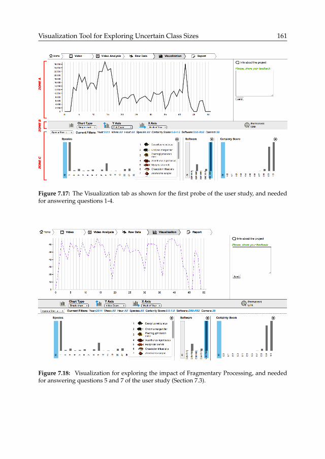
Visualization Tool for Exploring Uncertain Class Sizes 161
Figure 7.17: The Visualization tab as shown for the first probe of the user study, and neededfor answering questions 1-4.
Figure 7.18: Visualization for exploring the impact of Fragmentary Processing, and neededfor answering questions 5 and 7 of the user study (Section 7.3).

162 Chapter 7
Figure 7.19: Visualization for exploring the impact of Fragmentary Processing, and neededfor answering questions 6 and 7 (Section 7.3).
B. Exploring classification uncertainty
Considering that the trends in fish population sizes are not due to varying numbersof videos, users can question the reliability of the species recognition. The widgetCertainty Score shows the quality of fish appearances (Figure 7.1). The more fish withhigh certainty scores, the more reliable the species recognition. Users can use thecertainty scores to estimate potential biases due to species recognition errors. Forexample, Figures 7.20-7.21 compare the classification uncertainty for species 1 and 2.Higher certainty scores are observed for species 2, thus its recognition is likely to bemore reliable than for species 1. Similarly, users can compare the certainty scores forweek 35 with other weeks.
The classification uncertainty can be further detailed using the Video Analysis tab.However, this tab was excluded from our user study in Section 7.3, as we focus onevaluating the Visualization tab. The evaluation of the visualization of classificationerrors displayed in the Video Analysis tab is discussed in Chapter 6. The user studypresented in this chapter focuses on the usage of certainty scores as an alternativemetric of classification uncertainty.
In future work, the classification uncertainty should be represented in the Visual-ization tab by applying the methods for estimating classification errors in end-resultsintroduced in Chapter 5. However, this chapter focuses on evaluating the multipleview design of the Visualization tab, the menus to modify the graph’s axes, and theusage of certainty scores. The Fish4Knowledge user interface was implemented be-fore we developed the error estimation methods in Chapter 5. These error estimationmethods were not implemented within the Fish4Knowledge user interface, becauseadditional uncertainty assessment methods are required to measure the impact of

Visualization Tool for Exploring Uncertain Class Sizes 163
errors from the Tracking component (Section 4.4.1, p.67). The challenge of assess-ing the uncertainty that propagates from the Tracking component to high-level classsizes remains unaddressed (Section 8.1.1, p.178). Therefore, the Fish4Knowledgeuser interface could only provide measurements of the Species Recognition Errors atthe level of individual fish images, and not at the level of entire fish trajectories.
Figure 7.20: Widgets showing the certainty scores for species 1.
Figure 7.21: Widgets showing the certainty scores for species 2, and needed for answeringquestion 18 of the user study (Section 7.3).
C. Comparing class sizes
For comparing the population sizes for each species, users have several options:
• Display the Species widget (e.g., Figure 7.21 right)• Select Species as the dimension represented by the main graph’s x-axis.• Select Stacked chart in the Chart Type menu, and select Species as the dimension
used for decomposing the fish counts (e.g., Figure 7.3 p.fc).
7.3 Evaluation
This section reports a user study that evaluates how the interface design supportsuser awareness of uncertainty. The study focuses on the Visualization tab and aimsat identifying usability issues with the interface layout and interaction design. Thestudy also investigates how providing certainty scores (Figure 7.1, indicating po-tential Species Recognition Errors), numbers of videos (Figure 7.13, showing potentialFragmentary Processing), and mean number of fish per video (Figure 7.14, compen-sation potential Fragmentary Processing) address user information needs on theseuncertainty factors (Table 7.1).
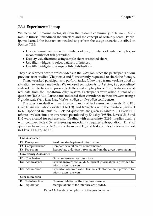
164 Chapter 7
7.3.1 Experimental setup
We recruited 10 marine ecologists from the research community in Taiwan. A 20-minute tutorial introduced the interface and the concept of certainty score. Partic-ipants learned the interactions needed to perform the usage scenario described inSection 7.2.3:
• Display visualizations with numbers of fish, numbers of video samples, ormean number of fish per video.
• Display visualizations using simple chart or stacked chart.• Use filter widgets to select datasets of interest.• Use filter widgets to compare fish distributions.
They also learned how to watch videos in the Video tab, since the participants of ourprevious user studies (Chapters 2 and 3) recurrently requested to check the footage.
Then, we asked participants to perform tasks, following a framework inspired bysituation awareness methods. We exposed participants to 3 probes, i.e., predefinedstates of the interface with preselected filters and graph options. The interface showedreal data from the Fish4Knowledge system. Participants were asked a total of 20questions(Table 7.3). Participants indicated their confidence in their answers using a5-grade scale (Very Low, Low, Moderate, High or Very High confidence).
The questions dealt with various complexity of Fact assessment (levels F1 to F3),Uncertainty evaluation (levels U1 to U3), and Interaction with the interface (levels I1to I2), specified in Table 7.2. Related questions are given in Table 7.3. Levels F1-3refer to levels of situation awareness postulated by Endsley (1988b). Levels U1-3 andI1-2 were created for our use case. Dealing with uncertainty (U2-3) implies dealingwith complex facts (F3), as assessing uncertainty requires extrapolation. Thus allquestions from levels U2-3 are also from level F3, and task complexity is synthesisedin 4 levels F1, F2, U2, U3.
Fact AssessmentF1 Perception Read one single piece of information.F2 Comprehension Compare several pieces of information.F3 Projection Extrapolate unknown information from the given information.
Uncertainty AssessmentU1 Conclusive Only one answer is entirely true.U2 Ambivalence Several answers are valid. Sufficient information is provided to
inform users’ answers.U3 Assumption Several answers are valid. Insufficient information is provided to
inform users’ answers.
User InteractionI1 No Interaction No manipulation of the interface is needed.I2 Exploration Manipulations of the interface are needed.
Table 7.2: Levels of complexity of the questionnaire.
Visualization Tool for Exploring Uncertain Class Sizes 165
The questionnaire was designed to draw attention to two uncertainty factors:Species Recognition Errors and Fragmentary Processing (Table 7.1). Issues with Frag-mentary Processing were emphasized in questions Q5 and Q11-13. These questionsrequired participants to inspect the numbers of video samples, and were asked beforethe questions requiring users to inspect the fish population sizes. Prior to questionQ5 users dealt with absolute fish count and later with mean fish count per videosample, hence showing the effect Fragmentary Processing. Question Q13 explicitlyexamines the suitability of sampling size for scientific research.
In the following questions, we investigate whether participants acquired aware-ness of uncertainty issues due to Fragmentary Processing. Participants were notexplicitly asked to inspect the numbers of video samples, and to use mean fish countper video instead of absolute fish counts. We consider that participants who do notinspect this information have not acquired the desired awareness of uncertainty.
Guiding participants’ attention may artificially enhance their awareness of Frag-mentary Processing. However this was desired both a priori, as Fragmentary Pro-cessing is an unfamiliar concept, and a posteriori, considering participants’ poorreactivity to this awareness factor.
Usability issues and wrong answers were reported. Under uncertainty (levelsU2-3), answers such as "I don’t know" were considered as one of the possible validanswers, and were not considered as wrong answers.
This experimental setup allowed to observe:
• How users interact with the visualization when seeking information (e.g., usingthe widgets’ overviews or the main graph).
• The usability issues that arise with either the layout or the interactions (e.g.,with questions of levels I1-2, with or without interactions).
• How user confidence varies among the levels of information complexity (levelsF1, F2, U2, U3).
• The quality of user awareness of uncertainty (e.g., confidence should be lowwith high uncertainty or wrong answers).
The small numbers of participants and questions for each condition (levels F1-F3,U1-U3, I1-I2) may not represent the general population, and our results may not begeneralizable. However, our experiment is suitable for identifying major usabilityissues, and for eliciting recommendations for refining the means to support userawareness of uncertainty.

166 Chapter 7
Question ComplexityProbe 1 (Fig. 7.17)Q1 What is the number of fish for the week 12? F1 U1 I1Q2 For which cameras are we counting the fish? F1 U1 I1Q3 Which week of the year has the most fish? F2 U1 I1Q4 At which period of the year can we observe the highest fish count? F3 U2 I2Q5 How many videos were analyzed for the week 12? F1 U1 I2Q6 What is the number of fish per video for the week 12? F1 U1 I2Q7 What is the fish abundance for the week 45? F3 U2 I2Q8 Which week of the year has the highest number of fish per video? F2 U1 I1Q9 What is the period of the year for which the fish population is the most abundant? F3 U2 I1Q10 Is it the same period of time for the camera 37? F3 U3 I2Probe 2 (Fig. 7.22)Q11 Is the number of video samples constant over hours of the day? F2 U1 I1Q12 Is the number of video samples constant over weeks of the year? F2 U1 I2Q13 Is the amount of video samples suitable for scientific research? F3 U3 I1Q14 Which is the most abundant species in HoBiHu? F2 U1 I1Q15 Which camera has the most abundant fish population from the species 2 (Chromis
Margaritifer)?F3 U3 I2
Q16 Do fish from species Chromis Margaritifer generally have high certainty scores? F2 U1 I2Q17 Is the abundance of species 2 (Chromis Margaritifer) lower than species 1 (Dascillus
Reticulatus)?F2 U1 I1
Q18 Is it because the video analysis may not correctly detect the species 2 (Chromis Margar-itifer)
F3 U3 I2
Probe 3 (Fig. 7.23)Q19 Is there a correlation in the occurrence of fish from species 9, 26 and 27 over weeks of
the year? (considering the entire dataset, for all time periods and all cameras)F3 U3 I2
Q20 Is there a correlation in the occurrence of fish from species 9, 26 and 27 over hours ofthe day?
F3 U3 I2
Table 7.3: The questionaire of the user study. Questions were provided in English and Chinese,and were translated by a native Chinese speaker from the Fish4Knowledge project.
User 1 User 2 User 3 User 4 User 5 User 6 User 7 User 8 User 9 User 10Level Err. Conf. Usa. Err. Conf. Usa. Err. Conf. Usa. Err. Conf. Usa. Err. Conf. Usa. Err. Conf. Usa. Err. Conf. Usa. Err. Conf. Usa. Err. Conf. Usa. Err. Conf. Usa.
Q1 F1 I1 5 3 5 5 5 5 5 5 4 5Q2 F1 I1 5 5 5 5 5 5 5 4 4 5Q3 F2 I1 5 5 X 5 5 5 5 5 5 4 5Q4 U2 I1 3 4 5 5 4 3 4 W 5 3 4Q5 F1 I2 4 4 5 5 W 5 W 4 W 3 W 2 4 3Q6 F1 I2 4 4 X 4 4 5 4 4 1 X 4 5Q7 U2 I2 W 5 W 5 W 4 W 5 W 5 W 3 X W 5 W 3 X W 2 W 5Q8 F2 I1 5 5 5 5 5 5 5 W 5 X 4 5 XQ9 U2 I1 3 4 5 5 5 4 5 4 X 4 4
Q10 U3 I1 4 W 4 X W 5 W 4 X W 5 X 5 5 4 W 4 X W 5 XQ11 F2 I1 5 W 5 W 3 5 5 W 4 5 4 4 4Q12 F2 I2 4 5 W 4 5 5 5 5 W 3 X 4 4Q14 F2 I1 5 5 5 5 5 5 5 5 4 5Q15 U3 I2 4 4 5 4 3 4 2 W 4 X 4 3Q16 F2 I2 4 3 4 5 5 5 5 5 4 5Q17 F2 I1 4 4 5 5 W 5 W 5 5 W 3 X 3 5Q18 U3 I2 W 1 W 3 W 4 5 W 2 5 4 4 3 W 2Q19 U3 I2 4 4 4 5 4 4 5 3 3 5Q20 U3 I2 4 3 4 5 5 5 5 4 W 2 X W 2 X
Table 7.4: Detail of incorrect answers (Err.), user confidence (Conf.) and usability issues (Usa.).

Visualization Tool for Exploring Uncertain Class Sizes 167
Figure 7.22: The second probe of the experiment.
Figure 7.23: The third probe of the experiment.

168 Chapter 7
7.3.2 Experiment results
The results are detailed in Table 7.4 and summarized in Figure 7.24. Question Q13was discarded since answer correctness is ambiguous: the most precise answer is"It depends on research goals" as replied by one single user. To analyse participants’answers, we partitioned questions into groups containing distinct questions andrepresenting task complexity (F1, F2, U2, or U3), interaction complexity (I1 or I2),answers’ validity (Right or Wrong), and usability (Issue or No issue). With thesegroups of questions, we can observe the impact of tasks and interface complexity onparticipants’ awareness of uncertainty.
Figure 7.24: Proportions of right and wrong answers (top) and usability issues (bottom) foreach question groups (x-axes).
Participants’ confidence in their answers is shown in Figure 7.25. Participantswere generally highly confident, even when answers were wrong or uncertainty washigh. Level 5 is often the default answer, but some participants consider level 4as the default, making comparisons difficult, e.g., for Participant 4, level 4 is weakconfidence while being the optimal confidence for Participant 9.
To compare participants’ confidence, we focus on confidence drifts (i.e., relativechanges in confidence) rather than absolute confidence levels. For instance, confi-dence drifts are calculated by 1) averaging each participant’s confidence for groupsF1 and F2 distinctively; 2) subtracting each participant’s average confidence to getthe participant’s confidence drift between groups F1 and F2.
We analyse confidence drift between question groups (Figure 7.26):• The groups F1-F2, F2-U2, and U2-U3 represent questions with increasing infor-
mation complexity.
• The groups I1-I2 represent questions involving interaction or not.
• The groups Right-Wrong (or R-W) represent questions which answers wereright or wrong.

Visualization Tool for Exploring Uncertain Class Sizes 169
• The groups NoIssue-Us.Issue represent questions for which no usability issueoccurred, or were usability issues were identified by the interviewers. Theusability issues are reported in Section 7.3.3.
We also distinguish the effect of uncertainty and user interface, represented with thefollowing question groups:• The groups Certain-Uncertain (F1∪F2 against U2∪U3) represent questions im-
pacted by uncertainty issues or not.
• The groups Certain,I1-Certain,I2 (Certain∩I1 against Certain∩I2) representquestions involving interaction or not, while uncertainty issues must be con-sidered.
• The groups Uncertain,I1-Uncertain,I2 (Uncertain∩I1 against Uncertain∩I2)represent questions involving interaction or not, while no uncertainty issuesneed to be considered.
Figure 7.25: Confidence levels for all questions (upper boxplots) and groups of questions(lower line charts, with mean +/- 2 standard deviations).

170 Chapter 7
Figure 7.26: Confidence drifts per question groups.
Except for the groups F1-F2, increasing question complexity yielded a decrease inparticipants’ confidence. Their confidence decreased whether the complexity arisefrom the information features3 or from the interface features4.
However, the statistical significance of the observed confidence drifts is not es-tablished. Using Welch t-test (compensating for the unequal variance shown inFigure 7.25), we tested the confidence drifts of each participant. For instance, weselected the answers of a single participant. We aggregated this participant’s confi-dence in the answers to questions from group F1 and F2. We then applied Welch teststo assess the statistical significance of the difference in the participant’s confidencebetween the groups F1 and F2 (i.e., the probability that the observed confidencedrift occurred by chance, while there is no actual confidence drift but just randomvariations of the participant’s confidence).
The resulting p-values are generally much greater than 0.05 (Figure 7.27). Thenumber of cases where p < 0.05 happened with a frequency of around 0.05, and thusmay be due to random effects. Each user’s confidence had mostly the same value(e.g., level 5 or 4 by default, Figure 7.25 top). Participants’ confidence was rarelylower than their default confidence levels. Thus, in general, participants’ confidencelevels do not differ significantly between question groups.
3 i.e., between the question groups F2-U2, U2-U3, Certain-Uncertain, and Right-Wrong4 i.e., between the question groups I1-I2, Us.Issue-NoIssue, CertainI1-CertainI2, and UncertainI1-
UncertainI2

Visualization Tool for Exploring Uncertain Class Sizes 171
0.0
0.2
0.4
0.6
0.8
1.0
p Va
lues
F1vsF2
F2vsU2
U2vsU3
I1vsI2
Rightvs
Wrong
No Issuevs
Usa.Issue
Certainvs
Uncert.
Uncert.I1 vs I2
CertainI1 vs I2
Figure 7.27: Results from Welch t-tests (each point represents a user). T-tests were skipped if auser’s confidence was equal for all answers, i.e., for groups F1-F2 (1 user), F2-U2 (1 user), CertainI1-CertainI2 (1 user). T-tests were skipped for group Us.Issue-NoIssue if a user had no usability issues(6 users).
However, two observations give credence to the conclusion that uncertainty andinteractivity had similar effects on participants’ confidence:
• Observation O1: Except for groups F1-F2, confidence consistently decreasedwith questions’ complexity. If the effect was random, confidence drifts wouldshow as many increases than decreases.
• Observation O2: Confidence drifts are the most significant for the groups I1-I2,with the lowest variance and p-values (Figure 7.27), and median drift similarto that of the groups Certain-Uncertain (Figure 7.26).
We noticed that wrong answers and usability issues had an important effect onparticipants’ confidence (Figure 7.25), but are outlying conditions (low numbersof observations, Figure 7.24). Further, wrong answers and usability issues oftenoccurred together. Thus we repeated the analysis on right answers with no usabilityissue, and obtained similar observations (O1-O2).
We conclude that either interacting with the visualization, or analysing uncer-tain data, had similar effects on users’ perception of uncertainty. This biases userawareness of uncertainty: low user confidence may not assess the strength of users’data interpretation, but may reflect difficulties with using the interface.
7.3.3 Interpretation and recommendations
This section discuss the insights drawn from the qualitative analysis of participants’answers and behaviors when interacting with the interface.

172 Chapter 7
Over-confidence - Participants’ confidence was generally high, even for wronganswers and uncertain information. Over-confidence may be due to the presenceof observers during the task, inducing a will to perform well (Hawthorne effect).Participants may feel the need to perform well, thus to express only sure answers.We recommend that studies of user awareness of uncertainty give strong incentivesfor users to express their low confidence. For example, the 5-grade Likert scalemay be reduced to a single checkbox for users to indicate when they are not fullyconfident.
Fragmentary Processing - Users overlooked uncertainty due to FragmentaryProcessing. No spontaneous Projection (F3) of possible scarcity of video samplesoccurred. For instance, questions Q7, 10, 19, and 20 did not show numbers of videos,and most users did not spontaneously investigate potential imbalances in numbersof videos. Hence answers were fortuitously correct, and no right answers weregiven to Q7 that concerned a time period for which no video samples were available.However, Perception (F1) and Comprehension (F2) of numbers of videos were correct(Q5, 11, 12).
Experimental setup - Issues with overlooking Fragmentary Processing may berelated to the experimental setup. The terminology may be ambiguous, e.g., "What isthe fish abundance?" (Q7) may be interpreted as a need for raw fish count (i.e., simplyreading the graph, instead of modifying it to check the numbers of of video samples).Further, the early prototype used for the experiment provided widget histogramsthat could only display raw fish counts, not the mean number of fish per videosample. Thus it may seem that raw fish count is the main metric for fish abundance.It may have deflected users’ attention from the mean number of fish per video, andthe potential issues with Fragmentary Processing.
Choice of metrics - Fragmentary Processing issues are similar to sampling sizeissues, e.g., insufficient number of samples, a well-known concern in marine ecology.However, Fragmentary Processing is specific to computer vision, and not assimi-lated by ecologists. They may expect video stream processing to be continuous,rarely missing videos. Hence we recommend that Fragmentary Processing issues arealways made explicit. Raw fish counts can be misleading, and by default, shouldnot be displayed. Mean number of fish per video could be displayed together withan indication of the sampling size, e.g., encoded as an extra visual dimension such astransparency, or by showing confidence intervals. Boxplots, a type of graph availablebut not investigated in this study, can also show sampling size, e.g., encoded in theirwidth (McGill et al. 1978). It may prevent memory-loss (e.g., forgetting the numbersof videos).
Ultimately, the metrics used to represent population sizes should integrate theestimation of classification errors introduced in Chapter 5. The number of fishaveraged over video sampled should be the corrected number of fish resulting fromChapter 5’s methods. Displaying variance estimates is also crucial to uncertaintyawareness. The variance estimates must considered both the variance related tothe number of video samples (equations (4.2) and (4.4), p.71), and the variance of

Visualization Tool for Exploring Uncertain Class Sizes 173
Chapter 5’s methods (related to class sizes of the test set and of the dataset underanalysis, Section 5.4, p.85).
This approach provides more complete information on the uncertainty in thecomputer vision end-results. However, it requires users to deal with highly complexinformation, involving several layers of uncertainty assessment and rather complexequations. Yet users must understanding the underlying methods that providedsuch results, otherwise they cannot make informed decisions when interpreting thepopulation sizes. Hence future work is required to investigate the means to ex-plain and visualize such complex information combining the uncertainty assessmentFragmentary Processing and Noise and Bias due to classification errors.
Certainty scores - No users spontaneously considered the certainty scores, whichare unfamiliar and complex. However, some users spontaneously noticed uncertainfactors not included in the scope of the tutorial and questions: issues with Fieldsof View, Duplicated Individuals and differentiating Biases from Noise (Table 7.1).Assessing these uncertainty issues may be more important to build end-users’ trustand confidence than providing certainty scores. Furthermore, using certainty scoresas filters may introduce biases in end-users’ data interpretation. For instance, the sizesof populations recognized with high certainty scores only may not be representativeof the actual population sizes. If the large majority of fish have average or lowcertainty scores, very high certainty scores are conceptually close to being outliers.Hence, certainty scores did not demonstrate opportunities for supporting users’uncertainty awareness.
Learning curve and usability - The increase in confidence observed between F1and F2 questions, although not statistically signifiant (p=0.07, Welch t-test), suggestsan effect of the learning curve. Overcoming slightly higher complexity may inducea sentiment of higher level of expertise. User confidence may be reinforced becausethey gained experience with the interface, while the information they had dealt withdoes not justify increased confidence.
Similarly, difficulties interacting with the interface, and using unfamiliar function-alities, may reduce user confidence. As users need to learn the interaction features,they may not be confident that their interactions with the interface, and thus theobtained information, are correct.
We thus recommend to provide tutorials and memos that summarize the basicuncertainty exploration steps needed for valid data analysis. These should be easilyaccessible from the user interface, for quick checks while interacting with the data.
Filter widgets - Predefined filters of the 3rd probe were often overlooked, proba-bly because participants did not select the filters up themselves. However, it suggestspotential attention tunnelling issues with the layout design. Users’ attention maybe directed to more salient features of the interface, e.g., the main graph, rather thanthe selected filters. In the next version of the interface, filters were reinforced andhighlighted in Zone B (Figure 7.3). The latest version of Zone B (e.g., Figure 7.13p.158) describes both the main graph and the filters in natural language, and servesas a title for the main graph.

174 Chapter 7
The dimensions not used for filtering (e.g., all years, all certainty scores, Fig-ure 7.23) can saturate users’ working memory, and are no longer displayed in therefined interface. Participants tried to click on the filter summary, thus we addedinteractions for resetting the filters (cross buttons next to each dimension in the filtersummary, e.g., Figure 7.13 p.158).
Interaction and layout design - The interaction design for manipulating thewidgets and the main graph was welcomed and easily understood ("It is very nice,I can display anything I want."). Participants used either the widgets’ histogramsand the main graph when appropriate. It suggests that our interaction design isreasonable, while our layout design raised most of the usability issues.
We recommend that uncertainty is always salient in the interface. It may com-plicate the layout design, yet it may be the best tradeoff regarding the high riskof misinterpretation. Our design of simple graphs in multiple views is intuitiveand quickly understood. However, it may over-simplify data exploration at thecost of concealing the uncertainties. Over-simplification may enhance attentiontunnelling, memory loss and over-confidence.
7.4 Conclusion
We presented a design for visualizing multidimensional and uncertain computervision results. We evaluated the interactive design for exploring the multiple dimen-sions and uncertainty factors of the data. It aims at limiting information overloadand interface cluttering, while facilitating the exploration of data dimensions withflexible visualizations. It supports preliminary data analyses for a wide range ofpotential usage of the dataset, which may be achieved with specialized data analysistechniques. Our design for preliminary data exploration can help users to familiar-ize themsleves with novel datasets, and identify issues and uncertainties that mayimpact further data analyses.
Our interaction design was found intuitive and easy to understand, although thedataset was unfamiliar to users. The layout and interaction principles can integrateinformation on the uncertainty factors presented in Chapter 4, the error estima-tion methods presented in Chapter 5, and the visualizations of classification errorspresented in Chapter 6. Thus the interface design addresses the requirement 4-dCommunicate uncertainty to end-users, identified in Chapter 2 (p.36).
Our design can contribute to similar use cases, possibly within domains otherthan marine ecology. For instance, the interface template was reused for a demon-stration of the SightCorp company’s classification system (Figure 7.28). However, forcommercial applications, the information provided on uncertainty factors require adifferent approach than for scientific applications. For instance, marketing strategiesand the impact on customers’ trust must be carefully considered.
Our evaluation method, inspired by Situation Awareness, allowed us to distin-guish issues of either layout or interaction design. This evaluation methodology canbe applied to other evaluations of interactive visualizations.

Visualization Tool for Exploring Uncertain Class Sizes 175
Figure 7.28: Reuse of the interface for the SightCorp company, where class sizes represent hu-man emotions recognized by the company’s computer vision system (https://sightcorp.com/).
Our main finding is that user confidence is generally high, and subjectively influ-enced by the interactions with the visualization: interaction complexity had effectssimilar to uncertainty itself. Using simple graphs with multiple views achieves highintuitiveness but may have negative effects on user awareness of uncertainty. Theintuitiveness of the graphs and interactions may have contributed to overconfidencethrough a sentiment of mastering the interface and its information, which led tooverlooking uncertainty issues. Furthermore, uncertainty assessment requires thevisualization of several graphs within multiple views, which may result in atten-tion tunnelling and memory loss, and induce misinterpretations and unawareness ofcrucial information on uncertainty.
We derive two main recommendations for improving the visualization interfaceand supporting user awareness of uncertainty:
• Salient and persistent display uncertainty measurements. The main visu-alization (e.g., used to explore population sizes) should always display indi-cations of the uncertainty issues, e.g., encoded with visual features such astransparency or boxplots. However, detailed information on uncertainty as-sessment methods should be displayed in dedicated tabs, to avoid clutteringthe main visualization.
• Exclude display of uncertainty-agnostic metrics. The main visualizationshould not display metrics that exclude all information on uncertainty issues.For example, to account for missing video samples, raw fish counts should not

176 Chapter 7
be displayed, and mean fish count per video sample are preferable. However,uncertainty-agnostic metrics are of interest for explaining the uncertainty as-sessment methods (e.g., how mean fish count per video sample are calculated).Hence, uncertainty-agnostic metrics should be displayed in the interface tabsexplaining the uncertainty assessment methods.
These findings contribute to answering our seventh research question: How caninteractive visualization tools support the exploration of computer vision results and theirmultifactorial uncertainties? We introduce a layout design (using tabs for exploringthe data processing steps) and an interaction design (swapping the dimensions rep-resented by the graphs’ axes) that provide support for exploring multidimensionaland uncertainty datasets, in the domain of computer vision and classification andbeyond. However, several challenges for supporting user awareness of uncertaintyremain unaddressed. In particular, future work is required for designing tutorialsand explanations, as discussed in Chapter 8.

Chapter 8Conclusion
This thesis investigated key uncertainty issues that impact end-users of computervision and classification systems, and the means to assess the resulting uncertainty.We identified high-level user requirements in the domain of computer vision forpopulation monitoring (Chapter 2). We collected insights on end-users’ developmentof informed trust in classification results provided by computer vision technologies(Chapter 3). From these insights, we identified key uncertainty factors of concerns toend-users (Chapter 4). We then developed uncertainty assessment methods and toolsthat address end-users’ concerns: statistical methods for estimating classificationerrors in end-results (Chapter 5), visualizations for assessing classification errors(Chapter 6), and an interactive visualization for exploring computer vision resultsand their multiple uncertainty factors (Chapter 7).
To conclude this thesis, we reflect upon higher-level insights we gained on ap-proaches to addressing uncertainty issues from the perspective of end-users. Ad-dressing end-user requirements may challenge uncertainty assessment practices (Sec-tion 8.1). Nonetheless, we recommend to develop a common framework for assessingclassification errors, addressing the concerns of both end-users and developers (Sec-tion 8.2). Such an endeavour requires the development of end-users’ classificationliteracy. Hence, finally, we discuss the need for developing classification literacy inthe general public (Section 8.3).
8.1 Practical challenges with end-users’ requirements
Whether tuning or using classifiers, both developers and end-users share the needfor estimating the errors to expect in practical applications. In practice, errors canarise from each software component integrated in the classification system (Chap-ter 4). Assessing the combined errors introduced by each component of a classifi-
177
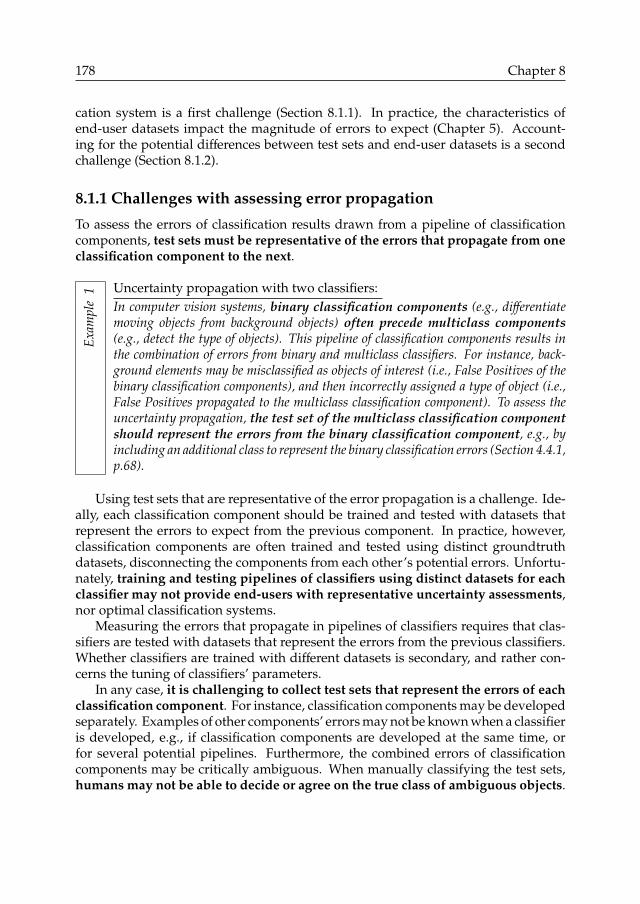
178 Chapter 8
cation system is a first challenge (Section 8.1.1). In practice, the characteristics ofend-user datasets impact the magnitude of errors to expect (Chapter 5). Account-ing for the potential differences between test sets and end-user datasets is a secondchallenge (Section 8.1.2).
8.1.1 Challenges with assessing error propagation
To assess the errors of classification results drawn from a pipeline of classificationcomponents, test sets must be representative of the errors that propagate from oneclassification component to the next.
Exam
ple
1 Uncertainty propagation with two classifiers:In computer vision systems, binary classification components (e.g., differentiatemoving objects from background objects) often precede multiclass components(e.g., detect the type of objects). This pipeline of classification components results inthe combination of errors from binary and multiclass classifiers. For instance, back-ground elements may be misclassified as objects of interest (i.e., False Positives of thebinary classification components), and then incorrectly assigned a type of object (i.e.,False Positives propagated to the multiclass classification component). To assess theuncertainty propagation, the test set of the multiclass classification componentshould represent the errors from the binary classification component, e.g., byincluding an additional class to represent the binary classification errors (Section 4.4.1,p.68).
Using test sets that are representative of the error propagation is a challenge. Ide-ally, each classification component should be trained and tested with datasets thatrepresent the errors to expect from the previous component. In practice, however,classification components are often trained and tested using distinct groundtruthdatasets, disconnecting the components from each other’s potential errors. Unfortu-nately, training and testing pipelines of classifiers using distinct datasets for eachclassifier may not provide end-users with representative uncertainty assessments,nor optimal classification systems.
Measuring the errors that propagate in pipelines of classifiers requires that clas-sifiers are tested with datasets that represent the errors from the previous classifiers.Whether classifiers are trained with different datasets is secondary, and rather con-cerns the tuning of classifiers’ parameters.
In any case, it is challenging to collect test sets that represent the errors of eachclassification component. For instance, classification components may be developedseparately. Examples of other components’ errors may not be known when a classifieris developed, e.g., if classification components are developed at the same time, orfor several potential pipelines. Furthermore, the combined errors of classificationcomponents may be critically ambiguous. When manually classifying the test sets,humans may not be able to decide or agree on the true class of ambiguous objects.
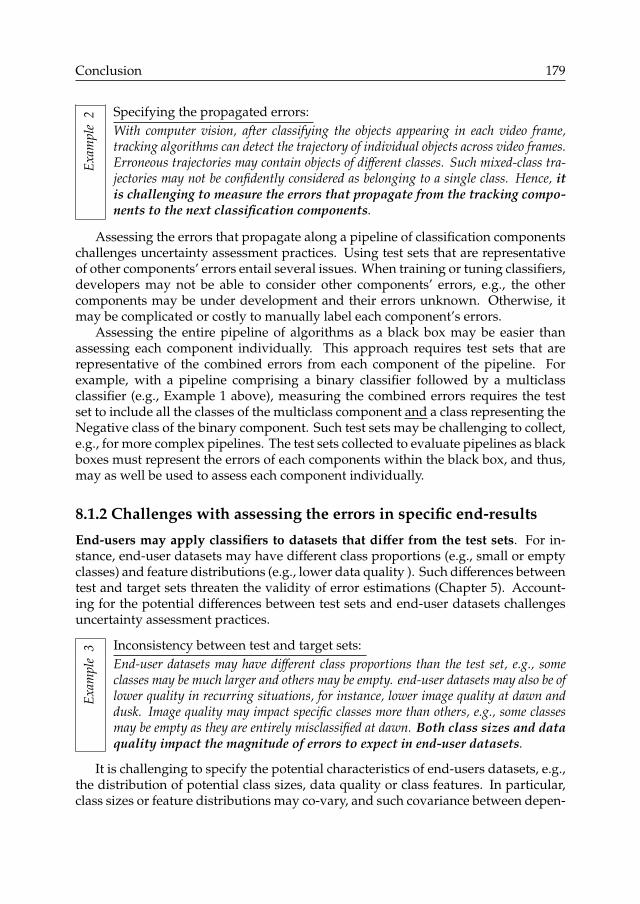
Conclusion 179Ex
ampl
e2 Specifying the propagated errors:
With computer vision, after classifying the objects appearing in each video frame,tracking algorithms can detect the trajectory of individual objects across video frames.Erroneous trajectories may contain objects of different classes. Such mixed-class tra-jectories may not be confidently considered as belonging to a single class. Hence, itis challenging to measure the errors that propagate from the tracking compo-nents to the next classification components.
Assessing the errors that propagate along a pipeline of classification componentschallenges uncertainty assessment practices. Using test sets that are representativeof other components’ errors entail several issues. When training or tuning classifiers,developers may not be able to consider other components’ errors, e.g., the othercomponents may be under development and their errors unknown. Otherwise, itmay be complicated or costly to manually label each component’s errors.
Assessing the entire pipeline of algorithms as a black box may be easier thanassessing each component individually. This approach requires test sets that arerepresentative of the combined errors from each component of the pipeline. Forexample, with a pipeline comprising a binary classifier followed by a multiclassclassifier (e.g., Example 1 above), measuring the combined errors requires the testset to include all the classes of the multiclass component and a class representing theNegative class of the binary component. Such test sets may be challenging to collect,e.g., for more complex pipelines. The test sets collected to evaluate pipelines as blackboxes must represent the errors of each components within the black box, and thus,may as well be used to assess each component individually.
8.1.2 Challenges with assessing the errors in specific end-results
End-users may apply classifiers to datasets that differ from the test sets. For in-stance, end-user datasets may have different class proportions (e.g., small or emptyclasses) and feature distributions (e.g., lower data quality ). Such differences betweentest and target sets threaten the validity of error estimations (Chapter 5). Account-ing for the potential differences between test sets and end-user datasets challengesuncertainty assessment practices.
Exam
ple
3 Inconsistency between test and target sets:End-user datasets may have different class proportions than the test set, e.g., someclasses may be much larger and others may be empty. end-user datasets may also be oflower quality in recurring situations, for instance, lower image quality at dawn anddusk. Image quality may impact specific classes more than others, e.g., some classesmay be empty as they are entirely misclassified at dawn. Both class sizes and dataquality impact the magnitude of errors to expect in end-user datasets.
It is challenging to specify the potential characteristics of end-users datasets, e.g.,the distribution of potential class sizes, data quality or class features. In particular,class sizes or feature distributions may co-vary, and such covariance between depen-

180 Chapter 8
dent variables cannot be captured by a single test set. It is also challenging to refineerror estimations to account for the characteristics of end-user datasets (e.g., usingerror rates specific to lower quality images, or other features).
Beside cases where test sets and end-user datasets differ significantly (e.g., dueto altered feature distributions), random differences among datasets can yield sig-nificant variance when estimating the classification errors in end-user datasets(Section 5.2.4, p.80). For instance, when estimating the number of errors to expectin a specific dataset, the variance magnitude may show that error estimations areunreliable, e.g., with extremely large confidence intervals.
Error estimations have particularly high variance when class sizes are small, ei-ther in test sets or end-user datasets (e.g., even with class sizes of several hundredsof items, Figure 5.1, p.81). Hence variance issues must be considered when as-sessing classification errors (e.g., using the Sample-to-Sample method introduced inSection 5.4, p.85).
The challenges with estimating errors in specific datasets are also challenges withevaluating of classifiers: if the test sets do not support reliable estimations of theerrors to expect in specific datasets, then the test sets do not provide reliable as-sessments of classifier performance. This is a first rationale for developing a unifieduncertainty assessment framework, encompassing both end-users’ and developers’tasks of tuning classifiers and estimating the errors to expect in specific end-results.
8.2 Unified classification assessment framework
When assessing classifiers, end-users and developers may have different goals andapproaches (Section 6.2, p.118). For instance, developers are primarily concernedwith reducing the errors of classifiers. Developers can tune classifiers to reducetheir errors, e.g., by setting parameters that are typically complex and unfamiliar toend-users.
End-users are primarily concerned with the errors that may occur when applyingclassifiers to their specific datasets (e.g., would this classifier or parameter settingreduce the errors for the most important classes?). Without understanding theerrors to expect in practical applications, end-users cannot assess which classifieror tuning parameters suit them best.
Developers may be provided with training and test datasets, but may not be pro-vided with information on the potential end-user datasets (e.g., would users applyclassifiers to datasets with potentially small or empty classes, or altered feature distri-butions?). Without understanding the datasets to expect in practical applications,developers cannot fine-tune classifiers’ tuning parameters.
Hence both end-users and developers need to consider the potential character-istics of end-user datasets. As discussed in Section 8.1, this entails several practicalchallenges:
• End-users may apply classifiers within a pipeline of classification components,
Conclusion 181
hence end-user datasets may include errors introduced by the previous clas-sification components. Collecting test sets that represent the errors of previousclassification components can be costly and complicated.
• End-users may apply classifiers to datasets where classes may have differentfeature distributions in recurring situations (e.g., lower data quality) whichbias error estimations (e.g., low image quality due to reduced natural lightyields higher error rates than those measured with test sets). Specifying thevariations of feature distributions can be costly and complicated, as is collectingtest sets that represent the potential feature distributions (e.g., how the featurevalues may covary).
• Even if end-users apply classifiers to datasets that are highly similar to the testsets, variance issues with random variations from the test sets may yield un-reliable error measurements (e.g., numbers of errors estimated with extremelylarge confidence intervals).
Collecting test sets that represent the variety of potential end-user datasets is a ma-jor practical challenge. Even if this challenge cannot be addressed, we advocate newparadigms for uncertainty assessments that can bridge the gap between end-usersand developers, i.e., between error measurement in test sets and error estimations inend-user datasets.
We argue that end-users should take part in classifier tuning, joining forces withdevelopers by using a unified uncertainty assessment framework (Section 8.2.1). Todevelop such uncertainty assessment framework, we advocate that error measure-ments should be mapped to datasets’ feature values (Section 8.2.2), and that thevariance of error measurements should be systematically considered (Section 8.2.3).
8.2.1 Tuning classifiers in collaboration with end-users
Tuning classifier parameters aims at minimising classification errors when applyingthe classifiers to end-user datasets. Developers can focus on reducing the errorsfor specific classes (e.g., the classes yielding most errors) or class features (e.g., thefeatures yielding the most errors). Developers should address end-users’ priorities,and reduce errors for the classes and features that are most important to end-users,e.g., the most frequent or the most valuable.
Hence tuning classifiers requires both technical expertise (i.e., knowledge ofthe relationships between classifiers’ parameters, feature distributions, and resultingerrors) and domain expertise (i.e., knowledge of the classes and feature distributionsthat are the most important or the most frequent). Enabling end-users to collaboratewith developers for tuning classifiers can overcome issues with test sets’ limitations.Extensive test sets are required to capture the potential variations of class proportionsand feature distributions. even if extensive test sets may not be collected, end-userscan use their domain expertise to guide developers attention to the most importantor frequent situations.

182 Chapter 8
Furthermore, classification technologies have become largely available in inte-grated libraries and frameworks (e.g., R, Python, Weka, RapidMiner). Classificationcomponents are readily accessible to a public with little to no expertise in theunderlying classification algorithms. The main tasks when implementing suchclassifiers consist of training and tuning existing components, rather than develop-ing new classification algorithms. In this context, classifiers disseminate to a publicwho may have more expertise in the application domain than in the classificationtechnologies. Thus a public with the expertise of end-users rather than develop-ers may be increasingly tasked with tuning classifiers. Hence the demand mayincrease for unified classification assessment frameworks, addressing both end-user-oriented and developer-oriented concerns. This trend also entails an increasing needfor developing the classification literacy of domain experts (Section 8.3).
8.2.2 Mapping error rates and feature distributions
The errors to expect in classification results are largely impacted by the featuredistributions of the datasets to classify. When estimating the number of errors inclassification results, existing error estimation methods are largely biased when fea-ture distributions differ between the test sets and the classified datasets (Section 5.6.3,p.103). However, specifying the relationships between error rates and feature distri-butions can support refinements of error estimations (Section 5.7, p.105).
Hence the magnitude of errors to expect should be estimated as a functionof the feature distributions. However, it may be practically impossible to collecttest sets for each combination of classes and feature values. For instance, "Because[Machine Learning (ML) models] typically have a large number of inputs, it is not possibleto thoroughly test even simple models, which leaves open the question of how a ML modelwill perform in a given situation." 1
Nonetheless, the relationships between error rates and feature distributionscan be estimated, e.g., using linear models such as those introduced in the LogisticRegression methods (Section 5.7.2.A, p.106). Provided with estimations of error ratesfor the feature distributions of interest, end-users may better assess the classificationuncertainty, and decide of the most important ranges of features for which errorsmust be reduced when tuning classifiers.
Furthermore, error measurements are often summarized into a single metric thatencompasses errors occurring in different situations. Developers often measurethe errors that occur over several parameter settings by using the Area Under theCurve (AUC) metric, i.e., by plotting classification errors as a function of parametersettings, and calculating the surface under the resulting curves (e.g., an ROC curve).We argue that AUC is not informative for end-users who apply classifiers with onlyone parameter setting, not all possible parameter settings.
1 Report from Informatics Europe and ACM Europe Technology Policy Committee (EUACM), WhenComputers Decide: European Recommendations on Machine-Learned Automated Decision Making, 2018 (p.10).URL: http://www.informatics-europe.org/component/phocadownload/category/10-reports.html?download=74
Conclusion 183
Mapping error rate estimations as a function of feature values can refine AUC-likesummary measures. It is more informative for end-users to plot errors as a functionof feature values, and to measure the areas under these curves. This measurementrepresents the errors that occur over several feature values. This approach is repre-sentative of the situations that may occur when applying classifiers, i.e., as the classfeatures may vary but not the parameter settings.
8.2.3 Uncovering variance issues
When estimating the number of errors in classification results, existing error estima-tion methods are unbiased if end-user datasets are similar to the test sets (e.g., withsimilar error rates). However, random error rate variations can have a significantimpact if class sizes are small, either in test sets or in end-user datasets. The vari-ance of error estimations can be critical e.g., even for class sizes of several hundredsof items Chapter 5, (Section 5.2.4 and Figure 5.1, p.81).
Hence we recommend that the variance of error measurements (i.e., in test sets)and error estimations (i.e., in end-user datasets) always be estimated. For exam-ple, when visualizing classification errors measured in test sets, confidence intervalsshould be drawn to represent how much error rate may randomly vary. Althoughsimple to compute, error rate variance is largely overlooked when assessing clas-sifiers. For example, ROC curves and Precision-Recall curves are seldom providedwith confidence intervals for the error rates they display.
The variance or error rates measured in test sets (i.e., random variations acrosspotential test sets) can be easily estimated using basic frequentist methods, e.g. forerror rates θ and class size n, V(θ) = θ(1 − θ)/n. When training and tuning classifiers, in-formation on the potential target sets may be unknown. In such cases, target sets canbe naively considered to be the same size as the test set. Using the Sample-to-Samplemethod (Section 5.4, p.85), the variance of error estimations can be naively estimated,e.g., for error rates θ′ in end-user datasets, Vnaive(θ′) = θ(1 − θ)/n + θ(1 − θ)/n = 2V(θ).
Variance estimates should be available when assessing classifiers and tuning theirparameters. Developers tend not to consider error variance when tuning classifiers,because the same test set is used to measure the errors entailed by the parametersettings, thus error variance is highly similar over the parameter settings. However,measuring variance can help direct attention to classes that exhibit high variance, asthe errors from these classes may need to be reduced in priority.
Further strategy can be investigated for reducing critical variance issues. Forinstance, the size of the training set may be reduced to increase the size of the testset. Such an approach may increase the error rate, but reduce the error rate variance(as the test set is larger). Estimating error rate variance is required to investigatethe gain and loss when choosing the sizes of training and test sets.
Further variance issues arise when assessing classification errors for specific fea-ture distributions. When assessing the errors that are specific to certain feature

184 Chapter 8
values, feature-specific error rates may be directly measured from the test set. If testsets do not contain examples of the feature values of interest, feature-specific errorrates can be estimated, e.g., using linear models (Section 8.2.2). In this case, varianceissues concern not only random variance across similar datasets (e.g., V(θ) = θ(1 − θ)/n
and V(θ′) = θ(1 − θ)/n + θ(1 − θ)/n′) but also the variance of the feature-specific error es-timation (e.g., with linear models, the squared errors between actual and predictederror rates).
Future work is required to investigate methods for deriving error rates to expectfor specific feature values, and for assessing the variance of such feature-specificerror estimation. Estimating and interpreting the variance error estimations is acomplex but necessary task, required for tuning classifiers and for assessing theerrors to expect in specific datasets. To enable end-users to harness such complex butnecessary uncertainty assessment, it is necessary to develop end-users’ classificationliteracy.
8.3 Developing classification literacy
Classification technologies already pervade many facets of society, impacting mostprofessional domains (e.g., data-driven organization) as well as our personal life(e.g., information retrieval, social media, insurance, health). These technologies,together with the availability of extensive data collection techniques, open new per-spectives and valuable opportunities. However, uncertainty issues remain a majorchallenge. Uncertainty can be readily overlooked as innovative applications thrive,and economic opportunities may prevail upon technological shortcomings. Yet, ifleft unaddressed, uncertainty issues can put end-users’ interests in jeopardy, andhave direct sociological or economical impacts.
Many application domains face crucial uncertainty issues, we give only a fewexamples here. When applying machine learning classification for scientific research(e.g., the Fish4Knowledge project) uncertainty issues compromise the scientific va-lidity of data interpretations. When classifying patients or cell images for medicaldiagnosis, classification errors can leave health issues undetected. When applyingmachine learning to predict inmates’ recidivism, biased prediction systems can yieldinadequate or discriminatory decisions when granting or postponing inmate release.When predicting the risks associated with loan applicants, biased prediction systemscan yield risky or unjust decisions when granting loans and calculating interest rates.When automatically classifying goods within factories, undetected defects can putconsumers at risk, and discarded but flawless goods yield direct economic loss.
Addressing uncertainty issues is crucial for developing trustworthy classificationsystems. For instance, the topic of trustable and explainable machine learning hasgained interest in recent years. However, existing work mainly targets an audi-ence of experts, e.g., engineers or researchers seeking to improve machine learningsystems, or exploring the sources of error. While most efforts are spent on uncover-ing how uncertainty arises in low-level machine learning algorithms, higher-level
Conclusion 185
uncertainty assessment from the perspective of end-users remains largely unad-dressed. In particular, little support is provided to domain experts with no expertisein machine learning.
It is crucial that non-expert end-users be provided with tools and methods forunderstanding classification uncertainty. End-users need to be aware of the prac-tical implications of classification errors for their specific applications. Consideringthe crucial impacts of uncertainty, e.g., regarding safety, economic, legal or moral im-plications, end-users must comprehend the uncertainty issues and make informeddecisions when choosing, tuning and using classification systems. These are thegoals, from a high-level perspective, to which this PhD thesis contributes.
Our research contributes to developing classification literacy with requirementsfor end-user-oriented uncertainty assessment (Chapter 2), insights on end-users’behaviours when assessing classification errors (Chapters 3, 6 and 7), visualizationtools for assessing classification errors and other uncertainty factors (Chapters 6and 7), and statistical methods for estimating classification errors in end-results(Chapter 5). However, many issues remain unaddressed.
First, uncertainty assessment methods are unavailable for key uncertainty fac-tors, e.g., error estimations under varying feature distributions (Section 5.6.3, p.103),human errors when labelling groundtruth test sets, and with computer vision tech-nologies, duplicated individuals and heterogeneous fields of views which bias classsize estimates (Section 4.4, p.67). Beyond developing end-user-oriented uncertaintyassessment methods, explaining the basic concepts of classification errors to end-users remains challenging. For instance, we identified crucial issues with the tech-nical terminology (Section 6.7, p.134).
Regarding the need to develop end-users’ classification literacy, we come to theconclusion that the most valuable investments in future research should be placedin developing tutorials and guidelines for explaining classification uncertainty. De-velopers of classification systems should be provided with guidelines to ensure thatthe uncertainty of their classification system is explained understandably and com-prehensively, and that their choices when tuning classifiers address end-users’ con-cerns. End-users should be provided with tutorials and guidelines that enable themto identify which uncertainty assessments are necessary, and require them from thedevelopers of classification systems.
Investigating tutorials’ understandability and completeness is also requiredfor enabling valid user studies. When conducting user studies of tools to dealwith classification results and their uncertainty, participants need to be providedwith explanations of the tools and the classification results and uncertainty. Theseexplanations can have critical impact on user studies. If explanations are not under-standable or incomplete, users may perform poorly. Hence, user performance maynot reflect the quality of the tools, but the quality of the explanations.

186 Chapter 8
8.4 Epilogue
The issues with machine learning uncertainty extend beyond those covered in thisthesis. For instance, besides the technical and educational implications discussed inthis conclusion, Informatics Europe and ACM Europe2 identify 4 other aspects ofmachine learning error and bias: the ethical, legal, economical, and societal implica-tions. Different communities need to work together to address the different aspectsof uncertainty issues. The public sector and civil society are crucial actors to drive theefforts required to address the implications of machine learning uncertainty. Publicinstitutions and non-profit organizations have the leverage and interests for requiringtransparent and accountable machine learning systems, while there is little benefitfor commercial organizations to invest in providing them. "While more fairness andjustice would of course benefit society as a whole, individual companies are not positioned toreap the rewards. For most of them, in fact, [harmful machine learning systems] appear tobe highly effective. Entire business models, such as for-profit universities and payday loans,are built upon them."3 As individual citizens and public servants are key stakeholdersin machine learning uncertainty problems, this reinforces my personal opinion thatessential and urgent future work is to invest in providing machine learning literacyto the general public.
2Report from Informatics Europe and ACM Europe Technology Policy Committee (EUACM), WhenComputers Decide: European Recommendations on Machine-Learned Automated Decision Making, 2018. URL:http://www.informatics-europe.org/component/phocadownload/category/10-reports.html?download=74
3Book by Cathy O’Neil, Weapons of Math Destruction, 2016 (p.202).

Appendix AStudy of User Trust andAcceptance
This appendix details participants’ answers in the user study introduced in Chapter 3.
• A summary of the questionnaire and related visualizations (Section A.1).
• The responses of each participant to the multiple choice questions (Tables A.1-A.3) and the free-form text questions (Tables A.5-A.7).
• Our interpretation of each participant’s responses (Section A.2).
A.1 Questionnaire
We briefly recap the four types of questions and the concepts they intend to assess.We then provide visualizations that were displayed together with the questionnaire(Figures A.3 to A.2, complementing Figures 3.1 to 3.2 p.42).
Acceptance - Questions Q6-A-i to -iv:• Question Q6-A-i evaluates the overall acceptance of the computer vision software.• Question Q6-A-ii evaluates the acceptance of computer vision uncertainty com-
pared to existing techniques in marine biology.• Question Q6-A-iii evaluates the acceptance of computer vision uncertainty for
scientific research in particular.• Question Q6-A-iv evaluates the personal attachment to the computer vision software.
187

188 Chapter A
Trust - Questions Q1 and Q6-T-i to -iii:• Question Q1 evaluates the overall trust in the computer vision results. It presented
an example of fish counts provided by a fish detection software (Figure A.3) andasked how the trends observed in the fish counts are likely to be representative ofreal trends. The data used was artificially generated, and trends were simulatedwith various intensity (e.g., important increase or decrease, to stagnating fishcounts), but presented as genuine to users. The same trends were presentedacross the steps of the experiment, so as to measure the impact that the additionalinformation introduced at each step had on user trust.
• Question Q6-T-i evaluates the perceived technical competence of the fish detectionsoftware, and is adapted from (Madsen and Gregor 2000).
• Question Q6-T-ii evaluates the perceived technical competence of the method used formeasuring fish detection errors.
• Question Q6-T-iii evaluates trust in the data produced by the video analysis soft-ware.
Actual Understanding - Questions Q2 to Q4:• Question Q2 evaluates the effective user understanding of the technical concepts
presented at each explanation step.• Question Q3 evaluates user understanding of the scope of uncertainty issues in-
volved in the computer vision system.• Question Q4 evaluates if user understanding through the practical use of the tech-
nical information. It asked to compare two software and identify the one yieldingthe fewest errors (Figure A.1-A.2). This question was omitted at Step 3 because in-formal feedback collected prior to the experiment indicated that our visualizationof classification errors for different thresholds were hard to understand. Further-more the concepts explained at the last step were likely to overwhelm non-expertusers. Thus we decided to avoid measuring user understanding of complex con-cepts using our poor data visualization support.
Perceived Understanding - Questions Q6-U-i to -iv:• Question Q6-U-i evaluates if users think they understand the technical information
provided in the tutorials.• Question Q6-U-ii evaluates if users think they fully understand the video analysis
processes, beyond the groundtruth evaluation process presented in the tutorials.• Question Q6-U-iii evaluates if users think they understand the implications of
using uncertain video analysis data containing classification errors for scientificpurposes.
• Question Q6-U-iv evaluates if users think they understand how to handle theclassification errors when performing scientific research based on the uncertainvideo analysis data (e.g., by applying statistical methods).
Information Needs - Questions Q3, Q5, and Q6-I-i to -v:• Question Q3 investigate information needs regarding uncertainty issues beyond
the technical concepts discussed in the explanations.• Question Q5 investigates marine ecologists’ need for estimating the number of

Study of User Trust and Acceptance 189
errors in classification end-results (i.e., using the methods introduced in Chapter 5).• Question Q6-I-i evaluates if the explanations fulfil user information needs on the
video analysis errors.• Question Q6-I-ii evaluates if the user thinks the explanations generally fulfils the
information needs on the video analysis method, while question Q6-I-iii evaluatesif the user needs more information for her/his particular interests.
• Question Q6-I-iv evaluates if the information was easy to understand. If the infor-mation is difficult to understand, users may need more details in the explanations,and a different formulation of the information.
• Question Q6-I-v evaluates if the information is relevant, i.e., if some informationis too detailed or superfluous, and does not address real user needs.
Figure A.1: The software to compare in question Q4 of Step 1 (Table 3.1).
Figure A.2: The software to compare in question Q4 of Step 2 (Table 3.1).

190 Chapter A
Figure A.3: The trends to assess in question Q1 (Table 3.1), at Step 1 to 3 (top to bottom).

Study of User Trust and Acceptance 191
ParticipantsQuestion Construct Scale P1 P2 P3 P4 P5 P6 P7 P8 P9 P10 P11 P12 P13 P14 P15Q1-i TRUST -2 to 2 1 1 0 0 0 -1 0 1 1 1 0 2 1 1 0Q1-ii TRUST -2 to 2 1 -1 0 0 -1 -1 0 1 2 -1 0 2 1 1 0Q1-iii TRUST -2 to 2 1 -1 0 0 0 1 0 1 0 2 0 0 1 1 0Q1-iv TRUST -2 to 2 1 1 0 0 0 1 0 0 0 2 0 0 1 1 0
Q2-i UNDERST.-act. 0 or 1 1 0 0 0 1 0 0 0 0 1 1 1 0 0 1Q2-ii UNDERST.-act. 0 or 1 - - - - - - - - - - - - - - -Q2-iii UNDERST.-act. 0 or 1 1 1 1 0 1 1 1 1 1 1 1 1 1 0 1
Q3-U-i UNDERST.-act. Y or N Y Y Y N Y Y Y N N Y Y N Y Y YQ3-I-i INFO NEED Y or N N N Y Y N Y Y N N N N Y N N YQ3-U-ii UNDERST.-act. Y or N Y Y Y Y Y Y Y N N Y Y N Y Y YQ3-I-ii INFO NEED Y or N N N Y N N N Y N N N N N N N NQ3-U-iii UNDERST.-act. Y or N Y Y Y Y Y Y Y Y Y N Y Y Y Y YQ3-I-iii INFO NEED Y or N N N N N N N Y N N Y N N N N NQ3-U-iv UNDERST.-act. Y or N Y Y Y Y Y Y Y N N Y Y N Y Y YQ3-I-iv INFO NEED Y or N N N Y N N Y Y N N Y N Y N N YQ3-U-v UNDERST.-act. Y or N Y Y Y Y Y Y Y Y N Y N Y Y Y YQ3-i-v INFO NEED Y or N N Y N Y N Y Y N N Y Y N N N NQ3-U-vi UNDERST.-act. Y or N Y Y Y Y Y N Y Y N Y N Y Y Y YQ3-I-vi INFO NEED Y or N N N N N N Y N N N N N N N N NQ3-U-vii UNDERST.-act. Y or N N Y Y Y Y Y Y Y N Y N Y Y Y YQ3-I-vii INFO NEED Y or N N N N N N N N N N N N N N N N
Q4-i UNDERST.-act. 0 or 1 1 1 1 1 1 1 1 1 1 1 1 1 1 1 1Q4-ii UNDERST.-act. 0 or 1 1 1 1 1 1 1 1 1 1 1 1 1 1 1 1
Q5 INFO NEED Y, N, ? Y Y Y N Y Y Y Y Y Y ? Y Y ? ?
Q6-A-i ACCEPT. -3 to 3 2 3 2 0 2 0 2 2 2 1 0 1 0 1 2Q6-A-ii ACCEPT. -3 to 3 2 2 -2 1 0 -1 -2 -1 0 -1 -2 -2 -2 1 0Q6-A-iii ACCEPT. -3 to 3 2 3 2 -2 1 -1 2 2 1 -2 -1 1 0 1 0Q6-A-iv ACCEPT. -3 to 3 2 3 2 -2 0 -1 2 2 2 2 -2 0 2 2 2Q6-T-i TRUST -3 to 3 2 2 0 0 0 0 1 2 0 0 1 -1 1 2 0Q6-T-ii TRUST -3 to 3 2 2 0 0 -1 1 0 1 0 1 0 1 0 1 0Q6-T-iii TRUST -3 to 3 2 2 1 1 0 -1 2 1 1 -1 -1 1 1 1 0Q6-U-i UNDERST.-perc. -3 to 3 1 2 2 -2 2 -1 1 -2 1 2 -2 -1 2 2 2Q6-U-ii UNDERST.-perc. -3 to 3 1 2 0 -2 -2 -1 1 -2 -2 -1 -1 -1 1 -2 -3Q6-U-iii UNDERST.-perc. -3 to 3 1 3 2 -1 1 1 0 -2 1 -2 1 1 2 1 2Q6-U-iv UNDERST.-perc. -3 to 3 1 2 0 -1 -1 1 0 -2 1 -2 1 -1 -1 -2 -3Q6-I-i INFO NEED -3 to 3 2 3 2 0 -1 1 2 2 2 -1 1 1 -1 -1 -2Q6-I-ii INFO NEED -3 to 3 2 1 -2 -2 -2 1 0 1 -2 -2 1 1 2 -2 -3Q6-I-iii INFO NEED -3 to 3 -2 -3 -2 -3 -2 -1 2 -2 -2 -2 -2 0 -2 -3 -3Q6-I-iv INFO NEED -3 to 3 1 -3 1 -2 0 1 1 -1 0 -1 -1 2 1 -2 -2Q6-I-v INFO NEED -3 to 3 2 3 2 2 2 0 0 2 2 1 -2 1 2 2 3
Table A.1: Answers to multiple choice questions at Step 1. Question Q2-ii was discarded becausetext feedback showed that users often misunderstood the term "manual fish count" as counts fromdiving observations, instead of counts from manual image labelling. Question Q5 evaluated the needfor information on the potential errors to expect in the classification results (Y when needed, N whennot needed, ? when user was not sure).

192 Chapter A
ParticipantsQuestion Construct Scale P1 P2 P3 P4 P5 P6 P7 P8 P9 P10 P11 P12 P13 P14 P15Q1-i TRUST -2 to 2 1 1 0 -2 0 1 0 1 1 1 0 2 1 1 0Q1-ii TRUST -2 to 2 1 -2 0 -2 0 -1 0 1 2 -1 0 2 1 1 0Q1-iii TRUST -2 to 2 1 -1 0 -2 0 1 0 1 0 1 0 1 1 1 0Q1-iv TRUST -2 to 2 1 1 0 -2 0 1 0 0 0 1 0 1 1 1 0
Q2-i UNDERST.-act. 0 or 1 1 1 0 1 1 1 1 1 1 1 1 1 1 0 1Q2-ii UNDERST.-act. 0 or 1 1 1 1 0 1 1 1 1 1 1 1 1 1 1 1Q2-iii UNDERST.-act. 0 or 1 1 1 1 0 1 1 1 1 1 1 1 1 1 0 1Q2-iv UNDERST.-act. 0 or 1 0 0 1 0 1 0 0 1 1 0 0 0 1 1 1Q2-v UNDERST.-act. 0 or 1 0 0 0 1 0 1 0 1 0 0 0 1 0 1 1Q2-vi UNDERST.-act. 0 or 1 0 0 0 0 1 1 1 1 0 1 0 1 0 1 1
Q4-i UNDERST.-act. 0 or 1 1 1 1 0 1 1 1 1 1 1 0 1 1 1 1Q4-ii UNDERST.-act. 0 or 1 1 0 1 0 1 1 1 0 1 0 0 1 1 1 1Q4-iii UNDERST.-act. 0 or 1 1 1 1 0 1 1 1 0 1 1 0 1 1 1 1
Q5 INFO NEED Y, N, ? Y Y Y Y Y Y Y Y Y Y ? Y Y Y Y
Q6-A-i ACCEPT. -3 to 3 2 3 2 0 2 1 2 2 1 1 0 2 0 1 2Q6-A-ii ACCEPT. -3 to 3 2 2 -2 0 1 -1 -2 0 -2 -1 -3 -1 -1 0 -2Q6-A-iii ACCEPT. -3 to 3 2 2 2 1 1 0 2 2 2 -1 0 2 1 1 0Q6-A-iv ACCEPT. -3 to 3 2 3 2 1 0 0 2 1 2 0 -1 -1 1 2 2Q6-T-i TRUST -3 to 3 2 3 2 0 0 -1 2 2 -2 -1 0 1 1 0 0Q6-T-ii TRUST -3 to 3 2 3 2 0 -1 1 1 1 1 -2 -1 1 0 1 -2Q6-T-iii TRUST -3 to 3 2 2 1 0 1 1 1 0 -1 0 -2 1 1 1 1Q6-U-i UNDERST.-perc. -3 to 3 1 3 2 -1 2 0 1 -2 1 -1 -2 1 1 1 2Q6-U-ii UNDERST.-perc. -3 to 3 1 3 0 2 -2 0 0 -1 0 -1 -2 1 1 -2 -3Q6-U-iii UNDERST.-perc. -3 to 3 1 2 2 1 1 1 1 -1 1 -2 -1 1 1 -1 2Q6-U-iv UNDERST.-perc. -3 to 3 1 2 1 1 -1 1 1 -1 1 -2 -1 -1 1 -1 2Q6-I-i INFO NEED -3 to 3 2 3 2 0 -1 1 2 1 1 1 -1 1 0 -1 1Q6-I-ii INFO NEED -3 to 3 2 2 0 0 -2 0 1 -1 -1 -2 -1 1 1 -1 -2Q6-I-iii INFO NEED -3 to 3 -2 -3 -1 0 -2 1 2 -2 0 -2 -2 -1 -1 -2 -3Q6-I-iv INFO NEED -3 to 3 1 2 0 -2 -1 0 2 1 1 -1 -1 1 0 -1 -2Q6-I-v INFO NEED -3 to 3 2 3 1 1 2 0 1 2 2 1 0 -1 2 2 2
Table A.2: Answers to multiple choice questions at Step 2.
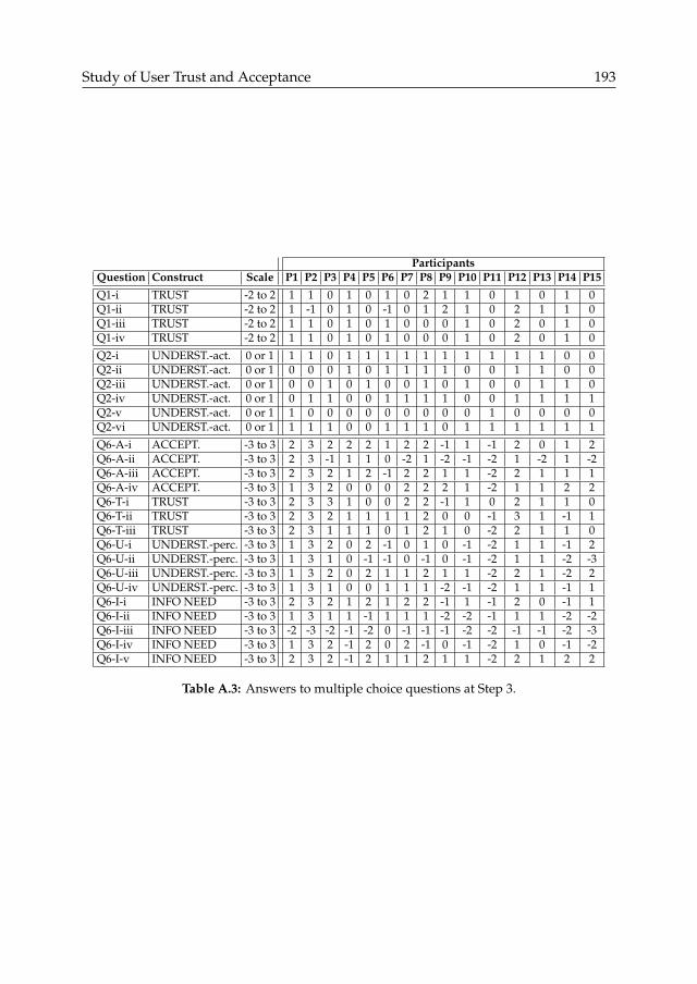
Study of User Trust and Acceptance 193
ParticipantsQuestion Construct Scale P1 P2 P3 P4 P5 P6 P7 P8 P9 P10 P11 P12 P13 P14 P15Q1-i TRUST -2 to 2 1 1 0 1 0 1 0 2 1 1 0 1 0 1 0Q1-ii TRUST -2 to 2 1 -1 0 1 0 -1 0 1 2 1 0 2 1 1 0Q1-iii TRUST -2 to 2 1 1 0 1 0 1 0 0 0 1 0 2 0 1 0Q1-iv TRUST -2 to 2 1 1 0 1 0 1 0 0 0 1 0 2 0 1 0
Q2-i UNDERST.-act. 0 or 1 1 1 0 1 1 1 1 1 1 1 1 1 1 0 0Q2-ii UNDERST.-act. 0 or 1 0 0 0 1 0 1 1 1 1 0 0 1 1 0 0Q2-iii UNDERST.-act. 0 or 1 0 0 1 0 1 0 0 1 0 1 0 0 1 1 0Q2-iv UNDERST.-act. 0 or 1 0 1 1 0 0 1 1 1 1 0 0 1 1 1 1Q2-v UNDERST.-act. 0 or 1 1 0 0 0 0 0 0 0 0 0 1 0 0 0 0Q2-vi UNDERST.-act. 0 or 1 1 1 1 0 0 1 1 1 0 1 1 1 1 1 1
Q6-A-i ACCEPT. -3 to 3 2 3 2 2 2 1 2 2 -1 1 -1 2 0 1 2Q6-A-ii ACCEPT. -3 to 3 2 3 -1 1 1 0 -2 1 -2 -1 -2 1 -2 1 -2Q6-A-iii ACCEPT. -3 to 3 2 3 2 1 2 -1 2 2 1 1 -2 2 1 1 1Q6-A-iv ACCEPT. -3 to 3 1 3 2 0 0 0 2 2 2 1 -2 1 1 2 2Q6-T-i TRUST -3 to 3 2 3 3 1 0 0 2 2 -1 1 0 2 1 1 0Q6-T-ii TRUST -3 to 3 2 3 2 1 1 1 1 2 0 0 -1 3 1 -1 1Q6-T-iii TRUST -3 to 3 2 3 1 1 1 0 1 2 1 0 -2 2 1 1 0Q6-U-i UNDERST.-perc. -3 to 3 1 3 2 0 2 -1 0 1 0 -1 -2 1 1 -1 2Q6-U-ii UNDERST.-perc. -3 to 3 1 3 1 0 -1 -1 0 -1 0 -1 -2 1 1 -2 -3Q6-U-iii UNDERST.-perc. -3 to 3 1 3 2 0 2 1 1 2 1 1 -2 2 1 -2 2Q6-U-iv UNDERST.-perc. -3 to 3 1 3 1 0 0 1 1 1 -2 -1 -2 1 1 -1 1Q6-I-i INFO NEED -3 to 3 2 3 2 1 2 1 2 2 -1 1 -1 2 0 -1 1Q6-I-ii INFO NEED -3 to 3 1 3 1 1 -1 1 1 1 -2 -2 -1 1 1 -2 -2Q6-I-iii INFO NEED -3 to 3 -2 -3 -2 -1 -2 0 -1 -1 -1 -2 -2 -1 -1 -2 -3Q6-I-iv INFO NEED -3 to 3 1 3 2 -1 2 0 2 -1 0 -1 -2 1 0 -1 -2Q6-I-v INFO NEED -3 to 3 2 3 2 -1 2 1 1 2 1 1 -2 2 1 2 2
Table A.3: Answers to multiple choice questions at Step 3.

194 Chapter A
Question - Participant - AnswerQ1 P5 Without any background information on the coral reef, location etc, it is very unlikely that any statement about
how likely it is that this trends may occur in reality. So can a trend like the one showed here be really happening?Yes it may happen. Can I say that this likely to be what is happening there? No I can’t without backgroundinformation on location, species composition, etc.
P6 A trend such as seen from April-May is possible, but only at certain dramatic circumstances. For instance asevere viral infection or something like that could decimated a population. Otherwise such a severe decrease isnot likely.
P7 Dear sir, madam, I am a terrestrial ecologist and therefore I am not very familiar with marine ecosystems. Forthis reason I find myself unqualified to give a thrustworthy judgement of the likelyness that the trends in aspictured in the above chart will occur in reality.
P10 The abundance of fish in a certain area depends on complex biological and physical processes, interactionsbetween behaviour, physiology, and habitat (e.g. depth, seabed) characteristics. In addition I think it is speciesdependend and therefore I would say it’s difficult to argue whether these trends are likely to be observed inreality.
P11 We need to have the real data or trend in reality. Otherwise, we will not be able to know whether the trend ofsoftware count is the same or different from the divers’ census count. Is this what you said the "reality"?
P12 For a small increase/decrease its hard to say if this is really what happened, due to some limitations of themethod... like what you actually want to sample in terms of the overall habitat in a certain area, this becauseyou only have a view of 8m for example. Depends on the sampling effort as well
Q2 P4 1.There are many schools of fish appear in the camera’s field of view, different experts count will be different,but the machine will not. 2.Appeared several times in the field of view, the expert will not repeat count for thesame fish, but the machine will repeat count.
P5 I think that 3rd reason is the most probable, considering the consistently lower counts by the software. Onequestion arises, are experts counting anything that they can identified as a fish, or only those that can they saywhat fish it is? If they do they are doing the former, advising them to do the later may take the counts closertogether.
P8 A single fish detected more then once compensates for the fishes that are being missed.P9 The first statement would lead to higher fish counts with the software than manually, this contradicts with
the background information. I do believe however that this software may count rocks as fish. Then the errorbetween manual and software counts would even be higher than 27% in reality.
P10 I believe that especialy statement 2 is of importance!P11 1. I do not know whether the software is good enough to distinguish the "fish" and "rock". I can only believe
the software can. 2. Diver can judge whether the fish swim out and in the camera field is the same or differentindividual. Certainly different divers may have different results. That is a bias by different observers. 3. somesmaller body size fish or cryptic fish may not be detected by software. Some fishes if they swim too far awayfrom the camera and could not be detected by software especially when the water visibility is not good. Diversshould be able to see better than camera especially when camera lens has biofouling problem.
P12 When doing the fish count manually it is more likely that the same fish wasnt been recorded several times.The reason for this is that you re better able to see differences in length and behavior between fish of thesame species. You dont have this problem when using stereo cameras and using a relative abundance, so themaximum number seen in one frame.
Q3 P2 benthic fish can be miss countP3 video blocked by an objectP11 If the camera field was changed. We should be able to detected by the monitor at lab. For the last two questions,
I can not really answer. Because we should have both data, one from software count and another from diverscount, in hand and then make a comparison study to find out is any other source of error.
P12 The range of view.. especially if you want to compare the videos. For instance, when coral is blocking the viewof the cameras. Also, the position of the cameras, because you can miss certain reef associated fish species whenthe cameras are pointing a bit upwards.
P13 inter observer differences?P14 I don’t know how you did the evalutation
Table A.4: Answers to free text questions at Step 1 (Part 1/2).
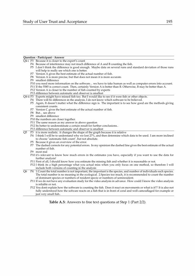
Study of User Trust and Acceptance 195
Question - Participant - AnswerQ4-i P3 Because it is closer to the expert’s count
P4 Because of interference may not much difference of A and B counting the fish.P5 I don’t think the difference is good enough. Maybe data on several runs and standard deviation of those runs
will help to really see which one is better.P7 Version A gives the best estimate of the actual number of fish.P8 Version A is more precise, but that does not mean it is more accurate.P9 smallest differenceP10 you need more information on the software... we have to take human as well as computer errors into account.P11 If the 5585 is correct count. Then, certainly Version A is better than B. Otherwise, B may be better than A.P12 Version A is closer to the number of fish counted by expertsP13 difference between automatic and observer is smallest
Q4-ii P3 Experts miight have missed fish too. But I would like to see if it were fish or other objects.P4 There will be differences in the analysis, I do not know which software to be believed.P5 Again, It doesn’t matter what the difference sign is. The important is to see how good are the methods giving
consistent counts.P7 Version C gives the best estimate of the actual number of fish.P8 But... see aboveP9 smallest differenceP10 the numbers are closer together.P11 The same reason as my answer in above questionP12 Its better to underestimate a certain result for further conclusions..P13 difference between automatic and observer is smallest
Q5 P3 it is more realistic. it changes the shape of the graph because it is relativeP4 I think I will be to understand why we lost 27%, and then determine which data to be used. I am more inclined
to choose "automatic fish count", but not absolute.P5 Because it gives an overview of the error.P7 The dashed corrects for any potential errors. In my opninion the dashed line gives the best estimate of the actual
number of fish.P9 most realP10 it’s relevant to know how much errors in the estimates you have, especially if you want to use the data for
further analysis!P11 First of all, I should know how you estimate the missing fish and whether it is reasonable or not.P12 I think its a high percentage what you actual miss when you only focus on one method, so therefore I will
include both versions of counting in the analysisQ6 P4 1.Count the total number is not important, the important is the species, and number of individuals each species.
The total number is no meaning in the ecological. 2.Species too much, it is recommended to count the numberof dominant species or numbers of resident specie or numbers of semiresident.
P11 If we do not have any evaluation study for the video analysis in advance. How could I know the video analysisis reliable or not.
P12 You dont explain how the software is counting the fish. Does it react on movements or what is it?? It is also notfully understood how the sofware reacts on a fish that is in front of coral and well camouflaged for example orjust very small fish..
Table A.5: Answers to free text questions at Step 1 (Part 2/2).

196 Chapter A
Question - Participant - AnswerQ1 P4 The trend is the focus, not the number. The trends of three methods are the same. So the results are the same.
There were nothings to be compared.P5 The new information don’t really solve the doubts expressed before. I don’t think it add too much. It is expected
by that type of software to have more or less constant errors, meaning that the trends are not going to changewith more information as the observed trend is in general proportional to the real one.
P11 MY answer or comments are still the same as my answer previously.P12 Im very convinced about the new line added to the graph with the fish count with estimated non-fish object.
Now you include that high percentage what you miss with automatically running the software to identify thefish, i.e small fish.
Q4-i P3 Higher percentage of TPP4 The trend is the focus, not the numbers.P5 not enough information. But of course a software that reduces both false negatives and false positives is
obviously better.P6 ’Cause it is the most accurate version and has the highest TP and lowest FP and FN.P7 Both the percentage of false positives and false negatives is smaller in version B.P9 smallest errorP10 less FP and less FN = more accurate count...P11 We should do some evaluation on the accuracy of video analysis first before I can answer this question.P12 Version B has relatively more True Positive in the model, and with a decline of false parametersP13 difference with manual count is mallest
Q4-ii P3 higher percentage of TP. Lower percentage of FNP4 Repeat, I take care the trend. Which methods I don’t care.P5 Not enough information. Although the software able to reduce false negatives without compromising the false
positives is better.P6 ’Cause it is the most accurate version and has the highest TP and lowest FN.P7 The percentage of false positives is equal for both versions. However, the percentage of false negatives is smaller
for version C.P9 smallest errorP10 you could argue more TP are counted in version C but the overall count of both version are the same... so you
can’t differentiate between them.P11 Same as aboveP12 More TP than FNP13 difference with manual count is smallest
Q4-iii P3 Higher percentage of TP. lower percentage of FPP4 Repeat, I take care the trend. Which methods I don’t care.P5 Again the same. Of course a software that reduces the number of false positives without increasing false
negatives is better.P6 ’Cause it is the most accurate version and has the lowest FP.P7 The percentage of false negatives is equal for both versions. However, the percentage of false positives is smaller
for version E.P9 smallest errorP10 Less FP detectedP11 Same as aboveP12 Total amount of counts which is True Positive relative to False Positive is higher. Less errorP13 difference with manual count is smallest
Q5 P3 It should be +20 % ?P4 Repeat, I take care the trend. Which methods I don’t care.P5 In this case the error seems constant all over the trend. But that may not be the case and I want to know when
that happensP6 The automatic fish count clearly underestimates (by 27%) the true population, the fish count without estimated
non-fish objects is good because it corrects for the non-fish objects but still misses the 27%. The fish count withestimated missing fish overestimates the true population because it doesn’t correct for the non-fish objects. Soa comparison of all three would be best, although it is the most laborious choice.
P7 It is always better to have an estimate of possible error-marginsP9 gives the best evaluation of the real situationP10 rather have the non-fish selections removed from my data-set then have more fish in my count of which a certain
number are no-fish...P11 Same as aboveP12 Im not entirely convinced about estimating the missing fish only from a percentage of all videos that has to be
analysed.Q6 P12 Is it also possible to automatically identify the fish species?
Table A.6: Answers to free text questions at Step 2.

Study of User Trust and Acceptance 197
Question - Participant - AnswerQ1 P11 I do not understand how these similarity were calculated. So I can not answer your questions appropriately.Q6 P4 All the ways to fix it only in order to get the correct results. But the trend is the focus, not the numbers. Start
trusted, it can only do so. If was "the garbage in, garbage out".P12 After reading and getting more information about errors that are produced with this method I get a better
feeling in how the system works. So it might be that some given answers of the first two tasks or not entirelycorrect to my understanding
Table A.7: Answers to free text questions at Step 3.
A.2 Interpretation of participant responses
Our interpretation of user responses investigates the impact that the technical in-formation introduced at each step had on user understanding, trust, acceptance andfulfilment of information needs. In particular, user trust, acceptance are compared withthe perceived and actual understanding, so as to identify uninformed trust and accep-tance. We considered both the quantitative measurements from the multiple choicequestions, and the qualitative feedback from free-form text questions.
Participant P1 - The explanation steps had almost no impact on of the measure-ments, which were all relatively high, except actual understanding which varied fromrelatively high to moderate. We assume that trust and acceptance were uninformed.
Participant P2 - Trust increased over step from moderate (middle score) to rela-tively large while acceptance remained relatively high. Actual Understanding was mod-erate at Step 1 and 2 decreased to average at Steps 3. The text feedback indicates anaccurate understanding, thus we assume trust and acceptance to be well-informed.Perceived Understanding was relatively high, and Information Needs increased frompartly to fairly fulfilled. This is consistent with our assumption that P8 seeks well-informed trust and acceptance.
Participant P3 - The explanation steps had little impact on trust and acceptance,which remained relatively high and slightly increased at Step 3. Actual Understandingremained relatively high, which is consistent with the text feedback. Thus we assumetrust and acceptance to be relatively well-informed. Perceived Understanding increasedover steps from very low to average, and information needs remained perceived aspartly fulfilled. This is consistent with our interpretation that P2 seeks well-informedtrust and acceptance.
Participant P4 - The explanation steps had a significant impact on trust and ac-ceptance Trust evolved from neutral (Step 1) to very low (Step 2) and relatively high(Step 3), while acceptance increased from relatively low to relatively high. Actual Un-derstanding was moderate at Step 1, although the text feedback indicates an excellentunderstanding. It significantly lowered at Step 2 and 3, as the text feedback indicatesa lost of interest for the materials. Perceived Understanding, however, increased afterStep 1 as P4 understood crucial aspects of uncertainty: 1) the classification errors canimpact the trends observed in the data; and 2) the variability of error rates can impactthe extrapolation of classification errors in the data (Section 3.5.1). The InformationNeeds increased from largely to partly unfulfilled, which indicates that P4 seeks well-informed trust. The text and oral feedback also indicated that P4 seeks well-informed

198 Chapter A
trust, that the Information Needs on other uncertainty factors are largely unfulfilled,and that acceptance increased as P4 was willing to conduct experiments with thepromising system (e.g., to assess the uncertainty issues).
Participant P5 - The explanation steps had little impact on trust and acceptance,although they slightly increased at each step. Trust remained moderate, and accep-tance relatively high. Actual Understanding was very high at Step 1 and 2, with textfeedback indicating an excellent understanding. Hence we assume that trust andacceptance were well-informed, although actual understanding was relatively low atStep 3. Perceived Understanding was moderate and information needs partly unfulfilled,although their scores improved at Step 3. This is consistent with our assumption thatP5 seeks well-informed trust and acceptance.
Participant P6 - The explanation steps had little impact on trust and acceptance,which remained relatively low and slightly increased at Step 2. Actual Understandingwas very high, but decreased at Step 3. Hence we assume that trust and acceptanceare well-informed. Perceived Understanding remained moderate, and information needspartly fulfilled. This is consistent with our assumption that P6 seeks well-informedtrust and acceptance.
Participant P7 - The explanation steps had little impact on trust and acceptance,which remained relatively neutral, i.e., close to the middle score (average of minimumand maximum score). Actual Understanding was relatively high and decreased atStep 3, which is consistent with the text feedback. Perceived Understanding remainedneutral, close to the middle score, and information needs were perceived as fairlyfulfilled. Hence we assume that P7 seeks well-informed trust and acceptance.
Participant P8 - Trust was relatively high and slightly increased at each step.Acceptance remained very high, close to the maximum score. Actual Understandingdecreased from high (Step 1) to low (Steps 2 and 3). Thus we assume trust andacceptance to be uninformed. Perceived Understanding was very high, increasing toreach the highest possible score, and the Information Needs increased from partly tofairly fulfilled. This is consistent with our assumption that trust and acceptance areuninformed.
Participant P9 - Trust remained moderate while acceptance decreased at each step,from relatively high to moderate. Actual Understanding was moderate to relativelyhigh, and the text feedback indicates an accurate understanding. Hence we assumethat trust and acceptance are well-informed, although understanding decreased atStep 3. Perceived Understanding and information needs increased and decreased to-gether with actual understanding. This is consistent with our assumption that P9seeks well-informed trust and acceptance.
Participant P10 - The explanation steps had little impact on trust and acceptance,which remained moderate although trust was lower at Step 2. Actual Understandingdecreased at each step from the maximum to the average score, although the textfeedback indicates an excellent understanding. Hence we assume that trust andacceptance are well-informed. Perceived Understanding remained relatively low, andinformation needs partly unfulfilled. This is consistent with our assumption that P10seeks well-informed trust and acceptance.
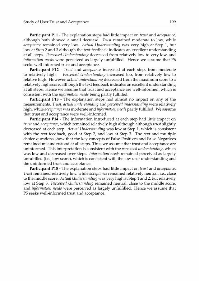
Study of User Trust and Acceptance 199
Participant P11 - The explanation steps had little impact on trust and acceptance,although both showed a small decrease. Trust remained moderate to low, whileacceptance remained very low. Actual Understanding was very high at Step 1, butlow at Step 2 and 3 although the text feedback indicates an excellent understandingat all steps. Perceived Understanding decreased from relatively low to very low, andinformation needs were perceived as largely unfulfilled. Hence we assume that P6seeks well-informed trust and acceptance.
Participant P12 - Trust and acceptance increased at each step, from moderateto relatively high. Perceived Understanding increased too, from relatively low torelative high. However, actual understanding decreased from the maximum score to arelatively high score, although the text feedback indicates an excellent understandingat all steps. Hence we assume that trust and acceptance are well-informed, which isconsistent with the information needs being partly fulfilled.
Participant P13 - The explanation steps had almost no impact on any of themeasurements. Trust, actual understanding and perceived understanding were relativelyhigh, while acceptance was moderate and information needs partly fulfilled. We assumethat trust and acceptance were well-informed.
Participant P14 - The information introduced at each step had little impact ontrust and acceptance, which remained relatively high although although trust slightlydecreased at each step. Actual Understanding was low at Step 1, which is consistentwith the text feedback, good at Step 2, and low at Step 3. The text and multiplechoice questions show that the key concepts of False Positives and False Negativesremained misunderstood at all steps. Thus we assume that trust and acceptance areuninformed. This interpretation is consistent with the perceived understanding, whichwas low and decreased over steps. Information needs remained perceived as largelyunfulfilled (i.e., low score), which is consistent with the low user understanding andthe uninformed trust and acceptance.
Participant P15 - The explanation steps had little impact on trust and acceptance.Trust remained relatively low, while acceptance remained relatively neutral, i.e., closeto the middle score. Actual Understanding was very high at Step 1 and 2, but relativelylow at Step 3. Perceived Understanding remained neutral, close to the middle score,and information needs were perceived as largely unfulfilled. Hence we assume thatP5 seeks well-informed trust and acceptance.


Bibliography
Alsallakh, B., Hanbury, A., Hauser, H., Miksch, S., and Rauber, A. (2014). Visualmethods for analyzing probabilistic classification datasets. IEEE Transactions onVisualization and Computer Graphics, 20(12). (cited pp. 118, 121, 123, and 124)
Amar, R., Eagan, J., and Stasko, J. (2005). Low-level components of analytic activityin information visualization. In Symposium on Information Visualization (Infovis),pages 111–117. IEEE. (cited pp. 145, 146, and 148)
Artz, D. and Gil, Y. (2007). A survey of trust in computer science and the semanticweb. Web Semantics: Science, Services and Agents on the World Wide Web, 5(2):58–71.(cited p. 45)
Beauxis-Aussalet, E. and Hardman, L. (2015). Multifactorial uncertainty assessmentfor monitoring population abundance using computer vision. In IEEE InternationalConference on Data Science and Advanced Analytics (DSAA). (cited pp. 78, 79, and 105)
Beauxis-Aussalet, E. and Hardman, L. (2016). Fish4Knowledge: Collecting and Ana-lyzing Massive Coral Reef Fish Video Data, chapter Appendix 1 - User Interface andUsage Scenario. Spinger. (cited p. 160)
Beauxis-Aussalet, E., Palazzo, S., Nadarajan, G., Arlasnova, E., Spampinato, C., andHardman, L. (2013). A video processing and data retrieval framework for fishpopulation monitoring. In ACM MultiMedia workshop on Multimedia Analysis forEcological Data (MAED). (cited p. 59)
Bohrnstedt, G. and Goldberger, A. (1969). On the exact covariance of products ofrandom variables. Journal of the American Statistical Association, 64(328):1439–1442.(cited p. 110)
Boom, B. J., Beauxis-Aussalet, E., Hardman, L., and Fisher, R. B. (2016). Uncertainty-aware estimation of population abundance using machine learning. MultimediaSystem Journal. (cited pp. 106, 111, 112, 113, and 117)
Boom, B. J., Huang, P. X., Beyan, C., Spampinato, C., Palazzo, S., He, J., Beauxis-Aussalet, E., Lin, S.-I., Chou, H.-M., Nadarajan, G., et al. (2012). Long-term un-derwater camera surveillance for monitoring and analysis of fish populations. In
201

202 Bibliography
Workshop on Visual observation and analysis of Animal and Insect Behaviour (VAIB), heldat the 21st International Conference on Pattern Recognition (ICPR). (cited p. 2)
Brooke, J. (1996). SUS - A quick and dirty usability scale. Usability evaluation inindustry, 189(194). (cited p. 128)
Buonaccorsi, J. P. (2010). Measurement Error: Models, Methods and Applications. CRCPress, Taylor and Francis. (cited pp. 76, 77, 78, 79, 91, 92, 94, and 111)
Cappo, M., Speare, P., and De’ath, G. (2004). Comparison of baited remote under-water video stations (bruvs) and prawn (shrimp) trawls for assessments of fishbiodiversity in inter-reefal areas of the great barrier reef marine park. Journal ofExperimental Marine Biology and Ecology, 302(2):123–152. (cited pp. 27 and 29)
Card, D. H. (1982). Using known map category marginal frequencies to improve es-timates of thematic map accuracy. Photogrammetric Engineering and Remote Sensing,48:431–439. (cited p. 76)
Cleveland, W. and McGill, R. (1984). Graphical perception: Theory, experimentation,and application to the development of graphical methods. Journal of the AmericanStatistical Association, 79(387). (cited pp. 121, 123, 124, and 137)
Cochran, W. G. (2007). Sampling techniques. John Wiley & Sons. (cited pp. 27 and 86)
Correa, C., Chan, Y.-H., and Ma, K.-L. (2009). A framework for uncertainty-awarevisual analytics. In IEEE Symposium on Visual Analytics Science and Technology(VAST), pages 51–58. (cited pp. 58 and 144)
Correll, M. and Gleicher, M. (2014). Error bars considered harmful: Exploring alter-nate encodings for mean and error. IEEE Transactions on Visualization and ComputerGraphics. (cited p. 140)
Csurka, G., Zeller, C., Zhang, Z., and Faugeras, O. D. (1997). Characterizing theuncertainty of the fundamental matrix. Computer vision and image understanding,68(1):18–36. (cited p. 61)
Drummond, C. and Holte, R. (2006). Cost curves: An improved method for visual-izing classifier performance. Machine Learning, 65(1). (cited pp. 118 and 119)
Elias, M. and Bezerianos, A. (2011). Exploration views: understanding dashboard cre-ation and customization for visualization novices. In Human-Computer Interaction–INTERACT, pages 274–291. Springer. (cited pp. 144, 145, and 148)
Elzen, S. v. d. and Wijk, J. J. v. (2011). Baobabview: Interactive construction andanalysis of decision trees. In IEEE Visual Analytics Science and Technology (VAST).(cited p. 118)

Bibliography 203
Endsley, M. R. (1988a). Design and evaluation for situation awareness enhancement.In Proceedings of the Human Factors and Ergonomics Society Annual Meeting, pages97–101. SAGE Publications. (cited p. 145)
Endsley, M. R. (1988b). Situation awareness global assessment technique (SAGAT).In Proceedings of the National Aerospace and Electronics Conference (NAECON), pages789–795. IEEE. (cited p. 164)
Endsley, M. R. (1995). Towards a theory of situation awareness in dynamic systems.Human factors, 37. (cited p. 127)
Fawcett, T. (2006). An introduction to ROC analysis. Pattern Recognition Letters, 27(8).(cited pp. 118 and 121)
Fieller, E. C. (1954). Some problems in interval estimation. Journal of the Royal StatisticalSociety. Series B. (cited p. 110)
Fisher, R. B., Chen-Burger, Y.-H., Giordano, D., Hardman, L., and Lin, F.-P., editors(2016). Fish4Knowledge: Collecting and Analyzing Massive Coral Reef Fish Video Data.Spinger. (cited p. 59)
Foody, G. M. (2002). Status of land cover classification accuracy assessment. RemoteSensing of Environment, 80(1):185–201. (cited p. 76)
Gill, T. and Hicks, R. (2006). Task complexity and informing science: A synthesis.Information Science Journal. (cited p. 132)
Grammel, L., Tory, M., and Storey, M. (2010). How information visualization novicesconstruct visualizations. IEEE Transactions on Visualization and Computer Graphics,16(6):943–952. (cited p. 145)
Grassia, A. and Sundberg, R. (1982). Statistical precision in the calibration and use ofsorting machines and other classifiers. Technometrics, 24(2):117–121. (cited pp. 76,77, and 79)
Griethe, H. and Schumann, H. (2006). The visualization of uncertain data: Methodsand problems. In SimVis, pages 143–156. (cited pp. 144 and 145)
Harvey, E., Fletcher, D., and Shortis, M. (2001). A comparison of the precisionand accuracy of estimates of reef-fish lengths determined visually by divers withestimates produced by a stereo-video system. Fisheries Bulletin, 99:63–71. (citedpp. 26 and 29)
Hay, A. M. (1988). The derivation of global estimates from a confusion matrix.International Journal of Remote Sensing, 9(8). (cited pp. 76 and 77)
Hay, A. M. (1989). Global estimates from a confusion matrix, a reply to jupp. Inter-national Journal of Remote Sensing, 10(9). (cited p. 78)

204 Bibliography
He, J., van Ossenbruggen, J., and de Vries, A. P. (2013). Do you need experts in thecrowd?: a case study in image annotation for marine biology. In Proceedings of the10th Conference on Open Research Areas in Information Retrieval, pages 57–60. (citedp. 62)
Heer, J., van Ham, F., Carpendale, S., Weaver, C., and Isenberg, P. (2008). Creationand collaboration: Engaging new audiences for information visualization. InInformation Visualization, pages 92–133. Springer. (cited pp. 144 and 148)
Hetrick, N. J., Simms, K. M., Plumb, M. P., and Larson, J. P. (2004). Feasibility of usingvideo technology to estimate salmon escapement in the Ongivinuk River, a clear-watertributary of the Togiak River. US Fish and Wildlife Service, King Salmon Fish andWildlife Field Office. (cited p. 27)
Hoffrage, U., Krauss, S., Martignon, L., and Gigerenzer, G. (2015). Natural frequenciesimprove bayesian reasoning in simple and complex inference tasks. Frontiers inPsychology. (cited p. 136)
Hossin, M. and Sulaiman, M. N. (2015). A review on evaluation metrics for dataclassification evaluations. International Journal of Data Mining and Knowledge Man-agement Process (IJDKP), 5(2). (cited pp. 119 and 121)
Huang, W., Eades, P., and Hong, S. (2009). Measuring effectiveness of graph visu-alizations: A cognitive load perspective. Information Visualization. (cited pp. 125,127, and 132)
Jousselme, A.-L., Maupin, P., and Bossé, É. (2003). Uncertainty in a situation analysisperspective. In Proceedings of the Sixth International Conference of Information Fusion.IEEE. (cited p. 146)
Katila, M. (2006). Forest Inverntory: Methodology and Applications, chapter Correctingmap errors in forest inventory estimates for small areas, pages 225–233. Number 13.Springer. (cited pp. 77 and 78)
Khan, A., Breslav, S., Glueck, M., and Hornbæk, K. (2015). Benefits of visualizationin the mammography problem. Int. J. Human-Computer Studies. (cited pp. 119and 136)
Kosinski, A. (2001). Cramer’s rule is due to cramer. Mathematics Magazine, 74:310–312.(cited pp. 82, 94, and 95)
Kraan, M., Uhlmann, S., Steenbergen, J., Van Helmond, A., and Van Hoof, L. (2013).The optimal process of self-sampling in fisheries: lessons learned in the nether-lands. Journal of fish biology, 83(4):963–973. (cited p. 26)
Krause, J., Dasgupta, A., Swartz, J., Aphinyanaphongs, Y., and Bertini, E. (2017).A workflow for visual diagnostics of binary classifiers using instance-level ex-planations. In IEEE Confrence on Visual Analytics Science and Technology. (cited p.118)

Bibliography 205
Lam, H., Bertini, E., Isenberg, P., Plaisant, C., and Carpendale, S. (2012). Empir-ical studies in information visualization: Seven scenarios. IEEE transactions onvisualization and computer graphics, 18(9). (cited p. 125)
Langlois, T., Chabanet, P., Pelletier, D., and Harvey, E. (2006). Baited underwatervideo for assessing reef fish populations in marine reserves. Fisheries Newsletter -South Pacific Commission, 118. (cited p. 27)
Levina, E. and Bickel, P. (2001). The earth mover? s distance is the mallows distance:Some insights from statistics. In null, page 251. IEEE. (cited p. 103)
Little, R. J. and Rubin, D. B. (2014). Statistical analysis with missing data. John Wiley &Sons. (cited p. 72)
Liu, S., Wang, X., Liu, M., and Zhu, J. (2017). Towards better analysis of machinelearning models: A visual analytics perspective. Visual Informatics. (cited p. 118)
Lowry, M., Folpp, H., Gregson, M., and Suthers, I. (2012). Comparison of baited re-mote underwater video (bruv) and underwater visual census (uvc) for assessmentof artificial reefs in estuaries. Journal of Experimental Marine Biology and Ecology,416–417:243–253. (cited pp. 27 and 29)
Madsen, M. and Gregor, S. (2000). Measuring human-computer trust. In Proceedingsof Eleventh Australasian Conference on Information Systems, pages 6–8. Citeseer. (citedpp. 45 and 188)
McAllister, D. J. (1995). Affect-and cognition-based trust as foundations for interper-sonal cooperation in organizations. Academy of management journal, pages 24–59.(cited p. 45)
McGill, R., Tukey, J. W., and Larsen, W. A. (1978). Variations of box plots. The AmericanStatistician, 32(1):12–16. (cited p. 172)
McGuinness, B. (2004). Quantitative analysis of situational awareness (QUASA):Applying signal detection theory to true/false probes and self-ratings. DTIC Doc-ument. (cited p. 146)
Micallef, L., Dragicevic, P., and Fekete, J.-D. (2012). Assessing the effect of visu-alizations on bayesian reasoning through crowdsourcing. IEEE Transactions onVisualization and Computer Graphics. (cited p. 119)
Murch, G. M. (1984). Physiological principles for the effective use of color. IEEEComputer Graphics and Applications. (cited p. 124)
Pang, A. T., Wittenbrink, C. M., and Lodha, S. K. (1997). Approaches to uncertaintyvisualization. The Visual Computer, 13(8):370–390. (cited pp. 33, 58, and 144)
206 Bibliography
Ren, D., Amershi, S., Lee, B., Suh, J., and Williams, J. (2017). Squares: Supportinginteractive performance analysis for multiclass classifiers. IEEE Transactions onVisualization and Computer Graphics, 23(1). (cited pp. 118, 121, 123, and 124)
Saerens, M., Latinne, P., and Decaestecker, C. (2001). Adjusting the output of aclassifier to new a priori probabilities: a simple procedure. Neural Computation,14:21–44. (cited pp. 102 and 106)
Sebastiani, F. (2015). An axiomatically derived measure for the evaluation of classifi-cation algorithms. In International Conference on The Theory of Information Retrieval.(cited p. 119)
Senge, R., Del Coz, J. J., and Hüllermeier, E. (2014). On the problem of error prop-agation in classifier chains for multi-label classification. In Data Analysis, MachineLearning and Knowledge Discovery, pages 163–170. Springer. (cited p. 61)
Shafait, F., Mian, A., Shortis, M., Ghanem, B., Culverhouse, P., Edgington, D., Cline,D., Ravanbakhsh, M., Seager, J., and Harvey, E. (2016). Fish identification fromvideos captured in uncontrolled underwater environments. ICES Journal of MarineScience, 73(10):2737–2746. (cited p. 27)
Shieh, M. S. (2009). Correction methods, approximate biases, and inference for misclassifieddata. PhD thesis, Univ. of Massachusetts. (cited pp. 76, 77, 78, 79, 89, 91, 92, 100,and 111)
Shneiderman, B. (1996). The eyes have it: A task by data type taxonomy for informa-tion visualizations. In Symposium on Visual Languages, pages 336–343. IEEE. (citedpp. 145 and 146)
Sokolova, M. and Lapalme, G. (2009). A systematic analysis of performance measuresfor classification tasks. Information Processing and Management, 45(4). (cited p. 119)
Spampinato, C., Beauxis-Aussalet, E., Palazzo, S., Beyan, C., van Ossenbruggen, J.,He, J., Boom, B., and Huang, X. (2014). A rule-based event detection system forreal-life underwater domain. Machine vision and applications, 25(1):99–117. (cited p.31)
Spampinato, C., Palazzo, S., Giordano, D., Kavasidis, I., Lin, F.-P., and Lin, Y.-T.(2012). Covariance based fish tracking in real-life underwater environment. InInternational Conference on Computer Vision Theory and Applications (VISAPP), pages409–414. (cited pp. 61, 62, and 67)
Talbot, J., Setlur, V., and Anand, A. (2014). Four experiments on the perception ofbar charts. IEEE Transactions on Visualization and Computer Graphics. (cited pp. 121and 124)
Tang, D., Stolte, C., and Bosch, R. (2004). Design choices when architecting visual-izations. Information Visualization, 3(2):65–79. (cited p. 144)

Bibliography 207
Taylor, M., Baker, J., and Suthers, I. (2013). Tidal currents, sampling effort and baitedremote underwater video (bruv) surveys: Are we drawing the right conclusions?Fisheries Research, 140(96–104). (cited p. 28)
Tenenbein, A. (1972). A double sampling scheme for estimating from misclassi-fied multinomial data with applications to sampling inspection. Technometrics,14(1):187–202. (cited pp. 76, 77, and 79)
Thomson, J., Hetzler, E., MacEachren, A., Gahegan, M., and Pavel, M. (2005). Atypology for visualizing uncertainty. In Visualization and Data Analysis (VDA),pages 146–157. (cited p. 144)
Tidwell, J. (2010). Designing interfaces: Patterns for effective interaction design. O’ReillyMedia, Inc. (cited p. 124)
Trevor, J., Russell, B., and Russell, C. (2000). Detection of spatial variability in relativedensity of fishes: comparison of visual census, angling, and baited underwatervideo. Marine Ecology Progress Series, 198:249–260. (cited p. 29)
van der Aalst, W. M. P., Blichler, M., and Heinzl, A. (2017). Responsible data science.Business and Information System Engineering, 59(5):311–313. (cited pp. 1 and 36)
van Deusen, P. C. (1996). Unbiased estimates of class proportions from thematicmaps. Photogrammetric Engineering and Remote Sensing, 62(4):409–412. (cited p. 76)
Viegas, F. B., Wattenberg, M., Van Ham, F., Kriss, J., and McKeon, M. (2007).Manyeyes: a site for visualization at internet scale. IEEE Transactions on Visu-alization and Computer Graphics, 13(6):1121–1128. (cited p. 149)
Walker, W. E., Harremoës, P., Rotmans, J., van der Sluijs, J. P., van Asselt, M. B.,Janssen, P., and Krayer von Krauss, M. P. (2003). Defining uncertainty: a conceptualbasis for uncertainty management in model-based decision support. Integratedassessment, 4(1):5–17. (cited p. 58)
Wang Baldonado, M. Q., Woodruff, A., and Kuchinsky, A. (2000). Guidelines forusing multiple views in information visualization. In Proceedings of the workingconference on Advanced visual interfaces, pages 110–119. ACM. (cited pp. 144, 145,146, 148, and 149)
Wickens, C. D. and Carswell, C. M. (1997). Information processing. Handbook ofhuman factors and ergonomics, pages 89–122. (cited p. 145)
Zhu, X. and Wu, X. (2004). Class noise vs. attribute noise: A quantitative study.Artificial Intelligence Review, 22(3):177–210. (cited p. 61)

208 Bibliography
List of SIKS dissertations published since 2011
2011
01 Botond Cseke (RUN), Variational Algorithms for Bayesian Inference in Latent Gaussian Models02 Nick Tinnemeier (UU), Organizing Agent Organizations. Syntax and Operational Semantics of an Organization-
Oriented Programming Language03 Jan Martijn van der Werf (TUE), Compositional Design and Verification of Component-Based Information Systems04 Hado van Hasselt (UU), Insights in Reinforcement Learning; Formal analysis and empirical evaluation of
temporal-difference05 Bas van der Raadt (VU), Enterprise Architecture Coming of Age - Increasing the Performance of an Emerging
Discipline.06 Yiwen Wang (TUE), Semantically-Enhanced Recommendations in Cultural Heritage07 Yujia Cao (UT), Multimodal Information Presentation for High Load Human Computer Interaction08 Nieske Vergunst (UU), BDI-based Generation of Robust Task-Oriented Dialogues09 Tim de Jong (OU), Contextualised Mobile Media for Learning10 Bart Bogaert (UvT), Cloud Content Contention11 Dhaval Vyas (UT), Designing for Awareness: An Experience-focused HCI Perspective12 Carmen Bratosin (TUE), Grid Architecture for Distributed Process Mining13 Xiaoyu Mao (UvT), Airport under Control. Multiagent Scheduling for Airport Ground Handling14 Milan Lovric (EUR), Behavioral Finance and Agent-Based Artificial Markets15 Marijn Koolen (UvA), The Meaning of Structure: the Value of Link Evidence for Information Retrieval16 Maarten Schadd (UM), Selective Search in Games of Different Complexity17 Jiyin He (UVA), Exploring Topic Structure: Coherence, Diversity and Relatedness18 Mark Ponsen (UM), Strategic Decision-Making in complex games19 Ellen Rusman (OU), The Mind’s Eye on Personal Profiles20 Qing Gu (VU), Guiding service-oriented software engineering - A view-based approach21 Linda Terlouw (TUD), Modularization and Specification of Service-Oriented Systems22 Junte Zhang (UVA), System Evaluation of Archival Description and Access23 Wouter Weerkamp (UVA), Finding People and their Utterances in Social Media24 Herwin van Welbergen (UT), Behavior Generation for Interpersonal Coordination with Virtual Humans On
Specifying, Scheduling and Realizing Multimodal Virtual Human Behavior25 Syed Waqar ul Qounain Jaffry (VU), Analysis and Validation of Models for Trust Dynamics26 Matthijs Aart Pontier (VU), Virtual Agents for Human Communication - Emotion Regulation and Involvement-
Distance Trade-Offs in Embodied Conversational Agents and Robots27 Aniel Bhulai (VU), Dynamic website optimization through autonomous management of design patterns28 Rianne Kaptein (UVA), Effective Focused Retrieval by Exploiting Query Context and Document Structure29 Faisal Kamiran (TUE), Discrimination-aware Classification30 Egon van den Broek (UT), Affective Signal Processing (ASP): Unraveling the mystery of emotions31 Ludo Waltman (EUR), Computational and Game-Theoretic Approaches for Modeling Bounded Rationality32 Nees-Jan van Eck (EUR), Methodological Advances in Bibliometric Mapping of Science33 Tom van der Weide (UU), Arguing to Motivate Decisions34 Paolo Turrini (UU), Strategic Reasoning in Interdependence: Logical and Game-theoretical Investigations35 Maaike Harbers (UU), Explaining Agent Behavior in Virtual Training36 Erik van der Spek (UU), Experiments in serious game design: a cognitive approach37 Adriana Burlutiu (RUN), Machine Learning for Pairwise Data, Applications for Preference Learning and Super-
vised Network Inference38 Nyree Lemmens (UM), Bee-inspired Distributed Optimization39 Joost Westra (UU), Organizing Adaptation using Agents in Serious Games40 Viktor Clerc (VU), Architectural Knowledge Management in Global Software Development41 Luan Ibraimi (UT), Cryptographically Enforced Distributed Data Access Control42 Michal Sindlar (UU), Explaining Behavior through Mental State Attribution43 Henk van der Schuur (UU), Process Improvement through Software Operation Knowledge44 Boris Reuderink (UT), Robust Brain-Computer Interfaces45 Herman Stehouwer (UvT), Statistical Language Models for Alternative Sequence Selection46 Beibei Hu (TUD), Towards Contextualized Information Delivery: A Rule-based Architecture for the Domain of
Mobile Police Work47 Azizi Bin Ab Aziz (VU), Exploring Computational Models for Intelligent Support of Persons with Depression48 Mark Ter Maat (UT), Response Selection and Turn-taking for a Sensitive Artificial Listening Agent49 Andreea Niculescu (UT), Conversational interfaces for task-oriented spoken dialogues: design aspects influencing
interaction quality
2012
01 Terry Kakeeto (UvT), Relationship Marketing for SMEs in Uganda

Bibliography 209
02 Muhammad Umair (VU), Adaptivity, emotion, and Rationality in Human and Ambient Agent Models03 Adam Vanya (VU), Supporting Architecture Evolution by Mining Software Repositories04 Jurriaan Souer (UU), Development of Content Management System-based Web Applications05 Marijn Plomp (UU), Maturing Interorganisational Information Systems06 Wolfgang Reinhardt (OU), Awareness Support for Knowledge Workers in Research Networks07 Rianne van Lambalgen (VU), When the Going Gets Tough: Exploring Agent-based Models of Human Performance
under Demanding Conditions08 Gerben de Vries (UVA), Kernel Methods for Vessel Trajectories09 Ricardo Neisse (UT), Trust and Privacy Management Support for Context-Aware Service Platforms10 David Smits (TUE), Towards a Generic Distributed Adaptive Hypermedia Environment11 J.C.B. Rantham Prabhakara (TUE), Process Mining in the Large: Preprocessing, Discovery, and Diagnostics12 Kees van der Sluijs (TUE), Model Driven Design and Data Integration in Semantic Web Information Systems13 Suleman Shahid (UvT), Fun and Face: Exploring non-verbal expressions of emotion during playful interactions14 Evgeny Knutov (TUE), Generic Adaptation Framework for Unifying Adaptive Web-based Systems15 Natalie van der Wal (VU), Social Agents. Agent-Based Modelling of Integrated Internal and Social Dynamics of
Cognitive and Affective Processes.16 Fiemke Both (VU), Helping people by understanding them - Ambient Agents supporting task execution and
depression treatment17 Amal Elgammal (UvT), Towards a Comprehensive Framework for Business Process Compliance18 Eltjo Poort (VU), Improving Solution Architecting Practices19 Helen Schonenberg (TUE), What’s Next? Operational Support for Business Process Execution20 Ali Bahramisharif (RUN), Covert Visual Spatial Attention, a Robust Paradigm for Brain-Computer Interfacing21 Roberto Cornacchia (TUD), Querying Sparse Matrices for Information Retrieval22 Thijs Vis (UvT), Intelligence, politie en veiligheidsdienst: verenigbare grootheden?23 Christian Muehl (UT), Toward Affective Brain-Computer Interfaces: Exploring the Neurophysiology of Affect
during Human Media Interaction24 Laurens van der Werff (UT), Evaluation of Noisy Transcripts for Spoken Document Retrieval25 Silja Eckartz (UT), Managing the Business Case Development in Inter-Organizational IT Projects: A Methodology
and its Application26 Emile de Maat (UVA), Making Sense of Legal Text27 Hayrettin Gurkok (UT), Mind the Sheep! User Experience Evaluation & Brain-Computer Interface Games28 Nancy Pascall (UvT), Engendering Technology Empowering Women29 Almer Tigelaar (UT), Peer-to-Peer Information Retrieval30 Alina Pommeranz (TUD), Designing Human-Centered Systems for Reflective Decision Making31 Emily Bagarukayo (RUN), A Learning by Construction Approach for Higher Order Cognitive Skills Improvement,
Building Capacity and Infrastructure32 Wietske Visser (TUD), Qualitative multi-criteria preference representation and reasoning33 Rory Sie (OUN), Coalitions in Cooperation Networks (COCOON)34 Pavol Jancura (RUN), Evolutionary analysis in PPI networks and applications35 Evert Haasdijk (VU), Never Too Old To Learn – On-line Evolution of Controllers in Swarm- and Modular Robotics36 Denis Ssebugwawo (RUN), Analysis and Evaluation of Collaborative Modeling Processes37 Agnes Nakakawa (RUN), A Collaboration Process for Enterprise Architecture Creation38 Selmar Smit (VU), Parameter Tuning and Scientific Testing in Evolutionary Algorithms39 Hassan Fatemi (UT), Risk-aware design of value and coordination networks40 Agus Gunawan (UvT), Information Access for SMEs in Indonesia41 Sebastian Kelle (OU), Game Design Patterns for Learning42 Dominique Verpoorten (OU), Reflection Amplifiers in self-regulated Learning43 Withdrawn44 Anna Tordai (VU), On Combining Alignment Techniques45 Benedikt Kratz (UvT), A Model and Language for Business-aware Transactions46 Simon Carter (UVA), Exploration and Exploitation of Multilingual Data for Statistical Machine Translation47 Manos Tsagkias (UVA), Mining Social Media: Tracking Content and Predicting Behavior48 Jorn Bakker (TUE), Handling Abrupt Changes in Evolving Time-series Data49 Michael Kaisers (UM), Learning against Learning - Evolutionary dynamics of reinforcement learning algorithms
in strategic interactions50 Steven van Kervel (TUD), Ontologogy driven Enterprise Information Systems Engineering51 Jeroen de Jong (TUD), Heuristics in Dynamic Sceduling; a practical framework with a case study in elevator
dispatching
2013
01 Viorel Milea (EUR), News Analytics for Financial Decision Support02 Erietta Liarou (CWI), MonetDB/DataCell: Leveraging the Column-store Database Technology for Efficient and
Scalable Stream Processing

210 Bibliography
03 Szymon Klarman (VU), Reasoning with Contexts in Description Logics04 Chetan Yadati (TUD), Coordinating autonomous planning and scheduling05 Dulce Pumareja (UT), Groupware Requirements Evolutions Patterns06 Romulo Goncalves (CWI), The Data Cyclotron: Juggling Data and Queries for a Data Warehouse Audience07 Giel van Lankveld (UvT), Quantifying Individual Player Differences08 Robbert-Jan Merk (VU), Making enemies: cognitive modeling for opponent agents in fighter pilot simulators09 Fabio Gori (RUN), Metagenomic Data Analysis: Computational Methods and Applications10 Jeewanie Jayasinghe Arachchige (UvT), A Unified Modeling Framework for Service Design.11 Evangelos Pournaras (TUD), Multi-level Reconfigurable Self-organization in Overlay Services12 Marian Razavian (VU), Knowledge-driven Migration to Services13 Mohammad Safiri (UT), Service Tailoring: User-centric creation of integrated IT-based homecare services to
support independent living of elderly14 Jafar Tanha (UVA), Ensemble Approaches to Semi-Supervised Learning Learning15 Daniel Hennes (UM), Multiagent Learning - Dynamic Games and Applications16 Eric Kok (UU), Exploring the practical benefits of argumentation in multi-agent deliberation17 Koen Kok (VU), The PowerMatcher: Smart Coordination for the Smart Electricity Grid18 Jeroen Janssens (UvT), Outlier Selection and One-Class Classification19 Renze Steenhuizen (TUD), Coordinated Multi-Agent Planning and Scheduling20 Katja Hofmann (UvA), Fast and Reliable Online Learning to Rank for Information Retrieval21 Sander Wubben (UvT), Text-to-text generation by monolingual machine translation22 Tom Claassen (RUN), Causal Discovery and Logic23 Patricio de Alencar Silva (UvT), Value Activity Monitoring24 Haitham Bou Ammar (UM), Automated Transfer in Reinforcement Learning25 Agnieszka Anna Latoszek-Berendsen (UM), Intention-based Decision Support. A new way of representing and
implementing clinical guidelines in a Decision Support System26 Alireza Zarghami (UT), Architectural Support for Dynamic Homecare Service Provisioning27 Mohammad Huq (UT), Inference-based Framework Managing Data Provenance28 Frans van der Sluis (UT), When Complexity becomes Interesting: An Inquiry into the Information eXperience29 Iwan de Kok (UT), Listening Heads30 Joyce Nakatumba (TUE), Resource-Aware Business Process Management: Analysis and Support31 Dinh Khoa Nguyen (UvT), Blueprint Model and Language for Engineering Cloud Applications32 Kamakshi Rajagopal (OUN), Networking For Learning; The role of Networking in a Lifelong Learner’s Profes-
sional Development33 Qi Gao (TUD), User Modeling and Personalization in the Microblogging Sphere34 Kien Tjin-Kam-Jet (UT), Distributed Deep Web Search35 Abdallah El Ali (UvA), Minimal Mobile Human Computer Interaction36 Than Lam Hoang (TUe), Pattern Mining in Data Streams37 Dirk Börner (OUN), Ambient Learning Displays38 Eelco den Heijer (VU), Autonomous Evolutionary Art39 Joop de Jong (TUD), A Method for Enterprise Ontology based Design of Enterprise Information Systems40 Pim Nijssen (UM), Monte-Carlo Tree Search for Multi-Player Games41 Jochem Liem (UVA), Supporting the Conceptual Modelling of Dynamic Systems: A Knowledge Engineering
Perspective on Qualitative Reasoning42 Léon Planken (TUD), Algorithms for Simple Temporal Reasoning43 Marc Bron (UVA), Exploration and Contextualization through Interaction and Concepts
2014
01 Nicola Barile (UU), Studies in Learning Monotone Models from Data02 Fiona Tuliyano (RUN), Combining System Dynamics with a Domain Modeling Method03 Sergio Raul Duarte Torres (UT), Information Retrieval for Children: Search Behavior and Solutions04 Hanna Jochmann-Mannak (UT), Websites for children: search strategies and interface design - Three studies on
children’s search performance and evaluation05 Jurriaan van Reijsen (UU), Knowledge Perspectives on Advancing Dynamic Capability06 Damian Tamburri (VU), Supporting Networked Software Development07 Arya Adriansyah (TUE), Aligning Observed and Modeled Behavior08 Samur Araujo (TUD), Data Integration over Distributed and Heterogeneous Data Endpoints09 Philip Jackson (UvT), Toward Human-Level Artificial Intelligence: Representation and Computation of Meaning
in Natural Language10 Ivan Salvador Razo Zapata (VU), Service Value Networks11 Janneke van der Zwaan (TUD), An Empathic Virtual Buddy for Social Support12 Willem van Willigen (VU), Look Ma, No Hands: Aspects of Autonomous Vehicle Control13 Arlette van Wissen (VU), Agent-Based Support for Behavior Change: Models and Applications in Health and
Safety Domains

Bibliography 211
14 Yangyang Shi (TUD), Language Models With Meta-information15 Natalya Mogles (VU), Agent-Based Analysis and Support of Human Functioning in Complex Socio-Technical
Systems: Applications in Safety and Healthcare16 Krystyna Milian (VU), Supporting trial recruitment and design by automatically interpreting eligibility criteria17 Kathrin Dentler (VU), Computing healthcare quality indicators automatically: Secondary Use of Patient Data and
Semantic Interoperability18 Mattijs Ghijsen (UVA), Methods and Models for the Design and Study of Dynamic Agent Organizations19 Vinicius Ramos (TUE), Adaptive Hypermedia Courses: Qualitative and Quantitative Evaluation and Tool Support20 Mena Habib (UT), Named Entity Extraction and Disambiguation for Informal Text: The Missing Link21 Kassidy Clark (TUD), Negotiation and Monitoring in Open Environments22 Marieke Peeters (UU), Personalized Educational Games - Developing agent-supported scenario-based training23 Eleftherios Sidirourgos (UvA/CWI), Space Efficient Indexes for the Big Data Era24 Davide Ceolin (VU), Trusting Semi-structured Web Data25 Martijn Lappenschaar (RUN), New network models for the analysis of disease interaction26 Tim Baarslag (TUD), What to Bid and When to Stop27 Rui Jorge Almeida (EUR), Conditional Density Models Integrating Fuzzy and Probabilistic Representations of
Uncertainty28 Anna Chmielowiec (VU), Decentralized k-Clique Matching29 Jaap Kabbedijk (UU), Variability in Multi-Tenant Enterprise Software30 Peter de Cock (UvT), Anticipating Criminal Behaviour31 Leo van Moergestel (UU), Agent Technology in Agile Multiparallel Manufacturing and Product Support32 Naser Ayat (UvA), On Entity Resolution in Probabilistic Data33 Tesfa Tegegne (RUN), Service Discovery in eHealth34 Christina Manteli (VU), The Effect of Governance in Global Software Development: Analyzing Transactive
Memory Systems.35 Joost van Ooijen (UU), Cognitive Agents in Virtual Worlds: A Middleware Design Approach36 Joos Buijs (TUE), Flexible Evolutionary Algorithms for Mining Structured Process Models37 Maral Dadvar (UT), Experts and Machines United Against Cyberbullying38 Danny Plass-Oude Bos (UT), Making brain-computer interfaces better: improving usability through post-
processing.39 Jasmina Maric (UvT), Web Communities, Immigration, and Social Capital40 Walter Omona (RUN), A Framework for Knowledge Management Using ICT in Higher Education41 Frederic Hogenboom (EUR), Automated Detection of Financial Events in News Text42 Carsten Eijckhof (CWI/TUD), Contextual Multidimensional Relevance Models43 Kevin Vlaanderen (UU), Supporting Process Improvement using Method Increments44 Paulien Meesters (UvT), Intelligent Blauw. Met als ondertitel: Intelligence-gestuurde politiezorg in gebiedsge-
bonden eenheden.45 Birgit Schmitz (OUN), Mobile Games for Learning: A Pattern-Based Approach46 Ke Tao (TUD), Social Web Data Analytics: Relevance, Redundancy, Diversity47 Shangsong Liang (UVA), Fusion and Diversification in Information Retrieval
2015
01 Niels Netten (UvA), Machine Learning for Relevance of Information in Crisis Response02 Faiza Bukhsh (UvT), Smart auditing: Innovative Compliance Checking in Customs Controls03 Twan van Laarhoven (RUN), Machine learning for network data04 Howard Spoelstra (OUN), Collaborations in Open Learning Environments05 Christoph Bösch (UT), Cryptographically Enforced Search Pattern Hiding06 Farideh Heidari (TUD), Business Process Quality Computation - Computing Non-Functional Requirements to
Improve Business Processes07 Maria-Hendrike Peetz (UvA), Time-Aware Online Reputation Analysis08 Jie Jiang (TUD), Organizational Compliance: An agent-based model for designing and evaluating organizational
interactions09 Randy Klaassen (UT), HCI Perspectives on Behavior Change Support Systems10 Henry Hermans (OUN), OpenU: design of an integrated system to support lifelong learning11 Yongming Luo (TUE), Designing algorithms for big graph datasets: A study of computing bisimulation and joins12 Julie M. Birkholz (VU), Modi Operandi of Social Network Dynamics: The Effect of Context on Scientific Collabo-
ration Networks13 Giuseppe Procaccianti (VU), Energy-Efficient Software14 Bart van Straalen (UT), A cognitive approach to modeling bad news conversations15 Klaas Andries de Graaf (VU), Ontology-based Software Architecture Documentation16 Changyun Wei (UT), Cognitive Coordination for Cooperative Multi-Robot Teamwork17 André van Cleeff (UT), Physical and Digital Security Mechanisms: Properties, Combinations and Trade-offs18 Holger Pirk (CWI), Waste Not, Want Not! - Managing Relational Data in Asymmetric Memories19 Bernardo Tabuenca (OUN), Ubiquitous Technology for Lifelong Learners

212 Bibliography
20 Lois Vanhée (UU), Using Culture and Values to Support Flexible Coordination21 Sibren Fetter (OUN), Using Peer-Support to Expand and Stabilize Online Learning22 Zhemin Zhu (UT), Co-occurrence Rate Networks23 Luit Gazendam (VU), Cataloguer Support in Cultural Heritage24 Richard Berendsen (UVA), Finding People, Papers, and Posts: Vertical Search Algorithms and Evaluation25 Steven Woudenberg (UU), Bayesian Tools for Early Disease Detection26 Alexander Hogenboom (EUR), Sentiment Analysis of Text Guided by Semantics and Structure27 Sándor Héman (CWI), Updating compressed colomn stores28 Janet Bagorogoza (TiU), Knowledge Management and High Performance; The Uganda Financial Institutions
Model for HPO29 Hendrik Baier (UM), Monte-Carlo Tree Search Enhancements for One-Player and Two-Player Domains30 Kiavash Bahreini (OU), Real-time Multimodal Emotion Recognition in E-Learning31 Yakup Koç (TUD), On the robustness of Power Grids32 Jerome Gard (UL), Corporate Venture Management in SMEs33 Frederik Schadd (TUD), Ontology Mapping with Auxiliary Resources34 Victor de Graaf (UT), Gesocial Recommender Systems35 Jungxao Xu (TUD), Affective Body Language of Humanoid Robots: Perception and Effects in Human Robot
Interaction
2016
01 Syed Saiden Abbas (RUN), Recognition of Shapes by Humans and Machines02 Michiel Christiaan Meulendijk (UU), Optimizing medication reviews through decision support: prescribing a
better pill to swallow03 Maya Sappelli (RUN), Knowledge Work in Context: User Centered Knowledge Worker Support04 Laurens Rietveld (VU), Publishing and Consuming Linked Data05 Evgeny Sherkhonov (UVA), Expanded Acyclic Queries: Containment and an Application in Explaining Missing
Answers06 Michel Wilson (TUD), Robust scheduling in an uncertain environment07 Jeroen de Man (VU), Measuring and modeling negative emotions for virtual training08 Matje van de Camp (TiU), A Link to the Past: Constructing Historical Social Networks from Unstructured Data09 Archana Nottamkandath (VU), Trusting Crowdsourced Information on Cultural Artefacts10 George Karafotias (VUA), Parameter Control for Evolutionary Algorithms11 Anne Schuth (UVA), Search Engines that Learn from Their Users12 Max Knobbout (UU), Logics for Modelling and Verifying Normative Multi-Agent Systems13 Nana Baah Gyan (VU), The Web, Speech Technologies and Rural Development in West Africa - An ICT4D
Approach14 Ravi Khadka (UU), Revisiting Legacy Software System Modernization15 Steffen Michels (RUN), Hybrid Probabilistic Logics - Theoretical Aspects, Algorithms and Experiments16 Guangliang Li (UVA), Socially Intelligent Autonomous Agents that Learn from Human Reward17 Berend Weel (VU), Towards Embodied Evolution of Robot Organisms18 Albert Meroño Peñuela (VU), Refining Statistical Data on the Web19 Julia Efremova (Tu/e), Mining Social Structures from Genealogical Data20 Daan Odijk (UVA), Context & Semantics in News & Web Search21 Alejandro Moreno Célleri (UT), From Traditional to Interactive Playspaces: Automatic Analysis of Player Behavior
in the Interactive Tag Playground22 Grace Lewis (VU), Software Architecture Strategies for Cyber-Foraging Systems23 Fei Cai (UVA), Query Auto Completion in Information Retrieval24 Brend Wanders (UT), Repurposing and Probabilistic Integration of Data; An Iterative and data model independent
approach25 Julia Kiseleva (TU/e), Using Contextual Information to Understand Searching and Browsing Behavior26 Dilhan Thilakarathne (VU), In or Out of Control: Exploring Computational Models to Study the Role of Human
Awareness and Control in Behavioural Choices, with Applications in Aviation and Energy Management Domains27 Wen Li (TUD), Understanding Geo-spatial Information on Social Media28 Mingxin Zhang (TUD), Large-scale Agent-based Social Simulation - A study on epidemic prediction and control29 Nicolas Höning (TUD), Peak reduction in decentralised electricity systems - Markets and prices for flexible
planning30 Ruud Mattheij (UvT), The Eyes Have It31 Mohammad Khelghati (UT), Deep web content monitoring32 Eelco Vriezekolk (UT), Assessing Telecommunication Service Availability Risks for Crisis Organisations33 Peter Bloem (UVA), Single Sample Statistics, exercises in learning from just one example34 Dennis Schunselaar (TUE), Configurable Process Trees: Elicitation, Analysis, and Enactment35 Zhaochun Ren (UVA), Monitoring Social Media: Summarization, Classification and Recommendation36 Daphne Karreman (UT), Beyond R2D2: The design of nonverbal interaction behavior optimized for robot-specific
morphologies

Bibliography 213
37 Giovanni Sileno (UvA), Aligning Law and Action - a conceptual and computational inquiry38 Andrea Minuto (UT), Materials that Matter - Smart Materials meet Art & Interaction Design39 Merijn Bruijnes (UT), Believable Suspect Agents; Response and Interpersonal Style Selection for an Artificial
Suspect40 Christian Detweiler (TUD), Accounting for Values in Design41 Thomas King (TUD), Governing Governance: A Formal Framework for Analysing Institutional Design and
Enactment Governance42 Spyros Martzoukos (UVA), Combinatorial and Compositional Aspects of Bilingual Aligned Corpora43 Saskia Koldijk (RUN), Context-Aware Support for Stress Self-Management: From Theory to Practice44 Thibault Sellam (UVA), Automatic Assistants for Database Exploration45 Bram van de Laar (UT), Experiencing Brain-Computer Interface Control46 Jorge Gallego Perez (UT), Robots to Make you Happy47 Christina Weber (UL), Real-time foresight - Preparedness for dynamic innovation networks48 Tanja Buttler (TUD), Collecting Lessons Learned49 Gleb Polevoy (TUD), Participation and Interaction in Projects. A Game-Theoretic Analysis50 Yan Wang (UVT), The Bridge of Dreams: Towards a Method for Operational Performance Alignment in IT-enabled
Service Supply Chains
2017
01 Jan-Jaap Oerlemans (UL), Investigating Cybercrime02 Sjoerd Timmer (UU), Designing and Understanding Forensic Bayesian Networks using Argumentation03 Daniël Harold Telgen (UU), Grid Manufacturing; A Cyber-Physical Approach with Autonomous Products and
Reconfigurable Manufacturing Machines04 Mrunal Gawade (CWI), Multi-core Parallelism in a Column-store05 Mahdieh Shadi (UVA), Collaboration Behavior06 Damir Vandic (EUR), Intelligent Information Systems for Web Product Search07 Roel Bertens (UU), Insight in Information: from Abstract to Anomaly08 Rob Konijn (VU) , Detecting Interesting Differences:Data Mining in Health Insurance Data using Outlier Detection
and Subgroup Discovery09 Dong Nguyen (UT), Text as Social and Cultural Data: A Computational Perspective on Variation in Text10 Robby van Delden (UT), (Steering) Interactive Play Behavior11 Florian Kunneman (RUN), Modelling patterns of time and emotion in Twitter #anticipointment12 Sander Leemans (TUE), Robust Process Mining with Guarantees13 Gijs Huisman (UT), Social Touch Technology - Extending the reach of social touch through haptic technology14 Shoshannah Tekofsky (UvT), You Are Who You Play You Are: Modelling Player Traits from Video Game Behavior15 Peter Berck (RUN), Memory-Based Text Correction16 Aleksandr Chuklin (UVA), Understanding and Modeling Users of Modern Search Engines17 Daniel Dimov (UL), Crowdsourced Online Dispute Resolution18 Ridho Reinanda (UVA), Entity Associations for Search19 Jeroen Vuurens (UT), Proximity of Terms, Texts and Semantic Vectors in Information Retrieval20 Mohammadbashir Sedighi (TUD), Fostering Engagement in Knowledge Sharing: The Role of Perceived Benefits,
Costs and Visibility21 Jeroen Linssen (UT), Meta Matters in Interactive Storytelling and Serious Gaming (A Play on Worlds)22 Sara Magliacane (VU), Logics for causal inference under uncertainty23 David Graus (UVA), Entities of Interest — Discovery in Digital Traces24 Chang Wang (TUD), Use of Affordances for Efficient Robot Learning25 Veruska Zamborlini (VU), Knowledge Representation for Clinical Guidelines, with applications to Multimorbidity
Analysis and Literature Search26 Merel Jung (UT), Socially intelligent robots that understand and respond to human touch27 Michiel Joosse (UT), Investigating Positioning and Gaze Behaviors of Social Robots: People’s Preferences, Percep-
tions and Behaviors28 John Klein (VU), Architecture Practices for Complex Contexts29 Adel Alhuraibi (UvT), From IT-BusinessStrategic Alignment to Performance: A Moderated Mediation Model of
Social Innovation, and Enterprise Governance of IT"30 Wilma Latuny (UvT), The Power of Facial Expressions31 Ben Ruijl (UL), Advances in computational methods for QFT calculations32 Thaer Samar (RUN), Access to and Retrievability of Content in Web Archives33 Brigit van Loggem (OU), Towards a Design Rationale for Software Documentation: A Model of Computer-
Mediated Activity34 Maren Scheffel (OU), The Evaluation Framework for Learning Analytics35 Martine de Vos (VU), Interpreting natural science spreadsheets36 Yuanhao Guo (UL), Shape Analysis for Phenotype Characterisation from High-throughput Imaging37 Alejandro Montes Garcia (TUE), WiBAF: A Within Browser Adaptation Framework that Enables Control over
Privacy

214 Bibliography
38 Alex Kayal (TUD), Normative Social Applications39 Sara Ahmadi (RUN), Exploiting properties of the human auditory system and compressive sensing methods to
increase noise robustness in ASR40 Altaf Hussain Abro (VUA), Steer your Mind: Computational Exploration of Human Control in Relation to
Emotions, Desires and Social Support For applications in human-aware support systems41 Adnan Manzoor (VUA), Minding a Healthy Lifestyle: An Exploration of Mental Processes and a Smart Environ-
ment to Provide Support for a Healthy Lifestyle42 Elena Sokolova (RUN), Causal discovery from mixed and missing data with applications on ADHD datasets43 Maaike de Boer (RUN), Semantic Mapping in Video Retrieval44 Garm Lucassen (UU), Understanding User Stories - Computational Linguistics in Agile Requirements Engineering45 Bas Testerink (UU), Decentralized Runtime Norm Enforcement46 Jan Schneider (OU), Sensor-based Learning Support47 Jie Yang (TUD), Crowd Knowledge Creation Acceleration48 Angel Suarez (OU), Collaborative inquiry-based learning
2018
01 Han van der Aa (VUA), Comparing and Aligning Process Representations02 Felix Mannhardt (TUE), Multi-perspective Process Mining03 Steven Bosems (UT), Causal Models For Well-Being: Knowledge Modeling, Model-Driven Development of
Context-Aware Applications, and Behavior Prediction04 Jordan Janeiro (TUD), Flexible Coordination Support for Diagnosis Teams in Data-Centric Engineering Tasks05 Hugo Huurdeman (UVA), Supporting the Complex Dynamics of the Information Seeking Process06 Dan Ionita (UT), Model-Driven Information Security Risk Assessment of Socio-Technical Systems07 Jieting Luo (UU), A formal account of opportunism in multi-agent systems08 Rick Smetsers (RUN), Advances in Model Learning for Software Systems09 Xu Xie (TUD), Data Assimilation in Discrete Event Simulations10 Julienka Mollee (VUA), Moving forward: supporting physical activity behavior change through intelligent tech-
nology11 Mahdi Sargolzaei (UVA), Enabling Framework for Service-oriented Collaborative Networks12 Xixi Lu (TUE), Using behavioral context in process mining13 Seyed Amin Tabatabaei (VUA), Computing a Sustainable Future14 Bart Joosten (UVT), Detecting Social Signals with Spatiotemporal Gabor Filters15 Naser Davarzani (UM), Biomarker discovery in heart failure16 Jaebok Kim (UT), Automatic recognition of engagement and emotion in a group of children17 Jianpeng Zhang (TUE), On Graph Sample Clustering18 Henriette Nakad (UL), De Notaris en Private Rechtspraak19 Minh Duc Pham (VUA), Emergent relational schemas for RDF20 Manxia Liu (RUN), Time and Bayesian Networks21 Aad Slootmaker (OUN), EMERGO: a generic platform for authoring and playing scenario-based serious games22 Eric Fernandes de Mello Araujo (VUA), Contagious: Modeling the Spread of Behaviours, Perceptions and Emo-
tions in Social Networks23 Kim Schouten (EUR), Semantics-driven Aspect-Based Sentiment Analysis24 Jered Vroon (UT), Responsive Social Positioning Behaviour for Semi-Autonomous Telepresence Robots25 Riste Gligorov (VUA), Serious Games in Audio-Visual Collections26 Roelof Anne Jelle de Vries (UT),Theory-Based and Tailor-Made: Motivational Messages for Behavior Change
Technology27 Maikel Leemans (TUE), Hierarchical Process Mining for Scalable Software Analysis
2019
01 Rob van Eijk (UL), Web Privacy Measurement in Real-Time Bidding Systems. A Graph-Based Approach to RTBsystem classification.

SummaryHandling classification uncertainty is a crucial challenge for supporting efficientand ethical classification systems. This thesis addresses uncertainty issues fromthe perspective of end-users with limited expertise in machine learning. We focuson uncertainties that pertain to estimating class sizes, i.e., numbers of objects perclass. We aim at enabling non-expert end-users to conduct uncertainty-aware andscientifically-valid analysis of class sizes.
We research the means to support end-users’ understanding of class size un-certainty. After investigating the specific use case of in-situ video monitoring ofanimal populations, where classes represent animal species, we derive generalizablemethods for:• Assessing the uncertainty factors and the uncertainty propagation that result
in high-level errors and biases in class size estimates.• Estimating the magnitude of classification errors in class size estimates.• Visualizing classification uncertainty when evaluating classification systems,
and interpreting class size estimates.
We first study the high-level information needs that can or cannot be addressedby computer vision techniques for monitoring animal populations. The uncertaintyissues inherent to each data collection technique, and high-level requirements foruncertainty assessment are identified. We further investigate the information thatsupport end-users in developing informed uncertainty assessments. We explorehow information about classification errors impacts users’ understanding, trust andacceptance of the computer vision system. We highlight unfulfilled informationneeds requiring additional uncertainty assessments, and high-level user-orientedinformation that uncertainty assessments must provide.
From these insights, we identify key uncertainty factors to address for enablingscientifically valid analyses of classification results. Our scope includes uncertaintyfactors beyond the computer vision system, arising from the conditions in which thesystem is deployed. We identify the interactions between uncertainty factors, howuncertainties propagates to high-level information, and the uncertainty assessmentmethods that are applicable or missing.
We further investigate uncertainty assessment methods for estimating the num-bers of errors in classification end-results, using error measurements performed withtest sets. Class sizes can be corrected to account for the potential False Positives andFalse Negatives in each class. We identify existing methods from statistics and epi-demiology, and highlight the unaddressed case of disjoint test and target sets, whichimpacts the variance of the error estimation results. We introduce 3 new methods:
215
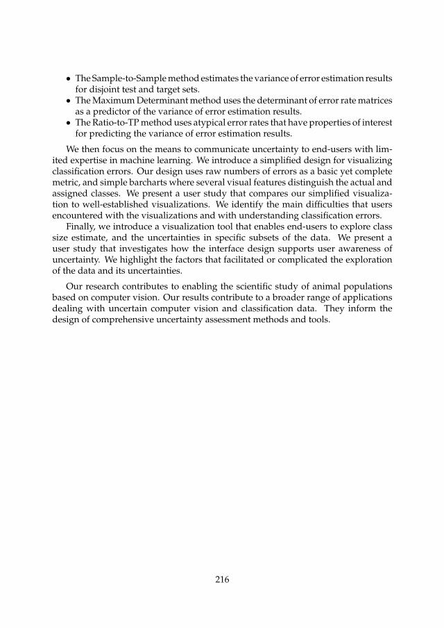
• The Sample-to-Sample method estimates the variance of error estimation resultsfor disjoint test and target sets.
• The Maximum Determinant method uses the determinant of error rate matricesas a predictor of the variance of error estimation results.
• The Ratio-to-TP method uses atypical error rates that have properties of interestfor predicting the variance of error estimation results.
We then focus on the means to communicate uncertainty to end-users with lim-ited expertise in machine learning. We introduce a simplified design for visualizingclassification errors. Our design uses raw numbers of errors as a basic yet completemetric, and simple barcharts where several visual features distinguish the actual andassigned classes. We present a user study that compares our simplified visualiza-tion to well-established visualizations. We identify the main difficulties that usersencountered with the visualizations and with understanding classification errors.
Finally, we introduce a visualization tool that enables end-users to explore classsize estimate, and the uncertainties in specific subsets of the data. We present auser study that investigates how the interface design supports user awareness ofuncertainty. We highlight the factors that facilitated or complicated the explorationof the data and its uncertainties.
Our research contributes to enabling the scientific study of animal populationsbased on computer vision. Our results contribute to a broader range of applicationsdealing with uncertain computer vision and classification data. They inform thedesign of comprehensive uncertainty assessment methods and tools.
216

SamenvattingHet omgaan met onzekerheid in classificatietaken is een cruciale uitdaging voorhet ondersteunen van efficiënte en ethisch verantwoorde classificatiesystemen. Ditproefschrift behandelt onzekerheidsvraagstukken vanuit het perspectief van eindge-bruikers die beperkte expertise hebben op het gebied van machine learning en syste-men voor beeldherkenning. We concentreren ons hierbij op onzekerheid ten aanzienvan het schatten van klassengroottes, oftewel het aantal gevallen per klasse. Hetdoel is om eindgebruikers zonder expertkennis in staat te stellen academisch verant-woorde data analyses m.b.t. klassengroottes uit te voeren, en hen hierbij rekening telaten houden met de onzekerheid die hierbij komt kijken.
We onderzoeken de middelen die eindgebruikers inzicht moeten bieden in deonzekerheid t.a.v. klassengroottes. Na het bestuderen van in-situ videomonitoringvan dierpopulaties hebben we algemeen toepasbare methoden ontwikkeld voor:• Het beoordelen van de onzekerheidsfactoren en de daarmee gepaard gaande
fouten en onzuiverheden bij het schatten van de klassengroottes.• Het visualiseren van de classificatieonzekerheid bij het beoordelen van classi-
ficatiesystemen en het interpreteren van schattingen van klassengroottes.• Het bepalen van de omvang van classificatiefouten bij het schatten van klas-
sengroottes.
Onze gebruikersstudies vormen een belangrijke basis door het analyseren van deinformatiebehoeften van de gebruikers (Hoofdstuk 2), waar aanvullend ook speci-fieke aandacht uitgaat naar de behoeften ten aanzien van de onzekerheid bij clas-sificatietaken (Hoofdstuk 3). Uit dit onderzoek concluderen we wat de belangrijkeonzekerheidsvraagstukken zijn en inventariseren we de methoden om de onzeker-heid te bepalen (Hoofdstuk 4). Vervolgens introduceren we nieuwe methoden voorhet schatten van het aantal fouten in de resultaten van classificatietaken en voor hetcorrigeren van de daaruit voortvloeiende vertekening bij het schatten van de klas-sengroottes (Hoofdstuk 5). Ten slotte onderzoeken we nieuwe visualisatietechniekenvoor het bepalen van classificatiefouten (Hoofdstuk 6) en voor het analyseren vanklassengroottes en bijbehorende onzekerheden (Hoofdstuk 7). We sluiten af met hetbespreken van de implicaties van onze resultaten (Hoofdstuk 8).
We beschrijven de informatie die kan worden geboden door systemen die voordigitale beeldherkenning worden ingezet in wetenschappelijk onderzoek naar dier-populaties. We bestuderen dit toepassingsdomein door marien ecologen te inter-viewen. Ook wordt een vergelijking gemaakt tussen de standaard technieken voorhet verzamelen van gegevens, op basis waarvan we algemene informatiebehoeftenafleiden. Na het interviewen van experts op het gebied van digitale beeldherkenning
217

identificeren we de behoeften die al dan niet middels video monitoringstechniekenkunnen worden ingevuld. Ten slotte bespreken we de onzekerheidsvraagstukken dieinherent zijn aan elke techniek voor het verzamelen van gegevens, en identificerenwe hoog-niveau eisen en wensen ten aanzien van het beoordelen van onzekerheid.
We onderzoeken de informatie die eindgebruikers ondersteunen bij de bepalingvan onzekerheid. Onze tweede gebruikersstudie onderzoekt hoe informatie overclassificatiefouten van invloed is op het begrip, het vertrouwen en de acceptatievan gebruikers met betrekking tot het systeem voor digitale beeldherkenning. Weverzamelen hiertoe aanvullende feedback van gebruikers ten aanzien van onzeker-heidsfactoren, en bespreken de relaties tussen het (on)begrip van onzekerheid, hetvertrouwen en de acceptatie van de gebruikers. Onze conclusies werpen licht oponvervulde informatiebehoeften die aanvullende technieken voor het bepalen vanonzekerheid vereisen, en tevens op de hoog-niveau informatie die met behulp vandeze technieken aan gebruikers moet worden aangeboden.
We identificeren de belangrijkste factoren van onzekerheid waar rekening meegehouden dient te worden bij wetenschappelijk valide analyses van beeldherken-ningsresultaten. We richten ons op in- situ video monitoringstechnologieën, zoalsdie geïmplementeerd zijn binnen het Fish4Knowledge systeem om tellingen van indi-viduele dieren per soort te uit te voeren met behulp van gefixeerde, niet-stereoscopischeonderwatercamera’s. We houden hierbij rekening met onzekerheidsfactoren die losstaan van het beeldherkenningssysteem en voortkomen uit de omgeving waarinhet systeem wordt ingezet (zoals het blikveld en de plaatsing van de camera). Nahet specificeren van het typische systeem voor beeldherkenning en de bijbehorenderandvoorwaarden voor implementatie, worden de onzekerheidsfactoren benoemddie uit interviews met marien ecologen en computerdeskundigen gedestilleerd zijn.Vervolgens identificeren we de interacties tussen onzekerheidsfactoren, en beschri-jven we hoe onzekerheid doorwerkt tot het niveau van hoog-niveau informatie. Tenslotte identificeren we de bestaande en missende technieken voor het bepalen vanonzekerheid.
We identificeren methoden voor het schatten van het aantal fouten in classifi-catieresultaten, waarbij we gebruik maken van de foutmetingen uit testsets. Dezemethoden leveren zuivere schattingen op van de klassengroottes en richten zichniet primair op het identificeren van welke specifieke items verkeerd zijn geclas-sificeerd. De klassengroottes kunnen op zo’n wijze worden gecorrigeerd dat ervoor elke klasse rekening wordt gehouden met potentiële foutpositieve en fout-negatieve gevallen (de zogenaamde false positives en false negatives). We reviewende bestaande statistische en epidemiologische methoden om schattingsfouten te cor-rigeren, en onderzoeken hun geschiktheid voor classificatiemodellen in de contextvan beeldherkenning. Vervolgens breiden we de correctiemethoden uit met hetschatten van het aantal fouten van de verschillende klassen. We identificeren deniet eerder verkende casus van disjuncte test- en doelsets, hetgeen implicaties heeftvoor de variantie van de resultaten van foutcorrectie en -schatting. We introducerenvervolgens drie nieuwe methoden:
218

• De Sample-to-Sample methode schat de variantie van de resultaten van fout-correctie en foutschatting in het geval van disjuncte test- en doelsets.
• De Ratio-to-TP methode gebruikt atypische foutratio’s die eigenschappen hebbendie relevant zijn voor het schatten van de variantie van de resultaten vanfoutschattingen.
• De Maximum-Determinant methode gebruikt de determinant van foutratio’s,geformuleerd als een confusion matrix, als een voorspeller van de variantievan de resultaten van foutschattingen, voorafgaand aan het toepassen van hetclassificatiemodel op de doelsets.
We introduceren een vereenvoudigd ontwerp voor het visualiseren van classi-ficatiefouten, d.w.z. van de fouten die gevonden zijn met behulp van een groundtruth testset en die standaard in een confusion matrix worden gepresenteerd. Wevermijden hierbij het weergeven van de foutratio, aangezien die verkeerd kunnenworden geïnterpreteerd. Vanuit onze ontwerpprincipes kiezen we voor absolutefoutaantallen als een eenvoudige maar complete meting, evenals voor eenvoudigebarcharts waar verschillende visuele kenmerken het onderscheid duiden tussen defeitelijke en geschatte klassen. We presenteren een gebruikersstudie die onze vereen-voudigde visualisatieaanpak vergelijkt met standaard visualisaties (ROC curve, con-fusion matrix en heatmap). We identificeren tenslotte de belangrijkste problemendie gebruikers tegenkomen bij het werken met de visualisaties en het begrijpen vanclassificatiefouten, hierbij rekening houdend met de basiskennis van de gebruiker.
We introduceren een uitgebreide visualisatietool waarmee eindgebruikers deklassengroottes kunnen monitoren en zij onzekerheden in specifieke subsets van degegevens kunnen onderzoeken. We introduceren een interactieontwerp voor het on-derzoeken van klassengroottes en de onderliggende onzekerheidsfactoren (zoals dekwaliteit van het videomateriaal en de tekortkomingen van het beeldherkenningsal-goritme). We onderzoeken middels een gebruikersstudie het interfaceontwerp en dewijze waarop deze gebruikers bewust maakt van de onzekerheden. We benoemende factoren die de exploratie van data en bijbehorende onzekerheden faciliteren ofbemoeilijken. Hierbij wordt er in het bijzonder aandacht besteed aan het feit datgebruikers zich niet altijd bewust zijn van cruciale onzekerheidsfactoren. We sluitenaf met aanbevelingen voor het verbeteren van het ontwerp van dergelijke interfaces.
Ons onderzoek draagt bij aan wetenschappelijke studies naar dierpopulaties opbasis van digitale beeldherkenning. Onze resultaten dragen bij aan uiteenlopendetoepassingen voor het omgaan met onzekerheid in systemen voor beeldherkenningen classificatie, in de zin dat zij de basis vormen voor het ontwerpen van een uitge-breide set van methoden en tools voor het bepalen van de onzekerheid.
219


Curriculum VitaeEmmanuelle (Emma) Beauxis-Aussalet was born and raised in France, until shemoved to The Netherlands for her PhD research. She obtained her first Bachelorof Graphic Design in 2004, and her second Bachelor of Webmaster-Webmarketer in2006. She then obtained a Master of Digital Communication in 2007 (cum laude).Her interest in digital technologies led her to obtain a second Master of ComputerScience in 2008, on the topic of Distributed Systems.
While studying for her Bachelors and her first Master, Emmanuelle worked part-time in communication agencies. She gained a 2-year professional experience asa webmaster and designer at CVB agency, working on internal communication andintranet websites for Renault. She gained a 1-year professional experience as a projectmanager at G2 agency (formely Grrrey), working on websites for major companies(SNCF, Varilux, Nokia). After finishing her second Master, she worked for 3 yearsat Thales as a R&D Engineer specialized in semantic technologies, system designand user interfaces. During her doctoral research, she worked for 2 years as a dataspecialist at LightHouse IP, providing the company with systems to collect, extractand analyze intellectual property data from over 100 data sources.
Emmanuelle conducted her doctoral research at the NWO institute CentrumWiskunde e Informatica (CWI) from 2011 to 2018. As part of the Information Accessgroup and the Fish4Knowledge project (http://www.fish4knowledge.eu), she addedher design skills to the team and gained knowledge of information retrieval, computervision, machine learning and statistics from her colleagues. She led the Classee project(http://classee.project.cwi.nl) in collaboration with the University of Amsterdam andAmsterdam Data Science. She started to work part-time in 2012, for personal reasons,and reduced her work hours in 2016 to take charge of her position at LightHouse IP.
Emmanuelle now works at the Digital Society School of the Amsterdam Uni-versity of Data Science (also known as the Hogeschool van Amsterdam, HvA). Herrole as the Senior Track Associate for the Data-Driven Transformation Track includessupervising learners and establishing research directions for innovative projects incollaboration with industrial partners. Her research interests include the transferand application of data-driven technologies for the best interest of society, the devel-opment of machine learning literacy in the general public, and the development ofexplainable and accountable artificial intelligence.
221


AcknowledgementsThe work presented in this thesis would have been impossible to carry out withoutthe support of many colleagues, friends and family members. Nothing at all couldhave happened without Lynda Hardman, from whom I have learned so much aboutacademic work and work-life balance. She has been able to see the best and the worstin me, and remained focused on bringing the best out of me. Her skills, rigor, patienceand outstanding human qualities were essential to my progress, and brought muchlight into my tunnel.
My colleagues from the Information Access group at CWI were also essential tomy progress. They kept my ignorance and morale in check, and their bright mindswere great sources of ideas and joy. The CWI Personnel and IT departments were oftremendous help too. I could always count on them when needed, and they makeit possible to work in one of the best working environments. Exchanging ideas withcolleagues from other research groups at CWI has been most stimulating, and at timesdecisive for my research. Among the great people with whom I worked, directly orindirectly, I am especially grateful to Arjen (de Vries), Nishant, Desmond, Joost,Tiziano, Martin, Elya, Jiyin, Myriam, Astrid, Tessel, Thaer, Gebre, Jacco, Martine,Bikkie, Erik, Peter, Tom, Arjen (de Rijke), Max, Hannes and Léon.
My colleagues within the Fish4Knowledge project were also outstanding. Ouradventures in Taiwan and Europe are unforgettable, especially when we ate bluejellyfish straight out of the sea at a Lanyu Island beach. For all the good momentswe shared, intellectually and culturally, I would like to thank Robert Fisher, Fang-Pang Lin, Professor Shao, Hsiu-Mei, Karen, Bas, Concetto, Simone, Isaak, Daniela,Phoenix, Cigdem, Gaya, and Jessica.
Alongside my doctoral research, I had the chance to work with extremely kindcolleagues at LightHouse IP. My special thanks go to Willem and Wiegert for theirunderstanding and flexibility, and for welcoming me as a researcher with such anatypical schedule. My luck with outstanding working environments now continueswithin the Digital Society School at the Amsterdam University of Applied Science.Each of my new colleagues, with their creative and diverse mindsets, lets me ap-preciate larger perspectives at the confluence of science, design and society. Findingmyself working among them gives a deeper meaning to my studies and work expe-riences. I am very much looking forward to the new adventures ahead of us.
Beyond my professional life, my personal life in Amsterdam has been rich andjolly thanks to the fantastic friends around me. There is much to stay about yourfriendship, and much to keep of the record. I would rather not mention any juicy
223

story or deep connection in particular, but let you remember them yourselves andknow that our time together is most precious to me. Of those who have broadenedmy mind and my smile, much is owed to Sergio, Maarten, Steven, Tiago, Dome,Andreia, Igor, Romulo, Bea, Luis, Ana Sofia, Noortje, Roberto, Laura, Fleur, Wout,Henrique, Delyana, Luka, Oana, Victoria, and Lorraine. My special thanks to Deba,Teresa, Eleni, Pablo, Bram and Ays, my CWI companions who were most supportiveand understanding.
My dear new friends from Amsterdam cannot overshadow my dear old friendsfrom France, in particular Loriane, Laure, Magali, Guillaume and Lola. It was asacrifice to leave you, but it certainly confirmed how important you are to me.A special thanks to my friend Gaëlle whose precious advice guided me into theacademic world, before and during my PhD.
My deepest gratitude goes to my family for their unfailing support. No matterhow far we may be from each other, knowing that you care for me was the mostpowerful source of strength. You were the invisible hand that carried me through themost difficult times, and that lifted my spirit at all times. What a blessing it is to beborn among you, my parents Marielle and François, and my siblings Romain, Yann,Pierre, David and Anna. This blessing extends to our grandparents, and to our largefamily with its many branches of cousins and (great) uncles and aunts. My mosttenderly geeky memories goes to my grandfather Lucien who taught me HTML andCSS, and fantastic stories about how he contributed to apply the first computers inthe industry, with punch cards and palm-sized transistors.
Le meilleur pour la fin, Ralph gave me essential support and insights, about research,life or music. I could not accurately portray his wisdom and patience, or the joy andpeace he brings to my life. He does not like me to go over the top, and although I amvery tempted to do so here to pay him the right tribute, I’ll keep it short: you are thebest.


Related Documents