STATISTICS 231 COURSE NOTES - University of Waterloopkates/LT3/jsdemos/... · STATISTICS 231 COURSE NOTES Original notes by Jerry Lawless Winter 2013 Edition. Contents ... holder

STATISTICS 231 COURSE NOTES

Original notes by Jerry Lawless

Winter 2013 Edition

Contents

INTRODUCTION TO STATISTICAL SCIENCE 2

1.1 Statistical Science . . . . . . . . . . . . . . . . . . . . . . . . . . . . . . . . . . . . . 2

1.2 Collection of Data . . . . . . . . . . . . . . . . . . . . . . . . . . . . . . . . . . . . . 3

1.3 Data Summaries . . . . . . . . . . . . . . . . . . . . . . . . . . . . . . . . . . . . . . 7

1.4 Probability Distributions and Statistical Models . . . . . . . . . . . . . . . . . . . . . 12

1.5 Data Analysis and Statistical Inference . . . . . . . . . . . . . . . . . . . . . . . . . . 16

1.6 Statistical Software . . . . . . . . . . . . . . . . . . . . . . . . . . . . . . . . . . . . 19

1.7 A More Detailed Example: Colour Classification by Robots . . . . . . . . . . . . . . 25

1.8 Appendix. The R Language and Software . . . . . . . . . . . . . . . . . . . . . . . . 30

1.9 Problems . . . . . . . . . . . . . . . . . . . . . . . . . . . . . . . . . . . . . . . . . 35

MODEL FITTING, MAXIMUM LIKELIHOOD ESTIMATION, AND MODEL CHECK-

ING 43

2.1 Statistical Models and Probability Distributions . . . . . . . . . . . . . . . . . . . . . 43

2.2 Estimation of Parameters (Model Fitting) . . . . . . . . . . . . . . . . . . . . . . . . 47

2.3 Likelihood Functions From Multinomial Models . . . . . . . . . . . . . . . . . . . . 54

2.4 Checking Models . . . . . . . . . . . . . . . . . . . . . . . . . . . . . . . . . . . . . 56

2.5 Problems . . . . . . . . . . . . . . . . . . . . . . . . . . . . . . . . . . . . . . . . . 60

PLANNING AND CONDUCTING EMPIRICAL STUDIES 66

3.1 Empirical Studies . . . . . . . . . . . . . . . . . . . . . . . . . . . . . . . . . . . . . 66

3.2 Planning a Study . . . . . . . . . . . . . . . . . . . . . . . . . . . . . . . . . . . . . 70

3.3 Data Collection . . . . . . . . . . . . . . . . . . . . . . . . . . . . . . . . . . . . . . 72

3.4 Problems . . . . . . . . . . . . . . . . . . . . . . . . . . . . . . . . . . . . . . . . . 73

STATISTICAL INFERENCE: ESTIMATION 75

4.1 Introduction . . . . . . . . . . . . . . . . . . . . . . . . . . . . . . . . . . . . . . . . 75

4.2 Some Distribution Theory . . . . . . . . . . . . . . . . . . . . . . . . . . . . . . . . 79

ii

1

4.3 Confidence Intervals for a Parameter . . . . . . . . . . . . . . . . . . . . . . . . . . . 88

4.4 Problems . . . . . . . . . . . . . . . . . . . . . . . . . . . . . . . . . . . . . . . . . 98

STATISTICAL INFERENCE: TESTING HYPOTHESES 106

5.1 Introduction . . . . . . . . . . . . . . . . . . . . . . . . . . . . . . . . . . . . . . . . 106

5.2 Testing Parametric Hypotheses with Likelihood Ratio Statistics . . . . . . . . . . . . . 110

5.3 Hypothesis Testing and Interval Estimation . . . . . . . . . . . . . . . . . . . . . . . 115

5.4 Problems . . . . . . . . . . . . . . . . . . . . . . . . . . . . . . . . . . . . . . . . . 116

GAUSSIAN RESPONSE MODELS 121

6.1 Introduction . . . . . . . . . . . . . . . . . . . . . . . . . . . . . . . . . . . . . . . . 121

6.2 Inference for a single sample from a Gaussian Distribution . . . . . . . . . . . . . . . 126

6.3 General Gaussian Response Models . . . . . . . . . . . . . . . . . . . . . . . . . . . 131

6.4 Inference for Paired Data . . . . . . . . . . . . . . . . . . . . . . . . . . . . . . . . . 136

6.5 Linear Regression Models . . . . . . . . . . . . . . . . . . . . . . . . . . . . . . . . 142

6.6 Model Checking . . . . . . . . . . . . . . . . . . . . . . . . . . . . . . . . . . . . . . 149

6.7 Problems . . . . . . . . . . . . . . . . . . . . . . . . . . . . . . . . . . . . . . . . . 151

TESTS AND INFERENCE PROBLEMS BASED ON MULTINOMIAL MODELS 161

7.1 Introduction . . . . . . . . . . . . . . . . . . . . . . . . . . . . . . . . . . . . . . . . 161

7.2 Goodness of Fit Tests . . . . . . . . . . . . . . . . . . . . . . . . . . . . . . . . . . . 162

7.3 Two-Way Tables and Testing for Independence of Two Variables . . . . . . . . . . . . 164

7.4 Problems . . . . . . . . . . . . . . . . . . . . . . . . . . . . . . . . . . . . . . . . . 169

CAUSE AND EFFECT 173

8.1 Introduction . . . . . . . . . . . . . . . . . . . . . . . . . . . . . . . . . . . . . . . . 173

8.2 Experimental Studies . . . . . . . . . . . . . . . . . . . . . . . . . . . . . . . . . . . 175

8.3 Observational Studies . . . . . . . . . . . . . . . . . . . . . . . . . . . . . . . . . . . 177

8.4 Problems . . . . . . . . . . . . . . . . . . . . . . . . . . . . . . . . . . . . . . . . . 178

References and Supplementary Resources 182

Statistical Tables 183

APPENDIX. ANSWERS TO SELECTED PROBLEMS 184

A Short Review of Probability 188

INTRODUCTION TO STATISTICAL SCIENCE

1.1 Statistical Science

Statistical science, or statistics, is the discipline that deals with the collection, analysis and interpreta-

tion of data, and with the study and treatment of variability and of uncertainty. If you think about it,

you soon realize that almost everything we do or know depends on data of some kind, and that there is

usually some degree of uncertainty present. For example, in deciding whether to take an umbrella on a

long walk we may utilize information from weather forecasts along with our own direct impression of

the weather, but even so there is usually some degree of uncertainty as to whether it will actually rain

or not. In areas such as insurance or finance, decisions must be made about what rates to charge for an

insurance policy, or whether to buy or sell a stock, on the basis of certain types of data. The uncertainty

as to whether a policy holder will have a claim over the next year, or whether a stock’s price will rise

or fall, is the basis of financial risk for the insurer and the investor.

In order to increase our knowledge about some area or to make better decisions, we must collect

and analyze data about the area in question. To discuss general ways of doing this, it is useful to have

terms that refer to the objects we are studying. The words “population”, “phenomenon” and “process”

are frequently used below; they are simply catch-all terms that represent groups of objects and events

that someone might wish to study.

Variability and uncertainty are present in most processes and phenomena in the real world. Uncer-

tainty or lack of knowledge is the main reason why someone chooses to study a phenomenon in the

first place. For example, a medical study to assess the effect of a new drug for controlling hyperten-

sion (high blood pressure) may be conducted by a drug company because they do not know how the

drug will perform on different types of people, what its side effects will be, and so on. Variability is

ever-present; people have varying degrees of hypertension, they react differently to drugs, they have

different physical characteristics. One might similarly want to study variations in currency or stock val-

ues, variation in sales for a company over time, or variation in hits and response times for a commercial

web site. Statistical science deals both with the study of variability in processes and phenomena, and

with good (i.e. informative, cost-effective) ways to collect and analyze data about such processes.

2

3

There are various possible objectives when one collects and analyzes data on a population, phenom-

enon, or process. In addition to pure “learning” or furthering knowledge, these include decision-making

and the improvement of processes or systems. Many problems involve a combination of objectives. For

example, government scientists collect data on fish stocks in order to further their scientific knowledge,

but also to provide information to legislators or groups who must set quotas or limits on commercial

fishing. Statistical data analysis occurs in a huge number of areas. For example, statistical algorithms

are the basis for software involved in the automated recognition of handwritten or spoken text; statis-

tical methods are commonly used in law cases, for example in DNA profiling or in determining costs;

statistical process control is used to increase the quality and productivity of manufacturing processes;

individuals are selected for direct mail marketing campaigns through statistical analysis of their char-

acteristics. With modern information technology, massive amounts of data are routinely collected and

stored. But data does not equal information, and it is the purpose of statistical science to provide and

analyze data so that the maximum amount of information or knowledge may be obtained. Poor or

improperly analyzed data may be useless or misleading.

Mathematical models are used to represent many phenomena, populations, or processes and to deal

with problems that involve variability we utilize probability models. These have been introduced and

studied in your first probability course, and you have seen how to describe variability and solve certain

types of problems using them. This course will focus more on the collection, analysis and interpreta-

tion of data, but the probability models studied earlier will be heavily used. The most important part of

probability for this course is the material dealing with random variables and their probability distribu-

tions, including distributions such as the binomial, hypergeometric, Poisson, multinomial, normal and

exponential. You should review your previous notes on this material.

Statistical science is a large discipline, and this course is only an introduction. Our broad objectives

are to discuss the collection, analysis and interpretation of data, and to show why this is necessary. By

way of further introduction we will outline important statistical topics, first data collection, and then

probability models, data analysis, and statistical inference. We should bear in mind that study of a

process or phenomenon involves iteration between model building, data collection, data analysis, and

interpretation. We must also remember that data are collected and models are constructed for a specific

reason. In any given application we should keep the big picture in mind (e.g. why are we studying this?

what else do we know about it?) even when considering one specific aspect of a problem.

1.2 Collection of Data

The objects of study in this course are usually referred to as either populations or processes. In essence

a population is just some collection of units (which can be either real or imagined), for example, the

4

collection of persons under the age of 18 in Canada as of September 1, 2012 or the collection of car

insurance policies issued by a company over a one year period. A process is a mechanism by which

output of some kind is produced; units can often be associated with the output. For example, hits on a

website constitute a process (the “units" are the distinct hits), as do the sequence of claims generated

by car insurance policy holders (the “units" are the individual claims). A key feature of processes is

that they usually occur over time, whereas populations are often static (defined at one moment in time).

Populations or processes are studied by defining variates or variables which represent character-

istics of units. These are usually numerical-valued and are represented by letters such as . For

example, we might define a variable as the number of car insurance claims from an individual policy

holder in a given year, or as the number of hits on a website over a specified one hour period. The

values of vary across the units in a population or process, this variability which generates uncertainty

and makes it necessary to study populations and processes by collecting data about them. By "data" we

mean here the values of the variates for specific units in the population.

In planning for the collection of data about some phenomenon, we must carefully specify what the

objectives of doing this are. Then, the feasibility of obtaining information by various means must be

considered, as well as to what extent it will be possible to answer questions of interest. This sounds

simple but is usually difficult to do well, especially with limited resources.

There are several ways in which data are commonly obtained. One is purely according to what is

available: that is, data are provided by some existing source. Huge amounts of data collected by many

technological systems are of this type, for example, data on credit card usage or on purchases made by

customers in a supermarket. Sometimes it is not clear exactly what "available" data represent, and they

may be unsuitable for serious analysis. For example, people who voluntarily provide data in a survey

may not be representative of the population at large. Statistical science stresses the importance of ob-

taining data so that they will be “objective" and provide maximal information. Three broad approaches

are often used to do this:

(i) Sample Surveys The object of many studies is a finite population of some sort (e.g. all persons

over 19 in Ontario; all cars produced by GM in the past year). In this case information may be

obtained by selecting a “representative” sample of individuals from the population and studying

them. Representativeness of the sample is usually achieved by selecting the sample members

randomly from those in the population. Sample surveys are widely used in government statistical

studies, economics, marketing, public opinion polls, sociology, and other areas.

(ii) Observational Studies An observational study is one in which data are collected about a process

or phenomenon (over which the observer has no control) in some objective way, often over some

period of time. For example, in studying risk factors associated with a disease such as lung

cancer, one might investigate all such cases (or perhaps a random sample of them) that occur

5

over a given time period. A distinction between a sample survey and an observational study is

that for the latter the “population” of interest is usually infinite or conceptual. For example, in

investigating risk factors for a disease we would prefer to think of the population as a conceptual

one consisting of persons at risk from the disease recently or in the future.

(iii) Experiments An experiment is a study in which the experimenter (i.e. the person collecting

the data) exercises some degree of control over the process being studied. This usually takes the

form of the experimenter being able to control certain factors in the process. For example, in

an engineering experiment to quantify the effect of temperature on the performance of personal

computers, we might decide to run an experiment with 40 PC’s, ten of which would be operated

at each of the temperatures 10, 20, 30, and 40 degrees Celsius.

The three types of studies described above are not mutually exclusive, and many studies involve

aspects of two or more of them. Here are some slightly more detailed examples.

Example 1.2.1 A sample survey about smoking

Suppose we wish to study the smoking behaviour of Ontario residents aged 14-20 years. (Think

about reasons why such studies are considered important.) Of course, people’s smoking habits and the

population referred to both change over time, so we will content ourselves with a “snapshot” of the

population at some point in time (e.g. the second week of September in a given year). Since we cannot

possibly contact all persons in the population, we decide to select a random sample of persons. The

data to be obtained from each person might consist of their age, sex, place of residence, occupation,

whether they currently smoke, and some additional information about their smoking habits and how

long they have smoked (if they are smokers or ex-smokers).

Note that we have to decide how large should be, and how we are going to obtain our random

sample. The latter question is, in particular, very important if we want to ensure that our sample is

indeed “representative” of the population. The amount of time and money available to carry out the

study heavily influences how we will proceed.

Example 1.2.2 A study about a manufacturing process

When a manufacturer produces a product in packages stated to weigh or contain a certain amount,

they are generally required by law to provide at least the stated amount in each package. Since there

is always some inherent variation in the amount of product which the manufacturing process deposits

in each package, the manufacturer has to understand this variation and set up the process so that no (or

only a very small fraction of) packages contain less than the required amount.

Consider, for example, soft drinks sold in nominal 26 ounce bottles. Because of inherent variation

in the bottle filling process (what might some sources of this be?), the amount of liquid that goes into

6

a bottle varies over a small range. Note that the manufacturer would like the variability in to be as

small as possible, and for bottles to contain at least 26 ounces. Suppose that the manufacturer has just

added a new filling machine to increase the plant’s capacity and wants to compare the new machine

with the older ones. She decides to do this by sampling some filled bottles from each machine and

accurately measuring the amount of liquid in each bottle; this will be an observational study.

How exactly should the data be collected? The machines may “drift” over time (i.e. the average or

the variability in the values of may vary systematically up or down over time) so we should randomly

select bottles over time from each machine; we would have to decide how many, and over what time

periods to collect them.

Example 1.2.3 Clinical trials in medicine

In medical studies of the treatment of disease, it is common to compare alternative treatments in

experiments called clinical trials. Consider, for example, persons who are considered at high risk of a

stroke. Some years ago it was established in clinical trials that small daily doses of aspirin (which acts

as a blood thinner) could lower the risk of stroke. This was done by giving some persons daily doses of

aspirin (call this Treatment 1) and others a daily dose of a placebo, that is, an inactive compound, given

in the same form as the aspirin (call this Treatment 2). The two groups of persons were then followed

for a period of time, and the number of strokes in each group was observed.

This sounds simple, but there are several important points. For example, patients should be assigned

to receive Treatment 1 or Treatment 2 in some random fashion so as to avoid unconscious bias (e.g.

doctors might otherwise tend to put persons at higher risk in the Aspirin group) and to “balance” other

factors (e.g. age, sex, severity of condition) across the two groups. It is also best not to let the patients

or their doctors know which treatment they are receiving. Many other questions must also be addressed.

For example, what variables should we measure as the basis for our data? What should we do about

patients who are forced to drop out of the study because of adverse side effects? Is it possible that the

Aspirin treatment works for the certain types of patients but not others? How long should the study go

on? How many persons should be included?

As an example of a statistical setting where the data are not obtained by a survey, experiment, or

even an observational study, consider the following.

Example 1.2.4 Direct marketing campaigns

With products or services such as credit cards it is common to conduct direct marketing campaigns

in which large numbers of individuals are contacted by mail and “invited” to acquire a product or

service. Such individuals are usually picked from a much larger number of persons on whom the com-

pany has information. For example, in a credit card marketing campaign a company might have data

on several million persons, pertaining to demographic (e.g. sex, age, place of residence), financial (e.g.

7

salary, credit cards held), spending, and other variates. Based on this data, the company wishes to select

persons whom it considers have a good chance of responding positively to the mailout. The challenge

is to use data from previous mail campaigns, along with the current data, to achieve as high a response

rate as possible.

1.3 Data Summaries

We noted in previous section that data consisting of measurements on variables of interest

are collected when we study a phenomenon or process. Data in raw form can be difficult to compre-

hend, especially if the volume is great or if there are large numbers of variables. Many methods of

summarizing data so they can be more easily understood have been developed. There are two main

types: graphical and numerical. We will consider a few important data summaries here.

The basic setup is as follows. Suppose that data on a variable is collected for units in a

population or process. By convention, we label the units as 1 2 and denote their respective

-value as 1 2 . We might also collect data on a second variate for each unit, and we

would denote the values as 1 2 . We often refer to 1 2 , 1 2 or

(1 1) (2 2) ( ) as samples or data sets, and refer to as the sample size.

First we describe some graphical summaries of data sets like this, and then we describe some nu-

merical summaries.

1.3.1 Numerical Summaries

Numerical data summaries are useful for describing features of a data set 1 . Important ones

are

• The mean (also called the sample mean) = 1

P=1

• the (sample) variance 2 =1

−1P=1

( − )2

• the (sample) standard deviation =q2

• the percentiles and quantiles: the ’th quantile or 100’th percentile is a -value () such that

a fraction of the values in the data set are below (). The values (5), (25) and (75)

are called the median, the lower quartile, and the upper quartile respectively. In fact, quantiles

8

are not uniquely defined for all -values in (0 1) for a given data set, and there are different

conventions for defining quantiles and percentiles. For example what is the median of the values

1 2 3 4 5 6? What is the lower quartile? The different conventions for defining quantiles

become identical as becomes large.

The mean and the percentiles and quantiles are easily understood. The variance and standard de-

viation measure the variability or “spread" of the -values in a data set, which is usually an important

characteristic. Another way to measure variability is in terms of the distance between a “low" and

“high" percentile, for example (10) and (90).

A final numerical summary is a frequency table. This is closely related to a histogram and, in fact, is

just a table showing the interval and their frequencies , as used in a histogram. For example, for the

200 male height measurements in Example 1.4.2, the frequency table corresponding to the bottom-left

histogram in Figure 1.1 is shown in Table 1.3.1.

Table 1.3.1 Frequency Table of Male Heights (in m.)Interval () Frequency()

[155 160) 2

[160 165) 13

[165 170) 48

[170 175) 64

[175 180) 42

[180 185) 25

[185 190) 6

Total 200

1.3.2 Graphical Summaries

We consider the first two types of plots for a data set 1 2 of numerical values. These are

called histograms and cumulative frequency plots.

Histograms

Consider measurements 1 2 on a variable . Partition the range of into intervals

= [−1 ) = 1 2 and then calculate for = 1

= number of values from 1 that are in .

The are called the observed frequencies for 1 ; note thatP

=1 = . A histogram is

a graph in which a rectangle is placed on each interval; the height of the rectangle for is chosen so

that the rectangle’s area is proportional to . Two main types of histogram are used:

9

(a) a “standard" histogram where the range of is taken to be finite and the are of equal length.

The height of the rectangle is taken to be . This type of histogram is similar to a bar chart.

(b) a “relative frequency" histogram, where the may or may not be of equal length. The height of

the rectangle for is chosen so that its area equals , which we call the relative frequency

for . Note that in this case the sum of the areas of all the rectangles in the histogram equals one.

Example 1.3.2

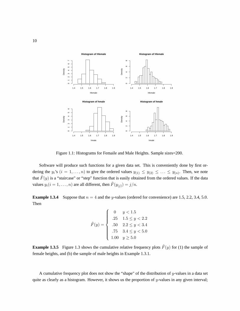
Figure 1.1 shows relative frequency histograms based on each of two samples, (a) heights of 200

females randomly selected from workers aged 18 - 60 in New Zealand, and (b) heights of 200 males,

selected from the same population. Heights are recorded in metres; the female heights range from 1.45

to 1.78m (57.1 to 70.1 in.) and the males heights from 1.59 to 1.88m (62.6 to 74.0 in.).

To construct a histogram, we have to choose the number () and location of the intervals. The

intervals are typically selected in such a way that each interval contains at least one -value from the

sample (that is, each ≥ 1). Software packages are used to produce histogram plots (see Section 1.6)

and they will either automatically select the intervals for a given data set or allow the user to specify

them.

The visual impression from a histogram can change somewhat according to the choice of intervals.

In Figure 1.1, the left-hand panels use 7 intervals and the right-hand use 17 for females and 15 for

males. Note that the histograms give a picture of the distribution of y values in the two samples. For

both females and males the distributions are fairly symmetrical-looking. To allow easy comparison of

female and male height distributions we have used the same y scale (x-axis) for males and females.

Obviously, the distribution of male heights is to the right of that for female heights, but the “spread"

and shape of the two distributions is similar.

Example 1.3.3 Different shapes of distributions can occur in data on a variable . Figure 1.2 shows

a histogram of the lifetimes (in terms of number of km driven) for the front brake pads on 200 new

mid-size cars of the same type. Notice that the distribution is less symmetrical than the ones in Figure

1.1; the brake pad lifetimes have a rather long right-hand tail. The high degree of variability in life-

times is due to the wide variety of driving conditions which different cars are exposed to, as well as to

variability in how soon car owners decide to replace their brake pads.

Cumulative frequency plots Another way to portray a data set 1 2 is to count the number

or proportion of values in the set which are smaller than any given value. This gives a function

() =number of values in 1 2 which are ≤

(1.1)

10

Histogram of hfemale

hfemale

Den

sity

1.4 1.5 1.6 1.7 1.8 1.9

01

23

45

67

Histogram of hfemale

hfemale

Den

sity

1.4 1.5 1.6 1.7 1.8 1.9

02

46

8

Histogram of hmale

hmale

Den

sity

1.4 1.5 1.6 1.7 1.8 1.9

01

23

45

6

Histogram of hmale

hmale

Den

sity

1.4 1.5 1.6 1.7 1.8 1.9

02

46

8

Figure 1.1: Histograms for Femaile and Male Heights. Sample sizes=200.

Software will produce such functions for a given data set. This is conveniently done by first or-

dering the ’s ( = 1 ) to give the ordered values (1) ≤ (2) ≤ ≤ (). Then, we note

that () is a “staircase" or “step" function that is easily obtained from the ordered values. If the data

values ( = 1 ) are all different, then (()) = .

Example 1.3.4 Suppose that = 4 and the -values (ordered for convenience) are 1.5, 2.2, 3.4, 5.0.

Then

() =

⎧⎪⎪⎪⎪⎪⎪⎨⎪⎪⎪⎪⎪⎪⎩

0 15

25 15 ≤ 22

50 22 ≤ 34

75 34 ≤ 50

100 ≥ 50

Example 1.3.5 Figure 1.3 shows the cumulative relative frequency plots () for (1) the sample of

female heights, and (b) the sample of male heights in Example 1.3.1.

A cumulative frequency plot does not show the “shape" of the distribution of -values in a data set

quite as clearly as a histogram. However, it shows us the proportion of -values in any given interval;

11

Figure 1.2: Lifetimes (in km driven) for Front Brake Pads on 200 Cars

the proportion in the interval ( ] is just () − (). In addition, this plot allows us to pinpoint

values such as the median (a -value such that half of the data values are below and half are above

) or the 100’th percentile (a -value () such that a proportion of the data values is less that

()), where 0 1. For example, we see from Figure 1.3.3 that the median (or (.5)) height for

females is about 1.60m (63.0 in) and for males, about 1.73m (68.1 in).

Other plots are also sometimes useful. The size of a data set can be small or large. Histograms

are not very useful when is less than about 20-30, and for small samples we often just plot the loca-

tions of -values on a line; an example is given in Section 1.7. A useful plot called the "strip-plot" for

comparing two or more data sets is given next.

Box plots

Sometimes we have two or more samples of -values, and we may wish to compare them. One way is

by plotting histograms or relative frequency plots for the different samples on the same graph or page;

we did this in Example 1.3.2 for the samples of female heights and male heights. The box plot is a plot

in which only certain values based on a data set are shown, in particular the median, upper and lower

quartiles (these are the 25th and 75th percentiles (.25) and (.75)), plus values equal to 1.5 times the

“inter-quantile range" (75)−(25) below (25) and above (75). Figure 1.4 shows such a plot

for the female heights and male heights data sets from Example 1.3.2.

From the boxplot we can determine, for example, that approximately 75% of the females have

heights less than 1.65 m. or that about 50% of males had heights between 1.7 and 1.79 m.

12

1.3 1.4 1.5 1.6 1.7 1.8 1.9 2.0

0.0

0.2

0.4

0.6

0.8

1.0

Cum. Rel. Freq. for F and M Heights

height(m)

Cum

. Rel

. Fre

q.

1.3 1.4 1.5 1.6 1.7 1.8 1.9 2.0

0.0

0.2

0.4

0.6

0.8

1.0

Figure 1.3: Cumulative relative frequency for Female (F) and Male (M) heights

Two-variable plots

Often we have data on two or more variables for each unit represented in a sample. For example, we

might have the heights and weights for samples of individuals. The data set can then be represented

as pairs, ( ) = 1 where and are the height and weight of the ’th person in the

sample.

When we have two such variables, a useful plot is a scatter plot, which is an − plot of the

points ( ) = 1 . This shows whether and tend to be related in some way. Figure

1.5 shows a scatterplot of heights and weights for 100 adult males. As is obvious from looking

at people around us, taller people tend to weigh more, but there is considerable variability in weight

across persons of the same height.

1.4 Probability Distributions and Statistical Models

Probability models are used to describe random processes. (For convenience we’ll often use the single

term “process" below but the terms population or phenomenon could also be inserted.) They help us

understand such processes and to make decisions in the face of uncertainty. They are important in

studies involving the collection and analysis of data for several reasons. These include:

(i) when studying a process scientifically, questions are often formulated in terms of a model for

the process. The questions of primary interest do not concern the data, but the data provides a

13

1 2

1.5

1.6

1.7

1.8

Box Plots of 200 M and 200 F Heights

Hei

ghts

(m)

Figure 1.4: Box Plots Based on 200 Female and 200 Male Heights in example 1.3.2. "F"=1,

"M"=2.

window to the population or the model.

(ii) the data collected in studying processes are variable, so random variables are often used in dis-

cussing and dealing with data,

(iii) studies of a process usually lead to inferences or decisions that involve some degree of uncer-

tainty, and probability is used to quantify this,

(iv) procedures for making decisions are often formulated in terms of models,

(v) models allow us to characterize processes, and to simulate them via computer experiments or

other means.

Consider a variable associated with the units in a population or process. To describe or “model"

the variability in -values we use probability distributions, which were introduced in your first proba-

bility course. This is done as follows: let be the value for a randomly chosen unit in the population or

process. Because this value is random (we do not know which unit will be chosen) we call a random

variable, and use a probability distribution to provide us with probabilities such as ( ≤ ≤ ). You

should review your probability notes(a limited review is given in an appendix to this chapter) and recall

that random variables are usually either discrete or continuous. A discrete random variable (r.v.) is

one for which the range (set of possible values) of is countable. A continuous r.v. is one whose

range consists of one or more continuous intervals of real numbers. For a discrete r.v. the probability

14

64 66 68 70 72

120

140

160

180

200

height (in.)

wei

ght (

lb.)

Figure 1.5: Scatterplot of Height vs. Weight for 100 Adult Males

function (p.f.) () is defined as

() = ( = ) for certain values of ∈

where = 1 2 3 a countable subset of R is the range of .For a continuous random

variables. the probability density function (p.d.f) () is such that for any interval ( ) contained in

,

( ≤ ≤ ) =

Z

()

Example 1.4.1 A Binomial Distribution

Consider a “toy" example in which a six-sided die is rolled repeatedly. This constitutes the target

process, and for a study we might roll the die a total of times. For this study, let denote the number

of rolls that result in the number 6. We treat it as a random variable since it is subject to random

variation. Assuming that the die has probability 16 of turning up the face "six" on any single roll, and

that the rolls are independent, the probability distribution of has probability function

( = ) = () =

µ

¶(16)(56)− = 0 1 (1.2)

This is called a binomial distribution. We should bear in mind that 1.2 is a model; for any real die the

assumption that a six has probability 16 could be slightly in error. However, 1.2 is a very accurate

model that closely represents variability for most real dice.

15

Example 1.4.2 An Exponential Distribution

Suppose that in a population of light bulbs the random variable represents the lifetime (say in

days) of a randomly chosen bulb. The continuous exponential distribution provides a good model for

many types of bulbs. For example, if the bulbs have an average lifetime of 100 days (2400 hours)

operation, then a distribution with p.d.f.

() = 01−01 0 (1.3)

would be suitable. Using this, we can compute probabilities such as

( 1000) =

Z ∞

1000

01−01 = 0368

Recall that the cumulative distribution function (c.d.f) is defined for a r.v. as

() = ( ≤ ) (1.4)

If is discrete then () =P≤

(); if is continuous then

() =

Z≤

()

Recall also that if ( ) is some function of , then the expectation (or “expected value") of ( ) is

defined as

[( )] =X

()() (1.5)

if is discrete and as

[( )] =

Z

()() (1.6)

if is continuous. Expectations are used in many settings, for example when costs, profits, or losses

are associated with a random variable. The expectation ( ) is called the mean of and is often

denoted by the Greek letter . The expectation [( − )2] is called the variance of and is often

denoted either as ( ) or with the Greek symbol 2. The square root =p ( ) is called the

standard deviation of , or ( ).

Your previous course introduced several families of probability distributions along with processes

or populations to which they are applied. Models such as the binomial, Poisson, exponential, normal

(Gaussian), and multinomial will be reintroduced and used in this course. The first few problems at the

end of the chapter provide a review of some models, and examples of where they are applied.

16

Many problems involve two or more random variables defined for any given unit. For example

1 could represent the height and 2 the weight of a randomly selected 30 year old male in some

population. In general, we can think of a random variable = (1 2 ) as being a vector of

length ≥ 1 This may make it necessary to consider multivariate probability distributions, which were

introduced in your last course for discrete random variables.

In many statistical applications there is a primary variable of interest, but there may be a number

of other variables 1 2 that affect , or are “related" to in some way. In this case we often refer

to as the “response" variable and 1 2 as “explanatory" variables or covariates. Many studies

are carried out for the purpose of determining how one or more explanatory variables are related to a

response variable. For example, we might study how the number of insurance claims for a driver is

related to their sex, age, and type of car (− variables). One reason for studying explanatory variables

is to search out cause and effect relationships. Another is that we can often use explanatory variables

to improve decisions, predictions or “guesses" about a response variable. For example, insurance com-

panies use explanatory variables in defining risk classes and determining life insurance premiums.

1.5 Data Analysis and Statistical Inference

Whether we are collecting data to increase our knowledge or to serve as a basis for making decisions,

proper analysis of the data is crucial. Two broad aspects of the analysis and interpretation of data may

be distinguished. The first is what we refer to as descriptive statistics: This is the portrayal of the

data, or parts of it, in numerical and graphical ways so as to show certain features. (On a historical

note, the word “statistics” in its original usage referred to numbers generated from data; today the word

is used both in this sense and to denote the discipline of Statistics.) We have considered methods of

doing this in Section 1.3. The terms data mining and knowledge discovery in data bases (KDD) refer

to exploratory data analysis where the emphasis is on descriptive statistics. This is often carried out on

very large data bases.

A second aspect of a statistical analysis of data is what we refer to as statistical inference: that is,

we use the data obtained in the study of a process or phenomenon to draw more general inferences

about the process or phenomenon itself. In general, we try to use study data to draw inferences about

some target population or process. This is a form of inductive inference, in which we reason from the

specific (the observed data) to the general (the target population or process). This may be contrasted

with deductive inference (as in logic and mathematics) in which we use general results (e.g. axioms)

to prove specific things (e.g. theorems).

This course introduces some basic methods of statistical inference. Two main types of problems

will be discussed, loosely referred to as estimation problems and hypothesis testing problems. In the

17

former, the problem is to estimate some feature of a process or population. For example, we may wish

to estimate the proportion of Ontario residents aged 14 - 20 who smoke, or to estimate the distribution

of survival times for certain types of AIDS patients. Another type of estimation problem is that of

“fitting” or selecting a probability model for a process.

Testing problems involve using the data to assess the truth of some question or hypothesis. For

example, we may hypothesize that in the 14-20 age group a higher proportion of females than males

smoke, or that the use of a new treatment will increase the average survival time of AIDS patients by

at least 50 percent. These questions can be addressed by collecting data on the populations in question.

Statistical analysis involves the use of both descriptive statistics and methods of estimation and

testing. As brief illustrations, we return to the first two examples of section 1.2.

Example 1.5.1 A smoking behaviour survey

Suppose that a random sample of 200 persons aged 14-20 was selected, as described in example

1.2.1. Let us focus only on the sex of each person in the sample, and whether or not they smoked. The

data are nicely summarized in a two-way frequency table such as the following:

No. of smokers No. of non-smokers Total

Female 32 66 98

Male 27 75 102

Total 59 141 200

If we wished to estimate, say, the proportion of females aged 14-20 in the population who smoke,

we might simply use the sample proportion = 3298 = 327. However, we would also like some

idea as to how close this estimate is likely to be to the actual proportion in the population. Note that if

we selected a second sample of 200 persons, we would very likely find a different proportion of females

who smoked. When we consider estimation problems later in the course, we will learn how to use a

probability model to calculate the uncertainty for this kind of study. For now, let us merely note what

kind of model seems appropriate.

Consider only the proportion of females who smoke, and suppose that we select females at

random. (This is not quite what was done in the above survey.) Then the number of women who

smoke is actually a random variable in the sense that before the data are collected, it is random. Suppose

now that the population of females from which the sample is drawn is very large and that a proportion

of the population are smokers. Then the probability distribution of is, to a very close approximation,

binomial with probability function

() = ( = ) =

µ

¶(1− )− for = 0 1

Knowing this will allow better estimation procedures to be developed later in the course.

18

Example 1.5.2 A soft drink bottle filler study

Recall example 1.2.2, and suppose that 26 ounce bottles are randomly selected from the output of

each of two machines, one old and one new, over a period of one week. The bottles were selected from

each machine’s output at roughly the same times. Accurate measurements of the amounts of liquid in

the bottles are as follows:

Old machine:27.8 28.9 26.8 27.4 28.0 27.4 27.1 28.0 26.6 25.6

24.8 27.1 25.7 27.9 25.3 26.0 27.3 27.4 25.7 26.9

27.3 25.2 25.6 27.0 26.2 27.3 24.8 27.1 26.7 26.8

26.6 26.6 28.6 27.0 26.6 27.3 25.9 27.6 27.6 28.3

28.0 26.4 25.4 26.7 27.8 27.4 27.3 26.9 26.9 26.9New Machine:

26.6 26.8 27.2 26.9 27.6 26.7 26.8 27.4 26.9 27.1

27.0 27.1 27.0 26.6 27.2 26.1 27.6 27.2 26.5 26.3

28.0 26.8 27.1 26.7 27.7 26.7 27.1 26.5 26.8 26.8

26.9 27.2 27.4 27.1 26.5 27.2 26.8 27.3 26.6 26.6

27.0 26.9 27.3 26.0 27.4 27.4 27.6 27.2 27.8 27.7

The amount of liquid that goes into a bottle is a random variable, and a main objective of this

study is to determine what the distribution of looks like for the old machine and for the new machine,

over the one week period of the study. For this to be really useful, we should check first that there are

no “drifts" or time trends in the data. Figure 1.6 gives a plot of vs. (order of production) for each

machine, and no trends are apparent. The random variable is continuous and so we would like to use

a continuous probability distribution as the model. It often turns out for problems involving weights

or measures that a normal distribution provides a suitable model. Recall that the distribution ( 2)

(which we will often call in this course a Gaussian distribution, denoted ( )) has probability

density function

(; ) =1√2

exp

(−12

µ−

¶2)−∞ ∞

and that probabilities are obtained by integrating it; recall also that = () and 2 = Var() are

the mean and variance of the distribution. (note: exp (a) is the same as .)

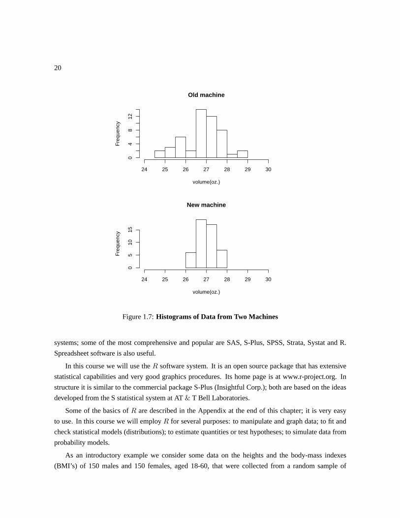
Before trying to use any particular model for , it is a good idea to “look” at the data. Figure

?? shows frequency histograms of the data from the old and new machines, respectively. It shows that

(i) the distributions of for the old and new machines each look like they might be well described

19

0 10 20 30 40 50

2526

2728

29

Old Machine

index

Vol

(oz.

)

0 10 20 30 40 50

26.0

27.0

28.0

New Machine

index

Vol

(oz.

)

Figure 1.6: Time Sequence Plot of Bottle Contents

by (different) normal distributions, (ii) the variability in the new machine’s distribution is considerably

less than in the old’s.

After this simple bit of descriptive statistics we could carry out a more thorough analysis, for

example fitting normal distributions to each machine. We can also estimate attributes of interest, such

as the probability a bottle will receive less than 26 ounces of liquid, and recommend adjustments that

could be made to the machines. In manufacturing processes it is important that the variability in the

output is small, and so in this case the new machine is better than the old one.

1.6 Statistical Software

Software is essential for data manipulation and analysis. It is also used to deal with numerical calcu-

lations, to produce graphics, and to simulate probability models. There exist many statistical software

20

Old machine

volume(oz.)

Fre

quen

cy

24 25 26 27 28 29 30

04

812

New machine

volume(oz.)

Fre

quen

cy

24 25 26 27 28 29 30

05

1015

Figure 1.7: Histograms of Data from Two Machines

systems; some of the most comprehensive and popular are SAS, S-Plus, SPSS, Strata, Systat and R.

Spreadsheet software is also useful.

In this course we will use the software system. It is an open source package that has extensive

statistical capabilities and very good graphics procedures. Its home page is at www.r-project.org. In

structure it is similar to the commercial package S-Plus (Insightful Corp.); both are based on the ideas

developed from the S statistical system at AT & T Bell Laboratories.

Some of the basics of are described in the Appendix at the end of this chapter; it is very easy

to use. In this course we will employ for several purposes: to manipulate and graph data; to fit and

check statistical models (distributions); to estimate quantities or test hypotheses; to simulate data from

probability models.

As an introductory example we consider some data on the heights and the body-mass indexes

(BMI’s) of 150 males and 150 females, aged 18-60, that were collected from a random sample of

21

workers in New Zealand. The data are listed below, along with a few summary statistics. The BMI is

often used to measure obesity or severely low weight. It is defined as follows:

=weight()height()2

There is some variation in what different types of guidelines refer to as “overweight", “underweight",

etc. One that is sometimes used by public health professionals is:

Underweight BMI 18.5

Normal 18.5 ≤ BMI 250

Overweight 25.0 ≤ BMI 300

Moderately Obese 30.0 ≤ BMI 350

Severely Obese 35.0 ≤ BMI

The data on heights are stored in two vectors (see the Appendix at the end of the chapter) called

hmale and hfemale; the BMI measurement are in vectors bmimale and bmifemale.

Heights and Body-Mass Index (BMI) Measurements for 150 Males and Females

NOTE: BMI = weight(kg)/height(m)**2

MALE HEIGHTS (m)- hmale

[1] 1.76 1.76 1.68 1.72 1.73 1.78 1.78 1.86 1.77 1.72 1.72 1.77 1.77 1.70 1.72

[16] 1.77 1.79 1.75 1.74 1.71 1.73 1.74 1.70 1.71 1.72 1.66 1.74 1.73 1.77 1.69

[31] 1.91 1.77 1.81 1.74 1.87 1.76 1.69 1.87 1.78 1.70 1.78 1.84 1.82 1.77 1.72

[46] 1.80 1.72 1.69 1.78 1.69 1.80 1.82 1.65 1.56 1.64 1.60 1.82 1.73 1.62 1.77

[61] 1.81 1.73 1.74 1.75 1.73 1.71 1.63 1.72 1.74 1.75 1.72 1.83 1.77 1.74 1.66

[76] 1.93 1.81 1.73 1.68 1.71 1.69 1.74 1.74 1.79 1.68 1.71 1.74 1.82 1.68 1.78

[91] 1.79 1.77 1.74 1.78 1.86 1.80 1.74 1.69 1.85 1.71 1.79 1.74 1.80 1.64 1.82

[106] 1.66 1.56 1.80 1.68 1.73 1.78 1.69 1.57 1.64 1.67 1.74 1.89 1.77 1.75 1.84

[121] 1.66 1.71 1.75 1.75 1.64 1.73 1.79 1.74 1.83 1.80 1.74 1.81 1.80 1.66 1.75

[136] 1.82 1.80 1.81 1.71 1.59 1.71 1.79 1.80 1.70 1.77 1.78 1.64 1.70 1.86 1.75

Min. 1st Qu. Median Mean 3rd Qu. Max.

1.56 1.71 1.74 1.744 1.79 1.93

FEMALE HEIGHTS (m)- hfemale

[1] 1.60 1.56 1.61 1.64 1.65 1.58 1.71 1.72 1.72 1.61 1.72 1.52 1.47 1.61 1.64

[16] 1.60 1.67 1.76 1.57 1.60 1.59 1.61 1.59 1.61 1.56 1.68 1.61 1.63 1.58 1.68

22

[31] 1.51 1.64 1.52 1.59 1.62 1.64 1.65 1.64 1.67 1.56 1.77 1.55 1.71 1.71 1.54

[46] 1.60 1.67 1.58 1.53 1.64 1.63 1.60 1.64 1.67 1.54 1.65 1.57 1.59 1.58 1.58

[61] 1.67 1.53 1.69 1.64 1.54 1.66 1.71 1.58 1.60 1.52 1.41 1.51 1.56 1.65 1.68

[76] 1.55 1.60 1.57 1.73 1.58 1.53 1.58 1.53 1.66 1.57 1.54 1.69 1.62 1.65 1.64

[91] 1.61 1.67 1.64 1.57 1.70 1.66 1.61 1.62 1.58 1.67 1.67 1.69 1.53 1.70 1.65

[106] 1.56 1.79 1.70 1.61 1.56 1.65 1.59 1.62 1.71 1.57 1.72 1.58 1.70 1.70 1.66

[121] 1.60 1.54 1.60 1.68 1.68 1.67 1.57 1.61 1.64 1.57 1.72 1.48 1.60 1.66 1.60

[136] 1.58 1.65 1.59 1.57 1.53 1.60 1.64 1.57 1.59 1.68 1.61 1.66 1.52 1.67 1.65


1.41 1.573 1.61 1.618 1.667 1.79

MALE BMI- bmimale

[1] 20.6 30.3 28.5 18.9 37.5 29.1 27.7 26.1 27.9 34.7 26.8 28.9 25.6 23.7 30.0

[16] 28.6 27.5 30.4 22.7 24.7 26.2 28.0 35.5 22.7 26.5 26.4 30.2 24.7 24.8 25.9

[31] 24.3 25.7 21.7 24.9 30.1 29.3 23.6 27.0 33.6 29.0 26.4 28.0 25.6 31.0 27.7

[46] 23.1 25.4 24.9 29.7 24.5 28.5 25.1 32.7 27.5 25.1 24.0 26.0 30.2 27.0 26.3

[61] 29.7 21.7 26.7 26.3 34.2 23.5 26.0 26.5 26.4 22.8 22.3 22.5 23.7 27.4 31.0

[76] 28.7 27.2 25.1 25.1 27.9 26.8 23.9 30.9 28.8 27.5 26.8 23.4 32.4 25.6 24.0

[91] 34.0 30.8 32.0 31.8 23.3 28.0 22.8 23.9 23.2 32.5 23.1 32.6 24.7 27.2 23.7

[106] 27.1 22.1 22.6 18.3 25.6 22.3 28.6 21.8 26.1 26.6 22.9 29.3 33.7 30.2 29.2

[121] 33.5 26.2 26.7 27.7 26.5 25.5 27.9 30.1 34.9 28.7 29.1 27.8 34.1 24.2 27.9

[136] 27.8 25.5 25.6 24.1 23.8 30.1 23.5 27.5 27.1 25.1 28.2 35.2 32.4 30.7 21.3


18.3 24.7 26.75 27.08 29.1 37.5

FEMALE BMI- bmifemale

[1] 23.4 21.2 31.2 27.1 25.9 26.8 28.8 24.3 36.2 37.0 37.5 37.2 28.4 20.7 25.1

[16] 18.9 20.4 27.7 30.1 27.9 19.8 27.0 23.3 17.5 25.8 23.2 21.2 26.8 25.9 21.6

[31] 34.2 20.3 37.9 32.7 22.7 25.9 35.6 32.0 32.2 19.8 23.3 32.7 22.7 22.8 27.0

[46] 21.3 22.7 23.7 25.6 21.4 32.8 30.3 29.0 27.7 29.4 26.3 26.2 28.0 29.1 24.6

[61] 28.4 22.5 33.2 29.6 26.1 27.8 26.8 26.8 32.4 38.8 23.5 33.7 30.2 29.1 26.8

[76] 36.4 19.0 24.5 23.1 33.9 26.5 31.0 26.1 29.8 23.4 31.2 28.4 26.7 27.3 24.1

[91] 20.7 25.0 23.6 33.1 23.1 32.2 24.8 22.5 29.9 26.9 28.5 27.5 26.3 29.7 21.9

[106] 26.3 20.3 21.5 24.5 31.1 31.3 34.0 31.9 27.2 16.4 20.3 29.1 25.7 23.4 27.6

23

[121] 26.4 28.4 24.8 29.1 25.6 29.4 26.2 29.7 22.8 21.5 21.3 29.9 17.6 28.3 24.1

[136] 28.3 24.0 25.4 23.9 24.3 30.4 28.6 25.0 23.8 36.0 31.5 21.8 29.4 30.8 28.1


16.4 23.42 26.8 26.92 29.7 38.8

Methods for summarizing data were discussed in Section 1.4. Both numerical and graphical sum-

maries can be obtained easily using . For example, mean () and () produce the mean and

variance 2 of a set of numbers 1 contained in the vector . The definitions of and 2 are

(see Section 1.3.2)

=1

X=1

2 =1

− 1X=1

( − )2

Using this we can find that the mean (average) heights for the 150 males in the sample is = 174 m

(68.5 in.) and for the 150 females is = 162 m (63.8 in.).

Figure 1.8: Histograms and Models for Height and BMI data

A histogram gives a picture of the data. Figure 1.8 shows relative frequency histograms for heights

and BMI’s for males and females. We also show normal distribution probability density functions

24

overlaid on each histogram. In each case we used a normal distribution ( 2) where the mean

and variance 2 were taken to equal and 2. For example, for the male heights we used = 174 and

2 = 004316. Note from Figure 1.8 that the normal (Gaussian) distributions agree only moderately

well with the observed data. Chapter 2 discusses probability models and comparisons of models and of

data in more detail.

The following code, reproduced from the Appendix, that illustrates how to look at the data and

produce plots like those in Figure 1.6.1.

EXAMPLE: BODY-MASS INDEX DATA

The R session below describes how to take data on the BMI measurements

for 150 males and 150 females and examine them, including the possibility

of fitting Gaussian distributions to the data.

The data are in vectors bmimale and bmifemale.

> summary(bmimale)


18.3 24.7 26.75 27.08 29.1 37.5

> summary(bmifemale)


16.4 23.42 26.8 26.92 29.7 38.8

sort(bmimale) #Sometimes its nice to look at the ordered sample

[1] 18.3 18.9 20.6 21.3 21.7 21.7 21.8 22.1 22.3 22.3 22.5 22.6 22.7 22.7 22.8

[16] 22.8 22.9 23.1 23.1 23.2 23.3 23.4 23.5 23.5 23.6 23.7 23.7 23.7 23.8 23.9

[31] 23.9 24.0 24.0 24.1 24.2 24.3 24.5 24.7 24.7 24.7 24.8 24.9 24.9 25.1 25.1

[46] 25.1 25.1 25.1 25.4 25.5 25.5 25.6 25.6 25.6 25.6 25.6 25.7 25.9 26.0 26.0

[61] 26.1 26.1 26.2 26.2 26.3 26.3 26.4 26.4 26.4 26.5 26.5 26.5 26.6 26.7 26.7

[76] 26.8 26.8 26.8 27.0 27.0 27.1 27.1 27.2 27.2 27.4 27.5 27.5 27.5 27.5 27.7

[91] 27.7 27.7 27.8 27.8 27.9 27.9 27.9 27.9 28.0 28.0 28.0 28.2 28.5 28.5 28.6

[106] 28.6 28.7 28.7 28.8 28.9 29.0 29.1 29.1 29.2 29.3 29.3 29.7 29.7 30.0 30.1

[121] 30.1 30.1 30.2 30.2 30.2 30.3 30.4 30.7 30.8 30.9 31.0 31.0 31.8 32.0 32.4

[136] 32.4 32.5 32.6 32.7 33.5 33.6 33.7 34.0 34.1 34.2 34.7 34.9 35.2 35.5 37.5

> sqrt(var(bmimale)) #Get the sample standard deviations

[1] 3.555644

> sqrt(var(bmifemale))

25

[1] 4.602213

> par(mfrow=c(1,2)) #Sets up graphics to do two side by side plots per page

> hist(bmimale,prob=T,xlim=c(15,40)) #Relative frequency histogram; the

xlim option specifies the range we want

for the x-axis.

> x<- seq(15,40,.01) #We’ll use this vector to plot a Gaussian pdf

> fx<- dnorm(x,27.08,3.56) #Computes values f(x) of the G(27.08,3.56) pdf; we

have estimated the distribution mean and standard

deviation from the sample values.

> lines(x,fx) #This function adds points (x,fx) to the latest plot created

and joins them up with lines. This creates a plot of the

pdf overlaid on the histogram.

> hist(bmifemale,prob=T,xlim=c(15,40)) #Now do a histogram for the female

data.

> fx<- dnorm(x,26.92,4.60) #Compute pdf f(x) for G(26.92,4.60) distribution

> lines(x,fx) # As previously

> q() #Quit the R session.

1.7 A More Detailed Example: Colour Classification by Robots

Inexpensive robots and other systems sometimes use a crude light sensor to identify colour-coded items.

In one particular application, items were one of five colours: White, Black, Green, Light Blue, Red.

The sensor determines a light intensity measurement from any given item and uses it to identify the

colour.

In order to program the robot to do a good job, experiments are conducted on the sensor, as follows:

items of different colours are passed by the sensor and the intensity readings are recorded. Table 1

shows some typical data for 10 Red and 10 White items. Note that all Red items (or all White items) do

not give the same -values. The reasons for the variability include variation in the colour and texture

of the items, variations in lighting and other ambient conditions, and variations in the angle at which

the item passes the sensor.

Table 1. Light intensity measurements for 10 Red and 10 White items

Red 47.6 47.2 46.6 46.8 47.8 46.8 46.3 46.5 47.6 48.8

White 49.2 50.1 48.8 50.6 51.3 49.6 49.3 50.8 48.6 49.8

Figure 1.9 shows a plot (called a “strip" plot) of similar data on 20 items of each of the five colours.

26

It is clear that the measurements for the Black items are well separated from the rest, but that there is

some overlap in the ranges of the intensities for some pairs of items.

To program the robot to “recognize" colour we must partition the range for into five regions,

one corresponding to each colour. There are various ways to do this, the simplest being to choose

values that minimize the number of misclassifications (incorrectly identified colours) in the data that

are available. Another approach is to model the variability in -values for each colour using a random

variable with a probability distribution and then to use this to select the partition. This turns out to

have certain advantages, and we will consider how this can be done.

light intensity

10 20 30 40 50 60

Black

Blue

Green

Red

White

Figure 1.9: Light Intensities for 20 Items of Each Colour

Empirical study has shown that for the population of White items has close to a Gaussian distri-

bution,

∼ ( )

Similarly, for Black, Green, Light Blue and Red items the distribution of is close to ( ),

( ), ( ) and ( ), respectively. The approximate values of and for each

colour are (we will discuss in Chapter 2 how to find such values)

27

Black = 257 = 24

Light Blue = 384 = 10

Green = 427 = 13

Red = 474 = 11

White = 498 = 12

The operators of the equipment have set the following decision rule (partition) for identifying the

colour of an item, based on the observed value :

Black ≤ 340Light Blue 340 ≤ 405Green 405 ≤ 452Red 452 ≤ 486White 486

We now consider a few questions that shed light on this procedure.

Question: Based on the Gaussian models, what are the probabilities an item colour is misclassified?

• This can be determined for each colour. For example, (Black item is misclassified) = ( 340) where ∼ (257 24)

= .0003.

(Red item is misclassified) = 1 - (452 ≤ 486) where ∼ (474 11)

= .1604.

• Note that colours may be classified incorrectly in more than one way. For example

(Red is misclassified as Green) = (405 ≤ 452) = 0227

(Red is misclassified as White) = ( 486) = 1377.

Question: What kind of data would we collect to check that the Gaussian models are satisfactory

approximations to the distributions of ?

• We would need to randomly select items of a specific colour, then use the sensor to get an inten-

sity measurement . By doing this for a large number of items, we would get measurements

1 which can be used to examine or fit parametric models for , using methods developed

in later chapters.

28

Question: Do we need to use a Gaussian model (or any other probability distribution) for this problem?

• No. We could use a completely “empirical” approach in which we used the sensor experimentally

with many items of different colours, then determined a “good” decision rule for identifying

colour from the observed data. (For example, we could, as mentioned above, do this so that the

total number of items misclassified was minimized.)

• To see how this would work, use to simulate, say 20, values for each colour, then try to pick

the cut-points for your decision rule.

Question: What are some advantages of using a probability model (assuming it fits the data)?

• It allows decision rules to be obtained and compared mathematically (or numerically).

• In more complicated problems (e.g. with more types of items or with multivariate measurements)

a direct empirical approach may be difficult to implement.

• Models allow comparisons to be made easily across similar types of applications. (For example,

sensors of similar types, used in similar settings.)

• Models are associated with “scientific” descriptions of measurement devices and processes.

Figure 1.10 shows the probability density functions for the Gaussian distributions for Black, Light

Blue, Green, Red and White items, which provides a clear picture of misclassification probabilities.

Given the models above, it is possible to determine an “optimal" partition of the -scale, according

to some criterion. The criterion that is often used is called the overall misclassification rate, and it is

defined as follows for this problem. Suppose that among all of the items which the robot encounters

over some period of time, that the fractions which are Black, Light Blue, Green, Red, and White are

and respectively (with + + + + = 1). Suppose also that

instead of the values above we consider arbitrary cut-points 1 2 3 4, so that if ≤ 1, the

decision is “Black", if 1 ≤ 2, the decision is “Light Blue", and so on. The overall probability a

randomly selected item is classified correctly (CC) is

(CC) = (|Black) (Black) + (|Blue) (Blue) + (|Green) (Green) + (|Red) (Red) + (|(1.7)

= ( ≤ 1) + (1 ≤ 2) + (2 ≤ 3) + (3 ≤ 4) + ( 4)

29

0 10 20 30 40 50 60

0.0

0.1

0.2

0.3

0.4

light intensity (y)

pdf(

y)

0 10 20 30 40 50 60

0.0

0.1

0.2

0.3

0.4

0 10 20 30 40 50 60

0.0

0.1

0.2

0.3

0.4

0 10 20 30 40 50 60

0.0

0.1

0.2

0.3

0.4

0 10 20 30 40 50 60

0.0

0.1

0.2

0.3

0.4

Figure 1.10: Distributions of Light Intensities for Items of Colours

where denote random variables with the(257 24)(384 10) (427 13)(474 11) (498 1

distributions respectively. It is not trivial to choose 1 2 3 4 to maximize this (and therefore

minimize the probability of incorrect classification) but it can be done numerically, for any set of

values for . Note that for given values for 1 2 3 4 we can readily calcu-

late (CC). For example, if = = 05; = = = 3, then with the values

1 = 340 2 = 405 3 = 452 4 = 486 used above we get, using to calculate the probabili-

ties in 1.7,

(CC) = 05[pnorm(340 257 24)] + 05[pnorm(405 384 10)− pnorm(340 384 10)]

+ 3[pnorm(452 427 13)− pnorm(405 427 13)]

+ 3[pnorm(486 474 11)− pnorm(452 474 11)] + 3[1− pnorm(486 498 12)]

= 05(9997) + 05(9821) + 3(9723) + 3(8396) + 3(8413)

= 895

Thus the probability of incorrect identification of a colour is .105. Note that if the “mix" of colours

30

that the robot sees changes (i.e. the values change) then (CC) changes. For example,

if there were more Black and fewer White items in the mix, the (CC) would go up. Problems 3 and

4 at the end of the chapter consider slightly simpler classification problems involving only two types

of “items". It is easier to maximize the (CC) in these cases. You should note that the general

problem of classification based on certain data is very common. Spam detection in your emailer, or

credit checking at the bank, fraud detection in a financial institution, and even legal institutions such as

courts are all examples where a classification takes place on the basis of noisy data.

1.8 Appendix. The R Language and Software

1.8.1 Some R Basics

R is a statistical software system that has excellent numerical, graphical and statistical capabilities.

There are Unix and Windows versions. These notes are a very brief introduction to a few of the features

of R. Web resources have much more information. You can also download a Unix or Windows version

of R to your own computer. R is invoked on Math Unix machines by typing R. The R prompt is . R

objects include variables, functions, vectors, arrays, lists and other items. To see online documentation

about something, we use the help function. For example, to see documentation on the function mean(),

type

help(mean).

In some cases help.search() is also helpful. The assignment symbol is - : for example,

x<- 15 assigns the value 15 to variable x.

To quit an R session in unix, type q()

1.8.2 Vectors

Vectors can consist of numbers or other symbols; we will consider only numbers here. Vectors are

defined using c(): for example,

x<- c(1,3,5,7,9)

defines a vector of length 5 with the elements given. Vectors and other classes of objects possess certain

attributes. For example, typing

length(x)

31

will give the length of the vector x. Vectors of length n are often a convenient way to store data values

for n individuals or units in a sample. For example, if there are variates x and y associated with any

given individual, we would define vectors for x and for y.

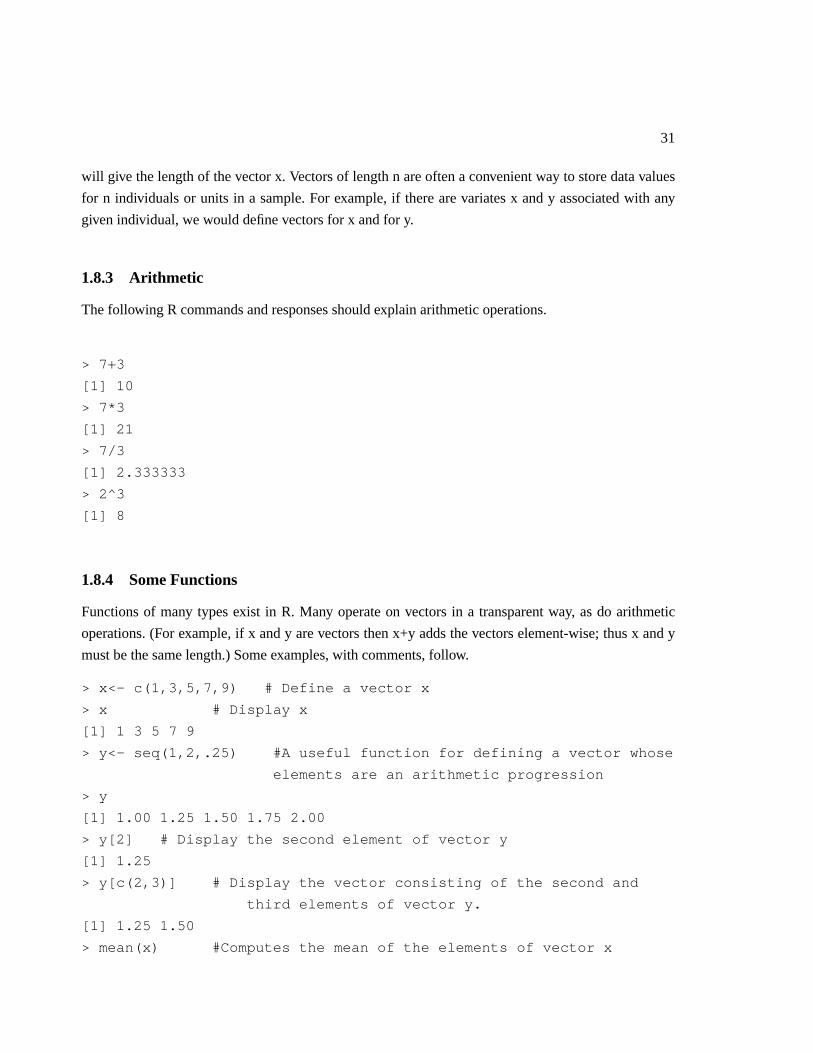
1.8.3 Arithmetic

The following R commands and responses should explain arithmetic operations.

> 7+3

[1] 10

> 7*3

[1] 21

> 7/3

[1] 2.333333

> 2^3

[1] 8

1.8.4 Some Functions

Functions of many types exist in R. Many operate on vectors in a transparent way, as do arithmetic

operations. (For example, if x and y are vectors then x+y adds the vectors element-wise; thus x and y

must be the same length.) Some examples, with comments, follow.

> x<- c(1,3,5,7,9) # Define a vector x

> x # Display x

[1] 1 3 5 7 9

> y<- seq(1,2,.25) #A useful function for defining a vector whose

elements are an arithmetic progression

> y

[1] 1.00 1.25 1.50 1.75 2.00

> y[2] # Display the second element of vector y

[1] 1.25

> y[c(2,3)] # Display the vector consisting of the second and

third elements of vector y.

[1] 1.25 1.50

> mean(x) #Computes the mean of the elements of vector x

32

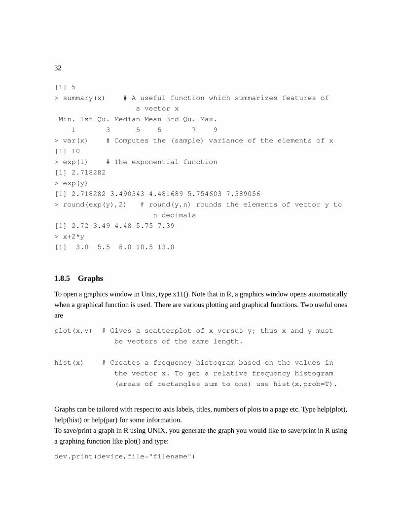
[1] 5

> summary(x) # A useful function which summarizes features of

a vector x


1 3 5 5 7 9

> var(x) # Computes the (sample) variance of the elements of x

[1] 10

> exp(1) # The exponential function

[1] 2.718282

> exp(y)

[1] 2.718282 3.490343 4.481689 5.754603 7.389056

> round(exp(y),2) # round(y,n) rounds the elements of vector y to

n decimals

[1] 2.72 3.49 4.48 5.75 7.39

> x+2*y

[1] 3.0 5.5 8.0 10.5 13.0

1.8.5 Graphs

To open a graphics window in Unix, type x11(). Note that in R, a graphics window opens automatically

when a graphical function is used. There are various plotting and graphical functions. Two useful ones

are

plot(x,y) # Gives a scatterplot of x versus y; thus x and y must

be vectors of the same length.

hist(x) # Creates a frequency histogram based on the values in

the vector x. To get a relative frequency histogram

(areas of rectangles sum to one) use hist(x,prob=T).

Graphs can be tailored with respect to axis labels, titles, numbers of plots to a page etc. Type help(plot),

help(hist) or help(par) for some information.

To save/print a graph in R using UNIX, you generate the graph you would like to save/print in R using

a graphing function like plot() and type:

dev.print(device,file="filename")

33

where device is the device you would like to save the graph to (i.e. x11) and filename is the name of

the file that you would like the graph saved to. To look at a list of the different graphics devices you

can save to, type

help(Devices).

To save/print a graph in R using Windows, you can do one of two things.

a) You can go to the File menu and save the graph using one of several formats (i.e. postscript, jpeg,

etc.). It can then be printed. You may also copy the graph to the clipboard using one of the formats

and then paste to an editor, such as MS Word. Note that the graph can be printed directly to a printer

using this option as well.

b) You can right click on the graph. This gives you a choice of copying the graph and then pasting to

an editor, such as MS Word, or saving the graph as a metafile or bitmap. You may also print directly

to a printer using this option as well.

1.8.6 Distributions

There are functions which compute values of probability or probability density functions, cumulative

distribution functions, and quantiles for various distributions. It is also possible to generate (pseudo)

random samples from these distributions. Some examples follow for the Gaussian distribution. For

other distribution information, type help(Poisson),

help(Binomial) etc.

> y<- rnorm(10,25,5) # Generate 10 random values from the Gaussian

distribution G(25,5); this is the same as

the normal distribution N(25,25). The values

are stored in the vector y.

> y # Display the values

[1] 22.50815 26.35255 27.49452 22.36308 21.88811 26.06676 18.16831 30.37838

[9] 24.73396 27.26640

> pnorm(1,0,1) # Compute P(Y<=1) for a G(0,1) random variable.

[1] 0.8413447

> qnorm(.95,0,1) # Find the .95 quantile (95th percentile) for G(0,1).

[1] 1.644854

34

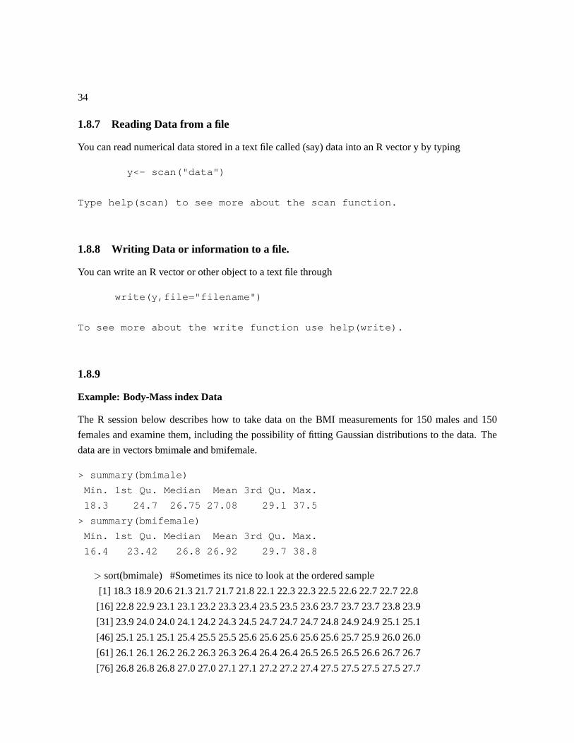
1.8.7 Reading Data from a file

You can read numerical data stored in a text file called (say) data into an R vector y by typing

y<- scan("data")

Type help(scan) to see more about the scan function.

1.8.8 Writing Data or information to a file.

You can write an R vector or other object to a text file through

write(y,file="filename")

To see more about the write function use help(write).

1.8.9

Example: Body-Mass index Data

The R session below describes how to take data on the BMI measurements for 150 males and 150

females and examine them, including the possibility of fitting Gaussian distributions to the data. The

data are in vectors bmimale and bmifemale.

> summary(bmimale)


18.3 24.7 26.75 27.08 29.1 37.5

> summary(bmifemale)


16.4 23.42 26.8 26.92 29.7 38.8

sort(bmimale) #Sometimes its nice to look at the ordered sample

[1] 18.3 18.9 20.6 21.3 21.7 21.7 21.8 22.1 22.3 22.3 22.5 22.6 22.7 22.7 22.8

[16] 22.8 22.9 23.1 23.1 23.2 23.3 23.4 23.5 23.5 23.6 23.7 23.7 23.7 23.8 23.9

[31] 23.9 24.0 24.0 24.1 24.2 24.3 24.5 24.7 24.7 24.7 24.8 24.9 24.9 25.1 25.1

[46] 25.1 25.1 25.1 25.4 25.5 25.5 25.6 25.6 25.6 25.6 25.6 25.7 25.9 26.0 26.0

[61] 26.1 26.1 26.2 26.2 26.3 26.3 26.4 26.4 26.4 26.5 26.5 26.5 26.6 26.7 26.7

[76] 26.8 26.8 26.8 27.0 27.0 27.1 27.1 27.2 27.2 27.4 27.5 27.5 27.5 27.5 27.7

35

[91] 27.7 27.7 27.8 27.8 27.9 27.9 27.9 27.9 28.0 28.0 28.0 28.2 28.5 28.5 28.6

[106] 28.6 28.7 28.7 28.8 28.9 29.0 29.1 29.1 29.2 29.3 29.3 29.7 29.7 30.0 30.1

[121] 30.1 30.1 30.2 30.2 30.2 30.3 30.4 30.7 30.8 30.9 31.0 31.0 31.8 32.0 32.4

[136] 32.4 32.5 32.6 32.7 33.5 33.6 33.7 34.0 34.1 34.2 34.7 34.9 35.2 35.5 37.5

> sqrt(var(bmimale)) #Get the sample standard deviations

[1] 3.555644

> sqrt(var(bmifemale))

[1] 4.602213

> par(mfrow=c(1,2)) #Sets up graphics to do two side by side plots per page

> hist(bmimale,prob=T,xlim=c(15,40)) #Relative frequency histogram; the

xlim option specifies the range we want

for the x-axis.

> x<- seq(15,40,.01) #We’ll use this vector to plot a Gaussian pdf

> fx<- dnorm(x,27.08,3.56) #Computes values f(x) of the G(27.08,3.56) pdf; we

have estimated the distribution mean and standard

deviation from the sample values.

> lines(x,fx) #This function adds points (x,fx) to the latest plot created

and joins them up with lines. This creates a plot of the

pdf overlaid on the histogram.

> hist(bmifemale,prob=T,xlim=c(15,40)) #Now do a histogram for the female

data.

> fx<- dnorm(x,26.92,4.60) #Compute pdf f(x) for G(26.92,4.60) distribution

> lines(x,fx) # As previously

> q() #Quit the R session.

NOTE: You can see from the histograms and Gaussian pdf plots that the Gaussian distribution does

not seem an especially good model for BMI variation. The Gaussian pdf’s are symmetric whereas the

distribution of BMI measurements looks somewhat asymmetric.

1.9 Problems

1. The binomial distribution is a discrete probability model with probability function of the form

() =

Ã

!(1− )− = 0 1

where 0 1 and is a positive integer. If is a random variable with probability function

() we write ∼ Bin( ).

36

A woman who claims to have special guessing abilities is given a test, as follows: a deck which

contains five cards with the numbers 1 to 5 is shuffled and a card drawn out of sight of the

woman. The woman then guesses the card, the deck is reshuffled with the card replaced, and

the procedure is repeated several times. Let represent the number of correct guesses by the

woman.

(a) Suppose an experiment consists of 20 repetitions, or guesses. If someone guesses “ran-

domly” each time, discuss why ∼ Bin(20 2) would be an appropriate model.

(b) Suppose the woman guessed correctly 8 times in 20 repetitions. Calculate ( ≥ 8) if

∼ Bin(20 2) and use the result to consider whether the woman might have a probability

of guessing correctly which is greater than 2.

(c) In a longer sequence of 100 repetitions over two days, the woman guessed correctly 32

times. Calculate ( ≥ 32) if ∼ Bin(100 2); you can use a normal approximation if

you wish. What do you conclude now?

2. The exponential distribution is a continuous probability model in which a random variable

has p.d.f.

() =1

−

≥ 0

where 0 is a parameter.

(a) Show that is the mean of . Graph the p.d.f. of .

(b) The exponential distribution is often found to be a suitable model for distributions of life-

times. The 30 observations 1 30 below, for example, are the lifetimes (in days) of a

random sample of a particular type of lightbulb, subjected to constant use:

23 261 87 7 120 14 62 47 225 71

246 21 42 20 5 12 120 11 3 14

71 11 14 11 16 90 1 16 52 95

The mean of these 30 numbers is = 596. It has been suggested that if an exponential

model is suitable for representing the distribution of lifetimes in the population of lightbulbs

from which they came, then in (1) should have a value of around 59.6. Why should this

be so?

(c) For the exponential distribution (1) with = 596, calculate

i) 1 = (0 ≤ 40)

37

ii) 2 = (40 ≤ 100)

iii) 3 = (100 ≤ 200)

iv) 4 = ( ≥ 200)Compare the values 301, 302, 303, 304 with the actual number of observations in

the four intervals [0 40), [40 100), [100 200), [200∞), respectively. Why should these

numbers agree fairly well if the exponential distribution is a suitable model?

(d) Use a graph created using R to compare the model (1) with the data observed.

3. The normal or Gaussian distribution is an important continuous probability model which

describes the variation in many types of physiological measurements very well. Recall that

∼ ( ) (or ∼ ( 2)) means that has a normal distribution with mean and stan-

dard deviation (variance 2).

Let be a variate representing the systolic blood pressure of a randomly selected woman in

a large population, grouped or stratified by age. Good models for for persons not taking any

medication have been found to be:

ages 17-24 ∼ (118 8)

ages 45-54 ∼ (130 9)

(a) Plot the probability density functions for the two models on the same graph using R.

(b) For each age group find the probability a randomly selected woman has blood pressure over

140.

(c) Suppose you were given the blood pressures 1 25 for 25 women from one of the two

age groups; you do not know which. Show that you could decide with near certainty which

group they came from by considering the value of = (1 + · · ·+ 25)25.

(d) Suppose you know that very close to 10% of the population of women are in each age group

and that you want to devise a rule for “deciding” which age group a woman is in, based on

knowing only her blood pressure . Good rules will be of the form: for some chosen value

0, decide that

age is 17-24 iff ≤ 0.

Assuming you are going to use this rule over and over again, find 0 so that the fraction of

decisions which are wrong is minimized.

38

4. A test for diabetes is based on glucose (sugar) levels in the blood, measured after fasting

for a specified period of time. For healthy people the glucose levels have close to a Gaussian

distribution with mean = 531 and standard deviation = 058. For

untreated diabetics is (close to) Gaussian with = 1174 and = 350.

A diagnostic test for diabetes can be based on a measurement for a given individual. Suppose

that we use the cutoff value 6.5, and diagnose someone as diabetic (diagnosis to be confirmed by

further tests) if 65.

(a) If a person is diabetic, what is the probability that they are diagnosed as such by the test?

(b) What is the probability that a nondiabetic is incorrectly diagnosed as being diabetic?

(c) The probability in part (a) is called the sensitivity of the test. We can increase it by choosing

a cutoff value which is less than 6.5. However, this will increase the probability of

incorrectly diagnosing nondiabetics, as in part (b). Recompute the probabilities in (a) and

(b) if = 60.

(d) What cutoff value do we need to make the sensitivity 0.98?

(Based on Exercise 6.6 in Wild and Seber, 1999)

5. Normal (Gaussian) approximation for binomial probabilities. If ∼ ( ) and is

large, the Gaussian distribution can be used to calculate approximate probabilities for . In

particular,

( ≤ )=

Ã − p(1− )

! = 0 1 (1.8)

where () is the cumulative distribution function (cdf) for the (0 1) distribution. A slightly

better approximation is to replace with + 5 in (2).

A mail campaign to sign up new customers for a particular credit card has in the recent past had

a success rate of about = 012 (i.e. about 1.2% of persons contacted sign up for the card).

(a) If 140,000 persons are sent the offer to sign up, what is the probability at least 1600 new

customers are obtained, if = 012?

(b) Suppose 2000 new customers were actually obtained. Would you conclude that this cam-

paign was more successful than other recent ones? Explain your answer.

39

6. Computer-generated (pseudo) random numbers. Consider a procedure designed to generate

sequences of digits ( = 1 2 ) such that for each

( = ) = 1 = 0 1 9

and such that 1 2 are statistically independent.

(a) Suggest two things that you might do in order to assess whether a given computer procedure

satisfies the above conditions. (Assume that you can use the procedure to generate, say,

1000 digits and that you will base your assessment on these values.)

(b) The next problem gives such a procedure∗, but is theoretically a little complicated to work

out its distribution mathematically. However, the distribution can be closely approximated

by computer simulation. You can generate a sequence 1 2 of length by the

command ← (0 : 9 = )

Generate a sequence of 1000 digits and plot a histogram of the data. (∗ You can use it to check,

for example, whether runs of odd and even digits are consistent with the randomness conditions.)

7. A runs test for randomness

Consider a process which produces binary sequences of 0’s and 1’s. The process is supposed to

have the property that for a sequence 1 2 of arbitrary length ,

( = 1) = = 1− ( = 0) = 1

1 are mutually independent.

In probability this is called a Bernoulli model.

One way to test whether a sequence “looks” like it could have come from a Bernoulli model

is to consider the number of runs (maximal subsequences of 0’s or 1’s) in the sequence; let the

random variable denote the number of runs.

(a) Consider a randomly generated sequence from the Bernoulli model and suppose there were

40

0’s and 1’s (+ = ). Try to prove that, conditional on and ,

( = ) =

⎧⎪⎪⎪⎪⎪⎪⎪⎪⎪⎪⎪⎪⎪⎪⎪⎪⎪⎨⎪⎪⎪⎪⎪⎪⎪⎪⎪⎪⎪⎪⎪⎪⎪⎪⎪⎩

2

Ã− 1 − 1

!Ã− 1 − 1

! +

= 2

− 1 − 1

− 1

+ − 1

− 1

− 1

+

= 2 + 1

(b) Part (a) is challenging. An approximation to the distribution of which is not conditional

on and may be based on the Central Limit Theorem. Let 1 be a Bernoulli

sequence of 0’s and 1’s and define the random variables

1 = 1 =

(0 if = −11 if 6= −1

Note that =

X=1

(why?) and use this to find () and Var() in terms of and ,

where = ( = 1) = 1− ( = 0).

(c) By the Central Limit Theorem, = [ − ()]Var()12 has a limiting (0 1) distri-

bution as → ∞. Use this to find the approximate probability of 20 or fewer runs in a

Bernoulli sequence with = 100, = 5.

(d) Outline how you could approximate the distribution of in part (b) by simulation. For the

case = 10 = 5 (i.e. sequences of length 10) generate 1000 sequences and obtain the

value for each one. Plot these in a histogram.

8. The data below show the lengths (in cm) of male and female coyotes captured in Nova Scotia.

41

Females

93.0 97.0 92.0 101.6 93.0 84.5 102.5 97.8 91.0 98.0 93.5 91.7

90.2 91.5 80.0 86.4 91.4 83.5 88.0 71.0 81.3 88.5 86.5 90.0

84.0 89.5 84.0 85.0 87.0 88.0 86.5 96.0 87.0 93.5 93.5 90.0

85.0 97.0 86.0 73.7

Males

97.0 95.0 96.0 91.0 95.0 84.5 88.0 96.0 96.0 87.0 95.0 100.0

101.0 96.0 93.0 92.5 95.0 98.5 88.0 81.3 91.4 88.9 86.4 101.6

83.8 104.1 88.9 92.0 91.0 90.0 85.0 93.5 78.0 100.5 103.0 91.0

105.0 86.0 95.5 86.5 90.5 80.0 80.0

(a) Obtain relative frequency histograms of the data for the females and the males using R.

(b) Compute the sample mean and standard deviation for the female and male coyotes.

Assuming = and = , plot the pdf’s for Gaussian distributions ( ) over top of

the histograms for the females and males. (Note: if you have measurements 1

then =P=1

and 2 =1

−1P=1

( − )2) (Based on Table 2.3.2 in Wild and Seber

1999)

9. The data below come from a study of the completion times for a task experienced by computer

users in a multiuser system. Each data point ( ) is the result of an experiment in which

terminals connected to the same server all initiated the same task. The variable is the average

time per task.

40 9.9 40 11.9 50 15.1 65 18.6

50 17.8 10 5.5 30 13.3 65 19.8

60 18.4 30 11.0 65 21.8

45 16.5 20 8.1 40 13.8

(a) Make a scatterplot of the data.

(b) Which variable is the response and which is the explanatory variable?

(Based on Wild and Seber 1999, Table 3.1.2)

10. The R system contains a lot of interesting data sets. Here’s how to look at a data set contained in

an array wtloss; it show the weight on each day of a special diet for a very obese 48-year old male

42

who weighed 184.35 kg before starting the diet. The data set is in the MASS package which is

part of R. First you need the command

library (MASS)

Then the command

wtloss

will display a data base called wtloss which has 52 rows and two columns. Column 1 gives the

day of the diet and Column 2 the person’s weight on that day. Obtain a scatterplot of weight vs.

day by the command

plot (wtloss $Days, wtloss $Weight, xlab = “Day", ylab = “Weight")

Does the weight appear to be a linear function of days on diet? Why would you expect that it

would not be linear if a long time period is involved?

MODEL FITTING, MAXIMUM

LIKELIHOOD ESTIMATION, AND

MODEL CHECKING

2.1 Statistical Models and Probability Distributions

A statistical model is a mathematical model that incorporates probability in some way. As described

in Section 1.4, our interest here is in studying variability and uncertainty in populations and processes.

This will be done by considering random variables that represent characteristics of the units or in-

dividuals in the population or process, and by studying the probability distributions of these random

variables. It is very important to be clear about what the “target" population or process is, and exactly

how the variables being considered are defined and measured. Chapter 3 discusses these issues. You

have already seen some examples in Chapter 1, and been reminded of material on random variables

and probability distributions that is taught in earlier courses.

A difficult step for beginners in probability and statistics is the choice of a probability model in

given situations. The choice of a model is usually driven by some combination of three factors:

1. Background knowledge or assumptions about the population on or process which lead to certain

distributions.

2. Past experience with data from the population or process, which has shown that certain distribu-

tions are suitable.

3. Current data, against which models can be assessed.

In probability theory, there is a lot of emphasis on factor 1 above, and there are many “families"

of probability distributions that describe certain types of situation. For example, binomial and Poisson

distributions were derived as models for outcomes in repeated trials and for the random occurrence

of events in time or space, respectively. The normal (Gaussian) distribution, on the other hand, is

43

44

often used to represent the distributions of continuous measurements such as the heights or weights of

individuals, but this is based more on past experience that such models are suitable than on factor 1

above.

In choosing a model we usually consider families of probability distributions. To be specific let

us suppose that for some discrete random variable we consider a family whose probability function

depends on one or more parameters :

( = ) = (; ) for

where is a countable (i.e. discrete) set of real numbers, the range of the random variable . In order

to apply the model to a specific problem we require a value for ; the selection of a value (let’s call it

) is often referred to as “fitting" the model or as “estimating" the value of . The next section gives a

way to do this.

Most applications require a series of steps in the formulation (the word “specification" is also used)

of a model. In particular, we often start with some family of models in mind, but find after examining

data and fitting the model that it is unsuitable in certain respects. (Methods for checking the suitability

of a model will be discussed in Section 2.4.) We then try out other models, and perhaps look at more

data, in order to work towards a satisfactory model. Doing this is usually an iterative process, which is

sometimes represented by diagrams such as

Collect and Examine data

↓Propose a (revised?) Model

. ↑Fit model −→ Check model

↓Draw Conclusions

Later courses in Statistics spend a lot of time on this process. In this course we will focus on settings

in which the models are not too complicated, so that model formulation problems are minimized.

Before considering how to fit a model, let us review briefly some important families of distributions

that were introduced in earlier courses.

Binomial Distribution

The discrete random variable (r.v.) has a binomial distribution if its probability function is of the

form

(; ) =

µ

¶(1− )− for = 0 1 (2.2)

45

where is a parameter with 0 1. This model arises in connection with repeated independent

trials, where each trial results in either an outcome “S" (with probability ) or “F" (with probability

1 − ). If equals the number of outcomes in a sequence of trials, it has theprobability function

2.2. We write ∼ ( ) to indicate this.

Poisson Distribution

The discrete r.v. has a Poisson distribution if its p.f. is of the form

(; ) = −

!for = 0 1 2

where is a parameter with 0. To indicate this we write ∼ Poisson (). It can be shown that

( ) = for this model. The Poisson distribution arises in settings where represents the number of

random events of some kind that occur over a fixed period of time, for example, the number of arrivals

in a queue or the number of hits on a web site in a 1 hour period. For this model to be suitable the

events must occur completely randomly in time. The Poisson distribution is also used to describe the

random occurrence of events in space.

Exponential Distribution

The continuous r.v. has an exponential distribution if its p.d.f. is of the form

(; ) =1

− 0

where is parameter with 0. To indicate this we write ∼ Exp(). It can be shown that

( ) = . The exponential distribution arises in some settings where represents the time until an

event occurs.

Gaussian (normal) Distribution

The continuous r.v. has a Gaussian (also called a normal) distribution if its p.d.f. is of the form

(; ) =1√2

−12(−)2 −∞ ∞

where and are parameters, with −∞ ∞ and 0. It can be shown that ( ) =

Var( ) = 2 ( ) = . We write either ∼ ( ) or ∼ ( 2) to indicate that has

this distribution. Note that in the former case, ( ) the second parameter is the standard deviation

whereas in the latter, ( 2) we specify the variance 2 for the parameter. Most software syntax

including requires that you input the standard deviation for the parameter. The normal (Gaussian)

distribution provides a suitable model for the distribution of measurements on characteristics like the

size or weight of individuals in certain populations, but is also used in many other settings. It is par-

ticularly useful in finance where it is the basis for the most common model for asset prices, exchange

46

rates, interest rates, etc.

Multinomial Distribution

This is a multivariate distribution in which the discrete r.v.’s 1 ( ≥ 2) have the joint p.f.

(1 = 1 = ) = (1 ; θ)

=!

1!2! !11

22

where each ( = 1 ) is an integer between 0 and , and they satisfy the conditionP=1

= .

The elements of the parameter vector θ = (1 2 ) satisfy 0 1 for = 1 andP=1

= 1. This distribution is a generalization of the binomial distribution. It arises when there are

repeated independent trials, where each trial results in one of types of outcomes (call them types

1 ), and the probability outcome occurs is . If ( = 1 ) is the number of times

that type occurs in a sequence of trials, then (1 ) have the joint distribution above. This is

indicated by (1 ) ∼ Mult(;θ)

SinceP=1

= we can if we wish rewrite (1 ;θ) using only − 1 variables, say

1 −1 (with replaced by 1 − − −1). We see that the multinomial distribution with

= 2 is just the binomial distribution, where the outcomes are type 1 (say) and the outcomes are

type 2.

We will also consider models that include explanatory variables, or covariates. For example, sup-

pose that the response variable is the weight (in kg) of a randomly selected female in the age range

16-25, in some population. A person’s weight is related to their height, so we might want to study

this relationship. A way to do this is to consider females with a given height (say in meters), and to

propose that the distribution of , given is Gaussian, ( + ). That is, we are proposing that

the average (expected) weight of a female depends linearly on her height: we write this as

( |) = +

Such models are considered in Chapters 6-8.

We now turn to the problem of fitting a model. This requires assigning numemrical values to the

parameters in the model (for example in the Gaussian model or in an exponential model).

47

2.2 Estimation of Parameters (Model Fitting)

Suppose a probability distribution that serves as a model for some random process depends on an

unknown parameter (possibly a vector). In order to use the model we have to “estimate" or specify a

value for . To do this we usually rely on some data that have been collected for the random variable in

question. It is important that such data be collected carefully, and we consider this issue in Chapter 3.

For example, suppose that the random variable Y represents the weight of a randomly chosen female

in some population, and that we were considering a Gaussian model, ∼ ( ). Since ( ) = ,

we might decide to randomly select, say, 10 females from the population, to measure their weights

1 2 10, and then to estimate by the average,

=1

10

10X=1

(2.3)

This seems sensible (why?) and similar ideas can be developed for other parameters; in particular,

note that must also be estimated, and think about how you might use 1 10 to do this. (Hint:

what does or 2 represent in the Gaussian model?). Before we move on note that although we are

estimating the parameter we did not write = 110

10P=1

! Why did we introduce a special notation

This serves a dual purpose, both to remind you that it is not exactly equal to the unknown value of

the parameter but also to indicate that it is a quantity derived from the data = 1 2 10 and is

therefore random. A different draw of the sample = 1 2 10 will result in a different value for

the random variable

Instead of albeit sensible but nevertheless ad hoc approaches to estimation as in (2.3), it is desirable

to have a general method for estimating parameters. Maximum likelihood is a very general method,

which we now describe.

Let the (vector) random variable represent potential data that will be used to estimate , and let

represent the actual observed data that are obtained in a specific application. Note that to write down

(), we must know (or make assumptions about) how the data were collected. It is usually assumed

here that the data consists of measurements on a random sample of population units. The likelihood

function for is then defined as

() = ( = ; ) ∈ Ω

where the parameter space Ω is the set of possible values for . Thus the likelihood function is the

probability that we will observe at random the observation considered as a function of the parame-

ter. Obviously values of the parameter that render our observation more probable would seem more

credible than those that render is less probableso values of for which () is large are those that ap-

pear more consistent with the observation The value that maximizes () for given data is called

48

the maximum likelihood estimate (MLE) of . This seems like a “sensible" approach, and it turns out

to have very good properties. Let us see how it works.

Example 2.2.1 (a public opinion poll).

We are surrounded by polls. They guide the policies of our political leaders, the products that

are developed by manufacturers, and increasingly the content of the media. For example the poll in

Figure ?? was conducted by Harris/Decima company under contract of the CAUT (Canadian Asso-

ciation of University Teachers). This is one of semi-annual poll on Post-Secondary Education and

Canadian Public Opinion, this one conducted in November 2010. Harris/Decima uses a telephone poll

of 2000 “representative” adults. Twenty-six percent of respondents agreed and 48% disagreed with the

following statement: " University and college teachers earn too much".

Harris/Decima declared their result were accurate to within±22 percent 19 times out of twenty but

the margin of error for regional, demographic or other subgroups is wider. What does this mean and

where did these estimates and intervals come from? Suppose that the random variable represents

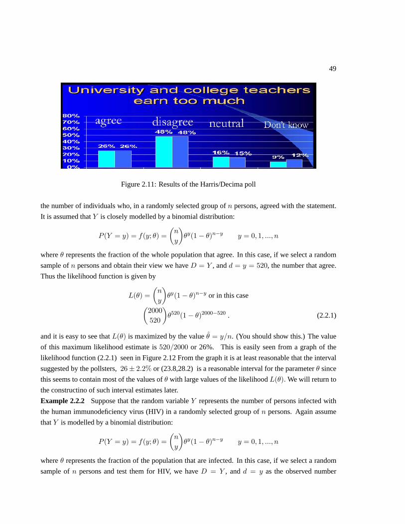
49

Figure 2.11: Results of the Harris/Decima poll

the number of individuals who, in a randomly selected group of persons, agreed with the statement.

It is assumed that is closely modelled by a binomial distribution:

( = ) = (; ) =

µ

¶(1− )− = 0 1

where represents the fraction of the whole population that agree. In this case, if we select a random

sample of persons and obtain their view we have = , and = = 520, the number that agree.

Thus the likelihood function is given by

() =

µ

¶(1− )− or in this caseµ

2000

520

¶520(1− )2000−520 . (2.2.1)

and it is easy to see that () is maximized by the value = . (You should show this.) The value

of this maximum likelihood estimate is 5202000 or 26%. This is easily seen from a graph of the

likelihood function (2.2.1) seen in Figure 2.12 From the graph it is at least reasonable that the interval

suggested by the pollsters, 26± 22% or (23.8,28.2) is a reasonable interval for the parameter since

this seems to contain most of the values of with large values of the likelihood () We will return to

the constructino of such interval estimates later.

Example 2.2.2 Suppose that the random variable represents the number of persons infected with

the human immunodeficiency virus (HIV) in a randomly selected group of persons. Again assume

that is modelled by a binomial distribution:

( = ) = (; ) =

µ

¶(1− )− = 0 1

where represents the fraction of the population that are infected. In this case, if we select a random

sample of persons and test them for HIV, we have = , and = as the observed number

50

Figure 2.12: Likelihood function for the Harris/Decima poll and corresponding interval estimate for

infected. Thus

() =

µ

¶(1− )− (2.2.1)

again () is maximized by the value = .

The likelihood function’s basic properties, for example where its maximum is and its shape, is not

affected if we multiply () by a constant. Indeed it is not the absolute value of the likelihood that is

important but the relative values at two different values of the parameter, e.g. (1)(2) and these

are also unaffected if we multiply () by a constant. In view of this we might define the likelihood

as ( = ; ) or any constant multiple of it, so, for example, we could drop the term¡

¢in (2.2.1)

and define () = (1− )− This function and (2.2.1) are maximized by the same value =

and have the same shape. Indeed we might rescale the likelihood function by dividing through by

the maximum so that the new maximum is 1. This rescaled version is called the relative likelihood

function

() = ()()

It is also convenient to define the log likelihood function,

() = log() ∈ Ω

Note that also maximizes (). (Why?) Because functions are often maximized by setting their

51

derivatives equal to zero1, we can usually obtain by solving the equation(s)

= 0 (2.2.2)

For example, from () = (1− )− we get () = log + (− ) log (1− ). Thus

=

− −

1−

and solving = 0 gives = .

In many applications the data are assumed to consist of a random sample 1 from some

process or population, where each has the probability density function (or probability function)

(; ). In this case = (1 ) and

() =

Y=1

(; ) (2.2.3)

(You should recall from Stat 230 that if 1 are independent then their joint p.d.f. is the product

of their individual p.d.f.’s) In addition, if we have independent data 1 and 2 about from two

independent studies, then since (1 = 12 = 2) = (1 = 1) (2 = 2)with independency

we can obtain the “combined" likelihood function () based on 1 and 2 together as

() = 1()2()

where () = ( = ; ) = 1 2

Example 2.2.3 Suppose that the random variable represents the lifetime of a randomly selected

light bulb in a large population of bulbs, and that follows an exponential distribution with p.d.f.

(; ) =1

− 0

where 0. If a random sample of light bulbs is tested and gives lifetimes 1 , then the

likelihood function for is

() =

Y=1

µ1

−

¶=1

−

Thus

() = − log − 1

X=1

1Can you think of an example of a continuous function () defined on the interval [0 1] for which the maximum

max0≤≤1 () is NOT found by setting 0() = 0?

52

and solving = 0, we get

=1

X=1

=

It is easily checked that this maximizes () and so it is the MLE.

Example 2.2.2 revisited. We can often write down a likelihood function in different ways. For the

random sample of persons who are tested for the HIV, for example, we could define for = 1

= (person tests positive for HIV.)

(Note: () is the indicator function; it equals 1 if is true and 0 if is false.) In this case the p.f.

for is (1; ) with

(; ) = (1− )1− for = 0 1

and the likelihood function is

() =

Y=1

(; )

= Σ(1− )−Σ

= (1− )−

where =P=1

. This is the same likelihood function as we obtained in Example 2.2.1, where we

used the fact that =P=1

has a binomial distribution, ( ).

Example 2.2.4 As an example involving more than one parameter, suppose that the r.v. has a

normal (Gaussian) distribution with p.d.f.

(; ) =1√2

exp

"−12

µ −

¶2#−∞ ∞

(Note: exp () means the same as .)

The random sample 1 then gives, with θ = ( ),

(θ) =

Y=1

(; )

= (2)−2− exp

"−12

X=1

µ −

¶2#

53

where −∞ ∞ and 0. Thus

(θ) = ( ) = − log − 1

22

X=1

( − )2 − (2) log(2)

We wish to maximize ( ) with respect to both parameters Solving (simultaneously)

=1

2

X=1

( − ) = 0

= −

+1

3

X=1

( − )2 = 0

we find that the MLE is θ = ( ), where

=1

X=1

=

=

"1

X=1

( − )2

#12

In many applications we encounter likelihood functions which cannot be maximized mathemati-

cally and we need to resort to numerical methods. The following example provides an illustration.

Example 2.2.5 The number of coliform bacteria in a random sample of water of volume ml has

close to a Poisson distribution:

( = ) = (; ) = −()

! = 0 1 2 (2.2.4)

where is the average number of bacteria per milliliter (ml) of water. There is an inexpensive test

which can detect the presence (but not the number) of bacteria in a water sample. In this case what we

get to observe is not , but rather the “presence” indicator ( 0), or

=

(1 if 0

0 if = 0

Note that from (2.2.4),

( = 1; ) = 1− − = 1− ( = 0; )

Suppose that water samples, of volumes 1 , are selected. Let 1 be the presence

indicators. The likelihood function is then the product of ( = ), or

() =

Y=1

(1− −)(−)1−

54

and

() =

X=1

[ log(1− −)− (1− )]

We cannot maximize () mathematically by solving = 0, so we must resort to numerical

methods. Suppose for example that = 40 samples gave data as follows:

(ml) 8 4 2 1

no. of samples 10 10 10 10

no. with = 1 10 8 7 3

This gives

() = 10 log(1− −8) + 8 log(1− −4) + 7 log(1− −2)

+ 3 log(1− −)− 21

Either maximizing () numerically for 0, or by solving = 0 numerically, we find the MLE

to be = 0478. A simple way to maximize () is to plot it, as shown in Figure 2.13; the MLE can

then be found by inspection or, more accurately, by iteration.

A few remarks about numerical methods are in order. Aside from a few simple models, it is not

possible to maximize likelihood functions mathematically. However, there exists powerful numerical

methods software which can easily maximize (or minimize) functions of one or more variables. Multi-

purpose optimizers can be found in many software packages; in the function () is powerful and

easy to use. In addition, statistical software packages contain special functions for fitting and analyzing

a large number of statistical models. The R package MASS (which can be accessed by the command

library (MASS)) has a function fitdistr that will fit many common models. and other packages are

also invaluable for doing arithmetic, graphical presentations, and for manipulation of data.

2.3 Likelihood Functions From Multinomial Models

Multinomial models are used in many statistical applications. From Section 2.1, the multinomial prob-

ability function takes the form (using for the probability of a type outcome instead of )

(1 ) =!

1! !

Y=1

1 = 0 1 ;

X =

55

0.0 0.1 0.2 0.3 0.4 0.5 0.6 0.7 0.8 0.9 1.0

-25

-24

-23

-22

-21

-20

-19

-18

-17

theta

log

likel

ihoo

d

Figure 2.13: The log likelihood function () for Example 2.2.5

If the ’s are to be estimated from data involving “trials", of which resulted in a type outcome

( = 1 ), then it seems obvious that

= ( = 1 ) (2.3.1)

would be a sensible estimate. This can also be shown to be the MLE for p = (1 ).2

2The log likelihood can be taken as (dropping the !(1! !) term for convenience) () ==1

log This is a

little tricky to maximize because the ’s satisfy a linear constraint,

= 1. The theory of Lagrange multiplier methods

for constrained optimization indicate that () can be maximized by solving the system of equations ∗()

= 0 ( =

1 ) ∗

= 0 where

∗( ) = ()− (=1

− 1)

Here, is called a Lagrange multiplier and it is easy to find that the solution is given by = = ( = 1 ).

56

Example 2.3.1 Each person is one of 4 blood types, labelled A,B,AB and O. (Which type a person

is has important consequences, for example in determining who they can donate blood to for a trans-

fusion.) Let 1 2 3 4 be the fraction of a population that has types A,B,AB,O, respectively. Now

suppose that in a random sample of 400 persons whose blood was tested, the numbers who were types

1 to 4 were 1 = 172 2 = 38 3 = 14 and 4 = 176 (note that 1 + 2 + 3 + 4 = 400).

Note that the random variables 1 2 3 4 that represent the number of type A,B,AB,O persons

we might get in a random sample of size = 400 follow a multinomial distribution, Mult(400; 1 2 3 4).

The MLE’s from the observed data are therefore

1 =172400

= 043 2 =38400

= 0095 3 =14400

= 0035 4 =176400

= 044

(As a check, note thatP

= 1). These give estimates of the population fractions 1 2 3 4.

(Note: studies involving much larger numbers of people put the values of the ’s for Caucasians at

close to 1 = 448 2 = 083 3 = 034 4 = 436)

In some problems the multinomial parameters 1 may be functions of fewer than − 1parameters. The following is an example.

Example 2.3.2 Another way of classifying a person’s blood is through their “M-N" type. Each person

is one of 3 types, labelled MM,MN and NN and we can let 1 2 3 be the fraction of the population

that is each of the 3 types. According to a model in genetics, the ’s can be expressed in terms of a

single parameter for human populations:

1 = 2 2 = 2(1− ) 3 = (1− )2

where is a parameter with 0 1. In this case we would estimate from a random sample giving

1 2 and 3 persons of types MM, MN and NN by using the likelihood function

() =

3Y=1

= [2]1 [2(1− )]2 [(1− )2]3

= 2121+2(1− )2+23

Example 2.4.2 in the next section considers some data for this setting.

2.4 Checking Models

The models used in this course are probability distributions for random variables that represent

measurement or variates in a population or process. A typical model has probability density function

57

(p.d.f) (; ) if is continuous, or probability function (p.f.) (; ) if is discrete, where is a

vector of parameter values. If a family of models is to be used for some purpose then it is important

to check that the model adequately represents the variability in . This can be done by comparing the

model with random samples 1 of -values from the population or process.

The probability model is supposed to represent the relative frequency of sets of -values in large

samples, so a fundamental check is to compare model probabilities and relative frequencies for a sam-

ple. Recall the definition of a histogram in Section 1.3 and let the range of be partitioned into

intervals = [−1 ) = 1 . From our model (; ) we can compute the values

= (−1 ≤ ) = 1 (2.4.1)

If the model is suitable, these values should be “close" to the values of the relative frequencies =

in the sample. (Recall that is the number of -values in the sample that are in the interval

). This method of comparison works for either discrete or continuous r.v’s. An example of each type

follows.

Example 2.4.1 Suppose that an exponential model for a positive-valued continuous r.v. has been

proposed, with p.d.f.

() = 01−01 0 (2.4.2)

and that a random sample of size = 20 has given the following values 1 20 (rounded to the

nearest integer):

10 32 15 26 157 99 109 88 39 118

61 104 77 144 338 72 180 63 155 140

For illustration purposes, let us partition the range of into 4 intervals [0,30),[30,70),[70,140), [140,∞).

The probabilities from the model (2.4.2) are for = 1 4,

=

Z

−101−01 = −01−1 − −01

and we find 1 = 261 2 = 244 3 = 250 4 = 247 (the numbers add to 1.002 and not 1.0

because of round-off). The relative frequencies = 20 from the random sample are 1 = 15 2 =

25 3 = 30 4 = 30. These agree fairly well with the model-based values , but we might wonder

about the first interval. We discuss how “close" we can expect the agreement to be following the next

example. With a sample of this small a size, the difference between 1 and 1 represented here does

not suggest that the model is inadequate.

This example is an artificial numerical illustration. In practice we usually want to check a family

of models for which one or more parameter values is unknown. Problem 2 in Chapter 1 discusses an

58

application involving the exponential distribution where this is the case. When parameter values are

unknown we first estimate them using maximum likelihood, and then check the resulting model. The

following example illustrates this procedure.

Example 2.4.2 In Example 2.3.2 we considered a model from genetics in which the probability a

person is blood type MM, MN or NN is 1 = 2 2 = 2(1− ) 3 = (1− )2, respectively. Suppose

a random sample of 100 individuals gave 17 of type MM, 46 of type MN, and 37 of type NN.

The relative frequencies from the sample are 1 = 17 2 = 46 3 = 37, where we use the

obvious “intervals" 1 = person is MM 2 = person is MN 3 = person is NN. (If we wish,

we can define the r.v. to be 1,2,3 according to whether a person is MM, MN or NN.) Since is

unknown, we must estimate it before we can check the family of models given above. From Example

2.3.2, the likelihood function for from the observed data is of multinomial form:

() = [2]17[2(1− )]46[(1− )2]37

where 0 1. Collecting terms, we find

() = log () = 80 log + 120 log (1− ) + constant

and = 0 gives the MLE = 40. The model-based probabilities for 1 2 3 are thus

1 = 2 = 16 2 = 2(1− ) = 48 3 = (1− )2 = 36

These agree quite closely with 1 2 3 and on this basis the model seems satisfactory.

The method above suffers from some arbitrariness in how the ’s are defined and in what consti-

tutes “close" agreement between the model-based probabilities and the relative frequencies =

. Some theory that provides a formal comparison will be given later in Chapter 7, but for now

we will just rely on the following simple guideline. If we consider the frequencies from the sample

as random variables, then they have a multinomial distribution, Mult (; 1 ), where is the

“true" value of (−1 ≤ ) in the population. In addition, any single has a binomial dis-

tribution, in( ). This means we can assess how variable either or = is likely to be,

in a random sample. From Stat 230, if is large enough then the distribution of is approximately

normal, ( (1− )). It then follows that

µ − 196

q(1− ) ≤ ≤ + 196

q(1− )

¶= 95

and thus (dividing by and rearranging)

Ã−196

r(1− )

≤ − ≤ 196

r(1− )

!= 95 (2.4.3)

59

This allows us to get a rough idea for what constitutes a large discrepancy between an observed relative

frequency and a true probability . For example when = 20 and is about .25, as in Example

2.4.1, we get from (2.5.3) that

(−19 ≤ − ≤ 19) = 95

That is, it is quite common for to differ from by up to .19. The discrepancy between 1 = 15 and

1 = 261 in Example 2.4.1 is consequently not unusual and does not suggest the model is inadequate.

For larger sample sizes, will tend to be closer to the true value . For example, with = 100

and =.5, (2.4.3) gives

(−10 ≤ − ≤ 10) = 95

Thus in Example 2.4.2, there is no indication that the model is inadequate. (We are assuming here that

the model-based values are like the true probabilities as far as (2.4.3) is concerned. This is not quite

correct but (2.4.3) will still serve as a rough guide. We are also ignoring that we have picked the largest

of the values = , as the binomial distribution is not quite correct either. Chapter 7 shows how to

develop checks of the model that get around these points.)

Graphical Checks

A graph that compares relative frequencies and model-based probabilities provides a nice picture

of the “fit" of the model to the data. Two plots that are widely used are based on histograms and

cumulative frequency functions () which are also called empirical c.d.f.’s, respectively.

The histogram plot for a continuous r.v. is as follows. Plot a relative frequency histogram of the

random sample 1 and superimpose on this a plot of the p.d.f. (; ) for the proposed model.

The area under the p.d.f. between values −1 and equals (−1 ≤ ) so this should agree

well with the area of the rectangle over [−1 ), which equals . The plots in Figure 1.6.1 for the

height and body-mass index data in Section 1.6 are of this type.

For a discrete r.v. we plot a histogram for the probability distribution (; ) and superimpose a

relative frequency histogram for the data, using the same intervals in each case.

A second graphical procedure is to plot the cumulative frequency function or empirical c.d.f.

(ECDF) () described by (1.3.1) in Section 1.3 and then to superimpose on this a plot of the model-

based c.d.f., (; ). If the model is suitable, the two curves should not be too far apart.

Example 2.4.3 Figure 2.14 shows a plot of the data on female heights from Section 1.6. We show

(a) a relative frequency histogram, with the (162 00637) p.d.f. superimposed (the MLE’s were

= 162 = 00637, from the data), and (b) a plot of the ECDF with the (162 00637) c.d.f.

superimposed. The two types of plots give complementary but consistent pictures. An advantage of

the distribution function comparison is that the exact heights in the sample are used, whereas in the

60

histogram - p.d.f. plot the data are grouped in forming the histogram. However, the histogram and

p.d.f. show the distribution of heights more clearly. Neither plot suggests strongly that the Gaussian

model is unsatisfactory. Note that the R function ecdf can be used to obtain ().

1.4 1.6 1.8

01

23

45

6

x height(m)

1.4 1.6 1.80.

00.

40.

8

Figure 2.14: Model and Data Comparisons for Female Heights

2.5 Problems

1. In modelling the number of transactions of a certain type received by a central computer for a

company with many on-line terminals the Poisson distribution can be used. If the transactions

arrive at random at the rate of per minute then the probability of transactions in a time interval

of length minutes is

( = ) = −()

! = 0 1 2

(a) The numbers of transactions received in 10 separate one minute intervals were as follows:

8, 3, 2, 4, 5, 3, 6, 5, 4, 1.

Write down the likelihood function for and find the m.l.e. .

(b) Estimate the probability that during a two-minute interval, no transactions arrive.

(c) Use function rpois() with the value = 41 to simulate the number of transactions

received in 100 one minute intervals. Calculate the sample mean and variance; are they

approximately the same? (Note that () =Var() = for the Poisson model.)

61

2. Consider the following two experiments whose purpose was to estimate , the fraction of a large

population with blood type B.

i) Individuals were selected at random until 10 with blood type B were found. The total

number of people examined was 100.

ii) 100 individuals were selected at random and it was found that 10 of them have blood type

B.

(a) Find the probability of the observed results (as a function of ) for the two experiments.

Thus obtain the likelihood function for for each experiment and show that they are pro-

portional.

The m.l.e. is therefore the same in each case: what is it?

(b) Suppose people came to a blood donor clinic. Assuming = 10, how large should be

to make the probability of getting 10 or more B- type donors at least .90? (The functions

gbinom() or pbinom() can help here.)

3. Consider Example 2.3.2 on M-N blood types. If a random sample of individuals gives 1 2

and 3 persons of types MM, MN, and NN respectively, find the MLE in the model.

4. Suppose that in a population of twins, males () and females ( ) are equally likely to occur and

that the probability that a pair of twins is identical is . If twins are not identical, their genders

are independent.

(a) Show that

() = ( ) =1 +

4

( ) =1−

2

(b) Suppose that pairs of twins are randomly selected; it is found that 1 are , 2 are

, and 3 are , but it is not known whether each set is identical or fraternal. Use

these data to find the m.l.e. of . What does this give if = 50 with 1 = 16, 2 = 16,

3 = 18?

(c) Does the model here appear to fit the data well?

5. Estimation from capture-recapture studies.

62

In order to estimate the number of animals, , in a wild habitat the capture-recapture method is

often used. In the scheme animals are caught, tagged, and then released. Later on animals

are caught and the number of these that bear tags are noted. The idea is to use this information

to estimate .

(a) Show that ( = ) =

Ã

! Ã −

−

!

Ã

!, under suitable assumptions.

(b) For observed , and find the value that maximizes the probability in part (a). Does

this ever differ much from the intuitive estimate = ? (Hint: The likelihood ()

depends on the discrete parameter , and a good way to find where () is maximized

over 1 2 3 is to examine the ratios ( + 1)())

(c) When might the model in part (a) be unsatisfactory?

6. The following model has been proposed for the distribution of the number of offspring in a

family, for a large population of families:

( = ) = = 1 2

( = 0) = (1− 2)(1− )

Here is an unknown parameter with 0 12.

(a) Suppose that families are selected at random and that is the number of families with

children (0 + 1 + = ). Obtain the m.l.e. .

(b) Consider a different type of sampling wherein a single child is selected at random and the

size of family the child comes from is determined. Let represent the number of children

in the family. Show that

( = ) = = 1 2

and determine .

(c) Suppose that the type of sampling in part (b) was used and that with = 33 the following

data are obtained:: 1 2 3 4

: 22 7 3 1

Obtain the m.l.e. and a 10% likelihood interval. Also estimate the probability a couple

has 0 children.

63

(d) Suppose the sample in (c) was incorrectly assumed to have arisen from the sampling plan

in (a). What would be found to be? This problem shows that the way the data have been

collected can affect the model for the response variable.

7. Radioactive particles are emitted randomly over time from a source at an average rate of per

second. In time periods of varying lengths 1 2 (seconds), the numbers of particles

emitted (as determined by an automatic counter) were 1 2 respectively.

(a) Give an estimate of from these data. What assumptions have you made to do this?

(b) Suppose that instead of knowing the ’s, we know only whether or not there was one or

more particles emitted in each time interval. Making a suitable assumption, give the like-

lihood function for based on these data, and describe how you could find the maximum

likelihood estimate .

8. Censored lifetime data. Consider the exponential distribution as a model for the lifetimes of

equipment. In experiments, it is often not feasible to run the study long enough that all the

pieces of equipment fail. For example, suppose that pieces of equipment are each tested for a

maximum of hours ( is called a “censoring time”) . The observed data are then as follows:

• (where 0 ≤ ≤ ) pieces fail, at times 1 .

• − pieces are still working after time .

(a) For the exponential model in Section 2.1, show that

( ) = exp(−)

(b) Give the likelihood function for based on the observed data described above. Show that

the m.l.e. is

=

X=1

+ (− )

(c) What does part (b) give when = 0? Explain this intuitively.

(d) A standard test for the reliability of electronic components is to subject them to large fluc-

tuations in temperature inside specially designed ovens. For one particular type of compo-

nent, 50 units were tested and = 5 failed before 400 hours, when the test was terminated,

with5P

=1

= 450 hours. Find .

64

9. Poisson model with a covariate. Let represent the number of claims in a given year for

a single general insurance policy holder. Each policy holder has a numerical “risk score”

assigned by the company, based on available information. The risk score may be used as a

covariate (explanatory variable) when modeling the distribution of , and it has been found that

models of the form

( = |) = −()()

! = 0 1 2

where () = exp(+ ), are useful.

(a) Suppose that randomly chosen policy holders with risk scores 1 had 1 2 claims, respectively, in a given year. Give the likelihood function for and based on these

data.

(b) Can and be found in algebraic form?

10. In a large population of males ages 40 - 50, the proportion who are regular smokers is (0

1) and the proportion who have hypertension (high blood pressure) is (0 1). If

the events (a person is a smoker) and (a person has hypertension) are independent, then for

a man picked at random from the population the probabilities he falls into the four categories

are respectively, (1− )

(1− ) (1− )(1− ). (Why?)

(a) Suppose that 100 men are selected and the numbers in each of the four categories are as

follows:Category

Frequency 20 15 22 43

Assuming that and are independent, write down the likelihood function for based

on the multinomial distribution, and maximize it to obtain and .

(b) Compute expected frequencies for each of the four categories. Do you think the model used

is appropriate? Why might it be inappropriate?

11. The course web page has data on the lifetimes of the right front disc brakes pads for a

specific car model. The lifetimes are in km driven, and correspond to the point at which

the brake pads in new cars are reduced to a specified thickness. The data on = 92

randomly selected cars are contained in the file brakelife.text.

65

(a) It is often found that the log lifetimes, = , are well modelled by a Gaussian

distribution. Fit such a model to the data, and then produce a plot of a relative fre-

quency histogram of the -data with the p.d.f. for superimposed on it, using and

for the values of and .

(Note: The p.d.f. of = exp( ) can be found from results in STAT 230, and is

() =1√2

−12(

log − )

2

0

¶(b) Suppose that instead of the model in part (a), you assumed that ∼ ( ). Repeat

the procedure in part (a). Which model appears to fit the data better?

PLANNING AND CONDUCTING

EMPIRICAL STUDIES

3.1 Empirical Studies

An empirical study is one which is carried out to learn about some real world population or process.

Several examples have been given in the preceding two chapters, but we have not yet considered the

various aspects of a study in any detail. It is the object of this chapter to do that; well-conducted studies

are needed to produce maximal information within existing cost and time constraints. Conversely, a

poor study can be worthless or even misleading.

It is helpful to break the process of planning and conducting a study into a series of parts or steps.

We describe below a formulation with the acronym PPDAC, proposed by Jock Mackay and Wayne

Oldford of University of Waterloo. Other similar formulations exist, and it should be remembered that

their purpose is to focus on the essential aspects of an empirical study. Although they are presented as a

series of steps, many studies, as well as the overall objective of learning about a population or process,

involve repeated passes through one or more steps.

The steps or aspects of a study that PPDAC refers to are as follows:

• Problem: a clear statement of the study’s objectives

• Plan: the procedures used to carry out the study, including the collection of data.

• Data: the physical collection of the data, as per the plan

• Analysis: the analysis of the data collected

• Conclusion: conclusions that are drawn from the study

We will discuss the Plan, Data, Analysis and Conclusion steps in sections following this one. First,

we consider some aspects of the Problem step.

66

67

The objectives of a study may be difficult to state precisely in some cases, because when trying to

learn about a phenomenon we are venturing into the unknown. However, we must state as clearly as

possible what we hope to learn, and (looking ahead) what the “output" or type of conclusions from our

study will be. Here are some terms that describe certain problems or objectives:

• causative: this means that an objective is to study (possible) causal relationships among factors

or variables. For example, we might want to study whether high amounts of fat in a person’s

diet increase their risk of heart disease, or whether a drug decreases the risk of a person having a

stroke.

• descriptive: this means that an objective is to describe the variability or other characteristics of

certain variables, or to describe relationships among variables. (There is no attempt to consider

causal connections.) For example, we may wish to estimate the percentage of persons who

are unemployed this month in different regions of Canada, and to relate this to their level of

education.

• analytic or inferential: this means that an objective is to generalize from the study to a larger

context or process. This is what is known as inductive inference. Causative objectives are one

type of analytic objective.

• technological: this refers to objectives involving predictions or decisions (e.g. develop a model

or algorithm to identify someone from biometric data, or to decide whether to sell a stock)

A distinction can often be made between what we call the target population (or process) and the

study population (or process). The former is what we really want to study, and what our objectives are

based on. The latter is what the units in the study are actually selected from. Sometimes the target and

study populations are the same but often they are not; in that case we aim to make the study population

as “similar" as possible to the target population. This will make generalizations from the study to the

target population plausible.

At the Problem step we must also consider what the “units" of the population or process are, what

variables will be used to study the units, and what characteristics or attributes of the variables we

want to examine. This can be difficult, especially in areas where the amount of “hard" scientific back-

ground is limited, because it involves quantification and measurement issues. Some things can be

quantified and measured easily and accurately (e.g. a person’s height, weight, age or sex) but many

cannot. For example, how can we measure the amount of fat in a person’s diet? Public opinion polls or

surveys are similarly tricky to design questions for, and we may not be sure what an answer represents.

For example (see Utts 20012), in a survey the following two questions were asked in the order shown:

68

1. How happy are you with life in general?

2. How often do you normally go out on a date?

There was almost no relationship between the respondents’ replies to the two questions. However,

when the order of the questions was reversed there was a strong relationship, with persons going out

frequently generally being happy. (Why might this occur?)

The units or individuals that are selected for a study are called a sample, because they usually

are a subset of all the units in the study population. In so far as it is possible, we attempt to select

a random sample of units from the study population, to ensure that the sample is “representative’.

Drawing a random sample of units from a population or process can be difficult logistically. (Think

about what this would involve for some of the studies discussed in chapters 1 and 2.) If our sample is not

representative of the study or target population, conclusions we draw may be inaccurate or incorrect;

this is often referred to as study bias. Also, ideally we have,

Sample ⊂ Study Population ⊂ Target Population

but in some cases the study population may not be a subset of the target population but only related

to it in some way. For example, our target population for a carcinogenicity study might be humans,

but experimental studies have to be conducted on laboratory mice or other animals. It is difficult to

generalize from a study on animals to a human population.

The selection of explanatory variables for a study is also important. In many problems there is

a large number of factors that might be related (in a causal way or not) to a response variable, and

we have to decide which of these to collect data on. For example, in an observational study on heart

disease we might include factors in the person’s diet, their age, weight, family history of heart disease,

smoking history and so on. Sometimes cause and effect diagrams are used to help us sort out factors

and decide what to measure, e.g.

Diet (Fat, sugar, ) &Smoking −→ Heart Disease

Family History %

We’ll conclude this section with a couple of examples that illustrate aspects of the Problem step.

Example 3.1.1. Blood thinners and risk of stroke

A study is to be undertaken to assess whether a certain drug that “thins" the blood reduces the risk of

stroke. The main objective is thus causative. The target population is hard to specify precisely; let us

69

just say it consists of persons alive and at risk of stroke now and in the future. The study population

will consist of individuals who can be “selected" to participate in the study; individual persons are

the units in the populations. In most such studies these are persons who come to a specific group of

doctors or medical facilities for care and treatment, and this may or may not be representative of the

target population. To make the study generalizable at least to the study population, we would want the

sample from the study population to be representative of it. We try to achieve this by drawing a random

sample of persons, but in medical studies this is complicated by the fact that a person has to agree to

participate if selected.

The choice of response variables depends on the study objectives but also partly on how long the

study will be conducted. Some examples of response variables are

(i) the number of strokes for a person over a specified “followup" period, say 3 years

(ii) the time until the first stroke occurs (if it does)

(iii) I(a stroke occurs within 3 years)

(iv) I(a stroke leading to major loss of function occurs within 3 years).

Once response variables have been defined, a specific objective is to compare attributes based on the

distributions of these variables for persons who receive the drug and for persons who do not. In ad-

dition, to avoid study bias we randomly assign either the drug or a “placebo" (which cannot be dis-

tinguished from the drug) to each person. You can think of this being done by flipping a coin: if its

Heads a person gets the drug, if Tails they get the placebo. As discussed earlier in Example 1.2.3, it

is also best not to let the person (or their doctor) know which “treatment" they are receiving. Finally,

one might want to also define and measure explanatory variables considered to be risk factors for stroke.

Example 3.1.2 Predicting success in university courses

Universities use certain variables to help predict how a student will do in their university program,

and to help decide whom to accept for a program. One objective might be to maximize the percentage

of students who pass first year, or who graduate from the program; another might be to have a formula

to use in the admissions process. Empirical studies for this problem usually collect data on certain

“explanatory" variables (e.g. for Math students these might include high school course marks, contest

marks, information (or a rating) for the person’s high school, and so on) for some collection of students

(e.g. all students entering the university program over some period). Response variables might

include university course marks or averages, or whether a person graduates. Obviously such a study

would involve collecting data over several years.

Note that for the admissions problem the target population is actually the population of students

who apply to the university program, whereas the study population consists only of these persons who

70

get admitted to the program (and who accept). This mismatch between the target and study populations

means that there is some doubt about how persons not admitted (but whose -variables are known)

would do in the program. For the problem of predicting a person’s success once they are admitted, we

can take the target population to be all students admitted (and accepting) over some time period. The

study population is more “representative" in this case. However, for this ( and for admissions deci-

sions), there is still a discrepancy between study and target populations: data on past years’ students

must be used for a target population consisting of this (or a future) year’s students.

3.2 Planning a Study

To plan a study we need to specify (i) the study population and its units, (ii) how (and how many) units

will be “selected" for the study, and (iii) how response and explanatory variables will be measured.

This assumes that at the Problem stage we have specified what variables are to be considered.

Recall from Chapter 1 that there are various types of studies. Three main types are:

(i) Surveys or random samples from a finite population of units. In this case there is a population

of, say, units (e.g. persons, widgets, transactions) and we randomly select ( ) for our

study. Public opinion polls or surveys on health, income, and other matters are often of this type,

as are random audits and quality inspections.

(ii) Experimental studies. In this case the person(s) conducting the study exercise control over

certain factors, or explanatory variables. These studies are often hard or expensive to conduct, but

are important for demonstrating causal relationships. Clinical trials involving medical treatments

(e.g. does a drug lower the risk of stroke?) and engineering experiments (e.g. how is the strength

of a steel bolt related to its diameter?) are examples of such studies.

(iii) Observational studies. In this case the data are collected on a study population or process over

which there is no control. The units selected for the study are often selected in some random way,

so as to make the selected units “representative". For example, we might collect data on a random

set of transactions in an audit study, or on a random sample of persons buying a particular product

in a marketing study. In medicine, we might compare the “risk profiles" of persons diagnosed

with a disease (e.g. diabetes) with persons not diagnosed with the disease.

Two main questions with observational studies are whether the study population is representative

of the target population, and whether the units chosen for the study are representative of the study pop-

ulation. It is sometimes impossible to generalize, or even to draw any conclusions, from observational

data.

71

Selecting random samples from a population or process can be challenging due to logistical prob-

lems as noted above. In addition, there is the question whether a process is stable over time. This

affects both the objectives of a study and the way units are sampled and measured. Entire books are

devoted to ways of drawing random or representative samples in different settings.

In settings where the population or process has a finite number of units, , we can draw a random

sample by measuring the units (say as 1 2 ) and then drawing numbers (usually without

replacement). This identifies the units selected for the sample. This can of course be hard or impossible

to implement in many settings; consider for example how you could select a sample of persons aged

18-25 and living in Canada on some specific date.

It is often taken for granted that measurements, or data, are “reliable". In fact, measurement of the

variables in a study may be subject to errors, and this should be considered in planning and analyzing

a study. If measurement errors are too severe, it may not even be worth doing the study. Consider the

following example.

Example 3.2.1 Piston diameters

Pistons for car engines must have very precise dimensions, but they vary slightly in key dimensions

such as diameter because of variability in the manufacturing process. Let denote the deviation of

a piston diameter from its desired value, and suppose that ∼ (0 ). The value of determines

the variability of the piston diameters; suppose that for the process to be acceptable it is necessary

that ≤ 1 (in some unspecified units). We can assess whether ≤ 1 by randomly selecting some

pistons and measuring their -values. However, suppose is measured using a crude tool so that what

we observe is not , but ∗ = + , where is the measurement error. If is independent of and

() = 2, then ( ∗) = ( ) + () = 2 + 2 and ( ∗) = (2 + 2)12. If is

large enough (e.g. suppose if = 1) then ( ∗) = (2+1)12, so even if is very small it “looks"

from our measurements that ( ∗) 1. In order to assess whether ≤ 1, the measurements ∗ alone

would be useless, and a more precise measurement process (method) is needed.

Most measurement methods have some degree of error. In many cases this has no significant effect,

but the only way to be sure is to understand (and study, if necessary) the measurement processes being

used. Note that in some problems the measurement may involve a definition that is somewhat vague or

subject to error. For example, if is the number of incidents of sexual abuse that a person was subjected

to over a 5 year period, then we should consider the definition of an “incident" and whether everyone

interprets this the same way.

Finally, the number of population units to be included in a study is a crucial issue, since it is directly

related to the amount of information that will be obtained. This topic will be discussed in subsequent

chapters so we will not consider it here.

72

3.3 Data Collection

The previous sections noted the need to define study variables clearly and to have satisfactory methods

of measuring them. It is difficult to discuss data collection except in the context of specific examples,

but we mention a few relevant points.

• errors can occur in recording data or entering it in a data base, as well as in measurement of

variables

• in many studies the “units" must be tracked and measured over a fairly long period of time (e.g.

consider a stroke study in which persons are followed for 3 years)

• when data are recorded over time or in different locations, the time and place for each measure-

ment should be recorded

• there may be departures from the study plan that arise over time (e.g. persons may drop out of

a medical study because of adverse reactions to a treatment; it may take longer than anticipated

to collect the data so the number of units sampled must be reduced). Departures from the plan

should be recorded since they may have an important impact on the analysis and conclusions

• in some studies the amount of data may be massive, so data base design and management is

important.

3.4 Analysis and Conclusions

The remainder of this course is focussed on statistical methods of data analysis and inference, so we

won’t discuss it in any detail here. Statistical analysis is a huge area, but there are a few major types of

analysis:

• estimation of characteristics of populations or processes (e.g. the unemployment rate in Ontario,

the probability a certain type of person has a stroke, the degree of association between dietary fat

and heart disease)

• testing hypotheses (e.g. Is dietary fat related to heart disease? Does a drug prevent strokes? Is

one computer sort algorithm better than another?)

• model building (e.g. produce a model relating lifestyle risk factors to the probability of a stroke;

produce a model relating the strength of a steel bolt to its diameter; produce a model that can

73

be used to identify customers for a targeted marketing campaign.) Models are often used for

classifying objects or units, or for making decisions.

• exploratory analysis: looking at data so as to uncover special structure or relationships. This

is often done without any specific objectives (e.g. hypotheses to test or attributes to estimate) in

mind. “Data mining" is an evocative term for this type of activity.

Statistical analysis uses a wide array of numerical and graphical methods. Several major topics in

statistical analysis are introduced in Chapters 4 to 8 which follow. Specific applications are used to

illustrate the methods and how conclusions are drawn from the analysis. Although we do not discuss

it much in the remaining chapters, we must remember that well planned and conducted studies are

important for drawing reliable conclusions.

3.4 Problems

1. Suppose you wish to study the smoking habits of teenagers and young adults, in order to un-

derstand what personal factors are relative to whether, and how much, a person smokes. Briefly

describe the main components of such a study, using the PPDAC framework. Be specific about

the target and study population, the sample, and what variables you would collect data on.

2. Suppose you wanted to study the relationship between a person’s “resting" pulse rate (heart beats

per minute) and the amount and type of exercise they get.

(a) List some factors (including exercise) that might affect resting pulse rate. You may wish to

draw a cause and effect diagram to represent potential causal factors.

(b) Describe briefly how you might study the relationship between pulse rate and exercise us-

ing (i) an observational study, and (ii) an experimental study.

3. A large company uses photocopiers leased from two suppliers A and B. The lease rates are

slightly lower for B’s machines but there is a perception among workers that they break down

and cause disruptions in work flow substantially more often. Describe briefly how you might

design and carry out a study of this issue, with the ultimate objective being a decision whether to

continue the lease with company B. What additional factors might affect this decision?

74

4. For a study like the one in Section 1.6, where heights and weights of individuals are to be

recorded, discuss sources of variation due to the measurement of and on any individual.

STATISTICAL INFERENCE:

ESTIMATION

4.1 Introduction

Many statistical problems involve the estimation of some quantity or attribute. For example, the fraction

of North American women age 16-25 who smoke; the 10th, 50th and 90th percentiles of body-mass

index (BMI) for Canadian males age 21-35; the probability a sensor will classify the colour of an item

correctly. The statistical approach to estimation is based on the following idea:

Develop a model for variation in the population or process you are considering, in which the at-

tribute or quantity you want to estimate is included, and a corresponding model for data collection.

As we will see, this leads to powerful methods for estimating unknown quantities and, importantly,

for determining the uncertainty in an estimate.

We have already seen in Chapter 2 that quantities that can be expressed as parameters in a statis-

tical model (probability distribution) can be estimated using maximum likelihood. Let us consider the

following example, make some important observations.

Example 4.1.1. Suppose we want to estimate quantities associated with BMI for some population of

individuals (e.g. Canadian males age 21-35). If the distribution of BMI values in the population is

well described by a Gaussian model, ∼ ( ), then by estimating and we can estimate any

quantity associated with the BMI distribution. For example,

(i) = ( ) is the average BMI in the population

(ii) is also the median BMI (50th percentile)

(iii) The 10th and 90th percentiles (.10 quantiles) for BMI are 10 = −128 and 90 = +128

(To see this, note for example that ( ≤ − 128) = ( ≤ −128) = 10, where

= ( − ) ∼ (0 1).)

75

76

(iv) The fraction of the population with BMI over 35.0 is = 1−Φ(350−

), where Φ() is the c.d.f

for a (0 1) random variable.

Thus, if we collected a random sample of, say, 150 individuals and found maximum likelihood

estimates (MLE’s) = 271 = 356 then estimates of the quantities in (i)-(iv) would be: (i)

and (ii) = 271, (iii) 10 = − 128 = 2254 90 = 3166 and (iv) = 0132.

The preceding example raises several issues, if we think about it.

• Where do we get our probability distribution? What if it isn’t a good description of the population

or process?

We discussed the first question in Chapters 1 and 2. It is important to check the adequacy (or “fit")

of the model; some ways of doing this were discussed in Chapter 2 and more will be considered

later in the course. If the model used is not satisfactory, we may not be able to use the estimates

based on it. In the data introduced in Section 1.5 it was not in fact clear that a Gaussian model

was suitable when is BMI. We will consider other models later.

• The estimation of parameters or population attributes depends on data collected from the popula-

tion or process, and the likelihood function is based on the probability of the observed data. This

implies that factors associated with the selection of sample units or the measurement of variables

(e.g. measurement error) must be included in the model. In the BMI example it has been as-

sumed that a BMI was measured without error for a random sample of units (persons) from the

population. In these notes it is typically assumed that the data came from a random sample of

population units, but in any given application we would need to design the data collection plan

to ensure this assumption is valid.

• Estimates such as = 271 surely cannot be equal to the average BMI in the population. How

far away from is it likely to be? If I take a sample of only = 50 persons, would I expect the

estimate to be as “good" as based on 150 persons? (What does “good" mean?)

The third point is what we will focus on in this chapter; it is assumed that we can deal with the first

two points with ideas introduced in Chapters 1 and 2.

Estimators and Sampling Distributions

Suppose that some attribute or parameter is to be estimated. We assume that a random sample

1 can be drawn from the population or process in question, from which can be estimated. In

general terms an estimate of , denoted as , is some function of the observed sample 1 :

= (1 ) (4.1.1)

77

Maximum likelihood provides a general method for obtaining estimates, but other methods also exist.

For example, if = ( ) = is the average (mean) value of in the population, then the sample mean

= is an intuitively sensible estimate; it is the MLE if has a Gaussian distribution but because

of the Central Limit Theorem it is a good estimate of more generally. Thus, while we will use ML

estimation a great deal, you should remember that the discussion below applies to estimates of any

type. The problem facing us is how to determine or quantify the uncertainty in an estimate. We do this

using sampling distributions, which are based on the following point. If we select random samples

on repeated occasions, then the estimates obtained from the different samples will vary. For example,

five separate random samples of = 50 persons from the same male population described in Section

1.6 gave five estimates = of ( ): 1.723, 1.743, 1.734, 1.752, 1.736 (meters).The variability in

estimates obtained from repeated samples of the same size is termed a sampling distribution. More

precisely, we define this as follows. Let the r.v.’s 1 represent the observations in a random

sample, and associate with the estimate given by (4.1.1) a random variable

= (1 ) (4.1.2)

We call the estimator of corresponding to . (We will always use to denote an estimate and to

denote the corresponding estimator.) The distribution of is called the sampling distribution of the

estimator.

Since is a function of the r.v.’s 1 we can find its distribution, at least in principle. Two

ways to do this are (i) using mathematics and (ii) by computer simulation. Once we know the sampling

distribution of an estimator (we can think of this as describing an estimation procedure, if we wish)

then we are in the position to express the uncertainty in an estimate. The following example illustrates

how this is done: we examine the probability that the estimator is “close" to .

Example 4.1.2 Suppose we want to estimate the mean = ( ) of a random variable, and that a

Gaussian distribution ∼ ( ) describes variation in in the population. Let 1 represent

a random sample from the population, and consider the estimator

= =

X=1

for . At this point, we recall some probability theory which says that the distribution of is also

Gaussian, ( √). Let us now consider the probability that |− | is less than or equal to some

specified value ∆. We have

(|− | ≤ ∆) = (−∆ ≤ ≤ +∆)

= (−∆√

≤ ≤ ∆

√

) (4.1.3)

78

where = ( − )(√) ∼ (0 1). Clearly, as increases, the probability (4.1.3) approaches

1. Furthermore, if we know (even approximately) then we can find the probability for any given ∆

and . For example, suppose represents the height of a male (in meters) in the population of Section

1.5, and that we take ∆ = 01. That is, we want to find the probability that | − | is no more than

.01 meters. Assuming = 07(), which is roughly what we estimated it to be in Section 1.5, (4.1.3)

gives the following results for a sample of size = 50 and for a sample of size = 100:

= 50 = (|− | ≤ 01) = (−101 ≤ ≤ 101) = 688

= 100 = (|− | ≤ 01) = (−143 ≤ ≤ 143) = 847

This indicates that a large sample is “better" in the sense that the probability is higher that will be

within .01m of the true (and unknown) average height in the population. It also allows us to express

the uncertainty in an estimate = from an observed sample 1 : we merely give probabilities

like the above for the associated estimator, which indicate the probability that any single random sample

will give an estimate within a certain distance of .

Example 4.1.3 In the preceding example we were able to work out the variability in the estimator

mathematically, using results about Gaussian probability distributions. In some settings we might not

be able to work out the distribution of an estimator mathematically; however, we could use simulation

to study the distribution. This approach can also be used to study sampling from a finite population of

values, 1 , where we might not want to use a continuous probability distribution for .

For illustration, consider the case where a variable has a ( ) distribution in the population, with

= 100 and = 50, and suppose we take samples = (1 ) of size , giving = . We can

investigate the distribution of by simulation, by

1. (i) generating a sample of size ; in this is done by

← ( 100 50)

(ii) computing = from the sample; in R this is done by

← ()

and then repeating this, say times. The values 1 can then be considered as a sample

from the distribution of , and we can study it by plotting a histogram or other plot of the values.

Exercise: Generate = 100 samples this way, and plot a histogram based on the values 1 100.

The approaches illustrated in the preceding examples can be used generally. Given an estimator ,

we can consider its sampling distribution and compute probabilities of the form (| − | ≤ ∆).

79

We need to be able to find the distributions of estimators and other variables. We now review some

probability results from Stat 230 and derive a few other results that will be used in dealing with estima-

tion and other statistical procedures.

4.2 Some Distribution Theory

4.2.1 Moment Generating Functions

Let be a random variable. The moment generating function (m.g.f) of is defined as

() = ( )

assuming that this expectation exists for all in some open set (− ) of real numbers ( 0). If

is continuous with p.d.f. () then

() =

Z ∞

−∞() (4.2.1)

and if is discrete with p.f. () then

() =X

() (4.2.2)

where the integral and sum in (4.2.1) and (4.2.2) are over the range of .

The m.g.f. is a transform, that is, a function () that is obtained from the function (). Not all

probability distributions have m.g.f.’s (since (4.2.1) or (4.2.2) may not exist in some cases) but if the

m.g.f. exists, it uniquely determines the distribution. That is, a m.g.f () can arise from only one

function ().

Example 4.2.1. Binomial Distribution

The m.g.f.3. for the distribution ( ) is () = ( + 1− )

We now give some simple theorems about m.g.f.’s, with applications. Moment generating functions

are so-called because from them we can derive the moments of a random variable as follows.

Theorem 4.2.14 Let the r.v. have m.g.f. (). Then for = 1 2 3

( ) =()

|=0 = ()(0) = Coefficient of

!in the power series representation of ()

3() =

=0

(1− )− =

=0

()(1− )− = ( + 1− ) by the binomial theorem.

4Proof: For simplicity consider a continuous r.v. . Then ()() =

∞−∞ () =

∞−∞

()

() =∞

−∞ () Therefore ()(0) =∞−∞ () = ( )

80

Example 4.2.35 Mean and Variance of Binomial Distribution

For ∼ ( ), ( ) = , and ( ) = (1− ).

Theorem 4.2.26 Let and be r.v.’s related by the fact that = + , where and are

constants. Then

() = () (4.2.3)

where () is the m.g.f for and () is the m.g.f. for .

Example 4.2.3 MGF’s for Gaussian Distributions

The moment generating function of ∼ ( ) is given by

() = +1222 (4.2.4)

Proof. First consider ∼ (0 1). If we can find () then we can get (), where ∼( ), from it. This is because = ( − ) ∼ (0 1), or = + . Thus

() = () (4.2.5)

by Theorem 4.2.2. To find (), we must evaluate

() =

Z ∞

−∞

1√2

−122

This can be obtained by “completing the square" in the exponent of the integrand: since

− 122 = −1

2[( − )2 − 2]

we get

() =

Z ∞

−∞

1√2

−12[(−)2−2]

= 122Z ∞

−∞

1√2

−12(−)2 =

122

since the integral is the integral of the p.d.f. for ( 1) and therefore equals 1. Now, using (4.2.3), we

get

() = +1222 (4.2.6)

as the m.g.f. for ∼ ( ).

Exercise: Verify using (4.2.4) that ( ) = and ( ) = 2.

5Proof: we have () = (+1−). This gives (1)() = (+1−)−1 and (2)() = (+1−)−1+(−1)()2(+1−)−2 Therefore( ) =(1)(0) = and so( 2) = (2)(0) = +(−1)2Finally ( ) = ( 2)− [( )]2 = (1− )

6Proof: () = ( ) = ((+)) = (()) = (()) = ()

81

Sums of Independent Random Variables We often encounter sums or linear combinations of inde-

pendent random variables, and m.g.f.’s are useful in dealing with them.

Theorem 4.2.3 Let 1 be mutually independent random variables with m.g.f.’s1() ()

Then the m.g.f. of

=

X=1

is

() =

Y=1

()

Proof.

() = () = ³

´=

ÃY=1

!

=

Y=1

¡

¢since the 0 are independent

=

Y=1

()

This allows us to prove a fundamental property of Gaussian random variables. If we take linear

combinations (such as averages or sums) of (independent) Gaussian random variables, the result is

also a Gaussian random variable. This is one reason that the Gaussian distribution is so popular. For

example in finance it is a great convenience in a model if the returns from individual investments are

each normally distributed, so too is the total return from the portfolio.

Theorem 4.2.4 Let 1 be independent r.v.’s with ∼ ( ). Then if 1 are

constants, the distribution of

=

X=1

is

ÃP=1

µP=1

22

¶12!.

Proof. By Theorems 4.2.2 and 4.2.3 we have the m.g.f. of as () = () =

(+122

2 2)

82

Thus

() =

Y=1

()

=

"ÃX=1

!+

1

2

ÃX=1

22

!2

#

This is the m.g.f. for a

ÃP=1

µP=1

22

¶12!r.v., which proves the theorem.

Corollary7 Suppose that 1 are independent r.v.’s with ∼ ( ) If =P

, then

∼ ( √)

The 2 (chi-squared) Distribution

The 2 distribution arises in statistics and probability not as a model, but as a distribution derived

from Gaussian r.v.’s. It is a continuous family of distributions on (0∞) with p.d.f.’s of the form

() =1

22Γ(2)(2)−1−2 0 (4.2.7)

where is a parameter with values in 1 2 . To denote that has p.d.f. (4.2.8) we write ∼ 2()

.

The parameter is referred to as the “degrees of freedom" (d.f.) parameter. The function Γ() in (4.2.7)

is the gamma function, defined as follows:

Γ() =

Z ∞

0

−1− (4.2.8)

for positive real numbers . It is easily shown that for integers = 1 2 3 we get Γ() = (− 1)!and integration by parts shows that for all 1,

Γ() = (− 1)Γ(− 1)

Problem 11 at the end of the chapter gives some results for the 2 distributions, including the fact

that its m.g.f. is

() = (1− 2)−2 (4.2.9)

and that its mean and variance are () = and () = 2. The c.d.f. () can be given in

closed algebraic form for even values of , but tables and software give the functions’s values. In the

7Proof: Consider theorem 4.2.4 with = = 2 and = 1 for = 1

83

functions ( ) and ( ) give the p.d.f. () and c.d.f. () for the 2()

distribution.

A table with selected values is given at the end of these notes.

We now give a pair of important results. The first shows that when we add independent chi-squared

random variables, the sum is also chi-squared, and the degrees of freedom simply sum.

Theorem 4.2.58 Let 1 be independent r.v.’s with ∼ 2() Then =P=1

has a 2

distribution with degrees of freedomP=1

i..e. ∼ 2

(=1

)

The next result shows why the chi-squared distribution is important whenever we study Gaussian

distributed random variables. It arises as the square of a standard normal random variable.

Theorem 4.2.6 If ∼ (0 1) then the distribution of = 2 is 2(1)

.

Proof. The m.g.f. of is

() = ( )

= (2

)

=

Z ∞

−∞

2 1√2

−122

=

Z ∞

−∞

1√2

−122(1−2)

This integral exists (is finite) provided 1 − 2 0, i.e., 12. Making the change of variable

= (1− 2)12 we get

() = (1− 2)−12Z ∞

−∞

1√2

−122

= (1− 2)−12

This is the m.g.f. for 2(1)

, so must have a 2(1)

distribution.

Furthermore if we add together the squares of several independent standard normal random vari-

ables then we are adding independent chi-squared random variables. The result can only be chi-

squared!

Corollary:9 If 1 are mutually independent (0 1) random variables and =P=1

2 then

∼ 2()

.

8Proof: has m.g.f. () = (1− 2)−2. Thus () ==1

() = (1− 2)−

=1

2

and this is the m.g.f. of

a 2 distribution with degrees of freedom=1

9Proof: By the theorem, each 2 has a 2(1) distribution. Theorem 4.2.5 then gives the result.

84

Limiting Distributions and Convergence in Probability

Sometimes we encounter a sequence of random variables 1 2 whose distributions converge to

some limit. Random variables are said to converge in distribution if their corrresponding cumulative

distribution functions converge. The following definition states this more precisely.

Definition (convergence in distribution): Let : = 1 2 be a sequence of r.v.’s with c.d.f.’s

() = 1 2 . If there is a c.d.f. () such that

lim→∞() = () (4.2.10)

at all points at which is continuous, then we say that the sequence of r.v.’s has a limiting distribu-

tion with c.d.f. (). We often write this as → , where is a r.v. with c.d.f. ().

A major use of limiting distributions is as approximations. In many problems the c.d.f. ()may

be complicated or intractable, but as → ∞ there is a much simpler limit (). If is sufficiently

large, we often just use () as a close approximation to ().

We will state and use some limiting distributions in these notes. A famous limiting distribution

called the Central Limit Theorem is contained in the following theorem. In essence the theorem states

that we may approximate the distribution of the sum of independent random variables using the normal

distribution. Of course the more summands, the better the approximation. A way to prove the theorem

is provided in Problem 4 at the end of the chapter.

Theorem 4.2.7 (Central Limit Theorem). Let 1 be independent r.v.’s, each having mean

() = and variance () = 2. Let =P=1

, and consider the “standardized" r.v.

=

P=1

−

√2

= − p2

Then as →∞ the distribution of converges to (0 1).10

Remark: For sufficiently large we may use the (0 1) distribution to approximate the distribution

of and thus to calculate probabilities forP=1

. Recall that constant times a normal random variable

is also normally distributed so the theorem also asserts that has a Gaussian distribution with mean

and standard deviationp2 The accuracy of the approximation depends on (bigger is better)

and also on the distributions of 1 2 .11

10It is an interesting question as to whether this implies the p.d.f. of converges to the normal p.d.f. Is it possible for a

sequence () to converge to a limit () and yet their derivatives do not converge, 0()9 ()?

11Suppose is your winning in a lottery on week and is either 1 million (with probability 10−6 or 0 with probability

1− 10−6 How close do you think the distribution of100=1

is to a normal distribution?

85

Remark: It is possible to use the theorem to approximate discrete as well as continuous distributions.

A very important case is the binomial distribution: let ∼ ( ) be a binomial r.v. Then as

→∞ the limiting distribution of

= − p(1− )

is (0 1). This is proved by noting that can be written as a sum of independent r.v.’s:

=

X=1

where ∼ (1 ) with = () = and 2 = () = (1− ). The result above is then

given by Theorem 4.2.7.

Exercise: Use the limiting Gaussian approximation to the binomial distribution to evaluate (20 ≤ ≤ 28) and (16 ≤ ≤ 32), when ∼ (60 4). Compare the answers with the exact

probabilities, obtained from the function ( ). (Note: Recall that when approximating a

discrete distribution we can use a continuity connection; this means here that we consider (195 ≤ ≤ 285) and (155 ≤ ≤ 325) when we apply the normal approximation.)

Besides convergence in distribution, there is another concept called convergence in probability

which we will mention briefly. A sequence of random variables : 1 2 is said to converge

in probability to the constant if,

lim→∞| − | ≥ = 0 for all 0 (4.2.11)

Loosely, this implies that however we define our tolerance the probability that is nearly equal to

(i.e. using this tolerance) gets closer and closer to 1. A major application of this concept is in showing

that certain estimators , based on a sample of size , converge to the true value of the parameter

being estimated as →∞ ( i.e. as sample size becomes arbitrarily large). Convergence in probability

will not be used much in this course, but is an important tool in more advanced discussions of statistical

theory. In fact we can show that the definition of convergence in distribution in (4.2.10)12 to a constant

is equivalent to convergence in (4.2.11)

4.2.2 Interval Estimation Using Likelihood Functions

The estimates and estimators discussed in Section 4.1 are often referred to as point estimates (and

estimators). This is because they consist of a single value or “point". The discussion of sampling

12What is the cumulative distribution function () of the constant and at what points is it continuous?

86

distributions shows how to address the uncertainty in an estimate, but we nevertheless prefer in most

settings to make this uncertainty an explicit part of the estimate. This leads to the concept of an interval

estimate, which takes the form

∈ () or ≤ ≤

where = 1(1 ) and = 2(1 ) are based on the observed data. Notice that this

provides an interval with endpoints and both of which depend on the data. With random variables

replacing the observed data, the endpoints = 1(1 ) and = 2(1 ) are random

variables and there is a specific probability (hopefully large) that the parameter falls in this random

interval, given by

( )

This probability, the coverage probability, gives an indication how good the interval estimate is. For

example if it is 0.95, this means that 95% of the time (i.e. 95% of the different samples we might draw),

the parameter falls in the interval ( ) so we can be reasonably safe in assuming on his occasion,

and for this dataset, it does so. In general, uncertainty in an interval estimate is explicitly stated by

giving the interval estimate along with the probability h ∈ ( )

i, when = 1(1 ) and

= 2(1 ) are the random variables associated with and .

The likelihood function can be used to obtain interval estimates for parameters in a very straight-

forward way. We do this here for the case in which the probability model involves only a single scalar

parameter . Models with two or more parameters will be considered later. Individual models often

have constraints on the parameters, so for example in the Gaussin distribution while the mean can take

any real number −∞ ∞ the standard deviation must be positive, i.e. 0 Similarly in the

binomial model the probability of success must lie in the interval [0 1] These constraints are usually

identified by requiring that the parameter falls in some set Ω, called the parameter space. As men-

tioned before we often multiply the likleihood function by a convenient scale, resulting in the relative

likelihood.

Definition: Suppose is scalar and that some observed data (say a random sample 1 ) have

given a likelihood function (). The relative likelihood function () is then defined as

() =()

()for ∈ Ω

where is the m.l.e. (obtained by maximizing ()) and Ω is the parameter space. Note that 0 ≤() ≤ 1 for all ∈ Ω.

Definition: A “” likelihood interval for is the set : () ≥ .

87

Actually, : () ≥ is not necessarily an interval unless () is unimodal, but this is the

case for all models that we consider. The motivation for this approach is that the values of that give

larger values of () (and hence ()) are the most plausible. The main challenge is to decide what

should be; we show later that choosing in the range 10 − 15 is often useful. If you return to the

likelihood for the Harris/Decima poll in Figure 2.12, note that the interval that the pollsters provided,

i.e. 26±22 percent looks like it was constructed such that the values of the likelihood at the endpoints

is around 1/10 of its maximum value so is in the range 0.10-0.15.

Example 4.3.1 Polls

Suppose is the proportion of people in a large population who have a specific characteristic. If

persons are randomly selected and is the number who have the characteristic, then ∼ Bin( ) is

a reasonable model and the observed data = gives the likelihood function

() =

Ã

!(1− )− 0 ≤ ≤ 1

We find = and then

() =(1− )−

(1− )−0 ≤ ≤ 1

Figure 4.15 shows the () functions for two polls:

Poll 1: = 200, = 80

Poll 2: = 1 000, = 400.

In each case = 40, but the relative likelihood function is more “concentrated” around for the larger

poll (Poll 2). The 10 likelihood intervals also reflect this:

Poll 1: () ≥ 1 for 33 ≤ ≤ 47

Poll 2: () ≥ 1 for 37 ≤ ≤ 43.

The graph also shows the log relative likelihood function,

() = log() = ()− ()

where () = log() is the log likelihood function. It’s often convenient to compute () instead of

() and to compute a likelihood interval by the fact that () ≥ if () ≥ log .

Likelihood intervals have desirable properties. One is that they become narrower as the sample size

increases, thus indicating that larger samples contain more information about . They are also easy to

obtain, since all we really have to do is plot the relative likelihood function () or () = ().

This approach can also be extended to deal with vector parameters, in which case (θ) ≤ gives

likelihood “regions" for θ.

The one apparent shortcoming of likelihood intervals so far is that we do not know how probable it

is that a given interval will contain the true parameter value. As a result we also do not have a basis for

88

0.30 0.35 0.40 0.45 0.50

-5

-4

-3

-2

-1

0

theta

log

RL

n=200

n=1000

0.30 0.35 0.40 0.45 0.50

0.0

0.2

0.4

0.6

0.8

1.0

theta

RL

n=200

n=1000

Figure 4.15: Relative Likelihood and log Relative Likelihood Functions for a Binomial Parameter

the choice of . Sometimes it is argued that values like = 10 or = 05 make sense because they

rule out parameter values for which the probability of the observed data is less than 110 or 120 of

the probability when = . However, a more satisfying approach is to apply the sampling distribution

ideas in Section 4.1 to the interval estimates, as discussed at the start of this section. This leads to the

concept of confidence intervals, which we describe next.

4.3 Confidence Intervals for a Parameter

To start we consider the coverage probability for any interval estimate, as follows.

In general, a likelihood interval or any other interval estimate for takes the form [(Y) (Y)],

where Y stands for the data the estimate is based on. Let the true unknown value of be 0. We now

ask: “What is the probability that (Y) ≤ 0 ≤ (Y)”? SinceY represents a random sample of some

kind this probability can be found by working with the probability distribution forY. The value

(0) = (Y) ≤ 0 ≤ (Y)

89

is called the coverage probability for the interval estimate. In practice, we try to find intervals for

which (0) is fairly close to 1 (values 90, 95 and 99 are often used) while keeping the interval fairly

short. Such interval estimates are called confidence intervals and the value of (0) is also called the

confidence coefficient.

To show that such intervals exist, consider the following simple example.

Example 4.4.1 Suppose that a random variable has a (0 1) distribution. That is, 0 = ( ) is

unknown but the standard deviation of is known to equal 1. Let the r.v.’s 1 represent a random

sample of -values, and consider the interval ( − 196−12 + 196−12), where =

X=1

is the sample mean. Since ∼ (0 −12), we find that

( − 196−12 ≤ 0 ≤ + 196−12) = (−196 ≤ − 0

−12≤ 196)

= (−196 ≤ ≤ 196) = 95

where ∼ (0 1). Thus the interval ( − 196−12 + 196−12) is a confidence interval for

with confidence coefficient (coverage probability) 95.

It is important to note the interpretation for a confidence interval: if the procedure in question

is used repeatedly then in a fraction (0) of cases the interval will contain the true value 0. If we

actually took a sample of size 16 in Example 4.4.1 and found that the observed mean was = 104,

then the observed .95 confidence interval would be ( − 1964 + 1964), or (9.91, 10.89). We

do not say that the probability of the observed interval 991 ≤ 0 ≤ 1089 is 95, but we have a high

degree of confidence that this interval contains 0.

Confidence intervals tend to become narrower as the size of the sample on which they are based

increases. For example, note the effect of in Example 4.4.1. We noted this characteristic earlier for

likelihood intervals, and we show a bit later that likelihood intervals are a type of confidence interval.

Note also that the coverage probability for the interval in the example did not depend on 0; we have

(0) = 95 for all 0. This is a highly desirable property because we’d like to know the coverage

probability while not knowing the value of the parameter (0) We next consider a general way to find

confidence intervals which have this property.

Pivotal Quantities and Confidence Intervals

Definition: A pivotal quantity = (1 ) is a function of a random sample 1 and

such that the distribution of the r.v. is fully known. That is, the distribution does not depend on

or other unknown information.

The motivation for this definition is that if the relationship ≤ (1 ) ≤ can be rewritten

as (1 ) ≤ ≤ (1 ), then [(1 ) (1 )] is a confidence interval for .

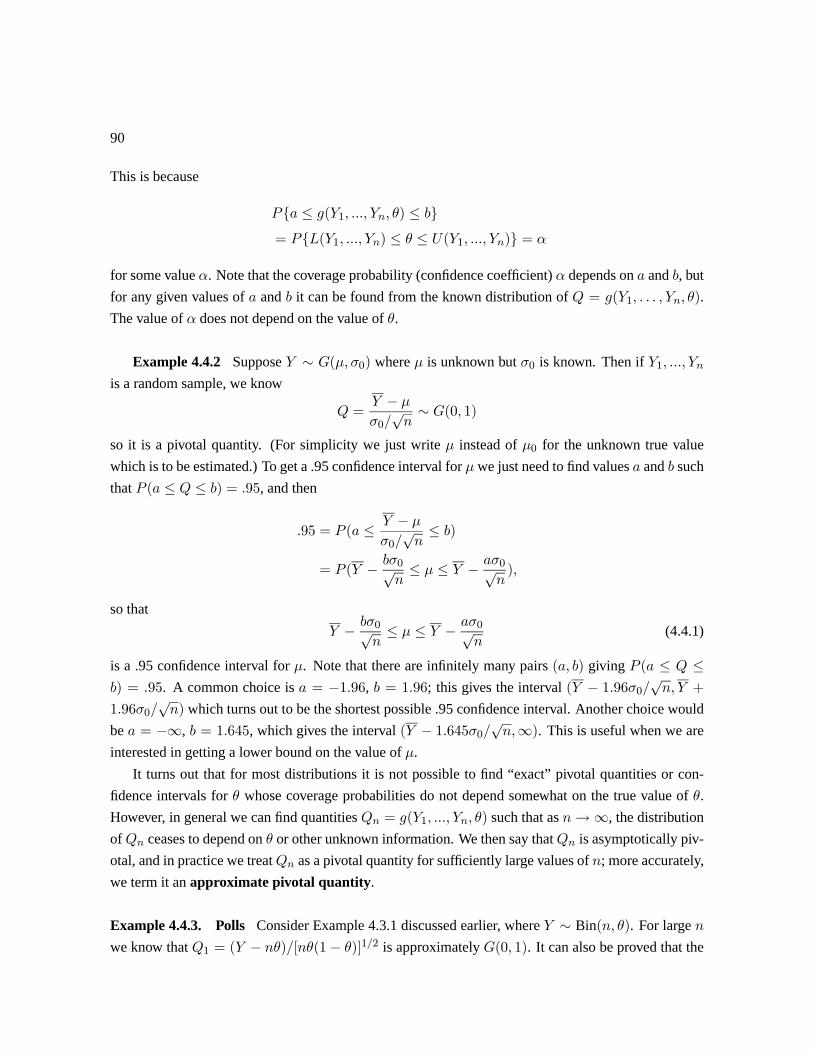
90

This is because

≤ (1 ) ≤ = (1 ) ≤ ≤ (1 ) =

for some value . Note that the coverage probability (confidence coefficient) depends on and , but

for any given values of and it can be found from the known distribution of = (1 ).

The value of does not depend on the value of .

Example 4.4.2 Suppose ∼ ( 0) where is unknown but 0 is known. Then if 1 is a random sample, we know

= −

0√∼ (0 1)

so it is a pivotal quantity. (For simplicity we just write instead of 0 for the unknown true value

which is to be estimated.) To get a .95 confidence interval for we just need to find values and such

that ( ≤ ≤ ) = 95, and then

95 = ( ≤ −

0√≤ )

= ( − 0√≤ ≤ − 0√

)

so that

− 0√≤ ≤ − 0√

(4.4.1)

is a .95 confidence interval for . Note that there are infinitely many pairs ( ) giving ( ≤ ≤) = 95. A common choice is = −196, = 196; this gives the interval ( − 1960

√ +

1960√) which turns out to be the shortest possible .95 confidence interval. Another choice would

be = −∞, = 1645, which gives the interval ( − 16450√∞). This is useful when we are

interested in getting a lower bound on the value of .

It turns out that for most distributions it is not possible to find “exact” pivotal quantities or con-

fidence intervals for whose coverage probabilities do not depend somewhat on the true value of .

However, in general we can find quantities = (1 ) such that as →∞, the distribution

of ceases to depend on or other unknown information. We then say that is asymptotically piv-

otal, and in practice we treat as a pivotal quantity for sufficiently large values of ; more accurately,

we term it an approximate pivotal quantity.

Example 4.4.3. Polls Consider Example 4.3.1 discussed earlier, where ∼ Bin( ). For large

we know that 1 = ( − )[(1− )]12 is approximately (0 1). It can also be proved that the

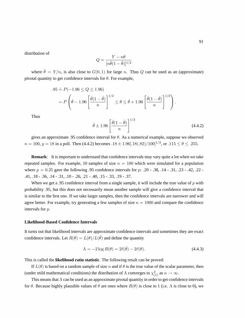
91

distribution of

= −

[(1− )]12

where = , is also close to (0 1) for large . Thus can be used as an (approximate)

pivotal quantity to get confidence intervals for . For example,

95= (−196 ≤ ≤ 196)

=

⎛⎝ − 196"(1− )

#12≤ ≤ + 196

"(1− )

#12⎞⎠

Thus

± 196"(1− )

#12(4.4.2)

gives an approximate .95 confidence interval for . As a numerical example, suppose we observed

= 100, = 18 in a poll. Then (4.4.2) becomes 18± 196[18(82)100]12, or 115 ≤ ≤ 255.

Remark: It is important to understand that confidence intervals may vary quite a lot when we take

repeated samples. For example, 10 samples of size = 100 which were simulated for a population

where = 025 gave the following .95 confidence intervals for : .20 - .38, .14 - .31, .23 - .42, .22 -

.41, .18 - .36, .14 - .31, .10 - .26, .21 - .40, .15 - .33, .19 - .37.

When we get a .95 confidence interval from a single sample, it will include the true value of with

probability .95, but this does not necessarily mean another sample will give a confidence interval that

is similar to the first one. If we take larger samples, then the confidence intervals are narrower and will

agree better. For example, try generating a few samples of size = 1000 and compare the confidence

intervals for .

Likelihood-Based Confidence Intervals

It turns out that likelihood intervals are approximate confidence intervals and sometimes they are exact

confidence intervals. Let () = ()() and define the quantity

Λ = −2 log() = 2()− 2() (4.4.3)

This is called the likelihood ratio statistic. The following result can be proved:

If () is based on a random sample of size and if is the true value of the scalar parameter, then

(under mild mathematical conditions) the distribution of Λ converges to 2(1)

as →∞.

This means thatΛ can be used as an approximate pivotal quantity in order to get confidence intervals

for . Because highly plausible values of are ones where () is close to 1 (i.e. Λ is close to 0), we

92

get confidence intervals by working from the probability

(2(1) ≤ )= (Λ ≤ )

= ((1 ) ≤ ≤ (1 )) (4.4.4)

Example 4.4.4 Consider the binomial model in Examples 4.3.1 and 4.4.3 once again. We have, after

rearrangement,

Λ = 2 log() + 2(1− ) log

Ã1−

1−

!

To get a .95 confidence interval for we note that (2(1)≤ 3841) = 95. To find the confidence

interval we have to find all values satisfying Λ ≤ 3841. This has to be done numerically, and

depends on the observed data. For example, suppose that we observe = 100, = 40. Thus = 40

and the observed value of Λ is a function of ,

() = 80 log(4) + 120 log

µ6

1−

¶

Figure 4.16 shows a plot of () and the line () = 3841 exactly, from which the confidence interval

can be extracted. Solving () ≤ 3841, we find that 307 ≤ ≤ 496 is the .95 confidence interval.

We could also use the approximate pivotal quantity in Example 4.4.3 for this situation. It gives the .95

confidence interval (4.4.2), which is 304 ≤ ≤ 496. The two confidence intervals differ slightly

(they are both based on approximations) but are extremely close.

We can now see the connection between likelihood intervals and confidence intervals. The likeli-

hood interval defined by () ≥ is the same as the confidence interval defined by Λ() ≤ −2 log .

For a .95 confidence interval we use Λ() ≤ 3841 (since (2(1)≤ 3841) = 95), which corresponds

to () ≥ 147. Conversely a .10 likelihood interval given by () ≥ 1 corresponds to Λ() ≤ 4605.Since (2

(1)≤ 4605) = 968, we see that a .10 likelihood interval is a confidence interval with

approximate confidence coefficient .968. Normally in statistical work, however, we use confidence

intervals with (approximate) confidence coefficients .90,.95 or .99, and we usually employ Λ()) rather

then () in discussions about likelihood-based interval estimates.

4.4.3 Choosing a Sample Size

We have seen in examples that confidence intervals for a parameter tend to get narrower as the sample

size increases. When designing a study we often decide how large a sample to collect on the basis of

(i) how narrow we would like confidence intervals to be, and (ii) how much we can afford to spend (it

costs time and money to collect data). The following example illustrates the procedure.

Example 4.4.5 Estimation of a Binomial Probability Suppose we want to estimate the probability

93

0.0 0.1 0.2 0.3 0.4 0.5 0.6 0.7 0.8 0.9 1.0

0

1

2

3

4

5

6

7

8

theta

LR(t

heta

)

Figure 4.16: Likelihood Ratio Statistic for Binomial Parameter

from a binomial experiment in which the response variable has a ( ) distribution. We will

assume that the approximate pivotal quantity

= −

[(1− ]12' (0 1) (4.4.5)

introduced in Example 4.4.3 will be used to get confidence intervals for (Using the likelihood ratio

statistic leads to a more difficult derivation and in any case, for large the LR confidence intervals are

very close to those based on .) Here is a criterion that is widely used for choosing the size of : pick

large enough so a .95 CI for is no larger than ± 03 Let’s see why this is used and where it leads.

From Example 4.4.3, we know that (see (4.4.2))

± 196"(1− )

#12

94

is an approximate .95 CI for . To make this CI ± 03 (or even shorter, say ± 025), we need large

enough that

196

"(1− )

#12≤ 03

This can be rewritten as

=

µ196

03

¶2(1− )

We of course don’t know what will be once we take our sample, but we note that the worst case

scenario is when = 5. So to be conservative, we find such that

=

µ196

03

¶2(05)2 = 1067

Thus, choosing = 1067 (or larger) will result in a .95 CI of the form ± , where ≤ 03. If you

look or listen carefully when polling results are announced, you’ll often hear words like “this poll is

accurate to within 3 percentage points 19 times out of 20." What this really means is that the estimator

(which is usually given in percentile form) satisfies (| − | ≤ 03) = 95, or equivalently, that the

actual estimate is the centre of a .95 confidence interval ± , for which = 03. In practice, many

polls are based on around 1050-1100 people, giving “accuracy to within 3 percent" (with probability

.95). Of course, one needs to be able to afford to collect a sample of this size. If we were satisfied

with an accuracy of 5 percent, then we’d only need = 480. In many situations this might not be

sufficiently accurate for the purpose of the study, however.

Exercise: Show that to make the .95 CI ± 02 or smaller, you need = 2401What should be to

make a .99 CI ± 02 or less?

Remark: Very large binomial polls ( ≥ 2000) are not done very often. Although we can in theory

estimate very precisely with an extremely large poll, there are two problems:

1. it is difficult to pick a sample that is truly random, so ∼ ( ) is only an approximation

2. in many settings the value of fluctuates over time. A poll is at best a snapshot at one point in

time.

As a result, the “real" accuracy of a poll cannot generally be made arbitrarily high.

Sample sizes can be similarly determined so as to give confidence intervals of some desired

length in other settings. We consider this topic again in Chapter 6.

95

Models With Two or More Parameters

When there is a vector θ = (1 ) of unknown parameters, we may want to get interval estimates

for individual parameters ( = 1 ) or for functions = (1 ). For example, with a

Gaussian model( )we might want to estimate and , and also the 90th percentile = +128

In some problems there are pivotal quantities which are functions of the data and (only) the parameter

of interest. We will use such quantities in Chapter 6, where we consider estimation and testing for

Gaussian models. There also exist approximate pivotal quantities based on the likelihood function and

m.l.e.’s. These are mainly developed in more advanced followup courses to this one, but we will briefly

consider this approach later in the notes.

It is also possible to construct confidence regions for two or more parameters. For example, sup-

pose a model has two parameters 1 2 and a likelihood function (1 2) based on observed data.

Then we can define the relative likelihood function

(1 2) =(1 2)

(1 2)

as in the scalar case. The set of pairs (1 2) which satisfy (1 2) ≥ is then called a p likelihood

region for (1 2). The concept of confidence intervals can similarly be extended to confidence re-

gions.

4.3.1 A Case Study: Testing Reliability of Computer Power Supplies

Components of electronic products often must be very reliable, that is, they must perform over long

periods of time without failing. Consequently, manufacturers who supply components to a company

that produces, e.g. personal computers, ,must satisfy the company that their components are reliable.

Demonstrating that a component is highly reliable is difficult because if the component is used

under "normal" conditions it will usually take a very long time to fail. It is generally not feasible for

a manufacturer to carry out tests on the component that last for a period of years (or even months, in

most cases) and there fore they use what are called accelerated life tests. These involve placing such

high levels of stress on the components that they fail in much less than the normal time. If a model

relating the level of stress to the lifetime of the component is known then such experiments can be used

to estimate lifetime at normal stress levels for the population from which the experimental units are

taken.

We consider below some life test experiments on power supplies for PC’s, with ambient temperature

being the stress factor. As the temperature increases, the lifetimes of components tend to decrease and

a temperature around 70 Celsius average lifetime tend to be of the order of 100 hours. The normal

96

usage temperature is around 20 C. The data in Table 4.5.1 show the lifetimes (i.e. times to failure) of

components tests at each of 40, 50, 60 and 70 C. The experiment was terminated after 600 hours

and for temperatures 40, 50 and 60 some of the 25 components being tested had still not failed.

Such observations are called censored: we know in each case only that the lifetime in question was

over 600 hours. In Table 4.5.1 the asterisks denote the censored observations.

It is known from past experience that at each temperature level lifetimes follow close to an ex-

ponential distribution; let us therefore suppose that at temperature ( = 40 50 60 70), component

lifetimes have probability density function

(; ) =1

− ≥ 0 (4.5.1)

where = ( ) is the mean lifetime. The likelihood function based on a sample consisting of both

censoring times and lifetimes is a little different from one based on a random sample of lifetimes. It is,

for the tests at temperature ,

() = Y

1

−

Y

− (4.5.2)

where stands for the set of lifetimes and the set of censoring times .

Question 1 Show that for the distribution 4.5.1, ( ) = − . Then describe how 4.5.2 is

obtained.

Note that 4.5.2 can be rewritten as

() =1

(4.5.3)

where = number of lifetimes observed =P=1

= sum of all lifetimes and censoring times.

Question 2 Assuming that the exponential model is correct, obtain m.l.e.’s 1 for the mean lifetime at

each of the former termperature levels 40 50 60 70. Graph the likelihood functions for 40 and 70

and comment on any qualitative differences.

Question 3 Check, perhaps using some kind of graph, whether the exponential model seems appropri-

ate. Engineers used a model (called the Arrhenius model) that relates the mean lifetime of a component

to the ambient temperature. This states that

= +

+ 2732 (4.5.4)

where is the temperature in degrees Celsius and and are parameters.

Questions 4 Make a plot of vs ( + 2732) − 1 for the four temperatures involved in the life

test experiment. Do the points lie roughly along a straight line? Give rough point estimators of and

97

. Extrapolate your plot or use your estimates of and to estimate the mean lifetime at = 20 C,

the normal temperature.

Question 5 A point estimate of at 20C is not very satisfactory. Outline how you might attempt

to get an interval estimate based on the likelihood function. Once armed with an interval estimate,

would you have many remaining qualms about indicating to the engineers what mean lifetime could be

expected at 20C? (Explain.)

Question 6 Engineers and statisticians have to design reliability tests like the one just discussed, and

considerations such as the following are often used.

Suppose that the mean lifetime at 20C is supposed to be about 90,000 hours and that at 70C you

know from past experience that its about 100 hours. If the model 4.5.4 applies, determine what and

must approximately equal and thus what is roughly equal to at 40, 50 and 60C. How might you

use this information in deciding how long a period of time to run the life test? In particular, give the

approximate expected number of uncensored lifetimes from an experiment that was terminated after

600 hours.

98

Table 1 Lifetimes (in hours) from an accelerated life test experiment in PC power supplies

Temperature70C 60C 50C 40C

2 1 55 78

5 20 139 211

9 40 206 297

10 47 263 556

10 56 347 600∗

11 58 402 600∗

64 63 410 600∗

66 88 563 600∗

69 92 600∗ 600∗

70 103 600∗ 600∗

71 108 600∗ 600∗

73 125 600∗ 600∗

75 155 600∗ 600∗

77 177 600∗ 600∗

97 209 600∗ 600∗

103 224 600∗ 600∗

115 295 600∗ 600∗

130 298 600∗ 600∗

131 352 600∗ 600∗

134 392 600∗ 600∗

145 441 600∗ 600∗

181 489 600∗ 600∗

242 600∗ 600∗ 600∗

263 600∗ 600∗ 600∗

283 600∗ 600∗ 600∗

Notes: Lifetimes are given in ascending order; asterisks(∗) denote censored observations.

4.4 Problems

1. Consider the data on heights of adult males and females from Chapter 1. (The data are on the

course web page.)

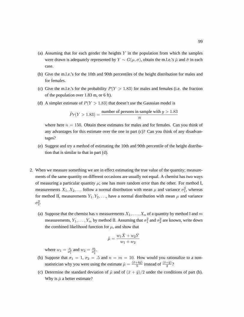
99

(a) Assuming that for each gender the heights in the population from which the samples

were drawn is adequately represented by ∼ ( ), obtain the m.l.e.’s and in each

case.

(b) Give the m.l.e.’s for the 10th and 90th percentiles of the height distribution for males and

for females.

(c) Give the m.l.e.’s for the probability ( 183) for males and females (i.e. the fraction

of the population over 1.83 m, or 6 ft).

(d) A simpler estimate of ( 183) that doesn’t use the Gaussian model is

( 183) =number of persons in sample with 183

where here = 150. Obtain these estimates for males and for females. Can you think of

any advantages for this estimate over the one in part (c)? Can you think of any disadvan-

tages?

(e) Suggest and try a method of estimating the 10th and 90th percentile of the height distribu-

tion that is similar to that in part (d).

2. When we measure something we are in effect estimating the true value of the quantity; measure-

ments of the same quantity on different occasions are usually not equal. A chemist has two ways

of measuring a particular quantity ; one has more random error than the other. For method I,

measurements 12 follow a normal distribution with mean and variance 21 , whereas

for method II, measurements 1 2 , have a normal distribution with mean and variance

22 .

(a) Suppose that the chemist has measurements 1 of a quantity by method I and

measurements, 1 by method II. Assuming that 21 and 22 are known, write down

the combined likelihood function for , and show that

=1 + 2

1 +2

where 1 = 21

and 2 =22

.

(b) Suppose that 1 = 1, 2 = 5 and = = 10. How would you rationalize to a non-

statistician why you were using the estimate = (+4)5

instead of (+)2

?

(c) Determine the standard deviation of and of ( + )2 under the conditions of part (b).

Why is a better estimate?

100

3. Suppose that a fraction of a large population of persons over 18 years of age never drink alcohol.

In order to estimate , a random sample of persons is to be selected and the number who do

not drink determined; the maximum likelihood estimate of is then = .

We want our estimate to have a high probability of being close to , and want to know how

large should be to achieve this.

(a) Consider the random variable and estimator∼ = . Describe how you could work

out the probability that −03 ≤ ∼ − ≤ 03, if you knew the values of and .

(b) Suppose that is .40. Determine how large should be in order to make (−03 ≤ ∼ − ≤

03) = 95. Use an approximation if you wish.

4. Proof of Central Limit Theorem (Special Case) Suppose 1 2 are independent r.v.’s with

() = () = 2 and that they have the same distribution, which has a m.g.f.

(a) Show that ( − ) has m.g.f. of the form (1 + 2

2+ terms in 3 4 ) and thus that

( − )√ has m.g.f of the form (1 + 2

2+ 0()), where 0() signifies a remainder

term with the property that → 0 as →∞.

(b) Let

=

X=1

( − )

√

=

√( − )

and note that its m.g.f. is of the form (1 + 2

2+ 0()). Show that as → ∞ this ap-

proaches the limit 22, which is the m.g.f. for (0 1). (Hint: For any real number a,

(1 + ) → as →∞.)

5. A sequence of random variables is said to converge in probability to the constant if for

all 0,

lim→∞| − | ≥ = 0

We denote this by writing → .

(a) If and are two sequences of r.v.’s with → 1 and

→ 2, show that

+ → 1 + 2 and

→ 12.

(b) Let 1 2 · · · be i.i.d. random variables with p.d.f. (; ). A point estimator based

on a random sample 1 · · · is said to be consistent for if → as →∞.

101

i. Let 1 · · · be i.i.d. (0 ). Show that is consistent for .

ii. Let ∼ ( ). Show that = is consistent for .

6. Refer to the definition of consistency in Problem 5(b). Difficulties can arise when the number of

parameters increases with the amount of data. Suppose that two independent measurements of

blood sugar are taken on each of individuals and consider the model

12 ∼ ( 2) = 1 · · ·

where 1 and 2 are the independent measurements. The variance 2 is to be estimated, but

the ’s are also unknown.

(a) Find the m.l.e. 2 and show that it is not consistent. (To do this you have to find the m.l.e.’s

for 1 as well as for 2.)

(b) Suggest an alternative way to estimate 2 by considering the differences

= 1 −2.

(c) What does represent physically if the measurements are taken very close

together in time?

7. Suppose that blood samples for people are to be tested to obtain information about , the

fraction of the population infected with a certain virus. In order to save time and money, pooled

testing is used: the samples are mixed together at a time to give pooled samples. A

pooled sample will test negative if all individuals are not infected.

(a) Give an expression for the probability that out of samples will be negative, if the

people are a random sample from the population. State any assumptions you make.

(b) Obtain a general expression for the maximum likelihood estimate in terms of , and .

(c) Suppose = 100, = 10 and = 89. Give the m.l.e. and relative likelihood function,

and find a 10% likelihood interval for .

(d) Discuss (or do it) how you would select an “optimal” value of to use for pooled testing,

if your objective was not to estimate but to identify persons who are infected, with the

smallest number of tests. Assume that you know the value of and the procedure would be

to test all persons individually each time a pooled sample was positive. (Hint: Suppose a

large number of persons must be tested, and find the expected number of tests needed.)

102

8. (a) For the data in Problem 4 of Chapter 2, plot the relative likelihood function () and

determine a .10 likelihood interval. Is very accurately determined?

(b) Suppose that we can find out whether each pair of twins is identical or not, and that it is

determined that of 50 pairs, 17 were identical. Obtain the likelihood function and m.l.e.

of in this case. Plot the relative likelihood function with the one in (a), and compare the

accuracy of estimation in the two cases.

9. Company A leased photocopiers to the federal government, but at the end of their recent contract

the government declined to renew the arrangement and decided to lease from a new vendor,

Company B. One of the main reasons for this decision was a perception that the reliability of

Company A’s machines was poor.

(a) Over the preceding year the monthly numbers of failures requiring a service call from

Company A were

16 14 25 19 23 12

22 28 19 15 18 29.Assuming that the number of service calls needed in a one month period has a Poisson

distribution with mean , obtain and graph the relative likelihood function () based on

the data above.

(b) In the first year using Company B’s photocopiers, the monthly numbers of service calls

were13 7 12 9 15 17

10 13 8 10 12 14.

Under the same assumption as in part (a), obtain () for these data and graph it on the

same graph as used in (a). Do you think the government’s decision was a good one, as far

as the reliability of the machines is concerned?

(c) Use the likelihood ratio statistic Λ() as an approximate pivotal quantity to get .95 confi-

dence intervals for for each company.

(d) What conditions would need to be satisfied to make the assumptions and analysis in (a) to

(c) valid? What approximations are involved?

10. The lifetime (in days) of a particular type of lightbulb is assumed to have a distribution with

p.d.f.

(;) =32−

2 0; 0

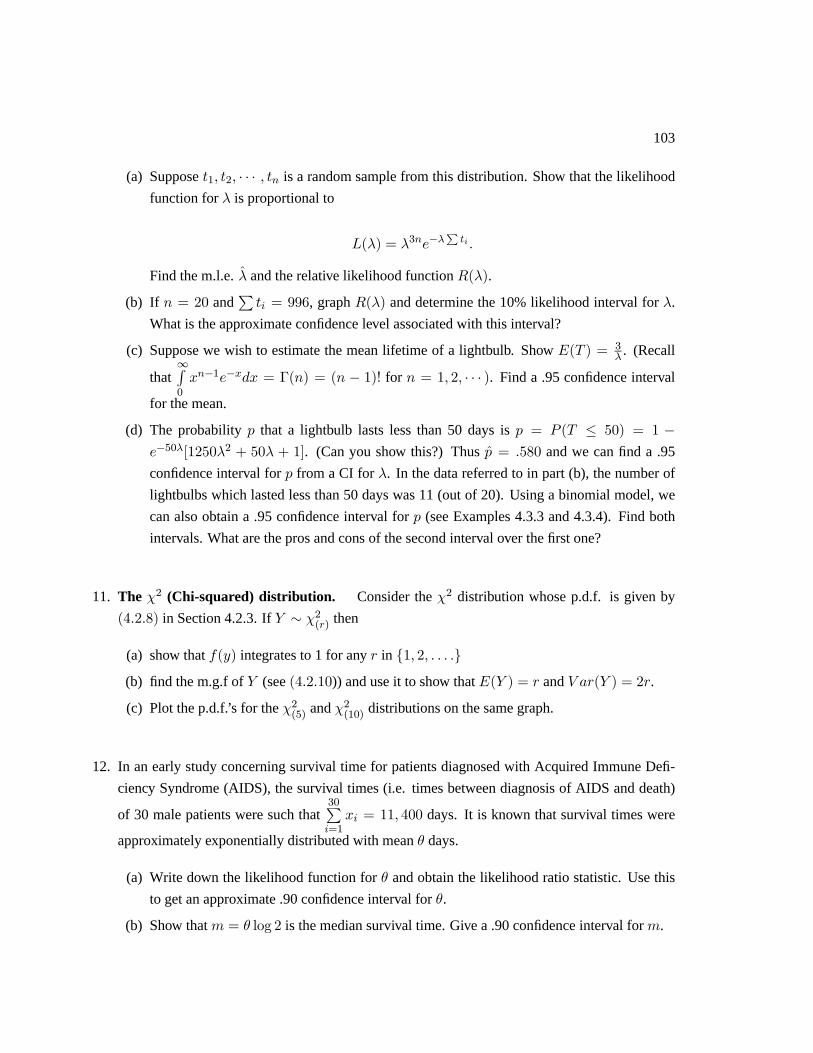
103

(a) Suppose 1 2 · · · is a random sample from this distribution. Show that the likelihood

function for is proportional to

() = 3−

Find the m.l.e. and the relative likelihood function ().

(b) If = 20 andP

= 996, graph () and determine the 10% likelihood interval for .

What is the approximate confidence level associated with this interval?

(c) Suppose we wish to estimate the mean lifetime of a lightbulb. Show ( ) = 3

. (Recall

that∞R0

−1− = Γ() = ( − 1)! for = 1 2 · · · ). Find a .95 confidence interval

for the mean.

(d) The probability that a lightbulb lasts less than 50 days is = ( ≤ 50) = 1 −−50[12502 + 50 + 1]. (Can you show this?) Thus = 580 and we can find a .95

confidence interval for from a CI for . In the data referred to in part (b), the number of

lightbulbs which lasted less than 50 days was 11 (out of 20). Using a binomial model, we

can also obtain a .95 confidence interval for (see Examples 4.3.3 and 4.3.4). Find both

intervals. What are the pros and cons of the second interval over the first one?

11. The 2 (Chi-squared) distribution. Consider the 2 distribution whose p.d.f. is given by

(428) in Section 4.2.3. If ∼ 2()

then

(a) show that () integrates to 1 for any in 1 2 (b) find the m.g.f of (see (4210)) and use it to show that ( ) = and ( ) = 2.

(c) Plot the p.d.f.’s for the 2(5)

and 2(10)

distributions on the same graph.

12. In an early study concerning survival time for patients diagnosed with Acquired Immune Defi-

ciency Syndrome (AIDS), the survival times (i.e. times between diagnosis of AIDS and death)

of 30 male patients were such that30P=1

= 11 400 days. It is known that survival times were

approximately exponentially distributed with mean days.

(a) Write down the likelihood function for and obtain the likelihood ratio statistic. Use this

to get an approximate .90 confidence interval for .

(b) Show that = log 2 is the median survival time. Give a .90 confidence interval for .

104

13. Let have an exponential distribution with p.d.f.

(; ) =1

− 0

where 0.

(a) Show that = 2 has a 2(2)

distribution. (Hint: compare the p.d.f. of with (4.2.8).)

(b) If 1 is a random sample from the exponential distribution above, prove that

= 2

X=1

∼ 2(2)

(You may use results in Section 4.2.) is therefore a pivotal quantity, and can be used to

get confidence intervals for .

(c) Refer to Problem 12. Using the fact that

³4319 ≤ 2(60) ≤ 7908

´= 90

obtain a .90 confidence interval for based on . Compare this with the interval found in

12(a). Which interval is preferred here? (Why?)

14. Two hundred adults are chosen at random from a population and each is asked whether informa-

tion about abortions should be included in high school public health sessions. Suppose that 70%

say they should.

(a) Obtain a 95% confidence interval for the proportion of the population who support abor-

tion information being included.

(b) Suppose you found out that the 200 persons interviewed consisted of 50 married couples

and 100 other persons. The 50 couples were randomly selected, as were the other 100 per-

sons. Discuss the validity (or non-validity) of the analysis in (a).

15. Consider the height data discussed in Problem 1 above. If heights are ( ) and = and

2 =P=1

( − )2 are the ML estimators based on a sample of size then it can be shown

that when is large,

=

√( − )

is very close to (0 1), and so it is approximately a pivotal quantity. Use to obtain a .99

confidence interval for for males and for females.

105

16. In the U.S.A. the prevalence of HIV (Human Immunodeficiency Virus) infections in the popula-

tion of child-bearing women has been estimated by doing blood tests (anonymized) on all women

giving birth in a hospital. One study tested 29,000 women and found that 64 were HIV positive

(had the virus). Give an approximate .99 confidence interval for , the fraction of the population

that is HIV positive.

State any concerns you feel about the accuracy of this estimate.

STATISTICAL INFERENCE: TESTING

HYPOTHESES

5.1 Introduction

There are often hypotheses that a statistician or scientist might want to “test” in the light of observed

data. Two important types of hypotheses are

(1) that a parameter vector has some specified value 0; we denote this as 0: = 0.

(2) that a random variable has a specified probability distribution, say with p.d.f. 0(); we denote

this as 0: ∼ 0().

The statistical approach to hypothesis testing is as follows: First, assume that the hypothesis 0

will be tested using some random data “Data”. Next, define a test statistic (also called a discrepancy

measure) = (Data) that is constructed to measure the degree of “agreement” between Data and

the hypothesis 0. It is conventional to define so that = 0 represents the best possible agreement

between the data and0, and so that the larger is, the poorer the agreement. Methods of constructing

test statistics will be described later. Third, once specific observed “data” have been collected, let

= (data) be the corresponding observed value of . To test , we now calculate the observed

significance level (also called the p-value), defined as

= ( ≥ ;0) (4.5.2)

where the notation “;0” means “assuming 0 is true”. If SL is close to zero then we are inclined

to doubt that 0 is true, because if it is true the probability of getting agreement as poor or worse

than observed is small. This makes the alternative explanation that 0 is false more appealing. In

other words, we must accept that one of the following two statements is correct.:

(a) 0 is true but by chance we have observed data that indicate poor agreement with 0, or

106

107

(b) 0 is false.

A SL less than about .05 provides moderately strong evidence against 0.

Example 5.1.1 Testing a binomial probability

Suppose that it is suspected that a 6-sided die has been “doctored” so that the number one turns up

more often than if the die were fair. Let = (die turns up one) on a single toss and consider the

hypothesis 0: = 16. To test 0, we toss the die times and observe the number of times that

a one occurs. Then “Data”= and a reasonable test statistic would then be either 1 = | −6| or

(if we wanted to focus on the possibility that was bigger than 1/6), = max(( − 6) 0).

Suppose that = 180 tosses gave = 44. Using , we get = 14 and the significance level is

(using the second definition of )

= ( ≥ 14;0)

= ( ≥ 44; = 16)

=

180X=44

Ã180

!(1

6)(5

6)180− = 005

This provides strong evidence against 0, and suggests that is bigger than 1/6.

Example 5.1.2 Suppose that in the experiment in Example 5.1.1 we observed = 35 ones in = 180

tosses. Now the SL is

= ( ≥ 35; = 16)

=

180X=35

Ã180

!(1

6)(56)180−

= 183

This probability is not especially small, so we conclude that there is no strong evidence against 0.

Note that we do not claim that 0 is true, only that there is no evidence that it is not true.

Example 5.1.3. Testing for bias in a measurement system

Two cheap scales and for measuring weight are tested by taking 10 weighings of a 1 kg weight on

each of the scales. The measurements on and are

: 1.026, 0.998, 1.017, 1.045, 0.978, 1.004, 1.018, 0.965, 1.010, 1.000

: 1.011, 0.966, 0.965, 0.999, 0.988, 0.987, 0.956, 0.969, 0.980, 0.988

108

Let represent a single measurement on one of the scales, and let represent the average measure-

ment ( ) in repeated weighings of a single 1 kg weight. If an experiment involving weighings is

conducted then a sensible test of 0: = 1 could be based on the test statistic

= | − 100|

where =P

. Since ' ( √), where = ( ) and 2 = Var( ), we can compute

the significance level (at least approximately) using a Gaussian distribution. Since we don’t know 2

we will estimate it by the sample variance 2 =P( − )2(− 1) in the calculations below.

The samples from scales and above give us

: = 10061 = 00230 = 00061

: = 09810 = 00170 = 00190

The SL for is (pretending = = 00230)

= ( ≥ 00061; = 100)= (| − 100| ≥ 00061)

=

µ¯ − 10000230

√10

¯≥ 00061

00230√10

¶= (|| ≥ 0839) where ∼ (0 1)

= 401

Thus there is no evidence of bias (that is, that 0: = 100 is false) for scale A.

For scale B, however, we get

=

µ¯ − 1000170

√10

¯≥ 0190

0170√10

¶= (|| ≥ 3534) = 0004

Thus there is strong evidence against 0: = 100, suggesting strongly that scale B is biased.

Finally, note that just because there is strong evidence against 0 for scale B, the degree of bias in

its measurements is not necessarily large. In fact, we can get an approximate .95 confidence interval

for = ( ) for scale B by using the approximate pivotal quantity

= −

√10' (0 1)

Since (−196 ≤ ≤ 196) = 95, we get the approximate .95 confidence interval ± 196√10,

or 0981 ± 011, or 0970 ≤ ≤ 0992. Thus the bias in measuring the 1 kg weight is likely fairly

109

small (about 1% - 3%).

The approach to testing hypothesis described above is very general and straightforward, but a few

points should be stressed:

1. If the SL is small (close to 0) then the test indicates strong evidence against 0; this is often

termed “statistically significant" evidence against 0. Rough rules of thumb are that 05

provides moderately strong evidence against 0 and that 01 provides strong evidence.

2. If the SL is not small we do not conclude by saying that 0 is true: we simply say there is

no evidence against 0. The reason for this “hedging" is that in most settings a hypotheses

may never be strictly “true". (For example, one might argue when testing 0 : = 16 in

Example 5.1.1 that no real die ever has a probability of exactly 16 for side 1.) Hypotheses can

be “disproved" (with a small degree of possible error) but not proved.

3. Just because there is strong evidence (“highly statistically significant" evidence) against a hy-

potheses 0, there is no implication about how “wrong" 0 is. For example in Example 5.3.1

there was strong evidence that scale B was biased (that is, strong evidence against 0: bias =

0), but the relative magnitude (1-3%) of the bias is apparently small. In practice, we try to sup-

plement a significant test with an interval estimate that indicates the magnitude of the departure

from 0. This is how we check whether a result is “ scientifically" significant as well as statis-

tically significant.

A drawback with the approach to testing described so far is that we are not told how to construct

test statistics D. Often there are “intuitively obvious" statistics that can be used; this is the case in the

examples of this section. However, in more complicated situations it is not always easy to come up

with a test statistic. In the next section we show how to use the likelihood function to construct test

statistics in general settings.

A final point is that once we have specified a test statistic D, we need to be able to compute the

significance level (5.1.1) for the observed data. This brings us back to distribution theory: in most cases

the exact probability (5.1.1) is hard to determine mathematically, and we must either use an approx-

imation or use computer simulation. Fortunately, for the tests in the next section we can usually use

approximations based on 2 distributions.

110

5.2 Testing Parametric Hypotheses with Likelihood Ratio Statistics

General Theory

First we show how test statistics can be constructed from the likelihood function for any hypothesis

0 that is specified in terms of one or more parameters. Let “Data” represent data generated from

a distribution with probability or probability density function (Data; θ) which depends on the -

dimensional parameter θ. Let Ω be the parameter space (set of possible values) for θ.

Consider a hypothesis of the form

0 : θ ∈ Ω0

where Ω0 ⊂ Ω and Ω0 is of dimension . The dimensions of Ω and Ω0 refer to the minimum

number of parameters (or “coordinates") needed to specify points in them. We can test 0 using as our

test statistic the likelihood ratio test statistic Λ, defined as follows:

Let (θ) = (Data; θ) be the likelihood function and let

θ denote the m.l.e. of θ over Ω

θ0 denote the m.l.e. of θ over Ω0.

Now let

Λ = 2(θ)− 2(θ0) = −2 log((θ0)

(θ)

) (5.2.1)

This seems like a sensible way to measure the degree of agreement between 0 and the observed data:

we look at the relative likelihood

(θ0) = (θ0)(θ)

of the “most likely" vector θ0 under 0 (i.e. when θ0 is in Ω0). If this is very small then there is

evidence against 0 (think why). The reason we take = Λ as the test statistic instead of (θ0) is

that Λ = −2(θ0) takes values ≥ 0, with Λ = 0 ((θ0) = 1) representing the best agreement

between 0 and the data. Also, it can be shown that under 0, the distribution of Λ becomes 2(−) as

the size of the data set becomes large. Large values of Λ (small values of (θ0)) indicate evidence

against 0 so the p-value (significance level) is

= (Λ ≥ Λ; 0)= (2(−) ≥ Λ) (5.2.2)

(Note: Here we are using Λ to represent the value of Λ obtained when we get the (numerical) data;

Λ represents the r.v. when we think, as usual, of the data as random variables, before they are collected.)

111

Some Examples

This approach is very general and can be used with many different types of problems. A few examples

follow.

(a) A single parameter model. Suppose has an exponential distribution with p.d.f. (; ) =1− ( ≥ 0). Test 0: = 0 (a given value) based on a random sample 1 . Thus

Ω = : 0, Ω0 = 0; = 1, = 0 and

() =

Y=1

(; )

(b) A model with two parameters. Suppose ∼ ( )with p.d.f. (; ) = 1√2

−12(

− )

2

(−∞

∞) θ = ( )

Test 0: = 0 based on a random sample 1 . Thus Ω = ( ) : −∞

∞ 0, Ω0 = ( 0)−∞ ∞; = 2, = 1 and

(θ) = ( ) =

Y=1

(; )

(c) Comparison of two parameters. Suppose we have data from two Poisson distributions with

p.f.’s (1;1) = −1 11

1!; (2;2) = −2

22

2!,

where 1 and 2 take values in 0 1 2 .

Test 0: 1 = 2 based on two independent random samples 1 ( = 1 1) and 2 ( =

1 2). Thus θ = (1 2) and Ω = (1 2) : 1 0 2 0, Ω0 = ( ) : 0, = 2, = 1 and

(θ) = (1 2) =

1Y=1

(1;1)

2Y=1

(2;2)

(d) A test about multinomial probabilities. Consider a multinomial p.f.

(1 ; 1 ) =!

1! · · · !11

22 · · ·

Ã0 ≤ ≤ P

=

!Test 0: = (α) where dim(α) = − 1. Thus θ = (1 ) and Ω =

(1 ) : 0 ≤ ≤ 1X1

= 1, Ω0 = (1 ) : = (α) for α ∈ Ω; = − 1, = and

(θ) = (1 ;θ)

112

We now consider problems that involve actual data, and describe the steps in the tests in more de-

tail. In many testing problems it is necessary to use numerical methods to maximize likelihoods and

find θ and θ0. In this course and the examples below we focus on problems in which these estimates

can be formed mathematically.

Example 5.2.1. Lifetimes of light bulbs. The variability in lifetimes of light bulbs (in hours, say,

of operation before failure) and other electrical components is often well described by an exponential

distribution with p.d.f. of the form

(; ) =1

− 0

where = ( ) is the average (mean) lifetime. A manufacturer claims that the mean life of a partic-

ular brand of bulbs is 2000 hours. We can examine that claim by testing the hypothesis

0 : = 2000

assuming that the exponential model applies.

Suppose for illustration that a random sample of 20 light bulbs was tested over a long period and

the total of the lifetimes 1 20 was observed to be20P=1

= 38 524 hours. (It turns out that

for the test below we need only the value ofP

and not the individual lifetimes 1 20 so we

haven’t bothered to list them. They would be needed, however to check that the exponential model was

satisfactory.)

Let us carry out a likelihood ratio test of 0. The setup is as described in Example (a) above: the

likelihood function based on a random sample 1 is

() =

Y=1

1

− =

1

−

Note that in terms of our general theory the parameter space of is Ω = : 0 and the parameter

space under 0 is the single point Ω = 2000. The dimensions of Ω and Ω0 are 1 and 0, respectively.

We use the likelihood ratio statistic Λ of (5.2.1) as our test statistic D. To evaluate this we first write

down the log likelihood function (noting that = 20 andP

= 38 524 here)

() = −20 − 38524

Next, we obtain by maximizing (): this gives

=38524

20= 19262 (hours)

113

Now we can compute the “observed" value of Λ from (5.2.1) as

Λ = 2()− 2(2000)

= −40 (2000)− 77048

+77048

2000

= 0028

The final computational step is to compute the significance level, which we do using the 2 approxi-

mation (5.2.2). This gives

= (Λ ≥ 0028;0 true)

= (2(1) ≥ 0028)= 087

The SL is not close to zero so we conclude that there is no evidence against 0 and against the

manufacturer’s claim that is 2000 hours. Although the m.l.e. was under 2000 hours (1926.2) it was

not sufficiently under to give conclusive evidence against 0 : = 2000.

Example 5.2.2 Comparison of Two Poisson Distributions. In problem 9 of Chapter 4 some

data were given on the numbers of failures per month for each of two companies’ photocopiers. To a

good approximation we can assume that in a given month the number of failures follows a Poisson

distribution with p.f. of the form

(;) = ( = ) = −

! = 0 1 2

where = ( ) is the mean number of failures per month. (This ignores that the number of days that

the copiers are used varies a little across months. Adjustments can be make to the analysis to deal with

this.)

The number of failures in 12 consecutive months for company A and company B’s copiers are given

below; there were the same number of copiers from each company in use.

Company A: 16 14 25 19 23 12 22 28 19 15 18 29

Company B: 13 7 12 9 15 17 10 13 8 10 12 14

Denote the value of for Company A’s copiers as and the value for Company B’s as . It

appears from the data that B’s copiers fail less often, but let us assess this formally by testing the

hypothesis

0 : =

114

This problem was sketched in Example (c) above. To handle it we consider the likelihood functions

for and based on the observed data and then the likelihood formed by combining them. The

likelihoods for and are

1() =

12Y=1

−

!= −12240 × c

1() =

12Y=1

−

!= −12140 × c

To test 0 we view the two Poisson distributions together as one big model, with the parameter

vector θ = ( ) In terms of the general framework for likelihood ratio tests the parameter space

for θ is Ω = ( ) : 0 0, and under 0 the parameter space becomes Ω0 =

( ) : = 0. The likelihood function for the “combined" model is the product of

1() and 2() since the two samples are independent:

(θ) = ( ) = 1()2()

We now carry out the steps for the test of 0 exactly as in the previous example, except that now Ω

has dimension = 2 and Ω0 has dimension = 1. First, we write down the log likelihood function,

(θ) = ( ) = −12 + 240 − 12 + 140 (5.2.3)

Next we find and 0. The m.l.e. maximizes ( ) in the unconstrained case. This can be done

by solving the maximum likelihood equations

= 0

= 0

which gives = 24012 = 200 and = 14012 = 11667. That is, θ = (200 11667) The

constrained m.l.e. θ0 maximizes ( ) under the constraint = . To do this we merely have

to maximize

( ) = −24 + 380

with respect to . Solving ( ) = 0, we find = 38024 = 15833(= ); that is,

θ0 = (15833 15833)

115

The next step is to compute to observed value of the likelihood ratio statistic, which from (5.2.1)

and (5.2.3) is

Λ = 2(θ)− 2(θ0)= 2(200 11667)− 2(15833 15833)= 2[68292− 66960]= 2664

Finally, we compute the significance level for the test, which by (5.2.2) is

(Λ ≥ 2664;0 true) = (2(1) ≥ 2664)= 25× 10−7

Our conclusion is that there is very strong evidence against the hypothesis; the test indicates that

Company B’s copiers have a lower rate of failure than Company A’s copiers.

We can follow this conclusion up by giving confidence intervals for and ; this indicates the

magnitude of the difference in the two failure rates. (The m.l.e.’s = 200 average failures per month

and = 1167 failures per month differ a lot, but we also give confidence intervals in order to express

the uncertainty in such estimates.)

Other hypothesis tests are considered in the remaining chapters of these notes. We conclude with

some short remarks about hypothesis testing and estimation.

5.3 Hypothesis Testing and Interval Estimation

Hypothesis tests that are of the form 0 : = 0, where is a scalar parameter, are very closely

related to interval estimates for . For likelihood ratio (LR) tests the connection is immediately obvious,

because the LR statistic

Λ = 2()− 2(0)

is used for both tests and confidence intervals. For a test, the significance level using (5.2.2) is

= (2(1) ≥ Λ(0)) (5.3.1)

where we write Λ(0) to remind us that we are testing 0 : = 0 On the other hand, to get a

confidence interval for with confidence coefficient we find by (4.4.4) all values 0 such that

Λ(0) ≤ 2(1) (5.3.2)

116

where 2(1)

is the quantile of a 2(1)

distribution; for example for a .95 confidence interval we use

2(1)95

= 384.

We now see the following by comparing (5.3.1) and (5.3.2):

• The parameter value 0 is inside an confidence interval given by (5.3.2) if and only if (iff) for

the test of 0 : = 0 we have ≥ 1− .

For example, 0 is inside the .95 confidence interval (CI) iff the significance level for 0 : = 0

satisfies ≥ 05, To see this note that

≥ 05

⇔ (2(1) ≥ Λ(0)) ≥ 05

⇔ Λ(0) ≤ 384⇔ 0 is inside 95

The connection between tests and confidence intervals can also be made when other test statistics

beside the LR statistic are used. If D is a test statistic for testing 0 : = 0 then we can obtain a .95

confidence interval for by finding all values 0 such that ≥ 05, or an CI by finding values 0such that ≥ 1− .

5.4 Problems

1. The accident rate over a certain stretch of highway was about = 10 per year for a period of

several years. In the most recent year, however, the number of accidents was 25. We want to

know whether this many accidents is very probable if = 10; if not, we might conclude that the

accident rate has increased for some reason. Investigate this question by assuming that the num-

ber of accidents in the current year follows a Poisson distribution with mean and then testing

0 : = 10. Use the test statistic = (0 − 10) where represents the number of

accidents in the most recent year.

2. Refer back to Problem 1 in Chapter 1. Frame this problem as a hypothesis test. What test statistic

is being used? What are the significance levels from the data in parts (b) and (c)?

3. The R function () generates pseudo random (0 1) (uniform distribution on (0 1)) ran-

dom variables. The command ← () will produce a vector of values 1 · · · .

117

(a) Give a test statistic which could be used to test that the ’s ( = 1 · · · ) are consistent

with a random sample from (0 1).

(b) Generate 1000 ’s and carry out the test in (a).

4. A company that produces power systems for personal computers has to demonstrate a high degree

of reliability for its systems. Because the systems are very reliable under normal use conditions,

it is customary to ‘stress’ the systems by running them at a considerably higher temperature than

they would normally encounter, and to measure the time until the system fails. According to a

contract with one PC manufacturer, the average time to failure for systems run at 70C should be

no less than 1,000 hours.

From one production lot, 20 power systems were put on test and observed until failure at 70.The 20 failure times 1 20 were (in hours)

374.2 544.0 1113.9 509.4 1244.3

551.9 853.2 3391.2 297.0 63.1

250.2 678.1 379.6 1818.9 1191.1

162.8 1060.1 1501.4 332.2 2382.0

(Note:20P1

= 18 6986)

Failure times are known to be approximately exponential with mean .

(a) Use a likelihood ratio test to test the hypothesis that = 1000 hours. Is there any evidence

that the company’s power systems do not meet the contracted standard?

(b) If you were a PC manufacturer using these power systems, would you like the company to

perform any other statistical analyses besides testing 0 : = 1000? Why?

5. In the Wintario lottery draw, six digit numbers were produced by six machines that operate

independently and which each simulate a random selection from the digits 0 1 9. Of 736

numbers drawn over a period from 1980-82, the following frequencies were observed for position

1 in the six digit numbers:

Digit (i): 0 1 2 3 4 5 6 7 8 9 Total

Frequency (): 70 75 63 59 81 92 75 100 63 58 736

Consider the 736 draws as trials in a multinomial experiment and let = (digit is drawn on

any trial), = 0 1 9. If the machines operate in a truly ‘random’ fashion, then we should

have = 1 ( = 0 1 9).

118

(a) Test this hypothesis using a likelihood ratio test. What do you conclude?

(b) The data above were for digits in the first position of the six digit Wintario numbers. Sup-

pose you were told that similar likelihood ratio tests had in fact been carried out for each of

the six positions, and that position 1 had been singled out for presentation above because it

gave the largest value of the test statistic, . What would you now do to test the hypothesis

= 1 ( = 0 1 2 9)? (Hint: You need to consider (largest of 6 independent ’s is

≥ obs).)

6. Testing a genetic model. Recall the model for the M-N blood types of people, discussed

in Examples 2.3.2 and 2.5.2. In a study involving a random sample of persons the numbers

1 2 3 (1 + 2 + 3 = ) who have blood types MM, MN and NN respectively has a

multinomial distribution with p.f.

(1 2 3) =!

1! 2! 3!11

22

33 ≥ 0

X =

and since 1 + 2 + 3 = 1 the parameter space Ω = (1 2 3) : ≥ 0P

= 1 has

dimension 2. The genetic model discussed earlier specified that 1 2 3 can be expressed in

terms of only a single parameter (0 1), as follows:

1 = 2 2 = 2(1− ) 3 = (1− )2 (5.4.1)

Consider (5.4.1) as a hypothesis 0 to be tested. In that case, the dimension of the parameter

space for (1 2 3) under 0 is 1, and the general methodology of likelihood ratio tests can be

applied. This gives a test of the adequacy of the genetic model.

Suppose that a sample with = 100 persons gave observed values 1 = 18 2 = 50 3 =

32 Test the model (5.4.1) and state your conclusion.

7. Likelihood ratio test for a Gaussian mean. Suppose that a r.v has a ( ) distribution

and that we want to test the hypothesis 0 : = 0, where 0 is some specified number. The

value of is unknown.

(a) Set this up as a likelihood ratio test. (Note that the parameter space is Ω = θ = ( ) :−∞ ∞ 0) Assume that a random sample 1 is available.

(b) Derive the LR statistic Λ and show that it can be expressed as a function of =√( −

0), where is the sample standard deviation and is the sample mean. (Note: the easily

proved identityX=1

( − 0)2 =

X=1

( − )2 + ( − 0)2 (5.4.2)

119

can be used here.)

8. Use of simulation to obtain significance levels. In some testing problems the distribution of the

test statistic D is so complicated it is not possible (or very difficult) to find the significance level,

= ( ≥ ;0 true)

mathematically. In many problems computer simulation can be used as an alternative. Here is

an approach that can be used with the “runs test" for randomness in a binary sequence that was

discussed in Problem 7 of Chapter 1. For illustration we consider sequences of length 50.

Let denote the number of runs in a sequence of 50 binary (0 or 1) digits. If the probability a

digit is 1 is then, from part (b) of Problem 7, Chapter 1, we have () = 1 + 98(1− ). If

= 5 (i.e. 0 and 1 both have probability .5) then () = 255. Thus, let us use

= |− 255|

as our statistic for testing the hypothesis

0: Digits come from a Bernoulli process with = 5

(a) Suppose you observe = 14 and want to find the SL. Since = 115,

= ( ≥ 115) = ( ≤ 14) + ( ≥ 37)

Evaluate this in the following way:

(i) Simulate a sequence of 50 independent binary digits, with (0) = (1) = 5

(ii) Determine and store it.

(iii) Repeat this 1000 times and determine the fraction of times that either ≤ 14 or ≥ 37.This is an approximation to SL (Why?).

Note: This problem is tricky because it requires that code be written to deal with step

(ii). Step (i) can be handled in the statistical software system by the command ←(50 1 5), which generates 50 independent (1 5) random variables. The vec-

tor thus is a random binary sequence of the type desired.

9. The Poisson model is often used to compare rates of occurrence for certain types of events in

different geographic regions. For example, consider regions with populations 1

and let ( = 1 ) be the annual expected number of events per person for region .

By assuming that the number of events for region in a given -year period has a Poisson

distribution with mean , we can estimate and compare the ’s or test that they are equal.

120

(a) Under what conditions might the stated Poisson model be reasonable?

(b) Suppose you observe values 1 for a given -year period. Describe how to test the

hypothesis that 1 = 2 = = .

(c) The data below show the numbers of children born with “birth defects" for 5 regions

over a given five year period, along with the total numbers of births for each region.

Test the hypothesis that the five rates of birth defects are equal.

: 2025 1116 3210 1687 2840

: 27 18 41 29 31

GAUSSIAN RESPONSE MODELS

6.1 Introduction

Gaussian models for response variables are very widely used in applications of statistics. We have

seen examples involving variables such as heights and body-mass index measurements of people pre-

viously in these notes. Many problems involve explanatory variables (which may be a vector) that

are related to a response ; in this case we can generalize the simple Gaussian model ∼ ( ) to

∼ ((x) (x)), where x is a vector of covariates (explanatory variables). The trick in creating

models in such settings is to decide on the forms for (x) and (x),

(x) = 1(x) (x) = 2(x)

To do this we rely on past information and on current data from the population or process in question.

Here are some examples of settings where Gaussian models could be used.

Example 6.1.1

The soft drink bottle filling process of Example 1.4.2 involved two machines (Old and New). For a

given machine it is reasonable to represent the distribution for the amount of liquid deposited in a

single bottle by a Gaussian distribution: ∼ ( ).

In this case we can think of the machines as being like a covariate, with and differing for the

two machines. We could write

∼ (0 0) ∼ ( )

for the old and new machines. In this case there is no formula relating and to the machines; they

are simply different.

Example 6.1.2 Price vs. Size of Commercial Buildings (Reference: Oldford and MacKay STAT

231 Course Notes, Ch. 16)

Ontario property taxes are based on "market value", which is determined by comparing a property to

121

122

the price of those which have recently been sold. The value of a property is separated into components

for land and for buildings. Here we deal with the value of the buildings only.

A large manufacturing company was appealing the assessed market value of its property, which

included a large building. Sales records were collected on the 30 largest buildings sold in the previous

three years in the area. The data are given in Table 6.1.1 and plotted in Figure 6.17 in a scatter plot,

which is a plot of the points ( ). They include the size of the building (in 2105) and the selling

price (in $ per 2).

The building in question was 4.47 x 105 2, with an assessed market value of $ 75 per 2.

Table 6.1.1 Size and Price of 30 Buildings

Size Price Size Price Size Price

3.26 226.2 0.86 532.8 0.38 636.4

3.08 233.7 0.80 563.4 0.38 657.9

3.03 248.5 0.77 578.0 0.38 597.3

2.29 360.4 0.73 597.3 0.38 611.5

1.83 415.2 0.60 617.3 0.38 670.4

1.65 458.8 0.48 624.4 0.34 660.6

1.14 509.9 0.46 616.4 0.26 623.8

1.11 525.8 0.45 620.9 0.24 672.5

1.11 523.7 0.41 624.3 0.23 673.5

1.00 534.7 0.40 641.7 0.20 611.8

The scatter plot shows that price () is roughly inversely proportional to size () but there is obvi-

ously variability in the price of buildings having the same area (size). In this case we might consider a

model where the price of a building of size is represented by a random variable , with

∼ ( ) = 0 + 1

where 0 and 1 are parameters. In this model we’ve assumed that = () = , a constant. Al-

ternatively, we could let it depend on somehow. (Note that the scatter plot does not provide much

information on how to do this, however.)

file=st241.fig611.ps,angle=0,width=

Example 6.1.3 Strength of Steel Bolts

The “breaking strength" of steel bolts is measured by subjecting a bolt to an increasing (lateral) force

123

241 notes Lawless/st241.fig611.ps 241 notes Lawless/st241.fig611.ps

Figure 6.17: Scatter Plot of Size vs. Price for 30 Buildings

and determining the force at which the bolt breaks. This force is called the breaking strength; it de-

pends on the diameter of the bolt and the material the bolt is composed of. There is variability in

breaking strengths: Two bolts of the same dimension and material will generally break at different

forces. Understanding the distribution of breaking strengths is very important in construction and other

areas.

The data below show the breaking strengths () of six steel bolts at each of five different bolt

diameters (). The data are plotted in Figure 6.18

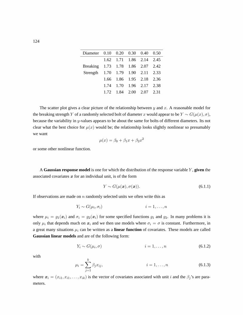
124

Diameter 0.10 0.20 0.30 0.40 0.50

1.62 1.71 1.86 2.14 2.45

Breaking 1.73 1.78 1.86 2.07 2.42

Strength 1.70 1.79 1.90 2.11 2.33

1.66 1.86 1.95 2.18 2.36

1.74 1.70 1.96 2.17 2.38

1.72 1.84 2.00 2.07 2.31

The scatter plot gives a clear picture of the relationship between and . A reasonable model for

the breaking strength of a randomly selected bolt of diameter would appear to be ∼ (() ),

because the variability in -values appears to be about the same for bolts of different diameters. Its not

clear what the best choice for () would be; the relationship looks slightly nonlinear so presumably

we want

() = 0 + 1+ 22

or some other nonlinear function.

A Gaussian response model is one for which the distribution of the response variable , given the

associated covariates x for an individual unit, is of the form

∼ ((x) (x)) (6.1.1)

If observations are made on randomly selected units we often write this as

∼ ( ) = 1

where = 1(x) and = 2(x) for some specified functions 1 and 2. In many problems it is

only that depends much on x and we then use models where = is constant. Furthermore, in

a great many situations can be written as a linear function of covariates. These models are called

Gaussian linear models and are of the following form:

∼ ( ) = 1 (6.1.2)

with

=

X=1

= 1 (6.1.3)

where x = (1 1 ) is the vector of covariates associated with unit and the ’s are para-

meters.

125


Figure 6.18: Scatter Plot of Diameter vs. Strength for Steel Bolts.

Remark: Sometimes the model (6.1.2) is written a little differently as

= + where ∼ (0 )

This splits into deterministic () and random () components.

These models are also referred to as linear regression models, and the ’s are called the re-

gression coefficients. (The term “regression" is used because it was introduced in the 19th century in

connection with these models. We won’t bother explaining just how the term arose.)

The model (6.1.2) plus (6.1.3) describes many situations well. The following are some illustrations.

1. ∼ ( ), where is the height of a random female, corresponds to x = (1) 1 =

2. The model in Example 6.1.2 had = 0 + 1 where was the building’s size. This can be

re-expressed as = 00 + 11 where 0 = 1 1 = (here we’ve used with = 0 1

for simplicity.)

126

3. The bolt strength model in Example 6.1.3 had () = 0 + 1+ 22.

This could be re-expressed as

= 01 + 11 + 22

where 0 = 1 1 = 2 = 2 .

Now we’ll consider estimation and testing procedures for Gaussian models. We begin in the next

section with models that have no covariates.

6.2 Inference for a single sample from a Gaussian Distribution

Suppose that ∼ ( ) models a response variable in some population or process. A random

sample 1 is selected, and we want to estimate the model parameters and possibly to test

hypotheses about them.

We have already seen in Section 2.2 that the MLE’s of and 2 are

= =1

X=1

2 =1

X=1

( − )2

A closely related point estimate of 2 is the sample variance,

2 =1

− 1X=1

( − )2

We now consider interval estimation and tests of and .

6.2.1 Confidence Intervals and Tests About and

If were known then, as discussed in Chapter 4,

= −

√∼ (0 1)

would be a pivotal quantity and could be used to get confidence intervals (CI’s) for . However, is

generally unknown. Fortunately it turns out that if we simply replace with either or in , then

we still have a pivotal quantity which we denote as . We will write in terms of since the formulas

below look a little simpler then, so is defined as

= −

√

(6.2.1)

127

Since is treated as a r.v. in (6.2.1) (we’ll use to represent both the r.v. and an observed value, for

convenience), does not have a (0 1) distribution. It turns out that its distribution in this case is

what is known as a student-t (or just “") distribution. We’ll digress briefly to present this distribution

and show how it arises.

Student - Distributions

This distribution arises when we consider independent r.v.’s ∼ (0 1) and ∼ 2()

and then define

the new r.v.

=

()12(6.2.2)

Then has a student - distribution with degrees if freedom (d.f.), and we write ∼ () to

denote this. The p.d.f. of can be shown by a bivariate change of variables method (we won’t do this)

to be

() = (1 +2

)−(+1)2 −∞ ∞ (6.2.3)

where Γ(·) is the gamma function and

= Γ

µ + 1

2

¶√Γ(2) (6.2.4)

This distribution is symmetric about = 0 and for large is closely approximated by the p.d.f. of

(0 1) Problem 1 at chapter’s end considers some properties of ().

Probabilities for the − are available from tables or computer software. In , the

c.d.f. value

() = (() ≤ ) (6.2.5)

is calculated as ( ). For example, (15 10) gives ((10) ≤ 15) as .918.

Confidence Intervals for

We can show using (6.2.2) that (6.2.1) has a -distribution with − 1 degrees of freedom:

= −

√∼ (−1) (6.2.6)

To do this we use the fact that

(i) = −√∼ (0 1)

(ii) =(−1)2

2∼ 2

(−1)

(iii) and 2 are independent.

128

(The results (ii) and (iii) are not too hard to show using multivariate calculus. Proofs are omitted

here but done in Stat 330.)

Then, we see that defined in (6.2.2) is just the r.v. here, so (6.2.6) follows and is a pivotal

quantity.

Therefore, to get an CI for we find values 1 and 2 such that

(1 ≤ (−1) ≤ 2) = =

µ1 ≤ −

√≤ 2

¶

This converts to

µ − 2

√≤ ≤ − 1

√

¶= (6.2.7)

so ( − 2√ − 1

√) is an CI.

Example 6.2.1 Scores for an IQ test administered to ten year olds in a very large population have

close to a Gaussian distribution ( ). A random sample of 10 children got test scores as follows:

103 115 97 101 100 108 111 91 119 101

We can obtain confidence intervals for the average IQ test score in the population by using the pivotal

quantity

= −

√10∼ (9)

Since (−2262 ≤ (9) ≤ 2262) = 95, for example, a 95 confidence interval for is ±2262

√10. For the data given above = 1046 and = 857, so the observed confidence inter-

val is 1046± 613, or 9847 ≤ ≤ 11073.

Remarks:

1. Confidence intervals for get narrower as increases. They are also narrower if is known

(though this is unusual). In the limit as →∞, the CI based on (6.2.6) is equivalent to using

and knowing that = . For example, if in Example 6.2.1 we know that = 857 then the .95

CI would use ± 196√ instead of ± 2262 √ when = 10. As increases, √

becomes arbitrarily close to zero so the CI’s shrink to include only the point .

2. If we have a rough idea what the value of is, we can determine the value of needed to make

a (.95,say) CI a given length. This is used in deciding how large a sample to take in a study.

3. Sometimes we want CI’s of the form (1 ) ≤ or (1 ) ≥ . These are ob-

tained by taking 1 = −∞ and 2 = ∞, respectively, in (6.2.7). For “two-sided" intervals we

usually pick 1 = −2 so that the interval is symmetrical about .

129

Exercise: Show that these provide the shortest CI with a given confidence coefficient .

Hypothesis Tests for

We may wish to test a hypothesis 0 : = 0, where 0 is some specified value. To do this we can

use the statistic

= | | = | − 0|√

(6.2.8)

Significance levels are obtained from the -distribution: if is the value of observed in a sample

giving mean and standard deviation , then

= ( ≥ ;0 true)

= (|(−1)| ≥ )

= 1− (− ≤ (−1) ≤ )

Example 6.2.2 For the setting in Example 6.2.1, test 0 : = 110. With (6.2.8) the observed value

of is then

=|1046− 110|857

√10

= 199

and the significance level is

= (|(9)| ≥ 199)= 1− (−199 ≤ (9) ≤ 199)= 078

This indicates there isn’t any strong evidence against 0 (Such tests are sometimes used to com-

pare IQ test scores for a sub-population (e.g. students in one school district) with a known mean for

a “reference" population.)

Remark: The likelihood ratio (LR) statistic could also be used for testing 0 : = 0 or for CI’s

for , but the methods above are a little simpler. In fact, it can be shown that the LR statistic for 0 is

a one-to-one function of | |; see Problem 2 at the end of the chapter.

Remark: The function t.test in R will obtain confidence intervals and test hypotheses about ; for a

data set use t.test(y).

Confidence Intervals or Tests for

From the results following (6.2.6) we have that

=(− 1)2

2∼ 2(−1) (6.2.9)

130

so is pivotal quantity and can be used to find CI’s for 2 or . To get an CI we find 1 2 such that

(1 ≤ 2(−1) ≤ 2) = =

µ1 ≤ (− 1)

2

2≤ 2

¶

This converts to

µ(− 1)2

2≤ 2 ≤ (− 1)

2

1

¶= (6.2.10)

so an CI for is

µq(−1)2

2

q(−1)2

1

¶ For “two-sided" CI’s we usually choose 1 and 2 such

that

(2(−1) 1) = (2(−1) 2) =1−

2

In some applications we are interested in an upper bound on (because small is “good" in some

sense); then we take 2 =∞ so the lower confidence limit in (6.2.10) is 0.

Example 6.2.3. A manufacturing process produces wafer-shaped pieces of optical glass for lenses.

Pieces must be very close to 25 mm thick, and only a small amount of variability around this can

be tolerated. If represents the thickness of a randomly selected piece of glass then, to a close ap-

proximation, ∼ ( ). Periodically, random samples of 15 pieces of glass are selected and the

values of and are estimated to see if they are consistent with = 25 and with being under .02

mm. On one such occasion the sample mean and sum of squares from the data were = 25009 andP( − )2 = 0002347.

Consider getting a .95 confidence interval for , using the pivotal quantity

=142

2=

P( − )2

2∼ 2(14)

Since (563 ≤ 2(14)≤ 2612) = 95, we find

(563 ≤P( − )2

2≤ 2612) =

ÃµP( − )2

2612

¶12≤ ≤

µP( − )2

563

¶12!= 95

This gives the observed confidence interval 0095 ≤ ≤ 0204. It seems plausible that ≤ 02, though

the right hand end of the .95 confidence interval is just over .02. A one-sided .95 CI is ≤ 0189; this

comes from (657 ≤ 2(14)≤ ∞) = 95

Hypothesis Tests for

Sometimes a test for 0 : = 0 is of interest. One approach is to use a likelihood ratio (LR)

statistic, as described in Chapter 4. It can be seen (see Problem 2) that the LR statistic Λ is a function

of = (− 1)22,Λ = − ()− (6.2.11)

131

This is not a one-to-one function of but Λ is 0 when = and is large when is much

bigger than or much less than 1 (i.e. when 220 is much bigger than one or much less than 1).

Since ∼ 2(−1), when 0 is true, we can use this to compute exact significance levels, in-

stead of using the 2(1)

approximation for Λ discussed in Chapter 4. The following simpler calculation

approximates this SL:

1. Obtain = (− 1)220 from the observed data.

2. If − 1 compute = 2 (2(−1) ≥ ).

If − 1 compute = 2 (2(−1) ≤ ).

Example 6.2.4 For the manufacturing process in Example 6.2.3, test the hypothesis 0 : = 008

(.008 is the desired or target value of the manufacturer would like to achieve).

Note that since the value = 008 is outside the two-sided .95 CI for in Example 6.2.3, the SL

for 0 based on the test statistic Λ (or equivalently, ) will be less than .05. To find the exact SL, we

follow the procedure above:

1. =142

0082= 3667

2. = 2 (2(14)≥ 3667) = 0017

This indicates very strong evidence against 0 and suggests that is bigger than .008.

6.3 General Gaussian Response Models

We now consider general models of the form (6.1.2) plus (6.1.3): ∼ ( ) with =P

=1

for independent units = 1 2 . For convenience we define the × matrix of covariate

values:

= ()× (6.3.1)

We now summarize some results about the MLE’s of the parameters β = (1 )0 and .

Some results about M.L.E.’s of β = (1 )0 and of

• Maximization of the likelihood function

(β ) =

Y=1

1√2

− 12

−

2

132

or of (β ) = log(β ) gives

β = ( 0)−1 0y 2 =1

X=1

( − )2

where × = (), y×1 = (1 )0 and =P

=1

. We also define

2 =1

−

X=1

( − )2 =

− 2

• For the estimators ( = 1 ) and 2 it can be proved that

∼ (

q2) = 1 (6.3.2)

=2

2=(− )2

2∼ 2(−) (6.3.3)

is independent of (1 ) (6.3.4)

In (6.3.2), are constants which are functions of the ’s.

Remark: The MLE is also a least squares (LS) estimate of . Least squares is a method

of estimation in linear models that predates maximum likelihood. Problem 16 describes least

squares methods.

• Recall the distribution theory for the (student) distribution. If ∼ (0 1) and ∼ 2()

then

the r.v.

= p (6.3.5)

has a () distribution.

This provides a way to get confidence intervals (or tests) for any . Because (6.3.2) implies

that

= −

√∼ (0 1)

and because of (6.3.3), then (6.3.5) implies that

= −

√∼ (−) (6.3.6)

so is a pivotal quantity for . In addition given in (6.3.3) is a pivotal quantity for 2 or .

133

Below we will consider some special types of Gaussian models which fall under the general theory.

However, we’ll alter the notation a bit for each model, for convenience.

Single Gaussian distribution

Here, ∼ ( ) = 1 i.e. = (we use instead of as parameter name). This model

was discussed in detail in Section 6.2, where we used

= −

√∼ (−1) =

(− 1)22

∼ 2(−1)

(Note: The 1 in (6.3.2) is 1 here; its easiest to get this by the fact that Var( ) = var() = 2,

proved earlier.)

Comparing Two Gaussian DistributionsG(μ1,σ) andG(μ2,σ)

Independent samples 11 12 11 from (1 )

21 22 22 from (2 ) are obtained.

(We use double subscripts for the ’s here, for convenience.)

Once again, stick with 1 and 2 as names of parameters. The likelihood function for 1, 2, is

(1 2 ) =

2Y=1

Y=1

1√2

−12(−

)2

Maximization gives the m.l.e.’s

1 =

1X=1

1

1= 1 2 =

2X=1

2

2= 2 2 =

1

1 + 2

2X=1

X=1

( − )2

Note that 2 = 11+2−2

2X=1

( − 1)2 = (1 + 2)2(1 + 2 − 2)

where 2 =1

−1

X=1

( − )2.

• To get CI’s for = 1 − 2 note that

=( 1 − 2)−

q

11+ 1

2

∼ (0 1) =(1 + 2 − 2)2

2∼ 2(1+2−2)

134

and so by (6.3.5)

=( 1 − 2)−

q

11+ 1

2

∼ (1+2−2) (6.3.7)

Confidence intervals or tests about can be obtained by using the pivotal quantity exactly as in

Section 6.2 for a single distribution.

Example 6.3.1. In an experiment to assess the durability of two types of white paint used on asphalt

highways, 12 lines (each 400 wide) of each paint were laid across a heavily traveled section of highway,

in random order. After a period of time, reflectometer readings were taken for each line of paint; the

higher the readings the greater the reflectivity and the visibility of the paint. The measurements of

reflectivity were as follows:

Paint A: 12.5, 11.7, 9.9, 9.6, 10.3, 9.6, 9.4, 11.3, 8.7, 11.5, 10.6, 9.7

Paint B: 9.4, 11.6, 9.7, 10.4, 6.9, 7.3, 8.4, 7.2, 7.0, 8.2, 12.7, 9.2

Statistical objectives are to test that the average reflectivity for paints A and B is the same, and if

there is evidence of a difference, to obtain a confidence interval for their difference. (In many problems

where two attributes are to be compared we start by testing the hypothesis that they are equal, even if

we feel there may be a difference. If there is no statistical evidence of a difference then we stop there.)

To do this it is assumed that, to a close approximation, reflectivity measurements 1 for paint A are

(1 1), and measurements 2 for paint B are (2 2). We can test : = 1 − 2 = 0 and

get confidence intervals for by using the pivotal quantity

=( 1 − 2)−

q112+ 1

12

∼ (22)

where it is assumed that 1 = 2 = , which is estimated by

2 =1

22

"12X=1

(1 − 1)2 +

12X=1

(2 − 2)2

#

To test : = 0 we use the test statistic = | |. From the data given above we find

1 = 12 1 = 104P(1 − 1)

2 = 1408 21 = 12800

2 = 12 2 = 90P(2 − 2)

2 = 3864 22 = 35127

This gives = 14 and 2 = 23964, and the observed test statistic = 222. The significance level

is then

= (|(22)| ≥ 222) = 038

135

This indicates there is fairly strong evidence against : 1 = 2. Since 1 2, the indication

is that paint A keeps its visibility better. A .95 confidence interval based on is obtained using the

fact that (−2074 ≤ (22) ≤ 2074) = 95. This gives the confidence interval for = 1 − 2 of

± 2074√6, or 009 ≤ ≤ 271. This suggests that although the difference in reflectivity (and

durability) of the paint is statistically significant, the size of the difference is not really large relative to

1 and 2 (look at 1 and 2).

The procedures above assume that the two Gaussian distributions have the same standard devia-

tions. Sometimes this isn’t a reasonable assumption (it can be tested using a LR test, but we won’t do

this here) and we must assume that ∼ (1 1) and 2 ∼ (2 2). In this case there is no exactly

pivotal quantity with which to get CI’s for = 1 − 2, but

=(1 − 2)− q

211+

222

' (0 1) (6.3.8)

is an approximate pivotal quantity that becomes exact as 1 and 2 become arbitrarily large.

To illustrate its use, consider Example 6.3.1, where we had 21 = 12800 22 = 35127. These

appear quite different but they are in squared units and 1 2 are small; the standard deviations 1 =

113 and 2 = 197 do not provide evidence against the hypothesis that 1 = 2 if a LR test is carried

out. Nevertheless, let us use (6.3.8) to get a .95 CI for . This gives the CI

(1 − 2)± 196s

211+

222

which with the data observed equals 1.4± 1.24, or .16≤ ≤ 264 This is not much different than the

interval obtained in Example 6.3.1.

Example 6.3.2 Scholastic Achievement Test Scores

Tests that are designed to “measure" the achievement of students are often given in various subjects.

Educators and others often compare results for different schools or districts. We consider here the

scores on a mathematics test given to Canadian students in the 5th grade. Summary statistics (sample

sizes, means, and standard deviations) of the scores for the students in two small school districts in

Ontario are as follows:

District A: = 278 = 602 = 1016

District B: = 345 = 581 = 902

The average score is somewhat higher in district A, and we will give a confidence interval for the

difference in average scores − in a model representing this setting. This is done by thinking

of the students in each district as a random sample from a conceptual population of “similar" students

136

writing “similar" tests. Assuming that in a given district the scores have a ( ) distribution, we

can test that the means and for districts and are the same, or give a CI for the difference.

(Achievement tests are usually designed so that the scores are approximately Gaussian, so this is a

sensible procedure.)

Let us get a .95 CI for = − using the pivotal quantity (6.3.8). This gives the CI

1 − 2 ± 196s

211+

222

which becomes 21± (196)(779) or 057 ≤ ≤ 163 Since = 0 is outside the .95 CI (and also the

.99 CI) we can conclude there is fairly strong evidence against the hypothesis that = , suggesting

that .

It is always a good idea to look carefully at the data and the distributions suggested for the two

groups, however; we should not rely only on a comparison of their means. Figure 6.3.1 shows a box plot

of the two samples; this type of plot was mentioned in Section 1.3. It shows both the median value and

other summary statistics of each sample: the upper and lower quartiles (i.e. 25th and 75th percentiles)

and the smallest and largest values. Figure 6.19 was obtained using the R function ().

Note that the distributions of marks for districts and are actually quite similar. The median

(and mean) is a little higher for district and because the sample sizes are so large, this gives a “statis-

tically significant" difference in a test that = . However, it would be a mistake to conclude that

the actual difference in the two distributions is very large. Unfortunately, “significant" tests like this

are often used to make claims about one group being “superior" to another.

Remark: The R function t.test will carry out the test above and will give confidence intervals for

− . This can be done with the command ( = ), where and are

the data vectors from and .

6.4 Inference for Paired Data

Although this and the next section are also special cases of the general Gaussian model of Section 6.3,

the procedures are sufficiently important that we give them their own sections.

Often experimental studies designed to compare means are conducted with pairs of units, where

the responses within a pair are not independent. The following examples illustrate this.

137


Figure 6.19: Box Plot of Math Test Scores for Two School Districts.

Example 6.4.1 Heights of Males vs Females

In a study in England, the heights of 1401 (brother, sister) pairs of adults were determined. One

objective of the study was to compare the heights of adult males and females; another was to examine

the relationship between the heights of male and female siblings.

Let 1 and 2 be the heights of the male and female, respectively , in the i’th (brother, sister) pair

( = 1 2 1401). Assuming that the pairs are sampled randomly from the population, we can use

them to estimate

1 = (1) 2 = (2)

and the difference = 1 − 2. However, the heights of related persons are not independent, so to

estimate the method in the preceding section would not be strictly usable; it requires that we have

independent random samples of males and females. In fact, the primary reason for collecting these

data was to consider the joint distribution of 1 2 and to examine their relationship. This topic is not

considered in this course, but a clear picture is obtained by plotting the points (1 2) in a scatter plot.

Example 6.4.2 Comparing Car Fuels

138

In a study to compare “standard" gasoline with gas containing an additive designed to improve mileage

(i.e. reduce fuel consumption), the following experiment was conducted:

Fifty cars of a variety of makes and engine sizes were chosen. Each car was driven in a standard

way on a test track for 1000 km, with the standard fuel (S) and also with the enhanced fuel (E). The

order in which the S and E fuels was used was randomized for each car (you can think of a coin being

tossed for each car, with fuel S being used first if a Head occurred) and the same driver was used for

both fuels in a given car. Drivers were different across the 50 cars.

Suppose we let 1 and 2 be the amount of fuel consumed (in litres) for the i’th car with the S and

E fuels, respectively. We want to estimate

= (1 − 2)

The fuel consumptions 1 2 for the i’th car are related, because factors such as size, weight and

engine size (and perhaps the driver) affect consumption. As in the preceding example it would likely

not be appropriate to treat the 1’s ( = 1 50) and 2’s ( = 1 50) as two independent

samples. Note that in this example it may not be of much interest to consider (1) and (2)

separately, since there is only a single observation on each car type for either fuel.

Two types of Gaussian models are used to represent settings involving paired data. The first involves

what is called a bivariate normal distribution for (1 2), and it could be used in Example 6.4.1. This

is a continuous bivariate model. Only discrete bivariate models were introduced in Stat 230 and we

will not consider this model here (it is studied in Stat 330), except to note an important property:

= 1 − 2 ∼ ( 2) (6.4.1)

where = 1−2 = (1)−(2). Thus, if we are interested in estimating or testing , we can do

this by considering the within-pair differences and using the methods for a single Gaussian model

in Section 6.2.

The second Gaussian model used with paired data has

1 ∼ (1 + 21) 2 ∼ (2 +

22)

where the ’s are unknown constants. Here it is assumed that 1 and 2 are independent r.v.’s, and

the ’s represent factors specific to the different pairs. This model also gives the distribution (6.4.1),

since

(1 − 2) = 1 − 2 ( cancels)

(1 − 2) = 21 + 22 = 2

This model seems relevant for Example 6.4.2, where refers to the i’th car type. Interestingly, the two

models for (1 2) can be connected; if the ’s are considered as Gaussian random variables in the

population of pairs of units then the result is that (1 2) have a bivariate normal model.

139

Thus, whenever we encounter paired data in which the variation in variables 1 and 2 is ade-

quately modeled by Gaussian distributions, we will make inferences about = 1 − 2 by working

with the model (6.4.1).

Example 6.4.1 revisited. The data on 1401 (brother, sister) pairs gave differences = 1−2 ( =1 1401) for which the sample mean and variance were

= 4895 in 2 =

P( − )2

1400= 65480 in2

Using the student− pivotal quantity (6.2.6), a two-sided .95 confidence interval for = () is

± 196√ where = 1401 (Note that (1400) is indistinguishable from (0 1).) This gives the

.95 CI 4895± 0134 inches, or 476 ≤ ≤ 503 in.

Remark: The method above assumes that the (brother, sister) pairs are a random sample from the

population of families with a living adult brother and sister. The question arises as to whether also

represents the difference in the average heights of all adult males and all adult females (call them 01and 02) in the population. Presumably 01 = 1 (i.e. the average height of all adult males equals

the average height of all adult males who also have an adult sister) and similarly 02 = 2, so does

represent this difference. However, it might be wise to check this assumption.

Recall our earlier Example 2.4.1 involving the difference in the average heights of males and fe-

males in New Zealand. This gave the estimate = 1− 2 = 6872− 6410 = 462 inches, which is a

little less than the difference in the example above. This is likely due to the fact that we are considering

two distinct populations, but it should be noted that the New Zealand data are not paired.

Pairing as an Experimental Design Choice

In settings were the population can be arranged in pairs, the estimation of a difference in means, =

1−2, can often be made more precise (shorter CI’s) by using pairing in the study. The condition for

this is that the association (or correlation) between 1 and 2 be positive. This is the case in both of

Examples 6.4.1 and 6.4.2, so the pairing in these studies is a good idea.

To illustrate this further, in Example 6.4.1 the height measurement on the 1401 males gave 1 =

69720 and 21 = 73861 and those on the females gave 2 = 64825 and 22 = 67832. If the males and

females were two independent samples (this is not quite right because the heights for the brother-sister

combinations are not independent, but the sample means and variances are close to what we would get

if we did have completely independent samples), then we could use the pivotal quantity (6.3.7) to get a

confidence interval for = 1 − 2. This gives the .95 CI 470 ≤ ≤ 509; we note that it is slightly

longer than the .95 CI 476 ≤ ≤ 503 obtained using the pairings.

To see why the pairing is helpful in estimating , suppose that 1 ∼ (1 21) and 2 ∼

140

(2 22), but that 1 and 2 are not necessarily independent ( = 1 2 ). The estimator of

is

= 1 − 2

and we have that () = = 1 − 2 and

() = (1) + (2)− 2(1 2)

=21+

22− 2

12

where 12 = (1 2). If 12 0, then () is smaller than when 12 = 0 (i.e. when 1 and

2 are independent). Therefore if we can collect a sample of pairs (1 2), this is better than two

independent random samples (one of 1’s and one of 2’s) for estimating . Note on the other hand

that if 12 0, then pairing is a bad idea since it increases the variance of .

The following example involves an experimental study with pairing.

Example 6.4.3. Fibre in Diet and Cholesterol Level

This example comes from the Stat 231 Course Notes, chapter 15. In the study 20 subjects (who were

actually volunteers from workers in a Boston hospital) with ordinary cholesterol levels were given a

low-fibre diet for 6 weeks and a high-fibre diet for another 6 week period. The order in which the two

diets were given was randomized for each subject (person), and there was a two-week gap between

the two 6 week periods, in which no dietary fibre supplements were given. A primary objective of the

study was to see if cholesterol levels are lower with the high-fibre diet.

Details of the study are given in the New England Journal of Medicine, volume 322 (January 18,

1990), pages 147-152, and in the Stat 231 Notes. These provide interesting comments on factors and

difficulties in the design of studies on the effects of diet. Here we will simply present the data from the

study and estimate the effect of the amount of dietary fibre.

Table 6.4.1 shows the cholesterol levels (in mmol per liter) for each subject, measured at the end

of each 6 week period. We’ll let the r.v.’s 1 2 represent the cholesterol levels for subject on the

high fibre and low fibre diets, respectively. We’ll also assume that the differences are represented by

the model

= 1 − 2 ∼ ( ) = 1 20

The differences are also shown in Table 6.4.1, and from them we calculate the sample mean and

standard deviation

= −020 = 0411

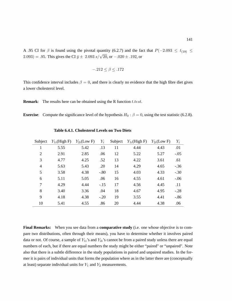
141

A .95 CI for is found using the pivotal quantity (6.2.7) and the fact that (−2093 ≤ (19) ≤2093) = 95. This gives the CI ± 2093

√20, or −020± 192, or

−212 ≤ ≤ 172

This confidence interval includes = 0, and there is clearly no evidence that the high fibre diet gives

a lower cholesterol level.

Remark: The results here can be obtained using the R function .

Exercise: Compute the significance level of the hypothesis 0 : = 0, using the test statistic (6.2.8).

Table 6.4.1. Cholesterol Levels on Two Diets

Subject 1(High F) 2(Low F) Subject 1(High F) 2(Low F)

1 5.55 5.42 .13 11 4.44 4.43 .01

2 2.91 2.85 .06 12 5.22 5.27 -.05

3 4.77 4.25 .52 13 4.22 3.61 .61

4 5.63 5.43 .20 14 4.29 4.65 -.36

5 3.58 4.38 -.80 15 4.03 4.33 -.30

6 5.11 5.05 .06 16 4.55 4.61 -.06

7 4.29 4.44 -.15 17 4.56 4.45 .11

8 3.40 3.36 .04 18 4.67 4.95 -.28

9 4.18 4.38 -.20 19 3.55 4.41 -.86

10 5.41 4.55 .86 20 4.44 4.38 .06

Final Remarks: When you see data from a comparative study (i.e. one whose objective is to com-

pare two distributions, often through their means), you have to determine whether it involves paired

data or not. Of course, a sample of 1’s and 2’s cannot be from a paired study unless there are equal

numbers of each, but if there are equal numbers the study might be either “paired" or “unpaired". Note

also that there is a subtle difference in the study populations in paired and unpaired studies. In the for-

mer it is pairs of individual units that forms the population where as in the latter there are (conceptually

at least) separate individual units for 1 and 2 measurements.

142

6.5 Linear Regression Models

Many studies involve covariates x, as described in Section 6.1. In this section we consider settings

where there is a single -variable. Problems with multiple -variables were mentioned in Sections 6.1

and 6.3, and are considered in Stat 331. We start by summarizing results from Sections 6.1 and 6.3.

Consider the model with independent ’s such that

∼ ( ) with = + (6.5.1)

(Note that this is of the form (6.1.2) and (6.1.3) with 1 = 2 = 1 = 1 2 = ).

• Once again, we can use the general results of Section 6.3 or just maximize the likelihood to get

the MLE’s: maximize

( ) =

Y=1

1√2

− 12

−−

2

to get =

, = − , 2 = 1

P=1( − − )

2 = 1( − )

where =X=1

( − )2, =X=1

( − )( − ), =X=1

( − )2.

Remark: In regression models we often “redefine" a covariate as 0 = − , where is a

constant value that makesP

0 close to zero. (Often we take = , which makesP

0 exactly

zero.) The reasons for doing this are that it reduces round-off errors in calculations, and that it makes

the parameter more interpretable. Note that does not change if we “centre" this way, because

( |)is() = + = + (0 + ) = (+ ) + 0

Thus, the intercept changes if we redefine , but not In the examples here we have kept the given

definition of , for simplicity.

We now consider how to get confidence intervals for quantities of interest. As usual, formulas are

written in terms of

2 =1

− 2X=1

( − )2

=1

− 2X=1

( − − )2

instead of 2.

143

Confidence Intervals for β

These are important because represents the increase in

() = ( |) = +

resulting from an increase of 1 in . As well, if = 0 then has no effect on (within the constraints

of this model).

From Section 6.3 we know that ∼ (√) for some constant . It’s easy to show this directly

here, and to obtain . Write as

=

=

X=1

( − )( − )

=

X=1

( − )

(since

X( − ) = 0)

=

X=1

where = ( − ). This is a linear combination of independent Gaussian r.v.’s and so its

distribution is also Gaussian, with

() =

X=1

()

=

X=1

( − )

(+ )

=

X=1

( − )

+

X=1

( − )

= 0 +

X=1

( − )2

(since

X( − )2 =

X( − ))

=

and

() =

X=1

2 ()

=

X=1

( − )2

22 =

2

Thus

∼ (√) (6.5.2)

144

and combining this with the fact that

=(− 2)2

2∼ 2(−2) (6.5.3)

and that and 2 are independent, we get as in (6.3.6) that

= −

√∼ (−2) (6.5.4)

This can be used as a pivotal quantity to get CI’s for , or to test hypotheses about .

Note also that (6.5.3) can be used to get CI’s or tests for , but these are usually of less interest than

inference about or the other quantities below.

Confidence Intervals for μ(x)

We are often interested in estimating () = + for a specified value of . We’ll derive a student

- pivotal quantity for doing this.

The MLE of () has associated estimator

() = + = + (− )

since = − . Thus () is a linear function of Gaussian r.v.’s (because and are) and so must

have a Gaussian distribution. Its mean and variance are

[()] = ( ) + (− )()

=1

X=1

() + (− )

=1

X=1

(+ ) + (− )

= + + (− )

= + = ()

and because and are independent (can be shown),

[()] = ( ) + (− )2 ()

=1

2

X=1

() + (− )22

= 2µ1

+(− )2

¶

145

Thus

() ∼

⎡⎣() s 1

+(− )2

⎤⎦and it then follows that

=()− ()

q1+(−)2

∼ (−2) (6.5.5)

This can be used as a pivotal quantity to get CI’s for ().

Remark: The parameter equals (0) so doesn’t require special treatment. Sometimes = 0 is a

value of interest but often it is not. In the following example it refers to a building of area 0, which is

nonsensical!

Remark: The results of the analyses below can be obtained using the R function , with the com-

mand ( ∼ ). We give the detailed results below to illustrate how the calculations are made. In R,

(( ∼ )) gives a lot of useful output.

Example 6.5.1 Price vs Size of Commercial Buildings

Example 6.1.2 gave data on the selling price per square meter () and area () of commercial buildings.

Figure 6.1.1 suggested that a model of the form (6.5.1) would be reasonable, so let us consider that.

We find easily that = 0954 = 5490 and = 22945 = −331668 =

489 46262 so we find

= −1445 = 6869 2 = 36437 = 1909

Note that is negative: the larger size buildings tend to sell for less per square meter. (The estimate

= −1445 indicates a drop in average price of $14450 per square meter for each increase of 1 unit

in ; remember ’s units are 2(105)) The line = + is often called the fitted regression line

for on , and if we plot it on the same graph as the points ( ) in the scatter plot Figure 6.1.1, we

see it passes close to the points.

A confidence interval for isn’t of major interest in the setting here, where the data were called on

to indicate a fair assessment value for a large building with = 447. One way to address this is to

estimate () when = 447. We get the MLE

(447) = + (447) = $4094

which we note is much below the assessed value of $75 per square meter. However, one can object that

there is uncertainty in (447), and that it would be better to give a CI. Using (6.5.5) and the fact that

146

(−2048 ≤ (28) ≤ 2048) = 95, we get a .95 CI for (447) as

(447)± 2048s1

30+(447− )2

or $4094 ± $2654, or $1440 ≤ (447) ≤ $6750. Thus the assessed value of $75 is outside this

range.

However (playing lawyer for the Assessor), we could raise another objection: since we are con-

sidering a single building (and not the average of all buildings) of size = 447(×105)2, we must

recognize that has a non-neglible variance. This suggests that what we should do is predict the

−value for a building with = 447, instead of estimating (447). We will temporarily leave the

example in order to develop a method to do this.

Prediction Intervals for Y

Suppose we want to estimate or predict the -value for a random unit which has a specific value

for its covariate We can get a pivotal quantity that can be used to give a prediction interval (or interval

“estimate") for , as follows.

Note that ∼ (() ) and, from above, that () ∼ (() ³1+

(−)2

´12). Also, is

independent of () since it is not connected to the existing sample. Thus

( − ()) = ( ) + (())

= 2 + 2µ1

+(− )2

¶Thus

− () ∼ (0

µ1 +

1

+(− )2

¶12)

and it also follows that

= − ()

q1 + 1

+

(−)2

∼ (−2) (6.5.6)

We can use the pivotal quantity to get interval estimates for , since

(1 ≤ ≤ 2)

=

⎛⎝()− 2

s1 +

1

+(− )2

≤ ≤ ()− 1

s1 +

1

+(− )2

⎞⎠We usually call these prediction intervals instead of confidence intervals, since isn’t a parameter

but a “future" observation.

147

Example 6.5.1 Revisited

Let us obtain a .95 prediction interval (PI) for when = 447. Using (6.5.6) and the fact that

(−2048 ≤ (28) ≤ 2048) = 95, we get the .95 PI

(447)± 2048s1 +

1

30+(447− )2

or −630 ≤ ≤ 8820 (dollars per square meter). The lower limit is negative, which is nonsensical.

This happened because we’re using a Gaussian model (in which can be positive or negative) in a

setting where (price) must be positive. Nonetheless, the Gaussian model fits the data well, so we’ll

just truncate the PI and take it to be 0 ≤ ≤ $8820.Now we find that the assessed value of $75 is inside this interval! On this basis its hard to say that

the assessed value is unfair (though it is towards the high end of the PI).

Note also that the value = 447 of interest is well outside the range of -values (.20 - 3.26) in

the data set of 30 buildings; look again at Figure 6.1.1. Thus any conclusions we reach are based on

an assumption that the linear model () = + applies beyond = 326 and out to = 447.

This may not be true, but we have no way to check it with the data we have. Note also that is a slight

suggestion in Figure 6.1.1 that ( ) may be smaller for larger -values. There is not sufficient

data to check this either.

Remark: Note from (6.5.5) and (6.5.6) that CI’s for () and PI’s from are wider the further away

is from . Thus, as we move further away from the “middle" of the ’s in the data, we get wider and

wider intervals for () or .

Example 6.5.2 Strength of Steel Bolts

Recall the data given in Example 6.1.3, where represented the breaking strength of a randomly

selected steel bolt and was the bolt’s diameter. A scatter plot of points ( ) for 30 bolts suggested

a nonlinear relationship between and . A bolt’s strength might be expected to be proportional to its

cross-sectional area, which is proportional to 2. Figure 6.5.1 shows a plot of points (2 ); it looks

quite linear.

Let us fit a linear model

∼ (+ 1 ) 1 = 2

to the data. We find (check these for yourself)

= 1667 = 2838 = 00515 = 02244

The fitted regression line = + 1 is shown on the scatter plot in Figure 6.20; the model appears

to fit well.

148

More as a numerical illustration, let us get a CI for , which represents the increase in average

strength (1) from increasing the diameter (and therefore also 1 = 2) by 1 unit. Using the pivotal

quantity (6.5.4) and the fact that (−2048 ≤ (28) ≤ 2048) = 95, we get the .95 CI

± 2048 √

or 2838± 0223

A .95 CI for the value of is therefore (2.605, 3.051).

Figure 6.5.1 Scatter Plot of Bolt Diameter Squared vs. Strength

file=st241.fig651.ps,angle=0,width=


Figure 6.20: Scatter Plot of Bolt Diameter Squared vs. Strength

Exercise: This model could be used to predict the breaking strength of a new bolt of given diameter

. Find a PI for a new bolt of diameter = 035.

149

6.6 Model Checking

There are two main components in Gaussian response models:

(i) the assumption that (given any covariates ) is Gaussian with constant standard deviation .

(ii) the assumption that = () is a given form like (6.1.3).

Models should always be checked, and in this case there are several ways to do this. Some of these

are based on what we term “residuals" of the fitted model: the residuals are the values

= − = 1

For example, if ∼ (+ ;) then = − − . The R function produces these values

as part of its output.

If ∼ ( ) then = − ∼ (0 ). The idea behind the ’s is that they can be

thought of as “observed" ’s. This isn’t exactly correct since we are using instead of in , but

if the model is correct, then the ’s should behave roughly like a random sample from the distribution

(0 ).

Plots of residuals are used as a model check. For example, we can

(1) Plot points ( ) = 1 . If the model is satisfactory these should lie within a horizontal

band around the line = 0

(2) Plot points ( ) = 1 . If the model is satisfactory we should get the same type of

pattern as for (1).

Departures from the “expected" pattern in (1) and (2) suggest problems with the model. For ex-

ample, if in (2) we see that the variability in the ’s is bigger for larger values , this suggests that

() = () is not constant, but may be larger when () is larger.

Figure 6.6.1 shows a couple of such patterns; the left hand plot suggests non-constant variance

whereas the right hand plot suggests that the function = () is not correctly specified.

In problems with only one -variable, a plot of () superimposed on the scatterplot of the data (as

in Figure 6.5.1) shows pretty clearly how well the model fits. The residual plots described are however,

very useful when there are two or more covariates in the model.

When there are no covariates in the model, as in Section 6.2, plots (1) and (2) are undefined. In this

case the only assumption is that ∼ ( ). We can still define residuals, either as

∗ = − or ∗ = −

150

where = and (we could alternatively use s) is the MLE of . One way to check the model is

to treat the ∗ ’s (which are called standardized residuals) as a random sample of values ( − ).

Since − ) ∼ (0 1) under our assumed model, we could plot the empirical c.d.f. (EDF) from

∗ ( = 1 ) and superimpose on it the (0 1) c.d.f. The two curves should agree well if the

Gaussian model is satisfactory. This plot can also be used when there are covariates, by defining the

standardized residuals

∗ =

=

−

= 1

We can also use the ∗ ’s in place of the ’s in plots (1) and (2) above; in fact that is what we did in

Figure 6.6.1. When the ∗ ’s are used the patterns in the plot are unchanged but the ∗ values tend to lie

in the range (-3,3). (think why this is so.)

Figure 6.6.1 Examples of Patterns in Residual Plots file=st241.fig661.ps,angle=0,width=


Figure 6.21: Examples of Patterns in Residual Plots

Example 6.6.1 Steel Bolts Let us define residuals

= − − = 1 30

151

for the model fitted in Example 6.5.3. Figure 6.22 shows a plot of the points (1 ); no deviation

from the expected pattern is observed. This is of course also evident from Figure 6.5.1.

A further check on the Gaussian distribution is shown in Figure 6.23. Here we have plotted the

EDF based on the 30 standardized residuals

∗ = − − 1

On the same graph is the (0 1) c.d.f. There is good agreement between the two curves.


Figure 6.22: Residual Plot for Bolt Strength Model

6.7 Problems

1. Student’s Distribution

Suppose that and are independent variates with

∼ (0 1); ∼ 2()

Consider the ratio

≡ √ ÷

152


Figure 6.23: EDF of Standard Residuals and (0 1) CDF

Then is a continuous variate. Its distribution is called the (Student’s) distribution with

degrees of freedom, and we write ∼ () for short. It can be shown by change of variables that

has pdf

() =

µ1 +

2

¶− +12

for −∞ ∞

where is a normalizing constant such that the total area under the pdf is 1:

= Γ

µ + 1

2

¶√ Γ

³2

´

The pdf is symmetric about the origin, and is similar in shape to the pdf of (0 1) but has more

probability in the tails. It can be shown that () tends to the (0 1) pdf as →∞.

(a) Plot the pdf for = 1 and = 5

(b) Find values such that

¡− ≤ (30) ≤

¢= 098;

¡(20) ≥

¢= 095

153

(c) Show that () is unimodal for all .

(d) Show that as →∞ () approaches the (0 1) limit () = 1√2−

122 .

(Note: To do this you will need to use the fact that → 1√2 as →∞; this is from a

property of gamma functions.)

2. Suppose that 1 · · · are independent ( ) observations.

(a) Show that the likelihood ratio statistic for testing a value of is given by (assume is

unknown)

Λ() = log³1 + 2

−1´

where =√( − ), with the sample standard deviation. (Note: The sample

variance 2 is defined asP( − )2(− 1).)

(b) Show that the likelihood ratio statistic for testing a value of is a function of

=(− 1)2

2

3. The following data are instrumental measurements of level of dioxin (in parts per billion) in 20

samples of a “standard” water solution known to contain 45 ppb dioxin.

44.1 46.0 46.6 41.3 44.8 47.8 44.5 45.1 42.9 44.5

42.5 41.5 39.6 42.0 45.8 48.9 46.6 42.9 47.0 43.7

(a) Assuming that the measurements are independent and ( 2), obtain a .95 confidence

interval for and test the hypothesis that = 45.

(b) Obtain a .95 confidence interval for . Of what interest is this scientifically?

4. A new method gave the following ten measurements of the specific gravity of mercury:

13.696 13.699 13.683 13.692 13.705

13.695 13.697 13.688 13.690 13.707

Assume these to be independent observations from ( 2).

(a) An old method produced measurements with standard deviation = 02. Test the hypoth-

esis that the new method has the same standard deviation as the old.

154

(b) A physical chemistry handbook lists the specific gravity of mercury as 13.75. Are the data

consistent with this value?

(c) Obtain 95% CI’s for and .

5. Sixteen packages are randomly selected from the production of a detergent packaging machine.

Their weights (in grams) are as follows:

287 293 295 295 297 298 299 300

300 302 302 303 306 307 308 311

(a) Assuming that the weights are independent ( 2) random variables, obtain .95 confi-

dence intervals for and .

(b) Let and 2 = 1−1

P( − )2 be the mean and variance in a sample of size , and let

represent the weight of a future, independent, randomly selected package. Show that

− ∼ ¡0 2

¡1 + 1

¢¢and then that

= −

q1 + 1

∼ (−1)

For the data above, use this as a pivotal to obtain a .95 “confidence” interval for .

6. A manufacturer wishes to determine the mean breaking strength (force) of a type of string to

“within a pound", which we interpret as requiring that the 95% confidence interval for a should

have length at most 2 pounds. If breaking strength of strings tested are ( ) and if 10

preliminary tests gaveP( − )2 = 80, how many additional measurements would you advise

the manufacturer to take?

7. To compare the mathematical abilities of incoming first year students in Mathematics and Engi-

neering, 30 Math students and 30 Engineering students were selected randomly from their first

year classes and given a mathematics aptitude test. A summary of the resulting marks (for the

math students) and (for the engineering students), = 1 30, is as follows:

Math students: = 30 = 120P( − )2 = 3050

Engineering students: = 30 = 114P( − )2 = 2937

Obtain a .95 confidence interval for the difference in mean scores for first year Math and Engi-

neering students, and test the hypothesis that the difference is zero.

155

8. A study was done to compare the durability of diesel engine bearings made of two different

compounds. Ten bearings of each type were tested. The following table gives the “times” until

failure (in units of millions of cycles):

Type I Type II

3.03 3.19

5.53 4.26

5.60 4.47

9.30 4.53

9.92 4.67

12.51 4.69

12.95 12.78

15.21 6.79

16.04 9.37

16.84 12.75

(a) Assuming that , the number of million cycles to failure, has a normal distribution with the

same variance for each type of bearing, obtain a .90 confidence interval for the difference

in the means 1 and 2 of the two distributions.

(b) Test the hypothesis that 1 = 2.

(c) It has been suggested that log failure times are approximately normally distributed, but

not failure times. Assuming that the log ’s for the two types of bearing are normally

distributed with the same variance, test the hypothesis that the two distributions have the

same mean. How does the answer compare with that in part (b)?

(d) How might you check whether or log is closer to normally distributed?

(e) Give a plot of the data which could be used to describe the data and your analysis.

9. Fourteen welded girders were cyclically stressed at 1900 pounds per square inch and the numbers

of cycles to failure were observed. The sample mean and variance of the log failure “times" were

= 14564 and 2 = 00914. Similar tests on four additional girders with repaired welds gave

= 14291 and 2 = 00422. Log failure times are assumed to be independent with a ( )

distribution.

(a) Test the hypothesis that the variance of is the same for repaired welds as for the normal

welds.

(b) Assuming equal variances, obtain a 90% confidence interval for the difference in mean log

failure time.

156

(c) Note that 1 − 2 in part (b) is also the difference in median log failure times, and obtain a

90% confidence interval for the ratio

median lifetime (cycles) for repaired welds

median lifetime (cycles) for normal welds

10. Let 1 · · · be a random sample from (1 1) and 1 · · · be a random sample from

(2 2). Obtain the likelihood ratio statistic for testing : 1 = 2 and show that it is a

function of = 2122, where 21 and 22 are the sample variances from the and samples.

11. Readings produced by a set of scales are independent and normally distributed about the true

weight of the item being measured. A study is carried out to assess whether the standard deviation

of the measurements varies according to the weight of the item.

(a) Ten weighings of a 10 kg. weight yielded = 10004 and = 0013 as the sample

mean and standard deviation. Ten weighings of a 40 kg. weight yielded = 39989

and = 0034. Is there any evidence of a difference in the standard deviations for the

measurements of the two weights?

(b) Suppose you had a further set of weighings of a 20 kg. item. How could you study the

question of interest further?

12. An experiment was conducted to compare gas mileages of cars using a synthetic oil and a con-

ventional oil. Eight cars were chosen as representative of the cars in general use. Each car was

run twice under as similar conditions as possible (same drivers, routes, etc.), once with the syn-

thetic oil and once with the conventional oil, the order of use of the two oils being randomized.

The average gas mileages were as follows:

Car 1 2 3 4 5 6 7 8

Synthetic oil 21.2 21.4 15.9 37.0 12.1 21.1 24.5 35.7

Conventional oil 18.0 20.6 14.2 37.8 10.6 18.5 25.9 34.7

(a) Obtain a .95 confidence interval for the difference in mean gas mileage, and state the as-

sumptions on which your analysis depends.

(b) Repeat (a) if the natural pairing of the data is (improperly) ignored.

(c) Why is it better to take pairs of measurements on eight cars rather than taking only one

measurement on each of 16 cars?

157

13. Consider the data in Problem 8 of Chapter 1 on the lengths of male and female coyotes.

(a) Fit separate Gaussian models for the lengths of males and females. Estimate the difference

in mean lengths for the two sexes.

(b) Estimate (1 2) (give the m.l.e.), where 1 is the length of a randomly selected female

and 2 is the length of a randomly selected male. Can you suggest how you might get a

confidence interval?

(c) Give separate CI’s for the average length of males and females.

14. Comparing sorting algorithms. Suppose you want to compare two algorithms A and B that

will sort a set of number into an increasing sequence. (The function sort ) will, for example,

sort the elements of the numeric vector .)

To compare the speed of algorithms A and B, you decide to “present" A and B with random

permutations of numbers, for several values of . Explain exactly how you would set up such

a study, and discuss what pairing would mean in this context.

15. Sorting algorithms continued. Two sort algorithms as in the preceding question were each run

on (the same) 20 sets of numbers (there were 500 numbers in each set). Times to sort the sets of

two numbers are shown below.

Set: 1 2 3 4 5 6 7 8 9 10

A: 3.85 2.81 6.47 7.59 4.58 5.47 4.72 3.56 3.22 5.58

B: 2.66 2.98 5.35 6.43 4.28 5.06 4.36 3.91 3.28 5.19

Set: 11 12 13 14 15 16 17 18 19 20

A: 4.58 5.46 3.31 4.33 4.26 6.29 5.04 5.08 5.08 3.47

B: 4.05 4.78 3.77 3.81 3.17 6.02 4.84 4.81 4.34 3.48

(a) Plot the data so as to illustrate its mean features.

(b) Estimate (give a CI) for the difference in the average time to sort with algorithms A and B,

assuming a Gaussian model applies.

(c) Suppose you are asked to estimate the probability that A will sort a randomly selected list

fast than B. Give a point estimate of this probability.

(d) Another way to estimate the probability in part (b) is just to notice that of the 20 sets of

numbers in the study, A sorted faster on 15. Indicate how you could also get a CI for

158

using this approach. (It is also possible to get a CI using the Gaussian model.)

16. Least squares estimation. Suppose you have a model where the mean of the response variable

given the covariates x has the form

= (|x) = (x;β) (6.7.1)

where β is a vector of unknown parameters. Then the least squares (LS) estimate of β based

on data (x ) = 1 is the value that minimizes the objective function

(β) =

X=1

[ − (x;β)]2

Show that the LS estimate of β is the same as the MLE of β in the Gaussian model ∼( ), when is of the form (6.7.1).

17. To assess the effect of a low dose of alcohol on reaction time, a sample of 24 student volunteers

took part in a study. Twelve of the students (randomly chosen from the 24) were given a fixed

dose of alcohol (adjusted for body weight) and the other twelve got a nonalcoholic drink which

looked and tasted the same as the alcoholic drink. Each student was then tested using software

that flashes a coloured rectangle randomly placed on a screen; the student has to move the cursor

into the rectangle and double click the mouse. As soon as the double click occurs, the process

is repeated, up to a total of 20 times. The response variate is the total reaction time (i.e. time to

complete the experiment) over the 20 trials.

The data on the times are shown below for the 24 students.

“Alcohol" Group: 1.33, 1.55, 1.43, 1.35, 1.17, 1.35, 1.17, 1.80, 1.68

1.19, 0.96, 1.46 ( = 1370 = 0235)

“Non-Alcohol" Group: 1.68, 1.30, 1.85, 1.64, 1.62, 1.69, 1.57, 1.82, 1.41,

1.78, 1.40, 1.43 ( = 1599 = 0180)

Analyze the data with the objective of seeing when there is any evidence that the dose of alcohol

increases reaction time. Justify any models that you use.

18. There are often both expensive (and highly accurate) and cheaper (and less accurate) ways of

measuring concentrations of various substances (e.g. glucose in human blood, salt in a can of

soup). The table below gives the actual concentration (determined by an expensive but very

159

accurate procedure) and the measured concentration obtained by a cheap procedure, for each

of 10 units.

x: 4.01 8.12 12.53 15.90 20.24 24.81 30.92 37.26 38.94 40.15

y: 3.70 7.80 12.40 16.00 19.90 24.90 30.80 37.20 38.40 39.40

(a) Fit a Gaussian linear regression model for given to the data and obtain .95 confidence

intervals for the slope and standard deviation . Use a plot to check the adequacy of the

model.

(b) Describe briefly how you would characterize the cheap measurement process’s accuracy to

a lay person.

(c) Assuming that the units being measured have true concentrations in the range 0-40, do you

think that the cheap method tends to produce a value that is lower than the true concentra-

tion? Support your answer with an argument based on the data.

19. The following data, collected by Dr. Joseph Hooker in the Himalaya mountains, relates at-

mospheric pressure to the boiling point of water. Theory suggests that a graph of log pressure vs.

boiling point should give a straight line.

Temp (F) Pres (in. Hg) Temp (F) Pres (in. Hg)

210.8 29.211 189.5 18.869

210.2 28.559 188.8 18.356

208.4 27.972 188.5 18.507

202.5 24.697 185.7 17.267

200.6 23.726 186.0 17.221

200.1 23.369 185.6 17.062

199.5 23.030 184.1 16.959

197.0 21.892 184.6 16.881

196.4 21.928 184.1 16.817

196.3 21.654 183.2 16.385

195.6 21.605 182.4 16.235

193.4 20.480 181.9 16.106

193.6 20.212 181.9 15.928

191.4 19.758 181.0 15.919

191.1 19.490 180.6 15.376

190.6 19.386

160

(a) Prepare a scatterplot of = log(Pressure) vs. =Temperature. Do the same for =Pressure

vs. . Which is better described by a linear model? Does this confirm the theory’s model?

(b) Fit a normal linear regression model for = log(Pressure) vs. . Are there any obvious

difficulties with the model?

(c) Obtain a .95 confidence interval for the atmospheric pressure if the boiling point of water

is 195F.

20. Consider the data in Problem 9 of Chapter 1, in which the variable was the average time to

complete tasks by computer users, and was the number of users on the system. Fit a regression

model, using as the explanatory variable. Give a .95 confidence interval for the mean of

when there are 50 users on the system.

21. (a) For the steel bolt experiment in Examples 6.1.3 and 6.5.2, use a Gaussian model to

(i) estimate the average breaking strength of bolts of diameter 0.35

(ii) estimate (predict) the breaking strength of a single bolt of diameter 0.35.

Give interval estimates in each case.

(b) Suppose that a bolt of diameter 0.35 is exposed to a large force that could potentially

break it. In structural reliability and safety calculations, is treated as a r.v. and if

represents the breaking strength of the bolt (or some other part of a structure), then the

probability of a “failure" of the bolt is ( ). Give a point estimate of this value if

∼ (160 10), where and are independent.

22. Optimal Prediction. In many settings we want to use covariates to predict a future value .

(For example, we use economic factors to predict the price of a commodity a month from

now.) The value is random, but suppose we know () = ( |) and ()2 = ( |).

(a) Predictions take the form = (), where (·) is our “prediction" function. Show that the

minimum achievable value of ( − )2 is minimized by choosing () = ().

(b) Show that the minimum achievable value of ( − )2, that is, its value when () =

() is ()2.

This shows that if we can determine or estimate (), then “optimal" prediction (in terms

of Euclidean distance) is possible. Part (b) shows that we should try to find covariates for

which ()2 = ( |) is as small as possible.

(c) What happens when ()2 is close to zero? (Explain this in ordinary English.)

TESTS AND INFERENCE PROBLEMS

BASED ON MULTINOMIAL MODELS

7.1 Introduction

Many important hypothesis testing problems can be addressed using multinomial models. An example

was given in Chapter 5, whose general ideas we will use here. To start, recall the setting in Example

(d) of Chapter 5, Section 2, where data were assumed to arise from a multinomial distribution with

probability function

(1 ; 1 ) =!

1! · · · !11 · · · (6.5.2)

where 0 ≤ ≤ andP

= . The multinomial probabilities satisfy 0 ≤ ≤ 1 andP

= 1,

and we define θ = (1 ). Suppose now that we wish to test the hypothesis

0 : = (α) = 1 (6.5.3)

where dim(α) = − 1.The likelihood function based on (7.1.1) is anything proportional to

(θ) =

Y=1

(6.5.4)

Let Ω be the parameter space for θ. It was shown earlier that (θ) is maximized over Ω by the vector

θ with = ( = 1 ). A likelihood ratio test of the hypothesis (7.1.2) is based on the

likelihood ratio statistic

Λ = 2(θ)− 2(θ0) = −2 log((θ0)

(θ)

) (6.5.5)

where θ0 maximizes (θ) under the hypothesis (7.1.2), which restricts θ to lie in a space Ω0 ⊂ Ω of

dimension . If 0 is true (that is, if θ really lies in Ω0) then the distribution of Λ is approximately

161

162

2(−) when is large, where = −1 is the dimension ofΩ. This enables us to compute significance

levels (-values) from observed data by using the approximation

(Λ ≥ Λobs;0)= (2(−) ≥ Λobs) (6.5.6)

This approximation is very accurate when is large and none of the ’s is too small; when the ’s

below all exceed 5 it is accurate enough for testing purposes.

The test statistic (7.1.4) can be written in a simple form. Let θ0 = (1 ) = (1() ())

denote the m.l.e. of θ under the hypothesis (7.1.2). Then, by (7.1.3), we get

Λ = 2(θ)− 2(0)

= 2

X=1

log()

Noting that = and defining “expected frequencies” under 0 as

= = 1

we can rewrite Λ as

Λ = 2

X=1

log() (6.5.7)

An alternative test statistic that was developed historically before Λ is the “Pearson” statistic

=

X=1

( − )2

(6.5.8)

This has similar properties to Λ; for example, both equal 0 when = for all = 1 and

are larger when ’s and ’s differ greatly. It turns out that, like Λ, the statistic also has a limiting

2(−) distribution, with = − 1, when 0 is true.

The remainder of this chapter consists of the application of the general methods above to some

important testing problems.

7.2 Goodness of Fit Tests

Recall from Section 2.5 that one way to check the fit of a probability distribution is by comparing the

’s (relative frequencies ) with the estimates from the distributional model. This is equivalent to

comparing the ’s (observed frequencies) and the ’s. In Section 2.5 this comparison was informal,

with only a rough guideline for how closely the ’s and ’s (or ’s and ’s) should agree.

It is possible to test the correctness of a parametric model by using an implied multinomial model.

We illustrate this through two examples.

163

Example 7.2.1. Recall Example 2.5.2, where people in a population are classified as being one

of three blood types MM, MN, NN. The proportions of the population that are these three types are

1, 2, 3 respectively, with 1 + 2 + 3 = 1. Genetic theory indicates, however, that the ’s can be

expressed in terms of a single parameter , as

1 = 2 2 = 2(1− ) 3 = (1− )2 (7.2.1)

Data collected on 100 persons gave 1 = 17, 2 = 46, 3 = 37, and we can use this to test

the hypothesis 0 that (7.2.1) is correct. (Note that (1 2 3) ∼ ( = 1001 2 3).) The

likelihood ratio test statistic is (7.1.6), but we have to find and then the ’s. The likelihood function

under (7.2.1) is

1() = (1() 2() 3())

= (2)17[2(1− )]46[(1− )2]37

= 80(1− )120

and we easily find that = 40. The expected frequencies are therefore 1 = 1002 = 16, 2 =

100[2(1 − )] = 48, 3 = 100[(1 − )2] = 36. Clearly these are close to the observed frequencies

1, 2, 3, and (7.1.6) gives the observed value Λobs = 017. The significance level is

(2(1) ≥ 017) = 68

so there is no evidence against the model (7.2.1).

The Pearson statistic (7.1.7) usually gives close to the same value as Λ when is large. In this case

we find that = 017.

Example 7.2.2. Continuous distributions can also be tested by grouping the data into intervals

and then using the multinomial model. Example 2.5.1 previously did this in an informal way for an

exponential distribution. For example, suppose that is thought to have an exponential distribution

with probability density function

(;) =1

− 0 (7.2.2)

Suppose a random sample 1 100 is collected and the objective is to test the hypothesis 0 that

(7.2.2) is correct. To do this we partition the range of into intervals = 1 , and count the

number of observations that fall into each interval. Under (7.2.2), the probability that an observation

lies in the ’th interval = ( ) is

() =

Z

(;) = 1 (7.2.3)

164

and if is the number of observations (’s) that lie in , then 1 follow a multinomial distrib-

ution with = 100. Thus we can test (7.2.2) by testing that (7.2.3) is true.

Consider the following data, which have been divided into = 7 intervals:

Interval 0-100 100-200 200-300 300-400 400-600 600-800 800

29 22 12 10 10 9 8

27.6 20.0 14.4 10.5 13.1 6.9 7.6

We have also shown expected frequencies , calculated as follows. The distribution of (1 7) is

multinomial with probabilities given by (7.2.3) when the model (7.2.2) is correct. In particular,

1 =

Z 100

0

1

− = 1− −100

and so on. Expressions for 2 7 are 2() = −100 − −200, 3() = −200 − −300,

4() = −300−−400, 5() = −400−−600, 6() = −600−−800, 7() = −800.

The likelihood function from 1 7 based on model (7.2.3) is then

1() =

7Y=1

()

It is possible to maximize 1() mathematically. (Hint: rewrite 1() in terms of the parameter =

−100 and find first; then = −100 ln .) This gives = 3103 and the expected frequencies

= 100() given in the table are then obtained.

The likelihood ratio statistic (7.1.6) gives Λobs = 191. The significance level is computed as

(Λ ≥ Λobs;0) = (2(5) ≥ 191) = 86

so there is no evidence against the model (7.2.3). Note that the reason the 2 degrees of freedom is 5 is

because = − 1 = 6 and = dim() = 1.

The goodness of fit test just given has some arbitrary elements, since we could have used different

intervals and a different number of intervals. Theory and guidelines as to how best to choose the

intervals can be developed, but we won’t consider this here. Rough guidelines for our purposes are to

chose 4-10 intervals, so that expected frequencies are at least 5.

7.3 Two-Way Tables and Testing for Independence of Two Variables

Often we want to assess whether two factors or variables appear to be related. One tool for doing this is

to test the hypothesis that the factors are independent (and thus statistically unrelated). We will consider

165

this in the case where both variables are discrete, and take on a fairly small number of possible values.

This turns out to cover a great many important settings.

Two types of studies give rise to data that can be used to test independence, and in both cases the

data can be arranged as frequencies in a two-way table. These tables are sometimes called “contin-

gency” tables in the statistics literature. We’ll consider the two types of studies in turn.

7.3.1 Cross-Classification of A Random Sample of Individuals

Suppose that individuals or items in a population can be classified according to each of two factors

and . For , an individual can be any of mutually exclusive types 1 2 and for an

individual can be any of mutually exclusive types 1 2 , where ≥ 2 and ≥ 2.If a random sample of individuals is selected, let denote the number that have -type and

-type . Let be the probability a randomly selected individual is combined type ( ). Note

thatX=1

X=1

=

X=1

X=1

= 1

and that the frequencies (11 12 ) follow a multinomial distribution with = classes.

To test independence of the and classifications, we consider the hypothesis

0 : = = 1 ; = 1 (7.3.1)

where 0 1, 0 1,X=1

= 1,X

=1

= 1. Note that = (an individual is -type

) and = (an individual is -type ), and that (7.3.1) is the standard definition for independent

events: ( ) = () ().

We recognize that testing (7.3.1) falls into the general framework of Section 7.1, where = ,

= −1, and the dimension of the parameter space under (7.3.1) is = (−1)+(−1) = +−2.All that needs to be done in order to use the statistics (7.1.6) or (7.1.7) to test 0 given by (7.3.1) is to

obtain the m.l.e.’s , under model (7.3.1), and then the expected frequencies . Under (7.3.1), the

likelihood function for the ’s is proportional to

1(αβ) =

Y=1

Y=1

(αβ)

=

Y=1

Y=1

() (7.3.2)

It is easy to maximize (αβ) = log(αβ) subject to the linear constraintsP

= 1,P

= 1.

This gives

=+

=

+

and = =

++

(7.3.3)

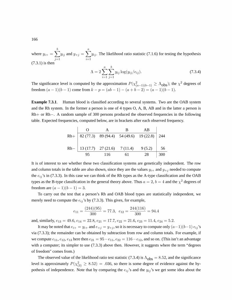
166

where + =X

=1

and + =

X=1

. The likelihood ratio statistic (7.1.6) for testing the hypothesis

(7.3.1) is then

Λ = 2

X=1

X=1

log() (7.3.4)

The significance level is computed by the approximation (2(−1)(−1) ≥ Λobs); the 2 degrees of

freedom (− 1)(− 1) come from − = (− 1)− (+ − 2) = (− 1)(− 1).

Example 7.3.1. Human blood is classified according to several systems. Two are the OAB system

and the Rh system. In the former a person is one of 4 types O, A, B, AB and in the latter a person is

Rh+ or Rh−. A random sample of 300 persons produced the observed frequencies in the following

table. Expected frequencies, computed below, are in brackets after each observed frequency.

O A B AB

Rh+ 82 (77.3) 89 (94.4) 54 (49.6) 19 (22.8) 244

Rh− 13 (17.7) 27 (21.6) 7 (11.4) 9 (5.2) 56

95 116 61 28 300

It is of interest to see whether these two classification systems are genetically independent. The row

and column totals in the table are also shown, since they are the values + and + needed to compute

the ’s in (7.3.3). In this case we can think of the Rh types as the A-type classification and the OAB

types as the B-type classification in the general theory above. Thus = 2, = 4 and the 2 degrees of

freedom are (− 1)(− 1) = 3.To carry out the test that a person’s Rh and OAB blood types are statistically independent, we

merely need to compute the ’s by (7.3.3). This gives, for example,

11 =(244)(95)

300= 773 12 =

244(116)

300= 944

and, similarly, 13 = 496, 14 = 228, 21 = 177, 22 = 216, 23 = 114, 24 = 52.

It may be noted that + = + and + = + , so it is necessary to compute only (−1)(−1) ’svia (7.3.3); the remainder can be obtained by subtraction from row and column totals. For example, if

we compute 11, 12, 13 here then 21 = 95−11, 22 = 116−12, and so on. (This isn’t an advantage

with a computer; its simpler to use (7.3.3) above then. However, it suggests where the term “degrees

of freedom" comes from.)

The observed value of the likelihood ratio test statistic (7.3.4) is Λobs = 852, and the significance

level is approximately (2(3)≥ 852) = 036, so there is some degree of evidence against the hy-

pothesis of independence. Note that by comparing the ’s and the ’s we get some idea about the

167

lack of independence, or relationship, between the two classifications. We see here that the degree of

dependence does not appear large.

Testing Equality of Multinomial Parameters from Two or More Groups

A similar problem arises when individuals in a population can be one of types 1 , but where

the population is sub-divided into groups 1 . In this case, we might be interested in whether

the proportions of individuals of types 1 are the same for each group. This is essentially

the same as the question of independence in the preceding section: we want to know whether the

probability that a person in population group is -type is the same for all = 1 . That is,

= ( |) and we want to know if this deends on or not.

Although the framework is superficially the same as the preceding section, the details are a little

different. In particular, the probabilities satisfy

1 + 2 + · · ·+ = 1 for each = 1 (7.3.5)

and the hypothesis we are interested in testing is

0 : p1 = p2 = · · · = p (7.3.6)

where p = (1 2 ). Furthermore, the data in this case arise by selecting specified num-

bers of individuals from groups = 1 and so there are actually multinomial distributions,

Mult(; 1 ).

If we denote the observed frequency of -type individuals in the sample from the ’th group as (where 1 + · · · + = ), then it can be shown that the likelihood ratio statistic for testing (7.3.6)

is exactly the same as (7.3.4), where now the expected frequencies are given by

=

³+

´ = 1 ; = 1 (7.3.7)

where = 1 + · · · + . Since = + the expected frequencies have exactly the same form as in

the preceding section, when we lay out the data in a two-way table with rows and columns.

Example 7.3.2. The study in Example 7.3.1 could have been conducted differently, by selecting a

fixed number of Rh+ persons and a fixed number of Rh− persons, and then determining their OAB

blood type. Then the proper framework would be to test that the probabilities for the 4 types O, A, B,

AB were the same for Rh+ and for Rh− persons, and so the methods of the present section apply. This

study gives exactly the same testing procedure as one where the numbers of Rh+ and Rh− persons in

the sample are random, as discussed.

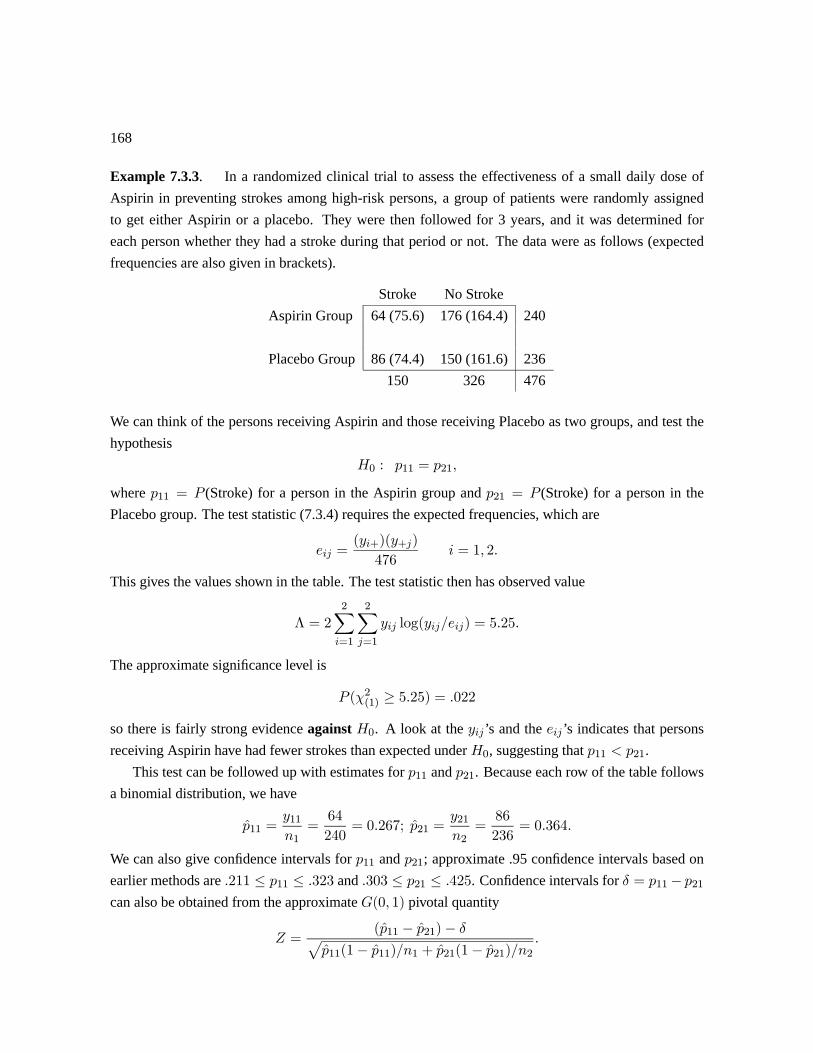
168

Example 7.3.3. In a randomized clinical trial to assess the effectiveness of a small daily dose of

Aspirin in preventing strokes among high-risk persons, a group of patients were randomly assigned

to get either Aspirin or a placebo. They were then followed for 3 years, and it was determined for

each person whether they had a stroke during that period or not. The data were as follows (expected

frequencies are also given in brackets).

Stroke No Stroke

Aspirin Group 64 (75.6) 176 (164.4) 240

Placebo Group 86 (74.4) 150 (161.6) 236

150 326 476

We can think of the persons receiving Aspirin and those receiving Placebo as two groups, and test the

hypothesis

0 : 11 = 21

where 11 = (Stroke) for a person in the Aspirin group and 21 = (Stroke) for a person in the

Placebo group. The test statistic (7.3.4) requires the expected frequencies, which are

=(+)(+)

476 = 1 2

This gives the values shown in the table. The test statistic then has observed value

Λ = 2

2X=1

2X=1

log() = 525

The approximate significance level is

(2(1) ≥ 525) = 022

so there is fairly strong evidence against 0. A look at the ’s and the ’s indicates that persons

receiving Aspirin have had fewer strokes than expected under 0, suggesting that 11 21.

This test can be followed up with estimates for 11 and 21. Because each row of the table follows

a binomial distribution, we have

11 =11

1=64

240= 0267; 21 =

21

2=86

236= 0364

We can also give confidence intervals for 11 and 21; approximate .95 confidence intervals based on

earlier methods are 211 ≤ 11 ≤ 323 and 303 ≤ 21 ≤ 425. Confidence intervals for = 11− 21

can also be obtained from the approximate (0 1) pivotal quantity

=(11 − 21)− p

11(1− 11)1 + 21(1− 21)2

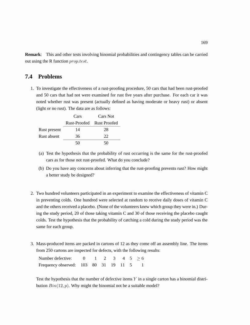
169

Remark: This and other tests involving binomial probabilities and contingency tables can be carried

out using the R function .

7.4 Problems

1. To investigate the effectiveness of a rust-proofing procedure, 50 cars that had been rust-proofed

and 50 cars that had not were examined for rust five years after purchase. For each car it was

noted whether rust was present (actually defined as having moderate or heavy rust) or absent

(light or no rust). The data are as follows:

Cars Cars Not

Rust-Proofed Rust Proofed

Rust present 14 28

Rust absent 36 22

50 50

(a) Test the hypothesis that the probability of rust occurring is the same for the rust-proofed

cars as for those not rust-proofed. What do you conclude?

(b) Do you have any concerns about inferring that the rust-proofing prevents rust? How might

a better study be designed?

2. Two hundred volunteers participated in an experiment to examine the effectiveness of vitamin C

in preventing colds. One hundred were selected at random to receive daily doses of vitamin C

and the others received a placebo. (None of the volunteers knew which group they were in.) Dur-

ing the study period, 20 of those taking vitamin C and 30 of those receiving the placebo caught

colds. Test the hypothesis that the probability of catching a cold during the study period was the

same for each group.

3. Mass-produced items are packed in cartons of 12 as they come off an assembly line. The items

from 250 cartons are inspected for defects, with the following results:

Number defective: 0 1 2 3 4 5 ≥ 6Frequency observed: 103 80 31 19 11 5 1

Test the hypothesis that the number of defective items in a single carton has a binomial distri-

bution (12 ). Why might the binomial not be a suitable model?

170

4. The numbers of service interruptions in a communications system over 200 separate weekdays

is summarized in the following frequency table:

Number of interruptions: 0 1 2 3 4 ≥ 5

Frequency observed: 64 71 42 18 4 1

Test whether a Poisson model for the number of interruptions on a single day is consistent

with these data.

5. The table below records data on 292 litters of mice classified according to litter size and number

of females in the litter.

Number of females

0 1 2 3 4 Total # of litters

1 8 12 20

Litter 2 23 44 13 80

Size 3 10 25 48 13 96

4 5 30 34 22 5 96

(a) For litters of size ( = 1 2 3 4) assume that the number of females in a litter follows

a binomial distribution with parameters and = (female). Test the binomial model

separately for each of the litter sizes = 2 = 3 and = 4. (Why is it of scientific

interest to do this?)

(b) Assuming that the binomial model is appropriate for each litter size, test the hypothesis that

1 = 2 = 3 = 4.

6. A long sequence of digits (0 1 9) produced by a pseudo random number generator was

examined. There were 51 zeros in the sequence, and for each successive pair of zeros, the

number of (non-zero) digits between them was counted. The results were as follows:

1 1 6 8 10 22 12 15 0 0

2 26 1 20 4 2 0 10 4 19

2 3 0 5 2 8 1 6 14 2

2 2 21 4 3 0 0 7 2 4

4 7 16 18 2 13 22 7 3 5

Give an appropriate probability model for the number of digits between two successive zeros,

if the pseudo random number generator is truly producing digits for which (any digit = ) =

1( = 0 1 9), independent of any other digit. Construct a frequency table and test the

171

goodness of fit of your model.

7. 1398 school children with tonsils present were classified according to tonsil size and absence or

presence of the carrier for streptococcus pyogenes. The results were as follows:

Normal Enlarged Much enlarged

Carrier present 19 29 24

Carrier absent 497 560 269

Is there evidence of an association between the two classifications?

8. The following data on heights of 210 married couples were presented by Yule in 1900.

Tall wife Medium wife Short wife

Tall husband 18 28 19

Medium husband 20 51 28

Short husband 12 25 9

Test the hypothesis that the heights of husbands and wives are independent.

9. In the following table, 64 sets of triplets are classified according to the age of their mother at

their birth and their sex distribution:

3 boys 2 boys 2 girls 3 girls Total

Mother under 30 5 8 9 7 29

Mother over 30 6 10 13 6 35

Total 11 18 22 13 64

(a) Is there any evidence of an association between the sex distribution and the age of the

mother?

(b) Suppose that the probability of a male birth is 0.5, and that the sexes of triplets are de-

termined independently. Find the probability that there are boys in a set of triples

( = 0 1 2 3), and test whether the column totals are consistent with this distribution.

10. A study was undertaken to determine whether there is an association between the birth weights

of infants and the smoking habits of their parents. Out of 50 infants of above average weight,

172

9 had parents who both smoked, 6 had mothers who smoked but fathers who did not, 12 had

fathers who smoked but mothers who did not, and 23 had parents of whom neither smoked. The

corresponding results for 50 infants of below average weight were 21, 10, 6, and 13, respectively.

(a) Test whether these results are consistent with the hypothesis that birth weight is independent

of parental smoking habits.

(b) Are these data consistent with the hypothesis that, given the smoking habits of the mother,

the smoking habits of the father are not related to birth weight?

CAUSE AND EFFECT

8.1 Introduction

As mentioned in Chapters 1 and 3, many studies are carried out with causal objectives in mind. That

is, we would like to be able to establish or investigate a possible cause and effect relationship between

variables and .

We use the word “causes" often; for example we might say that “gravity causes dropped objects to

fall to the ground", or that “smoking causes lung cancer". The concept of causation (as in “ causes

") is nevertheless hard to define. One reason is that the “strengths" of causal relationships vary a lot.

For example, on earth gravity may always lead to a dropped object falling to the ground; however, not

everyone who smokes gets lung cancer.

Idealized definitions of causation are often of the following form. Let be a response variate

associated with units in a population or process, and let be an explanatory variate associated with

some factor that may affect . Then, if all other factors that affect are held constant, let us change

(or observe different values of ) and see if changes. If it does we say that has a causal effect

on .

In fact, this definition is not broad enough, because in many settings a change in may only lead

to a change in in some probabilistic sense. For example, giving an individual person at risk of stroke

a small daily dose of aspirin instead of a placebo may not necessarily lower their risk. (Not everyone

is helped by this medication.) However, on average the effect is to lower the risk of stroke. One way

to measure this is by looking at the probability a randomly selected person has a stroke (say within 3

years) if they are given aspirin versus if they are not.

Therefore, a better idealized definition of causation is to say that changing should result in a

change in some attribute of the random variable (for example, its mean or some probability such as

( 0)). Thus we revise the definition above to say:

if all other factors that affect are held constant, let us change (or observe different values

of ) and see if some specified attribute of changes. If it does we say has a causal effect on .

These definitions are unfortunately unusable in most settings since we cannot hold all other factors

173

174

that affect constant; often we don’t even know what all the variables are. However, the definition

serves as a useful ideal for how we should carry out studies in order to show that a causal relationship

exists. What we do is try to design our studies so that alternative (to the variate ) explanations of what

causes changes in attributes of can be ruled out, leaving as the causal agent. This is much easier

to do in experimental studies, where explanatory variables may be controlled, than in observational

studies. The following are brief examples.

Example 8.1.1. Recall Example 6.1.3 concerning the (breaking) strength of a steel bolt and the

diameter of the bolt. It is clear that bolts with larger diameters tend to have higher strength, and it

seems clear on physical and theoretical grounds that increasing the diameter “causes" an increase in

strength. This can be investigated in experimental studies like that in Example 6.1.3, when random

samples of bolts of different diameters are tested, and their strengths determined.

Clearly, the value of does not determine exactly (different bolts with the same diameter don’t

have the same strength), but we can consider attributes such as the average value of . In the experiment

we can hold other factors more or less constant (e.g. the ambient temperature, the way the force is

applied; the metallurgical properties of the bolts) so we feel that the observed larger average values of

for bolts of larger diameter is due to a causal relationship.

Note that even here we have to depart slightly from the idealized definition of cause and effect. In

particular, a bolt cannot have its diameter changed, so that we can see if changes. All we can do

is consider two bolts that are as similar as possible, and are subject to the same explanatory variables

(aside from diameter). This difficulty arises in many experimental studies.

Example 8.1.2. Suppose that data had been collected on 10,000 persons ages 40-80 who had smoked

for at least 20 years, and 10,000 persons in the same age range who had not. There is roughly the

same distribution of ages in the two groups. The (hypothetical) data concerning the numbers with lung

cancer are as follows:

Lung Cancer No Lung Cancer

Smokers 500 9500 (10,000)

Non-Smokers 100 9900 (10,000)

There are many more lung cancer cases among the smokers, but without further information or

assumptions we cannot conclude that a causal relationship (smoking causes lung cancer) exists. Al-

ternative explanations might explain some or all of the observed difference. (This is an observational

study and other possible explanatory variables are not controlled.) For example, family history is an

important factor in many cancers; maybe smoking is also related to family history. Moreover, smoking

175

tends to be connected with other factors such as diet and alcohol consumption; these may explain some

of the effect seen.

The last example exemplifies that association (statistical dependence) between two variables

and does not imply that a causal relationship exists. Suppose for example that we observe a

positive correlation between and ; higher values of tend to go with higher values of in a

unit. Then there are at least three “explanations": (i) causes (meaning has a causative effect on

),(ii) causes , and (iii) some other factor(s) cause both and .

We’ll now consider the question of cause and effect in experimental and observational studies in a

little more detail.

8.2 Experimental Studies

Suppose we want to investigate whether a variate has a causal effect on a response variate . In an

experimental setting we can control the values of that a unit “sees". In addition, we can use one or

both of the following devices for ruling out alternative explanations for any observed changes in that

might be caused by :

(i) Hold other possible explanatory variables fixed.

(ii) Use randomization to control for other variables.

These are mostly simply explained via examples.

Example 8.2.1 Blood thinning and the risk of stroke

Suppose 500 persons that are at high risk of stroke have agreed to take part in a clinical trial to

assess whether aspirin lowers the risk of stroke. These persons are representative of a population of

high risk individuals. The study is conducted by giving some persons aspirin and some a placebo, then

comparing the two groups in terms of the number of strokes observed.

Other factors such as age, sex, weight, existence of high blood pressure, and diet also may affect the

risk of stroke. These variables obviously vary substantially across persons and cannot be held constant

or otherwise controlled. However, such studies use randomization in the following way: among the

study subjects, who gets aspirin and who gets a placebo is determined by a random mechanism. For

example, we might flip a coin (or draw a random number from 0 1), with one outcome (say Heads)

indicating a person is to be given aspirin, and the other indicating they get the placebo.

The effect of this randomization is to balance the other possible explanatory variables in the two

“treatment" groups (Aspirin and Placebo). Thus, if at the end of the study we observe that 20% of

the Placebo subjects have had a stroke but only 9% of the Aspirin subjects have, then we can attribute

176

the difference to the causative effect of the aspirin. Here’s how we rule out alternative explanations:

suppose you claim that its not the aspirin but dietary factors and blood pressure that cause this observed

effect. I respond that the randomization procedure has lead to those factors being balanced in the two

treatment groups. That is, the Aspirin group and the Placebo group both have similar variations in

dietary and blood pressure values across the subjects in the group. Thus, a difference in the two groups

should not be due to these factors.

Example 8.2.2. Driving speed and fuel consumption

(Adapted from Stat 230 Course Notes).

It is thought that fuel consumption in automobiles is greater at speeds in excess of 100 km per hour.

(Some years ago during oil shortages, many U.S. states reduced speed limits on freeways because of

this.) A study is planned that will focus on freeway-type driving, because fuel consumption is also

affected by the amount of stopping and starting in town driving, in addition to other factors.

In this case a decision was made to carry out an experimental study at a special paved track owned

by a car company. Obviously a lot of factors besides speed affect fuel consumption: for example,

the type of car and engine, tire condition, fuel grade and the driver. As a result, these factors were

controlled in the study by balancing them across different driving speeds. An experimental plan of the

following type was employed.

• 84 cars of eight different types were used; each car was used for 8 test drives.

• the cars were each driven twice for 600 km on the track at each of four speeds: 80,100,120 and

140 km/hr.

• 8 drivers were involved, each driving each of the 8 cars for one test, and each driving two tests at

each of the four speeds.

• The cars had similar initial mileages and were carefully checked and serviced so as to make them

as comparable as possible; they used comparable fuels.

• The drivers were instructed to drive steadily for the 600 km. Each was allowed a 30 minute rest

stop after 300 km.

• The order in which each driver did his or her 8 test drives was randomized. The track was large

enough that all 8 drivers could be on it at the same time. (The tests were conducted over 8 days.)

The response variate was the amount of fuel consumed for each test drive. Obviously in the analy-

sis we must deal with the fact that the cars differ in size and engine type, and their fuel consumption

177

will depend on that as well as on driving speed. A simple approach would be to add the fuel amounts

consumed for the 16 test drives at each speed, and to compare them (other methods are also possible).

Then, for example, we might find that the average consumption (across the 8 cars) at 80, 100, 120 and

140 km/hr were 43.0,44.1, 45.8 and 47.2 liters, respectively. Statistical methods of testing and estima-

tion could then be used to test or estimate the differences in average fuel consumption at each of the

four speeds. (Can you think of a way to do this?)

Exercise: Suppose that statistical tests demonstrated a significant difference in consumption across the

four driving speeds, with lower speeds giving lower consumption. What (if any) qualifications would

you have about concluding there is a causal relationship?

8.3 Observational Studies

In observational studies there are often unmeasured factors that affect the response . If these factors

are also related to the explanatory variable whose (potential) causal effect we are trying to assess,

then we cannot easily make any inferences about causation. For this reason, we try in observational

studies to measure other important factors besides .

For example, Problem 1 at the end of Chapter 7 discusses an observational study on whether rust-

proofing prevents rust. It is clear that an unmeasured factor is the care a car owner takes in looking

after a vehicle; this could quite likely be related to whether a person opts to have their car rust-proofed.

The following example shows how we must take note of measured factors that affect .

Example 8.3.1 Suppose that over a five year period, the applications and admissions to graduate studies

in Engineering and Arts faculties in a university are as follows:

No. Applied No. Admitted % Admitted

Engineering 1000 600 60% Men

200 150 75% Women

Arts 1000 400 40% Men

1800 800 44% Women

Total 2000 1000 50% Men

2000 950 47.5% Women

We want to see if females have a lower probability of admission than males. If we looked only

at the totals for Engineering plus Arts, then it would appear that the probability a male applicant is

admitted is a little higher than the probability for a female applicant. However, if we look separately at

178

Arts and Engineering, we see the probability for females being admitted appears higher in each case!

The reason for the reverse direction in the totals is that Engineering has a higher admission rate than

Arts, but the fraction of women applying to Engineering is much lower than for Arts.

In cause and effect language, we would say that the faculty one applies to (i.e. Engineering or Arts)

is a causative factor with respect to probability of admission. Furthermore, it is related to the gender

(M or F) of an applicant, so we cannot ignore it in trying to see if gender is also a causative factor.

Remark: The feature illustrated in the example above is sometimes called Simpson’s Paradox. In

probabilistic terms, it says that for events 1 2 and 1 , we can have

(|1) (|2) for each = 1

but have

(|1) (|2)

(Note that (|1) =P=1

(|1) (|1) and similarly for (|2), so they depend on what

(|1) and (|2) are.) In the example above we can take 1 = person is female, 2 =person is male, 1 = person applies to Engineering, 2 = person applies to Arts, and =

person is admitted.Exercise: Write down estimated probabilities for the various events based on Example 8.3.1, and so

illustrate Simpson’s paradox.

Epidemiologists (specialists in the study of disease) have developed guidelines or criteria which

should be met in order to argue that a causal association exists between a risk factor and a disease

(represented by a response variable = (person has the disease), for example). These include

• the need to account for other possible risk factors and to demonstrate that and are consistently

related when these factors vary.

• the demonstration that association between and holds in different types of settings

• the existence of a plausible scientific explanation

Similar criteria apply to other areas.

8.4 Problems

1. In an Ontario study, 50267 live births were classified according to the baby’s weight (less than or

greater than 2.5 kg.) and according to the mother’s smoking habits (non-smoker, 1-20 cigarettes

per day, or more than 20 cigarettes per day). The results were as follows:

179

No. of cigarettes 0 1-20 20

Weight ≤ 25 1322 1186 793

Weight 2.5 27036 14142 5788

(a) Test the hypothesis that birth weight is independent of the mother’s smoking habits.

(b) Explain why it is that these results do not prove that birth weights would increase if mothers

stopped smoking during pregnancy. How should a study to obtain such proof be designed?

(c) A similar, though weaker, association exists between birth weight and the amount smoked

by the father. Explain why this is to be expected even if the father’s smoking habits are

irrelevant.

2. One hundred and fifty Statistics students took part in a study to evaluate computer-assisted in-

struction (CAI). Seventy-five received the standard lecture course while the other 75 received

some CAI. All 150 students then wrote the same examination. Fifteen students in the standard

course and 29 of those in the CAI group received a mark over 80%.

(a) Are these results consistent with the hypothesis that the probability of achieving a mark

over 80% is the same for both groups?

(b) Based on these results, the instructor concluded that CAI increases the chances of a mark

over 80%. How should the study have been carried out in order for this conclusion to be

valid?

3. (a) The following data were collected some years ago in a study of possible sex bias in graduate

admissions at a large university:

Admitted Not admitted

Male applicants 3738 4704

Female applicants 1494 2827

Test the hypothesis that admission status is independent of sex. Do these data indicate a

lower admission rate for females?

(b) The following table shows the numbers of male and female applicants and the percentages

admitted for the six largest graduate programs in (a):

180

Men Women

Program Applicants % Admitted Applicants % Admitted

A 825 62 108 82

B 560 63 25 68

C 325 37 593 34

D 417 33 375 35

E 191 28 393 24

F 373 6 341 7

Test the independence of admission status and sex for each program. Do any of the pro-

grams show evidence of a bias against female applicants?

(c) Why is it that the totals in (a) seem to indicate a bias against women, but the results for

individual programs in (b) do not?

4. To assess the (presumed) beneficial effects of rust-proofing cars, a manufacturer randomly se-

lected 200 cars that were sold 5 years earlier and were still used by the original buyers. One

hundred cars were selected from purchases where the rust-proofing option package was included,

and one hundred from purchases where it was not (and where the buyer did not subsequently get

the car rust-proofed by a third party).

The amount of rust on the vehicles was measured on a scale in which the responses are assumed

roughly Gaussian, as follows:

1. Rust-proofed cars: ∼ (1 )

2. Non-rust-proofed cars: ∼ (2 )

Sample means and variances from the two sets of cars were found to be (higher means

more rust)

1. 1 = 11.7 1 = 2.1

2. 2 = 12.0 2 = 2.4

(a) Test the hypothesis that there is no difference in 1 and 2.

(b) The manufacturer was surprised to find that the data did not show a beneficial effect of

rust-proofing. Describe problems with their study and outline how you might carry out a

study designed to demonstrate a causal effect of rust-proofing.

181

5. In randomized clinical trials that compare two (or more) medical treatments it is customary not to

let either the subject or their physician know which treatment they have been randomly assigned.

(These are referred to as double blind studies.)

Discuss why not doing this might not be a good idea in a causative study (i.e. a study where you

want to assess the causative effect of one or more treatments).

6. Public health researchers want to study whether specifically designed educational programs about

the effects of cigarette smoking have the effect of discouraging people from smoking. One

particular program is delivered to students in grade 9, with followup in grade 11 to determine each

student’ s smoking “history". Briefly discuss some factors you’d want to consider in designing

such a study, and how you might address them.

References and Supplementary

Resources

R.J. Mackay and R.W. Oldford (2001). Statistics 231: Empirical Problem Solving (Stat 231 Course

Notes)

C.J. Wild and G.A.F. Seber (1999). Chance Encounters: A First Course in Data Analysis and Infer-

ence. John Wiley and Sons, New York.

J. Utts (2003). What Educated Citizens Should Know About Statistics and Probability. American

Statistician 57,74-79

182

Statistical Tables

183

APPENDIX. ANSWERS TO SELECTED

PROBLEMS

Chapter 1

1. (b) .032 (c) .003 (.002 using Gaussian approx.)

2. (c) 1 = 489, 2 = 325, 3 = 151, 4 = 035

3. (b) .003 and .133 (d) 0 = 1243

4. (a) .933 (b) .020 (c).949 and .117 (d) 4.56

5. (a) .9745

7. (a) () = 1 + 2(− 1)(1− )

(b) () = 2(− 1)(1− )[1− 2(1− )] + 2(− 2)(1− )(1− 2)2

(c) () = 505, () = 2475 and ( ≤ 20) 10−6

Chapter 2

1. (a) 4.1 (b) .000275

2. (a) .10 (b) = 140

3. (21 + 2)

4. (b) .28

6. (a) (0+3 )−[(0+3 )2−8 2]124

where =P

(b) = (1− )2

(c) = 195; ( = 0) = 758

184

185

(d) = 5

7. =P

P

9. (a) = 35 = 42

(b) 14.7, 20.3, 27.3 and 37.7

Chapter 4

1. (a) = 1744, = 0664(M) = 1618, = 0636 (F)

(b) 1.659 and 1.829 (M) 1.536 and 1.670 (F)

(c) .098 (M) and .0004 (F)

(d) 11/50=.073 (M) 0(F)

2. (c) 0.1414 and 0.1768, respectively

3. (b) = 1024

7. (b) = 1− ()1 (c) = 0116; interval approximately (.0056,.0207)

8. (a) 0 ≤ ≤ 548 (b) .10 likelihood interval is now 209 ≤ ≤ 490

10. (a) = 3P

(b) = 06024; 0450 ≤ ≤ 0785

(c) 95 CI for is (.0463,.0768) and for is 39.1 ≤ ≤ 648(d) CI’s are 408 ≤ ≤ 738 (using model) and 287 ≤ ≤ 794 (using binomial). The

binomial model involves fewer assumptions but gives a less precise (wider) interval.

(Note: the 1st CI can be obtained directly from the CI for in part (c).)

12. (a) = 380 days; CI is 2855 ≤ ≤ 5213(b) 1979 ≤ ≤ 3613

13. (b) 2883 ≤ ≤ 5279

14. (a) 637 ≤ ≤ 764

Chapter 5

1. = ( ≥ 15) = ( ≥ 25; = 10) = 000047

186

4. (a) statistic gives Λ0 = 0885 and = 76.

5. (a) Λ0 = 23605 and = 005

(b) = 1− 9956 = 03 now

6. Λ0 = 042 and = 84. There is no evidence against the model.

9. (c) statistic gives Λ0 = 373 and = (2(4)≥ 373) = 44. There is no evidence that

the rates are not equal.

Chapter 6

3. (a) 4328 ≤ ≤ 4553 (b) 182 ≤ ≤ 350

4. (a) 0 = 92022 = 12 and = 2 (2(9)≤ 12) = 0024 so there is strong evidence

against : = 02

(b) No: testing : = 1375 gives 001

(c) 13690 ≤ ≤ 13700 and 0050 ≤ ≤ 0132

5. (a) 29691 ≤ ≤ 30347; 455 ≤ ≤ 953(b) 2867 ≤ ≤ 3137

7. 75 ≤ ≤ 1125 where = 1 − 2

8. (a) 064 ≤ 1 − 2 ≤ 724(b) = 05 (c) = 07

9. (a) test gives = 4

(b) −011 ≤ 1 − 2 ≤ 557

12. (a) −023 ≤ ≤ 238 (b) −877 ≤ ≤ 1092

18. (a) = 09935, = −00866, = 02694. Confidence intervals are 0978 ≤ ≤ 1009 and

0182 ≤ ≤ 0516

19. (b) = 02087, = −1022, = 008389

(c) 95 prediction interval for (log ) is 3030 ≤ ≤ 3065 so for is 2070 ≤ ≤2143

Chapter 7

187

1. (a) statistic gives Λ0 = 817 and Pearson statistic 0 = 805. The is about .004 in

each case so there is strong evidence against .

2. statistic gives Λ0 = 570 and Pearson statistic 0 = 564. The is about .017 in each

case.

5. (a) statistics for = 2 3 4 are 1.11, 4.22, 1.36. The ’s are (2(1)≥ 111) = 29,

(2(2)≥ 422) = 12 and (2

(3)≥ 136) = 71, respectively.

(b) statistic is 7.54 and = (2(3)≥ 754) = 057

7. The statistic is 7.32 and = (2(2)≥ 732) = 026 so there is evidence against indepen-

dence and in favour of an association.

8. statistic is 3.13 and = (2(4)≥ 313) = 54. There is no evidence against indepen-

dence.

9. (a) statistic gives Λ0 = 057 and = (2(3)≥ 57) = 90 so there is no evidence of

association.

(b) statistic gives Λ0 = 544 and = (2(3)≥ 544) = 14 There is no evidence

against the binomial model.

10. (a) Λ0 = 108 and = (2(3)≥ 108) = 013

Chapter 8

1. (a) statistic is 480.65 so is almost zero; there is very strong evidence against indepen-

dence.

3. (a) statistic gives Λ0 = 112 and = 0

(b) Only Program shows any evidence of non-independence, and that is in the direction of a

lower admission rate for males.

A Short Review of Probability

188

STATISTICS 231 COURSE NOTES - University of Waterloopkates/LT3/jsdemos/... · STATISTICS 231 COURSE NOTES Original notes by Jerry Lawless Winter 2013 Edition. Contents ... holder

Documents