Statistical unit root test for edge detection in ultrasound images of vessels and cysts

Statistical unit root test for edgedetection in ultrasound images of vesselsand cysts

Mehdi MoradiS. Sara MahdaviJulian GuerreroRobert RohlingSeptimiu E. Salcudean

Statistical unit root test for edge detection inultrasound images of vessels and cysts

Mehdi MoradiS. Sara MahdaviJulian GuerreroRobert Rohling

Septimiu E. SalcudeanUniversity of British Columbia

Department of Electrical and Computer EngineeringVancouver V6T 1Z4, CanadaE-mail: [email protected]

Abstract. A new approach is proposed for edge detection in ultra-sound. The technique examines the image intensity profile for unitroots based on the Dickey–Fuller statistical test of stationarity. Theexistence of the unit root is a sign of nonstationarity and a possibleedge. A simple algorithm to build a segmentation method based onthis edge detection approach is also proposed, which is capable ofdelineating the perimeter of hollow structures such as blood vesselsand cysts. In this approach, the radial edge profiles originating fromthe center of the object of interest are scanned for the change fromstationary to nonstationary status. The algorithm treats the radialintensity profiles as a time series and uses the Dickey–Fuller statis-tical test along the radii to find the location at which the profilebecomes nonstationary. A priori criteria for edge continuity, shape,and size of the object of interest are applied to enhance the stabilityof the algorithm. The accuracy is demonstrated on simulated ultra-sound. Further, the method is examined on two different imagesets of blood vessels and validated based on contours marked byexperts. The worst case distance from expert contours is 1.8�0.3 mm. The average area difference between the expert and theextracted contours is∼6% and∼4% of the vessel area in the two data-sets. The proposed segmentation method is also compared to seg-mentation using active contours on ultrasound images of breastand ovarian cysts and shown to be accurate and stable. © 2013SPIE and IS&T [DOI: 10.1117/1.JEI.22.3.033013]

1 IntroductionUltrasound provides a noninvasive, inexpensive, and nonio-nizing medical imaging modality, suitable for a vast rangeof applications from diagnostic examinations to computer-assisted interventions.1 Accurate and reliable segmentationof ultrasound images is a critical step in many applications.Examples include volume study of cancerous tumors, detec-tion of cardiovascular complications such as thrombosis,characterization and grading of cysts and tumors, and plan-ning of radiotherapy procedures such as brachytherapy.Therefore, researchers have worked on various segmentationapproaches, including texture operators,2 spectral cluster-ing,3 active contours,4,5 a combination of intensity, texture,

and domain knowledge,6 statistical shape models,7 andgradient-based edge detection by Kalman filtering,8 to seg-ment ultrasound images. There is also a wide range of stat-istical approaches to ultrasound image segmentation basedon the assumption that image pixels are uncorrelated9,10,11

or partly correlated.12 See Refs. 1 and 13 for detailed surveys.Edge detection is an important component of many seg-

mentation techniques. Certain properties of ultrasoundimages pose challenges for edge detection algorithms. Inaddition to occasional shadowing and the dependence ofedge strength on the relative orientation of the beam to thereflector, ultrasound images contain speckle that is a result ofthe interactions of the coherent high-frequency mechanicalwaves with small scatterers. Gradient-based edge detectorsuse derivative operators such as the Prewitt and Sobel andthreshold the local maxima of the image gradient.14,15 Inthe case of ultrasound, these operators produce numerouslocal edges caused by the speckle pattern when used at asmall scale and incomplete detection when used at a largerscale. Other solutions have been sought by investigators toaddress edge detection specifically in ultrasound images.16–22

Despite success in some applications, issues of accuracy,sensitivity, and computational speed remain open problems.

Some of our previous research efforts were dedicated tousing a priori shapes to improve ultrasound segmenta-tion.23,24 For example, an elliptical model is assumed forthe object, gradient-based candidate edge points areextracted along radii originating from a point at the centerof the object, and the estimate is recursively improvedusing a modified Kalman filter. A significant improvementto such segmentation approaches can be achieved by remov-ing the need for derivative-based edge filters. The proposedapproach in the current work is a step in that direction basedon a statistical test of stationarity.

The statistical properties of regions of ultrasound imagesare known to change depending on tissue type. For example,the interior of vessels has different properties than the lumenand the surrounding tissue. These properties vary with cellsize and organization.25 The change in the statistical proper-ties of the image intensity at the boundaries of an organ indi-cates that statistical methods can be used for edge detection.To characterize this change, we rely on the Dickey–Fuller

Paper 13103 received Mar. 1, 2013; revised manuscript received Jul. 8,2013; accepted for publication Jul. 11, 2013; published online Aug. 19,2013.

0091-3286/2013/$25.00 © 2013 SPIE and IS&T

Journal of Electronic Imaging 033013-1 Jul–Sep 2013/Vol. 22(3)

Journal of Electronic Imaging 22(3), 033013 (Jul–Sep 2013)

(DF) test.26 The DF test, a very popular tool in econometrictime-series studies, examines the null hypothesis of nonsta-tionarity, which is equivalent to the existence of a unit root,against the hypothesis of stationarity for autoregressive (AR)processes. The change in the properties of the intensity pro-file from stationary to nonstationary can be due to the pas-sage of the profile through an edge. The main advantage ofthis method of edge detection is its robustness to speckle-induced local artifacts, which we illustrate on simulatedphantoms.

To illustrate the practical utility of the method, we developa simple segmentation method that takes advantage of thisedge detector. We use a manually selected central pointwithin the object of interest and search for the edge candi-dates in a range of distances from this seed point based onthe DF edge detector. The edge point is determined as thepixel along the radius where the incremental edge profile“becomes” and “stays” nonstationary when further pixelsare added. The radial intensity profiles are treated as timeseries and the DF statistical test is used along the radii tofind the location at which the profile becomes nonstationary.This algorithm is stabilized by limiting the search range andthe maximum possible deviation of the edge distance fromthe seed between two adjacent rays. It should be emphasizedthat this specific approach to segmentation is an exampleapplication of the proposed edge detection method that isparticularly suitable for vessels and cysts.

We report the results of several experiments as test appli-cations for the developed segmentation approach. Theseinclude a clinical study in which we compare the resultsof our segmentation with the expert segmentations acquiredon human vessel images. Preliminary results on limited datawere previously reported in a conference presentation.27 Theclinical motivation behind this work is that deep venousthrombosis (DVT) and atherosclerosis are diagnosed usingsegmented features in ultrasound images. In DVT, bloodclots or thrombi are formed within the lower body deepveins. These thrombi may occlude venous flow or breakoff from the vessel wall and cause a possibly fatal pulmonaryembolism. The diagnosis of this is through compressionultrasound examinations. In this test, the examiner appliesgentle ultrasound transducer pressure while imaging aregion. The imaged vein collapses unless there is a thrombusinside. Since early thrombi, which is the target of the com-pression test, and blood have similar echogenicity, it is oftennot possible to identify a thrombus from a single image.Therefore, several acquisitions and contouring in differentcompression levels are necessary. It has been shown thatautomatic image segmentation can help in standardizationof the ultrasound examination for DVT diagnosis.23

Also carotid artery ultrasound examinations can beimproved by automatic segmentation.8,28,29,30 Occlusive dis-ease, such as atherosclerosis in the left and right commoncarotid arteries, is a major cause of stroke.

Furthermore, we report segmentation of ovarian andbreast cysts. Lesion segmentation is a step in computer-aided diagnosis schemes targeting breast and ovariancancer.6,31 Region-based segmentation methods, such asSnake deformation,32 region growing,33,34 split-and-merge,35

and morphological watershed transformation36 have beenwidely explored for segmenting breast ultrasound images.We provide a comparison of our proposed method with an

active contour algorithm on these breast and ovarian cystimages to show that the proposed edge detection algorithmprovides accurate results.

In this paper, Sec. 2 discusses the basics of the statisticaltest used for edge detection and the resulting segmentationalgorithm, and also describes the data and methods used forvalidation. Section 3 provides the results of the validationtests on phantom and vessel images. Section 4 providesour discussions on parameters of the method and comparisonof its performance with active contours on a set of ovarianand breast cyst images. Section 5 gives the conclusions andrecommendations for future work.

2 Methods

2.1 DF Statistical TestOur methodology is designed to find the edges by scanningthe image in search for stable changes in the statistics of pixelintensities. In general, ultrasound images exhibit significantspatial correlation due to the large point spread function ofthe imaging system. In the literature, authors have appliedvarious mathematical models for the intensity distributionof homogeneous tissues in a ultrasound image, most notablyRayleigh distribution. Nevertheless, for the purpose of seg-menting vessels and cysts and other objects with a relativelyhypoechoic interior, high orders of correlation are insignifi-cant. In fact, we used the partial autocorrelation function(PACF)37 of the image intensity profiles to show that thelag value h ¼ 1 is sufficient for describing the dependencieswithin the hypoechoic interior of these hollow objects (seethe first paragraph in Sec. 3). Therefore, we describe the pro-posed statistical test for time series that can be modeled witha first-order AR [AR(1)] model. The augmented version ofthe DF test, described in Refs. 38 and 39, can be used formore complicated models for which the AR(1) assumptionis not valid.

An AR(1) time series, I, can be modeled as

I½t� ¼ ρI½t − 1� þ e½t�; (1)

where ρ is a real number and e is a sequence of independentnormal variables with mean 0 and variance σ2. I is stationaryif jρj < 1. If a unit root exists (jρj ¼ 1), then the variance of Iis tσ2, and therefore I is nonstationary. In many economicsapplications, the existence of the unit root, which is an indi-cation of a “shock” in the trend-stationary time series, isimportant for modeling and forecasting the future observa-tions. Dickey and Fuller26 provided a statistical method totest an AR model for the null hypothesis of the existenceof a unit root. Note that one can write

ΔI½t� ¼ I½t� − I½t − 1� ¼ ðρ − 1ÞI½t − 1� þ e½t�¼ γI½t − 1� þ e½t�; (2)

where γ ¼ ρ − 1. The DF test is formulated for γ as follows:

H0∶ γ ¼ 0; (3)

H1∶ γ < 0: (4)

Dickey and Fuller provide a nonstandard statistic τ, whichdepends on the number of observations, and provide tables ofcritical values for it. In other words, based on the calculated

Journal of Electronic Imaging 033013-2 Jul–Sep 2013/Vol. 22(3)

Moradi et al.: Statistical unit root test for edge detection in ultrasound images of vessels and cysts

value of τ, they provide the significance level at which thenull hypothesis above can be rejected. The implementationof the test involves estimating the value of γ. If the estimatedvalue is γ̂, the DF test statistic is26

τ ¼ γ̂ − 1

SEðγ̂Þ ; (5)

where SE is standard error (which is standard deviation di-vided by the square root of number of samples). The nullhypothesis is rejected when the test statistic is a large neg-ative number. Numerically, one needs to calculate the valueof the test statistic, τ, refer to the DF table, and determine thesignificance level at which nonstationarity can be rejected.For example, the 5% critical value is −1.65.

We have implemented the test in MATLAB. The ordinaryleast squares estimation of the AR(1) parameters is per-formed using MATLAB Statistics Toolbox. The DF statisticand the tables are imported from the implementation reportedin Ref. 40, which is publicly available through the MATLABCentral code exchange website.

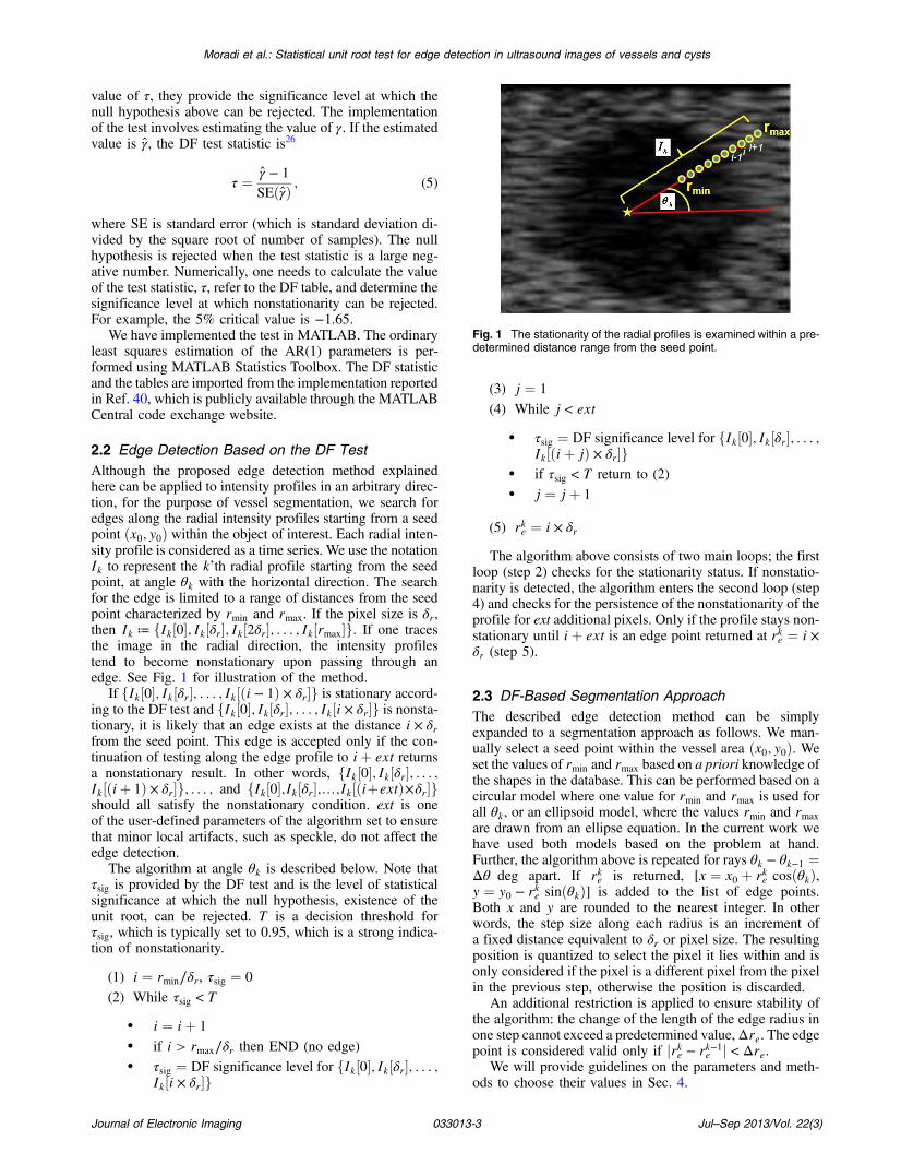
2.2 Edge Detection Based on the DF TestAlthough the proposed edge detection method explainedhere can be applied to intensity profiles in an arbitrary direc-tion, for the purpose of vessel segmentation, we search foredges along the radial intensity profiles starting from a seedpoint ðx0; y0Þ within the object of interest. Each radial inten-sity profile is considered as a time series. We use the notationIk to represent the k’th radial profile starting from the seedpoint, at angle θk with the horizontal direction. The searchfor the edge is limited to a range of distances from the seedpoint characterized by rmin and rmax. If the pixel size is δr,then Ik ≔ fIk½0�; Ik½δr�; Ik½2δr�; : : : ; Ik½rmax�g. If one tracesthe image in the radial direction, the intensity profilestend to become nonstationary upon passing through anedge. See Fig. 1 for illustration of the method.

If fIk½0�; Ik½δr�; : : : ; Ik½ði − 1Þ × δr�g is stationary accord-ing to the DF test and fIk½0�; Ik½δr�; : : : ; Ik½i × δr�g is nonsta-tionary, it is likely that an edge exists at the distance i × δrfrom the seed point. This edge is accepted only if the con-tinuation of testing along the edge profile to iþ ext returnsa nonstationary result. In other words, fIk½0�; Ik½δr�; : : : ;Ik½ðiþ 1Þ × δr�g; : : : ; and fIk½0�;Ik½δr�;:::;Ik½ðiþextÞ×δr�gshould all satisfy the nonstationary condition. ext is oneof the user-defined parameters of the algorithm set to ensurethat minor local artifacts, such as speckle, do not affect theedge detection.

The algorithm at angle θk is described below. Note thatτsig is provided by the DF test and is the level of statisticalsignificance at which the null hypothesis, existence of theunit root, can be rejected. T is a decision threshold forτsig, which is typically set to 0.95, which is a strong indica-tion of nonstationarity.

(1) i ¼ rmin∕δr, τsig ¼ 0

(2) While τsig < T

• i ¼ iþ 1

• if i > rmax∕δr then END (no edge)• τsig ¼ DF significance level for fIk½0�; Ik½δr�; : : : ;

Ik½i × δr�g

(3) j ¼ 1

(4) While j < ext

• τsig ¼ DF significance level for fIk½0�; Ik½δr�; : : : ;Ik½ðiþ jÞ × δr�g

• if τsig < T return to (2)• j ¼ jþ 1

(5) rke ¼ i × δr

The algorithm above consists of two main loops; the firstloop (step 2) checks for the stationarity status. If nonstatio-narity is detected, the algorithm enters the second loop (step4) and checks for the persistence of the nonstationarity of theprofile for ext additional pixels. Only if the profile stays non-stationary until iþ ext is an edge point returned at rke ¼ i ×δr (step 5).

2.3 DF-Based Segmentation ApproachThe described edge detection method can be simplyexpanded to a segmentation approach as follows. We man-ually select a seed point within the vessel area ðx0; y0Þ. Weset the values of rmin and rmax based on a priori knowledge ofthe shapes in the database. This can be performed based on acircular model where one value for rmin and rmax is used forall θk, or an ellipsoid model, where the values rmin and rmax

are drawn from an ellipse equation. In the current work wehave used both models based on the problem at hand.Further, the algorithm above is repeated for rays θk − θk−1 ¼Δθ deg apart. If rke is returned, [x ¼ x0 þ rke cosðθkÞ,y ¼ y0 − rke sinðθkÞ] is added to the list of edge points.Both x and y are rounded to the nearest integer. In otherwords, the step size along each radius is an increment ofa fixed distance equivalent to δr or pixel size. The resultingposition is quantized to select the pixel it lies within and isonly considered if the pixel is a different pixel from the pixelin the previous step, otherwise the position is discarded.

An additional restriction is applied to ensure stability ofthe algorithm: the change of the length of the edge radius inone step cannot exceed a predetermined value,Δre. The edgepoint is considered valid only if jrke − rk−1e j < Δre.

We will provide guidelines on the parameters and meth-ods to choose their values in Sec. 4.

Fig. 1 The stationarity of the radial profiles is examined within a pre-determined distance range from the seed point.

Journal of Electronic Imaging 033013-3 Jul–Sep 2013/Vol. 22(3)

Moradi et al.: Statistical unit root test for edge detection in ultrasound images of vessels and cysts

2.4 Data and Evaluation Methods2.4.1 Field II simulations

Three sets of computer-generated phantoms were generated,using Field II (Ref. 41), to examine different aspects of theproposed methods. In all three sets, simulations were gener-ated using 3.5 MHz as the center frequency. The speed ofsound was set to 1540 m∕s, and data were compressed toshow 60 dB of dynamic range.

Circular vessel simulations. The edge detection perfor-mance of the proposed method was first examined usingthe simulated ultrasound images of circular inclusionswith different contrast levels against the background. Asimulated phantom (2.5 cm width, 1 cm depth, 6 cm height)was created using the Field II simulator. This phantom con-sisted of 25,000 uniformly distributed scatterers andincluded three enclosures with different acoustic propertiesfrom the background. The amplitude of the scatterers had aGaussian distribution with mean of zero and standard devia-tions of 0.3, 0.2, and 0.05 inside the circular enclosures and0.5 in the background. Sixty-four active elements and 50lines per image were used. The phantom and the template

used to produce it are illustrated in Fig. 2. The B-modeimage size was 270 × 845 and the radius of the circular inclu-sion templates was equivalent to 98 pixels (10 mm) in theresulting B-mode image.

Ellipse vessel simulations. Depending on the amountof pressure applied during the DVT compression test, thevein could collapse and appear as an ellipse. Therefore,we used a set of elliptical phantom simulations to examinethe performance of the method for noncircular contours. The

vessel contour has an eccentricity value, e ¼ffiffiffiffiffiffiffiffiffiffiffiffi1 − b2

a2

q, where

a and b are the lengths of the major and the minor radii of theellipse. For the uncompressed vessel, e is close to 0 and for aheavily compressed vein e is close to 1. Four different ellip-ses with e ¼ ½0.0; 0.745; 0.866; 0.943� were used. Simulatedimages were of size 3 × 4 cm2 or 320 × 440 pixels. For tis-sue, 80,000 scatterers were randomly generated, and theiramplitudes were randomly set with a normal distribution,with mean 0 and standard deviation of 1. The scatterer den-sity within the interior of the vessels was set to 5% of thebackground.

Artifact simulations. The ability of the segmentationmethod to reject edge-like artifacts depends, to a large extent,on the parameter ext. To test this, we also created Field IIphantoms with an edge-like artifact included in them.The area within the artifact had a similar scatterer densityto the background (1700 scatterers per cm3); however theamplitude of the scatterers had a Gaussian distribution withstandard deviation of 0.31 for the background and 0.71 forthe artifact. Four phantoms were created with artifact thick-nesses of 1%, 2%, 3%, and 4% of the entire height of theimage. Figure 3 illustrates the templates and the resultingField II simulations for this set of phantoms. These phantomsare used in our analysis of the effect of parameter extin Sec. 4.

2.4.2 Human vessel data

For validation, the performance of the method was evaluatedon the human saphenous vein and artery images. Two setsof data were used for this purpose. Note that all these

Fig. 2 Field II simulated circular inclusion phantom with the originaltemplate. Note that the direction of ultrasound propagation matchedthe horizontal direction of this figure.

Fig. 3 Artifact phantoms along with their templates.

Journal of Electronic Imaging 033013-4 Jul–Sep 2013/Vol. 22(3)

Moradi et al.: Statistical unit root test for edge detection in ultrasound images of vessels and cysts

images were obtained during clinical practice, not healthyvolunteers.

Image set 1. The first set of images were used for exten-sive comparison with expert segmentations. Six differentvessels were segmented in three different ultrasound images:one image with the jugular vein and the common carotidartery (560 × 472 pixels) and two images depicting thesaphenous vein and artery (720 × 480 pixels). Three experts[one radiologist (Savvas Nicolaou) and two sonographers(Vicki Lessoway and Maureen Kennedy)] and an experi-enced graduate student segmented all images by tracingthe contour using an image editing application. Two ofthe experts (V.L. and M.K.) segmented all images twice,resulting in six expert tracings per image.

Image set 2. Three sets of 10 images each were collectedalong the length of the common femoral vein of threepatients without applying compression. The vessels withinthese 30 images were manually segmented by an expert inultrasound imaging who was trained for this purpose by aphysician. The segmentation was carried out by selectingpoints along the radial profiles used in our proposedapproach.

2.4.3 Evaluation measures

The resulting contours were compared to the reference con-tours for evaluation. The reference contour in the case ofphantom data was the original Field II template. For patientimage set 1, the average of the six available expert contourswas used as the reference. For patient image set 2, the avail-able manual segmentation was used as the reference.

To compare the automatic and reference contours, twoquantitative measures were used: the difference betweenthe area of the automatic contour and the reference contour,and the Hausdorff distance42 between the automatic andreference contour. It should be noted that the Hausdorff dis-tance is a very conservative measure that captures the worstperformance of the algorithm and results in high error valuesdue to outliers. In many applications, such outliers can bemodified with minimal user interaction. A less sensitive mea-sure is the absolute area difference between the two contours,which we also report.

3 ResultsIn order to determine if the radial intensity profiles can bemodeled as AR(1) processes, we analyzed the PACF ofthe intensity profiles extracted from human vessel images.In the worst case image within both image sets, for 81%of the intensity profiles extracted from the vessel image,

the PACF function only had significant values at lag h ¼ 1,confirming the AR(1) assumption (p < 0.05). On average,when all intensity profiles from all images were considered,the AR(1) assumption was satisfied in 91% of the profiles.Therefore, the nonaugmented DF test could be used asdescribed to determine the existence of a unit root in theintensity profiles. In our current implementation, we havedevised a solution for the problem of local artifacts alongrays that violate the AR(1) condition for that ray. Thesolution involves starting the segmentation from nine differ-ent seeds, automatically generated around the manuallyselected seed point, and averaging the resulting ninecontours.

3.1 Segmentation of Circular PhantomsThe segmentation of the circular phantoms described inFig. 2 is presented in Fig. 4. The parameters used in themethod were rmin ¼ 7 mm, rmax ¼ 13 mm, ext ¼ 1 mm,Δre ¼ 1.5 mm, Δθ ¼ 5 deg. One seed pixel within thecircle was manually selected and was used along witheight immediate neighbors to get the nine contours. Theresults presented in Fig. 4 are the average of nine contours.It should be noted that due to the random placement ofthe scatterers in the templates, and also due to the beamthickness modeled in Field II, the resulting simulationsare not perfect circles as opposed to the original templates.Nevertheless, besides the visual analysis of the results, onecan consider the similarity of the detected contour withthe reference template as a measure of success. For thethree inclusions, the average Hausdorff distance between theautomatic contour and the reference contour is 0.5� 0.3 mm(an average of 5% of the radius of the template). The areadifference is on average 2.1� 0.6% of the area of the refer-ence. This area difference includes the quantization error incomputation of the area enclosed in the automatic contour.

3.2 Ellipse PhantomsThe segmentation results for the ellipse simulations aredepicted in Fig. 5. For this segmentation experiment, rmin

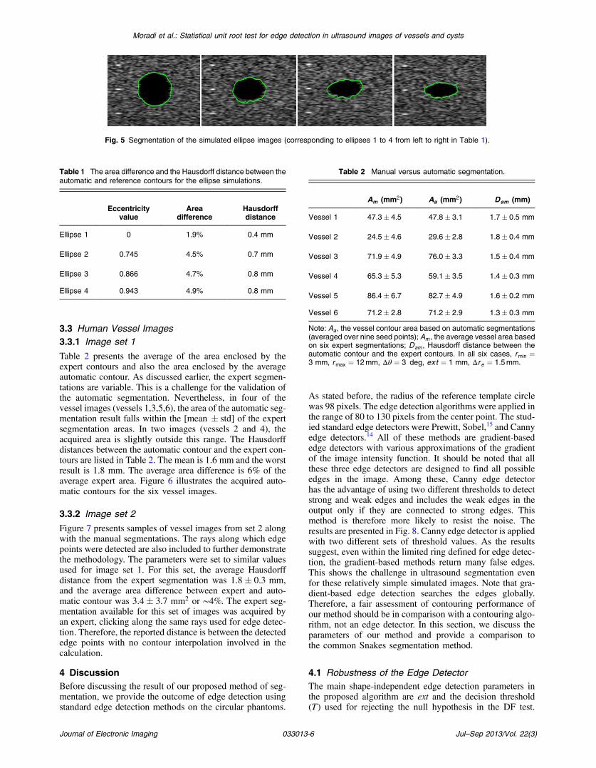
and rmax were extracted from the radius of the templateellipse at the corresponding angle. Specifically, rminðθÞ ¼rellipseðθÞ − 3 and rmaxðθÞ ¼ rellipseðθÞ þ 3 (units in mm).Other parameters were ext ¼ 1 mm, Δre ¼ 1.5 mm,Δθ ¼ 3 deg. Note that for the ellipse shapes, a smallerangle step size Δθ was used. Large values of Δθ resultedin undue smoothing of the shape in the sharp ends of thethinnest ellipse. The area difference and Hausdorff distancefor the four phantoms are presented in Table 1. The averagearea difference for ellipses with e > 0 is 4.7% and the aver-age Hausdorff distance is 0.8 mm.

Fig. 4 Phantom segmentation result with the proposed method.

Journal of Electronic Imaging 033013-5 Jul–Sep 2013/Vol. 22(3)

Moradi et al.: Statistical unit root test for edge detection in ultrasound images of vessels and cysts

3.3 Human Vessel Images3.3.1 Image set 1

Table 2 presents the average of the area enclosed by theexpert contours and also the area enclosed by the averageautomatic contour. As discussed earlier, the expert segmen-tations are variable. This is a challenge for the validation ofthe automatic segmentation. Nevertheless, in four of thevessel images (vessels 1,3,5,6), the area of the automatic seg-mentation result falls within the [mean � std] of the expertsegmentation areas. In two images (vessels 2 and 4), theacquired area is slightly outside this range. The Hausdorffdistances between the automatic contour and the expert con-tours are listed in Table 2. The mean is 1.6 mm and the worstresult is 1.8 mm. The average area difference is 6% of theaverage expert area. Figure 6 illustrates the acquired auto-matic contours for the six vessel images.

3.3.2 Image set 2

Figure 7 presents samples of vessel images from set 2 alongwith the manual segmentations. The rays along which edgepoints were detected are also included to further demonstratethe methodology. The parameters were set to similar valuesused for image set 1. For this set, the average Hausdorffdistance from the expert segmentation was 1.8� 0.3 mm,and the average area difference between expert and auto-matic contour was 3.4� 3.7 mm2 or ∼4%. The expert seg-mentation available for this set of images was acquired byan expert, clicking along the same rays used for edge detec-tion. Therefore, the reported distance is between the detectededge points with no contour interpolation involved in thecalculation.

4 DiscussionBefore discussing the result of our proposed method of seg-mentation, we provide the outcome of edge detection usingstandard edge detection methods on the circular phantoms.

As stated before, the radius of the reference template circlewas 98 pixels. The edge detection algorithms were applied inthe range of 80 to 130 pixels from the center point. The stud-ied standard edge detectors were Prewitt, Sobel,15 and Cannyedge detectors.14 All of these methods are gradient-basededge detectors with various approximations of the gradientof the image intensity function. It should be noted that allthese three edge detectors are designed to find all possibleedges in the image. Among these, Canny edge detectorhas the advantage of using two different thresholds to detectstrong and weak edges and includes the weak edges in theoutput only if they are connected to strong edges. Thismethod is therefore more likely to resist the noise. Theresults are presented in Fig. 8. Canny edge detector is appliedwith two different sets of threshold values. As the resultssuggest, even within the limited ring defined for edge detec-tion, the gradient-based methods return many false edges.This shows the challenge in ultrasound segmentation evenfor these relatively simple simulated images. Note that gra-dient-based edge detection searches the edges globally.Therefore, a fair assessment of contouring performance ofour method should be in comparison with a contouring algo-rithm, not an edge detector. In this section, we discuss theparameters of our method and provide a comparison tothe common Snakes segmentation method.

4.1 Robustness of the Edge DetectorThe main shape-independent edge detection parameters inthe proposed algorithm are ext and the decision threshold(T) used for rejecting the null hypothesis in the DF test.

Fig. 5 Segmentation of the simulated ellipse images (corresponding to ellipses 1 to 4 from left to right in Table 1).

Table 1 The area difference and the Hausdorff distance between theautomatic and reference contours for the ellipse simulations.

Eccentricityvalue

Areadifference

Hausdorffdistance

Ellipse 1 0 1.9% 0.4 mm

Ellipse 2 0.745 4.5% 0.7 mm

Ellipse 3 0.866 4.7% 0.8 mm

Ellipse 4 0.943 4.9% 0.8 mm

Table 2 Manual versus automatic segmentation.

Am (mm2) Aa (mm2) Dam (mm)

Vessel 1 47.3� 4.5 47.8� 3.1 1.7� 0.5 mm

Vessel 2 24.5� 4.6 29.6� 2.8 1.8� 0.4 mm

Vessel 3 71.9� 4.9 76.0� 3.3 1.5� 0.4 mm

Vessel 4 65.3� 5.3 59.1� 3.5 1.4� 0.3 mm

Vessel 5 86.4� 6.7 82.7� 4.9 1.6� 0.2 mm

Vessel 6 71.2� 2.8 71.2� 2.9 1.3� 0.3 mm

Note: Aa, the vessel contour area based on automatic segmentations(averaged over nine seed points); Am , the average vessel area basedon six expert segmentations; Dam , Hausdorff distance between theautomatic contour and the expert contours. In all six cases, rmin ¼3 mm, rmax ¼ 12mm, Δθ ¼ 3 deg, ext ¼ 1 mm, Δr e ¼ 1.5mm.

Journal of Electronic Imaging 033013-6 Jul–Sep 2013/Vol. 22(3)

Moradi et al.: Statistical unit root test for edge detection in ultrasound images of vessels and cysts

The primary advantage of the proposed method of edgedetection is the ability to use the parameter ext to set thelevel of resistance to possibly false edges. To illustratethis feature, we performed edge detection along axial rayswithin the artifact simulations described in Sec. 2 (Fig. 3).In each image, 15 lines normal to the artifact edge wereused as edge profiles. The length of the edge profiles was200 and we incrementally performed the DF test on theedge profiles starting with the time series formed asI½1∶50�, and then I½1∶51�; I½1∶52�; : : : ; I½1∶200�. Figure 9demonstrates the average of the 15 edge profiles and theresulting sequence of τsig values for the four simulatedimages. For the first edge artifact image (first image fromleft), the simulation image hardly shows an edge and, asexpected, the stationarity hypothesis is not rejected (τsigremains close to zero). For stronger edges in simulations2 to 4, as the thickness of the edge artifact increases, τsigrises at the edge and remains high for increasing distancesfrom the edge point. For the threshold value ofmeanðτsigÞ ¼ 0.5, the edge can be rejected in these four sim-ulations if a minimum ext value of 0, 5, 19, and 44 is chosen,respectively, for simulation images from left to right. Theext parameter, along with the decision threshold, controlsthe sensitivity of the edge detection algorithm. The useful-ness of this feature, however, depends on the resolution ofthe available images. In a low-resolution image, the value of

ext is limited by the size of the image and the presenceof other anatomical features in the vicinity of the structureof interest.

4.2 Shape ParametersThe three parameters that control the overall shape of thecontour are rmin, rmax, andΔre. For the human vessel images,we extracted the edge contours with fixed values of rmin andrmax. However, as described in the case of the ellipse simu-lations, one can extract these parameters from an ellipseequation. This becomes a necessity in the case of segmentingblood vessels under the compression of the ultrasound probe,which is a step in the ultrasound examination for diagnosis ofDVT. We noticed that the method is robust against increasingthe rmax value. If a strong edge exists, the test will only run torke þ ext. Therefore, the choice of a large value for rmax

ensures that the right range is examined and will not increasethe running time. In case of rmin, the lowest possible value islimited by the statistical nature of the DF test. The outcomeof the DF test cannot be trusted if the number of samples inthe time series is too small. In our implementation, the mini-mum possible rmin was set to 25 pixels (∼2.5 mm in the ves-sel images used in the study).

The function of the parameter Δre is to avoid large devi-ations of the edge contour and provide edge smoothing in

Fig. 6 Image set 1. Automatic segmentation of the human saphenous vein and artery in three different images. The vessels are successfullydistinguished from each other. In all six cases, rmin ¼ 3 mm and rmax ¼ 12 mm.

Journal of Electronic Imaging 033013-7 Jul–Sep 2013/Vol. 22(3)

Moradi et al.: Statistical unit root test for edge detection in ultrasound images of vessels and cysts

cases where the edges are subject to very weak echoes.Δre should be set to a fraction of rmax − rmin. In the vesselimages used in this study, we set this parameter toðrmax − rminÞ∕3.

The angular resolution, Δθ, controls the level of detail inthe edge contour. For images with sharp corners, smaller val-ues of Δθ should be considered. In general, for the vesselimages, due to the changing nature of anatomical features,we suggest a small value such as Δθ ¼ 3 deg. For phan-toms, we examined values up to Δθ ¼ 10 degwithout a sig-nificant loss in segmentation accuracy. The execution time ofthe algorithm is also primarily driven by the choice ofΔθ andthe size of the image. ForΔθ ¼ 3 deg, rmin ¼ 80 and rmax ¼120 on a personal computer with 3 GB of RAM and a2.8 GHz processor, the segmentation time was 0.7 s forthe circular simulation images (Fig. 4).

4.3 Comparison with an Active Contour MethodIn order to further validate the proposed method for edgedetection as a basis for accurate segmentation algorithms,we used the described methodology on images of cysts in

ultrasound images of breast and ovaries. The results werecompared to the outcome of segmentation using the iterativeactive contour method (Snakes), as implemented byHamarneh et al.43 The segmented structures, based on unitroot edge detection, are depicted in Fig. 10. Single seedpoints (also illustrated) were manually selected by the user.In all cases, rmin ¼ 25 pixels and the only tuned parameterwas rmax. The illustrated outcomes are averaged for nine ini-tializations. The segmentation results for the same imagesusing the Snakes algorithm are also provided in Fig. 10.To initialize the deformable contour, one needs to providea starting contour. For Snakes results, we provided 10 start-ing contours, each consisting of at least five points, and aver-aged the results (obvious outliers caused by local minimawere removed).

The comparison of the contours acquired from the twomethods showed that in both cases, the outcomes were accu-rate and DF contours were slightly closer to the manual con-tours. The segmentation error measured as the Hausdorffdistance between the manual contours and DF contourswas 7� 3%, and the distance between the manual contoursand Snakes contours was 9� 3%.

Fig. 7 Samples of image set 2. Vessel images (left) and segmentation outcomes (right, enlarged). The expert segmentation contour (yellow) isacquired by clicking points along the marked rays. The green contour demonstrates the automatic segmentation result.

Journal of Electronic Imaging 033013-8 Jul–Sep 2013/Vol. 22(3)

Moradi et al.: Statistical unit root test for edge detection in ultrasound images of vessels and cysts

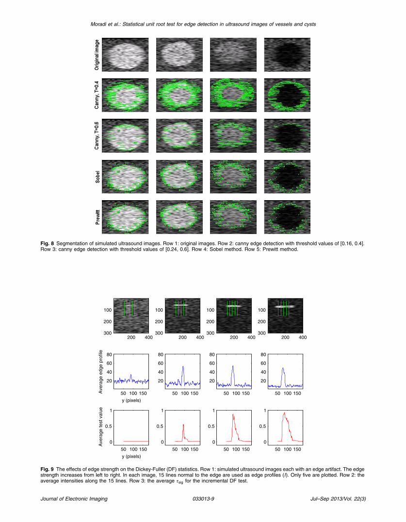
Fig. 8 Segmentation of simulated ultrasound images. Row 1: original images. Row 2: canny edge detection with threshold values of [0.16, 0.4].Row 3: canny edge detection with threshold values of [0.24, 0.6]. Row 4: Sobel method. Row 5: Prewitt method.

50 100 150

20

40

60

80

Ave

rage

edg

e pr

ofile

y (pixels)

50 100 150

0

0.5

1

Ave

rage

test

val

ue

y (pixels)

200 400

100

200

300

50 100 150

20

40

60

80

50 100 150

0

0.5

1

200 400

100

200

300

50 100 150

20

40

60

80

50 100 150

0

0.5

1

200 400

100

200

300

50 100 150

20

40

60

80

50 100 150

0

0.5

1

200 400

100

200

300

Fig. 9 The effects of edge strength on the Dickey-Fuller (DF) statistics. Row 1: simulated ultrasound images each with an edge artifact. The edgestrength increases from left to right. In each image, 15 lines normal to the edge are used as edge profiles (I). Only five are plotted. Row 2: theaverage intensities along the 15 lines. Row 3: the average τsig for the incremental DF test.

Journal of Electronic Imaging 033013-9 Jul–Sep 2013/Vol. 22(3)

Moradi et al.: Statistical unit root test for edge detection in ultrasound images of vessels and cysts

4.3.1 Initialization

Both the proposed method and the Snakes algorithm requirethe user to set a number of parameters. With our proposedmethod, these include the decision threshold T, angular res-olution Δθ, Δre, ext, rmin, and rmax. For Snakes, there aredifferent weighting factors and thresholds that depend onthe object shape and image intensity (13 different parametersare listed in one specific implementation43). The Snakesmethod also requires a starting contour. For the examplesillustrated here, the initialization required selection of atleast five points. By contrast, the initialization of the pro-posed approach requires the selection of only one startingseed point.

4.3.2 Speed

In the absence of a ground truth, the iterative Snakes algo-rithm does not provide a built-in stopping criteria. Therefore,the user should decide on the number of iterations neededto segment the structure. A typical number of iterationsrequired in the examples provided here was 100 (theexact number of iterations is provided in the captions ofFig. 10). One hundred iterations of the Snakes algorithmwere completed in 20.6 s. On the same PC and with an

angular resolution of Δθ ¼ 3 deg, the segmentation ofthese cyst images with our proposed approach was com-pleted in an average of 0.6 s. Since the presented resultis the average of nine initializations, this number should becorrected to 5.4 s.

4.3.3 Stability

The resulting contour in the proposed unit root approach canbe improved by repeating the initialization process and aver-aging. This can safeguard the outcome against the possibleoutliers caused by strong local artifacts. However, possibleoutliers that need the intervention of the user, or safeguardssuch as averaging, are not specific to the unit root method. Aswe witnessed in our experiments, and as Hamarneh et al.43

noted in using the Snakes algorithm, “The user should alsobe ready to intervene by placing constrained (forced) pointsto assist the snake if it clings to erroneous edges. Choosingthe weights and parameters of the snake model is an impor-tant and often tedious task.” As both Snakes and the unit rootmethod are considered semi-automatic algorithms, the needfor occasional intervention is understandable. However, webelieve that given the simple initialization of the unit root testand its significantly higher speed, intervention and/or aver-aging are more practical using this approach.

Fig. 10 Examples of the comparison of the proposed segmentation method with Snakes on breast cyst images (rows 1 and 2) and ovarian cyst(rows 3 and 4). Column 1: the initialization contour only used for Snakes (formed by manually clicking on five points). Column 2: outcome of theSnakes algorithm after 122, 227, 95, and 125 iterations from top to bottom. Column 3: the segmentation outcome using the proposedmethod, whichrequires one seed point (illustrated with a star).

Journal of Electronic Imaging 033013-10 Jul–Sep 2013/Vol. 22(3)

Moradi et al.: Statistical unit root test for edge detection in ultrasound images of vessels and cysts

4.3.4 Scope of applications

Our experience indicates that the criteria of statistical statio-narity assumption within the structure of interest is valid inultrasound images involving lesions and vessels that areeither hollow (such as vessels) or show fully developedspeckle with a different distribution from the background.One shortcoming of the proposed method is in areas ofvery weak echo overlapping with the edge of the artery/lesion, effectively extending the hollow appearance of thevessel into the surrounding tissue. While the parameter extis introduced to remedy these situations, if the area of theweak echo is large, the automatic contour could show anerror. As a clinical example, many investigators have devel-oped contouring methods for the prostate gland. We exam-ined the utility of our proposed method in that clinicalapplication and found that the method, when combinedwith a tapered ellipse shape model, can effectively contourthe prostate gland in the central section of the gland wherefully developed speckle and strong edges exist. However, atthe apex of the prostate gland, we often confront situations inwhich echoes are weak and leaking of the edge contour iscommon. This shortcoming is not specific to the DF meth-odology and has been observed in our other work.44 Thecommon approach for segmenting complex three-dimen-sional (3-D) shapes with the possibility of weak echoes incertain areas is to perform a two-dimensional (2-D) segmen-tation in the area of strongest edge, like the central gland incase of the prostate, and then to use that 2-D contour andprior knowledge of the 3-D shape informed partly by thelocal edges to build the 3-D model. We have used thisapproach in Refs. 44 and 45.

As mentioned before, the proposed unit root edge detec-tion approach has an excellent performance when theassumption of statistical stationarity within the structure ofinterest is valid. For optimal performance of the proposedsegmentation algorithm, shape geometry should be modeledsufficiently. On the contrary, deformable contours are notlimited by the shape models. This is the main advantageof the Snakes algorithm.

We should emphasize that the proposed edge detectionmethod can be a valuable tool within other segmentationframeworks that handle complex geometries. For example,active shape models (ASM)46 can be used for segmentationof ultrasound images. The ASM algorithm uses a statisticalshape model fit to a specific problem, overlays the model ona new instance of the object, and improves it by lookingfor better candidates around the points suggested by themodel as edge candidates. Gradient strength is normallyused for finding these better candidates. The DF edge detec-tor can replace or complement the gradient-based operatorsto improve the segmentation in the case of speckle-domi-nated ultrasound images.

5 ConclusionIn this paper we proposed an edge detection algorithm thatcan be used for segmentation of medical ultrasound images.The algorithm takes advantage of the DF test, a popular stat-istical test in econometric studies, which examines the nullhypothesis of existence of a unit root for an AR time series.The algorithm treats the radial intensity profiles as a timeseries and uses the DF statistical test along the radii tofind the location at which the profile becomes nonstationary.

Based on this test, we developed an accurate algorithm fordelineation of the borders of the vessels in clinical ultrasoundimages and also Field II simulated data. The method is fastand accurate as validated by comparison with expert delin-eation of the segmented structures. The main advantage ofthe method is its low sensitivity to local changes andspeckle-related local maxima in the edge profile differencefunction.

Our comparative study of the proposed segmentationmethod with Snakes showed that simple initialization,high speed, and stability are the advantages of the unit rootalgorithm. Both methods are found to be accurate. The mainadvantage of the Snakes algorithm is its ability to handlemore complex geometries. However, the proposed edgedetection approach can be used as a component in model-based approaches, such as those described in Refs. 8, 23,and 47, to segment more complex contour shapes. Thesemethods have been extended to 3-D shape segmentation,where a central 2-D contour is used for initialization.

AcknowledgmentsThe authors would like to thank Dr. Savvas Nicolaou,Dr. Vicki Lessoway, Dr. Maureen Kennedy, Dr. BassamA. Masri, and Dr. James McEwen for help with the clinicalstudy.

References

1. J. A. Noble and D. Boukerroui, “Ultrasound image segmentation: asurvey,” IEEE Trans. Med. Imag. 25(8), 987–1010 (2006).

2. W. Richard and C. Keen, “Automated texture-based segmentationof ultrasound images of the prostate,” Comput. Med. Imag. Graph.20(3), 131–140 (1996).

3. N. Archip et al., “Ultrasound image segmentation using spectralclustering,” Ultrasound Med. Biol. 31(11), 1485–1497 (2005).

4. G. Hamarneh and T. Gustavsson, “Combining Snakes and active shapemodels for segmenting the human left ventricle in echocardiographicimages,” in IEEE Comput. Cardiol., pp. 115–118 (2000).

5. H. M. Ladak et al., “Prostate boundary segmentation from 2D ultra-sound images,” Med. Phys. 27(8), 1777–1788 (2000).

6. A. Madabhushi and D. N. Metaxas, “Combining low-, high-level andempirical domain knowledge for automated segmentation of ultrasonicbreast lesions,” IEEE Trans. Med. Imag. 22(2), 155–169 (2003).

7. D. Shen, Y. Zhan, and C. Davatzikos, “Segmentation of prostate boun-daries from ultrasound images using statistical shape model,” IEEETrans. Med. Imag. 22(4), 539–551 (2003).

8. P. Abolmaesumi and M. R. Sirouspour, “An interacting multiple modelprobabilistic data association filter for cavity boundary extraction fromultrasound images,” IEEE Trans. Med. Imag. 23(6), 772–784 (2004).

9. M. Martin-Fernandez and C. Alberola-Lopez, “Maximum likelihoodsegmentation of ultrasound images with Rayleigh distribution,” Med.Image Anal. 9(6), 1–23 (2005).

10. C. Chesnaud, P. Refregier, and V. Boulet, “Statistical region Snake-based segmentation adapted to different physical noise models,”IEEE Trans. Pattern Anal. Mach. Intell. 21(11), 1145–1157 (1999).

11. A. Sarti et al., “Maximum likelihood segmentation of ultrasoundimages with Rayleigh distribution,” IEEE Trans. Ultrason.,Ferroelectr., Freq. Control 52, 947–960 (2005).

12. G. Slabaugh et al., “Statistical region-based segmentation of ultrasoundimages,” Ultrasound Med. Biol. 35(5), 781–795 (2009).

13. V. Shrimali, R. S. Anand, and V. Kumar, “Current trends in segmenta-tion of medical ultrasound B-mode images: a review,” IETE TechnicalRev. 26(1), 8–17 (2009).

14. J. Canny, “A computational approach to edge detection,” IEEE Trans.Pattern Anal. Mach. Intell. PAMI-8(6), 679–698 (1986).

15. R. C. Gonzales and R. E. Woods, Digital Image Processing, 2nd ed.,Prentice-Hall, New Jersey (2002).

16. R. N. Czerwinski, D. L. Jones, and W. D. O’Brien Jr., “Line andboundary detection in speckle images,” IEEE Trans. Image Process.7(12), 1700–1714 (1998).

17. G. Slabaugh, G. Unal, and T. C. Chang, “Information-theoretic featuredetection in ultrasound images,” in IEEE Engineering in Medicine andBiology, pp. 2638–2642 (2006).

18. S. D. Pathak et al., “Edge-guided boundary delineation in prostate ultra-sound images,” IEEE Trans. Med. Imag. 19(12), 1211–1219 (2000).

Journal of Electronic Imaging 033013-11 Jul–Sep 2013/Vol. 22(3)

Moradi et al.: Statistical unit root test for edge detection in ultrasound images of vessels and cysts

19. I. Wolf et al., “ROPES: a semiautomated segmentation method foraccelerated analysis of three-dimensional echocardiographic data,”IEEE Trans. Med. Imag. 21(9), 1091–1104 (2002).

20. Y. Yu and S. T. Acton, “Edge detection in ultrasound imagery usingthe instantaneous coefficient of variation,” IEEE Trans. ImageProcess. 13(12), 1640–1655 (2004).

21. D. M. Herrington et al., “Semi-automated boundary detection for intra-vascular ultrasound,” in IEEE Computers in Cardiology, pp. 103–106,IEEE, Piscataway, NJ (1992).

22. J. H. Kaspersen, T. Lang, and F. Lindseth, “Wavelet-based edge detec-tion in ultrasound images,” Ultrasound Med. Biol. 27(1), 88–99 (2001).

23. J. Guerrero et al., “Real-time vessel segmentation and tracking forultrasound imaging applications,” IEEE Trans. Med. Imag. 26(8),1079–1090 (2007).

24. S. S. Mahdavi et al., “Vibro-elastography for visualization of the pros-tate region,” Lec. Notes Comput. Sci. 5762, 339–347 (2009).

25. R. C. Waag, “A review of tissue characterization from ultrasonic scat-tering,” IEEE Trans. Biomed. Eng. BME-31(12), 884–893 (1984).

26. D. A. Dickey and W. A. Fuller, “Distribution of the estimators forautoregressive time series with a unit root,” J. Am. Stat. Assoc. 74(366),427–431 (1979).

27. M. Moradi et al., “Preliminary results of an ultrasound segmentationmethod based on statistical unit-root test of b-scan radial intensity pro-files,” in IEEE Ultrasonics Symp., pp. 1–4, IEEE, Piscataway, NJ(2009).

28. P. Abolmaesumi, M. R. Sirouspour, and S. E. Salcudean, “Real-timeextraction of carotid artery contours from ultrasound images,” inIEEE Symp. on Computer-Based Medical Systems, pp. 181–186,IEEE, Piscataway, NJ (2000).

29. C. Chen et al., “Segmentation of arterial geometry from ultrasoundimages using balloon models,” in IEEE Int. Symp. on BiomedicalImaging, pp. 2988–2991, IEEE, Piscataway, NJ (2004).

30. F. Mao et al., “Segmentation of carotid artery in ultrasound images:method development and evaluation technique,” Med. Phys. 27(8),1961–1970 (2000).

31. W. Gomez et al., “Computerized lesion segmentation of breastultrasound based on marker-controlled watershed transformation,”Med. Phys. 37(1), 82–95 (2010).

32. C. M. Chen, H. H. Lu, and Y. C. Lin, “An early vision-based Snakemodel for ultrasound image segmentation,” Ultrasound Med. Biol.26(2), 273–285 (2000).

33. K. Horsch et al., “Automatic segmentation of breast lesions on ultra-sound,” Med. Phys. 28(8), 1652–1659 (2001).

34. K. Drukker et al., “Computerized lesion detection on breast ultrasound,”Med. Phys. 29(7), 1438–1446 (2002).

35. J. Z. Cheng et al., “Cell-based two-region competition algorithm with amap framework for boundary delineation of a series of 2D ultrasoundimages,” Ultrasound Med. Biol. 33(10), 1640–1650 (2007).

36. Y. L. Huang and D. R. Chen, “Watershed segmentation for breast tumorin 2-D sonography,” Ultrasound Med. Biol. 30(5), 625–632 (2004).

37. R. H. Shumway and D. S. Stoffer, Time Series Analysis and ItsApplications, Springer, Heidelberg, Germany (2006).

38. G. Elliott, T. J. Rothenberg, and J. H. Stock, “Efficient tests for an autor-egressive unit root,” Econometrica 64(4), 813–836 (1996).

39. S. E. Said and D. A. Dickey, “Testing for unit roots in autoregressivemoving average models of unknown order,” Biometrika 71(3), 599–607(1984).

40. L. Kanzler, “A study of the efficiency of the foreign exchange marketthrough analysis of ultra-high frequency data,” Ph.D. dissertation,Oxford University, Oxford, UK (1998).

41. J. A. Jensen, “Field: a program for simulating ultrasound systems,” in10th NordicBaltic Conf. on Biomedical Imaging, Vol. 34, pp. 351–353(1996).

42. G. Gerig, M. Jomier, and M. Chakos, “Valmet: a new validation tool forassessing and improving 3D object segmentation,” Lec. Notes Comput.Sci. 2208, 516–523 (2001).

43. G. Hamarneh, A. Chodorowski, and T. Gustavsson, “Active contourmodels: application to oral lesion detection in color images,” inIEEE Int. Conf. Systems, Man, and Cybernetics, pp. 2458–2463,IEEE, Piscataway, NJ (2000).

44. S. S. Mahdavi et al., “Semi-automatic segmentation for prostate inter-ventions,” Med. Image Anal. 15(2), 226–237 (2011).

45. S. S. Mahdavi et al., “Fusion of ultrasound B-mode and vibro-elastog-raphy images for automatic 3-D segmentation of the prostate,” IEEETrans. Med. Imag. 31(11), 2073–2082 (2012).

46. T. Cootes et al., “The use of active shape models for locating structuresin medical images,” Image Vis. Comput. 12(6), 355–366 (1994).

47. S. S. Mahdavi et al., “Automatic prostate segmentation using fusedultrasound B-mode and elastography images,” Lec. Notes Comput.Sci. 6362, 76–83 (2010).

Biographies and photographs of the authors are not available.

Journal of Electronic Imaging 033013-12 Jul–Sep 2013/Vol. 22(3)

Moradi et al.: Statistical unit root test for edge detection in ultrasound images of vessels and cysts