Statistical Topology via Morse Theory, Persistence and ...

Cleveland State University Cleveland State University

EngagedScholarship@CSU EngagedScholarship@CSU

Mathematics Faculty Publications Mathematics Department

2010

Statistical Topology via Morse Theory, Persistence and Statistical Topology via Morse Theory, Persistence and

Nonparametric Estimation Nonparametric Estimation

Peter Bubenik Cleveland State University, [email protected]

Gunnar Carlsson Stanford University, [email protected]

Peter T. Kim University of Guelph, [email protected]

Zhiming Luo Keimyung University, [email protected]

Follow this and additional works at: https://engagedscholarship.csuohio.edu/scimath_facpub

Part of the Statistics and Probability Commons

How does access to this work benefit you? Let us know! How does access to this work benefit you? Let us know!

Original Citation Original Citation Bubenik, P., Carlsson, G., Kim, P. T., & Luo, Z.-M. (January 01, 2010). Statistical Topology via Morse Theory Persistence and Nonparametric Estimation. Contemporary Mathematics, 516, 75-92. arXiv:0908.3668v2

This Article is brought to you for free and open access by the Mathematics Department at EngagedScholarship@CSU. It has been accepted for inclusion in Mathematics Faculty Publications by an authorized administrator of EngagedScholarship@CSU. For more information, please contact [email protected].

arX

iv:0

908.

3668

v2 [

mat

h.ST

] 4

Mar

201

0

STATISTICAL TOPOLOGY VIA MORSE THEORY

PERSISTENCE AND NONPARAMETRIC ESTIMATION

PETER BUBENIK, GUNNAR CARLSON, PETER T. KIM,AND ZHI–MING LUO

Abstract. In this paper we examine the use of topological meth-ods for multivariate statistics. Using persistent homology fromcomputational algebraic topology, a random sample is used to con-struct estimators of persistent homology. This estimation proce-dure can then be evaluated using the bottleneck distance betweenthe estimated persistent homology and the true persistent homol-ogy. The connection to statistics comes from the fact that whenviewed as a nonparametric regression problem, the bottleneck dis-tance is bounded by the sup-norm loss. Consequently, a sharp as-ymptotic minimax bound is determined under the sup–norm riskover Holder classes of functions for the nonparametric regressionproblem on manifolds. This provides good convergence proper-ties for the persistent homology estimator in terms of the expectedbottleneck distance.

1. Introduction

Quantitative scientists of diverse backgrounds are being asked to ap-ply the techniques of their specialty to data which is greater in both sizeand complexity than that which has been studied previously. Massive,multivariate data sets, for which traditional linear methods are inad-equate, pose challenges in representation, visualization, interpretationand analysis. A common finding is that these massive multivariate datasets require the development of new statistical methodology and thatthese advances are dependent on increasing technical sophistication.Two such data-analytic techniques that have recently come to the foreare computational algebraic topology and geometric statistics.

2000 Mathematics Subject Classification. Primary 62C10, 62G08; Secondary41A15, 55N99, 58J90.

Key words and phrases. Bottleneck distance, critical values, geometric statis-tics, minimax, nonparametric regression, persistent homology, Plex, Riemannianmanifold, sublevel sets.

Support for the second author was partially funded by DARPA, ONR, Air ForceOffice of Scientific Research, and NSF..

Support for the third author was partially funded by NSERC grant DG 46204.1

2 P.BUBENIK, G.CARLSON, P.T. KIM, AND Z-M. LUO

Commonly, one starts with data obtained from some induced geo-metric structure, such as a curved submanifold of a numerical space,or, a singular algebraic variety. The observed data is obtained as arandom sample from this space, and the objective is to statisticallyrecover features of the underlying space.In computational algebraic topology, one attempts to recover qual-

itative global features of the underlying data, such as connectedness,or the number of holes, or the existence of obstructions to certain con-structions, based upon the random sample. In other words, one hopesto recover the underlying topology. An advantage of topology is thatit is stable under deformations and thus can potentially lead to robuststatistical procedures. A combinatorial construction such as the alphacomplex or the Cech complex, see for example [33], converts the datainto an object for which it is possible to compute the topology. How-ever, it is quickly apparent that such a construction and its calculatedtopology depend on the scale at which one considers the data. A multi–scale solution to this problem is the technique of persistent homology.It quantifies the persistence of topological features as the scale changes.Persistent homology is useful for visualization, feature detection andobject recognition. Applications of persistent topology include proteinstructure analysis [30], gene expression [11], and sensor networks [8]. Ina recent application to brain image data, a demonstration of persistenttopology in discriminating between two populations is exhibited [5].In geometric statistics one uses the underlying Riemannian structure

to recover quantitative information concerning the underlying probabil-ity distribution and functionals thereof. The idea is to extend statisticalestimation techniques to functions over Riemannian manifolds, utiliz-ing the Riemannian structure. One then considers the magnitude ofthe statistical accuracy of these estimators. Considerable progress hasbeen achieved in terms of optimal estimation [14, 12, 16, 26, 27, 19, 17].Other related works include [28, 29, 23, 1, 3]. There is also a growinginterest in function estimation over manifolds in the learning theoryliterature [7, 31, 2]; see also the references cited therein.Although computational algebraic topology and geometric statistics

appear dissimilar and seem to have different objectives, it has recentlybeen noticed that they share a commonality through statistical sam-pling. In particular, a pathway between them can be established byusing elements of Morse theory. This is achieved through the fact thatpersistent homology can be applied to Morse functions and comparisonsbetween two Morse functions can be assessed by a metric called thebottleneck distance. Furthermore, the bottleneck distance is boundedby the sup–norm distance between the two Morse functions on some

STATISTICAL TOPOLOGY 3

underlying manifold. This framework thus provides just enough struc-ture for a statistical interpretation. Indeed, consider a nonparametricregression problem on some manifold. Given data in this frameworkone can construct a nonparametric regression function estimator suchthat the persistent homology associated with this estimated regressionfunction is an estimator for the persistent homology of the true re-gression function, as assessed by the bottleneck distance. Since thiswill be bounded by the sup-norm loss, by providing a sharp sup–normminimax estimator of the regression function, we can effectively boundthe expected bottleneck distance between the estimated persistent ho-mology and the true persistent homology. Consequently, by showingconsistency in the sup-norm risk, we can effectively show consistencyin the bottleneck risk for persistent homology which is what we willdemonstrate. Let us again emphasize that the pathway that allows usto connect computational algebraic topology with geometric statisticsis Morse theory. This is very intriguing in that a pathway between thetraditional subjects of geometry and topology is also Morse theory.We now summarize this paper. In Section 2 we will lay down the

topological preliminaries needed to state our main results. In Section3, we go over the preliminaries needed for nonparametric regression ona Riemannian manifold. Section 4 states the main results where sharpsup-norm minimax bounds consisting of constant and rate, and sharpsup-norm estimators are presented. The connection to bounding thepersistent homology estimators thus ensues. Following this in Section5, a brief discussion of the implementation is given. Proofs to the mainresults are collected in Section 6. An Appendix that contains sometechnical material is included for completeness.

2. Topological Preliminaries

Let us assume thatM is a d−dimensional compact Riemannian man-ifold and suppose f : M → R is some smooth function. Consider thesublevel set, or, lower excursion set,

(2.1) Mf≤r := {x ∈ M | f(x) ≤ r} = f−1((−∞, r]).

It is of interest to note that for certain classes of smooth functions,the topology of M can be approached by studying the geometry of thefunction.To be more precise, for some smooth f : M → R, consider a point

p ∈ M where in local coordinates the derivatives, ∂f/∂xj vanishes.Then that point is called a critical point, and the evaluation f(p) iscalled a critical value. A critical point p ∈ M is called non-degenerate ifthe Hessian (∂2f/∂i∂j) is nonsingular. Such functions are called Morse

4 P.BUBENIK, G.CARLSON, P.T. KIM, AND Z-M. LUO

functions. Later we will see that differentiability is not needed whenapproached homologically.The geometry of Morse functions can completely characterize the

homotopy type of M by the way in which topological characteristicsof sublevel sets (2.1) change at critical points. Indeed classical Morsetheory tells us that the homotopy type of (2.1) is characterized by at-taching a cell whose dimension is determined by the number of negativeeigenvalues of the Hessian at a critical point to the boundary of theset (2.1) at the critical point. This indeed is a pathway that connectsgeometry with topology, and one in which we shall also use to bridgestatistics. Some background material in topology and Morse theory isprovided in Appendices A and B.As motivation let us consider a real valued function f that is a mix-

ture of two bump functions on the disk of radius 10 in R2, see Figure

2.1.

−5.0

−2.5

0.0 x

2.50.0

−5.0 −2.5

0.5

0.0 5.02.5y 5.0

1.0

1.5

2.0

Figure 2.1. A mixture of two bump functions and var-ious contours below which are the sublevel sets.

In this example, the maximum of f equals 2, so Mf≤2 = M. Thissublevel set is the disk and therefore has no interesting topology sincethe disk is contractible. In contrast, consider the sublevel sets whenr = 1, 1.2, and 1.5 (see Figures 2.2, 2.3 and 2.4).In these cases, the sublevel sets Mf≤r have non-trivial topology,

namely one, two and one hole(s) respectively, each of whose bound-aries is one-dimensional. This topology is detected algebraically by thefirst integral homology group H1(Mf≤r) which will be referred to asthe homology of degree 1 at level r. This group enumerates the topo-logically distinct cycles in the sublevel set. In the first and third cases,for each integer z ∈ Z, there is a cycle which wraps around the hole

STATISTICAL TOPOLOGY 5

−5.0

−2.5

0.0 x

2.50.0

−5.0 −2.5

0.25

0.0 5.02.5y 5.0

0.5

0.75

1.0

y

−2.5

−2.5

−5.0

x 0.0

0.0

−5.0

2.5

2.5

5.0

5.0

Figure 2.2. The sublevel set at r = 1 has one hole.

−5.0

−2.5

0.0 x

2.50.0

−5.0

0.25

−2.5 0.0 5.02.5

0.5

y 5.0

0.75

1.0

−5.0

y

5.0

5.0

x

−5.0

2.5

−2.5 0.0 2.5

0.0

−2.5

Figure 2.3. The sublevel set at r = 1.2 has two holes.

5.0

−2.5

x

2.5

2.5 5.0

−5.0

−2.5

0.0

−5.0

y

0.0

Figure 2.4. The sublevel set at r = 1.5 has one hole.

z times. We have H1(Mf≤r) = Z. In the second case, we have twogenerating non-trivial cycles and so H1(Mf≤r) = Z ⊕ Z. For a reviewof homology the reader can consult Appendix A for related discussions.

2.1. Persistent topology. A computational procedure for determin-ing how the homology persists as the level r changes is provided in[10, 33]. In the above example there are two persistent homology classes(defined below). One class is born when r = 1.1, the first sublevel setthat has two holes, and dies at r = 1.4 the first sublevel set for whichthe second hole disappears. The other class is born at r = 0 and persistsuntil r = 2. Thus the persistent homology can be completely describedby the two ordered pairs {(1.1, 1.4), (0, 2)}. This is called the reducedpersistence diagram (defined below) of f , denoted D(f). For a persis-tent homology class described by (a, b), call b−a its lifespan. From the

6 P.BUBENIK, G.CARLSON, P.T. KIM, AND Z-M. LUO

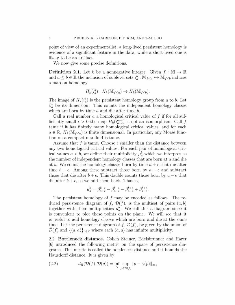
point of view of an experimentalist, a long-lived persistent homology isevidence of a significant feature in the data, while a short-lived one islikely to be an artifact.We now give some precise definitions.

Definition 2.1. Let k be a nonnegative integer. Given f : M → R

and a ≤ b ∈ R the inclusion of sublevel sets iba : Mf≤a → Mf≤b inducesa map on homology

Hk(iba) : Hk(Mf≤a) → Hk(Mf≤b).

The image of Hk(iba) is the persistent homology group from a to b. Let

βba be its dimension. This counts the independent homology classes

which are born by time a and die after time b.Call a real number a a homological critical value of f if for all suf-

ficiently small ǫ > 0 the map Hk(ia+ǫa−ǫ) is not an isomorphism. Call f

tame if it has finitely many homological critical values, and for eacha ∈ R, Hk(Mf≤a) is finite dimensional. In particular, any Morse func-tion on a compact manifold is tame.Assume that f is tame. Choose ǫ smaller than the distance between

any two homological critical values. For each pair of homological crit-ical values a < b, we define their multiplicity µb

a which we interpret asthe number of independent homology classes that are born at a and dieat b. We count the homology classes born by time a+ ǫ that die aftertime b − ǫ. Among these subtract those born by a − ǫ and subtractthose that die after b+ ǫ. This double counts those born by a− ǫ thatdie after b+ ǫ, so we add them back. That is,

µba = βb−ǫ

a+ǫ − βb−ǫa−ǫ − βb+ǫ

a+ǫ + βb+ǫa−ǫ.

The persistent homology of f may be encoded as follows. The re-duced persistence diagram of f , D(f), is the multiset of pairs (a, b)together with their multiplicities µb

a. We call this a diagram since itis convenient to plot these points on the plane. We will see that itis useful to add homology classes which are born and die at the sametime. Let the persistence diagram of f , D(f), be given by the union ofD(f) and {(a, a)}a∈R where each (a, a) has infinite multiplicity.

2.2. Bottleneck distance. Cohen–Steiner, Edelsbrunner and Harer[6] introduced the following metric on the space of persistence dia-grams. This metric is called the bottleneck distance and it bounds theHausdorff distance. It is given by

(2.2) dB(D(f),D(g)) = infγ

supp∈D(f)

‖p− γ(p)‖∞,

STATISTICAL TOPOLOGY 7

where the infimum is taken over all bijections γ : D(f) → D(g) and‖ · ‖∞ denotes supremum–norm over sets.For example, let f be the function considered at the start of this

section. Let g be a unimodal, radially-symmetric function on the samedomain with maximum 2.2 at the origin and minimum 0. We showedthat D(f) = {(1.1, 1.4), (0, 2)}. Similarly, D(g) = (0, 2.2). The bot-tleneck distance is achieved by the bijection γ which maps (0, 2) to(0, 2.2) and (1.1, 1.4) to (1.25, 1.25) and is the identity on all ‘diagonal’points (a, a). Since the diagonal points have infinite multiplicity thisis a bijection. Thus, dB(D(f),D(g)) = 0.2.In [6], the following result is proven:

(2.3) dB(D(f),D(g)) ≤ ‖f − g‖∞

where f, g : M → R are tame functions and ‖ · ‖∞ denotes sup–normover functions.

2.3. Connection to Statistics. It is apparent that most articles onpersistent topology do not as of yet incorporate statistical foundationsalthough they do observe them heuristically. The approach in [25] com-bines topology and statistics and calculates how much data is needed toguarantee recovery of the underlying topology of the manifold. A draw-back of that technique is that it supposes that the size of the smallestfeatures of the data is known a priori. To date the most comprehensiveparametric statistical approach is contained in [4]. In this paper, theunknown probability distribution is assumed to belong to a parametricfamily of distributions. The data is then used to estimate the level soas to recover the persistent topology of the underlying distribution.As far as we are aware no statistical foundation for the nonpara-

metric case has been formulated although [6] provide the topologicalmachinery for making a concrete statistical connection. In particular,persistent homology of a function is encoded in its reduced persistencediagram. A metric on the space of persistence diagrams between twofunctions is available which bounds the Hausdorff distance and this inturn is bounded by the sup–norm distance between the two functions.Thus by viewing one function as the parameter, while the other isviewed as its estimator, the asymptotic sup–norm risk bounds the ex-pected Hausdorff distance thus making a formal nonparametric statis-tical connection. This in turn lays down a framework for topologicallyclassifying clusters in high dimensions.

8 P.BUBENIK, G.CARLSON, P.T. KIM, AND Z-M. LUO

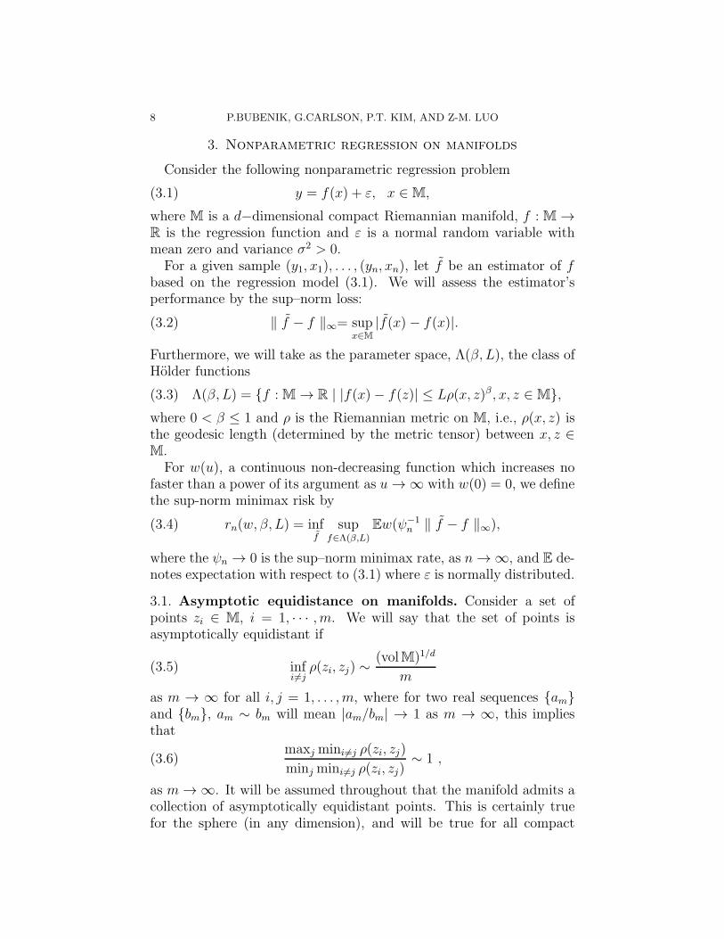
3. Nonparametric regression on manifolds

Consider the following nonparametric regression problem

(3.1) y = f(x) + ε, x ∈ M,

where M is a d−dimensional compact Riemannian manifold, f : M →R is the regression function and ε is a normal random variable withmean zero and variance σ2 > 0.For a given sample (y1, x1), . . . , (yn, xn), let f be an estimator of f

based on the regression model (3.1). We will assess the estimator’sperformance by the sup–norm loss:

(3.2) ‖ f − f ‖∞= supx∈M

|f(x)− f(x)|.

Furthermore, we will take as the parameter space, Λ(β, L), the class ofHolder functions

(3.3) Λ(β, L) = {f : M → R | |f(x)− f(z)| ≤ Lρ(x, z)β , x, z ∈ M},where 0 < β ≤ 1 and ρ is the Riemannian metric on M, i.e., ρ(x, z) isthe geodesic length (determined by the metric tensor) between x, z ∈M.For w(u), a continuous non-decreasing function which increases no

faster than a power of its argument as u→ ∞ with w(0) = 0, we definethe sup-norm minimax risk by

(3.4) rn(w, β, L) = inff

supf∈Λ(β,L)

Ew(ψ−1n ‖ f − f ‖∞),

where the ψn → 0 is the sup–norm minimax rate, as n→ ∞, and E de-notes expectation with respect to (3.1) where ε is normally distributed.

3.1. Asymptotic equidistance on manifolds. Consider a set ofpoints zi ∈ M, i = 1, · · · , m. We will say that the set of points isasymptotically equidistant if

(3.5) infi 6=j

ρ(zi, zj) ∼(volM)1/d

m

as m → ∞ for all i, j = 1, . . . , m, where for two real sequences {am}and {bm}, am ∼ bm will mean |am/bm| → 1 as m → ∞, this impliesthat

(3.6)maxj mini 6=j ρ(zi, zj)

minj mini 6=j ρ(zi, zj)∼ 1 ,

as m→ ∞. It will be assumed throughout that the manifold admits acollection of asymptotically equidistant points. This is certainly truefor the sphere (in any dimension), and will be true for all compact

STATISTICAL TOPOLOGY 9

Riemannian manifolds since the injectivity radius is strictly positive.We note that [27] makes use of this condition as well.We will need the following constants

(3.7) C0 = Ld/(2β+d)

(σ2volM (β + d)d2

vol Sd−1β2

)β/(2β+d)

,

(3.8) ψn =

(log n

n

)β/(2β+d)

,

and ‘vol’ denotes the volume of the object in question, where Sd−1 is

the (d−1)−dimensional unit sphere with vol Sd−1 = 2πd/2/Γ(d/2) andΓ is the gamma function.Define the geodesic ball of radius r > 0 centered at z ∈ M by

(3.9) Bz(r) = {x ∈ M |ρ(x, z) ≤ r} .We have the following result whose proof will be detailed in Section 6.1

Lemma 3.1. Let zi ∈ M, i = 1, · · · , m, be asymptotically equidistant.

Let λ = λ(m) be the largest number such that⋃m

i=1Bzi(λ−1) = M,

where Bzi(λ−1) is the closure of the geodesic ball of radius λ−1 around

zi. Then there is a C1 > 0 such that lim supm→∞mλ(m)−d ≤ C1.

3.2. An estimator. Fix a δ > 0 and let

m =

[C1

(L(2β + d)

δC0dψn

)d/β],

where C1 is a sufficiently large constant from Lemma 3.1, hence m ≤ nand m → ∞ when n → ∞ and for s ∈ R, [s] denotes the greatestinteger part.For the design points {xi : i = 1, . . . , n} onM, assume that

{xij ∈ M, j = 1, . . . , m

}

is an asymptotically equidistant subset on M. Let Aj, j = 1, . . . , m, bea partition of M such that Aj is the set of those x ∈ M for which xij isthe closest point in the subset {xi1 , . . . , xim}. Thus, for j = 1, . . . , m,

(3.10) Aj =

{x ∈ M | ρ(xij , x) = min

k=1,...,m{ρ(xik , x)}

}.

Let Aj , j = 1, . . . , m be as in (3.10) and define 1Aj(x) to be the

indicator function on the set Aj and consider the estimator

(3.11) f(x) =

m∑

j=1

aj1Aj(x),

10 P.BUBENIK, G.CARLSON, P.T. KIM, AND Z-M. LUO

where for L > 0, 0 < β ≤ 1,

aj =

∑ni=1Kκ,xij

(xi)yi∑ni=1Kκ,xij

(xi),

Kκ,xij(ω) =

(1− (κρ(xij , ω))

β)+,

κ =

(C0ψn

L

)−1/β

,

and s+ = max(s, 0), s ∈ R. We remark that when m is sufficientlylarge hence κ is also large, the support set of Kκ,xij

(ω) is the closed

geodesic ball Bxij(κ−1) around xij for j = 1, . . . , m.

4. Main Results

We now state the main results of this paper. The first result pro-vides an upper bound for the estimator (3.11), where the function w(u)satisfies w(0) = 0, w(u) = w(−u), w(u) does not decrease, and w(u)increases not faster than a power as u→ ∞.

Theorem 4.1. For the regression model (3.1) and the estimator (3.11),we have

supf∈Λ(β,L)

Ew(ψ−1n

∥∥∥f − f∥∥∥∞

)≤ w (C0) ,

as n→ 0, where ψn = (n−1 logn)β/(2β+d).

We have the asymptotic minimax result for the sup–norm risk.

Theorem 4.2. For the regression model (3.1)

limn→∞

rn(w, β, L) = w (C0) .

In particular, we have the immediate result.

Corollary 4.3. For the regression model (3.1) and the estimator (3.11),

supf∈Λ(β,L)

E

∥∥∥f − f∥∥∥∞

∼ C0

(log n

n

)β/(2β+d)

as n→ ∞.

We note that the above generalizes earlier one-dimensional results in[20, 21], where the domain is the unit interval, whereas [18] generalizesthis result to higher dimensional unit spheres.Now that a sharp sup–norm minimax estimator has been found we

would like to see how we can use this for topological data analysis. Thekey is the sup–norm bound on the bottleneck distance for persistencediagrams. In particular, for the regression function f in (3.1) and f the

STATISTICAL TOPOLOGY 11

estimator (3.11), we have the persistence diagram D(f) as well as an

estimator of the persistence diagram D(f). Using the results of Section2.2, and in particular (2.3), we have

(4.1) dB

(D(f),D(f)

)≤∥∥∥f − f

∥∥∥∞.

Let Λt(β, L) denote the subset of tame functions in Λ(β, L). By corol-lary 4.3, the following result is immediate.

Corollary 4.4. For the nonparametric regression model (3.1), let f be

defined by (3.11). Then for 0 < β ≤ 1 and L > 0,

supf∈Λt(β,L)

EdB

(D(f),D(f)

)≤ Ld/(2β+d)

(σ2volM (β + d)d2

vol Sd−1β2

log n

n

)β/(2β+d)

as n→ 0.

5. Discussion

To calculate the persistence diagrams of the sublevel sets of f , we

suggest that because of the way f is constructed, we can calculateits persistence diagrams using a triangulation, T of the manifold inquestion.

We can then filter T using f as follows. Let r1 ≤ r2 ≤ . . . ≤ rm be

the ordered list of values of f on the vertices of the triangulation. For1 ≤ i ≤ m, let Ti be the subcomplex of T containing all vertices v with

f(v) ≤ ri and all edges whose boundaries are in Ti and all faces whoseboundaries are in Ti. We obtain the following filtration of T ,

φ = T0 ⊆ T1 ⊆ T2 ⊆ · · · ⊆ Tm = T .Because the critical points of f only occur at the vertices of T , Morsetheory guarantees that the persistent homology of the sublevel sets of

f equals the persistent homology of the above filtration of T .Using the software Plex, [9], we calculate the persistent homology,

in degrees 0, 1, 2, ..., d of the triangulation T filtered according tothe estimator. Since the data will be d–dimensional, we do not expectany interesting homology in higher degrees, and in fact, most of theinteresting features would occur in the lower degrees.A demonstration of this is provided in [5] for brain image data, where

the topology of cortical thickness in an autism study takes place. Thepersistent homology, in degrees 0, 1 and 2 is calculated for 27 subjects.Since the data is two–dimensional, we do not expect any interestinghomology in higher degrees. For an initial comparison of the autis-tic subjects and control subjects, we take the union of the persistence

12 P.BUBENIK, G.CARLSON, P.T. KIM, AND Z-M. LUO

diagrams, see Fig. 4 in [5] page 392. We note the difference in thetopological structures as seen through the persistent homologies be-tween the autistic and control group, particularly, as we move awayfrom the diagonal line. A test using concentration pairings reveal groupdifferences.

6. Proofs

Our proofs will use the ideas from [18] and [20].

6.1. Upper Bound. We first prove the earlier lemma.

Proof of Lemma 3.1. Let (U , (xi)) be any normal coordinate chart cen-tered at xi, then the components of the metric at xi are gij = δij , so√|gij(xi)| = 1, see [22]. Consequently,

vol (Bxi(λ−1)) =

∫

B(λ−1)

√|gij(expxi

(x))|dx =√

|gij(expxi(t))|

∫

B(λ−1)

dx

∼ vol (B(λ−1)) = vol (B(1))λ−d = vol (Sd−1)λ−d/d .

The first line uses the integration transformation, where expxi: B(λ−1) →

Bxi(λ−1) is the exponential map from the tangent space TMxi

→ M.The second line uses the integral mean value theorem and r is the radiusfrom the origin to point x in the Euclidean ball B(λ−1). The third lineis asymptotic as λ→ ∞ and uses the fact that |gij(expxi

(t))| → 1 whenλ→ ∞. In the fourth line vol (B(1)) is the volume of d-dimensional Eu-clidean unit ball. The last line uses the fact vol (B(1)) = vol (Bd−1)/d.Let λ′ = λ′(m) > 0 be the smallest number such that Bxi

((λ′)−1)are disjoint. Then λ−1 = c(m)× (λ′)−1, where c(m) > 1 and c(m) → 1as m→ ∞. Consequently

vol (M) ≥m∑

i=1

vol (Bxi((λ′)−1)) ∼ mvol (Sd−1)(λ′)−d/d.

Thus lim supm→∞mλ(m)−d = lim supm→∞ c(m)dm(λ′)−d ≤ dvol (M)vol (Sd−1)

.

�

We now calculate the asymptotic variance of aj for j = 1, . . . , m.Let

M =

[nvol(Bxij

(κ−1))

vol(M)

].

STATISTICAL TOPOLOGY 13

Then,

var(aj) =σ2∑n

i=1K2κ,xij

(xi)

(∑n

i=1Kκ,xij(xi))2

∼σ2vol (Bxij

(κ−1))∫Bxij

(κ−1)(1− (κρ(xij , ω))

β)2dω

M(∫Bxij

(κ−1)(1− (κρ(xij , ω))

β)dω)2

=σ2vol (Bxij

(κ−1))∫B(κ−1)

(1− (κr)β)2√|giij(expxij

(x))|dx

M (∫B(κ−1)

(1− (κr)β)√|giij(expxij

(x)))|dx)2.

This last expression evaluates as

σ2vol (Bxji(κ−1))

√|giij(expxij

(t))|∫ κ−1

0

∫ π

0· · ·∫ π

0

∫ 2π

0(1− (κr)β)2rd−1drdσd−1

M |giij(expxij(t′))|(

∫ κ−1

0

∫ π

0· · ·∫ κ−1

0

∫ π

0· · ·∫ π

0

∫ 2π

0(1− (κr)β)2rd−1drdσd−1)2

so that we have

var(aj) ∼σ2vol (Bxij

(κ−1))dvol (Bd)∫ κ−1

0(1− (κr)β)2rd−1dr

M d2vol (Bd)2(∫ κ−1

0(1− (κr)β)rd−1dr)2

= σ2κdvol (M)2d(β + d)

nvol (Sd−1)(2β + d)

as n→ ∞, where dσd−1 is the spherical measure on Sd−1.

Lemma 6.1.

limn→∞

P

(ψ−1n ‖ fn − Efn ‖∞> (1 + δ)C0

2β

2β + d

)= 0

Proof. Denote Zn(x) = fn(x)− Efn(x). Define

D2n = var(ψ−1

n Zn(xj)) = ψ−2n var(aj) ∼

2β2C20

d(2β + d) logn.

Denote y = (1 + δ)C02β/(2β + d). Then

y2

D2n

=2d(1 + δ)2 log n

2β + d.

14 P.BUBENIK, G.CARLSON, P.T. KIM, AND Z-M. LUO

For sufficiently large n, Zn(xj) ∼ N(0, ψ2nD

2n), hence as n→ ∞,

P(‖ ψ−1

n Zn ‖∞> y)

≤ P

(max

i=1,··· ,mψ−1n |Zn(xj)| > y

)

≤ mP

(D−1

n ψ−1n |Zn(xj)| >

y

Dn

)

≤ m exp

{−1

2

y2

D2n

}= m exp

{−d(1 + δ)2 logn

2β + d

}.

Therefore

P(‖ ψ−1

n Zn ‖∞> y)≤ n−d((1+δ)2−1)/(2β+d)(log n)−d/(2β+d)Dn

(L(2β + d)

δC0d

)d/β

.

�

Lemma 6.2.

lim supn→∞

supf∈Λ(β,L)

ψ−1n ‖ f − Efn ‖∞≤ (1 + δ)C0

d

2β + d

Proof. We note that

‖ f − Ef ‖∞ = maxj=1,...,m

supx∈Aj

|f(x)− Ef(x)|

≤ maxj=1,...,m

supx∈Aj

(|f(x)− f(xj)|+ |Ef(xj)− f(xj)|

)

≤ maxj=1,...,m

(|Ef(xj)− f(xj)|+ L sup

x∈Aj

ρ(x, xj)β

).

When m is sufficiently large, Aj ⊂ Bxj(λ−1), hence by Lemma 3.1

lim supn→∞

supx∈Aj

ρ(x, xj) ≤ lim supn→∞

λ−1 ≤ lim supn→∞

(C1

m

)1/d

.

Thus

lim supn→∞

supx∈Aj

ψ−1n ρ(x, xj)

β ≤ lim supn→∞

ψ−1n

(C1

m

)β/d

≤ δC0d

L(2β + d).

STATISTICAL TOPOLOGY 15

For j = 1, · · · , m,

|Ef(xij )− f(xij )| = |Eaj − f(xij )| =∣∣∣∣∣

∑mj=1Kκ,xi

(xij )f(xij )∑mj=1Kκ,xi

(xij )− f(xi)

∣∣∣∣∣

≤∑m

j=1Kκ,xi(xij )|f(xij)− f(xi)|∑m

j=1Kκ,xi(xij )

≤L∫Bxi

(κ−1)(1− (κρ(xi, ω))

β)ρ(xi, ω))βdω

∫Bxi

(κ−1)(1− (κρ(xi, ω))β)dω

∼ L

κβd

2β + d= C0ψn

d

2β + d

as n→ ∞. �

Proof of the upper bound.

limn→∞

P

(ψ−1n ‖ f − f ‖∞> (1 + δ)C0

)

≤ limn→∞

P

(ψ−1n ‖ f − Ef ‖∞ +ψ−1

n ‖ Ef − f ‖∞> (1 + δ)C0

)

≤ limn→∞

P

(ψ−1n ‖ f − Ef ‖∞ +(1 + δ)C0

d

2β + d> (1 + δ)C0

)

= limn→∞

P

(ψ−1n ‖ f − Ef ‖∞> (1 + δ)C0

2β

2β + d

)= 0

the second inequality uses Lemma 6.2 and the last line uses Lemma 6.1.Let gn be the density function of ψ−1

n ‖ f − f ‖∞, then

lim supn→∞

Ew2(ψ−1n ‖ fn − f ‖∞)

= lim supn→∞

(∫ (1+δ)C0

0

w2(x)gn(x)dx+

∫ ∞

(1+δ)C0

w2(x)gn(x)dx

)

≤ w2((1 + δ)C0) + lim supn→∞

∫ ∞

(1+δ)C0

xαgn(x)dx = w2((1 + δ)C0) ≤ B <∞,

where the constant B does not depend on f , the third lines uses theassumption on the power growth and non-decreasing property of the

16 P.BUBENIK, G.CARLSON, P.T. KIM, AND Z-M. LUO

loss function w(u). Using the Cauchy-Schwartz inequality, we have

lim supn→∞

Ew(ψ−1n ‖ fn − f ‖∞)

≤ w((1 + δ)C0) lim supn→∞

P

(ψ−1n ‖ f − f ‖∞≤ (1 + δ)C0

)

+ lim supn→∞

{Ew2(ψ−1

n ‖ fn − f ‖∞)P(ψ−1n ‖ f − f ‖∞> (1 + δ)C0)

}1/2

= w((1 + δ)C0).

�

6.2. The lower bound. We now prove the lower bound result on M.

Lemma 6.3. For sufficiently large κ, let N = N(κ) be such that

N → ∞ when κ → ∞ and xi ∈ M, i = 1, · · · , N , be such that xi areasymptotically equidistant,and such that Bxi

(κ−1) are disjoint. There

is a constant 0 < D <∞ such that

(6.1) lim infκ→∞

N(κ)κ−d ≥ D.

Proof. Let κ′ > 0 be the largest number such that⋃N(κ)

i=1 Bxi((κ′)−1) =

M. Then

(κ′)−1 = c(κ)× κ−1

where c(κ) > 1 and c(κ) → const. ≥ 1 as κ→ ∞.

vol (M) ≤N∑

i=1

vol (Bxi((κ′)−1)) ∼ Nvol (Sd−1)(κ′)−d/d

Thus

lim infκ→∞

N(κ)κ−d = lim infκ→∞

c(κ)−dN(κ′)−d ≥ const.× dvol (M)

vol (Sd−1).

�

Let Jκ,x : M → R, and

Jκ,x = Lκ−βKκ,x(x) = Lκ−β(1− (κd(x, x))β)+,

where κ > 0, x ∈ M. Let N = N(κ) be the greatest integer such thatthere exists observations xi ∈ M, i = 1, · · · , N (with possible relabel-ing) in the observation set {xi, i = 1, · · · , n} such that the functionsJκ,xi

have disjoint supports. From (6.1)

lim infκ→∞

N(κ)κ−d ≥ const.

STATISTICAL TOPOLOGY 17

Let

C(κ, {xi}) ={

N∑

i=1

θiJκ,xi: |θi| ≤ 1, i = 1, · · · , N

},

where C(κ, {xi}) ⊂ Λ(β, L) when 0 < β ≤ 1. The complete class ofestimators for estimating f ∈ C(κ, {xi}) consists of all of the form

(6.2) fn =

N∑

i=1

θiJκ,xi

where θi = δi(z1, · · · , zN ), i = 1, · · · , N , and

zi =

∑nj=1 Jκ,xi

(xj)yj∑nj=1 J

2κ,xi

(xj).

When fn is of the form (6.2) and f ∈ C(κ, {xi}) then‖ fn − f ‖∞ ≥ max

i=1,··· ,N|fn(xi)− f(xi)| = |Jκ,x1

(x1)| ‖ θ − θ ‖∞

= Lκ−β ‖ θ − θ ‖∞Hence

rn ≥ inffn

supf∈C(κ,{xi})

Ew(ψ−1n ‖ fn − f ‖∞)

≥ infθ

sup|θi|≤1

Ew(ψ−1ε Lκ−β ‖ θ − θ ‖∞),

where the expectation is with respect to a multivariate normal distri-bution with mean vector θ and the variance-covariance matrix σ2

NIN ,

where IN is theN×N identity matrix and σ2N = var(z1) = σ2/

∑Nj=1 J

2κ,xi

(xj).Fix a small number δ such that 0 < δ < 2 and

C ′0 = Ld/(2β+d)

((2− δ)vol (M)(β + d)d2

2vol (Sd−1)β2

)β/(2β+d)

and

κ =

(C ′

0ψε

L

)−1/β

.

Since

σ−1N = σ−1

√√√√N∑

j=1

J2κ,xi

(xj) ∼√

(2− δ)d

2β + dlogn

≤√(2− δ)(log(logn/n)−d/(2β+d))

=√2− δ

√log(cons× κd) =

√2− δ

√logN

18 P.BUBENIK, G.CARLSON, P.T. KIM, AND Z-M. LUO

by (6.1), it follows that if

σ−1N ≤

√2− δ

√logN

for some 0 < δ < 2, then

infθ

sup|θi|≤1

Ew(‖ θ − θ ‖∞) → w(1),

as N → ∞, butψ−1n Lκ−β = C ′

0.

By the continuity of the function w, we have

infθ

sup|θi|≤1

Ew(ψ−1n Lκ−β ‖ θ − θ ‖∞) → w(C ′

0),

when N → ∞. Since δ was chosen arbitrarily, the result follows.

Appendix A. Background on Topology

In this appendix we present a technical overview of homology as usedin our procedures. For an intensive treatment we refer the reader tothe excellent text [32].Homology is an algebraic procedure for counting holes in topological

spaces. There are numerous variants of homology: we use simplicialhomology with Z coefficients. Given a set of points V , a k-simplex is anunordered subset {v0, v1, . . . , vk} where vi ∈ V and vi 6= vj for all i 6= j.The faces of this k-simplex consist of all (k − 1)-simplices of the form{v0, . . . , vi−1, vi+1, . . . , vk} for some 0 ≤ i ≤ k. Geometrically, the k-simplex can be described as follows: given k+1 points in R

m (m ≥ k),the k-simplex is a convex body bounded by the union of (k − 1) lin-ear subspaces of Rm of defined by all possible collections of k points(chosen out of k+1 points). A simplicial complex is a collection of sim-plices which is closed with respect to inclusion of faces. Triangulatedsurfaces form a concrete example, where the vertices of the triangula-tion correspond to V . The orderings of the vertices correspond to anorientation. Any abstract simplicial complex on a (finite) set of pointsV has a geometric realization in some R

m. Let X denote a simplicialcomplex. Roughly speaking, the homology of X , denoted H∗(X), is asequence of vector spaces {Hk(X) : k = 0, 1, 2, 3, . . .}, where Hk(X)is called the k-dimensional homology of X . The dimension of Hk(X),called the k-th Betti number of X , is a coarse measurement of thenumber of different holes in the space X that can be sensed by usingsubcomplexes of dimension k.For example, the dimension of H0(X) is equal to the number of con-

nected components of X . These are the types of features (holes) in X

STATISTICAL TOPOLOGY 19

that can be detected by using points and edges– with this constructionone is answering the question: are two points connected by a sequenceof edges or not? The simplest basis for H0(X) consists of a choice ofvertices in X , one in each path-component of X . Likewise, the sim-plest basis for H1(X) consists of loops in X , each of which surroundsa hole in X . For example, if X is a graph, then the space H1(X)encodes the number and types of cycles in the graph, this space hasthe structure of a vector space. Let X denote a simplicial complex.Define for each k ≥ 0, the vector space Ck(X) to be the vector spacewhose basis is the set of oriented k-simplices of X ; that is, a k-simplex{v0, . . . , vk} together with an order type denoted [v0, . . . , vk] where achange in orientation corresponds to a change in the sign of the co-efficient: [v0, . . . , vi, . . . , vj, . . . , vk] = −[v0, . . . , vj , . . . , vi, . . . , vk] if oddpermutation is used.For k larger than the dimension of X , we set Ck(X) = 0. The

boundary map is defined to be the linear transformation ∂ : Ck → Ck−1

which acts on basis elements [v0, . . . , vk] via

(A.1) ∂[v0, . . . , vk] :=k∑

i=0

(−1)i[v0, . . . , vi−1, vi+1, . . . , vk].

This gives rise to a chain complex: a sequence of vector spaces andlinear transformations

· · · ∂→ Ck+1∂→ Ck

∂→ Ck−1 · · · ∂→ C2∂→ C1

∂→ C0

Consider the following two subspaces of Ck: the cycles (those sub-complexes without boundary) and the boundaries (those subcomplexeswhich are themselves boundaries) formally defined as:

• k − cycles: Zk(X) = ker(∂ : Ck → Ck−1)• k − boundaries: Bk(X) = im(∂ : Ck+1 → Ck)

A simple lemma demonstrates that ∂ ◦ ∂ = 0; that is, the boundaryof a chain has empty boundary. It follows that Bk is a subspace ofZk. This has great implications. The k-cycles in X are the basicobjects which count the presence of a “hole of dimension k” in X . But,certainly, many of the k-cycles in X are measuring the same hole; stillother cycles do not really detect a hole at all – they bound a subcomplexof dimension k+ 1 in X . We say that two cycles ζ and η in Zk(X) arehomologous if their difference is a boundary:

[ζ ] = [η] ↔ ζ − η ∈ Bk(X).

20 P.BUBENIK, G.CARLSON, P.T. KIM, AND Z-M. LUO

The k-dimensional homology of X , denoted Hk(X) is the quotientvector space

(A.2) Hk(X) :=Zk(X)

Bk(X).

Specifically, an element of Hk(X) is an equivalence class of homol-ogous k-cycles. This inherits the structure of a vector space in thenatural way [ζ ] + [η] = [ζ + η] and c[ζ ] = [cζ ].A map f : X → Y is a homotopy equivalence if there is a map

g : Y → X so that f ◦g is homotopic to the identity map on Y and g◦fis homotopic to the identity map on X . This notion is a weakeningof the notion of homeomorphism, which requires the existence of acontinuous map g so that f ◦g and g ◦f are equal to the correspondingidentity maps. The less restrictive notion of homotopy equivalenceis useful in understanding relationships between complicated spacesand spaces with simple descriptions. We say two spaces X and Y arehomotopy equivalent, or have the same homotopy type if there is ahomotopy equivalence from X to Y . This is denoted by X ∼ Y .By arguments utilizing barycentric subdivision, one may show that

the homology H∗(X) is a topological invariant of X : it is indeed aninvariant of homotopy type. Readers familiar with the Euler character-istic of a triangulated surface will not find it odd that intelligent count-ing of simplices yields an invariant. For a simple example, the readeris encouraged to contemplate the “physical” meaning of H1(X). Ele-ments ofH1(X) are equivalence classes of (finite collections of) orientedcycles in the 1-skeleton of X , the equivalence relation being determinedby the 2-skeleton of X.Is it often remarked that homology is functorial, by which it is meant

that things behave the way they ought. A simple example of this whichis crucial to our applications arises as follows. Consider two simplicialcomplexes X and X ′. Let f : X → X ′ be a continuous simplicial map:f takes each k-simplex of X to a k′-simplex of X ′, where k′ ≤ k. Then,the map f induces a linear transformation f# : Ck(X) → Ck(X

′). It isa simple lemma to show that f# takes cycles to cycles and boundariesto boundaries; hence there is a well-defined linear transformation onthe quotient spaces

f∗ : Hk(X) → Hk(X′), f∗([ζ ]) = [f#(ζ)].

This is called the induced homomorphism of f on H∗. Functorialitymeans that (1) if f : X → Y is continuous then f∗ : Hk(X) → Hk(Y )

STATISTICAL TOPOLOGY 21

is a group homomorphism; and (2) the composition of two maps g ◦ finduces the composition of the linear transformation: (g ◦f)∗ = g∗ ◦f∗.

Appendix B. Background on Geometry

The development of Morse theory has been instrumental in classify-ing manifolds and represents a pathway between geometry and topol-ogy. A classic reference is Milnor [24].For some smooth f : M → R, consider a point p ∈ M where in

local coordinates the derivative vanishes, ∂f/∂x1 = 0, . . . , ∂f/∂xd = 0.Then that point is called a critical point, and the evaluation f(p) iscalled a critical value. A critical point p ∈ M is called non-degenerate ifthe Hessian (∂2f/∂i∂j) is nonsingular. Such functions are called Morsefunctions.Since the Hessian at a critical point is nondegenerate, there will be

a mixture of positive and negative eigenvalues. Let η be the numberof negative eigenvalues of the Hessian at a critical point called theMorse index. The basic Morse lemma states that at a critical pointp ∈ M with index η and some neighborhood U of p, there exists localcoordinates x = (x1, . . . , xd) so that x(p) = 0 and

f(q) = f(p)− x1(q)2 − · · · − xη(q)

2 + xη+1(q)2 + · · ·xd(q)2

for all q ∈ U .Based on this result one is able to show that at a critical point p ∈ M,

with f(p) = a say, that the sublevel set Mf≤a has the same homotopytype as that of the sublevel set Mf≤a−ε (for some small ε > 0) withan η-dimensional cell attached to it. In fact, for a compact M, itshomotopy type is that of a cell complex with one η-dimensional cellfor each critical point of index η. This cell complex is known as a CWcomplex in homotopy theory, if the cells are attached in the order oftheir dimension.The famous set of Morse inequalities states that if βk is the k−th

Betti number and mk is the number of critical points of index k, then

β0 ≤ m0

β1 − β0 ≤ m1 −m0

β2 − β1 + β0 ≤ m2 −m1 +m0

· · ·

χ(M) =

d∑

k=0

(−1)kβk =

d∑

k=0

(−1)kmk

where χ denotes the Euler characteristic.

22 P.BUBENIK, G.CARLSON, P.T. KIM, AND Z-M. LUO

References

[1] Angers, J.F., Kim, P.T. (2005). Multivariate Bayesian function estimation.Ann Statist 33, 2967-2999.

[2] Belkin, M., Niyogi,P. (2004). Semi-Supervised Learning on Riemannian Man-ifolds. Mach Learn 56, 209-239.

[3] Bissantz, N., Hohage, T., Munk, A., Ruymgaart, F. (2007). Convergence ratesof general regularization methods for statistical inverse problems and applica-tions. SIAM J Numerical Analysis 45, 2610-2636.

[4] Bubenik, P., Kim, P.T. (2007). A statistical approach to persistent homology.Homology Homotopy and Applications 9, 337-362.

[5] Chung, M.K., Bubenik, P., Kim, P.T. (2009). Persistence Diagrams of CorticalSurface Data. LNCS: Proceedings of IPMI 2009, 5636, 386–397.

[6] Cohen-Steiner, D., Edelsbrunner, H., and Harer, J. (2005). Stability of persis-tence diagrams. In SCG ’05: Proceedings of the twenty-first annual symposium

on Computational geometry. New York: ACM Press, 263–271.[7] Cucker, F., Smale, S. (2002). On the mathematical foundations of learning.

Bull Amer Math Soc 39, 1-49.[8] de Silva, V., Ghrist, R. (2007). Homological sensor networks. Notic Amer Math

Soc 54, 10-17.[9] de Silva, V. and Perry, P. (2005). Plex version 2.5. Available online at

http://math.stanford.edu/comptop/programs/plex.[10] Edelsbrunner, H., Letscher, D., and Zomorodian, A. (2001). Topological per-

sistence and simplification. Discrete Comput. Geom. 28, 511-533.[11] Edelsbrunner, H., Dequent, M-L., Mileyko, Y. and Pourquie, O. Assessing

periodicity in gene expression as measured by microarray data. Preprint.[12] Efromovich, S. (2000). On sharp adaptive estimation of multivariate curves.

Math Methods Statist 9, 117–139.[13] Essen, D.C. van (1997). A tension–based theory of morphogenesis and compact

wiring in the central nervous system. Nature 385, 313–318.[14] Hendriks, H. (1990). Nonparametric estimation of a probability density on a

Riemannian manifold using Fourier expansions. Ann Statist 18, 832–849.[15] Hilgetag, C.C. and Barbas, H. (2006) Role of mechanical factors in the mor-

phology of the primate cerebral cortex. PLoS Computational Biology. 2, 146–159.

[16] Kim, P.T., Koo, J.Y. (2005). Statistical inverse problems on manifolds. J

Fourier Anal Appl 11, 639–653.[17] Kim, P.T, Koo, J.Y. and Luo, Z. (2009). Weyl eigenvalue asymptotics and

sharp adaptation on vector bundles. J Multivariate Anal. In press.[18] Klemela, J. (1999). Asymptotic minimax risk for the white noise model on the

sphere. Scand J Statist 26, 465–473.[19] Koo, J.Y., Kim, P.T. (2008). Asymptotic minimax bounds for stochastic de-

convolution over groups. IEEE Transactions on Information Theory 54, 289 -298.

[20] Korostelev, A. P. (1993). An asymptotically minimax regression estimator inthe uniform norm up to exact constant. Theory Probab. Appl. 38, 737-743.

[21] Korostelev, A. P., Nussbaum, M. (1996). The asymptotic minimax constantfor sup-norm loss in nonparametric density estimation. Bernoulli 5, 1099-1118.

STATISTICAL TOPOLOGY 23

[22] Lee, J. M. (1997). Riemannian Manifolds: An introduction to curvature.

Springer.[23] Mair, B.A., Ruymgaart, F.H. (1996). Statistical inverse estimation in Hilbert

scales. SIAM J Appl Math 56, 1424-1444.[24] Milnor, J. (1963). Morse Theory. Annals of Math Studies. 51, Princeton Uni-

versity Press, Princeton.[25] Niyogi, P., Smale, S., and Weinberger, S. (2008). Finding the homology of

submanifolds with high confidence from random samples. Discrete and Com-

putational Geometry 39, 419–441.[26] Pelletier, B. (2005). Kernel density estimation on Riemannian manifolds. Stat

Prob Letter 73, 297-304.[27] Pelletier, B. (2006). Non-parametric regression estimation on a closed Rie-

mannian manifold. J Nonparametric Statist 18, 57-67.[28] Rooij, A.C.M. van, Ruymgaart, F.H. (1991). Regularized deconvolution on the

circle and the sphere. In Nonparametric Functional Estimation and Related

Topics (G. Roussas, ed.) 679–690. Kluwer, Amsterdam.[29] Ruymgaart, F.H. (1993). A unified approach to inversion problems in statistics.

Math Methods Statist, 2, 130-146.[30] Sacan, A., Ozturk, O., Ferhatosmanoglu, H. and Wang, Y. (2007). Lfm-pro: A

tool for detecting significant local structural sites in proteins. Bioinformatics

6 709-716[31] Smale, S., Zhou, D.-X. (2004). Shannon sampling and function reconstruction

from point values. Bull Amer Math Soc 41 279-305.[32] Spanier, E. H. (1966). Algebraic Topology. New York: Springer.[33] Zomorodian, A., Carlsson, G. (2005). Computing persistent homology.Discrete

Comput. Geom. 33, 249-274.

Department of Mathematics, Cleveland State University, Cleve-

land, Ohio 44115-2214

E-mail address : [email protected]

Department of Mathematics, Stanford University, Stanford, Cali-

fornia 94305

E-mail address : [email protected]

Department of Mathematics and Statistics, University of Guelph,

Guelph, Ontario N1G 2W1, Canada

E-mail address : [email protected]

Department of Statistics, Keimyung University, Dalseo-Gu, Daegu,

704-701, Korea

E-mail address : [email protected]