Statistical Signal Processing Techniques for Coherent Transversal Beam Dynamics in Synchrotrons Vom Fachbereich 18 Elektrotechnik und Informationstechnik der Technischen Universit¨at Darmstadt zur Erlangung der W¨ urde eines Doktor-Ingenieurs (Dr.-Ing.) genehmigte Dissertation von M.Sc. Mouhammad Alhumaidi geboren am 01.01.1984 in Raqa (Syrien) Referent: Prof. Dr.-Ing. Abdelhak M. Zoubir Korreferent: Prof. Dr.-Ing. Harald Klingbeil Tag der Einreichung: 21.01.2015 Tag der m¨ undlichen Pr¨ ufung: 04.03.2015 D 17 Darmstadt, 2015

Welcome message from author
This document is posted to help you gain knowledge. Please leave a comment to let me know what you think about it! Share it to your friends and learn new things together.
Transcript
Statistical Signal Processing Techniques for
Coherent Transversal Beam Dynamics in
Synchrotrons
Vom Fachbereich 18Elektrotechnik und Informationstechnikder Technischen Universitat Darmstadt
zur Erlangung der Wurde einesDoktor-Ingenieurs (Dr.-Ing.)genehmigte Dissertation
vonM.Sc. Mouhammad Alhumaidi
geboren am 01.01.1984 in Raqa (Syrien)
Referent: Prof. Dr.-Ing. Abdelhak M. ZoubirKorreferent: Prof. Dr.-Ing. Harald KlingbeilTag der Einreichung: 21.01.2015Tag der mundlichen Prufung: 04.03.2015
D 17
Darmstadt, 2015


To my family

I
Acknowledgments
I would like to thank all people who have supported and inspired me during my doctoral
work.
I especially wish to thank Prof. Dr.-Ing. Abdelhak Zoubir for supervising this work.
It is really an honor and a pleasure to be supervised by an outstanding professor who
gave me a highly inspiring mix of freedom in work and research with guidance that
made my time as doctoral student in his Signal Processing Group very pleasurable.
I wish to thank Jurgen Florenkowski, Kevin Lang, Dr. Udo Blell, Thomas Lommel,
Dr. Vladimir Kornilov, and Rahul Singh from the GSI Helmholzzentrum fur Schwe-
rionenforschung GmbH for the inspiring talks, and technical support and help during
the implementation of the TFS project.
I wish to thank Prof. Dr.-Ing. Harald Klingbeil who acted as co-referent of the disser-
tation.
My thanks go to my ex-colleagues from the Signal Processing Group at TU Darmstadt.
I was very happy to work in such a convivial environment. Thanks to Raquel Fandos,
Christian Debes, Philipp Heidenreich, Wassim Suleiman, Michael Leigsnering, Jurgen
Hahn, Christian Weiss, Adrian Sosic, Sara Al-Sayed, Mark Ryan Balthasar, Nevine
Demitri, Michael Fauss, Gokhan Gul, Lala Khadidja Hamaidi, Di Jin, Sahar Khawatmi,
Michael Lang, Michael Muma, Tim Schack, Freweyni Kidane Teklehaymanot, Simon
Rosenkranz, Weaam Alkhaldi, Ahmed Mustafa, Fiky Suratman, Feng Yin, Yacine
Chakhchoukh, Stefan Leier, Waqas Sharif, Zhihua Lu, Gebremichael Teame, Renate
Koschella, and Hauke Fath.
I wish to thank the friends in Darmstadt and the guests of the International Generation
Meeting (IGM) who made Darmstadt to my home city in Germany.
I wish to thank my parents Saada & Omar Alhumaidi for their immeasurably great
and unconditional love and support since I was born. I wish also to thank my brothers
and sisters and the rest of my family.
Last but not least, I am most grateful to my wife Nour Abboud and my son Ryan
Alhumaidi for their love, understanding, encouragement, support, and joy.

III
Kurzfassung
Transversal koharente Strahlschwingungen konnen in Synchrotronen direkt nach der
Injektion aufgrund der Positions- und Winkelfehler, die durch ungenaue Reaktion des
Injektions-Kickers entstehen, auftreten. Daruber hinaus wird der Bedarf nach hoheren
Strahlintensitaten immer großer bei heutigen Teilchenbeschleunigeranlagen, was zu
starkeren Wechselwirkungen zwischen den Strahlteilchen und den Komponenten des
Teilchenbeschleunigers fuhrt, da die Starke der durch die zu beschleunigenden Teilchen
erzeugten Elektromagnetischen Felder bei hoherer Strahlintensitaten ansteigt. Dies
erhoht folglich das Potential koharenter Instabilitaten. Dadurch werden unerwunschte
Strahlschwingungen auftreten, wenn die naturliche Dampfung unzureichend wird, die
durch die Instabilitaten entstehenden koharenten Strahlschwingungen zu unterdrucken.
Die Instabilitaten und Strahlschwingungen konnen generell sowohl in transversaler als
auch vertikaler Richtung auftreten. In der vorliegenden Arbeit werden nur transversal
koharente Strahlschwingungen betrachtet.
Im Normalbetrieb eines Teilchenbeschleunigers sind transversale Strahlschwingun-
gen unerwunscht, da sie durch das Emittanzwachstum mittels der Dekoharenz der
Oszillationen der einzelnen Teilchen des Strahls zu Strahlqualitatsverschlechterung
fuhren. Die Ursache der Dekoharenz der Oszillationen der einzelnen Teilchen ist die
Tune-Unscharfe. Bei einem Collider fuhrt die Emittanzaufblahung beispielsweise zu
niedrigerer Luminositat und somit schlechterer Kollisionenqualitat [1, 2]. Aus diesem
Grunde mussen die Strahlschwingungen fur einen besseren Betrieb des Teilchenbeschle-
unigers unterdruckt werden. Zu diesem Zweck sind Transversale Feedback-Systeme
(TFS) sehr wirksam. Sie messen die Strahlschwingungen mittels der sogenannten
Pickup Sonden (PU) und korrigieren den Strahl dementsprechend mittels Aktuatoren,
die als Kicker benannt werden [3, 4].
In dieser Dissertation wird ein neuartiges Konzept zur Verwendung mehrerer PUs fur
die Schatzung der Strahlablage an der Beschleunigerstelle mit 90◦ Phasenvorschub vor
der Kickerstelle vorgestellt. Die Signale aus den verschiedenen PUs mussen so verzogert
werden, dass sie dem gleichen Bunch entsprechen. Anschließend wird eine gewichtete
Summe dieser verzogerten Signale als Schatzer des Feedbackkorrektursignals berech-
net. Die Gewichtungskoeffizienten werden so berechnet, dass ein erwartungstreuer
Schatzer erreicht wird. D.h. der Ausgangswert dieses Schatzers der echten Strahlablage
an der Stelle mit 90◦ Phasenvorschub vor dem Kicker entspricht, wenn die PUs die
Strahlablage ohne Rauschen messen wurden. Ferner muss der Schatzer minimale
Rauschleistung am Ausgang unter allen linearen erwartungstreuen Schatzern bieten.
Dieses Konzept wird in einem anderen neuartigen Ansatz zur Bestimmung optimaler

IV
PU-Kicker Stellenkonstellation am Beschleunigerring angewandt. Die Optimalitat wird
hier im Sinne vom minimalen Rauscheffekt auf die Feedbackqualitat betrachtet. Ein
neues Design von einem TFS fur die Schwerionensynchrotrone SIS 18 und SIS 100 bei
der GSI wurden im Rahmen dieser Arbeit entwickelt und auf FPGA implementiert.
Das Korrektursignal vom TFS wird in der Regel basierend auf den Transfermatrizen
zwischen den PUs und dem Kicker berechnet. Diese Parameter werden normalerweise
von der Beschleunigersteuerung geliefert. Die Transfermatrizen konnen jedoch auf-
grund von Magnetfeld- Fehlern, Imperfektionen, Magneten-Alterung und Versatz von
ihren Nominalwerten abweichen. Daher kann die Verwendung der fehlerhaften Nomi-
nalwerte der Transfer-Optik in der Berechnung des TFS Korrektursignals zu Feedback-
qualitatsverlust und somit Strahlstorungen fuhren.
Um diese Problematik zu beheben, stellen wir ein neuartiges Konzept fur robuste Feed-
backsysteme gegenuber Optikfehlern und Ungewissheiten vor. Wir nehmen mehrere
PUs und einen Kicker fur jede transversale Richtung an. Es werden Storanteile in
den Transfermatrizen zwischen den PUs und dem Kicker berucksichtigt. Anschließend
wird ein erweiterter Kalman-Filter eingesetzt, um aus den Messwerten an den PUs das
Feedbackkorrektursignal sowie die Storterme in den Transfermatrizen zu schatzen.
Des Weiteren stellen wir ein Verfahren zur Messung des Phasenvorschubs sowie der
Amplitudenskalierung zwischen dem Kicker und den PUs vor. Direkt nach Anregung
durch einen starken Kick werden die PU-Signale erfasst. Anschließend wird der Second-
Order Blind Identification (SOBI) Algorithmus zur Zerlegung der aufgezeichneten
verrauschten Signale in eine Mischung von unabhangigen Quellen angewandt [5, 6].
Schließlich bestimmen wir die erforderlichen Optik-Parameter durch die Identifizierung
und Analyse der durch den Kick entstehenden Betatronschwingung auf der Grundlage
ihrer raumlichen und zeitlichen Muster.
Die Magneten der Beschleunigeroptik konnen unerwunschte lineare und nicht-lineare
Storfelder [7] aufgrund von Fabrikationssfehlern oder Alterung erzeugen. Diese
Storfelder konnen unerwunschte Resonanzen anregen, die zusammen mit der Raum-
ladungstuneunscharfe zu langfristigen Strahlverlusten fuhren konnen. Dies fuhrt daher
zur Verkleinerung der dynamischen Apertur [8–10]. Daher ist die Kenntnis der linearen
und nicht-linearen magnetischen Storfelder in der Beschleunigeroptik bei Synchrotro-
nen sehr entscheidend fur die Steuerung und Kompensierung potentieller Resonanzen
und den daraus folgenden Strahlverlusten und Strahlqualitatsverschlechterungen. Dies
ist unabdingbar, insbesondere bei Beschleunigern mit hoher Strahlintensitat. Da die
Beziehung zwischen den Strahlschwingungen an den PU Stellen eine Manifestierung
der Beschleunigeroptik ist, kann sie fur die Bestimmung der linearen und nicht-linearen
V
Optik-Komponenten ausgenutzt werden. So konnen transversale Strahlschwingungen
gezielt zu Diagnosezwecken bei gesondertem Diagnosebetrieb des Beschleunigers an-
geregt werden.
Wir stellen in dieser Arbeit ein neuartiges Verfahren zur Detektierung und Schatzung
nicht-linearer Optikkomponenten auf der zwischen zwei PUs liegenden Strecke mittels
der Analyse der erfassten Signale an diesen zwei PUs und einem dritten vor. Abhang-
ing von den nicht- linearen Komponenten auf der Beschleunigeroptik-Strecke zwischen
den PUs folgt die Strahlablage an den Stellen dieser PUs einem entsprechenden mul-
tivariaten Polynom. Nach der Berechnung der Kovarianzmatrix der Polynomterme
setzten wir die Generalized Total Least Squares (GTLS) Methode zur Berechnung der
Modellparameter, und somit der nicht-linearen Komponenten, ein. Fur die Modellord-
nungsselektion verwenden wir Hypothesen-Tests mittels Bootstrap-Technik. Konfiden-
zintervalle der Modellparameter werden ebenfalls durch Bootstrap-Technik bestimmt.

VII
Abstract
Transversal coherent beam oscillations can occur in synchrotrons directly after injec-
tion due to errors in position and angle, which stem from inaccurate injection kicker
reactions. Furthermore, the demand for higher beam intensities is always increasing in
particle accelerators. The wake fields generated by the traveling particles will be in-
creased by increasing the beam intensity. This leads to a stronger interaction between
the beam and the different accelerator components, which increases the potential of
coherent instabilities. Thus, undesired beam oscillations will occur when the natural
damping is not enough to attenuate the oscillations generated by the coherent beam-
accelerator interactions. The instabilities and oscillations can be either in transversal or
longitudinal direction. In this work we are concerned with transversal beam oscillations
only.
In normal operation, transversal beam oscillations are undesired since they lead to
beam quality deterioration and emittance blow up caused by the decoherence of the
oscillating beam. This decoherence is caused by the tune spread of the beam particles.
The emittance blow up reduces the luminosity of the beam, and thus the collision
quality [1,2]. Therefore, beam oscillations must be suppressed in order to maintain high
beam quality during acceleration. A powerful way to mitigate coherent instabilities is
to employ a feedback system. A Transversal Feedback System (TFS) senses instabilities
of the beam by means of Pickups (PUs), and acts back on the beam through actuators,
called kickers [3, 4].
In this thesis, a novel concept to use multiple PUs for estimating the beam displacement
at the position with 90◦ phase advance before the kicker is proposed. The estimated
values should be the driving feedback signal. The signals from the different PUs are
delayed such that they correspond to the same bunch. Subsequently, a weighted sum of
the delayed signals is suggested as an estimator of the feedback correction signal. The
weighting coefficients are calculated in order to achieve an unbiased estimator, i.e., the
output corresponds to the actual beam displacement at the position with 90◦ phase
advance before the kicker for non-noisy PU signals. Furthermore, the estimator must
provide the minimal noise power at the output among all linear unbiased estimators.
This proposed concept is applied in our new approach to find optimal places for the PUs
and the kicker around the accelerator ring such that the noise effect on the feedback
quality is minimized. A new TFS design for the heavy ions synchrotrons SIS 18 and
SIS 100 at the GSI has been developed and implemented using FPGA.
The correction signal of transverse feedback system is usually calculated according
to the transfer matrices between the pickups and the kickers. However, errors due
VIII
to magnetic field imperfections and magnets misalignment lead to deviations in the
transfer matrices from their nominal values. Therefore, using the nominal values of
the transfer optics with uncertainties leads to feedback quality degradation, and thus
beam disturbances.
Therefore, we address a novel concept for feedback systems that are robust against
optics errors or uncertainties. One kicker and multiple pickups are assumed to be used
for each transversal direction. We introduce perturbation terms to the transfer matrices
between the kicker and the pickups. Subsequently, the Extended Kalman Filter is used
to estimate the feedback signal and the perturbation terms using the measurements
from the pickups.
Moreover, we propose a method for measuring the phase advances and amplitude
scaling between the positions of the kicker and the Beam Position Monitors (BPMs).
Directly after applying a kick on the beam by means of the kicker, we record the BPM
signals. Subsequently, we use the Second-Order Blind Identification (SOBI) algorithm
to decompose the recorded noised signals into independent sources mixture [5, 6]. Fi-
nally, we determine the required optics parameters by identifying and analyzing the
betatron oscillation sourced from the kick based on its mixing and temporal patterns.
The accelerator magnets can generate unwanted spurious linear and non-linear fields [7]
due to fabrication errors or aging. These error fields in the magnets can excite unde-
sired resonances leading together with the space charge tune spread to long term beam
losses and reducing dynamic aperture [8–10]. Therefore, the knowledge of the linear
and non-linear magnets errors in circular accelerator optics is very crucial for control-
ling and compensating resonances and their consequent beam losses and beam quality
deterioration. This is indispensable, especially for high beam intensity machines. For-
tunately, the relationship between the beam offset oscillation signals recorded at the
BPMs is a manifestation of the accelerator optics, and can therefore be exploited in the
determination of the optics linear and non-linear components. Thus, beam transversal
oscillations can be excited deliberately for purposes of dignostics operation of particle
accelerators.
In this thesis, we propose a novel method for detecting and estimating the optics lattice
non-linear components located in-between the locations of two BPMs by analyzing the
beam offset oscillation signals of a BPMs-triple containing these two BPMs. Depend-
ing on the non-linear components in-between the locations of the BPMs-triple, the
relationship between the beam offsets follows a multivariate polynomial accordingly.
After calculating the covariance matrix of the polynomial terms, the Generalized Total
Least Squares method is used to find the model parameters, and thus the non-linear

IX
components. A bootstrap technique is used to detect the existing polynomial model
orders by means of multiple hypothesis testing, and determine confidence intervals for
the model parameters.

XI
Contents
1 Introduction and Motivation 1
1.1 Motivation . . . . . . . . . . . . . . . . . . . . . . . . . . . . . . . . . . 1
1.2 State-of-the-Art . . . . . . . . . . . . . . . . . . . . . . . . . . . . . . . 3
1.3 Contributions . . . . . . . . . . . . . . . . . . . . . . . . . . . . . . . . 3
1.4 Publications . . . . . . . . . . . . . . . . . . . . . . . . . . . . . . . . . 5
1.5 Thesis Overview . . . . . . . . . . . . . . . . . . . . . . . . . . . . . . . 6
2 Transversal Particle Movement in Synchrotrons 7
2.1 Synchrotron . . . . . . . . . . . . . . . . . . . . . . . . . . . . . . . . . 7
2.1.1 FODO Cells . . . . . . . . . . . . . . . . . . . . . . . . . . . . . 9
2.1.2 Particle Movement . . . . . . . . . . . . . . . . . . . . . . . . . 10
2.1.3 Emittance . . . . . . . . . . . . . . . . . . . . . . . . . . . . . . 11
2.2 Beam Instabilities . . . . . . . . . . . . . . . . . . . . . . . . . . . . . . 13
2.2.1 Resistive Wall Impedance . . . . . . . . . . . . . . . . . . . . . 15
2.2.2 Cavity High Order Modes . . . . . . . . . . . . . . . . . . . . . 16
2.2.3 Other Beam Instability Sources . . . . . . . . . . . . . . . . . . 16
2.2.4 Generic Countermeasures . . . . . . . . . . . . . . . . . . . . . 17
3 Transverse Feedback System and Noise Minimization 19
3.1 Motivation . . . . . . . . . . . . . . . . . . . . . . . . . . . . . . . . . . 19
3.2 Transverse Feedback System . . . . . . . . . . . . . . . . . . . . . . . . 20
3.3 Using Multiple Pickups in TFS for Noise Power Minimization . . . . . 23
3.3.1 System Model . . . . . . . . . . . . . . . . . . . . . . . . . . . . 23
3.3.2 Optimal Linear Combiner . . . . . . . . . . . . . . . . . . . . . 26
3.3.2.1 Analytical Solution . . . . . . . . . . . . . . . . . . . . 27
3.3.2.2 Alternative Solution . . . . . . . . . . . . . . . . . . . 28
3.3.2.3 Example . . . . . . . . . . . . . . . . . . . . . . . . . . 31
3.4 Optimal Pickups-Kicker Placement for Noise Power Minimization . . . 31
3.4.1 Changing Optics . . . . . . . . . . . . . . . . . . . . . . . . . . 33
3.5 Results . . . . . . . . . . . . . . . . . . . . . . . . . . . . . . . . . . . . 34
3.5.1 Optimal Linear Combiner . . . . . . . . . . . . . . . . . . . . . 36
3.5.1.1 Correlated Noise . . . . . . . . . . . . . . . . . . . . . 38
3.5.2 Optimal Pickups-Kicker Placement . . . . . . . . . . . . . . . . 39
3.6 Implementation . . . . . . . . . . . . . . . . . . . . . . . . . . . . . . . 42
3.6.1 Data Transfer and Bandwidth . . . . . . . . . . . . . . . . . . . 44
3.6.2 Synchronization . . . . . . . . . . . . . . . . . . . . . . . . . . . 45
3.6.3 System Overview . . . . . . . . . . . . . . . . . . . . . . . . . . 46

XII Contents
4 Transverse Feedback System and Optics Uncertainties 49
4.1 Motivation . . . . . . . . . . . . . . . . . . . . . . . . . . . . . . . . . . 49
4.2 Robust TFS . . . . . . . . . . . . . . . . . . . . . . . . . . . . . . . . . 50
4.2.1 System Model . . . . . . . . . . . . . . . . . . . . . . . . . . . . 51
4.2.2 Robustification . . . . . . . . . . . . . . . . . . . . . . . . . . . 53
4.2.3 Observability . . . . . . . . . . . . . . . . . . . . . . . . . . . . 54
4.2.4 Observer . . . . . . . . . . . . . . . . . . . . . . . . . . . . . . . 57
4.3 Optics Transfer Determination . . . . . . . . . . . . . . . . . . . . . . . 59
4.3.1 System Model . . . . . . . . . . . . . . . . . . . . . . . . . . . . 59
4.3.2 Source Separation . . . . . . . . . . . . . . . . . . . . . . . . . . 62
4.3.3 Optics Transfer Determination . . . . . . . . . . . . . . . . . . . 63
4.4 Results . . . . . . . . . . . . . . . . . . . . . . . . . . . . . . . . . . . . 64
4.4.1 Robust TFS . . . . . . . . . . . . . . . . . . . . . . . . . . . . . 65
4.4.2 Optics Transfer Determination . . . . . . . . . . . . . . . . . . . 68
5 Non-Linear Optics Components Detection and Measurement 71
5.1 Motivation . . . . . . . . . . . . . . . . . . . . . . . . . . . . . . . . . . 71
5.2 System Model . . . . . . . . . . . . . . . . . . . . . . . . . . . . . . . . 73
5.3 Parameter Estimation . . . . . . . . . . . . . . . . . . . . . . . . . . . 75
5.3.1 Noise Covariance Matrix . . . . . . . . . . . . . . . . . . . . . . 76
5.3.2 Total Least Squares Estimation . . . . . . . . . . . . . . . . . . 78
5.4 Optics Error Order Detection . . . . . . . . . . . . . . . . . . . . . . . 79
5.4.1 Adjusted P-Value . . . . . . . . . . . . . . . . . . . . . . . . . . 80
5.4.2 False Discovery Rate Controlling Adjusted P-Value . . . . . . . 81
5.4.3 Familywise Error Rate Controlling Adjusted P-Value . . . . . . 82
5.4.3.1 Step-Down Adjusted P-Value . . . . . . . . . . . . . . 83
5.4.4 Adjusted P-Value for Restricted Combinations . . . . . . . . . . 85
5.4.5 Bootstrap Adjusted P-Value . . . . . . . . . . . . . . . . . . . . 87
5.5 Confidence Intervals . . . . . . . . . . . . . . . . . . . . . . . . . . . . 88
5.5.1 Bootstrap Confidence Intervals . . . . . . . . . . . . . . . . . . 90
5.6 Results . . . . . . . . . . . . . . . . . . . . . . . . . . . . . . . . . . . . 91
5.6.1 Simulated Data . . . . . . . . . . . . . . . . . . . . . . . . . . . 92
5.6.2 Real Data . . . . . . . . . . . . . . . . . . . . . . . . . . . . . . 96
6 Conclusions and Outlook 99
6.1 Conclusions . . . . . . . . . . . . . . . . . . . . . . . . . . . . . . . . . 99
6.2 Outlook . . . . . . . . . . . . . . . . . . . . . . . . . . . . . . . . . . . 101
List of Acronyms 103

Contents XIII
List of Symbols 107
Bibliography 111
Lebenslauf 119

1
Chapter 1
Introduction and Motivation
Particle accelerators are facilities for accelerating charged particles by means of electro-
magnetic fields. They are very important devices for fundamental and applied research
in physics and have a wide range of applications. They can be used as colliders, light
sources, in particle therapy for treating tumors to fight cancer, or in many other ap-
plications [11, 12].
The very first concepts of particle accelerators were based on electrostatic fields, like
the Cockcroft and Walton as well as the Van de Graaff accelerator. The acceleration
capability of such concepts is however limited by the breakdown voltage. Therefore,
new concepts of particle accelerators using alternating electromagnetic fields were de-
veloped meanwhile. The main topology of particle accelerators can be either linear or
circular. In linear accelerators, particles are accelerated in a straight line where the
acceleration capability is limited by the length of the accelerator. The advantage of
Circular accelerators over linear ones is that the particles can travel very long distances
during acceleration to nearly reach the speed of light. Therefore, they usually allow
much higher energies. Linear accelerators are usually employed as injector into circular
accelerators. Synchrotrons are the most powerful modern circular accelerators. They
can nowadays provide energies up to some TeV like the Large Hadron Collider (LHC)
at CERN.
1.1 Motivation
Beam transversal oscillations are undesired since they lead to beam quality deteriora-
tion and emittance blow up caused by the decoherence of the oscillating beam. This
decoherence is caused by the tune spread of the beam particles. The emittance blow
up reduces the luminosity of the beam, and thus the collision quality [1, 2]. There-
fore, beam oscillations must be suppressed in order to maintain high beam quality
during acceleration. A powerful way to mitigate coherent instabilities is to employ
a feedback system. A Transversal Feedback System (TFS) senses instabilities of the
beam by means of Pickups (PUs), and acts back on the beam through actuators, called
kickers [3, 4].
2 Chapter 1: Introduction and Motivation
In general, the signals at the PUs are disturbed by noise, which could make the Signal-
to-Noise power Ratio (SNR) unacceptably low. This will worsen the feedback correction
quality as it leads to beam heating [13,14] and emittance blow up [4]. For this issue, we
address in this work a novel approach for mitigating noise at the PUs using more than
two PUs at different positions to estimate the feedback correction signal. Furthermore,
we address another approach for finding the best positions to place the PUs and the
kicker among all possible free locations around the accelerator ring, which are not
occupied by other accelerator devices. The PUs and the kicker should be placed such
that the noise generated at the PUs causes the smallest disturbance to the feedback
quality.
The feedback signal is calculated based on the accelerator optics, i.e., the transfer
matrices between the PUs and the kicker. Thus, any deviations in the optics parameters
from the known nominal values lead to perturbations in the calculated feedback signal.
Therefore, the beam will be disturbed and get worse. There are many reasons for
optics errors in particle accelerators, e.g., magnetic field imperfections and magnets
misalignments. Consequently, the optics transfer between the kicker and the PUs must
be measured precisely in order to get real values and reach a better feedback quality. In
this work, we address a method for measuring the phase advance and amplitude ratio
between the beam oscillation at the kicker and the PUs positions. A novel concept for
robust feedback system against optics errors or uncertainties is addressed in this work
as well.
The accelerator magnets can generate unwanted spurious linear and non-linear fields
[15] due to fabrication errors or aging. These error fields in the magnets can excite
undesired resonances leading together with the space charge tune spread to long term
beam losses and reducing dynamic aperture [16, 17]. Therefore, these magnets er-
rors and their impact on the beam must be studied and evaluated in order to control
and compensate them for better machine operation, such that the demand for higher
beam intensity can be fulfilled. Thus, the measurement of the linear and non-linear
error components in circular accelerator optics is indispensable, especially for high
intensity machines. In this work, we address a novel Lightweight approach for exploit-
ing transversal beam oscillations to detect and determine optics linear and non-linear
components in a circular particle accelerator without requiring extensive measurement
campaigns.

1.2 State-of-the-Art 3
1.2 State-of-the-Art
The feedback correction signal applied by the kicker of the TFS must have a 90◦ phase
advance with respect to the betatron oscillation signal at the kicker position in order
to have a damping impact. This can be achieved by passing the signal of one PU
through a feedback filter, e.g., finite impulse response (FIR) filter with suitable phase
response at the fractional tune frequency, with proper delay [4]. The number of the
filter taps can be increased in order to have more degrees of freedom for optimizing the
filter response, e.g., to have maximum flatness around the working point for robustness
against tune changes [4,18], higher selectivity for better rejection of undesired frequency
components [4], minimum amplitude response at specific frequencies that should not
be fed back [19], stabilize different tune frequencies simultaneously [20]. Advanced
concepts from the control theory have been applied also in the design of the feedback
filter [21]. These approaches introduce however extra turns delay depending on how
many taps the FIR filter consists of.
In [3], an approach was proposed to calculate the feedback correction signal using PUs
located at two different positions along the accelerator ring for each of the horizontal
and vertical directions, which is the smallest number of PUs for determining the beam
trace space since only beam offsets can be measured by the PUs, but not the angles of
the beam. Nevertheless, this approach does not consider the harmful noise at the PUs
neither the robustness of the system against unwanted deviations.
The closed orbit (CO) response to the steering angle change, i.e., orbit response matrix
(ORM), has been exploited to provide information on the linear magnetic field errors
[22–24]. In [8,9,25], the Non-Linear Tune Response Matrix (NTRM) technique has been
proposed to be used to diagnose non-linear magnetic field components, which extends
the ORM analogy to the non-linear errors. In this method the tune response to the
deformed closed orbit is explored for the reconstruction of sextupolar components [8].
The utilization of non-linear chromaticity measurement in determining the non-linear
optics model has been presented in [26,27]. These methods are however very costly and
require extensive measurement campaigns since the tune must be measured many times
over different steering constellations. Furthermore, they have difficulties in estimating
non-linear components with mixed and higher orders.
1.3 Contributions
The major contributions of this thesis are listed in the following:

4 Chapter 1: Introduction and Motivation
• TFS Noise Power Minimization: A novel concept to use multiple PUs for
estimating the beam displacement at the position with 90◦ phase advance before
the kicker is proposed. The estimated values should be the driving feedback sig-
nal. The signals from the different PUs are delayed such that they correspond to
the same bunch. Subsequently, a weighted sum of the delayed signals is suggested
as an estimator of the feedback correction signal. The weighting coefficients are
calculated in order to achieve an unbiased estimator, i.e., the output corresponds
to the actual beam displacement at the position with 90◦ phase advance before
the kicker for non-noisy PU signals. Furthermore, the estimator must provide the
minimal noise power at the output among all linear unbiased estimators. This
proposed concept is applied in our new approach to find optimal places for the
PUs and the kicker around the accelerator ring such that the noise effect on the
feedback quality is minimized.
A new TFS design for the heavy ions synchrotrons SIS 18 and SIS 100 at the GSI
has been developed and implemented on an FPGA board using the hardware
description language VHDL. Furthermore, many tests and measurements with
the system electronic modules and sub-modules has been conducted in the lab
and with real beam in the accelerator during the system implementation phase.
Many hardware operation and implementation challenges have been solved on
the way to the system integration.
• TFS with Optics Uncertainties: A method for measuring the phase advances
and amplitude scaling between the positions of the kicker and the BPMs is pro-
posed. Directly after applying a kick on the beam by means of the kicker, we
record the BPM signals. Consequently, we use the Second-Order Blind Identifica-
tion (SOBI) algorithm to decompose the noised recorded signals into independent
sources mixture. Finally, we determine the required optics parameters by iden-
tifying and analyzing the betatron oscillation sourced from the kick based on its
mixing and temporal patterns.
Furthermore, we address a novel concept for robust feedback system against
optics errors or uncertainties. This concept can be applied independently as an
alternative of the previous method using optics parameters with uncertainties due
to the robustness. A kicker and multiple pickups are assumed to be used for each
transversal direction. We introduce perturbation terms to the transfer matrices
between the kicker and the pickups, which are important for the calculation of
the feedback correction signal. Subsequently, the Extended Kalman Filter is
used to estimate the feedback signal and the perturbation terms by means of the
measurements from the pickups. The observability of the proposed model has
been analyzed and proven within this thesis.
1.4 Publications 5
• Non-Linear Optics Components Detection and Measurement: A novel
method for estimating lattice non-linear components located in-between the po-
sitions of two BPMs by analyzing the beam offset signals of a BPMs triple con-
taining these two BPMs is proposed. Depending on the nonlinear components
in-between the locations of the BPMs triple, the relationship between the beam
offsets follows a multivariate polynomial. After calculating the covariance matrix
of the polynomial terms, the Generalized Total Least Squares method is used to
find the model parameters, and thus the non-linear components. Subsequently,
detection and orders determination of the non-linear components is achieved us-
ing multiple testing for restricted combinations based on bootstrap techniques.
bootstrap techniques are also used to determine confidence intervals for the model
parameters.
1.4 Publications
Internationally Refereed Journal Articles
• M. Alhumaidi and A.M. Zoubir, “Using Multiple Pickups for Transverse Feedback
Systems and Optimal Pickups-Kicker Placement for Noise Power Minimization”.
Submitted to Nuclear Instruments and Methods in Physics Research A.
• M. Alhumaidi and A.M. Zoubir, “Bootstrap Techniques for the Detection of
Optics Non-Linear Components in Particle Accelerator”. To be submitted.
Internationally Refereed Conference Papers
• M. Alhumaidi and A.M. Zoubir, “Optics Non-Linear Components Measurement
Using BPM Signals”. In Proceedings of the 2nd International Beam Instrumen-
tation Conference (IBIC 2013), pp. 279 - 282, Oxford, UK, September 2013.
• T. Rueckelt, M. Alhumaidi and A.M. Zoubir, “Realization of Transverse Feedback
System for SIS18/100 using FPGA”. In Proceedings of the 2nd International
Beam Instrumentation Conference (IBIC 2013), pp. 128 - 131, Oxford, UK,
September 2013.
• M. Alhumaidi and A.M. Zoubir, “Determination of Optics Transfer Between the
Kicker and BPMs for Transverse Feedback System”. In Proceedings of the 4th
International Particle Accelerator Conference (IPAC’13), pp. 2923 - 2925, Shang-
hai, China, May 2013.
6 Chapter 1: Introduction and Motivation
• M. Alhumaidi and A.M. Zoubir, “A Robust Transverse Feedback System”. In
Proceedings of the 3rd International Particle Accelerator Conference (IPAC’12),
pp. 2843 - 2845, New Orleans, Louisiana, USA, May 2012.
• M. Alhumaidi and A.M. Zoubir, “A Transverse Feedback System using Multiple
Pickups for Noise Minimization”. In Proceedings of the 2nd International Particle
Accelerator Conference (IPAC’11), pp. 487 - 489, San Sebastin, Spain, September
2011.
Technical Reports
• M. Alhumaidi, U. Blell, J. Florenkowski and V. Kornilov, “TFS for
SIS18/SIS100”. In GSI Scientific Report 2012.
• M. Alhumaidi, U. Blell, J. Florenkowski and V. Kornilov, “Status and Results of
the TFS for SIS18/SIS100”. In GSI Scientific Report 2013.
1.5 Thesis Overview
The thesis is outlined as follows: Chapter 2 presents an introduction to particle accel-
erators, synchrotrons in particular. It describes the focusing, and particle transversal
movement model. Furthermore, it gives an overview of possible sources for beam in-
stabilities and oscillations.
Chapter 3 describes the TFS, and considers the problem of the minimization of the
noise power applied by the TFS on the beam. The use of multiple PUs, and finding the
optimal places for the PUs and the kicker around the accelerator ring are addressed in
this chapter.
In Chapter 4, the problem of the TFS with optics uncertainties is considered. A
method for determining the optics transfer between the kicker and the PUs, as well as
the robustification of the TFS against optics uncertainties are addressed here.
Non-linear optics components detection and estimation are considered in Chapter 5.
The problem of orders determination, and confidence interval estimation for the non-
linear model parameters are tackled in this chapter.
Conclusions are summarized in Chapter 6. An outlook for future work is presented in
this chapter as well.
7
Chapter 2
Transversal Particle Movement in
Synchrotrons
This chapter gives an introduction to the physics ruling the particle movement in
the synchrotron, particularly in the transversal direction. The general structure of
a synchrotron is firstly presented. The optics and focusing principles and equations
in synchrotrons are discussed here. Potential sources for beam instabilities are lastly
introduced.
2.1 Synchrotron
A synchrotron is a special type of cyclic accelerators with time dependent magnetic
and electric fields. It is called synchrotron since the electromagnetic fields must be
synchronized with the accelerated beam of particles [28–33].
The movement of charged particles in accelerators is enforced by the Lorentz force
given by~F = q( ~E + ~V × ~B), (2.1)
where ~E is the electric field, ~B the magnetic field, ~V the particle speed, and q the
particle charge.
Since the particles travel very long distances inside synchrotrons, transverse focusing
is a major function of an accelerator. Equation (2.1) shows that the magnetic force is
perpendicular to the particle direction, and can only lead to beam deflection without
increasing velocity. Therefore in high energy accelerators, magnetic fields are em-
ployed for focusing and bending, and electric fields for acceleration. The electric fields
are usually generated by resonance cavities, and magnetic fields by electric magnets.
The bending is usually done via uniform magnetic fields generated by dipolar electric
magnets, and focusing via magnetic field gradients generated by quadrupolar electric
magnets [28–33].
Figure 2.1 shows an overview of the heavy ions synchrotron SIS 18 at the GSI in
Darmstadt, Germany [3, 34]. One can see from the figure that this synchrotron is
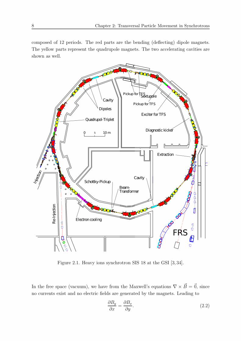
8 Chapter 2: Transversal Particle Movement in Synchrotrons
composed of 12 periods. The red parts are the bending (deflecting) dipole magnets.
The yellow parts represent the quadrupole magnets. The two accelerating cavities are
shown as well.
0 5 10 m
Schottky-Pickup
Transformer
Sextupole
Extraction
FRS
Electron cooling
Cavity
Cavity
Inje
ctio
n
Diagnostic kicker
Dipoles
Beam-
Re-
Inje
ctio
n
Quadrupol-Triplet
Exciter for TFS
Pickup for TFS
Pickup for TFS
Figure 2.1. Heavy ions synchrotron SIS 18 at the GSI [3, 34].
In the free space (vacuum), we have from the Maxwell’s equations ∇ × ~B = ~0, since
no currents exist and no electric fields are generated by the magnets. Leading to
∂By
∂x=
∂Bx
∂y. (2.2)

2.1 Synchrotron 9
The quadrupole magnetic field can be written as
Bx = B0y
a, By = B0
x
a. (2.3)
The focusing strength for a quadrupole magnet is defined as [28, 35]
κx =q
p0
∂By
∂x, κy = − q
p0
∂Bx
∂y. (2.4)
Therefore, magnetic field gradients that provide focusing in the horizontal direction x,
provide defocusing in the vertical direction y and vice versa. This motivates the use of
FODO cells [28, 31, 32].
2.1.1 FODO Cells
Most of synchrotrons, storage rings, as well as beam transfer lines are composed of
periodic segments of focusing/defocusing quadrupoles with drift tubes in-between. This
is the strong focusing concept of the so called FODO cells. Figure 2.2 shows an example
for a sequence of two FODO cells.
Figure 2.2. FODO cells.
With this optics structure, the focusing strength κ alternates between positive (focus-
ing), zero (drift tube), and negative (defocusing) in each transverse direction. Using the
general movement equations px = Fx and py = Fy one can write the particle transversal
movement equation in FODO cells after neglecting the effect of dipole magnets as
x′′(s) + κ(s)x(s) = 0 (2.5a)
y′′(s)− κ(s)y(s) = 0, (2.5b)
these are the so called Hill equations, where s denotes the longitudinal position around
the accelerator ring.

10 Chapter 2: Transversal Particle Movement in Synchrotrons
2.1.2 Particle Movement
The transversal movement of the particles inside a synchrotron is described by the
solution of Equations (2.5). When the function κ(s) is periodic, i.e., κ(s+L) = κ(s) for
some positive value L, i.e., the circumference of a circular accelerator, the transversal
movement equations can be solved by the Courant-Snyder ansatz. We show the solution
only for x(s) since the solution for y(s) has the same form. The general solution for
the Hill equation is given as [28, 36, 37]
x(s) =√ǫ√
β(s) cos(Ψ(s) + Ψ0), (2.6)
where
Ψ′(s) =1
β(s). (2.7)
The betatron function β(s) is a continuous function, which depends on the focusing
strength κ(s) and thus the lattice structure. ǫ and Ψ0 depend on the initial conditions.
Equation (2.7) shows that the phase of the betatron motion Ψ(s) changes faster for
smaller values of β(s).
The number of betatron oscillations a particle does after one turn is called the tune Q.
It is a very important machine parameter, where the optics lattice must be designed
such that the working point of the tunes is set far from resonance points. The tune
can be calculated based on Equation (2.7) as
Q =1
2π
L∫
0
1
β(s)ds. (2.8)
Equation (2.6) can alternatively be written as
x(s) = a0√
β(s) cos(Ψ(s)) + b0√
β(s) sin(Ψ(s)). (2.9)
Without loss of generality, we consider the starting position s = 0 such that Ψ(0) = 0.
the derivative of x with respect to s at this position is then given by
x′(0) = −a0α(0)√
β(0)+ b0
1√
β(0), (2.10)
with
α(s) = −β ′(s)
2. (2.11)
2.1 Synchrotron 11
One finds therefore
a0 =x(0)√
β(0), (2.12a)
b0 =√
β(0)x′(0) +α(0)√
β(0)x(0). (2.12b)
By substituting Equations (2.12) in Equation (2.9) and the derivative of x(s), and
solving the system of equations one can write in matrix form(x(s)x′(s)
)
= M ·(x(0)x′(0)
)
, (2.13)
where the transfer matrix is given by
M =
√ββ0[cos(Ψ) + α0 sin(Ψ)]
√ββ0 sin(Ψ)
−1√ββ0
[(1 + αα0) sin(Ψ) + (α− α0) cos(Ψ)]√
β0
β[cos(Ψ)− α sin(Ψ)]
, (2.14)
where β = β(s), β0 = β(0), α = α(s), α0 = α(0), and Ψ = Ψ(s).
Equation (2.13) shows that the beam displacement x and angle x′ can be calculated at
any position around the accelerator ring by knowing them at an initial position via a
transfer matrix dependency.
This section deals with particle movement ruled by the linear, i.e., ideal, lattice struc-
ture of the particle accelerator. Generally however, non-linear optics components are
present. This can be intentionally placed for other purposes, e.g., for chromaticity
correction or Landau damping increase, or it can be non-linear error components in
the lattice magnets. In this situation, the relationship between the beam oscillation
signals at different PUs is a manifestation of the accelerator optics linear and non-linear
components, and can therefore be exploited in the determination of the optics linear
and non-linear components [38].
2.1.3 Emittance
According to Liouville’s theorem one can see that trace space of particles with the same
value ǫ fulfills at every location s the equation [28, 36, 37]
γx2 + 2αxx′ + βx′2 = ǫ, (2.15)
where
γ(s) =1 + α(s)2
β(s), (2.16)
12 Chapter 2: Transversal Particle Movement in Synchrotrons
β, α, and γ are called Courant-Snyder parameters.
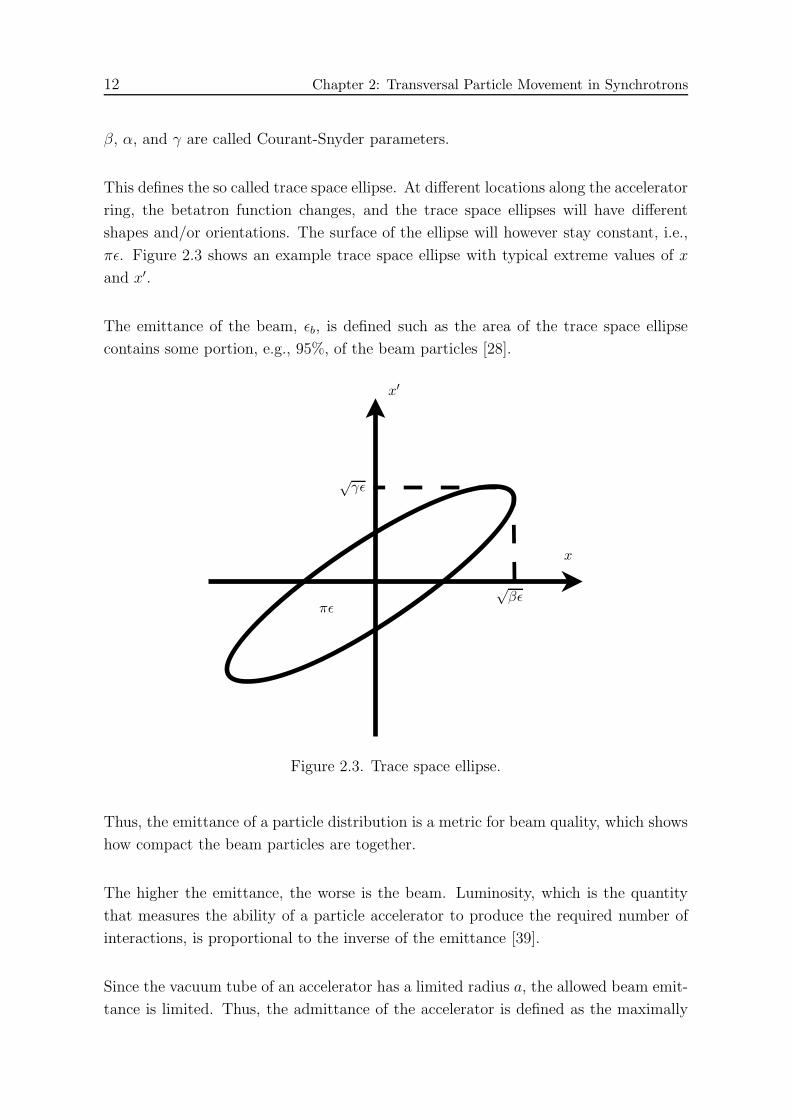
This defines the so called trace space ellipse. At different locations along the accelerator
ring, the betatron function changes, and the trace space ellipses will have different
shapes and/or orientations. The surface of the ellipse will however stay constant, i.e.,
πǫ. Figure 2.3 shows an example trace space ellipse with typical extreme values of x
and x′.
The emittance of the beam, ǫb, is defined such as the area of the trace space ellipse
contains some portion, e.g., 95%, of the beam particles [28].
πǫ
x
x′
√γǫ
√βǫ
Figure 2.3. Trace space ellipse.
Thus, the emittance of a particle distribution is a metric for beam quality, which shows
how compact the beam particles are together.
The higher the emittance, the worse is the beam. Luminosity, which is the quantity
that measures the ability of a particle accelerator to produce the required number of
interactions, is proportional to the inverse of the emittance [39].
Since the vacuum tube of an accelerator has a limited radius a, the allowed beam emit-
tance is limited. Thus, the admittance of the accelerator is defined as the maximally
2.2 Beam Instabilities 13
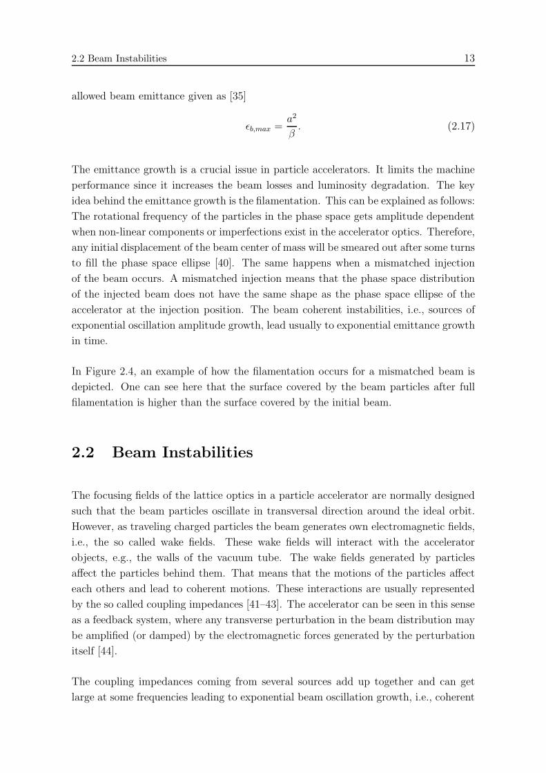
allowed beam emittance given as [35]
ǫb,max =a2
β. (2.17)
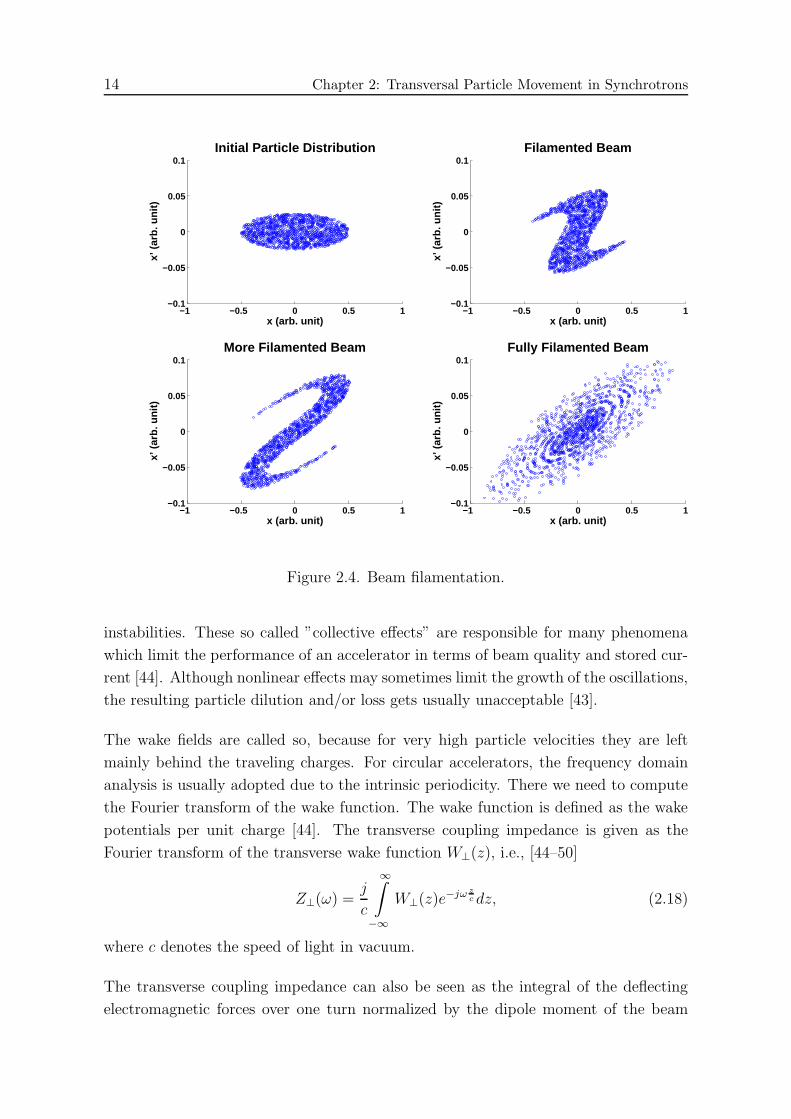
The emittance growth is a crucial issue in particle accelerators. It limits the machine
performance since it increases the beam losses and luminosity degradation. The key
idea behind the emittance growth is the filamentation. This can be explained as follows:
The rotational frequency of the particles in the phase space gets amplitude dependent
when non-linear components or imperfections exist in the accelerator optics. Therefore,
any initial displacement of the beam center of mass will be smeared out after some turns
to fill the phase space ellipse [40]. The same happens when a mismatched injection
of the beam occurs. A mismatched injection means that the phase space distribution
of the injected beam does not have the same shape as the phase space ellipse of the
accelerator at the injection position. The beam coherent instabilities, i.e., sources of
exponential oscillation amplitude growth, lead usually to exponential emittance growth
in time.
In Figure 2.4, an example of how the filamentation occurs for a mismatched beam is
depicted. One can see here that the surface covered by the beam particles after full
filamentation is higher than the surface covered by the initial beam.
2.2 Beam Instabilities
The focusing fields of the lattice optics in a particle accelerator are normally designed
such that the beam particles oscillate in transversal direction around the ideal orbit.
However, as traveling charged particles the beam generates own electromagnetic fields,
i.e., the so called wake fields. These wake fields will interact with the accelerator
objects, e.g., the walls of the vacuum tube. The wake fields generated by particles
affect the particles behind them. That means that the motions of the particles affect
each others and lead to coherent motions. These interactions are usually represented
by the so called coupling impedances [41–43]. The accelerator can be seen in this sense
as a feedback system, where any transverse perturbation in the beam distribution may
be amplified (or damped) by the electromagnetic forces generated by the perturbation
itself [44].
The coupling impedances coming from several sources add up together and can get
large at some frequencies leading to exponential beam oscillation growth, i.e., coherent
14 Chapter 2: Transversal Particle Movement in Synchrotrons
−1 −0.5 0 0.5 1−0.1
−0.05
0
0.05
0.1
x (arb. unit)
x’ (
arb.
uni
t)Initial Particle Distribution
−1 −0.5 0 0.5 1−0.1
−0.05
0
0.05
0.1
x (arb. unit)
x’ (
arb.
uni
t)
Filamented Beam
−1 −0.5 0 0.5 1−0.1
−0.05
0
0.05
0.1
x (arb. unit)
x’ (
arb.
uni
t)
More Filamented Beam
−1 −0.5 0 0.5 1−0.1
−0.05
0
0.05
0.1
x (arb. unit)
x’ (
arb.
uni
t)
Fully Filamented Beam
Figure 2.4. Beam filamentation.
instabilities. These so called ”collective effects” are responsible for many phenomena
which limit the performance of an accelerator in terms of beam quality and stored cur-
rent [44]. Although nonlinear effects may sometimes limit the growth of the oscillations,
the resulting particle dilution and/or loss gets usually unacceptable [43].
The wake fields are called so, because for very high particle velocities they are left
mainly behind the traveling charges. For circular accelerators, the frequency domain
analysis is usually adopted due to the intrinsic periodicity. There we need to compute
the Fourier transform of the wake function. The wake function is defined as the wake
potentials per unit charge [44]. The transverse coupling impedance is given as the
Fourier transform of the transverse wake function W⊥(z), i.e., [44–50]
Z⊥(ω) =j
c
∞∫
−∞
W⊥(z)e−jω z
c dz, (2.18)
where c denotes the speed of light in vacuum.
The transverse coupling impedance can also be seen as the integral of the deflecting
electromagnetic forces over one turn normalized by the dipole moment of the beam
2.2 Beam Instabilities 15
current. It describes in other words the Lorentz forces acting on the beam due to
the surroundings, i.e., the accelerator components [3, 49, 50]. Due to the increasing
demand for higher beam intensities in modern particle accelerators, the forces acting
on the beam get higher, which leads to more dangerous beam instabilities and losses [4].
The transverse wake function is the outcome of the effects of all accelerator components.
For a given component, it is basically its Green function in time domain, i.e., response
to a pulse excitation [50]. The transverse coupling impedance is a characteristic of the
beam environment, i.e., the accelerator, but not of the beam itself.
The transverse coupling impedance given in Equation (2.18) is a complex function. The
real part of this function is called the resistive part, and is responsible for the growth
or damping of beam coherent oscillations. The imaginary part in contrast induces tune
shift [3, 51]
In general, there are many sources for potential beam instabilities. We give in the
following an overview of the major components and sources of the transverse coupling
impedance in particle accelerator rings [3, 4, 51, 52].
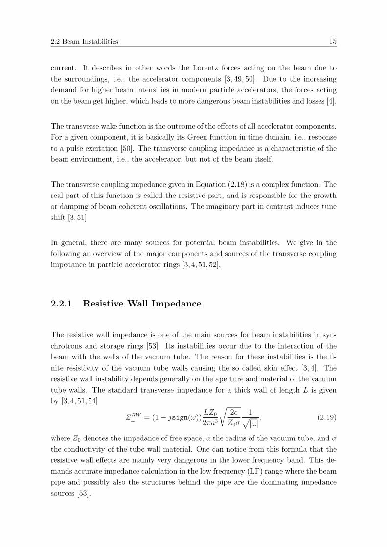
2.2.1 Resistive Wall Impedance
The resistive wall impedance is one of the main sources for beam instabilities in syn-
chrotrons and storage rings [53]. Its instabilities occur due to the interaction of the
beam with the walls of the vacuum tube. The reason for these instabilities is the fi-
nite resistivity of the vacuum tube walls causing the so called skin effect [3, 4]. The
resistive wall instability depends generally on the aperture and material of the vacuum
tube walls. The standard transverse impedance for a thick wall of length L is given
by [3, 4, 51, 54]
ZRW⊥ = (1− jsign(ω))
LZ0
2πa3
√2c
Z0σ
1√
|ω|, (2.19)
where Z0 denotes the impedance of free space, a the radius of the vacuum tube, and σ
the conductivity of the tube wall material. One can notice from this formula that the
resistive wall effects are mainly very dangerous in the lower frequency band. This de-
mands accurate impedance calculation in the low frequency (LF) range where the beam
pipe and possibly also the structures behind the pipe are the dominating impedance
sources [53].
16 Chapter 2: Transversal Particle Movement in Synchrotrons
2.2.2 Cavity High Order Modes
High spurious resonances of the particle accelerator cavity structure can be excited by
the traveling beam and act back on the beam itself. High Order Modes (HOMs) of the
cavities can couple with the wake fields generated by the beam particles, depending on
the beam distribution, and affect the following particles leading to resonances, which
increase the beam instabilities. This can occur in the horizontal as well as vertical
direction [4,55]. This kind of instabilities affects the beam around the HOM resonance
frequencies of the cavity. Therefore, its coupling impedance will have peaks at these
resonance frequencies.
Beam instabilities due to cavity HOM can be mitigated through proper design of the
cavity structure and employing mode dampers, e.g., antennas and resistive loads [4,56].
The full HOM spectrum of the cavity has to be analyzed already during the design
phase in order to identify potentially dangerous modes, and to define their damping
requirements. This can be achieved using beam simulation codes dedicated for this
purpose [55].
2.2.3 Other Beam Instability Sources
Vacuum chamber discontinuities, or abrupt changes of the vacuum chamber cross sec-
tion, can excite beam instabilities. Furthermore, small cavity-like structures located
along the vacuum chamber, e.g., in the Beam Position Monitors (BPMs), can interact
with beam such that HOMs of these structures get excited [3, 4]. The effect of these
instability sources can be reduced by a proper design of the vaccum chamber and the
various installed objects and devices of the accelerator [4, 57].
Depending on the shape of the beam profile, capacitive coupling of the beam with the
wall of the vacuum chamber will occur. This is the so called space charge impedance,
which has a pure imaginary contribution to total impedance of the particle accelerator.
This coupling is basically dominant for non-relativistic beams, i.e., at lower energy [3].
The molecules of the rest gas in the vacuum chamber can be ionized through the
collisions with the traveling charged beam. The interaction of the ionized molecules of
the rest gas with traveling beam can lead to coherent resonant oscillations [4].
We have given so far an overview of the most important potential sources for beam
coherent instabilities and possible cures. Besides these suggested cures that reduce

2.2 Beam Instabilities 17
unwanted beam instabilities by acting directly on the sources, there are many other
methods used in particle accelerators [4]. We give a short overview of these methods
in the following subsection.
2.2.4 Generic Countermeasures
Coherent bunch instabilities can be mitigated by increasing the Landau damping. This
can be achieved by increasing the betatron tune spread via increasing the momentum
spread of the beam particles [4, 56]. The demand for higher beam intensities is al-
ways increasing for modern accelerators. This leads to stronger interaction between
the traveling beam and accelerator objects, which increases the potential of coherent
transversal instabilities. Therefore, passive measures become not enough to attenu-
ate the beam oscillations and instabilities generated by the coherent beam-accelerator
interactions. Thus, active measures by means of feedback system must be employed.


19
Chapter 3
Transverse Feedback System and Noise
Minimization
In this chapter, we give an introduction to Transverse Feedback Systems (TFS). Fur-
ther, we explain our proposed novel concept to use multiple pickups (PUs) for estimat-
ing the beam displacement at the position with 90◦ phase advance before the kicker
position. The estimated values should be the driving feedback correction signal. The
signals from the different PUs are delayed such that they correspond to the same bunch
in every sample. Subsequently, a weighted sum of the delayed signals is suggested as an
estimator of the feedback correction signal. The weighting coefficients are calculated in
order to achieve an unbiased estimator, i.e., the output corresponds to the actual beam
displacement at the position with 90◦ phase advance before the kicker for non-noisy
PU signals. Furthermore, the estimator must provide the minimal noise power at the
output among all linear unbiased estimators.
Further, this concept is applied in a new approach to find optimal places for the pickups
and the kicker around the accelerator ring such that the noise effect on the feedback
quality is minimized. Simulation results and system design for the heavy ions syn-
chrotrons SIS 18 at the GSI are given at the end of this chapter.
3.1 Motivation
Transversal coherent beam oscillations have many sources in synchrotrons. They can
occur directly after injection due to inaccurate injection kicker reactions leading to
errors in position and angle of the beam after injection. Furthermore, the demand
for higher beam intensities in modern particle accelerator facilities is always growing.
The consequence of higher beam intensities is the increase of the interaction between
the traveling beam and accelerator components, which strengthen the potential of
coherent transversal instabilities. Thus, beam oscillations will occur when the natural
damping becomes not enough to attenuate the oscillations generated by the coherent
beam-accelerator interactions [4].
Due to the tune spread of the beam particles, de-coherence and filamentation will
occur to the oscillating beam. That leads to emittance blow up, which is harmful
20 Chapter 3: Transverse Feedback System and Noise Minimization
to the beam since it deteriorates the beam quality by increasing the beam losses and
reducing the luminosity of colliders [1,58], i.e., number of interactions (useful collisions)
per second [1,2,39]. Therefore, strong beam oscillations can not be tolerated, and must
be suppressed in order to maintain high beam quality during acceleration cycle.
Coherent bunch instabilities can be mitigated by optimizing and controlling the particle
accelerator objects and modules and their coupling impedances, and by increasing the
Landau damping of the beam. This can be be achieved by increasing the betatron tune
spread through increasing the momentum spread of the beam particles [4,56]. However,
the always increasing demand for higher beam intensities leads to the fact that passive
measures lack of the ability to stabilize the beam oscillations and instabilities. Thus,
active measures by means of feedback system must be employed [4].
A very powerful mean for suppressing the coherent beam instabilities is the use of
feedback systems. Transversal Feedback Systems (TFS) sense the instabilities of the
beam by means of sensors, called Pickups (PUs), and act back on the beam by means
of actuators, called kickers [3, 4].
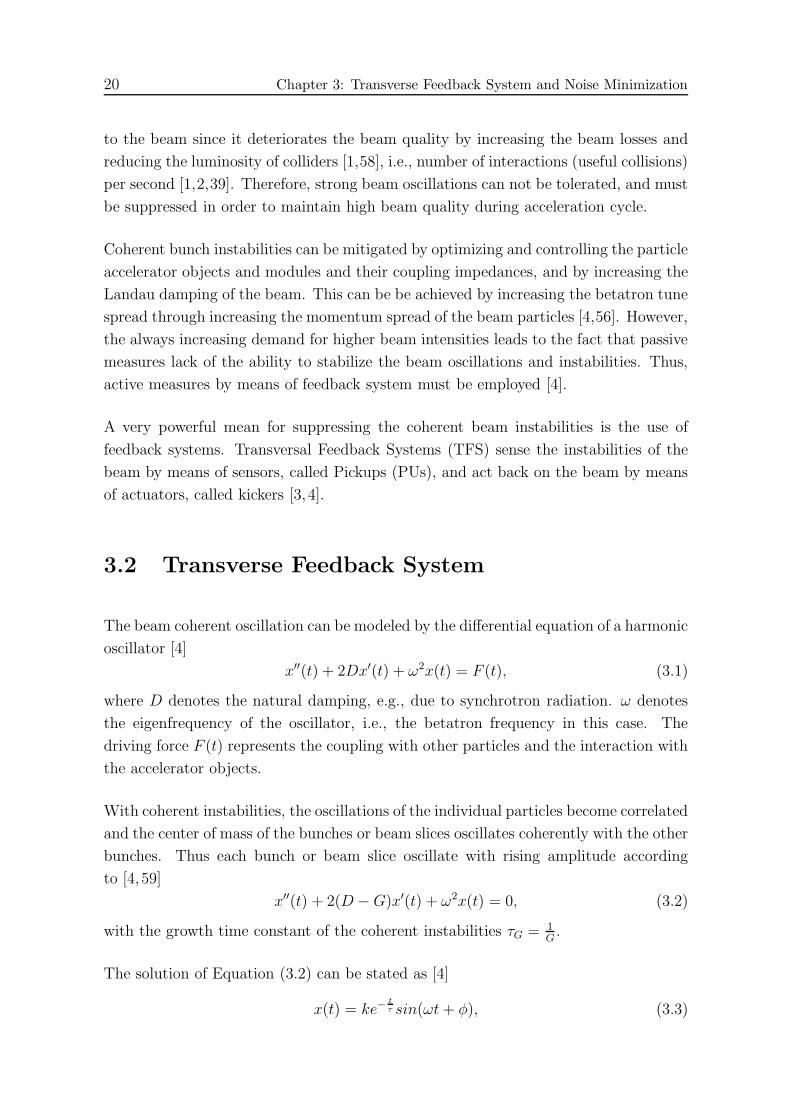
3.2 Transverse Feedback System
The beam coherent oscillation can be modeled by the differential equation of a harmonic
oscillator [4]
x′′(t) + 2Dx′(t) + ω2x(t) = F (t), (3.1)
where D denotes the natural damping, e.g., due to synchrotron radiation. ω denotes
the eigenfrequency of the oscillator, i.e., the betatron frequency in this case. The
driving force F (t) represents the coupling with other particles and the interaction with
the accelerator objects.
With coherent instabilities, the oscillations of the individual particles become correlated
and the center of mass of the bunches or beam slices oscillates coherently with the other
bunches. Thus each bunch or beam slice oscillate with rising amplitude according
to [4, 59]
x′′(t) + 2(D −G)x′(t) + ω2x(t) = 0, (3.2)
with the growth time constant of the coherent instabilities τG = 1G.
The solution of Equation (3.2) can be stated as [4]
x(t) = ke−tτ sin(ωt+ φ), (3.3)

3.2 Transverse Feedback System 21
where τ = 1D−G
. The beam becomes stable whenD ≥ G, otherwise the beam oscillation
grows exponentially.
The TFS action must affect the beam motion by compensating the growth rate. This
happens when the feedback correction signal applies to the beam a force proportional
to the derivative of the beam oscillation, i.e., Ffb(t) = −2Dfbx′(t), such that the beam
oscillation equation turns to
x′′(t) + 2(D −G +Dfb)x′(t) + ω2x(t) = 0. (3.4)
The TFS will be able to stabilize the beam, i.e., damp the beam oscillation, when its
gain fulfills the following inequality
D −G+Dfb > 0. (3.5)
Depending on the way how the feedback system senses and acts back on the beam
instabilities, there are two main types [4]:
• Frequency domain TFS: Controls unstable beam modes in frequency domain.
It is also called Mode-by-mode TFS. This concept is feasible when the number
of potentially unstable frequencies is small enough, otherwise alternative time
domain feedback must be employed.
• Time domain TFS: acts on the beam based on each sampled value by the Beam
Position Monitor (BPM). When the action rate gets less, and every bunch of the
beam gets one turn-by-turn kick, it is called bunch-by-bunch feedback system.
The correction signal for each sample must act on the same beam slice corre-
sponding to that sample via proper adjustable delay lines. This is the concept
we adopt in this thesis.
Figure 3.1 shows a block diagram of the TFS. The BPM senses the beam displacement
in horizontal and vertical direction by means of four plates. The signals of the BPM
plates get merged by the combiner in order to get the beam displacement and the sum
signal corresponding to the beam intensity. The role of the detector is to translate the
BPM signal into the base-band. The heterodyne technique in telecommunications can
be used in this part of the TFS [4]. Due to numerous advantages,e.g., reproducibility,
programmability, easier and efficient integration, performance, and ability of more
sophisticated processing, the signal processing part of the TFS is done nowadays only

22 Chapter 3: Transverse Feedback System and Noise Minimization
BPM
Combiner
Detector AD Digital Signal
Processing DA
Power Amp.
Kicker
Figure 3.1. Block diagram of TFS.
in the digital domain using Digital Signal Processors (DSP) and/or FPGA. Therefore,
converters from analog to digital and vice versa are required in the TFS. To close the
feedback loop, the kicker equipped with a power amplifier is used to correct the beam
position.
Since the beam oscillation motion has a sinusoidal form, the feedback correction signal
applied by the kicker, i.e., actuator, corresponding to the derivative of the beam oscil-
lation must have a 90◦ phase advance with respect to the betatron oscillation signal
at the kicker position in order to have a damping impact. This can be achieved by
passing the signal of one PU through a feedback filter, e.g., finite impulse response
(FIR) filter with suitable phase response at the fractional tune frequency, with proper
delay [4]. The number of the filter taps can be increased in order to have more degrees
of freedom for optimizing the filter response, e.g., to have maximum flatness around
the working point for robustness against tune changes [4,18], higher selectivity for bet-
ter rejection of undesired frequency components [4], minimum amplitude response at
specific frequencies that should not be fed back [19], stabilize different tune frequencies
simultaneously [20]. Advanced concepts from the control theory have been applied
also in the design of the feedback filter [21]. These approaches introduce however extra
turns delay depending on how many taps the FIR filter consists of.
In [3], an approach was proposed to calculate the horizontal and vertical beam displace-
ments at the position with 90◦ phase difference before the kicker using PUs located at
two different positions along the accelerator ring for each of the horizontal and vertical
directions. The reason for requiring PUs at two different positions for defining the
beam trace space is that only beam displacements from the ideal trajectory can be
measured by the PUs, but not the angles of the beam. Nevertheless, this approach
does not consider the harmful noise at the PUs neither the robustness of the system

3.3 Using Multiple Pickups in TFS for Noise Power Minimization 23
against unwanted deviations.
In general, the signals at the PUs are disturbed by noise. The Signal-to-Noise power
Ratio (SNR) can be unacceptably low or not high enough. This is the case especially
for lower currents where the beam is getting corrected by a big noise portion during
the feedback. That will worsen the feedback correction quality as it leads to beam
heating [13,14] and emittance blow up [4], as already mentioned in the previous chapter.
3.3 Using Multiple Pickups in TFS for Noise Power
Minimization
In this section, we address a novel approach for mitigating noise at the PUs using
more than two PUs at different positions to estimate the feedback correction signal
for the kicker position, which has 90◦ phase difference from the betatron motion at
this position. This is done by calculating a weighted sum of the PUs signals after
proper synchronization [60, 61]. The idea here is to have more degrees of freedom
using more PUs to adjust the sum weights such that the noise power contained in
the estimated signal is minimized, while keeping a correct formula for calculating the
beam displacement at the position with 90◦ phase advance before the kicker position
in absence of PUs noise.
This is the Best Linear Unbiased Estimator (BLUE). Ideally, one would like to have
the Minimum-Variance Unbiased Estimator (MVUE). The maximum likelihood esti-
mator (MLE) is a well known preferable estimator in this sense due to its asymptotic
optimality. This requires however the knowledge of the probability density of the noise.
Furthermore, it leads to optimization problems that generally do not have analytical
solutions, but must be solved iteratively. This is not really applicable for a TFS that
needs calculations in real time. Also, in the special case of Gaussian noise with the
linear model, the MLE becomes the same as the BLUE [62].
3.3.1 System Model
For each position along the synchrotron ring, three coordinate axes are defined, which
determine the different possible beam displacements from the ideal trajectory. Fig-
ure 3.2 shows the transversal directions at some point along the accelerator ring: x-
axis for horizontal displacement, and y-axis for vertical displacement. The longitudinal
direction axis is marked by s.
24 Chapter 3: Transverse Feedback System and Noise Minimization
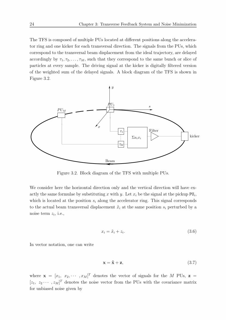
The TFS is composed of multiple PUs located at different positions along the accelera-
tor ring and one kicker for each transversal direction. The signals from the PUs, which
correspond to the transversal beam displacement from the ideal trajectory, are delayed
accordingly by τ1, τ2, . . . , τM , such that they correspond to the same bunch or slice of
particles at every sample. The driving signal at the kicker is digitally filtered version
of the weighted sum of the delayed signals. A block diagram of the TFS is shown in
Figure 3.2.
PUM
PU1
τ1
τM
Σaixi
Filter
kicker
Beam
x
y
s
Figure 3.2. Block diagram of the TFS with multiple PUs.
We consider here the horizontal direction only and the vertical direction will have ex-
actly the same formulae by substituting x with y. Let xi be the signal at the pickup PUi,
which is located at the position si along the accelerator ring. This signal corresponds
to the actual beam transversal displacement xi at the same position si perturbed by a
noise term zi, i.e.,
xi = xi + zi. (3.6)
In vector notation, one can write
x = x + z, (3.7)
where x = [x1, x2, · · · , xM ]T denotes the vector of signals for the M PUs, z =
[z1, z2 · · · , zM ]T denotes the noise vector from the PUs with the covariance matrix
for unbiased noise given by
3.3 Using Multiple Pickups in TFS for Noise Power Minimization 25
Rzz = E{zzT}. (3.8)
In Equation (3.7), x = [x1, x2 · · · , xM ]T denotes the actual beam displacements vector
at the PUs positions s1, s2, · · · , sM .
The noise part in the signal can be caused by different sources, e.g., thermal noise
generated by the PUs electronics and disturbances from other devices. Thermal noise
can be modeled as white noise spectrally shaped by the front-end electronics of each of
the PUs. This noise part is basically uncorrelated between the signals from different
PUs. The PUs can produce thermal noise powers different from each other when
they are not similar, or placed in different environments, like in cryostat or room
temperature. The disturbances at the PUs depend mainly on the locations of the PUs,
and could be correlated between some neighbored PUs. This noise contribution could
have narrow-band or wide-band spectral components, depending on the disturbers.
According to Equation (2.13) and Equation (2.14) the beam displacement at the posi-
tion sk90 with 90◦ phase advance before the kicker position can be calculated using the
beam status at the position of PUi in the form(x(sk90)x′(sk90)
)
=
(Ai Bi
Ci Di
)
·(x(si)x′(si)
)
. (3.9)
Therefore, one can calculate xk90 using the beam displacements xi1 and xi2 at the
positions si1 and si2 of PUi1 and PUi2 , where i1, i2 ∈ {1, 2, · · · , M}, according to the
vector summation approach introduced in [3] as
x(sk90) = α1,i1,i2xi1 + α2,i1,i2 xi2 , (3.10)
where
α1,i1,i2 =Ai1Bi2Di1 −Bi1Ci1Bi2
Bi2Di1 −Di2Bi1
, (3.11)
and
α2,i1,i2 =Bi1Ci2Bi2 − Bi1Di2Ai2
Bi2Di1 −Di2Bi1
. (3.12)
Thus, the estimator of the feedback correction signal for the kicker position can be
expressed by
xi1,i2 = α1,i1,i2xi1 + α2,i1,i2xi2
= α1,i1,i2xi1 + α2,i1,i2xi2 + α1,i1,i2zi1 + α2,i1,i2zi2
= xk90 + zi1,i2 (3.13)
26 Chapter 3: Transverse Feedback System and Noise Minimization
where xk90 = x(sk90) is the ideal feedback correction signal driving the kicker, α1,i1,i2
and α2,i1,i2 are constants, which depend on the lattice functions of the accelerator
according to Courant-Snyder Ansatz [28, 36, 63]. In Equation (3.13), zi1,i2 denotes the
noise part in the estimate of the feedback correction signal.
The noise-free signals at each PU for each bunch are sinusoidal with the fractional-tune
frequency with different phases, considering a linear lattice. Therefore, the turn-wise
weighted sum of these signals will give a sinusoidal signal with the same frequency,
where the phase and amplitude are proportional to the summation weights. In practice
however, only kicking on the second or a later turn is feasible. This kicking delay will
only affect the required phase shift, and hence the weighting factors.
3.3.2 Optimal Linear Combiner
In order to mitigate the disturbing noise part in the estimation of the feedback correc-
tion signal at the kicker position, we address a new approach to calculating an optimally
weighted sum of the signals from multiple PUs to be the feedback correction.
The idea of this approach is to filter out the noise from the PU signals by estimating
the beam displacement at the position sk90 located 90◦ before the kicker as a weighted
sum of the signals from M PUs, i.e., three or more. The weighting coefficients must
be calculated in an optimal way such that the power of the noise part at the estimator
output signal is minimized and the weighted sum of the actual beam displacement at
the PUs positions without noise corresponds to the actual beam displacement at the
position sk90.
The optimization problem can be formulated as follows
[a1, · · · , aM ] = argmina1,··· ,aM
E{|M∑
i=1
aizi|2} (3.14a)
s.t.
M∑
i=1
aixi(t) = xk90(t), ∀t ∈ R. (3.14b)
This is a convex optimization problem and can be reformulated as
aopt = [a1, · · · , aM ]T = argmina
aTRzza (3.15a)

3.3 Using Multiple Pickups in TFS for Noise Power Minimization 27
s.t. aTbr = 1 (3.15b)
aTbi = 0, (3.15c)
where br ∈ RM and bi ∈ RM are the real and imaginary parts of the phasors of the PU
signals, respectively. The betatron oscillation at the position with 90◦ phase advance
with respect to the kicker is considered here as a reference for the phasors.
Many iterative methods exist to solve such a convex optimization problem efficiently.
However, a closed form solution would be more preferable since this solution will be
applied on a later approach with exhaustive search nested iterations.
3.3.2.1 Analytical Solution
The Method of Lagrange Multipliers can be used to find an analytical solution for
the optimization problem given in Equations (3.15). The Lagrange function of this
problem is given as
L = aTRzza+ λr(aTbr − 1) + λia
Tbi. (3.16)
A solution can be found by solving the equation
∇a,λr,λiL = 0, (3.17)
therefore,
2Rzza = −λrbr − λibi (3.18)
aTbr = 1 (3.19)
aTbi = 0. (3.20)
From Equation (3.18), one finds
a = −λr
2R−1
zz br −λi
2R−1
zz bi, (3.21)
28 Chapter 3: Transverse Feedback System and Noise Minimization
substituting in Equation (3.19) and Equation (3.20) one finds out that
λr =−2bi
TR−1zz bi
biTR−1
zz bibrTR−1
zz br − (brTR−1
zz bi)2(3.22)
λi =2br
TR−1zz bi
biTR−1
zz bibrTR−1
zz br − (brTR−1
zz bi)2(3.23)
Subsequently, the optimal weights aopt can be found by substituting the values of λr
and λi given in Equation (3.22) and Equation (3.23) into Equation (3.21) as
aopt =R−1
zz brbiTR−1
zz bi −R−1zz bibr
TR−1zz bi
biTR−1
zz bibrTR−1
zz br − (brTR−1
zz bi)2, (3.24)
leading to the optimal noise power
PNmin = aToptRzzaopt. (3.25)
3.3.2.2 Alternative Solution
The optimization problem stated in Equation (3.14) can also be solved by reformulating
it using vector summations of PU signals pairwise as follows: The beam displacement
signal at the position sk90 with 90◦ phase advance with respect to the kicker position
can be estimated according to the vector summation approach using any two of the M
PU signals. Consider the consecutive signal pairs {x1, x2}, {x2, x3}, · · · , {xM−1, xM},The estimates can be written in matrix notation as follows
x1,2
x2,3...
xM−1,M
= Λ
x1
x2...
xM
(3.26)
= Λx +Λz (3.27)
=
xk90...
xk90
+Λz (3.28)
where the matrix Λ is given via the vector summation of the above mentioned PU
pairs by
3.3 Using Multiple Pickups in TFS for Noise Power Minimization 29
Λ =
α1,1,2 α2,1,2 0 · · · 00 α1,2,3 α2,2,3 0 · · · 0
0 0. . .
. . . 0 · · ·...
... · · · 0. . .
. . . · · ·0 · · · 0 · · · α1,M−1,M α2,M−1,M
(3.29)
When the consecutive PUs of some pairs are located with betatron phase shift of
kπ, k ∈ Z, it is not possible to construct the vector summation. In this special case,
the PUs must be reordered and M −1 independent pairs must be considered such that
the vector summation can be achieved for all given new pairs, and the matrix Λ must
be constructed accordingly.
Let w = [w1, w2, · · · , wM−2, 1−M−2∑
i=1
wi]T , then the following holds:
wT
x1,2
x2,3...
xM−1,M
= xk90 +wTΛz ∀w1, · · · , wM−2 ∈ RM−2 (3.30)
The optimization problem given in Equation (3.14) is equivalent to finding the opti-
mal vector wopt which minimizes the power of the noise term in Equation (3.30), i.e.,
E|wTΛz|2, where the optimal weights can be written as
aTopt = wT
optΛ. (3.31)
The reason for this equivalence is that both problems have the same number of dimen-
sions, i.e., ND = M − 2, in addition to describing the same unbiased estimator with
minimized noise.
The vector w can be written in the following form
w = Dw + eM−1 (3.32)
where

30 Chapter 3: Transverse Feedback System and Noise Minimization
w = [w1, w2, · · · , wM−2]T , (3.33)
eM−1 = [0, 0, · · · , 0, 1]T ∈ RM−1, (3.34)
and D ∈ RM−1×M−2 with all ones in the main diagonal, all −1 on the last row, and
zeros elsewhere.
Therefore, the noise power is given by
PN = E|wTΛz|2
= wTDTΛRzzΛTDw
+ 2wTDTΛRzzΛTeM−1
+ eTM−1ΛRzzΛTeM−1
(3.35)
An optimal solution wopt can be found by setting the derivative of PN with respect to
w to zero and solving, i.e.,
∂PN
∂w
∣∣∣∣wopt
= 0 (3.36)
for which the solution is found to be
wopt = −(DTΛRzzΛTD)−1DTΛRzzΛ
TeM−1 (3.37)
Finally, the optimal weights aopt can be calculated using Equation (3.31) and Equa-
tion (3.37), i.e.,
aopt = (−D(DTΛRzzΛTD)−1DTΛRzzΛ
TeM−1 + eM−1)TΛ. (3.38)
3.4 Optimal Pickups-Kicker Placement for Noise Power Minimization 31
3.3.2.3 Example
In order to illustrate the equivalence between the solutions given in Equation (3.24)
and Equation (3.38), we consider the following example:
Let the kicker be placed at a position with a phase of −90◦. The phase reference of the
betatron oscillation at the position with 90◦ phase advance with respect to the kicker
has thus zero phase. Suppose we have PU1, PU2 and PU3 with the phases 120◦, 180◦
and 240◦, respectively, and the same β values as at the kicker position. Therefore, we
have br = [−0.5,−1,−0.5]T and bi = [0.866, 0,−0.866]T . Assuming Rzz = I3 to be
the identity matrix of dimensions 3 × 3 for i.i.d. noise at the PUs, we find according
to Equation (3.21) using the optimal values for λi and λr that the optimal weights are
aopt = [−0.333,−0.667,−0.333].
Taking the pairs {PU1, PU3} and {PU3, PU2}, and according to Equation (3.29), we have
Λ =
(−1 −1 00 0 −1
)
.
Having D = [1,−1]T and eM−1 = [0, 1]T , and applying Equation (3.38), we come up
with the same weights as before.
3.4 Optimal Pickups-Kicker Placement for Noise
Power Minimization
In the previous section, we introduced the optimal linear unbiased minimum variance
estimator by using multiple PUs and one kicker for the TFS, where the positions
s1, · · · , sM of the PUs and sk of the kicker are fixed and known a priori. However, if
the PUs and the kicker are placed in the accelerator without any further considerations,
except for free space, the performance of the TFS might be limited or even poor, even
when using an optimal approach for calculating the feedback correction signal based
on the given combination of the PU signals. This can be the case, especially when the
randomly chosen positions of the PUs and the kicker are close to the worst possible
positions, or very far away from the ideal positions.
In this section, we address a new approach for finding the best positions to place the
PUs and the kicker among all possible free locations around the accelerator ring, which
are not occupied by other accelerator devices. The PUs and the kicker should be

32 Chapter 3: Transverse Feedback System and Noise Minimization
placed such that the noise generated at the PUs causes the smallest disturbance to the
feedback quality. As a metric for the noise disturbance, we use the SNR at the feedback
correction signal estimate for the kicker position. The noise power is considered here
at the output of the previously mentioned MVUE, which is the lowest possible noise
power at the output of a linear unbiased estimator of the feedback correction signal for
the given placement.
Since the beam displacement at the position with 90◦ betatron phase shift from the
kicker position is the signal of interest for this approach, we take the squared value of
the maximum possible amplitude at that position as a measure for the signal power.
From the trace-space ellipse depicted in Figure 2.3, one can see that the maximum at
a specific position s is given by
xk max(s) =√
β(s)ǫ, (3.39)
where ǫ is scaling factor, which is independent of the position s. Therefore, we take
the signal power as
PSig = |xk max(s)|2 ∼ β(s). (3.40)
Hence, the SNR in one transversal (horizontal or vertical) direction for the given loca-
tions of the PUs and the kicker can be written as
SNRx/y =βx/y(sk)
PNx/ymin(s1, s2, · · · , sM , sk)
, (3.41)
where the minimum noise power for a specific transversal direction PNx/yminis given
in Equation (3.25). Thus, the SNR value depends on the betatron value βx/y(sk)
and PNx/ymin(s1, s2, · · · , sM , sk), which depend according to Equation (3.35) and
Equation (3.37) on the noise covariance matrix Rzz, and the parameters αij stated in
Equation (3.29). These parameters again depend on the Twiss parameters for the PUs
and kicker locations, and the phase differences between the PUs and the kicker. In
summary, the SNR value depends on all of the Twiss parameters and phases for the
PUs and kicker positions.

3.4 Optimal Pickups-Kicker Placement for Noise Power Minimization 33
Since the PUs and the kicker are devices for both of the horizontal and vertical direc-
tions at once, the optimized SNR value should include the summation of the SNRs of
both transversal directions, i.e.,
SNR = SNRx + SNRy. (3.42)
The optimal positions [s1, s2, · · · , sM , sk] of the PUs and the kicker can thus be
calculated by
[s1, s2, · · · , sM , sk] = argmaxs1,s2,··· ,sM ,sk
SNR (3.43a)
s.t. [s1, s2, · · · , sM , sk] ∈ FM+1, (3.43b)
where F is the ensemble of unoccupied positions around the accelerator ring, where
the PUs and the kicker can be placed at.
3.4.1 Changing Optics
The previous design technique requires the lattice functions to be constant during the
acceleration cycle, i.e., constant focusing. However, the focusing can be changed during
acceleration, e.g., from triplet mode to doublet mode as at the SIS 18 at the GSI in
Darmstadt [3].
The quadrupole magnets of the SIS 18 are distributed around the accelerator ring in
twelve segments. Each segment contains a triplet of quadrupoles. This constellation
can provide low and smooth betatron function [34]. This increases the acceptance of
the machine at the injection energy, which is important to cope with the injection
errors.
Nevertheless, the beam extraction requires higher betatron values. This can be fulfilled
using doublets of quadrupole magnets in the twelve segments of the accelerator ring
[3, 34]. Therefore, the transition from the triplet optics at the injection energy to
the doublet optics at the extraction energy level is passed continuously during the
acceleration ramp.
For this variable focusing, an average value or a weighted average of the SNR, depending
on the importance, can be maximized. In the case of smoothly changing focusing optics

34 Chapter 3: Transverse Feedback System and Noise Minimization
like from triplet to doublet, the averaging of the SNR can be done via a cycle variable
τfocusing, which defines for instance the strength of triplet operation at the SIS 18.
τfocusing = 0 corresponds to doublet mode and τfocusing = 1 corresponds to triplet
mode. Therefore, the optimal positions of the PUs and the kicker can be calculated
for variable focusing by
sopt = argmaxs
∫ 1
0
w(τ)SNR(τ) dτ (3.44a)
s.t. s = [s1, s2, · · · , sM , sk] ∈ FM+1, (3.44b)
where w(τ) is a weighting function, which can be chosen constant for uniform averaging
over an acceleration cycle.
3.5 Results
In this section, we show simulation results of the previously addressed approaches in
this chapter for the heavy ions synchrotron SIS 18 at the GSI, which has a circumference
of 216 m.
In the SIS 18, there are 12 PUs for the horizontal and the vertical directions, which
are located periodically along the synchrotron ring. There is also one feedback kicker
for both transversal directions. The phase difference between each two neighbouring
pickups corresponds to the machine tune of every transversal direction divided by 12.
For the horizontal direction, we have a phase difference of 129.3◦ between each two
neighbouring pickups, and for the vertical direction 99.2◦. During the acceleration, fo-
cusing changes continuously from the triplet mode to the doublet mode, which changes
the betatron functions during each acceleration cycle, without changing the tune. The
machine tunes for the horizontal and vertical directions are respectively Qx = 4.31 and
Qy = 3.31.
The betatron functions βx(s) and βy(s) along the SIS 18 ring in the triplet and doublet
modes are shown in Figure 3.3. The 12 periodical sections are clearly remarkable.
Moreover, one can notice that the betatron function in the horizontal direction in the
doublet mode has higher values than in the triplet mode. This is required for the
extraction system [3, 34].
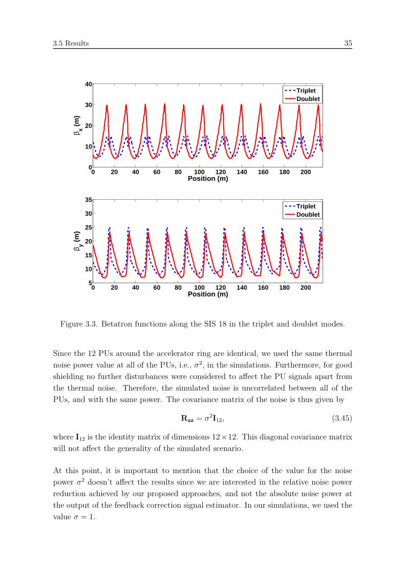
3.5 Results 35
0 20 40 60 80 100 120 140 160 180 2000
10
20
30
40
Position (m)
β x (m
)
TripletDoublet
0 20 40 60 80 100 120 140 160 180 2005
10
15
20
25
30
35
Position (m)
β y (m
)
TripletDoublet
Figure 3.3. Betatron functions along the SIS 18 in the triplet and doublet modes.
Since the 12 PUs around the accelerator ring are identical, we used the same thermal
noise power value at all of the PUs, i.e., σ2, in the simulations. Furthermore, for good
shielding no further disturbances were considered to affect the PU signals apart from
the thermal noise. Therefore, the simulated noise is uncorrelated between all of the
PUs, and with the same power. The covariance matrix of the noise is thus given by
Rzz = σ2I12, (3.45)
where I12 is the identity matrix of dimensions 12×12. This diagonal covariance matrix
will not affect the generality of the simulated scenario.
At this point, it is important to mention that the choice of the value for the noise
power σ2 doesn’t affect the results since we are interested in the relative noise power
reduction achieved by our proposed approaches, and not the absolute noise power at
the output of the feedback correction signal estimator. In our simulations, we used the
value σ = 1.
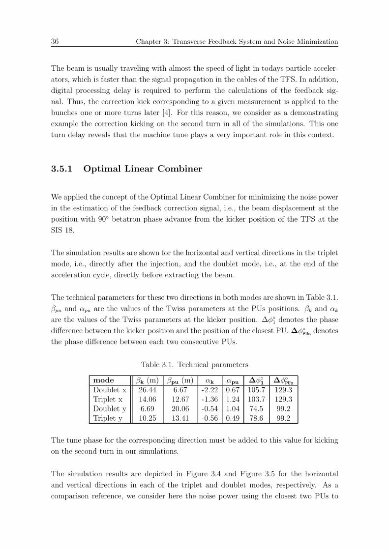
36 Chapter 3: Transverse Feedback System and Noise Minimization
The beam is usually traveling with almost the speed of light in todays particle acceler-
ators, which is faster than the signal propagation in the cables of the TFS. In addition,
digital processing delay is required to perform the calculations of the feedback sig-
nal. Thus, the correction kick corresponding to a given measurement is applied to the
bunches one or more turns later [4]. For this reason, we consider as a demonstrating
example the correction kicking on the second turn in all of the simulations. This one
turn delay reveals that the machine tune plays a very important role in this context.
3.5.1 Optimal Linear Combiner
We applied the concept of the Optimal Linear Combiner for minimizing the noise power
in the estimation of the feedback correction signal, i.e., the beam displacement at the
position with 90◦ betatron phase advance from the kicker position of the TFS at the
SIS 18.
The simulation results are shown for the horizontal and vertical directions in the triplet
mode, i.e., directly after the injection, and the doublet mode, i.e., at the end of the
acceleration cycle, directly before extracting the beam.
The technical parameters for these two directions in both modes are shown in Table 3.1.
βpu and αpu are the values of the Twiss parameters at the PUs positions. βk and αk
are the values of the Twiss parameters at the kicker position. ∆φ◦1 denotes the phase
difference between the kicker position and the position of the closest PU. ∆φ◦PUs denotes
the phase difference between each two consecutive PUs.
Table 3.1. Technical parameters
mode βk (m) βpu (m) αk αpu ∆φ◦1 ∆φ◦
PUs
Doublet x 26.44 6.67 -2.22 0.67 105.7 129.3Triplet x 14.06 12.67 -1.36 1.24 103.7 129.3Doublet y 6.69 20.06 -0.54 1.04 74.5 99.2Triplet y 10.25 13.41 -0.56 0.49 78.6 99.2
The tune phase for the corresponding direction must be added to this value for kicking
on the second turn in our simulations.
The simulation results are depicted in Figure 3.4 and Figure 3.5 for the horizontal
and vertical directions in each of the triplet and doublet modes, respectively. As a
comparison reference, we consider here the noise power using the closest two PUs to
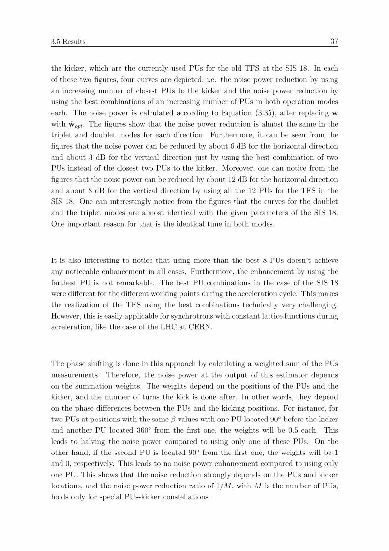
3.5 Results 37
the kicker, which are the currently used PUs for the old TFS at the SIS 18. In each
of these two figures, four curves are depicted, i.e. the noise power reduction by using
an increasing number of closest PUs to the kicker and the noise power reduction by
using the best combinations of an increasing number of PUs in both operation modes
each. The noise power is calculated according to Equation (3.35), after replacing w
with wopt. The figures show that the noise power reduction is almost the same in the
triplet and doublet modes for each direction. Furthermore, it can be seen from the
figures that the noise power can be reduced by about 6 dB for the horizontal direction
and about 3 dB for the vertical direction just by using the best combination of two
PUs instead of the closest two PUs to the kicker. Moreover, one can notice from the
figures that the noise power can be reduced by about 12 dB for the horizontal direction
and about 8 dB for the vertical direction by using all the 12 PUs for the TFS in the
SIS 18. One can interestingly notice from the figures that the curves for the doublet
and the triplet modes are almost identical with the given parameters of the SIS 18.
One important reason for that is the identical tune in both modes.
It is also interesting to notice that using more than the best 8 PUs doesn’t achieve
any noticeable enhancement in all cases. Furthermore, the enhancement by using the
farthest PU is not remarkable. The best PU combinations in the case of the SIS 18
were different for the different working points during the acceleration cycle. This makes
the realization of the TFS using the best combinations technically very challenging.
However, this is easily applicable for synchrotrons with constant lattice functions during
acceleration, like the case of the LHC at CERN.
The phase shifting is done in this approach by calculating a weighted sum of the PUs
measurements. Therefore, the noise power at the output of this estimator depends
on the summation weights. The weights depend on the positions of the PUs and the
kicker, and the number of turns the kick is done after. In other words, they depend
on the phase differences between the PUs and the kicking positions. For instance, for
two PUs at positions with the same β values with one PU located 90◦ before the kicker
and another PU located 360◦ from the first one, the weights will be 0.5 each. This
leads to halving the noise power compared to using only one of these PUs. On the
other hand, if the second PU is located 90◦ from the first one, the weights will be 1
and 0, respectively. This leads to no noise power enhancement compared to using only
one PU. This shows that the noise reduction strongly depends on the PUs and kicker
locations, and the noise power reduction ratio of 1/M , with M is the number of PUs,
holds only for special PUs-kicker constellations.
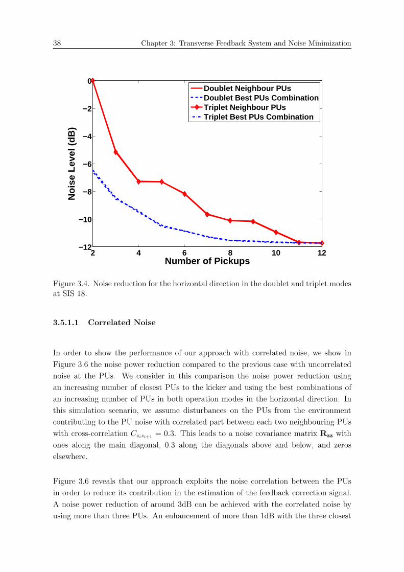
38 Chapter 3: Transverse Feedback System and Noise Minimization
2 4 6 8 10 12−12
−10
−8
−6
−4
−2
0
Number of Pickups
Noi
se L
evel
(dB
)
Doublet Neighbour PUsDoublet Best PUs CombinationTriplet Neighbour PUsTriplet Best PUs Combination
Figure 3.4. Noise reduction for the horizontal direction in the doublet and triplet modesat SIS 18.
3.5.1.1 Correlated Noise
In order to show the performance of our approach with correlated noise, we show in
Figure 3.6 the noise power reduction compared to the previous case with uncorrelated
noise at the PUs. We consider in this comparison the noise power reduction using
an increasing number of closest PUs to the kicker and using the best combinations of
an increasing number of PUs in both operation modes in the horizontal direction. In
this simulation scenario, we assume disturbances on the PUs from the environment
contributing to the PU noise with correlated part between each two neighbouring PUs
with cross-correlation Czizi+1= 0.3. This leads to a noise covariance matrix Rzz with
ones along the main diagonal, 0.3 along the diagonals above and below, and zeros
elsewhere.
Figure 3.6 reveals that our approach exploits the noise correlation between the PUs
in order to reduce its contribution in the estimation of the feedback correction signal.
A noise power reduction of around 3dB can be achieved with the correlated noise by
using more than three PUs. An enhancement of more than 1dB with the three closest

3.5 Results 39
2 4 6 8 10 12−8
−7
−6
−5
−4
−3
−2
−1
0
Number of Pickups
Noi
se L
evel
(dB
)
Doublet Neighbour PUsDoublet Best PUs CombinationTriplet Neighbour PUsTriplet Best PUs Combination
Figure 3.5. Noise reduction for the vertical direction in the doublet and triplet modesat SIS 18.
PUs to the kicker, and 2dB with the best two and three PU combinations is achieved
by exploiting the noise correlation.
3.5.2 Optimal Pickups-Kicker Placement
We used the approach of optimal pickups-kicker placement to evaluate the goodness of
the current positions of the PUs and the kicker for the TFS at the SIS 18. In order to
do that, we used the optimization problem given in Equation (3.44) to find the best
positions for the PUs and the kicker. Furthermore, we apply the same optimization
problem, but replaced max with min, in order to find the worst positions for the PUs
and the kicker.
Thus, comparing the overall SNR (the objective function of the optimization problem)
of the current PUs and kicker positions with the ones of the worst and the best possible
positions, gives a meaningful indication on how fortunate the current positions are for
the TFS.
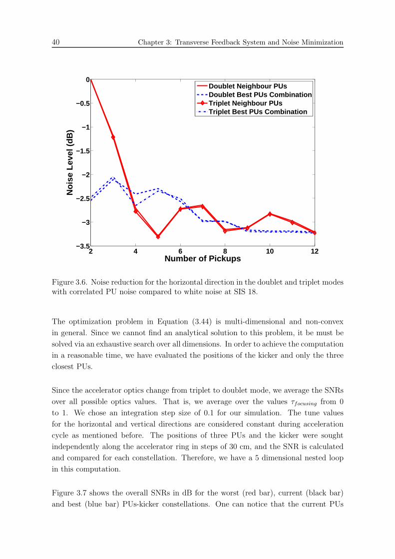
40 Chapter 3: Transverse Feedback System and Noise Minimization
2 4 6 8 10 12−3.5
−3
−2.5
−2
−1.5
−1
−0.5
0
Number of Pickups
Noi
se L
evel
(dB
)
Doublet Neighbour PUsDoublet Best PUs CombinationTriplet Neighbour PUsTriplet Best PUs Combination
Figure 3.6. Noise reduction for the horizontal direction in the doublet and triplet modeswith correlated PU noise compared to white noise at SIS 18.
The optimization problem in Equation (3.44) is multi-dimensional and non-convex
in general. Since we cannot find an analytical solution to this problem, it be must be
solved via an exhaustive search over all dimensions. In order to achieve the computation
in a reasonable time, we have evaluated the positions of the kicker and only the three
closest PUs.
Since the accelerator optics change from triplet to doublet mode, we average the SNRs
over all possible optics values. That is, we average over the values τfocusing from 0
to 1. We chose an integration step size of 0.1 for our simulation. The tune values
for the horizontal and vertical directions are considered constant during acceleration
cycle as mentioned before. The positions of three PUs and the kicker were sought
independently along the accelerator ring in steps of 30 cm, and the SNR is calculated
and compared for each constellation. Therefore, we have a 5 dimensional nested loop
in this computation.
Figure 3.7 shows the overall SNRs in dB for the worst (red bar), current (black bar)
and best (blue bar) PUs-kicker constellations. One can notice that the current PUs
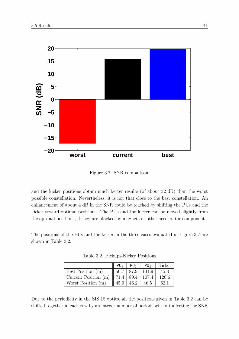
3.5 Results 41
worst current best−20
−15
−10
−5
0
5
10
15
20
SN
R (
dB)
Figure 3.7. SNR comparison.
and the kicker positions obtain much better results (of about 32 dB) than the worst
possible constellation. Nevertheless, it is not that close to the best constellation. An
enhancement of about 4 dB in the SNR could be reached by shifting the PUs and the
kicker toward optimal positions. The PUs and the kicker can be moved slightly from
the optimal positions, if they are blocked by magnets or other accelerator components.
The positions of the PUs and the kicker in the three cases evaluated in Figure 3.7 are
shown in Table 3.2.
Table 3.2. Pickups-Kicker Positions
PU1 PU2 PU3 KickerBest Position (m) 50.7 87.9 141.9 45.3Current Position (m) 71.4 89.4 107.4 120.6Worst Position (m) 45.9 46.2 46.5 62.1
Due to the periodicity in the SIS 18 optics, all the positions given in Table 3.2 can be
shifted together in each row by an integer number of periods without affecting the SNR
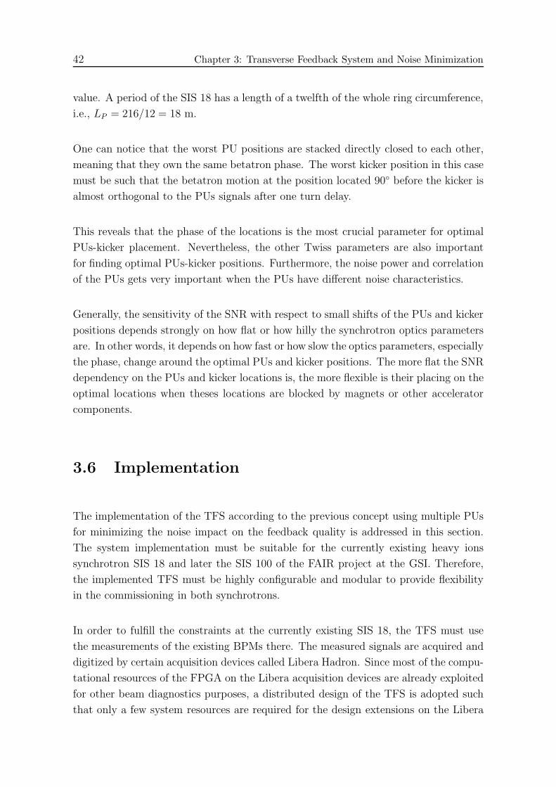
42 Chapter 3: Transverse Feedback System and Noise Minimization
value. A period of the SIS 18 has a length of a twelfth of the whole ring circumference,
i.e., LP = 216/12 = 18 m.
One can notice that the worst PU positions are stacked directly closed to each other,
meaning that they own the same betatron phase. The worst kicker position in this case
must be such that the betatron motion at the position located 90◦ before the kicker is
almost orthogonal to the PUs signals after one turn delay.
This reveals that the phase of the locations is the most crucial parameter for optimal
PUs-kicker placement. Nevertheless, the other Twiss parameters are also important
for finding optimal PUs-kicker positions. Furthermore, the noise power and correlation
of the PUs gets very important when the PUs have different noise characteristics.
Generally, the sensitivity of the SNR with respect to small shifts of the PUs and kicker
positions depends strongly on how flat or how hilly the synchrotron optics parameters
are. In other words, it depends on how fast or how slow the optics parameters, especially
the phase, change around the optimal PUs and kicker positions. The more flat the SNR
dependency on the PUs and kicker locations is, the more flexible is their placing on the
optimal locations when theses locations are blocked by magnets or other accelerator
components.
3.6 Implementation
The implementation of the TFS according to the previous concept using multiple PUs
for minimizing the noise impact on the feedback quality is addressed in this section.
The system implementation must be suitable for the currently existing heavy ions
synchrotron SIS 18 and later the SIS 100 of the FAIR project at the GSI. Therefore,
the implemented TFS must be highly configurable and modular to provide flexibility
in the commissioning in both synchrotrons.
In order to fulfill the constraints at the currently existing SIS 18, the TFS must use
the measurements of the existing BPMs there. The measured signals are acquired and
digitized by certain acquisition devices called Libera Hadron. Since most of the compu-
tational resources of the FPGA on the Libera acquisition devices are already exploited
for other beam diagnostics purposes, a distributed design of the TFS is adopted such
that only a few system resources are required for the design extensions on the Libera
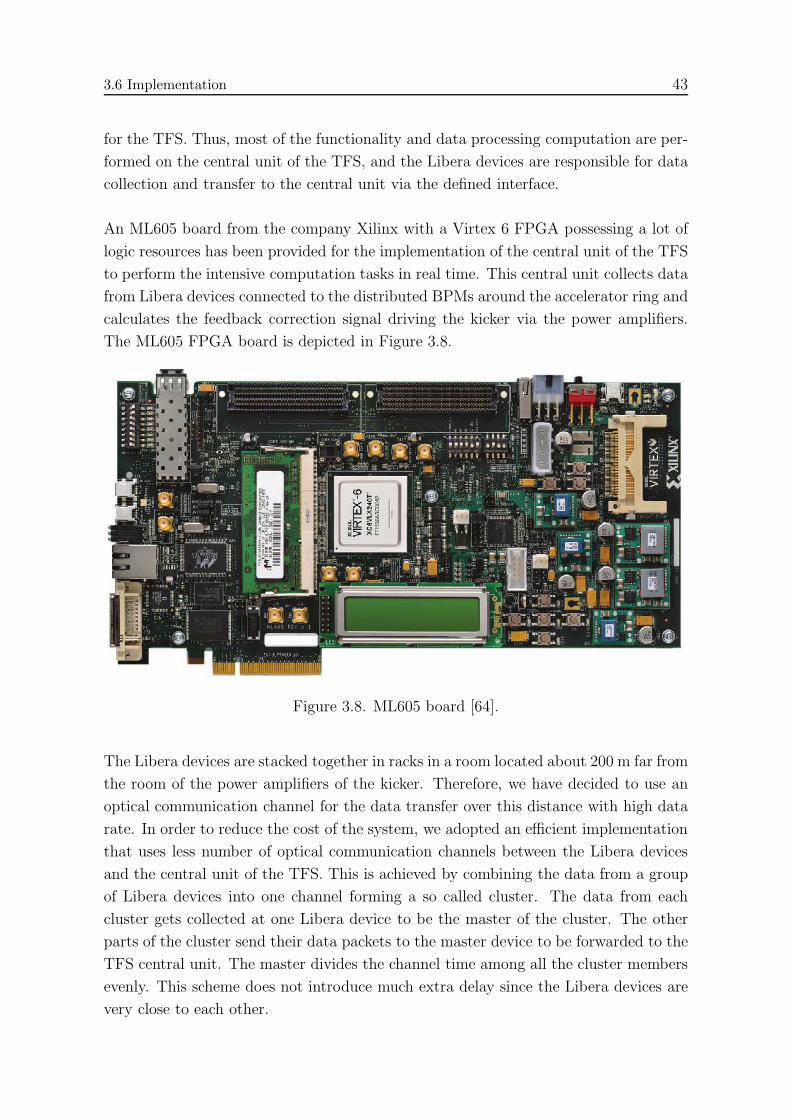
3.6 Implementation 43
for the TFS. Thus, most of the functionality and data processing computation are per-
formed on the central unit of the TFS, and the Libera devices are responsible for data
collection and transfer to the central unit via the defined interface.
An ML605 board from the company Xilinx with a Virtex 6 FPGA possessing a lot of
logic resources has been provided for the implementation of the central unit of the TFS
to perform the intensive computation tasks in real time. This central unit collects data
from Libera devices connected to the distributed BPMs around the accelerator ring and
calculates the feedback correction signal driving the kicker via the power amplifiers.
The ML605 FPGA board is depicted in Figure 3.8.
Figure 3.8. ML605 board [64].
The Libera devices are stacked together in racks in a room located about 200 m far from
the room of the power amplifiers of the kicker. Therefore, we have decided to use an
optical communication channel for the data transfer over this distance with high data
rate. In order to reduce the cost of the system, we adopted an efficient implementation
that uses less number of optical communication channels between the Libera devices
and the central unit of the TFS. This is achieved by combining the data from a group
of Libera devices into one channel forming a so called cluster. The data from each
cluster gets collected at one Libera device to be the master of the cluster. The other
parts of the cluster send their data packets to the master device to be forwarded to the
TFS central unit. The master divides the channel time among all the cluster members
evenly. This scheme does not introduce much extra delay since the Libera devices are
very close to each other.

44 Chapter 3: Transverse Feedback System and Noise Minimization
The possible number of Libera devices in a cluster depends on the speed of the opti-
cal channel and the data rate required by each device that depends on the required
sampling rate for calculating the feedback correction signal, which depends on the
bandwidth of the potential instabilities to be stabilized.
As a communication protocol between the TFS central unit and the masters of the
Libera clusters as well as between the members of the clusters and their masters, we
have used the Aurora core provided by Xilinx Core Generator, which uses the Multi-
Gigabit Transceivers (MGT) built in the FPGA chip as channel lanes. All the clocking
and reset logic required for the communication is generated within this core. Aurora
is a scalable open protocol, lightweight, link-layer protocol that is used to move data
across point-to-point serial links via a transparent interface to the physical layer, i.e.,
MGTs. It is a very efficient low-latency protocol that uses the least possible amount
of logic while offering a rich, highly configurable feature set [65].
3.6.1 Data Transfer and Bandwidth
The Aurora communication module performs a basic error checking logic based on the
8B/10B block encoding. It checks if an incoming word at the receiver is conform with
the codebook. This error checking feature introduces extra overhead in the channel
usage. Therefore, the actual data transmission rate is 80% of the overall channel rate
for the 8B/10B block encoding. In order to maintain a stable communication channel,
the aurora protocol reinitialize the channel and reestablish the communication when a
longer sequence of erroneous words has been received [65, 66].
For the communication channels between the Libera devices and the central unit of the
TFS we operate the Aurora cores with a maximum speed of 2.5 Gbps. The actual data
rate with this channel speed is due to the aforementioned overhead for error control 2
Gbps each. With a sampling rate at the Liberas of 25 Mega samples per second, the
TFS is able to stabilize the frequency band up to 12.5 MHz. We have set the packet size
for each channel to 32 bit. Therefore, the communication rate is 62.5 Mega packets per
second. Within these packets the signal samples from the BPMs, the synchronization
time stamps, as well as the control and addressing overhead are transmitted.
The Libera devices are equipped with Analog to Digital Converters (ADCs) that can
provide a high precision and small quantization noise with 14 bits per sample. Every
sample representing the beam position in the horizontal and vertical directions contains
2 ∗ 14 = 28 bits. A whole packet must be dedicated for such a sample together
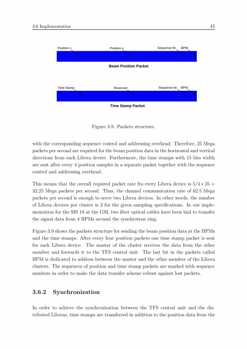
3.6 Implementation 45
Position x Position y
BPMTime Stamp
Beam Position Packet
Time Stamp Packet
BPM
Reserved
Sequence Nr.
Sequence Nr.
Figure 3.9. Packets structure.
with the corresponding sequence control and addressing overhead. Therefore, 25 Mega
packets per second are required for the beam position data in the horizontal and vertical
directions from each Libera device. Furthermore, the time stamps with 15 bits width
are sent after every 4 position samples in a separate packet together with the sequence
control and addressing overhead.
This means that the overall required packet rate fro every Libera device is 5/4 ∗ 25 =
32.25 Mega packets per second. Thus, the channel communication rate of 62.5 Mega
packets per second is enough to serve two Libera devices. In other words, the number
of Libera devices per cluster is 2 for the given sampling specifications. In our imple-
mentation for the SIS 18 at the GSI, two fiber optical cables have been laid to transfer
the signal data from 4 BPMs around the synchrotron ring.
Figure 3.9 shows the packets structure for sending the beam position data at the BPMs
and the time stamps. After every four position packets one time stamp packet is sent
for each Libera device. The master of the cluster receives the data from the other
member and forwards it to the TFS central unit. The last bit in the packets called
BPM is dedicated to address between the master and the other member of the Libera
clusters. The sequences of position and time stamp packets are marked with sequence
numbers in order to make the data transfer scheme robust against lost packets.
3.6.2 Synchronization
In order to achieve the synchronization between the TFS central unit and the dis-
tributed Liberas, time stamps are transferred in addition to the position data from the
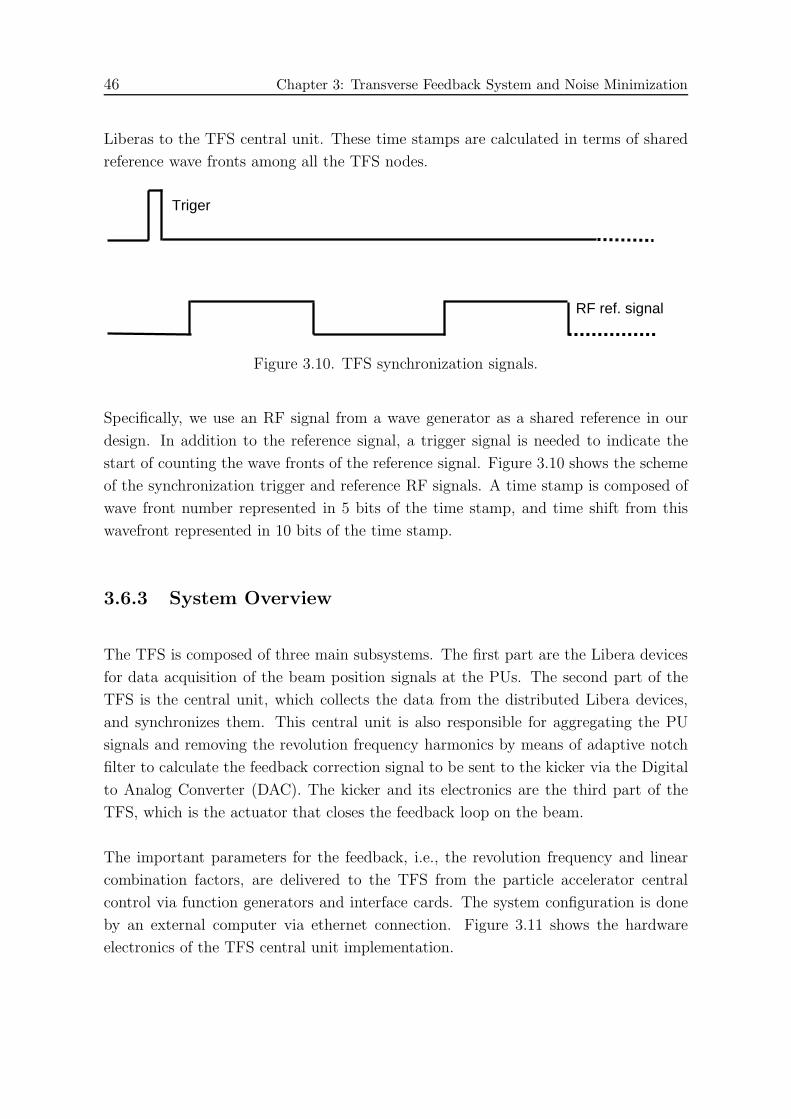
46 Chapter 3: Transverse Feedback System and Noise Minimization
Liberas to the TFS central unit. These time stamps are calculated in terms of shared
reference wave fronts among all the TFS nodes.
Triger
RF ref. signal
Figure 3.10. TFS synchronization signals.
Specifically, we use an RF signal from a wave generator as a shared reference in our
design. In addition to the reference signal, a trigger signal is needed to indicate the
start of counting the wave fronts of the reference signal. Figure 3.10 shows the scheme
of the synchronization trigger and reference RF signals. A time stamp is composed of
wave front number represented in 5 bits of the time stamp, and time shift from this
wavefront represented in 10 bits of the time stamp.
3.6.3 System Overview
The TFS is composed of three main subsystems. The first part are the Libera devices
for data acquisition of the beam position signals at the PUs. The second part of the
TFS is the central unit, which collects the data from the distributed Libera devices,
and synchronizes them. This central unit is also responsible for aggregating the PU
signals and removing the revolution frequency harmonics by means of adaptive notch
filter to calculate the feedback correction signal to be sent to the kicker via the Digital
to Analog Converter (DAC). The kicker and its electronics are the third part of the
TFS, which is the actuator that closes the feedback loop on the beam.
The important parameters for the feedback, i.e., the revolution frequency and linear
combination factors, are delivered to the TFS from the particle accelerator central
control via function generators and interface cards. The system configuration is done
by an external computer via ethernet connection. Figure 3.11 shows the hardware
electronics of the TFS central unit implementation.
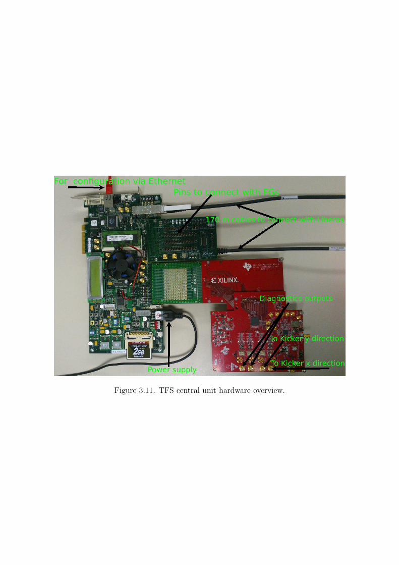
Figure 3.11. TFS central unit hardware overview.

49
Chapter 4
Transverse Feedback System and Optics
Uncertainties
The correction signal of transverse feedback system is usually calculated according
to the transfer matrices between the pickups and the kickers. However, errors due
to magnetic field imperfections and magnets misalignment lead to deviations in the
transfer matrices from their nominal values. Therefore, using the nominal values of
the transfer optics with uncertainties leads to feedback quality degradation, and thus
beam disturbances.
In this chapter, we address a novel concept for robust feedback system against optics
errors or uncertainties. A kicker and multiple pickups are assumed to be used for
each transversal direction. We introduce perturbation terms to the transfer matrices
between the kicker and the pickups. Subsequently, the Extended Kalman Filter is used
to estimate the feedback signal and the perturbation terms using the measurements
from the pickups. We assume here that the optics parameters do not change fast such
that they stay almost constant over a few turns in order to have enough measurements
for the given parameters to be identifiable.
Moreover, we propose a method for measuring the phase advances and amplitude
scaling between the positions of the kicker and the BPMs. Directly after applying a
kick on the beam by means of the kicker, we record the BPM signals. Consequently, we
use the Second-Order Blind Identification (SOBI) algorithm to decompose the recorded
noisy signals into independent sources mixture [5,6]. Finally, we determine the required
optics parameters by identifying and analyzing the betatron oscillation sourced from the
kick based on its mixing and temporal patterns. Results for the heavy ions synchrotron
SIS 18 at the GSI are shown the end of this chapter. This approach can be applied as an
alternative to the previous approach such that the updated measured parameters can
be used in a simple (non-robust) feedback system. The updated measured parameters
can of course still be used with a robust feedback system.
4.1 Motivation
Two or more PUs can be used to calculate the feedback correction signal for driving
the kicker of the TFS without using an FIR filter in order to avoid extra turns delay,

50 Chapter 4: Transverse Feedback System and Optics Uncertainties
as already discussed in the previous chapter. At least two PUs at different positions
are required for defining the beam trace space since only beam displacements from
the ideal trajectory can be measured by the PUs, but not the angles of the beam [3].
Multiple optimally placed PUs can be used to minimize the noise contribution in the
feedback correction signal, as we proposed in the previous chapter. This enhances the
feedback quality and reduces beam heating by the TFS noise [60, 61].
The proper coefficients of the FIR filter as well as the combination coefficients of multi-
ple PU signals for calculating the feedback correction signal of the TFS are calculated
based on the accelerator optics parameters, i.e., the transfer matrices between the kicker
and the PUs [4, 60, 61]. Therefore, any deviations in the optics parameters from their
known nominal values due to magnetic field imperfections, magnets misalignment, and
the aging of the magnets lead to disturbances in the calculated feedback correction
signal, and thus feedback quality deterioration when using the nominal optics values.
Consequently, the beam will be disturbed and its quality get worse.
In order to cope with this problematic, a novel concept for robust feedback system
against optics errors or uncertainties is addressed in this chapter. Furthermore, a
method for precise measurement of the optics transfer between the kicker and the PUs
to get the actual values and reach better feedback quality is presented as an alternative
or a complement of the TFS robustification concept.
4.2 Robust TFS
A feedback system that uses one kicker and multiple pickups for each transversal di-
rection is assumed. We introduce perturbation terms to the transfer matrices between
the PUs and the kicker for each of the beam oscillation transversal directions. Subse-
quently, the Extended Kalman Filter is employed to estimate the feedback correction
signal as well as the perturbation terms by means of the measured data from the
distributed PUs [67].
We address a bunch-by-bunch feedback system, which deals with the signals of different
bunches as parallel channels. The signals from the PUs, which correspond to the
transversal beam displacements, are delayed accordingly, such that they correspond
to the same bunch in every time sample. The delay terms are fixed portions of the
revolution time that usually gets estimated online, e.g., via the Schottky spectrum,
with enough accuracy for the required bandwidth of the TFS. Therefore, we do not
consider the robustification of the TFS against the uncertainties in these delay terms.

4.2 Robust TFS 51
The driving signal at the kicker is the output of the digital processing of the delayed
PUs signals. As we already mentioned in the previous chapter, the driving signal of
the kicker, i.e., the feedback correction signal, must be an estimation of the beam
displacement at the position sk90 with 90◦ phase advance before the kicker location.
The block diagram of the TFS model is depicted in Figure 3.2.
4.2.1 System Model
Let x(n) = [x1(n), · · · , xM (n)]T be the vector of the beam positions (horizontal or
vertical) at the M PUs at the nth turn for one of the bunches. Therefore, the measure-
ment vector x(n) will be, like in the previous chapter, this positions vector distorted
by the noise vector z(n) = [z1(n), · · · , zM(n)]T ∼ N(0, Rzz) of the PUs. This can be
written as
x(n) = x(n) + z(n). (4.1)
According to Equation (2.13) the beam displacement x and angle x′ can be calculated
at any position around the accelerator ring by knowing them at some specific position
via a transfer matrix dependency. Therefore, we define
xK(n) = [xK(n), x′K(n)]
T (4.2)
to be the beam status vector at the nth turn, where xK(n) is the beam position at the
kicker location, and x′K(n) is the beam angle at this place.
The beam status vector at turn n+ 1 can be found in dependence of the beam status
vector at turn n according to the accelerator optics model. It will be the multiplication
of the complete turn transfer matrix MKK(n) by the kicked beam status vector at turn
n superposed with the kick. Furthermore, small disturbances are added to this model.
Thus,
xK(n+ 1) = MKK(n) · xK(n) +DK(n + 1) + np(n + 1), (4.3)
where
DK(n + 1) = [0, ∆x′DK(n+ 1)]T , (4.4)
is the kick applied on the beam by the kicker at turn n, and np(n) = [np1(n), np2(n)]T ∼
N(0, Rnn) denotes the disturbances in the beam position and angle due to the model
uncertainties, non-linear errors in the lattice of the synchrotron, and external interfering
sources.
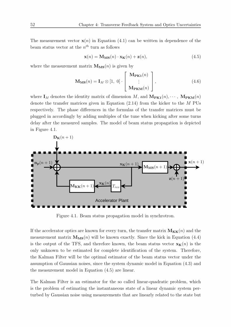
52 Chapter 4: Transverse Feedback System and Optics Uncertainties
The measurement vector x(n) in Equation (4.1) can be written in dependence of the
beam status vector at the nth turn as follows
x(n) = MMS(n) · xK(n) + z(n), (4.5)
where the measurement matrix MMS(n) is given by
MMS(n) = IM ⊗ [1, 0] ·
MPK1(n)...
MPKM(n)
, (4.6)
where IM denotes the identity matrix of dimension M , and MPK1(n), · · · , MPKM(n)
denote the transfer matrices given in Equation (2.14) from the kicker to the M PUs
respectively. The phase differences in the formulas of the transfer matrices must be
plugged in accordingly by adding multiples of the tune when kicking after some turns
delay after the measured samples. The model of beam status propagation is depicted
in Figure 4.1.
Accelerator Plant
MKK(n+ 1)xK(n)
xK(n+ 1)
Trev
MMS(n+ 1)np(n+ 1) x(n+ 1)
DK(n+ 1)
z(n+ 1)
Figure 4.1. Beam status propagation model in synchrotron.
If the accelerator optics are known for every turn, the transfer matrix MKK(n) and the
measurement matrix MMS(n) will be known exactly. Since the kick in Equation (4.4)
is the output of the TFS, and therefore known, the beam status vector xK(n) is the
only unknown to be estimated for complete identification of the system. Therefore,
the Kalman Filter will be the optimal estimator of the beam status vector under the
assumption of Gaussian noises, since the system dynamic model in Equation (4.3) and
the measurement model in Equation (4.5) are linear.
The Kalman Filter is an estimator for the so called linear-quadratic problem, which
is the problem of estimating the instantaneous state of a linear dynamic system per-
turbed by Gaussian noise using measurements that are linearly related to the state but
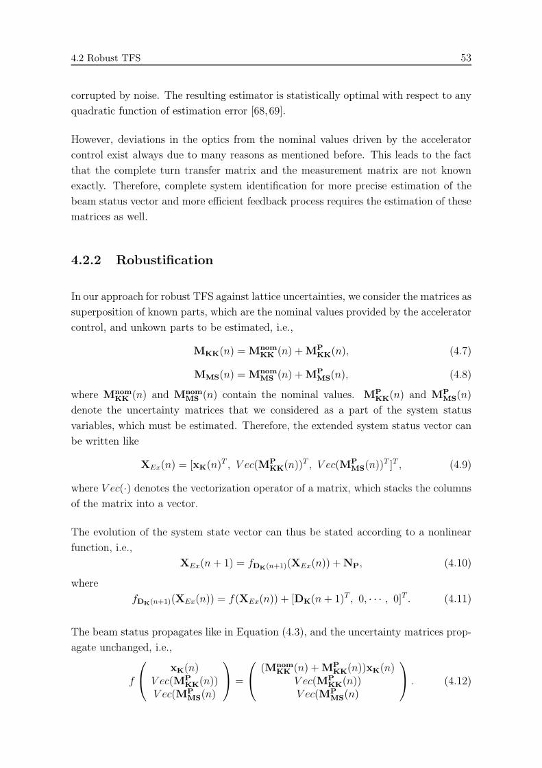
4.2 Robust TFS 53
corrupted by noise. The resulting estimator is statistically optimal with respect to any
quadratic function of estimation error [68, 69].
However, deviations in the optics from the nominal values driven by the accelerator
control exist always due to many reasons as mentioned before. This leads to the fact
that the complete turn transfer matrix and the measurement matrix are not known
exactly. Therefore, complete system identification for more precise estimation of the
beam status vector and more efficient feedback process requires the estimation of these
matrices as well.
4.2.2 Robustification
In our approach for robust TFS against lattice uncertainties, we consider the matrices as
superposition of known parts, which are the nominal values provided by the accelerator
control, and unkown parts to be estimated, i.e.,
MKK(n) = MnomKK (n) +MP
KK(n), (4.7)
MMS(n) = MnomMS (n) +MP
MS(n), (4.8)
where MnomKK (n) and Mnom
MS (n) contain the nominal values. MPKK(n) and MP
MS(n)
denote the uncertainty matrices that we considered as a part of the system status
variables, which must be estimated. Therefore, the extended system status vector can
be written like
XEx(n) = [xK(n)T , V ec(MP
KK(n))T , V ec(MP
MS(n))T ]T , (4.9)
where V ec(·) denotes the vectorization operator of a matrix, which stacks the columns
of the matrix into a vector.
The evolution of the system state vector can thus be stated according to a nonlinear
function, i.e.,
XEx(n+ 1) = fDK(n+1)(XEx(n)) +NP, (4.10)
where
fDK(n+1)(XEx(n)) = f(XEx(n)) + [DK(n + 1)T , 0, · · · , 0]T . (4.11)
The beam status propagates like in Equation (4.3), and the uncertainty matrices prop-
agate unchanged, i.e.,
f
xK(n)V ec(MP
KK(n))V ec(MP
MS(n)
=
(MnomKK (n) +MP
KK(n))xK(n)V ec(MP
KK(n))V ec(MP
MS(n)
. (4.12)

54 Chapter 4: Transverse Feedback System and Optics Uncertainties
The measurement model can be formulated as
x(n) = h(XEx(n)) + z(n), (4.13)
where
h(XEx(n)) = (MnomMS (n) +MP
MS(n)) · xK(n). (4.14)
The TFS must implement an observer of the system parameters jointly based on the
measured data at the PUs. The beam correction signal will be the estimated beam
displacement with 90◦ phase advance. The model of the extended beam status propa-
gation with the observer for the TFS fMnom
KK,Mnom
MS(·) is depicted in Figure 4.2.
TFS
Accelerator Plant
MKK(n+ 1)xK(n)
xK(n+ 1)
Trev
MMS(n+ 1)np(n+ 1) x(n+ 1)
DK(n+ 1)
z(n+ 1)
XEx(n+ 1) = fMnom
KK,Mnom
MS(xn,Mn
KK,Mn
MS,xn+1
MS)D
n+1
K= [0, gx90
n+1]T
Figure 4.2. Extended status vector propagation model in synchrotron and TFS ob-server.
4.2.3 Observability
Before we start with the design of the observer for the TFS, we first study the observ-
ability of the system model stated in Equation (4.10) and Equation (4.13).
Define
Θ = {h(fDK(j) ◦ · · · ◦ fDK(1)(·)) | ∀j ≥ 0}. (4.15)

4.2 Robust TFS 55
In [70], it has been proven that the criterion for the system to be locally observable
around XEx(0) is that
dim
(
∂Θ(XEx)
∂XEx
∣∣∣∣XEx(0)
)
= n, (4.16)
where n = dim(XEx), i.e., the number of extended system status parameters.
For constant optics and errors over the time, and therefore constant complete turn
transfer matrix and measurement matrix, we show in the following how to check
whether the observability of the whole system is given according to the aforementioned
criterion.
Usually, even when the accelerator lattice functions change during the acceleration
cycle like the case of SIS 18 at the GSI, the changing rate of the accelerator optics is
much slower than the beam revolution frequency in the accelerator ring. Therefore,
the accelerator optics can be considered constant during a small number of beam
revolutions. Thus, it is sufficient to show that the observability criterion is fulfilled for
constant accelerator optics over a few number of beam turns.
In order to verify the observability condition in Equation (4.16), we first calculate and
stack the Jacobian matrices in JΘ(XEx(0)) for some set of
Θj(XEx(0)) = h(fDK(j) ◦ · · · ◦ fDK(1)(XEx(0))), with j ∈ {1, 2, · · · , L}, (4.17)
where
L =⌈ n
M
⌉
. (4.18)
M denotes the number of the measurements per turn, i.e., number of the PUs. The
Jacobian matrices are defined as
JΘj(XEx(0)) =
∂Θj(XEx)
∂XEx
∣∣∣∣XEx(0)
. (4.19)
Secondly, we calculate the rank of JΘ(XEx(0)). If rank(JΘ(XEx(0))) = n, then the sys-
tem is locally observable around XEx(0), otherwise we extend the matrix JΘ(XEx(0))
by taking bigger number of turns than L. If the rank stays less than the number of
extended model parameters in spite of the extensions of the Jacobian matrices, the
system is considered unobservable.
Assuming small deviations in the transfer matrices from their nominal values given
by the accelerator, it is enough to show that the criterion of the system observability
is fulfilled around the zero perturbations of the whole turn matrix MKK(n) and the
56 Chapter 4: Transverse Feedback System and Optics Uncertainties
measurement matrix MMS(n), i.e., around the nominal values with MPKK(0) = 02×2
and MPMS(0) = 0M×2, for all possible values of the initial beam status vector xK(0)
defined in Equation (4.2).
Thus, the observability criterion has to be fulfilled according to Equation (4.16) around
all possible values of the status parameters vector of the form
XEx(0) =[xK(0)
T , V ec(02×2)T , V ec(0M×2)
T]T
, (4.20)
where we consider the observability of the matrices around their nominal values as
mentioned before. xK(0) must be swept such that all possible beam displacements and
directions are covered, i.e., the rank of the stacked Jacobian matrices over some turns
is considered concerning all possible beam initial conditions.
According to Equation (4.11), Equation (4.14), and Equation (4.15), the possible ele-
ments of Θ can only have the form
Θ =
{
MMS(j)
[j∏
i=1
(MKK(i))xK(0) +
j∑
i=0
(j∏
k=i+1
(MKK(k))DK(i)
)]
| ∀j ≥ 0
}
,
(4.21)
where the measurement matrix MMS and the whole revolution transfer matrix MKK
are described in Equation (4.7) and Equation (4.8), respectively, and j is assumed to
be small enough such that the matrices MMS and MKK can be considered constant
during j consecutive revolutions. It follows then
Θ =
{
MMS
[
MKKjxK(0) +
j∑
i=0
(MKK
j−iDK(i))
]
| ∀j ≥ 0
}
. (4.22)
For the simple case when the TFS is turned off, i.e., the TFS gain is set to zero, and
the beam is not being kicked, we have
Θ ={MMSMKK
jxK(0) | ∀j ≥ 0}. (4.23)
The functions in Equation (4.23) are linearly dependent on xK(0), i.e., in the form
g1(MMS,MKK)xK(0)+ g2(MMS,MKK)x′K(0). Therefore, the derivatives with respect
to XEx(0) for calculating the Jacobian matrices will have the first two columns inde-
pendent of xK(0), and the rest of the columns linearly dependent on xK(0). We have
thus
JΘ
([αxK(0)
T , V ec(MPKK(0))
T , V ec(MPMS(0))
T]T)
= JΘ
([xK(0)
T , V ec(MPKK(0))
T , V ec(MPMS(0))
T]T)
diag(1, 1, α, · · · , α).(4.24)
4.2 Robust TFS 57
Therefore, the rank of JΘ(XEx(0)) is not affected by scaling the beam status vector,
and thus the number of dimensions of JΘ (XEx(0)) is independent of the magnitude of
xK(0). That means that it is enough to sweep only the phase of the beam status vector
xK(0) while keeping constant magnitude and check the rank of the stacked Jacobian
matrices in order to show the system observability. In other words, it is enough to
sweep the beam status vector over the unitary circle.
In order to calculate the stacked Jacobian matrices JΘ (XEx(0)), we use the following
rules according to the results in [71]:
∂MMSMKKjxK
∂xK
= MMSMKKj , (4.25)
∂(MMSMKKjxK)i
∂(MMS)mn= δim(MKK
jxK)n, (4.26)
∂(MMSMKKjxK)i
∂MKK
=
j−1∑
r=0
(MKKr)T ((MMS)i.)
TxK
T(MKK
j−r−1)T
, (4.27)
where (·)i denotes the ith element of a vector, (·)i· denotes the ith line of a matrix,
1 ≤ i ≤ M , and 1 ≤ n ≤ 2.
Since the differentials of the perturbation matricesMPKK andMP
MS are equivalent to the
differentials of the matrices MKK and MMS around their nominal values, respectively,
we calculate the derivatives in Equation (4.26) and Equation (4.27) at the nominal
values MnomKK and Mnom
MS .
4.2.4 Observer
The optimal observer of a discrete-time controlled process described by a linear differ-
ence equation like Equation (4.3) with linear dependency of the measurements on the
system status vector to be estimated like Equation (4.5) is the Kalman filter. It is the
optimal estimator for the so called linear-quadratic problem [69, 72, 73].
The Kalman filter is not optimal anymore when the propagation of the system state
vector as well as the measurement relation is according to a non-linear equation like
in our robustification model in Equation (4.10) and Equation (4.13). However, a well
known solution is to linearize the state vector propagation model as well as the measure-
ment model around the current estimate. This is the so called Extended Kalman Filter
(EKF) [69, 72]. This approach has been successfully applied in many applications in
58 Chapter 4: Transverse Feedback System and Optics Uncertainties
signal processing. The model linearization is equivalent to taking the first order Taylor
series of the model equation. This is done via calculating the partial derivatives of the
system state propagation and measurement functions with respect to the system state
vector, i.e., the Jacobian matrices for the system state vector propagation function and
the measurement function
Φn =∂f(XEx)
∂XEx
∣∣∣∣XEx(n)
, (4.28)
H(n) =∂h(XEx)
∂XEx
∣∣∣∣XEx(n)
, (4.29)
where XEx(n) denotes the a posteriori estimate of the system state vector at the turn
n. The process function f(XEx) and the measurement function h(XEx) are described
in Equation (4.12) and Equation (4.14), respectively.
The EKF is not optimal solution for our problem since it is not linear, it performs
however a good sub-optimal approach that works well for systems with no high non-
linearity like the case of our model with only second order non-linearity. It works
iteratively as follows [69, 72]:
1. Prediction
• Compute the predicted state estimate
X−Ex(n+ 1) = fDK(n+1)(X
+Ex(n)) (4.30)
• Compute the predicted measurement
x(n + 1) = h(X−Ex(n+ 1))
= M−MS(n+ 1) · x−
K(n+ 1)(4.31)
• Compute the a priori covariance matrix
P−(n+1) = ΦnP
+(n)Φ
Tn +RNN, (4.32)
2. Update
• Conditioning the predicted estimate on the measurement
X+Ex(n+ 1) = X−
Ex(n+ 1) +K(n+1) · (x(n+ 1)
− x(n+ 1))(4.33)
4.3 Optics Transfer Determination 59
• Compute the a posteriori covariance matrix
P+(n+1) = [I−K(n+1)H(n+1)]P
−(n+1) (4.34)
The Kalman gain at turn n+ 1 is given by
K(n+1) = P−(n+1) ·HT
(n+1)
· [H(n+1)P−(n+1)H
T(n+1) +RZZ]
−1,(4.35)
The estimation of the extended state vector is done iteratively at every turn. The
extended state vector is first predicted based on the estimate of the state of the previous
turn according to the state propagation model. The predicted values are then adjusted
according to the measured values at the PUs. For the initialization of the algorithm
we can use the nominal values of the transfer an measure matrices, and the output of
the estimator discussed in the previous chapter for the beam state vector.
The advantage of the EKF is that, in addition to estimating the system state, it gives
an estimate of the precision in the estimated values as given within the covariance
matrix P.
4.3 Optics Transfer Determination
In this section, we address a method for measuring the phase advance and amplitude
ratio between the beam oscillation at the kicker and the PUs positions. A rigid kick
is applied on the beam, and the PU signals are recorded. The Second-Order Blind
Identification (SOBI) algorithm [5, 6] is used subsequently to separate different beam
oscillation sources from the noisy PU signals. The required optics parameters deter-
mination follows then by identifying, analyzing, and fitting the betatron oscillation on
horizontal and vertical direction.
4.3.1 System Model
Let the TFS be composed of M PUs and a kicker located at different places around
the accelerator ring. In order to make the required optics measurements for the TFS,
we first of all perform a rigid initial kick on the beam by means of the kicker. We
then start recording the turn-by-turn PU signals directly after the initial kick. The

60 Chapter 4: Transverse Feedback System and Optics Uncertainties
turn-by-turn PU signal is calculated by averaging the displacement over a whole bunch.
This averaging reduces the thermal noise power generated by the PUs.
The recorded beam transversal motion contains components sourced from different
phenomena, e.g., betatron oscillation, head-tail modes, and synchrotron oscillation [74].
Suppose we record the PU signals over N turns. Let
xi = [xi(1), · · · , xi(N)] ∈ R1×N (4.36)
denote the signal recorded from the ith PU. This vector is the contribution of the beam
transversal motion and the noise from the ith PU, i.e.,
xi = xi + zi, (4.37)
where the vector xi represents the actual beam transversal offsets over the N turns at
the position of the ith PU, and zi denotes the disturbing noise vector generated at this
PU.
Let
X = [xT1 , · · · ,xT
M ]T ∈ RM×N (4.38)
denote the matrix of the recorded signals over N turns from all the M PUs stacked
together.
Assume the beam transversal motion is composed of K components driven by various
sources. The recorded signals vector can be then written as
X = AS+ Z, (4.39)
where Z denotes the noise terms, which are assumed to be independent zero-mean
Gaussian with variance σ2, and S ∈ RK×N denotes the source signals. A ∈ RM×K is
the source mixing matrix, which represents the coupling between the sources on the
betatron motion.
After kicking a bunch in the transversal direction, it will perform transversal oscillation
that contains components from the coherent betatron oscillation with the coherent tune
frequency. The initial phase of the recorded oscillation at some PU corresponds to the
phase difference between the kicker position and the position of this PU.
Furthermore, decoherence of the transverse bunch oscillation will occur, meaning that
the amplitude of the oscillation will decrease over the time. This is a direct result

4.3 Optics Transfer Determination 61
of the tune spread of the bunch particles due to the momentum spread and machine
chromaticity. Recoherence of the transverse oscillation will follow after a while cor-
responding to the synchrotron period in a linear focusing lattice [75]. Therefore, the
bunch transverse oscillation in vertical or horizontal direction can be stated as
x(n) = a(n) sin(Qn + φ0), (4.40)
where Q denotes the coherent tune, and φ0 is the initial phase. a(n) denotes the
amplitude function of the transverse oscillation, and it can be written as [75–77]
a(n) = a0 exp
{
−2
(ξQ0δpQs
sin(πQsn)
)2}
, (4.41)
where a0 denotes the initial amplitude that depends on the strength of the rigid kick ,
ξ the chromaticity, δp the RMS momentum spread, and Qs the tune of the synchrotron
oscillation. This amplitude has also an exponentially decreasing trend due to the
Landau damping.
Figure 4.3 shows recorded turn-by-turn beam oscillation at the heavy ions synchrotron
SIS 18 at the GSI [75]. One can observe that this signal matches to the above described
model.
-1
-0.5
0
0.5
1
0 500 1000 1500 2000 2500 3000 3500 4000
Bun
ch O
ffset
(ar
b. u
nits
)
time (turns)
Figure 4.3. Recorded turn-by-turn beam oscillation in the vertical plane at SIS 18 [75].
62 Chapter 4: Transverse Feedback System and Optics Uncertainties
4.3.2 Source Separation
The model parameters in Equation (4.40) and Equation (4.41) can be estimated with
smaller error after removing the contribution of the irrelevant sources. Therefore, the
separation of the sources contributing to the beam transversal oscillation according to
Equation (4.39) is a very important step for a precise calculation of the parameters of
the betatron oscillation.
The SOBI is a source separation technique based on the coherence of the source sig-
nals, which estimates the mixing matrix and separates the sources. This technique is
considered to be more robust in poor signal to noise ratios due to utilizing second-order
statistics, i.e., spatial covariance matrices of the measurements [5, 78].
The covariance matrix of the source signals is defined as
CSS(τ) = E{S(t)S(t + τ)T }, (4.42)
which is diagonal when the sources are independent.
From Equation (4.39) one can see that
CXX(τ) = ACSS(τ)AT + δ(τ)σ2I, (4.43)
where δ(·) denotes the Dirac function. This means that the mixing matrix A is a
diagonalizer of the measurements covariance matrix CXX(τ) for τ 6= 0. This is a very
important property to perform the source separation.
The SOBI algorithm can be performed to determine the mixing matrix A and the
sources S as in the following steps [5, 6]:
1. Perform eigenvalue decomposition on CXX(0)
2. Put the K largest eigenvalues into the diagonal matrix ΛS, and the corresponding
eigenvectors into the matrix US. These eigenvalues represent the source signals,
and the smallest ones represent the white noise
3. Define
V = Λ− 1
2S UT
S , (4.44)
and
Ψ = VX (4.45)

4.3 Optics Transfer Determination 63
4. Estimate the covariance matrices CΨΨ(τk) for some delay time values τk, and
calculate
CΨΨ(τk) =CΨΨ(τk) +CΨΨ(τk)
T
2(4.46)
5. Find a matrix W which jointly diagonalizes all of the CΨΨ(τk) for the selected
time lags, i.e.,
CΨΨ(τk) = WDWT . (4.47)
6. The mixing matrix is thus given by
A = V−1W, (4.48)
and the corresponding source signals are
S = WTVX, (4.49)
where V−1 = USΛ12S .
Using the results of the SOBI algorithm, the phase and amplitude transfer between the
kicker position and the PUs can be determined in the vertical and horizontal direction.
4.3.3 Optics Transfer Determination
After the source signals and the corresponding mixing matrices have been determined,
the components of the betatron oscillation in some direction, e.g., horizontal direction,
can be identified by its tune frequency, which must be closed to the nominal value.
This betatron oscillation must have two components with orthogonal phases since the
PU signals include this oscillation with different phases.
The betatron oscillation should follow the model described in Equation (4.40) and
Equation (4.41) in beam offset and angle. Therefore, the beam oscillation following
the kick will occur according to the decoherence/recoherence model with a maximum
amplitude proportional to the kick, and zero initial phase since the oscillation is sup-
posed to start from zero offset, assuming a stable beam. Thus, the phase transfer
between the kicker position and the PUs is equal to the initial phases of the beta-
tron oscillation recorded at each PU. The amplitude transfer is then the ratio of the
maximum amplitude for each PU and the kick.
Within the extracted components of the betatron oscillation some portion of the noise
is superimposed. Therefore, a nonlinear fitting approach is used to determine the initial
64 Chapter 4: Transverse Feedback System and Optics Uncertainties
phase and the amplitude parameters in the two betatron components. Let α1 and α2
denote the estimated initial amplitudes of these components, and ϕ1 and ϕ2 denote the
estimated phases. The amplitude ratio of the betatron oscillation between the position
of the kicker and PUi can be written as
Tβi=
√
α21(Aib1)
2 + α22(Aib2)
2
βKDK, (4.50)
and the phase transfer
∆Φi = arctan(α1(Aib1)
α2(Aib2)) + ϕ1, (4.51)
where (Aibj ) denotes the element within the mixing matrix corresponding to the signal
of PUi and betatron component j ∈ {1, 2}, and DK represents the kick strength. βK
is the value of the beta function at the kicker position, which is assumed to be known
precisely from a previous measurement campaign.
The value of βK appears only in the formula of the amplitude transfer in Equation
(4.50) as a scaling factor of all parameters. Therefore, the errors in measuring βK
affect the estimate of the feedback correction signal using our approach of the MVUE
only by a scaling factor without changing the right phase, which is very crucial for
correctly damping feedback.
Since the two betatron components for some transversal direction resulting from the
SOBI algorithm are orthogonal, the following must hold
ϕ2 ≈ ϕ1 +π
2. (4.52)
This can be exploited to enhance the phase estimation from the nonlinear fitting. In
this case, both phases can be estimated from each component and averaged over the
two estimates.
4.4 Results
In this section, we show simulation results of the above addressed approaches in this
chapter for the heavy ions Synchrotron SIS 18 at the GSI. In the SIS 18, there are
12 beam position PUs for the horizontal and vertical directions, which are located
periodically along the synchrotron ring. There is also one kicker for each transversal
direction.
As already discussed in the previous chapter, the transversal focusing optics change
continuously in this synchrotron from the so called triplet mode to the doublet mode
during the acceleration cycle. This leads to non-constant betatron functions during
operation.

4.4 Results 65
4.4.1 Robust TFS
We show in this section simulation results for the triplet mode in the horizontal di-
rection for using the two closest PUs to the kicker. The nominal values of the twiss
parameters for the PUs and the kicker are shown in Table 3.1. The nominal tune for
the horizontal direction is Qnomx = 4.31. The phase difference between the kicker and
the first PU has a nominal value ∆φnom1 = 103.7◦, and the phase difference between
the two PUs is ∆φnomPUs = 129.3◦ nominally.
Using the values in Table 3.1 and substituting in Equation (2.14) we find the nominal
whole turn transfer matrix as
MnomKK =
(−1.6326 13.0727−0.1884 0.8964
)
. (4.53)
Assuming feedback in the second turn, the measurement matrix is given as
MnomMS =
(−1.5208 7.71260.5724 3.5444
)
. (4.54)
In order to check the observability of the system model stated in Equation (4.10)
and Equation (4.13) around nominal values of whole turn transfer matrix and the
measurement matrix, we calculate the rank of the stacked Jacobian matrices of Θ
given in Equation (4.22) for 0 ≤ j ≤ 4. As already discussed in a previous section, it
is enough to sweep the initial beam state vector around the unitary circle, i,e, xK(0) =
[cos(φ), sin(φ)]T , φ ∈ [0, 360[ (deg.), in order to show the observability of the given
system for any possible beam offset and angle.
Figure 4.4 depicts the determinant of the stacked Jacobian matrix for the considered
number of turns with noisy TFS kicks. The determinant values are far from 0, which
shows that the stacked Jacobian matrix is far from being singular for any possible
initial beam offset and angle. Therefore, the robust system formulation is observable,
and we show results for our suggested observer in the following.
We assume an actual tune of Qx = 4.15 for the horizontal direction. This corresponds
to about 60◦ deviation from the nominal tune value. The deviations in the considered
actual values of the phase advances between the kicker and the first PU as well as
between the two PUs from the nominal values are assumed to be 30%. The nominal
and actual values of the Twiss parameters for the PUs and the kicker are shown in
Table 4.1.
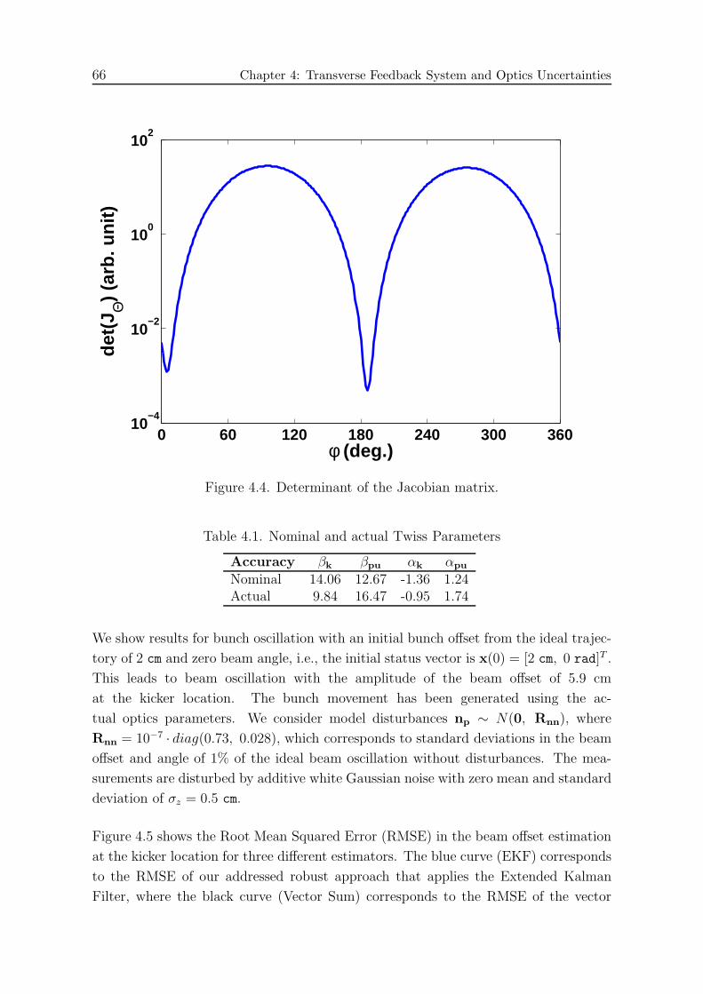
66 Chapter 4: Transverse Feedback System and Optics Uncertainties
0 60 120 180 240 300 36010
−4
10−2
100
102
φ (deg.)
det(
JΘ
) (a
rb. u
nit)
Figure 4.4. Determinant of the Jacobian matrix.
Table 4.1. Nominal and actual Twiss Parameters
Accuracy βk βpu αk αpu
Nominal 14.06 12.67 -1.36 1.24Actual 9.84 16.47 -0.95 1.74
We show results for bunch oscillation with an initial bunch offset from the ideal trajec-
tory of 2 cm and zero beam angle, i.e., the initial status vector is x(0) = [2 cm, 0 rad]T .
This leads to beam oscillation with the amplitude of the beam offset of 5.9 cm
at the kicker location. The bunch movement has been generated using the ac-
tual optics parameters. We consider model disturbances np ∼ N(0, Rnn), where
Rnn = 10−7 · diag(0.73, 0.028), which corresponds to standard deviations in the beam
offset and angle of 1% of the ideal beam oscillation without disturbances. The mea-
surements are disturbed by additive white Gaussian noise with zero mean and standard
deviation of σz = 0.5 cm.
Figure 4.5 shows the Root Mean Squared Error (RMSE) in the beam offset estimation
at the kicker location for three different estimators. The blue curve (EKF) corresponds
to the RMSE of our addressed robust approach that applies the Extended Kalman
Filter, where the black curve (Vector Sum) corresponds to the RMSE of the vector
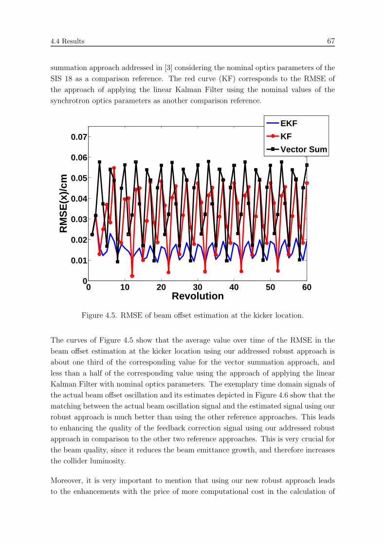
4.4 Results 67
summation approach addressed in [3] considering the nominal optics parameters of the
SIS 18 as a comparison reference. The red curve (KF) corresponds to the RMSE of
the approach of applying the linear Kalman Filter using the nominal values of the
synchrotron optics parameters as another comparison reference.
0 10 20 30 40 50 600
0.01
0.02
0.03
0.04
0.05
0.06
0.07
Revolution
RM
SE
(x)/
cm
EKF
KF
Vector Sum
Figure 4.5. RMSE of beam offset estimation at the kicker location.
The curves of Figure 4.5 show that the average value over time of the RMSE in the
beam offset estimation at the kicker location using our addressed robust approach is
about one third of the corresponding value for the vector summation approach, and
less than a half of the corresponding value using the approach of applying the linear
Kalman Filter with nominal optics parameters. The exemplary time domain signals of
the actual beam offset oscillation and its estimates depicted in Figure 4.6 show that the
matching between the actual beam oscillation signal and the estimated signal using our
robust approach is much better than using the other reference approaches. This leads
to enhancing the quality of the feedback correction signal using our addressed robust
approach in comparison to the other two reference approaches. This is very crucial for
the beam quality, since it reduces the beam emittance growth, and therefore increases
the collider luminosity.
Moreover, it is very important to mention that using our new robust approach leads
to the enhancements with the price of more computational cost in the calculation of
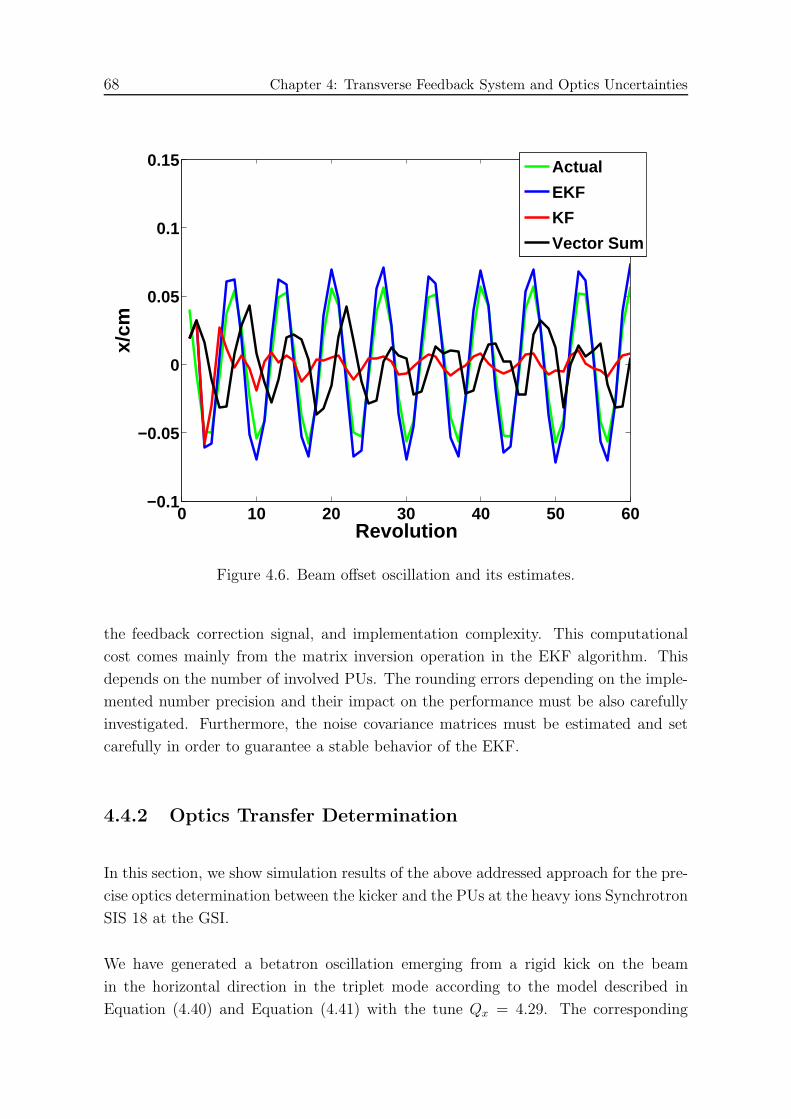
68 Chapter 4: Transverse Feedback System and Optics Uncertainties
0 10 20 30 40 50 60−0.1
−0.05
0
0.05
0.1
0.15
Revolution
x/cm
Actual
EKF
KF
Vector Sum
Figure 4.6. Beam offset oscillation and its estimates.
the feedback correction signal, and implementation complexity. This computational
cost comes mainly from the matrix inversion operation in the EKF algorithm. This
depends on the number of involved PUs. The rounding errors depending on the imple-
mented number precision and their impact on the performance must be also carefully
investigated. Furthermore, the noise covariance matrices must be estimated and set
carefully in order to guarantee a stable behavior of the EKF.
4.4.2 Optics Transfer Determination
In this section, we show simulation results of the above addressed approach for the pre-
cise optics determination between the kicker and the PUs at the heavy ions Synchrotron
SIS 18 at the GSI.
We have generated a betatron oscillation emerging from a rigid kick on the beam
in the horizontal direction in the triplet mode according to the model described in
Equation (4.40) and Equation (4.41) with the tune Qx = 4.29. The corresponding

4.4 Results 69
signals were generated at the 12 PUs according to the betatron parameters of the SIS
18 listed in Table 3.1. A small coupling part from the vertical and the longitudinal
oscillations, as well as Gaussian measurement noise with standard deviation of 25% of
highest signal amplitude were added. Using the above described method we were able
to determine the phase advances with about 2◦ error, and the amplitude scaling with
a less than 5% error.

71
Chapter 5
Non-Linear Optics Components Detection
and Measurement
The knowledge of the linear and non-linear magnets errors in circular accelerator op-
tics is very crucial for controlling and compensating resonances and their consequent
beam losses and beam quality deterioration. This is indispensable, especially for high
beam intensity machines. Fortunately, the relationship between the beam offset os-
cillation signals recorded at the BPMs is a manifestation of the accelerator optics,
and can therefore be exploited in the determination of the optics linear and non-linear
components.
In this chapter, we propose a novel method for detecting and estimating the optics lat-
tice non-linear components located in-between the locations of two BPMs by analyzing
the beam offset oscillation signals of a BPMs-triple containing these two BPMs. De-
pending on the non-linear components in-between the locations of the BPMs-triple, the
relationship between the beam offsets follows a multivariate polynomial accordingly.
After calculating the covariance matrix of the polynomial terms, the Generalized Total
Least Squares method is used to find the model parameters, and thus the non-linear
components. A bootstrap technique is used to detect the existing polynomial model
orders by means of multiple hypothesis testing, and determine confidence intervals for
the model parameters. Results for synthetic and real data recorded at the heavy ions
synchrotron SIS 18 at the GSI are shown.
5.1 Motivation
In high energy particle accelerators, magnetic fields are usually employed for beam
focusing and deflection since the corresponding Lorentz force gets stronger for higher
velocities, and electric fields are used for beam acceleration. Synchrotrons use cavities
to generate the accelerating electric fields synchronized in phase and frequency with
the beam, and electric magnets to generate the focusing and deflecting magnetic fields
with proper strengths depending on the beam energy.
Constant magnetic fields, i.e., with zero gradient, generated by dipole magnets with
proper strength are usually used for beam deflection in synchrotrons. Linear magnetic
72 Chapter 5: Non-Linear Optics Components Detection and Measurement
fields, i.e., with constant gradient, generated by quadrupole magnets are usually used
for beam focusing. Periodic sequences of focusing/defocusing quadrupole magnets with
drift tubes in-between called FODO cells are usually used for focusing in horizontal and
vertical directions. This is called the strong focusing. Furthermore, other non-linear
magnetic fields generated by sextupole or octupole magnets can be applied on purpose,
e.g., for chromaticity compensation or slow beam extraction.
In addtion to the required magnetic fields, the magnets can generate unwanted spurious
linear and non-linear magnetic fields [7] due to fabrication imperfection of the magnets
and the aging of the magnets materials. These error fields in the magnets excite
undesired resonances leading together with the space charge tune spread to beam
quality deterioration, long term beam losses, and reducing the dynamic aperture [8,9].
Therefore, these magnets errors and their impact on the beam must be studied and
evaluated thoroughly in order to control and compensate their distorting contribution
on the accelerated beam for a better machine operation, such that the demand for
higher beam intensity can be fulfilled. Thus, the detection and measurement of the
linear and non-linear error components in circular accelerator optics is indispensable,
especially for high intensity machines.
The utilization of the non-linear chromaticity measurement for determining the non-
linear optics model by exploiting the nonlinear dependence of the tune on the relative
momentum offset has been presented in [26, 27, 79]. In [8, 9, 25], The Non-Linear Tune
Response Matrix (NTRM) technique has been proposed to be used for diagnosing non-
linear magnetic field components. These methods are however very costly and require
long measurement campaigns apart from having difficulties in estimating non-linear
components with mixed orders.
In this chapter, we address a novel Lightweight approach for determining optics linear
and non-linear components in a circular particle accelerator without demanding heavy
measurement campaigns. The relationship between the beam offset oscillation signals
recorded at the BPMs is a manifestation of the accelerator optics, and can be therefore
exploited in order to determine the optics linear and non-linear components. A pencil
like beam is preferred with this approach in order to get rid of finite beam size effects on
the BPM signals. Such a beam can be reached by an optimized one turn injection [25].
We estimate the lattice non-linear components located in-between the locations of two
BPMs by analyzing the beam offset oscillation signals of a BPMs-triple containing these
two BPMs. The Generalized Total Least Squares method is applied on the recorded
BPM signals after a proper preprocessing for parameter estimation, and a bootstrap
technique is used to to detect the existing model orders and determine confidence
intervals for the model parameters.
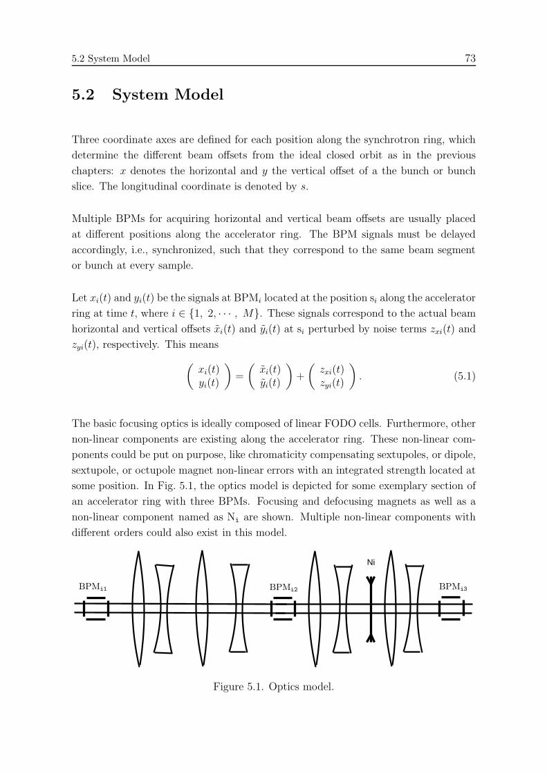
5.2 System Model 73
5.2 System Model
Three coordinate axes are defined for each position along the synchrotron ring, which
determine the different beam offsets from the ideal closed orbit as in the previous
chapters: x denotes the horizontal and y the vertical offset of a the bunch or bunch
slice. The longitudinal coordinate is denoted by s.
Multiple BPMs for acquiring horizontal and vertical beam offsets are usually placed
at different positions along the accelerator ring. The BPM signals must be delayed
accordingly, i.e., synchronized, such that they correspond to the same beam segment
or bunch at every sample.
Let xi(t) and yi(t) be the signals at BPMi located at the position si along the accelerator
ring at time t, where i ∈ {1, 2, · · · , M}. These signals correspond to the actual beam
horizontal and vertical offsets xi(t) and yi(t) at si perturbed by noise terms zxi(t) and
zyi(t), respectively. This means
(xi(t)yi(t)
)
=
(xi(t)yi(t)
)
+
(zxi(t)zyi(t)
)
. (5.1)
The basic focusing optics is ideally composed of linear FODO cells. Furthermore, other
non-linear components are existing along the accelerator ring. These non-linear com-
ponents could be put on purpose, like chromaticity compensating sextupoles, or dipole,
sextupole, or octupole magnet non-linear errors with an integrated strength located at
some position. In Fig. 5.1, the optics model is depicted for some exemplary section of
an accelerator ring with three BPMs. Focusing and defocusing magnets as well as a
non-linear component named as Ni are shown. Multiple non-linear components with
different orders could also exist in this model.
Ni
BPMi1 BPMi2 BPMi3
Figure 5.1. Optics model.

74 Chapter 5: Non-Linear Optics Components Detection and Measurement
For the sake of simplicity, we assume that the non-linear components exist between
BPMi2 and BPMi3, and not between BPMi1 and BPMi2. This constelllation can be
found in any particle accelerator, if there are no non-linear components between at least
two BPMs. In this case, one could take a BPM triple containing these two BPMs, and
our assumption would not affect the applicability of our approach. Such BPMs could
be for instance bounding a section without magnets errors, or without magnets at all,
i,e, a drift tube.
Under this assumption, the beam offset and angle directly before the location of the
non-linear components can be written in linear dependence on the beam offsets at
BPMi1 and BPMi2, i.e.,
xNi(t)xNi(t)
′
yNi(t)yNi(t)
′
= Mi
xi1(t)xi2(t)yi1(t)yi2(t)
(5.2)
where xNi(t), yNi(t), xNi(t)′, and yNi(t)
′ denote the beam horizontal and vertical offsets,
and horizontal and vertical angles, respectively. The matrix Mi can contain coupling
terms between the horizontal and vertical direction depending on the skewing of the
linear magnets.
Since the beam offsets at the location of BPMi3 can be written as a multivariate
polynomial function of the beam status, i.e., horizontal and vertical offsets and angles,
directly before the non-linear components, one can write it as a multivariate polynomial
of the beam offsets at the locations of BPMi1 and BPMi2 depending on the orders and
the number of the non-linear components. Therefore,
(xi3(t)yi3(t)
)
= f(xi1(t), xi2(t), yi1(t), yi2(t)), (5.3)
where f(.) is a multivariate polynomial of an order that depends on the non-linear
components. Hence, one can write for some order N
xi3(t) =∑
i+j+k+l≤N
αijklxi1(t)ixi2(t)
j yi1(t)kyi2(t)
l (5.4a)
yi3(t) =∑
i+j+k+l≤N
λijklxi1(t)ixi2(t)
j yi1(t)kyi2(t)
l, (5.4b)
where the parameters αijkl and λijkl of this model are a direct manifestation of the linear
and non-linear optics lattice components of the accelerator section located between
BPMi1 and BPMi3.

5.3 Parameter Estimation 75
5.3 Parameter Estimation
The model parameters of the relationship between the beam offset oscillations at dif-
ferent BPM locations in Equation (5.4) that depend on the optics linear and non-linear
components between the locations of these BPMs can be estimated via fitting the model
to the noisy measured data at the BPMs.
The dependency of the measurements at the BPMs on the model parameters described
in Equation (5.1) and Equation (5.4) represents an errors-in-variables regression sys-
tem. Such a model can be solved using a Generalized Total Least Squares (GTLS)
approach.
After collecting measurements over K samples from each BPM, the GTLS problem
can be stated as
Y ≈ Xβ, (5.5)
where
Y =
xi3(1) yi3(1)...
...xi3(K) yi3(K)
∈ R
K×2, (5.6)
and
X =
X1(1) · · · XT (1)...
......
X1(K) · · · XT (K)
∈ R
K×T , (5.7)
where X1(1), · · · , XT (i) denote the multivariate polynomial terms
xi1(t)ixi2(t)
jyi1(t)kyi2(t)
l, i + j + k + l ≤ N constructed from the measured val-
ues at the BPMs. β ∈ RT×2 denotes the matrix of the corresponding stacked model
parameters such that αijkl constitute the first column and λijkl constitute the second
column.
With different polynomial coefficients in the horizontal and vertical directions at
BPMi3, the formulated GTLS in Equation (5.5) can be splitted into two problems
that can be solved separately for each direction.
The matrices X and Y contain the values of the corresponding terms with the actual
beam offsets at the locations of the BPMs and noise perturbation terms, i.e.,
X = X+ ZX, (5.8)
Y = Y + ZY. (5.9)
76 Chapter 5: Non-Linear Optics Components Detection and Measurement
Define
Z = vec([ZX, ZY]), (5.10)
the condition for the Total Least Squares (TLS) estimator of the true parameters
stacked in the matrix β to be consistent, i.e., βTLS → βtrue in probability as K → ∞,
is that the vector Z has a zero mean with a covariance matrix that is multiple of the
identity matrix [80, 81].
Since this condition is not fulfilled in our estimation problem in Equation (5.5) due
to the given structure of X, The GTLS method must be applied, or pre-processing
(pre-whitening) must be undertaken on the data before the TLS estimator can be
applied. The first step in this algorithm is to calculate the covariance matrix RZZ of
Z in Equation (5.10).
5.3.1 Noise Covariance Matrix
In order to find a consistent estimates of the model parameters, the covariance matrix
of the noise in the polynomial terms Xijkl = xi1(t)ixi2(t)
jyi1(t)kyi2(t)
l, i+ j+k+ l ≤ N
must be first calculated. The elements of the covariance matrix can be calculated for
all possible polynomial terms starting with the lower order terms, and follow up with
increasing orders using the results of the previous lower orders.
We show in the following the calculation steps of the covariance matrix elements for up
to the second order polynomial terms, i.e., with the existence of sextupolar magnetic
field, as a demonstrating example. This corresponds to model polynomials of the form
p(xi, xj , yi, yj) =a1xi + a2xj + a3yi + a4yj + a5x2i + a6x
2j+
a7xixj + a8y2i + a9y
2j + a10yiyj.
(5.11)
This leads to a noise covariance matrix with 10 dimensions, and thus 55 elements to
be calculated due to the symmetry.
We define CZXi1j1k1l1ZXi2j2k2l2
to be the cross-covariance of the noise terms in Xi1j1k1l1
and Xi2j2k2l2 . From Equation (5.1) one can see that
CZxiZyj= E(zxizyj) = 0 ∀i, j, (5.12)
CZxiZxj= E(zxizxj) = CZyiZyj
= E(zyizyj) = 0 ∀i 6= j, (5.13)
and
CZxiZxj= E(zxizxj) = CZyiZyj
= E(zyizyj) = σ2 ∀i = j. (5.14)

5.3 Parameter Estimation 77
Furthermore, we have
xi2 = (xi + zxi)
2 = x2i + 2xizxi + zxi
2
︸ ︷︷ ︸
noise part
, (5.15)
yi2 = (yi + zyi)
2 = y2i + 2yizyi + zyi2
︸ ︷︷ ︸
noise part
, (5.16)
xixj = (xi + zxi)(xj + zxj) = xixj + xizxj + xjzxi + zxizxj︸ ︷︷ ︸
noise part
, (5.17)
yiyj = (yi + zyi)(yj + zyj) = yiyj + yizyj + yjzyi + zyizyj︸ ︷︷ ︸
noise part
, (5.18)
and
xiyj = (xi + zxi)(yj + zyj) = xiyj + xizyj + yjzxi + zxizyj︸ ︷︷ ︸
noise part
. (5.19)
Therefore, we have
CZxi2Zyj
2 = CZxi2Zyj
= CZxiZyj2 = CZxi
2Zxj= CZyi
2Zyj= CZxixjZyi
2 = 0 ∀i, j, (5.20)
CZxixjZxi
= CZxixjZyi
= 0 ∀i, j, (5.21)
CZxi2Zxj
2 = CZyi2Zyj
2 = 0 ∀i 6= j, (5.22)
CZxi2Zxi
2 = E{(2xizxi + zxi
2 − E{2xizxi + zxi2})2
}= σ2
(4E{x2
i }+ 2σ2), (5.23)
CZyi2Zyi
2 = E{(2yizyi + zyi
2 − E{2yizyi + zyi2})2
}= σ2
(4E{y2i }+ 2σ2
), (5.24)
CZxixjZxi2 = E
{(2xizxi + zxi
2 − σ2)(xizxj + xjzxi + zxizxj)}
= 2σ2E {xixj} ∀i, j,(5.25)
CZyiyjZyi2 = E
{(2yizyi + zyi
2 − σ2)(yizyj + yjzyi + zyizyj)}
= 2σ2E {yiyj} ∀i, j,(5.26)
CZxixjZxixj= E {(xizxj + xjzxi + zxizxj)(xizxj + xjzxi + zxizxj)}= σ2
(E{x2i
}+ E
{x2j
}+ σ2
)∀i, j,
(5.27)
and
CZyiyjZyiyj= E {(yizyj + yjzyi + zyizyj)(yizyj + yjzyi + zyizyj)}= σ2
(E{y2i}+ E
{y2j}+ σ2
)∀i, j,
(5.28)
78 Chapter 5: Non-Linear Optics Components Detection and Measurement
where the estimates of E{x2i }, E{y2i }, E{xixj}, and E{yiyj} that depend on the actual
beam offsets can be according to Equation (5.15), Equation (5.16), Equation (5.17),
and Equation (5.18) calculated as
E{x2i } = E{x2
i } − σ2 ≈K∑
k=1
xi(k)2 − σ2, (5.29)
E{y2i } = E{y2i } − σ2 ≈K∑
k=1
yi(k)2 − σ2, (5.30)
E{xixj} = E{xixj} ≈K∑
k=1
xi(k)xj(k), (5.31)
E{yiyj} = E{yiyj} ≈K∑
k=1
yi(k)yj(k), (5.32)
Thus, all the elements of the noise covariance matrix RZZ for the model polynomial
terms up to the second order are stated in the above equations. The other correspond-
ing elements of the noise covariance matrix for higher order polynomial terms can be
calculated in a similar way as above.
5.3.2 Total Least Squares Estimation
After calculating the noise covariance matrix, the model parameters in the matrix
βTLS,p can be estimated by means of the TLS approach. Define
Cp = [Xp Y], (5.33)
where
Xp = X R− 1
2ZZ . (5.34)
Let Cp = UΣVT be the singular value decomposition of of Cp defined in Equa-
tion (5.33), where Σ = diag(σ1, · · · , σT+2) with σ1 ≥ · · · ≥ σT+2 are the singular
values of Cp. The TLS solution with the preprocessed data can be written as fol-
lows [80, 81]
βTLS,p = −V(1:T,T+1:T+2)V(T+1:T+2,T+1:T+2)−1. (5.35)
The corresponding TLS residuals estimate is given by
∆CTLS,p = [∆Xp ∆Y] = −Udiag(0, · · · , 0, σT+1, σT+2)VT . (5.36)
5.4 Optics Error Order Detection 79
Thus, the estimate of the actual parameters is given by
βTLS = R− 1
2ZZ βTLS,p. (5.37)
Assuming known linear optics along the path of interest of the particle accelerator
optics, i.e., between BPMi1 and BPMi3, the strength and location of the non-linear
components can be determined through exhaustive search to fit the estimated param-
eters.
5.4 Optics Error Order Detection
The task of determining the existing orders in the optics model in Equation (5.4)
that depend on the optics linear and non-linear components is very fundamental.
Without the knowledge of the existing polynomial orders, the measured beam off-
set data will fit better with increasing number of model polynomial terms, i.e.,
Xijkl = xi1(t)ixi2(t)
jyi1(t)kyi2(t)
l. This leads however to the so called over-fitting and
deteriorating the estimation of the true optics model parameters, since the noise part
in the measured data get fitted in the TLS parameter estimation when assuming a
higher model complexity than the reality.
Define the hypothesis
Hm : αimjmkmlm = 0 or λimjmkmlm = 0, m ≤ M, (5.38)
this is called the null hypothesis that states that the corresponding multivariate poly-
nomial term does not exist with in the optics model equation. The complement of this
hypothesis is then given by
H′m : αimjmkmlm 6= 0 or λimjmkmlm 6= 0, m ≤ M. (5.39)
The problem of optics model selection can be therefore stated as selecting or rejecting
the hypotheses Hm over all possible polynomial terms of interest. Thus, all pairs of
hypotheses Hm and their complements H′m must be evaluated against each other. The
individual tests of the hypotheses pairs can be made conservative in order to cope with
the multiplicity dilemma and control the Family Wise Error (FWE), which is generally
defined as the probability of rejecting any true null hypothesis. This procedure is called
Simultaneous Test Procedure (STP) [82, 83].

80 Chapter 5: Non-Linear Optics Components Detection and Measurement
The STP has been applied to several applications of statistical signal processing. The
implementation of STP in multiband spectrum sensing for cognitive radio has been
addressed in [84]. In [85], STP procedure has been applied to source enumeration. The
determination of optimal sensor location has been addressed in [86] using STP. The
application of STP in distributed detection has been addressed in [87, 88].
A very important concept in the hypothesis testing is the p-value, which is defined
as the probability that the test statistic can have its observed value or greater when
there is no causal basis, i.e., when the null hypothesis is true. The null hypothesis is
usually rejected when the corresponding p-value for the observed test statistic is less
than some significance level, e.g., 0.005 [89]. The problem when having multiple testing
is that the multiplicity adjusted p-value can be much greater than the p-value of the
single pair hypothesis testing problem [83]. Therefore, there are many multiple testing
procedures that solve the multiplicity problem by making the tests of the individual
hypotheses pairs more conservative [83,84]. Thus, with the STP procedures an overall
model control is provided instead of controlling the individual optics polynomial terms.
5.4.1 Adjusted P-Value
Usually it is possible to calculate an adjusted p-value for each test of every null hypoth-
esis Hm versus its complement H′m that counts for multiplicity. The adjusted p-value
is set such that the decision to reject the null hypothesis is obtained with FWE = α.
The mathematical definition of an adjusted p-value for some hypotheses pair testing,
pm, can be stated as [83]
pm = inf{α | Hm is rejected at FWE = α}. (5.40)
This is the smallest significance level for rejecting the hypothesis Hm with a multiple
(simultaneous) test procedure.
The adjusted p-value is always greater than the observed value. If the joint distribution
of the p-values for the hypotheses pairs is known, one can calculate a single step
adjusted p-value as [83]
pm = Pr(minn≤M
Pn ≤ pm | HC0 ), (5.41)
where HC0 represents the case when all the null hypotheses Hm, m ≤ M are true. This
is the so called FWEC in contrast to the FWEP that is calculated under partial set of
null hypotheses.

5.4 Optics Error Order Detection 81
In [90], another approach has been addressed to solve the multiplicity problem via
controlling the False Discovery Rate (FDR), which is defined as the proportion of falsely
rejected null hypotheses among all rejected null hypotheses. This kind of multiple
testing is less conservative than the FWE controlling testing, and has thus more testing
power.
For evaluating the performance of the model selection procedure, there are several met-
rics. The Familywise Miss Detection (FWM) is defined as the probability of declaring
at least one truly existing polynomial term as non-existing, i.e., accepting at least
one null hypothesis when its complement hypothesis is true. The False Alarm Ratio
(FAR) is defined as the ratio of falsely rejected true null hypotheses among all true
null hypotheses.
5.4.2 False Discovery Rate Controlling Adjusted P-Value
Benjamini and Hochberg have developed a new multiple testing procedure that controls
the FDR [82, 90]. In general, when some complement hypotheses are true, i.e., their
corresponding polynomial terms exist in the optics model, the FDR is smaller or equal
to the FWE [84]. This means that controlling the FWE leads to controlling the FDR.
Therefore, controlling the FDR is less conservative than controlling the FWE. Thus,
the test procedures that control the FDR have more power.
The Benjamini-Hochberg Procedure (BHP) starts with ordering the p-values pi1 ≤· · · ≤ pim ≤ · · · ≤ piM for the null hypotheses Hi1, · · · , Him , · · · , HiM . Subsequently, it
calculates the maximal index such that
mmax = max(
1 ≤ m ≤ M : pim ≤ mα
M
)
. (5.42)
Thus, the null hypotheses Hi1, · · · , Himmaxmust be rejected, and their complement hy-
potheses declared true, where the rest are accepted null hypotheses.
This BHP controls the FDR at level α when all null hypotheses are true. This gives
in general more testing power than the methods controlling the FWE. The testing
power of the BHP can however be very low, when many null hypotheses are not true.
Therefore, an Adaptive Benjamini-Hochberg Procedure (A-BHP) has been addressed
in order to improve the testing power when some null hypotheses are false [82, 90].
This algorithm is composed of two main steps. The first step is to estimates the
current configuration of true/false hypotheses, and thus the number of the true null
82 Chapter 5: Non-Linear Optics Components Detection and Measurement
hypotheses. Then, it proceeds with the original simultaneous testing of the BHP using
the estimated number of the true null hypotheses M0.
The estimate of the number of true null hypotheses can be written as [82, 90, 91]
M0 = min
[⌈1
Sm0+1
⌉
,M
]
, (5.43)
where
Sm =1− pim
M + 1−m, (5.44)
with m0 is the first index starting from m = 1 and up that fulfills Sm+1 < Sm. Thus,
the A-BHP can be summarized as in Algorithm 1 [82, 90, 91]
Algorithm 1: Adaptive Benjamini-Hochberg Procedure
1 Calculate the p-values for the hypotheses Hm, 1 ≤ m ≤ M ;2 Order the p-values pi1 ≤ · · · ≤ pim ≤ · · · ≤ piM for the null hypothesesHi1 , · · · , Him , · · · , HiM ;
3 If the condition pim ≥ mαM
is fulfilled by all p-values, all null hypotheses areaccepted. Otherwise, continue with the following steps;
4 Estimate the number of true null hypotheses M0 according to Equation (5.43);5 Starting with piM and down, find the first index mf that does not fulfill thecondition pimf
>mfα
M0;
6 Reject all hypotheses Hi1 , · · · , Himf, i.e., their corresponding polynomial terms
exist within the optics model, and accept the rest;
5.4.3 Familywise Error Rate Controlling Adjusted P-Value
The simplest single step adjusted p-value approach without knowing the joint distri-
bution of the p-values is the Bonferroni method, which rejects the hypothesis Hm and
accept its complement H′m when the p-value pm is less than the significance level α/M ,
where FWE = α. This leads to the Bonferroni conservative single step adjusted p-value
of [83, 92]
pm = min(Mpm, 1). (5.45)
Another related single step adjusted p-value method is the Sidak method, which rejects
the hypothesis Hm when the observed p-value pm is less than 1− (1−α)1/M . This leads
to the Sidak adjusted p-value that can be calculated based on the total number M of
hypotheses pairs as [82, 83]
pm = 1− (1− pm)M . (5.46)
5.4 Optics Error Order Detection 83
The Sidak adjusted p-value leads to an exact value of the FWE assuming all null hy-
potheses Hm, m ≤ M are true when the p-values are independently and uniformly
distributed [83,93]. Nevertheless, the aforementioned Bonferroni and Sidak single step
adjusted p-value methods become very conservative when the p-values of the hypothe-
ses pairs are highly correlated with each others. In the extreme case when the p-values
of the hypotheses pairs are perfectly correlated, i.e., completely depend on each other,
the single step adjusted p-value in Equation (5.41) becomes [83]
pm = Pr(minn≤M
Pn ≤ pm | HC0 )
= Pr(Pm ≤ pm | HC0 ) = pm.(5.47)
This gives a much smaller real adjusted p-value than the results of the Bonferroni and
Sidak single step methods.
The adjusted p-values with the single step methods are basically calculated based on the
minimum p-value distribution. These methods are able to keep the FWE controlled,
but this is done with the price of less power of detecting the true complement hy-
potheses, which is defined as the probability of detecting true complement hypotheses.
Intuitively, the minimum p-value distribution should be applied only on the minimum
observed p-value. Thus, the power of detecting true complement hypotheses can be
enhanced while keeping the FWE controlled [83].
5.4.3.1 Step-Down Adjusted P-Value
The step-down methods use the distribution of the minimum p-value to adjust only
the minimum observed p-value. Subsequently, the minimum of the observed p-value
of the remaining set of p-values is adjusted using the distribution of the minimum
p-value of the remaining set. The p-values are thus adjusted according to always
decreasing sets of p-values, which increase the power of detecting the true complement
hypotheses [83, 94, 95].
The sequentially rejective algorithm by Holm based on the Bonferroni inequality starts
with ordering the p-values pi1 ≤ · · · ≤ pim ≤ · · · ≤ piM for the null hypotheses
Hi1 , · · · , Him , · · · , HiM . When the first null hypothesis Hi1 with the smallest p-value
pi1 has to be accepted, then all other null hypotheses have to be accepted as well.
Otherwise, Hi1 is rejected, i.e., its complement hypothesis is accepted, and we continue
with the same test for the subset of remaining M − 1 hypotheses. If Hi2 has to be
rejected based on its adjusted p-value within the smaller subset, we continue the test
procedure with the smaller subset of remaining M − 2 hypotheses, and so on and

84 Chapter 5: Non-Linear Optics Components Detection and Measurement
so forth until all hypotheses pairs has been tested. This procedure is equivalent to
adjusting the p-values for the single hypotheses pairs as following [83, 96–98]
pi1 = min (Mpi1 , 1)
...
pim = min(max(pim−1 , (M −m+ 1)pim), 1
)
...
piM = min(max(piM−1
, piM ), 1).
(5.48)
The min function is to ensure that the adjusted p-values are less or equal to 1, where
the max function is to ensure that the order of the adjusted p-values is the same as
of the original observed p-values. The Sidak adjustment of the p-values within the
subsets of the hypotheses can also be applied in the Equations (5.48) instead of the
Bonferroni adjustment in order to get more powerful tests.
The previous Holm’s algorithm stays conservative with the Bonferroni and the Sidak
p-value adjustments within the subsets of hypotheses since the resulting adjusted p-
values can still be too large. The p-value adjustments can be made less conservative,
and thus the power of the test get increased by applying the original definition of
the single step adjusted p-values in Equation (5.41) instead of the Bonferroni and
the Sidak adjustments. Thus, the sequentially step-down adjusted p-values can be
calculated more precisely as [83]
pi1 = Pr( min1≤n≤M
Pin ≤ pi1 | HC0 )...
pim = max
(
pim−1 , P r( minm≤n≤M
Pin ≤ p(m) | HC0 ))
...
piM = max(piM−1
, P r(PiM ≤ piM | HC0 )).
(5.49)
The max function is still applied here in order to ensure that the order of the ad-
justed p-values is the same as of the original observed p-values. Since the min is
taken over always smaller sets of p-values, the resulting step-down adjusted p-values
in Equations (5.49) are always smaller than the single step adjusted p-values in Equa-
tion (5.41). This is the reason for increasing the power of the tests using the step-down
adjusted p-values.

5.4 Optics Error Order Detection 85
5.4.4 Adjusted P-Value for Restricted Combinations
The hypotheses Hm with 1 ≤ m ≤ M can be dependent on each other, e.g., restricted
with some combinations such that the truth or falsehood of some hypotheses implies
the truth or falsehood of some others. In such a case, the aforementioned step-down
adjusted p-values will still be able to protect the FWE. Nevertheless, they are then
considered conservative as they do not incorporate the logical dependencies and re-
strictions of the hypotheses that can lead to smaller adjustment of the p-values, and
thus increasing the power of the test procedure. This will happen also when controlling
the FDR.
In our addressed optics model, the existence of some terms of the multivariate polyno-
mial implies the existence of some other terms. This means that rejecting or accepting
some hypothesis implies rejecting or accepting another set of hypotheses. For instance,
the existence of coupling terms of the horizontal direction with the vertical direction
that can be stemmed from magnets skewness or higher order magnetic field errors
implies the existence of coupling terms of the vertical direction with the horizontal
direction, and vice versa.
In [99], a procedure that incorporates combinations constraints has been addressed
based on the Bonferroni adjustment. This procedure has been made less conservative
to gain more power of the test using the Sidak adjustment in [100]. The dependence
structures for the restricted combinations has been incorporated in [83] using a re-
sampling method of the original distributions in order to have more precise calculated
p-values based on the definition in Equation (5.41). The adjusted p-values restricted
hypotheses combinations can be stated as [83]
pi1 = Pr( min1≤n≤M
Pin ≤ pi1 | HC0 )...
pim = max
(
p(m−1), maxK∈Sm
[Pr(minn∈K
P(n) ≤ p(m) | HC0 )])
...
piM = max(piM−1
, P r(PiM ≤ piM | HC0 )),
(5.50)
where Sm, 1 ≤ m ≤ M are defined as the groups of sets of hypotheses including Hm
that can be true at the stage m of the test, when all previously tested hypotheses are

86 Chapter 5: Non-Linear Optics Components Detection and Measurement
false, i.e.,
S1 = S
...
Sm =
{
K ⊂ S | rm ∈ K, and ( ∩n∈K
Hn)⋂
( ∩1≤l≤m−1
H′rl) 6= Ø
}
...
SM = {{rM}} ,
(5.51)
with S = {1, · · · , m, · · · ,M}. If the resulting set from Equation (5.51) for some value
m is empty, we take Sm = {{rm}} [83].
In this work, we address the restricted hypotheses combinations by considering the test
statistics Tbr for the collections Br, 1 ≤ r ≤ R of hypotheses that can be either true or
false together. A collection Br can be for instance the hypotheses corresponding to the
polynomial terms of the x− y and y − x couplings, or the polynomial terms of second
order resulting from a sextupolar element. We define the test statistics as
Tbr =∑
m∈Br
β2Hm, (5.52)
where βHm denotes the estimated polynomial coefficient corresponding to the hypothesis
Hm.
The single tests are performed such that all the null hypotheses Hm, m ∈ Br are
declared to be false together, and their complements are accepted if
Tbr ≥ tr. (5.53)
Otherwise, they are accepted, and the corresponding polynomial terms are declared as
not included in the optics model polynomial.
The decision thresholds for the single tests tr are set such that their corresponding
p-values are less than the given significance level α, i.e.,
pr ≤ α. (5.54)
The aforementioned multiple testing procedures that control the FWE, as well as the
FDR must be applied in the case of restricted combinations on the p-values of the R
hypotheses collections Br defined as
pr = Pr(Tbr ≥ Tbr,ob | all Hm, m ∈ Br are true), 1 ≤ r ≤ R, (5.55)
where Tbr,ob denote the observed values of the test statistics defined in Equation (5.52).
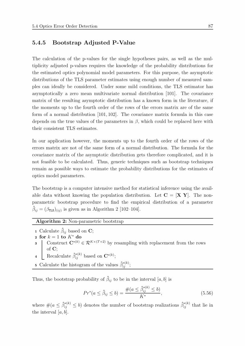
5.4 Optics Error Order Detection 87
5.4.5 Bootstrap Adjusted P-Value
The calculation of the p-values for the single hypotheses pairs, as well as the mul-
tiplicity adjusted p-values requires the knowledge of the probability distributions for
the estimated optics polynomial model parameters. For this purpose, the asymptotic
distributions of the TLS parameter estimates using enough number of measured sam-
ples can ideally be considered. Under some mild conditions, the TLS estimator has
asymptotically a zero mean multivariate normal distribution [101]. The covariance
matrix of the resulting asymptotic distribution has a known form in the literature, if
the moments up to the fourth order of the rows of the errors matrix are of the same
form of a normal distribution [101, 102]. The covariance matrix formula in this case
depends on the true values of the parameters in β, which could be replaced here with
their consistent TLS estimates.
In our application however, the moments up to the fourth order of the rows of the
errors matrix are not of the same form of a normal distribution. The formula for the
covariance matrix of the asymptotic distribution gets therefore complicated, and it is
not feasible to be calculated. Thus, generic techniques such as bootstrap techniques
remain as possible ways to estimate the probability distributions for the estimates of
optics model parameters.
The bootstrap is a computer intensive method for statistical inference using the avail-
able data without knowing the population distribution. Let C = [X Y]. The non-
parametric bootstrap procedure to find the empirical distribution of a parameter
βij = (βTLS)(ij) is given as in Algorithm 2 [102–104].
Algorithm 2: Non-parametric bootstrap
1 Calculate βij based on C;2 for k = 1 to K∗ do
3 Construct C∗(k) ∈ RK×(T+2) by resampling with replacement from the rowsof C;
4 Recalculate β∗(k)ij based on C∗(k);
5 Calculate the histogram of the values β∗(k)ij ;
Thus, the bootstrap probability of βij to be in the interval [a, b] is
Pr∗(a ≤ βij ≤ b) =#(a ≤ β
∗(k)ij ≤ b)
K∗ , (5.56)
where #(a ≤ β∗(k)ij ≤ b) denotes the number of bootstrap realizations β
∗(k)ij that lie in
the interval [a, b].

88 Chapter 5: Non-Linear Optics Components Detection and Measurement
The asymptotic consistency of the non-parametric bootstrap procedure for the TLS
estimator has been already shown in [102].
Let’s consider as an example an accelerator section with 3 BPMs containing a sex-
tupolar magnet error in vertical direction with a magnetic field of the form−→B y =
k(x2 − y2)−→e y. Furthermore, we consider skewed magnets such that lead coupling be-
tween the horizontal and vertical beam oscillations. Thus, the beam offset relation
polynomial for the horizontal beam oscillation of this scenario at BPM3 can be written
with respect to the beam offsets at the other BPMs of the given section in the form
x3 = λ1x1+λ2x2+λ3x12+λ4x2
2+λ5x1x2+λ6y12+λ7y2
2+λ8y1y2+λ9y1+λ10xy. (5.57)
Figure 5.2 shows the real distribution of the model parameters estimated by Monte-
Carlo simulations (solid lines), and the bootstrap distribution of the estimation of the
model parameters. One can notice from the figure that the bootstrap distributions of
the estimation of the model parameters match very well to the corresponding Monte-
Carlo distributions.
Since the p-values and the thresholds of the test statistics are calculated under the true
null hypotheses, the distributions of the test statistics under the null hypotheses must
be reconstructed. The bootstrap distribution of the test statistic Tbr for the collection
Br, 1 ≤ r ≤ R under the null hypotheses can be constructed as in Algorithm 3, which
is similar to the algorithm stated in Table 3.3 in [103].
Thus, the bootstrap p-value for the collection Br can be calculated using the result of
Algorithm 3 as the proportion of bootstrap test statistic values that are greater than
the observed value of the test statistic for the original data set, i.e.,
pr =#(Tb
∗(k)r ≥ Tbr,ob)
K∗ , (5.58)
where Tbr,ob denotes the observed value of the test statistic.
5.5 Confidence Intervals
After selecting the proper optics model and the existing multivariate polynomial terms,
the parameters of the selected model can be estimated with better quality since over-
fitting is avoided with estimating the true model. A very important aspect of the
parameter estimates is their reliability. Since the parameter estimation is applied
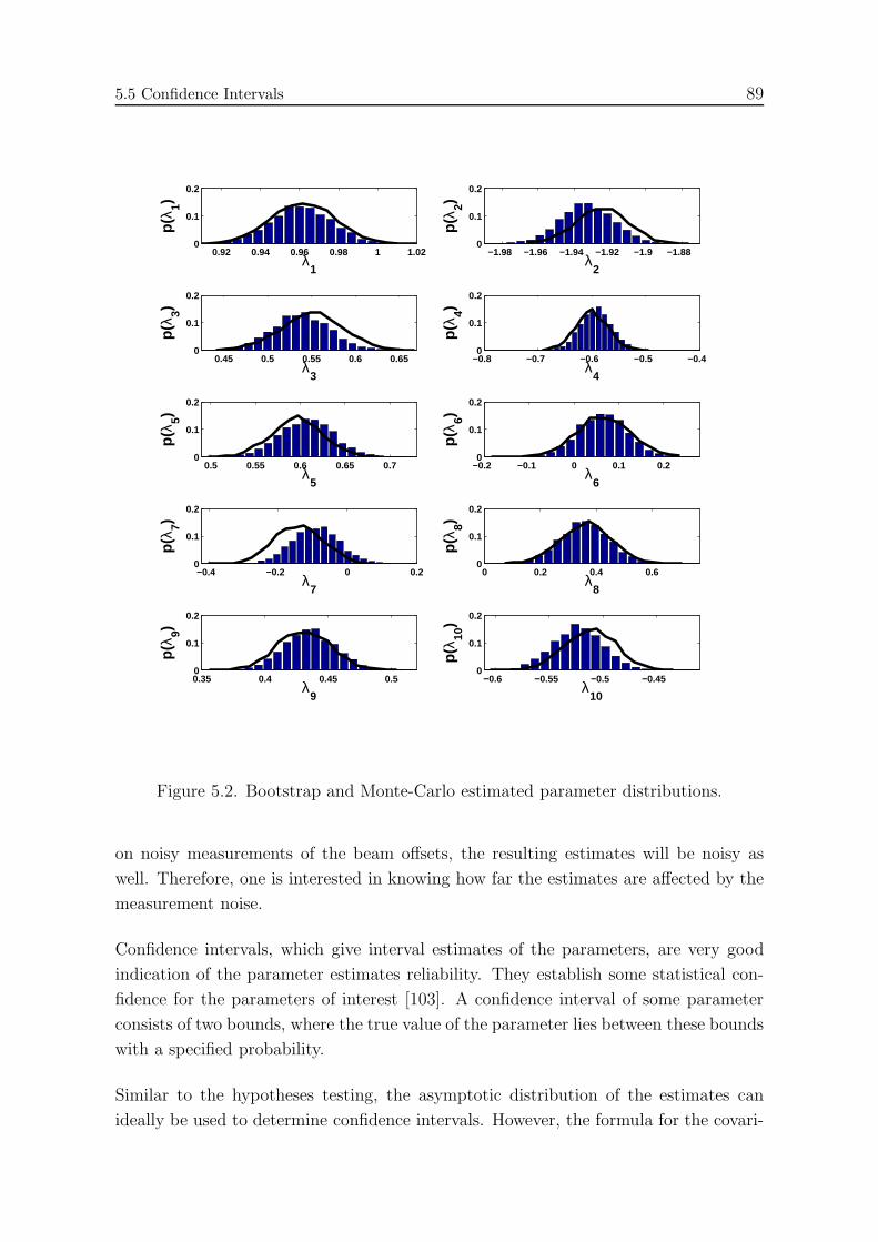
5.5 Confidence Intervals 89
0.92 0.94 0.96 0.98 1 1.020
0.1
0.2
λ1
p(λ 1)
−1.98 −1.96 −1.94 −1.92 −1.9 −1.880
0.1
0.2
λ2
p(λ 2)
0.45 0.5 0.55 0.6 0.650
0.1
0.2
λ3
p(λ 3)
−0.8 −0.7 −0.6 −0.5 −0.40
0.1
0.2
λ4
p(λ 4)
0.5 0.55 0.6 0.65 0.70
0.1
0.2
λ5
p(λ 5)
−0.2 −0.1 0 0.1 0.20
0.1
0.2
λ6
p(λ 6)
−0.4 −0.2 0 0.20
0.1
0.2
λ7
p(λ 7)
0 0.2 0.4 0.60
0.1
0.2
λ8
p(λ 8)
0.35 0.4 0.45 0.50
0.1
0.2
λ9
p(λ 9)
−0.6 −0.55 −0.5 −0.450
0.1
0.2
λ10
p(λ 10
)
Figure 5.2. Bootstrap and Monte-Carlo estimated parameter distributions.
on noisy measurements of the beam offsets, the resulting estimates will be noisy as
well. Therefore, one is interested in knowing how far the estimates are affected by the
measurement noise.
Confidence intervals, which give interval estimates of the parameters, are very good
indication of the parameter estimates reliability. They establish some statistical con-
fidence for the parameters of interest [103]. A confidence interval of some parameter
consists of two bounds, where the true value of the parameter lies between these bounds
with a specified probability.
Similar to the hypotheses testing, the asymptotic distribution of the estimates can
ideally be used to determine confidence intervals. However, the formula for the covari-

90 Chapter 5: Non-Linear Optics Components Detection and Measurement
Algorithm 3: Bootstrap under null hypotheses
1 Calculate Cp according to Equation (5.33);2 Calculate the residuals ∆CTLS,p according to Equation (5.36);3 Calculate the centered residuals by subtracting the mean value, i.e.,
∆CTLS,p = ∆CTLS,p −∆CTLS,p;
4 Calculate Cp = [Xp Y] = Cp −∆CTLS,p;
5 Calculate βrTLS,p = R
12ZZβ
rTLS, where βr
TLS denotes the parameter estimates fromEquation (5.37) with setting the corresponding parameters of the collection Br
to zero;6 for k = 1 to K∗ do
7 Construct ∆C∗(k)TLS,p = [∆Xp
∗(k) ∆Y∗(k)] ∈ RK×(T+2) by resampling with
replacement from the rows of ∆CTLS,p;
8 Calculate Y∗(k) = βrTLS,pXp +∆Y∗(k) ;
9 Calculate Xp∗(k) = Xp +∆Xp
∗(k) ;
10 Calculate β∗(k)TLS,p by applying the TLS estimator on C
∗(k)TLS,p = [Xp
∗(k) Y∗(k)];
11 Calculate β∗(k)TLS = R
− 12
ZZ β∗(k)TLS,p;
12 Calculate the test statisticTb∗(k)r for β
∗(k)TLS according to Equation (5.52);
13 Calculate the histogram of the values Tb∗(k)r ;
ance matrix of the asymptotic distribution is complicated, and cannot be calculated
as already mentioned before. Thus, bootstrap techniques remain as possible ways to
calculate confidence intervals for the model parameters.
5.5.1 Bootstrap Confidence Intervals
Let C = [X Y]. The non-parametric bootstrap procedure to find the empirical confi-
dence interval with confidence probability 1−α of a parameter βij = (βTLS)(ij) is given
in Algorithm 4 [102–104].
The strength of the bootstrap comes from its ability for statistical inference even in
complicated situations, as well as its higher accuracy compared to the normal approx-
imation approach [104]. Higher order accuracy of the bootstrap can be achieved by
dealing the studentized distribution of the estimators [103, 104]. This bootstrap tech-
nique is called percentile-t bootstrap, and can be performed as in Algorithm 5 [103,104].
Furthermore, the bootstrap technique can be performed on the parametric model of
the data in a similar way as in Algorithm 3. In this case, the residuals and the es-
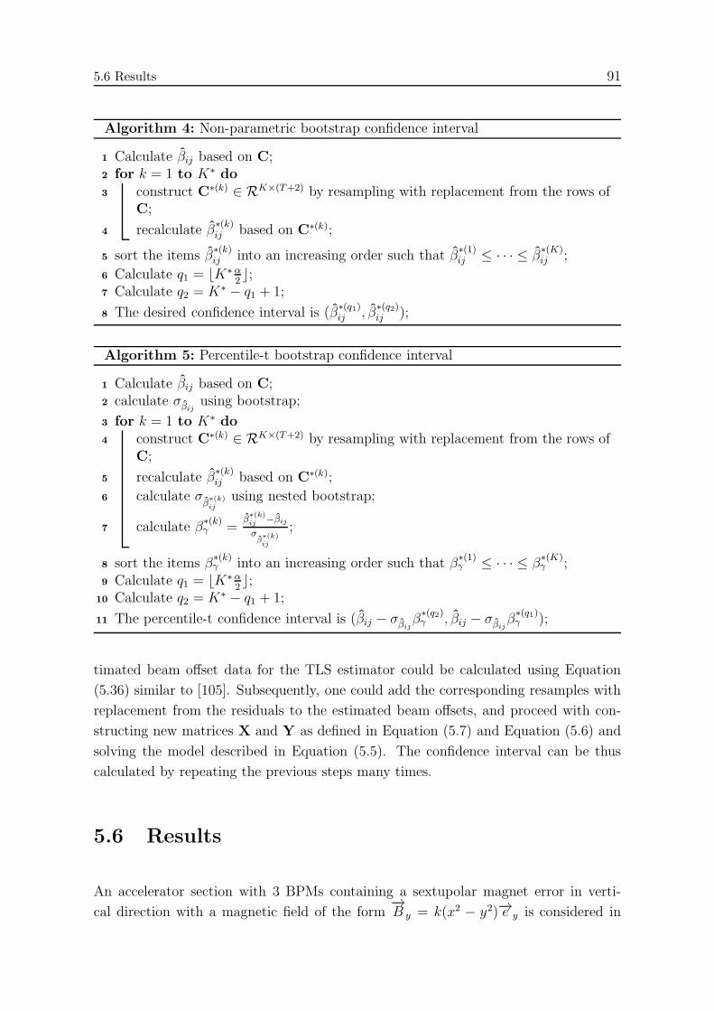
5.6 Results 91
Algorithm 4: Non-parametric bootstrap confidence interval
1 Calculate βij based on C;2 for k = 1 to K∗ do
3 construct C∗(k) ∈ RK×(T+2) by resampling with replacement from the rows ofC;
4 recalculate β∗(k)ij based on C∗(k);
5 sort the items β∗(k)ij into an increasing order such that β
∗(1)ij ≤ · · · ≤ β
∗(K)ij ;
6 Calculate q1 = ⌊K∗ α2⌋;
7 Calculate q2 = K∗ − q1 + 1;
8 The desired confidence interval is (β∗(q1)ij , β
∗(q2)ij );
Algorithm 5: Percentile-t bootstrap confidence interval
1 Calculate βij based on C;2 calculate σβij
using bootstrap;
3 for k = 1 to K∗ do
4 construct C∗(k) ∈ RK×(T+2) by resampling with replacement from the rows ofC;
5 recalculate β∗(k)ij based on C∗(k);
6 calculate σβ∗(k)ij
using nested bootstrap;
7 calculate β∗(k)γ =
β∗(k)ij −βij
σβ∗(k)ij
;
8 sort the items β∗(k)γ into an increasing order such that β
∗(1)γ ≤ · · · ≤ β
∗(K)γ ;
9 Calculate q1 = ⌊K∗ α2⌋;
10 Calculate q2 = K∗ − q1 + 1;
11 The percentile-t confidence interval is (βij − σβijβ∗(q2)γ , βij − σβij
β∗(q1)γ );
timated beam offset data for the TLS estimator could be calculated using Equation
(5.36) similar to [105]. Subsequently, one could add the corresponding resamples with
replacement from the residuals to the estimated beam offsets, and proceed with con-
structing new matrices X and Y as defined in Equation (5.7) and Equation (5.6) and
solving the model described in Equation (5.5). The confidence interval can be thus
calculated by repeating the previous steps many times.
5.6 Results
An accelerator section with 3 BPMs containing a sextupolar magnet error in verti-
cal direction with a magnetic field of the form−→B y = k(x2 − y2)−→e y is considered in
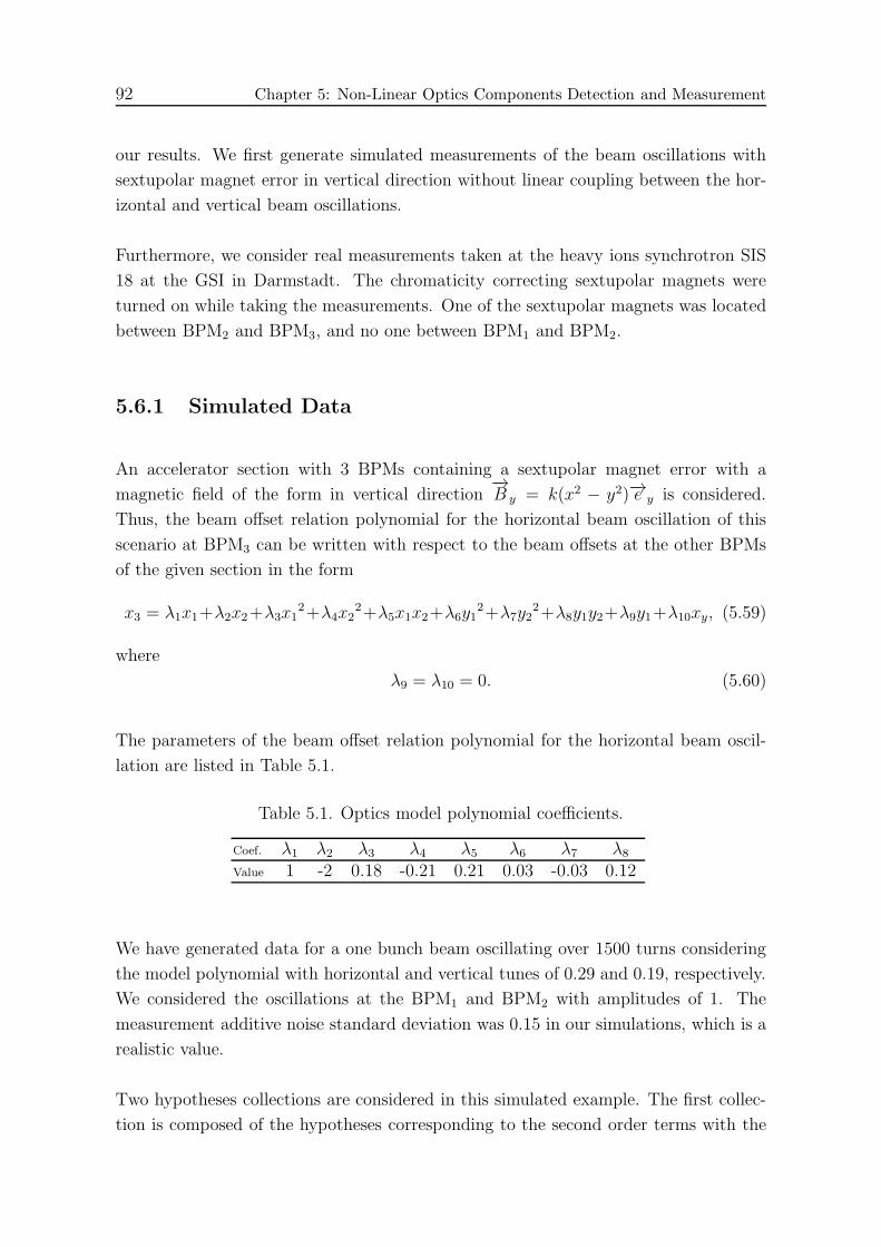
92 Chapter 5: Non-Linear Optics Components Detection and Measurement
our results. We first generate simulated measurements of the beam oscillations with
sextupolar magnet error in vertical direction without linear coupling between the hor-
izontal and vertical beam oscillations.
Furthermore, we consider real measurements taken at the heavy ions synchrotron SIS
18 at the GSI in Darmstadt. The chromaticity correcting sextupolar magnets were
turned on while taking the measurements. One of the sextupolar magnets was located
between BPM2 and BPM3, and no one between BPM1 and BPM2.
5.6.1 Simulated Data
An accelerator section with 3 BPMs containing a sextupolar magnet error with a
magnetic field of the form in vertical direction−→B y = k(x2 − y2)−→e y is considered.
Thus, the beam offset relation polynomial for the horizontal beam oscillation of this
scenario at BPM3 can be written with respect to the beam offsets at the other BPMs
of the given section in the form
x3 = λ1x1+λ2x2+λ3x12+λ4x2
2+λ5x1x2+λ6y12+λ7y2
2+λ8y1y2+λ9y1+λ10xy, (5.59)
where
λ9 = λ10 = 0. (5.60)
The parameters of the beam offset relation polynomial for the horizontal beam oscil-
lation are listed in Table 5.1.
Table 5.1. Optics model polynomial coefficients.
Coef. λ1 λ2 λ3 λ4 λ5 λ6 λ7 λ8
Value 1 -2 0.18 -0.21 0.21 0.03 -0.03 0.12
We have generated data for a one bunch beam oscillating over 1500 turns considering
the model polynomial with horizontal and vertical tunes of 0.29 and 0.19, respectively.
We considered the oscillations at the BPM1 and BPM2 with amplitudes of 1. The
measurement additive noise standard deviation was 0.15 in our simulations, which is a
realistic value.
Two hypotheses collections are considered in this simulated example. The first collec-
tion is composed of the hypotheses corresponding to the second order terms with the
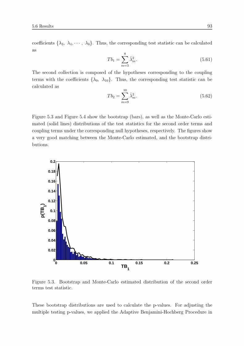
5.6 Results 93
coefficients {λ3, λ4, · · · , λ8}. Thus, the corresponding test statistic can be calculated
as
Tb1 =8∑
m=3
λ2m. (5.61)
The second collection is composed of the hypotheses corresponding to the coupling
terms with the coefficients {λ9, λ10}. Thus, the corresponding test statistic can be
calculated as
Tb2 =
10∑
m=9
λ2m. (5.62)
Figure 5.3 and Figure 5.4 show the bootstrap (bars), as well as the Monte-Carlo esti-
mated (solid lines) distributions of the test statistics for the second order terms and
coupling terms under the corresponding null hypotheses, respectively. The figures show
a very good matching between the Monte-Carlo estimated, and the bootstrap distri-
butions.
0 0.05 0.1 0.15 0.2 0.250
0.02
0.04
0.06
0.08
0.1
0.12
0.14
0.16
0.18
0.2
TB1
p(T
B1)
Figure 5.3. Bootstrap and Monte-Carlo estimated distribution of the second orderterms test statistic.
These bootstrap distributions are used to calculate the p-values. For adjusting the
multiple testing p-values, we applied the Adaptive Benjamini-Hochberg Procedure in
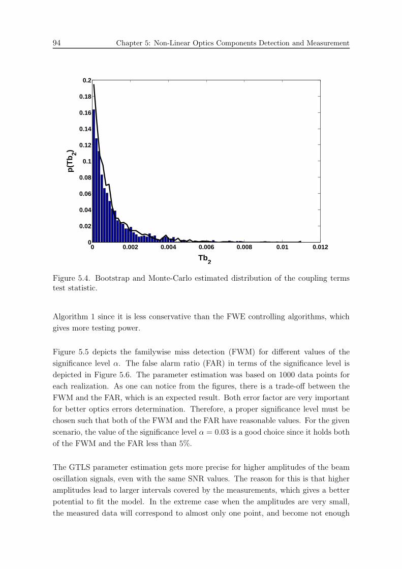
94 Chapter 5: Non-Linear Optics Components Detection and Measurement
0 0.002 0.004 0.006 0.008 0.01 0.0120
0.02
0.04
0.06
0.08
0.1
0.12
0.14
0.16
0.18
0.2
Tb2
p(T
b2)
Figure 5.4. Bootstrap and Monte-Carlo estimated distribution of the coupling termstest statistic.
Algorithm 1 since it is less conservative than the FWE controlling algorithms, which
gives more testing power.
Figure 5.5 depicts the familywise miss detection (FWM) for different values of the
significance level α. The false alarm ratio (FAR) in terms of the significance level is
depicted in Figure 5.6. The parameter estimation was based on 1000 data points for
each realization. As one can notice from the figures, there is a trade-off between the
FWM and the FAR, which is an expected result. Both error factor are very important
for better optics errors determination. Therefore, a proper significance level must be
chosen such that both of the FWM and the FAR have reasonable values. For the given
scenario, the value of the significance level α = 0.03 is a good choice since it holds both
of the FWM and the FAR less than 5%.
The GTLS parameter estimation gets more precise for higher amplitudes of the beam
oscillation signals, even with the same SNR values. The reason for this is that higher
amplitudes lead to larger intervals covered by the measurements, which gives a better
potential to fit the model. In the extreme case when the amplitudes are very small,
the measured data will correspond to almost only one point, and become not enough
5.6 Results 95
0 0.01 0.02 0.03 0.04 0.05 0.06 0.07 0.08 0.09 0.10
0.1
0.2
0.3
0.4
0.5
0.6
0.7
0.8
0.9
α
FW
M
Figure 5.5. Familywise miss detection in terms of the significance level.
to fit the model even with higher number of measurements that only lead to reducing
the impact of the noise, but does not give extra information about the model to be
fitted.
In Figure 5.7, we show the 95% confidence interval estimates for the model parameters
using non-parametric bootstrap described in Algorithm 4. The measurement noise
standard deviation was taken 0.6, and the oscillation signal amplitudes 4, which keeps
the same SNR value as in the previous simulations.
The coverage rates of the true model parameter values of the 95% and 97% confidence
intervals have been estimated using 1000 independent realizations. The resulting cov-
erage rates listed in Table 5.2 show a very good agreement with the given nominal
confidence probabilities.
The results in Fig. 5.7 can be used to determine the strength and location of the sex-
tupolar magnet error using an exhaustive search optimization due to the non-convexity.
The parameters with a tighter confidence intervals can be given more weights in the
search objective function since they are less affected by the measurement noise, more
reliable, and have higher accuracy.
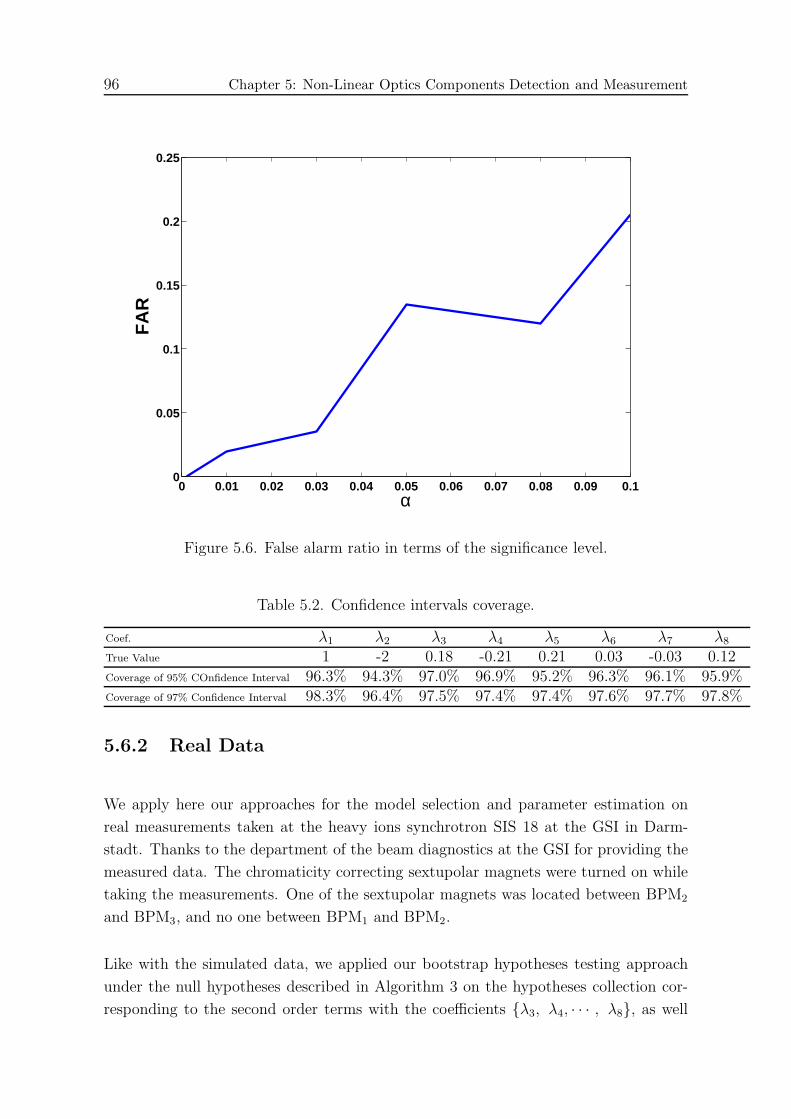
96 Chapter 5: Non-Linear Optics Components Detection and Measurement
0 0.01 0.02 0.03 0.04 0.05 0.06 0.07 0.08 0.09 0.10
0.05
0.1
0.15
0.2
0.25
α
FA
R
Figure 5.6. False alarm ratio in terms of the significance level.
Table 5.2. Confidence intervals coverage.
Coef. λ1 λ2 λ3 λ4 λ5 λ6 λ7 λ8
True Value 1 -2 0.18 -0.21 0.21 0.03 -0.03 0.12Coverage of 95% COnfidence Interval 96.3% 94.3% 97.0% 96.9% 95.2% 96.3% 96.1% 95.9%Coverage of 97% Confidence Interval 98.3% 96.4% 97.5% 97.4% 97.4% 97.6% 97.7% 97.8%
5.6.2 Real Data
We apply here our approaches for the model selection and parameter estimation on
real measurements taken at the heavy ions synchrotron SIS 18 at the GSI in Darm-
stadt. Thanks to the department of the beam diagnostics at the GSI for providing the
measured data. The chromaticity correcting sextupolar magnets were turned on while
taking the measurements. One of the sextupolar magnets was located between BPM2
and BPM3, and no one between BPM1 and BPM2.
Like with the simulated data, we applied our bootstrap hypotheses testing approach
under the null hypotheses described in Algorithm 3 on the hypotheses collection cor-
responding to the second order terms with the coefficients {λ3, λ4, · · · , λ8}, as well
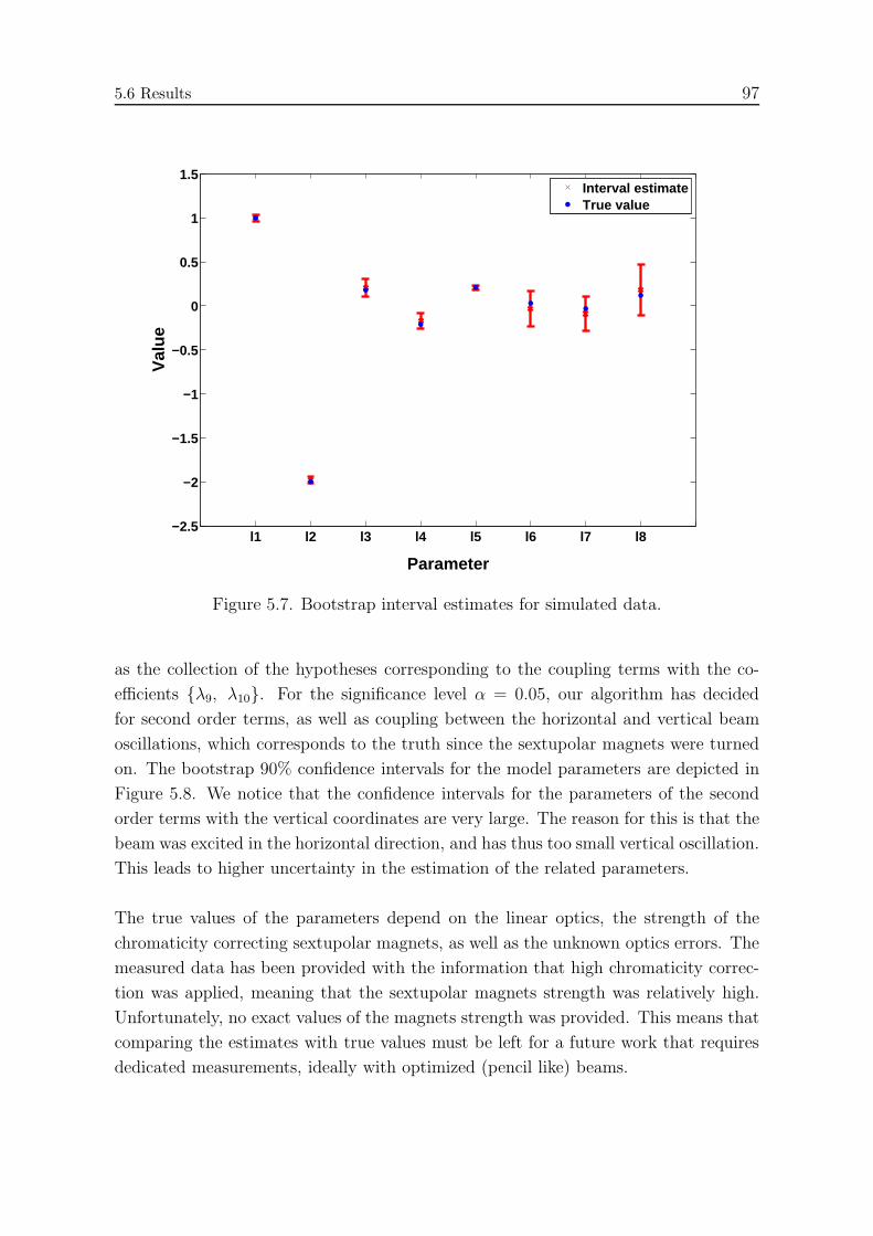
5.6 Results 97
l1 l2 l3 l4 l5 l6 l7 l8−2.5
−2
−1.5
−1
−0.5
0
0.5
1
1.5
Parameter
Val
ue
Interval estimateTrue value
Figure 5.7. Bootstrap interval estimates for simulated data.
as the collection of the hypotheses corresponding to the coupling terms with the co-
efficients {λ9, λ10}. For the significance level α = 0.05, our algorithm has decided
for second order terms, as well as coupling between the horizontal and vertical beam
oscillations, which corresponds to the truth since the sextupolar magnets were turned
on. The bootstrap 90% confidence intervals for the model parameters are depicted in
Figure 5.8. We notice that the confidence intervals for the parameters of the second
order terms with the vertical coordinates are very large. The reason for this is that the
beam was excited in the horizontal direction, and has thus too small vertical oscillation.
This leads to higher uncertainty in the estimation of the related parameters.
The true values of the parameters depend on the linear optics, the strength of the
chromaticity correcting sextupolar magnets, as well as the unknown optics errors. The
measured data has been provided with the information that high chromaticity correc-
tion was applied, meaning that the sextupolar magnets strength was relatively high.
Unfortunately, no exact values of the magnets strength was provided. This means that
comparing the estimates with true values must be left for a future work that requires
dedicated measurements, ideally with optimized (pencil like) beams.
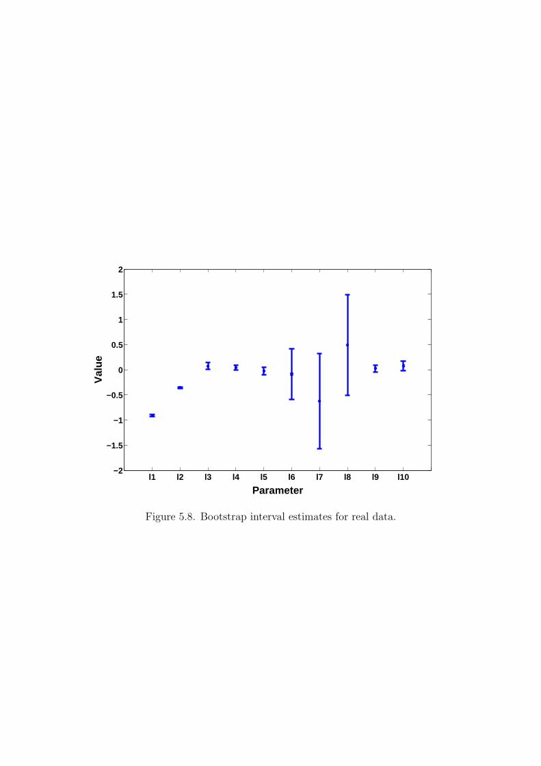
l1 l2 l3 l4 l5 l6 l7 l8 l9 l10−2
−1.5
−1
−0.5
0
0.5
1
1.5
2
Parameter
Val
ue
Figure 5.8. Bootstrap interval estimates for real data.

99
Chapter 6
Conclusions and Outlook
In this thesis, advanced signal processing techniques have been addressed for coher-
ent transversal beam oscillations in synchrotrons. We started on the one hand with
the normal accelerator operation, where the beam oscillations are a negative effect that
leads to operation quality deterioration, and needs hence to be mitigated. On the other
hand, we considered the beam coherent transversal oscillations as a useful diagnostics
source during diagnostics operation of particle accelerators. In this Chapter, the con-
clusions of this thesis and suggested directions for future research with this topic are
drawn.
6.1 Conclusions
For the normal operation of particle accelerators, we declared the beam transversal
oscillations as undesired since they lead to beam quality deterioration and emittance
blow up caused by the decoherence of the oscillating beam. The emittance blow up
reduces the luminosity of the beam, and thus the collision quality [1, 2]. Therefore,
beam oscillations must be suppressed in order to maintain high beam quality during
acceleration. A powerful way to mitigate coherent instabilities is to employ a feedback
system.
In order to cope with the noise generated at the TFS PUs, we have proposed a novel
concept to use multiple PUs for estimating the beam displacement at the position with
90◦ phase advance before the kicker. The estimated values should be the driving feed-
back signal. The signals from the different PUs are delayed such that they correspond
to the same bunch. Subsequently, a weighted sum of the delayed signals is suggested
as an estimator of the feedback correction signal. The weighting coefficients are cal-
culated in order to achieve an unbiased estimator, i.e., the output corresponds to the
actual beam displacement at the position with 90◦ phase advance before the kicker
for non-noisy PU signals. Furthermore, the estimator must provide the minimal noise
power at the output among all linear unbiased estimators. This proposed concept is
applied in our new approach to find optimal places for the PUs and the kicker around
the accelerator ring such that the noise effect on the feedback quality is minimized. A
new TFS design for the heavy ions synchrotrons SIS 18 and SIS 100 at the GSI has
been developed and implemented using FPGA.

100 Chapter 6: Conclusions and Outlook
Our simulation results have shown significant enhancements in the SNR by applying
this technique on the heavy ions synchrotron SIS 18 at the GSI. However, we should
have in mind the implementation challenges of this technique, where multiple PU
signals must be synchronized and processed in parallel. Our new approach to find
optimal places for the PUs and the kicker around the accelerator ring has been used to
evaluate the positions of the current PUs and the kicker at the SIS 18. The simulation
results for the kicker and the three closest PUs have shown that the current positions
are good, but still not optimal.
Furthermore, we address a novel concept for robust feedback system against optics
errors or uncertainties. A kicker and multiple pickups are assumed to be used for
each transversal direction. We introduced perturbation terms to the transfer matrices
between the kicker and the pickups. Subsequently, the Extended Kalman Filter was
used to estimate the feedback correction signal and the perturbation terms using the
measurements from the pickups. The observability of the system model has been shown
for the SIS 18 at the GSI. The simulation results have shown significant reduction in
the estimation error with optics uncertainties compared to non-robust approaches.
Moreover, we proposed a method for measuring the phase advances and amplitude
scaling between the positions of the kicker and the BPMs. Directly after applying a
kick on the beam by means of the kicker, we record the BPM signals. Subsequently, we
use the Second-Order Blind Identification (SOBI) algorithm to decompose the recorded
noised signals into independent sources mixture [5, 6]. Finally, we determine the re-
quired optics parameters by identifying and analyzing the betatron oscillation sourced
from the kick based on its mixing and temporal patterns. For a simulated scenario
with the physical parameters of the SIS 18, we could reach very high precision in the
estimation of the TFS required parameters.
For the diagnostics operation of particle accelerators, beam transversal oscillations can
be excited deliberately. We proposed in this thesis a novel method for detecting and
estimating the optics lattice non-linear components located in-between the locations of
two BPMs by analyzing the beam offset oscillation signals of a BPMs-triple containing
these two BPMs. Depending on the non-linear components in-between the locations of
the BPMs-triple, the relationship between the beam offsets follows a multivariate poly-
nomial accordingly. After calculating the covariance matrix of the polynomial terms,
the Generalized Total Least Squares method was used to find the model parameters,
and thus the non-linear components. Bootstrap techniques were used to detect the ex-
isting polynomial model orders by means of multiple hypothesis testing, and determine
confidence intervals for the model parameters. We have shown a very good matching
between the real and bootstrap distributions by means of Monte-Carlo simulations.
6.2 Outlook 101
Furthermore, we have shown that choosing a proper significance value is crucial for
better model selection, and thus better optics model estimation. Our simulation re-
sults have shown a good performance of our model selection approaches, and very good
coverage of the confidence intervals.
6.2 Outlook
In the future, further research with theoretical and simulation studies of the TFS and
its performance can be conducted while taking the space charge effects in particle
accelerators with very high beam intensities into consideration. The emittance blow-
up and luminosity can be evaluated for different scenarios of the space charge, TFS
gains, and SNRs.
Furthermore, experimental tests can be performed with implemented TFS using mul-
tiple PUs, as well as robust TFS on real accelerated beams in particle accelerators.
More intensive investigations can be conducted on the behavior and dynamics of the
robust feedback system and its stability. Intensive diagnostics of the beam emittance
and profile can be conducted during the operation of the TFS with different scenarios,
and beam properties.
Further research can be conducted in developing more signal processing techniques to
robustify the functionality of TFS against strong space charge effects and deformations
of the beams during acceleration.
Concerning the diagnostics operation, further experiments and measurement cam-
paigns can be conducted to test our addressed approaches for determining non-linear
accelerator optics components and errors. The resulting model orders and the confi-
dence intervals for the corresponding model parameters should be utilized in the search
for the locations and strengths or integrated strengths of the optics non-linear com-
ponents around the accelerator ring. The strength and location search can be done
via minimizing some cost functions, which must be related to the estimated confidence
intervals, as well as the differences between the estimated model parameters, and the
multivariate polynomial coefficients resulting from each given location, orientation, and
strength of nonlinear magnetic components. Deep theoretical performance analysis of
the developed methods can be conducted by evaluating their reliability and consistency.
Moreover, different modeling techniques of the accelerator optics, and its way of man-
ifestation on the beam transversal, and even longitudinal oscillations at different loca-
tions can be developed and investigated.


103
List of Acronyms
TFS Transverse Feedback System
RTFS Robust Transverse Feedback System
PU Pickup
BPM Beam Position Monitor
FG Function Generator
LF Low Frequency
HF High Frequency
BOSS Beam Offset Signal Suppressor
BTF Beam Transfer Function
GSI GSI Helmholzzentrum fur Schwerionenforschung GmbH (Helmholz
Center for Heavy Ions Research)
CERN Conseil Europeen pour la Recherche Nucleaire (European
Organization for Nuclear Research)
HOM Higher Order Mode
WF Wake Field
RWI Resistive Wall Impedance
FODO Focusing/Defocusing with drift distance in-between
SIS Schwerionensynchrotron (Heavy Ions Synchrotron)
LHC Large Hadron Collider
DSP Digital Signal Processor
MVUE Minimum Variance Unbiased Estimator
BLUE Best Linear Unbiased Estimator
MLE Maximum Likelihood Estimator
LS Least Squares
104 List of Acronyms
TLS Total Least Squares
GTLS Generalized Total Least Squares
FWE Family Wise Error
FER Familywise Error Rate
FWM Familywise Missdetection
FAR False Alarm Ratio
FDR False Discovery Rate
STP Simultaneous Test Procedure
BHP Benjamini-Hochberg Procedure
A-BHP Adaptive Benjamini-Hochberg Procedure
CI Confidence Interval
FPGA Field-Programmable Gate Array
MGT Multi-Gigabit Transceiver
ADC Analog to Digital Converter
DAC Digital to Analog Converter
Gbps Giga bit per Second
SFP Small Form-factor Pluggable
RF Radio Frequency
MMSE Minimum Mean Square Error
MSE Mean Square Error
RMSE Root Mean Square Error
VS Vector Summation
KF Kalman Filter
EKF Extended Kalman Filter
SOBI Second Order Blind Identification

105
SNR Signal-to-Noise Ratio
SVD Singular Value Decomposition
FIR Finite Impulse Response
IIR Infinite Impulse Response
CO Closed Orbit
ORM Orbit Response Matrix
NTRM Non-linear Tune Response Matrix
FAIR Facility for Antiproton and Ion Research


107
List of Symbols
~E Electric Field
~B Magnetic Field
s Longitudal Coordinate
x Horizontal Coordinate
y Vertical Coordinate
κx Focusing Strength in Horizontal Direction
κy Focusing Strength in Vertical Direction
p Particle Momentum
β(s) Betatron Function
α(s) Betatron Alpha Function
γ(s) Betatron Gamma Function
Ψ(s) Betatron Phase
βx(s) Betatron Function in Horizontal Direction
αx(s) Betatron Alpha Function in Horizontal Direction
γx(s) Betatron Gamma Function in Horizontal Direction
Ψx(s) Betatron Phase in Horizontal Direction
βy(s) Betatron Function in Vertical Direction
αy(s) Betatron Alpha Function in Vertical Direction
γy(s) Betatron Gamma Function in Vertical Direction
Ψy(s) Betatron Phase in Vertical Direction
βpu Betatron Function at the PUs Positions
αpu Betatron Alpha Function at the PUs Positions
γpu Betatron Gamma Function at the PUs Positions
βk Betatron Function at the Kicker Position
αk Betatron Alpha Function at the Kicker Position
γk Betatron Gamma Function at the Kicker Position
∆φ1 Phase Difference between the Kicker and the Closest PU
∆φPUs Phase Difference between Two Consecutive PUs
M Number of PUs
ǫ Emittance
Q Tune
Qx Horizontal Tune
Qy Vertical Tune

108 List of Symbols
q Fractional Tune
qx Fractional Horizontal Tune
qy Fractional Vertical Tune
a Radius of Vaccum Chamber
W⊥(z) Transverse Wake Function
Z⊥(ω) Fourier Transform of the Transverse Wake Function
c Speed of Light in Vacuum
ZRW⊥ Resistive Wall Impedance
Z0 impedance of free space
σ Conductivity of the Vaccum Tube Wall Material
f Frequency
f0 Revolution Frequency
D Natural Damping
Dfb Feedback Damping
F (t) Force of Coupling with Other Particles
τG Growth Time
Rzz Noise Covariance Matrix
xi Beam Offset at PUi
sk90 Location with 90◦ before the Kicker
xk90 Beam Offset at the Location sk90
aopt Optimal Weights Vector
br Real Part of the Phasors of the PU Signals
bi Imaginary Part of the Phasors of the PU Signals
L Lagrange Function
∇a,λr,λiL Gradiant of the Lagrange Function
λr The Real Parts Lagrange Multiplier
λi The Imaginary Parts Lagrange Multiplier
PN Noise Power
PNmin Optimal Noise Power
ND Number of Dimensions
PSig Signal Power
SNRx/y SNR in Horizontal/Vertical Direction
F Ensemble of Unoccupied Locations around the Accelerator Ring
τfocusing Index of Changing Optics
w(τ) Weighted Averaging Window

109
LP Accelerator Ring Circumference
xK(n) Beam Offset at the Kicker Location at the nth Turn
x′K(n) Beam Angle at the Kicker Location at the nth Turn
xK(n) Beam Status Vector at the Kicker Location at the nth Turn
MKK Complete Turn Transfer Matrix
MMS Measurement Matrix
DK The Kick Vector
np Model Noise
z Measurement Noise
MPKi Transfer Matrix from the Kicker to PUi
MnomKK Nominal Complete Turn Transfer Matrix
MnomMS Nominal Measurement Matrix
MPKK Uncertainty of the Complete Turn Transfer Matrix
MPMS Uncertainty of the Measurement Matrix
XEx Extended Status Vector
S Source Signals Vector
A Source Mixing Matrix
ξ chromaticity
δp RMS Momentum Spread
Qs Synchrotron Oscillation Tune
CSS(τ) Covariance Matrix of the Source Signals
βTLS TLS Parameter Estimate
pm Adjusted p-Value
Tbr Test Statistic for Hypothesis Hr
tr Decision Threshold for Hypothesis Hr
C Set of complex numbers
R Set of real numbers
Z Set of integer numbers
(·)T Transpose of a vector or matrix
(·)H Conjugate transpose of a vector or matrix
(·)∗ Conjugate of a scalar, vector, or matrix
(·)+ Pseudoinverse of a vector or matrix
(·)−1 Inverse of a square matrix
| · | Absolute value of a scalar
|| · || Euclidean norm or 2-norm of a vector

111
Bibliography
[1] E. Keil, W. Schnell, and P. Strolin, “Feedback damping of horizontal beamtransfer errors,” Tech. Rep., CERN, October 1969.
[2] V.M. Zhabitsky, “The transverse damping systems for sis100 & sis300,” Tech.Rep., GSI and Joint Institute for Nuclear Research, 2006.
[3] R. Rojko, New Concepts for Transverse Beam Stability in High-Current Heavy-Ion Synchrotrons, Ph.D. thesis, TU Darmstadt, 2003.
[4] M. Lonza, “Multi-bunch feedback systems,” in Cern Accelerator School, Sigtuna,SWEDEN, 2007.
[5] A. Belouchrani, K. Abed-Meraim, Jean-Francois Cardoso, and E. Moulines, “Ablind source separation technique using second-order statistics,” IEEE Transac-tions on Signal Processing, vol. 45, pp. 434–444, 1997.
[6] X. Huang, S. Y. Lee, E. Prebys, and R. Tomlin, “Application of independentcomponent analysis for beam diagnosis,” in Proceedings of the PAC05, 2005.
[7] S. Y. Lee, Accelerator Physics, World Scientific Publishing Company Incorpo-rated, 2012.
[8] G. Franchetti, A. Parfenova, and I. Hofmann, “Measuring localized nonlinearcomponents in a circular accelerator with a nonlinear tune response matrix,”Physical Review Special Topics-Accelerators and Beams, vol. 11, no. 9, pp. 094001,2008.
[9] A. Parfenova, G. Franchetti, and I. Hofmann, “Measuring ring nonlinear com-ponents via induced linear feeddown,” in EPAC08, 2008, pp. 3137–3139.
[10] J. Irwin, “Understanding nonlinear effects and losses,” Tech. Rep. SLAC-PUB-95-6831, SLAC, 1995.
[11] Gerhard Kraft, “Tumor therapy with heavy charged particles,” Progress inParticle and Nuclear Physics, vol. 45, pp. S473–S544, 2000.
[12] Phillip Sprangle, Antonio Ting, Eric Esarey, and Amnon Fisher, “Tunable, shortpulse hard x-rays from a compact laser synchrotron source,” Journal of appliedphysics, vol. 72, no. 11, pp. 5032–5038, 1992.
[13] J. Peterson W. Chou, “The ssc transverse feedback systems,” Tech. Rep., Su-perconducting Super Collider Laboratory, 1993.
[14] M. Kirk, U. Blell, and O. Boine-Frankenheim, “Maschinenexperimente zurtransversalen strahlanregung und inbetriebnahme des tfs am sis,” Tech. Rep.,GSI, 1992.
[15] Frank Zimmermann, “Comparison of calculated with measured dynamic aper-ture,” Tech. Rep., Stanford Linear Accelerator Center, Menlo Park, CA (UnitedStates). Funding organisation: USDOE, Washington, DC (United States), 1994.

112 Bibliography
[16] G. Franchetti and I. Hofmann, “Resonance trapping due to space charge andsynchrotron motion, in theory, simulations, and experiments,” Proceedings of the39th ICFA advanced beam dynamics workshop, 2007.
[17] A. Bazzani, E. Todesco, G. Turchetti, and G. Servizi, “Cern yellow report 94-02,”1994.
[18] D. Bulfone, V. Forchi, M. Lonza, and L. Zambon, “Bunch-by-bunch controlof instabilities with the elettra/sls digital feedback systems,” in Proceedings ofICALEPCS 2003, 2003.
[19] T. Nakamura et al., “Transverse bunch-by-bunch feedback system for the spring-8storage ring,” in 9th European Particle Accelerator Conference, Lucerne, Switzer-land, 2004.
[20] W.X. Cheng et al., “Single-loop two dimensional transverse feedback for photonfactory,” in Proceedings of EPAC2006, Edinburgh, Scotland, 2006.
[21] H. Hindi et al., “A formal approach to the design of multibunch feedback systems:Lqg controllers,” in Proceedings of EPAC94, London, UK, 1994.
[22] James Safranek, “Experimental determination of storage ring optics using orbitresponse measurements,” Nuclear Instruments and Methods in Physics ResearchSection A: Accelerators, Spectrometers, Detectors and Associated Equipment, vol.388, no. 1, pp. 27–36, 1997.
[23] Y. Chung, G. Decker, and K. Evans Jr, “Closed orbit correction using singularvalue decomposition of the response matrix,” in Particle Accelerator Conference,1993., Proceedings of the 1993. IEEE, 1993, pp. 2263–2265.
[24] M. Boge, M. Dehler, T. Schilcher, V. Schlott, and R. Ursic, “Fast closed or-bit control in the sls storage ring,” in Particle Accelerator Conference, 1999.Proceedings of the 1999. IEEE, 1999, vol. 2, pp. 1129–1131.
[25] A. Parfenova and G. Franchetti, “Linear and nonlinear beam optics studies inthe sis18,” in PAC09, 2009, vol. 9, pp. 3826–3828.
[26] R. Tomas, G. Arduini, G. Rumolo, F. Zimmermann, and A. Faus-Golfe, “Im-proved algorithms to determine the non-linear optics model of the sps from non-linear chromaticity,” in Proceedings of PAC07. IEEE, 2007, pp. 4231–4233.
[27] G. Arduini, F. Zimmermann, A. Faus-Golfe, and R. Tomas, “2003–2004 nonlinearoptics measurements and modeling for the cern sps,” in Proceedings of 2005Particle Accelerator Conference. IEEE, 2005, pp. 1171–1173.
[28] K. Wille, The physics of particle accelerators: an introduction, Oxford UniversityPress, 2000.
[29] Philip J Bryant and Kjell Johnsen, The principles of circular accelerators andstorage rings, Cambridge University Press, 2005.

Bibliography 113
[30] Mario Conte and William W MacKay, An introduction to the physics of particleaccelerators, vol. 160, World Scientific, 1991.
[31] Richard Clinton Fernow, Introduction to experimental particle physics, Cam-bridge University Press, 1989.
[32] Helmut Wiedemann et al., Particle accelerator physics, vol. 314, Springer, 2007.
[33] Donald A Edwards and Mike J Syphers, An introduction to the physics of highenergy accelerators, John Wiley & Sons, 2008.
[34] B. Franczak, “Sis parameter list,” Tech. Rep., GSI, 1987.
[35] Oliver Boine-Frankenheim, “Introduction to accelerator physics,” Lecture notes,2010, TU Darmstadt.
[36] P. J. Bryant, “Beam transfer lines,” in Jyvaeskylae 1992, Proceedings, Generalaccelerator physics, Geneva, 1992, CERN, vol. 1, pp. 219–238.
[37] E. Wilson, “ransverse beam dynamics,” in Jyvaeskylae 1992, Proceedings, Gen-eral accelerator physics, Geneva, 1992, CERN, vol. 1, pp. 131–158.
[38] M. Alhumaidi and A.M. Zoubir, “Optics non-linear components measurementusing bpm signals,” in Proceedings of IBIC2013, Oxford, UK, 2013.
[39] Werner Herr and Bruno Muratori, “Concept of luminosity,” in CERN AcceleratorSchool (CAS): Intermediate Course on Accelerator Physics, Zeuthen, Germany,2003, pp. 361–378.
[40] M. Giovannozzi, “Sources of emittance growth,” in Cern Accelerator School(CAS), 2011.
[41] J. S. Berg, “Coherent modes for multiple nonrigid bunches in a storage ring,” .
[42] P. J. Bryant and K. Johnsen, “The principles of circular accelerators and storagerings,” Cambridge Univ. Pr., 1993.
[43] B. Zotter and F. Sacherer, “Transverse instabilities of relativistic particle beamsin accelerators and storage rings,” International School Of Particle Accelerators,1977.
[44] L. Palumbo, V.G. Vaccaro, and M. Zobov, “Wake fields and impedance,” Tech.Rep., Laboratori Nazinali di Frascati, 1994.
[45] A. Hofmann, “Beam instabilities,” in CERN Accelerator School. CERN, 1993,pp. 307–330.
[46] A. Hofmann, “Kinetic theory,” in CERN Accelerator School, 1993, pp. 259–274.
[47] L. Palumbo, V. G. Vaccaro, and M. Zobov, “Wake fields and impedance,” 1994,LNF-94-041-P.
114 Bibliography
[48] H. Wiedemann, “Particle accelerator physics: Basic principles and linear beamdynamics,” Springer, 1993.
[49] T. Weiland and R. Wanzenberg, “Wake fields and impedance,” 1991, DESY-M-91-06.
[50] G. Rumolo, “Beam instabilities,” in Cern Accelerator School (CAS), 2011.
[51] Alexander Wu Chao, Physics of Collective Beam Instabilities in High EnergyAccelerators, Wiley, 1993.
[52] W. Chou, “Review of beam instability studies for the ssc,” in Proceedings of theParticle Accelerator Conference 1995, 1995.
[53] U. Niedermayer and O. Boine-Frankenheim, “Analytical and numerical calcula-tions of resistive wall impedances for thin beam pipe structures at low frequen-cies,” Nuclear Instruments and Methods in Physics Research A, vol. 687, pp.51–61, 2012.
[54] L. Wang et al., “Resistive wall instability in the damping rings of the ilc,” Tech.Rep., SLAC, 2006.
[55] M. Schuh, F.Gerigk, J.Tueckmantel, and C.P.Welsch, “Higher order mode anal-ysis of the spl cavities,” in Proceedings of IPAC’10, 2010.
[56] R.A. Bosch and C.S. Hsue, “Suppression of longitudinal coupled-bunch instabil-ities by a passive higher harmonic cavity,” in Proceedings of the Particle Accel-erator Conference 1993, 1993.
[57] M. Zobov, R. Boni, A. Gallo, A. Ghigo, F. Marcellini, L. Palumbo, M. Serio,B. Spataro, and G. Vignola, “Measures to reduce the impedance of parasiticresonant modes in the daone vacuum chamber,” in 14th Advanced ICFA BeamDynamics Workshop, 1997.
[58] V. M. Zhabitsky, “The transverse damping systems for sis100 & sis300,” Tech.Rep., GSI and Joint Institute for Nuclear Research.
[59] M. Svandrlik, C. J. Bocchetta, A. Fabris, F. Iazzourene, E. Karantzoulis, R. Na-gaoka, C. Pasotti, L. Tosi, R. P. Walker, and A. Wrulich, “The cure of multibunchinstabilities in elettra,” in Proceedings of the PAC95, 1995.
[60] M. Alhumaidi and A.M. Zoubir, “Using multiple pickups for transverse feedbacksystems and optimal pickups-kicker placement for noise power minimization,”Nuclear Instruments and Methods in Physics Research Section A, vol. 761, pp.79–85, 2014.
[61] M. Alhumaidi and A. M. Zoubir, “A transverse feedback system using multi-ple pickups for noise minimization,” in 2nd International Particle AcceleratorConference, San Sebastian, SPAIN, 2011.
[62] Robert M. Gray and Lee D. Davisson, An Introduction to Statistical SignalProcessing, Cambridge University Press, 2004.
Bibliography 115
[63] P. J. Bryant and K. Johnsen, The Principles of Circular Accelerators and StorageRings, Cambridge University Press, 1993.
[64] Xilinx, “Virtex-6 fpga ml605 evaluation kit,” .
[65] Xilinx, “Aurora link-layer protocol,” .
[66] Xilinx, “Logicore tm ip aurora 8b/10b v5.2 user guide,” July 2010.
[67] M. Alhumaidi and A.M. Zoubir, “A robust transverse feedback system,” in 3rdInternational Particle Accelerator Conference, New Orleans, Louisiana, USA,2012.
[68] Rudolph Emil Kalman, “A new approach to linear filtering and prediction prob-lems,” Journal of Fluids Engineering, vol. 82, no. 1, pp. 35–45, 1960.
[69] M. S. Grewal and A.P. Andrews, Kalman Filtering: Theory and Practice UsingMATLAB, John Wiley & Sons, 2001.
[70] Francesca Albertini and Domenico D’Alessandro, “Remarks on the observabilityof nonlinear discrete time systems,” in System Modelling and Optimization, pp.155–162. Springer, 1996.
[71] Kaare Brandt Petersen and Michael Syskind Pedersen, “The matrix cookbook,”Technical University of Denmark, pp. 7–15, 2008.
[72] Greg Welch and Gary Bishop, “An introduction to the kalman filter,” 1995.
[73] Arthur Gelb, Applied optimal estimation, MIT press, 1974.
[74] M. Alhumaidi, J. Grieser, and A.M. Zoubir, “Determination of optics transferbetween the kicker and bpms for transverse feedback system,” in Proceedings ofIPAC2013, 2013.
[75] Vladimir Kornilov and Oliver Boine-Frankenheim, “Transverse decoherence andcoherent spectra in long bunches with space charge,” Physical Review SpecialTopics-Accelerators and Beams, vol. 15, no. 11, pp. 114201, 2012.
[76] S.Y. Lee., “Decoherence of kicked beams ii,” Tech. Rep., SSCL, 1991.
[77] R.E. Meller, A.W. Chao, J.M. Peterson, S.G. Peggs, and M. Furman, “Decoher-ence of kicked beams,” Tech. Rep. No. SSC-N-360, SSC Report, 1987.
[78] Lieven De Lathauwer and Josephine Castaing, “Second-order blind identificationof underdetermined mixtures,” in Independent Component Analysis and BlindSignal Separation, pp. 40–47. Springer, 2006.
[79] G. Arduini, R. Tomas, F. Zimmermann, A. Faus-Golfe, and N. Iida, “2002nonlinear optics measurements and modelling for the cern sps,” in Proceedingsof the 2003 Particle Accelerator Conference. IEEE, 2003, vol. 4, pp. 2240–2242.

116 Bibliography
[80] Sabine Van Huffel and Joos Vandewalle, “Analysis and properties of the general-ized total least squares problem ax≈b when some or all columns in a are subjectto error,” SIAM Journal on Matrix Analysis and Applications, vol. 10, no. 3, pp.294–315, 1989.
[81] Ivan Markovsky and Sabine Van Huffel, “Overview of total least-squares meth-ods,” Signal processing, vol. 87, no. 10, pp. 2283–2302, 2007.
[82] Yosef Hochberg and Ajit C. Tamhane, Multiple comparison procedures, JohnWiley & Sons, Inc., 1987.
[83] Peter H. Westfall and S. Stanley Young, Resampling-based multiple testing: Ex-amples and methods for p-value adjustment, vol. 279, John Wiley & Sons, 1993.
[84] Fiky Y. Suratman, Spectrum Sensing in Cognitive Radio: Bootstrap and Sequen-tial Detection Approaches, Ph.D. thesis, TU Darmstadt, 2014.
[85] Pei-Jung Chung, Johann F. Bohme, Christoph F. Mecklenbrauker, and Alfred O.Hero, “Detection of the number of signals using the benjamini-hochberg proce-dure,” Signal Processing, IEEE Transactions on, vol. 55, no. 6, pp. 2497–2508,2007.
[86] Abdelhak M. Zoubir and Johann F. Bohme, “Bootstrap multiple tests appliedto sensor location,” IEEE Transactions on Signal Processing, vol. 43, no. 6, pp.1386–1396, 1995.
[87] Priyadip Ray and Pramod K. Varshney, “False discovery rate based sensor deci-sion rules for the network-wide distributed detection problem,” IEEE Transac-tions on Aerospace and Electronic Systems, vol. 47, no. 3, pp. 1785–1799, 2011.
[88] Erhan Baki Ermis and Venkatesh Saligrama, “Distributed detection in sensornetworks with limited range multimodal sensors,” IEEE Transactions on SignalProcessing, vol. 58, no. 2, pp. 843–858, 2010.
[89] Gerard V. Dallal, The little handbook of statistical practice, Gerard V. Dallal,1999.
[90] Yoav Benjamini and Yosef Hochberg, “Controlling the false discovery rate: apractical and powerful approach to multiple testing,” Journal of the Royal Sta-tistical Society. Series B (Methodological), pp. 289–300, 1995.
[91] Yoav Benjamini and Yosef Hochberg, “On the adaptive control of the false discov-ery rate in multiple testing with independent statistics,” Journal of Educationaland Behavioral Statistics, vol. 25, no. 1, pp. 60–83, 2000.
[92] Sanat K. Sarkar, “False discovery and false nondiscovery rates in single-stepmultiple testing procedures,” The Annals of Statistics, pp. 394–415, 2006.
[93] Wenge Guo and Joseph Romano, “A generalized sidak-holm procedure and con-trol of generalized error rates under independence,” Statistical applications ingenetics and molecular biology, vol. 6, no. 1, 2007.
Bibliography 117
[94] Charles W. Dunnett and Ajit C. Tamhane, “Step-down multiple tests for com-paring treatments with a control in unbalanced one-way layouts,” Statistics inMedicine, vol. 10, no. 6, pp. 939–947, 1991.
[95] Mark J. van der Laan, Sandrine Dudoit, and Katherine S. Pollard, “Multipletesting. part ii. step-down procedures for control of the family-wise error rate,”Statistical Applications in Genetics and Molecular Biology, vol. 3, no. 1, 2004.
[96] Sture Holm, “A simple sequentially rejective multiple test procedure,” Scandi-navian journal of statistics, pp. 65–70, 1979.
[97] Yosef Hochberg, “A sharper bonferroni procedure for multiple tests of signifi-cance,” Biometrika, vol. 75, no. 4, pp. 800–802, 1988.
[98] Burt S. Holland and Margaret DiPonzio Copenhaver, “An improved sequentiallyrejective bonferroni test procedure,” Biometrics, pp. 417–423, 1987.
[99] Juliet Popper Shaffer, “Modified sequentially rejective multiple test procedures,”Journal of the American Statistical Association, vol. 81, no. 395, pp. 826–831,1986.
[100] Burt S. Holland and Margaret DiPonzio Copenhaver, “An improved sequentiallyrejective bonferroni test procedure,” Biometrics, pp. 417–423, 1987.
[101] Leon Jay Gleser, “Estimation in a multivariate” errors in variables” regressionmodel: large sample results,” The Annals of Statistics, pp. 24–44, 1981.
[102] Michal Pesta, “Total least squares and bootstrapping with applications in cali-bration,” Statistics: A Journal of Theoretical and Applied Statistics, vol. 47, no.5, pp. 966–991, 2013.
[103] Abdelhak M. Zoubir and D. Robert Iskander, Bootstrap techniques for signalprocessing, Cambridge University Press, 2004.
[104] Dimitris N. Politis, “Computer-intensive methods in statistical analysis,” IEEESignal Processing Magazine, vol. 15, no. 1, pp. 39–55, 1998.
[105] Bogdan Matei and Peter Meer, “Bootstrapping errors-in-variables models,” inVision Algorithms: Theory and Practice, pp. 236–252. Springer, 2000.


119
Lebenslauf
Name: Mouhammad Alhumaidi
Anschrift: Ulmer Straße 8 — 87700 Memmingen
Geburtsdatum: 01.01.1984
Geburtsort: Raqa / Syrien
Familienstand: verheiratet
Schulausbildung
09/1989-06/1998 Grund- und Mittelschule in Ratlah, Raqa / Syrien
09/1998-07/2001 Alrasheed Gymnasium in Raqa / Syrien
Studium
09/2001-12/2006 Studium der Kommunikationstechnik amHigher Institute for Applied Sciences and Technology(HIAST), Damaskus, Syrien,Studienabschluß: Engineering Diploma
10/2008-10/2010 Studium der Elektrotechnik und Informationstechnik,Vertiefung: Nachrichten- und Kommunikationsstech-nik, an derTU Darmstadt,Studienabschluß: Master of Science
Berufstatigkeit
11/2010-10/2014 wissenschaftlicher Mitarbeiter amFachgebiet Signalverarbeitung,Institut fur Nachrichtentechnik,Technische Universitat Darmstadt
seit 10/2014 Entwicklungsingenieur Algorithmik fur Radarsysteme,Continental AG


Erklarung laut §9 der Promotionsordnung
Ich versichere hiermit, dass ich die vorliegende Dissertation allein und nur unterVerwendung der angegebenen Literatur verfasst habe. Die Arbeit hat bisher nochnicht zu Prufungszwecken gedient.
Darmstadt, 14. Januar 2015,

Related Documents