Statistical Shape Models Using Elastic-String Representations

Statistical Shape Models Using Elastic-StringRepresentations

Anuj Srivastava1, Aastha Jain2, Shantanu Joshi1, and David Kaziska3

1 Florida State University, Tallahassee, FL, USA2 Indian Institute of Technology, N. Delhi, India

3 Air Force Institute of Technology, Dayton, OH, USA

Abstract. To develop statistical models for shapes, we utilize an elas-tic string representation where curves (denoting shapes) can bend andlocally stretch (or compress) to optimally match each other, resulting ingeodesic paths on shape spaces. We develop statistical models for cap-turing variability under the elastic-string representation. The basic ideais to project observed shapes onto the tangent spaces at sample means,and use finite-dimensional approximations of these projections to im-pose probability models. We investigate the use of principal componentsfor dimension reduction, termed tangent PCA or TPCA, and study (i)Gaussian, (ii) mixture of Gaussian, and (iii) non-parametric densitiesto model the observed shapes. We validate these models using hypothe-sis testing, statistics of likelihood functions, and random sampling. It isdemonstrated that a mixture of Gaussian model on TPCA captures bestthe observed shapes.

1 Introduction

Analysis of shapes is emerging as an important tool in recognition of objectsfrom their images. As an example, one uses the contours formed by boundariesof objects, as they appear in images, to characterize the objects themselves. Sincethe objects can occur at arbitrary locations, scales, and planar rotations, withoutchanging their appearances, one is interested in the shapes of these contours,rather than the contours themselves. This motivates the development of toolsfor statistical analysis of shapes of simple, closed curves in R

2. A statisticalanalysis is beneficial in many situations. For instance, in cases where the observedimage is low quality due to clutter, low resolution, or obscuration, one can usethe contextual knowledge to impose prior models on expected shapes, and use aBayesian framework to improve shape extraction performance. Such applicationsrequire a broad array of tools for analyzing shapes: geometric representationsof shapes, metrics for quantifying shape differences, algorithms for computingshape statistics such as means and covariances, and tools for testing competinghypotheses on given shapes.

Analysis of shapes of planar curves has been of a particular interest recentlyin the literature. Klassen [1] have described a geometric technique to parame-terize curves by their arc lengths, and to use their angle functions to represent

P.J. Narayanan et al. (Eds.): ACCV 2006, LNCS 3851, pp. 612–621, 2006.c© Springer-Verlag Berlin Heidelberg 2006

Statistical Shape Models Using Elastic-String Representations 613

and analyze shapes. Similar constructions for analysis of closed curves were alsostudied in [2, 3]. Using the representations and metrics described in [1], [4] de-scribe techniques for clustering, learning, and testing of planar shapes. One majorlimitation of this approach is that all curves are parameterized by arc length,and the resulting transformations from one shape into another are restricted tobending only. Local stretching or compression of shapes is not allowed. Mio [5]resolved this issue by introducing a representation that allows both bending andstretching of shapes to match each other. The geodesic paths resulting from thisapproach seem more natural as interesting features, such as corners, are betterpreserved while constructing geodesics, in this approach. This representation ofplanar shapes is called an elastic string model.

Our goal in this paper is to use elastic string model to study several prob-ability models for capturing observed shape variability. Similar to approachespresented in [6, 4], we project observed shapes onto the tangent spaces at sam-ple means, and further reduce their dimensions using PCA. Thus, we obtain alow-dimensional representations of shapes called TPCA. On tangent principalcomponents (TPCs) of observed shapes we study: (i) Gaussian, (ii) nonpara-metric, and (iii) mixture of Gaussian models. The first two have been studiedearlier for non-elastic shapes in [4]. To study model performances, we: (i) syn-thesize random shapes from these models, (ii) test amongst competing modelsusing likelihood ratio, and (iii) compare statistics of likelihood on training andtest data. This framework leads to stochastic shape models that can be usedas priors in future Bayesian extraction of shapes from low-quality images. Toillustrate these ideas we have used shapes from the ETH databases.

Rest of this paper is organized as follows. Section 2 summarizes elastic-stringmodels for shape representations. Section 3 proposes three candidate probabil-ity models for capturing shape variability, while Sections 4 and 5 study theseprobability models via synthesis and hypothesis testing.

2 Elastic Strings Representation

Here we summarize the main ideas behind elastic-string representations of planarshapes, originally described in Mio et al [5].

2.1 Shape Representation

Let α : [0, 2π] → R2 be a smooth parametric curve such that α′(t) �= 0, ∀t ∈

[0, 2π]. The velocity vector is α′(t) = eφ(t)ejθ(t), where φ : [0, 2π] → R andθ : [0, 2π] → R are smooth, and j =

√−1. The function φ is the log-speed of

α and θ is the angle function. φ(t) measures the rate at which the interval [0, 2π]is stretched or compressed at t to form the curve α; φ(t) > 0 indicates localstretching near t, and φ(t) < 0 local compression. Curves parameterized by arclength have φ ≡ 0. We will represent α via the pair (φ, θ) and denote by H thecollection of all such pairs.

Parametric curves that differ by rigid motions or uniform scalings of the plane,or by re-parameterizations are treated as representing the same shape. The pair

614 A. Srivastava et al.

(φ, θ) is already invariant to translations of the curve. Rigid rotations and uni-form scalings are removed by restricting to the space,

C = {(φ, θ) ∈ H :� 2π

0eφ(t)dt = 2π,

12π

� 2π

0θ(t)eφ(t)dt = π,

� 2π

0eφ(t)ejθ(t)dt = 0},

C is called the pre-shape spaces of planar elastic strings. There are two possibleways of re-parameterizing a closed curve, without changing its shape: (i) Oneis to change the placement of origin t = 0 on the curve. This change can berepresented as the action of a unit circle S

1 on a shape (φ, θ), according to:s · (φ(t), θ(t)) = (φ(t − s), θ(t − s) + s). (ii) Re-parameterizations of α thatpreserve orientation and the property that α′(t) �= 0, ∀t, are those obtained bycomposing α with an orientation-preserving diffeomorphism γ : [0, 2π] → [0, 2π].Let D be the group of all such mappings. These mappings define a right actionof D on H by

(φ, θ) · γ = (φ ◦ γ + log γ′ , θ ◦ γ). (1)

◦ denotes composition of functions. The space of all (shape-preserving) re-parametrization of a shape in C is thus given by S

1 × D. The resulting shapespace is the space of all equivalence classes induced by these shape preservingtransformations. It can be written as a quotient space S = (C/D)/S

1.What metric can used to compare shapes in this space? Mio [5] suggests that,

given (φ, θ) ∈ H, let hi and fi, i = 1, 2, represent infinitesimal deformations ofφ and θ, resp. , so that (h1, f1) and (h2, f2) are tangent vectors to H at (φ, θ).For a, b > 0, define 〈(h1, f1), (h2, f2)〉(φ,θ) as

a

∫ 1

0h1(t)h2(t) eφ(t) dt + b

∫ 1

0f1(t)f2(t) eφ(t) dt. (2)

It can be shown that re-parameterizations preserve the inner product, i.e., S1×D

acts on H by isometries. The elastic properties of the curves are built-in tothe model via the parameters a and b, which can be interpreted as tensionand rigidity coefficients, respectively. Large values of the ratio a/b indicate thatstrings offer higher resistance to stretching and compression than to bending; theopposite holds for a/b small. In this paper we fix a value of a/b that balancesbetween bending and stretching.

2.2 Geodesic Paths in Shape Spaces

An important tool in this shape analysis is to construct geodesic paths, i.e.paths of smallest lengths, between arbitrary two shapes. Given the complicatedgeometry of S, this task is not straightforward, at least not analytically. Onesolution is to use a computational approach, where the search for geodesicsis treated as an optimization problem with iterative numerical updates. Thisapproach is called the shooting method. Given a pair of shapes α1 ≡ (φ1, θ1) andα2 ≡ (φ2, θ2), one solves:

mins∈S1,γ∈D,g∈Tα1(C)

‖Ψ1(α1; g) − (s · (α2)) · γ‖2 (3)

Statistical Shape Models Using Elastic-String Representations 615

where Ψt(α; g) denotes a geodesic path starting at a shape α in the direction g,and parameterized by time t. Also, ‖·‖ is the L

2 norm on H. Basically, one solvesfor the shooting direction g∗ such that the geodesic from α1 in the direction g∗

gets as close to the orbit of α2 under shape preserving transformations [5]. Letd(α1, α2) ≡ ‖g∗‖ denote the length of geodesics connecting the shapes α1 andα2. This construction helps define the exponential map: expα(g) = Ψ1(α; g) andits inverse exp−1

α (β) = g such that Ψ1(α; g) = β.

2.3 Sample Mean of Shapes

Since the shape space S is nonlinear, the definitions of sample statistics, suchas means and covariances, are not conventional. Earlier papers [7, 8] suggest theuse of Karcher mean to define mean shapes as follows. For α1, . . . , αn in S, andd(αi, αj) the geodesic length between αi and αj , the Karcher mean is definedas the element µ ∈ S that minimizes the quantity

∑ni=1 d(µ, αi)2. A gradient-

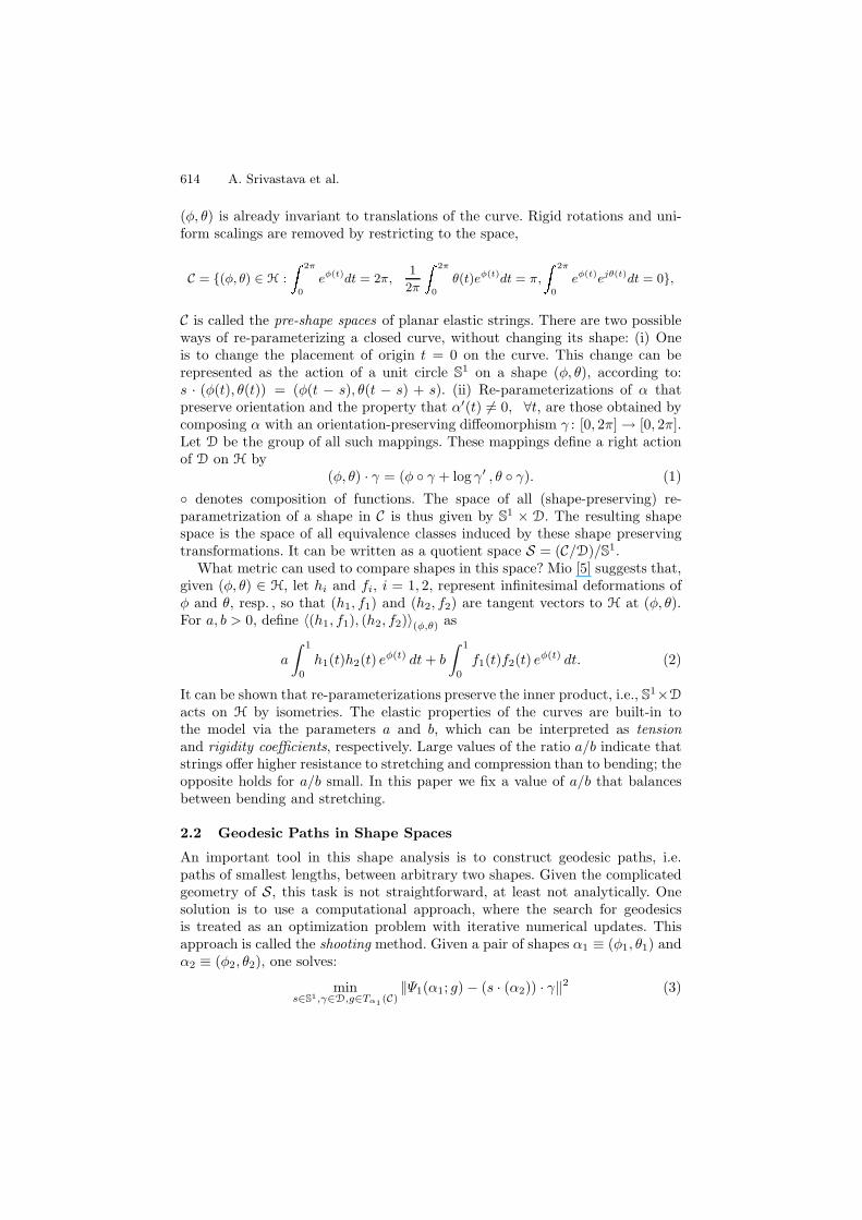
based, iterative algorithm for computing the Karcher mean is presented in [8, 1].Shown in Figure 1 are some examples of three classes of shapes – dogs, pears,and mugs – used in the experiments here, and the Figure 2 shows Karcher meansof shapes in these three classes. Let µ be the mean shape and for any shape α,let g ∈ Tµ(S) be such that Ψ1(µ; g) = α. Then, α called the exponential of g,i.e. expµ(g), and conversely, g = exp−1

µ (α). As described next, statistics of α arestudied through statistics of its map onto the tangent space at the mean.

Fig. 1. Examples of three classes of shapes – dogs, pears, and mugs – from the ETHdatabase that are studied in this paper, with the numbers used in test and training

3 Statistical Shape Models

Our goal is to derive and analyze probability models for capturing observedshapes. The task of learning probability models on spaces like S is difficult for twomain reasons. Firstly, they are nonlinear spaces and therefore classical statisticalapproaches, associated with the vector spaces, do not apply directly. Secondly,these are infinite-dimensional spaces and do not allow component-by-componentmodeling that is traditionally followed in finite-dimensional vector spaces. Thesolution involves making two approximations. First, we project elements of Sonto the tangent space Tµ(S), which is a vector space, and therefore, better suitedto statistical modeling. This is performed using the inverse exponential mapexp−1

µ . Second, we perform dimension reduction in Tµ(S) using PCA. Together,

616 A. Srivastava et al.

0 10 20 30 40 50 60 70 80 900

0.005

0.01

0.015

0.02

0.025

0.03

0.035

0.04

0.045

0.05

0 20 40 60 80 100 1200

0.002

0.004

0.006

0.008

0.01

0.012

0.014

0.016

0.018

0.02

0 20 40 60 80 100 1200

0.002

0.004

0.006

0.008

0.01

0.012

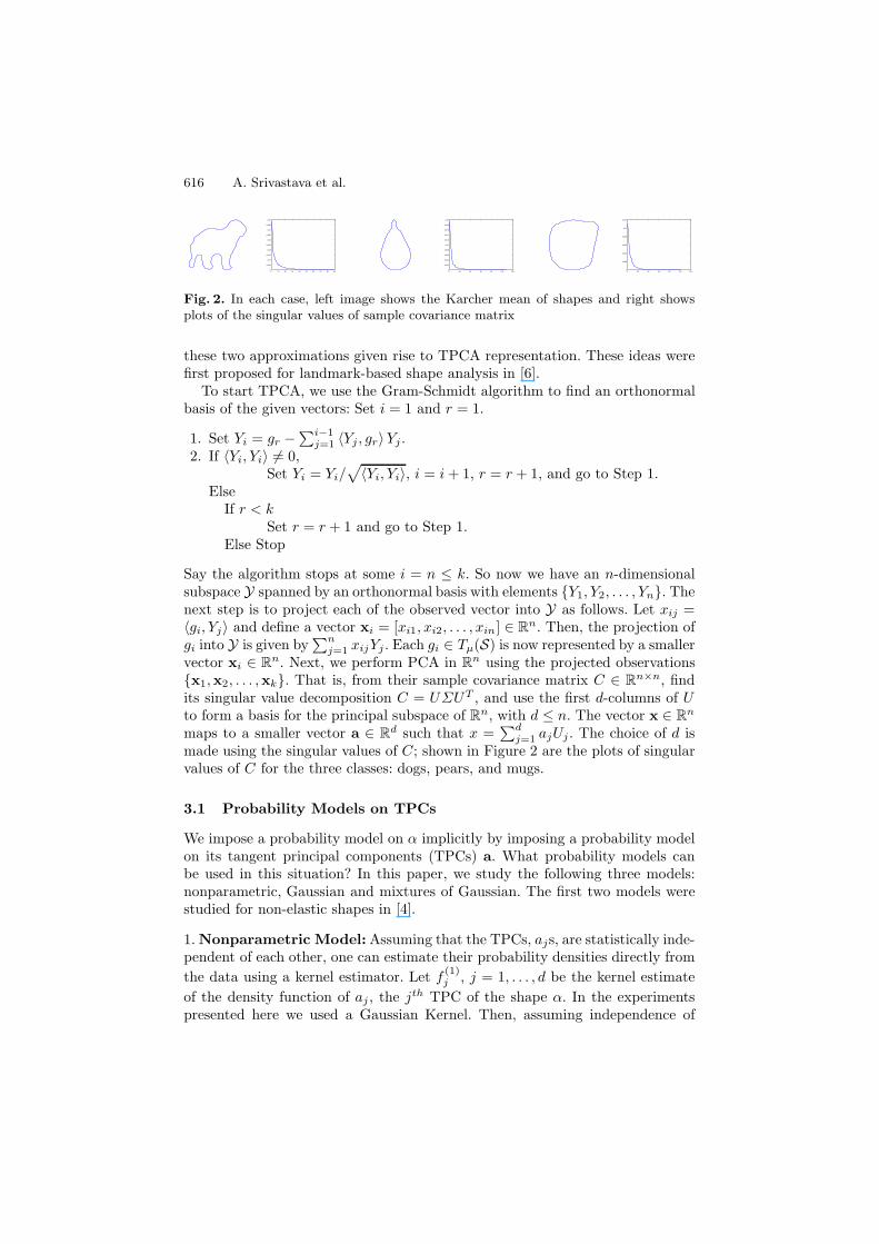
Fig. 2. In each case, left image shows the Karcher mean of shapes and right showsplots of the singular values of sample covariance matrix

these two approximations given rise to TPCA representation. These ideas werefirst proposed for landmark-based shape analysis in [6].

To start TPCA, we use the Gram-Schmidt algorithm to find an orthonormalbasis of the given vectors: Set i = 1 and r = 1.

1. Set Yi = gr −∑i−1

j=1 〈Yj , gr〉Yj .2. If 〈Yi, Yi〉 �= 0,

Set Yi = Yi/√

〈Yi, Yi〉, i = i + 1, r = r + 1, and go to Step 1.Else

If r < kSet r = r + 1 and go to Step 1.

Else Stop

Say the algorithm stops at some i = n ≤ k. So now we have an n-dimensionalsubspace Y spanned by an orthonormal basis with elements {Y1, Y2, . . . , Yn}. Thenext step is to project each of the observed vector into Y as follows. Let xij =〈gi, Yj〉 and define a vector xi = [xi1, xi2, . . . , xin] ∈ R

n. Then, the projection ofgi into Y is given by

∑nj=1 xijYj . Each gi ∈ Tµ(S) is now represented by a smaller

vector xi ∈ Rn. Next, we perform PCA in R

n using the projected observations{x1,x2, . . . ,xk}. That is, from their sample covariance matrix C ∈ R

n×n, findits singular value decomposition C = UΣUT , and use the first d-columns of Uto form a basis for the principal subspace of R

n, with d ≤ n. The vector x ∈ Rn

maps to a smaller vector a ∈ Rd such that x =

∑dj=1 ajUj . The choice of d is

made using the singular values of C; shown in Figure 2 are the plots of singularvalues of C for the three classes: dogs, pears, and mugs.

3.1 Probability Models on TPCs

We impose a probability model on α implicitly by imposing a probability modelon its tangent principal components (TPCs) a. What probability models canbe used in this situation? In this paper, we study the following three models:nonparametric, Gaussian and mixtures of Gaussian. The first two models werestudied for non-elastic shapes in [4].

1. Nonparametric Model: Assuming that the TPCs, ajs, are statistically inde-pendent of each other, one can estimate their probability densities directly fromthe data using a kernel estimator. Let f

(1)j , j = 1, . . . , d be the kernel estimate

of the density function of aj , the jth TPC of the shape α. In the experimentspresented here we used a Gaussian Kernel. Then, assuming independence of

Statistical Shape Models Using Elastic-String Representations 617

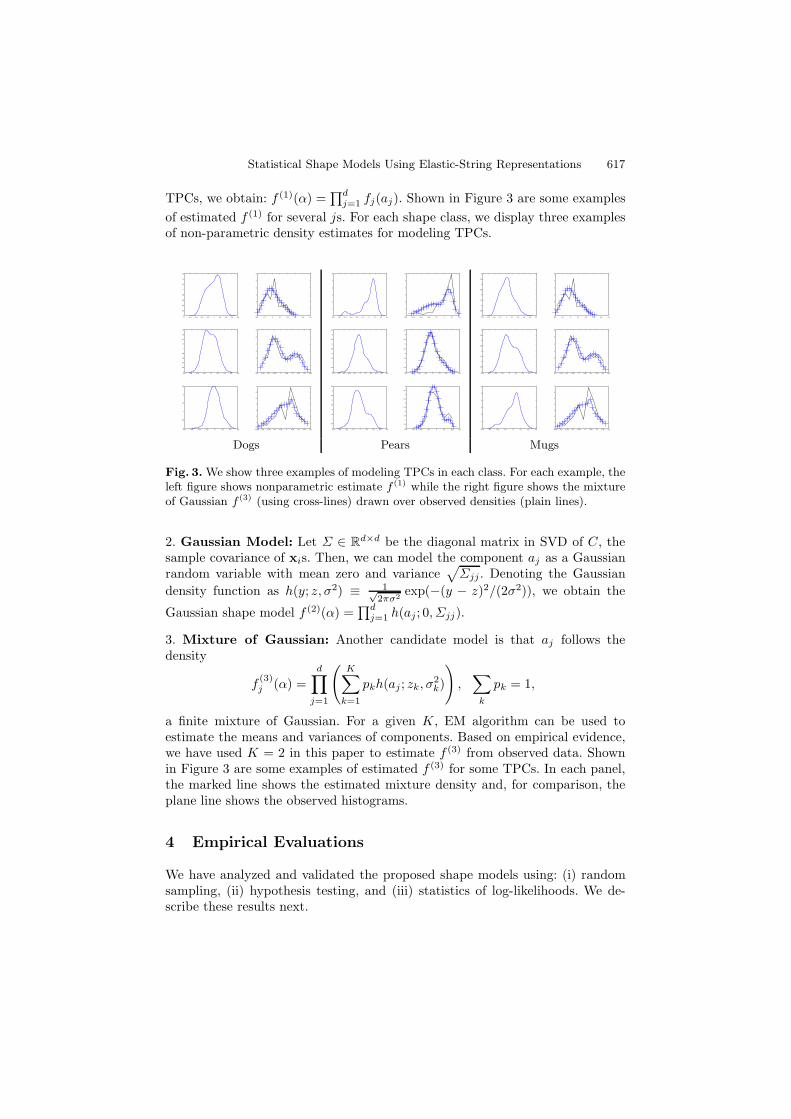
TPCs, we obtain: f (1)(α) =∏d

j=1 fj(aj). Shown in Figure 3 are some examplesof estimated f (1) for several js. For each shape class, we display three examplesof non-parametric density estimates for modeling TPCs.

−1 −0.8 −0.6 −0.4 −0.2 0 0.2 0.4 0.6 0.80

0.2

0.4

0.6

0.8

1

1.2

1.4

1.6

−0.2 −0.1 0 0.1 0.2 0.3 0.4 0.50

1

2

3

4

5

6

−0.8 −0.6 −0.4 −0.2 0 0.2 0.4 0.6 0.80

0.2

0.4

0.6

0.8

1

1.2

1.4

1.6

1.8

−0.2 −0.15 −0.1 −0.05 0 0.05 0.1 0.15 0.2 0.250

1

2

3

4

5

6

−0.8 −0.6 −0.4 −0.2 0 0.2 0.4 0.60

0.5

1

1.5

2

2.5

−0.25 −0.2 −0.15 −0.1 −0.05 0 0.05 0.1 0.15 0.20

1

2

3

4

5

6

7

−0.6 −0.5 −0.4 −0.3 −0.2 −0.1 0 0.1 0.2 0.30

1

2

3

4

5

6

−0.5 −0.4 −0.3 −0.2 −0.1 0 0.1 0.20

1

2

3

4

5

6

−0.5 −0.4 −0.3 −0.2 −0.1 0 0.1 0.2 0.3 0.4 0.50

0.5

1

1.5

2

2.5

3

3.5

4

4.5

−0.4 −0.3 −0.2 −0.1 0 0.1 0.2 0.3 0.40

0.5

1

1.5

2

2.5

3

3.5

4

4.5

−0.4 −0.3 −0.2 −0.1 0 0.1 0.2 0.3 0.40

0.5

1

1.5

2

2.5

3

3.5

4

4.5

−0.4 −0.3 −0.2 −0.1 0 0.1 0.2 0.30

0.5

1

1.5

2

2.5

3

3.5

4

4.5

5

−0.4 −0.3 −0.2 −0.1 0 0.1 0.2 0.3 0.4 0.50

0.5

1

1.5

2

2.5

3

3.5

4

−0.2 −0.1 0 0.1 0.2 0.3 0.4 0.50

1

2

3

4

5

6

−0.4 −0.3 −0.2 −0.1 0 0.1 0.2 0.3 0.40

0.5

1

1.5

2

2.5

3

3.5

4

−0.2 −0.15 −0.1 −0.05 0 0.05 0.1 0.15 0.2 0.250

1

2

3

4

5

6

−0.4 −0.3 −0.2 −0.1 0 0.1 0.2 0.30

1

2

3

4

5

6

−0.25 −0.2 −0.15 −0.1 −0.05 0 0.05 0.1 0.15 0.20

1

2

3

4

5

6

7

Dogs Pears Mugs

Fig. 3. We show three examples of modeling TPCs in each class. For each example, theleft figure shows nonparametric estimate f (1) while the right figure shows the mixtureof Gaussian f (3) (using cross-lines) drawn over observed densities (plain lines).

2. Gaussian Model: Let Σ ∈ Rd×d be the diagonal matrix in SVD of C, the

sample covariance of xis. Then, we can model the component aj as a Gaussianrandom variable with mean zero and variance

√Σjj . Denoting the Gaussian

density function as h(y; z, σ2) ≡ 1√2πσ2 exp(−(y − z)2/(2σ2)), we obtain the

Gaussian shape model f (2)(α) =∏d

j=1 h(aj ; 0, Σjj).

3. Mixture of Gaussian: Another candidate model is that aj follows thedensity

f(3)j (α) =

d∏j=1

(K∑

k=1

pkh(aj ; zk, σ2k)

),

∑k

pk = 1,

a finite mixture of Gaussian. For a given K, EM algorithm can be used toestimate the means and variances of components. Based on empirical evidence,we have used K = 2 in this paper to estimate f (3) from observed data. Shownin Figure 3 are some examples of estimated f (3) for some TPCs. In each panel,the marked line shows the estimated mixture density and, for comparison, theplane line shows the observed histograms.

4 Empirical Evaluations

We have analyzed and validated the proposed shape models using: (i) randomsampling, (ii) hypothesis testing, and (iii) statistics of log-likelihoods. We de-scribe these results next.

618 A. Srivastava et al.

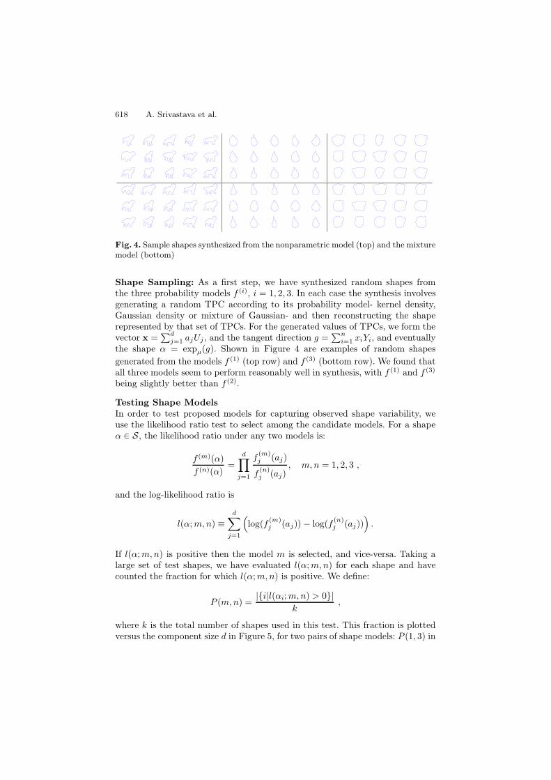
Fig. 4. Sample shapes synthesized from the nonparametric model (top) and the mixturemodel (bottom)

Shape Sampling: As a first step, we have synthesized random shapes fromthe three probability models f (i), i = 1, 2, 3. In each case the synthesis involvesgenerating a random TPC according to its probability model- kernel density,Gaussian density or mixture of Gaussian- and then reconstructing the shaperepresented by that set of TPCs. For the generated values of TPCs, we form thevector x =

∑dj=1 ajUj , and the tangent direction g =

∑ni=1 xiYi, and eventually

the shape α = expµ(g). Shown in Figure 4 are examples of random shapesgenerated from the models f (1) (top row) and f (3) (bottom row). We found thatall three models seem to perform reasonably well in synthesis, with f (1) and f (3)

being slightly better than f (2).

Testing Shape ModelsIn order to test proposed models for capturing observed shape variability, weuse the likelihood ratio test to select among the candidate models. For a shapeα ∈ S, the likelihood ratio under any two models is:

f (m)(α)f (n)(α)

=d∏

j=1

f(m)j (aj)

f(n)j (aj)

, m, n = 1, 2, 3 ,

and the log-likelihood ratio is

l(α; m, n) ≡d∑

j=1

(log(f (m)

j (aj)) − log(f (n)j (aj))

).

If l(α; m, n) is positive then the model m is selected, and vice-versa. Taking alarge set of test shapes, we have evaluated l(α; m, n) for each shape and havecounted the fraction for which l(α; m, n) is positive. We define:

P (m, n) =|{i|l(αi; m, n) > 0}|

k,

where k is the total number of shapes used in this test. This fraction is plottedversus the component size d in Figure 5, for two pairs of shape models: P (1, 3) in

Statistical Shape Models Using Elastic-String Representations 619

5 10 15 20 25 30 35 400

0.1

0.2

0.3

0.4

0.5

0.6

0.7

0.8

0.9

1

5 10 15 20 25 30 35 400

0.1

0.2

0.3

0.4

0.5

0.6

0.7

0.8

0.9

1

5 10 15 20 25 30 35 400

0.1

0.2

0.3

0.4

0.5

0.6

0.7

0.8

0.9

1

5 10 15 20 25 30 35 400

0.1

0.2

0.3

0.4

0.5

0.6

0.7

0.8

0.9

1

5 10 15 20 25 30 35 400

0.1

0.2

0.3

0.4

0.5

0.6

0.7

0.8

0.9

1

5 10 15 20 25 30 35 400

0.1

0.2

0.3

0.4

0.5

0.6

0.7

0.8

0.9

1

dogs pears mugs

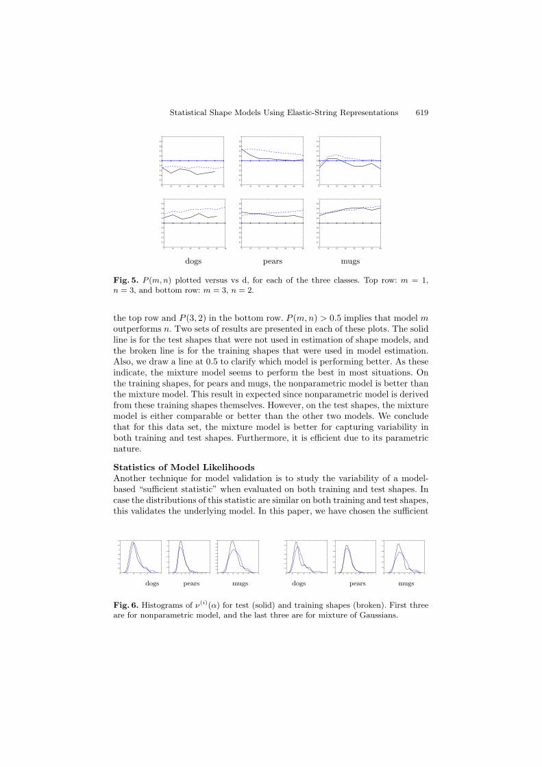
Fig. 5. P (m,n) plotted versus vs d, for each of the three classes. Top row: m = 1,n = 3, and bottom row: m = 3, n = 2.

the top row and P (3, 2) in the bottom row. P (m, n) > 0.5 implies that model moutperforms n. Two sets of results are presented in each of these plots. The solidline is for the test shapes that were not used in estimation of shape models, andthe broken line is for the training shapes that were used in model estimation.Also, we draw a line at 0.5 to clarify which model is performing better. As theseindicate, the mixture model seems to perform the best in most situations. Onthe training shapes, for pears and mugs, the nonparametric model is better thanthe mixture model. This result in expected since nonparametric model is derivedfrom these training shapes themselves. However, on the test shapes, the mixturemodel is either comparable or better than the other two models. We concludethat for this data set, the mixture model is better for capturing variability inboth training and test shapes. Furthermore, it is efficient due to its parametricnature.

Statistics of Model LikelihoodsAnother technique for model validation is to study the variability of a model-based “sufficient statistic” when evaluated on both training and test shapes. Incase the distributions of this statistic are similar on both training and test shapes,this validates the underlying model. In this paper, we have chosen the sufficient

−35 −30 −25 −20 −15 −10 −50

0.02

0.04

0.06

0.08

0.1

0.12

0.14

−50 −45 −40 −35 −30 −25 −20 −15 −10 −5 00

0.02

0.04

0.06

0.08

0.1

0.12

−50 −45 −40 −35 −30 −25 −20 −15 −100

0.01

0.02

0.03

0.04

0.05

0.06

0.07

0.08

0.09

0.1

−35 −30 −25 −20 −15 −10 −5 00

0.02

0.04

0.06

0.08

0.1

0.12

0.14

−50 −45 −40 −35 −30 −25 −20 −15 −10 −5 00

0.02

0.04

0.06

0.08

0.1

0.12

−50 −45 −40 −35 −30 −25 −20 −15 −100

0.02

0.04

0.06

0.08

0.1

0.12

dogs pears mugs dogs pears mugs

Fig. 6. Histograms of ν(i)(α) for test (solid) and training shapes (broken). First threeare for nonparametric model, and the last three are for mixture of Gaussians.

620 A. Srivastava et al.

statistic to be proportional to negative log-likelihood of an observed shape. Thatis, we define ν(i)(α) ∝ − log(f (i)(α)), where the proportionality implies that theconstants have been ignored. Shown in Figure 6 are some examples of this studyfor the nonparametric (first three) and the mixture model (last three). Theseplots shows histograms of ν(i)(α) values for both test and training shapes, foreach of the three shape classes. It is evident that the histograms for training andtest sets are quite similar in all these examples, and hence, validate the proposedmodels.

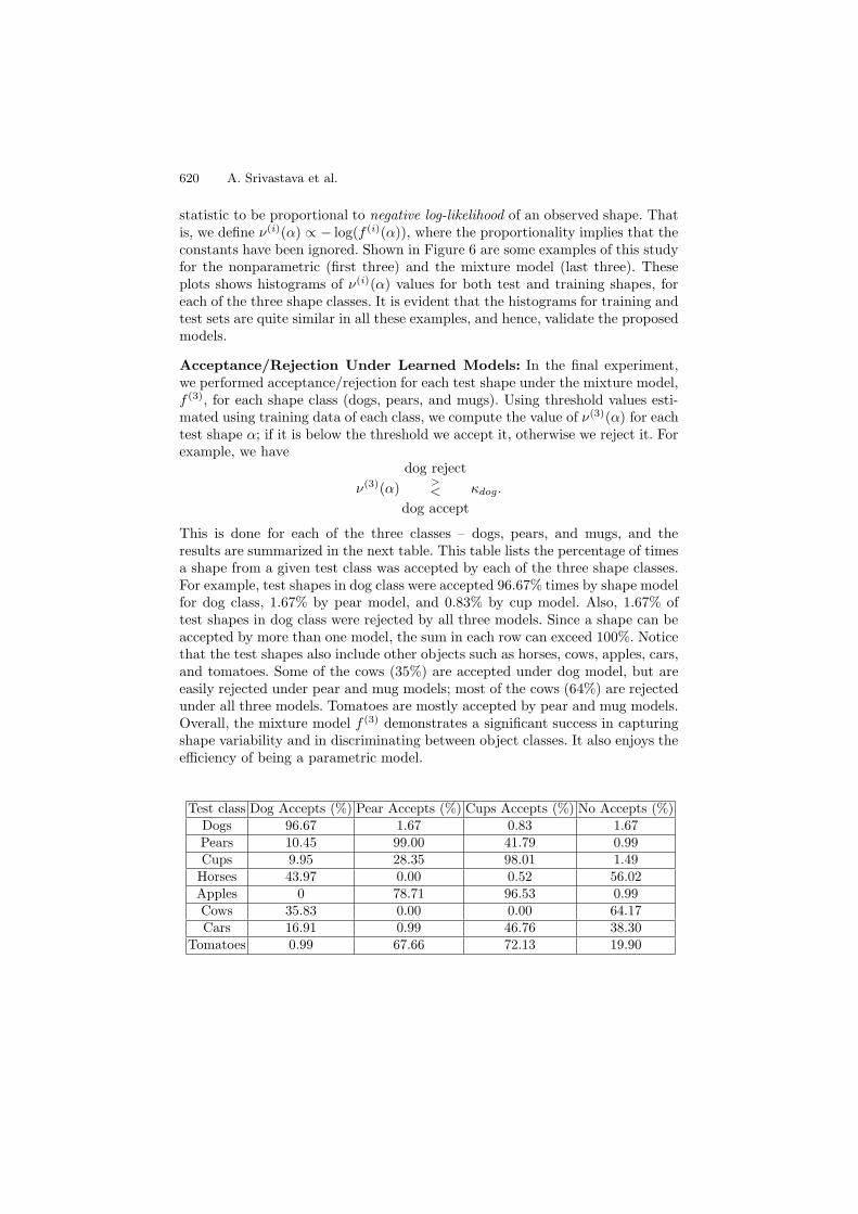
Acceptance/Rejection Under Learned Models: In the final experiment,we performed acceptance/rejection for each test shape under the mixture model,f (3), for each shape class (dogs, pears, and mugs). Using threshold values esti-mated using training data of each class, we compute the value of ν(3)(α) for eachtest shape α; if it is below the threshold we accept it, otherwise we reject it. Forexample, we have

ν(3)(α)dog reject

><

dog acceptκdog.

This is done for each of the three classes – dogs, pears, and mugs, and theresults are summarized in the next table. This table lists the percentage of timesa shape from a given test class was accepted by each of the three shape classes.For example, test shapes in dog class were accepted 96.67% times by shape modelfor dog class, 1.67% by pear model, and 0.83% by cup model. Also, 1.67% oftest shapes in dog class were rejected by all three models. Since a shape can beaccepted by more than one model, the sum in each row can exceed 100%. Noticethat the test shapes also include other objects such as horses, cows, apples, cars,and tomatoes. Some of the cows (35%) are accepted under dog model, but areeasily rejected under pear and mug models; most of the cows (64%) are rejectedunder all three models. Tomatoes are mostly accepted by pear and mug models.Overall, the mixture model f (3) demonstrates a significant success in capturingshape variability and in discriminating between object classes. It also enjoys theefficiency of being a parametric model.

Test class Dog Accepts (%) Pear Accepts (%) Cups Accepts (%) No Accepts (%)Dogs 96.67 1.67 0.83 1.67Pears 10.45 99.00 41.79 0.99Cups 9.95 28.35 98.01 1.49Horses 43.97 0.00 0.52 56.02Apples 0 78.71 96.53 0.99Cows 35.83 0.00 0.00 64.17Cars 16.91 0.99 46.76 38.30

Tomatoes 0.99 67.66 72.13 19.90

Statistical Shape Models Using Elastic-String Representations 621

5 Conclusion

We have presented results from statistical analysis of planar shapes under elas-tic string models. Using TPCA representation of shapes, three candidate modelswere presented: nonparametric, Gaussian, and a mixture of Gaussian. We eval-uated these models using (i) random sampling, (ii) likelihood ratio tests, (iii)similarity of (distributions of) sufficient statistics on training and test shapes,and (iv) acceptance/rejection of test shapes under the models estimated fromthe corresponding training shapes. All three models do reasonably well in ran-dom sampling and likelihood ratio test. However, the mixture model emerges asthe best model for capturing shape variability and efficiency. We therefore con-jecture that mixture of Gaussians are sufficient for modeling TPCs of observedshapes for use as prior shape models in future Bayesian inferences.

References

1. Klassen, E., Srivastava, A., Mio, W., Joshi, S.: Analysis of planar shapes usinggeodesic paths on shape spaces. IEEE Pattern Analysis and Machine Intelligence26 (March, 2004) 372–383

2. Younes, L.: Optimal matching between shapes via elastic deformations. Journal ofImage and Vision Computing 17 (1999) 381–389

3. Michor, P.W., Mumford, D.: Riemannian geometries on spaces of plane curves.Journal of the European Mathematical Society to appear (2005)

4. Srivastava, A., Joshi, S., Mio, W., Liu, X.: Statistical shape analysis: Clustering,learning and testing. IEEE Transactions on Pattern Analysis and Machine Intelli-gence 27 (2005) 590–602

5. Mio, W., Srivastava, A.: Elastic string models for representation and analysis ofplanar shapes. In: Proc. of IEEE Computer Vision and Pattern Recognition. (2004)

6. Dryden, I.L., Mardia, K.V.: Statistical Shape Analysis. John Wiley & Son (1998)7. Le, H.L., Kendall, D.G.: The Riemannian structure of Euclidean shape spaces: a

novel environment for statistics. Annals of Statistics 21 (1993) 1225–12718. Karcher, H.: Riemann center of mass and mollifier smoothing. Communications on

Pure and Applied Mathematics 30 (1977) 509–541