Thèse de doctorat NNT: 2020UPASQ003 Statistical Properties of the Euclidean Random Assignment Problem Thèse de doctorat de l’université Paris-Saclay École doctorale n ◦ 569 : innovation thérapeutique : du fondamental à l’appliqué (ITFA) Spécialité de doctorat: biochimie et biologie structurale Unité de recherche: Université Paris-Saclay, CEA, CNRS, Institute for Integrative Biology of the Cell (I2BC), 91198, Gif-sur-Yvette, France. Référent: Université de Versailles-Saint-Quentin-en-Yvelines Thèse présentée et soutenue en visioconférence totale le 16/10/2020 par Matteo Pietro D’ACHILLE Composition du jury: Michel LEDOUX Président Professeur, Université de Toulouse – Paul-Sabatier Charles BORDENAVE Rapporteur DR CNRS, Aix-Marseille Université Massimiliano GUBINELLI Rapporteur Professeur, Université rhénane Frédéric-Guillaume de Bonn Guilhem SEMERJIAN Examinateur MCF, Université PSL, École Normale Supérieure Lenka ZDEBOROVÁ Examinatrice DR CNRS, Université Paris-Saclay, CEA Paris-Saclay William JALBY Directeur Professeur, Université Paris-Saclay, UVSQ Olivier RIVOIRE Codirecteur CR CNRS, Université PSL, Collège de France Andrea SPORTIELLO Codirecteur CR CNRS, Université Sorbonne Paris Nord Sergio CARACCIOLO Invité Professeur, Université de Milan et INFN

Welcome message from author
This document is posted to help you gain knowledge. Please leave a comment to let me know what you think about it! Share it to your friends and learn new things together.
Transcript
Thès
e de
doc
tora
tNNT:2020UPA
SQ003
Statistical Propertiesof the Euclidean
Random Assignment Problem
Thèse de doctorat de l’université Paris-Saclay
École doctorale n 569 : innovation thérapeutique : dufondamental à l’appliqué (ITFA)
Spécialité de doctorat: biochimie et biologie structuraleUnité de recherche: Université Paris-Saclay, CEA, CNRS, Institute forIntegrative Biology of the Cell (I2BC), 91198, Gif-sur-Yvette, France.
Référent: Université de Versailles-Saint-Quentin-en-Yvelines
Thèse présentée et soutenue en visioconférence totalele 16/10/2020 par
Matteo Pietro D’ACHILLE
Composition du jury:
Michel LEDOUX PrésidentProfesseur, Université de Toulouse – Paul-SabatierCharles BORDENAVE RapporteurDR CNRS, Aix-Marseille UniversitéMassimiliano GUBINELLI RapporteurProfesseur, Université rhénane Frédéric-Guillaume de BonnGuilhem SEMERJIAN ExaminateurMCF, Université PSL, École Normale SupérieureLenka ZDEBOROVÁ ExaminatriceDR CNRS, Université Paris-Saclay, CEA Paris-Saclay
William JALBY DirecteurProfesseur, Université Paris-Saclay, UVSQOlivier RIVOIRE CodirecteurCR CNRS, Université PSL, Collège de FranceAndrea SPORTIELLO CodirecteurCR CNRS, Université Sorbonne Paris NordSergio CARACCIOLO InvitéProfesseur, Université de Milan et INFN

Remerciements
Plusieurs personnes ont contribué à la réalisation de cette thèse de doctorat.Je tiens tout d’abord à remercier William Jalby, Olivier Rivoire et Andrea
Sportiello d’avoir accepté d’en être les co-directeurs, de m’avoir fourni des cri-tiques constructives et de m’avoir dirigé vers questions toujours interessantes avecpassion et grande hauteur de vue.Je remercie Sergio Caracciolo pour ses encouragements et pour notre collab-
oration de longue date. Nos discussions ont influencé en profondeur ma façond’aborder les problèmes et, par consequence, le contenu du présent travail. GabrieleSicuro est également remercié pour notre collaboration efficace de longue date et delongue portée. Dario Benedetto et Emanuele Caglioti sont remerciés pour plusieursdiscussions intéressantes, dont certaines sont contenues dans notre premier travailcommun (172 ).Carlo Sbordone et le Secrétariat de l’Accademia di Scienze Fisiche e Matematiche
à Naples sont remerciés pour leur disponibilité et de m’avoir permis d’accéder auremarque (3 ).Charles Bordenave et Massimiliano Gubinelli sont remerciés d’avoir accepté
d’être les rapporteurs de cette thèse. Michel Ledoux, Guilhem Semerjian et LenkaZdeborová sont remerciés de m’avoir fait l’honneur de siéger dans le jury de thèse.Sophie Lemaire, Clément Nizak, Pierre Pansu et Kay Wiese sont remerciés pour
encouragements lors de certaines étapes importantes du voyage doctoral.Anna Paola Muntoni, Edoardo Sarti et Steven Schulz ont lu attentivement le
Chapitre 1 et sont donc remerciés.Enfin, Christine Bailleul, Nicole Braure, Marie Fontanillas et Isabelle Moudenner-
Cohen sont remerciées pour leur assistance administrative compétente.Je tiens à remercier les institutions qui m’ont soutenu pendant les trois an-
nées du voyage doctoral, à Paris comme à l’extérieur. Il s’agit: de l’Université deVersailles–Saint–Quentin–en–Yvelines, qui m’a accordé le contrat doctoral; du Col-lège de France, pour son environnement de recherche passionnant et pour l’accèsà d’excellentes classes de français; de l’Université Sorbonne Paris Nord, qui m’aoffert des conditions de travail idéales et m’a honoré du poste de membre associéau Laboratoire d’Informatique; et de l’Université Paris-Saclay, qui m’a accordéun poste de doctorant-enseignant puis de vacataire d’enseignement en Mathéma-tiques à Orsay. Le Centre CEA de Saclay est remercié pour son hospitalité lorsde la réalisation d’une partie de ces travaux. Je remercie l’Académie polonaise dessciences et Jacek Miękisz de leur hospitalité et des conditions de travail optimales
i

à l’occasion d’un séjour de deux semaines en 2018 au Centre Banach de Varsovie.Finalement je remercie tous ceux qui m’ont soutenu de loin dans ce voyage
malgré les difficultés engendrées par la pandémie, en particulier Lucia, Giuseppe,Ornella & Sergio et Roberto. Merci à toi, Sandra, de ta patience, tes sourires etdu tiramisu.
ii
Résumé substantiel
Cette thèse de doctorat concerne un problème d’optimisation combinatoire aléa-toire introduit par Mézard et Parisi comme modèle-jouet de verre de spin en di-mension finie (50 ). Une première motivation pour entreprendre cet effort est queles verres de spin, malgré leur rôle importants ces dernières années, se sont révéléesassez difficiles à résoudre ( trouver l’énergie de l’état fondamental d’un verre despin en dimension finie est un problème NP -dur ) de sorte que, à certains égards,ils restent mystérieuses surtout au-delà de l’approximation de champ moyen, oùl’etude rencontre des difficultés même numériques; d’où l’intérêt pour un cadrethéorique qui dépasse le champ moyen tout en partageant les caractéristiques debase d’un verre de spin ( voir désordre et frustration ) tout en restant attachable,tant analytiquement que à l’ordinateur.Dans ce problème, les lois microscopiques de l’interaction sont données une fois
pour toutes et l’aléa est associé aux positions de certains constituants élémentaires» placés dans un espace par ailleurs homogène. Cette hypothèse complique con-sidérablement l’étude des propriétés typiques d’intérêt par rapport au problèmed’assignation aléatoire en dimension infinie précédemment étudié par Mézard–Parisi (40 ), et ensuite rigoureusement par Aldous (88 ). Maintenant, les constitu-ants élémentaires peuvent modéliser des atomes ou des impuretés. Mathématique-ment, ce sont deux familles de n éléments chacune : ils peuvent être représentéscomme l’ensemble des sommets V pKn,nq d’un graphe bipartite complet Kn,n ( c’est-à-dire, les éléments correspondent aux deux ensembles partis du graphe ). Nousappellerons dorénavant ces familles des points les « bleus » et « rouges », et nousleur réserverons deux symboles spéciaux : B et R. Enfin, le choix de la loi deprobabilité associée aux positions de B et R dépend du type de questions que l’onveut poser, et certaines hypothèses seront nécessaires. Par exemple, si B et Rsont des particules d’encre qui ont été vigoureusement mélangées dans un verred’eau, l’hypothèse d’une distribution uniforme de B et R dans le volume d’eausemble raisonnable pour la plupart des objectifs pratiques ; au contraire, si B sontdes vélos qui doivent être déposés dans des raquettes (R) dans la ville de Paris,l’hypothèse d’une distribution uniforme pour R ne semble pas appropriée.Pour nous situer dans un cadre suffisamment général, nous supposons que B “
tbiuni“1 et R “ trju
nj“1 sont des familles de variables aléatoires i.i.d. réparties
selon une certaine mesure ν ( qui est une donnée du problème ). Par exemple,dans un scénario typique, ν est supportée sur ( un sous-ensemble de ) un espacemétrique M ; ou les points d’une couleur ( comme l’étaient les raquettes dans
iii
l’exemple de Paris ) sont fixés sur une grille d-dimensionnelle, et les autres sont desvariables aléatoires i.i.d. comme ci-dessus ( sinon nous n’aurions pas de caractèrealéatoire ). Dans tous cas, nous appelons la distribution de probabilité associée àla mesure ν l’ ensemble statistique ou désordre, et nous nommons la donnée de Bet R échantillonnée à partir d’une telle distribution une instance ou réalisation dudésordre. L’interaction entre bi et rj ( c’est-à-dire le coût de l’assignation de bi àrj ) a une intensité cij :“ cpbi, rjq pour une certaine fonction c : MˆMÑ R. Lesn2 nombres réels tcijuni,j“1, qui peuvent être considérés comme positives, peuventêtre arrangés dans une matrice de coût d’assignation non symétrique, nˆ n
c “
¨
˚
˚
˚
˝
cpb1, r1q cpb1, r2q . . .
... . . .cpbn, r1q cpbn, rnq
˛
‹
‹
‹
‚
,
qui peut être interprétée comme la matrice de contiguïté pondérée du graph Kn,n.Un premier énoncé équivalent mais plus succinct en langage physique est quel’hamiltonienne pour ce système ne comprend que des interactions à deux corpsinter-couleurs∗.
La caractéristique essentielle qui empêche ce cadre de modéliser, par exemple,un plasma à deux composants, est qu’une fois qu’un bleu est couplé à un rougedans une configuration, il disparaît du système. Une configuration est codée parune permutation π P Sn et a énergie
Hpπq “nÿ
i“1
ciπpiq “ Tr rPπ cs ,
où Pπ est la matrice de permutation de π ( c’est-à-dire, Pi,j “ δj,πpiq ). Plusgénéralement, la fonction de coût C peut jouer le rôle d’une énergie, d’une fonctionde fitness, ou d’une distance générique. En principe, on peut considérer des fonc-tions de coût encore plus générales C : MˆMÑ R, mais nous ne discuterons pasce cas ici. Afin de modéliser les aspects de base d’un système physique critique, etnotamment l’invariance de translation, de rotation et d’échelle, nous nous limitonsdans ce travail à une fonction de coût C : RÑ R` qui est le monôme |x|p dans la
∗C’est-à-dire que, en analogie avec l’électrostatique où B et R représentent respectivement des chargesélectrostatiques unitaires positives et négatives, nous négligerons la répulsion de Coulomb.
iv
fonction de distance D†, c’est à dire
cppqij “ CpDpbi, rjqq “ Dp
pbi, rjq, i, j “ 1, . . . , n ,
où nous avons remarqué la dépendance de la matrice c du nombre réel p, appelél’exposant « énergie-distance ». Dans ce travail, D est exclusivement la distanceeuclidienne d-dimensionnelle, mais il est clair que d’autres choix pour la métriqueD sont possibles. Enfin, une assignation optimale πopt satisfait
Hopt :“ Hpπoptq “ minπPSn
Hpπq ,
où la variable aléatoire Hopt est appelée l’énergie de l’état fondamental.Le choix d’un espace métrique pM,Dq, d’un ensemble statistique pour les posi-
tions aléatoires de B et R, et d’un exposant p identifie un problème d’assignationaléatoire bien défini qui on appelle problème d’assignation aléatoire euclidien( ou ERAP de l’acronyme de sa traduction anglais, Euclidean Random As-signment Problem ). Une étude des propriétés statistiques de Hopt en fonctiondu triple ppM,Dq, pνR, νBq, pq constitue la principale contribution de ce manuscrit.Le Chapitre 1 est une promenade à travers divers concepts et idées que nous
avons pu identifier comme un contexte plausible pour ce travail de thèse. Comptetenu de la nature introductive du chapitre, nous privilégions un style discursif etdonnons la priorité aux motivations plutôt qu’à l’exhaustivité, en fournissant aulecteur intéressé quelques points d’entrée vers les littératures connexes par le biaisde critiques et d’articles de référence. L’accent est mis sur les méthodes existanteset les liens pertinents avec d’autres sujets. Ce faisant, nous souhaitons transmet-tre au moins en partie les idées remarquablement unifiantes qui sous-tendent notrediscussion et, nous l’espérons, quelques raisons d’en considérer certaines à la lu-mière du problème examiné dans cette thèse de doctorat. Suivent des exemplesoù nous discutons des notions physiques de solution sous-optimales et de passagede niveau dans un cadre algorithmique, et une discussion de certains liens avecd’autres problèmes à l’interface de la physique théorique, des probabilités et del’informatique théorique. Le Chapitre 1 est clos par un plan du manuscrit et uneliste des contributions nouvelles contenues dans cet ouvrage.Dans le Chapitre 2 nous étudions le cas unidimensionnel pour p et désordre
quelconque. Après avoir résumé l’état de l’art, nous présentons certains nouveauxrésultats tels que la distribution asymptotique de Hopt dans la cas M “ le cercleunitaire à p “ 2 pour un désordre uniforme, exprimée en termes de la fonction ϑ4 deJacobi ( Eq. 2.3.3.15 ) ; une étude de l’asymptotique de l’espérance mathématique
†Nous rappelons qu’une distance D sur un espace métrique M est une application binaire symétriqueet définie positive D : M ˆM Ñ R` qui satisfait l’inégalité triangulaire. Si cela n’est pas évidentd’après le contexte, nous indiquerons un espace métrique avec l’écriture explicite pM,Dq.
v
de Hopt pour different choix du desordre à p ě 1 ( « anomalous scaling » ),d’abord avec une méthode inspirée par la régularisation avec cutoff en théoriequantique des champs ( § 2.5, voir aussi l’article (169 ) ), puis avec une approcheanalytique–combinatoire à n fini ( § 2.6, article correspondant en preparation ).Dans § 2.7, dédiée au cas concave p P p0, 1q, nous présentons les « appariementsde Dyck », des solutions sous-optimales dont nous avons calculé l’asymptotiquede l’énergie moyenne. Sur la base de simulations numériques approfondies, nousconjecturons que les appariements de Dyck partagent la meme asymptotique duvrai état fondamental à moins d’une constante multiplicative dépendante de p( Conjecture 2.7.1 ). Cette section correspond à la publication (173 ), et nousa permis de compléter la section à d “ 1 du diagramme de phase du ERAP,qui, remarquablement, présente deux nouveaux points critiques, respectivement àp “ 1
2et p “ 1 ( Fig. 2.17 ).
Dans le Chapitre 3, nous considérons le cas bi-dimensionnel à p “ 2 sur la base del’approche de théorie de champs proposée par Caracciolo–Lucibello–Parisi–Sicuro( CLPS ) (145 ). En particulier, dans la § 3.1 nous présentons de nouveaux ré-sultats concernant les differences des énergies entre deux variétés RiemanniennesΩ,Ω1 et montrons qui ces differences peuvent être obtenues à partir du spectre del’opérateur Laplace-Beltrami de la variété. Nous avons vérifié nos prédictions an-alytiques à l’aide d’expériences numériques approfondies pour de nombreux choixde variétés ( voir les figures 3.3,3.8 ). Cette section a donné lieu au travail (172 ).Dans § 3.2 nous obtenons des relations linéaires approximatives entre les énergies
des problèmes où les configurations des points sont liées par des transformationsde symétrie qui préservent le spectre de l’opérateur de Laplace–Beltrami de lavariété.Dans § 3.3, toujours basée sur l’approche CLPS, nous étudions le problème défini
sur les 2-torus T2 à p “ 2 dans le cas « Grid–Poisson », c’est à dire, une variante duproblème où les points d’une des deux couleurs sont fixés sur une grille déterministe( dans ce cas, la grille carrée bi-dimensionnelle ). Dans ce cas, nous développonsl’idée que le champ de transport ( c’est-à-dire le champ vectoriel associant lesbleus aux rouges dans la solution optimale ) peut satisfaire, par analogie avecl’électrodynamique, une « décomposition d’Helmholtz » dans une partie longitu-dinale et une partie transverse. Nous étudions en details les propriétés statistiquesdes deux composantes pour le cas d’une distribution uniforme des points et nousmontrons que la partie longitudinale et la partie transverse contribuent à un ordredifférent dans l’asymptotique du coût moyen optimal.Le Chapitre 4 concerne un extension du ERAP au cas d’une dimension de Haus-
dorff dH P p1, 2q. Dans cette étude, primairement numérique, nous considérons despoints bleus et rouges uniformément distribués sur deux ensembles fractals ( «fractal de Peano » et « fractal de Cesàro » ) qui fournissent une interpolation
vi

différente de l’intervalle p1, 2q dimension de Hausdorff. En particulier, grâce à dessimulations numériques approfondies, nous obtenons evidence que, modulo uneconstante multiplicative, l’exposant leading du cout moyen optimal soit le memepour les deux fractals dans une grande région du plan pp, dHq.Enfin, le Chapitre 5 contient quelques conclusions provisoires et une sélection
de perspectives de recherche.
vii
Contents
Page
1 Introduction 1§1.1 Background . . . . . . . . . . . . . . . . . . . . . . . . . . . . . . 1§1.2 Random Assignment Problems and extensions . . . . . . . . . . . 6§1.3 The Euclidean Random Assignment Problem . . . . . . . . . . . . 9§1.4 On approximate solutions and level crossing . . . . . . . . . . . . 11
1.4.1 On approximate solutions and greedy heuristics . . . . . 121.4.2 On crossings of ground state energies . . . . . . . . . . . 151.4.3 Possible persistence of transition near p “ 1 at d “ 2 . . . 16
§1.5 Some related topics . . . . . . . . . . . . . . . . . . . . . . . . . . 17§1.6 Plan of the Thesis and list of contributions . . . . . . . . . . . . . 20
2 One-dimensional Euclidean Random Assignment Problems 21§2.1 On convex, concave and C-repulsive regimes . . . . . . . . . . . . 21§2.2 Poisson-Poisson, Grid-Poisson ERAPs & the Brownian Bridge . . 24§2.3 Lattice and continuum modes of the optimal transport field at p “ 2 28
2.3.1 Unit interval at fixed n . . . . . . . . . . . . . . . . . . . 282.3.2 Unit interval in the nÑ 8 limit . . . . . . . . . . . . . . 322.3.3 Distribution of Hopt on the unit circle in the nÑ 8 limit 35
§2.4 Beyond uniform disorder: anomalous vs bulk scaling of xHopty atp ě 1 . . . . . . . . . . . . . . . . . . . . . . . . . . . . . . . . . . 39
§2.5 Anomalous Scaling of the Optimal Cost in the One-DimensionalRandom Assignment Problem . . . . . . . . . . . . . . . . . . . . 402.5.1 Notations . . . . . . . . . . . . . . . . . . . . . . . . . . . 402.5.2 The problem of regularization . . . . . . . . . . . . . . . 432.5.3 Applications . . . . . . . . . . . . . . . . . . . . . . . . . 442.5.4 Conclusions . . . . . . . . . . . . . . . . . . . . . . . . . 57
§2.6 Combinatorial and analytic approach to anomalous scaling: uni-versality classes . . . . . . . . . . . . . . . . . . . . . . . . . . . . 582.6.1 Notations and setting . . . . . . . . . . . . . . . . . . . . 582.6.2 Families of distributions . . . . . . . . . . . . . . . . . . . 61
viii
2.6.3 General technical facts . . . . . . . . . . . . . . . . . . . 642.6.4 Ensembles in which the average cost is infinite . . . . . . 692.6.5 Family of stretched exponentials with endpoint at infinity
ρie,α and ρ`ie,α . . . . . . . . . . . . . . . . . . . . . . . . . 712.6.6 Estimation of complete homogeneous functions . . . . . . 782.6.7 Non-integer values of s . . . . . . . . . . . . . . . . . . . 822.6.8 Family with finite endpoint, algebraic zero ρfa,β . . . . . . 852.6.9 On sub-leading contributions at the critical line 2pp`βq “
pβ . . . . . . . . . . . . . . . . . . . . . . . . . . . . . . . 902.6.10 Family of distributions with endpoint at infinity and al-
gebraic zero ρia,β . . . . . . . . . . . . . . . . . . . . . . . 942.6.11 Family of distributions with internal endpoint, algebraic
zero ρsa,β . . . . . . . . . . . . . . . . . . . . . . . . . . . 962.6.12 Ln,p,β (Rn,p,β) in the bulk region . . . . . . . . . . . . . . 1002.6.13 Ln,p,β (Rn,p,β) in the anomalous regime and on the critical
line . . . . . . . . . . . . . . . . . . . . . . . . . . . . . . 1032.6.14 Section provisional conclusions . . . . . . . . . . . . . . . 106
§2.7 The Dyck bound in the concave regime . . . . . . . . . . . . . . . 1072.7.1 Problem statement and models of random assignment
considered . . . . . . . . . . . . . . . . . . . . . . . . . . 1072.7.2 Choice of randomness for B and R . . . . . . . . . . . . . 1072.7.3 Synthesis of results . . . . . . . . . . . . . . . . . . . . . 1102.7.4 Basic facts . . . . . . . . . . . . . . . . . . . . . . . . . . 1102.7.5 Basic properties of the optimal matching . . . . . . . . . 1112.7.6 Reduction of the PPP model to the ES model . . . . . . 1132.7.7 The Dyck matching . . . . . . . . . . . . . . . . . . . . . 1152.7.8 Numerical results and the average cost of the optimal
matching . . . . . . . . . . . . . . . . . . . . . . . . . . . 122§2.8 Chapter provisional conclusions and research perspectives . . . . . 125
2.8.1 Convex regime . . . . . . . . . . . . . . . . . . . . . . . . 125
3 Field-theoretic approach to the Euclidean Random AssignmentProblem 131§3.1 Random Assignment Problems on 2d manifolds . . . . . . . . . . 132
3.1.1 Regularisation through the integral of the zero-mean reg-ular part of the Green function . . . . . . . . . . . . . . . 135
3.1.2 Zeta regularisation and the Kronecker mass . . . . . . . . 1363.1.3 Connection between Robin and Kronecker masses . . . . 1373.1.4 Applications . . . . . . . . . . . . . . . . . . . . . . . . . 1383.1.5 Numerical results . . . . . . . . . . . . . . . . . . . . . . 1533.1.6 Uniform–Poisson transportation and grid effects . . . . . 154
ix
3.1.7 Section provisional conclusions . . . . . . . . . . . . . . . 156§3.2 On approximate linear relations among energies . . . . . . . . . . 157
3.2.1 General remarks . . . . . . . . . . . . . . . . . . . . . . . 1573.2.2 On linear relations in domains with no symmetries . . . . 1613.2.3 Kronecker masses in the case of involutions . . . . . . . . 1633.2.4 Section provisional conclusions . . . . . . . . . . . . . . . 170
§3.3 The Lattice Helmholtz decomposition of the transport field on T2
at p “ 2 . . . . . . . . . . . . . . . . . . . . . . . . . . . . . . . . 1713.3.1 Setup and notations . . . . . . . . . . . . . . . . . . . . . 1723.3.2 Longitudinal and transverse contributions to the ground
state energy Hopt . . . . . . . . . . . . . . . . . . . . . . 1753.3.3 Synthesis of results . . . . . . . . . . . . . . . . . . . . . 1763.3.4 Statistical properties of ∆φ and ∆ψ in coordinate repre-
sentation . . . . . . . . . . . . . . . . . . . . . . . . . . . 1763.3.5 Two-point correlation functions . . . . . . . . . . . . . . 1783.3.6 On L2
A
|x∆φ|2E
and L2A
|y∆ψ|2E
. . . . . . . . . . . . . . 1803.3.7 Section provisional conclusions and perspectives . . . . . 184
4 Euclidean Random Assignment Problems at non integer Haus-dorff dimensions dH P p1, 2q 185§4.1 Introduction . . . . . . . . . . . . . . . . . . . . . . . . . . . . . . 185§4.2 Setup . . . . . . . . . . . . . . . . . . . . . . . . . . . . . . . . . . 186§4.3 Choice of randomness . . . . . . . . . . . . . . . . . . . . . . . . . 187
4.3.1 Peano fractal . . . . . . . . . . . . . . . . . . . . . . . . . 1874.3.2 Cesàro fractal . . . . . . . . . . . . . . . . . . . . . . . . 189
§4.4 Numerical protocol, data analysis, and results . . . . . . . . . . . 191§4.5 On the qualitative behavior of γCpPq
pp,dHqand evidence of universality 193
§4.6 Energy approximate linear relations . . . . . . . . . . . . . . . . . 194§4.7 Energy profile at fixed disorder along the p2, dHq line in the Cesàro
fractal . . . . . . . . . . . . . . . . . . . . . . . . . . . . . . . . . 196§4.8 Conclusions and research perspectives . . . . . . . . . . . . . . . . 197
5 General provisional conclusions and research perspectives 198
Appendices 208
A 209§A.1 The number of edges of length 2k ` 1 in a Dyck matching at size
n (§ 2.7.7) . . . . . . . . . . . . . . . . . . . . . . . . . . . . . . . 209
x
§A.2 Expansion of the generating function Spz; pq via singularity anal-ysis (§ 2.7.7) . . . . . . . . . . . . . . . . . . . . . . . . . . . . . . 213
B 216§B.1 The first Kronecker limit formula (§ 3.1.2) . . . . . . . . . . . . . 216
C 218§C.1 Calculus on the square lattice (§ 3.3) . . . . . . . . . . . . . . . . 218
Bibliography 221
List of Figures
1.1 Example Von Neumann game at n “ 5 . . . . . . . . . . . . . . . 21.2 Typical time analysis of Jonker-Volgenant algorithm . . . . . . . . 41.3 Different dynamics of row-column-minima and saddle point con-
figurations . . . . . . . . . . . . . . . . . . . . . . . . . . . . . . . 131.4 Evidence of energy tradeoff around p˚ “ 2 . . . . . . . . . . . . . 141.5 Evidence for crossing of ground state energies as a function of
energy-distance exponent . . . . . . . . . . . . . . . . . . . . . . . 151.6 Evidence of transition around p˚ “ 1 at d “ 2 . . . . . . . . . . . 16
2.1 Pictorial representation of the solution in one dimension . . . . . . 232.2 Example Grid-Poisson and Poisson-Poisson instance at d “ 1 . . . 252.3 Sample path from the Brownian Bridge vs rescaled optimal trans-
port field . . . . . . . . . . . . . . . . . . . . . . . . . . . . . . . . 262.4 Cumulative distribution function ofHopt for the Grid-Poisson prob-
lem on the unit circle (theory vs experiments) . . . . . . . . . . . 382.5 Comparison with numerical experiments (exponential and Rayleigh
distributions) . . . . . . . . . . . . . . . . . . . . . . . . . . . . . 482.6 Comparisons with numerical experiments (Pareto distribution) . . 502.7 Comparison with numerical experiments for the distribution in
Eq. (2.5.3.18) . . . . . . . . . . . . . . . . . . . . . . . . . . . . . 532.8 Comparison with numerical experiments (“gapped” distribution,
Eq. (2.5.3.34)) . . . . . . . . . . . . . . . . . . . . . . . . . . . . . 562.9 Members from ρfa,β family and corresponding Rβ functions. . . . . 85
xi
2.10 Critical hyperbola separating the region of anomalous and bulkscaling for the class ρfa,β . . . . . . . . . . . . . . . . . . . . . . . 89
2.11 Members from ρsa,β family and corresponding Rβ functions. . . . . 962.12 Critical hyperbola separating the region of anomalous and bulk
scaling for the class ρsa,β . . . . . . . . . . . . . . . . . . . . . . . 1002.13 Example of instance encoding in the PPP model . . . . . . . . . . 1082.14 The Dyck matching πDyck associated to the Dyck bridge σ in the
example of Figure 2.13. . . . . . . . . . . . . . . . . . . . . . . . . 1162.15 Numerical evidences for the Dyck upper bound conjecture . . . . 1232.16 Fit of scaling coefficients as a function of p . . . . . . . . . . . . . 1242.17 State of the art on bulk scaling exponent depending on p . . . . . 1272.18 Supporting Figure to resarch problem 1 . . . . . . . . . . . . . . . 1292.19 Supporting Figure to resarch problem 2 . . . . . . . . . . . . . . . 130
3.1 Pictorial representation of an assignment at n “ 3 on a torus gen-erated by quotient of R2 with a periodic lattice, with fundamentalparallelogram and the corresponding base vectors. . . . . . . . . . 140
3.2 Contour plot of =pτq|ηpτq|4 in the complex plane τ . . . . . . . . . 1413.3 Relative differences on expected ground state energies on the rect-
angle Rpρq, on the torus Tpiρq and on the Boy surface with respectto the case ρ “ 1 as a function of ρ (theory vs experiments) . . . . 142
3.4 The Cylinder. . . . . . . . . . . . . . . . . . . . . . . . . . . . . . 1443.5 The Möebius strip. . . . . . . . . . . . . . . . . . . . . . . . . . . 1453.6 The Klein bottle. . . . . . . . . . . . . . . . . . . . . . . . . . . . 1473.7 The Boy surface. . . . . . . . . . . . . . . . . . . . . . . . . . . . 1483.8 Absolute shift of ground state energies for the cylinder Cpρq, the
Möebius strip Mpρq and the Klein bottle Kpρq with respect to thecase ρ “ 1 (theory vs experiments) . . . . . . . . . . . . . . . . . 149
3.9 Typical scatter plot of numerical data (n “ 103, 103 points) cor-responding to δEp1q (Eq. 3.2.1.8) for a domain with an involution(see § 3.2.3). . . . . . . . . . . . . . . . . . . . . . . . . . . . . . . 160
3.10 Comparison of Eq. 3.2.2.5 (dotted black line) and results of nu-merical experiments, obtained by a linear fit as in Fig. 3.9 (bluedots with error bars). The horizontal black, dashed line denotesthe value when the two involved sets have the same cardinality,α “ 1 (τ “ 12). . . . . . . . . . . . . . . . . . . . . . . . . . . . . 163
3.11 (Left) An instance from Example 2 (n “ 25). (Right) An instancefrom Example 3 (n “ 50). . . . . . . . . . . . . . . . . . . . . . . 165
3.12 Pictorial rules of lattice calculus for lattice diagonal derivativesand laplacian . . . . . . . . . . . . . . . . . . . . . . . . . . . . . 174
3.13 Direct estimation of sub-leading constant . . . . . . . . . . . . . . 177
xii
3.14 Histograms of rescaled laplacians of φ and ψ fields, and sym-metrized log probability functions (experiments vs fits) . . . . . . 177
3.15 Experimental evidence for the inequality 3.3.4.1 . . . . . . . . . . 1783.16 Expected contributions of Fourier modes to the ground state en-
ergy at n “ 2116, and trigonometric functions sharing the samesymmetries . . . . . . . . . . . . . . . . . . . . . . . . . . . . . . . 182
3.17 Fits of longitudinal contribution and transverse contribution in 1n 183
4.1 Example instances on the Peano fractal at increasing Hausdorffdimensions (n “ 212) . . . . . . . . . . . . . . . . . . . . . . . . . 188
4.2 Example instances on the Cesàro fractal at increasing Hausdorffdimensions (n “ 212) . . . . . . . . . . . . . . . . . . . . . . . . . 190
4.3 Empirical evidence for universality . . . . . . . . . . . . . . . . . . 1934.4 Example approximate energy linear relations at varying dH (Peano
fractal at p “ 2) . . . . . . . . . . . . . . . . . . . . . . . . . . . . 1944.5 Avg. energy profiles on the Cèsaro fractal at p “ 2 at varying dH . 1964.6 Universality for the problem on Peano and Cesàro fractals at (ex-
ample at pdH , pq “ p1.5, 1.33q) . . . . . . . . . . . . . . . . . . . . 197
5.1 Example instance of an ERAP on a Brownian loop (n “ 212,p “ 1) 204
xiii

d Chapter 1 D
Introduction
This chapter starts with a “promenade” through various concepts and ideas whichwe have been able to identify as a plausible background to this work. We favora discorsive style and give priority to motivations over completeness, providingto the interested reader some entry points to (many) related literatures throughreviews and milestone papers. Emphasis is put on existing methods and relevantconnections with other topics. In doing so, we wish to convey at least in partthe remarkably unifying ideas which underlie our discussion and, hopefully, somereasons to consider any of them in the light of the problem considered in this PhDThesis, the “Euclidean Random Assignment Problem”. A self-contained definitionof this problem is given § 1.3, which can be used as a reference for the remainingpart of the manuscript, and it is followed by an example where we discuss thephysical notion of level crossing in an algorithmic setting. A discussion of somepossibly interesting connections with other problems at the interface of theoreticalphysics, mathematics and theoretical computer science follows. The chapter endswith the plan of the manuscript and a list of novel contributions contained in thiswork.
1.1. Background
In a seminar held at Princeton in 1951 and reported in the second volume of theseries “Contributions to the Theory of Games” (14 ), von Neumann considered
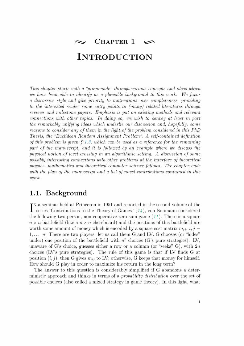
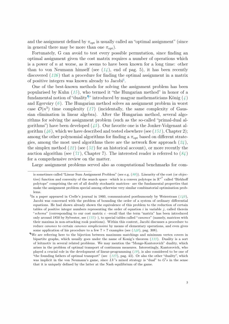
the following two-person, non-cooperative zero-sum game (11 ). There is a squarenˆ n battlefield (like a nˆ n chessboard) and the positions of this battlefield areworth some amount of money which is encoded by a square cost matrix mij, i, j “1, . . . , n. There are two players: let us call them G and LV. G chooses (or “hides”under) one position of the battlefield with n2 choices (G’s pure strategies). LV,unaware of G’s choice, guesses either a row or a column (or “seeks” G), with 2nchoices (LV’s pure strategies). The rule of this game is that if LV finds G atposition pi, jq, then G gives mij to LV; otherwise, G keeps that money for himself.How should G play in order to maximize his return in the long term?The answer to this question is considerably simplified if G abandons a deter-
ministic approach and thinks in terms of a probability distribution over the set ofpossible choices (also called a mixed strategy in game theory). In this light, what
1
0 1 2 3 4
01
23
4
2 7 3 2 6
5 10 6 8 4
10 6 3 7 6
3 6 3 6 6
8 3 10 5 2
0
2
4
6
8
10
$
0 1 2 3 4
01
23
4
0 0 0 0.28 0
0 0.057 0 0 0
0 0 0.19 0 0
0.19 0 0 0 0
0 0 0 0 0.28
0.00
0.05
0.10
0.15
0.20
0.25
prob
.
Figure 1.1. – (Left) Example battlefield m for von Neumann’s game at n “ 5(annotated prizes are in $ currency). (Right) G’s optimal mixed strategy for thebattlefield on the left requires G to choose m4,4 “ 2$ (upper right corner) about7 times in 25 turns, and m1,1 “ 10$ slightly more than 1 time out of 20 turns(but never the other 10$ bills).
von Neumann’s paper shows is that the optimal mixed strategy depends on a smallproportion of positions (i.e. n out of the n2 available positions). These n positionsare found by interchanging the columns (or rows) of the matrix cij :“ ´1mij untilits trace is minimal. Rows and columns incident to those n positions span thewhole battlefield, thus identifying one out of the n! “ npn´ 1q ¨ ¨ ¨ ways of placingn rooks (chess pieces) at non-attacking positions onto the n ˆ n chessboard (anexample game at n “ 5 is given in Fig. 1.1). These special n positions constitutean assignment of n row elements to n column elements (and vice-versa), and canthus be specified by a permutation of n objects, which we will generically callπopt
∗ †. The problem of finding a πopt is usually called “the assignment problem‡”
∗A permutation of a finite set is a bijection on that set. The set of all permutations equipped withcomposition “˝2 is a group called the symmetric group which we denote by Sn. In the game ofvon Neumann, if G looks for a rearrangement of rows instead of columns (i.e., if G “rotates” thebattlefield by an angle π
2), he finds the permutation π´1
opt, the unique group inverse of πopt satisfyingπopt ˝ π
´1opt “ π´1
opt ˝ πopt “ p1, . . . , nq in one line notation.†von Neumann (14 ) also shows that, rather intuitively, G’s should think probabilistically and choosethe position tpk, πoptpkqqu
nk“1 with probability proportional to 1mkπoptpkq
(the higher the reward, thehigher the chance of LV considering a row or column containing that position). von Neumann’sseminal contribution has been extensively discussed later on, possibly due to its many connectionswith other important problems at the time, such as the Birkhoff-Von Neumann Theorem on doublystochastic matrices (see e.g. (12 )) (to not be confused with the anterior pair of fundamental works (5 ,7 ) by the same authors concerning ergodic theory), or with the problem of allocation of indivisibleresources in economics (16 ).
‡An assignment problem is a linear combinatorial optimisation problem in which the function to beminimised (the cost or energy function) is a sum over the entries of a cost matrix. For this reason, it
2
and the assignment defined by πopt is usually called an “optimal assignment” (sincein general there may be more than one πopt).Fortunately, G can avoid to test every possible permutation, since finding an
optimal assignment given the cost matrix requires a number of operations whichis a power of n at worse, as it seems to have been known for a long time: otherthan to von Neumann himself (see (14 ), end of pag. 5), it has been recentlydiscovered (126 ) that a procedure for finding the optimal assignment in a matrixof positive integers was known already to Jacobi§.One of the best-known methods for solving the assignment problem has been
popularised by Kuhn (15 ), who termed it “the Hungarian method” in honor of afundamental notion of “duality¶” introduced by magyar mathematicians König (4 )and Egerváry (6 ). The Hungarian method solves an assignment problem in worstcase Opn3q time complexity (17 ) (incidentally, the same complexity of Gaus-sian elimination in linear algebra). After the Hungarian method, several algo-rithms for solving the assignment problem (such as the so-called “primal-dual al-gorithms”) have been developed (45 ). Our favorite one is the Jonker-Volgenant al-gorithm (46 ), which we have described and tested elsewhere (see (151 ), Chapter 2);among the other polynomial algorithms for finding a πopt based on different strate-gies, among the most used algorithms there are the network flow approach (24 ),the simplex method (22 ) (see (52 ) for an historical account), or more recently theauction algorithm (see (71 ), Chapter 7). The interested reader is referred to (84 )for a comprehensive review on the matter.Large assignment problems served also as computational benchmarks for com-
is sometimes called “Linear Sum Assignment Problem” (see e.g. (80 )). Linearity of the cost (or objec-tive) function and convexity of the search space –which is a convex polytope in Rn
2
called “Birkhoffpolytope” comprising the set of all doubly stochastic matrices– are the fundamental properties thatmake the assignment problem special among otherwise very similar combinatorial optimisation prob-lems.
§In a paper appeared in Crelle’s journal in 1860, communicated posthumously by Weierstrass (140 ),Jacobi was concerned with the problem of bounding the order of a system of ordinary differentialequations. He had shown already shown the equivalence of this problem to the reduction of certaintables of positive integer numbers representing the order of equation i in variable j, called therein“schema” (corresponding to our cost matrix c –recall that the term “matrix” has been introducedonly around 1850 by Sylvester, see (135 )–), to special tables called “canones” (namely, matrices withtheir maxima in non-attacking rook positions). Within this context, Jacobi discusses a procedure toreduce canones to certain canones simplicissimi by means of elementary operations, and even givessome application of his procedure to a few 7ˆ 7 examples (see (140 ), pag. 308).
¶We are referring here to the bijection between maximum matchings and minimum vertex covers inbipartite graphs, which usually goes under the name of Konig’s theorem (133 ). Duality is a sortof leitmotiv in several related problems. We may mention the “Monge-Kantorovich” duality, whicharises in the problem of optimal transport of continuum measures. Interestingly, Kantorovich, whoplayed a crucial role in the development of linear-programming (19 ), is also considered to be one of“the founding fathers of optimal transport” (see (127 ), pag. 43). Or also the other “duality”, whichwas implicit in the von Neumann’s game, since LV ’s mixed strategy is “dual” to G1s in the sensethat it is uniquely defined by the latter at the Nash equilibrium of the game.
3
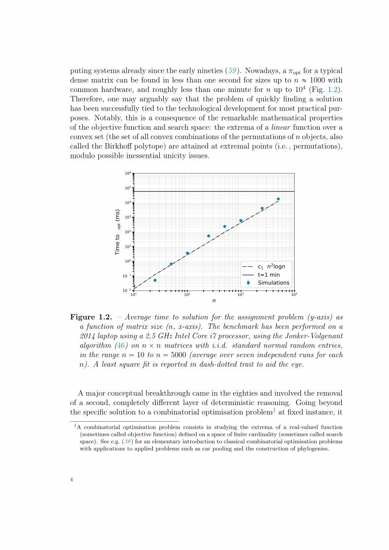
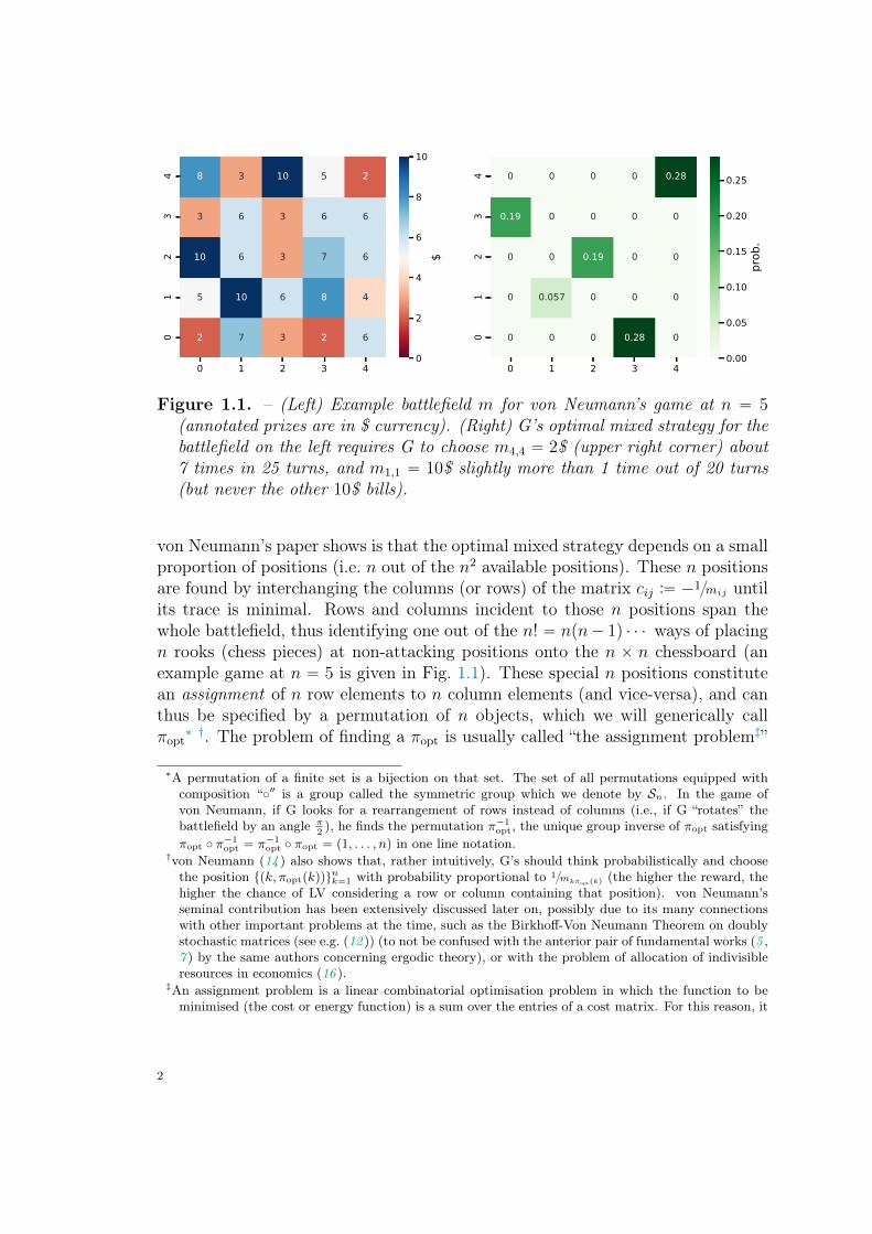
puting systems already since the early nineties (59 ). Nowadays, a πopt for a typicaldense matrix can be found in less than one second for sizes up to n « 1000 withcommon hardware, and roughly less than one minute for n up to 104 (Fig. 1.2).Therefore, one may arguably say that the problem of quickly finding a solutionhas been successfully tied to the technological development for most practical pur-poses. Notably, this is a consequence of the remarkable mathematical propertiesof the objective function and search space: the extrema of a linear function over aconvex set (the set of all convex combinations of the permutations of n objects, alsocalled the Birkhoff polytope) are attained at extremal points (i.e. , permutations),modulo possible inessential unicity issues.
101 102 103 104
n
10−2
10−1
100
101
102
103
104
105
106
Time to π
opt (ms)
c1 ⋅ n2lognt=1 minSimulations
Figure 1.2. – Average time to solution for the assignment problem (y-axis) asa function of matrix size (n, x-axis). The benchmark has been performed on a2014 laptop using a 2,5 GHz Intel Core i7 processor, using the Jonker-Volgenantalgorithm (46) on n ˆ n matrices with i.i.d. standard normal random entries,in the range n “ 10 to n “ 5000 (average over seven independent runs for eachn). A least square fit is reported in dash-dotted trait to aid the eye.
A major conceptual breakthrough came in the eighties and involved the removalof a second, completely different layer of deterministic reasoning. Going beyondthe specific solution to a combinatorial optimisation problem‖ at fixed instance, it
‖A combinatorial optimisation problem consists in studying the extrema of a real-valued function(sometimes called objective function) defined on a space of finite cardinality (sometimes called searchspace). See e.g. (38 ) for an elementary introduction to classical combinatorial optimisation problemswith applications to applied problems such as car pooling and the construction of phylogenies.
4
was realized that, when considering instead random instances of an optimizationproblem, the typical properties of the solution were accessible with the methodsof statistical mechanics in the presence of a quenched randomness (in our caseof the assignment problem/von Neumann’s game, this amounts to think at theprizes of matrix m as random variables). The new viewpoint has been pioneeredby physicists Mézard and Parisi (40 ), and Orland (41 ), who considered some sta-tistical properties of minimum weight perfect matchings of the random complete(bipartite) graph (40 ). The basic idea, which dates back at least to Kirkpatricket al. (36 ), is to interpret the problem as a single disordered physical system, andrecover the optimal solution as a suitable zero temperature limit of a quenched freeenergy. Generally, the constraints of the underlining combinatorial problem forbidthe existence of microscopic configurations satisfying all the couplings, which isa well-known feature arising in the physics of disordered physical systems calledfrustration (31 , 44 ). In particular, the ground state of the system corresponds tothe ensemble of globally optimal solutions induced by the distribution of randominteractions, and may share the original, fixed instance symmetries only on aver-age ∗∗. Of course, while this program is appealing, one may argue that 1) thereis a certain degree of arbitrariness in considering a “stochastic” version of the as-signment problem (instead of other problems), also in consideration that we havenot yet motivated such an effort with practical problems where this study may beuseful; and 2) the game may not be worth the candle, due to possible specificitiesof the assignment problem which are not shared by other combinatorial problems.Indeed, what does make the assignment problem so special, among other prob-lems? We shall try to address point 2) in § 1.4 by showing that, before any furtherdevelopments, stochastic assignment problems are a suitable test-ground for inves-tigating even advanced features of disordered systems, such as level crossing, in anextremely simple way. We believe that this feature, besides its clear pedagogicalvalue, can be useful in the challenge of understanding finite dimensional disorderedsystems. In order to partially address point 1), in the next section we shall take asmall detour to review the development of the simplest, and most studied (mean-field) stochastic version of the assignment problem, and some further remarks onthe nature and implications of statistical physics approaches in this area.
∗∗A detailed discussion of the several applications of methods and ideas from the statistical physics ofdisordered systems to ensembles of combinatorial optimisation problems is beyond the scope of thepresent work. The interested reader is referred to the classical book (44 ) for an introduction, andto (90 ) and (124 ) for discussions more oriented towards information theory and interdisciplinaryapplications.
5
1.2. Random Assignment Problems andextensions
In the “random assignment problem ∗” (40 , 41 ) the cost matrix becomes a randommatrix with independent and identically distributed entries. The problem has
been studied extensively, so that we can take its historical development as anopportunity to illustrate a nice example of fruitful interaction between physicists,mathematicians and theoretical computer scientists around the broad themes ofuniversality and phase transitions.Concerning the first theme, in (40 ) Mézard and Parisi showed that consider-
able insight on the problem can be obtained by looking only at the very smalledges. More precisely, by means of the replica method, they have shown thatthe (appropriately rescaled) large n limit of the expected optimal cost (that is,the expected ground state energy in the physical picture) depends on just a realnumber r, the leading exponent in the small argument expansion of the involvedprobability density function†. In particular, at r “ 0 (that is, for probability distri-butions taking a finite value at zero), the limit is given by the non-trivial constantζp2q “ π2
6‡, a remarkable result that was rigorously proven§ about fifteen years
later by Aldous (88 ).In the meantime, Parisi uploaded a preprint on the arXiv (77 ) claiming the
much stronger conjecture that the exact, finite n expected value of the optimalcost in the random assignment with i.i.d. exponential entries of unit mean equalsřnk“1
1k2 (unpublished). Proofs of the Parisi conjecture, and of its generalisationto the case of rectangular assignment cost matrices termed the Coppersmith-Sorkin
∗The random assignment problem has been conceived as a mean-field (or infinite-dimensional) modelof “spin glass”. Spin glasses were originally introduced by Edwards and Anderson (25 ) as theoreticalmodels for understanding experiments showing sharp peaks in the susceptibility of certain magneticalloys (see e.g. (42 ) for a review). A well-studied model of mean-field spin glass is due to Sher-rington and Kirkpatrick (26 , 32 ). The SK model is often called an “infinite-dimensional” (or also“fully connected”) model because (roughly speaking) the microscopic configurations consist of Isingspins placed on the vertices of the complete graph Kn, and interacting through
`
n2
˘
centered andindependent random normal interactions (see (142 ) for a comprehensive review). The solution ofthe SK model is due to Parisi (33–35 ) and has been put on rigorous grounds by Talagrand (113 )building on ideas by Guerra (97 ).
†Loosely speaking, the universality of r in ρpxq „ xr as x Ñ 0 is understood in terms of the leadingtail behavior of the Laplace transform of ρpxq
ż C
0
dx e´txxr „ t´pr`1q
for large t.‡An early investigation of the value of the limit constant in the case of matrix entries uniformlydistributed in r0, 1s is due to Donath (23 ).
§Together with the possibly counter-intuitive result, also derived in (40 ), that the probability for a linkof arbitrarily small length to enter an optimal assignment is roughly 12.
6
conjecture (73 ), have appeared later on (98 , 107 ), resulting in a number of prob-abilistic and combinatorial results of independent interest. Random assignmentproblems and extensions, and more generally statistical properties of Euclideanfunctionals of discrete sets (58 ) remain a topic of mathematical interest especiallyin probability, where more recently some work has been devoted to study recursivedistributional equations in connection with the cavity method (105 ). Existenceand unicity of a relevant quantity in the whole range r P p0,8q for this problem,the so-called Parisi order parameter, has been proven only recently (146 , 150 ).If cross-fertilization between statistical physics and probability around the theme
of universality may certainly appear not at all surprising, it is remarkable thatmethods from statistical physics of disordered systems have been useful also ata research frontier in the direction of theoretical computer science. This fron-tier, broadly speaking, aims at understanding and quantifying the complexity ofcombinatorial problems borrowing from physics the notion of phase transition.Following (86 ), let us recall first that a possible measure of complexity of a
problem ¶ involves the largest possible time spent by an algorithm for findingthe solution, depending on the size of the problem (worst-case analysis). Afterdevising the algorithm, one derives the leading scaling behavior of the largesttime to solution over a given class of instances, depending on the size n. If suchleading scaling is a polynomial, the problem belongs to the P class. Besides theassignment problem, other well-known P problems are to find a spanning tree ofminimal total weight on a weighted graph (MST) (which is solved in polynomialtime with greedy methods such as Prim’s algorithm (133 )) and to test whether agiven number is prime (101 ). However, there are also problems for which it is notknown if a polynomial time algorithm for finding an optimal solution exists but,instead, the optimality of a known solution “given by an oracle” can be certifiedin polynomial time (NP problems). Lastly, the NP class contains a sub-class ofproblems, termed NP -complete problems, comprising the hardest NP problems,and the general opinion is that a polynomial time algorithm for solving them doesnot exist. A prototypical example is to find the shortest closed path among a set ofn cities, visiting each city exactly once, also called the Traveling Salesman Problem(TSP). Many efforts have been devoted to this problem since it can be shown thata polynomial algorithm for the TSP could be used to solve any other NP -completeproblem in polynomial time. Indeed, establishing if there are NP problems whichare not in the P class is a formulation of the well-known P ?
“ NP problem, a majoropen theoretical problem in computational complexity theory. However, a major
¶The classification into complexity classes refers more properly to decision problems. However, anyoptimization problem can be casted as a decision problem upon application of a threshold (forexample, in the von Neumann’s game, given a battlefield m, should G expect to gain more than10 $ applying its optimal mixed strategy?). In our discussion, when discussing complexity of anoptimization problem, we shall always implicitly refer to its decision version.
7
contribution of the statistical mechanical approach has been to focus on the averageproperties of the solution, which can be quite different from the worst case one.Indeed, for several random such problems (such as the two dimensional randomdecision version of TSP (63 )), a scalar parameter could be identified, exhibiting acritical value associated to the onset of hard instances, in analogy with the behaviorof an order parameter in the physics of phase transitions. Perhaps the most knownsuccess in this area is due to Mézard–Parisi–Zecchina, who have shown that, for therandom 3sat (a NP -hard decision problem), the parameter is the ratio of variablesover clauses, and unveiled a SAT-UNSAT transition in the phase diagram followingthe spin glass interpretation (93 ). Moreover, the information gained from theiranalytic approach could be used to build performing algorithms for finding thesolution in particular regions.
Coming back to the random assignment, the general belief is that, qualitatively,there should be no such phase transition‖. However, an extension of the randomassignment problem to the case of k partite graphs has been proposed, termed theMulti-Index Matching Problem (104 ) (MIMP). In a MIMP (which is NP -hard fork ě 3) it has been shown by means of the cavity method that the replica symmetricphase is unstable below a critical temperature, requiring replica symmetry to bebroken for consistency (106 ). The results were extensively supported by numericalexperiments but still await to be put on rigorous grounds.
Despite its own interest, in this work we shall not discuss further the infinite di-mensional random assignment problem (nor any other mean-field model), nor pur-sue further the theme of phase transitions and computational complexity which,for the problem that we are going to discuss, is still at its infancy (if not its con-ception..), and will be addressed only indirectly. For a review on the statisticalmechanical approach to phase transitions in optimization problems, the readermay consult (89 ) and the references therein; for recent results on the randomassignment problem with usual methods from statistical physics, see our recentpaper (153 ). Besides an extended review of the problem, it contains an analyt-ical derivation (using the replica method under the replica symmetric ansatz),comforted by numerical experiments, that the aforementioned Mézard–Parisi uni-versality property does not persist at the level of sub-leading asymptotics, with anexample in which one can infer whether the support of the distribution is finitefrom the sign of the finite-size correction.
‖This on the account that the solution, which has been obtained under the so-called ansatz of replicasymmetry (40 ), has been confirmed a posteriori by independent rigorous methods. However, directarguments are still lacking (to the best of our knowledge).
8
1.3. The Euclidean Random AssignmentProblem
Instead, this manuscript concerns a different stochastic assignment problem,which also had early consideration by Mézard and Parisi as a prototypical
model of finite-dimensional spin glass (50 ). At instance with the random as-signment problem, which in some cases can be considered as its “mean-field”approximation, the problem is termed finite-dimensional since, heuristically, itinvolves microscopic variables placed in a d-dimensional space, in analogy withfinite-dimensional spin glasses. A first motivation to undertake this effort is thatspin glasses, despite their breakthrough role in recent years, have shown to be quitehard to solve (to find the ground state energy of a Sherrington-Kirkpatrick modelis NP -hard) so that, in certain respects, they remain mysterious especially beyondthe mean-field approximation, where they face difficulties even numerically. Thus,the development of a theoretical framework that goes beyond mean-field whilesharing all the basic features of a spin glass (namely disorder and frustration) andremains manageable (both to analytical and computational investigations) may beof value.In this model the microscopic laws of interaction are given once and for all.
The quenched randomness, instead that to edges, is now associated to the randompositions of some “elementary constituents” (i.e. to vertices of the bipartite graph)placed in an otherwise homogeneous ambient space. This assumption complicatesconsiderably the study of typical properties. The “elementary constituents” modelatoms or impurities. Mathematically, they are two families of n elements each:they can be represented as the vertex set V pKn,nq of a complete bipartite graphKn,n (that is, elements correspond to the two partite sets of the graph). For thesake of brevity, from now on we will refer to such families (or equivalently to theirgraph theoretical representation) as “blue” and “red” points, and reserve for themtwo special symbols: B and R. Lastly, the choice of randomness for modelingthe positions of B and R depends on the kind of questions that one may want toask, and some assumptions will be necessary. For example, if B and R are inkparticles that have been vigorously mixed in a glass of water, the assumption ofB and R uniformly distributed in the water volume appears to be reasonable formost practical purposes; on the contrary, if B are bikes which must be reportedto deposit rackets (R) in the city of Paris, the assumption of uniform distributionfor R does not appear to be appropriate.To accommodate ourselves in a sufficiently general setting, we shall assume that
B “ tbiuni“1 and R “ trju
nj“1 are families of i.i.d. random variables distributed
according to some measure ν (which is a datum of the problem). For example,in a typical scenario, ν will be supported on (a subset of) a metric space M;
9
or the points of one color (as the rackets in the Paris example were) are fixedon a deterministic d-dimensional grid, and the others are i.i.d. random variablesas above (otherwise we would have no randomness). In any case, we will callthe probability distribution associated to the measure ν the statistical ensembleor disorder distribution, and name the datum of B and R sampled from such adistribution an instance or realisation of the disorder. The interaction betweenbi and rj (that is, the cost of assigning bi to rj) has an intensity cij :“ cpbi, rjqfor some function c : M ˆM Ñ R. The n2 real numbers tcijuni,j“1 (which maybe taken to be positive w.l.o.g.) can be arranged into a non-symmetric, n ˆ nassignment cost matrix
c “
¨
˚
˝
cpb1, r1q cpb1, r2q . . .... . . .
cpbn, r1q cpbn, rnq
˛
‹
‚
, (1.3.0.1)
which can be interpreted as the weighted adjacency matrix of the underlininggraph Kn,n. A first equivalent but more succinct statement in physical languageis that the hamiltonian for this system comprises only inter-color, two-body in-teractions∗. The essential feature preventing this framework from modeling e.g. atwo-components plasma, is that once a blue is coupled to a red in a configuration,it “disappears” from the system. We shall encode a configuration by a permutationπ P Sn with energy
Hpπq “nÿ
i“1
ciπpiq “ Tr rPπ cs , (1.3.0.2)
where Pπ is the permutation matrix of π (that is, Pi,j “ δj,πpiq). More generally, thecost function C may play the role of an energy, of a fitness function, or of a moregeneral distance† in the problem of interest (such as hamming distance, if B andR represent strings taken from an alphabet). In order to share basic requirementsfor a physical system at criticality, and namely translational, rotational and scaleinvariance, in this work we shall restrict ourselves to a cost function C : R Ñ R`which is a simple monomial |x|p in the underlining distance function D‡, namely
cppqij “ CpDpbi, rjqq “ Dp
pbi, rjq, i, j “ 1, . . . , n , (1.3.0.3)
∗That is, in an analogy with electrostatics where B and R represent respectively positive and negativeunit electrostatic charges, we shall neglect Coulomb repulsion.
†In principle, one can consider even more general cost functions C : M ˆM Ñ R, but we will notdiscuss this case further here.
‡We recall that a distance D on a metric space M is a symmetric and positive definite binary mapD : MˆMÑ R` which satisfies the triangular inequality. If not obvious from the context, we willindicate a metric space with the explicit writing pM,Dq.
10
where we have stressed the dependence of the matrix c on the real number p,termed the “energy-distance” exponent. In this work, D will be almost exclusivelyd-dimensional Euclidean distance, but it is understood that other choices for themetric D are possible. Finally, an optimal assignment πopt satisfies
Hopt :“ Hpπoptq “ minπPSn
Hpπq , (1.3.0.4)
where the random variable Hopt is called the ground state energy.The choice of a metric space pM,Dq, of a statistical ensemble for the random
positions of B and R, and of an exponent p identifies a well-defined stochas-tic assignment problem which is called the Euclidean Random AssignmentProblem (or “ERAP” for brevity). A study of statistical properties of Hopt de-pending on the triple ppM,Dq, pνR, νBq, pq constitutes the main contribution ofthis manuscript.
1.4. On approximate solutions and level crossing
Let us expand on the statistical mechanical approach to the ERAP and pointout some qualitative features of the problem as further motivations to our
work. We will consider a two-dimensional system, which in several respects isthe most interesting case∗, and discuss, at a fixed realization of the disorder as afunction of p,
) a study of the energy of two canonical excited states, obtained via two simplegreedy heuristics;
) an analysis of the ground state energies and their relative rank as p varies;
) an investigation of the distribution of the Euclidean lengths of the edgesentering in the ground state.
In the first case, it will turn out that the greedy heuristics are not strikingly good,in the sense that the energies of these canonical but otherwise generic states are notgood approximations of the ground state, and that moreover their performancesappear to exhibit (statistically) a cross-over as a function of p. In the second case,we will show that ground states energies at p ă 1 (p ą 1) appear to have a definedorder at p ă 1 (p ą 1), and that such ordering is reversed at p ą 1 (p ă 1)through level crossings in between. Optimal solution at p ą 1 are typically bad
∗For the sake of definiteness, we will consider here a specific statistical ensemble (a “Grid Poisson ERAPon the unit square”, see § 3.3 for definitions), but it should be noted that our analyses, which dependonly on the cost matrix, may be of possible interest also beyond the ERAP setting.
11
candidate solutions at p ă 1, and viceversa. In the third case, we will show that thedistribution of the lengths appears to display a transition from a bell-shaped oneat p ą 1 to a bi-modal one (with an algebraic tail for large values of the Euclideanlength) at p ă 1, a further signature of the persistence of the well-understoodtransition in the one dimensional problem (see § 2.1 for details). The presence ofsuch interesting cooperative effects can be taken as an indication that the systemis poised, in some sense, near a critical point (even at zero temperature).
1.4.1. On approximate solutions and greedy heuristics
Algorithm 1: Row-columnminimal configurationInput : Cost matrix cppqOutput: Permutation πrcm
1 Function rcm(cppq):2 πrcm Ð void3 iÐ 0
4 while i ă size(cppq) do5 pj, kq Ð arg min cppq
6 πrcmpjq Ð k
7 cppqpj, :q Ð `8
8 cppqp:, kq Ð `8
9 iÐ i` 1
10 end11 return πrcm
Algorithm 2: Saddle point or row-column minimax configurationInput : Cost matrix cppqOutput: Permutation πsp
1 Function sp(cppq):2 πsp Ð void3 iÐ 0
4 while i ă size(cppq) do
5 pj, kq Ð arg maxl Prows
ˆ
arg mins Pcolumns
cppq˙
6 πsppjq Ð k
7 delete row j in cppq
8 delete column k in cppq9 iÐ i` 1
10 end11 return πsp
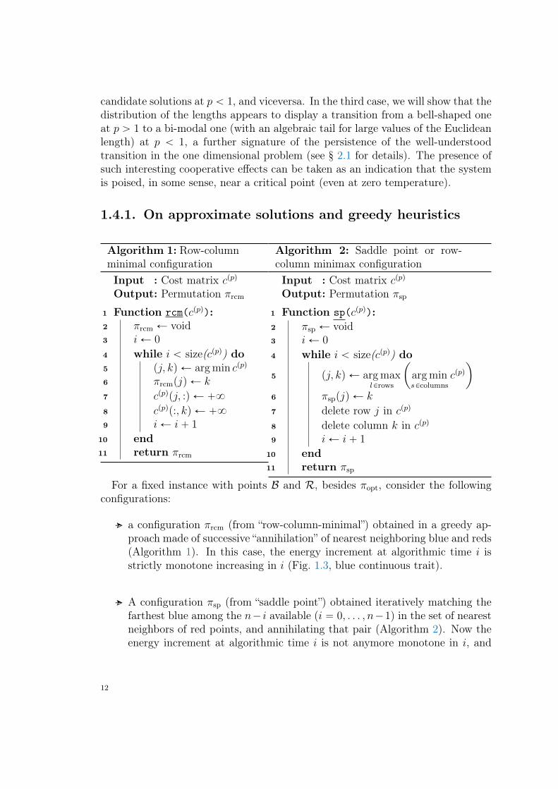
For a fixed instance with points B and R, besides πopt, consider the followingconfigurations:
a configuration πrcm (from “row-column-minimal”) obtained in a greedy ap-proach made of successive “annihilation” of nearest neighboring blue and reds(Algorithm 1). In this case, the energy increment at algorithmic time i isstrictly monotone increasing in i (Fig. 1.3, blue continuous trait).
A configuration πsp (from “saddle point”) obtained iteratively matching thefarthest blue among the n´ i available (i “ 0, . . . , n´1) in the set of nearestneighbors of red points, and annihilating that pair (Algorithm 2). Now theenergy increment at algorithmic time i is not anymore monotone in i, and
12
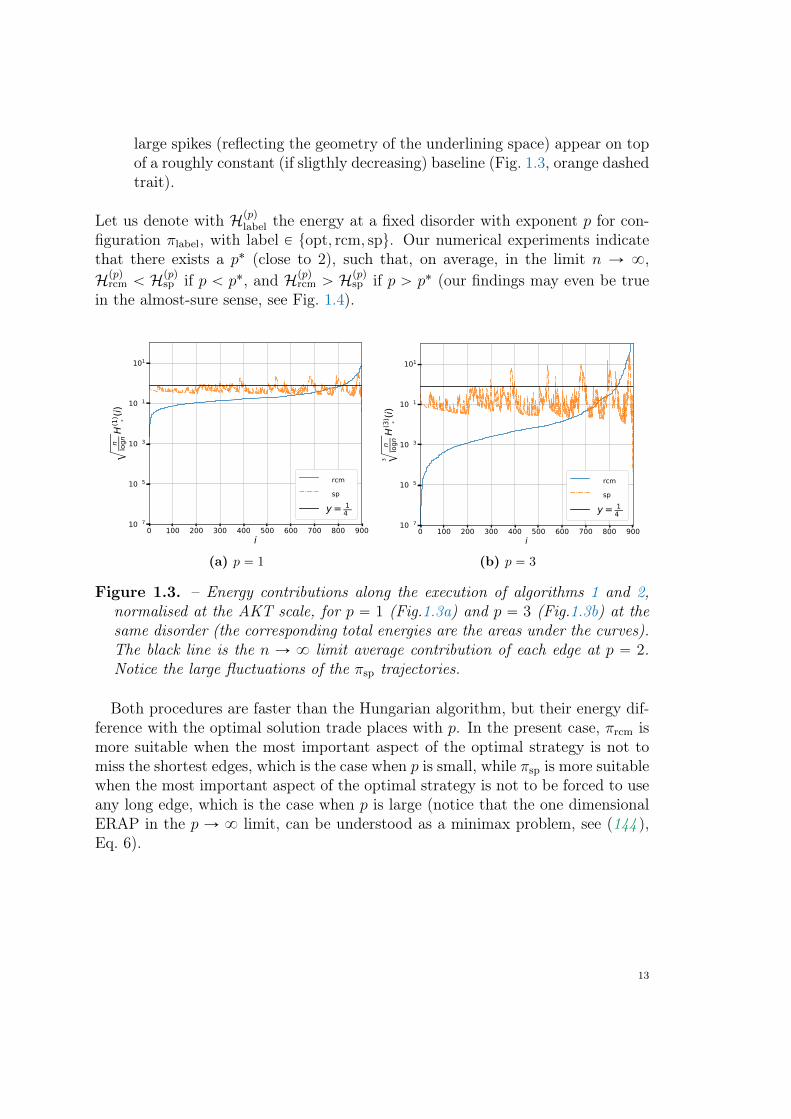
large spikes (reflecting the geometry of the underlining space) appear on topof a roughly constant (if sligthly decreasing) baseline (Fig. 1.3, orange dashedtrait).
Let us denote with Hppqlabel the energy at a fixed disorder with exponent p for con-
figuration πlabel, with label P topt, rcm, spu. Our numerical experiments indicatethat there exists a p˚ (close to 2), such that, on average, in the limit n Ñ 8,Hppq
rcm ă Hppqsp if p ă p˚, and Hppq
rcm ą Hppqsp if p ą p˚ (our findings may even be true
in the almost-sure sense, see Fig. 1.4).
0 100 200 300 400 500 600 700 800 900i
10−7
10−5
10−3
10−1
101
√n lognH(1)
π*(i)
πrcmπspy= 1
4π
(a) p “ 1
0 100 200 300 400 500 600 700 800 900i
10−7
10−5
10−3
10−1
101
3 √n lognH(3)
π*(i)
πrcmπspy= 1
4π
(b) p “ 3
Figure 1.3. – Energy contributions along the execution of algorithms 1 and 2,normalised at the AKT scale, for p “ 1 (Fig.1.3a) and p “ 3 (Fig.1.3b) at thesame disorder (the corresponding total energies are the areas under the curves).The black line is the n Ñ 8 limit average contribution of each edge at p “ 2.Notice the large fluctuations of the πsp trajectories.
Both procedures are faster than the Hungarian algorithm, but their energy dif-ference with the optimal solution trade places with p. In the present case, πrcm ismore suitable when the most important aspect of the optimal strategy is not tomiss the shortest edges, which is the case when p is small, while πsp is more suitablewhen the most important aspect of the optimal strategy is not to be forced to useany long edge, which is the case when p is large (notice that the one dimensionalERAP in the p Ñ 8 limit, can be understood as a minimax problem, see (144 ),Eq. 6).
13
22 23 24 25 26 27
(0.5)opt
20
22
24
26
28
30
32
34
36
(0.5)
labe
l
y= xlabel=rcmlabel=spErm
0.4 0.5 0.6 0.7 0.8 0.9 1.0
(2)opt
0.5
1.0
1.5
2.0
2.5
3.0
(2)
labe
l
y= xlabel=rcmlabel=spErm
0.000 0.002 0.004 0.006 0.008 0.010 0.012 0.014 0.016
(4.0)opt
0.0
0.1
0.2
0.3
0.4
0.5
0.6
0.7
(4.0)
labe
l
y= xlabel=rcmlabel=spErm
0.04 0.06 0.08 0.10 0.12
(3.0)opt
0.0
0.2
0.4
0.6
0.8
1.0
1.2
(3.0)
labe
ly= xlabel=rcmlabel=spErm
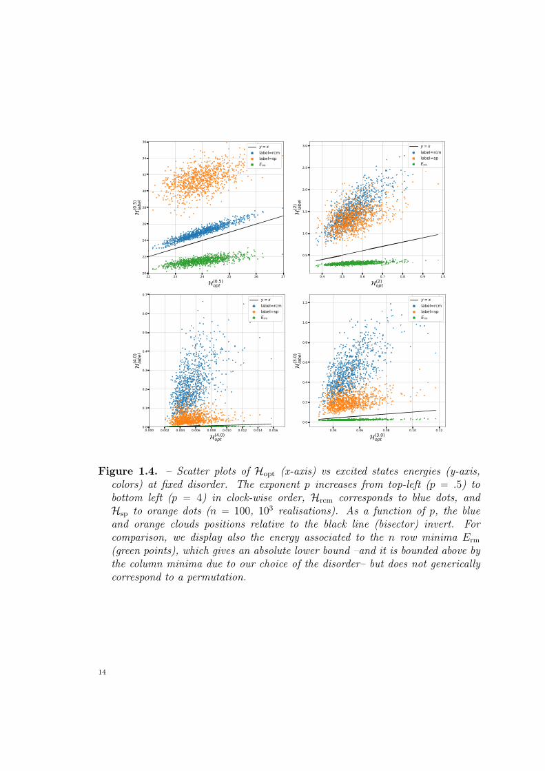
Figure 1.4. – Scatter plots of Hopt (x-axis) vs excited states energies (y-axis,colors) at fixed disorder. The exponent p increases from top-left (p “ .5) tobottom left (p “ 4) in clock-wise order, Hrcm corresponds to blue dots, andHsp to orange dots (n “ 100, 103 realisations). As a function of p, the blueand orange clouds positions relative to the black line (bisector) invert. Forcomparison, we display also the energy associated to the n row minima Erm
(green points), which gives an absolute lower bound –and it is bounded above bythe column minima due to our choice of the disorder– but does not genericallycorrespond to a permutation.
14
1.4.2. On crossings of ground state energies
For a fixed instance of B and R, and n large, let πppqopt be the optimal assignment atexponent p, and let Hpp1qpπ
pp2q
opt q be the energy for the ground state at p “ p2, eval-uated at exponent p1. By definition, if p1 ‰ p2 then Hpp1qpπ
pp2q
opt q ě Hpp1qpπpp1q
opt q “
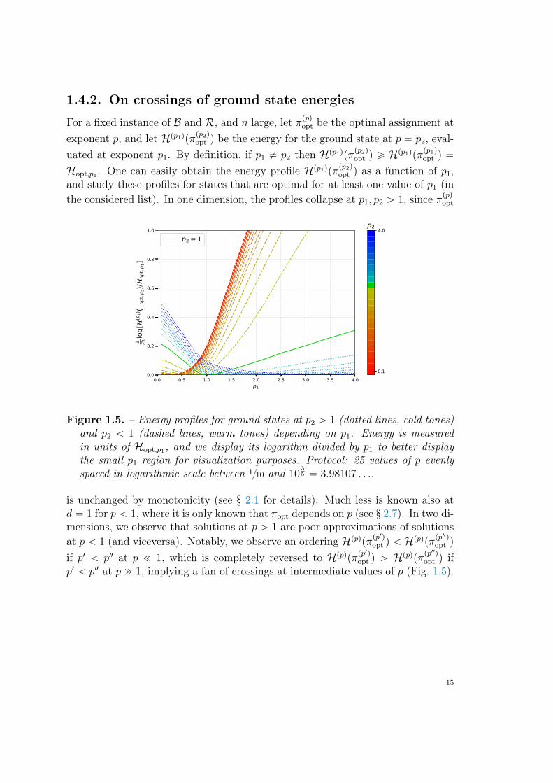
Hopt,p1 . One can easily obtain the energy profile Hpp1qpπpp2q
opt q as a function of p1,and study these profiles for states that are optimal for at least one value of p1 (inthe considered list). In one dimension, the profiles collapse at p1, p2 ą 1, since πppqopt
0.0 0.5 1.0 1.5 2.0 2.5 3.0 3.5 4.0p1
0.0
0.2
0.4
0.6
0.8
1.0
1 p 1log[
(p1)(π
opt,p 2)/
opt,p 1]
p2=1
0.1
4.0p2
Figure 1.5. – Energy profiles for ground states at p2 ą 1 (dotted lines, cold tones)and p2 ă 1 (dashed lines, warm tones) depending on p1. Energy is measuredin units of Hopt,p1, and we display its logarithm divided by p1 to better displaythe small p1 region for visualization purposes. Protocol: 25 values of p evenlyspaced in logarithmic scale between 110 and 10
35 “ 3.98107 . . ..
is unchanged by monotonicity (see § 2.1 for details). Much less is known also atd “ 1 for p ă 1, where it is only known that πopt depends on p (see § 2.7). In two di-mensions, we observe that solutions at p ą 1 are poor approximations of solutionsat p ă 1 (and viceversa). Notably, we observe an ordering Hppqpπ
pp1qopt q ă Hppqpπ
pp2qopt q
if p1 ă p2 at p ! 1, which is completely reversed to Hppqpπpp1qopt q ą Hppqpπ
pp2qopt q if
p1 ă p2 at p " 1, implying a fan of crossings at intermediate values of p (Fig. 1.5).
15
1.4.3. Possible persistence of transition near p “ 1 at d “ 2
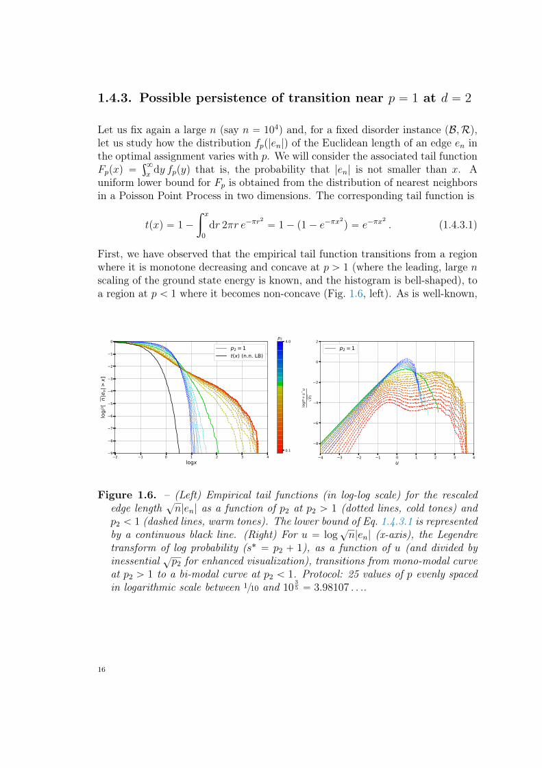
Let us fix again a large n (say n “ 104) and, for a fixed disorder instance pB,Rq,let us study how the distribution fpp|en|q of the Euclidean length of an edge en inthe optimal assignment varies with p. We will consider the associated tail functionFppxq “
ş8
xdy fppyq that is, the probability that |en| is not smaller than x. A
uniform lower bound for Fp is obtained from the distribution of nearest neighborsin a Poisson Point Process in two dimensions. The corresponding tail function is
tpxq “ 1´
ż x
0
dr 2πr e´πr2
“ 1´ p1´ e´πx2
q “ e´πx2
. (1.4.3.1)
First, we have observed that the empirical tail function transitions from a regionwhere it is monotone decreasing and concave at p ą 1 (where the leading, large nscaling of the ground state energy is known, and the histogram is bell-shaped), toa region at p ă 1 where it becomes non-concave (Fig. 1.6, left). As is well-known,
−2 −1 0 1 2 3 4logx
−9
−8
−7
−6
−5
−4
−3
−2
−1
0
logℙ
[√n|e
n|>x]
p2=1t(x) (n.n. LB)
0.1
4.0p2
−4 −3 −2 −1 0 1 2 3 4u
−8
−6
−4
−2
0
2
log
+s*
u√p 2
p2=1
Figure 1.6. – (Left) Empirical tail functions (in log-log scale) for the rescalededge length
?n|en| as a function of p2 at p2 ą 1 (dotted lines, cold tones) and
p2 ă 1 (dashed lines, warm tones). The lower bound of Eq. 1.4.3.1 is representedby a continuous black line. (Right) For u “ log
?n|en| (x-axis), the Legendre
transform of log probability (s˚ “ p2 ` 1), as a function of u (and divided byinessential
?p2 for enhanced visualization), transitions from mono-modal curve
at p2 ą 1 to a bi-modal curve at p2 ă 1. Protocol: 25 values of p evenly spacedin logarithmic scale between 110 and 10
35 “ 3.98107 . . ..
16
this corresponds to a double regime in the Mellin transform of ρ:
rMfps psq :“
ż
dx fppxqxs´1
“ ps´ 1q
ż
dxFppxqxs´2
“t“log x
ps´ 1q
ż
dt eGptq`ps´1qt
(1.4.3.2)
where Gptq “ logFppxq|t“log x. Indeed, the extremum for the integrand t˚psq, whichgives the logarithm of the Euclidean lengths of edges contributing to the momentsof ρ, is a smooth function of s if G is concave but discontinuous otherwise. Noticethat the Mellin transform rMfpspsq is essentially the evaluation of Hpp1qpπ
pp2q
opt q atp1 “ s´1. Hence, the loss of concavity describes here a sort of “moral bi-modality”,in the sense that, in Hpp1qpπ
pp2q
opt q, there is a domination of short or long edges if p1
is smaller or greater than a certain threshold, that we conjecture to be at aroundp2. The optimal solution balances the contribution of long and short edges, as canbe seen in Fig. 1.6 (right).
1.5. Some related topics
In our previous discussions, several connections with other research topics be-yond the original statistical physics motivation were mentioned (explicitly or
implicitly). In this section, we wish to emphasize some other connections since,we believe, a methodological transfer of methods and ideas between the involvedcommunities could be of general benefit.In recent years many efforts have been devoted to a fundamental problem in the
Calculus of Variations, which is how to optimally transport continuum measuresone into another, or the “Monge–Kantorovich problem” (see (161 ) for an histor-ical introduction and (114 ) for a discussion of related problems). It is a simpleexercise to show that the ground state energy Hopt in an ERAP (Eq. 1.3.0.2) isproportional to (the p-th power of) the p-Wasserstein (or Kantorovich) distancebetween the empirical measures associated to B and R∗. Another way to statethis correspondence is: for measures supported onto a finite collection of points,
∗Let pY,DYq be a Polish metric space, that is, a metric space which is also complete –every Cauchysequence converges in Y– and separable –Y contains a countable dense set– (common Polish metricspaces are: C, the d-dimensional torus Td, unit-cube Qd, sphere Sd. The interested reader mayconsult (62 ), Chapter 3). Following Villani (127 ), the p-Wasserstein distance (to the power p)between two probability measures µ1, µ2 on a Polish metric space pY,DYq is
W pp pµ1, µ2q :“ inf
νPµ1ˆµ2
ż
Ydνpx, yqDp
Ypx, yq , (1.5.0.1)
where the infimum is taken among all the product measures ν P µ1 ˆ µ2 with marginals µ1 andµ2. Given an ERAP on pY,DYq, consider the empirical measures for an instance B “ tbiuni“1 and
17
transference plans of optimal transport (127 ) are in bijection with the Birkhoffpolytope of doubly stochastic matrices. The correspondence can be traced back atleast to Kantorovich’s work (see (127 ), Chapter 3 and (158 ) for a recent discus-sion). This connection will play an important role in Chapter 3. On a parallel line,starting from the seminal work of Beardwood–Halton–Hammersley (18 ), interesthas arisen around almost-sure limits of Euclidean functionals of finite randompoint sets, including the length functional in the random minimum spanning treeproblem, or the aforementioned traveling salesman problem, even in a self-similarsetting embedded in two dimensional Euclidean space (54 ). See (58 ) for an entrypoint, and (69 , 79 ) for monographs. See also (136 ) for a recent account andresults on bipartite Euclidean functionals.A second connection deals with the aforementioned longstanding program of
statistical physics approaches to computational complexity theory. It emerges ifone insists in thinking that the Hungarian method plays a similar role as Gaussianelimination in linear algebra (49 )†. The basic observation is that, from the per-spective of linear programming, the assignment problem constitutes only a “slight”(but crucial) modification of combinatorial problems in a different complexity class,such as the traveling salesman problem (TSP), which is NP-complete (39 ), as itfalls in the same class of the 3SAT problem (130 ). The situation shares analogywith a “slight” modification of the 3SAT, called 3-XOR-SAT, which is solvable inpolynomial time (for example using Gaussian elimination on Z2Z, see also (115 )).Hence, the general hope is that the ERAP may serve as a paradigm toy-model sim-plification for gaining insights on stochastic versions of more difficult NP-completeproblems, and a possibly comparative tool to understand what makes them diffi-cult.A third connection further emerges if one insists on the statistical mechanical
description of an ERAP beyond the ground state. In fact, the canonical partitionfunction at inverse temperature β (in units of Boltzmann’s constant) of any ERAP
R “ triuni“1 defined by
ρBpxq “1
n
ÿ
biPBδpx´ biq , ρRpxq “
1
n
ÿ
rkPRδpx´ rkq , (1.5.0.2)
where δ is Dirac’s function. Then by straightforward computation
nW pp pρB, ρRq “ Hopt (1.5.0.3)
as announced.†Actually, there is more to the analogy since the optimal cost to an assignment problem can be directlyseen as a certain determinant of the cost matrix. The price to pay for such an interpretation, whichis in the same spirit of the statistical physics approach to optimization problems, is to consider “zero-temperature free energies”, or, more precisely, to formulate the assignment problem on the so-called“tropical semi-ring” (instead of the ring of real numbers) (152 ). Informally, one replaces x ` y byminpx, yq and xy by x` y.
18
is the permanent of the Hadamard exponential of the nˆn cost matrix cppq‡. Sucha correspondence, where both sides are quite generally little understood, allows toask several questions in both languages. On physical grounds, one would like toaccess the full quenched free energy fqpβq “ ´ 1
βErlnZpβqs (E denoting expecta-
tion with respect to the disorder distribution), or at least some asymptotics forfqpβq for large β. However, the study of excited states in the ERAP (and in otherstochastic optimisation problems) turned out to be very difficult, as the spectrumcan show non-trivial features (see e.g. § 1.4), so that very little is known about theexcited states even for the simplest disorder distributions (see (100 ) for some workin this direction). On mathematical grounds, the different viewpoint offered bythe ERAP may be useful in understanding the statistical properties of permanentsof positive random matrices, a topic of interest in probability but considerably lessunderstood than random determinants (see e.g. (53 , 66 )). Moreover, here onemay notice that the permanent constitutes a “slight” (but crucial) modificationof the determinant, and functions interpolating between the permanent and thedeterminant have been studied from different viewpoints during the years (70 ).In our opinion, the exploration of such themes in the light of computational com-plexity theory may also be of possible general benefit.Regarding applications, as we have already mentioned, an ERAP is so elemen-
tary in his description that, under appropriate choice of the statistical ensemble forB and R, it may conceivably describe several important real-life situations, someof which have been already been hinted at in § 1.5. For another, consider a linearchain, in some configuration within a solvent constituted of monomers which maybe “charged” (e.g., they have different electronegativity). The optimal electrostaticpairing of the molecule (say, the optimal pattern of hydrogen bonds) can be rea-sonably described by an ERAP whose cost or fitness matrix is determined by afunction of the Euclidean distance of the candidate positive and negative pairs. Ina natural, simplified parametrization, we can imagine that the system is describedby two parameters: the fractal effective dimension of the system, d, and the costexponent, p (that is, the cost for connecting a pair of monomers at distance rscales as rp). Our focus in this manuscript will mostly be on theoretical aspects,but a discussion of another possibly useful application of our framework is givenat the end of Chapter 5.
‡That is, defining rW pβqsij :“ e´βcppqij for the cost matrix cppq with exponent p, the partition function
of the corresponding ERAP at inverse temperature β is
Zpβq “ÿ
πPSne´β
řni“1 c
ppqiπpiq “
ÿ
πPSn
nź
i“1
e´βc
ppqiπpiq “ perm rW pβqs , (1.5.0.4)
where perm rW pβqs is a polynomial of degree n in the W pβqij ’s with positive coefficients, and thetwo quantities are equal in distribution.
19
1.6. Plan of the Thesis and list of contributions
The manuscript develops as follows: in Chapter 2, focused on the problemin one dimension, we present some new results using mostly analytic and
combinatorial methods (plus a conjecture supported by numerical experiments).In Chapter 3, we investigate some aspects of the problem in dimension two, such asthe regularization of the asymptotic series of the ground state energy. The studybuilds on a recently proposed continuum field theoretical approach (145 , 148 ) andinvolves also the verification of theoretical predictions by numerical experiments.At the end of the Chapter 3, we pose the basis of a finite n, lattice statisticalfield theory approach for which we report some promising preliminary results. InChapter 4, we address the question of universality at intermediate dimensions withthe introduction of an ERAP at fractal dimension and an extensive numericalinvestigation of relevant ground state energies scaling exponents. Some specificresearch problems are reported at the end of each chapter. Novel contributionsdiscussed in this manuscript resulted in the following works (published, submittedor in preparation):
) 2018: Anomalous scaling of the optimal assignment in the one dimen-sional Random Assignment Problem,
with Sergio Caracciolo and Gabriele Sicuro, published in the Journal of Sta-tistical Physics (169 ).
) 2019: The Dyck bound in the concave 1-dimensional random assign-ment model,
with Sergio Caracciolo, Vittorio Erba and Andrea Sportiello, published inthe Journal of Physics A: Mathematical and Theoretical (173 ).
) 2020: Random Assignment Problems on 2d manifolds,
with Dario Benedetto, Emanuele Caglioti, Sergio Caracciolo, Gabriele Sicuroand Andrea Sportiello, submitted (172 ).
) 2020: Anomalous scaling of the optimal assignment in the one dimen-sional Random Assignment Problem: some rigorous results,
with Andrea Sportiello, in preparation (174 ).
) 2020: Euclidean Random Assignment Problems at non-integer Haus-dorff dimensions dH P p1, 2q,
with Andrea Sportiello, in preparation (175 ).
Some provisional conclusions are given in Chapter 5 followed by a discussion ofresearch perspectives.
20
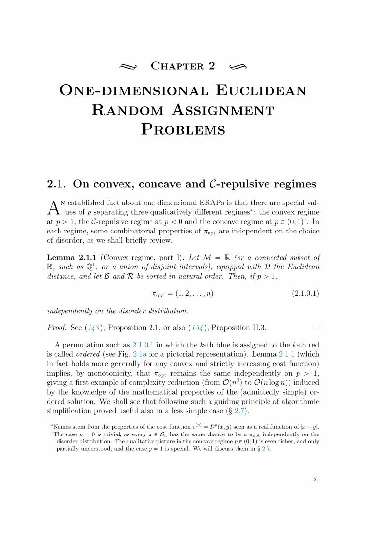
d Chapter 2 D
One-dimensional EuclideanRandom Assignment
Problems
2.1. On convex, concave and C-repulsive regimes
An established fact about one dimensional ERAPs is that there are special val-ues of p separating three qualitatively different regimes∗: the convex regime
at p ą 1, the C-repulsive regime at p ă 0 and the concave regime at p P p0, 1q†. Ineach regime, some combinatorial properties of πopt are independent on the choiceof disorder, as we shall briefly review.
Lemma 2.1.1 (Convex regime, part I). Let M “ R (or a connected subset ofR, such as Q1, or a union of disjoint intervals), equipped with D the Euclideandistance, and let B and R be sorted in natural order. Then, if p ą 1,
πopt “ p1, 2, . . . , nq (2.1.0.1)
independently on the disorder distribution.
Proof. See (143 ), Proposition 2.1, or also (154 ), Proposition II.3.
A permutation such as 2.1.0.1 in which the k-th blue is assigned to the k-th redis called ordered (see Fig. 2.1a for a pictorial representation). Lemma 2.1.1 (whichin fact holds more generally for any convex and strictly increasing cost function)implies, by monotonicity, that πopt remains the same independently on p ą 1,giving a first example of complexity reduction (from Opn3q to Opn log nq) inducedby the knowledge of the mathematical properties of the (admittedly simple) or-dered solution. We shall see that following such a guiding principle of algorithmicsimplification proved useful also in a less simple case (§ 2.7).
∗Names stem from the properties of the cost function cppq “ Dppx, yq seen as a real function of |x´ y|.
†The case p “ 0 is trivial, as every π P Sn has the same chance to be a πopt independently on thedisorder distribution. The qualitative picture in the concave regime p P p0, 1q is even richer, and onlypartially understood, and the case p “ 1 is special. We will discuss them in § 2.7.
21
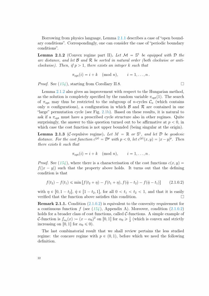
Borrowing from physics language, Lemma 2.1.1 describes a case of “open bound-ary conditions”. Correspondingly, one can consider the case of “periodic boundaryconditions”.
Lemma 2.1.2 (Convex regime part II). Let M “ S1 be equipped with D thearc distance, and let B and R be sorted in natural order (both clockwise or anti-clockwise). Then, if p ą 1, there exists an integer k such that
πoptpiq “ i` k pmod nq, i “ 1, . . . , n .
Proof. See (154 ), starting from Corollary II.8.
Lemma 2.1.2 also gives an improvement with respect to the Hungarian method,as the solution is completely specified by the random variable πoptp1q. The searchof πopt may thus be restricted to the subgroup of n-cycles Cn (which containsonly n configurations), a configuration in which B and R are contained in one“large” permutation cycle (see Fig. 2.1b). Based on these results, it is natural toask if a πopt must have a prescribed cycle structure also in other regimes. Quitesurprisingly, the answer to this question turned out to be affirmative at p ă 0, inwhich case the cost function is not upper bounded (being singular at the origin).
Lemma 2.1.3 (C-repulsive regime). Let M “ R or S1, and let D be geodesicdistance. For the cost function cppq “ Dp with p ă 0, let cppqpx, yq “ |x´ y|p. Thenthere exists k such that
πoptpiq “ i` k pmod nq, i “ 1, . . . , n .
Proof. See (154 ), where there is a characterisation of the cost functions cpx, yq “fp|x ´ y|q such that the property above holds. It turns out that the definingcondition is that
fpt2q ´ fpt1q ď min rfpt2 ` ηq ´ fpt1 ` ηq, fpη ´ t2q ´ fpη ´ t1qs (2.1.0.2)
with η P r0, 1 ´ t2s, η P r1 ´ t2, 1s, for all 0 ă t1 ă t2 ă 1, and that it is easilyverified that the function above satisfies this condition.
Remark 2.1.1. Condition (2.1.0.2) is equivalent to the convexity requirement fora continuous function f (see (154 ), Appendix A). Moreover, condition (2.1.0.2)holds for a broader class of cost functions, called C-functions. A simple example ofC-function is fα0pxq :“ px´ α0q
2 on r0, 1s for α0 ě12(which is convex and strictly
increasing on r0, 1s for α0 ď 0).
The last combinatorial result that we shall review pertains the less studiedregime: the concave regime with p P p0, 1q, before which we need the followingdefinition.
22
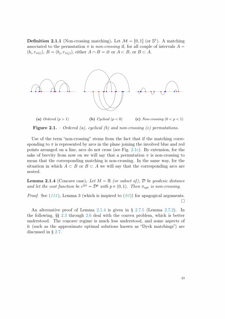
Definition 2.1.1 (Non-crossing matching). Let M “ r0, 1s (or S1). A matchingassociated to the permutation π is non-crossing if, for all couple of intervals A “pbi, rπpiqq, B “ pbj, rπpjqq, either AXB “ ∅ or A Ă B, or B Ă A.
(a) Ordered pp ą 1q (b) Cyclical pp ă 0q (c) Non-crossing p0 ă p ă 1q
Figure 2.1. – Ordered (a), cyclical (b) and non-crossing (c) permutations.
Use of the term “non-crossing” stems from the fact that if the matching corre-sponding to π is represented by arcs in the plane joining the involved blue and redpoints arranged on a line, arcs do not cross (see Fig. 2.1c). By extension, for thesake of brevity from now on we will say that a permutation π is non-crossing tomean that the corresponding matching is non-crossing. In the same way, for thesituation in which A Ă B or B Ă A we will say that the corresponding arcs arenested.
Lemma 2.1.4 (Concave case). Let M “ R (or subset of), D be geodesic distanceand let the cost function be cppq “ Dp with p P p0, 1q. Then πopt is non-crossing.
Proof. See (151 ), Lemma 3 (which is inspired to (82 )) for apagogical arguments.
An alternative proof of Lemma 2.1.4 is given in § 2.7.5 (Lemma 2.7.2). Inthe following, §§ 2.3 through 2.6 deal with the convex problem, which is betterunderstood. The concave regime is much less understood, and some aspects ofit (such as the approximate optimal solutions known as “Dyck matchings”) arediscussed in § 2.7.
23
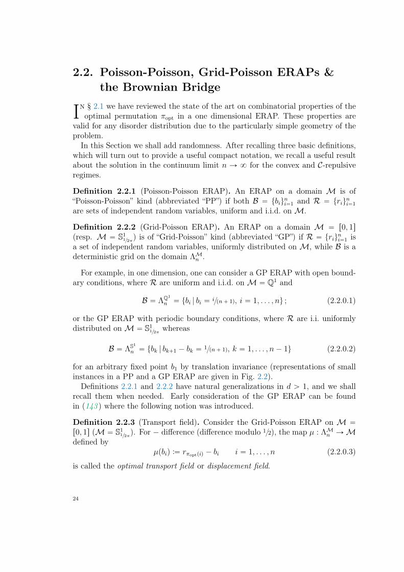
2.2. Poisson-Poisson, Grid-Poisson ERAPs &the Brownian Bridge
In § 2.1 we have reviewed the state of the art on combinatorial properties of theoptimal permutation πopt in a one dimensional ERAP. These properties are
valid for any disorder distribution due to the particularly simple geometry of theproblem.In this Section we shall add randomness. After recalling three basic definitions,
which will turn out to provide a useful compact notation, we recall a useful resultabout the solution in the continuum limit n Ñ 8 for the convex and C-repulsiveregimes.
Definition 2.2.1 (Poisson-Poisson ERAP). An ERAP on a domain M is of“Poisson-Poisson” kind (abbreviated “PP”) if both B “ tbiu
ni“1 and R “ triu
ni“1
are sets of independent random variables, uniform and i.i.d. on M.
Definition 2.2.2 (Grid-Poisson ERAP). An ERAP on a domain M “ r0, 1s(resp. M “ S1
12π) is of “Grid-Poisson” kind (abbreviated “GP”) if R “ triu
ni“1 is
a set of independent random variables, uniformly distributed on M, while B is adeterministic grid on the domain ΛM
n .
For example, in one dimension, one can consider a GP ERAP with open bound-ary conditions, where R are uniform and i.i.d. on M “ Q1 and
B “ ΛQ1
n “ tbi | bi “ ipn` 1q, i “ 1, . . . , nu ; (2.2.0.1)
or the GP ERAP with periodic boundary conditions, where R are i.i. uniformlydistributed on M “ S1
12πwhereas
B “ ΛS1
n “ tbk | bk`1 ´ bk “ 1pn` 1q, k “ 1, . . . , n´ 1u (2.2.0.2)
for an arbitrary fixed point b1 by translation invariance (representations of smallinstances in a PP and a GP ERAP are given in Fig. 2.2).Definitions 2.2.1 and 2.2.2 have natural generalizations in d ą 1, and we shall
recall them when needed. Early consideration of the GP ERAP can be foundin (143 ) where the following notion was introduced.
Definition 2.2.3 (Transport field). Consider the Grid-Poisson ERAP on M “
r0, 1s (M “ S112π
). For ´ difference (difference modulo 12), the map µ : ΛMn ÑM
defined byµpbiq :“ rπoptpiq ´ bi i “ 1, . . . , n (2.2.0.3)
is called the optimal transport field or displacement field.
24
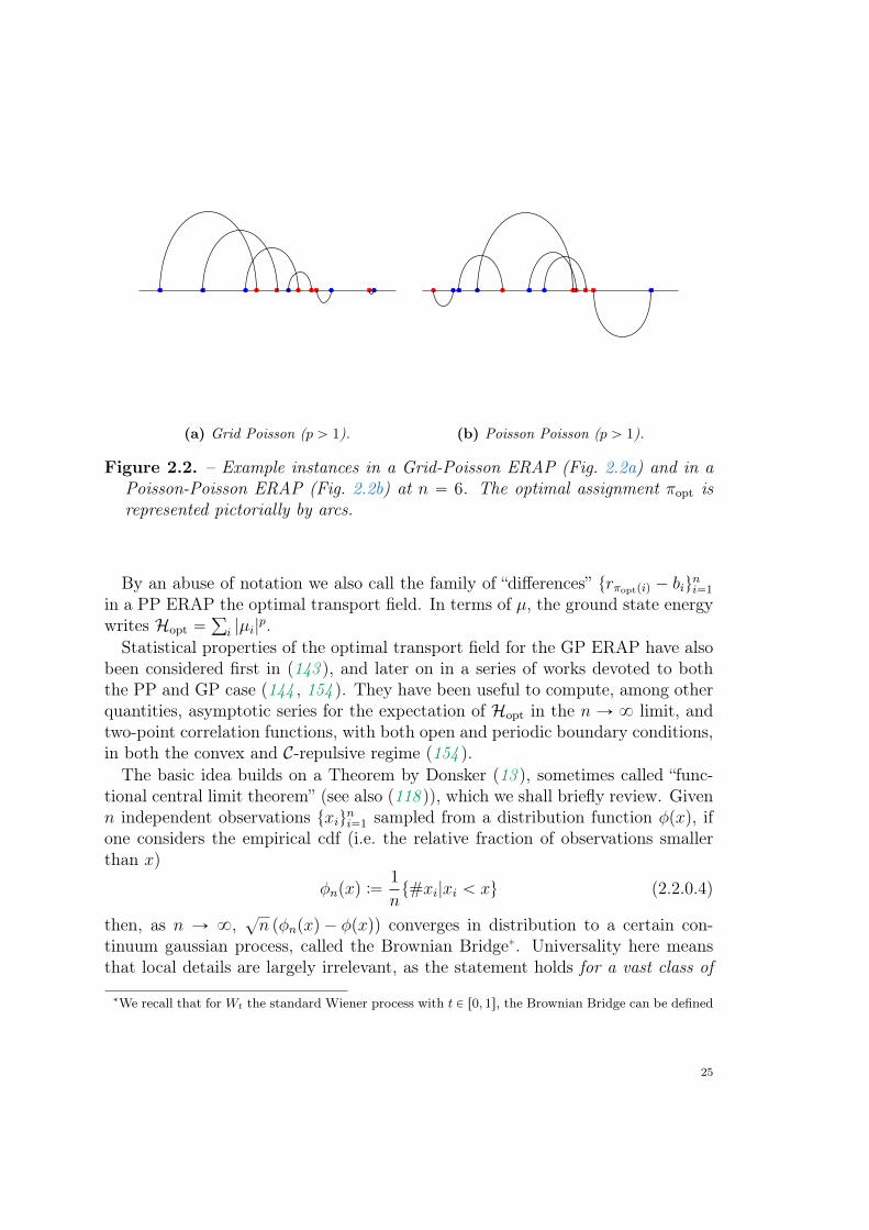
(a) Grid Poisson (p ą 1). (b) Poisson Poisson (p ą 1).
Figure 2.2. – Example instances in a Grid-Poisson ERAP (Fig. 2.2a) and in aPoisson-Poisson ERAP (Fig. 2.2b) at n “ 6. The optimal assignment πopt isrepresented pictorially by arcs.
By an abuse of notation we also call the family of “differences” trπoptpiq ´ biuni“1
in a PP ERAP the optimal transport field. In terms of µ, the ground state energywrites Hopt “
ř
i |µi|p.
Statistical properties of the optimal transport field for the GP ERAP have alsobeen considered first in (143 ), and later on in a series of works devoted to boththe PP and GP case (144 , 154 ). They have been useful to compute, among otherquantities, asymptotic series for the expectation of Hopt in the n Ñ 8 limit, andtwo-point correlation functions, with both open and periodic boundary conditions,in both the convex and C-repulsive regime (154 ).The basic idea builds on a Theorem by Donsker (13 ), sometimes called “func-
tional central limit theorem” (see also (118 )), which we shall briefly review. Givenn independent observations txiuni“1 sampled from a distribution function φpxq, ifone considers the empirical cdf (i.e. the relative fraction of observations smallerthan x)
φnpxq :“1
nt#xi|xi ă xu (2.2.0.4)
then, as n Ñ 8,?n pφnpxq ´ φpxqq converges in distribution to a certain con-
tinuum gaussian process, called the Brownian Bridge∗. Universality here meansthat local details are largely irrelevant, as the statement holds for a vast class of
∗We recall that for Wt the standard Wiener process with t P r0, 1s, the Brownian Bridge can be defined
25
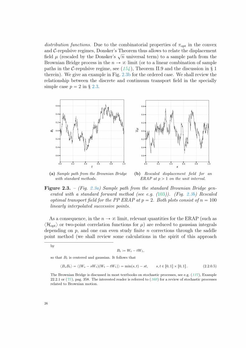
distribution functions. Due to the combinatorial properties of πopt in the convexand C-repulsive regimes, Donsker’s Theorem thus allows to relate the displacementfield µ (rescaled by the Donsker’s
?n universal term) to a sample path from the
Brownian Bridge process in the nÑ 8 limit (or to a linear combination of samplepaths in the C-repulsive regime, see (154 ), Theorem II.9 and the discussion in § 1therein). We give an example in Fig. 2.3b for the ordered case. We shall review therelationship between the discrete and continuum transport field in the speciallysimple case p “ 2 in § 2.3.
0.0 0.2 0.4 0.6 0.8 1.0t
−0.6
−0.4
−0.2
0.0
0.2
0.4
0.6
B t
(a) Sample path from the Brownian Bridgewith standard methods.
0.0 0.2 0.4 0.6 0.8 1.0x
−0.6
−0.4
−0.2
0.0
0.2
0.4
0.6
√ nμ
(b) Rescaled displacement field for anERAP at p ą 1 on the unit interval.
Figure 2.3. – (Fig. 2.3a) Sample path from the standard Brownian Bridge gen-erated with a standard forward method (see e.g. (103)). (Fig. 2.3b) Rescaledoptimal transport field for the PP ERAP at p “ 2. Both plots consist of n “ 100linearly interpolated successive points.
As a consequence, in the nÑ 8 limit, relevant quantities for the ERAP (such asxHopty or two-point correlation functions for µ) are reduced to gaussian integralsdepending on p, and one can even study finite n corrections through the saddlepoint method (we shall review some calculations in the spirit of this approach
byBt :“Wt ´ tW1,
so that Bt is centered and gaussian. It follows that
xBsBty “ xpWs ´ sW1qpWt ´ tW1qy “ minps, tq ´ st, s, t P r0, 1s ˆ r0, 1s . (2.2.0.5)
The Brownian Bridge is discussed in most textbooks on stochastic processes, see e.g. (137 ), Example22.2.1 or (75 ), pag. 358. The interested reader is referred to (160 ) for a review of stochastic processesrelated to Brownian motion.
26
in § 2.4, see (154 ) for a detailed account). Theoretical predictions have beenconfirmed by extensive numerical experiments (143 , 144 , 154 ). In conclusion, letus comment on a simple consequence of the remarkable “universality property”underlining our discussion at p ą 1. If the disorder probability density functionhas connected support and does not vanish, the ground state energy is made of ncontributions which are typically of order pn´12qp, so that
xHopty |pě1 „ cpn1´p2
p1` op1qq , nÑ 8 , (2.2.0.6)
with a constant cp depending on p and on the choice of distribution (the scalingexponent of sub-leading corrections may depend on the boundary conditions).Notice that the leading order in Eq. 2.2.0.6 is much larger than the scaling ofthe lower bound ELB
n . The latter is found by assigning points in their Euclideanneighborhoods, so that ELB
n „ nn´pd|d“1 “ n1´p, and is self-averaging by thecentral limit theorem. As a side remark, it is worth noticing that this “universalproperty” can be traced back at least to the work of Kolmogorov (see (8 ), Teorema1, or (57 ), § 2 for an english translation), which is often quoted as the basis of awide-spread goodness-of-fit test in non-parametric statistics, named Kolmogorov-Smirnov statistics (10 ). We will come back to this point in § 2.5.1. By completelyanalogous arguments it is simply seen that in the C-repulsive regime
xHopty |pď0 „1
2pn p1` op1qq , nÑ 8 , (2.2.0.7)
for both S1 and Q1, where the factor 12“
|M|
2is the typical length of an edge in
the optimal assignment (see (154 ) for further details).If on the contrary the disorder distribution is discontinuous and/or vanishes, the
problem is considerably more difficult and the scaling properties of xHopty requirefurther efforts to be unveiled, as we will discuss in § 2.6.
27
2.3. Lattice and continuum modes of the optimaltransport field at p “ 2
In this Section we shall discuss some statistical properties of both discrete andcontinuum Fourier modes of the displacement field (Def. 2.2.3) in the special
case p “ 2, where we have already seen that limnÑ8 xHopty exists and is finite(Eq. 2.2.0.6). The discussion is elementary in that it combines discrete/continuumFourier analysis and manipulations of moment generating functions. At fixed n,among other things we shall show that, both in the discrete and continuum case,the problem is “diagonalized” by an appropriate (discrete or continuum) Fouriertransform, and the ground state is decomposed into a sum of centered gaussian,uncorrelated modes. We will also show that mode correlations, at finite n, areexactly proportional to the inverse lattice Laplacian associated to our choice ofgrid. For the continuum case, we shall derive exact expressions for the probabilitiesof contributions from any given mode to Hopt. We will give an expression of thefull distribution of Hopt in terms of an elliptic ϑ4 function in the case of periodicboundary conditions as an application. Besides the intrinsic value of our discussion,which employs old tools but appears to be new in the literature, we shall discussour calculations in some details also in prevision of the analogous discussion onlattice Fourier modes of the optimal transport field in the more challenging two-dimensional case of Chapter 3.
2.3.1. Unit interval at fixed n
Let us consider M “ Q1, blue points on the grid B “ tbiuni“1, bi “i
n`1with i “
1, . . . , n, with the addition of the two endpoints at 0 and 1. For the displacementfield defined by
µi :“ ri ´i
n` 1, i “ 0, . . . , n` 1, (2.3.1.1)
where reds are R “ triuni“1 Y t0, 1u, the ground state energy is just
Hopt “
n`1ÿ
i“0
µ2i . (2.3.1.2)
Consider the red ri, which is distributed according to
Pipriq :“
$
’
&
’
%
δpr0q for i “ 0
i`
ni
˘
ri´1i p1´ riq
n´i for 1 ď i ď n
δprn`1 ´ 1q for i “ n` 1 ,
(2.3.1.3)
28
where δ is Dirac function. It follows that
xrki y “pi` k ´ 1q!n!
pi´ 1q! pn` kq!(2.3.1.4)
and therefore the moment generating function is an hypergeometric function
xe´wriy “ÿ
kě0
pi` k ´ 1q!n!
pi´ 1q! pn` kq!
p´wqk
k!“ 1F1pi;n` 1;´wq . (2.3.1.5)
In particular from Eq. 2.3.1.5 we read the balancing condition
xriy “i
n` 1(2.3.1.6)
and, using for j ě i the discrete Wiener formula
Pijpri, rjq :“ i pj ´ iq
ˆ
n
i, j ´ i, n´ j
˙
ri´1i prj ´ riq
j´i´1p1´ rjq
n´j , (2.3.1.7)
we get
xrirjy “i pj ` 1q
pn` 1qpn` 2q(2.3.1.8)
for j ě i. It follows that the transport field satisfies
xµiy “ 0
xµiµjy “i pn` 1´ jq
pn` 1q2pn` 2q.
(2.3.1.9)
As a consequence we recover the exact expression for the expected ground stateenergy
xHopty “
nÿ
i“1
xµ2i y “
n
6 pn` 1q(2.3.1.10)
which is half of the well-known Poisson-Poisson value (see e.g. (154 ), Eq. 54). Letus go now to momentum space. Since µ satisfies Dirichlet boundary conditions,we can perform the expansion
µs :“
c
2
n` 1
nÿ
l“1
µl sin
ˆ
πls
n` 1
˙
, s “ 1, . . . , n, (2.3.1.11)
29
corresponding to the discrete momenta
ps :“πs
n` 1, s “ 1, . . . , n. (2.3.1.12)
We immediately getxµsy “ 0, s “ 1, . . . , n, (2.3.1.13)
and
xµ2sy “
2
n` 1
nÿ
i,j“1
xµiµjy sin
ˆ
πis
n` 1
˙
sin
ˆ
πjs
n` 1
˙
“2
n` 1
nÿ
i“1
i pn` 1´ iq
pn` 1q2pn` 2qsin2
ˆ
πis
n` 1
˙
`
4
n` 1
nÿ
i“1
nÿ
j“i`1
i pn` 1´ jq
pn` 1q2pn` 2qsin
ˆ
πis
n` 1
˙
sin
ˆ
πjs
n` 1
˙
,
(2.3.1.14)
where Eq. 2.3.1.9 has been used. Using the orthogonality relation (δij is the Kro-necker symbol)
2
n` 1
nÿ
s“1
sin
ˆ
πis
n` 1
˙
sin
ˆ
πjs
n` 1
˙
“ δij , (2.3.1.15)
we can easily verify the Parseval’s identity
nÿ
s“1
xµ2sy “
nÿ
i“1
xµ2i y . (2.3.1.16)
Eq. 2.3.1.14 becomes
xµ2sy “
1
4p2` 3n` n2q sin2´
πs2pn`1q
¯ “1
pn` 1qpn` 2q
1
p2s
, s “ 1, . . . , n,
(2.3.1.17)where we have introduced the lattice Laplacian p2
p :“ 2 sinp
2(2.3.1.18)
which for small p satisfiesp2“ p2
`Opp4q . (2.3.1.19)
Eq. 2.3.1.17 provides exactly the contribution toHopt from the s-th discrete Fouriermode of µ in terms of the inverse lattice Laplacian. Incidentally, notice that
30
combining Eqs. 2.3.1.10 and 2.3.1.16 gives
nÿ
s“1
1
p2s
“n pn` 2q
6. (2.3.1.20)
This fact can be alternatively obtained using the result in (72 , B.27) with L “2n` 2
2n`1ÿ
s“0
1
4 sin2`
πsn`1
˘
` α2“
2pn` 1q
α?
4` α2coth
”
2pn` 1q arcsinh´α
2
¯ı
(2.3.1.21)
coupled with the identity
2n`1ÿ
s“0
1
4 sin2`
πsn`1
˘
` α2“ 2
n´1ÿ
s“1
1
4 sin2`
πsn`1
˘
` α2`
1
4` α2`
1
α2(2.3.1.22)
in the ॠ0 limit, since
nÿ
s“1
1
p2s
“ limαÑ0
n´1ÿ
s“1
1
4 sin2`
πsn`1
˘
` α2“
“ limαÑ0
1
2
„
2pn` 1q
α?
4` α2coth
”
2pn` 1q arcsinh´α
2
¯ı
´1
4` α2´
1
α2
“npn` 2q
6(2.3.1.23)
as claimed. Lastly, the mode-mode correlation is
xµsµty “2
n` 1
nÿ
i,j“1
xµiµjy sin
ˆ
πis
n` 1
˙
sin
ˆ
πjt
n` 1
˙
(2.3.1.24)
“2
n` 1
nÿ
i“1
i pn` 1´ iq
pn` 1q2pn` 2qsin
ˆ
πis
n` 1
˙
sin
ˆ
πit
n` 1
˙
` (2.3.1.25)
2
n` 1
nÿ
i“1
i´1ÿ
j“1
j pn` 1´ iq
pn` 1q2pn` 2qsin
ˆ
πis
n` 1
˙
sin
ˆ
πjt
n` 1
˙
` (2.3.1.26)
2
n` 1
nÿ
i“1
nÿ
j“i`1
i pn` 1´ jq
pn` 1q2pn` 2qsin
ˆ
πis
n` 1
˙
sin
ˆ
πjt
n` 1
˙
. (2.3.1.27)
31
By performing the sum over j and using the orthonormality relation we get
xµsµty “1
2 pn` 1q2pn` 2q sin2´
πs2pn`1q
¯
nÿ
i“1
sin
ˆ
πis
n` 1
˙
sin
ˆ
πit
n` 1
˙
(2.3.1.28)
“δst
4 pn` 1qpn` 2q sin2´
πs2pn`1q
¯ (2.3.1.29)
as claimed. Notice that
limnÑ8
δst
4 pn` 1qpn` 2q sin2´
πs2pn`1q
¯ “δstπ2s2
. (2.3.1.30)
Regarding the Poisson Poisson case, recall that in this case for B “ tbiuni“1 and
R “ triuni“1 in increasing order the displacement field is
µi :“ bi ´ ri (2.3.1.31)
but now
xriy “xbiy “i
n` 1
xrirjy “xbibjy “i pj ` 1q
pn` 1qpn` 2q
(2.3.1.32)
for j ě i. It follows that
xµiy “ 0
xµiµjy “ 2ipn` 1´ jq
pn` 1q2pn` 2q
(2.3.1.33)
and the whole analysis develops as in the Grid Poisson case, up to a factor 2 (i.e.,compare Eqs. 2.3.1.33 and 2.3.1.9).
2.3.2. Unit interval in the nÑ 8 limit
Let us consider the Grid-Poisson case first, and let us take the continuum limitnÑ `8 as ?
n` 1µi Ñ µpxiq (2.3.2.1)
32
with xi P r0, 1s so that µpxiq from well-known properties of the Brownian Bridgeprocess for x1 ď x2
xµpx1qµpx2qy “ x1p1´ x2q . (2.3.2.2)
We have
µs :“?
2
ż 1
0
dxµpxq sinpπsxq (2.3.2.3)
with s P N, and the orthonormality relations
2
ż 1
0
dx sinpπsxq sinpπtxq “ δst . (2.3.2.4)
Then
xµsµty “ 2
ż 1
0
dx
ż 1
0
dy xµpxqµpyqy sinpπsxq sinpπtyq (2.3.2.5)
“ 2
ż 1
0
dx
ż 1
0
dy rθpy ´ xqxp1´ yq` (2.3.2.6)
θpx´ yqyp1´ xqs sinpπsxq sinpπtyq (2.3.2.7)
“2
π2t2
ż 1
0
dx sinpπsxq sinpπtxq (2.3.2.8)
“δstπ2t2
, (2.3.2.9)
where θpxq is Heaviside function (compare to Eq. 2.3.1.30). Now, as the µpxqare centered Gaussian variables, also the µs are centered Gaussian variables, withvariance pπsq´2. Recalling Parseval’s identity Hopt “
ř
sě1 µ2s, we find for the
moment generating function
xe´wHopty “ xe´wř8s“1 µ
2sy “
8ź
s“1
ÿ
ksě0
p´wqks
ks!xµ2ks
s y (2.3.2.10)
“
8ź
s“1
ÿ
ksě0
p´wqks
ks!
p2ks ´ 1q!!
pπsq2ks(2.3.2.11)
“
8ź
s“1
1b
1` 2wpπsq2
(2.3.2.12)
“
d ?2w
sinh`?
2w˘ . (2.3.2.13)
33
In particular, as for a fixed mode
xe´wµ2sy “
1b
1` 2wpπsq2
, (2.3.2.14)
the probability to get a contribution Es to Hopt by the s-th mode is given by theinverse Laplace transform
ρGPHopt
pEsqdEs :“ xδpEs ´ µ2sqydEs “
d
πs2
2Ese´
12π2s2EsdEs , (2.3.2.15)
where δpxq is Dirac function. The cdf is thus
ΦGPs pzq “
ż z
0
dEs ρGPHopt
pEsq “ erf
ˆ
πs
c
z
2
˙
. (2.3.2.16)
where erfpxq denotes the standard error function. For the Poisson-Poisson case,let us set
µs “ ξs ´ ηs, s “ 1, . . . , n, (2.3.2.17)
which are the contributions from R and B once their average values is subtracted.The moment generating function becomes
xe´wHopty “ xe´wř8s“1pξs´ηsq
2
y “
8ź
s“1
ÿ
ksě0
p´wqks
ks!xpξs ´ ηsq
2ksy
“
8ź
s“1
ÿ
ksě0
p´wqks
ks!
ÿ
jsě0
ˆ
2ks2js
˙
xξ2ks´2jss η2js
s y
“
8ź
s“1
ÿ
ksě0
p´wqks
ks! pπsq2ks
ÿ
jsě0
ˆ
2ks2js
˙
p2ks ´ 2js ´ 1q!!p2js ´ 1q!!
“
8ź
s“1
ÿ
ksě0
p´2wqks
ks!
p2ks ´ 1q!!
pπsq2ks
“
8ź
s“1
1b
1` 4wpπsq2
“
d
2?w
sinhp2?wq
.
(2.3.2.18)
34
In this case the probability to get a contribution Es from the s-th mode is
ρPPHopt
pEsqdEs :“ xδpEs ´ µ2sqydEs “
d
πs2
4Ese´
14π2s2EsdEs (2.3.2.19)
whose cdf isΦPPs pzq “
ż z
0
dEs ρPPHopt
pEsq “ erf
ˆ
πs?z
2
˙
. (2.3.2.20)
A simple relationship between the Poisson-Poisson and Grid-Poisson case
ΦPPs p2zq “ ΦGP
s pzq (2.3.2.21)
holds for each s.
2.3.3. Distribution of Hopt on the unit circle in the nÑ 8
limit
Let us consider the problem on M “ S1 in the continuum limit. In this case thetransport field is
µptq :“ Bt ´
ż 1
0
dτ Bτ , (2.3.3.1)
where Bt is the Brownian Bridge. As xµptqy must be independent from t and withvanishing average on S1, we get
xµptqy “ 0 ,
xµptqµpt` τqy “1
12´τp1´ τq
2.
(2.3.3.2)
Now the Fourier modes are
µs “
ż 1
0
dxµpxq e2πisx (2.3.3.3)
with s P Zzt0u, complemented with the orthonormality conditionsż 1
0
dx e2πips´tqx“ δst . (2.3.3.4)
As µpxq P R we must haveµ˚s “ µ´s (2.3.3.5)
35
and we soon getxµsy “ 0 . (2.3.3.6)
For the correlations, for s, t P Zzt0u
xµ˚s µty “
ż 1
0
dx
ż 1
0
dy xµpxqµpyqy e2πip´sx`tyq
“
ż 1
0
dx
ż 1
0
dy xµpxqµpx` yqy e2πirpt´sqx`tysq
“ δst
ż 1
0
dy xµp0qµpyqy e2πity
“ ´δst2
ż 1
0
dy yp1´ yq e2πity
“δst
4π2s2.
(2.3.3.7)
The ground state energy is
xHopty “
ż 1
0
dt xµ2ptqy “
1
12, (2.3.3.8)
which coincides with Eq. (2.3.3.2) at τ “ 0, a result first derived in (143 ). Thesame result may be recovered also through Parseval’s identity, since
xHopty :“ÿ
s‰0
x|µs|2y “ 2
ÿ
sě1
x|µs|2y “
2
4π2
ÿ
sě1
1
s2“
2
4π2ζp2q “
1
12(2.3.3.9)
as announced. The ground state energy moment generating function is
@
e´wHoptD
“
A
e´2wř
sě1 |µs|2E
“
8ź
s“1
ÿ
ksě0
p´2wqks
ks!x|µs|
2ksy
“
8ź
s“1
ÿ
ksě0
p´2wqks
ks!
ks!
p2πsq2ks
“
8ź
s“1
1
1` w2π2s2
“
a
w2
sinh“a
w2
‰ .
(2.3.3.10)
36
Using the expansion from (21 )a
w2
sinh“a
w2
‰ “ÿ
sě1
cs1
1` w2π2s2
(2.3.3.11)
where
cs “ limwÑ´2π2s2
`
1` w2π2s2
˘a
w2
sinh“a
w2
‰ “
limwÑ1
p1´ wq πs?w
sinpπs?wq
“ limεÑ0
ε πs
sin“
πs`
1´ ε2
˘‰ “ 2 p´1qs´1 , (2.3.3.12)
we can inverse Laplace transform Eq. (2.3.3.10) and show that the pdf of theground state energy can be written as
ρHoptpEsq “ÿ
sě1
p´1qs´14π2s2 e´2π2s2Es (2.3.3.13)
whose cdf is the elliptic ϑ-function
ΦGPpxq “ ϑ4
´
0, e´2π2x¯
. (2.3.3.14)
Under the change of variables τpxq “ 2πix, an alternative expression for ΦGPpxqis
ϑ4
´
0, e´2π2x¯
“
η2´
τpxq2
¯
ηpτpxqq(2.3.3.15)
where η is the Dedekind function (see also Eq. B.1.0.8 and the discussion therein).By our previous remarks, for the distribution of Hopt in the Poisson-Poisson casewe just have
ΦPPp2xq “ ΦGP
pxq. (2.3.3.16)
Eq. 2.3.3.15 nicely agrees with results of numerical experiments in both the GPand PP case already at moderately small values of n (Fig. 2.4).
37
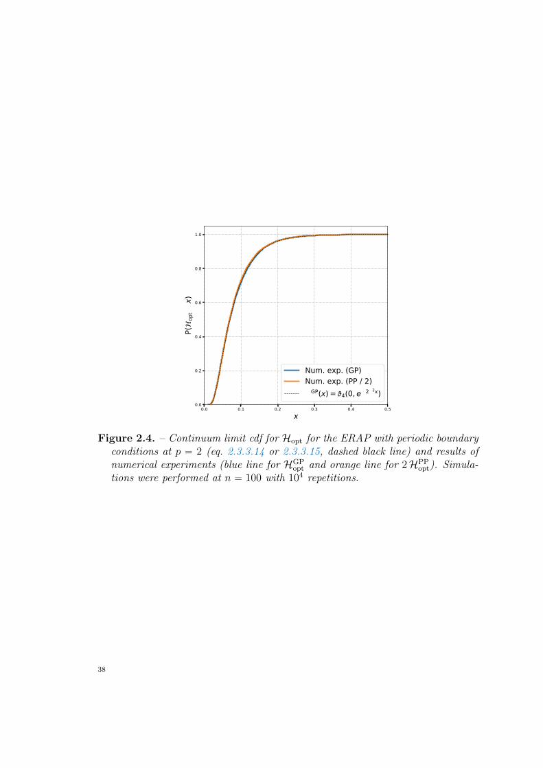
0.0 0.1 0.2 0.3 0.4 0.5x
0.0
0.2
0.4
0.6
0.8
1.0
P(op
t≤x)
Num. exp. (GP)Num. exp. (PP / 2)ΦGP(x) = 4(0, e−2π2x)
Figure 2.4. – Continuum limit cdf for Hopt for the ERAP with periodic boundaryconditions at p “ 2 (eq. 2.3.3.14 or 2.3.3.15, dashed black line) and results ofnumerical experiments (blue line for HGP
opt and orange line for 2HPPopt). Simula-
tions were performed at n “ 100 with 104 repetitions.
38
2.4. Beyond uniform disorder: anomalous vsbulk scaling of xHopty at p ě 1
As anticipated in Eq. 2.2.0.6, for general p ě 1 it is well established that xHopty
is of order „ n1´p2 as long as the disorder distribution satisfies some mildrequirements (namely, its support is compact and the distribution does not vanish).Heuristically, this is because an extensive number of edges all contribute at thesame scale (the one fixed by Donsker’s Theorem). The optimal transport fieldconverges weakly to the Brownian Bridge process (up to constants in n), a factthat can be exploited to compute several quantities of interest in the continuumlimit. What if such requirements on the disorder distribution are removed?In the following Section we shall discuss a simple method, inspired by cutoff
regularisation methods of quantum field theories, to partially address this questionand compute the aforementioned constants in some cases. The essence of themethod is that leading and/or sub-leading constants for the asymptotics of xHopty
are computable from a possibly divergent one-dimensional integral, provided thevalue of a certain cutoff constant is fixed by the results of (extremely simple)numerical experiments (if necessary). This is an analogy with Physics, whereso-called coupling constants must be fitted to experimentally measured values inorder to have finite results. The method, which is simple but conjectural, hasbeen applied to a number of choices for the disorder distribution, and comparisonwith results of numerical experiments have served to clarify both its value andlimitations. The latter have started to be more properly addressed by the finite napproach of § 2.6.
39
2.5. Anomalous Scaling of the Optimal Cost inthe One-Dimensional Random AssignmentProblem
The content of this Section has been published in (173 ).
2.5.1. Notations
Let us consider a PDF ρpxq : R Ñ R` on the real line,ş`8
´8dx ρpxq “ 1 with a
supportΩ :“ tx P R|ρpxq ą 0u (2.5.1.1)
so that ρpxq “ 0 @x P RzΩ. Let us denote by Ω the closure of Ω, possibly includ-ing the points at infinity. The cumulative function Φpxq and the complementarycumulative Φpxq :“ 1´ Φpxq are
Φpxq :“
ż x
´8
ρpξq d ξ “: 1´ Φpxq. (2.5.1.2)
Let us suppose now that blue points B and red points R are two sets of pointsgenerated on the line, independently and with the same PDF ρ. As usual, we willassume B and R are labeled in the natural order of the real line, that is in such away that bi ă bi`1 and ri ă ri`1 for i “ 1, . . . , n´ 1. Consider the transport field
µk :“ rk ´ bk, k “ 1, . . . , n (2.5.1.3)
which extends the analogous quantity for the Poisson-Poisson case (see § 2.2), atp ě 1,
εn :“ xHopty “
nÿ
k“1
ż
|µ|p Prrµk P dµs. (2.5.1.4)
where we have used the notation z P dx ô z P px, x ` dxq. As a generalisationof Eq. 2.3.1.3 (which corresponds to the case of uniform distribution for whichΦpxq “ x), for a general disorder Φ we just have
Prrxk P dxs “
ˆ
n
k
˙
Φn´kpxq d Φk
pxq, (2.5.1.5)
so that the distribution of µk is
Prrµk P dµs “ dµ
ˆ
n
k
˙2 ij
δpµ´y`xqΦn´kpxqΦn´k
pyq d Φkpxq d Φk
pyq . (2.5.1.6)
40
In order to evaluate εn we may just write∗
εn “
ij
ΩˆΩ
|y ´ x|pnÿ
k“1
n
ˆ
n
k
˙2
Φn´kpxqΦn´k
pyq d Φkpxq d Φk
pyq (2.5.1.7a)
“
ij
ΩˆΩ
|y ´ x|p 2F1
„
1´ n, 1´ n; 1;Φpxq
Φpxq
Φpyq
Φpyq
d Φnpxq d Φn
pyq. (2.5.1.7b)
Up to now no approximation has been performed. A nontrivial large n limitof Eq. (2.5.1.6) can be obtained setting, for each value of k, k “ pn ` 1qs andintroducing the variables ξ and η such that
Φpxq “ s`ξ?n, Φpyq “ s`
η?n, (2.5.1.8a)
in such a way that s is kept fixed when n Ñ `8. This rescaling has a clearinterpretation if we observe that an optimal assignment configuration between Band R for p ą 1 can be mapped, through the cumulative function Φ, to an optimalassignment configuration of the same type between points uniformly distributedon r0, 1s, being Φ ordering preserving. We will develop this remark in § 2.6.3.
As shown in Refs. (144 , 154 ) and recalled in § 2.2, the optimal assignmentbetween random points uniformly distributed on the unit interval is asymptot-ically equivalent to a Brownian Bridge process after a rescaling of the type inEq. (2.5.1.8a) is performed. This also implies that, as a consequence of Kol-mogorov’s universality, the (rescaled) transport field itself can be expressed, inthe n Ñ `8 limit, in terms of the Brownian bridge process composed with the(inverse) cumulative function Φ´1. Assuming that Ω “ Ω and that Ω is connected— i.e., that pρ ˝ Φ´1q psq ‰ 0 for all s P r0, 1s —, we have
Φ´1
ˆ
s`ξ?n
˙
“ Φ´1psq `
ξ?nΨpsq
` o
ˆ
1?n
˙
, (2.5.1.8b)
∗To obtain Eq. (3.1.0.2) we have introduced the Gauss hypergeometric function
2F1ra, b; c; zs :“ř8
k“0paqkpbqkpcqk
zk
k!, pxqk :“
śk´1n“0px` nq,
and we have used the fact that
řnk“1
`
nk
˘2k2zk “ n2z
ř8
k“0p1´nqkp1´nqk
p1qk
zk
k!“ n2z 2F1 r1´ n, 1´ n; 1; zs .
41
where we have introduced the function
Ψpsq :“`
ρ ˝ Φ´1˘
psq. (2.5.1.8c)
A similar equation holds for Φ´1 ps` η?nq†. This fact suggests that, in order to
obtain a non trivial nÑ `8 limit, µk must be rescaled as
µk “µpsq?n. (2.5.1.8d)
Recall also that1
n` 1ď s ď 1´
1
n` 1, (2.5.1.9)
a fact that will have important consequences in the following. At the leading order,we may write the PDF of µ as
Prrµpsq P dµs “ dµ
ij
δ
ˆ
µ´η ´ ξ
ρ pΦ´1psqq
˙ exp´
´ξ2`η2
2sp1´sq
¯
2πsp1´ sqd ξ d η
“ dµΨpsq
2a
πsp1´ sqexp
#
´rΨpsqs2
4sp1´ sqµ2
+
.
(2.5.1.10)
If the involved Riemann’s sums converge, the sum over k in Eq. (2.5.1.7a) can bereplaced with an integral over s
εn “
˜
ż 1
0
d ssp2 p1´ sq
p2
rΨpsqsp
ż `8
´8
|µ|pe´
µ2
4
2?π
dµ
¸
n1´p2p1` op1qq (2.5.1.11a)
“
˜
2p?π
Γ
ˆ
p` 1
2
˙ż 1
0
«
a
sp1´ sq
Ψpsq
ffp
d s
¸
n1´p2p1` op1qq (2.5.1.11b)
“
ˆ
2p?π
Γ
ˆ
p` 1
2
˙ż
Ω
dxΦp2 pxqΦ
p2 pxq
ρp´1pxq
˙
n1´p2p1` op1qq (2.5.1.11c)
which is the leading constant appearing in our argument of Eq. 2.2.0.6, and guar-antees the so-called bulk scaling εn “ O
`
n1´p2˘
for large n. This result can bestated in a slightly different way by saying that, if ρpxq has compact and connectedsupport, then
εn “ n1´p2 2p?π
Γ
ˆ
p` 1
2
˙ż
Ω
dxΦp2 pxqΦ
p2 pxq
ρp´1pxq` o
ˆ
1
np2´1
˙
. (2.5.1.11d)
†We will develop further these points in § 2.6.3.
42
On the other hand, we will say that εn has an anomalous scaling whenever theintegral diverges. We will show now how information on the anomalous scalingcan be extracted from the very same expression in Eqs. (2.5.1.11d) by means of aregularization recipe.
2.5.2. The problem of regularization
The recipe provided by Eqs. (2.5.1.11) for the calculation of the asymptotic of εnmight fail due to the presence of divergences that have been neglected assumingΩ “ Ω connected, as may happen for some PDFs. To explore this possibility, wewill now relax the condition Ω “ Ω, but not the assumption that the closure Ω isconnected. The set ΩzΩ is therefore given at most by isolated points (possibly atinfinity). We will consider a disconnected Ω in § 2.5.3.The divergence of the expression in Eq. (2.5.1.11) suggests that limn n
p2´1εn “`8, but gives no hints about the scaling of np2´1εn in n. In this case, a regulariza-tion can be performed which takes into account the discrete nature of the problem,i.e., the finiteness of n. Such a regularization will allow us to extract informationon the anomalous scaling of εn and, possibly, on the coefficients appearing in theleading or sub-leading asymptotics. Under the hypothesis Ω ‰ Ω with Ω con-nected, the expression in Eq. (2.5.1.11b) may diverge due to the presence of apoint x˚ P BΩ (possibly at infinity) such that limxÑx˚ ρpxq “ 0. In particular,denoting by s˚ “ limxÑx˚ Φpxq P r0, 1s, a non-integrable divergence appears inEq. (2.5.1.11b) if
Ψpsq “
$
’
&
’
%
O`
s12`1p˘
if s˚ “ 0,O`
|s´ s˚|1p˘
if 0 ă s˚ ă 1,O`
p1´ sq12`1p˘
if s˚ “ 1.(2.5.2.1)
Assuming that Ω is connected, Ω ‰ Ω does not automatically imply the presenceof an anomalous scaling of εn: this is therefore a necessary, but not sufficient,condition.We avoid the divergence by means of a cut-off. The correct cut-off to be
adopted is suggested by the very approximations we have performed to obtainEqs. (2.5.1.11) from Eq. (3.1.0.2), that is an exact expression.A first regularization rule is obtained by taking into account Eq. (2.5.1.9) and
therefore substitutingş1
0d sÑ
ş1´c1nc0n
d s in Eq. (2.5.1.11b), where c0 and c1 are twopositive regularizing constants that are unspecified at this level. The regularizationis required to obtain the proper leading scaling of the asymptotic εn only if anonintegrable singularity appears in the integral in Eq. (2.5.1.11b) at s˚ “ 0and/or s˚ “ 1, and it provides information on the scaling of the op1q corrections
43
otherwise.If a nonintegrable pole s˚ P p0, 1q is present, Eq. (2.5.1.8a) suggests to incor-
porate a finite-size correction removing an open ball centered at s˚ having radiusc˚?n for some positive regularizing constant c˚ to be determined. Indeed, in
Eq. (2.5.1.8a) we have approximated the quantity Φpxkq, image of the position ofthe kth point through the cumulative Φ, with its average value s “ kpn ` 1q´1,introducing an error that scales as O p1?nq.In all cases, it is clear that the coefficients appearing in the scaling of εn obtained
after the regularization will depend on the introduced regularizing constants, thathave to be determined by means of a fit procedure. We will give now some examplesof the approach described above, comparing the obtained predictions with theresults of numerical simulations.
2.5.3. Applications
Absence of singularity: the flat distribution
Let us start from the simplest case M “ Ω “ r0, 1s, the Poisson-Poisson case(Def. 2.2.1) discussed in § 2.3.2 at p “ 2. Here, blue and red points are extractedwith uniform distribution ρpxq “ θpxqθp1 ´ xq. The flat PDF case requires noregularization, being Ψpsq “ 1 and therefore we will briefly recall the final resultonly as an application of Eq. (2.5.1.11b) for the sake of completeness and for com-parison with other cases studied below. The integral in Eq. (2.5.1.11b) convergesfor any p ą ´2 and gives
εn “ n1´p2 Γ pp2` 1q
p` 1` o
ˆ
1
np2´1
˙
. (2.5.3.1)
which is the expected ground state energy of our problem at p ą 1 only. Inparticular, at p “ 2, we have limn εn “ 13, a result which can be alternativelyderived via the nÑ 8 limit of the exact formula, valid @n, that is
εn “nÿ
k“1
k2
ˆ
n
k
˙21
ij
0
py ´ xq2 p1´ xqn´k p1´ yqn´k xk´1yk´1 dx d y
“1
3
n
n` 1.
(2.5.3.2)
Notice that this exact result is exactly two times the exact result for the Grid-Poisson case obtained by different methods in Eq. 2.3.1.10.
44
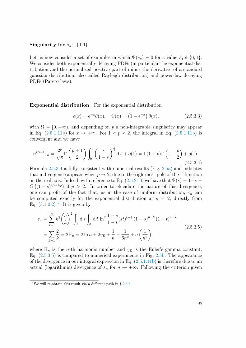
Singularity for s˚ P t0, 1u
Let us now consider a set of examples in which Ψps˚q “ 0 for a value s˚ P t0, 1u.We consider both exponentially decaying PDFs (in particular the exponential dis-tribution and the normalized positive part of minus the derivative of a standardgaussian distribution, also called Rayleigh distribution) and power-law decayingPDFs (Pareto laws).
Exponential distribution For the exponential distribution
ρpxq “ e´xθpxq, Φpxq “`
1´ e´x˘
θpxq, (2.5.3.3)
with Ω “ r0,`8q, and depending on p a non-integrable singularity may appearin Eq. (2.5.1.11b) for x Ñ `8. For 1 ă p ă 2, the integral in Eq. (2.5.1.11b) isconvergent and we have
np2´1εn “
2p?π
Γ
ˆ
p` 1
2
˙ż 1
0
ˆ
s
1´ s
˙p2
d s` op1q “ Γp1` pqΓ´
1´p
2
¯
` op1q.
(2.5.3.4)Formula 2.5.3.4 is fully consistent with numerical results (Fig. 2.5a) and indicatesthat a divergence appears when pÑ 2, due to the rightmost pole of the Γ functionon the real axis. Indeed, with reference to Eq. (2.5.2.1), we have that Ψpsq “ 1´s “O`
p1´ sq12`1p˘
if p ě 2. In order to elucidate the nature of this divergence,one can profit of the fact that, as in the case of uniform distribution, εn canbe computed exactly for the exponential distribution at p “ 2, directly fromEq. (3.1.0.2) ∗. It is given by
εn “nÿ
k“1
k2
ˆ
n
k
˙2 ż 1
0
d s
ż 1
0
d t ln2 1´ s
1´ tpstqk´1
p1´ sqn´k p1´ tqn´k
“
nÿ
k“1
2
k“ 2Hn “ 2 lnn` 2γE `
1
n´
1
6n2` o
ˆ
1
n2
˙
,
(2.5.3.5)
where Hn is the n-th harmonic number and γE is the Euler’s gamma constant.Eq. (2.5.3.5) is compared to numerical experiments in Fig. 2.5b. The appearanceof the divergence in our integral expression in Eq. (2.5.1.11b) is therefore due to anactual (logarithmic) divergence of εn for n Ñ `8. Following the criterion given
∗We will re-obtain this result via a different path in § 2.6.6.
45
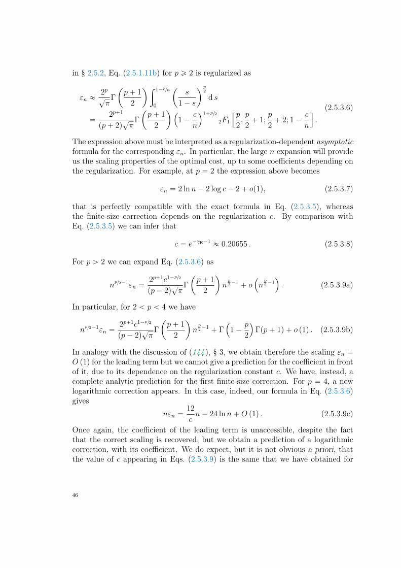
in § 2.5.2, Eq. (2.5.1.11b) for p ě 2 is regularized as
εn «2p?π
Γ
ˆ
p` 1
2
˙ż 1´cn
0
ˆ
s
1´ s
˙p2
d s
“2p`1
pp` 2q?π
Γ
ˆ
p` 1
2
˙
´
1´c
n
¯1`p2
2F1
”p
2,p
2` 1;
p
2` 2; 1´
c
n
ı
.
(2.5.3.6)
The expression above must be interpreted as a regularization-dependent asymptoticformula for the corresponding εn. In particular, the large n expansion will provideus the scaling properties of the optimal cost, up to some coefficients depending onthe regularization. For example, at p “ 2 the expression above becomes
εn “ 2 lnn´ 2 log c´ 2` op1q, (2.5.3.7)
that is perfectly compatible with the exact formula in Eq. (2.5.3.5), whereasthe finite-size correction depends on the regularization c. By comparison withEq. (2.5.3.5) we can infer that
c “ e´γE´1« 0.20655 . (2.5.3.8)
For p ą 2 we can expand Eq. (2.5.3.6) as
np2´1εn “
2p`1c1´p2
pp´ 2q?π
Γ
ˆ
p` 1
2
˙
np2´1` o
´
np2´1¯
. (2.5.3.9a)
In particular, for 2 ă p ă 4 we have
np2´1εn “
2p`1c1´p2
pp´ 2q?π
Γ
ˆ
p` 1
2
˙
np2´1` Γ
´
1´p
2
¯
Γpp` 1q ` o p1q . (2.5.3.9b)
In analogy with the discussion of (144 ), § 3, we obtain therefore the scaling εn “O p1q for the leading term but we cannot give a prediction for the coefficient in frontof it, due to its dependence on the regularization constant c. We have, instead, acomplete analytic prediction for the first finite-size correction. For p “ 4, a newlogarithmic correction appears. In this case, indeed, our formula in Eq. (2.5.3.6)gives
nεn “12
cn´ 24 lnn`O p1q . (2.5.3.9c)
Once again, the coefficient of the leading term is unaccessible, despite the factthat the correct scaling is recovered, but we obtain a prediction of a logarithmiccorrection, with its coefficient. We do expect, but it is not obvious a priori, thatthe value of c appearing in Eqs. (2.5.3.9) is the same that we have obtained for
46
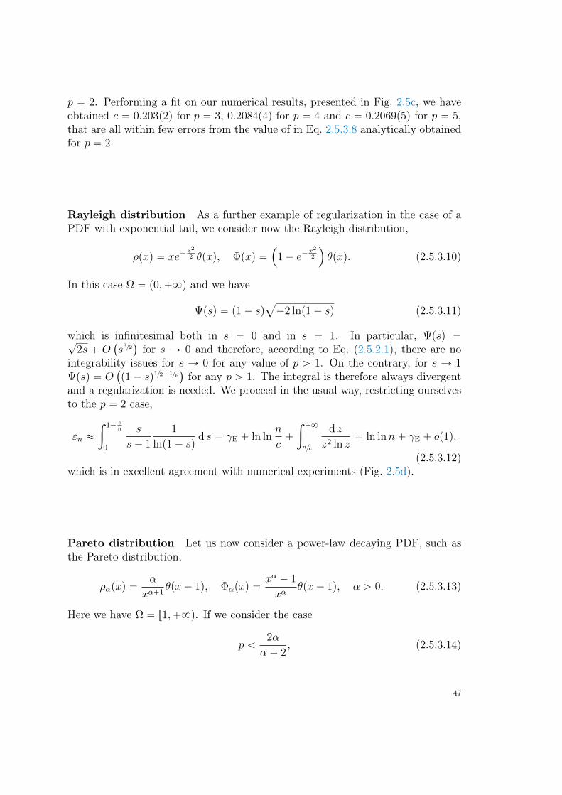
p “ 2. Performing a fit on our numerical results, presented in Fig. 2.5c, we haveobtained c “ 0.203p2q for p “ 3, 0.2084p4q for p “ 4 and c “ 0.2069p5q for p “ 5,that are all within few errors from the value of in Eq. 2.5.3.8 analytically obtainedfor p “ 2.
Rayleigh distribution As a further example of regularization in the case of aPDF with exponential tail, we consider now the Rayleigh distribution,
ρpxq “ xe´x2
2 θpxq, Φpxq “´
1´ e´x2
2
¯
θpxq. (2.5.3.10)
In this case Ω “ p0,`8q and we have
Ψpsq “ p1´ sqa
´2 lnp1´ sq (2.5.3.11)
which is infinitesimal both in s “ 0 and in s “ 1. In particular, Ψpsq “?2s ` O
`
s32˘
for s Ñ 0 and therefore, according to Eq. (2.5.2.1), there are nointegrability issues for s Ñ 0 for any value of p ą 1. On the contrary, for s Ñ 1Ψpsq “ O
`
p1´ sq12`1p˘
for any p ą 1. The integral is therefore always divergentand a regularization is needed. We proceed in the usual way, restricting ourselvesto the p “ 2 case,
εn «
ż 1´ cn
0
s
s´ 1
1
lnp1´ sqd s “ γE ` ln ln
n
c`
ż `8
nc
d z
z2 ln z“ ln lnn` γE ` op1q.
(2.5.3.12)which is in excellent agreement with numerical experiments (Fig. 2.5d).
Pareto distribution Let us now consider a power-law decaying PDF, such asthe Pareto distribution,
ραpxq “α
xα`1θpx´ 1q, Φαpxq “
xα ´ 1
xαθpx´ 1q, α ą 0. (2.5.3.13)
Here we have Ω “ r1,`8q. If we consider the case
p ă2α
α ` 2, (2.5.3.14)
47
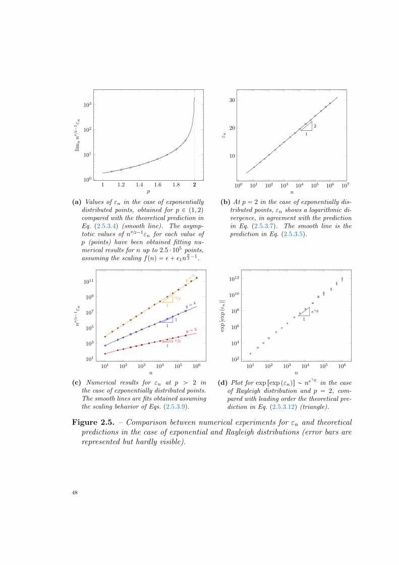
1 1.2 1.4 1.6 1.8 2100
101
102
103
2p
lim
nn
p/2−1ε n
(a) Values of εn in the case of exponentiallydistributed points, obtained for p P p1, 2qcompared with the theoretical prediction inEq. (2.5.3.4) (smooth line). The asymp-totic values of np2´1εn for each value ofp (points) have been obtained fitting nu-merical results for n up to 2.5 ¨ 105 points,assuming the scaling fpnq “ ε` ε1n
p2´1.
100 101 102 103 104 105 106 107
10
20
30
1
2
n
ε n
(b) At p “ 2 in the case of exponentially dis-tributed points, εn shows a logarithmic di-vergence, in agreement with the predictionin Eq. (2.5.3.7). The smooth line is theprediction in Eq. (2.5.3.5).
101 102 103 104 105 106101
103
105
107
109
1011
p = 3
1
1/2
p = 4
1
1
p =5
1
3/2
n
np/2−1ε n
(c) Numerical results for εn at p ą 2 inthe case of exponentially distributed points.The smooth lines are fits obtained assumingthe scaling behavior of Eqs. (2.5.3.9).
101 102 103 104 105 106102
104
106
108
1010
1012
1
eγE
n
exp[exp(ε
n)]
(d) Plot for exp rexp pεnqs „ neγE in the case
of Rayleigh distribution and p “ 2, com-pared with leading order the theoretical pre-diction in Eq. (2.5.3.12) (triangle).
Figure 2.5. – Comparison between numerical experiments for εn and theoreticalpredictions in the case of exponential and Rayleigh distributions (error bars arerepresented but hardly visible).
48
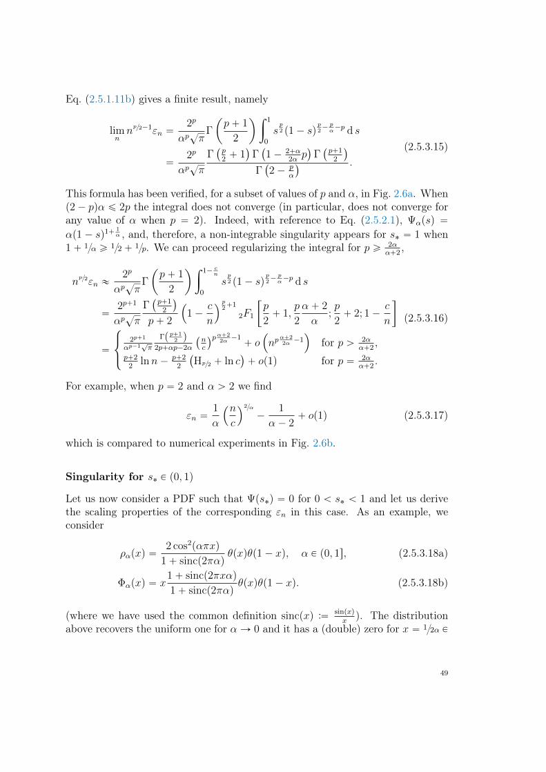
Eq. (2.5.1.11b) gives a finite result, namely
limnnp2´1εn “
2p
αp?π
Γ
ˆ
p` 1
2
˙ż 1
0
sp2 p1´ sq
p2´pα´p d s
“2p
αp?π
Γ`
p2` 1
˘
Γ`
1´ 2`α2αp˘
Γ`
p`12
˘
Γ`
2´ pα
˘ .
(2.5.3.15)
This formula has been verified, for a subset of values of p and α, in Fig. 2.6a. Whenp2´ pqα ď 2p the integral does not converge (in particular, does not converge forany value of α when p “ 2). Indeed, with reference to Eq. (2.5.2.1), Ψαpsq “
αp1´ sq1`1α , and, therefore, a non-integrable singularity appears for s˚ “ 1 when
1` 1α ě 12` 1p. We can proceed regularizing the integral for p ě 2αα`2
,
np2εn «
2p
αp?π
Γ
ˆ
p` 1
2
˙ż 1´ c
n
0
sp2 p1´ sq
p2´pα´p d s
“2p`1
αp?π
Γ`
p`12
˘
p` 2
´
1´c
n
¯
p2`1
2F1
„
p
2` 1,
p
2
α ` 2
α;p
2` 2; 1´
c
n
“
$
&
%
2p`1
αp´1?π
Γp p`12 q
2p`αp´2α
`
nc
˘pα`22α´1` o
´
npα`22α´1¯
for p ą 2αα`2
,p`2
2lnn´ p`2
2
`
Hp2 ` ln c˘
` op1q for p “ 2αα`2
.
(2.5.3.16)
For example, when p “ 2 and α ą 2 we find
εn “1
α
´n
c
¯2α
´1
α ´ 2` op1q (2.5.3.17)
which is compared to numerical experiments in Fig. 2.6b.
Singularity for s˚ P p0, 1q
Let us now consider a PDF such that Ψps˚q “ 0 for 0 ă s˚ ă 1 and let us derivethe scaling properties of the corresponding εn in this case. As an example, weconsider
ραpxq “2 cos2pαπxq
1` sincp2παqθpxqθp1´ xq, α P p0, 1s, (2.5.3.18a)
Φαpxq “ x1` sincp2πxαq
1` sincp2παqθpxqθp1´ xq. (2.5.3.18b)
(where we have used the common definition sincpxq :“ sinpxqx
). The distributionabove recovers the uniform one for αÑ 0 and it has a (double) zero for x “ 12α P
49
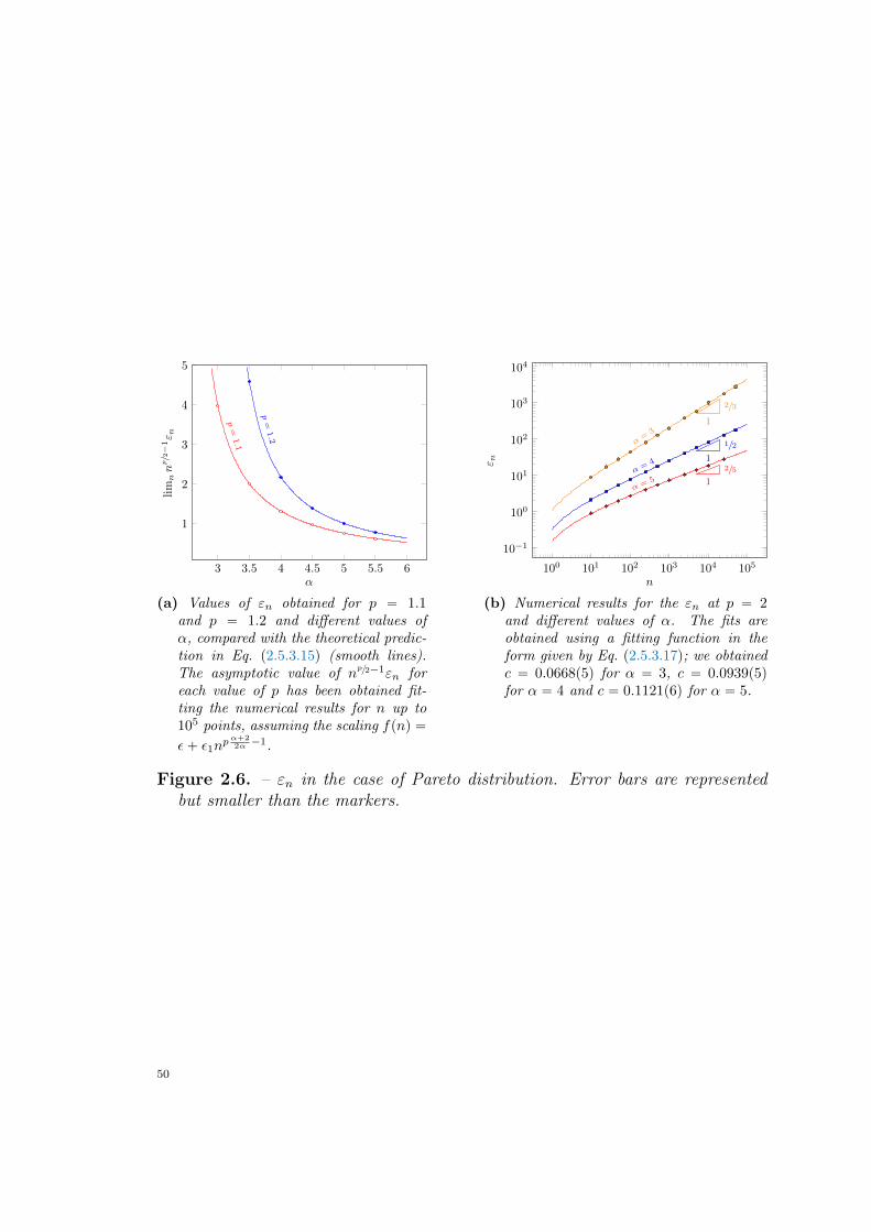
3 3.5 4 4.5 5 5.5 6
1
2
3
4
5
p=
1.1
p=
1.2
α
lim
nn
p/2−1ε n
(a) Values of εn obtained for p “ 1.1and p “ 1.2 and different values ofα, compared with the theoretical predic-tion in Eq. (2.5.3.15) (smooth lines).The asymptotic value of np2´1εn foreach value of p has been obtained fit-ting the numerical results for n up to105 points, assuming the scaling fpnq “ε` ε1n
pα`22α ´1.
100 101 102 103 104 10510−1
100
101
102
103
104
α=
31
2/3
α =4 1
1/2
α = 5 1
2/5
n
ε n
(b) Numerical results for the εn at p “ 2and different values of α. The fits areobtained using a fitting function in theform given by Eq. (2.5.3.17); we obtainedc “ 0.0668p5q for α “ 3, c “ 0.0939p5qfor α “ 4 and c “ 0.1121p6q for α “ 5.
Figure 2.6. – εn in the case of Pareto distribution. Error bars are representedbut smaller than the markers.
50
r12, 1s if α P r12, 1s. The support is therefore Ω “ r0, 1szt12αu. In particular, forα P r12, 1s, we have
Ψαpsq “p6παq23
3a
2` 2 sincp2παqps´ s˚q
23` o
´
ps´ s˚q23¯
,
with s˚ :“1
2α
1
1` sincp2παq. (2.5.3.19)
Therefore, by the general exposition given above, there are three different regimesfor the asymptotic of εn depending on α.For α P p0, 12q the asymptotic of εn is finite for any value of p ą 1. The integral
in Eq. (2.5.1.11b) has been evaluated numerically and the prediction has beencompared with our numerical results in Fig. 2.7a with excellent agreement.When α “ 12 the singularity s˚ moves to 1. We obtain the regularized integral
np2´1εn “
2p?π
Γ
ˆ
p` 1
2
˙ż 1´
c123?n
0
dxΦp2αpxqΦ
p2αpxq
ρp´1α pxq
` op1q
9
$
’
&
’
%
np6´1 for p ą 6,
lnn for p “ 6,constant for 1 ă p ă 6.
(2.5.3.20)
We verified the scaling above in Fig. 2.7c. In the p “ 6 case, in particular, we have
n2εn “160
27π4lnn`Op1q. (2.5.3.21)
For α P p12, 1s, instead, there is a singularity in s˚ P r12, 1q and the regular-ization procedure has to be modified. In this case we have to exclude from theintegration domain a ball centered in s˚ and radius Op1?nq. Observing that
Φ´1α
ˆ
1
2αp1` sincp2απqq˘
c?n
˙
“1
2α˘
1
α3
d
3cp1` sincp2παqq
2π2?n
` o
ˆ
16?n
˙
”1
2α˘
cα6?n` o
ˆ
16?n
˙
,
(2.5.3.22)
and denoting the “regularized” domain by
Ωα :“ r0, 1sz
ˆ
1
2α´
cα6?n,
1
2α`
cα6?n
˙
, (2.5.3.23)
51
we can write the regularized integral as
np2´1εn “
2p?π
Γ
ˆ
p` 1
2
˙ż
Ωα
dxΦp2αpxqΦ
p2αpxq
ρp´1α pxq
` op1q
9
$
’
&
’
%
n2p´3
6 for p ą 32,lnn for p “ 32,constant for 1 ă p ă 32,
(2.5.3.24)
where we limited ourselves to the leading asymptotics. The scaling predicted byEq. (2.5.3.24) has been confirmed by numerical experiments at p “ 2, 3 (Fig. 2.7b).For p “ 32 in particular, we find
n34´1εn “
Γ p14q
6α p1` sincp2παqq
ˆ
1` sincp2παq ´ 12α
2απ2
˙34
lnn`Op1q. (2.5.3.25)
In Fig. 2.7d we show our numerical results for this case, once again in agreementwith the prediction. Remark that the different regularization applied in this caseimplies a completely different scaling of the asymptotic of εn with respect to theone obtained for s˚ “ 1.
Assignment on disjoint intervals: an example
In the examples above, and in the general remarks in § 2.5.2, we have alwaysassumed that the domain Ω is such that Ω is a connected interval, and thereforeΦ is an invertible function on Ω. This is not the case if the domain Ω has a “gap”.In this Section we will study the effects of such a gap on the asymptotic of εn.We will limit ourselves to the case Ω “ A Y B with A, B connected intervalssuch that A X B “ ∅. In the following we will assume that @x P A and @y P B,x ă y. To avoid complications due to the presence of singularities in the integrals,we will also assume that Ω “ Ω. The lack of invertibility of Φ is due in thiscase to the fact that limxÑsupA Φpxq “ limxÑinf B Φpxq “ s, despite the fact thata “ supA ‰ inf B “ b. We expect that our approach proposed in § 2.5 fails inthis situation, because the transport field µk in Eq. (2.5.1.3) is not infinitesimal ingeneral for nÑ `8.In the simple case mentioned here, Ω “ A Y B with A X B “ ∅, the exact
formula in Eq. (3.1.0.2) can be written as
εn “
ż
dµ |µ|p8ÿ
k“1
”
ppAAqk pµq ` p
pBBqk pµq ` p
pABqk pµq ` p
pBAqk pµq
ı
. (2.5.3.26)
52
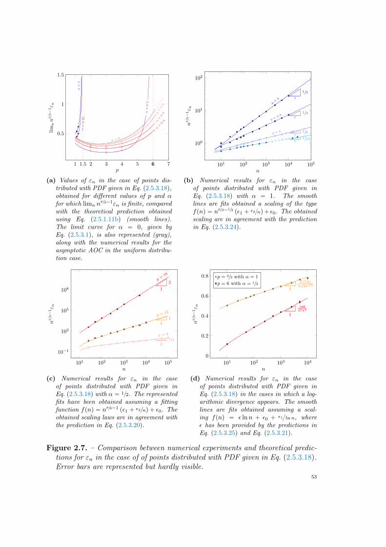
1 2 3 4 5 6 7
0.5
1
1.5
1.5 6
α = 0
α=
0.1
α=
0.2
α=
0.3
α=
0.4
α=
0.5
α=
0.7
5
α=
1
p
lim
nnp/2−1ε n
(a) Values of εn in the case of points dis-tributed with PDF given in Eq. (2.5.3.18),obtained for different values of p and αfor which limn n
p2´1εn is finite, comparedwith the theoretical prediction obtainedusing Eq. (2.5.1.11b) (smooth lines).The limit curve for α “ 0, given byEq. (2.5.3.1), is also represented (gray),along with the numerical results for theasymptotic AOC in the uniform distribu-tion case.
101 102 103 104 105
100
101
102
p = 1.8 11/10
p = 2
1
1/6
p =2.5 1
1/3
p=
3 1
1/2
n
np/2−1ε n
(b) Numerical results for εn in the caseof points distributed with PDF given inEq. (2.5.3.18) with α “ 1. The smoothlines are fits obtained a scaling of the typefpnq “ n
p3´12 pε1 ` ε2nq` ε0. The obtainedscaling are in agreement with the predictionin Eq. (2.5.3.24).
101 102 103 104 105
10−1
102
105
108
p = 8
11/3
p = 12
11
p =18
1
2
n
np/2−1ε n
(c) Numerical results for εn in the caseof points distributed with PDF given inEq. (2.5.3.18) with α “ 12. The representedfits have been obtained assuming a fittingfunction fpnq “ n
p6´1 pε1 ` ε2nq ` ε0. Theobtained scaling laws are in agreement withthe prediction in Eq. (2.5.3.20).
101 102 103 1040
0.2
0.4
0.6
0.8
1
Γ(5/4)
3√
2π3/2
1
16027π4
n
np/2−1ε n
p = 3/2 with α = 1
p = 6 with α = 1/2
(d) Numerical results for εn in the caseof points distributed with PDF given inEq. (2.5.3.18) in the cases in which a log-arithmic divergence appears. The smoothlines are fits obtained assuming a scal-ing fpnq “ ε lnn ` ε0 ` ε1lnn, whereε has been provided by the predictions inEq. (2.5.3.25) and Eq. (2.5.3.21).
Figure 2.7. – Comparison between numerical experiments and theoretical predic-tions for εn in the case of of points distributed with PDF given in Eq. (2.5.3.18).Error bars are represented but hardly visible.
53
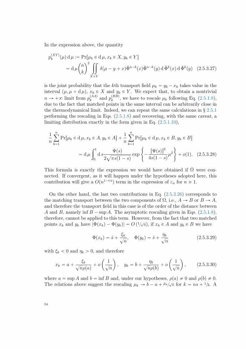
In the expression above, the quantity
ppXY qk pµq dµ :“ Prrµk P dµ, xk P X, yk P Y s
“ dµ
ˆ
n
k
˙2 ij
XˆY
δpµ´ y ` xqΦn´kpxqΦn´k
pyq d Φkpxq d Φk
pyq (2.5.3.27)
is the joint probability that the kth transport field µk “ yk´ xk takes value in theinterval pµ, µ ` dµq, xk P X and yk P Y . We expect that, to obtain a nontrivialnÑ `8 limit from p
pAAqk and ppBBqk , we have to rescale µk following Eq. (2.5.1.8),
due to the fact that matched points in the same interval can be arbitrarily close inthe thermodynamical limit. Indeed, we can repeat the same calculations in § 2.5.1performing the rescaling in Eqs. (2.5.1.8) and recovering, with the same caveat, alimiting distribution exactly in the form given in Eq. (2.5.1.10),
1
n
nÿ
k“1
Prrµk P dµ, xk P A, yk P As `1
n
nÿ
k“1
Prrµk P dµ, xk P B, yk P Bs
“ dµ
ż 1
0
d sΨpsq
2a
πsp1´ sqexp
#
´rΨpsqs2
4sp1´ sqµ2
+
` op1q. (2.5.3.28)
This formula is exactly the expression we would have obtained if Ω were con-nected. If convergent, as it will happen under the hypotheses adopted here, thiscontribution will give a Opn1´p2q term in the expression of εn for n " 1.
On the other hand, the last two contributions in Eq. (2.5.3.26) corresponds tothe matching transport between the two components of Ω, i.e., AÑ B or B Ñ A,and therefore the transport field in this case is of the order of the distance betweenA and B, namely inf B ´ supA. The asymptotic rescaling given in Eqs. (2.5.1.8),therefore, cannot be applied to this term. However, from the fact that two matchedpoints xk and yk have |Φpxkq ´ Φpykq| “ O p1?nq, if xk P A and yk P B we have
Φpxkq “ s`ξk?n, Φpykq “ s`
ηk?n
(2.5.3.29)
with ξk ă 0 and ηk ą 0, and therefore
xk “ a`ξk
?nρpaq
` o
ˆ
1?n
˙
, yk “ b`ηk
?nρpbq
` o
ˆ
1?n
˙
, (2.5.3.30)
where a “ supA and b “ inf B and, under our hypotheses, ρpaq ‰ 0 and ρpbq ‰ 0.The relations above suggest the rescaling µk Ñ b ´ a ` µk
?n for k “ ns ` 12. A
54
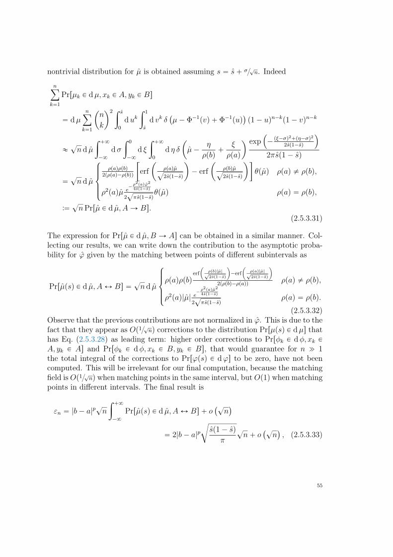
nontrivial distribution for µ is obtained assuming s “ s` σ?n. Indeed
nÿ
k“1
Prrµk P dµ, xk P A, yk P Bs
“ dµnÿ
k“1
ˆ
n
k
˙2 ż s
0
dukż 1
s
d vk δ`
µ´ Φ´1pvq ` Φ´1
puq˘
p1´ uqn´kp1´ vqn´k
«?n d µ
ż `8
´8
dσ
ż 0
´8
d ξ
ż `8
0
d η δ
ˆ
µ´η
ρpbq`
ξ
ρpaq
˙ exp´
´pξ´σq2`pη´σq2
2sp1´sq
¯
2πsp1´ sq
“?n d µ
$
’
’
&
’
’
%
ρpaqρpbq2pρpaq´ρpbqq
„
erf
ˆ
ρpaqµ?2sp1´sq
˙
´ erf
ˆ
ρpbqµ?2sp1´sq
˙
θpµq ρpaq ‰ ρpbq,
ρ2paqµ e´ρ2paqϕ2
4sp1´sq
2?πsp1´sq
θpµq ρpaq “ ρpbq,
:“?nPrrµ P d µ, AÑ Bs.
(2.5.3.31)
The expression for Prrµ P d µ, B Ñ As can be obtained in a similar manner. Col-lecting our results, we can write down the contribution to the asymptotic proba-bility for ϕ given by the matching between points of different subintervals as
Prrµpsq P d µ, AØ Bs “?n d µ
$
’
’
&
’
’
%
ρpaqρpbqerf
ˆ
ρpbq|µ|?2sp1´sq
˙
´erf
ˆ
ρpaq|µ|?2sp1´sq
˙
2pρpbq´ρpaqqρpaq ‰ ρpbq,
ρ2paq|µ| e´ρ2paqµ2
4sp1´sq
2?πsp1´sq
ρpaq “ ρpbq.
(2.5.3.32)Observe that the previous contributions are not normalized in ϕ. This is due to thefact that they appear as Op1?nq corrections to the distribution Prrµpsq P dµs thathas Eq. (2.5.3.28) as leading term: higher order corrections to Prrφk P dφ, xk PA, yk P As and Prrφk P dφ, xk P B, yk P Bs, that would guarantee for n " 1the total integral of the corrections to Prrϕpsq P dϕs to be zero, have not beencomputed. This will be irrelevant for our final computation, because the matchingfield is Op1?nq when matching points in the same interval, but Op1q when matchingpoints in different intervals. The final result is
εn “ |b´ a|p?n
ż `8
´8
Prrµpsq P d µ, AØ Bs ` o`?
n˘
“ 2|b´ a|pc
sp1´ sq
π
?n` o
`?n˘
, (2.5.3.33)
55
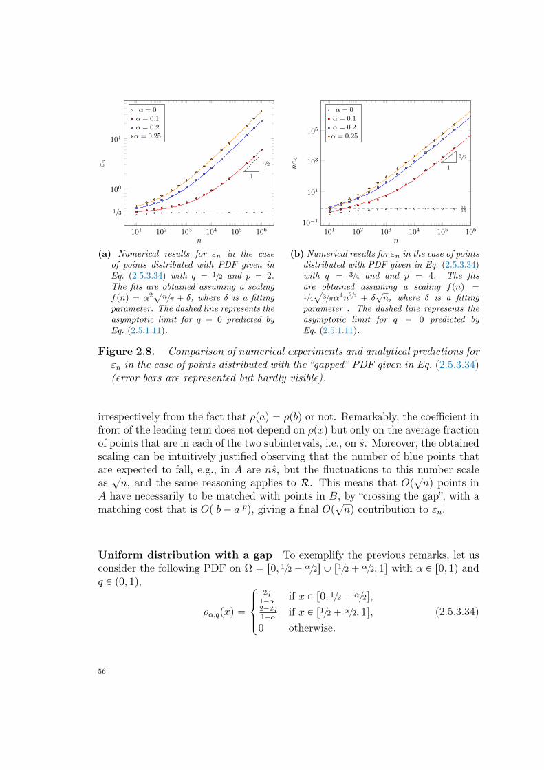
101 102 103 104 105 106
100
101
1/3
1
1/2
n
ε nα = 0
α = 0.1
α = 0.2
α = 0.25
(a) Numerical results for εn in the caseof points distributed with PDF given inEq. (2.5.3.34) with q “ 12 and p “ 2.The fits are obtained assuming a scalingfpnq “ α2
a
nπ ` δ, where δ is a fittingparameter. The dashed line represents theasymptotic limit for q “ 0 predicted byEq. (2.5.1.11).
101 102 103 104 105 10610−1
101
103
105
1115
1
3/2
n
nε n
α = 0
α = 0.1
α = 0.2
α = 0.25
(b) Numerical results for εn in the case of pointsdistributed with PDF given in Eq. (2.5.3.34)with q “ 34 and and p “ 4. The fitsare obtained assuming a scaling fpnq “14
a
3πα4n32 ` δ
?n, where δ is a fitting
parameter . The dashed line represents theasymptotic limit for q “ 0 predicted byEq. (2.5.1.11).
Figure 2.8. – Comparison of numerical experiments and analytical predictions forεn in the case of points distributed with the “gapped” PDF given in Eq. (2.5.3.34)(error bars are represented but hardly visible).
irrespectively from the fact that ρpaq “ ρpbq or not. Remarkably, the coefficient infront of the leading term does not depend on ρpxq but only on the average fractionof points that are in each of the two subintervals, i.e., on s. Moreover, the obtainedscaling can be intuitively justified observing that the number of blue points thatare expected to fall, e.g., in A are ns, but the fluctuations to this number scaleas?n, and the same reasoning applies to R. This means that Op
?nq points in
A have necessarily to be matched with points in B, by “crossing the gap”, with amatching cost that is Op|b´ a|pq, giving a final Op
?nq contribution to εn.
Uniform distribution with a gap To exemplify the previous remarks, let usconsider the following PDF on Ω “ r0, 12´ α2s Y r12` α2, 1s with α P r0, 1q andq P p0, 1q,
ρα,qpxq “
$
’
&
’
%
2q1´α
if x P r0, 12´ α2s,2´2q1´α
if x P r12` α2, 1s,
0 otherwise.(2.5.3.34)
56
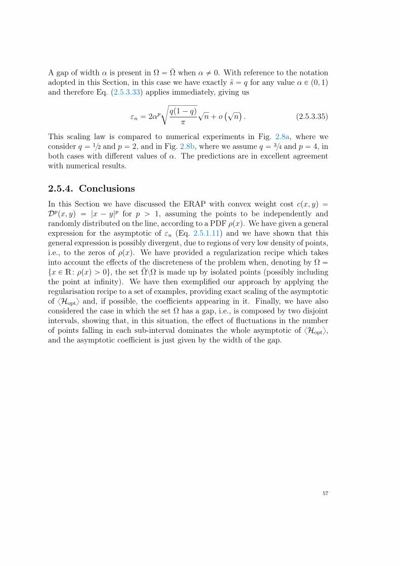
A gap of width α is present in Ω “ Ω when α ‰ 0. With reference to the notationadopted in this Section, in this case we have exactly s “ q for any value α P p0, 1qand therefore Eq. (2.5.3.33) applies immediately, giving us
εn “ 2αpc
qp1´ qq
π
?n` o
`?n˘
. (2.5.3.35)
This scaling law is compared to numerical experiments in Fig. 2.8a, where weconsider q “ 12 and p “ 2, and in Fig. 2.8b, where we assume q “ 34 and p “ 4, inboth cases with different values of α. The predictions are in excellent agreementwith numerical results.
2.5.4. ConclusionsIn this Section we have discussed the ERAP with convex weight cost cpx, yq “Dppx, yq “ |x ´ y|p for p ą 1, assuming the points to be independently andrandomly distributed on the line, according to a PDF ρpxq. We have given a generalexpression for the asymptotic of εn (Eq. 2.5.1.11) and we have shown that thisgeneral expression is possibly divergent, due to regions of very low density of points,i.e., to the zeros of ρpxq. We have provided a regularization recipe which takesinto account the effects of the discreteness of the problem when, denoting by Ω “tx P R : ρpxq ą 0u, the set ΩzΩ is made up by isolated points (possibly includingthe point at infinity). We have then exemplified our approach by applying theregularisation recipe to a set of examples, providing exact scaling of the asymptoticof xHopty and, if possible, the coefficients appearing in it. Finally, we have alsoconsidered the case in which the set Ω has a gap, i.e., is composed by two disjointintervals, showing that, in this situation, the effect of fluctuations in the numberof points falling in each sub-interval dominates the whole asymptotic of xHopty,and the asymptotic coefficient is just given by the width of the gap.
57
2.6. Combinatorial and analytic approach toanomalous scaling: universality classes
The continuum method discussed in § 2.5 allows to deal with the calculationof asymptotic constants if the involved integrals are convergent, and, when
this is not the case, suggested a simple regularisation recipe for understanding thescaling of xHopty in some cases.Although that regularisation recipe could be written in general (such as in the
case of a probability density of points vanishing at the frontier of the support),being non-rigorous, it could predict wrong scalings in some cases (such as in thecase of probability density functions vanishing in the interior of their support).Moreover, in the spirit of universality, one may want to know a priori what
properties of the PDF are relevant for determining deviations from the bulk scalingbehavior of xHopty. The latter task appears to be more difficult to attain throughcontinuum methods, given the broad variety of possible scaling behaviors of xHopty
which we have found for natural choices of PDF already (power law, logarithmicand even log-log scalings).A possibility is to take a step back from continuum methods and study the origin
of anomalous scalings of xHopty “from scratch”, that is, from an analysis of relativecontributions of individual edges (or evaluations of transport field) entering theoptimal assignment at finite n, and look at their relative magnitudes dependingon the choice of PDF. A promising indication in this direction, which has beenalready foreseen in § 2.3, is that unexpectedly deep analogies (and new facts) haveemerged upon studying the problem at finite n and then postponing the n Ñ 8
limit as much as possible (see e.g. Eq. 2.3.1.17). These aspects altogether suggestthat such a program might not be hopeless, and this is precisely the philosophy andcontent of the present Section, an extension of which constitutes the manuscriptin preparation (174 ).
2.6.1. Notations and setting
As above, let us consider B and R sorted in natural order on M “ R (or asubset of), that is we have n blue points x1 ď x2 ď . . . ď xn and n red pointsy1 ď y2 ď . . . ď yn. The points of each color are the sorted list of n i.i.d. randomvariables, sampled according to a probability density ρpxq (which is the same forred and blue). We call Rpxq its cumulant, and R´1puq the inverse cumulant orquantile function. As a result, we can equivalently consider the extraction of ui’sand vj’s, uniform and independent in r0, 1s, and xi “ R´1puiq, yi “ R´1pviq
∗.
∗This fact is very much exploited in low-dimensional statistics, where it is sometimes called “inversetransform sampling” or “inversion method” (43 ).
58
For π a permutation of size n, the cost function Hpx,yqpπq is determined by areal parameter p ą 0, and is
Hppqpx,yqpπq “
nÿ
i“1
|xi ´ yπpiq|p (2.6.1.1)
(the dependence of H from p may be omitted when clear).We call πppqopt one optimal matching of the given instance for the exponent p,
that is, one matching π that minimises the expression above, πid the (unique)identity matching πidpiq “ i (see Lemma 2.1.1), and πDyck the (unique) Dyckmatching† (these two notions are independent of p). We call Hppq
optpx, yq, Hppqid px, yq
and HppqDyckpx, yq the function H
ppq evaluated at π “ πopt, πid and πDyck, respectively.Recall from § 2.5 that πopt “ πid if p ą 1. Here, we will also use the fact thatπopt “ πDyck at p “ 1. Our goal is to evaluate, as precisely as possible (and at leastto the leading asymptotics for n large), the quantity
@
Hppqopt
D
ρ,n, that is averaged
over the possible instances of size n sampled according to ρ, determined by thetriple pρpxq, p, nq.As we have already mentioned, the Poisson-Poisson case has already been ex-
tensively studied. The case of ρpxq uniform on the interval r0, 1s has been studiedin (154 ) for the case p ě 1 real, and in the variant in which p ă 0 (more precisely,in (154 ) results are established for a whole class of cost functions, called there “C-functions”, which include the latter case). Recently (170 ), exploiting a connectionwith Selberg integrals, an exact expression in terms of p and n has been obtainedfor the case of ρpxq uniform on r0, 1s and p ě 1 real, namely
xHoptyn “ nΓp1` p2q
p` 1
Γpn` 1q
Γpn` 1` p2q
“Γp1` p2q
p` 1n1´p2
ˆ
1´ppp` 2q
8n`Opn´3
q
˙
.
(2.6.1.2)
The case p P p0, 1s is the most challenging one, and investigations have beenstarted only recently (173 ) (plus a companion paper in preparation). We reporta summary for the asymptotic behavior of xHopty in Table 2.1.When ρ is a smooth function valued on a compact connected interval, and log ρ
is bounded on the domain, the asymptotics above does not change, that is, thescaling exponent is universal within this class of densities. Furthermore, the edges
†For σ P t0, 1un denoting the interlacing of blue and red points on the real line, we anticipate theconstruct of its Dyck matching πDyck as follows: first, construct a Dyck bridge by replacing the `1and ´1 of σ by up- and down-steps, then, pair, in the unique possible way, up- and down-steps whichare at the same height and such that the segment connecting their mid-points doesn’t cross the walk.See § 2.7 for further details.
59
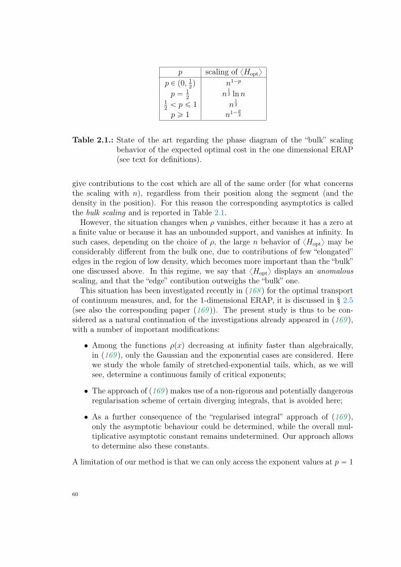
p scaling of xHopty
p P p0, 12q n1´p
p “ 12
n12 lnn
12ă p ď 1 n
12
p ě 1 n1´ p2
Table 2.1.: State of the art regarding the phase diagram of the “bulk” scalingbehavior of the expected optimal cost in the one dimensional ERAP(see text for definitions).
give contributions to the cost which are all of the same order (for what concernsthe scaling with n), regardless from their position along the segment (and thedensity in the position). For this reason the corresponding asymptotics is calledthe bulk scaling and is reported in Table 2.1.However, the situation changes when ρ vanishes, either because it has a zero at
a finite value or because it has an unbounded support, and vanishes at infinity. Insuch cases, depending on the choice of ρ, the large n behavior of xHopty may beconsiderably different from the bulk one, due to contributions of few “elongated”edges in the region of low density, which becomes more important than the “bulk”one discussed above. In this regime, we say that xHopty displays an anomalousscaling, and that the “edge” contibution outweighs the “bulk” one.This situation has been investigated recently in (168 ) for the optimal transport
of continuum measures, and, for the 1-dimensional ERAP, it is discussed in § 2.5(see also the corresponding paper (169 )). The present study is thus to be con-sidered as a natural continuation of the investigations already appeared in (169 ),with a number of important modifications:
• Among the functions ρpxq decreasing at infinity faster than algebraically,in (169 ), only the Gaussian and the exponential cases are considered. Herewe study the whole family of stretched-exponential tails, which, as we willsee, determine a continuous family of critical exponents;
• The approach of (169 ) makes use of a non-rigorous and potentially dangerousregularisation scheme of certain diverging integrals, that is avoided here;
• As a further consequence of the “regularised integral” approach of (169 ),only the asymptotic behaviour could be determined, while the overall mul-tiplicative asymptotic constant remains undetermined. Our approach allowsto determine also these constants.
A limitation of our method is that we can only access the exponent values at p “ 1
60
and p ě 2 even integer, and we can only conjecture that the results extend to realvalues of p in suitable intervals, via the analytic continuation which is naturallysuggested by the formula.
2.6.2. Families of distributions
As we explain at the end of Section 2.6.3, the possible anomalous behaviour ofa general distribution ρpxq can be “decomposed” on the zeroes of this function,and, for each zero, only the local properties of ρ in a neighbourhood of the zerowill determine the leading anomalous behaviour. Because of these facts, once weclassify the possible local behaviours of main interest, we would have identifiedthe possible universality classes of anomalous behaviour in our model, and it willsuffice to study, for each universality class, a single distribution ρ which has onezero in the class. This analysis is performed here.
Distribution with a gap
First of all, the support of ρpxq can be connected or not. If it is not connected, wesay that there is a gap. We start by analysing this simple situation.Without loss of generality, say that the support of ρ is contained in s ´ 8, 0s Y
ra,`8r, with a ą 0, and that the integrals of ρ in these two intervals are q and1´ q, with 0 ă q ă 1. Then, we have N´
r and N´b red and blue points on the left,
and N`r “ n´N´
r and N`b “ n´N´
b on the right. On average, both N´r and N´
b
are » qn. However, these quantities fluctuate, independently, asymptotically in aGaussian way, with variance qp1´ qqn, so that their difference δn :“ N´
r ´N´b is
Gaussian with variance 2qp1´ qqn.While the bulk energy is of the order of Ebulkpnq „ n1´ p
2 , we have a trivial lowerbound to the contribution to the energy coming from the δn ! W edges that jumpacross the gap, which has the form
a
4qp1´ qqπ ap?n. Whenever p ą 1, already
this rough lower bound is leading over the bulk behaviour. When p “ 1, as πid
is still optimal, we know that there is an optimal solution with exactly δn edgesjumping across the gap, so that the energy of an instance is exactly the energyof the same instance in which the points on the right part are translated by ´a,plus a δn. So, calling ρ1 the translated density, we have that the average energy atp “ 1 satisfies the relation
Enpρq “
˜
Enpρ1q ` a
c
4qp1´ qq
π
?n
¸
p1` op1qq . (2.6.2.1)
In this section we do not address the complicated concave case p ă 1 (which weleave to a future work), so that the analysis above completely solves the case of a
61
density with a gap, and from now on we will only consider densities with connectedsupport (more precisely, with a support with connected closure).
Types of zeroes
For a smooth function ρpxq on a connected support sa, br, with a value x0 suchthat ρpx0q “ 0 (or limxÑx0 ρpxq “ 0), there are three possibilities:
Finite endpoint: when the zero x0 is the endpoint a (or b), and it is finite.
Endpoint at infinity: when the zero x0 is the endpoint a (or b), and it is a “ ´8(or b “ `8).
We will consider the following two possible behaviours (let us write fpxq « gpxqwhen lnpfpxqgpxqq lnpfpxqgpxqq Ñ 0)
Stretched-exponential: ρpxq « expp´|x ´ x0|´αq for x Ñ x0, when x0 is finite,
and ρpxq « expp´xαq for x large, when x0 “ `8.
Algebraic: ρpxq « |x´ x0|β´1 for xÑ x0, when x0 is finite, and ρpxq « x´β´1 for
x large, when x0 “ `8.
In principle, in the case of an internal zero, we could have different behaviors onthe two sides, however, for sake of simplicity, we will not investigate this case.In light of the universality of the anomalous behaviour discussed above, and of
the crucial role of the function R´1puq in the analytical treatment of the Lemmasin Section 2.6.3, we will choose one representative function for each of the casesdescribed above (and, in particular, whenever the zero x0 is finite, we will choosex0 “ 0), namely:
Endpoint at infinity, stretched exponential: for α ą 0, we consider the distri-butions ρie,αpxq “ αxα´1 expp´xαq, with support on r0,8r. In this caseRie,αpxq “ expp´xαq and R´1
ie,αpuq “ p´ lnuq1α .
Finite endpoint, algebraic zero: for β ą 0, we consider the distributions ρfa,βpxq “
βxβ´1 with support on r0, 1s. In this case Rfa,βpxq “ xβ, and R´1fa,βpuq “ u
1β .
Endpoint at infinity, algebraic zero: for β ą 0, we consider the distributionsρia,βpxq “ βx´β´1 with support on r1,8r. In this case Ria,βpxq “ x´β,and R´1
ia,βpuq “ u´1β .
Internal, algebraic zero: in this case we just consider the distributions ρsa,βpxq “12ρfa,βp|x|q with support on r´1, 1s. Thus Rsa,βpxq “
12psignpxq |x|β ` 1q, and
R´1sa,βpuq “ signp2u´ 1q |2u´ 1|
1β .
62
For each family of distributions we shall establish a “phase diagram” couplingthe relevant parameter, α for the exponential cases and β for the algebraic cases,to the energy-distance exponent p. In the stretched exponential case parametrizedby α, we will show that the leading scaling is a power of log n and obtain both theexponent and leading coefficients explicitly. In the algebraic cases parametrizedby β, in the phase diagram in the plane pβ, pq there is a region where there is noanomalous behavior (that is, the bulk contribution to the energy is larger than theone coming from the summands in the window around the zero), and in this regionthe energy is just given by the integral which is the continuum limit of Eq. 2.6.4,which has indeed only integrable singularities. Then, the complementary regionconsists of points where the anomalous contribution is leading. In this case wewill also provide an evaluation of the constant in front of the leading anomalousterm (we will derive the critical line for the internal algebraic zero case and onlysketch the computations of aforementioned quantities, leaving the details to appearelsewhere). Then, universality implies that for any distribution we can evaluatethe associated constant, by the appropriate decomposition of bulk part of theintegral, and of windows around the zeroes. Finally, on the boundary between thetwo regions, there is a critical line where the type of zero is marginally-anomalous.It is often the case that, in this situation, the anomalous behaviour is larger of thebulk one just by a logarithmic factor. In these cases we will try to establish boththe leading constant, in front of the logarithmic factor, and the first sub-leadingcorrection.
Families of prob. dens. leading scaling of xHopty
Stretched exponential (sec. 2.6.5)
#
2s2 rlnpnqs2s´1 p “ 2
2ζpp´ 1qspp! rlnpnqsps´1qp p ě 4 even
Finite endpoint, algebraic zero (sec. 2.6.8)
$
’
&
’
%
bβ,pn1´p2 Bulk regime
aβ,pn´pβ Anomalous regime
Qppqn2p2´βq lnn Critical line β “ 2ppp ´ 2q
Internal endpoint, algebraic zero (sec. 2.6.11)
$
’
&
’
%
2Bβ,pn1´p2 Bulk regime
p2Aβ,p `Kβ,pqn12p1´pβq Anomalous regime
Rppqnp2´βqp2p1´βqq lnn Critical line β “ ppp ´ 1q
Table 2.2.: Summary of results for the families of probability distributions consid-ered in this paper (left column), with corresponding leading asymp-totics of xHopty (right column). Here, ζ denotes Riemann’s zeta func-tion, and the functions bβ,p, aβ,p, Qppq, Bβ,p, Aβ,p, Kβ,p, Rppq are givenexplicitly in the corresponding sections.
63
2.6.3. General technical factsIn this section we establish various general lemmas, which apply to the study ofall the distributions listed in the previous section, and in fact to any density ρpxq.Recall that we call ρpxq the probability density (which is the same for red and
blue points), Rpxq its cumulant, and R´1puq the inverse of R.As we have seen, the probability that the k-th point of one given color is in
a given infinitesimal interval, xk P rR´1puq, R´1pu ` duqs, is given by the Betadistribution
Pn,kpuq du :“n!
pk ´ 1q!pn´ kq!uk´1
p1´ uqn´k du . (2.6.3.1)
Correspondingly, averages of a function F pxkq can be performed as
xF pxkqyρ,n “
ż 1
0
duPn,kpuqF pR´1puqq . (2.6.3.2)
Call pz1, . . . , z2nq the sorted list of the union on the xi’s and the yj’s, that is zkis k-th point of the 2n points, irrespectively on the color. The probability thatthis point is in a given neighbourhood zk P rR´1puq, R´1pu ` duqs, is given by asimilar Beta distribution P2n,kpuq du. As a result, averages of a function F pzkq canbe performed as
xF pzkqyρ,n “
ż 1
0
duP2n,kpuqF pR´1puqq . (2.6.3.3)
More generally, averages of a function of t points, F pzk1 , zk2 , . . . , zktq, for 1 ďk1 ă k2 ă . . . ă kt ď 2n, are described by a multi-dimensional Beta distribution,supported on the t-dimensional simplex 0 “ u0 ď u1 ď ¨ ¨ ¨ ď ut ď ut`1 “ 1
P2n,k1,...,ktpu1, . . . , utq du1 ¨ ¨ ¨ dut
:“2n!
pk1 ´ 1q!pk2 ´ k1 ´ 1q! ¨ ¨ ¨ pkt ´ kt´1 ´ 1q!p2n´ ktq!
ˆ uk1´11 pu2 ´ u1q
k2´k1´1¨ ¨ ¨ put ´ ut´1q
kt´kt´1´1p1´ utq
2n´kt du1 ¨ ¨ ¨ dut(2.6.3.4)
and we have
xF pzk1 , . . . , zktqyρ,n “
ż
0ďu1﨨¨ďutď1
du1 ¨ ¨ ¨ dut P2n,k1,...,ktpu1, . . . , utqF pR´1pu1q, . . . , R
´1putqq .
(2.6.3.5)We will use these properties in order to write the summands of our cost function
in terms of suitable averages over the Beta distribution. The first Lemma concernsthe case of p even.
64
Lemma 2.6.1 (Case p ě 2 even). Let R´1ρ puq be the quantile function correspond-
ing to density ρ. Define
Mpρqn,k,` “
@
x`kD
ρ,n“@
R´1ρ puq
`D
Pn,k, ` P N . (2.6.3.6)
Then, for p ě 2 even, we have
A
Hppqopt
E
ρ,n“
nÿ
k“1
pÿ
q“0
ˆ
p
q
˙
p´1qp´qMpρqn,k,qM
pρqn,k,p´q . (2.6.3.7)
Proof. When p ě 1, we know that Hopt “ Hid (see Lemma 2.1.1), and thus we cansimply calculate
A
Hppqpx,yqpπidq
E
ρ,n, a procedure that involves no optimisation. By
definition of πid we just have
Hppqpx,yqpπidq “
nÿ
k“1
|xk ´ yk|p . (2.6.3.8)
By linearity, we can just write
A
Hppqpx,yqpπidq
E
ρ,n“
nÿ
k“1
Eρ,p,npkq (2.6.3.9)
Eρ,p,npkq “
ż 1
0
du dv Pn,kpuqPn,kpvq |R´1ρ puq ´R
´1ρ pvq|
p . (2.6.3.10)
If p is an even integer we can drop the absolute value and write
Eρ,p,npkq “pÿ
q“0
ż 1
0
du dv Pn,kpuqPn,kpvq
ˆ
p
q
˙
p´1qp´qR´1ρ puq
qR´1ρ pvq
p´q
“
pÿ
q“0
ˆ
p
q
˙
p´1qp´q@
R´1ρ puq
qD
Pn,k
@
R´1ρ puq
p´qD
Pn,k.
(2.6.3.11)
The second Lemma concerns the case p “ 1. In this case we have an annoyingabsolute value in the expression (2.6.3.10) for Eρ,p,npkq, and we do not know howto perform the calculation along the same line of Lemma 2.6.1. However, we havean alternate strategy that allows us to access our desired quantity. Instead ofusing the relation Hopt “ Hid, we profit of the degeneracy at p “ 1 and use insteadHopt “ HDyck.Let us consider the ordered list of zi’s (from the right) of the 2n points, and let
65
us define pnpk1, k2q as the probability that the k1-th and k2-th steps of a randomDyck bridge are paired in πDyck (thus, in particular, pnpk1, k2q ‰ 0 only if k2´k1 isodd). Various declinations of the function pnpk1, k2q have been calculated in (173 ).A version that we need here is as follows. Using the shortcut h “ k2´k1´1
2, and Ch
for the Catalan’s number, we have
pnpk1, k2q “Ch`
2nn
˘
„ˆ
2n´ 2h´ 2
n´ h´ 1
˙
`1` p´1qk1`1
2
ˆ
k1 ´ 1k1´1
2
˙ˆ
2n´ k22n´k2
2
˙
.
(2.6.3.12)A related quantity is qnp`q, which is the average number of edges pijq in πDyck suchthat i ď ` ă j, that is
qnp`q “ÿ
iď`ją`
pnpi, jq , (2.6.3.13)
that is, the average of the absolute value of the height of the Dyck bridge in `. Wehave the following:
Proposition 2.6.2. If `n! 1, we have
qnp`q “
„
ÿ
0ďkă `2
2´2k
ˆ
2k
k
˙ˆ
1`Oˆ
`
n
˙˙
(2.6.3.14)
while if `, n´ ` " 1 we have
qnp`q »
c
2
π
c
`p2n´ `q
2n. (2.6.3.15)
Proof. For the case `, n ´ ` " 1, we can apply the Stirling approximation tothe expression for the absolute value of the height of the Dyck bridge in `. Thisgives the Wiener formula for the associated Brownian Bridge, with the appropriatescaling factors. Integrating |x| over the resulting Gaussian distribution gives theclaimed result.
For the case `n! 1, we can apply the Stirling approximation to the binomials
`
2nn
˘
,`
2n´2h´2n´h´1
˘
and`2n´k2
2n´k22
˘
in (2.6.3.12), and approximatea
n`Opk1, k2q factorsby?n. This leads to an analogue of equation (2.6.3.12), valid for generic Dyck
walks instead of Dyck bridges (that is, walks not constrained to have height 0 at2n). Thus, in this regime the distribution of the height of the Dyck bridge in ` iswell-approximated by the analogous distribution for the Dyck walk, which is just
66
the binomial distribution. As a result we have
qnp`q » qp`q :“ÿ
k“0
2´`ˆ
`
k
˙
|2k ´ `| . (2.6.3.16)
Now, these quantities satisfy a simple recursion: calling `1 “ `´ 1,
qp`q “ 2´`ÿ
k
ˆˆ
`´ 1
k ´ 1
˙
`
ˆ
`´ 1
k
˙˙
|2k ´ `|
“ 2´`1´1
ÿ
k1
ˆˆ
`1
k1
˙
|2k1 ´ `1 ` 1| `
ˆ
`1
k1
˙
|2k1 ´ `1 ´ 1|
˙
.
(2.6.3.17)
As for n P Z we have |n` 1| ` |n´ 1| “ 2|n| ` 2δn,0, we get
qp`` 1q “
#
qp`q ` is odd;qp`q ` 2´`
`
``2
˘
` is even. (2.6.3.18)
Lemma 2.6.3 (Case p “ 1). For a probability density ρ, let M pρqn,k,q be defined as
in Lemma 2.6.1. Then at p “ 1
xHoptyρ,1,n “ xHDyckyρ,1,n “
2n´1ÿ
l“1
qnplq´
Mpρq2n,l`1,1 ´M
pρq2n,l,1
¯
. (2.6.3.19)
Proof. Since the cost is a linear function of the positions, we haveA
HppqDyck
E
ρ,n“
ÿ
k1ăk2
pnpk1, k2q xzk2 ´ zk1yρ,n (2.6.3.20)
where zi’s is the ordered list of the 2n points. But zk2 ´ zk1 is a special case of afunction F pzk1 , zk2q, and thus is calculated through the case t “ 2 of the formulas(2.6.3.4) and (2.6.3.5), that is we have, by defining the quantity
Enpk1, k2q :“ xzk2 ´ zk1yρ,n “
ż
0ďuďvď1
du dv P2n,k1,k2pu, vqpR´1ρ puq ´R
´1ρ pvqq
(2.6.3.21)that
A
Hp1qDyck
E
ρ,n“
ÿ
k1ăk2
pnpk1, k2qEnpk1, k2q . (2.6.3.22)
So we need to evaluate the RHS of equation (2.6.3.21). A useful general fact is that
67
the expression for this specific function F pzk1 , zk2q seperates in the two variables,so that in fact we just have
Enpk1, k2q “
ż
0ďuď1
duP2n,k1puqR´1ρ puq ´
ż
0ďvď1
dv P2n,k2pvqR´1ρ pvq
“Mpρq2n,k1,1
´Mpρq2n,k2,1
.
(2.6.3.23)
The claimed expression then follows by telescoping.
Now we state a Proposition concerning the bulk behaviour at p ě 1 which hasbeen implicitly used in (169 ) (see also (154 ), appendix B). A corollary of this factis that, if ρ vanishes in more than one point, the anomalous contributions comingfrom the various zeroes can be treated separately.
Proposition 2.6.4. Let ρ, R and R´1 be as above. For every u such that ρpxqis continuous and strictly-positive in a neighbourhood of x “ R´1puq, the limitlimn,kÑ8
knÑu
np2Eρ,p,npkq exists, is finite, and is given by
limn,kÑ8knÑu
np2Eρ,p,npkq “
Γ`
p`12
˘
?π
˜
2a
up1´ uq
ρpR´1puqq
¸p
. (2.6.3.24)
We only give a sketch of proof of this fact. Let us call uk “ Rpxkq and vk “ Rpykq,and let us inspect the expression (2.6.3.10). By the conditions on ρ, we can use theCLT to infer that the quantities uk´u and vk´u are asymptotically independentcentered Gaussian random variables with variance kpn´kq
n3 (and the error terms canbe easily handled at this point). Similarly, calling x “ R´1puq, also xk ´ x andyk ´ x are asymptotically independent centered Gaussian random variables, nowwith variance 1
ρpxq2kpn´kqn3 (at this point the error terms are more subtle, and involve
the Taylor series of the logarithm of ρ around x). As a result, their difference is acentered Gaussian random variable with variance 2
ρpxq2kpn´kqn3 . As we have
ż 8
´8
dx|x|p?
2πσe´
x2
2σ2 “p?
2σqp?π
Γ`
p`12
˘
(2.6.3.25)
we deduce that
limn,kÑ8knÑu
np2Eρ,p,npkq “ lim
n,kÑ8knÑu
np2
´
4ρpxq2
kpn´kqn3
¯
p2
?π
Γ`
p`12
˘
“Γ`
p`12
˘
?π
˜
2a
up1´ uq
ρpR´1puqq
¸p
,
(2.6.3.26)
68
as was to be proven.
Now, suppose to work at n large but finite, and suppose that ρ vanishes in afinite list of points tx1, . . . , xmu (which may include ˘8). The images tu1, . . . , umuunder R are thus a list of values on r0, 1s. Fix some “window” value W „ nγ, with12ă γ ă 1. We can use Proposition 2.6.4 on all k such that minjp|k ´ nuj|q ą W ,
and perform a more careful analysis on the remaining values of k. Such a valueof the window is chosen in order to have, asymptotically, two crucial properties.On one side, it is large enough that the proposition above can be applied because,up to exponentially-rare events, the approximation of ρpx1q in a neighbourhoodof x “ R´1pknq by the value at x, and the use of CLT, are legitimate. On theother side, it is small enough that, for n large enough, the set of k’s which needa more careful analysis is split into m intervals, one per zero xj of the density, sothat the zeroes of ρ can be treated separately. Also, the window is small enoughthat the contribution of each of these intervals of values of k to the total energydepends on the shape of ρ only through the value of uj, and through the leadinglocal behaviour of ρpxq in a neighbourhood of x “ xj.
Once we classify the possible local behaviours of main interest, we would haveidentified the possible universality classes of anomalous behaviour in this model.This justifies the restriction of the analysis to the families of distributions describedin Section 2.6.2.
2.6.4. Ensembles in which the average cost is infinite
When the support of the distribution ρ is not compact, it may be the case thatxHoptyn “ 8 also when n ă 8. We want to identify this situation, in order toexclude a priori the corresponding region from the study of the phase diagram.
Say that the support is contained within the interval r0,`8r, and label thepoints tz1, . . . , z2nu from right to left. Assume, w.l.o.g., that z1 is blue (the othercase is treated identically). Then, there is a probability qnpkq “
`
2n´k´2n´1
˘
`
2n´1n
˘
that the right-most red point is zk`2. As z1 must be connected to some point ofopposite color, and zk`2 is the nearest one, we have
Hopt ě pz1 ´ zk`2qp (2.6.4.1)
69
that is, using (2.6.3.5),
xHoptyn ě xpz1 ´ zk`2qpyρ,n “
n´1ÿ
k“0
qnpkq
ż
0ďuďvď1
dudv P2n,1,k`2pu, vqpR´1puq ´R´1
pvqqp
“
n´1ÿ
k“0
`
2n´k´2n´1
˘
`
2n´1n
˘
ż
0ďuďvď1
dudv2n! pv ´ uqkp1´ vq2n´k´2
k!p2n´ k ´ 2q!pR´1
puq ´R´1pvqqp
“ 2n2n´1ÿ
k“0
ˆ
n´ 1
k
˙ż
0ďuďvď1
dudv pv ´ uqkp1´ vq2n´k´2pR´1
puq ´R´1pvqqp
“ 2n2
ż
0ďuďvď1
dudv pp1´ uqp1´ vqqn´1pR´1
puq ´R´1pvqqp .
(2.6.4.2)
This is the general expression for our trivial lower bound to the optimal cost, whichwe shall check for finiteness.As v ě u, a slightly simpler bound is given by
xpz1 ´ zk`2qpyρ,n ě Xn,p :“ 2n2
ż
0ďuďvď1
dudv p1´vq2n´2pR´1
puq´R´1pvqqp . (2.6.4.3)
In general, when the support is on the positive real axis,∗ we haveR´1puq ą R´1pvq,and we can perform an expansion, to get, for the quantity in Eq. 2.6.4.3,
Xn,p
2n2“
ÿ
`ě0
p´1q`ˆ
p
`
˙ż
0ďuďvď1
dudv p1´ vq2n´2R´1puqp´`R´1
pvq` . (2.6.4.4)
In the specific case of our endpoint at infinity, algebraic zero family of distributionsρia,β (see § 2.6.2) we have
Xn,p
2n2“
ÿ
`ě0
p´1q`ˆ
p
`
˙ż
0ďuďvď1
dudv p1´ vq2n´2u´p´`β v´
`β . (2.6.4.5)
When pβ ă 1 we can use the general integralż
0ďuďvď1
dudv p1´vq2n´2uavb “1
a` 1
ż 1
0
dv p1´vq2n´2va`b`1“
p2n´ 2q!Γpa` b` 2q
pa` 1qΓp2n` a` b` 1q(2.6.4.6)
∗When this is not the case, because the support is r´a,`8r, we can just translate the distributionby a. When the support is the whole real axis, we can still perform the analysis, by “folding” thesupport, using the fact Hoptpx1, . . . , xn; y1, . . . , ynq ě Hoptp|x1|, . . . , |xn|; |y1|, . . . , |yn|q.
70
which gives
Xn,p
2n2“
ÿ
`ě0
p´1q`ˆ
p
`
˙
p2n´ 2q!Γp2´ pβq
p1´ p´`βqΓp2n` 1´ p
βq
“p2n´ 2q!Γp1´ p
βq
Γp2n` 1´ pβq
Γp1` β ´ pqΓp1` pq
Γp1` βq
(2.6.4.7)
that is, for large n, whenever p ă β,
Xn,p » npβ
Γp1´ pβqΓp1` β ´ pqΓp1` pq
21´ pβΓp1` βq
(2.6.4.8)
Conversely, when p ě β this expression diverges, as is also evinced from theanalytic continuation of the result, which has a factor Γp1 ´ p
βq which is singular
in the limit pÕ β.As a result, we evince that, for our family of distributions with endpoint at
infinite, algebraic zero, we just have xHoptyn “ 8 whenever p ě β. Also, we havea first glance to an “anomalous behaviour”: recalling that the bulk energy scales asn1´p2 (see Table 2.1), we see that the leading behaviour in n of xpz1 ´ zk`2q
pyρ,ntakes over the bulk behaviour at least in the region fpβq ă p ă β, for
fpβq “
$
’
&
’
%
ββ`1
β ď 1β2
1 ď β ď 2β
β2`12 ď β .
(2.6.4.9)
2.6.5. Family of stretched exponentials with endpoint atinfinity ρie,α and ρ`ie,α
Let us consider the 1-parameter family of stretched exponential distributions de-pending on a parameter α ą 0
ρie,αpxq dx “ αxα´1 expp´xαqθpxq dx (2.6.5.1)
that is Rαpxq “ expp´xαqθpxq and hence
R´1α puq “ p´ lnuq
1α . (2.6.5.2)
We will use the shortcut s “ 1α. We will call
Eps,pqn :“ xHoptyρie,α,p,n(2.6.5.3)
71
and our goal is to study the function Eps,pqn . A second family of measures also
depending on a parameter α ą 0 is
ρ`ie,αpxq dx “ αxα´1 expp1´ xαqθpx´ 1q dx (2.6.5.4)
for which Rαpxq “ expp1´ xαqθpx´ 1q and hence
R´1α`puq “ p1´ lnuq
1α “ p1´ lnuqs . (2.6.5.5)
We will correspondingly call
Eps`,pq
n :“ xHoptyρ`ie,α,p,n(2.6.5.6)
and we also aim to study the function Eps`,pq
n .As we will see, this second family of distributions will make the calculations more
cumbersome. However, it has the advantage that ρ`ie,αpxq, contrarily to ρie,αpxq ingeneral, is neither vanishing nor diverging at the left endpoint of the support, sothat we know for sure than any anomalous scaling of the cost (w.r.t. the case ofuniform distribution) must come from the tail located at `8, and not from thesecond singularity in 0 (or from a combination of the two effects). As we will see aposteriori, the singularity in zero gives a less relevant anomalous scaling than thesingularity at infinity, as Eps,pqn and Eps
`,pqn do have the same leading asymptotics.
Exact and asymptotic results at p ą 1 even
Let us consider the family of distributions (2.6.5.1) first. From Lemma 2.6.1, wejust need to compute for q, k, n P N the integral
Mn,k;q :“
ż 1
0
duPn,kpuqp´ lnuqq. (2.6.5.7)
Of course Mk,n;0 “ 1, since the Pn,k distributions (eq. (2.6.3.1)) are normalized.From this point onward, we will assume the basic notions of the theory of Sym-
metric Functions (see for example (76 ), chapter one). Let us introduce the alphabet
Ak,n :“
"
1
k,
1
k ` 1, . . . ,
1
n
*
(2.6.5.8)
and let us use the symbol hkpXq for the complete homogeneous symmetric func-tion of degree k, in the alphabet X, (and, for future convenience, ekpXq for theelementary symmetric functions), that is, in the case of a finite alphabet of size m
72
X “ tx1, . . . , xmu, the functions
hk px1, . . . , xmq “ÿ
1ďj1ď...ďjkďm
xj1xj2 ¨ ¨ ¨ xjk , (2.6.5.9)
ek px1, . . . , xmq “ÿ
1ďj1ă...ăjkďm
xj1xj2 ¨ ¨ ¨ xjk . (2.6.5.10)
We also set the useful convention h0pXq “ e0pXq “ 1. We have
Lemma 2.6.5.Mn,k;q “ q!hqpAk,nq . (2.6.5.11)
In order to establish Lemma 2.6.5 we will need a useful (simple) technical Lemma:
Lemma 2.6.6. Let p P N. Let Apqq “ apqp ` ap´1q
p´1 ` . . .` a0 be a polynomialof degree at most p. Then we have
pÿ
q“0
ˆ
p
q
˙
p´1qp´qApqq “ p! ap . (2.6.5.12)
Proof of Lemma 2.6.6. Rewrite Apqq as
Apqq “pÿ
k“0
bkqpq ´ 1q ¨ ¨ ¨ pq ´ k ` 1q . (2.6.5.13)
In particular, bp “ ap. In this basis we have
pÿ
q“0
ˆ
p
q
˙
p´1qp´qApqq “pÿ
k“0
bk
pÿ
q“0
ˆ
p
q
˙
p´1qp´qqpq ´ 1q ¨ ¨ ¨ pq ´ k ` 1q
“
pÿ
k“0
bk
pÿ
q“k
p!
q!pp´ qq!p´1qp´qqpq ´ 1q ¨ ¨ ¨ pq ´ k ` 1q
“
pÿ
k“0
bk p!
pp´ kq!
p´kÿ
r“0
pp´ kq!
r!pp´ k ´ rq!p´1qpp´kq´r “
pÿ
k“0
bk p!
pp´ kq!δp,k “ p! bp
(2.6.5.14)
This completes the proof.
Proof of Lemma 2.6.5. Using the fact ´ ln t “ limuÑ0t´u´1u
, we can write Mn,k;p “
limuÑ0Mn,k;ppuq, where the expression
Mn,k;ppuq :“
ż 1
0
dt tk´1p1´ tqn´k
ˆ
t´u ´ 1
u
˙pΓpn` 1q
ΓpkqΓpn´ k ` 1q(2.6.5.15)
73
is well-defined for u ă p´1, and in particular in a neighborhood of u “ 0. Ex-panding the binomial pt´u ´ 1qp, we recognise that each term in the sum can beevaluated in terms of a Beta integral, and we just get
Mn,k;ppuq “ u´pxpt´u ´ 1qpyPn,k
“ u´ppÿ
q“0
ˆ
p
q
˙
p´1qp´qxt´quyPn,k
“ u´ppÿ
q“0
ˆ
p
q
˙
p´1qp´qΓpn` 1qΓpk ´ quq
ΓpkqΓpn` 1´ quq
“ u´ppÿ
q“0
ˆ
p
q
˙
p´1qp´qnź
h“k
´
1´qu
h
¯´1
“ u´ppÿ
q“0
ˆ
p
q
˙
p´1qp´qÿ
`ě0
q`u`h`pAk,nq .
(2.6.5.16)
At this point, Lemma 2.6.6 allows to compute the limit uÑ 0 straightforwardly:
Mn,k;p “ limuÑ0
u´ppÿ
q“0
ˆ
p
q
˙
p´1qp´qÿ
`ě0
q`u`h`pAk,nq
“ limuÑ0
u´p`
p! uphppAk,nq `Opup`1q˘
“ p! hppAk,nq .
(2.6.5.17)
Since M pie,sqn,k,l “Mn,k;sl, Lemma 2.6.5 implies
Eps,pq,npkq “pÿ
q“0
ˆ
p
q
˙
p´1qp´qMn,k;sqMn,k;spp´qq
“
pÿ
q“0
p´1qqˆ
p
q
˙
psqq!pspp´ qqq! hsqpAk,nqhspp´qqpAk,nq .
(2.6.5.18)
As of our second family of distributions (2.6.5.4), M pie,α`qn,k,q :“ xp1´ lnuqsqyPn,k can
still be written in terms of the Mn,k,h’s, namely
Mpie,α`qn,k,q “
sqÿ
r“0
ˆ
sq
r
˙
Mn,k;r (2.6.5.19)
74
so that by Lemma 2.6.1 we have
Eps`,pq,npkq “ÿ
0ďqďp0ďrďsq
0ďr1ďspp´qq
ˆ
p
q
˙ˆ
sq
r
˙ˆ
spp´ qq
r1
˙
p´1qp´qMn,k,rMn,k,r1
“ÿ
0ďqďp0ďrďsq
0ďr1ďspp´qq
ˆ
p
q
˙ˆ
sq
r
˙ˆ
spp´ qq
r1
˙
p´1qp´qr!r1! hrpAk,nqhr1pAk,nq
(2.6.5.20)
where in the last step Lemma 2.6.5 has again been used.In the case s “ 1, corresponding to an exponential decay at `8, an important
simplification occurs and we have an exact result. Call Hpt,Xq “ř
`ě0 h`pXqt` “
ś
xPXp1´ txq´1 and Ept,Xq “
ř
`ě0 e`pXqt` “
ś
xPXp1` txq. Then
Ep1,pq,npkq “ p!pÿ
q“0
p´1qqhqpAk,nqhp´qpAk,nq
“ p!rtpsHpt, Ak,nqHp´t, Ak,nq .
(2.6.5.21)
For X “ tx1, x2, . . .u, call X2 the alphabet X2 “ tx21, x
22, . . .u. We obviously have
Hpt,XqHp´t,Xq “ Hpt2, X2q, and we recognise
Ep1,pq,npkq “ p!rtpsHpt2, A2k,nq “ p!hp2pA
2k,nq (2.6.5.22)
(recall that we assumed that p is even). Also, Ep1`,pq,npkq “ Ep1,pq,npkq, as in factρ`ie,αpxq “ ρie,αpx´ 1q at α “ 1, and of course the cost function is invariant undera global translation of the 2n points.For general s we only have an asymptotic result. Call as customary pkpXq
the power-sum functions pkpXq “ř
xPX xk. Define P pt,Xq “
ř
kě1 k´1pkpXqt
k ∗.Then we have Hpt,Xq “ exppP pt,Xqq and Ept,Xq “ expp´P p´t,Xqq. The firstof these two formulas provides polynomial expressions in the pj’s for the hi’s. If allthe elements of the alphabet X are real-positive, the generalised-mean inequalitiesimply that ppjpXqq1j form a decreasing monotonic sequence.
In a situation in which p1 "?p2, we can study a perturbative expansion of the
expressions for Eps,pq,npkq and Eps`,pq,npkq w.r.t. this parameter. Call P`pt,Xq “
∗Note that, contrarily to Hpt,Xq, and its companion Ept,Xq for elementary symmetric functions, inwhich there exists a single natural definition, in literature there exist different choices of definitionfor a generating function P pt,Xq, and we have chosen the one that is more convenient in our context,so our formulas involving P may differ from the ones the reader is accustomed to.
75
P pt,Xq ´ tp1pXq. Then we have
hkpXq “ rtksHpt,Xq “ rtks exppP pt,Xqq “
kÿ
`“0
1
pk ´ `q!p1pXq
k´`rt`s exppP`pt,Xqq .
(2.6.5.23)Let us start the analysis with the case of the family in eq. (2.6.5.1). Substitutingeq. (2.6.5.23) in (2.6.5.18), gives
Eps,pq,npkq “pÿ
q“0
p´1qqˆ
p
q
˙
psqq!pspp´ qqq!ÿ
`,`1
p1pAk,nqsp´`´`1
psq ´ `q!pspp´ qq ´ `1q!
ˆ`
rt`s exppP`pt, Ak,nqq˘`
rt`1
s exppP`pt, Ak,nqq˘
.
(2.6.5.24)
The smaller ` and `1 are, the larger is the power of p1, which, under our assumption,is the leading factor. However, the associated factor psqq!pspp´qqq!
psq´`q!pspp´qq´`1q!is a polynomial
in q of degree ` ` `1, so that by Lemma 2.6.6 we know that all the contributionswith ```1 ă p vanish exactly. The leading contribution thus comes from the termswith `` `1 “ p, which give
Eps,pq,npkq »pÿ
q“0
p´1qqˆ
p
q
˙
psqq!pspp´ qqq!ÿ
`
p1pAk,nqps´1qp
psq ´ `q!pspp´ qq ´ pp´ `qq!
ˆ`
rt`s exppP`pt, Ak,nqq˘`
rtp´`s exppP`pt, Ak,nqq˘
“ p! spp1pAk,nqps´1qp
ˆ
pÿ
`“0
p´1q´``
rt`s exppP`pt, Ak,nqq˘`
rtp´`s exppP`pt, Ak,nqq˘
“ p! spp1pAk,nqps´1qp
rtps`
exppP`pt, Ak,nqq exppP`p´t, Ak,nqq˘
(2.6.5.25)
Now observe that
exppP`pt,Xqq exppP`p´t,Xqq “ exppP`pt,Xq ` P`p´t,Xqq
“ exppP pt,Xq ` P p´t,Xqq “ Hpt2, X2q
(2.6.5.26)
so that, in conclusion,
Eps,pq,npkq » p! spp1pAk,nqps´1qp hp2pA
2k,nq . (2.6.5.27)
Note that this approximated formula for generic s matches the exact formula ats “ 1, equation (2.6.5.22).
76
The validity of the approximation above relies on the fact that p1pAk,nq „ lnpnq´lnpkq `Op1q whenever n " k, while phpAk,nq „ 1
h´1pk1´h ´ n1´hq if n " k " 1, so
that, in any case, whenever n " k we have that p1?p2 is at least of order lnpnq.
Within the same precision of approximation, we can thus replace p1pAk,nq withlnpnq in (2.6.5.27), and get
Eps,pq,npkq “ p! sp lnpnqps´1qp hp2pA2k,nq
`
1`Opp1` ln kq lnnq˘
. (2.6.5.28)
This implies the possibly surprising fact that the ratio of the average weights ofthe k1-th and k2-th edges of the matching, whenever n " k1, k2, depends only onp, and not on α “ 1s.Now we perform the analysis with the more complicated expression (2.6.5.20).
We have
Eps`,pq,npkq “ÿ
0ďqďp0ďrďsq
0ďr1ďspp´qq
ˆ
p
q
˙ˆ
sq
r
˙ˆ
spp´ qq
r1
˙
p´1qp´qr!r1! hrpAk,nqhr1pAk,nq
“ÿ
0ďqďp0ďrďsq
0ďr1ďspp´qq0ď`ďr
0ď`1ďr1
ˆ
p
q
˙ˆ
sq
r
˙ˆ
spp´ qq
r1
˙
p´1q´qr!r1!
ˆp1pAk,nq
r`r1´`´`1
pr ´ `q!pr1 ´ `1q!
`
rt`s exppP`pt, Ak,nqq˘`
rt`1
s exppP`pt, Ak,nqq˘
.
(2.6.5.29)
Consider the sum over r. Isolating only the relevant factors gives
ÿ
0ďrďsq
ˆ
sq
r
˙
r!p1pAk,nq
r´`
pr ´ `q!“
psqq!
psq ´ `q!
ÿ
`ďrďsq
ˆ
sq ´ `
r ´ `
˙
p1pAk,nqr´`
“psqq!
psq ´ `q!pp1pAk,nq ` 1qsq´`
(2.6.5.30)
This gives that Eps`,pq,npkq has exactly the same expression (2.6.5.24) for Eps,pq,npkq,with p1pAk,nq replaced by p1pAk,nq ` 1. As a result, we can obtain directly theanalogue of (2.6.5.27)
Eps`,pq,npkq » p! sppp1pAk,nq ` 1qps´1qp hp2pA2k,nq . (2.6.5.31)
Note again that this approximated formula for generic s matches the exact for-mula (2.6.5.22) for s “ 1.
77
As in the previous case, within the same precision of approximation, we mayreplace p1pAk,nq ` 1 with lnpnq and get
Eps`,pq,npkq “ p! sp lnpnqps´1qp hp2pA2k,nq
`
1`Opp1` ln kq lnnq˘
“ Eps,pq,npkq`
1`Opp1` ln kq lnnq˘ (2.6.5.32)
as announced.
2.6.6. Estimation of complete homogeneous functionsEquations (2.6.5.28) and (2.6.5.32) provide explicit expressions for Eps,pq,npkq andEps`,pq,npkq, and thus for the desired quantity E
ps,pqn “
řnk“1Eps,pq,npkq (and its
s` analogue). Nonetheless, we are left with the task of estimating the relevantquantity
Fn,q :“nÿ
k“1
hqpA2k,nq . (2.6.6.1)
We do this in the present section. Each monomial entering the sum has the form
1
i21i22 ¨ ¨ ¨ i
2q
(2.6.6.2)
for some q-tuple 1 ď i1 ď i2 ď ¨ ¨ ¨ ď iq ď n. Such a monomial enters exactly i1times in the sum. Thus we can write
Fn,q “ÿ
1ďi1ďi2﨨¨ďiqďn
1
i1 i22 ¨ ¨ ¨ i2q
“
nÿ
k“1
1
khq´1pA
2k,nq . (2.6.6.3)
When q “ 1 this simply givesFn,1 “ Hn (2.6.6.4)
where Hn is the n-th Harmonic number, and in particular, from the well-knownperturbative expansion for Hn,
Fn,1 “ lnpnq ` γ `1
2n`Op1n2
q . (2.6.6.5)
When q ě 2, as for a real-positive alphabet we have 1q!h1pXq
q ď hqpXq ď h1pXqq,
we have in particular that hq´1pA2k,Nq „ k´pq´1q for n " k, and the whole sum is
convergent in the limit nÑ 8.In this limit, we can identify the exact result (2.6.6.3) with a special case of the
so-called “symmetric sums”, or “multiple ζ˚ values” (56 ) which are modificationsof multiple ζ values that generalise classical special values of the Riemann’s ζ
78
function (61 ). Multiple ζ values are not new in physics, as they naturally arise,for example, in the calculation of scattering amplitudes in perturbative quantumfield theory (67 ).
We have, for q ě 2,F`8,q “ ζ˚p2q´1, 1q . (2.6.6.6)
It is a well-known fact that ζ˚p2, 1q “ ζp2, 1q ` ζp3q (by simple inspection), andthat ζp2, 1q “ ζp3q (by a famous identity of Euler, see e.g. (74 ) for a derivation).This gives
F`8,2 “ 2ζp3q . (2.6.6.7)
More generally we have ζ˚p2q´1, 1q “ 2ζp2q ´ 1q (this result can be found as (3a)in (119 ), or also as (1.8) in (132 ) or in (111 ), example (b) with m “ 1), so thatfor generic q ě 2 we have the result
F`8,q “ 2ζp2q ´ 1q . (2.6.6.8)
Combining (2.6.6.8) with (2.6.5.28) and (2.6.5.32) finally gives, for s and p2 pos-itive integers,
Eps,pqn » Eps`,pq
n »
"
2s2 lnpnq2s´1 p “ 22ζpp´ 1qspp! lnpnqps´1qp p ě 4
. (2.6.6.9)
Notice that at s “ 1 eq. (2.6.6.9) is the leading order asymptotics of the known,exact result for the exponential distribution (see (169 ), eq. 23), namely
Ep1,2qn “
nÿ
k“1
1
k. (2.6.6.10)
Hence, for a generic distribution composed both of a bulk part with a stretchedexponential tail, an anomalous scaling of the optimal cost is always observed atp ě 2.
Case of s integer and p “ 1
Using our general Theorem 2.6.3, for the first family of distributions we just have
En,spk1, k2q “ xp´ lnuqsyP2n,k1´ xp´ lnuqsyP2n,k2
“M2n,k1,s ´M2n,k2,s
(2.6.6.11)
79
In the case of the second family we have
En,s`pk1, k2q “ xp1´ lnuqsyP2n,k1´ xp1´ lnuqsyP2n,k2
“
sÿ
r“0
ˆ
s
r
˙
`
M2n,k1,r ´M2n,k2,r
˘
.(2.6.6.12)
Yet again the s “ 1 (that is, of exponential tail) case is specially simple∗, and wejust obtain the exact formula
En,1pk1, k2q “ En,1`pk1, k2q “ h1pAk1,2nq ´ h1pAk2,2nq “
k2´1ÿ
`“k1
1
`. (2.6.6.15)
In the general stretched exponential case s ‰ 1, for the first family of distributions,we have
1
s!En,spk1, k2q “ hspAk1,2nq ´ hspAk2,2nq “
k2´1ÿ
`“k1
1
`hs´1pA`,2nq . (2.6.6.16)
For the second family we have the analogous
1
s!En,s`pk1, k2q “
k2´1ÿ
`“k1
1
`
sÿ
r“1
ˆ
s
r
˙
hr´1pA`,2nq . (2.6.6.17)
∗Notice that the same expression in Eq. (2.6.6.15) is obtained if we consider another distributionwith simple exponential tail, such as a logistic pdf ρpxqdx “ e´x
p1`e´xq2dx. Indeed, in this case
Rp´1qpuq “ log 1´u
uand we have
M logisticn,k,1 “
A
Rp´1qpuq
E
Pn,k
“ ψp0qpn´ k ` 1q ´ ψp0qpkq “n´k`1ÿ
l“k
1
l, (2.6.6.13)
where ψpmqpzq :“ Bm`1
Bum`1 ln pΓpzqq is a the PolyGamma function of order m. Therefore
Elogisticn,1 pk1, k2q “M logistic
2n,k1,1´M logistic
2n,k2,1“
k2´1ÿ
l“k1
1
l(2.6.6.14)
as announced.
80
As a result we have
Eps,1qn “ s!2n´1ÿ
`“1
qnp`q
`hs´1pA`,2nq ,
Eps`,1q
n “ s!2n´1ÿ
`“1
qnp`q
`
sÿ
r“1
ˆ
s
r
˙
hr´1pA`,2nq .
(2.6.6.18)
Now, under our assumptions
hspA`,2nq »1
s!p1pA`,2nq
s“
1
s!plnp2nq ´ ln `` γE `Op1`qqs, (2.6.6.19)
so that, upon introducing x “ `p2nq, l ! n, Theorem 2.6.3 implies
Eps,1qn » s!2n´1ÿ
`“1
c
2
π
c
`p2n´ `q
2n
1
`
1
ps´ 1q!plnp2nq ´ ln `qs´1
» 2sn
ż 1
0
dx
c
2
π
1?
2n
c
1´ x
xp´ lnxqs´1
“ s?πn
2
π
ż 1
0
dx
c
1´ x
xp´ lnxqs´1
(2.6.6.20)
(and the same expression for Eps`,1q
n ). Note how now the leading contributioncomes from the bulk, and the terms ` “ Θp1q are sub-leading, so that there isno anomalous exponent, as
?n coincides is the bulk (Dyck) behavior at p “ 1
(see table 2.1). In this regime eq. (2.6.6.20) recovers also the asymptotic constantsdepending on s, eq. (15b) in (169 ). The first few values are
?π, 2
?πp1` ln 4q,
π3 ` 3πp2` 2 ln 4q ` pln 4q2?π
, . . . , s “ 1, 2, 3, . . . .
(2.6.6.21)Incidentally the integrals 2
π
ş1
0dx
b
1´xxp´ lnxqs just make by means of our standard
trick (used e.g. in eq.(2.6.5.16)) the combinations
limuÑ0
u´ssÿ
q“0
ˆ
s
q
˙
p´1qs´qΓp1
2´ quqΓp2q
Γp12qΓp2´ quq
, (2.6.6.22)
81
which are indeed polynomial combinations of Riemann ζpsq’s and ln 4. They aregiven by
Ys :“2
π
ż 1
0
dx
c
1´ x
xp´ lnxqs “
Bs
BusΓp1
2´ uqΓp2q
Γp12qΓp2´ uq
ˇ
ˇ
ˇ
ˇ
u“0
“Bs
Bus1
1´ u
Γp12´ uq
Γp12qΓp1´ uq
ˇ
ˇ
ˇ
ˇ
u“0
“Bs
Bus4u
1´ u
Γp1´ 2uq
Γp1´ uq2
ˇ
ˇ
ˇ
ˇ
u“0
(2.6.6.23)
where the duplication formula for the Gamma function has been used. Indeed, theYs are obtained from the fundamental quantities
Xs :“Bs
Busln
Γp12´ uq
Γp2´ uq
ˇ
ˇ
ˇ
ˇ
u“0
, (2.6.6.24)
which satisfy
Xs “
"
ψp0qp2q ´ ψp0qp12q “ 1` ln 4 s “ 1ps´ 1q!p1` p2s´1 ´ 1q2ζpsqq s ě 2 ,
(2.6.6.25)
(ψpmqpzq are the PolyGamma functions of order m) simply via
ÿ
kě0
tk
k!Yk “ exp
ˆ
ÿ
kě1
tk
k!Xk
˙
. (2.6.6.26)
2.6.7. Non-integer values of s
When s “ 1α is not an integer, the functions R´1α ptq and R´1
α`ptq are not poly-nomials of p´ ln tq, and we cannot use directly our formula for the moments inLemma 2.6.5. Nonetheless, we can access some information on Mn,k,s when s isnot an integer, through a strategy that we now illustrate.
For s P R` rN, let s “ S ´ σ, with S P N and σ P p0, 1q. Then we will use therepresentation
p´ ln tqs “ p´ ln tqSp´ ln tq´σ “ limuÑ0
ˆ
t´u ´ 1
u
˙S ż 8
0
dxxσ´1
Γpσqexppx ln tq .
(2.6.7.1)
82
As a result we have
Mn,k;s “ limuÑ0
ż 8
0
dxxσ´1
Γpσq
ż 1
0
dt tk´1p1´ tqn´k
ˆ
t´u ´ 1
u
˙S
txΓpn` 1q
ΓpkqΓpn´ k ` 1q
“ limuÑ0
u´Sż 8
0
dxxσ´1
Γpσq
Sÿ
q“0
ˆ
S
q
˙
p´1qS´q
ˆ
ż 1
0
dt tk´1p1´ tqn´ktx´qu
Γpn` 1q
ΓpkqΓpn´ k ` 1q
“ limuÑ0
u´Sż 8
0
dxxσ´1
Γpσq
Sÿ
q“0
ˆ
S
q
˙
p´1qS´q
ˆΓpk ` x´ quqΓpn´ k ` 1q
Γpn` 1` x´ quq
Γpn` 1q
ΓpkqΓpn´ k ` 1q
“
ż 8
0
dxxσ´1
Γpσq
Γpk ` xqΓpn` 1q
ΓpkqΓpn` 1` xq
ˆ limuÑ0
u´SSÿ
q“0
ˆ
S
q
˙
p´1qS´qΓpk ` x´ quqΓpn` 1` xq
Γpk ` xqΓpn` 1` x´ quq
“
ż 8
0
dxxσ´1
Γpσq
Γpk ` xqΓpn` 1q
ΓpkqΓpn` 1` xqS!hSpAk`x,n`xq
(2.6.7.2)
where, consistently with our previous notation, Ak`x,n`x is the alphabet where theinverse of the symbols are shifted by x, tpk ` xq´1, pk ` x ` 1q´1, . . . , pn ` xq´1u.Note that
Γpk ` xqΓpn` 1q
ΓpkqΓpn` 1` xq“
nź
`“k
´
1´x
`
¯
(2.6.7.3)
which is both equal to Ep´x,Ak`x,n`xq “ expp´P px,Ak`x,n`xqq and toHp´x,Ak,nq “exppP p´x,Ak,nqq. Thus we can give the two representations
Mn,k;s “ S!
ż 8
0
dxxσ´1
Γpσqe´P px,Ak`x,n`xq rtSs eP pt,Ak`x,n`xq
“ S!
ż 8
0
dxxσ´1
ΓpσqeP p´x,Ak,nq rtSs eP pt,Ak`x,n`xq
(2.6.7.4)
The second representation is specially convenient when s ă 1, that is S “ 1. In
83
this case we just have
Mn,k;1´σ “
ż 8
0
dxxσ´1
ΓpσqeP p´x,Ak,nqp1pAk`x,n`xq (2.6.7.5)
and we can write
p1pAk`x,n`xq “ p1pAk,nq ´ xp2pAk,nq ` x2p3pAk,nq ´ x
3p4pAk,nq ` ¨ ¨ ¨ (2.6.7.6)
Let us just write pj for pjpAk,nq. Then we have
Mn,k;1´σ “
ż 8
0
dxxσ´1
Γpσqp1e
´xp1 exp
ˆ
x2p2
2´x3p3
3` ¨ ¨ ¨
˙ˆ
1´xp2
p1
`x2p3
p1
´ ¨ ¨ ¨
˙
.
(2.6.7.7)
Again, p1 is a “large” parameter (of order lnn whenever n " k, and of order 1when n „ k, but in this case pj „ k´j`1 ! 1 for j ě 2), so that we can treatperturbatively the two rightmost factors in Eq. (2.6.7.7), and get
Mn,k;1´σ “ p1´σ1
˜
1`ÿ
`ě2
ˆ
1´ σ
`
˙
`! p´`1
ÿ
pm2,m3,...qř
j jmj“`
ź
jě2
pmjj
jmjmj!
¸
(2.6.7.8)
where we recall that pj “ pjpAk,nq, and we have the following the result.
Lemma 2.6.7. Call sa “ sps ´ 1qps ´ 2q ¨ ¨ ¨ ps ´ a ` 1q. For m “ pm2,m3, . . .q,call |m| :“
ř
j jmj. Then for all s ą 0 we have
Mn,k;s “ ps1ÿ
pm2,m3,...q
s|m|p´|m|1
ź
jě2
pmjj
jmjmj!. (2.6.7.9)
Remark 2.6.1. If s P N Mn,k;s is a special evaluation of the complete Bell poly-nomial Bspx1, . . . , xsq (see e.g. (96 )) at xi “ pi´1q!pi or, equivalently, it is propor-tional to the cycle index of the symmetric group Ss acting on the formal variablesp1, . . . , ps. That is
Mn,k;s “ Bspp1, 2p2, . . . , ps´ 1q!psq “ s!hspAk,nq , (2.6.7.10)
which coincides with our result (Eq. (2.6.5.17)) if s is an integer. Our approach al-lows to study e.g. the gaussian case s “ 12 also considered in the case of continuummeasures (168 ). The details of this calculation, where rather delicate cancellationsat the level of Eq. 2.6.5.25 happen, will be the subject of a future investigation.
84
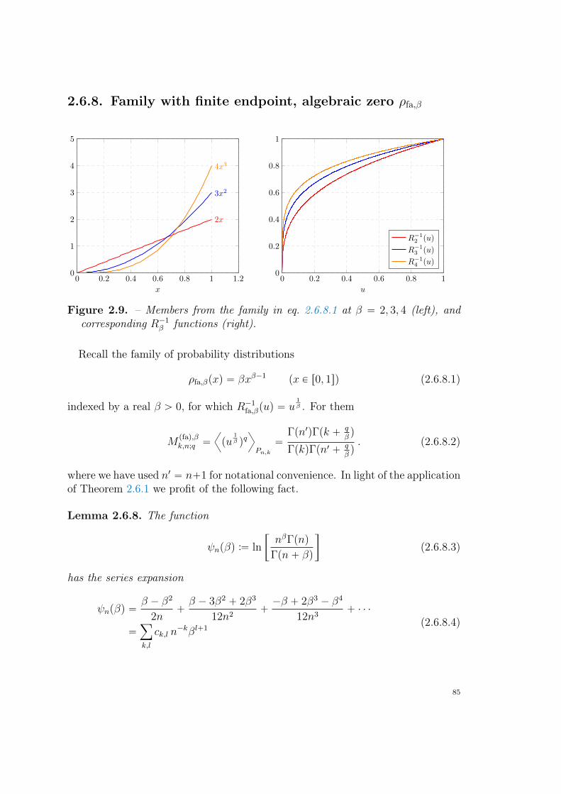
2.6.8. Family with finite endpoint, algebraic zero ρfa,β
0 0.2 0.4 0.6 0.8 1 1.20
1
2
3
4
5
2x
3x2
4x3
x
0 0.2 0.4 0.6 0.8 10
0.2
0.4
0.6
0.8
1
u
R−12 (u)
R−13 (u)
R−14 (u)
Figure 2.9. – Members from the family in eq. 2.6.8.1 at β “ 2, 3, 4 (left), andcorresponding R´1
β functions (right).
Recall the family of probability distributions
ρfa,βpxq “ βxβ´1px P r0, 1sq (2.6.8.1)
indexed by a real β ą 0, for which R´1fa,βpuq “ u
1β . For them
Mpfaq,βk,n;q “
A
pu1β qqE
Pn,k“
Γpn1qΓpk ` qβq
ΓpkqΓpn1 ` qβq. (2.6.8.2)
where we have used n1 “ n`1 for notational convenience. In light of the applicationof Theorem 2.6.1 we profit of the following fact.
Lemma 2.6.8. The function
ψnpβq :“ ln
„
nβΓpnq
Γpn` βq
(2.6.8.3)
has the series expansion
ψnpβq “β ´ β2
2n`β ´ 3β2 ` 2β3
12n2`´β ` 2β3 ´ β4
12n3` ¨ ¨ ¨
“ÿ
k,l
ck,l n´kβl`1
(2.6.8.4)
85
where
ck,` “ p´1qkBk´`Γpkq
Γp`qΓpk ´ `` 1q, k ě 1, 0 ď ` ď k, (2.6.8.5)
and Bs is the s-th Bernoulli number.∗
Now, at leading order in 1n, the coefficient of βp in
eψnpβq “ exp
¨
˚
˝
´β2
2n
ÿ
kě10ďlďk
p´2ck,lq
ˆ
β
n
˙2k´l´1 ˆβ2
n
˙´pk´lq
˛
‹
‚
(2.6.8.7)
concentrates around the term with k “ l “ 1 (that is, at the minimum of 2k´ l´1within the range k ě 1, 0 ď l ď k), and we can work with just the first term ineq. (2.6.8.4). We thus get
Mpfaq,βk,n;q „
$
&
%
Γpk` qβq
Γpkqn´qβ k small
exp´
´ 12n
´
q2
β
¯
p1´ x´1q
¯
xqβ x “ kn1“ Θp1q
(2.6.8.8)
which by Theorem 2.6.1 gives
Epβ,pq,npkq “pÿ
q“0
ˆ
p
q
˙
p´1qp´qMpfaq,βk,n;q M
pfaq,βk,n;p´q
„
$
’
’
&
’
’
%
n´pβpř
q“0
`
pq
˘
p´1qp´qΓpk` q
βqΓpk` p´q
βq
Γ2pkqk small
xpβpř
q“0
`
pq
˘
p´1qp´qexp´
´1´x´1
2nβ2 pq2 ` pp´ qq2q `O
`
1n2
˘
¯
x “ kn1“ Θp1q .
(2.6.8.9)
Let us consider first the contributions coming from edges that are “far” from theregion of low density of points, k “ xn1 (i.e. the bulk regime). By Lemma 2.6.6,
∗A further series expansion, satisfied by the difference of contiguous expressions (2.6.8.3), to be com-bined with the fact that ψ1pβq “ ´ ln Γpβq, is that, for n ě 2,
ψnpβq ´ ψn´1pβq “ p1´ βq log
ˆ
n´ 1
n
˙
´ log
ˆ
1`β ´ 1
n
˙
“1´ β
n2
8ÿ
m“0
p1´ βqm`1´ 1
pm` 2qnm. (2.6.8.6)
.
86
we just have
Epβ,pq,npkq „ xpβˆ
´1` x´1
nβ2
˙p21
Γpp2` 1q, k “ xn1 . (2.6.8.10)
Therefore, given a cutoff Λ “ Op?nq, the Riemann’s sumsřnk“Λ may be trans-
formed into integrals without affecting the leading asymptotics, giving
Epβ,pq,n „ n1´p2
ż 1
Λn
dx xpβ´p2P pxq, (2.6.8.11)
where P pxq is a polynomial in x. The integral in (2.6.8.11) does not diverge as longas p
β´
p2ą ´1, and in this case we may just take the limit Λ Ñ 0 and make the
substitutionş1
ΛnÑ
ş1
0(we “remove” the ultraviolet cutoff Λ, in physics language),
to get the following result.
Lemma 2.6.9 (Bulk regime). For the family ρfa,β with a finite endpoint, algebraiczero of order β ´ 1 (2.6.8.1), if
2β ` 2p´ pβ ą 0 (2.6.8.12)
thenEpβ,pq,n “ n1´p2bβ,p p1` op1qq , (2.6.8.13)
where
bβ,p “p!
pp2q!βp
ż 1
0
dx xpβp´1` x´1qp2
“p!
pp2q!βp
Γ`
p2` 1
˘
Γ´
1´ ppβ´2q2β
¯
Γ´
2` pβ
¯ .
(2.6.8.14)
Remark 2.6.2. In the β Ñ 1` limit, the distribution ρfa,1 recovers the uniformdistribution supported on r0, 1s, and we just get
limβÑ1`
bβ,p “p!
pp2q!
Γ`
p2` 1
˘
Γ p1` p2q
Γ p2` pq
“Γp1` p2q
p` 1,
(2.6.8.15)
which coincides with the known leading asymptotic constant, Eq. (2.6.1.2).
Let us consider now the anomalous contributions coming from edges in the region
87
of the zero, that is, Eq. (2.6.8.9) at small k. We have
Epβ,pq,npkq „ n´pβΛÿ
k“1
1
Γ2pkq
pÿ
q“0
ˆ
p
q
˙
p´1qqΓ
ˆ
k `q
β
˙
Γ
ˆ
k `p´ q
β
˙
, (2.6.8.16)
which, at first sight, may seem to grow as kpβ. However, one easily sees thatthe cancellations due to the
`
pq
˘
p´1qq combination lower the growth in k down tothe one of the bulk contribution, that is, Epβ,pq,npkq „ n´pβk
pβ´p2 . Recalling the
hypergeometric identity
8ÿ
k“1
Γpk ` aqΓpk ` bq
Γ2pkq“ Γp´1´ a´ bq
Γpa` 1q
Γp´aq
Γpb` 1q
Γp´bq, (2.6.8.17)
when the sum in Eq. 2.6.8.16 does not diverge, we can just take Λ Ñ 8 limit (i.e.we remove the infrared cutoff) † and get the following result.
Lemma 2.6.10 (Strict anomaly). For the family with a finite endpoint, algebraiczero of order β ´ 1 ρfa,β (Eq. 2.6.8.1), if
2β ` 2p´ pβ ă 0 (2.6.8.19)
thenEpβ,pq,n „ aβ,pn
´pβ (2.6.8.20)
where
aβ,p “ Γp´1´ pβqpÿ
q“0
ˆ
p
q
˙
p´1qqΓp1` q
βqΓp1` p´q
βq
Γp´ qβqΓp´p´q
βq
. (2.6.8.21)
Lastly, let us consider the limiting case
2β ` 2p´ pβ “ 0 , (2.6.8.22)
which defines a critical hyperbola (Fig. 2.10).In this case the anomalous and bulk contributions are of the same order (that
is, Epn,pq „ Ebulkpn,pq`E
tailpn,pq at leading order in n), and we need to keep a finite cutoff
†Inserting the Γ function definitions in eq. 2.6.8.16, and then summing over q and k leads to
Epβ,pq,n „ n´pβż 8
0
dt1t1
dt2t2e´pt1`t2qpt
1β
1 ´ t1β
2 qp
˜
I0p2?t1t2q ´ 1´
pt1t2qΛ`1
Γ2pΛ` 2q
8ÿ
s“0
pt1t2qs
ppΛ` 2qsq2
¸
,
(2.6.8.18)where I0pxq is the modified Bessel function of the first kind of order 0, so that the last term isnegligible in the Λ Ñ8 limit.
88
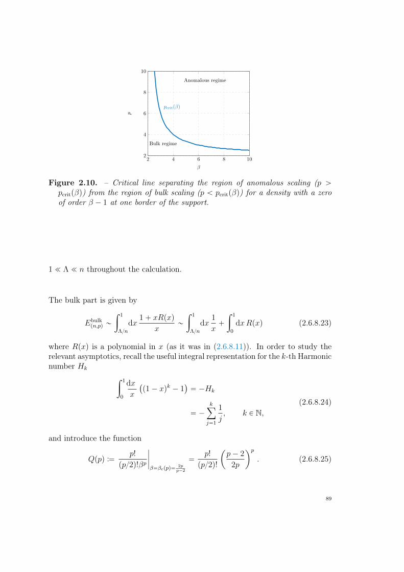
2 4 6 8 102
4
6
8
10
pcrit(β)
Anomalous regime
Bulk regime
β
p
Figure 2.10. – Critical line separating the region of anomalous scaling (p ąpcritpβq) from the region of bulk scaling (p ă pcritpβq) for a density with a zeroof order β ´ 1 at one border of the support.
1 ! Λ ! n throughout the calculation.
The bulk part is given by
Ebulkpn,pq „
ż 1
Λn
dx1` xRpxq
x„
ż 1
Λn
dx1
x`
ż 1
0
dxRpxq (2.6.8.23)
where Rpxq is a polynomial in x (as it was in (2.6.8.11)). In order to study therelevant asymptotics, recall the useful integral representation for the k-th Harmonicnumber Hk
ż 1
0
dx
x
`
p1´ xqk ´ 1˘
“ ´Hk
“ ´
kÿ
j“1
1
j, k P N,
(2.6.8.24)
and introduce the function
Qppq :“p!
pp2q!βp
ˇ
ˇ
ˇ
ˇ
β“βcppq“2pp´2
“p!
pp2q!
ˆ
p´ 2
2p
˙p
. (2.6.8.25)
89
Eq. (2.6.8.23) then becomes
Ebulkpn,pq „ n1´p2
ż 1
Λn
dxQppq
xp1´ xqp2 “n1´p2Qppq rplnn´ ln Λq`
`
ˆ
1`1
2` . . .`
2
p
˙
.
(2.6.8.26)
Now we have to deal with the small k part contributing to Etailpn,pq.
2.6.9. On sub-leading contributions at the critical line2pp` βq “ pβ
Recall that for a series of general term ak s.t. ak „ ckfor large k, we have
Λÿ
k“1
ak “Λÿ
k“1
´
ak ´c
k
¯
` cHΛ
“
8ÿ
k“1
´
ak ´c
k
¯
` cHΛ `Oˆ
1
Λ
˙
“ c pln Λ` γEq ` limxÑ1´
˜
clnp1´ xq
x`
8ÿ
k“1
akxk´1
¸
`Oˆ
1
Λ
˙
.
(2.6.9.1)
Recall also thatÿ
kě1
Γpk ` aqΓpk ` bq
Γ2pkqxk´1
“ Γpa` 1qΓpb` 1q2F1 pa` 1, b` 1; 1;xq (2.6.9.2)
where 2F1 pm,n; q;xq is Gauss hypergeometric function. We thus have
Etail,βpn,pq „ σpn
1´ p2 (2.6.9.3)
with
σp :“
«
Qppqpln Λ` γEq ` limxÑ1´
˜
pÿ
q“0
ˆ
p
q
˙
p´1qqΓ
ˆ
1`q
β
˙
Γ
ˆ
1`p´ q
β
˙
¨
¨2F1
ˆ
1`q
β, 1`
p´ q
β; 1;x
˙
`Qppqln p1´ xq
x
˙
(2.6.9.4)
90
(the last term being lnp1´zqz
“ 2F1 p1, 1; 2; zq), and by simple comparison witheq. (2.6.8.26) we have the following crucial remark.
Remark 2.6.3. At leading order in n, the bulk (resp. tail) part of the energy car-ries a `Qppq log Λ (resp., ´Qppq log Λ) contribution, so that the quantity Etail
pn,pq `
Ebulkpn,pq is independent on Λ.
We wish now to evaluate the relevant limit
σp :“ σp ´Qppq plog Λ` γEq
“ limxÑ1´
˜
pÿ
q“0
ˆ
p
q
˙
p´1qqΓ
ˆ
1`q
β
˙
Γ
ˆ
1`p´ q
β
˙
2F1
ˆ
1`q
β, 1`
p´ q
β; 1;x
˙
`Qppqln p1´ xq
x
˙
(2.6.9.5)
on the critical line βc “ 2pp´2
. In order to do so, we need to manipulate 2F1 pa, b; c;xqwhen a ` b ´ c P N, and this can be done with the aid of formulas 15.8.12 and15.8.10 of https://dlmf.nist.gov/15.8. For a “ 1` q
β, b “ 1` p´q
βand c “ 1, since
at the critical line
c´ b´ a “ 1´
ˆ
1`p´ 2
2pq
˙
´
ˆ
1` pp´ qqp´ 2
2p
˙
“ ´p
2,
(2.6.9.6)
using the identity 15.8.12 we get
2F1
ˆ
1`q
βc, 1`
p´ q
βc; 1;x
˙
“ p1´ xq´p2 2F1
ˆ
´p´ q
βc,´
q
βc; 1;x
˙
. (2.6.9.7)
Using the other identity 15.8.10, with
a “ 1´p
2`
q
βc“ ´
p´ q
βc,
b “ ´q
βc,
c “ a` b`p
2,
(2.6.9.8)
so that Γ`
a` p2
˘
“ Γ´
1` qβ
¯
and Γ`
b` p2
˘
“ Γ´
p2´
qβ
¯
, and Eq. 2.6.9.7, we
91
easily get
σp “ limxÑ1´
#
Qppqlog p1´ xq
x` p1´ xq´p2
pÿ
q“0
ˆ
p
q
˙
p´1qqΓ
ˆ
1`q
βc
˙
Γ
ˆ
1`p´ q
βc
˙
¨
¨
»
–
1
Γ´
1` qβc
¯
Γ´
p2´
qβc
¯
p2´1ÿ
k“0
p1´ p2`
qβcqkp´
qβcqkp
p2´ k ´ 1q
k!px´ 1qk`
´px´ 1q
p2
Γ´
1´ p2`
qβc
¯
Γ´
´qβc
¯
ÿ
kě0
p1` qβcqkp
p2´
qβcqk
k!pk ` p2q!
p1´ xqk¨
¨
ˆ
log p1´ xq ´ ψpk ` 1q ´ ψpk `p
2` 1q ` ψpk ` 1`
q
βcq ` ψ
ˆ
p
2´
q
βc` k
˙˙*
.
(2.6.9.9)
where paqk is Pochhammer symbol and ψ is the Digamma function. Eq. 2.6.9.9 canbe considerably simplified by the following remarks. First of all, we can discardthe whole first summand in square parentheses, which is a polynomial of degreestrictly ă p in q and thus lie in the kernel of
řpq“0
`
pq
˘
p´1qq. Secondly, we candiscard all terms with k ě 1 in the second summand in square parentheses, asthey vanish in the x Ñ 1´ limit. Hence, by straightforward algebra, we are justleft with
σp “ limxÑ1´
»
–Qppqlog p1´ xq
x`p´1q1`
p2
pp2q!
pÿ
q“0
ˆ
p
q
˙
p´1qqΓ´
1` qβc
¯
Γ´
1` p´qβc
¯
Γ´
´qβc
¯
Γ´
´p´qβc
¯
¨
ˆ
log p1´ xq ´ ψp1q ´ ψ´
1`p
2
¯
` ψ
ˆ
1`q
βc
˙
` ψ
ˆ
p
2´
q
βc
˙˙
.
(2.6.9.10)
Now, the symmetry of Eq. 2.6.9.10 suggests to consider the function
γpzq :“Γpz ` 1q
Γp´zq“
Γ2pz ` 1q
πsin pπzq (2.6.9.11)
92
in terms of which we have the remarkable simplification
p´1qp2`1
pp2q!
pÿ
q“0
ˆ
p
q
˙
p´1qqγp q
βq
γp qβ´
p2q“p´1q
p2`1
pp2q!
pÿ
q“0
ˆ
p
q
˙
p´1qq
«
ˆ
q
βc
˙p2
ff2sinpπ q
βcq
sin´
π´
qβc´
p2
¯¯
looooooooomooooooooon
“p´1qp2 at p even
“ ´1
pp2q!
pÿ
q“0
ˆ
p
q
˙
p´1qq
«
ˆ
q
βc
˙p2
ff2
“ ´p!
pp2q!
1
βpc
“ ´Qppq ,
(2.6.9.12)
where we have used, recalling the falling factorial notation sa “ sps ´ 1qps ´2q ¨ ¨ ¨ ps´ a` 1q, that
p2´1ź
l“0
ˆ
q
βc´ l
˙
“
ˆ
q
βc
˙p2
(2.6.9.13)
so that´
qβ
¯
p2 is the ordinary generating function for the Stirling numbers of the
first kindˆ
q
βc
˙p2
“
p2ÿ
k“0
s´p
2, k¯
ˆ
q
βc
˙k
. (2.6.9.14)
Hence, since limxÑ1´ Qppq´
log p1´xqx
´ log p1´ xq¯
“ 0, we can perform the xÑ 1´
limit, noting that all contributions independent on q just give a ´Qppq factor, andget the following
Lemma 2.6.11 (Tail contribution at the critical line). For the family ρfa,β, thetail contribution at the critical line has no logarithmic correction. It is given by
Etail,βcpn,pq „ n1´ p
2
”
Qppq´
H p2´ 2γE
¯
` υp
ı
(2.6.9.15)
where Hk is the k-th harmonic number, γE the Euler-Mascheroni constant, andthe
υp :“ ´1
pp2q!
pÿ
q“0
ˆ
p
q
˙
p´1qq
«
ˆ
q
βc
˙
p2
ff2ˆ
ψ
ˆ
1`q
βc
˙
` ψ
ˆ
p
2´
q
βc
˙˙
(2.6.9.16)for ψ the Digamma function.
Lemma 2.6.11 combined with Eq. 2.6.8.26 imply that for this family of distribu-
93
tions, at the critical line
Epβc,pq,n “ n1´ p2 lnnQppq
ˆ
1`Oˆ
1
log n
˙˙
(2.6.9.17)
which is always (even if only logarithmically) leading over the Selberg contribution„ n1´ p
2 . We shall call the emergence of a logarithmic correction to scaling alongthe critical line a marginal anomaly. We remark the particularly small range ofthe constants at the critical line, Qpr2, 4sq “
“
0, 364
‰
.
2.6.10. Family of distributions with endpoint at infinityand algebraic zero ρia,β
Let us recall our family of probability densities depending on a parameter β ą 0
ρia,βpxqdx “β
xβ`1θpx´ 1qdx (2.6.10.1)
for which, counting from the right, R´1ia,βpuq “
`
1u
˘1β . We have a duality relation
with the family with finite endpoint, algebraic zero ρfa,β (see Section 2.6.8), underthe transformation β Ñ ´β. We thus immediately get
Mpiaq,βk,n;q “
Γpn` 1qΓpk ´ qβq
ΓpkqΓpn` 1´ qβq“M
pfaq,´βk,n;q “M
pfaq,βk,n;´q . (2.6.10.2)
(compare with eq. (2.6.8.2)).We get immediately
Epβ,pq,npkq “pÿ
q“0
ˆ
p
q
˙
p´1qqMpiaq,βk,n;q M
piaq,βk,n;p´q “
pÿ
q“0
ˆ
p
q
˙
p´1qqMpfaq,βk,n;´qM
pfaq,βk,n;´p`q
„
$
&
%
npβřpq“0
`
pq
˘
p´1qqΓpk´ q
βqΓpk` p`q
βq
Γ2pkqk small
x´pβřpq“0
`
pq
˘
p´1qqexp´
´1´x´1
2nβ2 pq2 ` pp´ qq2q `O
`
1n2
˘
¯
x “ kn1“ Θp1q .
(2.6.10.3)
Still by duality, the critical line is given by
2pp´ βq “ ´pβ (2.6.10.4)
(or also pcpβq “ 2ββ`2
), and in this case the bulk regime is at p ă pcpβq, and thestrictly anomalous one at p ą pcpβq. Therefore, the asymptotic coefficient is just
94
given by Eq. 2.6.8.14 under β Ñ ´β, that is
biaβ,p :“ bfa
´β,p “Γpp` 1q
βp
Γp1´ β`22βpq
Γp2´ pβq
, (2.6.10.5)
which recovers (169 ), Eq. 29 upon renaming β “ α and the use of Legendreformula for the Γ function.
95
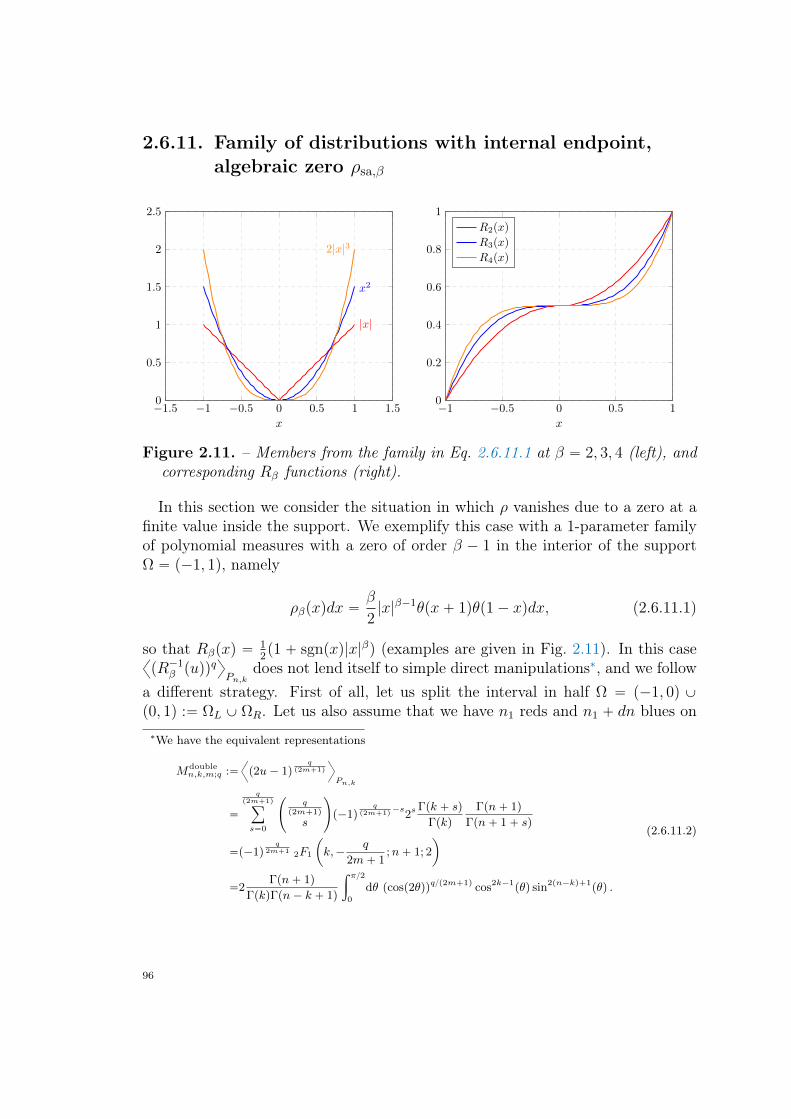
2.6.11. Family of distributions with internal endpoint,algebraic zero ρsa,β
−1.5 −1 −0.5 0 0.5 1 1.50
0.5
1
1.5
2
2.5
|x|
x2
2|x|3
x
−1 −0.5 0 0.5 10
0.2
0.4
0.6
0.8
1
x
R2(x)
R3(x)
R4(x)
Figure 2.11. – Members from the family in Eq. 2.6.11.1 at β “ 2, 3, 4 (left), andcorresponding Rβ functions (right).
In this section we consider the situation in which ρ vanishes due to a zero at afinite value inside the support. We exemplify this case with a 1-parameter familyof polynomial measures with a zero of order β ´ 1 in the interior of the supportΩ “ p´1, 1q, namely
ρβpxqdx “β
2|x|β´1θpx` 1qθp1´ xqdx, (2.6.11.1)
so that Rβpxq “12p1 ` sgnpxq|x|βq (examples are given in Fig. 2.11). In this case
@
pR´1β puqq
qD
Pn,kdoes not lend itself to simple direct manipulations∗, and we follow
a different strategy. First of all, let us split the interval in half Ω “ p´1, 0q Yp0, 1q :“ ΩL Y ΩR. Let us also assume that we have n1 reds and n1 ` dn blues on
∗We have the equivalent representations
Mdoublen,k,m;q :“
A
p2u´ 1qq
p2m`1q
E
Pn,k
“
qp2m`1qÿ
s“0
˜
qp2m`1q
s
¸
p´1qq
p2m`1q´s
2sΓpk ` sq
Γpkq
Γpn` 1q
Γpn` 1` sq
“p´1qq
2m`1 2F1
ˆ
k,´q
2m` 1;n` 1; 2
˙
“2Γpn` 1q
ΓpkqΓpn´ k ` 1q
ż π2
0
dθ pcosp2θqqqp2m`1q cos2k´1pθq sin2pn´kq`1
pθq .
(2.6.11.2)
96
the left of the zero; and n2`dn reds and n2 blues on the right, with n1`n2`dn “ n(we may assume that dn ě 0, otherwise the argument is identical upon exchangingreds and blues). As usual, we wish to evaluate Hid, so that, on ΩL, we wish toassign the n1 red points to the left-most n1 blue points, in order, and on ΩR,we wish to assign the n2 blue points with the rightmost n2 red points; lastly, wewant to assign dn blue points in ΩL to the dn leftmost red points on ΩR. Withthis decomposition, it is advantageous to enumerate points starting from the zero(around which the largest contributions are expected a priori) allowing to extendfinite sums to series. Hence, we shall enumerate points from left to right on ΩR
and from right to left on ΩL.Let Bnpmq “
14n
`
2nm
˘
, and let n1r (resp., n1b) be the number of red (resp., blue)points to the left of the zero. Let us introduce
$
’
&
’
%
n1 “ min pn1r, n1bq
n2 “ n´max pn1r, n1bq
n3 “ n´ n1 ´ n2 “ max pn1r, n1bq ´min pn1r, n
1bq .
(2.6.11.3)
The total energy is given by
Eβn,p “
ÿ
n1r,n1bě0
Bnpn1bqBnpn
1rq ¨
«
n1ÿ
k1“1
E`
|R´1n1 puk1q ´R
´1n1`n3puk1`n3q|
p˘
`
`
n2ÿ
k2“1
E`
|R´1n2 puk2q ´R
´1n2`n3puk2`n3q|
p˘
`
n3ÿ
k3“1
E`
|R´1n1`n3puk3q `R
´1n2`n3pun3`1´k3q|
p˘
ff
“ÿ
n1r,n1bě0
Bnpn1bqBnpn
1rq
«
n1ÿ
k1“1
Lk1,p,β `n2ÿ
k2“1
Rk2,p,β `
n3ÿ
k3“1
Ck3,p,β
ff
(2.6.11.4)
Hence in eq. (2.6.11.4) the L (R) contributions come from edges falling entirelywithin ΩL (resp. ΩR); and the C contributions (notice the plus sign in theirdefinitions) come from edges “on top” of the zero, that is, edges matching pointsin ΩL to points in ΩR. It can be easily calculated that
xR´1n1 puk1q
qy “
Γ´
k1 ` qβ
¯
Γpk1q
Γpn1 ` 1q
Γ´
n1 ` 1` qβ
¯ . (2.6.11.5)
Expanding the binomials in eq. 2.6.11.4 at p ą 1 and even, the three contributions
97
are constituted of simple ratios of Γ functions, respectively (note that there is nominus sign p´1qq in the third expression)
Lk1,p,β “pÿ
q“0
ˆ
p
q
˙
p´qqΓ´
k1 ` qβ
¯
Γpk1q
Γpn1 ` 1q
Γ´
n1 ` 1` qβ
¯
Γ´
k1 ` n3 ` p´qβ
¯
Γpk1 ` n3q
Γpn1 ` n3 ` 1q
Γ´
n1 ` n3 ` 1` p´qβ
¯ ,
Rk2,p,β “
pÿ
q“0
ˆ
p
q
˙
p´qqΓ´
k2 ` qβ
¯
Γpk2q
Γpn2 ` 1q
Γ´
n2 ` 1` qβ
¯
Γ´
k2 ` n3 ` p´qβ
¯
Γpk2 ` n3q
Γpn2 ` n3 ` 1q
Γ´
n2 ` n3 ` 1` p´qβ
¯ ,
Ck3,p,β “pÿ
q“0
ˆ
p
q
˙Γ´
k3 ` qβ
¯
Γpk3q
Γpn1 ` n3 ` 1q
Γ´
n1 ` n3 ` 1` qβ
¯
Γ´
n3 ` 1´ k3 ` p´qβ
¯
Γpn3 ` 1´ k3q
Γpn2 ` n3 ` 1q
Γ´
n2 ` n3 ` 1` p´qβ
¯ ,
(2.6.11.6)
so that, calling
Ln,p,β “n1ÿ
k1“1
Lk1,p,β, Rn,p,β “
n2ÿ
k2“1
Rk2,p,β, Cn,p,β “n3ÿ
k3“1
Ck3,p,β, (2.6.11.7)
the energy is given by Eβn,p “ Ln,p,β ` Cn,p,β ` Rn,p,β. The first remark is that
n1 ´ n2“ Op?nq (almost surely) so that, at q
β“ Op1q, we get
Γpn1 ` 1q
Γ´
n1 ` 1` qβ
¯ “Γ`
n1 ´ n2` n
2` 1
˘
Γ´
n1 ´ n2` n
2` 1` q
β
¯ “
´n
2
¯´qβ
ˆ
1`Oˆ
1?n
˙˙
(2.6.11.8)
(and an analogous expression mutatis mutandi for ratios of Γ functions involvingn2 and n3, and terms in which q Ø p ´ q). Let us focus first on the centralcontribution C. Since 1
Γpk3qΓpn3`1´k3q“ 1
pn3´1q!
`
n3´1k3´1
˘
, we just get
Ck3,p,β „´n
2
¯´pβ
pÿ
q“0
ˆ
p
q
˙Γ´
k3 ` qβ
¯
Γpk3q
Γ´
n3 ` 1´ k3 ` p´qβ
¯
Γpn3 ` 1´ k3q
„
´n
2
¯´pβ
ż 8
0
dt
ż 8
0
du´
t1β ` u
1β
¯p tk3´1un
3´k3
pn3 ´ 1q!
ˆ
n3 ´ 1
k3 ´ 1
˙
e´pt`uq .
(2.6.11.9)
98
Hence
Cn,p,β „´n
2
¯´pβ
ż 8
0
dt
ż 8
0
du´
t1β ` u
1β
¯p pt` uqn3´1
pn3 ´ 1q!e´pt`uq
„
ż 1
0
dx´
x1β ` p1´ xq
1β
¯p ´n
2
¯´pβ
ż 8
0
dVV n3` p
β
pn3 ´ 1q!e´V
„ Kβ,p
´n
2
¯´pβ
Γ´
n3 ` 1` pβ
¯
Γpn3q,
(2.6.11.10)
where the change of variables t “ V x and u “ V p1´xq (such thatdudt “ VdV dx )has been suggested by the homogeneity properties of the integrand, and the limitconstants are just
Kβ,p “
pÿ
q“0
ˆ
p
q
˙Γ´
1` qβ
¯
Γ´
1` p´qβ
¯
Γ´
2` pβ
¯ (2.6.11.11)
(notice the absence of the p´1qq term). Since also n3 “ Op?nq (almost surely),so that
Γ´
n3 ` 1` pβ
¯
Γpn3q“ n
12p1` p
βq
ˆ
1`Oˆ
1?n
˙˙
, (2.6.11.12)
we just have
Cn,p,β “ n´pβn
12p1` p
βqKβ,p p1` op1qq “ n
12p1´ p
βqKβ,p p1` op1qq . (2.6.11.13)
Thus, a contribution from edges jumping above the region of low density ofpoints scales as the bulk one, n1´ p
2 , if it were that the contributions of the L andR parts have no stronger scaling,
p` β “ pβ . (2.6.11.14)
Eq. (2.6.11.14) defines a critical hyperbola pcpβq “ ββ´1
(or equivalently βcppq “pp´1
) separating the anomalous from the bulk regime (Fig. 2.12). Incidentally,except for a factor 2 at lhs, it corresponds to the critical line for the family ofdensities with a single zero, eq. (2.6.8.22).Let us now evaluate the “single-sided” contributions to the energy Ln,p,β (Rn,p,β
can be evaluated analogously). We shall address the evaluation in two ways:
1. an approach inspired by § 2.5 and valid for the bulk regime β ă βc, in whichwe threat k1 in Lk1,p,β as a variable of order n. The explicit expression of
99
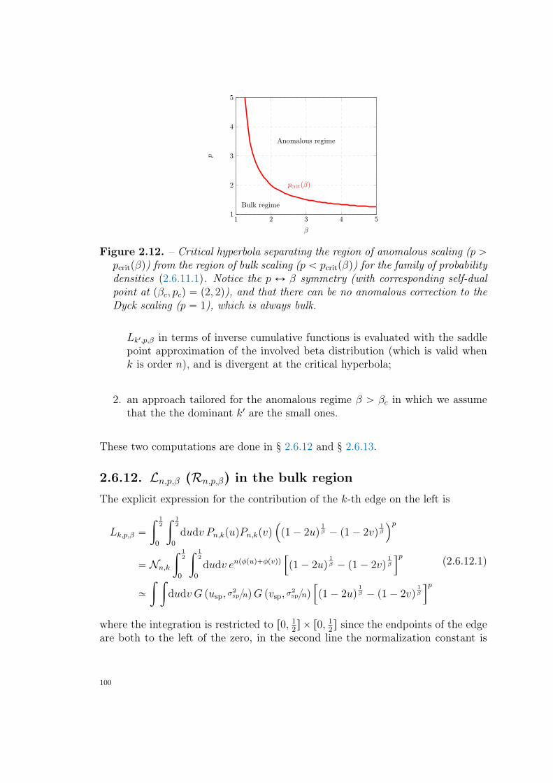
1 2 3 4 51
2
3
4
5
pcrit(β)
Anomalous regime
Bulk regime
β
p
Figure 2.12. – Critical hyperbola separating the region of anomalous scaling (p ąpcritpβq) from the region of bulk scaling (p ă pcritpβq) for the family of probabilitydensities (2.6.11.1). Notice the p Ø β symmetry (with corresponding self-dualpoint at pβc, pcq “ p2, 2q), and that there can be no anomalous correction to theDyck scaling (p “ 1), which is always bulk.
Lk1,p,β in terms of inverse cumulative functions is evaluated with the saddlepoint approximation of the involved beta distribution (which is valid whenk is order n), and is divergent at the critical hyperbola;
2. an approach tailored for the anomalous regime β ą βc in which we assumethat the the dominant k1 are the small ones.
These two computations are done in § 2.6.12 and § 2.6.13.
2.6.12. Ln,p,β (Rn,p,β) in the bulk regionThe explicit expression for the contribution of the k-th edge on the left is
Lk,p,β “
ż 12
0
ż 12
0
dudv Pn,kpuqPn,kpvq´
p1´ 2uq1β ´ p1´ 2vq
1β
¯p
“ Nn,k
ż 12
0
ż 12
0
dudv enpφpuq`φpvqq”
p1´ 2uq1β ´ p1´ 2vq
1β
ıp
»
ż ż
dudv G pusp, σ2spnqG pvsp, σ
2spnq
”
p1´ 2uq1β ´ p1´ 2vq
1β
ıp
(2.6.12.1)
where the integration is restricted to r0, 12s ˆ r0, 1
2s since the endpoints of the edge
are both to the left of the zero, in the second line the normalization constant is
100
Nn,k “`
n´1k
˘2, and in the third line Gpm,σ2q is a gaussian of mean m and varianceσ2. It is obtained from the quadratic expansion around the extremum of
φptq :“k ´ 1
nlog ptq `
n´ k
nlog p1´ tq (2.6.12.2)
so that ddtφptq|t“tsp “ 0 and 1
σ2sp“ d2
dt2φptq|t“tsp . Let us put u “ usp ` δu and
v “ vsp`δv, and let us expand´
p1´ 2uq1β ´ p1´ 2vq
1β
¯p
around the saddle point.We have
´
p1´ 2uq1β ´ p1´ 2vq
1β
¯p
“ p1´ 2uspqpβ
«
ˆ
1`2
1´ 2usp
δu
˙1β
´
ˆ
1`2
1´ 2usp
δv
˙1β
ffp
(2.6.12.3)since usp “ vsp. Calling c “ 2
1´2usp, we can now perform the integrations and get
ż
duG pusp, σ2spnq p1` cδuq
qβ “
ÿ
a
ca
a!
ˆ
q
β
˙
a
xδuay “ÿ
a even
ca
a!
ˆ
q
β
˙
a
ˆ
σ2sp
n
˙
a2
pa´ 1q!!
ż
dv G pvsp, σ2spnq p1` cδvq
p´qβ “
ÿ
b
cb
b!
ˆ
p´ q
β
˙
b
@
δvbD
“ÿ
b even
cb
b!
ˆ
p´ q
β
˙
b
ˆ
σ2sp
n
˙
b2
pb´ 1q!!
(2.6.12.4)
where pyqk “ ypy ` 1q ¨ ¨ ¨ py ` k ´ 1q. We are thus left with
Lk,p,β » p1´ 2uspqpβ
ż ż
dudv G pusp, σ2spnqG pvsp, σ
2spnq
ÿ
q
ˆ
p
q
˙
p´1qp´q p1` cδuqqβ p1` cδvq
p´qβ
“ p1´ 2uspqpβ
ÿ
q
ˆ
p
q
˙
p´1qp´qÿ
a,b even
ca`b
a!b!
ˆ
q
β
˙
a
ˆ
p´ q
β
˙
b
ˆ
σ2sp
n
˙
a`b2
pa´ 1q!!pb´ 1q!!
“ p1´ 2uspqpp 1
β´1q 2p
p!
βp
ˆ
σsp?n
˙pÿ
a`b“pa,b even
pa´ 1q!!pb´ 1q!!
a!b!
(2.6.12.5)
101
where from the second to the third line we have used Lemma 2.6.6 (which hasforced a` b “ p). But
ÿ
a`b“pa,b even
pa´ 1q!!pb´ 1q!!
a!b!“ 2´
p2
ÿ
a`b“pa,b even
1`
a2
˘
!
1`
b2
˘
!“ 2´
p2
ÿ
a`b“pa,b even
1`
a2
˘
!
1`
b2
˘
!
`
p2
˘
!`
p2
˘
!
“2´
p2
`
p2
˘
!
ÿ
a`b“pa,b even
`
p2
˘
!`
a2
˘
!`
b2
˘
!
“1
`
p2
˘
!.
(2.6.12.6)
Now we can evaluate Ln,p,β in the regime x “ kn(for x P r0, 12s). The saddle point
equation becomes
usp “k
n” x, σ2
sp “ xp1´ xq (2.6.12.7)
so that
Ln,p,β » n1´ p2
2p
βpp!`
p2
˘
!
ż 12
0
dx p1´ 2xqpp1β´1q rxp1´ xqs
p2 . (2.6.12.8)
Lastly, since
ż 12
0
dx p1´ 2xqa rxp1´ xqsbt“1´2x“ 21´2b
ż 1
0
dt tap1´ t2qb
“s“t2“ 2´2b
ż 1
0
ds sa`1
2´1p1´ sqb`1´1
“ 2´2bΓ`
a`12
˘
Γpb` 1q
Γ`
a`12` b` 1
˘
(2.6.12.9)
we just get that, in the bulk regime p´
1β´ 1
¯
ă 1 (see Fig. 2.12),
Ln,p,β “ n1´ p2Bβ,p p1` op1qq (2.6.12.10)
with
Bβ,p “1
βp
Γpp` 1qΓ´
p2β´
p2` 1
2
¯
Γ´
p2β` 3
2
¯ , (2.6.12.11)
102
and Rn,p,β “ Ln,p,β by symmetry.
Remark 2.6.4. Let us call the total energy of the single-sided contributions (i.e.the sum of left and right contributions)
Esa,L`Rp,β pnq “ Ln,p,β `Rn,p,β . (2.6.12.12)
In the β Ñ 1` limit, the distribution ρsa,1 recovers the uniform distribution sup-ported on the interval Ω “ r´1, 1s and there is no central term, so that the totalenergy is asymptotically
Esa,L`Rp,1 pnq “ n1´ p
2 2
?πΓpp` 1q
Γ`
p2` 3
2
˘ p1` op1qq . (2.6.12.13)
On the other hand, the asymptotic series for the energy where points are uniformlydistributed on r0, 1s is (see Eq. (2.6.1.2))
sp,n “ n1´p2 Γp1` p2q
p` 1p1` op1qq , (2.6.12.14)
so that their ratio is
Esa,L`Rp,1 pnq
sp,n“
ˆ
|Ω|
|r0, 1s|
˙p
p1` op1qq “ 2p p1` op1qq (2.6.12.15)
as expected.
2.6.13. Ln,p,β (Rn,p,β) in the anomalous regime and on thecritical line
Recall from Eq. 2.6.11.6 that
Lk1,p,β “pÿ
q“0
ˆ
p
q
˙
p´qqΓ´
k1 ` qβ
¯
Γpk1q
Γ´
k1 ` n3 ` p´qβ
¯
Γpk1 ` n3q
´n
2
¯´pβ (2.6.13.1)
so that, for Λ1 !?n, we have
ÿ
k1“1,...,Λ1
Lk1,p,β Àÿ
k1
pÿ
q“0
ˆ
p
q
˙
pk1qqβ pk1 ` n3q
p´qβ
´n
2
¯´pβ
« Λ1
`?n˘pβ
´n
2
¯´pβ“ cΛ1n
´p
2β “ o´
n12´
p2β
¯
“ o pCn,p,βq
(2.6.13.2)
103
which is always sub-leading with respect to the central contribution Cn,p,β. Hence,the contribution from the first Λ1 edges may be discarded without affecting theleading scaling and for k1 "
?n the continuous approximation of the sum with an
integral up to the appropriate upper cutoff Λ2 can be done. Calling k1 “ ζn1 andn1 “ ξ
?n, so that k1 “ ζξ
?n, we have that max pζξ
?nq “ n
2, so that Λnpξq “
?n
2ξ
(observe that a.s. ξ “ Θp1q). We thus get
Ln,p,β “n1ÿ
k1“Op?nqLk1,p,β „
?n
ż
?n2
0
dζ Lζξ?n,p,β
“?n
ż
?n2
0
dζpÿ
q“0
ˆ
p
q
˙
p´1qq`
ζ?n˘p´qβ`
pζ ` ξq?n˘qβ
´n
2
¯´pβ
“ n12p1´
pβ q2
pβ
C
ż
?n2
0
dζpÿ
q“0
ˆ
p
q
˙
p´1qqζp´qβ pζ ` ξq
qβ
G
ξ
(2.6.13.3)
where x. . .yξ denotes average with respect to the distribution of ξ. But ξ?n
d“
m1 `m2 with m1,m2 indep. and distrib. with pbinomial, where
pbinomialpmq “1
a
2πn14
e´ m2
2n14 dm , (2.6.13.4)
i.e. ppξqdξ “ 2?πe´ξ
2θpξqdξ, so that, in particular xξαy “
Γpα`12 q?π
. Setting η “ ξζ,we get
Ln,p,β “ n12p1´
pβ q2
pβ
C
ξpβ
ż Λnpξq
0
dηpÿ
q“0
ˆ
p
q
˙
p´1qqηp´qβ pη ` 1q
qβ
G
ξ
. (2.6.13.5)
Since a.s. Λnpξq " 1, we may split the integration asż Λnpξq
0
dη ηapη ` 1qb “
ż 1
0
dη ηaÿ
`ě0
ˆ
b
l
˙
η` `
ż Λnpξq
1
dη ηa`bÿ
`ě0
ˆ
b
l
˙
η´`
“ÿ
`ě0
ˆ
b
l
˙„
1
a` `` 1` ρp`´ a´ b´ 1,Λpξqq
(2.6.13.6)
where
ρpx, yq “
#
1x`O
´
1?n
¯
x ‰ 0
ln y `Op1q x “ 0 .(2.6.13.7)
104
We thus get
Ln,p,β “ n12p1´
pβ q2
pβ
C
pÿ
q“0
ˆ
p
q
˙
p´1qqÿ
`ěp
ˆ
qβ
`
˙
«
1p´qβ` `` 1
` ρ
ˆ
p
β` `´ 1,Λpξq
˙
ff
ξpβ
G
ξ
(2.6.13.8)where the second sum has been restricted to ` ě p as the discarded terms wouldbe zeroed in light of Lemma 2.6.6. In the anomalous region above the criticalhyperbola β ` p “ βp, p
β` ` ´ 1 ą 0 for all β ą p. If we are on the critical
hyperbola, then the only dangerous term is ` “ p. In the first case (see thefunction ρ) we have no further dependence on ξ and
A
ξpβ
E
ξ“
Γ´
1` pβ
2
¯
?π
(2.6.13.9)
is factored out. In the second case there is one single “dangerous” term from theupper extremum of integration
B
ln
ˆ?n
2ξ
˙
ξpβ
F
ξ
“
ˆ
1
2lnn´ ln 2
˙ Γ´
1` pβ
2
¯
?π
´1
2
Γ´
1` pβ
2
¯
?π
ψ
˜
1` pβ
2
¸
(2.6.13.10)
where ψ is the Digamma function. In conclusion
Ln,p,β „ n12p1´
pβ q2
pβ
Γ´
1` pβ
2
¯
?π
¨
¨
$
’
’
’
’
’
’
’
’
’
’
’
’
&
’
’
’
’
’
’
’
’
’
’
’
’
%
pÿ
q“0
ˆ
p
q
˙
p´1qqÿ
`ěp
ˆ
qβ
`
˙
«
1p´qβ` `` 1
`1
pβ` `´ 1
ff
p` β ă pβ
pÿ
q“0
ˆ
p
q
˙
p´1qq
«
ˆ
qβ
p
˙
˜
1p´qβ` p` 1
`1
2lnn` p` β “ pβ
´12ψ´
1` pβ
2
¯
´ ln 2¯
`ÿ
`ěp
ˆ
qβ
`
˙
˜
1p´qβ` `` 1
`1
pβ` `´ 1
¸ff
.
(2.6.13.11)
In particular, we have a logarithmic correction to scaling on the critical hyperbolaβ “ ppp ´ 1q:
Lemma 2.6.12 (Marginal anomaly for the family ρsa). At the critical line p`β “
105
pβ where Cn,p, pp´1“ opLn,p, p
p´1q, we have
Epp´1n,p “ Ln,p, p
p´1`Rn,p, p
p´1` . . . “ n1´p2Rppq lnn
ˆ
1`Oˆ
1
lnn
˙˙
(2.6.13.12)
withRppq “
2p´1
?πp!´p
2´ 1
¯
!
ˆ
p´ 1
p
˙p
. (2.6.13.13)
Instead in the anomalous region p ą βpβ ´ 1q Ln,p,β,Rn,p,β and Cn,p,β are of thesame order and we get
Eβn,p “ n
12p1´
pβ q p2Aβ,p `Kβ,pq p1` op1qq , p` β ă pβ, (2.6.13.14)
where
Aβ,p “ 2pβ
Γ´
1` pβ
2
¯
?π
pÿ
q“0
ˆ
p
q
˙
p´1qqÿ
`ěp
ˆ
qβ
`
˙
«
1p´qβ` `` 1
`1
pβ` `´ 1
ff
(2.6.13.15)and Kp,β is given in Eq. 2.6.11.11.
2.6.14. Section provisional conclusionsIn this Section we have studied possible anomalous scaling behaviors of the optimalcost in the convex regime p ě 1. We have derived phase diagrams which involvep and the relevant exponent characterizing the kind of zero of the probabilitydistribution of points at a finite or infinite endpoint. For stretched exponentialdistributions parametrized by α, the leading scaling is „ a1pα, pq plnnq
a2pα,pq, andwe have explicitly determined both a1 and a2. During the derivation, severalconnections to topics (and recent results) in number theory have emerged, suchas with multiple zeta values (§ 2.6.6). For the algebraic cases parametrized by β,an even simpler pattern has emerged: in the pp, βq plane hyperbolae separate abulk from an anomalous region. The hyperbolae are 2pp ` βq “ pβ for the caseof a finite endpoint, and p ` β “ pβ for the case of an internal endpoint (finiteand infinite endpoints being related by β Ñ ´β). In the bulk regimes the leadingscaling is the Donsker’s Theorem one (i.e. „ n1´p2), and the leading coefficientshave been determined explicitly; in the anomalous regimes the leading scalingshave also been determined explicitly being respectively „ n´pβ and „ n12p1´pβq.The corresponding leading constants have been also obtained. In both cases, at thecritical lines a logarithmic correction to scaling was found (“marginally anomalousscaling”), and the leading and first-sub-leading coefficients were also obtained.
106
2.7. The Dyck bound in the concave regime
The content of this Section has been published in (173 ).
2.7.1. Problem statement and models of randomassignment considered
Contrary to the convex regime p ą 1, where in d “ 1 the optimal matching iscompletely determined, and the C-repulsive case p ă 0, where in d “ 1 it is knownthat the optimal matching has certain cyclic properties and can thus be readilyfound in a subset of the symmetric group, the non-crossing property is not sufficientto fully characterize the optimal assignment; the regime 0 ă p ă 1 is thus muchmore challenging to study.The relevance of non-crossing matching configurations among elementary units
aligned on a line has emerged both in physics and in biology. In the latter case,this is due to the fact that they appear in the study of the secondary structure ofsingle stranded DNA and RNA chains in solution (85 ). These chains tend to foldin a planar configuration, in which complementary nucleotides are matched, andplanar configurations are exactly described by non-crossing matchings betweennucleotides. The secondary structure of a RNA strand is therefore a problem ofoptimal matching on the line, with the restriction on the optimal configurationto be planar (95 , 110 , 141 ). The statistical physics of the folding process ishighly non-trivial and it has been investigated by many different techniques (91 ,99 ), also in presence of disorder and in search for glassy phases (64 , 87 , 91 , 92 ,141 ). Therefore, as a further motivation for the present work, understanding thestatistical properties of the solution to ERAP with a concave cost function couldyeld results and techniques to better understand these models of RNA secondarystructure.
2.7.2. Choice of randomness for B and RLet us fix Ω to be a segment, that is we consider the problem with open bound-ary conditions (the alternate possible choice of considering Ω as a circle is notconsidered here).Notice that in the literature Ω is typically taken to be deterministically the unit
segment r0, 1s, while in this §we will find easier to work with a segment r0, Ls, whereL may be a stochastic variable, whose distribution depends on n. We will work inthe framework of constant density, that is EpLq „ n, so that, for comparison withthe existing literature, our results should be corrected by multiplying by a factorof the order n´p.
107
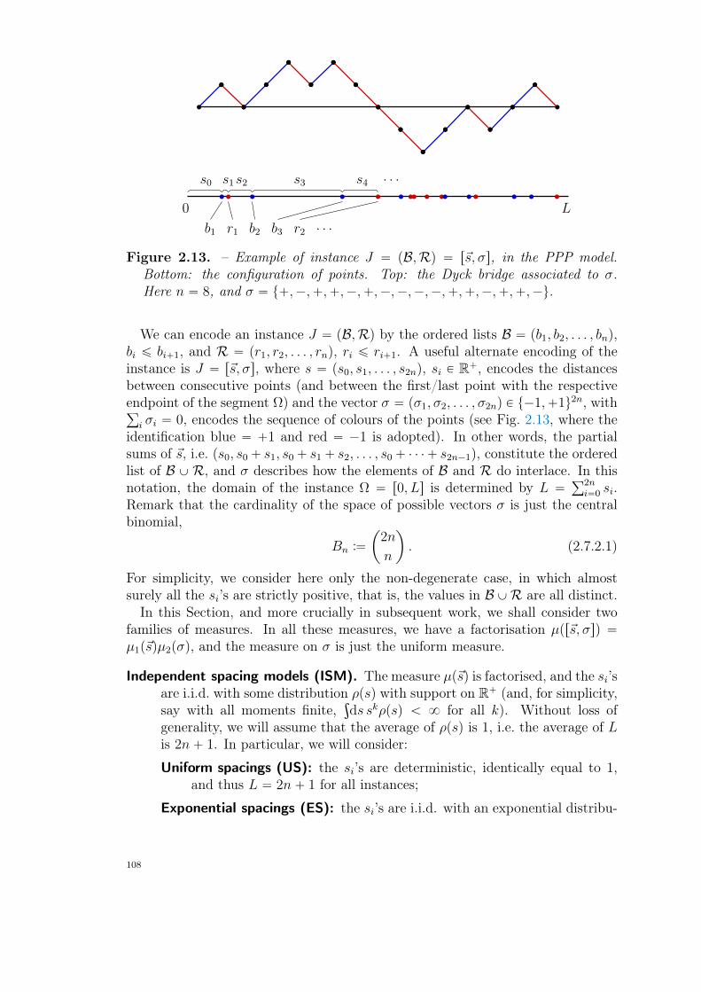
b1 r1 b2 b3 r2 ¨ ¨ ¨
s0 s1s2 s3 s4 ¨ ¨ ¨
0 L
Figure 2.13. – Example of instance J “ pB,Rq “ r~s, σs, in the PPP model.Bottom: the configuration of points. Top: the Dyck bridge associated to σ.Here n “ 8, and σ “ t`,´,`,`,´,`,´,´,´,´,`,`,´,`,`,´u.
We can encode an instance J “ pB,Rq by the ordered lists B “ pb1, b2, . . . , bnq,bi ď bi`1, and R “ pr1, r2, . . . , rnq, ri ď ri`1. A useful alternate encoding of theinstance is J “ r~s, σs, where s “ ps0, s1, . . . , s2nq, si P R`, encodes the distancesbetween consecutive points (and between the first/last point with the respectiveendpoint of the segment Ω) and the vector σ “ pσ1, σ2, . . . , σ2nq P t´1,`1u2n, withř
i σi “ 0, encodes the sequence of colours of the points (see Fig. 2.13, where theidentification blue “ `1 and red “ ´1 is adopted). In other words, the partialsums of ~s, i.e. ps0, s0` s1, s0` s1` s2, . . . , s0` ¨ ¨ ¨ ` s2n´1q, constitute the orderedlist of B YR, and σ describes how the elements of B and R do interlace. In thisnotation, the domain of the instance Ω “ r0, Ls is determined by L “
ř2ni“0 si.
Remark that the cardinality of the space of possible vectors σ is just the centralbinomial,
Bn :“
ˆ
2n
n
˙
. (2.7.2.1)
For simplicity, we consider here only the non-degenerate case, in which almostsurely all the si’s are strictly positive, that is, the values in BYR are all distinct.In this Section, and more crucially in subsequent work, we shall consider two
families of measures. In all these measures, we have a factorisation µpr~s, σsq “µ1p~sqµ2pσq, and the measure on σ is just the uniform measure.
Independent spacing models (ISM). The measure µp~sq is factorised, and the si’sare i.i.d. with some distribution ρpsq with support on R` (and, for simplicity,say with all moments finite,
ş
ds skρpsq ă 8 for all k). Without loss ofgenerality, we will assume that the average of ρpsq is 1, i.e. the average of Lis 2n` 1. In particular, we will consider:
Uniform spacings (US): the si’s are deterministic, identically equal to 1,and thus L “ 2n` 1 for all instances;
Exponential spacings (ES): the si’s are i.i.d. with an exponential distribu-
108
tion ρpsq “ g1psq “ expp´sq, and thus L concentrates on 2n ` 1, buthas a variance of order n.
Exchangeable process model (EPM). This is a generalisation of the ISM above,but now the si’s are not necessarily i.i.d., they are instead exchangeablevariables, that is, for all 0 ď i ă 2n,
µps0, . . . , si, si`1, . . . , s2nq “ µps0, . . . , si`1, si, . . . , s2nq . (2.7.2.2)
In particular, within this class of models we could have that µ is supportedon the hyper-tetrahedron T2n described by si ě 0, and L “
ř
i si “ 2n ` 1.In this paper, we will consider:
Poisson Point Process (PPP): the si’s are the spacings among the sortedlist of 0, 2n`1, and 2n uniform random points in the interval r0, 2n`1s.
Each of these three models has its own motivations. The PPP case is, in a sense,the most natural one for what concerns applications and the comparison withthe models in arbitrary dimension d. Implicitly, it is the one described in theintroduction. The ES case is useful due to a strong relation with the PPP case(see Remark 2.7.1 and Lemma 2.7.5 later on in Section 2.7.6). In a sense, it is the“Poissonisation” of the PPP case (where in this case it is the quantity L that hasbeen “Poissonised”, that is, it is taken stochastic with its most natural underlyingmeasure, instead of deterministic). The US case will prove out, in future work, tobe the most tractable case for what concerns lower bounds to the optimal cost.As all of the measures above are factorized in σ and ~s, and the measure over σ
is uniform, it is useful to define two shortcuts for two recurrent notions of average.
Definition 2.7.1. For any quantity ApJq “ Apσ,~sq, we denote by A the averageof A over σ
A :“ EσpAq “1
Bn
ÿ
σ
Apσ,~sq ; (2.7.2.3)
This average is independent from the choice of model among the classes above.We denote by
xAy :“ Eµp~sqpAq (2.7.2.4)
the average of A over ~s, with its appropriate measure dependence on the choiceof model. Finally, we denote by EnpAq the result of both averages, in which westress the dependence from the size parameter n in the measure, that is
EnpAq :“ Eσ,µp~sqpAq “ xAy “ xAy . (2.7.2.5)
For a given instance, parametrised as J “ pB,Rq, or as J “ r~s, σs, (and in which
109
the cost function also has an implicit dependence from the exponent p), we willcall as usual πopt one optimal configuration, so that HoptpJq “ HJpπoptq.
2.7.3. Synthesis of results
In this Section we will introduce the notion of Dyck matching πDyck of an instanceJ and we will compute its average cost HDyck :“ EnpHJpπDyckqq for the measuresES and PPP (with a brief discussion on the US case).In particular we prove the following theorem:
Theorem 2.7.1. For the three measures ES, US and PPP, let EnpHDyckq denotethe average cost of the Dyck matchings. Then
EnpHDyckq »
$
&
%
n 0 ď p ă 12
n lnn p “ 12
n12`p 1
2ă p ď 1
(2.7.3.1)
where apnq » bpnq if apnqbpnq
tends to a finite, non-zero constant when nÑ 8.
This Theorem follows directly from the combination of our suitable Lemmas,namely Proposition 2.7.6 and Corollary 2.7.6 appearing later on. In fact, our re-sults are more precise than what is stated in the Theorem above (we describe thefirst two orders in a series expansion for large n, including formulas for the associ-ated multiplicative constants), details are given in the forementioned propositions.The average cost of Dyck matchings provides an upper bound on the average
cost of the optimal solution; numerical simulations for the PPP measure, describedin Section 2.7.8, suggest the following conjecture, that we leave for future investi-gations:
Conjecture 1. For the three measures ES, US and PPP, and all 0 ă p ă 1,
limnÑ8
EnpHoptq
EnpHDyckq“ kp , (2.7.3.2)
with 0 ă kp ă 1.
2.7.4. Basic facts
Before starting our main proof, let us introduce some more notations, and recallsome basic properties of the optimal solution for convenience.
110
2.7.5. Basic properties of the optimal matchingA Dyck path of semi-length n is a lattice path from p0, 0q to p2n, 0q consisting ofn ‘up’ steps (i.e. steps of the form p1, 1q) and n ‘down’ steps (i.e., steps p1,´1q),which never goes below the x-axis. There are Cn Dyck path of semi-length n,where
Cn “
ˆ
2n
n
˙
´
ˆ
2n
n` 1
˙
“1
n` 1
ˆ
2n
n
˙
(2.7.5.1)
are the Catalan numbers. Therefore the generating function for the Dyck paths is
Cpzq :“ÿ
kě0
Ckzk“
1´?
1´ 4z
2z“
2
1`?
1´ 4z(2.7.5.2)
The historical name ‘Dyck path’ is somewhat misleading, as it leaves us with nonatural name for the most obvious notion, that is, the walks of length n with stepsin tp1, 1q, p1,´1qu. With analogy with the theory of Brownian motion (which re-lates to lattice walks via the Donsker’s theorem) (160 ), we will define four types ofpaths, namely walks, meanders, bridges and excursions, according to the followingtable:
yp2nq “ 0 ypxq ě 0 @xwalk no no
meander no yesbridge yes no
excursion yes yes
(of course, by “no” we mean “not necessarily”). Thus, in fact, the “paths” are themost constrained family of walks, that is the excursions.In general a Dyck path (i.e., a Dyck excursion) can touch the x-axis several
times. We shall call an irreducible Dyck excursion a Dyck path which touches thex-axis only at the two endpoints. It is trivially seen that the generating functionfor the irreducible Dyck excursions is simply z Cpzq. As we said above a Dyckbridge is a walk made with the same kind of steps of Dyck paths, but without therestriction of remaining in the upper half-plane, and which returns to the x-axis.The generating function for the Dyck bridges is
Bpzq :“1
1´ 2z Cpzq“
1?
1´ 4z“
ÿ
kě0
Bkzk (2.7.5.3)
with Bk the central binomials (2.7.2.1), and k is the semi-length of the bridge(just like excursions, all Dyck bridges must have even length). The factor 2 in thefunctional form of Bpzq in terms of Cpzq enters because a bridge is a concatenationof irreducible excursions, each of which can be in the upper- or the lower-half-plane.
111
Now, it is clear that each configuration σ corresponds uniquely to a Dyck bridgeof semi-length n, with σi “ `1 or ´1 if the i-th step of the walk is an up or downstep, respectively.In a Dyck walk we shall call pkbluepiq, hbluepiqq the two coordinates of the mid-
point of the i-th ascending step of the walk (minus p12, 1
2q, in order to have integer
coordinates and enlighten the notation), and call pkredpiq, hredpiqq the coordinatesof the mid-point of the i-th descending step (again, minus p1
2, 1
2q). For e “ pi, jq
an edge of a matching π, call e “ kbluepiq´kredpjq the horizontal distance on thewalk, and |e| “ |bi ´ rj| the Euclidean distance on the domain segment.For a given Dyck bridge σ, we say that π P Sn is non-crossing if, for every
pair of distinct edges e1 “ pi1, j1q and e2 “ pi2, j2q in π, we do not have thepattern kbluepi1q ă kbluepi2q ă kredpj1q ă kredpj2q, or the analogous patterns withkbluepi1q Ø kredpj1q, or kbluepi2q Ø kredpj2q, or p¨q1 Ø p¨q2 (recall Lemma 2.1.4, seealso bottom part of Figure 2.14). Note that the notion of π being non-crossingonly uses the vector σ.For a given Dyck bridge σ, we say that π P Sn is sliced if, for every edge
e “ pi, jq P π, we have hbluepiq “ hredpjq.Two easy Lemmas have a crucial role in our analysis.
Lemma 2.7.2. All the optimal matchings are non-crossing.
Proof. (This is Lemma 2.1.4. However, the proof appears to be new and for thisreason we report it here.) The proof is by absurd. Suppose that π is a crossingoptimal matching. If we have a pattern as kBpi1q ă kredpj2q ă kredpj1q ă kBpi2q,then the matching π1 with edges e11 “ pi1, j2q and e12 “ pi2, j1q has HJpπ
1q ă HJpπq,because |e11| ă |e1| and |e12| ă |e2|.If we have a pattern as kBpi1q ă kBpi2q ă kredpj1q ă kredpj2q, then again the
matching π1 with edges e11 “ pi1, j2q and e12 “ pi2, j1q has HJpπ1q ă HJpπq, although
this holds for a more subtle reason. Calling a “ x2´x1, b “ y1´x2 and c “ y2´y1,we have |e1| “ a` b, |e2| “ b` c, |e11| “ a` b` c and |e12| “ b. It is the case that,for a, b, c ą 0 and 0 ă p ă 1,
pa` bqp ` pb` cqp ą pa` b` cqp ` bp . (2.7.5.4)
A proof of this inequality goes as follows. Call F pa, b, cq “ pa ` bqp ` pb ` cqp ´pa` b` cqp ´ bp. We have F pa, b, 0q “ 0, and
1
p
B
BcF pa, b, cq “
1
pb` cq1´p´
1
pa` b` cq1´pą 0 . (2.7.5.5)
All the other possible crossing patterns are in the first or the second of the formsdiscussed above, up to trivial symmetries.
112
The second Lemma states that a necessary condition for an optimal matchingto be optimal is to be sliced.
Lemma 2.7.3. All the optimal matchings are sliced.
Proof. The proof is by absurd. Suppose that π is a non-sliced optimal matching.If we have pi, jq P π with hbluepiq ‰ hredpjq, say hbluepiq ´ hredpjq “ δh ‰ 0, wehave that the point xi is matched to yj, and that, between xi and yj, there arenblue and nred blue and red points, respectively, with nblue ´ nred “ ´δh ‰ 0. Sothere must be at least |δh| points inside the interval pxi, yjq which are matchedto points outside this interval, and thus, together with pi, jq, constitute pairs ofcrossing edges. So, by Lemma 2.7.2, π cannot be optimal.The slicing of optimal assignments was studied in (134 ).
2.7.6. Reduction of the PPP model to the ES modelTheorem 2.7.1 (and, hopefully, Conjecture 1), in principle, shall be proven forthree different models, Uniform Spacings (US), Exponential Spacings (ES) andthe Poisson Point Process (PPP). However, as we anticipated, the PPP case is aminor variant of ES. In this Section we give a precise account of this fact.The starting point is a relation between the two measures:
Remark 2.7.1. We can sample a pair r~s 1, σs with the measure µESn by sampling
a pair r~s, σs with the measure µPPPn , a value L P R` with the measure g2n`1pLq “
L2n
p2nq!expp´Lq dL, and then defining s1i “ si
L2n`1
.
Indeed, the measure on ~s in the PPP can be seen as the measure over indepen-dent exponential variables conditioned to the value of the sum; thus, the procedureleads at sight to a measure over ~s 1 which is unbiased within vectors ~s 1 with thesame value of L “
ř
i s1i. Then, from the independence of the spacings in the ES
model we easily conclude that the distribution of L must be exactly g˚p2n`1q1 pLq,
i.e. the convolution of 2n` 1 exponential distributions.More precisely, for k an integer, define the Gamma measure
gkpxq :“xk´1
Γpkqe´x “ g˚k1 pxq . (2.7.6.1)
We use the same notation for its analytic continuation to k real positive.We introduce (the analytic continuation of) the rising factorial (following a
notation due to Knuth (55 )):
np :“Γpn` pq
Γpnq“
ż
dx gnpxqxp . (2.7.6.2)
113
This choice of notation is motivated by the fact that n1 “ n1 “ n, and that, forn " p2, np “ npp1`Opp2nqq. More precisely we have:
Lemma 2.7.4. For 0 ď p ď 1 and n ą 1
pn` p´ 1qp ď np ď np . (2.7.6.3)
Proof. It is well known that the Gamma function is logarithmically convex (147 ).In particular, for any 0 ď p ď 1,
ln Γpn` pq ď p1´ pq ln Γpnq ` p ln Γpn` 1q “ ln Γpnq ` p lnn , (2.7.6.4)
that is
np “ exppln Γpn` pq ´ ln Γpnqq ď exppp lnnq “ np . (2.7.6.5)
Analogously, we have
ln Γpnq ď p1´pq ln Γpn`pq`p ln Γpn`p´1q “ ln Γpn`pq´p lnpn`p´1q , (2.7.6.6)
that is
np “ exppln Γpn` pq ´ ln Γpnqq ě exppp lnpn` p´ 1qq “ pn` p´ 1qp . (2.7.6.7)
See (139 ) for a recent review of inequalities involving np. Summing up, Re-mark 2.7.1 and Lemma 2.7.4 allow to prove that:
Lemma 2.7.5. The following inequalities hold:ˆ
2n
2n` 1
˙pp1´pq
EpHESoptq ď EpHPPP
opt q ď EpHESoptq . (2.7.6.8)
Also the corresponding inequalities with Hopt replaced by HDyck do hold, as well asfor any other quantity Hpπ˚pJqq, whenever π˚ is some matching determined by theinstance, and invariant under scaling of the instance, that is π˚r~s, σs “ π˚rλ~s, σs.
Proof. For compactness of notation, we do the proof only for the Hopt case, butthe generalisation is straightforward. Of course, Hrλ~s,σspπq “ λpHr~s,σspπq forall instances r~s, σs, all configurations π, and all scaling factors λ ą 0 (so asπ˚r~s, σs “ π˚rλ~s, σs, it follows that Hrλ~s,σspπ˚rλ~s, σsq “ λpHr~s,σspπ
˚r~s, σsq). Inparticular, Hoptprλ~s, σsq “ λpHoptpr~s, σsq. In light of Remark 2.7.1, we can de-scribe the average over µESr~s, σs in terms of an average over µPPPr~s, σs, and over
114
g2n`1pLq. More precisely
EpHESoptq “
ż
dµESr~s1, σsHoptpr~s
1, σsq
“
ż
dµPPPr~s, σs
ż
dLg2n`1pLq
ˆ
L
2n` 1
˙p
Hoptpr~s, σsq
“ EpHPPPopt q
ż
dLg2n`1pLq
ˆ
L
2n` 1
˙p
“ EpHPPPopt q
p2n` 1qp
p2n` 1qp.
(2.7.6.9)
The upper bound follows directly from Lemma 2.7.4. The lower bound follows as:
p2n` 1qp
p2n` 1qpě
ˆ
1´1´ p
2n` 1
˙p
ě
ˆ
1´1
2n` 1
˙pp1´pq
(2.7.6.10)
where first one uses Lemma 2.7.4, then the inequality p1 ´ qεqp ě p1 ´ εqpq (validfor ε, p, q P r0, 1s), with ε “ 1
2n`1and q “ 1´ p.
In light of this Lemma, it is sufficient to consider Theorem 2.7.1 (and Conjecture1) only for the US and ES models.The precise statement of our conclusions is the following:
Corollary.
EPPPn pHDyckq “ EESn pHDyckq`
1`O`
n´1˘˘
. (2.7.6.11)
The relevance of this statement lies in the fact that, in the forthcoming equa-tion (2.7.7.1), we provide an expansion for EESn pHDyckq in which corrections ofrelative order 1n appear as the third term in the expansion (and we provide ex-plicit results only for the first two terms). As a result, the very same conclusionsthat we have for the ES model do apply verbatim to the PPP model.
2.7.7. The Dyck matching
For every instance r~s, σs, there is a special matching, that we call πDyck, whichis sliced and non-crossing for σ. This is the matching obtained by the canonicalpairing of up- and down-steps within every excursion of the Dyck bridge (seeFigure 2.14 for an example). In analogy with our notation HoptpJq “ HJpπoptq, letus introduce the shortcut HDyckpJq “ HJpπDyckq.
115
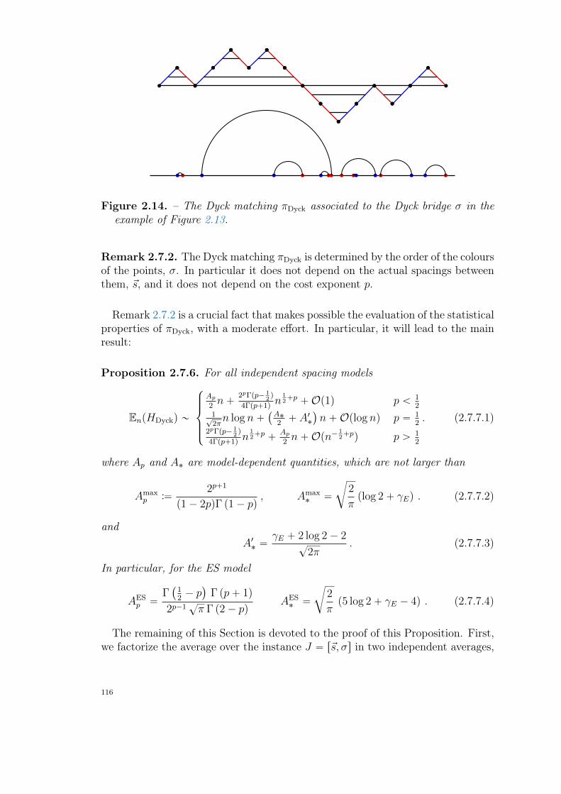
Figure 2.14. – The Dyck matching πDyck associated to the Dyck bridge σ in theexample of Figure 2.13.
Remark 2.7.2. The Dyck matching πDyck is determined by the order of the coloursof the points, σ. In particular it does not depend on the actual spacings betweenthem, ~s, and it does not depend on the cost exponent p.
Remark 2.7.2 is a crucial fact that makes possible the evaluation of the statisticalproperties of πDyck, with a moderate effort. In particular, it will lead to the mainresult:
Proposition 2.7.6. For all independent spacing models
EnpHDyckq „
$
’
’
&
’
’
%
Ap2n`
2pΓpp´ 12q
4Γpp`1qn
12`p `Op1q p ă 1
21?2πn log n`
`
A˚2` A1˚
˘
n`Oplog nq p “ 12.
2pΓpp´ 12q
4Γpp`1qn
12`p `
Ap2n`Opn´ 1
2`pq p ą 1
2
(2.7.7.1)
where Ap and A˚ are model-dependent quantities, which are not larger than
Amaxp :“
2p`1
p1´ 2pqΓ p1´ pq, Amax
˚ “
c
2
πplog 2` γEq . (2.7.7.2)
andA1˚ “
γE ` 2 log 2´ 2?
2π. (2.7.7.3)
In particular, for the ES model
AESp “
Γ`
12´ p
˘
Γ pp` 1q
2p´1?π Γ p2´ pq
AES˚ “
c
2
πp5 log 2` γE ´ 4q . (2.7.7.4)
The remaining of this Section is devoted to the proof of this Proposition. First,we factorize the average over the instance J “ r~s, σs in two independent averages,
116
the average over σ and the one over ~s (see Definition 2.7.1):
EnpHDyckq “ E
˜
nÿ
i“1
Ji,πDyckpiq
¸
“
nÿ
i“1
xJi,πDyckpiqy
“ B´1n
ÿ
σ
nÿ
i“1
@
|kBpiq ´ kredpπσDyckpiqq|
pD
,
(2.7.7.5)
where in the last line we emphasize that πDyck depends only on σ, as stated inRemark 2.7.2, and we adopted again the shortcut Bn “
`
2nn
˘
for the total numberof configurations σ.Due to the fact that the spacings si are independent, the quantity appearing
above, x|kBpiq ´ kredpπσDyckpiqq|
py, only depends on the length e “ 2k ` 1 of thecorresponding link e “ pi, πDyckpiqq, via the formula
Sppqk :“
@
|kBpiq ´ kredpπσDyckpiqq|
pD
“
Bˆ 2kÿ
j“0
sj
˙pF
, (2.7.7.6)
where the sj’s are i.i.d. variables sampled with the distribution ρpsq (that is, inthe ES model, i.i.d. exponential random variables).Then, as a general paradigm for observables of the form
ř
ePπ xF p|e|qy, we rewritethe sum over all possible σ and over all links e of a given matching π “ πDyckpσqas a sum over the forementioned parameter k, with a suitable combinatorial factorvn,k:
ÿ
ePπ
xF p|e|qy “ B´1n
n´1ÿ
k“0
vn,k
B
F
ˆ 2kÿ
j“0
sj
˙F
(2.7.7.7)
vn,k “ÿ
σ
ÿ
ePπDyckpσq
δe,2k`1 . (2.7.7.8)
(note thatř
k vn,k “ nBn “ 2`
2n´1n
˘
). In particular, in our case,
EnpHDyckq “ B´1n
n´1ÿ
k“0
vn,k Sppqk . (2.7.7.9)
So we face two separate problems: (1) determining the combinatorial coefficientsvn,k, which are “universal” (i.e., the same for all independent-spacing models, for allcost exponents p and for all observables F as above); (2) determining the quantitiesSppqk , that is, the average over the Euclidean length |e| of the link (which depends
from the function fpsq that defines the independent-spacing model, and from the
117
exponent p).For what concerns Sppqk , this can be computed exactly both in the US and ES
cases: in the US case Sppqk “ p2k`1qp, as in fact |e| “ 2k`1 “ e deterministically,while in the ES case Sppqk “ Γp2k`1`pqΓp2k`1q. More generally, for any modelwith independent spacings we would have that Sppqk “
ş
dx xpf˚2k`1pxq that is, thesum of 2k`1 i.i.d. random variables is distributed as the p2k`1q-fold convolutionof the single-variable probability distribution. For the ES case this is exactly theGamma distribution g2k`1psq. Up to this point, we could have also evaluated theanalogous quantity for the PPP model, although with a bigger effort (but, fromSection 2.7.6, we know that this is not necessary).For what concerns vn,k, in Appendix A.1 we prove that
vn,k “ Ck
„
4n´k´1`n´ k
2Bn´k
“: CkVn´k´1 . (2.7.7.10)
In particular, the simple expression for Vn´k´1 gives in a straightforward way
V pzq :“8ÿ
j“0
Vjzj“ p1´ 4zq´1
` p1´ 4zq´32 . (2.7.7.11)
We pause to study the distribution of the lengths e of links in πDyck, that is,the normalised distribution (in k), with parameter n, given by the expressionvn,kpnBnq. It is known that planar secondary structures have a universal be-haviour for the tail of such a distribution, with exponent ´3
2. Indeed, by perform-
ing a large n expansion at fixed k, and then studying the large k behaviour, onehas
vn,knBn
“CknBn
”
4n´k´1`n´ k
2Bn´k
ı
nÑ8« 2Ck 4´k
kÑ8«
c
2
πk´
32 ,
(2.7.7.12)
reproducing the known behaviour.Equation (2.7.7.9), with the help of (2.7.7.10) and (2.7.7.11), can be used to
relate the generating functions
Epz; pq :“8ÿ
n“0
BnEnpHDyckq zn (2.7.7.13)
Spz; pq :“8ÿ
k“0
Ck Sppqk zk . (2.7.7.14)
118
Lemma 2.7.7.Epz; pq “ z V pzqSpz; pq (2.7.7.15)
Proof.
Epz; pq :“8ÿ
n“0
BnEnpHDyckqzn
“
8ÿ
n“0
n´1ÿ
k“0
CkVn´k´1Sppqk zn
“
ˆ 8ÿ
k“0
CkSppqk zk
˙ˆ 8ÿ
n“k`1
Vn´k´1zn´k
˙
“ z V pzqSpz; pq .
(2.7.7.16)
The behaviour at large k of Sppqk is determined by the theory of large deviations.Said heuristically, the sum of the 2k ` 1 i.i.d. variables si concentrates on 2k ` 1,with tails which are sufficiently tamed that the average of xp is equal to p2k `1qpp1`Opk´1qq. That is, Sppqk „ p2k ` 1qp „ 2pkp, and we have
CkSppqk „
2p?π
4kkp´32 . (2.7.7.17)
We recall a fundamental fact in the theory of generating functions: the singularitiesof a generating function determine the asymptotic behaviour of its coefficients. Inparticular, the modulus of the dominant singularity (that nearest to the origin)determines the exponential behaviour, and the nature of the singularity determinesthe subexponential behaviour (see (123 ), Ch. 6 for a comprehensive treatment ofsingularity analysis, and Appendix A.2 for a short summary of results). This tellsus that we just need an expression for Epz; pq around its dominant singularityto extract asymptotic information on the total cost, i.e. we just need to evaluateSpz; pq locally around the dominant singularity of Epz; pq.First of all, one needs to locate the dominant singularity of Spz; pq and compare
it with the z “ 14singularity of V pzq. From Equation 2.7.7.17, we find an expo-
nential behaviour „ 4n of the coefficient of Spz; pq, trivially due to the entropy ofDyck walks of length 2n, thus, the singularity must be in z “ 1
4. Notice that this
agrees with the dominant singularity of V pzq (which also is, essentially, a gener-ating function of Dyck walks up to algebraic corrections), so that both generatingfunctions will combine to give the final average-cost asymptotics.At the dominant singularity, the power-law behaviour of the coefficients is given
119
by a generating function of the kind
Spz; pq “ Ap `Bpp1´ 4zqgp ` opp1´ 4zqgpq , (2.7.7.18)
where Ap encodes the regular terms at the singularity, and opp1´ 4zqgpq accountsfor all other singular terms leading to non trivial subleading corrections (amongthem one finds power, logarithms. . . in the variable 1´ 4z).
In fact, in such a simple situation as in our case, we expect a more precisebehaviour, Spz; pq “ App1 `Op1 ´ 4zqq ` Bpp1 ´ 4zqgpp1 `Op1 ´ 4zqq, where wehave two series of corrections, in integer powers, associated to the regular andsingular parts of the expansion around the singularity (up to the special treatmentof the degenerate case gp P Z).Notice that Bp and gp can be found by computing the asymptotic behaviour of
the coefficients of Equation 2.7.7.18
Sppqk „
Bp
Γ p´gpq4kk´gp´1
“2p?π
4kkp´32 , (2.7.7.19)
giving, by comparison with Equation 2.7.7.17,
gp “1
2´ p Bp “
2p Γ`
p´ 12
˘
?π
. (2.7.7.20)
Nothing can be said on the coefficient Ap without performing the exact resumma-tion of the generating function at the singularity (possibly, after having subtracteda suitable diverging part).
This analysis results in an asymptotic expression for Epz; pq:
Epz; pq „1
4
«
App1´ 4zq´32 `
2p Γ`
p´ 12
˘
?π
p1´ 4zq´p1`pq
ff
(2.7.7.21)
for p ‰ 12, and
E`
z; p “ 12
˘
“1
4p1´ 4zq´
32
«
A 12`ε `
1
ε
c
2
π`
c
2
πlog
ˆ
1
1´ 4z
˙
` opεq
ff
“1
4p1´ 4zq´
32
«
A˚ `
c
2
πlog
ˆ
1
1´ 4z
˙
ff
(2.7.7.22)
for p “ 12, where ε “ p ´ 1
2. The hypothesis of Spz; pq being non-singular in p
120
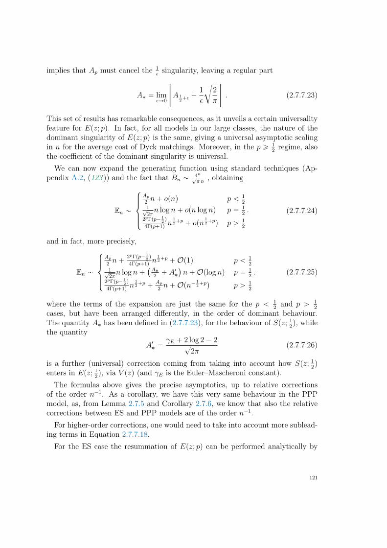
implies that Ap must cancel the 1εsingularity, leaving a regular part
A˚ “ limεÑ0
«
A 12`ε `
1
ε
c
2
π
ff
. (2.7.7.23)
This set of results has remarkable consequences, as it unveils a certain universalityfeature for Epz; pq. In fact, for all models in our large classes, the nature of thedominant singularity of Epz; pq is the same, giving a universal asymptotic scalingin n for the average cost of Dyck matchings. Moreover, in the p ě 1
2regime, also
the coefficient of the dominant singularity is universal.We can now expand the generating function using standard techniques (Ap-
pendix A.2, (123 )) and the fact that Bn „4n?π n
, obtaining
En „
$
’
’
&
’
’
%
Ap2n` opnq p ă 1
21?2πn log n` opn log nq p “ 1
2.
2pΓpp´ 12q
4Γpp`1qn
12`p ` opn
12`pq p ą 1
2
(2.7.7.24)
and in fact, more precisely,
En „
$
’
’
&
’
’
%
Ap2n`
2pΓpp´ 12q
4Γpp`1qn
12`p `Op1q p ă 1
21?2πn log n`
`
A˚2` A1˚
˘
n`Oplog nq p “ 12.
2pΓpp´ 12q
4Γpp`1qn
12`p `
Ap2n`Opn´ 1
2`pq p ą 1
2
(2.7.7.25)
where the terms of the expansion are just the same for the p ă 12and p ą 1
2
cases, but have been arranged differently, in the order of dominant behaviour.The quantity A˚ has been defined in (2.7.7.23), for the behaviour of Spz; 1
2q, while
the quantity
A1˚ “γE ` 2 log 2´ 2
?2π
(2.7.7.26)
is a further (universal) correction coming from taking into account how Spz; 12q
enters in Epz; 12q, via V pzq (and γE is the Euler–Mascheroni constant).
The formulas above gives the precise asymptotics, up to relative correctionsof the order n´1. As a corollary, we have this very same behaviour in the PPPmodel, as, from Lemma 2.7.5 and Corollary 2.7.6, we know that also the relativecorrections between ES and PPP models are of the order n´1.For higher-order corrections, one would need to take into account more sublead-
ing terms in Equation 2.7.7.18.For the ES case the resummation of Epz; pq can be performed analytically by
121
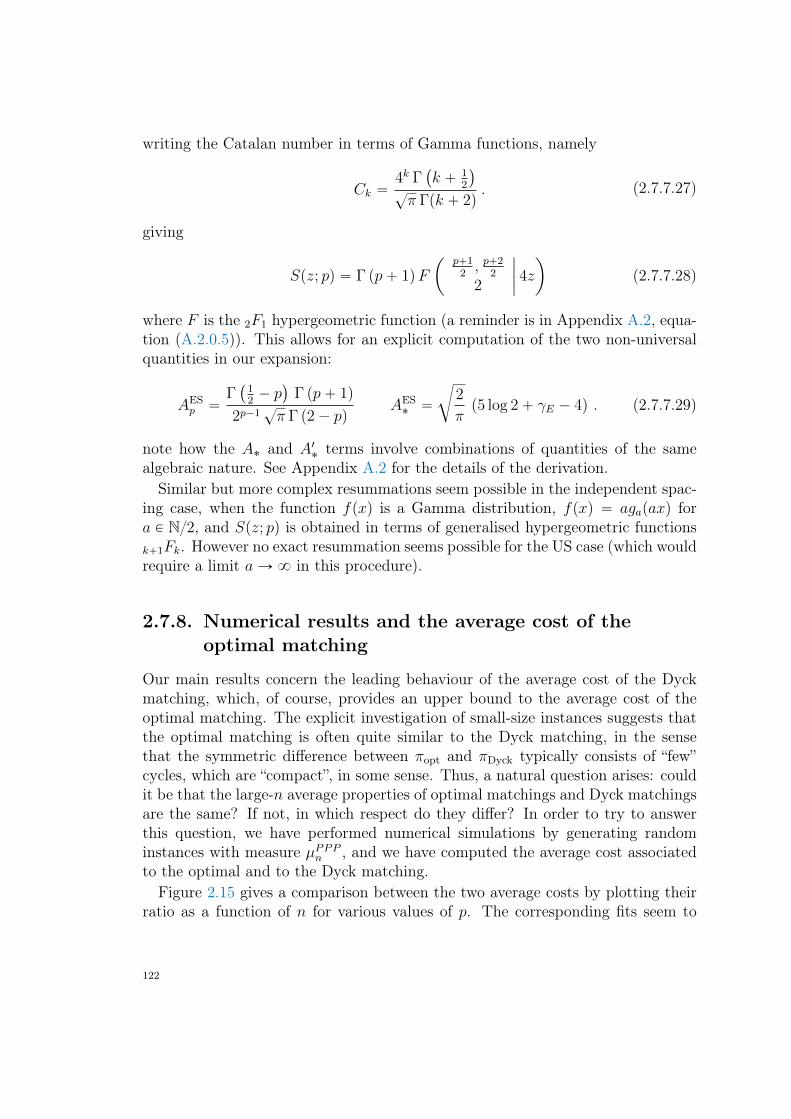
writing the Catalan number in terms of Gamma functions, namely
Ck “4k Γ
`
k ` 12
˘
?π Γpk ` 2q
. (2.7.7.27)
giving
Spz; pq “ Γ pp` 1qF
ˆ
p`12, p`2
2
2
∣∣∣∣ 4z
˙
(2.7.7.28)
where F is the 2F1 hypergeometric function (a reminder is in Appendix A.2, equa-tion (A.2.0.5)). This allows for an explicit computation of the two non-universalquantities in our expansion:
AESp “
Γ`
12´ p
˘
Γ pp` 1q
2p´1?π Γ p2´ pq
AES˚ “
c
2
πp5 log 2` γE ´ 4q . (2.7.7.29)
note how the A˚ and A1˚ terms involve combinations of quantities of the samealgebraic nature. See Appendix A.2 for the details of the derivation.Similar but more complex resummations seem possible in the independent spac-
ing case, when the function fpxq is a Gamma distribution, fpxq “ agapaxq fora P N2, and Spz; pq is obtained in terms of generalised hypergeometric functionsk`1Fk. However no exact resummation seems possible for the US case (which wouldrequire a limit aÑ 8 in this procedure).
2.7.8. Numerical results and the average cost of theoptimal matching
Our main results concern the leading behaviour of the average cost of the Dyckmatching, which, of course, provides an upper bound to the average cost of theoptimal matching. The explicit investigation of small-size instances suggests thatthe optimal matching is often quite similar to the Dyck matching, in the sensethat the symmetric difference between πopt and πDyck typically consists of “few”cycles, which are “compact”, in some sense. Thus, a natural question arises: couldit be that the large-n average properties of optimal matchings and Dyck matchingsare the same? If not, in which respect do they differ? In order to try to answerthis question, we have performed numerical simulations by generating randominstances with measure µPPPn , and we have computed the average cost associatedto the optimal and to the Dyck matching.Figure 2.15 gives a comparison between the two average costs by plotting their
ratio as a function of n for various values of p. The corresponding fits seem to
122
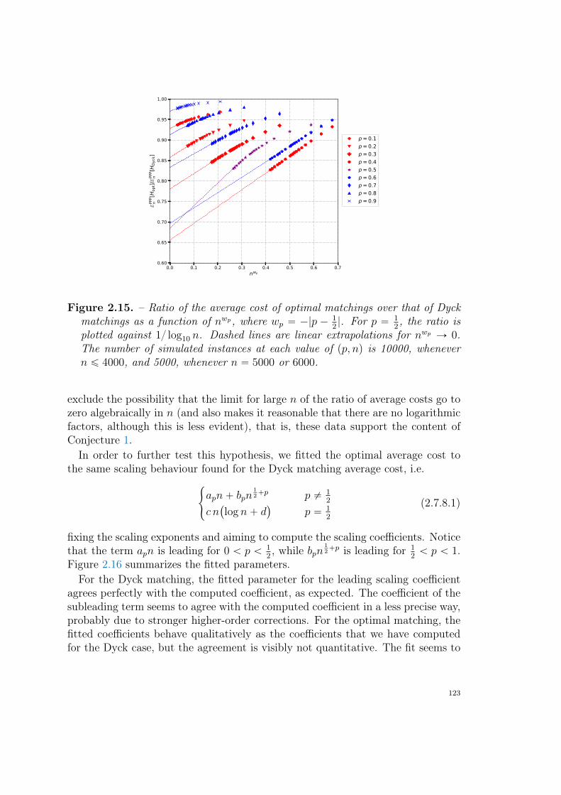
0.0 0.1 0.2 0.3 0.4 0.5 0.6 0.7nwp
0.60
0.65
0.70
0.75
0.80
0.85
0.90
0.95
1.00
PP
Pn
[Hop
t]/PP
Pn
[HDy
ck]
p=0.1p=0.2p=0.3p=0.4p=0.5p=0.6p=0.7p=0.8p=0.9
Figure 2.15. – Ratio of the average cost of optimal matchings over that of Dyckmatchings as a function of nwp, where wp “ ´|p ´ 1
2|. For p “ 1
2, the ratio is
plotted against 1 log10 n. Dashed lines are linear extrapolations for nwp Ñ 0.The number of simulated instances at each value of pp, nq is 10000, whenevern ď 4000, and 5000, whenever n “ 5000 or 6000.
exclude the possibility that the limit for large n of the ratio of average costs go tozero algebraically in n (and also makes it reasonable that there are no logarithmicfactors, although this is less evident), that is, these data support the content ofConjecture 1.In order to further test this hypothesis, we fitted the optimal average cost to
the same scaling behaviour found for the Dyck matching average cost, i.e.#
apn` bpn12`p p ‰ 1
2
c n`
log n` d˘
p “ 12
(2.7.8.1)
fixing the scaling exponents and aiming to compute the scaling coefficients. Noticethat the term apn is leading for 0 ă p ă 1
2, while bpn
12`p is leading for 1
2ă p ă 1.
Figure 2.16 summarizes the fitted parameters.For the Dyck matching, the fitted parameter for the leading scaling coefficient
agrees perfectly with the computed coefficient, as expected. The coefficient of thesubleading term seems to agree with the computed coefficient in a less precise way,probably due to stronger higher-order corrections. For the optimal matching, thefitted coefficients behave qualitatively as the coefficients that we have computedfor the Dyck case, but the agreement is visibly not quantitative. The fit seems to
123
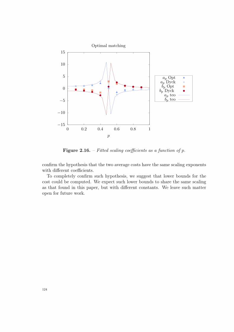
−15
−10
−5
0
5
10
15
0 0.2 0.4 0.6 0.8 1
p
Optimal matching
ap Optap Dyckbp Optbp Dyckap teobp teo
Figure 2.16. – Fitted scaling coefficients as a function of p.
confirm the hypothesis that the two average costs have the same scaling exponentswith different coefficients.To completely confirm such hypothesis, we suggest that lower bounds for the
cost could be computed. We expect such lower bounds to share the same scalingas that found in this paper, but with different constants. We leave such matteropen for future work.
124
2.8. Chapter provisional conclusions andresearch perspectives
In this Chapter we have investigated the one dimensional Euclidean RandomAssignment Problem. After reviewing the state of the art, we have presented
some new results concerning both the convex and concave regime. For the sake ofclarity, let us split our concluding remarks, provisional conclusions and perspectivesin two paragraphs according to the involved regimes.
2.8.1. Convex regime
In the case p “ 2 several variants of the problem can be studied in much detailessentially due to Fourier Duality. Here, we have focused on the statistical prop-erties of the optimal transport field in both the Poisson-Poisson and Grid-Poissonproblem, both in the continuum and in the discrete setting. In particular, in thecase of the Poisson-Poisson problem on the unit circle, we have shown that, in thecontinuum, the full ground state energy distribution is given explicitly as an el-liptic ϑ4 function, a calculation comforted by the results of numerical experimentsalready for moderately small values of n.Then, we have considered the case p ě 1 for a general probability distribution
(not necessarily finitely supported) of blue and red points. In such a case we havestudied the occurrence of an anomalous scaling with respect to the bulk behavior(the one fixed by the well-known brownian bridge qualitative picture) for a numberof exemplifying choices of the probability density function.In particular in § 2.5 we have studied this problem via a continuum approach
which reduces the calculation of asymptotic constants to quadratures (if the in-volved integrals converge). If the involved integrals do not converge, the methodsuggests a cutoff-based regularization procedure to deal with the singularity(ies).The energy scaling behavior can be obtained by fixing a single unknown scalarparameter to a numerically determined value, which is easily accessible since thesolution is ordered. The predictions of the method have been extensively verifiedby numerical experiments. We have also shown, through Beta integrals at fixedn, an exact expression of the expected ground state energy for points distributedaccording to an exponential of mean 1, a result which appears to be new in theliterature. We notice that the importance of the discussed regularization methodis not restricted to the one-dimensional ERAP. Indeed, analogous formulas for theexpected optimal costs appear also in other one-dimensional random optimizationproblems, such as the random Euclidean 2-matching and the Traveling SalesmanProblem in the bipartite and the monopartite case. The understanding of theproper regularization to be adopted, when the simpler expression cannot be used
125
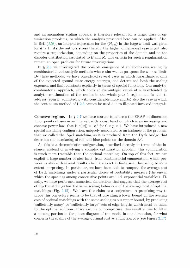
and an anomalous scaling appears, is therefore relevant for a larger class of op-timization problems, to which the analysis presented here can be applied. Also,in Ref. (149 ), an integral expression for the xHopty in the large n limit was givenfor d ą 1. As the authors stress therein, the higher dimensional case might alsorequire a regularization, depending on the properties of the domain and on thedisorder distribution associated to B and R. The criteria for such a regularizationremain an open problem for future investigations.In § 2.6 we investigated the possible emergence of an anomalous scaling by
combinatorial and analytic methods whose aim was to postpone the nÑ 8 limit.By these methods, we have considered several cases in which logarithmic scalingof the expected ground state energy emerges, and determined both the scalingexponent and limit constants explicitly in terms of special functions. Our analytic-combinatorial approach, which holds at even-integer values of p, is extended byanalytic continuation of the results in the whole p ě 1 region, and is able toaddress (even if, admittedly, with considerable more efforts) also the case in whichthe continuum method of § 2.5 cannot be used due to ill-posed involved integrals.
Concave regime. In § 2.7 we have started to address the ERAP in dimension1, for points chosen in an interval, with a cost function which is an increasing andconcave power law, that is cp|x|q “ |x|p for 0 ă p ă 1. We have introduced a newspecial matching configuration, uniquely associated to an instance of the problem,that we called the Dyck matching, as it is produced from the Dyck bridge thatdescribes the interlacing of red and blue points on the domain M.As this is a deterministic configuration, described directly in terms of the in-
stance, instead of involving a complex optimisation problem, this configurationis much more tractable than the optimal matching. On top of this fact, we canexploit a large number of nice facts, from combinatorial enumeration, which pro-vides us also with several results which are exact at finite size, this being, to someextent, surprising. In particular, we have been able to compute the average costof Dyck matchings under a particular choice of probability measure (the one inwhich the spacings among consecutive points are i.i.d. exponential variables). Fi-nally, we have performed numerical simulations that suggest that the average costof Dyck matchings has the same scaling behaviour of the average cost of optimalmatchings (Fig. 2.15). We leave this claim as a conjecture. A promising way toprove this conjecture seems to be that of providing a lower bound on the averagecost of optimal matchings with the same scaling as our upper bound, by producing“sufficiently many” or “sufficiently large” sets of edge-lengths which must be takenby the optimal solution. If we assume our conjecture, this result allows to fill ina missing portion in the phase diagram of the model in one dimension, for whatconcerns the scaling of the average optimal cost as a function of p (see Figure 2.17).
126
p
Scaling(p)
0 1 2-1
1
12
12
n n1−p
√n log n
√n n1−
p2
Figure 2.17. – Scaling exponent of the average optimal cost as a function of p,in the case of cost function Cp|x|q “ `|x|p (that is, attractive case for p ą 0and repulsive case for p ă 0). In red (solid line), our conjectured result. Inblack (dashed line), existing results from (154) (notice that we have rescaled ourresults of Theorem 2.7.1 by a factor p2n`1q´p in order to make the comparison,i.e. we plotted the result for M “ r0, 1s).
These new facts highlight a much richer structure that what could have been pre-dicted in light of the previous results alone, with the concatenation of four distinctregions, and a new special point with logarithmic corrections at p “ 12.The case of uniformly spaced points needs further analysis in the region p ă 12.
One can define an interpolating family of independent spacing models, which en-compasses both the ES and US cases, by taking as function fpsq the Gammadistribution αgαpαsq, for α ą 0. For example, when α is an integer, each si isdistributed as a sum of α i.i.d. exponential random variables, each with meanα´1. The ES case is, of course, α “ 1, while, due to the central limit theorem,the US model is the limit as α tends to infinity. This generalised model appearsto be treatable with the same technique that we employed for the pure ES casewhenever α is a half-integer: the generating function of the average cost can becomputed exactly in this case, and involves more and more complicated hypergeo-metric functions as α grows (namely, if α “ k2, we have a kFk´1 hypergeometricfunction). Performing singularity analysis over such functions is a challenging task,which builds on classical results on generalised hypergeometric functions (due toNørlund and Bühring), that we leave for future work.
127
Besides the above directions, for which an attacking strategy is at sight, otherspecific problems in the concave regime can be identified, for the understanding ofwhich an alternative point of view may be useful. We sketch two of them in thefollowing, in the form of Research Problems.
Research Problem 1 (Beyond the rule of three). We have recalled in severaloccasions (Lemmas 2.1.4 and 2.7.2) a characteristic property of the optimal per-mutation πopt in the concave one dimensional regime, namely the non-crossingproperty. A further property is due to McCann (see (82 ), Theorem 2.5), whohas shown that a πopt in the concave regime must satisfy a geometric nestinginequality called “rule of three”. The name comes from the fact that, for twonested intervals A “ pbi, rπpiqq and B “ prπpjq, bjq corresponding to the situationbi ă rπpjq ă bj ă rπpiq (or the one with reverse inequality signs),
|B| ď1
3|A| , (2.8.1.1)
which is true for all strictly increasing, concave cost functions (as the non-crossingproperty). Unfortunately, the non-crossing property is not sufficient to fully char-acterize πopt, and neither the rule of three is, so that the space of possible solutionsremains fairly large (a partial reason for the introduction of Dyck matchings).Therefore, the discovery of additional properties could help to reduce the size ofthe space of the possible solutions. By the way, for the cost function |x´ y|p withp P p0, 1q, one can show that a bound tighter than the rule of three holds directlyfrom the nesting requirement. For two nested sets B and A as above, consider theinequality
|B| ď kppq|A|
and call the lengths of three involved intervals in a nested configuration x, 1 and y(e.g. from left to right). In this parametrization, the nesting requirement becomes
1` px` y ` 1qp ď xp ` yp (2.8.1.2)
(which is false for any concave strictly increasing cost function if 1 ` x ` y ď 3according to McCann). However, the requirement is already false for a larger con-stant in our case. To see this, fix z “ x`y which gives the equivalent parametriza-tion
1` p1` zqp ď ptzqp ` pp1´ tqzqp (2.8.1.3)
that has to be true for all t P r0, 1s, and it is easy to show that the worst case isattained at t “ 12. In this parametrization, we simply have that kppq “ 1
1`zppq,
where zppq solves1` p1` zqp “ 2
´z
2
¯p
(2.8.1.4)
128
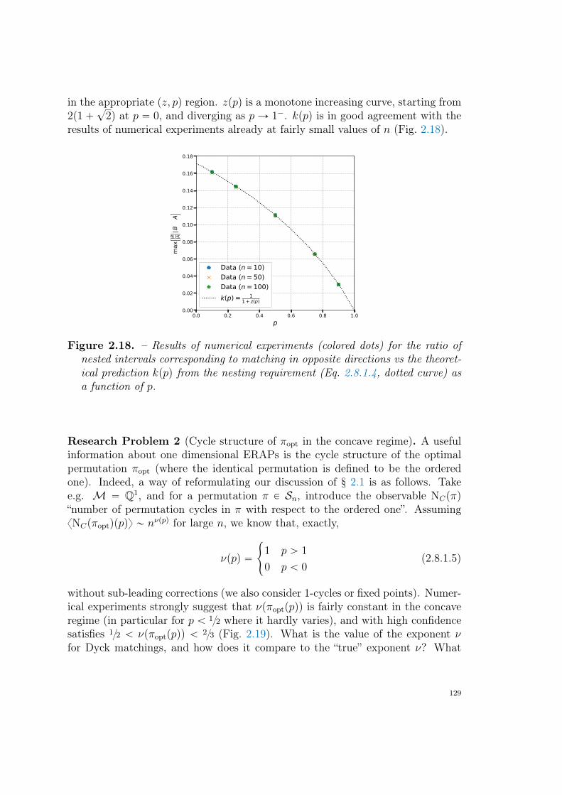
in the appropriate pz, pq region. zppq is a monotone increasing curve, starting from2p1`
?2q at p “ 0, and diverging as pÑ 1´. kppq is in good agreement with the
results of numerical experiments already at fairly small values of n (Fig. 2.18).
0.0 0.2 0.4 0.6 0.8 1.0p
0.00
0.02
0.04
0.06
0.08
0.10
0.12
0.14
0.16
0.18
max
[|B|
|A||B⊂A ]
Data (n=10)Data (n=50)Data (n=100)k(p) = 1
1+ z(p)
Figure 2.18. – Results of numerical experiments (colored dots) for the ratio ofnested intervals corresponding to matching in opposite directions vs the theoret-ical prediction kppq from the nesting requirement (Eq. 2.8.1.4, dotted curve) asa function of p.
Research Problem 2 (Cycle structure of πopt in the concave regime). A usefulinformation about one dimensional ERAPs is the cycle structure of the optimalpermutation πopt (where the identical permutation is defined to be the orderedone). Indeed, a way of reformulating our discussion of § 2.1 is as follows. Takee.g. M “ Q1, and for a permutation π P Sn, introduce the observable NCpπq“number of permutation cycles in π with respect to the ordered one”. AssumingxNCpπoptqppqy „ nνppq for large n, we know that, exactly,
νppq “
#
1 p ą 1
0 p ă 0(2.8.1.5)
without sub-leading corrections (we also consider 1-cycles or fixed points). Numer-ical experiments strongly suggest that νpπoptppqq is fairly constant in the concaveregime (in particular for p ă 12 where it hardly varies), and with high confidencesatisfies 12 ă νpπoptppqq ă 23 (Fig. 2.19). What is the value of the exponent νfor Dyck matchings, and how does it compare to the “true” exponent ν? What
129
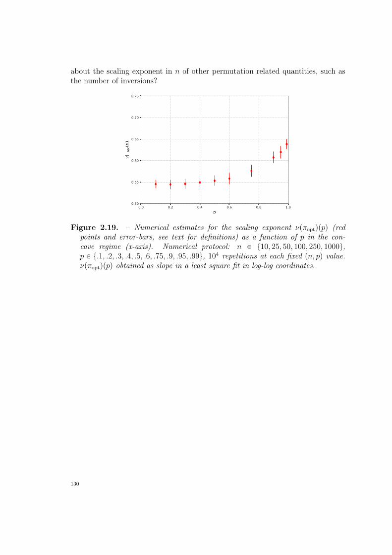
about the scaling exponent in n of other permutation related quantities, such asthe number of inversions?
0.0 0.2 0.4 0.6 0.8 1.0p
0.50
0.55
0.60
0.65
0.70
0.75
ν(π o
pt(p)
Figure 2.19. – Numerical estimates for the scaling exponent νpπoptqppq (redpoints and error-bars, see text for definitions) as a function of p in the con-cave regime (x-axis). Numerical protocol: n P t10, 25, 50, 100, 250, 1000u,p P t.1, .2, .3, .4, .5, .6, .75, .9, .95, .99u, 104 repetitions at each fixed pn, pq value.νpπoptqppq obtained as slope in a least square fit in log-log coordinates.
130
d Chapter 3 D
Field-theoretic approach tothe Euclidean RandomAssignment Problem
It is a longstanding question to understand the asymptotic behaviour, for large n,of the expected ground state energy EΩpnq for a domain Ω in general dimension.
When d ě 2, the results are very partial for any choice of a domain Ω, includingthe conceptually simplest ones (like the unit hypercube, or the unit hypertorus),and any value of p, including the special cases p “ 1 and p “ 2. A first attempt wascarried on by Mézard and Parisi (50 ) that showed how, for d ą 2, the random-linkresult can be used as a zero-order approximation for the finite-dimensional solution,adding perturbatively a series of corrections. In the same years, a remarkableresult was obtained by Ajtai and coworkers (37 ) for d “ 2: they proved that, ifthe problem is considered on the unit square Ω “ r0, 1s2, then EΩpnq „ lnn.∗
Recently, the forementioned result has been refined. In particular, by meansof non-rigorous arguments, in Refs. (145 , 148 ) it was claimed that, on the unitsquare R :“ r0, 1s2,
ERpnq “1
2πlnn` 2cRpnq (3.0.0.1)
where cRpnq “ oplnnq (the factor 2 is for later convenience). This result has beenlater rigorously proved by Ambrosio and coworkers (164 ) and extended to any2-dimensional compact manifold Ω (163 ). The latter paper also proves rigorousbounds for cΩ, namely that cΩpnq “ Op
?lnn ln lnnq. It has been recently conjec-
tured that Eq. (3.0.0.1) holds also in the case of points generated from non-uniformdensities (166 ). In the following Section we wish to argue, in the context of thefield-theoretic approach to this problem, that all possibly divergent terms in cΩpnqare universal, in the sense that the first finite-size correction depending on the do-main Ω is a constant, verify this statement for several (flat and curved) manifolds,and compare our predictions with numerical experiments for several choices of thesurfaces Ω.
∗More precisely Ajtai et al. studied the case p “ 1, but they also sketch how their analysis can beextended to p a positive integer, and predicted the scaling EΩpnq „ n1´ p
2 plnnqp2 in this generality.
See also (167 ) for a recently proposed alternative proof of the AKT theorem.
131
3.1. Random Assignment Problems on 2d
manifolds
The content of this Section is part of a submitted paper (172 ).
Let M ” Ω Ă R2 be a compact domain, and let us assume that B “ tXiuni“1
and R “ tYiuni“1 are generated via a homogeneous Poisson Point Process (PPP)
on Ω. Let us introduce the two atomic measures
νX :“dx
n
nÿ
i“1
δXi ,
νY :“d y
n
nÿ
i“1
δYi .
(3.1.0.1)
The energy of a permutation π P Sn is
Enpπ|B,Rq :“nÿ
i“1
|Xi ´ Yπpiq|2, (3.1.0.2)
where |x ´ y| is two dimensional Euclidean distance between the points x and y.The average ground state energy is
En,Ω :“ ErminπEnpπ|B,Rqs (3.1.0.3)
where E denotes expectation w.r.t. the disorder distribution. We have recalled inthe Introduction (Eq. 1.5.0.3) that
minπEnpπ|X ,Y q “ nW 2
2 pνX , νY q (3.1.0.4)
holds, whereW 22 is the squared Kantorovich distance between the measures 3.1.0.1,
and promised to elaborate further on this connection in a subsequent Chapter.This is where we do it.Under the hypothesis that the atomic measures in Eq. (3.1.0.1) have the same
distribution limit, in (144 , 145 , 148 ) it has been suggested to solve the ERAP bymeans of a linearization of the Monge-Ampère equation which solves the variationalproblem in the continuum. The result requires a proper regularization that takesinto account the finite-n effects to avoid divergences. In this approach, a closeanalogy naturally emerges between the evaluation of the ground state energy in theERAP and the evaluation of the electrostatic energy of n`n particles of oppositecharge, respectively located at the blue and red points. In a sense, the proposed
132
linearization follows the opposite track of the suggestion by Born and Infeld (9 ) ofa non-linear version of electrodynamics to solve the problem of divergencies. Seealso the more recent proposals by Brenier for fluid motion (83 , 102 ).
In order to fix some notations, let us introduce, for each permutation π, acorresponding field µπ, such that µπpXiq “ Yπpiq ´ Xi, corresponding to the mapT , so that the energy of a configuration can be written as
Enpπ|X ,Y q “ż
Ω
µ2πpxqνX pdxq. (3.1.0.5)
On the other hand, the field µπ has to satisfy a mass-conservation condition, i.e.,for any function φ : Ω Ñ R,
ż
Ω
φpx` µπpxqqνX pdxq “
ż
Ω
φpxqνY pdxq, x P Ω. (3.1.0.6)
This condition is simply a rewriting of the fact that µπ corresponds to a permu-tation that maps bijectively blue points onto red points. The idea is now to writedown a Lagrangian that combines the cost expression in Eq. (3.1.0.2) with themass-conservation condition in Eq. (3.1.0.6) as
Lrµ, φs :“
ż
Ω
µ2pxqνX pdxq `
ż
Ω
rφpx` µpxqqνX pxq ´ φpxqνY pdxqs , (3.1.0.7)
where φ plays the role of a Lagrange multiplier. Here we dropped the subscript π,whose meaning is incorporeted in the condition (3.1.0.6). The optimal map µpxqsatisfies the nonlinear Lagrange equations obtained from the Lagrangian above.The next observation, at this point, is that for n Ñ `8 we expect µpxq Ñ 0 forany x P Ω, due to the fact that the matched pairs become infinitesimally close.Setting
δνpxq :“1
n
nÿ
i“1
rδpx´Xiq ´ δpx´ Yiqs , (3.1.0.8)
the Lagrangian is approximated, in this limit, by its linearized version,
Lrµ, φs :“
ż
Ω
“
µ2pxq ` µpxq ¨∇φpxq
‰
dx`
ż
Ω
δνpxqφpxq dx, (3.1.0.9)
where we have used the fact that the flux of the field µ through the boundary iszero (points cannot be moved outside Ω) and νX pdxq
nÑ`8ÝÝÝÝÑ dx, uniform measure.
133
The new Lagrangian is extremized for µ and φ satisfying the equations
µpxq “ ´∇φpxq, (3.1.0.10a)∇ ¨ µpxq “ δνpxq, (3.1.0.10b)
implying the Poisson equation
∆φpxq “ δνpxq (3.1.0.10c)
to be solved with Neumann boundary conditions. Here ∆ :“ ´∇2 :“ ∆Ω (notethe minus sign) is the Laplacian operator on Ω. Starting from these equations andusing the fact that
Erδνpxqδνpyqs “2
npδpx´ yq ´ 1q (3.1.0.11)
in Ref. (148 ) it is argued that, for n " 1, the formal result
En,Ω “ ´2 Tr ∆´1Ω (3.1.0.12)
holds, where ∆´1Ω is the inverse Laplace operator on Ω. The expected ground state
energy is therefore directly related to the spectrum of the Laplacian on the domainΩ, a result that is valid in the limit of the linearization approximation (148 ).Moreover, the arguments above can be repeated replacing Neumann boundaryconditions with other boundary conditions, depending on the domain of interest.The simple intuition to regularize the Eq. (3.1.0.12) is observing that, at finite n,there is an intrinsic lengthscale in the problem, i.e., the typical distance betweena point and its nearest neighbour. This lengthscale goes as n´12 for large n andeffectively induces a cutoff that allows us to neglect the largest eigenvalues of theLaplacian (148 ). At the leading order, the details of such a cut-off are not relevantand Eq. (3.1.0.12) becomes
EnrΩs “1
2πlog n` 2cΩ ` op1q, (3.1.0.13)
for some constant cΩ depending on the cut-off (the inessential factor 2 appears formatters of convention) and possibly on n. The leading term in Eq. (3.1.0.13) isindeed the correct result on the unit square Ω “ r0, 1s2 (see Refs. (163–165 ) forproofs), the presence of a logarithm being known since the work of Ajtai, Komlósand Tusnády (37 ).
134
3.1.1. Regularisation through the integral of thezero-mean regular part of the Green function
Consider the Green function Gpx, yq of the Laplacian on the orthogonal comple-ment of the locally constant functions, defined by
ż
Ω
Gpx, yq∆fpyq d y “ fpxq ´
ż
Ω
fpyq d y, (3.1.1.1)
where f is a test function defined on Ω. The Green function is symmetric andsatisfies the equations
∆yGpx, yq “ δpx´ yq ´ 1, (3.1.1.2a)BnGpx, yq|yPBΩ “ 0. (3.1.1.2b)
where BnGpx, yq|yPBΩ is the normal derivative with respect to the boundary BΩof the domain. The equations above identify a unique Green function up to anadditive constant: we will fix this constant adopting the convention
ż
Ω
Gpx, yq dx “ 0. (3.1.1.2c)
The operator ∆´1 is thus defined then by
∆´1fpxq :“
ż
Ω
Gpx, yqfpyq d y. (3.1.1.3)
It is well-known that the Green function of ∆Ω can be written as
GΩpx, yq “ ´1
2πln |x´ y| `mpyq `O p|x´ y|q (3.1.1.4)
and is thus logarithmically divergent in the ultraviolet limit x Ñ y (which is theclassical issue of self-interaction in two-dimensional electrostatics, as Gpx, yq canbe interpreted as the potential generated at position y by a unit charge at positionx).Following Ref. (148 ), a regularization can be performed starting from the cor-
relation function of the optimal transport field áµ which is the gradient of theLagrange multiplier, µ “ ∇φ, where ∆φ “ δν. It is
Cpx, yq :“ nE rµpxq ¨ µpyqs “ 2
ż
Ω
∇xGpz, xq ¨∇yGpz, yq d z. (3.1.1.5)
The “diagonal” Cpx, xq ” nErµ2pxqs plays the role of a “cost density” and the
135
optimal cost is given by its “trace” EnrΩs “ş
ΩCpx, xq dx. The quantity Cpx, xq is
itself divergent for any x P Ω and must be regularized. Let us introduce thereforeΩδ “ ΩzBδpxq, where Bδpxq is the ball of radius 0 ă δ ! 1 centered in x. We canintroduce a regularized version of Cpx, xq,
Cδpxq :“ 2
ż
Ωδ
|∇xGpz, xq|2 d z, (3.1.1.6)
and a corresponding “regularized cost”
EδrΩs :“
ż
Ω
Cδpxq dx “ 2
ij
ΩˆΩ
∇x pGpz, xq∇xGpz, xqq θp|z ´ x| ą δq dx d z
“ 2
ż
Ω
d z
ż
S“BBδpzq
Gpz, uqBnGpz, uq|uPS dS
(3.1.1.7)
where the second integral runs over the border BBδpzq :“ tx P Ω: |x ´ z| “ δuof Bδpzq, and Bn is the derivative in the direction of the versor orthogonal to thesurface of the ball Bδpzq. For 0 ă δ ! 1, the inner integral can be estimated usingthe expression in Eq. 3.1.1.4, so that
EδrΩs “ ´ln δ
π` 2
ż
Ω
mpxq dx`Opδq. (3.1.1.8)
The logarithmic divergence is recovered in the ultraviolet limit δ Ñ 0, and theconstant part depends only on the local function mpyq, sometimes called Robinmass (120 , 125 ), which determines the corrections only through its integral
RΩ :“
ż
Ω
mpxq dx. (3.1.1.9)
3.1.2. Zeta regularisation and the Kronecker mass
Eq. (3.1.0.12) can be rewritten as
EnrΩs “ 2ÿ
iě1
1
λi(3.1.2.1)
where 0 “ λ0 ă λ1 ď λ2 ď . . . is the spectrum of ´∆Ω, and the sum is loga-rithmically divergent for any domain Ω (recall that Weyl’s law in two dimensionsimplies that the number N pλq of eigenvalues less then λ grows as λ, and thereforeř
i λ´1i „
ş
λ´1 d N pλq). A widely adopted way to regularize expressions such as
136
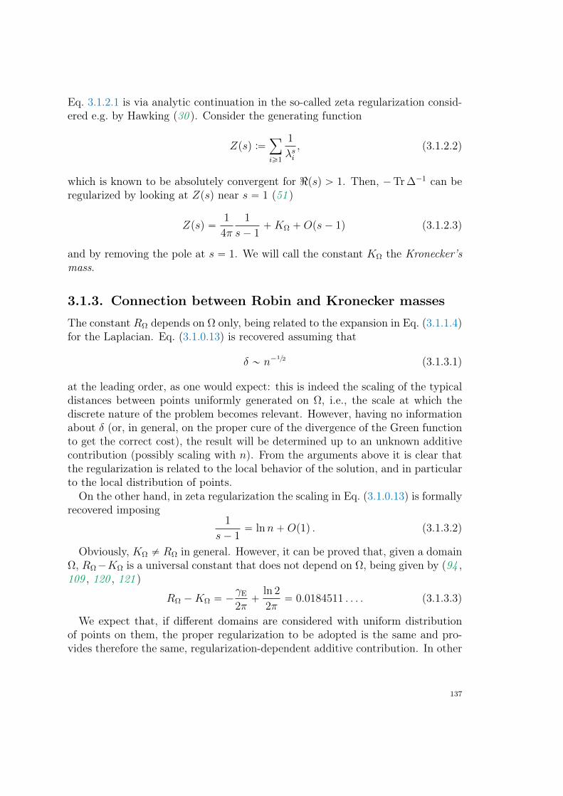
Eq. 3.1.2.1 is via analytic continuation in the so-called zeta regularization consid-ered e.g. by Hawking (30 ). Consider the generating function
Zpsq :“ÿ
iě1
1
λsi, (3.1.2.2)
which is known to be absolutely convergent for <psq ą 1. Then, ´Tr ∆´1 can beregularized by looking at Zpsq near s “ 1 (51 )
Zpsq “1
4π
1
s´ 1`KΩ `Ops´ 1q (3.1.2.3)
and by removing the pole at s “ 1. We will call the constant KΩ the Kronecker’smass.
3.1.3. Connection between Robin and Kronecker masses
The constant RΩ depends on Ω only, being related to the expansion in Eq. (3.1.1.4)for the Laplacian. Eq. (3.1.0.13) is recovered assuming that
δ „ n´12 (3.1.3.1)
at the leading order, as one would expect: this is indeed the scaling of the typicaldistances between points uniformly generated on Ω, i.e., the scale at which thediscrete nature of the problem becomes relevant. However, having no informationabout δ (or, in general, on the proper cure of the divergence of the Green functionto get the correct cost), the result will be determined up to an unknown additivecontribution (possibly scaling with n). From the arguments above it is clear thatthe regularization is related to the local behavior of the solution, and in particularto the local distribution of points.On the other hand, in zeta regularization the scaling in Eq. (3.1.0.13) is formally
recovered imposing1
s´ 1“ lnn`Op1q . (3.1.3.2)
Obviously, KΩ ‰ RΩ in general. However, it can be proved that, given a domainΩ, RΩ´KΩ is a universal constant that does not depend on Ω, being given by (94 ,109 , 120 , 121 )
RΩ ´KΩ “ ´γE
2π`
ln 2
2π“ 0.0184511 . . . . (3.1.3.3)
We expect that, if different domains are considered with uniform distributionof points on them, the proper regularization to be adopted is the same and pro-vides therefore the same, regularization-dependent additive contribution. In other
137
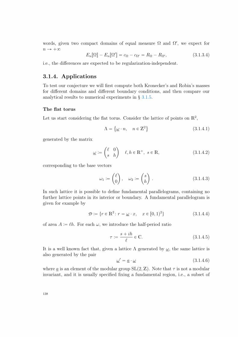
words, given two compact domains of equal measure Ω and Ω1, we expect fornÑ `8
EnrΩs ´ EnrΩ1s “ cΩ ´ cΩ1 “ RΩ ´RΩ1 , (3.1.3.4)
i.e., the differences are expected to be regularization-independent.
3.1.4. ApplicationsTo test our conjecture we will first compute both Kronecker’s and Robin’s massesfor different domains and different boundary conditions, and then compare ouranalytical results to numerical experiments in § 3.1.5.
The flat torus
Let us start considering the flat torus. Consider the lattice of points on R2,
Λ “
ω ¨ n, n P Z2(
(3.1.4.1)
generated by the matrix
ω :“
ˆ
` 0s h
˙
`, h P R`, s P R, (3.1.4.2)
corresponding to the base vectors
ω1 :“
ˆ
`0
˙
, ω2 :“
ˆ
sh
˙
. (3.1.4.3)
In such lattice it is possible to define fundamental parallelograms, containing nofurther lattice points in its interior or boundary. A fundamental parallelogram isgiven for example by
D :“ tr P R2 : r “ ω ¨ x, x P r0, 1q2u (3.1.4.4)
of area A :“ `h. For each ω, we introduce the half-period ratio
τ :“s` ih
`P C. (3.1.4.5)
It is a well known fact that, given a lattice Λ generated by ω, the same lattice isalso generated by the pair
ω1 “ a ¨ ω (3.1.4.6)
where a is an element of the modular group SLp2,Zq. Note that τ is not a modularinvariant, and it is usually specified fixing a fundamental region, i.e., a subset of
138
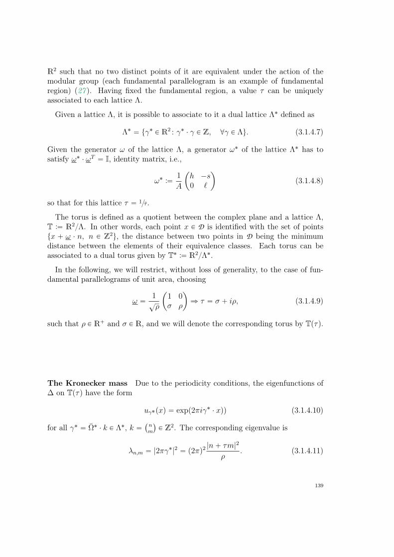
R2 such that no two distinct points of it are equivalent under the action of themodular group (each fundamental parallelogram is an example of fundamentalregion) (27 ). Having fixed the fundamental region, a value τ can be uniquelyassociated to each lattice Λ.
Given a lattice Λ, it is possible to associate to it a dual lattice Λ˚ defined as
Λ˚ “ tγ˚ P R2 : γ˚ ¨ γ P Z, @γ P Λu. (3.1.4.7)
Given the generator ω of the lattice Λ, a generator ω˚ of the lattice Λ˚ has tosatisfy ω˚ ¨ ωT “ I, identity matrix, i.e.,
ω˚ :“1
A
ˆ
h ´s0 `
˙
(3.1.4.8)
so that for this lattice τ “ 1τ.
The torus is defined as a quotient between the complex plane and a lattice Λ,T :“ R2Λ. In other words, each point x P D is identified with the set of pointstx ` ω ¨ n, n P Z2u, the distance between two points in D being the minimumdistance between the elements of their equivalence classes. Each torus can beassociated to a dual torus given by T˚ :“ R2Λ˚.
In the following, we will restrict, without loss of generality, to the case of fun-damental parallelograms of unit area, choosing
ω “1?ρ
ˆ
1 0σ ρ
˙
ñ τ “ σ ` iρ, (3.1.4.9)
such that ρ P R` and σ P R, and we will denote the corresponding torus by Tpτq.
The Kronecker mass Due to the periodicity conditions, the eigenfunctions of∆ on Tpτq have the form
uγ˚pxq “ expp2πiγ˚ ¨ xqq (3.1.4.10)
for all γ˚ “ Ω˚ ¨ k P Λ˚, k “`
nm
˘
P Z2. The corresponding eigenvalue is
λn,m “ |2πγ˚|2“ p2πq2
|n` τm|2
ρ. (3.1.4.11)
139
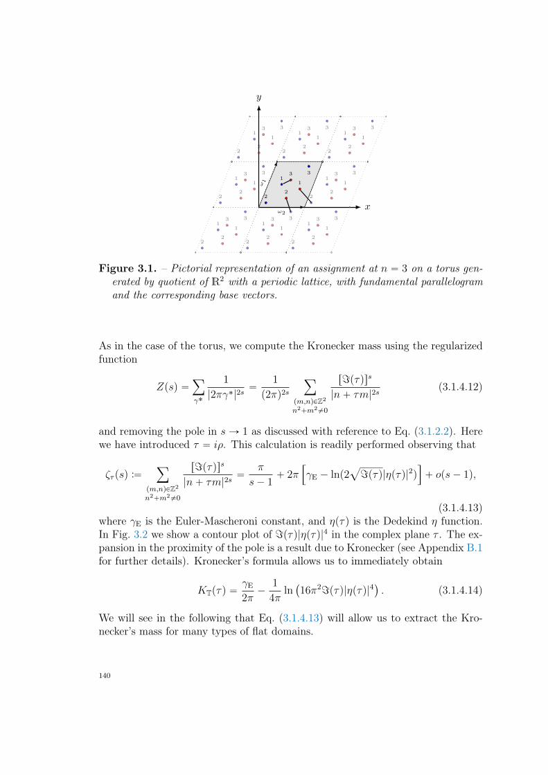
y
x
1
2
3
2
1
31
2
3
2
1
3
1
2
3
2
1
31
2
3
2
1
31
2
3
2
1
3
1
2
3
2
1
31
2
3
2
1
31
2
3
2
1
3
ω1
ω2
1
2
3
2
1
3
Figure 3.1. – Pictorial representation of an assignment at n “ 3 on a torus gen-erated by quotient of R2 with a periodic lattice, with fundamental parallelogramand the corresponding base vectors.
As in the case of the torus, we compute the Kronecker mass using the regularizedfunction
Zpsq “ÿ
γ˚
1
|2πγ˚|2s“
1
p2πq2s
ÿ
pm,nqPZ2
n2`m2‰0
r=pτqss|n` τm|2s
(3.1.4.12)
and removing the pole in sÑ 1 as discussed with reference to Eq. (3.1.2.2). Herewe have introduced τ “ iρ. This calculation is readily performed observing that
ζτ psq :“ÿ
pm,nqPZ2
n2`m2‰0
r=pτqss|n` τm|2s
“π
s´ 1` 2π
”
γE ´ lnp2a
=pτq|ηpτq|2qı
` ops´ 1q,
(3.1.4.13)where γE is the Euler-Mascheroni constant, and ηpτq is the Dedekind η function.In Fig. 3.2 we show a contour plot of =pτq|ηpτq|4 in the complex plane τ . The ex-pansion in the proximity of the pole is a result due to Kronecker (see Appendix B.1for further details). Kronecker’s formula allows us to immediately obtain
KTpτq “γE
2π´
1
4πln`
16π2=pτq|ηpτq|4˘
. (3.1.4.14)
We will see in the following that Eq. (3.1.4.13) will allow us to extract the Kro-necker’s mass for many types of flat domains.
140
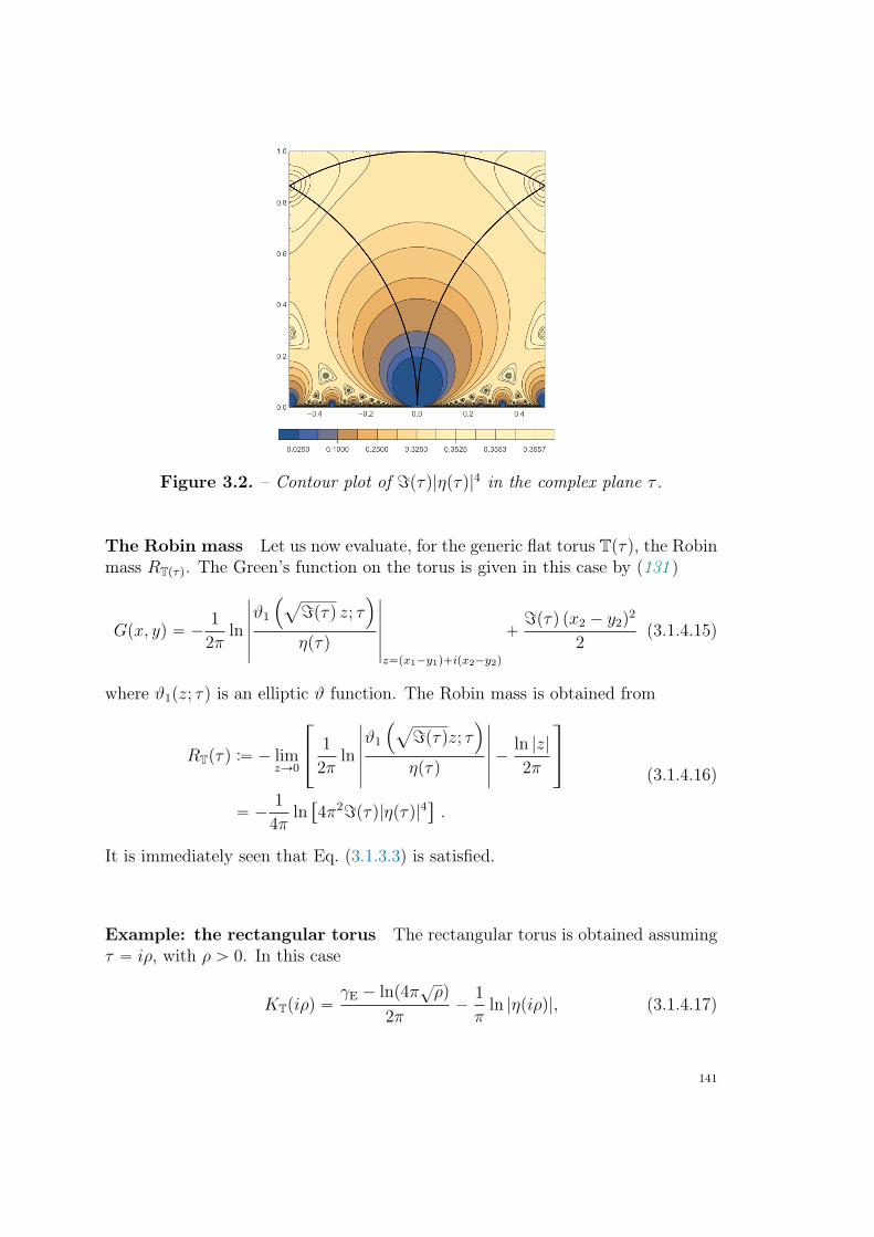
Figure 3.2. – Contour plot of =pτq|ηpτq|4 in the complex plane τ .
The Robin mass Let us now evaluate, for the generic flat torus Tpτq, the Robinmass RTpτq. The Green’s function on the torus is given in this case by (131 )
Gpx, yq “ ´1
2πln
ˇ
ˇ
ˇ
ˇ
ˇ
ˇ
ϑ1
´
a
=pτq z; τ¯
ηpτq
ˇ
ˇ
ˇ
ˇ
ˇ
ˇ
z“px1´y1q`ipx2´y2q
`=pτq px2 ´ y2q
2
2(3.1.4.15)
where ϑ1pz; τq is an elliptic ϑ function. The Robin mass is obtained from
RTpτq :“ ´ limzÑ0
»
–
1
2πln
ˇ
ˇ
ˇ
ˇ
ˇ
ˇ
ϑ1
´
a
=pτqz; τ¯
ηpτq
ˇ
ˇ
ˇ
ˇ
ˇ
ˇ
´ln |z|
2π
fi
fl
“ ´1
4πln“
4π2=pτq|ηpτq|4‰
.
(3.1.4.16)
It is immediately seen that Eq. (3.1.3.3) is satisfied.
Example: the rectangular torus The rectangular torus is obtained assumingτ “ iρ, with ρ ą 0. In this case
KTpiρq “γE ´ lnp4π
?ρq
2π´
1
πln |ηpiρq|, (3.1.4.17)
141
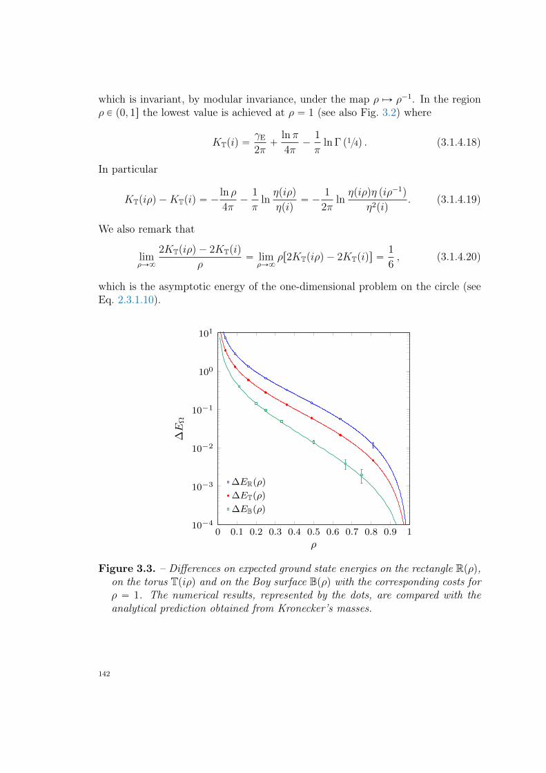
which is invariant, by modular invariance, under the map ρ ÞÑ ρ´1. In the regionρ P p0, 1s the lowest value is achieved at ρ “ 1 (see also Fig. 3.2) where
KTpiq “γE
2π`
ln π
4π´
1
πln Γ p14q . (3.1.4.18)
In particular
KTpiρq ´KTpiq “ ´ln ρ
4π´
1
πlnηpiρq
ηpiq“ ´
1
2πlnηpiρqη piρ´1q
η2piq. (3.1.4.19)
We also remark that
limρÑ8
2KTpiρq ´ 2KTpiq
ρ“ lim
ρÑ8ρr2KTpiρq ´ 2KTpiqs “
1
6, (3.1.4.20)
which is the asymptotic energy of the one-dimensional problem on the circle (seeEq. 2.3.1.10).
0 0.1 0.2 0.3 0.4 0.5 0.6 0.7 0.8 0.9 110−4
10−3
10−2
10−1
100
101
ρ
∆E
Ω
∆ER(ρ)
∆ET(ρ)
∆EB(ρ)
Figure 3.3. – Differences on expected ground state energies on the rectangle Rpρq,on the torus Tpiρq and on the Boy surface Bpρq with the corresponding costs forρ “ 1. The numerical results, represented by the dots, are compared with theanalytical prediction obtained from Kronecker’s masses.
142
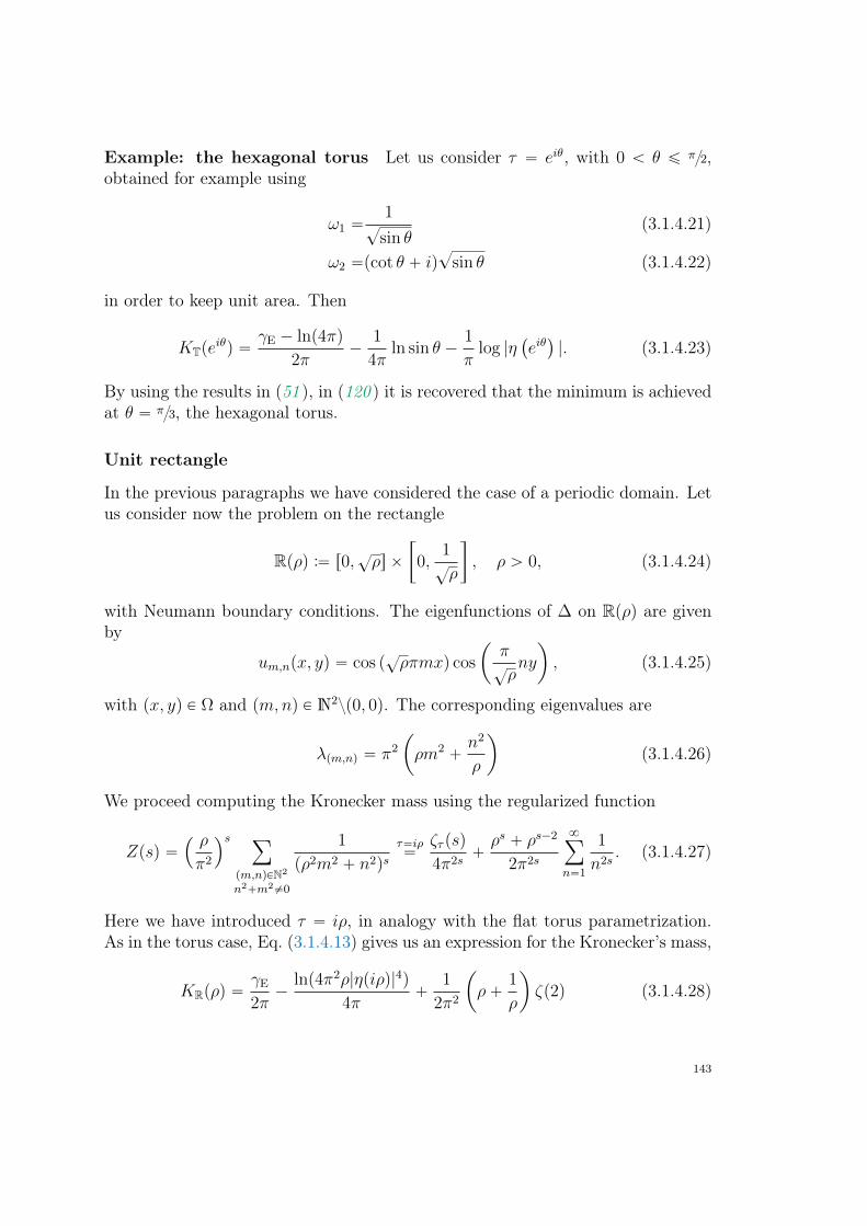
Example: the hexagonal torus Let us consider τ “ eiθ, with 0 ă θ ď π2,obtained for example using
ω1 “1
?sin θ
(3.1.4.21)
ω2 “pcot θ ` iq?
sin θ (3.1.4.22)
in order to keep unit area. Then
KTpeiθq “
γE ´ lnp4πq
2π´
1
4πln sin θ ´
1
πlog |η
`
eiθ˘
|. (3.1.4.23)
By using the results in (51 ), in (120 ) it is recovered that the minimum is achievedat θ “ π3, the hexagonal torus.
Unit rectangle
In the previous paragraphs we have considered the case of a periodic domain. Letus consider now the problem on the rectangle
Rpρq :“ r0,?ρs ˆ
„
0,1?ρ
, ρ ą 0, (3.1.4.24)
with Neumann boundary conditions. The eigenfunctions of ∆ on Rpρq are givenby
um,npx, yq “ cos p?ρπmxq cos
ˆ
π?ρny
˙
, (3.1.4.25)
with px, yq P Ω and pm,nq P N2zp0, 0q. The corresponding eigenvalues are
λpm,nq “ π2
ˆ
ρm2`n2
ρ
˙
(3.1.4.26)
We proceed computing the Kronecker mass using the regularized function
Zpsq “´ ρ
π2
¯s ÿ
pm,nqPN2
n2`m2‰0
1
pρ2m2 ` n2qsτ“iρ“
ζτ psq
4π2s`ρs ` ρs´2
2π2s
8ÿ
n“1
1
n2s. (3.1.4.27)
Here we have introduced τ “ iρ, in analogy with the flat torus parametrization.As in the torus case, Eq. (3.1.4.13) gives us an expression for the Kronecker’s mass,
KRpρq “γE
2π´
lnp4π2ρ|ηpiρq|4q
4π`
1
2π2
ˆ
ρ`1
ρ
˙
ζp2q (3.1.4.28)
143
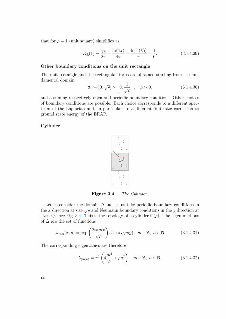
that for ρ “ 1 (unit square) simplifies as
KRp1q “γE
2π`
lnp4πq
4π´
ln Γ p14q
π`
1
6. (3.1.4.29)
Other boundary conditions on the unit rectangle
The unit rectangle and the rectangular torus are obtained starting from the fun-damental domain
D :“ r0,?ρs ˆ
„
0,1?ρ
, ρ ą 0, (3.1.4.30)
and assuming respectively open and periodic boundary conditions. Other choicesof boundary conditions are possible. Each choice corresponds to a different spec-trum of the Laplacian and, in particular, to a different finite-size correction toground state energy of the ERAP.
Cylinder
12
32
1
3
12
32
1
3
12
32
1
3
Figure 3.4. – The Cylinder.
Let us consider the domain D and let us take periodic boundary conditions inthe x direction at size ?ρ and Neumann boundary conditions in the y direction atsize 1
?ρ, see Fig. 3.4. This is the topology of a cylinder Cpρq. The eigenfunctions
of ∆ are the set of functions
um,npx, yq “ exp
ˆ
2iπmx?ρ
˙
cos pπ?ρnyq , m P Z, n P N. (3.1.4.31)
The corresponding eigenvalues are therefore
λpm,nq “ π2
ˆ
4m2
ρ` ρn2
˙
m P Z, n P N. (3.1.4.32)
144
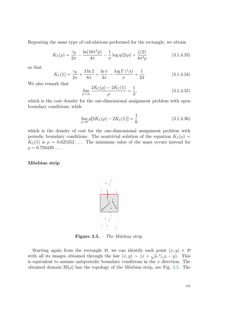
Repeating the same type of calculations performed for the rectangle, we obtain
KCpρq “γE
2π´
lnp16π2ρq
4π´
1
πlog ηp2iρq `
ζp2q
4π2ρ(3.1.4.33)
so thatKCp1q “
γE
2π`
3 ln 2
8π`
lnπ
4π´
log Γ p14q
π`
1
24. (3.1.4.34)
We also remark thatlimρÑ8
2KCpρq ´ 2KCp1q
ρ“
1
3, (3.1.4.35)
which is the cost density for the one-dimensional assignment problem with openboundary conditions, while
limρÑ0
ρr2KCpρq ´ 2KCp1qs “1
6(3.1.4.36)
which is the density of cost for the one-dimensional assignment problem withperiodic boundary conditions. The nontrivial solution of the equation KCpρq “KCp1q is ρ “ 0.625352 . . . . The minimum value of the mass occurs instead forρ “ 0.793439 . . . .
Möebius strip
12
32
1
3
12
32
1
3
12
32
1
3
Figure 3.5. – The Möebius strip.
Starting again from the rectangle D, we can identify each point px, yq P Dwith all its images obtained through the law px, yq „ px `
?ρ, 1
?ρ ´ yq. This
is equivalent to assume antiperiodic boundary conditions in the x direction. Theobtained domain Mpρq has the topology of the Möebius strip, see Fig. 3.5. The
145
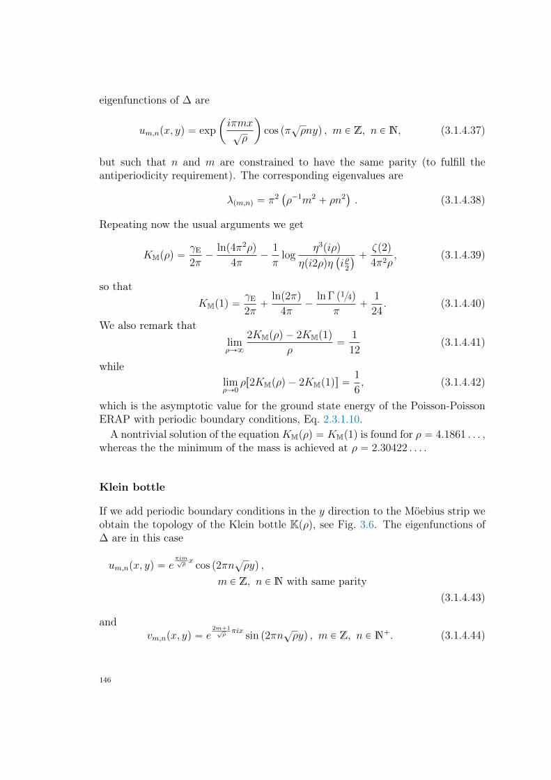
eigenfunctions of ∆ are
um,npx, yq “ exp
ˆ
iπmx?ρ
˙
cos pπ?ρnyq , m P Z, n P N, (3.1.4.37)
but such that n and m are constrained to have the same parity (to fulfill theantiperiodicity requirement). The corresponding eigenvalues are
λpm,nq “ π2`
ρ´1m2` ρn2
˘
. (3.1.4.38)
Repeating now the usual arguments we get
KMpρq “γE
2π´
lnp4π2ρq
4π´
1
πlog
η3piρq
ηpi2ρqη`
iρ2
˘ `ζp2q
4π2ρ, (3.1.4.39)
so thatKMp1q “
γE
2π`
lnp2πq
4π´
ln Γ p14q
π`
1
24. (3.1.4.40)
We also remark thatlimρÑ8
2KMpρq ´ 2KMp1q
ρ“
1
12(3.1.4.41)
whilelimρÑ0
ρr2KMpρq ´ 2KMp1qs “1
6, (3.1.4.42)
which is the asymptotic value for the ground state energy of the Poisson-PoissonERAP with periodic boundary conditions, Eq. 2.3.1.10.A nontrivial solution of the equationKMpρq “ KMp1q is found for ρ “ 4.1861 . . . ,
whereas the the minimum of the mass is achieved at ρ “ 2.30422 . . . .
Klein bottle
If we add periodic boundary conditions in the y direction to the Möebius strip weobtain the topology of the Klein bottle Kpρq, see Fig. 3.6. The eigenfunctions of∆ are in this case
um,npx, yq “ eπim?ρx
cos p2πn?ρyq ,
m P Z, n P N with same parity(3.1.4.43)
andvm,npx, yq “ e
2m`1?ρπix
sin p2πn?ρyq , m P Z, n P N`. (3.1.4.44)
146
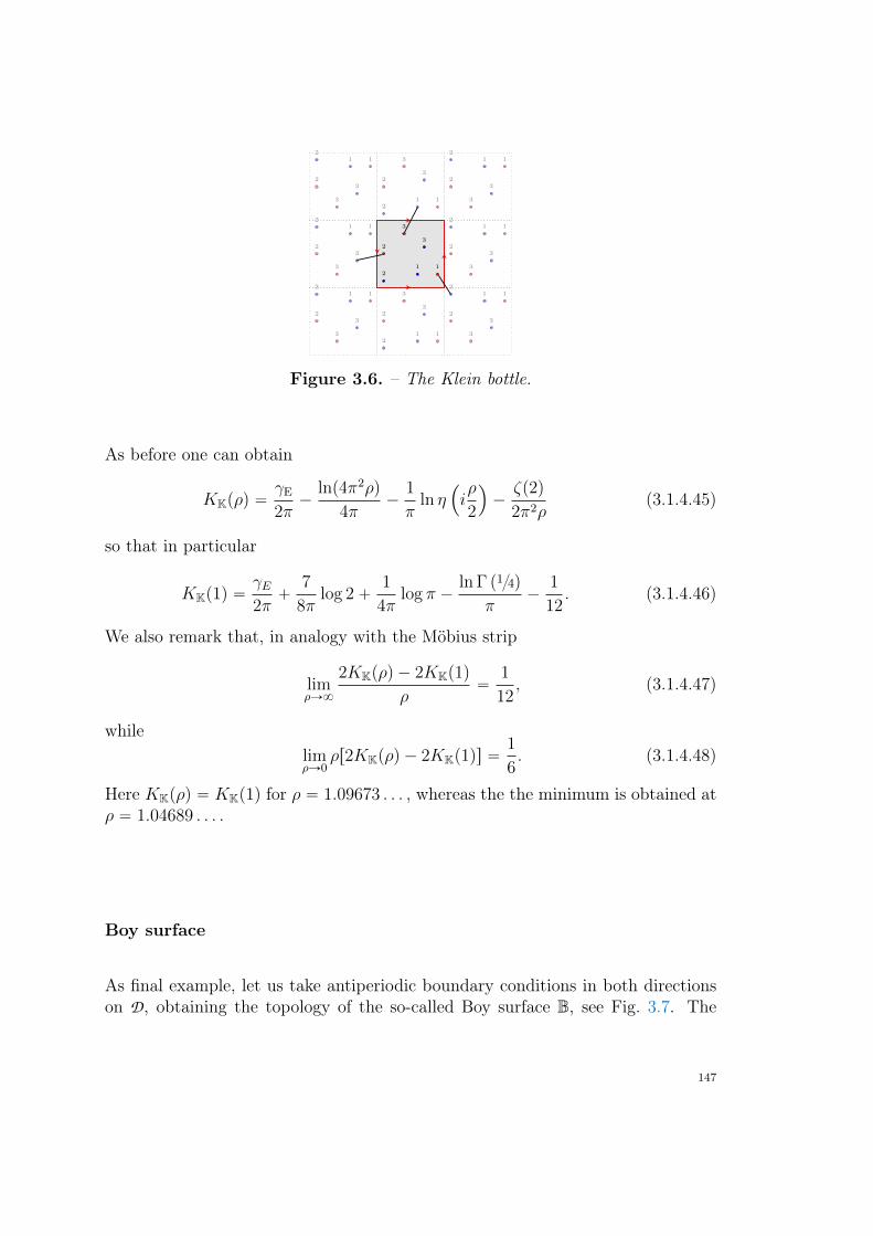
12
32
1
3 12
32
1
3
12
32
1
3
12
32
1
3 12
32
1
3
12
32
1
3
12
32
1
3 12
32
1
3
12
32
1
3
Figure 3.6. – The Klein bottle.
As before one can obtain
KKpρq “γE
2π´
lnp4π2ρq
4π´
1
πln η
´
iρ
2
¯
´ζp2q
2π2ρ(3.1.4.45)
so that in particular
KKp1q “γE2π`
7
8πlog 2`
1
4πlog π ´
ln Γ p14q
π´
1
12. (3.1.4.46)
We also remark that, in analogy with the Möbius strip
limρÑ8
2KKpρq ´ 2KKp1q
ρ“
1
12, (3.1.4.47)
whilelimρÑ0
ρr2KKpρq ´ 2KKp1qs “1
6. (3.1.4.48)
Here KKpρq “ KKp1q for ρ “ 1.09673 . . . , whereas the the minimum is obtained atρ “ 1.04689 . . . .
Boy surface
As final example, let us take antiperiodic boundary conditions in both directionson D, obtaining the topology of the so-called Boy surface B, see Fig. 3.7. The
147
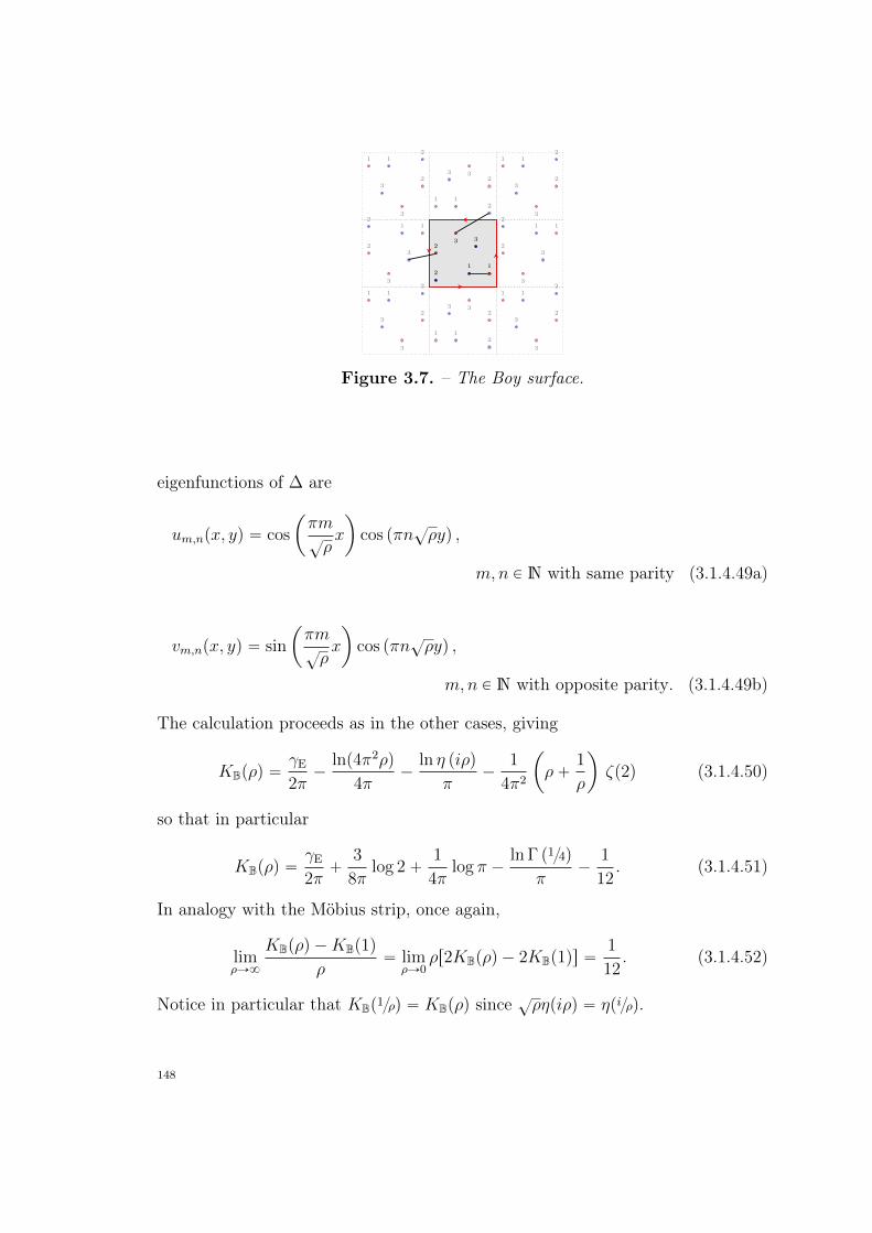
12
32
1
3
12
32
1
3
12
32
1
3
12
32
1
3
12
32
1
3
12
32
1
3
12
32
1
3
12
32
1
3
12
32
1
3
Figure 3.7. – The Boy surface.
eigenfunctions of ∆ are
um,npx, yq “ cos
ˆ
πm?ρx
˙
cos pπn?ρyq ,
m, n P N with same parity (3.1.4.49a)
vm,npx, yq “ sin
ˆ
πm?ρx
˙
cos pπn?ρyq ,
m, n P N with opposite parity. (3.1.4.49b)
The calculation proceeds as in the other cases, giving
KBpρq “γE
2π´
lnp4π2ρq
4π´
ln η piρq
π´
1
4π2
ˆ
ρ`1
ρ
˙
ζp2q (3.1.4.50)
so that in particular
KBpρq “γE
2π`
3
8πlog 2`
1
4πlog π ´
ln Γ p14q
π´
1
12. (3.1.4.51)
In analogy with the Möbius strip, once again,
limρÑ8
KBpρq ´KBp1q
ρ“ lim
ρÑ0ρr2KBpρq ´ 2KBp1qs “
1
12. (3.1.4.52)
Notice in particular that KBp1ρq “ KBpρq since?ρηpiρq “ ηpiρq.
148
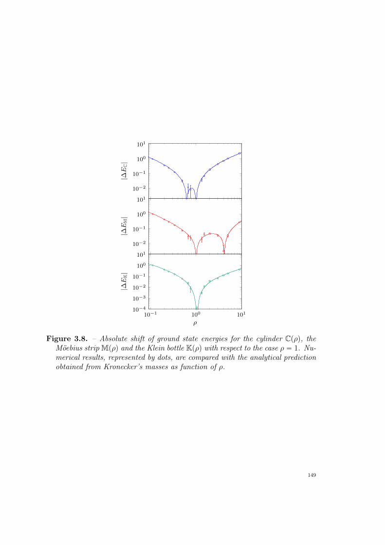
10−2
10−1
100
101
|∆E
C|
10−2
10−1
100
101
|∆E
M|
10−1 100 10110−4
10−3
10−2
10−1
100
101
ρ
|∆E
K|
Figure 3.8. – Absolute shift of ground state energies for the cylinder Cpρq, theMöebius strip Mpρq and the Klein bottle Kpρq with respect to the case ρ “ 1. Nu-merical results, represented by dots, are compared with the analytical predictionobtained from Kronecker’s masses as function of ρ.
149
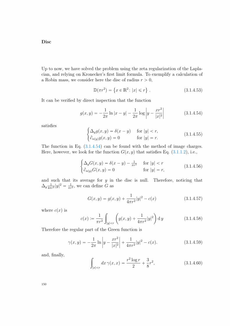
Disc
Up to now, we have solved the problem using the zeta regularization of the Lapla-cian, and relying on Kronecker’s first limit formula. To exemplify a calculation ofa Robin mass, we consider here the disc of radius r ą 0,
Dpπr2q “
x P R2 : |x| ď r(
. (3.1.4.53)
It can be verified by direct inspection that the function
gpx, yq “ ´1
2πln |x´ y| ´
1
2πlog
ˇ
ˇ
ˇ
ˇ
y ´xr2
|x|2
ˇ
ˇ
ˇ
ˇ
(3.1.4.54)
satisfies#
∆ygpx, yq “ δpx´ yq for |y| ă r,
Bnpyqgpx, yq “ 0 for |y| “ r.(3.1.4.55)
The function in Eq. (3.1.4.54) can be found with the method of image charges.Here, however, we look for the function Gpx, yq that satisfies Eq. (3.1.1.2), i.e.,
#
∆yGpx, yq “ δpx´ yq ´ 1πr2 for |y| ă r
BnpyqGpx, yq “ 0 for |y| “ r,(3.1.4.56)
and such that its average for y in the disc is null. Therefore, noticing that∆y
14πr2 |y|
2 “ 1πr2 , we can define G as
Gpx, yq “ gpx, yq `1
4πr2|y|2 ´ cpxq (3.1.4.57)
where cpxq is
cpxq :“1
πr2
ż
|y|ăr
ˆ
gpx, yq `1
4πr2|y|2
˙
d y (3.1.4.58)
Therefore the regular part of the Green function is
γpx, yq “ ´1
2πln
ˇ
ˇ
ˇ
ˇ
y ´xr2
|x|2
ˇ
ˇ
ˇ
ˇ
`1
4πr2|y|2 ´ cpxq. (3.1.4.59)
and, finally,ż
|x|ăr
dx γpx, xq “r2 log r
2`
3
8r2, (3.1.4.60)
150
where we used the fact that c is a radial function, and we repeatedly applied thedivergence Theorem. In particular, the Robin mass for the disc of area 1 is
RD “1
π
ˆ
3
8´
lnπ
4
˙
. (3.1.4.61)
The Kronecker mass is readily obtained using Eq. (3.1.3.3). Observe that theKronecker mass can be also directly estimated using the spectrum of the Laplacianon the disc.
Other surfaces
Unit sphere S2
The transportation problem on the surface of the sphere S2 has already been con-sidered in Ref. (159 ), where the problem of trasporting a uniform mass distributioninto a set of random points on S2 is analized. Here we consider the problem inour usual setting, i.e., a transportation between two atomic measures of randompoints. As in the previous cases, the information on the finite-size corrections ispartially contained in the spectrum of the Laplace-Beltrami operator on the man-ifold. It is well-known that the eigenfunctions of ´∆ on the surface of a sphereof radius r are the spherical harmonics Yl,mpθ, φq with l P N and m P Z with´l ď m ď l. The corresponding eigenvalues are
λl,m “lpl ` 1q
r2with multiplicity 2l ` 1. (3.1.4.62)
By fixing unit area of the surface taking r “ p4πq´12, we proceed using the zetaregularization, i.e., computing
Zpsq “1
p4πqs
ÿ
lě1
2l ` 1
rlpl ` 1qss. (3.1.4.63)
In this case we just recall that for the Riemann zeta function
ζpsq :“ÿ
kě1
1
ks“
1
s´ 1` γE `Ops´ 1q (3.1.4.64)
so that
Zpsq “1
4πps´ 1q´
lnp4πq
4π`γE
2π´
1
4π`Ops´ 1q. (3.1.4.65)
151
The Kronecker mass for the unit sphere is thus
KS2 “ ´lnp4πq
4π`γE
2π´
1
4π. (3.1.4.66)
Projective sphere PS
The real projective sphere PS2 is obtained from the sphere S2 by identificationof antipodal points. The eigenfunctions of the Laplace-Beltrami operator are stillthe spherical harmonics Yl,mpθ, φq with l P N and m P Z, ´l ď m ď l, but wehave to restrict ourselves to eigenfunctions that invariant under the transformationpθ, πq ÞÑ pπ ´ θ, φ ` πq, i.e., to even values of l. Working on the unit-area sphereas before, we get the zeta function
Zpsq “1
p4πqs
ÿ
lě1
4l ` 1
r2lp2l ` 1qss
“1
4πps´ 1q´
lnp2πq
4π`γE
2π´
1
2π`Ops´ 1q (3.1.4.67)
so that the Kronecker’s mass is
KPS2 “ ´lnp2πq
4π`γE2π´
1
2π. (3.1.4.68)
152
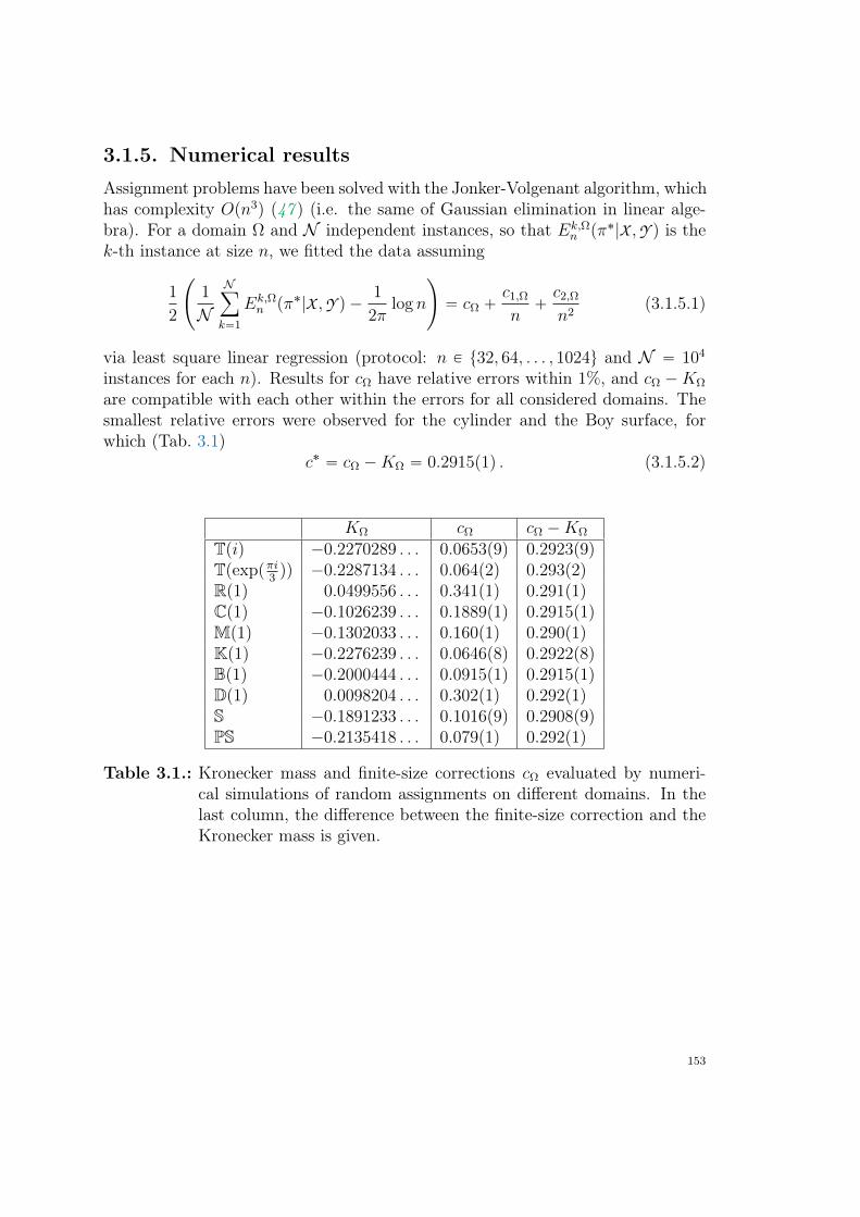
3.1.5. Numerical resultsAssignment problems have been solved with the Jonker-Volgenant algorithm, whichhas complexity Opn3q (47 ) (i.e. the same of Gaussian elimination in linear alge-bra). For a domain Ω and N independent instances, so that Ek,Ω
n pπ˚|X ,Y q is thek-th instance at size n, we fitted the data assuming
1
2
˜
1
NNÿ
k“1
Ek,Ωn pπ˚|X ,Y q ´
1
2πlog n
¸
“ cΩ `c1,Ω
n`c2,Ω
n2(3.1.5.1)
via least square linear regression (protocol: n P t32, 64, . . . , 1024u and N “ 104
instances for each n). Results for cΩ have relative errors within 1%, and cΩ ´KΩ
are compatible with each other within the errors for all considered domains. Thesmallest relative errors were observed for the cylinder and the Boy surface, forwhich (Tab. 3.1)
c˚ “ cΩ ´KΩ “ 0.2915p1q . (3.1.5.2)
KΩ cΩ cΩ ´KΩ
Tpiq ´0.2270289 . . . 0.0653p9q 0.2923p9qTpexppπi
3qq ´0.2287134 . . . 0.064p2q 0.293p2q
Rp1q 0.0499556 . . . 0.341p1q 0.291p1qCp1q ´0.1026239 . . . 0.1889p1q 0.2915p1qMp1q ´0.1302033 . . . 0.160p1q 0.290p1qKp1q ´0.2276239 . . . 0.0646p8q 0.2922p8qBp1q ´0.2000444 . . . 0.0915p1q 0.2915p1qDp1q 0.0098204 . . . 0.302p1q 0.292p1qS ´0.1891233 . . . 0.1016p9q 0.2908p9qPS ´0.2135418 . . . 0.079p1q 0.292p1q
Table 3.1.: Kronecker mass and finite-size corrections cΩ evaluated by numeri-cal simulations of random assignments on different domains. In thelast column, the difference between the finite-size correction and theKronecker mass is given.
153
3.1.6. Uniform–Poisson transportation and grid effects
Up to now, we have considered the transportation between two sets of pointsuniformly generated on the given domain. A related and also interesting problemis the optimal transportation from the uniform measure on Ω to a set of n points(obtained by a Poisson process) on the same domain. We will refer to this problemas to the Uniform–Poisson (UP) problem. The functional approach described inSection 3.1 can be repeated to consider this case, substituting νY pxq with νupxq “ 1and observing then that in this case Erδνpxqδνpxqs “ n´1pδpx ´ yq ´ 1q) †. Thefinal expression for the cost is
EunrΩs “ Tr ∆´1, (3.1.6.1)
that, upon regularization, reads
EunrΩs “
1
4πlnn` cuΩ ` op1q. (3.1.6.2)
The correctness of the leading term coefficient has been proven in Ref. (164 ).Eq. (3.1.6.1) differs from Eq. (3.1.0.12) by an overall factor 2: however, there isno guarantee that cΩ “ cuΩ at fixed Ω as one might naively expect. One intuitivereason is that the nature of the transportation is, at small scale, different in thetwo problems. In Ref. (164 ) it is proved that
cΩ ď cuΩ. (3.1.6.3)
As in the PP case, however, the value of the constant cuΩ is out of the reach of thelinear approximation.One way to numerically approximate the uniform distribution, and then estimate
cuΩ, is to perform an assignment between two sets of points, supposing that oneof them (e.g., the blue ones) is fixed on a grid and not random. We will call thisversion of the problem Grid–Poisson (GP) problem. The approach in Ref. (148 )predicts indeed for this case the same Eq. (3.1.6.1), so that the average optimalcost is
EgnrΩs “
1
4πlnn` cgΩ ` op1q. (3.1.6.4)
with a constant cgΩ ‰ cuΩ. For example, let us consider the case of the unit squarewith n “ L2 and let us take a square grid, in positions L´1 p12` n, 12`mq,n “ 1, . . . , L and m “ 1, . . . , L. In this case, we numerically estimate the constant
†That is, in this variant of the problem the density cross-correlation is halved with respect to thePoisson-Poisson case, in analogy with the discussion about Eq. 2.3.1.9.
154
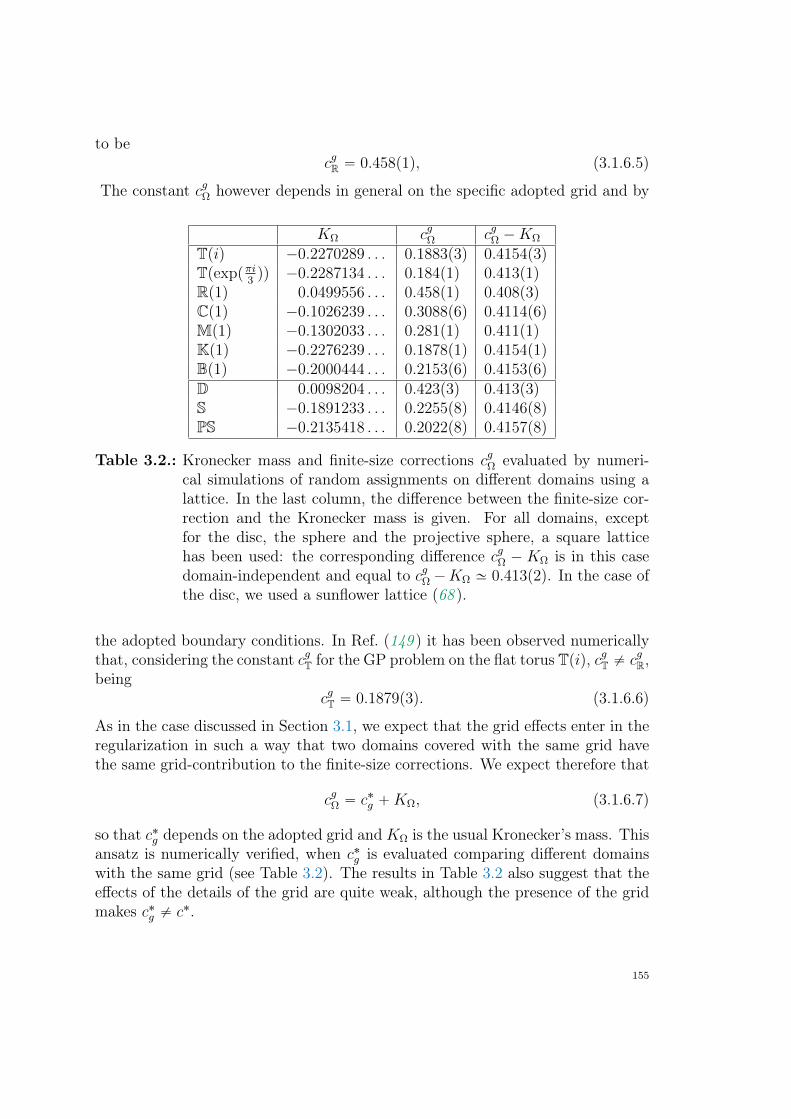
to becgR “ 0.458p1q, (3.1.6.5)
The constant cgΩ however depends in general on the specific adopted grid and by
KΩ cgΩ cgΩ ´KΩ
Tpiq ´0.2270289 . . . 0.1883p3q 0.4154p3qTpexppπi
3qq ´0.2287134 . . . 0.184p1q 0.413p1q
Rp1q 0.0499556 . . . 0.458p1q 0.408p3qCp1q ´0.1026239 . . . 0.3088p6q 0.4114p6qMp1q ´0.1302033 . . . 0.281p1q 0.411p1qKp1q ´0.2276239 . . . 0.1878p1q 0.4154p1qBp1q ´0.2000444 . . . 0.2153p6q 0.4153p6qD 0.0098204 . . . 0.423p3q 0.413p3qS ´0.1891233 . . . 0.2255p8q 0.4146p8qPS ´0.2135418 . . . 0.2022p8q 0.4157p8q
Table 3.2.: Kronecker mass and finite-size corrections cgΩ evaluated by numeri-cal simulations of random assignments on different domains using alattice. In the last column, the difference between the finite-size cor-rection and the Kronecker mass is given. For all domains, exceptfor the disc, the sphere and the projective sphere, a square latticehas been used: the corresponding difference cgΩ ´ KΩ is in this casedomain-independent and equal to cgΩ ´KΩ » 0.413p2q. In the case ofthe disc, we used a sunflower lattice (68 ).
the adopted boundary conditions. In Ref. (149 ) it has been observed numericallythat, considering the constant cgT for the GP problem on the flat torus Tpiq, cgT ‰ cgR,being
cgT “ 0.1879p3q. (3.1.6.6)
As in the case discussed in Section 3.1, we expect that the grid effects enter in theregularization in such a way that two domains covered with the same grid havethe same grid-contribution to the finite-size corrections. We expect therefore that
cgΩ “ c˚g `KΩ, (3.1.6.7)
so that c˚g depends on the adopted grid andKΩ is the usual Kronecker’s mass. Thisansatz is numerically verified, when c˚g is evaluated comparing different domainswith the same grid (see Table 3.2). The results in Table 3.2 also suggest that theeffects of the details of the grid are quite weak, although the presence of the gridmakes c˚g ‰ c˚.
155
As aforementioned, the constants cgΩ are different from cuΩ. However, as intu-itively expected, they provide some information on cuΩ. For example, by classicalconvexity properties of the squared Kantorovich distance, it can be proved that,given n “ L2 and considering a squared Lˆ L grid on the unit flat 2-torus,
cgT ´1
6ď cuT ď cgT. (3.1.6.8)
One can perform a transportation between a grid of cardinality M and a set ofn random points. Proceeding in this way, it can be proved that the GP constantapproaches the UP one for M " n (see (172 ), Appendix A).
3.1.7. Section provisional conclusionsIn this Section we have considered the random assignment problem of two setsof n points on a smooth, two-dimensional manifold Ω of unit area. Within thelinearization framework of the field-theoretical formulation of the problem, wehave studied the asymptotic series of the expected ground state energies beyondthe known leading log n divergence. We have argued that, in the remainder, thefirst Ω-dependent finite size corrections contribute to the constant (in n) part ofthe expected ground state energy. These contributions can been computed exactlyusing zeta-regularization of the trace of the inverse Laplace-Beltrami operator onΩ in several variations. Our analysis, which has been applied to a number ofdifferent manifolds (from the unit square to the projective sphere) suggests thefollowing picture: the remainder “splits” into an Ω independent part, dependingon the choice of local randomness (among the ones considered in this section) andon the choice of grid; and a “geometric” correction depending only on the manifoldΩ, and not on the local choice of randomness or grid. The latter quantity canbe computed either directly as the Kronecker’s mass in zeta regularization, oras a Robin mass from the regular part of the appropriate Green function, thetwo constants differing by a universal constant, as established in a Theorem dueto Morpurgo. Our numerical experiments strongly suggest that, indeed, (withinour computational limitations) the remainder does not diverge with n (while it iscurrently only known that it diverges at most as
?log n log log n (163 )). A further
investigation of such a remainder part (and possibly its limit value in the nÑ 8
limit) is an interesting open question.
156
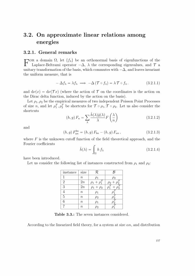
3.2. On approximate linear relations amongenergies
3.2.1. General remarks
For a domain Ω, let tfλu be an orthonormal basis of eigenfunctions of theLaplace-Beltrami operator ´∆, λ the corresponding eigenvalues, and T a
unitary transformation of the basis, which commutes with´∆, and leaves invariantthe uniform measure, that is
´∆fλ “ λfλ ùñ ´∆ pT ˝ fλq “ λ T ˝ fλ . (3.2.1.1)
and dνpxq “ dνpT xq (where the action of T on the coordinates is the action onthe Dirac delta function, induced by the action on the basis).Let ρ1, ρ2 be the empirical measures of two independent Poisson Point Processes
of size n, and let ρT1 , ρT2 be shortcuts for T ˝ ρ1, T ˝ ρ2. Let us also consider theshortcuts
ph, gqFn “ÿ
λ
hpλqgpλq
λF
ˆ
λ
n
˙
(3.2.1.2)
andph, gqF bn
an “ ph, gqFbn ´ ph, gqFan , (3.2.1.3)
where F is the unknown cutoff function of the field theoretical approach, and theFourier coefficients
hpλq “
ż
Ω
h fλ (3.2.1.4)
have been introduced.Let us consider the following list of instances constructed from ρ1 and ρ2:
instance size R B1 n ρ1 ρ2
2 2n ρ1 ` ρT1 ρ2 ` ρ
T2
3 2n ρ1 ` ρ2 ρT1 ` ρT2
4 n ρ1 ρT15 n ρ2 ρT26 n ρ1 ρT27 n ρ2 ρT1
Table 3.3.: The seven instances considered.
According to the linearized field theory, for a system at size αn, and distribution
157
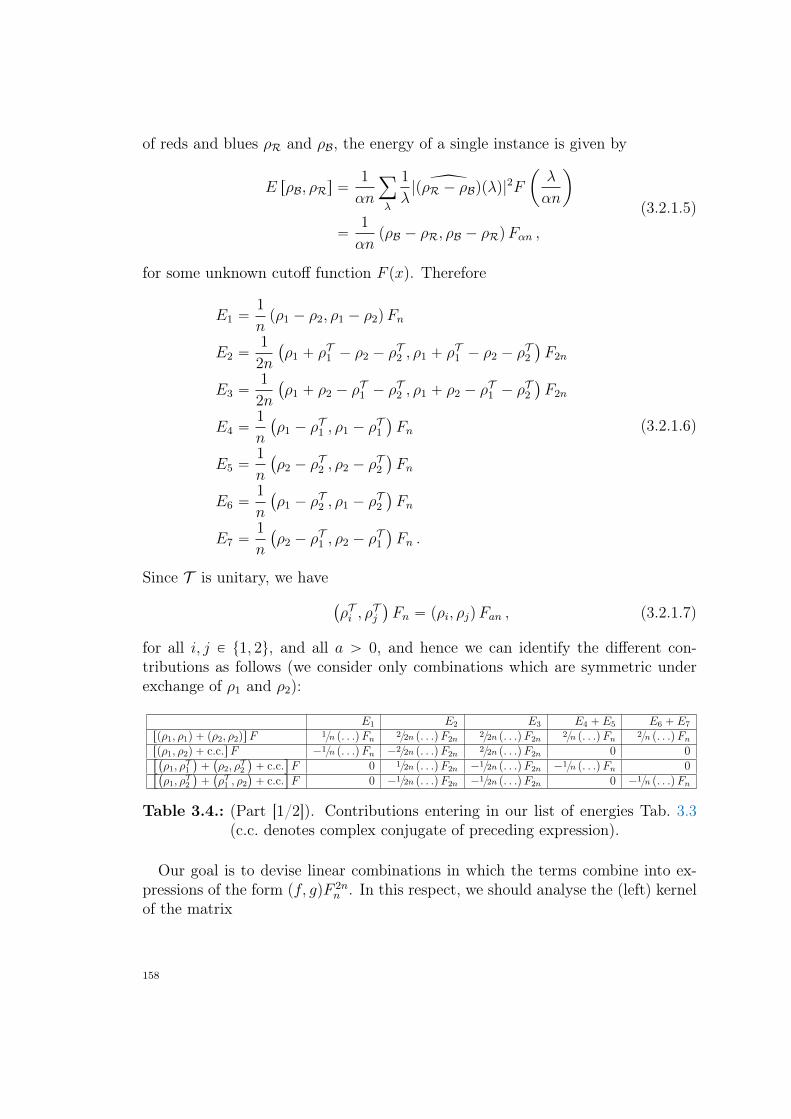
of reds and blues ρR and ρB, the energy of a single instance is given by
E rρB, ρRs “1
αn
ÿ
λ
1
λ| pρR ´ ρBqpλq|
2F
ˆ
λ
αn
˙
“1
αnpρB ´ ρR, ρB ´ ρRqFαn ,
(3.2.1.5)
for some unknown cutoff function F pxq. Therefore
E1 “1
npρ1 ´ ρ2, ρ1 ´ ρ2qFn
E2 “1
2n
`
ρ1 ` ρT1 ´ ρ2 ´ ρ
T2 , ρ1 ` ρ
T1 ´ ρ2 ´ ρ
T2
˘
F2n
E3 “1
2n
`
ρ1 ` ρ2 ´ ρT1 ´ ρ
T2 , ρ1 ` ρ2 ´ ρ
T1 ´ ρ
T2
˘
F2n
E4 “1
n
`
ρ1 ´ ρT1 , ρ1 ´ ρ
T1
˘
Fn
E5 “1
n
`
ρ2 ´ ρT2 , ρ2 ´ ρ
T2
˘
Fn
E6 “1
n
`
ρ1 ´ ρT2 , ρ1 ´ ρ
T2
˘
Fn
E7 “1
n
`
ρ2 ´ ρT1 , ρ2 ´ ρ
T1
˘
Fn .
(3.2.1.6)
Since T is unitary, we have`
ρTi , ρTj
˘
Fn “ pρi, ρjqFan , (3.2.1.7)
for all i, j P t1, 2u, and all a ą 0, and hence we can identify the different con-tributions as follows (we consider only combinations which are symmetric underexchange of ρ1 and ρ2):
E1 E2 E3 E4 ` E5 E6 ` E7
rpρ1, ρ1q ` pρ2, ρ2qsF 1n p. . .qFn 22n p. . .qF2n22n p. . .qF2n
2n p. . .qFn 2n p. . .qFnrpρ1, ρ2q ` c.c.sF ´1n p. . .qFn ´22n p. . .qF2n
22n p. . .qF2n 0 0“`
ρ1, ρT1
˘
``
ρ2, ρT2
˘
` c.c.‰
F 0 12n p. . .qF2n ´12n p. . .qF2n ´1n p. . .qFn 0“`
ρ1, ρT2
˘
``
ρT1 , ρ2
˘
` c.c.‰
F 0 ´12n p. . .qF2n ´12n p. . .qF2n 0 ´1n p. . .qFn
Table 3.4.: (Part [1/2]). Contributions entering in our list of energies Tab. 3.3(c.c. denotes complex conjugate of preceding expression).
Our goal is to devise linear combinations in which the terms combine into ex-pressions of the form pf, gqF 2n
n . In this respect, we should analyse the (left) kernelof the matrix
158
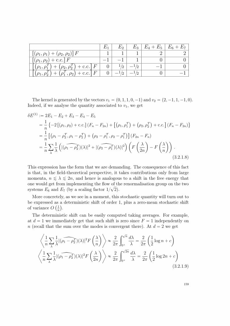
E1 E2 E3 E4 ` E5 E6 ` E7
rpρ1, ρ1q ` pρ2, ρ2qsF 1 1 1 2 2rpρ1, ρ2q ` c.c.sF ´1 ´1 1 0 0“`
ρ1, ρT1
˘
``
ρ2, ρT2
˘
` c.c.‰
F 0 12 ´12 ´1 0“`
ρ1, ρT2
˘
``
ρT1 , ρ2
˘
` c.c.‰
F 0 ´12 ´12 0 ´1
The kernel is generated by the vectors v1 “ p0, 1, 1, 0,´1q and v2 “ p2,´1, 1,´1, 0q.Indeed, if we analyse the quantity associated to v1, we get
δEp1q :“ 2E1 ´ E2 ` E3 ´ E4 ´ E5
“1
n
´2 rpρ1, ρ2q ` c.c.s pFn ´ F2nq `“`
ρ1, ρT1
˘
``
ρ2, ρT2
˘
` c.c.‰
pFn ´ F2nq(
“1
n
“`
ρ1 ´ ρT2 , ρ1 ´ ρ
T2
˘
``
ρ2 ´ ρT1 , ρ2 ´ ρ
T1
˘‰
pF2n ´ Fnq
“1
n
ÿ
λ
1
λ
´
| pρ1 ´ ρT2 qpλq|2` | pρ2 ´ ρT1 qpλq|
2¯
ˆ
F
ˆ
λ
2n
˙
´ F
ˆ
λ
n
˙˙
.
(3.2.1.8)
This expression has the form that we are demanding. The consequence of this factis that, in the field-theoretical perspective, it takes contributions only from largemomenta, n À λ À 2n, and hence is analogous to a shift in the free energy thatone would get from implementing the flow of the renormalisation group on the twosystems E6 and E7 (by a scaling factor 1
?2).
More concretely, as we see in a moment, this stochastic quantity will turn out tobe expressed as a deterministic shift of order 1, plus a zero-mean stochastic shiftof variance O
`
1n
˘
.The deterministic shift can be easily computed taking averages. For example,
at d “ 1 we immediately get that such shift is zero since F “ 1 independently onn (recall that the sum over the modes is convergent there). At d “ 2 we get
C
1
n
ÿ
λ
1
λ| pρ1 ´ ρT2 qpλq|
2F
ˆ
λ
n
˙
G
«2
2π
ż
?n
0`
dλ
λ“
2
2π
ˆ
1
2log n` c
˙
C
1
n
ÿ
λ
1
λ| pρ1 ´ ρT2 qpλq|
2F
ˆ
λ
2n
˙
G
«2
2π
ż
?2n
0`
dλ
λ“
2
2π
ˆ
1
2log 2n` c
˙
(3.2.1.9)
159
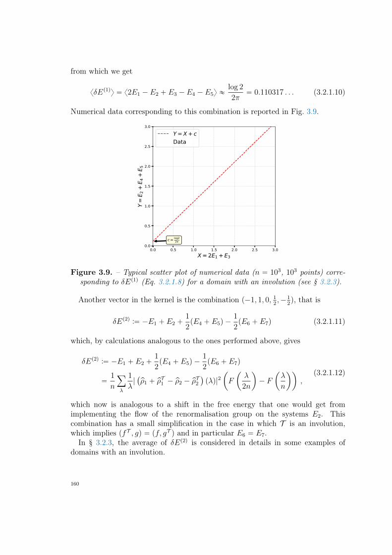
from which we get
xδEp1qy “ x2E1 ´ E2 ` E3 ´ E4 ´ E5y «log 2
2π“ 0.110317 . . . (3.2.1.10)
Numerical data corresponding to this combination is reported in Fig. 3.9.
0.0 0.5 1.0 1.5 2.0 2.5 3.0X = 2E1 + E3
0.0
0.5
1.0
1.5
2.0
2.5
3.0
Y=
E 2+
E 4+
E 5
c = log22
Y = X + cData
Figure 3.9. – Typical scatter plot of numerical data (n “ 103, 103 points) corre-sponding to δEp1q (Eq. 3.2.1.8) for a domain with an involution (see § 3.2.3).
Another vector in the kernel is the combination p´1, 1, 0, 12,´1
2q, that is
δEp2q :“ ´E1 ` E2 `1
2pE4 ` E5q ´
1
2pE6 ` E7q (3.2.1.11)
which, by calculations analogous to the ones performed above, gives
δEp2q :“ ´E1 ` E2 `1
2pE4 ` E5q ´
1
2pE6 ` E7q
“1
n
ÿ
λ
1
λ|`
pρ1 ` pρT1 ´ pρ2 ´ pρT2˘
pλq|2ˆ
F
ˆ
λ
2n
˙
´ F
ˆ
λ
n
˙˙
,(3.2.1.12)
which now is analogous to a shift in the free energy that one would get fromimplementing the flow of the renormalisation group on the systems E2. Thiscombination has a small simplification in the case in which T is an involution,which implies pfT , gq “ pf, gT q and in particular E6 “ E7.In § 3.2.3, the average of δEp2q is considered in details in some examples of
domains with an involution.
160
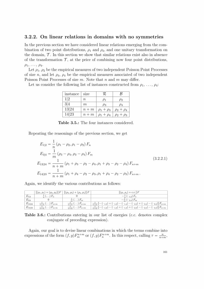
3.2.2. On linear relations in domains with no symmetries
In the previous section we have considered linear relations emerging from the com-bination of two point distributions, ρ1 and ρ2, and one unitary transformation onthe domain, T . In this section we show that similar relations exist also in absenceof the transformation T , at the price of combining now four point distributions,ρ1, . . . , ρ4.Let ρ1, ρ2 be the empirical measures of two independent Poisson Point Processes
of size n, and let ρ3, ρ4 be the empirical measures associated of two independentPoisson Point Processes of size m. Note that n and m may differ.Let us consider the following list of instances constructed from ρ1, . . . , ρ4:
instance size R B1|2 n ρ1 ρ2
3|4 m ρ3 ρ4
13|24 n`m ρ1 ` ρ3 ρ2 ` ρ4
14|23 n`m ρ1 ` ρ4 ρ2 ` ρ3
Table 3.5.: The four instances considered.
Repeating the reasonings of the previous section, we get
E1|2 “1
npρ1 ´ ρ2, ρ1 ´ ρ2qFn
E3|4 “1
mpρ3 ´ ρ4, ρ3 ´ ρ4qFm
E13|24 “1
n`mpρ1 ` ρ3 ´ ρ2 ´ ρ4, ρ1 ` ρ3 ´ ρ2 ´ ρ4qFn`m
E14|23 “1
n`mpρ1 ` ρ4 ´ ρ2 ´ ρ3, ρ1 ` ρ4 ´ ρ2 ´ ρ3qFn`m .
(3.2.2.1)
Again, we identify the various contributions as follows:
rpρ1, ρ1q ` pρ2, ρ2qsF rpρ3, ρ3q ` pρ4, ρ4qsF rpρi, ρjq ` c.c.sF
E1|21np. . .qFn 0 ´ 1
np¨ 1,2qFn
E3|4 0 1mp. . .qFm ´ 1
mp¨ 3,4qFm
E13|241
n`mp. . .qFn`m
1n`m
p. . .qFn`m1
n`mr´ p¨ 1,2q ` p¨ 1,3q ´ p¨ 1,4q ´ p¨ 2,3q ` p¨ 2,4q ´ p¨ 3,4qsFn`m
E14|231
n`mp. . .qFn`m
1n`m
p. . .qFn`m1
n`mr´ p¨ 1,2q ´ p¨ 1,3q ` p¨ 1,4q ` p¨ 2,3q ´ p¨ 2,4q ´ p¨ 3,4qsFn`m
Table 3.6.: Contributions entering in our list of energies (c.c. denotes complexconjugate of preceding expression).
Again, our goal is to devise linear combinations in which the terms combine intoexpressions of the form pf, gqF n`m
m or pf, gqF n`mn . In this respect, calling τ “ n
n`m,
161
we should analyse the (left) kernel of the matrix
E1|21τ
0 ´ 1τ
0 0 0 0 0
E3|4 0 11´τ
0 0 0 0 0 ´ 11´τ
E13|24 1 1 ´1 1 ´1 ´1 1 ´1
E14|23 1 1 ´1 ´1 1 1 ´1 ´1
Now the kernel is generated by a unique vector, p´2τ,´2p1 ´ τq, 1, 1q. Indeed, ifwe analyse the quantity associated to this vector, we get
δEp3q :“ ´2τE1|2 ´ 2p1´ τqE3|4 ` E13|24 ` E14|23
“1
n`m
pρ1 ´ ρ2, ρ1 ´ ρ2qFn`mn ` pρ3 ´ ρ4, ρ3 ´ ρ4qF
n`mm
(
“1
n`m
ÿ
λ
1
λ
„
| pρ1 ´ ρ2qpλq|2
ˆ
F
ˆ
λ
n`m
˙
´ F
ˆ
λ
n
˙˙
`
` | pρ3 ´ ρ4qpλq|2
ˆ
F
ˆ
λ
n`m
˙
´ F
ˆ
λ
m
˙˙
.
(3.2.2.2)
This expression has the form that we are demanding. The consequence of thisfact is that, in the field-theoretical perspective, if both n and m are large, it takescontributions only from large momenta, n,m À λ À n`m, and hence is analogousto a shift in the free energy that one would get from implementing the flow of therenormalisation group on the two systems E1|2 (by a scaling factor
?τ) and E3|4
(by a scaling factor?
1´ τ). And also, yet again, this stochastic quantity willturn out to be expressed as a deterministic shift of order 1 (which is a functionof τ), plus a zero-mean stochastic shift of variance O
`
1n` 1
m
˘
. As previously, thedeterministic shift can be easily computed taking averages, and at d “ 1 is zerosince F “ 1 as the sum over the modes is convergent there. At d “ 2 we get
C
1
n
ÿ
λ
1
λ| pρi ´ ρjqpλq|
2F
ˆ
λ
n
˙
G
«2
2π
ż
?n
0`
dλ
λ“
2
2π
ˆ
1
2log n` c
˙
(3.2.2.3)
from which we have
xδEp3qy “ x´2τE1|2 ´ 2p1´ τqE3|4 ` E13|24 ` E14|23y
«2
2π
„ˆ
1
2logpn`mq ` c
˙
p´2τ ´ 2p1´ τq ` 1` 1q ` τ log τ ` p1´ τq logp1´ τq
“2
2πrτ log τ ` p1´ τq logp1´ τqs
(3.2.2.4)
162
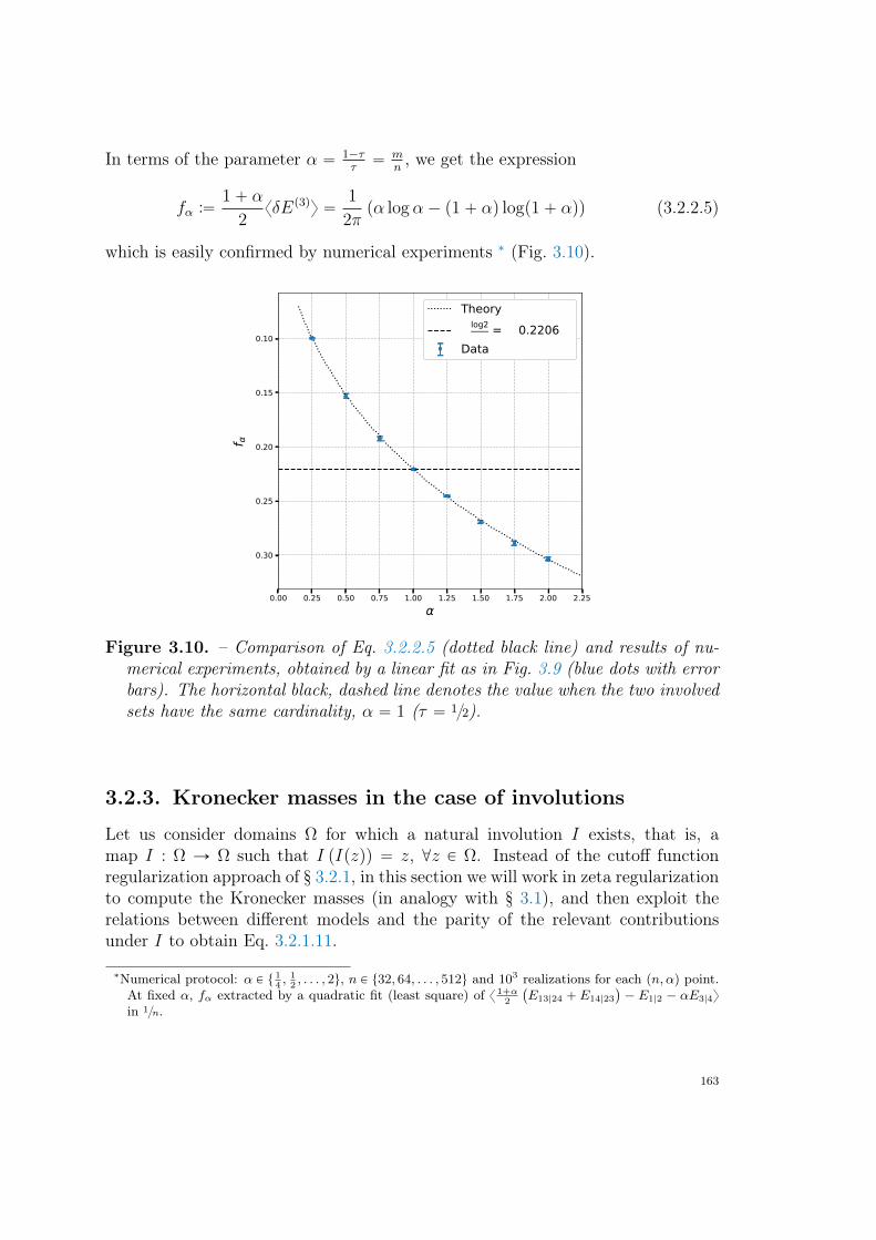
In terms of the parameter α “ 1´ττ“ m
n, we get the expression
fα :“1` α
2xδEp3qy “
1
2πpα logα ´ p1` αq logp1` αqq (3.2.2.5)
which is easily confirmed by numerical experiments ∗ (Fig. 3.10).
0.00 0.25 0.50 0.75 1.00 1.25 1.50 1.75 2.00 2.25α
−0.30
−0.25
−0.20
−0.15
−0.10
f α
Theory−log2
π = −0.2206…Data
Figure 3.10. – Comparison of Eq. 3.2.2.5 (dotted black line) and results of nu-merical experiments, obtained by a linear fit as in Fig. 3.9 (blue dots with errorbars). The horizontal black, dashed line denotes the value when the two involvedsets have the same cardinality, α “ 1 (τ “ 12).
3.2.3. Kronecker masses in the case of involutions
Let us consider domains Ω for which a natural involution I exists, that is, amap I : Ω Ñ Ω such that I pIpzqq “ z, @z P Ω. Instead of the cutoff functionregularization approach of § 3.2.1, in this section we will work in zeta regularizationto compute the Kronecker masses (in analogy with § 3.1), and then exploit therelations between different models and the parity of the relevant contributionsunder I to obtain Eq. 3.2.1.11.
∗Numerical protocol: α P t 14, 1
2, . . . , 2u, n P t32, 64, . . . , 512u and 103 realizations for each pn, αq point.
At fixed α, fα extracted by a quadratic fit (least square) of x 1`α2
`
E13|24 ` E14|23
˘
´ E1|2 ´ αE3|4y
in 1n.
163
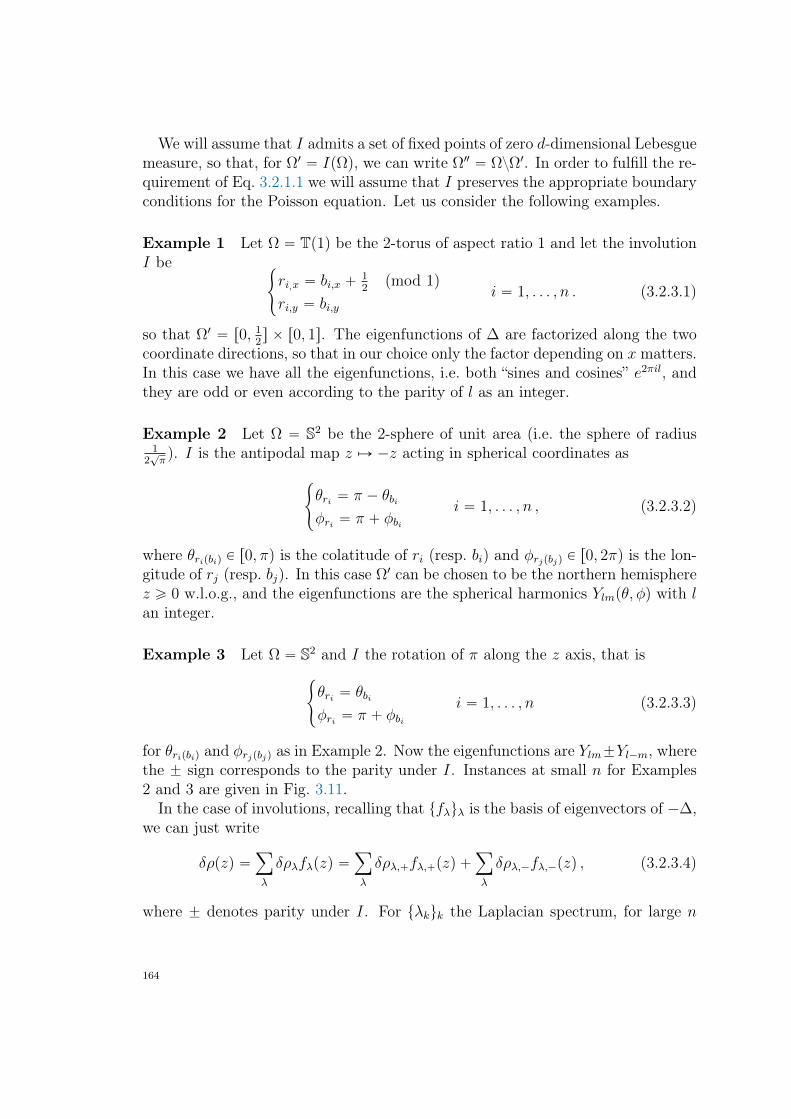
We will assume that I admits a set of fixed points of zero d-dimensional Lebesguemeasure, so that, for Ω1 “ IpΩq, we can write Ω2 “ ΩzΩ1. In order to fulfill the re-quirement of Eq. 3.2.1.1 we will assume that I preserves the appropriate boundaryconditions for the Poisson equation. Let us consider the following examples.
Example 1 Let Ω “ Tp1q be the 2-torus of aspect ratio 1 and let the involutionI be
#
ri,x “ bi,x `12pmod 1q
ri,y “ bi,yi “ 1, . . . , n . (3.2.3.1)
so that Ω1 “ r0, 12s ˆ r0, 1s. The eigenfunctions of ∆ are factorized along the two
coordinate directions, so that in our choice only the factor depending on x matters.In this case we have all the eigenfunctions, i.e. both “sines and cosines” e2πil, andthey are odd or even according to the parity of l as an integer.
Example 2 Let Ω “ S2 be the 2-sphere of unit area (i.e. the sphere of radius1
2?π). I is the antipodal map z ÞÑ ´z acting in spherical coordinates as
#
θri “ π ´ θbiφri “ π ` φbi
i “ 1, . . . , n , (3.2.3.2)
where θripbiq P r0, πq is the colatitude of ri (resp. bi) and φrjpbjq P r0, 2πq is the lon-gitude of rj (resp. bj). In this case Ω1 can be chosen to be the northern hemispherez ě 0 w.l.o.g., and the eigenfunctions are the spherical harmonics Ylmpθ, φq with lan integer.
Example 3 Let Ω “ S2 and I the rotation of π along the z axis, that is#
θri “ θbiφri “ π ` φbi
i “ 1, . . . , n (3.2.3.3)
for θripbiq and φrjpbjq as in Example 2. Now the eigenfunctions are Ylm˘Yl´m, wherethe ˘ sign corresponds to the parity under I. Instances at small n for Examples2 and 3 are given in Fig. 3.11.In the case of involutions, recalling that tfλuλ is the basis of eigenvectors of ´∆,
we can just write
δρpzq “ÿ
λ
δρλfλpzq “ÿ
λ
δρλ,`fλ,`pzq `ÿ
λ
δρλ,´fλ,´pzq , (3.2.3.4)
where ˘ denotes parity under I. For tλkuk the Laplacian spectrum, for large n
164
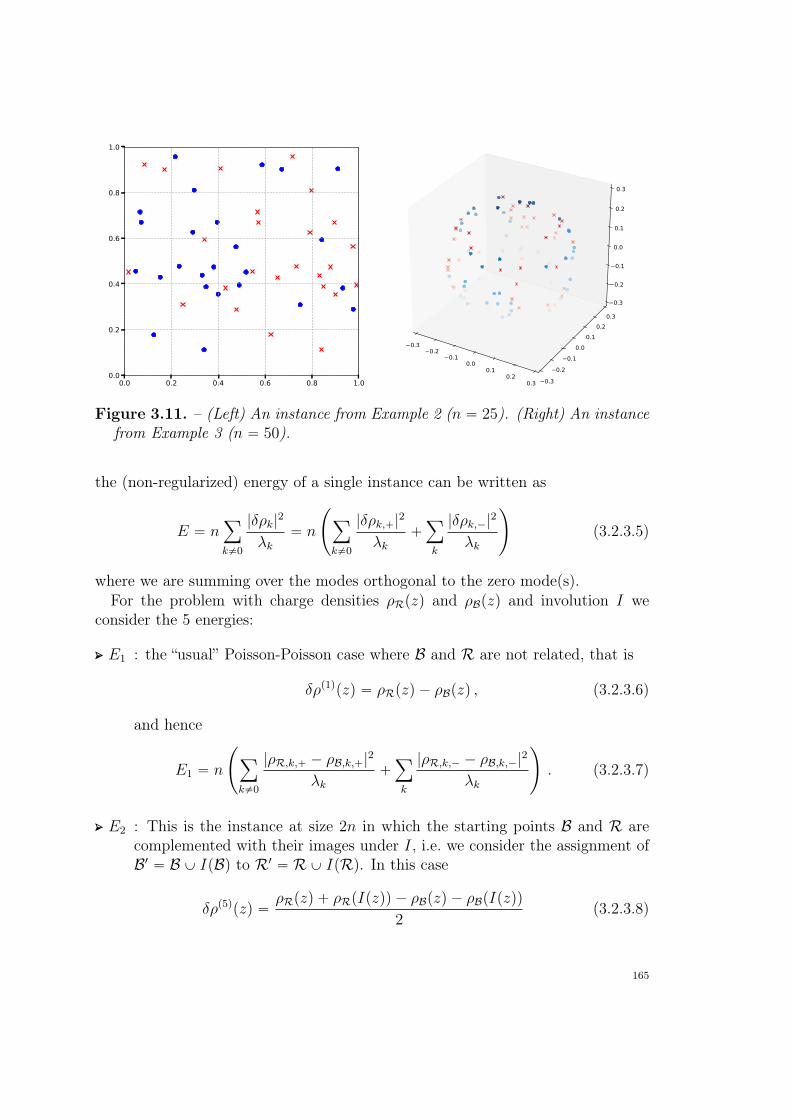
0.0 0.2 0.4 0.6 0.8 1.00.0
0.2
0.4
0.6
0.8
1.0
0.30.2
0.10.0
0.10.2
0.3 0.30.2
0.10.0
0.10.2
0.3
0.3
0.2
0.1
0.0
0.1
0.2
0.3
Figure 3.11. – (Left) An instance from Example 2 (n “ 25). (Right) An instancefrom Example 3 (n “ 50).
the (non-regularized) energy of a single instance can be written as
E “ nÿ
k‰0
|δρk|2
λk“ n
˜
ÿ
k‰0
|δρk,`|2
λk`ÿ
k
|δρk,´|2
λk
¸
(3.2.3.5)
where we are summing over the modes orthogonal to the zero mode(s).For the problem with charge densities ρRpzq and ρBpzq and involution I we
consider the 5 energies:
) E1 : the “usual” Poisson-Poisson case where B and R are not related, that is
δρp1qpzq “ ρRpzq ´ ρBpzq , (3.2.3.6)
and hence
E1 “ n
˜
ÿ
k‰0
|ρR,k,` ´ ρB,k,`|2
λk`ÿ
k
|ρR,k,´ ´ ρB,k,´|2
λk
¸
. (3.2.3.7)
) E2 : This is the instance at size 2n in which the starting points B and R arecomplemented with their images under I, i.e. we consider the assignment ofB1 “ B Y IpBq to R1 “ RY IpRq. In this case
δρp5qpzq “ρRpzq ` ρRpIpzqq ´ ρBpzq ´ ρBpIpzqq
2(3.2.3.8)
165
so that only the even parts under I survive, giving
E2 “ 2nÿ
k‰0
|ρB,k,` ´ ρR,k,`|2
λk. (3.2.3.9)
) E4 : now B are distributed according to ρRpIpzqq, so that
δρp3qpzq “ ρRpzq ´ ρRpIpzqq “ ´δρp3qpIpzqq (3.2.3.10)
is odd under I, and hence
E4 “ 4nÿ
k
|ρR,k,´|2
λk. (3.2.3.11)
) E5 : same as above, but with B Ø R, and hence
E5 “ 4nÿ
k
|ρB,k,´|2
λk. (3.2.3.12)
) E7 : now ρRpzq “ ρRpIpzqq, so that
δρp2qpzq “ ρRpIpzqq ´ ρBpzq (3.2.3.13)
and
E7 “ n
˜
ÿ
k‰0
|ρR,k,` ´ ρB,k,`|2
λk`ÿ
k
|ρR,k,´ ` ρB,k,´|2
λk
¸
. (3.2.3.14)
We remark that E6 “ E7 for an involution.
Example 1
Let us consider first the one dimensional torus, for which flpzq “ e2πilz with l P Z,so that the parity under I is just the parity of l as an integer. We have for theunrestricted sums
xE1y “ xE7y “1
π2
8ÿ
l“1
1
l2“
1
π2ζp2q “
1
6, (3.2.3.15)
166
as is well-known. The sum over the odd modes gives
xE4y “ xE5y “2
π2
8ÿ
l“0
1
p2l ` 1q2“
1
4(3.2.3.16)
while the sum over even modes gives
xE2y “2
π2
8ÿ
l“1
1
p2lq2“
1
12(3.2.3.17)
so that in one dimension we get
@
δEp2qD
“
B
´E1 ` E2 `1
2pE4 ` E5q ´ E7
F
“ ´1
6`
1
12`
1
2
ˆ
1
4`
1
4
˙
´1
6
“´2` 1` 3´ 2
12“ 0
(3.2.3.18)
as expected.
For the two-dimensional torus, recall that the spectral zeta function (Eq. 3.1.4.13)satisfies, at aspect ratio 1,
2ÿ
k‰0
1
λsk“
2
p2πq2s
ÿ
pn,mq‰p0,0q
1
pn2 `m2qs
“8
p2πq2s
8ÿ
n,m“1
1
pn2 `m2qs `
8
p2πq2s
ÿ
lě1
1
l2s
“2
p2πq2s
„
π
s´ 1` 2π
`
γE ´ log 2|ηpiq|2˘
` ops´ 1q
(3.2.3.19)
where η is Dedekind’s function. Therefore, around s “ 1, we get for the unre-stricted sums
xE1y “ xE7y “1
2πps´ 1q`
1
π
“
γE ` log?π ´ 2 log Γp14q
‰
` ops´ 1q (3.2.3.20)
where we can directly read the Kronecker mass. The sum over the odd modes is
8
p2πq2s
8ÿ
n“0
8ÿ
m“1
1
rp2n` 1q2 `m2ss `
4
p2πq2s
8ÿ
l“0
1
p2l ` 1q2s(3.2.3.21)
167
so that, expanding around s “ 1, we get
xE4y “ xE5y “1
2πps´ 1q`
1
π
„
γE `1
2log?
2`1
2log π ´ 2 log Γp12q
` ops´ 1q .
(3.2.3.22)Lastly, the sum over the even modes is
“2
p2πq2s
ÿ
pn,mq‰p0,0q
1
p4n2 `m2qs
“8
p2πq2s
8ÿ
n“1
8ÿ
m“1
1
r4n2 `m2ss `
4
p2πq2s
8ÿ
l“0
1
p2lq2s`
4
p2πq2s
8ÿ
n“1
1
n2s
“21´s
p2πq2s
„
π
s´ 1` 2π
´
γE ´ log p2?
2|ηp2iq|2q¯
` ops´ 1q
(3.2.3.23)
so that near s “ 1 we get
xE2y “1
2πps´ 1q`
1
π
„
γE ´1
2log?
2`1
2log π ´ 2 log Γp14q
` ops´ 1q .
(3.2.3.24)Reminding that at leading order xE2y „
log 2n2π
(since in instance 2 the size is 2n),we just have
xE2y “ xE4y “ xE5y (3.2.3.25)
so that@
δEp2qD
“log 2
2π(3.2.3.26)
as expected.
168
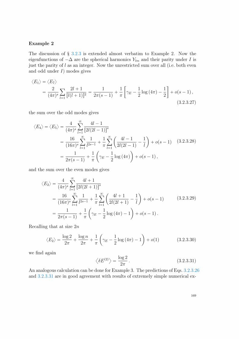
Example 2
The discussion of § 3.2.3 is extended almost verbatim to Example 2. Now theeigenfunctions of ´∆ are the spherical harmonics Ylm and their parity under I isjust the parity of l as an integer. Now the unrestricted sum over all (i.e. both evenand odd under I) modes gives
xE1y “ xE7y
“2
p4πqs
ÿ
l“1
2l ` 1
rlpl ` 1qs2“
1
2πps´ 1q`
1
π
„
γE ´1
2log p4πq ´
1
2
` ops´ 1q ,
(3.2.3.27)
the sum over the odd modes gives
xE4y “ xE5y “4
p4πqs
8ÿ
l“1
4l ´ 1
r2lp2l ´ 1qss
“16
p16πqs
8ÿ
l“1
1
l2s´1`
1
π
8ÿ
l“1
ˆ
4l ´ 1
2lp2l ´ 1q´
1
l
˙
` ops´ 1q
“1
2πps´ 1q`
1
π
ˆ
γE ´1
2log p4πq
˙
` ops´ 1q ,
(3.2.3.28)
and the sum over the even modes gives
xE2y “4
p4πqs
8ÿ
l“1
4l ` 1
r2lp2l ` 1qss
“16
p16πqs
8ÿ
l“1
1
l2s´1`
1
π
8ÿ
l“1
ˆ
4l ` 1
2lp2l ` 1q´
1
l
˙
` ops´ 1q
“1
2πps´ 1q`
1
π
ˆ
γE ´1
2log p4πq ´ 1
˙
` ops´ 1q .
(3.2.3.29)
Recalling that at size 2n
xE2y “log 2
2π`
log n
2π`
1
π
ˆ
γE ´1
2log p4πq ´ 1
˙
` op1q (3.2.3.30)
we find again@
δEp2qD
“log 2
2π. (3.2.3.31)
An analogous calculation can be done for Example 3. The predictions of Eqs. 3.2.3.26and 3.2.3.31 are in good agreement with results of extremely simple numerical ex-
169
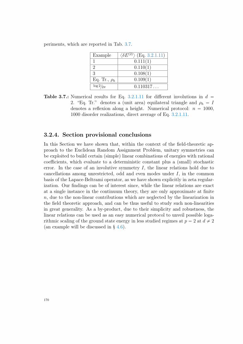
periments, which are reported in Tab. 3.7.
Example xδEp2qy (Eq. 3.2.1.11)1 0.111p1q2 0.110p1q3 0.108p1qEq. Tr., ρh 0.109p1qlog 22π 0.110317 . . .
Table 3.7.: Numerical results for Eq. 3.2.1.11 for different involutions in d “2. “Eq. Tr.” denotes a (unit area) equilateral triangle and ρh “ Idenotes a reflexion along a height. Numerical protocol: n “ 1000,1000 disorder realizations, direct average of Eq. 3.2.1.11.
3.2.4. Section provisional conclusionsIn this Section we have shown that, within the context of the field-theoretic ap-proach to the Euclidean Random Assignment Problem, unitary symmetries canbe exploited to build certain (simple) linear combinations of energies with rationalcoefficients, which evaluate to a deterministic constant plus a (small) stochasticerror. In the case of an involutive symmetry I, the linear relations hold due tocancellations among unrestricted, odd and even modes under I, in the commonbasis of the Lapace-Beltrami operator, as we have shown explicitly in zeta regular-ization. Our findings can be of interest since, while the linear relations are exactat a single instance in the continuum theory, they are only approximate at finiten, due to the non-linear contributions which are neglected by the linearization inthe field theoretic approach, and can be thus useful to study such non-linearitiesin great generality. As a by-product, due to their simplicity and robustness, thelinear relations can be used as an easy numerical protocol to unveil possible loga-rithmic scaling of the ground state energy in less studied regimes at p “ 2 at d ‰ 2(an example will be discussed in § 4.6).
170
3.3. The Lattice Helmholtz decomposition of thetransport field on T2 at p “ 2
In the previous Section we have considered the ERAP for several two dimen-sional compact geometries and discussed a persistence of universality beyond
the leading asymptotics by considering a functional analytical and a zeta regular-ization of the logarithmically divergent ground state energy. Among other things,we have shown that the relative ground state energies for domains with rectan-gular fundamental polygons at varying aspect ratios are given exactly in terms ofcertain logarithmic ratios of the Dedekind η function (provided the domains havethe same area). However, the overall constant, common to all these domains, can-not be determined with the methods of the previous sections, and remains elusive(we cannot even exclude that it is not a constant, but rather a slowly-increasingfunction of n).In this Section we wish to investigate further the grid-regularization approach.
Somehow in analogy with § 2.3, we will set aside continuum methods and discussa lattice statistical field theory approach to this problem, with an emphasis onthe statistical properties of the optimal transport field and its Fourier modes.After introducing the appropriate formalism (the one of lattice calculus, aspectsuseful for our discussion are reported in Appendix C.1), one can work out someconsequences of the theory which appear to not be easily accessible by continuummethods. However one is left with the task of understanding the scaling limitof the theory, as it is non-obvious a priori if expectations of relevant observables(such as the ground state energy) depend on the particular lattice chosen, anaspect that we shall discuss elsewhere. More generally, the sub-leading, constantterm is not accessible to the linearized field theoretical approach, whose Euler-Lagrange equations give the optimal transport field as µ “ ∇φ, or equivalently,only a divergence part is present. Therefore, here we start to study the correctionto the linearized theory perturbatively, in which φ also admits a curl part, in thehope that this approach will help clarifying aspects inaccessible to the linearizedtheory.For this reason, in this Section we shall start this endeavor by considering the
simplest possible case, namely, the two dimensional Grid-Poisson ERAP with pe-riodic conditions (or on T2), in which e.g. the blue points sit on a regular squaregrid. Here, Fourier Duality at p “ 2 and the well-known self-duality of the squarelattice at d “ 2 imply considerable simplifications of the theory. A guiding prin-ciple in our discussion is the notion of a natural “change of variables” on the 2ndegrees of freedom of the field. The change of variable, which is inspired by elec-trodynamics, consists in decomposing the optimal transport field (which is definedon the direct lattice) as a sum of appropriate longitudinal and transverse part,
171
namely, “derivatives” of potentials (which are defined on the dual lattice). The de-composition is the analogue of the Helmholtz decomposition in electrodynamics,where an electric field can be written as the sum of a conservative and a solenoidalpart. In particular, we shall elucidate some statistical properties of the latticelaplacians of both potentials, both in coordinate and momentum representations,which turn out to be very different. Then we shall study their Fourier modes andreport numerical evidence that their contributions to the (unknown) asymptoticseries of the expected ground state energy are at different orders in n.
3.3.1. Setup and notations
Let us consider the Grid-Poisson ERAP on the flat two dimensional torus T2, thatis, for n “ L2 and L an integer, blues B “ tbiuni“1 sit on a LˆL square grid whichcan be chosen by translation invariance to be
Λn “
"
0,1
L, . . . , 1´
1
L
*
ˆ
"
0,1
L, . . . , 1´
1
L
*
, (3.3.1.1)
where ˆ denotes Cartesian product. Reds are Poisson, that is R “ triuni“1 is a
family of i.i. random variables uniformly distributed on the unit square Q2. Thedual lattice is obtained by translating rigidly Λn by p12L, 12Lq, that is
Λn :“
"
1
2L,
3
2L, . . . , 1´
1
2L
*
ˆ
"
1
2L,
3
2L, . . . , 1´
1
2L
*
. (3.3.1.2)
We impose periodic boundary conditions so that the squared distance betweentwo points z1 “ pz1,x, z1,yq and z2 “ pz2,x, z2,yq is
D2T2pz1, z2q “ rmin p|z1,x ´ z2,x|, 1´ |z1,x ´ z2,x|qs
2`rmin p|z1,y ´ z2,y|, 1´ |z1,y ´ z2,y|qs
2 .(3.3.1.3)
At fixed disorder R, the nˆ n assignment cost matrix is thus
cp2qkl :“ D2
T2pbk, rlq, k, l “ 1, . . . n, (3.3.1.4)
so that the energy of a microscopic configuration is just
Hpπq :“nÿ
k“1
cp2qkπpkq (3.3.1.5)
for a permutation π. As usual, a πopt satisfies
Hopt :“ Hpπoptq “ minπPSn
Hpπq . (3.3.1.6)
172
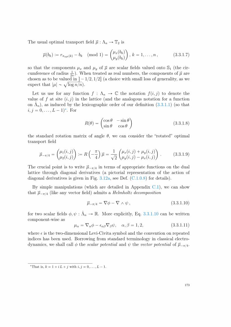
The usual optimal transport field áµ : Λn Ñ T2 is
áµpbkq :“ rπoptpkq ´ bk pmod 1q “
ˆ
µxpbkqµypbkq
˙
, k “ 1, . . . , n , (3.3.1.7)
so that the components µx and µy of áµ are scalar fields valued onto S1 (the cir-cumference of radius 1
2π). When treated as real numbers, the components of áµ are
chosen as to be valued in s´ 12, 12s (a choice with small loss of generality, as weexpect that |µ| „
a
log nn).
Let us use for any function f : Λn Ñ C the notation fpi, jq to denote thevalue of f at site pi, jq in the lattice (and the analogous notation for a functionon Λn), as induced by the lexicographic order of our definition (3.3.1.1) (so thati, j “ 0, . . . , L´ 1)∗. For
Rpθq “
ˆ
cos θ ´ sin θsin θ cos θ
˙
(3.3.1.8)
the standard rotation matrix of angle θ, we can consider the “rotated” optimaltransport field
áµ´π4 “
ˆ
µ1pi, jqµ2pi, jq
˙
:“ R´
´π
4
¯
áµ “1?
2
ˆ
µxpi, jq ` µypi, jqµypi, jq ´ µxpi, jq
˙
. (3.3.1.9)
The crucial point is to write áµ´π4 in terms of appropriate functions on the duallattice through diagonal derivatives (a pictorial representation of the action ofdiagonal derivatives is given in Fig. 3.12a, see Def. (C.1.0.8) for details).
By simple manipulations (which are detailed in Appendix C.1), we can showthat áµ´π4 (like any vector field) admits a Helmholtz decomposition
áµ´π4 “ ∇φ´∇^ ψ , (3.3.1.10)
for two scalar fields φ, ψ : Λn Ñ R. More explicitly, Eq. 3.3.1.10 can be writtencomponent-wise as
µα “ ∇αφ´ εαβ∇βψ, α, β “ 1, 2, (3.3.1.11)
where ε is the two-dimensional Levi-Civita symbol and the convention on repeatedindices has been used. Borrowing from standard terminology in classical electro-dynamics, we shall call φ the scalar potential and ψ the vector potential of áµ´π4.
∗That is, k “ 1` i L` j with i, j “ 0, . . . , L´ 1.
173
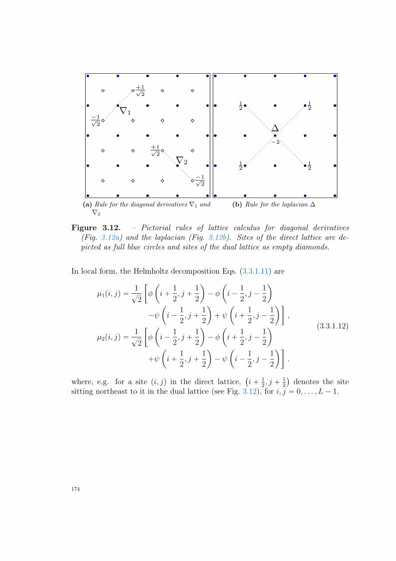
∇1
+1√2
−1√2
∇2
+1√2
−1√2
(a) Rule for the diagonal derivatives ∇1 and∇2
∆
12
12
12
12
−2
(b) Rule for the laplacian ∆
Figure 3.12. – Pictorial rules of lattice calculus for diagonal derivatives(Fig. 3.12a) and the laplacian (Fig. 3.12b). Sites of the direct lattice are de-picted as full blue circles and sites of the dual lattice as empty diamonds.
In local form, the Helmholtz decomposition Eqs. (3.3.1.11) are
µ1pi, jq “1?
2
„
φ
ˆ
i`1
2, j `
1
2
˙
´ φ
ˆ
i´1
2, j ´
1
2
˙
´ψ
ˆ
i´1
2, j `
1
2
˙
` ψ
ˆ
i`1
2, j ´
1
2
˙
,
µ2pi, jq “1?
2
„
φ
ˆ
i´1
2, j `
1
2
˙
´ φ
ˆ
i`1
2, j ´
1
2
˙
`ψ
ˆ
i`1
2, j `
1
2
˙
´ ψ
ˆ
i´1
2, j ´
1
2
˙
.
(3.3.1.12)
where, e.g. for a site pi, jq in the direct lattice,`
i` 12, j ` 1
2
˘
denotes the sitesitting northeast to it in the dual lattice (see Fig. 3.12), for i, j “ 0, . . . , L´ 1.
174
3.3.2. Longitudinal and transverse contributions to theground state energy Hopt
In continuing to pursue the analogy with the local formulation of electrodynamicsin terms of potentials, one is tempted to take derivatives of the Helmholtz decom-position for áµ´π
4, Eq. (3.3.1.11). This task, which is standard in the continuum,
is not straightforwardly accomplished on the lattice if one uses the standard dis-crete directional derivatives, as fields and potentials cannot be defined on the samespace in the discrete setting. This fact was among our motivations for introducingdiagonal derivatives (Eq. (C.1.0.9)).
Let us recall the divergence and curl of a vector field áE : ΛnpΛnq Ñ T2
∇ ¨ áE “∇αEα ,
∇^áE “ εαβ∇αEβ, pα, β “ 1, 2q .(3.3.2.1)
Taking the divergence (resp., the curl) of both sides in the Helmholtz decomposi-tion 3.3.1.10 for áµ´π
4, by simple manipulation (e.g. specialize Eq. (C.1.0.12) to φ
and ψ) we just get
∇ ¨ áµ´π4 “ ∇αµα “∆φ,
∇^ áµ´π4 “ εαβ∇αµβ “∆ψ ,(3.3.2.2)
where also the laplacian is a lattice laplacian, more precisely it is the diagonallattice laplacian described in Appendix C.1, and here depicted in Fig. 3.12b. Atthis point, using (3.3.2.2) and straightforward lattice calculus computations (whichare recalled for convenience in Appendix C.1), we can separate the ground stateenergy Hopt (Eq. (3.3.1.6)) into a sum of two contributions, as
Hopt “ páµ,áµq “ páµ´π4,áµ´π4q “ “ p∇αφ´ εαβ∇βψ, µαq
“ ´pφ,∇αµαq ´ pψ, εαβ∇αµβq
“ ´pφ,∆φq ´ pψ,∆ψq
“ Hpφq`Hpψq .
(3.3.2.3)
Borrowing terminology from classical electrodynamics, we shall callHpφq :“ ´pφ,∆φqand Hpψq :“ ´pψ,∆ψq, respectively, the longitudinal and transverse contributionsto the ground state energy Hopt. We remark that such a decomposition, as theanalogue decomposition in continuum electrodynamics, is independent on the dis-order distribution, in the same manner as Maxwell’s equations are valid for anydistribution of charges. Everything we have discussed up to now is indeed validbeyond our current choice of red points uniformly distributed on the domain, and
175
in fact can be performed for any lattice vector field µ, even if it does not correspondto the optimal transport field of an ERAP.
3.3.3. Synthesis of results
In the following we shall introduce “the charges”, and namely, we will study somestatistical properties of the scalar fields ∆φ and ∆ψ (and hence φ and ψ uponinversion of the lattice laplacian), both in coordinate and momentum representa-tions, in the special case of R uniformly distributed on the torus. We will showthat upon simple rescaling and translation ∆φ is log-normally distributed, while∆ψ is gaussian, and give numerical estimates for their two point-correlation func-tions. Afterwards, we will go to Fourier space and estimate the large n limit ofexpected longitudinal and transverse contributions
Enpφq :“@
HpφqD
,
Enpψq :“@
HpψqD (3.3.3.1)
which will turn out to be of qualitatively different nature (and quantitativelydifferent order of magnitudes) inside the asymptotic expansion for the expectedtotal ground state energy En :“ xHopty. In particular, we shall discuss their relativecontribution to Eq. 3.1.6.4 for Ω “ Tp1q, namely
En “1
4πlog n` c0 `O
ˆ
1
n
˙
“ Enpφq ` Enpψq (3.3.3.2)
where the constant c0 is estimated∗ “directly” (Fig. 3.13) to c0 “ 0.1875p4q, inagreement with 0.1879p3q of previous numerical studies (see (149 ), Eq. 60).
3.3.4. Statistical properties of ∆φ and ∆ψ in coordinaterepresentation
Independently on n “ L2, the empirical histograms of L∆φ` 2 can be reasonablydescribed by a lognormal distribution (Fig. 3.14, top); the histograms for L∆ψare well described by a single, centered gaussian (Fig. 3.14, bottom) of standarddeviation σ “ 0.6349p1q (obtained by bootstrapping).
Observation 3.3.1. ∆φ and ∆ψ appear to satisfy the inequality (Fig. 3.15)
L p|∆ψ| ´∆φq ď 2 (3.3.4.1)
∗Numerical protocol: n P t64, 144, 256, 400, 576, 784, 1444, 2116u, 104 realisations for each n.
176
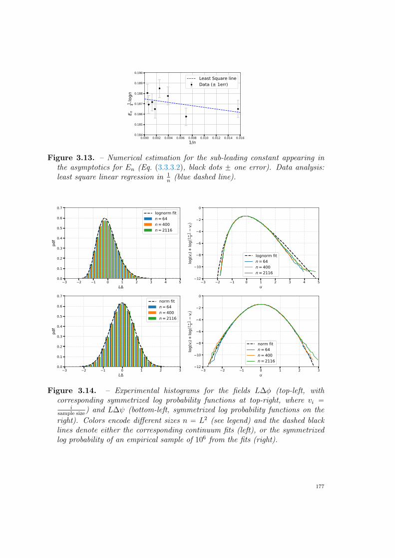
0.000 0.002 0.004 0.006 0.008 0.010 0.012 0.014 0.0161/n
0.184
0.185
0.186
0.187
0.188
0.189
0.190
E n−
1 4πlogn
Least Square lineData (± 1err)
Figure 3.13. – Numerical estimation for the sub-leading constant appearing inthe asymptotics for En (Eq. (3.3.3.2), black dots ˘ one error). Data analysis:least square linear regression in 1
n(blue dashed line).
−3 −2 −1 0 1 2 3 4 5LΔϕ
0.0
0.1
0.2
0.3
0.4
0.5
0.6
0.7
lognormΔfitn=64n=400n=2116
−3 −2 −1 0 1 2 3 4 5u
−12
−10
−8
−6
−4
−2
0
log(v i)+
log (
s+1
s−v i)
lognormΔfitn=64n=400n=2116
−3 −2 −1 0 1 2 3LΔψ
0.0
0.1
0.2
0.3
0.4
0.5
0.6
0.7
normΔfitn=64n=400n=2116
−3 −2 −1 0 1 2 3u
−12
−10
−8
−6
−4
−2
0
log(v i)+
log (
s+1
s−v i)
normΔfitn=64n=400n=2116
Figure 3.14. – Experimental histograms for the fields L∆φ (top-left, withcorresponding symmetrized log probability functions at top-right, where vi “
isample size
) and L∆ψ (bottom-left, symmetrized log probability functions on theright). Colors encode different sizes n “ L2 (see legend) and the dashed blacklines denote either the corresponding continuum fits (left), or the symmetrizedlog probability of an empirical sample of 106 from the fits (right).
177
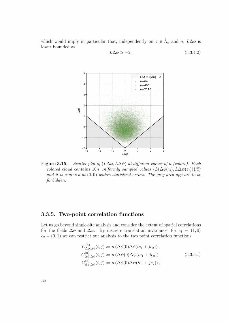
which would imply in particular that, independently on z P Λn and n, L∆φ islower bounded as
L∆φ ě ´2 . (3.3.4.2)
3 2 1 0 1 2 3L
2
1
0
1
2
3
4
5
LL = L| | 2n=64n=400n=2116
Figure 3.15. – Scatter plot of pL∆φ, L∆ψq at different values of n (colors). Eachcolored cloud contains 10n uniformly sampled values tLp∆φpziq, L∆ψpziqqu
10ni“1
and it is centered at p0, 0q within statistical errors. The grey area appears to beforbidden.
3.3.5. Two-point correlation functions
Let us go beyond single-site analysis and consider the extent of spatial correlationsfor the fields ∆φ and ∆ψ. By discrete translation invariance, for e1 “ p1, 0qe2 “ p0, 1q we can restrict our analysis to the two point correlation functions
Cpnq∆φ,∆φpi, jq :“ n x∆φp0q∆φpie1 ` je2qy ,
Cpnq∆ψ,∆ψpi, jq :“ n x∆ψp0q∆ψpie1 ` je2qy ,
Cpnq∆φ,∆ψpi, jq :“ n x∆φp0q∆ψpie1 ` je2qy ,
(3.3.5.1)
178
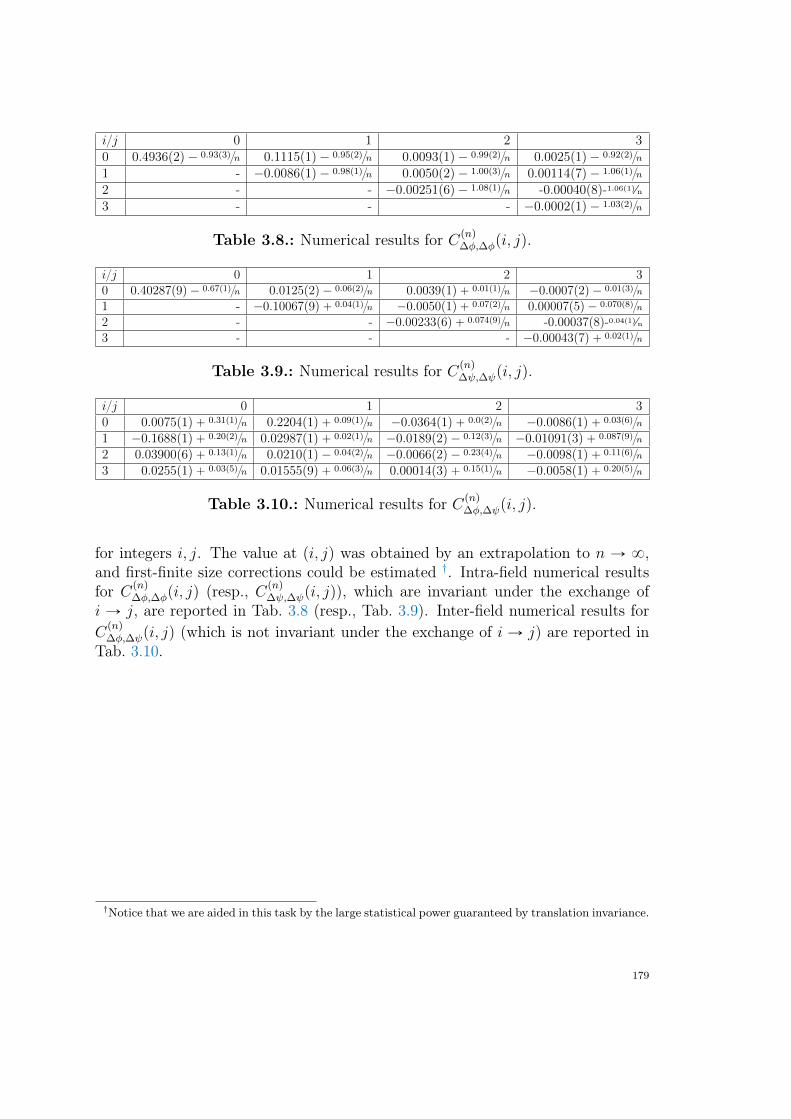
ij 0 1 2 30 0.4936p2q ´ 0.93p3qn 0.1115p1q ´ 0.95p2qn 0.0093p1q ´ 0.99p2qn 0.0025p1q ´ 0.92p2qn
1 - ´0.0086p1q ´ 0.98p1qn 0.0050p2q ´ 1.00p3qn 0.00114p7q ´ 1.06p1qn
2 - - ´0.00251p6q ´ 1.08p1qn -0.00040(8)-1.06(1)⁄n3 - - - ´0.0002p1q ´ 1.03p2qn
Table 3.8.: Numerical results for Cpnq∆φ,∆φpi, jq.
ij 0 1 2 30 0.40287p9q ´ 0.67p1qn 0.0125p2q ´ 0.06p2qn 0.0039p1q ` 0.01p1qn ´0.0007p2q ´ 0.01p3qn
1 - ´0.10067p9q ` 0.04p1qn ´0.0050p1q ` 0.07p2qn 0.00007p5q ´ 0.070p8qn
2 - - ´0.00233p6q ` 0.074p9qn -0.00037(8)-0.04(1)⁄n3 - - - ´0.00043p7q ` 0.02p1qn
Table 3.9.: Numerical results for Cpnq∆ψ,∆ψpi, jq.
ij 0 1 2 30 0.0075p1q ` 0.31p1qn 0.2204p1q ` 0.09p1qn ´0.0364p1q ` 0.0p2qn ´0.0086p1q ` 0.03p6qn
1 ´0.1688p1q ` 0.20p2qn 0.02987p1q ` 0.02p1qn ´0.0189p2q ´ 0.12p3qn ´0.01091p3q ` 0.087p9qn
2 0.03900p6q ` 0.13p1qn 0.0210p1q ´ 0.04p2qn ´0.0066p2q ´ 0.23p4qn ´0.0098p1q ` 0.11p6qn
3 0.0255p1q ` 0.03p5qn 0.01555p9q ` 0.06p3qn 0.00014p3q ` 0.15p1qn ´0.0058p1q ` 0.20p5qn
Table 3.10.: Numerical results for Cpnq∆φ,∆ψpi, jq.
for integers i, j. The value at pi, jq was obtained by an extrapolation to n Ñ 8,and first-finite size corrections could be estimated †. Intra-field numerical resultsfor Cpnq∆φ,∆φpi, jq (resp., Cpnq∆ψ,∆ψpi, jq), which are invariant under the exchange ofi Ñ j, are reported in Tab. 3.8 (resp., Tab. 3.9). Inter-field numerical results forCpnq∆φ,∆ψpi, jq (which is not invariant under the exchange of i Ñ j) are reported in
Tab. 3.10.
†Notice that we are aided in this task by the large statistical power guaranteed by translation invariance.
179
3.3.6. On L2A
|x∆φ|2E
and L2A
|y∆ψ|2E
In this Section we shall provide the numerical estimation of the typical transverseand longitudinal contributions through Fourier analysis. The Fourier componentsof ∆φ and ∆ψ are (see C.1.0.4)
x∆φppq “1
L
ÿ
zPΛn
e´iz¨p∆φpzq
y∆ψppq “1
L
ÿ
zPΛn
e´iz¨p∆ψpzq .(3.3.6.1)
Recalling the modified laplacian in momentum space
p2mod :“ p2
´1
2p2
1p22 , (3.3.6.2)
we are thus concerned with the expectation of the random variables (see Eq. C.1.0.19)
Hpφq“
ÿ
p‰0
n|x∆φ|2
p2mod
and Hpψq“
ÿ
p‰0
n|y∆ψ|2
p2mod
, (3.3.6.3)
which are two-dimensional analogues of Eq. 2.3.3.9. Heatmaps of n|x∆φppq|2 andn|y∆ψppq|2 at large n are reported in Fig. 3.16a. The longitudinal part (left) dis-plays the characteristic area near n “ p0, 0q (upper left-corner and periodic images)responsible for the logarithmic divergence, and also remarkable rotational symme-try around n “ pL
2, L
2q. The transverse part (right) shares the same symmetries
of p2mod, with the small n “ p0, 0q and large n “ pL
2, L
2q wavelengths both de-
pleted, and connected through a saddle-point at n “ pL4, L
4q‡ . On the basis of
these observations, the numerical data were fitted as follows. Let us consider thesix-dimensional linear subspace spanned by fr,spx, yq “ cos
`
2πLrx˘
cos`
2πLsy˘
with
‡Notice that the zero mode at n “ p0, 0q corresponds to the conservation lawÿ
z
∆φpzq “ 0 , (3.3.6.4)
and the one at n “ pL2, L
2q corresponding to the vanishing of the “checkerboard” sum
L´1ÿ
i,j“0
p´1qi`j∆ψpi, jq “ 0 . (3.3.6.5)
180
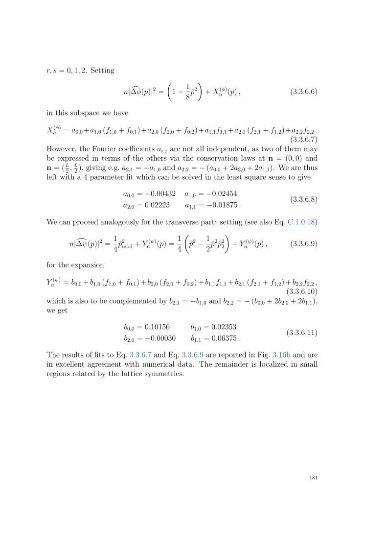
r, s “ 0, 1, 2. Setting
n|x∆φppq|2 “
ˆ
1´1
8p2
˙
`Xpφqn ppq , (3.3.6.6)
in this subspace we have
Xpφqn “ a0,0`a1,0 pf1,0 ` f0,1q`a2,0 pf2,0 ` f0,2q`a1,1f1,1`a2,1 pf2,1 ` f1,2q`a2,2f2,2 .
(3.3.6.7)However, the Fourier coefficients ai,j are not all independent, as two of them maybe expressed in terms of the others via the conservation laws at n “ p0, 0q andn “ pL
2, L
2q, giving e.g. a2,1 “ ´a1,0 and a2,2 “ ´pa0,0 ` 2a2,0 ` 2a1,1q. We are thus
left with a 4 parameter fit which can be solved in the least square sense to give
a0,0 “ ´0.00432 a1,0 “ ´0.02454
a2,0 “ 0.02223 a1,1 “ ´0.01875 .(3.3.6.8)
We can proceed analogously for the transverse part: setting (see also Eq. C.1.0.18)
n|y∆ψppq|2 “1
4p2
mod ` Ypψqn ppq “
1
4
ˆ
p2´
1
2p2
1p22
˙
` Y pψqn ppq , (3.3.6.9)
for the expansion
Y pψqn “ b0,0` b1,0 pf1,0 ` f0,1q` b2,0 pf2,0 ` f0,2q` b1,1f1,1` b2,1 pf2,1 ` f1,2q` b2,2f2,2 ,(3.3.6.10)
which is also to be complemented by b2,1 “ ´b1,0 and b2,2 “ ´pb0,0 ` 2b2,0 ` 2b1,1q,we get
b0,0 “ 0.10156 b1,0 “ 0.02353
b2,0 “ ´0.00030 b1,1 “ 0.06375 .(3.3.6.11)
The results of fits to Eq. 3.3.6.7 and Eq. 3.3.6.9 are reported in Fig. 3.16b and arein excellent agreement with numerical data. The remainder is localized in smallregions related by the lattice symmetries.
181
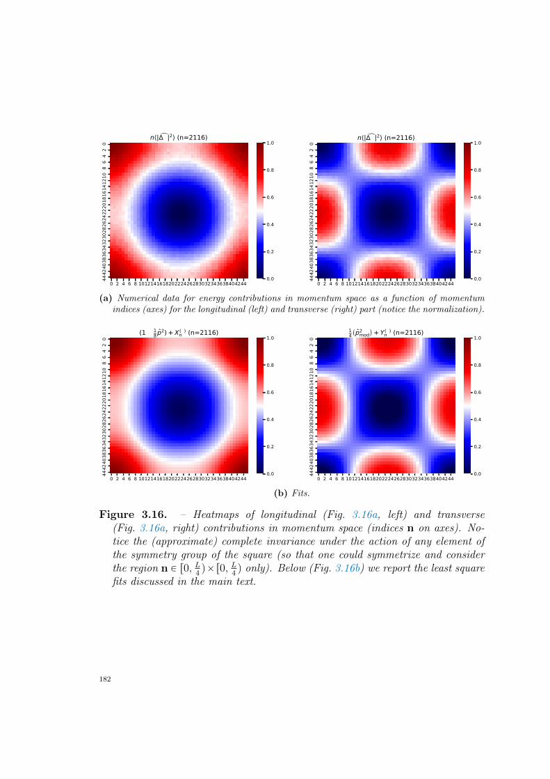
0 2 4 6 8 101214161820222426283032343638404244
02
46
810
1214
1618
2022
2426
2830
3234
3638
4042
44
n⟨| Δϕ|2⟩⟨Δn=2116⟩
0.0
0.2
0.4
0.6
0.8
1.0
0 2 4 6 8 101214161820222426283032343638404244
02
46
810
1214
1618
2022
2426
2830
3234
3638
4042
44
n⟨| Δψ|2⟩⟨Δn=2116⟩
0.0
0.2
0.4
0.6
0.8
1.0
(a) Numerical data for energy contributions in momentum space as a function of momentumindices (axes) for the longitudinal (left) and transverse (right) part (notice the normalization).
0 2 4 6 8 101214161820222426283032343638404244
02
46
810
1214
1618
2022
2426
2830
3234
3638
4042
44
(1− 18 p2) +X(ϕ)
n (n=2116)
0.0
0.2
0.4
0.6
0.8
1.0
0 2 4 6 8 101214161820222426283032343638404244
02
46
810
1214
1618
2022
2426
2830
3234
3638
4042
44
14( p2mod)+ Y(ψ)n (n=2116)
0.0
0.2
0.4
0.6
0.8
1.0
(b) Fits.
Figure 3.16. – Heatmaps of longitudinal (Fig. 3.16a, left) and transverse(Fig. 3.16a, right) contributions in momentum space (indices n on axes). No-tice the (approximate) complete invariance under the action of any element ofthe symmetry group of the square (so that one could symmetrize and considerthe region n P r0, L
4qˆr0, L
4q only). Below (Fig. 3.16b) we report the least square
fits discussed in the main text.
182
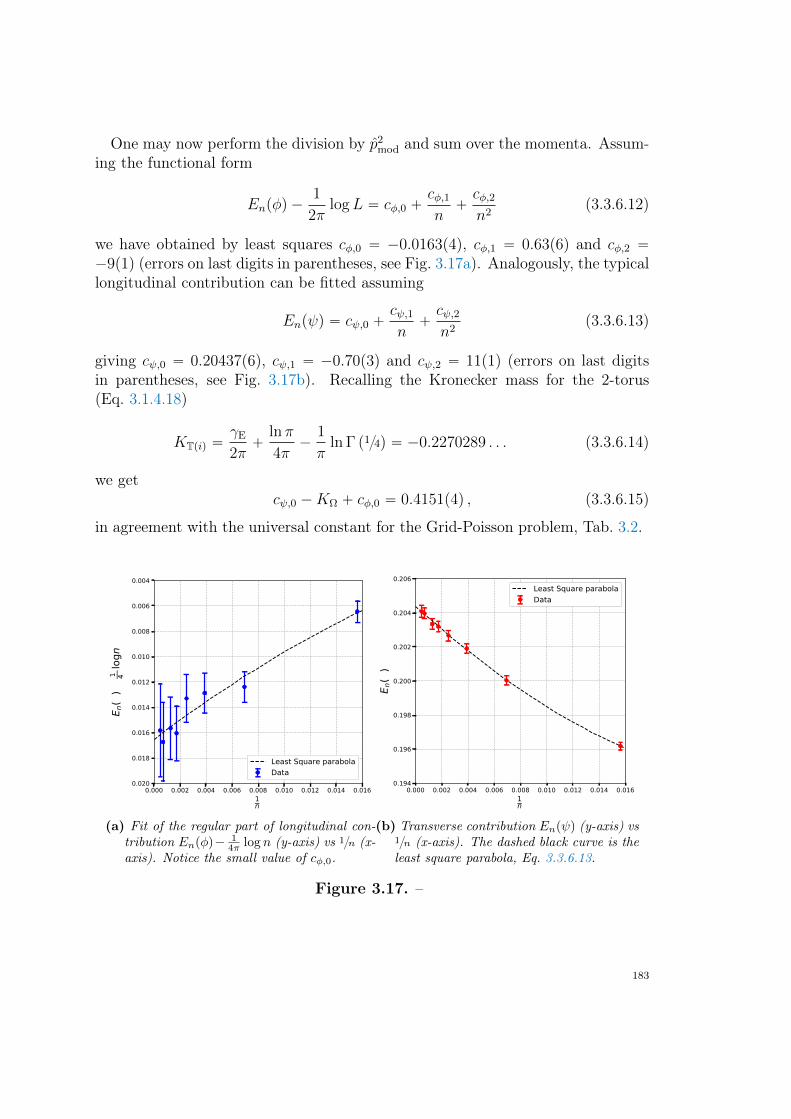
One may now perform the division by p2mod and sum over the momenta. Assum-
ing the functional form
Enpφq ´1
2πlogL “ cφ,0 `
cφ,1n`cφ,2n2
(3.3.6.12)
we have obtained by least squares cφ,0 “ ´0.0163p4q, cφ,1 “ 0.63p6q and cφ,2 “´9p1q (errors on last digits in parentheses, see Fig. 3.17a). Analogously, the typicallongitudinal contribution can be fitted assuming
Enpψq “ cψ,0 `cψ,1n`cψ,2n2
(3.3.6.13)
giving cψ,0 “ 0.20437p6q, cψ,1 “ ´0.70p3q and cψ,2 “ 11p1q (errors on last digitsin parentheses, see Fig. 3.17b). Recalling the Kronecker mass for the 2-torus(Eq. 3.1.4.18)
KTpiq “γE
2π`
lnπ
4π´
1
πln Γ p14q “ ´0.2270289 . . . (3.3.6.14)
we getcψ,0 ´KΩ ` cφ,0 “ 0.4151p4q , (3.3.6.15)
in agreement with the universal constant for the Grid-Poisson problem, Tab. 3.2.
0.000 0.002 0.004 0.006 0.008 0.010 0.012 0.014 0.0161n
−0.020
−0.018
−0.016
−0.014
−0.012
−0.010
−0.008
−0.006
−0.004
E n(ϕ)−
1 4πlogn
Least Square parabolaData
(a) Fit of the regular part of longitudinal con-tribution Enpφq´ 1
4π log n (y-axis) vs 1n (x-axis). Notice the small value of cφ,0.
0.000 0.002 0.004 0.006 0.008 0.010 0.012 0.014 0.0161n
0.194
0.196
0.198
0.200
0.202
0.204
0.206
E n(ψ)
Least Square parabolaData
(b) Transverse contribution Enpψq (y-axis) vs1n (x-axis). The dashed black curve is theleast square parabola, Eq. 3.3.6.13.
Figure 3.17. –
183
3.3.7. Section provisional conclusions and perspectivesIn this Section we have introduced a statistical field theory approach to the GP-ERAP, in which blue points sit on a deterministic square grid and red points areuniformly distributed on the domain. In particular, we have considered some con-sequences of the theory for the special case pd, pq “ p2, 2q. Inspired by classicalelectrodynamics, we have examined a “change of variables” for the optimal trans-port field and shown that the new variables have a different statistical nature: theiraverage values contribute at different orders in the asymptotic expansion of theground state energy. More precisely, the longitudinal (or conservative) part, whichis associated to an approximately lognormal field, and through Fourier analysis,fully responsible for the well-known logarithmic divergence of the expected groundstate energy; and a transverse (or solenoidal) part, associated to a gaussian fieldappearing to enjoy the self-averaging property in the large n limit, and contribut-ing to the ground state energy through a constant plus corrections in 1n that havebeen numerically estimated with good precision. Not only the sum of (the regularpart of) transverse and longitudinal contributions recovers within errors the knownnumerically estimated constant (149 )
c0 “ 0.1879p3q 0.1880p4q “ cφ ` cψ (3.3.7.1)
but, once the Kronecker mass of the torus is taken into account, the longitudinalpart carries most of the sub-leading constant (Eq. 3.3.6.15). In doing so, wehave also devised the stable numerical method of § 3.3.6, which indicates theway to the theoretical understanding of the origin of such strange sub-leadingconstants. As a by-product, our findings imply that the cutoff function F forthe GP-ERAP is different from the one of the PP-ERAP, and also different from1, as one could have possibly guessed. Lastly, we remark that the Helmholtzdecomposition can be readily applied for studying the GP-ERAP in which randompoints are distributed with a measure different from the uniform measure and,without conceptual modifications, to other choices for the grid, and thus mayserve as useful tool for investigating anomalous behaviors in two dimensions.
184
d Chapter 4 D
Euclidean RandomAssignment Problems at non
integer Hausdorffdimensions dH P p1, 2q
4.1. Introduction
Despite recent efforts, even at integer values of p and d and for the simplestchoices of disorder, the phase diagram of an ERAP (that is, the leading
exponent of the expected ground state energy En for large n as a function ofpp, dq) remains in part mysterious. It has already been established that, alreadyin the “simplest” case d “ 1, it is rather rich (154 , 169 ) especially in the concaveregion p P p0, 1q. In this case we have conjectured the existence of a critical pointwith logarithmic scaling
En „?n log n “ n1´ p
d plog2p nq|pp,dq“p12,1q (4.1.0.1)
separating a trivial region (p P r0, 12q) where a nearest neighbor argument applies,En „ n1´ p
d |d“1 from the Dyck scaling region at p P p12, 1s where En „?n (see
Fig. 2.17). On the other hand, at d ą 2 with uniform disorder, it is known (60 )that points are optimally assigned with high probability in their Euclidean neigh-borhoods, so that
En „ cp,dn´
n´1d
¯p
(4.1.0.2)
for asymptotic constants cp,d which are not known in closed form but can beaddressed by the mean-field theory (namely, the random assignment problem)with Mézard-Parisi exponent 1pr ` 1q “ 1 ´ pd (154 ). It is not known how thecritical points at pp, dq “ p12, 1q and pp, dq “ p1, 1q “enter” as critical lines in thephase diagram at generic pp, dq, and vanish at d ą 2.As we have recalled in Chapter 3, many efforts have been devoted during the
years to the special case d “ 2, where the ground state energy is logarithmicallydivergent at large n (see § 3.1) and logarithmic corrections may already appear at
185
d “ 1, if the disorder distribution vanishes (§ 2.6).In this Chapter we shall take a first step into the unknown (as far as we know)
region of the phase diagram with the introduction of a notion of ERAP at non-integer Hausdorff dimensions dH P p1, 2q. In this problem, the disorder distributionis identical for B “ tbdHi uni“1 Ă M and R “ trdHi u
ni“1 Ă M, and it is the uniform
measure supported on a fractal set M. The fractal sets depend on a simple ge-ometrical parameter in a way that the corresponding Hausdorff dimensions givedifferent interpolations of the interval dH P p1, 2q, providing us a simple proxy foruniversality of the energy leading scaling exponent.It is interesting to notice that statistical properties of sets of points sampled from
measures supported on fractal sets using the two dimensional distance have beenconsidered during the years for vastly different reasons, ranging from grow rates ofthe number of points defining the convex hull of a random sample of size n (81 ) tothe crossover transition in the distribution of nearest-neighbors distances, in con-nection with random matrix theory (108 , 112 ). Our main motivations stem fromthe question of whether universal behavior extends “beyond” d “ 2, in particularin the perspective of one dimensional anomalous behavior, § 2.6. The latter sug-gested that, beyond the bulk behavior, the scaling is determined by “holes” in thesupport of the disorder distribution (i.e. endpoints of the measure µ at d “ 1). Asa consequence, one is naturally led to wonder about the geometry of the optimalassignment also at higher dimensions, in a situation in which neighborhoods ofblue and red points are not anymore homogeneous but, from the point of view ofthe embedding space, are full of inhomogeneities.
4.2. SetupFor a real number p ą 0, consider the random variable
Hopt “ minπPSn
nÿ
i“1
DppbdHπpiq, r
dHi q , (4.2.0.1)
where Sn is the symmetric group on n objects and D2px, yq “ř2i“1pxi´ yiq
2 is the(squared) two dimensional Euclidean distance. Denoting with xOyM expectationof observable O with respect to the uniform measure on M, we wish to investigatethe large n asymptotics of the expected ground state energy
EMn,pp,dHq
:“ xHoptyM (4.2.0.2)
depending on pp, dHq and on the fractal set M considered.
186
4.3. Choice of randomness
4.3.1. Peano fractalThe construction of our first fractal is inspired by properties of space-filling curves,such as the Peano curve (1 ) (see also e.g. (117 ), Chapter 2). Consider the aspectratio parameter αpPeanoq P r0, 1s depending on the Hausdorff dimension dH as
αpPeanoq “ p2dH´1
´ 1q1dH (4.3.1.1)
and introduce the deterministic quantities
P “1
2p1` αdHpPeanoqq
´
1, αdHpPeanoq, α
dHpPeanoq, 1
¯
,
Λ “1
2
´
1, αdHpPeanoq, α
dHpPeanoq, 1
¯
,
Φ “ p1, i,´i, 1q,
V “1
2
`
0, 1, 1` iαpPeanoq, 1˘
.
(4.3.1.2)
Calling R the cumulative distribution function of P, and R´1 its inverse function,draw a random integer i “ tR´1puqu, i P t1, 2, 3, 4u, for u chosen uniformly in r0, 1s,where txu is the largest integer smaller than x. For P “ pξ, zq P C2, Eq. (4.3.1.2)and i uniquely define the random map fP : C2 Ñ C2
fPpP q :“ pΛiΦiξ, z ` Viξq . (4.3.1.3)
Starting from an initial datum P0 “ p1, 0q, we apply fP recursively as
Pg “ f gPpP0q “ fP ˝ fP ¨ ¨ ¨ ˝ fPloooooooomoooooooon
g times
pP0q (4.3.1.4)
for a suitably large g∗, and then consider the second component of Pg, zg :“ pPgq2.We will say that zg (which can be either a red or blue point) is uniformly distributedon the Peano fractal of Hausdorff dimension dH . In order to enforce the y Ø ´ysymmetry, as an additional step we consider either zg or zg with probability 12(z being the complex conjugate of z). Example instances of the disorder from thePeano fractal at increasing Hausdorff dimensions are displayed in Fig. 4.1.
∗In our settings g “ 10 appeared to be large enough to prevent issues due to floating point precision.
187
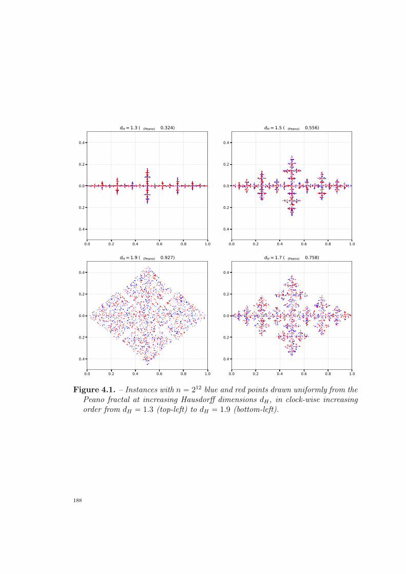
0.0 0.2 0.4 0.6 0.8 1.0
−0.4
−0.2
0.0
0.2
0.4
dH=1.3 (α(Peano)≈0.324)
0.0 0.2 0.4 0.6 0.8 1.0
−0.4
−0.2
0.0
0.2
0.4
dH=1.5 (α(Peano)≈0.556)
0.0 0.2 0.4 0.6 0.8 1.0
−0.4
−0.2
0.0
0.2
0.4
dH=1.9 (α(Peano)≈0.927)
0.0 0.2 0.4 0.6 0.8 1.0
−0.4
−0.2
0.0
0.2
0.4
dH=1.7 (α(Peano)≈0.758)
Figure 4.1. – Instances with n “ 212 blue and red points drawn uniformly from thePeano fractal at increasing Hausdorff dimensions dH , in clock-wise increasingorder from dH “ 1.3 (top-left) to dH “ 1.9 (bottom-left).
188
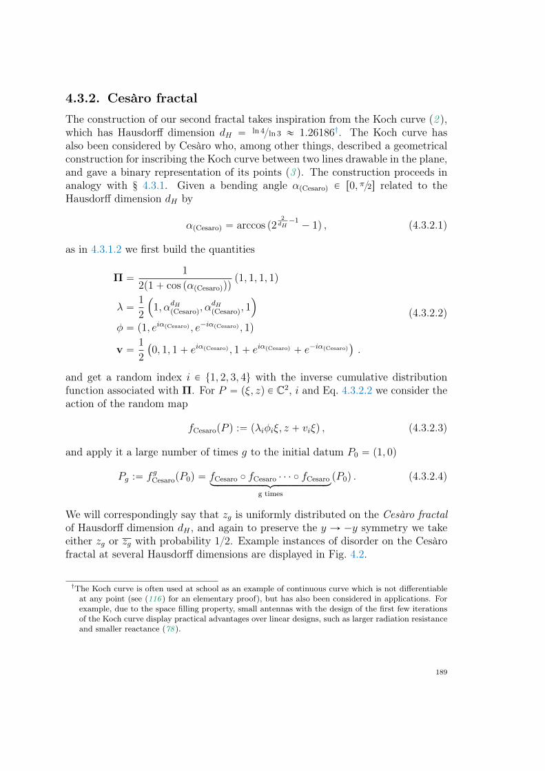
4.3.2. Cesàro fractalThe construction of our second fractal takes inspiration from the Koch curve (2 ),which has Hausdorff dimension dH “ ln 4ln 3 « 1.26186†. The Koch curve hasalso been considered by Cesàro who, among other things, described a geometricalconstruction for inscribing the Koch curve between two lines drawable in the plane,and gave a binary representation of its points (3 ). The construction proceeds inanalogy with § 4.3.1. Given a bending angle αpCesaroq P r0, π2s related to theHausdorff dimension dH by
αpCesaroq “ arccos p22dH´1´ 1q , (4.3.2.1)
as in 4.3.1.2 we first build the quantities
Π “1
2p1` cos pαpCesaroqqqp1, 1, 1, 1q
λ “1
2
´
1, αdHpCesaroq, α
dHpCesaroq, 1
¯
φ “ p1, eiαpCesaroq , e´iαpCesaroq , 1q
v “1
2
`
0, 1, 1` eiαpCesaroq , 1` eiαpCesaroq ` e´iαpCesaroq˘
.
(4.3.2.2)
and get a random index i P t1, 2, 3, 4u with the inverse cumulative distributionfunction associated with Π. For P “ pξ, zq P C2, i and Eq. 4.3.2.2 we consider theaction of the random map
fCesaropP q :“ pλiφiξ, z ` viξq , (4.3.2.3)
and apply it a large number of times g to the initial datum P0 “ p1, 0q
Pg :“ f gCesaropP0q “ fCesaro ˝ fCesaro ¨ ¨ ¨ ˝ fCesaroloooooooooooooooomoooooooooooooooon
g times
pP0q . (4.3.2.4)
We will correspondingly say that zg is uniformly distributed on the Cesàro fractalof Hausdorff dimension dH , and again to preserve the y Ñ ´y symmetry we takeeither zg or zg with probability 12. Example instances of disorder on the Cesàrofractal at several Hausdorff dimensions are displayed in Fig. 4.2.
†The Koch curve is often used at school as an example of continuous curve which is not differentiableat any point (see (116 ) for an elementary proof), but has also been considered in applications. Forexample, due to the space filling property, small antennas with the design of the first few iterationsof the Koch curve display practical advantages over linear designs, such as larger radiation resistanceand smaller reactance (78 ).
189
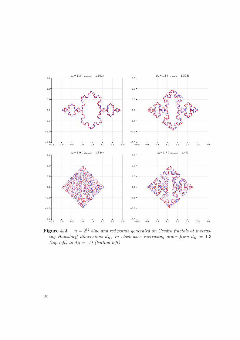
−0.5 0.0 0.5 1.0 1.5 2.0 2.5 3.0−1.5
−1.0
−0.5
0.0
0.5
1.0
1.5dH=1.3 (α(Cesaro)≈1.101)
−0.5 0.0 0.5 1.0 1.5 2.0 2.5 3.0−1.5
−1.0
−0.5
0.0
0.5
1.0
1.5dH=1.5 (α(Cesaro)≈1.308)
−0.5 0.0 0.5 1.0 1.5 2.0 2.5 3.0−1.5
−1.0
−0.5
0.0
0.5
1.0
1.5dH=1.9 (α(Cesaro)≈1.534)
−0.5 0.0 0.5 1.0 1.5 2.0 2.5 3.0−1.5
−1.0
−0.5
0.0
0.5
1.0
1.5dH=1.7 (α(Cesaro)≈1.44)
Figure 4.2. – n “ 212 blue and red points generated on Cesàro fractals at increas-ing Hausdorff dimensions dH , in clock-wise increasing order from dH “ 1.3(top-left) to dH “ 1.9 (bottom-left).
190
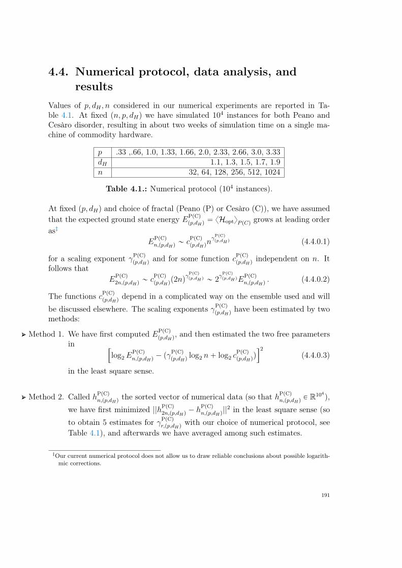
4.4. Numerical protocol, data analysis, andresults
Values of p, dH , n considered in our numerical experiments are reported in Ta-ble 4.1. At fixed pn, p, dHq we have simulated 104 instances for both Peano andCesàro disorder, resulting in about two weeks of simulation time on a single ma-chine of commodity hardware.
p .33 ,.66, 1.0, 1.33, 1.66, 2.0, 2.33, 2.66, 3.0, 3.33dH 1.1, 1.3, 1.5, 1.7, 1.9n 32, 64, 128, 256, 512, 1024
Table 4.1.: Numerical protocol (104 instances).
At fixed pp, dHq and choice of fractal (Peano (P) or Cesàro (C)), we have assumedthat the expected ground state energy EPpCq
pp,dHq“ xHoptyP pCq grows at leading order
as‡
EPpCqn,pp,dHq
„ cPpCqpp,dHq
nγ
PpCqpp,dH q (4.4.0.1)
for a scaling exponent γPpCqpp,dHq
and for some function cPpCqpp,dHq
independent on n. Itfollows that
EPpCq2n,pp,dHq
„ cPpCqpp,dHq
p2nqγ
PpCqpp,dH q „ 2
γPpCqpp,dH qE
PpCqn,pp,dHq
. (4.4.0.2)
The functions cPpCqpp,dHq
depend in a complicated way on the ensemble used and will
be discussed elsewhere. The scaling exponents γPpCqpp,dHq
have been estimated by twomethods:
) Method 1. We have first computed EPpCqpp,dHq
, and then estimated the two free parametersin
”
log2EPpCqn,pp,dHq
´ pγPpCqpp,dHq
log2 n` log2 cPpCqpp,dHq
q
ı2
(4.4.0.3)
in the least square sense.
) Method 2. Called hPpCqn,pp,dHq
the sorted vector of numerical data (so that hPpCqn,pp,dHq
P R104),
we have first minimized ||hPpCq2n,pp,dHq
´ hPpCqn,pp,dHq
||2 in the least square sense (so
to obtain 5 estimates for γPpCqr,pp,dHq
with our choice of numerical protocol, seeTable 4.1), and afterwards we have averaged among such estimates.
‡Our current numerical protocol does not allow us to draw reliable conclusions about possible logarith-mic corrections.
191
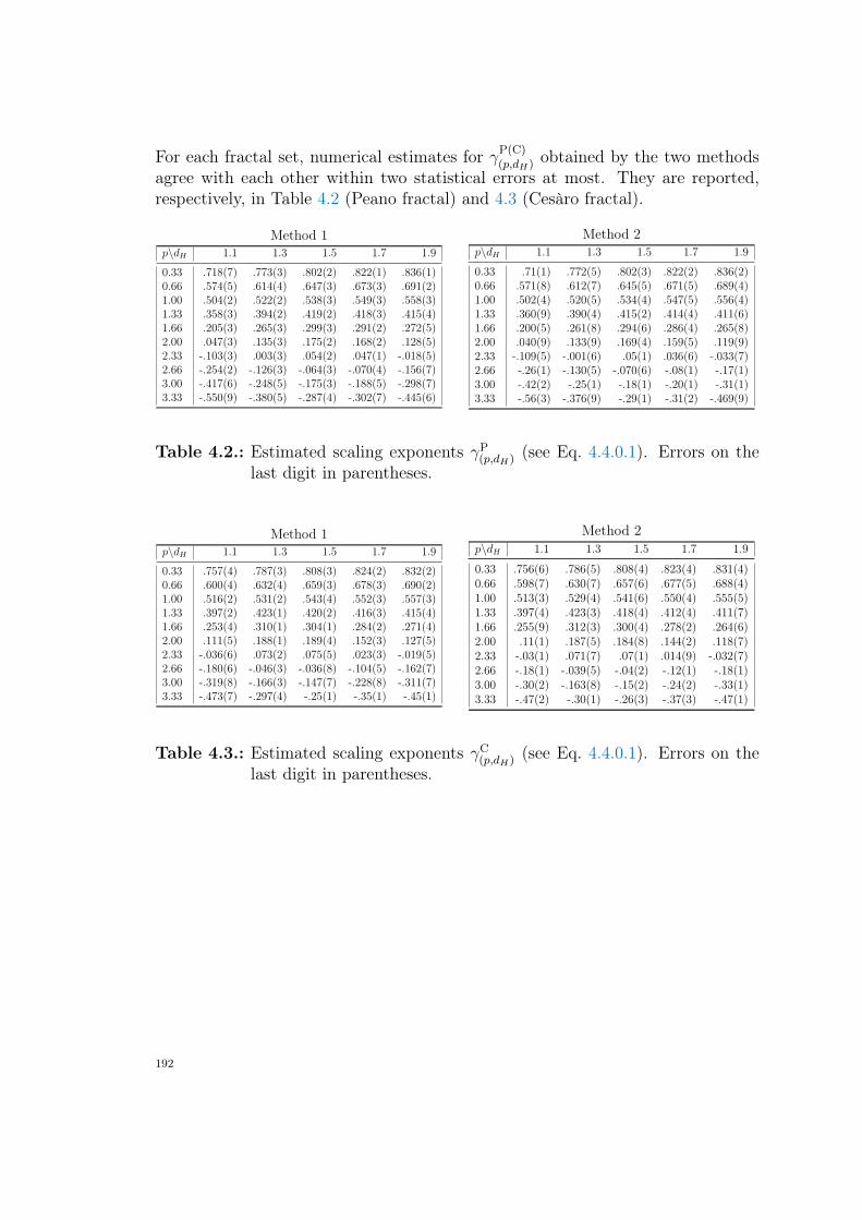
For each fractal set, numerical estimates for γPpCqpp,dHq
obtained by the two methodsagree with each other within two statistical errors at most. They are reported,respectively, in Table 4.2 (Peano fractal) and 4.3 (Cesàro fractal).
Method 1p\dH 1.1 1.3 1.5 1.7 1.9
0.33 .718(7) .773(3) .802(2) .822(1) .836(1)0.66 .574(5) .614(4) .647(3) .673(3) .691(2)1.00 .504(2) .522(2) .538(3) .549(3) .558(3)1.33 .358(3) .394(2) .419(2) .418(3) .415(4)1.66 .205(3) .265(3) .299(3) .291(2) .272(5)2.00 .047(3) .135(3) .175(2) .168(2) .128(5)2.33 -.103(3) .003(3) .054(2) .047(1) -.018(5)2.66 -.254(2) -.126(3) -.064(3) -.070(4) -.156(7)3.00 -.417(6) -.248(5) -.175(3) -.188(5) -.298(7)3.33 -.550(9) -.380(5) -.287(4) -.302(7) -.445(6)
Method 2p\dH 1.1 1.3 1.5 1.7 1.9
0.33 .71(1) .772(5) .802(3) .822(2) .836(2)0.66 .571(8) .612(7) .645(5) .671(5) .689(4)1.00 .502(4) .520(5) .534(4) .547(5) .556(4)1.33 .360(9) .390(4) .415(2) .414(4) .411(6)1.66 .200(5) .261(8) .294(6) .286(4) .265(8)2.00 .040(9) .133(9) .169(4) .159(5) .119(9)2.33 -.109(5) -.001(6) .05(1) .036(6) -.033(7)2.66 -.26(1) -.130(5) -.070(6) -.08(1) -.17(1)3.00 -.42(2) -.25(1) -.18(1) -.20(1) -.31(1)3.33 -.56(3) -.376(9) -.29(1) -.31(2) -.469(9)
Table 4.2.: Estimated scaling exponents γPpp,dHq
(see Eq. 4.4.0.1). Errors on thelast digit in parentheses.
Method 1p\dH 1.1 1.3 1.5 1.7 1.9
0.33 .757(4) .787(3) .808(3) .824(2) .832(2)0.66 .600(4) .632(4) .659(3) .678(3) .690(2)1.00 .516(2) .531(2) .543(4) .552(3) .557(3)1.33 .397(2) .423(1) .420(2) .416(3) .415(4)1.66 .253(4) .310(1) .304(1) .284(2) .271(4)2.00 .111(5) .188(1) .189(4) .152(3) .127(5)2.33 -.036(6) .073(2) .075(5) .023(3) -.019(5)2.66 -.180(6) -.046(3) -.036(8) -.104(5) -.162(7)3.00 -.319(8) -.166(3) -.147(7) -.228(8) -.311(7)3.33 -.473(7) -.297(4) -.25(1) -.35(1) -.45(1)
Method 2p\dH 1.1 1.3 1.5 1.7 1.9
0.33 .756(6) .786(5) .808(4) .823(4) .831(4)0.66 .598(7) .630(7) .657(6) .677(5) .688(4)1.00 .513(3) .529(4) .541(6) .550(4) .555(5)1.33 .397(4) .423(3) .418(4) .412(4) .411(7)1.66 .255(9) .312(3) .300(4) .278(2) .264(6)2.00 .11(1) .187(5) .184(8) .144(2) .118(7)2.33 -.03(1) .071(7) .07(1) .014(9) -.032(7)2.66 -.18(1) -.039(5) -.04(2) -.12(1) -.18(1)3.00 -.30(2) -.163(8) -.15(2) -.24(2) -.33(1)3.33 -.47(2) -.30(1) -.26(3) -.37(3) -.47(1)
Table 4.3.: Estimated scaling exponents γCpp,dHq
(see Eq. 4.4.0.1). Errors on thelast digit in parentheses.
192
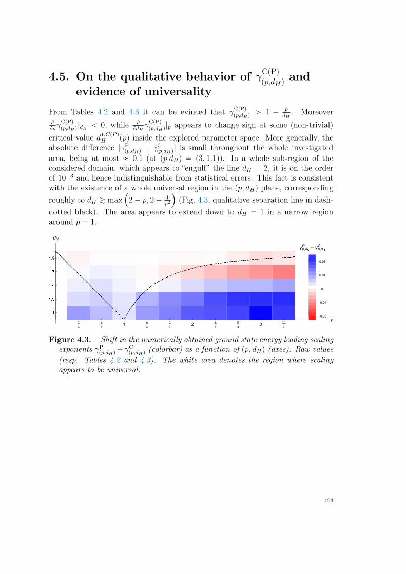
4.5. On the qualitative behavior of γCpPqpp,dHq
andevidence of universality
From Tables 4.2 and 4.3 it can be evinced that γCpPqpp,dHq
ą 1 ´ pdH
. MoreoverB
Bpγ
CpPqpp,dHq
|dH ă 0, while B
BdHγ
CpPqpp,dHq
|p appears to change sign at some (non-trivial)
critical value d˚,CpP qH ppq inside the explored parameter space. More generally, theabsolute difference |γP
pp,dHq´ γC
pp,dHq| is small throughout the whole investigated
area, being at most « 0.1 (at pp,dHq “ p3, 1.1q). In a whole sub-region of theconsidered domain, which appears to “engulf” the line dH “ 2, it is on the orderof 10´3 and hence indistinguishable from statistical errors. This fact is consistentwith the existence of a whole universal region in the pp, dHq plane, correspondingroughly to dH Á max
´
2´ p, 2´ 1p2
¯
(Fig. 4.3, qualitative separation line in dash-dotted black). The area appears to extend down to dH “ 1 in a narrow regionaround p “ 1.
-0.08
-0.04
0.
0.04
0.08
γp,dHP
- γp,dHC
1
3
2
31
4
3
5
32
7
3
8
33
10
3
p
11
1
1
1
1.9
dH
Figure 4.3. – Shift in the numerically obtained ground state energy leading scalingexponents γP
pp,dHq´γC
pp,dHq(colorbar) as a function of pp, dHq (axes). Raw values
(resp. Tables 4.2 and 4.3). The white area denotes the region where scalingappears to be universal.
193
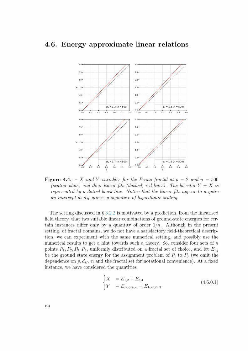
4.6. Energy approximate linear relations
0.0 0.5 1.0 1.5 2.0 2.5 3.00.0
0.5
1.0
1.5
2.0
2.5
3.0
Y
dH = 1.3 (n = 500)
0.0 0.5 1.0 1.5 2.0 2.5 3.00.0
0.5
1.0
1.5
2.0
2.5
3.0
dH = 1.5 (n = 500)
0.0 0.5 1.0 1.5 2.0 2.5 3.0X
0.0
0.5
1.0
1.5
2.0
2.5
3.0
Y
dH = 1.7 (n = 500)
0.0 0.5 1.0 1.5 2.0 2.5 3.0X
0.0
0.5
1.0
1.5
2.0
2.5
3.0
dH = 1.9 (n = 500)
Figure 4.4. – X and Y variables for the Peano fractal at p “ 2 and n “ 500(scatter plots) and their linear fits (dashed, red lines). The bisector Y “ X isrepresented by a dotted black line. Notice that the linear fits appear to acquirean intercept as dH grows, a signature of logarithmic scaling.
The setting discussed in § 3.2.2 is motivated by a prediction, from the linearisedfield theory, that two suitable linear combinations of ground-state energies for cer-tain instances differ only by a quantity of order 1n. Although in the presentsetting, of fractal domains, we do not have a satisfactory field-theoretical descrip-tion, we can experiment with the same numerical setting, and possibly use thenumerical results to get a hint towards such a theory. So, consider four sets of npoints P1, P2, P3, P4, uniformly distributed on a fractal set of choice, and let Ei,jbe the ground state energy for the assignment problem of Pi to Pj (we omit thedependence on p, dH , n and the fractal set for notational convenience). At a fixedinstance, we have considered the quantities
#
X “ E1,2 ` E3,4
Y “ E1Y3,2Y4 ` E1Y4,2Y3
(4.6.0.1)
194
where e.g. E1Y3,2Y4 denotes the optimal cost of assigning the set P1YP3 to P2YP4
(i.e. an assignment problem between two sets of 2n points each). Independentlyon the considered fractal set and robustly in the range of considered pp, dHq values,Y and X appear to satisfy in good approximation a linear relation (that is, thescatter plots X vs Y describe a cloud of variance of order 1 along a direction andof order 1n in the orthogonal direction). An example is provided in Fig. 4.4 forthe Peano case. These findings may be useful for acquiring information on scalingexponents γP
pp,dHq(e.g. via the slope of least square linear regression) and sub-
leading constants, in presence of pure logarithmic scaling (i.e. via the intercepts).
195
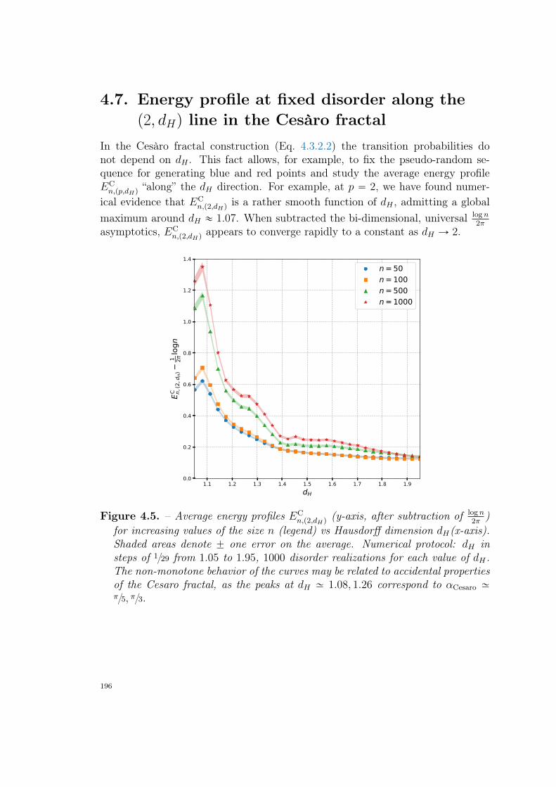
4.7. Energy profile at fixed disorder along thep2, dHq line in the Cesàro fractal
In the Cesàro fractal construction (Eq. 4.3.2.2) the transition probabilities donot depend on dH . This fact allows, for example, to fix the pseudo-random se-quence for generating blue and red points and study the average energy profileECn,pp,dHq
“along” the dH direction. For example, at p “ 2, we have found numer-ical evidence that EC
n,p2,dHqis a rather smooth function of dH , admitting a global
maximum around dH « 1.07. When subtracted the bi-dimensional, universal logn2π
asymptotics, ECn,p2,dHq
appears to converge rapidly to a constant as dH Ñ 2.
1.1 1.2 1.3 1.4 1.5 1.6 1.7 1.8 1.9dH
0.0
0.2
0.4
0.6
0.8
1.0
1.2
1.4
EC n,(2
,dH)
1 2lo
gn
n = 50n = 100n = 500n = 1000
Figure 4.5. – Average energy profiles ECn,p2,dHq
(y-axis, after subtraction of logn2π
)for increasing values of the size n (legend) vs Hausdorff dimension dH(x-axis).Shaded areas denote ˘ one error on the average. Numerical protocol: dH insteps of 129 from 1.05 to 1.95, 1000 disorder realizations for each value of dH .The non-monotone behavior of the curves may be related to accidental propertiesof the Cesaro fractal, as the peaks at dH » 1.08, 1.26 correspond to αCesaro »π5, π3.
196
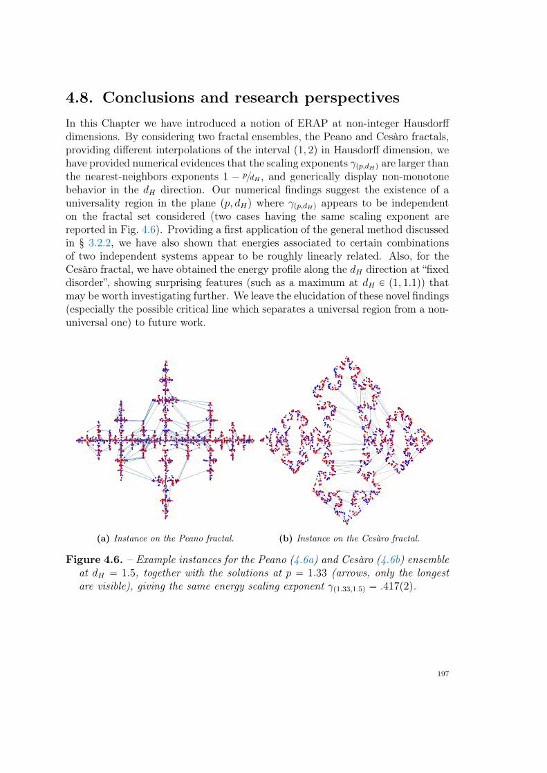
4.8. Conclusions and research perspectivesIn this Chapter we have introduced a notion of ERAP at non-integer Hausdorffdimensions. By considering two fractal ensembles, the Peano and Cesàro fractals,providing different interpolations of the interval p1, 2q in Hausdorff dimension, wehave provided numerical evidences that the scaling exponents γpp,dHq are larger thanthe nearest-neighbors exponents 1 ´ pdH, and generically display non-monotonebehavior in the dH direction. Our numerical findings suggest the existence of auniversality region in the plane pp, dHq where γpp,dHq appears to be independenton the fractal set considered (two cases having the same scaling exponent arereported in Fig. 4.6). Providing a first application of the general method discussedin § 3.2.2, we have also shown that energies associated to certain combinationsof two independent systems appear to be roughly linearly related. Also, for theCesàro fractal, we have obtained the energy profile along the dH direction at “fixeddisorder”, showing surprising features (such as a maximum at dH P p1, 1.1q) thatmay be worth investigating further. We leave the elucidation of these novel findings(especially the possible critical line which separates a universal region from a non-universal one) to future work.
(a) Instance on the Peano fractal. (b) Instance on the Cesàro fractal.
Figure 4.6. – Example instances for the Peano (4.6a) and Cesàro (4.6b) ensembleat dH “ 1.5, together with the solutions at p “ 1.33 (arrows, only the longestare visible), giving the same energy scaling exponent γp1.33,1.5q “ .417p2q.
197
d Chapter 5 D
General provisionalconclusions and research
perspectives
In this PhD Thesis we have studied a random combinatorial optimization prob-lem, the Euclidean Random Assignment Problem. Our focus has been on
the statistical properties of the optimal configuration, depending on the energy-distance exponent p and on the dimension and geometry of the ambient space. Inparticular, we have presented some new contributions on the asymptotic behaviorof the cost at low dimensions, where the Parisi–Mézard mean-field description isless satisfactory.In one dimension (Chapter 2) we have reviewed the state of the art and discussed
some properties of Fourier modes of the optimal solution at p “ 2, both in thediscrete and continuum case. As an application, we have shown that the proba-bility distribution of the ground state energy can be written in terms of an ellipticfunction in the latter case on the circle. The determination of such a probabilitydistribution for general finite p ą 1 remains an open problem.In the one dimensional ordered regime, motivated by the problem with non-
uniform disorder, we have introduced the notion of an anomalous scaling. In thiscase, the leading asymptotic behavior of the ground state energy is determined bya sub-extensive number of edges, the ones nearer to a depleted region. In order tostudy possible anomalous behaviors we have first considered a simple continuummethod, inspired by cutoff regularisation methods in quantum field theory, whichreduces the problem to the study of convergence (and possible regularization)of an integral (169 ). If the integral diverges, the anomalous behavior can bedetermined fixing a constant by trivial numerical experiments. If the integral is notdivergent, the problem is “reduced to quadratures”. It is truly remarkable that ourphysical motivations led us to consider questions that, in the continuum, appearto be related to topics of current interest in probability (see e.g. the extensivememory (168 )).Still in the ordered regime, we have also shown that, at the price of setting
aside simpler continuum methods, in the problem at finite n a qualitatively sim-ple picture appears, where anomalous and bulk scaling are separated by critical
198
lines. The critical lines are hyperbolic relations involving only two parameters,the energy distance exponent p and the leading exponent characterizing the localbehavior of the pdf of B and R near endpoints at a finite or infinite value. Gener-ically, logarithmic corrections appear at the critical line (marginally-anomalousscaling), and for a generic stretched-exponential tail. Our combinatorial approachhas allowed us to address also the case in which the continuum method does notexist (due to non-convergence of Riemann’s sums), and to point out several con-nections with topics in Number Theory (such as, in particular, with multiple zetavalues). Anomalous behaviors at p P p0, 1q is not expected, except for a “gapped”distribution, and at p P p12, 1s where the the system is marginal. We shall elucidatethis matter elsewhere.
In the concave or non-crossing regime, we have introduced the notion of Dyckmatching, a sub-optimal configuration independent on both p and the disorderdistribution and completely determined by the ordered list of colors. We havegiven analytical expressions for the energy scaling of Dyck matchings throughanalytic-combinatorial methods. On the basis of numerical experiments, we haveconjectured that the scaling behavior of the expected energy of Dyck matchingsand ground state energy coincide. Our conjecture implies a logarithmic correctionto scaling at p “ 12, the origin of which should be investigated further. A proofof our conjecture is still incomplete (it goes through the determination of lowerbounds which have the same scaling of the Dyck upper bound), but it is underdevelopment, and we are optimistic on its completion in a near future. On thecontrary, the analytical determination of the constant in front of the true asymp-totics for the ground-state energy (or, in other words, the asymptotics of the ratiobetween the cost of the Dyck matching and the optimal cost), besides the boundsthat would be implied by the forementioned analysis, seems out of reach with ourtechniques.
In two dimensions (Chapter 3), we have focused on the case p “ 2 using bothcontinuum and lattice methods, investigating (among other aspects) the logarith-mically divergent series for the expected ground state energy, predicted by theCaracciolo–Lucibello–Parisi–Sicuro formalism, beyond the leading divergence. Fora generic Riemannian manifold, we have argued, within the linearization frame-work of the field theoretical approach to this problem, that universality persistsat sub-leading level with respect to the leading log n behavior. Among other as-pects, we have related several regularisations methods for the divergent traces ofthe inverse Laplace-Beltrami operators on the manifold: the integral of the Robinmass and the Kronecker mass via zeta regularization. We have considered theproblem for several domains and shown that Robin and Kronecker masses are theonly relevant quantities in determining relative energies for different manifolds.Moreover, for domains with a rectangular fundamental polygon, we have given
199
explicit expression for shifts at varying aspect ratios, in terms of linear combi-nations of rational functions and logarithmic ratios of the Dedekind η function,admitting non trivial extrema. Our findings point at the existence of a universalconstant for the Poisson-Poisson problem, independent on the considered domainand regularisation method used. On the basis of extensive numerical experiments,in the accompanying paper (172 ) we have given a four-digit estimate of this con-stant, with the hope of comparing this result with a future theoretical prediction.In § 3.2 we have studied some conditions under which, in the linearised theory,the energies of a collection of related instances are not linearly independent. Inparticular we have considered 1) instances built acting on the domain Ω with aspectrum preserving, unitary transformation: among them, some explicit examplesof involutive symmetries have been studied in details, also in zeta reguralization;and 2) instances built via the union of independent point processes. As a by-product, the study of the latter case has indicated a simple numerical procedurefor providing evidence of logarithmic scaling of the ground state energy. As inthe field-theoretical approach our predicted linear relations are exact (and withsimple coefficients), our findings constitute a promising tool to study non-linearcontributions in a rather general setting, and will be the content of a future paper.
In order to elucidate the grid-regularised problem (or Grid-Poisson problem),where ultraviolet divergence of the theory are automatically removed, we haveintroduced a lattice statistical field theory approach and studied some of its prop-erties in the case of the square grid on the two dimensional torus. By means ofappropriate lattice calculus operators, we have been naturally led to an exact de-composition of the optimal transport field µ “ ∇φ`∇^ψ, where the conservativepart ∇φ and solenoidal part ∇ ^ ψ are in complete analogy with the Helmholtzdecomposition of classical electrodynamics. For the choice of uniform distributionof one set of points, the statistical properties of the potentials φ and ψ appear tobe very different, contributing at different orders to the asymptotic series of theexpected ground state energy. In particular, the conservative part appears to beresponsible of the log n divergence (plus possible sub-leading divergencies, whichcannot be addressed by our current methods), while the transverse part appearsto converge to a finite (and grid-dependent) constant in the large n limit. Ourfindings appear to be very promising and certainly require further investigation.In particular, with only technical modifications, our proposed statistical field the-ory approach may be applied to other choices for the grid (such as the hexagonallattice), giving different UV regularizations. It would be interesting to comparethe results for the same disorder to understand if and in what sense they give thesame continuum limit. Also, the approach can be readily extended to other choicesof the “charges” (that is, disorder distribution associated to red points other thanuniform). The latter extension appears to be particularly promising towards devel-
200
oping an understanding of two-dimensional anomalous behaviors. For example, itis known that stretched edges may contribute additional logarithmic terms to theleading behavior of ErHopts, such as in the case of a gaussian disorder on M “ R2,where ErHopts „ c plog nq2 for some unknown constant c, as was recently shownby Talagrand (162 ) and Ledoux (171 ).
Finally, in order to understand a possible phase diagram of the model in theplane pp, dq, interpolating between the known results for integer values of d, wehave introduced a notion of ERAP at non integer Hausdorff dimensions. By con-sidering two fractal ensembles, the Peano and Cesàro fractals, which give differentinterpolations of the interval p1, 2q in Hausdorff dimension, we have addressed thesimplest possible question, namely if there is an indication of universal scaling ofthe ground state energy at Hausdorff dimensions different from 2. On the basisof extensive numerical experiences, we have strong evidence of the persistence ofsuch a universal scaling well below dH “ 2, and exhibited very different geometriesresulting in the same scaling exponent (see Fig. 4.6), suggesting that the scalingexponent should be a function of p and the Hausdorff dimension only. The ana-lytical determination of such exponents giving the extent of such universal regionas a function of p will be a matter of future work.
A major unsatisfactory point of our work concerns the problem at p ‰ 2. Thespecial role of the problem at p “ 2 is interesting on its own, and possibly stillto be explored on the basis of our introductory remarks (Fig. 1.4) which seem toindicate that the solution at p “ 2 could capture most features of the solutionsat pp ´ ε, p ` εq for some ε ą 0. However, as at p ‰ 2 tools such as Fouriertransforms or lattice duality do not appear to be easily exploitable (of course,Fourier transform always exists, but the fact that the energy is the `2 norm of thetransport field, instead of the `p norm as is generally the case, is an importantsimplification, as only the `2 norm is preserved by Fourier transform), so thatthe problem is much less understood (even more so at the rigorous level). Ouropinion is that substantial mathematical work may profit from the many numericalevidences accumulated during the years (144 , 151 ). Besides the need of a bettermathematical understanding of these problems which –as we stressed in severaloccasions– have been already capable of stimulating mathematical work, severalphysical questions remains untouched by our present work, especially in the light ofthe physics of spin-glasses. To mention but one, the existence, determination andcharacterization of glassy phases for the ERAP is not established. Neither replicanor cavity calculation to address this problem is known (to the best of the authorknowledge). Some work in this direction has been started only recently, addressingmono-partite Euclidean matching problem (156 ) (which however, contrarily to themean-field case, in low dimension has a completely different thermodynamics w.r.t.the bipartite case).
201
Another major unsatisfactory point pertains the little studied case p “ 1, whichappears to be special at d “ 1 as it separates the Dyck from the ordered regime. Inparticular, in two dimensions, one easily shows that edges connecting optimally as-signed points cannot cross. Heuristically, this two dimensional non-crossing prop-erty appears to promote the formation of “long combs” in the optimal transportfield, regions where the typical edge is much longer than
b
lognn
in finite vol-ume. Consequences of the non-crossing property in two dimension have not beenworked out even in the simplest cases, and it is expected that the field-theoreticalapproach should not hold in this case. Extensions in two dimensions for p ă 0also appear also to be interesting, as this problem may share analogies with thetwo-components log-gas (155 ) (except that one does not consider intra-color con-tributions).Lastly, it appears fair to state that the phase diagram of the Euclidean Ran-
dom Assignment Problem at low dimensions displays interesting but still poorlyunderstood features. For example, we have given strong experimental evidence ofpersistence of universality below d “ 2 (in a certain sense), and have evidence ofa phase transition, accompanied by a logarithmic correction factor at the criticalpoint, at pd, pq “ p1, 12q.Specific research problems, the resolution of which may in our opinion help to
find an angle of attack to some of the previous questions, have been detailed atthe end of each Chapter in the hope of providing “soft” entry points to the topic.In the following, we would like to mention five, broader research themes sharingtight relations with the present work in the hope of promoting new approaches topossibly interesting problems on a longer time-scale research perspective.
202
Permanent of random matrices and ERAP at non-zero temperature.We have mentioned in the introduction that the canonical partition function ofan ERAP at finite temperature Zpβq satisfies Zpβq “ permrW pβqs, where permis matrix permanent and the positive matrix W pβq is the Hadamard (entry-wise)exponential of the assignment cost matrix (see Eq. 1.5.0.4). The statistical prop-erties of the “elementary excitations” in an ERAP, that is, closed cycles of evenlength (in units of edges of the underlining bipartite graph) which are alternat-ing on the optimal solution, are well-exposed if the cost matrix is brought in theso-called Hungarian gauge (that is, with the zeros of assigned positions along thediagonal, as in the standard output of the Hungarian algorithm). Let W phqpβq bethe Hadamard exponential of the assignment cost matrix in the Hungarian gauge.As the bound |det rW pβqs| ď Zpβq is gauge-invariant, a promising research di-rection appears to be the study of the distribution of |detpFW phqpβqq|, where Fijis an uniformly random complex number of modulus 1 and FW is element-wisemultiplication of the matrices. A study of the statistical properties of the complexzeros of perm rW pβqs, depending on β ą 0 and the choice of µ, in the nÑ 8 limitappears also to be a promising research perspective in this direction. Lastly, forα P C, a possible generalization of the partition function is
φpα, βq “ÿ
πPSnαn´νpπq
nź
i“1
W pβqiπpiq, (5.0.0.1)
where νpπq is the number of cycles in the permutation π. Eq. (5.0.0.1) is related tothe α-permanent considered by Vere-Jones and others (70 , 138 ), and provides aninterpolation between the determinant (α “ ´1) and permanent (α “ 1), and athigh temperatures β Ñ 0 reduces to φpα, 0q “
śn´1j“1 p1`kαq (that is, the ordinary
generating function of the Stirling numbers of the first kind).
ERAP and the d-dimensional Brownian loop. Very little is known for anERAP in which M has non-integer Hausdorff dimension dH , even considering acost function which can be canonically related to the dimension of an ambientspace. For example, on the basis of numerical evidences, we have argued that thescaling exponent of ErHopts appears to be universal in a region pminpdHq ă p ăpmaxpdHq comprising the line p “ 1, and expanding at large dH (see Chapter 4,Fig. 4.3). Within this context, one is naturally led to consider blue and red pointsdistributed with the (e.g.) uniform measure on a d-dimensional Brownian loop (aninstance at d “ 2 being shown in Fig. 5.1). We propose that the latter may be aconceivable natural model for a charged polymer in solution. One finds that localviolations of the “charge neutrality” condition are associated with “bottlenecks”of a certain physical flow. Especially at d “ 2, a possible connection between
203
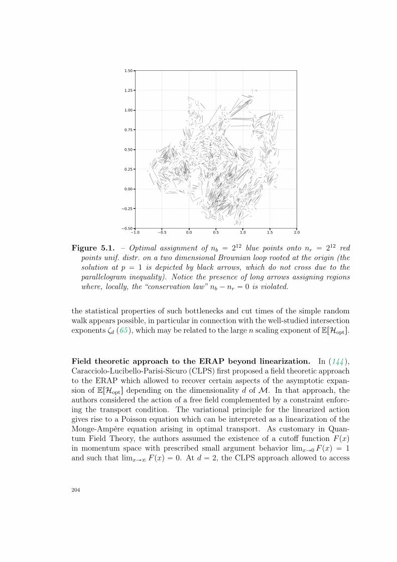
1.0 0.5 0.0 0.5 1.0 1.5 2.00.50
0.25
0.00
0.25
0.50
0.75
1.00
1.25
1.50
Figure 5.1. – Optimal assignment of nb “ 212 blue points onto nr “ 212 redpoints unif. distr. on a two dimensional Brownian loop rooted at the origin (thesolution at p “ 1 is depicted by black arrows, which do not cross due to theparallelogram inequality). Notice the presence of long arrows assigning regionswhere, locally, the “conservation law” nb ´ nr “ 0 is violated.
the statistical properties of such bottlenecks and cut times of the simple randomwalk appears possible, in particular in connection with the well-studied intersectionexponents ζd (65 ), which may be related to the large n scaling exponent of ErHopts.
Field theoretic approach to the ERAP beyond linearization. In (144 ),Caracciolo-Lucibello-Parisi-Sicuro (CLPS) first proposed a field theoretic approachto the ERAP which allowed to recover certain aspects of the asymptotic expan-sion of ErHopts depending on the dimensionality d of M. In that approach, theauthors considered the action of a free field complemented by a constraint enforc-ing the transport condition. The variational principle for the linearized actiongives rise to a Poisson equation which can be interpreted as a linearization of theMonge-Ampère equation arising in optimal transport. As customary in Quan-tum Field Theory, the authors assumed the existence of a cutoff function F pxqin momentum space with prescribed small argument behavior limxÑ0 F pxq “ 1and such that limxÑ8 F pxq “ 0. At d “ 2, the CLPS approach allowed to access
204
the leading (Ajtai-Komlós-Tusnàdy) behavior, which, in retrospective, is typicalof the renormalization group acting on the critical dimension, where the definingterm appearing in the action is a marginal operator. However, sub-leading termsof the asymptotic series are not directly accessible with this approach. Moreover,the alternative PDE approach introduced by Ambrosio-Stra-Trevisan (164 ), whichallowed to establish rigorously the value of limit constants, also cannot go beyondthe leading behavior and does not appear to be easily generalizable, due to essen-tial technical aspects in their proof. However, in the field theoretical approach, onecan go beyond linearization and consider the full perturbative series arising fromthe exact action. This approach allows to describe the full distribution of Hopt
by means of a diagrammatic (possibly asymptotic) series with intriguing combi-natorial properties (some results having been presented by Sportiello at the IHP).We wish to develop further these aspects, in particular in connection with theextension of the ERAP at arbitrary densities on possibly non-compact underlyingspaces M, and explore the connections of this problem with the recently intro-duced classification of the scaling of ErHopts into anomalous and bulk regimes forthe ERAP at d “ 1.
On logarithmic derivatives of the Dedekind η function appearing in reg-ularisations of the ERAP at d “ 2 and p “ 2. In § 3.1 we have consideredtwo regularization schemes for the ERAP at pp, dq “ p2, 2q on several highly sym-metrical domains M, also in connection to certain classical invariants expressedin terms of the the spectrum of the Laplace-Beltrami operator associated to thesurface M (51 , 120 ). We have also considered a regularisation of the (logarith-mically) divergent spectral sum by performing the analytic continuation of theassociated zeta function in the Kronecker limit. The method allowed for exam-ple to compute differences in sub-leading constants among different domains Mand M1. The theoretical predictions were in excellent agreement with numericalexperiments performed on several geometries.A motivation behind this work was that very little is known about the asymp-
totic series of ErHopts beyond the now-established universal „ 12π
log n behavior,and indeed no method appears to be currently able to address this problem directly.In our studies we have considered domains with a rectangular, l1ˆ l2 fundamen-
tal polygon (such as the cylinder or the torus), and shifts at fixed geometry butvariable aspect ratio ρ “ l1
l2. Quite surprisingly, we have observed a number of in-
stances in which such relative energies between different geometries admit (unique)global extrema at non-trivial values of the aspect ratio ρ. In these “extremal ge-ometries” a fundamental building block appeared to be logarithmic derivatives ofthe Dedekind η function. More precisely, optimal ρ are determined by solutions
205
to equations of the typea
ρ2`b
ρ“ ic
η1piρq
ηpiρq(5.0.0.2)
where η is the Dedekind function, and a, b, c P R, and we have been able to solvethese kind of equations only numerically. On the other hand, it is well-known thatthe rhs of Eq. 5.0.0.2, at certain special values of ρ (which are not extremal for ourconsidered problems), reduces to the evaluation of series of reciprocal hyperbolicfunctions (see e.g. Prop. 2.25 in (29 ), and (157 )), and some of these series havealready been considered in the context of the Neumann problem on the rectan-gle (28 ). The possibility that different extremal geometries (that is, optimal aspectratios for different domains M) may be related through non-trivial relationshipappears to be an interesting research perspective.
Cycle structure of the optimal permutation for the ERAP on a generalgraph. We have argued that an understanding of the combinatorial structureof the optimal configuration πopt for an ERAP in cases where B and R can benaturally ordered (as in d “ 1 and M “ R) can be very useful, but has beenpossible for a handful choices of the cost function only. Indeed, combinatorialresults either allowed to study the exact solution with analytical methods (e.g.when cpxq “ |x|p and p ą 1, in which case πopt is the identity, or p ă 0, in whichcase πopt is cyclical (154 )), either served as a guiding principle for the introductionof approximate solutions, such as the “Dyck matchings” (173 ), which conjecturallyhave the same asymptotic behavior of the optimal one. In this direction, evenweaker notions of order for points could be further exploited. A typical examplewould be to consider points distributed along the edges of some graphs (such asstar graphs). In such a problem, starting from the simples choices of cost function,is it possible to relate the combinatorial properties of πopt (or the πopts?) to thetopology of the graph?
Dynamics of indistinguishable agents. Tracking the motion of many identi-cal agents can be seen as an assignment problem in which the positions of agentsat time ti (B) have to be assigned to positions of agents at time ti`1 (R) bypreserving their individual identities. An analogous construction arises in theFeynman-Kac representation of the Bose gas, upon interpreting time as inversetemperature (122 ). If ti`1 ´ ti is sufficiently small, and the cost function is themaximum likelihood function for “recognising” the dynamics (e.g., cpxq “ |x|2 isthe maximum likelihood function for diffusive motion, or balistic motion with mi-nor modifications), one expects the transport field to correspond to the actualdisplacement field in the limit ti`1´ ti Ñ 0. An approximate algorithm to addresssimilar questions, based on belief propagation, has been already applied to turbu-
206

lent flow (129 ). However, in many real-life situations of interest, the motion ofmany individual agents displays long-range correlations. For example, evidenceshave been reported that the motion of a flock of birds displays an intriguing col-lective response to external perturbations (128 ). How to extend the assignmentapproach to such dynamical situations in order to understand deviations from un-correlated dynamics appears to be an interesting research perspective, especiallyin light of the availability of extensive empirical data.We hope to address some of these research directions in future work.
207

Appendices
208
d Appendix A D
A.1. The number of edges of length 2k ` 1 in aDyck matching at size n (§ 2.7.7)
The goal of this Appendix is to compute the coefficients vn,k, crucially used inthe calculation of the average cost of the Dyck matching, starting with Eq. 2.7.7.9.These coefficients count, among the n edges of all the possible
`
2nn
˘
Dyck matchingson 2n points, the number of edges e of length e “ 2k ` 1. That is, vn,k pn´1q!2
2p2n´1q!
is the probability that, taking a random Dyck matching πDyck uniformly, and anedge e P πDyck uniformly, we have e “ 2k ` 1.Dyck matchings correspond to Dyck “bridges”, w.r.t. the notation introduced in
§ 2.7.5. We proceed with the calculation by first computing the analogous quantityon a restricted ensemble, associated to Dyck “excursions” (that is, the ordinaryDyck paths), which are Dyck bridges satisfying the extra condition
řji“1 σi ě 0
for all 1 ď j ď 2n.In the whole class of Dyck paths of length 2n there are
rn,k :“n´ k ` 1
2Ck Cn´k “
1
2Ck Bn´k (A.1.0.1)
edges of length e “ 2k`1 (see http://oeis.org/A141811), with 0 ď k ď n´1.These numbers obey the recursion relation, which determines them univocally(together with the initial conditions)
rn,k “ CkCn´k´1 `
n´1ÿ
m“0
rrm,k Cn´m´1 ` rn´m´1,k Cms . (A.1.0.2)
The recursion can be understood in terms of a first-return decomposition. If wedecompose the path into its first return, i.e. the portion between its left endpointand its first zero (say at position 2m` 2, 0 ă m ă n´ 1), and into its tail, i.e. theremaining portion of the path on the right, then:
• the first term counts all the paths in which the link between the first stepand the first zero is of the required length. The multiplicity of paths in
209
which this situation arise is given by all the possible paths composing thefirst excursion times all the possible paths composing the tail;
• the sum counts, for all the possible positions of the first zero, the possiblelinks of the required length hidden in the first excursion or in the tail of thepath. To count links of the required length hidden in the first excursion,one can use rm,l itself, times all the possible tails Cn´m´1. The tail case issymmetric.
It is easy to prove by induction that
rn,k “ Ck Rn´k´1 (A.1.0.3)
and the recursion reduces to
Rs “ Cs ` 2s´1ÿ
m“1
Cs´mRm´1 . (A.1.0.4)
By introducing the generating function
Rpzq :“ÿ
ně0
Rn zn (A.1.0.5)
we get the equationRpzq “ Cpzq ` 2 z CpzqRpzq (A.1.0.6)
and therefore
Rpzq “Cpzq
1´ 2 z Cpzq“ CpzqBpzq “
1
2 z
„
1?
1´ 4 z´ 1
“ ´1
2 z`
1
2 z`
ÿ
ně0
Bn`1
2zn “
ÿ
ně0
Bn`1
2zn
(A.1.0.7)
indeednÿ
k“1
CkBn´k “Bn`1
2. (A.1.0.8)
It follows thatRn´k´1 “
Bn´k
2(A.1.0.9)
as announced.The preliminary computation of the rn,k coefficients suggests to use the same
210
technique for the vn,k, and provides an ingredient to write a recursion for the vn,k:
vn,k “ 2Ck Bn´k´1 ` 2n´1ÿ
m“0
prm,k Bn´m´1 ` vn´m´1,k Cmq
“ 2Ck Bn´k´1 `
n´1ÿ
m“k`1
Ck Bm´k Bn´m´1 ` 2n´1ÿ
m“k`1
vm,k Cn´m´1
“ 2Ck Bn´k´1 `
n´k´1ÿ
m“1
Ck BmBn´k´m´1 ` 2n´k´1ÿ
m“1
vm`k,k Cn´k´m´1
(A.1.0.10)
and if we again setvn,k :“ CkVn´k´1 (A.1.0.11)
we get
Vs “ 2Bs `
sÿ
m“1
BmBs´m ` 2sÿ
m“1
Vm´1Cs´m
“Bs `
sÿ
m“0
BmBs´m ` 2sÿ
m“1
Vm´1Cs´m
“Bs ` 4s ` 2sÿ
m“1
Vm´1Cs´m .
(A.1.0.12)
We introduce now the generating function
V pzq :“ÿ
kě0
Vk zk (A.1.0.13)
to get the relation
V pzq “1
?1´ 4 z
`1
1´ 4 z` 2 z
1´?
1´ 4 z
2 zV pzq (A.1.0.14)
so that
V pzq “1
1´ 4 z`
1
p1´ 4 zq32
“ÿ
kě0
„
4k `p2k ` 1q!
pk!q2
zk , (A.1.0.15)
which is our seeked result. We can finally check that the recursion above is indeed
211
satisfied, as
vn,k “Ck
„
4n´k´1`p2n´ 2k ´ 1q!
rpn´ k ´ 1q!s2
“Ck
„
4n´k´1`pn´ kq2
2 pn´ kqBn´k
“ 4n´k´1Ck ` pn´ kq rn,k .
(A.1.0.16)
212
A.2. Expansion of the generating function Spz; pq
via singularity analysis (§ 2.7.7)
Singularity analysis is a technique that allows to extract information on the co-efficients of a generating function fpzq when an explicit series expansion aroundz “ 0 is not available. Roughly speaking, two main principles hold (see e.g. (123 ,pg. 227)):
1. the moduli of the singularities of f dictate the asymptotic exponential growthof its coefficients. If z “ a is a singularity of fpzq “
ř
ně0 fnzn, then fn „
|a|´n;
2. the nature of the singularities of f dictate the asymptotic sub-exponentialgrowth of its coefficients, i.e. they determine the (typically polynomial orlogarithmic) function θpnq such that fn „ |a|´n θpnq.
We will specialise this analysis to the case of a single singularity, along the realpositive axis, which is pertinent to series with positive coefficients, and no oscil-latory behaviour. Generalizations of these principles (and of the related theorembelow) for the case of multiple singularities at the same radius hold as well, butin our case are not relevant and will not be discussed.The main result that we are going to need is a theorem (see (123 , Theorem
VI.4)) that states that if fpzq is a “well-behaved” complex function analytic in 0,with a singularity at z “ ζ ` i0 such that
fpzq “ σpzζq ` opτpzζqq (A.2.0.1)
for some functions σ “ř
ně0 σnzn and τ “
ř
ně0 τnzn in the span of the reference
set
S “!
p1´ zqαˆ
1
zlog
1
1´ z
˙βˇ
ˇ
ˇα, β P C
)
, (A.2.0.2)
thenfn “ ζ´nσn ` opζ
´nτnq . (A.2.0.3)
Here, “well behaved” means that there exists an indented disk of radius biggerthan ζ, with the indentation that specifically excludes z “ ζ ` i0, where fpzq canbe analytically continued. This means that the theorem is applicable to functionswith very general singularities (isolated poles, branch cuts, . . . ), and in particularto hypergeometric functions.The reference set S is composed of functions whose expansion can be computed
exactly thanks to generalizations of the binomial theorem. These functions are
213
ubiquitous in series expansions around poles of complex functions, so that thetheorem is extremely versatile.In our specific case of the ES model, the generating function to study is of the
formfpzq “ sp4zqF
ˆ
a, bc
∣∣∣∣ 4z
˙
(A.2.0.4)
where spzq P spanS is singular at z “ 1, and F “ 2F1 is the p2, 1q-hypergeometricfunction defined by
F
ˆ
a, bc
∣∣∣∣ z˙ “ ÿ
ně0
Γpn` aq
Γpaq
Γpn` bq
Γpbq
Γpcq
Γpn` cq
zn
n!, (A.2.0.5)
or, equivalently, by
F
ˆ
a, bc
∣∣∣∣ z˙ “ ÿ
ně0
snzn
n!; (A.2.0.6)
sn`1
sn“pa` nqpb` nq
c` n; s1 “ 1 . (A.2.0.7)
To expand and study the hypergeometric function around z “ 1, a celebrated“inversion formula” due to Gauss is available
F
ˆ
a, bc
∣∣∣∣ z˙ “ΓpcqΓpc´ a´ bq
Γpc´ aqΓpc´ bqF
ˆ
a, ba` b` 1´ c
∣∣∣∣ 1´ z
˙
`
ΓpcqΓpa` b´ cq
ΓpaqΓpbqp1´ zqc´a´bF
ˆ
c´ a, c´ bc` 1´ a´ b
∣∣∣∣ 1´ z
˙
.
(A.2.0.8)
This formula restates the seeked expansion around z “ 0 in terms of an expansionnear the singularity at z “ 1. As the hypergeometric function is analytic in z “ 0,the singular behaviour at z “ 1 of the right-hand side combination is described bythe power-law prefactors in the inversion formula.In our specific case, a “ p`1
2, b “ p`2
2and c “ 2 with p P r0, 1s, giving c´a´b “
1´2p2P r´1
2, 1
2s. Thus, the leading terms of the expansion of fpzq are:
fpzq “ sp4zq
„
ΓpcqΓpc´ a´ bq
Γpc´ aqΓpc´ bq`
ΓpcqΓpa` b´ cq
ΓpaqΓpbqp1´ 4zqc´a´b
`Θpp1´ 4zq, p1´ 4zqc´a´b`1q
. (A.2.0.9)
The above expression is valid only for p ‰ 12. A limit procedure combines the
214
diverging Γ’s and the p1´ 4zq term to give
fpzq “ sp4zq
„
´1
Γp34qΓp5
4q
`
lnp1´ 4zq ` 2γE ` ψ0
`
34
˘
` ψ0
`
54
˘˘
`Θpp1´ 4zq lnp1´ 4zqq
. (A.2.0.10)
where γE is the Euler-Mascheroni constant and ψ0 is the digamma function. Thelimit is to be performed with care: each term must be written as a function ofε “ p ´ 1
2and expanded in powers series. The expansion of the hypergeometric
functions must be performed using their definition. When everything is expanded,opεq are discarded taking the limit ε Ñ 0, and the leading terms in the p1 ´ 4zqare found by taking n “ 0 in the sum of the hypergeometric function definition.
215
d Appendix B D
B.1. The first Kronecker limit formula (§ 3.1.2)
In this Appendix we will summarize some results obtained in the realm of analyticnumber theory that have been useful to obtain our results. General references forour discussion are Siegel (20 ) (Chapter 1) and Lang (48 ).
Let z P C. The Riemann ζ-function ζpzq is defined in the half-plane <pzq ą 0by
ζpzq :“ÿ
kě1
1
kz. (B.1.0.1)
The series converges absolutely for <pzq ě 1` ε for every ε ą 0. Riemann provedthat ζpzq has an analytic continuation in the whole z-plane which is regular excepta simple pole at z “ 1 with residue 1. At z “ 1, ζpzq has an expansion
ζpzq ´1
z ´ 1“
8ÿ
k“1
ż k`1
k
du`
k´z ´ u´z˘
“ γE ` opz ´ 1q. (B.1.0.2)
As generalization of the Riemann ζ-function, we consider a positive-definite binaryquadratic form, in the real variables u, v P R
Qpu, vq :“ au2` 2buv ` cv2 (B.1.0.3)
where, a, b, c P R and a ą 0 and d :“ ac´ b2 ą 0. Let us define
ζQpzq :“ÿ
pm,nqPZ2
n2`m2‰0
1
rQpm,nqsz. (B.1.0.4)
216
Now
Qpu, vq “a
ˆ
u`b
a
˙2
`v2d
a
“a
˜
u`b` i
?d
av
¸˜
u`b´ i
?d
av
¸
“a|u` τv|2
(B.1.0.5)
where
τ “b` i
?d
a(B.1.0.6)
with =pτq “ a´1?d ą 0.
If d “ 1, ζQpzq ” ζτ pzq, associated to Q, is defined for <pzq ą 1 can be analyt-ically continued into a regular function for <pzq ą 12 except for a simple pole atz “ 1 with residue π, and the function ζQpzq, has an expansion (first limit formulaof Kronecker)
ζτ psq ´π
z ´ 1“ 2π
”
γE ´ lnp2a
=pτq|ηpτq|2qı
` opz ´ 1q, (B.1.0.7)
where
ηpzq :“ eπiz12
8ź
n“1
`
1´ e2πinz˘
(B.1.0.8)
is the Dedekind η-function (27 ), which satisfies the functional equations
ηpz ` 1q “eπi12 ηpzq (B.1.0.9a)
η
ˆ
´1
z
˙
“?´izηpzq . (B.1.0.9b)
Known particular values are
ηpiq “Γ p14q
2π34« 0.76823 (B.1.0.10a)
ηp2iq “Γ p14q
2118π34« 0.59238 (B.1.0.10b)
ηp4iq “´
´1`?
2¯14 Γ p14q
22916π34« 0.35092 . (B.1.0.10c)
217
d Appendix C D
C.1. Calculus on the square lattice (§ 3.3)
In this Appendix we shall recall some basic definitions of calculus on the lattice.Our review could have been independent on the two-dimensional Grid-PoissonERAP, but for the sake of definiteness we shall restrict to the square lattice usedin § 3.3.
For a complex valued function f defined on the d-dimensional regular lattice,for ν “ 1, . . . , d recall the positive and negative directional derivatives
∇`ν fpzq :“fpz ` eνq ´ fpzq
∇´ν fpzq :“fpzq ´ fpz ´ eνq “ ∇`
ν fpz ´ eνq(C.1.0.1)
in terms of which the lattice laplacian is
∆fpzq :“ÿ
ν
∇´ν ∇`
ν fpzq “ÿ
ν
∇`ν ∇´
ν fpzq
“ÿ
ν
rfpz ` eνq ` fpz ´ eνq ´ 2fpzqs
“ÿ
ν
“
∇`ν ´∇´
ν
‰
fpzq .
(C.1.0.2)
∆ is a self-adjoint operator with respect to the lattice inner product defined, forany two complex valued functions f, g : Λn Ñ C, by
pf, gq “ÿ
zPΛn
fpzqgpzq , (C.1.0.3)
where z is complex conjugate of z (an analogous definition holds for the duallattice). In our setting at d “ 2, where n “ L2, the discrete Fourier representationof a function f is
fpzq “1
L
ÿ
p
eip¨zfppq (C.1.0.4)
218
where the discrete lattice momenta p “ 2πL
ˆ
n1
n2
˙
depend on pn1, n2q P Z2. It
follows that∆fppq “ ´ p2 fppq (C.1.0.5)
wherepi :“ 2 sin
pi2, i “ 1, 2 (C.1.0.6)
is a generalization of Eq. 2.3.1.18. If vector fields are considered, Definition C.1.0.4holds component-wise, and when obvious we shall always understand sum overcomponents, so that e.g.
Hopt “ páµ,áµq “
2ÿ
i“1
pµi, µiq . (C.1.0.7)
A main tool of our discussion are diagonal derivatives, which informally are finitedifferences operators acting “between” the direct and the dual lattice. More pre-cisely, for a function h : Λn Y Λn Ñ C, defined both on the direct lattice Λn andon the dual lattice Λn, they are defined as
∇1hpi, jq “1?
2
„
h
ˆ
i`1
2, j `
1
2
˙
´ h
ˆ
i´1
2, j ´
1
2
˙
,
∇2hpi, jq “1?
2
„
h
ˆ
i´1
2, j `
1
2
˙
´ h
ˆ
i`1
2, j ´
1
2
˙ (C.1.0.8)
for i, j “ 0, . . . L ´ 1 (see Fig. 3.12a for a graphical rule). In terms of diagonalderivatives, it is possible to introduce the divergence and curl of any vector fieldáE : ΛnpΛnq Ñ T2. They are the scalar fields
∇ ¨ áE “∇αEα ,
∇^áE “ εαβ∇αEβ, pα, β “ 1, 2q,(C.1.0.9)
where εαβ is the 2-dimensional Levi-Civita symbol (and the convention on repeatedindices has been used). Remark that for a complex valued vector field defined onΛnpΛnq, its divergence and curl are defined on ΛnpΛnq. Moreover, they satisfy thezero-sum conservation laws
ÿ
zPΛnpΛnq
p∇ ¨ áEqpzq “ÿ
zPΛnpΛnq
p∇^áEqpzq “ 0 (C.1.0.10)
219
by two-dimensional telescoping∗. On the other hand, recall that the lattice lapla-cian ∆ acts either “on” the direct or “on” the dual lattice, but not “between” them:for any function f : ΛnpΛnq Ñ C, we can write locally
p∆fqpi, jq “1
2rf pi` 1, j ` 1q ` f pi´ 1, j ´ 1q ` f pi´ 1, j ` 1q`
f pi` 1, j ´ 1q ´ 4fpi, jqs . (C.1.0.12)
for i, j “ 0, . . . L´ 1 (see Fig. 3.12b for a graphical rule). Of course, the laplacianof any function also satisfies the zero-sum condition
ÿ
zPΛnpΛnq
p∆fqpzq “ 0 . (C.1.0.13)
To elucidate the combined effect of our “rotation” (Eq. 3.3.1.9) and expression ofthe rotated field in terms of diagonal derivatives (Defs. C.1.0.8), it may be usefulto observe that the divergence of áµ´π4 can be written locally as
`
∇ ¨ áµ´π4˘
ˆ
i`1
2, j `
1
2
˙
“µ1 pi` 1, j ` 1q ´ µ1 pi, jq ` µ2 pi, j ` 1q ´ µ2 pi` 1, jq
?2
“µx pi` 1, j ` 1q ´ µx pi, jq ´ µx pi, j ` 1q ` µx pi` 1, jq
2`
µy pi` 1, j ` 1q ´ µy pi, jq ` µy pi, j ` 1q ´ µy pi` 1, jq
2,
(C.1.0.14)
or, in terms of the standard directional lattice derivatives and ordinary áµ compo-nents as
`
∇ ¨ áµ´π4˘
ˆ
i`1
2, j `
1
2
˙
“ ∇`x
„
µxpi, j ` 1q ` µxpi, jq
2
`∇`y
„
µypi` 1, jq ` µypi, jq
2
“ ∇`x µxpi, jq `∇`
y µypi, jq `∇`x∇`
y
„
µxpi, jq ` µypi, jq
2
.
(C.1.0.15)
∗Indeed, the stronger conservation lawsÿ
zPΛnpΛnq
p∇iáEqpzq “ 0, i “ 1, 2 (C.1.0.11)
hold separately.
220
Correspondingly, the curl can be written as
`
∇^ áµ´π4˘
ˆ
i`1
2, j `
1
2
˙
“µ2 pi` 1, j ` 1q ´ µ2 pi, jq ´ µ1 pi, j ` 1q ` µ1 pi` 1, jq
?2
“´µx pi` 1, j ` 1q ` µx pi, jq ´ µx pi, j ` 1q ` µx pi` 1, jq
2`
µy pi` 1, j ` 1q ´ µy pi, jq ´ µy pi, j ` 1q ` µy pi` 1, jq
2
“∇`x
„
µypi, j ` 1q ` µypi, jq
2
´∇`y
„
µxpi` 1, jq ` µxpi, jq
2
“∇`x µypi, jq ´∇`
y µxpi, jq `∇`x∇`
y
„
µypi, jq ´ µxpi, jq
2
.
(C.1.0.16)
As of the role of the modified lattice laplacian, observe that it follows from ourdefinition 3.3.1.10 that the components of áµ´π4 have the Fourier representation
µ1pzq “ i
?2
L
ÿ
p
eip¨z”
sinpx ` py
2φppq ´ sin
py ´ px2
ψppqı
µ2pzq “ i
?2
L
ÿ
p
eip¨z”
sinpy ´ px
2φppq ` sin
px ` py2
ψppqı
(C.1.0.17)
and hence †
`
∇ ¨ áµ´π4˘
pzq “ ´2
L
ÿ
p
eip¨z”
sin2 px ` py2
` sin2 px ´ py2
ı
φppq
“ ´1
L
ÿ
p
eip¨z„
p2´p2
1p21
2
φppq,
`
∇^ áµ´π4˘
pzq “ ´1
L
ÿ
p
eip¨z„
p2´p2
1p22
2
ψppq .
(C.1.0.19)
†As can be readily verified using the trigonometric identity
2 sin2 p1 ` p2
2` 2 sin2 p1 ´ p2
2“ 2´ cospp1 ` p2q ´ cospp1 ´ p2q
“ 2´ 2 cos p1 cos p2 “ 2´ 2
ˆ
1´p2
1
2
˙ˆ
1´p2
2
2
˙
“ p21 ` p
22 ´
p21p
22
2.
(C.1.0.18)
221
Bibliography
1. G. Peano, Sur une courbe, qui remplit toute une aire plane. MathematischeAnnalen 36, 157–160, DOI 10.1007/BF01199438 (1890) (cit. on p. 187).
2. H von Koch, Sur une courbe continue sans tangente, obtenue par une con-struction géométrique élémentaire. Ark. Mat. Astron. Fys. 1, 681–702 (1904)(cit. on p. 189).
3. E. Cesàro, Remarques sur la courbe de von Koch. Atti della Reale Accademiadi Scienze Fisiche e Matematiche (1905) (cit. on pp. i, 189).
4. D. Konig, Uber Graphen und ihre Anwendung auf Determinantentheorieund Mengenlehre. Mathematische Annalen 77, 453–465, DOI 10.1007/BF01456961 (1916) (cit. on p. 3).
5. G. D. Birkhoff, Proof of the Ergodic Theorem. Proceedings of the NationalAcademy of Sciences 17, 656–660, DOI 10.1073/pnas.17.2.656 (1931)(cit. on p. 2).
6. J. Egervàry, Matrixok kombinatorius tulajdonságairól (in Hungarian), 38:16–28. Matematikai és Fizikai Lapok 38, 16–28 (1931) (cit. on p. 3).
7. J. V. Neumann, Proof of the Quasi-Ergodic Hypothesis. Proceedings of theNational Academy of Sciences 18, 70–82, DOI 10.1073/pnas.18.1.70(1932) (cit. on p. 2).
8. A. N. Kolmogorov, Sulla Determinazione Empirica di Una Legge di Dis-tribuzione. Giornale dell’Istituto Italiano degli Attuari 4, 83–91 (1933) (cit.on p. 27).
9. M. Born, L. Infeld, Foundations of the new field theory. Proceedings of theRoyal Society of London. Series A, Containing Papers of a Mathematicaland Physical Character 144, 425–451, DOI 10.1098/rspa.1934.0059(1934) (cit. on p. 133).
10. F. J. Massey, The Kolmogorov-Smirnov Test for Goodness of Fit. Journal ofthe American Statistical Association 46, 68, DOI 10.2307/2280095 (1951)(cit. on p. 27).
11. J. Nash, Non-Cooperative Games. The Annals of Mathematics 54, 286, DOI10.2307/1969529 (1951) (cit. on p. 1).
222
12. G. B. Dantzig, “Comments on J. Von Neumann’s ’The problem of opti-mal assignment in a two-person game’”, tech. rep. (RAND CORP SANTAMONICA CA, 1952., 1952) (cit. on p. 2).
13. M. D. Donsker, Justification and Extension of Doob’s Heuristic Approach tothe Kolmogorov- Smirnov Theorems. The Annals of Mathematical Statistics23, 277–281, DOI 10.1214/aoms/1177729445 (1952) (cit. on p. 25).
14. J. von Neumann, in Contributions to the Theory of Games (AM-28), VolumeII, ed. by H. W. Kuhn, A. W. Tucker (Princeton University Press, Princeton,1953), pp. 5–12, DOI 10.1515/9781400881970-002 (cit. on pp. 1–3).
15. H. W. Kuhn, The Hungarian method for the assignment problem. NavalResearch Logistics Quarterly 2, 83–97, DOI 10 . 1002/ nav . 3800020109(1955) (cit. on p. 3).
16. T. C. Koopmans, M. Beckmann, Assignment Problems and the Location ofEconomic Activities. Econometrica 25, 53, DOI 10.2307/1907742 (1957)(cit. on p. 2).
17. J. Munkres, Algorithms for the Assignment and Transportation Problems.Journal of the Society for Industrial and Applied Mathematics 5, 32–38,DOI 10.1137/0105003 (1957) (cit. on p. 3).
18. J. Beardwood, J. H. Halton, J. M. Hammersley, The shortest path throughmany points. Mathematical Proceedings of the Cambridge Philosophical So-ciety 55, 299–327, DOI 10.1017/S0305004100034095 (1959) (cit. on p. 18).
19. L. V. Kantorovich, Mathematical Methods of Organizing and Planning Pro-duction. Management Science 6, 366–422, DOI 10.1287/mnsc.6.4.366(1960) (cit. on p. 3).
20. C. L. Siegel, On advanced analytic number theory (Tata Institute of Funda-mental Research, 1961) (cit. on p. 216).
21. G. S. Watson, Goodness-of-fit tests on a circle. Biometrika 48, 109–114,DOI 10.1093/biomet/48.1-2.109 (1961) (cit. on p. 37).
22. G. B. Dantzig, Linear Programming and Extensions, ed. by Intergovern-mental Panel on Climate Change (RAND Corporation, Cambridge, 1963),vol. 53, pp. 1–30, DOI 10.7249/R366, arXiv: arXiv:1011.1669v3 (cit. onp. 3).
23. W. E. Donath, Algorithm and Average-value Bounds for Assignment Prob-lems. IBM Journal of Research and Development 13, 380–386, DOI 10.1147/rd.134.0380 (1969) (cit. on p. 6).
223
24. J. Edmonds, R. M. Karp, Theoretical Improvements in Algorithmic Effi-ciency for Network Flow Problems. Journal of the ACM (JACM) 19, 248–264, DOI 10.1145/321694.321699 (1972) (cit. on p. 3).
25. S. F. Edwards, P. W. Anderson, Theory of spin glasses. J. Phys. F: MetalPhys. 5, 965–974, DOI 10.1002/pssb.2220700123 (1975) (cit. on p. 6).
26. D. Sherrington, S. Kirkpatrick, Solvable model of a spin-glass. Physical Re-view Letters 35, 1792–1796, DOI 10.1103/PhysRevLett.35.1792, arXiv:arXiv:1011.1669v3 (1975) (cit. on p. 6).
27. T. M. Apostol, in, vol. 24, pp. 47–73, DOI 10.1007/978-1-4684-9910-0_3(cit. on pp. 139, 217).
28. F. P. Sayer, The sums of certain series containing hyperbolic functions.Fibonacci Quart 14, 215–223 (1976) (cit. on p. 206).
29. B. C. Berndt, Modular transformations and generalizations of several for-mulae of Ramanujan. Rocky Mountain Journal of Mathematics 7, 147–190,DOI 10.1216/RMJ-1977-7-1-147 (1977) (cit. on p. 206).
30. S. W. Hawking, Zeta function regularization of path integrals in curvedspacetime. Communications in Mathematical Physics 55, 133–148, DOI 10.1007/BF01626516 (1977) (cit. on p. 137).
31. J Vannimenus, G Toulouse, Theory of the frustration effect. II. Ising spinson a square lattice. Journal of Physics C: Solid State Physics 10, L537–L542, DOI 10.1088/0022-3719/10/18/008 (1977) (cit. on p. 5).
32. S. Kirkpatrick, D. Sherrington, Infinite-ranged models of spin-glasses. Phys-ical Review B 17, 4384–4403, DOI 10.1103/PhysRevB.17.4384, arXiv:arXiv:1011.1669v3 (1978) (cit. on p. 6).
33. G. Parisi, Toward a mean field theory for spin glasses. Physics Letters A 73,203–205, DOI 10.1016/0375-9601(79)90708-4 (1979) (cit. on p. 6).
34. G. Parisi, A sequence of approximated solutions to the S–K model for spinglasses. Journal of Physics A: Mathematical and General 13, L115–L121,DOI 10.1088/0305-4470/13/4/009 (1980) (cit. on p. 6).
35. G. Parisi, The order parameter for spin glasses: A function on the interval0–1. Journal of Physics A: Mathematical and General 13, 1101–1112, DOI10.1088/0305-4470/13/3/042 (1980) (cit. on p. 6).
36. S Kirkpatrick, C. D. Gelatt Jr, M. P. Vecchi, Optimization by SimulatedAnnealing. Science 220, 671–680, DOI 10.1126/science.220.4598.671,arXiv: arXiv:1011.1669v3 (1983) (cit. on p. 5).
37. M. Ajtai, J. Komlós, G. Tusnády, On optimal matchings. Combinatorica 4,259–264, DOI 10.1007/BF02579135 (1984) (cit. on pp. 131, 134).
224
38. L. R. Foulds, Combinatorial Optimization for Undergraduates (Springer US,New York, NY, 1984), DOI 10.1007/978-1-4613-9511-9 (cit. on p. 4).
39. E. L. Lawler, The traveling salesman problem: a guided tour of combinatorialoptimization.Wiley-Interscience Series in Discrete Mathematics (1985) (cit.on p. 18).
40. M. Mézard, G. Parisi, Replicas and optimization. Journal de Physique Let-tres 46, 771–778, DOI 10.1051/jphyslet:019850046017077100 (1985)(cit. on pp. iii, 5, 6, 8).
41. H. Orland, Mean-field theory for optimization problems. Journal de PhysiqueLettres 46, 763–770, DOI 10.1051/jphyslet:019850046017076300 (1985)(cit. on pp. 5, 6).
42. K. Binder, A. P. Young, Spin glasses: Experimental facts, theoretical con-cepts, and open questions. Reviews of Modern Physics 58, 801–976, DOI10.1103/RevModPhys.58.801 (1986) (cit. on p. 6).
43. L. Devroye, Non-Uniform Random Variate Generation (Springer New York,New York, NY, 1986), DOI 10.1007/978-1-4613-8643-8 (cit. on p. 58).
44. M Mezard, G. Parisi, M Virasoro, Spin Glass Theory and Beyond (WORLDSCIENTIFIC, World Scie, 1986), vol. 9, DOI 10.1142/0271 (cit. on p. 5).
45. G. Carpaneto, P. Toth, Primal-dual algrorithms for the assignment problem.Discrete Applied Mathematics 18, 137–153, DOI 10.1016/0166-218X(87)90016-3 (1987) (cit. on p. 3).
46. R. Jonker, A. Volgenant, A shortest augmenting path algorithm for denseand sparse linear assignment problems. Computing 38, 325–340, DOI 10.1007/BF02278710 (1987) (cit. on pp. 3, 4).
47. R. Jonker, A. Volgenant, A shortest augmenting path algorithm for denseand sparse linear assignment problems. Computing 38, 325–340, DOI 10.1007/BF02278710 (1987) (cit. on p. 153).
48. S. Lang, in Elliptic Functions (Springer New York, New York, NY, 1987),pp. 267–278, DOI 10.1007/978-1-4612-4752-4_20 (cit. on p. 216).
49. K. Mulmuley, U. V. Vazirani, V. V. Vazirani, Matching is as easy as matrixinversion. Combinatorica 7, 105–113, DOI 10.1007/BF02579206 (1987)(cit. on p. 18).
50. M. Mézard, G. Parisi, The Euclidean matching problem. Journal de Physique49, 2019–2025, DOI 10.1051/jphys:0198800490120201900 (1988) (cit. onpp. iii, 9, 131).
225
51. B. Osgood, R. Phillips, P. Sarnak, Extremals of determinants of Laplacians.Journal of Functional Analysis, DOI 10.1016/0022-1236(88)90070-5(1988) (cit. on pp. 137, 143, 205).
52. G. B. Dantzig, in A history of scientific computing (ACM, New York, NY,USA, 1990), vol. 28, pp. 141–151, DOI 10.1145/87252.88081 (cit. on p. 3).
53. V. L. Girko, Theory of Random Determinants (Springer Netherlands, Dor-drecht, 1990), vol. 13, pp. 231–232, DOI 10.1007/978-94-009-1858-0(cit. on p. 19).
54. S. P. Lalley, Travelling salesman with a self-similar itinerary. Probabilityin the Engineering and Informational Sciences 4, 1–18, DOI 10. 1017/S026996480000142X (1990) (cit. on p. 18).
55. G. P. Jelliss, R. L. Graham, D. E. Knuth, O. Patashnik, Concrete Math-ematics, a Foundation for Computer Science. The Mathematical Gazette,DOI 10.2307/3619021 (1991) (cit. on p. 113).
56. M. Hoffman, Multiple harmonic series. Pacific Journal of Mathematics 152,275–290, DOI 10.2140/pjm.1992.152.275 (1992) (cit. on p. 78).
57. A. N. Shiryayev, in Selected Works of A. N. Kolmogorov, ed. by A. N.Shiryayev (Springer Netherlands, Dordrecht, 1992), pp. 139–146, DOI 10.1007/978-94-011-2260-3_15 (cit. on p. 27).
58. J. M. Steele, Probability and problems in euclidean combinatorial optimiza-tion. Statistical Science 8, 48–56, DOI 10.1214/ss/1177011083 (1993)(cit. on pp. 7, 18).
59. Y. Lee, J. B. Orlin, in Large Scale Optimization, ed. by W. Hager, D. Hearn,P. Pardalos (Springer US, Boston, MA, 1994), pp. 206–244, DOI 10.1007/978-1-4613-3632-7_12 (cit. on p. 4).
60. M. Talagrand, The Transportation Cost from the Uniform Measure to theEmpirical Measure in Dimension >=3. The Annals of Probability 22, 919–959, DOI 10.1214/aop/1176988735 (1994) (cit. on p. 185).
61. D. Zagier, Values of Zeta Functions and Their Applications. First EuropeanCongress of Mathematics Paris, July 6–10, 1992, 497–512, DOI 10.1007/978-3-0348-9112-7_23 (1994) (cit. on p. 79).
62. A. S. Kechris, Classical Descriptive Set Theory (Springer New York, NewYork, NY, 1995), vol. 156, DOI 10.1007/978-1-4612-4190-4 (cit. onp. 17).
63. I. P. Gent, T. Walsh, The TSP phase transition. Artificial Intelligence 88,349–358, DOI 10.1016/S0004-3702(96)00030-6 (1996) (cit. on p. 8).
226
64. P. G. Higgs, Overlaps between RNA Secondary Structures. Physical ReviewLetters 76, 704–707, DOI 10.1103/PhysRevLett.76.704 (1996) (cit. onp. 107).
65. G. Lawler, Cut Times for Simple Random Walk. Electronic Journal of Prob-ability 1, 1–24, DOI 10.1214/EJP.v1-13 (1996) (cit. on p. 204).
66. G. Rempala, Asymptotic behavior of random permanents. Random Opera-tors and Stochastic Equations 4, 33–42, DOI 10.1515/rose.1996.4.1.33(1996) (cit. on p. 19).
67. D. J. Broadhurst, D. Kreimer, Association of multiple zeta values with pos-itive knots via Feynman diagrams up to 9 loops. Physics Letters, Section B:Nuclear, Elementary Particle and High-Energy Physics 393, 403–412, DOI10.1016/S0370-2693(96)01623-1 (1997) (cit. on p. 79).
68. E. B. Saff, A. B. Kuijlaars, Distributing many points on a sphere. Mathe-matical Intelligencer, DOI 10.1007/BF03024331 (1997) (cit. on p. 155).
69. J. M. Steele, Probability Theory and Combinatorial Optimization (SIAM,1997), p. 159 (cit. on p. 18).
70. D. Vere-Jones, Alpha-permanents and their applications to multivariategamma, negative binomial and ordinary binomial distributions. New ZealandJournal of Mathematics 26, 125–149 (1997) (cit. on pp. 19, 203).
71. D. P. Bertsekas, Network Optimization: Continuous and Discrete Methods,xiii, 593 p. (Cit. on p. 3).
72. S. Caracciolo, A. Pelissetto, Corrections to finite-size scaling in the lattice N-vector model for N = infty. Physical Review D 58, 105007, DOI 10.1103/PhysRevD.58.105007 (1998) (cit. on p. 31).
73. D. Coppersmith, G. B. Sorkin, in Lecture Notes in Computer Science (in-cluding subseries Lecture Notes in Artificial Intelligence and Lecture Notesin Bioinformatics), vol. 1518, pp. 319–330, DOI 10.1007/3-540-49543-6_25 (cit. on p. 7).
74. P. Flajolet, B. Salvy, Euler sums and contour integral representations. Ex-perimental Mathematics, DOI 10.1080/10586458.1998.10504356 (1998)(cit. on p. 79).
75. I. Karatzas, S. E. Shreve, Brownian Motion and Stochastic Calculus (SpringerNew York, New York, NY, 1998), vol. 113, DOI 10.1007/978-1-4612-0949-2 (cit. on p. 26).
76. I. G. I. MacDonald, Symmetric functions and Hall polynomials (Oxforduniversity press, 1998), vol. 13, pp. 180–183 (cit. on p. 72).
227
77. G. Parisi, A Conjecture on random bipartite matching. arXiv 2, 2, arXiv:9801176 (cond-mat) (1998) (cit. on p. 6).
78. C. Puente, J. Romeu, R. Pous, J Ramis, A Hijazo, Small but long Kochfractal monopole. Electronics Letters 34, 9–10, DOI 10.1049/el:19980114(1998) (cit. on p. 189).
79. J. E. Yukich, Probability Theory of Classical Euclidean Optimization Prob-lems (Springer Berlin Heidelberg, Berlin, Heidelberg, 1998), vol. 1675, DOI10.1007/BFb0093472 (cit. on p. 18).
80. R. E. Burkard, E. Çela, inHandbook of Combinatorial Optimization (SpringerUS, Boston, MA, 1999), pp. 75–149, DOI 10.1007/978-1-4757-3023-4_2(cit. on p. 3).
81. I. Hueter, The convex hull of samples from self-similar distributions. Ad-vances in Applied Probability 31, 34–47, DOI 10.1239/aap/1029954264(1999) (cit. on p. 186).
82. R. J. McCann, Exact solutions to the transportation problem on the line.Proceedings of the Royal Society of London. Series A: Mathematical, Phys-ical and Engineering Sciences 455, 1341–1380, DOI 10.1098/rspa.1999.0364 (1999) (cit. on pp. 23, 128).
83. Y. Brenier, Derivation of the Euler equations from a caricature of Coulombinteraction. Communications in Mathematical Physics, DOI 10.1007/s002200000204(2000) (cit. on p. 133).
84. M. Dell’Amico, P. Toth, Algorithms and codes for dense assignment prob-lems: the state of the art. Discrete Applied Mathematics 100, 17–48, DOI10.1016/S0166-218X(99)00172-9 (2000) (cit. on p. 3).
85. P. G. Higgs, RNA secondary structure: physical and computational aspects.Quarterly Reviews of Biophysics 33, 199–253, DOI 10.1017/S0033583500003620(2000) (cit. on p. 107).
86. S. Mertens, Computational Complexity for Physicists. Computing in Sci-ence and Engineering 4, 31, DOI 10.1109/5992.998639, arXiv: 0012185(cond-mat) (2000) (cit. on p. 7).
87. A. Pagnani, G. Parisi, F. Ricci-Tersenghi, Glassy Transition in a DisorderedModel for the RNA Secondary Structure. Physical Review Letters 84, 2026–2029, DOI 10.1103/PhysRevLett.84.2026 (2000) (cit. on p. 107).
88. D. J. Aldous, The ζ(2) limit in the random assignment problem. RandomStructures and Algorithms 18, 381–418, DOI 10.1002/rsa.1015, arXiv:0010063v1 (2001) (cit. on pp. iii, 6).
228
89. O. C. Martin, R. Monasson, R. Zecchina, Statistical mechanics methodsand phase transitions in optimization problems. Theoretical Computer Sci-ence 265, 3–67, DOI 10.1016/S0304-3975(01)00149-9, arXiv: 0104428(cond-mat) (2001) (cit. on p. 8).
90. H. Nishimori, Statistical Physics of Spin Glasses and Information Processing(Oxford University Press, Internatio, 2001), p. 252, DOI 10.1093/acprof:oso/9780198509417.001.0001 (cit. on p. 5).
91. R. Bundschuh, T. Hwa, Statistical mechanics of secondary structures formedby random RNA sequences. Physical Review E 65, 031903, DOI 10.1103/PhysRevE.65.031903 (2002) (cit. on p. 107).
92. E. Marinari, A. Pagnani, F. Ricci-Tersenghi, Zero-temperature properties ofRNA secondary structures. Physical Review E - Statistical Physics, Plasmas,Fluids, and Related Interdisciplinary Topics 65, 7, DOI 10.1103/PhysRevE.65.041919 (2002) (cit. on p. 107).
93. M. Mezard, Analytic and Algorithmic Solution of Random SatisfiabilityProblems. Science 297, 812–815, DOI 10.1126/science.1073287 (2002)(cit. on p. 8).
94. C. Morpurgo, Sharp inequalities for functional integrals and traces of confor-mally invariant operators. Duke Mathematical Journal 114, 477–553, DOI10.1215/S0012-7094-02-11433-1 (2002) (cit. on p. 137).
95. H. Orland, A. Zee, RNA folding and large N matrix theory. Nuclear PhysicsB 620, 456–476, DOI 10.1016/S0550-3213(01)00522-3, arXiv: 0106359(cond-mat) (2002) (cit. on p. 107).
96. J. Riordan, Introduction to Combinatorial Analysis (John Wiley and Sons,New York, Dover, 2002) (cit. on p. 84).
97. F. Guerra, Broken replica symmetry bounds in the mean field spin glassmodel. Communications in Mathematical Physics 233, 1–12, DOI 10.1007/s00220-002-0773-5, arXiv: 0205123 (cond-mat) (2003) (cit. on p. 6).
98. S. Linusson, J. Wästlund, A proof of Parisi’s conjecture on the randomassignment problem. Probab. Theory Relat. Fields 62, 1–7, DOI 10.1007/s00440-003-0308-9Svante (2003) (cit. on p. 7).
99. M. Müller, Statistical physics of RNA folding. Physical Review E 67, 021914,DOI 10.1103/PhysRevE.67.021914 (2003) (cit. on p. 107).
100. A. Pagnani, G. Parisi, M. Ratiéville, Near-optimal configurations in mean-field disordered systems. Physical Review E 68, 046706, DOI 10.1103/PhysRevE.68.046706, arXiv: 0307250 (cond-mat) (2003) (cit. on p. 19).
229
101. M. Agrawal, N. Kayal, N. Saxena, PRIMES is in P. Annals of Mathematics160, 781–793, DOI 10.4007/annals.2004.160.781 (2004) (cit. on p. 7).
102. Y. Brenier, A Note on Deformations of 2D Fluid Motions Using 3D Born-Infeld Equations.Monatshefte fur Mathematik 142, 113–122, DOI 10.1007/s00605-004-0240-9 (2004) (cit. on p. 133).
103. P. Glasserman, in, pp. 79–184, DOI 10.1007/978-0-387-21617-1_3 (cit.on p. 26).
104. O. C. Martin, M. Mézard, O. Rivoire, Frozen glass phase in the multi-index matching problem. Physical Review Letters 93, 19–22, DOI 10.1103/PhysRevLett.93.217205 (2004) (cit. on p. 8).
105. D. J. Aldous, A. Bandyopadhyay, A survey of max-type recursive distri-butional equations. The Annals of Applied Probability 15, 1047–1110, DOI10.1214/105051605000000142, arXiv: 0401388v3 (arXiv:math) (2005)(cit. on p. 7).
106. O. C. Martin, M. Mézard, O. Rivoire, Random multi-index matching prob-lems. Journal of Statistical Mechanics: Theory and Experiment, 159–193,DOI 10.1088/1742-5468/2005/09/P09006 (2005) (cit. on p. 8).
107. C. Nair, B. Prabhakar, M. Sharma, Proofs of the Parisi and Coppersmith-Sorkin Random assignment conjectures. Random Structures and Algorithms27, 413–444, DOI 10.1002/rsa.20084 (2005) (cit. on p. 7).
108. J. Sakhr, J. M. Nieminen, Poisson-to-Wigner crossover transition in thenearest-neighbor statistics of random points on fractals. Physical Review E- Statistical, Nonlinear, and Soft Matter Physics 72, 1–4, DOI 10.1103/PhysRevE.72.045204, arXiv: 0511042 (nlin) (2005) (cit. on p. 186).
109. J. Steiner, A geometrical mass and its extremal properties for metrics onS2. Duke Mathematical Journal 129, 63–86, DOI 10.1215/S0012-7094-04-12913-6 (2005) (cit. on p. 137).
110. G. Vernizzi, H. Orland, A. Zee, Enumeration of RNA Structures by MatrixModels. Physical Review Letters 94, 168103, DOI 10.1103/PhysRevLett.94.168103, arXiv: 0411004 (q-bio) (2005) (cit. on p. 107).
111. Y. Ohno, N. Wakabayashi, Cyclic sum of multiple zeta values. Acta Arith-metica 123, 289–295, DOI 10.4064/aa123-3-5 (2006) (cit. on p. 79).
112. J. Sakhr, J. M. Nieminen, Spacing distributions for point processes on aregular fractal. Physical Review E - Statistical, Nonlinear, and Soft MatterPhysics 73, 1–12, DOI 10.1103/PhysRevE.73.036201 (2006) (cit. onp. 186).
230
113. M. Talagrand, The Parisi formula. Annals of Mathematics 163, 221–263,DOI 10.4007/annals.2006.163.221 (2006) (cit. on p. 6).
114. A. M. Vershik, Kantorovich metric: Initial history and little-known appli-cations. Journal of Mathematical Sciences 133, 1410–1417, DOI 10.1007/s10958-006-0056-3 (2006) (cit. on p. 17).
115. J. Raymond, A. Sportiello, L. Zdeborová, Phase diagram of the 1-in-3 satisfi-ability problem. Physical Review E - Statistical, Nonlinear, and Soft MatterPhysics 76, 1–30, DOI 10.1103/PhysRevE.76.011101, arXiv: 0702610(cond-mat) (2007) (cit. on p. 18).
116. Š. Ungar, The Koch Curve: A Geometric Proof. The American MathematicalMonthly 114, 61–66, DOI 10.1080/00029890.2007.11920392 (2007) (cit.on p. 189).
117. G. Edgar,Measure, Topology, and Fractal Geometry, ed. by G. Edgar (SpringerNew York, New York, NY, 2008), DOI 10.1007/978-0-387-74749-1 (cit.on p. 187).
118. J.-F. Marckert, One more approach to the convergence of the empiricalprocess to the Brownian bridge. Electronic Journal of Statistics 2, 118–126,DOI 10.1214/07-EJS131 (2008) (cit. on p. 25).
119. Y. Ohno, W. Zudilin, Zeta stars. Communications in Number Theory andPhysics 2, 325–347, DOI 10.4310/CNTP.2008.v2.n2.a2 (2008) (cit. onp. 79).
120. K. Okikiolu, A negative mass theorem for the 2-torus. Communications inMathematical Physics, DOI 10.1007/s00220-008-0644-9 (2008) (cit. onpp. 136, 137, 143, 205).
121. K. Okikiolu, Extremals for logarithmic hardy-littlewood-sobelov inequalitieson compact manifolds. Geometric and Functional Analysis 17, 1655–1684,DOI 10.1007/s00039-007-0636-5 (2008) (cit. on p. 137).
122. V. Betz, D. Ueltschi, Spatial Random Permutations and Infinite Cycles.Communications in Mathematical Physics 285, 469–501, DOI 10.1007/s00220-008-0584-4 (2009) (cit. on p. 206).
123. P. Flajolet, R. Sedgewick, Analytic Combinatorics (Cambridge UniversityPress, Cambridge, 2009), pp. 1–810, DOI 10.1017/CBO9780511801655 (cit.on pp. 119, 121, 213).
124. M. Mézard, A. Montanari, Information, Physics, and Computation, DOI10.1093/acprof:oso/9780198570837.001.0001 (cit. on p. 5).
231
125. K. Okikiolu, A Negative Mass Theorem for Surfaces of Positive Genus.Communications in Mathematical Physics 290, 1025–1031, DOI 10.1007/s00220-008-0722-z (2009) (cit. on p. 136).
126. F. Ollivier, Looking for the order of a system of arbitrary ordinary dif-ferential equations. Applicable Algebra in Engineering, Communication andComputing 20, 7–32, DOI 10.1007/s00200-009-0087-3 (2009) (cit. onp. 3).
127. C. Villani, Optimal Transport, old and new (Springer Berlin Heidelberg,Berlin, Heidelberg, Springer, 2009), vol. 338, p. 998, DOI 10.1007/978-3-540-71050-9 (cit. on pp. 3, 17, 18).
128. A. Cavagna et al., Scale-free correlations in starling flocks. Proceedings ofthe National Academy of Sciences 107, 11865–11870, DOI 10.1073/pnas.1005766107, arXiv: 0911.4393 (2010) (cit. on p. 207).
129. M. Chertkov, L. Kroc, F. Krzakala, M. Vergassola, L. Zdeborová, Infer-ence in particle tracking experiments by passing messages between images.Proceedings of the National Academy of Sciences of the United States ofAmerica 107, 7663–7668, DOI 10.1073/pnas.0910994107 (2010) (cit. onp. 207).
130. R. M. Karp, in 50 Years of Integer Programming 1958-2008 (Springer BerlinHeidelberg, Berlin, Heidelberg, 2010), pp. 219–241, DOI 10.1007/978-3-540-68279-0_8 (cit. on p. 18).
131. C.-S. Lin, C.-L. Wang, Elliptic functions, Green functions and the meanfield equations on tori. Annals of Mathematics 172, 911–954, DOI 10.4007/annals.2010.172.911 (2010) (cit. on p. 141).
132. J. M. Borwein, W. Zudilin, Math honours: multiple zeta values. Computing353, 752–798 (2011) (cit. on p. 79).
133. G. Chartrand, P. Zhang, A first course in graph theory (Dover Publications,Inc., 2012), p. 450 (cit. on pp. 3, 7).
134. J. Delon, J. Salomon, A. Sobolevski, Local matching indicators for transportproblems with concave costs. SIAM J. Discr.Math 26, 801–827, DOI 10.1137/110823304 (2012) (cit. on p. 113).
135. J. J. Sylvester, The Collected Mathematical Papers of James Joseph Sylvester:Volume 1, 1837-1853 (Cambridge University Press, 2012), p. 664 (cit. onp. 3).
136. F. Barthe, C. Bordenave, Combinatorial Optimization Over Two RandomPoint Sets. 483–535, DOI 10.1007/978-3-319-00321-4_19 (2013) (cit. onp. 18).
232
137. A. A. Borovkov, Probability Theory (Springer London, London, 2013), DOI10.1007/978-1-4471-5201-9 (cit. on p. 26).
138. H. Crane, Some algebraic identities for the α-permanent. Linear Algebraand Its Applications 439, 3445–3459, DOI 10.1016/j.laa.2013.09.028,arXiv: 1304.1772 (2013) (cit. on p. 203).
139. G. J. O. Jameson, Inequalities for Gamma Function Ratios. The AmericanMathematical Monthly 120, 936, DOI 10.4169/amer.math.monthly.120.10.936 (2013) (cit. on p. 114).
140. C. G. J. Jacobi, in C. G. J. Jacobi’s Gesammelte Werke, ed. by K. Weier-strass (Cambridge University Press, Cambridge, 2013), vol. 5, pp. 191–216,DOI 10.1017/CBO9781139567992.003 (cit. on p. 3).
141. S. K. Nechaev, A. N. Sobolevski, O. V. Valba, Planar diagrams from opti-mization for concave potentials. Physical Review E, Statistical, nonlinear,and soft matter physics 87, 012102, DOI 10.1103/PhysRevE.87.012102(2013) (cit. on p. 107).
142. D. Panchenko, The Sherrington-Kirkpatrick Model (Springer New York,New York, NY, 2013), DOI 10.1007/978-1-4614-6289-7 (cit. on p. 6).
143. E. Boniolo, S. Caracciolo, A. Sportiello, Correlation function for the Grid-Poisson Euclidean matching on a line and on a circle. Journal of StatisticalMechanics: Theory and Experiment 2014, P11023, DOI 10.1088/1742-5468/2014/11/P11023, arXiv: arXiv:1403.1836v3 (2014) (cit. on pp. 21,24, 25, 27, 36).
144. S. Caracciolo, G. Sicuro, One-dimensional Euclidean matching problem: ex-act solutions, correlation functions, and universality. Physical Review. E,Statistical, nonlinear, and soft matter physics 90, 042112, DOI 10.1103/PhysRevE.90.042112 (2014) (cit. on pp. 13, 25, 27, 41, 46, 132, 201, 204).
145. S. Caracciolo, C. Lucibello, G. Parisi, G. Sicuro, Scaling hypothesis for theEuclidean bipartite matching problem. Physical Review E 90, 012118, DOI10.1103/PhysRevE.90.012118 (2014) (cit. on pp. vi, 20, 131, 132).
146. J. Larsson, The Minimum Perfect Matching in Pseudo-dimension 0<q<1.arXiv, 1–14, arXiv: 1403.3635 (2014) (cit. on p. 7).
147. E. Artin, The Gamma function (Courier Dover Publications, 2015) (cit. onp. 114).
148. S. Caracciolo, G. Sicuro, Quadratic Stochastic Euclidean Bipartite MatchingProblem. Physical Review Letters 115, 230601, DOI 10.1103/PhysRevLett.115.230601 (2015) (cit. on pp. 20, 131, 132, 134, 135, 154).
233
149. S. Caracciolo, G. Sicuro, Scaling hypothesis for the Euclidean bipartitematching problem. II. Correlation functions. Physical Review E 91, 062125,DOI 10.1103/PhysRevE.91.062125 (2015) (cit. on pp. 126, 155, 176, 184).
150. J. Salez, The Mézard-Parisi equation for matchings in pseudo-dimensiond>1. Electronic Communications in Probability 20, 1–7, DOI 10.1214/ECP.v20-3791, arXiv: arXiv:1409.2813v1 (2015) (cit. on p. 7).
151. M. D’Achille, On Two Linear Assignment Problems: Random Assignmentand Euclidean Bipartite Matching. MSc Thesis, University of Milan (2016)(cit. on pp. 3, 23, 201).
152. D. Maclagan, B. Sturmfels, Introduction to Tropical Geometry, vol. 118,pp. 233–237, DOI 10.1365/s13291-016-0133-6, arXiv: 0709.1049 (cit.on p. 18).
153. S. Caracciolo, M. P. D’Achille, E. M. Malatesta, G. Sicuro, Finite-size cor-rections in the random assignment problem. Physical Review E 95, 052129,DOI 10.1103/PhysRevE.95.052129, arXiv: arXiv:0711.3445v1 (2017)(cit. on p. 8).
154. S. Caracciolo, M. D’Achille, G. Sicuro, Random Euclidean matching prob-lems in one dimension. Physical Review E 96, 042102, DOI 10 . 1103 /PhysRevE.96.042102, arXiv: 1707.05541 (2017) (cit. on pp. 21, 22, 25–27,29, 41, 59, 68, 127, 185, 206).
155. T. Leblé, S. Serfaty, O. Zeitouni, Large Deviations for the Two-DimensionalTwo-Component Plasma. Communications in Mathematical Physics 350,301–360, DOI 10.1007/s00220-016-2735-3, arXiv: 1510.01955 (2017)(cit. on p. 202).
156. C. Lucibello, G. Parisi, G. Sicuro, One-loop diagrams in the random Eu-clidean matching problem. Physical Review E 95, DOI 10.1103/PhysRevE.95.012302, arXiv: 1609.09310 (2017) (cit. on p. 201).
157. C. Xu, Some infinite series involving hyperbolic functions. arXiv: 1707.06673 (2017) (cit. on p. 206).
158. H. Brezis, Remarks on the Monge–Kantorovich problem in the discrete set-ting. Comptes Rendus Mathematique 356, 207–213, DOI 10.1016/j.crma.2017.12.008 (2018) (cit. on p. 18).
159. N. Holden, Y. Peres, A. Zhai, Gravitational allocation on the sphere. Pro-ceedings of the National Academy of Sciences 115, 9666–9671, DOI 10.1073/pnas.1720804115, arXiv: 1704.08238 (2018) (cit. on p. 151).
160. J. Pitman, M. Yor, A guide to Brownian motion and related stochasticprocesses. 0, arXiv: 1802.09679 (2018) (cit. on pp. 26, 111).
234
161. F. Santambrogio, A short story on optimal transport and its many applica-tions. 1–16, DOI 10.14760/SNAP-2018-013-EN (2018) (cit. on p. 17).
162. M. Talagrand, Scaling and non-standard matching theorems. Comptes Ren-dus Mathematique, DOI 10.1016/j.crma.2018.04.018 (2018) (cit. onp. 201).
163. L. Ambrosio, F. Glaudo, Finer estimates on the 2-dimensional matching prob-lem. Journal de l’École polytechnique — Mathématiques 6, 737–765, DOI10.5802/jep.105 (2019) (cit. on pp. 131, 134, 156).
164. L. Ambrosio, F. Stra, D. Trevisan, A PDE approach to a 2-dimensionalmatching problem. Probability Theory and Related Fields, DOI 10.1007/s00440-018-0837-x, arXiv: 1611.04960 (2019) (cit. on pp. 131, 134, 154,205).
165. L. Ambrosio, F. Glaudo, D. Trevisan, On the optimal map in the 2-dimensionalrandom matching problem. Discrete and Continuous Dynamical Systems -A 39, 7291–7308, DOI 10.3934/dcds.2019304, arXiv: 1903.12153 (2019)(cit. on p. 134).
166. D. Benedetto, E. Caglioti, Euclidean randommatching in 2D for non-constantdensities. 2, 1–14, arXiv: 1911.10523 (2019) (cit. on p. 131).
167. S. Bobkov, M. Ledoux, A simple Fourier analytic proof of the AKT optimalmatching theorem. 1, 1–20, arXiv: 1909.06193 (2019) (cit. on p. 131).
168. S. Bobkov, M. Ledoux, One-dimensional empirical measures, order statistics,and Kantorovich transport distances. Memoirs of the American Mathemat-ical Society 261, 0–0, DOI 10.1090/memo/1259 (2019) (cit. on pp. 60, 84,198).
169. S. Caracciolo, M. D’Achille, G. Sicuro, M. D’Achille, G. Sicuro, Anoma-lous Scaling of the Optimal Cost in the One-Dimensional Random Assign-ment Problem. Journal of Statistical Physics 174, 846–864, DOI 10.1007/s10955-018-2212-9, arXiv: 1803.04723 (2019) (cit. on pp. vi, 20, 60, 68,79, 81, 95, 185, 198).
170. S. Caracciolo, A. Di Gioacchino, E. M. Malatesta, L. G. Molinari, Selberg in-tegrals in 1D random Euclidean optimization problems. Journal of Statisti-cal Mechanics: Theory and Experiment 2019, 063401, DOI 10.1088/1742-5468/ab11d7 (2019) (cit. on p. 59).
171. M. Ledoux, On Optimal Matching of Gaussian Samples. Journal of Mathe-matical Sciences 238, 495–522, DOI 10.1007/s10958-019-04253-6 (2019)(cit. on p. 201).
235
172. D. Benedetto et al., Random assignment problems on 2d manifolds. 1–33,arXiv: 2008.01462 (2020) (cit. on pp. i, vi, 20, 132, 156, 200).
173. S. Caracciolo, M. P. D’Achille, V. Erba, A. Sportiello, The Dyck bound inthe concave 1-dimensional random assignment model. Journal of PhysicsA: Mathematical and Theoretical 53, 064001, DOI 10.1088/1751-8121/ab4a34, arXiv: 1904.10867 (2020) (cit. on pp. vi, 20, 40, 59, 66, 107, 206).
174. M. D’Achille, A. Sportiello, Anomalous scaling of the optimal cost in the one-dimensional Euclidean Random Assignment Problem: some rigorous results.In preparation (cit. on pp. 20, 58).
175. M. D’Achille, A. Sportiello, The Euclidean Random Assignment Problem atnon-integer Hausdorff dimension dH P p1, 2q. In preparation (cit. on p. 20).
236
Titre: Propriétés statistiques du problème de l’assignation aléatoire euclidienne
Mots clés: Problème de l’assignation aléatoire, Problème du transport de Monge-Kantorovitch,Théorie statistique des champs, Systèmes désordonnés en dimension finie
Résumé: Etant donné 2n points, n “rouge”et n “bleu”, dans un espace euclidien, la résolu-tion du problème d’assignation euclidienne as-socié consiste à trouver la bijection entre lespoints rouges et bleus qui minimise une fonc-tionnelle des positions de points. Dans la ver-sion stochastique de cette problème, les pointssont un processus de point de Poisson, et uncertain intérêt a développé au fil des ans sur lespropriétés typiques et moyennes de la solutiondans la limite n → ∞. Cette thèse de doctorat
porte sur ce problème dans un certain nombrede cas ( plusieurs résultats exacts en d = 1, ladérivation de certaines propriétés fines en d = 2,en partie encore conjecturales, un étude des frac-tales auto-similaires avec 1 < dH < 2, . . . ). Enparticulier, nous présentons de nouvelles contri-butions sur le comportement asymptotique ducoût de la solution, motivé, parmi autres, par laphysique des systèmes désordonnés, et par desrésultats en analyse fonctionnelle sur le prob-lème de Monge–Kantorovich dans le continuum.
Title: Statistical Properties of the Euclidean Random Assignment Problem
Keywords: Random Assignment Problem, Monge-Kantorovich transportation problem, Sta-tistical field theory, Disordered systems in finite dimension
Abstract: Given 2n points, n “red” and n“blue”, in a Euclidean space, solving the asso-ciated Euclidean Assignment Problem consistsin finding the bijection between red and bluepoints that minimizes a functional of the pointpositions. In the stochastic version of this prob-lem, the points are a Poisson Point Process, andsome interest has developed over the years onthe typical and average properties of the so-lution in the limit n → ∞. This PhD thesis
investigates this problem in a number of cases(many exact results in d = 1, the derivation ofsome fine properties in d = 2, in part still con-jectural, an investigation on self-similar fractalswith 1 < dH < 2, . . . ). In particular, we presentnew contributions on the asymptotic behavior ofthe cost of the solution, motivated (among oth-ers) by the physics of Disordered Systems, andby results in Functional Analysis on the Monge–Kantorovich problem in the continuum.
Université Paris-SaclayEspace Technologique / Immeuble DiscoveryRoute de l’Orme aux Merisiers RD 128 / 91190 Saint-Aubin, France
Related Documents