Statistical Physics (526)

Statistical Physics (526)

Daniel M. Sussman

December 26, 2020

Contents

Preface 5Sources . . . . . . . . . . . . . . . . . . . . . . . . . . . . . . . . . . . . . . . 5Notation . . . . . . . . . . . . . . . . . . . . . . . . . . . . . . . . . . . . . . 6

0 Thermodynamics: review and background 70.1 Thermodynamics: a phenomenological description of equilibrium properties of

macroscopic systems . . . . . . . . . . . . . . . . . . . . . . . . . . . . . . . 70.2 0th Law . . . . . . . . . . . . . . . . . . . . . . . . . . . . . . . . . . . . . . 80.3 1st Law . . . . . . . . . . . . . . . . . . . . . . . . . . . . . . . . . . . . . . 100.4 2nd Law . . . . . . . . . . . . . . . . . . . . . . . . . . . . . . . . . . . . . . 120.5 Carnot Engines . . . . . . . . . . . . . . . . . . . . . . . . . . . . . . . . . . 13

0.5.1 Thermodynamic Temperature Scale . . . . . . . . . . . . . . . . . . . 140.5.2 Clausius’ Theorem . . . . . . . . . . . . . . . . . . . . . . . . . . . . 15

0.6 3rd Law . . . . . . . . . . . . . . . . . . . . . . . . . . . . . . . . . . . . . . 170.6.1 Nernst-Simon statement of the third law . . . . . . . . . . . . . . . . 170.6.2 Consequences . . . . . . . . . . . . . . . . . . . . . . . . . . . . . . . 180.6.3 Brief discussion . . . . . . . . . . . . . . . . . . . . . . . . . . . . . . 18

0.7 Various thermodynamic potentials (Appendix H of Pathria) . . . . . . . . . 190.7.1 Enthalpy . . . . . . . . . . . . . . . . . . . . . . . . . . . . . . . . . . 190.7.2 Helmholtz Free energy . . . . . . . . . . . . . . . . . . . . . . . . . . 200.7.3 Gibbs Free Energy . . . . . . . . . . . . . . . . . . . . . . . . . . . . 200.7.4 Grand Potential . . . . . . . . . . . . . . . . . . . . . . . . . . . . . . 200.7.5 Changing variables . . . . . . . . . . . . . . . . . . . . . . . . . . . . 20

0.8 Two bits of math! . . . . . . . . . . . . . . . . . . . . . . . . . . . . . . . . . 210.8.1 Extensivity (and Gibbs-Duhem) . . . . . . . . . . . . . . . . . . . . . 210.8.2 Maxwell relations . . . . . . . . . . . . . . . . . . . . . . . . . . . . . 21

1 Probability 241.1 A funny observation . . . . . . . . . . . . . . . . . . . . . . . . . . . . . . . 241.2 Basic Definitions . . . . . . . . . . . . . . . . . . . . . . . . . . . . . . . . . 251.3 Properties of single random variables . . . . . . . . . . . . . . . . . . . . . . 251.4 Important distributions . . . . . . . . . . . . . . . . . . . . . . . . . . . . . . 29

1.4.1 Binomial distribution . . . . . . . . . . . . . . . . . . . . . . . . . . . 291.4.2 Poisson distribution . . . . . . . . . . . . . . . . . . . . . . . . . . . . 291.4.3 Gaussian distribution . . . . . . . . . . . . . . . . . . . . . . . . . . . 30

1

1.5 Properties of multiple random variables . . . . . . . . . . . . . . . . . . . . . 311.6 Math of large numbers . . . . . . . . . . . . . . . . . . . . . . . . . . . . . . 34

1.6.1 The Central Limit Theorem . . . . . . . . . . . . . . . . . . . . . . . 341.6.2 Adding up exponential quantities . . . . . . . . . . . . . . . . . . . . 35

1.7 Information Entropy . . . . . . . . . . . . . . . . . . . . . . . . . . . . . . . 371.7.1 Shannon entropy . . . . . . . . . . . . . . . . . . . . . . . . . . . . . 381.7.2 Information, conditional entropy, and mutual information . . . . . . . 391.7.3 Unbiased estimation of probabilities . . . . . . . . . . . . . . . . . . . 40

2 Kinetic Theory: from Liouville to the H-theorem 422.1 Elements of ensemble theory . . . . . . . . . . . . . . . . . . . . . . . . . . . 43

2.1.1 Phase space of a classical system . . . . . . . . . . . . . . . . . . . . 432.1.2 Liouville’s theorem and its consequences . . . . . . . . . . . . . . . . 442.1.3 Equilibrium ensemble densities . . . . . . . . . . . . . . . . . . . . . 45

2.2 BBGKY hierarchy . . . . . . . . . . . . . . . . . . . . . . . . . . . . . . . . 472.3 The Boltzmann Equation – intuitive version . . . . . . . . . . . . . . . . . . 502.4 Boltzmann a la BBGKY . . . . . . . . . . . . . . . . . . . . . . . . . . . . . 52

2.4.1 BBGKY for a dilute gas . . . . . . . . . . . . . . . . . . . . . . . . . 522.5 The H-Theorem . . . . . . . . . . . . . . . . . . . . . . . . . . . . . . . . . . 572.6 Introduction to hydrodynamics . . . . . . . . . . . . . . . . . . . . . . . . . 59

2.6.1 Collision-conserved quantities . . . . . . . . . . . . . . . . . . . . . . 602.6.2 Zeroth-order hydrodynamics . . . . . . . . . . . . . . . . . . . . . . . 622.6.3 First-order hydrodynamics . . . . . . . . . . . . . . . . . . . . . . . . 64

3 Classical Statistical Mechanics 663.1 The microcanonical ensemble and the laws of thermodynamics . . . . . . . . 66

3.1.1 0th Law . . . . . . . . . . . . . . . . . . . . . . . . . . . . . . . . . . 673.1.2 1st Law . . . . . . . . . . . . . . . . . . . . . . . . . . . . . . . . . . 683.1.3 2nd Law . . . . . . . . . . . . . . . . . . . . . . . . . . . . . . . . . . 693.1.4 The ideal gas in the microcanonical ensemble . . . . . . . . . . . . . 693.1.5 Gibbs’ Paradox: What’s up with mixing entropy? . . . . . . . . . . . 71

3.2 The canonical ensemble . . . . . . . . . . . . . . . . . . . . . . . . . . . . . . 723.2.1 The partition function as a generator of moments . . . . . . . . . . . 733.2.2 The ideal gas in the canonical ensemble . . . . . . . . . . . . . . . . . 75

3.3 Gibbs canonical ensemble . . . . . . . . . . . . . . . . . . . . . . . . . . . . 753.4 The grand canonical ensemble . . . . . . . . . . . . . . . . . . . . . . . . . . 76

3.4.1 Number fluctuations in the grand canonical ensemble . . . . . . . . . 773.4.2 Thermodynamics in the grand canonical ensemble . . . . . . . . . . . 783.4.3 The ideal gas in the grand canonical ensemble . . . . . . . . . . . . . 79

3.5 Failures of classical statistical mechanics . . . . . . . . . . . . . . . . . . . . 803.5.1 Dilute diatomic gases . . . . . . . . . . . . . . . . . . . . . . . . . . . 803.5.2 Black-body radiation . . . . . . . . . . . . . . . . . . . . . . . . . . . 82

2

4 Quantum Statistical Mechanics 854.1 The classical limit of a quantum partition function . . . . . . . . . . . . . . 854.2 Microstates, observables, and dynamics . . . . . . . . . . . . . . . . . . . . . 87

4.2.1 Quantum microstates . . . . . . . . . . . . . . . . . . . . . . . . . . . 874.2.2 Quantum observables . . . . . . . . . . . . . . . . . . . . . . . . . . . 884.2.3 Time evolution of states . . . . . . . . . . . . . . . . . . . . . . . . . 88

4.3 The density matrix and macroscopic observables . . . . . . . . . . . . . . . . 894.3.1 Basic properties of the density matrix . . . . . . . . . . . . . . . . . . 89

4.4 Quantum ensembles . . . . . . . . . . . . . . . . . . . . . . . . . . . . . . . . 904.4.1 Quantum microcanonical ensemble . . . . . . . . . . . . . . . . . . . 904.4.2 Quantum canonical ensemble . . . . . . . . . . . . . . . . . . . . . . 914.4.3 Quantum grand canonical ensemble . . . . . . . . . . . . . . . . . . . 914.4.4 Example: Free particle in a box . . . . . . . . . . . . . . . . . . . . . 914.4.5 Example: An electron in a magnetic field . . . . . . . . . . . . . . . . 93

4.5 Quantum indistinguishability . . . . . . . . . . . . . . . . . . . . . . . . . . 934.5.1 Two identical particles . . . . . . . . . . . . . . . . . . . . . . . . . . 934.5.2 N identical particles . . . . . . . . . . . . . . . . . . . . . . . . . . . 944.5.3 Product states for non-interacting particles . . . . . . . . . . . . . . . 94

4.6 The canonical ensemble density matrix for non-interacting identical particles 964.6.1 Statistical interparticle potential . . . . . . . . . . . . . . . . . . . . . 98

4.7 The grand canonical ensemble for non-interacting identical particles . . . . . 994.8 Ideal quantum gases . . . . . . . . . . . . . . . . . . . . . . . . . . . . . . . 102

4.8.1 High-temperature and low-density limit of ideal quantum gases . . . . 1034.9 Ideal Bose gases . . . . . . . . . . . . . . . . . . . . . . . . . . . . . . . . . . 104

4.9.1 Pressure . . . . . . . . . . . . . . . . . . . . . . . . . . . . . . . . . . 1064.9.2 Heat capacity . . . . . . . . . . . . . . . . . . . . . . . . . . . . . . . 106

4.10 Ideal Fermi gases . . . . . . . . . . . . . . . . . . . . . . . . . . . . . . . . . 108

5 Interacting systems 1115.1 From cumulant expansions... . . . . . . . . . . . . . . . . . . . . . . . . . . . 111

5.1.1 Moment expansion . . . . . . . . . . . . . . . . . . . . . . . . . . . . 1115.1.2 Cumulant expansion . . . . . . . . . . . . . . . . . . . . . . . . . . . 112

5.2 ...to cluster expansions! . . . . . . . . . . . . . . . . . . . . . . . . . . . . . . 1155.2.1 Diagrammatic representation of the canonical partition function . . . 1165.2.2 The cluster expansion . . . . . . . . . . . . . . . . . . . . . . . . . . 117

5.3 Virial expansion for a dilute gas . . . . . . . . . . . . . . . . . . . . . . . . . 1195.4 The van der Waals equation . . . . . . . . . . . . . . . . . . . . . . . . . . . 121

5.4.1 The second virial coefficient for a Lennard-Jones interaction . . . . . 1215.4.2 Approximate but physical treatment of B2 . . . . . . . . . . . . . . . 1225.4.3 The van der Waals equation . . . . . . . . . . . . . . . . . . . . . . . 123

6 Phase transitions 1276.1 Mean field condensation . . . . . . . . . . . . . . . . . . . . . . . . . . . . . 127

6.1.1 Maxwell construction, once again . . . . . . . . . . . . . . . . . . . . 1296.2 The law of corresponding states . . . . . . . . . . . . . . . . . . . . . . . . . 131

3

6.3 Critical point behavior of a van der Waals fluid . . . . . . . . . . . . . . . . 1336.4 Another mean field theory, more critical exponents . . . . . . . . . . . . . . 135

6.4.1 Mean-field Ising model . . . . . . . . . . . . . . . . . . . . . . . . . . 1356.4.2 Critical point behavior . . . . . . . . . . . . . . . . . . . . . . . . . . 136

6.5 Landau’s phenomenological theory . . . . . . . . . . . . . . . . . . . . . . . 1386.6 Correlations and fluctuations . . . . . . . . . . . . . . . . . . . . . . . . . . . 142

6.6.1 Correlation function for a specific model . . . . . . . . . . . . . . . . 1426.7 Critical exponents . . . . . . . . . . . . . . . . . . . . . . . . . . . . . . . . . 145

6.7.1 Dimensional analysis and mean field theory . . . . . . . . . . . . . . 1476.8 Scaling hypothesis . . . . . . . . . . . . . . . . . . . . . . . . . . . . . . . . 148

6.8.1 The static scaling hypothesis . . . . . . . . . . . . . . . . . . . . . . . 149

4

Abstract and sources

This is a set of lecture notes prepared for PHYS 526: Statistical Physics (Emory, Spring2020). It is somewhat more verbose than what I will actually write on the board, but farfrom a comprehensive textbook.

There are undoubtedly typos and errors in this document: please email any correctionscorrections to:

[email protected]

There are large variations in how I wrote these notes as the semester progressed – thiswas my first time teaching, and what I needed out of a set of lecture notes on day 1 was...quite different from what I needed for recording zoom lectures by the end of the suddenlyonline semester.

Sources used

These notes are not original. They represent a merging of many of the sources that I learnedstat mech from, as well as resources I’ve been reading over the course of the semester. As Isaid on the syllabus for the class, “Graduate-level statistical physics is a subject with manyavailable textbooks and wide disagreements about which one(s) to use.” For these notes Ihave particularly drawn from:

1. Pathria & Beale (Statistical Mechanics, 3rd edition; Primary source),

2. Kardar (lectures & Statistical Physics of particles ; Primary source),

3. Goldenfeld (Lectures on Phase Transitions and the Renormalization Group; generalsecondary source, especially for chapter on phase transitions),

4. Preskill (Chapter 10 of his Quantum Information notes for discussion on informationentropy and mutual information.)

5. David Tong (Chapter 2 of his lecture notes on Kinetic Theory, Chapter 1 of his noteson Statistical Physics for parts of Chapter 3 of this document)

6. Huang (Chapter 5 for some parts of hydrodynamics. Also, the structure of this book– which is, not surprisingly, echoed in Kardar – has inspired the progression of topicscovered here)

7. Sethna (Entropy, Order Parameters, and Complexity; general source)

8. Kadanoff (book; general source)

5

Basic notation in the text

Triple lines, like so:

refer to estimated lecture breaks. These lost meaning once courses moved online (when Istarted recording individual sections or subsections as lectures – no need to stick to recordin 75-minute blocks!).

Text that appears in blue in these documents are things that I probably won’t write onthe board, but will likely be discussed, or provide (hopefully) useful additional context, etc.My use of this command varies strongly by chapter at the moment, and is most present earlyon in the notes.Text that appears in red in these documents are things that I intend to not go over in lec-tures, and which are perhaps not related to the core ideas of the course but are necessaryto complete particular derivations. A first example are some elements of classical scatteringtheory that appears in Chapter 3: Calculating the differential cross sections that appearthere are not particularly in the scope of the class, but the definitions help us get to theBoltzmann equation.

6

Chapter 0

Thermodynamics1: review andbackground

0.1 Thermodynamics: a phenomenological description

of equilibrium properties of macroscopic systems

“Suppose you’ve got theoretical physics cracked. Suppose you know all the fun-damental laws of Nature, the properties of the elementary particles and the forcesat play between them. How can you turn this knowledge into an understandingof the world around us? More concretely, if I give you a box containing 1023 par-ticles and tell you their mass, their charge, their interactions, and so on, whatcan you tell me about the stuff in the box?There’s one strategy that definitely won’t work: writing down the Schrodingerequation for 1023 particles and solving it. That’s typically not possible for 23particles, let alone 1023. What’s more, even if you could find the wavefunction ofthe system, what would you do with it? The positions of individual particles areof little interest to anyone. We want answers to much more basic, almost childish,questions about the contents of the box. Is it wet? Is it hot? What colour is it?Is the box in danger of exploding? What happens if we squeeze it, pull it, heatit up? How can we begin to answer these kind of questions starting from thefundamental laws of physics?The purpose of this course is to introduce the dictionary that allows you trans-late from the microscopic world where the laws of Nature are written to theeveryday macroscopic world that we’re familiar with. This will allow us to be-gin to address very basic questions about how matter behaves.” – David Tong,Lecture notes on Statistical Physics

We begin with a few phenomenological definitions:

1“Thermodynamics is a funny subject. The first time you go through it, you don’t understand it at all.The second time you go through it, you think you understand it, except for one or two small points. Thethird time you go through it, you know you don’t understand it, but by that time you are used to it, so itdoesn’t bother you any more.” – Arnold Sommerfeld, As quoted in: J.Muller, Physical Chemistry in Depth(Springer Science and Business Media, 1992)

7

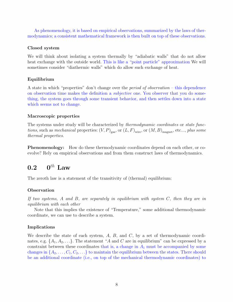
As phenomenology, it is based on empirical observations, summarized by the laws of ther-modynamics; a consistent mathematical framework is then built on top of these observations.

Closed system

We will think about isolating a system thermally by “adiabatic walls” that do not allowheat exchange with the outside world. This is like a “point particle” approximation We willsometimes consider “diathermic walls” which do allow such exchange of heat.

Equilibrium

A state in which “properties” don’t change over the period of observation – this dependenceon observation time makes the definition a subjective one. You observer that you do some-thing, the system goes through some transient behavior, and then settles down into a statewhich seems not to change.

Macroscopic properties

The systems under study will be characterized by thermodynamic coordinates or state func-tions, such as mechanical properties: (V, P )gas, or (L, F )wire, or (M,B)magnet, etc..., plus somethermal properties.

Phenomenology: How do these thermodynamic coordinates depend on each other, or co-evolve? Rely on empirical observations and from them construct laws of thermodynamics.

0.2 0th Law

The zeroth law is a statement of the transitivity of (thermal) equilibrium:

Observation

If two systems, A and B, are separately in equilibrium with system C, then they are inequilibrium with each other

Note that this implies the existence of “Temperature,” some additional thermodynamiccoordinate, we can use to describe a system.

Implications

We describe the state of each system, A, B, and C, by a set of thermodynamic coordi-nates, e.g. A1, A2, . . .. The statement “A and C are in equilibrium” can be expressed by aconstraint between these coordinates that is, a change in A1 must be accompanied by somechanges in A2, . . . , C1, C2, . . . to maintain the equilibrium between the states. There shouldbe an additional coordinate (i.e., on top of the mechanical thermodynamic coordinates) to

8

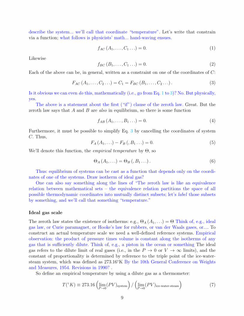
describe the system... we’ll call that coordinate “temperature”. Let’s write that constrainvia a function; what follows is physicists’ math... hand-waving ensues.

fAC (A1, . . . , C1 . . .) = 0. (1)

LikewisefBC (B1, . . . , C1 . . .) = 0. (2)

Each of the above can be, in general, written as a constraint on one of the coordinates of C:

FAC (A1, . . . , C2 . . .) = C1 = FBC (B1, . . . , C2 . . .) . (3)

Is it obvious we can even do this, mathematically (i.e., go from Eq. 1 to 3)? No. But physically,yes.

The above is a statement about the first (“if”) clause of the zeroth law. Great. But thezeroth law says that A and B are also in equilibrium, so there is some function

fAB (A1, . . . , B1 . . .) = 0. (4)

Furthermore, it must be possible to simplify Eq. 3 by cancelling the coordinates of systemC. Thus,

FA (A1, . . .)− FB (, B1 . . .) = 0. (5)

We’ll denote this function, the empirical temperature by Θ, so

ΘA (A1, . . .) = ΘB (, B1 . . .) . (6)

Thus: equilibrium of systems can be cast as a function that depends only on the coordi-nates of one of the systems. Draw isotherm of ideal gas?

One can also say something along the lines of “The zeroth law is like an equivalencerelation between mathematical sets – the equivalence relation partitions the space of allpossible thermodynamic coordinates into mutually distinct subsets; let’s label those subsetsby something, and we’ll call that something “temperature.”

Ideal gas scale

The zeroth law states the existence of isotherms: e.g., ΘA (A1, . . .) = Θ Think of, e.g., idealgas law, or Curie paramagnet, or Hooke’s law for rubbers, or van der Waals gases, or.... Toconstruct an actual temperature scale we need a well-defined reference systems. Empiricalobservation: the product of pressure times volume is constant along the isotherms of anygas that is sufficiently dilute. Think of, e.g., a piston in the ocean or something The idealgas refers to the dilute limit of real gases (i.e., in the P → 0 or V → ∞ limits), and theconstant of proportionality is determined by reference to the triple point of the ice-water-steam system, which was defined as 273.16K By the 10th General Conference on Weightsand Measures, 1954. Revisions in 1990? .

So define an empirical temperature by using a dilute gas as a thermometer:

T (K) ≡ 273.16(

limP→0

(PV )system

)/(

limP→0

(PV )ice-water-steam

)(7)

9

0.3 1st Law

The first law is a statement about the conservation of energy, adapted for thermal systems.We’ll formulate it as:

Statement

If the state of an adiabatically isolated system is changed by work, the amount of work isonly a function of the initial and final coordinates of the system. Draw, fake system witha spring, magnet, etc., a coordinate space representation with initial and final points, andmany paths between them. ∆W doesn’t depend on path

Consequences

We infer the existence of another state function, the internal energy E(X). Think abouthow the path-independence of the work we have to do when pushing a ball up a frictionlesshill in classical mechanics lets us deduce a potential energy.

∆W = E(Xf )− E(Xi) (8)

Similarly, in the same sense that the zeroth law let us construct some function of coordinatesthat was relevant to equilbrium, the first law allows us to define another function, the internalenergy.Draw some squiggly paths on the board.

The real content of the first law is when we violate the condition. That is, allow wallsthat permit heat exchange, so that ∆W 6= Ef − Ei. We, of course, still believe energy is agood, conserved quantity, so define heat :

∆Q = (Ef − Ei)−∆W. (9)

Clearly, though, ∆Q and ∆W are not separate functions of state, so we will use notationlike:

dE(X) = dQ+ dW, (10)

Where d means a differential where the thing is a function of state, and d means that thething is path-dependent. Note the sign convention, here, where work and heat add energyto the system.

Quasi-static transformation

A QS transformation is one which is done sufficiently slowly enough to maintain the systemin equilibrium everywhere along the path. For such a transformation the work done on thesystem can thus be related to changes in the thermodynamic coordinates. Let’s divide thestate functions, X, into generalized displacements x and generalized forces J . Then, in a QStransformation

dW =∑i

Jidxi (11)

10

Common generalized coordinates

System generalized force generalized displacement

Wire tension F length LFilm surface tension σ area AFluid pressure −P volume V

Magnet field B magnetization M

Note that the displacements are generally extensive and the forces are generally intensive.Question: We’ve written

dE =∑i

Jidxi + ? (12)

What is dQ? probably depends on T . What is it conjugate to?

Response functions

The usual way of characterizing the behavior of a system (measured from changes in ther-modynamic coordinates with external probes). E.g.:

Force constants Measure the ratio of displacements to forces (think spring constants).For example, isothermal compressibility of a gas : κT = 1

V∂V∂P

∣∣T

Thermal response Response to change in temperature, such as the expansivity of a gasαP = 1

V∂V∂T

∣∣P

Heat capacity Changes in temperature upon adding heat. Note that heat is not a statefunction, so the path is important! Example: For an ideal gas we could calculate CV = dQ

dT

∣∣V

and CP = dQdT

∣∣P

, and CP has to be bigger since we use some heat to change the volume:

CV =dQ

dT

∣∣∣∣V

=dE − dW

dT

∣∣∣∣V

=dE + PdV

dT

∣∣∣∣V

=∂E

∂T

∣∣∣∣V

. (13)

CP =dQ

dT

∣∣∣∣P

=dE − dW

dT

∣∣∣∣P

=dE + PdV

dT

∣∣∣∣P

=∂E

∂T

∣∣∣∣P

+ P∂V

∂T

∣∣∣∣P

.

Joule’s free expansion experiment

Take an adiabatically isolated gas, and let it expand (adiabatically, but we don’t need QS.Draw on the board a two-chambered system) from Vi to Vf . Joule observed that the initialand final temperatures are the same! Tf = Ti = T .

So, ∆Q = 0 and ∆W = 0, so ∆E = 0. We conclude that the internal energy actuallydepends only on temperature: E(P, V, T ) = E(T ), i.e., a product of P and V . Note that sinceE depends only on T , ∂E

∂T

∣∣V

= ∂E∂T

∣∣P

, and we can simplify the heat capacity expressions:

CP − CV = P∂V

∂T

∣∣∣∣P

=PV

T= NkB. (14)

11

That last equality is a statement of extensivity, that PV/T is proportional to an amount ofstuff, and kB ≈ 1.4× 10−23J/K.

0.4 2nd Law

Why does heat flow from hot to cold? Why are there no perpetual motion machines thatwork by turning water into ice while doing work? There are many equivalent formulationsof the 2nd law; in part because it is fun, we’ll see how practical concerns about burning coalto do stuff leads directly to the idea of entropy and its inevitable increase!

Kelvin’s statement

No process is possible whose sole result is the complete conversion of heat to work (“No idealengines”)

Clausius’ statement

No process is possible whose sole result is the transfer of heat from cold to hot (“No idealrefrigerators”)

Idealized work machines

We’ll quantify these statements by defining “figures of merit” for an ideal engine and anideal refrigerators.

The efficiency of an engine, a machine which takes QH of heat from a source, convertssome of it to work W , and dumps some QC of it into a sink, is

η =W

QH

=QH −QC

QH

≤ 1. (15)

The performance of a refrigerator, an engine running backwards, is

ω =QC

W=

QC

QH −QC

(16)

Of course, Kelvin and Clausius’ formulations are equivalent! To see this, hook up anideal engine to a fridge, and you get an ideal fridge (so, not Kelvin implies not Clausius).Additionally, run an ideal fridge and take the heat from the exhaust to power an engine andyou get an ideal engine (so, not Clausius implies not Kelvin). Thus, Kelvin ⇐⇒ Clausius.

This seems trivial; with an excursion through Carnot Engines we’ll see that it lets usanswer a question posed in section 0.3, when we wrote:

dE =∑i

Jidxi + ?

12

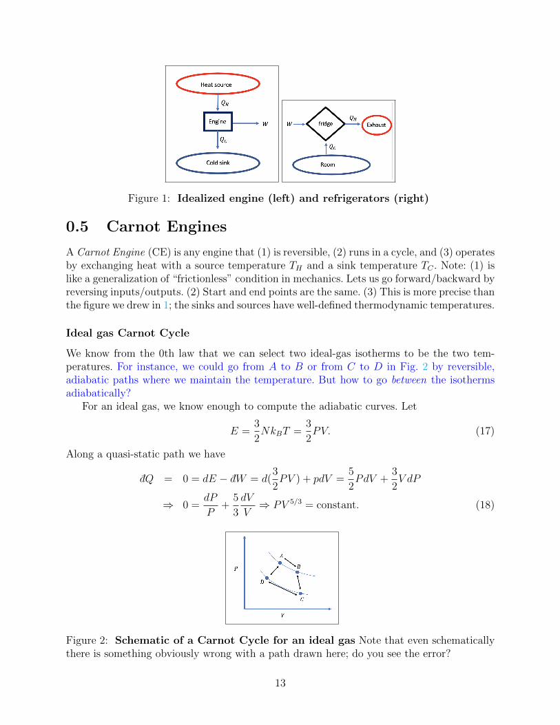
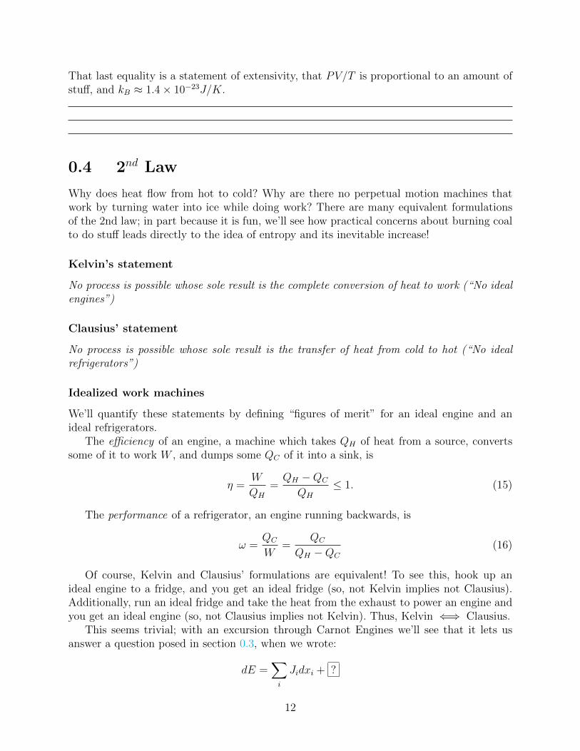
Figure 1: Idealized engine (left) and refrigerators (right)

0.5 Carnot Engines

A Carnot Engine (CE) is any engine that (1) is reversible, (2) runs in a cycle, and (3) operatesby exchanging heat with a source temperature TH and a sink temperature TC . Note: (1) islike a generalization of “frictionless” condition in mechanics. Lets us go forward/backward byreversing inputs/outputs. (2) Start and end points are the same. (3) This is more precise thanthe figure we drew in 1; the sinks and sources have well-defined thermodynamic temperatures.

Ideal gas Carnot Cycle

We know from the 0th law that we can select two ideal-gas isotherms to be the two tem-peratures. For instance, we could go from A to B or from C to D in Fig. 2 by reversible,adiabatic paths where we maintain the temperature. But how to go between the isothermsadiabatically?

For an ideal gas, we know enough to compute the adiabatic curves. Let

E =3

2NkBT =

3

2PV. (17)

Along a quasi-static path we have

dQ = 0 = dE − dW = d(3

2PV ) + pdV =

5

2PdV +

3

2V dP

⇒ 0 =dP

P+

5

3

dV

V⇒ PV 5/3 = constant. (18)

Figure 2: Schematic of a Carnot Cycle for an ideal gas Note that even schematicallythere is something obviously wrong with a path drawn here; do you see the error?

13

It’s fun to see (i.e., will probably be a homework problem), that one can construct adiabaticsfor any two-parameter system with internal energy E(J, x).

Carnot’s Theorem

Off all engines operating between TH and TC , the Carnot engine is the most efficient!

Proof Take a Carnot Engine, and use a non-Carnot-Engine’s output to run the CE as arefrigerator. Let primes refer to heat connected to the Carnot engine, and unprimes to theNCE. The net effect is to transfer heat QH − Q′H = QC − Q′C from TH to TC . Clausius’formulation tells us you can’t transfer negative heat, so QH ≥ Q′H . But the amount of work,W , was the same, so

W

QH

≤ W

Q′H⇒ ηCE ≥ ηNCE. (19)

0.5.1 Thermodynamic Temperature Scale

We established (by finding the adiabatic paths) that we can (in theory) construct a CarnotEngine using an ideal gas. All Carnot engines operating between TH and TC have the sameefficiency show by using 1 to run the other backwards, and vice verse, so ηCE1 = ηCE2 . Thus,the efficiency is independent of the engine; it must depend only on the temperatures, i.e. wehave η(TH , TC). So, already, if you can build a CE, it lets us define T independent of anymaterial properties, just by knowing efficiencies of CE’s at different T .

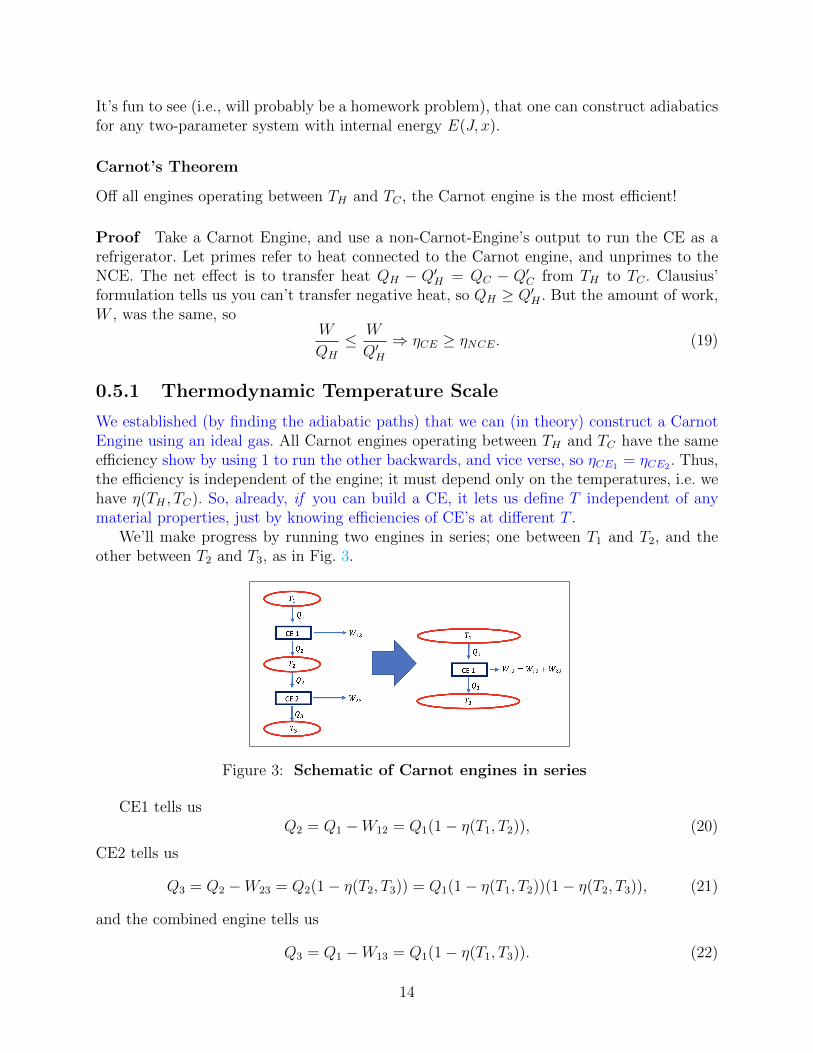
We’ll make progress by running two engines in series; one between T1 and T2, and theother between T2 and T3, as in Fig. 3.

Figure 3: Schematic of Carnot engines in series

CE1 tells usQ2 = Q1 −W12 = Q1(1− η(T1, T2)), (20)

CE2 tells us

Q3 = Q2 −W23 = Q2(1− η(T2, T3)) = Q1(1− η(T1, T2))(1− η(T2, T3)), (21)

and the combined engine tells us

Q3 = Q1 −W13 = Q1(1− η(T1, T3)). (22)

14

Comparing those last two expressions tells us

(1− η(T1, T3)) = (1− η(T1, T2))(1− η(T2, T3)), (23)

which is a constraint on the functional form that η can take. We postulate that

(1− η(T1, T2)) =Q2

Q1

≡ f(T2)

f(T1). (24)

By convention, let f(T ) = T . Thus

η(TH , TC) =TH − TCTH

. (25)

We’ve done it! Up to a constant of proportionality, Eq. 25 defines a thermodynamictemperature (and we’ll again set the constant using the triple point of water-ice-steam). Byrunning a Carnot cycle for an ideal gas you can show that the ideal gas scale and the thermo-dynamic temperature scale are identical. This is not useful, but rather conceptual in showingthat temperature is not something that depends on the properties of a particular material.Fun note: thermodynamic temperatures must be positive, otherwise Kelvin’s Formulationcould be violated

0.5.2 Clausius’ Theorem

Statement

For any cyclic process, with path parameterized by s∮dQ(s)

T (s)≤ 0, (26)

where the heat dQ(s) is an amount of heat delivered to the system at temperature T (s) weneed not be in equilibrium, so what is T (s)? The heat of the “machine” delivering the heat.

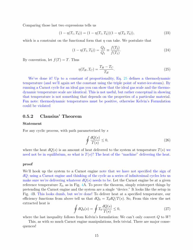
proof

We’ll hook up the system to a Carnot engine note that we have not specified the sign ofdQ; using a Carnot engine and thinking of the cycle as a series of infinitesimal cycles lets usmake sure we’re delivering whatever dQ(s) needs to be. Let the Carnot engine be at a givenreference temperature T0, as in Fig. 4A. To prove the theorem, simply reinterpret things bypretending the Carnot engine and the system are a single “device.” It looks like the setup inFig. 4B. This looks dumb, but we’re done! To deliver heat at a specified temperature, ourefficiency functions from above tell us that dQ0 = T0dQ/T (s). So, From this view the netextracted heat is ∮

dQ0(s) =

∮T0dQ(s)

T (s)≤ 0, (27)

where the last inequality follows from Kelvin’s formulation: We can’t only convert Q to W !This, as with so much Carnot engine manipulations, feels trivial. There are major conse-

quences!

15

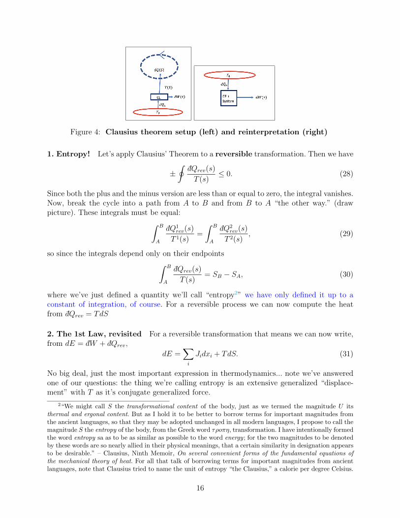
Figure 4: Clausius theorem setup (left) and reinterpretation (right)

1. Entropy! Let’s apply Clausius’ Theorem to a reversible transformation. Then we have

±∮dQrev(s)

T (s)≤ 0. (28)

Since both the plus and the minus version are less than or equal to zero, the integral vanishes.Now, break the cycle into a path from A to B and from B to A “the other way.” (drawpicture). These integrals must be equal:∫ B

A

dQ1rev(s)

T 1(s)=

∫ B

A

dQ2rev(s)

T 2(s), (29)

so since the integrals depend only on their endpoints∫ B

A

dQrev(s)

T (s)= SB − SA, (30)

where we’ve just defined a quantity we’ll call “entropy2” we have only defined it up to aconstant of integration, of course. For a reversible process we can now compute the heatfrom dQrev = TdS

2. The 1st Law, revisited For a reversible transformation that means we can now write,from dE = dW + dQrev,

dE =∑i

Jidxi + TdS. (31)

No big deal, just the most important expression in thermodynamics... note we’ve answeredone of our questions: the thing we’re calling entropy is an extensive generalized “displace-ment” with T as it’s conjugate generalized force.

2“We might call S the transformational content of the body, just as we termed the magnitude U itsthermal and ergonal content. But as I hold it to be better to borrow terms for important magnitudes fromthe ancient languages, so that they may be adopted unchanged in all modern languages, I propose to call themagnitude S the entropy of the body, from the Greek word τρoπη, transformation. I have intentionally formedthe word entropy sa as to be as similar as possible to the word energy ; for the two magnitudes to be denotedby these words are so nearly allied in their physical meanings, that a certain similarity in designation appearsto be desirable.” – Clausius, Ninth Memoir, On several convenient forms of the fundamental equations ofthe mechanical theory of heat. For all that talk of borrowing terms for important magnitudes from ancientlanguages, note that Clausius tried to name the unit of entropy “the Clausius,” a calorie per degree Celsius.

16

3. Entropy increases for irreversible transformations Suppose we make an irre-versible change as we go from state A to B, but then complete the cycle by making areversible transformation from B back to A. Clausius tells us that∫ B

A

dQ

T+

∫ A

B

dQrev

T≤ 0⇒

∫ B

A

dQ

T≤ SB − SA, (32)

which tells us that, in differential form, dQ ≤ TdS for any transformation. For an adiabaticprocess, with dQ = 0, we’ve just learned that dS ≥ 0. As a system approaches equilibrium,apparently the arrow of time points in the direction of increasing entropy, since changes ina system’s internal state can only increase S.

4. How many independent variables do I need to describe an equilibrium system?From Eq. 31 we see that if there n ways of doing mechanical work to a system (the n pairsJi, xi), then we need n+ 1 independent coordinates to describe equilibrium systems (i.e.,if you know E then then J ’s and x’s are connected. This gives us freedom we’ll exploit laterin defining different ensembles, etc. For example, suppose we choose as our coordinates Eand all of the displacements xi; Eq. 31 gives us the relations

∂S

∂E

∣∣∣∣xi

=1

T.

−∂S∂xi

∣∣∣∣E,xj 6=i

=JiT. (33)

0.6 3rd Law

I said last class I wouldn’t discuss this next – I’ve changed my mind, but we’ll be very brief!We know from the second law how to compute the difference in entropy between two statepoints at the same temperature: we make sure we perform operations reversibly, and thencalculate ∆S =

∫dQrev/T .

0.6.1 Nernst-Simon statement of the third law

The change in entropy associated with a system undergoing a reversible, isothermal processapproaches zero as the temperature approaches 0K:

limT→0

∆S(T )→ 0. (34)

Stronger Nernst statement

The entropy of all systems at absolute zero is a universal constant, which we will define tobe the zero point of the entropy scale: limT→0 S(X,T ) = 0.

17

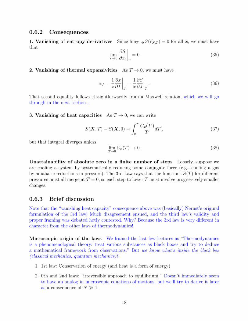
0.6.2 Consequences

1. Vanishing of entropy derivatives Since limT→0 S(~rX,T ) = 0 for all x, we must havethat

limT→0

∂S

∂xi

∣∣∣∣T

= 0 (35)

2. Vanishing of thermal expansivities As T → 0, we must have

αJ =1

x

∂x

∂T

∣∣∣∣J

=1

x

∂S

∂J

∣∣∣∣T

. (36)

That second equality follows straightforwardly from a Maxwell relation, which we will gothrough in the next section...

3. Vanishing of heat capacities As T → 0, we can write

S(X, T )− S(X, 0) =

∫ T

0

Cx(T ′)

T ′dT ′, (37)

but that integral diverges unlesslimT→0

Cx(T )→ 0. (38)

Unattainability of absolute zero in a finite number of steps Loosely, suppose weare cooling a system by systematically reducing some conjugate force (e.g., cooling a gasby adiabatic reductions in pressure). The 3rd Law says that the functions S(T ) for differentpressures must all merge at T = 0, so each step to lower T must involve progressively smallerchanges.

0.6.3 Brief discussion

Note that the “vanishing heat capacity” consequence above was (basically) Nernst’s originalformulation of the 3rd law! Much disagreement ensued, and the third law’s validity andproper framing was debated hotly contested. Why? Because the 3rd law is very different incharacter from the other laws of thermodynamics!

Microscopic origin of the laws We framed the last few lectures as “Thermodynamicsis a phenomenological theory: treat various substances as black boxes and try to deducea mathematical framework from observations.” But we know what’s inside the black box(classical mechanics, quantum mechanics)!

1. 1st law: Conservation of energy (and heat is a form of energy)

2. 0th and 2nd laws: “irreversible approach to equilibrium.” Doesn’t immediately seemto have an analog in microscopic equations of motions, but we’ll try to derive it lateras a consequence of N 1.

18

3. 3rd law: We’ll soon see statistical mechanical expressions like S = k ln g, where g isa measure of the degeneracy of states: S → 0 ⇒ g = O(1) as T → 0. In classicalmechanics, this is simply not true! Just think of an ideal gas!. But, as T → 0, CM isnot appropriate. It is hardly surprising, then, that a law whose validity actually restson quantum mechanics was not well-understood or properly justified before QM itselfwas.

0.7 Various thermodynamic potentials (Appendix H of

Pathria)

Mechanical equilibrium occurs at a minimum of a potential energy e.g., the mechanicalequilibrium of a mass between springs, etc. etc.. Thermal equilibrium similarly occurs atthe extremum of an appropriately defined thermodynamic potential. For example, in ourdiscussion of Clausius’ Theorem (Sec. 0.5.2) we found that the entropy of an adiabaticallyisolated system increases after any change until it reaches a maximum in equilibrium. Butwhat about systems that are not adiabatically isolated? Or systems which are subject tomechanical work? In this section we will define a handful of thermodynamic potentials thatare applicable.

Analogy with a mechanical system Briefly, suppose we have a mass on a spring con-nected to a fixed wall, and let x be the deviation of the mass’s position away from theequilibrium rest length of the spring. We take the potential energy to be U(x) = kx2/2,which is clearly minimized when x = 0. What if we apply an external force – what will bethe new position of the mass? We could define a net potential energy which encompassesthis external work, H = kx2/2 − Jx, and set the variation of this with respect to x to bezero:

∂H

∂x= 0⇒ xeq = J/k, and Heq =

−J2

2K. (39)

0.7.1 Enthalpy

What if the system is still adiabatically isolated (dQ = 0), but comes to equilibrium under aconstant external force? We define enthalpy, by analogy with the mechanical example above,as

H = E − J · x. (40)

Variations in this quantity are given by

dH = dE − d(J · x) = TdS + J · dx− x · dJ − J · dx = TdS − x · dJ . (41)

Note that in general, at constant J the work added to the system is dW ≤ J · δx (whereequality occurs for reversible processes), so by the first law and making use of dQ = 0 wehave dE ≤ J · dx, which means that δH ≤ 0 as a system approaches equilibrium.

19

0.7.2 Helmholtz Free energy

What if the system is undergoing an isothermal (constant T ) transformation in the absenceof mechanical work (dW = 0)? We define the Helmholtz free energy

F = E − TS, (42)

which has variations given by

dF = dE − d(TS) = TdS + J · dx− SdT − TdS = −SdT + J · dx. (43)

Note that Clausius’ theorem said that at constant T the heat added to the system is con-strained by dQ ≤ TdS, so making us of dW = 0 we have dE = dQ ≤ TdS, so δF ≤ 0.

0.7.3 Gibbs Free Energy

What if the system is undergoing an isothermal transformation in the presence of mechanicalwork done at constant external force? We define the Gibbs free energy by

G = E − TS − J · x, (44)

which has variations given by

dG = dE − d(TS)− d(J · x) = · · · = −SdT − x · dJ . (45)

Note that in this case, we have both dW ≤ J · δx and dQ ≤ TdS, so δG ≤ 0

0.7.4 Grand Potential

Traditionally “chemical work” is treated separately from mechanical work... for chemicalequilibrium in the case of no mechanical work, we define the Grand potential by

G = E − TS − µ ·N , (46)

where N refer to the number of particles of different chemical species, and µ refers to thechemical potential for each of them. Variations in G satisfy

dG = −SdT + J · dx−N · dµ. (47)

0.7.5 Changing variables

In the last several subsections we’ve seen how to use Legendre transformations to movebetween different natural variables depending on the physical situation we find ourselves in.So, for instance, for adiabatically isolated systems with constant external force, we look atthe enthalpy, which has natural variables H(J , S); for isothermal transformations with noexternal work we look at the Helmholtz free energy, which has natural variables F (x, T ),

20

etc. The equilibrium conjugate variables can then by found by partial differentiation. Forinstance, the equilibrium force and entropy can be found from F by

Ji =∂F

∂xi

∣∣∣∣T,xj 6=i

and S = − ∂F

∂T

∣∣∣∣x

. (48)

Are there any limits on the manipulations we can perform here? For each set of conjugateforce/displacement variables, can we always transform to choose whatever we want? No..Let’s see why

0.8 Two bits of math!

0.8.1 Extensivity (and Gibbs-Duhem)

Let’s look at the differential for E, including chemical work:

dE = TdS + J · dx+ µ · dN . (49)

In general the extensive quantities are proportional to the size of the system, which we canwrite mathematically as

E(λS, λx, λN ) = λ(S,x,N ). (50)

Please note that this is not a requirement, nor does it have the same footing as the rest ofthe laws of thermodynamics; it is simply a statement about the behavior of “most things.”Let’s take the above and differentiate with respect to λ and then evaluate at λ = 1. Thisgives

∂E

∂S

∣∣∣∣x,N

S +∂E

∂xi

∣∣∣∣S,xj 6=i,N

xi +∂E

∂Nα

∣∣∣∣S,x,Nβ 6=α

Nα = E(S,x,N ). (51)

Note that the partial derivates here are (in order) T , Ji, and µα. This leads to what somepeople write as the fundamental equation of thermodynamics:

E = TS + J · x+ µ ·N . (52)

Combining equations 49 and 52 lead to a constraint on allowed variations of the intensivecoordinates:

SdT + x · dJ +N · dµ = 0, (53)

which is the Gibbs-Duhem relation. Again, this is valid for extensive systems, as definedby Eq. 50. Also, this answers the question at the end of the last section: you cannot (use-fully) transform to a potential where the natural coordinates are all intensive, because theseintensive coordinates are not all independent.

0.8.2 Maxwell relations

“Maxwell relations” follow from combining thermodynamic relationships with the basic prop-erties of partial derivatives. If f , x, and y are mutually related, we can write

df(x, y) =∂f

∂x

∣∣∣∣y

dx+∂f

∂y

∣∣∣∣x

dy, (54)

21

and we will then combine this with symmetry of second derivations,

∂

∂x

∂f

∂y=

∂

∂y

∂f

∂x, (55)

to related various thermodynamic derivatives.

Example

For instance, let’s start with dE = TdS + Jidxi. We know, mathematically, that we canimmediately write

T =∂E

∂S

∣∣∣∣x

and Ji =∂E

∂xi

∣∣∣∣S,xj 6=i

. (56)

We can take the mixed derivatives and discover a relationship:

∂2E

∂S∂xi=

∂T

∂xi

∣∣∣∣S

=∂Ji∂S

∣∣∣∣x

, (57)

where we might call the latter equality a Maxwell relation.

Strategy for deriving Maxwell relations

There are several tricks to remembering how to rapidly find the Maxwell relation relevantto a particular expression. In the homework you will go through a method using Jacobianmatrices.

Logically, though, it’s not so hard to always construct them on the fly. Suppose someoneasks you to find a Maxwell relation for

∂A

∂B

∣∣∣∣C

. (58)

We’ll do the following: (1) write down the fundamental expression for dE, (2) transform itso that A will appear in a first derivative and B and C are differentials, and (3) profit.

Worked example:

I want to know (∂µ/∂P )|T for an ideal gas.

Step 1 We writedE = TdS − PdV + µdN. (59)

Step 2 We note that µ is already in a position to appear in first derivatives. Moving on,

d(E − PV ) = TdS − V dP + µdN (60)

d(E − PV − ST ) = −TdS − V dP + µdN. (61)

22

We did not really care what the name of (E − PV − ST ) was, let’s just call it Y . Clearly

µ =∂Y

∂N

∣∣∣∣T,P

and V =∂Y

∂P

∣∣∣∣T,N

, (62)

so∂µ

∂P

∣∣∣∣T

=∂V

∂N

∣∣∣∣T

. (63)

Step 3 We’re done.

23

Chapter 1

Probability

In the last chapter we treated thermodynamics as a phenomenological theory, building up aconsistent mathematical framework that expressed the consequences of experimental obser-vations of various black box systems. Ultimately we will want to see how these propertiesarise from the microscopic rules that real systems evolve according to; to do so we will beexpressing the statistical consequences of having large numbers of interacting units. In thisbrief chapter we will cover the parts of probability theory that we will be using. Since muchof this is standard definitional stuff, we will also be sure to cover calculational methods andtricks that will serve us down the road.

1.1 A funny observation

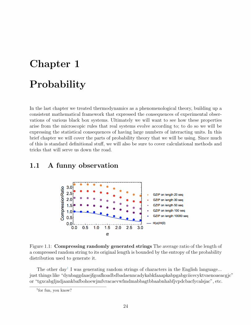
Figure 1.1: Compressing randomly generated strings The average ratio of the length ofa compressed random string to its original length is bounded by the entropy of the probabilitydistribution used to generate it.

The other day1 I was generating random strings of characters in the English language...just things like “dynbaggdaaejfgoafkoadbdbadaenncadykabkfaaapkabpgabgciicecyktvaenoaeacgjc”or “tgxcabgljndjaankbafbohoewjmfvracaevwfmdmabbagtbbaabnhabfjvpdcbacfycalsjac”, etc.

1for fun, you know?

24

I started compressing these strings using an off-the-shelf algorithm on my computer, gzip,and compared the length of the compressed string to the length of the original string. Irepeated this a bunch of times, for sequences of different length, and for different proba-bility distributions from which I was generating my random strings (if you’re curious, theywere power-law distributions parameterized by a decay strength α). The results are in Fig.1.1, and I was shocked! Apparently, as I started compressing longer and longer strings, theamount I was able to compress them was bounded by what I’ve labeled H(α) in the figure– the entropy of the probability distribution! How is entropy – which so far seems like athermodynamic concept – related to computation and information compression? Let’s findout!

1.2 Basic Definitions

Random variable: A random variable x is a measurable variable described by a set ofpossible outcomes, S. This could be a discrete set, as for a coin Scoin = heads, tails, or acontinuous range, as for a particle’s velocity Svx = −∞ ≤ vx ≤ ∞. We call each elementof such a set as an event E ⊂ S

Probability We will assign a value, called the probability to each event, denoted p(E),which has the following properties:

1. positivity: p(E) ≥ 0

2. additivity: p(A or B) = p(A) + p(B) if A and B are distinct.

3. normalization: p(S) = 1.

We’re not mathematicians, so we won’t be starting from here and proving stuff. Rather, youmay wonder, “how will we determine p(E)?” By one of two ways:

1. Objectively: (experimentally, frequentist) p(E) is the frequency of outcome in manytrials:p(E) = limN→∞NE/N

2. Subjectively: (theoretically, Bayesian) Based on our uncertainty among all outcomes.We’ll see this is what we’ll really use in stat phys! We’ll formalize this later.

1.3 Properties of single random variables

Let’s focus on random variables which are continuous and real-valued (the specialization todiscrete ones is straightforward; we’ll see an example in the next section).

Cumulative probability function: P (x) = probability(E ⊂ [−∞, x]). This must be amonotonically increasing function, with P (−∞) = 0 and P (∞) = 1.

25

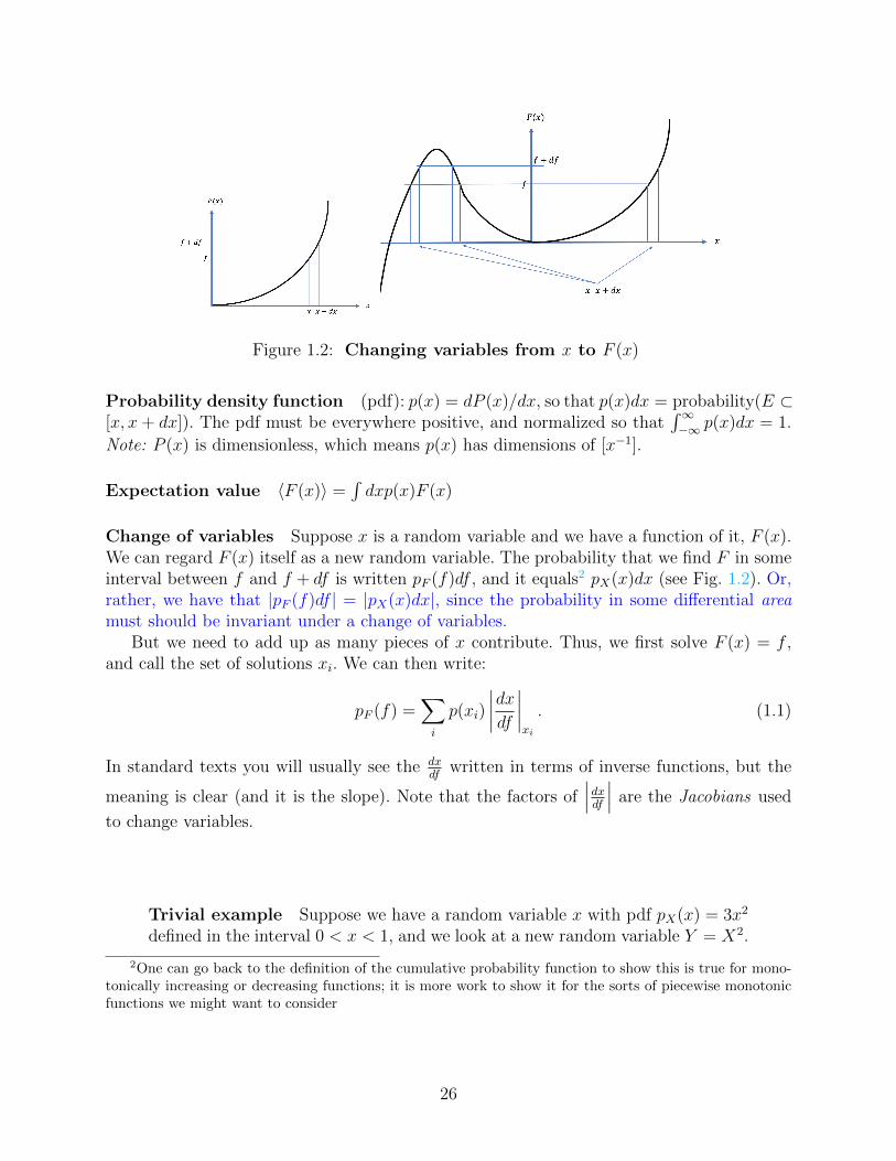
Figure 1.2: Changing variables from x to F (x)

Probability density function (pdf): p(x) = dP (x)/dx, so that p(x)dx = probability(E ⊂[x, x + dx]). The pdf must be everywhere positive, and normalized so that

∫∞−∞ p(x)dx = 1.

Note: P (x) is dimensionless, which means p(x) has dimensions of [x−1].

Expectation value 〈F (x)〉 =∫dxp(x)F (x)

Change of variables Suppose x is a random variable and we have a function of it, F (x).We can regard F (x) itself as a new random variable. The probability that we find F in someinterval between f and f + df is written pF (f)df , and it equals2 pX(x)dx (see Fig. 1.2). Or,rather, we have that |pF (f)df | = |pX(x)dx|, since the probability in some differential areamust should be invariant under a change of variables.

But we need to add up as many pieces of x contribute. Thus, we first solve F (x) = f ,and call the set of solutions xi. We can then write:

pF (f) =∑i

p(xi)

∣∣∣∣dxdf∣∣∣∣xi

. (1.1)

In standard texts you will usually see the dxdf

written in terms of inverse functions, but the

meaning is clear (and it is the slope). Note that the factors of∣∣∣dxdf ∣∣∣ are the Jacobians used

to change variables.

Trivial example Suppose we have a random variable x with pdf pX(x) = 3x2

defined in the interval 0 < x < 1, and we look at a new random variable Y = X2.

2One can go back to the definition of the cumulative probability function to show this is true for mono-tonically increasing or decreasing functions; it is more work to show it for the sorts of piecewise monotonicfunctions we might want to consider

26

This is easily invertible in the range, and we can write x(y) =√y, and dx/dy =

y−1/2/2. Thus

pY (y) = pX(x)

∣∣∣∣ 1

2√y

∣∣∣∣ =3

2(√y)2 1√y

=3

2

√y, (1.2)

defined in the range 0 < y < 1.

2-valued example Suppose instead that we have a random variable x where

p(x) =λ

2exp (−λ|x|) ,

defined for any x on the real line. We want to know the probability density func-tion for the random variable F (x) = x2. There are, by inspection, two solutionsto F (x) = f (when f is positive!), and they are x = ±

√f . The derivatives we

need are |dx/df | = | ± 12√f|. Thus, we have:

pF (f) =λ

2exp(−λ

∣∣∣√f∣∣∣) ∣∣∣∣ 1

2√f

∣∣∣∣+λ

2exp(−λ

∣∣∣−√f∣∣∣) ∣∣∣∣ −1

2√f

∣∣∣∣ =λ exp

(−λ√f)

2√f

,

for any f > 0 (and pF (f) = 0 for f < 0).

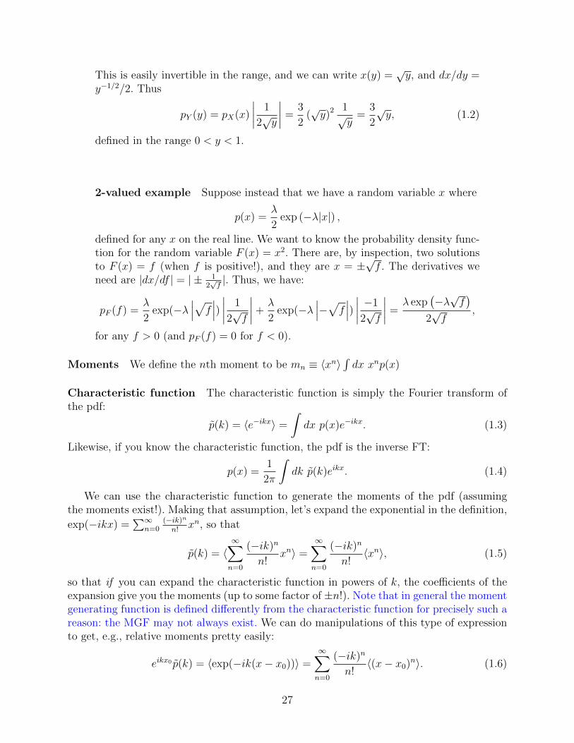
Moments We define the nth moment to be mn ≡ 〈xn〉∫dx xnp(x)

Characteristic function The characteristic function is simply the Fourier transform ofthe pdf:

p(k) = 〈e−ikx〉 =

∫dx p(x)e−ikx. (1.3)

Likewise, if you know the characteristic function, the pdf is the inverse FT:

p(x) =1

2π

∫dk p(k)eikx. (1.4)

We can use the characteristic function to generate the moments of the pdf (assumingthe moments exist!). Making that assumption, let’s expand the exponential in the definition,

exp(−ikx) =∑∞

n=0(−ik)n

n!xn, so that

p(k) = 〈∞∑n=0

(−ik)n

n!xn〉 =

∞∑n=0

(−ik)n

n!〈xn〉, (1.5)

so that if you can expand the characteristic function in powers of k, the coefficients of theexpansion give you the moments (up to some factor of ±n!). Note that in general the momentgenerating function is defined differently from the characteristic function for precisely such areason: the MGF may not always exist. We can do manipulations of this type of expressionto get, e.g., relative moments pretty easily:

eikx0 p(k) = 〈exp(−ik(x− x0))〉 =∞∑n=0

(−ik)n

n!〈(x− x0)n〉. (1.6)

27

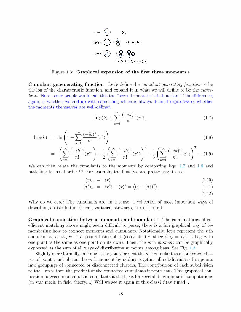
Figure 1.3: Graphical expansion of the first three moments s

Cumulant genenerating function Let’s define the cumulant generating function to bethe log of the characteristic function, and expand it in what we will define to be the cumu-lants. Note: some people would call this the “second characteristic function.” The difference,again, is whether we end up with something which is always defined regardless of whetherthe moments themselves are well-defined.

ln p(k) ≡∞∑n=1

(−ik)n

n!〈xn〉c. (1.7)

ln p(k) = ln

(1 +

∞∑n=1

(−ik)n

n!〈xn〉

)(1.8)

=

(∞∑n=1

(−ik)n

n!〈xn〉

)− 1

2

(∞∑n=1

(−ik)n

n!〈xn〉

)2

+1

3

(∞∑n=1

(−ik)n

n!〈xn〉

)3

+ · · ·(1.9)

We can then relate the cumulants to the moments by comparing Eqs. 1.7 and 1.8 andmatching terms of order kn. For example, the first two are pretty easy to see:

〈x〉c = 〈x〉 (1.10)

〈x2〉c = 〈x2〉 − 〈x〉2 =⟨(x− 〈x〉)2

⟩(1.11)

(1.12)

Why do we care? The cumulants are, in a sense, a collection of most important ways ofdescribing a distribution (mean, variance, skewness, kurtosis, etc.).

Graphical connection between moments and cumulants The combinatorics of co-efficient matching above might seem difficult to parse; there is a fun graphical way of re-membering how to connect moments and cumulants. Notationally, let’s represent the nthcumulant as a bag with n points inside of it (conveniently, since 〈x〉c = 〈x〉, a bag withone point is the same as one point on its own). Then, the mth moment can be graphicallyexpressed as the sum of all ways of distributing m points among bags. See Fig. 1.3.

Slightly more formally, one might say you represent the nth cumulant as a connected clus-ter of points, and obtain the mth moment by adding together all subdivisions of m pointsinto groupings of connected or disconnected clusters. The contribution of each subdivisionto the sum is then the product of the connected cumulants it represents. This graphical con-nection between moments and cumulants is the basis for several diagrammatic computations(in stat mech, in field theory,...) Will we see it again in this class? Stay tuned...

28

1.4 Important distributions

1.4.1 Binomial distribution

Given a discrete random variable with two outcomes, which occur with probability pA andpB = 1− pA, the binomial distribution gives the probability that event A occurs exactly NA

times out of N trials. It is equal to

PN(NA) =

(N

NA

)pNAA pN−NAB ,

(N

NA

)=

N !

NA!(N −NA)!. (1.13)

The characteristic function for the discrete distribution is

pN(k) = 〈e−ikNA〉 =N∑

NA=0

N !

NA!(N −NA)!pNAA pN−NAB e−ikNA =

(pAe

−ik + pB)N

. (1.14)

This has the properties that we can easily relate the cumulant generating function for theN -trial case to that of the 1-trial case:

ln pN(k) = N ln(PAe

−ik + pB)

= N ln p1(k). (1.15)

For a single trial, NA can only be either zero or one, which means that we must have〈Nm

A 〉 = pA for all powers m. Combining this property of the moments with the abovefeature of the cumulants, we learn that the cumulants for the N -trial case are

〈NA〉c = NpA, 〈N2A〉c = N

(pA − p2

A

)= NpApB, (1.16)

and higher order cumulants can be easily calculated. We’ll see that this type of feature –where there is a trivial relation between an independent thing repeated N times and thecase of an individual trial – will be of great use as we build up statistical mechanics.

1.4.2 Poisson distribution

We’ll get at the Poisson distribution, a continuous pdf, relating it to the binomial distribution.Consider a process in time where two properties hold. First, the probability of observing(exactly) one event in the interval [t, t+dt] is proportional to dt in the limit dt→ 0. Second,suppose the probability of observing an event in different intervals is uncorrelated. Example:radioactive decay. Then, the Poisson distribution is the probability of observing exactly Mevents in the interval T .

We get the details of the distribution by imagining dividing up the interval T into manysegments of length dt, say N = T/dt 1 such that dt is so small the probability ofobserving more than one event is negligible. So, in each segment we have an event occurringwith probability p = αdt and no event occurring with probability q = 1 − p. From ourexpression for the binomial distribution, we immediately know the characteristic functionfor this process:

p(k) =(pe−ik + q

)N= lim

dt→0

(1 + αdt((e−ik − 1)

)T/dt= exp

(α(e−ik − 1)T

), (1.17)

29

where the last equality is an example of the famous Euler limit formula. Knowing the char-acteristic function, we can take the inverse Fourier transform to get the pdf:

p(x) =

∫ ∞−∞

dk

2πexp

(α(e−ik − 1)T + ikx

). (1.18)

This can be solved You, the reader should verify this! by expanding the exponential, andusing ∫ ∞

−∞

dk

2πe−ik(x−M) = δ(x−M)

to get the probability of M events in a time T for a process characterized by α as

pαT (M) = e−αT(αT )M

M !. (1.19)

Additionally, the cumulants can be read off of the expansion of the log characteristic function

ln pαT (k) = αT (e−ik − 1) = αT∞∑n=1

(−ik)n

n!⇒ 〈Mn〉c = αT. (1.20)

That is, while the binomial distribution has the property that every moment is the same,the Poisson distribution has the property that every cumulant is the same.

1.4.3 Gaussian distribution

We will definitely, definitely use this, you know? Define the gaussian pdf as

p(x) =1√

2πσ2exp

(−(x− λ)2

2σ2

). (1.21)

The characteristic function is compute by the usual means of completing the square insidethe integral, a trick I believe we all know:

p(k) =

∫dx√2πσ2

exp

(−ikx− (x− λ)2

2σ2

)(1.22)

= e−ikλ∫

dy√2πσ2

exp

(−iky − y2

2σ2+k2σ2

2− k2σ2

2

), for y = x− λ (1.23)

= e−ikλ−k2σ2

2

∫dz√2πσ2

exp

(−z2

2σ2

), for z = y + ikσ2 (1.24)

= exp

(−ikλ− k2σ2

2

)(1.25)

A manipulation that shows that the Fourier transform of a Gaussian is, itself, a Gaussian.The cumulants of this are easily identified:

ln p(k) = −ikλ− k2σ2

2, (1.26)

30

immediately showing that

〈x〉c = λ, 〈x2〉c = σ2, 〈xn>2〉c = 0. (1.27)

So, the Gaussian is completely specified by its first two cumulants, and all moments involveonly products of one- and two-point clusters.

1.5 Properties of multiple random variables

Joint probability density function We define, by analogy, the joint pdf p(x1, x2, . . . , xN)as

p(x) = limdxi→0

prob. of outcome in (x1, x1 + dx1), . . . , (xN , xN + dxN)dx1dx2 · · · dxN

. (1.28)

The normalization of the joint PDF is

px(S) = 1 =

∫dNxp(x), (1.29)

and iff the N random variables are independent, then the joint pdf simplifies to the productof the individual probability density functions:

p(x) =N∏i=1

pi(xi)). (1.30)

Joint characteristic function is just the N -dimensional Fourier transform:

p(k) = 〈exp(−ik · x〉 =

∫ (∏i

dxie−ikixi

)p(x1, . . . , xN). (1.31)

Joint moments and cumulants Are defined perfectly analogously with the momentsand cumulants of single random variable distributions. Recall that last lecture we talkedabout moments as related to the coefficient of the relevant power of k... more generally wecan express these as the following derivatives:

〈xm11 xm2

2 · · ·xmNN 〉 =

[∂

∂(−ik1)

]m1

· · ·[

∂

∂(−ikN)

]mNp(k)|k=0 (1.32)

〈xm11 xm2

2 · · ·xmNN 〉c =

[∂

∂(−ik1)

]m1

· · ·[

∂

∂(−ikN)

]mNln p(k)|k=0 . (1.33)

As a simple – but perhaps the most important – example, the “co-variance” between tworandom variables is

〈x1x2〉c = 〈x1x2〉 − 〈x1〉〈x2〉. (1.34)

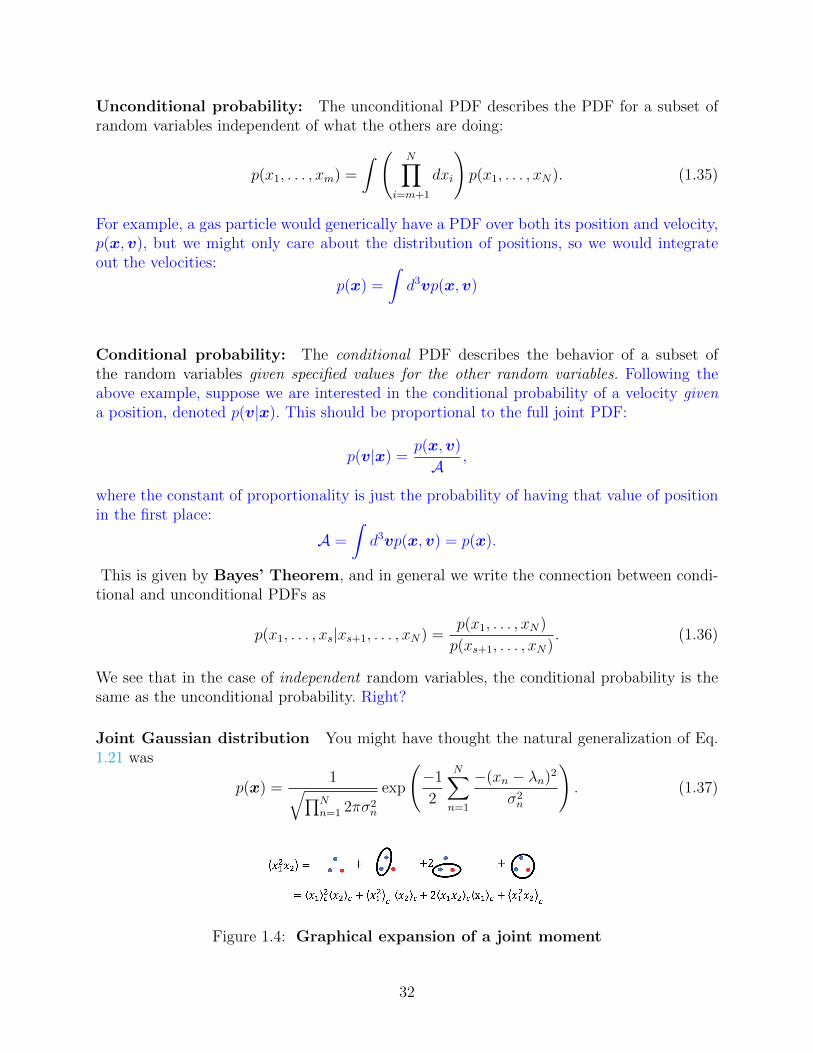
The graphical expansion we wrote earlier still applies; one just has to label the points bythe corresponding variables. See Fig. 1.4.

31

Unconditional probability: The unconditional PDF describes the PDF for a subset ofrandom variables independent of what the others are doing:

p(x1, . . . , xm) =

∫ ( N∏i=m+1

dxi

)p(x1, . . . , xN). (1.35)

For example, a gas particle would generically have a PDF over both its position and velocity,p(x,v), but we might only care about the distribution of positions, so we would integrateout the velocities:

p(x) =

∫d3vp(x,v)

Conditional probability: The conditional PDF describes the behavior of a subset ofthe random variables given specified values for the other random variables. Following theabove example, suppose we are interested in the conditional probability of a velocity givena position, denoted p(v|x). This should be proportional to the full joint PDF:

p(v|x) =p(x,v)

A,

where the constant of proportionality is just the probability of having that value of positionin the first place:

A =

∫d3vp(x,v) = p(x).

This is given by Bayes’ Theorem, and in general we write the connection between condi-tional and unconditional PDFs as

p(x1, . . . , xs|xs+1, . . . , xN) =p(x1, . . . , xN)

p(xs+1, . . . , xN). (1.36)

We see that in the case of independent random variables, the conditional probability is thesame as the unconditional probability. Right?

Joint Gaussian distribution You might have thought the natural generalization of Eq.1.21 was

p(x) =1√∏N

n=1 2πσ2n

exp

(−1

2

N∑n=1

−(xn − λn)2

σ2n

). (1.37)

Figure 1.4: Graphical expansion of a joint moment

32

but this neglects the potential for cross-correlations! The most general form is, instead,

p(x) =1√

(2π)N detCexp

(−1

2

N∑n,m=1

(xn − λn)(xm − λm) (C)−1nm

), (1.38)

where the matrix C is symmetric, and for p(x) to be a well-defined probability the matrixC must be positive definite. We can write this somewhat more compactly as

p(x) =1√

(2π)N detCexp

(−1

2(x− λ)TC−1(x− λ)

). (1.39)

The matrix C is called the covariance matrix. If one goes through and performs the fouriertransform on the above joint PDF, one finds

p(k) = exp

(−ik · λ− 1

2kTCk

), (1.40)

or, in index notation,

p(k) = exp

(−ikmλm −

1

2kmCmnkn

). (1.41)

The latter re-writing lets us immediately read off the joint cumulants of the joint Gaussiandistribution:

〈xm〉c = λm, 〈xmxn〉c = Cmn, (1.42)

with all higher-order cumulants vanishing.

Note that there is an important special case when λ = 0. Consider the jointcumulant

〈xn11 x

n22 · · ·x

nNN 〉 , (1.43)

and think about the combinatorics of the graphical expansion we’ve been dis-cussing.First, if the sum of the ni is odd, then in the graphical expansion there is no wayto avoid a term with an odd-power cumulant, and in this special case of the jointGaussian distribution with λ = 0, all such terms are zero!Second, if the sum is odd, we know that there will only be contributions fromcombinations of covariances : all even-power cumulants with power greater thantwo vanish because we are dealing with the joint Gaussian. Thus, the cumulantcan be obtained by all ways of summing over pairs of the random variables. Forexample,

〈xixjxkxl〉 = CijCkl + CikCjl + CilCjk, (1.44)

where it didn’t matter if the i, j, k, l were distinct. For instance:⟨x2

1x2x3

⟩= C11C23 + 2C12C13. (1.45)

This property of the joint Gaussian distribution is sometimes summarized as:

〈xn11 x

n22 · · ·x

nNN 〉 =

0 if

∑α nα is odd

Sum over all pairwise contractions of covariances else(1.46)

In this formulation, we see the analogy of Wick’s Theorem applied to fields.

33

1.6 Math of large numbers

We typically think of statistical mechanics being relevant when the number of microscopicdegrees of freedom, N , becomes very large; indeed, in the thermodynamic limit, N → ∞,a number of mathematical simplifications become available to our analysis of how systemsbehave.

1.6.1 The Central Limit Theorem

The central limit theorem, which I trust we have all encountered before, is a core enginein allowing us to make precise statements of the sort we encountered in thermodynamics.For instance, we observed that heat flows from hot to cold – not sometimes, or most of thetime, but always. If we’re going to make probabilistic arguments at the microscopic core,how do we end up with precise, essentially deterministic thermodynamic statements? We’llmake the case for the classical CLT, by the way, not the Lyapunov or other versions withweaker conditions.

Let’s start by considering the sum of N random variables, X =∑N

i=1 xi, where therandom variables xi have some joint PDF p(x). What is the cumulant generating functionof the sum, ln pX(k)? Well,

ln pX(k) = ln⟨e−ikX

⟩= ln

⟨exp(−ik

N∑i=1

xi

⟩= ln px (k1 = k, k2 = k, . . . , kN = k) , (1.47)

That is, it is the same as the log of the joint characteristic function of the xi, but evaluatedat the same k. Let’s expand each side of the above equation, writing things so we can easilymatch powers of k:

∞∑n=1

(−ik)n

n!〈Xn〉c = (−ik)

N∑i=1

〈xi〉c +(−ik)2

2!

N∑i,j=1

〈xixj〉c + . . . (1.48)

Matching terms of order kn, we see that

〈X〉c =∑i

〈xi〉c, 〈X2〉c =∑i,j

〈xixj〉c, . . . (1.49)

Now, we specialize to the case of the classical central limit theorem by supposing thatthe xi are both independent, so that p(x1, . . . , xN) = p1(x1)p2(x2) · · · pN(xN) and identicallydistributed, i.e., each of the labeled probability distributions pi(x1) are the same, so that

p(x1, . . . , xN) =N∏i=1

p(xi). (1.50)

This combination of conditions, independent and identically distributed, is often abbreviatediid. Now, the fact that the variables are independent means that the cross-correlations in

34

Eq. 1.49 vanish (do you see why the math tells us this?), so that in the double sum onlyterms with i = j contribute. Thus, we get that

〈Xm〉c =N∑i=1

〈xmi 〉c (1.51)

. The condition of identically distributed takes us back to the case we looked at with thebinomial distribution: the cumulants of N repeated but independent draws from the samedistribution are easily related to the cumulants of the single-random-variable distribution:

〈Xm〉c =N∑i=1

〈xmi 〉c = N 〈xm〉c . (1.52)

The (classical) Central Limit Theorem follows directly. Define a new random variable tobe

y =X −N 〈x〉c√

N, (1.53)

and then one computes its cumulants:

〈y〉c = 0,⟨y2⟩c

=〈X2〉c√N

=⟨x2⟩c, 〈ym〉 =

N 〈xm〉cNm/2

. (1.54)

In words: as N becomes large, distribution for a sum of random variables with mean µ andvariance σ2 converges to a distribution that itself has a finite mean, a variance that onlygrows as

√N , and higher-order cumulants that all decay to zero as N →∞. Thus, sums of

random variables converge to normal distributions, rather ignoring the details of what theoriginal random variables looked like (up to some point). Note that the condition is really onthe existence of the moments in question, and a condition on how correlated the variablesare allowed to be:

N∑i1,...im

〈xi1 . . . xim〉c O(Nm/2).

1.6.2 Adding up exponential quantities

In stat mech we tend to run into (1) intensive variables (like T , P , etc.), which are indepen-dent of system size (O(N0)), (2) extensive variables (like S, V , etc.), which scale linearlywith system size (O(N1)), and (3) exponential variables (like volumes of phase space), whichare independent of system size (O(V N) = O(eaN). Of course, polynomial dependences, etc.,are also possible and sometimes arise (especially in interesting systems). The behavior ofadding exponential quantities together makes calculating thermodynamic limits possible

35

Summing exponentials

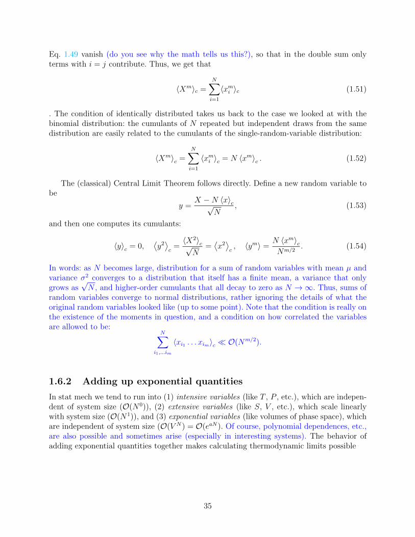
Frist, suppose we have a sum of a large number of exponentially large numbers:

S =N∑i=1

Ei, (1.55)

where the terms 0 ≤ E1 ∼ O(exp(Nai)) and we are summing up N ∼ O(NP ), a number ofterms that grows at most polynomial in N .

Claim We can approximate the entire sum just by the largest term! That is,

S ≈ Emax. (1.56)

proof We mean that claim in a specific sense, as follows. First, it is clear that the we canbound the sum by

Emax ≤ S ≤ NEmax. (1.57)

Now, let’s switch to an intensive variable by first taking lnS and then dividing by N . Thisgives the bounds:

EmaxN≤ lnS

N≤ Emax

N+

lnNN

, (1.58)

butlnNN

=p lnN

N(1.59)

according to our assumption, and this goes to zero as N →∞. Thus,

limN→∞

lnS

N=

ln EmaxN

= amax. (1.60)

So, even if the second-largest ai is only slightly less than the maximum one, upon exponen-tiation N times it gets completely dominated by the larger term. Think about going fromthe microcanonical ensemble (where you specified precisely all of the energies, NV E, andare summing over energy levels), or the canonical ensemble (where you do not, NV T ); youget the same result because the system behavior is dominated by the most likely energy.

Integrating exponentials – Saddle-point integrations

We generalize the above result to get a simple version of saddle-point integration3. We wishto make a similar claim about the integral, I =

∫dx exp(Nφ(x)) being dominated by the

place where the function φ(x) itself is maximized. Well, let’s Taylor expand φ about itsmaximum xm (which I emphasize so you remember the first derivative vanishes and thesecond derivative is negative):

I =

∫dx exp

(Nφ(xm)− N

2|φ′′(xm)|(x− xm)2 + · · ·

)(1.61)

3c.f. the section of Pathria in Chapter 3 which treats more general integrands with integration paths inthe complex plane

36

This term has two types of corrections encoded in that set of · · · . First, of course, thereare the higher-order terms in the expansion of the function φ(x) about its maximum value;these terms lead to a power series in 1/N . Second, there could be contributions to this sumfrom additional local maximum. But, by arguments similar to those made in the previoussubsection, any such contribution will be completely subdominant! Thus, we truncate theseries at quadratic order as above and write

I = eNφ(xm)

∫dx exp

(−N

2|φ′′(xm)|(x− xm)2

), (1.62)

which is just another Gaussian integral, but one missing its normalization factor, so

I = eNφ(xm)

√2π

N |φ′′(xm)|⇒ lim

N→∞

ln IN

= φ(xm). (1.63)

Note / example: Stirling’s approximation The above machinery can be used to deriveStirling’s approximation for the factorial. Start by noting that

N ! =

∫ ∞0

xNe−x, (1.64)

which can be see by starting with∫∞

0exp(−αx) = 1/α, and then taking N derivatives and

setting α = 1. Some rearrangements of the above equation (writing φ(x) = ln x − x/N),expanding about xm = N , and doing the Gaussian integral gets you to

N ! = NNe−N√

2πN

(1 +O

(1

N

)), (1.65)

the log of which is Stirling’s formula. Filling in the missing steps should be straightforward,but also an excellent way to make sure you understand the machinery of this method.

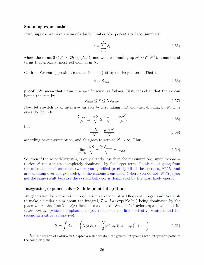
1.7 Information Entropy

We end this chapter by thinking about an information-based view of what we mean byentropy, one introduced by Shannon in a groundbreaking 1948 paper4. We will discuss theconnection between information and entropy, and by thinking about ‘unbiased” ways ofassigning probabilities, we will formalize the subjective procedure of assigning probabilitiesdiscussed at the beginning of this chapter.

4which you can read at this harvard site:http://people.math.harvard.edu/ ctm/home/text/others/shannon/entropy/entropy.pdf. Note that Shannonnamed the symbol of entropy H, after Boltzmann’s H-theorem, which we’ll encounter in the very nextchapter.

37

1.7.1 Shannon entropy

We briefly change our focus from thermodynamics and statistical physics to a setting whichseems very different: the problem of sending messages over a wire. We begin by imagining asource trying to send us a message from an “alphabet” of k characters, a1, . . . , ak that havean discrete associated probability distribution p(ai), X = ai, p(ai). (Think, for instance,of the actual alphabet, where indeed some letters appear more frequently than others in realmessages.), where we will assume that the characters are iid (In real messages there are, ofcourse, correlations; we neglect them in this idealized setting). With this assumption, theprobability that the source sends the n-character message x = x1x2 · · ·xn is just

p(x) =n∏i=1

p(xi). (1.66)

Let’s denote the entire ensemble of n-length messages chosen with the assumption that thexi are iid by Xn.

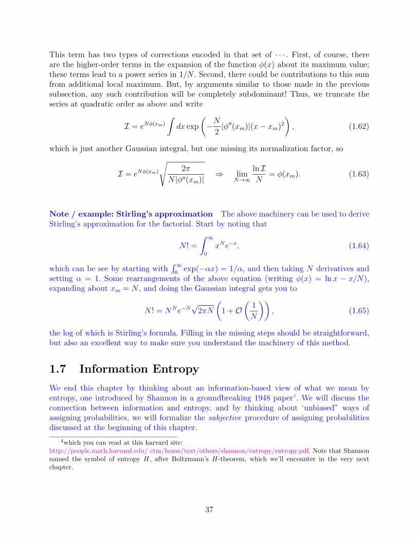
Compressing messages Suppose the length of the message, n, grows very large. In thissetting, is it possible to compress the message into a shorter string that conveys the same“information”? As long as p(ai) is not uniform, then yes! The total number of messages iskn, but for large n, we expect each character to occur about ni = np(ai) +O(n−1/2) times.So the number of typical strings, g, is not kn but rather

g =n!∏k

i=1(np(ai))!. (1.67)

Applying Stirling’s formula, we find that

log2 g ≡ nH(X) ≈ −nk∑i=1

p(ai) log2 p(ai), (1.68)

where H(X) is the Shannon entropy of the ensemble X = ai, p(ai). If we imagine adoptinga code for messages of length n where integers label “typical” messages of such length, atypical n-letter string could be communicated using about nH(X) bits. To be extra explicit,for discrete probability distributions with values pi we will be defining the entropy in thisway:

S = H(X) = −〈ln p〉 = −∑i

pi ln pi. (1.69)

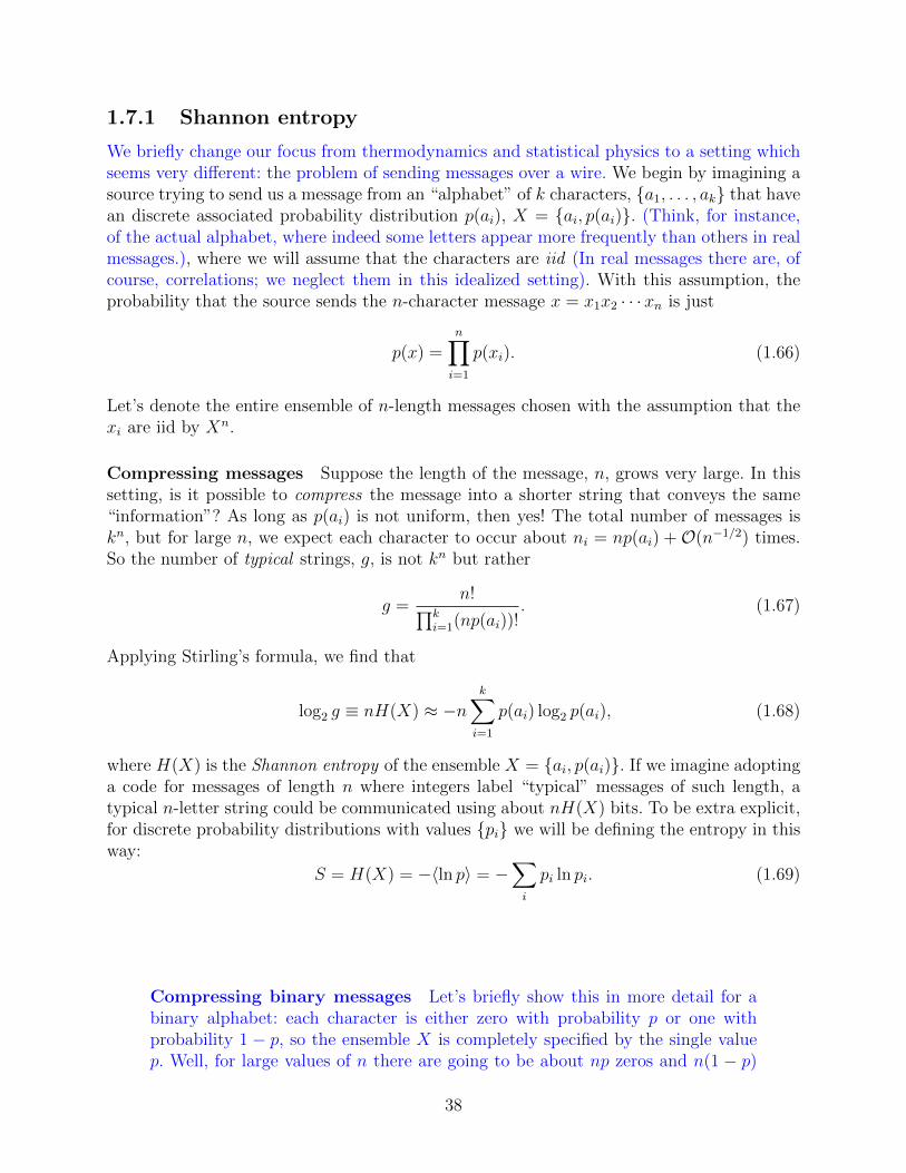
Compressing binary messages Let’s briefly show this in more detail for abinary alphabet: each character is either zero with probability p or one withprobability 1 − p, so the ensemble X is completely specified by the single valuep. Well, for large values of n there are going to be about np zeros and n(1 − p)

38

ones, and the number of distinct strings of this form is given by the binomialcoefficient. So, using log x! = x log x− x+O(log x), we have:

log g = log

(n

np

)= log

(n!

(np)!(n(1− p))!

)(1.70)

≈ n log n− n− (np log(np)− np+ n(1− p) log(n(1− p))− n(1− p))(1.71)

= nH(p), (1.72)

for H(p) = −p log p− (1− p) log(1− p). (1.73)

What about actual compression? Again, we make up an integer code that labelsevery typical message. There are about 2nH(p) messages, and a priori typicalmessages occur with equal frequency, so we need to specify a given message bya binary string whose length is about nH(p). If p = 1/2 (and thus H(p) = 1for log2) we haven’t done anything: we need as many bits to communicate themessage as there are in the message. But if the probability p 6= 1/2, our new codeshortens typical messages. The insight here is that we don’t need a codeword forevery message, just typical ones, since the probability of atypical messages isnegligible!

1.7.2 Information, conditional entropy, and mutual information

The Shannon entropy is a way of quantifying our ignorance (per letter) about the output of asource operating with X: if the source sends an n-character message, we need about nH(X)bits to know the message. Information quantifies how much knowledge you gain by knowingthe probability distribution the characters came from, i.e., “if you know the pi, how manyfewer bits do I need to transmit to tell you the source’s (typical) message?”. Well, the totalreduction in the number of bits for a n length message from the alphabet of k characters is

n log2 k − (−n∑i

pi log2 pi) = n

(log2 k +

∑i

pi log2 pi

). (1.74)

Given a knowledge of the pi, we define the information per bit as

I(X) = log2 k +∑i

pi log2 pi, (1.75)

so that information and entropy are the same (up to signs and constants).

information and entropy of the uniform distribution As a quick example,suppose we have a uniform distribution of k characters, pi = 1/k. Well:

S = k

(1

klog2

1

k

)= log2

1

k(1.76)

I = log2 k + log2

1

k= 0. (1.77)

39

So, the entropy is the log of the number of equal-probability characters (soundfamiliar from the microcanonical ensemble?), and there is no information in thedistribution.

information and entropy of a delta function distribution The oppo-site extreme is also trivial to work out. Suppose the distribution is such that aparticular event definitely happens: pi = δα,i. Well:

S = 0 (1.78)

I = log2 k. (1.79)

By knowing the distribution you already know everything about the outcome ofan n-length message, and the entropy (a quantification of ignorance) is zero.

Finally, suppose we have two correlated sources of information, X and Y (for uncorrelatedsources we would have p(x, y) = pX(x)pY (y)). Then, if I read a message in Y n I can furtherreduce my ignorance about a message generated by Xn (if I know the correlations!), whichmeans I should be able to further compress messages in Xn than I could without access toY . This is captured by the conditional entropy,

H(X|Y ) = H(XY )−H(Y ) = 〈− log(p(x, y) + log p(y)〉 = 〈− log p(x|y)〉 , (1.80)

where we see the conditional probability distribution introduced earlier in this chapter. Un-surprisingly (given the connection between information and entropy above), the mutual in-formation is closely connected: The information about X gained when you learn about Y(again, “the number of fewer bits per letter needed to specify X when Y is known) is

I(X;Y ) = H(X)−H(X|Y )

= H(X) +H(Y )−H(XY ) (1.81)

= H(Y )−H(Y |X),

which is a quantification of the degree to which X and Y are correlated, and is symmetricunder the interchange of X and Y as we see above.

1.7.3 Unbiased estimation of probabilities

We can now use the entropy as a way to quantify subjective estimates/assignments of prob-abilities! To start, if we have no information, the unbiased estimate is that every outcomeis equally likely. Indeed, we saw above that the uniform distribution encodes no informationand maximizes the entropy. Given additional information, we obtain the unbiased estimateby maximizing entropy subject to the constraints.

To give an example, suppose we observe a random variable for a while and observethat it has a specific mean value, 〈F (x)〉 = f . We want make an unbiased estimate of the

40

probabilities pi, and we will use Lagrange multipliers (α, β) to impose the two constraintswe now know about the probability distribution (that it is normalized and has a specificmean):

S (pi, α, β) = −∑i

pi ln pi − α

(∑i

pi − 1

)− β

(∑i

piF (xi)− f

). (1.82)

Maximizing this with respect to the pi:

0 = dSdpi

= − ln pi − 1− α− βF (xi) (1.83)

⇒ pi = e−(1+α)e−βF (xi). (1.84)

Given this form (which should remind you of Boltzmann weights!), we can then solve for αand β that satisfy the given constraints.

41

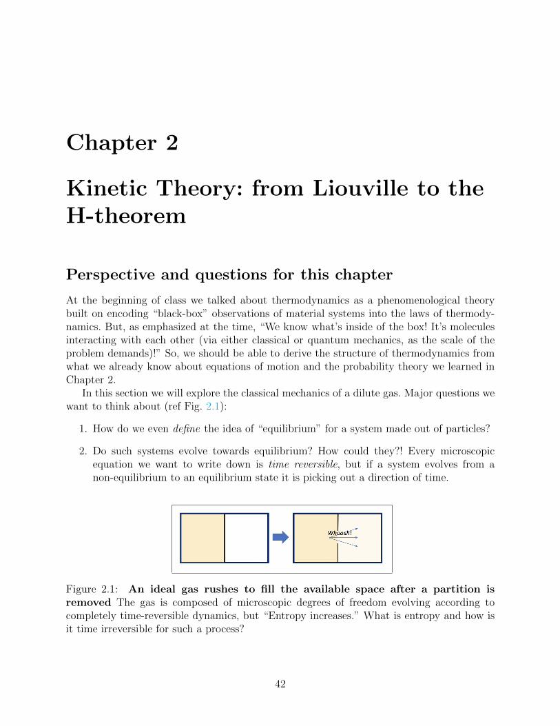
Chapter 2

Kinetic Theory: from Liouville to theH-theorem

Perspective and questions for this chapter

At the beginning of class we talked about thermodynamics as a phenomenological theorybuilt on encoding “black-box” observations of material systems into the laws of thermody-namics. But, as emphasized at the time, “We know what’s inside of the box! It’s moleculesinteracting with each other (via either classical or quantum mechanics, as the scale of theproblem demands)!” So, we should be able to derive the structure of thermodynamics fromwhat we already know about equations of motion and the probability theory we learned inChapter 2.

In this section we will explore the classical mechanics of a dilute gas. Major questions wewant to think about (ref Fig. 2.1):

1. How do we even define the idea of “equilibrium” for a system made out of particles?

2. Do such systems evolve towards equilibrium? How could they?! Every microscopicequation we want to write down is time reversible, but if a system evolves from anon-equilibrium to an equilibrium state it is picking out a direction of time.

Figure 2.1: An ideal gas rushes to fill the available space after a partition isremoved The gas is composed of microscopic degrees of freedom evolving according tocompletely time-reversible dynamics, but “Entropy increases.” What is entropy and how isit time irreversible for such a process?

42

Sources for this chapter: The material here will cover most of Pathria, Chapter 2;thanks to the work we did in the lectures on Probability we will also either implicitly orexplicitly cover Pathria Chapter 3.1 - 3.3. We will also be covering the BBGKY hierarchyand Boltzmann’s H-theorem, which are not in Pathria.

2.1 Elements of ensemble theory

2.1.1 Phase space of a classical system1

We want to connect a thermodynamic description of a system – which is captured by onlya handful of coordinates, like V,N, T, etc. – with a classical microstate, which is specifiedby the positions and momenta of each of my N particles: µ = q1,p1, . . . , qN ,pN, which isa point in a 6N -dimensional phase space (and which is, hence, hard to draw). Since we’restarting with a classical mechanical description, we’ll say the system is governed by someHamiltonian, H, so that the equations of motions we’ll work with are

dpidt

= − ∂H∂qi

= pidqidt

= ∂H∂pi

= qi,(2.1)

and where time-reversal invariance means that if we reverse the direction of time we transformp→ −p and q(t)→ q(−t).

Now, given that there are a handful of thermodynamic coordinates describing the systemand ∼ 1023 describing the classical microstate, it will not surprise us that there is a many-to-one mapping between equilibrium states and microstates. How do we formalize this?Let’s start by imagining we have N “copies” of the same macrostate of our system, eachcorresponding to a different representative microstate, and we’ll think about the ensembledensity function,

ρ(p, q, t) = limN→∞,dΓ→0

dN (p, q, t)

NdΓ, (2.2)

where

dΓ =N∏i=1

d3pid3qi

is how we’ll be writing classical phase space volume differentials and dN is the number ofmicrostates corresponding to the target macrostate in our differential box. Note that if weintegrate ρ over all of phase space we get∫

dΓρ(p, q) =

∫dNN

= 1, (2.3)

so we see that between positivity (we’re counting numbers of points, so it’s not negative)and the above, the ensemble density is actually a probability density function. We alreadyknow things, then, like computing expectation values:

〈A〉 =

∫dΓρ(p, q, t)A(p, q)

1This section covers Pathria 2.1

43

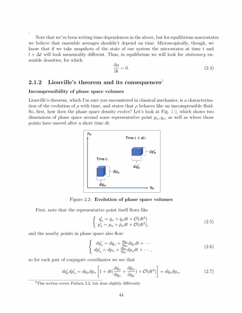
.Note that we’ve been writing time dependences in the above, but for equilibrium macrostates

we believe that ensemble averages shouldn’t depend on time. Microscopically, though, weknow that if we take snapshots of the state of our system the microstates at time t andt + ∆t will look measurably different. Thus, in equilibrium we will look for stationary en-semble densities, for which

∂ρ

∂t= 0. (2.4)

2.1.2 Liouville’s theorem and its consequences2

Incompressibility of phase space volumes

Liouville’s theorem, which I’m sure you encountered in classical mechanics, is a characteriza-tion of the evolution of ρ with time, and states that ρ behaves like an imcompressible fluid.So, first, how does the phase space density evolve? Let’s look at Fig. 2.2, which shows twodimensions of phase space around some representative point pα, qα, as well as where thosepoints have moved after a short time dt.

Figure 2.2: Evolution of phase space volumes

First, note that the representative point itself flows likeq′α = qα + qαdt+O(dt2)p′α = pα + pαdt+O(dt2),

(2.5)

and the nearby points in phase space also flow:dq′α = dqα + ∂qα

∂qαdqαdt+ · · ·

dp′α = dpα + ∂pα∂pα

dpαdt+ · · · , (2.6)

so for each pair of conjugate coordinates we see that

dq′αdp′α = dqαdpα

[1 + dt(

∂qα∂qα

+∂pα∂qα

) +O(dt2)

]= dqαdpα, (2.7)

2This section covers Pathria 2.2, but done slightly differently

44

where the last equality holds because the term proportional to dt vanishes by equality ofmixed partials. This is the just the familiar statement that Hamiltonian dynamics preservesphase space volumes: dΓ = dΓ′.

Liouville’s theorem

The above has consequences for our ensemble density. All of the states dN that were orig-inally near (p, q) move to the neighborhood of (p′, q′), but occupy the same phase spacevolume. Thus, dN /dΓ is unchanged, and ρ itself behaves like an incompressible fluid.Givenhow phase space transforms, we can write

ρ(p, q, t) = ρ(p′, q′, t+ dt). (2.8)

Expanding out this expression, we can write

ρ(p, q, t) = ρ (p+ pdt, q + qdt, t+ dt) (2.9)

= ρ(p, q, t) +

[∑α

pα∂ρ

∂pα+ qα

∂ρ

∂qα+∂ρ

∂t

]dt+O(dt2). (2.10)

Let’s define the total derivative (or “streamline derivative”) of a function f as

d

dtf(p, q, t) =

∂f

∂t+∑α

∂f

∂pαpα +

∂f

∂qαqα, (2.11)

where the interpretation is that d/dt is the derivative as you flow (following the evolution ofthe volume of fluid as it moves through phase space), whereas the partial derivative ∂/∂t islike sitting a fixed position in space and watching the changes in f in time at that location.Anyway, the equation for ρ says that

dρ

dt= 0 =

∂ρ

∂t+∑α

(−∂H∂qα

)∂ρ

∂pα+

(∂H∂pα

)∂ρ

∂qα(2.12)

⇒ ∂ρ

∂t= H, ρ, (2.13)

where we have defined the Poisson bracket3

A,B =∑i

∂A

∂qi

∂B

∂pi− ∂A

∂pi

∂B

∂qi(2.14)

2.1.3 Equilibrium ensemble densities

We can combine Liouville’s theorem above with our criteria that in equilibrium ρ is stationaryto come up with a criteria for equilibrium:

∂ρeq(q,p)

∂t= 0 = H, ρeq. (2.15)

3Using curly braces, not the weird straight bracket of Pathria. Shots fired. I am going to use Pathria’s /Goldstein’s sign convention here, though, instead of Landau’s.

45

In principle, we now have to solve the system of 6N variables coming from setting the Poissonbracket to zero. In practice, we’ll guess! We have already required that in equilibrium ρ hasno explicit time derivative; we could also assume it has no dependence on q or p at all:ρeq = const. is certainly a valid solution of the above (which is like saying the ensembleof systems corresponding to the equilibrium macrostate are uniformly distributed throughphase space).

More generally, though allow implicit dependencies on the phase space coordinates andlet ρ be an arbitrary function of H:

ρeq(H),H =∑i

(∂ρ

∂H∂H∂qi

)∂H∂pi−(∂ρ

∂H∂H∂pi

)∂H∂qi

= 0. (2.16)

For example, choosingρ(H) = δ(H− E)

gives us the microcanonical ensemble, and choosing

ρ(H) ∝ exp(−βH(q,p))

gives us the canonical ensemble.Even more generally, while we’re in the business of simply guessing solutions to Eq. 2.15,

we can assume that ρ is an arbitrary function of bothH itself and of any conserved quantities.To see why, we first note that if some quantity A is conserved under the Hamiltonian,A,H = 0. Then, using the same manipulations as above, we can write

ρeq(H, A),H =∂ρ

∂HH,H+

∂ρ

∂AA,H = 0, (2.17)

satisfying our condition for ρeq to be an equilibrium distribution.

Time dependence of observables

It is perhaps worth explicitly pointing out that to find the time dependence of some ensembleaverage of a quantity A, we do:

d

dt〈A〉 =

∫dΓ∂ρ(p, q, t)

∂tA(p, q) (2.18)

=3N∑i=1

∫dΓA(p, q)H, ρ, (2.19)

where the key note is that you cannot just bring the total time derivative inside the integralsign. One can then write out the Poisson bracket and change the partial derivatives acting onρ by integration by parts Make sure we’re all okay with this! If you’re reading this, actuallydo the manipulations to go from the above to the below. This leads to:

d

dt〈A〉 =

3N∑i=1

∫dΓρ

[(∂A

∂pi

∂H∂qi− ∂A

∂qi

∂H∂pi

)+ A

(∂2H∂pi∂qi

− ∂2H∂qi∂pi

)](2.20)

= −∫dΓρH, A = 〈A,H〉 (2.21)

46

2.2 BBGKY4 hierarchy

Starting comments

We are about to embark on a sequence of formal manipulations, so it is worth emphasizingwhere we are going today (and why). In the last lecture we addressed the first question posedat the start of the chapter – “How do we define the idea of equilibrium for a system describedmicroscopically as a collection of particles?” – by thinking about stationary ensemble densityfunctions.

Departing from the sequence in Pathria, the rest of the chapter will be devoted to thesecond question: if we start from a non-equilibrium density, can we show it evolves towardsequilibrium (a la Fig. 2.1 – an experiment which we know reproducibly leads from oneequilibrium state to another)? Where does time irreversibility come from?

We have already seen “entropy” defined in two seemingly very different ways: entropy asa thermodynamic state function somehow related to heat and temperature, and entropy inthe information theoretic sense as a quantification of our ignorance about the output of aprobabilistic source. By the end of the chapter we will see yet another version of entropy:the Boltzmann version of entropy, capturing information about one-particle densities.

BBGKY

In the last lecture we encountered the ensemble density, ρ(p1, . . . ,pN , . . . , qN , t), but ingeneral this contains far more microscopic information than we would ever need to computeor describe equilibrium properties (for instance – knowledge of the typical behavior of justa single particle would be sufficient to calculate the pressure of a gas. Let’s define the one-particle density as the expectation value of finding any of the N particles at some particularlocation with some particular momentum:

f1(p, q, t) =

⟨N∑i=1

δ3(p− pi)δ3(q − qi)

⟩= N

∫ N∏i=2

dViρ(p1 = p, q1 = q,p2, . . . ,pN , qN),

(2.22)where dVi = d3pid

3qi. The general s-particle density is defined similarly, integrating over thes+ 1 through Nth variables:

fs(p1, . . . , qs, t) =N !

(N − s)!ρs(p1, . . . , qs, t), (2.23)

4Bogoliubov-Born-Green-Kirkwood-Yvon. Some aspects introduced by Yvon in 1935; hierarchy writtenout by Bogoliubov in 1945, Kirkwood did kinetic transport work in 1945/1946; and Born and Green usedan analogous structure for the kinetic theory of liquids in 1946

47

where

ρs(p1, . . . , qs, t) =

∫ N∏i=s+1

dVi(p1, . . . , qN , t) (2.24)

is just the unconditional pdfs for the coordinates of s of the particles. These fs functionsdiffer from the unconditional pdfs by a simple normalization factor, and we’ll see why eachis vaguely preferable in different situations.

Now, this is a lovely set of definitions. What we really want is a way of expressing the timeevolution of these s-particle densities (e.g., if we can tell the pressure from f1, then knowingf1(t) will let us study how pressure equilibrates in time as we go from one equilibrium stateto the other;again, c.f. Fig. 2.1). Well,

∂fs∂t

=N !

(N − s)!

∫ N∏i=s+1

dVi∂ρ

∂t=

N !

(N − s)!

∫ N∏i=s+1

dViH, ρ. (2.25)

It would be quite difficult to make any interesting headway here for a truly arbitrary Hamil-tonian, so let’s consider the case of up to two-body interactions:

H =N∑i=1

[p2i

2m+ U(qi)

]+

1

2

N∑i,j=1

V (qi − qj), (2.26)

where U is some external potential and V is some pairwise inter-particle potential. What’sour strategy going to be? Well, we have to integrate over a Poisson bracket, so integrationby parts will be extremely useful whenever we’re taking a derivative with respect to one ofthe variables we’re integrating over. Because of this, let’s partition the sums into dummyvariables running over the first s particle coordinates, running over the last N − s, and crossterms:

H = Hs +HN−s +Hx (2.27)

Hs =s∑i=1

[p2i

2m+ U(qi)

]+

1

2

s∑i,j=1

V (qi − qj) (2.28)

HN−s =N∑

i=s+1

[p2i

2m+ U(qi)

]+

1

2

N∑i,j=s+1

V (qi − qj) (2.29)

Hx =s∑i=1

N∑j=s+1

V (qi − qj). (2.30)

This lets us write∂ρs∂t

=

∫ N∏i=s+1

dViHs +HN−s +Hx, ρ, (2.31)

and we’ll take each part of the Poisson bracket in turn.

48

Self term, Hs Notice that the variables we are integrating over do not show up in ρs orHs, so we can interchange the order of integrations and differentiations and write∫ N∏

i=s+1

dViHs, ρ = Hs,

(∫ N∏i=s+1

dViρ

) = Hs, ρs. (2.32)

This has a natural interpretation / connection to what we already know: if there are only sparticles, we have just re-written the Liouville equation.

Just the non-s particle terms, HN−s We will handle all of these terms via integrationby parts: ∫ N∏

i=s+1

dVi

N∑j=1

(∂ρ

∂pj· ∂HN−s

∂qj− ∂ρ

∂qj· ∂HN−s

∂pj

)(2.33)

= [surface terms] +

∫ N∏i=s+1

dViρ

(∂2HN−s

∂pi∂qi− ∂2HN−s

∂qi∂pi

)= 0. (2.34)

Cross terms, Hx Apparently if there is going to be anything interesting it will come fromthese cross terms. We’re making progress, here:∫ N∏

i=s+1

dVi

N∑j=1

[∂ρ

∂pj· ∂Hx

∂qj− ∂ρ

∂qj· ∂Hx

∂pj

](2.35)

=

∫ N∏i=s+1

dVi

([s∑

k=1

∂ρ

∂pk·

N∑j=s+1

∂V (qk − qj)∂qk

]+

[N∑

j=s+1

∂ρ

∂pj·

s∑k=1

∂V (qj − qk)∂qk

])(2.36)

=s∑

k=1

∫ N∏i=s+1

dVi∂ρ

∂pk·

N∑j=s+1

∂V (qk − qj)∂qk

(2.37)

where in the first step we have used the fact that Hx is independent of any pi, and in thesecond step yet another integration by parts shows that the second term above vanishes.Physically, we expect that we can treat all of the j = s+ 1, . . . , N particles equivalently, sowe change the labels of our sums and replace the sum by (N − s) equivalent integrations:∫ N∏

i=s+1

dViHx, ρ = (N − s)s∑i=1

∫dVs+1

∂V (qi − qs+1)

∂qi· ∂∂pi

(∫ N∏s+2

dViρ

). (2.38)

Notice that the final term in parentheses, above, is just ρs+1. This, at last, is the key con-nection we wanted to make.

Combining everything: the hierarchy Using either ρs or fs, we have a connectionbetween different s-body densities:

∂fs∂t− Hs, fs =

s∑i=1

∫dVs+1

∂V (qi − qs+1)

∂qi· ∂fs+1

∂pi. (2.39)

49

This, at last, is the BBGKY Hierarchy! But why have we gone through the trouble?? Wenow have a hierarchy of relations: the 1-body density is given by a self-term plus a sum over2-body terms, the 2-body density is given by a self-term plus a sum over 3-body terms, andso on... You may think to yourself, “Great – we’ve replaced a very complicated function ofO(1023) variables with set of O(1023) coupled equations... what a day!” But this is actuallyquite useful – the hierarchy has isolated the simplest variables, e.g. f1, which are often themost physically important. Then, given a particular problem we want to solve, we can injectphysical approximations to decide what terms in the hierarchy can be truncated, simplified,etc., as we are about to see.

2.3 The Boltzmann Equation – intuitive version5

Figure 2.3: “Eleganz sei die Sache der Schuster und Schneider” is apparently a thingBoltzmann said. Does that inspire excitement for this section?

Going from the BBGKY hierarchy to the Boltzmann equation is fussy (cf. the quote inFig. 2.3), and so we begin with a hand-wavy derivation in which we basically just guess theright answer first to provide some intuition. Let’s write the first level of the hierarchy as

∂f1

∂t= H1, f1+

(∂f1

∂t

)coll

, (2.40)

where we know the thing we’ve labeled “coll” above,(∂f1

∂t

)coll

=

∫dV2

∂Φ12

∂q1

· ∂

∂p1

f2, (2.41)

5This section follows in part the treatment in David Tong’s notes, available here, from his course onKinetic Theory, and in part the treatment in Kardar’s Statistical Physics of Particles.

50

represents the way single particles change their momenta by collisions with a second particle.Well, let’s assume that collisions are local, so a particle at q with momentum p collides witha second particle also at q but with momentum p2; after this collision the particles havenew momenta p′1 and p′2, respectively. If we use the scattering function ω(p,p2|p′1,p′2) tokeep track of the information about the dynamics of the collision process (we’ll get intomore detail later, but in general this is something you can just compute given the pairwisepotential V (q)), we can write the rate at which the collision process happens as

rate = ω(p,p2|p′1,p′2)f2(q1 = q, q2 = q,p1 = p,p2, t)d3p2d

3p′1d3p′2. (2.42)

That is, the rate is proportional to the details of the scattering process times f2, which itselfgives us the probability of of having particles with (q,p) and (q,p2) in the first place. Notethat when using this in Eq. 2.41 we need to consider both scattering out of the state wherethe particle has momentum p but also into the state with momentum p. This suggests acollision integral with two terms:(∂f1

∂t

)coll

=

∫d3p2d

3p′1d3p′2 [ω(p′1,p

′2|p,p2)f2(q, q,p′1,p

′2)− ω(p,p2|p′1,p′2)f2(q, q,p,p2)] .

(2.43)Let’s put some generic constraints on the scattering function (without knowing much

about the details of the interparticle interactions). Of course it should only by nonzero ifmomentum and energy are conserved, and first we assume that any external potential onlyvaries on scales much larger than the interaction range relevant to the collisions. So, ω isonly nonzero if

p+ p2 = p′1 + p′2, p2 + p22 = p′21 + p′22 .

We want to say that the scattering rate is unchanged if you simple exchange the ingoing andthe outgoing momenta (and that it also doesn’t depend on where the collisions take place),so that:

ω(p,p2|p′1,p′2) = ω(p′1,p′2|p,p2).

We can use this to simplify the collision integral:(∂f1

∂t

)coll

=

∫d3p2d

3p′1d3p′2ω(p′1,p

′2|p,p2) [f2(q, q,p′1,p

′2)− f2(q, q,p,p2)] . (2.44)

To finish the “derivation” of the Boltzmann equation and write a closed equation for f1,we make a final, big approximation (“the assumption of molecular chaos”) that momenta ofthe two particles are uncorrelated:

f2(q, q,p,p2) = f1(q,p)f1(q,p2). (2.45)

This, perhaps, doesn’t look so strong an assumption on its surface, but looking at how f2

enters the rate of collision expressions we’ve written down, we see that we are more explicitlyassuming that the momenta are uncorrelated before the collision, and then after the collisionthe momenta follow from conservation properties during the scattering process. This has,quite sneakily, been a means to smuggle in an arrow of time. We will see the implicationswhen we get to the H-theorem later in the chapter.

51

For now, let’s just finish putting the pieces together by writing the Boltzmann equationitself:

∂f1

∂t− H1, f1 =

∫d3p2d

3p′1d3p′2ω(p′1,p

′2|p,p2) [f1(q,p′1)f1(q,p′2)− f1(q,p)f1(q,p2)]

(2.46)Shoemakers and tailors, indeed. The Boltzmann equation combines derivatives and integralsand nonlinearity all at the same time, and exact solutions to it are not so easy to come by.But in this framework we can show that systems do reach equilibrium if they start out ofit, and we didn’t have to add friction or some other means of dissipating energy; we justhad to innocuously assume that momenta are uncorrelated before collisions. Let first do asomewhat more formal derivation, making use of the hierarchy we sketched out earlier.

2.4 Boltzmann a la BBGKY

Now that we know where we are heading, let’s derive the Boltzmann equation with a bit morerigor. After having done so, we’ll ask ourselves about the consequences of the Boltzmannequation. What do its solutions tell us about the behavior of equilibrium states? What doesit say about the origin of irreverisbility?

2.4.1 BBGKY for a dilute gas

You may have noticed that so far we have not used the fact that we are studying a dilute gas– that is about to change as we are finally in a position to make some physically motivatedapproximations to the BBGKY hierarchy. Let’s start by explicitly writing the first two levelsof the hierarchy, where for notational ease we’ll write the derivative of the pairwise potentialas a force:

∂V (qi−qj)∂qi

=∂Φij∂qi

, which is the contribution to the force on i from j. Our first twolevels are: [

∂

∂t− ∂U

∂q1

· ∂

∂p1

+p1

m· ∂

∂q1

]f1 =

∫dV2

∂Φ12

∂q1

· ∂

∂p1

f2, (2.47)

[∂

∂t− ∂U

∂q1

· ∂

∂p1

− ∂U

∂q2

· ∂

∂p2

+p1

m· ∂

∂q1

+p2

m· ∂

∂q2

− ∂Φ12

∂q1

·(

∂

∂p1

− ∂

∂p2

)]f2 =∫

dV3

[∂Φ13

∂q1

· ∂

∂p1

+∂Φ23

∂q2

· ∂

∂p2

]f3. (2.48)

Relative importance of terms

Would you like to write/TEX the next level? Neither would I. Let’s think physically aboutthe terms in the above two levels: We’ve arranged things so that every term in the squarebrackets has dimensions of inverse time, so lets estimate the typical magnitudes of the various

52

terms! We’re studying a gas, and a reasonable speed for a gas particle at room temperatureis on the order of c = 100m/s; to make a characteristic time, the typical length scale willdepend on the nature of the term in question.

1. First, there is a characteristic time related to the external potential, like τ−1U ∼ ∂U

∂q· ∂∂p

:these are spatial variations in the external potential, which we will typically think oftaking place over basically macroscopic distances, where the characteristic length L isat least a millimeter. Very roughly, that would give us:

τU ∼ L/v ∼ 10−5s

2. Next there are terms that scale like a typical collision duration, like τ−1c ∼ ∂Φ

∂q· ∂∂p

; thatis, these terms have a magnitude which should be commensurate with the durationover which two particles are within a characteristic effective range of the potential, d.If we restrict ourselves to reasonably short-range interaction potentials (van der Waals,or, say, Lennard-Jones interactions), this effective distance is on the scale of angstroms,d ∼ 10−10m. Very roughly, that would give us:

τc ∼ d/v ∼ 10−12s

3. Finally, there are collisional terms like

τ−1x ∼

∫dV

∂Φ

∂q· ∂∂pNρs+1

ρs

The integral has some non-zero contribution over a volume that scales like the char-acteristic volume of the potential, d3, and the ratio Nρs+1/ρs is like a probability offinding an additional particle in the vicinity of the s particles, which should be of theorder of the particle number density, n = N/V ∼ 1026m−3. Combining this and theabove gives, very roughly:

τx ∼τcnd3∼ 1

nvd2∼ 10−8s

What does all of this buy us? Well, we see that the second level (and all higher-s levels) ofthe hierarchy is balance between three competing terms: something like τ−1

U , something likeτ−1c , and something like τ−1

x . Well, as long as we are in the dilute limit, we see that the termson the RHS of Eq. 2.48 are orders of magnitude smaller than the terms on the LHS, and sowe approximate these levels of the hierarchy just by the balance of terms that are like τ−1

U

and τ−1c .

In contrast, the first level is different. It has no terms that are like τ−1c , and so we have

no choice but to keep all of the terms.

Basic closure

This illustrates a common strategy in kinetic (and other) theories...at first glance the hier-archy does not seem helpful, because it is not closed (i.e., to solve for ρs one needs to know

53

ρs+1). However, we can try to come up with a model/theory/approximation that governs thehigher-order levels of the hierarchy; the quality of our predictions will then be related to thequality of our closure of the theory. In the present case, explicitly, we have[

∂

∂t− ∂U

∂q1

· ∂

∂p1

+p1

m· ∂

∂q1

]f1 =

∫dV2

∂Φ12

∂q1

· ∂

∂p1

f2, (2.49)

[∂

∂t− ∂U

∂q1

· ∂

∂p1

− ∂U

∂q2

· ∂

∂p2

+p1

m· ∂

∂q1

+p2

m· ∂

∂q2

− ∂Φ12

∂q1

·(

∂

∂p1

− ∂

∂p2

)]f2 = 0.

(2.50)You may wonder if this closure is sufficient to break the time-reversal symmetry of theunderlying equations of motion. It is not! At this stage we have the collisions which willin principle allow us to relax to equilibrium, but everything is still time-reversible. So weproceed with a sequence of physically motivated approximations...

Continued simplifications

Let’s focus on the evolution of the two-body term. In particular, we expect that most of thechanges we are interested in are those that are due to the changes wrought by collisions,rather than the slower changes of evolutions under the effect of the external potential. So,Eqs. 2.49,2.50 we will ignore the terms related to ∂U

∂q. Additionally, we see that in Eq. 2.50

the collision term depends not on absolute positions but on relative positions (which makessense! they’re collisions!), so let’s switch coordinates to the center of mass, relative positionframe (and similarly for momenta):

R =1

2(q1 + q2), r = (q1 − q2),P = (p1 + p2),p =

1

2(p1 − p2).

We now have a distribution function f2(R, r,P ,p, t), where the distribution function de-pends on the center of mass variables, R,P “slowly”, and has a much faster dependence onthe the relative coordinates r,p which vary over the small distance d and the time scale τc.

Since the relative distributions in f2 vary so quickly, we assume that in a since f2 reachesequilibrium and then enters the dynamics of f1. That is, we focus in on time intervals thatare long compared to τc (but perhaps short compared to τU), to get the “steady state”behavior of f2 at small relative distances that are relevant to the collision term. Combiningthe approximations in the above paragraph, we have(

p

m· ∂∂r− ∂Φ(r)

∂r· ∂∂p

)f2 ≈ 0. (2.51)

This is the right form to allow us to start massaging the collision term in the RHS of theequation for f1:(

∂f1

∂t

)coll

=

∫dV2

∂Φ12

∂q1

· ∂

∂p1

f2 =

∫dV2

∂Φ(r)

∂r·[∂

∂p1

− ∂

∂p2

]f2

=1

m

∫|r|≤d

dV2(p1 − p2) · ∂f2

∂r. (2.52)

54

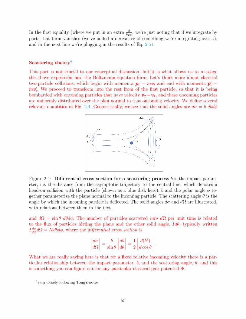
In the first equality (where we put in an extra ∂∂p2

, we’re just noting that if we integrate by

parts that term vanishes (we’ve added a derivative of something we’re integrating over...),and in the next line we’re plugging in the results of Eq. 2.51.

Scattering theory6

This part is not crucial to our conceptual discussion, but it is what allows us to massagethe above expression into the Boltzmann equation form. Let’s think more about classicaltwo-particle collisions, which begin with momenta pi = mvi and end with momenta p′i =mv′i. We proceed to transform into the rest from of the first particle, so that it is beingbombarded with oncoming particles that have velocity v2−v1, and these oncoming particlesare uniformly distributed over the plan normal to that oncoming velocity. We define severalrelevant quantities in Fig. 2.4. Geometrically, we see that the solid angles are dσ = b dbdφ

Figure 2.4: Differential cross section for a scattering process b is the impact param-eter, i.e. the distance from the asymptotic trajectory to the central line, which denotes ahead-on collision with the particle (shown as a blue disk here); b and the polar angle φ to-gether parameterize the plane normal to the incoming particle. The scattering angle θ is theangle by which the incoming particle is deflected. The solid angles dσ and dΩ are illustrated,with relations between them in the text.

and dΩ = sin θ dθdφ. The number of particles scattered into dΩ per unit time is relatedto the flux of particles hitting the plane and the other solid angle, Idθ, typically writtenI dσdΩdΩ = Ibdbdφ, where the differential cross section is∣∣∣∣ dσdΩ

∣∣∣∣ =b

sin θ

∣∣∣∣dbdθ∣∣∣∣ =

1

2

∣∣∣∣ d(b2)

d cos θ

∣∣∣∣ .What we are really saying here is that for a fixed relative incoming velocity there is a par-ticular relationship between the impact parameter, b, and the scattering angle, θ, and thisis something you can figure out for any particular classical pair potential Φ.

6very closely following Tong’s notes

55

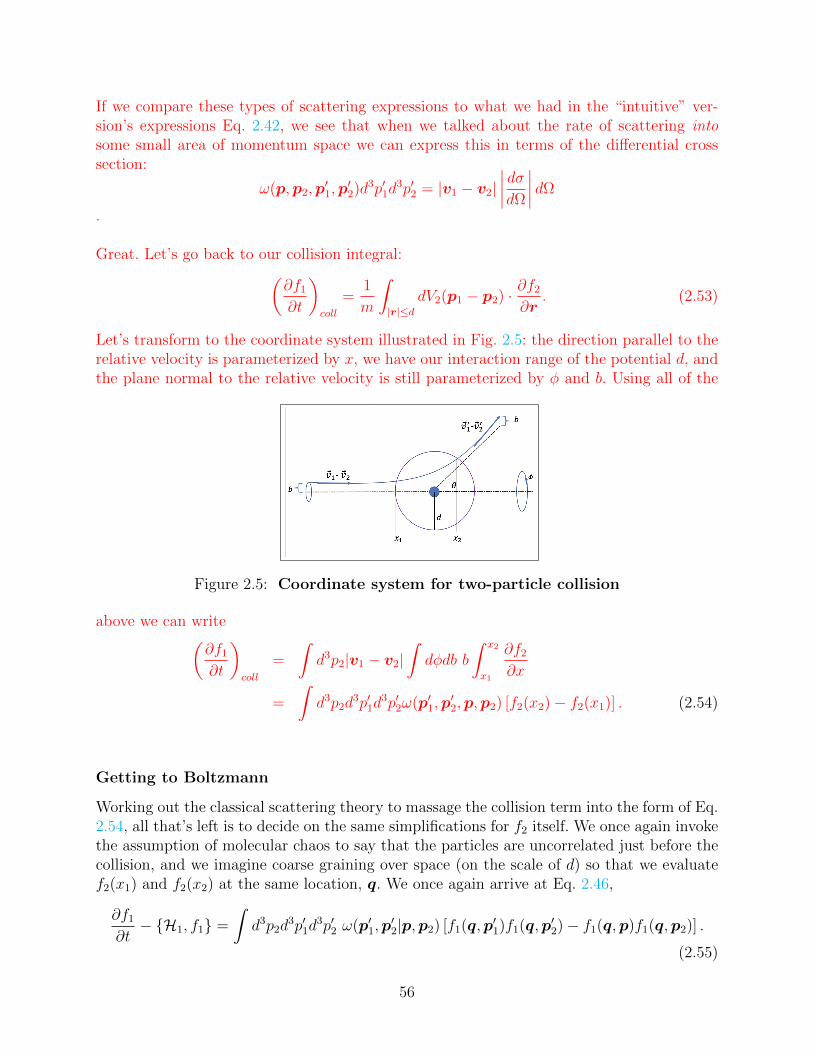
If we compare these types of scattering expressions to what we had in the “intuitive” ver-sion’s expressions Eq. 2.42, we see that when we talked about the rate of scattering intosome small area of momentum space we can express this in terms of the differential crosssection:

ω(p,p2,p′1,p

′2)d3p′1d

3p′2 = |v1 − v2|∣∣∣∣ dσdΩ

∣∣∣∣ dΩ

.

Great. Let’s go back to our collision integral:(∂f1

∂t

)coll

=1

m

∫|r|≤d

dV2(p1 − p2) · ∂f2

∂r. (2.53)

Let’s transform to the coordinate system illustrated in Fig. 2.5: the direction parallel to therelative velocity is parameterized by x, we have our interaction range of the potential d, andthe plane normal to the relative velocity is still parameterized by φ and b. Using all of the

Figure 2.5: Coordinate system for two-particle collision

above we can write(∂f1

∂t

)coll

=

∫d3p2|v1 − v2|

∫dφdb b

∫ x2

x1

∂f2

∂x

=

∫d3p2d

3p′1d3p′2ω(p′1,p

′2,p,p2) [f2(x2)− f2(x1)] . (2.54)

Getting to Boltzmann

Working out the classical scattering theory to massage the collision term into the form of Eq.2.54, all that’s left is to decide on the same simplifications for f2 itself. We once again invokethe assumption of molecular chaos to say that the particles are uncorrelated just before thecollision, and we imagine coarse graining over space (on the scale of d) so that we evaluatef2(x1) and f2(x2) at the same location, q. We once again arrive at Eq. 2.46,

∂f1

∂t− H1, f1 =

∫d3p2d

3p′1d3p′2 ω(p′1,p

′2|p,p2) [f1(q,p′1)f1(q,p′2)− f1(q,p)f1(q,p2)] .

(2.55)

56

2.5 The H-Theorem

We are finally ready to begin addressing the second question we asked at the very beginning ofthe chapter. We have been dancing around the question of how is it that thermodynamics tellsus that systems will eventually settle into equilibrium states – which involves an arrow of timethat distinguishes past from future – even though the equations of motion are fundamentallyinvariant under the reversal of time. Specifically, we’ll first show that within the framework ofthe Boltzmann equation, entropy does indeed increase7 and systems do indeed equilibrate8.

So what is the H-Theorem, exactly? Let’s define a (possibly) time-dependent quantity,H(t), defined by

H(t) =

∫d3qd3p f1(q,p, t) log (f1(q,p, t)) . (2.56)

Had we not already progressed through Chapters 1 and 2 this might seem like a somewhatstrange-looking function, but we instantly recognize the form. f1 is (possibly up to a factor ofnormalization) a probability density function, and we recognize H as something like 〈log f1〉,which is intimately related to the Shannon entropy associated with the probability function(or, from the sign convention, really the information content).

H-Theorem: If f1 satisfies the Boltzmann equation, then

dH

dt≤ 0, (2.57)

where we have added the frame around the equation because it is a microscopic statementof the increase of entropy with time!

Proof:

We take the time derivative in the same way we took the time derivative of ensemble aver-age quantities earlier in the chapter: H only has a time dependence through explicit time-dependences:

dH

dt=

∫d3qd3p (log f1 + 1)

∂f1

∂t=

∫d3qd3p log f1

∂f1

∂t, (2.58)

where we exploited the fact that∫d3rd3pf1 = N is independent of time, so

∫∂tf1 = 0. Using

the fact that f1 satisfies the Boltzmann equation, we can write the above as

dH

dt=

∫d3qd3p log f1

(∂U

∂q1

· ∂f1

∂p1

− p1

m· ∂f1

∂q1

+

(∂f1

∂t

)coll

). (2.59)

Actually, though, the first two terms in the above equation vanish: to see this we integrateby parts twice, first moving the derivative from f1 onto the log f1 term, and then from the

7this section8next section

57

log f1 term back onto the f1. Thus, in fact, the time evolution of H is entirely governed bythe collision terms:

dH

dt=

∫d3qd3p log f1

(∂f1

∂t

)coll

=

∫d3qd3p1d

3p2d3p′1d

3p′2ω (p′1,p′2|p1,p2) log f1(p1) [f1(p′1)f1(p′2)− f1(p1)f1(p2)] .(2.60)

In the above I’m suppressing the q and t arguments, and named the dummy integrationvariable p1.

To make progress, we play with the dummy indices. First, let’s relabel 1↔ 2, which onlychanges the argument of the log. Adding the resulting (equivalent) expression and averagingit with the original expression gives a more symmetric expression:

dH

dt=

1

2

∫d3qd3p1d

3p2d3p′1d

3p′2ω (p′1,p′2|p1,p2) log [f1(p1)f1(p2)] [f1(p′1)f1(p′2)− f1(p1)f1(p2)] .

(2.61)We can play the same trick with the incoming and outgoing momenta, swapping p ↔ p′,while simultaneously making use of the symmetry properties of the scattering processes9.This gives us

dH

dt=−1

2

∫d3qd3p1d

3p2d3p′1d

3p′2ω (p′1,p′2|p1,p2) log [f1(p′1)f1(p′2)] [f1(p′1)f1(p′2)− f1(p1)f1(p2)] .

(2.62)Finally, we average the above two numbered equations to get

dH

dt=−1

4

∫d3qd3p1d

3p2d3p′1d

3p′2ω (p′1,p′2|p1,p2)

× [log [f1(p′1)f1(p′2)]− log [f1(p1)f1(p2)]] [f1(p′1)f1(p′2)− f1(p1)f1(p2)] .(2.63)

You may feel like this sequence of manipulations – averaging different versions of thesame expression together to get a symmetric-looking expression – has done us little good,but we’re actually done! Let’s think about the terms in the integral. First, the scattering rate,ω, is definitionally a positive quantity. Second, the terms involving f1 have been manipulatedinto the form

(log a− log b) (a− b) ,which, given the positivity of f1, is always a positive number! Thus,

dH

dt≤ 0 ⇔ dS

dt≥ 0

A few comments are in order:

1. The arrow of time, again, emerges from the assumption of molecular chaos. If we haddecided that the rate of scattering was proportional to f2 after the collision insteadof before, and still kept f2 ∼ f1f1, we would have found dH

dt≥ 0, suggesting entropy

decreases as we move into the future. Clearly some real subtleties are in the assumptionswe made!

9∫d3p′1d

3p′2ω(p′1, p′2|p1, p2) =

∫d3p′1d

3p′2ω(p1, p2|p′1, p′2)

58

2. Note also that the H-theorem permits the time derivative of H to vanish (i.e., it’s nota strict inequality). We will see (in the homework) that some distributions satisfy anotion of “local equilibrium” by satisfying a condition of detailed balance, making dH

dt

vanish by satisfying:f1(p′1)f1(p′2) = f1(p1)f1(p2).

These distributions are not quite in equilibrium, as they do not satisfy the streamingterms, but they do make the collision terms vanish. These systems have things likedensities, temperatures, drift velocities, etc., varying over space. We’ll see more aboutthis in the next section.

2.6 Introduction to hydrodynamics10

The equilibrium properties of a macroscopic system are governed by thermodynamics, but wesaid at the outset of this chapter that we also care about, e.g., the common situation shownin Fig. 2.1. What happens if you start we an equilibrium system and perturb it (perhapsin a large way, as by suddenly and radically expanding the volume available for a gas)?Hydrodynamics provides a systematic way to think about characteristically long-wavelength,low-energy excitations of a system. Phenomenologically one can write down hydrodynamicequations based on the symmetries of a system, but here (in the context of the Boltzmannequation) we’ll see that you can also explicitly derive hydrodynamic descriptions by startingwith the microscopic dynamics of a system.

To motivate a bit of what follows, let us think about the equilibrium condition in thecontext of the Boltzmann equation, which is that dH

dt= 0. This sets up the following tension,

which we will resolve in this section: One way to satisfy this condition is to satisfy theconstraints of local equilibrium, writing a candidate one-body distribution which takes theform

f(p, r) = exp

(−α(r)− β(r)

(p− π(r))2

2m

), (2.64)

where α, β, and π are functions of the spatial coordinates. A distribution of this form sets thetime-derivative of H to zero, but it does not satisfy Boltzmann’s equation itself! We saw quitegenerically when discussing the Liouville equation that the left hand side of the Boltzmannequation, even if there is no explicit time dependence, requires the Poisson bracket of theone-particle distribution and the one-particle Hamiltonian to vanish, H1, f1 = 0; given theset of conserved quantities this tells us that in general f1 in global equilibrium should justbe a function of H1:

f(p, r) ∝ exp

(β

(p2

2m+ U(r)

)). (2.65)

10“Hydrodynamics is what you get if you take thermodynamics and splash it.” – David Tong. Anyway,there are many references available if you want to go deeper into this subject. The treatment here is kind ofa cross between the treatment in Kardar’s “Statistical physics of fields” and David Tong’s lecture notes onKinetic Theory, with a tiny splash of Chapter 5 of Huang’s “Statistical Mechanics”, 2nd edition.

59

These, in general, are not the same. The key is that the Boltzmann equation is built on aseparation of time scales that we can physically interpret. At the fastest, collisional timescale, we approximate f2 ∼ f1f1, where there are correlations in these quantities. On timescales related to the mean time between collisions, τx, f1 relaxes to a local equilibrium form,and quantities that are conserved in collisions reach this state of local equilibrium. Finally,there is a subsequent slow relaxation to the global equilibrium state, governed not by thecollision terms or intergrals over the collision terms, but by the streaming terms on the LHSof the Boltzmann equation.

2.6.1 Collision-conserved quantities

Let’s think about a function over the single-particle phase space, A(r,p) – this could bedensity, or kinetic energy, or... but importantly, we are thinking of quantities that do nothave explicit time-dependences. Now, we want to think about the typical way that A varieswith space, so we will integrate over momentum. This could be motivated by saying it ismore common to experimentally measure spatial dependences than momentum dependencesof the kind of systems we’re studying, but more relevantly I would say the following: Whenwe started with the Liouville equation there was complete symmetry between p and q, butin the derivation of the Boltzmann equation we started treating the two inequivalently. Toreflect the fact that p and q are no longer on the same footing, I’ll switch from q to r torepresent position. So, let’s define averages of A as

〈A(r, t)〉 =

∫d3pA(r,p)f1(r,p, t)∫

d3pf1(r,p, t).

Note that the denominator of the above expression is just a local number density of particles,

n(r, t) =

∫d3pf1(r,p, t), (2.66)

so

〈A(r, t)〉 =1

n(r, t)

∫d3pA(r,p)f1(r,p, t) (2.67)

Importantly, the time-dependence of these average quantities only come through the factthat f1 can evolve in time.

We’re not going to be interested in arbitrary choices of A: ultimately we want to thinkabout the kind of slowly-varying quantities that are relevant as we are approaching equilib-rium, and we know from our discussion above that typically terms involved in the collisionintegral will vary over a fast time scale. So, we want quantities A that will vanish whenintegrated against the collision part of the Boltzmann equation. I.e., we want A’s that havethe property ∫

d3pA(r,p)

(∂f1

∂t

)coll

= 0.

We can insert the expression for the collision term and go through precisely the same kindof manipulations we did in Sec. 2.5 to find that the A’s that have this property obey

A(r,p1) + A(r,p2) = A(r,p′1) + A(r,p′2). (2.68)

That is, they are properties that are conserved in the course of a collision.

60

Time evolution of collision-conserved quantities: Before we investigate the particularA’s of interest, let’s write down the general way that A changes with time if f1 satisfies theBoltzmann equation. To do this, we start with the Boltzmann equation, which we will fromnow on occasionally write as

Lf1 = C[f1, f1], (2.69)

where L = ∂t + pαm∂α +Fα∂pα and C[f1, f1] =

(∂f1∂t

)coll

. Let’s multiply by a collision-invariantA(r,p) and integrate both sides

∫d3p. The RHS will vanish (by definition of how we’re

choosing the A), leaving us with∫d3p A(r,p)

(∂

∂t+pαm∂α + Fα∂pα

)f1(r,p, t) = 0, (2.70)

where F is the external force, F = −∇U (and the rest of the notation should be clear...i.e. with the summation convention p

m· ∂∂r

= pαm∂α). We can simplify this expression (for

instance by integrating the term involving the external potential by parts) and various simplemanipulations. Making use of how we defined the angle brackets here to be averages overmomenta, we can write the above expression as (suppressing dependencies, and with v =p/m)

∂

∂t〈nA〉+

∂

∂r· 〈nvA〉 − n

⟨v · ∂A

∂r

⟩− n

⟨F · ∂A

∂p

⟩= 0. (2.71)

Specific collision-conserved quantities

Let’s apply this general expression to quantities which we know are conserved in a collision.

Particle number The most trivial thing conserved in a collision between particles issimply the number of particles !. If we insert the choice A = 1 into Eq. 2.71, we simply get

∂tn+ ∂α(nua) = 0. (2.72)

This result is often written using the particle current, J(r, t) = n(r, t)u(r, t). It is thecontinuity equation, expressing the fact that if particle number is conserved, variations inlocal particle density are related to particle currents. Note that we have introduced a newquantity, u = 〈v〉

Momentum Linear functions of the momentum are also conserved during collisions, andit is convenient to look not at A = p, but rather at the momentum relative to the meanlocal velocity we just defined. Choosing A = c ≡ p/m−u and substituting it into Eq. 2.71,and exploiting the fact that we defined things so that 〈cα〉 = 0, we find

∂tuα + uβ∂βuα =Fαm− 1

mn∂βPαβ, (2.73)

where the pressure tensor for the fluid is

Pαβ ≡ mn 〈cαcβ〉 . (2.74)

This expression is like a generalized Newton’s law, telling us that the fluid elements experi-ence accelerations that come both from the external forces and also gradients in the pressuretensor.

61

Kinetic energy Finally, we look at the kinetic energy of the particles as our last collision-conserved quantity. As before, it is slightly easier to work with the relative kinetic energy,A = m

2(v−u)2 = m

2c2. We substitute this into Eq. 2.71, and go through some simplifications

to find

∂tε+ uα∂αε = − 1

n∂αhα −

1

nPαβuαβ, (2.75)

where I have just introduced the average local kinetic energy :

ε ≡⟨mc2

2

⟩,

the local heat flux :

hα ≡nm

2

⟨cαc

2⟩,

and the strain rate tensor :

uαβ =1

2(∂αuβ + ∂βuα) .

Equations 2.72, 2.73, and 2.75 form a set of coupled equations for the time evolution ofthe particle density n the local average velocity u, and the local average kinetic energy ε(which is itself going to be related to the temperature!). But the equations are not closed, asto calculate those three quantities we would need expressions for the pressure tensor and theheat flux. We next show how we can build up approximations, using the Boltzmann equation,to these quantities to finally get a simple, hydrodynamic description of how systems approachequilibrium.

2.6.2 Zeroth-order hydrodynamics

Let’s make progress by straight-up guessing a functional form for the one-body distributionfunction f1. Our logic in making this guess is that we know the collision term will inducefast relaxations, so if we want a distribution function which only varies slowly, a good placeto start would be with a distribution function that satisfies C[f1, f1] = 0. Let’s take one suchsolution which we already met in Eq. 2.64; getting the normalization correct and introducinga new variable that we’ll suspiciously label T , we’ll take our zeroth-order guess, denoted f 0

1 ,to be

f 01 (p, r, t) =

n(r, t)

(2πmkBT (r, t))3/2exp

[−(p−mu(r, t))2

2mkBT (r, t)

](2.76)

This Gaussian form is clearly normalized so that, e.g.,∫d3pf 0

1 = n, 〈p/m〉0 = u, and

〈cαcβ〉0 = kBTmδαβ. This lets us calculate the approximations for the pressure tensor, energy

density, and heat flux:

P 0αβ = nkBTδαβ, ε =

3

2kBT, h0 = 0.

The equations we derived by thinking about collision conserved quantities are very simplein this approximation. Defining the material derivative

Dt ≡ ∂t + uβ∂β

62

we get:

Dtn = −n∂αuαmDtuα = Fα −

1

n∂α(nkBT )

DtT = −2

3T∂αuα. (2.77)

The inadequacy of zeroth-order hydrodynamics: Sadly, these very simple equationsdo a terrible job of describing the relaxation of a system to equilibrium. Let’s imagine startingwith a system with initial u0 = 0 in the absence of external forces F = 0, and making asmall perturbation:

n(r, t) = n+ δn(r, t), T (r, t) = T + δT (r, t). (2.78)

We want to study what happens to these small perturbations, so we expand Eqs. 2.77 tofirst order in (δn, δT,u), where we note that to first order the material derivative is justDt = ∂t +O(u), so our linearized zeroth order equations become:

∂tδn = −n∂αuα

m∂tuα = −kBTn

∂αδn− kB∂αδT

∂tδT = −2

3T ∂αuα. (2.79)

The easiest way to investigate the effect of our perturbations is to take Fourier transforms,

A(k, ω) =

∫d3qdt A(r, t) exp [i(k · r − ωt)] ,

where A is any of (δn, δT,u). This gives us the matrix equation

ω

δnuαδT

=

0 nkβ 0kB Tmn

δαβkβ 0 kBmδαβkβ

0 23T kβ 0

δnuβδT

. (2.80)

This matrix has the following modes: There are two modes describing a transverse shear flowin a uniform and isothermal gas (n = n, T = T ), with the velocity field varying transverseto its orientation, e.g. u = f(x, t)y, and both have ω = 0. There is another ω = 0 modedescribing a gas with uniform pressure nkBT , where n and T may be spatially varying butwith a constant product. Lastly, there is a mode with variations along the direction of k;the eigenvector looks like:

vlongitudinal =

n|k|ω(k)23T |k|

, ω(k) = ±√

5kBT

3m|k|.

Well, shoot. Apparently within this approximation none of our conserved quantities relaxto equilibrium if we apply a little perturbation: shear flow persists forever, sound modes haveundamped oscillations, etc.

63

2.6.3 First-order hydrodynamics

Perhaps this should not have surprised us: we picked something that satisfied local equilib-rium, but it is straightforward to check that Lf 0

1 6= 0. Actually, it’s more straightforward toshow that if n, T, uα satisfy the zeroth-order hydrodynamic equations, then the effect of Lon the log of the zeroth-order approximation for f1 is

L[ln f 0

1

]=

m

kBT

(cαcβ −

δαβ3c2

)uαβ +

(mc2

2kBT− 5

2

)cαT∂αT. (2.81)

Our instinct for moving forward is to note that, although the RHS of the above is notzero, it depends on gradients of temperature and on the local velocity. In a sense, then, if westick to long-wavelength variations in T and u we are “close” to a solution. Thus, we will tryto construct first-order hydrodynamics by adding a little something extra to the distribution:

f 11 = f 0

1 + δf1. (2.82)

Relaxation time approximation What happens if we act on f 11 with our collision op-

erator?

C[f 11 , f

11 ] =

∫d3p2d

3p′1d3p′2ω(p′1,p

′2|p1,p2) [f1(p′1)f1(p′2)− f1(p1)f1(p2)] (2.83)

=

∫d3p2d

3p′1d3p′2ω(p′1,p

′2|p1,p2)

[f 0

1 (p′1)δf1(p′2) + δf1(p′1)f 01 (p′2)− f 0

1 (p1)δf1(p2)− δf1(p1)f 01 (p2)

],

where we have used the fact that f 01 vanishes in the collision integral and dropped any terms

of order (δf1)2. We now have a linear function of δf1, albeit a messy one to work with. Atthis point there is a proper way to proceed11, and a physically just fine way to proceed,which has the great virtue of being much easier while still capturing the dissipational piecethat was missing from our zeroth-order description. We simply approximate

C[f 11 , f

11 ] ≈ −δf1

τx, (2.84)

which is called the relaxation time approximation or the single collision time approximationor using the BGK operator 12. With this approximation the Boltzmann equation is

∂f 01 + δf1

∂t− H1, f

01 + δf1 =

−δf1

τx, (2.85)

but we assume that δf1 f 01 , so we ignore the δf1 on the LHS. We can then explicitly work

out the additional contribution to our improved estimate:

δf1 = −τx[(

mc2

2kBT− 5

2

)c

T· ∂T∂r

+m

kBT

(cαcβ −

δαβ3c2

)uαβ

]f 0

1 . (2.86)

11The Chapman-Enskog expansion, doing a careful expansion in δf112Bhatnagar-Gross-Krook, 1954

64

One can use this improved description to calculate corrections to various quantities. Forexample, the first-order estimate of the pressure tensor becomes

P 1αβ = nkBTδαβ − 2nkBTτx

(uαβ −

δαβ3uγγ

), (2.87)

and the heat flux acquires a dependence on spatial gradients in the temperature. These areimportant: they say that shear flows get opposed by off-diagonal terms in the pressure tensor,and that spatial variations in temperature generate heat flows that in turn smooth out thosevariations! These are the sorts of effects that cause the relaxation to equilibrium.

In case you’re curious, if I’ve TEX’ed this correctly the matrix equation corresponding tothe first-order hydrodynamic equations after a Fourier transformation look like

ω

δnuαδT

=

0 nδαβkβ 0kB Tmn

δαβkβ −i µmn

(k2δαβ +

kαkβ3

)kBmδαβkβ

0 23T δαβkβ −i2Kk2

3kB n

δn

uβδT

, (2.88)

where K = (5nk2BT τx)/(2m) and µ = nkBT τx is a viscosity coefficient. The important point

of writing this is the ability to verify that now all of the modes have an imaginary component(either they are strictly imaginary eigenvalues (for variations in pressure and for transverseshear modes) or complex ones (for longitudinal sound modes), so that we know that over longtime scales perturbations to the gas die away, and the gas eventually reaches its equilibriumstate.

You’ll go through a simple example of first-order hydrodynamics in the homework!

65

Chapter 3

Classical Statistical Mechanics1

Statistical mechanics is connected with the phenomenological, “thermodynamical” view ofmacroscopic properties we saw in Chapter 1 via a probabilistic description of large numbers ofdegrees of freedom. In this chapter we will focus not on microscopic theories for which we canstudy both equilibrium and approach-to-equilibrium dynamics as in Chapter 3, but rather onattempting to provide probability distributions that connect microstates to macrostates. Wewill use the idea of unbiased estimates of probability to assign these probability distributionsfor different equilibrium ensembles, and use the mathematics of the large-N limit to showthat the ensembles are equivalent in the thermodynamic limit.

3.1 The microcanonical ensemble and the laws of ther-

modynamics

We begin, just as we did in the chapter on Thermodynamics, with a simplified version of oursystem of interest, taking an adiabatically isolated state. In the absence of adding heat orwork to the system, the macrostate M is specified completely by the internal energy E, theset of generalized coordinates x, and the number of particles N : M(E,x, N). In the absenceof any other information, or any knowledge of other conserved quantities, we say that at aminimum the Hamiltonian evolution equations conserve the total energy of the system, sothat the evaluation of the Hamiltonian on a microstate µ is H(µ) = E.

The central postulate of statistical mechanics is that the equilibrium probabilitydistribution is

p(E,x,N)(µ) =1

Ω(E,x, N)·

1 if H(µ) = E0 otherwise

(3.1)

This is often called “the assumption of equal a priori probabilities,” and we see that it isthe same as the unbiased estimate of probability given only a constraint of constant energyE. Certainly we saw that this is one of the allowed assignments consistent with Liouville’s

1In this chapter we’ll basically go through Pathria Chapters 2-4... because of the way we started thiscourse, though, we’ve already done much of the work!

66

theorem, although it is not the only one! Although, having seen the chapter on probability,we are not surprised by this assignment of probability it is nevertheless a deep assumption,

There is a potential subtlety in defining the normalization factor2 Ω here: as written, inorder to make p a properly normalized probability density function (so that it integrates tounity), we want Ω to be the area of the relevant surface of fixed energy E over the microscopicphase space. You might be worried about defining probability densities that are non-zero onlyon a surface, and so we sometimes define a microstate in the microcanonical ensemble to bewithin ∆ of the specified energy: E − 1

2∆ ≤ H(µ) ≤ E + 1

2∆. The normalization Ω′ is now

the volume of a shell rather than the area of a surface, and Ω′ ≈ Ω∆. We will see that, sinceΩ is typically exponentially large in E, which is itself typically proportional to N , that thedifference between the surface area and the shell volume is negligible, so we’ll go back andforth between Ω and Ω′ freely.

We define the entropy of the uniform probability distribution exactly as you by nowexpect:

S(E,x, N) = kB ln Ω(E,x, N), (3.2)

where we have introduce a factor called “kB” so that entropy has units of energy divided bytemperature. Note, by the way, that we know from Liouville that under canonical transforma-tions volumes in phase space are invariant, and for the transformed probability distributionstays uniform on the transformed phase-space surface of constant energy. This tells us thatboth Ω and S are invariant under canonical coordinate changes.

To highlight the interconnections with the beginning of this class, we now show thatEq. 3.1 can be used to derive the laws of thermodynamics (with the exception of Nernst’stheorem, which as we hinted at the time requires quantum mechanics).

3.1.1 0th Law

Let’s think about bringing two previously isolated microcanonical systems, which originallyhad energies E1 and E2, into contact in a way that lets them exchange heat, but not work.Certainly the combined system has energy E = E1 + E2, and we assume (by assuming thatthe interactions between the systems are small) that the microstate of the combined systemcorresponds to a pair of microstates of the components. We’ll write this as µ = µ1 ⊗ µ2,assuming H(µ) = H1(µ1) +H2(µ2). We thus write the fundamental postulate, Eq. 3.1 as

pE(µ) =1

Ω(E)·

1 if H1(µ1) +H2(µ2) = E0 otherwise

. (3.3)

We have a fixed total energy, so we can compute the normalization factor as

Ω(E) =

∫dE1 Ω1(E1)Ω2(E − E1) =

∫dE1 exp

[S1(E1) + S2(E2)

kB

]. (3.4)

We written the normalization factor for our probability this way to make contact withour “sums and integrals of exponentials” discussion in a previous chapter! We think (and

2“we must learn how to count the number of states it is possible for a system to have or, more precisely,how to avoid having to count that number” – David Goodstein, States of Matter

67

will see later) that entropy is extensive, so that S1 and S2 are proportional to the numberof particles in the system. We use the simple (i.e., non-complex) saddle-point method toapproximate the integral by the maximum of the integrand, giving us

S(E) = kB ln Ω(E) ≈ S1(E∗1) + S2(E∗2), (3.5)

where the starred quantities are the values that maximize the value of the integrand. Wecan calculate this values of setting the first derivative (w/r/t E1) of the exponent above tozero, which gives us:

∂S1

∂E1

∣∣∣∣x1,N1

=∂S2

∂E2

∣∣∣∣x2,N2

. (3.6)

In words, there are many joint microstates which sum to a total energy of E, but there areexponentially more microstates sitting near (E∗1 , E

∗2), and so the system eventually flows

from (E1, E2) to (E∗1 , E∗2). We get no information about the time dynamics of this process;

just the end result, which is a place where Eq. 3.6 is satisfied.Also, ah ha!! We have found a condition satisfied by two systems that come into equilib-

rium with each other: the have equal partial derivatives of entropy with respect to energy(holding everything else fixed)! To be consistent with what we had from phenomenologicalthermodynamics, we’ll choose a particular name for the state function corresponding to thiscondition:

∂S

∂E

∣∣∣∣x

=1

T. (3.7)

3.1.2 1st Law

Let’s think about what happens to S of a system in the microcanonical ensemble when wevary the generalized displacements3 by δx This does a work on the system dW = J · δx,and changes the internal energy to E + dW . To first order, the change in entropy of such avariation is

δS = S(E + J · δx,x+ δx)− S(E,x) =

(∂S

∂E

∣∣∣∣x

J +∂S

∂x

∣∣∣∣E

)· δx. (3.8)

Now, what does it mean to be in equilibrium? We say we have an equilibrium state atsome value of E and some set of generalized displacements x, and we have said that allconsistent microstates are equally probable. Well, the above equation says that spontaneouschanges in the system will occur, taking us into more likely states, unless the terms in theparentheses vanish! Thus, a condition to be in equilibrium is that

∂S

∂xi

∣∣∣∣E,xj 6=i

= −JiT, (3.9)

where we have used the relationship between temperature and ∂S/∂E from the zeroth law.With this constraint on the variations, we get that in general

dS(E,x) =∂S

∂EdE +

∂S

∂xdx =

dE

T− J · dx

T⇒ dE = TdS + J · dx. (3.10)

3for the remainder of this section I’m going to be TEX-lazy and stop distinguishing mechanical workfrom chemical work.... it’s all just x now.

68

Wow – it’s the first law! And where we’ve, of course, identified dQ = TdS.

3.1.3 2nd Law4

The second law is almost obvious, almost by construction, given what we have set up sofar. Indeed, you already know from the section of unbiased estimates that we are assigningprobabilities in a way that maximizes the entropy subject to the constraint on the energy.For instance, consider our example from the zeroth law of bringing two equilibrium statesat E1 and E2 into contact. Well, clearly

S(E) ≡ kB ln Ω(E1 + E2) ≥ S1(E1) + S2(E2),

which must be true since the two states of the original system are a subset of the possiblecombined joint microstates.

Note that we can make additional mathematical statements by considering variations ofentropy. When two systems are first brought into contact but have not yet reached equilib-rium, the equality in Eq. 3.6 does not yet hold. Instead we have

δS =

(∂S1

∂E1

∣∣∣∣x1

− ∂S2

∂E2

∣∣∣∣x2

)δE1 =

(1

T1

− 1

T2

)δE1 ≥ 0. (3.11)

Thus we recover Clausius’ statement of the second law: we know the variations in S arepositive as we move towards a new equilibirum state, and we see that heat flows from thehotter to the colder system.

Note that, in principle, these are all probabilistic statements: it is merely much morelikely that a combined system ends up at (E∗1 , E

∗2) rather than it’s initial and (E1, E2).

This obscures just how much work “much” is doing in the previous sentence, though: thenumber of microstates available grows exponentially with system size, and so if we were toask how long we would have to wait before seeing our combined system at (E1, E2) ratherthan (E∗1 , E

∗2), the answer would be related to an exponential of that exponential. Needing

to wait this long to see something is a practical definition of saying “you will never see that.”

3.1.4 The ideal gas in the microcanonical ensemble

We return to our favorite toy system for illustrating concepts, the ideal gas of N particles.We ignore any particle interactions, and say we have

H =N∑i=1

p2i

2m+ U(qi),

4“The law that entropy always increases holds, I think, the supreme position among the laws of Nature.If someone points out to you that your pet theory of the universe is in disagreement with Maxwell’s equations- then so much the worse for Maxwell’s equations. If it is found to be contradicted by observation - well,these experimentalists do bungle things sometimes. But if your theory is found to be against the SecondLaw of Thermodynamics I can give you no hope; there is nothing for it to collapse in deepest humiliation.”– Arthur Eddington, New Pathways in Science

69

where the potential U simply imposes strict confinement to a box of volume V (i.e., wetake U(qi) = 0 if particle i is inside the box and ∞ if it is outside the box). Explicitly, themicrocanonical ensemble has a probability density function

p(µ) =1

Ω(E, V,N)·

1 if∑

i(p2i /(2m)) = E ± 1

2∆E and qi ∈ box

0 otherwise. (3.12)

We can calculate Ω by the requirement that p(µ) is properly normalized, i.e.,∫ ∏

i dVip(µ) =1. The integrals over qi are all trivial: each of those N integrals just gives a factor of V . Theintegral over the momenta is down by noting we are constraining the momenta to a (finite-thickness shell around a) surface of a hypersphere, given by

∑Ni p

2i = 2mE. We thus need

to know the area of a 3N -dimensional sphere of radius R =√

2mE. The relevant formulafor a d-dimensional sphere is

Ad =2πd/2

(d/2− 1)!Rd−1, (3.13)

where it is easy to check that this gives the right result in 2D (and 3D, since (1/2)! =√π/2).

Putting this together, with d = 3N , we calculate:

Ω(E, V,N) = V N 2π3N/2

(3N/2− 1)!(2mE)(3N−1)/2∆E (3.14)

The entropy of the ideal gas is then just the log of this normalization factor. UsingStirling’s approximation:

S(E, V,N) = kB

[N lnV +

3N

2ln(2πmE)− 3N

2ln

3N

2+

3N

2

]= NkB ln

[V

(4πemE

3N

)3/2], (3.15)

where in the first line we have dropped terms of order 1, and of order lnE ∝ lnN by arguingthe latter are small compared to these terms of order N in the thermodynamic limit.

With the entropy in hand, and writing dS = 1TdE + P

TdV − µ

TdN we can get the usual

properties of the ideal gas by differentiating the entropy as appropriate. For instance,

1

T=

∂S

∂E

∣∣∣∣N,V

=3

2

NkBE⇒ E =

3

2NkBT,

the usual equipartition result in the absence of a potential. Similarly,

P

T=

∂S

∂V

∣∣∣∣N,E

=NkBV⇒ PV = NkBT,

the ideal gas equation of state.As a final example of a simple calculation, what about the probability distribution for

finding a particle with some momentum vector p1? Well, we can calculate the unconditional

70

PDF by integrating out everything else:

p(p1) =

∫d3q1

N∏i=2

dVip(µ)

= VΩ(E − p1

2m, V,N − 1)

Ω(E, V,N). (3.16)

One can explicitly check (by plugging in the result of Eq. 3.14, using Stirling’s formula,and noting that p2

1/E is a number of order 1/N) that this explicitly gives you a Maxwell-Boltzmann distribution for the momentum:

p(p1) =1

(2πmkBT )3/2exp

(−p2

1

2mkBT

)We derived the Maxwell-Boltzmann distribution result for the velocities in a dilute gas

of non-interacting particles, but it is actually much more general, and Maxwell’s originalderivation relies on nothing by rotational invariance. It’s cool, so I reproduce it here: Considerthe distribution of velocities in, say, the x direction, and call that distribution p(vx). Byrotational symmetry we have the same distribution in the y and z directions. Rotationalsymmetry also guarantees that the full distribution cannot depend on the particular directionfor the momentum, but only on the speed c =

√v · v. So, we want functions pc(c) and p(vx)

that satisfypc(c)dvxdvydvz = p(vx)p(vy)p(vz)dvxdvydvz.

Remarkably, there is only one solution which satisfies this, and it is

p(vx) = A exp(−Bv2

x

),

for some constants A and B. Thus, the distribution of speeds must be

pc(c)dvxdvydvz = 4πc2pc(c)dc = 4πA3c2e−Bc2

dc.

Nifty. Determining that the coefficients have specific values, like B = m2kBT

as in the idealgas, requires a harder microscopic calculation of the sort we just did.

3.1.5 Gibbs’ Paradox: What’s up with mixing entropy?

You will notice that Eq. 3.15, giving the entropy of an ideal gas, has a major flaw: we expectentropy to be extensive, but under a transformation (E, V,N)→ (λE, λV, λN) the entropyactually changes to λ(S+NkB lnλ) rather than λS. There are these extra contributions thatcome from the integration over positions, like V N , and this additional contribution is relatedto the entropy of mixing distinct gases. Gibbs’ paradox, the fact that this expression for theentropy suggests an increase even if two identical gases are mixed, is subtle, with some tothis day arguing that its resolution must be quantum mechanical5 and others arguing that

5see, e.g., Kardar’s “Statistical Physics of Particles”

71

the paradox is toothless and can be resolved classically6. We will come back to this issuewhen we talk about quantum statistical mechanics; I would be delighted if one of you wantedto discuss the classical issue as an in-class presentation (as described on the syllabus).

As our yet-to-be-understood resolution to the paradox, we will from now on modify ourphase-space measure for identical particles to be

dΓ =1

h3NN !

N∏i=1

d3qid3pi. (3.17)

3.2 The canonical ensemble

In the last section we defined the microcanonical ensemble by considering a macrostatewith a specified energy, E, and we were able to derive an expression for the temperate asT−1 = ∂S

∂E

∣∣x.In the chapter on thermodynamics, though, we saw that E and T are both

functions of state, and that it should be possible to instead start with statistical descriptionin which the temperature of a macrostate is prescribed and an expression for the energy isderived.

Welcome to the canonical ensemble, in which we specify the macrostate M(T,x). Wethink of prescribing the temperature of the system by putting it in thermal contact with thereservoir, which is another macroscopic system that is so large that it’s own temperaturedoes not change as a result of interacting with the system of interest (think, for instance, oftossing a warm pebble into the ocean – the temperature of the pebble will surely equilibratewith the temperature of the ocean, and no thermometer reading the temperature of theocean will notice the difference).

The goal of the statistical mechanical formulation of thermodynamics is to write downmicrostate probabilities that we can associate with macrostates, p(µ) (and from there derivethermodynamic consequences), and here, too, we rely on the central postulate of statisticalmechanics, Eq. 3.1! Let’s define the system to be in microstate µ with energy HS(µ) and thereservoir to be in microstate µR with energyHR(µR), satisfying Etotal = HS(µ)+HR(µR).Thejoint probability of the microstates µS ⊗ µR is then assumed to be

p(µS ⊗ µR) =1

ΩS⊕R(Etotal)·

1 if HS(µ) +HR(µR) = Etotal0 otherwise

(3.18)

Ultimately, though, we are not interested in this microcanonical joint-probability distributionfor the combined system, we want the unconditional PRF for the microstates. But this wecan obtain (as expected) by summing the joint PDF over the microstates of the reservoir:

p(µ) =∑µR

p(µS ⊗ µR) (3.19)

6see Jayne’s discussion, or that of Frenkel’s more recent article

72

We make progress, here, by doing something similar to how we calculated p(p1) in themicrocanonical ensemble in Eq. 3.16: we say that by looking at a specific system microstateµ, the sum over reservoir states in the above equation is restricted to run over microstateswith HR(µR) = Etotal −HS(µ):

p(µS ⊗ µR) =ΩR(Etotal −HS(µ))

ΩS⊕R(Etotal). (3.20)

Let’s focus on the numerator for now (noting that the denominator, which just providesan overall normalization, can always be effectively recovered by imposing a normalizationcondition of p(µ) when we’re done). Well, ΩR is related to the entropy of the reservoir:

ΩR(Etotal −HS(µ))

ΩS⊕R(Etotal)∝ exp

(SR(Etotal −HS(µ))

kB

). (3.21)

Let’s write that entropy expression as

SR

(Etotal

(1− Hs(µ)

Etotal

))≈ SR(Etotal)−Hs(µ)

∂SR∂ER

= SR(Etotal)−HS(µ)

T,

where we have finally used our assumption that the reservoir is (energetically) humongousrelative to the system. Combining this approximation with our evaluation of the unconditionalPDF, we ultimately arrive at the canonical probability distribution for a microstate with aspecified temperature and set of generalized displacements:

p(µ) =1

Z(T,x)e−βH(µ), (3.22)

where I’ve dropped subscripts, introduced β = (kBT )−1, and defined the partition function

Z(T,x) =∑µ

e−βH(µ) . (3.23)

3.2.1 The partition function as a generator of moments

So, we’ve specified the temperature of the system, and it is exchanging energy back andforth with the reservoir to maintain that temperature. The energy of the system is now arandom variable, which we’ll call E so that the notation doesn’t get too confusing. What isthe probability distribution associated with E? Glad you asked! We change variables from µto H(µ) and get

p(E) =∑µ

p(µ)δ (H(µ)− E) =1

Ze−βE

∑µ

δ (H(µ)− E) ,

but the sum over delta functions just picks out the number of microstates with the appro-priate energy Ω(E), which is related to the entropy, so

p(E) =Ω(E)e−βE

Z=

1

Zexp

[S(E)

kB− EkBT

]=

1

Zexp [−βF (E)] , (3.24)

73

where F = E − TS(E) is obviously going to be related to the Helmholtz free energy. We canfurther simplify by noting that both S and E should be extensive, so we should be able toapproximate sums of exponentials by the dominant term... we expect the probability to besharply peaked about some most probably energy, E∗, and so we approximate the partitionfunction as

Z =∑µ

e−βH(µ) =∑E

e−βF (E) ≈ e−βF (E∗). (3.25)

So, the method of most probable values suggests a logarithmic relationship between F andZ. This is reinforced by the method of mean values, where we compute the average energyof the system as

〈H〉 =∑µ

H(µ)exp (−βH(µ))

Z= − 1

Z

∂

∂β

∑µ

e−βH = −∂ lnZ

∂β. (3.26)

This, too, suggests the identification of the Helmholtz free energy as

F (T,x) = −kBT lnZ(T,x). (3.27)

Are the mean and most probable values close? They should be if the above identi-fication is to make sense via the two routes we just described! We can address this questionby looking at the variance of the energy and comparing it to the mean. Notice that thepartition function, viewed as function of β, is proportional to the characteristic function ofH, with β standing in for the combination ik. So, we can easily generate moments by takingderivatives of Z with respect to β, e.g:

− ∂Z

∂β=∑µ

He−βH, ∂2Z

∂β2=∑µ

H2e−βH. (3.28)

From this, we see that the first moment is just

〈H〉 = 〈H〉c = − 1

Z

∂Z

∂β= −∂ lnZ

∂β(3.29)

With a moment generating function comes a cumulant generating function, here just lnZ!Generally, taking care of the minus signs, we have

〈Hn〉c = (−1)n∂n lnZ

∂βn,

and explicitly

⟨H2⟩c

=∂2 lnZ

∂β2= −∂ 〈H〉c

∂β= kBT

2 ∂ 〈H〉∂T

∣∣∣∣x

⇒⟨H2⟩c

= kBT2Cx,

where have identified that the variance of the energy is related to the heat capacity. Comparethis condition to the stability requirement in HW 1 for why the heat capacity had to bepositive! Also, to answer the question posed just above, note that every cumulant of H is

74

proportional to N , which itself tells you that the relative error√〈H2〉c/ 〈H〉c ∼ N−1/2, so

that it vanishes in the thermodynamic limit. Thus, the mean energy and most probableenergy are identical as N →∞.

Note, by the way, that with all of the above identifications, we can define the entropyusing Eq. 3.22 directly, as

S = −kB 〈p(µ)〉 = kB 〈(−βH− lnZ)〉 =E − FT

, (3.30)

recovering the familiar expression for the Helmholtz free energy.

3.2.2 The ideal gas in the canonical ensemble

Let’s explicitly show that the canonical ensemble returns familiar relations for an ideal gas.The probability distribution is

p(µ) =1

Zexp

(−β

N∑i=1

p2i

2m

)·

1 if qi ∈ box0 otherwise

, (3.31)

and we compute the partition function (with the correction to the phase space measure fromEq. 3.17!) as

Z(T, V,N) =

∫1

N !

N∏i=1

d3qid3pi

h3exp

(−β

N∑i=1

p2i

2m

)=V N

N !

(2πmkBT

h2

)3N/2

. (3.32)

The free energy is

F = −kBT lnZ = −NkBT(

ln

(V e

N

)+

3

2ln

(2πmkBT

h2

)), (3.33)

and using dF (T, V,N) = −SdT−PdV +µdN we can extract the usual properties of the idealgas. For example, the entropy is −S = ∂F

∂T

∣∣V,N

= F−ET

, and P = − ∂F∂V

∣∣T,N

= NkBTV

. Note that

the very form of the probability distribution in Eq. 3.31 tells us the microcanonical resultwe had for p(p1), that the momenta of the particles are drawn from independent Gaussiandistributions.

3.3 Gibbs canonical ensemble

Briefly7, it is sometimes more convenient to work in an ensemble where the internal energycan change by exchanging heat with a reservoir (as in the canonical ensemble) but also byexchanging work.The macrostate M(T,J) is now specified by the temperature and forcesacting on the system, and we view both the energy and the generalized coordinates x asrandom variables (but not including chemical work, which we will treat in the grand canonical

7i.e., entirely by analogy with the last section

75

ensemble shortly... thus, N is fixed). We proceed just as above, and find that the microstatesof the system have a probability distribution

p(µ) =exp (−βH(µ) + βJ · x)

Z(T,N,J), (3.34)

where the Gibbs partition function is

Z(T,N,J) =∑µ,x

exp (−βH(µ) + βJ · x) . (3.35)

We can use, again, either the “most probable value” or “mean value” method to relate theexpectation values of the generalized displacements to the Gibbs partition function, like

〈x〉 = kBT∂ lnZ∂J

, (3.36)

and we use the thermodynamic result that x = −∂G∂J

to make the identification

G(T,N,J) = −kBT lnZ, (3.37)

where we have again written the Gibbs free energy encountered in Chapter 1 as G = E −TS − x · J . On can, for instance, extract the enthalpy H = E − x · J = −∂ lnZ

∂β, or the heat

capacity at constant force as CJ = ∂H∂T

3.4 The grand canonical ensemble

We now generalize once more from the canonical ensemble to the grand canonical ensemble.For the canonical ensemble we said that even though energy was a conserved quantity, it oftenmakes more sense8 to put a system in contact with a reservoir of heat so that temperatureis the fixed quantity and E becomes a random variable as the system and the reservoirexchange heat. We measure temperature all the time, but when, after all, was the last timeyou precisely measured the energy of a macroscopically large system? In the same way, itoften behooves us to generalize yet further and allow our system to also exchange particlenumber with the reservoir – now both N and E are variables and the expectation values,〈N〉 and 〈E〉 are identified with thermodynamically interested quantities. For this system werequire that the reservoir be at a fixed value of temperature T and chemical potential µ, andwe now create a probability distribution corresponding for the grand canonical ensemble, inwhich the macrostates are functions of M(T, µ,x).

Notationally, since µ is the chemical potential, I’ll be careful about using µS to refer to amicrostate of the system we’re interested in. The probability density function for µS is again

8and, as we will see in later chapters, often makes it easier to calculate

76

derived by invoking the fundamental postulate and summing over all states of the reservoir,ultimately giving

p(µS) =1

Q(T, µ,x)exp [−βH(µS) + βµN(µS)] , (3.38)

where N(µS) is the number of particles in microstate µS, and where Q is the grand partitionfunction:

Q(T, µ,x) =∑µS

exp [βµN(µS)− βH(µ)] . (3.39)

We can usefully rearrange the above summation by first grouping together all of the mi-crostates with the same number of particles in them. Letting HN refer to the Hamiltonianassociated with the N -particle system, we write

Q(T, µ,x) =∞∑N=0

eβµN∑µS

e−βHN (µS) =∞∑N=0

zN∑µS

e−βHN (µS), (3.40)

where we have additionally defined the fugacity9 z = exp(βµ). Notice, by the way, that thesecond sum – over microstates with a particular number of particles – are the canonicalpartition functions associated with an N -particle system, so we can additionally write

Q(T, z,x) =∞∑N=0

zNZN(T,x), defining Z0 ≡ 1. (3.41)

This form makes it seem that to calculate the grand canonical partition function we need tohave already calculated the canonical partition function. In principle we indeed do, but inlater chapters10 we’ll see how we can sometimes make great progress in evaluating Q evenin situations where evaluating Z is very difficult.

3.4.1 Number fluctuations in the grand canonical ensemble

Earlier we showed the generic equivalence of the canonical and microcanonical ensembles asN → ∞ by establishing that the average value of the energy and the most probable valueof the energy became indistinguishable in the thermodynamic limit. Here we do the samething by considering both the mean and most typical value of the number of particles. Wenote that from the definition of Q we can read off the total weight of the microstates withN particles, the probability for finding the system with N particles is

p(N) =eβµNZ(T,N,x)

Q(T, µ,x). (3.42)

We write the average as

〈N〉 =1

Q∂Q∂(βµ)

=∂ lnQ∂(βµ)

, (3.43)

9Derived from fugere, to flee. The term was popularized in an early textbook by Gilbert Lewis and MerleRandall as an “escaping tendency,” referring to the flow of matter between phases, and playing a similar roleto temperature in the flow of heat.

10both on quantum stat mech and on interacting systems

77

and the variance as

⟨N2⟩c

=⟨N2⟩− 〈N〉2 =

1

Q∂2Q∂(βµ)2

−(∂ lnQ∂(βµ)

)2

=∂2 lnQ∂(βµ)2

=∂ 〈N〉∂(βµ)

. (3.44)

We again see that the variance is proportional to 〈N〉, so we again get that the relative fluc-tuations, σN/ 〈N〉 vanish in the thermodynamic limit. This suggests the equivalence of thegrand canonical ensemble with the others, but have we been a little too glib, here? Let’s help-fully re-write the above, using some thermodynamic relationships that are straightforwardto derive, as

〈N2〉c〈N〉2

=kBT

VκT , (3.45)

where κT is once again the isothermal compressibility. From this we see that the relativeRMS fluctuations in particle density are ordinarily O(N−1/2), but we will sometimes seeexceptions. In particular, interesting things happen near phase transitions, and one oftensees the compressibility of a system grow very large. For instance, near a liquid-vapor phasetransition at temperature Tc experiments suggest that that isothermal compressibility itselfscales with system size, like κT (Tc) ∼ N0.63, suggesting unusually large fluctuations of particledensity near the critical point. Such fluctuations can be seen in experiments11.

So, under these sorts of circumstances the formalism associated with the grand canonicalensemble could in principle give non-identical answers as the formalism associated with thecanonical ensemble. In these cases, we have no choice but to use the grand canonical ensemble.Also, you may be wondering where the unsual real-number exponent came from in the aboveexperimental statement about density fluctuations at the liquid-vapor transition... we willsee at the end of class where, in principle, such exponents come from.

3.4.2 Thermodynamics in the grand canonical ensemble

From the above, we now once again approximate the sum in Eq. 3.39 by its single largestterm, which corresponds to the typical value of N (note that we feel free to go back andforth between fugacity and chemical potential representations as we see fit):

Q(T, µ,x) = limN→∞

∞∑N=0

[eβµNZ(T,N,x)

]≈ eβµN

∗−βF = e−βG, (3.46)

whereG(T, µ,x) = E − TS − µN = −kBT lnQ

is the grand potential (which we first met in Chapter 1), which is up to a factor of −kBTwhat Pathria defines as the q-potential. We can recover typical thermodynamic relationshipsusing dG = −SdT−Ndµ+J ·dx, and extract pressures or heat capacities by usual derivativemanipulations.

11check out, for instance, some of the critical opalescence videos that are easy to find on youtube

78

3.4.3 The ideal gas in the grand canonical ensemble

We once again churn through our standard example, the ideal gas, for the grand canonicalensemble. We have a macrostate M(T, µ, V ), where the corresponding microstates are overparticle positions and momenta with an indefinite number of particles in the specified volume.Introducing the thermal de Broglie wavelength12 λ = h/

√2πmkBT , the grand partition

function is

Q(T, µ, V ) =∞∑N=0

eβµN1

N !

∫ ( N∏i=1

dVih3

)exp

[−β

N∑i=1

p2i

2m

]

=∞∑N=0

1

N !eβµN

(V

λ3

)N= exp

(eβµ

V

λ3

)(3.47)

⇒ G(T, µ, V ) = −kBT lnQ = −kBTeβµV

λ3(3.48)

We can immediately read off things like13

P = − ∂G∂V

∣∣∣∣T,µ

= kBTz

λ3

or

N = − ∂G∂µ

∣∣∣∣T,V

=zV

λ3⇒ PV = NkBT,

as we have come to expect the equation of state for the ideal gas to look.Notice, also, that G for an ideal gas only depends on a single extensive variable: V . Since

we Expect G to itself be extensive14, it must be that G ∝ V . We have a name for the constantof proportionality: “pressure,” so G(T, V, µ) = −P (T, µ)V . This makes for an easy methodof computing pressures of systems that depend only on one extensive variable15.

It is worth saying a bit more about the chemical potential, here. Rearranging that lastexpression for N gives

µ = kBT log

(λ3N

V

), (3.49)

and if λ3 < V/N , as we certainly expect if we are to be doing classical calculations in the firstplace, then the chemical potential is negative! Is it clear why this makes sense? By writing

12Anticipating future developments in this course, λ helps characterize the regime in which classicalstatistical mechanics is typically valid: if λ is roughly the same order of the typical separation betweenparticles then quantum effects become important.

13switching back to the fugacity, largely to save on TEXtime14i.e., satisfying G(T, λV, µ) = λG(T, V, µ)15As we’ll see in the chapter on Quantum statistical mechanics, for example, when we calculate the grand

partition function of ideal quantum gases.

79

µ as conjugate to N , we intuitively think of it as the energy cost associated with adding anextra particle to the system, but we need to look more carefully at the definition:

µ =∂E

∂N

∣∣∣∣S,V

.

That is, µ is the energy cost of adding a particle at fixed entropy and volume. In general,adding a particle will in fact increase the entropy (since there are more ways of partitioningthe available energy), so if we are holding entropy fixed then the system must be loweringits energy when adding a particle. Hence, µ < 0 for the classical ideal gas.

3.5 Failures of classical statistical mechanics

Classical statistical mechanics is an incredibly powerful framework for understanding thephysical properties of many systems, but it certainly has limitations. We have already seenthe Gibbs paradox and our current, somewhat ad hoc solution of throwing in a factor of N !to account for classically indistinguishable particles. We have also seen that in going fromS = −

∑i pi ln pi to S = −

∫dx p(x) ln p(x) there is a problem of choosing units, and in the

last few sections we have introduced a random factor of h to fix the unit problem withoutunderstanding why a particular scale of coarse-graining is appropriate or what the value ofh actually is. In this section we also emphasize that there are observable, low-temperaturephenomena for which classical mechanics makes incorrect predictions, further necessitatingthe introduction of quantum mechanical to our description. The following subsections providea few concrete illustrations.

3.5.1 Dilute diatomic gases

Actually, classical statistical mechanics fails to predict heat capacities both in the gaseousphase and and in the solid phase... not a great track record. Let’s see what happens for adilute gas of diatomic molecules.

We’ll take a simplified view and consider diatomic molecules consisting of two atoms ina bound state, and let’s write down an idealized, classical model for such a molecule: twoequal masses connected by a spring. So, in addition to the usual translational modes we’vebeen considering, the molecule can also move via (a) rotations in which the molecule rigidlyrotates about either of the two axes16 normal to the symmetry axis, with moment of inertiaI, and (b) vibrations in which the molecule oscillates along the axis of symmetry.

We first assume that the gas is sufficiently dilute that the molecules behave independently,so that the total partition function is

Z(N) =ZN

1

N !,

Where Z1 is the partition function for a single diatomic molecule. We further assume thatthree modes of molecular motion are all independent, in which case the single-molecule

16we neglect the rotation about the axis of symmetry, arguing that it has a low moment of inertia comparedto the other two. We’ll see that this is hardly the problem.

80

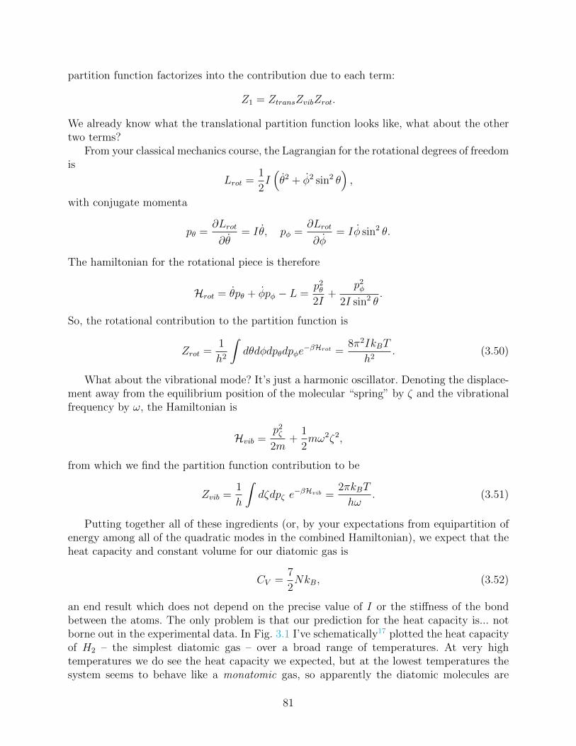
partition function factorizes into the contribution due to each term:

Z1 = ZtransZvibZrot.

We already know what the translational partition function looks like, what about the othertwo terms?

From your classical mechanics course, the Lagrangian for the rotational degrees of freedomis

Lrot =1

2I(θ2 + φ2 sin2 θ

),

with conjugate momenta

pθ =∂Lrot

∂θ= Iθ, pφ =

∂Lrot

∂φ= Iφ sin2 θ.

The hamiltonian for the rotational piece is therefore

Hrot = θpθ + φpφ − L =p2θ

2I+

p2φ

2I sin2 θ.

So, the rotational contribution to the partition function is

Zrot =1

h2

∫dθdφdpθdpφe

−βHrot =8π2IkBT

h2. (3.50)

What about the vibrational mode? It’s just a harmonic oscillator. Denoting the displace-ment away from the equilibrium position of the molecular “spring” by ζ and the vibrationalfrequency by ω, the Hamiltonian is

Hvib =p2ζ

2m+

1

2mω2ζ2,

from which we find the partition function contribution to be

Zvib =1

h

∫dζdpζ e

−βHvib =2πkBT

hω. (3.51)

Putting together all of these ingredients (or, by your expectations from equipartition ofenergy among all of the quadratic modes in the combined Hamiltonian), we expect that theheat capacity and constant volume for our diatomic gas is

CV =7

2NkB, (3.52)

an end result which does not depend on the precise value of I or the stiffness of the bondbetween the atoms. The only problem is that our prediction for the heat capacity is... notborne out in the experimental data. In Fig. 3.1 I’ve schematically17 plotted the heat capacityof H2 – the simplest diatomic gas – over a broad range of temperatures. At very hightemperatures we do see the heat capacity we expected, but at the lowest temperatures thesystem seems to behave like a monatomic gas, so apparently the diatomic molecules are

81

Figure 3.1: (Schematic) heat capacity of hydrogen gas vs logarithmically scaledtemperature. That “NA” is a typo, and should just be N , of course.

neither rotating nor vibrating. Even away from the typical “very low temperatures” weexpect to see quantum effects in – that is, even at room temperature! – there is a largediscrepancy between our prediction and the actual heat capacity, and apparently there arerotations but not vibrations (we’ll see how we picked out that particular mode later).

This behavior was arguably the first time that quantum mechanics revealed itself inexperiments, and scientists at the end of the 19th century were increasingly unsettled.

3.5.2 Black-body radiation18

The classical failure of the calculation of the black-body spectrum (i.e., what light is emittedfrom a source at a particular temperature) and its quantum resolution is a story that I suspectis familiar from previous courses in quantum mechanics. Very briefly, then, we consider ourfirst quantum gas: a gas of photons. In principle we are interested in the emission spectrumof an idealized substance that can absorb photons of any wavelength and reflects none ofthem. In a real atomic system there would be a (potentially) interesting pattern of absorptionand emission lines, but we ignore such details for now and consider our idealized substancewhich, at zero temperature, would appear black (hence the name).

So, we know a photon is characterized by its wavelength λ or its frequency ω = 2πc/λ = kcfor speed of light c and wavevector k, with energy E = ~ω. An important fact about photonsis that they are not conserved : there is no reason that the walls of our black-body substance

17Actual data available from NIST, if you’re interested18“It was an act of desperation. For six years I had struggled with the blackbody theory. I knew the

problem was fundamental and I knew the answer. I had to find a theoretical explanation at any cost, exceptfor the inviolability of the two laws of thermodynamics.” – Max Planck, in a letter to R. W. Wood, 1931

82

couldn’t absorb a photon and then emit two19. Thus, when we calculate quantities in thecanonical ensemble we need to make sure that we sum over possible states with differentnumbers of photons, since they are allowed states. Equivalently, we can imagine that wework in the grand canonical ensemble, but with chemical potential µphoton = 0.

To build up the partition function, let’s first consider photons with a particular frequencyω; N such photons would have energy E = N~ω, and summing over the allowed N gives apartial partition function

Zω = 1 + e−β~ω + e−2β~ω + e−3β~ω + · · · = 1

1− e−β~ω. (3.53)

We assume that the different frequencies are independent, and the total partition functionis a product of independent partition functions, so we can write the logarithm as a sum:

logZ =

∫ ∞0

dωg(ω) logZω,

where g(ω) is the density of states : g(ω)dω counts the number of states in the frequencyrange between ω and ω + dω. We can calculate this by, say, assuming periodic boundaryconditions in a box of linear size L, which then permits wavevectors k = 2πnx, ny, nz,where nx, ny, nz are all integers. Planck suggested that the allowed values of energy mustbe quantized,

HEM =∑k,α

~ck(nα(k) +

1

2

), nα(k) = 0, 1, 2, . . . ,

where α refers to the polarization of the photon. One can use this to compute the associateddensity of states for the photon gas. For now I’ll ignore terms relating to the factor of 1/2above, since we usually only care about (or can detect!) energy differences. Taking intoaccount the fact that photons can come in two polarization states, one eventually gets

g(ω)dω =V ω2

π2c3dω.

Combing these results, we get that

lnZ =

∫ ∞0

dωg(ω) logZω = − V

π2c3

∫ ∞0

dω ω2 ln(1− e−β~ω

). (3.54)

From this we can get, e.g., the energy stored in the photon gas:

E = −∂ lnZ

∂β=

V ~π2c3

∫ ∞0

dωω3

eβ~ω − 1=

V

π2c3

(kBT )4

~3

∫ ∞0

dxx3

ex − 1. (3.55)

That last integral can be explicitly evaluated (with some work), with the end result

E

V=

π2k4B

15~3c3T 4. (3.56)

19Of course, you know this, as you demonstrate the non-conservation of photon number every time youchange the state of a (functional) light switch

83

The free energy F = −kBT lnZ can be calculated; integration by parts (to take care ofthe log inside the integral) gets us to

F = − V π2

45~3c3(kBT )4, (3.57)

from which we can calculate, e.g., the pressure due to electromagnetic radiation as

P = − ∂F

∂V

∣∣∣∣T

=E

3V=

4σ

3cT 4,

where

σ =π2k4

B

60~3c2= 5.67× 10−8 J

sm2K4

is the Stefan constant20

We didn’t really emphasize the way the classical version of the above calculation fails, asI’m sure you’ve seen it before. Briefly, classically we should think that the Hamiltonian forthe EM field can be written in terms of the normal modes characterized by k, so that theenergy looks like a collection of independent harmonic oscillators corresponding to photonsof different wave-number and polarization. Classically, though, there is no limit on the sizeof k, leading to the ultraviolet catastrophe: we assign kBT of equipartitioned energy to eachindependent quadratic mode of H, leading to an infinite amount of energy stored in thehigh-frequency modes. This is... not physical.

By the way, all along we discarded the terms related to the extra 1/2 in HEM . Had wekept those terms around we would have found things like

P = − ∂F

∂V

∣∣∣∣T

= P0 +E

3V,

where P0 is an infinite zero-point pressure. Usually, this infinite zero-point pressure cancelswith some other part of your calculation, but not always! Differences in this quantity P0 leadto Casimir forces between, e.g., conducting plates, which can be experimentally measured.

20the value of which in SI units is particularly easy to remember, since it is “five (point) six seven times(ten to the negative) eight.”

84

Chapter 4

Quantum Statistical Mechanics1

Quantum statistical mechanics should be inherently quantum mechanical, statistical in na-ture, and able to resolve some of the issues with classical statistical mechanics that we en-countered at the end of the last chapter2. When considering blackbody radiation we alreadyintroduced a simplistic version of quantum mechanical effects by forcing the energy levels ofthe photon gas to be quantized, and we assumed that the quantum mechanical microstateswere specified by this quantized energy and governed by a probability distribution relatedto the Boltzmann weights.

Why were we allowed to make such assumptions? What is the traditional resolution ofGibbs’ paradox? Why is Planck’s constant floating around in classical partition functions?In this chapter we formalize a quantum description of statistical mechanics by following thesteps that led us to the classical description (Chapters 3 and 4).

4.1 The classical limit of a quantum partition function

Let’s jump right in and explain why there are factors of 1/h in the classical partition func-tions. Classically, we defined the partition function for a single classical particle as an integralover phase space:

Z1 =1

h3

∫d3qd3pe−βH(p,q),

where the 1/h was required to get the units right (i.e., so that Z is dimensionless), but wherethere was a particular value of h to use: Planck’s constant h = 2π~ ≈ 6.6 × 10−34Js. Whyis there this quantum-mechanical number in our classical formulas? We don’t need to waveour hands: we can derive it.

To keep things simple, let’s consider a single particle in one dimension, so that it’s Hamil-tonian is

H =p2

2m+ V (q),

where p is the momentum operator and q is the position operator.

1Selections from Pathria Chapter 5-8; the majority of Chapter 5, 6.1, 6.2, and at the thermodynamicsof ideal Bose and Fermi gases

2Future editions of these notes will maintain the parallelism.

85

Writing the eigenstates in the energy basis, with |n〉 associated with energy En, thequantum partition function3 is

Z =∑n

e−βEn =∑n

〈n|e−βH |n〉, (4.1)

where the operator

e−βH =∞∑n=0

(−1)n(βH)n

n!.

In general, by the way, we can think of functions of matrices in this way, taking f(M) =∑∞i=0 aiM

i for a matrix M are where the ai define the power series of the function. It isoften, though, easier to write down the matrix in a basis which diagonalizes M . Let’s writethe diagonalized version of the matrix as M ; in the diagonalizing basis any function can bewritten as

f(M) =

f(M11) 0 0 0 · · ·

0 f(M22) 0 0 · · ·... 0 f(M33) 0 · · ·...

.... . . . . . . . .

. (4.2)

One can then transform back into whichever basis you like. This procedure is a natural wayto define the log, as in expressions for the entropy in terms of the density matrix ρ,

S = −kBTr (ρ log ρ) . (4.3)

As usual we are free to insert the identity operator, constructed by summing over anycomplete basis of states. We’ll do this with both the position eigenvectors and the momentumeigenvectors:

1 =

∫dq|q〉〈q|, 1 =

∫dp|p〉〈p|.

We first add two copies of the position-eigenstate identity to the partition function, on eitherside of the e−βH :

Z =∑n

〈n|∫dq|q〉〈q|e−βH

∫dq′|q′〉〈q′|n〉

=

∫dqdq′〈q|e−βH |q′〉

∑n

〈q′|n〉〈n|q〉

=

∫dq〈q|e−βH |q〉, (4.4)

where in the last line we replaced∑

n |n〉〈n| with the identity operator and used 〈q′|q〉 =δ(q′ − q) and integrated over q′. So far the result of this manipulation is to replace a sumover energy eigenstates with an integral over position eigenstates4.

3We’ll see this more explicitly soon, but the form should be familiar enough that you don’t object...4we can do this with any complete basis; as we’ll see shortly we can write the partition function without

referencing a specific basis by Z = Tr(e−βH

)86

Let’s take the classical limit of this partition function, by which we mean that we’lltypically neglect terms that are of order h. We exploit this by trying to factorize e−βH intoa position and a momentum piece, remembering that5

eAeB = exp

(A+ B +

1

2[A, B] + · · · ,

)(4.5)

where we additionally recall the commutation relation [q, p] = i~. Taking the classical limitmeans we neglect the corrections to the naive factorization, writing

e−βH = e−βp2/(2m)e−βV (q) +O(~). (4.6)

To complete the derivation, let’s carefully start transitioning exponentiated operators intoordinary functions:

Z =

∫dq 〈q|e−βp2/(2m)e−βV (q)|q〉

=

∫dq e−βV (q)〈q|e−βp2/(2m)|q〉

=

∫dqdpdp′ e−βV (q)〈q|p〉〈p|e−βp2/(2m)|p′〉〈p′|q〉

=1

2π~

∫dqdp e−βH(p,q), using 〈q|p〉 =

1√2π~

eipq/~. (4.7)

Thus, we see the natural consequence of the underlying quantum mechanical descriptioneven when we take the classical limit and do our best to ignore ~.

4.2 Microstates, observables, and dynamics

4.2.1 Quantum microstates

With that as an appetizer, let’s write down a few definitions6 to get us more properlystarted on quantum statistical mechanics. Classically, we started with microstates for Nparticles that were specified by a point in 6N -dimensional phase space and governed byHamiltonian evolution equations. Quantum mechanically, of course, positions and momentaare not independently observable, so this is a poor choice of microstate. Instead, a quantumsystem is specified by a unit vector in a Hilbert space7, |ψ〉. Given a set of orthonormal basisvectors |n〉 we can write the microstate as

|ψ〉 =∑n

〈n|ψ〉|n〉, (4.8)

5Baker-Campbell-Hausdorff formula6I will, naturally, assume you already know quantum mechanics, so here we’re just dotting some i’s7A generalization of Euclidean space: a Hilbert space H is a vector space equipped with an inner product

whose induced distance function makes H a complete metric space

87

where the 〈n|ψ〉 are complex numbers, where we keep in mind that 〈ψ|n〉 = 〈n|ψ〉∗, thecomplex conjugate.

As a unit vector, ψ is normalized so that

〈ψ|ψ〉 =∑n

〈ψ|n〉〈n|ψ〉 = 1, (4.9)

4.2.2 Quantum observables

Classically, in Chapter 3 we introduced observable functions of phase space, A (p, q). Quan-tum mechanically, observables get promoted to operators by substituting the position andmomentum operators for the position and momentum variables in the classical expressions8,e.g. A, as we saw in the first part of this chapter. Just as classically we had the Poissonbracket, pi, qj = δij, here we have the commutation relation [pa, qb] = paqb − qbpa = ~

iδab,

and we can write our observables, if we wish, as functions of the position and momentum:A(p, q).

Unlike in classical mechanics, in addition to the (classical) probabilistic nature of ourensembles, quantum mechanically our observables themselves are matrices that don’t havedefinite values; i.e., they are not uniquely determined for a particular microstate. This ad-ditional randomness means the observables are themselves random variables, so we mustcontent ourselves with their expectation values, defined as

〈A〉 = 〈ψ|A|ψ〉 =∑m,n

〈ψ|m〉〈m|A|n〉〈n|ψ〉. (4.10)

Since we demand real observables, the operators A must be Hermitian9: A† = A.

4.2.3 Time evolution of states

Classically we got a lot of mileage out of the hamiltonian evolution of the phase spacecoordinates. The quantum mechanical state vector has a time evolution given by

i~∂

∂t|ψ(t)〉 = H|ψ(t)〉. (4.11)

It is often convenient to work in the basis which diagonalizes the Hamiltonian (i.e., thebasis formed by the energy eigenstates), satisfying H|n〉 = En|n〉 where En are the “eigen-energies.” In such a basis, exploiting the orthonormality of the basis 〈m|n〉 = δmn lets uswrite the time evolution of the state as

i~d

dt〈n|ψ(t)〉 = En〈n|ψ(t)〉 ⇒ 〈n|ψ(t)〉 = exp

(−iEnt

~

)〈n|ψ(0)〉. (4.12)

Probably the first basis we learn about is composed of the spatial coordinates, |qi〉, forwhich

ψ (q1, q2, . . . , qN) ≡ 〈qi|ψ〉is the wavefunction.

8after, of course, properly symmetrizing products, for instance pq → (pq + qp)/29which is why we worried about symmetrizing position and momentum when going from classical to

quantum operators.

88

4.3 The density matrix and macroscopic observables

Classically, macrostates are specified by just a few thermodynamic coordinates, and westudied ensembles of large numbers of microstates µs, which were equipped with a probabilityps ≡ p(µs), which corresponded to a given macrostate. We often don’t have precise knowledgeof the microstate (i.e., the system is not a pure state); more generally we expect it to be amixed state, existing as an incoherent mixtures of being in a variety of quantum states10.

We similarly start out with a mixed state, an incoherent mixture of states |ψα〉 withprobabilities pα. The ensemble average of the expectation value of an observable in such amixed state is

¯〈A〉 =∑α

pα〈ψα|A|ψα〉 =∑α,m,n

pα〈ψα|m〉〈n|ψα〉〈m|A|n〉

=∑m,n

〈m|A|n〉〈n|ρ|m〉 = Tr (ρA) , (4.13)

where we have introduced the density matrix ρ, which in a given basis is

ρ =∑α

pα|ψα〉〈ψα|, (4.14)

and where the trace of an operator is the sum over the diagonal elements, Tr (M) =∑α〈Φα|M |Φα〉, which is independent of which basis Φα you use.

4.3.1 Basic properties of the density matrix

1. Sufficiency: All measurements in quantum mechanics involve expectation values ofoperators. Thus, the density matrix contains sufficient information for anything wemight want to do.

2. Pure states: The density matrix corresponds to a pure state, a state with a definitewavefunction ψ, if and only if ρ = |ψ〉〈ψ|, hence if and only if ρ2 = ρ.

3. Positive definite: The eigenvalues of ρ are all positive, since for any state

〈φ|ρ|φ〉 =∑n

pn〈φ|ψn〉〈ψn|φ〉 =∑n

pn|〈φ|ψn〉|2 ≥ 0.

4. Normalization: Since the ψα are themselves normalized, we have

Tr (ρ) =∑n

pn〈ψn|ψn〉 =∑n

pn = 1.

5. Hermiticity: By inspection, the density matrix is Hermitian, with ρ† = ρ.

10Not in a superposition, of states, by the way. A quick example: take a spin in the up-down basis. Thesuperposition state 2−1/2(|↑〉+ |↓〉) is a diagonally polarized state. An unpolarized spin is a mixture of halfup and half down, described by a density matrix 1

2 (|↑〉〈↑|+ |↓〉〈↓|). The latter is what we mean.

89

Time evolution of the density matrix

Classically we had Liouville’s theorem for the evolution of the density, dρdt

= ∂ρ∂t− H, ρ;

what do we have here? Again working in the energy eigenbasis, we can write

i~∂tρ =∑n

pni~∂t (|ψn〉〈ψn|)

=∑n

pn [H|ψn〉〈ψn| − |ψn〉〈ψn|H]

= Hρ− ρH = [H, ρ] . (4.15)

4.4 Quantum ensembles

With this structure, we can follow the same logic that we did in the classical case: we defineequilibrium by having none of the averages of the observables vary with time, which can besatisfied if we choose an equilibrium density matrix so that ∂tρ = 0. Just as when we weredealing with Poisson brackets, we accomplish this by having the density matrix be a functionof the Hamiltonian itself, along with any conserved quantities A, ρ(H,A1, . . .), that satisfy[H,Ai] = 0.

4.4.1 Quantum microcanonical ensemble

We define the microcanonical ensemble, specified by (E,x, N), but enforcing a fixed valuefor the ensemble average energy. We choose our density matrix

ρ(E) =δ(H − E)

Ω(E),

where in the energy eigen-basis we can write this as

〈m|ρ|n〉 =∑α

pα〈m|ψα〉〈ψα|n〉 =

Ω−1 if En = E, and m = n0 otherwise

(4.16)

The first of those two conditions we recognize as the equivalent of the assumption of equal apriori probabilities The second, quantum mechanical condition is the assumption of randoma priori phases, in which we don’t get contributions from off-diagonal terms (even if theyhave degenerate and correct energies) because we assume the mixed state is in an incoherentsuperposition of the basis states. Finally, note that from the normalization condition on thedensity matrix, Ω(E) is again just counting the number of (eigen)states of H with the correctenergy E.

90

4.4.2 Quantum canonical ensemble

You know what’s coming: Now we’re fixing temperature T = β−1 by putting our quantumsystem in contact with a reservoir. Considering the above two assumptions for the combinedsystem, we find that the density matrix for the system of interest is

ρ(β) =e−βH

Z(β), (4.17)

where the normalization condition on the density matrix leads to the quantum canonicalpartition function for N particles,

ZN(β) = Tr(e−βH

)=∑n

e−βEn . (4.18)

As one would expect from the above formulas, the expectation value of a physical observableis given by

〈A〉 = Tr(ρA)

=1

Z(β)Tr(Ae−βH

)=

Tr(Ae−βH

)Tr(e−βH

) (4.19)

4.4.3 Quantum grand canonical ensemble

For completeness – and because we’ll see it again soon – in the grand canonical ensemble weno longer fix the number of particles11. The density matrix is

ρ(β, µ) =e−βH+βµN

Q, (4.20)

where the grand canonical partition function is

Q(β, µ) = Tr(e−βH+βµN

)=

∞∑N=0

eβµNZN(β). (4.21)

4.4.4 Example: Free particle in a box

Suppose we care about the quantum canonical ensemble version of a single particle in a boxof volume V . Working in the coordinate basis, the Hamiltonian is

H =p2

2m= − ~2

2m∇2, (4.22)

which has energy eigenstates |k〉 specified by

〈r|k〉 =e−k·r√V, Ek =

~2k2

2m. (4.23)

11Microstates with an indefinite number of particles span a Fock space, which is a set of Hilbert spacesassociated with zero or more quantum particles

91

What are the allowed k? Assuming for simplicity periodic boundary conditions for a cubeof side length L, we can have k = 2π

L(lx, ly, lz), where the lα are integers. So, the space of

microstates is enormously larger than in the classical case: rather than 6 degrees of freedomper particle, one can have countably infinite numbers of states per particle. In the limitL→∞ the partition function becomes

Z =∑k

e−β~2k22m = V

∫d3k

(2π)3e−

β~2k22m

=V

(2π)3

(√2πmkBT

~

)3

=V

λ3, (4.24)

for λ = h/√

2πmkBT , which indeed coincides with our classical calculation when we use theright (adjusted) phase space measure.

What about the elements of the density matrix itself? We can compute

〈r′|ρ|r〉 =∑k

〈r′|k〉e−βEk

Z〈k|r〉

=λ3

V

∫V

d3k

(2π)3

e−ik·(r−r′)

Ve−

β~2k22m

=1

Vexp

(−π (r − r′)2

λ2

). (4.25)

What does this mean? The diagonal elements are all 〈r|ρ|r〉 = V −1, the common expectationthat the probability for finding the particle is uniform throughout the box. The off-diagonalterms are a quantum-mechanical effect, measuring the “spontaneous transition” betweencoordinates r and r′, giving a measure of the “intensity” of the wave packet some distancefrom the center of the packet. Said another way, the spatial extent of the packet is a measureof the uncertainty involved in locating the particle position. This quantum mechanical effectvanishes in the β → 0 limit, as the density matrix elements approach delta functions.

Finally, we can compute the expectation value of the Hamiltonian itself, 〈H〉 = Tr(Hρ)

.

I’ll spare you the straightforward integrals in class – we’ve already calculated the partition

function Z = Tr(e−βH

), so the result is the last line of:

〈H〉 = Tr(Hρ)

=Tr(He−βH

)Tr(e−βH

)= − ∂

∂βln Tr

(e−βH

)=

3

2kBT. (4.26)

Utterly expected.

92

4.4.5 Example: An electron in a magnetic field

Suppose we care about the quantum canonical ensemble version of a single electron in amagnetic field. The election has spin ~σ/2 and a magnetic moment µB = e~

2mc(nothing to do

with the chemical potential; it’s just standard notation to use µ here, too), where σ is thePauli spin operator.

When we apply a magnetic field, B, the electron can have either spin up or spin down.If we take the applied field to be along z, the configurational part of the Hamiltonian is

H = −µBσ ·B. (4.27)

Life is easier when we work in the basis in which the Hamiltonian is diagonal, i.e.,

H = −µBBσz, (4.28)

where

σx =

(0 11 0

), σy =

(0 −ii 0

), σz =

(1 00 −1

). (4.29)

From this it is straightforward to calculate the density matrix:

ρ =e−βH

Tr(e−βH

)=

1

eβµBB + e−βµBB

(eβµBB 0

0 e−βµBB

), (4.30)

from which we can calculate, e.g., the expectation value for σz:

〈σz〉 = Tr (ρσz) =eβµBB − e−βµBB

eβµBB + e−βµBB= tanh (βµBB) , (4.31)

an expression I’m quite sure you’ve seen in other classes.

4.5 Quantum indistinguishability

4.5.1 Two identical particles

Suppose we were to write down a simple two-particle Hamiltonian, for two particles of equalmass and with an interaction potential that depended only on the relative separation:

H(1, 2) =p2

1

2m+p2

2

2m+ V (|r1 − r2|).

Clearly this Hamiltonian is symmetric under the exchange of particle label,H(1, 2) = H(2, 1).Classically, our labeling of particles is meaningful (think, for instance, of running a computersimulation of a system of classical particles, in which there are Monte Carlo exchanges ofparticle identity that can take place), but for identical quantum mechanical particles theselabels are arbitrary and convey no physical meaning.

93

For instance, the probability of finding two identical particles at positions r1 and r2 isgiven by |ψ(r1, r2)|2 = |ψ(r2, r1)|2. As long as the wavefunction is single-valued this leads totwo distinct possibilities12:

ψ(r1, r2) =

ψ(r2, r1) for bosons−ψ(r2, r1) for fermions

. (4.32)

4.5.2 N identical particles

Starting with a wavefunction for N particles, ψ(r1, . . . , rN), we generalize the above byintroducing a permutation operator P , of which there are N ! possible permutation operatorswe might consider for our set of particles. We’ll adopt the notation

Pψ(r1, . . . , rN) =

ψ(r1, . . . , rN) for bosons

(−1)Pψ(r1, . . . , rN) for fermions(4.33)

to represent the two classes of Hilbert spaces we might find ourselves in. Here we take (−1)P

to represent the parity13 of the permutation under question: if P can be represented by aneven number of pairwise particle exchanges then (−1)P = 1, and if it can be represented byan odd number of pairwise exchanges the (−1)P = −1.

Note that the Hamiltonian for the particles, H, must be symmetric: PH = H, but theHamiltonian can admit eigenstates of different symmetries under the action of the permuta-tion operator. The same Hamiltonian will thus allow eigenstates of either total symmetry ortotal anti-symmetry: the statistics one want to study must be specified independently of theHamiltonian, and so one studies only a subspace (either the fermionic subspace, in whicheigenstates are anti-symmetric, or the bosonic subspace, in which eigenstates are symmetric)of the total Hilbert space. Let’s see a convenient way of representing these subspaces.

4.5.3 Product states for non-interacting particles

We consider an N -particle Hamiltonian which is just a collection of single-particle Hamilto-nians14 for free particles in a box of volume V :

H =N∑α=1

p2i

2m=

N∑α=1

− ~2

2m∇2α. (4.34)

Each of the single-particle Hamiltonians can be diagonalized by writing it in the energybasis, |kα〉 with energy ~2k2

α/(2m), and we will build our N -particle wavefunction out ofthese one-particle eigen-pieces.

12Because the square of the exchange operator must be the identity matrix. For single-valued functionsthis restriction means that there can only be a complex phase shift under the operation of a single applicationof the exchange operator, so the square being the identity means the phase shift can only be 0 (bosons) orπ (fermions). You may have heard, though, of anyons! These have multi-valued wavefunctions, and in twodimensions one can find other allowed statistics without this constraint on the value of the phase shift.

13In Pathria’s notation, what I will eventually write as ηP is denoted δP = (±1)[P ]

14“Hamiltonia”?

94

We define a product state as

|k1, . . . ,kN〉× ≡ |k1〉|k2〉 · · · |kN〉, (4.35)

where in the coordinate representation the product state is

〈r1, . . . , rN |k1, . . . ,kN〉× =1

V N/2exp

(−i∑α

kα · rα

), (4.36)

and of course

H|k1, . . . ,kN〉× =

(∑α

~2k2α

2m

)|k1, . . . ,kN〉×. (4.37)

These product states are very convenient to work with, but they are too general! That is,they are appropriate for distinguishable particles, but for indistinguishable particles they donot have the correct symmetry for either bosons or fermions.

To show how we can compactly write either fermionic or bosonic states, let’s start bydefining a symbol

η =

1 for bosons−1 for fermions

, (4.38)

and we will write things like |k〉+ and |k〉− for bosonic and fermionic states, respectively.

Fermionic eigenstates

We build the set of possible fermionic states by summing over all possible permutations ofthe product state, but including the appropriate anti-symmetrizing factor:

|k1, . . . ,kN〉− =1√N−

∑P

(−1)PP |k1, . . . ,kN〉×, (4.39)

where N− = N ! is a factor that ensures proper normalization of our fermionic eigenstate.Because of the anti-symmetrization, if there are any value kα appears more than once thewhole eigenstate vanishes, and so anti-symmetrization is only possible if there are N distinctkα. This is why we know there are as many distinct terms in the sum as there are particles,and thus why N− = N !. For example, a three-particle anti-symmetrized state is15

|123〉− =|123〉× + |231〉× + |312〉× − |213〉× − |321〉× − |132〉×√

6(4.40)

Bosonic eigenstates

Formally, we write the bosonic states similarly, as sum of possible permutations of the productstate with a factor of (+1)P = 1 accounting for the parity of each permutation:

|k1, . . . ,kN〉+ =1√N+

∑P

(+1)PP |k1, . . . ,kN〉×. (4.41)

15for convenience, let k1 = 1, etc.

95

Bosons, though, are allowed to have states in which the same kα appears multiple times, socomputing the normalization factor is slightly more complicated. To see this, consider thebosonic state |121〉+ (i.e., a state in which there are two identical k and one unlike k. Wesee that

|121〉+ =1√N+

(|112〉× + |121〉× + |211〉× + |112〉× + |121〉× + |211〉×)

=2√N+

(|112〉× + |121〉× + |211〉×) , (4.42)

so for proper normalization of |121〉+ we need N+ = 12. The combinatorial generalization isthat if each k is repeated nk times in the N -particle bosonic state, then N+ = N !

∏k nk!.

We can see this by requiring

1 = +〈k|k〉+ =1

N+

∑P,P ′

× 〈P ′k|Pk〉×

=N !

N+

∑P

× 〈k|Pk〉×, (4.43)

but the 〈k|Pk〉 vanish by orthogonality unless the permuted set of wavevectors matchesthe original, which happens nk! times for each repeated k. Thus,

1 =N !∏

k nk!

N+

⇒ N+ = N !∏k

nk!. (4.44)

Compact notation

Actually, though, since for a fermionic state nk can only be zero or one (again, the antisym-metrization gets rid of any states with multiply repeated k), we can combine the bosonicand fermionic notation above into:

|k1, . . . ,kN〉η =1√Nη

∑P

ηPP |k1, . . . ,kN〉×. (4.45)

For both bosons and fermions Nη = N !∏

k nk!, and note that the states end up beinguniquely specified by the set of occupation numbers, nk, with the constraint∑

k

nk = N. (4.46)

4.6 The canonical ensemble density matrix for non-

interacting identical particles

We first write down the canonical density matrix for non-interacting sets of identical parti-cles (and from it obtain the canonical partition function). This section is a bit of a technical

96

calculation; at the end we will understand where the 1/N ! in the classical partition func-tion comes from, and we will see how the quantum statistics of non-interacting identicalparticles are approximately equivalent to introducing either attractive or repulsive classicalinteractions which are felt over distances comparable to the thermal de Broglie wavelength.

In the position basis this is 〈r′|ρN |r〉η, where we know ρN will be diagonal in theenergy basis:

〈r′1, . . . , r′N |ρN |r1, . . . , rN〉η =∑

krestricted

[1

Nη

∑P,P ′

ηPηP′〈r′|P ′ k〉ρ(k)〈P k|r〉

].

(4.47)The density matrix is (c.f. Eq. 4.17)

ρN(k) =exp

(−β∑N

α=1~2k2α2m

)ZN

, (4.48)

and the “restricted” sum above makes sure that every unique indistinguishable particle stateappears exactly once (correctly accounting for either bosonic or fermionic statistics). Thatrestriction is, in fact, a bit cumbersome, so it is more convenient to sum over all k andthen correct for any over-counting. Since the states are specified by the occupation numbers,and since (again) for fermions the ηPηP

′cancels all contributions from terms with nk > 1,

we can do this via ∑krestricted

=∑k

∏k nk!

N !(4.49)

Making this change (combined with the factor of 1/Nη = 1/(N !∏

k nk!)), gives

〈r′|ρN |r〉η =∑k

1

(N !)2

∑P,P ′

ηPηP′

ZNe

(−β∑Nα=1

~2k2α2m

)〈r′|P ′ k〉〈P k|r〉. (4.50)

We reorder the sums and replace the sum over k with an integral to get

〈r′|ρN |r〉η =1

(N !)2ZN

∑P,P ′

ηPηP′∫ ( N∏

α=1

V d3kα(2π)3

)e

(−β ~2k2α

2m

)e−i

∑Nα (kPα·rα−kP ′α·r′α)

V N.

(4.51)Perhaps you feel that we have made things worse rather than better; fortunately, we are

undeterred. Let’s introduce a new label γ = Pα, α = P−1γ to keep track of permutations.We’ll make use of the fact that for functions / operators / variables f and g we can sum overindices

∑α f(Pα)g(α) =

∑γ f(γ)g(P−1γ); this allows us to focus on a particular wavevector:

〈r′|ρN |r〉η =1

(N !)2ZN

∑P,P ′

ηPηP′N∏α=1

∫d3kα(2π)3

e−ikα·

(rP−1α−r

′(P ′)−1α

)−β ~2k2α

2m . (4.52)

The Gaussian integrals in this expression give∫d3kα(2π)3

e−ikα·

(rP−1α−r

′(P ′)−1α

)−β ~2k2α

2m =1

λ3exp

(− π

λ2

(rP−1α − r′(P ′)−1α

)2). (4.53)

97

Using this result and setting µ = P−1α we get

〈r′|ρN |r〉η =1

ZNλ3N(N !)2

∑P,P ′

ηPηP′exp

(− π

λ2

N∑µ=1

(rµ − r′(P ′)−1Pµ

)2). (4.54)

The last step is to do one of the two sums over the permutations. We define Q = (P ′)−1P ,and since ηP = ηP

−1we can write ηPηP

′= η(P ′)−1P = ηQ. With this, and summing over one

set of N ! permutations, we arrive at

〈r′|ρN |r〉η =1

ZNλ3NN !

∑Q

ηQ exp

(− π

λ2

N∑µ=1

(rµ − r′Qµ

)2

). (4.55)

We can finally get the canonical partition function by enforcing the normalization of thedensity matrix:

Tr (ρ) = 1 ⇒∫ N∏

α=1

d3rα〈r|ρN |r〉η = 1 (4.56)

⇒ ZN =1

λ3NN !

∫ N∏α=1

d3rα∑Q

ηQ exp

(− π

λ2

N∑µ=1

(rµ − rQµ)2

). (4.57)

We see that the quantum mechanical partition function has within it a sum over the N !permutations of identical particles, the classical result,

ZN =1

N !

(V

λ3

)N,

corresponds to the term in which there are no exchanges, that is, where Q is the identity.We see that there are lots of other terms involving products of terms like

exp(− π

λ2(r1 − r2)2

),

but as T →∞, λ→ 0 and these quantum corrections vanish.

4.6.1 Statistical interparticle potential

Before we try to evaluate Eq. 4.57, let’s pause to think about perturbations away from theinfinite temperature limit. Clearly the lowest order correction from the classical canonicalpartition function involves permutations which just exchange two particles. So, let’s considerthe simplest possible (non-trivial) case, where N = 2 and

∑Q is a sum over the identity and

either a symmetric or antisymmetric exchange of particles. The partition function is

Z2 =1

2!

(V

λ3

)2 [1 +

η

23/2

λ3

V

], (4.58)

98

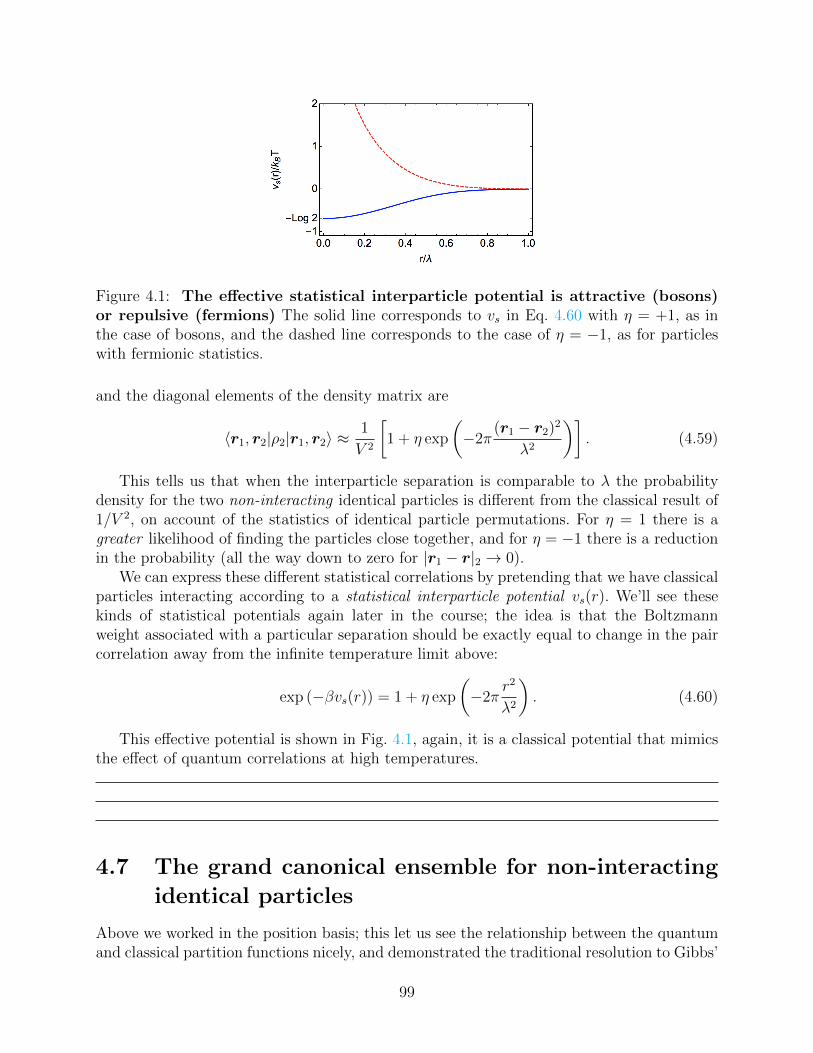
Figure 4.1: The effective statistical interparticle potential is attractive (bosons)or repulsive (fermions) The solid line corresponds to vs in Eq. 4.60 with η = +1, as inthe case of bosons, and the dashed line corresponds to the case of η = −1, as for particleswith fermionic statistics.

and the diagonal elements of the density matrix are

〈r1, r2|ρ2|r1, r2〉 ≈1

V 2

[1 + η exp

(−2π

(r1 − r2)2

λ2

)]. (4.59)

This tells us that when the interparticle separation is comparable to λ the probabilitydensity for the two non-interacting identical particles is different from the classical result of1/V 2, on account of the statistics of identical particle permutations. For η = 1 there is agreater likelihood of finding the particles close together, and for η = −1 there is a reductionin the probability (all the way down to zero for |r1 − r|2 → 0).

We can express these different statistical correlations by pretending that we have classicalparticles interacting according to a statistical interparticle potential vs(r). We’ll see thesekinds of statistical potentials again later in the course; the idea is that the Boltzmannweight associated with a particular separation should be exactly equal to change in the paircorrelation away from the infinite temperature limit above:

exp (−βvs(r)) = 1 + η exp

(−2π

r2

λ2

). (4.60)

This effective potential is shown in Fig. 4.1, again, it is a classical potential that mimicsthe effect of quantum correlations at high temperatures.

4.7 The grand canonical ensemble for non-interacting

identical particles

Above we worked in the position basis; this let us see the relationship between the quantumand classical partition functions nicely, and demonstrated the traditional resolution to Gibbs’

99

paradox for identical particles16. But explicitly calculating the sum over allowed permutationsin Eq. 4.57 for either Bosonic or Fermionic states is... daunting, to say the least. We can firstmake our life a little bit easier by working with the canonical partition function in the basisfor which the Hamiltonian is diagonal. Here

ZN = Tr(e−βHN

)=

∑krestricted

η 〈k|e−β∑Nα=1 Ekα |k〉η. (4.61)

We’ve switched from the particular single-particle Hamiltonian with only kinetic energy inthe last section to arbitrary single-particle Hamiltonians that have some set of energy levelscharacterized by energies Ekα (so, these could be free particles in a box, or quantum harmonicoscillators, etc.). We still have this restriction on the k, which we work around as follows.

We recall that the allowed states can be specified by the occupation numbers, nk, foreach k:

ZN =∑

krestricted

e−β∑Nα=1 Ekα

=∑

nkrestricted

exp

(−β∑k

Ekαnk

). (4.62)

Furthermore, we have gone from sums over symmetry-restricted sets of k to restricted sumsover the occupation numbers:∑

k

nk = N, and nk =

0 or 1 fermions0, 1, 2, . . . bosons

(4.63)

Performing this restricted sum over occupations numbers is still difficult, so we move tothe grand canonical ensemble:

Qη =∞∑N=0

zNZN =∞∑N=0

eβµN∑

nkrestricted

exp

(−β∑k

Ekαnk

)(4.64)

=∑N=0

∑nkrestricted

∏k

exp [−β (Ek − µ)nk]

, (4.65)

where the subscript η reminds us that the restriction on the sum implicitly depends on thequantum statistics in question. At last we see the utility of moving to the grand canonicalensemble: the double summation above – first over a restricted set of occupation numbersat fixed N , and then over all N – is equivalent to simply summing over all values of thedifferent occupation numbers independently for each k.

We now haveQη =

∑nkη

∏k

exp [−β (Ek − µ)nk] , (4.66)

16i.e., now we have recovered both the factors of h and N ! we introduced in an ad-hoc way earlier

100

where nkη reminds us that the sum over occupation numbers is either∑1

nk=0 for fermionsor∑∞

nk=0 for bosons. We can evaluate the sums over the occupation numbers independentlyfor each k above; explicitly, we can write

Qη =∑

nk1,nk2

,...

[(ze−βEk0

)n0(ze−βEk1

)n1 · · ·]

=

[∑n0

(ze−βEk1

)n0

][∑n1

(ze−βEk1

)n1

]· · · (4.67)

for fermions this just gives us two terms per k, and for bosons we get a simple geometricseries as long as that series converges :

Q− =∏k

[1 + exp (βµ− βEk)] , (4.68)

Q+ =∏k

[1− exp (βµ− βEk)]−1 , with Ek − µ > 0 ∀k. (4.69)

Thermodynamically we usually want to take derivatives of the log of the above expressions,so we combine them compactly as

logQη = −η∑k

ln [1− η exp (βµ− βEk)] . (4.70)

From this we can calculate the usual suspects. For instance, we typically want to know howmany particles we actually have for a given value of the chemical potential. Recall thatclassically we know that the unconditional probability of finding N particles in the systemis

p(N) =eβµNZNQ

,

and here we have products of independent single-particle states. So, we very similarly canwrite down the probability of having a particular set of occupation numbers:

pη (nk) =1

Qη

∏k

exp [−β (Ek − µ)nk] . (4.71)

From this we can pull down the average occupation number of a particular state with energyEk, as

〈nk〉η = − ∂ lnQη∂ (βEk)

=1

exp (βEk − βµ)− η. (4.72)

From this the average number of particles at fixed µ is

Nη =∑k

〈nk〉η =∑k

1

z−1eβEk − η(4.73)

and the average energy is

Eη =∑k

Ek 〈nk〉η =∑k

Ek

z−1eβEk − η(4.74)

101

4.8 Ideal quantum gases

In the rest of the chapter we will specialize the above results to the case of ideal quantumgases, looking at some of the thermodynamic properties of both ideal Fermi and Bose gases.Before we dive into the details, it is worth saying a few words about what we will get out ofthis exploration. Classically, the ideal gas is a prime example we keep coming back to, and itprovides a starting point for understanding real gases, but it’s a pretty poor starting pointfor just about any other system (solids, dense liquids, etc).

The quantum ideal gas turns out to be much more applicable. Non-interacting systemsof bosons are surprisingly accurate descriptors of photons (as one could anticipate from ourearlier discussion of blackbody radiation), phonons (and giving insight into the heat capacityof solids), as well as actual dilute gases of bosons. You might be surprised to learn that thenon-interacting approximation for fermions also apply to a range of systems! For instance,electrons are charged, and the interactions between electrons in an atom, or a material, alwaysmake a large contribution to the energy. Nevertheless, a gas of non-interacting fermions isa powerful description of atoms, metals, insulators, neutron stars, etc. Not a free gas offermions: the trick is that collections of interacting fermions often act like collections ofnon-interacting fermions sitting in a modified external potential17.

To specialize to (non-relativistic) idealized gases, we make the specific choice for theenergies Ek = ~2k2/(2m), where the energy levels have a degeneracy g associated with thespin s of the particles, g = 2s + 1, and where

∑k → V

∫d3k/(2π)3. The evaluation of the

grand canonical partition function gives us the following results for the pressure, numberdensity, and energy density:

βPη =lnQηV

= −ηg∫

d3k

(2π)3ln[1− ηze−β

~2k22m

], (4.75)

nη =Nη

V= g

∫d3k

(2π)3

(z−1eβ

~2k22m − η

)−1

, (4.76)

εη =EηV

= g

∫d3k

(2π)3

~2k2

2m

(z−1eβ

~2k22m − η

)−1

. (4.77)

With a little more work we can manipulate these expressions into a more manageable form.For what’s to come, let’s define the following families of functions that are closely related towhat are typically called Bose-Einstein and Fermi-Dirac integrals:

f ηm(z) ≡ 1

(m− 1)!

∫ ∞0

dxxm−1

z−1ex − η; (4.78)

these functions are closely related to the polylogarithm18. We’re going to want m to takenon-integer values, so recall that we really mean the gamma function above19.

17See Sethna’s “Statistical Mechanics: Entropy, Order Parameters, and Complexity” for a slightly ex-panded discussion of this point. If anyone want to talk about Landau-Fermi liquid theory that could be acool presentation topic!

18The polylogarithm is defined by Lim(z) =∑∞α=1

zα

αm (plus the analytic continuation in the complexplane). Note that fηm(z) = ηLim(ηz).

19Γ(m) = (m− 1)!, with, e.g., (1/2)! =√π/2, etc.

102

With this definition in hand, let’s make the obvious change of variables in the abovethermodynamic expressions to x = β~2k2/(2m), i.e., k = 2

√π

λx1/2. To show an explicit

calculation, we substitute this into the equation for the pressure, integrate by parts, and endup with a very compact expression:

βPη = = −ηg∫

d3k

(2π)3ln[1− ηze−β

~2k22m

]= − 2ηg

λ3√π

∫ ∞0

dx x1/2 ln(1− ηze−x

)=

4g

3λ3√π

∫dx

x3/2

z−1ex − η=

g

λ3f η5/2(z). (4.79)

Similarly, we can now compactly write the three thermodynamic expressions above as

βPη =g

λ3f η5/2(z)

nη =g

λ3f η3/2(z) (4.80)

εη =3

2Pη.

Beautiful. These equations are a complete description of the thermodynamics of ideal Fermiand Bose gases, but of course we usually want equations of state where P is a function ofthe density and the temperature; here we have implicit relations between both P and n withthe fugacity. We would like, therefore, to invert the middle equation20 and know z in termsof the density, so we need to understand the behavior of the f ηm(z).

4.8.1 High-temperature and low-density limit of ideal quantumgases

The simplest limit to consider – in which we can continue to treat Fermions and Bosonssimultaneously – is the high-T , small-n limit in which z is small. For small z one can performa systematic expansion of the integral defining f ηm(z) (and you should step through thisexercise!), but for brevity we will use the fact noted in footnote 18, by which we can write

f ηm(z) = ηLim(ηz) =∞∑α=1

ηα+1 zα

αm= z + η

z2

2m+z3

3m+ · · · (4.81)

We see that for z 1, f ηm(z) 1 and hence nη and Pη are all small, too – the calculationis nicely self-consistent. We are now in a position to find a relationship for z in terms of n(rather than the current n in terms of z in Eq. 4.80): we rearrange Eq. 4.80 as

z = d− η z2

23/2− z3

33/2− · · · , (4.82)

20you might say that in picking a name for a complicated integral we’ve just parameterized our ignorance,without gaining any understanding yet

103

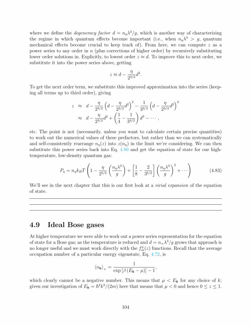
where we define the degeneracy factor d = nηλ3/g, which is another way of characterizing

the regime in which quantum effects become important (i.e., when nηλ3 > g, quantum

mechanical effects become crucial to keep track of). From here, we can compute z as apower series to any order in n (plus corrections of higher order) by recursively substitutinglower order solutions in. Explicitly, to lowest order z ≈ d. To improve this to next order, wesubstitute it into the power series above, getting

z ≈ d− η

23/2d2.

To get the next order term, we substitute this improved approximation into the series (keep-ing all terms up to third order), giving

z ≈ d− η

23/2

(d− η

23/2d2)2

− 1

33/2

(d− η

23/2d2)3

≈ d− η

23/2d2 +

(1

4− 1

33/2

)d3 − · · · ,

etc. The point is not (necessarily, unless you want to calculate certain precise quantities)to work out the numerical values of these prefactors, but rather than we can systematicallyand self-consistently rearrange nη(z) into z(nη) in the limit we’re considering. We can thensubstitute this power series back into Eq. 4.80 and get the equation of state for our high-temperature, low-density quantum gas:

Pη = nηkBT

(1− η

25/2

(nηλ

3

g

)+

[1

8− 2

35/2

](nηλ

3

g

)2

+ · · ·

)(4.83)

We’ll see in the next chapter that this is our first look at a virial expansion of the equationof state.

4.9 Ideal Bose gases

At higher temperature we were able to work out a power series representation for the equationof state for a Bose gas; as the temperature is reduced and d = n+λ

3/g grows that approach isno longer useful and we must work directly with the f ηm(z) functions. Recall that the averageoccupation number of a particular energy eigenstate, Eq. 4.72, is

〈nk〉+ =1

exp [β (Ek − µ)]− 1,

which clearly cannot be a negative number. This means that µ < Ek for any choice of k;given our investigation of Ek = ~2k2/(2m) here that means that µ < 0 and hence 0 ≤ z ≤ 1.

104

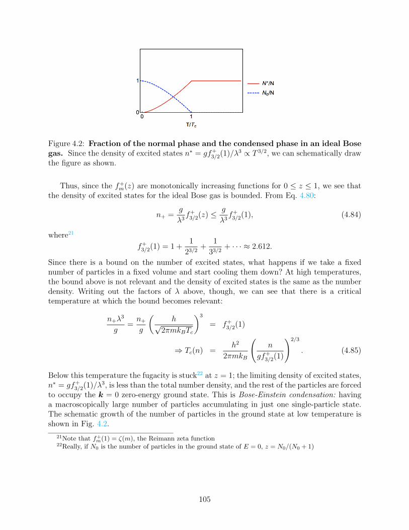
Figure 4.2: Fraction of the normal phase and the condensed phase in an ideal Bosegas. Since the density of excited states n∗ = gf+

3/2(1)/λ3 ∝ T 3/2, we can schematically drawthe figure as shown.

Thus, since the f+m(z) are monotonically increasing functions for 0 ≤ z ≤ 1, we see that

the density of excited states for the ideal Bose gas is bounded. From Eq. 4.80:

n+ =g

λ3f+

3/2(z) ≤ g

λ3f+

3/2(1), (4.84)

where21

f+3/2(1) = 1 +

1

23/2+

1

33/2+ · · · ≈ 2.612.

Since there is a bound on the number of excited states, what happens if we take a fixednumber of particles in a fixed volume and start cooling them down? At high temperatures,the bound above is not relevant and the density of excited states is the same as the numberdensity. Writing out the factors of λ above, though, we can see that there is a criticaltemperature at which the bound becomes relevant:

n+λ3

g=n+

g

(h√

2πmkBTc

)3

= f+3/2(1)

⇒ Tc(n) =h2

2πmkB

(n

gf+3/2(1)

)2/3

. (4.85)

Below this temperature the fugacity is stuck22 at z = 1; the limiting density of excited states,n∗ = gf+

3/2(1)/λ3, is less than the total number density, and the rest of the particles are forcedto occupy the k = 0 zero-energy ground state. This is Bose-Einstein condensation: havinga macroscopically large number of particles accumulating in just one single-particle state.The schematic growth of the number of particles in the ground state at low temperature isshown in Fig. 4.2.

21Note that f+m(1) = ζ(m), the Reimann zeta function22Really, if N0 is the number of particles in the ground state of E = 0, z = N0/(N0 + 1)

105

4.9.1 Pressure

We now turn to the pressure of the low-temperature phase of this system. For T < Tc wehave z = 1, and our thermodynamic expression given earlier gives us

βP+ =g

λ3f+

5/2(1) ≈ 1.341g

λ3, (4.86)

a pressure which is independent of n and proportional to T 5/2. We can use our expressionfor the critical temperature to note, by the way, that at Tc we have

P (Tc)V =f+

5/2(1)

f+3/2(1)

(NkBTc) ≈ 0.5134NKBTc, (4.87)

and we see that right at the transition the pressure of an ideal Bose gas is about half of whatwould be expected from a classical gas. More generally, for T < Tc we can write

P (T ) =

(T

Tc

)5/2

P (Tc) =f+

5/2(1)

f+3/2(1)

N −N0

VkBT, (4.88)

showing that only the excited particles contribute to the pressure23.

4.9.2 Heat capacity

Let’s look a little closer at the transition from high- to low-temperature Bose gases bystudying the heat capacity. Looking again at Eq. 4.80 to get an expression for the energy,we see the heat capacity (at constant volume and particle number) is

CV,N =∂Eη∂T

∣∣∣∣V,N

=15V gkB

4λ3f+

5/2(z) +3V gkBT

2λ3

df+5/2(z)

dz

dz

dT. (4.89)

Note that the first term contributes for the entire range of T , but the second term does not:z only appreciably varies above the critical temperature, so the second term only contributesfor T > Tc. What are the limits here? At low temperatures we set z = 1, ignore the secondterm, and have

CV =15V gkB

4λ4f+

5/2(1) ∼ T 3/2, at low T.

At high temperatures we know z < 1 and dz/dT < 0, and from monotonicity thatf+

5/2(z) < f+5/2(1), so we expect that the heat capacity has a maximum at Tc. Let’s see this

explicitly by evaluating the derivatives in the second term above to get our full expressionfor the heat capacity. The first one is straightforward. Using the definition in footnote 18,we have

d

dzf+m(z) =

1

zf+m−1(z),

23Which makes sense: only the excited fraction of the Bose gas has finite momentum

106

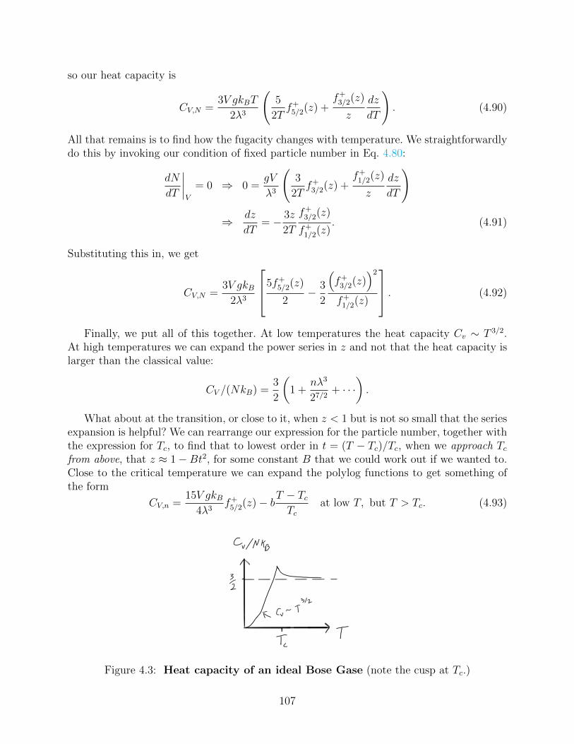
so our heat capacity is

CV,N =3V gkBT

2λ3

(5

2Tf+

5/2(z) +f+

3/2(z)

z

dz

dT

). (4.90)

All that remains is to find how the fugacity changes with temperature. We straightforwardlydo this by invoking our condition of fixed particle number in Eq. 4.80:

dN

dT

∣∣∣∣V

= 0 ⇒ 0 =gV

λ3

(3

2Tf+

3/2(z) +f+

1/2(z)

z

dz

dT

)

⇒ dz

dT= − 3z

2T

f+3/2(z)

f+1/2(z)

. (4.91)

Substituting this in, we get

CV,N =3V gkB

2λ3

5f+5/2(z)

2− 3

2

(f+

3/2(z))2

f+1/2(z)

. (4.92)

Finally, we put all of this together. At low temperatures the heat capacity Cv ∼ T 3/2.At high temperatures we can expand the power series in z and not that the heat capacity islarger than the classical value:

CV /(NkB) =3

2

(1 +

nλ3

27/2+ · · ·

).

What about at the transition, or close to it, when z < 1 but is not so small that the seriesexpansion is helpful? We can rearrange our expression for the particle number, together withthe expression for Tc, to find that to lowest order in t = (T − Tc)/Tc, when we approach Tcfrom above, that z ≈ 1−Bt2, for some constant B that we could work out if we wanted to.Close to the critical temperature we can expand the polylog functions to get something ofthe form

CV,n =15V gkB

4λ3f+

5/2(z)− bT − TcTc

at low T, but T > Tc. (4.93)

Figure 4.3: Heat capacity of an ideal Bose Gase (note the cusp at Tc.)

107

This is a heat capacity which is continuous at Tc (i.e., it will match the value from theT < Tc calculation, from the first term), but which has a discontinuous24 derivative! Thebehavior is schematically shown in Fig. 4.3. Now, in physics we’re used to dealing withfunctions that are smooth and well-behaved; where do these sort of discontinuities comefrom? In the following chapter we’ll more systematically look at interacting systems andphase transitions. First, we wrap up the chapter with a quick look at degenerate Fermigases.

4.10 Ideal Fermi gases

Just as in the case of the ideal Bose gas, when d = n−λ3/g approaches unity we can no

longer usefully rely on the power series expansions of the f ηm(z) in Eq. 4.80, and we muststart working with the full set of equations there. In the limit that T → 0 we can look atthe average fermi occupation number for states associated with k:

〈nk〉− =1

eβ(Ek−µ) + 1=

1 Ek < µ0 otherwise

. (4.94)

At T = 0 this is just a step function, so at zero temperature all of the single-particle statesup to Ek = εF , the fermi energy, are completely filled, forming the so-called fermi sea. Thecorresponding wavenumber is25 referred to as the fermi wavenumber, kF . For an ideal gaswith Ek = ~2k2/(2m), these are related by

N =∑|k|≤kF

g = gV

∫k≤kf

d3k

(2π)3=gV

6π2k3F , (4.95)

so

kF =

(6π2n

g

)1/3

, εF =~2

2m

(6π2n

g

)2/3

(4.96)

Schematically the behavior of the occupation numbers are shown in Fig. 4.4.We need to do some work to investigate the finite-temperature behavior (i.e., for large z).

Here we follow Sommerfeld’s approach, and first take Eq. 4.78 and perform an integrationby parts:

f−m(z) =1

m!

∫ ∞0

dx xmd

dx

(−1

ex−ln z + 1

), (4.97)

where we’ve just written z−1 as e− ln z for convenience. We then say that we know the fermioccupation itself changes very rapidly from 1 to zero across εF , so the derivative above

24Or does it? I’ve been a bit sloppy here, going back and forth about whether below Tc z = 1 orz = (N0)/(N0 + 1). In fact, for any finite N the cusp will be smoothed out. Many more details on thisto come!

25shockingly

108

Figure 4.4: Fermi occupation numbers The dotted line shows the zero-temperature limit,and the solid curve shows the finite temperature result.

must be sharply peaked. We expand about this peak of the derivative (which occurs whenx = ln z), by setting x = ln z+ t and taking the new integration variable −∞ ≤ t ≤ ∞. Thistrick gives us:

f−m(z) ≈ 1

m!

∫ ∞−∞

dt (ln z + t)md

dt

(−1

et + 1

)=

1

m!

∫ ∞−∞

dt∞∑α=0

[(m

α

)tα (ln z)m−α

]d

dt

(−1

et + 1

)=

(ln z)m

m!

∞∑α=0

m!

α!(m− α)!(ln z)−α

∫ ∞−∞

dt tαd

dt

(−1

et + 1

). (4.98)

The last type of integral appearing above can be manipulated (exploiting the anti-symmetryof the integrand under exchange of sign of t, etc.) to give:

1

α!

∫ ∞−∞

dt tαd

dt

(−1

et + 1

)=

0 if α is odd

2(α−1)!

∫∞0dt t

α−1

et+1if α is even

, (4.99)

and in that last expression we recognize an expression which is just 2f−α (1). So, we combinethe above two equations, and exploit the fact that other people have computed the integralsassociated with f−m(1), to give the Sommerfeld expansion:

limz→∞

f−m(z) =(ln z)m

m!

∞∑αeven

2f−α (1)m!

(m− α)!(ln z)−α

=(ln z)m

m!

(1 +

π2

6

m(m− 1)

(ln z)2+ · · ·

). (4.100)

109

To first approximation, explicitly, we have

f−5/2(z) ≈ 8 (ln z)5/2

15√π

(1 +

5π2

8 (ln z)2 + · · ·)

f−3/2(z) ≈ 4 (ln z)3/2

3√π

(1 +

π2

8 (ln z)2 + · · ·)

(4.101)

f−1/2(z) ≈ 2 (ln z)1/2

√π

(1− π2

24 (ln z)2 + · · ·)

We can now plug these results into Eq. 4.80. When z 1 the degeneracy factor is

n−λ3

g= f−3/2(z) ≈ 4 (ln z)3/2

3√π

(1 +

π2

8 (ln z)2 + · · ·). (4.102)

The leading term reproduces our earlier result for the fermi energy:

βεF =β~2

2m

(6π2n

g

)2/3

=

(3nλ3

4√π

)2/3

= ln z (4.103)

which gives a chemical potential of

µ = kBT ln z ≈ εF

(1− π2

12

(kBT

εF

)2). (4.104)

Note that this is positive at low temperatures and negative at high temperatures, suggestingthat the chemical potential changes sign at a fermi temperature TF ∼ εF/kB. The energydensity E/V = 3P/2, and the low-temperature pressure is

βP− =g

λ3

8 (ln z)5/2

15√π

(1 +

5π2

8 (ln z)2 + · · ·)

(4.105)

With the help of our previous expression (relating the fermi energy to ln z, for instance), wecan write this as a power series in temperature, as

P− =2

5εFn−

(1 +

5π2

12

(kBT

εF

)2

+ · · ·

). (4.106)

Unlike a classical gas, the degenerate fermi gas has finite pressure (and internal energy) evenat zero temperature. Additionally, the heat capacity,

CVNkB

=1

NkB

∂E

∂T=π2

2

kBT

εF(4.107)

varies as the first power of temperature at low T (something which is quite general in fermigases, regardless of the dimension). This reflects the fact that only a small fraction (of orderT/TF ) of the particles are excited at temperature T , and most of the particles do not feel theeffects of the finite temperatures. Each of those excited particles gains about kBT of energy,hence CV ∼ (T/TF ). Additionally, we see that the heat capacity at low temperature is muchsmaller than the classical expectation of 3NkN/2.

110

Chapter 5

Interacting systems

So far we have almost exclusively1 focused on ideal systems in which the units compos-ing the system did not interact with each other via interparticle potentials. This simpli-fication helped us more clearly understand the structure of our statistical descriptions ofmacroscopic systems (and, helpfully, let us solve everything analytically) – and for quantummechanical systems we even saw that non-interacting Bose and Fermi systems can exhibitrich/interesting behaviors.

However. Interactions are responsible for the amazing variety of phases of matter andmaterial behaviors! Since most physical systems that we encounter cannot be describedwithout considering interactions, in this chapter and the next we’ll start building up ways ofincorporating interactions into our statistical mechanical formalism. This chapter will focuson systematic expansions, in which an idealized, non-interacting system serves as a usefulstarting point. Implicitly, for instance, throughout the next sections you can imagine thatwe’re trying to describe the properties of a dilute gas.

5.1 From cumulant expansions...

5.1.1 Moment expansion

Let’s return to the idea of a classical system2 and start with a general Hamiltonian in theabsence of an external potential:

H =N∑i=1

p2i

2m+ U (r) ,

where we’ve written a general interaction potential, U , which could be an arbitrary functioninvolving the spatial coordinates of the particles.

1With the exception of introducing some interactions in Chapter 3 to get to the Boltzmann equation2With our corrected phase-space measure

111

In the canonical ensemble the partition function would be

Z(N, V, T ) =1

N !h3N

∫ (∏i

d3pid3ri

)exp

(−β

N∑i=1

p2i

2m

)e−βU(r)

=1

N !

(V

λ3

)N ∫ ∏i

d3riV

e−βU(r), (5.1)

where in the second line we’ve done the integral over momenta and taken the liberty ofmultiplying and dividing by N copies of the system volume V . We’ve done this because nowwe see terms directly related to ideal, non-interacting quantities. The prefactor is just theideal gas partition function, and the integral is like doing an average over particle positionswhere there are no correlations between the particle positions – exactly as if the positionswere those from an ideal gas with no interactions. Using the notation where a superscript(0) refers to these ideal-gas like quantities or averages, we can write the canonical partitionfunction as

Z(N, V, T ) ≡ Z(0)(N, V, T )⟨e−βU(r)⟩(0)

(5.2)

= Z(0)∑l

(−β)l

l!

⟨U l⟩(0)

. (5.3)

This looks like a moment-based perturbative description of a system: when U = 0 we recoverthe ideal gas which we know how to solve, and when U is solve we can calculate correctionssystematically. As we’ll see shortly, this direct moment-based expansion is often not espe-cially useful: at short ranges there are often strong repulsions (Pauli exclusion, or hard-corerepulsion between particles, or... ), so the moments of U need not be small. Nevertheless,working with this will lead us to an expansion which is useful.

5.1.2 Cumulant expansion

We know that what we often want to work with is the log of the partition function, so let’sreplace our moment expansion with a cumulant expansion: we see above that Z is actinglike a generator of moments, so taking the log gives us a generator of cumulants:

logZ = logZ(0) +∞∑l=1

(−β)l

l!

⟨U l⟩(0)

c. (5.4)

At this point we specialize the form of the interparticle potential away from complete gen-erality, and study potentials, φ that are pairwise in nature,

U =∑i<j

φ (ri − rj) ≡ φ (rij) , (5.5)

where we’ve introduce the notation rij to represent vector separations between pairs ofparticles, which we’ll be seeing a lot of in the next sections.

Writing out the first few terms of this cumulant expansion, we have

logZ = logZ(0) − β 〈U〉(0) +β2

2

(⟨U2⟩(0) −

(〈U〉(0)

)2)

+ · · · (5.6)

Let’s evaluate these first few cumulants for our pairwise potential.

112

First cumulant

The first cumulant is quite straightforward, recognizing that for each pair of particles wepick as the interacting pair we’re going to get copies of the same result:

〈U〉(0) =∑i<j

∫ (∏α

d3rαV

)φ(ri − rj)

=N(N − 1)

2

∫d3r1

V

d3r2

V· · · d

3rNV

φ(r1 − r2)

=N(N − 1)

2V

∫d3rφ(r), (5.7)

where in the last line we’ve let r = r12. There you go: someone hands you a particularinterparticle potential (Lennard-Jones, or screened Coulomb, or...), and you go off, calculatean integral, and you’ve got the first term in the cumulant expansion.

Second cumulant

Let’s write out the second cumulant as⟨U2⟩(0)

c=∑i<jk<l

[〈φ(rij)φ(rkl)〉(0) − 〈φ(rij)〉(0) 〈φ(rkl)〉(0)

]. (5.8)

This is a sum over(N(N−1)

2

)2

total terms, and it is helpful to divide those into three classes

of terms:

All particle labels are distinct, i.e., i, j, k, l are all different indices. In this case we canlook at the second moment and see

〈φ(rij)φ(rkl)〉(0) =

∫ (∏α

d3rαV

)φ(rij)φ(rkl)

=

(∫d3riV

d3rjV

φ(rij)

)(∫d3rkV

d3rlV

φ(rkl)

)= 〈φ(rij)〉(0) 〈φ(rkl)〉(0) . (5.9)

Thus, these terms do not make any contribution to 〈U2〉(0).

One particle label is shared i.e., we have i, j, k = i, l as the four labels. We can make asimilar argument for neglecting this class of terms, too. We first write

〈φ(rij)φ(ril)〉(0) =

∫d3rid

3rjd3rl

V 3φ(rij)φ(ril), (5.10)

and then change variables in the integration from ri, rj, rl to ri, rij, ril . This leaves us with

〈φ(rij)φ(ril)〉(0) =

∫d3rid

3rijd3ril

V 3φ(rij)φ(ril) = 〈φ(rij)〉(0) 〈φ(ril)〉(0) , (5.11)

which again means these terms do not contribute to 〈U2〉(0).

113

The same pair is considered twice i.e., i = k, j = l. Well, the second cumulant doesn’tvanish, and these are the remaining terms which we do need to keep track of. There areN(N−1)

2terms of this form, and they all contribute identically. Thus, our complete expression

for the second cumulant is

⟨U2⟩(0)

c=N(N − 1)

2

[∫d3rijV

φ2(rij)−(∫

d3rijV

φ(rij)

)2]. (5.12)

So far, we have the following expansion for the log of the partition function:

logZ = logZ(0)+N(N − 1)

2

[−β∫

d3r

Vφ(r) +

β2

2

(∫d3r

Vφ2(r)−

(∫d3r

Vφ(r)

)2)

+ · · ·

].

(5.13)We now consider the thermodynamic limit, V,N →∞, and we find

logZ ≈ N log

(V e

Nλ3

)+N2

2V

[−β∫

d3rφ(r) +β2

2

∫d3rφ2(r) + · · ·

]. (5.14)

If we now, for instance, want to know the pressure of our system, we take the appropriatederivative and find

βP =∂ logZ

∂V(5.15)

=N

V− 1

2

(N

V

)2 [−β∫

d3rφ(r) +β2

2

∫d3rφ2(r) + · · ·

]+O

((N

V

)3).

What have we done? We’ve basically written the equation of state of the system as a per-turbation organized in powers of density, where the contribution at each order in density isa sum over a series of terms involving integrals of powers of the pairwise potential.

As written, this sort of cumulant expansion is still not very helpful. Why? Because fortypical interactions there are large forces keeping molecules apart. For instance, one commonpotential is the Lennard-Jones potential:

φ(r) = 4ε

[(σr

)12

−(σr

)6], (5.16)

where ε is related to the depth of the potential well and σ to the range over which therepulsion is felt. Where do these sorts of potential come from? The attractive r−6 part comesfrom fluctuating dipoles of electrically neutral atoms. Recall that if there were two interactingpermanent dipole moments, p1 and p2, the potential energy would scale as p1p2/r

3. Thereare no permanent dipoles for neutral atoms, but atoms can acquire transient dipoles throughquantum fluctuations. If the first atom has a transient dipole p1 it will induce an electricfield, which will in turn induce a dipole in the second atom p2 ∼ E ∼ p1/r

3. The resultingenergy thus scales as p1p2/r

3 ∼ r−6; this is typically called the van der Waals attraction.The r−12 term is meant to reflect the rapid transition to strong repulsion as the atoms getvery close. The exact form is not so important, and the common choice of a term like r−12

is simply a mathematical convenience.

114

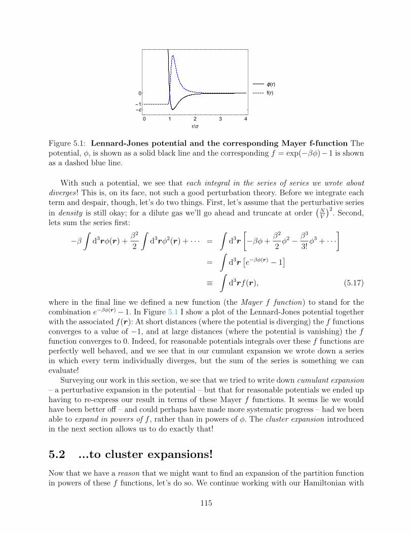
0 1 2 3 4

-ϵ-1

0

r/σ

ϕ(r)

f(r)

Figure 5.1: Lennard-Jones potential and the corresponding Mayer f-function Thepotential, φ, is shown as a solid black line and the corresponding f = exp(−βφ)−1 is shownas a dashed blue line.

With such a potential, we see that each integral in the series of series we wrote aboutdiverges ! This is, on its face, not such a good perturbation theory. Before we integrate eachterm and despair, though, let’s do two things. First, let’s assume that the perturbative series

in density is still okay; for a dilute gas we’ll go ahead and truncate at order(NV

)2. Second,

lets sum the series first:

−β∫

d3rφ(r) +β2

2

∫d3rφ2(r) + · · · =

∫d3r

[−βφ+

β2

2φ2 − β3

3!φ3 + · · ·

]=

∫d3r

[e−βφ(r) − 1

]≡

∫d3rf(r), (5.17)

where in the final line we defined a new function (the Mayer f function) to stand for thecombination e−βφ(r)− 1. In Figure 5.1 I show a plot of the Lennard-Jones potential togetherwith the associated f(r): At short distances (where the potential is diverging) the f functionsconverges to a value of −1, and at large distances (where the potential is vanishing) the ffunction converges to 0. Indeed, for reasonable potentials integrals over these f functions areperfectly well behaved, and we see that in our cumulant expansion we wrote down a seriesin which every term individually diverges, but the sum of the series is something we canevaluate!

Surveying our work in this section, we see that we tried to write down cumulant expansion– a perturbative expansion in the potential – but that for reasonable potentials we ended uphaving to re-express our result in terms of these Mayer f functions. It seems lie we wouldhave been better off – and could perhaps have made more systematic progress – had we beenable to expand in powers of f , rather than in powers of φ. The cluster expansion introducedin the next section allows us to do exactly that!

5.2 ...to cluster expansions!

Now that we have a reason that we might want to find an expansion of the partition functionin powers of these f functions, let’s do so. We continue working with our Hamiltonian with

115

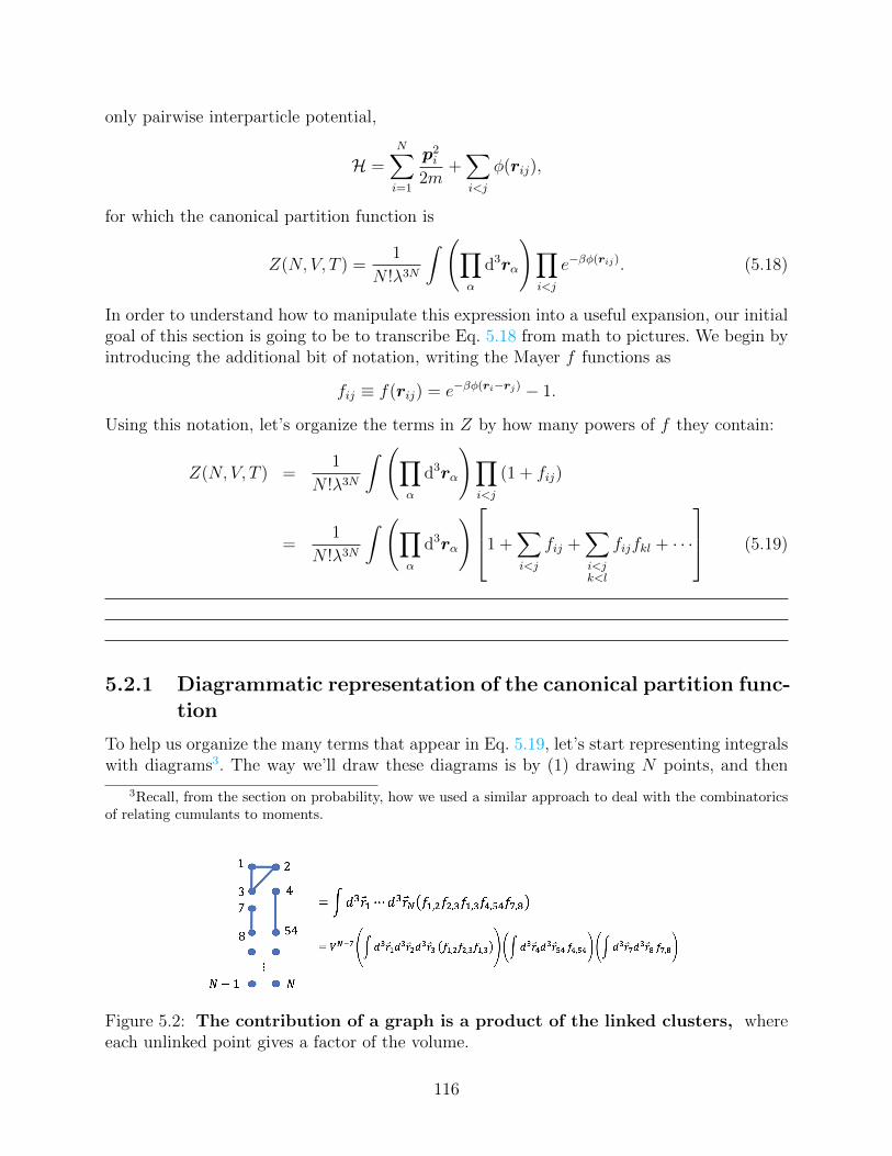
only pairwise interparticle potential,

H =N∑i=1

p2i

2m+∑i<j

φ(rij),

for which the canonical partition function is

Z(N, V, T ) =1

N !λ3N

∫ (∏α

d3rα

)∏i<j

e−βφ(rij). (5.18)

In order to understand how to manipulate this expression into a useful expansion, our initialgoal of this section is going to be to transcribe Eq. 5.18 from math to pictures. We begin byintroducing the additional bit of notation, writing the Mayer f functions as

fij ≡ f(rij) = e−βφ(ri−rj) − 1.

Using this notation, let’s organize the terms in Z by how many powers of f they contain:

Z(N, V, T ) =1

N !λ3N

∫ (∏α

d3rα

)∏i<j

(1 + fij)

=1

N !λ3N

∫ (∏α

d3rα

)1 +∑i<j

fij +∑i<jk<l

fijfkl + · · ·

(5.19)

5.2.1 Diagrammatic representation of the canonical partition func-tion

To help us organize the many terms that appear in Eq. 5.19, let’s start representing integralswith diagrams3. The way we’ll draw these diagrams is by (1) drawing N points, and then

3Recall, from the section on probability, how we used a similar approach to deal with the combinatoricsof relating cumulants to moments.

Figure 5.2: The contribution of a graph is a product of the linked clusters, whereeach unlinked point gives a factor of the volume.

116

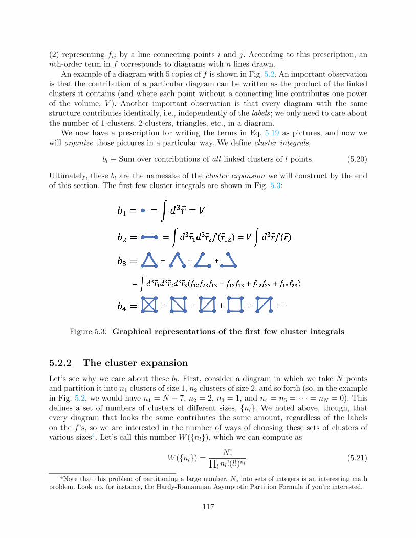
(2) representing fij by a line connecting points i and j. According to this prescription, annth-order term in f corresponds to diagrams with n lines drawn.

An example of a diagram with 5 copies of f is shown in Fig. 5.2. An important observationis that the contribution of a particular diagram can be written as the product of the linkedclusters it contains (and where each point without a connecting line contributes one powerof the volume, V ). Another important observation is that every diagram with the samestructure contributes identically, i.e., independently of the labels ; we only need to care aboutthe number of 1-clusters, 2-clusters, triangles, etc., in a diagram.

We now have a prescription for writing the terms in Eq. 5.19 as pictures, and now wewill organize those pictures in a particular way. We define cluster integrals,

bl ≡ Sum over contributions of all linked clusters of l points. (5.20)

Ultimately, these bl are the namesake of the cluster expansion we will construct by the endof this section. The first few cluster integrals are shown in Fig. 5.3:

Figure 5.3: Graphical representations of the first few cluster integrals

5.2.2 The cluster expansion

Let’s see why we care about these bl. First, consider a diagram in which we take N pointsand partition it into n1 clusters of size 1, n2 clusters of size 2, and so forth (so, in the examplein Fig. 5.2, we would have n1 = N − 7, n2 = 2, n3 = 1, and n4 = n5 = · · · = nN = 0). Thisdefines a set of numbers of clusters of different sizes, nl. We noted above, though, thatevery diagram that looks the same contributes the same amount, regardless of the labelson the f ’s, so we are interested in the number of ways of choosing these sets of clusters ofvarious sizes4. Let’s call this number W (nl), which we can compute as

W (nl) =N !∏

l nl!(l!)nl. (5.21)

4Note that this problem of partitioning a large number, N , into sets of integers is an interesting mathproblem. Look up, for instance, the Hardy-Ramanujan Asymptotic Partition Formula if you’re interested.

117

How did we arrive at this expression? Our strategy was essentially to first pick any particularpartitioning into nl l-cluster. We first overcount everything by considering every possiblepermutation of the labels, giving us the N ! in the numerator above. Having overcounted,we now divide out to account for diagram symmetries. First, for each individual l-cluster,we note that the permutations of labels within that cluster give the same diagram (e.g.,a line from point 1 to point 2 is unchanged when the labels 1 and 2 are permuted); thisgives us a factor of (l!) for each of the nl clusters of size l. Additionally, we have to considerpermutations of labels that replace all of the labels of one cluster of size l with a differentcluster of size l (e.g., a line from point 1 to 2 and from 5 to 6 is unchanged when labels (1 and5) and (2 and 6) are permuted); this gives us the additional factor of nl! in the denominator.

I highly encourage you to get a feel for this by playing around. Try drawing, say, 5 or 6points, break them up into clusters of different sizes, and get a feel for the combinatorics.

With this counting of the number of different types of diagrams, we can write the canon-ical partition function as

Z =1

N !λ3N

∑nlrestricted

W (nl)∏l

bnll , (5.22)

where the restriction is that every point has to be in a cluster,∑

l lnl = N . From the lastchapter, this situation should feel quite familiar: we have another case where a constrainedsum in the canonical ensemble is making our life difficult. In exactly the same way as before,this difficulty is lifted by moving to the grand canonical ensemble.

So, we write down the grand partition function, noting that the sum over all possibleN of a restricted sum on the nl is equivalent to performing an unrestricted sum over thenl:

Q =∞∑N=0

eβµNZN

=∑nl

1

N !λ3N

(eβµ)∑

l lnl N !∏l

bnllnl!(l!)nl

=∏l

∞∑nl=0

(eβµ

λ3

)lnl bnllnl!(l!)nl

. (5.23)

In the last line we recognize that we have written something like∏l

∑nl

1

nl![· · ·]nl ,

which is just the expansion of an exponential. Thus, we find5

Q =∏l

exp

[(eβµ

λ3

)l(bll!

)], (5.24)

5if you’re comparing these expression with Pathria, or other texts, please note that different authorsuse slightly different conventions in the definitions of the cluster integrals; in particular, sometimes the blaccount for the factors of l! in that divide it in the expressions I’m writing.

118

i.e.,

⇒ logQ =∞∑l=1

(eβµ

λ3

)l(bll!

)(5.25)

Before we make use of this expression for the grand canonical partition function, it is worththinking for a moment about the graphical expressions we wrote for cumulants and moments.The graphical interpretation of the above result is that the log of the sum over all graphs isequivalent to the sum over only the connected clusters.

5.3 Virial expansion for a dilute gas

We consider, now, a dilute gas, and our goal for this section is to write a virial expansionfor the equation of state of the dilute gas, i.e., something of the form

βP = B1(T )N

V+B2(T )

(N

V

)2

+B3(T )

(N

V

)3

+ · · · , (5.26)

where we’ve written temperature-dependent coefficients Bi for the powers of density. For adilute gas we can certainly exploit the extensivity condition to write the grand potential as

− βG = logQ = −β (E − TS − µN) = βPV. (5.27)

Just as in Chapter 4 when we discussed the ideal gas in the grand canonical ensemble, wesee that the grand potential is proportional to the volume; comparing with Eq. 5.25 we seethat in fact each cluster integral bl ∝ V . We thus define a version of the cluster integralswith this volume dependence removed,

bl ≡blV,

in terms of which we can write the pressure as

βP =∑l

(eβµ

λ3

)lbll!. (5.28)

At the same time, we know that, specifying the chemical potential µ in the grand canonicalensemble we can compute the expected number density of particles as

n =N

V=

1

V

∂ logQ∂ (βµ)

=∑l

l

(eβµ

λ3

)lbll!. (5.29)

Simplifying the notation by writing a dimensional version of the fugacity, x ≡ eβµ/λ3, wearrive at the equation of state for a dilute gas:

βP =∑l

xlbll!

n =∑l

lxlbll!. (5.30)

119

This is... not exactly what we typically want. Just as in the chapter on quantum statisticalmechanics, what we want is the pressure as a function of density, but what we have is thepressure as a function of fugacity together with a separate equation relating the numberdensity to the fugacity. We encountered this exact situation in looking at ideal quantumgases, and we resolve it in the same way.

So, we write out the series expansion for n,

n = b1x+ b2x2 +

b3

2x3 + · · · (5.31)

Rearranging this (and noting that b1 = 1), we have

x = n− b2x2 − b3

2x3 − · · · , (5.32)

which we can self-consistently solve to any desired order by substituting the ith-order solutionfor x into the (i+ 1)th-order expression. Starting with the first order approximation x1 ≈ n,we get

x1 = n+O(n2)

x2 = n− b2n2 +O

(n3)

x3 = n− b2

(n− b2n

2)2 − b3

2

(n− b2n

2)3

+O(n4)

= n− b2n2 +

(2b2

2 −b3

2

)n3 +O

(n4), (5.33)

and so on. We can now substitute this into the equation for the pressure; to get an expansioncorrect to order i we use the xi expression obtained by the above procedure. So, for instance,to third order we write (collecting all terms up to third order in the number density)

βP = b1x+b2

2x2 +

b3

3!x3

= n− b2n2 +

(b2

2 −b3

3

)n3 +O

(n4). (5.34)

In general, we have a result of the form

βP = n+∞∑l=2

Bl(T )nl, (5.35)

as desired! The first term, B1 = 1, reproduces the ideal gas result. The second term is

B2(T ) = − b2

2= −1

2

∫d3r

[e−βφ(r) − 1

], (5.36)

which diagrammatically is −1/2 times what we drew as a line between two points. Wecalculate the third term diagrammatically, as illustrated in Fig. 5.4, and find

B3(T ) = −1

3

∫d3r12d3r13f(r12)f(r13)f(r12 − r13) (5.37)

120

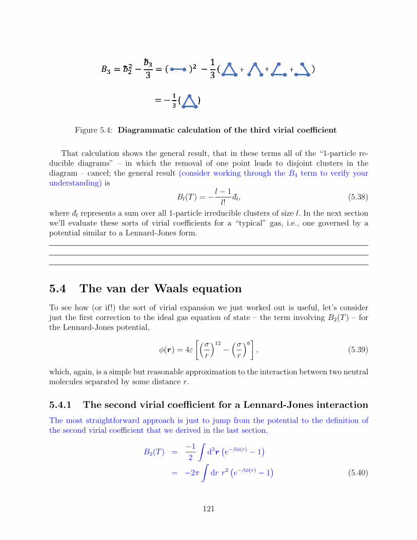
Figure 5.4: Diagrammatic calculation of the third virial coefficient

That calculation shows the general result, that in these terms all of the “1-particle re-ducible diagrams” – in which the removal of one point leads to disjoint clusters in thediagram – cancel; the general result (consider working through the B4 term to verify yourunderstanding) is

Bl(T ) = − l − 1

l!dl, (5.38)

where dl represents a sum over all 1-particle irreducible clusters of size l. In the next sectionwe’ll evaluate these sorts of virial coefficients for a “typical” gas, i.e., one governed by apotential similar to a Lennard-Jones form.

5.4 The van der Waals equation

To see how (or if!) the sort of virial expansion we just worked out is useful, let’s considerjust the first correction to the ideal gas equation of state – the term involving B2(T ) – forthe Lennard-Jones potential,

φ(r) = 4ε

[(σr

)12

−(σr

)6], (5.39)

which, again, is a simple but reasonable approximation to the interaction between two neutralmolecules separated by some distance r.

5.4.1 The second virial coefficient for a Lennard-Jones interaction

The most straightforward approach is just to jump from the potential to the definition ofthe second virial coefficient that we derived in the last section,

B2(T ) =−1

2

∫d3r

(e−βφ(r) − 1

)= −2π

∫dr r2

(e−βφ(r) − 1

)(5.40)

121

That integral looks unfamiliar, but one can express the answer in terms of the Kummerconfluent hypergeometric function6

1F1(a; b; z), and the Gamma function:

B2(T ) =−πσ3 (βε)1/4

3√

2

[Γ

(−1

4

)1F1

(−1

4;1

2; βε

)+ 2√βεΓ

(1

4

)1F1

(1

4;3

2; βε

)](5.41)

Is this helpful? This is, indeed, what you get by plugging things into, e.g., Mathematica,and you could plot the behavior of this second virial coefficient as you vary the temperaturefor various values of the Lennard-Jones parameters. This “plug-and-chug” approach, whiletechnically correct, obscures the physical picture of how we expect a dilute gas to behave.

5.4.2 Approximate but physical treatment of B2

Let’s do a better job of capturing the physics by making a rougher approximation to themolecular interactions. In particular, let’s replace the Lennard-Jones potential with the func-tion

φ(r) =

∞ r < σ

−ε(σr

)6r > σ

. (5.42)

This approximate potential captures the following main features of the Lennard-Jones po-tential: it has the van der Waals r−6 at large distances, it has an attractive well of depth ε atshort distances, and it is strongly (in fact, infinitely !) repulsive within a characteristic size ofthe molecular core. Note that this simpler form makes it clear that σ is like the characteristicdiameter of one of the interacting molecules.

With this simpler potential we can compute the second virial coefficient as

B2(T ) = −1

2

∫d3r

(e−βφ(r) − 1

)= −1

2

[−4πσ3

3+ 4π

∫ ∞σ

dr r2(eβε(

σr )

6

− 1)]

. (5.43)

The first term above reflects an excluded volume in the potential we have written down.Keeping in mind that we are trying to describe a dilute gas at reasonably high temperatures,let’s further approximate the second term by assuming βε 1, that is, that we are at highT relative to the well depth. We will use this approximation to write a series expansion forthe exponential of the potential:

eβφ ≈ βε(σr

)6

+O (βε)2 .

With this approximation, the integral can be easily carried out:

B2(T ) = −1

2

[(−4πσ3

3

)+

4πσ3

3βε

]=

Ω

2[1− βε] , where Ω =

4πσ3

3. (5.44)

6As a series expansion, 1F1(a; b; z) =∑∞n=0

a(n)zn

b(n)n!, where a(n) is the “rising factorial,” a(0) = 1, a(1) = a,

a(n) = a(a+ 1) · · · (a+ n− 1), etc.

122

This is a nice, compact expression for the second virial coefficient: we see a small perturbativecorrection that comes in at high temperatures, with an overall scale set by the excludedvolume of the molecules.

A few comments are in order, directed at the question of “when should this approximationbe reasonable?” Two obvious conditions stand out.

First, this is clearly meant to be a low-density expansion, but what we do mean by “low”in this context? As with any series expansion, we want the ratio of consecutive terms to besmall, and the ratio of the correction to the ideal term is ∼ B2

ρ2

ρ∼ Ω

ρ−1 . Note that Ω is

close to an atomic volume, so one can think of the above ratio as ∼ ρgasρliquid

. That is, when the

density of the system is such that the gas is close to liquifying, we should assume our seriesapproximation is insufficient.

Second, in our expansion of the attractive tail, we assumed that βε 1. If βε & 1for these attractive potentials, we could not have done a reasonable series expansion in thefirst place. In general, for low temperatures the ground state of a system with attractiveinteractions is not a gas, but a dense collection of molecules sticking together.

There is an additional consideration, which speaks to our ability to factor out the Ω termin the series expansion we wrote. The fact that we could do this speaks to the sense that theshort-ranged part of the potential dominates the integral we had to do. In this context thereis a sense in which potentials which fall of faster than r−3 are “short ranged;” for potentialslike φ ∼ r−3 there are terms which are logarithmic in the size of the system, and for evenlonger-ranged potentials the whole expansion fails.

5.4.3 The van der Waals equation

Finally, we can write down the equation of state based on our approximate treatment of thesecond virial coefficient:

βP = n+n2

2Ω (1− βε)

⇒ β

(P +

n2Ω

2ε

)= n

(1 +

nΩ

2+ · · ·

). (5.45)

Since we’re only being accurate to order n2 in the above expression, we’re free to re-writethe right-hand side as

n

(1 +

nΩ

2+ · · ·

)≈ n

1− nΩ2

+ · · · .

Using this rearranging, we arrive at the van der Waals equation of state:

P =NkBT

V − NΩ2

− εΩ

2

(N

V

)2

, (5.46)

which is often presented as(P + a

(N

V

)2)

(V − bN) = NkBT.

123

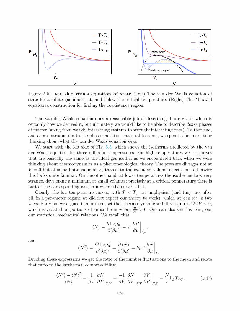
Figure 5.5: van der Waals equation of state (Left) The van der Waals equation ofstate for a dilute gas above, at, and below the critical temperature. (Right) The Maxwellequal-area construction for finding the coexistence region.

The van der Waals equation does a reasonable job of describing dilute gases, which iscertainly how we derived it, but ultimately we would like to be able to describe dense phasesof matter (going from weakly interacting systems to strongly interacting ones). To that end,and as an introduction to the phase transition material to come, we spend a bit more timethinking about what the van der Waals equation says.

We start with the left side of Fig. 5.5, which shows the isotherms predicted by the vander Waals equation for three different temperatures. For high temperatures we see curvesthat are basically the same as the ideal gas isotherms we encountered back when we werethinking about thermodynamics as a phenomenological theory. The pressure diverges not atV = 0 but at some finite value of V , thanks to the excluded volume effects, but otherwisethis looks quite familiar. On the other hand, at lower temperatures the isotherms look verystrange, developing a minimum at small volumes; precisely at a critical temperature there ispart of the corresponding isotherm where the curve is flat.

Clearly, the low-temperature curves, with T < Tc, are unphysical (and they are, afterall, in a parameter regime we did not expect our theory to work), which we can see in twoways. Early on, we argued in a problem set that thermodynamic stability requires δPδV < 0,which is violated on portions of an isotherm where ∂P

∂V> 0. One can also see this using our

our statistical mechanical relations. We recall that

〈N〉 =∂ logQ∂(βµ)

= V∂P

∂µ

∣∣∣∣T,v

,

and ⟨N2⟩

=∂2 logQ∂(βµ)2

=∂ 〈N〉∂(βµ)

= kBT∂N

∂µ

∣∣∣∣T,v

.

Dividing these expressions we get the ratio of the number fluctuations to the mean and relatethat ratio to the isothermal compressibility:

〈N2〉 − 〈N〉2

〈N〉=

1

βV

∂N

∂P

∣∣∣∣T,V

=−1

βV

∂N

∂V

∣∣∣∣P,T

∂V

∂P

∣∣∣∣N,T

=N

VkBTκT . (5.47)

124

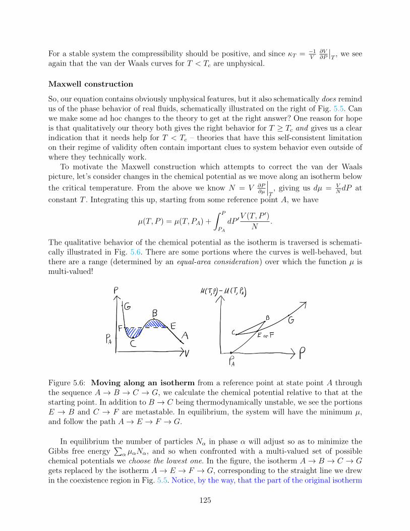
For a stable system the compressibility should be positive, and since κT = −1V

∂V∂P

∣∣T

, we seeagain that the van der Waals curves for T < Tc are unphysical.

Maxwell construction

So, our equation contains obviously unphysical features, but it also schematically does remindus of the phase behavior of real fluids, schematically illustrated on the right of Fig. 5.5. Canwe make some ad hoc changes to the theory to get at the right answer? One reason for hopeis that qualitatively our theory both gives the right behavior for T ≥ Tc and gives us a clearindication that it needs help for T < Tc – theories that have this self-consistent limitationon their regime of validity often contain important clues to system behavior even outside ofwhere they technically work.

To motivate the Maxwell construction which attempts to correct the van der Waalspicture, let’s consider changes in the chemical potential as we move along an isotherm below

the critical temperature. From the above we know N = V ∂P∂µ

∣∣∣T

, giving us dµ = VNdP at

constant T . Integrating this up, starting from some reference point A, we have

µ(T, P ) = µ(T, PA) +

∫ P

PA

dP ′V (T, P ′)

N.

The qualitative behavior of the chemical potential as the isotherm is traversed is schemati-cally illustrated in Fig. 5.6. There are some portions where the curves is well-behaved, butthere are a range (determined by an equal-area consideration) over which the function µ ismulti-valued!

Figure 5.6: Moving along an isotherm from a reference point at state point A throughthe sequence A → B → C → G, we calculate the chemical potential relative to that at thestarting point. In addition to B → C being thermodynamically unstable, we see the portionsE → B and C → F are metastable. In equilibrium, the system will have the minimum µ,and follow the path A→ E → F → G.

In equilibrium the number of particles Nα in phase α will adjust so as to minimize theGibbs free energy

∑α µαNα, and so when confronted with a multi-valued set of possible

chemical potentials we choose the lowest one. In the figure, the isotherm A→ B → C → Ggets replaced by the isotherm A→ E → F → G, corresponding to the straight line we drewin the coexistence region in Fig. 5.5. Notice, by the way, that the part of the original isotherm

125

which gets replaced is not just the part where the thermodynamic stability condition wasviolated, but is actually a larger region! In these additional parts of the isotherm the systemis metastable, rather than being strictly stable or unstable.

This Maxwell construction qualitatively succeeds, in that it now gives us largely the cor-rect physical behavior, but it certainly feels weird! It required us to start with an approximatetheory, consider regions of that theory where the behavior was clearly unphysical, and thentry to sweep any unpleasantness under the rug. This was all done, additionally, in a regimewhere it is not at all clear that simply doing a better job with our perturbative expansionwould be of any help. In the next chapter we’ll take a more principled approach to theseissues.

126

Chapter 6

Phase transitions

In the last few chapters we have been preoccupied with various methods of calculating par-tition functions, both for ideal and for interacting systems. In principle, once we know apartition function we can calculate any thermodynamic properties that we might be inter-ested in. As we discussed a particular perturbative approach to calculating the partitionfunction for a dilute gas – and then had to patch it up via Maxwell’s construction in orderto describe both a gas and a liquid state – you may be wondering: if it is even clear that asingle partition function can actually describe multiple phases?

In fact, perhaps you have an even deeper concern. Phase transitions are characterized bydiscontinuities in the free energy or its derivatives, and the free energy can be written as

Z = e−βF = Tr(e−βH

),

where I’m using the trace notation to indicated a schematic sum over all of the degrees offreedom in the Hamiltonian, H. But most H that we study are non-singular functions oftheir degrees of freedom, so the partition function is just a sum of a large number of terms,each of which is exp (some analytic function). How could such a sum be non-analytic, andcan a single partition function even describe a phase transition (let alone multiple phases)?

A deep understanding of the answer to these questions, together with an understandingof how near critical points whole classes of disparate systems behave in the same way, hasonly been understood for, say, the last 50 years1. In this chapter we will discuss meanfield models of phase transitions, critical points, Landau theory for phase transitions, therelationship between fluctuations and correlations, and the scaling hypothesis for behaviornear critical points. This will lead us right up to the precipice of the renormalization group2;time permitting I will try to throw together a few bonus lectures on this.

6.1 Mean field condensation

As a way of sliding from the last chapter to this one we’ll return again to the van der Waalsequation, but now with a somewhat different approach. In the section on interacting systems

1Perhaps making the subject the most “modern” of the graduate physics curriculum? Hmm...2Or, since an anomalously large number of the professors I took graduate classes used British English,

the “renormalisation group.”

127

we were confronted with the problem of computing, say, the canonical partition function

Z(V, T,N) =1

N !h3N

∫ ∏i

d3pd3q exp

(−β∑i

p2i

2m

)exp

(−β∑i<j

φ(rij)

), (6.1)

and with a great deal of effort we constructed a perturbative expansion to do just that in thehigh-temperature / low-density regime. We then muddled along and argued we could workwith the resulting equations even when the system was cooled below the Tc associated withthe gas transitioning to a liquid. It felt dubious.

Our goal is still to approximate the partition function, but let’s consider instead a meanfield calculation, in which we assume that the potential energy contribution of a particle iscomputed based on its interactions with an average – and uniform – background of particles.First, rather than specifying that we are working with a Lennard-Jones pairwise potential,let’s just think of any potential which (1) has a “hard-core” component for r < σ, (2)is sufficiently short-ranged, and (3) has some attractive part of the potential, where thepotential well has integrated area −u. In our approximation for the Lennard-Jones potential,for instance, we would have −u = −εΩ. Next, we first consider the actual (fluctuating)distribution of particle density,

n(r) =∑i

δ (r − ri) ,

in terms of which we could write the potential energy of our system as

U (ri) =1

2

∫d3rd3r′ n(r)n(r′)φ(r − r′). (6.2)

We now assume that the system has uniform density, and approximate n(r) ≈ n = N/V .Then the typical energy, U , is

U =n2

2

∫d3rd3r′φ(r − r′)

=n2V

2

∫d3rφ(r)

=−un2V

2. (6.3)

We substitute this average energy into Eq. 6.1 for the canonical partition function, andwe get

Z =1

N !λ3Nexp

(βuN2

2V

)∫ ∏i

d3ri. (6.4)

We make one last approximation before we do the remaining integral over spatial coordinates,and that is a Ω/V expansion in how we treat the excluded volume effects. To first order in

128

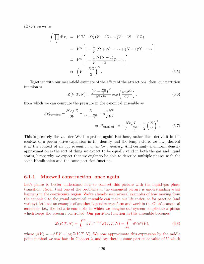
(Ω/V ) we write∫ ∏i

d3ri = V (V − Ω) (V − 2Ω) · · · (V − (N − 1)Ω)

= V N

[1− 1

V(Ω + 2Ω + · · ·+ (N − 1)Ω) + · · ·

]= V N

[1− 1

V

N(N − 1)

2Ω + · · ·

]≈

(V − NΩ

2

)N. (6.5)

Together with our mean-field estimate of the effect of the attractions, then, our partitionfunction is

Z(V, T,N) =

(V − NΩ

2

)NN !λ3N

exp

(βuN2

2V

), (6.6)

from which we can compute the pressure in the canonical ensemble as

βPcanonical =∂ logZ

∂V=

N

V − NΩ2

− βu2

N2

V 2

⇒ Pcanonical =NkBT

V − NΩ2

− u

2

(N

V

)2

. (6.7)

This is precisely the van der Waals equation again! But here, rather than derive it in thecontext of a perturbative expansion in the density and the temperature, we have derivedit in the context of an approximation of uniform density. And certainly a uniform densityapproximation is the sort of thing we expect to be equally valid in both the gas and liquidstates, hence why we expect that we ought to be able to describe multiple phases with thesame Hamiltonian and the same partition function.

6.1.1 Maxwell construction, once again

Let’s pause to better understand how to connect this picture with the liquid-gas phasetransition. Recall that one of the problems in the canonical picture is understanding whathappens in the coexistence region. We’ve already seen several examples of how moving fromthe canonical to the grand canonical ensemble can make our life easier, so for practice (andvariety), let’s see an example of another Legendre transform and work in the Gibb’s canonicalensemble, i.e., the isobaric ensemble, in which we imagine our system coupled to a pistonwhich keeps the pressure controlled. Our partition function in this ensemble becomes

Z(P, T,N) =

∫ ∞0

dV e−βPVZ(V, T,N) =

∫ ∞0

dV eψ(V ), (6.8)

where ψ(V ) = −βPV + logZ(V, T,N). We now approximate this expression by the saddlepoint method we saw back in Chapter 2, and say there is some particular value of V which

129

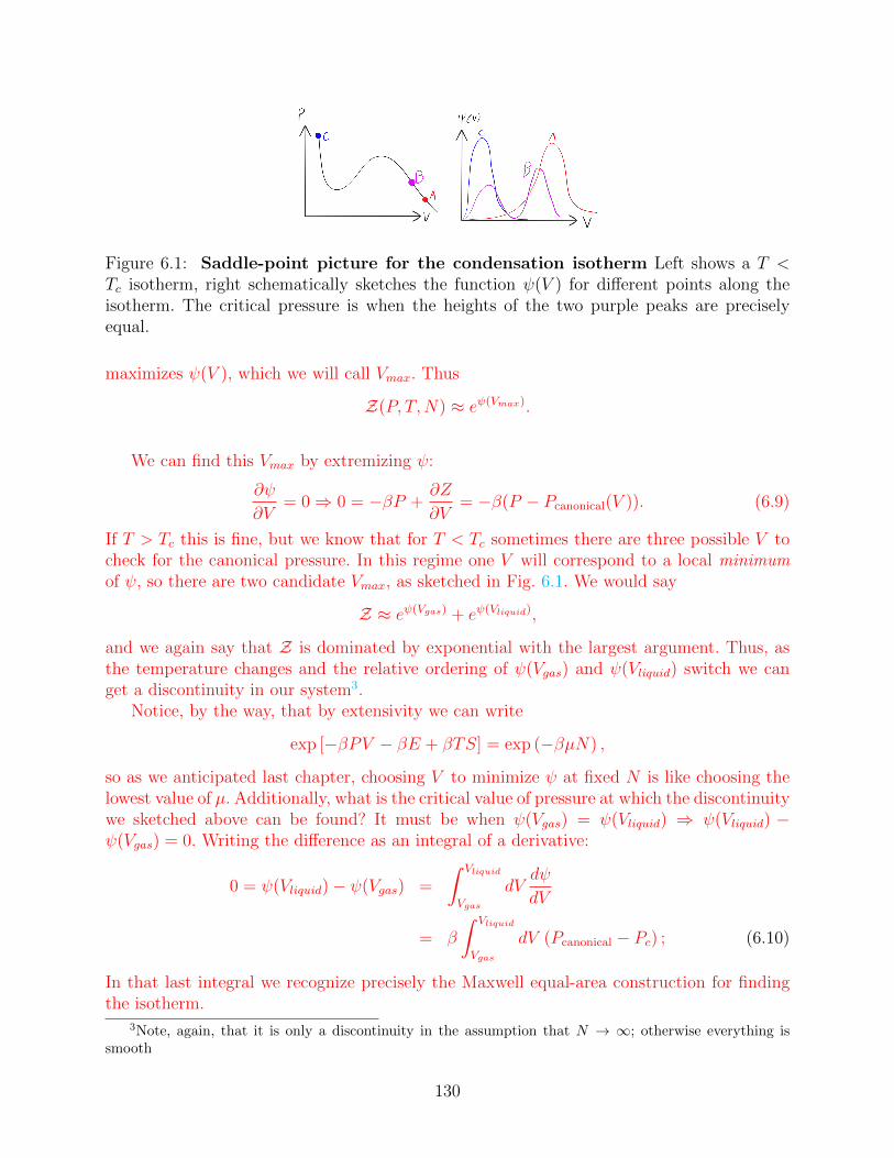
Figure 6.1: Saddle-point picture for the condensation isotherm Left shows a T <Tc isotherm, right schematically sketches the function ψ(V ) for different points along theisotherm. The critical pressure is when the heights of the two purple peaks are preciselyequal.

maximizes ψ(V ), which we will call Vmax. Thus

Z(P, T,N) ≈ eψ(Vmax).

We can find this Vmax by extremizing ψ:

∂ψ

∂V= 0⇒ 0 = −βP +

∂Z

∂V= −β(P − Pcanonical(V )). (6.9)

If T > Tc this is fine, but we know that for T < Tc sometimes there are three possible V tocheck for the canonical pressure. In this regime one V will correspond to a local minimumof ψ, so there are two candidate Vmax, as sketched in Fig. 6.1. We would say

Z ≈ eψ(Vgas) + eψ(Vliquid),

and we again say that Z is dominated by exponential with the largest argument. Thus, asthe temperature changes and the relative ordering of ψ(Vgas) and ψ(Vliquid) switch we canget a discontinuity in our system3.

Notice, by the way, that by extensivity we can write

exp [−βPV − βE + βTS] = exp (−βµN) ,

so as we anticipated last chapter, choosing V to minimize ψ at fixed N is like choosing thelowest value of µ. Additionally, what is the critical value of pressure at which the discontinuitywe sketched above can be found? It must be when ψ(Vgas) = ψ(Vliquid) ⇒ ψ(Vliquid) −ψ(Vgas) = 0. Writing the difference as an integral of a derivative:

0 = ψ(Vliquid)− ψ(Vgas) =

∫ Vliquid

Vgas

dVdψ

dV

= β

∫ Vliquid

Vgas

dV (Pcanonical − Pc) ; (6.10)

In that last integral we recognize precisely the Maxwell equal-area construction for findingthe isotherm.

3Note, again, that it is only a discontinuity in the assumption that N → ∞; otherwise everything issmooth

130

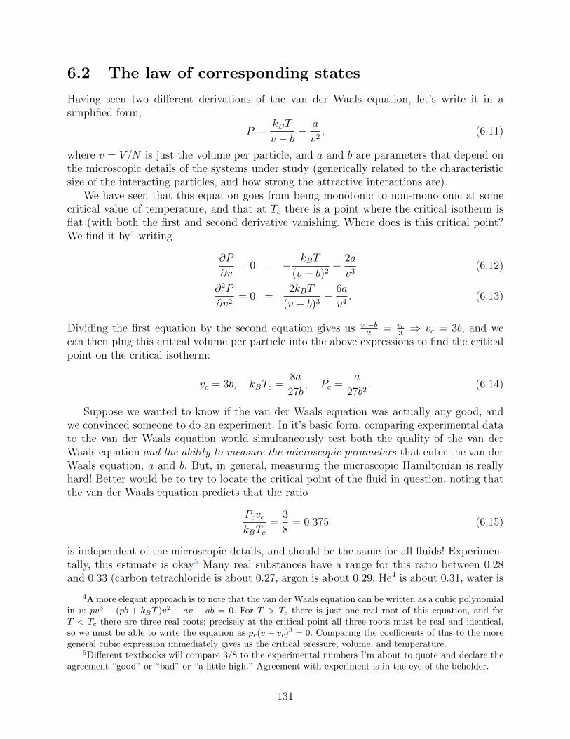
6.2 The law of corresponding states

Having seen two different derivations of the van der Waals equation, let’s write it in asimplified form,

P =kBT

v − b− a

v2, (6.11)

where v = V/N is just the volume per particle, and a and b are parameters that depend onthe microscopic details of the systems under study (generically related to the characteristicsize of the interacting particles, and how strong the attractive interactions are).

We have seen that this equation goes from being monotonic to non-monotonic at somecritical value of temperature, and that at Tc there is a point where the critical isotherm isflat (with both the first and second derivative vanishing. Where does is this critical point?We find it by4 writing

∂P

∂v= 0 = − kBT

(v − b)2+

2a

v3(6.12)

∂2P

∂v2= 0 =

2kBT

(v − b)3− 6a

v4. (6.13)

Dividing the first equation by the second equation gives us vc−b2

= vc3⇒ vc = 3b, and we

can then plug this critical volume per particle into the above expressions to find the criticalpoint on the critical isotherm:

vc = 3b, kBTc =8a

27b, Pc =

a

27b2. (6.14)

Suppose we wanted to know if the van der Waals equation was actually any good, andwe convinced someone to do an experiment. In it’s basic form, comparing experimental datato the van der Waals equation would simultaneously test both the quality of the van derWaals equation and the ability to measure the microscopic parameters that enter the van derWaals equation, a and b. But, in general, measuring the microscopic Hamiltonian is reallyhard! Better would be to try to locate the critical point of the fluid in question, noting thatthe van der Waals equation predicts that the ratio

PcvckBTc

=3

8= 0.375 (6.15)

is independent of the microscopic details, and should be the same for all fluids! Experimen-tally, this estimate is okay5 Many real substances have a range for this ratio between 0.28and 0.33 (carbon tetrachloride is about 0.27, argon is about 0.29, He4 is about 0.31, water is

4A more elegant approach is to note that the van der Waals equation can be written as a cubic polynomialin v: pv3 − (pb + kBT )v2 + av − ab = 0. For T > Tc there is just one real root of this equation, and forT < Tc there are three real roots; precisely at the critical point all three roots must be real and identical,so we must be able to write the equation as pc(v − vc)3 = 0. Comparing the coefficients of this to the moregeneral cubic expression immediately gives us the critical pressure, volume, and temperature.

5Different textbooks will compare 3/8 to the experimental numbers I’m about to quote and declare theagreement “good” or “bad” or “a little high.” Agreement with experiment is in the eye of the beholder.

131

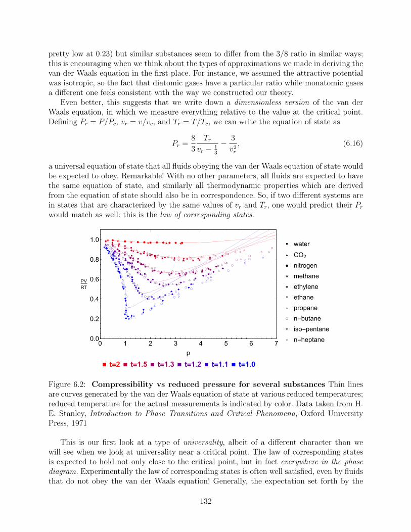
pretty low at 0.23) but similar substances seem to differ from the 3/8 ratio in similar ways;this is encouraging when we think about the types of approximations we made in deriving thevan der Waals equation in the first place. For instance, we assumed the attractive potentialwas isotropic, so the fact that diatomic gases have a particular ratio while monatomic gasesa different one feels consistent with the way we constructed our theory.

Even better, this suggests that we write down a dimensionless version of the van derWaals equation, in which we measure everything relative to the value at the critical point.Defining Pr = P/Pc, vr = v/vc, and Tr = T/Tc, we can write the equation of state as

Pr =8

3

Trvr − 1

3

− 3

v2r

, (6.16)

a universal equation of state that all fluids obeying the van der Waals equation of state wouldbe expected to obey. Remarkable! With no other parameters, all fluids are expected to havethe same equation of state, and similarly all thermodynamic properties which are derivedfrom the equation of state should also be in correspondence. So, if two different systems arein states that are characterized by the same values of vr and Tr, one would predict their Prwould match as well: this is the law of corresponding states.

0 1 2 3 4 5 6 70.0

0.2

0.4

0.6

0.8

1.0

p

PVRT

water

CO2 nitrogen

methane

ethylene

ethane

propane

n-butane

iso-pentane

n-heptane

t=2 t=1.5 t=1.3 t=1.2 t=1.1 t=1.0

Figure 6.2: Compressibility vs reduced pressure for several substances Thin linesare curves generated by the van der Waals equation of state at various reduced temperatures;reduced temperature for the actual measurements is indicated by color. Data taken from H.E. Stanley, Introduction to Phase Transitions and Critical Phenomena, Oxford UniversityPress, 1971

This is our first look at a type of universality, albeit of a different character than wewill see when we look at universality near a critical point. The law of corresponding statesis expected to hold not only close to the critical point, but in fact everywhere in the phasediagram. Experimentally the law of corresponding states is often well satisfied, even by fluidsthat do not obey the van der Waals equation! Generally, the expectation set forth by the

132

corresponding states hypothesis is that we should be able to write the equation of state as

P

Pc= f

(T

Tc,v

vc

)(6.17)

for some function f which might be related to the van der Waals derivation, but might becompletely different. A demonstration of this correspondence is shown in Fig. 6.2, showingthe ratio PV/T vs reduced pressure for several substances. None of them follow the vander Waals equation particularly well, but do demonstrate the expectation that, for instance,this ratio when plotted against reduced pressure at a fixed reduced temperature should beindependent of the fluid being measured.

6.3 Critical point behavior of a van der Waals fluid

To see why we might have expected the law of corresponding states, at least near a criticalpoint, let’s imagine expanding the equation of state close to the critical point6. We definethe reduced variables

π = Pr − 1 =P − PcPc

, ν = vr − 1, τ = Tr − 1,

in terms of which the reduced equation of state becomes

3ν3 + π(1 + ν)2(2 + 3ν) = 8τ(1 + ν)2. (6.18)

We’ll use this simplified form to study the relationship between our reduced variables andvarious thermodynamic quantities, and the compare those relationships to experimentallyobtained results.

Critical isotherm: Along the critical isotherm, for which τ = 0, we can easily expand Eq.6.18 for close to the critical point (i.e., for small π and ν), and we find

π ≈ −3

2ν3 ⇒ (P − Pc) ∼ (v − vc)3 . (6.19)

Volume differences: We next look at how ν depends on τ as the critical point is ap-proached from low temperatures. Rewriting Eq. 6.18 as

3ν3 + 8(π − 1)ν2 + (7π − 16τ)ν + 2(π − 4τ) = 0,

we next recognize that near the critical point the coexistence curve is symmetric. This meansthat near the critical point, when we consider the polynomial in ν, we should have two rootsthat are approximately equal in magnitude (with opposite signs), and a third root which isvery close to zero. Comparing this consideration to the above equation means that

π − 4τ ≈ 0⇒ π ≈ 4τ, (6.20)

and so for the other possible values of ν we need to solve ν2 + 8τν + 4τ = 0. Doing so gives

limT→T−c

ν ≈ ±2|τ |1/2 ⇒ limT→T−c

(vgas − vliquid) ∼ (Tc − T )1/2 . (6.21)

6afterwards, we’ll see why this approach has made a subtle but tremendously important mistake!

133

Critical isochore: Finally, for this comparison, we look at the isothermal compressibility,which is essentially determined by

κτ ∼ −∂ν

∂π

∣∣∣∣τ

≈ 2

7π + 9ν2 − 16τ.

If we approach the critical point along the critical isochore (ν = 0) from the high-temperatureside, we get

limT→T+

c

− ∂ν

∂π

∣∣∣∣τ

≈ 1

6τ⇒ lim

T→T+c

κT (vc) ∼ (T − Tc)−1 (6.22)

We did these calculations in the context of the van der Waals equation of state, butactually all we have really assumed is that our system is (a) mechanically stable and (b)analytic, in that close to the critical point we could expand the pressure like

P (T, v) = Pc + α(T − Tc)− a(T − Tc)(v − vc) +b

2(T − Tc)(v − vc)2 − c

6(v − vc)3 + · · · ,

where mechanical stability tells us that the coefficient a > 0 above Tc and c > 0 at Tc. Whatwe arrive at is a prediction of universal singular behavior near the critical point, with variousexponents characterizing the strength of the singularities.

Writing the above results using conventional names for the exponents, we can write

limT→T+

c

κT (vc) ∼ (T − Tc)−γ

limT→T−c

(vgas − vliquid) ∼ (Tc − T )β (6.23)

(P − Pc) ∼ (v − vc)δ .

In our mean field calculation we had

γ = 1, δ = 3, β = 1/2.

Experimentally, it is found that there are singularities in all of these quantities near thecritical point, but the exponents are

γ ≈ 1.2, δ ≈ 4.8, β ≈ 0.32

On the one hand, that’s not too bad! The δ exponent doesn’t look great, but β and γaren’t so far off. On the other hand, usually in physics we are willing to make “spherical cow”approximations as we build our theories – i.e. capturing the basic, often qualitative behaviorof some phenomenon of interest – as long as we are convinced that systematically improvingour approximations will lead to systematically closer quantitative agreement with reality.The (perhaps surprising!) fact is that until the development of the theory of modern criticalphenomena is was not possible even in principle to account for the difference between, say,γ = 1 in the theory and γ ≈ 1.2 in real life. After all, as emphasized a few paragraphsabove, all we have really done to come up with our theoretical critical exponents was assumestability and analyticity near the critical point! The physical systems are indeed stable,

134

so apparently we made some subtly but mightily wrong assumption when we treated theequation of state as analytic near the critical point.

As a hint at what went wrong, recall from the last chapter that the ratio 〈N2〉 / 〈N〉 ∝ κT ,but then we showed that near the critical point that the isothermal compressibility divergesnear the critical point. That is, the fluctuations in particle number are enormous relativeto the mean number: in short, our “mean field” assumption of uniform density cannot becorrect close to the critical point. Somehow, by neglecting these fluctuations we were led toqualitatively correct beliefs about the behavior of fluids (corresponding states, divergencesnear the critical point), but were left in a quantitative pickle, with no apparent systematicway to improve our understanding of the exponents. The final few sections of this course willintroduce a few of the big ideas in critical phenomenon; for those interested in more details Iparticularly like Goldenfeld’s Lectures on Phase Transitions and the Renormalization Groupand Kardar’s Statistical Physics of Fields.

6.4 Another mean field theory, more critical exponents

6.4.1 Mean-field Ising model

So far we have been focusing our set of examples heavily on fluids (ideal gases, dilute gases,van der Waals fluids below Tc...), and here we will briefly discuss a7 mean field theory forthe Ising model.

We consider a nearest-neighbor Ising model on a d-dimensional hypercubic lattice com-posed of spins s; the Hamiltonian for the spins, with coupling constant J in an externalfield B, is

H = −J∑〈ij〉

sisj −B∑i

si, (6.24)

and we are interested in the magnetization

m =1

N〈si〉 =

1

Nβ

∂(logZ)

∂B. (6.25)

A mean field approximation for this problem follows by writing the interactions betweenneighboring spins assuming the fluctuations of neighboring spins away from the average issmall. That is, we approximate

sisj = ([si −m] +m) ([sj −m] +m)

= (si −m)(sj −m) +m ((si −m) + (sj −m)) +m2

≈ m(si + sj)−m2, (6.26)

and our mean field Hamiltonian is just

H ≈ JNqm2

2− (Jqm+B)

∑i

si, (6.27)

7Just a comment: mean field theories are not unique descriptions of a system! There are often many waysto generate a mean field theory and the results need not be identical. In general, all mean field theories forthe same system will share the same scaling near a critical point, but will typically differ in their calculationsof of non-universal features.

135

where q is the number of nearest neighbors (q(d) = 2d for the hypercubic lattice). We havetransformed our problem into a non-interacting Ising model in an effective external field,where

Beff = B + Jqm.

The partition function is now easily expressible as N copies of the non-interacting case:

Z = e−βJNqm2/2(e−βBeff + eβBeff

)N= 2Ne−βJNqm

2/2 coshN (βBeff ) . (6.28)

Finally, we self-consistently determine what the value of m is using m = 1N〈si〉 = 1

Nβ∂(logZ)∂B

;the result is

m = tanh (βB + βJqm) . (6.29)

6.4.2 Critical point behavior

First, in the absence of an external field, our mean field equation is m = tanh (βJqm), andsince tanh x ≈ x − x3/3 + · · · the slope of m near the origin is βJq. If βJq < 1, the onlysolution to the mean field equation is m = 0; if, however, βJq > 1 there are three solutions:m = 0 or m = ±m0 (and the m = 0 solution turns out to be unstable, just like the putativemiddle solution for the volume at a particular pressure when T < Tc in the van der Waalsequation).

Given this zero-field critical temperature, kBTc = Jq, let’s define the reduced inversetemperature τ = Tc/T , let’s apply the hyperbolic trig identity

tanh (a+ b) =tanh a+ tanh b

1 + tanh a tanh b

to Eq. 6.29 to obtain

tanh (βB) =m− tanh (mτ)

1−m tanh (mτ). (6.30)

Close to the critical point, where we expect both the field and the magnetization to be small,we can expand this to obtain

βB ≈ m(1− τ) +m3

(τ − τ 2 +

τ 3

3+ · · ·

)+ · · · (6.31)

From this, we can read off some critical exponents. In the absence of an external field wecan approach Tc from below, and we see

m2 ∼ Tc − TTc

+ · · · ⇒ m ∼ ± (Tc − T )1/2 . (6.32)

Conventionally, this critical exponent is called β, and here β = 1/2.We can also look at how the external field and the magnetization are related along the

crtical isotherm (here, denoted τ = 1). We immediately see

B ∼ m3; (6.33)

136

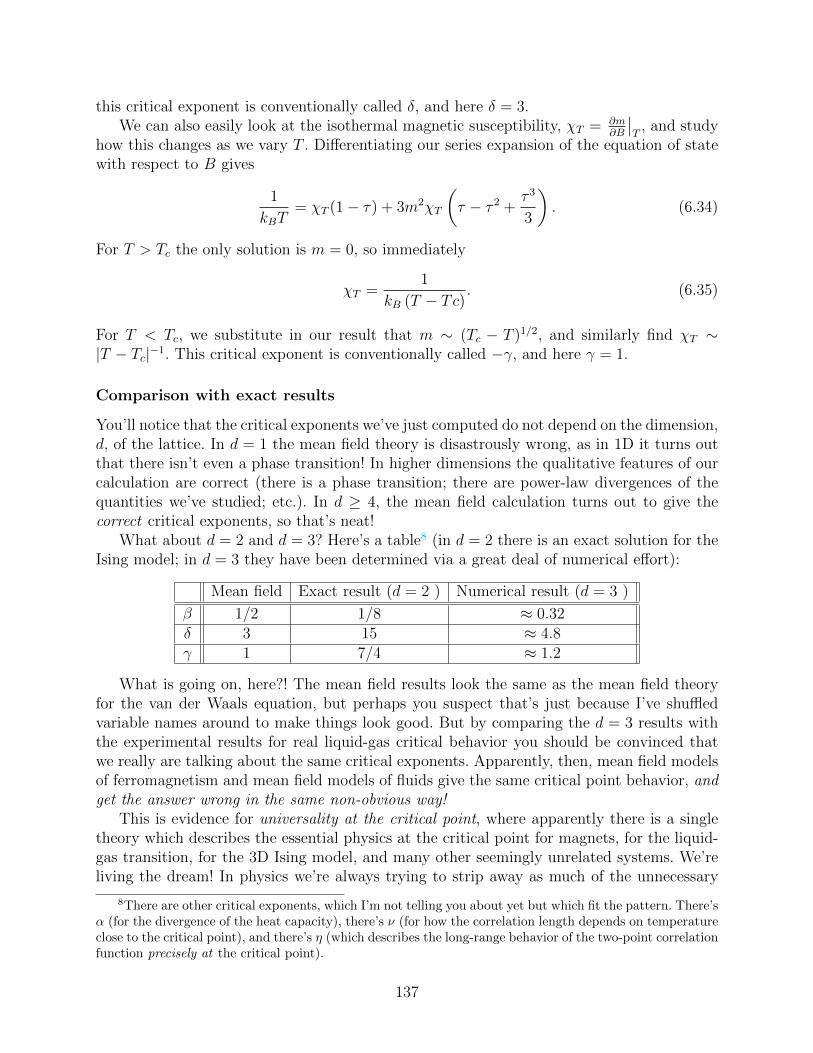
this critical exponent is conventionally called δ, and here δ = 3.We can also easily look at the isothermal magnetic susceptibility, χT = ∂m

∂B

∣∣T

, and studyhow this changes as we vary T . Differentiating our series expansion of the equation of statewith respect to B gives

1

kBT= χT (1− τ) + 3m2χT

(τ − τ 2 +

τ 3

3

). (6.34)

For T > Tc the only solution is m = 0, so immediately

χT =1

kB (T − Tc). (6.35)

For T < Tc, we substitute in our result that m ∼ (Tc − T )1/2, and similarly find χT ∼|T − Tc|−1. This critical exponent is conventionally called −γ, and here γ = 1.

Comparison with exact results

You’ll notice that the critical exponents we’ve just computed do not depend on the dimension,d, of the lattice. In d = 1 the mean field theory is disastrously wrong, as in 1D it turns outthat there isn’t even a phase transition! In higher dimensions the qualitative features of ourcalculation are correct (there is a phase transition; there are power-law divergences of thequantities we’ve studied; etc.). In d ≥ 4, the mean field calculation turns out to give thecorrect critical exponents, so that’s neat!

What about d = 2 and d = 3? Here’s a table8 (in d = 2 there is an exact solution for theIsing model; in d = 3 they have been determined via a great deal of numerical effort):

Mean field Exact result (d = 2 ) Numerical result (d = 3 )

β 1/2 1/8 ≈ 0.32δ 3 15 ≈ 4.8γ 1 7/4 ≈ 1.2

What is going on, here?! The mean field results look the same as the mean field theoryfor the van der Waals equation, but perhaps you suspect that’s just because I’ve shuffledvariable names around to make things look good. But by comparing the d = 3 results withthe experimental results for real liquid-gas critical behavior you should be convinced thatwe really are talking about the same critical exponents. Apparently, then, mean field modelsof ferromagnetism and mean field models of fluids give the same critical point behavior, andget the answer wrong in the same non-obvious way!

This is evidence for universality at the critical point, where apparently there is a singletheory which describes the essential physics at the critical point for magnets, for the liquid-gas transition, for the 3D Ising model, and many other seemingly unrelated systems. We’reliving the dream! In physics we’re always trying to strip away as much of the unnecessary

8There are other critical exponents, which I’m not telling you about yet but which fit the pattern. There’sα (for the divergence of the heat capacity), there’s ν (for how the correlation length depends on temperatureclose to the critical point), and there’s η (which describes the long-range behavior of the two-point correlationfunction precisely at the critical point).

137

detail from a system as we can, and apparently near a critical point “Nature” does all thehard work for us!

As an aside, the pattern we saw above as we varied the dimension of our model understudy is pretty generic: when you write down a mean field theory there is a dimension ator below which which the theory fails completely (called the lower critical dimension, dl),a dimension at or above which the theory gives the right answers (called the upper criticaldimension, dc). For dl < d < dc mean field theory often returns crudely correct phasediagrams that are wrong or, worse, misleading near critical points. Sadly for mean fieldtheory, life tends to happen in between dl and dc.

6.5 Landau’s phenomenological theory

If seemingly very different mean field theories – for very different physical systems! – giverise to the same essential behavior near their respective critical points, your instinct is thatthere ought to be a unified way of looking at phase transitions that reveals why this shouldbe the case. Landau’s phenomenological theory9 of phase transitions serves exactly thisrole, focusing on understanding the universal behavior of physical systems based on twogeneral considerations: analyticity and symmetry. The Landau approach to phase transitionsis typically only qualitatively correct (as we are about to see, it gives exactly the samecritical exponents as mean field theory), but it (a) let’s us understand universality and (b)is extremely straightforward, letting you compute mean field critical exponents for systemsin different universality classes with typically great rapidity.

Landau theory postulates the existence of an object, L, called the Landau free energydensity (it is not a thermodynamic free energy density, and it need not be convex). Thetheory starts by identifying an order parameter of the system, η, which is a quantity that istypically zero in a high-temperature or disordered phase, and non-zero in an ordered phase:For the liquid-gas transition one can take the difference in densities between the phases(η = vgas − vliquid), for the Ising model magnet we can take the magnetization (η = m),for a superconductor it is related to off-diagonal long-range order in the one-particle densitymatrix, etc. Order parameters for a particular system need not be unique, and depending onthe nature of the problem they can be scalars, vectors, etc., although here we will assume itis a scalar.

Once we have identified an order parameter, we want to construct an L that will act likea free energy density (and has dimensions of energy per volume), insofar as we will computethermodynamic quantities by taking appropriate derivatives of L. We construct L via thefollowing constraints:

1. The state of the system is specified by the global minimum of L with respect to η.

2. L must be consistent with the symmetries of the system.

3. Near the critical point, L is an analytic function of η and any coupling constants, which

9To be distinguished from a version of Landau theory which is motivated by systematic calculationstarting with a microscopic Hamiltonian. This more complicated version is typically not more insightful.

138

I’ll denote as K here. Thus, for instance, for a spatially uniform system we can write

L =∑n=0

an(K)ηn (6.36)

4. In the disordered phase the order parameter should be η = 0, while it should be smalland non-zero in the ordered phase.

The Landau free energy density for a magnetic system

Let’s see how these constraints let us build L for a particular example: we’ll choose the kindof Ising model we just discussed in the last section. By the third and the fourth constraint,near Tc we can expand L as a Taylor series, and since we expect η to be small, we don’t needto go to very high order. We’ll write

L =4∑

n=0

anηn, (6.37)

where the coefficients an could depend on the Ising model coupling term J , the external fieldB, the temperature T , or whatever else happens to be in our model.

Additionally, from the first constraint we have that L is extremized by solving

∂L∂η

= a1 + 2a2η + 3a3η2 + 4a4η

3 = 0. (6.38)

Since we want η = 0 to be the solution for T > Tc, we have a1 = 0.Finally, what about the symmetry constraint? Consider our Ising model in the absence

of any external field, B = 0: certainly the Hamiltonian here is invariant under the flipping ofevery spin10, and we expect that the probability of finding the system with a particular valueof the magnetization has the property P (η) = P (−η). We expect, since we want L to behavelike a free energy, that P ∼ exp (−βL), so we require for this model that L(η) = L(−η). Thefact that L is even implies that in our Taylor series ai = 0 for every odd value of i. Thus, wehave

L = a0 + a2η2 + a4η

4 +O(η6), (6.39)

with the additional constraint that a4 > 0 (if it is not, then L above would be minimized byη →∞, and we want η to be finite and small... if a4 is negative for a particular system, oneneeds to include higher order terms to stabilize the system.

What remains is to ask, for the Ising ferromagnet, about the temperature dependence ofthe coefficients ai. First11, a0 is the value of L in the high temperature phase, and in generalwe expect this coefficient to vary smoothly (i.e., without divergence) through the criticaltemperature. It represents, in a sense, degrees of freedom which are not described by (andare certainly not coupled to) the order parameter; it may be important for some detailedcalculations, but we will typically set it to zero.

10Including the field, the Ising model has Z2 symmetry associated with H(B, J, si) = H(−B, J,−si)11or zeroth

139

Next, we expand the fourth-order coefficient as

a4 = a(0)4 +

T − TcTc

a(1)4 + · · · , (6.40)

where the notation indicates the part of the coefficient associated with a particular order ofthis series expansion. As it turns out, the temperature dependence in a4 does not controlthe overall behavior of the system near Tc, so we will just assume that a4 is some positiveconstant.

That leaves only a2, which we similarly expand:

a2 = a(0)2 +

T − TcTc

a(1)2 + · · · .

Once again, though, we want to find η = 0 for T > Tc and η 6= 0 for T < Tc. Comparingwith Eq. 6.38, whose solution (for a1 = a3 = 0) is

η = 0 or η = ±√−a2

2a4

, (6.41)

we see that we want to set a(0)2 = 0 and a

(1)2 to some positive constant to ensure that the

order parameter is non-zero below Tc. Thus

a2 =T − TcTc

a(1)2 + · · · , (6.42)

and as with a4, it is this lowest order term which dominates behavior near the critical point.Finally, we now reintroduce the possibility of an external field. This breaks the even

symmetry of the system, and we know from the Ising model Hamiltonian that it adds ana1 = −B term. Dropping some of the cumbersome notation and introducing a and b asphenomenological constants, we have our final expression for the Landau free energy densityfor the Ising model universality class in the absence of spatial variations:

L = −Bη + atη2 +b

2η4, where t =

T − TcTc

(6.43)

In principle we are allowed by symmetry to now also add an a3 term; a calculation reveals thatit is not a leading term near the critical point, so we’ve neglected it for now. In general, L isconstructed by writing down all possible scalar terms which are powers of the order parameter(or the order parameter components, if the order parameter itself is more complicated thana scalar that are consistent with the symmetry of the system.

Critical exponents

For the above L, we now compute a few critical exponents. The β exponent is the one thatcharacterizes the divergence of m with t below Tc. From the above, we already know that

η =

√−at2b

, (6.44)

140

so we read off β = 1/2.We next differentiate L with respect to η to find the magnetic equation of state:

B = 2atη + 2bη3. (6.45)

On the critical isotherm (t = 0) we immediately see B ∼ η3, and this is our δ = 3 exponent.The isothermal magnetic susceptibility is

χT =∂η(B)

∂B

∣∣∣∣T

=1

2 (at+ 3bη(B)2), (6.46)

where η(B) is the value of the order parameter in the presence of the external field, i.e., thesolution to Eq. 6.45. The exponent γ characterizes the divergence of the susceptibility atzero field. For t > 0 we know η = 0 so χT = (2at)−1. For t < 0 we know η = (−at/b)1/2 soχT = (−4at)−1. In either case, γ = 1.

Ignoring fluctuations... not variations

We very briefly note that Landau theory neglects the (important!) effects of fluctuations, butit does not only apply to homogeneous systems. It is straightforward to generalize the ideasabove to the case where the order parameter can be a spatially varying one: η = η(r), andif this were a class on statistical field theory we would spend a lot of time thinking aboutthese cases (this would also let us write down critical exponents related to the divergence ofcorrelation lengths in the system). When we do treat spatially inhomogeneous systems, weneed to add the constraint that

5. L should be a local function, depending only on a finite number of spatial gradients ofthe order parameter.

As with the earlier construction, the gradient terms we write down must be consistent withthe symmetry of the system; for the Ising model where we keep only even terms, the lowestorder term is the square of the gradient, which would give the Landau free energy of

L =

∫dr[L (η(r)) + ζ (∇η(r))2] , (6.47)

where ζ is some new positive constant and L is the homogenous L of the preceding notes. Ingeneral for this symmetry there are also terms like (∇η)4 and (∇2η)2), etc., and here we’vejust written the lowest order gradient term12.

Just a note about statistical field theories.12“Why isn’t there a term like η∇2η, which is of the same order as the term we did use, it’s perfectly

isotropic, and it has the right m→ −m symmetry?” I hear you asking. The above form is customary becausewe know the identity

∇ · (η∇η) = η∇2η + (∇η)2,

which implies ∫dr η∇2η = −

∫dr (∇η)2 +

∫dS · η∇η.

In the thermodynamic limit we neglect the surface term, so in general we pick either (∇η(r))2

or η∇2η, butnot both.

141

6.6 Correlations and fluctuations

Having introduced the idea that the order parameter might have spatial variations, we nowintroduce a dimensionless two-point correlation function:

G(r − r′) =1

η2

[〈η(r)η(r′)〉 − η2

]=

1

η2〈(η(r)− η) (η(r′)− η)〉 . (6.48)

This quantity measures correlations between the fluctuations of the order parameter at dif-ferent distances13, and it is deeply linked to some of the thermodynamic properties of thesystem.

For instance, suppose as the order parameter we chose the spatially varying density field,ρ(r). The total number of particles is N =

∫ddrρ(r), and the integral over G is∫

ddrddr′G(r − r′) =1

ρ2

∫ddrddr′

[〈ρ(r)ρ(r′)〉 − ρ2

]=

1

ρ2

[⟨N2⟩− 〈N〉2

]. (6.49)

Translational symmetry gives us one of the integrals over G for free, and we recognize aconnection between the number fluctuations and the isothermal compressibility of the system.Combing everything, then, gives us∫

ddrG(r) = kBTκT . (6.50)

This is an example of a fluctuation-susceptibility relation, and is the equilibrium limit of themore general fluctuation-dissipation relation.

6.6.1 Correlation function for a specific model

To be definite, let’s calculate the two-point correlation function for a system described bythe Ising universality class Landau theory. The spatially varying order parameter will beη(r), the external field will be B(r), and we’ll write the Landau free energy as

L =

∫ddr

[(at)η2 +

1

2bη4 −Bη +

c

2(∇η)2

], (6.51)

where a, b, c are phenomenological parameters and t is the reduced distance to the criticalpoint. If the system was uniform we would relate the typical value of the order parameter tothe appropriate derivative of the free energy: 〈η〉 = − ∂L

∂B. In the presence of spatial variations,

these partial derivatives get replaced by functional derivatives.

Functional differentiation

Suppose F [η(r)] is a functional14 of η(r). The functional derivative of F with respect to thefunction η is defined as

δF

δη(r′)= lim

ε→0

F [η(r) + εδ(r − r′)]− F [η(r)]

ε. (6.52)

13We have assumed translational symmetry in writing G(r − r′); more generally we would have G(r, r′)14Just as a function is a map – accepting, say, a set of numbers and returning an output number – a

functional is a map that accepts a function of a set of numbers and returns an output number

142

This generalizes the definition of the usual derivative, and the operation satisfies propertieslike

δ

δη(r)

∫ddr′η(r′) = 1

δ

δη(r)η(r′) = δ(r − r′) (6.53)

δ

δη(r)

∫ddr′

1

2(∇η(r′))

2= −∇2η(r).

That last expression, which you probably can see that we’re about to use, involves an inte-gration by parts that neglects the surface term.

Linear response

With those definitions, we compute the expectation value of the order parameter via func-tional differentiation:

〈η(r)〉 = − δL

δB(r). (6.54)

This implies that a small change in the external field would cause a small change in theLandau energy

δL = −∫

ddr′ 〈η(r′)〉 δB(r′). (6.55)

Since the susceptibility is a measure of how the order parameter changes when the fieldchanges, we have

χT (r, r′) = − δ

δB(r′)

(δL

δB(r)

). (6.56)

Treating L as if it is related to a partition function, L = −kBT logZ (for the purposes ofremembering which thermodynamic derivatives we want to take), we re-write this as

χT (r, r′) = kBT

[1

Z

δ2Z

δB(r)δB(r′)− 1

Z

δZ

δB(r)

1

Z

δZ

δB(r′)

]= β [〈η(r)η(r′)〉 − 〈η(r)〉 〈η(r′)〉]= βG(r − r′), (6.57)

again connecting response functions with correlation functions. Note that, using tildes todenote Fourier transforms, one connects isothermal susceptibility with the wave-vector de-pendent susceptibility χ(k) = βG(k) as

χT ≡ limk→0

χ(k) = β G(k)∣∣∣k=0

= β

∫ddrG(r), (6.58)

as in Eq. 6.50.

143

The correlation function

Enough dithering, let’s calculate the two-point correlation function from Eq. 6.51. To dothis, we extremize the Landau free energy to find the spatially varying field that the systemwill adopt in equilibrium. I.e., we set δL

δη(r)= 0. This tells us that η(r) must satisfy

2atη(r) + 2bη3(r)−B(r)− c∇2η(r) = 0. (6.59)

We then (functionally) differentiate this expression with respect to the spatially varying field:

δ

δB(r′)

[2atη(r) + 2bη3(r)−B(r)− c∇2η(r)

]= 0

⇒ β[−c∇2 + 2at+ 6bη2(r)

]G(r − r′) = δ(r − r′). (6.60)

Well, would you look at that! The correlation function is a Green’s function; seems like aretroactively good reason to have used G for it...

We can simplify the above expression by noting that for translationally invariant systemsthe order parameter η we want is just the equilibrium value from the homogenous Landautheory calculation we did earlier: η = 0 for t > 0 and η = ±

√−at/b for t < 0. We now

introduce the correlation length, ξ, noting that G(r − r′) satisfies(−∇2 + ξ−2(t)

)G(r − r′) =

kBT

cδ(r − r′), (6.61)

where

ξ(t) =

√c

2atfor t > 0√

− c4at

for t < 0

∼ |t|−1/2. (6.62)

Great, given that G(r−r′) satisfies such an equation, what does it look like? The Fouriertransform of Eq. 6.61 gives

G(k) =kBT

c

1

k2 + ξ−2. (6.63)

Evaluated at k = 0, this gives us the isothermal susceptibility (a measurable quantity forthe system) in terms of the microscopic parameter c and the correlation length:

χT = βG(0) =ξ2

c,

with which we can write the two-point correlation function as

G(k) =kBTχT (t)

1 + k2ξ2. (6.64)

In real space one can take the inverse Fourier transform (i.e. “look it up in a table”), or onecan solve the real-space differential equation in polar coordinates. I’ll spare you the detailsfor now. Using the correlation length as our unit of length and defining ρ = r/ξ, the resultis:

c

kBTξd−2G(ρ) =

e−r/ξ for d = 1

K d−22

(r/ξ)

(2π)d/2(r/ξ)(d−2)/2 for d ≥ 2, (6.65)

144

where the Kn are modified spherical Bessel functions of the third kind. We really are mostinterested in the short- and long-range behavior of these functions, which are

Kn(x) ∼(π2x

)1/2e−x, for x→∞

Kn(x) ∼ Γ(n)2

(x2

)−n, for x→ 0 (6.66)

K0(x) ∼ − log x , for x→ 0.

Combining everything, very close to Tc the correlation length has diverged, so we justneed the r ξ limit of the Kn. For d = 2 we use the special log form appropriate to K0,and for d > 2 all of the powers of ξ conveniently cancel out, giving us

G(r) ∼

log (ξ/r) for d = 2r2−d for d > 2

. (6.67)

Far from the critical point, though, ξ is small; taking the r ξ limit of the Kn gives (ford ≥ 2)

G(r) ∼ kBT

c

exp (−r/ξ)r(d−1)/2

1

ξ(d−3)/2, (6.68)

where I’ve dropped prefactors related to 2’s and π’s for simplicity.

Comments on the correlation length

From the preceding analysis, and from the definition of G(r), we see that ξ is a measureof the spatial extent over which correlations extend. In mean field models of the Ising typewe predicted ξ ∼ |t|−1/2; far from the critical temperature the correlation length will beon the same scale as something microscopic (distance between spins, or the range of theattractive part of the Lennard-Jones interaction, or...), and any fluctuations in the localorder parameter away from the average value will quickly wash out.

As T → Tc, though, ξ → ∞, and correlations can extend over the entire system. Eventhough the actual interactions in the system are short-ranged, long-range order can prop-agate. Since the correlations are essentially macroscopic, the microscopic differences thatdistinguish one system from another likely are irrelevant at such macroscopic scales; this isan important clue for building a general understanding of critical phenomena.

6.7 Critical exponents

We pause to briefly summarize (and comment on) the most important critical exponentsthat characterize various systems. In all of these cases we are investigating the idea that,close to the critical point, some thermodynamic quantity has the limiting form of a powerlaw. Letting t = (T − Tc)/Tc and looking a quantity f , when we write

f(t) ∼ tλ

what we mean is

λ = limt→0

log f(t)

log t. (6.69)

145

This is a particularly relevant point when remembering (a) there may be other, non-dominantpower law behavior near the exponent; we are capturing just the leading order term, and (b)sometimes we quote an exponent as having the value zero. This can either mean that thethermodynamic quantity has a discontinuity or that it has a logarithmic divergence ratherthan a power-law one. This last possibility comes from comes from using the identity

log t = limλ→0

[1− e−λ log t

λ

]= lim

λ→0

[1− t−λ

λ

]. (6.70)

Suppose we are considering a system with Landau free energy L, order parameter m, andordering field B.

δ : All critical exponents except for this one are evaluated at B = 0. In the presence of thefield, though, δ characterizes the relationship between the field and the order parameter:

m ∼ B1/δ. (6.71)

α : The divergence of the heat capacity is measured via α. In principle, the divergencecould be different on the two sides of the transition, which is commonly denoted by writingα for the divergence above Tc and α′ for the divergence below Tc.

C = −T ∂2L∂T 2

∼ |t|−α. (6.72)

In mean field α = 0 (in the form of a discontinuity); the Ising model has α = 0 (in the logdivergence form) for d = 2 and α ≈ 0.11 for d = 3.

β : Below the critical temperature, where the order parameter is non-zero, it diverges like

m ∼ |t|β. (6.73)

γ : The divergence of the low-field susceptibility is measured by γ; it, too, can in principlehave different values above and below the transition:

χ =∂m

∂B

∣∣∣∣B=0

∼ |t|−γ. (6.74)

ν : The last two critical exponents on this list are related to the behavior of the two pointcorrelation function. We did a mean-field calculation that suggested the correlation lengthdiverged near t = 0 like ξ ∼ |t|−1/2. There’s no reason to expect for real systems that themean field prediction here is correct, so we introduce ν:

ξ ∼ |t|−ν . (6.75)

Mean field theory for the Ising universality class has ν = 1/2, ν = 1, 0.63 in two and threedimensional Ising models, respectively.

146

η : Finally, we want to characterize how the two-point correlation function behaves preciselyat the critical point (t = 0). Our mean field theory (using the r ξ limit of the Kn)predicted that G(r) ∼ r−(d−2), and again, we expect real experiments could differ from this.We introduce the exponent η to measure how wrong mean field is at t = 0:

G(r) ∼ r−(d−2+η). (6.76)

Mean field theory for the Ising universality class has η = 0, η = 1/4, 0.032 in the two andthree dimensional Ising models, respectively. Experimentally these small exponents are hardto measure

6.7.1 Dimensional analysis and mean field theory

To emphasize just how surprising it should be that mean field theory gets the critical ex-ponents wrong, and the surprising sense in which a diverging correlation length does notmean that the system has completely forgotten about microscopic length scales, let’s writea dimensionless version of the Landau free energy of the Ising type in the absence of anexternal field:

βL =

∫ddr

1

2(∇φ)2 +

r0

2φ2 +

1

4u0φ

4. (6.77)

In terms of our earlier expressions, this is just writing

φ = η√βc, r0 =

2at

c, u0 =

2b

βc2. (6.78)

Let’s think about the correlation function in terms of basic dimensional analysis. Using thebracket notation to denote the dimension of various quantities, we have [βL] = 1 (i.e., isdimensionless), so each separate term in the integrand must be dimensionless, too. Thus:[∫

ddr(∇φ)2

]= 1⇒ (xd)(x−2) [φ]2 = 1, (6.79)

where x denotes units of length. From this, we immediately get

[φ] = x1−d/2, [r0] = x−2, [u0] = xd−4. (6.80)

So, what does dimensional analysis say about the correlation length? Clearly [ξ] = x,but from the above equation the only independent quantity with units of length is r0, withdimensions [r0] = x−2. So, apparently, we’re done: by dimensional analysis we get that

ξ ∼ r−1/20 ∼ |t|−1/2,

where in the last line we remember that r0 ∝ t. In some sense, then, the deep mystery ishow could this have been wrong?

The answer is that we ignored one other source of an independent length scale in ourdimensional analysis! In particular, there is a microscopically small length scale embeddedin the problem – say, the spacing between lattice sites in our Ising model – an apparently ifmean field is wrong we need to include this length scale.

147

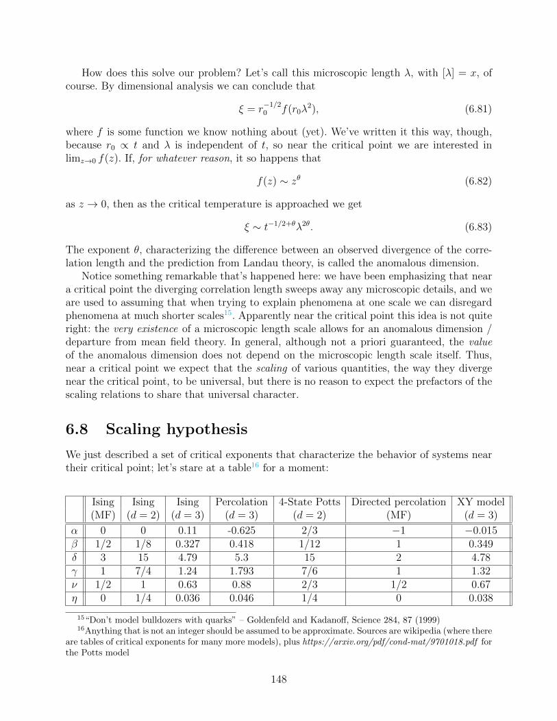
How does this solve our problem? Let’s call this microscopic length λ, with [λ] = x, ofcourse. By dimensional analysis we can conclude that

ξ = r−1/20 f(r0λ

2), (6.81)

where f is some function we know nothing about (yet). We’ve written it this way, though,because r0 ∝ t and λ is independent of t, so near the critical point we are interested inlimz→0 f(z). If, for whatever reason, it so happens that

f(z) ∼ zθ (6.82)

as z → 0, then as the critical temperature is approached we get

ξ ∼ t−1/2+θλ2θ. (6.83)

The exponent θ, characterizing the difference between an observed divergence of the corre-lation length and the prediction from Landau theory, is called the anomalous dimension.

Notice something remarkable that’s happened here: we have been emphasizing that neara critical point the diverging correlation length sweeps away any microscopic details, and weare used to assuming that when trying to explain phenomena at one scale we can disregardphenomena at much shorter scales15. Apparently near the critical point this idea is not quiteright: the very existence of a microscopic length scale allows for an anomalous dimension /departure from mean field theory. In general, although not a priori guaranteed, the valueof the anomalous dimension does not depend on the microscopic length scale itself. Thus,near a critical point we expect that the scaling of various quantities, the way they divergenear the critical point, to be universal, but there is no reason to expect the prefactors of thescaling relations to share that universal character.

6.8 Scaling hypothesis

We just described a set of critical exponents that characterize the behavior of systems neartheir critical point; let’s stare at a table16 for a moment:

Ising Ising Ising Percolation 4-State Potts Directed percolation XY model(MF) (d = 2) (d = 3) (d = 3) (d = 2) (MF) (d = 3)

α 0 0 0.11 -0.625 2/3 −1 −0.015β 1/2 1/8 0.327 0.418 1/12 1 0.349δ 3 15 4.79 5.3 15 2 4.78γ 1 7/4 1.24 1.793 7/6 1 1.32ν 1/2 1 0.63 0.88 2/3 1/2 0.67η 0 1/4 0.036 0.046 1/4 0 0.038

15“Don’t model bulldozers with quarks” – Goldenfeld and Kadanoff, Science 284, 87 (1999)16Anything that is not an integer should be assumed to be approximate. Sources are wikipedia (where there

are tables of critical exponents for many more models), plus https://arxiv.org/pdf/cond-mat/9701018.pdf forthe Potts model

148

In the early 60s, as mean field results were known and as some finite-dimensional estimateswere obtained by numerical estimates, people started noticing that these exponents did notseem to be independent. For instance, the exponent values seem to satisfy

α + 2β + γ = 2 (6.84)

γ − β(δ − 1) = 0 (6.85)

γ − ν(2− η) = 0, (6.86)

which are often called the Rushbrooke, Widom, and Fisher identities, respectively. Sincethen, there have been various proofs that thermodynamics requires (via, say, the convexityof the free energy, or the relative sizes of CP and CV certain inequalities to be satisfied, forinstance

α + 2β + γ ≥ 2,

but that in the actual data these thermodynamic inequalities are saturated.

6.8.1 The static scaling hypothesis

The static scaling hypothesis17 is an attempt to encode multiple features of the behaviorof a system near the critical point in a single expression; as we will see, assuming thishypothesis allows one to strengthen the thermodynamic inequalities mentioned above forthe relationships between exponents into equalities – which is good, because the equalitiesare satisfied.

Let’s focus on a magnetic system, where just to keep you on your toes I’ll write m for themagnetization and h for the external field (in units of kBT ); t will still stand for the reduceddistance to the critical point. We want to simultaneously encode two things we have alreadyseen:

m(t = 0, h) = ±C1|h|1/δ and m(t, h = 0) =

0 t > 0

±C2|t|β t < 0. (6.87)

One of Widom’s many insights was that, staying in a regime where |t| 1 and |h| 1,both of these results can be expressed as

m(t, h) =

tβF+(h/t∆) t > 0

(−t)βF−(h/(−t)∆) t < 0, (6.88)

where we assume that β and the gap exponent ∆ are universal, as are the scaling functionsabove and below the critical temperature, F+ and F−. At first glance we don’t know verymuch about these scaling functions, but the requirement that Eq. 6.88 reproduce the resultsin Eq. 6.87 will let us both put some constraints on F+ and F− and also derive relationshipsbetween the critical exponents.

First, we’ll show that the gap exponent is actually not a new critical exponent at all!Consider the susceptibility in the low-field limit, χT ∝ ∂m

∂h

∣∣h=0

. Differentiating Eq. 6.88 withrespect to h gives

χT ∝ |t|β∂F±(h/|t|∆)

∂h

∣∣∣∣h=0

∝ |t|β

|t|∆∂F±(x)

∂x

∣∣∣∣x=0

∼ |t|β−δF ′±(0). (6.89)

17B. Widom, (1963)

149

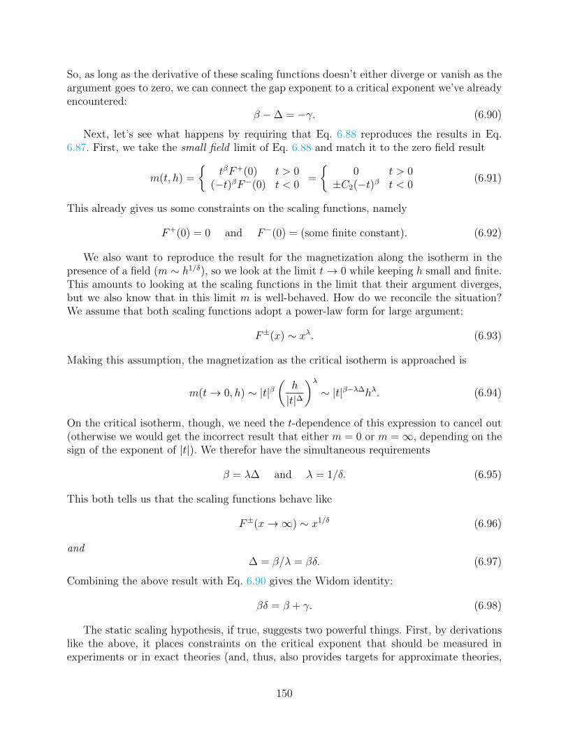
So, as long as the derivative of these scaling functions doesn’t either diverge or vanish as theargument goes to zero, we can connect the gap exponent to a critical exponent we’ve alreadyencountered:

β −∆ = −γ. (6.90)

Next, let’s see what happens by requiring that Eq. 6.88 reproduces the results in Eq.6.87. First, we take the small field limit of Eq. 6.88 and match it to the zero field result

m(t, h) =

tβF+(0) t > 0

(−t)βF−(0) t < 0=

0 t > 0

±C2(−t)β t < 0(6.91)

This already gives us some constraints on the scaling functions, namely

F+(0) = 0 and F−(0) = (some finite constant). (6.92)

We also want to reproduce the result for the magnetization along the isotherm in thepresence of a field (m ∼ h1/δ), so we look at the limit t→ 0 while keeping h small and finite.This amounts to looking at the scaling functions in the limit that their argument diverges,but we also know that in this limit m is well-behaved. How do we reconcile the situation?We assume that both scaling functions adopt a power-law form for large argument:

F±(x) ∼ xλ. (6.93)

Making this assumption, the magnetization as the critical isotherm is approached is

m(t→ 0, h) ∼ |t|β(

h

|t|∆

)λ∼ |t|β−λ∆hλ. (6.94)

On the critical isotherm, though, we need the t-dependence of this expression to cancel out(otherwise we would get the incorrect result that either m = 0 or m =∞, depending on thesign of the exponent of |t|). We therefor have the simultaneous requirements

β = λ∆ and λ = 1/δ. (6.95)

This both tells us that the scaling functions behave like

F±(x→∞) ∼ x1/δ (6.96)

and∆ = β/λ = βδ. (6.97)

Combining the above result with Eq. 6.90 gives the Widom identity:

βδ = β + γ. (6.98)

The static scaling hypothesis, if true, suggests two powerful things. First, by derivationslike the above, it places constraints on the critical exponent that should be measured inexperiments or in exact theories (and, thus, also provides targets for approximate theories,

150

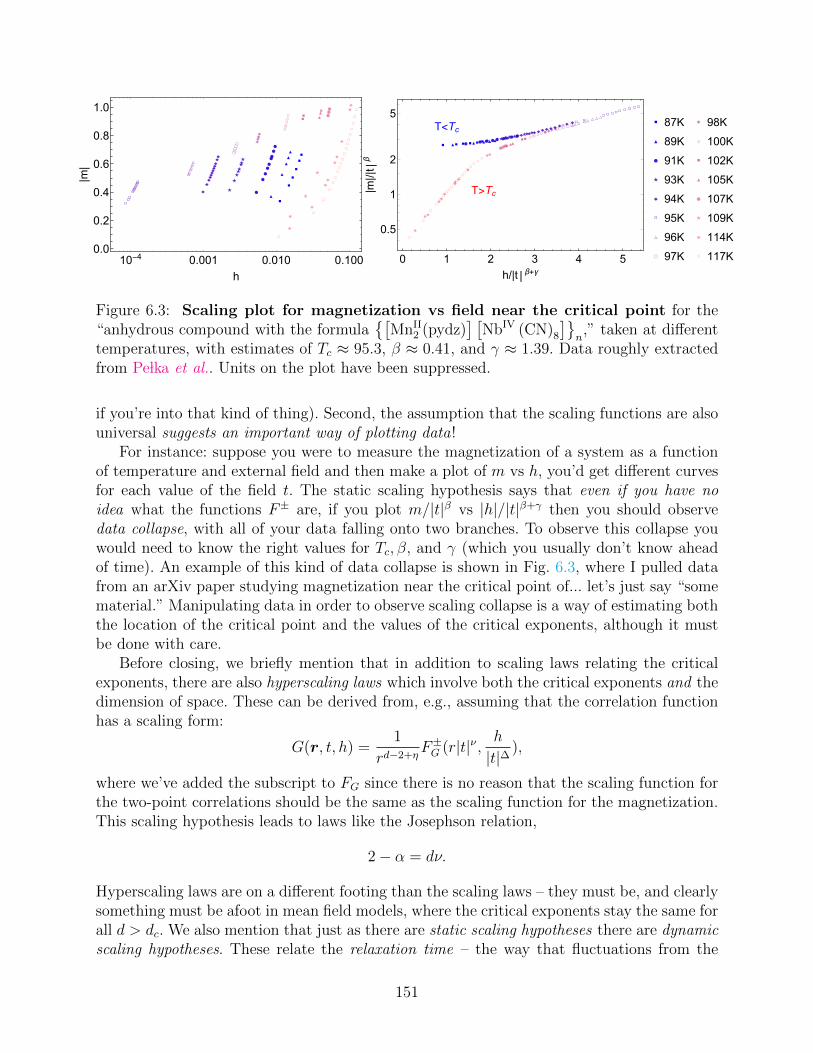
10-4 0.001 0.010 0.1000.0

0.2

0.4

0.6

0.8

1.0

h

|m|

T>Tc

0 1 2 3 4 5

0.5

1

2

5

h/|t β+γ

|m|/|t

β

T<Tc 87K

89K

91K

93K

94K

95K

96K

97K

98K

100K

102K

105K

107K

109K

114K

117K

Figure 6.3: Scaling plot for magnetization vs field near the critical point for the“anhydrous compound with the formula

[MnII

2 (pydz)] [

NbIV (CN)8

]n,” taken at different

temperatures, with estimates of Tc ≈ 95.3, β ≈ 0.41, and γ ≈ 1.39. Data roughly extractedfrom Pe lka et al.. Units on the plot have been suppressed.

if you’re into that kind of thing). Second, the assumption that the scaling functions are alsouniversal suggests an important way of plotting data!

For instance: suppose you were to measure the magnetization of a system as a functionof temperature and external field and then make a plot of m vs h, you’d get different curvesfor each value of the field t. The static scaling hypothesis says that even if you have noidea what the functions F± are, if you plot m/|t|β vs |h|/|t|β+γ then you should observedata collapse, with all of your data falling onto two branches. To observe this collapse youwould need to know the right values for Tc, β, and γ (which you usually don’t know aheadof time). An example of this kind of data collapse is shown in Fig. 6.3, where I pulled datafrom an arXiv paper studying magnetization near the critical point of... let’s just say “somematerial.” Manipulating data in order to observe scaling collapse is a way of estimating boththe location of the critical point and the values of the critical exponents, although it mustbe done with care.

Before closing, we briefly mention that in addition to scaling laws relating the criticalexponents, there are also hyperscaling laws which involve both the critical exponents and thedimension of space. These can be derived from, e.g., assuming that the correlation functionhas a scaling form:

G(r, t, h) =1

rd−2+ηF±G (r|t|ν , h

|t|∆),

where we’ve added the subscript to FG since there is no reason that the scaling function forthe two-point correlations should be the same as the scaling function for the magnetization.This scaling hypothesis leads to laws like the Josephson relation,

2− α = dν.

Hyperscaling laws are on a different footing than the scaling laws – they must be, and clearlysomething must be afoot in mean field models, where the critical exponents stay the same forall d > dc. We also mention that just as there are static scaling hypotheses there are dynamicscaling hypotheses. These relate the relaxation time – the way that fluctuations from the

151

typical order parameter decay away – to the correlation length, and bring with them bothnew critical exponents and new relationships between those exponents.

Finally, you may be wondering where these scaling laws in fact derive from. The mainphysical idea is the diverging correlation length, ξ, is responsible for all of the singularbehavior near the critical point. We’ve already indicated that this vague statement cannotbe completely true, but the idea is the following: consider just the part of the free energydensity which has the singularity, and by dimensional analysis write it as

LskBT

∼ ξ−d(c0 + c1

(λ1

ξ

)π1+ c2

(λ2

ξ

)π2+ · · ·

). (6.99)

Here the λi are a list of any microscopic length scales in the problem, the ci are coefficientsthat depend at most weakly on temperature, and the πi > 0.

With those assumptions, in the t→ 0 limit the leading behavior is dominated by

Ls ∼ ξ−d ∼ |t|dν ,

and this immediately leads to the Josephson relation:

t−α ∼ C = −T ∂2Ls∂T 2

∼ |t|dν−2 ⇒ dν = 2− α. (6.100)

This, perhaps, feels a bit unsatisfying: we do not really know a priori that, given a quantity Awith [A] = xy we should always take the dimensionless quantity Aξ−y in our scaling theory– why might it not be the case that we should take Aξz−yλ−z, mixing and matching thediverging length scale with one of the microscopic ones? Ultimately, the answers to all ofthese questions rely on the theory of the renormalization group: RG lets us see where scalinghypotheses come from, it gives criteria for which measurables acquire anomalous dimensions,allows us to calculate those anomalous dimensions, and (with a little bit of help) lets us derivethe particular forms of scaling functions.

152