Statistical modelling of district-level residential electricity use in NSW, Australia

ORIGINAL ARTICLE

Statistical modelling of district-level residential electricity usein NSW, Australia

Fanny Boulaire • Andrew Higgins • Greg Foliente •

Cheryl McNamara

Received: 6 September 2012 / Accepted: 12 March 2013 / Published online: 31 March 2013

� Springer Japan 2013

Abstract Electricity network investment and asset man-

agement require accurate estimation of future demand in

energy consumption within specified service areas. For this

purpose, simple models are typically developed to predict

future trends in electricity consumption using various

methods and assumptions. This paper presents a statistical

model to predict electricity consumption in the residential

sector at the Census Collection District (CCD) level over

the state of New South Wales, Australia, based on spatial

building and household characteristics. Residential house-

hold demographic and building data from the Australian

Bureau of Statistics (ABS) and actual electricity con-

sumption data from electricity companies are merged for

74 % of the 12,000 CCDs in the state. Eighty percent of

the merged dataset is randomly set aside to establish the

model using regression analysis, and the remaining 20 % is

used to independently test the accuracy of model prediction

against actual consumption. In 90 % of the cases, the

predicted consumption is shown to be within 5 kWh per

dwelling per day from actual values, with an overall state

accuracy of -1.15 %. Given a future scenario with a shift

in climate zone and a growth in population, the model is

used to identify the geographical or service areas that are

most likely to have increased electricity consumption. Such

geographical representation can be of great benefit when

assessing alternatives to the centralised generation of

energy; having such a model gives a quantifiable method to

selecting the ‘most’ appropriate system when a review or

upgrade of the network infrastructure is required.

Keywords Electricity demand � Network planning �Housing � Household � Regression analysis

Introduction

For utility companies to plan the most cost-effective and

environmentally responsible electricity network mainte-

nance and upgrade solutions to deal with increasing energy

consumption (Cuevas-Cubria et al. 2010), they need a

better understanding of the key factors that drive future

demand by service areas with reasonable accuracy. In

particular, the projected residential sector demand, by

specified districts or locations, is of significant interest and

importance because of the diverse and uncertain nature of

factors that drive electricity use in this sector (Benesh

2000; Riedy and Partridge 2006). In addition, the resi-

dential sector lends itself well to serious consideration of

potentially cost-effective alternatives to centralised elec-

tricity generation, such as distributed energy systems with

low or zero greenhouse gas (GHG) emissions (Lilley et al.

2009). This paper aims to develop a model that identifies

the key variables that can be used to predict the spatial

distribution of electricity demand in the residential sector at

Handled by Vinod Tewari, The Energy and Resources Institute

(TERI) University, India.

F. Boulaire � G. Foliente � C. McNamara

CSIRO Ecosystem Sciences, Highett, VIC 3190, Australia

Present Address:

F. Boulaire

QUT Creative Industries, Brisbane, QLD 4000, Australia

F. Boulaire (&)

Queensland University of Technology, 2 George Street,

P Block, Level 8, Brisbane, QLD 4000, Australia

e-mail: [email protected]

A. Higgins

CSIRO Ecosystem Sciences, Dutton Park, QLD 4102, Australia

123

Sustain Sci (2014) 9:77–88

DOI 10.1007/s11625-013-0206-8

district-level resolution in the state of New South Wales

(NSW), Australia.

For the first time in Australia, a new set of reliable

residential energy consumption data has been collected and

aggregated in NSW at the Australian Bureau of Statistics

(ABS) Census Collection District (CCD) level (although

variable across the state, in a typical Australian urban area,

a CCD would include about 250 households). In this paper,

we consider residential electricity billing data obtained

from two utilities for 8,883 CCDs, representing 74 % of all

possible NSW CCDs. Given the demographic and housing

stock differences between CCDs in NSW, this provides a

huge scope for statistical modelling to capture the spatial

sensitivity of the numerous demographic and building

variables to energy consumption. Following a brief litera-

ture review of residential energy modelling methods, this

paper presents the development, validation and sample

application of a statistical model that links the detailed

datasets of residential energy consumption, based on bill-

ing data from utility companies, with spatially based

building features and socio-demographic characteristics of

households from the ABS.

Literature review

Modelling and analysis of energy consumption for housing

stock in a specified area or jurisdictional boundary—e.g.

city, state or country—have been undertaken using either a

bottom-up or a top-down approach (Swan and Ugursal

2009; Kavgic et al. 2010). Top-down approaches are usu-

ally based on highly aggregated data (usually national

statistical data) and are not suitable for identifying the

geographical and demographic sensitivities. The bottom-up

approach typically involves aggregating energy consump-

tion from granular units, ranging from the individual house

through to regional scales. Energy consumption at these

granular units is usually sampled data, actual or simulated.

Bottom-up modelling techniques may be based on

building physics, statistical models or a hybrid combination

of the two (Kavgic et al. 2010; Swan et al. 2009).

An approach based on building physics has many

advantages but requires a large amount of technical data

that is usually not easy to obtain. In this approach, a

detailed residential building model, such as AccuRate

(Delsante 2005) or the AusZEH Design Tool (Ren et al.

2011) in Australia, is used to dynamically simulate the

energy consumption of a house in a given location (or

climate zone), and where its orientation and specific

structure and building envelope, age or retrofit state are

considered. Some tools consider the potential energy

demand for space conditioning only, while others also

explicitly include household occupancy patterns and all

plug-in appliances and equipment. The building stock

simulation is performed starting with a typology of repre-

sentative houses (e.g. detached versus semi-detached

houses, number of bedrooms, climate zone etc.) and rep-

resentative households, which are then aggregated over the

stock of housing in the defined geographic area. Shimoda

et al. (2004) used this type of approach for the housing

stock of Osaka, Japan, and simulated the impact of changes

in floor area for the whole city. To be effective at a spec-

ified level of geographical granularity, the approach needs

to be calibrated against a wide representation of actual

household billing data.

In the second approach, observed or measured datasets

are fitted with statistical or mathematical models, instead of

physical building simulation. For example, Aydinalp et al.

(2003) and Farahbakhsh et al. (1998) used the billing data

of 2,050 houses in their Survey of Household Energy Use

database to construct a neural network that estimates

energy use under different retrofit and demographic vari-

ables. These are aggregated over housing stock in their

Canadian Residential Energy End-use Model (CREEM). A

different example using statistical models from survey data

includes the work of Hens et al. (2001), who used three

statistical equations for modelling energy consumption at

the house scale based on heating and general appliances.

These models were then applied across the Belgian housing

stock to assess the GHG emissions given the evolution of

average housing stock and sources of electricity. Howard

et al. (2012) developed a model that provides the annual

end-use energy consumption intensities for a range of

buildings in New York City using a robust multiple linear

regression. The Residential and Commercial Building

Energy Consumption Surveys were used to calculate the

end-use ratios, which were input into the model. The output

of the model was then used to produce a spatial distribution

of building energy consumption of each tax lot in the city.

Lins et al. (2002) and Hsiao et al. (1995) applied condi-

tional demand modelling to appliance and billing data

gathered from household surveys of appliance use. Time of

day demand was the main focus and the sensitivity to

location could be considered if a much larger survey

dataset was available.

The Canadian Hybrid Residential End-Use Energy and

Emissions Model (CHREM) combines the use of a high-

resolution building performance simulation package for

space heating and cooling loads and a statistical model

based on neural networks to estimate the annual energy

consumption for appliances, lighting and domestic hot

water systems (Swan et al. 2009).

Aydinalp et al. (2003) compared three methods for

estimating energy consumption at a housing stock scale—

aggregation of simulated building typologies, conditional

demand analysis and neural networks. The conditional

78 Sustain Sci (2014) 9:77–88

123

demand method is an extension to their aggregation

method by considering energy usage across different types

of appliances and demographics. The neural network

model was applied in the absence of complete datasets for

housing stock, demographics or energy use within different

types of houses. An alternative to the conditional demand

method has been a cluster method by Jones et al. (2001) to

identify building features (e.g. age, location, floor area)

with similar energy consumption properties.

Mills (2010) utilised an alternative approach to roughly

estimate the residential energy consumption in Queensland,

Australia, without using a simulation model or a formal data-

fitting model. Instead, he used his expertise and experience

in qualitatively integrating summary information gathered

by government departments (local, state and federal) about

housing stock (age, type and energy efficiency rating),

demographics (distribution of people across housing types,

household sizes, tenure), and energy types and use across

appliances (appliance profiles across demographics, peak

energy demand versus average energy demand, hot water

systems and utilisation of different appliances). Where

needed, he made adjustments to national data to make them

reasonably match what might be expected in Queensland.

His method provided a simple platform to assess opportu-

nities for reducing GHG emissions from home energy use.

A common limitation to all of the above studies is that

they lack a set of reliable residential energy consumption

data needed for model validation, which is critical to

improve or increase confidence in the model’s predictive

capability. These datasets can be obtained from individual

households comprising the housing stock or geographical

area of study, but are usually protected by privacy laws,

and entire datasets can only be released with the consent of

every billed customer—an almost impossible scenario.

Alternatively, billed data aggregated to an area large

enough to preserve individual household privacy rights but

small enough to meaningfully link housing and household

variables with that area’s total energy consumption will be

ideal for this purpose. In this paper, the billed electricity

consumption data aggregated to the CCD level from the

NSW energy companies was obtained for most of the

CCDs across the state (74 %). Having aggregated elec-

tricity consumption data for these CCDs and the ABS

housing and demographic statistics for each CCD is a

unique opportunity for modelling energy consumption

across an entire state that can be validated with a high level

of geographical granularity.

Data collection and aggregation

Two main sources of data were used to quantify the rela-

tionship between the energy consumption and the

households and dwellings characteristics. The first was the

2006 ABS census data, which provided information on the

demographics and households characteristics at the CCD

level. The second source was the residential billing data

from the different energy companies in NSW, which con-

tained the energy consumption over different periods of

time and locations. Energy consumption data for this study

were selected for the year 2009, as this was the year for

which consistent data were available over the different

datasets. While data sources for energy and other charac-

teristics are 3 years apart, the potential misalignment of

data from the two sources was assumed to be minor or

negligible, as household demographics were not expected

to change dramatically over that short period of time. Due

to the non-homogeneity of the datasets, the first phase of

work involved harmonising the data to obtain a consistent

dataset, so that sensible relationships could be drawn; this

is the objective of this section. The data and their charac-

teristics, as well as the required adjustments, are presented

here for the different types of data.

Demographics data

The initial dataset obtained from the 2006 ABS census

contained 11,967 records grouped at the CCD level and had

249 fields describing the different information about the

population and the housing characteristics. The information

provided by the census did not allow its direct use in the

analysis because of its format. Indeed, it did not give

average information for each of the categories but, instead,

contained 20 main categories of information, within which

different subclasses were available. For example, infor-

mation about age was given in the category ‘‘age group’’,

where 11 subcategories were available containing the

number of respondents within each of these categories. As

such, there was x number of residents in the age group

‘‘15–19’’, y in the age group ‘‘20–24’’ etc. Having the data

described in such a way means that they cannot be used

when analysing data and modelling. Consequently, the data

were manipulated so that averages could be derived from

the initial dataset. Median values for each subclass were

multiplied by the number of respondents and later averaged

over all the subclasses to get the final average for the CCD.

For example, if considering the age group of the respon-

dents with only the two values given above (i.e. age groups

‘‘15–19’’ and ‘‘20–24’’), this would have resulted in an

average age for the CCD of (17 9 x ? 22 9 y)/(x ? y),

where x and y are the number of respondents in each of

these groups. Such transformations of the data were done

so that one single value could be used which represents the

average age of respondents within each CCD. Keeping the

original subcategories would have resulted in too many

parameters to deal with and very little additional

Sustain Sci (2014) 9:77–88 79

123

information. When the data were not numerical, other

forms of information were derived, such as proportion of

respondents in a given category. This was the case for the

gender category for example; the number of male and

female respondents was given as two subcategories and

was translated as a single parameter, i.e. as the proportion

of male respondents. One variable can be used in a

meaningful manner, without losing any information.

Thirteen new factors were derived from the initial

dataset, as shown in Table 1, where the categories from

which they are derived are also indicated. Some of these

categories led to many different factors, showing the

information in different ways, which could be more or less

informative. New factors were also created that were a

combination of two initial categories, such as the free

household income, which is the amount of money available

once the rent or the mortgage has been paid.

Not all the fields had sufficient information and did not

show links to energy consumption; they are, however, still

given in the table for completeness.

Geographical component data

Because of the geographical nature of the electricity con-

sumption data (being aggregated at the CCD level) and

after noticing from a few trials of models that some areas

consistently under-predicted or over-predicted, additional

factors were introduced to the dataset which referenced the

location of the CCD. A few factors were tested, such as a

climate zones identifier, the area of each CCD in square

kilometres and the distance from the centre of the CCD to

the capital city Sydney (with the aim of indicating the type

of life environment: rural, suburban or city life).

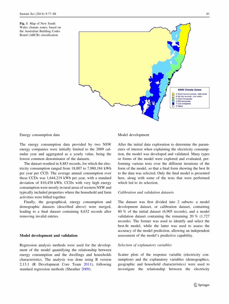
The climate zone identifier was eventually selected, as it

represented best the location variable in the model and

explained most of the variation; it was the only one kept

when developing the model. Figure 1 shows the different

climate zones for NSW (identified by values 2–8), based on

the Australian Building Codes Board (ABCB) classifica-

tion (ABCB 2011). Climate zone 1 (hot humid summer,

warm winter) does not exist in NSW.

Table 1 Parameter categories,

number of subcategories and

derived factors for use in the

analysis

Category name Number of

subcategories

Derived factors

Total population 3 pMale: proportion of males

Age groups and ages (2 types of

grouping)

33 avAge: average age

avAgeAd: average age for adults

avAgeCh: average age for children

pChAd: average proportion of children and

adults

Number of residents 7 avNumRes: average number of residents

Bedrooms 9 avNumBed: average number of bedrooms

Individual income 13 avIndInc: average individual income

Household income 18 avHousInc: average household income

Housing loan repayment 13 avHLR: average house loan repayment

pFreeTen: proportion of free tenure (fully

owned)

avHousFreeInc: average household free

income

Rent 12 avRent: average weekly rent

Field of work 21

Tenure 6

Dwelling type 13

Internet connection 7

Labour force 10

Tertiary education 8

Field of study 15

Transport to work 36

Motor vehicles 8

Education 14

Occupancy 2

80 Sustain Sci (2014) 9:77–88

123

Energy consumption data

The energy consumption data provided by two NSW

energy companies were initially limited to the 2009 cal-

endar year and aggregated as a yearly value, being the

lowest common denominator of the datasets.

The dataset resulted in 8,883 records, for which the elec-

tricity consumption ranged from 18,007 to 7,980,184 kWh

per year per CCD. The average annual consumption over

these CCDs was 1,644,219 kWh per year, with a standard

deviation of 810,458 kWh. CCDs with very high energy

consumption were mostly in rural areas of western NSW and

typically included properties where the household and farm

activities were billed together.

Finally, the geographical, energy consumption and

demographic datasets (described above) were merged,

leading to a final dataset containing 8,632 records after

removing invalid entries.

Model development and validation

Regression analysis methods were used for the develop-

ment of the model quantifying the relationship between

energy consumption and the dwellings and households

characteristics. The analysis was done using R version

2.13.1 (R Development Core Team 2011), following

standard regression methods (Sheather 2009).

Model development

After the initial data exploration to determine the param-

eters of interest when explaining the electricity consump-

tion, the model was developed and validated. Many types

or forms of the model were explored and evaluated, per-

forming various tests over the different iterations of the

form of the model, so that a final form showing the best fit

to the data was selected. Only the final model is presented

here, along with some of the tests that were performed

which led to its selection.

Calibration and validation datasets

The dataset was first divided into 2 subsets: a model

development dataset, or calibration dataset, containing

80 % of the initial dataset (6,905 records), and a model

validation dataset containing the remaining 20 % (1,727

records). The former was used to identify and select the

best-fit model, while the latter was used to assess the

accuracy of the model prediction, allowing an independent

assessment of the model’s predictive capability.

Selection of explanatory variables

Scatter plots of the response variable (electricity con-

sumption) and the explanatory variables (demographics,

geographic and household characteristics) were used to

investigate the relationship between the electricity

Fig. 1 Map of New South

Wales climate zones, based on

the Australian Building Codes

Board (ABCB) classification

Sustain Sci (2014) 9:77–88 81

123

consumption data and the demographics and household

characteristics variables. Such plots are useful to inform the

analyst on the form of the regression model. Here, these

plots showed that a limited number of the parameters

described in Table 1 was of interest in modelling the

energy consumption. Also, some parameters showed a non-

linear relationship with the response variable, and different

forms of the explanatory variables and the response vari-

able were tested, such as the inverse and logarithm func-

tions. Tests of multi-collinearity were also performed,

limiting some factors of interest to those that did not show

multi-collinearity. The set of independent variables was

consequently reduced to those that showed stronger cor-

relation with the electricity consumption, and they are

presented in the model form below.

Model form

A general method employed to define a model is to express

the response variable as a linear (or transformed linear)

function of all the available population characteristics, and

narrowing it down to only keep those parameters that

explain most of the variation. This was applied to this

dataset, following the initial investigation of the explana-

tory variables and limiting the subset of parameters for the

model through the comparison of the adjusted coefficient

of determination (or adjusted R2) values and Akaike

information criterion (AIC) values. The selected model

from all of the regression models considered is presented

below in transformed linear form:

logðElectricity consumptionÞ ¼ aþ b0 logðNpÞþ b1 logðNdÞ þ b2Nb þ b3Hi þ b4pfT þ b5ClimZ ð1Þ

which can also be directly expressed (for direct

application) as:

Electricity consumption ¼ expðaþ b0 logðNpÞþ b1 logðNdÞ þ b2Nb þ b3Hi þ b4pfT þ b5ClimZÞ ð2Þ

where Np is the total number of people, Nd is the total

number of dwellings, Nb is the average number of bed-

rooms, Hi is the household income, pfT is the proportion of

free tenancy and ClimZ is the climate zone.

Outliers and leverage points, and multi-collinearity

During the initial model fittings, points that did not follow

the general trend of the dataset were identified. Eight

outliers and leverage points, which represent 0.1 % of the

calibration dataset, were identified through the different

tests assessing the validity of the model. Leverage points

are data points which have x-values that have an unusually

large effect on the estimated regression model, while out-

liers do not follow the pattern set by the bulk of the data

when one takes into account the given model (Kutner et al.

2005). After thoroughly examining these points, they were

discarded from the dataset because they were shown to

have too much of an influence on the dataset without jus-

tification. Six of these points had very low values for their

energy consumption, while the rest of their characteristics

(populations and housing) were amongst the average of the

whole population; the remaining two points had unusual

characteristics in their demographics data, due to data

mismatches, such as mixed farming and household billing.

Multi-collinearity among the predictor variables was

investigated using the variation inflation factor (VIF), with

a value of 10 commonly used as the threshold for consid-

ering variables to be correlated. All variables were well

below 4, except for Np and Nd, which had a VIF of 7.9 and

7.7, respectively. It might be argued that these variables

need to be transformed or one of them be discarded,

because they are somewhat correlated; however, they were

kept on the basis that other tests showed appropriate results

to warrant their presence (O’Brien 2007). Also, they show

different aspects of the population that influence electricity

consumption. The information provided by these two

variables concerns not only the number of people in each

CCD but also the density of the CCDs, which is an indi-

cation of the life environment mentioned above (rural,

suburban or city life).

Model fitting

The model was fitted as per equation Eq. 1. The model

parameters and their estimates are given in Table 2. This

table shows the standard error for each parameter, their

t-value and their p-value [columns titled Pr([|t|)]. The

p-values for the model are very small for all the parame-

ters, meaning they are statistically significant at the 99 %

Table 2 Estimate of parameters

Estimate Standard error t-value Pr([|t|)

Intercept 7.58E?00 3.29E-02 230.235 \2e-16

log(Np) 1.74E-01 1.20E-02 14.485 \2e-16

log(Nd) 7.74E-01 1.33E-02 58.002 \2e-16

Nb 3.90E-01 6.42E-03 60.816 \2e-16

Hi 1.46E-04 6.56E-06 22.257 \2e-16

pfT -3.64E-02 5.78E-03 -6.295 3.27E-10

ClimZ4 2.94E-01 9.43E-03 31.15 \2e-16

ClimZ5 1.28E-01 8.65E-03 14.785 \2e-16

ClimZ6 1.50E-01 1.06E-02 14.128 \2e-16

ClimZ7 1.53E-01 1.22E-02 12.527 \2e-16

82 Sustain Sci (2014) 9:77–88

123

confidence level and their use in the model is appropriate.

This model has an adjusted R2 value of 0.8645 and an AIC

of -23,313.

From the estimates of the parameters, we note that:

• The energy consumption increases as the total number

of persons and dwellings increase in the CCD, which is

also the case when the average number of bedrooms

increases in the dwellings.

• When the household income increases, so does the

energy consumption. However, the increase is not as

high as for the previous factors.

• With an increase in the proportion of ‘free’ tenancies,

i.e. when households do not have any more repay-

ments on their house, the energy consumption

decreases. This means that those CCDs which have

a high proportion of households who have already

paid for their house consume less electricity than

others. This could be explained by the fact that these

households might be able to spend that extra amount

of money on newer or more efficient appliances or in

photovoltaics (PVs) installed on their roofs—more

detailed analysis needs to be undertaken in order to

verify such assumptions.

• The climate zone parameter indicates that, for the

zones with a colder climate, the energy consumption

tends to increase. However, climate zone 4 is the one

that shows most of the increase, with the other 3 zones

(5, 6 and 7) having coefficients on the same order of

magnitude.

Validation of the fit of the model

Once the model had been fitted, tests were performed to

assess its validity. Plots of the standardised residuals against

the predictors and plots of the standardised residuals against

the fitted values for the model were analysed. These graphs

showed that the points were scattered randomly around the

horizontal axis and displayed constant variability looking

along the horizontal axis, indicating a lack of bias of pre-

dictor variables. However, some points had a higher value

for their residuals than expected if the model was perfectly

well fitted, but those values were still reasonable.

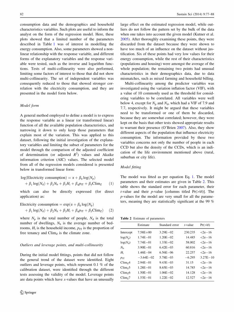
Diagnostic plots were also used to assess the validity of

the model and the final plot showing the observed response

variable against the fitted values is shown in Fig. 2a for the

calibration dataset.

If the model was perfectly fitted, the points would all be

situated on the line. Here, most of the points are along the

line, even if some departure can be observed, especially for

the higher values of energy consumption. While the model

is not perfect, it shows a good fit.

Assessing the model’s predictive capability

The quality of the model was assessed by applying it to the

validation dataset, which is an independent dataset. Indeed,

this dataset was created using 20 % of the initial dataset

and was not used for the development of the model. The

model was then applied to this dataset, providing the

Fig. 2 Plots of the observed response variable (energy consumption) against the fitted values—model calibration dataset (a) and model

validation dataset (b)

Sustain Sci (2014) 9:77–88 83

123

predicted energy consumption for each of the CCDs

described in this subset according to their characteristics.

These values were then compared to the actual energy

consumption, giving a measure of the quality of the model.

The adjusted R2 value for the test dataset was 0.8245.

A graph of the predicted energy consumption against the

observed values was plotted, as shown in Fig. 2b. As in the

case of the calibration dataset, most points for the valida-

tion set lay close to the line, which is very satisfactory; the

closer the prediction to the line, the more accurate it is.

The residual from the model (0.03399) was also com-

pared with the variance of the residual from the validation

dataset. The residual from the validation dataset was cal-

culated as the difference between the logarithm of the

observed energy consumption and the logarithm of the

fitted energy consumption, which gave a value of 0.03034.

The two values are reasonably close, reinforcing the con-

fidence in the capacity of the model to predict rather

appropriately.

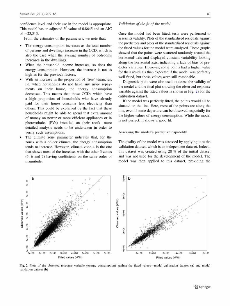
Finally, the difference between the predicted and the

actual value for consumption was plotted on a map (Fig. 3)

to see if some patterns could be observed amongst the

CCDs that would explain some of the error according to

their geographical characteristics. In order to have a better

representation of the difference in the prediction compared

to the actual value, the energy was transformed into con-

sumption per dwelling rather than at the CCD level, and

per day, which is a more intuitive way of understanding

this type of data.

The difference in electricity consumption prediction

amongst the CCDs ranked from -5,168 to 9,680 kWh per

annum and per dwelling (or -14.15 to 26.5 kWh per day

and per dwelling). The percentages of CCDs for which the

error in their prediction was less than 500, 1,000, 2,000 and

5,000 kWh per annum in absolute value were, respectively,

37, 66, 90 and 99 %. When translated on a daily basis, this

means that 90 % of the predictions were within 5 kWh a

day per dwelling (shown in the different shades of green on

the map). Most of the CCDs (51.3 %) had their energy

consumption predicted within 2 kWh of their actual daily

consumption, which is rather reasonable.

Plotting the difference in prediction allows the identifi-

cation of areas for which the model did not perform that

well. It can be observed here that most CCDs for which the

difference in the prediction was greater than 5.5 kWh per

day are located mainly in rural areas.

The error in the predictions, defined as (predicted

data - actual data)/(actual data) 9 100 in (%), was also

calculated. A histogram of the error in prediction is given

in Fig. 4, which shows that most of the CCDs’ error is

within 10 % of their actual value; 68 % are within 15 %

and 80 % are within 20 %. A few CCDs had a very large

error in prediction; these were, once again, for those CCDs

located in rural areas (in the darkest shades of green and

red on the map). As noted earlier in the discussion of the

nature of the billing data obtained from the utility com-

panies, this could be overcome by separating the tariffs for

mixed farming/household billing in rural areas.

Fig. 3 Geographical representation of the difference in prediction compared to the actual electricity consumption (absolute value)—New South

Wales and zoom on the Sydney area

84 Sustain Sci (2014) 9:77–88

123

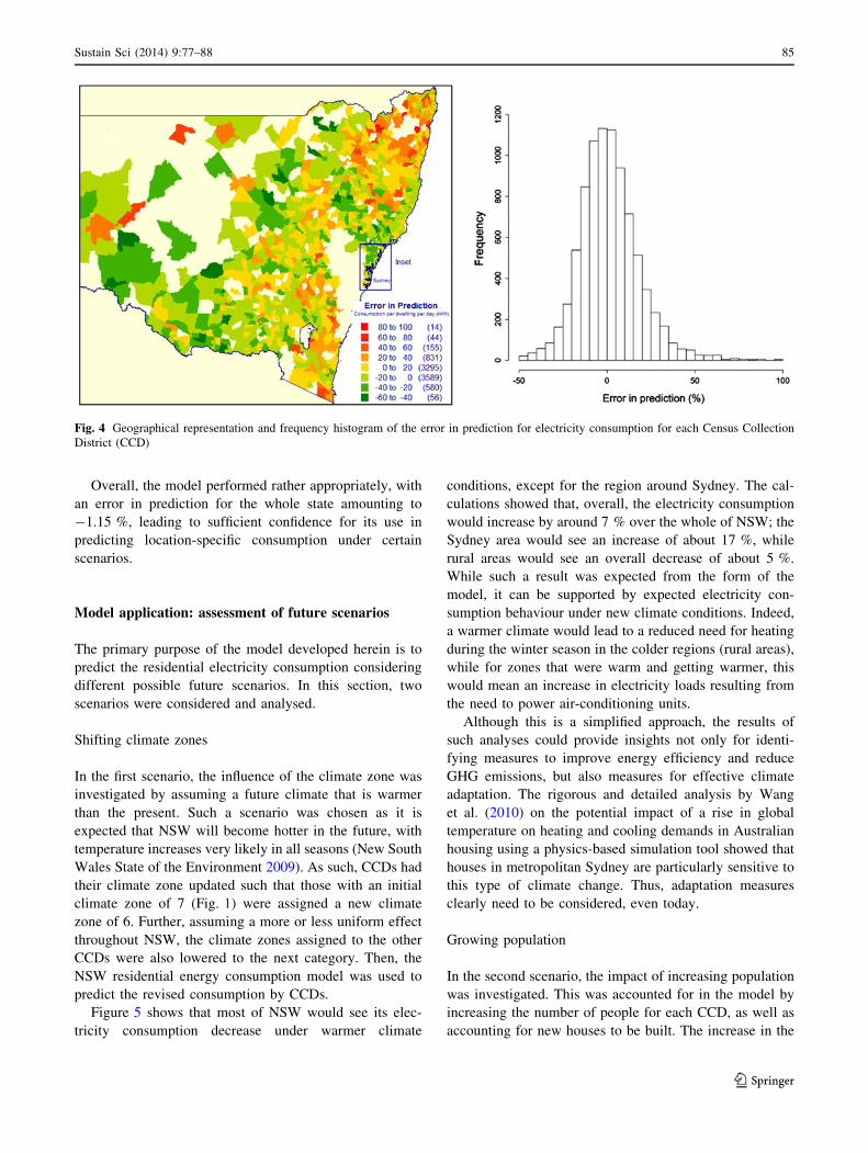
Overall, the model performed rather appropriately, with

an error in prediction for the whole state amounting to

-1.15 %, leading to sufficient confidence for its use in

predicting location-specific consumption under certain

scenarios.

Model application: assessment of future scenarios

The primary purpose of the model developed herein is to

predict the residential electricity consumption considering

different possible future scenarios. In this section, two

scenarios were considered and analysed.

Shifting climate zones

In the first scenario, the influence of the climate zone was

investigated by assuming a future climate that is warmer

than the present. Such a scenario was chosen as it is

expected that NSW will become hotter in the future, with

temperature increases very likely in all seasons (New South

Wales State of the Environment 2009). As such, CCDs had

their climate zone updated such that those with an initial

climate zone of 7 (Fig. 1) were assigned a new climate

zone of 6. Further, assuming a more or less uniform effect

throughout NSW, the climate zones assigned to the other

CCDs were also lowered to the next category. Then, the

NSW residential energy consumption model was used to

predict the revised consumption by CCDs.

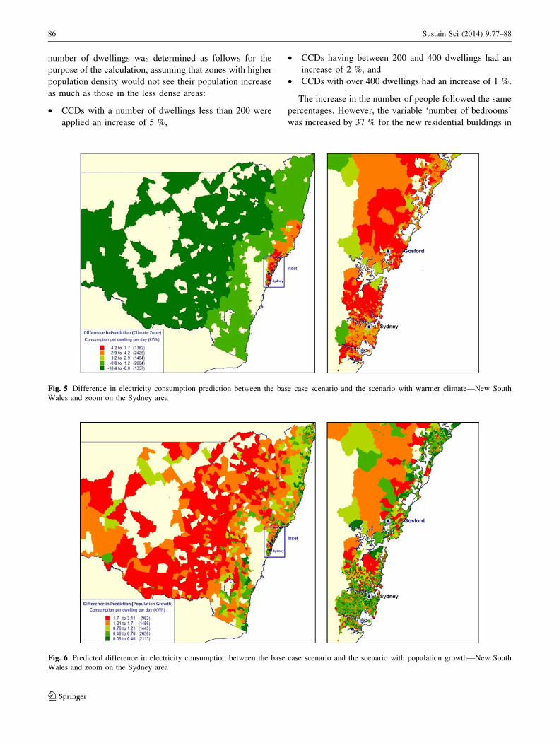
Figure 5 shows that most of NSW would see its elec-

tricity consumption decrease under warmer climate

conditions, except for the region around Sydney. The cal-

culations showed that, overall, the electricity consumption

would increase by around 7 % over the whole of NSW; the

Sydney area would see an increase of about 17 %, while

rural areas would see an overall decrease of about 5 %.

While such a result was expected from the form of the

model, it can be supported by expected electricity con-

sumption behaviour under new climate conditions. Indeed,

a warmer climate would lead to a reduced need for heating

during the winter season in the colder regions (rural areas),

while for zones that were warm and getting warmer, this

would mean an increase in electricity loads resulting from

the need to power air-conditioning units.

Although this is a simplified approach, the results of

such analyses could provide insights not only for identi-

fying measures to improve energy efficiency and reduce

GHG emissions, but also measures for effective climate

adaptation. The rigorous and detailed analysis by Wang

et al. (2010) on the potential impact of a rise in global

temperature on heating and cooling demands in Australian

housing using a physics-based simulation tool showed that

houses in metropolitan Sydney are particularly sensitive to

this type of climate change. Thus, adaptation measures

clearly need to be considered, even today.

Growing population

In the second scenario, the impact of increasing population

was investigated. This was accounted for in the model by

increasing the number of people for each CCD, as well as

accounting for new houses to be built. The increase in the

Fig. 4 Geographical representation and frequency histogram of the error in prediction for electricity consumption for each Census Collection

District (CCD)

Sustain Sci (2014) 9:77–88 85

123

number of dwellings was determined as follows for the

purpose of the calculation, assuming that zones with higher

population density would not see their population increase

as much as those in the less dense areas:

• CCDs with a number of dwellings less than 200 were

applied an increase of 5 %,

• CCDs having between 200 and 400 dwellings had an

increase of 2 %, and

• CCDs with over 400 dwellings had an increase of 1 %.

The increase in the number of people followed the same

percentages. However, the variable ‘number of bedrooms’

was increased by 37 % for the new residential buildings in

Fig. 5 Difference in electricity consumption prediction between the base case scenario and the scenario with warmer climate—New South

Wales and zoom on the Sydney area

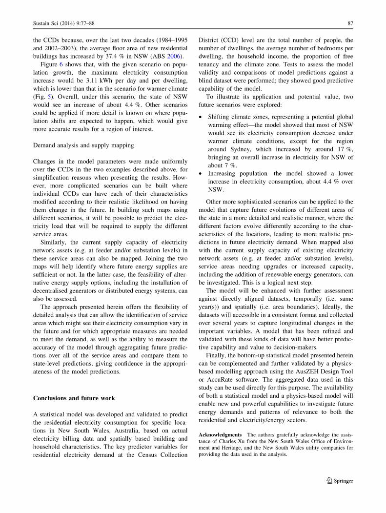
Fig. 6 Predicted difference in electricity consumption between the base case scenario and the scenario with population growth—New South

Wales and zoom on the Sydney area

86 Sustain Sci (2014) 9:77–88

123

the CCDs because, over the last two decades (1984–1995

and 2002–2003), the average floor area of new residential

buildings has increased by 37.4 % in NSW (ABS 2006).

Figure 6 shows that, with the given scenario on popu-

lation growth, the maximum electricity consumption

increase would be 3.11 kWh per day and per dwelling,

which is lower than that in the scenario for warmer climate

(Fig. 5). Overall, under this scenario, the state of NSW

would see an increase of about 4.4 %. Other scenarios

could be applied if more detail is known on where popu-

lation shifts are expected to happen, which would give

more accurate results for a region of interest.

Demand analysis and supply mapping

Changes in the model parameters were made uniformly

over the CCDs in the two examples described above, for

simplification reasons when presenting the results. How-

ever, more complicated scenarios can be built where

individual CCDs can have each of their characteristics

modified according to their realistic likelihood on having

them change in the future. In building such maps using

different scenarios, it will be possible to predict the elec-

tricity load that will be required to supply the different

service areas.

Similarly, the current supply capacity of electricity

network assets (e.g. at feeder and/or substation levels) in

these service areas can also be mapped. Joining the two

maps will help identify where future energy supplies are

sufficient or not. In the latter case, the feasibility of alter-

native energy supply options, including the installation of

decentralised generators or distributed energy systems, can

also be assessed.

The approach presented herein offers the flexibility of

detailed analysis that can allow the identification of service

areas which might see their electricity consumption vary in

the future and for which appropriate measures are needed

to meet the demand, as well as the ability to measure the

accuracy of the model through aggregating future predic-

tions over all of the service areas and compare them to

state-level predictions, giving confidence in the appropri-

ateness of the model predictions.

Conclusions and future work

A statistical model was developed and validated to predict

the residential electricity consumption for specific loca-

tions in New South Wales, Australia, based on actual

electricity billing data and spatially based building and

household characteristics. The key predictor variables for

residential electricity demand at the Census Collection

District (CCD) level are the total number of people, the

number of dwellings, the average number of bedrooms per

dwelling, the household income, the proportion of free

tenancy and the climate zone. Tests to assess the model

validity and comparisons of model predictions against a

blind dataset were performed; they showed good predictive

capability of the model.

To illustrate its application and potential value, two

future scenarios were explored:

• Shifting climate zones, representing a potential global

warming effect—the model showed that most of NSW

would see its electricity consumption decrease under

warmer climate conditions, except for the region

around Sydney, which increased by around 17 %,

bringing an overall increase in electricity for NSW of

about 7 %.

• Increasing population—the model showed a lower

increase in electricity consumption, about 4.4 % over

NSW.

Other more sophisticated scenarios can be applied to the

model that capture future evolutions of different areas of

the state in a more detailed and realistic manner, where the

different factors evolve differently according to the char-

acteristics of the locations, leading to more realistic pre-

dictions in future electricity demand. When mapped also

with the current supply capacity of existing electricity

network assets (e.g. at feeder and/or substation levels),

service areas needing upgrades or increased capacity,

including the addition of renewable energy generators, can

be investigated. This is a logical next step.

The model will be enhanced with further assessment

against directly aligned datasets, temporally (i.e. same

year(s)) and spatially (i.e. area boundaries). Ideally, the

datasets will accessible in a consistent format and collected

over several years to capture longitudinal changes in the

important variables. A model that has been refined and

validated with these kinds of data will have better predic-

tive capability and value to decision-makers.

Finally, the bottom-up statistical model presented herein

can be complemented and further validated by a physics-

based modelling approach using the AusZEH Design Tool

or AccuRate software. The aggregated data used in this

study can be used directly for this purpose. The availability

of both a statistical model and a physics-based model will

enable new and powerful capabilities to investigate future

energy demands and patterns of relevance to both the

residential and electricity/energy sectors.

Acknowledgments The authors gratefully acknowledge the assis-

tance of Charles Xu from the New South Wales Office of Environ-

ment and Heritage, and the New South Wales utility companies for

providing the data used in the analysis.

Sustain Sci (2014) 9:77–88 87

123

References

Australian Building Codes Board (ABCB) (2011) Climate zone maps.

http://www.abcb.gov.au/en/major-initiatives/energy-efficiency/

climate-zone-maps. Retrieved 1 Oct 2011

Australian Bureau of Statistics (ABS) (2006) Australian home size

is growing. http://www.abs.gov.au/ausstats/[email protected]/Previous

products/1301.0Feature%20Article262005?opendocument&tab

name=Summary&prodno=1301.0&issue=2005&num=&view.

Retrieved 3 Aug 2011

Aydinalp M, Ugursal VI, Fung AS (2003) Modelling of residential

energy consumption at the national level. Int J Energy Res

27:441–453

Benesh D (2000) Electricity demand forecast—demand forecast for

2001 to 2011. Queensland Competition Authority (QCA).

http://www.qca.org.au/files/QLDElectricityDemandForecast.pdf

Cuevas-Cubria C, Schultz A, Petchey R, Maliyasena A, Sandu S

(2010) Energy in Australia 2010 (ISSN 1833-038). Australian

Government, Department of Resources, Energy and Tourism.

http://adl.brs.gov.au/data/warehouse/pe_abarebrs99014444/energy

AUS2010.pdf

Delsante A (2005) Is the new generation of building energy rating

software up to the task? A review of AccuRate. Paper presented

at ABCB conference ‘Building Australia’s Future’, Surfers

Paradise, Australia, 11–15 September 2005

Farahbakhsh H, Ugursal VI, Fung AS (1998) A residential end-use

energy consumption model for Canada. Int J Energy Res

22:1133–1143

Hens H, Verbeeck G, Verdonck B (2001) Impact of energy efficiency

measures on the CO2 emissions in the residential sector, a large

scale analysis. Energy Build 33:275–281

Howard B, Parshall L, Thompson J, Hammer S, Dickinson J, Modi V

(2012) Spatial distribution of urban building energy consumption

by end use. Energy Build 45:141–151. doi:10.1016/j.enbuild.

2011.10.061

Hsiao C, Mountain DC, Illman KH (1995) A Bayesian integration of

end-use metering and conditional-demand analysis. J Bus Econ

Stat 13(3):315–326

Jones PJ, Lannon S, Williams J (2001) Modelling building energy use

at urban scale. Paper presented at the seventh international

IBPSA conference, Rio de Janeiro, Brazil, 13–15 August 2001

Kavgic M, Mavrogianni A, Mumovic D, Summerfield A, Stevanovic

Z, Djurovic-Petrovic M (2010) A review of bottom-up building

stock models for energy consumption in the residential sector.

Build Environ 45(7):1683–1697. doi:10.1016/j.buildenv.2010.

01.021

Kutner MH, Nachtsheim CJ, Neter J, Li W (2005) Applied linear

statistical models, 5th edn. McGraw-Hill/Irwin, New York

Lilley B, Szatow A, Jones T (2009) Intelligent grid—a value

proposition for distributed energy in Australia. In: CSIRO (ed)

National Research Flagships—Energy Transformed; CSIRO

Lins MPE, da Silva ACM, Rosa LP (2002) Regional variations in

energy consumption of appliances: conditional demand analysis

applied to Brazilian households. Ann Oper Res 117(1):235–246.

doi:10.1023/a:1021533809914

Mills D (2010) Greenhouse gas emissions from energy use in

Queensland homes. Sustainability Innovation Division, Depart-

ment of Environment and Resource Management, Queensland

Government

New South Wales State of the Environment (2009) Chapter 2:

Climate change. http://www.environment.nsw.gov.au/soe/soe

2009/chapter2/chp_2.1.htm. Retrieved 19 Mar 2012

O’Brien RM (2007) A caution regarding rules of thumb for variance

inflation factors. Qual Quant 41(5):673–690. doi:10.1007/

s11135-006-9018-6

R Development Core Team (2011) R: a language and environment for

statistical computing. http://www.R-project.org

Ren Z, Foliente G, Chan W-Y, Chen D, Syme M (2011) AusZEH

design: software for low-emission and zero-emission house design

in Australia. Paper presented at building simulation 2011: 12th

conference of the International Building Performance Simulation

Association, Sydney, Australia, 14–16 November 2011

Riedy C, Partridge E (2006) Study of factors influencing electricity

use in Newington. Institute for Sustainable Futures, UTS,

Sydney, Australia, pp 1–114

Sheather SJ (2009) A modern approach to regression with R. Springer

Texts in Statistics. doi:10.1007/978-0-387-09608-7

Shimoda Y, Fujii T, Morikawa T, Mizuno M (2004) Residential end-

use energy simulation at city scale. Build Environ 39:959–967

Swan LG, Ugursal VI (2009) Modeling of end-use energy consump-

tion in the residential sector: a review of modeling techniques.

Renew Sustain Energy Rev 13(8):1819–1835. doi:10.1016/j.rser.

2008.09.033

Swan L, Ugursal VI, Beasuoleil-Morrison I (2009) Implementation of

a Canadian residential energy end-use model for assessing new

technology impacts. Paper presented at the eleventh international

IBPSA conference, Glasgow, Scotland, 27–30 July 2009

Wang X, Chen D, Ren Z (2010) Assessment of climate change impact

on residential building heating and cooling energy requirement

in Australia. Build Environ 45(7):1663–1682. doi:10.1016/

j.buildenv.2010.01.022

88 Sustain Sci (2014) 9:77–88

123