Statistical modeling for validation of hydrometric data ...apuss.insa-lyon.fr/CityNet/Paper_Farida_Hamioud.pdf · 1 Statistical modeling for validation of hydrometric data issued

1

Statistical modeling for validation of hydrometricdata issued from the sewer networks

Farida HAMIOUD1, Claude JOANNIS2 and José RAGOT3

1LCPC; Laboratoire Central des Ponts et Chaussées, route de Bouaye BP 2941. 44341 Bouguenaiscedex Tel. /Fax: 33(0) 2 40 84 58 84/59 98; [email protected], Tel. /Fax: 33(0) 2 40 84 58 86/59 98; [email protected] (Centre de Recherche en Automatique de Nancy); CRAN-ENSEM. 2, Avenue de laForet de Haye. 54516 Vandoeuvre cedex France, Tel/Fax : 33(0)3 83 5956 82/56 44 [email protected]

ABSTRACT

The continuous but imperfectly reliable measurements issued from sewer networks require aprocessing for validation. This processing is divided into two parts: detection to identify suspectmeasurements and diagnosis, to specify the origin of anomalies and to conclude the reliabilityconcerned measurements. This paper deals with building of several models for detection usinglinear regression. The measurements are given in different time steps; minute, hour and day. Theycan be provided directly from sensors (source data: water depth and water velocity) or can beelaborated (water flow rates). The built models have been tested using recorded data from themonitoring system of district of Nantes.

KEYWORDS

Correlation, diagnosis, flow-rate, modeling, multiple correlation, validation.

INTRODUCTION

Measurements in the sewer networks are difficult and disturbed. A high reliability would require alarge effort of investment (civil engineering, redundancy of sensors) and of maintenance, whichwould be justified for applications of real time control. It may be not suited for objectives of aposteriori analysis, which does not require sets of perfectly continuous data. For these applicationsof the availability ratios ranging 90 to 95 % are often quoted, this corresponds to thirty days offailure per sensor and per year. However false results can considerably disturb an assessment, whichconversely could afford some missing data. It is thus preferable to eliminate from the analyses thepresumably erroneous data.

The validation of the results of measurement comprises 2 phases (Aumond and Joannis, 2003,Aumond and al., 2001): A phase of detection, which is based on one (even several) forecast of themeasure or some of its statistical characteristics. This forecast results from a model, which canextrapolate the values or the characteristics observed in the past on the variable to validate, or toexploit relations between the variable to be validated and others measures at the same time(Boukhris 1998). It can be very simple - correlation, even identity in the case of a materialredundancy - or be elaborated, rain-flow rate model for example. A too significant deviationbetween a measured value and one (or several) envisaged value constitutes an anomaly, which canbe due:- To the measurement to be validated,- To the measurements used in entry of the models;

2

- To the models, used out of their field of validity;- Or to a combination of these causes.A phase of diagnosis, of which the purpose is to identify the origin of the anomaly, at least in termof localization (measurement, model, entry of the model), and if possible propose a more detailedexplanation, in particular on the nature of the implied dysfunction.Different methods for validating the data such as statistical tests, decision theory, the filtering ofsignals (Ragot 90, Bennis 96) and the technique of redundancy (Perreault and al. 91, Piatyzec 2000)gives a several methods for the default and aberrant values detection in the data series.

In this paper, we use a linear regression with OLS, Orthogonal least squares procedure (chen, 1991)to build different models for the detection stage. The paper contains three sections. After theintroduction section, we describe the materials and the method of our work. Then, we presentsimulation results using the real measurements issued from the sewer network of Nantes. Finally, aconclusion and perspectives section is given to conclude our described method and to present thefuture work based on this approach.

MATERIALS AND METHODS

Description of the sewer network of Nantes

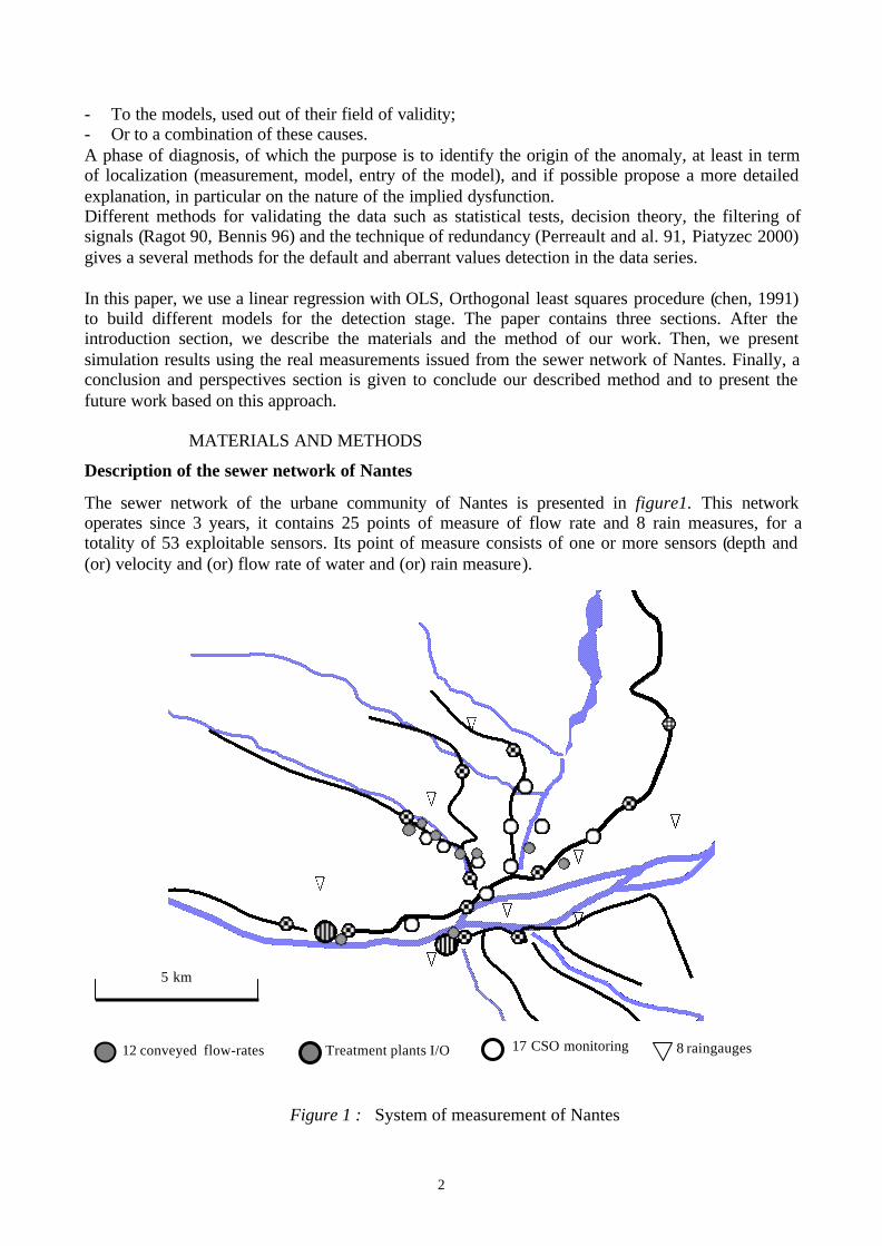
The sewer network of the urbane community of Nantes is presented in figure1. This networkoperates since 3 years, it contains 25 points of measure of flow rate and 8 rain measures, for atotality of 53 exploitable sensors. Its point of measure consists of one or more sensors (depth and(or) velocity and (or) flow rate of water and (or) rain measure).

Figure 1 : System of measurement of Nantes

5 km

17 CSO monitoring 8 raingauges12 conveyed flow-rates Treatment plants I/O

3

Preprocessing

On the data processing level, we represented each measure by a vector of data (signal) and acorresponding time vector (variables time steps). We synchronize between all these signals (fixedtime step: to obtain one vector of fixed time step), with resampling procedure. Then, we havefiltered these signals for eliminate all possible perturbations (anomalies) in them.For the rain measure, we consider one signal, it represent a median of all the rain measures.

Filtering

We proceed for this, by a filtering technique whose performances are related on the nature of thesignals (level of water, flow rate) and also on the existing number of disturbances. The first quiteinteresting filtering for detection, elimination then estimate of the too aberrant values. Thesesystematic errors, are often due to events non-random or accidental, the filter we used is theTrimming-Winsorizing (Ragot, 1990) filter. This filter conserves the quality of median, that is anestimator of central parameter of population, more powerful than the mean. It allowed the twooperations: trimming which consists of exclude a certain number of observations, which are moredistant from median, to characterize a sample. Winsorizing allows reconstitution of excluded valuesby the nearest conserved values. We applied after a Low Pass Filter, which is quite suitable inhydrology to eliminate the great fluctuations (undesirable noises in the chronological series). Inpreceding work (Berrada an al., 1996), filtering is employed to validate the data. This is veryinteresting for the local validation (validate the signals separately). In our work, the filtering isnecessary for constructing models. The performances of models are related of those of filters (agood filtering enables us to establish more powerful models).

Modeling

For each variable to be estimated, we built different models of multiple regression. These aredifferent according to the time step (Aumond and Joannis, 2001), the number of explanatory signalsand the consideration or not of the rain measure.

Number and nature of explanatory signals

The nature of explanatory signals is fixed by the nature of the signal to be explained:• The water depth; h or the water velocity; v on a given point are explained by the others waterdepths and the water velocities, completed by the rain measure (median) and given by the followingrelation: ),( kji vhfh = , i, j: integers and dNji :1, = with Nd: number of depths, Nv: number ofvelocities and NQ: number of flow rates on the sewer network.• The flow rate; Q on a given point is explained by the flow rates on the others point, included arain measure: with :1 , ), ,( jiNjimeasurerainQfQ Qji ≠== and NQ: number of flow rates onthe sewer network.The multiple regression techniques allow us to take into account in the model a set of selectednumber of explanatory signals among the global set, this selection is different according to the usedtechnique for selection. We use the OLS method and we fixed for this method a stop criterion forselection of signals. This criterion allows us to limit the maximum number of explanatory signals,given by the number nmax(Yi), Yi the signal to be explained. We identified different models (Olssonand Newell, 1999) when taking one or two, …or nmax(Yi) variables.

4

OLS regression

This method of selection is a forward regression, which allowed us to select significant regressorsaccording to error reduction ratio (to be minimized) due to each regressor. This error reduction ratiois calculated from the set of all signals in the sewer network except signal to be estimated andrepresent a variance reduction rate (which should be maximized) of the signal to be explained. Wefixed also a stop criteria FPE; final prediction error (Saporta, 1990) from which we stop selection ofregressors when its minimum is reached.Consider the following relation of linear regression model:

EXY += θ (1)

where Y is the signal to be explained (estimated); the depth, velocity or flow rate measurement andX is the set of all explanatory signals.Consider the orthogonal decomposition of the regression matrix X given as follows:

WAX = (2)

where A is the upper singular matrix and ] ...[ 1 NwwW = , is an orthogonal matrix.

The model (1) can be than written as: EWgY += , where g is the vector of weight ] ...[ 1 nggg = ,such that

gA =θ (3)

Knowing A and g , θ can be calculated with the last relation cited above

We define the error criterion: ggEE TT +=Φ , which may be expressed as ∑=

−=ΦN

iii

Ti

T gwwYY1

2)(

and the error reduction rate as: YYgwwr Tii

Tii /)(][ 2= , i is an indicator of the selected regressor.

The following condition should be satisfied for each selection: ζ<− ∑=

h

kkr

1

][1 , where 10 << ζ is a

chosen tolerance. We take in our work 0=ζ , and we stop selection when a stop criteria (FPE; finalprediction error reached its minimum. The FPE is defined hereafter.Let’s define: Yest ; the estimated value defined as Wg=Yest , res: the residue defined as

Y-Yest=res and var(res); the variance of the residue expressed as mN

(res)(res)= res)

t

−varvar

var( ,

where t is the transpose , N: number of samples in each signal and m is the number of selectedsignals (explanatory signals).The FPE is given by the following relation

NmNm

res=FPE/1/1

)var( −+

(4)

RESULTS

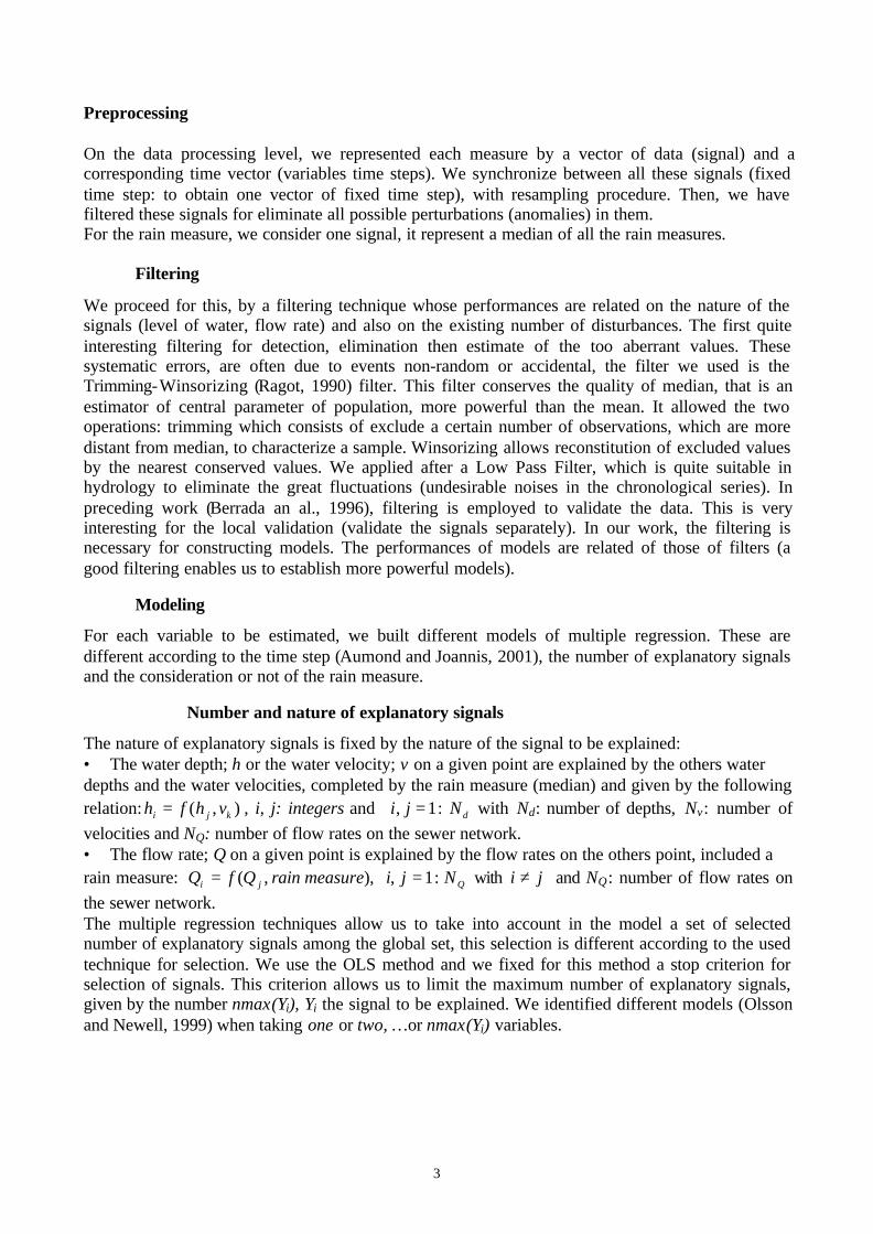
Our method of models identifying is applied on the data measurement of the sewer network given infigure 1. Results obtained are presented hereafter, where we take the flow rate to be estimated(explained) : Q35, that we note directly with its rank 35 in the sewer network.We represent in figure 2 the stop criteria ; FPE for the OLS selection with different time steps.We remark on the graphs that the minimum of the stop criterion is fine defined when time stepincreases. In each graph of figure 2, we represented the stop criterion. When this criterion havereached its minimum, we chose the corresponding number of regressors. For example on figure 2.cwe stop our selection when 04186.8 −= eFPE and we obtained five regressors.

5

Figure 2: FPE criterion for OLS method

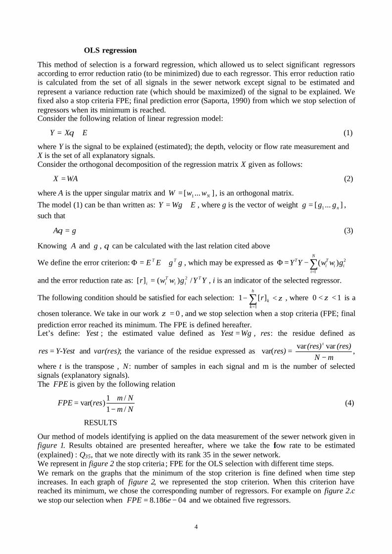
We represent in figure 3, the filtered flow rate Q35 and its estimated value. In figure 3.a, theestimated signal represent an output of model identified by the explanatory signals taking by thefinal selection (when stop criterion is reached its minimum). In the figure 3.b, we represent withfiltered flow rate, the estimated flow rate given by the different regressors (built models fordifferent selection taken before the final selection)

a. Selection: Q27+Q39+Q46+Q32+rain b. Different selections: Q27 , Q27+Q39 , Q27+Q39 +Q46 , Q27+Q39+Q46+Q32 , Q27+Q39+Q46+Q32+rain.

Figure3: Filtered flow rate and its estimated for a given selection, time step = 1day

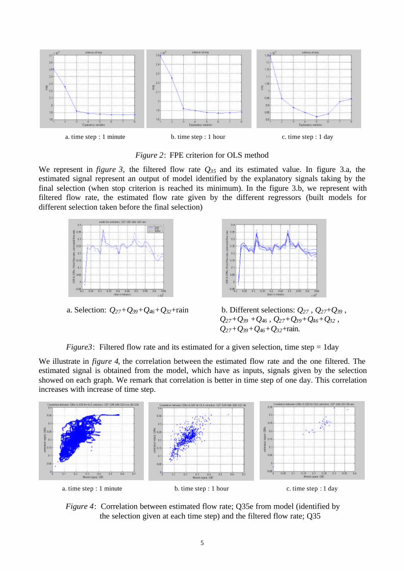
We illustrate in figure 4, the correlation between the estimated flow rate and the one filtered. Theestimated signal is obtained from the model, which have as inputs, signals given by the selectionshowed on each graph. We remark that correlation is better in time step of one day. This correlationincreases with increase of time step.

Figure 4: Correlation between estimated flow rate; Q35e from model (identified by the selection given at each time step) and the filtered flow rate; Q35

a. time step : 1 minute b. time step : 1 hour c. time step : 1 day

a. time step : 1 minute c. time step : 1 dayb. time step : 1 hour

6

Let us remark that we have taken a model given by selection chosen by the stop criterion. But wecan also take only the first signal of the given selection and so we obtain one model. With this ideawe can form several models if we take any earlier selection before the final selection given by thestop criterion. This is important for our stage of detection.

In the following table, always for the flow rate Q35, we illustrate the different regressors (selectedsignals, error reduction ratio which represented by accuracy of each selection, and parameters ofeach regressors (models)). The flow rate signals are given by the following sensors: 6 18 24 2732 35 39 46 and then named 463935322724186 QQQQQQQQ . The 38th data vector representsthe rain measure. This table is taken for a fixed time step of one day and with considering the rainmeasurement.Table 2: OLS selection with time step = 1day

Stage Selected flow rates Accuracy (r) Model parameters

12345678

Q27

Q46

Q32

Q6

Rain measure (stop selection)Q18 (not select)Q24 (not select)Q39 (not select)

0.019480.0134120.0113180.00983870.00854330.00787820.00780000.0071131

-1.06450.3374

-0.344021.3204-1.0707

The OLS method allowed us to select signals, which represent the input of model (explanatorysignals). The results of the selection with are given in the table 3, we have also calculated the MSE;mean square error, given in the following table for each model to see the performance of the builtmodel.

Table 3: Comparison results of estimation by: OLS method

Method Steptime

Selection of explanatory signal MSE Correlation(estimated signal,

filtered signal)

OLS methodwithout rainmeasure

OLS method withrain measure

1minute1 hour1 day

1minute1 hour1 day

Q27 Q39 Q46 Q32 Q6 Q24 Q18

Q27 Q39 Q46 Q32 Q6 Q24 Q18

Q27 Q46 Q32 Q6 Q18 Q39 Q24

Q27 Q39 Q46 Q32 rain Q6 Q24

Q27 Q39 Q46 rain Q32 Q6

Q27 Q46 Q32 Q6 rain

0.0018760.0018530.000571

0.0018650.0018210.000496

0.7620.7640.918

0.7630.7680.931

Using data records containing fictitious errors, and raw data for the October 2001. The resultsdemonstrate the effectiveness and advantages of taking different time steps and considering rainmeasurement.

7

CONCLUSION AND PERSPECTIVES

In this work, we have built different models with applying the OLS method. We have shown thatthe method was more efficient when the time step is changed (specifically when it increased), itmeant that a time step for an hour and a day gives an efficient estimators (models). We have shownthat the rain measurement contribute (even sometimes less) and this by observing the MSE whenidentifying models specially in the OLS method with time step equal to one day in the table 3.These models have allowed us to estimate the different signals on the sewer network. Theseestimated signals would represent in the future work the data base from which we wish to detectsuspect deviations. This will be done by analyzing evolution of residual criterion (sum of weightedsquares deviations (Ragot, 1990), this criterion is compared with a threshold. If the criterion islower than this threshold, the estimated signals (estimated measures) are accepted and no sensor isconsidered defective. Otherwise, if the criterion is upper than threshold. The detection procedurewill be considered. Each signal is suspected individually; When one measured signal is isolated, Wewill proceed to a new reconciliation of the remaining data (directly or by recurrence from theprecedent configuration) and for a new up date of residual criterion. This calculation will be madeseverally in the case of our network (which contains several measure points); the lower criterion isthan compared to a threshold. If the criterion is lower than a threshold, the eliminated sensor in thisconfiguration will be declared defective. Else we redo computation by taking two, then three,then…suspect sensors. This method is efficient but the number of computation will be fastimportant. An other method based on the same idea but faster than the method cited above. Itutilizes error detection by examining normalized corrections. When reconciliation is done, we willevaluate the residual criterion Rφ ; which follows Khi2 distribution with n degrees of freedom. Theprobability φP will be compared to a threshold CP defined by user.

Step 1: CPP ≤φ . The validated signals by reconciliation are accepted and no sensor is defective.

Step 2: CPP >φ . The normalized corrective terms are evaluated. The sensor corresponding of a

higher term is declared defective and the corresponding measure will be eliminated. The matrix ofvariance-covariance of data and true data will be estimated again (up dated estimation), (directly orrecurrently). A new criterion could be computed and the probability φP is evaluated.

Step 3: CPP ≤φ . The defective sensor is the one localized in the precedent step. The default

detection procedure is stopped.Step 4: CPP >φ . The normalized corrective terms will be recalculated and an other sensor,corresponding to a maximum normalize corrective term is presumed defective. The true magnitudeswill be estimated again (up dated estimation), but we will take only a points not suspected in step 2.After recalculating the criterion, the procedure will continue in step 2.

With this procedure, the number of necessary iterations for localization of defective sensors is equalto the number of defective sensors. Moreover, the volume of calculation to do in each iterationmight be restraint if the modifications of estimations are realized by establishing recurrences.

8

REFERENCES

Aumond M. and Joannis C. (2001), Construction de profils journaliers types pour la validation derésultats de mesures de débits en réseaux d’assainissement. 2ème colloque automatique etenvironnement . St Etienne, 4-5-6.

Aumond M., Rufflé S. and Joannis C. (2003). validation de résultats de mesure pourl’autosurveillance des réseaux d’assainissement, méthodologie et exemples. Rapport Agence del’Eau Loire Bretagne.

Aumond M., Piatyszek E., Faure D. and Joannis C. (2001). Méthodes automatisées de validation derésultats de mesures de débit en réseaux d’assainissement, Rapport Ministère de l’aménagement etde l’environnement.

Bennis S., Berrada F. and Bernard F. (2000). Métodologie de validation des donnéeshydrométriques en temps réel dans un réseau d’ assainissement urbain. Revues des sciences del’eau, Rev. Sci. Eau 483-498.

Berrada F., Bennis S. and Gagnon L. (1996). Validation des données hydrométriques par destechniques univariées de filtrage. Can. J. Civ. Eng. 23: 872-892.

Boukhris B. (1998). Identification de systèmes non- linéaires par une approche multi- modèle-application à la modélisation de la relation pluie-débit pour le diagnostic de fonctionnement decapteurs. Thèse INPL, Nancy.

Chen S., Cowan C. F. N. and Grant P. M. (1991). Orthogonal Least Squares learning algorithm forradial basis functions networks, IEEE Trans. On Neural Networks, vol. 2, n° 2, pp. 302-309.

Rapport (2001) Méthodes automatisées de validation de résultats de mesures de débit en réseaux d’assainissement. Laboratoire Central des Ponts et Chaussées, RHEA, Nancy Centre International del’ Eau.

Mourad M. and Krajewski J. L. B. co-édition avec l’ école Nationale Supérieure des Mines de StEtienne. (2002). Prévalidation automatique de données envirenmentales en hydrologie urbaine. Éd.Hermes.

Olsson G. and newel B. (1999), Modelling, Diagnosis and Control. IWA Publishing.

Perreault L., Roy R., Bobée B. et Mathier L. (1991). Validation et estimation des apportsjournaliers. Institut national de la recherche scientifique-Eau. Université du Quebec, rapportscientifique n° 271. pp. 1-29.

Piatyzec E., Voigniet P., Graillot D. (2000). Fault detection on a sewer network by a combination ofa Kalman filter and a binary sequential probability ratio test. Journal of Hydrology 230, 258-268.

Ragot J. et al. (1990), validation de données et diagnostic. Éd. Hermes. Paris.

Saporta G. (1990),. Probabilités: Analyse des Données et Statistique. Éd. TECHNIP.