Statistical Mechanics Lecture Notes 3 - Quantum statistics ...web.iitd.ac.in/~sankalpa/statmech3.pdf · Statistical Mechanics Lecture Notes 3 ... equations that controls the dynamics

Statistical Mechanics Lecture Notes 3 - Quantum

statistics and its applications

Sankalpa Ghosh, Physics Department, I I T Delhi

April 8, 2008

This part has been mostly taken from Amit and Verbin, Bhattacharjee,Pathria and Reif and some updating to correct the innumerable typos andto supplement some portion will go on and students will be informed.

1 Grand Canonical Ensemble

Q(T, V, µ) =∑

N

eβµN∑

i

e−βEi

=∑

N

eβµNZ(T, V,N)

= eβ[µN−F (T,V,N)]

Following relations are useful

P =1

β

∂ ln Q

∂V

N =1

β

∂ ln Q

∂µ

We also define the thermodynamic potential for the Grand canonicalensemble namely

Ω = −kT ln Q

which is the genralization of the relation

F = −kT ln Z

1

for the canonical ensembleWe also have the standard thermodynamic relations from the following

relation for ΩdΩ = −SdT − PdV −Ndµ

2 Introduction

The passage to the statistical mechanics of systems identical quantum par-ticles is achieved in two steps. First step is the appearance of the quantumstates. These are generally obtained from stationary or time dependentequations that controls the dynamics of the quantum state. For example,in the well known framework of non-relativistic quantum mechanics, suchstates correspond to the solutions of the Schro equations. The second stepis how the particles are distributed in these quantum states. This is wherequantum statistics comes into the picture. This two steps also has to beconsistent with each other since the quantum description of any entity (callit particles or whatever) is very different from its classical description.

In the first step one takes into consideration that quantum particlescannot be described by full specifications of their co-ordinate and momentum, because of the uncertainty principle. Instead particles are described bywave functions which satisfy by container to which are they are confined. Ifthe particles are non-interacting , then they are independent of each otherand each particle is described by its own wave function.

We shall take a particular example . The wave function of a particle in arectangular box is a standing in each of the three perpendicular directions.As we know, the wave function of a particle in a rectangular box is a standingwave in each of the three perpendicular directions . Such a state is specifiedby three integers n, p, q which determine the allowed wavelengths, or wavenumbers along the three perpendicular directions and the correspondingthree components of the De broglie momentum. Such a set of three integersthat determine the state of the particle , we denote it schematically as asingle index k.

The principal effect of quantum Mechanics on the thermodynamic prop-erties of the systems of identical particles is brought about by the quantummechanical constraints on the identification of allowed, distinguishable mi-croscopic state of the system. Such constraints follow from the symmetryproperties that must be obeyed by wave function of many identical parti-cles. The discussion of the underlying wavefunction requires more advancedintroduction of the quantum mechanics. Here it suffices to mention that all

2

possible quantum particles may be divided into two types

• Fermi Dirac particles or (Fermions) No single particle states can beoccupied by more than one particle. This is Pauli’s exclusion principle.Here the states are characterized by the occupation numbers that canbe either 0 and 1. The any set of 0, 1 occupation numbers correspondto a microscopic state of the system. Fermions are found to posseshalf-integer spins

• Bose- Einstein particles ( or bosons) single particle states can canbe occupied by any number of particles, but for any distribution ofoccupation numbers there is a single microscopic state of the system.

Let us now briefly mention about two different ways of iden identifyingthe microscopic state of of system of many particles. Both ways used singleparticle states denoted by k. In the first way we can only treat distin-guishable particles by labeling the microscopic states with N numbers withkj with j = 1, · · · , N . It leads to partition function which is the N − thpower of the partition function of a single particle partition function.

This way is incompatible with the indistinguishability of the identicalparticles and leads to the Gibb’s paradox and remedied by introducing thefactor 1

N ! in the partition function.The alternative way of specifying the microscopic states uses occupation

number nk. The partition sum will be then over all possible sets of theoccupation number over all possible single particle states respecting the con-straint on the total number of particles. This some can be carried out toreproduce the classical result for the partition function, provided one keepsin mind that the number of N -particle states that correspond to a givendistribution of nk’s is

N !n1!n2!···nk!··· .On the other hand in quantum statistics a state with a given set of nk cor-respond to a single microscopic state. This makes computing the canonicalpartition sum for the systems of particles impossible.

2.1 Thermodynamics of Fermions and Bosons

The partition function of an ideal gas of identical particles is a sum over allvalues of nk as follows:

Z =∑

n1,n2,··· ,nk,···

eβE(n1,n2,··· ,nk,··· )

3

If we neglect the forces between the particles, the total energy of thestates is the sum of single particles energy and is given by

E =∑

k

nkǫk

Thus we have

Z =∑

n1,n2,··· ,nk,···

exp[−β(n1ǫ1 + n2ǫ2 + · · ·+ nkǫk + · · ·+ · · · )]

The above sum cannot be written as a product of independent sums overeach occupation number because of the constraint

∑

k

nk = N

and therefore,

Z 6=∑

n1

(

e−βǫ1n1)

(

∑

n2

e−βǫ2n2)

· · ·(

∑

nk

e−βǫknk)

· · ·

Since what is blocking the factorization of the canonical partition func-tion, is the constraint implied by the fixed number of particles , we turn togrand canonical ensemble. The constraint is removed at the expense of thechemical potential µ.

We turn to eq. where a microscopic state α is characterized by all theoccupation number nk. The set nk determines the total number ofparticles via the above mentioned constraints. Hence the Grand canonicalpartition function or the grand partition function

Q(T, V, µ) =∑

α

[β(µN − Ei)]

=∑

nk

exp[

∞∑

k=1

nk(µ− ǫk)]

Now there is constraint on the occupation numbers. They take on inde-pendent values , provided those are consistent with the particles statistics.Hence it is possible to write Q as

4

Q =∏

k

∑

nk

eβ(µ−ǫk)nk

We now now need to calculate the summations in the above product,namely

Qk =∑

nk

eβ(µ−ǫk)nk

Quantum statistics dictates two options, either nk = 0, 1, for a gas offermions or nk = 0, 1, · · · ,∞ for bosons.

QFk =

1∑

nk=0

= 1 + eβ(µ−ǫk)

while for bosons the right hand side is an infinite geometric series

QBk =

∞∑

k=0

eβ(µ−ǫk)

= (1− eβ(µ−ǫk))−1

Note that the above summation converges only when µ is lower than allenergy levels of the system including the ground level. If the ground level isǫ1 = 0, then the chemical potential is 0.

Conversely for the fermions the summation consists only of two termsand thus there is no such constraint and thus there is no such constarint onthe chemical potential of a gas of fermions.

Next step is to calculate the thermodynamic potential which is the equiv-alent of the free energy for a grand canonical potential.

The Thermodynamic potential can be readily calculated from the grandpartition function.

ΩF = − 1

β

∑

k

ln(1 + eβ(µ−ǫk))

ΩB = − 1

β

∑

k

ln(1 + eβ(µ−ǫk))

5

From these expressions for Ω, and given the energy we can proceed tocalculate all the thermodynamic properties of the system, as function T , Vand µ.

In the grand canonical ensemble the number of particles are not fixed.However the probability distribution of the different states is such that thenumber actually fluctuates very little around an average number that isdetermined by T, V, µ.

This average is given by

NF = −(∂ΩF

∂µ)V,T =

∑

k

1

eβ(ǫk−µ) + 1

NB = −(∂ΩB

∂µ)V,T =

∑

k

1

eβ(ǫk−µ) − 1

Now NF and NB are actually average number of particles in states atthermodynamic equilibrium and in principle should be denoted by < N >.But since the fluctuation is very small we retain the notation without <>.

Since N is a sum over all single particle states each term of the sumcorresponds to a given single particle state k, the average number of particlesin the state. For a state k with energy ǫk.

< n(F )k > =

1

eβ(ǫk−µ) + 1

< n(B)k > =

1

eβ(ǫk−µ) − 1

The above quantities are also known as the occupation number for fermionsand bosons.

The average number of bosons in a given state looks familiar. In thederivation of the specific heat of solid the average number of excitation of aharmonic oscillator is given exactly by the same expression with µ = 0. Theconnection between them becomes clear if the excited states of the harmonicoscillator is treated as particles phonons with energy ~ω. Then theaverage number of phonons with a frequency ω in the crystal is the averagedegree of excitation of the oscillator that was discussed in the earlier case.

The average occupation number for the fermions is consistent with thePauli exclusion principle. The denominator is always greater than 1. If the

variable n(F )k takes the value 0 and 1 only, then its thermal average must

6

be less than 1 and hence the average < n(F )k >< 1. Bosons on the other

hand do not obey Pauli exclusion principle and at low temperature try toaccumulate at the ground state.

−5 0 50

0.5

1

β(εk−µ)

<nkB>

<nkF>

Figure 1: The Fermi and Bose occupation number. Lower part of the bothcurves are identical and same as Maxwell Boltzman statistics

Only the thermal fluctuation stop them all ending up in the ground state.In fact that the above form of < nB

k > reveals that indeed the occupationnumber increases with decreasing ǫk and diverges for ǫk → µ

In the figure we have plotted the occupation number as a function ofβ(ǫ − µ). This allows us to study the behavior on ǫ at constant T , oralternatively the dependence of temperature T at fixed energy T .

As can be seen from the above plot, for large values β(ǫ − µ) the twographs merge, since the exponential dominates the denominator. . This iswhere the both distribution tends towards the classical approximation. -the Maxwell Boltzmann distribution.

3 Ideal gas in the classical limit—Derivation using

quantum statistics

3.1 Quantum states of a single particle

Consider a free particle . The wave function ( probability amplitude) of thefree particle is just plane wave

Ψ = Aei(κ·r−ωt)

7

The energy and the momentum of the particle follows

ǫ = ~ω

p = ~κ

ǫ =p2

2m=

~2k2

2m

All these can be systematically derived from the Schroinger equationwhich is

i~∂Ψ

∂t= HΨ

Where

H =1

2mp2 = − ~

2

2m∇2

Solving these equation we can generate all the above results. Now weshall worry about the boundary conditions.

We use the following set of boundary condition, by assuming an idealgas in a three dimensional box, namely

Ψ(x + Lx, y, z) = Ψ(x, y, z)

Ψ(x, y + Ly, z) = Ψ(x, y, z)

Ψ(x, y, z + Lz) = Ψ(x, y, z) (1)

For obvious reasons, such set of boundary conditions are called periodicboundary conditions.

The solutions of the Schroinger equation with these boundary conditionsstraightforwardly yields

Ψ = eiκ·r = eiκxx+κyy+κzz

κx =2π

Lxnx

κy =2π

Lyny

κz =2π

Lznz

ǫ =2π2

~2

m

(n2x

L2x

+n2

y

L2y

+n2

z

L2z

)

8

The number of translational states that lies in the range of the wave-vector κ and κ + dκ

Since

δnx =Lx

2πdkx

we get

ρd3κ = δnxδnyδnz

=LxLyLz

(2π)3dkxdkydkz

=V

(2π)3d3k

The quantity ρ is called the density of states and plays a very importantrole in the calculation of various quantities.

We can also use the expression p = ~κ and or ǫ = ~2

2mκ2 to rewrite thedensity of states in terms of either momentum or energy

ρpd3p = V

d3p

h3

ρǫdǫ =V

4π2

(2m)3

2

~3ǫ

1

2 dǫ

3.2 Evaluation of the Canonical partition function

As we have noted the major difficulty in evaluating the canonical parti-tion function for a non-interacting set of indistinguishable quantum particleswhich

Z(N) =∑

nr

e−β(n1ǫ1+n2ǫ2+··· )

where nr = 0, 1, 2, · · · , comes from the constraint

∑

r

nr = N

This problem is avoided by going to the Grand canonical ensemble wherethe number of particles can be varied. Here we will show that once we knowthe Grand partition function it is possible to recover the partition function.The scheme comes from the observation that in a thermodynamic systemthe fluctuation around the number of particles about the mean number ofparticles vanishes. The grand partition function can be thought of as a sum

9

of some function of canonical partition functions ( for classical system thisis obvious) of subsystems each of which has a definite number of particles.Now it is clear that we are interested in the value of Z(N ′) only at N ′ = Nwhich corresponds to the most probable configuration of the system underequilibrium condition. This Z(N) can be evaluated by finding out the sharpmaxima of the function Z(N ′) exp(−αN ′) which in turn will determine theparameter N ′ from the equilibrium condition

Since a sum of this functions Z(N ′) exp(−αN ′) over all possible valuesof N ′ thus selects only those term of interest near N ′ = N and hence wecan write

∑

N ′

Z(N ′)e−αN ′

= Z(N)e−αN∆∗N ′

Now the Grand partition function(Q) and canonical partition function(Z) are related by

Q =∑

N ′

Z(N ′)e−αN ′

Using the fact that Z(N ′) has a sharp maxima we can actually write

ln Z(N) = αN + ln Q (2)

where we have neglected terms of order ln ∆∗N ′ which is utterly negligiblecompared to other terms of the order N .

For fermions and bosons

ln Q = ±∑

r

ln(1± e−α−βǫr)

Thisln Z(N) = αN ±

∑

r

ln(1± e−α−βǫr)

Maximization of Z(N ′) exp(−αN ′) will then determine α = − µkT

The first important thing is to note the behavior of the partition functionin the classical limit

For that we shall go to the limit of sufficiently low density or sufficientlyhigh temperature when the classical limit is valid

As we have just noted that the canonical partition function of the gasmay be given (to a very good approximation) given by

lnZ = −βµN ±∑

k

ln(1± eβ(µ−ǫk))

10

Consider the gas when N is very small with a given volume. The con-straint of total number of particles then immediately imply that < nk >is also small for any k or exp(β(ǫk − µ)) ≫ 1 for all states k. Under thissituation the distribution is like Maxwell Boltzmann.

Another limit is to keep the number of particles same , but to go to a veryhigh temperature. Since β ← 0 and increasing number of terms with largevalue ǫk will only contribute to the partition function. To prevent this sumto exceed some given N −βµ has to be sufficiently large so that each termis sufficiently small. This again mean exp(β(ǫk − µ) ≫ 1, the limit wherethe distribution behaves in a classical way. Thus one arrives at a conclusionthat if the concentration is made sufficiently low or the temperature is madesufficiently high then we can think of classical limit.

Here in what will follow we shall calculate the canonical partition func-tion in this classical limit

4 Ideal Gas in the classical limit

We introduce the notation−βµ = α

In the classical limit, both FD and BE statistics reduces to

< nk >= e−α−βǫk

Now by definition∑

k

e−α−βǫk = N

Since chemical potential does not depends on k summation, we thereforehave

eβµ = e−α = N(∑

k

e−βǫk)−1

Thus we get

< nk >= Ne−βǫk

∑

k e−βǫk

Hence it follows that in the classical limit of sufficiently low density orsufficiently high temperature the quantum distribution laws whether FD orBE reduce to MB distribution.

Now in the classical limit

11

ln Z = αN ±∑

r

ln(1± e−alpha−βǫr)

≈ αN ±∑

r

(±e−alpha−βǫr)

≈ αN + N

⇒ α = − lnN + ln(∑

r

e−βEr

This gives

ln Z = −N ln N + N + N ln(∑

r

exp(−βǫr)

Now this is indeed not equal to the partition function ZMB of a classicalgas of N identical particles evaluated earlier where

lnZMB = N ln(∑

r

e−βǫr)

This readily gives

ln Z = ln ZMB − (N ln N −N)

= ln ZMB − ln N ! (3)

Thus we have

Z =ZMB

N !

So finally we have

ln Z = N(ln ξ − ln N + 1)

withξ =

∑

k

e−βǫk

Now for an ideal monatomic gas as we have computed

ξ =∑

κx,κy,κz

exp[

− β~2

2m(κ2

x + κ2y + κ2

z)]

The exponential term factors out giving

12

ξ = (∑

κx

e−β~

2

2mκ2

x)(∑

κy

e−β~

2

2mκ2

y)(∑

κz

e−β~

2

2mκ2

z)

Successive terms in the the sum like over κx = 2pinx

Lxcorrespond to a

very small increment ∆κx = 2piLx

in κx and therefore differ very little foreach other.

Thus we get

| ∂

∂κx([e−

β~2

2mκ2

x)(2π

Lx

)

| ≪ (e−β~

2

2mκ2

x)

Provided this condition is satisfied it is an excellent approximation re-place the sum in the partition function by the corresponding integral, namely,

∞∑

κx=−∞

e−β~

2

2mκ2

x =

∫ ∞

−∞

(Lx

2πdκx

)

e−β~

2

2mκ2

x

=Lx

2π(2πm

β~2)

1

2

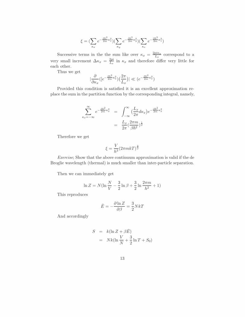
Therefore we get

ξ =V

h3(2πmkT )

3

2

Exercise; Show that the above continuum approximation is valid if the deBroglie wavelength (thermal) is much smaller than inter-particle separation.

Then we can immediately get

lnZ = N(lnN

V− 3

2ln β +

3

2ln

2πm

h2+ 1)

This reproduces

E = −∂ ln Z

∂β=

3

2NkT

And accordingly

S = k(ln Z + βE)

= Nk(lnV

N+

3

2ln T + S0)

13

The constant

S0 =3

2ln

2πmk

h2+

5

2

is now not arbitrary like in the classical case and has been determined interms of the Planck’s constant.

Exercise; Explicitly generalize the above calculate for the entropy wherethe ideal monatomic gas has J possible spin states.

The above Quantum Mechanical calculation has the following importantconsequences

• The correct dependence of ln Z on N , the factor N ! is an automaticconsequence of the theory. Thus the Gibb’s paradox does not arise andln Z behaves properly like an extensive quantity under simultaneouschange of scale N and V

• Also the constant S0 is now determined correctly in terms of the Planckconstant

These modifications are all due to the introduction of the new quantitycalled chemical potential , namely

µ = (∂F

∂N)V,T = −kT (

∂Z

∂N)V,T

Based on the above derivation we can see that

=1

βln

ξ

N

Chemical potential particularly determined the equilibrium between var-ious phases and control the number of transferred particles from one phaseto another. . It also depends on various quantities N and ~ for example (for large N , however N dependence is negligible).

4.1 Average occupation per state

4.1.1 Fermions

We know that

< nk >F =1

eβ(ǫk−µ) + 1

It is instructive to picture the average occupation per state for differenttemperature.

14

0 5 100

1

2Fermi Distribution

ε

<n>

F

µ

T=0

T=T1

T=T2

T2 > T

1

Figure 2:The Fermi Distribution at different temperature

For T = 0, β = ∞. Here for ǫk < µ, exp(β(ǫk − µ)) ← 0 and hence onaverage there is one particle state in this energy range. On the other handfor ǫk > µ,exp(β(ǫk−µ))←∞ and hence < nk >← 0. Thus all particles areaccommodated in the states below the chemical potential µ and distributionis like that of step function. The chemical potential µ at T = 0 is called theFermi energy ǫF . For temperature T > 0 the distribution develops a tail forǫk > µ with < nk >= 1

2 at ǫk = µ. As the temperature increases the tailbecomes more and more pronounced.

4.1.2 Bosons

In the case of the Bosons

< nk >B=1

eβ(ǫk−µ) + 1

Here the important point to note is that since < nk > must exist forǫk = 0, one must have exp(−βµ) ≥ 1 or µ ≤ 0. Thus the chemical potentialfor bosons must be less than or equal to 0. This is same as the conditionthat ensures sum appears in the grand partition function should convergefor all ǫk ≥ 0. For those bosons which do not obey the particle conservation,the chemical potential is identically 0. This is due to the fact total numberof particles is now a variable which is fixed in equilibrium by the condition ofminimum free energy and hence µ = ( ∂F

∂N )V,T = 0. For those bosons where

15

the chemical potential vanishes at a finite temperature, the phenomenon ofBose-Einstein condensation occurs.

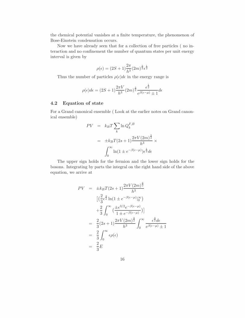
Now we have already seen that for a collection of free particles ( no in-teraction and no confinement the number of quantum states per unit energyinterval is given by

ρ(ǫ) = (2S + 1)2π

h3(2m)

3

2 ǫ1

2

Thus the number of particles ρ(ǫ)dǫ in the energy range is

ρ(ǫ)dǫ = (2S + 1)2πV

h3(2m)

3

2ǫ

1

2

eβ(ǫ−µ) ± 1dǫ

4.2 Equation of state

For a Grand canonical ensemble ( Look at the earlier notes on Grand canon-ical ensemble)

PV = kBT∑

k

ln QF,Bk

= ±kBT (2s + 1)2πV (2m)

3

2

h3×

∫ ∞

0ln(1± e−β(ǫ−µ))ǫ

1

2 dǫ

The upper sign holds for the fermion and the lower sign holds for thebosons. Integrating by parts the integral on the right hand side of the aboveequation, we arrive at

PV = ±kBT (2s + 1)2πV (2m)

3

2

h3

[(2

3ǫ

3

2 ln(1± e−β(ǫ−µ)|∞0)

+2

3

∫ ∞

0

(±ǫ3/2e−β(ǫ−µ)

1± e−β(ǫ−µ)

)]

=2

3(2s + 1)

2πV (2m)3

2

h3

∫ ∞

0

ǫ3

2 dǫ

eβ(ǫ−µ) ± 1

=2

3

∫ ∞

0ǫρ(ǫ)

=2

3E

16

Where E is the average energy of the system. The above result, as shouldbe clear from the derivation is true both for the bosons and the Fermions.In fact, this also holds for the classical gas.

5 Examples of Fermi distribution

5.1 Degenerate Fermi Gas

A collection of independent fermions is called degenerate if it is at verylow temperature or if its density is very high. The characteristic of thedegenerate Fermi Gas is that distribution function f(ǫ) = 1 if ǫ < µ and 0if ǫ > 0 . This is because temperature of the gas can be considered to beabsolute 0 and the limiting form of the Fermi distribution discussed earlieris obtained. Let us consider spin 1

2 fermions ( for example, electron). Thenthe density of state is

ρ(ǫ)dǫ = 2 · 2πV(2m

h

)3

2 ǫ1

2 dǫ, for ǫ < µ

= 0, for ǫ > µ

If the total number of fermions is N then,

N =

∫ µ

0ρ(ǫ)dǫ

= 4πV(2m

h

)3

22

3· µ 3

2

=8π

3V

(2m

h

)3

2 ε3

2

F

Where we identify the chemical potential µ at absolute 0 as the Fermienergy εF . In terms of the number density n = N

V the fermi energy can bewritten as

ǫ =(3n

8π

)2

3~

2

2m

The Fermi temperature TF is defined through

εF = kBTF

The Fermi velocity

17

νF =

√

2εF

m

and the Fermi momentum as pF = mνF . Since the Fermi temperature isproportional to the two-third power of density and hence a high densityFermi density gas has a high Fermi temperature. The Fermi gas is calleddegenerate if its temperature is much lower than TF . This is generally thecriterion if the limiting form of the distribution for the degenerate gas isapplicable in a given situation or not.

The total energy of non relativistic degenerate is given by

E =

∫

ǫρ(ǫ)dǫ

= 4piV(2m

h2

)3

2

∫ εF

0ǫ

3

2 dǫ

=8

3πV

(2m

h2

)3

2 ε3

23

5εF

=3

5NεF

The pressure exerted by a Fermi Gas is found from the general expression

P =2

3

E

V

Thus we get the well know formulae for the pressure exterted by a de-genrate Fermi Gas known as Fermi pressure

P =2

3n · εF =

2

5nkTF

Thus one pictures the degenerate Fermi gas as being at absolute zero withall levels below ǫ = εF occupied, the occupancy factor being (2s + 1), wheres is the spin of the fermions. The number of fermions and the zero pointkinetic energy coming from the uncertainty principle allows the gas to exertpressure which is given by the above equation. One natural manifestation ofsuch intense Fermi pressure is the white dwarf stars, which we shall describenow.

5.2 White Dwarf and Chandrasekhar Limit

The brightness of a star diminishes as the color become redder and in thebrightness against color plot most of the stars lie in a strip. Certain starts

18

are brighter than their red colour warrants - these are known as red giantsand certain stars are than their white color would suggest- these are whitedwarfs. The reson for their dimness is the absence of hydrogen. The massof the star is provided by the helium nuclei while the stability is providedby the ionized electrons. The mass of star will try to drive its towardsgravitational collapse- this is prevented by the zero point pressure exertedby electrons which can be considered as degenerate Fermi gas.

We consider Fermi Gas electrons to consist of N particles. The numberof nucleons is then 2N and the mass of the star is approximately 2Nmn,where the Mn is the nucleon mass . Knowing the approximate mass of thestar we can estimate N and from the approximate size estimate , the volumeV . Thus the density n = N

V is known and hence the Fermi temperature ofthe star. It turns out to be TF = 1011K, the temperature of the star 107K.Hence the elctron gas can be taken to be at zero temperature and thuscompletely degenerate.

The role of nucleons is to provide the mass while the role of the elec-trons is to exert the pressure. The typical energy of the electrons is muchlarge than the rest mass of the electrons and hence we need the relativisticexpression for energy in calculating the pressure of the degenerate electrongas.

E = V · 8πh3

∫ pF

0

√

(p2c2 + m2c4)p2dp

= V8π

h3· c

∫ pF

0

(

1 +m2c2

2p2+ · · ·

)

· p3dp

= V8π

h3· c

(p4F

4+

m2

c24p2

F + · · ·)

= V8π

h3· m

4c5

4(X4

F + X2F + · · ·

)

where XF = pF

mc .Here E is the free energy The Pressure can be obtained by differentiating

E with respect to V , as

P = −(∂E

∂V

)

T

= −2π

h3m4c5(X4

F + X2F + V

∂X2F

∂V(2X2

F + 1) + · · · )

The important thing to note is that E is here free energy. Rest of the partare the details of derivation from the book of Bhattacharjee. It is basically

19

equating the Fermi pressure exerted by the degenerate gas of electrons toexpand the system against the gravitation pull generated by the mass of thenucleons and from that the calculation of the mass limit beyond which thegravitational pull will be too high to be counterbalanced by the Fermi pressure.Very few natural phenomenon brings together such an interplay between theclassical gravitational effect and quantum Fermi pressure effect demonstratedfirst time by Chandrasekhar

Now

V · ∂

∂VX2

F = 2V∂

∂V

εF

mc2

=2

mc2V · ∂εF

∂V

=2

mc2V · ∂

∂V

[ h2

2m

( 3

8π

N

V

)2

3]

= −4

3

mεF

m2c2= −2

3X2

F

Thus we get the following expression for the pressure

P = −2πm4c5

h3(X4

F + X2F −

4

3X4

F −2

3X4

F )

=2πm4c5

3h3(X4

F −X2F )

In terms of the mass and the radius of the star, we can write

M = 2Nmn, V =4

3πR3

leading to

2mn.n =3M

4πR3, or, n =

3M

8πmnR3

andXF = M

1

3 R

Where dimensionless mass and radius are respectively given by

M =9π

8

M

mn

and

R =Rh

mc

20

Therefore in terms of M and R, we have

P = K(M

4

3

R4−−M

2

3

R2

)

with

K =2π

3mc2

(mc

h

)3

The equilibrium radius is found by equating the work done against thepressure to the gravitational potential energy. The gravitational potentialenergy of a system of total mass M and radius R is

V (R) = −αGM2

R= −αG

(8mn

9π

)2 mc

h

M2

R

where α is a number of order unity and can be fully determined onlywhen the density is known as function of the radial distance. The workdone against the pressure is

W =

∫ R

∞P4πr2dr

= 4π(h

mc)3

∫ R

∞P (r)4πr2dr

which must be equated to the potential energy V (R). Differentiatingboth these terms with respect to R we get

4πR2p(R) = αG(8mn

9π

)2(mc

h

)4 M2

R2

Thus we finally get

K(M

4

3

R4− M

2

3

R2

)

= K ′M2

R4

with

K ′ =αg

4π

(8πmn

9π

)2(mc

h

)4

Solving the equation we get

R2 = M2

3

(

1− (M

M0)

2

3

)

21

where

M0

2

3 =K

K ′

=2π3 mc2

(

mch

)3

αG4π

(

8mn

9π

)2(mch

)4

=27π

64α

hc

Gm2n

Clearly for R to exist, we must have M ≤ M0 Thus M0 is the upperlimit of a mass of a white dwarf star. The dimensionless number hc

Gm2n

is

1039

For α 1, the corresponding dimensionless mass M is almost Msum. Whenproper estimate of α is taken it can be shown the upper limit is 1.4Msun,the famous Chandrasekhar limit.

6 Specific heat of electron gas

So far we have discussed only the case of T = 0, namely the highest oc-cupied energy state. We now consider the case of finite temperature whenit is possible to populate the energy above the chemical potential µ andconsequently the chemical potential is now going to be a function of thetotal number of particles N and the temperature T . Here that temperaturedependent chemical potential will be determined.

The way we proceed is to use the following equation of state

PV =2

3E =

2

3

2V

4π2(2m

h2)

3

2

∫ ∞

0

ǫ3

2 dǫ

exp(β(ǫ− µ)) + 1

For spin s fermions the factor 2 associated with fermions is replaced by2s + 1. we need to evaluate the above integral.

We note∫ ∞

0

∫ ∞

0

ǫ3

2 dǫ

exp(β(ǫ− µ)) + 1= (kBT )

5

2

∫ ∞

−βµ

(x + µβ)3

2

ex + 1dx

= (kBT )5

2 I(µβ)

If we now use even more compact notation α = µβ, then we get to sovethe integral

I(α) =

∫ ∞

−α

(x + α)3

2

ex + 1dx

22

The full evaluation of this integral in term of known analytic function isnot possible and hence a perturbation approach is taken.

The full details is there in Bhattacharjee. The basic idea is that thoughone considers a finite temperature nevertheless we only consider low tem-perature.

Hence α = µkBT ≫ 1 and thus a perturbation expansion is possible

I(α) =

∫ ∞

−α

(x + α)3

2

ex + 1dx

=

∫ 0

−α

(x + α)3

2

ex + 1dx +

∫ ∞

0

(x + α)3

2

ex + 1dx

=

∫ α

0

(α− x)3

2

e−x + 1dx +

∫ ∞

0

(x + α)3

2

ex + 1dx

=

∫ α

0(α− x)

3

2ex

ex + 1dx +

∫ ∞

0

(x + α)3

2

ex + 1dx

=

∫ α

0

(α− x)3

2

dx−

∫ α

0(α− x)

3

21

ex + 1dx

+

∫ ∞

0

(x + α)3

2

ex + 1dx

=2

5α

5

2 +

∫ ∞

0dx

(α + x)3

2 − |(α− x)| 32ex + 1

+

∫ ∞

α

|α + x| 32ex + 1

dx...

It can be shown that

(α + x)3

2 − |(α− x)| 32 = 3α1

2 x + 0( 1√

α

)

After sum algebra (see Bhattacharjee) we finally arrive

I(α) =2

5α

5

2 +π2

4α

1

2 + O(1

α1

2

)

We shall now substitute the above formula in the equation

PV =2

3E

23

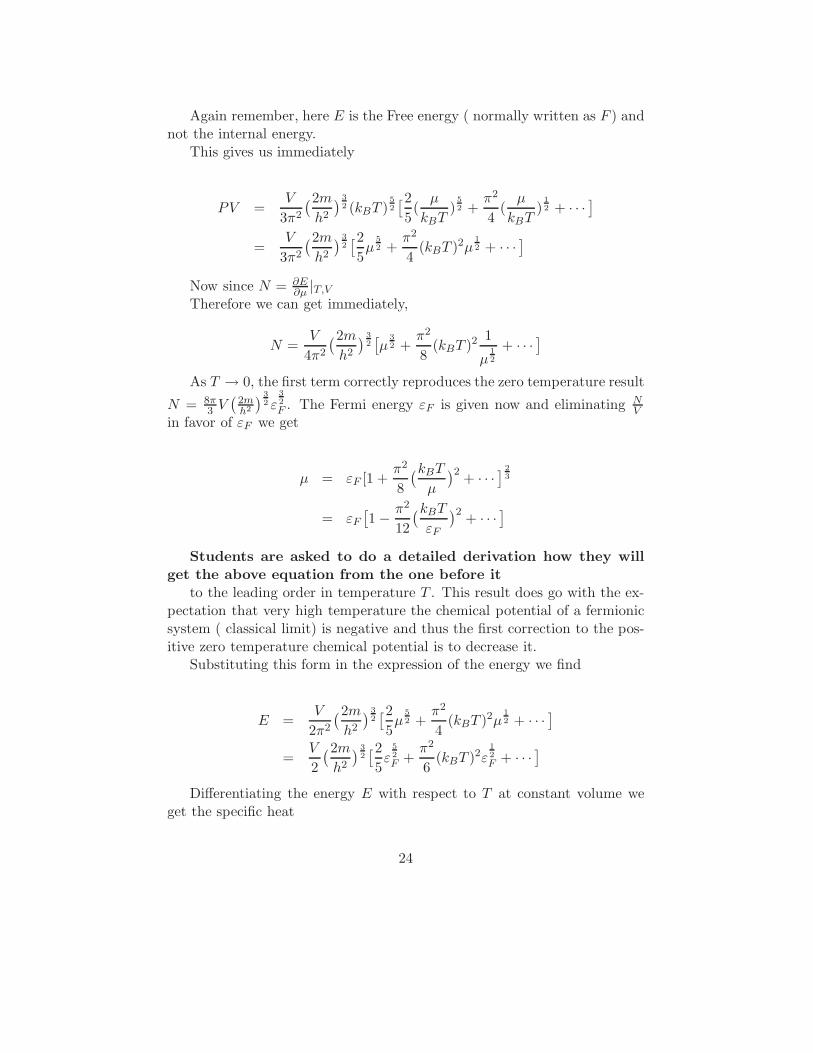
Again remember, here E is the Free energy ( normally written as F ) andnot the internal energy.

This gives us immediately

PV =V

3π2

(2m

h2

)3

2 (kBT )5

2

[2

5(

µ

kBT)

5

2 +π2

4(

µ

kBT)

1

2 + · · ·]

=V

3π2

(2m

h2

)3

2[2

5µ

5

2 +π2

4(kBT )2µ

1

2 + · · ·]

Now since N = ∂E∂µ |T,V

Therefore we can get immediately,

N =V

4π2

(2m

h2

)3

2[

µ3

2 +π2

8(kBT )2

1

µ1

2

+ · · ·]

As T → 0, the first term correctly reproduces the zero temperature result

N = 8π3 V

(

2mh2

)3

2 ε3

2

F . The Fermi energy εF is given now and eliminating NV

in favor of εF we get

µ = εF [1 +π2

8

(kBT

µ

)2+ · · ·

]2

3

= εF

[

1− π2

12

(kBT

εF

)2+ · · ·

]

Students are asked to do a detailed derivation how they will

get the above equation from the one before it

to the leading order in temperature T . This result does go with the ex-pectation that very high temperature the chemical potential of a fermionicsystem ( classical limit) is negative and thus the first correction to the pos-itive zero temperature chemical potential is to decrease it.

Substituting this form in the expression of the energy we find

E =V

2π2

(2m

h2

)3

2[2

5µ

5

2 +π2

4(kBT )2µ

1

2 + · · ·]

=V

2

(2m

h2

)3

2[2

5ε

5

2

F +π2

6(kBT )2ε

1

2

F + · · ·]

Differentiating the energy E with respect to T at constant volume weget the specific heat

24

CV =∂E

∂T|V

=V

2π2

(2m

h2

)3

2π2

3k2

Bε1

2

F T + · · ·

=π2

2NkB

kBT

εF+ · · ·

In deriving the last line we have used the relation between N and εF .Thus as T ← 0, we have

CV =π2

2NkB

kBT

εF

which vanishes linearly with T as T tends to zero. This is to be contrastedwith the T 3 dependence of the contribution to the vibration of the nucleiforming the crystal lattice. The full specific heat will be given by bothcontribution. At very low temperature the linear part dominates whereasat very high temperature the cubic part will dominate. The results are insurprisingly good agreement with a wide variety of metal.

6.1 Emission of electrons from a metal surface

This is not covered in the lecture but has been provided as a tuto-

rial problem We consider a metal in equilibrium with a dilute electron gasat very low temperature. The periodic distribution of the ions which pro-duces the periodic potential in which the electrons move is interrupted at thesurface giving rise to a potential barrier which is needed to be overcome if anelectron is to leave the surface. We model this barrier by giving an electronthe at the bottom of the conduction band an energy −V . The maximumkinetic energy of the of an electron is, to a good extent, if the temperatureis sufficiently low, is equal to the Fermi energy εF . The minimum energyrequired to eject a metal is therefore

W = V − εF

which is called the workfucntion of the metal. Now to calculate the chem-ical potentail of this electron gas inside the metal, we note that the Fermidistribution for particles having momentum between p and p + dp is givenby

25

< nF >=1

eβ( p2

2m+V−µ) + 1

and at very low temperature the standard calculation of the Fermi energyyields

εF = V + µ

thus giving the expect result

µ = −W

inside the metal.Generally outside the metal the density of the electron gas is very low and

hence corresponds to a situation where the Fermi distribution will reduceto the classical distribution and thus the number of electrons between p

abd p + dp will be given by eβ( p2

2m−µ0) whereas µ0 is the chemical potential

outside the metal. If the total number of electron is N and the volume is Vthen outside the metal

N = 2.V4π

h3

∫ ∞

0p2e−

p2

2mkT eµ0

kBT dp

The factor 2 comes because of the two available spin states.Solving the integral we get the density of the electrons in terms of the

chemical potential

n = 2 ·(2πmkT

h2

)3

2 eµ0

kBT

For equilibrium between the metal and the electron Gas, the chemicalpotentials must be equal and hence

µ0 = µ = −W

Thus we get

n = 2(2πmkT

h2

)3

2 e− W

kBT =

WkBT

λ3

The equilibrium here achieved is a dynamical one. In that, in every unittime interval, a certain number of electrons strike the metal surface per unitarea per unit time and a fraction of them are absorbed. To keep the numberof electrons fixed an equal number of electrons must energy from the metalsurface per unit area per unit time. This gives the emission current from

26

the metal surface. The number of electrons with momentum between pz andpz + dpz ( the surface is at z = 0) and with the density already mentionedstriking a unit area of metal in unit time

2nλ3

h3

∫∞−∞ dpx

∫∞−∞ dpy

∫∞−∞ dpzvze

− p2

2mkT

And hence the total number of electrons striking the metal surface perunit area is

N = 2e− W

kBT

h3

∫ ∞

−∞dpx

∫ ∞

−∞dpy

∫ ∞

−∞dpz

pz

me−

p2

2mkT

= 2 · 2πmkBT

h2

kBT

he− W

kBT

If the reflection coefficient of the metal surface is r, then the numberof electrons absorbed on the metal surface per unit area per unit time is

(1−r)4πmkBTh2

kBTh e

− WkBT and this must equal to the emission rate. Thus the

emission current is given by the formulae

I = (1− r)4πmkBT

h2

kBT

he− W

kBT

The factor e− W

kBT reflects the depletion of the current due to potentialbarrier.

7 Bose Einstein Condensation

From the last part we have the relation

PV =3

2E

Now by definition

N =∂(PV )

∂µ

27

The last equation follows from the fact

N =∑

i

< ni >

= kT∑

i1

eβ(ǫi−µ) − 1

= kT∑

i

∂

∂µln Qi

B,F

=∂

∂µ(kT ln Q)|T,V

=∂

∂µ(PV )|T,V

Thus we getSubstituting the result for E we finally get,

N = ±(2s + 1)2πV

h3(2m)

3

2

∫ ∞

0

±ǫ1

2 dǫ

eβ(ǫ−µ) ± 1

The idea is eliminate the chemical potential with the help of the aboveequation and getting an equation of state of the form

7.1 Bose Einstein condensation

The chemical potential of system of spinless bosons (s = 0) is related to thenumber of particles through the equation

N = V · 2π(2m

h2

)

∫ ∞

0

ǫ1

2 dǫ

eβ(ǫ−µ) − 1

For a dilute Bose gas, that is the classical limit exp(−βµ) ≫ 1. Thismeans the chemical potential is a large negative value. Now we shall considera limit where exp(−βµ) ≈ 1. For a given chemical potential, as we decreasethe temperature , the value of exp(−βµ) will decrease and will approachunity. Now let us look at this following puzzling behavior,

According to the previous formulation

n(µ) =N

V= 2π

(2m

h2

)

∫ ∞

0

ǫ1

2 dǫ

eβ(ǫ−µ) − 1

We are interested in the behavior of the Boson gas at the low temper-atures. Since the Pauli principle does not apply to Boson, they tend to

28

concentrate to the lowest energy level and it is only the thermal fluctuationthat will prevent them all occupying the ground state of the system. At lowtemperature, when the thermal fluctuation will be less, we can thus expectthat a macroscopic number of boson to occupy the ground level of the sys-tem, namely ǫ = 0. Accordingly we find that at low temperature number oforder of bosons in the ground state is N then

N ≈ 1

exp(−βµ)− 1

µ ≈ −kT

N

• At first sight such a behavior makes sense because it is consistent withthe tendency that chemical potential to decrease with the high tem-perature and also consistent with the requirement that the chemicalpotential should be negative (since the lowest energy available is 0).

• However this formulae is in direct contradiction with the expression ofthe density given before it. This equation gives the density of particlesas a sum of the contribution from all energies. We find there thecontribution to the integral coming from the region near ǫ 0 is 0.Thus the occupation of the ground level which is very large at lowtemperature

• This difficulty leads to a paradox which is a consequence of relationbetween the density of particles and the chemical potential. As we cansee the integral on the right hand side is an increasing function of µsince the integrand at a given value of µ is an increasing function ofµ. But the integral cannot become larger than its value at µ = 0 sinceµ cannot become positive. Consequently the right hand side of thisequation has an upper bound which is its value at µ = 0 . This wouldimply that the density n at a given temperature, of our non-interactingboson gas cannot rise above a certain maximum value, determined bythe maximum on the right hand side.

• This conclusion is, of course, unreasonable, since it is impossible forthere to be a restriction on the number of non-interacting bosons ina given volume. Even fermions which obey the Pauli principle do notresist the addition of fermions. They only force the new fermions tooccupy the higher energy levels. Now suppose a system is prepared ata density and temperature for which there exist a solution for µ, as T

29

is lowered the solution disappears. Moreover at T = 0 the equationwill allow only 0 density which is clearly absurd. So the question iswhat went wrong?

7.2 The rationale for condensation

In order to clarify the reason for this inconsistency we look at the calculationof various quantities using the density of states. Namely calculation of theThermodynamic potential Ω ( the analogue of free energy for grand par-tition function) and its derivatives which gives us various thermodynamicquantities.

As we know we do all these calculations by invoking the notion of densityof states, namely the number of states that lies in between energy ǫ andǫ + dǫ, denoted by n(ǫ)dǫ. We then multiply any quantity by this density ofstates after taking into consideration their bosonic or the fermionic characterand obtain the thermodynamic value of that quantity. For example thethermodynamic potential Ω itself for an ideal gas of bosons with spin 0

ΩB =4πV kT

h3

∫ ∞

0ln

[

1− exp(

β(µ− p2

2m))]

p2dp

and then differentiating with respect to µ we get the average number ofbosons, namely which is given at the beginning of this section. All these havebeen obtained by replacing the summation over a discrete momentum statesk by an integration over a continuous momentum. But since n(ǫ) ∝ ǫ

1

2 , thismeans that density of states goes to 0 as we approach the ground state sincen(0) = 0. Thus we are loosing the huge contribution that goes into theground state.

If the temperature is not too low ( or the density is not too high) theoccupation of the ground level does not differ greatly from that of the otherlevels. In that condition, each of the term entering in the expression of thethermodynamic potential is of the order N , where as sum is of the order N .Hence the error introduced in neglecting the ground level is insignificant.

But at low temperature the chemical potential tends to 0 as 1N since

µ ≈ −kTN and the terms corresponding the the ground level in the various

sum must be examined more closely. For example in the sum for Ω , thecontribution from ground state

30

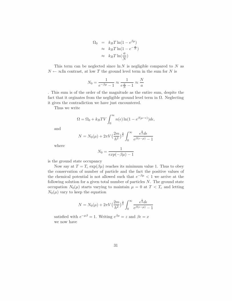
Ω0 = kBT ln(1− eβµ)

≈ kBT ln(1− e−aN )

≈ kBT ln(a

N)

This term can be neglected since ln N is negligible compared to N asN ←∞In contrast, at low T the ground level term in the sum for N is

N0 =1

e−βµ − 1≈ 1

e aN − 1

≈ N

a

. This sum is of the order of the magnitude as the entire sum, despite thefact that it orginates from the negligible ground level term in Ω. Neglectingit gives the contradiction we have just encountered.

Thus we write

Ω = Ω0 + kBTV

∫ ∞

0n(ǫ) ln(1− eβ(µ−ǫ))dǫ,

and

N = N0(µ) + 2πV(2m

h2

)3

2

∫ ∞

0

ǫ1

2 dǫ

eβ(ǫ−µ) − 1

where

N0 =1

exp(−βµ)− 1

is the ground state occupancyNow say at T = Tc exp(βµ) reaches its minimum value 1. Thus to obey

the conservation of number of particle and the fact the positive values ofthe chemical potential is not allowed such that e−βµ < 1 we arrive at thefollowing solution for a given total number of particles N . The ground stateoccupation N0(µ) starts varying to maintain µ = 0 at T < Tc and lettingN0(µ) vary to keep the equation

N = N0(µ) + 2πV(2m

h2

)3

2

∫ ∞

0

ǫ1

2 dǫ

eβ(ǫ−µ) − 1

satisfied with e−µβ = 1. Writing eβµ = z and βǫ = xwe now have

31

N = N0 + 2πV2mkBT

h2

∫ ∞

0

zx1

2 e−x

1− ze−xdx

= N0 + V(2πmkBT

h2

)3

2 ζ3/2(z)

Where the function

ζ3/2(z) =

∞∑

k=0

zk+1

(k + 1)3

2

The algebra is the following

∫ ∞

0dx

zx1

2 e−x

1− ze−x=

∫ ∞

0dx

∞∑

k=0

zk+1x1

2 e−(k+1)x

=

∞∑

k=0

zk+1

(k + 1)3/2

1

2

√π

This is clearly a monotonically increasing function for z > 0 and risesfrom 0 at z = 0 to 2.612 at z = 1 and the derivative is discontinuous atz = 1. indcating a phase transition.

Now we can write

N0 = N − V(2πmkBT

h2

)3

2 ζ3/2(z)

The highest T at which N0 is not equal to 0 is given by Tc which satisfies

(2πmkBTc

h2

)3

2 ζ3/2(1) =N

V= n

For the T < Tc, z have already reached unity and cannot change anymore and hence the particle density in the ground state has to change ac-cordingly as

n0 =N0

V=

N

V−

(2πmkBT

h2

)3

2 ζ3/2(1)

= n(

1− (T

Tc)

3

2

)

This phenomenon is known as Bose Einstein condensation. Beyond acritical temperature the occupation of the ground state is macroscopic

32

7.3 Thermodynamic quantities below T = TC

When T < TC ; In this range the total energy is obtained by noting thatµ = 0 and only the particles outside the condensate contribute. We haveoriginally,

N = N0(µ) + 2πV(2mkBT

h2

)3

2

∫ ∞

0

x1

2 dx

e−µβ(ex − 1)

Now it is clear that the part N0 does not have any contribution to theenergy. Consequently, the energy is given by

E =

∫ ∞

0dǫǫn(ǫ)

Following the same steps as before, namely expanding the denominatorin a power series and using the properties of the Gamma function Γ(n+1) =nΓ(n)

E = 2πV(2mkBT

h2

)3

2

∫ ∞

0

x3

2 dx

(ex − 1)

= 2πV(2mkBT

h2

)3

2 kBT1

2· 32

√πζ 5

2

=3

2V

(2πmkBT

h2

)3

2 kBTζ 5

2

=3

2NkBT

( T

TC

)3

2

ζ 5

2

ζ 3

2

=3

2

1.341

2.312NkBT

( T

TC

)3

2

= 0.770NkBT( T

TC

)3

2

The equation of state follows as

PV =3

2E = 0.513NkBT

( T

TC

)3

2

Or, the pressure is given by

P =(2πmkBT

h2

)3

2 kT5

2 ζ 5

2

Differentiating the energy E with respect to T will give the specific heatat constant volume as

33

CV = 1.925NkB

( T

TC

)3

2

The entropy is obtained by integrating CT and hence

S = 1.282NkB

( T

TC

)3

2

When T > TC ; Now N0 = 0 and z = exp(βµ) has to be fixed from theequation

N = N0(µ) + 2πV(2m

h2

)3

2

∫ ∞

0

ǫ1

2 dǫ

eβ(ǫ−µ) − 1

This immediately yields,

N = V(2πmkBT

h2

)3

2 ζ 3

2

(z)

The energy is given by

E = 2πV(2πmkBT

h2

)3

2

∫ ∞

0

x3

2 dx1zex − 1

=3

2V

(2πmkBT

h2

)3

2 ζ 5

2

(z)kBT

To find out the entropy we note that in the grand canonical ensemble

E − TS − µN = −PV = −3

2E

Thus

TS =5

3E − µN

S =5

2kBV

(2πmkBT

h2

)3

2 ζ 5

2

(z)−NkB ln Z

C =15

4kBV

(2πmkBT

h2

)3

2 ζ 5

2

+3

2V kBT

(2πmkBT

h2

)3

2 × d

dzζ 5

2

(z) · ∂z

∂T|N,V

To find out the derivative ∂z∂T we use the relation

34

N

V=

(2πmkBT

h2

)3

2 ζ 3

2

(z)

Since the LHS is a constant, we get after differentiating

0 =3

2T

1

2 ζ 3

2

+ T3

2d

dzζ 3

2

(z) · ∂z

∂T∂z

∂T= − 3

2T

[ d

dzζ 3

2

]−1ζ 3

2

(z)

Using the definition of ζn =∑∞

k=0zk+1

(k+1)n we finally get

1

z

∂z

∂T= − 3

2T

ζ 3

2

(z)

ζ 1

2

(z)

Thus we finally get

C =15

4kBV

(2πmkBT

h2

)3

2 ζ 5

2

(z) − 9

4NkB

ζ 3

2

(z)

ζ 1

2

(z)

Thus if we consider the Thermodynamic quantities like E and S and Cabove and below the critical temperature T = TC we found that they arecontinous at T = TC . However we have noted ( also given as a tutorialproblem) that in the low temperature phase the pressure is independent ofvolume and hence studying the isotherms. If we hod T fixed and vary Vfrom large values to smaller one going from dilute classical to the degenerategas then at a critical V given by

[2πmkBTC

h2

]3

2 ζ 3

2

(1) =N

VC

The condensate phenomenon will set at V = Vc implying that there willbe a finite condensate N determined by

N0 = N(

1− V

Vc

)

In the P − V diagram the pressure does not change in the range 0 <V < VC and then decreases with increasing V .

For higher temperature the critical VC occurs at smaller and smallervalues. The flat part of each curve can be thought of the co-existence of twophases, a standard feature of first order transition.

35

Since the pressure in this regime is solely dependent on temperature, wefound the slope of the vapor pressure curve as

dP

dT=

5

2ζ 5

2

(1)[2πmkBTC

h2

]3

2 · kB

Now for an isotherm at temperature T , the specific volume are zero andVc

N for the condensate and the gas phase respectively. From that, using theClausius Clapeyron equation we can calculate the latent heat of transitionper particle as

L = T(Vc

N− 0

)

· dP

dT

=5

2

ζ5/2(1)

ζ3/2(z)· kBT

Thus the condensation has certain features of first order phase transition.

7.4 Behavior of the chemical potential near the transition

We are interested how the chemical potential behaves ( how it goes to 0 froma large negative value ) as the transition temperature T = TC is approachedfrom the top (from the side T > Tc

To find out that we note that at T > Tc, for fixed N and V we have

T3

2 ζ 3

2

(z) =N

V= constant

Now µ = 0 implies z = exp(βµ) = 1Therefore, taking the differential near z = 1 at T = TC , we have

3

2ζ 3

2

(1)δT

Tc= −

dζ 3

2

(z)

dz|z=1δz

Howeverdζ 3

2

(z)

dz |z=1 ia a divergent quantity and hence we should inspectthis divergence more carefully

We can write

dζ 3

2

(z)

dz|z=1δz = ζ 3

2

(1 + δz) − ζ 3

2

(1)

We can provide the integral representation of the above expression bywriting

36

dζ 3

2

(z)

dz|z=1δz =

1

Γ(32)

∫ ∞

0

[ 1ex

1+δz − 1− 1

ex − 1

]

=1

Γ(32)

∫ ∞

0

dxx1

2 δzex

(ex − 1)(

ex

1+δz − 1)

The following features are important

• δZ ← 0, the integral is completely dominated by the small x-regimeThe denominator becomes 0 if we set δz = 0 and x = 0. Hence toretain the leading order correction in δz it suffices to linearize ex.

• The integral is well defined only for negative δz which is as it shouldbe since the maximum value of z (z = 1) is achieved at T = Tc and zhas to decrease as T increases above TC .

We thus set δz = −ε and upon linearizing ex we get

εd

dzζ 3

2

(z)|z=1 =ε

Γ(3/2)

∫ ∞

0

dx√ε· 1

x + ε

=π√

ε

Γ(32)

Substituting this in the equation

3

2ζ 3

2

(1)δT

Tc= −

dζ 3

2

(z)

dz|z=1δz

we get

√ε =

3

2

ζ 3

2

Γ(3/2)

π

δT

Tc

ε =9

4

(

ζ 3

2

Γ(3/2)

π

)2(δT

Tc)2

z[δµ

kBT− µ

kBT

δT

T]|T Tc,µ 0,z 1 =

9

4

(

ζ 3

2

Γ(3/2)

π

)2(δT

Tc)2

δµ =9

4kBTc

(

ζ 3

2

Γ(3/2)

π

)2(δT

Tc)2

37

The slope of the chemical potential is consequently discontinuous at T =TC .

This leads to interesting consequences for the slop of the specific heat.If we go back to the physical meaning of chemical potential this is obvious.

We can now expand the energy as a function of z and T near z = 1 andT = TC in a Taylor series ( keeping N and V fixed).

Then we have

E(T, z) = E(Tc, 1) +(δE

δT

)

Tc,1deltaT +

(δE

δz

)

Tc,1deltaz

+1

2

(δ2E

δT 2

)

Tc,1(deltaT )2 + · · ·

We do not need any further terms since δz O((δT )2).Now using the value of the derivatives it can be easily shown that the

slope of the specific heat as T approached TC from above is given by

(dCV

dT

)

T←Tc= −0.776

NkB

Tc

Using the expression of specific heat when TC is approached from belowone can show

(dCV

dT

)

T←T−

c= 2.89

NkB

Tc

The specific heat thus has maximum at T = TC (kink) and slope discon-tinuity of 3.66NkB

T .

• All the above derivations are true only for a non-interacting Bose gaswill change drastically even in the presence of any interaction.

• Another important thing is in all these derivations we have assumedthat the total number of particles is conserved. This is essential forcondensation and hence in a system with no such conservation law,for example, photon or phonon gas, it is not possible to have BoseEinstein condensation.

• The system of cold atoms where all the recent experiments of BEC tookplace is harmonically trapped and very weakly interacting. The BoseEinstein condensation happens in such system have its own character-istics ( some of them will come out upon solving the tutorial problems)

38

8 Examples for the Bose Einstein systems

We shall basically discuss two examples. One that of a photon gas. Be-cause of the zero chemical potential of a photon gas, which means there isno conservation of the photon number, photons cannot condense. A gas ofphotons behaves otherwise like the ideal gas of atoms except that it’s chem-ical potential is 0 and rest mass is also zero and energy momentum relaionis relativistic (linear). With these inputs one can just get Planck’s distribu-tion straightforwardly from the expression of occupation number of photons.One must compare the derivations with the derivation of the kinetic theoryof gases from canonical distribution function. One here gets distribution ofIntensity as a function of frequency and wavelength and verify various wellknown laws, like Raley Jeans, Staefan Boltzman, or Wein displace ment lawstarightforwardly.

9 Planck’s theory of Black Body radiation; Red-

erivation from BE statistics

Black Body radiation is modeled as a cavity enclosed by matter such thatthe electromagnetic radiation inside that cavity is in thermal equilibriumwith the matter that encloses it. Radiation in the cavity can have differentfrequencies and different wavelength. The distribution of the energy as afunction of the wavelength is what we like to evaluate. To begin with,classically the e.m. radiation can be described by the electric field thatsatisfies the Maxwell’s equation

∇2~E =1

c2

∂2~E∂t2

The solutions of the above equation can be written in the form of planewaves, namely

~E = ~Aei(k·r−ωt) = ~E0(r)e−iωt

with

κ =ω

c, κ = |κ|

Now, as according to Plank’s such electromagnetic waves are quantized, thenthe associated quanta, known as photons is described in familiar way as a

39

relativistic particle with momentum p and energy ǫ such that

ǫ = ~ω = hν

p = ~k

Since an electromagnetic wave also have to satisfy the Maxwell’s equation( there is no charge inside the cavity)

~∇ · ~E = 0

This gives, with the help of plain wave solutions that we have mentioned

κ · ~E = 0

Thus for each κ there are only two perpendicular directions of the electricfield that can be specified. In terms of photons this means there are twopossible directions of polarizations.

Now since photons are partciles, according to the quantum mechanics,not all possible values of κ is allowed and only certain discrete values whichwill reflect the boundary conditions are allowed. Let us take an enclosure inthe form of a parallelepiped with edges with length Lx, Ly and Lz. Supposethe smallest of these length, call it L≫ λ, where the λ = 2π

κ is the longestwavelength of significance in this discussion.

Then we can again neglect the situation at the boundary and describethe radiation in terms of simple traveling waves. As we have already learnedfrom the calculation from the density of states, that to eliminate the effectof the walls, we just put the periodic boundary condition. The enumerationof possible states of the photon are then same as possible values of κ of aparticle in a box with periodic boundary condition.

Now rest of the calculation will be very similar to the derivation ofthe kinetic theory of gases using classical statistical mechanics. Here onlythe enumeration of the states and the distribution function will take intoconsideration quantum mechanical nature of the photons.

ρ(k)d3κ = the mean number of states

per unit volume with

one specified direction of polarization

when wavevector lies in between

κ and κ + dκ

=nǫ

(2π)3d3k

40

Each of this state has energy

ǫ = ~ω = ~cκ

The quantum statistics or more specifically the bosonic nature of photonenters in the fact that the mean number photon with a definite value of κis given by,

nǫ =1

eβǫ − 1

Calculating the average occupation number for photon is simple since ithas 0 chemical potential. namely, Let us consider the photon is in the states with energy ǫs. Then the average occupation number of photon in thatcase which we shall denote as ns is given by

ns =

∑

n1,n2,··· nse−β(n1ǫ1+n2ǫ2+···+nsǫs+··· )

∑

n1,n2,··· e−β(n1ǫ1+n2ǫ2+···+nsǫs+··· )

=− 1

β∂

∂ǫs

∑

e−βnsǫs

∑

e−βnsǫs

= − 1

β

∂

∂ǫsln(

∑

e−βnsǫs)

The particles being boson ns can take any integer value between 0 and∞. Thus the above sum is a G.P. series given by

∑

e−βnsǫs = (1− eβǫs)−1

Thus we have

ns =1

eβǫs − 1

Thus the corresponding mean number of photons is simply

f(k)d3k =1

eβ~ω − 1

d3k

(2π)3

Note f(κ) de4pends on |κ| = κ only. Now k is a vector (wave numberalong three different direction) where as ω is a scalar, related with each otherthrough the relation

ω = c|k|Then the mean number of photons per unit volume with both direction

of polarization with angular frequency in the range ω and ω+dω, is given by

41

summing over all the volumes in the κ space contained within the sphericalshell of radius κ = ω

c and κ + dκ ( basically we are eliminating the angulardependence of κ through integration since the energy density is independentof it). This is just

2f(κ)4πκ2dκ =8π

(2πc2)3ω2dω

eβ~ω − 1

Let u(ω;T ) be the mean energy per unit volume in the frequency rangebetween ω and ω + dω with both direction of polarization. This will beobtained by simply multiplying the above quantity with the energy ~ω.Thus we have

u(ω;T ) =~

π2c3

ω3dω

eβ~ω − 1

The significant dimensionless parameter is

η = β~ω = ~ωkBT

In terms of this

u(ω, T ) =~

π2c3

(kBT

~

)4 η3dη

eη − 1

If we now plot the function π2c3~3

k4B

uT 4 as a function of η we shall find that

it is peaked at η ≈ 3.Now this peak will remain at the same η even at a different temperature.

Thus we get a simple scaling relation. If the peak occurs at a frequency ω1

at temperature T1, it will occur at different frequency ω2 at temperature T2

such that

~ω1

kBT1=

~ω2

kBT2ω1

T1=

ω2

T2

This result is known as Wein’s displacement law.The mean energy density is given by by

u0(T ) =

∫ ∞

0u(T ;ω)dω

=~

π2c3

(kBT

~

)4∫ ∞

0

η3dη

eη − 1

=π2

15

(kBT )4

(c~)3

42

In the last line we have used∫ ∞

0

η3dη

eη − 1=

π4

15

This is Stefan Boltzman law.We can also calculate the radiation pressure. The pressure contribution

to a photon in the state s with energy ǫs is given by −∂ǫs

∂VHence the mean pressure due to all the photons is given by

p =∑

s

ns

(

− ∂ǫs

∂V

)

Now

ǫs = ~ω

= ~c(κ2x + κ2

y + κ2z)

1

2

= ~c2π

L(n2

x + n2y + n2

z)1

2

Here we take Lx = Ly = Lz = L.Thus

ǫs = CL−1 = CV −1/3

here C is some constant. Thus substituting this volume in the formulaof the pressure we get

p =1

3V

∑

s

nsǫs =1

3u0

The radiation pressure can be also calcuated in the following differentways

p =1

β(∂ ln Z

∂V)

Also we can use the detail kinetic argument. For example photons im-pinging on an area dA of the container wall normal to the z direction impartto it in unit time a mean z component of the momentum G+

z . In equilibriuman equal number of photons leaves the wall and gives rise to an equal mo-mentum flow −G+

z in the opposite direction. Hence the net force per unitarea, or pressure is given by

p =1

dA[G+

z − (−G+z ] =

2G+z

dA

43

Now

G+z =

1

dt

∫

κz>0[2f(κ)dκ(cdtdA cos θ)(~κz)

From that one can easily find the same expression for the radiation pres-sure.

Thus all the conclusions of Planck’s law can be reestablished using BoseEinstein distribution.

9.1 Superfluidity of liquid Helium

The second example is that of the superfluidity of liquid Helium. Which weshall discuss rather phenomenologically, I mean without going in to rigor-ous derivations and same procedure will be followed for the Bose Einsteincondensation of cold atomic gases. Historically this was also the first casewhere a condensate has been formed had been suspected by F. London asan explanation of certain peculiar behavior of Liquid behavior.

Basically after having found that an ideal boson gas behaves at lowtemperature very differently from a Boltzman gas, the following questionarises:; In what physical conditions does this behavior manifests itself.

First we need to have an estimate of the critical temperature TC . Forexample for the lightest element hydrogen , the atomic mass being 1− .7×10−24 gr , we obtain a critical temperature 7K. For heavier elements thecritical temperature is even less.

The problem of seeing the Bose Einstein condensation in nature is thatat this extremely low temperature , all substances are either solid and liquidand hence cannot ne further cooled. However liquid Helium liquefies at 4.2Kand does not freeze at even absolute 0. Particularly liquid Helium He4 havebosonic atoms and may be treated as an ideal candidate for Bose Einsteincondensation.

A very interesting properties of the He4 around this region of low tem-perature is its extremely low viscosity 20µP . In fact it has been knownfrom twenties from the work of Kapitza and others that at the tempear-ture 2.17K the liquid helium changes its properties drastically and has beencharacterized by two different phases above and below this temperature.

Particularly in the phase Helium II He4 shows a frictionless flow throughthe capillary. This is known as superfluidity.It also has an enormously highthermal conductivity 104 − 105. All these properties particularly lead to F.London to think of this phase transition of Helium at 2.17K as a manifes-tation of Bose Einstein condensation.

44

According to London’s explanation at this temperature a macroscopicnumber of atoms populate the ground state while the other half populatethe exited state, both being behaving as different phases. The ground stateatoms behave like a superfluid where as the the excited atoms behave likea normal fluid. This is known as two fluid theory of Helium and obtainedexperimental support. For example, because of these two fluid the measure-ment of viscosity can give very different result depending on the methodof measuring the viscosity. For example it has been shown the Helium cancrawl along a capillary immersed in it. This happens mostly due to thesuperfluid phase. The viscosity of the normal components keeps it awayfrom taking part in this crawling. On the other hand if the entire fluid isrotated in a bucket, then it is only the normal fluid that takes part. Super-fluid can rotate only through the creation of vortices. Thus in this type ofmeasurements only the normal fluid takes part as a result the viscosity isvery high.

The huge thermal conductivity is also a reflection of fact that HeIIconsists of two different components. The heating of a certain region Awith respect to a nearby region B leads to a difference of concentration ofof the atoms of the superfluid component , since their number decreaseswith increasing temperature. As a result the concentration of the superfluidcomponent in the region of A is lowered and a current has to flow from theregion B to A. The current causes an increase in the total density and totalpressure in the region A which in turn gives rise to a current of the normalcomponent from the region A to B. In a steady state in which temperaturegradient is created TA > TB between the two regions a super-current willflow from A to B and a normal current will flow from B to A.

Since the atoms of the superfluid component are all in the ground levelthey cannnot carry heat. On the other hand the normal component cancarry heat and the temperature difference that is created is accompaniedby a flow of heat from the hot region to the cold region. This mechanismof heat transfer is very efficient. For example because of this HeII boildwithout creating bubble. Any local temperature rise near the boiling pointdoes not lead to the evaporation of the boiling area and to the appearanceof a bubble since the heat is immediately carried to the edge of the liquidcausing the surface to evaporate.

9.2 Critical temperature

If the phase transition of the Helium is related to the Bose Einstein con-densation then the transition temperature should be very close to TC . And

45

indeed substituting the approximate values of the parameter for Helium wefound TC 3K which is close to the transition temperature 2.17K ( given thecrudity of the calculation of Tc where He4 is treated as ideal gas whereas inreality it is strongly interacting.)

The next issue is the specific heat. In the earlier calculation we havecalculated the specific heat below and above the transition temperature.

As we have learned that the specific heat at TC when approached fromthe above and below of TC shows different slope. That is very clearly demon-strated in the experimental behavior of the liquid Helium

9.3 How Bose Einstein condensation leads to superfluidity:

Landau

We consider the motion of a body in a liquid. The viscosity of the liquidis expressed as a frictional force acting on the moving body, originating inthe collisions between the body and the molecules of the liquid. Thereforeit is possible to give a satisfactory account of viscosity of gases consideringthere molecules as free particles colliding from time to time with the body.However in a liquid since the molecules are correlated the the effect of suchcollision is collective. Therefore a body moving through a liquid and losingenergy due collision with the molecules will loose the energy to the liquid asa whole and not to a single molecule as in the case of a Gas. This was alsothe spirit behind the evaluation of the specific heat of a crystal by assumingthat the crystal vibrate in a collective manner. However because of theperiodicity of the crystal it is much easier there to evaluate the frequency ofthese collective modes of the vibration and to find out the dispersion of thesemodes . However we can take clues about this modes from the experimentalfacts.

Added with these facts that liquid Helium is a quantum liquid. . Wetherefore assume that sound waves excited by a moving body through suchliquid He4 may be treated as quantum harmonic oscillators where eachoscillator is characterized by its wave vector q and frequency ω. We thusmodel liquid helium at very low temperature a a collection of such collectiveexcitations above a quantum mechanical ground state. These excitationsare bosonic and are at Thermodynamic equilibrium ( T fixed) with the restof the quantum liquid and a body moving through the He4 will basicallyexcite such low temperature collective modes. We call them phonons.

If the body moves through the liquid excites a phonon with momentum~q and energy ǫ(q) then we get from the conservation laws

46

p = p′ + ~q

p2

2M=

p′2

2M+ ǫ(q)

It turns out that above two equations can be satisfied only within anarrow range of velocities. If these condition is not satisfies then the bodywill move through the liquid cannot gives rise to the excitation of phononsand hence superfluidity follows.

Solving these two equation simutaneously we get

~q · v =(~q)2

2M+ ǫ(q)

The right hand side of this equation is positive. Hence the angle θbetween v and q has to be acute. The most efficient case is θ = 0 In thiscase the velocity of the body will attains the minimum value which will stillallow the phonon to be excited with momentum ~q. Thus the body has tomove with a minimum velocity ( known as Landau’s critical velocity) givenby

vmin =ǫ(q)

~q

For phononsǫ(q) = csq

where cs is the velocity of sound in liquid helium which is 237ms−1.Thus a body that will move through liquid Helium at very low temperaturewith a speed less than 237ms−1 will face no friction.

For an ideal Bose gas excitation are like free particles. Show that in thatcase the critical velocity can be 0. Thus an ideal Bose gas does not showsuperfluidity even though it can be condensed.

( For more details please read D. J. Amit 497− 503)

9.4 A short note on the Bose Einsetin condensation

As we all know Bose Einstein condensation happens in three dimension dueto the saturation of the number of particles in the higher levels ( all levelsexcept one for which ǫ = 0)

So how one will calculate the number of particles in these exited levels.This is somewhat mathematically delicate. We call this number N ′max

47

As we have discussed

N ′max =

∫ ∞

0

dǫn(ǫ)

eβ(ǫ−µ) − 1(4)

Now we are concerned with the lower limit of this integral.At low temperature and very close to the ǫ = 0, we can separate con-

tribution due to the region near lower limit of the integral in the followingway

limδ→0

∫ λ1

δ

dǫn(ǫ)

eβ(ǫ−µ) − 1

The integrand of this integrand, near its lower limit at very low temper-ature upn expansion gives

δ1

2

(βδ) + (βδ)2 + · · · − 1

If we reatin only the first term ( since δ → 0) the integral becomes

≈∫

δ−1

2 dδ . After performing this integral then we set δ = 0 to see that thecontribution due to the lower limit of the integral vanishes. If one set δ = 0within the integral itself one will get a spurious divergence. Therefore theway to take the limit is very delicate here.

One can employ the similar technique in 2D and 1D where one getslogarithmic and power law like divergence.

48

Hertzprung-Russel Diagram http://www.telescope.org/btl/lc4.html

1 of 1 04/10/2007 10:19 AM

Hertzprung-Russel Diagram

Life Cycle Menu Relative Size of Stars

Copyright 1993 Bradford Technology Limited, Armagh Planetarium and Mayfield Consultants. Automatic

HTML conversion by Mark J Cox on Tue Jan 30 09:30:04 GMT 1996

Figure 3:Russel-Hertzprung (RH) plot

49

Figure 4: T

50