HAL Id: tel-03189126 https://tel.archives-ouvertes.fr/tel-03189126 Submitted on 2 Apr 2021 HAL is a multi-disciplinary open access archive for the deposit and dissemination of sci- entific research documents, whether they are pub- lished or not. The documents may come from teaching and research institutions in France or abroad, or from public or private research centers. L’archive ouverte pluridisciplinaire HAL, est destinée au dépôt et à la diffusion de documents scientifiques de niveau recherche, publiés ou non, émanant des établissements d’enseignement et de recherche français ou étrangers, des laboratoires publics ou privés. Statistical mechanics and thermodynamics of systems with conformational transitions : applications to biological macromolecules Manon Benedito To cite this version: Manon Benedito. Statistical mechanics and thermodynamics of systems with conformational tran- sitions : applications to biological macromolecules. Other. Centrale Lille Institut, 2020. English. NNT : 2020CLIL0015. tel-03189126

Welcome message from author
This document is posted to help you gain knowledge. Please leave a comment to let me know what you think about it! Share it to your friends and learn new things together.
Transcript
HAL Id: tel-03189126https://tel.archives-ouvertes.fr/tel-03189126
Submitted on 2 Apr 2021
HAL is a multi-disciplinary open accessarchive for the deposit and dissemination of sci-entific research documents, whether they are pub-lished or not. The documents may come fromteaching and research institutions in France orabroad, or from public or private research centers.
L’archive ouverte pluridisciplinaire HAL, estdestinée au dépôt et à la diffusion de documentsscientifiques de niveau recherche, publiés ou non,émanant des établissements d’enseignement et derecherche français ou étrangers, des laboratoirespublics ou privés.
Statistical mechanics and thermodynamics of systemswith conformational transitions : applications to
biological macromoleculesManon Benedito
To cite this version:Manon Benedito. Statistical mechanics and thermodynamics of systems with conformational tran-sitions : applications to biological macromolecules. Other. Centrale Lille Institut, 2020. English.�NNT : 2020CLIL0015�. �tel-03189126�
Numéro d’ordre : 410
Centrale Lille
Thèsepour obtenir le grade de :
Docteur
dans la spécialité
« Micro et nano technologies, acoustique et télécommunications »
par
Manon Benedito
Doctorat délivré par Centrale Lille
Mécanique statistique et thermodynamique des systèmes avectransitions conformationnelles : applications aux macromolécules
biologiques
Statistical mechanics and thermodynamics of systems withconformational transitions: applications to biological
macromolecules
Soutenance le 10 décembre 2020 devant le jury composé de :
M. Enrico Carlon Professeur à KU Leuven, ITP (Rapporteur)M. John Palmeri Directeur de recherche CNRS, Charles Coulomb (Rapporteur)Mme Hélène Montès Professeur à l’ESPCI, SIMM (Examinatrice, Présidente)Mme Cendrine Moskalenko Maître de conférence à l’ENS de Lyon, Lab. Phys. (Examinatrice)M. Jean-Marc Victor Directeur de recherche CNRS, LPTMC (Examinateur)M. Stefano Giordano Chargé de recherche CNRS, IEMN (Directeur de thèse)M. Pier Luca Palla Maître de conférence à l’Université de Lille, IEMN (Co-encadrant)M. Philippe Pernod Professeur à Centrale Lille, IEMN (Invité)
Thèse préparée au Laboratoire International Associé (LIA) LEMAC/LICSIEMN - Cité Scientifique - Avenue Henri Poincaré
CS 60069 - 59 652 Villeneuve d’Ascq CedexEcole Doctorale SPI 072


This thesis is dedicated to our beloved Neelah and Barbabelle.


Ad impossibilia nemo tenetur

Acknowledgments
First of all, I would like to thank Stefano Giordano, my supervisor, for his in�nite pa-
tience and knowledge. I deeply thank him for his unfailing support throughout the PhD,
and for his presence, a constant source of motivation. Each moment spent with Stefano
was a source of learning, re�ection and open-mindedness. I appreciate the answers he
provided each time to my many questions, scienti�c or not. I am deeply indebted to him
for his humanity and his kindness. This PhD is the most interesting experiment of my life.
I sincerely acknowledge Pier Luca Palla for his numerical contribution and his kindness.
I would like as well to thank my thesis brother, Pierre, for listening, his precious advice
and his perfect compliments. Many thanks also to Aurélien, for his serenity and his skills
in LATEX, to Romain, for his calm and his optimism, and to Nicolas Tiercelin, my o�ce
partner, for his kindness. I am really grateful to Olivier Bou-Matar, Philippe Pernod,
Yannick Dusch, Karim Talbi, Marc Goueygou, Cécile Ghouila-Houri and Yuxin Liu for
their help and their kindness during the courses at Centrale. I would like to sincerely
acknowledge Michaël Baudoin and Farzam Zoueshtiagh for guiding me through my uni-
versity career and allowing me to discover the IEMN. Finally, I would like to thank the
whole AIMAN-FILMS team for making me feel welcome.
I would also like to extend my thanks for funding my PhD to the Ecole Centrale de
Lille and the Hauts-de-France region.
I am also very grateful to Hélène Montès, Cendrine Moskalenko, Jean-Marc Victor
and Philippe Pernod for their participation as members of my thesis committee, and to
Enrico Carlon and John Palmeri for kindly accepting to review this manuscript.
The PhD is a very special period in someone's life. I was very fortunate to be sur-
rounded by nice people, starting with my family. Special thanks to my wonderful mum,
my dad, my two beloved sisters, my granny, my dear cousin and my cats. I would also

like to thank my friends from the bottom of my heart, Audrey, Carole, Eve-Anne, and
Blandine, on who I can rely on for many years, and Lucie and Frettt, for their constant
presence (unlike the French trains). I am in�nitely grateful to Theo and Carmelo for their
friendship and advice. I am deeply grateful to my favorite Auchan team, and particularly
to Louise, Elaine, Rachel, Juliette et Morgane. I express all my gratitude to my super
coach Malika, for her invigorating �tness classes, and to Isabelle and Eric, for their open-
mindedness. I also thank my IT friends Benjamin and Cyril for the healthy and balanced
meals we shared. Many thanks to Lore for kindly helping me improve my English.
Finally, I would like to express all my gratitude and love to my life partner Jeremy,
whose unconditional support is a real strength. His humour and world view are a great
source of inspiration, which I hope it will last for a very long time.
Résumé en français
Le travail présenté dans cette thèse est consacré à l'étude du comportement ther-
moélastique des macromolécules d'origine biologique, telles que l'ADN et les protéines.
En e�et, de nombreuses macromolécules présentent un comportement bistable avec des
transitions conformationnelles lorsqu'elles sont soumises à des expériences de traction.
La réponse de ces macromolécules à la déformation suscite un vaste intérêt scienti�que,
que ce soit au niveau de la modélisation mathématique, de la simulation numérique ou
des expériences de spectroscopie de force. Les principaux dispositifs de spectroscopie de
force auxquels nous nous réfèrerons pour la comparaison des données sont présentés dans
l'introduction, ainsi que les principales macromolécules étudiées et les motivations et buts
de notre étude. De plus, les transitions conformationnelles sont observées dans d'autres
domaines tels que la mécanique des phénomènes plastiques de la rupture.
Dans cette thèse, nous nous intéressons à la modélisation mathématique par la mé-
canique statistique de chaînes composées d'unités bistables, c'est-à-dire d'unités présen-
tant deux états (ou conformations) stables. Les chaînes d'unités bistables que nous étu-
dions sont composées d'un faible nombre d'unités, de telle sorte que nos études se situent
loin de la limite thermodynamique. Ceci implique la considération de deux ensembles
statistiques, les ensembles de Gibbs et de Helmholtz, pouvant mener à des comporte-
ments di�érents. La modélisation mathématique de la réponse des macromolécules à la
déformation et aux �uctuations thermiques permet de tester dé�nitivement la validité de
la mécanique statistique des petits systèmes, grâce à la comparaison avec les résultats
expérimentaux obtenus par la spectroscopie de force à l'échelle de la molécule unique, qui
fournit de précieuses informations sur les réponses statiques et dynamiques induites par
les forces appliquées. Notamment, nous comparerons les réponses force-extension de la
�lamine et de la titine obtenues par spectroscopie de force avec celles obtenues à l'aide de
notre modèle.
Le but des théories présentées dans ce manuscrit est d'obtenir les fonctions de partition
pour les ensembles de Gibbs et de Helmholtz, à l'aide de la méthode des variables de
spin. En e�et, les fonctions de partition permettent d'accéder aux valeurs moyennes
des observables physiques d'intérêt. La méthode des variables de spin consiste en la
décomposition d'une énergie potentielle bistable en deux paraboles, chacune identi�ée
grâce à une variable de spin. Ainsi, chaque parabole correspond à un état, plié ou déplié,
de la macromolécule.
La description de l'approche par les variables de spin fait l'objet du second chapitre,
où sont également présentées la thermodynamique des petits systèmes avec transitions
conformationnelles et la statistique complète des chaînes d'unités bistables.
Puis vient le troisième chapitre concernant l'extensibilité des liens entre les unités
bistables d'une chaîne. La prise en compte de l'élasticité des unités est primordiale, car elle
joue un rôle majeur dans la dé�nition de la relation force-extension de la macromolécule.
L'analyse détaillée d'une chaîne d'unités extensibles est fournie et le modèle de chaîne
idéale a été utilisé pour l'étude. Nous obtenons la fonction de partition de Gibbs exacte
en introduisant de relativement hautes valeurs de la constante élastique, en cohérence
avec les macromolécules réelles. Comme la fonction de partition de Helmholtz ne peut
pas être obtenue par intégration directe en raison des interactions implicites engendrées
par la condition isométrique, elle est calculée à partir de la fonction de partition de Gibbs
à l'aide de la transformée de Laplace. Sa forme dé�nitive est obtenue en termes de
polynômes d'Hermite à index négatif.
La quatrième partie permet, quant à elle, de considérer les interactions entre les unités
bistables d'une chaîne, grâce au modèle d'Ising et à son coe�cient λ. Ce modèle permet
de traiter di�érents cas, comme celui d'une interaction positive (λ > 0, assimilable à une
interaction ferromagnétique), c'est-à-dire que le dépliage d'une unité favorise celui d'unités
adjacentes, ou encore celui d'une interaction négative (λ < 0, assimilable à une interac-
tion antiferromagnétique), c'est-à-dire que le dépliage d'une unité empêche celui d'unités
adjacentes. Les interactions sont prises en compte dans l'ensemble de Gibbs grâce à la
technique des matrices de transfert. Quant à la fonction de partition de Helmholtz, elle est
obtenue à partir de la fonction de partition de Gibbs à l'aide de la transformée de Laplace.
Nous étudions dans un premier temps le système loin de la limite thermodynamique. Puis
nous proposons l'exploration de cas asymptotiques (faible et forte interactions), ainsi que
l'évolution de la relation force-extension à la limite thermodynamique pour l'ensemble de
Gibbs. En�n, nous généralisons la théorie pour prendre en compte l'élasticité des liens et
les interactions d'Ising.
Dans la cinquième partie, il est question d'hétérogénéité, paramètre important pour
déterminer la séquence de dépliage dans le repliement des protéines, mais également pour
représenter au mieux les macromolécules réelles, tout comme l'ajout de l'élasticité et des
interactions. Le caractère hétérogène des unités est introduit au niveau énergétique grâce
au spin. En e�et, introduire l'hétérogénéité au niveau énergétique des unités permet de
casser la symétrie et crée une inégalité parmi les probabilités de dépliage. Ainsi, à chaque
instance de dépliage, la probabilité de dépliage d'une unité donnée tend vers 1 et celle
des autres tend vers 0. La fonction de partition de Gibbs est obtenue par intégration
directe. Quant à celle d'Helmholtz, elle est obtenue sous une forme explicite grâce à la
transformée de Laplace et à la forme basée sur le déterminant des formules de Newton-
Girard. Finalement, le concept d'identi�abilité est proposé, a�n de mesurer la capacité
du système à identi�er la séquence de dépliage la plus probable.
En�n, il a été démontré que la vitesse de traction des molécules a une in�uence sur
la hauteur des pics de force et donc sur la relation force-extension. Ainsi, dans le dernier
chapitre, la dynamique de la déformation est décrite à l'aide de la méthode de Langevin,
qui permet de prédire la réponse force-extension des macromolécules biologiques dépliées
par les techniques de spectroscopie de force à une vitesse de traction donnée. L'approche
par la méthode de Langevin peut être acceptée comme compromis entre les méthodes
basées sur les simulations de dynamique moléculaire et d'autres résultats obtenus par des
approximations analytiques, dans le but de considérer un rang plus large de vitesses de
traction.


Publications
Some ideas and �gures have appeared previously in the following publications:
1. M. Benedito and S. Giordano, J. Chem. Phys. 149, 054901 (2018),
DOI: 10.1063/1.5026386 [1],
2. M. Benedito and S. Giordano, Phys. Rev. E 98, 052146 (2018),
DOI: 10.1103/PhysRevE.98.052146 (Editor's suggestion) [2],
3. M. Benedito, F. Manca, and S. Giordano, Inventions 4, 19 (2019),
DOI: 10.3390/inventions4010019 [3],
4. M. Benedito and S. Giordano, Phys. Lett. A 384, 1-9 (2020),
DOI: 10.1016/j.physleta.2019.126124 [4],
5. M. Benedito, F. Manca, P. L. Palla, and S. Giordano, Phys. Biol. 17,
056002 (2020), DOI: 10.1088/1478-3975/ab97a8 [5].


Contents
1 State of the art and motivations 1
1.1 Why nanomechanics of macromolecules? . . . . . . . . . . . . . . . . . . . 1
1.1.1 Structural stability of proteins . . . . . . . . . . . . . . . . . . . . . 1
1.1.2 Dynamics of macromolecules . . . . . . . . . . . . . . . . . . . . . . 2
1.1.3 Thermodynamics of small systems . . . . . . . . . . . . . . . . . . . 5
1.1.4 Mechanical consequences on health . . . . . . . . . . . . . . . . . . 7
1.2 Single-molecule force spectroscopy . . . . . . . . . . . . . . . . . . . . . . . 8
1.2.1 Conventional and high-speed atomic force microscope . . . . . . . . 10
1.2.2 Magnetic tweezers . . . . . . . . . . . . . . . . . . . . . . . . . . . . 12
1.2.3 Optical tweezers . . . . . . . . . . . . . . . . . . . . . . . . . . . . . 13
1.2.4 MEMS . . . . . . . . . . . . . . . . . . . . . . . . . . . . . . . . . . 14
1.3 DNA, RNA and models . . . . . . . . . . . . . . . . . . . . . . . . . . . . 17
1.3.1 DNA and RNA . . . . . . . . . . . . . . . . . . . . . . . . . . . . . 17
1.3.2 Freely jointed chain model and worm-like chain model . . . . . . . . 22
1.4 Proteins . . . . . . . . . . . . . . . . . . . . . . . . . . . . . . . . . . . . . 26
1.5 Structures with bistability . . . . . . . . . . . . . . . . . . . . . . . . . . . 31
1.6 Motivations and goals . . . . . . . . . . . . . . . . . . . . . . . . . . . . . 33
2 Introduction to the thermodynamics of small systems and the spin vari-
able method 39
2.1 Thermodynamics of small systems . . . . . . . . . . . . . . . . . . . . . . . 39
2.1.1 Introduction . . . . . . . . . . . . . . . . . . . . . . . . . . . . . . . 39
2.1.2 Thermodynamics of chains with conformational transitions . . . . . 42
2.2 Applications of the spin variable method . . . . . . . . . . . . . . . . . . . 50
2.2.1 One dimensional system . . . . . . . . . . . . . . . . . . . . . . . . 50
2.2.1.1 The Gibbs ensemble . . . . . . . . . . . . . . . . . . . . . 52
2.2.1.2 The Helmholtz ensemble . . . . . . . . . . . . . . . . . . . 56
i

2.2.2 Bistable freely jointed chain . . . . . . . . . . . . . . . . . . . . . . 59
2.2.2.1 The Gibbs ensemble . . . . . . . . . . . . . . . . . . . . . 60
2.2.2.2 The Helmholtz ensemble . . . . . . . . . . . . . . . . . . . 63
2.3 Full statistics of conjugated thermodynamic ensembles in chains of two-
state units . . . . . . . . . . . . . . . . . . . . . . . . . . . . . . . . . . . . 69
2.3.1 Con�gurational partition functions and force-extension relations in
the Gibbs and the Helmholtz ensembles . . . . . . . . . . . . . . . . 69
2.3.2 Complete probability densities in the Gibbs and the Helmholtz en-
sembles . . . . . . . . . . . . . . . . . . . . . . . . . . . . . . . . . 73
2.3.3 Probability density of the couple (xN , xN) versus f within the Gibbs
ensemble . . . . . . . . . . . . . . . . . . . . . . . . . . . . . . . . . 75
2.3.4 Probability density of the couple (f , f) versus xN within the Helmholtz
ensemble . . . . . . . . . . . . . . . . . . . . . . . . . . . . . . . . . 79
2.3.5 Final comparison . . . . . . . . . . . . . . . . . . . . . . . . . . . . 86
3 Extensible two-state freely jointed chain 87
3.1 Introduction . . . . . . . . . . . . . . . . . . . . . . . . . . . . . . . . . . . 87
3.2 Two-state freely jointed chain with extensible units: the Gibbs ensemble . . 88
3.3 Two-state freely jointed chain with extensible units: the Helmholtz ensemble100
3.3.1 An integral calculation . . . . . . . . . . . . . . . . . . . . . . . . . 103
3.3.2 The Hermite elements with negative index . . . . . . . . . . . . . . 107
3.3.3 The partition function and related results . . . . . . . . . . . . . . 110
3.4 Conclusion . . . . . . . . . . . . . . . . . . . . . . . . . . . . . . . . . . . . 117
4 Two-state freely jointed chain with Ising interactions 119
4.1 Introduction . . . . . . . . . . . . . . . . . . . . . . . . . . . . . . . . . . . 119
4.2 Example of biological cooperativity . . . . . . . . . . . . . . . . . . . . . . 122
4.3 Two-state freely jointed chain with Ising interactions: the Gibbs ensemble . 125
4.4 Two-state freely jointed chain with Ising interactions: the Helmholtz ensemble134
4.5 Explicit expression for the Helmholtz response under weak Ising interaction:
|λ| � kBT . . . . . . . . . . . . . . . . . . . . . . . . . . . . . . . . . . . . 142
4.6 Explicit expression for the Helmholtz response under strong Ising ferro-
magnetic interaction: λ� kBT . . . . . . . . . . . . . . . . . . . . . . . . 146
4.7 Explicit expression for the Helmholtz response under strong Ising anti-
ferromagnetic interaction: λ� −kBT . . . . . . . . . . . . . . . . . . . . . 148
4.8 The thermodynamic limit . . . . . . . . . . . . . . . . . . . . . . . . . . . 155
ii

4.9 Ising interactions coupled with extensible units . . . . . . . . . . . . . . . . 160
4.10 Conclusion . . . . . . . . . . . . . . . . . . . . . . . . . . . . . . . . . . . . 162
5 Two-state heterogeneous chains 167
5.1 Introduction . . . . . . . . . . . . . . . . . . . . . . . . . . . . . . . . . . . 167
5.2 Examples of unfolding pathway . . . . . . . . . . . . . . . . . . . . . . . . 168
5.3 Two-state heterogeneous one-dimensional system . . . . . . . . . . . . . . . 170
5.3.1 The Gibbs ensemble . . . . . . . . . . . . . . . . . . . . . . . . . . 170
5.3.2 The Helmholtz ensemble . . . . . . . . . . . . . . . . . . . . . . . . 174
5.4 Unfolding pathway identi�ability . . . . . . . . . . . . . . . . . . . . . . . 185
5.5 Conclusion . . . . . . . . . . . . . . . . . . . . . . . . . . . . . . . . . . . . 192
6 Pulling speed dependence of the force-extension response of bistable
chains 195
6.1 Introduction . . . . . . . . . . . . . . . . . . . . . . . . . . . . . . . . . . . 195
6.2 Out-of-equilibrium statistical mechanics through the Langevin approach . . 197
6.3 Analytical and numerical results . . . . . . . . . . . . . . . . . . . . . . . . 203
6.3.1 Device without intrinsic elasticity . . . . . . . . . . . . . . . . . . . 203
6.3.2 Device with intrinsic elasticity . . . . . . . . . . . . . . . . . . . . . 207
6.4 Theory meets experiments . . . . . . . . . . . . . . . . . . . . . . . . . . . 209
6.4.1 Modelling the dynamic stretching of �lamin . . . . . . . . . . . . . 210
6.4.2 Modelling the dynamic stretching of titin . . . . . . . . . . . . . . . 213
6.5 Conclusion . . . . . . . . . . . . . . . . . . . . . . . . . . . . . . . . . . . . 216
Conclusions and perspectives 217
Bibliography 226
iii

iv

Table of acronyms
ABP Acting-binding proteinAFM Atomic force microscopeB-DNA Nucleic acid double helixddFLN4 Fourth domain of Distyostelium discoideum �laminDNA Deoxyribonucleic aciddsDNA Double-stranded deoxyribonucleic acidFJC Freely jointed chainGFP Green �uorescent proteinHS-AFM High-speed atomic force microscopeHS-FS High-speed force spectroscopyLOT LASER optical tweezersMD Molecular dynamicsMEMS Micro-electro-mechanical systemsmRNA Messenger ribonucleic acidNMR Nuclear magnetic resonanceRNA Ribonucleic acidrRNA Ribosomal ribonucleic acidS-DNA Stretched deoxyribonucleic acidSMFS Single-molecule force spectroscopySNT Silicon nanotweezersssDNA Single-stranded deoxyribonucleic acidTPR Tetratricopeptide repeattRNA Transfer ribonucleic acidTWLC Twistable worm-like chainWLC Worm-like chain
v

vi
Chapter 1
State of the art and motivations
1.1 Why nanomechanics of macromolecules?
Nanomechanics of macromolecules is an important area of study, involved in many
research �elds. The application spectrum of this activity is wide, ranging from theoretical
developments in statistical mechanics to applications in biology and related areas. The
importance of taking nanomechanics of macromolecules into account is demonstrated be-
low by the di�erent points discussed, which concern the structural stability of proteins, the
dynamics of macromolecules, the thermodynamics of small systems and the mechanical
consequences on health.
1.1.1 Structural stability of proteins
Proteins are polymers made up of units, also called monomers or amino acids (see
Fig.1.1). Amino acids are organic molecules, of vital importance for our bodies. They
serve, for instance, as hormones, enzyme precursors and neurotransmitters. They are
needed for many of the metabolic processes which take place in our bodies every day. In
biochemistry, proteins have several levels of structure, like the primary structure which
represents the sequence of amino acids [6, 7]. A change in the amino acids sequence can
a�ect the structure of a molecule and cause problems in its function. This can lead to
diseases, e.g. sickle cell disease. Sickle cell disease is an inherited disorder a�ecting the
hemoglobin of red blood cells. This protein is essential for respiratory function, since it
allows the transport of oxygen in our body. It is also involved in the elimination of carbon
dioxide. For people with sickle cell disease, hemoglobin is abnormal, as seen in Fig.1.2.
This disease comes from a point mutation on the 6th amino acid of the chromosome 11,
where glutamine is replaced by valine. When the concentration of oxygen in the blood
decreases, it deforms the red blood cells, which then take the shape of sickles, instead
1
of being biconcave. This results in several characteristic symptoms of the disease, like
chronic anemia, painful vaso-occlusive attacks and increased risk of infection [8]. The
second level of protein organisation is called secondary structure and is useful to identify
folded regions of the protein. The most common folded structures are α-helix and β-sheet,
which are controlled by hydrogen bonds.
Then, the tertiary or three-dimensional structure of a protein refers to its organisation
and folding in space. This folding gives to the protein its functionality. A well-know
structure-function relationship concerns antigen-antibody bond. An antigen is a natural
or synthetic macromolecule that, when recognised by antibodies or cells of an organism's
immune system, is able to trigger an immune response in the organism. If the antibody
does not have the correct form, it can not �x to the antigen. Therefore, the speci�c bond
between them can not be established and the immune response does not occur. So the
tertiary structure of many macromolecules controls the relation between structure and
functions of proteins and macromolecules. Under the action of some factors, the spa-
tial con�guration of proteins can be destroyed, leading to changes in their physical and
chemical properties and to removal of their biological activity. The capacity of macro-
molecules to keep e�ective their spatial con�guration against mechanical factors must be
tested to evaluate their ability to conserve their functions, in particular thanks to the
force spectroscopy (see Section 1.2). Generally, this phenomenon is called protein denat-
uration and these proteins are known as denatured proteins or inactive proteins. In other
words, denatured proteins lose their biological activity and they can no longer perform
their speci�c biological functions. For instance, if a macromolecule is pulled with a large
force, it loses its biological function as the force reduces the structural stability of the
protein. For an enzyme, it represents the loss of its catalytic capacity. For an antibody,
it represents the loss of its ability to bind to an antigen. So, the mechanical actions on
biological macromolecules can lead to crucial modi�cations in their functions, with crucial
physiological consequences.
1.1.2 Dynamics of macromolecules
Many biological processes take place in the cell, like cell cycles, protein biosynthesis
or replication. These processes have characteristic times, depending on the shape and the
function of involved molecules and therefore on the underlying mechanics. The dynamic
mechanical response is very important, especially for the characteristic times of speci�c
internal processes and chemical processes. The classical pictures in books and the static
measurements through NMR or X-ray di�raction could give the inaccurate impression
2

Figure 1.1 � Scheme of amino acids. Proteins are made up of subunits called amino acids.An amino acid is made up of a central carbon atom, known as the α-carbon, covalentlybound to a hydrogen atom, an amino group (NH2), a carboxyl group (COOH), and aside chain group (R group). The side chains of the 20 standard amino acids are shown inthis �gure, where the amino acids are grouped according to the properties of their sidechains. Nonpolar, aliphatic amino acids (yellow) have hydrocarbon side chains and aretypically hydrophobic. The aliphatic polar uncharged amino acids (purple) contain anamino or hydroxyl group and can form hydrogen bonds with atoms in other polar aminoacids or water molecules. Aromatic amino acids (green) contain an aromatic ring andcan be nonpolar or polar. The sulfur containing amino acids (orange) are named cysteineand methionine. The side chain of methionine is hydrophobic. The side chain of cysteinecan form covalent disulphide bonds with other cysteine residues due to the sulfur-hydryl(SH) group found on its side-chain. At neutral pH the charged amino acids can be eithercharged negative, (acidic, red) or positive (basic, blue) [6].
3
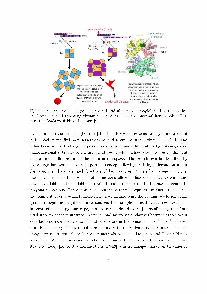
Figure 1.2 � Schematic diagram of normal and abnormal hemoglobin. Point mutationon chromosome 11 replacing glutamine by valine leads to abnormal hemoglobin. Thismutation leads to sickle cell disease [9].
that proteins exist in a single form [10, 11]. However, proteins are dynamic and not
static. Weber quali�ed proteins as �kicking and screaming stochastic molecules� [12] and
it has been proved that a given protein can assume many di�erent con�gurations, called
conformational substates or metastable states [13�15]. These states represent di�erent
geometrical con�gurations of the chain in the space. The protein can be described by
the energy landscape, a very important concept allowing to bring information about
the structure, dynamics, and functions of biomolecules. To perform these functions,
most proteins need to move. Protein motions allow to ligands like O2 to enter and
leave myoglobin or hemoglobin or again to substrates to reach the enzyme center in
enzymatic reactions. These motions can either be thermal equilibrium �uctuations, since
the temperature creates �uctuations in the system modifying the dynamic evolution of the
system, or again non-equilibrium relaxations, for example induced by chemical reactions.
In terms of the energy landscape, motions can be described as jumps of the system from
a substate to another substate. At nano- and micro-scale, changes between states occur
very fast and rate coe�cients of �uctuations are in the range from fs−1 to s−1, or even
less. Hence, many di�erent tools are necessary to study dynamic behaviours, like out-
of-equilibrium statistical mechanics or methods based on Langevin and Fokker-Planck
equations. When a molecule switches from one substate to another one, we can use
Kramers theory [16] or its generalisations [17�19], which manages characteristic times to
4
switch between two states of bistability. This large spectrum of theories is very useful to
describe dynamic biological systems, since it is often able to summarise the behaviours of
complex systems with simple stochastic rules.
1.1.3 Thermodynamics of small systems
Why using statistical mechanics instead of classical mechanics to study macromolecules
like DNA, proteins or other biological structures? In fact, for small systems, the energy
related to the thermal �uctuations is comparable to the mechanical energy (for instance,
energy accumulated in elastic bonds, i.e. the enthalpic contributions). Imagine a polymer
whose one end is �xed, which only moves with thermal �uctuations. In this case, the
polymer is randomly distributed on a sphere centred on the �xed end as it freely and
isotropically explores the whole con�gurational phase space. To align polymer i.e. to
extend it, the other end is now pulled. The polymer reacts against this deformation by
creating an entropic force, as it prefers to be in the con�guration of a sphere centred on
�xed end. If the temperature of the system is high, the polymer wants to explore all con-
�gurations randomly. If a mechanical force is pulled on it, the polymer is stretched and
an entropic force is created to go against the aligned con�guration, which prevents the
exploration of the phase space. Therefore, to study the behaviour of macromolecules and
create some pertinent models, several forces have to be taken into account at nano-scale
where thermal �uctuations play a crucial role. Entropic forces represent the paradigmatic
example. Statistical mechanics allow to do so.
Hence, we can use statistical mechanics to study macromolecules made of monomers, like
proteins or DNA. Here, we focus on the nanomechanics of macromolecules. To do so,
we can consider two di�erent systems, yielding two di�erent results. We can consider
a molecular chain with the �rst end-terminal tethered on a substrate. Firstly, we can
imagine to apply a force at the second end of the macromolecule (Gibbs ensemble) or,
secondly, to prescribe the spatial position of this second end (Helmholtz ensemble). Then,
we suppose to measure the force-extension relation in both cases. If the system under con-
sideration consists of in�nitely many units, the statistical mechanics results under these
di�erent conditions are identical, as observed in Fig.1.3, when the number of particles
increases [20]. In this case, the thermodynamic limit is attained and it represents the
limit for a large number of monomers. However, if a system consists of few units as it is
sometimes the case for proteins, equivalence between the ensembles is lost. The latter can
be observed in real life biological experiments. In this case, single-molecule force spec-
troscopy techniques are useful to show non-equivalence between ensembles. Gibbs and
5

Figure 1.3 � Force�extension curves for Gibbs and ensembles. The response at constantapplied force, i.e. in the Gibbs ensemble, shows a plateau force. This behaviour hasbeen observed in the over-stretching of DNA, and in polysaccharides such as the dex-tran. Regarding the Helmholtz ensemble, with N = 4, 6, 10, 300 units, when the chainlength is increased, the width of the peaks is decreased until, at a large enough N , theforce�extension curve approaches again the plateau curve of the Gibbs ensemble. Onecan see the convergence between both ensembles for a su�ciently high N [20].
Helmholtz ensembles made up of few units are an example of ensembles which verify the
non-equivalence. The Gibbs ensemble is typically referred to as the isotensional bound-
ary condition. Typically, the force-extension response observed shows a plateau force,
which the threshold force for which all units unfold at the same time. The Helmholtz
ensemble, for its part, is referred to as the isometric boundary condition. Typically, the
force-extension response shows a saw-tooth pattern, with force peaks, each peak corre-
sponding to the unfolding of a unit of the chain. In the case of small systems, if the force
is imposed or the extension is prescribed, di�erent mechanical responses are observed.
Theory predicts these di�erences and they are veri�ed and tested in experiments with
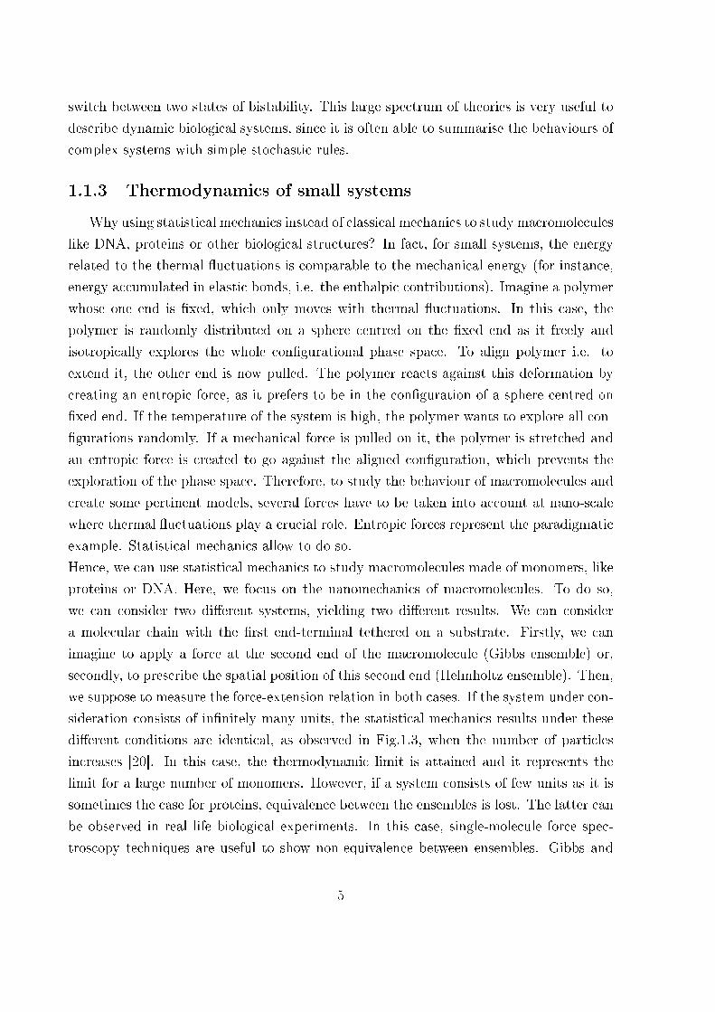
macromolecules, as observed in Fig.1.4 and Fig.1.5. It is important to underline that the
di�erences in the ensembles behaviours can be appreciated both with equilibrium and
non-equilibrium statistical mechanics. These di�erences will be studied in detail in this
thesis for several particular cases. We note that the non-equivalence of the ensembles can
be observed also in special cases at the thermodynamic limit (e.g., con�ned polymers or
adhesion of polymers) [21�23].
6
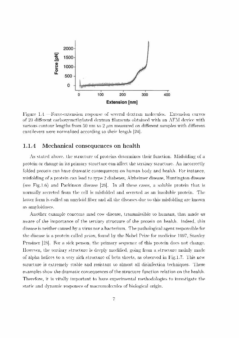
Figure 1.4 � Force-extension response of several dextran molecules. Extension curvesof 20 di�erent carboxymethylated dextran �laments obtained with an AFM device withvarious contour lengths from 50 nm to 2 µm measured on di�erent samples with di�erentcantilevers were normalised according to their length [24].
1.1.4 Mechanical consequences on health
As stated above, the structure of proteins determines their function. Misfolding of a
protein or change in its primary structure can a�ect the tertiary structure. An incorrectly
folded protein can have dramatic consequences on human body and health. For instance,
misfolding of a protein can lead to type 2 diabetes, Alzheimer disease, Huntington disease
(see Fig.1.6) and Parkinson disease [26]. In all these cases, a soluble protein that is
normally secreted from the cell is misfolded and secreted as an insoluble protein. The
latter form is called an amyloid �ber and all the diseases due to this misfolding are known
as amyloidoses.
Another example concerns mad cow disease, transmissible to humans, that made us
aware of the importance of the tertiary structure of the protein on health. Indeed, this
disease is neither caused by a virus nor a bacterium. The pathological agent responsible for
the disease is a protein called prion, found by the Nobel Prize for medicine 1997, Stanley
Prusiner [28]. For a sick person, the primary sequence of this protein does not change.
However, the tertiary structure is deeply modi�ed, going from a structure mainly made
of alpha helices to a very rich structure of beta sheets, as observed in Fig.1.7. This new
structure is extremely stable and resistant to almost all disinfection techniques. These
examples show the dramatic consequences of the structure-function relation on the health.
Therefore, it is vitally important to have experimental methodologies to investigate the
static and dynamic responses of macromolecules of biological origin.
7
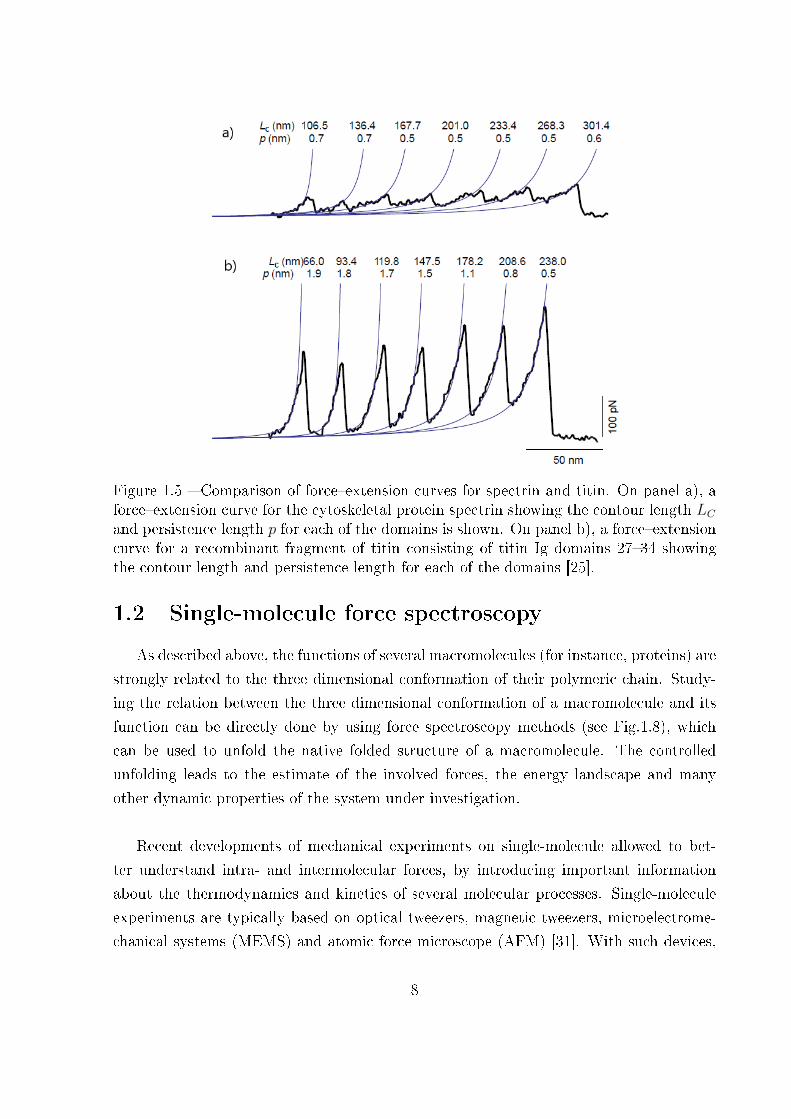
Figure 1.5 � Comparison of force�extension curves for spectrin and titin. On panel a), aforce�extension curve for the cytoskeletal protein spectrin showing the contour length LCand persistence length p for each of the domains is shown. On panel b), a force�extensioncurve for a recombinant fragment of titin consisting of titin Ig domains 27�34 showingthe contour length and persistence length for each of the domains [25].
1.2 Single-molecule force spectroscopy
As described above, the functions of several macromolecules (for instance, proteins) are
strongly related to the three dimensional conformation of their polymeric chain. Study-
ing the relation between the three dimensional conformation of a macromolecule and its
function can be directly done by using force spectroscopy methods (see Fig.1.8), which
can be used to unfold the native folded structure of a macromolecule. The controlled
unfolding leads to the estimate of the involved forces, the energy landscape and many
other dynamic properties of the system under investigation.
Recent developments of mechanical experiments on single-molecule allowed to bet-
ter understand intra- and intermolecular forces, by introducing important information
about the thermodynamics and kinetics of several molecular processes. Single-molecule
experiments are typically based on optical tweezers, magnetic tweezers, microelectrome-
chanical systems (MEMS) and atomic force microscope (AFM) [31]. With such devices,
8
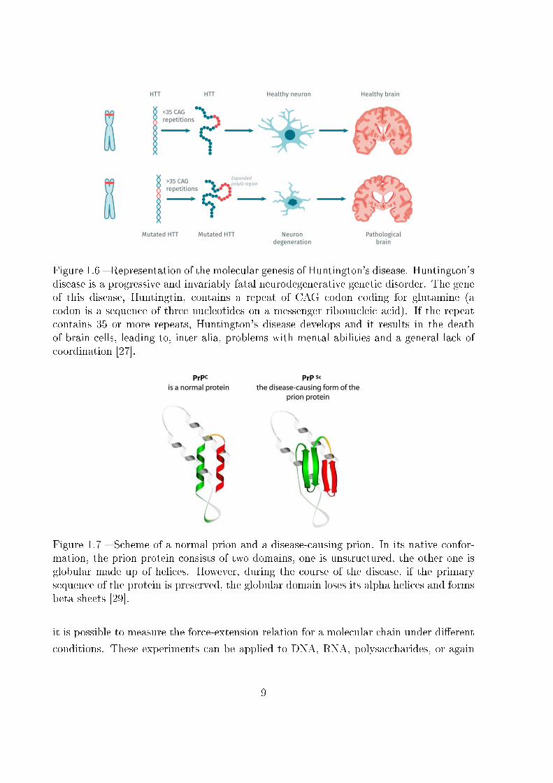
Figure 1.6 � Representation of the molecular genesis of Huntington's disease. Huntington'sdisease is a progressive and invariably fatal neurodegenerative genetic disorder. The geneof this disease, Huntingtin, contains a repeat of CAG codon coding for glutamine (acodon is a sequence of three nucleotides on a messenger ribonucleic acid). If the repeatcontains 35 or more repeats, Huntington's disease develops and it results in the deathof brain cells, leading to, inter alia, problems with mental abilities and a general lack ofcoordination [27].
Figure 1.7 � Scheme of a normal prion and a disease-causing prion. In its native confor-mation, the prion protein consists of two domains, one is unstructured, the other one isglobular made up of helices. However, during the course of the disease, if the primarysequence of the protein is preserved, the globular domain loses its alpha helices and formsbeta sheets [29].
it is possible to measure the force-extension relation for a molecular chain under di�erent
conditions. These experiments can be applied to DNA, RNA, polysaccharides, or again
9

Figure 1.8 � Schematic illustration of a dynamic force spectroscopy experiment. A receptoris immobilized on the surface, and the ligand is connected via a linker to the tip of anAFM cantilever which serves as a force transducer. The distance between surface and tipcan be controlled with a piezoelectric element [30].
proteins. The above techniques permit a clearer comprehension of the equilibrium and
out-of-equilibrium thermodynamics of small systems and the experimental veri�cation of
the small systems thermodynamics. These devices explore a large range of sti�ness. For
example, LASER optical tweezers (LOT) and magnetic tweezers are considered as soft de-
vices, with a sti�ness from 10−4 to 100 pN/nm, whereas AFM and MEMS are considered
as a hard device, with a sti�ness from 100 to 102 pN/nm.
1.2.1 Conventional and high-speed atomic force microscope
The atomic force microscope is a well-known technique invented in 1985 by Gerd Bin-
nig, Calvin Quate and Christoph Gerber and commercialised for the �rst time in 1989 [32].
The AFM is a high-resolution scanning probe microscopy instrument allowing to reach
the atomic resolution. In its primary operation mode, also known as "contact mode",
AFM allows to visualise the topography of a sample surface by scanning it horizontally
with a sharp tip placed at the extremity of a cantilever. As high-resolution imaging tool,
it permits to measure the roughness of a sample surface.
The two main components of the AFM are the cantilever, which acts as a �exible sensor
and a piezoelectric positioner, in order to control the sample position in the nanometric
range. An AFM consists of a cantilever, mounted on a cantilever holder, whose position
is controlled by a piezoelectric device. A focused laser beam is re�ected o� the surface
10
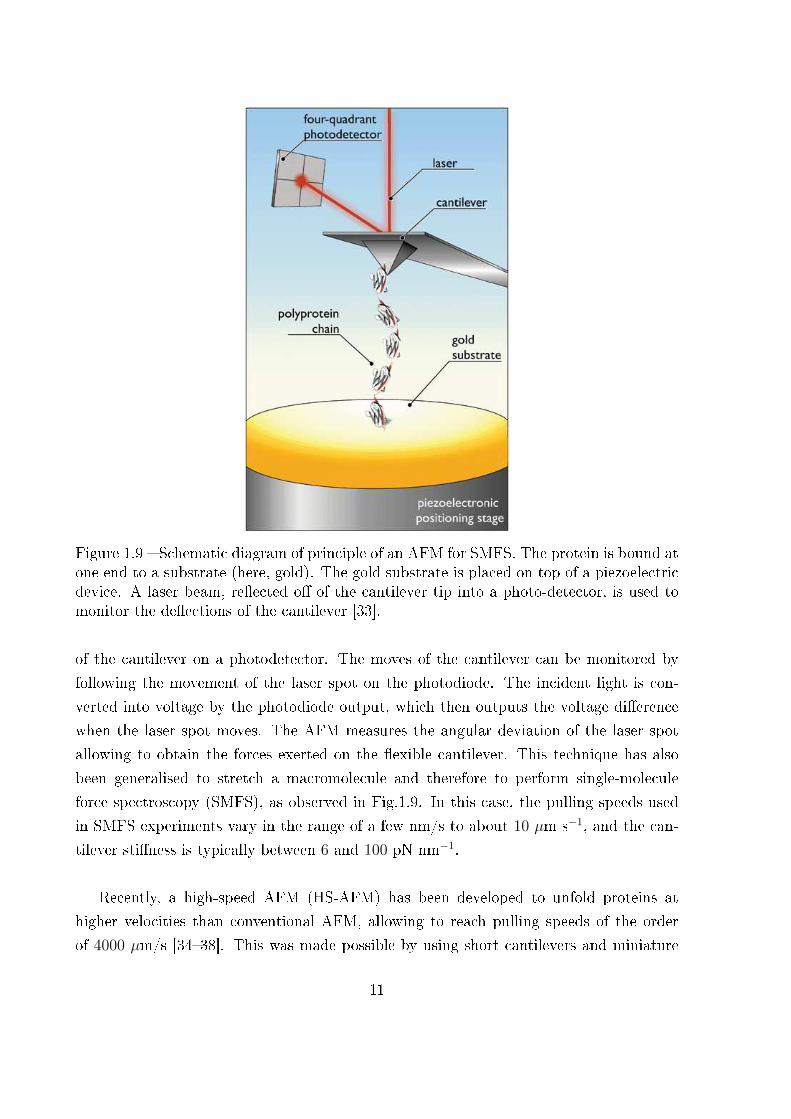
Figure 1.9 � Schematic diagram of principle of an AFM for SMFS. The protein is bound atone end to a substrate (here, gold). The gold substrate is placed on top of a piezoelectricdevice. A laser beam, re�ected o� of the cantilever tip into a photo-detector, is used tomonitor the de�ections of the cantilever [33].
of the cantilever on a photodetector. The moves of the cantilever can be monitored by
following the movement of the laser spot on the photodiode. The incident light is con-
verted into voltage by the photodiode output, which then outputs the voltage di�erence
when the laser spot moves. The AFM measures the angular deviation of the laser spot
allowing to obtain the forces exerted on the �exible cantilever. This technique has also
been generalised to stretch a macromolecule and therefore to perform single-molecule
force spectroscopy (SMFS), as observed in Fig.1.9. In this case, the pulling speeds used
in SMFS experiments vary in the range of a few nm/s to about 10 µm s−1, and the can-
tilever sti�ness is typically between 6 and 100 pN nm−1.
Recently, a high-speed AFM (HS-AFM) has been developed to unfold proteins at
higher velocities than conventional AFM, allowing to reach pulling speeds of the order
of 4000 µm/s [34�38]. This was made possible by using short cantilevers and miniature
11
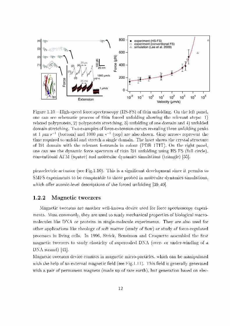
Figure 1.10 � High-speed force spectroscopy (HS-FS) of titin unfolding. On the left panel,one can see schematic process of titin forced unfolding showing the relevant steps: 1)relaxed polyprotein, 2) polyprotein stretching, 3) unfolding of one domain and 4) unfoldeddomain stretching. Two examples of force-extension curves revealing three unfolding peaksat 1 µm s−1 (bottom) and 1000 µm s−1 (top) are also shown. Gray arrows represent thetime required to unfold and stretch a single domain. The inset shows the crystal structureof I91 domain with the relevant ÿ-strands in colour (PDB 1TIT). On the right panel,one can see the dynamic force spectrum of titin I91 unfolding using HS-FS (full circle),conventional AFM (square) and molecular dynamics simulations (triangle) [35].
piezoelectric actuator (see Fig.1.10). This is a signi�cant development since it permits to
SMFS experiments to be comparable to those probed in molecular dynamics simulations,
which o�er atomic-level descriptions of the forced unfolding [39,40].
1.2.2 Magnetic tweezers
Magnetic tweezers are another well-known device used for force spectroscopy experi-
ments. Most commonly, they are used to study mechanical properties of biological macro-
molecules like DNA or proteins in single-molecule experiments. They are also used for
other applications like rheology of soft matter (study of �ow) or study of force-regulated
processes in living cells. In 1996, Strick, Bensimon and Croquette assembled the �rst
magnetic tweezers to study elasticity of supercoiled DNA (over- or under-winding of a
DNA strand) [41].
Magnetic tweezers device consists in magnetic micro-particles, which can be manipulated
with the help of an external magnetic �eld (see Fig.1.11). This �eld is generally generated
with a pair of permanent magnets (made up of rare earth), but generation based on elec-
12
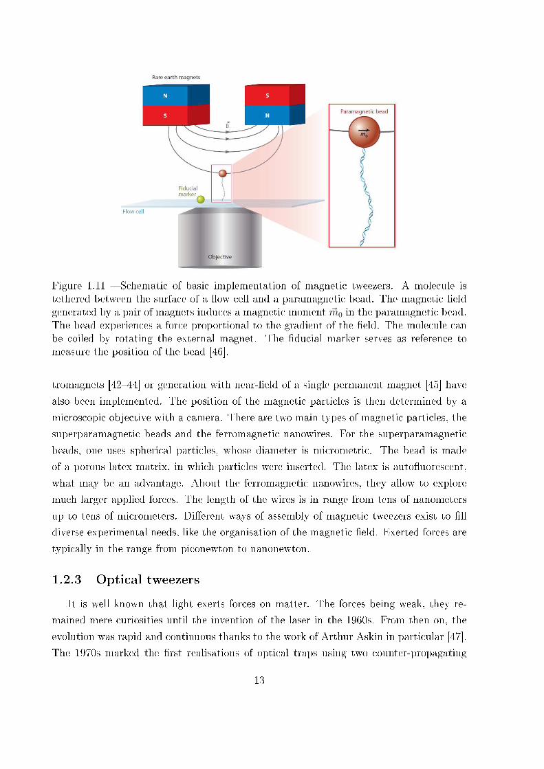
Figure 1.11 � Schematic of basic implementation of magnetic tweezers. A molecule istethered between the surface of a �ow cell and a paramagnetic bead. The magnetic �eldgenerated by a pair of magnets induces a magnetic moment ~m0 in the paramagnetic bead.The bead experiences a force proportional to the gradient of the �eld. The molecule canbe coiled by rotating the external magnet. The �ducial marker serves as reference tomeasure the position of the bead [46].
tromagnets [42�44] or generation with near-�eld of a single permanent magnet [45] have
also been implemented. The position of the magnetic particles is then determined by a
microscopic objective with a camera. There are two main types of magnetic particles, the
superparamagnetic beads and the ferromagnetic nanowires. For the superparamagnetic
beads, one uses spherical particles, whose diameter is micrometric. The bead is made
of a porous latex matrix, in which particles were inserted. The latex is auto�uorescent,
what may be an advantage. About the ferromagnetic nanowires, they allow to explore
much larger applied forces. The length of the wires is in range from tens of nanometers
up to tens of micrometers. Di�erent ways of assembly of magnetic tweezers exist to �ll
diverse experimental needs, like the organisation of the magnetic �eld. Exerted forces are
typically in the range from piconewton to nanonewton.
1.2.3 Optical tweezers
It is well known that light exerts forces on matter. The forces being weak, they re-
mained mere curiosities until the invention of the laser in the 1960s. From then on, the
evolution was rapid and continuous thanks to the work of Arthur Askin in particular [47].
The 1970s marked the �rst realisations of optical traps using two counter-propagating
13
beams, the �rst experiments of optical levitation of microspheres and the �rst realisation
of a single laser beam strongly focused by a high digital aperture objective, creating an
optical gradient force. The year 1986 is considered as the birth year of optical tweez-
ers [48]. On the one hand, optical tweezers allow the precise handling of objects without
any contact, with the consequence of remaining in a perfectly sterile environment during
handling. On the other hand, the forces generated by optical tweezers are typically equiv-
alent to the forces involved in a large number of cellular processes (adhesion, cytoskeletal
mechanics, motricity, operation of molecular motors, etc.). Other �elds than biology use
optical tweezers, such as photochemistry or physics, such as the study and control of
colloidal particles, the setting in motion and control by a light beam of micromotors or
micropumps [49]. The essential elements for making optical tweezers are a laser beam,
a high numerical aperture microscope objective, a sample containing the objects to be
manipulated and a viewing device (see Fig.1.12). To account for the forces by the optical
trap, it is necessary to rely on Lorentz-Mie's generalised theory that describes di�usion
of the light by an object of any shape. The re�ected rays contribute to the di�usion force
that pushes the object in the direction of the laser beam, but the refracted beams incident
at a high angle will keep the bead at the focus point, where the light intensity is highest,
thanks to gradient forces. The trap is stable as soon as the gradient forces exceed the
di�usion forces.
Dynamic studies of single molecules such as DNA or RNA molecules have progressed
through manipulations using optical tweezers. It is now possible to measure the force
applied to a DNA molecule that is attached at one end to the surface of a holder and
at the other end, to a latex bead that is held in place with the optical tweezers, as seen
in Fig.1.13. In this way, the elasticity of DNA can be measured directly. Separation of
the DNA double helix is achievable through the action of a mechanical force exerted with
optical tweezers. It was thus possible to determine the force with which the nitrogenous
base pairs are bound and it was established that these forces vary according to the base
pair sequence. Optical tweezers allowed the identi�cation of defective DNA structures
like base mismatches, missing bases or crosslinks. The latter occur in DNA with high
frequency and must be e�ciently identi�ed and repaired to avoid direct consequences
such as genetic mutations [51�54].
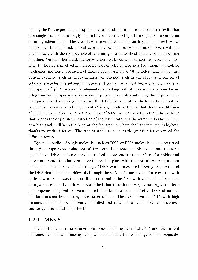
1.2.4 MEMS
Last but not least come microelectromechanical systems (MEMS) and the related
micromechatronics and microsystems, which constitute the technology of microscopic de-
14

Figure 1.12 � Scheme of the general principle of optical tweezers. a) Essential elementsfor optical tweezers. b) Scheme of the general device. c) Physical principle of opticaltweezers [50].
Figure 1.13 � Scheme of optical tweezers used to directly measure DNA elasticity [50].
vices, especially those with moving parts. MEMS were developed in the early 1970s as
derivatives of microelectronics and were �rst commercialised in the 1980s with silicon
pressure sensors, that quickly replaced older techniques and still form a signi�cant part
of the MEMS market. Since then, the MEMS �eld has been booming. These devices
are used in many �elds like automotive, aeronautics, medicine, biology, telecommunica-
tions and in several "everyday" applications such as high-de�nition television sets or car
airbags.
15
Generally, MEMS are made up of components from 1 to 100 µm. Devices holding MEMS
generally range in size from 20 micrometres to a millimetre. They usually consist of a cen-
tral component that processes data (an integrated circuit chip such as microprocessor) and
several components that interact with the environment (such as microsensors). Due to the
large surface area to volume ratio of MEMS, forces created by ambient electromagnetism
(e.g., electrostatic charges and magnetic moments) and �uid dynamics (e.g., surface ten-
sion and viscosity) have to be more taken into account for design than with larger scale
mechanical devices. Considering surface chemistry makes the di�erence between MEMS
technology and molecular nanotechnology or molecular electronics. Moreover, devices like
AFM, optical tweezers and magnetic tweezers are bulky and rather expensive. Some ex-
periments need to be realised in tiny or con�ned areas and MEMS allow to �ll these gaps.
The fabrication of MEMS evolved thanks to the process technology in semiconductor
device fabrication, i.e. the basic techniques are deposition of material layers, patterning
by photolithography and etching to obtain the required shapes. The materials used for
MEMS manufacturing are silicon, polymers, metal and ceramics.
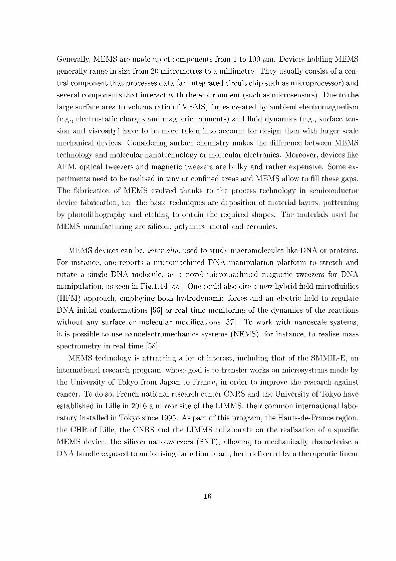
MEMS devices can be, inter alia, used to study macromolecules like DNA or proteins.
For instance, one reports a micromachined DNA manipulation platform to stretch and
rotate a single DNA molecule, as a novel micromachined magnetic tweezers for DNA
manipulation, as seen in Fig.1.14 [55]. One could also cite a new hybrid �eld micro�uidics
(HFM) approach, employing both hydrodynamic forces and an electric �eld to regulate
DNA initial conformations [56] or real time monitoring of the dynamics of the reactions
without any surface or molecular modi�cations [57]. To work with nanoscale systems,
it is possible to use nanoelectromechanics systems (NEMS), for instance, to realise mass
spectrometry in real time [58].
MEMS technology is attracting a lot of interest, including that of the SMMIL-E, an
international research program, whose goal is to transfer works on microsystems made by
the University of Tokyo from Japan to France, in order to improve the research against
cancer. To do so, French national research center CNRS and the University of Tokyo have
established in Lille in 2016 a mirror site of the LIMMS, their common international labo-
ratory installed in Tokyo since 1995. As part of this program, the Hauts-de-France region,
the CHR of Lille, the CNRS and the LIMMS collaborate on the realisation of a speci�c
MEMS device, the silicon nanotweezers (SNT), allowing to mechanically characterise a
DNA bundle exposed to an ionising radiation beam, here delivered by a therapeutic linear
16
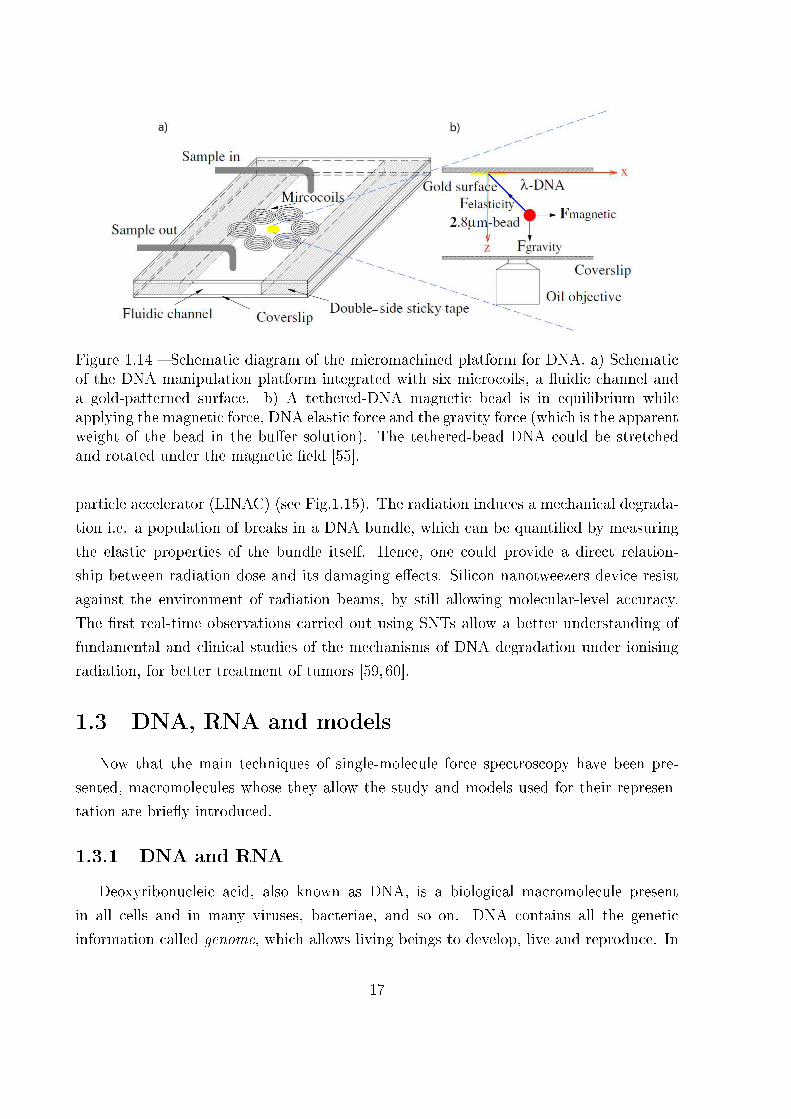
Figure 1.14 � Schematic diagram of the micromachined platform for DNA. a) Schematicof the DNA manipulation platform integrated with six microcoils, a �uidic channel anda gold-patterned surface. b) A tethered-DNA magnetic bead is in equilibrium whileapplying the magnetic force, DNA elastic force and the gravity force (which is the apparentweight of the bead in the bu�er solution). The tethered-bead DNA could be stretchedand rotated under the magnetic �eld [55].
particle accelerator (LINAC) (see Fig.1.15). The radiation induces a mechanical degrada-
tion i.e. a population of breaks in a DNA bundle, which can be quanti�ed by measuring
the elastic properties of the bundle itself. Hence, one could provide a direct relation-
ship between radiation dose and its damaging e�ects. Silicon nanotweezers device resist
against the environment of radiation beams, by still allowing molecular-level accuracy.
The �rst real-time observations carried out using SNTs allow a better understanding of
fundamental and clinical studies of the mechanisms of DNA degradation under ionising
radiation, for better treatment of tumors [59,60].
1.3 DNA, RNA and models
Now that the main techniques of single-molecule force spectroscopy have been pre-
sented, macromolecules whose they allow the study and models used for their represen-
tation are brie�y introduced.
1.3.1 DNA and RNA
Deoxyribonucleic acid, also known as DNA, is a biological macromolecule present
in all cells and in many viruses, bacteriae, and so on. DNA contains all the genetic
information called genome, which allows living beings to develop, live and reproduce. In
17
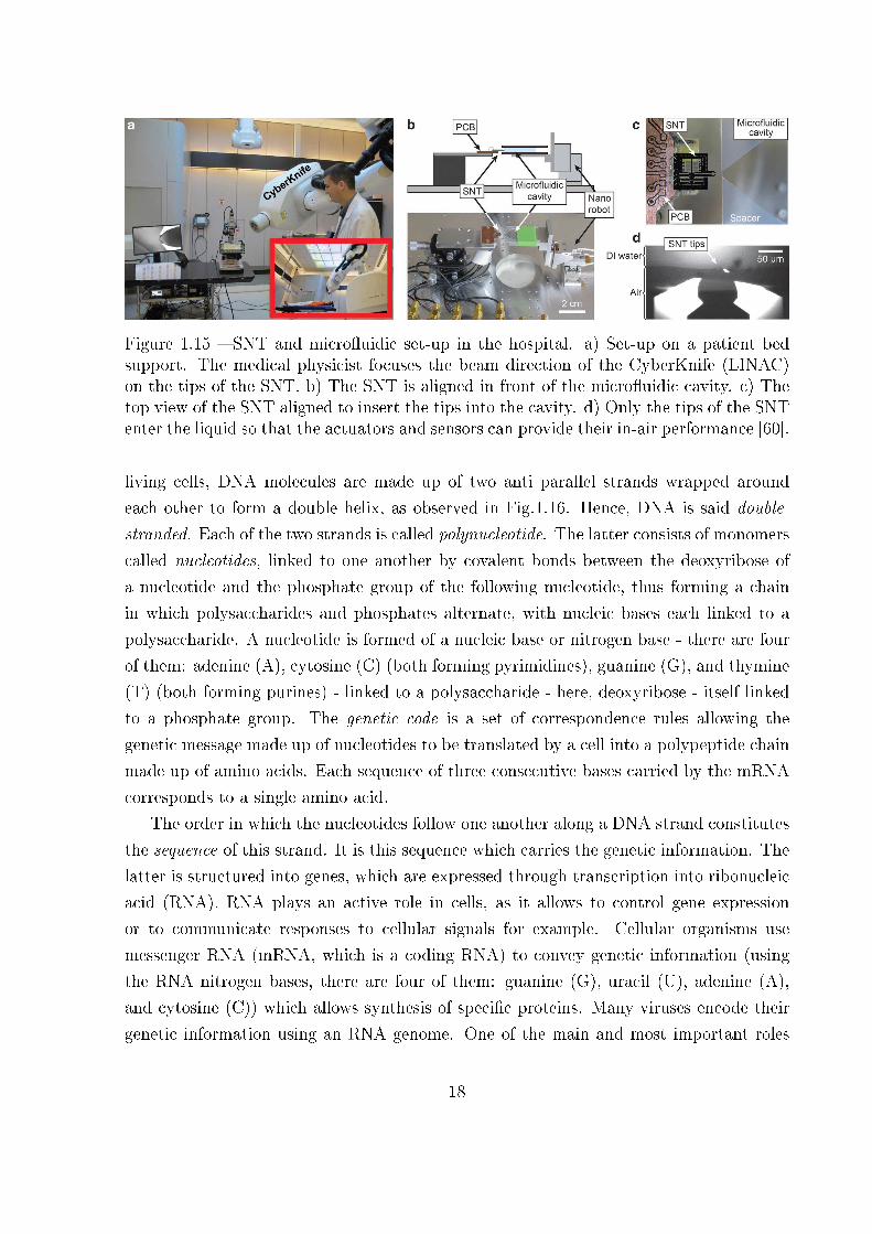
Figure 1.15 � SNT and micro�uidic set-up in the hospital. a) Set-up on a patient bedsupport. The medical physicist focuses the beam direction of the CyberKnife (LINAC)on the tips of the SNT. b) The SNT is aligned in front of the micro�uidic cavity. c) Thetop view of the SNT aligned to insert the tips into the cavity. d) Only the tips of the SNTenter the liquid so that the actuators and sensors can provide their in-air performance [60].
living cells, DNA molecules are made up of two anti parallel strands wrapped around
each other to form a double helix, as observed in Fig.1.16. Hence, DNA is said double-
stranded. Each of the two strands is called polynucleotide. The latter consists of monomers
called nucleotides, linked to one another by covalent bonds between the deoxyribose of
a nucleotide and the phosphate group of the following nucleotide, thus forming a chain
in which polysaccharides and phosphates alternate, with nucleic bases each linked to a
polysaccharide. A nucleotide is formed of a nucleic base or nitrogen base - there are four
of them: adenine (A), cytosine (C) (both forming pyrimidines), guanine (G), and thymine
(T) (both forming purines) - linked to a polysaccharide - here, deoxyribose - itself linked
to a phosphate group. The genetic code is a set of correspondence rules allowing the
genetic message made up of nucleotides to be translated by a cell into a polypeptide chain
made up of amino acids. Each sequence of three consecutive bases carried by the mRNA
corresponds to a single amino acid.
The order in which the nucleotides follow one another along a DNA strand constitutes
the sequence of this strand. It is this sequence which carries the genetic information. The
latter is structured into genes, which are expressed through transcription into ribonucleic
acid (RNA). RNA plays an active role in cells, as it allows to control gene expression
or to communicate responses to cellular signals for example. Cellular organisms use
messenger RNA (mRNA, which is a coding RNA) to convey genetic information (using
the RNA nitrogen bases, there are four of them: guanine (G), uracil (U), adenine (A),
and cytosine (C)) which allows synthesis of speci�c proteins. Many viruses encode their
genetic information using an RNA genome. One of the main and most important roles
18

Figure 1.16 � Structure of DNA double helix showing the structure of the four nucleicbases: adenine, cytosine, guanine and thymine. The atoms in the structure are colour-coded by element and the detailed structures of two base pairs are shown in the bottomright [61].
Figure 1.17 � Scheme of RNA role between DNA and protein [62].
is protein synthesis in ribosomes (macromolecules composed of RNA and proteins). This
process uses transfer RNA (tRNA) molecules to deliver amino acids to the ribosome,
where ribosomal RNA (rRNA, both non-coding) then links amino acids together to form
coded proteins. Some RNA roles are shown in Fig.1.17.
The association of DNA and proteins in which DNA is compacted in the nucleus in
eukaryotic cells is called chromatin. The latter consists of a combination of DNA and
proteins of two types: histones and non-histones, as seen in Fig.1.18. On the one hand,
19
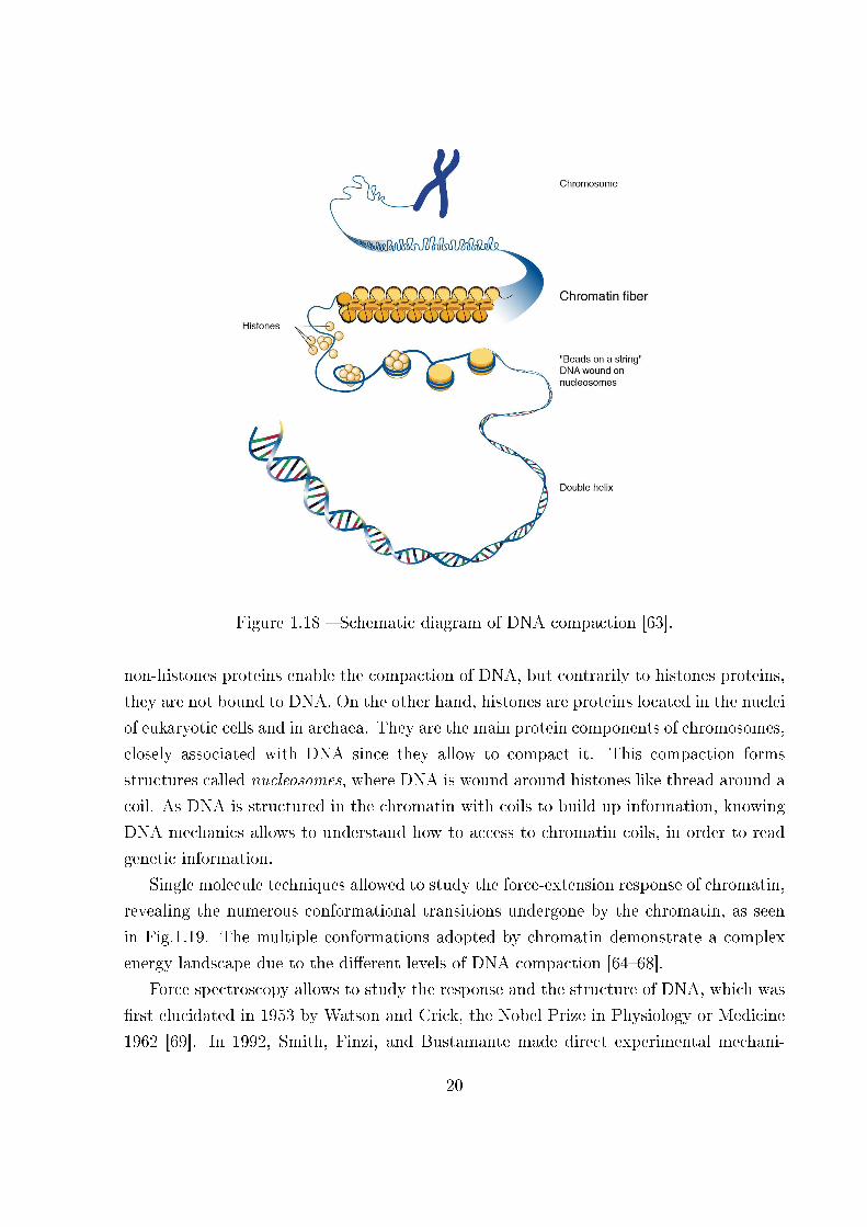
Figure 1.18 � Schematic diagram of DNA compaction [63].
non-histones proteins enable the compaction of DNA, but contrarily to histones proteins,
they are not bound to DNA. On the other hand, histones are proteins located in the nuclei
of eukaryotic cells and in archaea. They are the main protein components of chromosomes,
closely associated with DNA since they allow to compact it. This compaction forms
structures called nucleosomes, where DNA is wound around histones like thread around a
coil. As DNA is structured in the chromatin with coils to build up information, knowing
DNA mechanics allows to understand how to access to chromatin coils, in order to read
genetic information.
Single molecule techniques allowed to study the force-extension response of chromatin,
revealing the numerous conformational transitions undergone by the chromatin, as seen
in Fig.1.19. The multiple conformations adopted by chromatin demonstrate a complex
energy landscape due to the di�erent levels of DNA compaction [64�68].
Force spectroscopy allows to study the response and the structure of DNA, which was
�rst elucidated in 1953 by Watson and Crick, the Nobel Prize in Physiology or Medicine
1962 [69]. In 1992, Smith, Finzi, and Bustamante made direct experimental mechani-
20

Figure 1.19 � Detailed analysis of the unfolding of a single chromatin �ber. a) A zoom inon the high-force region shows discrete steps in extension. Dashed gray lines represent theextensions of all states that are composed of extended and fully unwrapped nucleosomes.The black line shows the best match between individual data points and the variousstates of unwrapping. b) Unfolding of a 15*197 nucleosome repeat lengths chromatin�ber at low force. Below 7 pN the extension starts to deviate from a string of extendednucleosomes (gray dashed lines). A single transition (black dashed line) does not capturethe force-extension data [64].
cal measurements on DNA by using magnetic beads [70]. They obtained extension versus
force curves for individual DNA molecules at three di�erent salt concentrations with forces
in the range from 10−14 to 10−11 N. These results have been completely understood from
the theoretical point of view thanks to the works of Marko and Siggia [71,72]. In Fig.1.20,
force-extension response of DNA is shown and compared to two elastic behaviour models,
studied in the next Section. We anticipate that the DNA mechanism is well reproduced
by the WLC model, rather than the FJC model [71, 72]. In the following, the DNA
molecule has been pulled with larger forces and an overstretching phenomenon has been
observed [73]. In particular, a force plateau at around 65 pN has been measured in the
force-extension curve, as seen in Fig.1.21. This speci�c behaviour has been interpreted
in terms of a transition similar to the one observed within the Gibbs ensemble in other
macromolecules, such as several proteins and polysaccharides. The real molecular origin of
this transition has been largely investigated and a debate exists on the DNA conformation
after the overstretching: many researchers think that there is a simple mechanical denat-
uration leading to a transformation of the double-stranded DNA into two single-stranded
DNA [74,75]; however, other researchers have proposed the existence of a new DNA con-
21
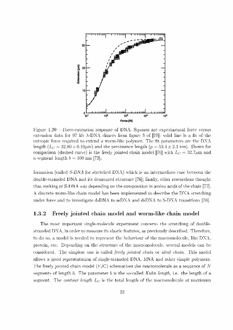
Figure 1.20 � Force-extension response of DNA. Squares are experimental force versusextension data for 97 kb λ-DNA dimers from �gure 3 of [70]; solid line is a �t of theentropic force required to extend a worm-like polymer. The �t parameters are the DNAlength (LC = 32.80 + 0.10µm) and the persistence length (p = 53.4± 2.3 nm). Shown forcomparison (dashed curve) is the freely jointed chain model [70] with LC = 32.7µm anda segment length b = 100 nm [72].
formation (called S-DNA for stretched DNA) which is an intermediate case between the
double-stranded DNA and its denatured structure [76]; �nally, other researchers thought
that melting or S-DNA was depending on the composition in amino acids of the chain [77].
A discrete worm-like chain model has been implemented to describe the DNA stretching
under force and to investigate dsDNA to ssDNA and dsDNA to S-DNA transitions [78].
1.3.2 Freely jointed chain model and worm-like chain model
The most important single-molecule experiment concerns the stretching of double-
stranded DNA, in order to measure its elastic features, as previously described. Therefore,
to do so, a model is needed to represent the behaviour of the macromolecule, like DNA,
protein, etc. Depending on the structure of the macromolecule, several models can be
considered. The simplest one is called freely jointed chain or ideal chain. This model
allows a good representation of single-stranded DNA, RNA and other simple polymers.
The freely jointed chain model (FJC) schematizes the macromolecule as a sequence of N
segments of length b. The parameter b is the so-called Kuhn length, i.e. the length of a
segment. The contour length LC is the total length of the macromolecule at maximum
22
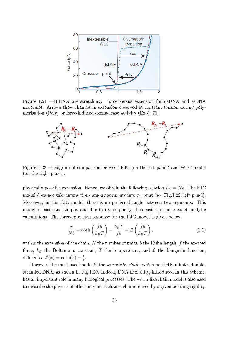
Figure 1.21 � B-DNA overstretching. Force versus extension for dsDNA and ssDNAmolecules. Arrows show changes in extension observed at constant tension during poly-merisation (Poly) or force-induced exonuclease activity (Exo) [79].
Figure 1.22 � Diagram of comparison between FJC (on the left panel) and WLC model(on the right panel).
physically possible extension. Hence, we obtain the following relation LC = Nb. The FJC
model does not take interactions among segments into account (see Fig.1.22, left panel).
Moreover, in the FJC model, there is no preferred angle between two segments. This
model is basic and simple, and due to its simplicity, it is easier to make exact analytic
calculations. The force-extension response for the FJC model is given below:
x
Nb= coth
(fb
kBT
)− kBT
fb= L
(fb
kBT
), (1.1)
with x the extension of the chain, N the number of units, b the Kuhn length, f the exerted
force, kB the Boltzmann constant, T the temperature, and L the Langevin function,
de�ned as L(x) = coth(x)− 1x.
However, the most used model is the worm-like chain, which perfectly mimics double-
stranded DNA, as shown in Fig.1.20. Indeed, DNA �exibility, introduced in this scheme,
has an important role in many biological processes. The worm-like chain model is also used
to describe the physics of other polymeric chains, characterised by a given bending rigidity.
23
Compared to the previous model, an important parameter is added and it concerns the
angles between the segments composing the polymer. In the ideal chain model, no forces
are necessary to fold the chain. However, in the WLC model, we introduce an energy
depending on the angles between adjacent segments (see Fig.1.22, right panel). More
speci�cally, the energy is set to zero if all segments are aligned and therefore a force can
be applied to fold or bend the chain. This property is taken into consideration by means
of a new parameter called persistence length, p, which is de�ned by the ratio between the
mechanical �exibility or bending sti�ness and the energy of thermal �uctuations. Hence,
it takes into account the balance between enthalpic and entropic contributions [71]. We
remark that the bending sti�ness can be calculated through the product of the Young
modulus, E, multiplied by the moment of inertia, I. Moreover, in the WLC model,
the length ` is set to zero and the number of segments N tends to in�nity, so that the
contour length remains constant: LC = N`. A discrete version of the WLC has been
developed which allows higher forces to be considered and the behaviour of DNA to be
better approximated [80�82]. The partition function cannot be calculated exactly either.
An example of use of the WLC model for the tenascin protein is shown in Fig.1.23. The
behaviour of a chain with the WLC model is the following:
f =kBT
p
[1
4
(1− x
LC
)2
− 1
4+
x
LC
], (1.2)
with f the exerted force, kB the Boltzmann constant, T the temperature, p the persistence
length, x the extension of the chain, and LC the contour length. From the physical point
of view, the persistence length p can be de�ned as the length over which correlations in
the direction of the tangent are lost.
Currently, the accepted model for the double-stranded DNA is the twistable worm-like
chain model (TWLC), which allows to describe helicoidal double-stranded DNA response
under both applied forces and torques [83]. However, this model is not in agreement with
experiments realised on DNA with magnetic torque tweezers [84, 85]. Recently, a model
was proposed to correctly take account of both bending and torsional sti�ness by adding
a coupling term between twist and bend deformations [86,87].
A comparison between the FJC and the WLC to model the behaviour of a polyprotein
can be observed in Fig.1.24. The approximation with the FJC model is reasonable,
however, the approximation with the WLC is quantitatively better. Nevertheless, in our
study, we develop models for chains composed of many units and therefore, we chose to
consider simpler models, like FJC, to be able to take account of several extensions, such
24

Figure 1.23 � The entropic elasticity of tenascin protein and domain unfolding. a) Theentropic elasticity of proteins can be described by the WLC (worm-like chain) equation(inset), which expresses the relationship between force F and extension x of a proteinusing its persistence length p and its contour length LC . k is Boltzmann's constant andT is the absolute temperature. b) The saw-tooth pattern of peaks that is observed whenforce is applied to extend the protein corresponds to sequential unravelling of individualdomains of a modular protein. As the distance between substrate and cantilever increases(from state 1 to state 2) the protein elongates, generating a restoring force that bendsthe cantilever. When a domain unfolds (state 3) the free length of the protein increases,returning the force on the cantilever to near zero. Further extension again results inforce on the cantilever (state 4). The last peak represents the �nal extension of theunfolded protein prior to detachment from the AFM tip. c) Consecutive unfolding peaksof recombinant human tenascin-C were �tted using the WLC model. The contour length(LC) for each of the �ts is shown; the persistence length p was �xed at 0.56 nm [25].
as the interactions among the units and to obtain analytical results. The WLC model
allows for considering a single unit, whereas we use the FJC model to represent the whole
curve of the force-extension response of the macromolecular chain. Thus, we favour the
FJC, a simpler model.
25

Figure 1.24 � Examples of the use of polymer elasticity models to �t to protein unfoldingdata from SMFS force versus extension experiments. a) The freely jointed chain (FJC)model is shown, with a Kuhn length of 0.22 nm for the force extension curve of thepolyprotein (pL)5. b) The worm like chain (WLC) model is shown, with a persistencelength, p, of 0.39 nm for the same data, (pL)5. c) A comparison of the model �t to thedata for one protein unfolding event in the polyprotein chain for the FJC (blue) and WLC(red) models with an p of 0.4 nm and b ≈ 2p = 0.8 nm [6].
1.4 Proteins
Most of the functions in living beings depends on proteins, also called polypeptides,
which are biological macromolecules present in all living cells. There are many di�erent
types of proteins, representing 50 % of the dry mass of cells and playing a variety of
roles for the organism. For example, proteins allow to accelerate chemical reactions, to
store amino acids to biosynthesize other proteins, to defence the organism, they also serve
for structural support, cell communication and movement. A human body has tens of
thousands of proteins. Each of these proteins has its own structure and function. These
conformations are among the most complex biological structures and can be studied using
SMFS techniques. As an example of complexity, if one observes the Fig.1.25, a pulling
speed-dependence of the force peaks can be observed, meaning that the intensity of the
force peaks increases when the pulling speed is increased. Such e�ects will be taken into
account further in this manuscript.
26
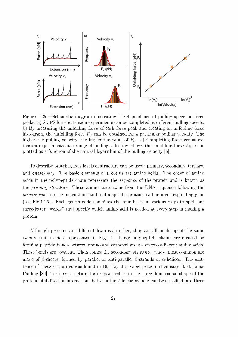
Figure 1.25 � Schematic diagram illustrating the dependence of pulling speed on forcepeaks. a) SMFS force-extension experiments can be completed at di�erent pulling speeds.b) By measuring the unfolding force of each force peak and creating an unfolding forcehistogram, the unfolding force FU can be obtained for a particular pulling velocity. Thehigher the pulling velocity, the higher the value of FU . c) Completing force versus ex-tension experiments at a range of pulling velocities allows the unfolding force FU to beplotted as a function of the natural logarithm of the pulling velocity [6].
To describe proteins, four levels of structure can be used: primary, secondary, tertiary,
and quaternary. The basic elements of proteins are amino acids. The order of amino
acids in the polypeptide chain represents the sequence of the protein and is known as
the primary structure. These amino acids come from the DNA sequence following the
genetic code, i.e the instructions to build a speci�c protein reading a corresponding gene
(see Fig.1.26). Each gene's code combines the four bases in various ways to spell out
three-letter "words" that specify which amino acid is needed at every step in making a
protein.
Although proteins are di�erent from each other, they are all made up of the same
twenty amino acids, represented in Fig.1.1. Large polypeptide chains are created by
forming peptide bonds between amino and carboxyl groups on two adjacent amino acids.
These bonds are covalent. Then comes the secondary structure, whose most common are
made of β-sheets, formed by parallel or anti-parallel β-strands or α-helices. The exis-
tence of these structures was found in 1951 by the Nobel prize in chemistry 1954, Linus
Pauling [89]. Tertiary structure, for its part, refers to the three-dimensional shape of the
protein, stabilised by interactions between the side chains, and can be classi�ed into three
27
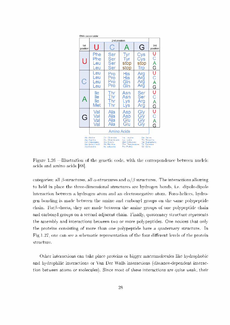
Figure 1.26 � Illustration of the genetic code, with the correspondence between nucleicacids and amino acids [88].
categories: all β-structures, all α-structures and α/β structures. The interactions allowing
to held in place the three-dimensional structures are hydrogen bonds, i.e. dipole-dipole
interaction between a hydrogen atom and an electronegative atom. Forα-helices, hydro-
gen bonding is made between the amine and carbonyl groups on the same polypeptide
chain. Forβ-sheets, they are made between the amine groups of one polypeptide chain
and carbonyl groups on a second adjacent chain. Finally, quaternary structure represents
the assembly and interactions between two or more polypeptides. One notices that only
the proteins consisting of more than one polypeptide have a quaternary structure. In
Fig.1.27, one can see a schematic representation of the four di�erent levels of the protein
structure.
Other interactions can take place proteins or bigger macromolecules like hydrophobic
and hydrophilic interactions or Van Der Walls interactions (distance-dependent interac-
tion between atoms or molecules). Since most of these interactions are quite weak, their
28

Figure 1.27 � Diagram of the four levels of structure of a protein [90].
energy may be comparable to the thermal energy �uctuations. This point explains the
complexity of the proteins folding problem and justify the use of equilibrium and non-
equilibrium statistical mechanics.
Once the structure of proteins has been studied, the latter can be classi�ed in three
main classes, represented in Fig.1.28, by the properties of their environment and the con-
cerned interactions.
The �rst class concerns globular proteins. These proteins are water soluble, hence they
are often studied. As the name suggests, they form a globular shape. This results from
an assembly of di�erent secondary structures. These secondary elements form to pro-
29
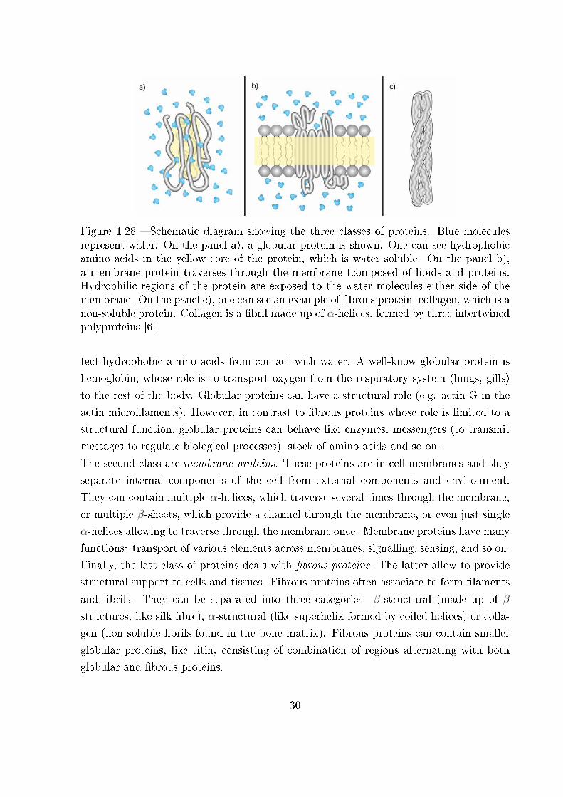
Figure 1.28 � Schematic diagram showing the three classes of proteins. Blue moleculesrepresent water. On the panel a), a globular protein is shown. One can see hydrophobicamino acids in the yellow core of the protein, which is water soluble. On the panel b),a membrane protein traverses through the membrane (composed of lipids and proteins.Hydrophilic regions of the protein are exposed to the water molecules either side of themembrane. On the panel c), one can see an example of �brous protein, collagen, which is anon-soluble protein. Collagen is a �bril made up of α-helices, formed by three intertwinedpolyproteins [6].
tect hydrophobic amino acids from contact with water. A well-know globular protein is
hemoglobin, whose role is to transport oxygen from the respiratory system (lungs, gills)
to the rest of the body. Globular proteins can have a structural role (e.g. actin G in the
actin micro�laments). However, in contrast to �brous proteins whose role is limited to a
structural function, globular proteins can behave like enzymes, messengers (to transmit
messages to regulate biological processes), stock of amino acids and so on.
The second class are membrane proteins. These proteins are in cell membranes and they
separate internal components of the cell from external components and environment.
They can contain multiple α-helices, which traverse several times through the membrane,
or multiple β-sheets, which provide a channel through the membrane, or even just single
α-helices allowing to traverse through the membrane once. Membrane proteins have many
functions: transport of various elements across membranes, signalling, sensing, and so on.
Finally, the last class of proteins deals with �brous proteins. The latter allow to provide
structural support to cells and tissues. Fibrous proteins often associate to form �laments
and �brils. They can be separated into three categories: β-structural (made up of β
structures, like silk �bre), α-structural (like superhelix formed by coiled helices) or colla-
gen (non soluble �brils found in the bone matrix). Fibrous proteins can contain smaller
globular proteins, like titin, consisting of combination of regions alternating with both
globular and �brous proteins.
30
1.5 Structures with bistability
Most proteins can be viewed as composed of multistable units. Linus Pauling and
Alfred Mirsky quali�ed in 1936 the denatured proteins they studied as "by the absence
of a uniquely de�ned con�guration" [91]. The modern statistical mechanical picture of
protein folding is represented by a funneled energy landscape. In Fig.1.29, a simpli�ed
two-dimensional projection of the energy landscape is shown and nevertheless, it looks
very complex [92]. To simplify the study of such macromolecules, a two-state energy
landscape is often considered. Indeed, many macromolecules of biological origin show a
two-state behaviour, like DNA, RNA or proteins. This two-state behaviour is associated
to two con�gurational states, namely folded and unfolded states. Creating mathematical
models is very useful to predict the behaviour of such structures. In practical terms, the
�rst energy well is associated to the folded (or native) position, energetically the most sta-
ble position. The second potential well represents the unfolded state and is a metastable
state.
At the thermodynamic equilibrium, if the system is far from the thermodynamic limit
i.e. the number of units is small, di�erent cases (or statistical ensembles) have to be
studied. As seen before, di�erences between isometric and isotensional ensembles can be
studied in small systems thanks to statistical mechanics. In the Gibbs ensemble, units
are independent from each other. Their folding or unfolding only depends on applied
forces or temperature e�ects. However, in the Helmholtz ensemble, an implicit inter-
action is created between the units because of the �xed length of the chain (isometric
condition). Therefore, the calculation of the Helmholtz partition function is complicated
due to implicit interactions leading to bonds between units. The mechanics of bistable
chains embedded in a thermal bath is one of the most studied subject in this manuscript.
The modelling of bistable systems is not only useful for the understanding of macro-
molecules, but also relevant for the understanding of the muscle operating principle [94,95].
In this case, bistable mechanical models are able to describe the physical mechanisms of
the two passive and active regimes. Again, the study of bistable chains is also important
in material science to investigate several plastic phenomena. For instance, a sawtooth-like
pattern appears in the force-extension response of several non-biological systems under-
going discrete phase transformations, like ferromagnetic alloys, nano-intended substrates
and plastic materials. A typical case concerns nanowires undergoing phase transforma-
tions [96�98]. When stretched, these structures present a �rst force peak higher than the
others. This corresponds to an overtstress or a nucleation stress. The nucleation is the
31

Figure 1.29 � Energy landscape of globular proteins. The protein energy landscape isrepresented by the free energy of the protein as a function of some reaction coordinates.Transiently unfolded proteins are in a higher state of energy. When exploring their energylandscape proteins transit spontaneously through di�erent folding states, before eventu-ally ending up in their native state, which is the lowest energy state. This phenomenonis known as the folding funnel. Within the minimum of the native state, a multitude ofsubstates, known as conformational substates, are constantly explored [93].
creation of a new crystal structure and therefore of a phase between two interfaces. Using
Ising-like models makes a lot of sense as it confers weight to interfaces. As a matter of
fact, a parallel can be drawn between the �rst force peak observed in Fig.1.30 and the
�rst force peak obtaining with bistable chain in the case of a ferromagnetic-like interac-
tion under isometric condition (cf. Chapter 4). This is explained by the cost of creating
interfaces. A higher force is required to counteract the stable state in which the system
is in, a state in which it would remain if it were not constrained.
In several arti�cial systems, particular performances have obtained with the bistability,
like bistable mechanical metamaterials with a negative Poisson ratio (auxetic media) [99]
or systems to control the waves propagation [100]. Models based on chains of bistable
units with transitions between two states have been also adopted to model hysteretic
behaviours and martensitic transformations in continuum mechanics [101�107], or again
energy dissipation with shock reduction [108], like protection in car crash thanks to energy
32
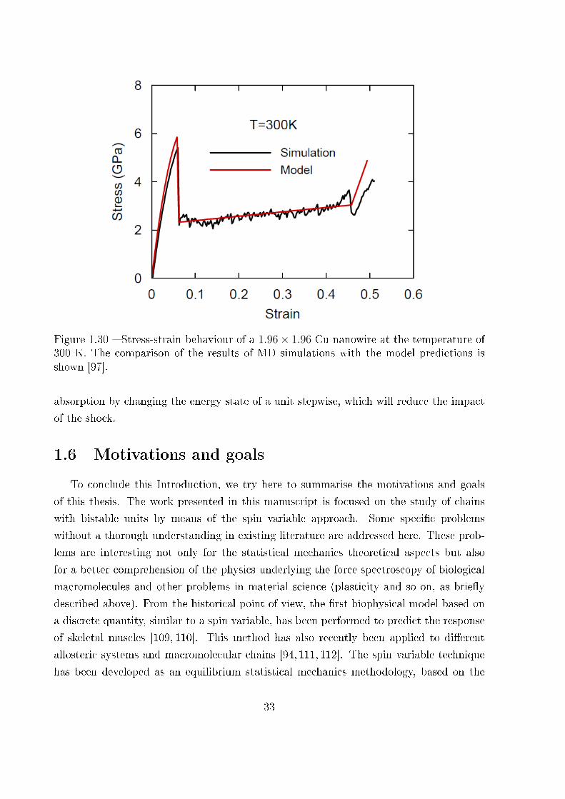
Figure 1.30 � Stress-strain behaviour of a 1.96× 1.96 Cu nanowire at the temperature of300 K. The comparison of the results of MD simulations with the model predictions isshown [97].
absorption by changing the energy state of a unit stepwise, which will reduce the impact
of the shock.
1.6 Motivations and goals
To conclude this Introduction, we try here to summarise the motivations and goals
of this thesis. The work presented in this manuscript is focused on the study of chains
with bistable units by means of the spin variable approach. Some speci�c problems
without a thorough understanding in existing literature are addressed here. These prob-
lems are interesting not only for the statistical mechanics theoretical aspects but also
for a better comprehension of the physics underlying the force spectroscopy of biological
macromolecules and other problems in material science (plasticity and so on, as brie�y
described above). From the historical point of view, the �rst biophysical model based on
a discrete quantity, similar to a spin variable, has been performed to predict the response
of skeletal muscles [109, 110]. This method has also recently been applied to di�erent
allosteric systems and macromolecular chains [94, 111, 112]. The spin variable technique
has been developed as an equilibrium statistical mechanics methodology, based on the
33

introduction of a set of discrete variables, to describe the thermo-mechanical properties
of a bistable chain under arbitrary external conditions [113]. The aim of this methodol-
ogy is to obtain for both Gibbs and Helmholtz ensembles the partition functions, central
functions of statistical mechanics allowing to obtain values like mean extension or mean
force. A two-state freely jointed chain made up of bistable units is typically considered,
with a stable folded state and a metastable unfolded state i.e. each unit is in only one
of the two possible states (folded or unfolded). Introducing the spin variables permits to
consider a simpler energy pro�le for the units. Indeed, the spin variable indicates in which
of the two potential wells the unit is. Consequently, the potential energy, instead of being
approximated by a bistable continuous function (with two minima), can be divided into
two simpler parabolic functions. This point allows to do rather straightforward calcula-
tions. In this thesis, models for force-extension response of bistable chains are developed,
permitting to take into account di�erent extensions and generalisations of the existing
spin models. These models are developed for both Gibbs and Helmholtz ensembles, as
the force-extension response depends on the applied boundary condition for bistable units.
We successively introduced intrinsic elasticity, interactions through the Ising model, het-
erogeneity and dynamics.
First of all, we add intrinsic elasticity to the existing model. In the classical bistable
freely jointed model, the wells are considered with a very large sti�ness (ideally in�nite)
in order to simplify the calculations. This assumption is coherent with the classical freely
jointed chain where each bond is inextensible. We use in this part of the thesis the spin
variables approach to identify the folded or unfolded state of the chain units by taking into
account units with a �nite elasticity, a property often neglected, while it plays a major
role in determining the force-extension response. Indeed, the most of macromolecules of
biological origin show an intrinsic elasticity, which can be hardly approximated with inex-
tensible bonds. We obtain the complete solution for a speci�c case, namely the two-state
freely jointed chain with extensible units stretched in the three-dimensional case. The
partition function of the isotensional (Gibbs) ensemble is obtained in an exact analytic
form by direct integration. Thanks to the generalisation with negative indices of the Her-
mite polynomials, also the partition function of the isometric (Helmholtz) can be written
in an exact form. These original results allow to interpret stretching experiments, oper-
ated from the entropic regime up to the unfolding processes, by considering an extensible
bistable chain.
Then, it seems obvious to add interactions among the units to the existing models. One of
the main motivations to deal with interactions comes from tandem repeat proteins [114].
34
These proteins are de�ned as several (at least, two) adjacent copies having the same or
very similar sequence motifs, generated by internal duplications. The repetition of the
sequence ranges from a single amino-acid up to domains of 100 or more residues. Some
tandem repeat proteins are far from each other in the sequence, however they are near in
the con�gurational space and can interact despite the distance. Introducing interactions
permits to take account of mutual interactions between units. Hence, the systems con-
sidered in this part are bistable and cooperative. It means that each unit can undergo a
transition between the folded and unfolded states and the transition of one unit a�ects
the transition of the others. To better understand the behaviour of both bistable and
cooperative chains, we chose the simple Ising model. The Ising coe�cient, λ, allows to
consider several cases, like the case of a "positive" interaction i.e. the unfolding of one
unit favours the unfolding of other units, or the case of a "negative" interaction, where
the unfolding of unit encourages other units not to unfold. We provide evidence that the
cooperativity, measured by the Ising interaction coe�cient, strongly modi�es the force-
extension response of the chain and its con�gurational properties. Adding interactions
makes our model more realistic. This scheme, in addition to represent the behaviour of
some proteins, is able to explain the nucleation stress in nanowires, as brie�y discussed
above.
To bring the model even closer to reality, the heterogeneity of the chain has be to be
taken into account. Until now, we considered the case of a bistable chain composed of the
same units. The units sequence was homogeneous, at energetic levels for instance. For
a homogeneous system (with all the units identical) in a given condition, the probability
of unfolding is the same for all units, depending on the extension of the chain. If experi-
ments (real or numerical) are made to �nd unfolding pathway of a bistable chain made of
homogeneous bistable units, di�erent unfolding pathways are observed having the same
probability to occur. On the contrary, for a strongly heterogeneous system (units with
di�erent length, sti�ness, energy level, etc), the probability of unfolding one unit tends
to one and to zero for the others and the unfolding pathway can be obtained and iden-
ti�ed with a given probability. Introducing heterogeneity of a macromolecular chain is
really important to get closer from the behaviour of the real chains. Indeed, when a given
unit unfolds, the value of the corresponding spin changes and we are theoretically able
to obtain the sequence of transition. The latter will permit to reconstruct the unfolding
pathway. As a matter of fact, the ultimate goal is to �nd thermomechanical properties
but also more re�ned properties like the unfolding pathway, the relative probability of
unfolding for a couple of units, etc. From the statistical mechanics point of view, the
35
heterogeneity can be considered as a quenched disorder introduced within the system.
Quenched disorder is a disorder that remains in the system in spite of its evolution and
is consequently not associated to the thermal �uctuations. In the Chapter dedicated to
the heterogeneity, we investigate the behaviour of a chain made of bistable units with
an heterogeneous distribution of energy jumps between the folded and unfolded states,
with deterministic and random distributions of the energy jumps in both isotensional and
isometric conditions. We obtained the closed form expression of the partition function
thanks to the Laplace-Fourier relation between Gibbs and Helmholtz partition functions
and the determinant form of the so-called Newton-Girard formulae (see details in Chapter
5). We observed that in the case of homogeneous chains, no unfolding pathway can be
identi�ed. On the contrary, we prove that the unfolding pathway is described by the
ascending order of the energy jumps between folded and unfolded states in the case of
heterogeneous units. The statistical properties of this pathway are studied in detail.
Finally, the transition from equilibrium to non-equilibrium statistical mechanics is inves-
tigated in the last Chapter of this manuscript. In previous Chapters, systems of bistable
chains were studied at thermodynamic equilibrium. The thermodynamic equilibrium cor-
responds to a very low velocity (ideally, zero) of increasing extension of the chain i.e.
each time the length of the chain increases, the chain is considered to reach a state of
equilibrium (quasi-static transformations). In real life, with available devices of force spec-
troscopy, it is not possible to pull on the molecular chain with velocities low enough to
exactly work at thermodynamic equilibrium. Currently, analytic solutions and molecular
dynamics simulations are applied to solve the problem. However, analytic solutions per-
mit to work only with very low extension speeds and molecular dynamics, with very high
extension speeds, because of computational cost, limiting the total simulation time. Here,
the aim is to develop theoretical and numerical models to be able to work with arbitrary
extension speeds (of course in a reasonable physically given range). The main motivation
comes from the experimental observation of measures of the peak forces depending on
the pulling speed (see Fig.1.25). Instantaneous forces play an important role since they
deform the energy landscape, modifying the energy jumps and consequently the frequency
of folding and unfolding events. Indeed, we observe that the intensity of the peak forces
measured within the Helmholtz ensemble are strongly dependent on the extension speed
applied to the chain. This point will give the possibility to validate the model against real
data of titin, a heavy chain and �lamin, a light chain. To do so, we will work with the
overdamped Langevin approximation, where the inertial term is neglected, leading up to
a �rst order di�erential equation instead of a second order equation, classically describing
36

the motion evolution of the system. Its implementation allows for investigating the e�ect
of the pulling rate and of the device intrinsic elasticity on the chain unfolding response.
Our model allows for considering pulling speed ranging from the standard AFM to the
HS-AFM. A stochastic Monte Carlo scheme is also used to introduce the bistability in an
alternative way.
37

38
Chapter 2
Introduction to the thermodynamics of
small systems and the spin variable
method
2.1 Thermodynamics of small systems
In this Section, we show how the spin variable method can be used to obtain correct
general results concerning the thermodynamics of chains with conformational transitions.
2.1.1 Introduction
As previously said, the whole stretching behaviour of macromolecules (composed of
entropic, enthalpic, unfolding and over-stretching regimes) can be experimentally studied
through SFMS methods. In particular, the unfolding of the units of a chain, governed
by the conformational transitions between two (or more) states, is an important process,
e.g., observed in polypeptides and nucleic acids. These transitions can modify parameters
like the length, the energetic level and the elastic properties of the units of the chains,
and they can be taken into account by means of a potential energy exhibiting two (or
more) minima corresponding to the stable states or con�gurations.
Today, many e�orts are devoted to the application of theoretical physics methods
to the complexity of the biological context [115]. Accordingly, models introducing a
speci�c Hamiltonian for the system and allowing to calculate the pertinent partition
function and, eventually, the thermal and mechanical macroscopic properties, are devel-
oped for macromolecules of biological origin [116�121]. Classically, as previously intro-
duced, macromolecules without con�gurational transitions can be studied through the
FJC model [120, 122], the WLC model [71, 117, 123] and many other generalised ap-
39
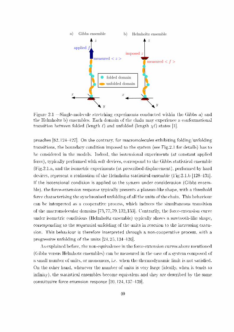
x
y
z
x
y
z
Gibbs ensemble Helmholtz ensemble
applied f
imposed z
measured < z >measured < f >
a) b)
folded domain
unfolded domain
Figure 2.1 � Single-molecule stretching experiments conducted within the Gibbs a) andthe Helmholtz b) ensembles. Each domain of the chain may experience a conformationaltransition between folded (length `) and unfolded (length χ`) states [1].
proaches [82,124�127]. On the contrary, for macromolecules exhibiting folding/unfolding
transitions, the boundary condition imposed to the system (see Fig.2.1 for details) has to
be considered in the models. Indeed, the isotensional experiments (at constant applied
force), typically performed with soft devices, correspond to the Gibbs statistical ensemble
(Fig.2.1.a, and the isometric experiments (at prescribed displacement), performed by hard
devices, represent a realisation of the Helmholtz statistical ensemble (Fig.2.1.b [128�131].
If the isotensional condition is applied to the system under consideration (Gibbs ensem-
ble), the force-extension response typically presents a plateau-like shape, with a threshold
force characterising the synchronised unfolding of all the units of the chain. This behaviour
can be interpreted as a cooperative process, which induces the simultaneous transition
of the macromolecular domains [73,77,79,132,133]. Contrarily, the force-extension curve
under isometric conditions (Helmholtz ensemble) typically shows a sawtooth-like shape,
corresponding to the sequential unfolding of the units in reaction to the increasing exten-
sion. This behaviour is therefore interpreted through a non-cooperative process, with a
progressive unfolding of the units [24,25,134�136].
As explained before, the non-equivalence in the force-extension curves above mentioned
(Gibbs versus Helmhotz ensembles) can be measured in the case of a system composed of
a small number of units, or monomers, i.e. when the thermodynamic limit is not satis�ed.
On the other hand, whenever the number of units is very large (ideally, when it tends to
in�nity), the statistical ensembles become equivalent and they are described by the same
constitutive force-extension response [20,124,137�139].
40
In order to get a wider comprehension of this complex scenario, several theoretical
approaches have been so far proposed in literature. Concerning the Gibbs ensemble, the
plateau-like response observed for double-stranded DNA has been largely investigated
with thermodynamic approaches, statistical mechanics and molecular dynamics simula-
tions [68, 74�77, 140]. A similar response has been also observed for long polysaccharides
(e.g.,dextran) and modelled through a continuous two-state model [24, 128,141].
In a like manner, theoretical developments have been adopted to model the sawtooth-
like response observed within the Helmholtz ensemble. Theories for titin, RNA hairpins
and other macromolecules have been elaborated through Landau-like free energies, �rst-
order phase transition, Langevin equations, and Ising models [142�147]. A more general
point of view about two-state systems driven by hard or soft devices can be found in the
mechanical literature concerning discrete systems with multi-basin energy landscapes,
Fermi-Pasta-Ulam chains of bistable elements, and structures undergoing discrete phase
transformations [104,105,107,148].
We present here a general methodology to study the thermodynamics of a system
composed of two-state units and subjected to di�erent boundary conditions. The main
idea consists in associating to each unit a discrete variable (or spin variable), able to
de�ne the state of the unit itself. Such a variable represents a sort of "bit", assuming
the values 0 and 1 for the folded and the unfolded states, respectively. The spin variables
are considered as dynamic variables, thus belonging to the extended phase space of the
system. From the historical point of view, the �rst biophysical model based on a dis-
crete quantity, similar to a spin variable, has been performed to predict the response of
skeletal muscles [109, 110]. This method has been recently applied to di�erent allosteric
systems and macromolecular chains as well [94, 111�113]. The introduction of the spin
variables allows to strongly facilitate the calculation of the partition functions, preserving
at the same time a good accuracy of results [113]. Brie�y, an arbitrary potential function
composed of two minima can be substituted by two quadratic potentials and the switch-
ing between them is governed by the corresponding spin variable. This method works
for both Gibbs and Helmholtz ensembles, allowing to draw direct comparisons between
isotensional and isometric conditions. We remark that the spin variables approach can
be only adopted for systems at thermodynamic equilibrium. As a matter of fact, the
quadratic potentials and the associated spin variables are not su�cient to describe the
dynamics, since the characteristic relaxation times strongly depend on the energy barriers
between the potential wells. This is a well-known result, encoded within the Kramers rate
formula, originally formulated to study chemical reactions [16], and recently generalised
41
for arbitrary systems with nonconvex energy landscapes [149, 150]. Hence, we use in the
following the spin variable approach both in Helmholtz and Gibbs ensembles and we show
how it allows to obtain well-known general results of the thermodynamics.
2.1.2 Thermodynamics of chains with conformational transitions
We introduce here a general methodology to describe the problem of the conforma-
tional transitions in chains undergoing typical folding/unfolding processes. It means that
each domain or unit of the chain may be in two states, corresponding to di�erent chemical
conformations. The potential energy of the system is therefore constituted of two wells,
which can be explored during the dynamics of the system. To simplify the description of
the system, considered at thermodynamic equilibrium, it is often convenient to introduce
discrete variables or spins, which are able to indicate what basin is explored for each unit
of the chain. Consequently, the more general form of the Hamiltonian for such a system
can be written as
H =N∑i=1
~pi · ~pi2M
+ U (~r1, ..., ~rN , S1, ..., SN)−N∑i=1
µiSi, (2.1)
where Si ∈ {0, 1} are the spin variables ∀i = 1, ..., N introduced in the potential energy
U . A domain is said folded (i.e. it is in the �rst energy well) when Si = 0 and unfolded
(i.e. it is in the second energy well) when Si = 1. The �rst term represents the kinetic
energy (~pi are the linear momenta of the units and M is their mass) and the second term
represents the potential energy depending on the units positions ~ri and on the spins Si.
Finally, the third term represents the e�ect of the external chemical environment on the
state of the domains: if µi > 0, the unfolded state is favoured, and conversely, if µi < 0,
the folded state is favoured. From the experimental point of view, the chemical potentials
µi may mimic the presence of some chemical substances, able to induce or to impede
the units unfolding. An interesting example concerns the e�ect of ethidium molecules on
the force-induced melting of DNA [151]. As discussed below in our model, the chemical
potential is able to shift the e�ective energy jump between folded and unfolded states
of a given bistable system. This exactly corresponds to the experimental observations in
response to an increasing concentration of ethidium, which reported an increase of the
DNA transition force and of the e�ective energy jump between states before and after the
transition [151].
It is important to remark that the introduced Hamiltonian function corresponds to
a coarse-graining approach, applied to the actual molecular architecture of the system.
42
Indeed, the concept of units above introduced corresponds to a speci�c ensemble of atoms
with a well-de�ned behaviour, summarised within the coarse-grained potential energy. Of
course, we could have considered an exact Hamiltonian with a very large number of de-
grees of freedom (all the atomic coordinates and momenta as, e.g., introduced in classical
molecular dynamics), but we propose a simpli�cation to provide analytic developments
and corresponding physical interpretations. Therefore, when we mention a physical prop-
erty of one unit (elastic constant or others), we have to keep in mind that it represents the
collective response of the atoms of the unit, and not a real or intrinsic property of an exact
Hamiltonian. Then, these properties of units may be considered temperature-dependent
being de�ned at the mesoscopic scale. This is similar to the expansion of the Landau free
energy used to describe critical phenomena, where the coe�cients depend on temperature
for the same reason. The coarse-graining approach also leads to the following issue in
writing Eq.(2.1): since the extremities of a given unit ~ri−1 and ~ri are associated to the
momenta ~pi−1 and ~pi, it means that we assume the mass concentrated at points ~ri, while
in the real case the mass is distributed between ~ri−1 and ~ri on all the atoms composing
the unit. This is a typical approximation used to describe a one-dimensional chain [152],
but it should be kept in mind since each unit is �nally identi�ed by the two positions of
extremities and by one spin variable.
As an example, a concrete case can be described by the following potential energy
U = −N−1∑i=1
λi(2Si − 1)(2Si+1 − 1) +N∑i=1
1
2k(Si) [‖~ri − ~ri−1‖ − `(Si)]2
+N∑i=1
v(Si) +N−1∑i=1
1
2κ(Si)
(~ti+1 − ~ti
)2, (2.2)
where the �rst term represents an Ising interaction among the states of the units (λi being
the interaction coe�cients and 2Si − 1 = ±1 if Si = 0, 1), the second and third terms
represent the spring-like behaviour of the two-state domains (k, ` and v are the elastic
constant, the equilibrium length and the basal energy, respectively, of the states), and
the last term represents a discrete worm-like-chain interaction among the units (κ is the
bending constant related to the persistence length p = `κkBT
and ~ti = (~ri − ~ri−1)/‖~ri −~ri−1‖). The Ising scheme represents an interaction among the spin variables, with two
adjacent units favoured to be in the same state if λi > 0 or favoured to be in opposite
states if λi < 0. The typical case arising in protein structures corresponds to a positive
interaction and allows the interpretation of cooperativity of the folding/unfolding process
[153]. An interesting example of cooperativity in forced unfolding concerns the case of
43
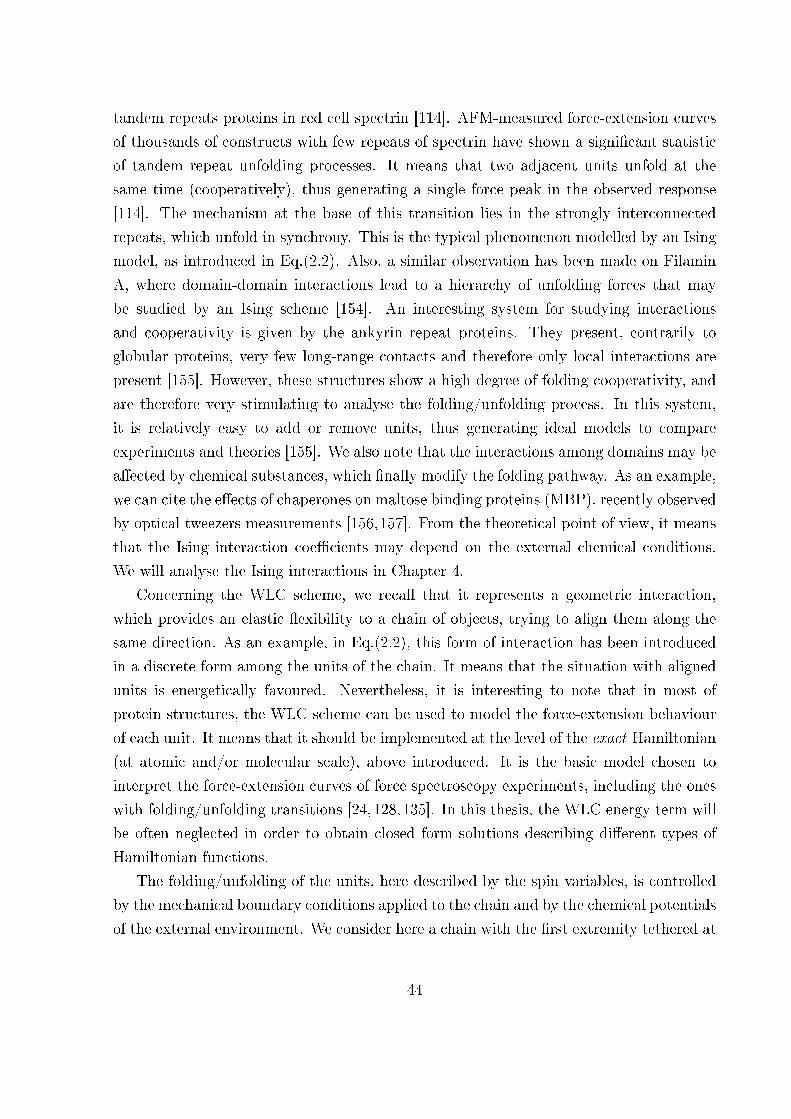
tandem repeats proteins in red cell spectrin [114]. AFM-measured force-extension curves
of thousands of constructs with few repeats of spectrin have shown a signi�cant statistic
of tandem repeat unfolding processes. It means that two adjacent units unfold at the
same time (cooperatively), thus generating a single force peak in the observed response
[114]. The mechanism at the base of this transition lies in the strongly interconnected
repeats, which unfold in synchrony. This is the typical phenomenon modelled by an Ising
model, as introduced in Eq.(2.2). Also, a similar observation has been made on Filamin
A, where domain-domain interactions lead to a hierarchy of unfolding forces that may
be studied by an Ising scheme [154]. An interesting system for studying interactions
and cooperativity is given by the ankyrin repeat proteins. They present, contrarily to
globular proteins, very few long-range contacts and therefore only local interactions are
present [155]. However, these structures show a high degree of folding cooperativity, and
are therefore very stimulating to analyse the folding/unfolding process. In this system,
it is relatively easy to add or remove units, thus generating ideal models to compare
experiments and theories [155]. We also note that the interactions among domains may be
a�ected by chemical substances, which �nally modify the folding pathway. As an example,
we can cite the e�ects of chaperones on maltose binding proteins (MBP), recently observed
by optical tweezers measurements [156,157]. From the theoretical point of view, it means
that the Ising interaction coe�cients may depend on the external chemical conditions.
We will analyse the Ising interactions in Chapter 4.
Concerning the WLC scheme, we recall that it represents a geometric interaction,
which provides an elastic �exibility to a chain of objects, trying to align them along the
same direction. As an example, in Eq.(2.2), this form of interaction has been introduced
in a discrete form among the units of the chain. It means that the situation with aligned
units is energetically favoured. Nevertheless, it is interesting to note that in most of
protein structures, the WLC scheme can be used to model the force-extension behaviour
of each unit. It means that it should be implemented at the level of the exact Hamiltonian
(at atomic and/or molecular scale), above introduced. It is the basic model chosen to
interpret the force-extension curves of force spectroscopy experiments, including the ones
with folding/unfolding transitions [24,128,135]. In this thesis, the WLC energy term will
be often neglected in order to obtain closed form solutions describing di�erent types of
Hamiltonian functions.
The folding/unfolding of the units, here described by the spin variables, is controlled
by the mechanical boundary conditions applied to the chain and by the chemical potentials
of the external environment. We consider here a chain with the �rst extremity tethered at
44
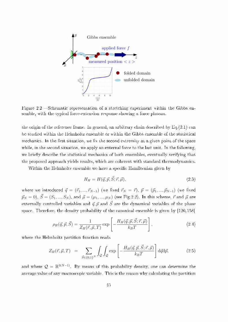
Figure 2.2 � Schematic representation of a stretching experiment within the Gibbs en-semble, with the typical force-extension response showing a force plateau.
the origin of the reference frame. In general, an arbitrary chain described by Eq.(2.1) can
be studied within the Helmholtz ensemble or within the Gibbs ensemble of the statistical
mechanics. In the �rst situation, we �x the second extremity at a given point of the space
while, in the second situation, we apply an external force to the last unit. In the following,
we brie�y describe the statistical mechanics of both ensembles, eventually verifying that
the proposed approach yields results, which are coherent with standard thermodynamics.
Within the Helmholtz ensemble we have a speci�c Hamiltonian given by
HH = H(~q, ~p, ~S;~r, ~µ), (2.3)
where we introduced ~q = (~r1, ..., ~rN−1) (we �xed ~rN = ~r), ~p = (~p1, ..., ~pN−1) (we �xed
~pN = 0), ~S = (S1, ..., SN), and ~µ = (µ1, ..., µN) (see Fig.2.2). In this scheme, ~r and ~µ are
externally controlled variables and ~q, ~p and ~S are the dynamical variables of the phase
space. Therefore, the density probability of the canonical ensemble is given by [120,158]
ρH(~q, ~p, ~S) =1
ZH(~r, ~µ, T )exp
[−HH(~q, ~p, ~S;~r, ~µ)
kBT
], (2.4)
where the Helmholtz partition function reads
ZH(~r, ~µ, T ) =∑
~S∈{0,1}N
∫Q
∫Q
exp
[−HH(~q, ~p, ~S;~r, ~µ)
kBT
]d~qd~p, (2.5)
and where Q = R3(N−1). By means of this probability density, one can determine the
average value of any macroscopic variable. This is the reason why calculating the partition
45

function is of vital importance in the statistical mechanics. In particular, the average
value of the force ~f = ∂HH∂~r
needed to �x ~rN = ~r and the average value of each spin
variable Si can be easily obtained through the introduction of the Helmholtz free energy
F = −kBT logZH . Indeed, straightforward calculations yield⟨~f⟩
= ∂F∂~r
and⟨~S⟩
=
−∂F∂~µ, which represent two macroscopic or thermodynamic relations. Moreover, the �rst
and second principles for quasi-static transformations can be derived as follows from
previous statements. First of all, we de�ne a quasi-static transformation through the
time evolution of ~r(t), ~µ(t) and T (t), which are considered as externally controlled "slow-
varying" variables. Under these hypotheses, we can assume that the canonical distribution
in Eq.(2.4) remains valid also in this "weak" out-of-equilibrium regime. Therefore, we can
evaluate the rate of change of the internal energy U , de�ned as the average value of the
Helmholtz Hamiltonian
dUdt
=∑~S
∫Q
∫Q
d
dt(HHρH) d~qd~p
=∑~S
∫Q
∫Q
(∂HH
∂~µ· d~µ
dt+∂HH
∂~r· d~r
dt
)ρHd~qd~p+
∑~S
∫Q
∫QHH
dρHdt
d~qd~p
= −⟨~S⟩· d~µ
dt+⟨~f⟩· d~r
dt+∑~S
∫Q
∫QHH
dρHdt
d~qd~p, (2.6)
where all the sums on ~S are performed over {0, 1}N . The �rst two terms represent the
chemical and the mechanical work per unit of time, respectively, done on the system, while
the third one describes the rate of heat entering the system. The latter can be further
elaborated by de�ning η = F−HHkBT
and ρH = eη. Since∑
~S
∫Q
∫Q e
ηd~qd~p = 1, the derivative
with respect to the time gives∑
~S
∫Q
∫Q e
ηηd~qd~p = 0, and since F is independent of ~S, ~q
and ~p, we can also write that∑
~S
∫Q
∫QFeηηd~qd~p = 0. The last term in Eq.(2.6) can be
therefore rewritten as∑~S
∫Q
∫QHH
dρHdt
d~qd~p =∑~S
∫Q
∫QHHe
ηηd~qd~p
=∑~S
∫Q
∫Q
(HH −F) eηηd~qd~p. (2.7)
Now, since HH −F = −kBTη, we also have∑~S
∫Q
∫QHH
dρHdt
d~qd~p = −kBT∑~S
∫Q
∫Qeηηηd~qd~p. (2.8)
46

This expression can be easily interpreted by considering the average value of the variable
η given by 〈η〉 =∑
~S
∫Q
∫Q e
ηηd~qd~p and its time derivatives
d 〈η〉dt
=∑~S
∫Q
∫Qeηηd~qd~p+
∑~S
∫Q
∫Qeηηηd~qd~p. (2.9)
Since the �rst integral is zero for previous calculations, we eventually obtain∑~S
∫Q
∫QHH
dρHdt
d~qd~p = −kBTd 〈η〉
dt= T
dSdt, (2.10)
where we introduced the entropy of the system as
S = −kB 〈log ρH〉 = −kB∑~S
∫Q
∫QρH log ρHd~qd~p. (2.11)
The �rst and the second principles of the thermodynamics for quasi-static transformations
can be �nally summed up through the balance equation
dUdt
= −⟨~S⟩· d~µ
dt+⟨~f⟩· d~r
dt+ T
dSdt. (2.12)
Hence, we proved that the macroscopic thermodynamics is perfectly coherent with the
approach based on the spin variables, introduced to analyse systems with conformational
transitions. In addition, the average value of the relation HH − F = −kBTη yields
F = U − TS, which corresponds to the macroscopic de�nition of Helmholtz free energy.
By di�erentiating with respect to the time, we also have
dFdt
= −⟨~S⟩· d~µ
dt+⟨~f⟩· d~r
dt− S dT
dt, (2.13)
from which we can deduce the two already introduced equations⟨~f⟩
= ∂F∂~r
and⟨~S⟩
=
−∂F∂~µ
and the important relation S = −∂F∂T, giving the entropy in terms of the Helmholtz
free energy.
Concerning the Gibbs ensemble, we can introduce the following extended Hamiltonian
HG = H(~q, ~p, ~S; ~µ)− ~f · ~rN , (2.14)
where the second term represents the energy associated to the external force applied to the
last unit of the chain (see Fig.2.3). Here, we introduced ~q = (~r1, ..., ~rN), ~p = (~p1, ..., ~pN),~S = (S1, ..., SN), and ~µ = (µ1, ..., µN). In this scheme, ~f and ~µ are externally controlled
47

Figure 2.3 � Schematic representation of a stretching experiment within the Helmholtzensemble, with the typical force-extension response showing a sawtooth-like behaviour.
variables and ~q, ~p and ~S are the dynamical variables of the phase space. Therefore, the
density probability of the canonical ensemble is given by [120,158]
ρG(~q, ~p, ~S) =1
ZG(~f, ~µ, T )exp
[−HG(~q, ~p, ~S; ~f, ~µ)
kBT
], (2.15)
where the Gibbs partition function reads
ZG(~f, ~µ, T ) =∑
~S∈{0,1}N
∫P
∫P
exp
[−HG(~q, ~p, ~S; ~f, ~µ)
kBT
]d~qd~p, (2.16)
and where P = R3N . As before, the most important expected values can be evaluated
through the introduction of the Gibbs free energy G = −kBT logZG. Simple calculations
yield indeed 〈~r〉 = −∂G∂ ~f
(where ~r = ~rN) and⟨~S⟩
= −∂G∂~µ, which represent two classical
thermodynamic relations. Also in this isotensional case, we can introduce a quasi-static
transformation through the time evolution of ~f(t), ~µ(t) and T (t), which are, as before,
externally controlled "slow-varying" variables. We can assume that the canonical distri-
bution in Eq.(2.15) remains valid and we can evaluate the rate of change of the average
value of the Gibbs Hamiltonian, which is the so-called enthalpy HdHdt
=∑~S
∫P
∫P
d
dt(HGρG) d~qd~p
=∑~S
∫P
∫P
(∂HG
∂~µ· d~µ
dt+∂HG
∂ ~f· d~f
dt
)ρGd~qd~p+
∑~S
∫P
∫PHG
dρGdt
d~qd~p
= −⟨~S⟩· d~µ
dt− 〈~r〉 · d~f
dt+∑~S
∫P
∫PHG
dρGdt
d~qd~p. (2.17)
48
While the �rst two terms represent the power (chemical and mechanical) supplied to the
system, the third term is the rate of heat transferred to the system. A calculation similar
to the one developed for the Helmholtz ensemble allows us to rewrite this last term as
follows
dHdt
= −⟨~S⟩· d~µ
dt− 〈~r〉 · d~f
dt+ T
dSdt, (2.18)
where the entropy for the Gibbs ensemble is given by
S = −kB 〈log ρG〉 = −kB∑~S
∫P
∫PρG log ρGd~qd~p. (2.19)
We can straightforwardly prove the thermodynamic relation G = H− TS and we obtain
the rate of change of the Gibbs free energy as
dGdt
= −⟨~S⟩· d~µ
dt− 〈~r〉 · d~f
dt− S dT
dt. (2.20)
The last energy balance immediately delivers the relations 〈~r〉 = −∂G∂ ~f
and⟨~S⟩
= −∂G∂~µ,
previously demonstrated, and the result S = − ∂G∂T, corresponding to the macroscopic
de�nition of entropy.
The two schemes here outlined represent a complete description able to deliver thermo-
mechanical response of a macromolecular chain undergoing conformational transitions
under isometric or isotensional boundary conditions. We proved that the introduction of
additional "spin" variables to describe the folding or unfolding of the units leaves unal-
tered the general results of the thermodynamics, thus being well-grounded and promising
for applications. As an example, the application of this methodology to the bistable freely
jointed chain can be found in the recent literature [113]. It is important to remark that
the thermo-elastic response may be di�erent for the two introduced ensembles if we con-
sider chains composed of a small number N of units [120]. On the other hand, when the
thermodynamic limit is attained (ideally for N →∞), the two ensembles become equiv-
alent and they exhibit the same physical response [20, 124, 137�139]. This equivalence
property is valid for non-branched single chains without con�nements, i.e. freely �uctuat-
ing in the whole space [20]. Therefore, in our analysis, the only constraints consist in the
punctual boundary conditions de�ning the Helmholtz and the Gibbs ensembles. However,
it is noteworthy to mention that some particular cases on non-equivalence between dual
canonical ensembles have been recently discussed for con�ned polymer chains [21�23].
49
2.2 Applications of the spin variable method
In the Section 2.1, we presented some general results of thermodynamics obtained
with the help of the spin variable method. Here, the spin variable approach is described
in detail, for speci�c one-dimensional and three-dimensional systems. The study of these
two cases has already been published in Ref. [113]. They are here presented to introduce
the spin variable method in the simplest cases, without any of the extensions which will be
proposed in the following, like elasticity or again Ising interactions. Moreover, we show an
example to prove that the spin variables method is not also useful to obtain average values
of positions or forces but also to determine the complete probability density describing
systems with bistability.
2.2.1 One dimensional system
In this Section, we present the spin variable approach applied to a system that can be
analytically solved for both the Gibbs (isotensional) ensemble and the Helmholtz (isomet-
ric) ensemble. The aim is to obtain closed form expressions, useful to better understand
the physics of the phenomena underlying the bistability in complex systems.
A one-dimensional system composed of N units with mechanical bistability is con-
sidered here. This means that each unit of the chain can be described by a symmetric
potential energy function U(x) exhibiting four minima (equilibrium points) at x = ±`and x = ±χ`, where χ represents the elongation ratio between the unfolded and folded
con�gurations (see Fig.2.4). Moreover, the potential energy assumes the minimum value
U = 0 for x = ±` and the minimum value U = ∆E for x = ±χ`. In order to simplify
analysis and calculations, instead of considering the complex continuous potential func-
tion represented in Fig.2.4 (blue dashed line), we introduce an additional discrete variable
y, which behaves as a spin. This variable belongs to the phase space of the system and,
therefore, is a standard variable of the statistical mechanics. The variable y assumes the
values in the set S = {±1,±χ} and allows to identify what basin the system is exploring.
So, the multimodal energy function is substituted with this simpler expression
U(x, y) = v(y) +1
2k0(y)(x− y`)2, (2.21)
where we consider v(±1) = 0, v(±χ) = ∆E, k0(±1) = k and k0(±χ) = h. By varying
the value of the spin variable in S, the potential energy in Eq.(2.21) provides the four
parabolic wells represented in Fig.2.4 (red solid lines). The latter permit to fully describe
the behaviour of the system represented by the multimodal energy pro�le when we assume
50

−xf = −ℓ−xu = −χℓ xf = ℓ xu = χℓ0 x
U
∆E ∆Ek k
hh
y = −χ
y = −1 y = 1
y = χ
Figure 2.4 � Multistable symmetric potential energy of a single domain (blue dashed line)and its approximation by means of four parabolic pro�les (red solid lines) [113].
to work at thermodynamic equilibrium. Similar assumptions have been introduced and
analysed in recent literature [105,150].
Here come some comments on the energy pro�le proposed in Fig.2.4. We introduced
four potential wells (two folded and two unfolded) for the following reasons. Since we study
a one-dimensional system, the consideration of positive (x > 0) and negative (x < 0)
orientations of the elements allows to model the four constitutives regimes (entropic,
enthalpic, unfolding and over-stretching). Indeed, if a system whose the �rst end-terminal
is tethered at x = 0 and the second end-terminal free to �uctuate (without externally
applied forces) is considered, we obtain that the mean value of the position of the second
end-terminal is zero because of the random orientation of the domains (almost domains
folded, 50% towards x > 0 and 50% towards x < 0). Incidentally, it means that the force-
extension curve passes through the origin of the axes. If a weak applied force (positive
or negative) is applied, the chain is in the entropic regime and the number of domains
oriented in the direction of the force slightly increases. In these conditions, the mechanical
reaction of the system is governed by the stochastic distribution of the di�erently oriented
domains (entropy) and not by the actual spring-like behaviour of the elements. Then, if
a larger force is applied, we act on the real elasticity of the domains and therefore the
enthalpic regime gives way to the unfolding process up to the over-stretching regime,
described below for both Gibbs and Helmholtz ensembles.
In conclusion, the entropic behaviour of a system under weak applied force can be
represented by the four wells energy pro�le handled by the spin variable. This aspect is
naturally introduced in two- or three-dimensional models by the higher dimensionality,
which automatically induces a larger number of degrees of freedom (see Section 2.2.2 for
details).
51
2.2.1.1 The Gibbs ensemble
The total potential energy of the system in the Gibbs ensemble (isotensional condition)
can be written as
UGtot(~x, ~y; f) =
N∑i=1
U(xi − xi−1, yi)− fxN , (2.22)
where f is the force applied to the last element, ~x = (x1, x2, ..., xN) are continuous variables
and ~y = (y1, y2, ..., yN) are discrete spin variables. For this system, we can de�ne the
partition function ZG, as follows
ZG(f) =∑y1∈S
...∑yN∈S
∫<...
∫<e− U
Gtot
kBT dx1...dxN , (2.23)
where the variable ~x is integrated whereas ~y is summed. Since we use orthogonal coordi-
nates, the kinetic energy only depends on the linear momentum variables and the potential
energy only on ~x and ~y. Therefore, the kinetic energy has not been considered because
its integral results in a non in�uential multiplicative constant in the partition function,
ZG(f). Eq.(2.22) can now be substituted in Eq.(2.23). To calculate the integral, we apply
the change of variables x1 − x0 = ξ1, x2 − x1 = ξ2,..., xN − xN−1 = ξN , from which we
get xn =∑N
j=1 ξj (with x0 = 0). The change of variables within the multiple integral
must be applied by considering that d~x = Jd~ξ, where the quantity J is the Jacobian of
the transformation, i.e. J = | det[∂~x/∂~ξ]|, where [∂~x/∂~ξ]ij is the matrix of the partial
derivatives ∂xi/∂ξj. We can easily prove that J = 1 for our change of variables and,
therefore, we get d~ξ = d~x. Hence, we obtain
ZG(f) =∑~y∈SN
∫<N
exp
{N∑j=1
[−U(ξj; yj)
kBT+
fξjkBT
]}d~ξ
=
{∑y∈S
∫ +∞
−∞exp
[−U(ξ; y)
kBT+
fξ
kBT
]dξ
}N
=
{∑y∈S
exp
[−v(y)
kBT
]I(f)
}N
, (2.24)
where the integral I(f) is de�ned as
I(f) =
∫ +∞
−∞exp
[− k0(y)
2kBT(ξ − y`)2 +
fξ
kBT
]dξ. (2.25)
52
This integral can be calculated in an explicit form by means of the well-known expression∫ +∞
−∞e−αx
2
eβxdx =
√π
αeβ2
4α (α > 0). (2.26)
The �nal result can be written as follows
I(f) =
√2πkBT
k0(y)exp
[y`f
kBT+
f 2
2kBTk0(y)
]. (2.27)
Coming back to the partition function, we obtain
ZG(f) = (2πkBT )N2
{∑y∈S
√1
k0(y)exp
[1
kBT
(f 2
2k0(y)+ y`f − v(y)
)]}N
= (8πkBT )N2
∑s∈{1,χ}
√1
k0(s)exp
[1
kBT
(f 2
2k0(s)− v(s)
)]
× coshs`f
kBT
}N
. (2.28)
The last sum can be evaluated as
ZG(f) = (8πkBT )N2 DN , (2.29)
by writing
D =
√1
kexp
(f 2
2kBTk
)cosh
(`f
kBT
)+ φ
√1
hexp
(f 2
2kBTh
)cosh
(χ`f
kBT
),(2.30)
and φ = exp(− ∆EkBT
). It is particularly noticeable that there is no interaction between
the elements of the chain in the Gibbs ensemble. Consequently, we can write the parti-
tion function as a power with exponent N . A similar result can be found in Eq.(34) of
Ref. [105], describing the statistical behaviour of a Fermi-Pasta-Ulam chain of bistable
elements. Also in this case a soft device leads to the independence of the bistable units.
With the help of the expression xN = −∂Utot/∂f , the extension of the chain can be
directly calculated and its average value is therefore 〈xN〉 = 〈−∂Utot/∂f〉. It can be
simply evaluated by means of the partition function, as 〈xN〉 = kBT ∂/∂f(logZG). The
calculation eventually gives
〈xN〉N`
=
{√1
kexp
(f 2
2kBTk
)[f
k`cosh
(`f
kBT
)+ sinh
(`f
kBT
)]
+χφ
√1
hexp
(f 2
2kBTh
)[f
χ`hcosh
(χ`f
kBT
)+ sinh
(χ`f
kBT
)]}/D. (2.31)
53
In the simpler case with k = h, we get
〈xN〉N`
=f
k`+
sinh
(`f
kBT
)+ χφ sinh
(χ`f
kBT
)cosh
(`f
kBT
)+ φ cosh
(χ`f
kBT
) . (2.32)
We can also calculate the average value of the spin variable 〈y〉 = 〈yi〉 ∀i, which is inde-
pendent of the characteristics of the elements considered in the chain and is given by
〈y〉 = 〈yi〉 =ND ∀i, (2.33)
where
N =
√1
kexp
(f 2
2kBTk
)sinh
(`f
kBT
)+ χφ
√1
hexp
(f 2
2kBTh
)sin
(χ`f
kBT
),(2.34)
and D is given in Eq.(2.30). In the simpler case with k = h, we get
〈y〉 =
sinh
(`f
kBT
)+ χφ sinh
(χ`f
kBT
)cosh
`f
kBT+ φ cosh
(χ`f
kBT
) . (2.35)
By combining Eq.(2.32) with Eq.(2.35), we immediately obtain 〈xN 〉N`
= fk`
+ 〈y〉 or, equiv-alently,
f = k
(〈xN〉N− ` 〈y〉
). (2.36)
This constitutive equation represents a spring-like behaviour with an equilibrium length
directly modulated by the average value of the spin variables.
An example of force-extension response and spin variable behaviour is represented in
Fig.2.5 for h = k. In the curve of f`kBT
versus 〈xN 〉N`
, a force plateau corresponding to
f ∗ = ± ∆E(χ−1)`
or, equivalently, f∗`kBT
= ± ∆E(χ−1)kBT
is observed. Equivalently, in the curve
of f`kBT
versus 〈y〉, we can identify the regions 〈y〉 = ±1 and 〈y〉 = ±χ with a transition
corresponding to the same force f ∗. This behaviour can be interpreted as a cooperative
process, with a threshold force f ∗ leading to the transition of all the units of the chain
at the same time. As far as DNA is concerned, it is possible to retrieve the value of its
force plateau by using the following parameters: ∆E = 3, 8KBT , ` = 3, 4 Å, χ = 1, 7
and (χ − 1)` = 2, 4Å. The value of the threshold force thus obtained is about 65 pN,
corresponding to the well-known experimental value [79].
54
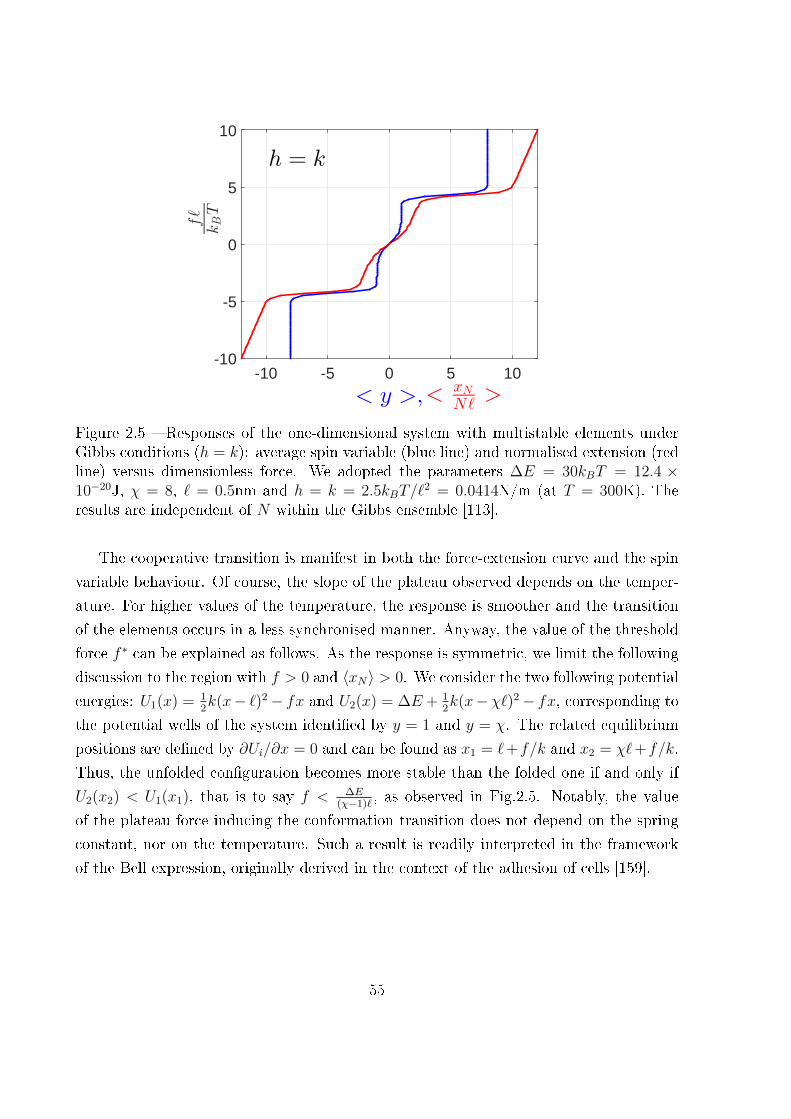
< y >,-10 -5 0 5 10
fℓ
kBT
-10
-5
0
5
10
< xN
Nℓ>
h = k
Figure 2.5 � Responses of the one-dimensional system with multistable elements underGibbs conditions (h = k): average spin variable (blue line) and normalised extension (redline) versus dimensionless force. We adopted the parameters ∆E = 30kBT = 12.4 ×10⁻²⁰J, χ = 8, ` = 0.5nm and h = k = 2.5kBT/`
2 = 0.0414N/m (at T = 300K). Theresults are independent of N within the Gibbs ensemble [113].
The cooperative transition is manifest in both the force-extension curve and the spin
variable behaviour. Of course, the slope of the plateau observed depends on the temper-
ature. For higher values of the temperature, the response is smoother and the transition
of the elements occurs in a less synchronised manner. Anyway, the value of the threshold
force f ∗ can be explained as follows. As the response is symmetric, we limit the following
discussion to the region with f > 0 and 〈xN〉 > 0. We consider the two following potential
energies: U1(x) = 12k(x− `)2− fx and U2(x) = ∆E + 1
2k(x−χ`)2− fx, corresponding to
the potential wells of the system identi�ed by y = 1 and y = χ. The related equilibrium
positions are de�ned by ∂Ui/∂x = 0 and can be found as x1 = `+f/k and x2 = χ`+f/k.
Thus, the unfolded con�guration becomes more stable than the folded one if and only if
U2(x2) < U1(x1), that is to say f < ∆E(χ−1)`
, as observed in Fig.2.5. Notably, the value
of the plateau force inducing the conformation transition does not depend on the spring
constant, nor on the temperature. Such a result is readily interpreted in the framework
of the Bell expression, originally derived in the context of the adhesion of cells [159].
55
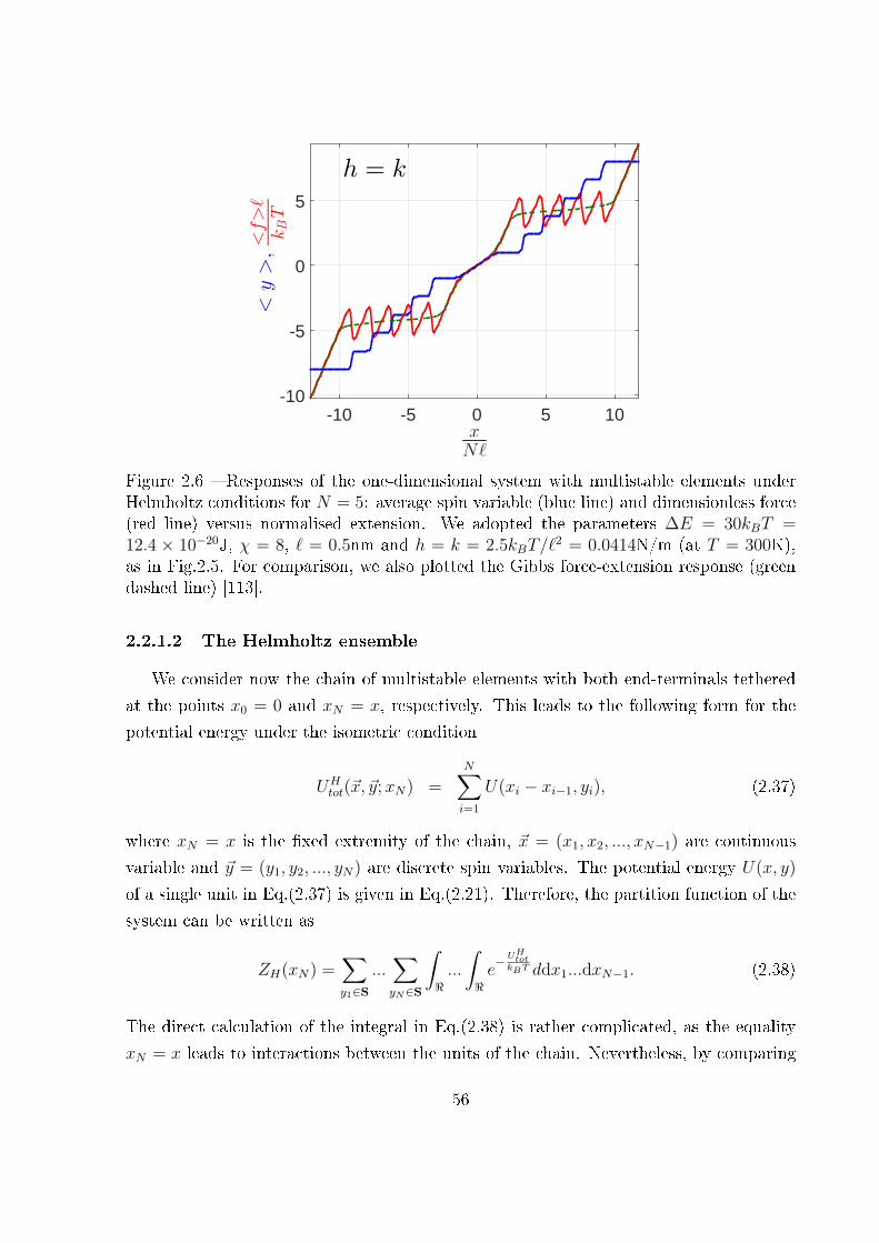
xNℓ
-10 -5 0 5 10
<f>ℓ
kBT
-10
-5
0
5
<y>,
h = k
Figure 2.6 � Responses of the one-dimensional system with multistable elements underHelmholtz conditions for N = 5: average spin variable (blue line) and dimensionless force(red line) versus normalised extension. We adopted the parameters ∆E = 30kBT =12.4 × 10⁻²⁰J, χ = 8, ` = 0.5nm and h = k = 2.5kBT/`
2 = 0.0414N/m (at T = 300K),as in Fig.2.5. For comparison, we also plotted the Gibbs force-extension response (greendashed line) [113].
2.2.1.2 The Helmholtz ensemble
We consider now the chain of multistable elements with both end-terminals tethered
at the points x0 = 0 and xN = x, respectively. This leads to the following form for the
potential energy under the isometric condition
UHtot(~x, ~y;xN) =
N∑i=1
U(xi − xi−1, yi), (2.37)
where xN = x is the �xed extremity of the chain, ~x = (x1, x2, ..., xN−1) are continuous
variable and ~y = (y1, y2, ..., yN) are discrete spin variables. The potential energy U(x, y)
of a single unit in Eq.(2.37) is given in Eq.(2.21). Therefore, the partition function of the
system can be written as
ZH(xN) =∑y1∈S
...∑yN∈S
∫<...
∫<e− U
Htot
kBT ddx1...dxN−1. (2.38)
The direct calculation of the integral in Eq.(2.38) is rather complicated, as the equality
xN = x leads to interactions between the units of the chain. Nevertheless, by comparing
56
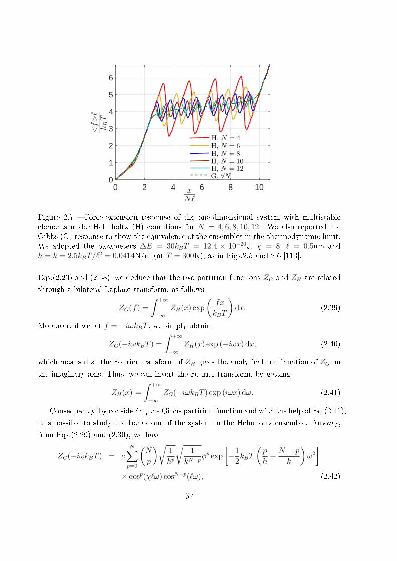
xNℓ
0 2 4 6 8 10
<f>ℓ
kBT
0
1
2
3
4
5
6
H, N = 4
H, N = 6
H, N = 10H, N = 12G, ∀N
H, N = 8
Figure 2.7 � Force-extension response of the one-dimensional system with multistableelements under Helmholtz (H) conditions for N = 4, 6, 8, 10, 12. We also reported theGibbs (G) response to show the equivalence of the ensembles in the thermodynamic limit.We adopted the parameters ∆E = 30kBT = 12.4 × 10⁻²⁰J, χ = 8, ` = 0.5nm andh = k = 2.5kBT/`
2 = 0.0414N/m (at T = 300K), as in Figs.2.5 and 2.6 [113].
Eqs.(2.23) and (2.38), we deduce that the two partition functions ZG and ZH are related
through a bilateral Laplace transform, as follows
ZG(f) =
∫ +∞
−∞ZH(x) exp
(fx
kBT
)dx. (2.39)
Moreover, if we let f = −iωkBT , we simply obtain
ZG(−iωkBT ) =
∫ +∞
−∞ZH(x) exp (−iωx) dx, (2.40)
which means that the Fourier transform of ZH gives the analytical continuation of ZG on
the imaginary axis. Thus, we can invert the Fourier transform, by getting
ZH(x) =
∫ +∞
−∞ZG(−iωkBT ) exp (iωx) dω. (2.41)
Consequently, by considering the Gibbs partition function and with the help of Eq.(2.41),
it is possible to study the behaviour of the system in the Helmholtz ensemble. Anyway,
from Eqs.(2.29) and (2.30), we have
ZG(−iωkBT ) = cN∑p=0
(N
p
)√1
hp
√1
kN−pφp exp
[−1
2kBT
(p
h+N − pk
)ω2
]× cosp(χ`ω) cosN−p(`ω), (2.42)
57
where c is an unimportant multiplicative constant. By using the Newton development
cosn x =1
2ne−inx
n∑t=0
(n
t
)e2itx, (2.43)
we obtain from Eqs.(2.41) and (2.42)
ZH(x) = c
N∑p=0
p∑q=0
N−p∑s=0
(N
p
)(p
q
)(N − ps
)√1
hp
√1
kN−pφp
×∫ +∞
−∞exp
[−1
2kBT
(p
h+N − pk
)ω2
]× exp [iω(2χ`q − χ`p+ 2`s− `N + `p+ x)] dω. (2.44)
The integral in Eq.(2.44) can be evaluated in a closed form by means of the standard
expression ∫ +∞
−∞e−αx
2
eiβxdx =
√π
αe−
β2
4α (α > 0), (2.45)
eventually giving
ZH(x) = cN∑p=0
p∑q=0
N−p∑s=0
(N
p
)(p
q
)(N − ps
)1√
ph
+ N−pk
√1
hp
√1
kN−pφpe−ϕ
2
, (2.46)
where
ϕ =2χ`q − χ`p+ 2`s− `N + `p+ x√
2kBT(ph
+ N−pk
) . (2.47)
In this case, it is important to remark that the resulting partition function can not be
written in terms of a power with exponent N . Therefore, the Helmholtz (isotensional)
condition induces an e�ective interaction between the elements. The origin of this inter-
action is not explicitly de�ned in the potential energy of the system (as, e.g., in the Ising
model), but comes from the speci�c boundary conditions characterising the Helmholtz
ensemble. Our result can be compared with Eq.(20) of Ref. [105], obtained for a Fermi-
Pasta-Ulam chain with bistable elements. This work permits to con�rm that using hard
devices leads to interaction among the elements (see also Fig.13 of Ref. [105] for the com-
parison of the mechanical response with soft or hard devices). Now, the average value
of the overall force 〈f〉 = −kBT∂/∂x logZH applied to the system and the average value
of the spin variables 〈y〉 =⟨
1N
∑Ni=1 yi
⟩describing the transitions can be calculated as
follows
58
〈f〉 =
N∑p=0
p∑q=0
N−p∑s=0
(N
p
)(p
q
)(N − ps
) √2kBT
ph
+ N−pk
√1
hp
√1
kN−pφpϕe−ϕ
2
N∑p=0
p∑q=0
N−p∑s=0
(N
p
)(p
q
)(N − ps
)1√
ph
+ N−pk
√1
hp
√1
kN−pφpe−ϕ
2
, (2.48)
〈y〉 =
1
N
N∑p=0
p∑q=0
N−p∑s=0
(N
p
)(p
q
)(N − ps
)1√
ph
+ N−pk
√1
hp
√1
kN−pφpQe−ϕ
2
N∑p=0
p∑q=0
N−p∑s=0
(N
p
)(p
q
)(N − ps
)1√
ph
+ N−pk
√1
hp
√1
kN−pφpe−ϕ
2
, (2.49)
where Q = (χp− 2χq +N − p− 2s).
An application of Eqs.(2.48) and (2.49) can be found in Fig.2.6 where the average
spin variable and the dimensionless force are represented versus the normalised extension
for h = k and N = 5 (with the same parameters than those used in Fig.2.5). The
force-extension response for the Gibbs condition is also shown for comparison. A non-
cooperative behaviour is observed, showing that the units unfold progressively with the
increasing total length of the system. This is a non-synchronised process, characterised
by the picks visible in the Helmholtz force-extension relation and by the sequence of steps
characterising the average value of the spin variable. In conclusion, whereas in the Gibbs
ensemble, the unfolding of the domains is a collective (cooperative) process, leading to
a force plateau in the force-extension curve, in the Helmholtz ensemble, the unfolding of
the domains is a non-cooperative process, speci�c to each unit, leading to a sawtooth-like
force-extension curve.
In Fig.2.7, the force-extension curve in the Helmholtz ensemble for di�erent values of
N = 4, 6, 8, 10 and 12 is shown. It is particularly noticeable that for an increasing number
N of elements, the Helmholtz response converges to the Gibbs one, by progressively
reducing the pick-to-pick distance in the sawtooth pattern. This is in perfect agreement
with recent results concerning the ensembles equivalence in the thermodynamic limit
[20,139].
2.2.2 Bistable freely jointed chain
In this Section, we elaborate a generalisation of the classical freely jointed chain model
in order to introduce the two-state behaviour in the elements of the system. The model
59
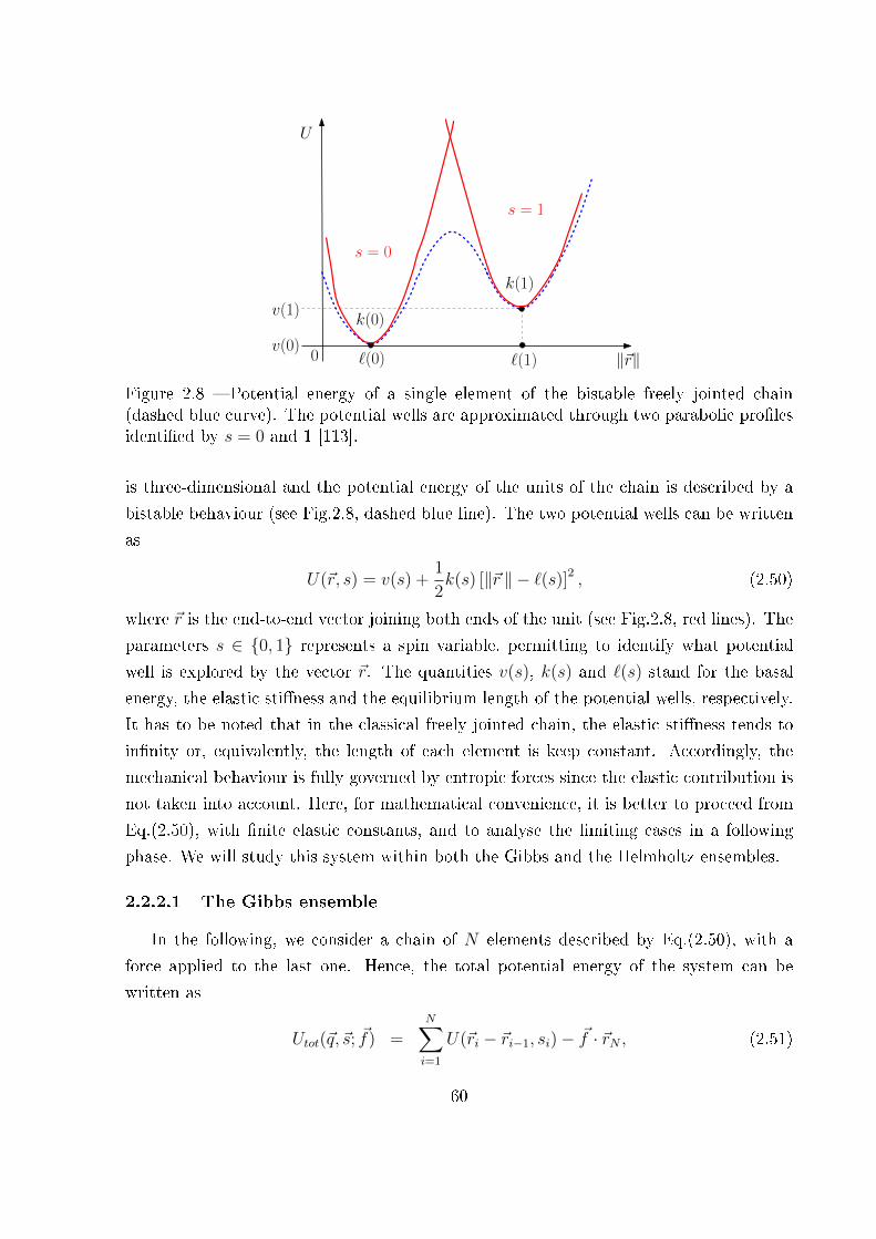
ℓ(0) ℓ(1) ‖~r‖0
v(1)k(0)
k(1)
U
v(0)
s = 0
s = 1
Figure 2.8 � Potential energy of a single element of the bistable freely jointed chain(dashed blue curve). The potential wells are approximated through two parabolic pro�lesidenti�ed by s = 0 and 1 [113].
is three-dimensional and the potential energy of the units of the chain is described by a
bistable behaviour (see Fig.2.8, dashed blue line). The two potential wells can be written
as
U(~r, s) = v(s) +1
2k(s) [‖~r ‖ − `(s)]2 , (2.50)
where ~r is the end-to-end vector joining both ends of the unit (see Fig.2.8, red lines). The
parameters s ∈ {0, 1} represents a spin variable, permitting to identify what potential
well is explored by the vector ~r. The quantities v(s), k(s) and `(s) stand for the basal
energy, the elastic sti�ness and the equilibrium length of the potential wells, respectively.
It has to be noted that in the classical freely jointed chain, the elastic sti�ness tends to
in�nity or, equivalently, the length of each element is keep constant. Accordingly, the
mechanical behaviour is fully governed by entropic forces since the elastic contribution is
not taken into account. Here, for mathematical convenience, it is better to proceed from
Eq.(2.50), with �nite elastic constants, and to analyse the limiting cases in a following
phase. We will study this system within both the Gibbs and the Helmholtz ensembles.
2.2.2.1 The Gibbs ensemble
In the following, we consider a chain of N elements described by Eq.(2.50), with a
force applied to the last one. Hence, the total potential energy of the system can be
written as
Utot(~q, ~s; ~f) =N∑i=1
U(~ri − ~ri−1, si)− ~f · ~rN , (2.51)
60
where ~q = (~r1, ..., ~rN) is the generalised coordinates vector containing all positions ~r1, ..., ~rN ,
~s = (s1, ..., sN) is the vector of all spin variables, and ~f is the force applied to the last
element of the chain. The partition function can be therefore calculated by summing the
discrete (spin-like) variables and integrating the continuous (coordinates) ones, as follows
ZG(~f) =∑
s1∈{0,1}
...∑
sN∈{0,1}
∫<3N
e−Utot(~q,~s;
~f)kBT d~q. (2.52)
We apply the change of variables ~ξ1 = ~r1−~r0, ~ξ2 = ~r2−~r1,..., ~ξN = ~rN −~rN−1 to evaluate
the integral over the vector ~q, leading to∑N
k=1~ξk = ~rN −~r0 and d~q = d~ξ1...d~ξN . By �xing
~r0 at the origin of axes, we obtain
ZG =
∑s∈{0,1}
∫<3
exp
[−U(~ξ, s)
kBT+~f · ~ξkBT
]d~ξ
N
, (2.53)
which means, giving the power of N , that the partition function is multiplicative with
respect to the elements of the chain (as observed in Eq.(2.28)). Since the system spher-
ically symmetric, we can choose an arbitrary direction for the applied force. Thus, to
further simplify Eq.(2.53), we set ~f = (0, 0, f) and we change the variables accord-
ing to ~ξ = (ξ cosϕ sinϑ, ξ sinϕ sinϑ, ξ cosϑ). As d~ξ = ξ2 sinϑdξdϕdϑ, ‖~ξ‖ = ξ and~f · ~ξ = fξ cosϑ, we get the following simpler form of the partition function
ZG = c
∑s∈{0,1}
e− v(s)kBT
∫ ∞0
exp
[− k(s)
2kBT[ξ − `(s)]2
] sinh(
fξkBT
)fξkBT
ξ2dξ
N
, (2.54)
where c stands represents a non in�uential multiplicative constant. As already noted in
the case of the one-dimensional model within the Gibbs ensemble, the elements of the
chain do not interact and this point leads to a partition function which is in the form of
a power with exponent N .
The speci�c properties of the two potential wells can now be described, namely v(0) =
0, `(0) = `, k(0) = K and v(1) = ∆E, `(1) = χ`, k(1) = K, where χ is the elongation
ratio between the unfolded and folded equilibrium lengths. Then, we get
ZG = c
∫ ∞
0
e− K
2kBT[ξ−`]2
sinh(
fξkBT
)fξkBT
ξ2dξ
+φ
∫ ∞0
e− K
2kBT[ξ−χ`]2
sinh(
fξkBT
)fξkBT
ξ2dξ
N
, (2.55)
61

< s >,0 1 2 3
fℓ
kBT
0
5
10
15
20
25
30
<r>Nℓ
Figure 2.9 � Average normalised extension (red line) and normalised spin variable (blueline) versus the dimensionless force for the bistable freely jointed chain under Gibbs con-ditions. We adopted the parameters ∆E = 30kBT and χ = 3 (at T = 300K). The curvesare independent of N within the Gibbs ensemble [113].
where φ = exp(− ∆EkBT
). To evaluate the limit for K approaching in�nity, the latter
form of the partition function can be used. This allows to properly de�ne the bistable
freely jointed chain. For this purpose, we can use the Dirac delta function property√απe−α(x−x0)2 →
α→∞δ(x− x0), eventually yielding
ZG = c
{sinh y
y+ χφ
sinh(χy)
y
}N, (2.56)
where we introduced the dimensionless force y = `fkBT
. If the system under consideration
is not bistable, the second term in Eq.(2.56) vanishes, and we obtain
ZG = c
{sinh y
y
}N, (2.57)
which is the classical partition function of the freely jointed chain model [120, 122, 124].
The cases with �nite values of the elastic constant will be considered in the next Chap-
ter. The following standard relation permits to �nd the force-extension response for the
bistable freely jointed 〈r〉 = kBT∂ logZG∂f
, producing the important result
〈r〉 = N`L(y) + χ2φL(χy) sinh(χy)
sinh y
1 + χφ sinh(χy)sinh y
, (2.58)
62
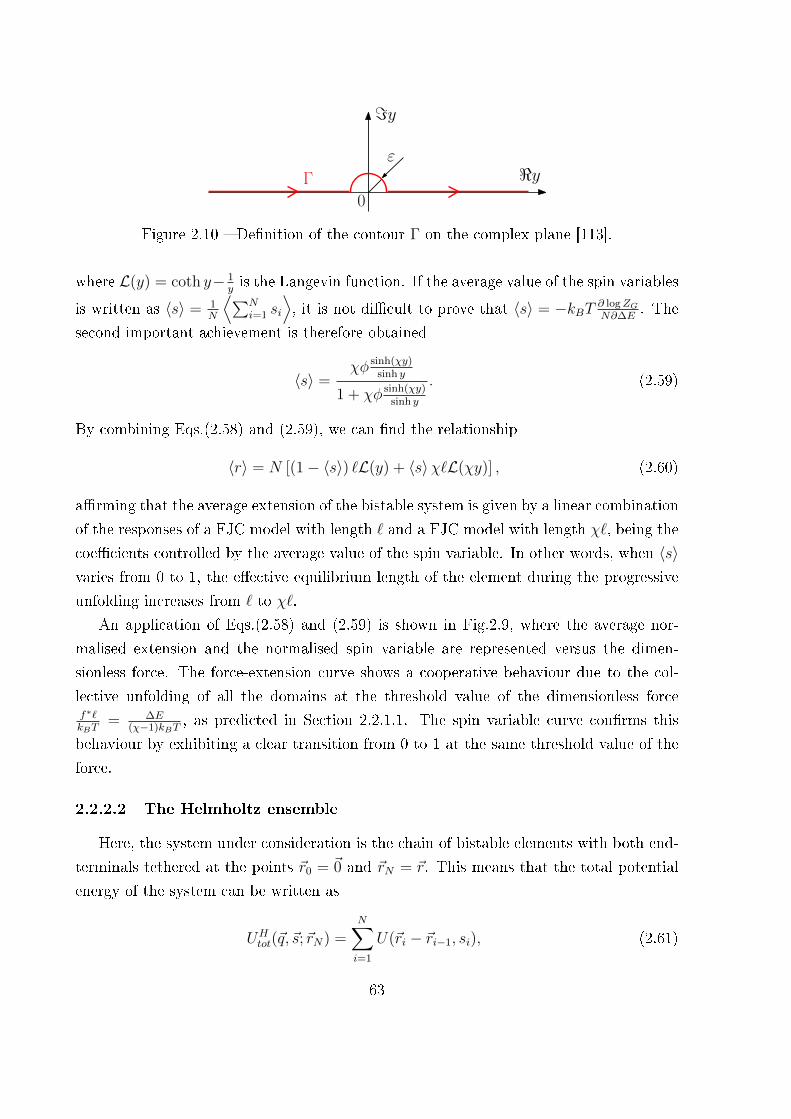
ε
ℑy
ℜyΓ
0
Figure 2.10 � De�nition of the contour Γ on the complex plane [113].
where L(y) = coth y− 1yis the Langevin function. If the average value of the spin variables
is written as 〈s〉 = 1N
⟨∑Ni=1 si
⟩, it is not di�cult to prove that 〈s〉 = −kBT ∂ logZG
N∂∆E. The
second important achievement is therefore obtained
〈s〉 =χφ sinh(χy)
sinh y
1 + χφ sinh(χy)sinh y
. (2.59)
By combining Eqs.(2.58) and (2.59), we can �nd the relationship
〈r〉 = N [(1− 〈s〉) `L(y) + 〈s〉χ`L(χy)] , (2.60)
a�rming that the average extension of the bistable system is given by a linear combination
of the responses of a FJC model with length ` and a FJC model with length χ`, being the
coe�cients controlled by the average value of the spin variable. In other words, when 〈s〉varies from 0 to 1, the e�ective equilibrium length of the element during the progressive
unfolding increases from ` to χ`.
An application of Eqs.(2.58) and (2.59) is shown in Fig.2.9, where the average nor-
malised extension and the normalised spin variable are represented versus the dimen-
sionless force. The force-extension curve shows a cooperative behaviour due to the col-
lective unfolding of all the domains at the threshold value of the dimensionless forcef∗`kBT
= ∆E(χ−1)kBT
, as predicted in Section 2.2.1.1. The spin variable curve con�rms this
behaviour by exhibiting a clear transition from 0 to 1 at the same threshold value of the
force.
2.2.2.2 The Helmholtz ensemble
Here, the system under consideration is the chain of bistable elements with both end-
terminals tethered at the points ~r0 = ~0 and ~rN = ~r. This means that the total potential
energy of the system can be written as
UHtot(~q, ~s;~rN) =
N∑i=1
U(~ri − ~ri−1, si), (2.61)
63

where ~rN = ~r is the �xed extremity of the chain, ~q = (~r1, ..., ~rN−1) is the generalised
coordinates vector containing all positions ~r1, ..., ~rN−1, and ~s = (s1, ..., sN) is the vector
of all spin variables. The potential energy U(~r, s) of a single unit in Eq.(2.61) is given in
Eq.(2.50). The partition function of this system can be written as
ZH(~rN) =∑
s1∈{0,1}
...∑
sN∈{0,1}
∫<3(N−1)
e−U
Htot(~q,~s;~rN )
kBT d~q. (2.62)
The comparison of Eqs.(2.52) and (2.62) allows to deduce the relation between the two
partition functions ZG and ZH through a three-dimensional bilateral Laplace transform,
as follows
ZG(~f) =
∫<3
ZH(~r) exp
(~r · ~fkBT
)d~r. (2.63)
Moreover, since the problem is spherically symmetric, we easily get the following relation-
ship
ZH(r) = c
∫ +∞
−∞ZG(iη)
η
rsin
(ηr
kBT
)dη, (2.64)
and by substituting Eq.(2.56), we get the important integral expression
ZH(r) = c
∫ +∞
−∞
{sin y
y+ χφ
sin(χy)
y
}Ny
rsin(ry`
)dy. (2.65)
If the studied system is not bistable, the partition function can be formulated as
ZH(r) = c
∫ +∞
−∞
{sin y
y
}Ny
rsin(ry`
)dy, (2.66)
a result which has been largely studied by Rayleigh [160], Polya [161], Treloar [162], and
Wang and Guth [163] to analyse the behaviour of chains and chains networks.
Here, in order to study the behaviour of the chain in the Helmholtz ensemble, we
elaborate Eq.(2.65) in closed form. The function to integrate in Eq.(2.65) is regular on
the real axis and analytical on a strip |=my| < M for an arbitraryM ∈ <. Then, insteadof integrating on the whole real axis, the path Γ shown in Fig.2.10 is used. Therefore, we
can write
ZH(r) = −ic∫
Γ
{sin y
y+ χφ
sin(χy)
y
}Ny
reiry` dy. (2.67)
By developing the power in previous expression and by using the expansion
sinn x =1
(2i)neinx
n∑t=0
(n
t
)(−1)te−2itx, (2.68)
64

ε
ℑy
ℜyΓR0
R CR
Figure 2.11 � Contour in the complex plane used to solve the integral for a > 0 [113].
we obtain
ZH(r) =c
2N iN+1r
N∑k=0
N−k∑p=0
k∑q=0
(N
k
)(N − kp
)×(k
q
)(−1)p+q(χφ)k
∫Γ
e−iΛy
yN−1dy, (2.69)
where we de�ned
Λ = k −N + 2p− χk + 2χq − r
`. (2.70)
For the following calculations, we call a the parameter Λ and m the parameter N − 1.
We evaluate the integral∫
Γeiay
ymdy over the contour Γ shown in Fig.2.10. To begin, we
suppose a ∈ < and a > 0. In this case, we observe that on the imaginary axis, we have
eiay = e−a=my, which is a decreasing to zero function for =my > 0. So, we consider the
contour in Fig.2.11 and we write∮ΓR∪CR
eiay
ymdy = 0, (2.71)
since the function is holomorphic within ΓR ∪ CR. We also have∫ΓR
eiay
ymdy +
∫CR
eiay
ymdy = 0. (2.72)
Since limR→∞∫CR
eiay
ymdy = 0 for the Jordan lemma and ΓR → Γ when R→∞, we obtain
the �rst result ∫Γ
eiay
ymdy = 0 if a > 0. (2.73)
65
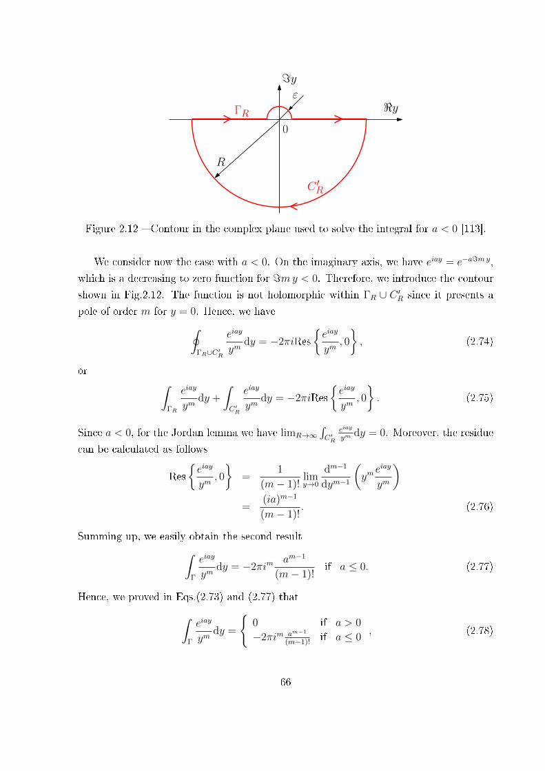
ε
ℑy
ℜyΓR
0
R
C ′R
Figure 2.12 � Contour in the complex plane used to solve the integral for a < 0 [113].
We consider now the case with a < 0. On the imaginary axis, we have eiay = e−a=my,
which is a decreasing to zero function for =my < 0. Therefore, we introduce the contour
shown in Fig.2.12. The function is not holomorphic within ΓR ∪ C ′R since it presents a
pole of order m for y = 0. Hence, we have∮ΓR∪C′R
eiay
ymdy = −2πiRes
{eiay
ym, 0
}, (2.74)
or ∫ΓR
eiay
ymdy +
∫C′R
eiay
ymdy = −2πiRes
{eiay
ym, 0
}. (2.75)
Since a < 0, for the Jordan lemma we have limR→∞∫C′R
eiay
ymdy = 0. Moreover, the residue
can be calculated as follows
Res{eiay
ym, 0
}=
1
(m− 1)!limy→0
dm−1
dym−1
(ym
eiay
ym
)=
(ia)m−1
(m− 1)!. (2.76)
Summing up, we easily obtain the second result∫Γ
eiay
ymdy = −2πim
am−1
(m− 1)!if a ≤ 0. (2.77)
Hence, we proved in Eqs.(2.73) and (2.77) that∫Γ
eiay
ymdy =
{0 if a > 0
−2πim am−1
(m−1)!if a ≤ 0
, (2.78)
66
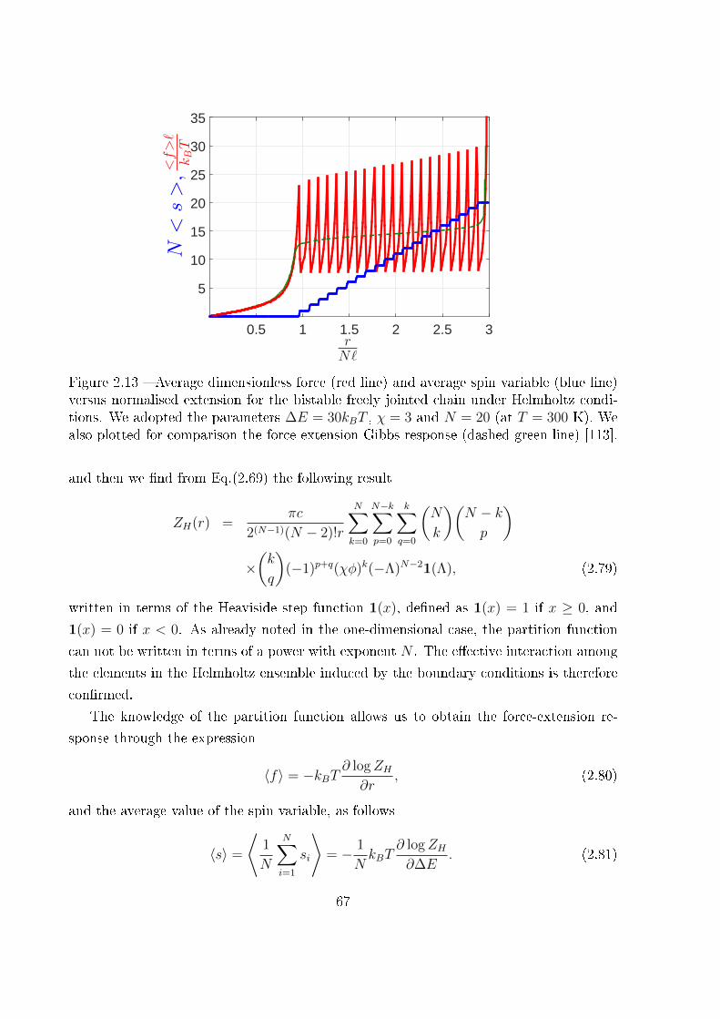
rNℓ
0.5 1 1.5 2 2.5 3
N<
s>,
5
10
15
20
25
30
35
<f>ℓ
kBT
Figure 2.13 � Average dimensionless force (red line) and average spin variable (blue line)versus normalised extension for the bistable freely jointed chain under Helmholtz condi-tions. We adopted the parameters ∆E = 30kBT , χ = 3 and N = 20 (at T = 300 K). Wealso plotted for comparison the force-extension Gibbs response (dashed green line) [113].
and then we �nd from Eq.(2.69) the following result
ZH(r) =πc
2(N−1)(N − 2)!r
N∑k=0
N−k∑p=0
k∑q=0
(N
k
)(N − kp
)×(k
q
)(−1)p+q(χφ)k(−Λ)N−21(Λ), (2.79)
written in terms of the Heaviside step function 1(x), de�ned as 1(x) = 1 if x ≥ 0, and
1(x) = 0 if x < 0. As already noted in the one-dimensional case, the partition function
can not be written in terms of a power with exponent N . The e�ective interaction among
the elements in the Helmholtz ensemble induced by the boundary conditions is therefore
con�rmed.
The knowledge of the partition function allows us to obtain the force-extension re-
sponse through the expression
〈f〉 = −kBT∂ logZH∂r
, (2.80)
and the average value of the spin variable, as follows
〈s〉 =
⟨1
N
N∑i=1
si
⟩= − 1
NkBT
∂ logZH∂∆E
. (2.81)
67
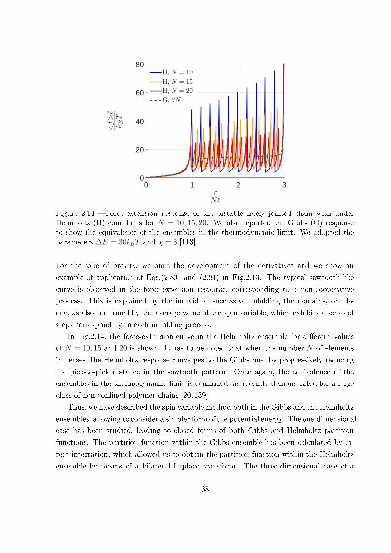
rNℓ
0 1 2 3
<f>ℓ
kBT
0
20
40
60
80H, N = 10
H, N = 15
H, N = 20
G, ∀N
Figure 2.14 � Force-extension response of the bistable freely jointed chain with underHelmholtz (H) conditions for N = 10, 15, 20. We also reported the Gibbs (G) responseto show the equivalence of the ensembles in the thermodynamic limit. We adopted theparameters ∆E = 30kBT and χ = 3 [113].
For the sake of brevity, we omit the development of the derivatives and we show an
example of application of Eqs.(2.80) and (2.81) in Fig.2.13. The typical sawtooth-like
curve is observed in the force-extension response, corresponding to a non-cooperative
process. This is explained by the individual successive unfolding the domains, one by
one, as also con�rmed by the average value of the spin variable, which exhibits a series of
steps corresponding to each unfolding process.
In Fig.2.14, the force-extension curve in the Helmholtz ensemble for di�erent values
of N = 10, 15 and 20 is shown. It has to be noted that when the number N of elements
increases, the Helmholtz response converges to the Gibbs one, by progressively reducing
the pick-to-pick distance in the sawtooth pattern. Once again, the equivalence of the
ensembles in the thermodynamic limit is con�rmed, as recently demonstrated for a large
class of non-con�ned polymer chains [20,139].
Thus, we have described the spin variable method both in the Gibbs and the Helmholtz
ensembles, allowing to consider a simpler form of the potential energy. The one-dimensional
case has been studied, leading to closed forms of both Gibbs and Helmholtz partition
functions. The partition function within the Gibbs ensemble has been calculated by di-
rect integration, which allowed us to obtain the partition function within the Helmholtz
ensemble by means of a bilateral Laplace transform. The three-dimensional case of a
68
bistable freely jointed chain has also been studied, yielding both Gibbs and Helmholtz
partition functions in closed form. These results permitted us to give an interpretation of
the cooperative (synchronised) and non-cooperative (non-synchronised) responses of the
folding/unfolding processes. Finally, important values like average value of the extension
(in the Gibbs ensemble), or the force (Helmholtz ensemble), or again the spin variable (in
both ensembles) can now be easily evaluated. The three-dimensional case with a �nite
elasticity will be studied in Chapter 3.
2.3 Full statistics of conjugated thermodynamic ensem-
bles in chains of two-state units
Typically, in the theoretical analyses conducted to study the behaviour of two-state
systems under isotensional or isometric conditions, the considered quantities correspond
to the average values of the �uctuating variables. Consequently, the average extension and
force are respectively considered in the Gibbs and the Helmholtz ensembles. However, it
is important to study the actual distributions of these �uctuating or stochastic variables,
in order to better understand the random behaviour of these systems and to draw more
re�ned comparisons with experiments. Indeed, it is important to underline that the
experimental activities may probe not only the average values of the relevant quantities
but also their actual distribution. Basically, this is achieved by a very large statistics of
the trajectories of the system under investigation, which allows for a good exploration
of the phase space and, consequently, for the determination of the pertinent probability
densities. Therefore, we propose here a methodology to determine the exact distributions
or probability densities of the pertinent quantities de�ned in both Gibbs and Helmholtz
ensembles. In particular, for the Gibbs ensemble, we determine the distribution of the
couple (xN , xN), where xN is the extension of a chain of N two-state elements (under
applied deterministic force), and, for the Helmholtz ensemble, the distribution of (f , f),
where f is the measured force (under prescribed deterministic extension).
2.3.1 Con�gurational partition functions and force-extension re-
lations in the Gibbs and the Helmholtz ensembles
We consider a very simple one-dimensional system (a toy model) composed of N
elements with mechanical bistability, connected in series to compose a chain. Each element
of the chain is represented by a symmetric potential energy function U(x) showing two
minima at x = ±` (see Fig.2.15). The variable y assumes its values in the set S = {±1}
69
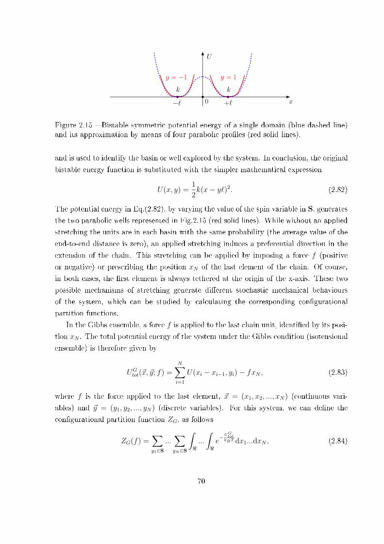
−` +`0 x
U
k k
y = −1 y = 1
Figure 2.15 � Bistable symmetric potential energy of a single domain (blue dashed line)and its approximation by means of four parabolic pro�les (red solid lines).
and is used to identify the basin or well explored by the system. In conclusion, the original
bistable energy function is substituted with the simpler mathematical expression
U(x, y) =1
2k(x− y`)2. (2.82)
The potential energy in Eq.(2.82), by varying the value of the spin variable in S, generates
the two parabolic wells represented in Fig.2.15 (red solid lines). While without an applied
stretching the units are in each basin with the same probability (the average value of the
end-to-end distance is zero), an applied stretching induces a preferential direction in the
extension of the chain. This stretching can be applied by imposing a force f (positive
or negative) or prescribing the position xN of the last element of the chain. Of course,
in both cases, the �rst element is always tethered at the origin of the x-axis. These two
possible mechanisms of stretching generate di�erent stochastic mechanical behaviours
of the system, which can be studied by calculating the corresponding con�gurational
partition functions.
In the Gibbs ensemble, a force f is applied to the last chain unit, identi�ed by its posi-
tion xN . The total potential energy of the system under the Gibbs condition (isotensional
ensemble) is therefore given by
UGtot(~x, ~y; f) =
N∑i=1
U(xi − xi−1, yi)− fxN , (2.83)
where f is the force applied to the last element, ~x = (x1, x2, ..., xN) (continuous vari-
ables) and ~y = (y1, y2, ..., yN) (discrete variables). For this system, we can de�ne the
con�gurational partition function ZG, as follows
ZG(f) =∑y1∈S
...∑yN∈S
∫<...
∫<e− U
Gtot
kBT dx1...dxN , (2.84)
70

-2 -1 0 1 2-30
-20
-10
0
10
20
30
-1 -0.5 0 0.5 1-30
-20
-10
0
10
20
30
Figure 2.16 � Average force-extension curves and average spin variables (plotted by meansof dimensionless quantities) for the Gibbs ensemble with N = 5 and k`2
kBT=10, 15, 30,
100 [3].
where the variable ~x is integrated whereas the variable ~y is summed. We can now substi-
tute Eq.(2.83) in Eq.(2.84) and we eventually obtain the result
ZG(f) =
(8πkBT
k
)N2[exp
(f 2
2kBTk
)cosh
(`f
kBT
)]N. (2.85)
The extension of the chain can be directly calculated through the expression xN =
−∂Utot/∂f and its average value is therefore 〈xN〉 = 〈−∂Utot/∂f〉. It can be simply
evaluated by means of the con�gurational partition function, as 〈xN〉 = kBT ∂/∂f(logZG).
The calculation eventually gives
〈xN〉N`
=f
k`+ tanh
(`f
kBT
). (2.86)
We can also calculate the average value of the spin variable 〈y〉 = 〈yi〉 ∀i, which is inde-
pendent of the element considered in the chain and is given by
〈y〉 = 〈yi〉 = tanh
(`f
kBT
)∀i. (2.87)
An application of Eqs.(2.86) and (2.87) can be found in Fig.2.16. The force-extension
curves have been plotted with dimensionless quantities and only one parameter de�nes the
shape of the response, namely the elastic constant taken here into consideration through
the dimensionless ratio k`2
kBT. It represents the ratio between the elastic (enthalpic) energy
and the thermal energy. In these force-extension curves, we note a force plateau (for
f = 0) corresponding to the synchronised switching (sometimes called cooperative) of the
N units. This behaviour is con�rmed by the average spin variable (which is independent
71
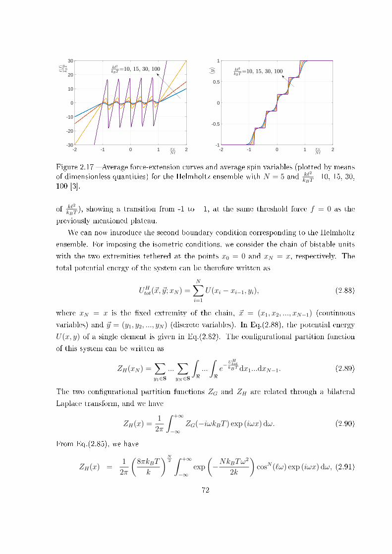
-2 -1 0 1 2-30
-20
-10
0
10
20
30
-2 -1 0 1 2-1
-0.5
0
0.5
1
Figure 2.17 � Average force-extension curves and average spin variables (plotted by meansof dimensionless quantities) for the Helmholtz ensemble with N = 5 and k`2
kBT=10, 15, 30,
100 [3].
of k`2
kBT), showing a transition from -1 to +1, at the same threshold force f = 0 as the
previously mentioned plateau.
We can now introduce the second boundary condition corresponding to the Helmholtz
ensemble. For imposing the isometric conditions, we consider the chain of bistable units
with the two extremities tethered at the points x0 = 0 and xN = x, respectively. The
total potential energy of the system can be therefore written as
UHtot(~x, ~y;xN) =
N∑i=1
U(xi − xi−1, yi), (2.88)
where xN = x is the �xed extremity of the chain, ~x = (x1, x2, ..., xN−1) (continuous
variables) and ~y = (y1, y2, ..., yN) (discrete variables). In Eq.(2.88), the potential energy
U(x, y) of a single element is given in Eq.(2.82). The con�gurational partition function
of this system can be written as
ZH(xN) =∑y1∈S
...∑yN∈S
∫<...
∫<e− U
Htot
kBT dx1...dxN−1. (2.89)
The two con�gurational partition functions ZG and ZH are related through a bilateral
Laplace transform, and we have
ZH(x) =1
2π
∫ +∞
−∞ZG(−iωkBT ) exp (iωx) dω. (2.90)
From Eq.(2.85), we have
ZH(x) =1
2π
(8πkBT
k
)N2∫ +∞
−∞exp
(−NkBTω
2
2k
)cosN(`ω) exp (iωx) dω, (2.91)
72
and the calculation of the integral delivers
ZH(x) =1
2π
(2πkBT
k
)N2
N∑t=0
(N
t
)√2kπ
NkBTexp
[− k
2NkBT(x+ 2t`−N`)2
]. (2.92)
Now, we can evaluate the average value of the overall force 〈f〉 = −kBT∂/∂x(logZH)
applied to the system and the average value of the spin variables 〈y〉 =⟨
1N
∑Ni=1 yi
⟩describing the transitions, as follows
〈f〉 =
∑Nt=0
(Nt
)kN
(x+ 2t`−N`) exp[− k
2NkBT(x+ 2t`−N`)2
]∑N
t=0
(Nt
)exp
[− k
2NkBT(x+ 2t`−N`)2
] , (2.93)
and
〈y〉 =
1N
∑Nt=0
(Nt
)(N − 2t) exp
[− k
2NkBT(x+ 2t`−N`)2
]∑N
t=0
(Nt
)exp
[− k
2NkBT(x+ 2t`−N`)2
] . (2.94)
An example of application of Eqs.(2.93) and (2.94) can be found in Fig.2.17, where
we show the force-extension response and the average spin variable for the Helmholtz
ensemble. As before, the force-extension curves have been plotted with dimensionless
quantities and only one parameter de�nes the shape of the response, namely the elastic
constant taken here into consideration through the dimensionless ratio k`2
kBT. We observe
that the force-extension curve is composed of a number of peaks corresponding to the
non-synchronised (sequential) switching of the units. Sometimes, this behaviour is called
non-cooperative in order to underline the independent transitions of the units. This is
con�rmed by the step-wise curve representing the average spin variable versus the chain
extension. Each step corresponds to the switching of a unit induced by the increasing
extension of the chain.
2.3.2 Complete probability densities in the Gibbs and the Helmholtz
ensembles
We are interested here not only in the average value of the �uctuating quantities,
but also in the complete probability densities. The knowledge of these more re�ned
quantities allows for the determination of expected values of higher order such as variances,
covariances and so on, very important to fully characterise the statistical properties of
these systems. We de�ne here the probability density of the system in the whole phase
space within both the Gibbs and the Helmholtz statistical ensembles. These results will
73

be used in the following Sections to �nd the probability density of the speci�c quantities
characterising the Gibbs and Helmholtz statistical ensembles.
Concerning the Gibbs ensemble, we can de�ne the total energy of the system as
EG(~v, ~x, ~y; f) =N∑i=1
1
2mv2
i + UGtot(~x, ~y; f)
=N∑i=1
1
2mv2
i +N∑i=1
U(xi − xi−1, yi)− fxN , (2.95)
where vi is the velocity of the i-th particle of the chain and ~v, ~x, ~y ∈ <N while f ∈ <.The complete probability density in the phase space is therefore given by the canonical
distribution
ρG(~v, ~x, ~y; f) =exp
[− 1kBT
EG(~v, ~x, ~y; f)]
(√2πkBTm
)NZG(f)
, (2.96)
where the term(√
2πkBTm
)Nhas been added to normalise the kinetic part of the Boltz-
mann factor and the con�gurational partition function ZG(f) is given in Eq.(2.85). Of
course, we have that∑~y∈{−1,+1}N
∫~x∈<N
∫~v∈<N
ρG(~v, ~x, ~y; f)d~vd~x = 1∀f ∈ <. (2.97)
Similarly, for the Helmholtz ensemble we can de�ne the total energy as
EH(~v, ~x, ~y;xN) =N−1∑i=1
1
2mv2
i + UHtot(~x, ~y;xN) =
N−1∑i=1
1
2mv2
i +N∑i=1
U(xi − xi−1, yi), (2.98)
where, as before, vi is the velocity of the i-th particle of the chain and ~v, ~x ∈ <N−1, ~y ∈ <Nwhile xN ∈ <. In this case, the complete probability density in the phase space is given
by the canonical distribution
ρH(~v, ~x, ~y;xN) =exp
[− 1kBT
EH(~v, ~x, ~y;xN)]
(√2πkBTm
)N−1
ZH(xN)
, (2.99)
where the term(√
2πkBTm
)N−1
has been added to normalise the kinetic part of the Boltz-
mann factor and the con�gurational partition function ZH(xN) is given in Eq.(2.92). Of
74
course, we have that∑~y∈{−1,+1}N
∫~x∈<N−1
∫~v∈<N−1
ρH(~v, ~x, ~y;xN)d~vd~x = 1 ∀ xN ∈ <. (2.100)
The two probability densities here described will be used to obtain a full statistics repre-
senting the behaviour of the two isotensional and isometric ensembles.
2.3.3 Probability density of the couple (xN , xN) versus f within
the Gibbs ensemble
Since the force f is imposed within the Gibbs ensemble, we can measure the extension
of the chain. The latter is a random variable that must be de�ned by its probability
density, in order to have a complete description of its behaviour. Here, for the sake of
completeness, we elaborate the probability density %G(xN , xN ; f) for the couple (xN , xN),
where we de�ned xN = vN . In this case, to obtain the probability density, we have to
sum or to integrate all the variables di�erent from vN and xN in the complete density
probability de�ned in Eq.(2.96). It means that we can write
%G(xN , xN ; f) =∑
~y∈{−1,+1}N
∫x1
...
∫xN−1
∫v1
...
∫vN−1
ρH(~v, ~x, ~y;xN)
×dvN−1...dv1dxN−1...dx1. (2.101)
Now, it is not di�cult to recognise that the integral over the positions x1,...,xN−1 im-
mediately leads to the con�gurational partition function of the Helmholtz ensemble and
the integral over the velocities v1,...,vN−1 can be directly calculated with the classical
Gaussian integral. Eventually, we obtain
%G(xN , xN ; f) =
√m
2πkBTexp
(1
2mx2
N
) exp(fxNkBT
)ZH(xN)
ZG(f). (2.102)
This is the most important result of this Section, which represents the probability density
of the couple (xN , xN) for any value of the applied force f within the Gibbs ensemble.
We remark that this probability density can be factorised in two terms representing the
density of xN and the density of xN . The �rst factor simply corresponds to the Maxwell
distribution for the one-dimensional velocity
%G(xN) =
√m
2πkBTexp
(1
2mx2
N
). (2.103)
75
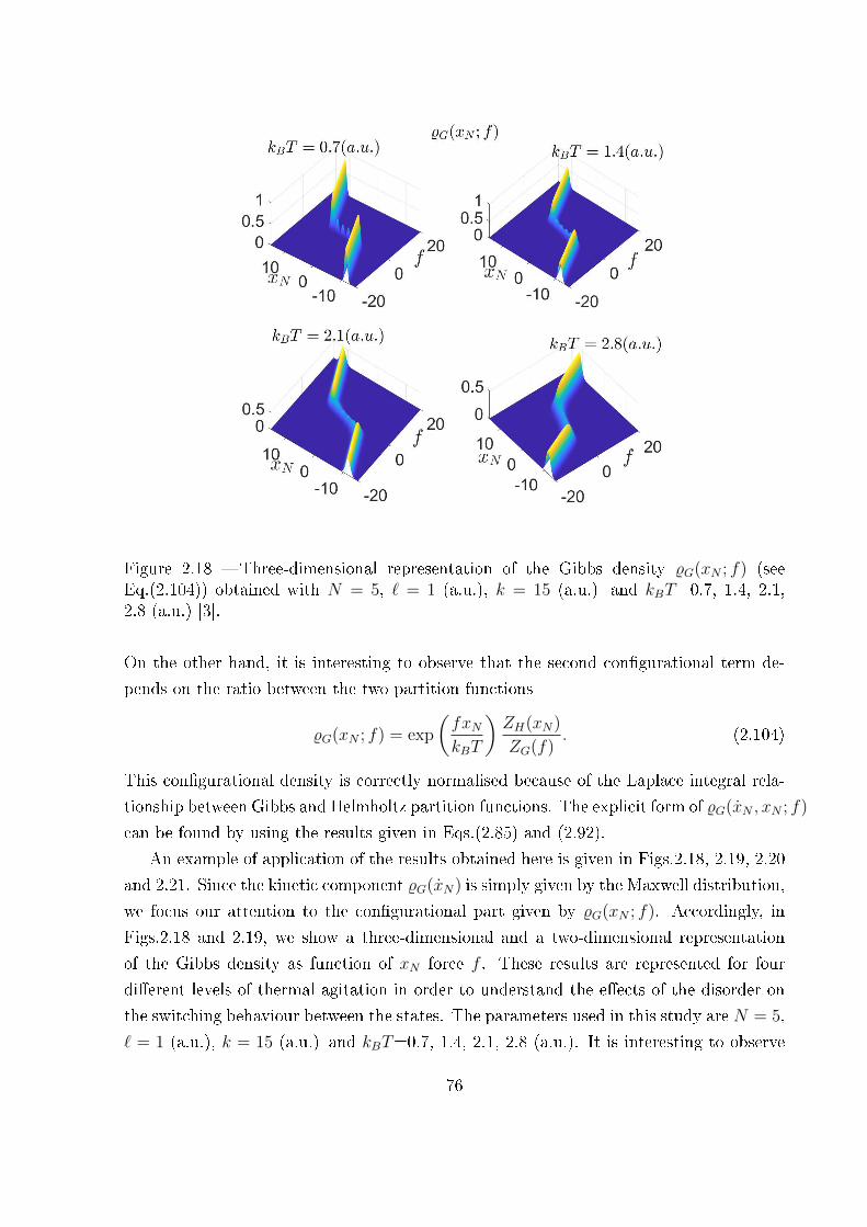
Figure 2.18 � Three-dimensional representation of the Gibbs density %G(xN ; f) (seeEq.(2.104)) obtained with N = 5, ` = 1 (a.u.), k = 15 (a.u.) and kBT=0.7, 1.4, 2.1,2.8 (a.u.) [3].
On the other hand, it is interesting to observe that the second con�gurational term de-
pends on the ratio between the two partition functions
%G(xN ; f) = exp
(fxNkBT
)ZH(xN)
ZG(f). (2.104)
This con�gurational density is correctly normalised because of the Laplace integral rela-
tionship between Gibbs and Helmholtz partition functions. The explicit form of %G(xN , xN ; f)
can be found by using the results given in Eqs.(2.85) and (2.92).
An example of application of the results obtained here is given in Figs.2.18, 2.19, 2.20
and 2.21. Since the kinetic component %G(xN) is simply given by the Maxwell distribution,
we focus our attention to the con�gurational part given by %G(xN ; f). Accordingly, in
Figs.2.18 and 2.19, we show a three-dimensional and a two-dimensional representation
of the Gibbs density as function of xN force f . These results are represented for four
di�erent levels of thermal agitation in order to understand the e�ects of the disorder on
the switching behaviour between the states. The parameters used in this study are N = 5,
` = 1 (a.u.), k = 15 (a.u.) and kBT=0.7, 1.4, 2.1, 2.8 (a.u.). It is interesting to observe
76
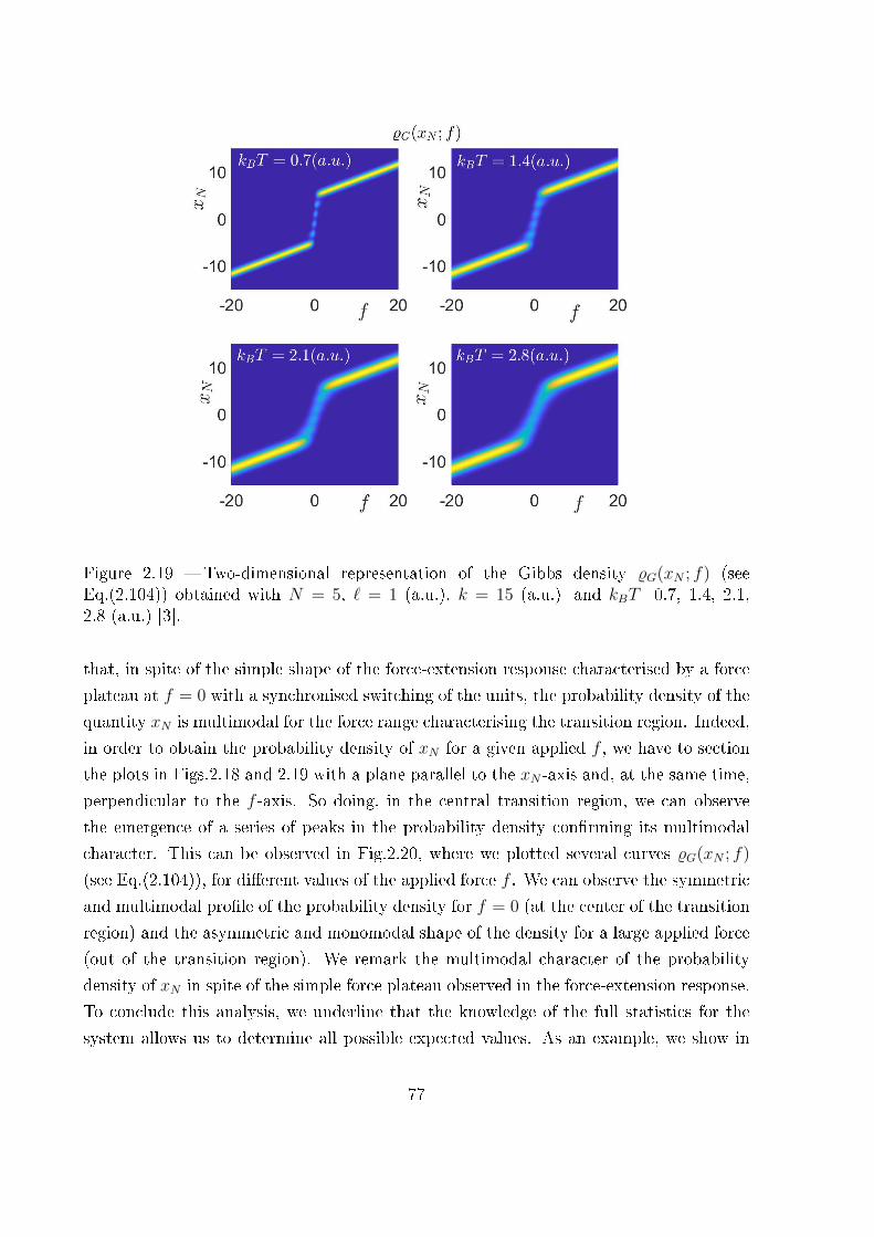
Figure 2.19 � Two-dimensional representation of the Gibbs density %G(xN ; f) (seeEq.(2.104)) obtained with N = 5, ` = 1 (a.u.), k = 15 (a.u.) and kBT=0.7, 1.4, 2.1,2.8 (a.u.) [3].
that, in spite of the simple shape of the force-extension response characterised by a force
plateau at f = 0 with a synchronised switching of the units, the probability density of the
quantity xN is multimodal for the force range characterising the transition region. Indeed,
in order to obtain the probability density of xN for a given applied f , we have to section
the plots in Figs.2.18 and 2.19 with a plane parallel to the xN -axis and, at the same time,
perpendicular to the f -axis. So doing, in the central transition region, we can observe
the emergence of a series of peaks in the probability density con�rming its multimodal
character. This can be observed in Fig.2.20, where we plotted several curves %G(xN ; f)
(see Eq.(2.104)), for di�erent values of the applied force f . We can observe the symmetric
and multimodal pro�le of the probability density for f = 0 (at the center of the transition
region) and the asymmetric and monomodal shape of the density for a large applied force
(out of the transition region). We remark the multimodal character of the probability
density of xN in spite of the simple force plateau observed in the force-extension response.
To conclude this analysis, we underline that the knowledge of the full statistics for the
system allows us to determine all possible expected values. As an example, we show in
77

-10 -5 0 5 100
0.1
0.2
0.3
0.4
0.5
0.6
0.7
Figure 2.20 � Examples of multimodal curves obtained through the Gibbs density%G(xN ; f) (see Eq.(2.104)). On the left panel, the two-dimensional representation of theGibbs density is shown with the cuts corresponding to the curves plotted on the rightpanel. We used N = 5, ` = 1 (a.u.), k = 15 (a.u.), kBT=1 (a.u.) and di�erent values ofthe applied force f , as indicated in the legend [3].
-20 -10 0 10 20-1
0
1
2
3
4
5
6
Figure 2.21 � Variance of xN obtained by the Gibbs density %G(xN ; f). As before, weused N = 5, ` = 1 (a.u.), k = 15 (a.u.) and kBT=0.7, 1.4, 2.1, 2.8 (a.u.) [3].
Fig.2.21 the behaviour of the variance of the position in terms of the applied force f and
the thermal energy kBT . We note that the variance is higher in the transition region,
78

where the two states of each unit can coexist. Moreover, we observe a larger variance for
higher temperatures, as expected. Finally, we also note that the multimodal character
of the probability density is smeared out by the integration process applied to calculate
the variances. This behaviour will be shown to be dual with respect to the Helmholtz
ensemble response, which is the subject of the next Section.
2.3.4 Probability density of the couple (f , f) versus xN within the
Helmholtz ensemble
The problem of �nding the probability density for f and f when xN is imposed is
more complicated since, in this case, the variables f and f do not belong to the phase
space and, therefore, we can not integrate the super�uous variables in order to get the
searched density. To cope with this problem, we �rst introduce the standard technique
to deal with a function of random variable. We suppose to have two random variables
x and y, linked by a function y = g(x). If Fx(x) and fx(x) are distribution function and
probability density of the random variable x, we search for the same quantities Fy(y) and
fy(y) for y = g(x). We use the symbol ξ for the elements of the probability space and we
can write
Fx(x) = Pr {ξ : x(ξ) ≤ x} , (2.105)
and
fx(x) =d
dxFx(x). (2.106)
Moreover, we can state that
Fy(y) = Pr {ξ : y(ξ) ≤ y} = Pr {ξ : g(x(ξ)) ≤ y}
=
∫g(x)≤y
fx(x)dx =
∫ +∞
−∞1(y − g(x))fx(x)dx, (2.107)
where 1(z) is the Heaviside step function. Therefore, we can obtain the probability density
of y = g(x) by di�erentiation
fy(y) =d
dyFy(y)
=d
dy
∫ +∞
−∞1(y − g(x))fx(x)dx
=
∫ +∞
−∞δ(y − g(x))fx(x)dx, (2.108)
79
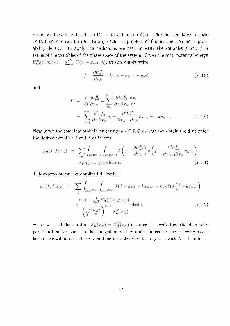
where we have introduced the Dirac delta function δ(z). This method based on the
delta functions can be used to approach the problem of �nding the Helmholtz prob-
ability density. To apply this technique, we need to write the variables f and f in
terms of the variables of the phase space of the system. Given the total potential energy
UHtot(~x, ~y;xN) =
∑Ni=1 U(xi − xi−1, yi), we can simply write
f =∂UH
tot
∂xN= k(xN − xN−1 − yN`) (2.109)
and
f =d
dt
∂UHtot
∂xN=
N−1∑i=1
∂2UHtot
∂xi∂xN
dxidt
=N−1∑i=1
∂2UHtot
∂xi∂xNvi =
∂2UHtot
∂xN−1∂xNvN−1 = −kvN−1. (2.110)
Now, given the complete probability density ρH(~v, ~x, ~y;xN), we can obtain the density for
the desired variables f and f as follows
%H(f , f ;xN) =∑~y
∫~x∈<N−1
∫~v∈<N−1
δ
(f − ∂UH
tot
∂xN
)δ
(f − ∂2UH
tot
∂xN−1∂xNvN−1
)×ρH(~v, ~x, ~y;xN)d~xd~v. (2.111)
This expression can be simpli�ed delivering
%H(f , f ;xN) =∑~y
∫~x∈<N−1
∫~v∈<N−1
δ (f − kxN + kxN−1 + kyN`) δ(f + kvN−1
)
×exp
[− 1kBT
EH(~v, ~x, ~y;xN)]
(√2πkBTm
)N−1
ZNH (xN)
d~xd~v, (2.112)
where we used the notation ZH(xN) = ZNH (xN) in order to specify that the Helmholtz
partition function corresponds to a system with N units. Indeed, in the following calcu-
lations, we will also need the same function calculated for a system with N − 1 units.
80

The elaboration of %H(f , f ;xN) can be continued as follows
%H(f , f ;xN) =1(√
2πkBTm
)N−1
ZNH (xN)
×∑~y
∫~x∈<N−1
∫~v∈<N−1
δ (f − kxN + kxN−1 + kyN`) δ(f + kvN−1
)
× exp
(− m
2kBT
N−1∑i=1
v2i
)exp
[− k
2kBT
N∑i=1
(xi − xi−1 − yi`)2
]d~xd~v
=1(√
2πkBTm
)N−1
ZNH (xN)
∫<N−2
exp
(− m
2kBT
N−2∑i=1
v2i
)dv1...dvN−2
×∫<
1
kδ
(1
kf + vN−1
)exp
(− m
2kBTv2N−1
)dvN−1
×∑~y
∫~x∈<N−1
1
kδ
(f
k− xN + xN−1 + yN`
)exp
[− k
2kBT
×N−2∑i=1
(xi − xi−1 − yi`)2
]exp
[− k
2kBT(xN−1 − xN−2 − yN−1`)
2
]× exp
[− k
2kBT(xN − xN−1 − yN`)2
]d~x, (2.113)
where we used the property δ(ax) = 1|a|δ(x). We remember now that
∫ +∞−∞ exp(−αx2) =√
παfor α > 0, we perform the integrals of the delta functions over vN−1 and xN−1, and
we get
%H(f , f ;xN) =1√
2πkBTm
ZNH (xN)
1
kexp
(− m
2k2kBTf 2
)exp
(− 1
2kkBTf 2
)
×∑~y
∫~x∈<N−2
1
kexp
[− k
2kBT
N−2∑i=1
(xi − xi−1 − yi`)2
]
× exp
[− k
2kBT(xN −
1
kf − yN`− xN−2 − yN−1`)
2
]×dx1...dxN−2. (2.114)
81

We can now recall the explicit de�nition of ZNH (xN) (see Eq.(2.89)), and we also introduce
the exact expression for ZN−1H (xN−1)
ZNH (xN) =
∑y1∈S
...∑yN∈S
∫<...
∫<
exp
[− k
2kBT
N∑i=1
(xi − xi−1 − yi`)2
]×dx1...dxN−1, (2.115)
ZN−1H (xN−1) =
∑y1∈S
...∑
yN−1∈S
∫<...
∫<
exp
[− k
2kBT
N−1∑i=1
(xi − xi−1 − yi`)2
]×dx1...dxN−2. (2.116)
So, in Eq.(2.114), we can identify the partition function ZN−1H (xN−1) calculated for xN−1 =
xN − 1kf − yN`, by obtaining
%H(f , f ;xN) =1
k2
√2πkBTm
exp
(− m
2k2kBTf 2
)exp
(− 1
2kkBTf 2
)
×∑
yNZN−1H
(xN − 1
kf − yN`
)ZNH (xN)
, (2.117)
or, equivalently,
%H(f , f ;xN) =1
k2
√2πkBTm
exp
(− m
2k2kBTf 2
)exp
(− 1
2kkBTf 2
)
×ZN−1H
(xN − 1
kf − `
)+ ZN−1
H
(xN − 1
kf + `
)ZNH (xN)
. (2.118)
This is the �nal result for the probability density within the Helmholtz ensemble. It
is interesting to observe that it can be written in terms of the two partition functions
ZNH (xN) and ZN−1
H (xN−1), corresponding to systems of size N and N − 1, respectively.
We can split this probability density in two independent components describing sep-
arately f and f , as follows
%H(f) =1
k√
2πkBTm
exp
(− m
2k2kBTf 2
), (2.119)
%H(f ;xN) =1
kexp
(− 1
2kkBTf 2
)ZN−1H
(xN − 1
kf − `
)+ ZN−1
H
(xN − 1
kf + `
)ZNH (xN)
,(2.120)
and it is not di�cult to prove the normalisation of the two results.
82
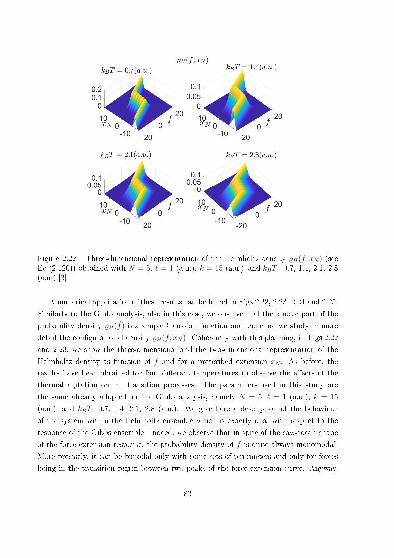
Figure 2.22 � Three-dimensional representation of the Helmholtz density %H(f ;xN) (seeEq.(2.120)) obtained with N = 5, ` = 1 (a.u.), k = 15 (a.u.) and kBT=0.7, 1.4, 2.1, 2.8(a.u.) [3].
A numerical application of these results can be found in Figs.2.22, 2.23, 2.24 and 2.25.
Similarly to the Gibbs analysis, also in this case, we observe that the kinetic part of the
probability density %H(f) is a simple Gaussian function and therefore we study in more
detail the con�gurational density %H(f ;xN). Coherently with this planning, in Figs.2.22
and 2.23, we show the three-dimensional and the two-dimensional representation of the
Helmholtz density as function of f and for a prescribed extension xN . As before, the
results have been obtained for four di�erent temperatures to observe the e�ects of the
thermal agitation on the transition processes. The parameters used in this study are
the same already adopted for the Gibbs analysis, namely N = 5, ` = 1 (a.u.), k = 15
(a.u.) and kBT=0.7, 1.4, 2.1, 2.8 (a.u.). We give here a description of the behaviour
of the system within the Helmholtz ensemble which is exactly dual with respect to the
response of the Gibbs ensemble. Indeed, we observe that in spite of the saw-tooth shape
of the force-extension response, the probability density of f is quite always monomodal.
More precisely, it can be bimodal only with some sets of parameters and only for forces
being in the transition region between two peaks of the force-extension curve. Anyway,
83
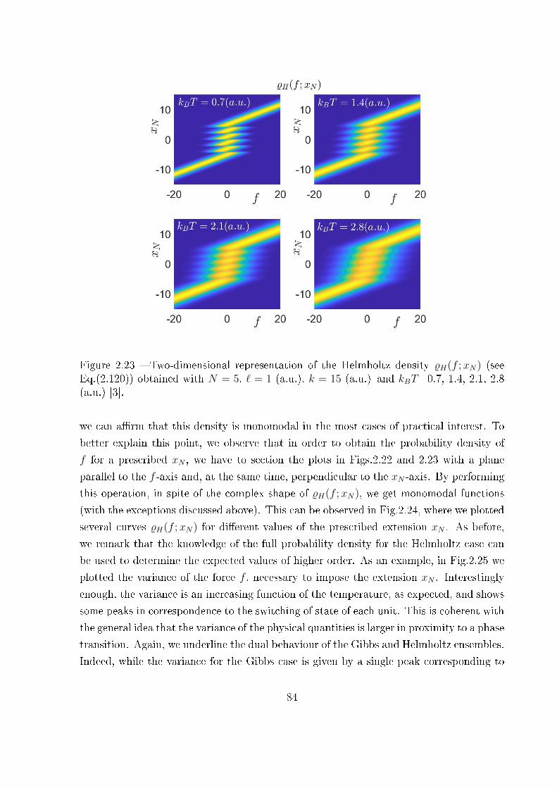
Figure 2.23 � Two-dimensional representation of the Helmholtz density %H(f ;xN) (seeEq.(2.120)) obtained with N = 5, ` = 1 (a.u.), k = 15 (a.u.) and kBT=0.7, 1.4, 2.1, 2.8(a.u.) [3].
we can a�rm that this density is monomodal in the most cases of practical interest. To
better explain this point, we observe that in order to obtain the probability density of
f for a prescribed xN , we have to section the plots in Figs.2.22 and 2.23 with a plane
parallel to the f -axis and, at the same time, perpendicular to the xN -axis. By performing
this operation, in spite of the complex shape of %H(f ;xN), we get monomodal functions
(with the exceptions discussed above). This can be observed in Fig.2.24, where we plotted
several curves %H(f ;xN) for di�erent values of the prescribed extension xN . As before,
we remark that the knowledge of the full probability density for the Helmholtz case can
be used to determine the expected values of higher order. As an example, in Fig.2.25 we
plotted the variance of the force f , necessary to impose the extension xN . Interestingly
enough, the variance is an increasing function of the temperature, as expected, and shows
some peaks in correspondence to the switching of state of each unit. This is coherent with
the general idea that the variance of the physical quantities is larger in proximity to a phase
transition. Again, we underline the dual behaviour of the Gibbs and Helmholtz ensembles.
Indeed, while the variance for the Gibbs case is given by a single peak corresponding to
84
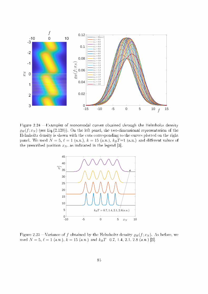
-15 -10 -5 0 5 10 150
0.02
0.04
0.06
0.08
0.1
0.12
Figure 2.24 � Examples of monomodal curves obtained through the Helmholtz density%H(f ;xN) (see Eq.(2.120)). On the left panel, the two-dimensional representation of theHelmholtz density is shown with the cuts corresponding to the curves plotted on the rightpanel. We used N = 5, ` = 1 (a.u.), k = 15 (a.u.), kBT=1 (a.u.) and di�erent values ofthe prescribed position xN , as indicated in the legend [3].
-10 -5 0 5 100
5
10
15
20
25
30
35
40
45
Figure 2.25 � Variance of f obtained by the Helmholtz density %H(f ;xN). As before, weused N = 5, ` = 1 (a.u.), k = 15 (a.u.) and kBT=0.7, 1.4, 2.1, 2.8 (a.u.) [3].
85

the synchronised transition of the units, for the Helmholtz ensemble, we have a peak for
each transition, underlying the sequential behaviour of this process.
2.3.5 Final comparison
The results obtained for the speci�c case of a chain of two-state elements show the
emergence of an intriguing duality between the two ensembles. For the isotensional con-
dition, the force-extension curve is monotone with a characteristic force plateau and the
density %(xN ; f) is multimodal in the transition region (near xN = 0 and f = 0). Con-
versely, for the isometric condition, the force-extension curve is composed of a series of
peaks while the density %(f ;xN) is simply monomodal. This duality is also re�ected in
the behaviour of the variances of these processes. In the Gibbs ensemble, we obtained
a monomodal variance σ2x with the symmetric peak at f = 0, whereas in the Helmholtz
ensemble we obtained a multimodal variance σ2f with a peak for each transition value
of xN . Of course, the peaks of variance must be explained through large �uctuations
characterising the switching of the units states (classically, it is typical for the phase
transitions).
86
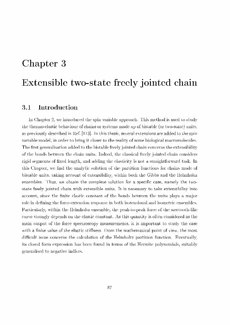
Chapter 3
Extensible two-state freely jointed chain
3.1 Introduction
In Chapter 2, we introduced the spin variable approach. This method is used to study
the thermo-elastic behaviour of chains or systems made up of bistable (or two-state) units,
as previously described in Ref. [113]. In this thesis, several extensions are added to the spin
variable model, in order to bring it closer to the reality of some biological macromolecules.
The �rst generalisation added to the bistable freely jointed chain concerns the extensibility
of the bonds between the chain units. Indeed, the classical freely jointed chain considers
rigid segments of �xed length, and adding the elasticity is not a straightforward task. In
this Chapter, we �nd the analytic solution of the partition functions for chains made of
bistable units, taking account of extensibility, within both the Gibbs and the Helmholtz
ensembles. Thus, we obtain the complete solution for a speci�c case, namely the two-
state freely jointed chain with extensible units. It is necessary to take extensibility into
account, since the �nite elastic constant of the bonds between the units plays a major
role in de�ning the force-extension response in both isotensional and isometric ensembles.
Particularly, within the Helmholtz ensemble, the peak-to-peak force of the sawtooth-like
curve strongly depends on the elastic constant. As this quantity is often considered as the
main output of the force spectroscopy measurements, it is important to study the case
with a �nite value of the elastic sti�ness. From the mathematical point of view, the most
di�cult issue concerns the calculation of the Helmholtz partition function. Eventually,
its closed form expression has been found in terms of the Hermite polynomials, suitably
generalised to negative indices.
87
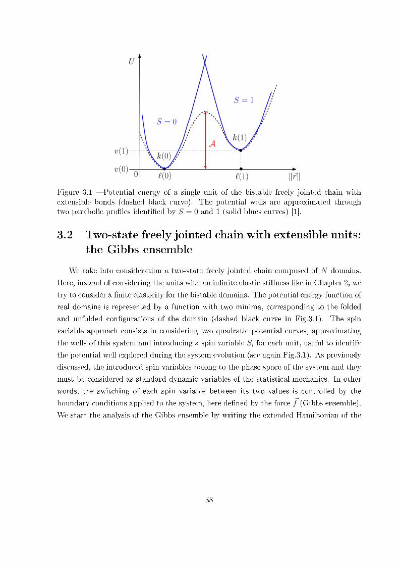
ℓ(0) ℓ(1) ‖~r‖0
v(1)k(0)
k(1)
U
v(0)
S = 0
S = 1
A
Figure 3.1 � Potential energy of a single unit of the bistable freely jointed chain withextensible bonds (dashed black curve). The potential wells are approximated throughtwo parabolic pro�les identi�ed by S = 0 and 1 (solid blues curves) [1].
3.2 Two-state freely jointed chain with extensible units:
the Gibbs ensemble
We take into consideration a two-state freely jointed chain composed of N domains.
Here, instead of considering the units with an in�nite elastic sti�ness like in Chapter 2, we
try to consider a �nite elasticity for the bistable domains. The potential energy function of
real domains is represented by a function with two minima, corresponding to the folded
and unfolded con�gurations of the domain (dashed black curve in Fig.3.1). The spin
variable approach consists in considering two quadratic potential curves, approximating
the wells of this system and introducing a spin variable Si for each unit, useful to identify
the potential well explored during the system evolution (see again Fig.3.1). As previously
discussed, the introduced spin variables belong to the phase space of the system and they
must be considered as standard dynamic variables of the statistical mechanics. In other
words, the switching of each spin variable between its two values is controlled by the
boundary conditions applied to the system, here de�ned by the force ~f (Gibbs ensemble).
We start the analysis of the Gibbs ensemble by writing the extended Hamiltonian of the
88
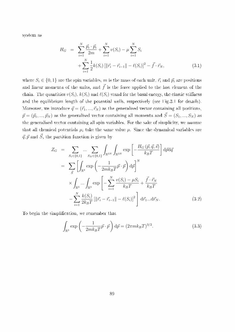
system as
HG =N∑i=1
~pi · ~pi2m
+N∑i=1
v(Si)− µN∑i=1
Si
+N∑i=1
1
2k(Si) [‖~ri − ~ri−1‖ − `(Si)]2 − ~f · ~rN , (3.1)
where Si ∈ {0, 1} are the spin variables, m is the mass of each unit, ~ri and ~pi are positions
and linear momenta of the units, and ~f is the force applied to the last element of the
chain. The quantities v(Si), k(Si) and `(Si) stand for the basal energy, the elastic sti�ness
and the equilibrium length of the potential wells, respectively (see Fig.3.1 for details).
Moreover, we introduce ~q = (~r1, ..., ~rN) as the generalised vector containing all positions,
~p = (~p1, ..., ~pN) as the generalised vector containing all momenta and ~S = (S1, ..., SN) as
the generalised vector containing all spin variables. For the sake of simplicity, we assume
that all chemical potentials µi take the same value µ. Since the dynamical variables are
~q, ~p and ~S, the partition function is given by
ZG =∑
S1∈{0,1}
...∑
SN∈{0,1}
∫R3N
∫R3N
exp
[−HG (~p, ~q, ~s)
kBT
]d~pd~q
=∑~S
[∫R3
exp
(− 1
2mkBT~p · ~p
)d~p
]N
×∫R3
...
∫R3
exp
[−
N∑i=1
v(Si)− µSikBT
+~f · ~rNkBT
−N∑i=1
k(Si)
2kBT[‖~ri − ~ri−1‖ − `(Si)]2
]d~r1...d~rN . (3.2)
To begin the simpli�cation, we remember that∫R3
exp
(− 1
2mkBT~p · ~p
)d~p = (2πmkBT )3/2. (3.3)
89

Then, we perform the change of variables ~ξ1 = ~r1−~r0, ..., ~ξN = ~rN −~rN−1. We have that
d~r1...d~rN = d~ξ1...d~ξN . By �xing ~r0 = 0 and knowing that ~rN =∑N
i=1~ξi, we obtain
ZG = (2πmkBT )3N/2∑~S
∫R3
...
∫R3
exp
[−
N∑i=1
v(Si)− µSikBT
−N∑i=1
k(Si)
2kBT
×[‖~ξi‖ − `(Si)
]2
+1
kBT~f ·
N∑i=1
~ξi
]d~ξ1...d~ξN
= (2πmkBT )3N/2∑~S
N∏i=1
∫R3
exp
[−v(Si)− µSi
kBT− k(Si)
2kBT
[‖~ξi‖ − `(Si)
]2
+~f · ~ξikBT
]d~ξi. (3.4)
It is important to remark that within the Gibbs ensemble, the elements of the chain do
not interact and this point leads to a factorised partition function, namely in the form of a
power with exponent N . We can further simplify the calculation by means of the spherical
coordinates ~ξ = (ξ cosϕ sinϑ, ξ sinϕ sinϑ, ξ cosϑ). Because of the spherical symmetry of
the problem, we set ~f = (0, 0, f). Since d~ξ = ξ2 sinϑdξdϕdϑ, ‖~ξ‖ = ξ and ~f · ~ξ = fξ cosϑ,
we get the following simpler form of the partition function
ZG = (2πmkBT )3N/2
[∑S
∫R3
exp
(−v(S)− µS
kBT− k(S)
2kBT
[‖~ξ‖ − `(S)
]2
+~f · ~ξkBT
)d~ξ
]N
= (2πmkBT )3N/2
[∑S
exp
(−v(S)− µS
kBT
)∫ +∞
0
∫ 2π
0
∫ π
0
exp
(− k(S)
2kBT
× [ξ − `(S)]2 +fξ cos θ
kBT
)ξ2 sin θdθdϕdξ
]N. (3.5)
We know that∫ 2π
0dϕ = 2π, and by de�ning η = cos θ and so dη = − sin θdθ, we obtain∫ π
0
sin θ exp
(fξ cos θ
kBT
)dθ
=
∫ 1
−1
exp
(fξη
kBT
)dη
=2kBT
fξsinh
(fξ
kBT
). (3.6)
90
The Gibbs partition function becomes
ZG = (2πmkBT )3N/2(4π)N
[∑S
exp
(−v(S)− µS
kBT
)
×∫ +∞
0
exp
(− k(S)
2kBT[ξ − `(S)]2
) sinh(
fξkBT
)fξkBT
ξ2dξ
N . (3.7)
Then, in order to specify the shape of the potential wells represented in Fig.3.1, we
consider `(0) = `, `(1) = χ`, v(0) = 0, v(1) = ∆E and k(0) = k(1) = k. In addition,
from now on, we neglect the non in�uential multiplicative constant within the partition
function. Hence, by replacing the corresponding values, we obtain
ZG(f) =
∫ +∞
0
exp
[− k
2kBT(ξ − `)2
] sinh(
fξkBT
)fξkBT
ξ2dξ + exp
(−∆E − µ
kBT
)
×∫ +∞
0
exp
[− k
2kBT(ξ − χ`)2
] sinh(
fξkBT
)fξkBT
ξ2dξ
N . (3.8)
We note that the chemical potential µ acts on the system by simply shifting the energy
jump ∆E. We can rewrite the expression of ZG under the form
ZG = {I1 + I2}N , (3.9)
with I1 =
∫ +∞0
exp[− k
2kBT(ξ − `)2
]sinh
(fξkBT
)fξkBT
ξ2dξ;
I2 = φ∫ +∞
0exp
[− k
2kBT(ξ − χ`)2
]sinh
(fξkBT
)fξkBT
ξ2dξ;
φ = exp(−∆E−µ
kBT
).
(3.10)
To begin, we calculate the �rst integral
I1 =
∫ +∞
0
exp
[− k
2kBT(ξ − `)2
] sinh(
fξkBT
)fξkBT
ξ2dξ, (3.11)
91

and then, we will determine the value of the second one by substituting ` with χ` and by
multiplying it by φ.
I1 =
{∫ +∞
0
exp
(− k
2kBTξ2
)exp
(k
kBTξ`
)exp
(− k
2kBT`2
)×kBT
2fξ
[exp
(fξ
kBT
)− exp
(− fξ
kBT
)]}dξ
=kBT
2fexp
(− k
2kBT`2
)∫ +∞
0
exp
(− k
2kBTξ2
)×[exp
(k`+ f)ξ
kBT− exp
(k`− f)ξ
kBT
]ξdξ. (3.12)
We calculate the integral A, in order to deduce I1
A =
∫ +∞
0
exp(−αx2
)exp (βx) dx
= exp
(β2
4α
)∫ +∞
0
exp
[−α(x− β
2αx
)2]
dx. (3.13)
Then, we use the change of variable y = x− β2α, from which we get
A = exp
(β2
4α
)∫ +∞
− β2α
exp(−αy2
)dy. (3.14)
We let t2 = αy2, which means that t =√αy and dy = 1√
αdt. We �nally obtain
A =1√α
exp
(β2
4α
)∫ +∞
− β2√α
exp(−t2)
dt. (3.15)
We know that the error function, erf(x), can be written as erf(x) = 2√π
∫ x0
exp (−t2) dt.
Thus, we obtain
A =1√α
exp
(β2
4α
) √π
2
[erf (+∞)− erf
(− β
2√α
)]. (3.16)
With the help of the following results, namely erf (+∞) = 1 and erf(−x) = −erf(x), we
get
A =1
2
√π
αexp
(β2
4α
)[1 + erf
(β
2√α
)]. (3.17)
92
Then, we try to obtain the value of the integral B =∫ +∞
0exp (−αx2) exp (βx)xdx by
deriving the integral A. Hence, we straightforwardly obtain
B =∂A
∂β
=∂
∂β
(1
2
√π
αexp
(β2
4α
)[1 + erf
(β
2√α
)])=
1
2α+
β
4α
√π
αexp
(β2
4α
)[1 + erf
(β
2√α
)]. (3.18)
We continue the calculation of the integral I1, where we let α = k2kBT
, β1 = k`+fkBT
and
β2 = k`−fkBT
, to compare Eq.(3.12) with Eq.(3.18). We get
I1 =kBT
2fexp
(− k
2kBT`2
)[1
4α
√π
α
(β1 exp
(β2
1
4α
)×[1 + erf
(β1
2√α
)]− β2 exp
(β2
2
4α
)[1 + erf
(β2
2√α
)])]=
kBT
2fexp
(− k
2kBT`2
)kBT
2k
√2πkBT
k
{(k`+ f
kBT
)× exp
((k`+ f)2
k2BT
2
kBT
2k
)[1 + erf
(k`+ f
2kBT
√2kBT
k
)]
−(k`− fkBT
)exp
((k`− f)2
k2BT
2
kBT
2k
)[1 + erf
(k`− f2kBT
√2kBT
k
)]}. (3.19)
We develop the calculation and we obtain
I1 =(kBT )2
4kf
√2πkBT
kexp
(f 2
2kkBT
){(k`+ f
kBT
)exp
(2k`f
2kkBT
)[1 + erf
(k`+ f√2kkBT
)]−(k`− fkBT
)exp
(− 2k`f
2kkBT
)[1 + erf
(k`− f√2kkBT
)]}. (3.20)
The �nal result can be written under the following simpli�ed form
I1 =kBT
4f
√2πkBT
kexp
(f 2
2kkBT
){(`+
f
k
)exp
(`f
kBT
)[1 + erf
(k`+ f√2kkBT
)]−(`− f
k
)exp
(− `f
kBT
)[1 + erf
(k`− f√2kkBT
)]}. (3.21)
The next step consists in considering extensible bonds with relatively high values of the
elastic constant k. Typical values of the elastic constants obtained from experiments as
well as ab initio calculations can be found in the literature and are perfectly compatible
93
with such approximations [164�167]. It is necessary to consider the case of relatively
high values of the elastic constant in order to approximate the erf by an exponential
function. Indeed, as the Fourier transform will be used to obtain the Helmholtz partition
function from the Gibbs partition function, terms of the Gibbs partition function have to
be integrable. In this case, we can use the asymptotic expression erf(x) ' 1 − 1√πxe−x
2,
holding for large values of x. We consider fk� `, so the argument of error function is
k`± f√2kkBT
≈ k`√2kkBT
=
√k`√
2kBT. (3.22)
Therefore, we can write
erf
( √k`√
2kBT
)' 1−
√2kBT√π√k`
exp
(− k`2
2kBT
). (3.23)
For high values of k, we can �nally consider that erf(
k`±f√2kkBT
)' 1. Hence,
I1 =kBT
4f
√2πkBT
kexp
(f 2
2kkBT
)×[2
(`+
f
k
)exp
(`f
kBT
)− 2
(`− f
k
)exp
(− `f
kBT
)]=
kBT
4f
√2πkBT
kexp
(f 2
2kkBT
)[` sinh
(`f
kBT
)+f
kcosh
(`f
kBT
)]. (3.24)
We de�ne the adimensional force y = `fkBT
, and the ratio α = kBTk`2
between thermal and
elastic energies. So, we also have
I1 = `2
√2πkBT
kexp
(f 2
2kkBT
)[kBT
f`2` sinh
(`f
kBT
)+
(kBT
f`2
)f
kcosh
(`f
kBT
)]= `2
√2πkBT
kexp
(f 2
2kkBT
)[sinh y
y+ α cosh y
]. (3.25)
The total partition function of the extensible bistable freely jointed chain is composed of
I1 and I2 with I2 = φI1 (`→ χ`). It means that y → χy and α→ αχ2 . Then, I2 becomes
I2 = φ`2χ2
√2πkBT
kexp
(f 2
2kkBT
)[sinh(χy)
χy+
α
χ2coshχy
]= φ`2
√2πkBT
kexp
(f 2
2kkBT
)[χ sinh(χy)
y+ α coshχy
]. (3.26)
94

The exponential term can be written in terms of y and α (with y = `fkBT
and α = kBTk`2
) as
exp
(f 2
2kkBT
)= exp
(k2BT
2y2
2`2kkBT
)= exp
(kBTy
2
2`2k
)= exp
(αy2
2
). (3.27)
By replacing the corresponding terms, the partition function becomes
Z(1)G (f) =
[sinh y
y+ α cosh y + φχ
sinh(χy)
y+ φα cosh(χy)
]Nexp
(Nαy2
2
). (3.28)
This is the �rst approximation that we obtained by simply neglecting the e�ect of the
error function in the exact calculation. Another level of approximation can be obtained
by developing the term into brackets to the �rst order in α. If we let{a = sinh y
y+ φχ sinh(χy)
y;
b = cosh y + φ cosh(χy);(3.29)
and we suppose that α� 1, then we can write
(a+ αb)N = aN(
1 + αb
a
)N≈ aN
(1 +Nα
b
a
)= aN +NαaN−1b. (3.30)
The second approximation for the partition function is therefore
Z(2)G (f) =
[(sinh y
y+ φχ
sinh(χy)
y
)N+Nα
(sinh y
y+ φχ
sinh(χy)
y
)N−1
× (cosh y + φ cosh(χy))
]exp
(Nαy2
2
). (3.31)
Finally, the third approximation can be obtained by completely neglecting the linear terms
in α in previous expressions
Z(3)G (f) =
(sinh y
y+ φχ
sinh(χy)
y
)Nexp
(Nαy2
2
). (3.32)
The exponential term depending on α is responsible for the elasticity of the chain. The
same result without bistability (i.e. with φ = 0), has been discussed in recent literature
[168, 169]. Moreover, the case with bistability but without extensibility of the units is
considered in Chapter 2. In this situation, the partition function simply reduces to
ZG(f) =
(sinh y
y+ φχ
sinh(χy)
y
)N. (3.33)
95

As discussed previously, the macroscopic behaviour of this system is described by the
Gibbs free energy G = −kBT logZG. The force-extension response for the bistable freely
jointed chain with extensible elements under isotensional condition can be found through
〈r〉 = −∂G∂f
= kBT∂ logZG∂f
= `∂ logZG∂y
. (3.34)
On the other hand, we can de�ne the average value of the spin variables as 〈s〉 =1N〈∑N
i=1 Si〉. We can rewrite the de�nition of the Hamiltonian within the Gibbs ensemble
HG (~q, ~p, S) =N∑i=1
~pi · ~pi2m
+N∑i=1
v(Si)− µN∑i=1
Si
+N∑i=1
1
2k(Si) [‖~ri − ~ri−1‖ − `(Si)]2 − ~f · ~rN . (3.35)
The only variable depending on ∆E is the basal energy v (Si) and its value changes
according to the spin. If the spin S takes the value 0, we have v (0) = 0 and if it takes
the value 1, we have v (1) = ∆E. This means that
N∑i=1
v (Si) = ∆EN∑i=1
Si. (3.36)
Therefore we get
HG (~q, ~p, S) =N∑i=1
~pi · ~pi2m
+ ∆EN∑i=1
Si − µN∑i=1
Si
+N∑i=1
1
2k(Si) [‖~ri − ~ri−1‖ − `(Si)]2 − ~f · ~rN . (3.37)
We can derive the Hamiltonian according to ∆E
∂HG
∂ (∆E)=
N∑i=1
Si. (3.38)
In the same way, we can write the Gibbs partition function
ZG =∑
S1∈{0,1}
...∑
SN∈{0,1}
∫~p
∫~q
exp
(− HG
kBT
)d~pd~q. (3.39)
96

We can derive ZG according to ∆E
∂ZG∂ (∆E)
=∑
S1∈{0,1}
...∑
SN∈{0,1}
∫~p
∫~q
exp
(− HG
kBT
)(− 1
kBT
) N∑i=1
Sid~pd~q. (3.40)
As 〈s〉 = 1N
⟨∑Ni=1 Si
⟩, we get
〈s〉 =
(−kBT
N
)∂ZG∂(∆E)
ZG
=
(−kBT
N
)1
ZG
∂ZG∂ (∆E)
. (3.41)
And we �nally obtain
〈s〉 =
(−kBT
N
)∂ logZG∂ (∆E)
. (3.42)
We can also write it like
N 〈s〉 =∂G∂∆E
= −∂G∂µ
. (3.43)
The explicit application of Eq.(3.34) to Eq.(3.32) yields
〈r〉 = N`
[L(y) + χ2φL(χy) sinh(χy)
sinh y
1 + χφ sinh(χy)sinh y
+ αy
], (3.44)
where L(y) = coth y − 1yis the Langevin function. On the other hand, by applying
Eq.(3.43) to Eq.(3.32), we get
〈s〉 =χφ sinhχy
sinh y
1 + χφ sinhχysinh y
, (3.45)
which does not depend on α. By combining Eqs.(3.44) and (3.45), we can �nd the
relationship
〈r〉 = N` [(1− 〈s〉)L(y) + 〈s〉χL(χy) + αy] , (3.46)
stating that the average extension of the extensible bistable system is given by a combi-
nation of the responses of two freely jointed chain models with lengths ` and χ`, and by
a linear term taking into account the elasticity of the system.
A �rst example of application of Eqs.(3.34) and (3.43) is given in Fig.3.2, where we
compare a system with extensibility described by the exact Eq.(3.9) or by the approxi-
mated Eq.(3.32) and another system without extensibility described by Eq.(3.33). First of
97
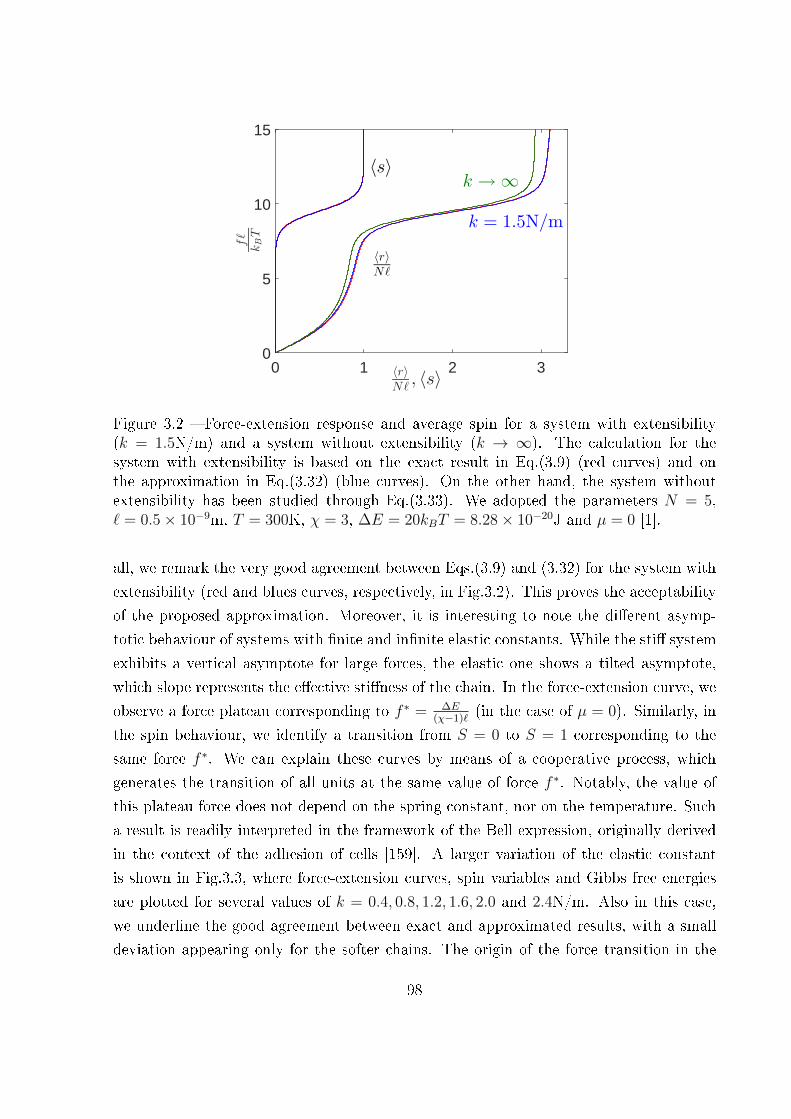
〈r〉Nℓ
, 〈s〉0 1 2 3
fℓ
kBT
0
5
10
15
〈s〉
〈r〉Nℓ
k → ∞
k = 1.5N/m
Figure 3.2 � Force-extension response and average spin for a system with extensibility(k = 1.5N/m) and a system without extensibility (k → ∞). The calculation for thesystem with extensibility is based on the exact result in Eq.(3.9) (red curves) and onthe approximation in Eq.(3.32) (blue curves). On the other hand, the system withoutextensibility has been studied through Eq.(3.33). We adopted the parameters N = 5,` = 0.5× 10⁻⁹m, T = 300K, χ = 3, ∆E = 20kBT = 8.28× 10⁻²⁰J and µ = 0 [1].
all, we remark the very good agreement between Eqs.(3.9) and (3.32) for the system with
extensibility (red and blues curves, respectively, in Fig.3.2). This proves the acceptability
of the proposed approximation. Moreover, it is interesting to note the di�erent asymp-
totic behaviour of systems with �nite and in�nite elastic constants. While the sti� system
exhibits a vertical asymptote for large forces, the elastic one shows a tilted asymptote,
which slope represents the e�ective sti�ness of the chain. In the force-extension curve, we
observe a force plateau corresponding to f ∗ = ∆E(χ−1)`
(in the case of µ = 0). Similarly, in
the spin behaviour, we identify a transition from S = 0 to S = 1 corresponding to the
same force f ∗. We can explain these curves by means of a cooperative process, which
generates the transition of all units at the same value of force f ∗. Notably, the value of
this plateau force does not depend on the spring constant, nor on the temperature. Such
a result is readily interpreted in the framework of the Bell expression, originally derived
in the context of the adhesion of cells [159]. A larger variation of the elastic constant
is shown in Fig.3.3, where force-extension curves, spin variables and Gibbs free energies
are plotted for several values of k = 0.4, 0.8, 1.2, 1.6, 2.0 and 2.4N/m. Also in this case,
we underline the good agreement between exact and approximated results, with a small
deviation appearing only for the softer chains. The origin of the force transition in the
98
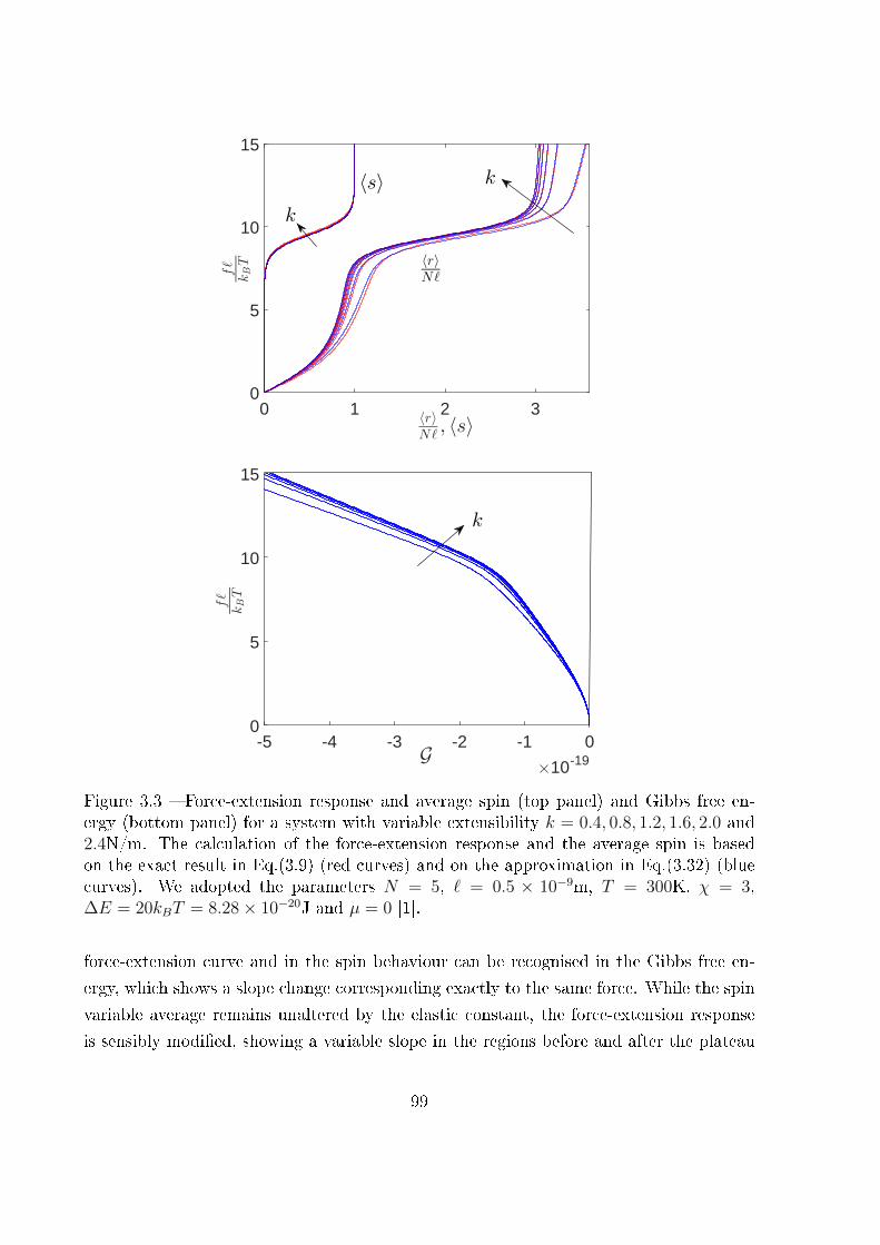
〈r〉Nℓ
, 〈s〉0 1 2 3
fℓ
kBT
0
5
10
15
k
〈s〉
〈r〉Nℓ
k
G×10-19
-5 -4 -3 -2 -1 0
fℓ
kBT
0
5
10
15
k
Figure 3.3 � Force-extension response and average spin (top panel) and Gibbs free en-ergy (bottom panel) for a system with variable extensibility k = 0.4, 0.8, 1.2, 1.6, 2.0 and2.4N/m. The calculation of the force-extension response and the average spin is basedon the exact result in Eq.(3.9) (red curves) and on the approximation in Eq.(3.32) (bluecurves). We adopted the parameters N = 5, ` = 0.5 × 10⁻⁹m, T = 300K, χ = 3,∆E = 20kBT = 8.28× 10⁻²⁰J and µ = 0 [1].
force-extension curve and in the spin behaviour can be recognised in the Gibbs free en-
ergy, which shows a slope change corresponding exactly to the same force. While the spin
variable average remains unaltered by the elastic constant, the force-extension response
is sensibly modi�ed, showing a variable slope in the regions before and after the plateau
99

corresponding to the transition. The knowledge of chain behaviour under the isotensional
or Gibbs ensemble is the starting point for the understanding of the isometric ensemble,
as discussed in the next Section.
3.3 Two-state freely jointed chain with extensible units:
the Helmholtz ensemble
We consider now the isometric condition (within the Helmholtz ensemble), where the
last unit of the chain is considered as tethered at a given point ~r of the space. In this
case, we can therefore write the Hamiltonian of the system under the form
HH =N−1∑i=1
~pi · ~pi2m
+N∑i=1
v(Si)− µN∑i=1
Si
+N∑i=1
1
2k(Si) [‖~ri − ~ri−1‖ − `(Si)]2 , (3.47)
where ~rN = ~r is �xed. Consequently, we also consider ~pN = 0. In this situation, we intro-
duce ~q = (~r1, ..., ~rN−1) as the generalised vector containing all positions, ~p = (~p1, ..., ~pN−1)
as the generalised vector containing all momenta, and ~S = (S1, ..., SN) as the generalised
vector of all spin variables. Similarly to Section 3.2, we assume that all chemical poten-
tials µi take the same value µ. The partition function can be written in terms of these
dynamic variables
ZH =∑
S1∈{0,1}
...∑
SN∈{0,1}
∫R3N−3
∫R3N−3
exp
−HH
(~p, ~q, ~S
)kBT
d~pd~q
=∑~S
[∫R3
exp
(− 1
2mkBT~p · ~p
)d~p
]N−1 ∫R3
...
∫R3
exp
[−
N∑i=1
v(Si)− µSikBT
−N∑i=1
k(Si)
2kBT[‖~ri − ~ri−1‖ − `(Si)]2
]d~r1...d~rN−1. (3.48)
It is not di�cult to realise that the calculation of this partition function is much more
complicated than the Gibbs partition function. Indeed, we can not apply a change of
variables in order to factorise the multi-dimensional integral. From the physical point of
view, this di�culty depends on the isometric condition, inducing an e�ective interaction
among the units and so �xing the sum of all vectors ~ri − ~ri−1 (for i from 1 to N). This
problem will produce a �nal result which can not be written under the form of a power
100

with exponent N . An useful technique to cope with this di�culty is the following. By
comparing Eqs.(3.2) and (3.48), we deduce that the two partition functions ZG and ZHare related through a three-dimensional bilateral Laplace transform, as
ZG(~f) =
∫R3
ZH(~r) exp
(~r · ~fkBT
)d~r, (3.49)
where, as usual, we neglect the non-in�uential multiplicative constants in the partition
function. Moreover, by considering the spherical symmetry of the problem, we easily
obtain the inverse relationship
ZH(r) =
∫ +∞
−∞ZG(iη)
η
rsin
(ηr
kBT
)dη, (3.50)
where we have introduced the analytic continuation of the function ZG(r) to the imaginary
axis, leading to ZG(iη). We can also write that
ZH(r) =
∫ +∞
−∞ZG
(ikBT
y
)y
rsin(ry`
)dy. (3.51)
By substituting Eq.(3.32) in Eq.(3.51), we get the important integral expression
ZH(r) =
∫ +∞
−∞
{sin y
y+ χφ
sin(χy)
y
}Nexp
(−Nαy2
2
)y
rsin(ry`
)dy. (3.52)
With the help of ex = cosx+ i sinx, we can also write it like
ZH(r) = −i∫ +∞
−∞
{sin y
y+ χφ
sin(χy)
y
}Nexp
(−Nαy2
2
)y
rexp
(iry
`
)dy. (3.53)
The analysis of such an integral for α = 0 (i.e. without elasticity) has been performed in
recent literature [113] and in Chapter 2. Previous investigations considered the case with
α = 0 and φ = 0, thus dealing with the classical FJC model under isometric condition
[160�163]. However, the presence of a �nite elasticity of the units, quanti�ed by the
parameter α 6= 0, completely modi�es the approach to be used to obtain a closed form
expression for ZH(r). Here, we elaborate Eq.(3.53) in order to get such a closed form
expression, useful to better explain the chain behaviour within the Helmholtz ensemble.
The function to integrate in Eqs.(3.52) or (3.53) is regular on the real axis and analytic (or
holomorphic) on a strip |Im y| < M for an arbitrary M ∈ R. Then, instead of integrating
on the whole real axis, we can use the path Γ shown in Fig.3.4. This will be useful to
elaborate the partition function integral and to write it in a form without singularities at
the origin.
101
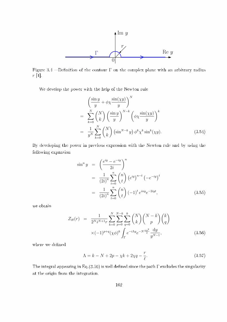
r
Im y
Re yΓ
0
Figure 3.4 � De�nition of the contour Γ on the complex plane with an arbitrary radiusr [1].
We develop the power with the help of the Newton rule(sin y
y+ φχ
sin(χy)
y
)N=
N∑k=0
(N
k
)(sin y
y
)N−k (φχ
sin(χy)
y
)k=
1
yN
N∑k=0
(N
k
)(sinN−k y
)φkχk sink(χy). (3.54)
By developing the power in previous expression with the Newton rule and by using the
following expansion
sinn y =
(eiy − e−iy
2i
)n=
1
(2i)n
n∑t=0
(n
t
)(eiy)n−t (−e−iy)t
=1
(2i)n
n∑t=0
(n
t
)(−1)t einye−2iyt, (3.55)
we obtain
ZH(r) =1
2N iN+1r
N∑k=0
N−k∑p=0
k∑q=0
(N
k
)(N − kp
)(k
q
)×(−1)p+q(χφ)k
∫Γ
e−iΛye−Nαy2
2dy
yN−1, (3.56)
where we de�ned
Λ = k −N + 2p− χk + 2χq − r
`. (3.57)
The integral appearing in Eq.(3.56) is well de�ned since the path Γ excludes the singularity
at the origin from the integration.
102
3.3.1 An integral calculation
To complete the calculation of the partition function, we have to determine the value
of
Im(a, b) =
∫Γ
eiaye−by2 dy
ym, (3.58)
where a ∈ R, b > 0, m ∈ N and the path Γ is given in Fig.3.4. To this aim, we begin to
introduce the closed paths ABCD shown in Fig.3.5. To understand the suitability of this
approach, we �rstly consider the segment CD on the paths shown in Fig.3.5. Here, we
have y = s+ iβ where s ∈ R is a variable and β ∈ R is a constant that we will determine
with the purpose of simplifying the integral calculation. Therefore, we get∫CD
eiaye−by2 dy
ym= −
∫ +R
−Reia(s+iβ)e−b(s+iβ)2 ds
(s+ iβ)m
= −e−aβebβ2
∫ +R
−Reis(a−2bβ)e−bs
2 ds
(s+ iβ)m, (3.59)
and we can let β = a/(2b) to remove the imaginary exponential from the integral. Here,
the value of R is de�ned in Fig.3.5. Hence, the result can be written as∫CD
eiaye−by2 dy
ym= e−
a2
2b eba2
4b2
∫ +R
−R
e−bs2ds
(s+ iβ)m
= −e−a2
4b
∫ +R
−R
e−bs2ds
(s+ i a2b
)m, (3.60)
and, by applying the limit for R → ∞ and the change of variable η =√bs, it assumes
the �nal form
limR→∞
∫CD
eiaye−by2 dy
ym= −e−a
2
4b
∫ +∞
−∞
e−η2dη
√b(
η√b
+ i a2b
)m= −e−a
2
4b
∫ +∞
−∞
e−η2dη
√b 1√
bm
(η + i a
2√b
)m= −bm−1
2 e−a2
4b
∫ +∞
−∞
e−η2dη(
η + i a2√b
)m . (3.61)
This expression, of course, is valid for both negative and positive values of a.
For the calculation of the integral in Eq.(3.58), we have to consider two separate cases.
If a > 0 or β > 0, the path shown in Fig.3.5.a does not contain the origin of the complex
103

r
Im y
Re y
Γ 0A B
CD β > 0
−R R
a)
r
Im y
Re y
Γ 0A B
CD
β < 0
−R R
b)
Figure 3.5 � De�nition of the contours ABCD on the complex plane for β > 0 a) andβ < 0 b) [1].
plane and therefore the function to integrate is holomorphic within the path. In this
situation, we can directly apply the Cauchy theorem stating that(∫AB
+
∫BC
+
∫CD
+
∫DA
)eiaye−by
2 dy
ym= 0. (3.62)
Now, in the limit for R→∞, it is not di�cult to prove that the integrals on the segments
BC and DA vanish and, as the integral on CD is the opposite of the one on AB, we get
the �rst result for a > 0
Im(a, b) = bm−1
2 e−a2
4b
∫ +∞
−∞
e−η2dη
(η + i a2√b)m. (3.63)
If a < 0 or β < 0, the path shown in Fig.3.5.b contains the origin of the complex plane,
which corresponds to a singular point of the function to integrate. Hence, the residue
theorem delivers(∫AB
+
∫BC
+
∫CD
+
∫DA
)eiaye−by
2 dy
ym= −2πiRes
{eiaye−by
2
ym, 0
}, (3.64)
where the residue can be easily calculated since the singular point is a pole or order m
Res
{eiaye−by
2
ym, 0
}=
1
(m− 1)!
dm−1
dym−1
(eiaye−by
2)y=0
. (3.65)
104

The derivative in Eq.(3.65) can be elaborated through the general rule
dm−1
dym−1[f(y)g(y)] =
m−1∑k=0
(m− 1
k
)dkf(y)
dykdm−1−kg(y)
dym−1−k . (3.66)
If g(y) = eiay, we simply have
dm−1−kg(y)
dym−1−k = (ia)m−1−keiay. (3.67)
On the other hand, if f(y) = e−by2, the calculation of the derivative of order k is more
involved. One method is based on the following result∫ +∞
0
e−αx2
eβxdx =1
2
√π
αeβ2
4α
[1 + erf
(β
2√α
)], (3.68)
proved in Section 3.2. Since we need∫ +∞
−∞e−αx
2
eβxdx, (3.69)
we �rst elaborate ∫ 0
−∞e−αx
2
eβxdx =
∫ 0
−∞e−αy
2
e−βy (−dy)
=
∫ +∞
0
e−αx2
e−βxdx
=1
2
√π
αeβ2
4α
[1 + erf
(− β
2√α
)], (3.70)
having used Eq.(3.68), with β → −β. Now, we sum these two equations and we get∫ +∞
−∞e−αx
2
eβxdx =1
2
√π
αeβ2
4α
[2 + erf
(β
2√α
)+ erf
(− β
2√α
)]. (3.71)
Here, we have that erf(x) = −erf(−x), and therefore∫ +∞
−∞e−αx
2
e−βxdx =
√π
αeβ2
4α . (3.72)
We can substitute β = iy and b = 14α
to obtain∫ +∞
−∞e−
x2
4b eixydx =√
4πbe−by2
, (3.73)
105
It means that the Fourier transform of e−x2
4b is proportional to e−by2. Incidentally, if b = 1
2
(i.e. 14b
= b), then we obtain the eigenvectors of the Fourier transform. We can calculate
the derivative as
dk
dyke−by
2
=1√4πb
dk
dyk
∫ +∞
−∞e−
x2
4b eixydx
=1√4πb
∫ +∞
−∞e−
x2
4b (ix)k eixydx. (3.74)
Therefore,
dkf(y)
dyk=
1√4πb
∫ +∞
−∞e−
x2
4b (ix)keixydx. (3.75)
Hence, if we consider y = 0, we get(dkf(y)
dyk
)y=0
=ik√4πb
∫ +∞
−∞xke−
x2
4b dx. (3.76)
Then, we observe that the result is di�erent from zero only for k even. Since∫ +∞−∞ e−αx
2dx =√
πα(see Eq.(3.72) with β = 0), we get∫ +∞
−∞−x2e−αx
2
dx =d
dα
√π
α
=√π
(−1
2
)α−3/2
= −1
2
√π
α3, (3.77)
or we can also write ∫ +∞
−∞x2e−αx
2
dx =1
2
√π
α3=
1
2α
√π
α. (3.78)
Again ∫ +∞
−∞−x4e−αx
2
dx =1
2
√π
(−3
2
)α−5/2
= −3
4
√π
√1
α5. (3.79)
We can sum it up like ∫ +∞
−∞x2ne−αx
2
dx =1
αn+1/2
(2n)!
(22n)n!
√π
=Γ(n+ 1
2
)αn+1/2
, (3.80)
106

and ∫ +∞
−∞x2n+1e−αx
2
dx = 0. (3.81)
In particular, by �xing α = 14b, we eventually obtain(
dke−by2
dyk
)y=0
=
{(−4b)n√
πΓ(n+ 1
2
)if k = 2n,
0 if k = 2n+ 1,(3.82)
where Γ(z) is the Euler Gamma function. By combining Eqs.(3.66), (3.67) and (3.82), we
can rewrite the residue de�ned in Eq.(3.65) as
Res
{eiaye−by
2
ym, 0
}=
m−1∑k=0
(ia)m−1−k
k!(m− 1− k)!
(−4b)k/2
2√π
Γ
(k + 1
2
)[1 + (−1)k
]. (3.83)
Therefore, the residue theorem written in the form of Eq.(3.64), and considered for R→∞, gives the �nal result for a < 0
Im(a, b) = bm−1
2 e−a2
4b
∫ +∞
−∞
e−η2dη
(η + i a2√b)m
−m−1∑k=0
2πi(ia)m−1−k
k!(m− 1− k)!
(−4b)k/2
2√π
Γ
(k + 1
2
)[1 + (−1)k
]. (3.84)
To conclude, Eq.(3.63) for a > 0 and Eq.(3.84) for a < 0 represent the integral Im(a, b)
de�ned in Eq.(3.58) in terms of a second integral, which is the subject of the following
discussion.
3.3.2 The Hermite elements with negative index
First of all, we observe that the integral
Jm(x) =
∫ +∞
−∞
e−η2dη
(η + ix)m, (3.85)
appearing in Eqs.(3.63) and (3.84) with x = a/(2√b), is simpler than Im(a, b) since it
is calculated over the real axis and there is no imaginary exponent in the function to
integrate. To approach its calculation, we recall the following integral representation of
the Hermite polynomials [170,171]
Hm(z) =2m√π
∫ +∞
−∞(iη + z)me−η
2
dη
=(2i)m√π
∫ +∞
−∞(η − iz)me−η
2
dη. (3.86)
107
If we compare Jm with the last representation of Hm, we note that Jm is formally related
to H−m, which represents an Hermite element with negative index. We underline that
the representation of the Hermite polynomials in Eq.(3.86) makes sense also for negative
values of m. However, we will see that these functions are not polynomials but they
exhibit several properties similar to those of the classical Hermite polynomials. To the
author knowledge, these functions have been �rstly introduced and studied in Ref. [172]
but no other analysis or application can be found in the literature. Anyway, by replacing
m with −m in Eq.(3.86), we de�ne
H−m(z) =1
(2i)m√π
∫ +∞
−∞
e−η2dη
(η − iz)m, (3.87)
and we introduce their properties. Following Ref. [172], we analyse the �rst element
H−1(z). We simply have
H−1(z) =1
2i√π
∫ +∞
−∞
e−η2dη
η − iz
=1
2i√π
∫ +∞
−∞
η + iz
η2 + z2e−η
2
dη
=1
2√π
∫ +∞
−∞
z
η2 + z2e−η
2
dη. (3.88)
Indeed, the imaginary part is zero since it corresponds to an odd function integrated
over a symmetric interval (−∞,+∞). From Eq.(3.88), we deduce that H−1(z) is an odd
function of z. Then we can study H−1(z) for z > 0. Under this hypothesis, we de�ne
u = η/z and we obtain
H−1(z) =1
2√π
∫ +∞
−∞
e−u2z2du
1 + u2(z > 0), (3.89)
from which we easily deduce the particular value limz→0+ H−1(z) =√π/2. In addition,
Eq.(3.89) allows us to get a di�erential equation for H−1(z) (z > 0). By di�erentiation,
we have
d
dzH−1(z) = − z√
π
∫ +∞
−∞
u2e−u2z2du
1 + u2
= − z√π
∫ +∞
−∞
(1 + u2
1 + u2− 1
1 + u2
)e−u
2z2
du
= −1 + 2zH−1(z). (3.90)
Now, the di�erential equation H ′−1(z) = −1+2zH−1(z) is linear and can be directly solved
for z > 0 with the initial condition H−1(0+) =√π/2 proved above. A straightforward
108

calculation yields
H−1(z) =
√π
2ez
2
[1− erf (z)] , z > 0. (3.91)
Since H−1(z) is odd, i.e. H−1(−z) = −H−1(z), we can also calculate its values for z < 0.
By means of the �rst two functions H0(z) = 1 ∀z and H−1(z) given in Eq.(3.91), we can
determine all other Hermite elements with negative index through the following recursive
formula
H−(n+1)(z) =1
2nH−(n−1)(z)− z
nH−n(z). (3.92)
Following again Ref. [172], Eq.(3.92) can be proved as
H−(n−1)(z) =1
(2i)n−1√π
∫ +∞
−∞
e−η2dη
(η − iz)n−1
=1
(2i)n−1√π
∫ +∞
−∞
η − iz(η − iz)n
e−η2
dη
=1
(2i)n−1√π
∫ +∞
−∞
ηe−η2dη
(η − iz)n
− iz
(2i)n−1√π
∫ +∞
−∞
e−η2dη
(η − iz)n. (3.93)
Now, the �rst integral in the result of Eq.(3.93) can be elaborated by parts, eventually
obtaining ∫ +∞
−∞
ηe−η2dη
(η − iz)n= −n
2
∫ +∞
−∞
e−η2dη
(η − iz)n+1. (3.94)
Thus, Eq.(3.93) becomes H−(n−1)(z) = 2nH−(n+1)(z) + 2znH−n(z), which is equivalent to
Eq.(3.92). This recursive law allows us to a�rm that H−n(z) is odd if n is odd and that
H−n(z) is even if n is even. We underline that the Hermite elements with n < 0 are not
polynomials, contrarily to the classical Hermite polynomials, de�ned with n > 0. Many
other interesting properties of this sequence of functions can be found in Ref. [172]. For
the sake of completeness, the �rst functions are reported below for z > 0
H0(z) = 1,
H−1(z) =√π
2ez
2erfc (z) ,
H−2(z) = 12−√π
2zez
2erfc (z) ,
H−3(z) = −14z +
√π
4
(12
+ z2)ez
2erfc (z) ,
H−4(z) = 112
(1 + z2)−√π
4z(
12
+ 13z2)ez
2erfc (z) ,
(3.95)
109

z-10 -5 0 5 10
H−n(z)
-1
-0.5
0
0.5
1H
−1(z)
H−2(z)
H−3(z)
H−4(z)
H−5(z)
Figure 3.6 � Plot of the �rst Hermite elements with negative index. We observe thatH−n(z) is odd if n is odd and that that H−n(z) is even if n is even [1].
where erfc(z) = 1− erf(z) is the complementary error function. Their plot can be found
in Fig.3.6. From the computational point of view, the calculation of ez2erfc (z) must be
done with the following asymptotic expansion (for z > 4) [170,171]
√πzez
2
erfc (z) ∼ 1 +M∑m=1
(−1)m1 · 3 · ...(2m− 1)
(2z2)m, (3.96)
with a su�ciently large value of M .
3.3.3 The partition function and related results
We can now summarise the obtained results and address the determination of the
Helmholtz partition function. Coming back to the calculation of the integral de�ned in
Eq.(3.85), we have �nally obtained the following result, written in terms of the functions
H−m(z)
Jm(x) = (2i)m√πH−m(−x). (3.97)
110
The integral Im(a, b) de�ned in Eq.(3.58) can be therefore solved by Eq.(3.63) for a > 0
and by Eq.(3.84) for a < 0, rewritten and uni�ed here in the compact form
Im(a, b) =√π
{bm−1
2 e−a2
4b (2i)mH−m
(− a
2√b
)+1(−a)
m−1∑h=0
(ia)m−1−h(−4b)h/2
ih!(m− 1− h)!Γ
(h+ 1
2
)[1 + (−1)h
]}, (3.98)
where 1(x) represents the Heaviside step function, de�ned as 1(x) = 1 if x ≥ 0, and
1(x) = 0 if x < 0. We can write that
ZH(r) =1
2N1
iN+1
1
r
N∑k=0
N−k∑p=0
k∑q=0
(N
k
)(N − kp
)(k
q
)(−1)p+q (3.99)
×(χφ)k
[√π
(Nα
2
)N−22
(2i)N1e−Λ2
2NαH−N+1
(Λ√2Nα
)− 1(Λ)2πi
×m−1∑h=0
(ia)m−1−h
h!(m− 1− h)!
(−2Nα)h/2
2√π
Γ
(h+ 1
2
)[1 + (−1)h
]].
To conclude, we can simplify Eq.(3.98) to obtain the �nal form of the Helmholtz partition
function
ZH(r) = − 1
2r
N∑k=0
N−k∑p=0
k∑q=0
(N
k
)(N − kp
)(k
q
)(−1)p+q
×(χφ)k
[√π
(Nα
2
)N−22
e−Λ2
2NαH−N+1
(Λ√2Nα
)
+ 1(Λ)
[N2 −1]∑h=0
(−1)N−1π(
Λ2
)N−2
h!(N − 2− 2h)!
(Nα
2Λ2
)h , (3.100)
where [x] represents the �oor function giving the greatest integer that is less than or equal
to x and Λ depends on k, p and q through Eq.(3.57). This result is the most important
achievement of this Section and allows us to determine the complete response of the two-
state freely jointed chain with extensible lengths in terms of force-extension curve and
average value of the spin variables. Interestingly enough, Eq.(3.100) represents a closed
form expression since all sums are performed over �nite ranges and the Hermite elements
are known recursively, as discussed above. As a check of the procedure, we can see that
if α = 0 (i.e. in�nite sti�ness) the �rst term within the brackets vanishes and the second
111
one is given only by the addend with k = 0. Hence, the partition function simpli�es to
give
ZH(r) =π
2(N−1)(N − 2)!r
N∑k=0
N−k∑p=0
k∑q=0
(N
k
)(N − kp
)×(k
q
)(−1)p+q(χφ)k(−Λ)N−21(Λ), (3.101)
in perfect agreement with Chapter 2. In any case, we remark that Eqs.(3.100) and (3.101)
can not be written as a power with exponent N . It means that within the Helmholtz
ensemble there is an e�ective interaction among the elements induced by the isometric
boundary conditions. However, this interaction is not explicitly written in the Hamiltonian
of the system (as, e.g., in the Ising model) but comes from the prescribed positions of the
two chain extremities.
All thermodynamic properties can be evaluated through the Helmholtz free energy
F = −kBT logZH . For instance, the force-extension response is given by the expression
〈f〉 =∂F∂r
, (3.102)
and the average value of the spin variable is as
N 〈s〉 =∂F∂∆E
= −∂F∂µ
. (3.103)
Of course, both 〈f〉 and 〈s〉 could be written in closed form by performing the indicated
derivatives. However, for the sake of brevity, we omit this development and we show
an example of application of Eqs.(3.102) and (3.103) in Fig.3.7, where we compare an
elastic system described by Eq.(3.100) with a sti� one described by Eq.(3.101). In the
top panel, we show the force-extension curve for the sti� system with k → ∞ and for
the elastic one with k = 1.5N/m. Moreover, to better compare the responses, we added
the Gibbs force-extension responses for both cases. In the bottom panel, the average
value of the spin variables is also represented for the sti� and the soft systems. These
results prove a non-cooperative behaviour characterised by a progressive unfolding of
units in response to the increasing overall length. This behaviour corresponds to a series
of peaks in the force-extension curves and to a staircase function for the spin variable.
Any peak or step corresponds to an unfolding process induced by the increasing extension.
The overall behaviour is therefore completely di�erent from the Gibbs ensemble, where
all units undergo the conformational transition at the same time. Anyway, for the soft
system, we observe a sensibly reduced peak-to-peak force in the force-extension curve and,
112

rNℓ
0 1 2 3
〈f〉ℓ
kBT
0
10
20
30
40
50
60
k → ∞
k = 1.5N/m
r
Nℓ
0 1 2 3
N〈s〉
0
2
4
6
8
k → ∞
k = 1.5N/m
Figure 3.7 � Force-extension response (top panel) and average spin (bottom panel) for asystem with extensibility (k = 1.5N/m) and a system without extensibility (k →∞). Thecalculation for the system with extensibility is based on Eq.(3.100) (red curves) while thesystem without extensibility has been studied through Eq.(3.101) (blue curves). In thetop panel, we also added the Gibbs force-extension responses for both cases. We adoptedthe parameters N = 8, ` = 0.5× 10⁻⁹m, T = 300K, χ = 3, ∆E = 20kBT = 8.28× 10⁻²⁰Jand µ = 0 [1].
correspondingly, a smoother transition in the steps of the average spin variable. Therefore,
it is important to underline that relatively soft polymers (with small elastic constant) can
have peak-to peak forces much smaller than ones predicted by the two-state freely jointed
113
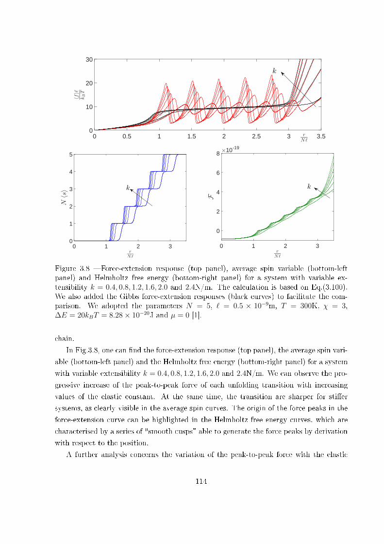
rNℓ
0 0.5 1 1.5 2 2.5 3 3.5
〈f〉ℓ
kBT
0
10
20
30
k
r
Nℓ
0 1 2 3
N〈s〉
0
1
2
3
4
5
k
r
Nℓ
0 1 2 3
F
×10-19
0
2
4
6
8
k
Figure 3.8 � Force-extension response (top panel), average spin variable (bottom-leftpanel) and Helmholtz free energy (bottom-right panel) for a system with variable ex-tensibility k = 0.4, 0.8, 1.2, 1.6, 2.0 and 2.4N/m. The calculation is based on Eq.(3.100).We also added the Gibbs force-extension responses (black curves) to facilitate the com-parison. We adopted the parameters N = 5, ` = 0.5 × 10⁻⁹m, T = 300K, χ = 3,∆E = 20kBT = 8.28× 10⁻²⁰J and µ = 0 [1].
chain.
In Fig.3.8, one can �nd the force-extension response (top panel), the average spin vari-
able (bottom-left panel) and the Helmholtz free energy (bottom-right panel) for a system
with variable extensibility k = 0.4, 0.8, 1.2, 1.6, 2.0 and 2.4N/m. We can observe the pro-
gressive increase of the peak-to-peak force of each unfolding transition with increasing
values of the elastic constant. At the same time, the transition are sharper for sti�er
systems, as clearly visible in the average spin curves. The origin of the force peaks in the
force-extension curve can be highlighted in the Helmholtz free energy curves, which are
characterised by a series of "smooth cusps" able to generate the force peaks by derivation
with respect to the position.
A further analysis concerns the variation of the peak-to-peak force with the elastic
114

rNℓ
0.8 1 1.2 1.4 1.6
〈f〉ℓ
kBT
0
5
10
15
20
∆f
fmin
k
fmax
T = 750◦K
T = 300◦K
Figure 3.9 � Shape of the �rst peaks in the force-extension curves for two temperaturesT = 300K and T = 750K and for several values of k = (0.3 + 0.15n)N/m, n = 0, ..., 18.One can see the exact de�nition of the peak-to-peak force for the �rst peak holding foreach force-extension curve. We adopted the parameters N = 5, ` = 0.5× 10⁻⁹m, χ = 3,∆E = 8.28× 10⁻²⁰J and µ = 0 [1].
constant k and the temperature T . In Fig.3.9, we can observe the shape of the �rst
peaks for two temperatures T = 300K and T = 750K and for several values of k =
(0.3 + 0.15n)N/m, n = 0, ..., 18. We can observe the strong reduction of the force peak
with increasing elastic constant and/or temperature. Concerning the decrease of the
peak with the temperature, we remark that the spinoidal behaviour of the force-extension
curve (negative slope in some regions) is characterised by a critical temperature, de�ned
as follows. For supercritical temperatures, the slope (or the e�ective sti�ness) is always
positive and for subcritical temperatures, it is negative in some regions. This concept of
critical temperature for the chain within the Helmholtz ensemble is similar to the concept
of Curie temperature governing the ferromagnetic-paramagnetic transition in magnetic
materials. This point has been recently discussed in Refs. [111�113]. Interestingly enough,
we notice that the chain with a negative e�ective sti�ness (spinoidal behaviour), exhibited
in speci�c working conditions, can be viewed as a metamaterial [111] and this property
can be mimicked in bioinspired nanostructures [173]. In Fig.3.10, one can �nd the the
variation of the peak-to-peak force (as de�ned in Fig.3.9) in terms of elastic constant and
temperature. We can see that the force peak becomes negligible for low values of k and
high values of T . This plot shows the importance of considering the correct value of k
115

k0.5 1 1.5 2 2.5 3
〈∆f〉ℓ
kBT
0
5
10
15
20
T
∆f = fmax − fmin
Figure 3.10 � Behaviour of the peak-to-peak force de�ned in Fig.3.9 versus elastic constantand temperature. We varied the elastic constant in the range k = (0.3 + 0.15n)N/m,n = 0, ..., 18 and the temperature as T = (300+50m), m = 0, ..., 9. We observe the strongreduction of the force peak with the increasing of temperature and/or elastic constant.We adopted the parameters N = 5, ` = 0.5 × 10⁻⁹m, χ = 3, ∆E = 8.28 × 10⁻²⁰J andµ = 0 [1].
for modelling the folding-unfolding processes of macromolecular chains. Indeed, the force
peaks are typically considered as output of real experiments and their values are used
to draw quantitative conclusions about mechanical and thermodynamic properties of the
macromolecule.
Finally, we show in Fig.3.11 the behaviour of the system as a function of the number
of units of the chain. This is an important analysis since it concerns the validity of the
ensembles equivalence in the thermodynamic limit. In Fig.3.11, one can �nd the results
for N from 2 to 8 for a system with an elastic constant k = 1N/m. It is interesting to
remark that for an increasing value of N , the peak-to-peak force is progressively reduced,
con�rming the convergence of the Helmholtz ensemble to the Gibbs ensemble for N →∞. Indeed, if two ensembles are equivalent, the corresponding force-extension curves
must coincide. This is perfectly coherent with known results concerning the ensembles
equivalence in the thermodynamic limit, as discussed in recent literature [20,139].
116

rNℓ
0 0.5 1 1.5 2 2.5 3
〈f〉ℓ
kBT
0
10
20
30
N
r
Nℓ
0 1 2 3
N〈s〉
0
2
4
6
8N
r
Nℓ
0 1 2 3
F
×10-19
0
2
4
6
N
Figure 3.11 � Force-extension response (top panel), average spin variable (bottom-leftpanel) and Helmholtz free energy (bottom-right panel) for a system with a variable numberof units N = 2, 3, 4, 5, 6, 7, and 8. The calculation is based on Eq.(3.100). We alsoadded the Gibbs force-extension responses (black curves) to facilitate the comparison.We adopted the parameters k = 1N/m, ` = 0.5 × 10⁻⁹m, T = 300K, χ = 3, ∆E =20kBT = 8.28× 10⁻²⁰J and µ = 0 [1].
3.4 Conclusion
To conclude, we provided in detail the analysis of a two-state freely jointed chain with
extensible bonds. Despite the complexity of the calculation of the partition function,
especially within the Helmholtz ensemble, we added the extensibility to the units, an
important point to describe real macromolecules. To exactly calculate the Gibbs par-
tition function, we applied an approximation considering relatively high values of the
elastic constant de�ning the extensibility of the units. This is coherent according to
the parameters of most of macromolecules of biological interest. Concerning the Gibbs
ensemble, we obtained the exact partition function by direct integration. The latter is
then used to calculate the elastic response of the system and the average value of the
spin variable. We observed that for a given threshold force, the spin exhibits a transi-
117

tion, showing the cooperative (or synchronised) behaviour of the chain within the Gibbs
ensemble. Regarding the Helmholtz ensemble, the implicit interaction induced by the iso-
metric condition complicates the direct calculation of the partition function. Indeed, the
partition function cannot be factorised due to the interdependence of the units extensions.
Both partition functions can be connected through a Laplace transform. This property
is typically exploited in classical literature to prove the equivalence of the ensembles in
the thermodynamic limit [120,124]. Here, this property is used to obtain the closed form
expression for the Helmholtz partition function in terms of the Hermite elements with a
negative index. The Hermite polynomials have been introduced in literature in Ref. [172],
however, to the author's knowledge, the study here presented is the �rst application to a
physical problem. Contrarily to the Gibbs ensemble, the average spin variable, calculated
with the help of the Helmholtz partition function, exhibits a stepwise behaviour, show-
ing the non-cooperative (or non-synchronised) behaviour of the chain. Moreover, as seen
in Fig.3.8, the force-extension response within the Helmholtz ensemble depends on the
intrinsic sti�ness of the units. A weak sti�ness of the chain may strongly reduce the am-
plitude of the force peaks of the response. It means that for force-extension experiments,
sti� macromolecules can be rather used than soft macromolecules to study cooperativ-
ity and other conformational properties. To conclude, in this Chapter, the spin variable
approach is adopted to study bistable chains with extensibility. The next step, to bring
our model closer to reality, involves the consideration of the possible interactions existing
among units.
118
Chapter 4
Two-state freely jointed chain with
Ising interactions
4.1 Introduction
The purpose of this Chapter is to introduce in the model interactions existing among
the units of a macromolecular chain, with the help of the Ising scheme, combined with
the spin variable method. We remember that, from the historical point of view, the
statistical models with interactions have been introduced to explain phase transitions in
condensed matter. For instance, Wilhelm Lenz invented the original Ising model and gave
it as a problem to his student, Ernst Ising. The one-dimensional model was solved by
Ising himself during his PhD in 1924. The obtained result, contrarily to the expectations,
did not describe any phase transition. Two decades later, the two-dimensional model
was solved by Lars Onsager (see Fig.4.1). This quite complex calculation showed for the
�rst time a phase transition in an exactly solvable model of the statistical mechanics. In
following studies, the Ising scheme (and many other interaction schemes) have been used to
describe di�erent features of the phase transitions but also to develop models with complex
interactions in other physical and biophysical directions. In our context, we adopt the
Ising scheme to introduce a cooperative or anti-cooperative behaviour in the folding and
unfolding processes of the units of a chain. The study of interactions existing among units
is mainly motivated by repeat tandem proteins [114]. These proteins are de�ned as several
(at least, two) adjacent copies having the same or very similar sequence motifs, generated
by internal duplications. The repetition of the sequence ranges from a single amino-acid up
to domains of 100 or more residues. Interactions among units of the chain do not depend
on the place of the units in the sequence. Indeed, even if units are far apart in the sequence,
they can be next to each other in the con�gurational space, which may lead to interactions.
119

Figure 4.1 � Insert published on the occasion of the 90th anniversary of the Ising model[174].
A �rst reported case concerns the tandem repeats in red cell spectrin [114], where two
units simultaneously unfold because of their strong interaction. Similar observations have
been made on Filamin A [154], where domain-domain interactions lead to a hierarchy
of unfolding forces and the Ising model is appropriate to study them. Indeed, we can
introduce a positive Ising contribution which favours the same state (folded or unfolded)
for adjacent units, or a negative Ising contribution which favours the di�erent state for
adjacent units. While these forms of interactions have been observed in speci�c couples of
units in real protein chains, we introduce in our model the interaction term for all couples
of adjacent units to simplify the analysis.
Hence, the systems considered in this Chapter are bistable and cooperative. There-
fore, each unit can undergo transitions from folded to unfolded states or from unfolded to
folded states, and the transition of one unit a�ects the transition of the others, favourably
or not. The Ising model has been chosen to better understand both bistable and coop-
erative systems because it is one of the simplest interaction scheme and it directly works
on the spin variables. The Ising coe�cient, λ, is the parameter enabling to establish the
desired type of interaction. This Ising coe�cient allows to consider, for instance, the
case of a "positive" interaction with λ > 0, leading to the unfolding of units favoured by
120

the previous unfolding of other units. A "negative" interaction with λ < 0 can also be
considered, when the unfolding of units can prevent other units from unfolding. We pro-
vide evidence that the cooperativity, measured by the Ising interaction coe�cient, strongly
modi�es the force-extension response of the chain, and its con�gurational properties. This
scheme is not only useful to better understand the behaviour of real macromolecules, but
it also enables to explain the nucleation stress in nanowires [96�98], an important topic
in material science. While the Gibbs ensemble will be studied by means of the classical
transfer matrix method [175], typically adopted for one-dimensional interacting models,
the Helmholtz ensemble presents major di�culties and will be approached once again by
exploiting the Laplace transform relationship between the Gibbs and Helmholtz partition
functions [120].
We take into consideration a chain of N two-state elements (see Fig.4.2.a), each de-
scribed by a bistable potential energy with a stable folded state and a metastable unfolded
state (see Fig.4.2.b). The two potential wells in Fig.4.2.b can be characterised by the elas-
tic constant k(Si), the equilibrium length `(Si) and the basal energy v(Si), where Si is a
discrete variable (or spin variable) assuming values in {−1,+1}, used to distinguish one
well from the other. We state that Si = +1 corresponds to unfolded elements, whereas
Si = −1 corresponds to folded ones. This description suggests that the bistable energy
potential can be represented by two quadratic potentials approximating the real wells of
the units (see again Fig.4.2.b) [113]. In this case, the discrete variables belong to the phase
space of the system and allow to specify the explored well for each unit. The introduction
of the discrete or spin variables also allows the direct implementation of an interaction
between adjacent elements of the chain, e.g. described by a classical Ising Hamiltonian.
The overall Hamiltonian of this system can be therefore written as
H = −λN−1∑i=1
SiSi+1 − µN∑i=1
Si +N∑i=1
[v(Si) +
1
2k(Si) [‖~ri − ~ri−1‖ − `(Si)]2
]. (4.1)
The �rst term in Eq.(4.1) represents the Ising interaction among spin variables, the second
term represents the e�ect of a chemical potential, and the third one describes the spring-
like behaviour of each unit placed between positions ~ri−1 and ~ri, ∀i = 1, ..., N . We
remark that λ > 0 tries to force all elements to be folded or unfolded (ferromagnetic-
like interaction), whereas λ < 0 tries to force all elements to be alternatively folded and
unfolded (anti-ferromagnetic-like interaction). The parameter µ is a sort of external �eld
or chemical potential (µ > 0 tries to unfold the domains and µ < 0 tries to fold them).
In the following, we suppose to embed the system in a thermal bath at the temperature
T , we consider the system at thermodynamic equilibrium and we study the e�ects of
121
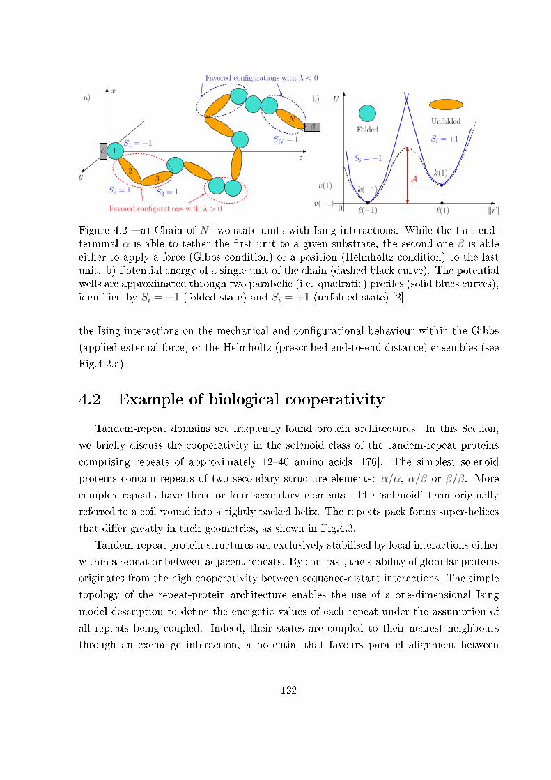
`(−1) `(1) k~rk0
v(1)k(−1)
k(1)
U
v(−1)
Si = −1
Si = +1
A
a) b)x
y
z
FoldedUnfolded
1
23
N
S1 = −1
S2 = 1 S3 = 1
SN = 1
Favored configurations with λ > 0
Favored configurations with λ < 0
α
β
Figure 4.2 � a) Chain of N two-state units with Ising interactions. While the �rst end-terminal α is able to tether the �rst unit to a given substrate, the second one β is ableeither to apply a force (Gibbs condition) or a position (Helmholtz condition) to the lastunit. b) Potential energy of a single unit of the chain (dashed black curve). The potentialwells are approximated through two parabolic (i.e. quadratic) pro�les (solid blues curves),identi�ed by Si = −1 (folded state) and Si = +1 (unfolded state) [2].
the Ising interactions on the mechanical and con�gurational behaviour within the Gibbs
(applied external force) or the Helmholtz (prescribed end-to-end distance) ensembles (see
Fig.4.2.a).
4.2 Example of biological cooperativity
Tandem-repeat domains are frequently found protein architectures. In this Section,
we brie�y discuss the cooperativity in the solenoid class of the tandem-repeat proteins
comprising repeats of approximately 12�40 amino acids [176]. The simplest solenoid
proteins contain repeats of two secondary structure elements: α/α, α/β or β/β. More
complex repeats have three or four secondary elements. The `solenoid' term originally
referred to a coil wound into a tightly packed helix. The repeats pack forms super-helices
that di�er greatly in their geometries, as shown in Fig.4.3.
Tandem-repeat protein structures are exclusively stabilised by local interactions either
within a repeat or between adjacent repeats. By contrast, the stability of globular proteins
originates from the high cooperativity between sequence-distant interactions. The simple
topology of the repeat-protein architecture enables the use of a one-dimensional Ising
model description to de�ne the energetic values of each repeat under the assumption of
all repeats being coupled. Indeed, their states are coupled to their nearest neighbours
through an exchange interaction, a potential that favours parallel alignment between
122

Figure 4.3 � Secondary structure representations of solenoid tandem-repeat proteins.From top left to bottom right (PDB identi�ers in parenthesis): ARM-repeat proteinβ-catenin (2Z6H), HEAT-repeat protein PR65 (1B3U), Ankyrin-repeat protein gankyrin(1UOH), HEAT-repeat protein Importin-β (3ND2), leucine-rich repeat (LRR) protein Ri-bonuclease Inhibitor (1BNH), TPR protein RapI (4I1A), β-helical repeat protein carbonicanhydrase (1QRE) [176].
Figure 4.4 � Structures of di�erent Rap proteins (C-terminus in red) depicting a possiblemode of action. When the TPR domain binds to a signalling peptide, it causes theRap protein to adopt a compact, or `closed' conformation. Upon binding an interactionpartner, however, conformational changes in the TPR domain are minimal, whereas theN-terminal three-helix bundle �ips by approximately 180�[176].
states. Folding cooperativity of repeat proteins breaks down above approximately 100�150
amino acids, similar to the cooperativity limit of globular proteins.
In recent years, a family of bacterial regulators has been largely investigated: the
RRNPP family. The name of these peptide-sensing regulators refers to the founding
members of the family, Rap-Rgg-NprR-PlcR-Prgx. They all have the same domain or-
ganisation: an N-terminal three-helix bundle, a �exible helical linker and a C-terminal
tratricopeptide repeats (TPR, as shown in Fig.4.3) capable of binding short peptides of
�ve to eight residues [176]. The homologous structures of Rap proteins have been used
to propose a mechanism of action for signal transduction (see Fig.4.4). The compact
123
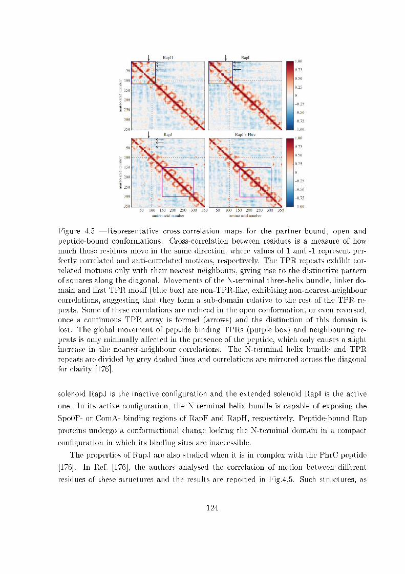
Figure 4.5 � Representative cross-correlation maps for the partner-bound, open andpeptide-bound conformations. Cross-correlation between residues is a measure of howmuch these residues move in the same direction, where values of 1 and -1 represent per-fectly correlated and anti-correlated motions, respectively. The TPR repeats exhibit cor-related motions only with their nearest neighbours, giving rise to the distinctive patternof squares along the diagonal. Movements of the N-terminal three-helix bundle, linker do-main and �rst TPR motif (blue box) are non-TPR-like, exhibiting non-nearest-neighbourcorrelations, suggesting that they form a sub-domain relative to the rest of the TPR re-peats. Some of these correlations are reduced in the open conformation, or even reversed,once a continuous TPR array is formed (arrows) and the distinction of this domain islost. The global movement of peptide binding TPRs (purple box) and neighbouring re-peats is only minimally a�ected in the presence of the peptide, which only causes a slightincrease in the nearest-neighbour correlations. The N-terminal helix bundle and TPRrepeats are divided by grey dashed lines and correlations are mirrored across the diagonalfor clarity [176].
solenoid RapJ is the inactive con�guration and the extended solenoid RapI is the active
one. In its active con�guration, the N-terminal helix bundle is capable of exposing the
Spo0F- or ComA- binding regions of RapF and RapH, respectively. Peptide-bound Rap
proteins undergo a conformational change locking the N-terminal domain in a compact
con�guration in which its binding sites are inaccessible.
The properties of RapJ are also studied when it is in complex with the PhrC peptide
[176]. In Ref. [176], the authors analysed the correlation of motion between di�erent
residues of these structures and the results are reported in Fig.4.5. Such structures, as
124
clearly shown, exhibit correlated motion only with their nearest neighbours, giving rise
to the distinctive pattern of squares along the diagonal and con�rming the applicability
of the Ising scheme. The binding of the peptide marginally increases nearest-neighbour
correlation at the centre (purple box in Fig.4.5). Moreover, movements of the N-terminal
three-helix bundle, linker domain and �rst TPRs repeat (blue box in Fig.4.5) are strongly
correlated (non-nearest-neighbour), suggesting that they form a sub-domain relative to
the rest of the TPR repeats. Finally, the Rap proteins are a good example of a system
where nearest-neighbour interactions in a repeat array are su�ciently strong to justify a
two-state modelling with a superposed Ising scheme.
4.3 Two-state freely jointed chain with Ising interac-
tions: the Gibbs ensemble
We consider now the extended Hamiltonian
HG = −λN−1∑i=1
SiSi+1 − ~f · ~rN − µN∑i=1
Si
+N∑i=1
[v(Si) +
1
2k(Si) [‖~ri − ~ri−1‖ − `(Si)]2
]. (4.2)
Here, ~f is the applied force to the last element, identi�ed by its position ~rN . We suppose
that quantities ~ri ∈ R3 and Si ∈ {−1,+1} ∀i ∈ {1...N} belong to the phase space of the
system. Moreover, to �x ideas, we always consider ~r0 = 0. The statistical mechanics of
the system can be introduced by calculating the Gibbs partition function, as
ZG(~f) =∑
S1∈{0,1}
...∑
SN∈{0,1}
∫R3
...
∫R3
exp
[−HG
({Si}, {~ri})kBT
]d~r1...d~rN
=∑
S1∈{0,1}
...∑
SN∈{0,1}
exp
(λ
kBT
N−1∑i=1
SiSi+1
)exp
(µ
kBT
N∑i=1
Si
)
× exp
[− 1
kBT
N∑i=1
v(Si)
]∫R3N
exp
(~f · ~rNkBT
)
× exp
[−1
2
N∑i=1
k(Si)
kBT[‖~ri − ~ri−1‖ − `(Si)]2
]d~r1...d~rN . (4.3)
125
The integral I =∫R3N ...d~r1...d~rN can be developed by means of the change of variables
~ξ1 = ~r1 − ~r0; ~ξ2 = ~r2 − ~r1; ...; ~ξN = ~rN − ~rN−1, giving
I =
∫R3N
exp
[−1
2
N∑i=1
k(Si)
kBT[‖ξi‖ − `(Si)]2
]exp
(~f
kBT·N∑i=1
~ξi
)d~ξ1...d~ξN . (4.4)
To further simplify the integral, we suppose that ~f = (0, 0, f) (the direction of the force can
be �xed without limiting the generality of the calculation since the system is isotropic) and
we introduce the spherical coordinates for the vectors ~ξi : ~ξi = (ξi cosϕi sin θi; ξi sinϕi sin θi; ξi cos θi).
Therefore, ‖~ξi‖ = ξ ; ~f · ~ξi = fξi cos θi and d~ξi = ξ2i sin θidξidϕidθi, and the integral be-
comes
I =
∫B
exp
[−1
2
N∑i=1
k(Si)
kBT[ξi − `(Si)]2
]exp
(N∑i=1
fξi cos θikBT
)
×N∏i=1
ξ2i sin θidξidϕidθi, (4.5)
with B = [(0; +∞)× (0; 2π)× (0;π)]N . The calculation can be developed as follows
I = (2π)N∫
[0;+∞]Nexp
[−1
2
N∑i=1
k(Si)
kBT[ξi − `(Si)]2
](N∏i=1
ξ2i
)
×∫
[0;π]Nexp
(N∑i=1
fξi cos θikBT
)N∏i=1
sin θidθidξi
= (2π)NN∏i=1
{∫ +∞
0
exp
[−1
2
k(Si)
kBT[ξi − `(Si)]2
]ξ2i
2kBT
fξi
× sinh
(fξikBT
)dξi
}
= (4π)NN∏i=1
∫ +∞
0
exp
[−1
2
k(Si)
kBT[ξi − `(Si)]2
] sinh(fξikBT
)fξikBT
ξ2i dξi
. (4.6)
Now, the integral I can be strongly simpli�ed if we make the assumption to deal with
a freely jointed chain model with elements of �xed lengths. It is equivalent to say that
k(+1) = k(−1) → +∞. The case with �nite sti�ness of the wells will be considered in
a following Section. If we use the property√
απe−αx
2 → δ(x), when α → ∞, we simplify
the result for I, with c a constant, as
I = c×N∏i=1
∫ +∞
0
δ [ξi − `(Si)]sinh
(fξikBT
)fξikBT
ξ2i
`2dξi, (4.7)
126
where `2 = `2(−1) i.e. ` = `(−1). We �nally obtain
I = c×N∏i=1
sinh[f`(Si)kBT
]f`(Si)kBT
`2(Si)
`2dξi. (4.8)
Eventually, the partition function assumes the simpler form
ZG(~f) =∑
S1∈{0,1}
...∑
SN∈{0,1}
{exp
(λ
kBT
N−1∑i=1
SiSi+1
)exp
(µ
kBT
N∑i=1
Si
)
× exp
[− 1
kBT
N∑i=1
v(Si)
]N∏i=1
sinh[f`(Si)kBT
]f`(Si)kBT
`2(Si)
`2dξi
. (4.9)
We have now to approach the problem of calculating the sums over the spin variables.
To this aim, a more symmetric form of Eq.(4.9) can be obtained by observing that
N∏i=1
ci =√c1
[N−1∏i=1
√cici+1
]√cN , (4.10)
with ci > 0, whatever i. So we have
ZG(f) =∑
S1∈{0,1}
...∑
SN∈{0,1}
exp
(µ
2kBTS1
)exp
[ −1
2kBTv(S1)
]√c1
N−1∏i=1
{exp
(λ
kBTSiSi+1
)
× exp
[µ
2kBT(Si + Si+1)
]exp
[ −1
2kBT[v(Si) + v(Si+1)]
]√cici+1
}× exp
(µ
2kBTSN
)exp
[ −1
2kBTv(SN)
]√cN , (4.11)
where we de�ned
ci =sinh
[f`(Si)kBT
]f`(Si)kBT
`2(Si)
`2. (4.12)
We de�ne `(−1) = `; v(−1) = 0 and `(+1) = χ`; v(+1) = ∆E, where χ is the ratio
between unfolded and folded lengths, and ∆E is the energy jump between the wells. The
next step to elaborate the Gibbs partition function consists in adopting the technique of
the transfer matrix and then we can write
ZG(f) = ~V TTN−1~V , (4.13)
127
where we have
~V =
e− µ
2kBT
√sinh
(f`kBT
)f`kBT
eµ
2kBT e− ∆E
2kBT
√χ
sinh(f`χkBT
)f`kBT
(4.14)
or
~V =
[ √2p√2q
](4.15)
if we de�ne
p =1
2e− µkBT
sinh ξ
ξ, (4.16)
q =1
2e
µkBT χφ
sinh(χξ)
ξ, (4.17)
where
φ = e− ∆EkBT , (4.18)
ξ =f`
kBT. (4.19)
Moreover,
T =
eλ
kBT e− µkBT
sinh ξξ
e− λkBT e
− ∆E2kBT
√sinh ξξχ sinh(χξ)
ξ
e− λkBT e
− ∆E2kBT
√sinh ξξχ sinh(χξ)
ξe
λkBT e
µkBT χ sinh(χξ)
ξe− ∆EkBT
(4.20)
or again
T = 2
[pe
λkBT
√pqe
−λkBT
√pqe
−λkBT qe
λkBT
]. (4.21)
Since we are studying the thermodynamics of small systems (small N), we need to calcu-
late the exact value of the partition function given in Eq.(4.13) and not its approximation
evaluated for a large value of N , corresponding to the thermodynamic limit. Now, we can
simply calculate the eigenvalues of the transfer matrix T, obtaining
λ1,2 = eλ
kBT (p+ q)±√e
2λkBT (p− q)2 + 4e
−2λkBT pq
= eλ
kBT
[(p+ q)±
√(p+ q)2 − 4pq
(1− e
−4λkBT
)]. (4.22)
128
We note that if λ1 corresponds to the sign "+" and λ2 to the sign "−", then λ1 > λ2 > 0.
Now, we need to explicitly determine the matrix power TN−1. We introduce the general
theory for an arbitrary matrix function: let f(x) : R → R a function with a Taylor
development f(x) =∑+∞
k=0Ckxk, converging in a region D ⊂ C. Then, we consider a
matrix A (M × M), with all eigenvalues in D: λj ∈ D, whatever j = 1, ...,M . So,
we de�ne the value f(A) by the series expansion f(A) =∑+∞
k=0 CkAk. We propose an
e�cient technique to determine f(A) with a �nite number of operations. We consider the
characteristic polynomial PA(x) associated to the matrix A
PA(x) = det(A− x1) (4.23)
with solutions being the eigenvalues ofA. We also remember the Cayley-Hamiltonian the-
orem stating that PA(A) = 0. In general, we know the procedure for dividing polynomials
as
n(x)
d(x)= q(x) +
r(x)
d(x)(4.24)
or n(x) = q(x)d(x) + r(x), where ∂n = P, ∂d = D, ∂q = M − D and ∂r = D − 1.
We say that n(x) is the dividend, d(x) is the divisor, q(x) is the quotient and r(x)
is the remainder. The important point is that the remainder has a lower degree than
the divisor. The quantities q(x) and r(x) are unique and the procedure is the so-called
Euclidean division. Now, we apply this operation to f(x)PA(x)
, getting
f(x)
PA(x)= q(x) +
r(x)
PA(x)(4.25)
or f(x) = q(x)PA(x) + r(x), with ∂r = M − 1 if A is a matrix M ×M . So, by using
the Cayley-Hamilton theorem, we obtain that f(A) = r(A) with ∂r = M − 1. We �nally
have to �nd the M coe�cient of the polynomial r(x). If λi is a simple root of PA(x), we
can write f(λi) = q(λi)PA(λi) + r(λi) or f(λi) = r(λi), which is a condition to obtain the
coe�cients of r(x). If λi has multiplicity 2 in PA(x), then we can write
f(x) = q(x)PA(x) + r(x), (4.26)
f ′(x) = q′(x)PA(x) + q(x)P′
A(x) + r′(x), (4.27)
and we have
f(λi) = r(λi), (4.28)
f ′(λi) = r′(λi). (4.29)
129
In conclusion, we have the following property: if PA(x) = (−1)M(x− λ1)m1 ...(x− λr)mr ,with
∑ri=1 mi = M , we can consider r(x) =
∑M−1k=0 rkx
k where the coe�cients rk can be
obtained through the system
f (α)(λi) = r(α)(λi), (4.30)
with 0 < α < mi − 1, whatever i from 1 to r.
In our case, we search for TN−1 with a 2 x 2 matrix T(M = 2) having eigenvalues λ1 and
λ2, as
TN−1 = α1 + βT, (4.31)
with
λN−11 = α + βλ1, (4.32)
λN−12 = α + βλ2, (4.33)
from which we get
α =λ1λ
N−12 − λ2λ
N−11
λ1 − λ2
, (4.34)
β =λN−1
1 − λN−12
λ1 − λ2
, (4.35)
or equivalently
TN−1 =λN−1
1 − λN−12
λ1 − λ2
T +λ1λ
N−12 − λ2λ
N−11
λ1 − λ2
1. (4.36)
Therefore, the partition function becomes
ZG(~f) = ~V TTN−1~V =λN−1
1 − λN−12
λ1 − λ2
~V TT~V +λ1λ
N−12 − λ2λ
N−11
λ1 − λ2
~V T ~V . (4.37)
Thus, we have
~V T ~V =[√
2p√
2q] [ √2p√
2q
]= 2p+ 2q = 2(p+ q), (4.38)
~V TT~V =[√
2p√
2q] [ 2pe
λkBT 2e
− λkBT√pq
2e− λkBT√pq 2qe
λkBT
][ √2p√2q
]= 4p2e
λkBT + 4pqe
− λkBT + 4pqe
− λkBT + 4q2e
λkBT
= 4eλ
kBT
[(p+ q)2 − 2pq(1− e−
2λkBT )
]. (4.39)
130
With some other modi�cations, we get
λ1 + λ2 = 2eλ
kBT (p+ q) = eλ
kBT ~V T ~V (4.40)
λ1 − λ2 = 2eλ
kBT
√(p+ q)2 − 4pq
(1− e−
4λkBT
). (4.41)
We try to write ~V T ~V and ~V TT~V in terms of λ1, λ2 and eλ
kBT . Therefore,
~V T ~V = x(λ1 + λ2), (4.42)
with x = exp− λkBT . From (4.41), we calculate (λ1 − λ2)2
(λ1 − λ2)2 = 4e2λkBT
[[(λ1 + λ2)
1
2e− λkBT
]2
− 4pq(
1− e−4λkBT
)]. (4.43)
So we get
x2
4
(λ2
1 + 2λ1λ2 + λ22 − λ2
1 + 2λ1λ2 + λ22
)= 4pq
(1− e−
4λkBT
). (4.44)
And �nally
pq =1
4
λ1λ2x2
(1− x2)(1 + x2). (4.45)
Therefore, from (4.39), we obtain
~V TT~V =4
x
[(x2
)2
(λ1 + λ2)2 − 2
4
λ1λ2x2
(1− x4)(1− x2)
]=
x(1 + x2)(λ1 + λ2)2 − 2xλ1λ2
1 + x2. (4.46)
The �nal calculus of ZG(f) gives
ZG(f) =λN−1
1 − λN−12
λ1 − λ2
(x3 + x)(λ1 + λ2)2 − 2λ1λ2
1 + x2
+λ1λ
N−12 − λ2λ
N−11
λ1 − λ2
x(λ1 + λ2)
=x
(λ1 − λ2)(1 + x2)
[(λN−1
1 − λN−12 )
((1 + x2)(λ2
1 + λ22 + 2λ1λ2)− 2λ1λ2
)+(λ1 + λ2)(λ1λ
N−12 − λ2λ
N−11 )(1 + x2)
]. (4.47)
Then, we calculate the term into brackets[(λN−1
1 − λN−12 )
((1 + x2)(λ2
1 + λ22 + 2λ1λ2)− 2λ1λ2
)+ (λ1 + λ2)
×(λ1λN−12 − λ2λ
N−11 )(1 + x2)
]= λN−1
1 λ1(λ1 − λ2)− λN−12 λ2(λ2 − λ1)
+x2(λN−11 − λN−1
2 )(λ1 + λ2)2 + x2(λ21λ
N−12 − λ2λ
N1 + λ1λ
N2 − λ2
2λN−11 )
= λN1[λ1 − λ2 + x2(λ1 + λ2)
]− λN2
[λ2 − λ1 + x2(λ1 + λ2)
]. (4.48)
131

Finally, we get the following form of the Gibbs partition function
ZG(f) =x
1 + x2
[λN1
(1 + x2λ1 + λ2
λ1 − λ2
)+ λN2
(1− x2λ1 + λ2
λ1 − λ2
)], (4.49)
where
x = e− λkBT , (4.50)
λ1,2 =1
x
[p+ q ±
√(p+ q)2 − 4pq(1− x4)
], (4.51)
p =1
2e− µkBT
sinh ξ
ξ, (4.52)
q =1
2e
µkBT χφ
sinh(χξ)
ξ, (4.53)
ξ =f`
kBT, (4.54)
φ = e− ∆EkBT . (4.55)
As usual, we obtain the force-extension response as
〈r〉 = kBT∂ logZG(f)
∂f= kBT
1
ZG
∂ZG∂f
. (4.56)
We also note that Si+12
gives 0 for folded elements and 1 for unfolded elements. There-
fore,the quantity⟨∑N
i=1Si+1
2
⟩is the average number of unfolded elements. The term∑N
i=1 v(Si) of the Hamiltonian function previously seen can also be written as∑N
i=1Si+1
2∆E,
therefore we have
N∑i=1
Si + 1
2=∂HG
∂∆E. (4.57)
It follows that⟨∑N
i=1Si+1
2
⟩can be evaluated through the expression
⟨N∑i=1
Si + 1
2
⟩=
∑~S
∫∂HG∂∆E
e− HGkBT d~r∑
~S
∫e− HGkBT d~r
, (4.58)
which can be simpli�ed to give⟨N∑i=1
Si + 1
2
⟩= −kBT
∂
∂∆Elog[ZG(f)], (4.59)
corresponding to the average value of unfolded domains. It is useful to introduce here
the Gibbs free energy of the system G = −kBT logZG. The above expected values can be
132
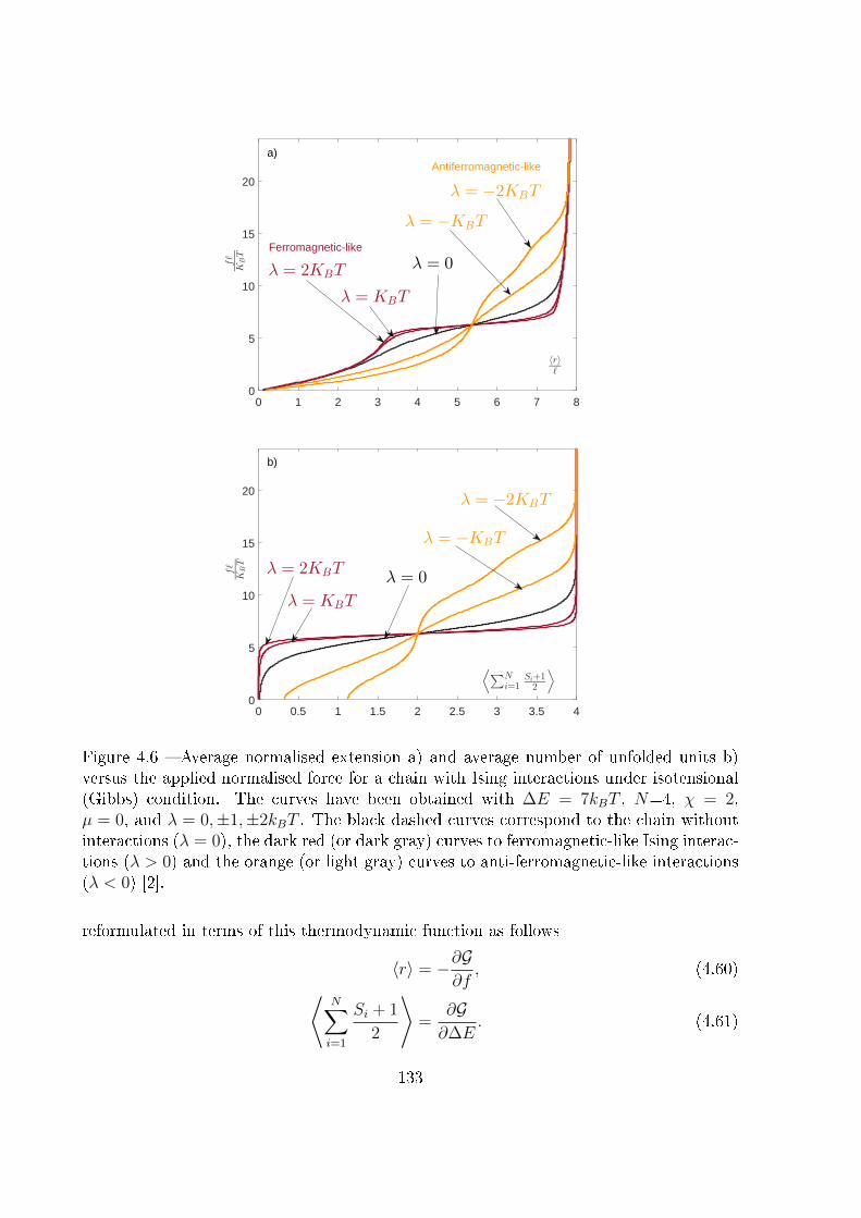
0 1 2 3 4 5 6 7 8
〈r〉ℓ
0
5
10
15
20
fℓ
KBT
λ = 0
λ = −KBT
λ = −2KBT
Antiferromagnetic-like
λ = KBT
λ = 2KBT
Ferromagnetic-like
a)
0 0.5 1 1.5 2 2.5 3 3.5 4
⟨
∑Ni=1
Si+1
2
⟩
0
5
10
15
20
fℓ
KBT
λ = 0λ = 2KBT
λ = KBT
λ = −KBT
λ = −2KBT
b)
Figure 4.6 � Average normalised extension a) and average number of unfolded units b)versus the applied normalised force for a chain with Ising interactions under isotensional(Gibbs) condition. The curves have been obtained with ∆E = 7kBT , N=4, χ = 2,µ = 0, and λ = 0,±1,±2kBT . The black dashed curves correspond to the chain withoutinteractions (λ = 0), the dark red (or dark gray) curves to ferromagnetic-like Ising interac-tions (λ > 0) and the orange (or light gray) curves to anti-ferromagnetic-like interactions(λ < 0) [2].
reformulated in terms of this thermodynamic function as follows
〈r〉 = −∂G∂f
, (4.60)⟨N∑i=1
Si + 1
2
⟩=
∂G∂∆E
. (4.61)
133
The knowledge of ZG or G allows therefore the determination of both the average extension
of the chain and the average number of unfolded units as function of the applied force
and temperature.
An application of Eqs.(4.60) and (4.61) can be found in Fig.4.6. First of all, we dis-
cuss the curves for λ = 0, i.e. without Ising interactions: in the force-extension curve
(Fig.4.6.a), we note a force plateau corresponding to the synchronised unfolding of the
N units. This behaviour is con�rmed by the number of unfolded units (Fig.4.6.b), which
shows a transition from 0 to N , at the same threshold force as the previously mentioned
plateau. This force plateau is the classical result of force spectroscopy experiments con-
ducted with soft devices [24, 68, 76, 77, 133, 141] (see also previous Chapters for a wider
discussion). The Ising interactions modify this scenario as follows: if λ > 0, the units
are favoured to be in the same state and the transition is therefore sharper than the
one observed for λ = 0; on the other hand, if λ < 0, it is easier to unfold the �rst
units and the response is therefore smoother. It is interesting to note that, for strong
anti-ferromagnetic-like interactions, even with f = 0, we can have a positive number of
unfolded units because of the energetic compromise between λ and ∆E. Indeed, when we
observe unfolded units with f = 0, the cooperativity e�ect is stronger than the energy
jump between folded and unfolded states. We �nally remark that the curves in Fig.4.6 are
valid for any value of ` and T . If, as an example, we consider ` = 0.4nm and T = 300K,
we get a plateau force at f = 70 pN, which is coherent, e.g., with the DNA overstretching
transition [130].
4.4 Two-state freely jointed chain with Ising interac-
tions: the Helmholtz ensemble
We consider now the Helmholtz ensemble where the last element of the chain is �xed
at a given arbitrary position (isometric condition). The Hamiltonian reads
HH = λ
N−1∑i=1
SiSi+1 − µN∑i=1
Si
+N∑i=1
[v(Si) +
1
2k(Si) [‖~ri − ~ri−1‖ − `(Si)]2
], (4.62)
134
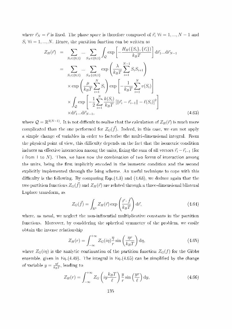
where ~rN = ~r is �xed. The phase space is therefore composed of ~ri ∀i = 1, ..., N − 1 and
Si ∀i = 1, ..., N . Hence, the partition function can be written as
ZH(~r) =∑
S1∈{0,1}
...∑
SN∈{0,1}
∫Q
exp
[−HH({Si}, {~ri})
kBT
]d~r1...d~rN−1
=∑
S1∈{0,1}
...∑
SN{∈0,1}
exp
(λ
kBT
N−1∑i=1
SiSi+1
)
× exp
(µ
kBT
N∑i=1
Si
)exp
[− 1
kBT
N∑i=1
v(Si)
]
×∫Q
exp
[−1
2
N∑i=1
k(Si)
kBT[‖~ri − ~ri−1‖ − `(Si)]2
]×d~r1...d~rN−1, (4.63)
where Q = R3(N−1). It is not di�cult to realise that the calculation of ZH(~r) is much more
complicated than the one performed for ZG(~f). Indeed, in this case, we can not apply
a simple change of variables in order to factorise the multi-dimensional integral. From
the physical point of view, this di�culty depends on the fact that the isometric condition
induces an e�ective interaction among the units, �xing the sum of all vectors ~ri−~ri−1 (for
i from 1 to N). Then, we have now the combination of two forms of interaction among
the units, being the �rst implicitly encoded in the isometric condition and the second
explicitly implemented through the Ising scheme. An useful technique to cope with this
di�culty is the following. By comparing Eqs.(4.3) and (4.63), we deduce again that the
two partition functions ZG(~f) and ZH(~r) are related through a three-dimensional bilateral
Laplace transform, as
ZG(~f) =
∫R3
ZH(~r) exp
(~r · ~fkBT
)d~r, (4.64)
where, as usual, we neglect the non-in�uential multiplicative constants in the partition
functions. Moreover, by considering the spherical symmetry of the problem, we easily
obtain the inverse relationship
ZH(r) =
∫ +∞
−∞ZG(iη)
η
rsin
(ηr
kBT
)dη, (4.65)
where ZG(iη) is the analytic continuation of the partition function ZG(f) for the Gibbs
ensemble, given in Eq.(4.49). The integral in Eq.(4.65) can be simpli�ed by the change
of variable y = η`kBT
, leading to
ZH(r) =
∫ +∞
−∞ZG
(iykBT
`
)y
rsin(yr`
)dy, (4.66)
135

where, as before, we neglected the non-in�uential multiplicative constant. Coherently
with our assumptions, the variables p and q assume the form
p =1
2e− µkBT
sin y
y=p
y, (4.67)
q =1
2e
µkBT χφ
sin(χy)
y=q
y. (4.68)
Accordingly, the eigenvalues of the transfer matrix become
λ1,2 =1
xy
[p+ q ±
√(p+ q)2 − 4pq(1− x4)
]=λ1,2
y, (4.69)
where p = py, q = qy, and λ1,2 = λ1,2y. Hence, the analytic continuation of the Gibbs
partition function becomes
ZG
(iykBT
`
)=
x
1 + x2
1
yN
[λm1
(1 + x2 λ1 + λ2
λ1 − λ2
)
+λN2
(1− x2 λ1 + λ2
λ1 − λ2
)], (4.70)
where, importantly, λ1 and λ2 depend on y only through sin(y) and sin(χy). In particular,
when χ is an integer (or also a rational number), ZG is composed of a periodic function
of y divided by yN . So we have
ZG
(iykBT
`
)=
1
yNP (y), (4.71)
where P (y) = P (y + Ly) for a given Ly and we have
P (y) =x
1 + x2
[λN1
(1 + x2 λ1 + λ2
λ1 − λ2
)
+λN2
(1− x2 λ1 + λ2
λ1 − λ2
)]. (4.72)
If we consider integer values of χ, P (y) is periodic with a period of Ly = 2π, and it can
be developed in Fourier series, as
P (y) =+∞∑
k=−∞
Ckeiky, (4.73)
where
Ck =1
2π
∫ 2π
0
P (y)e−ikydy. (4.74)
136
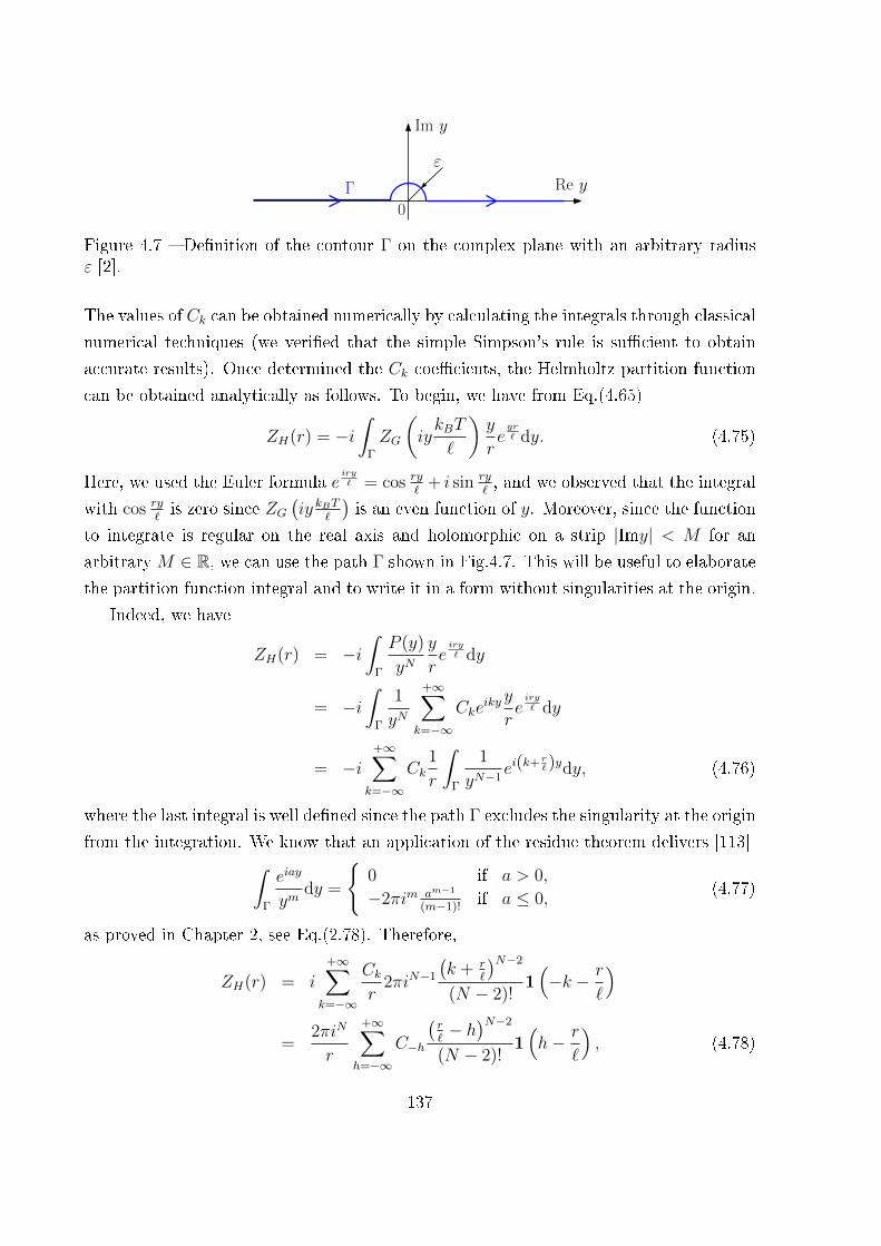
ε
Im y
Re yΓ
0
Figure 4.7 � De�nition of the contour Γ on the complex plane with an arbitrary radiusε [2].
The values of Ck can be obtained numerically by calculating the integrals through classical
numerical techniques (we veri�ed that the simple Simpson's rule is su�cient to obtain
accurate results). Once determined the Ck coe�cients, the Helmholtz partition function
can be obtained analytically as follows. To begin, we have from Eq.(4.65)
ZH(r) = −i∫
Γ
ZG
(iykBT
`
)y
reyr` dy. (4.75)
Here, we used the Euler formula eiry` = cos ry
`+ i sin ry
`, and we observed that the integral
with cos ry`is zero since ZG
(iy kBT
`
)is an even function of y. Moreover, since the function
to integrate is regular on the real axis and holomorphic on a strip |Imy| < M for an
arbitraryM ∈ R, we can use the path Γ shown in Fig.4.7. This will be useful to elaborate
the partition function integral and to write it in a form without singularities at the origin.
Indeed, we have
ZH(r) = −i∫
Γ
P (y)
yNy
reiry` dy
= −i∫
Γ
1
yN
+∞∑k=−∞
Ckeiky y
reiry` dy
= −i+∞∑
k=−∞
Ck1
r
∫Γ
1
yN−1ei(k+ r
` )ydy, (4.76)
where the last integral is well de�ned since the path Γ excludes the singularity at the origin
from the integration. We know that an application of the residue theorem delivers [113]∫Γ
eiay
ymdy =
{0 if a > 0,
−2πim am−1
(m−1)!if a ≤ 0,
(4.77)
as proved in Chapter 2, see Eq.(2.78). Therefore,
ZH(r) = i
+∞∑k=−∞
Ckr
2πiN−1
(k + r
`
)N−2
(N − 2)!1(−k − r
`
)=
2πiN
r
+∞∑h=−∞
C−h
(r`− h)N−2
(N − 2)!1(h− r
`
), (4.78)
137
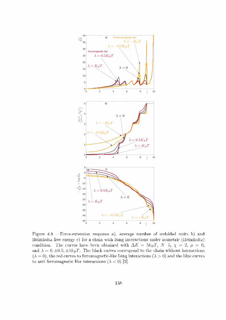
0 2 4 6 8 10rℓ
0
5
10
15
20
25
30
35
40
〈f〉ℓ
KBT
λ = 0
λ = 0.5KBT
λ = KBT
Ferromagnetic-like
λ = −0.5KBT
Antiferromagnetic-like
λ = −KBT
a)
0 2 4 6 8 10r
ℓ
0
1
2
3
4
5
⟨
∑
N i=1
Si+1
2
⟩
λ = 0
λ = 0.5KBT
λ = KBT
λ = −0.5KBT
λ = −KBT
b)
0 2 4 6 8 10r
ℓ
-45
-40
-35
-30
-25
-20
-15
-10
-5
0
5
−
F
KBT=
logZH
λ = 0
λ = 0.5KBT
λ = KBT
λ = −0.5KBTλ = −KBT
c)
Figure 4.8 � Force-extension response a), average number of unfolded units b) andHelmholtz free energy c) for a chain with Ising interactions under isometric (Helmholtz)condition. The curves have been obtained with ∆E = 5kBT , N=5, χ = 2, µ = 0,and λ = 0,±0.5,±1kBT . The black curves correspond to the chain without interactions(λ = 0), the red curves to ferromagnetic-like Ising interactions (λ > 0) and the blue curvesto anti-ferromagnetic-like interactions (λ < 0) [2].
138
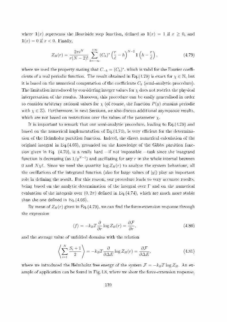
where 1(x) represents the Heaviside step function, de�ned as 1(x) = 1 if x ≥ 0, and
1(x) = 0 if x < 0. Finally,
ZH(r) =2πiN
r(N − 2)!
+∞∑h=−∞
(Ch)∗(r`− h)N−2
1(h− r
`
), (4.79)
where we used the property stating that C−h = (Ch)∗, which is valid for the Fourier coe�-
cients of a real periodic function. The result obtained in Eq.(4.79) is exact for χ ∈ N, butit is based on the numerical computation of the coe�cients Ck (semi-analytic procedure).
The limitation introduced by considering integer values for χ does not restrict the physical
interpretation of the results. Moreover, this procedure can be easily generalised in order
to consider arbitrary rational values for χ (of course, the function P (y) remains periodic
with χ ∈ Z). Furthermore, in next Sections, we also discuss additional asymptotic results,
which are not based on restrictions over the values of the parameter χ.
It is important to remark that our semi-analytic procedure, leading to Eq.(4.79) and
based on the numerical implementation of Eq.(4.74), is very e�cient for the determina-
tion of the Helmholtz partition function. Indeed, the direct numerical calculation of the
original integral in Eq.(4.66), grounded on the knowledge of the Gibbs partition func-
tion given in Eq. (4.70), is a really hard � if not impossible � task since the integrand
function is decreasing (as 1/yN−1) and oscillating for any r in the whole interval between
0 and Nχ`. Since we need the quantity logZH(r) to analyse the system behaviour, all
the oscillations of the integrand function (also for large values of |y|) play an important
role in de�ning the result. For this reason, our procedure leads to very accurate results,
being based on the analytic determination of the integral over Γ and on the numerical
evaluation of the integrals over (0, 2π) de�ned in Eq.(4.74), which are much more stable
than the one de�ned in Eq.(4.66).
By mean of ZH(r) given in Eq.(4.79), we can �nd the force-extension response through
the expression
〈f〉 = −kBT∂
∂rlogZH(r) =
∂F∂r
, (4.80)
and the average value of unfolded domains with the relation⟨N∑i=1
Si + 1
2
⟩= −kBT
∂
∂∆ElogZH(r) =
∂F∂∆E
, (4.81)
where we introduced the Helmholtz free energy of the system F = −kBT logZH . An ex-
ample of application can be found in Fig.4.8, where we show the force-extension response,
139
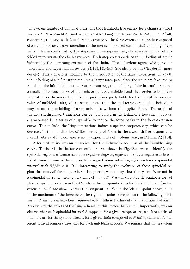
the average number of unfolded units and the Helmholtz free energy for a chain stretched
under isometric condition and with a variable Ising interaction coe�cient. First of all,
concerning the case with λ = 0, we observe that the force-extension curve is composed
of a number of peaks corresponding to the non-synchronised (sequential) unfolding of the
units. This is con�rmed by the step-wise curve representing the average number of un-
folded units versus the chain extension. Each step corresponds to the unfolding of a unit
induced by the increasing extension of the chain. This behaviour agrees with previous
theoretical and experimental results [24,135,141�146] (see also previous Chapter for more
details). This scenario is modi�ed by the introduction of the Ising interactions. If λ > 0,
the unfolding of the �rst units requires a larger force peak since the units are favoured to
remain in the initial folded state. On the contrary, the unfolding of the last units requires
a smaller force since most of the units are already unfolded and they prefer to be in the
same state as the majority. This interpretation equally holds for the plot of the average
value of unfolded units, where we can note that the anti-ferromagnetic-like behaviour
may induce the unfolding of some units also without the applied force. The origin of
the non-synchronised transitions can be highlighted in the Helmholtz free energy curves,
characterised by a series of cusps able to induce the force peaks in the force-extension
curve. To conclude, the Ising interactions induce a speci�c cooperativity, which can be
detected in the modi�cation of the hierarchy of forces in the sawtooth-like response, as
recently observed in force spectroscopy experiments of proteins (e.g., in Filamin A) [154].
A form of criticality can be noticed for the Helmholtz response of the bistable Ising
chain. To do this, in the force-extension curves shown in Fig.4.8.a, we can identify the
spinoidal regions, characterised by a negative slope or, equivalently, by a negative di�eren-
tial sti�ness. It means that, for each force peak observed in Fig.4.8.a, we have a spinoidal
interval with ∂f/∂r < 0. It is interesting to study the evolution of these spinoidal re-
gions in terms of the temperature. In general, we can say that the system is or not in
a spinoidal phase depending on values of r and T . We can therefore determine a sort of
phase diagram, as shown in Fig.4.9, where the end-points of each spinoidal interval (on the
extension axis) are shown versus the temperature. While the left end-point corresponds
to the maximum of the force peak, the right end-point corresponds to the following mini-
mum. These curves have been represented for di�erent values of the interaction coe�cient
λ to explore the e�ects of the Ising scheme on this critical behaviour. Importantly, we can
observe that each spinoidal interval disappears for a given temperature, which is a critical
temperature for the system. Hence, for a given chain composed ofN units, there areN dif-
ferent critical temperatures, one for each unfolding process. We remark that, for a system
140
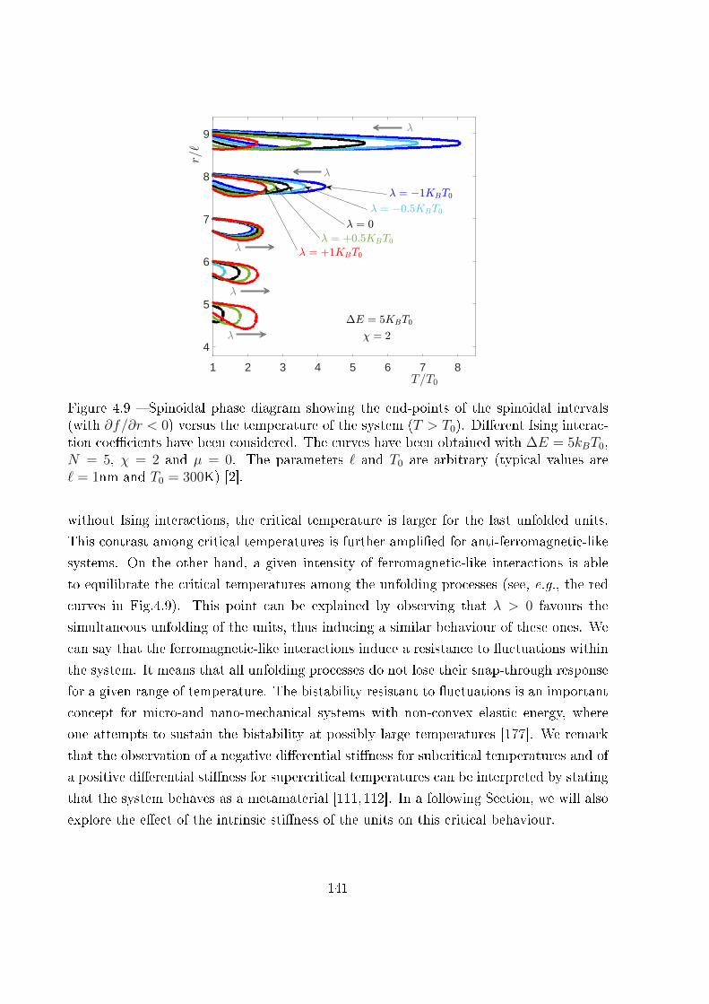
1 2 3 4 5 6 7 8
4
5
6
7
8
9
Figure 4.9 � Spinoidal phase diagram showing the end-points of the spinoidal intervals(with ∂f/∂r < 0) versus the temperature of the system (T > T0). Di�erent Ising interac-tion coe�cients have been considered. The curves have been obtained with ∆E = 5kBT0,N = 5, χ = 2 and µ = 0. The parameters ` and T0 are arbitrary (typical values are` = 1nm and T0 = 300K) [2].
without Ising interactions, the critical temperature is larger for the last unfolded units.
This contrast among critical temperatures is further ampli�ed for anti-ferromagnetic-like
systems. On the other hand, a given intensity of ferromagnetic-like interactions is able
to equilibrate the critical temperatures among the unfolding processes (see, e.g., the red
curves in Fig.4.9). This point can be explained by observing that λ > 0 favours the
simultaneous unfolding of the units, thus inducing a similar behaviour of these ones. We
can say that the ferromagnetic-like interactions induce a resistance to �uctuations within
the system. It means that all unfolding processes do not lose their snap-through response
for a given range of temperature. The bistability resistant to �uctuations is an important
concept for micro-and nano-mechanical systems with non-convex elastic energy, where
one attempts to sustain the bistability at possibly large temperatures [177]. We remark
that the observation of a negative di�erential sti�ness for subcritical temperatures and of
a positive di�erential sti�ness for supercritical temperatures can be interpreted by stating
that the system behaves as a metamaterial [111,112]. In a following Section, we will also
explore the e�ect of the intrinsic sti�ness of the units on this critical behaviour.
141
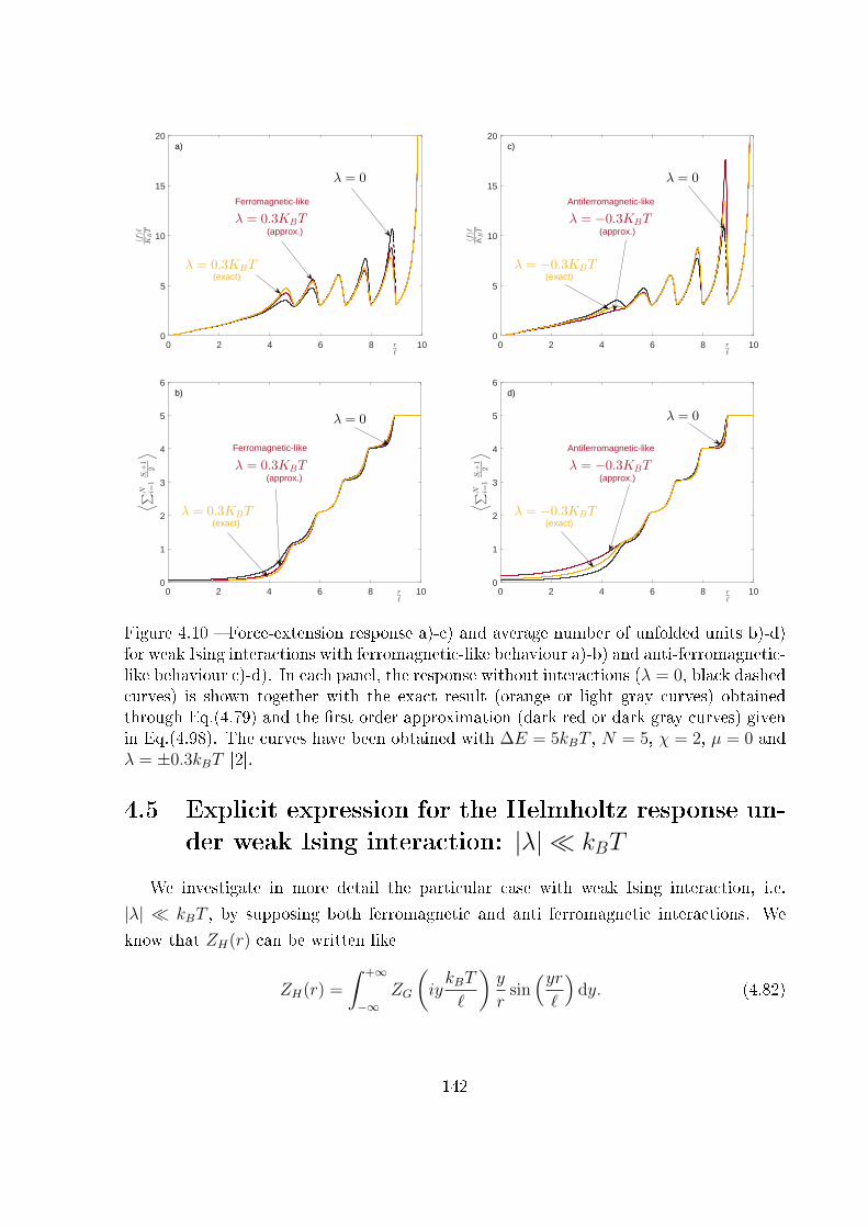
0 2 4 6 8 10rℓ
0
5
10
15
20〈f〉ℓ
KBT
λ = 0
(approx.)
Ferromagnetic-like
λ = 0.3KBT
λ = 0.3KBT(exact)
a)
0 2 4 6 8 10rℓ
0
5
10
15
20
〈f〉ℓ
KBT
λ = 0
(approx.)λ = −0.3KBT
Antiferromagnetic-like
(exact)λ = −0.3KBT
c)
0 2 4 6 8 10r
ℓ
0
1
2
3
4
5
6
⟨
∑
N i=1
Si+1
2
⟩
λ = 0
λ = 0.3KBT(approx.)
Ferromagnetic-like
(exact)λ = 0.3KBT
b)
0 2 4 6 8 10r
ℓ
0
1
2
3
4
5
6
⟨
∑
N i=1
Si+1
2
⟩
λ = 0
λ = −0.3KBT(approx.)
Antiferromagnetic-like
(exact)λ = −0.3KBT
d)
Figure 4.10 � Force-extension response a)-c) and average number of unfolded units b)-d)for weak Ising interactions with ferromagnetic-like behaviour a)-b) and anti-ferromagnetic-like behaviour c)-d). In each panel, the response without interactions (λ = 0, black dashedcurves) is shown together with the exact result (orange or light gray curves) obtainedthrough Eq.(4.79) and the �rst order approximation (dark red or dark gray curves) givenin Eq.(4.98). The curves have been obtained with ∆E = 5kBT , N = 5, χ = 2, µ = 0 andλ = ±0.3kBT [2].
4.5 Explicit expression for the Helmholtz response un-
der weak Ising interaction: |λ| � kBT
We investigate in more detail the particular case with weak Ising interaction, i.e.
|λ| � kBT , by supposing both ferromagnetic and anti ferromagnetic interactions. We
know that ZH(r) can be written like
ZH(r) =
∫ +∞
−∞ZG
(iykBT
`
)y
rsin(yr`
)dy. (4.82)
142
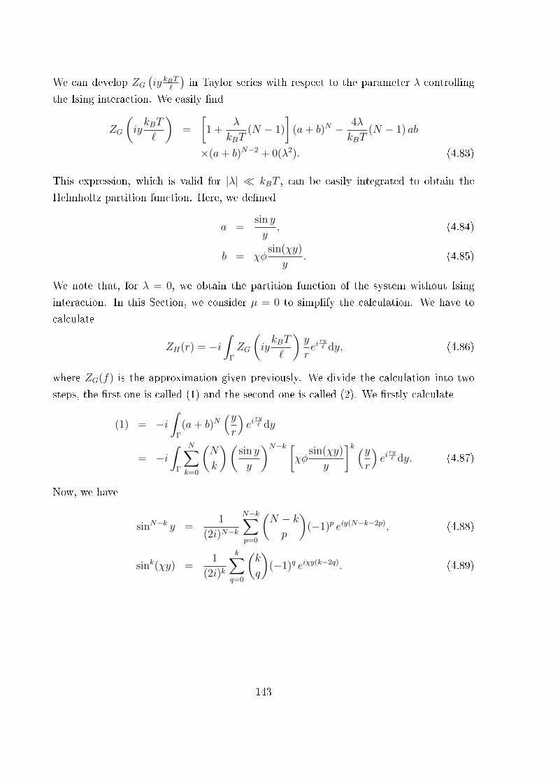
We can develop ZG(iy kBT
`
)in Taylor series with respect to the parameter λ controlling
the Ising interaction. We easily �nd
ZG
(iykBT
`
)=
[1 +
λ
kBT(N − 1)
](a+ b)N − 4λ
kBT(N − 1) ab
×(a+ b)N−2 + 0(λ2). (4.83)
This expression, which is valid for |λ| � kBT , can be easily integrated to obtain the
Helmholtz partition function. Here, we de�ned
a =sin y
y, (4.84)
b = χφsin(χy)
y. (4.85)
We note that, for λ = 0, we obtain the partition function of the system without Ising
interaction. In this Section, we consider µ = 0 to simplify the calculation. We have to
calculate
ZH(r) = −i∫
Γ
ZG
(iykBT
`
)y
reiry` dy, (4.86)
where ZG(f) is the approximation given previously. We divide the calculation into two
steps, the �rst one is called (1) and the second one is called (2). We �rstly calculate
(1) = −i∫
Γ
(a+ b)N(yr
)eiry` dy
= −i∫
Γ
N∑k=0
(N
k
)(sin y
y
)N−k [χφ
sin(χy)
y
]k (yr
)eiry` dy. (4.87)
Now, we have
sinN−k y =1
(2i)N−k
N−k∑p=0
(N − kp
)(−1)p eiy(N−k−2p), (4.88)
sink(χy) =1
(2i)k
k∑q=0
(k
q
)(−1)q eiχy(k−2q). (4.89)
143

Then, we �nd
(1) = −i∫
Γ
1
yN
N∑k=0
N−k∑p=0
k∑q=0
(N
k
)(N − kp
)(k
q
)1
(2i)N(−1)p+q (χφ)k
×eiy(N−k−2p+χk−2qχ)y
reiry` dy
= − 1
2N iN−1
1
r
N∑k=0
N−k∑p=0
k∑q=0
(N
k
)(N − kp
)(k
q
)(−1)p+q (χφ)k
×∫
Γ
eiy(N−k−2p+χk−2qχ+ r`)
yN−1dy. (4.90)
Now, we use the integral∫Γ
eiay
yNdy =
{0 if a > 0,
−2πiN aN−1
(N−1)!if a ≤ 0.
(4.91)
Hence, we obtain
(1) =π
2N−1
1
r(N − 2)!
N∑k=0
N−k∑p=0
k∑q=0
(N
k
)(N − kp
)(k
q
)×(−1)p+q (χφ)k (−λ)N−2 1(λ), (4.92)
where
−λ = N − k − 2p+ χk − 2χq +r
`. (4.93)
Now, we calculate the second integral given by
(2) = −i∫
Γ
ab (a+ b)N−2 y
reiry` dy
= −i∫
Γ
abN−2∑k=0
(N − 2
k
)bkaN−2k y
reiry` dy
= −i∫
Γ
N−2∑k=0
(N − 2
k
)bk+1aN−1−k y
reiry` dy. (4.94)
144

Here again, we develop the powers
(2) = −i∫
Γ
N−2∑k=0
k+1∑q=0
N−1−k∑p=0
(N − 2
k
)(k + 1
q
)(N − 1− k
p
)y
reiry`
×(−1)p+q1
(2i)N1
yN(χφ)k+1 eiχy(k+1−q)e−iχyqeiy(N−1−k−p)e−iypdy
= −i∫
Γ
N−2∑k=0
k+1∑q=0
N−1−k∑p=0
(N − 2
k
)(k + 1
q
)(N − 1− k
p
)(−1)p+q
×(χφ)k+1
(2i)N1
r yN−1e(iy[N−1−k−p−p−χq−χq+χk+χ+ r
` ])dy. (4.95)
By using Eq.(4.91), we get
(2) =N−2∑k=0
k+1∑q=0
N−1−k∑p=0
(N − 2
k
)(k + 1
q
)(N − 1− k
p
)(−1)p+q
× (χφ)k+1 π
2N−1
1
r(N − 2)!(−λ0)N−2 1 (λ0) , (4.96)
where
−λ0 = N − 1− k − 2p− 2χq + χk + χ+r
`. (4.97)
Finally, the partition function reads
ZH(r) =π
2N−1(N − 2)!r
N∑k=0
N−k∑p=0
k∑q=0
(N
k
)(N − kp
)(k
q
)[1 +
λ
kBT(N − 1)
](−1)p+q
× (χφ)k (−λ)N−2 1(λ)− π
2N−1(N − 2)!r
N−2∑k=0
k+1∑q=0
N−1−k∑p=0
(N − 2
k
)(k + 1
q
)×(N − 1− k
p
)(−1)p+q (χφ)k+1 4λ
kBT(N − 1) (−λ0)N−2 1(λ0). (4.98)
This is the �nal form of the Helmholtz partition function, calculated under the hypothesis
of weak Ising interaction. In this expression, there are no limitations concerning the
parameter χ. We note that, for λ = 0, we obtain the partition function of the system
without Ising interactions, as discussed in recent literature [113]. In Fig.4.10, one can �nd
some results for λ = 0, λ = +0.3kBT and λ = −0.3kBT . We plotted the force-extension
curves and the average number of unfolded units for both ferromagnetic-like and anti-
ferromagnetic-like interactions. In each case, we compared the approximated result stated
in Eq.(4.98) (dark red or dark gray curves), the exact result given in Eq.(4.79) (orange
145
or light gray curves), and the response without Ising interactions (black dashed curves).
We note a good agreement between approximated and exact results both for λ < 0 and
λ > 0. Concerning the interpretation of the curves, the discussion reported at the end of
Section 4.4 remains valid for all results of Fig.4.10.
4.6 Explicit expression for the Helmholtz response un-
der strong Ising ferromagnetic interaction: λ �kBT
We introduce here an asymptotic development concerning the case of a strong Ising
ferromagnetic-like interaction. If λ → +∞, then e− λkBT → 0, and therefore it is not
di�cult to obtain the asymptotic expression for ZG(f) when λ→∞. The result is
ZG
(iykBT
`
)= exp
[λ(N − 1)
kBT
] [(sin y
y
)N+
(χφ
sin(χy)
y
)N]. (4.99)
Therefore, we easily determine the Helmholtz partition function, as
ZH(r) = −i∫
Γ
ZG
(iykBT
`
)y
reiry` dy
= −i∫
Γ
exp
[λ(N − 1)
kBT
] [sinN y + (χφ)N sinN(χy)
] 1
yN−1reiry` dy
= −i 1
(2i)Nexp
[λ(N − 1)
kBT
] N∑k=0
(N
k
)(−1)k
(1
r
)[(N − 2k + r
`
)N−2
(N − 2)!
×1(
2k −N − r
`
)(−2π)iN−1 + (χφ)N (−2π)iN−1
×(χN − 2χk + r
`
)N−2
(N − 2)!1(
2χk − χN − r
`
)]. (4.100)
Finally,
ZH(r) =π
2N−1r(N − 2)!exp
[λ(N − 1)
kBT
] N∑k=0
(N
k
)(−1)k
×[(N − 2k +
r
`
)N−2
1(
2k −N − r
`
)+ (χφ)N
(χN − 2χk +
r
`
)N−2
1(
2χk − χN − r
`
)]. (4.101)
which is valid for strong ferromagnetic-like Ising interactions.
An application of this expression is shown in Fig.4.11. In particular, we compare the
146

0 2 4 6 8 10rℓ
0
5
10
15
20
〈f〉ℓ
KBT
λ = 0.5jKBT(exact ∀j = 1, ..., 14)
Ferromagnetic-like
λ = 0
λ → ∞(asympt.)
a)
0 2 4 6 8 10rℓ
0
1
2
3
4
5
⟨
∑
N i=1Si+
12
⟩
λ = 0 λ = 0.5jKBT(exact ∀j = 1, ..., 14)
λ → ∞
(asympt.)
b)
0 2 4 6 8 10rℓ
-50
-40
-30
-20
-10
0
10
20
30
−
F
KBT=
logZH
λ = 0.5jKBT(exact ∀j = 1, ..., 14)
λ = 0
λ → ∞
(asympt.)
c)
Figure 4.11 � Force-extension response a), average number of unfolded units b) andHelmholtz free energy c) for a chain with strong ferromagnetic-like interactions. In eachpanel, the response without interactions (λ = 0, black dashed curves) is shown togetherwith the exact results for an increasing ferromagnetic interaction (λ = 0.5jkBT∀j =1, ..., 14, red or gray curves) and the asymptotic expansion (λ→∞, yellow or light graycurves) given in Eq.(4.101). The curves have been obtained with ∆E = 5kBT , N = 5,χ = 2 and µ = 0 [2].
147

approximated result in Eq.(4.101) (yellow or light gray curve) with the exact response
obtained from Eq.(4.79) for λ = 0.5, 1, 1.5, ..., 7kBT (red or gray curves) and with the
response without Ising interactions (black dashed curve). In Fig.4.11, one can �nd the
force-extention curves, the average number of unfolded units and the Helmholtz free en-
ergy. It is interesting to discuss the evolution of the overall behaviour of the system with
an increasing interaction coe�cient. Indeed, as λ is increased, the units are progressively
favoured to be in the same state, and therefore there is an increasing average number
of units which unfolds at r = N`. It means that the number of unfolding processes at
r = N` is a growing function of the Ising coe�cient λ, going from 1 with λ = 0 to N with
λ approaching in�nity. This can be seen in Fig.4.11.b, where this process is represented
by the series of red curves (or gray) with increasing λ, and it ends with the yellow (or
light gray) curve obtained through Eq.(4.101). The latter means that all units unfold at
the same time at r = N` when λ → ∞, and this behaviour is perfectly caught by the
asymptotic development. Accordingly, the peaks in the force-extension curve are strongly
modi�ed by increasing λ: while the �rst peak becomes more and more pronounced, the
others are progressively reduced, as shown in Fig.4.11.a. As a matter of fact, the �rst peak
corresponds to the simultaneous unfolding of the units when λ is very large. Hence, in the
limiting case of λ→∞, the force-extension curve is composed of only one peak (yellow or
light gray curve), as one can see in Fig.4.11.a. Of course, the origin of peaks modi�cation
in the force-extension curve and of the steps structure in the average number of unfolded
units can be observed in the plot of the Helmholtz free energy, shown in in Fig.4.11.c.
Here, we can see the evolution of the typical cusps with the increasing Ising coe�cient.
As an example, the collapse of all the force peaks into a single unfolding event explains
the tandem repeats behaviour in red cell spectrin, where two units unfold simultaneously
because of a strong cooperativity [114].
4.7 Explicit expression for the Helmholtz response un-
der strong Ising anti-ferromagnetic interaction: λ�−kBT
We discuss here the development of the theory under strong Ising anti-ferromagnetic-
like interactions. As before, we can develop the Gibbs partition function in Taylor series
for λ→ −∞, i.e. x = e− λkBT → +∞.
148
The result is
ZG
(iykBT
`
)= xN−1P
N2
[(1 +
1
2
S
P12
)+ (−1)N
(1− 1
2
S
P12
)]= xN−1
[P
N2
[1 + (−1)N
]+
1
2P
N−12 S
[1− (−1)N
]]. (4.102)
And so, we can summarise it as
ZG
(iykBT
`
)=
{xN−1P
N2 if N is even,
xN−1SPN−1
2 if N is odd.(4.103)
where
S =sin y
y+ χφ
sin(χy)
y= a+ b, (4.104)
P =sin y
yχφ
sin(χy)
y= ab. (4.105)
We �rst elaborate the Helmholtz partition function for N odd as
ZH(r) = −i∫
Γ
ZG
(iykBT
`
)y
reiry` dy
= −i∫
Γ
xN−1
yN−1[sin y + χφ sin(χy)] [χφ sin y sin(χy)]
N−12
1
reiry` dy
= −ixN−1
r(χφ)
N−12
∫Γ
1
yN−1
[sin
N+12 (y) sin
N−12 (χy)
+χφ sinN−1
2 (y) sinN+1
2 (χy)]eiry` dy. (4.106)
Now, we use the relation
sink y =1
(2i)k
k∑p=0
(k
p
)(−1)peiy(k−2p), (4.107)
and we have
ZH(r) = −ixN−1
r(χφ)
N−12
∫Γ
1
yN−1
1
(2i)N+1
2
N+12∑
p=0
(N+1
2
p
)(−1)peiy(
N+12−2p)
× 1
(2i)N−1
2
N−12∑
q=0
(N−1
2
q
)(−1)qeiyχ(
N−12−2q) + χφ
1
(2i)N−1
2
N−12∑
q=0
(N−1
2
q
)(−1)q
×eiy(N−12−2q) 1
(2i)N+1
2
N+12∑
p=0
(N+1
2
p
)(−1)peiyχ(
N+12−2p)
ei ry` dy. (4.108)
149
This expression can be reorganised like
ZH(r) = −ixN−1
r(χφ)
N−12
1
(2i)N
N+12∑
p=0
N−12∑
q=0
(N+1
2
p
)(N−1
2
q
)(−1)p+q
×[∫
Γ
1
yN−1eiy(
N+12−2p+χN−1
2−2χq+ r
` )dy
+χφ
∫Γ
1
yN−1eiy(
N−12−2q+χN+1
2−2χp+ r
` )dy
]. (4.109)
Now, since we know that∫Γ
eiay
ymdy = −2πim
am−1
(m− 1)!1(−a), (4.110)
we get
ZH(r) = −ixN−1
r(χφ)
N−12
1
(2i)N
N+12∑
p=0
N−12∑
q=0
(N+1
2
p
)(N−1
2
q
)(−1)p+q
×[−2πiN−1 (−λa)N−2
(N − 2)!1 (λa) + χφ(−2π)iN−1 (−λb)N−2
(N − 2)!1 (λb)
], (4.111)
where
λa = 2p− N + 1
2− χN − 1
2+ 2χq − r
`, (4.112)
λb = 2q − N − 1
2− χN + 1
2+ 2χp− r
`. (4.113)
We simplify the expression by reorganising it and we obtain the following expression for
the Helmholtz partition function under strong Ising anti-ferromagnetic interaction, for N
odd
ZH(r) =2π
2N
exp[− λkBT
(N − 1)]
(N − 2)!
1
r(χφ)
N−12
N+12∑
p=0
N−12∑
q=0
(N+1
2
p
)(N−1
2
q
)×(−1)p+q
[(−λa)N−2 1 (λa) + χφ (−λb)N−2 1 (λb)
]. (4.114)
150
We calculate now the same quantity for N even
ZH(r) = −i∫
Γ
ZG
(iykBT
`
)y
reiry` dy
= −i∫
Γ
xN−1
(sin y
yχφ
sin(χy)
y
)N2 y
reiry` dy
= −ixN−1 (χφ)N2
1
r
∫Γ
1
yN−1sin
N2 (y) sin
N2 (χy) ei
ry` dy
= −ixN−1 (χφ)N2
1
r
1
(2i)N
N2∑
p=0
N2∑
q=0
(N2
p
)(N2
q
)(−1)p+q
×(−2π)iN−1 (−λc)N−2 1
(N − 2)!1 (−λc) , (4.115)
where λc = 2p − N2
+ 2χq − χN2− r
`. Finally, we get the following expression for the
Helmholtz partition function under strong Ising anti-ferromagnetic interaction
ZH(r) =2π
2N
exp[− λkBT
(N − 1)]
(N − 2)!
1
r(χφ)
N2
N2∑
p=0
N2∑
q=0
(N2
p
)(N2
q
)×(−1)p+q (−λc)N−2 1 (λc) , (4.116)
which is valid for N even. The solutions given in Eqs.(4.114) and (4.116) represent the
most important result of this Section and must be discussed as follows.
An example of application of Eq.(4.114) for N odd can be found in Fig.4.12, where
force-extension curves, average number of unfolded units and Helmholtz free energy are
represented for several values of λ. When we consider an increasing value of |λ| (λ < 0),
we observe that the �rst force peaks tend to disappear while the last ones become more
and more pronounced (see Fig.4.12.a). This is coherent with the assumption that, in an
anti-ferromagnetic-like system, the favoured states are alternatively folded and unfolded.
Accordingly, with an increasing value of |λ| (λ < 0), we have an increasing number of
unfolded units in the initial con�guration with r = 0. Clearly, the maximum value of this
number of unfolded units with r = 0 is (N − 1)/2 and not (N + 1)/2 since the unfolded
units are costly from the energetic point of view and the system chooses the con�guration
with the smallest number of unfolded units between (N − 1)/2 and (N + 1)/2. This
overall interpretation of Fig.4.12 must be improved to better understand the yellow (or
light gray) curves corresponding to λ→∞. So, if we look at the equation for N odd, we
note that ZH(r) is di�erent from 0 where λa > 0 or λb > 0. It means that
2p− N + 1
2− χN − 1
2+ 2χq − r
`> 0 (4.117)
151
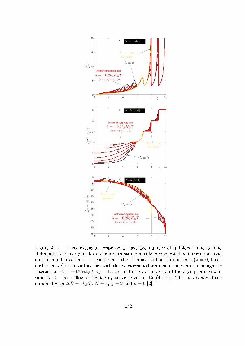
0 2 4 6 8 10rℓ
0
5
10
15
20
〈f〉ℓ
KBT
m=5 (odd)
Antiferromagnetic-like
λ = −0.25jKBT(exact ∀j = 1, ..., 6)
λ = 0
λ → −∞(asympt.)
N=5 (odd)a)
0 2 4 6 8 10rℓ
0
1
2
3
4
5
⟨
∑
N i=1Si+
12
⟩
Antiferromagnetic-like
λ = −0.25jKBT(exact ∀j = 1, ..., 6)
λ = 0
λ → −∞(asympt.)
N=5 (odd)b)
0 2 4 6 8 10rℓ
-45
-40
-35
-30
-25
-20
-15
-10
-5
0
−
F
KBT=
logZH
λ = 0
Antiferromagnetic-like
λ = −0.25jKBT(exact ∀j = 1, ..., 6)
(asympt.)
λ → −∞
c) N=5 (odd)
Figure 4.12 � Force-extension response a), average number of unfolded units b) andHelmholtz free energy c) for a chain with strong anti-ferromagnetic-like interactions andan odd number of units. In each panel, the response without interactions (λ = 0, blackdashed curve) is shown together with the exact results for an increasing anti-ferromagneticinteraction (λ = −0.25jkBT ∀j = 1, ..., 6, red or gray curves) and the asymptotic expan-sion (λ → −∞, yellow or light gray curve) given in Eq.(4.114). The curves have beenobtained with ∆E = 5kBT , N = 5, χ = 2 and µ = 0 [2].
152

0 1 2 3 4 5 6 7 8rℓ
0
5
10
15
20
〈f〉ℓ
KBT
λ = 0
λ = −0.25jKBT(exact ∀j = 1, ..., 6)
Antiferromagnetic-like
λ → −∞(asympt.)
N=4 (even)a)
0 1 2 3 4 5 6 7 8rℓ
0
0.5
1
1.5
2
2.5
3
3.5
4
⟨
∑
N i=1Si+
12
⟩
Antiferromagnetic-like
λ = −0.25jKBT(exact ∀j = 1, ..., 6)
λ → −∞(asympt.)
λ = 0
N=4 (even)b)
0 1 2 3 4 5 6 7 8rℓ
-35
-30
-25
-20
-15
-10
-5
0
−
F
KBT=
logZH
λ = 0
Antiferromagnetic-like
(exact ∀j = 1, ..., 6)
λ = −0.25jKBT
λ → −∞
(asympt.)
N=4 (even)c)
Figure 4.13 � Force-extension response a), average number of unfolded units b) andHelmholtz free energy c) for a chain with strong anti-ferromagnetic-like interactions andan even number of units. In each panel, the response without interactions (λ = 0, blackdashed curve) is shown together with the exact results for an increasing anti-ferromagneticinteraction (λ = −0.25jkBT ∀j = 1, ..., 6, red or gray curves) and the asymptotic expan-sion (λ → −∞, yellow or light gray curve) given in Eq.(4.116). The curves have beenobtained with ∆E = 5kBT , N = 4, χ = 2 and µ = 0 [2].
153
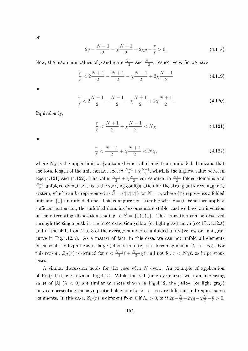
or
2q − N − 1
2− χN + 1
2+ 2χp− r
`> 0. (4.118)
Now, the maximum values of p and q are N+12
and N−12, respectively. So we have
r
`< 2
N + 1
2− N + 1
2− χN − 1
2+ 2χ
N − 1
2(4.119)
or
r
`< 2
N − 1
2− N − 1
2− χN + 1
2+ 2χ
N + 1
2. (4.120)
Equivalently,
r
`<N + 1
2+ χ
N − 1
2< Nχ (4.121)
or
r
`<N − 1
2+ χ
N + 1
2< Nχ, (4.122)
where Nχ is the upper limit of r`, attained when all elements are unfolded. It means that
the total length of the unit can not exceed N−12
+χN+12, which is the highest value between
Eqs.(4.121) and (4.122). The value N+12
+ χN−12
corresponds to N+12
folded domains andN−1
2unfolded domains: this is the starting con�guration for the strong anti-ferromagnetic
system, which can be represented as ~S = {↑↓↑↓↑} forN = 5, where {↑} represents a foldedunit and {↓} an unfolded one. This con�guration is stable with r = 0. When we apply a
su�cient extension, the unfolded domains become more stable, and we have an inversion
in the alternating disposition leading to ~S = {↓↑↓↑↓}. This transition can be observed
through the single peak in the force-extension yellow (or light gray) curve (see Fig.4.12.a)
and in the shift from 2 to 3 of the average number of unfolded units (yellow or light gray
curve in Fig.4.12.b). As a matter of fact, in this case, we can not unfold all elements
because of the hypothesis of large (ideally in�nite) anti-ferromagnetism (λ → −∞). For
this reason, ZH(r) is de�ned for r < N−12` + N+1
2χ` and not for r < Nχ`, as in previous
cases.
A similar discussion holds for the case with N even. An example of application
of Eq.(4.116) is shown in Fig.4.13. While the red (or gray) curves with an increasing
value of |λ| (λ < 0) are similar to those shown in Fig.4.12, the yellow (or light gray)
curves representing the asymptotic behaviour for λ→ −∞ are di�erent and require some
comments. In this case, ZH(r) is di�erent from 0 if Λc > 0, or if 2p−N2
+2χq−χN2− r
`> 0.
154
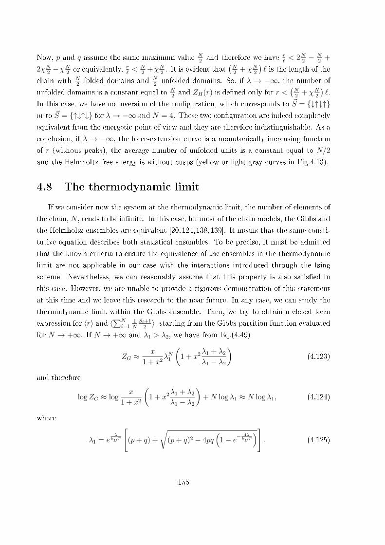
Now, p and q assume the same maximum value N2and therefore we have r
`< 2N
2− N
2+
2χN2−χN
2or equivalently, r
`< N
2+χN
2. It is evident that
(N2
+ χN2
)` is the length of the
chain with N2folded domains and N
2unfolded domains. So, if λ → −∞, the number of
unfolded domains is a constant equal to N2and ZH(r) is de�ned only for r <
(N2
+ χN2
)`.
In this case, we have no inversion of the con�guration, which corresponds to ~S = {↓↑↓↑}or to ~S = {↑↓↑↓} for λ→ −∞ and N = 4. These two con�guration are indeed completely
equivalent from the energetic point of view and they are therefore indistinguishable. As a
conclusion, if λ → −∞, the force-extension curve is a monotonically increasing function
of r (without peaks), the average number of unfolded units is a constant equal to N/2
and the Helmholtz free energy is without cusps (yellow or light gray curves in Fig.4.13).
4.8 The thermodynamic limit
If we consider now the system at the thermodynamic limit, the number of elements of
the chain, N , tends to be in�nite. In this case, for most of the chain models, the Gibbs and
the Helmholtz ensembles are equivalent [20,124,138,139]. It means that the same consti-
tutive equation describes both statistical ensembles. To be precise, it must be admitted
that the known criteria to ensure the equivalence of the ensembles in the thermodynamic
limit are not applicable in our case with the interactions introduced through the Ising
scheme. Nevertheless, we can reasonably assume that this property is also satis�ed in
this case. However, we are unable to provide a rigorous demonstration of this statement
at this time and we leave this research to the near future. In any case, we can study the
thermodynamic limit within the Gibbs ensemble. Then, we try to obtain a closed form
expression for 〈r〉 and 〈∑Ni=1
1NSi+1
2〉, starting from the Gibbs partition function evaluated
for N → +∞. If N → +∞ and λ1 > λ2, we have from Eq.(4.49)
ZG ≈x
1 + x2λN1
(1 + x2λ1 + λ2
λ1 − λ2
)(4.123)
and therefore
logZG ≈ logx
1 + x2
(1 + x2λ1 + λ2
λ1 − λ2
)+N log λ1 ≈ N log λ1, (4.124)
where
λ1 = eλ
kBT
[(p+ q) +
√(p+ q)2 − 4pq
(1− e−
4λkBT
)]. (4.125)
155

λ
kBT
20
1506 104
0.5
Ferrom
agnetic-like
Antiferrom
agnetic-like
2 fℓ
KBT0 5
lim
N→∞
〈r〉
Nℓ
-2
1
-4 0-6
1.5
2
a)
λ
kBT
20
1506
fℓKBT
104 Antiferrom
agnetic-like
20 5
-2-4
0.5
lim
N→∞〈1 N
∑N i=
1Si+
12
〉
0-6
1
Ferrom
agnetic-likeb)
Figure 4.14 � Average normalised extension a) and average number of unfolded unitsb) versus the applied normalised force and the coe�cient λ
kBTfor a chain with Ising
interactions at the thermodynamic equilibrium within the Gibbs ensemble.
We have
〈r〉 = kBT∂
∂flogZG ≈ kBT
∂
∂fN log λ1. (4.126)
Here,
p =1
2e− µkBT
sinh ξ
ξ, (4.127)
q =1
2e
µkBT
sinh(χξ)
ξχφ, (4.128)
156
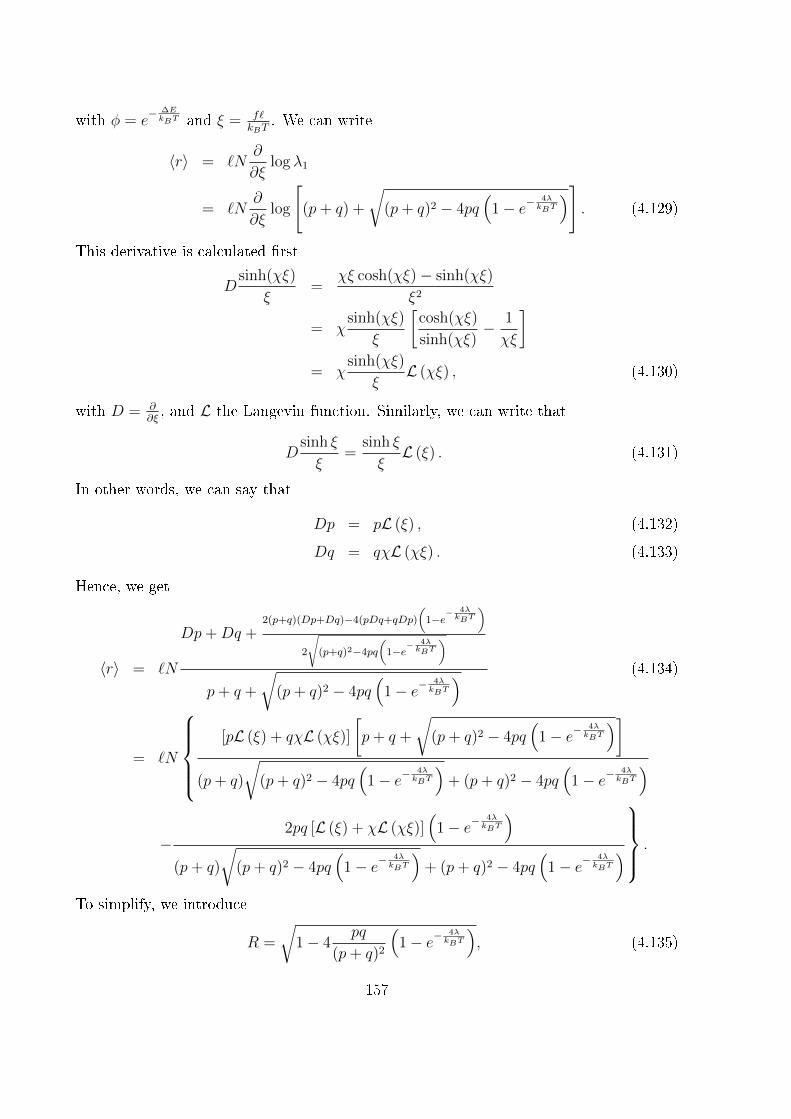
with φ = e− ∆EkBT and ξ = f`
kBT. We can write
〈r〉 = `N∂
∂ξlog λ1
= `N∂
∂ξlog
[(p+ q) +
√(p+ q)2 − 4pq
(1− e−
4λkBT
)]. (4.129)
This derivative is calculated �rst
Dsinh(χξ)
ξ=
χξ cosh(χξ)− sinh(χξ)
ξ2
= χsinh(χξ)
ξ
[cosh(χξ)
sinh(χξ)− 1
χξ
]= χ
sinh(χξ)
ξL (χξ) , (4.130)
with D = ∂∂ξ, and L the Langevin function. Similarly, we can write that
Dsinh ξ
ξ=
sinh ξ
ξL (ξ) . (4.131)
In other words, we can say that
Dp = pL (ξ) , (4.132)
Dq = qχL (χξ) . (4.133)
Hence, we get
〈r〉 = `N
Dp+Dq +2(p+q)(Dp+Dq)−4(pDq+qDp)
(1−e
− 4λkBT
)2
√(p+q)2−4pq
(1−e
− 4λkBT
)
p+ q +
√(p+ q)2 − 4pq
(1− e−
4λkBT
) (4.134)
= `N
[pL (ξ) + qχL (χξ)]
[p+ q +
√(p+ q)2 − 4pq
(1− e−
4λkBT
)](p+ q)
√(p+ q)2 − 4pq
(1− e−
4λkBT
)+ (p+ q)2 − 4pq
(1− e−
4λkBT
)
−2pq [L (ξ) + χL (χξ)]
(1− e−
4λkBT
)(p+ q)
√(p+ q)2 − 4pq
(1− e−
4λkBT
)+ (p+ q)2 − 4pq
(1− e−
4λkBT
) .
To simplify, we introduce
R =
√1− 4
pq
(p+ q)2
(1− e−
4λkBT
), (4.135)
157

and
ν =q
p+ q. (4.136)
Then, we have
1− ν = 1− q
p+ q=
p
p+ q, (4.137)
and we can write
R =
√1− 4ν(1− ν)
(1− e−
4λkBT
). (4.138)
Therefore, p+ q +
√(p+ q)2 − 4pq
(1− e−
4λkBT
)= (p+ q)(1 +R), and we obtain
〈r〉 = N`
pL(ξ)+qχL(χξ)p+q
− 21+R
pq(p+q)2 [L (ξ) + χL (χξ)]
(1− e−
4λkBT
)1− 4
1+Rpq
(p+q)2
(1− e−
4λkBT
)= N`
pL(ξ)+qχL(χξ)p+q
− 1−R2
1+R[L(ξ)+χL(χξ)]
2
1− 1−R2
1+R
, (4.139)
where we used the simple property 1−R2 = 4 pq(p+q)2
(1− e−
4λkBT
).
We �nally obtain
〈r〉N`
=1
R[(1− ν)L (ξ) + νχL (χξ)] +
(1− 1
R
) L (ξ) + χL (χξ)
2, (4.140)
which is the �rst important result in this Section. We can perform a similar calculation
to �nd ⟨N∑i=1
Si + 1
2
⟩= −kBT
∂
∂∆ElogZG
≈ −kBTN∂
∂∆Elog λ1. (4.141)
Since φ = e− ∆EkBT , we have that
∂∆
∂∆E=∂∆
∂φ
∂φ
∂∆E=∂∆
∂φφ
( −1
kBT
), (4.142)
where ∆ is an arbitrary function. So, we have⟨1
N
N∑i=1
Si + 1
2
⟩= φ
∂
∂φlog λ1. (4.143)
158
Therefore,⟨1
N
N∑i=1
Si + 1
2
⟩= φ
∂
∂φlog
[p+ q +
√(p+ q)2 − 4pq
(1− e−
4λkBT
)]
= φ
q′ +2(p+q)q′−4pq′
(1−e
− 4λkBT
)2
√(p+q)2−4pq
(1−e
− 4λkBT
)
p+ q +
√(p+ q)2 − 4pq
(1− e−
4λkBT
) , (4.144)
where q′ = ∂q∂φ
= qφ. Hence,
⟨1
N
N∑i=1
Si + 1
2
⟩=
q
√(p+ q)2 − 4pq
(1− e−
4λkBT
)+ (p+ q)q − 2pq
(1− e−
4λkBT
)[p+ q +
√(p+ q)2 − 4pq
(1− e−
4λkBT
)]√(p+ q)2 − 4pq
(1− e−
4λkBT
)=
q(q + p)R + (p+ q)q − 2pq(
1− e−4λkBT
)(p+ q)(R + 1)(p+ q)R
. (4.145)
Since 1−R2 = 4 pq(p+q)2
(1− e−
4λkBT
), we obtain⟨
1
N
N∑i=1
Si + 1
2
⟩=
q(p+ q)(R + 1)− 12(1−R2)(p+ q)2
(p+ q)2R(1 +R)
=q − 1
2(1−R)(p+ q)
(p+ q)R
=1
R
(q
p+ q
)+
1
2
(R− 1
R
). (4.146)
Finally, ⟨1
N
N∑i=1
Si + 1
2
⟩=
1
Rν +
1
2
(1− 1
R
), (4.147)
which is the second important result of this Section. Eq.(4.140) and Eq.(4.147), combined
with Eq.(4.136) and Eq.(4.138), give the complete solution for the system in thermody-
namic limit (i.e. N → ∞). A numerical application of these equations can be found
in Fig.4.14. Here, we show the average normalised extension and the average number of
unfolded units versus the applied normalised force and the Ising coe�cient λkBT
. We can
observe that for large and positive values of λ, all the units unfold cooperatively for a given
threshold force. This can be seen in the heavily pronounced force plateau in Fig.4.14.a
159
and in the sharp transition from 0 to 1 in Fig.4.14.b. On the other hand, for large and
negative values of λ, the units remain alternatively folded and unfolded for any value
of the applied force. This can be seen in the smooth force-extension curve correspond-
ing to a freely jointed chain response with half units folded and half units unfolded (see
Fig.4.14.a). Moreover, this behaviour is con�rmed by the average value of the number of
unfolded unit, which is equal to 12(see Fig.4.14.b). For intermediate values of λ, we can
observe a continuous transitional behaviour of the system from the anti-ferromagnetic to
the ferromagnetic response.
4.9 Ising interactions coupled with extensible units
We consider now a chain of bistable units characterised by a �nite intrinsic elastic
constant. We start the analysis by considering the Gibbs ensemble de�ned through the
extended Hamiltonian given in Eq.(4.2). Here, for the sake of simplicity, we suppose that
the folded and unfolded basins of the potential energy shown in Fig.4.2 exhibit the same
�nite elastic constant k(−1) = k(+1) = κ. In this case, it is not di�cult to prove that
Eq.(4.8) of Section 4.3 can be substituted by the approximated result
I = exp
(f 2
2κkBT
) N∏i=1
sinh[f`(Si)kBT
]f`(Si)kBT
`2(Si)
`2, (4.148)
which can be easily proved by calculating the exact solution of Eq.(4.6) and by considering
its approximation for relatively high values of κ. The details of this calculation can be
found in recent literature [1] and in Chapter 3. Typical values of κ for real macromolecules
are compatible with such approximations [168]. Coherently with Eq.(4.148), the Gibbs
partition function can be obtained as
ZG(f) =x
1 + x2exp
(Nαξ2
2
)×[λN1
(1 + x2λ1 + λ2
λ1 − λ2
)+ λN2
(1− x2λ1 + λ2
λ1 − λ2
)], (4.149)
where, with respect to Eq.(4.49) of Section 4.3, we only added an exponential term,
which is quadratic in the normalised force ξ = f`kBT
and de�ned through a coe�cient
α = kBTκ`2
. This latter represents the ratio between the thermal energy and the elastic
one, thus measuring the compromise between the enthalpic contribution and �uctuations.
The parameters x, λ1 and λ2 remain de�ned as in Section 4.3. Concerning the Helmholtz
ensemble, the system is described by the Hamiltonian in Eq.(4.62), where, as before,
160
we assume that k(−1) = k(+1) = κ. The calculation of the corresponding partition
function is based on the Laplace transform relation between the Gibbs and the Helmholtz
ensembles, summed up in Eq.(4.66). If we consider integer values for the parameter
χ (ratio between unfolded and folded lengths), the analytic continuation of the Gibbs
partition function assumes the form
ZG
(iykBT
`
)=
1
yNexp
(−Nαy
2
2
)P (y), (4.150)
where P (y) is the periodic function de�ned in Eq.(4.72) and described by the Fourier
coe�cients given in Eq.(4.74). The Helmholtz partition function can be �nally determined
as
ZH(r) = −i∫
Γ
ZG
(iykBT
`
)y
reyr` dy
= −i∫
Γ
P (y)
yNy
re−
Nαy2
2 eiry` dy
= −i+∞∑
k=−∞
Ck1
r
∫Γ
1
yN−1e−
Nαy2
2 ei(k+ r` )ydy
= −i+∞∑
k=−∞
Ck1
rJN−1
(k +
r
`,Nα
2
)(4.151)
where we used the Fourier development of the function P (y) in order to perform the
calculation. To complete the task, we have to calculate a sequence of integral of the form
JN(a, b) =
∫Γ
eiaye−by2 dy
yN, (4.152)
where a ∈ R, b > 0, N ∈ N and the path Γ is given in Fig.4.7. As largely discussed in
Chapter 3, an application of the complex variable method allows us to obtain the closed
form expression for this integral, as [1]
JN(a, b) =√π
{bN−1
2 e−a2
4b (2i)NH−N
(− a
2√b
)+1(−a)
N−1∑h=0
(ia)N−1−h(−4b)h/2
ih!(N − 1− h)!Γ
(h+ 1
2
)[1 + (−1)h
]}, (4.153)
where 1(x) represents the Heaviside step function, and H−N (z) are the generalisation of
the Hermite polynomials, obtained by considering negative indices (see Section 3.3.2 in
Chapter 3). We remember that they can be de�ned as [1, 172]
H−N(z) =1
(2i)N√π
∫ +∞
−∞
e−η2dη
(η − iz)N, (4.154)
161
and they can be obtained recursively through the following formula [1, 172]
H−(N+1)(z) =1
2NH−(N−1)(z)− z
NH−N(z), (4.155)
initialised with H0(z) = 1 ∀z ∈ R and H−1(z) =√π
2ez
2[1− erf (z)] for z > 0 and H−1(z)
odd, i.e. H−1(−z) = −H−1(z) [1,172]. This recursive law allows us to a�rm that H−N(z)
is odd if N is odd and that H−N(z) is even if N is even. We also remember that the
Hermite elements with N < 0 are not polynomials, contrarily to the classical Hermite
polynomials, de�ned with N > 0. Many other interesting properties of this sequence of
functions can be found in Ref. [172].
An application of the Gibbs and Helmholtz partition functions, stated in Eqs.(4.149)
and (4.151), respectively, is presented in Fig.4.15, where we show the force-extension
curves for two values of the constant κ, and for three values of the coe�cient λ. Firstly,
we note that the constant slope of the �nal part of the force-extension curves represents
the �nite e�ective sti�ness of the chain, after the unfolding processes. Moreover, it is
interesting to remark that the softer systems exhibit a sensibly reduced force peaks in the
Helmholtz response. This point can be also noticed by drawing a comparison between
Fig.4.8.a, obtained for κ→∞, and Fig.4.15, corresponding to �nite values of κ. A similar
phenomenon can be also observed in the phase diagram showing the critical behaviour of
the spinoidal response of the system. Indeed, we plotted in Fig.4.16 four phase diagrams
corresponding to four di�erent values of the elastic constant. We observe that the critical
temperatures of the unfolding processes are an increasing function of κ, similarly to the
previously discussed force peaks of the Helmholtz response. Besides, as already seen in
Fig.4.9 concerning the case with κ→∞, anti-ferromagnetic-like interactions amplify the
dissimilarity among the critical temperatures, while ferromagnetic-like interactions reduce
this contrast, eventually producing a more uniform response of the unfolding processes.
4.10 Conclusion
In this Chapter, we investigated the behaviour of a chain made of two-state units
coupled through an Ising interaction scheme with the coe�cient λ, providing a descrip-
tion of the e�ects of bistability and cooperativity in biological and arti�cial micro- and
nano-systems. Accordingly, we �rstly studied our model by means of the statistical me-
chanics of small systems, i.e. far from the thermodynamic limit. We analysed that the
force-extension response exhibits sharp or smooth transitions within the Gibbs ensemble
162
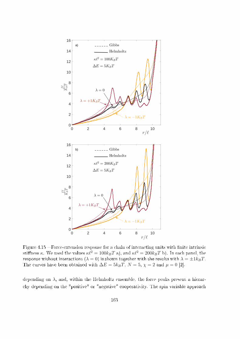
0 2 4 6 8 10r/ℓ
0
2
4
6
8
10
12
14
16
fℓ
KBT
κℓ2 = 100KBT
∆E = 5KBT
Gibbs
Helmholtz
λ = +1KBT
λ = 0
λ = −1KBT
a)
0 2 4 6 8 10r/ℓ
0
2
4
6
8
10
12
14
16
fℓ
KBT
Gibbs
Helmholtz
κℓ2 = 200KBT
∆E = 5KBT
λ = +1KBT
λ = 0
λ = −1KBT
b)
Figure 4.15 � Force-extension response for a chain of interacting units with �nite intrinsicsti�ness κ. We used the values κ`2 = 100kBT a), and κ`2 = 200kBT b). In each panel, theresponse without interactions (λ = 0) is shown together with the results with λ = ±1kBT .The curves have been obtained with ∆E = 5kBT , N = 5, χ = 2 and µ = 0 [2].
depending on λ, and, within the Helmholtz ensemble, the force peaks present a hierar-
chy depending on the "positive" or "negative" cooperativity. The spin variable approach
163
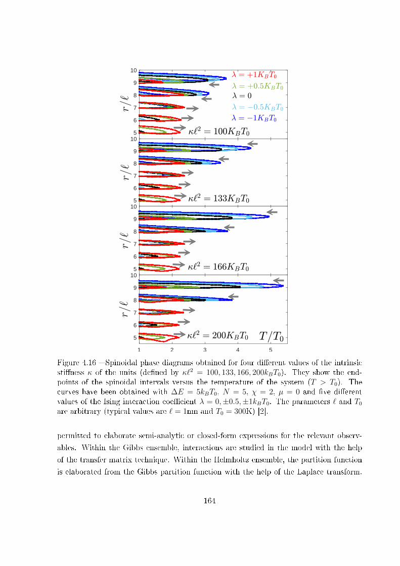
1 2 3 4 5
5
6
7
8
9
10
1 2 3 4 5
5
6
7
8
9
10
1 2 3 4 5
5
6
7
8
9
10
1 2 3 4 5
5
6
7
8
9
10
Figure 4.16 � Spinoidal phase diagrams obtained for four di�erent values of the intrinsicsti�ness κ of the units (de�ned by κ`2 = 100, 133, 166, 200kBT0). They show the end-points of the spinoidal intervals versus the temperature of the system (T > T0). Thecurves have been obtained with ∆E = 5kBT0, N = 5, χ = 2, µ = 0 and �ve di�erentvalues of the Ising interaction coe�cient λ = 0,±0.5,±1kBT0. The parameters ` and T0
are arbitrary (typical values are ` = 1nm and T0 = 300K) [2].
permitted to elaborate semi-analytic or closed-form expressions for the relevant observ-
ables. Within the Gibbs ensemble, interactions are studied in the model with the help
of the transfer matrix technique. Within the Helmholtz ensemble, the partition function
is elaborated from the Gibbs partition function with the help of the Laplace transform.
164
In addition, we propose results exploring asymptotic cases, and describing the behaviour
of the system under weak and strong Ising interactions (for both ferromagnetic-like and
anti-ferromagnetic-like schemes).
We also investigated a form of criticality exhibited by the system. Especially, our anal-
ysis focused on the critical behaviour of the spinoidal regions, characterising the part of
the isometric response, showing a negative di�erential elastic sti�ness. We proved that
each unfolding process exhibits a critical temperature de�ned by stating that we mea-
sure a negative di�erential sti�ness for subcritical temperatures and a positive di�erential
sti�ness for supercritical temperatures. This behaviour is in�uenced by the cooperativity,
which has the capability to make the critical temperatures of the unfolding processes more
uniform. We can therefore state that a positive cooperativity increases the resistance to
�uctuations, making the spinoidal intervals equally stable to temperature variations.
We �nally investigated the thermodynamic limit within the Gibbs ensemble and the gen-
eralisation of the theory with a �nite intrinsic elasticity of the units. A next improvement
to represent more realistic situations concerns the heterogeneity of all parameters de�ning
the properties of the chain units. Indeed, for the macromolecules of biological origin, such
as proteins, parameters should be freely chosen. Thus, it seems important to introduce
this point, in order to determine the full unfolding pathway, depending on the system
microstructure. As an example, this is directly related to the biological function of a
protein.
165

166

Chapter 5
Two-state heterogeneous chains
5.1 Introduction
In this Chapter, we investigate the behaviour of a chain of two-state units with a
heterogeneous distribution of the energy jumps between the folded and unfolded states.
For the sake of generality, we also consider the heterogeneous elastic constants, but we will
observe that they do not modify the qualitative behaviour of the chain. Previously, we
considered that all units were identical, being described by the potential energy of Fig.2.8
with the results discussed in previous Chapters 2, 3 and 4. The bimodal energy potential
of each unit is therefore composed of two potential wells with di�erent basal energies,
separated by a given energy barrier. For a chain made of homogeneous units, loaded by soft
or hard devices, all units have the same probability to unfold at each switching occurrence.
Therefore, it is impossible to identify an unfolding pathway, i.e. a sequence of well de�ned
unfolding processes. Conversely, the heterogeneity represents a quenched disorder from
the statistical mechanics point of view and is able to break the symmetry among the
units. Introducing an heterogeneous distribution of energy jumps will allow to obtain
an unfolding pathway, as the heterogeneity will generate di�erent unfolding probabilities
at each transition, eventually producing a preferential order in the units unfolding. It
is important to underline that the process corresponding to the complete unfolding of a
chain is a probabilistic event. Consequently, the observed pathway assumes a statistical
character. It means that if we repeat the experiment many times, we can observe, as
a result, di�erent unfolding pathways. As a matter of fact, the heterogeneity de�nes
di�erent probabilities for each pathway and therefore, it is possible to identify the most
probable unfolding pathway for a given chain. We will discuss this concept by introducing
the unfolding pathway identi�ability. It is worth noticing that the symmetry breaking
can also be obtained with non-local interactions between the units of the chain [178,179],
167
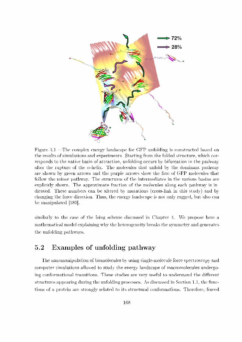
Figure 5.1 � The complex energy landscape for GFP unfolding is constructed based onthe results of simulations and experiments. Starting from the folded structure, which cor-responds to the native basin of attraction, unfolding occurs by bifurcation in the pathwayafter the rupture of the α-helix. The molecules that unfold by the dominant pathwayare shown by green arrows and the purple arrows show the fate of GFP molecules thatfollow the minor pathway. The structures of the intermediates in the various basins areexplicitly shown. The approximate fraction of the molecules along each pathway is in-dicated. These numbers can be altered by mutations (cross-link in this study) and bychanging the force direction. Thus, the energy landscape is not only rugged, but also canbe manipulated [180].
similarly to the case of the Ising scheme discussed in Chapter 4. We propose here a
mathematical model explaining why the heterogeneity breaks the symmetry and generates
the unfolding pathways.
5.2 Examples of unfolding pathway
The nanomanipulation of biomolecules by using single-molecule force spectroscopy and
computer simulations allowed to study the energy landscape of macromolecules undergo-
ing conformational transitions. These studies are very useful to understand the di�erent
structures appearing during the unfolding processes. As discussed in Section 1.1, the func-
tions of a protein are strongly related to its structural conformations. Therefore, forced
168
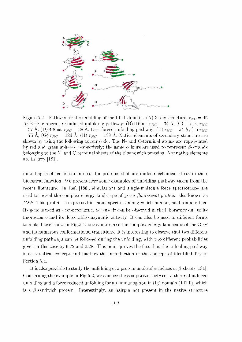
Figure 5.2 � Pathway for the unfolding of the 1TIT domain. (A) X-ray structure, rNC = 45Å; B�D temperature-induced unfolding pathway; (B) 0.6 ns, rNC = 34 Å, (C) 1.5 ns, rNC= 37 Å; (D) 4.8 ns, rNC = 38 Å. E�H forced unfolding pathway; (E) rNC = 54 Å; (F) rNC= 75 Å; (G) rNC = 126 Å; (H) rNC = 138 Å. Native elements of secondary structure areshown by using the following colour code. The N- and C-terminal atoms are representedby red and green spheres, respectively; the same colours are used to represent β-strandsbelonging to the N- and C-terminal sheets of the β-sandwich proteins. Nonnative elementsare in grey [181].
unfolding is of particular interest for proteins that are under mechanical stress in their
biological function. We present here some examples of unfolding pathway taken from the
recent literature. In Ref. [180], simulations and single-molecule force spectroscopy are
used to reveal the complex energy landscape of green �uorescent protein, also known as
GFP. This protein is expressed in many species, among which human, bacteria and �sh.
Its gene is used as a reporter gene, because it can be observed in the laboratory due to its
�uorescence and its detectable enzymatic activity. It can also be used in di�erent forms
to make biosensors. In Fig.5.1, one can observe the complex energy landscape of the GFP
and its numerous conformational transitions. It is interesting to observe that two di�erent
unfolding pathways can be followed during the unfolding, with two di�erent probabilities
given in this case by 0.72 and 0.28. This point proves the fact that the unfolding pathway
is a statistical concept and justi�es the introduction of the concept of identi�ability in
Section 5.4.
It is also possible to study the unfolding of a protein made of α-helices or β-sheets [181].
Concerning the example in Fig.5.2, we can see the comparison between a thermal induced
unfolding and a force reduced unfolding for an immunoglobulin (Ig) domain (1TIT), which
is a β-sandwich protein. Interestingly, an hairpin not present in the native structure
169
is formed in the stage H of the unfolding process induced by a force. Anyway, we can
observe that the overall unfolding process is composed of a well ordered sequence of minor
unfolding occurrences. Other similar examples are thoroughly described and discussed in
Ref. [181]. As previously discussed, we consider in this Chapter the case of a chain of
two-state heterogeneous units. Introducing the heterogeneity is of vital importance, since
it will allow to identify the di�erent conformational states. We prove, in particular, that
a small heterogeneity is su�cient to generate the unfolding pathways.
5.3 Two-state heterogeneous one-dimensional system
The study of the e�ect of the heterogeneity on the mechanical and con�gurational
behaviour of bistable chains will be performed on one-dimensional system in order to
simplify the mathematical complexity of the problem and therefore to better appreciate
the mechanisms at the origin of the unfolding pathway generation. We will analyse both
the Gibbs and the Helmholtz ensembles.
5.3.1 The Gibbs ensemble
We consider a one-dimensional chain aligned with the x-axis of a reference frame and
composed of N units, which are bistable (in each direction, x < 0 and x > 0). Hence,
they can be either folded or unfolded (in each direction). These two-state correspond to
a length ` for the folded state and to a length χ` for the unfolded one. The potential
energy of the units is described by
Ui(x, yi) = vi(yi) +1
2ki (x− yi`)2 , (5.1)
where vi(±1) = 0 and vi(±χ) = ∆Ei are the energy jumps between folded and unfolded
states (arbitrarily varying with i). This is coherent with the analysis performed in Section
2.2.1. The parameters ki represent the elastic constants of the units, which are indepen-
dent of the folded or unfolded state but possibly heterogeneous along the chain. Moreover,
yi is the spin variable and assumes the values in S = {±1,±χ}. The value of yi ∈ S allows
the identi�cation of the energy well explored by the i-th unit. We remark that the poten-
tial energy in Eq.(5.1) is symmetric with respect to the coordinate x, thus describing the
folding-unfolding process in both direction of x > 0 and x < 0 (see Fig.2.4). While the
model should be three-dimensional to exactly represent, e.g., the behaviour of real macro-
molecules, we adopt a one-dimensional scheme for the sake of simplicity. In this regard,
the passage at x = 0 is somewhat unphysical, but we will study extensions and forces only
170

in the positive direction. Since we consider a one-dimensional system, we introduced four
potential wells (two folded and two unfolded). Indeed, the consideration of positive and
negative orientations of the elements allows modelling entropic, enthalpic, unfolding and
over-stretching regimes, as discussed in Ref. [113] and in Section 2.2.1. As in previous
Chapters, it is also important to underline that the approximation introduced by the spin
variables allows us to perform an analytic study of the system under the hypothesis of
thermodynamic equilibrium [1,2,111�113]. However, if we consider the out-of-equilibrium
regime, the dynamics of the folding-unfolding process is also in�uenced by the energy bar-
rier between the states, as classically described by the reaction-rate Kramers theory [16].
Concerning the Gibbs ensemble, the total potential energy of the one-dimensional system
is given by
UG (~x, ~y, f) =N∑i=1
Ui [(xi − xi−1), yi]− f · xN −N∑i=1
giyi, (5.2)
where x0 = 0 and f is the applied force to the last element of the chain. Here, we de�ned
~x = (x1, ..., xN) ∈ RN and ~y = (y1, ..., yN) ∈ SN . Moreover, the quantities gi represent an
external �eld ~g directly acting on the con�gurational state of the elements (it acts as a
chemical potential) [1]. While we will consider ~g = 0 in the examples considered in this
Chapter, the vector ~g is very important from the mathematical point of view, to easily
calculate the heterogeneous average values of the spin variables (see Eqs.(5.10), (5.11),
(5.16) and (5.17) below). Therefore, we can write the partition function in the Gibbs
ensemble by summing the discrete spins and integrating the continuous coordinates We
have more explicitly
UG (~x, ~y, f) =N∑i=1
[vi(yi) +
1
2ki (xi − xi−1 − yi`)2
]− f · xN −
N∑i=1
giyi. (5.3)
Therefore, we can write the partition function in the Gibbs ensemble
ZG(f) =∑y1∈S
...∑yN∈S
∫R...
∫Re−UG(~x,~y,f)
kBT dx1...dxN . (5.4)
171
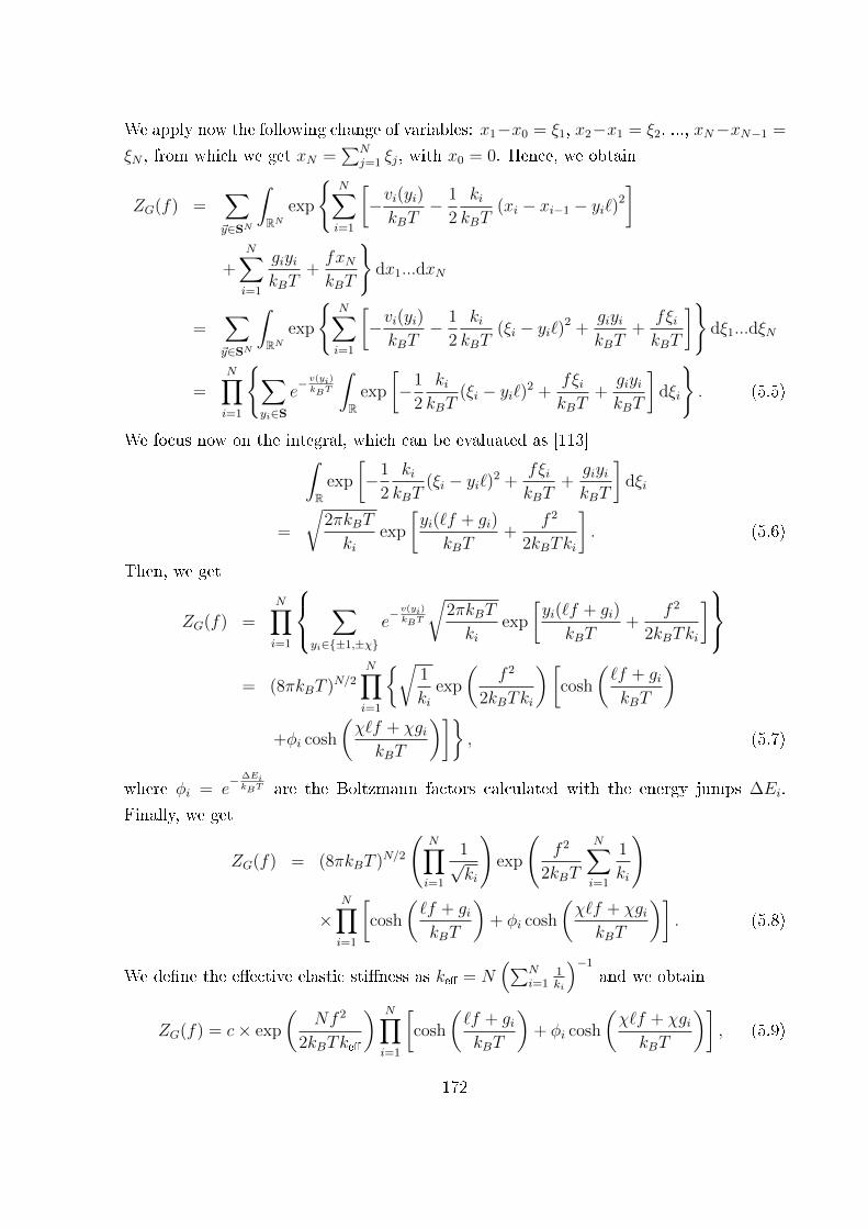
We apply now the following change of variables: x1−x0 = ξ1, x2−x1 = ξ2, ..., xN−xN−1 =
ξN , from which we get xN =∑N
j=1 ξj, with x0 = 0. Hence, we obtain
ZG(f) =∑~y∈SN
∫RN
exp
{N∑i=1
[−vi(yi)kBT
− 1
2
kikBT
(xi − xi−1 − yi`)2
]
+N∑i=1
giyikBT
+fxNkBT
}dx1...dxN
=∑~y∈SN
∫RN
exp
{N∑i=1
[−vi(yi)kBT
− 1
2
kikBT
(ξi − yi`)2 +giyikBT
+fξikBT
]}dξ1...dξN
=N∏i=1
{∑yi∈S
e− v(yi)
kBT
∫R
exp
[−1
2
kikBT
(ξi − yi`)2 +fξikBT
+giyikBT
]dξi
}. (5.5)
We focus now on the integral, which can be evaluated as [113]∫R
exp
[−1
2
kikBT
(ξi − yi`)2 +fξikBT
+giyikBT
]dξi
=
√2πkBT
kiexp
[yi(`f + gi)
kBT+
f 2
2kBTki
]. (5.6)
Then, we get
ZG(f) =N∏i=1
∑yi∈{±1,±χ}
e− v(yi)
kBT
√2πkBT
kiexp
[yi(`f + gi)
kBT+
f 2
2kBTki
]= (8πkBT )N/2
N∏i=1
{√1
kiexp
(f 2
2kBTki
)[cosh
(`f + gikBT
)+φi cosh
(χ`f + χgikBT
)]}, (5.7)
where φi = e−∆EikBT are the Boltzmann factors calculated with the energy jumps ∆Ei.
Finally, we get
ZG(f) = (8πkBT )N/2
(N∏i=1
1√ki
)exp
(f 2
2kBT
N∑i=1
1
ki
)
×N∏i=1
[cosh
(`f + gikBT
)+ φi cosh
(χ`f + χgikBT
)]. (5.8)
We de�ne the e�ective elastic sti�ness as ke� = N(∑N
i=11ki
)−1
and we obtain
ZG(f) = c× exp
(Nf 2
2kBTke�
) N∏i=1
[cosh
(`f + gikBT
)+ φi cosh
(χ`f + χgikBT
)], (5.9)
172

with c a constant. The macroscopic behaviour of the chain is described by the force-
extension response and by the average value of the spin variables, which can be obtained
through the Gibbs partition function as follows [1, 113]
〈xN〉 = kBT∂
∂flogZG, (5.10)
〈 yi 〉 = kBT∂
∂gilogZG. (5.11)
When the external �eld ~g is 0, these results may be evaluated as
〈xN〉 =f
ke�+
N∑i=1
`sinh
(`fkBT
)+ χφi sinh
(χ`fkBT
)cosh
(`fkBT
)+ φi cosh
(χ`fkBT
) , (5.12)
〈 yi 〉 =sinh
(`fkBT
)+ χφi sinh
(χ`fkBT
)cosh
(`fkBT
)+ φi cosh
(χ`fkBT
) . (5.13)
While the �rst expression represents the macroscopic mechanical response of the system,
the second one describes the con�gurational state (folded or unfolded) of the units in terms
of the applied force. Interestingly enough, Eqs.(5.12) and (5.13) can be combined to give
〈x〉 = Nfke�
+ `∑N
i=1〈 yi 〉, which represents a spring-like behaviour with the equilibrium
length controlled by the spin variables. An application of Eqs.(5.12) and (5.13) can be
found in Figs.5.3.b, 5.3.c, and 5.3.d, where the force-extension relation, the average spin
variables and the quantities ∂〈 yi 〉/∂〈x〉 versus 〈x〉 are represented for a homogeneous
chain with ∆Ei = ∆E ∀i (blue curves). These results describe a synchronous unfolding
of the units for a given threshold force given by f ∗ = ∆E/[(χ− 1)`] [113,130,159]. It is a
well-known behaviour observed in DNA [71, 73, 182], and in other molecules of biological
origin [132,183]. A second example can be found in Figs.5.3.j, 5.3.k, and 5.3.l, where the
same quantities have been shown for a heterogeneous chain, as represented in Fig.5.3.i.
In this case, while the force-extension curve is only slightly modi�ed, the spin variables
assume di�erent behaviours for the di�erent units, proving the emergence of an unfolding
pathway induced by the heterogeneity of the metastable states energy levels. Also, the
blue curve in Fig.5.3.k shows the mean value of the numbered curves and is similar to the
Gibbs response of the homogeneous case. This is true since we used the same parameter
χ for all the units of the chain. It is important to remark that, for an heterogeneous
parameter χ, we can have a di�erent behaviour between 〈yi〉 of the homogeneous chain
and 1N
∑Ni=1〈 yi 〉 of the heterogeneous chain. To conclude, we observe that the quantity
∂〈 yi 〉/∂〈x〉 can be considered as an approximated measure of the probability density
173

of the position x at which a transition occurs between the states of the i-th unit (see
below for details). Therefore, Fig.5.3.l con�rms the identi�cation of a unfolding sequence
induced by the heterogeneity. The analysis of the Gibbs ensemble is the starting point to
study the behaviour of the Helmholtz ensemble, which is the core of our investigation as
discussed below.
5.3.2 The Helmholtz ensemble
We are now interested in the case of a two-state heterogeneous one-dimensional system
in the Helmholtz ensemble. To analyse this system, we use the Fourier relation linking
the Gibbs and Helmholtz partition functions [20,124]
ZH(x) =
∫ +∞
−∞ZG(−iωkBT ) exp(iωx)dω. (5.14)
First of all, we have from Eq.(5.9)
ZG (−iωkBT ) = c× exp
(−Nω
2kBT
2ke�
) N∏i=1
[cosh
(gi − iω`kBT
kBT
)+φi cosh
(χgi − iχω`kBT )
kBT
)]. (5.15)
with c a constant. However, it is better to continue the calculation by observing that we
have to determine the following quantities, both for ~g = 0
〈f〉 = −kBT1
ZH
∂ZH∂x
, (5.16)
〈yj〉 = kBT1
ZH
∂ZH∂gj
. (5.17)
Therefore, we develop both ZH and ∂ZH(x)∂gj
with ~g = 0, as follows
ZH(x) =
∫ +∞
−∞e−Nω
2kBT
2ke� eiωxN∏i=1
(a+ φib) dω, (5.18)
∂ZH(x)
∂gj=
(− i
kBT
)∫ +∞
−∞[sin(ω`) + φjχ sin(ωχ`)]
×N∏
k=1,k 6=j
(a+ φkb) e−Nω
2kBT
2ke� eiωxdω, (5.19)
174
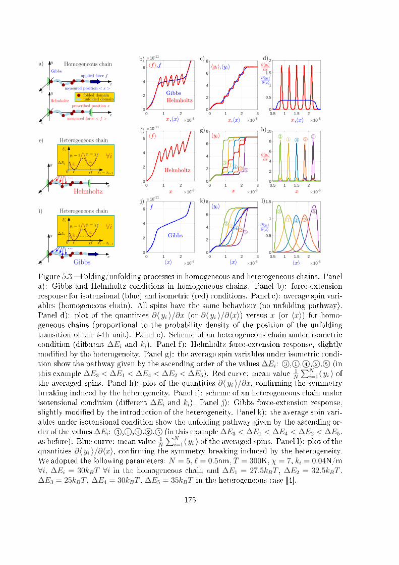
z
y
x
z
y
x
Gibbs
Helmholtz
applied force f
prescribed position x
measured position < x >
measured force < f >
folded domainunfolded domain
Homogeneous chaina)
0 1 2
10-8
0
2
4
6
10-11
0.5 1 1.5 2
10-8
0
0.5
1
1.5
2
0 1 2 3
10-8
0
2
4
6
8
z
y
x
` χ`0
Ui
yi = 1yi = χ
xi − xi−1
∆Ei
Heterogeneous chain
kiki
...
8i
e)
Helmholtz0 1 2
10-8
0
2
4
6
10-11
0 1 2 3
10-8
0
2
4
6
8
0.5 1 1.5 2
10-8
0
2
4
6
8
10
z
y
x
` χ`0
Ui
yi = 1yi = χ
xi − xi−1
∆Ei
Heterogeneous chain
kiki
...
8i
i)
Gibbs0 1 2
10-8
0
2
4
6
10-11
0 1 2 3
10-8
0
2
4
6
8
0.5 1 1.5 2
10-8
0
0.5
1
1.5
Figure 5.3 � Folding/unfolding processes in homogeneous and heterogeneous chains. Panela): Gibbs and Helmholtz conditions in homogeneous chains. Panel b): force-extensionresponse for isotensional (blue) and isometric (red) conditions. Panel c): average spin vari-ables (homogeneous chain). All spins have the same behaviour (no unfolding pathway).Panel d): plot of the quantities ∂〈 yi 〉/∂x (or ∂〈 yi 〉/∂〈x〉) versus x (or 〈x〉) for homo-geneous chains (proportional to the probability density of the position of the unfoldingtransition of the i-th unit). Panel e): Scheme of an heterogeneous chain under isometriccondition (di�erent ∆Ei and ki). Panel f): Helmholtz force-extension response, slightlymodi�ed by the heterogeneity. Panel g): the average spin variables under isometric condi-tion show the pathway given by the ascending order of the values ∆Ei: 3©, 1©, 4©, 2©, 5© (inthis example ∆E3 < ∆E1 < ∆E4 < ∆E2 < ∆E5). Red curve: mean value 1
N
∑Ni=1〈 yi 〉 of
the averaged spins. Panel h): plot of the quantities ∂〈 yi 〉/∂x, con�rming the symmetrybreaking induced by the heterogeneity. Panel i): scheme of an heterogeneous chain underisotensional condition (di�erent ∆Ei and ki). Panel j): Gibbs force-extension response,slightly modi�ed by the introduction of the heterogeneity. Panel k): the average spin vari-ables under isotensional condition show the unfolding pathway given by the ascending or-der of the values ∆Ei: 3©, 1©, 4©, 2©, 5© (in this example ∆E3 < ∆E1 < ∆E4 < ∆E2 < ∆E5,as before). Blue curve: mean value 1
N
∑Ni=1〈 yi 〉 of the averaged spins. Panel l): plot of the
quantities ∂〈 yi 〉/∂〈x〉, con�rming the symmetry breaking induced by the heterogeneity.We adopted the following parameters: N = 5, ` = 0.5nm, T = 300K, χ = 7, ki = 0.04N/m∀i, ∆Ei = 30kBT ∀i in the homogeneous chain and ∆E1 = 27.5kBT , ∆E2 = 32.5kBT ,∆E3 = 25kBT , ∆E4 = 30kBT , ∆E5 = 35kBT in the heterogeneous case [4].
175
where we omitted the unimportant multiplicative constant and we de�ned a = cos(ω`)
and b = cos(ωχ`). Hence, we calculate
N∏i=1
(a+ φib) = aN + aN−1b
N∑j=1
φj +1
2aN−2b2
∑i 6=j
φiφj +1
3!aN−3b3
×∑
i 6=j,k 6=j,i6=k
φiφjφk + ...+ bNφ1 × ...× φN
=N∑k=0
aN−kbkSk, (5.20)
with S0 = 1 and
Sk =1
k!
∑Ja 6=Jb∀a6=b
φj1 × ...× φjk. (5.21)
The quantities Sk are called elementary symmetric polynomials in the variables φ1...φN .
We describe here the theory for the calculation of such quantities and we postpone the
calculation of ∂ZH(x)∂gj
. We consider a polynomial f(x) de�ned as
f(x) =N∑k=0
akxk = a0 + a1x+ a2x
2 + ...+ aNxN , (5.22)
and we suppose that it has the N zeros φ1, ..., φN . It means that
f(x) = aN(x− φ1)× ...× (x− φN)
= aN
N∏k=1
(x− φk)
= aN
[xN − xN−1
N∑i=1
φi +1
2xN−2
N∑i 6=j
φiφj −1
3!xN−3
N∑i 6=j 6=k
φiφjφk + ...
+(−1)Nφ1 × ...× φN]
= aN[xN − xN−1S1 + xN−2S2 − xN−3S3 + ...+ (−1)NSN
]. (5.23)
We can also write
∑Ni=1 φi = −aN−1
aN= S1,
12
∑i 6=j φiφj = aN−2
aN= S2,
13!
∑i 6=j 6=k φiφjφk = −aN−3
aN= S3,
...φ1 × ...× φN = (−1)N a0
aN= SN .
(5.24)
176
The problem is to easily calculate all these quantities, which can be computationally
expensive because of the very important number of permutations. One possibility to
simplify the calculation is based on the introduction of the so-called power sums, de�ned
as
Ph =N∑t=1
φht . (5.25)
We consider, by de�nition, P0 = N . We search for the relation between the power sums
and the elementary symmetric polynomials. We have that
N∑k=0
akφkt = 0 ∀t = 1, ..., N, (5.26)
since φt is a zero of f(x). By multiplying this expression by φmt , we get
N∑k=0
akφk+mt = 0 ∀t = 1, ..., N, ∀m ≥ 0. (5.27)
We can sum over t from 1 to NN∑k=0
akPk+m = 0 ∀m ≥ 0. (5.28)
These equations allow the determination of all Ph if we know the �rst P1, ...PN−1, and we
remember that P0 = N . To get equations for P1, ...PN−1, we consider
f(x) = aN(x− φ1)× ...× (x− φN), (5.29)
and
f ′(x) =f(x)
x− φ1
+ ...+f(x)
x− φN
=N∑q=1
f(x)
x− φq. (5.30)
We can also write
f ′(x) =N∑q=1
f(x)
x− φq=
N∑q=1
∑Nk=0 akx
k
x− φq(5.31)
and, since φq is a zero of∑N
k=0 akxk, we can also get the expression
f ′(x) =N∑q=1
∑Nk=0 ak(x
k − φkq)x− φq
. (5.32)
177
Moreover, the term with k = 0 is zero and we obtain
f ′(x) =N∑q=1
∑Nk=1 ak(x
k − φkq)x− φq
. (5.33)
Now, we have to develop the expression xk−ykx−y . To do this, we need to calculate the
geometrical sum
S = 1 + x+ x2 + ...+ xN−1. (5.34)
We multiply it by x and we get
xS = x+ x2 + ...+ xN , (5.35)
or again
S − xS = 1− xN , (5.36)
eventually giving
S =1− xN1− x . (5.37)
We substitute x with yx, getting
1 +y
x+(yx
)2
+ ...+(yx
)N−1
=1−
(yx
)N1− y
x
, (5.38)
or, in another way of writing, we have
xN−1 + yxN−2 + y2xN−3 + ...+ yN−1 =xN − yNx− y . (5.39)
Therefore, we can �nally write
xk − ykx− y =
k−1∑j=0
yjxk−j−1. (5.40)
We use this result in Eq.(5.33) and we have
f ′(x) =N∑q=1
N∑k=1
ak
k−1∑j=0
φjqxk−j−1. (5.41)
Now, since Pj =∑N
q=1 φjq, we �nally get
f ′(x) =N∑k=1
k−1∑j=0
akPjxk−j−1. (5.42)
178
And, if we let i = k − j − 1 becoming j = k − i− 1, we can �nd the dual expression
f ′(x) =N∑k=1
k−1∑i=0
akPk−i−1xi, (5.43)
that we can compare with
f ′(x) =N∑i=0
aiixi−1 =
N∑i=1
iaixi−1. (5.44)
To do this comparison, we observe that
N∑k=1
k−1∑i=0
=N−1∑i=0
N∑k=i+1
. (5.45)
The previous observation allows us to draw a comparison between
f ′(x) =N∑k=1
k−1∑i=0
akPk−i−1xi =
N−1∑i=0
N∑k=i+1
akPk−i−1xi (5.46)
and
f ′(x) =N∑i=1
iaixi−1 =
N−1∑i=0
(i+ 1)ai+1xi. (5.47)
We �nd
(i+ 1)ai+1 =N∑
k=i+1
akPk−i−1 ∀i = 0, 1, ..., N − 1. (5.48)
For i = N − 1, we have a trivial identity since we get NaN = aNP0, hence P0 = N . So,
we can write
(i+ 1)ai+1 = Nai+1 +N∑
k=i+2
akPk−i−1 ∀i = 0, 1, ..., N − 2, (5.49)
and we �nally have (N − 1) equations, given by
−(N − i− 1)ai+1 =N∑
k=i+2
akPk−i−1 ∀i = 0, 1, ..., N − 2. (5.50)
We can express it in a more explicit way
−(N − 1)a1 = a2P1 +a3P2 + ... +aNPN−1,−(N − 2)a2 = a3P1 +a4P2 + ... +aNPN−2,...−3aN−3 = aN−2P1 +aN−1P2 +aNP3,−2aN−2 = aN−1P1 +aNP2,−aN−1 = aNP1.
(5.51)
179
The previous system of equations represents the link between (P1, ..., PN−1) and(a1
aN, ..., aN−1
aN
)=(
(−1)N−1SN−1, ..., S2,−S1
). We can also add the equation Eq. (5.28) for m = 0, namely
−Na0 = a1P1 + a2P2 + ...+ aNPN . (5.52)
With this equation, the system links (P1, ..., PN) with(a0
aN, ..., aN−1
aN
)=((−1)NSN , ...,−S1
).
Introducing the equation for m = 0 allows us to write the complete system as
−Na0 −a1P1 −a2P2 − ... −aN−1PN−1 = aNPN ,−(N − 1)a1 −a2P1 −a3P2 − ... −aN−1PN−2 = aNPN−1,−(N − 2)a2 −a3P1 −a4P2 − ... −aN−1PN−3 = aNPN−2,...−3aN−3 −aN−2P1 −aN−1P2 = aNP3,−2aN−2 −aN−1P1 = aNP2,−aN−1 = aNP1.
(5.53)
We can also write it in a matrix form
N P1 P2 P3 ... PN−3 PN−2 PN−1
0 N − 1 P1 P2 ... PN−4 PN−3 PN−2
0 0 N − 2 P1 ... PN−5 PN−4 PN−3
... ... ... ... ... ... ... ...0 0 0 0 ... 3 P1 P2
0 0 0 0 ... 0 2 P1
0 0 0 0 ... 0 0 1
a0
aNa1
aNa2
aN
...aN−3
aNaN−2
aNaN−1
aN
= −
PNPN−1
PN−2
...P3
P2
P1
. (5.54)
We apply the Kramer theory to the subsystem composed of the last (N − i) equations
and we get
aiaN
= −
det
PN−i P1 ... PN−i−3 PN−i−2 PN−i−1
PN−i−1 N − i− 1 ... PN−i−4 PN−i−3 PN−i−2
... ... ... ... ... ...P3 0 ... 3 P1 P2
P2 0 ... 0 2 P1
P1 0 ... 0 0 1
det
N − i P1 ... PN−i−3 PN−i−2 PN−i−1
0 N − i− 1 ... PN−i−4 PN−i−3 PN−i−2
... ... ... ... ... ...0 0 ... 3 P1 P2
0 0 ... 0 2 P1
0 0 ... 0 0 1
. (5.55)
180
In the �rst determinant, we move the �rst column to the last position, getting
aiaN
=(−1)N−i−1(−1)
(N − i)! det
P1 P2 ... PN−i−2 PN−i−1 PN−iN − i− 1 P1 ... PN−i−3 PN−i−2 PN−i−1
0 N − i− 2 ... PN−i−4 PN−i−3 PN−i−2
... ... ... ... ... ...0 0 ... P1 P2 P3
0 0 ... 2 P1 P2
0 0 ... 0 1 P1
.(5.56)
Finally, rotations of 180�do not alter the value of a determinant and therefore
aiaN
=(−1)N−i
(N − i)! det
P1 1 0 0 ... 0 0P2 P1 2 0 ... 0 0P3 P2 P1 3 ... 0 0... ... ... ... ... ... ...
PN−i−1 PN−i−2 PN−i−3 PN−i−4 ... P1 N − i− 1PN−i PN−i−1 PN−i−2 PN−i−3 ... P2 P1
. (5.57)
We remember that Si = (−1)i aN−iaN
or, equivalently, SN−i = (−1)N−i aiaN
, and we obtain
the �nal form of the elementary symmetric polynomials
SN−i =1
(N − i)! det
P1 1 0 0 ... 0 0P2 P1 2 0 ... 0 0P3 P2 P1 3 ... 0 0... ... ... ... ... ... ...
PN−i−1 PN−i−2 PN−i−3 PN−i−4 ... P1 N − i− 1PN−i PN−i−1 PN−i−2 PN−i−3 ... P2 P1
, (5.58)or again
Sj =1
j!det
P1 1 0 0 ... 0 0P2 P1 2 0 ... 0 0P3 P2 P1 3 ... 0 0... ... ... ... ... ... ...Pj−1 Pj−2 Pj−3 Pj−4 ... P1 j − 1Pj Pj−1 Pj−2 Pj−3 ... P2 P1
. (5.59)
This is the closed form relation between the elementary symmetric polynomials and the
power sums. These expressions can be named determinant form of the Newton-Girard
formulae [184�187]. With this result, we can now use the determinant form of the terms
Sj to develop the expressions of ZH and ∂ZH∂gj
, as indicated previously. We start with
ZH(x) and we can write
ZH(x) =
∫ +∞
−∞e−Nω
2kBT
2ke� eiωxN∏i=1
(a+ φib)dω
=
∫ +∞
−∞e−Nω
2kBT
2ke� eiωxN∑k=0
aN−kbkSkdω, (5.60)
181
with S0 = 1. So, we �rstly need the calculation of
A =
∫ +∞
−∞e−Nω
2kBT
2ke� eiωx [cos(ω`)]N−k [cos(χω`)]k dω
=
∫ +∞
−∞e−Nω
2kBT
2ke� eiωx(eiω` + e−iω`
2
)N−k (eiχω` + e−iχω`
2
)kdω
=N−k∑s=0
k∑q=0
1
2N
(N − ks
)(k
q
)∫ +∞
−∞eiω[x+`s−`(N−k−s)+χ`q−χ`(k−q)]
×e−Nω2kBT
2ke� dω. (5.61)
To solve this integral, we use the well-known relation∫ +∞
−∞e−αx
2
eiβxdx =
√π
αe−
β2
4α , (5.62)
so the equation becomes
A =N−k∑s=0
k∑q=0
1
2N
(N − ks
)(k
q
)√2πke�NkBT
e− ke�[x+`(2s−N+k+2χq−χk)]2
2NkBT . (5.63)
Finally, the �rst result is
ZH(x) =1
2N
√2πke�NkBT
N∑k=0
N−k∑s=0
k∑q=0
(N − ks
)(k
q
)e− ke�[x+`(2s−N+k+2χq−χk)]2
2NkBT Sk, (5.64)
where the Sk coe�cients are given by the determinants in Eq.(5.59). Concerning the
calculation of ∂ZH(x)∂gj
, we need to evaluate as in Eq.(5.19)
∂ZH(x)
∂gj=
(− i
kBT
)∫ +∞
−∞e−Nω
2kBT
2ke� eiωxN∏
k=1,k 6=j
[cos(ω`) + φk cos(ωχ`)]
× [sin(ω`) + φjχ sin(ωχ`)] dω. (5.65)
We can de�ne
S(j)k =
1
k!
∑ja 6=jb∀a6=b,jc 6=j∀j
φj1 × ...× φjk, (5.66)
where the quantities S(j)k (k = 1, ..., N − 1) are de�ned similarly to the quantities Sk
(k = 1, ..., N) but are based on the set containing all φ1, ..., φN except φj. They can
182
be simply calculated with the same technique based on the determinants, as shown in
Eq.(5.59). Hence we can write, after developing the power on N
∂ZH∂gj
=
(− i
kBT
)∫ +∞
−∞e−Nω
2kBT
2ke� eiωxN−1∑k=0
[cos(ω`)]N−1−k [cos(χω`)]k S(j)k
× [sin(ω`) + φjχ sin(χω`)] dω
=1
kBT
∫ +∞
−∞e−Nω
2kBT
2ke� eiωxN−1∑k=0
[cos(ω`)]N−1−k [cos(χω`)]k S(j)k
×(e−iω` − eiω`
2
)dω +
1
kBT
∫ +∞
−∞e−Nω
2kBT
2ke� eiωxN−1∑k=0
[cos(ω`)]N−1−k
× [cos(χω`)]k S(j)k χφj
(e−iωχ` − eiωχ`
2
)dω. (5.67)
We separately calculate the two integrals, called βk and γk. We begin the calculation of
βk by developing the powers
βk =
∫ +∞
−∞e−Nω
2kBT
2ke� eiωx [cos(ω`)]N−1−k [cos(χω`)]k(e−iω` − eiω`
2
)dω
=
∫ +∞
−∞e−Nω
2kBT
2ke� eiωxN−k−1∑s=0
(N − k − 1
s
)eiω`se−iω`(N−1−k−s) 1
2N−1−k
×k∑q=0
(k
q
)eiχω`qe−iχω`(k−q)
1
2k
(e−iω` − eiω`
2
)dω
=1
2N
N−k−1∑s=0
k∑q=0
(N − k − 1
s
)(k
q
)[∫ +∞
−∞e−Nω
2kBT
2ke� eiω[x+`(2s−N+k+2χq−χk)]dω
−∫ +∞
−∞e−Nω
2kBT
2ke� eiω[x+`(2s+2−N+k−2χq−χk)]dω
]. (5.68)
Finally, we get
βk =1
2N
√2πke�NkBT
N−k−1∑s=0
k∑q=0
(N − k − 1
s
)(k
q
)[e− ke�[x+`(2s−N+k+2χq−χk)]2
2NkBT
−e−ke�[x+`(2s−N+2+k+2χq−χk)]2
2NkBT
]. (5.69)
Now, we calculate the second integral, called γk
γk =
∫ +∞
−∞e−Nω
2kBT
2ke� eiωx [cos(ω`)]N−1−k [cos(χω`)]k(e−iωχ` − eiωχ`
2
)dω. (5.70)
183
We do the same calculation developed for βk and we obtain
γk =1
2N
√2πke�NkBT
N−k−1∑s=0
k∑q=0
(N − k − 1
s
)(k
q
)[e− ke�[x+`(2s−N+1−χ+k+2χq−χk)]2
2NkBT
−e−ke�[x+`(2s−N+1+χ+k+2χq−χk)]2
2NkBT
]. (5.71)
We get the �nal form of ∂ZH(x)∂gj
∂ZH(x)
∂gj=
1
kBT
N−1∑k=0
[(βk + χγkφj)S
(j)k
]. (5.72)
We can �nally deduce the expression of the force-extension response from Eqs.(5.16) and
(5.64) as
〈f〉 =
∑Nk=0
∑N−ks=0
∑kq=0
(N−ks
)(kq
)e− ke�ϕ
2
2NkBT ke�ϕSk∑Nk=0
∑N−ks=0
∑kq=0
(N−ks
)(kq
)e− ke�ϕ
2
2NkBT Sk
, (5.73)
with ϕ = x + `(2s − N + k + 2χq − χk) and the coe�cients Sk are given in Eq.(5.59).
Similarly, the expression for the average spin variable 〈yj〉 can be obtained from Eqs.(5.17)
and (5.72) as
〈yj〉 =
∑N−1k=0
(βkS
(j)k + γkφjχS
(j)k
)ZH
, (5.74)
where the coe�cients S(j)k are given in Eq.(5.66). Although the quenched disorder strongly
complicates the analysis of the system within the Helmholtz ensemble, the application of
the determinant expression in Eq.(5.59) or Eq.(5.66) (determining the elementary sym-
metric polynomials Sk or S(j)k related to the Boltzmann factors with arbitrary energy
jumps) allows for an analytic treatment of the problem. In particular, we are able to ob-
tain the partition function in Eq.(5.64) (along with its derivative in Eq.(5.72)) in closed
form and to derive expressions for the macroscopic observables.
A �rst simple application of these results can be found in Figs.5.3.b and 5.3.c, where
we plot 〈f〉 and 〈yi〉 versus the prescribed extension x for a homogeneous chain under
isometric condition (red curves). The behaviour of 〈f〉 and 〈yi〉 can be interpreted througha sequential unfolding of the units. This response is in good qualitative agreement with
several force spectroscopy measurements performed on proteins and other macromolecules
[135,142�145]. We also plotted ∂〈yi〉/∂x versus x in Fig.5.3.d. This quantity satis�es two
184
crucial properties: �rstly,∫ +∞
0(∂〈yi〉/∂x)dx = 〈yi〉(+∞)−〈yi〉(0) = χ (which means that
it can be normalised); secondly, 〈yi〉 is always non-decreasing, leading to a non-negative
function ∂〈yi〉/∂x. Hence, it follows that ∂〈yi〉/∂x can be used as a quantity approximately
measuring the probability density of the position x at which a transition occurs between
the states of the i-th unit. We remark that it is not a rigorous statement but a useful
practical approach to quantify the statistics of the unfolding processes. Fig.5.3.d shows
that at each transition occurrence, the switching probability is the same for all units of
the homogeneous chain. Therefore, no unfolding pathway can be identi�ed. We describe
now the behaviour of a heterogeneous chain, as represented in Fig.5.3.e. While the force-
extension curve in Fig.5.3.f is slightly modi�ed with respect to Fig.5.3.b, we observe that
the heterogeneity of the chain, which is a quenched disorder embedded in the system,
is able to perform a symmetry breaking generating an unfolding pathway. Indeed, the
numbered curves of the average spin variables in Fig.5.3.g are able to precisely identify
what unit is unfolded at each transition, indicating the actual sequence of unfolding
processes. Interestingly enough, the red curve in the same panel shows the average value
of these numbered curves and is similar to the Helmhotz response of the homogeneous
case. This is true since we used the same parameter χ for all the units of the chain. It
is important to remark that, for an heterogeneous parameter χ, we can have a di�erent
behaviour between 〈yi〉 of the homogeneous chain and 1N
∑Ni=1〈 yi 〉 of the heterogeneous
chain. Importantly, it follows that through the spin variables, we can now analyse the
unfolding pathway generated by the heterogeneity. This is further con�rmed by the
plots of ∂〈yi〉/∂x in Fig.5.3.h, where each curve is characterised by one pronounced peak
corresponding to the actual switching, and other smaller peaks measuring the uncertainty
in the pathway identi�cation (see next Section for details). Moreover, the numerical
results show that the unfolding pathway corresponds to the ascending order of the values
∆Ei. This implies that the equilibrium statistical mechanics of this system implements a
statistical sorting procedure. This result is independent of the heterogeneity of the elastic
constants ki since 〈f〉 and 〈yj〉 depend only on the e�ective sti�ness ke�.
5.4 Unfolding pathway identi�ability
While the described identi�cation of the unfolding pathway may seem a simple and
expected result, it is important to observe that: (i) the model elaborated mathematically
explains how the bistable chain can implement the above introduced statistical sorting
procedure, and the same methodology can be also applied to more realistic situations with
additional heterogeneous geometrical and/or physical parameters; (ii) the knowledge of
185
the average spin variables given in Eq.(5.74) is also useful to quantitatively evaluate the
identi�ability of the most probable unfolding pathway, i.e. of the most likely observed
unfolding sequence in a given experiment. This concept measures to what extend we are
able to identify the most probable unfolding pathway, which represents the sequence of
unfolding process observed the largest number of times if we conduct several identical
experiments. For the sake of brevity, we develop this concept only by considering the
Helmholtz ensemble. If we look at the density-like curve ∂〈yi〉/∂x for a given unit (see
Fig.5.3.h), the identi�ability can be de�ned as the relative di�erence between the largest
peak and the second largest peak. Indeed, this di�erence measures the capability to
properly identify the transition of that unit with respect to the other ones. Consequently,
if we consider the i-th unit, we can de�ne
Ii =Fm{∂〈yi〉∂x
}− Sm
{∂〈yi〉∂x
}Fm{∂〈yi〉∂x
} , (5.75)
where Fm and Sm are operators extracting the largest peak and the second largest peak,
respectively, of a given function. The identi�ability of the whole unfolding process can be
therefore de�ned by the average value of these quantities over the N units
I =1
N
N∑i=1
Ii. (5.76)
We �rst apply this concept to a chain composed of N = 5 units with uniformly dis-
tributed energy jumps ∆Ei/(kBT ) ∈ {α, α± ε, α± 2ε}, where the parameter ε measures
their dispersion. The resulting identi�ability I can be found in Fig.5.4, where it is plotted
versus ε and parametrized by the temperature T . We note that I = 0 for the homoge-
neous case with ε = 0, and I → 1 for increasing value of ε, being the limiting value
I = 1 related to the pathway identi�cation without uncertainty. We also observe that
increasing values of the temperature reduce the identi�ability, for a constant ε. This is
coherent with the idea that the thermal �uctuations are able to reduce the knowledge on
the con�gurational state of the system.
A plateau at around ε = 0.5 can be observed and is due to a particular phenomenon
observed for small values of ε. We explain this point as follows. We consider only the case
with T = 300K and N = 5. Then, we assume ∆Ei = {30, 30 + ε, 30− ε, 30 + 2ε, 30− 2ε}×kBT as in Fig.5.4 (the other parameters used being exactly as quoted in the caption of
Fig.5.4). We take a small value of ε, namely ε = 0.4. In Fig.5.5, we can now observe the
186
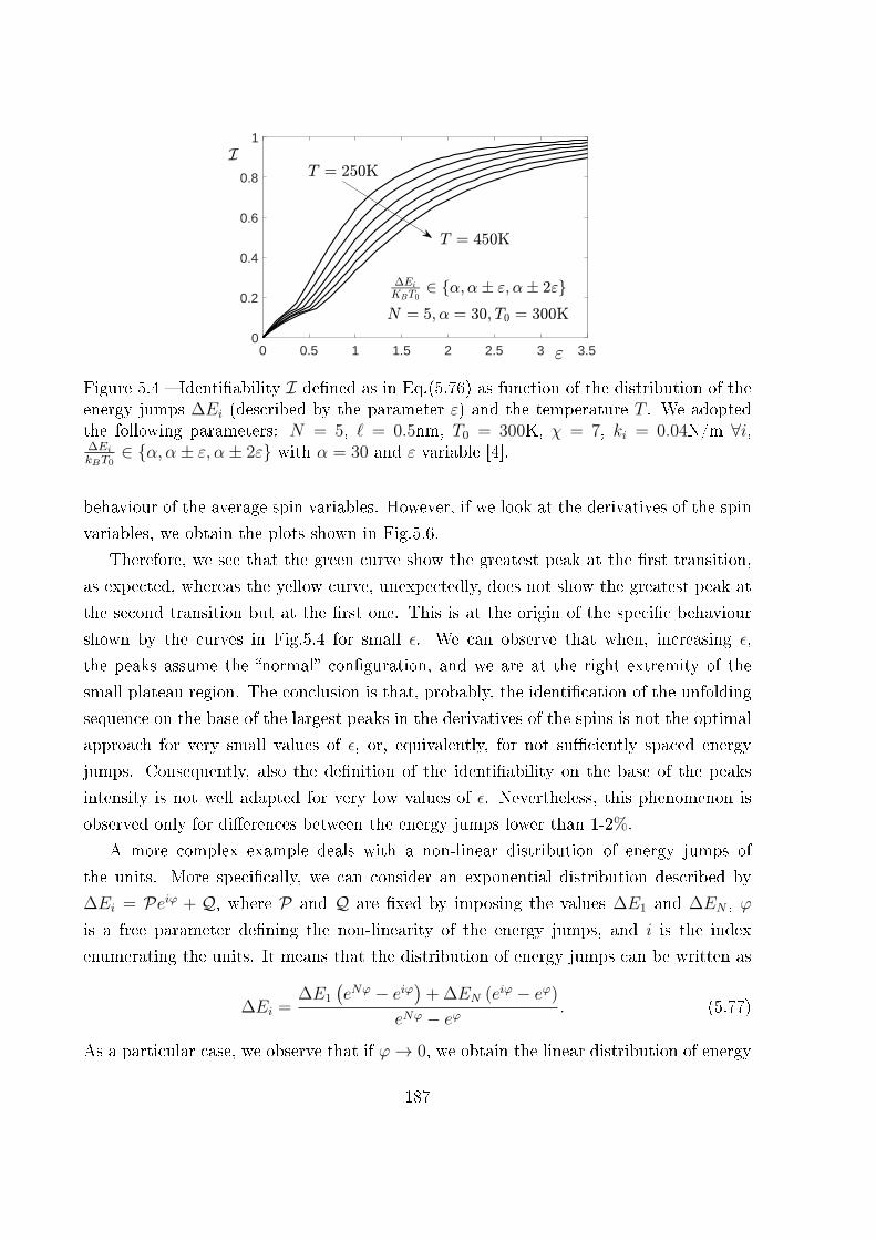
0 0.5 1 1.5 2 2.5 3 3.50
0.2
0.4
0.6
0.8
1
Figure 5.4 � Identi�ability I de�ned as in Eq.(5.76) as function of the distribution of theenergy jumps ∆Ei (described by the parameter ε) and the temperature T . We adoptedthe following parameters: N = 5, ` = 0.5nm, T0 = 300K, χ = 7, ki = 0.04N/m ∀i,∆EikBT0
∈ {α, α± ε, α± 2ε} with α = 30 and ε variable [4].
behaviour of the average spin variables. However, if we look at the derivatives of the spin
variables, we obtain the plots shown in Fig.5.6.
Therefore, we see that the green curve show the greatest peak at the �rst transition,
as expected, whereas the yellow curve, unexpectedly, does not show the greatest peak at
the second transition but at the �rst one. This is at the origin of the speci�c behaviour
shown by the curves in Fig.5.4 for small ε. We can observe that when, increasing ε,
the peaks assume the �normal� con�guration, and we are at the right extremity of the
small plateau region. The conclusion is that, probably, the identi�cation of the unfolding
sequence on the base of the largest peaks in the derivatives of the spins is not the optimal
approach for very small values of ε, or, equivalently, for not su�ciently spaced energy
jumps. Consequently, also the de�nition of the identi�ability on the base of the peaks
intensity is not well adapted for very low values of ε. Nevertheless, this phenomenon is
observed only for di�erences between the energy jumps lower than 1-2%.
A more complex example deals with a non-linear distribution of energy jumps of
the units. More speci�cally, we can consider an exponential distribution described by
∆Ei = Peiϕ + Q, where P and Q are �xed by imposing the values ∆E1 and ∆EN , ϕ
is a free parameter de�ning the non-linearity of the energy jumps, and i is the index
enumerating the units. It means that the distribution of energy jumps can be written as
∆Ei =∆E1
(eNϕ − eiϕ
)+ ∆EN (eiϕ − eϕ)
eNϕ − eϕ . (5.77)
As a particular case, we observe that if ϕ→ 0, we obtain the linear distribution of energy
187
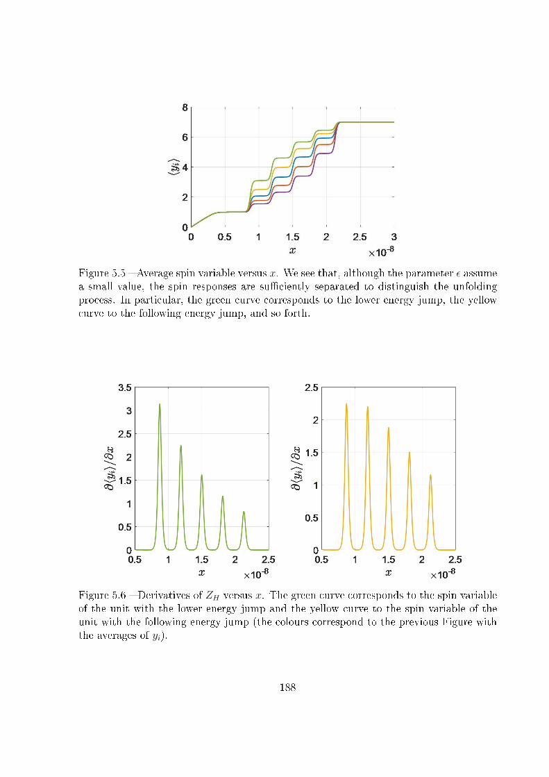
Figure 5.5 � Average spin variable versus x. We see that, although the parameter ε assumea small value, the spin responses are su�ciently separated to distinguish the unfoldingprocess. In particular, the green curve corresponds to the lower energy jump, the yellowcurve to the following energy jump, and so forth.
Figure 5.6 � Derivatives of ZH versus x. The green curve corresponds to the spin variableof the unit with the lower energy jump and the yellow curve to the spin variable of theunit with the following energy jump (the colours correspond to the previous Figure withthe averages of yi).
188
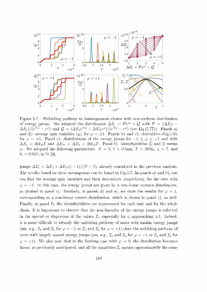
0 1 2 3
10-8
0
2
4
6
8
0 1 2 3
10-8
0
2
4
6
8
0.5 1 1.5 2
10-8
0
5
10
0.5 1 1.5 2
10-8
0
5
10
-1 0 10
0.5
1
1 2 3 4 51.2
1.3
1.4
1.5
1.610-19
Figure 5.7 � Unfolding pathway in heterogeneous chains with non-uniform distributionof energy jumps. We adopted the distribution ∆Ei = Peiϕ + Q with P = (∆EN −∆E1)/(eNϕ − eϕ) and Q = (∆E1e
Nϕ − ∆ENeϕ)/(eNϕ − eϕ) (see Eq.(5.77)). Panels a)
and d): average spin variables 〈yi〉 for ϕ = ±1. Panels b) and e): derivatives ∂〈yi〉/∂xfor ϕ = ±1. Panel c): distributions of the energy jumps for −1 ≤ ϕ ≤ +1 and with∆E1 = 30kBT and ∆EN = ∆E5 = 38kBT . Panel f): identi�abilities Ii and I versusϕ. We adopted the following parameters: N = 5, ` = 0.5nm, T = 300K, χ = 7, andki = 0.04N/m ∀i [4].
jumps ∆Ei = ∆E1 + ∆EN(i − 1)/(N − 1), already considered in the previous analysis.
The results based on these assumptions can be found in Fig.5.7. In panels a) and b), one
can �nd the average spin variables and their derivatives, respectively, for the case with
ϕ = −1. In this case, the energy jumps are given by a non-linear concave distribution,
as plotted in panel c). Similarly, in panels d) and e), we show the results for ϕ = 1,
corresponding to a non-linear convex distribution, which is shown in panel c), as well.
Finally, in panel f), the identi�abilities are represented for each unit and for the whole
chain. It is important to observe that the non-linearity of the energy jumps is re�ected
in the spread or dispersion of the values Ii, especially for ϕ approaching ±1. Indeed,
it is more di�cult to identify the unfolding pathway of units with similar energy jumps
(see, e.g., I4 and I5 for ϕ = −1 or I1 and I2 for ϕ = +1) than the unfolding pathway of
units with largely spaced energy jumps (see, e.g., I1 and I2 for ϕ = −1 or I4 and I5 for
ϕ = +1). We also note that in the limiting case with ϕ → 0, the distribution becomes
linear, as previously anticipated, and all the quantities Ii assume approximately the same
189
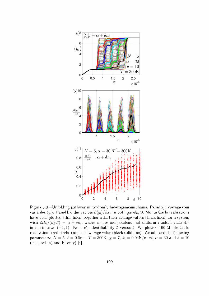
Figure 5.8 � Unfolding pathway in randomly heterogeneous chains. Panel a): average spinvariables 〈yi〉. Panel b): derivatives ∂〈yi〉/∂x. In both panels, 50 Monte-Carlo realisationshave been plotted (thin lines) together with their average values (thick lines) for a systemwith ∆Ei/(kBT ) = α + δni, where ni are independent and uniform random variablesin the interval (−1, 1). Panel c): identi�ability I versus δ. We plotted 100 Monte-Carlorealisations (red circles) and the average value (black solid line). We adopted the followingparameters: N = 5, ` = 0.5nm, T = 300K, χ = 7, ki = 0.04N/m ∀i, α = 30 and δ = 10(in panels a) and b) only) [4].
190
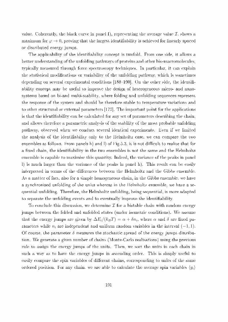
value. Coherently, the black curve in panel f), representing the average value I, shows amaximum for ϕ→ 0, proving that the largest identi�ability is achieved for linearly spaced
or distributed energy jumps.
The applicability of the identi�ability concept is twofold. From one side, it allows a
better understanding of the unfolding pathways of proteins and other bio-macromolecules,
typically measured through force spectroscopy techniques. In particular, it can explain
the statistical modi�cations or variability of the unfolding pathway, which is sometimes
depending on several experimental conditions [188�190]. On the other side, the identi�-
ability concept may be useful to improve the design of heterogeneous micro- and nano-
systems based on bi-and multi-stability, where folding and unfolding sequences represent
the response of the system and should be therefore stable to temperature variations and
to other structural or external parameters [177]. The important point for the applications
is that the identi�ability can be calculated for any set of parameters describing the chain,
and allows therefore a parametric analysis of the stability of the most probable unfolding
pathway, observed when we conduct several identical experiments. Even if we limited
the analysis of the identi�ability only to the Helmholtz case, we can compare the two
ensembles as follows. From panels h) and l) of Fig.5.3, it is not di�cult to realise that for
a �xed chain, the identi�ability in the two ensembles is not the same and the Helmholtz
ensemble is capable to maximise this quantity. Indeed, the variance of the peaks in panel
l) is much larger than the variance of the peaks in panel h). This result can be easily
interpreted in terms of the di�erences between the Helmholtz and the Gibbs ensemble.
As a matter of fact, also for a simple homogeneous chain, in the Gibbs ensemble, we have
a synchronised unfolding of the units whereas in the Helmholtz ensemble, we have a se-
quential unfolding. Therefore, the Helmholtz unfolding, being sequential, is more adapted
to separate the unfolding events and to eventually improve the identi�ability.
To conclude this discussion, we determine I for a bistable chain with random energy
jumps between the folded and unfolded states (under isometric conditions). We assume
that the energy jumps are given by ∆Ei/(kBT ) = α + δni, where α and δ are �xed pa-
rameters while ni are independent and uniform random variables in the interval (−1, 1).
Of course, the parameter δ measures the stochastic spread of the energy jumps distribu-
tion. We generate a given number of chains (Monte-Carlo realisations) using the previous
rule to assign the energy jumps of the units. Then, we sort the units in each chain in
such a way as to have the energy jumps in ascending order. This is simply useful to
easily compare the spin variables of di�erent chains, corresponding to units of the same
ordered position. For any chain, we are able to calculate the average spin variables 〈yi〉
191
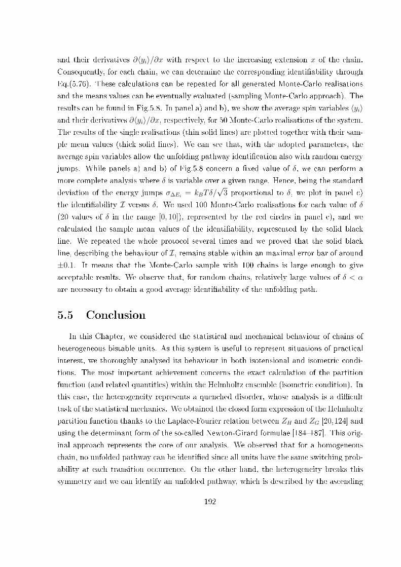
and their derivatives ∂〈yi〉/∂x with respect to the increasing extension x of the chain.
Consequently, for each chain, we can determine the corresponding identi�ability through
Eq.(5.76). These calculations can be repeated for all generated Monte-Carlo realisations
and the means values can be eventually evaluated (sampling Monte-Carlo approach). The
results can be found in Fig.5.8. In panel a) and b), we show the average spin variables 〈yi〉and their derivatives ∂〈yi〉/∂x, respectively, for 50 Monte-Carlo realisations of the system.
The results of the single realisations (thin solid lines) are plotted together with their sam-
ple mean values (thick solid lines). We can see that, with the adopted parameters, the
average spin variables allow the unfolding pathway identi�cation also with random energy
jumps. While panels a) and b) of Fig.5.8 concern a �xed value of δ, we can perform a
more complete analysis where δ is variable over a given range. Hence, being the standard
deviation of the energy jumps σ∆Ei = kBTδ/√
3 proportional to δ, we plot in panel c)
the identi�ability I versus δ. We used 100 Monte-Carlo realisations for each value of δ
(20 values of δ in the range [0, 10]), represented by the red circles in panel c), and we
calculated the sample mean values of the identi�ability, represented by the solid black
line. We repeated the whole protocol several times and we proved that the solid black
line, describing the behaviour of I, remains stable within an maximal error bar of around
±0.1. It means that the Monte-Carlo sample with 100 chains is large enough to give
acceptable results. We observe that, for random chains, relatively large values of δ < α
are necessary to obtain a good average identi�ability of the unfolding path.
5.5 Conclusion
In this Chapter, we considered the statistical and mechanical behaviour of chains of
heterogeneous bistable units. As this system is useful to represent situations of practical
interest, we thoroughly analysed its behaviour in both isotensional and isometric condi-
tions. The most important achievement concerns the exact calculation of the partition
function (and related quantities) within the Helmholtz ensemble (isometric condition). In
this case, the heterogeneity represents a quenched disorder, whose analysis is a di�cult
task of the statistical mechanics. We obtained the closed form expression of the Helmholtz
partition function thanks to the Laplace-Fourier relation between ZH and ZG [20,124] and
using the determinant form of the so-called Newton-Girard formulae [184�187]. This orig-
inal approach represents the core of our analysis. We observed that for a homogeneous
chain, no unfolded pathway can be identi�ed since all units have the same switching prob-
ability at each transition occurrence. On the other hand, the heterogeneity breaks this
symmetry and we can identify an unfolded pathway, which is described by the ascending
192

order of the energy jumps between folded and unfolded states of each unit. It means that
the system implements a statistical sorting procedure when we simply prescribe an in-
creasing distance between �rst and last units. Since this process has a statistical character,
we can de�ne the concept of identi�ability, which measures the capability to identify the
most probable unfolding pathway. This concept has been applied to deterministic (linear
and exponential) and random distributions of energy jumps. The results of this work can
be applied to the better interpretation of the force spectroscopy measurements of bio-
logical macromolecules [188�190] and to the accurate design of micro- and nano-systems
based on bistable chains with speci�c properties [177].
193

194
Chapter 6
Pulling speed dependence of the
force-extension response of bistable
chains
6.1 Introduction
The development of single-molecule force spectroscopy techniques has widely pro-
moted the study of the mechanical and kinetic properties of several biological macro-
molecules, such as proteins [6, 25, 33, 134, 191], nucleic acids (DNA [70, 71, 73, 182] and
RNA [192, 193]) and polysaccharides [24, 194, 195]. The static and dynamic responses
of such macromolecules are crucial for assessing the equilibrium and out-of-equilibrium
thermodynamics of small systems. The typical single-molecule experiment is conducted
by tethering the �rst end of the macromolecule and by moving its second end by means
of the force spectroscopy device, such as described in Chapter 1. For practical reasons,
these experiments are typically conducted by imposing a given pulling speed to the sec-
ond end of the chain. This point has crucial e�ects on the force-extension relation, which
shows a strong speed-dependent behaviour. Therefore, it is necessary to consider the
in�uence of the pulling speed on the force-extension response of a macromolecule, as the
force peaks increase with increasing speed [34, 196] (see Fig.6.1). Moreover, the recent
increasing of the pulling speeds used in force spectroscopy experiments with high-speed
AFM [34,35,37,38] requires the consideration of pulling speeds higher than in the existing
models. In Fig.6.1.a, it can be observed that the force peaks are nearly proportional to the
logarithm of the used pulling speed. The exploration of the response for di�erent pulling
speeds allows the reconstruction of the potential energy, as seen in Fig.6.1.b, and as dis-
cussed below. The histograms in Fig.6.1.c clearly show the increasing of the force peaks
when the pulling speed increases. Similarly, in Fig.6.2, a high-speed force spectroscopy
195
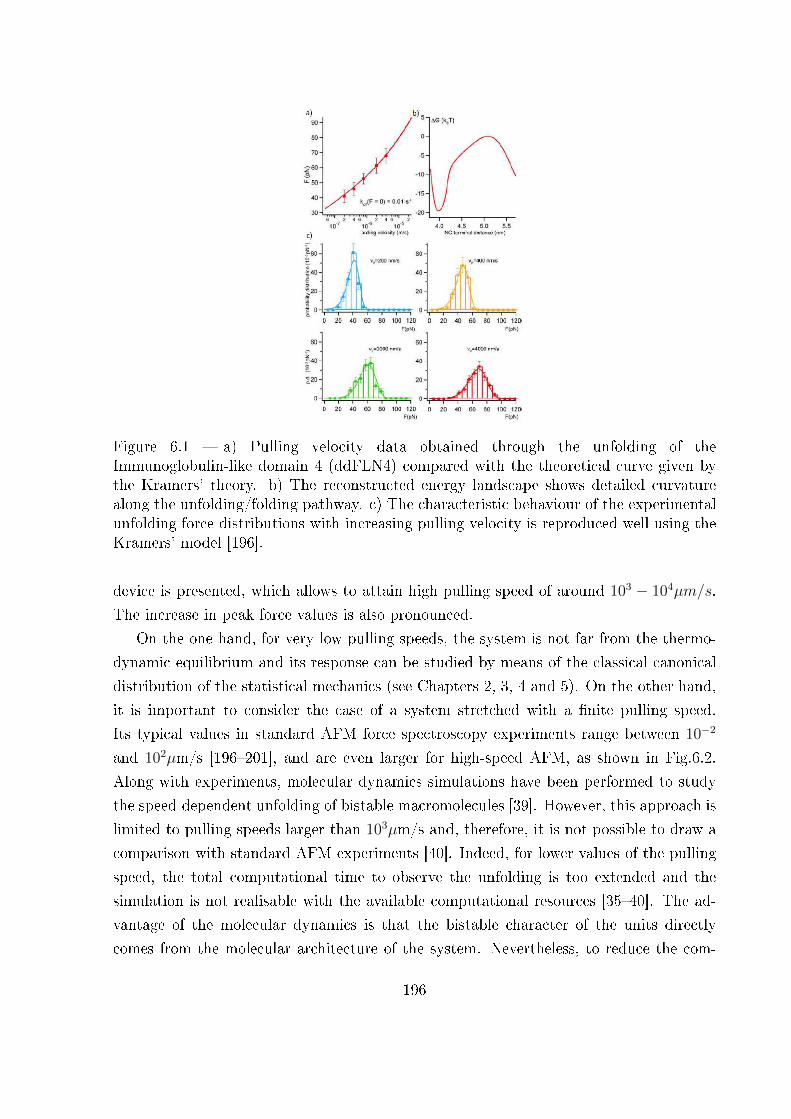
Figure 6.1 � a) Pulling velocity data obtained through the unfolding of theImmunoglobulin-like domain 4 (ddFLN4) compared with the theoretical curve given bythe Kramers' theory. b) The reconstructed energy landscape shows detailed curvaturealong the unfolding/folding pathway. c) The characteristic behaviour of the experimentalunfolding force distributions with increasing pulling velocity is reproduced well using theKramers' model [196].
device is presented, which allows to attain high pulling speed of around 103 − 104µm/s.
The increase in peak force values is also pronounced.
On the one hand, for very low pulling speeds, the system is not far from the thermo-
dynamic equilibrium and its response can be studied by means of the classical canonical
distribution of the statistical mechanics (see Chapters 2, 3, 4 and 5). On the other hand,
it is important to consider the case of a system stretched with a �nite pulling speed.
Its typical values in standard AFM force spectroscopy experiments range between 10−2
and 102µm/s [196�201], and are even larger for high-speed AFM, as shown in Fig.6.2.
Along with experiments, molecular dynamics simulations have been performed to study
the speed-dependent unfolding of bistable macromolecules [39]. However, this approach is
limited to pulling speeds larger than 103µm/s and, therefore, it is not possible to draw a
comparison with standard AFM experiments [40]. Indeed, for lower values of the pulling
speed, the total computational time to observe the unfolding is too extended and the
simulation is not realisable with the available computational resources [35�40]. The ad-
vantage of the molecular dynamics is that the bistable character of the units directly
comes from the molecular architecture of the system. Nevertheless, to reduce the com-
196
plexity of the molecular dynamics simulations, a coarse grained model can be adopted
and implemented through a kinetic Monte Carlo method [128, 202]. In this case, the
bistability of each unit is simply described by a two-state potential energy characterised
by the rates of the folding and unfolding processes. Hence, the reduced complexity of the
model allows to consider a larger range of pulling speeds. Nonetheless, in this approach,
only the folding and unfolding rates are considered to describe the bistable characters of
the units.
By considering the Kramers theory [16], the Bell approximation [159], and the Evans-
Ritchie more elaborated formalism [204], we can assert that the folding and unfolding
rates are directly related to the energy barrier ∆B and the energy jump ∆E between the
two states, as well as the mechanical action applied to the system. This point allows to
a�rm that we can estimate energetic features of the macromolecule (e.g., ∆B and/or ∆E)
from the force-extension response measured at di�erent pulling speeds (energy landscape
reconstruction). In fact, the observed unfolding forces are in�uenced by the dynamic
interplay between the transition rates and the applied pulling speed. Of course, much
theoretical work has been done to apply the Kramers, Bell and Evans-Ritchie theories
for decoding the force spectroscopy data and yielding the energetic parameters that gov-
ern the biomolecular processes [205]. This approach has generated a powerful class of
approximated results, which are of simple application in many di�erent regimes and con-
�gurations [149,150,203,206�209]. In the present Chapter, we propose an approach based
on the numerical implementation of the Langevin methodology. The classical Langevin
equations are equipped with the full description of an arbitrary potential energy mimicking
the bistable units. This method can be used to analyse force spectroscopy experimental
data in order to estimate biological features of the macromolecules, such as ∆E, ∆B or
other biochemical parameters. It allows for considering the whole range of pulling speeds
used in real experiments, including those of standard and high-speed AFM experiments.
Finally, the Langevin approach will be used to elucidate the role of the device in the
single-molecule measurements and to interpret experimental data concerning �lamin and
titin proteins.
6.2 Out-of-equilibrium statistical mechanics through the
Langevin approach
To introduce the out-of-equilibrium statistical mechanics of the pulling process, we
use the Langevin approach. It means that a friction term and a noise term are added to
197

Figure 6.2 � a) High-speed force spectroscopy (HS-FS) setup. An objective focuses thebeam of the superluminescent light-emitting diode (SLED) and collects the light re�ectedby the cantilever, �nally detected by a segmented photodiode. Titin I91 concatemers ofeight domains are immobilized on a tilted gold-coated surface via C-terminal cysteines.They are pulled by their N-terminal histidine tag with a nickel-coated tip at the endof a short cantilever. Tilting the sample surface further reduces hydrodynamic forces.Top inset shows a titin I91 domain (PDB ID: 1TIT) with relevant β-strands coloured inblue (A), yellow (A'), green (B), and red (G). Bottom inset shows a scanning electronmicrograph of a short cantilever. b) Force-extension curves acquired at three di�erentretraction velocities: 1, 100, and 1000 µm/s. The 1 µm/s curve is moving average��ltered(red trace, 65-µs time window). Times to unfold a single I91 domain are indicated byarrows. c) Unfolding force histograms of the 1, 100, and 1000 µm/s retraction velocityexperiments. d) Average unfolding forces versus retraction velocity obtained using HS-FS,conventional FS (error bars denote standard deviation), and steered molecular dynamicssimulations (data from Ref. [40]). Solid red line is the �t to the entire dynamic range ofHS-FS with the full microscopic model (from Ref. [203]) [34].
198
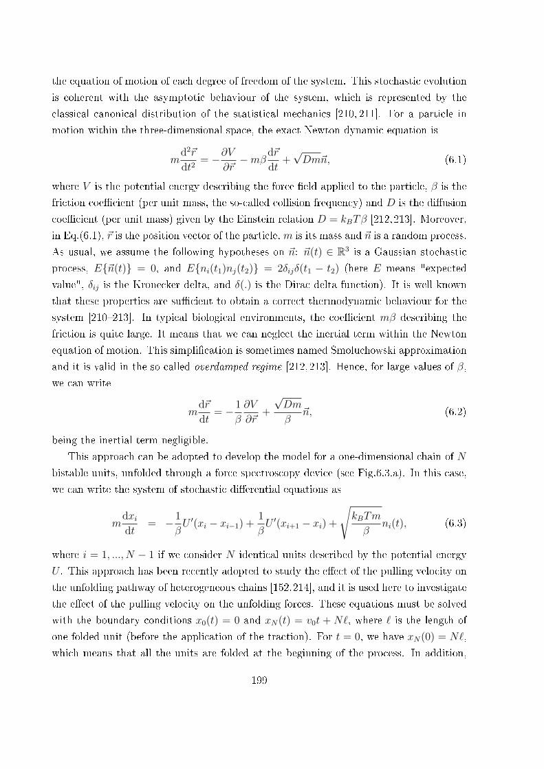
the equation of motion of each degree of freedom of the system. This stochastic evolution
is coherent with the asymptotic behaviour of the system, which is represented by the
classical canonical distribution of the statistical mechanics [210, 211]. For a particle in
motion within the three-dimensional space, the exact Newton dynamic equation is
md2~r
dt2= −∂V
∂~r−mβd~r
dt+√Dm~n, (6.1)
where V is the potential energy describing the force �eld applied to the particle, β is the
friction coe�cient (per unit mass, the so-called collision frequency) and D is the di�usion
coe�cient (per unit mass) given by the Einstein relation D = kBTβ [212,213]. Moreover,
in Eq.(6.1), ~r is the position vector of the particle, m is its mass and ~n is a random process.
As usual, we assume the following hypotheses on ~n: ~n(t) ∈ R3 is a Gaussian stochastic
process, E{~n(t)} = 0, and E{ni(t1)nj(t2)} = 2δijδ(t1 − t2) (here E means "expected
value", δij is the Kronecker delta, and δ(.) is the Dirac delta function). It is well known
that these properties are su�cient to obtain a correct thermodynamic behaviour for the
system [210�213]. In typical biological environments, the coe�cient mβ describing the
friction is quite large. It means that we can neglect the inertial term within the Newton
equation of motion. This simpli�cation is sometimes named Smoluchowski approximation
and it is valid in the so-called overdamped regime [212,213]. Hence, for large values of β,
we can write
md~r
dt= − 1
β
∂V
∂~r+
√Dm
β~n, (6.2)
being the inertial term negligible.
This approach can be adopted to develop the model for a one-dimensional chain of N
bistable units, unfolded through a force spectroscopy device (see Fig.6.3.a). In this case,
we can write the system of stochastic di�erential equations as
mdxidt
= − 1
βU ′(xi − xi−1) +
1
βU ′(xi+1 − xi) +
√kBTm
βni(t), (6.3)
where i = 1, ..., N − 1 if we consider N identical units described by the potential energy
U . This approach has been recently adopted to study the e�ect of the pulling velocity on
the unfolding pathway of heterogeneous chains [152,214], and it is used here to investigate
the e�ect of the pulling velocity on the unfolding forces. These equations must be solved
with the boundary conditions x0(t) = 0 and xN(t) = v0t + N`, where ` is the length of
one folded unit (before the application of the traction). For t = 0, we have xN(0) = N`,
which means that all the units are folded at the beginning of the process. In addition,
199
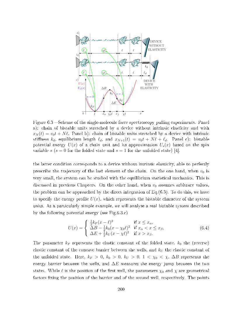
ℓ χℓ x
∆B
0
U(x)
χ0ℓxα xβ
∆E
ℓ χℓ ℓ ℓ
ℓ χℓ ℓ ℓ
kd
WITHOUT
DEVICE
DEVICEWITH
kF
kU
a)
b)
c)
k0
ℓd
s = 0s = 1
Us(x)
ELASTICITY
ELASTICITY
Figure 6.3 � Scheme of the single-molecule force spectroscopy pulling experiments. Panela): chain of bistable units stretched by a device without intrinsic elasticity and withxN(t) = v0t + N`. Panel b): chain of bistable units stretched by a device with intrinsicsti�ness kd, equilibrium length `d, and xN+1(t) = v0t + N` + `d. Panel c): bistablepotential energy U(x) of a chain unit and its approximation Us(x) based on the spinvariable s (s = 0 for the folded state and s = 1 for the unfolded state) [4].
the latter condition corresponds to a device without intrinsic elasticity, able to perfectly
prescribe the trajectory of the last element of the chain. On the one hand, when v0 is
very small, the system can be studied with the equilibrium statistical mechanics. This is
discussed in previous Chapters. On the other hand, when v0 assumes arbitrary values,
the problem can be approached by the direct integration of Eq.(6.3). To do this, we have
to specify the energy pro�le U(x), which represents the bistable character of the system
units. As a particularly simple example, we will analyse a real bistable system described
by the following potential energy (see Fig.6.3.c)
U(x) =
12kF (x− `)2 if x ≤ xα,
∆B − 12k0(x− χ0`)
2 if xα < x ≤ xβ,∆E + 1
2kU(x− χ`)2 if x > xβ.
(6.4)
The parameter kF represents the elastic constant of the folded state, k0 the (reverse)
elastic constant of the concave barrier between the wells, and kU the elastic constant of
the unfolded state. Here, kF > 0, k0 > 0, kU > 0, 1 < χ0 < χ, ∆B represents the
energy barrier between the wells, and ∆E measures the energy jump between the two
states. While ` is the position of the �rst well, the parameters χ0 and χ are geometrical
factors �xing the position of the barrier and of the second well, respectively. The points
200
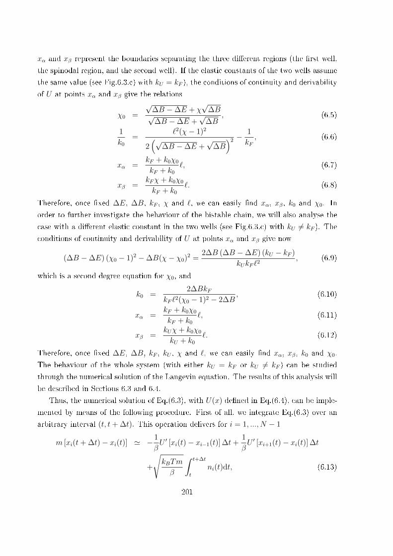
xα and xβ represent the boundaries separating the three di�erent regions (the �rst well,
the spinodal region, and the second well). If the elastic constants of the two wells assume
the same value (see Fig.6.3.c) with kU = kF ), the conditions of continuity and derivability
of U at points xα and xβ give the relations
χ0 =
√∆B −∆E + χ
√∆B√
∆B −∆E +√
∆B, (6.5)
1
k0
=`2(χ− 1)2
2(√
∆B −∆E +√
∆B)2 −
1
kF, (6.6)
xα =kF + k0χ0
kF + k0
`, (6.7)
xβ =kFχ+ k0χ0
kF + k0
`. (6.8)
Therefore, once �xed ∆E, ∆B, kF , χ and `, we can easily �nd xα, xβ, k0 and χ0. In
order to further investigate the behaviour of the bistable chain, we will also analyse the
case with a di�erent elastic constant in the two wells (see Fig.6.3.c) with kU 6= kF ). The
conditions of continuity and derivability of U at points xα and xβ give now
(∆B −∆E) (χ0 − 1)2 −∆B(χ− χ0)2 =2∆B (∆B −∆E) (kU − kF )
kUkF `2, (6.9)
which is a second degree equation for χ0, and
k0 =2∆BkF
kF `2(χ0 − 1)2 − 2∆B, (6.10)
xα =kF + k0χ0
kF + k0
`, (6.11)
xβ =kUχ+ k0χ0
kU + k0
`. (6.12)
Therefore, once �xed ∆E, ∆B, kF , kU , χ and `, we can easily �nd xα, xβ, k0 and χ0.
The behaviour of the whole system (with either kU = kF or kU 6= kF ) can be studied
through the numerical solution of the Langevin equation. The results of this analysis will
be described in Sections 6.3 and 6.4.
Thus, the numerical solution of Eq.(6.3), with U(x) de�ned in Eq.(6.4), can be imple-
mented by means of the following procedure. First of all, we integrate Eq.(6.3) over an
arbitrary interval (t, t+ ∆t). This operation delivers for i = 1, ..., N − 1
m [xi(t+ ∆t)− xi(t)] ' − 1
βU ′ [xi(t)− xi−1(t)] ∆t+
1
βU ′ [xi+1(t)− xi(t)] ∆t
+
√kBTm
β
∫ t+∆t
t
ni(t)dt, (6.13)
201

where ∆wi =∫ t+∆t
tni(t)dt are independent increments of the Wiener process [212, 213].
It follows that the quantities ∆wi are random Gaussian variables and ful�l the properties
E{∆wi} = 0 and E{∆wi∆wj} = 2∆tδij. We can therefore introduce the random vari-
ables Pi = 1√2∆t
∆wi, which are independent and normal Gaussian, thus described by the
probability density f(Pi) = 1√2πe−P
2i /2. The motion equations can be therefore written as
xi(t+ ∆t)− xi(t) ' −U ′ [xi(t)− xi−1(t)]∆t
mβ+ U ′ [xi+1(t)− xi(t)]
∆t
mβ
+√
2kBT
√∆t
mβPi. (6.14)
We can now observe that the time step ∆t controls the convergence of the numerical
scheme and the solution must be stable for decreasing values of ∆t. If we de�ne η = ∆tmβ
,
we obtain the �nal version of the �nite di�erence scheme of the Langevin equations for
i = 1, ..., N − 1
xi(t+ ∆t)− xi(t) ' −U ′ [xi(t)− xi−1(t)] η + U ′ [xi+1(t)− xi(t)] η+√
2kBT√ηPi. (6.15)
We draw the random numbers Pi [215], and we generate M realisations of the trajectory
to �nally determine their mean value [216].
The model so far introduced is represented by a chain of N bistable units with the
last unit directly connected to the device (without the intrinsic elasticity) able to apply a
traction de�ned by the uniform motion xN(t) = v0t+N` (see Fig.6.3.a). Actually, a force
spectroscopy device is typically characterised by its intrinsic elasticity, which is rather
important for the understanding of the system behaviour [217, 218]. Therefore, we also
introduce a second model where the last unit of the chain is connected to a device with a
given �nite elasticity (see Fig.6.3.b). It means that Eq.(6.3) must be substituted by the
following system of equations
mdxidt
= − 1
βU ′(xi − xi−1) +
1
βU ′(xi+1 − xi) +
√kBTm
βni(t), (6.16)
for i = 1, ..., N − 1 and
mdxNdt
= − 1
βU ′(xN − xN−1) +
1
βkd(xN+1 − xN − `d) +
√kBTm
βnN(t), (6.17)
for the device performing the force spectroscopy measurement. Here, kd represents the
intrinsic elasticity of the device, `d its intrinsic length, and the traction is described by
xN+1(t) = v0t+N`+ `d.
202
6.3 Analytical and numerical results
In this Section, we provide the analyses of four di�erent cases dealing with a bistable
chain (typically representing a protein) having the following properties: i) the same elastic
constants kF and kU in the folded and unfolded states, and a device without intrinsic
elasticity; ii) di�erent elastic constants kF and kU , and a device without intrinsic elasticity;
iii) the same elastic constants kF and kU , and a realistic device with kd and `d; iv) di�erent
elastic constants kF and kU , and a realistic device with kd and `d. The comparison of these
four di�erent cases is important to deduce some general features of the force-extension
relation, useful to better interpret and decipher the single-molecule experimental results.
In particular, this analysis will be able to shed light on the role of the force spectroscopy
device in the measured force-extension curves. We underline that in this Section, the
numerical calculations have been performed with reasonable parameters with respect to
real macromolecules but we decided not to refer to speci�c biological systems, in order to
show some general trends. However, we will show in Section 6.4 a direct comparison with
experiments conducted on �lamin and titin proteins.
6.3.1 Device without intrinsic elasticity
In Fig.6.4, we can �nd the results for the �rst case dealing with a chain with equal elas-
tic constants for the two wells and unfolded through a device without intrinsic elasticity.
We considered a macromolecule with N = 4 domains. In Fig.6.4.a, we show the energy
pro�le of the bistable units, where we can observe the energy barrier ∆B = 18kBT and
the energy jump ∆E = 10kBT . Then, in Fig.6.4.b, we show the force-extension curves for
di�erent pulling velocities v0. The dashed black curve corresponds to the theoretical result
obtained with v0 = 0. The other coloured curves represent the response of the chain with
an increasing pulling velocity. Each force-extension curve is obtained by averaging the
solution of the Langevin equation (see Eqs.(6.3) or (6.15)) overM = 2000 Monte Carlo re-
alisations of the process. The deviation between each coloured curve and the dashed black
curve measures how the process is far from the thermodynamic equilibrium. We remark
that, while the case with v0 = 0 is accessible with closed form mathematical expressions
based on the canonical distribution of the statistical mechanics, the out-of-equilibrium
behaviour can be only numerically explored by means of the Langevin formalism. The
important point is that the force peaks, representing the sequential unfolding of the chain
units (or protein domains), are more pronounced for larger values of the pulling velocity.
Therefore, following the experimental protocol, it is interesting to analyse the behaviour
203
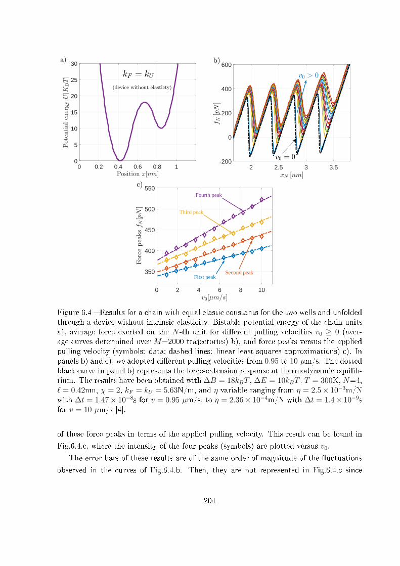
0 0.2 0.4 0.6 0.8 1Position x[nm]
0
5
10
15
20
25
30Potentialen
ergyU[K
BT]
a)
kF = kU
(device without elasticty)
2 2.5 3 3.5-200
0
200
400
600
0 2 4 6 8 10
350
400
450
500
550Fourth peak
Third peak
First peakSecond peak
Figure 6.4 � Results for a chain with equal elastic constants for the two wells and unfoldedthrough a device without intrinsic elasticity. Bistable potential energy of the chain unitsa), average force exerted on the N -th unit for di�erent pulling velocities v0 ≥ 0 (aver-age curves determined over M=2000 trajectories) b), and force peaks versus the appliedpulling velocity (symbols: data; dashed lines: linear least squares approximations) c). Inpanels b) and c), we adopted di�erent pulling velocities from 0.95 to 10 µm/s. The dottedblack curve in panel b) represents the force-extension response at thermodynamic equilib-rium. The results have been obtained with ∆B = 18kBT , ∆E = 10kBT , T = 300K, N=4,` = 0.42nm, χ = 2, kF = kU = 5.63N/m, and η variable ranging from η = 2.5× 10⁻³m/Nwith ∆t = 1.47× 10⁻⁸s for v = 0.95 µm/s, to η = 2.36× 10⁻⁴m/N with ∆t = 1.4× 10⁻⁹sfor v = 10 µm/s [4].
of these force peaks in terms of the applied pulling velocity. This result can be found in
Fig.6.4.c, where the intensity of the four peaks (symbols) are plotted versus v0.
The error bars of these results are of the same order of magnitude of the �uctuations
observed in the curves of Fig.6.4.b. Then, they are not represented in Fig.6.4.c since
204
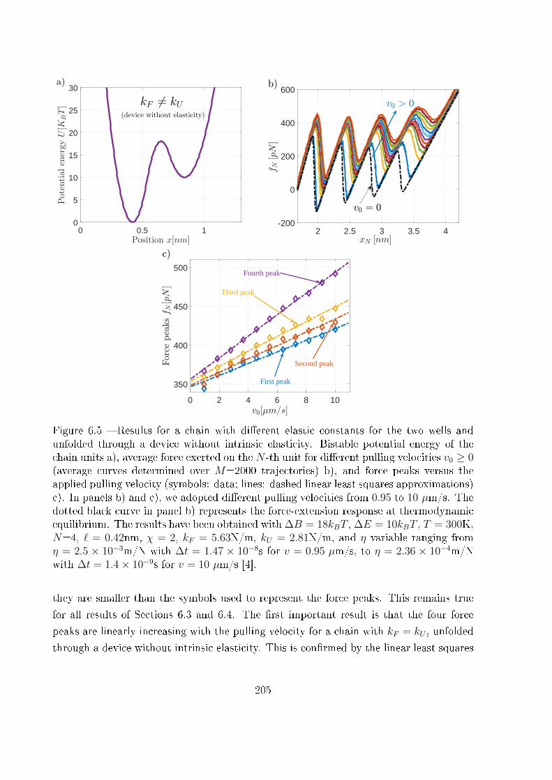
0 0.5 1Position x[nm]
0
5
10
15
20
25
30
Potentialen
ergyU[K
BT]
a)
kF 6= kU(device without elasticity)
2 2.5 3 3.5 4-200
0
200
400
600
0 2 4 6 8 10
350
400
450
500
First peak
Fourth peak
Third peak
Second peak
Figure 6.5 � Results for a chain with di�erent elastic constants for the two wells andunfolded through a device without intrinsic elasticity. Bistable potential energy of thechain units a), average force exerted on the N -th unit for di�erent pulling velocities v0 ≥ 0(average curves determined over M=2000 trajectories) b), and force peaks versus theapplied pulling velocity (symbols: data; lines: dashed linear least squares approximations)c). In panels b) and c), we adopted di�erent pulling velocities from 0.95 to 10 µm/s. Thedotted black curve in panel b) represents the force-extension response at thermodynamicequilibrium. The results have been obtained with ∆B = 18kBT , ∆E = 10kBT , T = 300K,N=4, ` = 0.42nm, χ = 2, kF = 5.63N/m, kU = 2.81N/m, and η variable ranging fromη = 2.5 × 10⁻³m/N with ∆t = 1.47 × 10⁻⁸s for v = 0.95 µm/s, to η = 2.36 × 10⁻⁴m/Nwith ∆t = 1.4× 10⁻⁹s for v = 10 µm/s [4].
they are smaller than the symbols used to represent the force peaks. This remains true
for all results of Sections 6.3 and 6.4. The �rst important result is that the four force
peaks are linearly increasing with the pulling velocity for a chain with kF = kU , unfolded
through a device without intrinsic elasticity. This is con�rmed by the linear least squares
205
approximations (dashed straight lines), shown in Fig.6.4.c. We remark that this behaviour
does not correspond to the typical experimental observation, where the force peaks show
a logarithmic trend with the pulling velocity. This trend, sometimes called Evans and
Ritchie law, is based on the classical Bell theory [159], and it is valid with the extension
speed varying over several orders of magnitude [135, 204, 219]. However, we remark that
such a logarithmic trend can sometimes be inexact, especially for quite large pulling
velocities [34�38]. In order to understand the speci�c features characterising the response
observed in single-molecule force spectroscopy experiments, we therefore explore the cases
with kF 6= kU and/or with a real device.
In Fig.6.5, we can �nd the results for a chain with kF 6= kU , unfolded by means of
a device without intrinsic elasticity. We considered kU = kF/2 and we assumed all the
other parameters exactly as in the case shown in Fig.6.4. The results shown in Fig.6.5 are
quite similar to the ones presented in Fig.6.4 and, in particular, the linear trend between
force peaks and pulling velocity is con�rmed also in this case with kF 6= kU . It means
that the di�erent elastic constants of the two energy wells describing the bistable units
are not at the origin of the dynamic behaviour experimentally observed (with the force
peaks proportional to the logarithm of the pulling velocity). Consequently, we consider in
the following Section the cases with a real device characterised by an intrinsic elasticity
and an intrinsic equilibrium length.
A �nal comment concerns the shape of the force-extension curves represented in Figs.6.4
and 6.5. In both cases, we observe that some lower peaks of the curves correspond to a
negative force. This is a speci�c behaviour induced by the fact that we are studying one-
dimensional systems. In fact, for one-dimensional systems, the idea of a protein chain as a
random coil with a complex distribution of domains is degenerated to a simple alignment
of units on one axis with a preferred total length given by j`+(N−j)χ` (with j = 0, ..., N).
Since the total length is exactly imposed by the device within the Helmholtz ensemble, it
is not di�cult to imagine con�gurations with either a pushing force (negative) or a pulling
one (positive), applied to the device. Of course, this apparently paradoxical behaviour
disappears for two- or three-dimensional geometries, where the exploration of the phase
space is more pertinent to polymer models [131]. Indeed, in these real multi-dimensional
cases, the pulling (negative) forces induce the geometrical rearrangement of the chain and
are not directly observed in the total force measured on the device. It is important to
underline that also the theoretical results obtained with the spin variables for v0 → 0
exhibit the same behaviour con�rming that it is related to the one-dimensional geometry
of our system. In spite of this limitation of our approach, we underline that the model is
206
able to correctly evaluate the force versus pulling velocity relation since at the transition
points the macromolecule is quite aligned along the traction direction.
6.3.2 Device with intrinsic elasticity
In Fig.6.6, we show the results for a chain with equal elastic constants for the two
wells and unfolded through a realistic device with intrinsic elasticity. Typically, the elastic
constant of the devices is much smaller than the elastic constant characterising the protein
domains. For the sake of de�niteness, in our case, we assume that kd = kF/8 = kU/8. The
comparison between kF = kU and kd can be observed in Fig.6.6.a, where the potential
energy of the units and of the device are represented. In Fig.6.6.b, the force-extension
response is shown with di�erent values of the pulling velocity. We remark that in this �gure
the curves are represented by plotting the force fN directly applied to the macromolecule
versus the traction xN+1 prescribed by the device.
The dashed black curve in Fig.6.6.b represents the force-extension relation at thermo-
dynamic equilibrium (v0 → 0) by means of the spin variables approach. The peaks of
force shown in Fig.6.6.b represent the sequential unfolding of the units and are quanti�ed
in Figs.6.6.c and 6.6.d. Here, these peaks are represented in terms of the pulling speed in
both linear and logarithmic scales, respectively.
From Fig.6.6.c, characterised by the linear scale of pulling velocity, we deduce that
the linearity between peaks and velocity is not con�rmed in the presence of a device with
intrinsic elasticity. Indeed, by observing Fig.6.6.d, we conclude that we have in this case
a linear dependence between force peaks and the logarithm of the pulling velocity, as
observed in most of experiments. We also observe that this linear relation is not veri�ed
for large values of the pulling velocity. Coherently, deviations from the linearity between
force peaks and the logarithm of the pulling velocity have been experimentally observed in
high-speed single-molecule measurements [34�38]. The dashed straight lines in Fig.6.6.d
represent the linear least squares approximations of the peaks data (for v0 < 2.5µm/s)
and con�rm the linear relation between the force peaks and log10 v0, at least for small
values of v0. This result underlines the crucial role of the realistic device, with its speci�c
sti�ness, in determining the force-extension response and the force peaks observed during
the molecule unfolding.
This scenario is also con�rmed for the case with kF 6= kU , as reported in Fig.6.7.
Finally, the model developed on the base of the Langevin equation is able to thoroughly
take into consideration the bistable character of the units of a given macromolecule as
well as the elasticity of the device used to generate the unfolding process. This point is
207
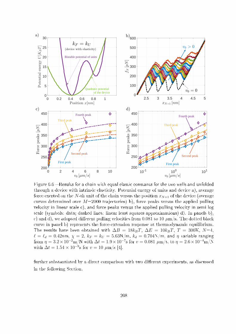
0 0.2 0.4 0.6 0.8 1Position x[nm]
0
5
10
15
20
25
30Potentialen
ergyU[K
BT]
a)
Quadratic potential of the device
kF = kU
Bistable potential of units
(device with elasticity)
2.5 3 3.5 4 4.5 50
100
200
300
400
500
600
0 2 4 6 8 10200
250
300
350
400
450
Third peak
Fourth peak
First peak
Second peak
10-1 100 101200
250
300
350
400
450
First peak
Third peak
Fourth peak
Second peak
Figure 6.6 � Results for a chain with equal elastic constants for the two wells and unfoldedthrough a device with intrinsic elasticity. Potential energy of units and device a), averageforce exerted on the N -th unit of the chain versus the position xN+1 of the device (averagecurves determined over M=2000 trajectories) b), force peaks versus the applied pullingvelocity in linear scale c), and force peaks versus the applied pulling velocity in semi-logscale (symbols: data; dashed lines: linear least squares approximations) d). In panels b),c) and d), we adopted di�erent pulling velocities from 0.081 to 10 µm/s. The dotted blackcurve in panel b) represents the force-extension response at thermodynamic equilibrium.The results have been obtained with ∆B = 18kBT , ∆E = 10kBT , T = 300K, N=4,` = `d = 0.42nm, χ = 2, kF = kU = 5.63N/m, kd = 0.704N/m, and η variable rangingfrom η = 3.2×10⁻²m/N with ∆t = 1.9×10⁻⁷s for v = 0.081 µm/s, to η = 2.6×10⁻⁴m/Nwith ∆t = 1.54× 10⁻⁹s for v = 10 µm/s [4].
further substantiated by a direct comparison with two di�erent experiments, as discussed
in the following Section.
208
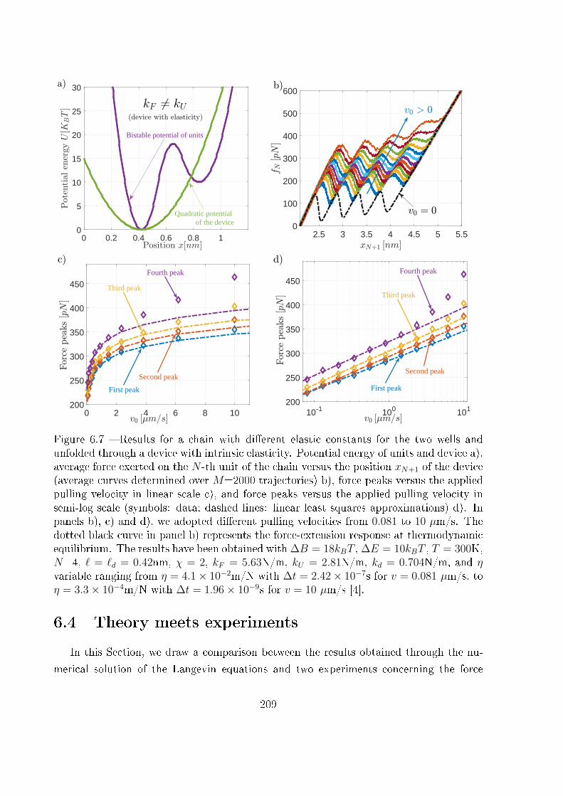
0 0.2 0.4 0.6 0.8 1Position x[nm]
0
5
10
15
20
25
30
Potentialen
ergyU[K
BT]
a)
Quadratic potential of the device
kF 6= kU
Bistable potential of units
(device with elasticity)
2.5 3 3.5 4 4.5 5 5.50
100
200
300
400
500
600
0 2 4 6 8 10200
250
300
350
400
450Fourth peak
Second peak
Third peak
First peak
10-1 100 101200
250
300
350
400
450Fourth peak
Third peak
First peak
Second peak
Figure 6.7 � Results for a chain with di�erent elastic constants for the two wells andunfolded through a device with intrinsic elasticity. Potential energy of units and device a),average force exerted on the N -th unit of the chain versus the position xN+1 of the device(average curves determined over M=2000 trajectories) b), force peaks versus the appliedpulling velocity in linear scale c), and force peaks versus the applied pulling velocity insemi-log scale (symbols: data; dashed lines: linear least squares approximations) d). Inpanels b), c) and d), we adopted di�erent pulling velocities from 0.081 to 10 µm/s. Thedotted black curve in panel b) represents the force-extension response at thermodynamicequilibrium. The results have been obtained with ∆B = 18kBT , ∆E = 10kBT , T = 300K,N=4, ` = `d = 0.42nm, χ = 2, kF = 5.63N/m, kU = 2.81N/m, kd = 0.704N/m, and ηvariable ranging from η = 4.1× 10⁻²m/N with ∆t = 2.42× 10⁻⁷s for v = 0.081 µm/s, toη = 3.3× 10⁻⁴m/N with ∆t = 1.96× 10⁻⁹s for v = 10 µm/s [4].
6.4 Theory meets experiments
In this Section, we draw a comparison between the results obtained through the nu-
merical solution of the Langevin equations and two experiments concerning the force
209
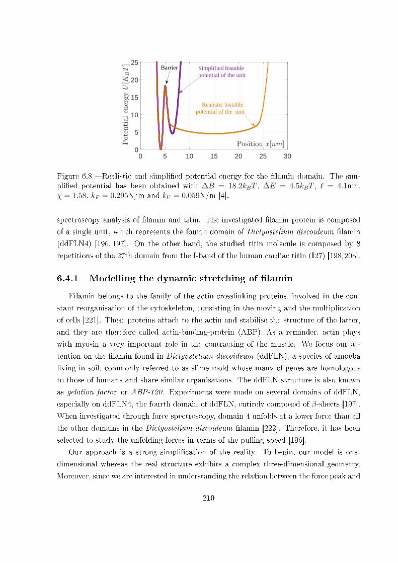
0 5 10 15 20 25 30
Position x[nm]0
5
10
15
20
25
Potentialen
ergyU[K
BT]
Simplified bistable potential of the unit
Realistic bistable potential of the unit
Barrier
Figure 6.8 � Realistic and simpli�ed potential energy for the �lamin domain. The sim-pli�ed potential has been obtained with ∆B = 18.2kBT , ∆E = 4.5kBT , ` = 4.1nm,χ = 1.58, kF = 0.295N/m and kU = 0.059N/m [4].
spectroscopy analysis of �lamin and titin. The investigated �lamin protein is composed
of a single unit, which represents the fourth domain of Dictyostelium discoideum �lamin
(ddFLN4) [196, 197]. On the other hand, the studied titin molecule is composed by 8
repetitions of the 27th domain from the I-band of the human cardiac titin (I27) [198,203].
6.4.1 Modelling the dynamic stretching of �lamin
Filamin belongs to the family of the actin-crosslinking proteins, involved in the con-
stant reorganisation of the cytoskeleton, consisting in the moving and the multiplication
of cells [221]. These proteins attach to the actin and stabilise the structure of the latter,
and they are therefore called actin-binding-protein (ABP). As a reminder, actin plays
with myosin a very important role in the contracting of the muscle. We focus our at-
tention on the �lamin found in Dictyostelium discoideum (ddFLN), a species of amoeba
living in soil, commonly referred to as slime mold whose many of genes are homologous
to those of humans and share similar organisations. The ddFLN structure is also known
as gelation factor or ABP-120. Experiments were made on several domains of ddFLN,
especially on ddFLN4, the fourth domain of ddFLN, entirely composed of β-sheets [197].
When investigated through force spectroscopy, domain 4 unfolds at a lower force than all
the other domains in the Dictyostelium discoideum �lamin [222]. Therefore, it has been
selected to study the unfolding forces in terms of the pulling speed [196].
Our approach is a strong simpli�cation of the reality. To begin, our model is one-
dimensional whereas the real structure exhibits a complex three-dimensional geometry.
Moreover, since we are interested in understanding the relation between the force peak and
210

x0 = 0
x
x2 = ℓd + ℓ + v0t
Domain 4 of Dictyostelium discoideum filamin
ddFLN4
x1kd
a)
10 15 20
0
20
40
60
80
100
0 2 4 6 8 100
5
10
15
20
25
30
Quadratic potential of the device
Bistable potential of the FILAMIN unit
0 2 4 6 8 10
40
50
60
70
10-1 100 10130
40
50
60
70
80
Figure 6.9 � Comparison between numerical results and experimental data for the �laminprotein. Panel a): scheme of the force spectroscopy experiment conducted on the �laminunit (N = 1). Image from the RCSB PDB (rcsb.org) of PDB ID 1KSR generated bythe NGL viewer with NMR data from Ref. [220]. Panel b): average force exerted onthe �lamin unit versus the prescribed device position (average curves determined overM=2000 trajectories). Panel c): assumed bistable potential energy of the �lamin andpotential energy of the AFM device. Panel d) and e): force peak versus the appliedpulling velocity in linear scale, and in semi-log scale, respectively. In panels b), d) and e),we adopted di�erent pulling velocities from 0.35 to 10 µm/s, coherently with experimentaldata [196]. The dashed black curve in panel b) represents the force-extension responseat thermodynamic equilibrium. The curves have been obtained with ∆B = 18.2kBT ,∆E = 4.5kBT , T = 300K, N=1, ` = 4.1nm, χ = 1.58, kF = 0.295N/m, kU = 0.059N/m,kd = 0.00985N/m, and η variable ranging from η = 2.6m/N with ∆t = 2.6 × 10⁻⁷s forv = 0.35 µm/s, to η = 0.09m/N with ∆t = 9.05× 10⁻⁹s for v = 10 µm/s [4].
211
the pulling velocity, the important features are concentrated in the transition region of the
dynamics. It means that, for our application, the relevant parts of the potential energy are
the �rst energy well and the following energy barrier. In fact, the peak force is determined
by the barrier crossing. Since, for the sake of simplicity, we represent the potential energy
with the three parabola expression given in Eq.(6.4), we are able to correctly represent
the �rst well and the barrier and we are forced to neglect the exact geometry of the second
well. This simpli�cation should not a�ect the force-velocity relation and can be found in
Fig.6.8, where we compare the realistic and the simpli�ed potential energy. We remark
that several theoretical approximations discussed in the Introduction consider only kF
and ∆B (and kd) for estimating the force-velocity relation. It is therefore important to
remember that our model is quite accurate from the point of view of this force-velocity
relation, but it does not take into account the correct geometry as previously discussed.
The parameters used to model the �rst energy well and the barrier correspond to the
values of the recent literature, obtained by means AFM experiments (under isometric
condition) [196, 197]. Importantly, the realistic geometry of the �lamin domain has been
completely detected by using magnetic tweezers force spectroscopy (under isotensional
condition) [223, 224]. It has been clearly proved that the step size (di�erence between
the energy minima corresponding to the folded and unfolded states) is around 12-18nm
and the total contour length of the unfolded domain is around 25-30nm, as schematically
shown in Fig.6.8.
In Fig.6.9.a, one can �nd the force spectroscopy AFM con�guration applied to the
ddFLN4 domain. The structure represented in Fig.6.9.a has been generated with the
nuclear magnetic resonance (NMR) spectroscopy data reported in Ref. [220]. The com-
parison between the numerical Langevin approach and the experimental data obtained
by force spectroscopy can be found in the other panels of Fig.6.9. In Fig.6.9.c, we can
observe the potential energies of domain (simpli�ed as discussed above) and device with
intrinsic elasticity, and we can observe that the device is much softer that the protein
under investigation. From Fig.6.9.b, we deduce the shape of the force-extension curves
for case with a single unit. We remark that in these curves, the force intensity is cor-
rect but the geometry of the domain (its step size) has not been respected as discussed
above. Moreover, we can observe that the force spectroscopy experiment is conducted
under conditions quite far from thermodynamic equilibrium. Indeed, the coloured curves
corresponding to the di�erent pulling speeds are rather far from the dashed black curve
representing the thermodynamic equilibrium. Nevertheless, we can see in Figs.6.9.d and e
that the force peaks are linearly depending on the logarithm of the applied pulling speed.
212
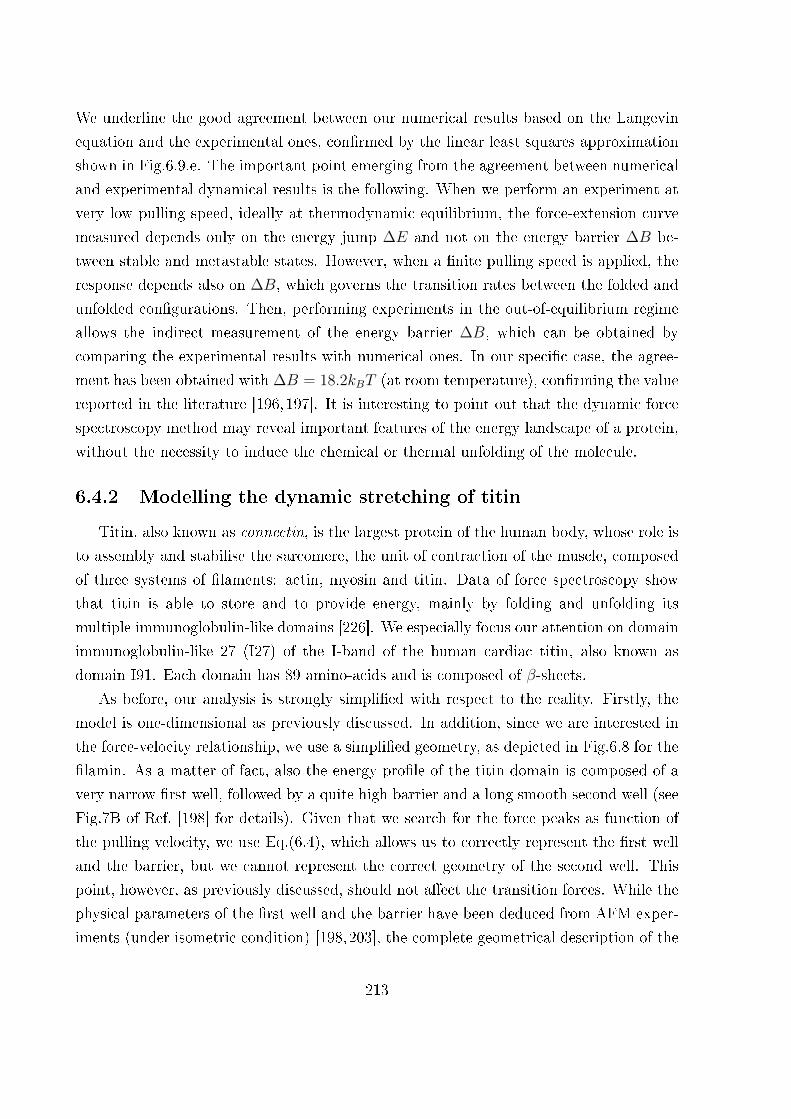
We underline the good agreement between our numerical results based on the Langevin
equation and the experimental ones, con�rmed by the linear least squares approximation
shown in Fig.6.9.e. The important point emerging from the agreement between numerical
and experimental dynamical results is the following. When we perform an experiment at
very low pulling speed, ideally at thermodynamic equilibrium, the force-extension curve
measured depends only on the energy jump ∆E and not on the energy barrier ∆B be-
tween stable and metastable states. However, when a �nite pulling speed is applied, the
response depends also on ∆B, which governs the transition rates between the folded and
unfolded con�gurations. Then, performing experiments in the out-of-equilibrium regime
allows the indirect measurement of the energy barrier ∆B, which can be obtained by
comparing the experimental results with numerical ones. In our speci�c case, the agree-
ment has been obtained with ∆B = 18.2kBT (at room temperature), con�rming the value
reported in the literature [196, 197]. It is interesting to point out that the dynamic force
spectroscopy method may reveal important features of the energy landscape of a protein,
without the necessity to induce the chemical or thermal unfolding of the molecule.
6.4.2 Modelling the dynamic stretching of titin
Titin, also known as connectin, is the largest protein of the human body, whose role is
to assembly and stabilise the sarcomere, the unit of contraction of the muscle, composed
of three systems of �laments: actin, myosin and titin. Data of force spectroscopy show
that titin is able to store and to provide energy, mainly by folding and unfolding its
multiple immunoglobulin-like domains [226]. We especially focus our attention on domain
immunoglobulin-like 27 (I27) of the I-band of the human cardiac titin, also known as
domain I91. Each domain has 89 amino-acids and is composed of β-sheets.
As before, our analysis is strongly simpli�ed with respect to the reality. Firstly, the
model is one-dimensional as previously discussed. In addition, since we are interested in
the force-velocity relationship, we use a simpli�ed geometry, as depicted in Fig.6.8 for the
�lamin. As a matter of fact, also the energy pro�le of the titin domain is composed of a
very narrow �rst well, followed by a quite high barrier and a long smooth second well (see
Fig.7B of Ref. [198] for details). Given that we search for the force peaks as function of
the pulling velocity, we use Eq.(6.4), which allows us to correctly represent the �rst well
and the barrier, but we cannot represent the correct geometry of the second well. This
point, however, as previously discussed, should not a�ect the transition forces. While the
physical parameters of the �rst well and the barrier have been deduced from AFM exper-
iments (under isometric condition) [198,203], the complete geometrical description of the
213

x0 = 0
x
xN+1 = ℓd +Nℓ + v0t
xN
...
N = 8
x1 xN−1
First repeat of titin I27 unit Eighth repeat of titin I27 unit
kd
a)
5 10 15 20
-100
0
100
200
300
400
500
0 1 2 30
10
20
30
40
50
60
Quadratic potential of the device
Bistable potential of the TITIN units
0 2 4 6 8 10
150
200
250
300
10-2 10-1 100 101
150
200
250
300
Figure 6.10 � Comparison between numerical results and experimental data for the titinprotein. Panel a): scheme of the force spectroscopy experiment conducted on the titinprotein (N = 8). Image from the RCSB PDB (rcsb.org) of PDB ID 1TIT generated bythe NGL viewer with NMR data from Ref. [225]. Panel b): average force exerted onthe titin molecule versus the prescribed device position (average curves determined overM=2000 trajectories). Panel c): assumed bistable potential energy of the titin proteinand potential energy of the AFM device. Panel d) and e): mean of the N = 8 force peaksversus the applied pulling velocity in linear scale, and in semi-log scale, respectively. Inpanels b), d) and e), we adopted di�erent pulling velocities from 0.1 to 10 µm/s, coherentlywith experimental data [198]. The dashed black curve in panel b) represents the force-extension response at thermodynamic equilibrium. The curves have been obtained with∆B = 37.5kBT , ∆E = 8.5kBT , T = 300K, N=8, ` = 0.5nm, χ = 5, kF = 9.94N/m,kU = 3.32N/m and kd = 0.166N/m, and η variable ranging from η = 8.45 × 10⁻²m/Nwith ∆t = 4.2 × 10⁻⁷s for v = 0.1 µm/s, to η = 8.45 × 10⁻⁴m/N with ∆t = 4.2 × 10⁻⁹sfor v = 10 µm/s [4].
214
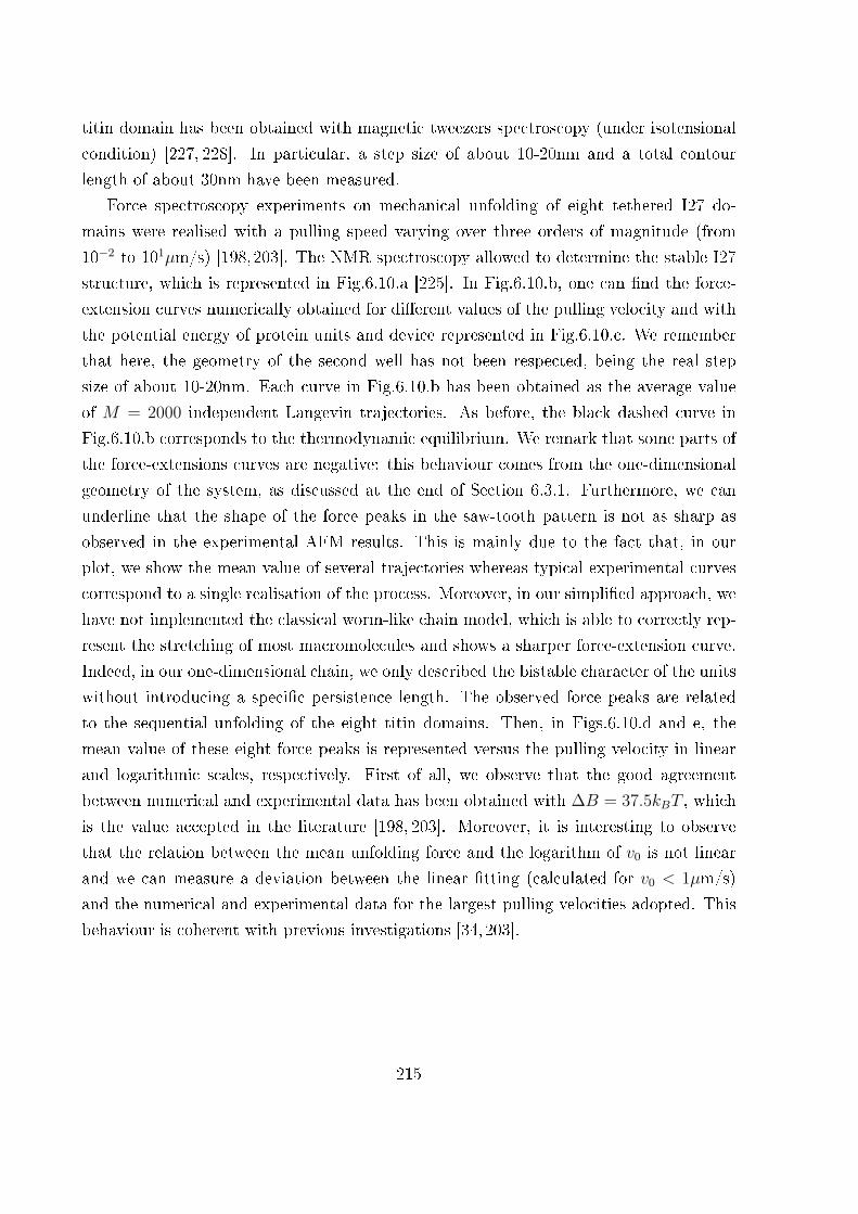
titin domain has been obtained with magnetic tweezers spectroscopy (under isotensional
condition) [227, 228]. In particular, a step size of about 10-20nm and a total contour
length of about 30nm have been measured.
Force spectroscopy experiments on mechanical unfolding of eight tethered I27 do-
mains were realised with a pulling speed varying over three orders of magnitude (from
10−2 to 101µm/s) [198,203]. The NMR spectroscopy allowed to determine the stable I27
structure, which is represented in Fig.6.10.a [225]. In Fig.6.10.b, one can �nd the force-
extension curves numerically obtained for di�erent values of the pulling velocity and with
the potential energy of protein units and device represented in Fig.6.10.c. We remember
that here, the geometry of the second well has not been respected, being the real step
size of about 10-20nm. Each curve in Fig.6.10.b has been obtained as the average value
of M = 2000 independent Langevin trajectories. As before, the black dashed curve in
Fig.6.10.b corresponds to the thermodynamic equilibrium. We remark that some parts of
the force-extensions curves are negative: this behaviour comes from the one-dimensional
geometry of the system, as discussed at the end of Section 6.3.1. Furthermore, we can
underline that the shape of the force peaks in the saw-tooth pattern is not as sharp as
observed in the experimental AFM results. This is mainly due to the fact that, in our
plot, we show the mean value of several trajectories whereas typical experimental curves
correspond to a single realisation of the process. Moreover, in our simpli�ed approach, we
have not implemented the classical worm-like chain model, which is able to correctly rep-
resent the stretching of most macromolecules and shows a sharper force-extension curve.
Indeed, in our one-dimensional chain, we only described the bistable character of the units
without introducing a speci�c persistence length. The observed force peaks are related
to the sequential unfolding of the eight titin domains. Then, in Figs.6.10.d and e, the
mean value of these eight force peaks is represented versus the pulling velocity in linear
and logarithmic scales, respectively. First of all, we observe that the good agreement
between numerical and experimental data has been obtained with ∆B = 37.5kBT , which
is the value accepted in the literature [198, 203]. Moreover, it is interesting to observe
that the relation between the mean unfolding force and the logarithm of v0 is not linear
and we can measure a deviation between the linear �tting (calculated for v0 < 1µm/s)
and the numerical and experimental data for the largest pulling velocities adopted. This
behaviour is coherent with previous investigations [34,203].
215

6.5 Conclusion
We presented an approach based on the overdamped Langevin formalism able to pre-
dict the force-extension response of biological macromolecules unfolded through a force
spectroscopy device at a given pulling speed. In particular, we proposed a model able to
work in the out-of-equilibrium regime of the statistical mechanics. This model is useful
to analyse the experimental data in order to estimate the main important biological and
biochemical features of the macromolecule under investigation.
The model presented considers an arbitrary continuous bistable potential energy for
describing the units of the macromolecule. This coarse-grained description has the ad-
vantage to require less computational resources than those required by the molecular
dynamics approach. As a matter of fact, each unit is de�ned by an e�ective bistable
energy, without taking into account the complete atomistic description of the molecular
architecture. On the other hand, the continuous description of the bistable potential
energy is more complete than the simpli�ed representation based on a limited set of pa-
rameters, which is often adopted in several analytical models. In this regard, the Langevin
approach can be seen as a good compromise between methods based on molecular dy-
namics simulations and others based on analytical approximations. Its implementation
allows for considering pulling speeds ranging from the standard AFM to the HS-AFM.
We show here a good agreement between the results obtained with this approach and the
experimental data concerning the unfolding of �lamin and titin.
216
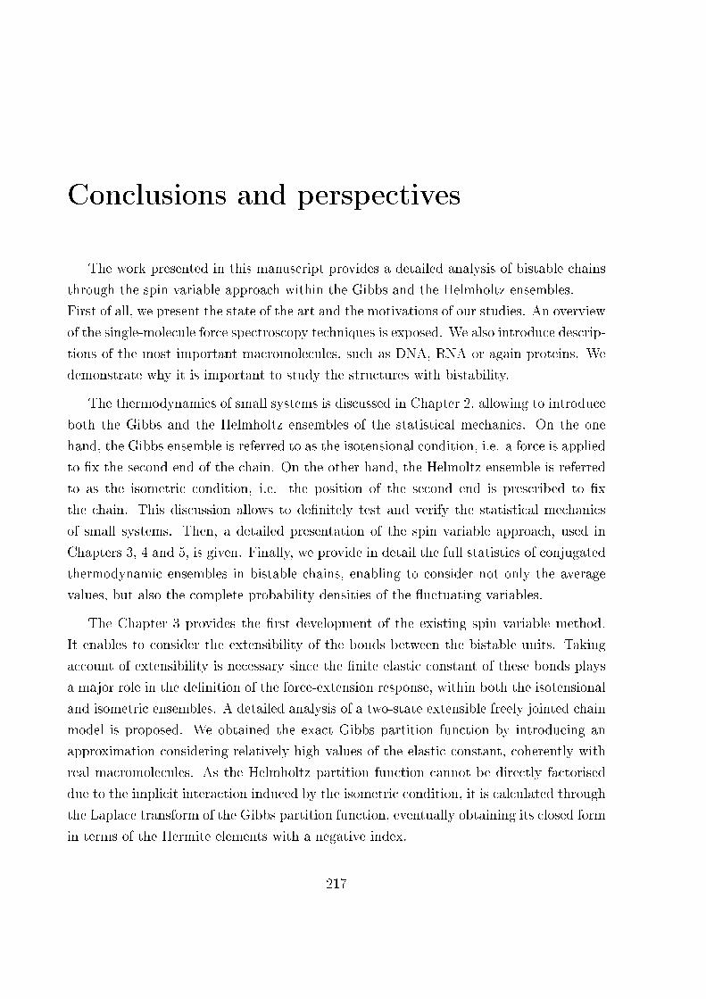
Conclusions and perspectives
The work presented in this manuscript provides a detailed analysis of bistable chains
through the spin variable approach within the Gibbs and the Helmholtz ensembles.
First of all, we present the state of the art and the motivations of our studies. An overview
of the single-molecule force spectroscopy techniques is exposed. We also introduce descrip-
tions of the most important macromolecules, such as DNA, RNA or again proteins. We
demonstrate why it is important to study the structures with bistability.
The thermodynamics of small systems is discussed in Chapter 2, allowing to introduce
both the Gibbs and the Helmholtz ensembles of the statistical mechanics. On the one
hand, the Gibbs ensemble is referred to as the isotensional condition, i.e. a force is applied
to �x the second end of the chain. On the other hand, the Helmoltz ensemble is referred
to as the isometric condition, i.e. the position of the second end is prescribed to �x
the chain. This discussion allows to de�nitely test and verify the statistical mechanics
of small systems. Then, a detailed presentation of the spin variable approach, used in
Chapters 3, 4 and 5, is given. Finally, we provide in detail the full statistics of conjugated
thermodynamic ensembles in bistable chains, enabling to consider not only the average
values, but also the complete probability densities of the �uctuating variables.
The Chapter 3 provides the �rst development of the existing spin variable method.
It enables to consider the extensibility of the bonds between the bistable units. Taking
account of extensibility is necessary since the �nite elastic constant of these bonds plays
a major role in the de�nition of the force-extension response, within both the isotensional
and isometric ensembles. A detailed analysis of a two-state extensible freely jointed chain
model is proposed. We obtained the exact Gibbs partition function by introducing an
approximation considering relatively high values of the elastic constant, coherently with
real macromolecules. As the Helmholtz partition function cannot be directly factorised
due to the implicit interaction induced by the isometric condition, it is calculated through
the Laplace transform of the Gibbs partition function, eventually obtaining its closed form
in terms of the Hermite elements with a negative index.
217

The Chapter 4 deals with the existing interactions among the units, with the help
of the Ising scheme. We investigate the behaviour of a chain of two-state units coupled
through an Ising interaction scheme. The coe�cient λ, representing the Ising interaction
coe�cient in the �nal partition functions provides a description of the e�ects of bistability
and cooperativity in biological and arti�cial micro- and nano-systems. We consider the
case of a positive interaction when λ > 0, which can be associated to a ferromagnetic-like
interaction, i.e. the unfolding a unit favours the unfolding of adjacent units. Conversely,
we also consider the case of a negative interaction when λ < 0, which can be associated
to an anti-ferromagnetic-like interaction, i.e. the folding of a unit prevents adjacent
units from unfolding. The interactions in the Gibbs partition function are studied in the
model with the help of the transfer matrix technique. Then, the Helmholtz partition
function is elaborated from the Gibbs partition function with the help of the Laplace
transform. We �rstly study the model far from the thermodynamic limit. In addition,
we propose results exploring asymptotic cases, such as weak and strong Ising interactions
(for both ferromagnetic-like and anti-ferromagneticlike schemes). We also provide the
study of bistable chains with Ising interactions at the thermodynamic limit within the
Gibbs ensemble. Finally, we generalise the theory for both extensible bonds and Ising
interactions.
The Chapter 5 provides the last development, performed at the thermodynamic equi-
librium, for a one-dimensional bistable chain through the spin variables method. The
heterogeneity is introduced within the energetic levels. The Helmholtz partition function
is obtained in closed form thanks to the Laplace transform and the determinant form of
the so-called Newton-Girard formulae. The heterogeneity of energetic levels of two-state
units allows to obtain the important unfolding sequence of the bistable chain, i.e. the so-
called unfolding pathway. Indeed, introducing various energetic levels of the units breaks
the symmetry and creates an inequality among the unfolding probabilities. Therefore, at
each switching occurence, once the heterogeneity introduced, the probability of unfolding
one given unit tends to 1, whereas the probability of the others tends to 0. It means that
the system implements a statistical sorting procedure. Eventually, the concept is iden-
ti�ability is proposed, to measure the capability to identify the most probable unfolding
pathway.
Finally, the Chapter 6 considers the case of an out-of-equilibrium bistable chain. In-
deed, it has been proved that the pulling speed exerts an in�uence on the amplitude of the
force peaks measured during stretching experiments on macromolecules. The presented
218

approach is based on the Langevin formalism, allowing to predict the force-extension re-
sponse of biological macromolecules unfolded through a force spectroscopy device at a
given pulling speed. The units of the macromolecule are described by an arbitrary con-
tinuous bistable potential. The Langevin approach can be seen as a good compromise
between methods based on molecular dynamics simulations and others based on analytical
approximations, in order to consider a wider range of pulling speeds (from standard to
high-speed AFM). Finally, we show a good agreement between the results obtained with
this approach and the experimental data concerning the unfolding of �lamin and titin.
The models introduced in this thesis are rather simple and paradigmatic, i.e. in-
troduced to study the e�ect of a single chain property to the �nal thermodynamic and
mechanical response. This choice permits to better discuss the theoretical origin of the
speci�c features of the force-extension curves observed in the di�erent situations and their
statistical character. Nevertheless, the models can be further improved to take into ac-
count other relevant physical and geometrical features. For instance, concerning the appli-
cation to macromolecules, the following generalisations can be considered: the dynamical
approach (out-of-equilibrium) should be applied to the case with Ising interactions; the
study of the heterogeneity should be generalised to deal with three-dimensional bistable
freely jointed chains (also with extensibility); the Ising interaction scheme could be gener-
alised to the case where the interactions are not only between neighbouring domains but
also long-range to better describe globular proteins and more complex system. Moreover,
recent works have provided evidence that the traction velocity applied to the chain with
a hard device plays an important role in de�ning the unfolding pathway [152, 229�231].
Therefore, it is important to fully analyse the interplay between the distribution of en-
ergy jumps and the applied traction velocity on the unfolding pathway. To do this, the
Langevin methodology could be combined with the spin variables technique in order to
fully describe the dynamics of the system.
In addition to the applications discussed in the present thesis, force spectroscopy allows
the study of many di�erent problems including, e.g., mechanical resistance of chemical
bonds. In this case, the force at which the bond breaks up can be directly measured [232].
Further, it is possible to map the energy landscape of the chemical bond under mechanical
force [233]. This is very important to investigate the antibody-antigen bond, and the
protein-protein or protein-living cell interactions [234]. Moreover, the adhesion of cells
on tissues or substrates is an interesting similar �eld of research concerning the so-called
Focal Adhesions, which are large macromolecular assemblies through which mechanical
forces are transmitted between the extracellular matrix and cells [235�237] (see Fig.7.1).
219

Figure 7.1 � Coarse-grained model for the mechanical response of the Focal Adhesions(FA). Left panel: schematic of a cell adhered to �brous Extra Cellular Matrix (ECM).The FA are formed at the periphery of the cell. Right panel: schematic of a coarse-grained model: stress �bers connect the FA and the nucleus. The FA is connected toECM through an integrin layer whose density is correlated with the �ber density underthe cell [238].
Also these problems can be approached with the statistical mechanics methodologies
introduced in this thesis.
On the other hand, in mechanics of materials, and more generally in material science,
similar behaviours have been observed in di�erent situations. First of all, in the plastic
behaviour of materials, each single plastic event can be explained through an instability,
which is able to switch the system from a ground state to a permanently deformed or
metastable state. These forms of micro-instabilities can be seen in di�erent shapes of
the force-extension (or stress-strain) response of plastic materials. For example, Lüders
bands are localised bands of plastic deformation observed in metals experiencing tensile
stresses, which usually starts at one end of the specimen and propagates toward the other
one [239]. During the bands propagation, the stress-strain curve is quite �at with some
�uctuations due to the internal microinstabilities (see Fig.7.2, left). Another example is
given by the Portevin-Le Chatelier e�ect, which can be observed as an unstable plastic
�ow during tensile tests of some dilute alloys (under certain regimes of strain rate and
temperature) [240]. In this case, a series of peaks can be seen in a region with a positive
slope of the stress-strain curve. These peaks represent the sequence of instabilities of the
plastic phenomenon (see Fig.7.2, center). Other manifestations of discontinuous defor-
mation are staircase creep and the Savart�Masson e�ect. They imply the formation of
steps on loading curves with a constant stress rate in a soft testing machine (see Fig.7.2,
right). There are relatively few studies on the Savart�Masson e�ect [241], although it was
discovered long before the Portevin-Le Chatelier e�ect.
Another important situation where the micro-instabilities between two states play a
central role is the adhesion of �lms and their peeling from a substrate [243] (see Fig.7.3,
220

Figure 7.2 � Three examples of stress strain curves of materials showing the Lüders bandsin the �rst case, the Portevin�Le Chatelier e�ect in the second case and the Savart�Massone�ect in the third one. In all these phenomena, we have a series of micro-instabilitiesgenerating the plastic behaviour [239,241,242].
Figure 7.3 � Microinstabilities in the peeling process (left) and in the crack propagation(right) [243,244].
left). In this context, one idea to improve and tailor the adhesion properties of arti�cial
materials is to use bioinspired geometries and mechanisms [244]. The combination of
thermal �uctuation and micro-instabilities is also at the origin of the fracture phenomena
in materials. If we think to a crystalline material, the propagation of a crack front must
be identi�ed by the gradual breaking of the atomic interactions along a line of the crystal
structure (see Fig.7.3, right). Therefore, each single crack propagation step is a form
of instability, which can be de�ned by assuming a maximum length of the interatomic
distance before rupture. Of course, the thermal �uctuations modify the crack propagation,
fostering the breaking of the interatomic bonds. In some cases, the temperature e�ects
can cause the crack generation and therefore we say that we have a thermally activated
crack propagation [245,246].
The observed similarities between the problems concerning micro-instabilities in bio-
physics and material science is of great importance, not only from the cultural point of
view, but also for the possibility to adopt the same techniques to approach very di�erent
themes. Indeed, the common denominator in all these examples, from both biophysics and
221

x0
U
s = +1s = −1
x0
U
s = +1
s = −1
a)
b)
ground statemetastable
broken state
unbroken state
∆E
∆x
state
Figure 7.4 � Paradigmatic potential energies of the system components for the two di�er-ent classes of micro-instabilities discussed in the main text: bistability between a folded(ground) state and an unfolded (metastable) state a), and damage process between theintact (unbroken) state and the damaged (broken) state b).
material science, is that some units of the system under investigation exhibit a two-state
or multi-state character. In particular, we can identify two classes of micro-instabilities.
On the one side, we can have a bistable (or multistable) behaviour between one ground
state and one (or more) metastable state. These admitted states represent di�erent con-
formations or con�gurations of the intact yet deformable system units. For instance, this
scheme corresponds to conformational transitions in macromolecules, as studied in this
thesis, or plastic transformations in solids. On the other side, we can also have transitions
between the broken or unbroken states of some breakable units of the system. In this case,
the system unit can switch from the intact condition to the damaged condition, and this
process can be reversible or not depending on the speci�c situation. Examples of this
scheme include deadhesion of cells, peeling of �lms or crack propagation.
To better appreciate the real di�erence between these two classes of micro-instabilities,
we can �nd in Fig.7.4 the potential energy U(x) describing the units behaviour in both
cases (we consider a one-dimensional geometry for the sake of simplicity). In the �rst case
(Fig.7.4.a), we have an elastic unit with two con�gurations (folded and unfolded) corre-
sponding to the two wells of the potential energy, having di�erent equilibrium lengths
and elastic constants. In the second case (Fig.7.4.b), we have a breakable mechanical
222

kk k k k k
kk
k
k
h h h h h
0 1 2 ξξ ξ−1 +1 NN−1... ...
y
kk k k k k
kk
k
k
h h h h h
0 1 2 ξξ ξ−1 +1 NN−1... ...
y
\Helmholtz" \Gibbs"
prescribed position yN+1
measured force hfi measured hyN+1i
applied force fa) b)
0 0−yM +yM
'
yi+1 yi−yi
k h
ff
Figure 7.5 � Scheme of the cohesion-decohesion process within both the Helmholtz a)and the Gibbs b) ensembles. While in the �rst case, we prescribe the position of thelast unit and we measure the average force 〈r〉, in the second case, we apply a forcef and we measure the average position of the last unit. In both cases, we consider ξunbroken vertical springs and N − ξ broken vertical springs. The energy potentials ϕ andΨ correspond to the horizontal and the vertical springs, respectively.
unit with the unbroken con�guration corresponding to the potential well, and the broken
con�guration corresponding to horizontal portion of the curve. Indeed, in this region the
exerted force is zero, which means that we are in the broken state of the unit. Peyrard,
Bishop and Dauxois have extensively studied the damage process between the intact (un-
broken) and damaged (broken) states. The adhesion-deadhesion model has been inspired
by their PBD model of DNA denaturation [247�250]. The method of the "spin variables"
discussed in this thesis has been largely adopted to model units with transitions between
ground and metastable states (see Fig.7.4.a). However, the case of units undergoing dam-
age processes between unbroken and broken states (Fig.7.4.b) must be further examined
and can be investigated by the same approach. As a matter of fact, the thermal e�ects
on the damage processes are still far from being fully understood. Therefore, an impor-
tant perspective of the spin variable approach is the analysis of the cohesion-decohesion
processes for complex systems, with the crucial e�ect of the temperature.
To do this, we can imagine a paradigmatic system representing the adhesion-deadhesion
of a �lm from a substrate. This basic system that may be approached is shown in Fig.7.5,
where one can �nd the �lm represented by the horizontal mass-spring chain, and grounded
to the substrate through a series of breakable springs. This con�guration mimics adhesion,
cohesion, and the rupture phenomena in general. The system is embedded in a thermal
bath to consider the thermal �uctuations and their e�ects on the adhesion mechanism.
This point makes the model well adapted to represent adhesion of cells, unzipping of hair-
pins, denaturation of DNA and other macromolecules, peeling of �lms from a substrate,
223
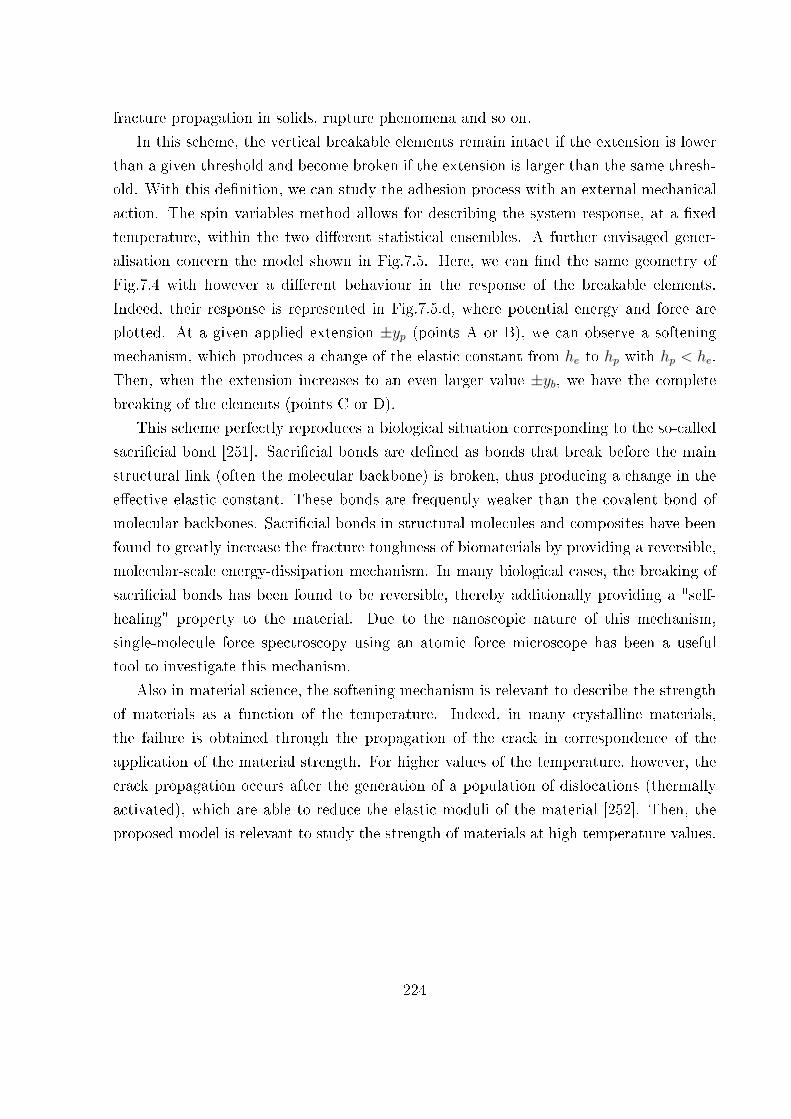
fracture propagation in solids, rupture phenomena and so on.
In this scheme, the vertical breakable elements remain intact if the extension is lower
than a given threshold and become broken if the extension is larger than the same thresh-
old. With this de�nition, we can study the adhesion process with an external mechanical
action. The spin variables method allows for describing the system response, at a �xed
temperature, within the two di�erent statistical ensembles. A further envisaged gener-
alisation concern the model shown in Fig.7.5. Here, we can �nd the same geometry of
Fig.7.4 with however a di�erent behaviour in the response of the breakable elements.
Indeed, their response is represented in Fig.7.5.d, where potential energy and force are
plotted. At a given applied extension ±yp (points A or B), we can observe a softening
mechanism, which produces a change of the elastic constant from he to hp with hp < he.
Then, when the extension increases to an even larger value ±yb, we have the complete
breaking of the elements (points C or D).
This scheme perfectly reproduces a biological situation corresponding to the so-called
sacri�cial bond [251]. Sacri�cial bonds are de�ned as bonds that break before the main
structural link (often the molecular backbone) is broken, thus producing a change in the
e�ective elastic constant. These bonds are frequently weaker than the covalent bond of
molecular backbones. Sacri�cial bonds in structural molecules and composites have been
found to greatly increase the fracture toughness of biomaterials by providing a reversible,
molecular-scale energy-dissipation mechanism. In many biological cases, the breaking of
sacri�cial bonds has been found to be reversible, thereby additionally providing a "self-
healing" property to the material. Due to the nanoscopic nature of this mechanism,
single-molecule force spectroscopy using an atomic force microscope has been a useful
tool to investigate this mechanism.
Also in material science, the softening mechanism is relevant to describe the strength
of materials as a function of the temperature. Indeed, in many crystalline materials,
the failure is obtained through the propagation of the crack in correspondence of the
application of the material strength. For higher values of the temperature, however, the
crack propagation occurs after the generation of a population of dislocations (thermally
activated), which are able to reduce the elastic moduli of the material [252]. Then, the
proposed model is relevant to study the strength of materials at high temperature values.
224
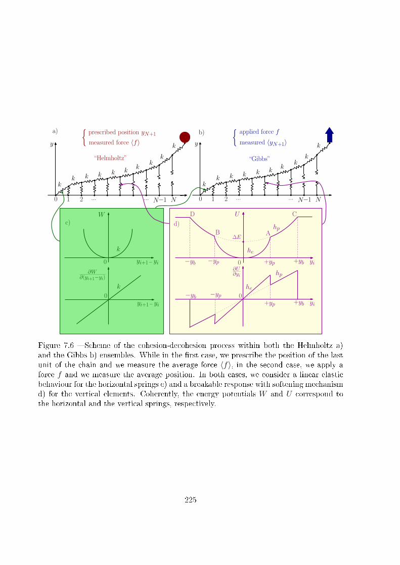
kk k k k k
kk
k
k
0 1 2 NN−1... ...
y
kk k k k k
kk
k
k
0 1 2 NN−1... ...
y
“Helmholtz” “Gibbs”
prescribed position yN+1
measured force 〈f〉 measured 〈yN+1〉
applied force fa) b)
0 0−yp +yp
W U
yi+1 yi− yi
k he
{{
hp
∆E
+yb−yb
0−yp
+yp
∂U∂yi
yi
he
hp
+yb
−yb0
∂W∂(yi+1−yi)
yi+1− yi
k
c) d)
AB
CD
Figure 7.6 � Scheme of the cohesion-decohesion process within both the Helmholtz a)and the Gibbs b) ensembles. While in the �rst case, we prescribe the position of the lastunit of the chain and we measure the average force 〈f〉, in the second case, we apply aforce f and we measure the average position. In both cases, we consider a linear elasticbehaviour for the horizontal springs c) and a breakable response with softening mechanismd) for the vertical elements. Coherently, the energy potentials W and U correspond tothe horizontal and the vertical springs, respectively.
225

226
Bibliography
[1] M. Benedito and S. Giordano. Thermodynamics of small systems with conforma-
tional transitions: The case of two-state freely jointed chains with extensible units.
The Journal of Chemical Physics, 149(5):054901, August 2018.
[2] M. Benedito and S. Giordano. Isotensional and isometric force-extension response of
chains with bistable units and Ising interactions. Physical Review E, 98(5):052146,
November 2018.
[3] M. Benedito, F. Manca, and S. Giordano. Full Statistics of Conjugated Thermody-
namic Ensembles in Chains of Bistable Units. Inventions, 4(1):19, March 2019.
[4] M. Benedito and S. Giordano. Unfolding pathway and its identi�ability in hetero-
geneous chains of bistable units. Physics Letters A, 384(5):126124, February 2020.
[5] M. Benedito, F. Manca, P. L. Palla, and S. Giordano. Rate-dependent
force�extension models for single-molecule force spectroscopy experiments. Physical
Biology, 17(5):056002, August 2020.
[6] M. L. Hughes and L. Dougan. The physics of pulling polyproteins: A review of single
molecule force spectroscopy using the AFM to study protein unfolding. Reports on
Progress in Physics. Physical Society (Great Britain), 79(7):076601, July 2016.
[7] T. R. Strick, M.-N. Dessinges, G. Charvin, N. H. Dekker, J.-F. Allemand, D. Ben-
simon, and V. Croquette. Stretching of macromolecules and proteins. Reports on
Progress in Physics, 66(1):1�45, December 2002.
[8] D. C. Rees, T. N. Williams, and M. T. Gladwin. Sickle-cell disease. The Lancet,
376(9757):2018�2031, December 2010.
[9] Sickle cell disease. https://www.inserm.fr/information-en-sante/dossiers-
information/drepanocytose.
227
[10] K. Wüthrich. NMR with Proteins and Nucleic Acids. Europhysics News, 17(1):11�
13, 1986.
[11] D. Ringe and G. A. Petsko. Study of protein dynamics by X-ray di�raction. In
Methods in Enzymology, volume 131 of Enzyme Structure Part L, pages 389�433.
Academic Press, January 1986.
[12] G. Weber. Energetics of Ligand Binding to Proteins. In C. B. An�nsen, John T. Ed-
sall, and Frederic M. Richards, editors, Advances in Protein Chemistry, volume 29,
pages 1�83. Academic Press, January 1975.
[13] R. H. Austin, K. W. Beeson, L. Eisenstein, H. Frauenfelder, and I. C. Gunsalus. Dy-
namics of ligand binding to myoglobin. Biochemistry, 14(24):5355�5373, December
1975.
[14] H. Frauenfelder, G. A. Petsko, and D. Tsernoglou. Temperature-dependent X-ray
di�raction as a probe of protein structural dynamics. Nature, 280(5723):558�563,
August 1979.
[15] H. Frauenfelder, S. G. Sligar, and P. G. Wolynes. The energy landscapes and motions
of proteins. Science, 254(5038):1598�1603, December 1991.
[16] H. A. Kramers. Brownian motion in a �eld of force and the di�usion model of
chemical reactions. Physica, 7(4):284�304, April 1940.
[17] J. S. Langer. Theory of the condensation point. Annals of Physics, 41(1):108�157,
January 1967.
[18] J. S. Langer. Theory of Nucleation Rates. Physical Review Letters, 21(14):973�976,
September 1968.
[19] J. S. Langer. Statistical theory of the decay of metastable states. Annals of Physics,
54(2):258�275, September 1969.
[20] F. Manca, S. Giordano, P. L. Palla, and F. Cleri. On the equivalence of thermody-
namics ensembles for �exible polymer chains. Physica A: Statistical Mechanics and
its Applications, 395:154�170, February 2014.
[21] A. M. Skvortsov, L. I. Klushin, and F. a. M. Leermakers. Negative compressibility
and nonequivalence of two statistical ensembles in the escape transition of a polymer
chain. The Journal of Chemical Physics, 126(2):024905, January 2007.
228

[22] D. I. Dimitrov, L. I. Klushin, A. Skvortsov, A. Milchev, and K. Binder. The es-
cape transition of a polymer: A unique case of non-equivalence between statistical
ensembles. The European Physical Journal E, 29(1):9�25, May 2009.
[23] A. M. Skvortsov, L. I. Klushin, A. A. Polotsky, and K. Binder. Mechanical des-
orption of a single chain: Unusual aspects of phase coexistence at a �rst-order
transition. Physical Review E, 85(3):031803, March 2012.
[24] M. Rief, F. Oesterhelt, B. Heymann, and H. E. Gaub. Single Molecule Force Spec-
troscopy on Polysaccharides by Atomic Force Microscopy. Science, 275(5304):1295�
1297, February 1997.
[25] T. E. Fisher, A. F. Oberhauser, M. Carrion-Vazquez, P. E. Marszalek, and J. M.
Fernandez. The study of protein mechanics with the atomic force microscope. Trends
in Biochemical Sciences, 24(10):379�384, October 1999.
[26] I. Rehman and S. Botelho. Biochemistry, Tertiary Structure, Protein. December
2017.
[27] Huntington's disease. https://fr.cisbio.eu/content/new-hope-for-huntingtons-
disease-drug-discovery/.
[28] S. B. Prusiner. Molecular biology of prion diseases. Science, 252(5012):1515�1522,
June 1991.
[29] Madcow disease. https://www.news-medical.net/health/How-Do-Prion-Diseases-
Spread-(French).aspx.
[30] S. Getfert. Escape processes far from thermal equilibrium : Path integrals and force
spectroscopy. 2009.
[31] S. S. Mandal. Force Spectroscopy on Single Molecules of Life. ACS Omega,
5(20):11271�11278, May 2020.
[32] G. Binnig, C. F. Quate, and C. Gerber. Atomic Force Microscope. Physical Review
Letters, 56(9):930�933, March 1986.
[33] T. Ho�mann and L. Dougan. Single molecule force spectroscopy using polyproteins.
Chemical Society Reviews, 41(14):4781�4796, June 2012.
229
[34] F. Rico, L. Gonzalez, I. Casuso, M. Puig-Vidal, and S. Scheuring. High-Speed Force
Spectroscopy Unfolds Titin at the Velocity of Molecular Dynamics Simulations.
Science, 342(6159):741�743, November 2013.
[35] F. Eghiaian, F. Rico, A. Colom, I. Casuso, and S. Scheuring. High-speed atomic
force microscopy: Imaging and force spectroscopy. FEBS Letters, 588(19):3631�
3638, October 2014.
[36] H. Takahashi, F. Rico, C. Chipot, and S. Scheuring. α-Helix Unwinding as Force
Bu�er in Spectrins. ACS Nano, 12(3):2719�2727, March 2018.
[37] C. Valotteau, F. Sumbul, and F. Rico. High-speed force spectroscopy: Microsecond
force measurements using ultrashort cantilevers. Biophysical Reviews, 11(5):689�
699, October 2019.
[38] F. Rico, A. Russek, L. González, H. Grubmüller, and S. Scheuring. Heterogeneous
and rate-dependent streptavidin�biotin unbinding revealed by high-speed force spec-
troscopy and atomistic simulations. Proceedings of the National Academy of Sciences
of the United States of America, 116(14):6594�6601, April 2019.
[39] F. Gräter, J. Shen, H. Jiang, M. Gautel, and H. Grubmüller. Mechanically induced
titin kinase activation studied by force-probe molecular dynamics simulations. Bio-
physical Journal, 88(2):790�804, February 2005.
[40] E. H. Lee, J. Hsin, M. Sotomayor, G. Comellas, and K. Schulten. Discovery through
the computational microscope. Structure (London, England: 1993), 17(10):1295�
1306, October 2009.
[41] T. R. Strick, J.-F. Allemand, D. Bensimon, A. Bensimon, and V. Croquette. The
Elasticity of a Single Supercoiled DNA Molecule. Science, 271(5257):1835�1837,
March 1996.
[42] J. K. Fisher, J. Cribb, K. V. Desai, L. Vicci, B. Wilde, K. Keller, R. M. Taylor,
J. Haase, K. Bloom, E. T. O'Brien, and R. Super�ne. Thin-foil magnetic force sys-
tem for high-numerical-aperture microscopy. The Review of scienti�c instruments,
77(2):023702�1�023702�9, February 2006.
[43] C. Gosse and V. Croquette. Magnetic tweezers: Micromanipulation and force mea-
surement at the molecular level. Biophysical Journal, 82(6):3314�3329, June 2002.
230
[44] C. Haber and D. Wirtz. Magnetic tweezers for DNA micromanipulation. Review of
Scienti�c Instruments, 71(12):4561�4570, November 2000.
[45] J. Yan, D. Skoko, and J. F. Marko. Near-�eld-magnetic-tweezer manipulation of
single DNA molecules. Physical Review E, 70(1):011905, July 2004.
[46] I. De Vlaminck and C. Dekker. Recent Advances in Magnetic Tweezers. Annual
Review of Biophysics, 41(1):453�472, 2012.
[47] A. Ashkin. History of Optical Trapping and Manipulation of Small Neutral Parti-
cles, Atoms, and Molecules. In Rudolf Rigler, Michel Orrit, and Thomas Basché,
editors, Single Molecule Spectroscopy: Nobel Conference Lectures, Springer Series in
Chemical Physics, pages 1�31. Springer, Berlin, Heidelberg, 2001.
[48] A. Ashkin, J. M. Dziedzic, J. E. Bjorkholm, and S. Chu. Observation of a single-
beam gradient force optical trap for dielectric particles. Optics Letters, 11(5):288�
290, May 1986.
[49] M. J. Lang and S. M. Block. Resource Letter: LBOT-1: Laser-based optical tweez-
ers. American Journal of Physics, 71(3):201�215, February 2003.
[50] J.-P. Galaup. La pince optique. Photoniques, (66):45�49, July 2013.
[51] M. Ribezzi-Crivellari and F. Ritort. Force Spectroscopy with Dual-Trap Optical
Tweezers: Molecular Sti�ness Measurements and Coupled Fluctuations Analysis.
Biophysical Journal, 103(9):1919�1928, November 2012.
[52] J. Camunas-Soler, M. Ribezzi-Crivellari, and F. Ritort. Elastic Properties of Nu-
cleic Acids by Single-Molecule Force Spectroscopy. Annual Review of Biophysics,
45(1):65�84, 2016.
[53] A. M. Monge, M. Manosas, and F. Ritort. Experimental test of ensemble inequiva-
lence and the �uctuation theorem in the force ensemble in DNA pulling experiments.
Physical Review E, 98(3):032146, September 2018.
[54] F. Landuzzi, X. Viader-Godoy, F. Cleri, I. Pastor, and F. Ritort. Detection of
single DNA mismatches by force spectroscopy in short DNA hairpins. The Journal
of Chemical Physics, 152(7):074204, February 2020.
231
[55] C.-H. Chiou and G.-B. Lee. A micromachined DNA manipulation platform for the
stretching and rotation of a single DNA molecule. Journal of Micromechanics and
Microengineering, 15:109�117, January 2005.
[56] F. Ren, Y. Zu, K. Kumar Rajagopalan, and S. Wang. Regulation of DNA con-
formations and dynamics in �ows with hybrid �eld micro�uidics. Biomicro�uidics,
6(4):044103, October 2012.
[57] M. C. Tarhan, N. La�tte, Y. Tauran, L. Jalabert, M. Kumemura, G. Perret, B. Kim,
A. W. Coleman, H. Fujita, and D. Collard. A rapid and practical technique for real-
time monitoring of biomolecular interactions using mechanical responses of macro-
molecules. Scienti�c Reports, 6(1):28001, June 2016.
[58] M. S. Hanay, S. Kelber, A. K. Naik, D. Chi, S. Hentz, E. C. Bullard, E. Colinet,
L. Dura�ourg, and M. L. Roukes. Single-protein nanomechanical mass spectrometry
in real time. Nature Nanotechnology, 7(9):602�608, September 2012.
[59] C. Yamahata, D. Collard, B. Legrand, T. Takekawa, M. Kumemura, G. Hashiguchi,
and H. Fujita. Silicon Nanotweezers With Subnanometer Resolution for the
Micromanipulation of Biomolecules. Journal of Microelectromechanical Systems,
17(3):623�631, June 2008.
[60] G. Perret, T. Lacornerie, F. Manca, S. Giordano, M. Kumemura, N. La�tte, L. Jal-
abert, M. C. Tarhan, E. F. Lartigau, F. Cleri, H. Fujita, and D. Collard. Real-time
mechanical characterization of DNA degradation under therapeutic X-rays and its
theoretical modeling. Microsystems & Nanoengineering, 2(1):1�9, December 2016.
[61] DNA. https://en.wikipedia.org/wiki/DNA.
[62] Types of RNA. https://www.news-medical.net/life-sciences/-Types-of-RNA-
mRNA-rRNA-and-tRNA-(French).aspx.
[63] Chromatin. https://www.genome.gov/genetics-glossary/Chromatin.
[64] H. Meng, K. Andresen, and J. van Noort. Quantitative analysis of single-molecule
force spectroscopy on folded chromatin �bers. Nucleic Acids Research, 43(7):3578�
3590, April 2015.
[65] M. Kruithof, F.-T. Chien, A. Routh, C. Logie, Daniela D., and J. van Noort. Single-
molecule force spectroscopy reveals a highly compliant helical folding for the 30-nm
chromatin �ber. Nature Structural & Molecular Biology, 16(5):534�540, May 2009.
232
[66] F.-T. Chien and J. Noort. 10 Years of Tension on Chromatin: Results from Sin-
gle Molecule Force Spectroscopy. Current pharmaceutical biotechnology, 10:474�85,
September 2009.
[67] Y. Cui and C. Bustamante. Pulling a single chromatin �ber reveals the forces
that maintain its higher-order structure. Proceedings of the National Academy of
Sciences of the United States of America, 97(1):127�132, January 2000.
[68] S. Cocco, J. F. Marko, R. Monasson, A. Sarkar, and J. Yan. Force-extension behav-
ior of folding polymers. The European Physical Journal E, 10(3):249�263, March
2003.
[69] J. D. Watson and F. H. C. Crick. Molecular Structure of Nucleic Acids: A Structure
for Deoxyribose Nucleic Acid. Nature, 171(4356):737�738, April 1953.
[70] S. B. Smith, L. Finzi, and C. Bustamante. Direct mechanical measurements
of the elasticity of single DNA molecules by using magnetic beads. Science,
258(5085):1122�1126, November 1992.
[71] J. F. Marko and E. D. Siggia. Stretching DNA. Macromolecules, 28(26):8759�8770,
December 1995.
[72] C. Bustamante, J. F. Marko, E. D. Siggia, and S. Smith. Entropic elasticity of
lambda-phage DNA. Science, 265(5178):1599�1600, September 1994.
[73] S. B. Smith, Y. Cui, and C. Bustamante. Overstretching B-DNA: The elastic re-
sponse of individual double-stranded and single-stranded DNA molecules. Science
(New York, N.Y.), 271(5250):795�799, February 1996.
[74] I. Rouzina and V. A. Bloom�eld. Force-induced melting of the DNA double helix
1. Thermodynamic analysis. Biophysical Journal, 80(2):882�893, February 2001.
[75] I. Rouzina and V. A. Bloom�eld. Force-induced melting of the DNA double helix.
2. E�ect of solution conditions. Biophysical Journal, 80(2):894�900, February 2001.
[76] S. Cocco, J. Yan, J.-F. Léger, D. Chatenay, and J. F. Marko. Overstretch-
ing and force-driven strand separation of double-helix DNA. Physical Review E,
70(1):011910, July 2004.
233

[77] N. Bosaeus, A. H. El-Sagheer, T. Brown, S. B. Smith, B. Åkerman, C. Bustamante,
and B. Nordén. Tension induces a base-paired overstretched DNA conformation.
Proceedings of the National Academy of Sciences, 109(38):15179�15184, September
2012.
[78] M. Manghi, N. Destainville, and J. Palmeri. Mesoscopic models for DNA stretching
under force: New results and comparison with experiments. The European Physical
Journal E, 35(10):110, October 2012.
[79] C. Bustamante, Z. Bryant, and S. B. Smith. Ten years of tension: Single-molecule
DNA mechanics. Nature, 421(6921):423�427, January 2003.
[80] O. Kratky and G. Porod. Röntgenuntersuchung gelöster Fadenmoleküle. Recueil
des Travaux Chimiques des Pays-Bas, 68(12):1106�1122, 1949.
[81] A. Rosa, T. X. Hoang, D. Marenduzzo, and A. Maritan. Elasticity of Semi�exible
Polymers with and without Self-Interactions. Macromolecules, 36(26):10095�10102,
December 2003.
[82] A. Rosa, T. X. Hoang, D. Marenduzzo, and A. Maritan. A new interpolation formula
for semi�exible polymers. Biophysical Chemistry, 115(2):251�254, April 2005.
[83] S. Doniach. Biological Physics: Energy, Information, Life. Physics Today, 57(11):63�
64, November 2004.
[84] J. Lipfert, J. W. J. Kerssemakers, T. Jager, and N. H. Dekker. Magnetic torque
tweezers: Measuring torsional sti�ness in DNA and RecA-DNA �laments. Nature
Methods, 7(12):977�980, December 2010.
[85] J. Lipfert, M. Wiggin, J.W. J. Kerssemakers, F. Pedaci, and N. H. Dekker. Freely
orbiting magnetic tweezers to directly monitor changes in the twist of nucleic acids.
Nature Communications, 2:439, August 2011.
[86] S. K. Nomidis, F. Kriegel, W. Vanderlinden, J. Lipfert, and E. Carlon. Twist-Bend
Coupling and the Torsional Response of Double-Stranded DNA. Physical Review
Letters, 118(21):217801, May 2017.
[87] S. K. Nomidis, E. Skoruppa, E. Carlon, and J. F. Marko. Twist-bend coupling and
the statistical mechanics of the twistable wormlike-chain model of DNA: Perturba-
tion theory and beyond. Physical Review E, 99(3):032414, March 2019.
234
[88] Genetic code. https://www.genome.gov/genetics-glossary/Genetic-Code.
[89] L. Pauling, R. B. Corey, and H. R. Branson. The structure of proteins: Two
hydrogen-bonded helical con�gurations of the polypeptide chain. Proceedings of the
National Academy of Sciences, 37(4):205�211, April 1951.
[90] Protein. https://www.genome.gov/genetics-glossary/Protein.
[91] A. E. Mirsky and L. Pauling. On the Structure of Native, Denatured, and Co-
agulated Proteins. Proceedings of the National Academy of Sciences of the United
States of America, 22(7):439�447, July 1936.
[92] J. Sabelko, J. Ervin, and M. Gruebele. Observation of strange kinetics in protein
folding. Proceedings of the National Academy of Sciences of the United States of
America, 96(11):6031�6036, May 1999.
[93] Y. Fichou. Hydration water dynamics of the tau protein in its native and amyloid
states. March 2015.
[94] M. Caruel and L. Truskinovsky. Physics of muscle contraction. Reports on Progress
in Physics, 81(3):036602, February 2018.
[95] M. Caruel, P. Moireau, and D. Chapelle. Stochastic modeling of chemical-
mechanical coupling in striated muscles. Biomechanics and Modeling in Mechanobi-
ology, 18(3):563�587, June 2019.
[96] H. A. Wu. Molecular dynamics study on mechanics of metal nanowire. Mechanics
Research Communications, 33(1):9�16, January 2006.
[97] W. Liang, D. J. Srolovitz, and M. Zhou. A micromechanical continuum model for
the tensile behavior of shape memory metal nanowires. Journal of the Mechanics
and Physics of Solids, 55(8):1729�1761, August 2007.
[98] X. Guo, W. Liang, and M. Zhou. Mechanism for the Pseudoelastic Behavior of FCC
Shape Memory Nanowires. Experimental Mechanics, 49(2):183�190, April 2009.
[99] A. Rafsanjani and D. Pasini. Bistable Auxetic Mechanical Metamaterials Inspired
by Ancient Geometric Motifs. Extreme Mechanics Letters, 9:291�296, 2016.
[100] S. Katz and S. Givli. Solitary waves in a bistable lattice. Extreme Mechanics Letters,
22:106�111, July 2018.
235
[101] I. Müller and P. Villaggio. A model for an elastic-plastic body. Archive for Rational
Mechanics and Analysis, 65(1):25�46, March 1977.
[102] B. Fedelich and G. Zanzotto. Hysteresis in discrete systems of possibly interacting
elements with a double-well energy. Journal of Nonlinear Science, 2(3):319�342,
September 1992.
[103] G. Puglisi and L. Truskinovsky. Thermodynamics of rate-independent plasticity.
Journal of the Mechanics and Physics of Solids, 53:655�679, March 2005.
[104] M. Caruel, J. M. Allain, and L. Truskinovsky. Mechanics of collective unfolding.
Journal of the Mechanics and Physics of Solids, 76:237�259, March 2015.
[105] Y. R. Efendiev and L. Truskinovsky. Thermalization of a driven bi-stable FPU chain.
Continuum Mechanics and Thermodynamics, 22(6):679�698, September 2010.
[106] A. Mielke and L. Truskinovsky. From Discrete Visco-Elasticity to Continuum Rate-
Independent Plasticity: Rigorous Results. Archive for Rational Mechanics and
Analysis, 203:577�619, February 2011.
[107] I. Benichou and S. Givli. Structures undergoing discrete phase transformation.
Journal of the Mechanics and Physics of Solids, 61(1):94�113, January 2013.
[108] S. Liu, A. I. Azad, and R. Burgueño. Architected materials for tailorable shear
behavior with energy dissipation. Extreme Mechanics Letters, 28:1�7, April 2019.
[109] A. F. Huxley and R. M. Simmons. Proposed Mechanism of Force Generation in
Striated Muscle. Nature, 233(5321):533�538, October 1971.
[110] T. L. Hill. Theory of muscular contraction extended to groups of actin sites. Pro-
ceedings of the National Academy of Sciences of the United States of America,
70(10):2732�2736, October 1973.
[111] M. Caruel, J.-M. Allain, and L. Truskinovsky. Muscle as a Metamaterial Operating
Near a Critical Point. Physical Review Letters, 110:248103, June 2013.
[112] M. Caruel and L. Truskinovsky. Statistical mechanics of the Huxley-Simmons model.
Physical Review E, 93(6):062407, June 2016.
[113] S. Giordano. Spin variable approach for the statistical mechanics of folding and
unfolding chains. Soft Matter, 13(38):6877�6893, October 2017.
236
[114] R. Law, P. Carl, S. Harper, P Dalhaimer, D.W. Speicher, and D. E. Discher. Co-
operativity in forced unfolding of tandem spectrin repeats. Biophysical Journal,
84(1):533�544, January 2003.
[115] W. Bialek. Perspectives on theory at the interface of physics and biology. Reports on
Progress in Physics. Physical Society (Great Britain), 81(1):012601, January 2018.
[116] M. V. Vol'kenshte��n. Con�gurational Statistics of Polymeric Chains. Interscience
Publishers, 1963.
[117] H. Kleinert. Path Integrals in Quantum Mechanics, Statistics, Polymer Physics,
and Financial Markets. World scienti�c, �fth edition, May 2009.
[118] R. H. Boyd and P. J. Phillips. The Science of Polymer Molecules. Cambridge
University Press, October 1996.
[119] M. Doi. Introduction to Polymer Physics. Clarendon Press, 1996.
[120] J. H. Weiner. Statistical Mechanics of Elasticity. Courier Corporation, February
2012.
[121] M. Rubinstein and R. H. Colby. Polymer Physics. OUP Oxford, June 2003.
[122] R. G. Winkler. Deformation of semi�exible chains. The Journal of Chemical Physics,
118(6):2919�2928, January 2003.
[123] G. Glatting, R. G. Winkler, and P. Reineker. Partition function and force extension
relation for a generalized freely jointed chain, May 2002.
[124] F. Manca, S. Giordano, P. L. Palla, R. Zucca, F. Cleri, and L. Colombo. Elasticity of
�exible and semi�exible polymers with extensible bonds in the Gibbs and Helmholtz
ensembles. The Journal of Chemical Physics, 136(15):154906, April 2012.
[125] F. Manca, S. Giordano, P. L. Palla, F. Cleri, and L. Colombo. Theory and Monte
Carlo simulations for the stretching of �exible and semi�exible single polymer chains
under external �elds. The Journal of Chemical Physics, 137(24):244907, December
2012.
[126] T. Su and P. K. Purohit. Thermomechanics of a heterogeneous �uctuating chain.
Journal of the Mechanics and Physics of Solids, 58(2):164�186, February 2010.
237
[127] J. Kierfeld, O. Niamploy, V. Sa-yakanit, and R. Lipowsky. Stretching of semi�exible
polymers with elastic bonds. The European Physical Journal E, 14(1):17�34, May
2004.
[128] M. Rief, J. M. Fernandez, and H. E. Gaub. Elastically Coupled Two-Level Systems
as a Model for Biopolymer Extensibility. Physical Review Letters, 81(21):4764�4767,
November 1998.
[129] H. J. Kreuzer, S. H. Payne, and L. Livadaru. Stretching a Macromolecule in an
Atomic Force Microscope: Statistical Mechanical Analysis. Biophysical Journal,
80(6):2505�2514, June 2001.
[130] F. Manca, S. Giordano, P. L. Palla, F. Cleri, and L. Colombo. Two-state theory
of single-molecule stretching experiments. Physical Review E, 87(3):032705, March
2013.
[131] S. Giordano. Helmholtz and Gibbs ensembles, thermodynamic limit and bistability
in polymer lattice models. Continuum Mechanics and Thermodynamics, 30(3):459�
483, May 2018.
[132] M. S. Z. Kellermayer, S. B. Smith, H. L. Granzier, and C. Bustamante. Folding-
Unfolding Transitions in Single Titin Molecules Characterized with Laser Tweezers.
Science, 276(5315):1112�1116, May 1997.
[133] J. Wang, T. B. Kouznetsova, R. Boulatov, and S. L. Craig. Mechanical gating of a
mechanochemical reaction cascade. Nature Communications, 7(1):13433, November
2016.
[134] A. Imparato, F. Sbrana, and M. Vassalli. Reconstructing the free-energy land-
scape of a polyprotein by single-molecule experiments. EPL (Europhysics Letters),
82(5):58006, May 2008.
[135] M. Rief, M. Gautel, F. Oesterhelt, J. M. Fernandez, and H. E. Gaub. Re-
versible Unfolding of Individual Titin Immunoglobulin Domains by AFM. Science,
276(5315):1109�1112, May 1997.
[136] M. Rief, J. Pascual, M. Saraste, and H. E. Gaub. Single molecule force spectroscopy
of spectrin repeats: Low unfolding forces in helix bundles. Journal of Molecular
Biology, 286(2):553�561, February 1999.
238
[137] F. Manca, S. Giordano, P. L. Palla, F. Cleri, and L. Colombo. Monte Carlo simu-
lations of single polymer force-extension relations. Journal of Physics: Conference
Series, 383:012016, October 2012.
[138] F. Manca, S. Giordano, P. L. Palla, F. Cleri, and L. Colombo. Response to �Com-
ment on `Elasticity of �exible and semi�exible polymers with extensible bonds in
the Gibbs and Helmholtz ensembles� ' [J. Chem. Phys. 138, 157101 (2013)]. The
Journal of Chemical Physics, 138(15):157102, April 2013.
[139] R. G. Winkler. Equivalence of statistical ensembles in stretching single �exible
polymers. Soft Matter, 6(24):6183�6191, November 2010.
[140] A. E. B. Pupo, F. Falo, and A. Fiasconaro. DNA overstretching transition induced
by melting in a dynamical mesoscopic model. The Journal of Chemical Physics,
139(9):095101, September 2013.
[141] F. Hanke and H. J. Kreuzer. Conformational transitions in single polymer molecules
modeled with a complete energy landscape: Continuous two-state model. The Eu-
ropean Physical Journal E, 22(2):163�169, February 2007.
[142] D. B. Staple, S. H. Payne, A. L. C. Reddin, and H. J. Kreuzer. Stretching and un-
folding of multidomain biopolymers: A statistical mechanics theory of titin. Physical
Biology, 6(2):025005, July 2009.
[143] A. Prados, A. Carpio, and L. L. Bonilla. Sawtooth patterns in force-extension curves
of biomolecules: An equilibrium-statistical-mechanics theory. Physical Review E,
88(1):012704, July 2013.
[144] L. L. Bonilla, A. Carpio, and A. Prados. Theory of force-extension curves for
modular proteins and DNA hairpins. Physical Review E, 91(5):052712, May 2015.
[145] D. De Tommasi, N. Millardi, G. Puglisi, and G. Saccomandi. An energetic model for
macromolecules unfolding in stretching experiments. Journal of The Royal Society
Interface, 10(88):20130651, November 2013.
[146] D. E. Makarov. A Theoretical Model for the Mechanical Unfolding of Repeat Pro-
teins. Biophysical Journal, 96(6):2160�2167, March 2009.
[147] C. Guardiani and F. Bagnoli. A toy model of polymer stretching. The Journal of
Chemical Physics, 125(8):084908, August 2006.
239

[148] G. Puglisi and L. Truskinovsky. Mechanics of a discrete chain with bi-stable ele-
ments. Journal of the Mechanics and Physics of Solids, 48(1):1�27, January 2000.
[149] I. Benichou and S. Givli. Rate Dependent Response of Nanoscale Structures Having
a Multiwell Energy Landscape. Physical Review Letters, 114(9):095504, March 2015.
[150] I. Benichou, Y. Zhang, O. K. Dudko, and S. Givli. The rate dependent response
of a bistable chain at �nite temperature. Journal of the Mechanics and Physics of
Solids, 95:44�63, October 2016.
[151] I. D. Vladescu, M. J. McCauley, I. Rouzina, and M. C. Williams. Mapping the
Phase Diagram of Single DNA Molecule Force-Induced Melting in the Presence of
Ethidium. Physical Review Letters, 95(15):158102, October 2005.
[152] C. A. Plata, F. Cecconi, M. Chinappi, and A. Prados. Understanding the de-
pendence on the pulling speed of the unfolding pathway of proteins. Journal of
Statistical Mechanics: Theory and Experiment, 2015(8):P08003, August 2015.
[153] P. Malhotra and J. B. Udgaonkar. How cooperative are protein folding and unfolding
transitions? Protein Science: A Publication of the Protein Society, 25(11):1924�
1941, November 2016.
[154] T. Xu, H. Lannon, S. Wolf, F. Nakamura, and J. Brujic. Domain-Domain Inter-
actions in Filamin A (16�23) Impose a Hierarchy of Unfolding Forces. Biophysical
Journal, 104(9):2022�2030, May 2013.
[155] D. Barrick, D. U. Ferreiro, and E. A. Komives. Folding landscapes of ankyrin
repeat proteins: Experiments meet theory. Current Opinion in Structural Biology,
18(1):27�34, February 2008.
[156] P. Bechtluft, R. G. H. van Leeuwen, M. Tyreman, D. Tomkiewicz, N. Nouwen, H. L
Tepper, A. J. M. Driessen, and S. J. Tans. Direct Observation of Chaperone-Induced
Changes in a Protein Folding Pathway. Science, 318(5855):1458�1461, November
2007.
[157] A. Mashaghi, G. Kramer, P. Bechtluft, B. Zachmann-Brand, A. J. M. Driessen,
B. Bukau, and S. J. Tans. Reshaping of the conformational search of a protein by
the chaperone trigger factor. Nature, 500(7460):98�101, August 2013.
240

[158] J. W. Gibbs. Elementary Principles in Statistical Mechanics Developed with Especial
Reference to the Rational Foundation of Thermodynamics. C. Scribner, 1902.
[159] G. I. Bell. Models for the speci�c adhesion of cells to cells. Science, 200(4342):618�
627, May 1978.
[160] Lord Rayleigh O. M. F.R.S. XXXI. On the problem of random vibrations, and of
random �ights in one, two, or three dimensions. The London, Edinburgh, and Dublin
Philosophical Magazine and Journal of Science, 37(220):321�347, April 1919.
[161] G. Polya. Berechnung eines bestimmten Integrals. Mathematische Annalen,
74(2):204�212, June 1913.
[162] L. R. G. Treloar. The statistical length of long-chain molecules. Transactions of the
Faraday Society, 42(0):77�82, January 1946.
[163] M. C. Wang and E. Guth. Statistical Theory of Networks of Non-Gaussian Flexible
Chains. The Journal of Chemical Physics, 20(7):1144�1157, July 1952.
[164] M. Radiom, P. Maroni, and M. Borkovec. In�uence of Solvent Quality on the
Force Response of Individual Poly(styrene) Polymer Chains. ACS Macro Letters,
6(10):1052�1055, October 2017.
[165] K. Wang, X. Pang, and S. Cui. Inherent Stretching Elasticity of a Single Polymer
Chain with a Carbon�Carbon Backbone. Langmuir, 29(13):4315�4319, April 2013.
[166] C. Friedsam, H. E. Gaub, and R. R. Netz. Probing surfaces with single-polymer
atomic force microscope experiments. Biointerphases, 1(1):MR1�MR21, March
2006.
[167] T. Hugel, M. Rief, M. Seitz, H. E. Gaub, and R. R. Netz. Highly Stretched Single
Polymers: Atomic-Force-Microscope Experiments Versus Ab-Initio Theory. Physical
Review Letters, 94(4):048301, January 2005.
[168] M. Radiom and M. Borkovec. In�uence of ligand-receptor interactions on force-
extension behavior within the freely jointed chain model. Physical Review E,
96(6):062501, December 2017.
[169] N. K. Balabaev and T. N. Khazanovich. Extension of chains composed of freely
joined elastic segments. Russian Journal of Physical Chemistry B, 3(2):242�246,
April 2009.
241

[170] I. S. Gradshteyn and I. M. Ryzhik. Table of Integrals, Series, and Products. Aca-
demic Press, New York, 1965.
[171] M. Abramowitz and I. A. Stegun. Handbook of Mathematical Functions with For-
mulas, Graphs, and Mathematical Tables. U.S. Government Printing O�ce, 1948.
[172] Y. Hu, T. Lindstrøm, B. Øksendal, J. Ubøe, and T. Zhang. Inverse Powers of White
Noise. 1993.
[173] A. A. Zadpoor. Mechanical meta-materials. Materials Horizons, 3(5):371�381, 2016.
[174] A. Taroni. 90 years of the Ising model. Nature Physics, 11(12):997�997, December
2015.
[175] R. J. Baxter. The inversion relation method for some two-dimensional exactly solved
models in lattice statistics. Journal of Statistical Physics, 28(1):1�41, May 1982.
[176] A. Perez-Riba, M. Synakewicz, and L. S. Itzhaki. Folding cooperativity and al-
losteric function in the tandem-repeat protein class. Philosophical Transactions of
the Royal Society of London. Series B, Biological Sciences, 373(1749), June 2018.
[177] M. Caruel and L. Truskinovsky. Bi-stability resistant to �uctuations. Journal of
the Mechanics and Physics of Solids, 109:117�141, December 2017.
[178] L. Truskinovsky and A. Vainchtein. The origin of nucleation peak in transforma-
tional plasticity. Journal of the Mechanics and Physics of Solids, 52(6):1421�1446,
June 2004.
[179] G. Puglisi. Hysteresis in multi-stable lattices with non-local interactions. Journal
of the Mechanics and Physics of Solids, 54(10):2060�2088, October 2006.
[180] M. Mickler, R. I. Dima, H. Dietz, C. Hyeon, D. Thirumalai, and M. Rief. Re-
vealing the bifurcation in the unfolding pathways of GFP by using single-molecule
experiments and simulations. Proceedings of the National Academy of Sciences,
104(51):20268�20273, December 2007.
[181] E. Paci and M. Karplus. Unfolding proteins by external forces and temperature:
The importance of topology and energetics. Proceedings of the National Academy
of Sciences, 97(12):6521�6526, June 2000.
242

[182] K.R. Chaurasiya, T. Paramanathan, M.J. McCauley, and M.C. Williams. Bio-
physical characterization of DNA binding from single molecule force measurements.
Physics of Life Reviews, 7(3):299�341, June 2010.
[183] J. Zakrisson, K. Wiklund, M. Servin, O. Axner, C. Lacoursière, and M. Andersson.
Rigid multibody simulation of a helix-like structure: The dynamics of bacterial
adhesion pili. European biophysics journal: EBJ, 44(5):291�300, July 2015.
[184] H. W. Turnbull. Theory of Equations. Oliver and Boyd, 4d ed., rev edition edition,
January 1947.
[185] H. W. Gould. The Girard-Waring Power Sum Formulas for Symmetric Functions
and Fibonacci Series. May, 1997.
[186] D. G. Mead. Newton's Identities. The American Mathematical Monthly, 99(8):749�
751, October 1992.
[187] D. Kalman. A Matrix Proof of Newton's Identities. Mathematics Magazine,
73(4):313�315, 2000.
[188] S.W. Englander and L. Mayne. The case for de�ned protein folding pathways.
Proceedings of the National Academy of Sciences of the United States of America,
114(31):8253�8258, June 2017.
[189] M. Yang, B. Yordanov, Y. Levy, R. Brüschweiler, and S. Huo. The sequence-
dependent unfolding pathway plays a critical role in the amyloidogenicity of
transthyretin. Biochemistry, 45(39):11992�12002, October 2006.
[190] A. Yadav, S. Paul, R. Venkatramani, and S. R. K. Ainavarapu. Di�erences in
the mechanical unfolding pathways of apo- and copper-bound azurins. Scienti�c
Reports, 8(1):1989, January 2018.
[191] H. Li, A. F. Oberhauser, S. B. Fowler, J. Clarke, and J. M. Fernandez. Atomic force
microscopy reveals the mechanical design of a modular protein. Proceedings of the
National Academy of Sciences, 97(12):6527�6531, June 2000.
[192] M. Bonin, R. Zhu, Y. Klaue, J. Oberstrass, E. Oesterschulze, and W. Nellen. Anal-
ysis of RNA �exibility by scanning force spectroscopy. Nucleic Acids Research,
30(16):e81, August 2002.
243
[193] J. Lipfert, G. M. Skinner, J. M. Keegstra, T. Hensgens, T. Jager, D. Dulin,
M. Köber, Z. Yu, S. P. Donkers, F.-C. Chou, R. Das, and N. H. Dekker. Double-
stranded RNA under force and torque: Similarities to and striking di�erences
from double-stranded DNA. Proceedings of the National Academy of Sciences,
111(43):15408�15413, October 2014.
[194] H. Li, M. Rief, P. Oesterhelt, H. E. Gaub, X. Zhang, and J. Shen. Single-molecule
force spectroscopy on polysaccharides by AFM � nanomechanical �ngerprint of α-
(1,4)-linked polysaccharides. Chemical Physics Letters, 305(3):197�201, May 1999.
[195] Grégory Francius, David Alsteens, Vincent Dupres, Sarah Lebeer, Sigrid De Keers-
maecker, Jos Vanderleyden, Hermann J. Gruber, and Yves F. Dufrêne. Stretching
polysaccharides on live cells using single molecule force spectroscopy. Nature Pro-
tocols, 4(6):939�946, 2009.
[196] M. Schlierf and M. Rief. Single-Molecule Unfolding Force Distributions Reveal a
Funnel-Shaped Energy Landscape. Biophysical Journal, 90(4):L33�L35, February
2006.
[197] M. Schlierf and M. Rief. Temperature Softening of a Protein in Single-molecule
Experiments. Journal of Molecular Biology, 354(2):497�503, November 2005.
[198] M. Carrion-Vazquez, A. F. Oberhauser, S. B. Fowler, P. E. Marszalek, S. E. Broedel,
J. Clarke, and J. M. Fernandez. Mechanical and chemical unfolding of a single
protein: A comparison. Proceedings of the National Academy of Sciences of the
United States of America, 96(7):3694�3699, March 1999.
[199] H. Lei, Y. Guo, X. Hu, C. Hu, X. Hu, and H. Li. Reversible Unfolding and Folding
of the Metalloprotein Ferredoxin Revealed by Single-Molecule Atomic Force Mi-
croscopy. Journal of the American Chemical Society, 139(4):1538�1544, January
2017.
[200] J. Xia, J. Zuo, and H. Li. Single molecule force spectroscopy reveals that the
oxidation state of cobalt ions plays an important role in enhancing the mechanical
stability of proteins. Nanoscale, 11(42):19791�19796, November 2019.
[201] K. Klamecka, P. M. Severin, L. F. Milles, H. E. Gaub, and H. Leonhardt. En-
ergy pro�le of nanobody-GFP complex under force. Physical Biology, 12(5):056009,
September 2015.
244

[202] W. T. King, M. Su, and G. Yang. Monte Carlo simulation of mechanical unfolding
of proteins based on a simple two-state model. International Journal of Biological
Macromolecules, 46(2):159�166, March 2010.
[203] G. Hummer and A. Szabo. Kinetics from Nonequilibrium Single-Molecule Pulling
Experiments. Biophysical Journal, 85(1):5�15, July 2003.
[204] E. Evans and K. Ritchie. Dynamic strength of molecular adhesion bonds. Biophys-
ical Journal, 72(4):1541�1555, April 1997.
[205] O. K. Dudko. Decoding the mechanical �ngerprints of biomolecules. Quarterly
Reviews of Biophysics, 49:e3, January 2016.
[206] O. K. Dudko, A. E. Filippov, J. Klafter, and M. Urbakh. Beyond the conventional
description of dynamic force spectroscopy of adhesion bonds. Proceedings of the
National Academy of Sciences, 100(20):11378�11381, September 2003.
[207] O. K. Dudko, G. Hummer, and A. Szabo. Intrinsic Rates and Activation Free
Energies from Single-Molecule Pulling Experiments. Physical Review Letters,
96(10):108101, March 2006.
[208] O. K. Dudko, G. Hummer, and A. Szabo. Theory, analysis, and interpretation
of single-molecule force spectroscopy experiments. Proceedings of the National
Academy of Sciences of the United States of America, 105(41):15755�15760, Oc-
tober 2008.
[209] C. A. Pierse and O. K. Dudko. Kinetics and Energetics of Biomolecular Folding
and Binding. Biophysical Journal, 105(9):L19�L22, November 2013.
[210] F. Manca, P.-M. Déjardin, and S. Giordano. Statistical mechanics of holonomic sys-
tems as a Brownian motion on smooth manifolds. Annalen der Physik, 528(5):381�
393, May 2016.
[211] S. Giordano. Stochastic thermodynamics of holonomic systems. The European
Physical Journal B, 92(8):174, August 2019.
[212] H. Risken. The Fokker-Planck Equation: Methods of Solution and Applications.
Springer Verlag, Berlin ; New York, April 1989.
245
[213] W. T. Co�ey, Y. P. Kalmykov, and J. T. Waldron. The Langevin Equation: With
Applications to Stochastic Problems in Physics, Chemistry and Electrical Engineer-
ing, volume 14 ofWorld Scienti�c Series in Contemporary Chemical Physics. World
scienti�c, second edition, March 2004.
[214] C. A. Plata and A. Prados. Modelling the unfolding pathway of biomolecules:
Theoretical approach and experimental prospect. arXiv:1706.02475 [cond-mat,
physics:physics, q-bio], 232:137�151, 2018.
[215] G. E. P. Box and M. E. Muller. A Note on the Generation of Random Normal
Deviates. Annals of Mathematical Statistics, 29(2):610�611, June 1958.
[216] Z. Schuss. Theory and Applications of Stochastic Processes: An Analytical Approach.
Applied Mathematical Sciences. Springer-Verlag, New York, 2010.
[217] G. Florio and G. Puglisi. Unveiling the in�uence of device sti�ness in single macro-
molecule unfolding. Scienti�c Reports, 9(1):4997, March 2019.
[218] L. Bellino, G. Florio, and G. Puglisi. The in�uence of device handles in single-
molecule experiments. Soft Matter, 15(43):8680�8690, November 2019.
[219] S. Izrailev, S. Stepaniants, M. Balsera, Y. Oono, and K. Schulten. Molecular
dynamics study of unbinding of the avidin-biotin complex. Biophysical Journal,
72(4):1568�1581, April 1997.
[220] P. Fucini, C. Renner, C. Herberhold, A. A. Noegel, and T. A. Holak. The re-
peating segments of the F-actin cross-linking gelation factor (ABP-120) have an
immunoglobulin-like fold. Nature Structural Biology, 4(3):223�230, March 1997.
[221] G. M. Popowicz, R. Müller, A. A. Noegel, M. Schleicher, R. Huber, and T. A.
Holak. Molecular structure of the rod domain of dictyostelium �lamin. Journal of
Molecular Biology, 342(5):1637�1646, October 2004.
[222] I. Schwaiger, M. Schleicher, A. A. Noegel, and M. Rief. The folding pathway of a
fast-folding immunoglobulin domain revealed by single-molecule mechanical exper-
iments. EMBO Reports, 6(1):46�51, January 2005.
[223] H. Chen, X. Zhu, P. Cong, M. P. Sheetz, F. Nakamura, and J. Yan. Di�erential
Mechanical Stability of Filamin A Rod Segments. Biophysical Journal, 101(5):1231�
1237, September 2011.
246
[224] H. Chen, S. Chandrasekar, M. P. Sheetz, T. P. Stossel, F. Nakamura, and J. Yan.
Mechanical perturbation of �lamin A immunoglobulin repeats 20-21 reveals poten-
tial non-equilibrium mechanochemical partner binding function. Scienti�c Reports,
3, April 2013.
[225] S. Improta, A. S. Politou, and A. Pastore. Immunoglobulin-like modules from titin
I-band: Extensible components of muscle elasticity. Structure, 4(3):323�337, March
1996.
[226] E. C. Eckels, R. Tapia-Rojo, J. A. Rivas-Pardo, and J. M. Fernández. The work
of titin protein folding as a major driver in muscle contraction. Annual review of
physiology, 80:327�351, February 2018.
[227] H. Chen, G. Yuan, R. S. Winardhi, M. Yao, I. Popa, J. M. Fernandez, and J. Yan.
Dynamics of Equilibrium Folding and Unfolding Transitions of Titin Immunoglob-
ulin Domain under Constant Forces. Journal of the American Chemical Society,
137(10):3540�3546, March 2015.
[228] G. Yuan, S. Le, M. Yao, H. Qian, X. Zhou, J. Yan, and H. Chen. Elasticity of
the Transition State Leading to an Unexpected Mechanical Stabilization of Titin
Immunoglobulin Domains. Angewandte Chemie (International ed. in English),
56(20):5490�5493, April 2017.
[229] M. S. Li and M. Kouza. Dependence of protein mechanical unfolding pathways
on pulling speeds. The Journal of Chemical Physics, 130(14):145102, April 2009.
Comment: 26 pages, 9 �gures, 1 table.
[230] C. Guardiani, D. Di Marino, A. Tramontano, M. Chinappi, and F. Cecconi. Explor-
ing the Unfolding Pathway of Maltose Binding Proteins: An Integrated Computa-
tional Approach. Journal of Chemical Theory and Computation, 10(9):3589�3597,
September 2014.
[231] C. A. Plata, Z. N. Scholl, P. E. Marszalek, and A. Prados. Relevance of the Speed
and Direction of Pulling in Simple Modular Proteins. Journal of Chemical Theory
and Computation, 14(6):2910�2918, June 2018.
[232] E. L. Florin, V. T. Moy, and H. E. Gaub. Adhesion forces between individual
ligand-receptor pairs. Science, 264(5157):415�417, April 1994.
247

[233] V. Barsegov, D. K. Klimov, and D. Thirumalai. Mapping the Energy Landscape
of Biomolecules Using Single Molecule Force Correlation Spectroscopy: Theory and
Applications. Biophysical Journal, 90(11):3827�3841, June 2006.
[234] J. W. Weisel, H. Shuman, and R. Litvinov. Protein-protein unbinding induced by
force: Single-molecule studies. Current Opinion in Structural Biology, 13(2):227�
235, April 2003.
[235] A. Fuhrmann and A. J. Engler. The Cytoskeleton Regulates Cell Attachment
Strength. Biophysical Journal, 109(1):57, July 2015.
[236] J. Helenius, C.-P. Heisenberg, H. E. Gaub, and D. J. Muller. Single-cell force
spectroscopy. Journal of Cell Science, 121(11):1785�1791, June 2008.
[237] A. Beaussart, S. El-Kirat-Chatel, R. M. A. Sullan, D. Alsteens, P. Herman, S. Der-
claye, and Y. F. Dufrêne. Quantifying the forces guiding microbial cell adhesion
using single-cell force spectroscopy. Nature Protocols, 9(5):1049�1055, May 2014.
[238] X. Cao, E. Ban, B. M. Baker, Y. Lin, J. A. Burdick, C. S. Chen, and V. B. Shenoy.
Multiscale model predicts increasing focal adhesion size with decreasing sti�ness in
�brous matrices, June 2017.
[239] W. Mason. The Lüders' Lines on Mild Steel. Proceedings of the Physical Society of
London, 23(1):305�333, December 1910.
[240] A. Yilmaz. The Portevin�Le Chatelier e�ect: A review of experimental �ndings.
Science and Technology of Advanced Materials, 12(6):063001, December 2011.
[241] A. A. Shibkov, A. E. Zolotov, M. A. Zheltov, and A. A. Denisov. Morphological
diagram of Savart-Masson bands of macrolocalized deformation. Crystallography
Reports, 57(1):105�111, January 2012.
[242] F. Chmelík, A. Ziegenbein, H. Neuhäuser, and P. Lukac. Investigating the
Portevin�Le Châtelier e�ect by the acoustic emission and laser extensometry tech-
niques. Materials Science and Engineering: A, 324:200�207, February 2002.
[243] P.-P. Cortet, M. Ciccotti, and L. Vanel. Imaging the stick�slip peeling of an ad-
hesive tape under a constant load. Journal of Statistical Mechanics: Theory and
Experiment, 2007(03):P03005, March 2007.
248
[244] V. Barreau, D. Yu, R. Hensel, and E. Arzt. Elevated temperature adhesion of
bioinspired polymeric micropatterns to glass. Journal of the Mechanical Behavior
of Biomedical Materials, 76:110�118, December 2017.
[245] G. Schoeck. Thermally activated crack-propagation in brittle materials. Interna-
tional Journal of Fracture, 44(1):1�14, July 1990.
[246] A. Cochard, O. Lengliné, K. J. Måløy, and R. Toussaint. Thermally activated crack
fronts propagating in pinning disorder: Simultaneous brittle/creep behaviour de-
pending on scale. Philosophical Transactions of the Royal Society A: Mathematical,
Physical and Engineering Sciences, 377(2136):20170399, January 2019.
[247] M. Peyrard and A. R. Bishop. Statistical mechanics of a nonlinear model for DNA
denaturation. Physical Review Letters, 62(23):2755�2758, June 1989.
[248] N. Theodorakopoulos, T. Dauxois, and M. Peyrard. Order of the Phase Transition
in Models of DNA Thermal Denaturation. Physical Review Letters, 85(1):6�9, July
2000.
[249] J. Palmeri, M. Manghi, and N. Destainville. Thermal denaturation of �uctuating
DNA driven by bending entropy. Physical Review Letters, 99(8):088103, August
2007.
[250] J. Palmeri, M. Manghi, and N. Destainville. Thermal denaturation of �uctuating
�nite DNA chains: The role of bending rigidity in bubble nucleation. Physical Re-
view. E, Statistical, Nonlinear, and Soft Matter Physics, 77(1 Pt 1):011913, January
2008.
[251] G. E. Fantner, E. Oroudjev, G. Schitter, L. S. Golde, P. Thurner, M. M. Finch,
P. Turner, T. Gutsmann, D. E. Morse, H. Hansma, and P. K. Hansma. Sacri-
�cial Bonds and Hidden Length: Unraveling Molecular Mesostructures in Tough
Materials. Biophysical Journal, 90(4):1411�1418, February 2006.
[252] S. S. Brenner. Mechanical Behavior of Sapphire Whiskers at Elevated Temperatures.
Journal of Applied Physics, 33(1):33�39, January 1962.
249

Statistical mechanics and thermodynamics of systems with conformational transi-
tions: applications to biological macromolecules
The thermo-elastic behaviour of biological macromolecules, such as DNA and proteins, is addressed
in a wide �eld of studies, with plenty of theoretical and practical applications. Mathematical modelling
of the macromolecules' response to deformation and to thermal �uctuations allows the validation of the
statistical mechanics of small systems, through the comparison with experimental results obtained by
force spectroscopy, thus providing information on the static and dynamic responses induced by applied
forces. These analyses are even more important for bistable macromolecules with conformational
transitions, corresponding to folding/unfolding processes between two stable positions. In order to
obtain analytically the force-deformation response of a chain composed of bistable units, it is necessary
to calculate the partition functions, which are essential objects of the statistical mechanics. Thus,
the bistable potential energy is decomposed into two parabolas, both corresponding to the folded
and unfolded states and identi�ed using the spin variables technique, largely used throughout the
manuscript. The �rst part of this thesis concerns the extensibility of the bonds between the bistable
units of a chain. The second part allows us to consider the interactions between the bistable units of
a chain, thanks to the Ising model. The third part deals with heterogeneity, an important parameter
to determine the unfolding sequence in proteins unfolding. Finally, in the last part, the dynamics of
deformation is described.
Keywords thermomechanics of macromolecules, statistical mechanics, chains of bistable units, sta-
tistical ensembles of Gibbs and Helmholtz, models for single-molecule force spectroscopy
Mécanique statistique et thermodynamique des systèmes avec transitions confor-
mationnelles : applications aux macromolécules biologiques
Le comportement thermoélastique des macromolécules biologiques, telles que l'ADN et les pro-
téines, est abordé dans un vaste champ d'études, aux nombreuses applications théoriques et pratiques.
La modélisation mathématique de la réponse des macromolécules à la déformation et aux �uctuations
thermiques permet de tester la validité de la mécanique statistique des petits systèmes, grâce à la
comparaison avec les résultats expérimentaux obtenus par la spectroscopie de force, qui fournit des
informations sur les réponses statiques et dynamiques induites par les forces appliquées. Ces analyses
sont encore plus importantes pour les macromolécules bistables présentant des transitions conforma-
tionnelles, correspondant à des processus de pliage/dépliage entre deux positions stables. Pour obtenir
analytiquement la réponse force-déformation d'une chaîne composée d'unités bistables, il est nécessaire
de calculer les fonctions de partition, essentielles en mécanique statistique. Ainsi, l'énergie potentielle
bistable est décomposée en deux paraboles, correspondant l'une et l'autre aux états plié et déplié et
identi�ées grâce à la technique des variables de spin, utilisée tout au long du manuscrit. La première
partie de cette thèse concerne l'extensibilité des liens entre les unités bistables d'une chaîne. La seconde
partie permet, quant à elle, de considérer les interactions entre les unités bistables d'une chaîne, grâce
au modèle d'Ising. Dans la troisième partie, il est question de l'hétérogénéité, paramètre important
pour déterminer la séquence de dépliage dans le repliement des protéines. En�n, dans la dernière
partie, la dynamique de la déformation est décrite.
Mots-clés thermomécanique des macromolécules, mécanique statistique, chaînes d'unités bistables,
ensembles statistiques de Gibbs et Helmholtz, modèles pour la spectroscopie de force à molécule unique
Related Documents