Statistical learning algorithms for identifying contrasting tillage practices with Landsat Thematic Mapper data

This article was downloaded by: [Prasanna Gowda]On: 27 March 2012, At: 08:22Publisher: Taylor & FrancisInforma Ltd Registered in England and Wales Registered Number: 1072954 Registeredoffice: Mortimer House, 37-41 Mortimer Street, London W1T 3JH, UK

International Journal of RemoteSensingPublication details, including instructions for authors andsubscription information:http://www.tandfonline.com/loi/tres20

Statistical learning algorithms foridentifying contrasting tillage practiceswith Landsat Thematic Mapper dataPijush Samui a , Prasanna H. Gowda b , Thomas Oommen c , TerryA. Howell b , Thomas H. Marek d & Dana O. Porter ea Centre for Disaster Mitigation and Management, VIT University,Vellore, Tamil Nadu, 632014, Indiab Conservation and Production Research Laboratory, USDA-ARS,Bushland, TX, 79012, USAc Department of Geological and Mining Engineering and Sciences,Michigan Technological University, Houghton, MI, 49931, USAd Texas AgriLife Research, Texas A&M University, Amarillo, TX,79106, USAe Texas AgriLife Extension, Texas A&M University, Lubbock, TX,79403, USA

Available online: 27 Mar 2012

To cite this article: Pijush Samui, Prasanna H. Gowda, Thomas Oommen, Terry A. Howell, ThomasH. Marek & Dana O. Porter (2012): Statistical learning algorithms for identifying contrasting tillagepractices with Landsat Thematic Mapper data, International Journal of Remote Sensing, 33:18,5732-5745

To link to this article: http://dx.doi.org/10.1080/01431161.2012.671555

PLEASE SCROLL DOWN FOR ARTICLE

Full terms and conditions of use: http://www.tandfonline.com/page/terms-and-conditions

This article may be used for research, teaching, and private study purposes. Anysubstantial or systematic reproduction, redistribution, reselling, loan, sub-licensing,systematic supply, or distribution in any form to anyone is expressly forbidden.

The publisher does not give any warranty express or implied or make any representationthat the contents will be complete or accurate or up to date. The accuracy of anyinstructions, formulae, and drug doses should be independently verified with primarysources. The publisher shall not be liable for any loss, actions, claims, proceedings,demand, or costs or damages whatsoever or howsoever caused arising directly orindirectly in connection with or arising out of the use of this material.

Dow

nloa

ded

by [

Pras

anna

Gow

da]

at 0

8:22

27

Mar

ch 2

012

International Journal of Remote SensingVol. 33, No. 18, 20 September 2012, 5732–5745

Statistical learning algorithms for identifying contrasting tillagepractices with Landsat Thematic Mapper data

PIJUSH SAMUI†, PRASANNA H. GOWDA*‡, THOMAS OOMMEN§,TERRY A. HOWELL‡, THOMAS H. MAREK¶ and DANA O. PORTER|

†Centre for Disaster Mitigation and Management, VIT University, Vellore,Tamil Nadu 632014, India

‡Conservation and Production Research Laboratory, USDA-ARS, Bushland,TX 79012, USA

§Department of Geological and Mining Engineering and Sciences, MichiganTechnological University, Houghton, MI 49931, USA

¶Texas AgriLife Research, Texas A&M University, Amarillo, TX 79106, USA|Texas AgriLife Extension, Texas A&M University, Lubbock, TX 79403, USA

(Received 5 April 2011; in final form 27 December 2011)

Tillage management practices have a direct impact on water-holding capacity,evaporation, carbon sequestration and water quality. This study examines the fea-sibility of two statistical learning algorithms, namely the least square supportvector machine (LSSVM) and relevance vector machine (RVM), for identifyingtwo contrasting tillage management practices using remote-sensing data. LSSVMis firmly based on statistical learning theory, whereas RVM is a probabilisticmodel where the training takes place in a Bayesian framework. Input to theLSSVM and RVM algorithms were reflectance values at different bandwidths andindices derived from Landsat Thematic Mapper (TM) data. Ground-truth data forthis study were collected from 72 commercial production fields in two countieslocated in the Texas High Plains of the south-central USA. Numerous LSSVM-and RVM-based tillage models were developed and evaluated for tillage classific-ation accuracy. The percentage correct and kappa statistic were used for the evalu-ation. The results showed that the best LSSVM and RVM models included the useof TM band 5 or vegetation indices that involved TM band 5, indicating sensitivityof near-infrared reflectance of crop residue cover on the surface. This is consistentwith other remote-sensing models reported in the literature. Overall classificationaccuracies of the best LSSVM and RVM models were 87.8 and 90.2%, respectively.The corresponding kappa statistics for those models were 0.75 and 0.80, respec-tively. Furthermore, comparison of the best LSSVM and RVM models with thepublished logistic regression-based tillage models developed with the same dataindicated the superiority of the RVM model over LSSVM and logistic regressionmodels in determining contrasting tillage practices with Landsat TM data.

1. Introduction

Tillage practices affect evaporation (Schwartz et al. 2010), infiltration (Vervoort et al.2001), run-off (Takken et al. 2001), carbon sequestration (West and Marland 2002)

*Corresponding author. Email: [email protected]

International Journal of Remote SensingISSN 0143-1161 print/ISSN 1366-5901 online © 2012 Taylor & Francis

http://www.tandfonline.comhttp://dx.doi.org/10.1080/01431161.2012.671555

Dow

nloa

ded

by [

Pras

anna

Gow

da]

at 0

8:22

27

Mar

ch 2

012

Statistical learning algorithms for identifying tillage 5733

and soil erosion (Takken et al. 2001) from agricultural fields due to wind and watererosion. Consequently, models that simulate agricultural systems require tillage asinput (Gowda et al. 2003). Therefore, identifying and mapping contrasting tillagepractices over large areas is an imperative task in environmental modelling. However,collecting tillage data over large areas is a time-consuming and costly task (Sudheeret al. 2010). In the past, researchers have developed and used different methods formapping tillage practices (DeGloria et al. 1986, Motsch et al. 1990). However, thesuccess of these methods depends on the interpreter’s ability (Sudheer et al. 2010).Recently, numerous regression-based spectral models have been adopted to deter-mine tillage practices (Sullivan et al. 2004, Thoma et al. 2004, Daughtry et al. 2005,Sullivan et al. 2006). Logistic regression-based tillage models are widely used statisti-cal tools for deriving tillage information from Landsat Thematic Mapper (TM) data(van Deventer et al. 1997; Vina et al. 2003, Bricklemyer et al. 2006, Gowda et al.2008). However, logistic regression models have some limitations: (1) they should bethoroughly evaluated before using them in different geographic regions to adjust thecut-point probability values (Gowda et al. 2008) and (2) available data are forced toconform to a predefined model form, which may not be correct for every location(Sudheer et al. 2010). Sudheer et al. (2010) successfully adopted artificial neural net-work (ANN) to identify contrasting tillage practices in the Texas High Plains. But theANN models have limitations such as lower convergence speed, a black box approach,less generalized performance and absence of probabilistic output (Park and Rilett1999, Kecman 2001).

In this study, the applicability of two new-generation statistical learning algo-rithms, namely the least square support vector machine (LSSVM) and relevance vectormachine (RVM), is verified for identifying two contrasting tillage practices using satel-lite remote-sensing data. LSSVM is similar to the support vector machine (SVM) andis based on statistical learning theory. However, LSSVM adopts a least squares linearsystem as a loss function instead of using quadratic programming as in SVM (Suykenset al. 1999). Researchers have successfully used LSSVM for solving different problemssuch as estimation of carbon content of agricultural land, site characterization, hyper-spectral image classification and crop identification (Tang et al. 2006, Mathur andFoody 2008, Samui and Sitharam 2008). RVM is a statistical learning algorithm devel-oped by Tipping (2000) that uses Bayesian inference to obtain parsimonious solutionsfor classification and regression problems compared to LSSVM. RVM has an identicalfunctional form to SVM, but provides probabilistic classification and uses ‘automaticrelevance determination’ to choose sparse basis sets (Bishop 1995), which pushes non-essential weights to 0. Recently, researchers have demonstrated the robustness of RVMfor applications such as land-cover classification, well-log acoustic velocity prediction,settlement of shallow foundations and seismic attenuation prediction (Foody 2008,Ghosh and Majumdar 2008, Samui and Sitharam 2008). The main objective of thisstudy was to evaluate the feasibility of adopting LSSVM and RVM for determiningcontrasting tillage practices in the Texas High Plains using Landsat TM data. Thegoals of this study were to

• develop and examine the feasibility of LSSVM- and RVM-based models forcollection of tillage information and

• conduct a comparison of the developed LSSVM and RVM models with logisticregression models reported by Gowda et al. (2008).

Dow

nloa

ded

by [

Pras

anna

Gow

da]

at 0

8:22

27

Mar

ch 2

012

5734 P. Samui et al.

2. Study area

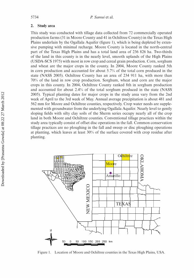
This study was conducted with tillage data collected from 72 commercially operatedproduction farms (31 in Moore County and 41 in Ochiltree County) in the Texas HighPlains underlain by the Ogallala Aquifer (figure 1), which is being depleted by exten-sive pumping with minimal recharge. Moore County is located in the north-centralpart of the Texas High Plains and has a total land area of 236 826 ha. Two-thirdsof the land in this county is in the nearly level, smooth uplands of the High Plains(USDA-SCS 1975) with most in row crop and cereal grain production. Corn, sorghumand wheat are the major crops in the county. In 2004, Moore County ranked 5thin corn production and accounted for about 5.7% of the total corn produced in thestate (NASS 2005). Ochiltree County has an area of 234 911 ha, with more than70% of the land in row crop production. Sorghum, wheat and corn are the majorcrops in this county. In 2004, Ochiltree County ranked 8th in sorghum productionand accounted for about 2.4% of the total sorghum produced in the state (NASS2005). Typical planting dates for major crops in the study area vary from the 2ndweek of April to the 3rd week of May. Annual average precipitation is about 481 and562 mm for Moore and Ochiltree counties, respectively. Crop water needs are supple-mented with groundwater from the underlying Ogallala Aquifer. Nearly level to gentlysloping fields with silty clay soils of the Sherm series occupy nearly all of the cropland in both Moore and Ochiltree counties. Conventional tillage practices within thestudy area typically consist of offset disc operations in the fall. Common conservationtillage practices are no ploughing in the fall and sweep or disc ploughing operationsat planting, which leaves at least 30% of the surface covered with crop residue afterplanting.

Ochiltree

Moore

Amarillo

OK

LA

HO

MA

TEXAS

NE

W M

EX

ICO

Figure 1. Location of Moore and Ochiltree counties in the Texas High Plains, USA.

Dow

nloa

ded

by [

Pras

anna

Gow

da]

at 0

8:22

27

Mar

ch 2

012

Statistical learning algorithms for identifying tillage 5735

3. Materials and methods

Development and evaluation of tillage models in this study mainly consisted oftwo steps: (1) development of models using the LSSVM and RVM techniques and(2) evaluation of tillage models with statistical measures of classification accuracy(i.e. percentage correct or overall classification accuracy and kappa (k) values). Twolevel-1 processed, precision-corrected Landsat TM scenes acquired, one on 10 May2005 for Ochiltree County (Path 30/Row 35) and the other on 17 May 2005 for MooreCounty (Path 31/Row 35), were used for developing and evaluating LSSVM- andRVM-based tillage models. On the day of the Landsat 5 satellite overpass, ground-truth data were collected from 31 and 41 randomly selected commercial productionfields planted with major crops in Moore and Ochiltree counties, respectively. Ground-truth data included geographic coordinates obtained using a handheld GPS, infraredimages taken at a 2 m height using the Agricultural Digital Camera (ADC, DycamInc., Chatsworth, CA, USA) and digital pictures of the residue cover taken with a5 megapixel digital camera.

Crop residue cover was estimated by classifying the infrared images usingMultispec© image processing software developed by the Purdue Research Foundation(West Lafayette, IN, USA). Tillage classification was based on the percentage of thesoil surface covered with crop residue. Conservation tillage systems were defined in thisstudy as those that retained at least 30% of the soil surface covered with crop residueafter a crop was planted. Ground-truth pixel locations on each image were identifiedusing the GPS coordinates for extracting spectral reflectance data for each TM bandimage. In Landsat TM data, reflectance values are stored as brightness values (or dig-ital numbers) in an 8 bit format. The raw brightness values for ground-truth pixelswere extracted and analysed using image processing software. For model developmentand evaluation, the mean reflectance data from nine pixels (the ground-truth pixeland the surrounding eight pixels) were used. The Moore County data set was usedfor model development/calibration and the Ochiltree County data set was used forevaluating the models. For LSSVM and RVM model development, indices were devel-oped with all possible combinations of two bands from all seven Landsat 5 TM bands.The TM indices included difference indices, sum indices, product indices, ratio indicesand normalized difference indices. A comparative study has also been conductedbetween the developed LSSVM- and RVM-based tillage models used in this studyand the logistic regression models developed by Gowda et al. (2008). Comparison hasbeen made for both training and testing data sets. The following subsections brieflydescribe the LSSVM and RVM methods and the model evaluation criteria used forevaluation.

3.1 Least square support vector machine

Vapnik (1995) introduced SVMs for solving pattern recognition problems. SVM mapsthe low-dimensional data to a higher dimensional space and constructs an optimalseparating hyperplane in the transformed space. This involves solving a quadratic pro-gramming problem. The dominant feature of SVM that makes it attractive is thatclasses that are non-linearly separable in the original feature space can be linearly sep-arated in the higher dimensional feature space. This makes SVM capable of solvingcomplex non-linear classification problems. The LSSVM uses the general concepts ofSVM but utilizes the formulation in least squares and, as a result, the solution fol-lows directly from solving a set of linear equations, instead of quadratic programming

Dow

nloa

ded

by [

Pras

anna

Gow

da]

at 0

8:22

27

Mar

ch 2

012

5736 P. Samui et al.

(Suykens and Vandewalle 1998). Further details on LSSVM can be found in Suykenset al. (2002). In this study, the collection of tillage information has been consideredas a binary classification problem. A binary classification problem is considered ashaving a set of training vectors (D) belonging to two separate classes:

D = {(x1, y1) , . . . , (xl, yl)} , x ∈ Rn, y ∈ {−1, +1} , (1)

where x ∈ Rn and is an n-dimensional data vector with each sample belonging toeither of two classes labelled as y ∈ {−1, +1} and l is the number of training data.In this study, we use different input parameters for seven different models as shown intable 1. In the current context of classifying the tillage information, the two classeslabelled as +1 and –1 are conservation tillage and conventional tillage, respectively.

For the case of two classes, one assumes the following:

wTϕ (xk) + b ≥ 1, if yk = +1 (conservation tillage) ,wTϕ (xk) + b ≤ 1, if yk = −1 (conventional tillage) ,

(2)

which is equivalent to

yk[wTφ (xk) + b

] ≥ 1, k = 1, . . . , l, (3)

where φ (·) is a non-linear function that maps the input space into a higher dimen-sional space, b is the bias, T is the transpose and w is the weight. According to thestructural risk minimization principle, the risk margin is minimized by formulatingthe following optimization problem:

minimize12

wTw + γ

2

l∑k=1

e2k,

subject to yk[wTφ (xk) + b

] = 1 − ek, k = 1, . . . , l,

(4)

where γ is the regularization parameter, determining the trade-off between the fittingerror minimization and smoothness, and ek is an error variable. This optimizationproblem (4) is solved by Lagrangian multipliers (Suykens et al. 1999), and its solutionis given by

y (x) = sign

[l∑

k=1

αkykK (x, xk) + b

], (5)

where αk is the Lagrange multiplier, K (x, xk) is the kernel function and sign(•) is thesignum function. Its resultant is +1 (conservation tillage) if the element is greater thanor equal to 0 and –1 (conventional tillage) if it is less than 0.

This study adopts the above methodology for classifying contrasting tillage prac-tices. In the LSSVM modelling, the data were divided into two subsets: a trainingdata set for constructing the model and a testing data set for estimating the modelperformance. Thus, in this study, a total of 31 data points in Moore County were con-sidered for training, and the other 41 data points in Ochiltree County were consideredfor testing. The training and testing data sets used in this study were also used by

Dow

nloa

ded

by [

Pras

anna

Gow

da]

at 0

8:22

27

Mar

ch 2

012

Statistical learning algorithms for identifying tillage 5737

Tab

le1.

Per

form

ance

ofdi

ffer

ent

LSS

VM

mod

els.

Mod

elIn

put

para

met

erD

esig

nva

lue

ofσ

Des

ign

valu

eof

γT

rain

ing

perf

orm

ance

(%)

Tes

ting

perf

orm

ance

(%)

Equ

atio

n

IT

M5

120

091

.475

.6y

=si

gn[ 35 ∑ i=

1α

iyi

exp

{ −(x i

−x)(

x i−x

)T

2

} −0.

0024

]

IIT

M5,

TM

62

1091

.485

.4y

=si

gn[ 35 ∑ i=

1α

iyi

exp

{ −(x i

−x)(

x i−x

)T

8

} +0.

0566

]

III

D15

,D16

260

88.6

87.8

y=

sign

[ 35 ∑ i=1α

iyi

exp

{ −(x i

−x)(

x i−x

)T

8

} +0.

1859

]

IVR

35,R

364

120

91.4

85.4

y=

sign

[ 35 ∑ i=1α

iyiex

p{ −(

x i−x

)(x i

−x)T

32

} +0.

1108

]

VR

45,R

462

150

91.4

87.8

y=

sign

[ 35 ∑ i=1α

iyi

exp

{ −(x i

−x)(

x i−x

)T

8

} +0.

5333

]

VI

ND

TI4

5,N

DT

I46

350

88.6

87.8

y=

sign

[ 35 ∑ i=1α

iyi

exp

{ −(x i

−x)(

x i−x

)T

18

} −0.

0194

]

VII

ND

TI1

5,N

DT

I56

390

91.4

87.8

y=

sign

[ 35 ∑ i=1α

iyi

exp

{ −(x i

−x)(

x i−x

)T

18

} +0.

4451

]

Not

e:D

15=

diff

eren

cebe

twee

nT

Mba

nds

1an

d5;

D16

=di

ffer

ence

betw

een

TM

band

s1

and

6;R

35,R

36,R

45an

dR

46=

rati

oof

TM

band

s3

and

5,3

and

6,4

and

5an

d4

and

6,re

spec

tive

ly;N

DT

I45,

ND

TI4

6,N

DT

I15

and

ND

TI5

6=

norm

aliz

eddi

ffer

ence

betw

een

TM

band

s4

and

5,4

and

6,1

and

5an

d5

and

6,re

spec

tive

ly.

Dow

nloa

ded

by [

Pras

anna

Gow

da]

at 0

8:22

27

Mar

ch 2

012

5738 P. Samui et al.

Gowda et al. (2008) to develop logistic regression-based tillage models. The radial

basis function(

K (x, xk) = exp{− (xk−x)(xk−x)T

2σ 2

})was adopted as a kernel function

for LSSVM. The design values of the regularization parameter, γ and width (σ ) ofthe radial basis function were determined by a trial-and-error approach during thetraining process.

3.2 Relevance vector machine

RVM, introduced by Tipping (2000), is a sparse linear model. The key feature of RVMis that its target function attempts to minimize the number of errors made in the train-ing data set while simultaneously minimizing the margin between feature spaces. Inthis section, a brief introduction on how RVM is used for classification is presented.Consider a set of example input vectors {xi}N

i=1 given along with a corresponding setof targets, t = {ti}N

i=1. For the classification problem, xi should belong to either of thetwo classes (−1, +1). In the current context of determination of tillage practice, thetwo classes are labelled as −1 for conventional tillage and +1 for conservation tillage.Table 2 shows different input parameters for different RVM models. RVM constructsa logistic regression model based on a set of sequence features derived from the inputpatterns, i.e.

P(C1

/x) ≈ σ {y (x; w)} , with y (x; w) =

N∑i=1

wi�i (x) + w0, (6)

where �i is the ith component of the basis vector function:

� (x) = (�1 (x) , �2 (x) , . . . , �N (X))T = [1, K (xi, x1) , K (xi, x2) , . . . , K (xi, xN )]T ,(7)

W = (W0, . . . , WN )T is a vector of weights, σ {y} = (1 + exp {−y})−1 is the logis-tic sigmoid link function and K

(xi, xj

)Nj=1 is the kernel term. Assuming a Bernoulli

distribution for P (t/x), the likelihood can be written as

P (t/w) =N∏

i=1

σ {y (xi; w)}ti [1 − σ {y (xi; w)}]1−ti . (8)

To form a Bayesian training criterion, we must also impose a prior distributionover the vector of model parameters or weights, p(w). The RVM adopts a separableGaussian prior, with a distinct hyperparameter, αi, for each weight:

p (w/α) =N∏

i=1

N(wi

/0, α−1

i

). (9)

The optimal parameters of the model are then derived by minimizing the penalizednegative log-likelihood:

log {P (t/w) p (w/α)} =N∑

i=1

[ti log yi + (1 − ti) log (1 − yi)] − 12

wTAw, (10)

Dow

nloa

ded

by [

Pras

anna

Gow

da]

at 0

8:22

27

Mar

ch 2

012

Statistical learning algorithms for identifying tillage 5739

Tab

le2.

Per

form

ance

ofdi

ffer

ent

RV

Mm

odel

s.

Mod

elIn

put

para

met

erD

esig

nva

lue

ofσ

Num

ber

ofre

leva

nce

vect

orT

rain

ing

perf

orm

ance

(%)

Tes

ting

perf

orm

ance

(%)

Equ

atio

n

IT

M5

0.05

794

.385

.4y

=35 ∑ i=

1w

iex

p{ −(

x i−x

)(x i

−x)T

0.00

5

}

IIT

M5,

TM

60.

0415

94.3

87.8

y=

35 ∑ i=1w

iex

p{ −(

x i−x

)(x i

−x)T

0.00

32

}

III

D15

,D16

0.03

1988

.687

.8y

=35 ∑ i=

1w

iex

p{ −(

x i−x

)(x i

−x)T

0.00

18

}

IVR

35,R

360.

047

91.4

85.4

y=

35 ∑ i=1w

iex

p{ −(

x i−x

)(x i

−x)T

0.00

32

}

VR

45,R

460.

036

91.4

90.2

y=

35 ∑ i=1w

iex

p{ −(

x i−x

)(x i

−x)T

0.00

18

}

VI

ND

TI4

5,N

DT

I46

0.1

391

.490

.2y

=35 ∑ i=

1w

iex

p{ −(

x i−x

)(x i

−x)T

0.02

}

VII

ND

TI1

5,N

DT

I56

0.07

491

.490

.2y

=35 ∑ i=

1w

iex

p{ −(

x i−x

)(x i

−x)T

0.00

98

}

Not

e:D

15=

diff

eren

cebe

twee

nT

Mba

nds

1an

d5;

D16

=di

ffer

ence

betw

een

TM

band

s1

and

6;R

35,

R36

,R

45an

dR

46=

rati

oof

TM

band

s3

and

5,3

and

6,4

and

5an

d4

and

6,re

spec

tive

ly;N

DT

I45,

ND

TI4

6,N

DT

I15

and

ND

TI5

6=

norm

aliz

eddi

ffer

ence

betw

een

TM

band

s4

and

5,4

and

6,1

and

5an

d5

and

6,re

spec

tive

ly.

Dow

nloa

ded

by [

Pras

anna

Gow

da]

at 0

8:22

27

Mar

ch 2

012

5740 P. Samui et al.

where yi = σ {y (xi; w)} and A = diag (α) is a diagonal matrix with non-zero elementsgiven by the vector of hyperparameters. Next, Laplace’s method is used to obtain aGaussian approximation to the posterior density of the weights:

p(w

/t, α

) ≈ N(w

/μ,

∑), (11)

where the posterior mean and covariance are, respectively, given by

μ = ∑�TBt and

∑ = [�TB� + A

]−1, (12)

in which B = diag (β1, β2, . . ., βN) is a diagonal matrix with βn = σ {y (xn)}[1 − σ {y (xn)}].

The hyperparameters are then updated to maximize their marginal likelihood,according to their efficient update formula:

αnewi = 1 − αiii

μ2i

, (13)

where μi is the ith posterior mean weight and∑

ii is the ith diagonal element of theposterior weight covariance and the quantity provides a measure of the degree towhich the associated parameter wi is determined by the data. This process is repeateduntil an appropriate convergence criterion is met. The outcome of this optimizationis that many elements of α go to infinity such that w will have only a few non-zeroweights that will be considered as relevance vectors. Training and testing data sets andthe kernel function used in the LSSVM model were used in the implementation ofthe RVM model for performance comparison purposes. Both LSSVM and RVM pro-grammes were constructed and implemented using MATLAB software (MATLAB2010).

3.3 Model evaluation

For the purpose of model evaluation, error matrices (Campbell 1987) were developedfor all LSSVM and RVM models to determine the percentage correct (overall classi-fication accuracy) and kappa coefficient (k) values. Percentage correct was calculatedby dividing the sum of correctly classified fields by the total number of fields examinedas follows:

percentage correct (%) =(

no. of data predicted correctlytotal no. of data

)× 100. (14)

The percentage correct values were computed separately for the training and testingdata of each of the LSSVM and RVM models. The ‘k’ value is a measure of the differ-ence between two maps and the agreement that might be contributed solely by chancematching of the two maps (Congalton and Green 1999). The k value was calculated as

k =(

O − E1 − E

), (15)

Dow

nloa

ded

by [

Pras

anna

Gow

da]

at 0

8:22

27

Mar

ch 2

012

Statistical learning algorithms for identifying tillage 5741

where O means observed, which is the percentage correct and E is the expected, whichis an estimate of the chance agreement to the observed. A k value of +1.0 indicatesperfect accuracy of the classification.

4. Results and discussion

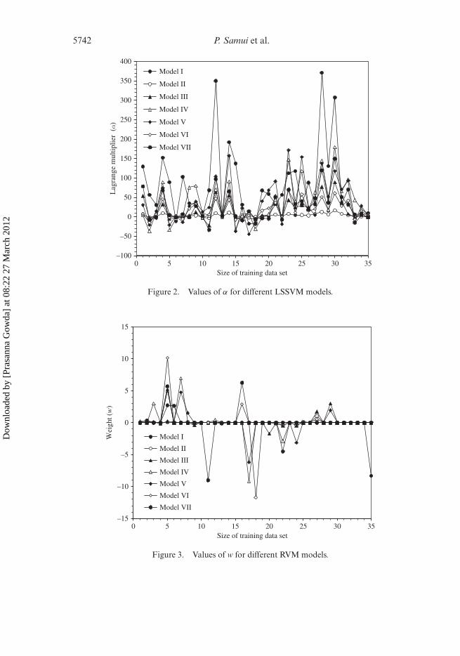
Tables 1 and 2 present performances of LSSVM and RVM models, respectively, andtable 3 presents comparison of their performances with logistic regression modelsreported by Gowda et al. (2008). Based on the training performance results, all theLSSVM models except III and VI performed better with a percentage correct valueof 91.4%. However, application of these models to the evaluation data set indicatedthat only models V, VI and VII maintained their high performance level with only5 out of 41 data points misclassified. Percentage correct and k values for these mod-els were 87.8% and 0.75 (table 3), respectively, indicating that LSSVM models may besuitable for identifying fields with contrasting tillage practices. The developed LSSVMhas also been used to develop an equation (by inputting the design values of σ and bfor different models in equation (5) modified for radial basis function) for predictionof tillage information. Table 1 shows the different equations for prediction of tillageinformation for different models. The values of α for different models are given infigure 2.

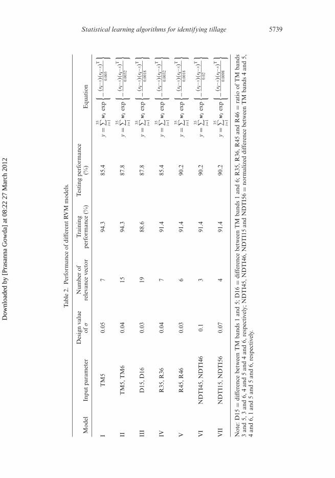
Comparison of RVM models in table 2 indicates that models that use individualbands (I and II) performed better with a percentage correct value of 94.3% withthe training/calibration data set. However, the percentage correct was reduced to85.4–87.8% when these models were applied to the evaluation data set. Models V,VI and VII that use ratio or normalized difference tillage indices performed betterthan those that use individual TM bands or difference indices. The percentage cor-rect values were consistently higher for both training (91.4%) and testing (90.2%) datasets. The k values for all three models were the same and equal to 0.8, indicating that

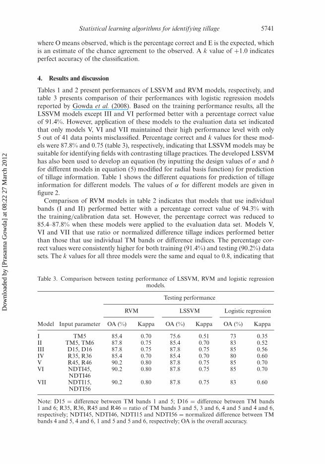
Table 3. Comparison between testing performance of LSSVM, RVM and logistic regressionmodels.

Testing performance

RVM LSSVM Logistic regression

Model Input parameter OA (%) Kappa OA (%) Kappa OA (%) Kappa

I TM5 85.4 0.70 75.6 0.51 73 0.35II TM5, TM6 87.8 0.75 85.4 0.70 83 0.52III D15, D16 87.8 0.75 87.8 0.75 85 0.56IV R35, R36 85.4 0.70 85.4 0.70 80 0.60V R45, R46 90.2 0.80 87.8 0.75 85 0.70VI NDTI45,

NDTI4690.2 0.80 87.8 0.75 85 0.70

VII NDTI15,NDTI56

90.2 0.80 87.8 0.75 83 0.60

Note: D15 = difference between TM bands 1 and 5; D16 = difference between TM bands1 and 6; R35, R36, R45 and R46 = ratio of TM bands 3 and 5, 3 and 6, 4 and 5 and 4 and 6,respectively; NDTI45, NDTI46, NDTI15 and NDTI56 = normalized difference between TMbands 4 and 5, 4 and 6, 1 and 5 and 5 and 6, respectively; OA is the overall accuracy.

Dow

nloa

ded

by [

Pras

anna

Gow

da]

at 0

8:22

27

Mar

ch 2

012

5742 P. Samui et al.

–100

–50

0

50

100

150

200

250

300

350

400

0 5 10 15 20 25 30 35

Lag

rang

e m

ultip

lier

(α)

Size of training data set

Model I

Model II

Model III

Model IV

Model V

Model VI

Model VII

Figure 2. Values of α for different LSSVM models.

–15

–10

–5

0

5

10

15

0 5 10 15 20 25 30 35

Wei

ght (

w)

Size of training data set

Model I

Model II

Model III

Model IV

Model V

Model VI

Model VII

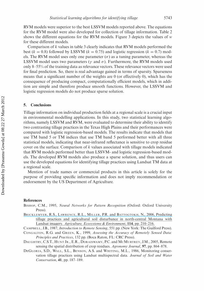
Figure 3. Values of w for different RVM models.

Dow

nloa

ded

by [

Pras

anna

Gow

da]

at 0

8:22

27

Mar

ch 2

012

Statistical learning algorithms for identifying tillage 5743

RVM models were superior to the best LSSVM models reported above. The equationsfor the RVM model were also developed for collection of tillage information. Table 2shows the different equations for the RVM models. Figure 3 depicts the values of wfor these different models.

Comparison of k values in table 3 clearly indicates that RVM models performed thebest (k = 0.8) followed by LSSVM (k = 0.75) and logistic regression (k = 0.7) mod-els. The RVM model uses only one parameter (σ ) as a tuning parameter, whereas theLSSVM model uses two parameters (γ and σ ). Furthermore, the RVM models usedonly 8–55% of the training data as relevance vectors. These relevance vectors were usedfor final prediction. So, there is real advantage gained in terms of sparsity. Sparsenessmeans that a significant number of the weights are 0 (or effectively 0), which has theconsequence of producing compact, computationally efficient models, which in addi-tion are simple and therefore produce smooth functions. However, the LSSVM andlogistic regression models do not produce sparse solution.

5. Conclusions

Tillage information on individual production fields at a regional scale is a crucial inputin environmental modelling applications. In this study, two statistical learning algo-rithms, namely LSSVM and RVM, were evaluated to determine their ability to identifytwo contrasting tillage practices in the Texas High Plains and their performances werecompared with logistic regression-based models. The results indicate that models thatuse TM band 5 or TM indices that use TM band 5 performed better with all threestatistical models, indicating that near-infrared reflectance is sensitive to crop residuecover on the surface. Comparison of k values associated with tillage models indicatedthat RVM models performed better than LSSVM- and logistic regression-based mod-els. The developed RVM models also produce a sparse solution, and thus users canuse the developed equations for identifying tillage practices using Landsat TM data ata regional scale.

Mention of trade names or commercial products in this article is solely for thepurpose of providing specific information and does not imply recommendation orendorsement by the US Department of Agriculture.

ReferencesBISHOP, C.M., 1995, Neural Networks for Pattern Recognition (Oxford: Oxford University

Press).BRICKLEMYER, R.S., LAWRENCE, R.L., MILLER, P.R. and BATTOGTOKH, N., 2006, Predicting

tillage practices and agricultural soil disturbance in north-central Montana withLandsat imagery. Agriculture, Ecosystems & Environment, 114, pp. 210–216.

CAMPBELL, J.B., 1987, Introduction to Remote Sensing, 551 pp. (New York: The Guilford Press).CONGALTON, R.G. and GREEN, K., 1999, Assessing the Accuracy of Remotely Sensed Data:

Principles and Practices, 132 pp. (Boca Raton, FL: CRC Press).DAUGHTRY, C.S.T., HUNT JR., E.R., DORAISWAMY, P.C. and MCMURTREY, J.M., 2005, Remote

sensing the spatial distribution of crop residues. Agronomy Journal, 97, pp. 864–878.DEGLORIA, S.D., WALL, S.L., BENSON, A.S. and WHITING, M.L., 1986, Monitoring conser-

vation tillage practices using Landsat multispectral data. Journal of Soil and WaterConservation, 41, pp. 187–189.

Dow

nloa

ded

by [

Pras

anna

Gow

da]

at 0

8:22

27

Mar

ch 2

012

5744 P. Samui et al.

FOODY, G.M., 2008, RVM-based multi-class classification of remotely sensed data. InternationalJournal of Remote Sensing, 29, pp. 1817–1823.

GHOSH, S. and MUJUMDAR, P.P., 2008, Statistical downscaling of GCM simulations to stream-flow using relevance vector machine. Advances in Water Resources, 31, pp. 132–146.

GOWDA, P.H., HOWELL, T.A., EVETT, S.R., CHAVEZ, J.L. and NEW, L., 2008, Remote sensingof contrasting tillage practices in the Texas Panhandle. International Journal of RemoteSensing, 29, pp. 477–3487.

GOWDA, P.H., MULLA, D.J. and DALZELL, B.J., 2003, Examining and targeting conservationtillage practices to steep/flat landscapes in the Minnesota River Basin. Journal of Soiland Water Conservation, 58, pp. 53–57.

KECMAN, V., 2001, Learning and Soft Computing: Support Vector Machines, Neural Networks,and Fuzzy Logic Models (Cambridge, MA: The MIT Press).

MATHUR, A. and FOODY, G.M., 2008, Crop classification by support vector machine with intel-ligently selected training data for an operational application. International Journal ofRemote Sensing, 29, pp. 2227–2240.

MATLAB, 2010, Users Guide (Natick, MA: Mathworks, Inc.).MOTSCH, B., SCHAAL, G., LYON, J.G. and LOGAN, T.J., 1990, Monitoring crop residue in Senaca

County, Ohio. In Proceedings of the ASPRS Meeting, Cleveland, OH (Bethesda, MD:American Society of Photogrammetry & Remote Sensing), pp. 66–76.

NASS, 2005, 2004 Texas Agricultural Statistics: Texas Agriculture by the Number, Bulletin 263(Austin, TX: Texas Field Office, U.S. Department of Agriculture, National AgriculturalStatistics Service).

PARK, D. and RILETT, L.R., 1999, Forecasting freeway link travel times with a multi-layerfeed forward neural network. Computer Aided Civil and Infrastructure Engineering, 14,pp. 358–367.

SAMUI, P. and SITHARAM, T.G., 2008, Least square support vector machine applied to settle-ment of shallow foundations on cohesionless soils. International Journal of Numericaland Analytical Methods in Geomechanics, 32, pp. 2033–2043.

SCHWARTZ, R.C., BAUMHARDT, R.L. and EVETT, S.R., 2010, Tillage effects on soil water redis-tribution and bare soil evaporation throughout a season. Soil & Tillage Research, 110,pp. 221–229.

SUDHEER, K.P., GOWDA, P.H., CHAUBEY, I. and HOWELL, T.A., 2010, Artificial neuralnetwork approach for mapping contrasting tillage practices. Remote Sensing, 2,pp. 579–590.

SULLIVAN, D.G., SHAW, J.N., MASK, P., RICKMAN, D., LUVALL, J. and WERSINGER, J.M., 2004,Evaluation of multispectral data for rapid assessment of in situ wheat straw residuecover. Soil Science Society of American Journal, 68, pp. 2007–2013.

SULLIVAN, D.G., TRUMAN, C.C., SCHOMBERG, H.H., ENDALE, D.M. and STRICKLAND, T.C.,2006, Evaluating techniques for determining tillage regime in the Southeastern CoastalPlain and Piedmont. Agronomy Journal, 98, pp. 1236–1246.

SUYKENS, J.A.K., DE, B.J., LUKAS, L. and VANDEWALLE, J., 2002, Weighted least squaressupport vector machines: robustness and sparse approximation. Neurocomputing, 48,pp. 85–105.

SUYKENS, J.A.K., LUKAS, L., VAN, D.P., DE, M.B. and VANDEWALLE, J., 1999, Leastsquares support vector machine classifiers: a large scale algorithm. In Proceedings ofthe European Conference on Circuit Theory and Design (ECCTD’99), Stresa, Italy,pp. 839–842.

SUYKENS, J.A.K. and VANDEWALLE, J., 1998, Nonlinear Modeling Advanced Black BoxTechniques (Boston, MA: Kluwer Academic Publishers).

TAKKEN, I., GOVERS, G., JETTEN, V., NACHTERGAELE, J., STEELGEN, A. and POESEN, J.,2001, Effect of tillage on runoff and erosion patterns. Soil & Tillage Research, 61,pp. 55–60.

Dow

nloa

ded

by [

Pras

anna

Gow

da]

at 0

8:22

27

Mar

ch 2

012

Statistical learning algorithms for identifying tillage 5745

TANG, H., QIU, J., VAN RANST, E. and LI, C., 2006, Estimations of soil organic carbon storagein cropland of China based on DNDC model. Geoderma, 134, pp. 200–206.

THOMA, D.P., GUPTA, G.C. and BAUER, M.E., 2004, Evaluation of optical remote sensingmodels for crop residue cover assessment. Journal of Soil and Water Conservation, 59,pp. 224–233.

TIPPING, M.E., 2000, The relevance vector machine. Advances in Neural Information ProcessingSystems, 12, pp. 625–658.

USDA-SCS, 1975, Soil Survey of Moore County, Texas (Washington, DC: Soil ConservationService, United States Department of Agriculture).

VAN DEVENTER, A.P., WARD, A.D., GOWDA, P.H. and LYON, J.G., 1997, Using ThematicMapper data to identify contrasting soil plains and tillage practices. PhotogrammetricEngineering & Remote Sensing, 63, pp. 87–93.

VAPNIK, V.N., 1995, The Nature of Statistical Learning Theory (New York: SpringerPublications).

VERVOORT, R.W., DABNEY, S.M. and ROMKENS, M.J.M., 2001, Tillage and row position effectson water and solute infiltration characteristics. Soil Science Society of America Journal,65, pp. 1227–1234.

VINA, A., PETERS, A.J. and JI, L., 2003, Use of multispectral Ikonos imagery for discriminatingbetween conventional and conservation agricultural tillage practices. PhotogrammetricEngineering & Remote Sensing, 69, pp. 537–544.

WEST, T.O. and MARLAND, G., 2002, A synthesis of carbon sequestration, carbon emissions,and net carbon flux in agriculture: comparing tillage practices in the United States.Agriculture, Ecosystems & Environment, 91, pp. 217–232.

Dow

nloa

ded

by [

Pras

anna

Gow

da]

at 0

8:22

27

Mar

ch 2

012