Statistical Keyword Detection in Literary Corpora - arXiv

arX

iv:c

s/07

0102

8v2

[cs

.CL

] 3

0 M

ay 2

008

EPJ manuscript No.(will be inserted by the editor)

Statistical Keyword Detection in Literary Corpora

Juan P. Herreraa and Pedro A. Puryb

Facultad de Matematica, Astronomıa y Fısica, Universidad Nacional de Cordoba,Ciudad Universitaria, X5000HUA Cordoba, Argentina

Received: 1st May 2007 / Received in final form 15 February 2008c© EDP Sciences, Societa Italiana di Fisica, Springer-Verlag 2008

Abstract. Understanding the complexity of human language requires an appropriate analysis of the statis-tical distribution of words in texts. We consider the information retrieval problem of detecting and rankingthe relevant words of a text by means of statistical information referring to the spatial use of the words.Shannon’s entropy of information is used as a tool for automatic keyword extraction. By using The Origin

of Species by Charles Darwin as a representative text sample, we show the performance of our detector andcompare it with another proposals in the literature. The random shuffled text receives special attention asa tool for calibrating the ranking indices.

PACS.

– 89.70.+c Information theory and communication theory– 05.45.Tp Time series analysis– 89.75.-k Complex systems

1 Introduction

Data mining for texts is a well-established area of naturallanguage processing [1]. Text mining is the computerisedextraction of useful answers from a mass of textual in-formation by machine methods, computer-assisted humanones, or a combination of both. A key problem in textmining is the extraction of keywords from texts for whichno a priori information is available. The problem of unsu-pervised extraction of relevant words from their statisticalproperties was first addressed by Luhn [2], who based hismethod on Zipf’s analysis of frequencies [3]. This analy-sis consists of counting the number of occurrences of eachdistinct word in a given text, and then generating a listof all these words ordered by decreasing frequency. In thislist, each word is identified by its position or Zipf’s rankin the list. The empirical observation of Zipf was that thefrequency of occurrence of the r–th rank in the list is pro-portional to r−1 (Zipf’s law). Luhn proposed the crudeapproach of excluding the words at both ends of the Zipf’slist and considering as keywords the remaining cases. Thelimitations of Luhn’s approach are known in the litera-ture [4].

The main goal of this work is to investigate unsuper-vised statistical methods for detecting keywords in literacytexts beyond the simple counting of word occurrences. In

a Present address: Argentina Software Development Cen-ter (ASDC), Intel Software, Cordoba, Argentina (e-mail:[email protected]).b Corresponding author (e-mail: [email protected]).

order to obtain statistically significant results we restrictour work to a large book, which can be used as a cor-pus what is thematically consistent throughout its entirelength. We are searching for relevance according to thetext’s context, but we will only use statistical informationabout the spatial use of the words in a text.

Particularly, the measure of content of information foreach word can be made by Shannon’s entropy. In thephysics literature, we can find several applications of theentropy concept to linguistics and natural language likeDNA sequences analysis [5,6,7], long-range correlationsmeasurements [8,9], language acquisition [10], authorshipdisputes [11,12], communication modelling [13], and statis-tical analysis of the linguistic role of words in corpora [14].

The organisation of the remainder of the article is asfollows. In Sec. 2 we first introduce the corpus used asa representative sample throughout this work. Later, inSec. 3 we review the algorithms proposed in the litera-ture based on the analysis of the statistical distribution ofwords in a text. Then, in Sec. 4 we discuss the behaviour ofthe indices in random texts. By using Shannon’s entropy,in Sec. 5 we propose another index based on the informa-tion content of the sequence of occurrences of each wordin the text. In Sec. 6 we use the glossary of the corpus formeasuring the performace of each index as keyword detec-tor. Finally, in Sec. 7 we present a summary of the work.Besides, mathematical details are given in appendices. InAppendix A we review the geometrical distribution, use-ful to random texts, and in Appendix B we calculate theentropy of a random text.

http://arxiv.org/abs/cs/0701028v2

2 Juan P. Herrera, Pedro A. Pury: Statistical Keyword Detection in Literary Corpora

2 Representative Corpus Sample

For our study, we will use a prototypical real text, i.e.,“On the Origin of Species by Means of Natural Selection,or The Preservation of Favoured Races in the Struggle forLife” [15] (usually abbreviated to The Origin of Species)by Charles Darwin (1859). The book was written with thevocabulary of a nineteenth-century naturalist but withfluid prose, combining first–person narrative with schol-arly analysis.

For the preparation of our working corpus we firstwithdrew any punctuation symbol from the text, mappedall words to uppercase and then used the simple tokeniza-tion method based on whitespaces [1]. We draw a distinc-tion between a word token versus a word type. For ourconvenience, we define a word type as any different stringof letters between two whitespaces. Thus, for our elemen-tary analysis, words like INSTINCT and INSTINCTS corre-spond to different word types in our corpus. On the otherhand, a word token is each individual occurrence of a givenword type. When the context refers to a particular wordtype, we will use indistinctly “word token” or simply “to-ken” to refer to an individual occurrence of the word typein the text.

The relevant words have not been explicitly defined inDarwin’s book, with exception of a glossary appended atthe end of the work. Therefore, the table of contens in thebeginning, the glossary and the analytical index, also in-serted at the end, were removed from our corpus. By doingthis, we avoid introducing obvious bias for the words usedin these parts. Thus, the prepared corpus includes 94% ofmaterial from the original Darwin’s book and has 192, 665word tokens and 8, 294 word types. In addition, the corpuscontains 842 paragraphs distributed in 16 chapters.

The glossary of the principal scientific terms used inthe book, prepared by Mr. W.S. Dallas, and the analyt-ical index, both appended at the end of the book, werewritten using 2, 418 word types. If we do not consider thefunction words, still remain 1, 679 word types (20% of thebook’s lexicon). With this information,, we prepared byhand a customed version of the glossary, by selecting 283word types (3.4% of the lexicon) with frequencies of occur-rence greater than 9. We have avoided word types with lessthan 9 occurrences because we cannot extract any signif-icant statistics from data obtained using such small sets.Thus, the criterion for selection was rather more arbitrary,but we think that all selected words are pertinent to thebook’s context. Our prepared version of the glossary willbe used later to evaluate the retrieval capabilities of dif-ferent keyword extractors.

3 Clustering as criterion for relevance of

words

The attraction between words is a phenomenon that playsan important role in both language processing and acqui-sition, and it has been modeled for information retrievaland speech recognition purposes [16,17]. Empirical data

0 200 400 600 800 1000inter-token distance

0

10

20

30

40

50

f

original textrandom text

NATURAL (rank: 53)

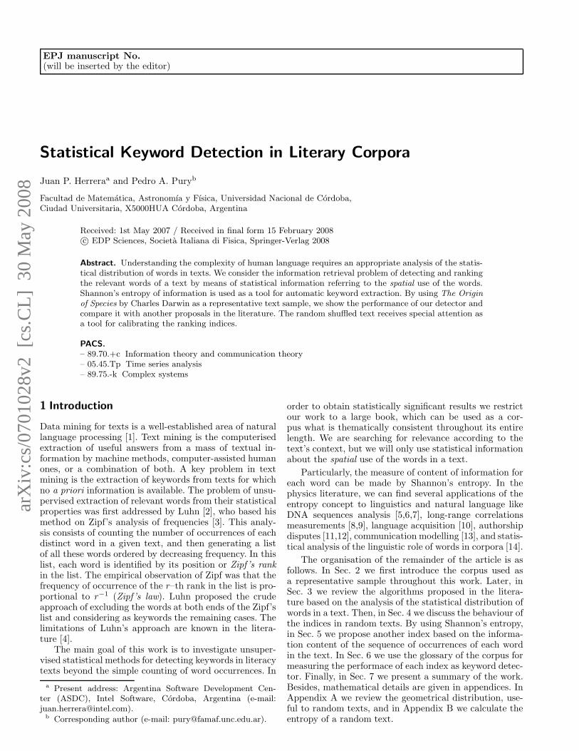
Fig. 1. Histogram of frequencies of distances between occur-rences of NATURAL (Zipf’s rank 53) in Darwin’s corpus.

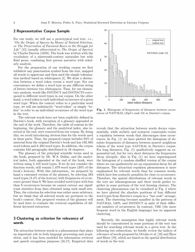
reveals that the attraction between words decays expo-nentially, while stylistic and syntactic constraints createa repulsion between words that discourages close occur-rences. In Fig. (1) we have plotted the histogram of ab-solute frequencies of distances between nearest neighbourtokens of the word type NATURAL in Darwin’s corpus.For long distances, Fig. (1) qualitatively suggests an ex-ponential tail, but for very short distances the frequenciesdecay abruptly. Also in Fig. (1) we have superimposedthe histogram of a random shuffled version of the corpuswhere we can qualitatively see an exponential decay for alldistances. The attraction–repulsion phenomenon is moreemphasized for relevant words than for common words,which have less syntactic penalties for close co-occurrence.Therefore, the spatial distributions of relevant words inthe text are inhomogeneous and these words gather to-gether in some portions of the text forming clusters. Theclustering phenomenon can be visualised in Fig. 2 wherewe have plotted the absolute positions of four differentword types from Darwin’s corpus in a “bar code” arrange-ment. The clustering becomes manifest in the patterns ofNATURAL, LIFE, and INSTINCT in spite of their differ-ent numbers of occurrences. In contrast, THE (the morefrequent word in the English language) has no apparentclustering.

Recently, the assumption that highly relevant wordsshould be concentrated in some portions of the text wasused for searching relevant words in a given text. In thefollowing two subsections, we briefly review the indices ofrelevance of words proposed by Ortuno et al. [18] and Zhouand Slater [19], which are based on the spatial distributionof words in the text.

Juan P. Herrera, Pedro A. Pury: Statistical Keyword Detection in Literary Corpora 3

0 50 k 100 k 150 k 200 k

t (✕ 1000)

THE (rank: 1)

NATURAL (rank: 53)

LIFE (rank: 72)

INSTINCT (rank: 405)

Fig. 2. Absolute positions (t) in the text, counted from thebeginning of Darwin’s corpus, of the word types: THE (13, 414occurrences), NATURAL (475 occurrences), LIFE (326 occur-rences), and INSTINCT (64 occurrences). To draw the picture,we set a very thin vertical line (of arbitrary height) at the po-sition of each occurrence.

3.1 σ–index

To study the spatial distribution of a given word type ina text, we can map the occurrences of the correspondingword tokens into a time series. For this task, we denoteby ti the absolute position in the corpus of the i–th oc-currence of a word token. Thus, we obtain the sequence{t0, t1, . . . , tn, tn+1}, where we are assuming that there aren word tokens. We have additionally included the bound-aries of the corpus, defining t0 = 0 and tn+1 = N + 1,where N is the total number of tokens in the corpus, inorder to take into account the space before the first oc-currence of a word token and the space after the last oc-currence of a token [19].

Given the sequence of inter–token distances

{t1 − t0, t2 − t1, . . . , tn − tn−1, tn+1 − tn} ,

the average distance between two successive word tokensis given by

µ =1

n+ 1

n∑

i=0

(ti+1 − ti) =N + 1

n+ 1, (1)

and the sample standard deviation of the set of spacingsbetween nearest neighbour word tokens (ti+1 − ti) is by

definition

s =

√

√

√

√

1

n− 1

n∑

i=0

((ti+1 − ti)− µ)2 . (2)

To eliminate the dependence on the frequency of oc-currence for different word types, in Ref. [18] the authorssuggest to normalise the token spacings, i.e., to measurethem in units of their corresponding mean value. Thus, wedefine

σ =s

µ. (3)

Given that the standard deviation grows rapidly whenthe inhomogeneity of the distribution of spacing ti+1 − tiincreases, Ortuno et al. [18] proposed σ as an indicator ofthe relevance of the words in the analysed text. In manycases, empirical evidence vindicates that large σ valuesgenerally correspond to terms relevant to the text consid-ered, and that common words have associated low valuesof σ. However, Zhou and Slater [19] pointed out that σ-index has some weaknesses. First, several obviously com-mon (relevant) words have relative high (low) σ values inseveral texts. Second, the index is not stable in the sensethat it can be strongly affected by the change of a singleoccurrence position. Third, high values of σ do not al-ways imply a cluster concentration. A big cluster of wordscan be splitted into smaller clusters without substantialchange in the σ value.

3.2 Γ–index

The σ-index is only based on the spacing between nearest-neighbour word tokens. To improve the performance in thesearching for relevance, Zhou and Slater [19] introduced anew index that uses more information from the sequenceof occurrences {t0, t1, . . . , tn, tn+1}. For this task, theseauthors consider the spacings wi = ti − ti−1, with i =1, . . . , n+1, and define the average separation around theoccurrence at ti as

d(ti) =wi+1 + wi

2=

ti+1 − ti−1

2, i = 1, . . . , n . (4)

The position ti is said to be a cluster point if d(ti) < µ.The new suggestion is that the relevance of a word in agiven text is related to the number of cluster points foundin it. Thus, in order to measure the degree of clusteriza-tion, the local cluster index at position ti is defined by

γ(ti) =

µ− d(ti)

µif ti is a cluster point

0 otherwise. (5)

Finally, a new index to measure relevance is obtained fromthe average of all cluster indices corresponding to a givenword type

Γ =1

n

n∑

i=1

γ(ti) . (6)

Γ -index is more stable than σ, but it is still based on localinformation and is computationally more time consumingto evaluate than σ.


4 Random text and shuffled words

In a completely random text we have an uncorrelated se-quence of tokens, and a word type w is only characterisedby its relative frequency of occurrence (pw). Thus, a ran-dom text can be generated by picking successively tokensby chance in such a way that at each position the proba-bility of finding a token, corresponding to the word typew, is pw. Obviously,

∑

w pw = 1. For the word type w, wehave in this manner defined a binomial experiment wherethe probability of success (occurrence) at each site in thetext is pw, and the probability of failure (non-occurrence)is (1 − pw). Therefore, the distribution of distances be-tween nearest neighbour tokens corresponding to the sameword type is geometrical. In Appendix A, we have com-piled some results of the geometrical distribution that areuseful for our next analyses.

Besides, its worth as comparative standard, the the-oretical random text has the virtue of being analyticallytractable. Also, from an empirical point of view, there isa workable fashion for building a random version of a cor-pus. In an actual corpus the probabilities of occurrencep are estimated from the relative frequencies n/N , wheren is the number of tokens corresponding to a given wordtype and N is the total number of tokens in the corpus.A random version of the text can be obtained by shufflingor permuting all the tokens. The random shuffling of allthe words has the effect of rescasting the corpus into anonsensical realization, keeping the same original tokenswithout discernible order at any level. However, both theZipf’s list of ranks and the frequency of occurrence of eachword type are kept intact.

The important point that we want to stress here is thatthe indices of relevance defined in the previous section arefunctions of the frequencies of occurrence of each wordtype. Thus, in a random text the values of these indiceschange with p, which has nonsense. In a truly randomtext, there are not relevant words. Therefore, to eliminatecompletely the dependence on frequency we need to renor-malise the indices with their values in the random versionof the corpus.

4.1 Renormalised σ–index

For a given probability distribution, σ is defined from thesecond– (µ2) and first–order (µ1) cumulant by

√µ2/µ1.

Thus, from Eq. (20) in Appendix A we find that in arandom text the value of σ–index is given by

σran =√

1− p . (7)

Hence, we renormalise the index to eliminate this depen-dence on relative frequency defining

σnor =s

µ

1√1− p

. (8)

For texts as large as corpora the importance of normalisa-tion factor given by Eq. (7) becomes negligible. For exam-ple, in Darwin’s corpus, N = 192, 665, and for the most

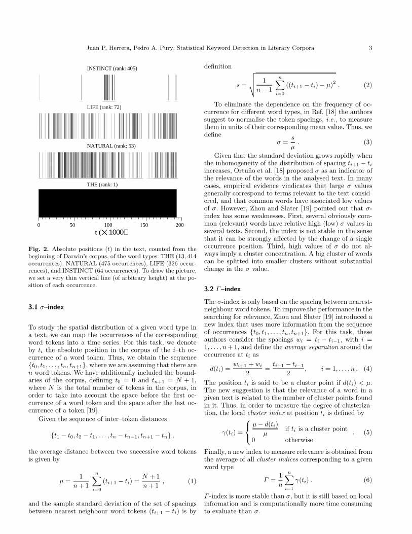
Fig. 3. Renormalised σ–index vs. Zipf’s rank for each wordin Darwin’s corpus (the first 4000 ranks). We have also plot-ted superposed the random version of the text (grey) and wehave marked by open circles the words corresponding to ourprepared glossary (red online).

frequent word type (THE) we have n = 13, 414 (n/N =0.0696). Thus, in the less significant case (the lowest valuefor σran) σran = 0.965, whereas σran = 1 for p = 0. How-ever, for shorter texts the significance of the normalisationmay become critical and the values of σ and σnor may bevery different for any word type.

In Fig. 3 we plot the values of σnor for the first 4000ranks in the Zipf’s list of Darwin’s corpus. The randomversion of the corpus is also plotted in the same graph.The “cloud of points” corresponding to the random textis distributed around the unitary value of σnor, but thewidth of the “cloud” grows with rank. This behaviour isdue to the fact that the frequency of occurrence decreasesas the rank increases (Zipf’s law), therefore the statisticsget worse. The words of our preparated version of theglossary are marked by open circles in Fig. 3. From Fig. 3,it is appreciable that most of the glossary words have highvalues of σnor.

4.2 Renormalised skewness

As in the case of σ, any cumulant contains partial infor-mation of the spatial distribution of words. Skewness isa parameter that describes the asymmetry of a distribu-tion. Mathematically, the skewness is measured using thesecond– (µ2) and third–order (µ3) cumulant of the distri-

bution according to κ = µ3/µ3/22 . Given that the distances

between nearest neighbour tokens are positive defined, thecorresponding distribution has positive skew, i.e., the up-per tail is longer than the the lower tail (see Fig. 1).


From Eq. (20), we find that in a random text the skew-ness of the distribution of distances between nearest neigh-bour tokens is given by

κran =2− p√1− p

; (9)

Thus, the skewness also depends on the relative frequencyof occurrence, p, in the random case. However, this depen-dence is also negligible for a corpora. In Darwin’s corpuswe obtain κran = 2.001 for the largest value p = 0.0696(the relative frequency of the word type THE), whereasκran = 2 for p = 0.

As a consequence, we can define another renormalisedquantity as we did with the σ–index. Thus, to eliminatethe dependence on the relative frequency of occurrence inthe random case, we write

κnor =µ3

µ3/22

√1− p

2− p. (10)

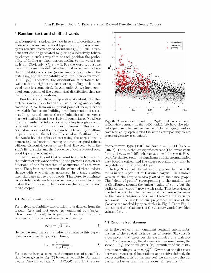
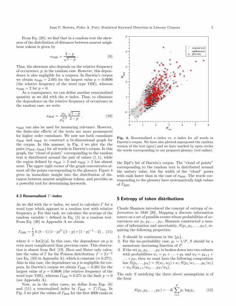
κnor can also be used for measuring relevance. However,the finite-size effects of the texts are more pronouncedfor higher order cumulants. We now use both cumulantsσnor and κnor to construct a bi-dimensional graph forthe corpus. In this manner, in Fig. 4 we plot the thepairs (σnor, κnor) for all words in Darwin’s corpus. In thisgraph, the “cloud of points” corresponding to the randomtext is distributed around the pair of values (1, 1), whilethe region defined by σnor > 2 and κnor > 2 has almostnone. The upper right corner of the graph concentrates al-most all the points corresponding to the glossary. Figure 4gives us immediate insight into the distribution of dis-tances between nearest neighbour tokens, and provides usa powerful tool for determining keywords.

4.3 Renormalised Γ–index

As we did with the σ–index, we need to calculate Γ for aword type which appears in a random text with relativefrequency p. For this task, we calculate the average of therandom variable γ defined in Eq. (5) in a random text.From Eq. (30) in Appendix A we obtain

Γran =1

2h (h−1) (1−p)h ((1−p)+(1−p)−1−2) , (11)

where h = Int[2/p]. In this case, the dependence on p iseven more complicated than previous cases. This observa-tion is absent from Ref. [19]. Zhou and Slater only calcu-late the value of Γ for the Poisson distribution: Γ = 2 e−2

(see Eq. (33) in Appendix A), which is constant (≈ 0.271).Also in this case, the dependence on p is negligible for cor-pora. In Darwin’s corpus we obtain Γran = 0.261 for thelargest value of p = 0.0696 (the relative frequency of theword type THE), whereas Γran ≈ 0.271 in the limit p → 0(see Appendix A).

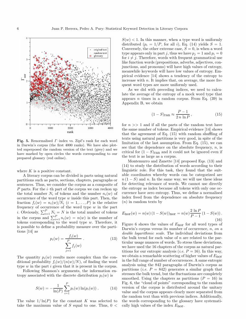
Now, as in the other cases, we define from Eqs. (6)and (11) a renormalised index by Γnor = Γ/Γran. InFig. 5 we plot the values of Γnor for the first 4000 ranks in

Fig. 4. Renormalised κ–index vs. σ–index for all words inDarwin’s corpus. We have also plotted superposed the randomversion of the text (grey) and we have marked by open circlesthe words corresponding to our prepared glossary (red online).

the Zipf’s list of Darwin’s corpus. The “cloud of points”corresponding to the random text is distributed aroundthe unitary value, but the width of the “cloud” growswith rank faster than in the case of σnor. The words cor-responding to the glossary have systematically high valuesof Γnor.

5 Entropy of token distributions

Claude Shannon introduced the concept of entropy of in-formation in 1948 [20]. Mapping a discrete informationsource on a set of possible events whose probabilities of oc-currences are p1, p2, . . . , pP , Shannon constructed a mea-sure of information and uncertainty, S(p1, p2, . . . , pP ), re-quiring the following properties:

1. S should be continuous in the {pi}.2. For the iso-probability case, pi = 1/P , S should be a

monotonic increasing function of P .3. If the set p1, p2, . . . , pP is broken down into two subsets

with probabilities w1 = p1 + . . .+ pk and w2 = pk+1 +. . .+ pP , then we must have the following compositionlaw S(p1, . . . pN ) = S(w1, w2)+w1 S(p1/w1, . . . pk/w1)+ w2 S(pk+1/w2, . . . pP /w2).

The only S satisfying the three above assumptions is ofthe form

S(p1, p2, . . . , pP ) = −K

P∑

i=1

pi log pi , (12)


Fig. 5. Renormalised Γ–index vs. Zipf’s rank for each wordin Darwin’s corpus (the first 4000 ranks). We have also plot-ted superposed the random version of the text (grey) and wehave marked by open circles the words corresponding to ourprepared glossary (red online).

where K is a positive constant.A literary corpus can be divided in parts using natural

partitions such as parts, sections, chapters, paragraphs orsentences. Thus, we consider the corpus as a composite ofP parts. For the i–th part of the corpus we can reckon upthe total number Ni of tokens and the number ni(w) ofoccurrence of the word type w inside this part. Then, thefraction fi(w) = ni(w)/Ni (i = 1, . . . , P ) is the relativefrequency of occurrence of the word type w in the part

i. Obviously,∑P

i=1Ni = N is the total number of tokens

in the corpus and∑P

i=1ni(w) = n(w) is the number of

tokens corresponding to the word type w. Therefore, itis possible to define a probability measure over the parti-tions [14] as

pi(w) =fi(w)

P∑

j=1

fj(w)

. (13)

The quantity pi(w) results more complex than the con-ditional probability fi(w)/(n(w)/N), of finding the wordtype w in the part i given that it is present in the corpus.

Following Shannon’s arguments, the information en-tropy associated with the discrete distribution pi(w) is

S(w) = − 1

ln(P )

P∑

i=1

pi(w) ln(pi(w)) . (14)

The value 1/ ln(P ) for the constant K was selected totake the maximum value of S equal to one. Thus, 0 <

S(w) < 1. In this manner, when a type word is uniformlydistributed (pi = 1/P , for all i), Eq. (14) yields S = 1.Conversely, the other extreme case, S = 0, is when a wordtype appears only in part j, thus we have pj = 1 and pi = 0for i 6= j. Therefore, words with frequent grammatical uselike function words (prepositions, adverbs, adjectives, con-junctions, and pronouns) will have high values of entropy,meanwhile keywords will have low values of entropy. Em-pirical evidence [14] shows a tendency of the entropy toincrease with n. It implies that, on average, the more fre-quent word types are more uniformly used.

As we did with preceding indices, we need to calcu-late the average of the entropy of a mock word type thatappears n times in a random corpus. From Eq. (39) inAppendix B, we obtain

(1− S)ran ≈ P − 1

2n lnP, (15)

for n >> 1 and if all the parts of the random text havethe same number of tokens. Empirical evidence [14] showsthat the agreement of Eq. (15) with random shuffling oftexts using natural partitions is very good, in spite of thelimitation of the last assumption. From Eq. (15), we cansee that the dependence on the absolute frequency, n, iscritical for (1− S)ran and it could not be ignored even ifthe text is as large as a corpus.

Montemurro and Zanette [14] proposed Eqs. (13) and(14) to study the distribution of words according to theirlinguistic role. For this task, they found that the suit-able coordinates whereby words can be categorized aren (1− S) and n. In the same way, we will use these ideasfor detecting relevance of words. We cannot use directlythe entropy as index because all tokens with only one oc-currence have zero entropy. Thus, we define a normalisedindex freed from the dependence on absolute frequency(n) in random texts by

Enor(w) = n(w) (1− S(w))nor = n(w)2 lnP

P − 1(1− S(w)) .

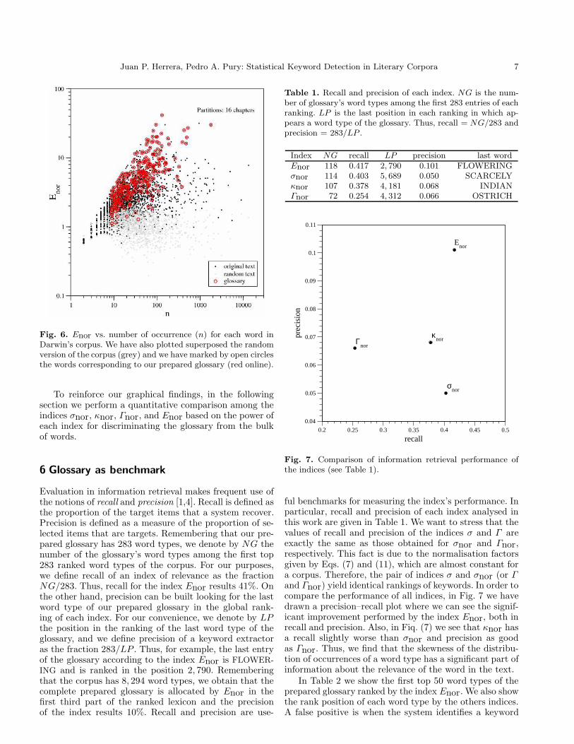
(16)Figure 6 shows the values of Enor for all word types ofDarwin’s corpus versus its number of occurrence, n, on adouble logarithmic scale. The individual deviations fromthe bulk trend for each value of n are related to the par-ticular usage nuances of words. To stress these deviations,we have used the 16 chapters of the corpus as natural par-titions for our entropic analysis (i.e. P = 16). In this way,we obtain a remarkable scattering of higher values of Enorin the full range of number of occurrences. A same entropicanalysis using the 842 paragraphs of Darwin’s corpus aspartitions (i.e. P = 842) generates a similar graph thatstresses the bulk trend, but the fluctuations are completelysmoothed. Using the chapters as partitions (P = 16) inFig. 6, the “cloud of points” corresponding to the randomversion of the corpus is distributed around the unitaryvalue and the corpus appears clearly more separated fromthe random text than with previous indices. Additionally,the words corresponding to the glossary have systemati-cally high values of the index Enor.


Fig. 6. Enor vs. number of occurrence (n) for each word inDarwin’s corpus. We have also plotted superposed the randomversion of the corpus (grey) and we have marked by open circlesthe words corresponding to our prepared glossary (red online).

To reinforce our graphical findings, in the followingsection we perform a quantitative comparison among theindices σnor, κnor, Γnor, and Enor based on the power ofeach index for discriminating the glossary from the bulkof words.

6 Glossary as benchmark

Evaluation in information retrieval makes frequent use ofthe notions of recall and precision [1,4]. Recall is defined asthe proportion of the target items that a system recover.Precision is defined as a measure of the proportion of se-lected items that are targets. Remembering that our pre-pared glossary has 283 word types, we denote by NG thenumber of the glossary’s word types among the first top283 ranked word types of the corpus. For our purposes,we define recall of an index of relevance as the fractionNG/283. Thus, recall for the index Enor results 41%. Onthe other hand, precision can be built looking for the lastword type of our prepared glossary in the global rank-ing of each index. For our convenience, we denote by LPthe position in the ranking of the last word type of theglossary, and we define precision of a keyword extractoras the fraction 283/LP . Thus, for example, the last entryof the glossary according to the index Enor is FLOWER-ING and is ranked in the position 2, 790. Rememberingthat the corpus has 8, 294 word types, we obtain that thecomplete prepared glossary is allocated by Enor in thefirst third part of the ranked lexicon and the precisionof the index results 10%. Recall and precision are use-

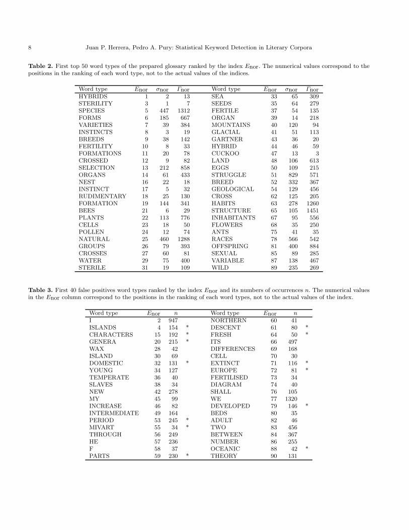
Table 1. Recall and precision of each index. NG is the num-ber of glossary’s word types among the first 283 entries of eachranking. LP is the last position in each ranking in which ap-pears a word type of the glossary. Thus, recall = NG/283 andprecision = 283/LP .

Index NG recall LP precision last wordEnor 118 0.417 2, 790 0.101 FLOWERINGσnor 114 0.403 5, 689 0.050 SCARCELYκnor 107 0.378 4, 181 0.068 INDIANΓnor 72 0.254 4, 312 0.066 OSTRICH

0.2 0.25 0.3 0.35 0.4 0.45 0.5

recall

0.04

0.05

0.06

0.07

0.08

0.09

0.1

0.11

prec

isio

n

Γnor

κnor

σnor

Enor

Fig. 7. Comparison of information retrieval performance ofthe indices (see Table 1).

ful benchmarks for measuring the index’s performance. Inparticular, recall and precision of each index analysed inthis work are given in Table 1. We want to stress that thevalues of recall and precision of the indices σ and Γ areexactly the same as those obtained for σnor and Γnor,respectively. This fact is due to the normalisation factorsgiven by Eqs. (7) and (11), which are almost constant fora corpus. Therefore, the pair of indices σ and σnor (or Γand Γnor) yield identical rankings of keywords. In order tocompare the performance of all indices, in Fig. 7 we havedrawn a precision–recall plot where we can see the signif-icant improvement performed by the index Enor, both inrecall and precision. Also, in Fiq. (7) we see that κnor hasa recall slightly worse than σnor and precision as goodas Γnor. Thus, we find that the skewness of the distribu-tion of occurrences of a word type has a significant part ofinformation about the relevance of the word in the text.

In Table 2 we show the first top 50 word types of theprepared glossary ranked by the index Enor. We also showthe rank position of each word type by the others indices.A false positive is when the system identifies a keyword


Table 2. First top 50 word types of the prepared glossary ranked by the index Enor. The numerical values correspond to thepositions in the ranking of each word type, not to the actual values of the indices.

Word type Enor σnor Γnor Word type Enor σnor ΓnorHYBRIDS 1 2 13 SEA 33 65 309STERILITY 3 1 7 SEEDS 35 64 279SPECIES 5 447 1312 FERTILE 37 54 135FORMS 6 185 667 ORGAN 39 14 218VARIETIES 7 39 384 MOUNTAINS 40 120 94INSTINCTS 8 3 19 GLACIAL 41 51 113BREEDS 9 38 142 GARTNER 43 36 20FERTILITY 10 8 33 HYBRID 44 46 59FORMATIONS 11 20 78 CUCKOO 47 13 3CROSSED 12 9 82 LAND 48 106 613SELECTION 13 212 858 EGGS 50 109 215ORGANS 14 61 433 STRUGGLE 51 829 571NEST 16 22 18 BREED 52 332 367INSTINCT 17 5 32 GEOLOGICAL 54 129 456RUDIMENTARY 18 25 130 CROSS 62 125 205FORMATION 19 144 341 HABITS 63 278 1260BEES 21 6 29 STRUCTURE 65 105 1451PLANTS 22 113 776 INHABITANTS 67 95 556CELLS 23 18 50 FLOWERS 68 35 250POLLEN 24 12 74 ANTS 75 41 35NATURAL 25 460 1288 RACES 78 566 542GROUPS 26 79 393 OFFSPRING 81 400 884CROSSES 27 60 81 SEXUAL 85 89 285WATER 29 75 400 VARIABLE 87 138 467STERILE 31 19 109 WILD 89 235 269

Table 3. First 40 false positives word types ranked by the index Enor and its numbers of occurrences n. The numerical valuesin the Enor column correspond to the positions in the ranking of each word types, not to the actual values of the index.

Word type Enor n Word type Enor nI 2 947 NORTHERN 60 41ISLANDS 4 154 * DESCENT 61 80 *CHARACTERS 15 192 * FRESH 64 50 *GENERA 20 215 * ITS 66 497WAX 28 42 DIFFERENCES 69 168ISLAND 30 69 CELL 70 30DOMESTIC 32 131 * EXTINCT 71 116 *YOUNG 34 127 EUROPE 72 81 *TEMPERATE 36 40 FERTILISED 73 34SLAVES 38 34 DIAGRAM 74 40NEW 42 278 SHALL 76 105MY 45 99 WE 77 1320INCREASE 46 82 DEVELOPED 79 146 *INTERMEDIATE 49 164 BEDS 80 35PERIOD 53 245 * ADULT 82 46MIVART 55 34 * TWO 83 456THROUGH 56 249 BETWEEN 84 367HE 57 236 NUMBER 86 255F 58 37 OCEANIC 88 42 *PARTS 59 230 * THEORY 90 131


that really is not one. In Table 3 we show the first top40 ranked (by Enor) word types not included in our pre-pared glossary. We can immediately see that several termsare not necessarily false positives. We have marked withan asterisk (*) in the table those word types that werenot previously selected in the prepared glossary, but thatappeared in the main entries of the original glossary ofDarwin’s book. Indeed, several more word types like thesecould have been included in our prepared glossary, too.Moreover, we could say that the word type I is relevant fora text that uses the first–person narrative, like Darwin’sbook. ISLAND and SLAVES were not used neither in thebook’s glossary nor in its index; however Enor ranks itadequately as a keyword. The word type F is also mean-ingful to the text. It appear in the proper nouns “Mr.F. Smith” and “Dr. F. Muller”, and in the collocations“F. sanguinea”, “F. rufescens”, “F. fusca”, “F. flava”, and“F. rufescens” which denote species. The observations inthe last paragraphs induce us to consider that the per-formance of the index Enor is better than what can beinferred from Table 1.

Moreover, the index Enor requires less computationalefforts that the others. Knowing the number of occur-rences of a word type, the implementation of the algorithmfor the variance or the skewness requires of one accumu-lator plus a counter for reckoning the number of tokensbetween nearest neighbour occurrences of the word type.While, for the entropic index, we only need one counter (ofnumber of occurrences) for each partition per word type.On the other hand, the algorithm for Γ requires threeaccumulators and for each occurrence of a word type weneed to determine if it corresponds to a cluster point.

7 Concluding remarks

In summary, in this work we addressed the issue of statis-tical distribution of words in texts. Particularly, we haveconcentrated on the statistical methods for detecting key-words in literacy text. We reviewed two indices (σ and Γ )previously proposed [18,19] for measuring relevance andwe improved them by considering their values in randomtexts. Additionally, we introduced κnor based on the skew-ness of the distribution of occurrences of a word and weproposed another index for keyword detection based onthe information entropy. Our proposals are very easy toimplement numerically and have performances as detec-tors as good as or better than the other indices. The ideasof this work can be applied to any natural language withwords clearly identified, without requiring any previousknowledge about semantics or syntax.

Acknowledgements

Contributions to Appendix B by Marcelo Montemurroare gratefully acknowledged. This work was partially sup-ported by grant from “Secretarıa de Ciencia y Tecnologıade la Universidad Nacional de Cordoba” (Code: 05/B370).

A The Geometrical distribution

In this Appendix we briefly review the basic results of thegeometrical distribution, scattered in the literature, thatare useful for this work. First, we consider an experimentwith only two possible outcomes for each trial (binomialexperiment). Repeated independent trials of the binomialexperiment are called Bernoulli trials if their probabilitiesremain constant throughout the trials. We denote by p theprobability of the “successful” outcome. Now, we are in-terested in the probability of success on the j–th trial aftera given success. Given that the trials are independent, weimmediately obtain the geometrical distribution

P (j) = (1− p)j−1 p , for j ≥ 1 . (17)

A.1 Moments and cumulants

The characteristic function of a stochastic variable X isdefined by G(k) =

⟨

ekX⟩

=∑

j≥1P (j) exp(kj). Thus, for

the geometrical distribution we obtain

G(k) =p ek

1− (1− p) ek. (18)

This function is also the moment generating function

〈Xn〉 = dnG

dkn

∣

∣

∣

∣

k=0

. (19)

Therefore, the first three cumulants of the geometrical dis-tribution are given by

µ1 = 〈X〉 = 1

p,

µ2 =⟨

X2⟩

− 〈X〉2 =1− p

p2,

µ3 =⟨

X3⟩

− 3⟨

X2⟩

〈X〉+ 2 〈X〉3 =(2− p) (1− p)

p3.

(20)

A.2 Addition of two geometrical variables

If X1 e X2 are geometrical distributed independent ran-dom variables, the distribution of the addition Y = X1 +X2 is

PY (j) =∑

m1+m2=j

P (m1,m2) , for j = 2, 3, . . . ,

(21)where the joint probability distribution of the variablesX1 e X2, P (m1,m2), is given by

P (m1,m2) = p2 (1−p)m1+m2−2 , for m1 ≥ 1, and m2 ≥ 1 .(22)

In this manner,

PY (j) =

j−1∑

m=1

P (m, j −m) =

j−1∑

m=1

p2 (1 − p)j−2 . (23)


Therefore

PY (j) = (j − 1) p2 (1 − p)j−2 , for j = 2, 3, . . . . (24)

Now, we are interested in the average of the randomvariable (recall Eq. (5))

γ =

1− Y

2µ, Y < 2µ

0 , Y ≥ 2µ, (25)

where Y is the addition of two independent geometricaldistributed random variables with mean µ = 1/p. By def-inition we have that

〈γ〉 =h∑

j=2

(

1− j

2µ

)

PY (n) , (26)

where PY (n) is given by Eq. (24) and h = Int[2µ]. Definingq = 1− p and using the identity

N∑

n=1

qn =q − qN+1

1− q(27)

we immediately obtain

h∑

n=j

PY (j) = p2d

dq

h∑

k=2

qk−1 = 1− h qh−1 + (h− 1) qh ,

(28)and

p

h∑

j=2

j PY (j) = p3d2

dq2

h∑

k=2

qk = 2− h (h+ 1) qh−1

+2 (h+ 1) (h− 1) qh − h (h− 1) qh+1 .

(29)

Therefore

〈γ〉 = 1

2h (h− 1) qh (q + q−1 − 2) . (30)

The Poisson distribution can be obtained from the ge-ometrical distribution in the limit p → 0. Expanding qz

into a Taylor series up to fourth order we obtain

qh+1 + qh−1 − 2 qh ≈ p2 + (1− h) p3 +1

2(2− 3h+ h2) p4 .

(31)Given that for p → 0 we have h >> 1, the last equationcan be recast as

qh+1 + qh−1 − 2 qh ≈ p2(

1− h p+ 1

2(hp)2

)

≈ p2 exp (−hp) .(32)

Finally, using that hp ≈ 2, we obtain that the average ofthe random variable γ for a Poisson distribution [19] is

〈γ〉 = 2 e−2 . (33)

B Entropy of a random text

Here, we derive the entropy of a random text in a moredetailed way that is described in Ref. [14].

We consider a corpus of N tokens as a composite ofP parts, with Ni tokens in the i–th part (i = 1, 2, . . . , P ).In a random corpus, the probability that a word type wappears in the part j is Nj/N . Thus, the probability thatw appears n1 times in part 1, n2 times in part 2, and soon, is the multinomial distribution

pw(n1, n2, . . . , nP ) = n!P∏

j=1

1

nj !

(

Nj

N

)nj

, (34)

where n =∑P

j=1nj is the absolute frequency (number of

tokens) of the word type w.For reasons of simplicity, in this Appendix we consider

the particular case in which all the parts have exactlythe same number of tokens, i.e. Ni = N/P . Hence, theprobability measure defined by Eq. (13) can be simplywritten as pi = ni/n and the information entropy definedby Eq. (14) results

S = − 1

lnP

P∑

i=1

ni

nln(ni

n

)

. (35)

Now, we are interested in the average value of the en-tropy over the distribution given by Eq. (34). We onlyneed to compute the average of each term of Eq. (35)using the marginal distributions, pw(ni), obtained fromEq. (34). All marginal distributions result binomials withmean n/P and variance n/P (1 − 1/P ). Thus, we obtainfor the average entropy

〈S〉 = − P

lnP

n∑

m=0

m

nln(m

n

)( n

m

) 1

Pm

(

1− 1

P

)n−m

.

(36)For highly frequent word types, n >> 1, we can ap-

proximate the binomial distribution by a Gaussian prob-ability function (G(x;µ, σ)) with mean µ = 1/P and vari-ance σ2 = (1/n)(P − 1)/P 2. Thus, Eq. (36) can be recastas

〈S〉 ≈ − P

lnP

∫ 1

0

x lnxG(x;µ, σ)dx . (37)

In the limit n >> 1, σ → 0 and the Gaussian probabilityfunction concentrates around its mean value µ. Using theexpansion of the function x lnx around µ,

x lnx ≈ µ lnµ+ (1 + lnµ)(x − µ) +1

2

1

µ(x− µ)2 , (38)

in Eq. (37) and remembering that∫ ∞

−∞

(x− µ)2 G(x;µ, σ)dx = σ2 ,

we finally obtain for a random text [14] that

〈S〉 ≈ 1− P − 1

2n lnP. (39)


References

1. C. Manning and H. Schutze, Foundations of Statistical

Natural Language Processing, (MIT Press, Cambridge,MA, 1999).

2. H. P. Luhn, The automatic creation of literature abstracts,IBM J. Res. Devel. 2, 159–165 (1958).

3. G. K. Zipf, Human Behavior and the Principle of Least Ef-

fort: An Introduction to Human Ecology, (Addison-Wesley,Cambridge, MA, 1949).

4. G. Salton and M. J. McGill, Introduction to Modern In-

formation Retrieval, (McGraw-Hill, New York, 1983).5. R. N. Mantegna, S. V. Buldyrev, A. L. Goldberger,

S. Havlin, C.-K. Peng, M. Simons and H. E. Stanley, Sys-tematic analysis of coding and noncoding DNA sequences

using methods of statistical linguistic, Phys. Rev. E 52,2939–2950 (1995).

6. H. Stanley, S. Buldyrev, A. Goldberger, S. Havlin, C.-K.Peng and M. Simons, Scaling features of noncoding DNA,Physica A 273, 1–18 (1999).

7. I. Grosse, P. Bernaola-Galvan, P. Carpena, R. Roman-Roldan, J. Oliver and H. E. Stanley, Analysis of symbolic

sequences using the Jensen-Shannon divergence, Phys.Rev. E 65, 041905 (2002).

8. W. Ebeling and T. Poschel, Entropy and long range cor-

relations in literary English, Europhys. Lett. 26, 241–246(1994).

9. W. Ebeling, T. Poschel and K.-F. Albrecht, Entropy,

transinformation and word distribution of information–

carrying sequences, Int. J. Bifurcation and Chaos 5, 51–61(1995) .

10. M. Cassandro, P. Collet, A. Galves and C. Galves, A

statistical–physics approach to language acquisition and

language change, Physica A 263, 427–437 (1999).11. A. Cohen, R. N. Mantegna and S. Havlin, Numerical anal-

ysis of word frequencies in artificial and natural language

texts, Fractals 5, 95–104 (1997).12. A. C.-C. Yang, C.-K. Peng, H.-W. Yien and A. L. Gold-

berger, Information categorization approach to literary au-

thorship disputes, Physica A 329, 473–483 (2003).13. R. F. i Cancho, Decoding least effort and scaling in signal

frequency distributions, Physica A 345, 275–284 (2005).14. M. A. Montemurro and D. H. Zanette, Entropic analysis of

the role of words in literary texts, Adv. Complex Systems5, 7–17 (2002).

15. The digital text file was obtained from Project Gutenberg:http://promo.net/pg

16. D. Beeferman, A. Berger and J. Lafferty, A model of lexicalattraction and repulsion, in Proceedings of the ACL-EACL

Joint Conferences (Madrid, Spain, 1997), pp. 373–380.17. T. Niesler and P. Woodland, Modelling word-pair relations

in a category-based language model, in Proceedings of the

IEEE International Conference on Acoustics, Speech and

Signal Processing, Vol. 2 (Munich, Germany, 1997), pp.795–798.

18. M. Ortuno, P. Carpena, P. Bernaola-Galvan, E. Munozand A. M. Somoza, Keyword detection in natural languages

and DNA, Europhys. Lett. 57, 759–764 (2002).19. H. Zhou and G. W. Slater, A metric to search for relevant

words, Physica A 329, 309–327 (2003).20. C. E. Shannon and W. Weaver, The Mathematical Theory

of Communication, (University of Illinois Press, Urbana,Illinois, 1949), reprinted with corrections from The Bell

System Technical Journal 27, pp. 379–423, 623–656, July,October, (1948).

http://promo.net/pg

Statistical Keyword Detection in Literary Corpora - arXiv

Documents