Test (1996) Vol. 5, No. 2, pp. 249-344 249 Statistical Inference and Monte Carlo Algorithms GEORGE CASELLA Biometrics Unit, Cornell University, Ithaca NY 14853, USA [Read before the Spanish Statistical Society at a meeting organized by the University of Granada on Friday, September 27, 1996] SUMMARY This review article looks at a small part of the picture of the interrelationship between statistical theory and computational algorithms, especially the Gibbs sampler and the Accept-Reject algorithm. We pay particular attention to how the methodologies affect and complement each other. Keywords: MARKOV CHAIN MONTE CARLO; GIBBS SAMPLING; ACCEPT-REJECT ALGORITHM; RAO-BLACKWELL THEOREM; IMPROPER PRIORS; DECISION THEORY. 1. INTRODUCTION Computations and statistics have always been intertwined. In particular, applied statistics has relied on computing to implement its solutions of real data problems. Here we look at another part of the relationship between statistics and computation, and examine a small part of how the theories not only are intertwined, but how they have influenced each other. With the explosion of methods based on Monte Carlo methods, par- ticularly those using Markov chain algorithms such as the Gibbs sampler, there has been a blurring of the distinction between the statistical model and the algorithmic model. This is particularly evident in the examples Received August 96; Revised September 96.

Welcome message from author
This document is posted to help you gain knowledge. Please leave a comment to let me know what you think about it! Share it to your friends and learn new things together.
Transcript
Test (1996) Vol. 5, No. 2, pp. 249-344
249
Statistical Inference and Monte Carlo Algorithms
GEORGE CASELLA Biometrics Unit, Cornell University, Ithaca NY 14853, USA
[Read before the Spanish Statistical Society at a meeting organized by the University of Granada on Friday, September 27, 1996]
SUMMARY
This review article looks at a small part of the picture of the interrelationship between statistical theory and computational algorithms, especially the Gibbs sampler and the Accept-Reject algorithm. We pay particular attention to how the methodologies affect and complement each other.
Keywords: MARKOV CHAIN MONTE CARLO; GIBBS SAMPLING;
ACCEPT-REJECT ALGORITHM; RAO-BLACKWELL THEOREM;
IMPROPER PRIORS; DECISION THEORY.
1. INTRODUCTION
Computations and statistics have always been intertwined. In particular, applied statistics has relied on computing to implement its solutions of real data problems. Here we look at another part of the relationship between statistics and computation, and examine a small part of how the theories not only are intertwined, but how they have influenced each other.
With the explosion of methods based on Monte Carlo methods, par- ticularly those using Markov chain algorithms such as the Gibbs sampler, there has been a blurring of the distinction between the statistical model and the algorithmic model. This is particularly evident in the examples
Received August 96; Revised September 96.
250 George Casella
of Section 3. There, the statistical model will typically be a hierarchical model, while the computational algorithm will be based on a set of con- ditional distributions. We will see that the manner in which we view the model can have a large impact on the validity of the statistical inference. It is therefore important to consider the statistical model that underlies the Monte Carlo algorithm.
We can also turn things around. When one uses a Monte Carlo algorithm to do a calculation, it is common to process the output by taking an average. However, we should realize that the output from a Monte Carlo algorithm can be viewed as data, with the algorithm itself playing the part of a statistical model. As such, taking a naive average may not be the most effective way of processing the output. In Section 4 we look at this question, and investigate the effect of classical decision theory on output from the Accept-Reject algorithm. We consider these improvements as a post-simulation processing of a generated sample, which is statistically superior to the original estimator, although they may be computationally inferior in taking more computer time. However, this latter concern can also be addressed with estimators that offer statistical improvement while only requiring a slight increase in computational effort.
We also emphasize that our approach and, in particular, the opti- mizations involved in the derivation of some of the improved estimators, is based on statistical rather than computational principles. The overall goal of the statistician is to process samples in an optimal way, and to make the best inference possible. To do so requires treating an algorithm as a statistical model, and (as far as possible) ignoring the computational issues.
Another consideration in the interplay of statistical theory and al- gorithms is the prospect of using the structure of the algorithm to more efficiently construct an optimal procedure. We illustrate this in Sec- tion 5, where we look at three examples. These examples use the Gibbs sampler, and show that we can use the iterative nature of the algorithm to implement procedures that are sometimes computationally feasible and can result in an optimal inference. We end the paper with a short discussion section.
Statistical Inference and Monte Carlo Algorithms 951
2. SYNTHESIS
Given the audience of this presentation, a digression may be in order into the Bayes/frequentist approaches to statistics. The topic of algorithms, particularly Monte Carlo algorithms, is a prime example of an area that is best handled statistically by a mixture of the Bayesian and frequentist approaches. Moreover, it seems that to completely analyze, understand, and optimize the relationship between a statistical model, its associated inference, and the algorithm used for computations, both Bayesian and frequentist ideas must be used.
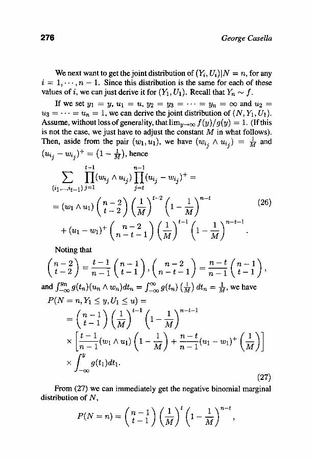
The Bayesian approach provides us with a means of constructing an estimator that, when evaluated according to its global risk performance, could result in an optimal frequentist estimator. This highlights impor- tant features of both the Bayesian and frequentist approaches. Although the Bayesian paradigm is well-suited for the construction of possibly optimal estimators, it is less well-suited for their global evaluation. The frequentist paradigm is quite complementary, as it is well-suited for global evaluations, but is less well-suited for construction.
We look at two examples, taken from Lehmann and Casella (1997).
Example 1. Rao-Blackwellizing the Gibbs Sampler. The Gibbs sam- pler (Geman and Geman 1984, Gelfand and Smith 1990) provides a method of computing Bayes estimators. These estimators are computed by averaging random variables and this averaging is improved if the Rao-Blackwell theorem is applied (Liu, Wong and Kong 1994, 1995). More precisely, in a typical use of the Gibbs sampler, our estimand is the actual Bayes estimator, which we are computing by generating random variables and averaging them. The validity of our method rests on the Ergodic Theorem (Law of Large Numbers). When the Rao-Blackwell theorem is applied to these averages, we get a new average with the same expectation (the actual value of the estimator) and smaller variance.
Thus, the calculation of a Bayes estimator is improved using a fre- quentist methodology. Moreover, monitoring convergence of the Gibbs sampler is essentially a frequentist problem, so again frequentist tech- niques can be used to improve Bayes estimators. ,~
The preceding example shows how frequentist methods can aid a Bayesian approach. The reverse is also true.
252 George Casella
Example 2. REML variance estimation. In the one-way random effects model
Yij = / 3 + u i + e i j ( j = l , , . . , n i , i = 1 , . . . , k ) (1)
where/3 is the overall mean, ui is a random effect, and ~ij is error, it is often of primary interest to estimate 0-2 and 0-~, the variance of the random effects ui and ~ij, respectively. Two basic problems must be overcome.
(a) Elimination of the effect of/3 from the estimates of 0 -2 and 0-2. As the latter are estimates of dispersion, they should not be affected by a change in the mean level.
(b) Interpretation of possibly negative estimates of variance, which can arise from some classical estimation methods (see Searle, et al. 1992, Section 3.5c).
Both (a) and (b) can be dealt with using frequentist methodologies. For example, the effect of/3 can be eliminated by requiring the vari- ance estimates to be translation invariant (one derivation of the so-called REML variance estimates; see Searle et al. 1992, Section 6.6 and Chap- ter 9) and the negativity problem can be handled by truncation.
Alternatively, a Bayesian model can eliminate both of these prob- lems in a straightforward way. First, the parameter/3 can be integrated out using a prior distribution, creating a marginal likelihood. Moreover,
2 will never be negative. Bayes estimates of o .2 and 0-e
Note that we are using the Bayesian approach to construct the es- timators. The evaluation of the estimators, and establishment of any optimality properties, can still be done using a frequentist global risk approach. <
Thus, it is important to view these two approaches as complemen- tary rather than adversarial, as together they provide a rich set of tools and techniques for the statistician. Moreover, there are situations and problems in which one or the other approach is better-suited, or even a combination may be best, so a statistician without a command of both approaches may be less than complete.
Statistical Inference and Monte Carlo Algorithms 953
3. ALGORITHMS AND STATISTICAL INFERENCE
In this section we look at how an algorithmic approach to a problem has fundamental repercussions on the statistical inference. In Section 3.1, where we mainly give details for the mixed linear model, we will see that approaching a problem through a Gibbs sampler can mask posterior impropriety. This can have a profound effect on the possible statistical inferences. In the most extreme cases, which are in no way pathological, evaluating a statistical model only through a Gibbs sampler can lead to erroneous, even nonsensical, inferences. This latter point is examined in Section 3.2.
3.1. How the Algorithm Affects the Posterior
The model equation of a general linear mixed model is given by
t = x / 3 + + (2)
where Y is an n x 1 vector of observations,/3 is a p • 1 vector of fixed effects (parameters), u is a q x 1 vector of random effects (random variables), X and Z are known design matrices whose dimensions are n x p and n x q, respectively, and e is an n x 1 vector of residual errors.
A typical set of error distributions (or priors) for the mixed model 2 ~,~ N q ( O , D ) where u has e[~r~ ~ Nn(O, Icr~) and ulcr12,. . . ,o r =
�9 .. u r ) , ui is qi x 1, D = and ~-~4=1 qi = q. The '-~i=1 qi i ' r subvectors of u correspond to the r different random factors in the experiment. It is also common to put a flat prior (Lebesgue measure) on the so-called fixed effects, represented by the vector/3. In classical mixed model inference, such an assumption is used in REML, or restricted maximum likelihood estimation. As it turns out, the type of prior used on/3 has no impact on what follows.
The variance components themselves, which are often the prime targets of inference, are often given power-type priors of the form
71"e(o'21b) (2((0-2) -(b+l) , 7ri(~lai)~ (o?) -(ai+l) , (3)
where the ai 's and b are known and the following conditional indepen- dence assumptions are in force: (1) given u, Y is conditionally indepen- dent of o-~,. . . , o-2, (2) given o-2, . . . , o-2, u is conditionally independent of/3 and 0-2, and (3)/3, 0-2, and o-~,. . . , 0-2 are a priori independent.
254 George Casella
All of these assumptions can be summarized in the hierarchical model
Y l u , cr2,/3 ~ Nn(X/3 + Zu, Ia~)
2 ,.~ Nq(O,D) 7re(cr2lb) c< (0"2) -(b+l) (4) rr(/3) c~ 1 u1 12,.. rr/(a~[ai) c((0?) -(ai+l) .
With the increased popularity of Monte Carlo algorithms such as the Gibbs sampler, the experimenter tends to pay less attention to the model specified by (4), and rather concentrates on the set of full conditionals, which make up the input into the Gibbs Markov chain. For our mixed model, these conditionals are given by
2/3) i C ( a , + q i f (o2lo"_i, y, u, fie, = 2 ' u (5)
n f (a2elo-,y,u,/3) = IG b+-~, 2 { ( y - ( X / 3 + Zu)) '
(y - (X/3 + Zu))} -1)
2 ( _2 n - l ~ - I ,w! f (ulo- ,y,o- , , /3) = Nq (Z 'Z+o,J_~ ) i_,
(y- - X/3), f f2(Z'Z q- cr2D-1) -1)
( ( 2 ( X t X ) -1 ) 2 u) = Np X t X ) -1 X ! (y Zu) , o- e f (/310", Y, o" e ,
where o" = (o-2,...,0-2), o"-i = (0"2,...,cri-1,0"i+1,...,0"2), IG stands for inverted gamma and we say that X ~ IG(r, s) if f x ( t ) c( t -r-1 exp( -1 / s t ) for positive t.
If 2ai < - q i for some i or 2b < - n , then at least one of the con- ditionals is improper, since the inverted gamma density is defined only when both parameters are positive (Berger 1985, p. 561). Clearly, one improper conditional implies an improper posterior.
Although it may be tempting to assume that propriety of the condi- tionals in (5) implies propriety of the posterior distribution, this is false. Indeed, there are many values of the vector (al, a2,. . , at, b) which si- multaneously yield proper conditionals (2ai > -qi Vi and 2b > - n )
Statistical Inference and Monte Carlo Algori thms 955
and an improper posterior. Thus, in general, if one incorrectly assumes propriety of a posterior and writes down a (false) proportionality state- ment like
2 2 ~r(a2, . . . , crr, a~ , u , ~]y ) c< f (y]u , a2, f~) f (ula2, . . . , r 2) r (6)
7r(~)Tr~(~ H 7ri(ty2]ai) i=1
where f is used to represent a generic density, it may happen that the Gibbs conditionals are all proper densities. Such a situation is very dangerous because, if the output from the Gibbs sampler fails to warn the user that the posterior is improper (which seems to be the common situation), the result could be an inference about a nonexistent posterior distribution. We will return to this point in Section 3.2.
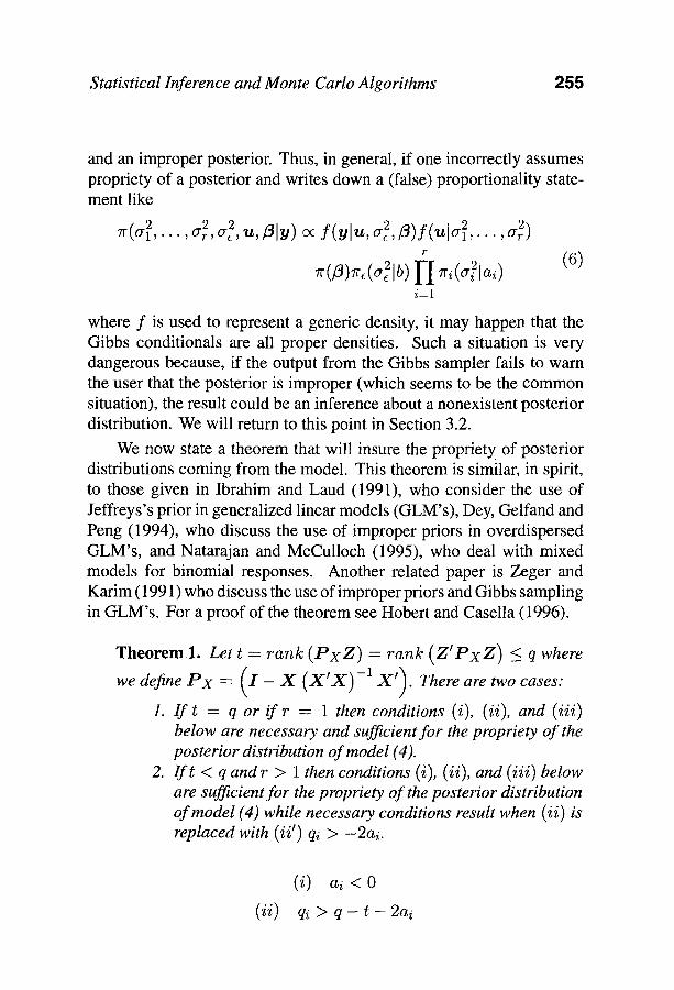
We now state a theorem that will insure the propriety of posterior distributions coming from the model. This theorem is similar, in spirit, to those given in Ibrahim and Laud (1991), who consider the use of Jeffreys's prior in generalized linear models (GLM's), Dey, Gelfand and Peng (1994), who discuss the use of improper priors in overdispersed GLM's, and Natarajan and McCulloch (1995), who deal with mixed models for binomial responses. Another related paper is Zeger and Karim (1991) who discuss the use of improper priors and Gibbs sampling in GLM's. For a proof of the theorem see Hobert and Casella (1996).
Theorem 1. L e t t = r a n k ( P x Z ) = r a n k ( Z ' P x Z ) < q where
we define P x = ( I - g ( X ' X ) -1 X ' ) . There are two cases:
1. I f t = q or i f r = 1 then conditions (i), (ii), and (i i i) below are necessary and sufficient f o r the propriety o f the posterior distribution o f model (4).
2. I f t < q a n d r > 1 thencondit ions (i), (ii), and (i i i) below are sufficient f o r the propriety o f the posterior distribution o f model (4) while necessary conditions result when (ii) is replaced with (ii ~) qi > - 2 a i .
(i) ai < 0
(ii) qi > q - t - 2ai
256 George Casella
(iii) n + 2 E a i + 2 b - p > O .
Thus, we see that it is relatively easy to check if the posterior distri- butions are proper, being merely a matter of counting categories. Also, conditions (i)-(iii) are intuitively reasonable, and can be interpreted as requiring that we have enough observations, in particular enough obser- vations on the variance components o -2 , to adequately control the tails of the posterior (large enough qi).
3.2. How the Algorithm Affects the Inference
In this section, we look at what can happen to the inference if one uses a set of Gibbs conditionals, all of which are proper, that do not correspond to a proper posterior. This situation was investigated in detail by Hobert and Casella (1995), and we will discuss a few of their findings.
A set of conditional densities such as those in (5) may, or may not, result in a proper posterior. However, the fact that may obscure the impropriety of the posterior is the functional compatibility of the set of densities. First consider the following simple example from Casella and George (1992).
Example 3. The exponential conditional densities
fl(x[Y) = ye -yz and f2(ylx) = xe -xy.
appear to be a pair of conditional densities, but there is no joint density function which will yield f l and f2 as conditional densities. If such a joint density did exist, the pair f l and f2 would be compatible. As one does not exist, this pair is incompatible. However, the non-integrable function 9(x, y) = e x p ( - x y ) , if treated as a joint density, does yield f l and f2 as its "conditionals". In such a case, where no proper 9(') exists, but an improper one does, we say that f l and f2 are functionally compatible. This is the dangerous case, as f l and f2 appear to be a set of conditional densities. This is exactly what can happen in (5) if the conditions of Theorem 1 are not satisfied. <~
When there are more than two variables, the definitions of compati- bility and functional compatibility become more involved, but the idea is
Statistical Inference and Monte Carlo Algorithms 257
the same. Compatibility of a set of densities was investigated by Besag (1974), Arnold and Press (1989), and Gelman and Speed (1993). They tended to focus on conditions under which a set of conditional densities could be used to uniquely determine the joint density, assuming that such a density existed. In our case, however, we cannot assume that such a joint density exists.
The major concern for a user of a Gibbs sampler based on a set of functionally compatible densities that are not compatible (that is, for which not proper joint density exists), is what inference can be made from the resulting Markov chain? This is the question investigated in detail by Hobert and Casella (1995), and the results are quite negative. They prove the following theorem.
Theorem 2. Let f l , . . . , f m be a set o f functionally compatible con- ditional densities on which a Gibbs sampler is based. The resulting Markov chain �9 is positive recurrent i f and only i f f l , . . . , fm are compatible.
Thus, a set of densities that are only functionally compatible will not result in a positive recurrent Markov chain. Hence, there cannot be any stationary probability distribution for the chain to converge to. Moreover, there is virtually no reasonable inference that can be made. Under some additional technical conditions (which are satisfied for most typical Gibbs samplers), it can be shown that if t : A --~ ~+ is a bounded measurable function for which, given e > 0, there exists a compact set C E A such that t (y) _< c V y E C c, then
l iminf 1 ~ t ( ~ i ) -- 0 a.s. (7) n ----~ o o n
i =1
In a typical Gibbs sampling application, one might estimate a posterior density 7r(Oly ) with an average of conditional posterior densities, say 7r(OIy ) ~--~ ( l / m ) Eim__l 7r(O]y, ,~i). It will often be the case that the den- sities 7r(Oly , hi) satisfy the conditions on the function t above. Hence, the only place the average ( l / m ) y'~im__l Tr(Oly ,/~i) can converge to is 0; or else it will not converge.
Gibbs samplers based on a set of densities that are not compatible result in Markov chains that are null, that is, they are either null recurrent
258 George Casella
or transient. In either case, there is no limiting probability distribution. However, output from the Gibbs sampler may produce nice looking pic- tures of the supposed marginal posterior densities, particularly when the posterior density is computed as an average of conditional densities. But there can be no actual distribution to which the Gibbs picture cor- responds. This was the problem with the Gibbs-based conclusions of Wang et al. (1993, 1994) and Gelfand et al. (1990) as they used models for which a posterior distribution did not exist.
An insidious feature of this situation is that a null Gibbs chain may be undetectable to the practitioner, that is, the resulting Monte Carlo ap- proximations appear completely reasonable. Moreover, not only do the Gibbs averages look reasonable, but the actual output from the Markov chain may appear reasonable. (Consider Geyer 1992, who published what he first believed to be proper Gibbs output, but later found that it corresponded to an improper posterior. He noted, in proof, that, "...(the model) produces an improper posterior, so the Gibbs sampler apparently converged when there was no stationary distribution for it to converge to. A run of one million iterations gave no hint of lack of convergence.." Thus, it is not surprising that a practitioner can be fooled into believing that the Gibbs chain is giving a reasonable inference.
In order to demonstrate just how reasonable some of these null Gibbs chains can appear, we give an example.
Example 4. The one-way random effects model (1) with a typical set of priors is
2
2 ~ (cr2~-(b+l) (8) /3 ,~ d/3 u ~ Nk (O, Io- 2) o-, , - , ,
o-2 ~ (o-2)-(a+1).
For a simulation study we set k = 7, ni = n = 5, o -2 = 5, o.2 = 2,
and /~ = 10. The vector (Ul , . . . ,UT) was simulated by generating seven iid N(0, 5) random variables and the vector (e11, . . . , c75) was simulated by generating 35 iid N(0, 2) random variables. We also set a = b = 0, which yields an improper posterior. A Gibbs chain was constructed using the conditionals given in (5). We denote the chain by
(O "2(j) , O "2(j), U/(j), fl(J)), j > 1. At the start, all parameters were set to
Statistical Inference and Monte Carlo Algorithms 259
one, except for the overall mean, 13, which was set to eight. The chain was first allowed to run for 55,000 iterations; keep in mind that the word "bum-in" is not appropriate for these initial iterations because the chain is null and is therefore not converging (in the usual sense). The sole purpose of these initial iterations was to provide the chain with ample opportunity to misbehave and alert us that something may be wrong; it never did. We chose 15,000 because a typical burn-in would probably be in the hundreds (see Gelfand et al. 1990 and Wang et al. 1993) so that if our chain did not misbehave during the burn-in stage, neither would that of an unknowing experimenter.
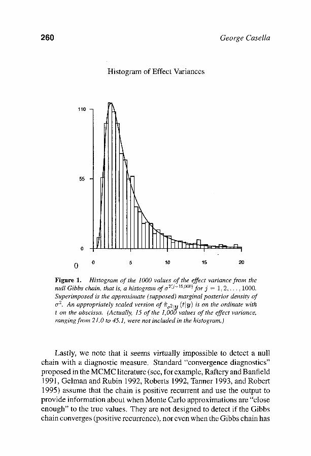
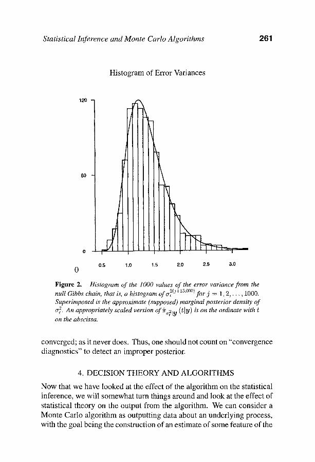
After the initial 55,000 iterations, the output from the 15,001st through the 16,000th was collected. Figure 1 is a histogram of the 1,000 effect variances from the null Gibbs chain, that is, 0-2(j+15,000), j = 1, 2 , . . . , 1000, with a Monte Carlo approximation of the supposed marginal posterior density superimposed. Figure 2 is the analog of Fig- ure 1 for the error variance component. The density approximations in Figures 1 and 2 were calculated using the usual "average of conditional densities" approximation. All of these plots appear perfectly reasonable even though the posterior distribution is improper and the Monte Carlo density approximations have almost sure pointwise limits of zero or no limit at all. Clearly, if one were unaware of the impropriety, plots like these could lead to seriously misleading conclusions.
This particular posterior is improper due to an infinite amount of mass near 0 -2 = 0. One might suspect that if the starting value of 0-2
were near zero, the o .2 component of the Gibbs chain would be absorbed at 0. This is not the case, however. In fact, the o .2 component and the random effects components move towards zero, but eventually they all return to a reasonable part of the space. For example, we started the chain with 0 .2 • 10 - 5 0 and after 20,000 iterations the 0-2 component was a p p r o x i m a t e l y 10 -122 and the largest magnitude of any of the random effects components was about 10 -60 . The chain was allowed to run for a total of one million iterations, after which all of the components were back in a reasonable part of the parameter space. This Gibbs chain behaves somewhat like one constructed with the exponential conditionals of Example 3 in that it leaves the "center" of the space for long periods of time, but eventually returns. Such behavior is consistent with null recurrence.
260 George Casella
Histogram of Effect Variances
110
55
I I I
0 0 5 10 15 20
Figure 1. Histogram of the 1000 values of the effect variance from the null Gibbs chain, that is, a histogram of or 2(j+15'~176176 for j = 1, 2 , . . . , 1000. Superimposed is the approximate (supposed) marginal posterior density of cr 2. An appropriately scaled version of #a21y (t]y) is on the ordinate with t on the abscissa. (Actually, 15 of the l,O00values of the effect variance, ranging from 21.0 to 45.1, were not included in the histogramJ
Lastly, we note that it seems virtually impossible to detect a null chain with a diagnostic measure. Standard "convergence diagnostics" proposed in the MCMC literature (see, for example, Raftery and Banfield 1991, Gelman and Rubin 1992, Roberts 1992, Tanner 1993, and Robert 1995) assume that the chain is positive recurrent and use the output to provide information about when Monte Carlo approximations are "close enough" to the true values. They are not designed to detect if the Gibbs chain converges (positive recurrence), nor even when the Gibbs chain has
Statistical Inference and Monte Carlo Algorithms 261
Histogram of Error Variances
60
I
120
I I
0 0.5 1.0 1.5 2.0 2.5 3.0
F i g u r e 2. Histogram of the 1000 values of the error variance from the 2(j+15,ooo) ~ . null Gibbs chain, that is, a histogram of a~ for 3 = 1, 2 , . . . , 1000.
Superimposed is the approximate (supposed) marginal posterior density of 2 An appropriately scaled version ofr ( t [ y ) is on the ordinate with 0"~.
on the abscissa.
converged; as it never does. Thus, one should not count on "convergence diagnostics" to detect an improper posterior.
4. DECISION THEORY AND ALGORITHMS
Now that we have looked at the effect of the algorithm on the statistical inference, we will somewhat turn things around and look at the effect of statistical theory on the output from the algorithm. We can consider a Monte Carlo algorithm as outputting data about an underlying process, with the goal being the construction of an estimate of some feature of the
262 George Casella
process. In this light, we can ask how to best process the data, and answer that question by applying statistical principles. In what follows, we apply one of the simplest principles, that of Rao-Blackwellization, to the output of an Accept-Reject Algorithm. For more details, including applications to the Metropolis-Hastings Algorithm, see Casella and Robert (1995, 1996a, 1996b, 1996c).
4.1. The Accept-Reject Algorithm as a Statistical Model
The Accept-Reject algorithm is based on the following lemma.
L e m m a 1. I f f and 9 are two densities, and there exists M < oc such that f ( x ) < M g ( x ) for every x, the random variable X pro- vided by the algorithm
1. Simulate Y ~ 9(Y);
2. Simulate U ~ /g[0, 1] and take X = Y i fU <_ f ( Y ) / M 9 ( Y ) ; otherwise, repeat step 1.
is distributed according to f .
When viewed statistically, we have the following description of the algorithm. A sequence Y1, Y2,.. �9 of independent random variables is generated from g along with a corresponding sequence U1, U2, . . . of uniform random variables. Given a function h, the Accept-Reject es- timator of 7- = E { h ( X ) } , based upon a sample X 1 , . . . , Xt generated according to Lemma 1, is given by
t 1
= T Z h(Xi). (9) i = l
Note that, conditional on the value t, the random variables X1, �9 �9 �9 Xt represent an iid sample from the distribution f . The Accept-Reject algorithm is usually implemented with a prespecified value of t, and the number of generated Y/'s is a random integer N satisfying
N N - 1
I(Ui <_ wi) = t and E I(Ui <_ wi) = t - 1, i=1 i=1
where we define wi = f (Y i ) /M9(Yi ) .
Statistical Inference and Monte Carlo Algorithms 2 6 3
When we evaluate (~AR as an estimator of ' r , we see an estimator that
1. Is based on extraneous information (the uniform random vari- ables).
2. Is, in fact, a randomized estimator, that scourge of statistics.
Classical statistical theory tells us that
1. We need an estimator that does not depend on the observed values of the uniform random variables.
2. I f an estimator is constructed by averaging over the uniform random variables, such an estimator will dominate 5AR by the Rao-Blackwell theorem.
It is straightforward to "Rao-Blackwel l ize" 5AR by noting that it can be written
N 1
5AR = -~ E I(Ui < wi)h(Y/) , (10) i=1
so the condit ional expectat ion
5RB = t "'" i=1
improves upon (10) by the Rao-Blackwel l Theorem.
Details of this calculation are carried out in Casella and Rober t (1996a), where it is established that
1 n = pih( ) (12)
i=1
where, for i = 1, �9 �9 �9 n - 1, Pi satisfies
Pi = P(Ui < wi lN = n, ~1 , . . . , Yn) n-2
E(il,...,it_2) E~ -2 Wij E j = t _ l ( 1 -- Wij) (13)
----- Wi ~_~(il,...,it_l ) yi~_l Wij YIjn=tl(1 -- Wij) '
while Pn = 1. The numerator sum is over all subsets of { 1 , . . . , i - 1, i + 1 , . . . , n - 1} of size t - 2, and the denominator sum is over all
subsets of size t - 1. The resulting est imator 5RB is an average over
264 George Casella
all the possible permutations of the realized sample, the permutations being weighted by their probabilities. The Rao-Blackwellized estimator is then a function only of (N, 1Q1),. . . , ]QN-1), YN), where ]Qi) denotes the order statistics.
Because of the identity
var(5) = var[E{6(U, Y)IY}] + E[var{5(U, Y)[Y}]. (14)
we see that the improvement that 5RB brings over 5AR is related to the size of E[var{5(U, Y)IY}]. This latter quantity can be interpreted as measuring the average variance in the estimator that is due to the auxiliary randomization, that is, the variance that is due to the uniform random variables. In some cases this quantity can be substantial.
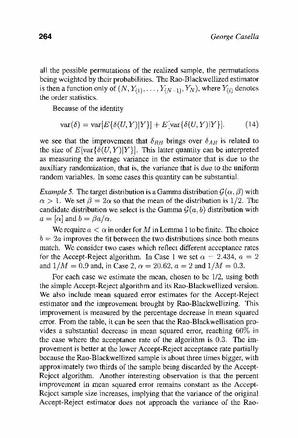
Example 5. The target distribution is a Gamma distribution ~(a , /3) with a > 1. We set/3 = 2c~ so that the mean of the distribution is 1/2. The candidate distribution we select is the Gamma G (a, b) distribution with a = [a] and b =/3a/c~.
We require a < a in order for M in Lemma 1 to be finite. The choice b = 2a improves the fit between the two distributions since both means match. We consider two cases which reflect different acceptance rates for the Accept-Reject algorithm. In Case 1 we set a = 2.434, a = 2 and 1/M = 0.9 and, in Case 2, a = 20.62, a = 2 and 1/M = 0.3.
For each case we estimate the mean, chosen to be 1/2, using both the simple Accept-Reject algorithm and its Rao-Blackwellized version. We also include mean squared error estimates for the Accept-Reject estimator and the improvement brought by Rao-Blackwellizing. This improvement is measured by the percentage decrease in mean squared error. From the table, it can be seen that the Rao-Blackwellisation pro- vides a substantial decrease in mean squared error, reaching 60% in the case where the acceptance rate of the algorithm is 0.3. The im- provement is better at the lower Accept-Reject acceptance rate partially because the Rao-Blackwellized sample is about three times bigger, with approximately two thirds of the sample being discarded by the Accept- Reject algorithm. Another interesting observation is that the percent improvement in mean squared error remains constant as the Accept- Reject sample size increases, implying that the variance of the original Accept-Reject estimator does not approach the variance of the Rao-
Statistical Inference and Monte Carlo Algorithms 965
Table 1. Estimation of a gamma mean, chosen to be 1/2, using the Accept- Reject Algorithm, based on 7,500 simulations.
Acceptance rate .9
AR AR RB AR Percent Sample Estimate Estimate MSE Decrease
Size 5An 5RB in MSE
t0 .5002 .5007 .0100 17.02 25 .5001 .4999 .0041 18.64 50 .4996 .4997 .0020 20.81 100 .4996 .4997 .0010 21.45
Acceptance rate .3
AR AR RB AR Percent Sample Estimate Estimate MSE Decrease
Size 5A~ 5RB in MSE
10 .5005 .5004 .0012 52.85 25 .4997 .5000 .0005 58.62 50 .4998 .5001 . 0002 60.49 100 .4995 .5001 .0001 61.60
Blackwellized estimator even as the sample size increases, We will return to this point in Section 5.2.
Computation of the Pi'S of (13) can be accomplished with a recursion relation, and will typically require a calculation of order n 2. This may represent, to some, an unacceptable increase in computation time given the size of the anticipated decrease in mean squared error. To some- what address this point, in Casella and Robert(1996b) we considered a simpler version of the Rao-Blackwell strategy that led to (12). Notice that, in what follows, we will simultaneously decrease computational complexity and increase statistical complexity.
266 George Casella
4.2. Termwise Rao-Blackwellization
Starting from the Accept-Reject estimator (10), rather than calculating the full conditional expectation, we can instead calculate the termwise conditional expectation. This accomplishes the goal of removing the uniform random variables but retains computational simplicity.
To calculate the termwise conditional expectation of (10), condi- tioning the ith term on (N, I~), we need the conditional distribution of Ui l, Y/, N = n. Although the original random variables are independent, the Accept-Reject algorithm stopping rule introduces a dependence in the sample. For example, for i = 1 , . . . , n - i the marginal distribution of Y/is
- 1 i n - t g ( y ) - - - ~ f ( y ) t f ( y ) + 1 re(y) -- n - n - 1 1 M
(15)
and Yn has marginal distribution f (y ) . It then can be shown that the resulting estimator, 5TRB is given by
1 n (~TRB -~ -s E E[Z(gi < wi)lY/]h(Yd
i=1 n-1 (16)
1 ( h ( y n ) + E b ( y i ) h ( Y i ) ) , t i=1
where
t - 1 f(y ) , i = l , . - - , n - 1 . (17)
n - i m(yi)
See the Appendix for details of these calculations.
We now have a seemingly reasonable estimator that is not compli- cated to compute, but its statistical properties are not as easy to establish as the full Rao-Blackwellized estimator (12). In fact, the Rao-Blackwell theorem does not apply to the estimator (16) because we did not con- dition on the entire estimator. To establish dominance of (~TRB of (16)
over (~AR of (9), we must calculate the variance of 5TRB, which involves n(n - 1)/2 covariance terms. Moreover, it can easily be seen that 5TnB cannot dominate 5AR in mean squared error. This is because the sum of the weights in (17) is random, and if the target function h(.) is a
Statistical Inference and Monte Carlo Algorithms 267
nonzero constant function, ~TRB will not estimate it correctly, while 5AR will. This major difficulty is also common to some importance sampling schemes and prohibits uniform domination results there. A solution to this drawback is to force the estimators to estimate constant functions correctly, which can be achieved by dividing the weights b(yi) by their sum, thus replacing (STt~B by its rescaled version
1 t - l ( ~ b(yi) h(y i ) ) . (18) = (h(yn) + ---i-- Ejn:- b(V )
Such rescalings seem common in practice, despite any concern about the effect of introducing a bias in the estimator. Such concerns need not cause worry, however, as the bias induced by this rescaling is of an higher order than the variance (Casella and Robert 1996b). The following theorem can then be established.
Theorem 3. For every function h, ~STr asymptotically dominates 5AR in terms of quadratic risk. More precisely, as t ~ ~ , if N = Op(t) then,
- _< E[( AR - -
where ~- = E[h(X)].
Moreover, the size of the improvement brought about by the rescaled estimator is truly impressive.
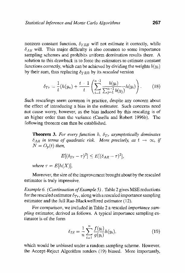
Example 6. (Continuation of Example 5). Table 2 gives MSE reductions for the rescaled estimator ~T~, along with a rescaled importance sampling estimator and the full Rao-Blackwellized estimator (12).
For comparison, we included in Table 2 a rescaled importance sam- pling estimator, derived as follows. A typical importance sampling es- timator is of the form
1 ~ f(Yi) 5IS ~- n i =1 g(Yi) h(yi), (19)
which would be unbiased under a random sampling scheme. However, the Accept-Reject Algorithm renders (19) biased. More importantly,
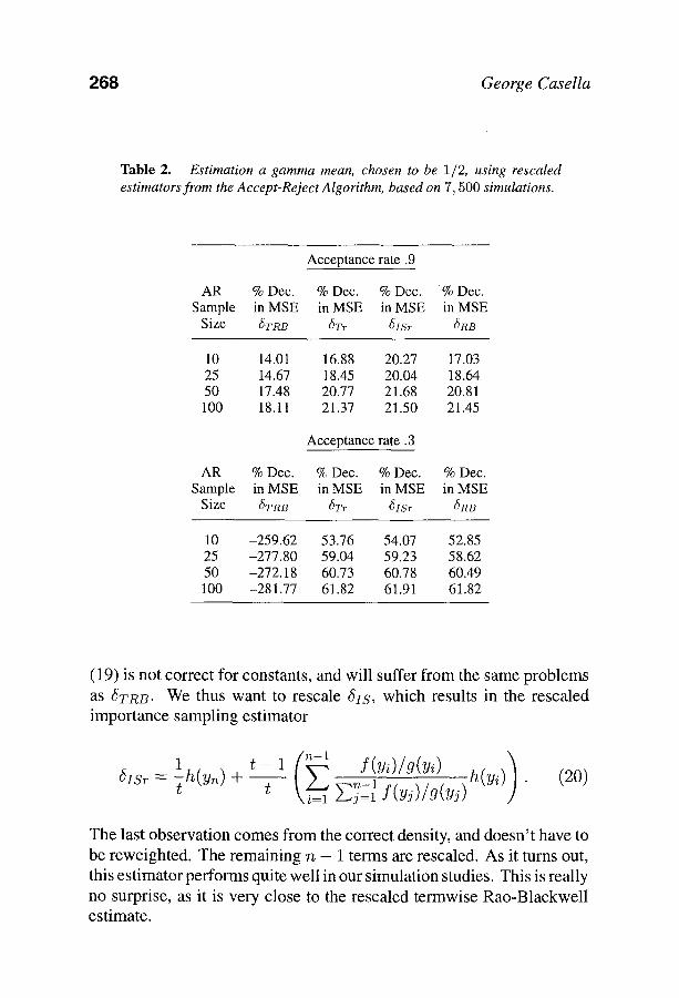
268 George Casel la
Table 2. Estimation a gamma mean, chosen to be 1/2, using rescaled estimators from the Accept-Reject Algorithm, based on 7, 500 simulations.
Acceptance rate .9
AR % Dec. % Dec. % Dec. % Dec. Sample inMSE inMSE inMSE inMSE
Size 6rnB 6T,. 6ISr 6RB
10 14.01 16.88 20.27 17.03 25 14.67 18.45 20.04 18.64 50 17.48 20.77 21.68 20.81 100 18.11 21.37 2 1 . 5 0 21.45
Acceptance rate .3
AR % Dec. % Dec. % Dec. % Dec. Sample inMSE inMSE inMSE inMSE
Size 6TR B 6Tr 61,5, r 6RB
10 -259.62 5 3 . 7 6 54.07 52.85 25 -277.80 5 9 . 0 4 59.23 58.62 50 -272.18 60.73 60.78 60.49 100 -281.77 61.82 61.91 61.82
(19) is not correct for constants, and will suffer f rom the same problems
as 6TRB. We thus want to rescale 6 i s , which results in the rescaled importance sampling estimator
1 t-l( h(vd). ISr = -[h(yn) + \ i = 1 Ejn -ll f ( Y J ) / g ( Y J )
(20)
The last observation comes f rom the correct density, and doesn ' t have to
be reweighted. The remaining n - I terms are rescaled. As it turns out, this estimator performs quite well in our simulation studies. This is really
no surprise, as it is very close to the rescaled termwise Rao-Blackwell estimate.
Statistical Inference and Monte Carlo Algorithms 269
There are a number of interesting points to notice about Table 2. First, termwise conditional expectation can actually make things worse, as @RB increases the MSE o v e r •AR. Although we knew that @_~B could not dominate for constant functions, the numerical example shows that even for more variable functions there may not be dominance.
The second striking thing to notice is that the improvement from the rescaled estimators @T and ~IsT is actually better than that of the Rao-Blackwellized estimator ~RB- This, no doubt, represents a favor- able variance/bias trade-off, but is still quite startling. The decrease in computation time of @r and ~SiSr over ~SRB can be quite substantial, and the fact that mean squared error is improved really underscores the power of rescaling.
It is interesting to note that the rescaling idea, making the weights sum to one, arose naturally as "the right thing to do", especially in light of the performance of the estimators when h(-) is constant. Many times we notice, or intuit, empirical adjustments that help in certain cases. We can use the structure of decision theory to formalize our intuition, and see if the empirical improvements will, in fact, be useful in a wide variety of cases. Here we see that the value of the rescaling is confirmed by the decision-theoretic calculation of Theorem 3 and a simulation study. We thus have a nice interplay between using our intuition to construct what we think is an improved estimator, and using theory to establish that we have, in fact, done so.
5. OTHER CONSIDERATIONS
In this section we review some recent work that further explores the structure of Monte Carlo algorithms, particularly the Gibbs sampler. The goals of these investigations are to understand how to better, or even optimally, process the output of the algorithm, and also to use the structure of the algorithm to help construct optimal procedures. It is interesting to note that both frequentist and Bayesian inferences benefit in the following examples. Unfortunately, these illustrations are somewhat less detailed, as some of the work is still in progress
27'0 George Casella
5.1. Constructing the Inference from the Algorithm
An endpoint of a Gibbs sampler is typically a sample from a poste- rior distribution 7r(Oly ), a distribution which may itself be intractable to work with. If a confidence set, or more specifically, a credible set, for 0 is desired, we may have to solve a difficult integral equation where the integrand may not be expressible in closed form. Specif- ically, suppose that we have a pair of conditional posterior densities zc(O[y, A) and zr(Aly, 0) in a Gibbs sampler Markov chain, and we are interested in inferences about zc(Oly). If we use the Gibbs sampler to generate the pairs (Oi, Ai), i = 1 ,2 , . - . , then, from the ergodic theo- rem, 7r(0]y) = l i m m ~ ( 1 / m ) ~2"~ i=1 7c(O]y, Ai). Suppose that, for a specified value of o~, we are interested in finding the value a* such that
f ~ * 7r(O]y)dO = o~, a lower confidence bound, a first approach would be to solve for a* in
2 - - 7c(Oly, Ai)dO = c~. m ec i = 1
As this calculation could be quite involved, we ask if the value a* can be constructed from the Gibbs sequence (Oi, Ai) in any simple way?
A first approach on the problem, developed in Eberly (1997), is the following. Writing II(-) for a distribution function, for example, I I (a ty ) = f~Tr(Oty)dO, calculate for each Ai a value ai such that II(ai lY, Ai) = "7, where the value of'7 will be determined shortly. (Note that in a typical Gibbs sampler, the full conditionals are usually very nice
1 m densities, so solving for the ais should be very quick.) Now ~ ~ i = 1 ai = ~ a ~, for some value a/, but it is not necessarily the case that a I = a*.
However, expanding II(ai lY, Ai) in a Taylor series around ~ yields
II(ai[y, Ai) ~ Yi(~ly, Ai ) + ( a i - ~)~-(fi[y, Ai).
Now sum both sides, and remember that II(aily, Ai) = '7 to get 1 m 1 m
"7 "~ - - E I-I(alY' Ai) + - - ~ (ai - ~)7c(g]y, Ai). m m
i = 1 i = 1
1 It can be established that ~ Em=l II(d[y, Ai) ~ II(a '[y), so we have the approximation
m
I Z ( a i _ ~ ) T r ( ~ l y , Ai) ' i----1
Statistical Inference and Monte Carlo Algorithms 971
1 m a which suggests setting 3' = c~ + ~ E i = l ( i - a )71(a lY, ,~i), with the hope that g ~ a I ~ a*.
This linear approximation seems to perform adequately in some situations, but can be improved upon by a quadratic Taylor series ap- proximation. Further work, in understanding the value and limitations of this approximation, and thoroughly developing the theory, is presently being done.
5.2. The Effect of Rao-Blackwellization
In Section 4.1 we alluded to the fact that Rao-Blackwellization will al- ways result in an appreciable variance reduction, even as the sample size (or the number of Monte Carlo iterations) increases. To address this point more precisely, consider the work of Levine (1996), who formu- lated this problem in terms of the asymptotic relative efficiency (ARE) of 50 = ( l / m ) ~ h(Xi) with respect to its Rao-Blackwellized version 51 = (1/m) ~ E[h(Xi) IY/], where the pairs (Xi, Yi) are generated from a Gibbs sampler with Xi ,~ f(xlY/_l ) and Y/,-~ f(ulXi). (Levine 1996 considers more complex Gibbs samplers, but we will only use this sim- ple case for illustration. The key property that the sampler need have is reversibility.) The ARE is a ratio of the variances of the limiting distribution for the two estimators, which are given by
(X3
o-~o = var(h(X)) + 2 ~ cov(Xo, Xk) (21) k= l
and
(3O
0-~1 = var(E[h(X)lY]) + 2 ~ cov(E[Xo[Yo],E[XklYk]). (22) k= l
Levine then proves the following theorem.
Theorem 4. If a sample { (Xi, Yi) }in0 is generated by the bivari- ate Gibbs sampler, then for all h(.) with finite variance, the ratio
2 2 o-60/o-61 _> 1, with equality if and only if var(h(X)) = var(E[h(X)lY]) = O.
272 George Casella
To see the amount of possible improvement, consider the following example.
Example 7. Let
where - 1 < p < 1. Assume interest lies in estimating # = E(X) . The Gibbs sampler can obtain samples from the bivariate normal distribution by alternately drawing random variables from
X I Y ~ N(pY, 1 - p2)
Y I X ,.~ N(pX, 1 - p2).
It can be shown that coy(X1, Xk) = p2k, for all k, and
1 0.2~ 2 60/0"61 = -~ > 1.
So, if 61 is less than 1/,o 2 times more complex than 60, then 61 should be used. Since E ( X I Y) = PY, it takes n + 2 floating point operations (flops) to compute 61 = ( I / n ) ~ . = 0 E ( X I Yk) as compared to n + I
X flops to compute 60 = ( I / n ) ~ = 0 k. Therefore, the cost of compu- tation, in terms of flops, is essentially the same, but there can be a vast gain in precision by using 61. ,~
5.3. Minimax Gibbs Samplers
An interesting example of the interplay between decision theory and Monte Carlo algorithms is given by the problem of optimizing the ran- dom scan Gibbs sampler (see, for example, Rosenthal 1995, Amit 1996, Roberts and Sahu 1996). The random scan Gibbs sampler is character- ized by selection probabilities c~1, �9 OLd. These probabilities determine the percentage of visits to a specific site or component of the d • I vector of interest X = ( X 1 , . . . , Xa) during a mn of the sampler. A standard approach is to choose the selection probabilities to provide the sampling strategy with the smallest convergence rate. However, choosing the se- lection probabilities according to such a criterion may be undesirable in
Statistical Inference and Monte Carlo Algorithms 273
practice. For example, the convergence rate is not only typically diffi- cult to compute and possibly mathematically intractable, but also may also ignore important features of the target distribution necessary for determining the optimal random scan, as we will see below.
Levine (1996) considers an alternative measure derived from statis- tical decision theoretic considerations, which seems to provide an attrac- tive criterion for choosing an appropriate random scan. Assume a ran- dom d • 1 vector X is generated by a random scan Gibbs sampler which
generates a Markov chain { X ( i ) } ~ I with stationary distribution 7r. Sup- pose interest lies in estimating # = E~(h(X)) where v a r ( h ( X ) ) < oc.
1 n If we estimate # with the sample mean/2 = g Y]'~i=l h(X( i ) ) , the optimal mean squared error scan is the one that minimizes the risk
(23)
Alternatively, we may consider the asymptotic risk
R(o~,h) = l im nR(n)(o~,h) n--.-+ o o
n - 1
i = 1 O 0
= w r (h (X) ) + cov (h(X(~ i = 1
(24) as a basis for choosing a random scan.
We note that the convergence rate of the random scan, the norm of the forward operator, can be expressed as
h
where the supremum is over all functions with finite variance. Thus we see that, when compared to (24), the convergence rate contains less information about the variance and covariances of the chain. It is in this sense that we feel that (24) is a better optimality measure.
274 George Casella
To use (24) as a criterion for selecting a scan, we would like it to produce a reasonable scan for any function h. This suggests that we might want to protect against the worst possible function h, with finite variance, by minimizing the maximum risk suPhR(O~, h). Levine (1996) develops a method for doing this, implementing an adaptive scan of the state space. That is, at each iteration the selection probabilities are updated via a sequence of sample points from the previous iteration, and may even use information from past iterations (which could destroy the Markov nature of the chain). However, the chain does converge, approaching the optimal random scan according to (24). Levine also discusses examples where this procedure can be implemented, however full implementation in a general setting is presently too computationally intensive to be useful. Approximations are being investigated for these cases.
6. DISCUSSION
Even though we have covered a lot of ground in understanding the in- terplay between statistical theory and computational algorithms, there is an enormous amount of work that we have not mentioned. We only alluded to the fundamental papers of Liu, Wong and Kong (1994, 1995), which provide an elegant and comprehensive treatment of the structure of the Gibbs sampler. Other work, such as Tanner and Wong (1987), Liu (1994), Tierney (1994) or Robert (1995), illustrates how statistical theory interfaces with Monte Carlo algorithms, most notably the Gibbs sampler and the Metropolis algorithm.
The other body of work we have not discussed is that which deals with missing data problems, using techniques such as the EM algorithm. Although EM and Gibbs share a similar underpinning, (see Casella and Berger 1995 for a view of the EM algorithm as a Gibbs sampler) they tend to be used in somewhat different ways. However, research in these methods, which also combines statistical theory with the computational algorithms, continues to flourish; see for example Smith and Roberts (1993), Meng and Rubin (1993), Liu and Rubin (1994), Meng (1994), Besag et al. (1995) and Meng and van Dyk (1996).
The message of this paper, which by now may be obscured in these sometime incoherent ramblings, is one that bears repeating. What we
Stat is t ical In ference a n d M o n t e Carlo A l g o r i t h m s 2 7 5
have done is to approach a new methodology, that of iterative Monte Carlo calculation, with the standard tools of the theoretical statistician. What resulted are procedures whose output and performance have been optimized from a statistical view. It sometimes may happen, as with the Rao-Blackwellized estimator of (12), or Section 5.3, that a statistically optimal answer may result in a difficult, or even prohibitive computa- tional burden. In such cases, statistical theory, in particular decision theory, can still provide answers. It then becomes a matter of specify- ing an alternate optimality criterion, or loss function, to take these other matters into account.
7. APPENDIX: THE TERMWISE WEIGHTS
To calculate the weights for the termwise Rao-Blackwellized estimator (16), it is necessary to derive the distribution of the uniform random variable conditional on the generated value of the candidate random variable. This is a rather straightforward exercise in distribution theory, and is only made complicated by the stopping rule of the Accept-Reject Algorithm.
From the Accept-Reject Algorithm of Lemma 1, we get a sequence Y1, ]I2,. . . of independent random variables generated from g along with a corresponding sequence U1, U2,.. �9 of uniform random variables. For a fixed sample size t, i.e. for a fixed number of accepted random vari- ables, the number of generated Y~'s is a random integer N. The joint distribution of ( N , Y1, . . . , Y N , U1, . . . , UN ) is given by
P ( N = n, Y1 <_ Y l , . . . , Y n <_ yn, U1 <_ U l , . . . ,Un ~ Un)
-~ g(tn)(Un A wn)dtn .. . g ( t m ) . . , g ( t n - 1 )
t-I n-I X E I I ( w i j AUij ) I I ( u i j - - W i j )+d t l ' ' ' d t n - l ,
(il ..... it_l) j = l j=t (2s)
where wi = f ( Y i ) / M g ( y i ) and the sum is over all subsets of { 1 , . . . , n - 1 } of size t - 1.
276 George Casella
We next want to get the joint distribution of (Y/, Ui)IN = n, for any i = 1 , . . - , n - 1. Since this distribution is the same for each of these values o f / , we can just derive it for ( ~ , U 0 . Recall that Yn ~ f .
If we set Yl = Y, ul = u, Y2 = Y 3 . . . . - - Y n = c<) and u2 =
u3 = " . = Un = 1, we can derive the joint distribution of (N, 1~, U1). Assume, without loss of generality, that limy__,~ f ( y ) / g ( y ) = 1. (If this is not the case, we just have to adjust the constant M in what follows).
a and Then, aside from the pair (Wl, ul) , we have (wij A uij) =
-- " ) + = ( 1 - ~ / ) , h e n c e (Uij Wzj t-1 n-1 1-I(w,j ^ u,j) 1-I (~,,~ - . , , j )+ =
(il,'..,it-i) j=l j=t -- (Wl /kUl) (?_~2) (~)t-2 (1-- ~ ) n-t
q-(Ul--Wl)+ (nnT21) (~)t-1 ( l - - ~ ) n-t-1.
Noting that (,:_~) = _ t _ , ( , , _ ~ ) , ( , , _ _~ ) _ _ , ,_ ,_ (o_,) n i t - n t 1 n - 1 t - 1 '
and v n oo f~_oog(tn)(un A wn)dtn = f~_oog(tn) ( ~ ) dtn = 1 , we have
P ( N = n, Yx <_ U, U1 <_ u) =
= (?-11) (~---)t-1 (1-~ --) • [n~l~(WlAUl) ( 1 - ~ - - - ) "~-
x fYoog(tl)dtl �9
n-t-1
n , (1)] n - 1 (ul - Wl) +
(26)
(27)
From (27) we can immediately get the negative binomial marginal distribution of N,
n-t - 1 P ( N = n ) = ( ? 1 ) ( 1 ) t ( X - 1 ) ,
Statistical Inference and Monte Carlo Algorithms 977
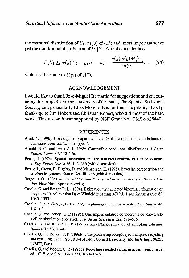
the marginal distribution of ]I1, re(y) of (15) and, most importantly, we get the conditional distribution of U11Y1, N and can calculate
P(U1 < w(y)lrl = y , N = n) = g(y)w(y)M~=--11 , ( 2 s )
which is the same as b(yi) of (17).
ACKNOWLEDGEMENT
I would like to thank Jost-Miguel Bernardo for suggestions and encour- aging this project, and the University of Granada, The Spanish Statistical Society, and particularly Elias Moreno Bas for their hospitality. Lastly, thanks go to Jim Hobert and Christian Robert, who did most of the hard work. This research was supported by NSF Grant No. DMS-9625440.
REFERENCES Amit, Y. (1996). Convergence properties of the Gibbs sampler for perturbations of
gaussians. Ann. Statist. (to appear). Arnold, B. C., and Press, S. J. (1989). Compatible conditional distributions. J. Amer.
Statist. Assoc. 84, 152-156. Besag, J. (1974). Spatial interaction and the statistical analysis of Lattice systems.
J. Roy. Statist. Soc. B 36, 192-236 (with discussion). Besag, J., Green, P., Higdon, D. and Mengersen, K. (1995). Bayesian computation and
stochastic systems. Statist. Sci. 10 1-66 (with discussion). Berger, J. O. (1985). Statistical Decision Theory and Bayesian Analysis, Second Edi-
tion. New York: Springer-Verlag. Casella, G. and Berger, R. L. (1994). Estimation with selected binomial information or,
do you really believe that Dave Winfield is batting .471 ? J. Amer. Statist. Assoc. 89, 1080-1090.
Casella, G. and George, E. I. (1992). Explaining the Gibbs sampler. Ann. Statist. 46, 167-174.
Casella, G. and Robert, C. P. (1995). Une impltmentation de thtor~me de Rao-black- well en simulation avec rejet. C. R. Acad. Sci. Paris 322, 571-576.
Casella, G. and Robert, C. P. (1996a). Rao-BlackweIlization of sampling schemes. Biometrika 83, 81-94.
Casella, G. and Robert, C. P.(1996b). Post-processing accept-reject samples: recycling and rescaling. Tech. Rep., BU-1311-M., Cornell University, and Tech. Rep., 9625, INSEE, Paris.
Casella, G. and Robert, C. P. (1996c). Recycling rejected values in accept-reject meth- ods. C. R. Acad. Sci. Paris 321, 1621-1626.
27'8 George Case l la
Dey, D. K., Gelfand, A. E. and Peng, E (1994. Overdispersed generalized linear models. Tech. Rep., University of Connecticut.
Eberly, L. E. (1997). Constructing Confidence Statements from the Gibbs Sampler. Ph.D. Thesis, Cornell University.
Gelfand, A. E., Hills, S. E., Racine-Poon, A. and Smith, A. F. M. (1990). Illustration of Bayesian inference in normal data models using Gibbs sampling. J. Amer. Statist. Assoc. 85, 972-985.
Gelfand, A. E. and Smith, A. E M. (1990). Sampling-based approaches to calculating marginal densities. J. Amer. Statist. Assoc. 85, 398-409.
Gelman, A. and Speed, T. P. (1993). Characterizing a joint probability distribution by conditionals. J. Roy. Statist. Soc. B 55, 185-188.
Geman, S. and Geman, D. (1984). Stochastic relaxation, Gibbs distributions, and the Bayesian restoration of images. IEEE Trans. Patt. Anal Mach. Intelligence 6, 721- 741.
Geyer, C. (1992). Practical Markov chain Monte Carlo. Statist. Sci. 7, 473-483. Hastings, W. K. (1970). Monte Carlo sampling using Markov chains and their appli-
cation. Biometrika 57, 77-109. Hill, B. M. (1965). Inference about Variance Components in the One-Way Model.
J. Amer. Statist. Assoc. 60, 806-825. Hobert, J. P. and Casella, G. (1995). Functional compatibility, Markov chains, and Gibbs
sampling with improper posteriors. Tech. Rep. BU-1280-M, Cornell University. Hobert, J. P. and Casella, G. (1996). The effect of improper priors on Gibbs sampling
in hierarchical linear mixed models. J. Amer. Statist. Assoc. (to appear). Ibrahim, J. G. and Laud, P. W. (1991). On Bayesian analysis of generalized linear
models using Jeffreys's prior. J. Amer. Statist. Assoc. 86, 981-986. Lehmann, E. L. and Casella, G. Theory of Point Estimation, Second Edition. New York:
Springer-Verlag. Levine, R. A. (1996). Optimizing convergence rates and variances in Gibbs sampling
schemes. Ph.D. Thesis, Cornell University. Liu, J. (1994). The collapsed Gibbs sampler in Bayesian computation with application
to a gene regulation problem. J. Amer. Statist. Assoc. 89, 958-966. Liu, C. and Rubin, D. B. (1994). The ECME algorithm: a simple extension of EM and
ECM with fast monotone convergence. Biometrika 81,633-648. Liu, J., Wong, W. H. and Kong, A. (1994). Covariance structure of the Gibbs sampler
with applications to the comparisons of estimators and augmentation schemes. Biometrika 81, 27-40.
Liu, J., Wong, W. H. and Kong, A. (1995). Correlation structure and convergence rate of the Gibbs sampler with various scans. J. Roy. Statist. Soc. B 57, 157-169.
Meng, X.-L. (1994). On the rate of convergence of the ECM algorithm. Ann. Statist. 22, 326-339.
Meng, X.-L. and Rubin, D. B. (1993). Maximum likelihood estimation via the ECM algorithm: a general framework. Biometrika 80, 267-278.
Statistical Inference and Monte Carlo Algor i thms 279
Meng, X-L. and van Dyk, D. (1996). (1993). THe EM algorithm - an old folk song sung to a fast new tune. J. Roy. Statist. Soc. B (to appear).
Metropolis, M. Rosenbluth, A., Rosenbluth, M., Teller, A. and Teller; E. (1953). Equa- tion of state calculations by fast computing machines. J. Chemical Phys. 21, 1087- 1092.
Natarajan, R. and McCulloch, C. E. (1995). A Note on the existence of the posterior distribution for a class of mixed models for binomial responses. Biometrika 82, 639--643.
Raftery, A. E. and Banfield, J. D. (1991). Stopping the Gibbs sampler, the use of morphology, and other issues in spatial statistics. Ann.lnst. Stat. Math. 43, 32--43.
Robert, C. (1995). Convergence control methods for Markov chain Monte Carlo algo- rithms. Statist. Sci. 10, 231-253.
Roberts, G. O. (1992). Convergence diagnostics of the Gibbs sampler. Bayesian Statis- tics 4 (J. M. Bernardo, J. O. Berger, A. P. Dawid and A. E M. Smith, eds.). Oxford: University Press, 775-782.
Roberts, G. O. and Sahu, S. K. (1996). Updating schemes, correlation structure, block- ing and parameterisation for the Gibbs sampler. Tech. Rep., University of Cam- bridge.
Rosenthal, J. S. (1995). Rates of convergence for Gibbs sampling for variance compo- nent models. Ann. Statist. 23, 740-761.
Searle, S. R., Casella, G. and McCulloch, C. E. (1992). Variance Components. New York: Wiley.
Smith, A. F. M. and Roberts, G. O. (1993). Bayesian computation via the Gibbs sampler and related Markov chain Monte Carlo methods. J. Roy. Statist. Soc. B 55, 3-23.
Tanner, M. A. (1993). Tools for Statistical Inference. New York: Springer-Verlag. Tanner, M. A. and Wong, W. (1987). The calculation of posterior distributions by data
augmentation. J. Amer. Statist. Assoc. 82, 805-811 (with discussion). Tierney, L. (1994). Markov chains for exploring posterior distributions. Ann. Statist. 22,
1701-1762. Wang, C. S., Rutledge, J. J. and Gianola, D. (1993). Marginal inferences about variance
components in a mixed linear model using Gibbs sampling. Genetique, Selection, Evolution 25, 41-62.
Wang, C. S., Rutledge, J. J. and Gianola, D. (1994). Bayesian analysis of mixed lin- ear models via Gibbs sampling with an application to litter size of iberian pigs. Genetique, Selection, Evolution 26, 1-25.
Zeger, S. L. and Karim, M. R. (1991). Generalized linear models with random effects: a Gibbs sampling approach. J. Amer. Statist. Assoc. 86, 79-86.
280 George Casella
DISCUSSION
JUAN FERRANDIZ (Universitat de ValOncia, Spain) First of all I would like to thank Professor Casella for this stimulating
paper. I have enjoyed reading these many good ideas exposed in so clear a style. I found his main message very important telling us that not only statistical practice can benefit from Markov Chain Monte Carlo (MCMC) methods but that these MCMC methods can still take advantage of well- known statistical ideas.
His second message, related to the Bayesian-frequentist controversy, has been particularly pleasing to me. I strongly agree with Professor Casella that
"... there are situations and problems in which one or the other approach is better-suited, or even a combination may be best, so a statistician without a command of both approaches may be less than complete."
In fact, as I was reading the paper, I was thinking how his sugges- tions could apply to a frequentist context: likelihood methods for spatial models arising from random variables associated to geographical sites (see e.g. Ferrfindiz et al., 1995).
Gibbs distributions are a natural choice in this context. Among them, the proposed automodels in Besag (1974) are particularly ap- pealing because the full conditionals determining joint distributions are well-known members of the exponential family.
The corresponding density of these models can be expressed as
p(x 10) = exp(t'O)h(x) c(O) (1)
through a suitable sufficient satistic t, where the normalizing constant c(0) is difficult to compute by standard numerical methods. This fact causes major problems on any inferential procedure based on the likeli- hood function (including Bayesian posteriors from any prior).
Geyer and Thompson (1992) propose estimating the ratio of con- stants
d(O) - c(0) _ E [ e x p ( t , ( 0 _ 0 0 ) ) 1 0 0 ] c(Oo)
by means of
d(O-") = 1 ~ exp(t~(O - 0o)) (2) n
Statistical Inference and Monte Carlo Algorithms 281
from a Markov chain simulation {xi : i = 1 , . . . , n} o fp (x [ 00). We can then estimate the likelihood function p(x [ O) in (1) up to a constant c(Oo).
Compatibility of Full Conditionals. Spatial automodels were proposed by Besag (1974) in his pioneering work after he considered the com- patibility of full conditionals in order to establish well-defined spatial models. For a finite number of sites and under the positivity condition (the support of the joint distribution equals the product of supports of the full conditionals) we have only to check summability of the joint density. This is not always easy to verify theoretically and it would be very interesting to develop statistical techniques to detect lack of summability directly from the output of the simulation algorithm. A first approach could be to run the algorithm several times from random starting points and check the homogeneity of the produced outputs in the long run. Example 4 in Section 3.2 probably would fail to show any anomalous behavior. I think this is an interesting problem that deserves further research.
Another interesting area of research could be how to relax the pos- itivity condition, which seems quite restrictive in some circumstances like, for instance, when we consider temporal concatenation of spatial distributions in order to build space-time models. It would also be the case, in the Bayesian context, when particular combinations of values of the random variables in the model are impossible.
Rao-BlackweUization. The main difficulty in the likelihood estimation approach for spatial models based on (2) above is the strong variability
of d(O) as [ 0 - 00 I becomes moderately large, producing a useless estimate of the likelihood function outside a small neighborhood of 00. The exponential form of the terms in the rhs of (2) make the extreme outliers of the simulated sequence {ti : i = 1 , . . . , n} dominate the sum.
This is a case where it would be worth considering the statistical processing of the output of the simulation algorithm in order to improve our likelihood estimates.
Gibbs sampling is easily implemented in this context because full conditionals p(xi [ x-i , O) are well-known distributions, and no accep- tance-rejection mechanism is present. I can not see how the Rao- Blackwellization proposed by Professor Casella in w could be applied.
282 George Casella
Perhaps, in this case, a robust estimator of the mean could be a good alternative.
Rao-Blackwellization, as proposed in Section 4, seems limited to acceptance-rejection algorithms, where ancillary uniform random vari- ables are used. Gibbs sampling can be stated as a particular case of Metropolis-Hastings algorithm, but with probability one of accepting every move, so that it is not possible to benefit from conditioning on the accepted values in the corresponding accept-reject process. Neither does it seem feasible to apply the ideas proposed in Section 5.2 of Rao- Blackwellising a data augmentation sampling scheme, For this to be done we need a convenient decomposition (t, s) of the observed vector :e in order to alternate sampling from p(t I s , 00) and p(s [ t, 00). This is not an obvious task.
Nevertheless, I think that the research' lines proposed by Profes- sor Casella are very promising. MCMC methods allow the growing complexity of the statistical models considered, and more complex Metropolis-Hastings algorithms are being used. Gibbs sampling has a poor mixing performance in high dimensional problems (as is usually the case of geographical: data) and more sophisticated algorithms are be- ing proposed (see e.g. Geyer and Thompson, 1995): The development of statistical treatments of their output has to be welcome as a means to strengthen their utility.
Inference from the Algorithm. On the other hand, the suggestions ex- posed in Section 5.1 seem worth exploring in the problem at hand. In fact, when we are trying to maximize a log-likelihood function estimate based on (2),
A
g(O l ~c ) = t ' O - log(d(0)) + constant (3)
the ratio of constants estimate d(O~) is mostly determined by the extreme outliers of the simulated sequence {ti : i -- 1 , . . . , n}. Maximization of (3) to get 0, our estimate of the true maximum likelihood estimator 0, will be based only on a few outermost observations ti.
Maybe it could be better to partition the whole sequence into small subsamples {{ti : i = ra + ] , . . . , ( r + l ) a } : r = O , . . . , n / a - 1}, from which we could get a sequence of log-likelihood estimates
{g(O I x)r : r = 0 , . . . , n / a - 1}. Their maximization will produce a
Statistical Inference and Monte Carlo Algorithms 983
sample: {Or : r = 0, . . . ,n/a - 1} of estimates of the true maximum likelihood estimator/). The characteristics of this sample could help in monitoring the maximization process: This is a challenging point whose potential benefits deserve further research.
B a y e s i a n readers can translate the problem above to their favorite framework by just adding the required prior 7r(O) to the likelihood (1) and trying to find the mode of the posterior.
Decision Theory and Algorithms. This is the idea in the paper that I liked the most: to embed MCMC algorithms in appropriate decision problems:. There are many decision s to make when running an MCMC procedure (sampling scheme, choice of estimator, stopping rule, etc.). Professor Casella has illustrated the benefit of this approach in some interesting cases. The relevant aspects in practice will come up once we establish the problem in a complete decision framework that takes into account the consequences of our choices. Although it seems in its first steps, I believe in a quick enriching development of this subject whose usefulness is foreseeable.
DANIEL PEiqA (Universidad Carlos III de Madrid, Spain)
When I first read this paper I was very disappointed. I found that I was in complete agreement with the main ideas presented on it and therefore my duty as a referee of playing devil's advocate was a very difficult one. Finally I accepted my limitations to be a good discussant of this paper and decided to say what I really believe: This is a wise paper and I am thankful to the editor of Test for giving me the opportunity to comment on it.
From my point o f view the paper: has three main messages. The first one is that: we can become better statisticians by adopting a prag~ matic approach in which Bayesian and frequentist inference are seen as complementary rather than adversariaL The second one is, that there is a risk that today's computer facilities lead us to forget about the intemal consistency of the model we are using. This point is very well illustrated by an example in which we may end up estimating, by Gibbs sampling, anon existent posterior distribution. The third messageis that we should apply the statistical analysis wepreach to the data generated by a com- puter algorithm a n d in this way we can: not only improve the present algorithm but also create new better ones.
284 George Casella
Professor Casella's point of view is that the Bayesian approach is better for the construction of optimal estimators whereas the frequentist one is better for the global evaluation of their properties. I agree on this point. Conditioning on the data has proved to be a very useful method to build estimators but it is not as useful to evaluate their properties which requires integration over the sample space. The same idea has been expressed in a different way by Box (1960) to explain the complementary role of these two statistical methodologies: we need Bayesian inference for estimation and frequentist inference for model checking.
The advantage of Bayesian inference is that it provides a general framework to combine different sources of information in model param- eter estimation. Also, as it is well known, any admissible frequentist estimate has a Bayesian interpretation and the Bayesian approach pro- vides straightforward solution in situation in which classical methods are controversial. To quote just but one example, consider the problem of estimating a vector parameter 0 by combining information from two normal random variables X and Y where E ( X ) = 0, E ( Y ) = 0 + ~, V a t ( X ) = o-21, and V a t ( Y ) = 7"21. Maximum likelihood leads to the simple estimate 0 -- X, and ( = Y - 0, in which information about 0 coming from Y is not taked into account in the estimation. Assum- ing prior distributions 7r(0) ,-~ N(0, voI), 7r(~) ~ N(O, "~I), and letting v0 --~ c~, it is easy to show that the mean of the posterior distribution is given by
0 .2
E(OIX, Y) = X - (0.2 + r2 + 72 ) ( X - Y)
and this estimate minimizes the Bayes risk and is admissible under weak regularity conditions. A related frequentist solution to this problem, in the spirit of James-Stein shrinkage estimator, has been developed by Green and Strawderman (1991). In particular, as they showed in their paper, this estimate can be seen as an empirical Bayes estimate. In general, sensible shrinkage estimators have a straightforward Bayesian justification whereas their derivation in terms of frequentist inference is not so clear. On the other hand, when testing a model without any specific alternative in mind, that is when we look at our model and data and try to see if our hypothesis and the observed data are compatible, we need to have in mind all the samples that might have been observed if the model
Statistical Inference and Monte Carlo Algorithms 285
was right. The justification of this is better understood in a frequentist point of view. This duality explains why developments in model criticism have mostly been carried out in the frequentist approach and much of the Bayesian literature in the area has just tried to justify frequentist ideas and procedures. For instance, we can find many examples in which Bayesian estimation ideas have lead to better frequentist procedures but there are very few examples of Bayesian diagnostic procedures which have improved the way we do model checking in practice. Some authors have argued that the Bayesian way to deal with this problem is to transform it in a model selection problem which is solved by computing the posterior probability
p(Y[Mi)p(Mi) p(MiIY) = Ep(YiMi)p(Mi )
where Y is the sample data and (M1, M2, ..., Mk) is a set of possible models to be considered. However this formulations has several prob- lems: (i) sometimes we do not have a set of alternative models and we just want to see if the one entertained can be considered a reasonable approximation; (ii) even if we have several models in mind the present application of Bayes theorem requires that we have a partition of the model space, that is the models must be incompatible. In general this is not the case. This is obvious when some models are nested, as when selecting between a linear or a quadratic regression, but in general if we are considering two alternative non-nested models they usually have some degree of overlap. Sometimes we can avoid the overlap by defin- ing all the possible combinations of cases as in selecting the best set of explanatory variables or in outliers problems in which the number of models is 2 n. However, this partitioning of the model space can not be carried out in a clear way in many situations in which we need to choose between several non nested nonlinear models.
In closing my comments on the first message of the paper I would like to stress my full agreement with the final statement of section 2 that both approaches provide to the statistician a better understanding and a more complete approach to statistics. For instance, Samaniago and Renau (1994) showed that the method to be recommended in a particular application depends crucially on the quality of the available prior information. The conclusion of all this is that both approaches
286 George Casella
needs to be taught and both should be present in any graduate training in statistics in either the Master or Ph.D. level.
The second important point made in the paper is that the algorithm approach used in a problem has fundamental repercussions on the sta- tistical inference. In the mixed model presented in the paper, assuming some standard non-informative priors for the variances, the posterior dis- tribution does not exist and the inference we obtain by Gibbs sampling does not make any sense. This result stress the need of a careful as- sessment of the prior distribution in the multiparameter situation mainly in the case in which have mean and variance parameters. Ibrahim and Laud (1991) have showed that if we use Jeffreys's priors under general conditions in generalized linear models the posterior does exit. The pa- per gives a theorem for the mixed model that is similar in spirit to the one given here and I would ask the author to comment a little bit more on this relationship.
I have found very interesting the application of the Rao-Blackwell theorem toimprove the Accept-Reject algorithm. It is a nice example of using the output of a statistical algorithm to improve it, and I would like to add three other examples to the ones presented in the paper.
The first one is using the information provided by Gibbs sampling to improve the convergence of the algorithm when the parameter space is high dimensional and there exists strong correlations among the pa- rameters. This idea has been used by Justel and Pefia (1996b) in outlier regression problems with strong masking. These authors showed that Gibbs sampling will fail in this case (Justel and Pefia, 1996a) and devise a procedure in which the first runs from the Gibbs sampling are used to learn about the structure of the problem and to modify the starting condition. In this way this modified adaptive Gibbs sampling converges to a solution whereas the standard algorithm does not. The second one is in resampling methods to compute robust estimators. The present algorithms are based on random sampling, and do not take into account the information obtained from previous drawing or from the structure of the problem. For instance, in regression problems we know that points with X variables close to the mean cannot at the same time be outliers and have a small residual. On the other hand we know that high leverage outliers will have a small residual whatever the value of the response variable. If we want to build robust estimates by sampling it seems to be more efficient than random sampling to use stratified sampling where
Statistical Inference and Monte Carlo Algorithms 287
the allocation takes into account the likelihood that each strata includes unidentified outliers. Pefia and Tiao (1992) showed, in a related prob- lem, that if instead of random sampling we use preliminary information to stratify the observations we can obtain a bettei" procedure. Finally, I believe that the use of time series models in the analysis of the output of sequential algorithm can lead to substantial improvement in judging convergence. In particular the use of multiple time series models in the analysis of the output of a parallel algorithm seems to be a promising area of future research.
In summary a have found this paper very stimulating and full of insights. It gives me a great pleasure to congratulate Professor Casella for this outstanding contribution to our journal.
DAVID RIOS INSUA (Universidad Politgcnica de Madrid, Spain)
Professor Casella makes a very interesting contribution to the study of relations between statistics and algorithms. This topic is extremely vast ranging from Monte Carlo tests and confidence intervals to resam- piing methods and the probabilistic analysis of algorithms. Casella has concentrated on the hottest topic in the area, that of Markov chain and Monte Carlo methods.
Since their popularisation in Gelfand and Smith (1990), these meth- ods have had a tremendous impact on Bayesian statistics, facilitating analysis of complex models, far more complex than we would have dreamed of a decade ago. Yet, with practice, we are recognising that life is not as simple as promised. Anyone who has done serious work in the area must have faced some of the many potential problems awaiting. As an example, in an earlier version of joint work with Peter Muller on Bayesian analysis of neural network models, we produced a seemingly sensible posterior described by a nice looking histogram. Many readers and listeners of this work were not able to suggest that the reported pos- terior was not right. We later discovered a bug in our programs, leading to the, what we believe now, right version of the posterior, see Muller and Rios Insua (1996). Incidentally, that was an example in which some of the MCMC folk theorems did not work. For example, blocking of some of the parameters did speed up the algorithms, but the same did not happen for other groups of parameters. A similar phenomenon happened with marginalisation.
288 George Casella
Reflecting on our experience and Casella's paper, three main ideas come to mind. The first one is that there is a clear need in the field to provide guidelines on reporting computational experiments. This is becoming more important given the increasing impact of simulation methods in Statistics, and the many phantom posteriors that we are dis- covering. Perhaps, an updated version of Hoaglin and Andrews (1975), not much followed so far, seems in order. These guidelines exist in other fields like mathematical programming, with very healthy effects.
The second one is that Markov chain Monte Carlo seems like a minefield and we need some kind of roadmap with suggestions of when to use what. Of course, we still need much more experience with the methods. Casella's paper is a nice step on uncovering the dangers of using improper priors within MCMC, namely that the posterior may be improper and this may be difficult to detect. One way forward, if, for convenience, we insist on adopting improper priors, could be to use sensitivity analysis, as follows. In many cases, there will be a sequence of proper priors converging to the desired improper prior. We could then compare the output produced with those proper priors and the improper prior. Computationally, the approach would not be too onerous, since we could adopt a sampling-resampling perspective, Smith and Gelfand (1992). Conceptually, the approach would provide a much better exploration of the posterior. Theoretically, the approach also entails a number of interesting problems.
As far as the specific example (Figures 1 and 2) in the paper is concerned, one would have expected much more mass near zero. We could wonder whether the sample sizes used are big enough, or whether there might have been problems with the random number generator used, which typically have problems generating numbers very close to 0 or 1.
The third idea is that in spite of Tierney's (1994) review, the sta- tistical literature has remained relatively ignorant of the operations re- search and traditional simulation literature, on issues like initialisation bias, output analysis and variance reduction, see Rios Insua et al (1997). In that direction, Casella's paper is also a fine contribution analyzing a strikingly powerful conditioning technique for variance reduction, based on variants of Rao-Blackwellization. One could wonder how this tech- nique compares with more traditional output analysis or variance reduc- tion methods, specially in the case of dependent data, rather than with independent data as with the Accept-Reject algorithm.
Statistical Inference and Monte Carlo Algorithms 289
As a final comment, in consonance with Casella's discussion on the interface between classical and Bayesian approaches, and his suggestion of viewing the output from a Monte Carlo algorithm as data, we would be curious to know whether, in his opinion, Bayesian statistics have much of a role in their analyses, given that in this context we are able to gather endless amounts of data.
JOSI~ M. BERNARDO (Universitat de Valkncia, Spain) I have very much enjoyed Professor Casella's exposition, and find
myself in basic agreement with most of his points. There are, however, some differences of interpretation that I would like to point out:
1. Proper versus improper priors. The disturbing fact that people have published Bayesian posteriors which apparently do not exist, be- cause they are based on undetected null Gibbs chains, may tempt some readers to conclude that this is yet another instance of the dangers of using improper priors and that all will be fine if proper priors had been used in the first place. But this is certainly not the case.
What probably happens in the examples described is that the Gibbs algorithm in fact is using an "automatic" proper approximation to the assumed improper prior, by selecting points in bounded approximations to the unbounded spaces, mirroring the proper approximation to an im- proper prior which may usually be obtained by truncation. However, if the prior (proper or improper) does not make sense in the problem at hand, the results are not going to be sensible. A prior which leads to an improper posterior will never make sense, but a proper approx- imation to that prior will not make sense either, even if it technically leads to a proper posterior. Generally speaking, one should not blame impropriety for the unsatisfactory results often obtained in multiparam- eter situations from the use of na'fve "default" priors, --marginalization paradoxes (Dawid, Stone and Zidek, 1972), strong inconsistency (Stein, 1959) or the null Gibbs chains discussed here--, for proper approxima- tions to those priors will not work either. What it is necessary is either to specify a true multivariate subjective prior, what is pragmatically of- ten next to impossible, - -and for some people it is even undesirable--, or to use a "sensible" default prior which, in particular, must lead to a posterior for the quantity of interest which is dominated by the data.
In the one-way random effects model discussed in Example 4, the use of the "standard" improper power priors on the variances is a well
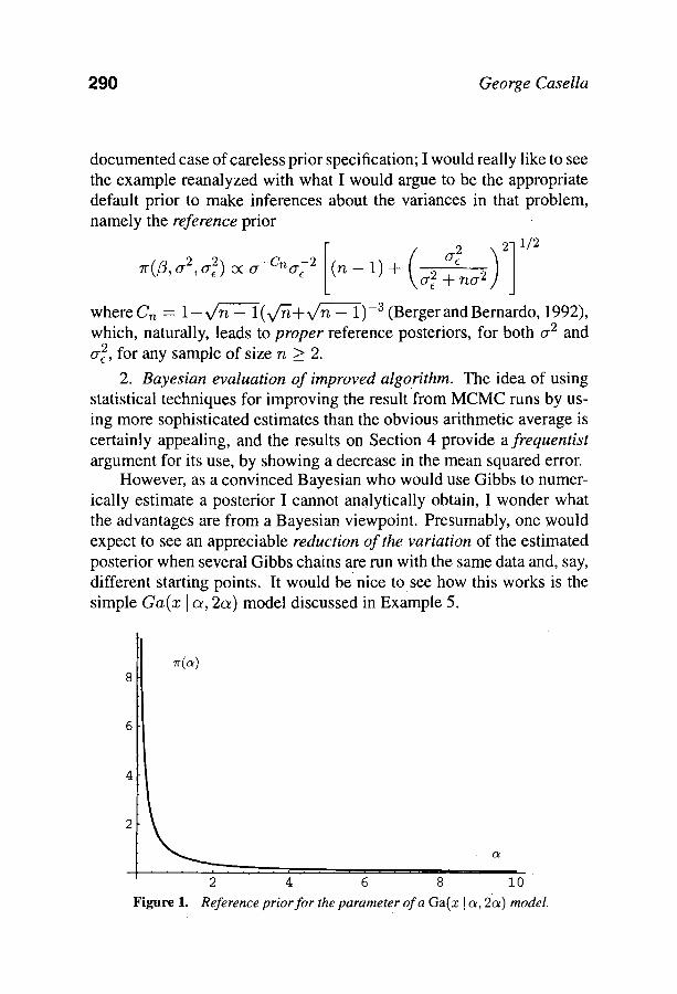
290 George Casella
documented case of careless prior specification; I would really like to see the example reanalyzed with what I would argue to be the appropriate default prior to make inferences about the variances in that problem, namely the reference prior
7r(/3,~r2,o -2) oc cr-Cno'/-2 (n - 1) + cr 2 + TtO" 2
where Cn = 1 - v / ~ - l ( v / - ~ + ~ ) -3 (BergerandBernardo, 1992), which, naturally, leads to proper reference posteriors, for both ~r 2 and cry, for any sample of size n _> 2.
2. Bayesian evaluation of improved algorithm. The idea of using statistical techniques for improving the result from MCMC runs by us- ing more sophisticated estimates than the obvious arithmetic average is certainly appealing, and the results on Section 4 provide a frequentist argument for its use, by showing a decrease in the mean squared error.
However, as a convinced Bayesian who would use Gibbs to numer- ically estimate a posterior I cannot analytically obtain, I wonder what the advantages are from a Bayesian viewpoint. Presumably, one would expect to see an appreciable reduction of the variation of the estimated posterior when several Gibbs chains are run with the same data and, say, different starting points. It would be nice to see how this works is the simple Ga(x l a, 2a) model discussed in Example 5.
~(~) 8
Figure 1.
(2
2 4 6 8 i0
Reference prior for the parameter of a Ga(z I a, 2~) model.
Statistical Inference and Monte Carlo Algorithms 291
Of course, the results may depend on the prior used. Since this is a one-parameter regular model, the reference prior is also Jeffreys' prior (Bernardo, 1979), namely
( 1)1, @,()
c~
where ~b t (.) is the trigamma, or first derivative of the digamma function, and c = (7r2/6 - 1) 1/2 ~ 0.65, shown in Figure 1. It may be seen that, in this case, the refence prior is actually close to the naive "positive parameter" prior 7r(a) ec c~ -~.
R A. GARdA-LOPEZ and A. GONZALEZ (Universidad de Granada, Spain)
We should first like to congratulate Professor Casella for his clear and detailed explanation of all the aspects concerning the interrelationship between statistical theory and computational algorithms, in particular the Gibbs sampler and the accept-reject algorithm. His talk has been highly methodological as far as all aspects of the choice of algorithm and its subsequent effects on the inference are concerned. What we consider to be especially important are the conditions for generating proper posteriors starting from proper conditionals in the Gibbs sampler. Some of the published results on this subject ought to be treated with a degree of caution because the compatibility of the proper conditionals (cf. Theorem 2 in Prof. Casella's paper) have not been adequately investigated.
Thus, one question we should like to put to Professor Casella refers directly to a technical aspect of his approach to the application of the Gibbs sampler. There are at least two widely known methods of gen- erating the Gibbs sample, the so-called single-path and multiple-path methods. Let us suppose that we have a random vector
U = (U1,. . . , Uk)
and that we can simulate the conditional distribution of
Ui [ ( V l , . . . , Ui-1, U i + l , . . . , Uk)
292 George Casella
by using the multiple-path method we draw m independent replicates of the first n cycles of Gibbs samples from the distribution of U, thus obtaining the vector
U(n j) {rr(J) rr(J) ~ = ~t~nl , . . . , t - ' n k ]
where (j) denotes the j-th replicate. It is clear that the successive cycles
on a particular path, U~ j), u~J),..., "U~ ~) are not independent but that
cycles from different paths, U (1), U(2), . . . , U(n m), are indeed indepen- dent.
With the single-path method you have only to generate one path long enough to obtain q values for r -t- q, where r is a point at which the Gibbs sampler converges. These q values then provide the basis for our estimation and they all obviously depend upon the starting values.
It has already been demonstrated (cf. Geman and Geman, 1984 and Liu, Wong and Kong, 1992a), that under general conditions, both methods result in convergence, i.e.
d Un ,U
Nevertheless, the dependence between the values generated with the single-path method exerts an influence on the resultant estimators (cf. Gelman and Rubin, 1991).
On the basis of these observations we consider it worth asking Pro- fessor Casella the following questions:
1. Are the Gibbs samples in his study based on single or multiple starting values?
2. Has he investigated to see how the choice of cycle values might affect the Gibbs samples thus produced and how this may in turn affect the main result (Theorem 2) with proper posteriors?
3. Do any results exist (similar to those of Theorem 2) for variations of Gibbs sampling as data augmentation (cf. Tanner and Wong, 1987) and substitution sampling (Gelfand and Smith, 1990)?
To come to another point raised in professor Casella's talk, that of improving the estimators by Rao-Blackwellizing them. It is known that in general the main problem lies in computing the estimators, but there are other, non-parametric methods of improving them, such as the
Statistical Inference and Monte Carlo Algorithms 293
double-bootstrap. Thus our question is: Have any empirical studies been made to compare the accuracy of the Rao-Blackwellization and double bootstrap methods?
The following contributions were later received in writting.
J. BERGER (Purdue University and Duke University, USA) I congratulate Dr. Casella on a very interesting article. He raises
important philosophical and practical questions. Perhaps the main emphasis of the article is the recommended blend-
ing of Bayesian methods (at least regarding MCMC) with frequentist methods. I am certainly also in favor of such, but do have one point of qualification that I think is important. The blendings that Dr. Casella actually uses as examples in the paper primarily involve the use of certain frequentist tools, as opposed to the use of frequentist inferences. For in- stance, he demonstrates uses (to a Bayesian) of the law of large numbers and the Rao-Blackwell theorem, two common frequentist tools. Few Bayesians would quarrel with use of such tools (although some might argue that the law of large numbers is as much a Bayesian as a frequentist tool - after all, the first general development of the central limit theorem was by Laplace, and done in an entirely Bayesian way). On the other hand, it is much harder to convince Bayesians that frequentist infer- ences themselves are of particular use. In the Bayesian's ideal world of the future, numerous frequentist tools will be taught and used, but little in the way of actual current frequentist inference would likely survive. (Many methods that are currently considered to be frequentist, such as maximum likelihood, would still be around, but would be explained as approximations to the Bayesian answers.) Today's frequentists operate in the reverse fashion; they typically admit the considerable value in use of Bayesian tools, but do not find much value in use of Bayesian inferences.
I have a question about Example 4. It has been claimed that, in situations such as this where the impropriety is due to a nonintegrable singularity, the Gibbs sampling output is often reasonable if one does not run the chain for too long. To be more precise, an easy "fix" for such problems is to remove the singularity from the space by, say, introducing the constraint o -2 > e, and the "claim" is that one will often get essentially the same answers from the original Gibbs chain if it is of moderate length
294 George Casella
and starts at a reasonable value. This can occur, of course, only if the chain is unlikely to visit too close to the singularity. From the author's experience, is this claim reasonable?
A different issue concerning impropriety, which I have experienced, relates to impropriety due to nonidentifiability. In Andrews, Berger, and Smith (1993) we encountered the fascinating phenomenon that the Gibbs chain for a very high dimensional improper posterior gave con- vergent estimates for "identifiable" parameters, but not for "nonidentifi- able" parameters. This allowed us to determine which parameters were nonidentifiable, and to adjust the model to correct the problem. Taken together with the "claim" in the previous paragraph, this might suggest that impropriety is not necessarily such a concern in hierarchical models; impropriety due to nonidentifiability will be obvious, while that due to singularities is unlikely to affect the answer. Although such a statement verges on sounding ridiculous, we must remember that we are operating in an arena where we will typically never be certain that the Gibbs chain has converged, even if we know that the posterior is proper. Hence all we really need is assurance that, in practice, problems do not seem to arise for the type of problem being considered (e.g., standard normal hierarchical models). While it is fun to speculate about such issues, I must admit that I would not really want to use an improper posterior my- self; see also Berger and Strawderman (1996) for additional conditions ensuring proper posteriors in hierarchical models.
Section 4 was quite interesting and had some nice surprises, but I note that it ends up essentially with the "status quo" being supported. The common understanding in use of "accept-reject" and "importance sampling" includes:
(i) Importance sampling gives more accurate estimates for a single h.
(ii) If one wants to simultaneously compute expectations for many h, but the same Y, accept-reject will often be computationally faster, especially if the acceptance rate is low (since then t will be considerably smaller than n).
iii) Rescaling by a correlated estimate of one is an important vari- ance reduction technique.
Statistical Inference and Monte Carlo Algorithms 295
Use of versions of Rao-Blackwellization does not really appear to add much here. Later examples in the paper do, however, show considerable gain in use of Rao-Blackwellization.
In Section 5.3, I am curious as to whether use of the optimal random scan based on the minimax criterion is actually superior to the optimal scan based on convergence rate (for other than the least favorable function h, of course).
A. R DAWID (University College London, UK)
The general idea of "Rao-Blackwellisation", as a way of improving an inference by eliminating unwanted stochastic variation, is an impor- tant and powerful one, as this paper reconfirms. I am surprised it is not used more widely, particularly in its simpler variants. For example, why does any one still do accept-reject sampling (Section 4.1) for Monte Carlo estimation of f based on a sample from 9? If the improvement ~RB of ~AR seems over-complex, a simpler approach is just to replace I(Ui <_ wi) by E{I(Ui < wi)} =- wi, leading back to the very simple importance sampling estimate 5z. This is the exact Rao-Blackwell im- provement on ~AR when the number N of I,~'s generated from 9 (but possibly rejected) is fixed, so that the number of retained terms in the accept-reject formula is random. I am not sure of the practical value of Casella's more intricate analysis, which takes into account the random- ness in N; and its dependence on the stopping rule offends against some of my deep intuitive feelings about inference. Does this extra complexity have a real pay-off?
A good way of thinking about importance sampling is as follows. We want to approximate the distribution with density f . To do so, we generate points (Yi) from another density 9, and to each Yi we attach weight wi = f (Yi)/9 (Yi). We end up with a discrete measure ~N, having mass wi at Yi (i = 1 , . . . , N). Normalizing this (by N for unbiasedness, or, better, by }---~N 1 wi to ensure total mass 1 and thereby improve overall accuracy) to PN, we get PN ~ P, the desired distribution with density f . The expectation of any function under PN then provides the importance sampling estimate of its expectation under P. From this viewpoint, accept-reject operates by forming an approximating distribution to P by thinning out the (Yi), only retaining Yi with probability proportional to wi; and attaching equal weights to the retained points. Its inefficiency is self-evident, and that it should have been proposed at all may be
296 George Casella
attributed to a subconscious feeling that a discrete distribution must have equal weight on every point - -a position that does not stand up to a moment's scrutiny.
Metropolis-Hastings simulation has similar features to accept-reject. Consider a M-H chain with proposal density q(y/ I Y) and acceptance probability c~(y, y/), satisfying detailed balance for a target distribution P having density f :
f ( y )q (y , l y ) a ( y , J ) - f ( y , )q (y l y , ) (~( j , y ) .
Let /3(y) := f a(y , y')q(y' I y)dy' be the overall probability of ac- cepting a proposal to move from y. Suppose that we continue until a fixed number N of proposals have been accepted. Ignoring burn- in, thinning, etc., estimation of # := E p { h ( Y ) } by its corresponding chain average is equivalent to estimating P by the (normalised) dis- crete measure on the successive accepted proposals x l , . . . , XN, with xi being assigned weight Wi, the number of trials starting from xi be- fore the next proposal is accepted. But Wi is random, with a geomet- ric distribution (conditioned on past x's) having mean wi := /3(xi) -1. "Rao-Blackwellisation" thus suggests it would be better to replace the observed number Wi of repetitions of xi by the new weight wi (assum- ing this can be calculated). If we can actually simulate directly from the embedded Markov chain of accepted proposals xl , x2, �9 �9 �9 XN, with transition density "/(x' I x) : = q(x' I x)c t (x ,x ' ) / /3(x) , a much more efficient procedure is obtained. If not, and we still have to generate and reject proposals, it should still be more efficient; and it seems likely that still further advantage could be taken of the rejected values, parallel to suggestions of Casella and Robert (1996b).
THOMAS J. DICICCIO and MARTIN T. WELLS (Cornell University USA)
It is a pleasure to participate in this discussion of Professor Casella's paper on the interplay between Markov Chain Monte Carlo (MCMC) algorithms and statistical inference. The underlying theme of this paper is statistical inference for parameters based on MCMC output. This dis- cussion begins with a few specific questions and then focusses on some relationships between the Casella's minimax decision theory approach of Section 5.3 and the literature on rates of convergence of MCMC methods via the second dominant eigenvalue.
Statistical Inference and Monte Carlo Algorithms 297
Professor Casella begins with a very welcome call to use Bayesian and frequentist approaches in a complementary way; in particular, his suggestion of using frequentist performance to distinguish between and improve upon estimators that arise from Bayesian considerations is most reasonable. In the context of the popular general linear mixed model, Professor Casella vividly demonstrates some seemingly catastrophic pit- falls that choosing a prior distribution can present. Theorem 1 identifies priors for this model that are appropriate from a Bayesian perspective. A natural question is whether any of these prior distributions produce in- ferences that are correct or nearly correct from a frequentist perspective. In particular, is there any compelling inferential rationale for choosing a = b = 1 in Example 4?
Figures 1 and 2 are certainly startling and distressing from aBayesian perspective. However, Professor Casella appears to have a firm under- standing of their behavior from the underlying "null Gibbs chains." Is it possible that, despite the Bayesian catastrophe, the algorithm could be used to produce reasonable frequentist inferences?
The Rao-Blackwellization and related methods described in Section 4 are ingenious and potentially very useful. It is not unreasonable to con- sider them from the viewpoint of frequentist inference, given the current interest in noninformative priors and probability matching. Typically, the upper 1 - o~ quantile of the marginal posterior density for a scalar pa- rameter of interest is an approximate upper 1 - oL confidence limit having coverage error of order O(n-1/2). Ifa Welch-Peers noninformative prior is used, this error might be reduced to O(n-1). If frequentist inference is the ultimate goal, given that the inferences obtained from the exact posterior distribution are at best rather approximate, is there any benefit necessarily to using Rao-Blackwellization? What is the interpretation of Tables 1 and 2 in connection with noniformative priors?
To view Professor Casella's minimax decision theory approach in connection with rates of convergence of MCMC methods and second dominant eigenvalues, some background results and notation is neces- sary. Let { X j } be a discrete-time homogenous Markov chain on X, with transition probability matrix P = {p(x, y) : x, y E 32}, where P ( x , y ) = P { X j = y I X j_ l = x}. Define the k-s tep transition probabilities by pk = { p ( k , x , y ) : x , y E 32}. The stationary mea- sure 7r(x) on 32 of course satisfies 7rP = 7r, that is, ~-~zTr(x)p(x,y) = 7r(y) Vff C A2. Let g2(Tr)be the Hilbert space of real-valued functions
298 George Casella
on ,-V with inner product < f I g > = ~-,x 7r(x)f(x)g(x). The equi- librium expectation o f f under 7r is then < f > - < f I 1 > = E~r(f), and we can think of (Pkf) (x) and (IIf)(x) as operators on g2(Tr) given by Pk(Z)(x ) = y~yp(k ,x ,y ) f (y ) and (1- i f ) (x)= ~-'~yTr(y)Z(y). The matrix II has rows equal to 7r and is an orthogonal projector on g2 (Tr) with range the constant functions. The autocovariance function of ~ i f (X i ) is
Cf(l i - J l) = E~{[f(Xi) - E~f(Xi)][ f (Xj) - Er f (Xj ) ]} ,
which also equals < f I (pli-Jl _ I I ) f > = < f I (P - II)li-Jlf > = < f I ( I - I I )pIJ-Jl ( I - I I ) f >. The autocorrelation function is pf(Itl) = Cf([tl) c f ( o ) �9
In Section 5.3 Professor Casella discusses the minimax properties of the Monte Carlo average estimate of the parameter # = Erh(X) . The limiting risk function R (n) (h) in (23), can be developed further by using the results of Peskun (1973). The fundamental matrix of Markov chains (Kemeny and Snell, 1983) Z = ( I - ( P - II)) -1 = I + } -~_ l (Pk - II) arises naturally in this limiting expression. It can be shown that
lira R(n)(h) = < h lQh >, n - - - , c ~
where Q = 2 Z - I - I I = ( I + P ) ( I - p ) - l ( I - I I ) . Moreover, by using the series representation of Z and the definition of the autocovariation function, it can be shown that limn--,~ R (n) (h) = ~-~-o Ch(k).
In this case of where {Xi} are independent, l imn-~R(n)(h) = < h [ ( I - I I )h > = Ch(O). The ratio
Th = 1 < h l O h > 2< h l ( I - I I ) h >
is known as the integrated relaxation time, see Sokal (1989) and Gidas (1995). There are n/2rh effectively independent samples in a run of length n. Note that "rh = �89 Y'~,i ph(i).
Professor Casella asserts that the risk function contains more infor- mation than is contained in the rate of convergence. This assertion can be seen using the ideas above. In the case where P is self-adjoint on
Statistical Inference and Monte Carlo Algorithms 999
g2(rc), that is < 9 [ Ph > = < Pg [ h >, one can relate the rate of con- vergence of the chain to the limiting risk. Let the ordered eigenvalues of P are 1 = /30 > /31 ~ f12 2 " '" ~ /3 > - 1 , where/3 equal the smallest eigenvalue. Much work (see Diaconis and Stroock, 1991) has focused on methods for bounding/31, fl, and/3, = max(/31, ] /3 [) that give rise to bounds on the rate of convergence of the chain to its station- ary distribution. As pointed out in Diaconis and Stroock (1991), there are advantages to studying I - P instead of P. The spectrum of I - P consists of numbers Ai = 1 - /3 i . Using the minimax representation of eigenvalues
< h [ ( I P)h > A1 = inf = i~fl l - ph(1)]
h < h l ( I - l - I ) h >
where the infimum is over all nonconstant functions h E g2 (~), this ratio is called the Rayleigh quotient and its numerator may be represented as
1 E ~ ( i ) p ( i ' J ) [ f ( i ) - f(j)12 . 2
i,j
The rate of convergence of the chain is determined by ~1 and hence by the infimum of ph(1) over h C g2(~) �9 Therefore, as limiting risk is essentially a series in ph(k) and/31 is related to ph(1), the limiting risk contains more information.
Using the ideas above we can study a special case of the random scan. Suppose the transition matrix is a mixture of two transition matrices, that is, P;~ = (1 - ,~)P1 + kP2. First, it is easy to see that Al(Pk) is a concave function of )~ using the minimax representation. As for %(P,x), a bit more work is needed. On the orthogonal complement of the constant functions, we have that Q = 2(1 - p ) - i _ I . Using the result of Caracciolo et al. (1990) that
< f t (A -l + B - 1 ) - l f >_< I< f t A f >-l + < f t B f >J-1
for A and B positive definite self-adjoint matrices, with A = (1 - A ) - I ( I - / : ' 1 ) -1 and B = A - I ( I - P1) -1 it follows that
(1 - ,k) < h i ( I - P1)-lh > +A < h i ( I - P2)-IA > < < h i [ ( 1 - A)(1 - P1) + A ( I - P2)J - lh > - 1 ,
300 George Casella
and
(Th(PA) -~ 1/2) -1 ~ (1 - A)[Th(P1) q- 1] -1 -}- ~[Th(P2 ) Jr- 1] -1 .
Hence both [-rh(P~) + 1] -1 and A2(P2) are concave functions of A. A consequence of this convexity is that
A2(Px) > min(A, 1 - A) sup Ae(P~,) 0<A<I
and
[wh(P~) -}- 1/2] -1 > min(A, 1 -- A) sup ['rh(PA ) ~- 1/2] -1. O<A<I
Hence the randomized approach with A = �89 is never more than a factor of 2 from the best value of A.
PAUL GUSTAFSON (University of British Columbia, USA) and LARRY WASSERMAN (Carnegie Mellon University, USA)
George Casella has presented us with an interesting perspective on the relationship between computing and statistical theory. He makes it clear that the two are inexorably intertwined. Each area enriches and informs the other. He has also emphasized that there is an inevitable mixture of Bayesian and frequentist ideas when one considers statistical computing algorithms and their relationships with inference.
We agree that both Bayesian and frequentist methods are necessary and that statistics is at its best when the two are in happy coexistence. Of course there are many who do not agree on this point and we hope that George's article will help convince the doubters (Bayesian or frequentist) of the need for both.
As should be clear by now, we have little disagreement with anything in this article. We do wish to raise a few points.
1. Averaging Conditional Densities Can Fail. The paper discusses several aspects of the "Rao-Blackwellization" of estimators applied to Monte Carlo output. The author also mentions the "usual average of conditional densities" estimator of a marginal density, which is in the same spirit as Rao-Blackwellized estimators of expectations. For brevity we will refer to this estimator as the ACD (Average of Conditional Den- sities) estimator. Conventional wisdom dictates that the ACD estimator
Statistical Inference and Monte Carlo Algorithms 301
of a posterior marginal density is the preferred estimator in any context where it can readily be calculated. We would like to point out a curi- ous and undesirable feature of the ACD estimator in certain hierarchical model settings.
We look at an artificially simple hierarchical model in order to il- lustrate this feature clearly. Specifically, consider a simplified version of Example 4, where/3 and 0 .2 are known, and the prior o n o.2 is locally uniform (a = -1 ) . Further, assume that ni = 1 for i = 1 , . . . , k, so that we can write Y/unambiguously. It is simple to verify that the joint posterior distribution on/_t and o.2 is proper. In what follows below, a density for o -2 evaluated at zero will be defined as the obvious limit.
If the goal is estimation of the marginal posterior density of o.2, the ACD estimator is
m
PACD(') -- ~'a21y('ly) = __1 Z lra2l~,y(" I#(i)' y) ' m
i=1
(1)
where {#(i)}ira__ 1 a r e the # vectors sampled by the Monte Carlo scheme. The conditional posterior distribution of o.2 I#, Y, which appears on the right-hand side of (1), is inverse gamma, with shape (k/2) - 1 and
x--,k #2 scale (1/2) z-~i=l i. On the other hand, the true marginal posterior distribution of o.Zly is identical to the conditional distribution of (T -
2 where T has an inverse gamma distribution with shape ~ > o.e,
(k/2) - 1 and scale (1/2) ~']ki_l(y i - /3 )2 . Thus the true posterior marginal density for o .2 is finite and positive at 0 .2 = 0. But since the inverse gamma density is always zero at 0 .2 = 0, the ACD density estimate is always zero at 0 .2 = 0, no matter how large a Monte Carlo sample is drawn. In other words, 7r 2[y(0]y) > 0 yet PACD(O) = O.
Thus the ACD estimator is inconsistent at 0 -2 = 0. It might be tempting to dismiss this concern, since it is only an issue at the boundary of the parameter space. But in fact an ACD estimate is going to be misleading about the shape of the posterior marginal density near zero. This is
especially true for data sets with ( l / k ) ~-~i=lk (Yi --/3)2 < o.e'2 In such cases, the true posterior marginal density for o .2 takes on its maximum value at zero and is monotone decreasing, which can be interpreted as evidence in favor of o .2 = 0. But for any Monte Carlo sample the ACD density estimate will be zero at o .2 = 0 and will be increasing on at
302 George Casella
least some small interval extending right from zero. This suggests that o .2 > 0. Thus the ACD estimator has great potential to be misleading about the posterior evidence concerning small values of o .2 .
This aberrant behavior has been illustrated in a very simple model where the posterior marginal distribution of the variance component can be obtained analytically. The behavior seems to occur quite generally, however, whenever a prior density which is positive at zero is specified for a variance component. The use of such priors seems quite appropriate in many contexts, even though inverse gamma priors, which vanish at zero, are much more commonly specified for variance components. The data cannot rule out the absence of a random effect (o .2 = 0), so it seems overly confident to use a prior which vanishes as o .2 goes to zero. In fact, one might argue that monotone decreasing prior densities should be specified, in order to favor parsimonious models. The Jeffreys prior for the simple model discussed above has a monotone decreasing density which is finite and positive at zero. One disadvantage of not using an inverse gamma prior is that the "conditional conjugacy" which drives the Gibbs sampler will be lost. The ACD approach can be extended to deal with this, however, based on work of Chen (1994). But Chen's density estimator will still have aberrant behavior near zero.
In one sense it is not surprising that the ACD estimator does not work well for variance component marginals with prior densities which are positive at zero. In such problems, the Bayes factor for testing the absence of random effects can be expressed as the Savage-Dickey density ratio, which is the ratio of posterior to prior marginal densities for the variance component, both evaluated at zero. For details see Verdinelli and Wasserman (1995). If the ACD estimator worked well for estimating the posterior marginal density at zero, then we would have an easy and reliable way to estimate the Bayes factor. But invariably Bayes factors are harder to compute than other posterior quantities. In this regard, we are not surprised that there is no free lunch via the ACD estimator.
2. Priors for Hierarchical Models. As discussed in the paper, choosing priors for hierarchical models is delicate. The dangers of improper posteriors are real and insidious. The theorems reviewed in the paper should prove valuable for guiding statistical practice. However, it seems that many statisticians try to deal with this problem by replacing improper priors with vague proper priors. This merely approximates an ill-defined
Statistical Inference and Monte Carlo Algorithms 303
posterior with a nearly ill-defined posterior. We would like to mention another solution to the problem.
One output of an inference from a hierarchical model is shrunken estimates. In some cases, conditionally on the hyperparameters, the shrunken estimates lie between the prior mean and the m.l.e's from a non-hierarchical model, i.e. ~Shrunk ~-- O~00 -~- (1 - a)0, say. It seems reasonable to place a uniform prior on the degree of shrinkage a. This implies a (proper) prior on the hyperparameters. This idea has been used by Strawderman (1971), Christiansen and Morris (1994), Daniels and Gatsonis (1996) and others. It is similar to a prior suggested by DuMouchel (1994). The full generality of the idea is explored in Daniels (1996). This prior seems to be a general way for providing proper reference priors for hierarchical models. Yet another alternative is to place a proper prior (such as half normal or half Cauchy) on the distance from the "null" sampling model in which the random effect is 0. Jeffreys pointed out that such strategies often lead to useful, proper reference priors.
As a general remark we would add that any time improper priors lead to trouble, we should not use vague proper priors. To do so is simply to approximate an ill defined solution. Instead, proper reference priors are called for. Similar problems occur in using Bayes factors to compare models. It is well known that improper priors lead to ill-defined Bayes factors. As Jeffreys made clear, the solution is not to use vague proper priors but rather, to use proper reference priors.
EDWARD I. GEORGE (University of Texas at Austin, USA)
Let me begin by congratulating Casella for a masterful paper which synthesizes and interweaves so many different ideas and points of view. There is much to comment on, as Casella seems to open up a whole new vista of ideas with each new section. However, for the sake of focus (and space), I would like to confine my comments to Section 3.2 which is concerned with the properties of Gibbs Markov chains when the Gibbs conditionals do not correspond to a proper posterior.
The key result of Section 3.2 is Theorem 2 which tells us that a Gibbs Markov chain will be positive recurrent if and only if the full conditionals correspond to a proper posterior. Just after presenting this, Casella goes on to show us (7), which at first glance suggests that useful information cannot be extracted from Markov chains which are not positive recurrent.
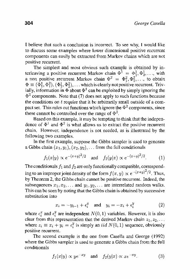
304 George Casella
I believe that such a conclusion is incorrect. To see why, I would like to discuss some examples where lower dimensional positive recurrent components can easily be extracted from Markov chains which are not positive recurrent.
The simplest and most obvious such example is obtained by in- terleaving a positive recurrent Markov chain 551 _= 55~, 551. . . , with a non positive recurrent Markov chain 552 = 552, 55~,..., to obtain 55 -- (55~, 5512), (55~, 55~),... which is clearly not positive recurrent. Triv- ially, information in 55 about 551 can be exploited by simply ignoring the 552 components. Note that (7) does not apply to such functions because the conditions on t require that it be arbitrarily small outside of a com- pact set. This rules out functions which ignore the 552 components, since these cannot be controlled over the range of 552.
Based on this example, it may be tempting to think that the indepen- dence of 551 and 552 is what allows us to extract the positive recurrent chain. However, independence is not needed, as is illustrated by the following two examples.
In the first example, suppose the Gibbs sampler is used to generate a Gibbs chain ( X l , Y l ) , (Z2 , Y2), �9 �9 �9 from the full conditionals
f l ( x [ y ) c< e -(x+y)2/2 and f2 (y lx ) a< e -(z+y)2/2. (1)
The conditionals f t and f2 are only functionally compatible, correspond-
ing to an improper joint density of the form f ( x , y) c< e -(z+y)2/2. Thus, by Theorem 2, the Gibbs chain cannot be positive recurrent. Indeed, the subsequences xl , x2 , . . , and Yl, Y2,..- are interrelated random walks. This can be seen by noting that the Gibbs chain is obtained by successive substitution into
y x and Yi : - x i + ~i xi = -Yi-1 + ~i (2)
x Y are independent N(0, 1) variables. However, it is also where Q and s clear from this representation that the derived Markov chain Zl, z2,. �9
Y is simply an i id N(O, 1) sequence, obviously where zi = xi + Yi ~ - c i
positive recurrent. The second example is the one from Casella and George (1992)
where the Gibbs sampler is used to generate a Gibbs chain from the full conditionals
fl(xlY) o( ye - zy and f2 (y lx ) o( xe -zy . (3)
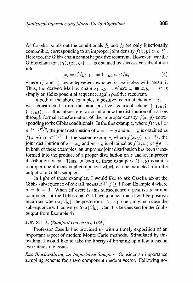
Statistical Inference and Monte Carlo Algorithms 305
As Casella points out the conditionals f l and f2 are only functionally compatible, corresponding to an improper joint density f (x , y) oc e -xv. Here too, the Gibbs chain cannot be positive recurrent. However, here the Gibbs chain (Xl, Yl), (x2, Y2), �9 �9 �9 is obtained by successive substitution into
x ~ / x i (4) xi = e i /Y i -1 and Yi = x and Y where Q c i are independent exponential variables with mean 1.
Y is Thus, the derived Markov chain Zl, z2 , . . , where zi =- xiYi : e i
simply an iid exponential sequence, again positive recurrent. In both of the above examples, a positive recurrent chain Zl, z2,. �9 �9
was constructed from the non positive recurrent chain ( x l , y l ) , (x2, Y2), . . . . It is interesting to consider how the distribution of z arises through formal transformation of the improper density f ( x , y) corre- sponding to the Gibbs conditionals. In the first example, where f (x, y) c<
e -(x+y)2/2, the joint distribution of z = x + y and w = y is obtained as
f ( z , W) O( e -z2/2. In the second example, where f ( x , y) c( e -zy, the 1 c - z joint distribution of z = xy and w = y is obtained as f ( z , w) o( - 5 �9
In both of these examples, an improper joint distribution has been trans- formed into the product of a proper distribution on z and an improper distribution on w. Thus, in both of these examples f ( x , y) contains a proper one-dimensional component which can be extracted from the output of a Gibbs sampler.
In light of these examples, I would like to ask Casella about the Gibbs subsequence of overall means/3(/), j > 1 from Example 4 where a = b = 0. When (if ever) is this subsequence a positive recurrent component of the Gibbs chain? I have a hunch that it will be positive recurrent when 7r(/3[y), the posterior of/3, is proper, in which case the subsequence will converge to 7r(/3[y). Can this be checked for the Gibbs output from Example 4?
JUN S. LIU (Stanford University, USA) Professor Casella has provided us with a timely exposition of an
important aspect of modem Monte Carlo methods. Stimulated by this reading, I would like to take the liberty of bringing up a few ideas on two interesting issues.
Rao-Blackwellizing an Importance Sampler. Consider an importance sampling scheme for a two-component random vector. Following no-
306 George Casella
tations of Professor Casella, we let the target distribution of (X, Y) be f (x , y) and let the trial sampling distribution be g(x, y). Of interest is the estimation of, say, ~- = E l {h (X , Y)}, for a given integrable function h. This can be achieved by using either rejection sampling, as demon- strated by Professor Casella, or importance sampling (IS). Suppose that we have drawn samples ( X X , Y I ) , �9 �9 � 9 (Xn, Yn) from g(x, y). A standard IS estimate of 7- is
1 n f (x ,y ) ~- = - E w(xi, yi)h(xi, Yi), where w(x, y) = 9(x, y)
n i = 1
A rescaled estimate, as illustrated in Section 4.2 and used in Casella and Robert (1996b), Kong et al. (1994), Liu (1996) etc., is
1 n n ~---~ ~ E w ( x i , Y i ) h ( x i , Y i ) , where W = E w ( x i , Y i ) .
i = 1 i = 1
Besides the advantage mentioned by Professor Casella, using the resca- led estimate ~ allows us the flexibility of knowing f and 9 only up to a normalizing constant. This advantage is much more pronounced in complicated problems (Kong et al. 1994). Because asymptotically the two estimates are equivalent and also because "7- is much more approach- able mathematically, we will use ? for theoretical discussions, although practically we advocate using "~ all the time.
There are two ways of Rao-Blackwellizing: conditioning on either X or Y. If conditioned on Y, for example, we have
Ea{w(X ,Y )h (X ,Y ) I Y = y} = / h ( x , y ' ~ f (x ' y ) g(x
= Wy(y)Ef{h(X, Z) I Z = y},
where Wy(y) = fy(y)/gy(y). A more efficient estimate than ? results: n
1 ~Wy(ydEf{h(X,Y))]Y=yi}. i = 1
When h is a function of one component alone, say h(x, y) = h(y), the estimate ;rrby is reduced to
n
1 E Wy(Yi)h(yi). i = 1
Statistical Inference and Monte Carlo Algorithms 30"l
A quite different intuitive interpretation of this R-B effect is that margi- nalization reduces importance sampling variation. MacEachern, Clyde, and Liu (1996) derived one special case of this fact, and Rubinstein (1981, Section 4.3.7) recorded another.
Under this formulation, the importance sampling can be treated ap- proximately as a Rao-Blackwellized rejection sampling; hence, it is statistically more efficient. This fact has been established by Casella and Robert (1996b) in a sophisticated setting and will be re-derived here more directly and heuristically. Let (Ii, y~), i = 1 , . . . , n, be jointly drawn according to the acceptance-rejection rule; that is, the Yi are iid from a trial distribution g(Y), and the conditional distribution [Ii I yi] is Bernoulli(r(yi)) with r(y) = f(y)/Mg(y). Suppose the stopping effect of this rejection sampling can be safely ignored. Then Ii plays the role of xi in the foregoing argument; and the R-B counterpart of tSAR in (10) of Casella is
1 n -E 5IS = n w(yi)h(yi). i-----1
Without loss of generality we assume that T = 0. Then, since M >_ maXy{W(y) },
nvar(SAR) ,~ Mvarf{h(Y)} > f Wmaxh2(y)Z(y)dy
f f(Y) h 2 - ~ (y)f(y)dy = Eg{w2(y)h2(y)} > J
= varg{w(y)h(y)} -= nvar(Sis ). An effort of comparing the two samplers with the Metropolized inde- pendence sampling was made in Liu (1996). Since the advantage of the rejection method is that exact draws from f can be obtained, it is sometimes useful to combine the two samplers when one wants to reduce importance sampling variations (Liu, Chen, and Wong 1996).
In many practical problems, the marginal weight Wy(y) is difficult to compute, whereas the conditional expectation Ef{h(X) [ Y = y} is relatively easy to obtain. In such cases, as shown in Kong et al. (1994), one can use a partial RB-estimate
n
1 E w ( x i ' Y i ) E f {h(X'Y) IY = Yi}, i = 1
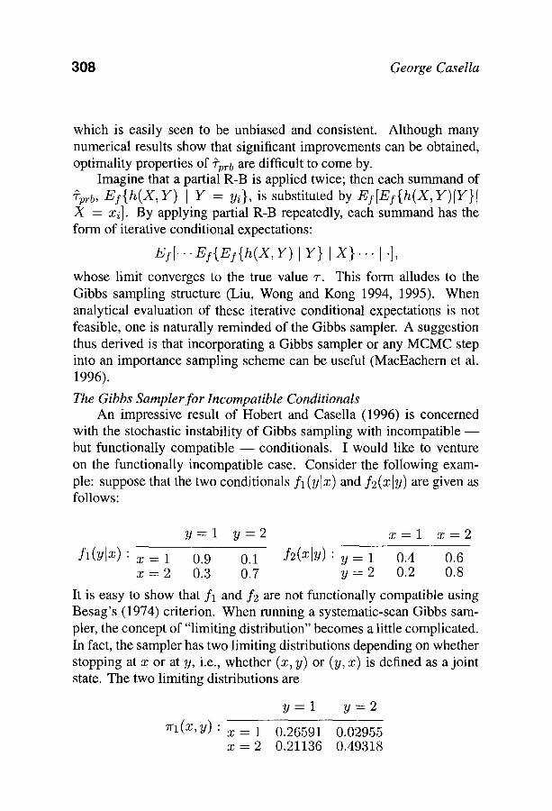
308 George Casella
which is easily seen to be unbiased and consistent. Although many numerical results show that significant improvements can be obtained, optimality properties of "7-prb are difficult to come by.
Imagine that a partial R-B is applied twice; then each summand of "~prb, Ey{h(X,Y) I Y = Yi}, is substituted by Ef[Ef{h(X,Y)IY}[ X = xi]. By applying partial R-B repeatedly, each summand has the form of iterative conditional expectations:
Ef[.. .EI{EI{h(X,Y) I Y} I X} . . . I'],
whose limit converges to the true value T. This form alludes to the Gibbs sampling structure (Liu, Wong and Kong 1994, 1995). When analytical evaluation of these iterative conditional expectations is not feasible, one is naturally reminded of the Gibbs sampler. A suggestion thus derived is that incorporating a Gibbs sampler or any MCMC step into an importance sampling scheme can be useful (MacEachern et al. 1996).
The Gibbs Sampler for Incompatible Conditionals An impressive result of Hobert and Casella (1996) is concerned
with the stochastic instability of Gibbs sampling with incompatible - - but functionally compatible - - conditionals. I would like to venture on the functionally incompatible case. Consider the following exam- ple: suppose that the two conditionals f l (y lx) and f2(xly ) are given as follows:
y = l y = 2 x = l x = 2
f l ( y [ x ) : x = 1 0.9 0.1 f2(xlY): y = 1 0.4 0.6 x = 2 0.3 0.7 y = 2 0.2 0.8
It is easy to show that f l and f2 are not functionally compatible using Besag's (1974) criterion. When running a systematic-scan Gibbs sam- pier, the concept of "limiting distribution" becomes a little complicated. In fact, the sampler has two limiting distributions depending on whether stopping at x or at y, i.e., whether (x, y) or (y, x) is defined as a joint state. Thetwol imi t ing distributions are
y = 1
~ l ( x , y ) : x = l 0.26591 x = 2 0.21136
y=2
0.02955 0.49318
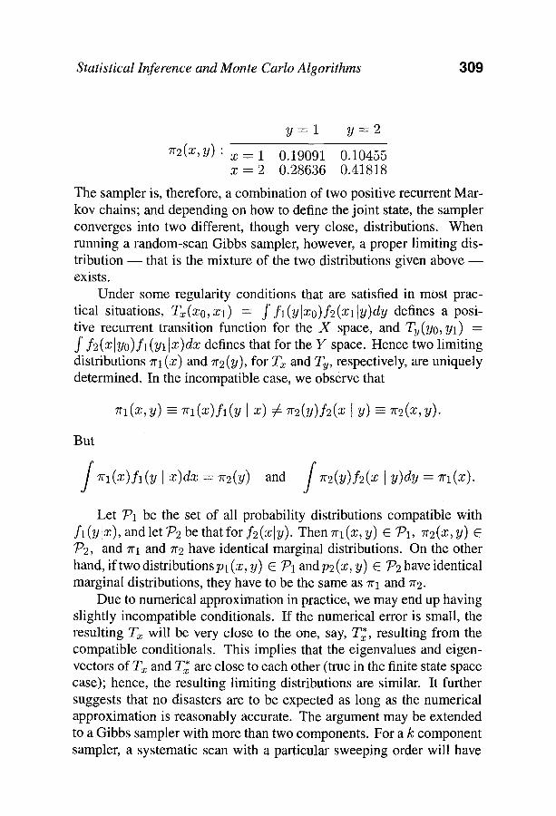
Statistical Inference and Monte Carlo Algorithms 309
y = l y = 2
7r2(x,y) �9 x = 1 0.19091 0.10455 x = 2 0.28636 0.41818
The sampler is, therefore, a combination of two positive recurrent Mar- kov chains; and depending on how to define the joint state, the sampler converges into two different, though very close, distributions. When running a random-scan Gibbs sampler, however, a proper limiting dis- tribution - - that is the mixture of the two distributions given above - - exists.
Under some regularity conditions that are satisfied in most prac- tical situations, Tx(xo,zl) = ff l(y[xo)f2(xl[y)dy defines a posi- tive recurrent transition function for the X space, and Tu(yo, yl) = f f2(xlyo)fl (yl [x)dx defines that for the Y space. Hence two limiting distributions 7rl (x) and 7r2(y), for Tx and Ty, respectively, are uniquely determined. In the incompatible case, we observe that
71"I(X,y) ~ 7rl(x)fl(y l x) 7 s 7r2(Y)f2(x l Y) = 7r2(x, y).
But
Trl(X)fl(y l x)dx = 7r2(y) and /Tr2(y)f2(x l Y)dY = 71"l(X).
Let 791 be the set of all probability distributions compatible with f l (y lx) , and let 792 be that for f2(xly). Then 7rl(X, y) C 791, 7r2(x, y) C 792, and 71" 1 and 7r2 have identical marginal distributions. On the other hand, if two distributions Pl (x, y) C 791 and P2 (x, y) C 792 have identical marginal distributions, they have to be the same as 7rl and 7r2.
Due to numerical approximation in practice, we may end up having slightly incompatible conditionals. If the numerical error is small, the resulting Tz will be very close to the one, say, T~, resulting from the compatible conditionals. This implies that the eigenvalues and eigen- vectors of Tz and T~ are close to each other (true in the finite state space case); hence, the resulting limiting distributions are similar. It further suggests that no disasters are to be expected as long as the numerical approximation is reasonably accurate. The argument may be extended to a Gibbs sampler with more than two components. For a k component sampler, a systematic scan with a particular sweeping order will have
310 George Casella
k limiting distributions, depending on which component the sampler stops. The total number of such limiting distributions is kt. The limit- ing distribution for a random-scan sampler is then a mixture of these k! distributions.
XIAO-LI MENG (The University of Chicago, USA) Posterior Checking. My discussion will focus on only one issue: check- ing the propriety of a posterior resulting from the Gibbs-sampler speci- fications. Professor Casella's article is much broader, touching on many issues that are of current interest to me (e.g., the emphasis on being re- ceptive to both frequentist and Bayesian perspectives; the interplay of algorithms and inferences; the connection between EM-type algorithms and the Gibbs sampler). However, due to stringent time constraints (being a father of a newborn and a 16-month-old, I had to prepare this discussion in between frequent posterior checking; no impropriety was found, though I did learn why it is a good idea to avoid a sensitive posterior), I have to skip this great opportunity for advertising several related papers that I authored or co-authored. Nevertheless, I want to thank the Editor, and of course the author, for providing me with such an opportunity.
Recursive De-conditioning and Conditional Compatibility. The need for checking the compatibility of conditional distributions reminds me of an identity I learned more than a year ago. Let p(xl, x2) be a probability density function with respect to a product measure # = #1 • #2 and with a support in the form ~1 • f~2; we thus are assuming the positivity assumption of Hammersley and Clifford (c.f., Besag, 1974). Then ]1
p(Xl) = p(x2 I Xl) #2(dx2) (1) 2 p(Xl Ix2)
which is a trivial consequence of the well-known identity
p(x2 Ix1) p(x2)
p(ml l m2) p(xl)" (2)
While identity (1) also provides an explicit formula showing how p(xl I x2) and p(x2 I Xl) uniquely determine p(xl, x2), it seems to be much
Statistical Inference and Monte Carlo Algorithms 311
less well-known than the standard formula for proving uniqueness:
p(Xl I Xt2) for any fixed E ft2, (3) p(xl) P (4 I z 0 '
which also is an immediate consequence of (2). I learned the expression (1) from a presentation by Ng (1995). My
immediate reaction was that it must be my ignorance that I had not seen (1) in this explicit form. However, Ng assured me that he had checked with several leading experts in this area (e.g.J. Besag, W. H. Wong), and it seemed that the identity (1) was "mysteriously" missing from the general literature. An apparent explanation for this "mystery" is that (1) is not useful in general for calculating p(xa) and thus p(xl, x2) since a main reason we use the Gibbs sampler is our inability to perform ana- lytical integration, which is required by (1). However, in the context of checking the compatibility ofp(xl { x2) and p(x2 ] Xl), the expression (3) offers no advantage over (1). Both require us first to check whether p(xl { x2) and p(x2 I Xl) are functionally compatible, which amounts to checking whether (2) is possible, that is, whether we can write
p(X2 I Xl ) p2(X2) p ( x l l x 2 ) pl(Xl)
(4)
for some (positive) functions Pi, i = 1, 2. Given (4) holds, we then need to check, for (1), whether ff~2 b2(x2) #2(dx2) is finite, or, for (3),
whether fa I i~1 (xx) #1 (dxl) is finite. Under (4), these two integrations must yield the same value (allowing +e~) by Fubini's theorem, and thus one can always choose one to check (e.g., xl and X2 may be of very different dimensions), as emphasized by Arnold and Press (1989). Of course, these arguments also imply that there is no advantage to using (1) in the simple case involving only p(xl I X2) and p(x2 I Xl).
Reading Section 3 of Casella's article (and Hobert and Casella, 1995) made me wonder about the comparison between (1) and (3) for checking the compatibility of {p(xi I X-{i}), 1 < i < m} when m > 2, where X = {Xl , . . . , Xm} and X - s denotes {xj, j ~ S}. I thus decided to take a closer look at this comparison and the rest of this discussion reports what it generated. I doubt anything I discuss here is new (though I have not seen the recursive scheme described below), since everything follows
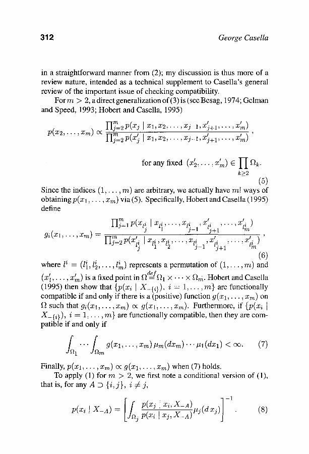
312 George Casella
in a straightforward manner from (2); my discussion is thus more of a review nature, intended as a technical supplement to Casella's general review of the important issue of checking compatibility.
For m > 2, a direct generalization of (3) is (see Besag, 1974; Gelman and Speed, 1993; Hobert and Casella, 1995)
m I I-Ij=2p(xj l x l , x2 , . . . , X j - I , X j + I , . . . ,Xtm) m ! YIj=2p(x} l x l , x2 , . . . , X j - I , X j + I , . . . ,X~)
for any fixed (x~ , . . . , X~m) C 1-I f~k. k_>2
(5) Since the indices ( 1 , . . . , m) are arbitrary, we actually have m! ways of obtaining p ( x l , . . . , Xm) via (5). Specifically, Hobert and Casella (1995) define
YIjm=l P(Xli I Xl~,' ' ' ,Xl~_l" ,X t.lz ," " " ,X t. ) 3 j+l l~
m 'l~ g i (X l , . . . ,Xm) : r i j=2p(x l i i X l~ ,Xl~ , . . . ,X l~_l ,X . . . ,xt . ) ' t j +1 ~ l~n
(6) where l i = (l~,/~,..., I/m) represents a permutation of ( 1 , . . . , m) and
(x~ , . . . , X~m) is a fixed point in f~deff~l • • f~m. Hobert and Casella (1995) then show that {p(xi I X-{i}), i = 1 , . . . , m} are functionally compatible if and only if there is a (positive) function g(x l , . . . , Xm) on f2 such that gi(xl , . . . ,Xm) c< g(xl , . . . ,Xm). Furthermore, if {p(xi I X_{i}), i = 1, . . . , m} are functionally compatible, then they are com- patible if and only if
f " " f ~ g(x l , . . . ,Xm)#m(dxm) '"# l (dx l ) <oc. (7) 1 m
Finally, p ( x l , . . . , Xm) ~: g ( X l , . . . , Xm) when (7) holds. To apply (1) for m > 2, we first note a conditional version of (1),
that is, for any A ~ { i , j} , i r j ,
p(xj I xi,X-A) (dxj) (S) p(xi I X _ A ) --~ p(xi I x j , X _ A ) # J
J
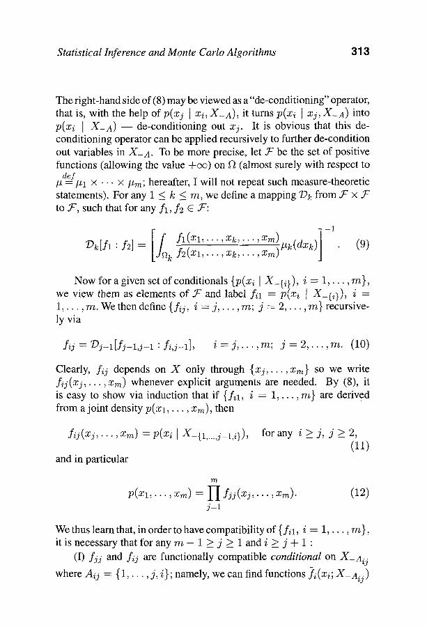
Statistical Inference and Monte Carlo Algorithms 313
The right-hand side of (8) may be viewed as a "de-conditioning" operator, that is, with the help of p(xj I xi, X-A), it turns p(xi I xj, X-A) into p(x i I X - A ) - - de-conditioning out xj. It is obvious that this de- conditioning operator can be applied recursively to further de-condition out variables in X-A. To be more precise, let .T" be the set of positive functions (allowing the value +oo) on f2 (almost surely with respect to
def # = #1 x -. . x Pro; hereafter, I will not repeat such measure-theoretic statements). For any 1 _< k < m, we define a mapping 7) k from 5 c x 9 t- to b c, such that for any f l , f2 E ~ :
ki,l: l= f2(Xl , -Xk, -Xm) #k(dxk)
-1
(9)
Now for a given set of conditionals {p(xi I X_{i}), i = 1 , . . . , m}, we view them as elements of 5 and label fil : p(xi t X-{ i} ) , i = 1 , . . . , m . Wethendef ine{f i j , i = j , . . . , m ; j = 2 , . . . , m } recursive- ly via
fij = {Dj- l [ f j - l , j - l : fi,j-1], i = j , . . . ,m; j = 2 , . . . ,m . (10)
Clearly, fij depends on X only through {xj , . . . ,Xm} so we write f i j (x j , . . . , xm) whenever explicit arguments are needed. By (8), it is easy to show via induction that if {fil, i = 1 , . . . , rn} are derived from a joint density p(x l , . . . , Xm), then
f i j (X j , . . . ,Xm) = p(xi ] X_{1,...,j_l,i}),
and in particular
for any i _ > j , j _ > 2 , (11)
m
p(xl , . . . ,Xm) = I I f j j (x j , . . . ,Xm). (12) j=l
We thus learn that, in order to have compatibility of {fil, i = 1 , . . . , rn}, it is necessary that for any rn - 1 _> j _> 1 and i _> j + 1 �9
(I) f j j and fij are functionally compatible conditional on X_Aij where Aij = { 1 , . . . , j , i}; namely, we can find functions fi(xi; X-Aij)
314 George Casella
C 5 c and -fj (xj;X_Aij) E .Y~ such that
fjj(xj,...,xm) X-A j) f i j (x j , . . . ,Xm) - ?i(xi;X_Aij)'
and
for (xj,... ,Xm) e H f~k; k>j
(13)
(II) The functions f i and .fj found in (13) must satisfy
f ?j(Xj; X-Aij) #j(dxj) = f ?i(Xi; X-Aij )
for X_Ai j C H ~k. k > j,kT~i
~i(dxi) < +0<2, (14)
Conditions (I) and (II) amount to the conditional compatibility of f j j and fij conditional o n X_Ai j . Because of (12), these conditions are also
sufficient for the compatibility of {fi l , i = 1 , . . . , m) . In other words, {p(xi ] X-{i}) , i = 1 , . . . , m} are compatible if and only if (I) and (II) are satisfied for all m - 1 > j _> 1 and i _> j + 1.
A matrix representation of {fij , i >_ j , j = 1 , . . . , m} perhaps can help to visualize the recursive de-conditioning process defined by (10). Table 1 gives the representation with m = 4, where we use [. I ~ .] to
denote conditional density (e.g., [4[3]aefp(x41x3)) and "k" to indicate the elimination (i .e. ,"de-conditioning") of Xk from the variables that are being conditioned on.
Table 1. A Matrix Representation of Recursive De-conditioning
f~j j = l j = 2 j = 3 j = 4
i = 1 [1 1234] i = 2 [2[ 1341 [21/I34] ~ [2 134] i = 3 [31 124] [31/124] ~ [3124] [31241 ~ [314] i = 4 [41 123] [41/I23]- [41 23] [4123]- [41 3] [4J~] -- [4]
Statistical Inference and Monte Carlo Algorithms 315
The matrix representation makes it easier to track the de-condi- tioning process, especially because each column corresponds to de- conditioning out one variable, starting from the finest conditioning (j = 1) recursively down to no conditioning (j = m). It also makes it clear that { f i l , i = 1 , . . . , m} are compatible if and only if {f i j , i > j } are conditionally compatible (as defined by (I) and (II)) for each j = 1 , . . . , m - 1 .
To illustrate the use of (I) and (II) for checking compatibility, let us consider the normal example used by Hobert and Casella (1995):
m 1
fil =--p(xi I X_{i}) (x exp{ - - -~(x i - -p iExk)2} , i~- 1,...,m. kr
(15) Here the pi's are constants, and the goal is to identify conditions on pi's under which {p(xi [ X_{i}), i = 1 , . . . , m} are compatible. Since for any i > 1 the only term in the exponential part of f l l / f i 1 involving x lx i is ( P l - - p i ) x l x i , (13) is satisfied if and only i fp l = Pi. This yields a necessary condition for the compatibility: Pi -~ P for all i. Under this necessary condition,
fll exp {--(1-: 2) (Xl-- lP-~Tli) 2}
{ ( f i l exp (1-~p21 xi -- lP--_pTli (16)
where Tli = Y~kr xk. It then follows that (14) holds if and only if
p2 < 1, under which
{ / fi2 c< exp (1 - - p2) xi Tl i i = 2 , . . . , m. (17) 2 1 - p '
No further integration is needed if we notice that checking the conditional compatibility of (17) is the same as that of (15) with Pi -- P, in the sense that both can be written as
fij c< exp - - ~ ( x i - /3j E xk) 2 } , i = j , . . . , m , j = 1 , 2 , k>j, kr
(18)
316 George Casella
w h e r e c l = 1, 2 = 1 - p 2 , 9 1 = P , 92 = Z l / ( 1 - Z l ) = p / ( 1 - p ) . Thus {fi2, i = 2 , . . . , m} are conditionally compatible if and only if /322 < 1. By induction, f o r j = 3 , . . . , m - 1, { f i j , i = j , . . . , m } are conditionally compatible if and only if/3~ < 1, where ~j = /3 j_1 / (1 - /3j-l) = p / ( 1 - ( j - 1)p). Thus {fi l , i--- 1 , . . . , m } are compatible if and only if/32 < 1 for all j = 2 , . . . , m - 1, which is equivalent to - 1 < p < 1 / ( m - 1). Hobert and Casella (1995) used (5)-(7) to reach this conclusion, which can also be obtained by noticing that the common correlation among { x l , . . . ,Xm} is given by p / ( 1 - (m - 2)p), which must be between - 1 / ( m - 1) and 1, exclusively.
Of course, the simplicity of this example is largely due to the sim- plicity of the model, especially due to the normality which is preserved under de-conditioning. In general, the requirement of analytically cal- culating the 79k mapping contradicts the goal of using the Gibbs sampler, and thus the recursive de-conditioning method via the 79k mapping, when used as a sufficient check, is typically useless in practice when m > 2 (except for special conditional densities, such as normal). This perhaps further explains why this method, though mathematically interesting, has been ignored in the literature (except, perhaps, in the written version of Ng (1 995), which I have not had an opportunity to study).
Fortunately, the comparative study is not without any positive mes- sage. The recursive de-conditioning scheme itself, as depicted in Table 1, has something to be recommended. In contrast to (5)-(7), it involves only two (conditional) functions at a time, and the check of the integra- bility only involves marginal integrations (see (14)). More importantly, it can tell us at which level of conditioning the densities (in fact which conditional density) become improper (e.g., for the normal example, {P(Xi I X-{1 ..... j - l , /}) , i >_ j} are proper for all j _< k but are im- proper when j = k + 1 if and only if (k - 1) - 1 > p > k -1, where 2 _< k _< m - 1). Such specific information can be useful when we modify parts of the model in order to achieve compatibility. In partic- ular, the conditional compatibility at the j = 1 level (see Table 1) can and should be checked first, since such a check does not require explicit calculation of the 79 mapping and if the conditional compatibility is vi- olated (e.g., if some of fi2's are determined to be improper) then our check is completed. (For the normal example, such a check immedi- ately declares that if any Pi 7 ~ Pj, or if the common p2 _> 1, then the
Statistical Inference and Monte Carlo Algorithms 317
conditional distributions given in (15) are incompatible.) As a necessary check (i.e., a screening check), this can be considerably simpler than the check using (6)-(7), which operates on the entire joint space. In some cases, it might even be possible to continue this check for conditional compatibility for a few more levels (e.g., j = 2 or 3) if we can arrange the variables x a , . . . , Xm such that the first few Dj mappings are analyti- cally feasible. It is also not entirely inconceivable that we can check the integrability of ratios of 79j's without explicitly calculating Dj.
Of course, ideally we would like to have a recursive de-conditioning scheme, similar to Table 1, using mappings that do not involve integra- tion. For example, it would be ideal if we could use the mapping defined by the following conditional version of (3):
p(Xl p(Xl [ Xt2,X-A)
I X-A) C< p(x~2 l x l , X _ z ) '
for any A ~ {1, 2} and any fixed x~ E ~2.
(19)
Although (19) is true, it does not yield a correct de-conditioning process when used recursively in a fashion similar to (10) because the normal- izing constant in (19) depends on A. I suspect that it is impossible to perform the type of recursive de-conditioning depicted in Table 1 with- out invoking integration (i.e., marginalization). However, it might be possible to construct a recursive checking scheme that is more effec- tive than the check based on (6)-(7), which is essentially a brute-force method and can be rather complicated (see, e.g., Hobert and Casella's (1996) proof of the quoted Theorem 1). I know Professor Casella enjoys working on challenging theoretical constructions, so I'd like to conclude my discussion by inviting him to a fishing trip for an effective recursive checking scheme. I cannot promise we will get anything, but the excite- ment of fishing (my favorite sport) is not knowing what you will get or when you will get it - - there is always a bigger one out there, the one that snapped my line before I could see it!
Acknowledgments. I thank K. Ng for an informative presentation, and A. Gelman, C. Liu, W. Rosenberger, and A. Zaslavsky for comments. The research was supported in part by NSA Grant MDA 904-96-1-0007 and NSF Grant DMS-9626691. This manuscript was prepared using computer facilities supported in part by several NSF grants awarded to
318 George Casella
the Department of Statistics at The University of Chicago, and by The University of Chicago Block Fund.
A. PHILIPPE (Universitd de Rouen, France) I first want to congratulate Professor Casella on such a coverage
of the multiple facets of the relationship between statistical theory and computational algorithms. I want to take advantage of this tribune to point out links between the Monte Carlo method with numerical methods used to approximate integrals. The standard Monte Carlo estimator is the empirical average. The convergence of this type of estimator is ensured by the Law of Large Numbers or the ergodic theorem. In this paper Professor Casella looks at the amount of statistical theory in the Monte Carlo method. The outputs of the Monte Carlo algorithm are considered as statistical data and therefore we can apply frequentist principles to improve upon the standard approach. An alternative to this approach is to consider the output as a set of points on which we can apply numerical quadrature. In particular, when we generate a sample from a density f, we can use it to build a Riemann sum, i.e. the trapezoidal approximation of the integral.
This method has been introduced by Yakowitz et aI (1978) in the par- ticular case of the uniform distribution, i.e. for functions with compact support. They show that the estimator thus produced improves (in terms of convergence rate) upon the empirical average as it reduces its variance. The properties obtained for this particular density can be generalized for arbitrary densities f (Philippe 1996). We discuss the different aspects of using Riemann sums in the Monte Carlo method. In the case of the Gibbs sampler, we show that we can produce an efficient estimator based on the Rao-Blackwellisation method and Riemann sums.
1. Riemann sums and the Monte Carlo method. Consider the estimation of the expectation IEY[h], where f is a density and h E /~1 (f) is a continuous function. For a sample (Xl , . . . , xn) from f, we denote the ordered sample by x(1 ) < . . . < z(n ). The resulting estimator (called Riemann's estimator) is given by
n - 1
= - h I
i=1 The convergence properties of the Riemann estimator are given in the following propositions.
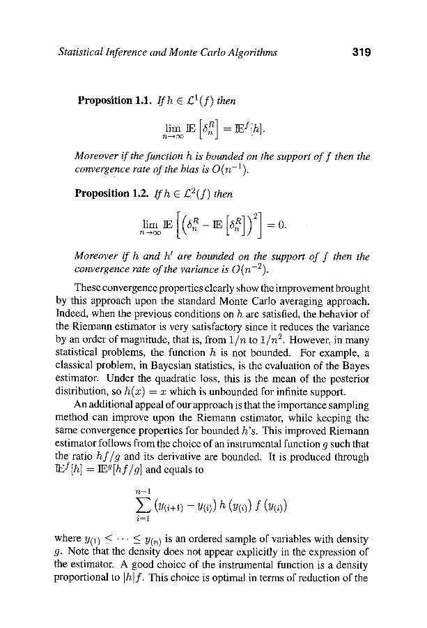
Statistical Inference and Monte Carlo Algorithms 319
Proposition 1.1. If h e E l ( f ) then
[ Zl :
Moreover if the function h is bounded on the support of f then the convergence rate of the bias is O(n-1).
Proposition 1.2. If h C/:2( f ) then
[( End]) lim IF, 6 ~ - I E 6 = 0 . n---~oo
Moreover if h and h I are bounded on the support of f then the convergence rate of the variance is O(n-2).
These convergence properties clearly show the improvement brought by this approach upon the standard Monte Carlo averaging approach. Indeed, when the previous conditions on h are satisfied, the behavior of the Riemann estimator is very satisfactory since it reduces the variance by an order of magnitude, that is, from 1In to 1In 2. However, in many statistical problems, the function h is not bounded. For example, a classical problem, in Bayesian statistics, is the evaluation of the Bayes estimator. Under the quadratic loss, this is the mean of the posterior distribution, so h(x) = x which is unbounded for infinite support.
An additional appeal of our approach is that the importance sampling method can improve upon the Riemann estimator, while keeping the same convergence properties for bounded h's. This improved Riemann estimator follows from the choice of an instrumental function 9 such that the ratio h f / 9 and its derivative are bounded. It is produced through IEf[h] = lEg[h f /g] and equals to
n - 1
(Y(i+l) - Y(i)) h (Y(i)) f (Y(i)) i=1
where Y0) -< "'" -< Y(n) is an ordered sample of variables with density 9. Note that the density does not appear explicitly in the expression of the estimator. A good choice of the instrumental function is a density proportional to [h If. This choice is optimal in terms of reduction of the
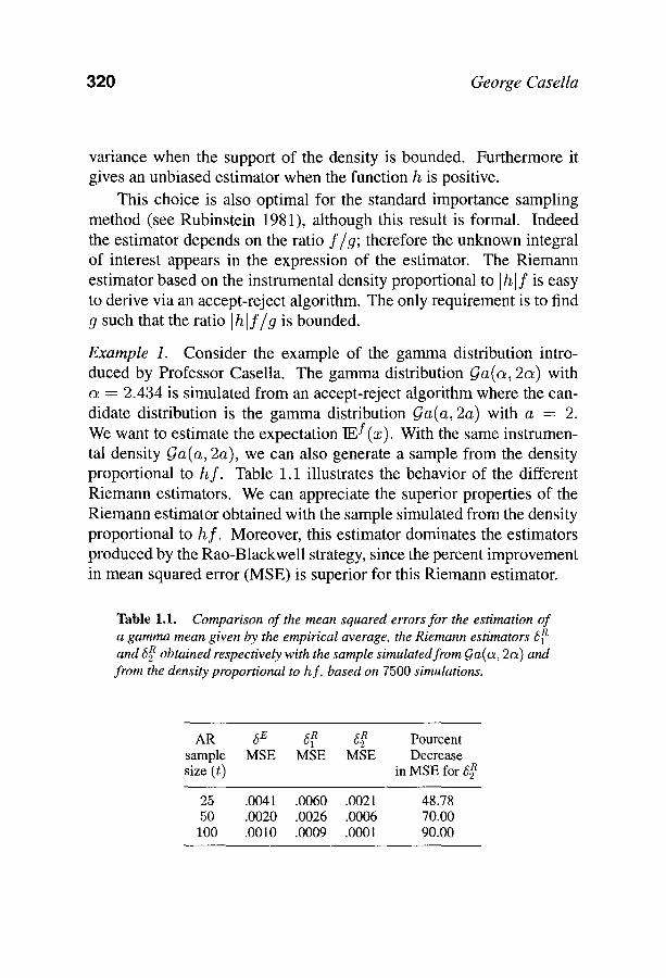
:320 George Casella
variance when the support of the density is bounded. Furthermore it gives an unbiased estimator when the function h is positive.
This choice is also optimal for the standard importance sampling method (see Rubinstein 1981), although this result is formal. Indeed the estimator depends on the ratio f / g ; therefore the unknown integral of interest appears in the expression of the estimator. The Riemann estimator based on the instrumental density proportional to I hL f is easy to derive via an accept-reject algorithm. The only requirement is to find 9 such that the ratio I h l f / 9 is bounded.
Example 1. Consider the example of the gamma distribution intro- duced by Professor Casella. The gamma distribution ~a(oL, 2o 0 with a = 2.434 is simulated from an accept-reject algorithm where the can- didate distribution is the gamma distribution ~a(a , 2a) with a = 2. We want to estimate the expectation IE f (z). With the same instrumen- tal density Ga(a, 2a), we can also generate a sample from the density proportional to h f . Table 1.1 illustrates the behavior of the different Riemann estimators. We can appreciate the superior properties of the Riemann estimator obtained with the sample simulated from the density proportional to h f . Moreover, this estimator dominates the estimators produced by the Rao-Blackwell strategy, since the percent improvement in mean squared error (MSE) is superior for this Riemann estimator.
Table 1.1. Comparison of the mean squared errors for the estimation of a gamma mean given by the empirical average, the Riemann estimators 6~ and <5~ obtained respectively with the sample simulated from Ga(a, 2a) and from the density proportional to h f, based on 7500 simulations.
AR 6 E 61 ~ 6~ Pourcent sample MSE MSE MSE Decrease size (t) in MSE for ~5~
25 .0041 .0060 .0021 48.78 50 .0020 .0026 .0006 70.00 100 .0010 .0009 .0001 90.00
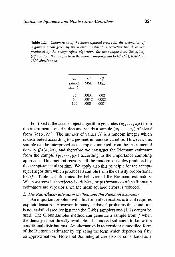
Statistical Inference and Monte Carlo Algorithms 321
Table 1.2. Comparison of the mean squared errors for the estimation of a gamma mean given by the Riemann estimators recycling the N values produced by the accept-reject algorithm, for the sample from Ga(a, 2a) ( 61 n) and for the sample from the density proportional to h f ( 52n), based on 7500 simulations.
AR 5~ 5-2 R sample MSE MSE size (t)
25 .0031 .002 50 .0012 .0002 100 . 0004 .0001
For fixed t, the accept-reject algorithm generates ( Y l , �9 � 9 YN) from the instrumental distribution and yields a sample (Xl,- �9 �9 xt) of size t from Ga(o~, 2o 0. The number of values N is a random integer which is distributed according to a geometric random variable. However, this sample can be interpreted as a sample simulated from the instrumental density Ca(a, 2a), and therefore we construct the Riemann estimator from the sample (Yl , ' - ' , YN) according to the importance sampling approach. This method recycles all the random variables produced by the accept-reject algorithm. We apply also this principle for the accept- reject algorithm which produces a sample from the density proportional to hr. Table 1.2 illustrates the behavior of the Riemann estimators. When we recycle the rejected variables, the performances of the Riemann estimators are superior since the mean squared errors is reduced.
2. The Rao-Blackwellisation method and the Riemann estimator. An important problem with this form of estimators is that it requires
explicit densities. However, in many statistical problems this condition is not satisfied (see for instance the Gibbs sampler) and (1.1) cannot be used. The Gibbs sampler method can generate a sample from f when the density is not directly available. It is indeed sufficient to know the conditional distributions. An alternative is to consider a modified form of the Riemann estimator by replacing the term which depends on f by an approximation. Note that this integral can also be considered as a
322 George Casella
multiple integral. However, the generalization of the Riemann estimator to larger dimensions is not efficient, as shown by Yakowitz et al. (1978).
The Rao-Blackwellisation method produces an estimator of the mar- ginal density (see Gelfand and Smith, 1990). This estimator of the density is given by
n
} ( x ) = n -1 ~ ~ (x14 , . . . , 4 ) - (2.1) t= l
Note that, when we use the Gibbs sampler algorithm, this estimator is available. Therefore, we can always get the following generalized form of the Riemann estimator :
n
,qR/RB -1 ~ " ~ ( ( t + l ) vn = n s ~,Xl -- x(t))h(x (t)) 7r(x ) 1 1 I~k2 ," ' , x �9 t= l \ k = l
(2.2) The computational cost of this estimator is higher than for the standard Riemann estimator but the efficiency is quite similar and it definitely improves upon the empirical average. The performances are illustrated in the case of the auto exponential model (Besag, 1974).
Example 2. Consider the density
f (Yl ,Y2) o( exp(--yl -- Y2 -- YlY2).
The corresponding conditional distribution are given by
YlIY2 ~ gxp(1 + Y2),
Y21Yl ~ $xp(1 + Yl).
Since the marginal density is known up to a constant factor, i.e.
e-y1 f l ( Y l ) 0( - - ,
1 +Yl
we can compare the Riemann estimators (1.1) and (2.1) with the empiri- cal average and the Rao-Blackwell estimator. By running a Monte-Carlo experiment 200 times, we build equal tailed confidence regions Cn such that, for fixed n,
P(e~n C C n ) = 1 - Ol.
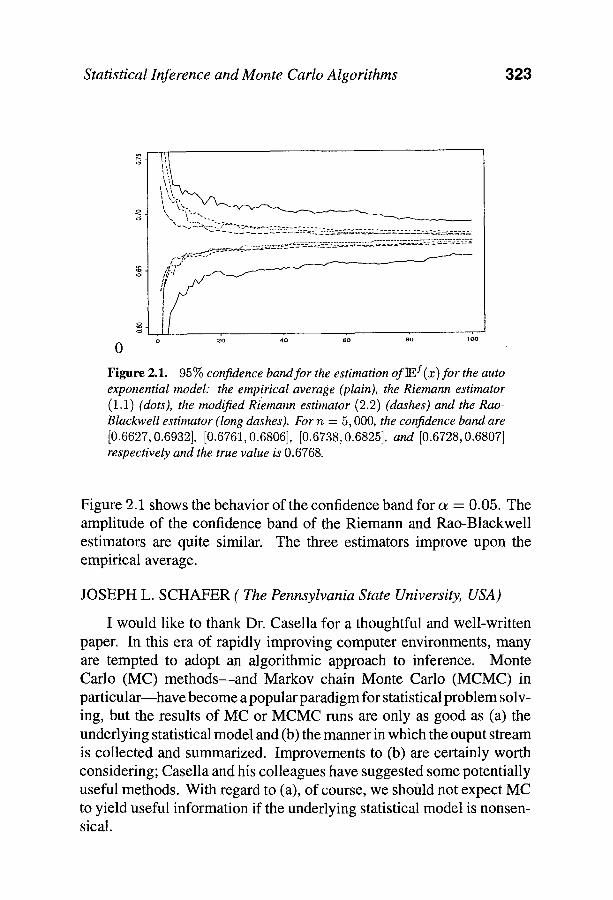
Statistical Inference and Monte Carlo Algorithms 323
....................................................................... v-.-zSL_.~.:.~'~'_~-_ zZ_'-L."
~ j
, j ' ; . . . . . o 2 t l 4 0 6 o s o l o o
0
Figure 2.1. 95% confidence band for the estimation of]Ef (z) for the auto exponential model: the emp(rical average (plain), the Riemann estimator (1.1) (dots), the modified Riemann estimator (2.2) (dashes) and the Rao- Blackwell estimator (long dashes). For n = 5,000, the confidence band are [0.6627, 0.6932], [0.6761, 0.6806], [0.6738, 0.6825], and [0.6728, 0.6807] respectively and the true value is 0.6768.
Figure 2.1 shows the behavior of the confidence band for o~ = 0.05. The amplitude of the confidence band of the Riemann and Rao-Blackwell estimators are quite similar. The three estimators improve upon the empirical average.
JOSEPH L. SCHAFER ( The Pennsylvania State University, USA)
I would like to thank Dr. Casella for a thoughtful and well-written paper. In this era of rapidly improving computer environments, many are tempted to adopt an algorithmic approach to inference. Monte Carlo (MC) methods--and Markov chain Monte Carlo (MCMC) in particular--have become a popular paradigm for statistical problem solv- ing, but the results of MC or MCMC runs are only as good as (a) the underlying statistical model and (b) the manner in which the ouput stream is collected and summarized. Improvements to (b) are certainly worth considering; Casella and his colleagues have suggested some potentially useful methods. With regard to (a), of course, we should not expect MC to yield useful information if the underlying statistical model is nonsen- sical.
324 George Casella
The methods of Sections 4-5 were motivated by principles of clas- sical decision theory. A decision theoretic perspective can be helpful, provided that we pay attention to the MC simulation's original purpose. If the goal is to draw inferences about a parameter h(O) of the data model for y, the Bayesian perspective suggests that we examine the posterior mean, variance, quantiles, etc. of h(O). MC algorithms yield estimates of these quantities which can, in principle, be made as accurate as desired by lengthening the simulation run. Casella et al. focus on improving the efficiency of these MC estimates. That goal, however, is one step removed from the statistician's ultimate purpose. Any reasonable MC estimator of E(h(O) [ y), even if it is not highly efficient, will be good enough if its mean-squared error is small relative to V(h(O) [ y). Im- proving the efficiency of MC estimators is not necessarily profitable if it does not substantially improve the quality of the point and interval estimates for h(O) itself.
A major theme of this paper is the interplay between the data model and the MC simulation method. I prefer to view the MC simulation an additional step of data collection, much like a second stage of sampling in a multistage survey. Let S(ra) denote the output stream from a simulation run of length m. If computational resources were unlimited, we could generate S (~176 and obtain inferences equivalent to those from the actual posterior distribution P(h(O) [ y). In reality we can generate only S (~), so the best inferences attainable will be those based on the reduced information in the posterior P(h(O) [ S(m)). Perhaps we should focus our efforts on approximating P(h(O) [ S(m)).
Rubin's (1987) rules for combining point and variance estimates from a multiply-imputed dataset are based on this type of argument. Multiple imputation (MI) assumes that we have m independent draws of the missing data from their posterior predictive distribution given the observed data. The MI point estimate is simply a Rao-Blackwellized estimate of the posterior mean of h(O), and the MI interval is a credible set based on an approximation to P(h(O) [ S (m)) where m may be very small. Allowances for the smallness of m are thus a built-in feature of the MI interval. Further discussion on the relationship between MI and Rao-Blackwellization is given by Schafer (1996). It may be profitable to consider how to approximate P(A(O) [ S(m)) for larger values of
Statistical Inference and Monte Carlo Algorithms 395
m, where S (m) represents possibly dependent draws of some type of sufficient statistic arising from MCMC.
ROBERT L. STRAWDERMAN (University of Michigan, USA)
It is a pleasure to be asked to participate in this discussion of Pro- fessor Casella's paper, which does an excellent job in describing the in- terplay between Monte Carlo (MC) algorithms and statistical inference. MC itself is an inherently frequentist idea, with "long-run average" con- vergence properties being the primary justification behind its use in most applications. I find it particularly interesting that the vast majority of applications in which MC methods (particularly of the Markov chain va- riety, or MCMC) have been put to use is in solving Bayesian problems. Evidently, frequentist and Bayesian techniques complement each other more than is often explicitly recognized.
A prominent underlying theme of this paper is that MC methods are a very useful yet imperfect tool for statistical inference. Since MC meth- ods have by definition a probabilistic basis, they can often be improved through clever statistical thinking. "Rao-Blackwellization" is indeed a clever method for optimizing an accept-reject (AR) algorithm; how- ever, it is easy to see this procedure becomes impractical very quickly. Termwise conditional expectation is shown to be quite useful, partic- ularly in conjunction with rescaling. The estimator 5Tr (Eqn. 18) is really an importance sampler in disguise; its rescaled pure importance sampling competitor 5Isr (Eqn. 20) is obviously so. It is known (e.g., Hesterberg, 1991, 1993) that simply dividing by the sum of the weights, while often effective, isn't necessarily an optimal procedure for improv- ing importance-based sampling estimates. I wish to comment briefly on this aspect in somewhat more detail, with the particular objective of improving upon both 6rr and 5rSr through the use of control vari- ares. Then, I'd like to propose one possible solution to the problem that Professor Casella poses in Section 5.1.
Let Y[N = n be a random variable having density re(y) (Eqn. 15). Then, we may write -r = Ey[h(X)] = E N [ E Y I N [ h ( Y ) f ( Y ) / m ( Y ) ] ] by the usual importance sampling identity. Notice the similarity here to the weights used in calculating 5TT, hence the importance sampling
326 George Casella
interpretation of @r- Setting d(Y) = h ( Y ) f (Y) /m(Y) , then obviously
EN[EYIN[h(Y)f(Y)/m(Y)] ] = tEN[EYIN[C(Y)] ] + EN[EyIN[d(Y ) - tic(Y)]]
for any function c(Y) and some constant 8. This is the key identity behind control variates in disguise; the optimal choice for t in terms of achieving minimum variance is t -= cov(d(Y), c(Y))/var(c(Y)) (cf. Hesterberg, 1991). Ideally, the more correlated c(Y) and h ( Y ) f ( Y ) / m ( Y ) , the larger the reduction in variance. This may be a difficult choice in practice; thus, for convenience, consider setting c(Y) = d (Y ) f (Y ) /g (Y ) = h(y ) f2 (Y) / (m(Y)g(Y) ) ; then, it is easy to see that #c = E[c(Y)] = Eg[h(Z)f2(Z)/g2(Z)], where Z has density g(-).
Now, let ~ bethe slope of the regression of d(yi) = h(yi)f(yi)/ m(yi) on c(yi), i - 1 . . . n - 1 where (Yl, . . . ,Yn-1) are the first n-1 accepted and rejected rv's. Although Yi and yj are correlated, each is an observation having marginal density m(.). I propose
as a competitor to (~Tr and 6ISr, Where dn-1, en-1 respectively denote the sample averages. Note that if y/, i = 1 . . . n - 1 were an iid sample, then @v asymptotically achieves the minimum variance among linear estimators of the form t # c + (dn -1 - fie-n-l). In practice, we may replace #c by an initial MC estimate/2c, the latter usually being very quick to obtain since g(-) (the AR density) is generally easy to sample from. I reran a small portion of the simulation study done by Professor Casella (with code written in S-Plus) to investigate whether this new estimator provides any additional improvement. The results, represented as a percentage decrease in MSE over 6AR , are summarized in Table 1.
The gains provided by 6cv are impressive here, and have been essen- tially obtained via linear regression; there are few techniques which are more statistical than that! An interesting question here is the asymptotic relative efficiency of this procedure compared to full Rao-Blackwelliza- tion.
Turning now to the question posed in Section 5.1, we wish to deter- mine a* such that
_1 [~* ~m r ( O l Y , Ai)dO = ol
m a - ~ i=1
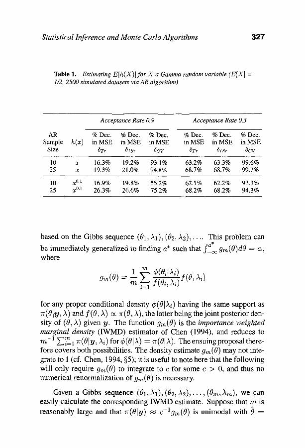
Statistical Inference and Monte Carlo Algorithms 397
Table 1. Estimating E[h(X)] for X a Gamma random variable (E[X] = 1/2, 2500 simulated datasets via AR algorithm)
Acceptance Rate 0.9 Acceptance Rate 0.3
AR % Dec. % Dec. % Dec. % Dec. % Dec. % Dec. Sample h(x) inMSE inMSE inMSE inMSE inMSE inMSE Size 6TT 61Sr 6CV 6Tr 618r 6OV
10 x 16.3% 19.2% 93.1% 63.2% 63.3% 99.6% 25 x 19.3% 21.0% 94.8% 68.7% 68.7% 99.7%
10 x ~ 16.9% 19.8% 55.2% 62.1% 62.2% 93.3% 25 x ~ 26.3% 26.6% 75.2% 68.2% 68.2% 94.3%
based on the Gibbs sequence (01,)~1), ( 0 2 , ) t 2 ) , . . . . This problem can
be immediately generalized to finding a* such that fa~ 9m(8)d8 = c~, where
gin(0) = 1 s r i=l f(Oi'Ai)f(8'Ai)
for any proper conditional density r having the same support as 7r(OlY, )0 and f(O, X) cx 7r(8, ~), the latter being the joint posterior den- sity of (0, A) given y. The function 9m(8) is the importance weighted marginal density (IWMD) estimator of Chen (1994), and reduces to m-1 ~iml 7f(81Y, I~i) for r ) = 7r(0iA ). The ensuing proposal there- fore covers both possibilities. The density estimate gm (8) may not inte- grate to 1 (cf. Chen, 1994, w it is useful to note here that the following will only require gin(8) tO integrate to c for some c > 0, and thus no numerical renormalization of 9m(8) is necessary.
Given a Gibbs sequence ( 8 1 , "~1), ( 8 2 , / ~ 2 ) , . . � 9 (8m, "~m), we can easily calculate the corresponding IWMD estimate. Suppose that m is reasonably large and that ~r(8ly) ~ c-lgra(O) is unimodal with 0 =
398 George Casella
argmaxogm(O ). Then, under some regularity conditions,
(-k(2)(O))v2 } P{O > a} (I'(Ra) + Ra I -- k(l)(a ) r
for k(O) = loggm(O), k(J)(o) = dk(o), and R a : sign(0)[2(k(0) -
k (a))] 1/2 (cf. DiCiccio and Martin, 1993, Eqn. 5). An exactly analogous result obtains in any higher dimensional problem; that is, the formula is exactly the same in the case where a marginal probability calculation is desired for a single component of a vector-valued parameter.
Let H(a; ~) = P{O > a} - o~; note that H(a; c~) is monotone in a. Replacing P{O > a} by the tail probability approximation above, the resulting approximation is monotone in a away from the posterior mean and the extreme tails. Hence, a bisection algorithm will quickly solve H(a*; o~) = 0 for a*; the advantage of bisection over, say, New- ton's method is that the former works without requiring derivatives. Use of this tail probability approximation requires maximization and taking derivatives of k (0) = log gm (0). This should not be of great concern, and will typically not pose a problem in practice. For simplicity, suppose that we have calculated { (ai, gm(ai)), / = 1 . . . b} on a reasonably fine grid (al . . . ab). Then, for example, to obtain an accurate estimate of 0 (the marginal posterior mode), one can fit a quadratic regression to k(O) in a neighborhood about the approximate mode (i.e.,, argmaxa i 9rn(ai)), and
then analytically calculate Oq (and also approximate k(Oq) and k (2) (bq)) using the estimated regression equation (cf. DiCiccio et al., 1996). Al- ternatively, we can take 0 = argmaxa i 9rn (ai) and calculate all derivatives numerically. Each keeps in the spirit of constructing the answer only from the Gibbs sequence.
To illustrate this technique we reanalyzed data from Farewell and Sprott (1988). A mixture model was proposed for analyzing count data; the two-parameter (conditional) likelihood function is given there, as are asymptotic confidence intervals based on the MLE's of the model parameters. This particular example can also be found in Spiegelhalter et al. (1996, BUGS Examples Manual, Volume II, pp. 11-12), where Gibbs sampling is used to construct 95% posterior intervals for the model parameters, both of which are probabilities (p and 0, say) and are assumed independent. The intervals there are found by generating a Gibbs chain
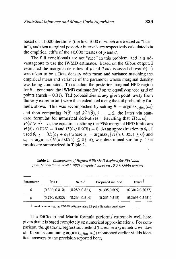
Statistical Inference and Monte Carlo Algorithms 329
based on 11,000 iterations (the first 1000 of which are treated as "burn- in"), and then marginal posterior intervals are respectively calculated via the empirical cdf's of the 10,000 iterates of p and 0.
The full conditionals are not "nice" in this problem, and it is ad- vantageous to use the IWMD estimator. Based on the Gibbs output, I estimated the marginal densities of p and 0 as discussed above; qS(. 1.) was taken to be a Beta density with mean and variance matching the empirical mean and variance of the parameter whose marginal density was being computed. To calculate the posterior marginal HPD region for 0, I generated the IWMD estimate for 0 on an equally-spaced grid of points (mesh = 0.01). Tail probabilities at any given point (away from the very extreme tail) were then calculated using the tail probability for- mula above. This was accomplished by setting t) = argmaxai9m(ai ) and then computing k(~)) and k(J)([9),j = 1,2, the latter via stan, dard formulas for numerical derivatives. Recalling that H(a ; c~) ---- P{O > a} - o~, the equations defining the 95% marginal HPD limits are H(Ou; 0.025) = 0 and H(OL; 0.975) = 0. As an approximation to Ou, I used 0 u j = 0.5(al + a2)where al = argmaxa{H(a;O.025 ) > 0} and a2 = argmina{H(a; 0.025) _< 0}; OL was determined similarly. The results are summarized in Table 2.
Table 2. Comparison of Highest 95% MPD Regions for PVC data from Farewell and Scott (1988) computed based on 10,000 Gibbs iterates
Parameter MLE BUGS Proposed method Exact]
0 (0.300, 0.810) (0.289, 0.823) (0.305,0.805) (0.3012,0.8037)
p (0.270, 0.520) (0.264, 0.514) (0.265,0.515) (0.2693,0.5151)
~ based on renormalized IWMD estimate using 32-point Gaussian quadrature
The DiCiccio and Martin formula performs extremely well here, given that it is based completely on numerical approximations. For com- parison, the quadratic regression method (based on a symmetric window of 10 points containing argmaxai9 m (ai)) mentioned earlier yields iden- tical answers to the precision reported here.
330 George Casella
REPLY TO THE DISCUSSION
First of all, I want to thank the organizers of the meeting, Professors Jos6 Bernardo and Elias Moreno for providing such a lively forum for the exchange of many stimulating ideas. Then I want to thank all of the discussants, who have raised so many interesting points and concerns that I could keep myself and my students busy for many years trying to answer them. For now, I will only try to provide a few thoughts. Since we are all working under time constraints, many of my comments will not be as complete as I would like them to be, but I still hope they will add something. (Indeed, I wish that I had more time to fully digest all of the extremely interesting points raised by the discussants, many with which I wholeheartedly agree.)
It seems to be most logical to arrange my responses by subject rather than people, and I will start with the one that, perhaps evoked the most comments.
1. The Bayes/Frequentist Synthesis
It is gratifying that most people agree that, as statisticians, our main con- cern should be to solve problems as best as we can, and use whatever tools are available. Such are the sentiments of Professors Berger, Gustafson and Wasserman, Ferr~ndiz, Pefia, and Strawderman, with Berger raising a particularly interesting point. My Examples 1 and 2 indeed show how the tools of one approach can help the other approach. The question of the inference, to me, is a somewhat different one in that the appropriate inference is a decision of the experimenter. Although I believe that, in many cases, the frequentist inference is the appropriate one, there are sit- uations where a Bayesian inference is more appropriate. Again, even in the question of inference, there is no (or, at least, little) need to argue. In consultation with the statistician, the experimenter should decide on the appropriate inference, and the statistician should help the experimenter make that inference in the best way possible.
The point is that we shouldn't have Bayesian and frequentist statis- ticians, we should have Bayesian and frequentist inference, to be appro- priately used and recommended by all statisticians.
Statistical Inference and Monte Carlo Algorithms 331
2. Computational Algorithms
At the very least, I am heartened that some of this work has resulted in people being sensitized (but not in the sense of Professor Meng) to the impact of the algorithm on the inference. The concerns of Professor Pefia are well founded, and the guidelines of Professor Rios Insua are quite important. As Professor Schafer points out, focusing on the algorithm may be one step removed from our ultimate purpose, but it is an important step. As we will see in Section 4.2, problems can appear even with seemingly reasonable MC estimators. But even more importantly, I believe that we are all beginning to approach theoretical problems in a new way, always thinking of the computations, and being concerned more with algorithms than theorems. Such an approach can only enhance our thinking and broaden our influence.
3. Posterior Distributions
The power variance priors of model (4) are mainly chosen because (i) experimenters tend to believe that improper priors reflect impartiality and (ii) they result in easy to simulate conditionals. As Professor Pefia notes, the Jeffreys priors considered by Ibrahim and Laud (1991) indeed give proper posterior distributions, as will Professor Bernardo's reference priors, as they both control the tail at zero. Any reanalysis with these priors will result in coherent inferences, the only drawback being that the conditional distributions are not as easy to sample from. However, the inferences are definitely superior.
The popularity of the power prior is an example of the algorithm overshadowing the statistics. Experimenters were so keen to make the Gibbs sampler work that they forgot to check the fundamentals of the model. Moreover, choosing a = b = 0 in (4), which usually is justified through an invariance argument, is extremely unfortunate as, for exam- ple, a = b = 1/2 would yield easily obtained conditionals and proper posterior distributions.
Many discussants had extremely interesting comments and concerns about this topic. I can loosely group those concerns in the following subsections.
3.1. Incompatibility. The property of compatibility of densities has received a lot of comment, and I am heartened that the discussants feel that this property is as important as Jim Hobert and I do. I should first
332 George Casella
mention that, in response to Professors Garcfa-L6pez and Gonzfilez, the results of Theorem 2 hold for the Data Augmentation Algorithm, which can be considered bivariate (but possibly vector valued) Gibbs sampling.
Professor Meng's discovery of his equation (1) is very interesting. It is one of those neat facts that, in hindsight, are totally obvious but, in foresight, are maddeningly difficult to see. I am not aware of the history of the representation, but had seen it presented as a special case of the Hammersley-Clifford Theorem by Robert (1996, Section 5.1.4, Lemma 5.3). It is a wonderful learning equation.
Professor Liu's comments on incompatible densities are also very interesting, and I would like to discuss how they fit in with Theorem 2. In Liu's notation, f l and f2 are proper densities which are not functionally compatible, but Tx(x,x') = f fl(xly)f2(ylx')dy and its counterpart Ty define positive recurrent transition functions. In some sense this is "almost as good" as being compatible, as there will exist limiting prob- ability distributions. Thus, although the inference is more complicated, there is a legitimate inference to be recovered here.
The key fact that gets these limiting distributions is that Tx and Ty define positive recurrent Markov chains. But what happens in the func- tionally compatible (but not compatible ) case? In this case, again using Liu's notation, the marginal distributions 71-1 and 7r2 will not be proper. This follows because, for example, f 71" 1 (y)dy = f f 7r 1 (x, y)dxdy and, by Theorem 2, this latter integral must be co, or else the densities would be compatible. Thus, the situation illustrated by Professor Lib cannot occur in the functionally compatible, but not compatible, case. As an example, consider the exponential densities of Example 3, which are not compatible. There we have
f x, = Ye-xYx 'e -yX 'dy- (x + '
and the invariant distribution is 7rl(X) = l /x, which is easily verified to be the solution to ~-l(X) = f Tx(X,X')Trl(x')dx', and is not a proper distribution.
Perhaps Professor Lib has uncovered a property more fundamental than compatibility. Compatibility will insure the existence of one lim- iting probability distribution, but if Tz and Ty define positive recurrent Markov chains there will be a collection of limiting probability distri- butions. In some cases, this may be enough to recover a reasonable
Statistical Inference and Monte Carlo Algorithms 333
statistical inference. Which leads us to subchains and submodels and the discussions of Professors George and Berger.
3.2. Inferences from an Improper Posterior. The arguments of Professor George are not compelling, because in every case the full Gibbs chain clearly contains extraneous pieces. To put it more formally, suppose that we are interested in inference about the parameter fl, and have a model that results in the full, improper posterior 7r(a, fl[y), where a is another parameter of the model, considered as a nuisance parameter when the inference is about/3. Inferences about/3 would be based on the marginal posterior 7r(/3[y), which should satisfy
7r(/3[y ) = / 7r(a, /31y)da. If so, then it is impossible for 7r(/31y ) to be proper, as
f ~r(/3,y)d/3= f Tr(a,/3,y)dad/3=cc. Thus there is no meaningful inference about the parameter/3 that can be recovered from the full model. (I also suspect that any inference about /3 in this model would be incoherent in the sense of Heath and Sudderth 1989).
So what about the experience of Berger, and the examples of George? These are instances in which there is reason to abandon the full model. That is, the transformations of George, and the "identifiability" of B erger are procedures for changing the model. In my illustration above, the parameter a would be somehow eliminated, and only/3 would be con- sidered, with a proper 7r(/3ly ). So my point is that if a model results in an improper full posterior, there is no lower dimensional inference based on the full model that can make sense. However, there may be a lower dimensional model that makes sense. I have no problem with this solution, but realize that the model is being changed in a fundamental way; we are not recovering anything from the improper posterior distri- bution. The interesting procedure discussed by Meng, that of recursive deconditioning seems to be an excellent candidate for searching for such lower dimensional models
3.3. Fixing Impropriety. If the posterior distribution is improper, an obvious fix is to replace it with a sufficiently "vague" proper prior that
334 George Casella
is close to it. This is the spirit of Berger's suggestion to constrain cr > 0 in Example 4. As the values of cr do not spend too much time near the singularity at zero (as noted at the end of Example 4), the constrained prior might be a reasonable approximation here. However, such a fix may not always work. Natarajan and McCulloch (1996) investigate the effects of replacing improper priors with vague, proper priors and find that there is no happy medium between "proper but diffuse" and "improper". In particular, in situations where the posterior does not exist, the Gibbs sampler can break down before the prior becomes diffuse enough to yield estimates that are reasonable approximations to the MLE. But I guess that my sentiments on this problem are most in line with Gustafson and Wasserman, when they state that to use a proper vague prior is "..simply to approximate an ill defined solution".
The behavior of this Gibbs chain also answers the comment of Rios Insua, who expected more mass near zero. Such behavior was not ex- hibited by the chain, even with many restarts and many long runs (which should have eliminated any problems due to sample size or starting points - a concern of Garcia-L6pez and Gonzalez). This also illustrates, once again, the (apparent) futility of trying to have the Gibbs output check itself for propriety.
4. Rao-Blackwellization
The technique of Rao-Blackwellization has expanded beyond the origi- nal idea of conditioning on a sufficient statistic. Indeed, in my thinking, it has expanded to encompass a class of techniques that aim at improv- ing estimators by taking advantage of the structure of the problem in whatever manner is available.
I don't believe that we have returned to the status quo, as stated by Berger. Even in situations where we end up with the same procedures, we also end up learning a lot (the gains of Rao-Blackwellization can be huge, and easy to obtain) and have not always returned to the status quo (the full Rao-Blackwellized estimator is still the only one to achieve substantial gains while retaining unbiasedness.) Although Femindiz rightly points out that the Rao-Blackwellization in the paper only applies to algorithms with ancillary random variables, the general approach goes far beyond this case. Perhaps the most important contribution is that we have stimulated thinking to search for better ways to process the output,
Statistical Inference and Monte Carlo Algorithms 335
searches that have resulted in procedures such as those put forth by Professors Phillipe and Strawderman which, in our expanded definition, are again some sort of Rao-Blackwellization.
Rao-Blackwellization is a type of smoothing, and the advantages of such smoothing are well documented. I was particularly interested in the interpretations of Professor Dawid that cast new light on impor- tance sampling, accept-reject, and weighted averages. Dawid's discus- sion clearly shows the drawback of the naive accept-reject average, and the advantage of the "Rao-Blackwellization" brought on by importance sampling.
Before replying to some of the other comments on Rao-Blackwell- ization, I would like to elaborate on a small point that has intrigued me for a while. Although it is clear that importance sampling is a desir- able technique when compared to accept-reject or Metropolis-Hastings averages, its usefulness in the Gibbs sampler is not at all clear. For a bivariate Gibbs sampler (X1 , ]I1), (X2 , ]I2), "" ", (Xm, Ym), where we generate Xi ,.o f(xlYi) and Y/+I ~ f(ytXi), a Gibbs estimate
1 m ~G = N }--~i=1 h(Xi) has an importance sampling counterpart
1 ~ f(Xi) (~IS = -'~ i=1 f(XilYi)
h(Xi)
(ignoring the possibility that the marginal f(x) may not be computable). An interesting fact is that
E [ f~)f(Xi) h(Xi) Xi] = h(Xi),
so, here, the naive Gibbs average is the "Rao-Blackwellization" of the importance sampling estimate. However, dominance does not follow immediately, as there are covariances to contend with. But, I can show that for m = 2, var(Sa) < vat(Sis). Thus, this may be saying that the Gibbs sampler is already "smooth enough", and there is no room for further smoothing.
4.1. Termwise Rao-Blackwellization. First a short comment on the discussions of Liu and Dawid about termwise conditioning, and the importance of the stopping rule-it cannot be ignored. The stopping rule brings us the fact that the accept-reject estimator (10) is both unbiased and
336 George Casella
"correct for constants". This is perhaps more clear when the estimator is written in the form (9), which can only be done with the knowledge of the value of t, that is, with knowledge of the stopping rule. The estimator 6is of Liu's discussion, that is,
n 1 (m)
~Is = n
/=I
cannot be directly related to either (9) or (10). It is a Rao-Blackwelliza- tion of
60 = - I[Ui < w(yi)]h(yi) n
i=1
under independent sampling and
v&r((~0) : v&r[E((~olY1,""", Yn)]-1- E [ v a r ( 6 o l Y 1 , . - . Yn)] n
- - + E [ v a r ( 5 o l Y 1 , - . . i=1
= var[61s] + E[var(6olY1,..- Yn)] _> var[5is].
But this does not prove dominance of (R1) over 5AR of (10) and, in- deed, this is not the case as bAR will dominate for constant functions as indicated by Table 2. So, in fact, without correcting for constants, or taking into account the stopping rule, neither 5Is nor 50 are particularly attractive estimators.
Professors Liu and Dawid also make similar points about the desir- ability of using weights based on marginal chains, where possible. The marginalization seems to smooth things out, and make it sometimes pos- sible to achieve variance reduction. However, there are some unforeseen pitfalls here-a built in computational difficulty in the marginalization. There is a need for trade-off in that the original algorithms will often replace an analytic calculation with computer time and random variable generation, and the marginalization may require a difficult analytic cal- culation, a point noted by Liu. For example, the proposal of Dawid, which seems to carry along with it some excellent variance reduction potential, also carries along a large computational burden. The follow- ing simple example was pointed out by Christian Robert, where we take
Statistical Inference and Monte Carlo Algorithms 337
7v(y) ~: e x p ( - y 2 / 2 ) , q(y[x) c< exp(-[x 2 + y2]/2) and the result- ing c~(x, y ) = min{u(y)q(xly)/Tr(x)q(y[x), 1}, the usual Metropolis- Hastings choice. We then get a fl(x) of the form
e (x ) = (Ixl- x) - x)
exp(x2/4) {1 - x)] + + x)]} +
making for a difficult simulation algorithm. Perhaps this problem should be approached using decision theory, where we balance ease of compu- tation with variance reduction through a loss function.
4.2. Subtleties. Next, I would like to elaborate on the point made by Gustafson and Wasserman about the failure of the average of conditional densities (ACD) to accurately estimate the marginal. At first, their ex- ample was bewildering to me, and there seemed to be no reason for such behavior. To better understand the "paradox" I reduced it to bare essen- tials, and learned the following. The failure of the ACD estimate has nothing to do with Gibbs sampling, impropriety, or Markov chains. It is, in fact, a failure to satisfy the assumptions of the Lebesgue Dominated Convergence Theorem!
Consider that in their example all of the relevant distributions are proper, and the Ergodic Theorem applies. Thus, if we obtain the random variables ul , u2 , . . . , we must have for each t
%21~,y(tlu(i), y) --+ %21~,u(tlu, y)m(uly)du, (R2) i=1
where m(uly ) is the proper marginal distribution of u. So (R2) holds for each t in the Gustafson/Wasserman example. It seems that there is a real mystery as to why the convergence fails at 0. But a little reflection brings an interesting realization. Write
7r(01y ) = lim 7rG21y(tly ) = lim J[" %21~,u(tlu, y)m(uly)du. t--~O t~O At t = 0, indeed for any t = to, the Monte Carlo sum converges to
m
1 > .%el~,y(tolu(i),y ) ~ f %zl~,v(tolu, y)m(uly)d u - - d
m i=1
= / l i r a %21~,y(tlu, y)m(ulu)du. J t-~t 0
338 George Casella
Thus, when we construct a Monte Carlo sum such as in (R2), we are implicitly interchanging the order of limit and integration ! It is straight- forward to check that Dominated Convergence will hold here for every to > 0, but fails at to = 0. This example illustrates that things can go wrong even when all distributions are proper.
4.3. Other Estimates. Comparing the performance of Rao-Blackwelli- zation to a weighted bootstrap, or double bootstrap, as suggested by Garcia-L6pez and Gonz~ilez, would be an interesting endeavor. As these procedures are related to importance sampling, we would expect reason- able performance and perhaps easy implementation. I hope to look into this in the future.
There were other very interesting competitors to the Rao-Blackwell improvement suggested by other discussants. First, I would like to further explore the control-variate estimator proposed by Strawderman, and try to understand why it does so incredibly well. The simple answer seems to be that it is based on a much bigger sample size. But the more interesting answer is that it takes even better advantage of the algorithmic construction.
I think of control variates as finding the appropriate unbiased es- timator of zero. To improve on an estimator 50(x) by the method of control variates, we find another estimator u(x), with known mean/z, and construct 61(x) =- 60(x) + b[u(x) - #] for some constant b. Then 50 and 61 have the same expected value, and var(61) -- "car(60) + var(u) + 2cov(60, u). If we choose b to have the optimal value b = -cov(60, u), then we achieve the maximal variance reduction var(51) = (1 - p2)var(60), where p is the correlation between 60 and u. Straw- derman has given us a methodology for implementing such a control variate scheme in any importance sampler. And why does it do so much better? The answer lies in his calculation of/2c. In a control variate scheme, this is a known parameter, and Strawderman estimates it by taking a very large sample from 9. So, in effect, his estimator is based on a much larger sample size than 6Tr or 6ISr. Is this an unfair com- parison? You bet it is! Is this an unfair estimator. No! In fact, it shows us another clever way of recycling the rejected random variables! This control variate scheme deserves further investigation. I would be very interested in seeing how it compares to 6Tr or 6ISr when we keep the number of generated random variables the same for each estimator.
Statistical Inference and Monte Carlo Algorithms 339
The discussion of Professor Phillipe is literally brimming with inge- nious ideas that not only yield new (and seemingly excellent) estimators, but also illustrates the benefits of intertwining algorithmic and statisti- cal thinking. Her Riemann sum estimator (1) appears to be a serious competitor to all of the other estimators developed in these pages, but I think the most interesting developments are in her subsequent estimator, where the instrumental density 9 is chosen to satisfy the boundedness requirements of her Propositions 1 and 2. What a terrific blending of algorithms and theory ! The use of the Gibbs average as a substitute for the marginal also has nice potential, although one must be on guard for difficulties such as those illustrated in Section 4.2.
5. Other Concerns
5.1. Multiple Paths. The question of multiple path Gibbs sampling was raised by both Bernardo and Garcfa-Ldpez and Gonzfilez, although in different contexts. Firstly, the number of paths used in the Gibbs sampler will not have any impact on propriety or compatibility, as these are properties of the underlying model, and the manner in which we observe the model cannot have any bearing. The question of how multiple paths can affect the variance of our estimate is also an interesting one, and prompted me to write the following.
Suppose that we have data Y, and want to calculate an estimate 5(Y) of 7- = E[5(Y)]. Using a Monte Carlo algorithm to calculate 5(Y) , we obtain an output string from the algorithm, a sample T of length k, and calulate ~Sk(Y ) as our approximation of 5(Y). Note that we could refer to 6(Y) as 6oo(Y), the value of the estimate based on an infinite sample from our algorithm, that is, a sample Too of infinite length. We then also have that E[Sk(Y)[Too] = 5(Y). Now suppose that we run the algorithm many times ( for example, a multiple path Gibbs sampler), and let T1,. �9 �9 Tm be m independent output strings from the algorithm, each
of size k. For each Ti calculate the valjues 5~ i) and take as our estimate
~k -- ml ~im__l 5~i). The following variance analysis, which may be similar in spirit to those discussed by Schafer, should apply whether we are considering Bayesian or frequentist measures.
340 George Casella
The variance of 5k is given by
var[6k(Y)] = var(E[Sk(Z)lT~]) + E[var(Sk(Y)lT~)] 1 2
= var[5(Y)] + mE[~-~] (R3)
where -r~ = var(b~ i) tTi), the variance that is only due to the algorithm, and is not due to the model. Now we can see the effect of multiple paths (m) and increasing the length of the chain (k). As k -* co, -r~ -+ 0, so increasing the length of the chain will reduce the variation due to the algorithm and also diminish the effect of Rao-Blackwellization (but, as we saw in Section 5.2, not erase it). However, increasing m, the number of paths, has no direct effect on z~, but still will reduce var(5). But this latter situation is less desirable, as we should strive to eliminate the variation due solely to the algorithm (which is under our control). Thus, this naive analysis seems to show that there is less to be gained in variance reduction, whether the criterion is Bayesian or frequentist, from running multiple chains.
Equation (R3) may also answer the concern of Rfos-Insua that our stream of "endless data" eliminates the role of Bayesian statistics. In- deed, a more careful analysis of (R3), and the effects of changing k and m would almost certainly need some form of prior input to help balance the effects of the model and the algorithm.
5.2. Accurate Approximations. Professor Strawderman reminds me of one of my own lessons, that of not forgetting that we are statisticians with a large box of tools. He brings the methods of higher-order asymptotics to bear on the Gibbs sampler, showing that the DiCiccio/Martin tail prob- ability approximation results in an extremely accurate approximation to the desired posterior probability in Section 5.1. Bravo. Professors Di- Ciccio and Wells also note the place for higher-order asymptotics, and make an interesting point about recovering a frequentist inference in the face of the Bayesian "catastrophe". Of course, whether the posterior distribution is proper has no bearing on the frequentist inference, which can always be made. However, under such catastrophic priors, such as a = b = 1, the Gibbs sampler cannot be used to produce reasonable fre- quentist inferences. Indeed, conjecturing based on the results of Nataran and McCulloch (1996), such catastrophic priors could leave us quite far from reasonable frequentist inference.
Statistical Inference and Monte Carlo Algorithms 341
Also, as noted by DiCiccio and Wells, there is much interest now in "probability matching", or finding prior distributions (such as Welch- Peers) that result in posterior probabilities that match frequentist prob- abilities. Although such priors are necessarily improper, they also nec- essarily must result in proper posterior distributions, hence avoiding the impropriety problems. This suggests that probability matching could be a reasonable basis for choosing a default prior and should be acceptable to an experimenter as an "impartial" choice. Moreover, I think there is still room for Rao-Blackwellization for, at the very least, it will serve to minimize the error due solely to the Monte Carlo algorithm.
5.3. Decision Theory. It is quite gratifying that the mixing of Decision Theory with algorithmic performance is viewed favorably by many of the discussants. The sentiments of Femindiz perhaps most closely reflect my own, in that I am hopeful for many benefits from embedding the algorithm in the appropriate decision problem.
The research here is still in the beginning stages, so although we have interesting possibilities, there are still few definite recommendations. I have no answer for Berger on the performance of the optimal minimax scan, but it seems that the calculations of Professors DiCiccio and Wells hold promise that we are looking at a good criterion. They have provided more convincing evidence that the risk function does a more complete job in capturing the essentials of the Markov chain.
ADDITIONAL REFERENCES IN THE DISCUSSION
Andrews, R., Berger, J. and Smith, M. (1993). Bayesian estimation of fuel economy potential due to technology improvements. Case Studies in Bayesian Statistics (C. Gatsonis, et al., eds.), 1-77. New York: Springer-Verlag.
Berger, J. O. and Bernardo, J. M. (1992). Reference priors in a variance compo- nents problem. Bayesian Analysis in Statistics and Econometrics (P. K. Goel and N. S. Iyengar, eds.). Berlin: Springer, 323-340.
Berger, J. and Strawderman, W. (1996). Choice of hierarchical priors: admissibility in estimation of normal means. Ann. Statist. 24, 931-951.
Bernardo, J. M. (1979). Reference posterior distributions for Bayesian inference. J. Roy. Statist. Soc. B 41, 113-147 (with discussion). Reprinted in Bayesian Inference (N. G. Poison and G. C. Tiao, eds.), Brookfield, VT: Edward Elgar, (1995), 229- 263.
Besag, J. (1974). Spatial interaction and the statistical analysis of lattice systems. J. Roy. Statist. Soc. B 36, 192-236 (with discussion).
3 4 2 George Casel la
Box, G. E. E (1980). Sampling and Bayes' inference in scientific modelling and ro- bustness. J. Roy. Statist. Soc. A 143, 383--430.
Caracciolo, S., Pelissetto, A. and Sokal, A. D. (1990). Nonlocal Monte Carlo algorithms for self-avoiding walks with fixed endpoints. J. Stat. Phys. 60, 7-53.
Chen, M. (1994). Importance-weighted marginal Bayesian posterior density estima- tion. J. Amer. Statist. Assoc. 89, 818-824.
Christiansen, C. and Morris, C. (1995). Hierarchical Poisson regression modeling. Tech. Rep., Department of Health Care Policy, Harvard.
Daniels, M. (1996). A prior for the variance in hierarchical models. Tech. Rep., De- partment of Statistics, Carnegie Mellon University.
Daniels, M. and Gatsonis, C. (1996). Multilevel hierarchical generalized linear models in health services research. Tech. Rep., Department of Health Care Policy, Harvard.
Dawid, A. E, Stone, M. and Zidek, J. V. (1973). Marginalization paradoxes in Bayesian and structural inference. J. Roy. Statist. Soc. B 35, 189-233 (with discussion).
Diaconis, E and Stroock, D. (1991). Geometric bounds for eigenvalues of Markov Chains. Ann. Appl. Probab. 1, 36-61.
DiCiccio, T. and Martin, M. (1993). Simple modifications for signed roots of likelihood ratio statistics. J. Roy. Statist. Soc. B 55, 305-316.
DiCiccio, T., Kass, R., Raftery, A. and Wasserman, L. (1996). Computing Bayes factors by combining simulation and asymptotic approximations. Tech. Rep., Carnegie- Mellon University, Pittsburgh PA.
DuMouchel, W. (1994). Hierarchical Bayes linear models for meta-analysis. Tech. Rep. 27, National Institute of Statistical Sciences.
Farewell, V. and Sprott, D. (1988). The use of a mixture model in the analysis of count data. Biometrics 44, 1191-1194.
Ferr~indiz, J., L6pez, A., Llopis, A., Morales, M. and Tejerizo, M. L. (1995). Spatial interaction between neighouring counties: cancer data in Valencia, (Spain). Bio- metrika 51,665-678.
Gelfand, A. and Rubin, D. R. (1991). A single series from the Gibbs sampler pro- vides a false sense of security. Bayesian Statistics 4 (J. M. Bernardo, J. O. Berger, A. E Dawid and A. E M. Smith, eds.). Oxford: University Press, 625-631.
Gelfand, A. E. and Smith, A. E M. (1990). Sampling based approaches to calculating marginal densities. J. Amer. Statist. Assoc. 85, 398--409.
Geman, S. and Geman, D. (1984). Stochastic Relaxation, Gibbs Distributions and the Bayesian Restoration of Images. IEEE Trans. Pattern. Anal. Mach. Intelligence 6, 721-741.
Geyer, C. J. and Thompson, E. A. (1992). Constrained Monte Carlo maximum likeli- hood calculations. J. Roy. Statist. Soc. B 54, 657-699 (with discussion).
Geyer, C. J. and Thompson, E. A. (1995). Annealing Markov Monte Carlo with appli- cations to ancestral inference. J. Amer. Statist. Assoc. 90, 909-920.
Green, E. J. and Strawderman, W. E. (1991). A James-Stein type estimator for com- bining unbiased and possibly biased estimators. J. Amer. Statist. Assoc. 6, 416, 1001-1006.
Statistical Inference and Monte Carlo Algori thms 3 4 3
Gidas, B. (1995). Metropolis-type Monte Carlo simulation algorithms and simulated annealing. In Topics in Contemporary Probability and Its Applications. (J. L. Snell, ed.). CRC Press.
Heath, D. and Sudderth, W. (1989). Coherent inference from improper priors and from finitely additive priors. Ann. Statist. 17, 907-919.
Hesterberg, T. (1991). Weighted average importance sampling and defensive mixture distributions. Tech. Rep. 148, Division of Biostatistics, Stanford University.
Hesterberg, T. (1993). Control variates and importance sampling for the bootstrap. ASA Proc. the Statist. Computing Section, ASA, Alexandria, VA, 40---48.
Hoaglin, D. and Andrews, D. (1975). The reporting of computation-based results in statistics. The American Statistician 29, 122-126.
Justel, A. and Pefa, D.(1996a). Gibbs sampling will fail in outlier problems with strong masking. J. Comp. Graphical Stat. 5, 176--189.
Justel, A and Pefia, D. (1996b). Bayesian unmasking in linear models. Tech. Rep., Uni- versidad Carlos III de Madrid.
Liu, J. S. (1996). Metropolized independent sampling with comparisons to rejection sampling and importance sampling. Statistics and Computing 6, 113-119.
Liu, J. S., Chen, R. and Wong, W. H: (1996). Rejection control and importance sampling. Tech. Rep., Department of Statistics, Stanford University.
Liu, J., Wong, W. H. and Kong, A. (1992a). Correlation Structure and convergence rate of the Gibbs sampler: Applications to the comparison of estimators and augmen- tation schemes. Tech. Rep. 299, University of Chicago.
Kemeny, J. G. and Snell, J. L. (1983). Finite Markov Chains. Berlin: Springer MacEachern, S. N., Clyde, M. A., and Liu, J. S. (1996). Sequential importance sampling
for nonparametric Bayes models: the next generation. Tech. Rep., Department of Statistics, Stanford University.
Muller, P. and Rfos Insua, D. (1996). Issues in the Bayesian analysis of neural network models. Tech. Rep., UPM.
Natarajan, R., and McCulloch, C. E. (1996). Gibbs sampling with diffuse priors: a valid approach to data-driven inference? Tech. Rep. BU-1313-M, Cornell University. Under revision for J. Comp. Graph. Statist.
Ng, K. W. (1995). On the inversion of Bayes theorem. Talk presented to the The 3rd ICSA Statistical Conference, August 17-20, 1995, Beijing, China.
Pefia, D. and Tiao G. C. (1992). Bayesian robustness functions for linear models. Bayesian Statistics 4 (J. M. Bernardo, J. O. Berger, A. P. Dawid and A. E M. Smith, eds.). Oxford: University Press
Philippe, A. (1996). Processing simulation output by Riemann sums. Tech. Rep. 02, Uni- versit6 de Rouen.
Peskun, P. H. (1973). Optimal Monte Carlo sampling using Markov chains. Bio- metrika 60, 607-612.
Rfos Insua, D., Rfos Insua, S. and Martin, J. (1997). Simulation: Methods and Appli- cations. RA-MA. (In Spanish)
344 George Casella
Robert, C. E (1996). Mgthodes de Monte Carlo par Chafnes de Markov. Paris: Eco- nomica.
Rubin, D. B. (1987). Multiple Imputation for Nonresponse in Surveys. New York: Wiley.
Rubinstein, R. Y. (1981). Simulation and the Monte Carlo Method. New York: Wiley. Samaniego, J. E and Renau, D. M. (1994). Towards a reconciliation of the Bayesian
and frequentist approaches to point estimation. J. Amer. Statist. Assoc. 89, 427, 947-957.
Schafer, J. L. (1996). Analysis of Incomplete Multivariate Data. London: Chapman and Hall, (in press).
Smith, A. and Gelfand, A. (1992). Bayesian statistics without tears. Amer. Stat. 46, 84-88.
Sokal, A. D. (1989). Monte Carlo Methods in Statistical Mechanics: Foundations and New Algorithms. Cours de Troisi~me Cycle de la Physique en Suisse Romande, Lausanne.
Spiegelhalter, D., Thomas, A., Best, N. and Gilks, W. (1996). BUGS: Bayesian Infer- ence Using Gibbs Sampling, Version 0.50. Cambridge: MRC Biostatistics Unit.
Stein, C. (1959). An example of wide discrepancy between fiducial and confidence intervals. Ann. Math. Statist. 30, 877-880.
Strawderman, W. E. (1971). Proper Bayes minimax estimators of the multivariate normal mean. Ann. Math. Statist. 42, 385-388.
Tanner, M. A. and Wong, W. H. (1991). The calculation of posterior distributions by data augmentation. J. Amer. Statist. Assoc. 82, 528-550, (with discussion).
Verdinelli, I. and Wasserman, L. (1995). Computing Bayes factors by using a general- ization of the Savage-Dickey density ratio. J. Amer. Statist. Assoc. 90, 614-618.
Yakowitz, S., Krimmel, J. E. and Szidorovszky, E (1978). Weighted Monte-Carlo integration. SIAM J. Numer. Anal. 15, 1289-1300.
Related Documents