Statistical Fundamentals: Using Microsoft Excel for Univariate and Bivariate Analysis Alfred P. Rovai The Normal Curve and z-Scores PowerPoint Prepared by Alfred P. Rovai Presentation © 2013 by Alfred P. Rovai Microsoft® Excel® Screen Prints Courtesy of Microsoft Corporation.

Statistical Fundamentals: Using Microsoft Excel for Univariate and Bivariate Analysis Alfred P. Rovai The Normal Curve and z-Scores PowerPoint Prepared.
Dec 11, 2015
Welcome message from author
This document is posted to help you gain knowledge. Please leave a comment to let me know what you think about it! Share it to your friends and learn new things together.
Transcript

Statistical Fundamentals: Using Microsoft Excel for Univariate and Bivariate Analysis
Alfred P. Rovai
The Normal Curve and z-Scores
PowerPoint Prepared by Alfred P. Rovai
Presentation © 2013 by Alfred P. Rovai
Microsoft® Excel® Screen Prints Courtesy of Microsoft Corporation.

Copyright 2013 by Alfred P. Rovai
Normal Curve
• The normal or Gaussian curve is a family of distributions.• It is a smooth curve and is referred to as a probability density
curve for a random variable, x, rather than a frequency curve as one sees in a histogram.– The area under the graph of a density curve over some interval represents
the probability of observing a value of the random variable in that interval.
• The family of normal curves has the following characteristics:– Bell-shaped– Symmetrical about the mean (the line of symmetry)– Tails are asymptotic (they approach but do not touch the x-axis)– The total area under any normal curve is 1 because there is a 100%
probability that the curve represents all possible occurrences of the associated event (i.e., normal curves are probability density curves)
– Involve a large number of cases

Copyright 2013 by Alfred P. Rovai
Normal Curve
Various normal curves are shown above. The line of symmetry for each is at μ (the mean). The curve will be peaked (skinnier or leptokurtic) if the σ
(standard deviation) is smaller and flatter or platykurtic if it is larger.

Copyright 2013 by Alfred P. Rovai
Empirical Rule
In a normal distribution with mean μ and standard deviation σ, the approximate areas under the normal curve are as follows:
• 34.1% of the occurrences will fall between μ and 1σ• 13.6% of the occurrences will fall between 1σ & 2σ• 2.15% of the occurrences will fall between 2σ & 3σ
If one adds percentages, approximately:
• 68% of the distribution lies within ± one σ of the mean.
• 95% of the distribution lies within ± two σ of the mean.
• 99.7% of the distribution lies within ± three σ of the mean.
These percentages are known as the empirical rule.
Given a normal curve (i.e., a density curve), if , μ = 10 and σ = 2, the probability that x is between 8 and 12 is .68.

Copyright 2013 by Alfred P. Rovai
When μ = 0 and σ = 1, the distribution is called the standard normal distribution.
• 34.1% of the occurrences will fall between 0 and 1• 13.6% of the occurrences will fall between 1 & 2• 2.15% of the occurrences will fall between 2 & 3

z-Scores
Copyright 2013 by Alfred P. Rovai
• A standard score is a general term referring to a score that has been transformed for reasons of convenience, comparability, etc.
• The basic type of standard score, known as a z-score, is a measure of a score’s distance from the mean in standard deviation units. – If z = 0, it’s on the mean.– If z = 1.5, it’s 1.5 standard deviations above the mean.– If z = -1, it’s 1.0 standard deviations below the mean.
• A z-score distribution is the standard normal distribution, N(0,1), with mean = 0 and standard deviation = 1. The formula for calculating z-scores from raw scores is
• Most other standard scores are linear transformations of z-scores, with different means and standard deviations. For example, T-scores, used in the Minnesota Multiphasic Personality Inventory (MMPI), have M = 50 and SD =10, and SAT scores have M = 500 and SD = 100.

Why z-Scores?
Copyright 2013 by Alfred P. Rovai
• Transforming raw scores to z-scores facilitates making comparisons, especially when using different scales.
• A z-score provides information about the relative position of a score in relation to other scores in a sample or population.– A raw score provides no information regarding the relative standing of
the score relative to other scores.– A z-score tells one how many standard deviations the score is from
the mean. It also provides the approximate percentile rank of the score relative to other scores. For example, a z-score of 1 is 1 standard deviation above the mean and equals the 84.1 percentile rank (50% of occurrences fall below the mean and 34.1% of the occurrences fall between 0 and 1; 50% + 34.1% = 84.1%).

Calculating z-Scores from Raw Scores
Copyright 2013 by Alfred P. Rovai
23 28.84 -5.84 6.24 -.9422 28.84 -6.84 6.24 -1.1033 28.84 4.16 6.24 .6719 28.84 -9.84 6.24 -1.58
X XX SD SD
XXz
A raw score of 23 equals a z-score of – .94, indicating both scores are .94 standard deviations below the mean.
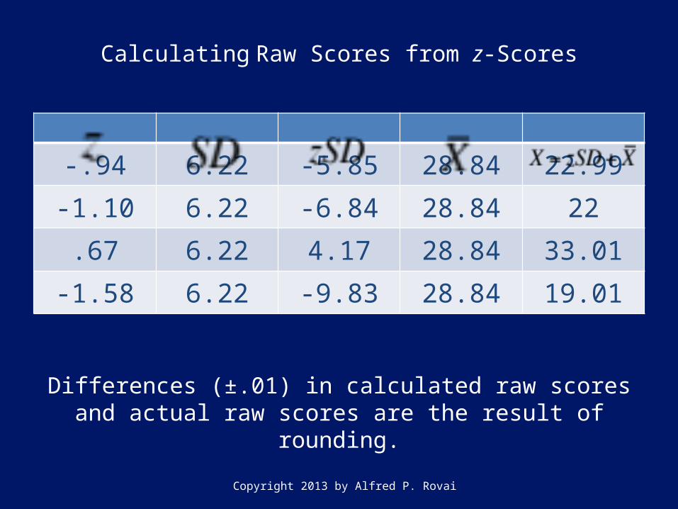
Calculating Raw Scores from z-Scores
Copyright 2013 by Alfred P. Rovai
-.94 6.22 -5.85 28.84 22.99-1.10 6.22 -6.84 28.84 22.67 6.22 4.17 28.84 33.01
-1.58 6.22 -9.83 28.84 19.01
Differences (±.01) in calculated raw scores and actual raw scores are the result of rounding.

Copyright 2013 by Alfred P. Rovai
Open the dataset Motivation.xlsx.Click the worksheet Descriptive Statistics tab (at the bottom of the worksheet).
File available at http://www.watertreepress.com/stats
TASK Convert classroom community (c_community) raw
scores into z-scores.

Copyright 2013 by Alfred P. Rovai
Excel includes the following function that converts raw scores to z-scores:
STANDARDIZE(number,AVERAGE(number1,number2,...),STDEV.P(number1,number2,...)). Returns a standardized value.
Enter the following formula in cell F2:=STANDARDIZE(A2,AVERAGE(A$2:A$170),STDEV.P(A$2:A$170)).
Click on cell F2, hold the Shift key down, and click on cell F170 in order to select the range F2:F170.
Using the Excel Edit menu, select Fill Down. The z-scores are displayed in column F.

Copyright 2013 by Alfred P. Rovai
An alternative method is to use the z-score formulaZ = (X – )/x̄� SD.
First, calculate the c-community mean in cell D2 using the formula =AVERAGE(A2:A170).
The mean is 28.84.

Copyright 2013 by Alfred P. Rovai
Next, calculate the c-community standard deviation in cell D6 using the formula
=STDEV.P(A2:A170). The standard deviation is 6.22.

Copyright 2013 by Alfred P. Rovai
Enter z-score formula in cell F2:=(A2-$D$2)/$D$6
Where D2 is the mean and D6 is the standard deviation. Note the use of absolute addresses for cells D2 and D6.
Click on cell F2, hold the Shift key down, and click on cell F170 in order to select the range F2:F170.
Using the Excel Edit menu, select Fill Down. The z-scores are displayed in column F.

Copyright 2013 by Alfred P. Rovai
Normal Curve & z-
Scores
End of Presentation
Related Documents