Statistical Exploratory Analysis of Genetic Algorithms This thesis is presented to the School of Computer Science & Software Engineering for the degree of Doctor of Philosophy of The University of Western Australia By Andrew Simon Timothy Czarn February 2008

Welcome message from author
This document is posted to help you gain knowledge. Please leave a comment to let me know what you think about it! Share it to your friends and learn new things together.
Transcript

Statistical Exploratory Analysis ofGenetic Algorithms
This thesis is
presented to the
School of Computer Science & Software Engineering
for the degree of
Doctor of Philosophy
of
The University of Western Australia
By
Andrew Simon Timothy Czarn
February 2008


c© Copyright 2008
by
Andrew Simon Timothy Czarn
iii

iv

Statistical Exploratory Analysis of
Genetic Algorithms
Genetic algorithms (GAs) have been extensively used and studied in com-
puter science, yet there is no generally accepted methodology for exploring
which parameters significantly affect performance, whether there is any interac-
tion between parameters and how performance varies with respect to changes in
parameters.
This thesis presents a rigorous yet practical statistical methodology for the ex-
ploratory study of GAs. This methodology addresses the issues of experimental
design, blocking, power and response curve analysis. It details how statistical anal-
ysis may assist the investigator along the exploratory pathway.
The statistical methodology is demonstrated in this thesis using a number of case
studies with a classical genetic algorithm with one-point crossover and bit-replacement
mutation. In doing so we answer a number of questions about the relationship
between the performance of the GA and the operators and encoding used. The
methodology is suitable, however, to be applied to other adaptive optimization
algorithms not treated in this thesis.
In the first instance, as an initial demonstration of our methodology, we describe
case studies using four standard test functions. It is found that the effect upon
performance of crossover is predominantly linear while the effect of mutation is
predominantly quadratic. Higher order effects are noted but contribute less to
v

overall behaviour. In the case of crossover both positive and negative gradients
are found which suggests using rates as high as possible for some problems while
possibly excluding it for others. For mutation, optimal rates appear higher than
earlier recommendations while supporting more recent work. The significance of
interaction and the best values for crossover and mutation are problem specific.
Secondly, an original benchmark test function is developed, FNn, and it is demon-
strated that as the test function increases in modality the interaction between
crossover and mutation becomes statistically significant. The effect of interaction
is striking when examining response curves, which illustrate distinct inflection. It
is conjectured that for highly modal functions the possibility of interaction between
crossover and mutation must be considered. Moreover, the practical implication of
interaction is that when attempting to fine tune a GA on highly modal problems
the optimal rates for crossover and mutation cannot be obtained independently.
All combinations of crossover and mutation, within given starting ranges, must be
investigated in order to allow for the interaction effect.
Thirdly, an important issue in GAs is the relationship between the difficulty of a
problem and the choice of encoding. Two questions remain unanswered: is there
a statistically demonstrable relationship between the difficulty of a problem and
the choice of encoding, and, if so, what is the actual mechanism by which this
occurs. In this thesis we use components of the statistical methodology developed
to demonstrate that the choice of encoding has a real effect upon the difficulty of
a problem. This is illustrated by showing how the use of Gray codes impedes the
performance on a lower modality test function compared with a higher modality
test function. Computer animation is then used to illustrate the actual mechanism
by which this occurs.
Fourthly, the traditional concept of a GA is that of selection, crossover and muta-
tion. However, a limited amount of data from the literature has suggested that the
niche for the beneficial effect of crossover upon GA performance may be smaller than
has traditionally been held. Based upon previous results on not-linear-separable
vi

problems an exploration is made by comparing two test problem suites, one com-
prising non-rotated functions and the other comprising the same functions rotated
by 45 degrees in the solution space rendering them not-linear-separable.
It is shown that for the difficult rotated functions the crossover operator is detri-
mental to the performance of the GA. It is conjectured that what makes a problem
difficult for the GA is complex and involves factors such as the degree of opti-
mization at local minima due to crossover, the bias associated with the mutation
operator and the Hamming Distances present in the individual problems due to the
encoding.
Furthermore, the GA was tested on a real world landscape minimization problem
to see if the results obtained would match those from the difficult rotated functions.
It is demonstrated that they match and that the features which make certain of the
test functions difficult are also present in the real world problem.
Overall, the proposed methodology is found to be an effective tool for revealing
relationships between a randomized optimization algorithm and its encoding and
parameters that are difficult to establish from more ad-hoc experimental studies
alone.
vii

viii

Preface
This Thesis contains published work which has been co-authored. The biblio-
graphic details of the works and where they appear in the thesis are set out
below.
1. Chapter 2: A.S.T. Czarn, C. MacNish, K. Vijayan B. Turlach, and R. Gupta.
Statistical exploratory analysis of genetic algorithms. IEEE Transactions on
Evolutionary Computation. Pages 405-421. Number 4, Volume 8, August,
IEEE Press, 2004.
This paper was nominated for the IEEE Best Paper Award.
2. Chapter 3: A.S.T. Czarn, C. MacNish, K. Vijayan and B. Turlach. Statisti-
cal exploratory analysis of genetic algorithms: the importance of interaction.
Proceedings of the 2004 IEEE Congress on Evolutionary Computation (CEC
2004). Pages 2288-2295. June, IEEE Press, 2004.
3. Chapter 4: A.S.T. Czarn, C. MacNish, K. Vijayan and B. Turlach. Statis-
tical exploratory analysis of genetic algorithms: the influence of Gray Codes
upon the difficulty of a problem. Proceedings of the 17th Australian Joint
Conference on Artificial Intelligence (AI 2004). Pages 1246-1252. LNAI 3339,
December, Springer, 2004.
ix

4. Chapter 5: A.S.T. Czarn, C. MacNish, K. Vijayan and B. Turlach. The
Detrimentality of Crossover. Proceedings of the 20th Australian Joint Con-
ference on Artificial Intelligence (AI 2007). Pages 632-636. LNAI 4830, De-
cember, Springer, 2007.
Though a number of authors are present on each individual publication, the au-
thors acted in a supervisory capacity only. It is the PhD candidate that has been
responsible for the work presented in this thesis, as signed by the PhD candidate
and supervisors below:
Andrew Czarn
Cara MacNish
Kaipillil Vijayan
x

Acknowledgements
Cara MacNish was instrumental in this part of my academic career. I respect
Cara as an individual of significant intellect and I humbly offer Cara my
profound thanks and appreciation.
I should like to also thank Kaipillil Vijayan for the honour of allowing me to complete
a PhD thesis under his supervision. I thank Kaipillil Vijayan also for his personal
support and assistance.
I could not have completed this doctorate without the collaboration of Berwin
Turlach to whom I also owe my profound thanks and appreciation.
During this doctorate I contracted a life-threatening illness which left sustained
problems with my health. However, with the support of an exceptional team of
health professionals I have been able to complete the present work. Thus, my many
thanks go to Simon Byrne, Philip Melling, Avonia Donnellan, Leanne Dusz, John
Kennedy, Richard O’Regan, Brian Russell and Andrew Klimaitis. However, special
thanks must go to John Martin, one of the most eminent people I will ever have
the pleasure to meet in this life.
In conclusion, I would like to thank my parents, Margot and Mark. I dedicate this
doctorate to my mother and to the memory of my late father who passed away
during its completion. May God bless these two people to whom I owe so much.
xi

xii

Contents
Statistical Exploratory Analysis of Genetic Algorithms v
Preface ix
Acknowledgements xi
1 Introduction 1
1.1 Genetic Algorithms . . . . . . . . . . . . . . . . . . . . . . . . . . . 2
1.2 Thesis Structure . . . . . . . . . . . . . . . . . . . . . . . . . . . . . 3
2 Statistical Methodology 7
2.1 Background . . . . . . . . . . . . . . . . . . . . . . . . . . . . . . . 8
2.2 Non-Statistical Exploratory Analysis . . . . . . . . . . . . . . . . . 9
2.3 Statistical Exploratory Analysis . . . . . . . . . . . . . . . . . . . . 11
2.4 Methods . . . . . . . . . . . . . . . . . . . . . . . . . . . . . . . . . 13
2.4.1 Choice of Standard Test Functions . . . . . . . . . . . . . . 13
2.4.2 Implementation of the GA . . . . . . . . . . . . . . . . . . . 14
2.4.3 Experimental Design and Statistical Test . . . . . . . . . . . 14
2.4.4 Choice of Level of Significance . . . . . . . . . . . . . . . . . 20
xiii

2.4.5 Level of Significance for Orthogonal Simultaneous Multiple
Comparisons . . . . . . . . . . . . . . . . . . . . . . . . . . 20
2.4.6 Power . . . . . . . . . . . . . . . . . . . . . . . . . . . . . . 21
2.4.7 Simultaneous Confidence Intervals for the Plotted Response
Curve . . . . . . . . . . . . . . . . . . . . . . . . . . . . . . 24
2.4.8 Pooled Analysis Design . . . . . . . . . . . . . . . . . . . . . 24
2.4.9 Estimates of Best Values for Parameters . . . . . . . . . . . 25
2.4.10 Workup Procedures to Ensure a Balanced ANOVA Design . 25
2.5 Results . . . . . . . . . . . . . . . . . . . . . . . . . . . . . . . . . . 27
2.5.1 Exploratory Analysis of Test Function F1 . . . . . . . . . . 27
2.5.2 Exploratory Analysis of Test Function F3 . . . . . . . . . . 34
2.5.3 Exploratory Analysis of Test Function F2 . . . . . . . . . . 36
2.5.4 Exploratory Analysis of Test Function F6 . . . . . . . . . . 38
2.6 Discussion . . . . . . . . . . . . . . . . . . . . . . . . . . . . . . . . 41
3 The Importance of Interaction 45
3.1 Background . . . . . . . . . . . . . . . . . . . . . . . . . . . . . . . 46
3.2 Methods . . . . . . . . . . . . . . . . . . . . . . . . . . . . . . . . . 47
3.2.1 Test Functions . . . . . . . . . . . . . . . . . . . . . . . . . 47
3.2.2 Power . . . . . . . . . . . . . . . . . . . . . . . . . . . . . . 48
3.3 Results . . . . . . . . . . . . . . . . . . . . . . . . . . . . . . . . . . 49
3.3.1 ANOVA Analysis of Test Functions . . . . . . . . . . . . . . 49
3.3.2 Polynomial Regression Analysis of Test Functions . . . . . . 49
3.3.3 Polynomial Regression Graphs of Test Functions FN5, FN6 51
3.4 Discussion . . . . . . . . . . . . . . . . . . . . . . . . . . . . . . . . 54
xiv

4 The Influence of Gray Encoding 57
4.1 Background . . . . . . . . . . . . . . . . . . . . . . . . . . . . . . . 57
4.2 Methods . . . . . . . . . . . . . . . . . . . . . . . . . . . . . . . . . 58
4.2.1 Test Functions . . . . . . . . . . . . . . . . . . . . . . . . . 59
4.2.2 Animation Analysis . . . . . . . . . . . . . . . . . . . . . . . 59
4.3 Results . . . . . . . . . . . . . . . . . . . . . . . . . . . . . . . . . . 60
4.3.1 Response Curve Analysis of FN3 and FN4 . . . . . . . . . . 60
4.3.2 Dot Diagram Analysis of FN3 and FN4 . . . . . . . . . . . 60
4.3.3 Dot Diagram Analysis of One Dimensional Projections . . . 61
4.3.4 Animation Analysis of FN31D and FN41D . . . . . . . . . . 63
4.3.5 Hamming Distances for FN31D and FN41D . . . . . . . . . . 65
4.4 Discussion . . . . . . . . . . . . . . . . . . . . . . . . . . . . . . . . 67
5 The Detrimentality of Crossover 69
5.1 Background . . . . . . . . . . . . . . . . . . . . . . . . . . . . . . . 70
5.2 Observations from Earlier Work . . . . . . . . . . . . . . . . . . . . 72
5.3 Methods . . . . . . . . . . . . . . . . . . . . . . . . . . . . . . . . . 74
5.3.1 Motivation for our Test Functions . . . . . . . . . . . . . . . 74
5.3.2 Power . . . . . . . . . . . . . . . . . . . . . . . . . . . . . . 75
5.3.3 Estimates of Optimal Values for Crossover and Mutation . . 76
5.4 Results . . . . . . . . . . . . . . . . . . . . . . . . . . . . . . . . . . 76
5.4.1 Exploratory Analysis of Test Functions FN1 to FN6 . . . . 76
5.4.2 Exploratory Analysis of test functions FN1R45 to FN6R45 77
5.5 Factors Affecting the Detrimentality of Crossover . . . . . . . . . . 78
5.5.1 Optimization Occurring at Local Minima due to Crossover . 78
xv

5.5.2 Bias Associated with the Mutation Operator . . . . . . . . . 81
5.5.3 Relationship between Gray Encoding and the Solution Space 83
5.6 Extending the Results to Difficult Practical Problems . . . . . . . . 87
5.7 Discussion . . . . . . . . . . . . . . . . . . . . . . . . . . . . . . . . 89
6 General Conclusions and Future Research 93
6.1 Statistical Methodology . . . . . . . . . . . . . . . . . . . . . . . . 93
6.2 The Importance of Interaction . . . . . . . . . . . . . . . . . . . . . 95
6.3 The Influence of Gray Encoding . . . . . . . . . . . . . . . . . . . . 96
6.4 The Detrimentality of Crossover . . . . . . . . . . . . . . . . . . . . 96
6.5 Future Research . . . . . . . . . . . . . . . . . . . . . . . . . . . . . 97
Bibliography 99
Appendices 105
A F1, F3, F2 and F6 105
A Results . . . . . . . . . . . . . . . . . . . . . . . . . . . . . . . . . . 105
B FN1 to FN6 125
B Results . . . . . . . . . . . . . . . . . . . . . . . . . . . . . . . . . . 125
C FN1R45 to FN6R45 and Landscape 20 101 133
C Results . . . . . . . . . . . . . . . . . . . . . . . . . . . . . . . . . . 133
xvi

List of Tables
1 Genetics and GA Terminology . . . . . . . . . . . . . . . . . . . . . 2
2 Recommendations for basic parameter settings . . . . . . . . . . . . 10
3 Recommendations for basic parameter settings using statistics. . . . 11
4 Details of the GA . . . . . . . . . . . . . . . . . . . . . . . . . . . . 15
5 Creating a data-file from replicates of blocks. . . . . . . . . . . . . . 16
6 Final ranges for crossover and mutation. . . . . . . . . . . . . . . . 27
7 F1-ANOVA of 100 replicates. . . . . . . . . . . . . . . . . . . . . . 28
8 F1-ANOVA of 500 replicates. . . . . . . . . . . . . . . . . . . . . . 30
9 F1-Pooled ANOVA analysis. . . . . . . . . . . . . . . . . . . . . . . 32
10 F1-Overall results for crossover and mutation. . . . . . . . . . . . . 34
11 F3-Pooled ANOVA analysis. . . . . . . . . . . . . . . . . . . . . . . 34
12 F3-Overall results for crossover and mutation. . . . . . . . . . . . . 35
13 F2-Pooled ANOVA analysis. . . . . . . . . . . . . . . . . . . . . . . 36
14 F2-Overall results for crossover and mutation. . . . . . . . . . . . . 38
15 F6-Pooled ANOVA analysis. . . . . . . . . . . . . . . . . . . . . . . 38
16 F6-Overall results for crossover and mutation. . . . . . . . . . . . . 41
17 ANOVA results of crossover 80% to 100% for FN5. . . . . . . . . . 50
18 Relationship between Local Minima and Detrimental Crossover . . 85
xvii

A-1 F1-Power with 100 replicates . . . . . . . . . . . . . . . . . . . . . . 105
A-2 F1-Power with 100 replicates continued . . . . . . . . . . . . . . . . 106
A-3 F1-Power with 500 replicates . . . . . . . . . . . . . . . . . . . . . . 107
A-4 F1-Power of the pooled analysis . . . . . . . . . . . . . . . . . . . . 108
A-5 F3-Power of the pooled analysis . . . . . . . . . . . . . . . . . . . . 109
A-6 F2-Power of the pooled analysis . . . . . . . . . . . . . . . . . . . . 110
A-7 F6-Power of the pooled analysis . . . . . . . . . . . . . . . . . . . . 111
A-8 F6-Power of the pooled analysis for crossover 0% to 15% . . . . . . 112
A-9 F1-Partitioned sum of squares with 100 replicates . . . . . . . . . . 113
A-10 F1-Partitioned sum of squares with 500 replicates . . . . . . . . . . 114
A-11 F1-Partitioned sum of squares of pooled analysis . . . . . . . . . . . 115
A-12 F3-Partitioned sum of squares of pooled analysis . . . . . . . . . . . 116
A-13 F2-Partitioned sum of squares of pooled analysis . . . . . . . . . . . 117
A-14 F2-Partitioned sum of squares of pooled analysis continued . . . . . 118
A-15 F6-Partitioned sum of squares of pooled analysis . . . . . . . . . . . 119
A-16 F6-Partitioned sum of squares of pooled analysis continued . . . . . 120
A-17 F6-Partitioned sum of squares of pooled analysis continued . . . . . 121
A-18 F6-Partitioned sum of squares of pooled analysis for crossover . . . 122
A-19 Equations of fitted response curves . . . . . . . . . . . . . . . . . . 123
B-1 ANOVA results of FN1 . . . . . . . . . . . . . . . . . . . . . . . . . 125
B-2 ANOVA results of FN2 and FN3 . . . . . . . . . . . . . . . . . . . 126
B-3 ANOVA results of FN4 and FN5 . . . . . . . . . . . . . . . . . . . 127
B-4 ANOVA results of FN6 . . . . . . . . . . . . . . . . . . . . . . . . . 128
B-5 Equations of fitted response curves for FN1 to FN6 . . . . . . . . . 129
xviii
B-6 Polynomial regression of FN1 to FN4 . . . . . . . . . . . . . . . . . 130
B-7 Polynomial regression of FN5 and FN6 . . . . . . . . . . . . . . . . 131
C-1 ANOVA results of FN1R45 . . . . . . . . . . . . . . . . . . . . . . 133
C-2 ANOVA results of FN1R45 and FN2R45 . . . . . . . . . . . . . . . 134
C-3 ANOVA results of FN4R45 and FN5R45 . . . . . . . . . . . . . . . 135
C-4 ANOVA results of FN6R45 and Landscape 20 101 . . . . . . . . . . 136
C-5 Equations of fitted response curves for FN1R45 to FN6R45 . . . . 137
C-6 Equations of fitted response curve for Landscape 20 101 . . . . . . 138
C-7 Polynomial Regression Tables for FN1R45 to FN6R45 and Land-
scape 20 101 . . . . . . . . . . . . . . . . . . . . . . . . . . . . . . 139
xix

List of Figures
1 Dot diagram for F1. Each dot represents an instance of censoring. . 26
2a F1-Crossover response curve plot with 100 replicates. . . . . . . . . 28
2b F1-Mutation response curve plot with 100 replicates. . . . . . . . . 29
3a F1-Linear curve fitted through simultaneous confidence intervals. . . 29
3b F1-Cubic curve fitted through simultaneous confidence intervals. . . 30
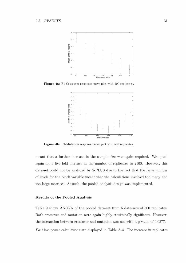
4a F1-Crossover response curve plot with 500 replicates. . . . . . . . . 31
4b F1-Mutation response curve plot with 500 replicates. . . . . . . . . 31
5a F1-Crossover response curve plot from pooled analysis. . . . . . . . 32
5b F1-Mutation response curve plot from pooled analysis. . . . . . . . 33
6a Fitted response curve: F1-crossover. . . . . . . . . . . . . . . . . . . 33
6b Fitted response curve: F1-mutation. . . . . . . . . . . . . . . . . . . 34
7a Fitted response curve: F3-crossover. . . . . . . . . . . . . . . . . . . 35
7b Fitted response curve: F3-mutation. . . . . . . . . . . . . . . . . . . 35
8a Fitted response curve: F2. . . . . . . . . . . . . . . . . . . . . . . . 37
8b Fitted response curve: F2-crossover. The solid line corresponds to
the lower mutation rate of 0.18 and the top dotted line to the upper
mutation rate of 0.24. This applies to all subsequent figures. . . . . 37
8c Fitted response curve: F2-mutation. . . . . . . . . . . . . . . . . . . 38
xx

9a Fitted response curve: F6. . . . . . . . . . . . . . . . . . . . . . . . 39
9b Fitted response curve: F6-crossover. . . . . . . . . . . . . . . . . . . 40
9c Fitted response curve: F6-mutation. . . . . . . . . . . . . . . . . . . 40
9d Fitted response curves for crossover 0% and 10%: F6-mutation. . . 41
10a Test function FN1. . . . . . . . . . . . . . . . . . . . . . . . . . . . 47
10b Test function FN6. . . . . . . . . . . . . . . . . . . . . . . . . . . . 48
11 Fitted response curves: FN5 -crossover. . . . . . . . . . . . . . . . . 50
12a Fitted response curve: FN5 -overall. . . . . . . . . . . . . . . . . . . 51
12b Fitted response curve: FN6 -overall. . . . . . . . . . . . . . . . . . . 51
13a Fitted response curves FN5 -mutation. . . . . . . . . . . . . . . . . 52
13b Fitted response curves FN6 -mutation. . . . . . . . . . . . . . . . . 52
14a Fitted response curve: FN3 -overall. . . . . . . . . . . . . . . . . . . 53
14b Fitted response curve: FN4 -overall. . . . . . . . . . . . . . . . . . . 53
15a Test Function: FN3. . . . . . . . . . . . . . . . . . . . . . . . . . . 59
15b Test Function: FN4. . . . . . . . . . . . . . . . . . . . . . . . . . . 60
16a Dot Diagram: FN3. . . . . . . . . . . . . . . . . . . . . . . . . . . . 61
16b Dot Diagram: FN4. . . . . . . . . . . . . . . . . . . . . . . . . . . . 61
17a Dot Diagram: FN31D . . . . . . . . . . . . . . . . . . . . . . . . . . 62
17b Dot Diagram: FN41D . . . . . . . . . . . . . . . . . . . . . . . . . . 62
18a FN31D : Chromosome population after applying a low mutation rate. 63
18b FN31D : Chromosome population after selection. . . . . . . . . . . . 63
19a FN31D : Chromosome population after applying a high mutation rate. 64
19b FN31D : Chromosome population after selection. . . . . . . . . . . . 64
20a FN41D : Chromosome population prior to applying mutation. . . . . 64
xxi
20b FN41D : Chromosome population after applying a low mutation rate. 65
20c FN41D : Chromosome population after selection. . . . . . . . . . . . 65
21a FN31D (HD=Hamming Distance). . . . . . . . . . . . . . . . . . . . 66
21b FN41D (HD=Hamming Distance). . . . . . . . . . . . . . . . . . . . 66
22 Landscape 20 101 from the Huygens Suite. . . . . . . . . . . . . . . 75
23a FN2R45 Initial Chromosome Population before Reproduction. . . . 79
23b FN2R45 Chromosome Population after Crossover. . . . . . . . . . . 80
23c FN2R45 Chromosome Population after Mutation. . . . . . . . . . . 81
24 Mutation Plot for Test function FN2R45. . . . . . . . . . . . . . . . 82
25 Probabilities associated with the movement of a single two bit chro-
mosome after mutation. . . . . . . . . . . . . . . . . . . . . . . . . 82
26a Heat Map of FN2R45 illustrating location of local minima along X
and Y axes. . . . . . . . . . . . . . . . . . . . . . . . . . . . . . . . 83
26b Heat Map of FN3R45 illustrating location of local minima along X
and Y axes. . . . . . . . . . . . . . . . . . . . . . . . . . . . . . . . 84
27a Response curve for test function FN2R45. . . . . . . . . . . . . . . 84
27b Response curve for test function FN3R45. . . . . . . . . . . . . . . 86
28a Hamming Distances for FN2R45. . . . . . . . . . . . . . . . . . . . 86
28b Hamming Distances for FN3R45. . . . . . . . . . . . . . . . . . . . 87
29 Probability of jumping Hamming Gap versus Mutation rate. . . . . 88
xxii

Chapter 1
Introduction
Since the era of ENIAC, the first successful high speed-computer developed in
the 1930s, an emerging component of computer science has been research into
artificial intelligence (AI). This encompasses areas such as natural language pro-
cessing, knowledge representation, automated reasoning, machine learning and evo-
lutionary computation.
A practical application of AI has been the use of computers to solve problems. In
order to formulate successful approaches researchers in artificial intelligence have
looked to processes found in nature, such as evolution, for assistance. As such the
development of this work has come under the heading of evolutionary computa-
tion, a general adaptable paradigm for problem solving especially well suited for
optimization problems [2].
Such adaptive algorithms are search algorithms which can be used to find solutions
to a variety of continuous and discrete problems. The general structure consists of
a population of candidate solutions which are adapted in parallel during successive
iterations with feedback obtained from an evaluation function [11]. Unlike algo-
rithms that operate on a single solution, adaptive algorithms make improvements
by combining the elements of good solutions to create better ones [34]. A classi-
cal example is genetic algorithms (GAs) [20]. While this thesis focusses on GAs
1

2 CHAPTER 1. INTRODUCTION
it should be noted that the methodology is readily applicable to other adaptive
algorithms.
1.1 Genetic Algorithms
GAs were originated by researchers including Holland who put forward the idea
of developing adaptive algorithms based upon processes seen in genetics [20]. The
relationship between genetics and GA terminology is illustrated in Table 1.
Table 1: Genetics and GA Terminology
Genetic Terminology Realisation in GAsGA Implementation
Chromosome Bit-stringGene Bit characterAllele Value 1 or 0Locus Bit-string position
Genotype StructurePhenotype Decoded structure (solution)Epistasis Nonlinearity
The classic GA works by encoding potential solutions to a problem as a series of bits
or genes on a bit-string or chromosome. The mechanics of a GA are straightforward:
in its simplest form new solutions are generated using crossover, where genes are
swapped over between pairs of chromosomes, and mutation, where the binary value
of a gene is inverted.
While the mechanics of a baseline GA are simple to describe and understand, the
way in which a GA actually searches the solution space has been more complex to
describe [2]. In addition, previously accepted aspects of GAs are being debated. For
example, while it has been traditionally maintained that crossover is a necessary
inclusion, the conjecture of naive evolution, where a GA contains selection and
mutation only, places this in question [12, 39].
Such debates have been fuelled by the fact that little research has been done on how
to decide whether a parameter significantly affects performance, how performance
1.2. THESIS STRUCTURE 3
varies with respect to changes in parameters, whether there is any interaction be-
tween parameters, and what ultimately are the best values or range of values for
the parameters which are implemented.
Given that there is no generally accepted methodology for exploring a GA in order
to address these important basic issues the present thesis comprises the following:
1. The formulation of a rigorous methodology for the statistical exploratory anal-
ysis of GAs with its application to a number of benchmark problems;
2. The application of this methodology to the issue of the importance of the
interaction between the crossover and mutation operators;
3. The application of this methodology to the issue of the relationship between
the encoding that is used and GA performance;
4. The application of this methodology to the issue of the detrimentality of
crossover for certain problems.
1.2 Thesis Structure
Expanding upon the above, the present thesis has the following structure:
Chapter 2 proposes a rigorous yet practical statistical methodology for the ex-
ploratory analysis of GAs. Section 2.1 of this chapter provides some background
to the problem of analyzing GA performance. This is followed in Section 2.2 by
a discussion of non-statistical exploratory work in this area. Section 2.3 exam-
ines work which has used a statistical construct, recognizing the appropriateness
of statistical analysis to this problem. However, a number of limitations are found
which include issues of experimental design, blocking, power calculations and re-
sponse curve analysis. In Section 2.4 the newly formulated statistical methodology
is described. Following this Section 2.5 illustrates the application of this method-
ology with case studies of benchmark problems from De Jong’s [9] and Schaffer’s
4 CHAPTER 1. INTRODUCTION
[6] test suites. This includes some unexpected outcomes, particularly on the use of
crossover. A discussion in Section 2.6 concludes this chapter.
Chapter 3 examines the issue of whether, in a GA, crossover and mutation interact
or whether each exerts its effect independently. Section 3.1 discusses studies which
have suggested that interaction between crossover and mutation may exist. Sec-
tion 3.2 gives an overview of the way in which the statistical methodology presented
in this thesis has been applied to a new test function, FNn, which has been uti-
lized to demonstrate the existence of interaction between crossover and mutation.
Section 3.3 links the existence of interaction between crossover and mutation with
the difficulty of the function defined in terms of modality. Section 3.4 provides a
concluding discussion to this chapter.
The first section of Chapter 4, Section 4.1, looks at the issue of the choice of encod-
ing and its impact upon GA performance since GA practitioners report differing
performances by changing the representation which is used [6, 37]. Section 4.2
reviews the methods used to investigate this question, including a description of
computer animation. Section 4.3 demonstrates how the choice of Gray encoding
may have a statistically demonstrable effect upon the difficulty of a problem, uti-
lizing results from both statistical analysis and computer animation. Section 4.4
provides a concluding discussion to this chapter.
Chapter 5 examines the issue of the detrimentality of crossover. This came about
as a limited amount of data from the literature suggested that the niche for the
beneficial effect of crossover upon GA performance may be smaller than has tradi-
tionally been held. Based upon not-linear-separable problems from earlier compo-
nents of this thesis we decided to explore this by comparing two test problem suites,
one comprising non-rotated functions and the other comprising the same functions
rotated by 45 degrees rendering them not-linear-separable. Section 5.1 examines
the issue of the detrimentality of crossover from the literature. Section 5.2 reviews
work from the previous chapters of this thesis which prompted the present research.

1.2. THESIS STRUCTURE 5
Section 5.3 briefly reviews the methods including any refinements to the statisti-
cal methodology. A discussion of the results obtained appears in Section 5.4 and
Section 5.6. Section 5.5 examines factors affecting the detrimentality of crossover.
Section 5.7 discusses the findings and suggests areas of future research.
Finally, Chapter 6 reviews general conclusions from this thesis. Limitations of the
thesis are discussed and areas for future research are suggested.

6 CHAPTER 1. INTRODUCTION

Chapter 2
Statistical Methodology
Adaptive algorithms such as GAs work by iteratively adapting members of a
population of potential solutions [2]. The individuals interact either through
the adaptation operators themselves, or through competitive selection mechanisms
for determining subsequent generations. If the adaptation strategy is successful,
the population (or part thereof) will converge on an optimal (or at least “good”)
solution.1
While the mechanics of each individual adaptation are quite straightforward, the
way individual changes affect the success of the population as a whole is more
difficult to determine. This is also true of the parameters that are used to fine tune,
or improve the success of, adaptive algorithms. Examples include population size,
mutation and crossover rates. Values for these parameters are most commonly set
through a process of trial and error, or based on recommendations from related
problems in the literature, rather than through statistically sound analysis of their
affects on performance.
This chapter presents a methodology designed to assess the impact of these pa-
rameters on GA performance. The methodology addresses issues of experimental
design, blocking, power calculation and response curve analysis. The approach is
1Readers unfamiliar with genetic algorithms are referred to [6] for a thorough introduction toGAs and examples of the range of applications to which they have been applied.
7

8 CHAPTER 2. STATISTICAL METHODOLOGY
demonstrated with case studies applying a baseline GA to benchmark problems
from De Jong’s [9] and Schaffer’s [6] test suites.
2.1 Background
GAs are used in search and optimization problems, such as finding the maximum or
minimum of a function in a given domain. The characteristics of GAs including bit-
string encodings, randomization and operator without domain knowledge [1], have
made the way in which a GA population converges on solutions has been more
complex to describe [2]. Holland put forward the idea of schemata [20]: similarity
templates describing a subset of strings with similarities at certain positions [17].
When the chromosome possesses these schemata its fitness improves. Operators
such as crossover and mutation work by altering chromosomes to contain more good
schemata. Goldberg elaborated by conceptualizing building blocks (highly-fit, short-
defining-length schemata) and implicit parallelism [17]. However, the increase in
sophistication and differences in implementations of GAs, such as quantum-inspired
GAs [31] and the use of transposition [40], has made it increasingly difficult to
propose newer models of convergence.
In addition, previously accepted aspects of GAs are being debated. For example,
while it has been traditionally maintained that crossover is a necessary inclusion,
the conjecture of naive evolution, a GA which contains selection and mutation only,
places this in question [12, 39]. Such debates have been fuelled by the fact that little
research has been done on how to decide whether a parameter significantly affects
performance and how performance varies with respect to changes in parameters.
There is currently no generally accepted methodology for exploring a GA in order
to address these issues.
The difficulty in developing such a methodology is illustrated by problems encoun-
tered in both working from theoretical models and real world data. In the first

2.2. NON-STATISTICAL EXPLORATORY ANALYSIS 9
instance, trying to formally describe GAs has been attempted using various math-
ematical approaches such as Markov chains [8, 19]. These approaches have been
limited by the complexity of the calculations. Moreover, the assumptions made
in much of the theoretical work may simply not be applicable nor attainable in
practice. There has therefore been a realization that research involving real world
data will be necessary in order to provide guidelines that may come to be generally
accepted by GA practitioners.
Initial empirical work of this kind was carried out by De Jong [9] whose experiments
resulted in a set of recommendations that came to represent early guidelines [39].
Later recommendations by Grefensette [18] using a meta-level GA (meta-GA) pro-
duced results which did not wholly agree with De Jong. The meta-GA approach is
limited in that independent runs of the meta-GA can result in different best values.
Furthermore, it does not provide any information as to whether any interaction
occurs nor the trend of the performance behaviour over the range of values studied.
A limited number of studies have made use of statistical analysis, recognizing the
ability of statistics to address many of these issues. However, as discussed in Sec-
tion 2.3, these studies have been limited by failing to fully address important issues
such as blocking for seed, calculating power and thorough response curve analysis.
Thus, results and recommendations from these studies, though obtained from real
practical experience, are still subject to debate.
The next sections look more closely at the various studies in this area. In doing so
the inconsistency of the results and the limitations of the methodologies are noted.
2.2 Non-Statistical Exploratory Analysis
As stated above, there is currently no generally accepted methodology for analyz-
ing the relationship between parameters and performance of a GA. Attempting to
mathematically describe GAs is complex and has not resulted in practical guide-
lines. This has given rise to various empirical studies which attempt to provide such

10 CHAPTER 2. STATISTICAL METHODOLOGY
data. However, both the methodologies and results have varied.
Early work was provided by De Jong who altered the values of parameters such
as population size, crossover rate and mutation rate in order to assess the effect
on performance. This was defined in terms of online performance, the average
performance of all chromosomes tested during the search, and offline performance,
the current best chromosome value for each iteration [39]. Five test problems of
increasing difficulty were used which became known as the De Jong suite [9]. Table 2
lists De Jong’s recommendations for optimal performance for the parameters listed.
Table 2: Recommendations for basic parameter settings
De Jong Population size 50-100
Crossover rate 0.60
Mutation rate 0.001
Grefensette Population size 30 (online)
Population size 80 (offline)
Crossover rate 0.95 (online)
Crossover rate 0.45 (offline)
Mutation rate 0.01 (online)
Mutation rate 0.01 (offline)
Freisleben and Hartfelder Population size 100 (maximal)
Crossover rate 0.49
Mutation rate 0.8-0.93
At this stage there was little evidence to dispel the idea that such data could
serve as generic guidelines for different problem domains. Hence, these data came
to represent guidelines for GA practitioners. Subsequent work, however, was not
consistent with these recommendations.
This is illustrated in the results of Grefensette who pioneered the use of meta-GAs
[18] for finding optimal values for parameters. His results for the De Jong suite
are shown in Table 2. Other studies using the meta-GA approach also produced
differing results, as seen in the work by Freisleben and Hartfelder [16] in the domain

2.3. STATISTICAL EXPLORATORY ANALYSIS 11
of neural network weights optimization (see Table 2).
2.3 Statistical Exploratory Analysis
As the previous studies did not clarify the relationship between parameters and per-
formance statistical analysis has been used for this purpose. For example, Schaffer
et al [39] conducted a factorial design study using the analysis of variance (ANOVA).
This study used the De Jong suite plus an additional five problems. The recom-
mendations for best online performance from this study are shown in Table 3. Close
examination of the best online pools suggested a relative insensitivity to crossover
which in turn suggested that naive evolution may be a powerful search algorithm
in its own right when using bit-string encoding [12, 39]. Work by Yao, Liu and Lin
suggests that this may also be true when using real values [43]. These data challenge
the traditional assumption that the crossover operator is a necessary inclusion in a
GA [6].
Statistics was also used by Petrovski, Wilson and McCall [33] who carried out
fractional factorial experiments in the domain of anti-cancer chemotherapy. These
were combined with linear regression in order to pinpoint which parameters were
significant and estimate their best values. The outcome measure, Ψ, was the number
of generations required in order to reach the feasible region in the solution space.
The results are shown in Table 3.
Table 3: Recommendations for basic parameter settings using statistics.
Schaffer et al Population size 20-30 (online)
Crossover rate 0.75-0.95 (online)
Mutation rate 0.005-0.01 (online)
Petrovski, Wilson Crossover rate using Ψ 0.6146
and McCall Mutation rate using Ψ 0.1981
Crossover rate using log(Ψ) 0.7600
Mutation rate using log(Ψ) 0.1069

12 CHAPTER 2. STATISTICAL METHODOLOGY
In overview, it is clear from both the non-statistical and statistical approaches that
results have varied, notably for mutation where the more recent studies, including
those using statistics, suggest higher rates. This may indicate a more complex effect
for this parameter or alternatively that best values are problem specific. Moreover,
the influence of differing problem domains must also be considered [42].
Importantly, however, the variation seen in these studies may also be a result of the
differing methodologies that have been employed and therefore suggests the need to
develop a generally accepted methodology for carrying out such exploratory work.
While statistics is promising for this purpose, a number of limitations need to be
addressed.
First, little attention has been given to blocking for seed as a source of variation
or noise. As pointed out by Davis [7], finding good settings for parameters can be
difficult due to the fact that the same parameter settings on the same problems
can lead to different results. In practice these differences can be traced to different
pseudo-random number generator seeds in the initialization of populations and in
the implementation of selection, crossover and mutation. Blocking for seed by
grouping experimental units into homogenous blocks, so that each run of the GA
for differing levels of crossover and mutation occurs with the same seeds, limits
the cause of variation within blocks to the parameters under study. In this way
variation or noise is reduced and comparisons are sharpened [24].
Adding to this, issues dealing with the calculation of power and sample size have
been ignored. This has meant that it is uncertain whether the studies carried out
have had adequate power and thus sample size to detect differences that could be
considered noteworthy. Sample sizes which are too small will generally fail to result
in statistical significance. This is particularly important if blocking is not carried
out since the data-set is akin to a completely randomized design. In such a design
effects may not be detected due to the extent of background noise in the data-set
produced by seed. Thus, a much larger sample size is required to detect effects of
interest.

2.4. METHODS 13
A detailed analysis of response curves has also been limited. It is important to
undertake such an analysis as it allows one to study the behaviour of the parameter
over the range of values implemented. Such data are useful in the optimization
process. For example, knowing that a parameter has a linear relationship to perfor-
mance may suggest that either the value for the parameter is set as high as possible
or that the parameter is excluded.
In the next section the experimental set-up is defined and the statistical methodol-
ogy is described.
2.4 Methods
Before describing our methodology we briefly introduce the test functions and the
GA used to illustrate our approach.
2.4.1 Choice of Standard Test Functions
It was important to select test functions which are well known. Initially, the first
three problems from the De Jong [9] suite were tackled which are relatively easy
for a GA to solve. This provided a useful set of problems, widely referenced in
the literature, on which to demonstrate the initial applicability of the statistical
methodology. These were F1 known as the SPHERE, F3 known as the STEP
function and F2 known as ROSENBROCK’S SADDLE.
Next a more difficult problem, Schaffer’s F6 [6], was tackled. These were all im-
plemented as minimization problems and are displayed in Equation 1, Equation 2,
Equation 3 and Equation 4, respectively:
f1(x) =3
∑
i=1
x2
i,−5.12 ≤ xi ≤ 5.12, (1)
f3(x) =5
∑
i=1
⌊xi⌋,−5.12 ≤ xi ≤ 5.12, (2)

14 CHAPTER 2. STATISTICAL METHODOLOGY
f2(x) = 100(x2 − x2
1)2 + (1 − x1)
2,−2.048 ≤ xi ≤ 2.048, (3)
f6(x) = 0.5 +(sin
√
x21 + x2
2)2 − 0.5
(1.0 + 0.001(x21 + x2
2))2,−100.0 ≤ xi ≤ 100.0. (4)
2.4.2 Implementation of the GA
The GA was implemented as detailed in Table 4. The implementation of the GA
was deliberately simple so that a clear and concise demonstration of the proposed
methodology and results could be made.
In this regard parameters such as the population size and bits per variable were not
varied but kept at the values shown in Table 4 and only crossover and mutation were
investigated in the present Thesis. The same methodology can be straightforwardly
applied to the many other parameters suggested in the literature.
2.4.3 Experimental Design and Statistical Test
In order to decide upon the most appropriate type of experimental design and
statistical test it was necessary to address several items:
1. Blocking for variation or noise due to seed.
2. Choice of an appropriate statistical test.
3. Statistical testing of individual parameters and their interactions.
4. Response curve analysis. This should allow for an estimate to be made of the
best value for individual parameters with confidence intervals.
2Probabilistic selection used here is the random selection of parents with the probability ofselection being directly proportional to the fitness of a chromosome.
3Mutation is implemented as described by Davis [6]. That is, if the probability test is passedthe binary bit is replaced by another binary bit that is randomly generated. Approximately fiftyper cent of the time the new bit will be the same as the old bit. The bit-flipping mutation rate istherefore half of the implemented mutation rate.

2.4. METHODS 15
Table 4: Details of the GA
Variable representation Bit-string
Bits per variable 22
Genes Binary value 1 or 0
Population size 50 chromosomes
Chromosome coding Gray coding
Selection Probabilistic selection 2
Experimental unit Blocks containing independent runs
of the GA for different
crossover and mutation rates
with the same seeds
Crossover Single point (randomly selected)
per variable
Mutation Randomly generated bit replacement 3
Performance measure Final epoch ie
epoch at which fitness of best
chromosome ≤ 10−10 of maximum fitness
for F1, F2 and F3
and
epoch at which fitness of best
chromosome ≤ 10−6 of maximum fitness
for F6
5. Calculation of power.
6. A methodology that is rigorous yet practical enough to be undertaken with
common statistical packages and available desktop computing power.
7. Statistical principles that can be generically applied to other adaptive algo-
rithms.
These are discussed in turn.
1. Blocking.

16 CHAPTER 2. STATISTICAL METHODOLOGY
The variation seen in GA runs is due to the differences in the starting
population and the probabilistic implementation of mutation and crossover.
This is in turn directly dependent on seed: the value used to generate the
pseudo-random sequences. In usual implementations of a GA the effect of
seed is not regulated and so the experimental design may be conceived as
being entirely randomized. In order to demonstrate statistically significant
effects a very large data-set is required in order to detect effects over and
above variation or noise due to seed.
To address this issue, it was necessary to control for the effect of seed via the
implementation of a randomized complete block design. In such a design every
combination of levels of parameters appears the same number of times in the
same block and in the present study the blocks are defined through seeds. For
example, if there are i levels of parameter A and j levels of parameter B then
each block contains all ij combinations.
Seed is used for blocking, thus ensuring that the seeds used to implement
items such as initialization of the starting population of chromosomes, selec-
tion, crossover and mutation are identical within each block. An increase in
sample size occurs by replicating blocks identical except for the seeds. This is
illustrated in Table 5. Replicates of this type are necessary to assess whether
the effects of parameters are significantly different from variation due to other
factors not controlled through seed.
Table 5: Creating a data-file from replicates of blocks.
Block Parameter A Parameter B Observations
Seed/s for block-replicate 1 i levels j levels ij
Seed/s for block-replicate 2 i levels j levels ij
Seed/s for block-replicate 3 i levels j levels ij...
......
...
Seed/s for block-replicate n i levels j levels ij
Total observations = ijn where ij ≥ 2
2.4. METHODS 17
2. ANOVA.
In order to compare performances for 2 or more parameters using a ran-
domized complete block design the statistical test for the equality of means
known as the analysis of variance (ANOVA) was used. In ANOVA the null
hypothesis is that the means for different levels of a parameter are equal.
The alternative hypothesis is that the means for levels of a parameter are
not equal and thus we conclude that the parameter has an effect upon the
response variable. The effect of one parameter on this response variable may
depend on the level of the other parameters. This is known as interaction.
ANOVA also formally tests whether interaction is present or not.
ANOVA is so called as it essentially splits the total variation in the observa-
tions into variation contributed by the parameters (crossover and mutation),
their interaction, block and error. Error is conceptualized in terms of resid-
uals which are simply the individual deviations of the observations from the
expected values.
Testing to ascertain if a parameter such as crossover or mutation has a sta-
tistically significant effect is a straightforward process. Firstly, the variation
contributed by the parameter adjusted by the number of levels of the parame-
ter is divided by the variation contributed by error adjusted by the number of
levels of the parameters and the observations. This results in a ratio which is
called an F value. Secondly, the probability that one would observe an F value
as large as that which is calculated under the null hypothesis is determined.
This is the p-value associated with the F value or simply Pr(F).
If the p-value is equal to or less than a chosen level of significance (see
Section 2.4.4) this is taken to suggest that the parameter has an effect upon
the response variable. A typical output from ANOVA is shown in Table 7 (see
page 28). If we examine the p-values at the 1% level of statistical significance,
we see that both crossover and mutation are highly significant. On the other
hand, the interaction term, with a p-value of 0.61, is non-significant. This
18 CHAPTER 2. STATISTICAL METHODOLOGY
means that there is no interaction occurring among crossover and mutation.
In other words, crossover and mutation are acting independently of each other.
In ANOVA the values for Pr(F) (p-values) are only (exactly) valid if the
responses are normally distributed. Although even moderate departures from
normality do not necessarily imply a serious violation of the assumptions on
which ANOVA is based [30], particularly for large sample sizes, it is standard
procedure to use methods such as plotting a histogram of the residuals or
constructing a normal probability plot of the residuals to verify normality of
the sampling populations. In the present research, analysis of the residuals did
not provide any evidence suggesting that the assumptions on which ANOVA
calculations are made were compromised.
3. Testing individual parameters and interaction.
ANOVA allows for the testing of significance of individual parameters per-
mitting the effect of crossover and mutation to be statistically demonstrated.
For issues which have been raised in the literature such as naive evolution
[12, 39], ANOVA provides evidence which may or may not support the inclu-
sion of the crossover parameter.
In addition, ANOVA allows for the testing of interaction between parame-
ters. Interaction is simply the failure of one parameter to produce the same
effect on the response variable at different levels of another parameter [30].
Examining interaction is important because a significant interaction means
the effect of each parameter cannot be considered independently of the others.
The interaction parameter is created by multiplying the crossover parameter
by the mutation parameter and adding this parameter to the ANOVA model.
4. Response curve analysis.
In ANOVA once a parameter is demonstrated to be statistically signifi-
cant the effect of the parameter may be modelled through an appropriate

2.4. METHODS 19
polynomial. Statistical testing can be carried out to assess if the shape of the
response curve is predominantly linear or is comprised of higher order polyno-
mials by partitioning the total variation of each parameter into its orthogonal
polynomial contrast terms.
Once the shape of the response curve is established, polynomial regres-
sion can be carried out to obtain estimates of the coefficients of the various
parameters in the response curve equation. Importantly, if the interaction pa-
rameter is significant in the ANOVA model then the overall equation must be
found. If not, then the equations for crossover and mutation can be obtained
separately.
For fitted response curves which are comprised of quadratic or higher com-
ponents we can obtain the derivatives and find the values where the deriva-
tives equal zero which yield estimates of the best value for each parameter.
Additionally, confidence intervals can be calculated if of interest.
However, if the fitted response curve is linear then a negative coefficient
will correspond solely to a best rate of 100% while a positive coefficient will
correspond solely to a best rate of 0% since the minimum of a straight line
can only occur at either end.
5. Power.
The calculation of power for ANOVA can be made by using the effect size in-
dex, f, as described by Cohen [5]. Power is discussed in detail in Section 2.4.6.
6. Availability.
ANOVA and regression are standard statistical models available in virtually
all statistical software packages which are used on desktop computers.
7. Applicability.
Randomized complete block design can be applied to other adaptive algo-
rithms with little difficulty. It simply requires that the seeds, or any other

20 CHAPTER 2. STATISTICAL METHODOLOGY
sources of noise, are kept identical within each replicate so that the source
can be blocked.
The GA was implemented in Java [41]. Statistical analysis was carried out using
S-PLUS [21]. Power calculations were carried out using GPOWER [14].
A number of aspects of the analysis are discussed in more detail below.
2.4.4 Choice of Level of Significance
There are 2 types of errors associated with statistical testing. A type I error is the
rejection of the null hypothesis when it is true. A type II error is the non-rejection
of the null hypothesis when the alternative hypothesis is true. The probability
of making a type I error is denoted by α and the probability of a type II error is
denoted by β. Since the null hypothesis represents the most conservative proposal it
is considered that a type I error is more serious than a type II error [24]. Thus, α is
generally and arbitrarily set at a low level. This level of significance is traditionally
set at values such as 10%, 5% or 1%.
For published research a level of significance of 1% is often used [26]. P-values less
than 1% suggest that the null hypothesis is strongly rejected or that the result is
highly statistically significant [24]. In the present study we have employed 1% as
our level of significance and correspondingly calculated 99% confidence intervals.
2.4.5 Level of Significance for Orthogonal Simultaneous Mul-
tiple Comparisons
In a situation of orthogonal simultaneous multiple comparisons within a parameter
it is necessary to modify the level of significance. This is because the probability
of achieving one or more statistically significant results in n simultaneous multiple
comparisons will exceed the level of significance chosen (1% in the present study).
2.4. METHODS 21
This is illustrated in Equation 5.
P (at least one significant result in n independent tests ) = 1 − (1 − α)n. (5)
This occurs in ANOVA when the sum of squares for each parameter is partitioned
into orthogonal contrast terms. In order to ensure that the probability of achieving
one or more statistically significant results in n simultaneous multiple comparisons is
exactly 1%, a modified level of significance was used for testing each of n orthogonal
polynomial contrast terms calculated in accordance with Equation 6.
Modified level of significance = 1 − (1 − α)1
n . (6)
Our approach is different from the Bonferroni method [21] which would simply
divide the overall level of significance by the number of simultaneous multiple com-
parisons. The Bonferroni method will ensure that the probability of achieving one
or more statistically significant results in n simultaneous multiple comparisons is no
greater than 1%. Thus, it yields an upper bound such that the actual probability
of achieving one or more statistically significant results in n simultaneous multiple
comparisons may be much smaller.
2.4.6 Power
As 1 − β is the probability of rejecting the null hypothesis when it is false, this is
known as the power of the test. A power of 80% (β = 0.2) when there is moderate
departure from the null hypothesis is considered desirable by convention [5]. The
value of β is related to sample size. A sample size that is too small will generally fail
to produce a significant result while a sample size that is too large may be difficult
to analyze (due to difficulties of handling large data sets) and wastes resources. It
is therefore necessary to have some means of calculating whether the size of the
sample chosen has sufficient power.
In order to calculate power it is necessary to specify the degree to which the null
hypothesis is false. This is quantifiable as a specific non-zero value using the unit-less

22 CHAPTER 2. STATISTICAL METHODOLOGY
effect size indices d and f as described by Cohen [5]. For ANOVA, by convention,
a small effect size is an f value of 0.10, a medium effect size is an f value of 0.25
and a large effect size is an f value of 0.40.
In this part of the present study differences in a specified number of epochs were
first converted to the effect size index, d, where:
d =µmax − µmin
σ, (7)
where µmax is the maximum mean over the levels of this parameter, µmin is the
smallest population mean over the levels of this parameter, and σ is the population
standard deviation.
This results in a unit-less number to index the degree of departure from the null
hypothesis of the alternative hypothesis, or more simply, the effect size one wishes
to detect [5].
Next, the conversion from d to f for ANOVA requires a knowledge of the pattern
of separation for all means for all k levels of the parameter. Patterns identified by
Cohen [5] are:
2.4. METHODS 23
1. Minimum variability: one mean at each end of d, the remaining k − 2 means
all at the midpoint.
2. Intermediate variability: the k means equally spaced over d.
3. Maximum variability: the means are all at the end points of d.
Tables are available for the conversion from d to f for each scenario. If the pattern
of separation is unknown an inspection of these tables illustrates that the most
conservative approach is to assume the minimum variability pattern which results
in f being at its smallest. In this case f is calculated as:
f = d
√
1
2k. (8)
It should be noted that power may be calculated a priori or post hoc. If the
population standard deviation is known from prior research one can calculate a
priori the sample size required to confer a specified power. On the other hand, if
the population standard deviation is unknown but can be estimated once the study
is concluded then post hoc power calculations indicate the ability of the present
sample size to detect specified effect sizes, given by Equation 7.
As the present thesis was exploratory in nature and a priori assumptions about the
population standard deviation could not be made post hoc calculations were strictly
adhered to. Thus, while statistical significance had not been demonstrated in the
ANOVA analysis for the interaction parameter, we continued to increase sample
size by a factor of 5. This was enacted until at least 80% power was achieved
for detecting a difference of 5 epochs for the interaction between crossover and
mutation. This is because f is smallest for the interaction parameter since k is
greatest for this parameter.
As a final remark, in the present research the calculation of power was based upon
the ability to detect a difference of at least 5 epochs as noted above. This number
was chosen as it most closely approximated the difference in the number of epochs
24 CHAPTER 2. STATISTICAL METHODOLOGY
detectable for the simplest problem, F1, if one had calculated power using an f of
0.4 (large effect).
2.4.7 Simultaneous Confidence Intervals for the Plotted Re-
sponse Curve
Plotting mean performance against parameter levels provides an initial estimate of
the shape of the response curve. However, the shape of the curve may be com-
promised if the sample size is insufficient. To gauge the reliability of the trend
99% simultaneous confidence intervals about each mean can be calculated. The z
value for calculating simultaneous confidence intervals for n levels of an individual
parameter corresponds to the probability given by equation 9.
Pz value = 1 −
1 − 0.991
n
2
. (9)
Note that while confidence intervals tighten as sample size increases, showing in-
creased confidence about the location of the population mean, there is still a great
deal of randomness in each individual run.
2.4.8 Pooled Analysis Design
If large data-sets are required these may not be able to be analyzed when a param-
eter has too many levels, as this results in the statistical software having to deal
with too many and too large matrices. In order to address this issue we devised a
pooled analysis design for the present study as follows:
1. For each individual experiment we calculated the mean of the performance
measure for each combination of crossover and mutation.
2. These data from individual experiments were concatenated into a new pooled
data file. The response variable was now the mean of the performance measure
averaged over the number of replicates in the individual experiment. This
2.4. METHODS 25
results in a smaller error variance, as the average of a number of observations
is expected to be closer than a single observation to the population mean.
Each individual experiment denoted one level of the block parameter.
3. Analysis was carried out in the same manner as for individual experiments.
2.4.9 Estimates of Best Values for Parameters
Once the coefficients are obtained from the polynomial regression model it is straight-
forward to obtain an estimate of the best value for the specified parameter by dif-
ferentiating and solving the response curve equation. 99% confidence intervals are
then calculated using Taylor’s Expansion (δ method) [36].
2.4.10 Workup Procedures to Ensure a Balanced ANOVA
Design
A balanced design for ANOVA occurs if no data are missing or censored. In our case
data is censored if that threshold is not reached and therefore stopping criterion not
satisfied for a run of the GA. A balanced design is desirable since it results in the
test statistic being more robust to small departures from the assumption of equal
variances for the number of treatments. In addition, the power of the ANOVA test
is maximized. This was achieved by two consecutive workup procedures which were
carried out for all four test functions.
Dot Diagrams
First, to minimize the occurrence of censoring in the present study a crude ex-
ploration of the parameter space was conducted. A data-set of an arbitrary 10
replicates was generated for all functions using an interval of 0 to 1 for both the
crossover (using an interval of 0.1) and mutation (using an interval of 0.01) param-
eters. If on at least one occasion the threshold was not reached for a particular
26 CHAPTER 2. STATISTICAL METHODOLOGY
crossover rate and mutation rate combination, this was shown as a dot on the
resultant dot diagram.
Figure 1: Dot diagram for F1. Each dot represents an instance of censoring.
0
0.2
0.8
1
0 0.2 0.8 1
Mut
atio
n ra
te
Crossover rate
As illustrated in Figure 1, for F1 mutation rates of less than 0.15 and greater than
zero were not associated with censoring. In contrast, all crossover rates from 0 to
1 were valid. Thus, at this point for F1 the rates which could be considered to
be reasonably free from censoring, so that the threshold value would be reached
or exceeded on every run of the GA, were crossover rates of 0 to 1, and mutation
rates of 0.01 to 0.14. The dot diagrams were also found useful to give us an initial
pictorial overview of the difficulty of a function (see Chapter 4).
Finalizing ranges for exploratory statistical analysis
Second, to further ensure that no censored data would appear in the data-sets for
analysis, and so finalize the ranges for exploratory statistical analysis to begin, we
conducted the following exercise.
Using crossover and mutation rates not associated with censoring from the dot
diagrams, an arbitrary 10 data-sets of 100 replicates each were generated. Using
S-PLUS the combination of crossover rate and mutation rate resulting in the best
performance was found in each data-set. When these 10 combinations were collated
they demonstrated the lowest and highest rates of crossover and mutation associated
with best performance. For F1 crossover ranged from 0.8 to 1 and mutation ranged

2.5. RESULTS 27
from 0.05 to 0.08.
However, to ensure that the ranges we would study could be considered robust we
allowed the ranges to widen one interval step on either side. Thus, as displayed in
Table 6, this made the finalized range for F1 for crossover 0.7 to 1 and for mutation
0.04 to 0.09.
As a result of these two consecutive workup procedures, a balanced ANOVA design
was achieved.
Table 6: Final ranges for crossover and mutation.
Test function Crossover final range Mutation final range
F1 0.7-1 0.04-0.09
F3 0.8-1 0.03-0.07
F2 0-0.7 0.18-0.24
F6 0-0.7 0.11-0.18
2.5 Results
2.5.1 Exploratory Analysis of Test Function F1
The results of analyzes of data-sets containing 100 replicates, 500 replicates and
pooled results from 5 data-sets of 500 replicates are described consecutively to
illustrate how statistics can be used to assist in exploratory analysis.
Results with 100 Replicates
Table 7 displays ANOVA of 100 replicates.
Crossover and mutation were both highly statistically significant while the inter-
action between crossover and mutation was not. Post hoc power calculations as
shown in Table A-1 show that while the power for detecting a difference of 5 epochs
28 CHAPTER 2. STATISTICAL METHODOLOGY
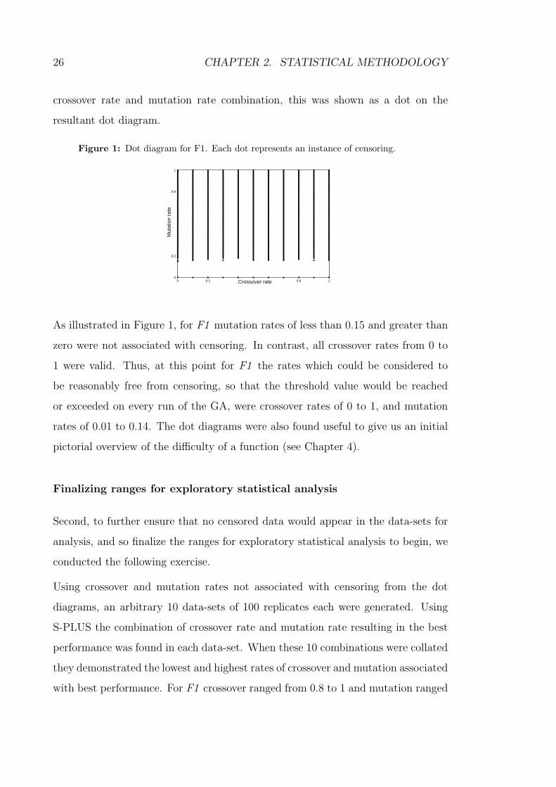
Table 7: F1-ANOVA of 100 replicates.
Parameter Df Sum of Sq Mean Sq F Value Pr(F)
Crossover 6 12347 2057.826 8.47756 0.0000000
Mutation 10 58701 5870.091 24.18282 0.0000000
Interaction 60 13664 227.733 0.93818 0.6117951
Block 99 51956 524.813 2.16205 0.0000000
Residuals 7524 1826361 242.738 - -
Residual standard error: 15.58005, Estimated effects are balanced.
was greater than 97% for both crossover and mutation the power for the interac-
tion parameter was only 3.38%. Thus, the use of 100 replicates was too small to
demonstrate statistical significance for interaction.
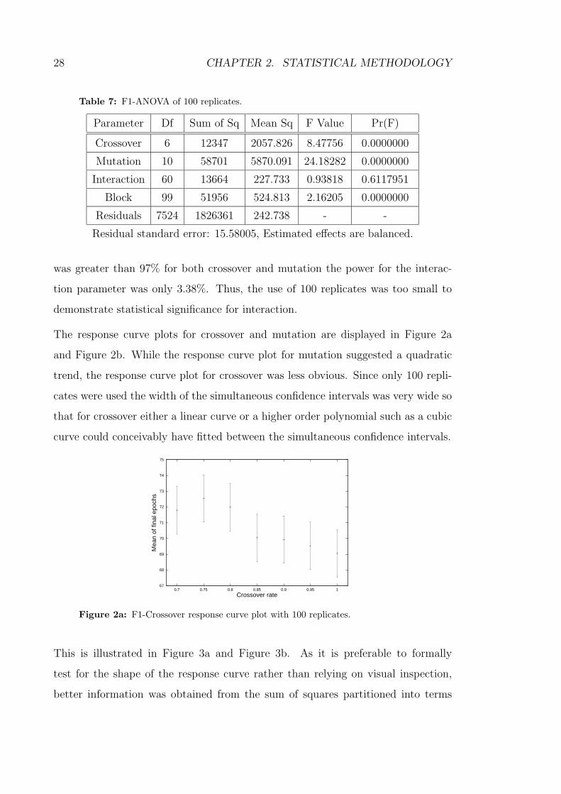
The response curve plots for crossover and mutation are displayed in Figure 2a
and Figure 2b. While the response curve plot for mutation suggested a quadratic
trend, the response curve plot for crossover was less obvious. Since only 100 repli-
cates were used the width of the simultaneous confidence intervals was very wide so
that for crossover either a linear curve or a higher order polynomial such as a cubic
curve could conceivably have fitted between the simultaneous confidence intervals.
67
68
69
70
71
72
73
74
75
0.7 0.75 0.8 0.85 0.9 0.95 1
Mea
n of
fina
l epo
chs
Crossover rate
Figure 2a: F1-Crossover response curve plot with 100 replicates.
This is illustrated in Figure 3a and Figure 3b. As it is preferable to formally
test for the shape of the response curve rather than relying on visual inspection,
better information was obtained from the sum of squares partitioned into terms

2.5. RESULTS 29
64
66
68
70
72
74
76
78
80
0.04 0.05 0.06 0.07 0.08 0.09
Mea
n of
fina
l epo
chs
Mutation rate
Figure 2b: F1-Mutation response curve plot with 100 replicates.
67
68
69
70
71
72
73
74
75
0.7 0.75 0.8 0.85 0.9 0.95 1
Mea
n of
fina
l epo
chs
Crossover rate
Figure 3a: F1-Linear curve fitted through simultaneous confidence intervals.
corresponding to orthogonal contrasts which represent polynomials. These data are
shown in Table A-9 and suggested a linear trend for crossover and a quadratic trend
for mutation.
However, given the lack of power associated with interaction it was necessary to
repeat the analysis using an increased sample size. Adhering to our protocol of
carrying out power calculations on a strictly post hoc basis we enacted a five fold
increase in the number of replicates.
Results with 500 Replicates
ANOVA of 500 replicates is shown in Table 8.

30 CHAPTER 2. STATISTICAL METHODOLOGY
67
68
69
70
71
72
73
74
75
0.7 0.75 0.8 0.85 0.9 0.95 1
Mea
n of
fina
l epo
chs
Crossover rate
Figure 3b: F1-Cubic curve fitted through simultaneous confidence intervals.
Table 8: F1-ANOVA of 500 replicates.
Parameter Df Sum of Sq Mean Sq F Value Pr(F)
Crossover 6 82952 13825.38 56.20533 0.0000000
Mutation 10 208227 20822.75 84.65223 0.0000000
Interaction 60 12386 206.44 0.83925 0.8079445
Block 499 237465 475.88 1.93464 0.0000000
Residuals 37924 9328542 245.98 - -
Residual standard error: 15.68375, Estimated effects are balanced.
A similar pattern for the overall results was evident. That is, a highly significant
result for crossover and mutation while a non-significant result for the interaction
parameter.
Table A-3 illustrates the improvement in power obtained by increasing the sample
size though the power associated with the interaction parameter remained below
the study threshold. The effect of increasing the number of replicates upon the
width of the simultaneous confidence intervals for the response curves is shown in
Figure 4a and Figure 4b. The increase in the number of replicates reduced the
width of the simultaneous confidence intervals producing clearer linear behaviour
for crossover and quadratic behaviour for mutation. Both trends were affirmed in
the partitioned sum of squares displayed in Table A-10.
However, the continued lack of power associated with the interaction parameter
2.5. RESULTS 31
68
69
70
71
72
73
74
0.7 0.75 0.8 0.85 0.9 0.95 1
Mea
n of
fina
l epo
chs
Crossover rate
Figure 4a: F1-Crossover response curve plot with 500 replicates.
67
68
69
70
71
72
73
74
75
76
77
78
0.04 0.05 0.06 0.07 0.08 0.09
Mea
n of
fina
l epo
chs
Mutation rate
Figure 4b: F1-Mutation response curve plot with 500 replicates.
meant that a further increase in the sample size was again required. We opted
again for a five fold increase in the number of replicates to 2500. However, this
data-set could not be analyzed by S-PLUS due to the fact that the large number
of levels for the block variable meant that the calculations involved too many and
too large matrices. As such, the pooled analysis design was implemented.
Results of the Pooled Analysis
Table 9 shows ANOVA of the pooled data-set from 5 data-sets of 500 replicates.
Both crossover and mutation were again highly statistically significant. However,
the interaction between crossover and mutation was not with a p-value of 0.0377.
Post hoc power calculations are displayed in Table A-4. The increase in replicates

32 CHAPTER 2. STATISTICAL METHODOLOGY
Table 9: F1-Pooled ANOVA analysis.
Parameter Df Sum of Sq Mean Sq F Value Pr(F)
Crossover 6 714.601 119.1002 256.1305 0.0000000
Mutation 10 2153.876 215.3876 463.2010 0.0000000
Interaction 60 38.977 0.6496 1.3970 0.0377493
Block 4 1.381 0.3453 0.7426 0.5635587
Residuals 304 141.359 0.4650 - -
Residual standard error: 0.6819076, Estimated effects are balanced.
now resulted in 100% power to detect a difference of 5 epochs for the interaction
parameter. As the power threshold of the study had been exceeded it was not
necessary to increase the sample size any further.
The response curve plots for crossover and mutation from the pooled analysis are
displayed in Figure 5a and Figure 5b. As can be seen the width of the simultaneous
confidence intervals has been further tightened. The partitioned sum of squares
shown in Table A-11 illustrated strong agreement with the plots. However, for
mutation a cubic effect was now significant though the quadratic effect remained
predominant as evidenced when comparing the magnitude of the respective sum of
squares.
68.5
69
69.5
70
70.5
71
71.5
72
72.5
73
73.5
0.7 0.75 0.8 0.85 0.9 0.95 1
Mea
n of
fina
l epo
chs
Crossover rate
Figure 5a: F1-Crossover response curve plot from pooled analysis.

2.5. RESULTS 33
68
69
70
71
72
73
74
75
76
77
0.04 0.05 0.06 0.07 0.08 0.09
Mea
n of
fina
l epo
chs
Mutation rate
Figure 5b: F1-Mutation response curve plot from pooled analysis.
In conclusion, these data suggested that both crossover and mutation are highly
important parameters in the GA for the F1 problem domain. The behaviour of
crossover is linear while the behaviour of mutation is predominantly quadratic with
some cubic component. The interaction observed between crossover and mutation
is not significant and therefore is of little practical importance.
Using polynomial regression separate fitted response curves for crossover and muta-
tion were obtained. These are illustrated in Figure 6a and Figure 6b and the equa-
tions are given in Table A-19. Using these equations the best values for crossover
and mutation were calculated and the overall results are displayed in Table 10.
68.5
69
69.5
70
70.5
71
71.5
72
72.5
73
0.7 0.75 0.8 0.85 0.9 0.95 1
Fin
al e
poch
Crossover rate
Figure 6a: Fitted response curve: F1-crossover.
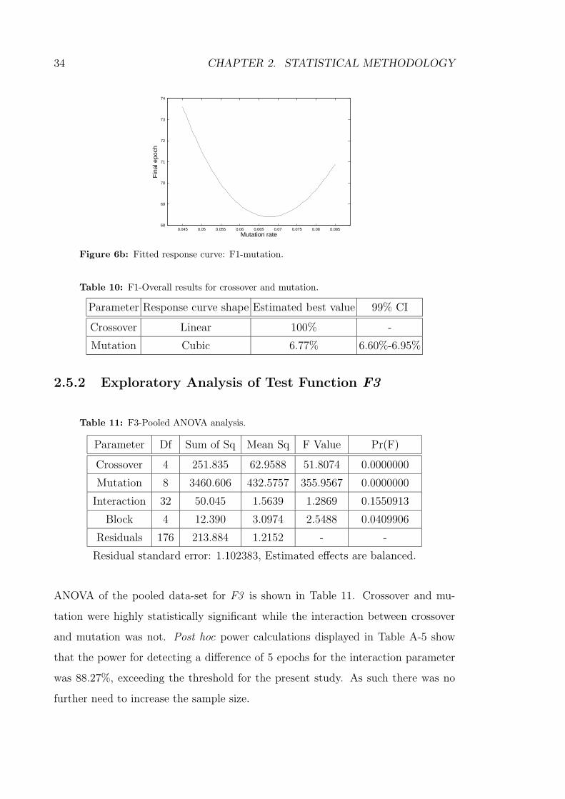
34 CHAPTER 2. STATISTICAL METHODOLOGY
68
69
70
71
72
73
74
0.045 0.05 0.055 0.06 0.065 0.07 0.075 0.08 0.085
Fin
al e
poch
Mutation rate
Figure 6b: Fitted response curve: F1-mutation.
Table 10: F1-Overall results for crossover and mutation.
Parameter Response curve shape Estimated best value 99% CI
Crossover Linear 100% -
Mutation Cubic 6.77% 6.60%-6.95%
2.5.2 Exploratory Analysis of Test Function F3
Table 11: F3-Pooled ANOVA analysis.
Parameter Df Sum of Sq Mean Sq F Value Pr(F)
Crossover 4 251.835 62.9588 51.8074 0.0000000
Mutation 8 3460.606 432.5757 355.9567 0.0000000
Interaction 32 50.045 1.5639 1.2869 0.1550913
Block 4 12.390 3.0974 2.5488 0.0409906
Residuals 176 213.884 1.2152 - -
Residual standard error: 1.102383, Estimated effects are balanced.
ANOVA of the pooled data-set for F3 is shown in Table 11. Crossover and mu-
tation were highly statistically significant while the interaction between crossover
and mutation was not. Post hoc power calculations displayed in Table A-5 show
that the power for detecting a difference of 5 epochs for the interaction parameter
was 88.27%, exceeding the threshold for the present study. As such there was no
further need to increase the sample size.

2.5. RESULTS 35
An examination of the partitioned sum of squares shown in Table A-12 confirmed
a linear trend for crossover and a quadratic trend for mutation. Using polynomial
regression the fitted response curves for crossover and mutation were obtained.
These are illustrated in Figure 7a and Figure 7b and the equations given in Table A-
19. Using these equations the best values for crossover and mutation were calculated
and the overall results are displayed in Table 12.
64.5
65
65.5
66
66.5
67
67.5
68
0.8 0.85 0.9 0.95 1
Fin
al e
poch
Crossover rate
Figure 7a: Fitted response curve: F3-crossover.
60
62
64
66
68
70
72
74
0.03 0.035 0.04 0.045 0.05 0.055 0.06 0.065 0.07
Fin
al e
poch
Mutation rate
Figure 7b: Fitted response curve: F3-mutation.
Table 12: F3-Overall results for crossover and mutation.
Parameter Response curve shape Estimated best value 99% CI
Crossover Linear 100% -
Mutation Quadratic 5.11% 5.07%-5.15%

36 CHAPTER 2. STATISTICAL METHODOLOGY
2.5.3 Exploratory Analysis of Test Function F2
Results of the pooled analysis
Table 13 shows ANOVA analysis of the pooled data-set for F2.
Table 13: F2-Pooled ANOVA analysis.
Parameter Df Sum of Sq Mean Sq F Value Pr(F)
Crossover 14 29291.3 2092.235 46.1088 0.000000000
Mutation 12 103575.8 8631.317 190.2173 0.000000000
Interaction 168 10717.5 63.795 1.4059 0.001550061
Block 4 820.0 205.006 4.5179 0.001298162
Residuals 776 35211.8 45.376 - -
Residual standard error: 6.736177, Estimated effects are balanced.
Crossover and mutation were highly statistically significant as was the interaction
between crossover and mutation with a p-value of 0.00155. Since the interaction pa-
rameter demonstrated strong statistical significance no further increments in sample
size were necessary.
Examination of the sum of squares partitioned into orthogonal polynomial contrast
terms as shown in Table A-13 suggested a linear trend for crossover and a cubic trend
for mutation with the predominant effect for the latter arising from the quadratic
term. Partitioning of the sum of squares of the interaction parameter showed only
a statistically significant effect (p-value less than 0.01) for the linear:linear term
(that is, the linear component of crossover multiplied by the linear component of
mutation).
As the interaction parameter was found to be significant, in contrast to the results
for F1 and F3, polynomial regression incorporating the linear by linear interaction
effect was used to obtain the overall 3-dimensional equation for the response curve
and this is given in Table A-19. Figure 8a illustrates this overall 3-dimensional
response curve and Figure 8b and Figure 8c illustrate 2-dimensional slices corre-
sponding to crossover and mutation, respectively.
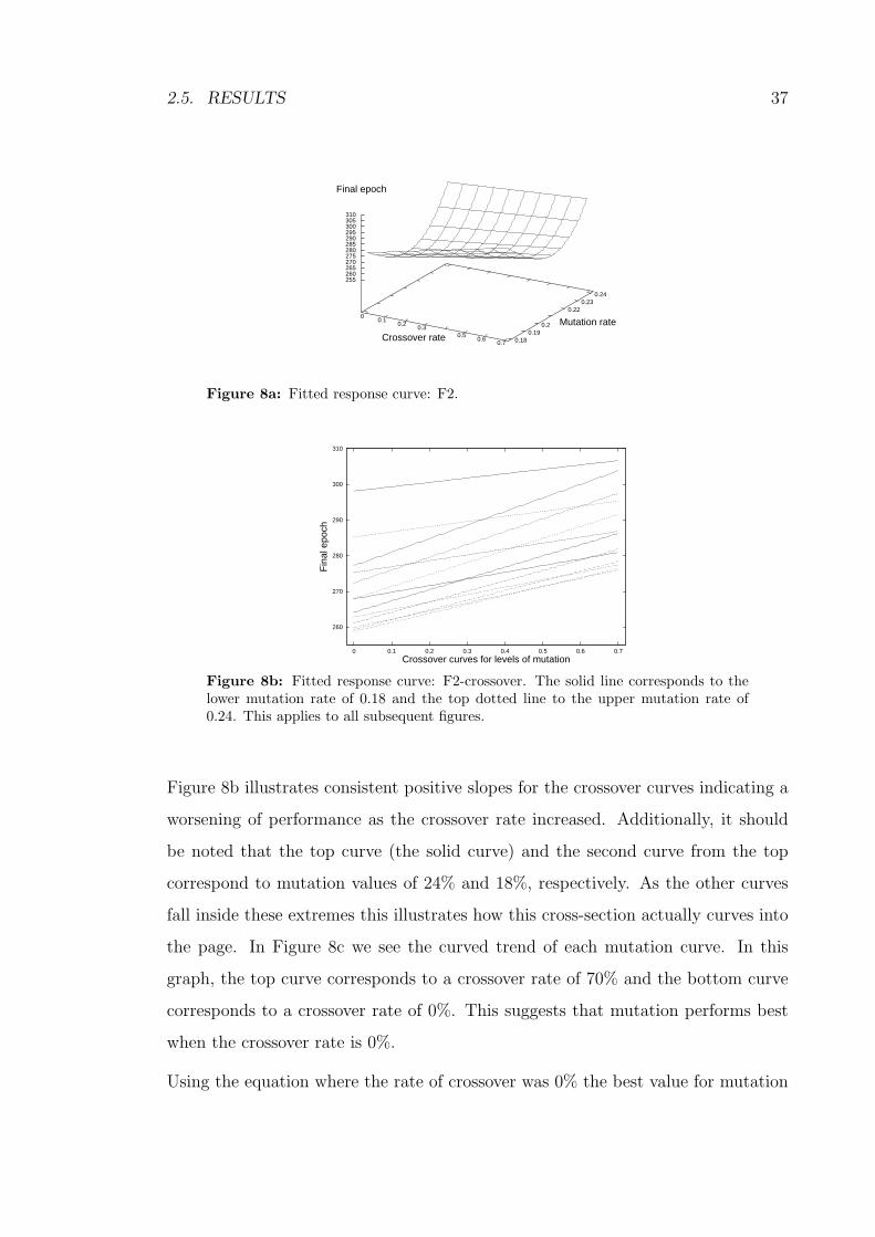
2.5. RESULTS 37
00.1
0.20.3
0.50.6
0.7Crossover rate 0.18
0.190.2
0.220.23
0.24
Mutation rate
255260265270275280285290295300305310
Final epoch
Figure 8a: Fitted response curve: F2.
260
270
280
290
300
310
0 0.1 0.2 0.3 0.4 0.5 0.6 0.7
Fin
al e
poch
Crossover curves for levels of mutation
Figure 8b: Fitted response curve: F2-crossover. The solid line corresponds to thelower mutation rate of 0.18 and the top dotted line to the upper mutation rate of0.24. This applies to all subsequent figures.
Figure 8b illustrates consistent positive slopes for the crossover curves indicating a
worsening of performance as the crossover rate increased. Additionally, it should
be noted that the top curve (the solid curve) and the second curve from the top
correspond to mutation values of 24% and 18%, respectively. As the other curves
fall inside these extremes this illustrates how this cross-section actually curves into
the page. In Figure 8c we see the curved trend of each mutation curve. In this
graph, the top curve corresponds to a crossover rate of 70% and the bottom curve
corresponds to a crossover rate of 0%. This suggests that mutation performs best
when the crossover rate is 0%.
Using the equation where the rate of crossover was 0% the best value for mutation
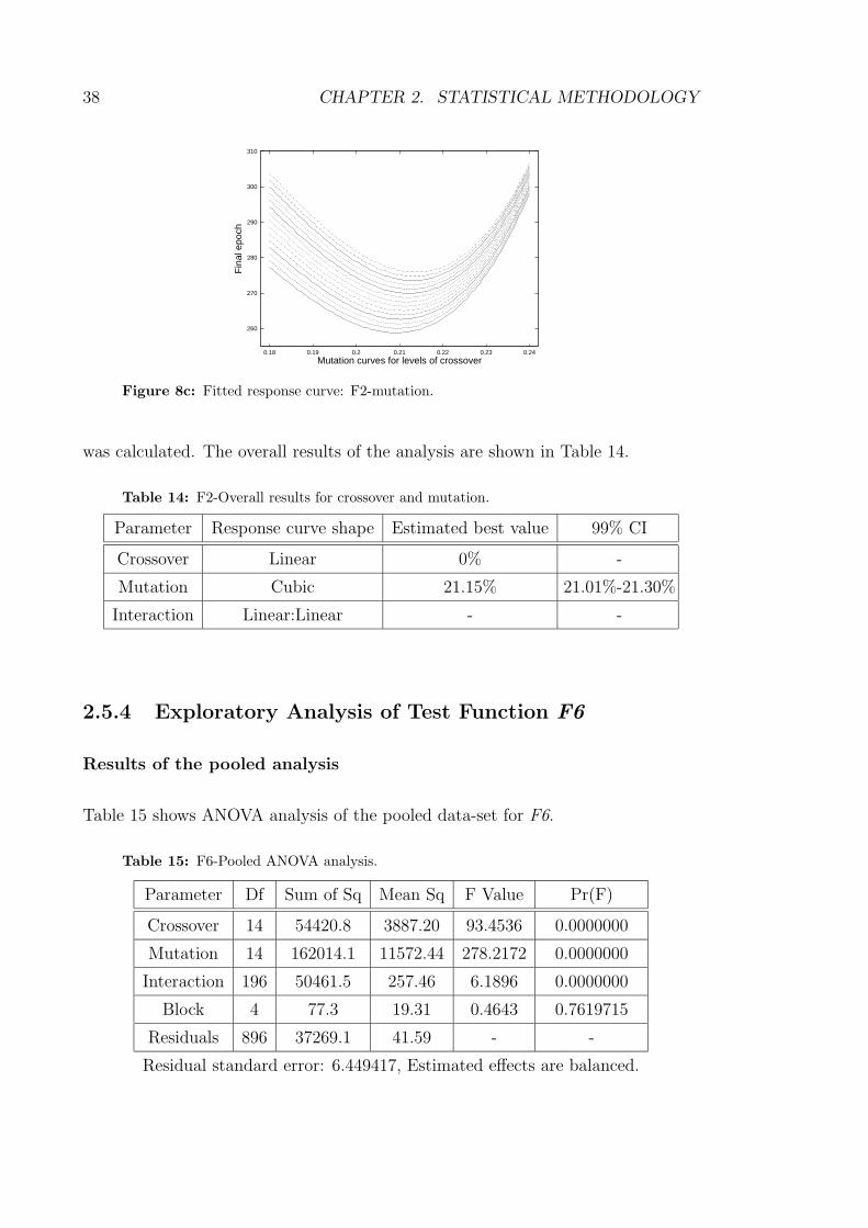
38 CHAPTER 2. STATISTICAL METHODOLOGY
260
270
280
290
300
310
0.18 0.19 0.2 0.21 0.22 0.23 0.24
Fin
al e
poch
Mutation curves for levels of crossover
Figure 8c: Fitted response curve: F2-mutation.
was calculated. The overall results of the analysis are shown in Table 14.
Table 14: F2-Overall results for crossover and mutation.
Parameter Response curve shape Estimated best value 99% CI
Crossover Linear 0% -
Mutation Cubic 21.15% 21.01%-21.30%
Interaction Linear:Linear - -
2.5.4 Exploratory Analysis of Test Function F6
Results of the pooled analysis
Table 15 shows ANOVA analysis of the pooled data-set for F6.
Table 15: F6-Pooled ANOVA analysis.
Parameter Df Sum of Sq Mean Sq F Value Pr(F)
Crossover 14 54420.8 3887.20 93.4536 0.0000000
Mutation 14 162014.1 11572.44 278.2172 0.0000000
Interaction 196 50461.5 257.46 6.1896 0.0000000
Block 4 77.3 19.31 0.4643 0.7619715
Residuals 896 37269.1 41.59 - -
Residual standard error: 6.449417, Estimated effects are balanced.
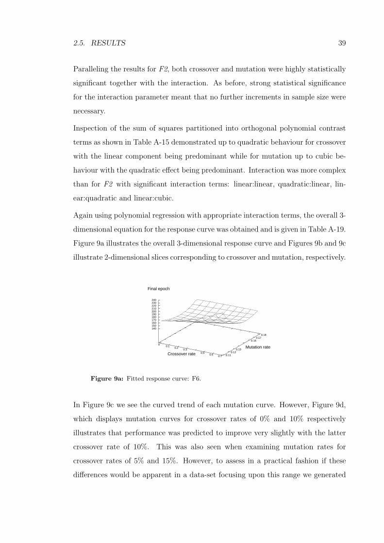
2.5. RESULTS 39
Paralleling the results for F2, both crossover and mutation were highly statistically
significant together with the interaction. As before, strong statistical significance
for the interaction parameter meant that no further increments in sample size were
necessary.
Inspection of the sum of squares partitioned into orthogonal polynomial contrast
terms as shown in Table A-15 demonstrated up to quadratic behaviour for crossover
with the linear component being predominant while for mutation up to cubic be-
haviour with the quadratic effect being predominant. Interaction was more complex
than for F2 with significant interaction terms: linear:linear, quadratic:linear, lin-
ear:quadratic and linear:cubic.
Again using polynomial regression with appropriate interaction terms, the overall 3-
dimensional equation for the response curve was obtained and is given in Table A-19.
Figure 9a illustrates the overall 3-dimensional response curve and Figures 9b and 9c
illustrate 2-dimensional slices corresponding to crossover and mutation, respectively.
00.1
0.20.3
0.50.6
0.7Crossover rate 0.11
0.120.13
0.160.17
0.18
Mutation rate
140150160170180190200210220230240
Final epoch
Figure 9a: Fitted response curve: F6.
In Figure 9c we see the curved trend of each mutation curve. However, Figure 9d,
which displays mutation curves for crossover rates of 0% and 10% respectively
illustrates that performance was predicted to improve very slightly with the latter
crossover rate of 10%. This was also seen when examining mutation rates for
crossover rates of 5% and 15%. However, to assess in a practical fashion if these
differences would be apparent in a data-set focusing upon this range we generated
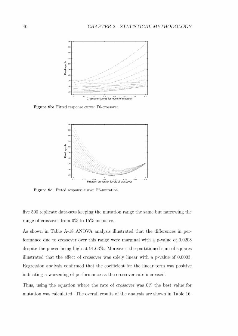
40 CHAPTER 2. STATISTICAL METHODOLOGY
150
160
170
180
190
200
210
220
230
240
0 0.1 0.2 0.3 0.4 0.5 0.6 0.7
Fin
al e
poch
Crossover curves for levels of mutation
Figure 9b: Fitted response curve: F6-crossover.
150
160
170
180
190
200
210
220
230
240
0.11 0.12 0.13 0.14 0.15 0.16 0.17 0.18
Fin
al e
poch
Mutation curves for levels of crossover
Figure 9c: Fitted response curve: F6-mutation.
five 500 replicate data-sets keeping the mutation range the same but narrowing the
range of crossover from 0% to 15% inclusive.
As shown in Table A-18 ANOVA analysis illustrated that the differences in per-
formance due to crossover over this range were marginal with a p-value of 0.0208
despite the power being high at 91.63%. Moreover, the partitioned sum of squares
illustrated that the effect of crossover was solely linear with a p-value of 0.0003.
Regression analysis confirmed that the coefficient for the linear term was positive
indicating a worsening of performance as the crossover rate increased.
Thus, using the equation where the rate of crossover was 0% the best value for
mutation was calculated. The overall results of the analysis are shown in Table 16.

2.6. DISCUSSION 41
150
160
170
180
190
200
210
220
230
240
0.11 0.12 0.13 0.14 0.15 0.16 0.17 0.18
Fin
al e
poch
Mutation curves for levels of crossover
0%10%
Figure 9d: Fitted response curves for crossover 0% and 10%: F6-mutation.
Table 16: F6-Overall results for crossover and mutation.
Parameter Response curve shape Estimated best value 99% CI
Crossover Quadratic 0% -
Mutation Cubic 15.01% 14.80%-15.22%
Interaction Linear:Linear - -
Quadratic:Linear - -
Linear:Quadratic - -
Linear:Cubic - -
2.6 Discussion
Genetic algorithms have been studied in computer science and used in real world
applications to find solutions to difficult problems. However, there is no generally
accepted methodology to assess which parameters significantly affect performance,
whether these parameters interact and how performance varies with respect to
changes in parameters. This chapter describes a statistical methodology for the
exploratory study of genetic and other adaptive algorithms addressing these issues.
Generically, once the algorithm and the problem domain have been specified, the
steps in the analysis are:
1. Identify sources of variation and modify the algorithm to generate blocked
runs.

42 CHAPTER 2. STATISTICAL METHODOLOGY
2. Use a workup procedure to minimize the appearance of censored observations
and to finalize starting ranges for parameters.
3. Generate an initial data-set consisting of an arbitrary number of replicates.
Typically, we have found 100 replicates to be a useful starting point.
4. Calculate power post hoc based upon a chosen effect size. If at least 80%
power is not achieved and the experiment resulted in observing no interaction
increase the sample size.
5. Conduct (pooled) ANOVA analysis and determine which parameters are sta-
tistically significant.
6. For parameters which are statistically significant partition the sum of squares
into polynomial contrast terms. Determine which polynomial terms are sta-
tistically significant.
7. Use polynomial regression to obtain the coefficients for the overall response
curve (if the interaction parameter is statistically significant) or to obtain
the coefficients for the response curve for each parameter separately (if the
interaction parameter is not statistically significant).
8. Differentiate and solve the response curve for each parameter to obtain best
values and calculate confidence intervals.
Before discussing the specific results of our study it should be prefaced that the
present research aimed to provide a statistical methodology by demonstrating its
practical use in well known test functions. In this regard, the number of parameters
and the suite of problems is restricted. Further research using a statistical approach
with an expanded set of parameters, in both continuous and discrete problem do-
mains, will be necessary to expand upon these initial findings.
The analysis of F1 illustrates the way in which our methodology was used to make
informed decisions when exploring the relationship between crossover and mutation

2.6. DISCUSSION 43
on a specified problem. Initially, workup procedures yielded starting ranges for
crossover and mutation. ANOVA of an initial data-set of 100 replicates demon-
strated a statistically significant effect upon performance of both crossover and
mutation with non-significance for the interaction parameter. Attempting to gauge
the shape of the response curve plots was compromised by the small sample size.
As seen, the width of the simultaneous 99% confidence intervals made it unclear as
to whether the trend for crossover was linear or included higher order components.
In contrast, the sum of squares partitioned into terms corresponding to orthogonal
polynomial contrasts demonstrated predominantly linear and quadratic trends for
crossover and mutation, respectively. Although this dispelled the ambiguity asso-
ciated with the data obtained from visual inspection, the subsequent power cal-
culations clearly showed a lack of power for the interaction parameter. Therefore,
increases in sample size were required. This was carried out until the appropriate
power for the interaction parameter was achieved. At this point polynomial regres-
sion was used to obtain fitted response curves and best values with 99% confidence
intervals were calculated.
Looking at the results from the suite of test functions together, crossover appears to
have a predominantly linear effect upon performance. For F1 and F3 the positive
gradient suggests selecting a rate as high as possible, while for F2 and F6 the
negative gradient suggests its possible exclusion. As noted earlier, Schaffer et al [39]
documented a relative insensitivity to crossover for these same functions and our
research adds to evidence supporting the effectiveness of naive evolution for certain
problems. Indeed, as suggested earlier, naive evolution may be a powerful search
algorithm in its own right as subtly commented by Eshelman [12]. Given that our
study has controlled for the effect of seed we may be obtaining a clearer perspective
of the actual behaviour of crossover than has been seen previously. Whatever the
case, the observation in our work that crossover appears predominantly linear and
that the direction of its slope is problem specific is certainly of practical interest.
It may be possible to correlate this behaviour with particular classes of problems
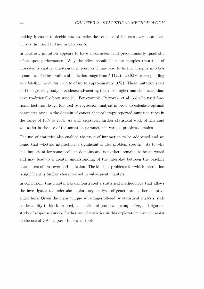
44 CHAPTER 2. STATISTICAL METHODOLOGY
making it easier to decide how to make the best use of the crossover parameter.
This is discussed further in Chapter 5.
In contrast, mutation appears to have a consistent and predominantly quadratic
effect upon performance. Why the effect should be more complex than that of
crossover is another question of interest as it may lead to further insights into GA
dynamics. The best values of mutation range from 5.11% to 20.92% (corresponding
to a bit-flipping mutation rate of up to approximately 10%). These mutation rates
add to a growing body of evidence advocating the use of higher mutation rates than
have traditionally been used [2]. For example, Petrovski et al [33] who used frac-
tional factorial design followed by regression analysis in order to calculate optimal
parameter rates in the domain of cancer chemotherapy reported mutation rates in
the range of 10% to 20%. As with crossover, further statistical work of this kind
will assist in the use of the mutation parameter in various problem domains.
The use of statistics also enabled the issue of interaction to be addressed and we
found that whether interaction is significant is also problem specific. As to why
it is important for some problem domains and not others remains to be answered
and may lead to a greater understanding of the interplay between the baseline
parameters of crossover and mutation. The kinds of problems for which interaction
is significant is further characterized in subsequent chapters.
In conclusion, this chapter has demonstrated a statistical methodology that allows
the investigator to undertake exploratory analysis of genetic and other adaptive
algorithms. Given the many unique advantages offered by statistical analysis, such
as the ability to block for seed, calculation of power and sample size, and rigorous
study of response curves, further use of statistics in this exploratory way will assist
in the use of GAs as powerful search tools.

Chapter 3
The Importance of Interaction
As previously discussed, adaptive algorithms such as GAs [6] work by iteratively
adapting members of a population of potential solutions. Individuals are
adapted through competitive selection mechanisms combined with operators such
as crossover and mutation. Since GAs were first developed an important question
has been whether crossover and mutation interact or whether each exerts its effect
independently in the algorithm.
On the basis of work presented in Chapter 2, particularly for Schaffer’s F6, a study
was conducted which examined the relationship between the occurrence of interac-
tion between crossover and mutation and increasing modality of a problem. The
statistical methodology was applied for assessing the impact of parameter settings
and calculating their optimal rates. The results of this work allowed some insight
as to when interaction first becomes significant and how this impacts upon the
practical task of obtaining optimal rates for crossover and mutation.
45

46 CHAPTER 3. THE IMPORTANCE OF INTERACTION
3.1 Background
The results of the limited number of studies touching upon the issue of interaction
have been conflicting. Petrovski and McCall [32], for example, carried out frac-
tional factorial experiments in the domain of cancer chemotherapy optimization
and found only weak interaction between parameters. On the other hand, Schaf-
fer et al [39] conducted a factorial design study which encompassed the De Jong
suite and Schaffer’s F6, and showed a statistically significant interaction between
crossover and mutation which appeared to be function independent.
The difference in the above results may be due to issues such as differing problem
domains and the different approaches undertaken. The previous chapter has ad-
dressed the limitations of the work of Schaffer et al. In a similar fashion the work of
Petrovski and McCall failed to control for the effect of seed, ignored issues dealing
with sample size and power, and a detailed analysis of response curves was not
considered.
In our own work it was demonstrated that the interaction between crossover and
mutation was significant for De Jong’s F2 and Schaffer’s F6 but not for De Jong’s
F1 nor De Jong’s F3. This led to two important questions.
1. What types of problems are likely to demonstrate statistical significance for
the interaction between crossover and mutation?
2. Where interaction between crossover and mutation is statistically significant,
what is the practical implication for obtaining optimal rates for these param-
eters?
In Section 3.2 a brief review is given of the statistical methodology as applied
to studying the test functions. The results of this research are then reported in
Section 3.3. A discussion in Section 3.4 concludes this chapter.

3.2. METHODS 47
3.2 Methods
The statistical methodology has already been described in Chapter 2. However,
aspects pertinent to this chapter are described below.
3.2.1 Test Functions
A generic test function was created, FNn, that increases in modality when the
integer variable, n, is incremented. That is, the function increases in the number of
local minima via an increase in peaks and troughs. We formulated this function to
elucidate if increasing modality was related to statistical significance for interaction.
This was of interest as, particularly for Schaffer’s F6 analyzed in Chapter 2, this was
a function that was both highly modal and exhibited strong statistical significance
for the interaction term. The generic test function, implemented as a minimization
problem, is described by Equation 10:
FNn(x1 , x2 ) =2
∑
i=1
0.5(1 − cos(nπxi
100)e−| xi
1000|),−100 ≤ xi ≤ 100. (10)
The test functions for n = 1 and n = 6 are shown in Figure 10a and Figure 10b,
respectively.
-100-50
050
100 -100
-50
0
50
100
0
0.5
1
1.5
2
Figure 10a: Test function FN1.
The research consisted of statistical analysis of test functions FN1 to FN6.
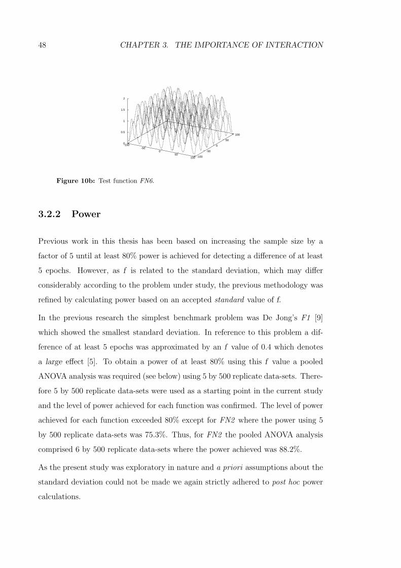
48 CHAPTER 3. THE IMPORTANCE OF INTERACTION
-100-50
050
100 -100
-50
0
50
100
0
0.5
1
1.5
2
Figure 10b: Test function FN6.
3.2.2 Power
Previous work in this thesis has been based on increasing the sample size by a
factor of 5 until at least 80% power is achieved for detecting a difference of at least
5 epochs. However, as f is related to the standard deviation, which may differ
considerably according to the problem under study, the previous methodology was
refined by calculating power based on an accepted standard value of f.
In the previous research the simplest benchmark problem was De Jong’s F1 [9]
which showed the smallest standard deviation. In reference to this problem a dif-
ference of at least 5 epochs was approximated by an f value of 0.4 which denotes
a large effect [5]. To obtain a power of at least 80% using this f value a pooled
ANOVA analysis was required (see below) using 5 by 500 replicate data-sets. There-
fore 5 by 500 replicate data-sets were used as a starting point in the current study
and the level of power achieved for each function was confirmed. The level of power
achieved for each function exceeded 80% except for FN2 where the power using 5
by 500 replicate data-sets was 75.3%. Thus, for FN2 the pooled ANOVA analysis
comprised 6 by 500 replicate data-sets where the power achieved was 88.2%.
As the present study was exploratory in nature and a priori assumptions about the
standard deviation could not be made we again strictly adhered to post hoc power
calculations.
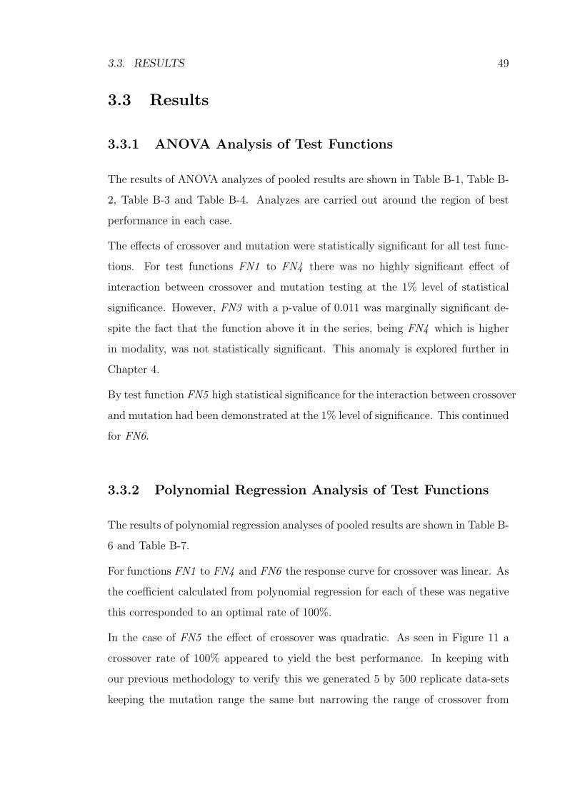
3.3. RESULTS 49
3.3 Results
3.3.1 ANOVA Analysis of Test Functions
The results of ANOVA analyzes of pooled results are shown in Table B-1, Table B-
2, Table B-3 and Table B-4. Analyzes are carried out around the region of best
performance in each case.
The effects of crossover and mutation were statistically significant for all test func-
tions. For test functions FN1 to FN4 there was no highly significant effect of
interaction between crossover and mutation testing at the 1% level of statistical
significance. However, FN3 with a p-value of 0.011 was marginally significant de-
spite the fact that the function above it in the series, being FN4 which is higher
in modality, was not statistically significant. This anomaly is explored further in
Chapter 4.
By test function FN5 high statistical significance for the interaction between crossover
and mutation had been demonstrated at the 1% level of significance. This continued
for FN6.
3.3.2 Polynomial Regression Analysis of Test Functions
The results of polynomial regression analyses of pooled results are shown in Table B-
6 and Table B-7.
For functions FN1 to FN4 and FN6 the response curve for crossover was linear. As
the coefficient calculated from polynomial regression for each of these was negative
this corresponded to an optimal rate of 100%.
In the case of FN5 the effect of crossover was quadratic. As seen in Figure 11 a
crossover rate of 100% appeared to yield the best performance. In keeping with
our previous methodology to verify this we generated 5 by 500 replicate data-sets
keeping the mutation range the same but narrowing the range of crossover from
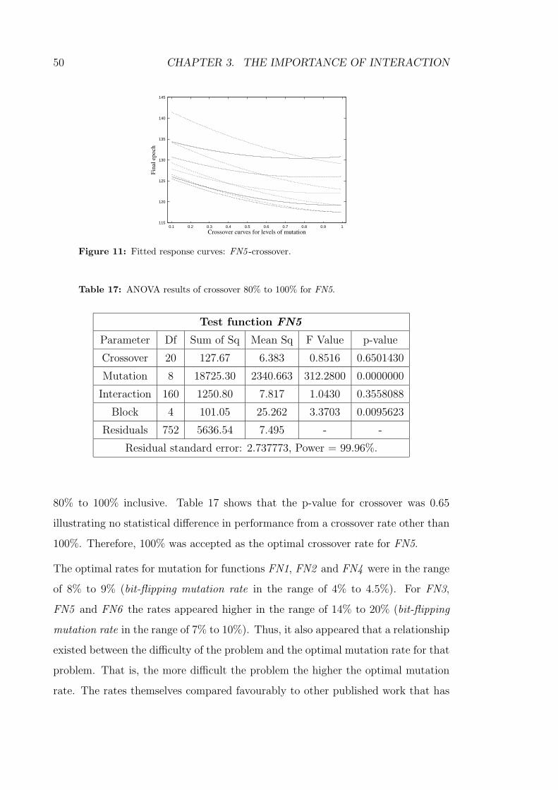
50 CHAPTER 3. THE IMPORTANCE OF INTERACTION
115
120
125
130
135
140
145
0.1 0.2 0.3 0.4 0.5 0.6 0.7 0.8 0.9 1
Fin
al e
poch
Crossover curves for levels of mutation
Figure 11: Fitted response curves: FN5 -crossover.
Table 17: ANOVA results of crossover 80% to 100% for FN5.
Test function FN5
Parameter Df Sum of Sq Mean Sq F Value p-value
Crossover 20 127.67 6.383 0.8516 0.6501430
Mutation 8 18725.30 2340.663 312.2800 0.0000000
Interaction 160 1250.80 7.817 1.0430 0.3558088
Block 4 101.05 25.262 3.3703 0.0095623
Residuals 752 5636.54 7.495 - -
Residual standard error: 2.737773, Power = 99.96%.
80% to 100% inclusive. Table 17 shows that the p-value for crossover was 0.65
illustrating no statistical difference in performance from a crossover rate other than
100%. Therefore, 100% was accepted as the optimal crossover rate for FN5.
The optimal rates for mutation for functions FN1, FN2 and FN4 were in the range
of 8% to 9% (bit-flipping mutation rate in the range of 4% to 4.5%). For FN3,
FN5 and FN6 the rates appeared higher in the range of 14% to 20% (bit-flipping
mutation rate in the range of 7% to 10%). Thus, it also appeared that a relationship
existed between the difficulty of the problem and the optimal mutation rate for that
problem. That is, the more difficult the problem the higher the optimal mutation
rate. The rates themselves compared favourably to other published work that has
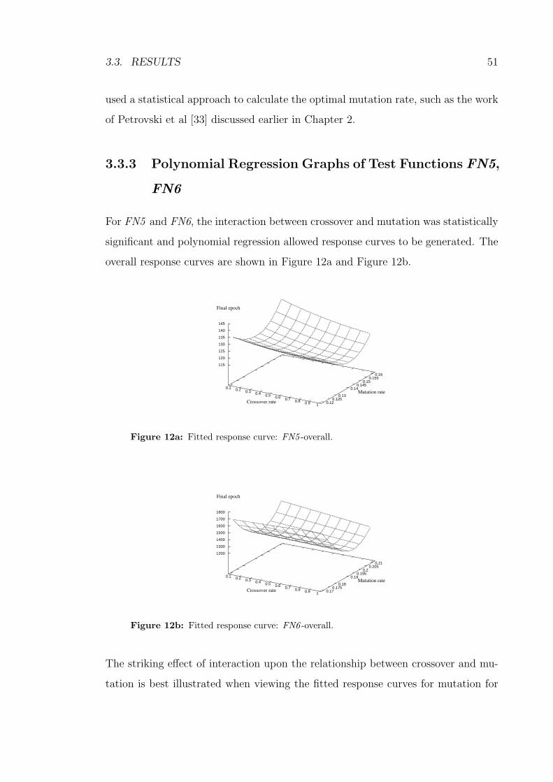
3.3. RESULTS 51
used a statistical approach to calculate the optimal mutation rate, such as the work
of Petrovski et al [33] discussed earlier in Chapter 2.
3.3.3 Polynomial Regression Graphs of Test Functions FN5,
FN6
For FN5 and FN6, the interaction between crossover and mutation was statistically
significant and polynomial regression allowed response curves to be generated. The
overall response curves are shown in Figure 12a and Figure 12b.
0.1 0.2 0.3 0.4 0.5 0.6 0.7 0.8 0.9 1Crossover rate 0.12
0.1250.13
0.140.145
0.150.155
0.16
Mutation rate
115
120
125
130
135
140
145
Final epoch
Figure 12a: Fitted response curve: FN5 -overall.
0.1 0.2 0.3 0.4 0.5 0.6 0.7 0.8 0.9 1Crossover rate 0.17
0.1750.18
0.190.195
0.20.205
0.21
Mutation rate
1200
1300
1400
1500
1600
1700
1800
Final epoch
Figure 12b: Fitted response curve: FN6 -overall.
The striking effect of interaction upon the relationship between crossover and mu-
tation is best illustrated when viewing the fitted response curves for mutation for
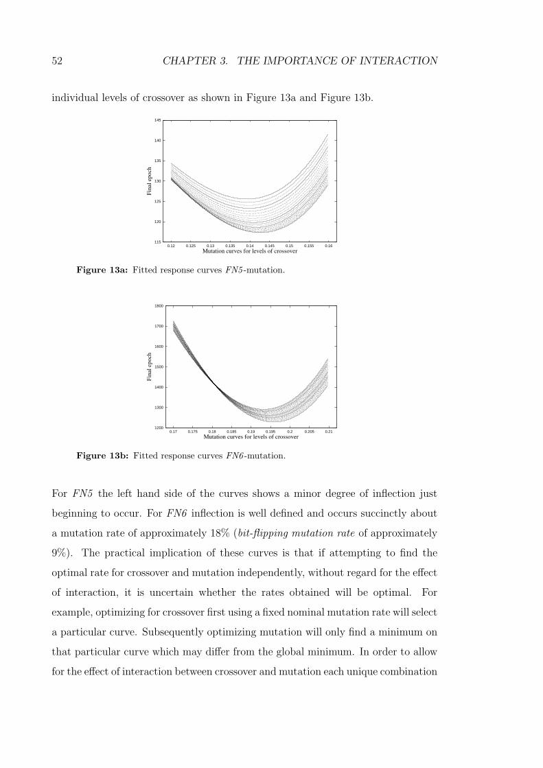
52 CHAPTER 3. THE IMPORTANCE OF INTERACTION
individual levels of crossover as shown in Figure 13a and Figure 13b.
115
120
125
130
135
140
145
0.12 0.125 0.13 0.135 0.14 0.145 0.15 0.155 0.16
Fin
al e
poch
Mutation curves for levels of crossover
Figure 13a: Fitted response curves FN5 -mutation.
1200
1300
1400
1500
1600
1700
1800
0.17 0.175 0.18 0.185 0.19 0.195 0.2 0.205 0.21
Fin
al e
poch
Mutation curves for levels of crossover
Figure 13b: Fitted response curves FN6 -mutation.
For FN5 the left hand side of the curves shows a minor degree of inflection just
beginning to occur. For FN6 inflection is well defined and occurs succinctly about
a mutation rate of approximately 18% (bit-flipping mutation rate of approximately
9%). The practical implication of these curves is that if attempting to find the
optimal rate for crossover and mutation independently, without regard for the effect
of interaction, it is uncertain whether the rates obtained will be optimal. For
example, optimizing for crossover first using a fixed nominal mutation rate will select
a particular curve. Subsequently optimizing mutation will only find a minimum on
that particular curve which may differ from the global minimum. In order to allow
for the effect of interaction between crossover and mutation each unique combination

3.3. RESULTS 53
of these parameters, within given starting ranges, must be assessed. An interesting
observation from this component of the research was that some problems with lower
modality appeared more difficult to solve than problems with higher modality.
00.1
0.20.3
0.40.5
Crossover rate 0.140.145
0.15
0.160.165
0.170.175
0.18
Mutation rate
750800850900950
100010501100115012001250
Final epoch
Figure 14a: Fitted response curve: FN3 -overall.
0.1 0.2 0.3 0.4 0.5 0.6 0.7 0.8 0.9 1Crossover rate 0.1
0.1050.11
0.120.125
0.130.135
0.14
Mutation rate
105110115120125130135140145150
Final epoch
Figure 14b: Fitted response curve: FN4 -overall.
Specifically this is illustrated by examining the response curve for FN3 shown in
Figure 14a as opposed to FN4 shown in Figure 14b. As can be seen, FN3 proved
the more difficult problem to solve despite the fact that it is lower in modality.
Moreover, the optimal mutation rate for FN3 was 17.45% (bit flipping mutation rate
of 8.72%) while that for FN4 was 8.41% (bit flipping mutation rate of 4.20%). As a
high mutation rate appears to be a marker for the difficulty of a problem this added
to the evidence supporting the conjecture that FN3 was a more difficult problem
to solve than FN4. This observation is explored in greater detail in Chapter 4.
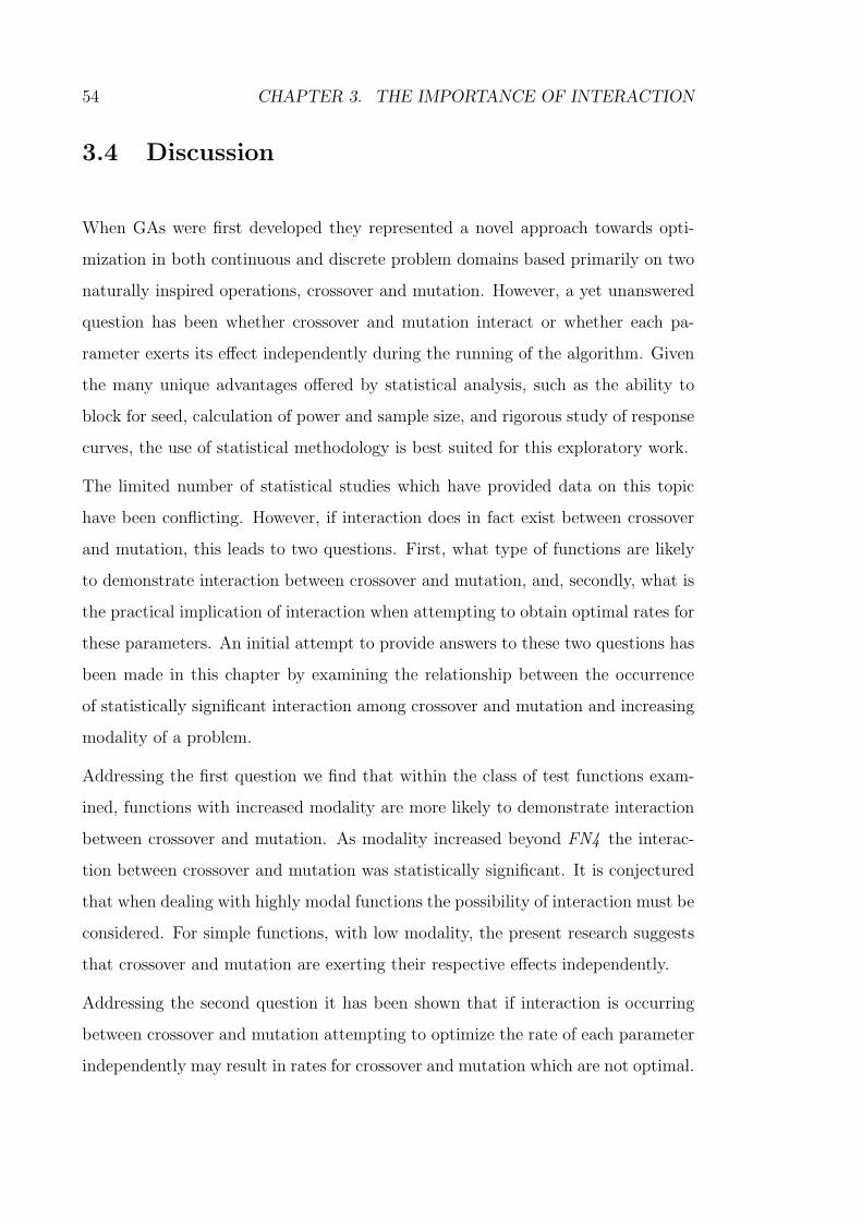
54 CHAPTER 3. THE IMPORTANCE OF INTERACTION
3.4 Discussion
When GAs were first developed they represented a novel approach towards opti-
mization in both continuous and discrete problem domains based primarily on two
naturally inspired operations, crossover and mutation. However, a yet unanswered
question has been whether crossover and mutation interact or whether each pa-
rameter exerts its effect independently during the running of the algorithm. Given
the many unique advantages offered by statistical analysis, such as the ability to
block for seed, calculation of power and sample size, and rigorous study of response
curves, the use of statistical methodology is best suited for this exploratory work.
The limited number of statistical studies which have provided data on this topic
have been conflicting. However, if interaction does in fact exist between crossover
and mutation, this leads to two questions. First, what type of functions are likely
to demonstrate interaction between crossover and mutation, and, secondly, what is
the practical implication of interaction when attempting to obtain optimal rates for
these parameters. An initial attempt to provide answers to these two questions has
been made in this chapter by examining the relationship between the occurrence
of statistically significant interaction among crossover and mutation and increasing
modality of a problem.
Addressing the first question we find that within the class of test functions exam-
ined, functions with increased modality are more likely to demonstrate interaction
between crossover and mutation. As modality increased beyond FN4 the interac-
tion between crossover and mutation was statistically significant. It is conjectured
that when dealing with highly modal functions the possibility of interaction must be
considered. For simple functions, with low modality, the present research suggests
that crossover and mutation are exerting their respective effects independently.
Addressing the second question it has been shown that if interaction is occurring
between crossover and mutation attempting to optimize the rate of each parameter
independently may result in rates for crossover and mutation which are not optimal.

3.4. DISCUSSION 55
In order to account for the effect of interaction all combinations of crossover and
mutation, within given starting ranges, must be trialed.
In conclusion, the research in this chapter has made an initial attempt to address
the importance of the interaction between crossover and mutation in GAs. Further
work of this kind, based on statistical methodology, will afford better insights into
the dynamics of GAs.

56 CHAPTER 3. THE IMPORTANCE OF INTERACTION

Chapter 4
The Influence of Gray Encoding
4.1 Background
An integral part of a GA is the type of knowledge representation that is used.
Traditionally, this has been bit encoding with variations such as binary or
Gray encoding. Though the operators such as selection and mutation have been
studied in some detail, comparatively less formal research has been conducted into
the type of knowledge representation that has been implemented.
GA practitioners have reported that changing the representation which is used in
GAs affects their performance [6, 37]. The ability to better understand the influence
of intrinsic factors in a GA such as the type of encoding used to represent potential
solutions is therefore a major topic of interest.
In the previous chapters interesting results were observed. Firstly, it was noted that
for difficult problems (problems with higher modality) increased mutation rates are
required. Secondly, as a problem became more difficult, due to increased modality
(more local optima), it is generally more likely to demonstrate highly statistically
significant interaction between crossover and mutation.
57

58 CHAPTER 4. THE INFLUENCE OF GRAY ENCODING
An unexpected result was that certain problems in our FNn test function series
appeared more difficult to solve despite the fact that they have lower modality.
Specifically, FN3 appeared a more difficult problem to solve than FN4. This is
in contrast to the trend of this test series of increasing difficulty with increasing
modality.
This finding led to two important questions which we sought to investigate, building
upon the work presented in the previous chapters:
1. Is there a demonstrable relationship between the difficulty of a problem and
the choice of encoding or could any observed change in performance be simply
due to the stochastic nature of the GA;
2. If the relationship between the difficulty of a problem and the choice of en-
coding is demonstrable and is thus a real effect, what is the actual mechanism
by which this occurs?
In this chapter we use components of our methodology to demonstrate that the type
of encoding used can have a real affect upon the difficulty of a problem. Animation
is then used to illustrate the actual mechanism by which this effect occurs. This is
illustrated using test functions FN3 and FN4 from Chapter 3.
In Section 4.2 a brief review is made of the test functions and methodology. The
results of the research are then reported in Section 4.3. A discussion in Section 4.4
concludes this chapter.
4.2 Methods
A detailed explanation of the statistical methodology can be found in Chapter 2.
Aspects most relevant to this chapter are described below.
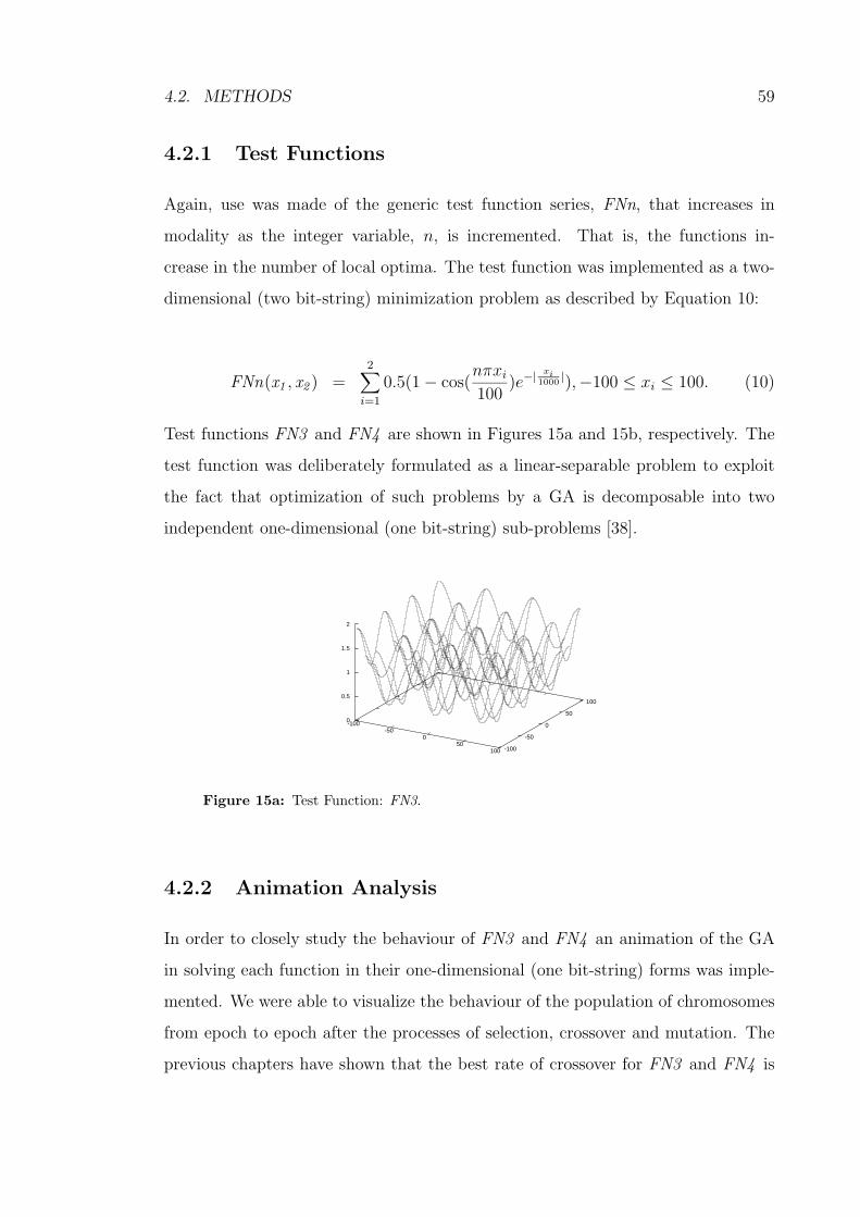
4.2. METHODS 59
4.2.1 Test Functions
Again, use was made of the generic test function series, FNn, that increases in
modality as the integer variable, n, is incremented. That is, the functions in-
crease in the number of local optima. The test function was implemented as a two-
dimensional (two bit-string) minimization problem as described by Equation 10:
FNn(x1 , x2 ) =2
∑
i=1
0.5(1 − cos(nπxi
100)e−| xi
1000|),−100 ≤ xi ≤ 100. (10)
Test functions FN3 and FN4 are shown in Figures 15a and 15b, respectively. The
test function was deliberately formulated as a linear-separable problem to exploit
the fact that optimization of such problems by a GA is decomposable into two
independent one-dimensional (one bit-string) sub-problems [38].
-100-50
050
100 -100
-50
0
50
100
0
0.5
1
1.5
2
Figure 15a: Test Function: FN3.
4.2.2 Animation Analysis
In order to closely study the behaviour of FN3 and FN4 an animation of the GA
in solving each function in their one-dimensional (one bit-string) forms was imple-
mented. We were able to visualize the behaviour of the population of chromosomes
from epoch to epoch after the processes of selection, crossover and mutation. The
previous chapters have shown that the best rate of crossover for FN3 and FN4 is

60 CHAPTER 4. THE INFLUENCE OF GRAY ENCODING
-100-50
050
100 -100
-50
0
50
100
0
0.5
1
1.5
2
Figure 15b: Test Function: FN4.
100%. Thus, the study of the behaviour of the chromosomes was carried out by
setting crossover at 100% and varying the rates of mutation in accordance with the
results from dot diagram analysis.
4.3 Results
4.3.1 Response Curve Analysis of FN3 and FN4
As previously discussed in Chapter 3, the number of epochs required to solve the
problem, as shown in the response curves, demonstrated that FN3 was the more
difficult problem to solve despite it being lower in modality (see Figure 14a and
Figure 14b).
4.3.2 Dot Diagram Analysis of FN3 and FN4
Dot diagram analysis of FN3 and FN4 are shown in Figures 16a and 16b.
For FN3 mutation rates of 10% or less were associated with censoring. In contrast,
for FN4 low rates of mutation were not associated with censoring. This assess-
ment of the two functions suggested that despite being lower in modality, FN3 was
proving a more difficult function to solve than FN4.
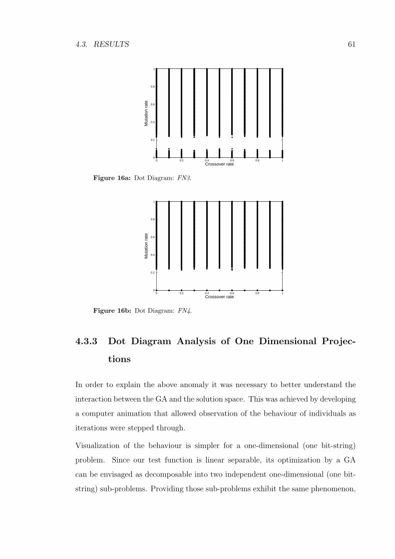
4.3. RESULTS 61
0
0.2
0.4
0.6
0.8
1
0 0.2 0.4 0.6 0.8 1
Mut
atio
n ra
te
Crossover rate
Figure 16a: Dot Diagram: FN3.
0
0.2
0.4
0.6
0.8
1
0 0.2 0.4 0.6 0.8 1
Mut
atio
n ra
te
Crossover rate
Figure 16b: Dot Diagram: FN4.
4.3.3 Dot Diagram Analysis of One Dimensional Projec-
tions
In order to explain the above anomaly it was necessary to better understand the
interaction between the GA and the solution space. This was achieved by developing
a computer animation that allowed observation of the behaviour of individuals as
iterations were stepped through.
Visualization of the behaviour is simpler for a one-dimensional (one bit-string)
problem. Since our test function is linear separable, its optimization by a GA
can be envisaged as decomposable into two independent one-dimensional (one bit-
string) sub-problems. Providing those sub-problems exhibit the same phenomenon,
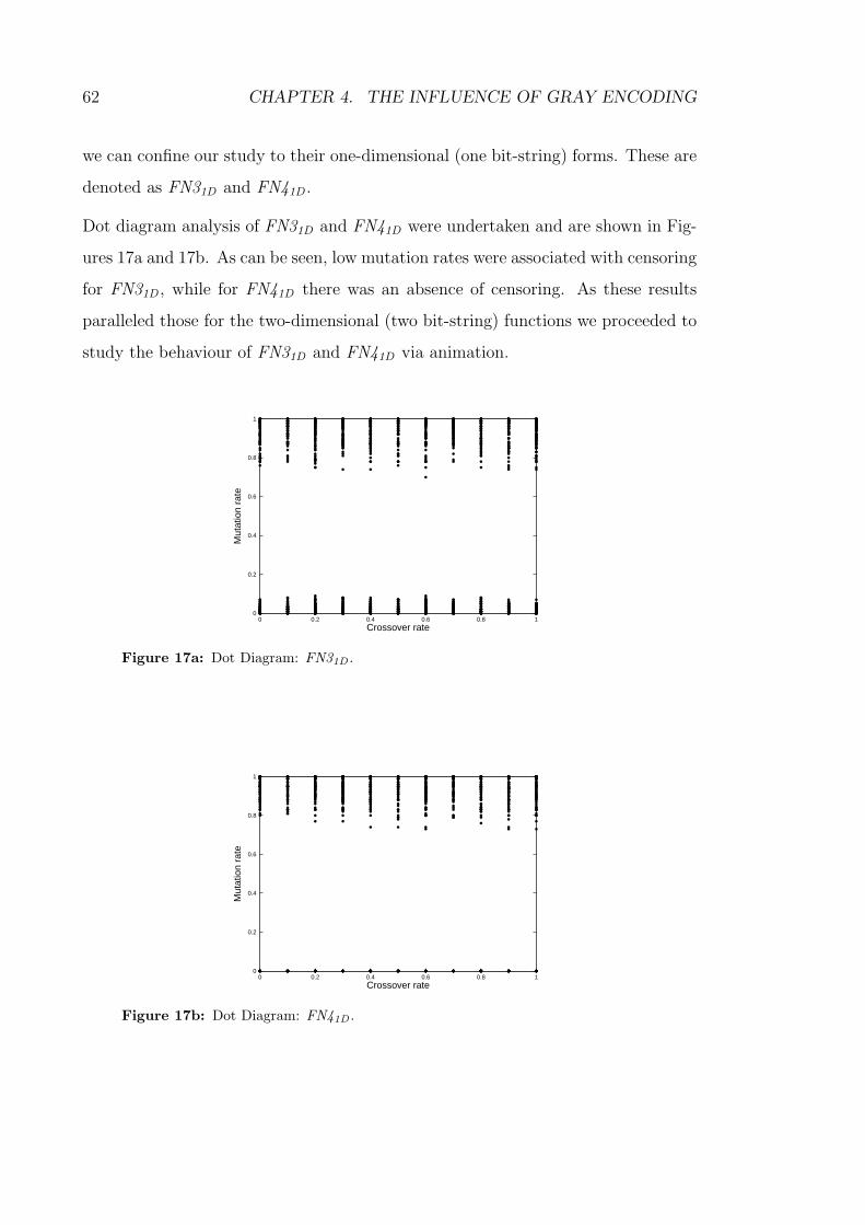
62 CHAPTER 4. THE INFLUENCE OF GRAY ENCODING
we can confine our study to their one-dimensional (one bit-string) forms. These are
denoted as FN31D and FN41D .
Dot diagram analysis of FN31D and FN41D were undertaken and are shown in Fig-
ures 17a and 17b. As can be seen, low mutation rates were associated with censoring
for FN31D , while for FN41D there was an absence of censoring. As these results
paralleled those for the two-dimensional (two bit-string) functions we proceeded to
study the behaviour of FN31D and FN41D via animation.
0
0.2
0.4
0.6
0.8
1
0 0.2 0.4 0.6 0.8 1
Mut
atio
n ra
te
Crossover rate
Figure 17a: Dot Diagram: FN31D .
0
0.2
0.4
0.6
0.8
1
0 0.2 0.4 0.6 0.8 1
Mut
atio
n ra
te
Crossover rate
Figure 17b: Dot Diagram: FN41D .
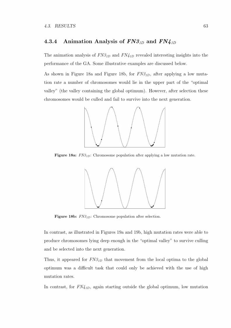
4.3. RESULTS 63
4.3.4 Animation Analysis of FN31D and FN41D
The animation analysis of FN31D and FN41D revealed interesting insights into the
performance of the GA. Some illustrative examples are discussed below.
As shown in Figure 18a and Figure 18b, for FN31D , after applying a low muta-
tion rate a number of chromosomes would lie in the upper part of the “optimal
valley” (the valley containing the global optimum). However, after selection these
chromosomes would be culled and fail to survive into the next generation.
Figure 18a: FN31D : Chromosome population after applying a low mutation rate.
Figure 18b: FN31D : Chromosome population after selection.
In contrast, as illustrated in Figures 19a and 19b, high mutation rates were able to
produce chromosomes lying deep enough in the “optimal valley” to survive culling
and be selected into the next generation.
Thus, it appeared for FN31D that movement from the local optima to the global
optimum was a difficult task that could only be achieved with the use of high
mutation rates.
In contrast, for FN41D , again starting outside the global optimum, low mutation
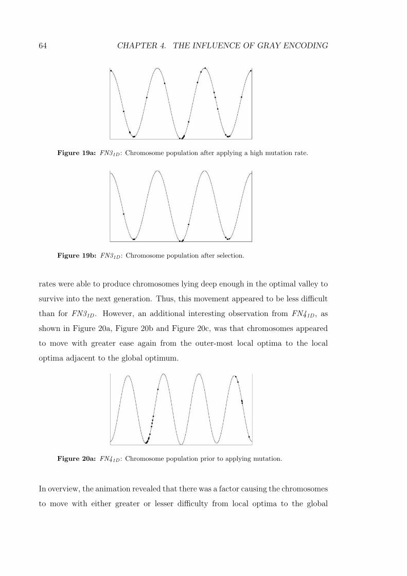
64 CHAPTER 4. THE INFLUENCE OF GRAY ENCODING
Figure 19a: FN31D : Chromosome population after applying a high mutation rate.
Figure 19b: FN31D : Chromosome population after selection.
rates were able to produce chromosomes lying deep enough in the optimal valley to
survive into the next generation. Thus, this movement appeared to be less difficult
than for FN31D . However, an additional interesting observation from FN41D , as
shown in Figure 20a, Figure 20b and Figure 20c, was that chromosomes appeared
to move with greater ease again from the outer-most local optima to the local
optima adjacent to the global optimum.
Figure 20a: FN41D : Chromosome population prior to applying mutation.
In overview, the animation revealed that there was a factor causing the chromosomes
to move with either greater or lesser difficulty from local optima to the global

4.3. RESULTS 65
Figure 20b: FN41D : Chromosome population after applying a low mutation rate.
Figure 20c: FN41D : Chromosome population after selection.
optimum. It was this factor that was making FN31D more difficult for the GA than
FN41D .
It was conjectured that the difficulty of jumping between local optima was related to
the number of coincident mutations required to make that transition. The probabil-
ity of a successful jump would therefore reduce with the product of the probabilities
of each individual mutation required. To test this hypothesis examination was made
of the number of bit changes required to pass between local optima in FN31D and
FN41D .
4.3.5 Hamming Distances for FN31D and FN41D
The number of bit changes required to jump from one bit-string to another is the
Hamming Distance of the bit-strings. Gray coding has been proposed as a good
encoding for applications such as GAs because the Hamming Distance between any
two adjacent solution candidates is one, as compared to binary encoding where all

66 CHAPTER 4. THE INFLUENCE OF GRAY ENCODING
bits may change in moving from one decimal integer to the next. The idea is that
this allows individuals to explore the solution space via small mutations.
0
0.2
0.4
0.6
0.8
1
HD = 12HD = 12
Figure 21a: FN31D (HD=Hamming Distance).
0
0.2
0.4
0.6
0.8
1
HD = 2 HD = 7 HD = 7 HD = 2
Figure 21b: FN41D (HD=Hamming Distance).
To find the mutations actually required for the GA to make progress in solving the
multi-modal problems the Hamming Distances between local optima were calcu-
lated. For FN31D , as illustrated in Figure 21a, the Hamming Distance between the
local optima and the global optimum was 12. In contrast for FN41D the Hamming
Distance between the local optima adjacent to the global optimum and the global
optimum was only 7. Since mutation probabilities are multiplicative (for example,
0.17 versus 0.112), there existed a much lower probability of chromosomes moving
into a sufficiently fit part of the optimal valley to survive selection for FN31D as
opposed to FN41D . This explained why higher mutation rates were necessary for
4.4. DISCUSSION 67
FN31D .
Furthermore, for FN41D the Hamming Distance between the outer-most local op-
tima and the local optima adjacent to the global optimum was only 2. Thus, it
proved easy for chromosomes to move into the local optima adjacent to the global
optimum. Hence, the fact that FN41D was more modal than FN31D was of little
consequence since the Hamming Distance between these local optima was compar-
atively small.
In overview, the results demonstrated by the dot diagram analysis, ANOVA, and
finally by animation analysis, all consistently demonstrated that FN3 was a more
difficult problem than FN4. By computing Hamming Distances it was found that,
despite FN31D being of lower modality than FN41D , these Hamming Distances were
significantly higher for FN31D making it a more difficult problem. This was a direct
result of the relationship between the encoding and the solution space.
4.4 Discussion
In respect of the intrinsic factors which may affect GA performance two important
questions have been whether there is a significant relationship between the difficulty
of a problem and the choice of encoding, and, if so, what is the actual mechanism
by which this occurs.
In this chapter the first question has been addressed by showing that a lower modal-
ity problem is more difficult to solve with a Gray encoding than a higher modality
problem. This is in contrast to the identified trend of problem difficulty increas-
ing with increasing modality. Specifically, response curve analysis and dot diagram
analysis suggested that FN3 is a more difficult problem than FN4, despite the
fact that FN4 is higher in modality. To investigate this further, since the original
functions are linear-separable, our test functions were decomposed into their one-
dimensional (one bit-string) forms. Subsequent dot diagram analysis confirmed the
ability to do so.

68 CHAPTER 4. THE INFLUENCE OF GRAY ENCODING
To address the second question animations of the GA in solving each function in
their one-dimensional (one bit-string) form were created which clearly demonstrated
that the ability of chromosomes to move between local optima and avoid culling in
the two functions was significantly different. Movement towards the global optimum
was much more difficult in FN31D than for FN41D .
The probability of a successful jump is dependent on the Hamming Distance. Calcu-
lation was therefore made of the Hamming Distances between local optima present
in the two functions and it was found that movement within FN31D was more dif-
ficult because of the significantly higher Hamming Distances involved. Moreover,
even though FN41D is higher in modality the very small Hamming Distance between
the outer-most local optima and the local optima adjacent to the global optimum
counteracted the influence of its increased modality. These Hamming Distances are
a result of the relationship between the encoding and the shape of the functions.
Chapter 5
The Detrimentality of Crossover
It has been traditionally maintained that the crossover operator is an integral
component of a GA. This has been held to the extent that some GA researchers
believe that it is the inclusion of the crossover operator that distinguishes GAs from
all other optimization algorithms [6].
Despite this, work by Eshelman and Schaffer [13], entitled Crossover’s Niche, sug-
gested that there exists a unique niche for which crossover is advantageous, and
that it is smaller than has traditionally been held in the GA community. Saloman
[38] suggested that Crossover’s Niche is linear-separable problems. From his work
with Rastrigin-like functions he conjectured that crossover implicitly exploits the
decomposability property of the fitness function: the optimization is decomposable
into n independent one-dimensional (one bit-string) sub-problems. If such a conjec-
ture is true, it adds further to the debate concerning crossover since most problems
in the real world are not-linear-separable, but tend to be non-linear, chaotic and
stochastic [10].
We explored Salomon’s conjecture to see if linear-separability was indeed linked to
crossover’s niche or whether other factors came into play in rendering the crossover
operator detrimental upon GA performance.
In Section 5.1 the literature on the detrimentality of crossover is reviewed. This
69

70 CHAPTER 5. THE DETRIMENTALITY OF CROSSOVER
is followed in Section 5.2 by a review of the work in the present thesis on this
subject. Section 5.3 briefly reviews the statistical methodology. Next, Section 5.4
and Section 5.6 details the results of our experiments with the latter carrying over
to a more difficult practical optimization problem. Section 5.5 reviews the factors
affecting the detrimentality of crossover. Section 5.7 concludes this chapter.
5.1 Background
As discussed above, from a traditional perspective it has been maintained that
crossover is a necessary inclusion in a GA. Mutation, on the other hand, has been
traditionally seen as a background operator with the unique role, as described by
Holland, of ensuring that no allele or value of a bit character (0 or 1) permanently
disappears from the population [20]. However, there is considerable debate with
some suggesting that the crossover operator may not always make a useful contri-
bution to GA performance. As Eshelman [12] subtly conjectured, naive evolution
(a GA which is composed of selection and mutation only) is a much more powerful
algorithm than many people in the GA community have been willing to admit.
The results of research into the detrimentality of crossover have been inconclu-
sive. As discussed above, Eshelman and Schaffer conjectured the idea of crossover’s
niche. The authors argued that what distinguishes the GA among population-based
hillclimbers is pairwise mating and that problems can be devised where crossover
is given a competitive advantage. However, as discussed before, many problems
do not have these features and it remains an open question as to how important
crossover may be for real world problems. In addition, because GAs are susceptible
to premature convergence the niche for which crossover is beneficial to GA perfor-
mance may be smaller than most GA practitioners maintain [13]. Moreover, Reeves
and Wright [35] suggested that the amount of information in a sample can never
be sufficient to enable one to decide on the amount of epistasis in a problem. This
implies that the problems that Eshelman and Schaffer describe as being most apt
5.1. BACKGROUND 71
for the crossover operator may not be easily recognizable in practice.
Jones [25] added to this by showing that a macromutational hillclimber (one that
involves large scale mutations) easily outperforms a standard GA on Holland’s Royal
Road problem [29] which has the properties that Eshelman and Schaffer ascribe to
problems residing in crossover’s niche. Thus, the niche may be even smaller than
Eshelman and Schaffer had intended.
Further evidence on the usefulness of crossover was contributed by Fogel and Atmar
[15] who conducted several experiments that required solving systems of linear equa-
tions. They concluded that the crossover operator provided no significant benefit.
Jansen and Wegener [22], on the other hand, proved that the crossover operator can
be useful if the current population of strings has a certain diversity. They proved
that an evolutionary algorithm can produce enough diversity such that the use of
crossover can speed up the expected GA optimization time from superpolynomial
to a polynomial of small degree. This was shown only for small crossover proba-
bilities, however, and they remarked that it was an open question as to whether
similar results could be shown for more realistic crossover rates [23]. Moreover, they
proved [23] that for some explicitly defined fitness function, namely the Royal Road
functions, a GA with crossover can optimize in expected polynomial time while all
evolutionary strategies based only on mutation (and selection) required exponential
time.
Statistical analyses of GA performance have failed to clarify this situation. As
discussed previously, Schaffer et al [39] conducted a factorial study using ANOVA
to examine the De Jong suite plus an additional five problems. Close examination
of the best on-line pools suggested a relative insensitivity to the crossover operator
when using Gray encoding. However, again this work did not block for seed, ignored
power calculations and was limited in its analysis of response curves.
Thus, in reference to the above studies three important questions were raised:
1. Can the crossover operator be statistically demonstrated to be detrimental for a
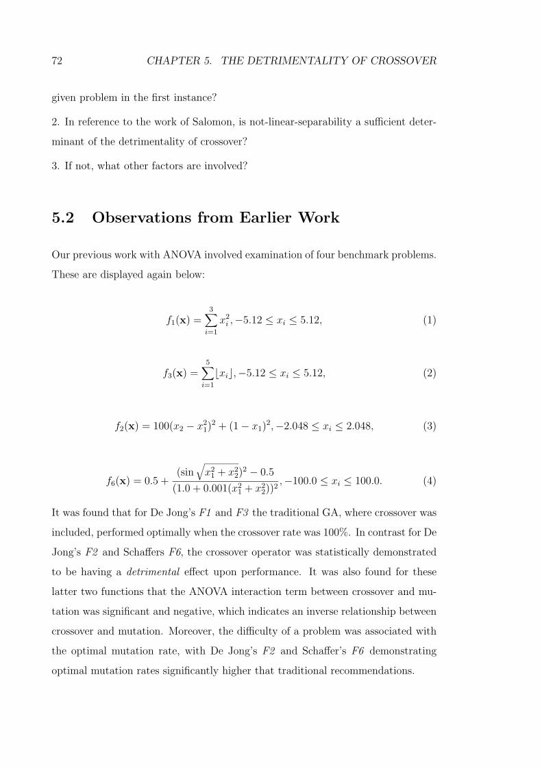
72 CHAPTER 5. THE DETRIMENTALITY OF CROSSOVER
given problem in the first instance?
2. In reference to the work of Salomon, is not-linear-separability a sufficient deter-
minant of the detrimentality of crossover?
3. If not, what other factors are involved?
5.2 Observations from Earlier Work
Our previous work with ANOVA involved examination of four benchmark problems.
These are displayed again below:
f1(x) =3
∑
i=1
x2
i,−5.12 ≤ xi ≤ 5.12, (1)
f3(x) =5
∑
i=1
⌊xi⌋,−5.12 ≤ xi ≤ 5.12, (2)
f2(x) = 100(x2 − x2
1)2 + (1 − x1)
2,−2.048 ≤ xi ≤ 2.048, (3)
f6(x) = 0.5 +(sin
√
x21 + x2
2)2 − 0.5
(1.0 + 0.001(x21 + x2
2))2,−100.0 ≤ xi ≤ 100.0. (4)
It was found that for De Jong’s F1 and F3 the traditional GA, where crossover was
included, performed optimally when the crossover rate was 100%. In contrast for De
Jong’s F2 and Schaffers F6, the crossover operator was statistically demonstrated
to be having a detrimental effect upon performance. It was also found for these
latter two functions that the ANOVA interaction term between crossover and mu-
tation was significant and negative, which indicates an inverse relationship between
crossover and mutation. Moreover, the difficulty of a problem was associated with
the optimal mutation rate, with De Jong’s F2 and Schaffer’s F6 demonstrating
optimal mutation rates significantly higher that traditional recommendations.

5.2. OBSERVATIONS FROM EARLIER WORK 73
When considering the possible difference in these functions that could produce such
varied results a clear demarcation between them was that De Jong’s F1 and F3 are
linear-separable1, echoing the conjecture made by Salomon that linear-separable
problems are crossover’s niche. In contrast, De Jong’s F2 and Schaffer’s F6 are
not-linear-separable problems. However the functions are also quite different in
structure, allowing explanations other than linear-separability.
To address the second question therefore, we compared two test functions differing
only in that one test function series was linear-separable while the other was not-
linear-separable.
The two test functions we decided to compare comprised firstly of the test function
series, FNn, which was used in Chapter 3 to examine the importance of the ANOVA
interaction term between crossover and mutation. This is a linear-separable problem
which increases in modality as the value for n increases.
The second test function series consisted of the same functions rotated by 45 degrees
in the solution space. This rotation rendered the series of problems, which we call
FNnR45, not-linear-separable.
By comparing the linear-separable form of the problem to the not-linear-separable
form we expected to see a difference in the effect of the crossover operator. Given
the suggestions from the literature and previous experience with linear-separable
versus not-linear-separable functions, it was conjectured that we would observe a
largely beneficial effect of crossover for the linear-separable problems, FNn, but a
detrimental effect for the not-linear-separable problems, FNnR45. Furthermore, if
the latter turned out to be true, then an attempt would be made to explain the
reasons why crossover acts detrimentally for not-linear-separable problems.
Finally, given the conjecture by Eshelman and Schaffer that it remains an open
question as to how important crossover may be for real-world problems [13] the
1We define linear-separable problems as those where the objective function can be written asa sum of univariate functions, which are allowed to be not-linear, where each of the functions cantake one component of the input vector as an argument.

74 CHAPTER 5. THE DETRIMENTALITY OF CROSSOVER
GA was trialed on a practical (but still highly multimodal) landscape minimization
problem to see if the results from the test functions would carry over to those
obtained on the real world landscape.
5.3 Methods
Our statistical methodolgy has been discussed in the previous chapters. Here we
focus on some aspects of the experimental setup for this particular chapter.
5.3.1 Motivation for our Test Functions
As discussed, to determine whether linear-separability is indeed a determining fac-
tor while minimizing other effects, we examined a series of functions of increasing
difficulty, while also examining the same functions in different orientations (that is,
the only difference was the frame of reference). We achieved this by rotating the
functions by 45 degrees rendering them not-linear-separable. We then tested the
algorithm on a newly devised benchmarking problem from the Huygens Suite [28].
These functions are detailed below:
1. Test functions FNn for n=1 to n=6, which are linear-separable equations, as
displayed in Equation 10 below:
FNn(x1 , x2 ) =2
∑
i=1
0.5(1 − cos(nπxi
100)e−| xi
1000|),−100 ≤ xi ≤ 100. (10)
2. Test function FNnR45 (R45 standing for the original test function FNn
having been rotated by 45 degrees in the solution space), being not-linear-
separable, for n=1 to n=6 as displayed in Equation 11 below:
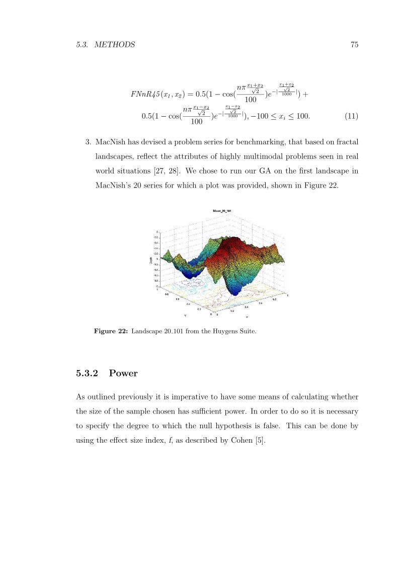
5.3. METHODS 75
FNnR45 (x1 , x2 ) = 0.5(1 − cos(nπ x1+x2√
2
100)e−|
x1+x2√
2
1000|) +
0.5(1 − cos(nπ x1−x2√
2
100)e−|
x1−x2√
2
1000|),−100 ≤ xi ≤ 100. (11)
3. MacNish has devised a problem series for benchmarking, that based on fractal
landscapes, reflect the attributes of highly multimodal problems seen in real
world situations [27, 28]. We chose to run our GA on the first landscape in
MacNish’s 20 series for which a plot was provided, shown in Figure 22.
Figure 22: Landscape 20 101 from the Huygens Suite.
5.3.2 Power
As outlined previously it is imperative to have some means of calculating whether
the size of the sample chosen has sufficient power. In order to do so it is necessary
to specify the degree to which the null hypothesis is false. This can be done by
using the effect size index, f, as described by Cohen [5].

76 CHAPTER 5. THE DETRIMENTALITY OF CROSSOVER
As f is related to the standard deviation, which may differ considerably according to
the problem under study, we again refined our previous methodology by calculating
power based on an accepted standard value of f.
Given the previous experience in power calculations with GA analysis, a value of
0.4 was utilized as a standard for the effect size when attempting to analyze the
performance of a GA. It should also be noted that in using this approach it is
possible to calculate power a priori and thus ascertain if a given sample size will
confer a required level of power. However, in this chapter we continued to adhere
to post hoc power calculations in line with the work of the previous chapters.
5.3.3 Estimates of Optimal Values for Crossover and Mu-
tation
The aim of the present research was to explore the detrimentality of crossover. That
is, to statistically determine the optimal crossover rate for each test function with
detrimental crossover corresponding to an optimal crossover rate of 0%. Therefore,
use was made of previous described methodology which enlisted polynomial regres-
sion to obtain an estimate of the optimal rate for both crossover and the mutation
operators.
5.4 Results
5.4.1 Exploratory Analysis of Test Functions FN1 to FN6
Full ANOVA tables and regression analyses for test functions FN1 to FN6 are to
be found in Table B-1 to Table B-7. The results showed that the crossover operator
proved beneficial to the performance of the GA in every instance: Table B-6 and
Table B-7 show that the optimal value of crossover was 100% for each of the six
functions.

5.4. RESULTS 77
5.4.2 Exploratory Analysis of test functions FN1R45 to
FN6R45
ANOVA tables and regression analyses for test functions FN1R45 to FN6R45 are
shown in Table C-1 to Table C-7. For the test function series, FNnR45, where the
test function FNn had been rotated by 45 degrees in the solution space, there was
a marked difference in the results obtained.
Firstly, crossover was detrimental for test functions FN2R45, FN4R45 and FN5R45,
where for these rotated forms the optimal crossover rate was 0%. This is in contrast
to the non-rotated form of these functions, as described above, where in each case
crossover proved to be beneficial. By contrast, crossover was beneficial for FN1R45,
FN3R45 and FN6R45. This shows that linear-separability alone is not a sufficient
indicator for the detrimentality of crossover.
Also, where crossover was shown to be detrimental the mutation rate was also
higher than in instances where crossover was having a beneficial effect. For example,
for FN2R45 the optimal mutation rate was 25.45% (bit flipping mutation rate of
12.72%), for FN4R45 the optimal mutation rate was 35.30% (bit flipping mutation
rate of 17.65%) and for FN5R45 the optimal mutation rate was 33.38% (bit flipping
mutation rate of 16.69%). In contrast, for FN1R45 the optimal mutation rate was
8.78% (bit flipping mutation rate of 4.39%), for FN3R45 the optimal mutation
rate was 12.36% (bit flipping mutation rate of 6.18%) and for FN6R45 the optimal
mutation rate was 12.97% (bit flipping mutation rate of 6.48%). Thus, in all cases
where crossover was detrimental the optimal mutation rate proved to be notably
greater than those instances where crossover was beneficial. These mutation rates
also reflected those obtained from the literature when a statistical approach was
adopted [33].
As noted above, as a high mutation rate is a conjectured marker for the difficulty
of a problem the above results indicate that the crossover operator proved to be
detrimental for the most difficult of the not-linear-separable rotated functions.
78 CHAPTER 5. THE DETRIMENTALITY OF CROSSOVER
5.5 Factors Affecting the Detrimentality of Crossover
In the preceding work it was demonstrated that crossover was detrimental for three
of the six not-linear-separable rotated functions analyzed. As indicated by the
optimal mutation rates, these proved to be the most difficult of the six functions
to solve. Thus, it is conjectured that crossover proves to have a detrimental effect
upon GA performance if the not-linear-separable problem is difficult for the GA to
solve.
What makes a GA hard to solve is a complex issue and involves factors such as the
degree of optimization occurring at local minima due to crossover, the bias of the
mutation operator and the Hamming Distances involved in the individual problems.
In the next sections each of these factors is discussed in turn.
5.5.1 Optimization Occurring at Local Minima due to Crossover
The first factor which influenced the difficulty of the problem for the GA was the
optimization occurring at local minima due to crossover. In order to discuss this
an investigation must firstly be carried out to determine what roles crossover, and
also mutation, are playing in the GA.
Figure 23a, Figure 23b, and Figure 23c show examples of chromosomes situated in
a heat map of function FN2R45. The heat map represents a view of the function
looking down from above with white areas denoting troughs and dark areas denoting
peaks. These heat maps show the location of the 50 chromosomes during iterations
of the GA to enable one to gain a pictorial understanding of their behaviour.
Figure 23a shows a population taken from a random epoch while solving FN2R45
(note that some chromosomes are occluded).
Figure 23b, shows the location of the chromosomes after crossover. The chromo-
somes have dissipated little, moving by only a small amount at the local minima
sites (denoted by the white areas). Crossover is performing its classical function of

5.5. FACTORS AFFECTING THE DETRIMENTALITY OF CROSSOVER 79
Figure 23a: FN2R45 Initial Chromosome Population before Reproduction.
exploitation within, or converging on, the local minima occupied by the chromo-
somes [20].
In contrast, in Figure 23c after mutation the chromosomes have dissipated more
widely over the solution space. In this sense, mutation is performing its classical
function of exploration of the solution space [20]. It is also important to note that
it is largely only with mutation that the chromosomes are able to move out of the
local optima that they are in and into newer regions of the solution space. This can
be seen visually by referring to the bottom right hand corner of Figure 23c where
several chromosomes have moved from the local optimum situated there into outer
lying regions of the solution space.
The heat maps shown are typical of all those reviewed. The maps showed that
while mutation was responsible for exploration of the solution space, crossover was
enacting exploitation at the sites of local minima.
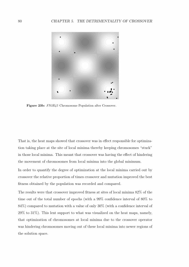
80 CHAPTER 5. THE DETRIMENTALITY OF CROSSOVER
Figure 23b: FN2R45 Chromosome Population after Crossover.
That is, the heat maps showed that crossover was in effect responsible for optimiza-
tion taking place at the site of local minima thereby keeping chromosomes “stuck”
in those local minima. This meant that crossover was having the effect of hindering
the movement of chromosomes from local minima into the global minimum.
In order to quantify the degree of optimization at the local minima carried out by
crossover the relative proportion of times crossover and mutation improved the best
fitness obtained by the population was recorded and compared.
The results were that crossover improved fitness at sites of local minima 82% of the
time out of the total number of epochs (with a 99% confidence interval of 80% to
84%) compared to mutation with a value of only 30% (with a confidence interval of
29% to 31%). This lent support to what was visualized on the heat maps, namely,
that optimization of chromosomes at local minima due to the crossover operator
was hindering chromosomes moving out of these local minima into newer regions of
the solution space.

5.5. FACTORS AFFECTING THE DETRIMENTALITY OF CROSSOVER 81
Figure 23c: FN2R45 Chromosome Population after Mutation.
5.5.2 Bias Associated with the Mutation Operator
The mutation operator corrupts the reproduction of genotypes thereby introducing
the variety that fuels natural selection [4]. This being said, there is discussion in the
literature as to the possible biases inherent in various implementations of mutation
and the degree to which this makes a problem hard for a GA to solve [3, 4].
Thus, to ascertain in the present work if there was any bias associated with the
mutation operator which might make the problems harder for the GA to solve, ex-
periments were carried out where many copies of a single chromosome were mutated
and then plotted onto a heat map surface of the rotated function. The chromosome
comprised of two bit strings, which were initially placed in the center of the local
minimum located in the bottom right hand corner of the heat map of FN2R45.
Figure 24 shows an example of this for FN2R45 using the optimal mutation rate of
25.45% (bit flipping mutation rate of 12.72%) with 10000 samples.
As can be seen, after mutation the chromosomes landed in a grid-like pattern along
the x and y directions illustrating that it is biased in the axial directions. The
reason for this may be explained using a simple example as follows.

82 CHAPTER 5. THE DETRIMENTALITY OF CROSSOVER
Figure 24: Mutation Plot for Test function FN2R45.
9%00
1011
0181%
9%
1%
Figure 25: Probabilities associated with the movement of a single two bit chromo-some after mutation.
Figure 25 illustrates the probabilities associated with moving in the x , y and di-
agonal directions for a single two bit chromosome. If we assume that a change in
a bit has a probability of 10%, then movement in either the x or y direction has
a probability of 9% (0.9 × 0.1). By contrast, movement in the diagonal direction
requires a change in both bit strings with a resultant probability of 1%. Also, the
probability of no change occurring to the chromosome, and hence no movement, is
81%.
Simplistically speaking, for the not-linear-separable problems investigated, the de-
gree to which this bias made the problem hard for the GA was related to the
percentage of the local minima which lay on the x and y axes, given that the global

5.5. FACTORS AFFECTING THE DETRIMENTALITY OF CROSSOVER 83
minimum was at the origin. In Figure 26a for FN2R45 none of the local minima
lay on the x or y axes compared with Figure 26b for FN3R45 where 4 of the 12
local minima lay on the x or y axes. Chromosomes in these local minima were more
likely to be shifted towards the global minimum due to the bias of the mutation
operator. Overviewing the results for all the rotated functions, it was observed that
if roughly 20% or more of the local minima lay along the x or y axes, as shown in
Table 18, the crossover operator proved to be beneficial for the function, otherwise
it was detrimental.
More generally speaking, this axial bias is a special case of the more general rela-
tionship between the problem encoding and the solution space, discussed below.
Figure 26a: Heat Map of FN2R45 illustrating location of local minima along X andY axes.
5.5.3 Relationship between Gray Encoding and the Solu-
tion Space
Figure 24 shows a bias not just in axial directions, but towards a grid-like pattern
with regions of higher density and others of much lower density. In general it is
much harder to make a “jump” to some areas of the space than others.

84 CHAPTER 5. THE DETRIMENTALITY OF CROSSOVER
Figure 26b: Heat Map of FN3R45 illustrating location of local minima along X andY axes.
The selection generator compounds the effect of this bias by eliminating candidates
that are part way towards a better local minimum but have low fitness.
An illustrative case for the rotated functions is that of FN2R45 and FN3R45. As
shown in the response curves depicted in Figure 27a and Figure 27b, FN2R45 was
the more difficult of the two functions for the GA. This is evidenced by the fact
that the number of epochs taken to reach the threshold was an order of magni-
tude greater. This is despite the fact that FN3R45 is the more modal of the two
functions.
0 0.05 0.1 0.15 0.2 0.25 0.3 0.35 0.4Crossover rate 0.23
0.24
0.26
0.27
0.28
Mutation rate
1100
1200
1300
1400
1500
1600
1700
1800
Final epoch
Figure 27a: Response curve for test function FN2R45.
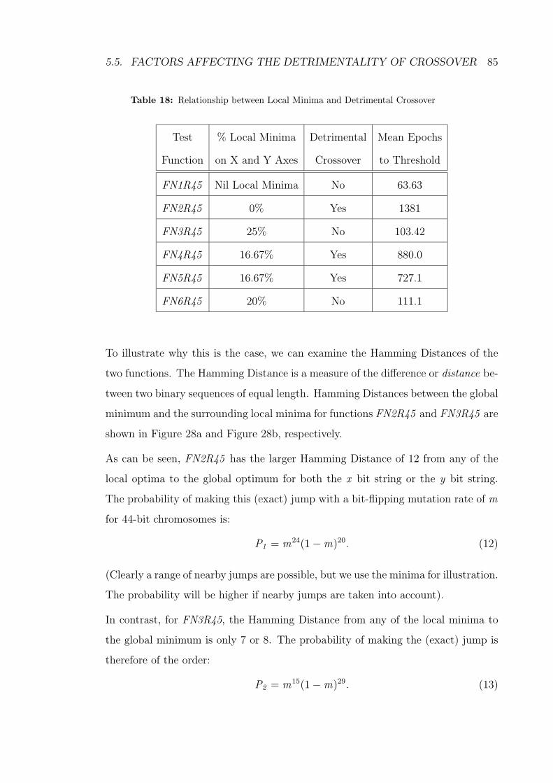
5.5. FACTORS AFFECTING THE DETRIMENTALITY OF CROSSOVER 85
Table 18: Relationship between Local Minima and Detrimental Crossover
Test % Local Minima Detrimental Mean Epochs
Function on X and Y Axes Crossover to Threshold
FN1R45 Nil Local Minima No 63.63
FN2R45 0% Yes 1381
FN3R45 25% No 103.42
FN4R45 16.67% Yes 880.0
FN5R45 16.67% Yes 727.1
FN6R45 20% No 111.1
To illustrate why this is the case, we can examine the Hamming Distances of the
two functions. The Hamming Distance is a measure of the difference or distance be-
tween two binary sequences of equal length. Hamming Distances between the global
minimum and the surrounding local minima for functions FN2R45 and FN3R45 are
shown in Figure 28a and Figure 28b, respectively.
As can be seen, FN2R45 has the larger Hamming Distance of 12 from any of the
local optima to the global optimum for both the x bit string or the y bit string.
The probability of making this (exact) jump with a bit-flipping mutation rate of m
for 44-bit chromosomes is:
P1 = m24(1 − m)20. (12)
(Clearly a range of nearby jumps are possible, but we use the minima for illustration.
The probability will be higher if nearby jumps are taken into account).
In contrast, for FN3R45, the Hamming Distance from any of the local minima to
the global minimum is only 7 or 8. The probability of making the (exact) jump is
therefore of the order:
P2 = m15(1 − m)29. (13)
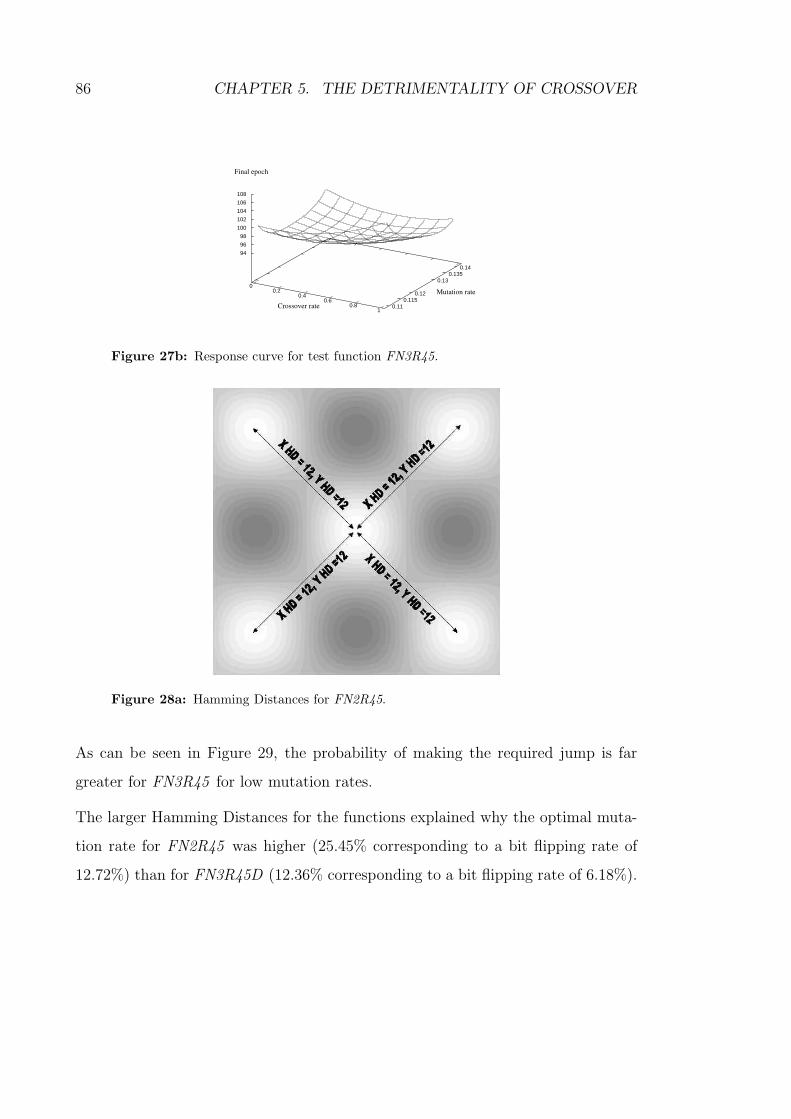
86 CHAPTER 5. THE DETRIMENTALITY OF CROSSOVER
00.2
0.40.6
0.81
Crossover rate 0.110.115
0.12
0.130.135
0.14
Mutation rate
94
96
98
100
102
104
106
108
Final epoch
Figure 27b: Response curve for test function FN3R45.
Figure 28a: Hamming Distances for FN2R45.
As can be seen in Figure 29, the probability of making the required jump is far
greater for FN3R45 for low mutation rates.
The larger Hamming Distances for the functions explained why the optimal muta-
tion rate for FN2R45 was higher (25.45% corresponding to a bit flipping rate of
12.72%) than for FN3R45D (12.36% corresponding to a bit flipping rate of 6.18%).
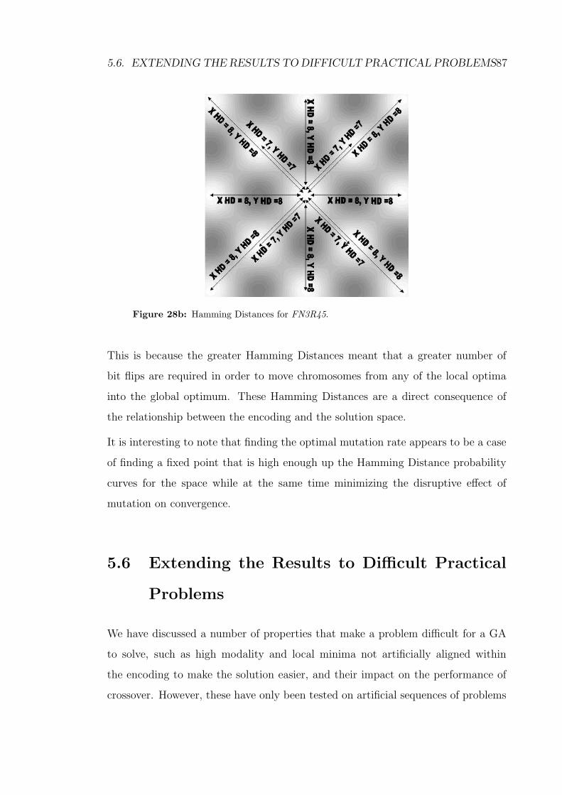
5.6. EXTENDING THE RESULTS TO DIFFICULT PRACTICAL PROBLEMS87
Figure 28b: Hamming Distances for FN3R45.
This is because the greater Hamming Distances meant that a greater number of
bit flips are required in order to move chromosomes from any of the local optima
into the global optimum. These Hamming Distances are a direct consequence of
the relationship between the encoding and the solution space.
It is interesting to note that finding the optimal mutation rate appears to be a case
of finding a fixed point that is high enough up the Hamming Distance probability
curves for the space while at the same time minimizing the disruptive effect of
mutation on convergence.
5.6 Extending the Results to Difficult Practical
Problems
We have discussed a number of properties that make a problem difficult for a GA
to solve, such as high modality and local minima not artificially aligned within
the encoding to make the solution easier, and their impact on the performance of
crossover. However, these have only been tested on artificial sequences of problems
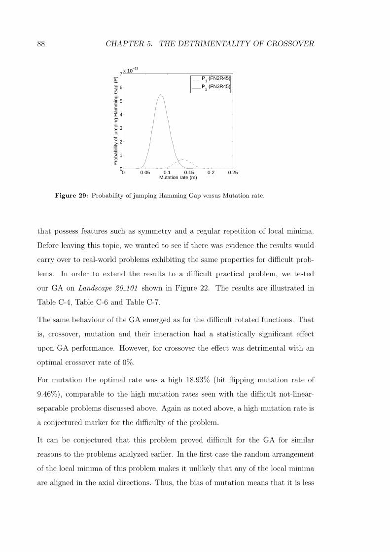
88 CHAPTER 5. THE DETRIMENTALITY OF CROSSOVER
0 0.05 0.1 0.15 0.2 0.250
1
2
3
4
5
6
7x 10
−13
Mutation rate (m)
Pro
babi
lity
of ju
mpi
ng H
amm
ing
Gap
(P
) P1 (FN2R45)
P2 (FN3R45)
Figure 29: Probability of jumping Hamming Gap versus Mutation rate.
that possess features such as symmetry and a regular repetition of local minima.
Before leaving this topic, we wanted to see if there was evidence the results would
carry over to real-world problems exhibiting the same properties for difficult prob-
lems. In order to extend the results to a difficult practical problem, we tested
our GA on Landscape 20 101 shown in Figure 22. The results are illustrated in
Table C-4, Table C-6 and Table C-7.
The same behaviour of the GA emerged as for the difficult rotated functions. That
is, crossover, mutation and their interaction had a statistically significant effect
upon GA performance. However, for crossover the effect was detrimental with an
optimal crossover rate of 0%.
For mutation the optimal rate was a high 18.93% (bit flipping mutation rate of
9.46%), comparable to the high mutation rates seen with the difficult not-linear-
separable problems discussed above. Again as noted above, a high mutation rate is
a conjectured marker for the difficulty of the problem.
It can be conjectured that this problem proved difficult for the GA for similar
reasons to the problems analyzed earlier. In the first case the random arrangement
of the local minima of this problem makes it unlikely that any of the local minima
are aligned in the axial directions. Thus, the bias of mutation means that it is less

5.7. DISCUSSION 89
likely that the global minimum will be found by chromosomes moving in the x and
y directions.
In reference to crossover, the fact that the surface of the Landscape 20 101 has
a great number of local minima means that it is very likely that crossover was
enacting optimization at the local minima sites. This is supported by the fact that
the optimal mutation rate was high at 18.93% (bit flipping mutation rate of 9.46%),
suggesting that a high mutation rate was required to get chromosomes to jump out
of regions of local minima where they were “stuck” due to local optimization carried
out by crossover.
5.7 Discussion
The traditional concept of a GA, that of selection, crossover and mutation, is being
challenged as literature has emerged which suggests that the crossover operator may
not necessarily be essential in a GA. However, there has not as yet been a direct sta-
tistical attempt to prove the detrimentality of crossover nor an attempt to describe
the conditions under which such detrimentality may occur. This chapter used our
statistical methodology to explore the issue of the detrimentality of crossover. In
particular, we were interested in establishing whether not-linear-separability was
a sufficient determinant of the detrimentality of crossover and if not, what other
factors was it characterized by.
In the first instance the results from the linear-separable test function series, FNn,
show that crossover is beneficial for these linear-separable problems. This concurs
with the suggestion of Salomon that Crossover’s Niche is in fact linear-separable
problems [38].
On the other hand, results from the rotated not-linear-separable test function series
demonstrated several instances where crossover was statistically proven to be detri-
mental. This occurred for not-linear-separable problems which required the highest
mutation rates, which has been a marker for the difficulty of a problem. Thus, what
90 CHAPTER 5. THE DETRIMENTALITY OF CROSSOVER
makes a not-linear-separable problem hard for a GA to solve is linked to whether
crossover will be detrimental to the performance of the GA solving the problem.
In the course of the present research it was found that three factors were involved
in making a not-linear-separable problem hard for the GA to solve. These were
optimization carried out by crossover at the sites of local minima, the bias of the
mutation operator and the Hamming Distances for the individual problems.
In the first case, the difficulty of a problem was impacted by the degree of opti-
mization at local minima carried out by the crossover operator. That is, crossover
was carrying out optimization on chromosomes “stuck” in local minima resulting in
their moving deeper into the local minima sites. Our experiments on this showed
that at least 80% of the time crossover improved the fitness of chromosomes at sites
of local minima.
Secondly, it was found that the mutation operator was biased along the x and y axes.
If a function had at least some of the local minima and the global minimum aligned
in the axial directions this made the problem easier to solve as the chromosomes
from these minima would be shifted with a greater likelihood towards the global
minimum.
Thirdly, the relationship between the problem and the solution space resulted in
situations where a less modal problem was actually more difficult to solve because of
the greater Hamming Distance between its local minima and the global minimum.
This was illustrated for FN2R45 and FN3R45 where the latter was the more modal
function, yet proved easier to solve as the Hamming Distances between its local
minima and its global minimum were lower.
Finally, the detrimentality of crossover was demonstrated on a difficult practical
problem, namely, a problem from the Huygens suite. The results showed that
crossover can be detrimental on a real world problem. The reasons for this occurring
may be extrapolated from the reasons found for the difficult rotated FNn problem
series. These include the degree of local optimization attributable to the crossover

5.7. DISCUSSION 91
operator and the bias of the mutation operator.
In conclusion, it has been demonstrated that crossover is statistically detrimental for
the difficult not-linear-separable problems and also the difficult real world problem
in the given configuration. Further research will be required to extend the class
of problems and illustrate if crossover can be demonstrated to be detrimental with
different encodings and in discrete problem domains. However, the results suggest
that crossover can prove to have a truly detrimental effect upon GA performance.
It should be noted that the results apply to specific (one-point) crossover operator
and mutation operator and further tests would be required to determine whether
other crossover operators (such as uniform crossover) and mutation give similar
results.

92 CHAPTER 5. THE DETRIMENTALITY OF CROSSOVER

Chapter 6
General Conclusions and Future
Research
Genetic algorithms have been the focus of extensive study in computer science
and have been applied to both theoretical and real world problems. How-
ever, there has been no generally accepted methodology to assess which parameters
significantly affect performance of genetic algorithms, whether these parameters in-
teract and how performance varies with respect to changes in parameters. The focus
of this thesis has been to formulate a statistical methodology for the exploratory
study of genetic and other adaptive algorithms and to demonstrate the application
of the methodology through the investigation of properties of a GA.
6.1 Statistical Methodology
The first part of the present thesis dealt with the development of a statistical
methodology for the exploratory analysis of genetic and other adaptive algorithms.
To recap, once the algorithm and the problem domain have been specified, the steps
in the statistical methodology proceed as follows:
1. Identify sources of variation and modify the algorithm to generate blocked
93

94 CHAPTER 6. GENERAL CONCLUSIONS AND FUTURE RESEARCH
runs.
2. Use a workup procedure to minimize the appearance of censored observations
and to finalize starting ranges for parameters.
3. Generate an initial data-set consisting of an arbitrary number of replicates.
Typically, we have found 100 replicates to be a useful starting point.
4. Calculate power based upon a chosen effect size. We recommend an effect
size index of 0.4 (large effect). If at least 80% power is not achieved and the
experiment resulted in observing no interaction increase the sample size.
5. Conduct (pooled) ANOVA analysis and determine which parameters are sta-
tistically significant.
6. For parameters which are statistically significant partition the sum of squares
into polynomial contrast terms. Determine which polynomial terms are sta-
tistically significant.
7. Use polynomial regression to obtain the coefficients for the overall response
curve (if the interaction parameter is statistically significant) or to obtain
the coefficients for the response curve for each parameter separately (if the
interaction parameter is not statistically significant).
8. Differentiate and solve the response curve for each parameter to obtain best
values and calculate confidence intervals.
The statistical methodology developed was initially trialed on well known test func-
tions. Looking at the results from the suite of test functions together, we found that
crossover appears to have a predominantly linear effect and that the direction of its
slope is problem specific. In contrast, mutation appears to have a predominantly
quadratic effect upon performance. The mutation rates observed advocate the use
of higher mutation rates than have traditionally been used. The use of statistics

6.2. THE IMPORTANCE OF INTERACTION 95
also enabled the issue of interaction to be addressed and we found that whether
interaction is significant is also problem specific.
These initial trials enabled the identification of key features affecting GA perfor-
mance that deserved more detailed investigation. Our subsequent work demon-
strated how the statistical methodology can assist in guiding the GA practitioner
to explore such features.
6.2 The Importance of Interaction
The second part of this thesis examined the issue of whether crossover and mutation
interact or if each parameter exerts its effect independently. This led to two impor-
tant questions. First, what type of functions are likely to demonstrate interaction
between crossover and mutation, and, secondly, what is the practical implication of
interaction when attempting to obtain optimal rates for these parameters. These
questions were addressed by examining the relationship between the occurrence of
statistically significant interaction among crossover and mutation and increasing
modality of a problem.
Addressing the first question it was found that functions with increased modality
are more likely to demonstrate interaction between crossover and mutation. It is
conjectured that when dealing with highly modal functions the possibility of inter-
action must be considered. For simple functions, with little or no multi-modality,
it is conjectured that crossover and mutation are exerting their respective effects
independently.
Addressing the second question it has been shown that if interaction is occurring
attempting to optimize the rate of crossover and mutation independently may result
in rates which are not optimal. In order to account for the effect of interaction all
combinations of crossover and mutation, within given starting ranges, must be
trialed.
96 CHAPTER 6. GENERAL CONCLUSIONS AND FUTURE RESEARCH
6.3 The Influence of Gray Encoding
The third part of this thesis explored which factors may affect GA performance.
This led to two important questions, namely, whether there is a statistically signif-
icant relationship between the difficulty of a problem and the choice of encoding,
and, if so, what is the actual mechanism by which this occurs.
In addressing the first question, this chapter demonstrated that a lower modality
problem may be significantly more difficult to solve with a Gray encoding than a
higher modality problem. This contrasts with the usual trend of problem difficulty
increasing with increasing modality.
In addressing the second question, animations of the GA clearly showed the ability
of chromosomes to move between local optima and avoid culling in the functions
studied. The probability of a successful jump is dependent on the Hamming Dis-
tance. Calculation was therefore made of the Hamming Distances between local op-
tima present in the two functions and it was found that movement within the lower
modality function was more difficult because of the significantly higher Hamming
Distances involved. These Hamming Distances are a direct result of the encoding.
In conclusion, it has been demonstrated that there is a real relationship between the
difficulty of a problem and the choice of encoding, in this instance Gray codes. It
has further been conjectured that the mechanism by which this occurs is related to
the different Hamming Distances occurring at specific regions in the solution space.
6.4 The Detrimentality of Crossover
In the first part of the present thesis an interesting observation was that the optimal
crossover rate for De Jong’s F2 and Schaffer’s F6 was 0% in our experimental set-up.
This implied that crossover was acting detrimentally on these occasions. A limited
amount of work has conjectured that the niche for the beneficial effect of crossover
upon GA performance is related to linear-separability, and this was borne in these

6.5. FUTURE RESEARCH 97
initial test functions. To explore this relationship in more detail, we compared two
problem suites, one of which was linear-separable and the other not-linear-separable
(the latter functions having been rotated by 45 degrees in the solution space).
Rather, we found that not-linear-separability was not, on its own, a sufficient deter-
minant for the detrimentality of crossover. It was shown that the crossover operator
was detrimental to the performance of the GA for difficult rotated functions. It is
conjectured that what makes a problem difficult for the GA involves factors such
as the degree of optimization at local minima due to crossover, the bias associated
with the mutation operator and the Hamming Distances present in the individual
problems due to the encoding.
Finally, the GA was tested on a real world landscape minimization problem to
ascertain if the results obtained would match those associated with the difficult
rotated functions. It was shown that they match and that the features which make
certain of the test functions difficult are also present in the real world problem.
6.5 Future Research
This thesis has demonstrated a statistical methodology that allows the investiga-
tor to undertake exploratory analysis of genetic and other adaptive algorithms.
This methodology has then been used to explore the issue of interaction between
crossover and mutation, the influence of the encoding used (in this thesis Gray en-
coding) and the detrimentality of crossover. Given the unique advantages offered
by statistical analysis, such as the ability to block for seed, calculation of power
and sample size, and rigorous study of response curves, further use of statistics will
assist in the development of GAs as powerful search tools.
This being said, there are a number of limitations in the present thesis which warrant
future research. In the first instance, the implementation of the GA was deliber-
ately simple so that a clear and concise demonstration of the proposed methodology
and results could be made. In this regard parameters such as the population size

98 CHAPTER 6. GENERAL CONCLUSIONS AND FUTURE RESEARCH
and bits per variable were not varied and only crossover and mutation were in-
vestigated in the present thesis. The methodology described in this thesis can be
straightforwardly applied to the many other parameters suggested in the literature
by including these as extra parameters.
Secondly, the functions examined in this thesis have been continuous functions.
There are, however, many other problem types to which this methodology may be
applied. Examples include constrained optimization problems, multi-objective opti-
mization problems and discrete combinatorial optimization problems. Application
of the statistical methodology presented in this thesis to these problem domains
and others would provide a greater understanding of the performance of genetic
algorithms.
Finally, this thesis has concerned itself solely with GAs. The methodology however
can be applied to other adaptive algorithms such as Particle Swarm Optimization
(PSO) and Differential Evolution in a similar fashion to that applied to GAs. Re-
search in this field would greatly increase our understanding about the comparative
performance of different types of adaptive algorithms and their sensitivity to the
parameters on which they are based.

Bibliography
[1] T Back, D Fogel and Z Michalewicz (editors). Handbook of Evolutionary Com-
putation. Oxford University Press, 1997.
[2] T Back, U Hammel and H Schwefel. Evolutionary computation: comments on
the history and current state. IEEE Transactions on Evolutionary Computa-
tion, Volume 1, Number 1, April 1997.
[3] S Bullock. Are artificial mutation biases unnatural? In European Conference
on Artificial Life, pages 64–73. Springer, 1999.
[4] S Bullock. Smooth operator? Understanding and visualising mutation bias.
Lecture Notes in Computer Science, Volume 2159, pages 602–612, Springer,
2001.
[5] J Cohen. Statistical Power Analysis for the Behavioral Sciences. Lawrence
Erlbaum, 1988.
[6] L Davis (editor). Handbook of genetic algorithms. Van Nostrand Reinhold,
1991.
[7] L Davis. Adapting operator probabilities in genetic algorithms. In Proc. Third
International Conference on Genetic Algorithms, pages 61–69, Morgan Kauf-
mann, 1989.
99

100 BIBLIOGRAPHY
[8] T E Davis and J C Principe. A markov chain framework for the simple genetic
algorithm. Evolutionary Computation, Volume 1, Number 3, pages 269–288,
1993.
[9] K A De Jong. Analysis of the Behavior of a Class of Genetic Adaptive Systems.
Phd dissertation, Department of Computer and Communication Sciences, Uni-
versity of Michigan, Ann Arbor, MI, 1975.
[10] S Droste, T Jansen and I Wegener. On the analysis of the (1+ 1) evolutionary
algorithm. Theoretical Computer Science, Volume 276, pages 51–81, 2002.
[11] A E Eiben, R Hinterding and Z Michalewicz. Parameter control in evolution-
ary algorithms. IEEE Transactions on Evolutionary Computation, Volume 3,
Number 2, pages 124–141, 1999.
[12] L Eshelman. Bit-climbers and naive evolution. Genetic Algorithms Digest,
Volume 5, Number 39, December 1991.
[13] L J Eshelman and J D Schaffer. Crossover’s niche. In Proc. Fifth International
Conference on Genetic Algorithms, pages 9–14, Morgan Kaufmann, 1993.
[14] F Faul and E Erdfelder. GPOWER: A priori, post-hoc, and compromise power
analyses computer program for MS-DOS. Available: http://www.psycho.uni-
duesseldorf.de/aap/projects/gpower/index.html. Bonn, FRG: Bonn Univer-
sity, Dep. of Psychology.
[15] D B Fogel and J W Atmar. Comparing genetic operators with gaussian mu-
tations in simulated evolutionary processes using linear systems. Biological
Cybernetics, Volume 63, Number 2, pages 111–114, 1990.
[16] B Freisleben and M Hartfelder. Optimization of genetic algorithms by genetic
algorithms. In Proc. International Conference on Aritifical Neural Nets and
Genetic Algorithms, pages 392–399. Springer-Verlag, 1993.

BIBLIOGRAPHY 101
[17] D E Goldberg. Genetic algorithms in search, optimization and machine learn-
ing. Addison-Wesley, 1989.
[18] J Grefenstette. Optimization of control parameters for genetic algorithms.
IEEE Transactions on Systems, Man, and Cybernetics, Volume SMC-16, Num-
ber 1, 1986.
[19] J He and X Yao. From an individual to a population: an analysis of the first
hitting time of population-based evolutionary algorithms. IEEE Transactions
on Evolutionary Computation, Volume 6, Number 5, pages 495–511, 2002.
[20] J H Holland. Adaptation in natural and artificial systems. University of Michi-
gan Press, 1975.
[21] Insightful. S-PLUS. Available: http://www.insightful.com/.
[22] T Jansen and I Wegener. The analysis of evolutionary algorithms - A proof
that crossover really can help. Algorithmica, Volume 34, pages 47–66, 2002.
[23] T Jansen and I Wegener. Real royal road functions-where crossover provably
is essential. Discrete Applied Mathematics, Volume 149, pages 111–125, 2005.
[24] R A Johnson and G K Bhattacharyya. Statistics: Principles and Methods.
John Wiley & Sons, 1996.
[25] T Jones. Crossover, macromutation, and population-based search. In Proc.
of the Sixth International Conference on Genetic Algorithms, pages 73–80,
Morgan Kaufman, 1995.
[26] R I Levin and D S Rubin. Applied Elementary Statistics. Prentice-Hall, 1980.
[27] C MacNish. Towards unbiased benchmarking of evolutionary and hybrid algo-
rithms for real-valued optimisation. To appear in Connection Science, special
issue on Evolutionary Learning and Optimization.

102 BIBLIOGRAPHY
[28] C MacNish. Benchmarking evolutionary and hybrid algorithms using random-
ized self-similar landscapes. In Proc. Sixth International Conference on Sim-
ulated Evolution and Learning SEAL, Volume 4247, pages 361–368. Springer,
2006.
[29] M Mitchell, S Forrest and J Holland. The royal road for genetic algorithms:
Fitness landscapes and GA performance. In Towards a Practice of Autonomous
Systems: Proc. of the First European Conference on Artificial Life, pages 245–
254. MIT Press, 1991.
[30] D C Montgomery. Design and Analysis of Experiments. John Wiley and Sons,
1976.
[31] A Narayanan and M Moore. Quantum inspired genetic algorithms. In Inter-
national Conference on Evolutionary Computation, pages 61–66. IEEE, 1996.
[32] A Petrovski and J McCall. Optimising GA parameters using statistical ap-
proaches. Technical report, Robert Gordon University, 1997.
[33] A Petrovski, A Wilson and J McCall. Statistical analysis of genetic algorithms
and inference about optimal factors. Technical report, Robert Gordon Univer-
sity, 1998.
[34] A Prugel-Bennett and J L Shapiro. Analysis of genetic algorithms using statis-
tical mechanics. Physical Review Letters, Volume 72, Number 9, pages 1305–
1309, 1994.
[35] C R Reeves and C C Wright. Genetic algorithms and the design of exper-
iments. In Evolutionary Algorithms: IMA Volumes in Mathematics and its
Applications, Volume 111, pages 207–226. Springer-Verlag, New York, 1999.
[36] J A Rice. Mathematical Statistics and Data Analysis. Duxbury Press, 1995.
[37] F Rothlauf. Representations for Genetic and Evolutionary Algorithms.
Springer, 2003.
BIBLIOGRAPHY 103
[38] R Salomon. Re-evaluating genetic algorithm performance under coordinate
rotation of benchmark functions: a survey of some theoretical and practical
aspects of genetic algorithms. BioSystems, Volume 39, Number 3, pages 263–
278, 1996.
[39] J D Schaffer, R A Caruana, L J Eshelman and R Das. A study of control
parameters affecting online performance of genetic algorithms for function op-
timization. In Proc. Third International Conference on Genetic algorithms,
pages 51–60. Morgan Kaufmann, 1989.
[40] A B Simoes and E Costa. Transposition versus crossover: an empirical study.
In Proc. Genetic and Evolutionary Computation Conference GECCO, pages
612–619. Morgan Kaufmann, 1999.
[41] Sun Microsystems, Inc. Java version 1.3.1 02.
[42] D H Wolpert and W G Macready. No free lunch theorems for optimization.
IEEE Transactions on Evolutionary Computation, Volume 1, Number 1, pages
67–82, 1997.
[43] X Yao, Y Liu and G Lin. Evolutionary programming made faster. IEEE
Transactions on Evolutionary Computation, Volume 3, Number 2, pages 82–
102, 1999.

104 BIBLIOGRAPHY
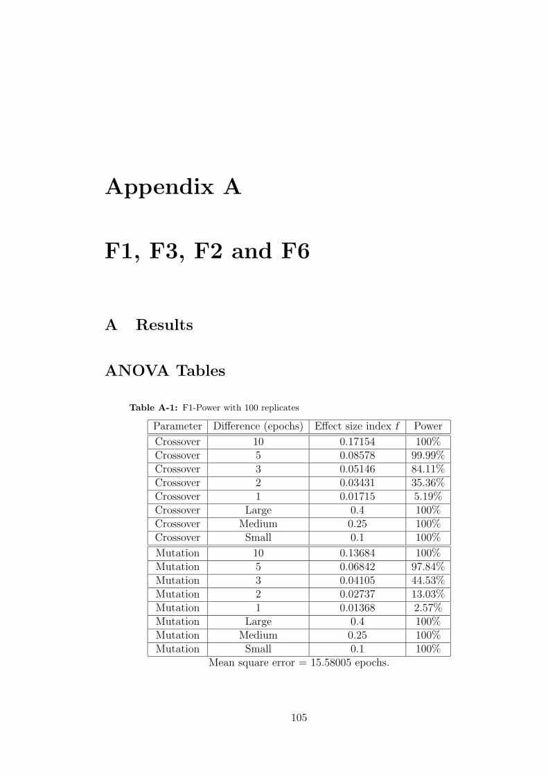
Appendix A
F1, F3, F2 and F6
A Results
ANOVA Tables
Table A-1: F1-Power with 100 replicates
Parameter Difference (epochs) Effect size index f Power
Crossover 10 0.17154 100%Crossover 5 0.08578 99.99%Crossover 3 0.05146 84.11%Crossover 2 0.03431 35.36%Crossover 1 0.01715 5.19%Crossover Large 0.4 100%Crossover Medium 0.25 100%Crossover Small 0.1 100%
Mutation 10 0.13684 100%Mutation 5 0.06842 97.84%Mutation 3 0.04105 44.53%Mutation 2 0.02737 13.03%Mutation 1 0.01368 2.57%Mutation Large 0.4 100%Mutation Medium 0.25 100%Mutation Small 0.1 100%
Mean square error = 15.58005 epochs.
105

106 APPENDIX A. F1, F3, F2 AND F6
Table A-2: F1-Power with 100 replicates continued
Parameter Difference (epochs) Effect size index f Power
Interaction 10 0.05172 27.58%Interaction 5 0.02586 3.38%
Interaction 3 0.01552 1.62%Interaction 2 0.01034 1.25%Interaction 1 0.00517 1.06%Interaction Large 0.4 100%Interaction Medium 0.25 100%Interaction Small 0.1 99.52%
Mean square error = 15.58005 epochs.
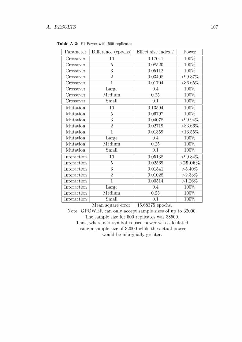
A. RESULTS 107
Table A-3: F1-Power with 500 replicates
Parameter Difference (epochs) Effect size index f Power
Crossover 10 0.17041 100%Crossover 5 0.08520 100%Crossover 3 0.05112 100%Crossover 2 0.03408 >99.37%Crossover 1 0.01704 >36.65%Crossover Large 0.4 100%Crossover Medium 0.25 100%Crossover Small 0.1 100%
Mutation 10 0.13594 100%Mutation 5 0.06797 100%Mutation 3 0.04078 >99.94%Mutation 2 0.02719 >83.66%Mutation 1 0.01359 >13.55%Mutation Large 0.4 100%Mutation Medium 0.25 100%Mutation Small 0.1 100%
Interaction 10 0.05138 >99.84%Interaction 5 0.02569 >29.06%
Interaction 3 0.01541 >5.40%Interaction 2 0.01028 >2.33%Interaction 1 0.00514 >1.26%Interaction Large 0.4 100%Interaction Medium 0.25 100%Interaction Small 0.1 100%
Mean square error = 15.68375 epochs.Note: GPOWER can only accept sample sizes of up to 32000.
The sample size for 500 replicates was 38500.Thus, where a > symbol is used power was calculatedusing a sample size of 32000 while the actual power
would be marginally greater.

108 APPENDIX A. F1, F3, F2 AND F6
Table A-4: F1-Power of the pooled analysis
Parameter Difference (epochs) Effect size index f Power
Crossover 10 3.9193 100%Crossover 5 1.9597 100%Crossover 3 1.1758 100%Crossover 2 0.78386 100%Crossover 1 0.39193 100%Crossover Large 0.4 100%Crossover Medium 0.25 90.39%Crossover Small 0.1 9.83%
Mutation 10 3.1265 100%Mutation 5 1.5633 100%Mutation 3 0.93796 100%Mutation 2 0.62531 100%Mutation 1 0.31265 97.94%Mutation Large 0.4 99.99%Mutation Medium 0.25 82.55%Mutation Small 0.1 6.96%
Interaction 10 1.1817 100%Interaction 5 0.59086 100%
Interaction 3 0.35452 79.01%Interaction 2 0.23634 23.79%Interaction 1 0.11817 3.11%Interaction Large 0.4 92.65%Interaction Medium 0.25 29.05%Interaction Small 0.1 2.33%
Mean square error = 0.6819076 epochs.

A. RESULTS 109
Table A-5: F3-Power of the pooled analysis
Parameter Difference (epochs) Effect size index f Power
Crossover 10 2.6652 100%Crossover 5 1.3326 100%Crossover 3 0.79956 100%Crossover 2 0.53304 100%Crossover 1 0.26652 75.25%Crossover Large 0.4 99.49%Crossover Medium 0.25 67.45%Crossover Small 0.1 6.26%
Mutation 10 1.9865 100%Mutation 5 0.99327 100%Mutation 3 0.59596 100%Mutation 2 0.39731 97.74%Mutation 1 0.19865 26.92%Mutation Large 0.40 97.93%Mutation Medium 0.25 51.41%Mutation Small 0.1 4.12%
Interaction 10 0.88840 100%Interaction 5 0.44420 88.27%
Interaction 3 0.26652 23.21%Interaction 2 0.17768 6.34%Interaction 1 0.08884 1.76%Interaction Large 0.4 75.30%Interaction Medium 0.25 18.64%Interaction Small 0.1 2.02%
Mean square error = 1.1865 epochs.

110 APPENDIX A. F1, F3, F2 AND F6
Table A-6: F2-Power of the pooled analysis
Parameter Difference (epochs) Effect size index f Power
Crossover 10 0.27104 100%Crossover 5 0.13552 56.28%Crossover 3 0.08131 11.87%Crossover 2 0.05421 4.05%Crossover 1 0.02710 1.53%Crossover Large 0.4 100%Crossover Medium 0.25 99.96%Crossover Small 0.1 22.88%
Mutation 10 0.29113 100%Mutation 5 0.14557 70.38%Mutation 3 0.08734 16.61%Mutation 2 0.05823 5.24%Mutation 1 0.02911 1.69%Mutation Large 0.40 100%Mutation Medium 0.25 99.98%Mutation Small 0.1 25.48%
Interaction 10 0.07517 2.04%Interaction 5 0.03759 1.21%
Interaction 3 0.02255 1.07%Interaction 2 0.01503 1.03%Interaction 1 0.00752 1.01%Interaction Large 0.4 99.97%Interaction Medium 0.25 62.57%Interaction Small 0.1 3.32%
Mean square error = 6.736177 epochs.

A. RESULTS 111
Table A-7: F6-Power of the pooled analysis
Parameter Difference (epochs) Effect size index f Power
Crossover 10 .28308 100%Crossover 5 .14154 72.65%Crossover 3 .08492 17.11%Crossover 2 .05661 5.30%Crossover 1 .02830 1.69%Crossover Large .4 100%Crossover Medium .25 99.99%Crossover Small .1 28.86%
Mutation 10 .28308 100%Mutation 5 .14154 72.65%Mutation 3 .08492 17.11%Mutation 2 .05661 5.30%Mutation 1 .02830 1.69%Mutation Large .4 100%Mutation Medium .25 99.99%Mutation Small .1 28.86%
Interaction 10 .07309 2.05%Interaction 5 .03654 1.21%
Interaction 3 .02192 1.07%Interaction 2 .01461 1.03%Interaction 1 .00730 1.01%Interaction Large 0.4 99.99%Interaction Medium 0.25 69.01%Interaction Small 0.1 3.56%
Mean square error = 6.449417 epochs.

112 APPENDIX A. F1, F3, F2 AND F6
Table A-8: F6-Power of the pooled analysis for crossover 0% to 15%
Parameter Difference (epochs) Effect size index f Power
Crossover 10 .32905 100%Crossover 5 .16452 91.63%
Crossover 3 .09871 29.32%Crossover 2 .06581 8.24%Crossover 1 .03290 2.02%Crossover Large .4 100%Crossover Medium .25 100%Crossover Small .1 30.54%
Mean square error = 5.372283 epochs.

A. RESULTS 113
Partitioned Sum of Squares
Table A-9: F1-Partitioned sum of squares with 100 replicates
Parameter Df Sum of Sq Mean Sq F Value Pr(F)
Crossover 6 12347 2057.83 8.4776 0.0000000
Crossover adjusted level of significance = 0.001673654Power of 1 1 10330 10329.82 42.5554 0.0000000
Power of 2 1 38 38.13 0.1571 0.6918712Power of 3 1 976 975.98 4.0207 0.0449809Power of 4 1 681 680.92 2.8052 0.0940032Power of 5 1 14 13.70 0.0564 0.8122398Power of 6 1 308 308.41 1.2705 0.2597008
Mutation 10 58701 5870.09 24.1828 0.0000000
Mutation adjusted level of significance = 0.001004529Power of 1 1 11389 11388.70 46.9176 0.0000000
Power of 2 1 44725 44724.56 184.2503 0.0000000
Power of 3 1 2 2.16 0.0089 0.9248439Power of 4 1 1069 1068.68 4.4026 0.0359176Power of 5 1 553 552.87 2.2776 0.1312950Power of 6 1 452 451.55 1.8602 0.1726404Power of 7 1 2 1.66 0.0068 0.9340925Power of 8 1 487 486.78 2.0054 0.1567837Power of 9 1 20 20.44 0.0842 0.7717104Power of 10 1 4 3.52 0.0145 0.9041185
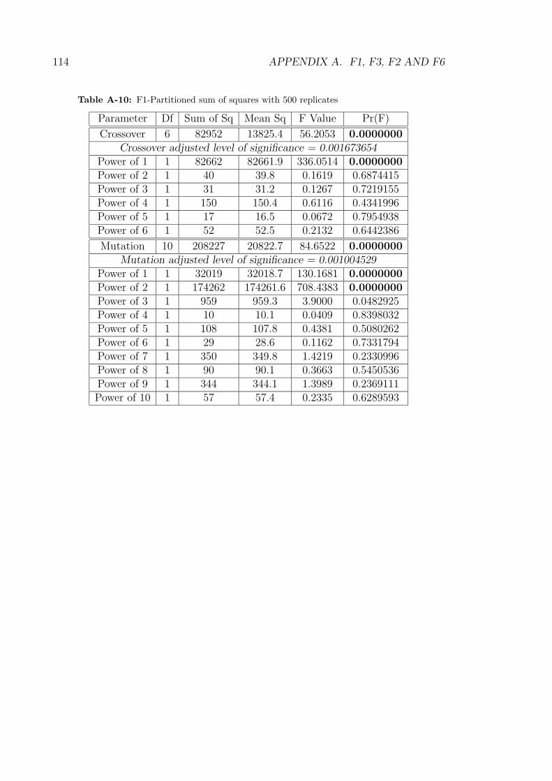
114 APPENDIX A. F1, F3, F2 AND F6
Table A-10: F1-Partitioned sum of squares with 500 replicates
Parameter Df Sum of Sq Mean Sq F Value Pr(F)
Crossover 6 82952 13825.4 56.2053 0.0000000
Crossover adjusted level of significance = 0.001673654Power of 1 1 82662 82661.9 336.0514 0.0000000
Power of 2 1 40 39.8 0.1619 0.6874415Power of 3 1 31 31.2 0.1267 0.7219155Power of 4 1 150 150.4 0.6116 0.4341996Power of 5 1 17 16.5 0.0672 0.7954938Power of 6 1 52 52.5 0.2132 0.6442386
Mutation 10 208227 20822.7 84.6522 0.0000000
Mutation adjusted level of significance = 0.001004529Power of 1 1 32019 32018.7 130.1681 0.0000000
Power of 2 1 174262 174261.6 708.4383 0.0000000
Power of 3 1 959 959.3 3.9000 0.0482925Power of 4 1 10 10.1 0.0409 0.8398032Power of 5 1 108 107.8 0.4381 0.5080262Power of 6 1 29 28.6 0.1162 0.7331794Power of 7 1 350 349.8 1.4219 0.2330996Power of 8 1 90 90.1 0.3663 0.5450536Power of 9 1 344 344.1 1.3989 0.2369111Power of 10 1 57 57.4 0.2335 0.6289593
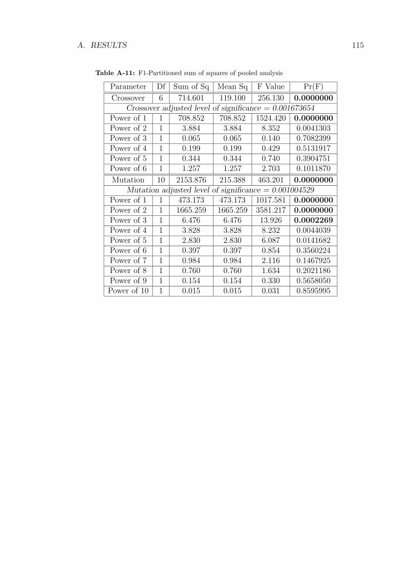
A. RESULTS 115
Table A-11: F1-Partitioned sum of squares of pooled analysis
Parameter Df Sum of Sq Mean Sq F Value Pr(F)
Crossover 6 714.601 119.100 256.130 0.0000000
Crossover adjusted level of significance = 0.001673654Power of 1 1 708.852 708.852 1524.420 0.0000000
Power of 2 1 3.884 3.884 8.352 0.0041303Power of 3 1 0.065 0.065 0.140 0.7082399Power of 4 1 0.199 0.199 0.429 0.5131917Power of 5 1 0.344 0.344 0.740 0.3904751Power of 6 1 1.257 1.257 2.703 0.1011870
Mutation 10 2153.876 215.388 463.201 0.0000000
Mutation adjusted level of significance = 0.001004529Power of 1 1 473.173 473.173 1017.581 0.0000000
Power of 2 1 1665.259 1665.259 3581.217 0.0000000
Power of 3 1 6.476 6.476 13.926 0.0002269
Power of 4 1 3.828 3.828 8.232 0.0044039Power of 5 1 2.830 2.830 6.087 0.0141682Power of 6 1 0.397 0.397 0.854 0.3560224Power of 7 1 0.984 0.984 2.116 0.1467925Power of 8 1 0.760 0.760 1.634 0.2021186Power of 9 1 0.154 0.154 0.330 0.5658050Power of 10 1 0.015 0.015 0.031 0.8595995
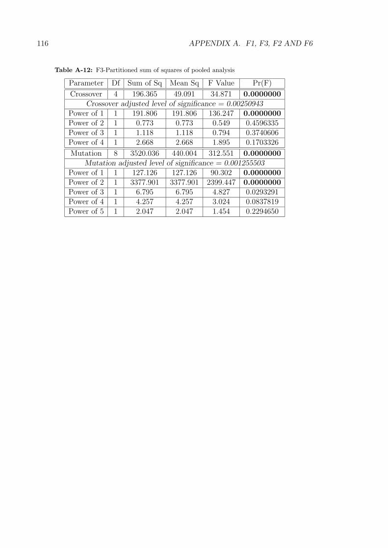
116 APPENDIX A. F1, F3, F2 AND F6
Table A-12: F3-Partitioned sum of squares of pooled analysis
Parameter Df Sum of Sq Mean Sq F Value Pr(F)
Crossover 4 196.365 49.091 34.871 0.0000000
Crossover adjusted level of significance = 0.00250943Power of 1 1 191.806 191.806 136.247 0.0000000
Power of 2 1 0.773 0.773 0.549 0.4596335Power of 3 1 1.118 1.118 0.794 0.3740606Power of 4 1 2.668 2.668 1.895 0.1703326
Mutation 8 3520.036 440.004 312.551 0.0000000
Mutation adjusted level of significance = 0.001255503Power of 1 1 127.126 127.126 90.302 0.0000000
Power of 2 1 3377.901 3377.901 2399.447 0.0000000
Power of 3 1 6.795 6.795 4.827 0.0293291Power of 4 1 4.257 4.257 3.024 0.0837819Power of 5 1 2.047 2.047 1.454 0.2294650
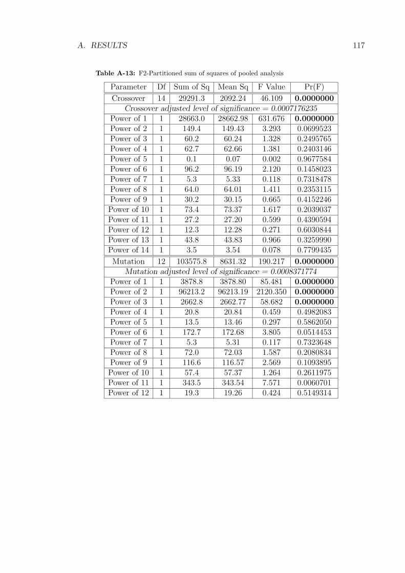
A. RESULTS 117
Table A-13: F2-Partitioned sum of squares of pooled analysis
Parameter Df Sum of Sq Mean Sq F Value Pr(F)
Crossover 14 29291.3 2092.24 46.109 0.0000000
Crossover adjusted level of significance = 0.0007176235Power of 1 1 28663.0 28662.98 631.676 0.0000000
Power of 2 1 149.4 149.43 3.293 0.0699523Power of 3 1 60.2 60.24 1.328 0.2495765Power of 4 1 62.7 62.66 1.381 0.2403146Power of 5 1 0.1 0.07 0.002 0.9677584Power of 6 1 96.2 96.19 2.120 0.1458023Power of 7 1 5.3 5.33 0.118 0.7318478Power of 8 1 64.0 64.01 1.411 0.2353115Power of 9 1 30.2 30.15 0.665 0.4152246Power of 10 1 73.4 73.37 1.617 0.2039037Power of 11 1 27.2 27.20 0.599 0.4390594Power of 12 1 12.3 12.28 0.271 0.6030844Power of 13 1 43.8 43.83 0.966 0.3259990Power of 14 1 3.5 3.54 0.078 0.7799435
Mutation 12 103575.8 8631.32 190.217 0.0000000
Mutation adjusted level of significance = 0.0008371774Power of 1 1 3878.8 3878.80 85.481 0.0000000
Power of 2 1 96213.2 96213.19 2120.350 0.0000000
Power of 3 1 2662.8 2662.77 58.682 0.0000000
Power of 4 1 20.8 20.84 0.459 0.4982083Power of 5 1 13.5 13.46 0.297 0.5862050Power of 6 1 172.7 172.68 3.805 0.0514453Power of 7 1 5.3 5.31 0.117 0.7323648Power of 8 1 72.0 72.03 1.587 0.2080834Power of 9 1 116.6 116.57 2.569 0.1093895Power of 10 1 57.4 57.37 1.264 0.2611975Power of 11 1 343.5 343.54 7.571 0.0060701Power of 12 1 19.3 19.26 0.424 0.5149314

118 APPENDIX A. F1, F3, F2 AND F6
Table A-14: F2-Partitioned sum of squares of pooled analysis continued
Parameter Df Sum of Sq Mean Sq F Value Pr(F)
Interaction 168 10717.5 63.79 1.406 0.0015501
Interaction adjusted level of significance = 0.00005982164.Only significant results shown.
Power of 1:Power of 1 1 2924.0 2923.96 64.438 0.0000000

A. RESULTS 119
Table A-15: F6-Partitioned sum of squares of pooled analysis
Parameter Df Sum of Sq Mean Sq F Value Pr(F)
Crossover 14 54420.8 3887.2 93.454 0.0000000
Crossover adjusted level of significance = 0.0007176235Power of 1 1 51558.8 51558.8 1239.544 0.0000000
Power of 2 1 2723.0 2723.0 65.465 0.0000000
Power of 3 1 0.1 0.1 0.002 0.9672032Power of 4 1 0.2 0.2 0.005 0.9438726Power of 5 1 14.2 14.2 0.340 0.5597281Power of 6 1 10.2 10.2 0.246 0.6203542Power of 7 1 5.0 5.0 0.121 0.7282759Power of 8 1 17.3 17.3 0.417 0.5187929Power of 9 1 59.5 59.5 1.430 0.2321141Power of 10 1 1.7 1.7 0.040 0.8419240Power of 11 1 0.0 0.0 0.000 0.9855772Power of 12 1 0.1 0.1 0.002 0.9613900Power of 13 1 30.7 30.7 0.739 0.3901418Power of 14 1 0.0 0.0 0.000 0.9893777
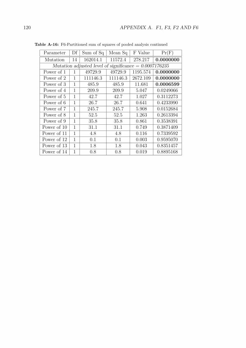
120 APPENDIX A. F1, F3, F2 AND F6
Table A-16: F6-Partitioned sum of squares of pooled analysis continued
Parameter Df Sum of Sq Mean Sq F Value Pr(F)
Mutation 14 162014.1 11572.4 278.217 0.0000000
Mutation adjusted level of significance = 0.0007176235Power of 1 1 49729.9 49729.9 1195.574 0.0000000
Power of 2 1 111146.3 111146.3 2672.109 0.0000000
Power of 3 1 485.9 485.9 11.681 0.0006599
Power of 4 1 209.9 209.9 5.047 0.0249066Power of 5 1 42.7 42.7 1.027 0.3112273Power of 6 1 26.7 26.7 0.641 0.4233990Power of 7 1 245.7 245.7 5.908 0.0152684Power of 8 1 52.5 52.5 1.263 0.2613394Power of 9 1 35.8 35.8 0.861 0.3538391Power of 10 1 31.1 31.1 0.749 0.3871409Power of 11 1 4.8 4.8 0.116 0.7339592Power of 12 1 0.1 0.1 0.003 0.9595070Power of 13 1 1.8 1.8 0.043 0.8351457Power of 14 1 0.8 0.8 0.019 0.8895168

A. RESULTS 121
Table A-17: F6-Partitioned sum of squares of pooled analysis continued
Parameter Df Sum of Sq Mean Sq F Value Pr(F)
Interaction 196 50461.5 257.5 6.190 0.0000000
Interaction adjusted level of significance = 0.00005127591.Only significant results shown.
Power of 1:Power of 1 1 34688.8 34688.8 833.966 0.0000000
Power of 2:Power of 1 1 1464.2 1464.2 35.200 0.0000000
Power of 1:Power of 2 1 5426.3 5426.3 130.457 0.0000000
Power of 1:Power of 3 1 925.8 925.8 22.257 0.0000028
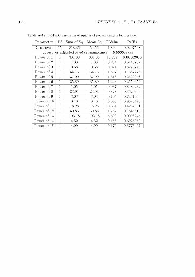
122 APPENDIX A. F1, F3, F2 AND F6
Table A-18: F6-Partitioned sum of squares of pooled analysis for crossover
Parameter Df Sum of Sq Mean Sq F Value Pr(F)
Crossover 15 818.36 54.56 1.890 0.0207598Crossover adjusted level of significance = 0.000669798
Power of 1 1 381.88 381.88 13.232 0.0002900
Power of 2 1 7.33 7.33 0.254 0.6143782Power of 3 1 0.68 0.68 0.024 0.8778748Power of 4 1 54.75 54.75 1.897 0.1687276Power of 5 1 37.90 37.90 1.313 0.2520953Power of 6 1 35.89 35.89 1.243 0.2650954Power of 7 1 1.05 1.05 0.037 0.8484232Power of 8 1 23.91 23.91 0.828 0.3629396Power of 9 1 3.03 3.03 0.105 0.7461390Power of 10 1 0.10 0.10 0.003 0.9528493Power of 11 1 18.28 18.28 0.634 0.4262661Power of 12 1 50.86 50.86 1.762 0.1846610Power of 13 1 193.18 193.18 6.693 0.0098245Power of 14 1 4.52 4.52 0.156 0.6925059Power of 15 1 4.99 4.99 0.173 0.6776497

A. RESULTS 123
Fitted response curves
Table A-19: Equations of fitted response curves
F1 Crossover Final epoch =82.35894 − 13.56899Cr
Mutation Final epoch =123.5819 − 1830.0797Mu+17956.7153Mu2 − 43781.1078Mu3
F3 Crossover Final epoch =77.99059 − 13.05733Cr
Mutation Final epoch =130.9682 − 2707.566Mu + 26493.42Mu2
F2 Overall Final epoch =−1415.7329 + 115.0829Cr + 30548.5413Mu−177255.5477Mu2 + 332182.6263Mu3
−428.4953(Cr ∗ Mu)
F6 Overall Final epoch =163.3295 + 2143.9363Cr + 222.2216Cr2
+2095.7379Mu − 30367.4855Mu2 + 105193.7584Mu3
−41244.8444(Cr ∗ Mu) − 1273.7673(Cr2 ∗ Mu)+260999.0679(Cr ∗ Mu2) − 543626.2156(Cr ∗ Mu3)
Crossover parameter level (Cr), Mutation parameter level (Mu).

124 APPENDIX A. F1, F3, F2 AND F6
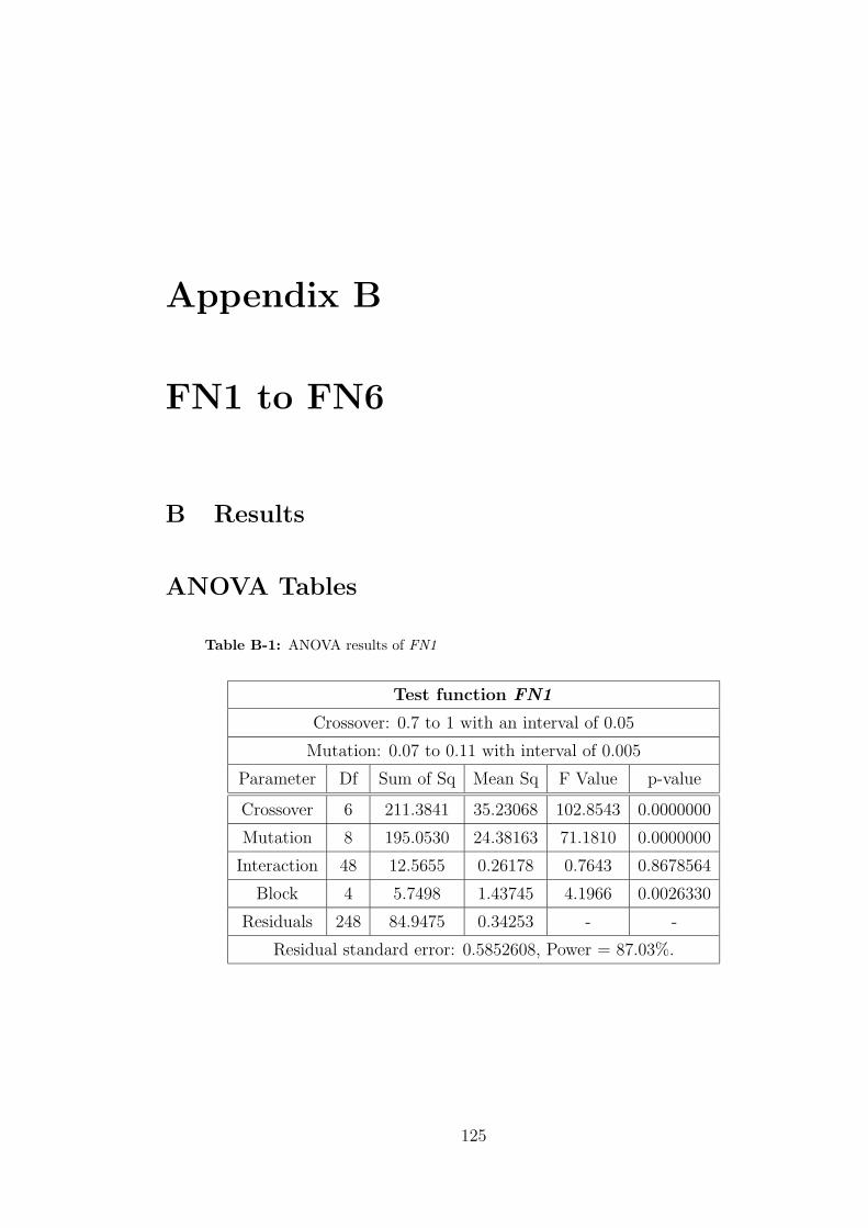
Appendix B
FN1 to FN6
B Results
ANOVA Tables
Table B-1: ANOVA results of FN1
Test function FN1
Crossover: 0.7 to 1 with an interval of 0.05
Mutation: 0.07 to 0.11 with interval of 0.005
Parameter Df Sum of Sq Mean Sq F Value p-value
Crossover 6 211.3841 35.23068 102.8543 0.0000000
Mutation 8 195.0530 24.38163 71.1810 0.0000000
Interaction 48 12.5655 0.26178 0.7643 0.8678564
Block 4 5.7498 1.43745 4.1966 0.0026330
Residuals 248 84.9475 0.34253 - -
Residual standard error: 0.5852608, Power = 87.03%.
125
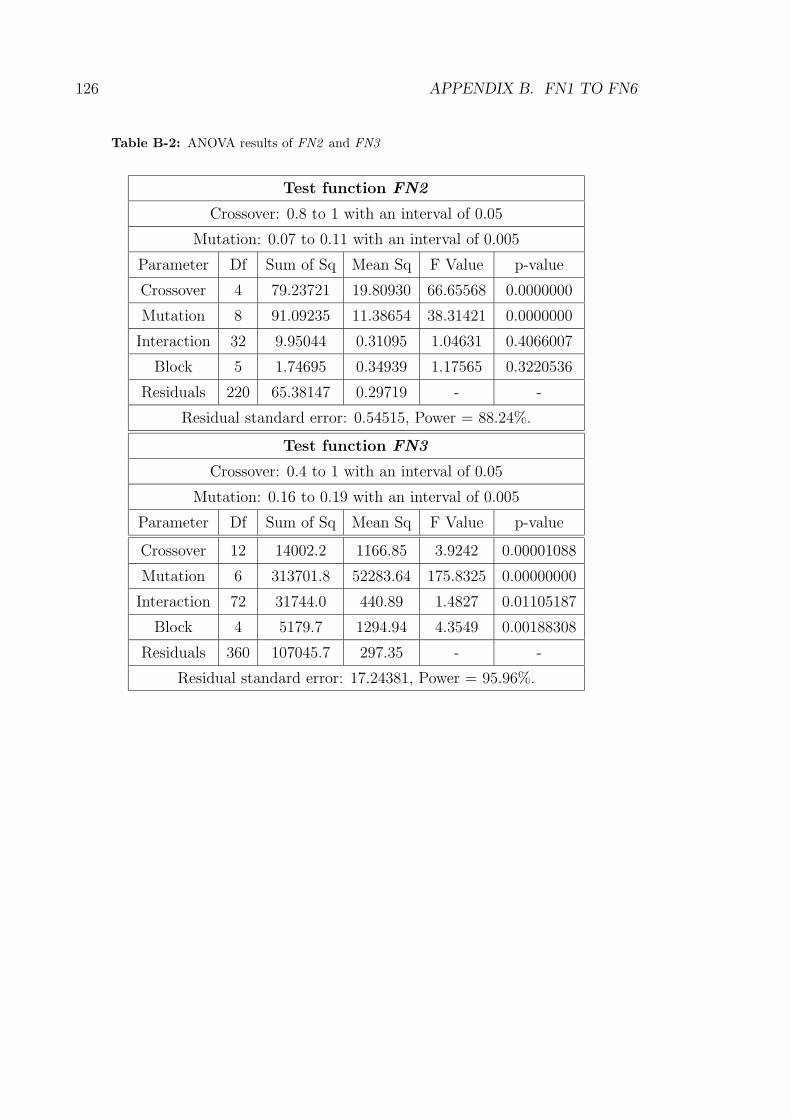
126 APPENDIX B. FN1 TO FN6
Table B-2: ANOVA results of FN2 and FN3
Test function FN2
Crossover: 0.8 to 1 with an interval of 0.05
Mutation: 0.07 to 0.11 with an interval of 0.005
Parameter Df Sum of Sq Mean Sq F Value p-value
Crossover 4 79.23721 19.80930 66.65568 0.0000000
Mutation 8 91.09235 11.38654 38.31421 0.0000000
Interaction 32 9.95044 0.31095 1.04631 0.4066007
Block 5 1.74695 0.34939 1.17565 0.3220536
Residuals 220 65.38147 0.29719 - -
Residual standard error: 0.54515, Power = 88.24%.
Test function FN3
Crossover: 0.4 to 1 with an interval of 0.05
Mutation: 0.16 to 0.19 with an interval of 0.005
Parameter Df Sum of Sq Mean Sq F Value p-value
Crossover 12 14002.2 1166.85 3.9242 0.00001088
Mutation 6 313701.8 52283.64 175.8325 0.00000000
Interaction 72 31744.0 440.89 1.4827 0.01105187
Block 4 5179.7 1294.94 4.3549 0.00188308
Residuals 360 107045.7 297.35 - -
Residual standard error: 17.24381, Power = 95.96%.
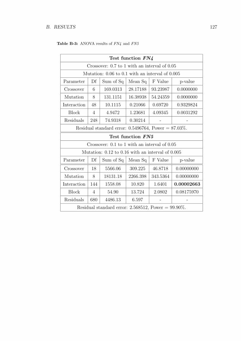
B. RESULTS 127
Table B-3: ANOVA results of FN4 and FN5
Test function FN4
Crossover: 0.7 to 1 with an interval of 0.05
Mutation: 0.06 to 0.1 with an interval of 0.005
Parameter Df Sum of Sq Mean Sq F Value p-value
Crossover 6 169.0313 28.17188 93.23987 0.0000000
Mutation 8 131.1151 16.38938 54.24359 0.0000000
Interaction 48 10.1115 0.21066 0.69720 0.9329824
Block 4 4.9472 1.23681 4.09345 0.0031292
Residuals 248 74.9318 0.30214 - -
Residual standard error: 0.5496764, Power = 87.03%.
Test function FN5
Crossover: 0.1 to 1 with an interval of 0.05
Mutation: 0.12 to 0.16 with an interval of 0.005
Parameter Df Sum of Sq Mean Sq F Value p-value
Crossover 18 5566.06 309.225 46.8718 0.00000000
Mutation 8 18131.18 2266.398 343.5364 0.00000000
Interaction 144 1558.08 10.820 1.6401 0.00002663
Block 4 54.90 13.724 2.0802 0.08175970
Residuals 680 4486.13 6.597 - -
Residual standard error: 2.568512, Power = 99.90%.
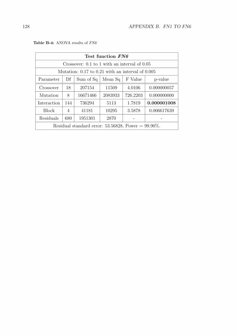
128 APPENDIX B. FN1 TO FN6
Table B-4: ANOVA results of FN6
Test function FN6
Crossover: 0.1 to 1 with an interval of 0.05
Mutation: 0.17 to 0.21 with an interval of 0.005
Parameter Df Sum of Sq Mean Sq F Value p-value
Crossover 18 207154 11509 4.0106 0.000000057
Mutation 8 16671466 2083933 726.2203 0.000000000
Interaction 144 736294 5113 1.7819 0.000001008
Block 4 41181 10295 3.5878 0.006617639
Residuals 680 1951301 2870 - -
Residual standard error: 53.56828, Power = 99.90%.

B. RESULTS 129
Fitted response curves
Table B-5: Equations of fitted response curves for FN1 to FN6
FN1 Crossover Final epoch =56.97715 − 8.15829Cr
Mutation Final epoch =81.23346 − 745.06687Mu+4338.52814Mu2
FN2 Crossover Final epoch =56.9028000 − 7.6368889Cr
Mutation Final epoch =7.877x101 − 6.652x10²Mu+3.765x10³Mu2
FN3 Crossover Final epoch =454.9500 − 26.0478Cr
Mutation Final epoch =9.540x10³ − 1.047x10⁵Mu+2.999x10⁵Mu2
FN4 Crossover Final epoch =51.395690 − 7.307079Cr
Mutation Final epoch =6.958x101 − 5.954x10²Mu+3.539x10³Mu2
FN5 Overall Final epoch =−218.5247 + 16.10332Cr + 8.586955Cr2
+11631.9485Mu − 113700.7892Mu2
+344700.9038Mu3 − 246.3479(Cr ∗ Mu)
FN6 Overall Final epoch =−3731.3012 + 892.2784Cr + 237189.8786Mu−2052110.9896Mu2 + 4964206.9821Mu3
−4941.4196(Cr ∗ Mu)Crossover parameter level (Cr), Mutation parameter level (Mu).
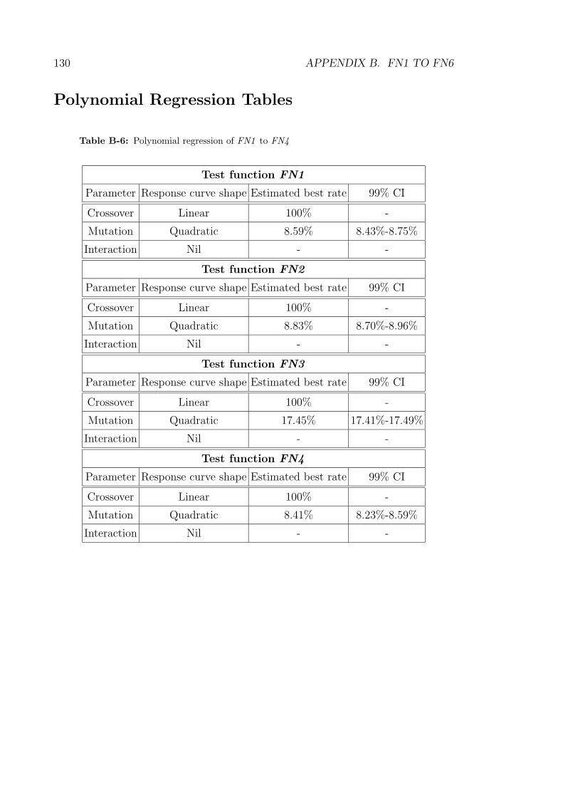
130 APPENDIX B. FN1 TO FN6
Polynomial Regression Tables
Table B-6: Polynomial regression of FN1 to FN4
Test function FN1
Parameter Response curve shape Estimated best rate 99% CI
Crossover Linear 100% -
Mutation Quadratic 8.59% 8.43%-8.75%
Interaction Nil - -
Test function FN2
Parameter Response curve shape Estimated best rate 99% CI
Crossover Linear 100% -
Mutation Quadratic 8.83% 8.70%-8.96%
Interaction Nil - -
Test function FN3
Parameter Response curve shape Estimated best rate 99% CI
Crossover Linear 100% -
Mutation Quadratic 17.45% 17.41%-17.49%
Interaction Nil - -
Test function FN4
Parameter Response curve shape Estimated best rate 99% CI
Crossover Linear 100% -
Mutation Quadratic 8.41% 8.23%-8.59%
Interaction Nil - -

B. RESULTS 131
Table B-7: Polynomial regression of FN5 and FN6
Test function FN5
Parameter Response curve shape Estimated best rate 99% CI
Crossover Quadratic 100% -
Mutation Cubic 14.11% 14.01%-14.21%
Interaction Linear:Linear - -
Test function FN6
Parameter Response curve shape Estimated best rate 99% CI
Crossover Linear 100% -
Mutation Cubic 19.47% 19.42%-19.53%
Interaction Linear:Linear - -

132 APPENDIX B. FN1 TO FN6

Appendix C
FN1R45 to FN6R45 and
Landscape 20 101
C Results
ANOVA Tables
Table C-1: ANOVA results of FN1R45
Test function FN1R45
Crossover: 0.6 to 1 with an interval of 0.05
Mutation: 0.07 to 0.12 with an interval of 0.005
Parameter Df Sum of Sq Mean Sq F Value p-value
Crossover 8 596.70 74.59 101.9350 <2x10⁻¹⁶
Mutation 10 1551.30 155.13 212.0105 <2x10⁻¹⁶
Interaction 80 54.96 0.69 0.9389 0.6263
Block 4 2.12 0.53 0.7242 0.5758
Residuals 392 286.83 0.73 - -
Residual standard error=0.8554008, Power=97.02%, Threshold=7.
133
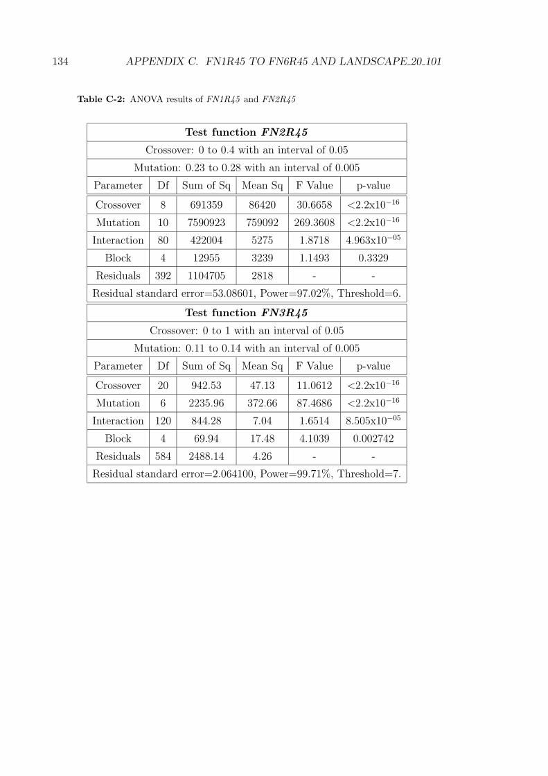
134 APPENDIX C. FN1R45 TO FN6R45 AND LANDSCAPE 20 101
Table C-2: ANOVA results of FN1R45 and FN2R45
Test function FN2R45
Crossover: 0 to 0.4 with an interval of 0.05
Mutation: 0.23 to 0.28 with an interval of 0.005
Parameter Df Sum of Sq Mean Sq F Value p-value
Crossover 8 691359 86420 30.6658 <2.2x10⁻¹⁶
Mutation 10 7590923 759092 269.3608 <2.2x10⁻¹⁶
Interaction 80 422004 5275 1.8718 4.963x10−05
Block 4 12955 3239 1.1493 0.3329
Residuals 392 1104705 2818 - -
Residual standard error=53.08601, Power=97.02%, Threshold=6.
Test function FN3R45
Crossover: 0 to 1 with an interval of 0.05
Mutation: 0.11 to 0.14 with an interval of 0.005
Parameter Df Sum of Sq Mean Sq F Value p-value
Crossover 20 942.53 47.13 11.0612 <2.2x10⁻¹⁶
Mutation 6 2235.96 372.66 87.4686 <2.2x10⁻¹⁶
Interaction 120 844.28 7.04 1.6514 8.505x10−05
Block 4 69.94 17.48 4.1039 0.002742
Residuals 584 2488.14 4.26 - -
Residual standard error=2.064100, Power=99.71%, Threshold=7.

C. RESULTS 135
Table C-3: ANOVA results of FN4R45 and FN5R45
Test function FN4R45
Crossover: 0 to 0.8 with an interval of 0.05
Mutation: 0.33 to 0.37 with an interval of 0.005
Parameter Df Sum of Sq Mean Sq F Value p-value
Crossover 16 1159371 72461 61.5758 <2.2x10⁻¹⁶
Mutation 8 1968603 246075 209.1107 <2.2x10⁻¹⁶
Interaction 128 402189 3142 2.6701 1.458x10⁻¹⁵
Block 4 6601 1650 1.4022 0.2317
Residuals 608 715477 1177 - -
Residual standard error=34.30410, Power=99.76%, Threshold=5.
Test function FN5R45
Crossover: 0 to 0.5 with an interval of 0.05
Mutation: 0.3 to 0.35 with an interval of 0.005
Parameter Df Sum of Sq Mean Sq F Value p-value
Crossover 10 756983 75698 84.9871 <2.2x10⁻¹⁶
Mutation 10 3162538 316254 355.0607 <2.2x10⁻¹⁶
Interaction 100 186328 1863 2.0919 1.301x10−07
Block 4 710 178 0.1994 0.9386
Residuals 480 427538 891 - -
Residual standard error=29.84466, Power=98.86%, Threshold=5.
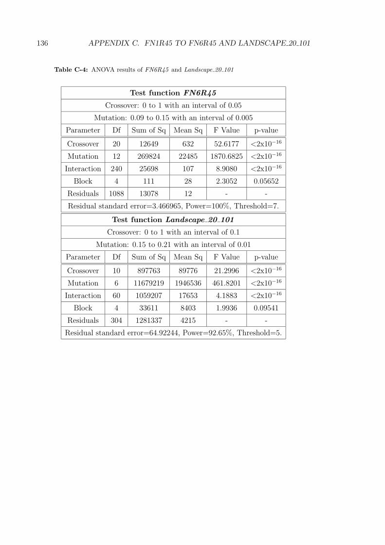
136 APPENDIX C. FN1R45 TO FN6R45 AND LANDSCAPE 20 101
Table C-4: ANOVA results of FN6R45 and Landscape 20 101
Test function FN6R45
Crossover: 0 to 1 with an interval of 0.05
Mutation: 0.09 to 0.15 with an interval of 0.005
Parameter Df Sum of Sq Mean Sq F Value p-value
Crossover 20 12649 632 52.6177 <2x10⁻¹⁶
Mutation 12 269824 22485 1870.6825 <2x10⁻¹⁶
Interaction 240 25698 107 8.9080 <2x10⁻¹⁶
Block 4 111 28 2.3052 0.05652
Residuals 1088 13078 12 - -
Residual standard error=3.466965, Power=100%, Threshold=7.
Test function Landscape 20 101
Crossover: 0 to 1 with an interval of 0.1
Mutation: 0.15 to 0.21 with an interval of 0.01
Parameter Df Sum of Sq Mean Sq F Value p-value
Crossover 10 897763 89776 21.2996 <2x10⁻¹⁶
Mutation 6 11679219 1946536 461.8201 <2x10⁻¹⁶
Interaction 60 1059207 17653 4.1883 <2x10⁻¹⁶
Block 4 33611 8403 1.9936 0.09541
Residuals 304 1281337 4215 - -
Residual standard error=64.92244, Power=92.65%, Threshold=5.

C. RESULTS 137
Fitted response curves
Table C-5: Equations of fitted response curves for FN1R45 to FN6R45
FN1R45 Crossover Final epoch =70.410317 − 8.471164Cr
Mutation Final epoch =1.048x10² − 9.756x10²Mu+5.556x10³Mu2
FN2R45 Overall Final epoch =3.666x10⁴ + 3.283x10³Cr − 2.811x10⁵Mu+5.569x10⁵Mu2 − 1.174x10⁴(Cr ∗ Mu)
FN3R45 Overall Final epoch =1.228x10⁴ + 2.619x101Cr + 9.058Cr2
−3.854x10⁵Mu + 4.577x10⁶Mu2
−2.419x10⁷Mu3 + 4.801x10⁷Mu4
−2.605x10²(Cr ∗ Mu)
FN4R45 Overall Final epoch =−1.260x10⁵ + 2.234x10³Cr + 1.203x10⁶Mu−3.768x10⁶Mu2 + 3.906x10⁶Mu3
−5.934x10³(Cr ∗ Mu)
FN5R45 Overall Final epoch =−6.428x10⁴ + 1.858x10³Cr + 6.774x10⁵Mu−2.316x10⁶Mu2 + 2.602x10⁶Mu3
−5.032x10³(Cr ∗ Mu)
FN6R45 Overall Final epoch =1.177x10³ + 7.129x10²Cr + 5.974x101Cr2
−3.074x10⁴Mu + 3.463x10⁵Mu2
−1.835x10⁶Mu3 + 3.845x10⁶Mu4
−1.633x10⁴(Cr ∗ Mu) − 4.103x10²(Cr2 ∗ Mu)+1.232x10⁵(Cr ∗ Mu2) − 3.084x10⁵(Cr ∗ Mu3)
Crossover parameter level (Cr), Mutation parameter level (Mu).

138 APPENDIX C. FN1R45 TO FN6R45 AND LANDSCAPE 20 101
Table C-6: Equations of fitted response curve for Landscape 20 101
Landscape 20 101 Overall Final epoch =2.214x10⁴ + 5.246x10³Cr − 3.141x10⁵Mu+1.485x10⁶Mu2 − 2.285x10⁶Mu3
−5.009x10⁴(Cr ∗ Mu) + 1.196x10⁵(Cr ∗ Mu2)Crossover parameter level (Cr), Mutation parameter level (Mu).

C. RESULTS 139
Polynomial Regression Tables
Table C-7: Polynomial Regression Tables for FN1R45 to FN6R45 and Land-
scape 20 101
FN1R45 Crossover 100%
Mutation 8.78%
FN2R45 Crossover 0%
Mutation 25.45%
FN3R45 Crossover 33.23%
Mutation 12.36%
FN4R45 Crossover 0%
Mutation 35.30%
FN5R45 Crossover 0%
Mutation 33.38%
FN6R45 Crossover 39.17%
Mutation 12.97%
Landscape 20 101 Crossover 0%
Mutation 18.93%
Related Documents