Christine A. Franklin (Chair) University of Georgia Anna E. Bargagliotti Loyola Marymount University Catherine A. Case University of Florida Gary D. Kader Appalachian State University Richard L. Scheaffer University of Florida Denise A. Spangler University of Georgia STATISTICAL EDUCATION OF TEACHERS SET

Welcome message from author
This document is posted to help you gain knowledge. Please leave a comment to let me know what you think about it! Share it to your friends and learn new things together.
Transcript
1 | Statistical Education of Teachers
StatiStical
Christine A. Franklin (Chair)University of Georgia
Anna E. BargagliottiLoyola Marymount University
Catherine A. CaseUniversity of Florida
Gary D. KaderAppalachian State University
Richard L. ScheafferUniversity of Florida
Denise A. SpanglerUniversity of Georgia
STATISTICAL
EDUCATION
OF TEACHERS SET


Preface ...............................................................................................i
Chapter 1: Background and Motivation for SET Report ........................................................1
Chapter 2: Recommendations ................................................5
Chapter 3: Mathematical Practices Through a Statistical Lens ....................................................9
Chapter 4: Preparing Elementary School Teachers to Teach Statistics ............................................... 13
Chapter 5: Preparing Middle-School Teachers to Teach Statistics ............................................... 21
Chapter 6: Preparing High-School Teachers to Teach Statistics .............................................. 29
Chapter 7: Assessment ........................................................... 39
Chapter 8: Overview of Research on the Teaching and Learning of Statistics in Schools ..........45
Chapter 9: Statistics in the School Curriculum: A Brief History ..................................................... 55
Appendix 1 ................................................................................... 61
Appendix 2 .................................................................................. 77
Contents

i | Statistical Education of Teachers
Preface
The Mathematical Education of Teachers (MET) (Conference Board of the Mathematical Sciences [CBMS], 2001) made recommendations regarding the mathematics PreK–12 teachers should know and how they should come to know it. In 2012, CBMS released MET II to update these recommendations in light of changes to the educational climate in the intervening decade, particularly the release of the Common Core State Standards for Mathematics (CCSSM) (NCACBP and CCSSO, 2010). Because of the emphasis on statistics in the Common Core and many states’ guidelines, MET II includes numer-ous recommendations regarding the preparation of teachers to teach statistics.
This report, The Statistical Education of Teachers ( ), was commissioned by the American Statisti-cal Association (ASA) to clarify MET II’s recommen-dations, emphasizing features of teachers’ statistical preparation that are distinct from their mathemati-cal preparation. SET calls for collaboration among mathematicians, statisticians, mathematics educa-tors, and statistics educators to prepare teachers to teach the intellectually demanding statistics in the PreK–12 curriculum, and it serves as a resource to aid those efforts.
This report (SET) aims to do the following:
• Clarify MET II’s recommendations for the statistical preparation of teachers at all grade levels: elementary, middle, and high school
• Address the professional development of teachers of statistics
• Highlight differences between statistics and mathematics that have important im-plications for teaching and learning
• Illustrate the statistical problem-solving process across levels of development
• Make pedagogical recommendations of particular relevance to statistics, includ-ing the use of technology and the role of assessment
Chapter 1 describes the motivation for SET in de-tail, highlighting ways preparing teachers of statistics is different from preparing teachers of mathematics.
Chapter 2 presents six recommendations regard-ing what statistics teachers need to know and the shared responsibility for the statistical education of teachers. This chapter is directed to those in leader-ship positions in school districts, colleges and uni-versities, and government agencies whose policies affect the statistical education of teachers.
Chapter 3 describes CCSSM as viewed through a statistical lens.
Chapters 4, 5, and 6 give recommendations for the statistical preparation and professional de-velopment of elementary-, middle-, and high-school teachers, respectively. These chapters are intended as a resource for those engaged in teacher prepara-tion or professional development.
Chapter 7 describes various strategies for assess-ing teachers’ statistical content knowledge.
Chapter 8 provides a brief review of the research lit-erature supporting the recommendations in this report.
Chapter 9 presents an overview of the history of statistics education at the PreK–12 level.
Appendix 1 includes a series of short examples and accompanying discussion that address particu-lar difficulties that may occur while teaching statis-tics to teachers.
Appendix 2 includes a sample activity handout for the illustrative examples presented in Chapters 4–6 that could be used in professional development courses or a classroom.
Web Resources The ASA provides a variety of outstanding and timely resources for teachers, including record-ed web-based seminars, the Statistics Teacher Network newsletter, and peer-reviewed lesson plans
PREFACE

Statistical Education of Teachers | iv
Preface
(STEW). These and other resources are available at www.amstat.org/education.
The National Council of Teachers of Mathematics (NCTM) offers exceptional classroom resources, includ-ing lesson plans and interactive web activities. NCTM has created a searchable classroom resources site that can be accessed at www.nctm.org/Classroom-Resources/Browse-All/#.
AudienceThis report is intended as a resource for all involved in the statistical education of teachers, both the ini-tial preparation of prospective teachers and the pro-fessional development of practicing teachers. Thus, the three main audiences are:
• Mathematicians and statisticians. Faculty members of mathematics and sta-tistics departments at two- and four-year collegiate institutions who teach cours-es taken by prospective and practicing teachers. They and their departmental colleagues set policies regarding the sta-tistical preparation of teachers.
• Mathematics educators and sta-tistics educators. Mathematics ed-ucation and statistics education faculty members—whether within colleges of education, mathematics departments, statistics departments, or other academ-ic units—are also an important audience
for this report. Typically, they are re-sponsible for the pedagogical education of mathematics and statistics teachers (e.g., methods courses, field experiences for prospective teachers). Outside of aca-deme, a variety of people are engaged in professional development for teachers of statistics, including state, regional, and school-district mathematics specialists. The term “mathematics educators” or “sta-tistics educators” includes this audience.
• Policy makers. This report is intended to inform educational administrators and policy makers at the national, state, school district, and collegiate levels as they work to provide PreK–12 students with a strong statistics education for an increasingly da-ta-driven world. Teachers’ preparation to teach statistics is central to this effort and is supported—or hindered—by institutional policies. These include national accreditation requirements, state certifications require-ments, and the ways in which these require-ments are reflected in teacher preparation programs. State and district supervisors make choices in the provision and funding of professional development. At the school level, scheduling and policy affect the type of learning experiences available to teachers. Thus, policy makers play important roles in the statistical education of teachers.

v | Statistical Education of Teachers
Preface
TerminologyTo avoid confusion, the report uses the following terminology:
• Student refers to a child or adolescent in a PreK–12 classroom.
• Teacher refers to an instructor in a PreK–12 classroom, but also may refer to prospective PreK–12 teachers in a college mathematics course (“prospective teacher” or “pre-service teacher” also is used in the latter case).
• Instructor refers to an instructor of pro-spective or practicing teachers. This term may refer to a mathematician, statistician, mathematics educator, statistics educator, or professional developer. The term statis-tics teacher educators is used to refer to this diverse group of instructors collectively.
AcknowledgmentsWe thank our colleagues Steven J. Foti, Tim Jacobbe, and Douglas L. Whitaker from the University of Florida for their contributions to SET. They provided insight and expertise that guided the evolution of the docu-ment from initial to final draft.
We also thank our colleagues Hollylynne S. Lee, Stephen J. Miller, Roxy Peck, Jamis Perritt, Susan A. Peters, Maxine Pfannkuch, Angela L.E. Walmsley, and Ann E. Watkins for their willingness to serve as reviewers. Their thoughtful comments improved the final document.
Finally, we acknowledge the support of the Ameri-can Statistical Association Board of Directors and the ASA-NCTM joint committee, as well as the assistance of ASA staff members Ron Wasserstein, Rebecca Nich-ols, Valerie Nirala, and Megan Ruyle.
ReferencesConference Board of the Mathematical Sciences.
(2001). The Mathematical Education of Teachers. Providence, RI, and Washington, DC: American Mathematical Society and Mathematical Associa-tion of America.
Conference Board of the Mathematical Sciences. (2012). The Mathematical Education of Teachers II. Providence, RI, and Washington, DC: American Mathematical Society and Mathematical Associa-tion of America.
National Governors Association Center for Best Prac-tices and Council of Chief State School Officers. (2010). Common Core State Standards for Mathe-matics. Washington, DC: Authors
Lesson Plans Available on Statistics Education Web for K–12 TeachersStatistics Education Web (STEW) is an online resource for peer-reviewed lesson plans for K–12 teachers. The lesson plans identify both the statistical concepts being devel-oped and the age range appropriate for their use. The statistical concepts follow the recommendations of the Guidelines for Assessment and Instruction in Statistics Educa-tion (GAISE) Report: A Pre-K-12 Curriculum Framework, Common Core State Stan-dards for Mathematics, and NCTM Principles and Standards for School Mathematics. The website resource is organized around the four elements in the GAISE framework: formulate a statistical question, design and implement a plan to collect data, analyze the data by measures and graphs, and interpret the data in the context of the original question. Teachers can navigate the site by grade level and statistical topic. Lessons follow Common Core standards, GAISE recommendations, and NCTM Principles and Standards for School Mathematics. Lesson Plans Wanted for Statistics Education WebThe editor of STEW is accepting submissions of lesson plans for an online bank of peer-reviewed lesson plans for K–12 teachers of mathematics and science. Lessons showcase the use of statistical methods and ideas in science and mathematics based on the framework and levels in the Guidelines for Assessment and Instruction in Statistics Education (GAISE) and Common Core State Standards. Consider submitting several of your favorite lesson plans according to the STEW template to [email protected].
For more information, visit www.amstat.org/education/stew.
Statistical Education of Teachers | 1
chaPter 1
CHAPTER 1Background and Motivation for SET Report
In an increasingly data-driven world, statistical litera-cy is becoming an essential competency, not only for researchers conducting formal statistical analyses, but for informed citizens making everyday decisions based on data. Whether following media coverage of current events, making financial decisions, or assessing health risks, the ability to process statistical information is critical for navigating modern society.
Statistical reasoning skills are also advantageous in the job market, as employment of statisticians is pro-jected to grow 27 percent from 2012 to 2022 (Bureau of Labor Statistics, 2014) and business experts predict a shortage of people with deep analytical skills (Manyika et al., 2011).
In keeping with the objectives of preparing students for college, career, and life, the Common Core State Standards for Mathematics (CCSSM) (NCACBP and CCSSO, 2010) and other state standards place heavy em-phasis on statistics and probability, particularly in grades 6–12. However, effective implementation of more rigor-ous standards depends to a large extent on the teachers who will bring them to life in the classroom. This report offers recommendations for the statistical preparation and professional development of those teachers.
The Guidelines for Assessment and Instruction in Statistics Education (GAISE) Report (Franklin et al., 2007) outlines a framework for statistics education at the PreK–12 level. The GAISE report identifies three developmental levels: Levels A, B, and C, which ideally match with the three grade-level bands—elementary, middle, and high school. However, the report empha-sizes that the levels are based on development in statis-tical thinking, rather than age.
The GAISE report also breaks down the statisti-cal problem-solving process into four components: formulate questions (clarify the problem at hand and formulate questions that can be answered with data), collect data (design and employ a plan to collect appro-priate data), analyze data (select and use appropriate graphical and numerical methods to analyze data), and interpret results (interpret the analysis, relating the in-terpretation to the original questions).
Likewise, the CCSSM and other standards recognize statistics as a coherent body of concepts connected across
grade levels and as an investigative process. To effective-ly teach statistics as envisioned by the GAISE framework and current state standards, it is important that teachers understand how statistical concepts are interconnected and their connections to other areas of mathematics.
Teachers also should recognize the features of statistics that set it apart as a discipline distinct from mathematics, particularly the focus on variability and the role of context. Across all levels and stages of the investigative process, statistics anticipates and accounts for variability in data. Whereas mathematics answers deterministic questions, statistics provides a coherent set of tools for dealing with “the omnipres-ence of variability” (Cobb and Moore, 1997)—natu-ral variability in populations, induced variability in experiments, and sampling variability in a statistic, to name a few. The focus on variability distinguish-es statistical content from mathematical content. For example, designing studies that control for variabili-ty, making use of distributions to describe variability, and drawing inferences about a population based on a sample in light of sampling variability all require con-tent knowledge distinct from mathematics.
In addition to these differences in content, statistical reasoning is distinct from mathematical reasoning, as the former is inextricably linked to context. Reasoning in mathematics leads to discovery of mathematical patterns underlying the context, whereas statistical reasoning is necessarily dependent on data and context and requires integration of concrete and abstract ideas (delMas, 2005).
This dependence on context has important impli-cations for teaching. For example, rote calculation of a correlation coefficient for two lists of numbers does little to develop statistical thinking. In contrast, using the concept of association to explore the link between, for example, unemployment rates and obesity rates integrates data analysis and contextual reasoning to identify a meaningful pattern amid variability.
Because statistics is often taught in mathematics classes at the pre-college level, it is particularly import-ant that teachers be aware of the differences between the two disciplines.
One noteworthy intersection between statistics and mathematics is probability, which plays a critical role in
2 | Statistical Education of Teachers
chaPter 1
statistical reasoning, but is also worthy of study in its own right as a subfield of mathematics. While teacher prepa-ration should include characterizations of probability as both a tool for statistics and as a component of mathe-matical modeling, this report focuses on probability pri-marily in the service of statistics. For example, a single instance of random sampling or random assignment is unpredictable, but probability provides ways to describe patterns in outcomes that emerge in the long run.
For teachers to understand statistical procedures like confidence intervals and significance tests, they must understand foundational probabilistic concepts that provide ways to quantify uncertainty. Thus, the SET report describes development of probabilistic concepts through simulation or the use of theoretical distribu-tions, such as the Normal distribution. On the other hand, topics further removed from statistical practice—such as specialized distributions and axiomatic ap-proaches to probability—are not detailed in this report.
It should be noted that current research is examin-ing the effects of integrating more probability model-ing into the school mathematics curriculum beginning at the middle grades. Through the use of dynamic sta-tistical software, the research is investigating the devel-opment of students’ understanding of connections be-tween data and chance (Konold and Kazak, 2008). This report strongly recommends that teacher preparation programs include probability modeling as a compo-nent of their mathematics education.
Because of the emphasis on statistical content in the CCSSM and other state standards, teachers of mathe-matics face high expectations for teaching statistics. Thus, the statistical education of teachers is critical and should be considered a priority for mathematicians and statisticians, mathematics and statistics educators, and those in leadership positions whose policies affect the preparation of teachers. The dramatic increase in statistical content at the pre-college level demands a coordinated effort to improve the preparation of pre-service teachers and to provide professional devel-opment for teachers trained before the implementation of the new standards.
The SET report reiterates MET II’s recommendation that statistics courses for teachers should be different from the theoretically oriented courses aimed toward science, technology, engineering, and mathematics majors and from the noncalculus-based introductory statistics courses taught at many universities. Where-as those courses often focus on mathematical proofs or a large number of specific statistical techniques, the courses SET recommends emphasize statistical thinking
and the statistical content knowledge and pedagogical content knowledge necessary to teach statistics as out-lined in the GAISE report and various state standards.
Effective teacher preparation must provide teachers not only with the statistical and mathematical knowl-edge sufficient for the content they are expected to teach, but also an understanding of foundational topics that come before and advanced topics that will follow. For example, grade 8 teachers are better equipped to guide students investigating patterns of association in bivari-ate data1 if they also understand the random selection process intended to produce a representative sample (taught in grade 7)2 and the types of inferences that can be drawn from an observational study (taught in high school)3. Note that although the linear equations often used to model an association in bivariate data would be familiar to anyone with a mathematics background, the process of statistical investigation requires content knowledge separate from mathematics content.
In addition to statistical content knowledge, teach-ers need opportunities to develop pedagogical content knowledge (Shulman, 1986). For example, effective teaching of statistics requires knowledge about com-mon student conceptions and thinking patterns, con-tent-specific teaching strategies, and appropriate use of curricula. Teachers should have the pedagogical knowledge necessary to assess students’ levels of un-derstanding and plan next steps in the development of their statistical thinking.
The SET report also highlights pedagogical recom-mendations of particular relevance to statistics, such as those related to technology and assessment. These recommendations apply to courses for pre-service teachers and professional development for practicing teachers, as well as to the elementary-, middle-, and high-school courses they teach. Ideally, the statistical education of teachers should model effective pedago-gy by emphasizing statistical thinking and conceptual understanding, relying on active learning and explo-ration of real data, and making effective use of tech-nology and assessment.
SET echoes the recommendation in the GAISE College Report (ASA, 2005) that technology should be used for developing concepts and analyzing data. An abstract concept such as the Central Limit Theorem can be developed (and visualized) through computer simulations instead of through mathematical proof. Calculations of p-values can be automated to allow more time to interpret the p-value and carefully con-sider the inferences that can be drawn based on its val-ue. The two goals of using technology for developing
1 Refer to CCSS 8.SP.1 – 8.SP.4
2 Refer to CCSS 7.SP.13 Refer to CCSS S-IC.1
and S-IC.3

Statistical Education of Teachers | 3
chaPter 1
concepts and analyzing data may be achieved with a single software package or with a number of comple-mentary tools (e.g., applets, graphing calculators, sta-tistical packages, etc.). SET does not endorse any par-ticular technological tools, but instead prescribes what teachers should be able to do with those tools.
Many aspects of the statistical education of teach-ers directly or indirectly hinge on assessment. As-sessment not only measures teachers’ understand-ing of key concepts, but also directs their focus and efforts. For example, SET recommends emphasis on conceptual understanding, but if tests only assess cal-culations, teachers will naturally emphasize the me-chanics instead of the underlying concepts. Thus, it is critical that teachers be assessed and, in turn, assess their students on conceptual and not merely proce-dural understanding. Further, assessment should emphasize the statistical problem-solving process,
requiring teachers to clearly communicate statistical ideas and consider the role of variability and context at each stage of the process. The assessments of sta-tistical understanding used by teacher educators are particularly important, as they are likely to influence how teachers assess their own students.
At every grade level—elementary, middle, and high school—the statistical education of teachers presents a different set of challenges and opportu-nities. Ideally, development of statistical literacy in students should begin at the elementary-school level (Franklin and Mewborn, 2006), with teachers prepared beyond the level of statistical knowledge expected of their students. In particular, elementary teachers should understand how foundational statis-tical concepts connect to content developed in later grades and other subjects across the curriculum. Ele-mentary teachers should receive statistics instruction
Rebecca Nichols/asa
Effective teacher preparation must provide teachers with an understanding of foundational topics.

4 | Statistical Education of Teachers
chaPter 1
in a manner that models effective pedagogy and em-phasizes the statistical problem-solving process.
Both MET I and MET II indicate middle-grade teachers should not receive the same type of mathemat-ical preparation as elementary generalists. Students are expected to begin thinking statistically at grade 6, and topics introduced in the middle grades include data col-lection design, exploration of data, informal inference, and association. Given the plethora of statistical topics at the middle-school level under the CCSSM and oth-er state standards, middle-school teachers should take courses that explore the statistical concepts in the mid-dle-school curriculum at a greater depth, develop peda-gogical content knowledge necessary to teach those con-cepts, and expose themselves to statistical applications beyond those required of their students.
High-school mathematics teachers typically major in mathematics, but the theoretical statistics cours-es often taken by mathematics majors do not suffi-ciently prepare them for the statistics topics they will teach. In many universities, teachers only take a proof-driven mathematical statistics course, while courses in data analysis may not count toward their major. High-school teachers should take courses that develop data-driven statistical reasoning and include experiences with statistical modeling in addition to those that develop knowledge of statistical theory.
The recommendations included in this report concern not only the quantity of preparation need-ed by teachers of statistics, but also the content and quality of that preparation. It is the responsibility of mathematicians, statisticians, mathematics edu-cators, statistics educators, professional developers, and administrators to provide teachers with cours-es and professional development that cultivate their statistical understanding, as well as the pedagogical knowledge to develop statistical literacy in the next generation of learners.
ReferencesAmerican Statistical Association. (2005). Guidelines
for Assessment and Instruction in Statistics Edu-cation: College Report. Alexandria, VA: Author.
Bureau of Labor Statistics, U.S. Department of Labor. (2014) Occupational Outlook Handbook, 2014–15 Edition. Retrieved from www.bls.gov.
Cobb, G., and Moore, D. (1997). Mathematics, sta-tistics, and teaching. The American Mathemati-cal Monthly, 104(9):801–823.
delMas, R. (2005). A comparison of mathematical and statistical reasoning. In Dani Ben-Zvi and Joan Garfield (Eds.), The Challenge of Develop-ing Statistical Literacy, Reasoning, and Thinking (pp. 79-95). New York, NY: Kluwer Academic Publishers.
Franklin, C., Kader, G., Mewborn, D., More-no, J., Peck, R., Perry, M., and Scheaffer, R. (2007). Guidelines and Assessment for In-struction in Statistics Education (GAISE) Re-port: A PreK-12 Curriculum Framework. Alexandria, VA: American Statistical As-sociation. Retrieved from www.amstat.org/ education/gaise.
Franklin, C., and Mewborn, D. (2006). The statis-tical education of pre K–12 teachers: A shared responsibility. In NCTM 2006 Yearbook: Think-ing and Reasoning with Data and Chance (pp. 335–344).
Konold, C., and Kazak, S. (2008). Reconnect data and chance. Technology Innovations in Statistics Education, 2(1). Retrieved from https://escholar-ship.org/uc/item/38p7c94v.
Manyika, J., Chui, M., Brown, B., Bughin, J., Dobbs, R., Roxburgh, C., and Hung Byers, A. (2011, May). Big Data: The Next Frontier for Innova-tion, Competition, and Productivity. Retrieved from www.mckinsey.com.
National Governors Association Center for Best Practices and Council of Chief State School Of-ficers. (2010). Common Core State Standards for Mathematics. Washington, DC: Authors.
Shulman, L.S. (1986). Those who understand: Knowledge growth in teaching. Educational Re-searcher, 15(2):4–14.
The recommendations included
in this report concern the quantity
of preparation needed by teachers
of statistics and also the content
and quality of that preparation.

Statistical Education of Teachers | 5
chaPter 2
This chapter offers six broad recommendations for the preparation of teachers of statistics. These recommen-dations are intended to provide educational leaders with support to initiate any needed changes in teacher educa-tion or professional development programs to support teachers in learning to teach statistics effectively. The recommendations speak to the content teachers need to know, the ways in which they should learn it, and who should be assisting them in developing this knowledge. In particular, Recommendations 5 and 6 elaborate on the shared responsibility for the preparation of teachers of statistics. For elementary-school and middle-school teachers, statistics is often embedded in mathematics courses; thus, statisticians, mathematicians, and math-ematics educators share responsibility for ensuring that all teachers are prepared to teach high-quality statistics content with appropriate instructional methods to the next generation of students.
The recommendations for teacher preparation in this document are intended to apply to teachers pre-pared via any pathway for teacher preparation and credentialing—including undergraduate, post-bac-calaureate, graduate, traditional, and alternative—whether university-based or not. As used here, the term “teacher of statistics” includes any teacher in-volved in the statistical education of PreK–12 stu-dents, including early childhood and elementary school generalist teachers; middle-school teachers; high-school teachers; and teachers of special needs students, English Language Learners, and other spe-cial groups, when those teachers have responsibility for supporting students’ learning of statistics.
These recommendations apply only to the statistics content teachers need to know, but the recommenda-tions assume teachers, both pre-service and in-service, will have the opportunity to learn about pedagogy as it relates to teaching statistics in other courses or venues.
While we advocate that those who teach teachers should model the type of pedagogy we want them to use with students, simply modeling pedagogy is not sufficient for teachers to develop the skills and commitments needed to teach in ways that help stu-dents learn statistical content with meaning and un-derstanding. Thus, it is important that the content
recommendations made in this document be paired with appropriate pedagogical learning.
General RecommendationsThe following recommendations draw heavily on those provided in Mathematical Education of Teachers II (CBMS, 2012). This report includes six recommenda-tions for the statistical preparation of PreK–12 teach-ers, presented as follows:
• Recommendations 1, 2, 3, and 4 deal with the ways PreK–12 teachers should learn
• Recommendation 5 addresses the shared responsibility of statistics teacher educa-tors in preparing statistically proficient teachers
• Recommendation 6 provides details about the statistics content preparation needed by teachers at elementary-school, middle-school, and high-school levels.
Statistics for TeachersRecommendation 1. Prospective teachers need to learn statistics in ways that enable them to develop a deep conceptual understanding of the statistics they will teach. The statistical content knowledge needed by teachers at all levels is substantial, yet quite different from that typ-ically addressed in most college-level introductory statis-tics courses. Prospective teachers need to understand the statistical investigative process and particular statistical techniques/methods so they can help diverse groups of students understand this process as a coherent, reasoned activity. Teachers of statistics must also be able to com-municate an appreciation of the usefulness and power of statistical thinking. Thus, coursework for prospective teachers should allow them to examine the statistics they will teach in depth and from a teacher’s perspective.
Recommendation 2. Prospective teachers should engage in the statistical problem-solving process—for-mulate statistical questions, collect data, analyze data, and interpret results—regularly in their courses. They
CHAPTER 2Recommendations
6 | Statistical Education of Teachers
chaPter 2
should be engaged in reasoning, explaining, and mak-ing sense of statistical studies that model this process. Although the quality of statistical preparation is more important than the quantity, Recommendations 3, 4, and 5 discuss the content teachers are expected to teach. Detailed recommendations for the amount and nature of their coursework for the various grade bands are discussed in Chapters 4, 5, and 6 of this report.
Recommendation 3. Because many currently practicing teachers did not have an opportunity to learn statistics during their pre-service preparation programs, robust professional development opportu-nities need to be developed for advancing in-service teachers’ understanding of statistics. In-service profes-sional development programs should be built on the same principles as those noted in Recommendations 1 and 2 for pre-service programs, with teachers actively engaged in the statistical problem-solving process. Re-gardless of the format of the professional development (university-based, district-based), it is important that statisticians with an interest in K–16 statistical educa-tion be involved in designing and, where possible, de-livering the professional development.
Recommendation 4. All courses and professional development experiences for statistics teachers should allow them to develop the habits of mind of a statis-tical thinker and problem-solver, such as reasoning, explaining, modeling, seeing structure, and general-izing. The instructional style for these courses should be interactive, responsive to student thinking, and problem-centered. Teachers should develop not only knowledge of statistics content, but also the ability to work in ways characteristic of the discipline. Chapter 3 elaborates on the Standards of Mathematical Practice as they apply to statistics.
Roles for Teacher Educators in StatisticsRecommendation 5. At institutions that prepare teachers or offer professional development, statistics teacher education must be recognized as an import-ant part of a department’s mission and should be undertaken in collaboration with faculty from statis-tics education, mathematics education, statistics, and mathematics. Departments need to encourage and re-ward faculty for participating in the preparation and professional development of teachers and becoming involved with PreK–12 mathematics education. De-partments also need to devote commensurate resourc-es to designing and staffing courses for prospective and
practicing teachers. Statistics courses for teachers must be a department priority. Instructors for such cours-es should be carefully selected for their statistical ex-pertise as well as their pedagogical expertise, and they should have opportunities to participate in regional and national professional development opportunities for statistics educators as needed. 4
Recommendation 6. Statisticians should recog-nize the need for improving statistics teaching at all levels. Mathematics education, including the statistical education of teachers, can be greatly strengthened by the growth of a statistics education community that includes statisticians as one of many constituencies committed to working together to improve statistics instruction at all levels and to raise professional stan-dards in teaching. It is important to encourage part-nerships between statistics faculty, statistics education faculty, mathematics education faculty, and mathe-matics faculty; between faculty in two- and four-year institutions; and between statistics faculty and school mathematics teachers, as well as state, regional, and school-district leaders.
In particular, as part of the mathematics education community, statistics teacher educators should sup-port the professionalism of teachers of statistics by do-ing the following:
• Endeavoring to ensure that K–12 teachers of statistics have sufficient knowledge and skills for teaching statistics at the level of certifica-tion upon receiving initial certification
• Encouraging all who teach statistics to strive for continual improvement in their teaching
• Joining with teachers at different levels to learn with and from each other
There are many initiatives, communities, and professional organizations focused on aspects of building professionalism in the teaching of mathe-matics and statistics. More explicit efforts are need-ed to bridge current communities in ways that build upon mutual respect and the recognition that these initiatives provide opportunities for professional growth for higher education faculty in mathematics, statistics, and education, as well as for the mathe-matics teachers, coaches, and supervisors in the PreK–12 community. Becoming part of a communi-ty that connects all levels of mathematics education
4 Statisticians work in depart-ments of various configura-
tions, ranging from stand-alone statistics departments
to departments of mathe-matical sciences that include mathematics, statistics, and computer science. For ease
of language, we use the term departments generically here
to mean any department in which statisticians reside.
Statistical Education of Teachers | 7
chaPter 2
will offer statisticians more opportunities to partici-pate in setting standards for accreditation of teacher preparation programs and teacher certification via standard and alternative pathways.
Specific RecommendationsThe paragraphs that follow provide an overview of the specific recommendations for the statistical education of teachers at various levels. These recommendations are elaborated in Chapters 4 (elementary), 5 (middle school), and 6 (high school).
Elementary SchoolProspective elementary school teachers should be pro-vided with coursework on fundamental ideas of ele-mentary statistics, their early childhood precursors, and middle school successors. The coursework could take three formats:
1. A special section of an introductory statis-tics course geared specifically to the content and instructional strategies noted above. This course can be designed to include all levels of teacher preparation students.
2. An entire course in statistical content for elementary-school teachers.
3. More time and attention given to statistics in existing mathematics content courses. Most likely, one course would be reconfigured to place substantial emphasis on statistics, but this would also likely result in reconfiguring the content of all courses in the sequence to make the time for the statistics content.
There is a great deal of mathematics and statistics content that is important for elementary-school teach-ers to know, so decisions about what to cut to make more room for statistics will be difficult. Thus, MET II advocates increasing the number of credit hours of instruction for elementary-school teachers to 12 credit hours. Note that these hours are all content-focused; pedagogy courses are in addition to these 12 hours.
Middle SchoolProspective middle school grades teachers of statistics should complete two courses:
1. An introductory course that emphasiz-es a modern data-analytic approach to
statistical thinking, a simulation-based introduction to inference using appro-priate technologies, and an introduction to formal inference (confidence intervals and tests of significance). This first course develops teachers’ statistical con-tent knowledge in an experiential, active learning environment that focuses on the problem-solving process and makes clear connections between statistical reasoning and notions of probability.
ThiNksTock
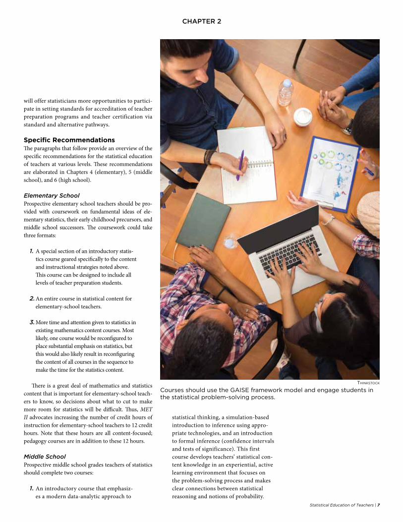
Courses should use the GAISE framework model and engage students in the statistical problem-solving process.

8 | Statistical Education of Teachers
chaPter 2
2. A second course that focuses on strengthening teachers’ conceptual understandings of the big ideas from Essential Understandings and the sta-tistical content of the middle-school curriculum. This course is also intended to develop teachers’ pedagogical content knowledge by providing strategies for teaching statistical concepts, integrating appropriate technology into their in-struction, making connections across the curriculum, and assessing statistical un-derstanding in middle-school students.
High SchoolProspective high-school teachers of mathematics should complete three courses:
1. An introductory course that emphasiz-es a modern data-analytic approach to statistical thinking, a simulation-based introduction to inference using appro-priate technologies, and an introduction to formal inference (confidence intervals and tests of significance)
2. A second course in statistical methods that builds on the first course and includes both randomization and classical procedures for comparing two parameters based on
both independent and dependent samples (small and large), the basic principles of the design and analysis of sample surveys and experiments, inference in the simple linear regression model, and tests of inde-pendence/homogeneity for categorical data
3. A statistical modeling course based on multiple regression techniques, including both categorical and numerical explan-atory variables, exponential and power models (through data transformations), models for analyzing designed experi-ments, and logistic regression models
Each course should include use of statistical soft-ware, provide multiple experiences for analyzing real data, and emphasize the communication of sta-tistical results.
These courses should use the GAISE framework model and engage teachers in the statistical prob-lem-solving process including study design. These courses are different from the more theoretically oriented probability and statistics courses typical-ly taken by science, technology, engineering, and mathematics (STEM) majors. Note that while some aspects of probability are fundamental to statistics, a classical probability course—while useful—does not satisfy the recommendations offered here. As dis-cussed in Chapter 1, we recommend the fundamen-tal notions of probability be developed as needed in the service of acquiring statistical reasoning skills.
ReferenceConference Board of the Mathematical Sciences.
(2012). The Mathematical Education of Teachers. Providence, RI: American Mathematical Society.
These courses should use
the GAISE framework model
and engage teachers in the
statistical problem-solving
process including study design.

Statistical Education of Teachers | 9
chaPter 3
CHAPTER 3Mathematical Practices Through a Statistical Lens
The upcoming chapters in this report provide recom-mendations for the statistics that elementary-, mid-dle-, and high-school teachers should know and how they should come to know it. However, the report also recognizes that knowledge of statistical content is supported by the processes and practices through which teachers and their students acquire and apply statistical knowledge.
The importance of processes and proficiencies that complement content knowledge are well recognized in mathematics education. In Principles and Standards for School Mathematics (PSSM) (2000), the National Coun-cil for Teachers of Mathematics (NCTM) presents five process standards that highlight ways of acquiring and using content knowledge: problem-solving, reasoning and proof, communication, connections, and represen-tations. In Adding It Up (2001), the National Research Council (NRC) breaks down mathematical proficiency into five interrelated strands: conceptual understanding, procedural fluency, strategic competence, adaptive rea-soning, and productive disposition. The Common Core State Standards for Mathematics (CCSSM) (2010) builds on the processes and proficiencies outlined by NCTM and NRC in its eight Standards for Mathematical Prac-tice. CCSSM describes the connection of practice stan-dards to mathematical content as follows:
The Standards for Mathematical Practice describe ways in which developing student practitioners of the discipline of mathe-matics increasingly ought to engage with the subject matter as they grow in mathe-matical maturity and expertise throughout the elementary-, middle-, and high-school years. Designers of curricula, assessments, and professional development should all attend to the need to connect the mathe-matical practices to mathematical content in mathematics instruction.
The Standards for Mathematical Content are a balanced combination of procedure and conceptual understanding. Expectations that begin with the word “understand” are often
especially good opportunities for connecting the practices to the content. Students who lack understanding of a topic may rely on procedures too heavily. Without a flexible base from which to work, they may be less likely to consider analogous problems, represent problems coherently, justify con-clusions, apply the mathematics to practical situations, use technology mindfully to work with the mathematics, explain the mathematics accurately to other students, step back for an overview, or deviate from a known procedure to find a shortcut. In short, a lack of understanding effectively prevents a student from engaging in the mathematical practices (NCACBP and CCSSO, 2010, p. 8).
The statistical education of teachers should be in-formed by the Standards for Mathematical Practice as seen through a statistical lens. This chapter interprets the eight practice standards presented in the CCSSM in terms of the practices necessary to acquire and apply statistics knowledge. The perspective of a “sta-tistical lens” is established through several sources, including the following:
• The PreK–12 GAISE Curriculum Frame-work (Franklin et al., 2007)
• Developing Essential Understanding of Statistics Grades 6–8 (Kader and Jacobbe, 2013)
• Developing Essential Understanding of Statistics Grades 9–12 (Peck, Gould, and Miller, 2013)
• The Challenge of Developing Statistical Literacy, Reasoning, and Thinking (Ben-Zvi and Garfield, 2004)
• Statistical Thinking in Empirical Enquiry (Wild and Pfannkuch, 1999)
10 | Statistical Education of Teachers
chaPter 3
The mathematicians, statisticians, and educators involved in the statistical preparation of teachers should strive to connect the mathematical practices through a statistical lens to statistical content in the instruction of teachers so teachers may, in turn, foster these practices in their students. In the descriptions that follow, we use the term “students” to parallel the Standards for Mathematical Practice in the Common Core State Standards; but, as with mathematics, the statistical practices also apply to teachers when they are learning the content.
1. Make sense of problems and persevere in solving them. Statistically proficient students understand how to carry out the four steps of the sta-tistical problem-solving process: formulating a statis-tical question, designing a plan for collecting data and carrying out that plan, analyzing the data, and inter-preting the results. In practice, the components of this process are interrelated, so students must continually ask themselves how each component relates to the oth-ers and the research topic under study:
• Can the question be answered with data? Will answering the statistical question pro-vide insight into the research topic under investigation?
• Will the data collection plan measure a variable(s) that provides appropriate data to address the statistical question? Does the plan provide data that allow for gen-eralization of results to a population or to establish a cause and effect conclusion?
• Do the analyses provide useful informa-tion for addressing the statistical question? Are they appropriate for the data that have been collected?
• Is the interpretation sound, given how the data were collected? Does the interpre-tation provide an adequate answer to the statistical question?
Students must persevere through the entire statis-tical problem-solving process, adapting and adjusting each component as needed to arrive at a solution that adequately connects the interpretation of results to the statistical question posed and the research topic under study. Additionally, students must be able to critique and evaluate alternative approaches (data collection plans and analyses) and recognize appropriate and in-appropriate conclusions based on the study design.
2. Reason abstractly and quantitatively. Sta-tistically proficient students understand the difference between mathematical thinking and statistical think-ing. Students engaged in mathematical thinking ask, “Where’s the proof?” They use operations, generaliza-tions, and abstractions to prove deterministic claims and understand mathematical patterns free of context. Students engaged in statistical thinking ask, “Where’s the data?” They reason in the presence of variability and anticipate, acknowledge, account for, and allow for variability in data as it relates to a particular context.
Although statistical thinking is grounded in a concrete context, it still requires reasoning with abstract concepts. For example, how to measure an
Rebecca Nichols/asa
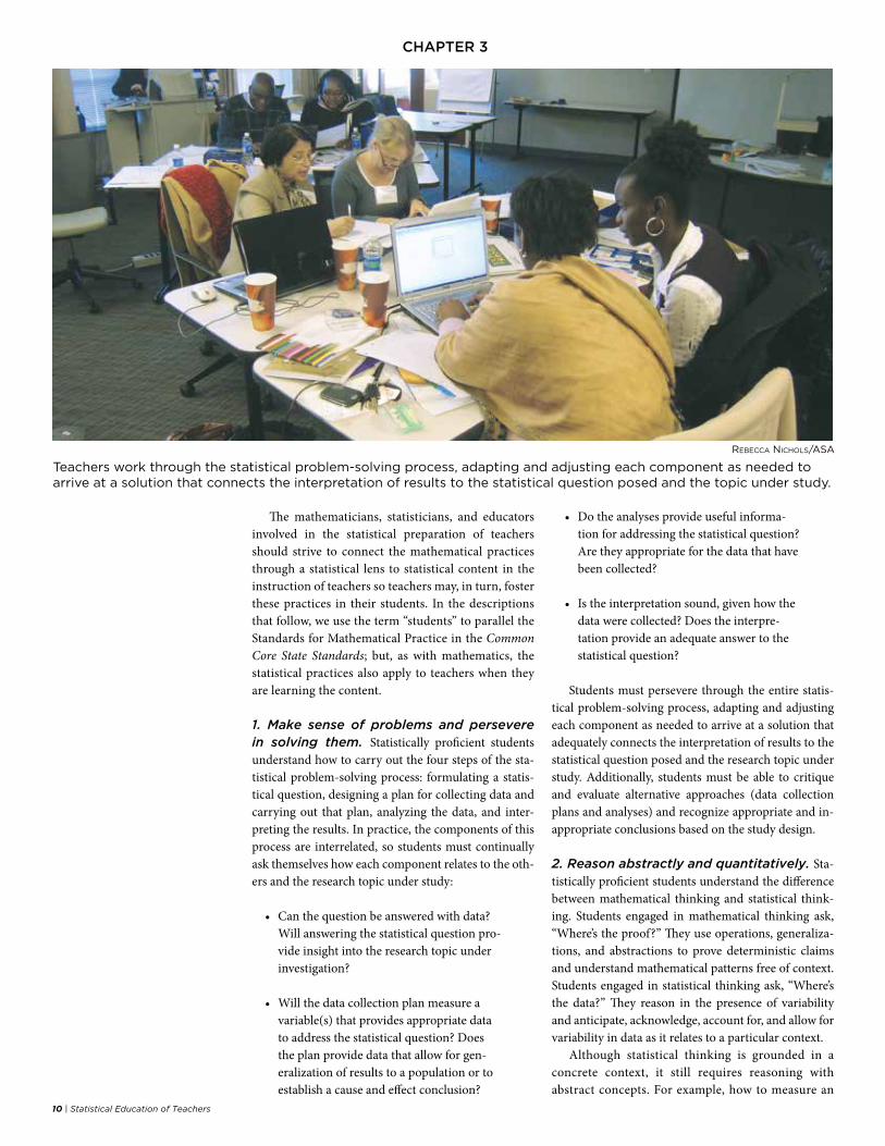
Teachers work through the statistical problem-solving process, adapting and adjusting each component as needed to arrive at a solution that connects the interpretation of results to the statistical question posed and the topic under study.
Statistical Education of Teachers | 11
chaPter 3
attribute in answering a statistical question, select-ing a reasonable summary statistic such as using the sample mean (which may be a value that does not exist in the data set) as a measure of center, in-terpreting a graphical representation of data, and understanding the role of sampling variability for drawing inferences—all of these require reasoning with abstractions.
3. Construct viable arguments and critique the reasoning of others. Statistically proficient students use appropriate data and statistical methods to draw conclusions about a statistical question. They follow the logical progression of the statistical prob-lem-solving process to investigate answers to a statis-tical question and provide insights into the research topic. They reason inductively about data, making in-ferences that take into account the context from which the data arose. They justify their conclusions, commu-nicate them to others (orally and in writing), and cri-tique the conclusions of others.
Statistically proficient students also are able to com-pare the plausibility of alternative conclusions and dis-tinguish correct statistical reasoning from that which is flawed. This is an especially important skill given the massive amount of statistical information in the media and elsewhere. Are appropriate graphs being used to represent the data, or are the graphs misleading? Are appropriate inferences being made based on the da-ta-collection design and analysis? Statistically proficient students are ‘healthy skeptics’ of statistical information.
4. Model with mathematics. Statistically profi-cient students can apply mathematics to help answer sta-tistical questions arising in everyday life, society, and the workplace. Mathematical models generally use equa-tions or geometric representations to describe structure. Statistical models build on mathematical models by including descriptions of the variability present in the data; that is, data = structure + variability.
For example, middle school students may use the mean to represent the center of a distribution of uni-variate data and the mean absolute deviation to model the variability of the distribution. High-school students may use the normal distribution (as defined by a math-ematical function) to model a unimodal, symmetric distribution of quantitative data or to model a sampling distribution of sample means or sample proportions. For bivariate data, students may use a straight line to model the relationship between two quantitative vari-ables. With consideration of the correlation coefficient
and residuals, the statistical interpretation of this lin-ear model takes into account the variability of the data about the line. The statistically proficient student un-derstands that statistical models are judged by whether they are useful and reasonably describe the data.
5. Use appropriate tools strategically. Sta-tistically proficient students consider the available tools when solving a statistical problem. These tools might include a calculator, a spreadsheet, applets, a statistical package, or tools such as two-way tables and graphs to organize and represent data. A tool might be a survey used to collect and measure the variable (attribute) of interest. The use of tools is to facilitate the practice of statistics. Tools can help us work more efficiently with analyzing the data so more time can be spent on understanding and communi-cating the story the data tell us.
For example, statistically proficient middle-school students may use technology to create boxplots to compare and analyze the distributions of two quan-titative variables. High-school students may use an applet to simulate repeated sampling from a certain population to develop a margin of error for quantify-ing sampling variability.
When developing statistical models, students know technology can enable them to visualize the results of varying assumptions, explore patterns in the data, and compare predictions with data. Statistically proficient students at various grade levels are able to use tech-nological tools to carry out simulations for exploring and deepening their understanding of statistical and probabilistic concepts. Students also may take advan-tage of chance devices such as coins, spinners, and dice for simulating random processes.
6. Attend to precision. Statistically proficient students understand that precision in statistics is not just computational precision. In statistics, one must be precise about ambiguity and variability. Students understand the statistical problem-solving process begins with the precise formulation of a statistical question that anticipates variability in the data col-lected that will be used to answer the question. Pre-cision is also necessary in designing a data-collection plan that acknowledges variability. Precision about the attributes being measured is essential.
After the data have been collected, students are precise about choosing the appropriate analyses and representations that account for the variability in the data. They display carefully constructed graphs with

12 | Statistical Education of Teachers
chaPter 3
clear labeling and avoid misleading graphs, such as three-dimensional pie charts, that misrepresent the data. As students interpret the analysis of the data, they are precise with their terminology and statistical language. For example, they recognize that ‘correla-tion’ is a specific measure of the linear relationship between two quantitative variables and not simply another word for ‘association.’ They recognize that ‘skew’ refers to the shape of a distribution and is not another word for ‘bias.’
Students can transition from exploratory statistics to inferential statistics by using a margin of error to quantify sampling variability around a point estimate. Students recognize the precision of this estimate de-pends partially upon the sample size—the larger the sample size, the smaller the margin of error.
As students interpret statistical results, they connect the results back to the original statistical question and provide an answer that takes the variability in the data into account. Statistically proficient students recognize that clear communication and precision with statistical language are essential to the practice of statistics.
7. Look for and make use of structure. Sta-tistically proficient students look closely to discover a structure or pattern in a set of data as they attempt to answer a statistical question. For univariate data, the mean or median of a distribution describes the center of the distribution—an underlying structure around which the data vary. Similarly, the equation of a straight line describes the relationship between two quanti-tative variables—a linear structure around which the data vary. Students use structure to separate the ‘signal’ from the ‘noise’ in a set of data—the ‘signal’ being the structure, the ‘noise’ being the variability. They look for patterns in the variability around the structure and rec-ognize these patterns can often be quantified.
For example, if there is a positive, linear trend in a set of bivariate quantitative data, then students can quantify this pattern with a correlation coefficient to measure strength of the linear association and use a regression line to predict the value of a response variable from the value of an explanatory variable. Statistically proficient students use statistical mod-eling to describe the variability associated with the identified structure.
8. Look for and express regularity in re-peated reasoning. Statistically proficient students maintain oversight of the process, attend to the details, and continually evaluate the reasonableness of their results as the y are carrying out the statistical prob-lem-solving process. Students recognize that proba-bility provides the foundation for identifying patterns in long-run variability, thereby allowing students to quantify uncertainty. Randomization produces proba-bilistic structure and patterns that are repeatable and can be quantified in the long run.
For example, in a statistical experiment with enough subjects, randomly assigning subjects to treat-ment groups will balance the groups with respect to potentially confounding variables so any statistically significant differences can be attributed to the treat-ments. In sampling from a defined population, se-lection of a random sample is a repeatable process and probability supports construction of a sampling distribution of the statistic of interest. Statistical-ly proficient students understand the different roles randomization plays in data collection and recognize it is the foundation of statistical inference methods used in practice.
ReferencesBen-Zvi, B., and Garfield, J. (Eds.). (2004). The Chal-
lenge of Developing Statistical Literacy, Reasoning, and Thinking. Dordrecht, The Netherlands: Kluw-er Academic Publishers.
Franklin, C., et al. (2007). Guidelines and Assessment for Instruction in Statistics Education (GAISE) Report: A PreK-12 Curriculum Framework. Alex-andria, VA: American Statistical Association.
Kader, G., and Jacobbe, T. (2013). Developing Essential Understanding of Statistics for Teaching Mathemat-ics in Grades 6-8. Reston, VA: NCTM.
Kilpatrick, J., Swafford, J., and Findell, B. (Eds). (2001). Adding It Up: Helping Children Learn Mathematics. National Research Council, Center for Education. Washington, DC: National Academy Press.
National Council of Teachers of Mathematics (NCTM). (2000). Principles and Standards for School Mathematics. Reston, VA: NCTM.
Peck, R., Gould, R., and Miller, S. (2013). Developing Essential Understanding of Statistics for Teaching Mathematics in Grades 9-12. Reston, VA: NCTM.
Wild, C., and Pfannkuch, M. (1999). Statistical think-ing in empirical enquiry. International Statistical Review, 67(3):223–265.
Statistically proficient students
look closely to discover a structure
or pattern in a set of data.
Statistical Education of Teachers | 13
chaPter 4
Expectations for Elementary School Students“Every high-school graduate should be able to use sound statistical reasoning to intelligently cope with the re-quirements of citizenship, employment, and family and to be prepared for a healthy, happy, and productive life.” (Franklin et al., 2007, p.1)
The foundations of statistical literacy must begin in the elementary grades PreK–5, where young students begin to develop data sense—an understanding that data are not simply numbers, categories, sounds, or pictures, but entities that have a context, vary, and may be useful for an-swering questions about the world that surrounds them.
Recommendations for developing statistical think-ing from key national reports such as the ASA’s PreK–12 GAISE Framework, NCTM’s Principles and Standards for School Mathematics, and CCSSM for students in grade levels PreK–5 include the following:
• Understand what comprises a statistical question
• Know how to investigate statistical ques-tions posed by teachers in a context of interest to young students
• Conduct a census of the classroom to collect data and design simple experiments to compare two treatments
• Distinguish between categorical and numerical data
• Sort, classify, and organize data
• Understand that data vary
• Understand the concept of a distribution of data and how to describe key features of this distribution
• Understand how to represent distribu-tions with tables, pictures, graphs, and numerical summaries
• Understand how to compare two distributions
• Use data to recognize when there is an association between two variables
• Understand how to infer analysis of data to the classroom from which data were produced and the limitations of this scope of inference if we want to infer beyond this classroom
Students should learn these elementary-grade topics using the statistical problem-solving perspective as de-scribed in the GAISE framework (Franklin et al., 2007):
• Know how to formulate a statistical ques-tion (anticipate variability in the data that will be collected) and understand how a statistical question differs from a mathemat-ical question
• Design a strategy for collecting data to address the question posed (acknowledge variability)
• Analyze the data (account for variability)
• Make conclusions from the analysis (taking variability into account) and connect back to the statistical question
The GAISE framework recommends students learn statistics in an activity-based learning environ-ment in which they collect, explore, and interpret data to address a statistical question. Students’ exploration and analysis of data should be aided by appropriate technologies capable of creating graphical displays of data and computing numerical summaries of data. Using the results from their analyses, students must have experiences communicating a statistical solu-tion to the question posed, taking into account the variability in the data and considering the scope of their conclusions based on the manner in which the data were collected.
CHAPTER 4Preparing Elementary School Teachers to Teach Statistics
14 | Statistical Education of Teachers
chaPter 4
The elementary grades provide an ideal environment for developing students’ appreciation of the role statistics plays in our daily lives and the world surrounding us. Not only does statistics reinforce important elementary-level mathematical concepts (such as measurement, counting, classifying, operations, fair share), it provides connec-tions to other curricular areas such as science and social studies, which also integrate statistical thinking. Elemen-tary-school teachers have the opportunity to help young children begin to appreciate the importance of under-standing the stories data tell across the school curricu-lum, not just the mathematical sciences. For instance, science fair projects can be a vehicle for encouraging stu-dents to develop the beginning tools for making sense of data and using the statistical investigative process.
Essentials of Teacher PreparationTo implement an elementary-grades curriculum in sta-tistics such as that envisioned in the GAISE framework and other national recommendations, elementary-grades teachers must develop the ability to implement and ap-preciate the statistical problem-solving process at a level that goes beyond what is expected of elementary-school students. Teachers must be equipped and confident in guiding students to develop the statistical knowledge and connections recommended at the elementary lev-el. Although the Common Core State Standards do not include a great deal of statistics in grades K–5, we pro-vide guidance on the content teachers need to know to meet content standards outlined by both the ASA and NCTM. Standards documents will change from time to time, so we are recommending a robust preparation for elementary-school teachers.
The primary goals of the statistical preparation of elementary-school teachers are three-fold:
1. Develop the necessary content knowledge and statistical reasoning skills to imple-ment the recommended statistics topics for elementary-grade students along with the content knowledge associated with the middle school–level statistics content (see CCSSM or Chapter 5 of this document). Statistical topics should be developed through meaningful experiences with the statistical problem-solving process.
2. Develop an understanding of how statistical concepts in middle grades build on content developed in elementary-grade levels and an understanding of how statistical content
in elementary grades is connected to other subject areas in elementary grades.
3. Develop pedagogical content knowl-edge necessary for effective teaching of statistics. Pre-service and practicing teachers should be familiar with common student conceptions, content-specific teaching strategies, strategies for assessing statistical knowledge, and appropriate integration of technology for developing statistical concepts.
In designing courses and experiences to meet these goals, teacher preparation programs must recognize that the PreK–12 statistics curriculum is conceptually based and not the typical formula-driven curriculum of sim-ply drawing graphs by hand and calculating results from formulas. Similarly, the statistics curriculum for teachers should be structured around the statistical problem-solv-ing process (as described under student expectations).
Elementary-school teacher preparation should in-clude, at a minimum, the following topics:
Formulate Questions• Understand a statistical question is asked
within a context that anticipates variability in data
• Understand measuring the same variable (or characteristic) on several entities results in data that vary
• Understand that answers to statistical ques-tions should take variability into account
Collect Data• Understand data are classified as either
categorical or numerical
º Recognize data are categorical if the possible values for the response fall into categories such as yes/no or favorite color of shoes
º Recognize data are numerical (quantitative) if the possible values take on numerical values that represent different quantities of the variable such as ages, heights, or time to complete homework
Statistical Education of Teachers | 15
chaPter 4
º Recognize quantitative data that are discrete, for example, if the possible values are countable such as the number of books in a student’s backpack
º Recognize quantitative data are con-tinuous if the possible values are not countable and can be recorded even more precisely to smaller units such as weight and time
• Understand a sample is used to predict (or estimate) characteristics of the population from which it was taken
º Recognize the distinction among a population, census, and sample
º Understand the difference between random sampling (a ‘fair’ way to select a sample) and non-random sampling
º Understand the scope of inference to a population is based on the method used to select the sample
• Understand experiments are conducted to compare and measure the effectiveness of treatments. Random allocation is a fair way to assign treatments to experimental units.
Analyze Data • Understand distributions describe key
features of data such as variability
º Recognize and use appropriate graphs (picture graph, bar graph, pie graph) and tables with counts and percent-ages to describe the distribution of categorical data
º Understand the modal category is a useful summary to describe the distri-bution of a categorical variable
º Recognize and use appropriate graphs (dotplots, stem and leaf plots, histo-grams, and boxplots) and tables to describe the distribution of quantita-tive data
º Recognize and use appropriate numer-ical summaries to describe characteris-tics of the distribution for quantitative data (mean or median to describe center; range, interquartile range, or mean absolute deviation to describe variability)
º Understand the shape of the distribu-tion for a quantitative variable influenc-es the numerical summary for center and variability chosen to describe the distribution
º Recognize the median and interquar-tile range are resistant summaries not affected by outliers in the distribution of a quantitative variable
• Understand distributions can be used to compare two groups of data
º Understand distributions for quantita-tive data are compared with respect to similarities and differences in center, variability, and shape, and this compar-ison is related back to the context of the original statistical question(s)
º Understand that the amount of overlap and separation of two distributions for quantitative data is related to the center and variability of the distributions
º Understand that distributions for cat-egorical data are compared with using two-way tables for cross classification of the categorical data and to proportions of data in each category, and this com-parison is related back to the context of the original statistical question(s)
• Explore patterns of association by using values of one variable to predict values of another variable
º Understand how to explore, describe, and quantify the strength and trend of the association between two quantita-tive variables using scatterplots, a cor-relation coefficient (such as quadrant
16 | Statistical Education of Teachers
chaPter 4
count ratio), and fitting a line (such as fitting a line by eye)
º Understand how to explore and describe the association between two categorical variables by comparing conditional proportions within two-way tables and using bar graphs
Interpret Results • Recognize the difference between a param-
eter (numerical summary from the popu-lation) and a statistic (numerical summary from a sample)
• Recognize that a simple random sample is a ‘fair’ or unbiased way to select a sample for describing the population and is the basis for inference from a sample to a population
• Recognize the limitations of scope of in-ference to a population depending on how samples are obtained
• Recognize sample statistics will vary from one sample to the next for samples drawn from a population
• Understand that probability provides a way to describe the ‘long-run’ random behavior of an outcome occurring and recognize how to use simulation to approximate probabilities and distributions
Experiences for teachers should include attention to common misunderstandings students may have regarding statistical and probabilistic concepts and developing strategies to address these conceptions. Some of these common misunderstandings are related to making sense of graphical displays and how to ap-propriately analyze and interpret categorical data. The research related to these common misunderstandings is discussed in Chapter 8. Examples related to the com-mon misunderstandings are included in Appendix 1.
Developing teachers’ communication skills is critical for teaching the statistical topics and concepts outlined above. The role of manipulatives (such as cubes to represent individual data points) and technology in learning statis-tics also must be an important aspect of elementary-school teacher preparation. Teachers must be proficient in using manipulatives to aide in the collection, exploration and
analysis, and interpretation of data. Teachers also are encouraged to become comfortable using statistical soft-ware (that supports dynamic visualization of data) and calculators for these purposes. The Mathematical Practice Standards as seen through a statistical lens are vital (see Chapter 3) for helping students and teachers develop the tools and skills to reason and communicate statistically.
Program Recommendations for Prospective and Practicing Elementary TeachersAll teachers (pre-service and in-service) need to learn statistics in the ways advocated for PreK–12 students to learn statistics in GAISE. In other words, they need to engage in all four parts of the statistical problem-solving process with various types of data (categorical, discrete numerical, continuous numerical).
At present, few institutions offer a statistics course specially designed for pre-service or in-service elemen-tary-school teachers. These teachers generally gain their statistics education through either an introductory sta-tistics course aimed at a more general audience or in a portion of a mathematics content course designed for ele-mentary-school teachers. Often, the standard introducto-ry statistics course does not address the content identified above at the level of depth needed by teachers, nor does it typically engage teachers in all aspects of the statistical process. Thus, while such a course might be an appropri-ate way for a future teacher to meet a university’s quan-titative reasoning requirements, it is not an acceptable substitute for the experiences described in this document.
Institutions typically offer from one to three math-ematics content courses for future teachers. In many cases, future teachers take these courses at two-year institutions prior to entering their teacher education programs. Generally, a portion of one of these courses is devoted to statistics content. Most of these courses are taught in mathematics departments and by a wide range of individuals, including mathematicians, mathematics educators, graduate students, and adjunct faculty mem-bers. While there is growing appreciation in the field for the importance of quality instruction in these courses, few are taught by individuals with expertise in statistics or statistics education. The job title of the person teach-ing these courses is far less important than the individu-al’s preparation for teaching the statistics component of the courses. As noted above, the individual must possess a deep understanding of statistics content beyond that being taught in the course and understand how to foster the investigation of this content by engaging teachers in the statistical problem-solving process.
Statistical Education of Teachers | 17
chaPter 4
Course Recommendations for Prospective TeachersThere are multiple ways the statistics content noted above could be delivered and configured, depending on the possibilities and limitations at each institution. What is clear is that most elementary-teacher preparation pro-grams need to devote far more time in the curriculum to statistics than is currently done. At best, statistics is half
of a course for future elementary teachers. At worst, it is a few days of instruction or skipped entirely. In many instances, the unit taught is “probability and statistics” and includes substantial attention to traditional math-ematical probability. We advocate a minimum of six weeks of instruction be devoted to the exploration of the statistical ideas noted above.
Among the possible options for providing appropriate statistical education for elementary school teachers are the following:
• A special section of an introductory statistics course geared to the content and instructional strate-gies noted above. This course can be designed to include all levels of teacher preparation students.
• An entire course in statistical content for elementary-school teachers.
• More time and attention given to statistics in existing mathematics content courses. Most likely, one course would be reconfigured to place substantial emphasis on statistics, but this would also likely result in reconfiguring the content of all courses in the sequence to make time for the statistics content. There is a great deal of mathematics and statistics content that is important for elementary-school teachers to know, so decisions about what to cut to make more room for statistics will be difficult. Thus, MET II advocates increasing the number of credit hours of instruction for elementary-school teachers to 12. Note that these hours are all content-focused; pedagogy courses are in addition to these 12 hours.
The recommendations above imply that those who teach statistics to future teachers need to be well versed in the statistical process and possess strong understand-ing of statistics content beyond what they are teaching to teachers. In addition, they should be able to articulate the ways in which statistics is different from mathematics. The PreK–12 GAISE framework emphasizes it is the focus on variability in data and the importance of context that sets statistics apart from mathematics. Peters (2010) also discusses the distinction in the article, “Engaging with the Art and Science of Statistics.” Many classically trained mathematicians have not had opportunities to explore and become comfortable with the statistical content top-ics and concepts outlined for elementary teachers. Thus, preparing to teach such courses will require collaboration among teacher educators of statistics.
Such courses must be taught with an emphasis on active engagement with the ideas through collect-ing data, designing experiments, representing data, and making inferences. Lecture is not appropriate as a primary mode of instruction in such courses. Such courses also need to be taught using manipulatives and technological tools and software that are available in schools, as well as more sophisticated technological
tools and software. Assessment in these courses should focus on assessing reasoning and understanding of the big ideas of statistics, not just the mechanics of com-puting a particular statistic. Chapter 7 provides a de-tailed discussion of assessment.
Professional Development Recommendations for Practicing TeachersCurrent elementary-school teachers are in need of professional development. It is critical that practicing teachers have opportunities for meaningful profession-al development. The content and pedagogy of the pro-fessional development should be similar to that previ-ously described for pre-service teachers.
Illustrative ExampleTo implement an elementary-school curriculum in sta-tistics like that envisioned in the GAISE framework, el-ementary-grades teachers must develop an appreciation of the statistical problem-solving process at a level that goes beyond what is expected of elementary school stu-dents. The following examples illustrate expectations for elementary-grades teachers across the four components of the statistical problem-solving process.
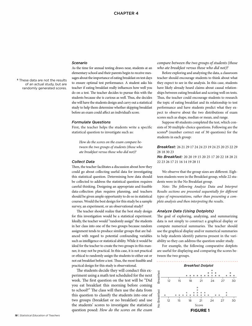
18 | Statistical Education of Teachers
chaPter 4
ScenarioAs the time for annual testing draws near, students at an elementary school and their parents begin to receive mes-sages about the importance of eating breakfast on test days to ensure optimal test performance. A student asks his teacher if eating breakfast really influences how well you do on a test. The teacher decides to pursue this with the students because she is curious as well. Thus, she decides she will have the students design and carry out a statistical study to help them determine whether skipping breakfast before an exam could affect an individual’s score.
Formulate QuestionsFirst, the teacher helps the students write a specific statistical question to investigate such as:
How do the scores on the exam compare be-tween the two groups of students (those who ate breakfast versus those who did not)?
Collect DataThen, the teacher facilitates a discussion about how they could go about collecting useful data for investigating this statistical question. Determining how data should be collected to address the statistical question requires careful thinking. Designing an appropriate and feasible data-collection plan requires planning, and teachers should be given ample opportunity to do so in statistical courses. Would the best design for this study be a sample survey, an experiment, or an observational study?
The teacher should realize that the best study design for this investigation would be a statistical experiment. Ideally, the teacher would “randomly assign” the students in her class into one of the two groups because random assignment tends to produce similar groups that are bal-anced with regard to potential confounding variables such as intelligence or statistical ability. While it would be ideal for the teacher to create the two groups in this man-ner, it may not be practical. In this case, it is not practical or ethical to randomly assign the students to either eat or not eat breakfast before a test. Thus, the most feasible and practical design for this study is observational.
The students decide they will conduct this ex-periment using a math test scheduled for the next week. The first question on the test will be “Did you eat breakfast this morning before coming to school?” The class will then use the data from this question to classify the students into one of two groups (breakfast or no breakfast) and use the students’ scores to investigate the statistical question posed: How do the scores on the exam
compare between the two groups of students (those who ate breakfast versus those who did not)?
Before exploring and analyzing the data, a classroom teacher should encourage students to think about what they expect to see in the analysis. In this case, students have likely already heard claims about causal relation-ships between eating breakfast and scoring well on tests. Thus, the teacher could encourage students to research the topic of eating breakfast and its relationship to test performance and have students predict what they ex-pect to observe about the two distributions of exam scores such as shape, median or mean, and range.
Suppose 40 students completed the test, which con-sists of 30 multiple-choice questions. Following are the scores5 (number correct out of 30 questions) for the students in each group:
Breakfast: 26 21 29 17 24 24 23 19 24 25 20 25 22 29 28 18 30 23No Breakfast: 20 20 19 15 20 25 17 20 22 18 28 21 22 23 26 17 21 16 14 19 28 11
We observe that the group sizes are different. Eigh-teen students were in the Breakfast group, while 22 stu-dents were in the No Breakfast group.
Note: The following Analyze Data and Interpret Results sections are presented sequentially for different types of representations, rather than presenting a com-plete analysis and then interpreting the results.
Analyze Data (Using Dotplots)The goal of exploring, analyzing, and summarizing data is not simply to construct a graphical display or compute numerical summaries. The teacher should use the graphical display and/or numerical summaries to help students identify patterns present in the vari-ability so they can address the question under study.
For example, the following comparative dotplots are useful for displaying and comparing the scores be-tween the two groups.
5 These data are not the results of an actual study, but are
randomly generated scores.
30
Breakfast Dotplot
No
Bre
akfa
stB
reakfa
st
12 15 18 21 24 27
12 15 18 21 24 27 30
30
Score
FIGURE 1

Statistical Education of Teachers | 19
chaPter 4
Looking at the dotplots there is a tendency for stu-dents in the Breakfast group to score higher than stu-dents in the No Breakfast group. The center of the scores for the Breakfast group is around 24 correct, while the center of the scores for the No Breakfast group is around 20 correct. The scores for each group appear to be rea-sonably symmetric about their respective centers. As the range for the scores in the No Breakfast group is 17 compared to a range of 13 for the Breakfast group, there appears to be more variability in the scores in the No Breakfast group than in the Breakfast group.
Interpret Results (Using Dotplots)While there is some overlap in scores between the two groups (scores between 17 and 28), there is also some separation. Specifically, four students in the No Break-fast group scored lower than anyone in the Breakfast group. On the other hand, three students in the Break-fast group scored higher than anyone in the No Break-fast group. Thus, although the dotplots show some over-lap in scores between the two groups, there is a tendency for students in the Breakfast group to score higher than students in the No Breakfast group.
Analyze Data (Using Boxplots)When sample sizes are different, comparing displays based on counts can sometimes be deceptive. Thus, a teacher should know it is useful to provide graphical dis-plays that do not depend on sample size. One such graph is the boxplot. A boxplot displays the intervals of each quarter of the data based on the Five-Number Summary (Minimum value, First Quartile, Median, Third Quartile, and Maximum value). Because the median is indicated in a boxplot, it provides more specific information about the center of the data than a dotplot. Additionally, the inter-quartile-range (IQR), a more informative measure of vari-ability than the range, is easily observed from a boxplot.
Boxplots are especially useful for comparing two groups of quantitative data because the overlap/sep-aration can be expressed in terms of percentages. The comparative boxplots below summarize the data on the exam scores for the two groups.
Based on the boxplots, the scores for the Breakfast group tend to be higher than the scores for the No Break-fast group. The median score for the Breakfast group is 24 correct, while the median score for the No Breakfast group is 20 correct. In fact, all five summary measures for the Breakfast group are higher than the correspond-ing measures for the No Breakfast group. The scores for each group appear to be reasonably symmetric about their respective medians. Although the range is greater for the No Breakfast group than the Breakfast group, the IQR for each group is 5, indicating similar amounts of variability in the middle 50% of scores.
Interpret Results (Using Boxplots)Teachers should be able to make and help students make a variety of observations about the data represented by the boxplots. For instance, while there is some overlap in scores between the groups (scores between 17 and 28), there is also some separation. More specifically, approx-imately 25% of the students in the No Breakfast group scored lower than anyone in the Breakfast group. On the other hand, the first quartile for the Breakfast group is 21, indicating that approximately 75% of teachers in the Breakfast group scored 21 or higher. In the No Breakfast group, fewer than half the students scored 21 or high-er. Thus, although the boxplots show some overlap in scores between the two groups, there is a tendency for students who ate breakfast to score higher than students who did not eat breakfast.
Analyze Data (Using Numerical Summaries)In the practice of statistics, technology is used to obtain numerical summaries for data. Although it is useful to have students calculate numerical summaries by hand at least once, the emphasis in the PreK–12 statistics curricu-lum is placed on the interpretation of the statistics, not the hand calculation of summary statistics using the formulas.
The mean is a commonly reported numerical sum-mary of quantitative data. The means for the scores in the two groups are reported below:
Breakfast Group No Breakfast Group
Mean: 23.7 20.1
Like the median, the mean provides information about the center of the data.
Two numerical summaries of the amount of vari-ability in quantitative data are the mean absolute devia-tion (MAD) and the standard deviation (SD). Although we would not expect K–5 students to be able to reason about the MAD and SD, teachers of K–5 students should
Breakfast Boxplot
10 15 20 25 30Score
10 15 20 25 30
Breakfast
No Breakfast
FIGURE 2

20 | Statistical Education of Teachers
chaPter 4
be able to engage in this kind of reasoning so they have a higher level of understanding of this scenario than is expected of their students.
The MAD and SD are reported below for each class.
Breakfast Group No Breakfast GroupMAD 2.98 3.20 SD 3.82 4.31
Each summary (MAD or SD) provides a measure of the typical difference between an observed score and the mean score. For example, the MAD indicates the 18 scores in the Breakfast group vary from 23.7 correct by 2.98 points on average and the 22 scores in the No Break-fast group vary from 20.1 correct by 3.20 points on aver-age. Because the MAD and SD for the No Breakfast group are a little larger than the MAD and SD for the Breakfast group, there is a little more variability in the scores for the No Breakfast group. However, the MAD and SD for both groups are fairly similar, indicating the variability in the scores is not very different for the two groups.
Interpret Results (of the Numerical Summaries)Teachers should note that the means capture the tendency of students in the Breakfast group to have higher scores, as displayed in the comparative dotplots. Specifically, the mean of the Breakfast group (23.7) is greater than the mean of the No Breakfast group (20.1). This tendency can be captured in a single statistic by reporting the dif-ference between the two sample means (23.7-20.1). Thus, students in the Breakfast group scored, on average, 3.6 points higher than those in the No Breakfast group. A comparison of the two groups focuses on this difference by asking, “Is a difference between means of 3.6 points a meaningful difference?” The answer to this question de-pends on two features of the data—the sample sizes and amounts of variability in the scores within the two groups.
One way to think about the magnitude of the dif-ference between the two means (3.6) is to express this difference relative to a measure of variability such as the MAD or SD.
Because the MADs are different for the two classes, we will use the larger MAD. We use the larger MAD to be on the cautious side, as we know mathematically having a larger denominator makes the ratio smaller, leaving us less likely to exaggerate the relationship. The difference between the means relative to the amount of variability is 3.6/3.2 = 1.125. Thus, the two means are 1.125 MADs apart.
Is this a meaningful difference? Although this quan-tity does not take into account the sample sizes, the ratio does provide a way to judge the difference in means with
respect to the amount of variability within each distri-bution. Specifically, this quantity gives some indication that the difference between the means (3.6) is meaning-ful—the difference is large relative to the variation with-in the data. Thus, it is reasonable to conclude that those students who eat breakfast tend to score higher on the test than those students who do not. There is evidence based on this sample of 40 students that eating breakfast is beneficial to higher performance on an assessment instrument. Developing Essential Understanding of Sta-tistics for Teaching Mathematics in Grades 6-8 (Kader and Jacobbe, 2013) offers a detailed discussion of how to compare two distributions for quantitative variables.
Based on the graphical and numerical analysis, it is tempting to say that eating breakfast was the cause for the higher mean score; however, teachers should understand we must be careful to not make a cause-and-effect conclusion because this was an observation-al study, not a randomized experiment. It is important that teachers be pushed to think statistically beyond the computation of a measure of center. Although it might be tempting to compute the mean or median of the test results and directly draw conclusions about the Breakfast group being better, teachers should be pushed to think about meaningfulness of the differ-ence in the manner outlined in this example. Through such an investigation teachers will be exposed to many of the content recommendations above and partake in the statistics investigative process.
ReferencesCommon Core State Standards Initiative (2010).
Common Core State Standards for Mathematics. Common Core State Standards (College- and Career-Readiness Standards and K–12 Standards in English Language Arts and Math). Washington, DC: National Governors Association Center for Best Practices and the Council of Chief State School Officers. Retrieved from www.corestandards.org.
Franklin, C., et al. (2007). Guidelines and Assessment for Instruction in Statistics Education (GAISE) Report: A PreK–12 Curriculum Framework. Alex-andria, VA: American Statistical Association.
Kader, G., and Jacobbe, T. (2013). Developing Essential Understanding of Statistics for Teaching Mathemat-ics in Grades 6–8. Reston, VA: NCTM.
National Council of Teachers of Mathematics (NCTM). (2000). Principles and Standards for School Mathematics. Reston, VA: NCTM.
Peters, S. (2010). Engaging in the arts and science of statistics. Mathematics Teacher, 103(7)

CHAPTER 5
Statistical Education of Teachers | 21
Expectations for Middle-School StudentsSince its inclusion in the National Council for Teach-er of Mathematics’ (NCTM) Curriculum and Eval-uation Standards for School Mathematics (1989), statistical content has gradually been expanded within the middle-school mathematics curriculum. The Common Core State Standards for Mathemat-ics (CCSSM) (2007) and other state standards em-phasize the importance of statistics and probability at the middle-school level. Thus, middle-school teachers are increasingly expected to teach units on statistical content.
Recommendations from reports such as CCSSM and NCTM’s Principles and Standards for School Mathematics (PSSM) (2000) and Curriculum Focal Points (2006) describe subject matter in statis-tics and probability within each of the three mid-dle-school grade levels. (In this chapter, the term “middle grades” or “middle school” refers to grade levels 6, 7, and 8.) Expectations of statistical under-standing for middle-school students generally in-clude the following:
• Understand the role of variability in statistical problem solving
• Explore, summarize, and describe patterns in variability in univariate data using numerical summaries and graphical representations, including:
º Frequencies, relative frequencies, and the mode for categorical data
º Measures of center and measures of variability for quantitative data
º Bar graphs for categorical data
º Dotplots, histograms, and boxplots for quantitative data
• Explore, summarize, and describe patterns of association in bivariate data based on:
º Two-way tables for bivariate categorical data
º Scatterplots for bivariate quantitative data
• Investigate random processes and un-derstand probability as a measure of the long-run relative frequency of an outcome, understand basic rules of probability, and ap-proximate probabilities through simulation
• Understand connections between probabil-ity, random sampling, and inference about a population
• Compare two data distributions and make informal inferences about differences be-tween two populations
These middle-grade topics should be developed from the statistical problem-solving perspective as de-scribed in the Guidelines and Assessment for Instruction in Statistics Education (GAISE) Report: A PreK–12 Curriculum Framework (Franklin et al., 2007). The GAISE problem-solving approach is built around four components: formulating a statistical question (antici-pating variability in the data), designing a plan for pro-ducing data (acknowledging variability) and collecting the data, exploring and analyzing the data (accounting for variability), and interpreting the results (taking vari-ability into account). The GAISE framework emphasiz-es the omnipresence of variability in data and recogniz-es the role of variability within each component.
To gain a sound understanding of the statistical topics in the middle-school curriculum, students should learn statistics in an activity-based learning environment in which they collect, explore, and interpret data to address statistical questions. Further, students’ exploration and analysis of data should be aided by appropriate technolo-gies, which, at a minimum, are capable of creating graphi-cal displays of data and computing numerical summaries
CHAPTER 5Preparing Middle-School Teachers to Teach Statistics

CHAPTER 5
22 | Statistical Education of Teachers
of data. Using the results from their analyses, students should consider the scope of their conclusions based on the manner in which the data were collected and com-municate an answer to the statistical question posed.
Essentials of Teacher PreparationThe primary goals of the statistical preparation of middle school teachers are three-fold:
1. Develop the necessary content knowl-edge and statistical reasoning skills to implement the recommended statistical topics for middle-grade students. Thus, teachers should achieve statistical content knowledge beyond that required of their students. Statistical topics should be devel-oped through meaningful experiences with the statistical problem-solving process.
2. Develop an understanding of how statistical concepts in middle grades build on the con-tent developed in elementary grades, provide a foundation for the content in high school, and are connected to other subject areas, including mathematics, in middle grades.
3. Develop pedagogical content knowledge necessary for effective teaching of statistics. Pre-service and practicing teachers should be familiar with common student concep-tions, content-specific teaching strategies, strategies for assessing statistical knowledge, and appropriate integration of technology for developing statistical concepts.
In addition to those topics covered in elementa-ry-teacher preparation, middle-school teacher prepara-tion should include at a minimum the following topics:
Formulate Questions• Distinguish between questions that require a
statistical investigation and those that do not
• Translate a “research” question into a ques-tion that can be answered with data and addressed through a statistical investiga-tion (e.g., see Scenario 1 of Appendix 1)
Collect Data• Identify appropriate variables for ad-
dressing a statistical question
• Distinguish between categorical and quanti-tative variables
• Recognize quantitative data may be either discrete (for example, counts, such as the number of pets a student has) or continuous (measurements, such as the height or weight of a student)
• Design a plan for collecting data
º Distinguish between observational studies and comparative experiments
º Use random selection in the design of a sampling plan
º Use random assignment in the design of a comparative experiment
º Recognize the connections between study design and interpretation of results; consider issues such as bias, confounding, and scope of inference
Analyze Data• Understand a data distribution describes the
variability present in data
º Use appropriate tabular and graphical representations and summaries (fre-quencies, relative frequencies, and the mode) of the distribution for categorical data
º Use appropriate graphical representa-tions and numerical summaries of the distribution for quantitative data; sum-marize by describing patterns in the variability (shape, center, and spread) and identifying values not fitting the overall pattern (outliers)
º Recognize when a normal distribution might be an appropriate model for a data distribution
º Recognize when a skewed distribution might be an appropriate model of a data distribution and understand the effects of skewness on measures of center and spread

CHAPTER 5
Statistical Education of Teachers | 23
• Use distributional reasoning strategies to compare two or more groups based on categorical data
º Compare modal categories
º Compare proportions within each category
• Use distributional reasoning strategies to com-pare two groups based on quantitative data
º Compare shapes, centers, and vari-ability
º Identify areas of overlap and separa-tion between the two distributions
º Understand how variability within groups affects comparisons between groups
• Explore and analyze patterns of association between two variables
º Distinguish between explanatory and response variables
º Summarize and interpret data on two categorical variables in a two-way table
º Summarize and interpret data on two quantitative variables in a scatterplot
º Use linear functions to model the association between two quantitative variables when appropriate
º Use a linear model to make predictions
º Use correlation to measure the strength of a linear association be-tween two quantitative variables
º Identify nonlinear relationships (e.g., power or exponential) between two quantitative variables
Interpret Results• Understand that one goal of statistical infer-
ence is to generalize results from a sample to some larger population
• Distinguish between population parame-ters and sample statistics
• Draw conclusions that are appropriate for the manner in which the data are collected
º Recognize that generalization from a sample requires random selection
º Recognize that statements about causation require random assignment
• Understand that random sampling from a population or random assignment in an experiment links the mathematical areas of statistics and probability
• Understand probability from a relative frequency perspective
º Use simulation models to explore the long-run relative frequency of outcomes
º Use the addition rule to calculate the probability of the union of disjoint events and the multiplication rule to calculate the probability of the inter-section of independent events
• Use simulation to explore, describe, and summarize the sample-to-sample variabili-ty (the sampling distribution) of a statistic
• Understand inferential reasoning through randomization and simulation to determine whether observed results are statistically significant
• Use simulation to develop a margin of error and explore the relationship between sample size and margin of error
• Use the normal distribution as appropriate to model distributions of sample statistics
As middle-school teachers develop statistical content knowledge, it is critical that they recognize the vertical connections of statistical topics across grade levels, the horizontal connections across the mathematics curriculum, and connections to other
CHAPTER 5
24 | Statistical Education of Teachers
subject areas. Statistics in the middle grades builds on the foundational experiences students have in the elementary grades and must strengthen and expand this foundation in preparation for students’ experi-ences with statistics in high school. Many statistical concepts developed in middle school are useful for reinforcing other areas of mathematical content with-in the middle-grades curriculum, including probabil-ity, measurement, number and operations, algebraic concepts, and linear functions. Additionally, most applications of statistics are in areas other than math-ematics (e.g., the sciences and social sciences), which provides students with opportunities to see connec-tions between the mathematical sciences and other areas of study. A thorough discussion of vertical and horizontal statistical connections, along with connec-tions across the middle-grades curriculum, is provid-ed in Developing Essential Understandings of Statistics, Grades 6–8 (Kader and Jacobbe, 2013, pages 81–90).
In addition to content knowledge, the preparation of middle-grade teachers should develop the peda-gogical knowledge necessary for effective teaching of statistics. Teachers should be introduced to common misunderstandings students have regarding statisti-cal and probabilistic concepts and learn to use appro-priate content-specific teaching strategies to address them. Some of the contexts in which common misun-derstandings occur include the following:
• The interpretation of graphical displays and tabular summaries of data
• The importance of random selection for obtaining a representative sample
• The notion of a sampling distribution
The research related to some of these misunder-standings is discussed in Chapter 8. Examples relat-ed to common misunderstandings are contained in Appendix 1.
The role of technology in learning statistics also must be an important aspect of middle-school teacher preparation. Teachers need to be comfort-able using technology to aid in the collection, explo-ration, analysis, and interpretation of data, as well as to develop concepts. While we do not recommend a specific technology, the technology/technologies chosen should have the capability to create dynamic graphical displays, produce numerical summaries of data, and perform simulations easily.
As students’ understanding of statistical con-cepts evolve, it is important that teachers learn the value of formative assessment. As noted in Chapter 7, writing statistical assessments is particularly dif-ficult because it requires disentangling mathemat-ical ideas and rote computational exercises from statistical thinking. Statistical assessments should emphasize conceptual understanding and interpre-tation over the application of formulas or algorith-mic thinking.
Recommendations for Prospective and Practicing TeachersMany of the topics described for the preparation of middle-school teachers are included in the traditional introductory college-level statistics course. However, this course alone is not adequate for preparing mid-dle-school teachers to teach the statistical content for middle-school students proposed by reports such as GAISE, CCSSM, and PSSM. Often, introductory sta-tistics courses pay little attention to formulating sta-tistical questions and give perfunctory attention to exploring and analyzing data. These courses frequently provide an axiomatic approach to probability, stress-ing the rules of probability instead of developing the concept of probability as a long-run relative frequency through simulation. Connections between statistics and probability are often ambiguous, and instead of fo-cusing on statistical reasoning, inference is approached as a collection of rote procedures.
NCTM’s Developing Essential Understandings of Statistics for Teaching Mathematics in Grades 6–8 (2013) provides a set of recommendations for prepar-ing middle-school teachers. This document describes four big ideas as a foundation for providing teachers with a deep understanding of the statistical content re-quired to teach statistics in middle school:
Big Idea 1: Distributions describe vari-ability in data.
Big Idea 2: Statistics can be used to compare two or more groups of data.
Big Idea 3: Bivariate distributions describe patterns or trends in the covari-ability in data on two variables.
Big Idea 4: Inferential statistics uses data in a sample selected from a popula-tion to describe features of the population.

CHAPTER 5
Statistical Education of Teachers | 25
The approach to developing statistical concepts in Essential Understandings is based on the notion that middle-grade teachers should experience the learn-ing of statistical concepts in ways similar to those of their students.
Course Recommendations for Prospective TeachersMET II (2012) recommends middle-school teachers take a course in statistics and probability beyond a modern technology-based introductory statistics course that includes topics on designing statistical studies, data analysis, and inferential reasoning.
In summary, this report recommends prospective middle-school statistics teachers acquire their statisti-cal knowledge base through the following courses:
A first course in statistics that develops teachers’ statistical content knowledge in an experiential, active learning environment that focuses on the problem-solving process and makes clear connections between statistical reasoning and notions of probability.
A second course that focuses on strengthening teachers’ conceptual understandings of the big ideas from Essential Understandings and the statistical content of the middle-school curriculum. This course also is intended to develop teachers’ pedagogical content knowledge by providing strategies for teaching statistical concepts, integrating appropriate technology into their instruction, making connections across the curriculum, and assessing statistical understanding in middle-school students.
Both courses should give teachers opportunities to ex-plore real problems that require them to do the following:
• Formulate statistical questions; design strat-egies for data collection and collect the data; explore, analyze, and summarize the data; and draw conclusions from the data
• Use dynamic statistical software or other modern technologies to aid in the collec-tion, analysis, and interpretation of data and enhance their learning and understanding of both statistical and probabilistic concepts
Professional Development Recommendations for Practicing TeachersBecause of the new emphasis on statistics in the mid-dle-grades mathematics curriculum, practicing mid-dle-school teachers are in need of professional develop-ment. Consequently, it is critical that practicing teachers have opportunities for meaningful professional develop-ment. The content and pedagogy of the professional de-velopment should be similar to that previously described for pre-service teachers.
Illustrative ExampleThe following example illustrates the complete statis-tical problem-solving process at the level expected of a middle-school teacher. Additional examples are pro-vided in Appendix 1.
Formulate QuestionsStatistical investigations undertaken in elementary school are typically based on questions posed by the teacher that can be addressed using data collected with-in the classroom. In middle school, the focus expands beyond the classroom, and students begin to formu-late their own questions. Because many investigations will be motivated by students’ interests, middle-school teachers must be skilled at constructing and refining sta-tistical questions that can be addressed with data.
For example, suppose a student is planning a project for the school’s statistics poster competition. The student recently read that consumption of bottled water is on the rise and wondered whether people actually prefer bot-tled water to tap or if they could even tell the difference between the two. When asked for advice about how to conduct a study, the teacher suggested having individuals drink two cups of water—one cup with tap water and one cup with bottled water. For each trial, the bottled water would be the same brand and the tap water would be from the same source. Not knowing which cup contained which type of water, each participant would identify the cup he/she believed to be the bottled water. Thus, a statis-tical question that could be investigated would be:
Are people more likely than not to correctly identify the cup with bottled water?
Collect DataTeachers must think carefully about how to collect data to address the above statistical question and how to
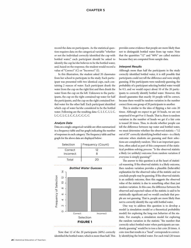
CHAPTER 5
26 | Statistical Education of Teachers
record the data on participants. As the statistical ques-tion requires data on the categorical variable “whether or not the individual correctly identified the cup with bottled water,” each participant should be asked to identify the cup he/she believes to be the bottled water, and, based on the response, the student would record a value of “Correct” (C) or “Incorrect” (I).
In this illustration, the student asked 20 classmates from her school to participate in the study. Each partic-ipant was presented with two identical cups, each con-taining 2 ounces of water. Each participant drank the water from the cup on the right first and then drank the water from the cup on the left. Unknown to the partic-ipants, the cup on the right contained tap water for half the participants, and the cup on the right contained bot-tled water for the other half. Each participant identified which cup of water he/she considered to be the bottled water. Following are the resulting data: C, I, I, C, I, I, C, I, C, C, I, C, I, C, C, I, C, C, C, C.
Analyze DataData on a single categorical variable are often summarized in a frequency table and bar graph indicating the number of responses in each category. The frequency table and bar graph for the above data are displayed below:
Note that 12 of the 20 participants (60%) correctly identified the bottled water, which is more than half. This
provides some evidence that people are more likely than not to distinguish bottled water from tap water. Note that the quantities “12” and “60%” are called statistics because they are computed from sample data.
Interpret ResultsAlthough more than half the participants in the study correctly identified bottled water, it is still possible that participants could not tell the difference and were simply guessing. If the participants were randomly guessing, the probability of a participant selecting bottled water would be 0.5, and we would expect about 10 of the 20 partic-ipants to correctly identify bottled water. However, this doesn’t guarantee that exactly 10 people will be correct, because there would be random variation in the number correct from one group of 20 participants to another.
This is similar to the idea of flipping a fair coin 20 times. Although we expect to get 10 heads, we are not surprised if we get 9 or 11 heads. That is, there is random variation in the number of heads we get if a fair coin is tossed 20 times. Thus, to decide whether people can tell the difference between tap water and bottled water, we must determine whether the observed statistic—“12 out of 20” correctly identifying bottled water—is a likely outcome when students are guessing and their selec-tions are completely random. This is an important ques-tion, often asked as part of this component of the statis-tical problem-solving process: “Is the observed statistic a likely (or unlikely) outcome from random variation if everyone is simply guessing?”
The answer to this question is at the heart of statisti-cal reasoning. If the observed statistic is a likely outcome, then random variation provides a plausible (believable) explanation for the observed value of the statistic and we conclude people may be guessing. If the observed statistic is an unlikely outcome, then this suggests the observed value of the statistic is due to something other than just random variation. In this case, the difference between the observed and expected values of the statistic is said to be statistically significant and we would conclude that peo-ple are not guessing. That is, people are more likely than not to correctly identify the cup with bottled water.
One way to address this question is to develop a model (a simulation model or a theoretical probability model) for exploring the long-run behavior of the sta-tistic. For example, a simulation model for exploring the random variation in the statistic “the number that correctly select bottled water when participants are ran-domly guessing” would be to toss a fair coin 20 times. A coin-toss that results in a “head” corresponds to correct-ly identifying the bottled water. For each trial (20 tosses
FIGURE 1
Bottled Water Guesses
Fre
qu
en
cy o
f S
ele
cti
on
Correct Incorrect
02
46
810
1214
Selection Frequency (Count)
CorrectIncorrect
Total 20
812
Selection

CHAPTER 5
Statistical Education of Teachers | 27
of the coin), record the number of heads. The dotplot summarizes the results for the “number of heads” from 100 trials of tossing a coin 20 times.
Based on the dotplot, getting 12 or more heads occurred in 19 of the 100 trials. So, if the coin is fair, the probability of getting 12 or more heads would be estimated at 0.19 based on this simulation. Thus, if par-ticipants cannot tell the difference and are randomly guessing, then 12 out of 20 people correctly identifying bottled water would not be a surprising outcome.
Applets for performing a simulation such as this are widely available (e.g., www.rossmanchance.com/applets). Using an applet, 10,000 repetitions of tossing a fair coin 20 times yielded the following dotplot (Figure 3) for the number of heads from each repetition. In the simulation, only about 4% of the 10,000 trials resulted in a number of heads that differed from the expected value by more than 4 heads. So, when flipping a fair coin 20 times, the probabil-ity of getting between 6 and 14 heads (inclusive) would be estimated to be 0.96. Thus, we can be fairly confident that the statistic (observed number of heads) will be within 4 of the expected number of heads (10). This value (±4), called the margin of error, tells us how much the statistic is likely to differ from the parameter due to random variation.
Number of Heads
Result of 10,000 Simulations
2 4 6 8 10 12 14 16 18
>=15<=5
As with the previous simulation, obtaining 12 heads (12 participants correctly identifying bottled water) is not a surprising outcome. Thus, because 12 out of 20 appears to be a likely outcome when the selection is random, the evidence against guessing is not very strong. Therefore, it is plausible that partic-ipants could not tell the difference between bottled water and tap water and were guessing which cup contained the bottled water.
Note that the statistical preparation of mid-dle-school teachers may include a more structured approach to solving this problem. This approach would consist of translating the statistical question into statements of the null and alternative hypotheses, estimating the p-value from the simulation, and using the p-value to describe the strength of the evidence against the hypothesis students are guessing. Also, this example could be expanded easily to one appropriate for preparing a high-school teacher. This expansion would include using the binomial probability distribu-tion as a mathematical model for describing the ran-dom variation in the number of heads out of 20 tosses and determining the exact p-value associated with the observed statistic.
ReferencesFranklin, C., et al. (2007). Guidelines and Assessment
for Instruction in Statistics Education (GAISE) Report: A PreK–12 Curriculum Framework. Alex-andria, VA: American Statistical Association.
Kader, G., and Jacobbe, T. (2013). Developing Essential Understanding of Statistics for Teaching Mathemat-ics in Grades 6–8. Reston, VA: NCTM.
National Council of Teachers of Mathematics (NCTM) (1989). Curriculum and Evaluation Standards for School Mathematics. Reston, VA: NCTM.
Common Core State Standards Initiative (2010). Common Core State Standards for Mathematics. Common Core State Standards (College- and Career-Readiness Standards and K–12 Standards in English Language Arts and Math). Washington, DC: National Governors Association Center for Best Practices and the Council of Chief State School Officers. Retrieved from www.corestandards.org.
National Council of Teachers of Mathematics (NCTM) (2000). Principles and Standards for School Mathematics. Reston, VA: NCTM.
National Council of Teachers of Mathematics (NCTM) (2006). Curriculum Focal Points. Reston, VA: NCTM. FIGURE 3
FIGURE 2
Result of 100 Simulations
2 4 6 8 10 12 14
Number of Heads
16

Statistical Education of Teachers | 29
chaPter 6
Expectations for High-School StudentsStatistical concepts in high school tend to be scattered throughout the curriculum, although it is increas-ingly common to find high schools offering a stand-alone statistics course in addition to an Advanced Placement (AP) statistics course. Statistical concepts appear in other mathematics courses, as well (e.g., re-gression is often discussed in algebra and geometry courses while discussing equations of lines).
State standards and nationally distributed stan-dards documents have increasingly emphasized statistics content at the high-school level over at least the past 40 years. Secondary teachers are thus required to teach a substantial amount of statistics by integrating it into mathematics courses and/or teaching designated stand-alone courses. Because of this, high-school teacher preparation needs to not only prepare teachers to teach statistics content, but also illustrate to teachers how the concepts are relat-ed and interwoven with mathematics.
One of the main areas in which this interweaving of statistics and mathematics is essential and explicit is modeling, which is becoming an important fea-ture of the high-school curriculum. Modeling gen-erally involves finding equations or mathematical systems that represent possible relationships among variables. If the variables produce data, then the modeling process must account for variation in the data and, thus, becomes statistical in nature.
High-school teachers should have experience modeling real-world situations, many of which be-gin with messy data sets that have to be “cleaned” (for example, by dealing with missing data and in-accurately recorded data) before any modeling is appropriate. Such key features of data analysis must be conveyed to students so they see the uses and misuses of statistical models, especially important in this age of Big Data. Teachers and students alike should come to appreciate the wisdom of statistician George Box (1987) in his famous dictum, “All mod-els are wrong; some models are useful.”
Recommended standards in statistics and prob-ability for high-school students from GAISE, the
CCSSM, NCTM, the College Board, and many state guidelines generally cover the following topics:
• Explore, summarize, and interpret univariate data, categorical and quantitative, including the normal model for data distributions
• Explore, summarize, and interpret bivariate categorical data based on two-way tables of frequencies and relative frequencies
• Explore bivariate quantitative data by way of scatterplots
• Construct and interpret simple linear mod-els for bivariate quantitative data
• Understand the role of randomization in designing studies and as the basis for statis-tical inference
• Understand the rules of probability, with emphasis on conditional probability, and using these rules in practical decision-mak-ing (e.g., knowing how to interpret risk)
• Model relationships among variables
Building on the spirit of statistics teaching and learning in the middle grades, these topics should be introduced from a data analytic perspective with re-al-world data and simulation of random processes be-ing prime instructional vehicles.
Essentials of Teacher PreparationHigh-school teachers should develop an understanding of statistical reasoning from a data and simulation per-spective and an appreciation for the effectiveness of such an approach in teaching and learning the basic tenets of statistics. As in the middle and elementary grades, this approach to statistics is built around four components of the problem-solving process of formulating questions, collecting data, analyzing data, and interpreting results, with emphasis on the omnipresence of variability and
CHAPTER 6Preparing High-School Teachers to Teach Statistics
30 | Statistical Education of Teachers
chaPter 6
the quantification of uncertainty as a necessary compo-nent of making valid conclusions.
The primary goals of statistical preparation for high-school teachers are three-fold:
1. Develop the necessary statistical reason-ing skills along with the content knowl-edge in statistics beyond the typical intro-ductory college course. Statistical topics should be developed through meaningful experiences with the statistical prob-lem-solving process.
2. Develop an understanding of how statistical concepts develop throughout PreK–8 and how they connect to high-school statistics content, as well as develop an understand-ing of how statistical concepts are related, or not related, to mathematical topics.
3. Develop pedagogical content knowledge necessary for effective teaching of statistics. Pre-service and practicing teachers should be familiar with common student concep-tions, content-specific teaching strategies, strategies for assessing statistical knowledge, and appropriate integration of technology for developing statistical concepts.
In meeting these goals, preparation programs should pay particular attention to common miscon-ceptions that students may have and discuss strategies and examples to address these misconceptions. Ad-ditional emphasis on technology use for high-school teachers is also an important aspect of teacher prepara-tion. Teachers not only need to be well versed in using dynamic statistical software to solve and understand problems, but they also need to feel comfortable teach-ing a statistical concept using technology as a tool.
Topics in data-driven statistical reasoning for high-school teachers should include at least the following in addition to those covered in elementary- and mid-dle-school teacher preparation.
Formulate Questions• Recognize questions that require a statisti-
cal investigation versus those that do not
• Develop statistical questions that help to focus a real issue (research question) on components that can be measured
Collect Data • Recognize appropriate data for answering
the posed statistical question
º Distinguish between categorical and quantitative variables
º Recognize that quantitative data may be either discrete (counts, such as the number of females in a class) or continuous (measurements, such as time or weight)
• Understand the role of random selection in sample surveys and the effect of sample size on the variability of estimates
• Understand the role of random assign-ment in experiments and its implications for cause-and-effect interpretations
• Understand the issues of bias and con-founding in nonrandomized observa-tional studies and their implications for interpretation
Analyze Data• Explore univariate data, both categorical
and quantitative
º Recognize situations for which the normal distribution might be an ap-propriate model for quantitative data distributions
º Recognize situations in which the data distributions tend to be skewed, and how the skewness affects mea-sures of center and spread
º Compare multiple univariate data sets, numerical and graphical
• Explore bivariate data, both categorical and quantitative
º Describe patterns of association as seen in two-way tables
º Describe patterns of association as seen in scatterplots
Statistical Education of Teachers | 31
chaPter 6
º Describe patterns of association between a categorical and a quantitative variable
º Construct and describe simple linear re-gression models and explain correlation
• Model rich real-world problems
º Describe patterns of association as seen in multiple pairwise scatterplots
º Fit and interpret multiple regression models including both numerical and categorical explanatory variables
º Fit and interpret exponential and power models
º Fit and interpret logistic regression models
Interpret Results• Understand basic probability from a relative
frequency perspective
º Understand additive and multiplica-tive rules
º Understand conditional probability and independence
º See the explicit connection between conditional probability and indepen-dence in two-way tables
º See the explicit connection of prob-ability to statistical inference and p-values
• Understand inferential reasoning through randomization and simulation
º Conduct tests of significance and approximate p-values
º Estimate population parameters and approximate margins of error
• Infer from small samples based on the bi-nomial and hypergeometric distributions,
calculating exact probabilities of possible outcomes
• Infer from large samples (using both confidence intervals and significance tests, as appropriate) for means and proportions based on the normal distribution of sample means and sample proportions
• Infer using the chi-square statistic for bivariate categorical data
Some of these topics in question formulation, data exploration, and informal inferential reasoning begin in middle-school curricula; however, they are further de-veloped in the high-school setting with a view toward extending their use to new and deeper concepts such as study design, the normal distribution, standard devia-tion, correlation, and formal inference procedures based on sampling distributions. It is important to note that the probability topics listed here are the ones that are criti-cal for understanding the statistical reasoning process, and are not intended to provide a full complement of probability topics that might be taught in a mathematics course on that subject. In fact, as will be expanded on below, many so-called statistics courses suffer from too much emphasis on probability.
Recommendations for Prospective and Practicing TeachersProgram Recommendations for Prospective High-School TeachersFor this data-analytic and randomization approach to teaching statistics, a traditional formula-oriented introductory statistics course is not appropriate for prospective teachers, because it emphasizes learning a set list of procedures over understanding statistical reasoning. Neither is the standard calculus-based in-troductory statistics and probability course designed to serve engineering and science majors in many in-stitutions appropriate, because such courses tend to overemphasize probability theory and present a more theoretical development of statistical methods. The GAISE College Report (www.amstat.org/education/gaise) provides an excellent set of recommendations for an introductory statistics course (or courses) aimed toward statistical reasoning (GAISE Report Executive Summary pp. 2):
1. Emphasize statistical literacy and develop statistical thinking.

32 | Statistical Education of Teachers
chaPter 6
2. Use real data.
3. Stress conceptual understanding, rather than mere knowledge of procedures.
4. Foster active learning in the classroom.
5. Use technology for developing conceptual understanding and analyzing data.
6. Use assessments to improve and evaluate student learning.
The report also provides informed advice about how these recommendations can be realized, along with outcomes that are essential for statistical literacy.
Such outcomes include believing and understanding that:
• Statistics begins with a question to investigate
• Data beat anecdotes
• Variability is natural, predictable, and quantifiable
• Association is not causation
• Statistical significance does not necessarily imply practical importance, especially for studies with large sample sizes
In summary, this report recommends that prospective high-school teachers of statistics acquire their knowledge base through the following courses:
1. An introductory course that emphasizes a modern data-analytic approach to statistical thinking, a simulation-based introduction to inference using appropriate technologies, and an introduction to formal inference (confidence intervals and tests of significance)
2. A second course in statistical methods that builds on the first and includes both randomization and classical procedures for comparing two parameters based on both independent and dependent samples (small and large), the basic principles of the design and analysis of sample surveys and experiments, inference in the simple linear regression model, and tests of independence/homoge-neity for categorical data
3. A statistical modeling course based on multiple regression techniques, including both categorical and numerical explanatory variables, exponential and power models (through data transformations), models for analyzing designed experiments, and logistic regression models
Each of the above courses should include the use of statistical software, provide multiple expe-riences with analyzing real data, and emphasize the communication of statistical results both orally and in writing.
Ideally, each of the first two courses should be taught with a pedagogical component for future teachers demonstrating effective methodologies for developing the subtle reasoning of statistics in students.
While a modern theory-based mathematical sta-tistics course is appropriate for high-school teachers of the subject, especially for prospective teachers of AP Statistics, it is strongly recommended that it not be
the only course exposing teachers to statistics in their curriculum. A theoretical course of this type should be taken after teachers develop an understanding of and appreciation for basic statistical reasoning expe-rienced from an empirical perspective and have some experience with statistical modeling.
Professional Development Programs for High-School TeachersBecause of the new emphasis on statistics in the curriculum, high-school teachers currently teach-ing are in need of professional development oppor-tunities that highlight the content and approach outline in the above. In general, any professional
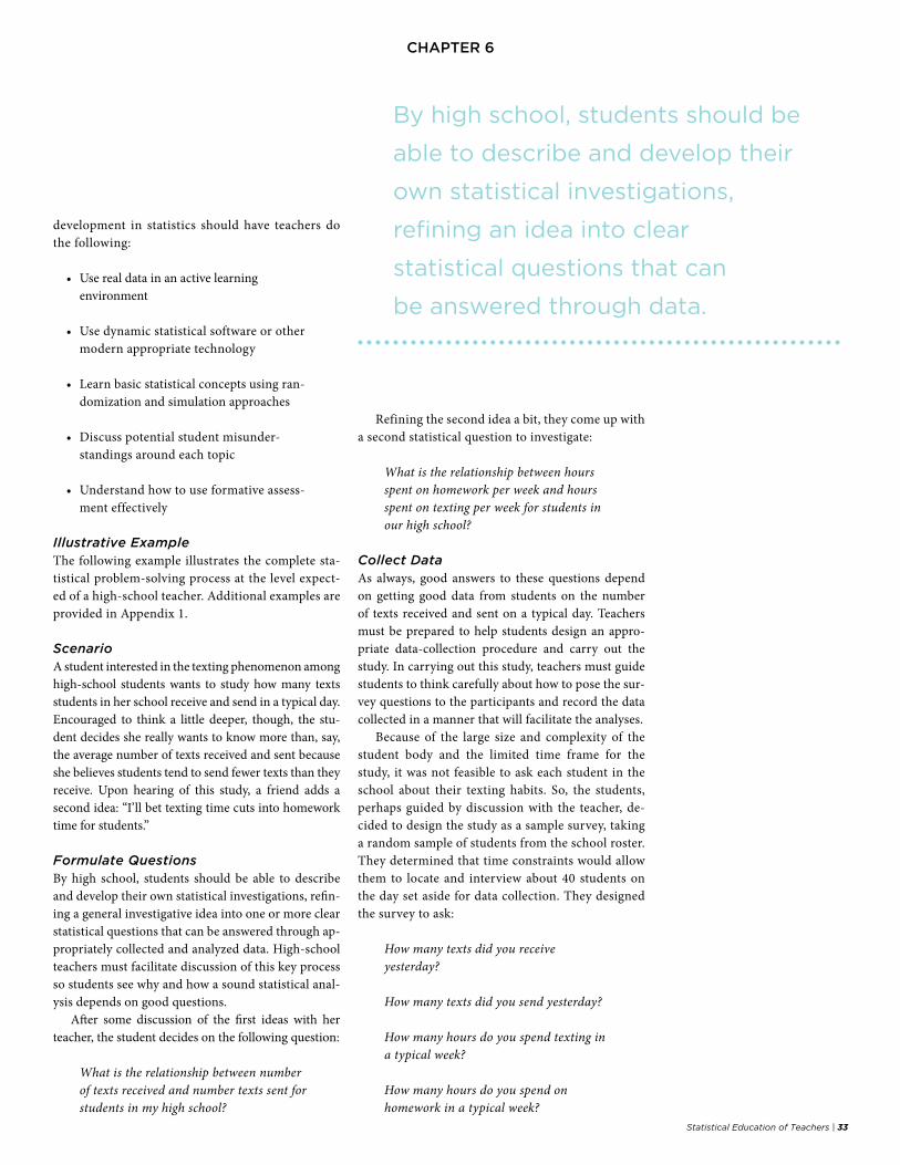
Statistical Education of Teachers | 33
chaPter 6
development in statistics should have teachers do the following:
• Use real data in an active learning environment
• Use dynamic statistical software or other modern appropriate technology
• Learn basic statistical concepts using ran-domization and simulation approaches
• Discuss potential student misunder-standings around each topic
• Understand how to use formative assess-ment effectively
Illustrative ExampleThe following example illustrates the complete sta-tistical problem-solving process at the level expect-ed of a high-school teacher. Additional examples are provided in Appendix 1.
ScenarioA student interested in the texting phenomenon among high-school students wants to study how many texts students in her school receive and send in a typical day. Encouraged to think a little deeper, though, the stu-dent decides she really wants to know more than, say, the average number of texts received and sent because she believes students tend to send fewer texts than they receive. Upon hearing of this study, a friend adds a second idea: “I’ll bet texting time cuts into homework time for students.”
Formulate QuestionsBy high school, students should be able to describe and develop their own statistical investigations, refin-ing a general investigative idea into one or more clear statistical questions that can be answered through ap-propriately collected and analyzed data. High-school teachers must facilitate discussion of this key process so students see why and how a sound statistical anal-ysis depends on good questions.
After some discussion of the first ideas with her teacher, the student decides on the following question:
What is the relationship between number of texts received and number texts sent for students in my high school?
Refining the second idea a bit, they come up with a second statistical question to investigate:
What is the relationship between hours spent on homework per week and hours spent on texting per week for students in our high school?
Collect DataAs always, good answers to these questions depend on getting good data from students on the number of texts received and sent on a typical day. Teachers must be prepared to help students design an appro-priate data-collection procedure and carry out the study. In carrying out this study, teachers must guide students to think carefully about how to pose the sur-vey questions to the participants and record the data collected in a manner that will facilitate the analyses.
Because of the large size and complexity of the student body and the limited time frame for the study, it was not feasible to ask each student in the school about their texting habits. So, the students, perhaps guided by discussion with the teacher, de-cided to design the study as a sample survey, taking a random sample of students from the school roster. They determined that time constraints would allow them to locate and interview about 40 students on the day set aside for data collection. They designed the survey to ask:
How many texts did you receive yesterday?
How many texts did you send yesterday?
How many hours do you spend texting in a typical week?
How many hours do you spend on homework in a typical week?
By high school, students should be
able to describe and develop their
own statistical investigations,
refining an idea into clear
statistical questions that can
be answered through data.
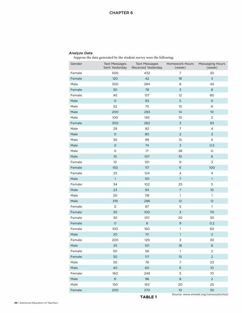
34 | Statistical Education of Teachers
chaPter 6
Analyze DataSuppose the data generated by the student survey were the following:
Gender Text Messages Sent Yesterday
Text Messages Received Yesterday
Homework Hours (week)
Messaging Hours (week)
Female 500 432 7 30
Female 120 42 18 3
Male 300 284 8 45
Female 30 78 3 8
Female 45 137 12 80
Male 0 93 5 0
Male 52 75 15 6
Male 200 293 14 10
Male 100 145 10 2
Female 300 262 3 83
Male 29 82 7 4
Male 0 80 2 3
Male 30 99 15 5
Male 0 74 3 0.5
Male 0 17 28 0
Male 10 107 10 6
Female 10 101 9 3
Female 150 117 6 100
Female 25 124 4 4
Male 1 101 7 1
Female 34 102 25 5
Male 23 83 7 10
Male 20 118 1 1
Male 319 296 12 12
Female 0 87 5 1
Female 30 100 3 70
Female 30 107 20 30
Female 0 8 9 0.2
Female 100 160 1 60
Male 20 111 1 2
Female 200 129 3 30
Male 25 101 18 6
Female 50 56 1 2
Female 30 117 15 2
Male 50 76 7 23
Male 40 60 6 10
Female 160 249 5 10
Male 6 96 8 2
Male 150 163 20 25
Female 200 270 10 30Source: www.amstat.org/censusatschool
TABLE 1
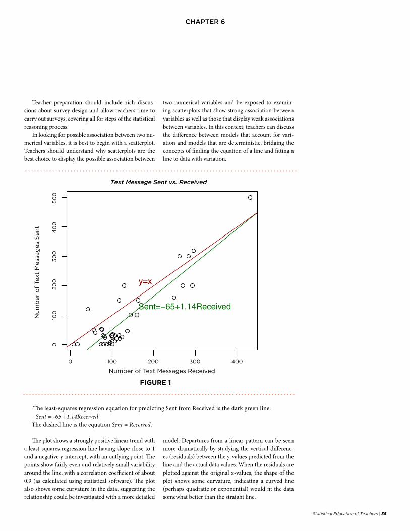
Statistical Education of Teachers | 35
chaPter 6
Text Message Sent vs. Received
Teacher preparation should include rich discus-sions about survey design and allow teachers time to carry out surveys, covering all for steps of the statistical reasoning process.
In looking for possible association between two nu-merical variables, it is best to begin with a scatterplot. Teachers should understand why scatterplots are the best choice to display the possible association between
two numerical variables and be exposed to examin-ing scatterplots that show strong association between variables as well as those that display weak associations between variables. In this context, teachers can discuss the difference between models that account for vari-ation and models that are deterministic, bridging the concepts of finding the equation of a line and fitting a line to data with variation.
The plot shows a strongly positive linear trend with a least-squares regression line having slope close to 1 and a negative y-intercept, with an outlying point. The points show fairly even and relatively small variability around the line, with a correlation coefficient of about 0.9 (as calculated using statistical software). The plot also shows some curvature in the data, suggesting the relationship could be investigated with a more detailed
model. Departures from a linear pattern can be seen more dramatically by studying the vertical differenc-es (residuals) between the y-values predicted from the line and the actual data values. When the residuals are plotted against the original x-values, the shape of the plot shows some curvature, indicating a curved line (perhaps quadratic or exponential) would fit the data somewhat better than the straight line.
0 100 200 300 400
010
020
030
040
050
0
Number of Text Messages Received
Num
ber o
f Tex
t Mes
sage
s Se
nt
Sent=−65+1.14Received
Text Messages Sent vs. Received
y=x
Number of Text Messages Received
0 100 200 300 400
50
04
00
30
020
010
00
Nu
mb
er
of
Text
Mess
ag
es
Sen
t
The least-squares regression equation for predicting Sent from Received is the dark green line:Sent = -65 +1.14Received
The dashed line is the equation Sent = Received.
FIGURE 1
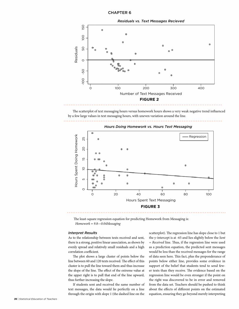
36 | Statistical Education of Teachers
chaPter 6
The scatterplot of text messaging hours versus homework hours shows a very weak negative trend influenced by a few large values in text messaging hours, with uneven variation around the line.
Residuals vs. Text Messages Recieved
Number of Text Messages Received
Resi
du
als
0 100 200 300 400
-10
0-5
010
05
015
00
Hours Doing Homework vs. Hours Text Messaging
Hours Spent Text Messaging
0 20 40 60 80 100
05
1015
20
25
Ho
urs
Sp
en
t D
oin
g H
om
ew
ork Regression
Interpret ResultsAs to the relationship between texts received and sent, there is a strong, positive linear association, as shown by evenly spread and relatively small residuals and a high correlation coefficient.
The plot shows a large cluster of points below the line between 60 and 120 texts received. The effect of this cluster is to pull the line toward them and thus increase the slope of the line. The effect of the extreme value at the upper right is to pull that end of the line upward, thus further increasing the slope.
If students sent and received the same number of text messages, the data would lie perfectly on a line through the origin with slope 1 (the dashed line on the
scatterplot). The regression line has slope close to 1 but the y-intercept is at -65 and lies slightly below the Sent = Received line. Thus, if the regression line were used as a prediction equation, the predicted sent messages would be less than the received messages for the range of data seen here. This fact, plus the preponderance of points below either line, provides some evidence in support of the belief that students tend to send few-er texts than they receive. The evidence based on the regression line would be even stronger if the point on the right was discovered to be in error and removed from the data set. Teachers should be pushed to think about the effects of different points on the estimated equation, ensuring they go beyond merely interpreting
The least-square regression equation for predicting Homework from Messaging is: Homework = 9.8—0.04Messaging
FIGURE 2
FIGURE 3
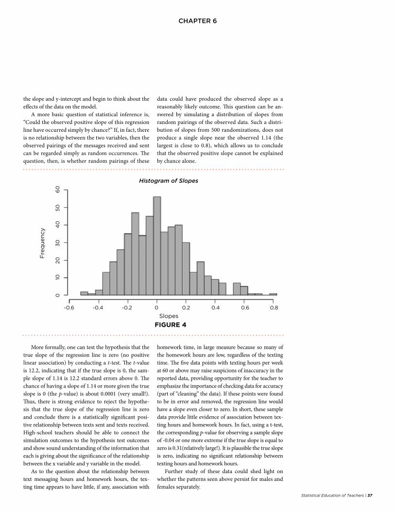
Statistical Education of Teachers | 37
chaPter 6
the slope and y-intercept and begin to think about the effects of the data on the model.
A more basic question of statistical inference is, “Could the observed positive slope of this regression line have occurred simply by chance?” If, in fact, there is no relationship between the two variables, then the observed pairings of the messages received and sent can be regarded simply as random occurrences. The question, then, is whether random pairings of these
data could have produced the observed slope as a reasonably likely outcome. This question can be an-swered by simulating a distribution of slopes from random pairings of the observed data. Such a distri-bution of slopes from 500 randomizations, does not produce a single slope near the observed 1.14 (the largest is close to 0.8), which allows us to conclude that the observed positive slope cannot be explained by chance alone.
More formally, one can test the hypothesis that the true slope of the regression line is zero (no positive linear association) by conducting a t-test. The t-value is 12.2, indicating that if the true slope is 0, the sam-ple slope of 1.14 is 12.2 standard errors above 0. The chance of having a slope of 1.14 or more given the true slope is 0 (the p-value) is about 0.0001 (very small!). Thus, there is strong evidence to reject the hypothe-sis that the true slope of the regression line is zero and conclude there is a statistically significant posi-tive relationship between texts sent and texts received. High-school teachers should be able to connect the simulation outcomes to the hypothesis test outcomes and show sound understanding of the information that each is giving about the significance of the relationship between the x variable and y variable in the model.
As to the question about the relationship between text messaging hours and homework hours, the tex-ting time appears to have little, if any, association with
homework time, in large measure because so many of the homework hours are low, regardless of the texting time. The five data points with texting hours per week at 60 or above may raise suspicions of inaccuracy in the reported data, providing opportunity for the teacher to emphasize the importance of checking data for accuracy (part of “cleaning” the data). If these points were found to be in error and removed, the regression line would have a slope even closer to zero. In short, these sample data provide little evidence of association between tex-ting hours and homework hours. In fact, using a t-test, the corresponding p-value for observing a sample slope of -0.04 or one more extreme if the true slope is equal to zero is 0.31(relatively large!). It is plausible the true slope is zero, indicating no significant relationship between texting hours and homework hours.
Further study of these data could shed light on whether the patterns seen above persist for males and females separately.
Histogram of Slopes
Fre
qu
en
cy
010
20
30
40
50
60
-0.6 -0.4 -0.2 0 0.2 0.4 0.6 0.8
Slopes
FIGURE 4
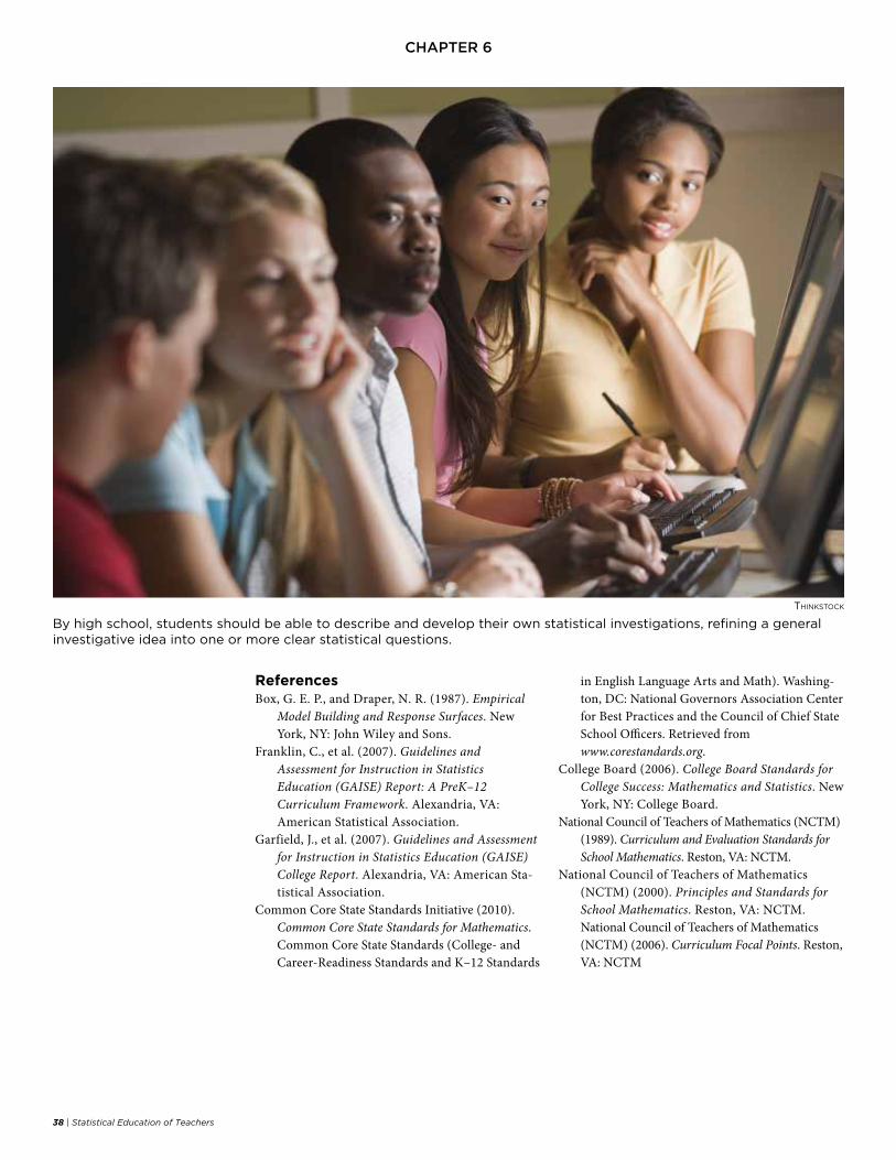
38 | Statistical Education of Teachers
chaPter 6
ReferencesBox, G. E. P., and Draper, N. R. (1987). Empirical
Model Building and Response Surfaces. New York, NY: John Wiley and Sons.
Franklin, C., et al. (2007). Guidelines and Assessment for Instruction in Statistics Education (GAISE) Report: A PreK–12 Curriculum Framework. Alexandria, VA: American Statistical Association.
Garfield, J., et al. (2007). Guidelines and Assessment for Instruction in Statistics Education (GAISE) College Report. Alexandria, VA: American Sta-tistical Association.
Common Core State Standards Initiative (2010). Common Core State Standards for Mathematics. Common Core State Standards (College- and Career-Readiness Standards and K–12 Standards
in English Language Arts and Math). Washing-ton, DC: National Governors Association Center for Best Practices and the Council of Chief State School Officers. Retrieved from www.corestandards.org.
College Board (2006). College Board Standards for College Success: Mathematics and Statistics. New York, NY: College Board.
National Council of Teachers of Mathematics (NCTM) (1989). Curriculum and Evaluation Standards for School Mathematics. Reston, VA: NCTM.
National Council of Teachers of Mathematics (NCTM) (2000). Principles and Standards for School Mathematics. Reston, VA: NCTM.National Council of Teachers of Mathematics (NCTM) (2006). Curriculum Focal Points. Reston, VA: NCTM
ThiNksTock
By high school, students should be able to describe and develop their own statistical investigations, refining a general investigative idea into one or more clear statistical questions.
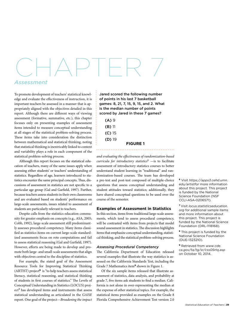
CHAPTER 7
Statistical Education of Teachers | 39
To promote development of teachers’ statistical knowl-edge and evaluate the effectiveness of instruction, it is important teachers be assessed in a manner that is ap-propriately aligned with the objectives detailed in this report. Although there are different ways of viewing assessment (formative, summative, etc.), this chapter focuses only on presenting examples of assessment items intended to measure conceptual understanding at all stages of the statistical problem-solving process. These items take into consideration the distinction between mathematical and statistical thinking, noting that statistical thinking is inextricably linked to context and variability plays a role in each component of the statistical problem-solving process.
Although this report focuses on the statistical edu-cation of teachers, many of the same issues apply when assessing either students’ or teachers’ understanding of statistics. Regardless of age, learners introduced to sta-tistics encounter the same principal concepts. Thus, dis-cussions of assessment in statistics are not specific to a particular age group (Gal and Garfield, 1997). Further, because teachers assess students in their own classrooms and are evaluated based on students’ performance on large-scale assessments, issues related to assessment of students are particularly relevant to teachers.
Despite calls from the statistics education commu-nity for greater emphasis on concepts (e.g., ASA, 2005; Cobb, 1992), large-scale assessment still predominant-ly assesses procedural competency. Many items classi-fied as statistics items on current large-scale standard-ized assessments focus on rote computations and fail to assess statistical reasoning (Gal and Garfield, 1997). However, efforts are being made to develop and pro-mote both large- and small-scale assessments that align with objectives central to the discipline of statistics.
For example, the stated goal of the Assessment Resource Tools for Improving Statistical Thinking (ARTIST) project6 is “to help teachers assess statistical literacy, statistical reasoning, and statistical thinking of students in first courses of statistics.” The Levels of Conceptual Understanding in Statistics (LOCUS) proj-ect7 has developed items and instruments that assess statistical understanding as articulated in the GAISE report. One goal of the project—Broadening the impact
and evaluating the effectiveness of randomization-based curricula for introductory statistics8 —is to facilitate assessment of introductory statistics courses to better understand student learning in “traditional” and ran-domization-based courses. The team has developed a pre-test and post-test composed of multiple-choice questions that assess conceptual understanding and student attitudes toward statistics; additionally, they have shared conceptual questions to be used over the course of the semester.
Examples of Assessment in StatisticsIn this section, items from traditional large-scale assess-ments, which tend to assess procedural competency, will be contrasted with items from projects that model sound assessment in statistics. The discussion highlights items that emphasize conceptual understanding, statisti-cal thinking, and the statistical problem-solving process.
Assessing Procedural CompetencyThe California Department of Education released several examples that illustrate the way statistics is as-sessed on the California Standards Test, including the Grade 7 Mathematics item9 shown in Figure 1.
Of the six sample items released that illustrate as-sessment of statistics, data analysis, and probability at grade 7, five items ask students to find a median. Cali-fornia is not alone in over-representing the median at the expense of other statistical topics. For example, the statistical items provided as examples on the Grade 8 Florida Comprehensive Achievement Test version 2.0
CHAPTER 7Assessment
6 Visit https://apps3.cehd.umn.edu/artistfor more information about this project. This project is funded by the National Science Foundation (NSF CCLI-ASA-0206571).
7 Visit locus.statisticseducation.org for additional sample items and more information about this project. This project is funded by the National Science Foundation (DRL-1118168).
8 This project is funded by the National Science Foundation (DUE-1323210).
9 Retrieved from www.cde.ca.gov/ta/tg/sr/css05rtq.asp on October 10, 2014.
Jared scored the following number of points in his last 7 basketball games: 8, 21, 7, 15, 9, 15, and 2. What is the median number of points scored by Jared in these 7 games?
(a) 9
(B) 11
(c) 15
(D) 19FIGURE 1
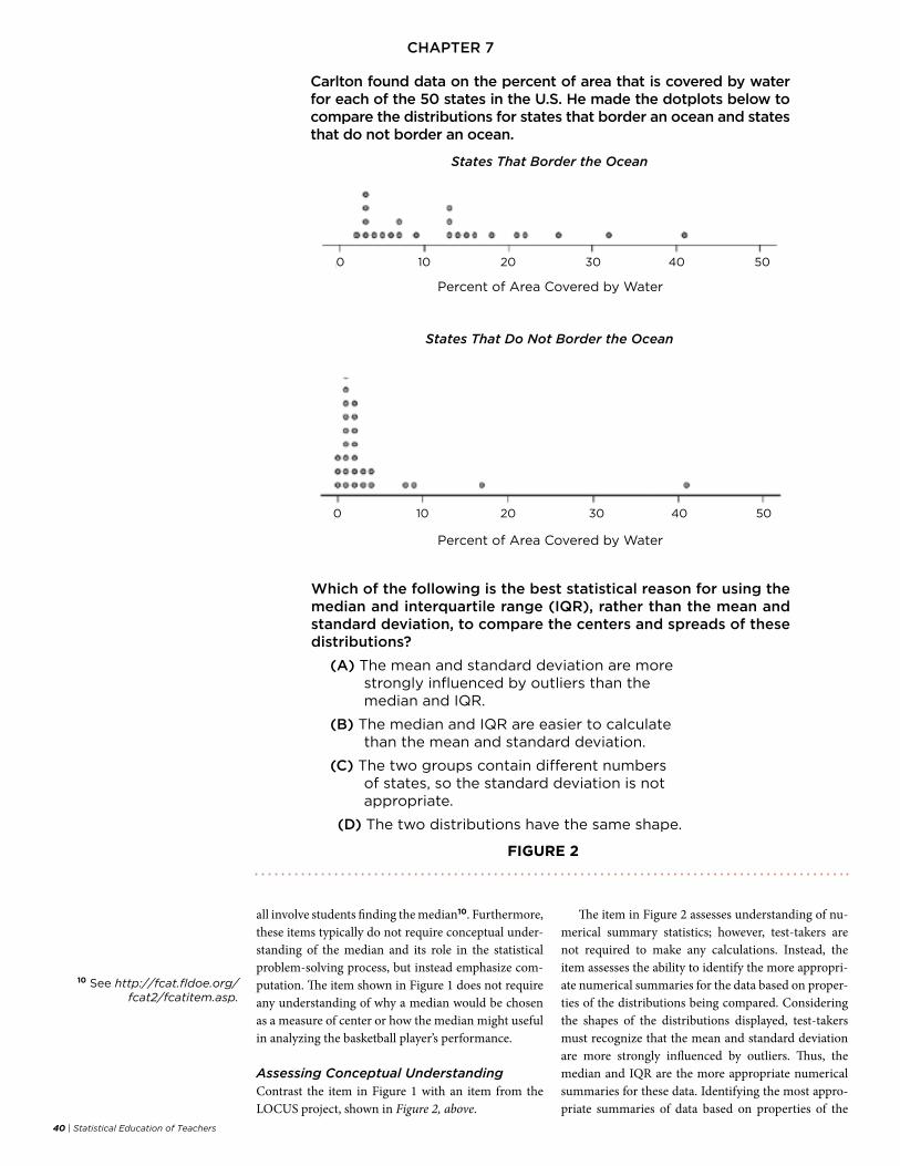
CHAPTER 7
40 | Statistical Education of Teachers
all involve students finding the median10. Furthermore, these items typically do not require conceptual under-standing of the median and its role in the statistical problem-solving process, but instead emphasize com-putation. The item shown in Figure 1 does not require any understanding of why a median would be chosen as a measure of center or how the median might useful in analyzing the basketball player’s performance.
Assessing Conceptual UnderstandingContrast the item in Figure 1 with an item from the LOCUS project, shown in Figure 2, above.
The item in Figure 2 assesses understanding of nu-merical summary statistics; however, test-takers are not required to make any calculations. Instead, the item assesses the ability to identify the more appropri-ate numerical summaries for the data based on proper-ties of the distributions being compared. Considering the shapes of the distributions displayed, test-takers must recognize that the mean and standard deviation are more strongly influenced by outliers. Thus, the median and IQR are the more appropriate numerical summaries for these data. Identifying the most appro-priate summaries of data based on properties of the
10 See http://fcat.fldoe.org/fcat2/fcatitem.asp.
Which of the following is the best statistical reason for using the median and interquartile range (iQr), rather than the mean and standard deviation, to compare the centers and spreads of these distributions?
(a) The mean and standard deviation are more strongly influenced by outliers than the median and IQR.
(B) The median and IQR are easier to calculate than the mean and standard deviation.
(c) The two groups contain different numbers of states, so the standard deviation is not appropriate.
(D) The two distributions have the same shape.
States That Border the Ocean
Percent of Area Covered by Water
States That Do Not Border the Ocean
Percent of Area Covered by Water
carlton found data on the percent of area that is covered by water for each of the 50 states in the U.S. he made the dotplots below to compare the distributions for states that border an ocean and states that do not border an ocean.
FIGURE 2
0 10 20 30 40 50
0 10 20 30 40 50
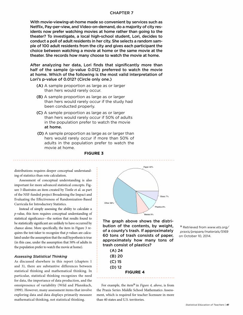
CHAPTER 7
Statistical Education of Teachers | 41
the graph above shows the distri-bution of the contents, by weight, of a county’s trash. if approximately 60 tons of trash consists of paper, approximately how many tons of trash consist of plastics?
(a) 24
(B) 20
(c) 15
(D) 12
distributions requires deeper conceptual understand-ing of statistics than rote calculation.
Assessment of conceptual understanding is also important for more advanced statistical concepts. Fig-ure 3 illustrates an item created by Tintle et al. as part of the NSF-funded project Broadening the Impact and Evaluating the Effectiveness of Randomization-Based Curricula for Introductory Statistics.
Instead of simply assessing the ability to calculate a p-value, this item requires conceptual understanding of statistical significance—the notion that results found to be statistically significant are unlikely to have occurred by chance alone. More specifically, the item in Figure 3 re-quires the test-taker to recognize that p-values are calcu-lated under the assumption that the null hypothesis is true (in this case, under the assumption that 50% of adults in the population prefer to watch the movie at home).
Assessing Statistical ThinkingAs discussed elsewhere in this report (chapters 1 and 3), there are substantive differences between statistical thinking and mathematical thinking. In particular, statistical thinking recognizes the need for data, the importance of data production, and the omnipresence of variability (Wild and Pfannkuch, 1999). However, many assessment items that involve exploring data and data displays primarily measure mathematical thinking, not statistical thinking.
For example, the item11 in Figure 4, above, is from the Praxis Series Middle School Mathematics Assess-ment, which is required for teacher licensure in more than 40 states and U.S. territories.
With movie-viewing-at-home made so convenient by services such as Netflix, Pay-per-view, and Video-on-demand, do a majority of city res-idents now prefer watching movies at home rather than going to the theater? to investigate, a local high-school student, lori, decides to conduct a poll of adult residents in her city. She selects a random sam-ple of 100 adult residents from the city and gives each participant the choice between watching a movie at home or the same movie at the theater. She records how many choose to watch the movie at home.
After analyzing her data, Lori finds that significantly more than half of the sample (p-value 0.012) preferred to watch the movie at home. Which of the following is the most valid interpretation of lori’s p-value of 0.012? (circle only one.)
(a) A sample proportion as large as or larger than hers would rarely occur.
(B) A sample proportion as large as or larger than hers would rarely occur if the study had been conducted properly.
(c) A sample proportion as large as or larger than hers would rarely occur if 50% of adults in the population prefer to watch the movie at home.
(D) A sample proportion as large as or larger than hers would rarely occur if more than 50% of adults in the population prefer to watch the movie at home.
FIGURE 3
11 Retrieved from www.ets.org/praxis/prepare/materials/5169
on October 10, 2014.
FIGURE 4
Paper 40%
Other 36%
Metals 9%
Plastics 8%
Glass 7%

CHAPTER 7
42 | Statistical Education of Teachers
Although data for Figure 4 are displayed in a circle graph, the item requires only mathematical thinking (use of percents or ratios to answer a deter-ministic question). The correct answer (D) can be calculated using the fact that the ratio of plastics to paper in the trash is 8% to 40% or 1 to 5, which is equivalent to a ratio of 12 tons to 60 tons. This solu-tion does not require any consideration of why the data are of interest, how the data were produced, or how these sample percentages might compare with population percentages. Contrast the item shown in Figure 4 with the LOCUS item in Figure 5.
The item in Figure 5 requires statistical think-ing. Test-takers are expected to make connections between the statistical question, how the data were collected, and how the results should be interpreted. In particular, the item requires test-takers to iden-tify statistical questions that can and cannot be an-swered using data from a sample survey involving randomly selected participants. The data are appro-priate for answering all questions presented except choice (B). Cause-and-effect conclusions are only appropriate based on data from experiments with random assignment.
Another important aspect of statistical thinking is a questioning attitude toward statistical claims, such as those presented in the media (Watson, 1997).
Watson (1997) presented the following open-ended formative assessment item, which allows students and teachers to “demonstrate statistical understand-ing and questioning ability which would not be pos-sible in a multiple-choice format” (p. 5). Figure 6 illustrates the relationship between a sample (poll conducted in Chicago) and a population (inference made about all U.S. high-school students), although these statistical terms are not explicitly mentioned.
Watson (1997) reports that some test-takers respond to the first question with criticism of the implications of the article’s claims, while others rec-ognized the sample might not be representative of the population. The geographical cues in the second part of the question provide another opportunity to recognize the sampling issue. In general, assessment items using the media provide a means to assess sta-tistical thinking as it occurs outside the classroom.
Assessing the Statistical Problem-Solving ProcessThe items previously presented emphasize various components of the statistical problem-solving pro-cess: formulating questions, collecting data, analyz-ing data, and interpreting results. In practice, the components of the process are inter-related, so it is often expedient to use items that address more than
a 13-year study of 1,328 adults random-ly selected from a population carefully monitored the personal habits and health conditions of participants. Per-sonal habits included tobacco use and coffee consumption. health conditions included incidence of stroke. Which of the following questions about this pop-ulation caNNOt be answered using data from this study?
(a) Are coffee drinkers more likely to smoke than adults who do not drink coffee?
(B) Does coffee con-sumption cause a reduction in the incidence of stroke?
(c) Do coffee drinkers have fewer strokes than adults who do not drink coffee?
(D) What percentage of the population are coffee drinkers?
FIGURE 5
“aBOUt 6 in 10 United States high-school students say they could get a handgun if they wanted one, a third of them within an hour, a sur-vey shows. The poll of 2,508 junior and senior high-school students in chicago also found 15 percent had actually carried a handgun within the past 30 days, with 4 percent taking one to school.”
(a) Would you make any criticisms of the claims in this article?
(B) If you were a high-school teacher, would this report make you refuse a job offer some-where else in the United States, say Colorado or Arizona? Why or why not?
FIGURE 6
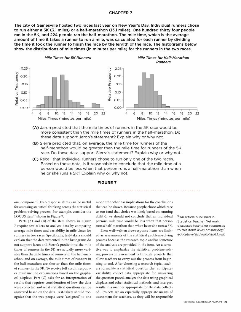
CHAPTER 7
Statistical Education of Teachers | 43
one component. Free-response items can be useful for assessing statistical thinking across the statistical problem-solving process. For example, consider the LOCUS item12 shown in Figure 7.
Parts (A) and (B) of the item shown in Figure 7 require test-takers to analyze data by comparing average mile times and variability in mile times for runners in two races. Specifically, test-takers should explain that the data presented in the histograms do not support Jaron and Sierra’s predictions: the mile times of runners in the 5K are actually more vari-able than the mile times of runners in the half-mar-athon, and on average, the mile times of runners in the half-marathon are shorter than the mile times of runners in the 5K. To receive full credit, respons-es must include explanations based on the graphi-cal displays. Part (C) asks for an interpretation of results that requires consideration of how the data were collected and what statistical questions can be answered based on the data. Test-takers should rec-ognize that the way people were “assigned” to one
race or the other has implications for the conclusions that can be drawn. Because people chose which race to run (and that choice was likely based on running ability), we should not conclude that an individual person’s mile time would be less when that person runs a half-marathon than when he or she runs a 5K.
Even well-written free-response items are limit-ed as assessments of the statistical problem-solving process because the research topic and/or structure of the analysis are provided in the item. An alterna-tive way to emphasize the statistical problem-solv-ing process in assessment is through projects that allow teachers to carry out the process from begin-ning to end. After choosing a research topic, teach-ers formulate a statistical question that anticipates variability, collect data appropriate for answering the question posed, analyze the data using graphical displays and other statistical methods, and interpret results in a manner appropriate for the data collect-ed. Projects are an especially appropriate means of assessment for teachers, as they will be responsible
the city of Gainesville hosted two races last year on New Year’s Day. individual runners chose to run either a 5K (3.1 miles) or a half-marathon (13.1 miles). One hundred thirty four people ran in the 5K, and 224 people ran the half-marathon. the mile time, which is the average amount of time it takes a runner to run a mile, was calculated for each runner by dividing the time it took the runner to finish the race by the length of the race. The histograms below show the distributions of mile times (in minutes per mile) for the runners in the two races.
(a) Jaron predicted that the mile times of runners in the 5K race would be more consistent than the mile times of runners in the half-marathon. Do these data support Jaron’s statement? Explain why or why not.
(B) Sierra predicted that, on average, the mile time for runners of the half-marathon would be greater than the mile time for runners of the 5K race. Do these data support Sierra’s statement? Explain why or why not.
(c) Recall that individual runners chose to run only one of the two races. Based on these data, is it reasonable to conclude that the mile time of a person would be less when that person runs a half-marathon than when he or she runs a 5K? Explain why or why not.
FIGURE 7
Miles Times (minutes per mile)
Mile Times for 5K Runners Mile Times for Half-Marathon Runners
Miles Times (minutes per mile)
Rela
tive F
req
uen
cy
Rela
tive F
req
uen
cy
0.00
0.05
0.10
0.15
0.20
0.25
4 6 8 10 12 14 16 18 20 22
12An article published in
Statistics Teacher Network
discusses test-taker responses
to this item: www.amstat.org/education/stn/pdfs/stn83.pdf.
4 6 8 10 12 14 16 18 20 22
0.00
0.05
0.10
0.15
0.20
0.25
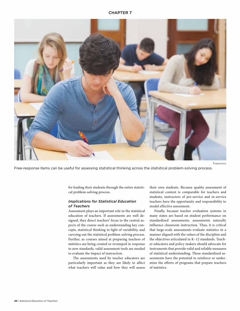
CHAPTER 7
44 | Statistical Education of Teachers
for leading their students through the entire statisti-cal problem-solving process.
Implications for Statistical Education of TeachersAssessment plays an important role in the statistical education of teachers. If assessments are well de-signed, they direct teachers’ focus to the central as-pects of the course such as understanding key con-cepts, statistical thinking in light of variability, and carrying out the statistical problem-solving process. Further, as courses aimed at preparing teachers of statistics are being created or revamped in response to new standards, valid assessment tools are needed to evaluate the impact of instruction.
The assessments used by teacher educators are particularly important as they are likely to affect what teachers will value and how they will assess
their own students. Because quality assessment of statistical content is comparable for teachers and students, instructors of pre-service and in-service teachers have the opportunity and responsibility to model effective assessment.
Finally, because teacher evaluation systems in many states are based on student performance on standardized assessments, assessments naturally influence classroom instruction. Thus, it is critical that large-scale assessments evaluate statistics in a manner aligned with the values of the discipline and the objectives articulated in K–12 standards. Teach-er-educators and policy makers should advocate for instruments that provide valid and reliable measures of statistical understanding. These standardized as-sessments have the potential to reinforce or under-mine the efforts of programs that prepare teachers of statistics.
ThiNksTock
Free-response items can be useful for assessing statistical thinking across the statistical problem-solving process.
Statistical Education of Teachers | 45
chaPter 8
The prior chapters of this report articulate and outline specific recommendations about teacher preparation in statistics at the different grade levels. The discussion of the research on the teaching and learning of statis-tics presented in this chapter provides a starting point to inform those implementing the recommendations on how specific topics within the recommendations can be approached and taught.
Despite significant attention given to teacher ed-ucation in mathematics (Ball, 1991; Ball and Bass, 2000; Franke et al., 2009; Hill and Ball, 2004), few re-search-based guidelines are in place concerning what teachers need to know to teach statistics effectively. Although still an emerging field, some research does exist on student learning of statistics, teacher under-standing of statistics, and teacher preparation in statis-tics. Furthermore, several expository pieces have been published highlighting ideas and advances in the field. The goal of this chapter is to present a brief overview of what is known and not known from the research on the teaching and learning of statistics in PreK–12. An example of a more complete review of the literature on research on statistics learning and reasoning can be found in Shaughnessy (2007).
Research on Differences Between Mathematical and Statistical Thinking and Reasoning Research in statistics education has prompted growing recognition of the differences between mathematical thinking and statistical thinking (Groth, 2007; Hannigan, Gill, and Leavy, 2013). For example, statistical thinking involves recognition of the need for data, the importance of data production, and the omnipresence of variability. Various models of student learning in statistics have been constructed in the literature emphasizing the need to reason in the presence of variability (Ben-Zvi and Fried-lander, 1997; Jones et al. 2004; Hoerl and Snee, 2001; Wild and Pfannkuch, 1999). The development of statistical thinking must begin with a problem one seeks to answer through the use of data. This process of sifting through data to answer a problem is analytical by nature and in-volves constant evaluation in relation to the question be-ing answered (Wild and Pfannkuch, 1999).
Hannigan, Gill, and Leavy (2013) conducted a study of prospective mathematics teachers using the Com-prehensive Assessment of Outcomes in a First Statistics (CAOS) course test and found that, despite the prospec-tive teachers having strong mathematics abilities, their results were not significantly better than those of stu-dents from nonquantitative disciplines. Based on these results, the authors suggest “statistical thinking is differ-ent from mathematical thinking and that a strong back-ground in mathematics does not necessarily translate to statistical thinking” (p. 446). They note that this finding has implications for teacher preparation, as it should not be assumed teachers can transfer their knowledge of mathematics to statistics in ways that will allow them to meet the increased expectations for teaching statistics.
Research on Student Statistical LearningSeveral studies and expository articles have focused on the nature of students’ statistical thinking (Saldanha and Thomson, 2002; Mokros and Russell, 1995; Cobb, McClain, and Gravemeijer, 2003; delMas, 2004; Jones, Langrall, and Mooney, 2007). Such papers have identi-fied topics and concepts that are difficult for students to learn and have suggested potential pedagogical ap-proaches that may help facilitate the teaching of specif-ic concepts (Garfield and Ben-Zvi, 2008; Bakker, 2004; Gil and Ben-Zvi, 2011; Lehrer, Kim, and Schauble, 2007; Dierdorp, Bakker, Eijkelhof, and Maanen, 2011). Often, students learning statistical concepts rely on computational methods to solve problems without un-derstanding the statistical ideas being discussed (Cher-vany et al., 1977; Stroup, 1984).
Several studies document the difficulties that arise with introductory concepts such as interpreting graphs and finding descriptive statistics such as measures of center and spread (e.g., Mokros and Russell, 1995; Cai, 2000; Capraro, Kulm, and Capraro, 2005; Friel, Curcio, and Bright, 2001; Konold and Pollatsek, 2002; Watson and Mortiz, 2000; Well and Gagnon, 1997) and with more complex concepts such as sampling methods, study design, and sampling distributions (e.g., Saldanha and Thomson, 2002; Cobb and Moore, 1997; Groth, 2003; Shaughnessy, 2007; Shaughnessy, Ciancetta, and Canada, 2004; Watson and Moritz, 2000). For example,
CHAPTER 8Overview of Research on the Teaching and Learning of Statistics in Schools
46 | Statistical Education of Teachers
chaPter 8
Lehrer, Kim, and Schauble (2007) worked with 5th- and 6th-grade students to “invent” and revise data displays, measures of center and variability, and investigating models of chance to account for variability. They found that when students developed their own measures of center and precision, they better understood how such measures related to a distribution.
A number of studies have found that students often have difficulty dealing with and accepting variability, despite the fundamental importance of this concept in statistics (Ben-Zvi and Garfield, 2004; Utts, 2003; Cobb, McClain, and Gravemeijer, 2003; delMas et al., 2007; Shaughnessy et al., 2004; Watson, Kelly, Callingham, and Shaughnessy 2003). The 2004 November issue of the Statistics Education Research Journal (SERJ) was dedicat-ed to research discussing student conceptions of vari-ability. Pfannkuch (2004) identified three themes that emerged from the studies contained in the special issue. First, thinking tools such as tables, graphs, and data vi-sualization software (dynamic statistical software) used by students are linked to reasoning about the variation observed. Second, reasoning about variability is integral to all stages of the statistical problem-solving process. Third, reasoning about variability is essential for both exploratory data analysis and classical inference.
Other studies also explore student understanding of variability. For example, Bakker (2004) used a design-re-search approach to test two instructional activities with 30 8th-grade students to see how students with little statistical background reason about sampling variabil-ity and data. Their results showed that using activities geared toward eliciting diagrammatic reasoning—such as making a diagram, experimenting with the diagram, and reflecting on the results—provided opportunities to promote student reasoning in meaningful ways.
Student learning related to other important topics in the PreK–12 statistics curriculum such as associa-tion among variables, both quantitative and categori-cal, also have been documented in research. Batanero, Estepa, Godino, and Green (1996) examined students’ conceptions of association in 2x2, 2x3, and 3x3 contin-gency tables. The authors characterized three incorrect conceptions of association—a determinist conception (students only consider variables dependent when there are no exceptions), a unidirectional conception (students only consider variables dependent when they are positively associated), and a localist conception (students use only part of the data in the table).
With respect to quantitative variables, research shows students have difficulty understanding that plotting points on a Cartesian graph can show the
relationship between two variables (Bell, Brekke, and Swan, 1987). Secondary students have difficulty see-ing overall patterns in the data when asked to read a scatterplot. This difficulty might stem from students tending to perceive data as a series of individual cases (case-oriented view), rather than as a whole with “char-acteristics that are not visible in any of the individual cases” (aggregate view) (Bakker, 2004, p. 64). Estepa and Batanero (1996) documented the prevalence of the case-oriented view by observing students reading scatterplots to judge associations between quantitative variables. Further, they noted students only detect a linear relationship when the correlation is strong.
Students also exhibit difficulty when using a line of fit to model data and when making predictions. Some con-ceptions cited in the literature are that the line should go through the maximum number of points possible, the line must go through the origin, there must be the same number of points above and below the line, the line must pass through the left-most and right-most points or the highest and lowest points on the scatterplot, or the line must be placed visually close to a majority or cluster of the points (Sorto, White, and Lesser, 2011). In his study of student understanding of covariation, Mori-tz (2004) found students often focused on a few points or a single variable, rather than bivariate data, and based judgments on prior beliefs instead of data.
Dierdorp, Bakker, Eijkelhof, and Maanen (2011) presented results from a teaching experiment with 12 11th-grade Dutch students. They found that imple-menting a teaching and learning strategy that focused around tasks inspired by authentic problems support-ed students’ learning about correlation and regression. Tasks that required students to collect and model their own data increased their need and desire for finding their own solutions and extending their knowledge.
To help address student difficulties with statistical learning, researchers have suggested particular instruc-tional approaches that lead students “to become aware of and confront” their misunderstandings (Garfield, 1995, p. 31). It is thus important to design activities and lessons that address and bring to the surface potential issues. For example, students could be asked to make guesses or predictions about data and random events and then compare their predictions to their findings (delMas, Garfield, and Chance, 1999; Garfield, 1995).
Shaughnessy (2007) noted that letting students en-gage with exploratory, open-ended tasks that ask stu-dents “what do you notice?” and “what do you won-der about?” prompts them to think more deeply about variability in data. To better understand variability,
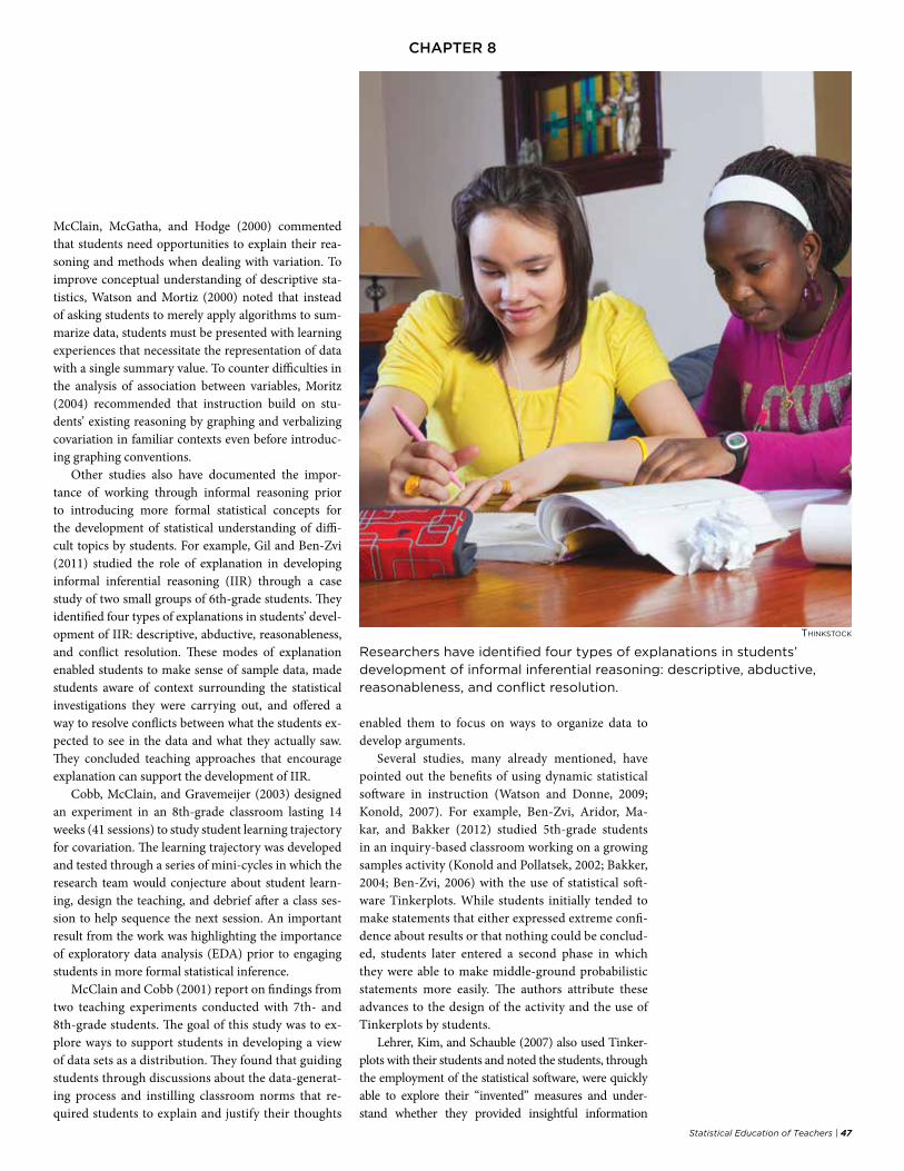
Statistical Education of Teachers | 47
chaPter 8
McClain, McGatha, and Hodge (2000) commented that students need opportunities to explain their rea-soning and methods when dealing with variation. To improve conceptual understanding of descriptive sta-tistics, Watson and Mortiz (2000) noted that instead of asking students to merely apply algorithms to sum-marize data, students must be presented with learning experiences that necessitate the representation of data with a single summary value. To counter difficulties in the analysis of association between variables, Moritz (2004) recommended that instruction build on stu-dents’ existing reasoning by graphing and verbalizing covariation in familiar contexts even before introduc-ing graphing conventions.
Other studies also have documented the impor-tance of working through informal reasoning prior to introducing more formal statistical concepts for the development of statistical understanding of diffi-cult topics by students. For example, Gil and Ben-Zvi (2011) studied the role of explanation in developing informal inferential reasoning (IIR) through a case study of two small groups of 6th-grade students. They identified four types of explanations in students’ devel-opment of IIR: descriptive, abductive, reasonableness, and conflict resolution. These modes of explanation enabled students to make sense of sample data, made students aware of context surrounding the statistical investigations they were carrying out, and offered a way to resolve conflicts between what the students ex-pected to see in the data and what they actually saw. They concluded teaching approaches that encourage explanation can support the development of IIR.
Cobb, McClain, and Gravemeijer (2003) designed an experiment in an 8th-grade classroom lasting 14 weeks (41 sessions) to study student learning trajectory for covariation. The learning trajectory was developed and tested through a series of mini-cycles in which the research team would conjecture about student learn-ing, design the teaching, and debrief after a class ses-sion to help sequence the next session. An important result from the work was highlighting the importance of exploratory data analysis (EDA) prior to engaging students in more formal statistical inference.
McClain and Cobb (2001) report on findings from two teaching experiments conducted with 7th- and 8th-grade students. The goal of this study was to ex-plore ways to support students in developing a view of data sets as a distribution. They found that guiding students through discussions about the data-generat-ing process and instilling classroom norms that re-quired students to explain and justify their thoughts
enabled them to focus on ways to organize data to develop arguments.
Several studies, many already mentioned, have pointed out the benefits of using dynamic statistical software in instruction (Watson and Donne, 2009; Konold, 2007). For example, Ben-Zvi, Aridor, Ma-kar, and Bakker (2012) studied 5th-grade students in an inquiry-based classroom working on a growing samples activity (Konold and Pollatsek, 2002; Bakker, 2004; Ben-Zvi, 2006) with the use of statistical soft-ware Tinkerplots. While students initially tended to make statements that either expressed extreme confi-dence about results or that nothing could be conclud-ed, students later entered a second phase in which they were able to make middle-ground probabilistic statements more easily. The authors attribute these advances to the design of the activity and the use of Tinkerplots by students.
Lehrer, Kim, and Schauble (2007) also used Tinker-plots with their students and noted the students, through the employment of the statistical software, were quickly able to explore their “invented” measures and under-stand whether they provided insightful information
ThiNksTock
Researchers have identified four types of explanations in students’ development of informal inferential reasoning: descriptive, abductive, reasonableness, and conflict resolution.
48 | Statistical Education of Teachers
chaPter 8
about the data. The software also gave students a tool to quickly investigate different scenarios of chance.
Ben-Zvi (2000) discusses how the use of powerful technological tools can shift activities to higher cogni-tive levels, change the objectives of an activity, provide access to graphics and visuals, and focus activities on transforming and analyzing representations for stu-dents. He discusses several statistical software packag-es and the advantages each provides.
In a book chapter, Biehler, Ben-Zvi, Bakker, and Makar (2013) discuss how technology can enhance student learning. They examine how features of dy-namic software such as Tinkerplots and Fathom can facilitate student understanding. Software can aid stu-dents in exploratory data analysis help develop stu-dents’ aggregate view of data.
As these examples illustrate, the research on student learning of statistics has implications for teaching, which has implications for the statistical education of teachers. Overall, the research has shown the importance of data exploration in informal ways, the importance of technol-ogy in furthering student understanding, and the impor-tance of designing activities that foster students’ statistical reasoning. The recommendations put forth for teacher preparation in this report align with this research base as they recommend courses for teachers focused on data ex-ploration aided by the use of technology.
Research on Teacher Statistical LearningHistorically, teacher preparation programs have not adequately developed the statistical content knowledge necessary for effective teaching of statistics in PreK–12. Rubin, Rubin, and Hammerman (2006) found that teachers’ statistical thinking is not substantially different than students’ statistical thinking. Like their students, teachers have gaps in their understanding of several basic concepts in statistics (Callingham, 1997; Greer and Ritson, 1994) as well as more complex con-cepts such as covariation and regression (Engel and Sedlmeier, 2011; Casey and Wasserman, 2015).
For example, the teachers studied by Jacobbe and Hor-ton (2010) were successful at reading data from graphical displays, but unsuccessful with questions that assessed higher levels of graphical comprehension. While most pre-service and in-service teachers can compute mea-sures of center, many lack a conceptual understanding of what the measures of center represent (Groth and Berg-ner, 2006; Jacobbe, 2012; Leavy and O’Laughlin, 2006).
Teachers also experience difficulty with the con-cept of variability. For example, Hammerman and
Rubin (2004) noted that secondary teachers involved in professional development discussed the variation in distributions using only segments and slices of the distributions and not the entire picture. Confrey and Makar (2002) discussed similar results with mid-dle-school teachers, who examined variation in dis-tributions by focusing on single points instead of the distribution as a whole.
Similarly, Makar and Confrey (2004) gave in-ser-vice secondary teachers student performance data and asked them to compare performance between different types of students. Only a few teachers were able to make comparisons by discussing the variation in the distributions; most teachers focused on a sin-gle summary such as the mean or made a very general statement about passing rates. In addition, Hannigan et al. (2013) indicated that the prospective teachers in their sample had particular difficulties with sampling variability. Bargagliotti et al. (2014) also noted several misunderstandings in-service teachers had about sam-pling variability, such as believing repeated samples were necessary to make inferential statements using sampling distributions.
In a 2013 study, Peters offered insights into factors that may lead teachers to understand variation. Peters examined the learning of five AP Statistics teachers and explored how reflection and discourse, data circum-stances that trigger dilemmas, retrospective methods, and teacher education play a role in teachers’ develop-ment of understanding statistical variation. Peters not-ed how teachers have a strong desire for an overarch-ing content framework, such as the statistical process noted in this report and in GAISE. Additionally, she highlighted how reflection, triggers, and retrospective methods allow teachers to obtain deeper understand-ing of variation.
Other studies also offered insights into increasing teacher understanding. For example, while studying 56 high-school teachers working on activities centered on comparing distributions and randomization testing, Madden (2011) found that statistically provocative, technologically provocative, and contextually provoca-tive tasks might increase teacher engagement in infor-mal inferential reasoning (IIR).
Leavy, Hannigan, and Fitzmaurice (2013) inter-viewed nine teachers at length to explore the factors influencing teachers’ attitudes toward statistics. They found mathematics teachers perceive statistics as diffi-cult to learn for reasons that include the uniqueness of statistical thinking and reasoning and the role of con-text and language in statistics.
Statistical Education of Teachers | 49
chaPter 8
Watson (2002) discussed an instrument devel-oped to profile teacher understanding and teaching needs for probability and statistics. In administering this instrument to 43 primary and secondary teachers in Australia, she found that primary teachers taught many activities related to data and chance to their stu-dents; however, the lessons did not lead to a coherent overall program. While the secondary teachers exhib-ited more coherent curriculum in their lessons, the lessons remained theoretical and teachers did not in-troduce activities, such as simulations, that would help students visualize the theory.
Teacher educators must consider these issues as they carefully plan to implement the recommenda-tions put forth in this report.
Research on Teacher Preparation in StatisticsThe emphasis on statistics at the pre-college level de-mands a targeted effort to improve the preparation of pre-service teachers and provide quality profession-al development for in-service teachers. Pfannkuch and Ben-Zvi (2011) stated that statistical courses for teachers should be developed around five major themes: (1) developing understanding of key statisti-cal concepts, (2) developing the ability to explore and learn from data, (3) developing statistical argumenta-tion, (4) using formative assessment, and (5) learning to understand students’ reasoning. The goals of such a course should be to offer good statistical content training for teachers; discuss student reasoning and how to build and scaffold students’ conceptions; and understand curricula, technology, and sequences of instructional activities that build students’ concep-tions across grade levels.
By analyzing online discourse among teachers, Groth (2008) concluded that teachers’ perceptions, interpretations, and understanding of the GAISE re-port guidelines might influence their classroom de-livery of the content. Based on these findings, Groth indicated teacher understanding and choices can in-fluence the statistics education experience of students in the classroom.
To affect teacher practice and ensure that practice is effective, a curriculum for teachers must incorpo-rate aspects of both statistical content knowledge and specialized teaching knowledge (Shulman, 1986). Building on the Mathematical Knowledge for Teach-ing (MKT) framework of Ball, Hill, and Bass (2005), Groth (2013) separated Statistical Knowledge for Teaching (SKT) into Subject Matter Knowledge and
Pedagogical Content Knowledge. Each is then subdi-vided further into three categories. For example, Sub-ject Matter Knowledge includes content knowledge specialized for teaching, while Pedagogical Content Knowledge includes knowledge about curriculum. Furthermore, Groth connected ideas of Pedagogically Powerful Ideas (Silverman and Thompson, 2008) and Key Developmental Understandings (Simon, 2006) to SKT. Within his SKT framework, Groth highlighted several examples in which statistical and mathemati-cal reasoning differ.
Currently, few research-based courses for pro-spective teachers or professional development work-shops are documented and offered specifically to pre-pare individuals to teach statistics (Bargagliotti et al., 2014; Garfield and Everson, 2009; Gould and Peck, 2004). Due to the meager offerings of specialized courses or programs, teachers are not to blame for their lack of preparation to teach statistical concepts effectively. Instead, research points to the vital need for teacher preparation programs that adequately ad-dress the statistical preparation of teachers.
The work of Heaton and Mickelson (2002, 2004) examines the collaborative efforts of a mathematics ed-ucator and statistician to help prospective elementary teachers develop statistical knowledge by incorporat-ing statistical investigation into existing elementary curricula. The collaboration offers insight into pre-ser-vice teachers’ statistical and pedagogical content knowledge based on their application of the process of statistical investigation themselves and with children.
Groth (2007) called for new kinds of statistics courses geared toward expanding statistical knowl-edge for teaching. Such knowledge should include not only statistical content knowledge (Cobb and Moore, 1997), but also discussions of best practices in teaching statistics and common student difficulties in learning statistics.
Shaughnessy (2007) described the critical need for professional development, saying, “Our teach-ing force is undernourished in statistical experi-ence, as statistics has not often been a part of many teachers’ own school mathematics programs” (p. 959). Franklin and Kader (2010) noted it is import-ant for teachers to not only be familiar with the sta-tistical content they teach, but also have a sound understanding of how their grade-level content fits with the statistics concepts taught in the grade lev-els below and above theirs.
Furthermore, the 2013 ASA and NCTM joint position statement advises, “The need is critical for
50 | Statistical Education of Teachers
chaPter 8
high-quality pre-service and in-service preparation and profes-sional development that supports PreK–12 teachers of mathe-matics, new and experienced, in developing their own statistical proficiency” (ASA-NCTM, 2013, p. 1).
ConclusionsAs the field of statistics education research develops, it is helpful to document ways to develop student and teacher statistical thinking. As noted above, several research studies and conference proceed-ings papers and expository pieces have focused on the types of issues that emerge while teaching and learning statistics in PreK–12 and in teacher preparation. In general, teacher preparation programs need to provide courses that align with research and give pre-ser-vice teachers opportunities to engage in the statistical investigative process as suggested throughout this report. Professional develop-ment should consider the research base outlined in this chapter to guide the development of statistical topics. Furthermore, as cur-ricula, lesson plans, and strategies are developed (for example, see lesson plans at www.amstat.org/education/stew and strategies such as learning trajectories outlined, for example, by Bargagliotti et al. 2014; Makar and Confrey, 2007; Makar, 2008; Cobb, McClain, and Gravemeijer, 2003), subsequent robust statistical studies are needed to test the effects on student and teacher statistical understanding. Studies, both large and small scale, linking teacher understanding to student understanding are also necessary.
ReferencesBall, D. (1991). Research on teaching mathematics: Making subject
matter knowledge part of the equation. In J. Brophy (Ed.) Advances in research on teaching: Teachers’ subject matter knowledge and classroom instruction (2:1–48). Greenwich, CT: JAI Press.
Ball, D. L., and Bass, H. (2000). Interweaving content and pedagogy in teaching and learning to teach: Knowing and using mathematics. In J. Boaler (Ed.) Multiple perspectives on the teaching and learning of mathematics (pp. 83–104). Westport: Ablex.
Ball, D. L., Hill, H. H., and Bass, H. (2005). Knowing mathe-matics for teaching: Who knows mathematics well enough to teach third grade, and how can we decide? American Mathematical Educator, Fall, 14–46.
Bargagliotti, A. E., Anderson, C., Casey, S., Everson, M., Franklin, C., Gould, R., Groth, R., Haddock, J., and Watkins, A. (2014). Project-SET materials for the teaching and learning of sampling variability and regression. International Conference of Teaching Statistics (ICOTS) conference proceedings, invited paper.
Bakker, A. (2004). Reasoning about shape as a pattern in vari-ability. Statistics Education Research Journal, 3(2):64–83.
Batanero, C., Estepa, A., Godino, J., and Green, D. (1996). Intuitive strategies and preconceptions about association
in contingency tables. Journal for Research in Mathematics Education, 27(2):151–169.
Biehler, B., Ben-Zvi, D., Bakker, A., and Makar, K. (2013). In Clements et al. (Eds.), Third international handbook of mathematics education, springer international handbook of education 27, DOI 10.1007/978-1-4614-4684-2_21. New York, NY: Springer Science + Business Media.
Bell, A., Brekke, G., and Swan, M. (1987). Misconceptions, conflict, and discussion in the teaching of graphical inter-pretation. In J. D. Novak (Ed.), Proceedings of the second international seminar: Misconceptions and educational strategies in science and mathematics (1:46–58). Ithaca, NY: Cornell University.
Ben-Zvi, D., Aridor, K., Makar, K., and Bakker, A. (2012). Stu-dents/ emergent articulations of uncertainty while making informal statistical inferences. International Journal of Mathematics Education.
Ben-Zvi, D. (2006). Scaffolding students’ informal inference and argumentation. In A. Rossman and B. Chance (Eds.) Proceedings of the seventh International Conference on Teaching of Statistics, Salvador, Bahia, Brazil, July 2–7, 2006. Voorburg, The Netherlands: International Sta-tistical Institute. www.stat.auckland.ac.nz/iase/publica-tions/17/2D1_BENZ.pdf.
Ben-Zvi, D. (2000). Toward understanding the role of techno-logical tools in statistical learning. Mathematical Thinking and Learning, 2:1–2, 127–155.
Ben-Zvi, D., and Garfield, J. (Eds.) The challenge of developing statistical literacy, reasoning, and thinking. Dordrecht, The Netherlands: Kluwer Academic.
Ben-Zvi, D., and Friedlander, A. (1997b). Statistical thinking in a technological environment. In J. Garfield and G. Burrill (Eds.) Research on the role of technology in teaching and learning statistics (pp. 45–55). Voorburg, The Netherlands: International Statistical Institute.
Callingham, R. (1997). Teachers’ multimodal functioning in relation to the concept of average. Mathematics Education Research Journal, 9:205–224.
Cai, J. (2000). Understanding and representing the arithmetic averaging algorithm: An analysis and comparison of U.S. and Chinese students’ responses. International Journal of Mathematical Education in Science and Technology, 31:839–855.
Capraro, M. M., Kulm, G., and Capraro, R. M. (2005). Middle grades: Misconceptions in statistical thinking. School Sci-ence and Mathematics, 105:165–174. DOI: 10.1111/j.1949-8594.2005.tb18156.x
Casey, S., and Wasserman, N. (2015). Teachers’ knowledge about informal line of best fit. Statistics Education Research Journal. In Press.
Chervany, N. L., Collier, R. D., Fienberg, S., and Johnson, P.
Statistical Education of Teachers | 51
chaPter 8
(1977). A framework for the development of mea-surement instruments for evaluating the introduc-tory statistics course. The American Statistician, 31(1):17–23.
Cobb, G. W., and Moore, D. S. (1997). Mathematics, statistics, and teaching. American Mathematical Monthly, 104:801–823.
Cobb, P., McClain, K., and Gravemeijer, K. (2003). Learning about statistical covariation. Cognition and Instruction, 21(1):1–78.
Confrey, J., and Makar, K. (2002). Developing second-ary teachers’ statistical inquiry through immer-sion in high-stakes accountability data. Paper presented at the Twenty-fourth Annual Meeting of the North American Chapter of the Interna-tional Group for the Psychology of Mathematics Education (PME-NA), Athens, GA.
delMas, R. C. (2004). A comparison of mathematical and statistical reasoning. In J. Garfield and D. Ben-Zvi (Eds.) The challenge of developing statis-tical literacy, reasoning, and thinking (pp. 79–95). Dordrecht, The Netherlands: Kluwer.
delMas, R., Garfield, J., Ooms, A., and Chance, B. (2007). Assessing students’ conceptual under-standing after a first course in statistics. Statistics Education Research Journal, 6(2):28–58.
delMas, R., Garfield, J., and Chance, B. (1999). A model of classroom research in action: Devel-oping simulation activities to improve students’ statistical reasoning. Journal of Statistics Educa-tion, 7(3).
Dierdorp, A., Bakker, A., Eijkelhof, H., and Maanen, J. (2011). Authentic practices as contexts for learn-ing to draw inferences beyond correlated data. Mathematical Thinking and Learning, 13:1–2, 132–151.
Engel, J., and Sedlmeier, P. (2011). Correlation and regression in the training of teachers. In C. Batanero, G. Burrill, and C. Reading (Eds.) Teaching statistics in school mathematics—challenges for teaching and teacher education: A joint ICMI/IASE study (pp. 247–258). New York, NY: Springer.
Estepa, A., and Batanero, C. (1996). Judgments of correlation in scatterplots: An empirical study of students’ intuitive strategies and preconceptions. Hiroshima Journal of Mathematics Education, 4:25–41.
Franke, M., Webb, N., Chan, A., Ing, M., Freund, D., and Battey, D. (2009). Teacher questioning to elicit students’ mathematical thinking in
elementary school. Journal of Teacher Education, 60(4):380–392.
Franklin, C., and Kader, G. (2010). Models of teacher preparation designed around the GAISE framework. In C. Reading (Ed.) Data and context in statistics education: Towards an ev-idence-based society. Proceedings of the eighth International Conference on Teaching Statistics (ICOTS8, July 2010), Ljubljana, Slovenia. Voor-burg, The Netherlands: International Statistical Institute. www.stat.auckland.ac.nz/~iase/ publications.php
Friel, Curcio, and Bright, (2001). Making sense of graphs: Critical factors influencing comprehen-sion and instructional implications. Journal for Research in Mathematics Education, 124–158.
Garfield, J. B., and Ben-Zvi, D. (2008). Developing students’ statistical reasoning: Connecting research and teaching practice. New York, NY: Springer Science and Business Media.
Garfield, J. (1995). How students learn statistics. Inter-national Statistical Review, 63:25–34.
Garfield, J., and Everson, M. (2009). Preparing teachers of statistics: A graduate course for future teachers. Journal of Statistics Education, 17(2):223–237.
Greer, B., and Ritson, R. (1994). Readiness of teachers in Northern Ireland to teach data handling. Pro-ceedings of the fourth International Conference on Teaching Statistics, Vol. 1. Marrakech, Morocco: National Organizing Committee of the Fourth International Conference on Teaching Statistics, pp. 49–56.
Gil, E., and Ben-Zvi, D. (2011). Explanations and context in the emergence of students’ informal inferential reasoning. Mathematical Thinking and Learning, 13:1, 87–108.
Groth, R. (2003). High school students’ levels of thinking in regard to statistical study design. Mathematics Education Research Journal, 15(3):252–269.
Groth, R. E. (2008). Assessing teachers’ discourse about the PreK–12 Guidelines for Assessment and Instruction in Statistics Education (GAISE). Statis-tics Education Research Journal, 7(1):16–39.
Groth, R. E. (2007). Toward a conceptualization of statistical knowledge for teaching. Journal for Research in Mathematics Education, 38:427–437.
Groth, R. E. (2013). Characterizing key developmen-tal understandings and pedagogically powerful ideas within a statistical knowledge for teaching
52 | Statistical Education of Teachers
chaPter 8
framework. Mathematical Thinking and Learning, 15:121–145.
Groth, R. E., and Bergner, J. A. (2006). Preservice elementary teachers’ conceptual and procedural knowledge of mean, median, and mode. Mathe-matical Thinking and Learning, 8:37–63.
Gould, R., and Peck, R. (2004). Preparing secondary mathematics educators to teach statistics. Curricu-lar Development in Statistics Education: Internation-al Association for Statistical Education, 278–283.
Hammerman, J. K., and Rubin, A. (2004). Strategies for managing statistical complexity with new soft-ware tools. Statistics Education Research Journal, 3(2):17–41.
Hannigan, A., Gill, O., and Leavy, A. (2013). An in-vestigation of prospective secondary mathematics teachers’ conceptual knowledge of and attitudes toward statistics. Journal of Mathematics Teacher Education, 16:427–449.
Heaton, R., and Mickelson, M. (2002).The learning and teaching of statistical investigation in teach-ing and teacher education. Journal of Mathematics Teacher Education, 5:35–39.
Mickelson, W. T., and Heaton, R. M. (2004). Prima-ry teachers’ statistical reasoning about data. In The challenge of developing statistical literacy, reasoning, and thinking (pp. 327–352). Springer Netherlands.
NCTM. (2013). Preparing PreK–12 teachers of statis-tics: A joint position statement of the American Statistical Association (ASA) and NCTM. Reston, VA: NCTM.
Hill, H. C., and Ball, D. L. (2004). Learning math-ematics for teaching: Results from California’s Mathematics Professional Development Institutes. Journal of Research in Mathematics Education, 35:330–351.
Hoerl, R.W., and Snee, R. D. (2001). Statistical thinking: Improving business performance. Pacific Grove, CA: Duxbury.
Jacobbe, T., and Horton, B. (2010). Elementary school teachers’ comprehension of data displays. Statis-tics Education Research Journal, 9:27–45.
Jacobbe, T. (2012). Elementary school teachers’ un-derstanding of the mean and median. Internation-al Journal of Science and Mathematics Education, 10(5):1143–1161.
Jones, G. A., Langrall, C. W., Mooney, E. S., and Thornton, C. A. (2004). Models of development in statistical reasoning. In D. Ben-Zvi and J. Gar-field (Eds.) The challenge of developing statistical
literacy, reasoning, and thinking (pp. 97–117). Dordrecht: Kluwer Academic.
Jones, G. A., Langrall, C. W., and Mooney, E. S. (2007). Research in probability: Responding to classroom realities. In F. K. Lester Jr. (Ed.) Second handbook of research on mathematics teaching and learning (pp. 909-955). Charlotte, NC: Information Age Publishing.
Konold, C. (2007). Designing a data tool for learn-ers. In M. Lovett and P. Shah (Eds.) Thinking with data (pp.267–291). New York, NY: Law-rence Erlbaum Associates.
Konold, C., and Pollatsek, A. (2002). Data analysis as the search for signals in noisy processes. Journal for Research in Mathematics Education, 33:259–289.
Konold, C., Pollatsek, A., Well, A., and Gagnon, A. (1997). Students analyzing data: Research of critical barriers. Research on the role of technolo-gy in teaching and learning statistics, 151.
Leavy, A., O’Loughlin, N. (2006). Preservice teach-ers’ understanding of the mean: Moving beyond the arithmetic average. Journal of Mathematics Teacher Education, 9:53–90.
Leavy, A., Fitzmaurice, O., and Hannigan, A. (2013). If you’re doubting yourself then, what’s the fun in that? An exploration of why prospec-tive secondary mathematics teachers perceive statistics as difficult. J. Stat. Educ, 21.
Lehrer, R., Kim, M., Schauble, L. (2007). Support-ing the development of conceptions of statistics by engaging students in measuring and model-ing variability. International Journal of Comput-ers for Mathematics Learning, 12:195–216.
Madden, S. (2011). Statistically, technologically, and contextually provocative tasks: Support-ing teachers’ informal inferential reasoning. Mathematical Thinking and Learning, 13:1–2, 109–131.
Makar, K. (2008). A model of learning to teach statistical inquiry. In C. Batanero, G. Burrill, C. Reading, and A. Rossman (Eds.) Joint ICMI/IASE study: Teaching statistics in school math-ematics. Challenges for teaching and teacher education. Proceedings of the ICMI Study and 2008 IASE Round Table Conference.
Makar, K., and Confrey, J. (2007). Moving the context of modeling to the forefront: Preservice teachers’ investigations of equity in testing. In W. Blum, P. Galbraith, H-W. Henn, and M. Niss (Eds.) Modelling and applications in mathematics
Statistical Education of Teachers | 53
chaPter 8
education: The 14th ICMI study (pp. 485–490). New York, NY: Springer.
Makar, K., and Confrey, J. (2004). Secondary teachers’ statistical reasoning in comparing two groups. In D. Ben-Zvi and J. Garfield (Eds.) The challenge of developing statistical literacy, reasoning, and think-ing (pp. 353–374). Boston, MA: Kluwer Academic Publishers.
McClain, K., and Cobb, P. (2001). Supporting stu-dents’ ability to reason about data. Educational Studies in Mathematics 45:103–129.
McClain, K., McGatha, M., and Hodge, L. L. (2000). Improving data analysis through discourse. Math-ematics Teaching in the Middle School, 5:548–553.
Mokros, J., and Russell, S. J. (1995). Children’s concepts of average and representativeness. Journal for Re-search in Mathematics Education, 26(1):20–39.
Moritz, J. (2004). Reasoning about covariation. In The challenge of developing statistical literacy, reasoning, and thinking (pp. 227–255). Springer Netherlands.
Peters, S. (2014). Developing understanding of statistical variation: Secondary statistics teach-ers’ perceptions and recollections of learning factors. Journal of Mathematics Teacher Education, 17(6):539–582.
Pfannkuch, M. (2005). Thinking tools and variation. SERJ Editorial Board, 83.
Pfannkuch, M., and Ben-Zvi, D. (2011). Developing teachers’ statistical thinking. In Teaching statistics in school mathematics—challenges for teaching and teacher education (pp. 323–333). Springer Netherlands.
Rubin, A., and Hammerman, J. (2006). Understanding data through new software representations. In G. Burrill (Ed.) Thinking and reasoning with data and chance: 2006 NCTM yearbook (pp. 241–256). Reston, VA: National Council of Teachers of Mathematics.
Saldanha, L., and Thomson, P. (2002). Conceptions of sample and their relationship to statistical inference. Educational Studies in Mathematics, 51:257–270.
Silverman, J., and Thompson, P. W. (2008). Toward a framework for the development of mathematical knowledge for teaching. Journal of Mathematics Teacher Education, 11(6):499–511.
Simon, M. A. (2006). Key developmental understand-ings in mathematics: A direction for investigating and establishing learning goals. Mathematical Thinking and Learning, 8(4):359–371.
Shaughnessy, J. M. (2007). Research on statistics learning and reasoning. In F. K. Lester (Ed.) Second handbook of research on mathematics teaching and learning (pp. 957–1009). Charlotte, NC: Informa-tion Age Publishing.
Shaughnessy, J. M., Ciancetta, M., and Canada, D. (2004). Types of students reasoning on sampling tasks. In Proceedings of the 28th Conference of the International Group for the Psychology of Mathe-matics Education, 4:177–184.
Shaughnessy, J. M. (2007). Research on statistics learning. Second handbook of research on mathe-matics teaching and learning, 957–1009.
Shulman, D. (1986). Those who understand: Knowledge growth in teaching. Educational Researcher, 15:4–14.
Stroup. (1984). The statistician and the pedagogical monster: Characteristics of effective instructors of large statistics classes. In Proceedings of the Section on Statistical Education. Washington, DC: American Statistical Association.
Sorto, M. A., White, A., and Lesser, L. (2011). Un-derstanding student attempts to find a line of fit. Teaching Statistics, 11(2):49–52.
Wild, C., and Pfannkuch, M. (1999). Statistical think-ing in empirical enquiry. International Statistical Review, 223–248.
Watson, J. (2005). The probabilistic reasoning of mid-dle school students. In Exploring probability in school (pp. 145–169). New York, NY: Springer.
Watson, J. M., Kelly, B. A., Callingham, R. A., and Shaughnessy, J. M. (2003). The measurement of school students’ understanding of statistical variation. International Journal of Mathematical Education in Science and Technology, 34(1):1–29.
Watson, J. (2001). Profiling teachers’ competence and confidence to teach particular mathematics topics: The case of chance and data. Journal of Mathematics Teacher Education, 4:305–337.
Watson, J., and Donne, J. (2009). TinkerPlots as a research tool to explore student understanding. Technology Innovations in Statistics Education, 3(1).
Watson, J. M., and Moritz, J. B. (2000). Development of understanding of sampling for statistical litera-cy. Journal of Mathematical Behavior, 19:109–136.
Watson, J. M., and Moritz, J. B. (2000). The lon-gitudinal development of understanding of average. Mathematical Thinking and Learning, 2(1–2):11–50.
Utts, J. (2003). What educated citizens should know about statistics and probability, The American Statistician, 57(2):74–79.


Statistical Education of Teachers | 55
chaPter 9
CHAPTER 9Statistics in the School Curriculum: A Brief History
Increasing importance has been placed on data analysis in the United States during the recent decade. Data-driven decision making and statistical studies have drawn interest from the general population and policymakers, as well as businesses and schools. Influenced by this new emphasis, data analysis has be-come a key component of the PreK–12 mathematics curricula across the country. For example, the number of students tak-ing AP Statistics increased from 7,500 in 1997 to 169,508 in 2013 (College Board, 2013) and statistics content is appearing in most state curriculum guidelines. As statistics is receiving ever-increasing prominence in the PreK–12 curriculum, it is of paramount importance that it also gains prominence in teacher education programs.
As sound teacher education should include an appreciation of history, this chapter presents a review of the history of statis-tics education in PreK–12, with material adapted from Scheaf-fer and Jacobbe (2014).
The Early Years: 1920s–1950sThe notion of introducing statistics and statistical thinking into the school mathematics curriculum has a long and varied his-tory of nearly a century. In the 1920s, as the United States was becoming ever more rapidly an industrialized urban nation (even introducing statistical quality control in manufacturing), proposed changes in the school mathematics curriculum were often cast in the framework of making mathematics more util-itarian and thus broadening the scope of its appeal. Among the recommendations found in The Reorganization of Mathemat-ics in Secondary Education, a 1923 report by the relatively new Mathematical Association of America (MAA) (National Com-mittee on Mathematical Requirements 1923), were that statis-tics be included in the junior-high school curriculum (grades 7, 8, and 9), more from a computational than an algebraic point of view, and that a course in elementary statistics be included in the high-school curriculum.
Those advocating for change in mathematics education were mathematicians and mathematics educators, and their proposals for statistics were heavily mathematical and prob-abilistic. Among this group, however, were some statisticians. One of the first statisticians to enter the discussions on school curriculum changes was Helen Walker, who taught statistics at Columbia University Teacher’s College from 1925 to 1957 and who served as president of the American Statistical Associa-tion (ASA) in 1944 and president of the American Educational Research Association (AERA) in 1949-1950. Viewing statistics as a service to the welfare of society, she argued for its inclu-sion in the high-school curriculum as an essential public need.
Any one vitally concerned with the teaching of high-school pupils and observant of the rapidly growing public need for some knowledge of quantitative meth-od in social problems must be asking what portions of statistical method can be brought within the compre-hension of high-school boys and girls, and in what way these can best be presented to them. (Walker, 1931, p. 125)
The years of WWII and its aftermath were a boon for statis-tics, in both research and education. In “Personnel and Train-ing Problems Created by the Growth of Applied Statistics in the United States,” the National Research Council’s (NRC) Commit-tee on Applied Mathematical Statistics stated that “definite ad-vantages would result if certain aspects of elementary statistics were effectively taught in the secondary schools” (NRC, 1947, p. 17). The committee further explained that progress in teach-ing statistics (both high school and college) was hindered by a shortage of adequately prepared teachers. This problem remains to this day and is the primary reason for this report.
Although these early efforts at building statistics into the school curriculum had limited successes along the way, the cumulative effect began to turn the tide in noticeable ways in the 1950s. In 1955, the College Entrance Examination Board (CEEB) appointed a commission on mathematics with the goal of “improving the program of college preparatory mathematics in the secondary schools” (p. 1). Members included Freder-ick Mosteller, a Harvard statistics professor; Robert Rourke, a high-school mathematics teacher; and George Thomas, a col-lege mathematics professor—all vitally interested in improving and expanding the teaching of statistics. The commission re-ported the following:
Statistical thinking is part of daily activities, and an introduction to statistical thinking in high school will enhance deductive thinking. Numerical data, frequency distribution tables, averages, medians, means, range, quartiles were to be introduced in 9th grade. A more formal examination of probability concepts should be introduced later (grade 12). (CEEB, 1959, p, 5)
Mosteller, Rourke, and Thomas wrote a book for a high-school statistics course, Introductory Probability with Statistical Applications: An Experimental Course (1957), that quickly be-came a best seller for the CEEB. Notice the emphasis on prob-ability, however, as compared to the emphasis on data analysis, which was to come into its own in the next two decades.

56 | Statistical Education of Teachers
chaPter 9
The Data Revolution: 1960sPrompted by a space race and computing power, the 1960s saw a data revolution that changed the inter-est in and practice of statistics. In that environment, the ASA president in 1968, Mosteller reached out to the National Council of Teachers of Mathematics (NCTM) to establish the ASA and NCTM Joint Com-mittee on Curriculum in Probability and Statistics. This committee developed materials for the schools that changed the tone of high-school statistics from an emphasis on probability to an emphasis on data.
Statistics: A Guide to the Unknown, one of the early publications of the joint committee, is a collection of essays—intended for the lay public, teachers, and stu-dents—that describes important real-life applications of statistics and probability. Statistics by Example, a series of four booklets, provided real examples with real data for students to analyze from data exploration and description through model building.
During this time, John Tukey—a professor of sta-tistics at Princeton and a friend of Mosteller’s—was
steering much of the emphasis in statistics away from mathematical theory and toward data analysis. He stated the following:
All in all, I have come to feel that my central interest is in data analysis, which I take to include, among other things: procedures for analyzing data, techniques for interpreting the results of such pro-cedures, ways of planning the gathering of data to make its analysis easier, more precise or more accurate, and all the machinery and results of (mathematical) statistics which apply to analyzing data. (Tukey, 1962, p. 6)
Tukey invented many of the data analytic proce-dures in common use today. The ASA/NCTM Joint Committee, under Mosteller’s influence, embraced the Tukey approach to data analysis and worked on adapting this approach to materials suitable for use at the school level. The combination of Mosteller, Tukey, and the advent of inexpensive computing drove the successes of statistics in the schools that came about over the next 40 years.
Progress, Not Perfection: 1970s-1990sHowever, the activities of the next 40 years were not unmitigated successes, and we still have not reached the intended level of “statistical reasoning for all.” In the 1970s, for example, the Conference Board of the Mathematical Sciences formed the National Advisory Committee on Mathematics Education (NACOME) to look into current trends. Statistics education was summarized in one key statement: “While probability instruction seems to have made some progress, sta-tistics instruction has yet to get off the ground.” (NA-COME, 1975, p. 45) The report stated that statistics should be given more attention because of its impor-tance in the life of every citizen.
Even though numerical information is encountered everywhere, in newspapers and in magazines, on radio and on television, few people have the training to accept such information critically and to use it effective-ly. (NACOME, 1975, p. 45)
Their recommendations on teaching statistics in-cluded “use statistical topics to illustrate and motivate
asa phoTo
Frederick Mosteller reached out to the National Council of Teachers of Mathematics (NCTM) to establish the ASA and NCTM Joint Committee on Curriculum in Probability and Statistics.
Statistical Education of Teachers | 57
chaPter 9
mathematics, emphasize statistics as an interdisci-plinary subject, and develop several separate cours-es dealing with statistics to meet varied local condi-tions.” (NACOME, 1975, p. 47). This advice is still worth heeding today.
NCTM’s An Agenda for Action: Recommendations for School Mathematics of the 1980s included numer-ous references to statistical topics that should play an increasing role in the mathematics curriculum (of-ten without using the term “statistics”). For example, the section on problem solving recommended more emphasis on methods of gathering, organizing, and interpreting information; drawing and testing infer-ences from data; and communicating results. The sec-tion on basic skills stated, “There should be increased emphasis on such activities as locating and processing quantitative information, collecting data, organizing and presenting data, interpreting data, drawing infer-ences and predicting from data” (NCTM, 1980, p. 4).
Building on these expanding interests in statistics and its earlier successes, the Joint Committee ob-tained a grant from the National Science Foundation (NSF) to begin the ASA-NCTM Quantitative Liter-acy Project (QLP). The QLP originally consisted of four booklets—Exploring Data, Exploring Probability, The Art and Technique of Simulation, and Exploring Surveys and Information from Samples—and a plan for carrying out many workshops across the country. (See Scheaffer, 1989 and 1991, for details.) The QLP did not foment a revolution, but the materials were well received and the workshops were successful in influencing a number of teachers and mathematics educators, especially some of those who would de-velop NSF-funded teaching materials for elementary and middle-school mathematics in the ensuing years (e.g., Connected Mathematics Project; Investigations in Number, Data, and Space).
Fortunately, the NCTM Board of Directors took note of the QLP as it was developing its 1989 Curriculum and Evaluation Standards for School Mathematics. This document called for statistics to be an integral part of the mathematics curriculum by giving it sta-tus as one of the five content strands to be taught throughout the school years.
Throughout the 1980s and 1990s, many other re-ports and activities came to the support of statistics education. In the early 1980s, the National Commission on Excellence in Education was appointed to study mathematics education in the country. Their report, A Nation at Risk, was highly supportive of statistics and probability, both directly and indirectly.
The teaching of mathematics in high school should equip graduates to:
• Understand geometric and algebraic concepts;
• Understand elementary probability and statistics;
• Apply mathematics in everyday situations
• Estimate, approximate, measure, and test the accuracy of their calculations (Nation-al Commission, 1983, p. 25)
By the 1990s, the National Research Council’s Mathematical Sciences Education Board (MSEB) was strongly aligned with the movement toward more sta-tistics in the mathematics curriculum of the schools.
If students are to be better prepared math-ematically for vocations as well as for every-day life, the elementary-school mathematics must include substantial subject matter other than arithmetic:
… Data analysis, including collection, organization, representation, and interpre-tation of data; construction of statistical tables and diagrams; and the use of data for analytic and predictive purposes
… Probability, introduced with simple experiments and data-gathering (MSEB, 1990, p. 42)
Secondary-school mathematics should introduce the entire spectrum of mathemat-ical sciences: ... data analysis, probability and sampling distributions, and inferential reasoning. (MSEB, 1990, p. 46)
Indeed, the1990s were a period of rapid develop-ment of state curriculum standards on data analysis, NSF support of teacher enhancement and materials development projects on statistics, and AP Statistics. As to the latter, it was the AP Calculus committee that led the development of AP Statistics as a second Ad-vanced Placement course in the mathematical scienc-es. (See Roberts, 1999, for details about the develop-ment of AP Statistics.)

58 | Statistical Education of Teachers
chaPter 9
One of the key questions delaying the approval of this course was the availability of teachers who could teach the subject in high school. Fortunately for the success of the AP course, teachers who had become leaders in the QLP volunteered to be the first AP Statistics teachers and to lead workshops to educate others. But the ever-in-creasing popularity of the course (and the retirement of those founding teachers) requires many more teachers with qualifications to teach the course effectively.
GAISE, Signature Event of the 2000s The emphasis on statistics education for all through the quantitative literacy programs of the 1980s set the stage for introducing AP Statistics in the 1990s. The success of the latter, in turn, reflected focus back on statistics education in the grades so as to prepare students for better access to and success in the AP program. This revisiting of PreK–12 sta-tistics education, sharpened somewhat by the MET I report of 2001, led to the Guidelines for Assessment and Instruction in Statistics Education: A PreK–12 Curriculum Framework (GAISE) (www.amstat.org/education/gaise) (Franklin et al., 2007). This report has been well received by statistics and mathematics educators and has served as the basis for revised curricula in statistics within many state guidelines and professional development programs.
The main goal of GAISE was to provide fairly de-tailed guidelines about how to achieve a statistically literate graduating high-school student at the end of the student’s PreK–12 education. The report aimed to accomplish two goals: (1) articulate differences between mathematics and statistics and (2) outline a two-dimensional framework for statistical learning.
One important feature of the framework is that, un-like the NCTM standards or any state standards outlined by grade, a student’s progression is based solely on student experience. In addition, the framework is not defined as a list of topics a student must complete. Instead, the report decomposes statistical thinking into four main process components (formulate questions, collect data, analyze data, and interpret results), within which a student’s level of knowledge (level A, B, or C) progresses. One of the pri-mary concerns that motivated the creation of the GAISE document was that “statistics … is a relatively new subject for many teachers who have not had an opportunity to develop sound understanding of the principles and con-cepts underlying the practices of data analysis that they are now called upon to teach” (Franklin et al., 2007, p. 5).
In 2010, the Common Core State Standards for Mathematics (CCSSM) were adopted by numerous states. The GAISE framework served as a foundation for the statistics standards in the CCSSM.
Why Mathematics? Why Schools?After nearly 100 years of attempts at getting a coher-ent, informative, useful statistics curriculum in the schools, one might ask, “Why in mathematics?” and “Why in the schools?” Taking the first question, many have suggested statistics should be part of the social sciences or sciences, where it is most used. Over the years, such attempts have been made in that direction, with the general result being that a few specialized techniques may gain footage in the curriculum (such as the chi-square test in biology or fitting regression models in physics) while a coherent curriculum in statistical thinking will not. In recent years, many mathematicians and mathematics educators have ac-cepted statistics as an important part of the mathe-matical sciences because of its emphasis on inductive reasoning and applying mathematics to important re-al-world problems. The following are two examples of this thinking, both in terms of reasoning and practice, coming from highly respected mathematicians David Mumford (a Field’s medalist) and George Polya (a re-nowned mathematician and educator).
For over two millennia, Aristotle’s logic has ruled over the thinking of western intellec-tuals. All precise theories, all scientific mod-els, even models of the process of thinking itself, have, in principle, conformed to the straight-jacket of logic. But from its shady beginnings devising gambling strategies and counting corpses in medieval London, probability theory and statistical inference now emerge as better foundations for scien-tific models, especially those of the process of thinking and as essential ingredients of theoretical mathematics, even the founda-tions of mathematics itself. We propose that this sea change in our perspective will affect virtually all of mathematics in the next century. (Mumford, 1999, p. 1)
We must distinguish between two types of reasoning: demonstrative and plausible.
Demonstrative reasoning is inherent in mathematics and in pure logic; in other branches of knowledge, it enters only insofar as the ideas in question seem to be raised to the logico-mathematical sphere. Demonstrative reasoning brings order and coherence to our conceptual

Statistical Education of Teachers | 59
chaPter 9
systems and is therefore indispensable in the development of knowledge, but it cannot supply us with any new knowledge of the world around us. Such knowledge can be obtained, in science as in everyday life, only through plausible reasoning. The inferences from analogy and inductive proofs of natural scientists, the statisti-cal arguments of economists, the docu-mentary evidence of historians, and the circumstantial evidence of lawyers can reasonably lay claim to our confidence, and to a very high degree, under favorable circumstances. But they are not demon-strative; all such arguments are merely plausible. (Polya, 2006, p. 36; reprinted from 1959)
As to the second question, the following quote from Theodore Porter, a historian of science, neatly sums up the arguments:
Statistical methods are about logic as well as numbers. For this reason, as well as on account of their pervasiveness in modern life, statistics cannot be the business of statisticians alone, but should enter into the schooling of every educated person. To achieve this would be a worthy goal for statistics in the coming decades. (Porter, 2001, p. 64)
In this information age, statistical reasoning should be part of everyone’s education, whether or not they are college bound. For the essence of statisti-cal reasoning to become part of an individual’s habits of mind, such education must begin early in a per-son’s schooling and be maintained over years of ed-ucational and practical experiences. Teachers remain a crucial ingredient to guide the process of learning statistical thinking.
ReferencesCollege Entrance Examination Board (CEEB). (1959).
Program for college preparatory mathematics. Iowa City, IA: Commission on Mathematics, Author.
Mathematical Sciences Education Board. (1990). Reshaping school mathematics. Washington, DC: National Research Council.
Mumford, D. (1999). The dawning of the age of stochasticity. Available at www.dam.brown.edu/
people/mumford/Papers/Dawning.pdf.National Advisory Committee on Mathematical
Education (NACOME). (1975). Overview and analysis of school mathematics grades K–12. Reston, VA: NCTM.
National Commission on Excellence in Education. (1983). A nation at risk: The imperative for edu-cational reform. Washington, DC: United States Department of Education.
National Committee on Mathematical Require-ments. (1923). The reorganization of mathematics in secondary education. Washington, DC: Mathe-matical Association of America (MAA).
National Council of Teachers of Mathematics (NCTM). (1980). An agenda for action: Recom-mendations for school mathematics of the 1980s. Reston, VA: Author.
National Council of Teachers of Mathematics (NCTM). (1989). Curriculum and evaluation standards for school mathematics. Reston, VA: Author. Available at www.nctm.org/standards/content.aspx?id=26629.
National Research Council (NRC). (1947). Report by the Committee on Applied Mathematical Statis-tics, Reprint and Circular Series, 128.
Polya, G. (2006). Mathematics as a subject for learn-ing plausible reasoning. Mathematics Teacher 100:5, 36.
Porter, T. (2001). Statistical futures. Amstat News, 291:61–64.
Roberts, R., Scheaffer, R., and Watkins, A. (1999). Advanced Placement Statistics—Past, present, and future. The American Statistician, 53(4).
Scheaffer, R. L. (1986). The Quantitative Literacy Project. Teaching Statistics, 8(2).
Scheaffer, R. L. (1991). The ASA-NCTM Quantitative Literacy Project: An overview. Proceedings of the 3rd International Conference on Teaching Statistics, 45–49.
Scheaffer, R. L., and Jacobbe, T. (2014). Statistics ed-ucation in the K–12 schools of the United States: A brief history. Journal of Statistics Education, 22(2).
Tukey, J. (1962). The future of data analysis. Annals of Mathematical Statistics, 33:1–67.
Walker, H. (1931). Mathematics and statistics. In Sixth Yearbook, Mathematics in Modern Life (pp. 111–135), Reston, VA: NCTM.
Walker, H. (1945). The Role of the American Statistical Association. Journal of the American Statistical Association, 40:1–10.

Statistical Education of Teachers | 61
aPPeNDix 1
APPENDIX 1This appendix includes a series of short examples and accompanying discussion that addresses particular difficulties that may occur while teaching statistics to teachers. The examples and difficulties presented are not meant to provide an exhaustive list of potential is-sues teacher educators may encounter when teaching pre- or in-service teachers. Instead, they are meant to highlight common subtleties and difficulties that arise. This appendix is organized into four sections:
1. Question/Design Alignment
2. Connections Between Data Type, Numerical Summaries, and Graphical Displays
3. Proportional Reasoning in Statistics
4. The Role of Randomness in Statistics
Question/Design Alignment Two interrelated components of the statistical process include formulating statistical questions and collecting data. Typically, a general problem or research topic is presented. To investigate the topic, one must understand
what specific statistical questions should be investigated and what data-collection method should be employed to answer those questions.
A statistical question is one that anticipates variability in the data that would be collect-ed to answer it and motivates the collection, analysis, and interpretation of data.
The formulation of questions is of particular im-portance for teachers, and thus for teacher preparation, because teachers must lead discussions and pose good questions in their own classrooms to motivate rich statistical investigations. It is important that teachers understand formulating statistical questions is not an easy exercise and is one that requires great precision in language. Formulating questions and data collection are topics outside the realm of traditional mathemati-cal reasoning and thus often are challenging for teach-ers, even those proficient in mathematics. Most im-portantly, teacher educators and teachers must ensure the questions being formulated and the accompanying data-collection plan align with the goal of the general problem or research topic being investigated.
SCENARIO 1: STRICT PARENTSStudents in a high-school mathematics class decided their term project would be a study of the strict-ness of the parents or guardians of students in the school. Their goal was to estimate the proportion of students in the school who thought of their parents or guardians as strict and the proportion of students in the school whose parents were strict. What would be some examples of questions that could be posed? What would be an appropriate study design for this study, given the students do not have time to interview all 1,000 students in the school?
In the strict parents scenario, teachers could for-mulate a question that makes the topic of strictness subjective. For example, a student may want to sur-vey the class by using the question, “Is your curfew 10 p.m.?” This question alludes to beliefs about strict-ness; however, it is not objective, since one student may consider 10 p.m. very strict while the next may consider it lenient, thus not shedding light on stu-dent beliefs about parent strictness. Therefore, this question does not align with the goal of uncovering
whether students believed their parents are strict. A better question would be to simply ask students “Do you believe your parents are strict?”
Another important issue is potential bias in survey questions, such as, “Don’t you think it is unfair for a parent to limit the use of your cell phone?” Questions like this lead the respondent to agree with the inter-viewer. Appropriate questions for measuring student beliefs might be: “Do you believe your parents are strict?” or “Do you feel your parents are strict?”
62 | Statistical Education of Teachers
aPPeNDix 1
To gauge whether parents are actually strict, the survey questions must provide some baseline measure of strictness. Appropriate questions might be along the following lines:
• Do you have a set number of hours you must spend on homework per day?
• Do you have a restriction on the amount of time you may spend for personal use of the web?
• Do you have a curfew on school nights?
Teachers need ample opportunity to practice de-signing questions and then designing data-collection methods accordingly to answer the questions.
SCENARIO 2: HOMEWORKA middle-school student thinks teachers at his school are giving too much homework, and he intends to make use of his statistics project to study his conjecture. This student needs to transition from this research topic to a statistical question to investigate. Which of the following questions would not be a good statistical question to investigate and why?
Some possible questions he could investigate are the following:
1. How many hours per week do students at this school spend on homework?
2. Do you think teachers at this school are giving too much homework?
3. How does the amount of time students spend on homework per week at our school compare with the amount of time students spend on homework per week at another school?
4. Is there an association between the number of minutes spent on homework each day and the amount of sleep students get on school nights?
While question (2)—“Do you think teachers at this school are giving too much homework?”—is not a statistical question to investigate, it is an appropriate survey question that could inform the problem of un-derstanding whether students think teachers assign too much homework at the school.
The other questions listed are, in fact, statistical questions a student could investigate. For question (1)—“How many hours per week do students at this school spend on homework?”—the student would need a sample of students at his school (ideally a random sample). Each student surveyed would report the num-ber of hours he/she spends per week on homework. The analysis of the data might include providing graphical displays of the homework times (a dotplot or histogram) along with appropriate numerical summaries, such as the mean homework time and the MAD of the home-work times for those surveyed. The interpretation of the data would include a description of the variability in the homework times based on the analysis. If the sample se-lected is a random sample, the student could provide a confidence interval on mean study time for all students
at his school. However, whether or not students are be-ing given too much homework would require knowl-edge of a baseline for the amount of time middle-school students are expected to spend on homework.
If a student chose to investigate question (3)—“How does the amount of time students spend on homework per week at our school compare with the amount of time students spend on homework per week at another school?”—then the data-collection method would switch to collecting samples of students from both schools (ideally random samples). All students surveyed would report the number of minutes he/she spends per day on homework. The analysis of the data could consist of providing comparative graphical dis-plays of the homework times (e.g., boxplots) along with appropriate numerical summaries of the data, such as the median homework time and the IQR of the home-work times for those surveyed. The interpretation of the data would include a comparison of five-number summaries along with identification of areas of over-lap and areas of separation between the two groups. If these were random samples and the difference between

Statistical Education of Teachers | 63
aPPeNDix 1
the median times were meaningful, then the student could generalize these results to the larger groups. However, if the median homework time for students at his school is higher than the median time at the oth-er school, this does not explicitly mean students at his school are getting too much homework.
Question (4)—“Is there a relationship between the number of minutes spent on homework each day and the amount of sleep students get on school nights?”—would be addressed by sampling students at the school (ideally a random sample). Each student surveyed would report the number of minutes he/she spends per week for one day and the amount of sleep the student got that night. The analysis of the data could consist of providing a scatterplot of the sleep time against home-work time. If the scatterplot displays a linear trend in the data, the student could also report a linear equation for predicting sleep time from homework time. The in-terpretation of the data would include a description of the relationship between sleep time and homework time. If sleep time is generally decreasing as homework time increases, this suggests time on homework may interfere with how much sleep students at this school get; however, this does not explicitly mean students at this school are getting too much homework.
Notice the difficulty in answering the research question. The answers to each statistical question might provide insight into the research question, but they do not explicitly provide an answer to the stu-dent’s question/conjecture.
Once one articulates the statistical question(s) to be investigated for the given topic or problem, then one must determine the appropriate study design, and in turn the appropriate method of analysis, and then draw conclusions. The example scenarios do not call for an experiment. However, the examples require selection of samples of students. Random sampling is necessary
to reduce the biases that might arise otherwise (like sampling only seniors or only friends of the math club for the strict parents scenario) and forms the basis of statistical inference.
Teachers must realize that this seemingly simple process of random selection will often, if not always, run into difficulties in practice, as the list of students may change nearly every day, some selected students may not cooperate, and so on. One of the best ways to generate a random sample of student names is to get a list of students, number the students from 1 to N, and then select random numbers between 1 and N to deter-mine which students to include in the sample.
Teachers will suggest other sampling plans, such as systematically sampling students from the lunch line, or sampling homerooms (clusters) rather than individual students. Teachers should have some un-derstanding of such alternative plans and recognize they may work, but not necessarily as well as a simple random sample. In addition, making valid inferences for the more complex design plans requires deeper insight into statistical methodology than is addressed in K–12 education.
Connections Between Data Type, Numerical Summaries, and Graphical DisplaysAn important aspect of the data analysis component is using the appropriate numerical summaries and graphical displays for the collected data and posed questions. Teachers should be particularly careful about choosing the correct summaries and displays for a data set given that they have to communicate statistical ideas to their respective classrooms. In gen-eral, teachers must be able to recognize that the type of data they have dictates what summaries and dis-plays are appropriate to use.
SCENARIO 3: SCHOOL COLORSA new elementary school has opened for the school year. Students are told their opinion is important in choos-ing a school color. To investigate the color preferences at the school, students need to develop the following statistical question that will, in turn, inform the decision of the school color:
Which color is most popular among students in the new elementary school?After collecting survey data from a random sample of students asking each student, “What is your favor-ite color from the following list: red, blue, and yellow?”, the children summarized the data and found that the favorite color was red for 16 children, the favorite color was blue for 18 children, and the favorite color was yellow for 13 children.
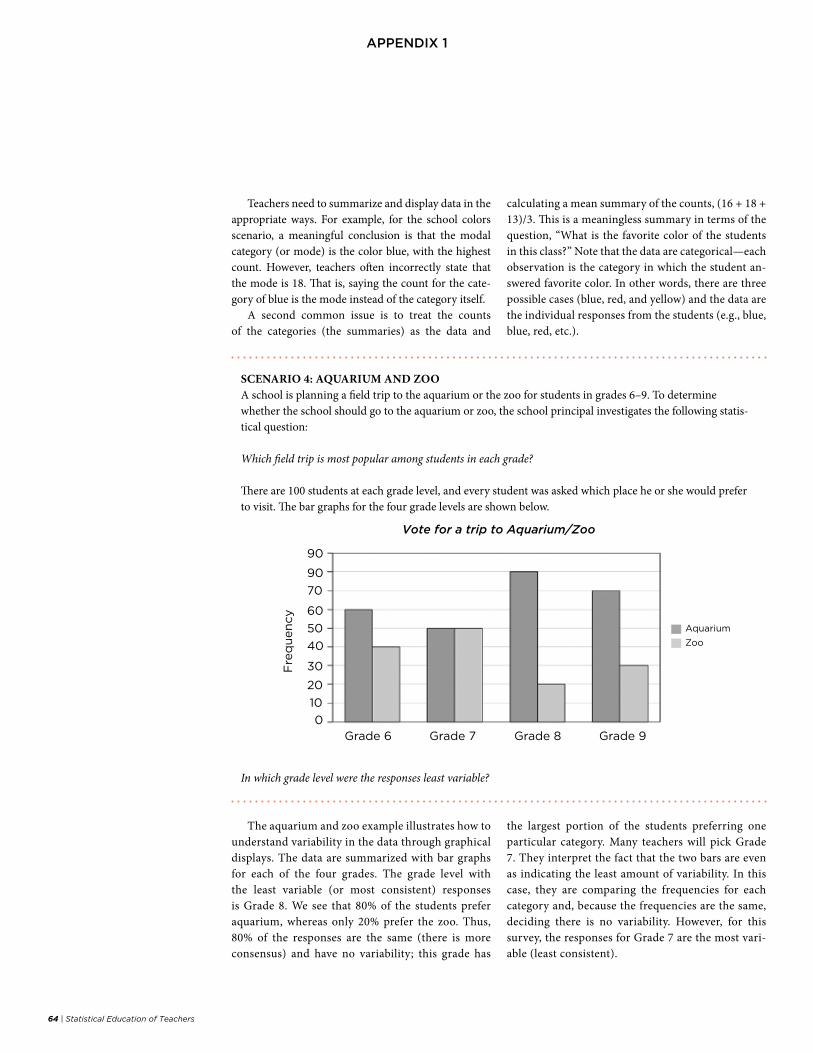
64 | Statistical Education of Teachers
aPPeNDix 1
Teachers need to summarize and display data in the appropriate ways. For example, for the school colors scenario, a meaningful conclusion is that the modal category (or mode) is the color blue, with the highest count. However, teachers often incorrectly state that the mode is 18. That is, saying the count for the cate-gory of blue is the mode instead of the category itself.
A second common issue is to treat the counts of the categories (the summaries) as the data and
calculating a mean summary of the counts, (16 + 18 + 13)/3. This is a meaningless summary in terms of the question, “What is the favorite color of the students in this class?” Note that the data are categorical—each observation is the category in which the student an-swered favorite color. In other words, there are three possible cases (blue, red, and yellow) and the data are the individual responses from the students (e.g., blue, blue, red, etc.).
SCENARIO 4: AQUARIUM AND ZOO A school is planning a field trip to the aquarium or the zoo for students in grades 6–9. To determine whether the school should go to the aquarium or zoo, the school principal investigates the following statis-tical question:
Which field trip is most popular among students in each grade?
There are 100 students at each grade level, and every student was asked which place he or she would prefer to visit. The bar graphs for the four grade levels are shown below.
Vote for a trip to Aquarium/Zoo
Grade 9Grade 8Grade 7Grade 60
10
20
30
40
50
60
70
90
Fre
qu
en
cy
The aquarium and zoo example illustrates how to understand variability in the data through graphical displays. The data are summarized with bar graphs for each of the four grades. The grade level with the least variable (or most consistent) responses is Grade 8. We see that 80% of the students prefer aquarium, whereas only 20% prefer the zoo. Thus, 80% of the responses are the same (there is more consensus) and have no variability; this grade has
the largest portion of the students preferring one particular category. Many teachers will pick Grade 7. They interpret the fact that the two bars are even as indicating the least amount of variability. In this case, they are comparing the frequencies for each category and, because the frequencies are the same, deciding there is no variability. However, for this survey, the responses for Grade 7 are the most vari-able (least consistent).
In which grade level were the responses least variable?
Aquarium
Zoo
90

Statistical Education of Teachers | 65
aPPeNDix 1
This example illustrates several concepts par-ticularly relevant to teacher preparation. Teachers need to be comfortable with communicating to par-ents about percentiles; however, confusion arises among the terms percent, percentiles, and z-scores. Teachers must understand clearly that making an assumption about the distribution of scores is the only way to get a reasonable approximate answer in this problem. Scaling the observed scores in terms of the number of standard deviations away from the mean (z-scores) maps the 30 on the ACT into 1.67 and the 700 on the SAT into 1.50. But these figures would be too confusing to report to most audiences and thus should be mapped into percentiles, which
turn out to be about 95 and 93, respectively. (Of course, technology allows one to go from the raw score to the percentile without the z transformation, but z-scores are a useful concept for teachers to un-derstand and experience.)
Using this process in reverse, the 90th percen-tiles for the two distributions are 28 for the ACT and 674 for the SAT. Teachers need practice with phrases such as “95 percent of the scores are below 30, the 95th percentile of the distribution that corresponds to a z-score of 1.67.” In addition, teachers should be taught to look carefully at the published percentile scores for these exams to see how closely they line up with those of a well-chosen normal distribution.
SCENARIO 5: SAT AND ACT PERCENTILES Scores on large-scale national tests tend to be mound-shaped with little skew, thus allowing the normal distribution to be a good model for their distributions. For a particular year, the ACT mathematics scores had a mean of about 20 and a standard deviation of about 6. The SAT math scores had a mean of about 520 with a standard deviation of about 120. How does an ACT score of 30 compare to an SAT score of 700? What was the 90th-percentile score for each exam?
SCENARIO 6: BRAIN WEIGHT V. BODY WEIGHTIt is hypothesized that larger animals have larger brains. If a relationship between body weight and brain weight existed, then body weight (a relatively easy measurement to make) could be used to predict brain weight (for which measurement is rather hard on the animal). What is the relationship between the body weight of an animal and brain weight of an animal? To explore this statistical question, data were obtained on the brain weight (in grams) and body weight (in kilograms) for a sample of 30 animals of differing species (see table below). What does a plot of the data reveal about the relationship? How could the relationship between brain weight and body weight be modeled?
The brain weight and body weight of different species (displayed in the table with other variables that will be referred to in this example) scenario illustrates an exam-
ple that necessitates careful graphical displays of data at multiple stages of the process to gain information about the relationship between brain weight and body weight.

66 | Statistical Education of Teachers
aPPeNDix 1
Species
Brain Weight measured in
grams (Brain_wt Gm)
Body Weight measured in ki-lograms (Brain_wt Body_wt Kg)
Natural Log of Brain Weight
(LnBrain)(LBr)
Natural Log of Body Weight
LnBody(LBo)
Species (f=fish, m=mammal)
Species Code (1=fish,
0=mammal)
Catfish 1.84 2.894 0.609766 1.06264 f 1
Barracuda 3.83 5.978 1.34286 1.78809 f 1
Mackerel 0.64 0.765 -0.44629 -0.26788 f 1
Salmon 1.26 3.93 0.231112 1.36864 f 1
brown_trout 0.57 0.292 -0.56212 -1.231 f 1
tuna 3.09 5.21 1.12817 1.65058 f 1
northern_trout 1.23 2.5 0.207014 0.916291 f 1
grizzly_bear 233.9 142.88 5.45489 4.96201 m 0
cheetah 2.45 22.2 0.896088 3.10009 m 0
lion 106.7 28.79 4.67002 3.36003 m 0
raccoon 40 5.175 3.68888 1.64384 m 0
Skunk 10.3 1.7 2.33214 0.530628 m 0
tiger 302 209 5.71043 5.34233 m 0
Wolf 152 29.94 5.02388 3.3992 m 0
Greyhound 105.9 24.49 4.6625 3.19826 m 0
Seal 442 107.3 6.09131 4.67563 m 0
Walrus 1126 667 7.02643 6.50279 m 0
Porpoise 1735 142.43 7.45876 4.95885 m 0
blue_whale 6800 58059 8.82468 10.9692 m 0
Bat 0.94 0.028 -0.06187 -3.57555 m 0
Mole 1.16 0.04 0.14842 -3.21888 m 0
Baboon 140 7.9 4.94164 2.06686 m 0
grey_monkey 66.6 4.55 4.1987 1.51513 m 0
chimpanzee 440 56.69 6.08677 4.0376 m 0
human 1377 74 7.22766 4.30407 m 0
Mouse 0.55 0.018 -0.59783 -4.01738 m 0
Squirrel 3.97 0.183 1.37877 -1.69827 m 0
rhinoceros 655 763 6.48464 6.63726 m 0
african_elephant 5712 6654 8.65032 8.80297 m 0
horse 618 461.76 6.42649 6.13505 m 0
TABLE 1
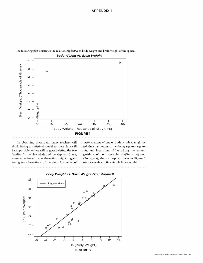
Statistical Education of Teachers | 67
aPPeNDix 1
Ln
(B
rain
Weig
ht)
In observing these data, many teachers will think fitting a statistical model to these data will be impossible; others will suggest deleting the two “outliers”—the blue whale and the elephant. Some, more experienced in mathematics, might suggest trying transformations of the data. A number of
transformations of one or both variables might be tried, the most common ones being squares, square roots, and logarithms. After taking the natural logarithms of both variables (ln(Brain_wt) and ln(Body_wt)), the scatterplot shown in Figure 2 looks reasonable to fit a simple linear model.
The following plot illustrates the relationship between body weight and brain weight of the species:
Body Weight vs. Brain Weight
0
Body Weight (Thousands of Kilograms)
Bra
in W
eig
ht
(Th
ou
san
ds
of
Gra
ms)
10 20 30 40 50 60
01
23
45
67
Body Weight vs. Brain Weight (Transformed)
02
46
-28
10
ln (Body Weight)
Regression
-6 -4 -2 0 2 4 6 8 10 12
FIGURE 1
FIGURE 2
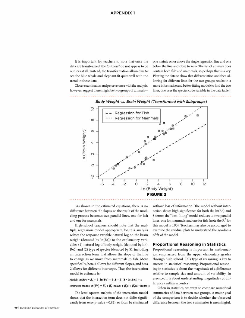
68 | Statistical Education of Teachers
aPPeNDix 1
It is important for teachers to note that once the data are transformed, the “outliers” do not appear to be outliers at all. Instead, the transformation allowed us to see the blue whale and elephant fit quite well with the trend in these data.
Closer examination and perseverance with the analysis, however, suggest there might be two groups of animals—
one mainly on or above the single regression line and one below the line and close to zero. The list of animals does contain both fish and mammals, so perhaps that is a key. Plotting the data to show that differentiation and then al-lowing for different lines for the two groups results in a more informative and better-fitting model (to find the two lines, one uses the species code variable in the data table.)
Body Weight vs. Brain Weight (Transformed with Subgroups)
-6 -4 -2 0 2 4 6 8 10 12
02
46
-28
10
Ln (Body Weight)
Ln
(B
rain
Weig
ht)
Regression for Fish
Regression for Mammals
As shown in the estimated equations, there is no difference between the slopes, so the result of the mod-eling process becomes two parallel lines, one for fish and one for mammals.
High-school teachers should note that the mul-tiple regression model appropriate for this analysis relates the response variable natural log on the brain weight (denoted by ln(Br)) to the explanatory vari-ables (1) natural log of body weight (denoted by ln(-Bo)) and (2) type of species (denoted by S), including an interaction term that allows the slope of the line to change as we move from mammals to fish. More specifically, beta 3 allows for different slopes, and beta 2 allows for different intercepts. Thus the interaction model to estimate is:
The least-squares analysis of the interaction model shows that the interaction term does not differ signifi-cantly from zero (p-value = 0.82), so it can be eliminated
without loss of information. The model without inter-action shows high significance for both the ln(Bo) and S terms; the “best-fitting” model reduces to two parallel lines, one for mammals and one for fish (note the R2 for this model is 0.90). Teachers may also be encouraged to examine the residual plots to understand the goodness of fit of the model.
Proportional Reasoning in StatisticsProportional reasoning is important in mathemat-ics, emphasized from the upper elementary grades through high school. This type of reasoning is key to success in statistical reasoning. Proportional reason-ing in statistics is about the magnitude of a difference relative to sample size and amount of variability. In essence, it is about understanding magnitudes of dif-ferences within a context.
Often in statistics, we want to compare numerical summaries of data between two groups. A major goal of the comparison is to decide whether the observed difference between the two summaries is meaningful.
FIGURE 3

Statistical Education of Teachers | 69
aPPeNDix 1
In statistics, the foundations for judging the size of a difference lie in proportional reasoning. Two factors are taken into account when comparing the size of the
difference between two proportions or between two means. These are (1) the group sizes and/or (2) the amount of variability within the data.
SCENARIO 7: MEDICAL SCREENING Understanding the results of medical screening tests is vitally important to the health of individuals and the functioning of the health care system. Such tests are not perfect, but the nature of the errors can be dangerously misleading. The figure shows what happens in a typical scenario of screening for HIV by use of the ELISA and Western Blot tests.
• For a population of heterosexual men exhibiting low-risk behavior, the rate of HIV infection is about 1 in 10,000. The true positive rate (sensitiv-ity) of these tests is about 99.9%. The true nega-tive rate (specificity) is 99.99%. Discuss how these two figures are used in the accompanying figure.
• The probability of a randomly selected person having a disease given that the screening says the disease is present is called the “positive predictive value.” Discuss how the positive predictive value is calculated in the HIV example. Why do you sup-pose the author used the smiley faces in this way?
The medical screening example illustrates that probabilities can always be interpreted as long-run relative frequencies. Generally, it is not obvious to teachers that a 0.01% infection rate can be interpreted as about one positive case in a typical group of 10,000 men, or, in other words, what can be expected in a random sample of 10,000 men. If a man is known to be infected, the expectation is that the highly accurate test will detect it.
On the other hand, of the 9,999 men not infect-ed, the expectation is that 9999(0.9999)=9998 will be tested as not infected, leaving 1 to be falsely detected as positive. The author, a medical doctor, finds the ex-pected frequencies are much easier for most patients to interpret than are the perplexing percentages.
Teachers should focus on seeing conditional prob-abilities as relative frequencies and reasoning out the conditional relative frequencies from the data, rather than through the memorizing formulas. Once the conditional probability is obtained, many will be surprised at how large it is, given the small infection rates and high rates of accuracy among the tests. The message: Conditioning can make a huge difference
in rates and depends crucially on the overall infec-tion rate. Now, suppose the infection rate doubles to 0.02%. How will that affect the conditional probabil-ity in question?
The conditional reasoning may be easier to see in a table, as shown, rather than a tree diagram.
Man + Man - Totals
test + 1 1 2
test - 0 9,998 9,998
totals 1 9,999 10,000
The condition of testing positive reduces the rel-evant cases to the first row of data; the chance of actually being positive given that the test was posi-tive is 1/2. If the infection rate doubles to 0.02%, the expected number of positives among those infected goes to approximately 2, and the conditional prob-ability of the chance of being positive given that the test is positive increases to 2/3. Thus, this probabili-ty is highly dependent upon the infection rate.
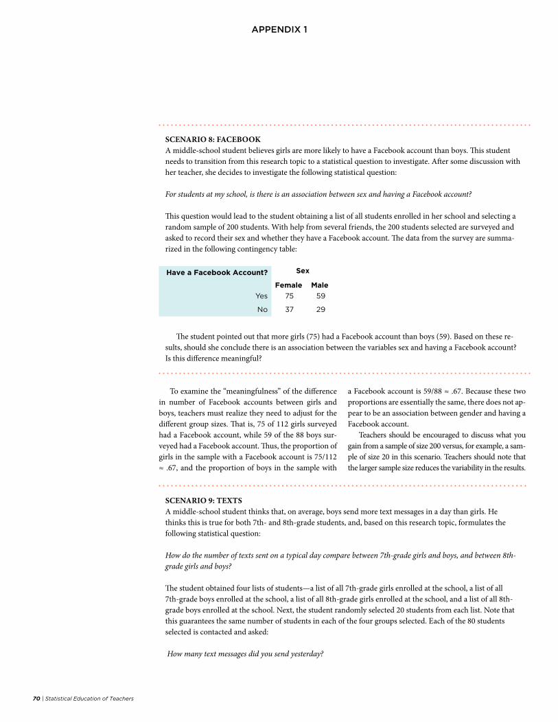
70 | Statistical Education of Teachers
aPPeNDix 1
SCENARIO 8: FACEBOOKA middle-school student believes girls are more likely to have a Facebook account than boys. This student needs to transition from this research topic to a statistical question to investigate. After some discussion with her teacher, she decides to investigate the following statistical question:
For students at my school, is there is an association between sex and having a Facebook account?
This question would lead to the student obtaining a list of all students enrolled in her school and selecting a random sample of 200 students. With help from several friends, the 200 students selected are surveyed and asked to record their sex and whether they have a Facebook account. The data from the survey are summa-rized in the following contingency table:
Have a Facebook Account? Sex
Female Male
Yes 75 59
No 37 29
The student pointed out that more girls (75) had a Facebook account than boys (59). Based on these re-sults, should she conclude there is an association between the variables sex and having a Facebook account? Is this difference meaningful?
To examine the “meaningfulness” of the difference in number of Facebook accounts between girls and boys, teachers must realize they need to adjust for the different group sizes. That is, 75 of 112 girls surveyed had a Facebook account, while 59 of the 88 boys sur-veyed had a Facebook account. Thus, the proportion of girls in the sample with a Facebook account is 75/112 ≈ .67, and the proportion of boys in the sample with
a Facebook account is 59/88 ≈ .67. Because these two proportions are essentially the same, there does not ap-pear to be an association between gender and having a Facebook account.
Teachers should be encouraged to discuss what you gain from a sample of size 200 versus, for example, a sam-ple of size 20 in this scenario. Teachers should note that the larger sample size reduces the variability in the results.
SCENARIO 9: TEXTSA middle-school student thinks that, on average, boys send more text messages in a day than girls. He thinks this is true for both 7th- and 8th-grade students, and, based on this research topic, formulates the following statistical question:
How do the number of texts sent on a typical day compare between 7th-grade girls and boys, and between 8th-grade girls and boys?
The student obtained four lists of students—a list of all 7th-grade girls enrolled at the school, a list of all 7th-grade boys enrolled at the school, a list of all 8th-grade girls enrolled at the school, and a list of all 8th-grade boys enrolled at the school. Next, the student randomly selected 20 students from each list. Note that this guarantees the same number of students in each of the four groups selected. Each of the 80 students selected is contacted and asked:
How many text messages did you send yesterday?
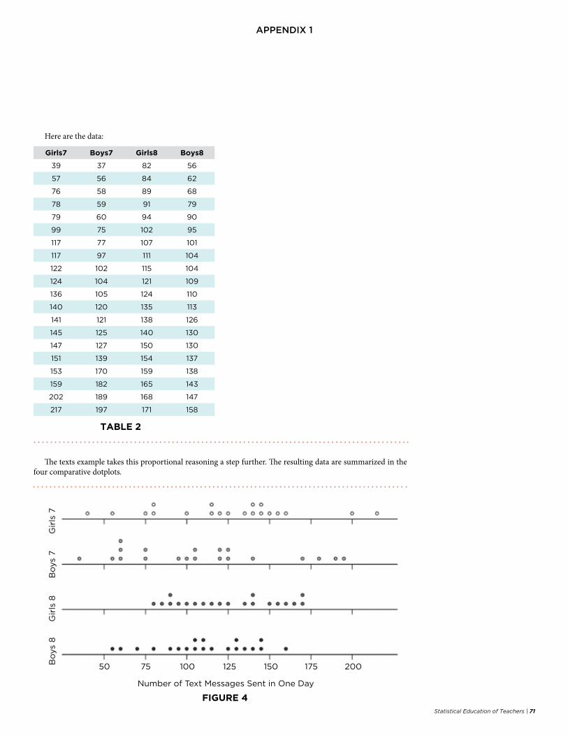
Statistical Education of Teachers | 71
aPPeNDix 1
Here are the data:
Girls7 Boys7 Girls8 Boys8
39 37 82 56
57 56 84 62
76 58 89 68
78 59 91 79
79 60 94 90
99 75 102 95
117 77 107 101
117 97 111 104
122 102 115 104
124 104 121 109
136 105 124 110
140 120 135 113
141 121 138 126
145 125 140 130
147 127 150 130
151 139 154 137
153 170 159 138
159 182 165 143
202 189 168 147
217 197 171 158
TABLE 2
FIGURE 4
The texts example takes this proportional reasoning a step further. The resulting data are summarized in the four comparative dotplots.
Number of Text Messages Sent in One Day
50 75 100 125 150 175 200Bo
ys
8G
irls
8G
irls
7B
oys
7
72 | Statistical Education of Teachers
aPPeNDix 1
Summary statistics for each group are:
Group Group Size
Mean StDev
7th-Grade Girls
20 125.0 44.8
7th-Grade Boys
20 110.0 47.5
8th-Grade Girls
20 125.0 29.7
8th-Grade Boys 20 110.0 29.1
Note that the difference between the means between girls and boys in the 7th grade is 15 texts. Thus, the 7th-grade girls sent, on average, 15 more texts than the 7th-grade boys. Also, this is the same difference when com-paring 8th-grade girls to 8th-grade boys. The 8th-grade girls sent, on average, 15 more texts than the 8th-grade boys. Thus, in absolute terms, the difference between the group means for both 7th- and 8th-grade boys and girls is the same. However, when evaluating the size of this dif-ference, teachers must use proportional reasoning to ex-amine this difference in centers in relation to the amount of variability in the data.
While the means for 7th-grade girls and boys are different, the standard deviations are fairly close (44.8 versus 47.5), indicating similar amounts of variability in number of texts sent for both 7th-grade girls and 7th-grade boys. Also, the standard deviations for 8th-grade girls and 8th-grade boys are fairly close (29.7 versus 29.1). Again, this indicates similar amounts of variability in the number of texts sent for both 8th-grade girls and 8th-grade boys. However, there is considerably less variability in the data on number of texts for the 8th-grade boys and girls than there is for the 7th-grade boys and girls. How does this affect the meaningfulness of the difference between groups?
For each grade level, teachers can judge the size of the difference between means by dividing the difference by a standard deviation (for a detailed example of this approach, see the Chapter 4 illustrative example). As long as the sample sizes are the same, this quantity pro-vides insight into how meaningful the observed differ-ence is for each class. For each grade, teachers can use the larger of the two standard deviations. Thus, for 7th graders, this quantity would be 15/47.5 = .32. For 8th graders, this quantity would be 15/29.7 = .51
Because this quantity is larger for 8th graders, the difference of 15 texts is more meaningful for 8th-grade students than it is for 7th-grade students.
As previously indicated, as long as the sample sizes are the same, this quantity provides useful information about the magnitude of the difference between mea-sures of center for two groups. When the sample sizes are different, sample size is also a factor teachers must consider when judging the magnitude of the difference.
The classical statistical procedure for comparing two population means based on independent random sample is the t-statistic, defined as:
, where
The t distribution for sample sizes of 20 or more is generally a robust distribution under the regular as-sumptions to use the t-test. The larger the t statistics, the stronger the evidence of a meaningful (significant) difference between the two sample means. Note that the denominator of the t statistic takes into account both the sample sizes and variability within each sample. Thus, the t statistic is measuring the magnitude of the differ-ence between the two sample means relative to both the sample sizes and amount of variability within each group. Also note that the smaller the denominator is, the larger the value for the t statistic. In this case, the larger the sample sizes are, the smaller the denominator. Also, the smaller the standard deviations (amounts of variability) are, the smaller the denominator.
The t statistic for comparing the mean number of texts of 7th-grade girls with 7th-grade boys is (yielding a p-value of ~0.3):
The t statistic for comparing the mean number of texts of 8th-grade girls with 8th-grade boys is (yielding a p-value of ~.1):

Statistical Education of Teachers | 73
aPPeNDix 1
Note the t statistic is larger for the 8th graders than for the 7th graders. This is because there is less variabil-ity in the data on 8th graders than 7th graders.
Therefore, while the girls in both 7th and 8th grade sent an average 15 texts more than boys in these sam-ples, this difference is more meaningful for the 8th graders than it is for the 7th graders. This is because there is less variability in the number of texts sent for the 8th graders than for the 7th graders.
The Role of Randomness in StatisticsRandom assignment and random selection are fun-damental concepts in statistics that teachers should understand. Although both are difficult in practice to achieve, they serve as key gold standards for dif-ferent aspects of statistics. While it is important to stress the importance of randomization in statistics, teachers should be aware that, in practice, conditions are far from ideal, so many statistical techniques are developed around what to do in light of not having ideal conditions.
Random selection is the backbone of statistical in-ference, as it provides a way to obtain a sample repre-sentative of the population. This notion is key to the construction and use of sampling distributions for in-ference. Teachers must have experience exploring and
working with the notion of sampling distributions, a concept that, if not given the adequate amount of time, can be confusing and mysterious. The focus of such ex-ploration should be around distinguishing among the population distribution, distribution of sample data, and sampling distributions.
Random assignment in an experiment is indis-pensable if one would like to claim causality of some type. Teachers should understand why random as-signment helps mitigate the effects of potential con-founding variables in an experiment. In particular, the distributions of potential confounding variables should be similar across conditions if random as-signment took place.
SCENARIO 10: HEALTHIER MENU School administrators are interested in providing a menu in the lunchroom that students like. The admin-istrators at a school plan to survey students to measure satisfaction with the new healthier menu in the lunchroom. They would like to answer the research question:
Do students like the new lunch menu at the school?
They survey the students by asking them the following survey questions (note these are survey questions, not statistical questions):
• Do you purchase food in the lunchroom?
• How many days a week do you purchase food in the lunchroom?
• Are you satisfied with your purchases?
• Do you like the food in the lunchroom?
To study whether students like the new lunchroom menu, teachers are expected to know that the results of such a survey can be generalized to the entire school only if the selected sample is a random sample from the entire
student body at the school. In discussing a method for obtaining a random sample, teachers may suggest pref-erence for other sampling methods that may not produce adequate samples to then make inferential statements.
Random assignment and random
selection are fundamental concepts
in statistics that teachers should
understand. Although both are
difficult in practice to achieve, they
serve as key gold standards for
different aspects of statistics.
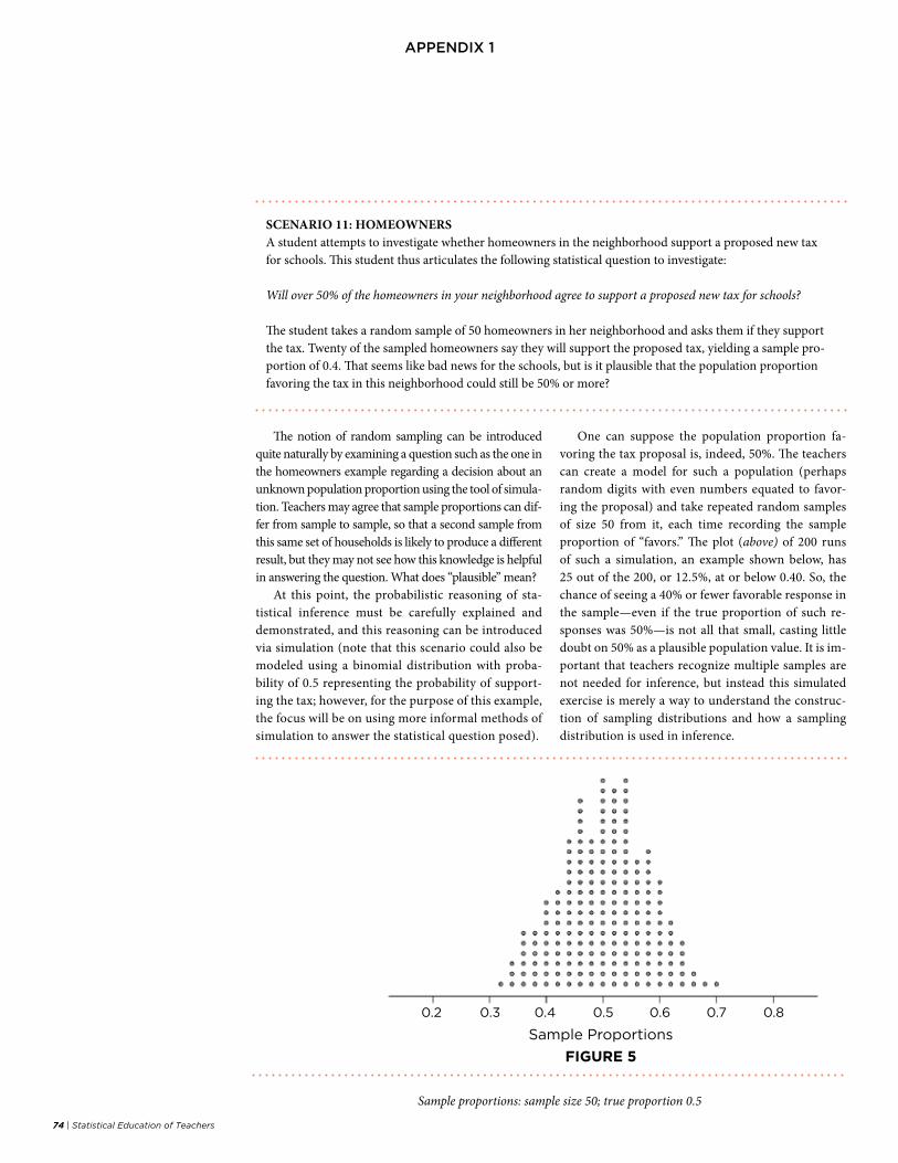
74 | Statistical Education of Teachers
aPPeNDix 1
SCENARIO 11: HOMEOWNERS A student attempts to investigate whether homeowners in the neighborhood support a proposed new tax for schools. This student thus articulates the following statistical question to investigate:
Will over 50% of the homeowners in your neighborhood agree to support a proposed new tax for schools?
The student takes a random sample of 50 homeowners in her neighborhood and asks them if they support the tax. Twenty of the sampled homeowners say they will support the proposed tax, yielding a sample pro-portion of 0.4. That seems like bad news for the schools, but is it plausible that the population proportion favoring the tax in this neighborhood could still be 50% or more?
The notion of random sampling can be introduced quite naturally by examining a question such as the one in the homeowners example regarding a decision about an unknown population proportion using the tool of simula-tion. Teachers may agree that sample proportions can dif-fer from sample to sample, so that a second sample from this same set of households is likely to produce a different result, but they may not see how this knowledge is helpful in answering the question. What does “plausible” mean?
At this point, the probabilistic reasoning of sta-tistical inference must be carefully explained and demonstrated, and this reasoning can be introduced via simulation (note that this scenario could also be modeled using a binomial distribution with proba-bility of 0.5 representing the probability of support-ing the tax; however, for the purpose of this example, the focus will be on using more informal methods of simulation to answer the statistical question posed).
One can suppose the population proportion fa-voring the tax proposal is, indeed, 50%. The teachers can create a model for such a population (perhaps random digits with even numbers equated to favor-ing the proposal) and take repeated random samples of size 50 from it, each time recording the sample proportion of “favors.” The plot (above) of 200 runs of such a simulation, an example shown below, has 25 out of the 200, or 12.5%, at or below 0.40. So, the chance of seeing a 40% or fewer favorable response in the sample—even if the true proportion of such re-sponses was 50%—is not all that small, casting little doubt on 50% as a plausible population value. It is im-portant that teachers recognize multiple samples are not needed for inference, but instead this simulated exercise is merely a way to understand the construc-tion of sampling distributions and how a sampling distribution is used in inference.
Sample Proportions
0.2 0.3 0.4 0.5 0.6 0.7 0.8
FIGURE 5
Sample proportions: sample size 50; true proportion 0.5
Statistical Education of Teachers | 75
aPPeNDix 1
SCENARIO 12: DOLPHINS Swimming with dolphins can certainly be fun, but is it also therapeutic for patients suffering from clinical depres-sion? To investigate this possibility, researchers recruited 30 subjects aged 18–65 with a clinical diagnosis of mild to moderate depression. Subjects were required to discontinue use of any antidepressant drugs or psychotherapy four weeks prior to the experiment and throughout the experiment. These 30 subjects went to an island off the coast of Honduras, where they were randomly assigned to one of two treatment groups. Both groups engaged in the same amount of swimming and snorkeling each day, but one group (the animal care program) did so in the presence of bottlenose dolphins. The other group (outdoor nature program) did not. At the end of two weeks, each subjects’ level of depression was evaluated, as it had been at the beginning of the study (Antonioli and Reveley, 2005).
The following table summarizes the results of this study:
Inferential reasoning should now move from sim-ulation to more formal methods developed from the normal distribution. The simulated distribution of sample proportions (the sampling distribution) has a mean of 0.49 and a standard deviation of 0.07. It can be modeled quite well by a normal distribution having that mean and standard deviation. But, we need not run a simulation each time we deal with a new propor-tion or sample size, because the underlying theory tells us that the mean of the sampling distribution of sample proportions will always equal the population propor-tion, p, and the standard deviation will be given by
where n is the sample size. These values are, respec-tively, 0.50 and 0.07 for the example, nearly identical
to the values from the simulation. Thus, the observed sample proportion of 0.40 is only 1.43 standard de-viations below the mean, not far enough to say it is outside the range of reasonably likely outcomes.
The randomization process can be repeated for other choices of the population proportion, resulting in an interval of “plausible values” for that parameter. An easier way to accomplish this, however, is to make use of the normal distribution model. If “reasonably likely” outcomes are set to be those in the middle 95% of the distribution of the sample proportion, , then any population proportion within about two stan-dard deviations—estimated using the sample propor-tion—of the observed would have that sample result within its reasonably likely range. Thus, all propor-tions within two standard deviations of the observed sample proportion form an interval of plausible values for the true population proportion.
Showed Substantial Improvement
No Substantial Improvement Total
animal care program (dolphin therapy)
10 5 15
Outdoor nature program (control group)
3 12 15
total 13 17 30
The dolphin study provides an example of an experiment that randomly assigns subjects to treat-ments. Notice that 10 of the patients in the Animal Care Program group showed substantial improve-ment compared to 3 of the Outdoor Nature Program group. Because the groups are the same size, we do not need to calculate proportions to compare. More of the people who swam with the dolphins improved.
It is possible, however, that this difference (10 vs. 3) could happen even if dolphin therapy was not effective, simply due to the random nature of putting subjects into groups (i.e., the luck of the draw). But if 13 of the 30 people were going to improve regardless of whether they swam with dolphins, we would have expected 6 or 7 to end up in each group; how unlikely is a 10/3 split by this random assignment process alone? If the answer is that
76 | Statistical Education of Teachers
aPPeNDix 1
this observed difference would be surprising if dolphin therapy were not effective, then we would have strong evidence to conclude that dolphin therapy is effective. Why? Because we would have to believe a rare event just happened to occur in this experiment otherwise.
It is possible to see whether the observed 10 im-provements under the dolphin therapy treatment is unusually large, given no treatment effect, by running a simulation of the randomization process. Suppose the 13 who improved are equally likely to improve under either treatment (no treatment effect). Then, any of the 10 “improvers” under the dolphin therapy just hap-pened to fall into that column by chance. How likely is it to get that result by chance alone?
One possible model of this process begins by choosing 13 red cards to indicate “improvers” and 17
black cards to represent “non-improvers.” Randomly select 15 cards from the 30 to place in the dolphin treatment category (the other 15 go in the control group) and count the number of “improvers” (red cards) among the 15. Repeat this randomization pro-cess many times (possibly with the aid of a computer) to generate a distribution of dolphin therapy “improv-ers,” and then calculate the proportion of these counts that are 10 or greater.
If this proportion turns out to be small, that ev-idence suggests the observed count of 10 is not like-ly to occur under the conditions of chance alone; the dolphin therapy seems to be having an effect. The plot above shows 100 runs of the simulation outlined above; 10 was equaled or exceeded only two times, a small chance indeed.
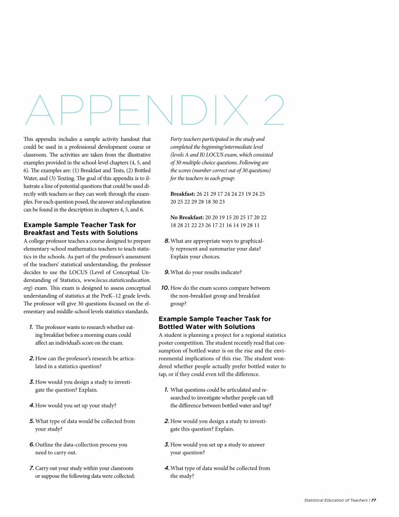
Statistical Education of Teachers | 77
aPPeNDix 2
This appendix includes a sample activity handout that could be used in a professional development course or classroom. The activities are taken from the illustrative examples provided in the school-level chapters (4, 5, and 6). The examples are: (1) Breakfast and Tests, (2) Bottled Water, and (3) Texting. The goal of this appendix is to il-lustrate a line of potential questions that could be used di-rectly with teachers so they can work through the exam-ples. For each question posed, the answer and explanation can be found in the description in chapters 4, 5, and 6.
Example Sample Teacher Task for Breakfast and Tests with SolutionsA college professor teaches a course designed to prepare elementary-school mathematics teachers to teach statis-tics in the schools. As part of the professor’s assessment of the teachers’ statistical understanding, the professor decides to use the LOCUS (Level of Conceptual Un-derstanding of Statistics, www.locus.statisticseducation.org) exam. This exam is designed to assess conceptual understanding of statistics at the PreK–12 grade levels. The professor will give 30 questions focused on the el-ementary and middle-school levels statistics standards.
1. The professor wants to research whether eat-ing breakfast before a morning exam could affect an individual’s score on the exam.
2. How can the professor’s research be articu-lated in a statistics question?
3. How would you design a study to investi-gate the question? Explain.
4. How would you set up your study?
5. What type of data would be collected from your study?
6. Outline the data-collection process you need to carry out.
7. Carry out your study within your classroom or suppose the following data were collected:
Forty teachers participated in the study and completed the beginning/intermediate level (levels A and B) LOCUS exam, which consisted of 30 multiple-choice questions. Following are the scores (number correct out of 30 questions) for the teachers in each group:
Breakfast: 26 21 29 17 24 24 23 19 24 25 20 25 22 29 28 18 30 23
No Breakfast: 20 20 19 15 20 25 17 20 22 18 28 21 22 23 26 17 21 16 14 19 28 11
8. What are appropriate ways to graphical-ly represent and summarize your data? Explain your choices.
9. What do your results indicate?
10. How do the exam scores compare between the non-breakfast group and breakfast group?
Example Sample Teacher Task for Bottled Water with SolutionsA student is planning a project for a regional statistics poster competition. The student recently read that con-sumption of bottled water is on the rise and the envi-ronmental implications of this rise. The student won-dered whether people actually prefer bottled water to tap, or if they could even tell the difference.
1. What questions could be articulated and re-searched to investigate whether people can tell the difference between bottled water and tap?
2. How would you design a study to investi-gate this question? Explain.
3. How would you set up a study to answer your question?
4. What type of data would be collected from the study?
APPENDIX 2
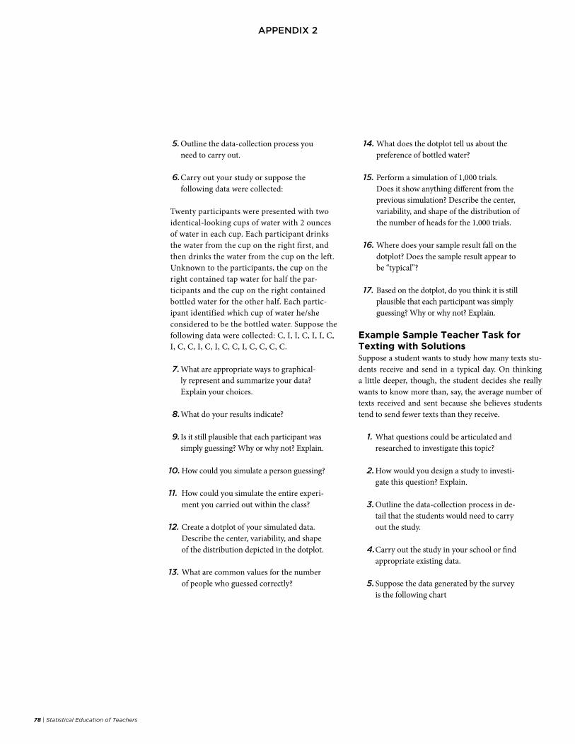
78 | Statistical Education of Teachers
aPPeNDix 2
5. Outline the data-collection process you need to carry out.
6. Carry out your study or suppose the following data were collected:
Twenty participants were presented with two identical-looking cups of water with 2 ounces of water in each cup. Each participant drinks the water from the cup on the right first, and then drinks the water from the cup on the left. Unknown to the participants, the cup on the right contained tap water for half the par-ticipants and the cup on the right contained bottled water for the other half. Each partic-ipant identified which cup of water he/she considered to be the bottled water. Suppose the following data were collected: C, I, I, C, I, I, C, I, C, C, I, C, I, C, C, I, C, C, C, C.
7. What are appropriate ways to graphical-ly represent and summarize your data? Explain your choices.
8. What do your results indicate?
9. Is it still plausible that each participant was simply guessing? Why or why not? Explain.
10. How could you simulate a person guessing?
11. How could you simulate the entire experi-ment you carried out within the class?
12. Create a dotplot of your simulated data. Describe the center, variability, and shape of the distribution depicted in the dotplot.
13. What are common values for the number of people who guessed correctly?
14. What does the dotplot tell us about the preference of bottled water?
15. Perform a simulation of 1,000 trials. Does it show anything different from the previous simulation? Describe the center, variability, and shape of the distribution of the number of heads for the 1,000 trials.
16. Where does your sample result fall on the dotplot? Does the sample result appear to be “typical”?
17. Based on the dotplot, do you think it is still plausible that each participant was simply guessing? Why or why not? Explain.
Example Sample Teacher Task for Texting with SolutionsSuppose a student wants to study how many texts stu-dents receive and send in a typical day. On thinking a little deeper, though, the student decides she really wants to know more than, say, the average number of texts received and sent because she believes students tend to send fewer texts than they receive.
1. What questions could be articulated and researched to investigate this topic?
2. How would you design a study to investi-gate this question? Explain.
3. Outline the data-collection process in de-tail that the students would need to carry out the study.
4. Carry out the study in your school or find appropriate existing data.
5. Suppose the data generated by the survey is the following chart
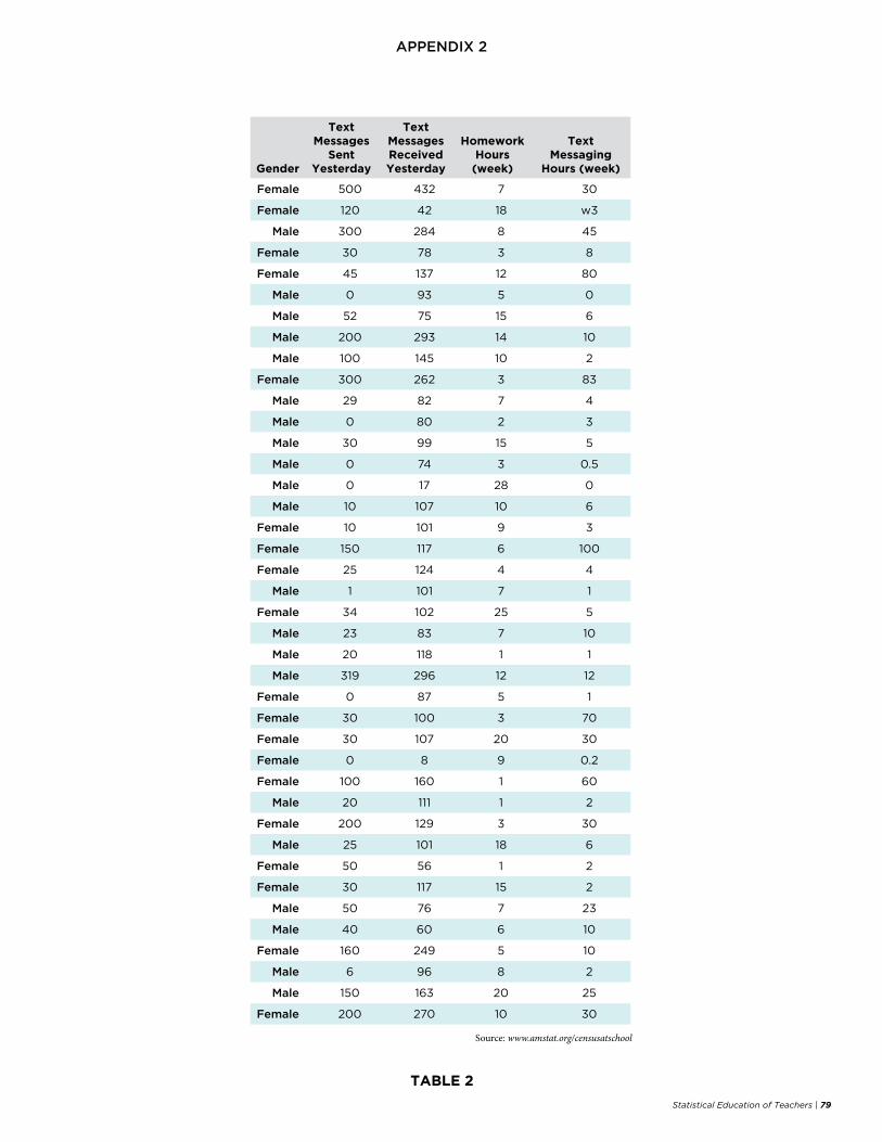
Statistical Education of Teachers | 79
aPPeNDix 2
Gender
Text Messages
Sent Yesterday
Text Messages Received Yesterday
Homework Hours
(week)
Text Messaging
Hours (week)
female 500 432 7 30
female 120 42 18 w3
Male 300 284 8 45
female 30 78 3 8
female 45 137 12 80
Male 0 93 5 0
Male 52 75 15 6
Male 200 293 14 10
Male 100 145 10 2
female 300 262 3 83
Male 29 82 7 4
Male 0 80 2 3
Male 30 99 15 5
Male 0 74 3 0.5
Male 0 17 28 0
Male 10 107 10 6
female 10 101 9 3
female 150 117 6 100
female 25 124 4 4
Male 1 101 7 1
female 34 102 25 5
Male 23 83 7 10
Male 20 118 1 1
Male 319 296 12 12
female 0 87 5 1
female 30 100 3 70
female 30 107 20 30
female 0 8 9 0.2
female 100 160 1 60
Male 20 111 1 2
female 200 129 3 30
Male 25 101 18 6
female 50 56 1 2
female 30 117 15 2
Male 50 76 7 23
Male 40 60 6 10
female 160 249 5 10
Male 6 96 8 2
Male 150 163 20 25
female 200 270 10 30
TABLE 2
Source: www.amstat.org/censusatschool
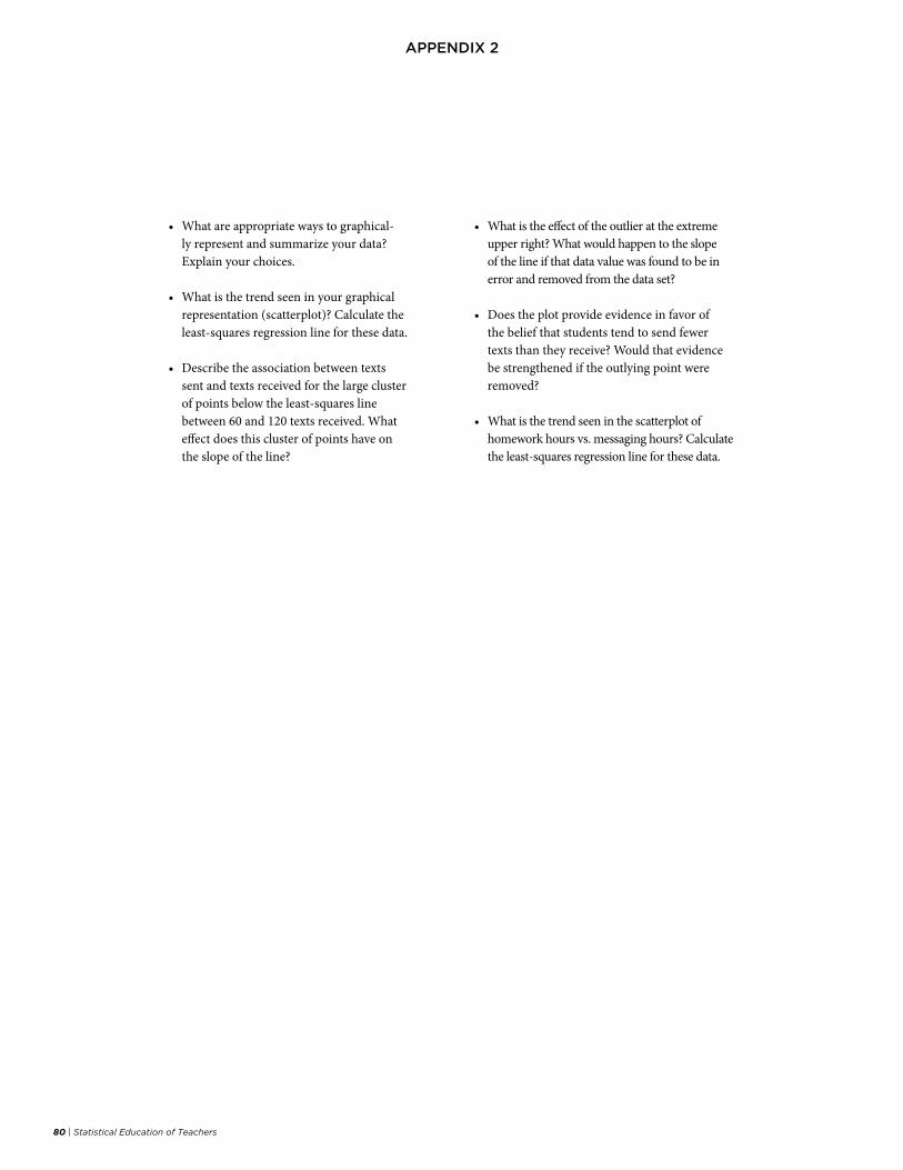
80 | Statistical Education of Teachers
aPPeNDix 2
• What are appropriate ways to graphical-ly represent and summarize your data? Explain your choices.
• What is the trend seen in your graphical representation (scatterplot)? Calculate the least-squares regression line for these data.
• Describe the association between texts sent and texts received for the large cluster of points below the least-squares line between 60 and 120 texts received. What effect does this cluster of points have on the slope of the line?
• What is the effect of the outlier at the extreme upper right? What would happen to the slope of the line if that data value was found to be in error and removed from the data set?
• Does the plot provide evidence in favor of the belief that students tend to send fewer texts than they receive? Would that evidence be strengthened if the outlying point were removed?
• What is the trend seen in the scatterplot of homework hours vs. messaging hours? Calculate the least-squares regression line for these data.


Statistical Education of Teachers | 82
aPPeNDix 2
Related Documents