International Conference on Flood Resilience: Experiences in Asia and Europe 5-7 September 2013, Exeter, United Kingdom Seith Mugume Dr. Diego Gomez Professor David Butler 1 Statistical downscaling methods for climate change impact assessment on urban rainfall extremes for cities in tropical developing countries – A review

Welcome message from author
This document is posted to help you gain knowledge. Please leave a comment to let me know what you think about it! Share it to your friends and learn new things together.
Transcript

International Conference on Flood Resilience:
Experiences in Asia and Europe
5-7 September 2013, Exeter, United Kingdom
Seith Mugume
Dr. Diego Gomez
Professor David Butler
1
Statistical downscaling methods for climate change impact
assessment on urban rainfall extremes for cities in tropical
developing countries – A review

Presentation outline
Background
Climate change impact assessment on urban hydrology
Overview of downscaling methods
Methodological suitability in tropical developing country cities
Conclusions
2

‘Top-Down’ climate impact assessment framework
3
Increasing
envelope of
uncertainty
Based on Wilby & Dessai (2010); Onof et al 2009; Sunyer et al 2012, Kendon et al. 2012
150 - 400 km monthly
(1.5) – 50 km daily
1 – 5 km 5 – 15 minutes
Energy & Land use
Driving forces
(population, income, lifestyle, technology)
Impact models (e.g.
urban flood models)
Regional Climate
Models (RCM)
Response options
Emission scenarios
General circulation
Models (GCM)
Spatial scale Temporal scale
Statistical downscaling

Climate change impact assessment at an urban scale
4
Willems et al. 2012
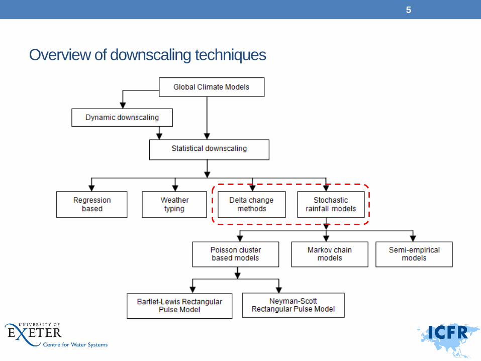
Overview of downscaling techniques
5
Statistical downscaling
• Use empirical-based relationships to convert course scale climate model
outputs to finer urban scales
Temporal downscaling
Spatial downscaling
• Key assumptions:
Local scale climate variables = f (large scale atmospheric variables)
Function can be deterministic or stochastic
Ratio remains unchanged under climate change
6
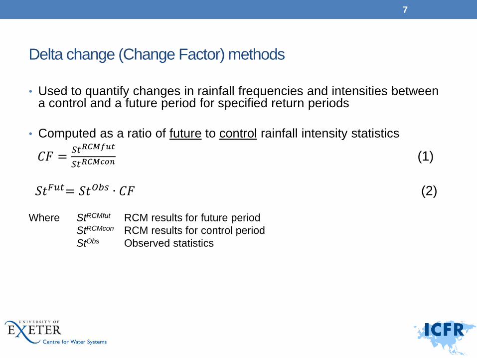
Delta change (Change Factor) methods
• Used to quantify changes in rainfall frequencies and intensities between a control and a future period for specified return periods
• Computed as a ratio of future to control rainfall intensity statistics
𝐶𝐹 =𝑆𝑡𝑅𝐶𝑀𝑓𝑢𝑡
𝑆𝑡𝑅𝐶𝑀𝑐𝑜𝑛 (1)
𝑆𝑡𝐹𝑢𝑡= 𝑆𝑡𝑂𝑏𝑠 ∙ 𝐶𝐹 (2)
Where StRCMfut RCM results for future period
StRCMcon RCM results for control period
StObs Observed statistics
7

Continuous versus event based change factors
8
0.00
0.20
0.40
0.60
0.80
1.00
1.20
1.40
1.60
1 2 3 4 5 6 7 8 9 10 11 12
Ch
an
ge
F
ac
tor
Month 2030 Ensemble Average 2050 Ensemble Average
2080 Ensemble AverageFigure 2: Example of historical 30 year 1-hour EULER II design
storm for Wuppertal (OBS) and downscaled version based on
future climate model projections (ECHAM5 and HADCM3
denoted as ECH and HAD respectively) (Olsson et al., 2012)
(Event based case)
Figure 1: Example of monthly change factors computed from an
ensemble of regional climate models for Kampala for future periods
2001-2030, 2041-2070 and 2071-2100 against a control period of
1961-1990 (Continuous case )
Merits
Easy and quick to apply
Preserves characteristics of observed data
Only relative changes transferred from climate
model data to observed time series
Demerits
Deterministic
Dependent on GCM/RCM model reliability
Requires equivalent climate model and
observed data
Uncertainties

Range of computed change factors
Uncertainty in CFs for February: 0.94 - 2.52
9
0.00
0.50
1.00
1.50
2.00
2.50
3.00
0 1 2 3 4 5 6 7 8 9 10 11 12
Ch
an
ge
F
ac
tor
Month
Monthly rainfall change factors for Kampala Control period (1961-1990): Future Period (2071-2080), Scenario RCP 4.5
MIROC-ESM CNRM-CM5 CanESM2 FGOALS-s2 BNU-ESM MIROC5 GFDL-ESM2G MIROC-ESM-CHEM GFDL-ESM2M MRI-CGCM3 BCC-CSM 1-1 2080 Ensemble Average

Stochastic rainfall models (Poisson cluster based)
• Plausible physical basis for simulation of hourly or daily rainfall
• Accurately simulate extreme rainfall events
• Model parameters computed by statistical analysis of observed rainfall data
• Change factors used to adjust model parameters
• Generalised Method of Moments for model parameter estimation
Estimates model parameter vector, θ by minimizing an objective function, S(θ|T) 𝑆 𝜃 𝑇 = 𝑤𝑖[𝑇𝑖 − 𝜏𝑖(𝜃)]
2𝑘𝑖=1 (3)
Where wi, Collection of weights
θ Model parameter vector
T Model of summary statistics computed from data
𝜏𝑖(𝜃) Expected value of T
• Model fitting and validation
• Disaggregation: Generates hourly or sub-hourly rainfall (e.g. 5 - 15 min)
10

Schematic of Poisson cluster rectangular pulse models
11
Wheater et al. 2005
(constant)
(Poisson process)
(Random no. of cells)
Clustering of rain cells
Barlet-Lewis Rectangular Pulse (BLRP) Model
Neyman Scott Rectangular Pulse (NSRP) Model
Aggregation at time, t

Neyman-Scott Rectangular Pulse Model
Parameter Description
λ-1 Average time between subsequent storm origins (h)
β-1 Average waiting time of rain cells after storm origin (h)
η-1 Average cell duration (h)
ϑ-1 Average no. of rain cells per storm
ξ-1 Average cell intensity (mm/h)
12
NSRP model parameters
Schematic representation of NSRP Model (Kilby et al. 2007)
Extreme value plot of annual maximum
rainfall for Heathrow (Kilby et al. 2007)
Comparison between NSRP
and a Markov Chain Model

Suitability for application in tropical developing countries cities
Limited case studies using statistical downscaling in cities in tropical
developing countries
Reasons?
• Limited or incomplete observed time series data sets
• Requirement of equivalent climate model and observed data sets
• Stochastic rainfall models not adapted to non-temperate climates
• Difficulty in model fitting due to indirect relationship between model
parameters and observable properties of rainfall sequences
• High uncertainties cascading from parent models
• Strong local convective influences affect reliability
13

Conclusions: Appropriate methodologies for tropical developing
country cities
• Climate sensitivity analyses using impact models
• Construction of climate analogues
• Use of delta change method (if reliable RCM data is available)
• CORDEX Africa experiments
• Regional climate data portals e.g. CSAG Group (University of Cape Town)
• Investigating the use of novel resilience based methodologies
• Identify critical system performance thresholds
• Evaluate system response and recovery behaviour under a range of future scenarios
• Identify and appraise adaptation options
14

International Conference on Flood Resilience:
Experiences in Asia and Europe
5-7 September 2013, Exeter, United Kingdom
Seith Mugume
Dr. Diego Gomez
Professor David Butler
15
Statistical downscaling methods for climate change impact
assessment on urban rainfall extremes for cities in tropical
developing countries – A review
Related Documents