Statistical designs and response surface techniques for the optimization of chromatographic systems

Page 1

Journal of Chromatography A, 1158 (2007) 2–14

Review

Statistical designs and response surface techniques for theoptimization of chromatographic systems

Sergio Luis Costa Ferreira a,∗, Roy Edward Bruns b, Erik Galvao Paranhos da Silva a,Walter Nei Lopes dos Santos c, Cristina Maria Quintella a, Jorge Mauricio David a,

Jailson Bittencourt de Andrade a, Marcia Cristina Breitkreitz b,Isabel Cristina Sales Fontes Jardim b, Benicio Barros Neto d

a Universidade Federal da Bahia, Instituto de Quımica, Campus Universitario de Ondina, Salvador, Bahia 40170-290, Brazilb Universidade Estadual de Campinas, Instituto de Quımica, Campinas, Sao Paulo 13084-971, Brazil

c Universidade Estadual de Santa Cruz, Departamento de Ciencias Exatas, Ilheus, Bahia 45650-000, Brazild Universidade Federal de Pernambuco, Departamento de Quımica fundamental, Recife, Pernanbuco 50740-540, Brazil

Available online 18 March 2007

Abstract

This paper describes fundamentals and applications of multivariate statistical techniques for the optimization of chromatographic systems.The surface response methodologies: central composite design, Doehlert matrix and Box–Behnken design are discussed and applications ofthese techniques for optimization of sample preparation steps (extractions) and determination of experimental conditions for chromatographicseparations are presented. The use of mixture design for optimization of mobile phases is also related. An optimization example involving a realseparation process is exhaustively described. A discussion about model validation is presented. Some applications of other multivariate techniquesfor optimization of chromatographic methods are also summarized.© 2007 Elsevier B.V. All rights reserved.

Keywords: Review; Multivariate techniques; Doehlert matrix; Box–Benhken design; Central composite design; Chromatographic methods; Optimization

Contents

1. Introduction. . . . . . . . . . . . . . . . . . . . . . . . . . . . . . . . . . . . . . . . . . . . . . . . . . . . . . . . . . . . . . . . . . . . . . . . . . . . . . . . . . . . . . . . . . . . . . . . . . . . . . . . . . . . . . . 32. Factorial and central composite designs . . . . . . . . . . . . . . . . . . . . . . . . . . . . . . . . . . . . . . . . . . . . . . . . . . . . . . . . . . . . . . . . . . . . . . . . . . . . . . . . . . . . . . 4

2.1. Application of central composite designs for optimization of chromatographic systems . . . . . . . . . . . . . . . . . . . . . . . . . . . . . . . . . . . . . 53. Box–Behnken designs . . . . . . . . . . . . . . . . . . . . . . . . . . . . . . . . . . . . . . . . . . . . . . . . . . . . . . . . . . . . . . . . . . . . . . . . . . . . . . . . . . . . . . . . . . . . . . . . . . . . . 5

3.1. Application of Box–Behnken designs for optimization of chromatographic methods . . . . . . . . . . . . . . . . . . . . . . . . . . . . . . . . . . . . . . . 74. Doehlert designs . . . . . . . . . . . . . . . . . . . . . . . . . . . . . . . . . . . . . . . . . . . . . . . . . . . . . . . . . . . . . . . . . . . . . . . . . . . . . . . . . . . . . . . . . . . . . . . . . . . . . . . . . . 7

4.1. Application of Doehlert design for optimization of chromatographic systems . . . . . . . . . . . . . . . . . . . . . . . . . . . . . . . . . . . . . . . . . . . . . . 95. Mixture designs . . . . . . . . . . . . . . . . . . . . . . . . . . . . . . . . . . . . . . . . . . . . . . . . . . . . . . . . . . . . . . . . . . . . . . . . . . . . . . . . . . . . . . . . . . . . . . . . . . . . . . . . . . . 9

5.1. Model validation . . . . . . . . . . . . . . . . . . . . . . . . . . . . . . . . . . . . . . . . . . . . . . . . . . . . . . . . . . . . . . . . . . . . . . . . . . . . . . . . . . . . . . . . . . . . . . . . . . . 105.2. Optimization example . . . . . . . . . . . . . . . . . . . . . . . . . . . . . . . . . . . . . . . . . . . . . . . . . . . . . . . . . . . . . . . . . . . . . . . . . . . . . . . . . . . . . . . . . . . . . . 115.3. Application of mixture design for optimization of chromatographic methods . . . . . . . . . . . . . . . . . . . . . . . . . . . . . . . . . . . . . . . . . . . . . 13

6. Other experimental designs used for the optimization of chromatographic methods . . . . . . . . . . . . . . . . . . . . . . . . . . . . . . . . . . . . . . . . . . . . . . 137. Conclusion . . . . . . . . . . . . . . . . . . . . . . . . . . . . . . . . . . . . . . . . . . . . . . . . . . . . . . . . . . . . . . . . . . . . . . . . . . . . . . . . . . . . . . . . . . . . . . . . . . . . . . . . . . . . . . 13

Acknowledgements . . . . . . . . . . . . . . . . . . . . . . . . . . . . . . . . . . . . . . . . . . . . . . . . . . . . . . . . . . . . . . . . . . . . . . . . . . . . . . . . . . . . . . . . . . . . . . . . . . . . . . . 13References . . . . . . . . . . . . . . . . . . . . . . . . . . . . . . . . . . . . . . . . . . . . . . . . . . . . . . . . . . . . . . . . . . . . . . . . . . . . . . . . . . . . . . . . . . . . . . . . . . . . . . . . . . . . . . 13

∗ Corresponding author. Tel.: +55 71 9117 8046; fax: +55 71 3235 5166.E-mail address: [email protected] (S.L.C. Ferreira).

0021-9673/$ – see front matter © 2007 Elsevier B.V. All rights reserved.doi:10.1016/j.chroma.2007.03.051

Page 2

hroma

1

stci

rctatTtt

smmdiewHtt

y

ptIdtfq

y

teTdmampsq

afTaap

nlboie

tsfclramFs

b

(

awtfstemt

itctTntcira

S.L.C. Ferreira et al. / J. C

. Introduction

Chromatographic analysis usually involves three steps:ample preparation, compound separation and compound quan-ification. Of these, the steps of sample preparation andompound separation have been frequently optimized employ-ng multivariate statistical techniques.

The multivariate statistical methods most used in chromatog-aphy and indeed in chemistry in general can be convenientlylassified according to how one decides which experiments areo be executed. All methods require the user to supply minimumnd maximum values for each factor that defines the experimen-al domain to be investigated during the optimization procedure.he combinations of the different factor levels used to perform

he actual experiments are then decided by which multivariateechnique is employed.

The most commonly used designs to determine responseurfaces are the full and fractional factorial designs and theore complex central composite, Box–Behnken, Doehlert andixture designs. Although the factorial designs can be used to

etermine simple response surfaces that are linear in all of thenvestigated factors, they are normally used to determine whichxperimental factors are the most important to investigate andhich factors do not significantly affect the experimental results.ere their use is discussed as a first stage in a multivariate inves-

igation where a linear response surface is determined. For awo-factor case, the response surface is given by the linear model

ˆ = b0 + b1x1 + b2x2 + b12x1x2 (1)

If the interaction term is negligible the response surface islanar. The more important the interaction term, the greater ishe degree of twisting the planar response surface experiences.f the linear model is not sufficient to represent the experimentalata adequately, more experiments can be performed in additiono those of factorial design. The central composite design is oftenormed in this way and its results can be used to determine auadratic response surface

ˆ = b0 + b1x1 + b2x2 + b11x21 + b22x

22 + b12x1x2 (2)

hat has curvature and can be used to predict factor lev-ls that produce maximum or minimum response values.he Box–Behnken and Doehlert designs can also be used toetermine these kinds of response surfaces and optimize chro-atographic factors such as temperature, column characteristics

nd flow rates. Mixture designs are used to vary proportions ofixture ingredients such as the solvent proportions of a mobile

hase. They differ from the other designs that optimize inten-ive properties like temperature or extensive ones like the totaluantity of material used in an experiment.

Rather than executing experiments that have been plannedccording to a statistical design, optimization can be done by per-orming experiments that are indicated by a sequential simplex.

he sequential simplex can be useful in certain situations, suchs instrument optimization when one is only trying to improvesingle response and the experiments are very fast. The sim-

lex algorithm even permits automatic optimization that does

s

cc

togr. A 1158 (2007) 2–14 3

ot necessarily require user intervention. However, most prob-ems in chromatography have multiple responses that need toe simultaneously optimized, like the retention factors of vari-us chromatographic peaks for which a single response functions inadequate. In this case the simplex procedure is not veryfficient.

One big advantage of applying the simplex procedure is thathe user does not have to understand even basic statistics to do auccessful optimization. No decision-making is necessary. Aftereeding initial factor levels and their proposed changes into theomputer, the user simply performs experiments at the factorevels indicated by the simplex algorithm. Three different algo-ithms can be applied, the basic simplex, the modified simplexnd the super-modified simplex. Our aim here is to discuss thoseethods that are generally more applicable in chromatography.or this reason the interested reader is referred to specializedequential simplex publications [1–4].

Multivariate optimization of chromatographic systems cane carried out using the following procedure

(i) Choose a statistical design to investigate the experimentalregion of interest.

(ii) Perform the experiments in random chronological order.iii) Perform analysis of variance (ANOVA) on the regression

results so that the most appropriate model with no evidenceof lack of fit can be used to represent the data. Validationis often not reported in response surface applications eventhough it is necessary for knowing whether the system isreally optimized or not.

Modern commercial statistical computer programs are avail-ble to help the research worker carry out each of these steps. Aide variety of designs are presented to the researcher for selec-

ion. Options are available for determining the random orderor experiment execution. The programs also allow the user toelect the models, linear, quadratic and others, he would like toest. After calculating the model coefficients and their standardrrors an ANOVA is available to the user to verify the quality ofodel fit to the data so the researcher can choose the best model

o represent the data.In this section, the experimental designs most frequently used

n chemistry for response surface determination are described sohe reader can have a basis for choosing designs for his appli-ations. Random execution of experiments is recommended sohat an accurate estimation of experimental error is obtained.he regression step does not require user intervention so it isot described here and the reader is referred to basic sources onhe subject [5–8] to learn how the computer carries out the cal-ulation. Then the validation of tentative models using ANOVAs detailed since this task requires a decision on the part of theesearcher about which models are adequate to represent the datand which models should be rejected because they suffer from

ignificant lack-of-fit to the data.

The principal chemometric tools used for optimization ofhromatographic systems are: two-level full factorial, centralomposite, Box–Behnken, Doehlert and mixture designs [9,10].

Page 3

4 hromatogr. A 1158 (2007) 2–14

2

fprltn

o

(

(

(

oumdldα

Tp

ipt

TCs

T

x

−

−

−

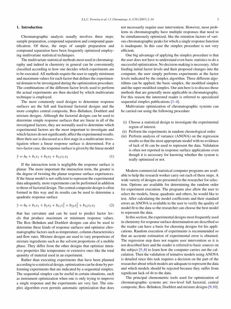
Fig. 1. Central composite designs for two and three factors. The gray dots formts

av

oDa

dpqa

S.L.C. Ferreira et al. / J. C

. Factorial and central composite designs

Central composite designs (CCD) combine [5–8] two-levelull or fractional factorial designs with additional axial or staroints and at least one point at the center of the experimentalegion being investigated. It allows the determination of bothinear and quadratic models. The CCD is a better alternative tohe full factorial three-level design since it demands a smallerumber of experiments while providing comparable results.

In general, a CCD for k factors, coded as (x1, . . ., xk), consistsf three parts:

1) A factorial (or cubic) design, containing a total of nfact pointswith coordinates xi = −1 or xi = +1, for i = 1, . . ., k;

2) An axial (or star) part, formed by nax = 2k points with alltheir coordinates null except for one that is set equal to acertain value α (or −α);

3) A total of nc runs performed at the center point, where, ofcourse, x1 = . . . xk = 0.

To build a central composite design, we need to specify eachf these three parts. We have to decide how many cubic points tose and where they will be, what will be the value of α, and howany replicate runs should be conducted at the center point. Two

esigns are presented in Table 1 and Fig. 1. The design on theeft accommodates two factors. The first four runs (22 factorialesign) make up the cubic part, the star design the last four (with= √

2) and there are three replicate runs at the center point.he three-factor case on the right has 23 = 8 runs with four centeroints and six axial points with α = 1.683.

Note that the codified values given in Table 1 only spec-fy the relative positions of the experimental design points. Inart, this determines the precision of the model coefficients andhe values predicted by the model. The researcher defines the

able 1oded factor levels for central composite designs for two- and three-factor

ystems

wo-factor Three-factor

1 x2 x1 x2 x3

1 −1 −1 −1 −11 −1 1 −1 −11 1 −1 1 −11 1 1 1 −10 0 −1 −1 10 0 1 −1 10 0 −1 1 11.414 0 1 1 11.414 0 0 0 00 −1.414 0 0 00 −1.414 0 0 0

0 0 0−1.683 0 0

1.683 0 00 −1.683 00 1.683 00 0 −1.6830 0 1.683

y

tlofabca

t(opwotdovoo

he cubic part—the runs of the 22 and 23 factorial. The black dots represent thetar parts.

ctual laboratory values that are linearly related to the codifiedalues.

The cubic points in Table 1 and Fig. 1 are the same as thosef full factorial designs although this is not strictly necessary.epending on the number of factors, it might even be unadvis-

ble, because it would require too many experiments.The total number of distinct levels in a central composite

esign is nfact + 2k + 1. Therefore, there are 2k + 2k + C0 totaloints where C0 is the number of center points. The completeuadratic model for k factors contains (k + 1)(k + 2)/2 parametersnd is given by

= β0 +∑

i

βixi +∑

i

βiix2i +

∑i<j

∑j

βijxixj + ε. (3)

With two factors, this model has six parameters. Since thewo-factor design in Table 1 has nine different combinations ofevels, we could estimate all of the model’s parameters usingnly two cubic points, corresponding to one of the two 22−1

ractions. In such a simple design, the economy is very smallnd hardly justifies destroying the symmetry of the cubic part,ut this procedure – choosing a fractional design instead of aomplete factorial to define the cubic points – becomes morettractive as the number of factors increases.

The value of α usually ranges from 1 to√

k. When α = √k,

he cubic and axial points are located on the (hyper)surface of ahyper)sphere, and the design is called spherical. This is the casef the two-factor design in Table 1 where all of the peripheraloints are on the circumference of a circle. At the other extreme,hen α = 1, the axial points are located at the centers of the sidesf the square part of the two-factor design and at the center ofhe faces of the cubic part of the three-factor design. This type ofesign is advantageous when the experimental space is squarer cubical, which occurs in a natural way when the factors are

aried independently of one another. It also has the advantagef only requiring three factor levels, which can be a big help ifne of the factors is qualitative.

Page 4

hroma

fcbrbba

cattawta5watthie

ppttir

ctiowiwTdta

sficnwd

α

wi

wrdaTaas

2o

tstttpcdam[mT

dw

couTi

lisscmustlwta

3

S.L.C. Ferreira et al. / J. C

If we choose α = √k, the star points will be placed farther

rom the center point as the number of factors increases. Thishoice should be made – if it is made at all – with much care,ecause we run the risk of leaving too much of the intermediateegion uninvestigated. With nine factors, for example, α woulde equal to 3. The experiments would tell us nothing about theehavior of the response surface in the 1–3 intervals along eachxis.

Box and Hunter [11] proposed the rotatability concept as ariterion for choosing the value of α. A design is called rotat-ble if the variance of its estimates, V(y), depends solely onhe distance from the center point, that is, if the precision ofhe predicted response is the same for all points situated on

(hyper)sphere around the center of the design. For a designhose cubic portion is a complete factorial or a fractional fac-

orial of resolution V, it can be demonstrated that rotatability isttained when α = 4

√nfact. Even if the resolution is not exactly

, this expression serves as a guide for choosing an α value,hich in any case should also be analyzed for its convenience

nd feasibility. If, for example, we are interested in investigatinghe region closer to the faces of the hypercube, then it is bettero choose an α value smaller than the rotatable one. On the otherand, it could happen that the chosen α value results in somempracticable runs. In this case, we would have to define newxperimental conditions for these runs.

The replicates at the center point have two main objectives:rovide a measure of pure error and stabilize the variance of theredicted response. To stabilize the variance, a rule of thumb iso make 3–5 repeated runs if α is close to

√k, and only one or

wo if it is close to 1. Between these extremes, 2–4 replicates arendicated. To obtain a more precise estimate of error, the moreeplicates the better.

Since three distinct parts form central composite designs, wean build them sequentially, according to necessity. If we happeno be in a region of the response surface where curvature is notmportant, there is no need to fit a quadratic model. The cubic partf the design is sufficient for fitting a linear model, from whiche can rapidly move to a more interesting region extending the

nvestigation. Even if we are in doubt about possible curvature,e can test its significance using the runs at the center point.hen, if the curvature is found significant, we can complete theesign with the axial points. Actually, we would be performinghe runs of the complete design in two blocks—first the cubicnd then the axial one.

Suppose that the response values in the axial block contain aystematic error in relation to the response values obtained in therst block. Under certain conditions, this error will not affect theoefficient estimates for the model, that is, the block effect willot confound itself with the effects of the other factors. Thisill occur if the design blocking is orthogonal, which in turnepends on the α value. Blocking will be orthogonal if√

nfact(nax + nc,ax)

=2(nfact + nc,fact)

, (4)

here nc,fact and nc,ax are the number of runs at the center pointn the cubic and axial blocks, respectively [6]. In general, when

crff

togr. A 1158 (2007) 2–14 5

e make a design with orthogonal blocks we are sacrificing itsotatability, but some designs do exist for which the two con-itions are approximately satisfied, and others for which bothre exactly satisfied. For example, the two factorial design inable 1 is both rotatable and orthogonal although the rotat-ble three-factor design is only approximately orthogonal. Morebout CCD can be found in several excellent texts on responseurface methodology [12–14].

.1. Application of central composite designs forptimization of chromatographic systems

The central composite design is one of the chemometricsechniques most employed for optimization of chromatographicystems [15,57–90]. It has been used for the determina-ion of the critical conditions of experimental factors duringhe optimization of extraction steps [15,57–66], derivatiza-ion reactions [67–69], separation steps [70–88], quantificationrocesses [89] and also robustness studies [90] involved inhromatographic methods. These methods were performed foretermination of organic and inorganic species in samples suchs water [15,68,71,72,75,88], drugs [69,73,79,85], biologicalatrices [59,62,67,74,82,86], wines [70,77], human plasma

63,65,66,78] and others. These applications using several chro-atographic techniques for quantification are summarized inable 2.

Other applications include use of the central compositeesign for optimizing the preparation of zirconized silica, whichas characterized for use as support in HPLC [16].Another paper proposes the modification of silica with zir-

onium oxide followed by sorption and thermal immobilizationf poly(methyltetradecylsiloxane) (PMTDS). This material wassed for preparation of a reversed stationary phase for HPLC.he immobilization step was optimized using a central compos-

te design [17].An off-line system consisting of ion-pair reversed-phase

iquid chromatography was proposed for separating arsen-te, arsenate, monomethylarsonate, dimethylarsinate, selenite,elenate, selenocystamine, selenocystine, selenomethionine andelenoethionine. Elution conditions were optimized using theentral composite design. The method was applied for the deter-ination of these species in the environment and in mammals,

sing as analytical technique graphite furnace atomic absorptionpectrometry [18]. Another paper by this research group usedhis system for the separation and determination of monomethy-arsonate, dimethylarsinate, selenomethionine and selenite in tapater employing inductively coupled plasma mass spectrome-

ry. The optimization of the separation step was also done usingcentral composite design [19].

. Box–Behnken designs

Box–Behnken designs constitute an alternative to central

omposite designs [20]. They are a class of rotatable or nearlyotatable second-order designs based on three-level incompleteactorial designs. Fig. 2 shows the Box–Behnken design for threeactors, corresponding to the coded values listed in Table 3. It is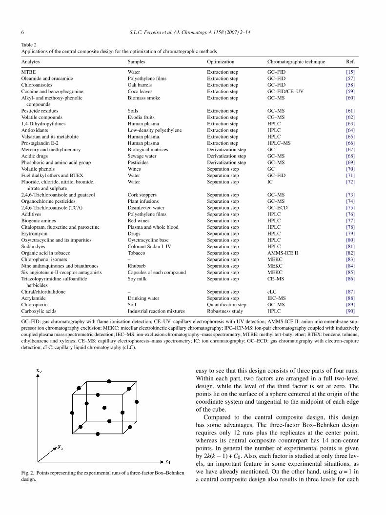

Page 5

6 S.L.C. Ferreira et al. / J. Chromatogr. A 1158 (2007) 2–14

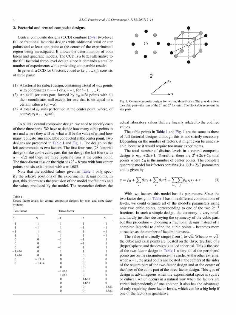
Table 2Applications of the central composite design for the optimization of chromatographic methods

Analytes Samples Optimization Chromatographic technique Ref.

MTBE Water Extraction step GC–FID [15]Oleamide and erucamide Polyethylene films Extraction step GC–FID [57]Chloroanisoles Oak barrels Extraction step GC–FID [58]Cocaine and benzoylecgonine Coca leaves Extraction step GC–FID/CE–UV [59]Alkyl- and methoxy-phenolic

compoundsBiomass smoke Extraction step GC–MS [60]

Pesticide residues Soils Extraction step GC–MS [61]Volatile compounds Evodia fruits Extraction step CG–MS [62]1,4-Dihydropyfidines Human plasma Extraction step HPLC [63]Antioxidants Low-density polyethylene Extraction step HPLC [64]Valsartan and its metabolite Human plasma. Extraction step HPLC [65]Prostaglandin E-2 Human plasma Extraction step HPLC–MS [66]Mercury and methylmercury Biological matrices Derivatization step GC [67]Acidic drugs Sewage water Derivatization step GC–MS [68]Phosphoric and amino acid group Pesticides Derivatization step GC–MS [69]Volatile phenols Wines Separation step GC [70]Fuel dialkyl ethers and BTEX Water Separation step GC–FID [71]Fluoride, chloride, nitrite, bromide,

nitrate and sulphateWater Separation step IC [72]

2,4,6-Trichloroanisole and guaiacol Cork stoppers Separation step GC–MS [73]Organochlorine pesticides Plant infusions Separation step GC–MS [74]2,4,6-Trichloroanisole (TCA) Disinfected water Separation step GC–ECD [75]Additives Polyethylene films Separation step HPLC [76]Biogenic amines Red wines Separation step HPLC [77]Citalopram, fluoxetine and paroxetine Plasma and whole blood Separation step HPLC [78]Erytromycin Drugs Separation step HPLC [79]Oxytetracycline and its impurities Oytetracycline base Separation step HPLC [80]Sudan dyes Colorant Sudan I–IV Separation step HPLC [81]Organic acid in tobacco Tobacco Separation step AMMS-ICE II [82]Chlorophenol isomers – Separation step MEKC [83]Nine anthraquinones and bianthrones Rhubarb Separation step MEKC [84]Six angiotensin-II-receptor antagonists Capsules of each compound Separation step MEKC [85]Triazolopyrimidine sulfoanilide

herbicidesSoy milk Separation step CE–MS [86]

Chiral/chlorthalidone – Separation step cLC [87]Acrylamide Drinking water Separation step IEC–MS [88]Chloropicrin Soil Quantification step GC–MS [89]Carboxylic acids Industrial reaction mixtures Robustness study HPLC [90]

GC–FID: gas chromatography with flame ionisation detection; CE–UV: capillary electrophoresis with UV detection; AMMS-ICE II: anion micromembrane sup-pressor ion chromatography exclusion; MEKC: micellar electrokinetic capillary chromatography; IPC–ICP-MS: ion-pair chromatography coupled with inductivelycoupled plasma mass spectrometric detection; IEC–MS: ion-exclusion chromatography–mass spectrometry; MTBE: methyl tert-butyl ether; BTEX: benzene, toluene,ethylbenzene and xylenes; CE–MS: capillary electrophoresis–mass spectrometry; ICdetection; cLC: capillary liquid chromatography (cLC).

Fig. 2. Points representing the experimental runs of a three-factor Box–Behnkendesign.

eWdpco

hrwpbewa

: ion chromatography; GC–ECD: gas chromatography with electron-capture

asy to see that this design consists of three parts of four runs.ithin each part, two factors are arranged in a full two-level

esign, while the level of the third factor is set at zero. Theoints lie on the surface of a sphere centered at the origin of theoordinate system and tangential to the midpoint of each edgef the cube.

Compared to the central composite design, this designas some advantages. The three-factor Box–Behnken designequires only 12 runs plus the replicates at the center point,hereas its central composite counterpart has 14 non-centeroints. In general the number of experimental points is given

y 2k(k − 1) + C0. Also, each factor is studied at only three lev-ls, an important feature in some experimental situations, ase have already mentioned. On the other hand, using α = 1 incentral composite design also results in three levels for each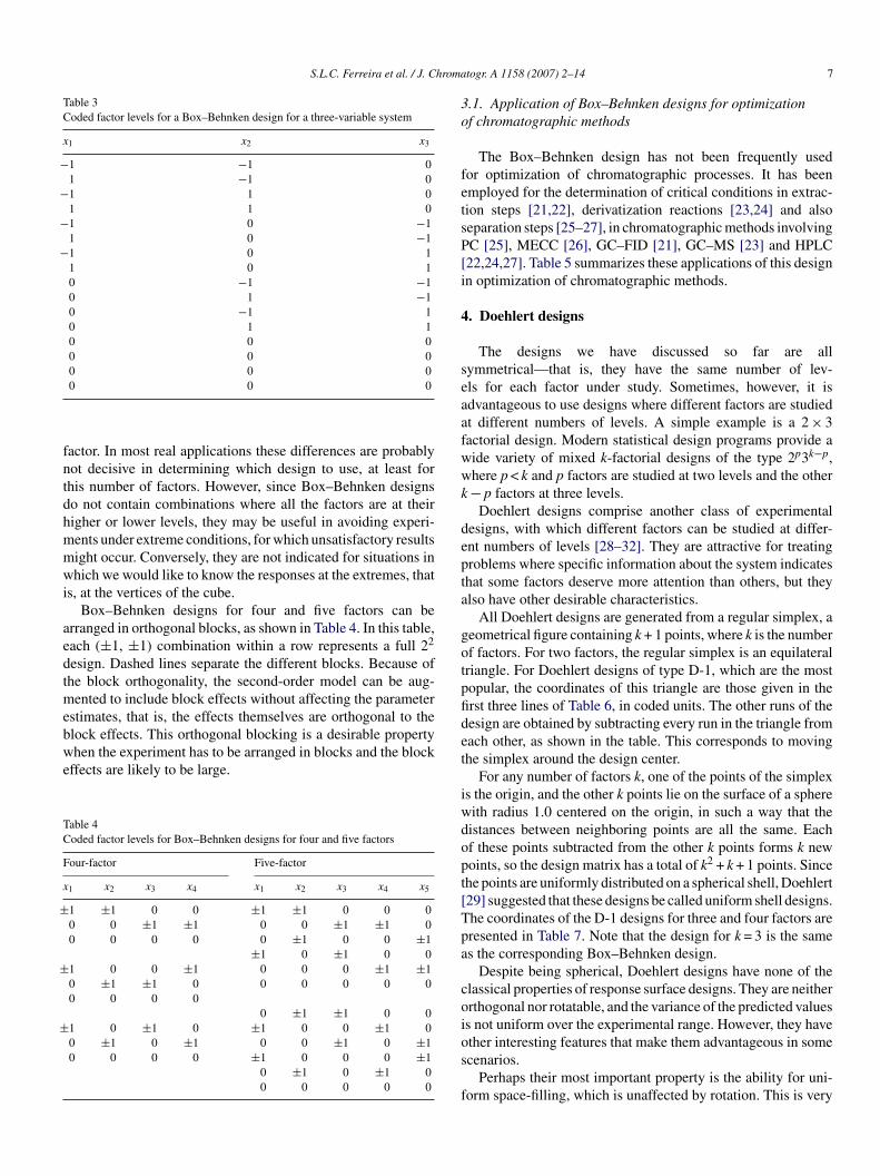

Page 6

S.L.C. Ferreira et al. / J. Chroma

Table 3Coded factor levels for a Box–Behnken design for a three-variable system

x1 x2 x3

−1 −1 01 −1 0

−1 1 01 1 0

−1 0 −11 0 −1

−1 0 11 0 10 −1 −10 1 −10 −1 10 1 10 0 00 0 00 0 0

fntdhmmwi

aedtmebwe

TC

F

x

±

±

±

3o

fetsP[i

4

seaafwwk

depta

gotpfide

0 0 0

actor. In most real applications these differences are probablyot decisive in determining which design to use, at least forhis number of factors. However, since Box–Behnken designso not contain combinations where all the factors are at theirigher or lower levels, they may be useful in avoiding experi-ents under extreme conditions, for which unsatisfactory resultsight occur. Conversely, they are not indicated for situations inhich we would like to know the responses at the extremes, that

s, at the vertices of the cube.Box–Behnken designs for four and five factors can be

rranged in orthogonal blocks, as shown in Table 4. In this table,ach (±1, ±1) combination within a row represents a full 22

esign. Dashed lines separate the different blocks. Because ofhe block orthogonality, the second-order model can be aug-

ented to include block effects without affecting the parameterstimates, that is, the effects themselves are orthogonal to thelock effects. This orthogonal blocking is a desirable property

hen the experiment has to be arranged in blocks and the block

ffects are likely to be large.

able 4oded factor levels for Box–Behnken designs for four and five factors

our-factor Five-factor

1 x2 x3 x4 x1 x2 x3 x4 x5

1 ±1 0 0 ±1 ±1 0 0 00 0 ±1 ±1 0 0 ±1 ±1 00 0 0 0 0 ±1 0 0 ±1

±1 0 ±1 0 01 0 0 ±1 0 0 0 ±1 ±10 ±1 ±1 0 0 0 0 0 00 0 0 0

0 ±1 ±1 0 01 0 ±1 0 ±1 0 0 ±1 00 ±1 0 ±1 0 0 ±1 0 ±10 0 0 0 ±1 0 0 0 ±1

0 ±1 0 ±1 00 0 0 0 0

t

iwdopt[Tpa

coios

f

togr. A 1158 (2007) 2–14 7

.1. Application of Box–Behnken designs for optimizationf chromatographic methods

The Box–Behnken design has not been frequently usedor optimization of chromatographic processes. It has beenmployed for the determination of critical conditions in extrac-ion steps [21,22], derivatization reactions [23,24] and alsoeparation steps [25–27], in chromatographic methods involvingC [25], MECC [26], GC–FID [21], GC–MS [23] and HPLC22,24,27]. Table 5 summarizes these applications of this designn optimization of chromatographic methods.

. Doehlert designs

The designs we have discussed so far are allymmetrical—that is, they have the same number of lev-ls for each factor under study. Sometimes, however, it isdvantageous to use designs where different factors are studiedt different numbers of levels. A simple example is a 2 × 3actorial design. Modern statistical design programs provide aide variety of mixed k-factorial designs of the type 2p3k−p,here p < k and p factors are studied at two levels and the other− p factors at three levels.

Doehlert designs comprise another class of experimentalesigns, with which different factors can be studied at differ-nt numbers of levels [28–32]. They are attractive for treatingroblems where specific information about the system indicateshat some factors deserve more attention than others, but theylso have other desirable characteristics.

All Doehlert designs are generated from a regular simplex, aeometrical figure containing k + 1 points, where k is the numberf factors. For two factors, the regular simplex is an equilateralriangle. For Doehlert designs of type D-1, which are the mostopular, the coordinates of this triangle are those given in therst three lines of Table 6, in coded units. The other runs of theesign are obtained by subtracting every run in the triangle fromach other, as shown in the table. This corresponds to movinghe simplex around the design center.

For any number of factors k, one of the points of the simplexs the origin, and the other k points lie on the surface of a sphereith radius 1.0 centered on the origin, in such a way that theistances between neighboring points are all the same. Eachf these points subtracted from the other k points forms k newoints, so the design matrix has a total of k2 + k + 1 points. Sincehe points are uniformly distributed on a spherical shell, Doehlert29] suggested that these designs be called uniform shell designs.he coordinates of the D-1 designs for three and four factors areresented in Table 7. Note that the design for k = 3 is the sames the corresponding Box–Behnken design.

Despite being spherical, Doehlert designs have none of thelassical properties of response surface designs. They are neitherrthogonal nor rotatable, and the variance of the predicted valuess not uniform over the experimental range. However, they have

ther interesting features that make them advantageous in somecenarios.

Perhaps their most important property is the ability for uni-orm space-filling, which is unaffected by rotation. This is very

Page 7

8 S.L.C. Ferreira et al. / J. Chromatogr. A 1158 (2007) 2–14

Table 5Applications of the Box–Behnken design in the optimization of chromatographic methods

Analyte Sample Optimization Chromatographic techniquea Ref.

Fatty acid composition Castor oil Extraction step GC–FID [21]Organochlorine pesticides Sediments Extraction step HPLC [22]Aminoglycoside antibiotics – Derivatization reaction GC–MS [23]Aliphatic aldehydes – Derivatization reaction HPLC [24]Aminoacids hydroxamates – Separation step PC [25]Captopril Commercial drugs Separation step HPLC [27]Mixture of sulphonamides, �-lactam

antibiotics and dehydrofolate– Separation step MECC [26]

PC: paper chromatography; MECC: micellar electrokinetic chromatography.a Analytical technique for quantification.

Table 6Coded factor levels for the two-factor Doehlert D-1 design

Run x1 x2 Subtraction

1a 0.0 0.02a 1.0 0.03a 0.5 0.8664b −1.0 0.0 1–25b −0.5 −0.866 1–36b −0.5 0.866 3–27b 0.5 −0.866 2–3

cmdpiw

aattacvlihvaAtD

TC

R

111111111122

a The runs in bold face are those defining the initial simplex.b The other runs are obtained by subtracting every run from each other.

onvenient when one wishes to cover an experimental range, noatter how irregular, with a uniform grid of points. Doehlert

esigns then can be displaced to more promising regions whilereserving some of the runs already carried out. This property isllustrated in Fig. 3. The initial two-factor design is a hexagon,here the letters BCDEFG denote its vertices. These points,

e

Db

able 7oded factor levels for the three- and four-factor Doehlert D-1 designs

un Three-factor

x1 x2 x3

1 0 0 02 1 0 03 0.5 0.866 04 0.5 0.289 0.8175 −1 0 06 −0.5 −0.866 07 −0.5 −0.289 −0.8178 0.5 −0.866 09 0.5 −0.289 −0.8170 −0.5 0.866 01 0 0.577 −0.8172 −0.5 0.289 0.8173 0 −0.577 0.81745678901

long with the A center point, define five levels for the x1 vari-ble but only three levels for x2. If the researchers decide to shifthe initial design to higher values of x1 and lower values of x2he PONLGFM hexagon can be used, which includes vertices Fnd G from the initial configuration. If experimentation is veryostly or lengthy, the values already observed for the F and Gertices can be retained. In case the researchers wish to raise theevels of both x1 and x2, displacement to the BGLKJIH hexagons warranted. This time, vertices B and G belong to the initialexagon. Finally, if it is decided to shift the levels of only oneariable, say x1, the experimenters might perform new runs onlyt the Q, R and S vertices to complete the new Doehlert designESRQCD, which has two lower levels along x1 while keeping

he same levels for x2. Note that the space-filling property ofoehlert designs is clearly illustrated in Fig. 3. No gaps in the

xperimental region are left as one hexagon substitutes another.Compared to central composite or Box–Behnken designs,

oehlert designs are more economical, especially as the num-er of factors increase. The basic hexagon in Fig. 3 has six points

Four factor

x1 x2 x3 x4

0 0 0 01 0 0 00.5 0.866 0 00.5 0.289 0.817 00.5 0.289 0.204 0.791

−1 0 0 0−0.5 −0.866 0 0−0.5 −0.289 −0.817 0−0.5 −0.289 −0.204 −0.791

0.5 −0.866 0 00.5 −0.289 −0.817 00.5 −0.289 −0.204 −0.791

−0.5 0.866 0 00 0.577 −0.817 00 0.577 −0.204 −0.791

−0.5 0.289 0.817 00 −0.577 0.817 00 0 0.613 −0.791

−0.5 0.289 0.204 0.7910 −0.577 0.204 0.7910 0 −0.613 0.791

Page 8

S.L.C. Ferreira et al. / J. Chroma

Fm

ltotpddsefipFosbFio

pcptoatmc

iTztti

tfia

cl

4c

ocDo

5

ppp

∑

ev

y

mmi

the concentration triangle shown in Fig. 4, is especially usefulfor ternary studies. The component proportions of this designare given in the middle columns of Table 9. Each point at avertex of the triangle represents a pure component or a mixture

ig. 3. Hexagonal Doehlert two-factorial design with three possible displace-ents in the experimental space.

ying on a circumference around the center point, whereas thewo-factor central composite design has eight points, also lyingn a circumference surrounding its center point. Likewise, thehree-factor Doehlert design has 13 points, but the central com-osite design requires 15. On the other hand, central compositeesigns are rotatable, a general property that Doehlert designso not have. Furthermore, since central composite designs con-ist of factorial and axial blocks, they provide the basis for anfficient sequential strategy. Linear models can be fitted in arst stage, after which the design can be augmented with com-lementary points, should quadratic models prove necessary.inally, using full designs, Doehlert or otherwise, to fit second-rder models is hardly practicable for more than four factors,ince a five factor quadratic model has twenty coefficients toe determined and it is unlikely that all factors will be relevant.ractional factorial screening designs to discriminate between

nert and relevant factors should always be applied before higherrder designs when many factors are being investigated.

Another very interesting feature of Doehlert designs is theossibility of introducing variations in new factors during theourse of an experimental study, without losing the runs alreadyerformed. Sometimes we might wish to study first – say – thewo factors that seem more promising, analyze the results, andnly then introduce variation in a third factor, then in a fourth,nd so on. With Doehlert D-1 designs this is possible, providedhat all potential factors of interest are introduced in the experi-

ents right from start, set at their average levels (that is, zero inoded units).

For example, let us say that there are four factors of potentialnterest. We can begin with the two-factor design defined inable 7, taking care to keep the levels of factors 3 and 4 fixed atero in all runs. Then, when we wish to study the influence ofhe two factors that have been kept fixed, we only have to add tohe initial design the runs corresponding to the rest of the rowsn the four-factor design in the Table 7.

As can be seen in Table 7, a Doehlert design of type D-1 withhree or more factors always has one factor at five levels (therst one), one factor at three levels (the last), and the others allt seven levels. Two other Doehlert design types, D-2 and D-3,

Fm

togr. A 1158 (2007) 2–14 9

an be generated by different simplexes and result in differentevel distributions.

.1. Application of Doehlert design for optimization ofhromatographic systems

Hu and Massart first proposed the use of Doehlert designs forptimization of methods by HPLC. Several examples of appli-ations were given [33]. Table 8 summarizes applications ofoehlert matrix for the optimization of chromatographic meth-ds.

. Mixture designs

Mixture designs [34] differ from those discussed up to thisoint since the properties of mixtures depend on ingredient pro-ortions, xi, and not on their absolute values. As such theseroportions are not independent variables since

q

i=1

xi = 1 for i = 1, 2, . . . q. (5)

As a consequence, mixture models have mathematicalxpressions that are different from those involving independentariables,

ˆ =q∑i

bixi+q∑

i�=j

q∑j

bijxixj+q∑

i�=j

q∑j �=k

q∑k

bijkxixjxk+ . . . , (6)

ost noticeably the absence of the constant b0 term. Experi-ental designs can be made for any number of components but

nvestigation of three-component systems is the most common.A simplex centroid design with axial points, presented in

ig. 4. A simplex centroid design with axial points for a three componentixture system.

Page 9

10 S.L.C. Ferreira et al. / J. Chromatogr. A 1158 (2007) 2–14

Table 8Application of Doehlert design for the optimization of chromatographic methods

Analytes Samples Optimization Chromatographic technique Ref.

Oxadiazon Ground water, agricultural soil, must,wine and human urine samples

Extraction step GC–MS [91]

Chloroanisoles Cork taint of red wine. Extraction step GC–ECD [92]Pesticides Passiflora alata infuses Extraction step GC–ECD [93]Chloroanisoles cork Cork Extraction step GC–TOF-MS [94]Heterocyclic Aromatic Amines Meat Extraction step HPLC [95]Biogenic amines – Derivatization reaction HPLC [96]Hydrocarbons Gasoline Separation step CG [97]Aromatic compounds Petroleum cuts Separation step HPLC [98]Cephalothin and its related substances – Separation step HPLC [99]Methylxanthines – Separation step HPLC [100]Mono-, di-, and polyaromatic compounds Middle distillate Separation step HPLC [101]Sodium cefazolin and related substances – Separation step HPLC [102]Cholesterol Reference materials Quantificationa CG [103]

Chloroanisoles: 2,4-dichloroanisole, 2,6-dichloroanisole, 2,4,6-trichloroanisole and pentachloroanisole; Pesticides: chlorotalonil, methyl parathion, malathion, �-e -flight

orotcpp

sas

y

hiptttr

TCd

M

1

st

mmmloh

tcpcmhct

ndosulfan and �-endosulfan; GC–TOF-MS: gas chromatography with time-ofa Estimation of the optimal amount of internal standard.

f components. The points centered on each leg of the triangleepresent 1:1 binary mixtures of the components or mixturesf their neighboring vertex points. The point in the center ofhe triangle represents a 1:1:1 ternary mixture of the three pureomponents or mixtures represented at the vertices. The axialoints contain a 2/3 portion of one of the ingredients and 1/6ortions of the other two.

This simplex centroid with axial point design is importantince it permits the evaluation and validation of linear, quadraticnd special cubic models. The special cubic model for a ternaryystem

ˆ = b1x1 + b2x2 + b3x3 + b12x1x2

+ b13x1x3 + b23x2x3 + b123x1x2x3 (7)

as seven terms. The first three represent the linear model, whichs only valid in the absence of interaction effects between com-onents, i.e. ideal solutions in physical chemistry. The next

hree terms represent synergic or antagonistic binary interac-ion effects for all possible pairs of components and, along withhe linear terms, forms the quadratic model. The last term rep-esents a ternary interaction effect and is usually important for

able 9oded pseudocomponent proportions for mobile phases of a simplex centroidesign with axial points and their resolution factor response values

ixture xACN xMeOH xTHF Resolution

1 1 0 0 0.99, 1.072 0 1 0 5.31, 5.643 0 0 1 4.12, 4.344 0.5 0.5 0 3.79, 3.985 0.5 0 0.5 3.88, 4.076 0 0.5 0.5 5.85, 6.167 0.333 0.333 0.333 5.22, 5.218 0.667 0.167 0.167 3.42, 3.509 0.167 0.667 0.167 5.80, 5.810 0.167 0.167 0.667 4.84, 4.83

pc

0

c

x

wd

5

t

mass spectrometry.

ystems having maximum or minimum values in the interior ofhe concentration triangle.

As stated earlier, each vertex can represent a chemicalixture. In this case, the optimization involves investigatingixtures of mixtures. In liquid chromatography, these chemicalixtures and/or pure components can be chosen to have simi-

ar chromatographic strengths or other properties that might aidptimization. The example discussed in a later section showsow this can be done.

Often it is not of interest or even possible to investigatehe entire range of proportion values, 0–100%, of the mixtureomponents. Many mixture optimization problems require theresence of all ingredients to form a satisfactory product. In theseases it is convenient to define pseudocomponents. Consider aixture for which the proportions of each vertex component

ave to obey non-zero lower limits, which we shall generi-ally call ai. Obviously the sum of all these limits must be lesshan one, otherwise the mixture would be impossible to pre-are. Considering the general case of a mixture containing qomponents,

≤ ai ≤ 1 andq∑

i=1

ai < 1. (8)

The levels of the mixture components in terms of pseudo-omponents, denoted by xi, are given by the expression

i = ci − ai

1 − ∑qi=1ai

for i = 1, 2 . . . q (9)

hich is a kind of variable coding like we have used for theesigns for independent variables.

.1. Model validation

The ANOVA table for model validation is the same for allhe above experimental designs and is presented in Table 10.

Page 10

S.L.C. Ferreira et al. / J. Chromatogr. A 1158 (2007) 2–14 11

Table 10Analysis of variance table for the least squares fit of a model that is linear in its parametersa

Source of variation Sum of squares Degr. freedom Mean square

Regression SSR =m∑i

ni∑j

(yi − y)2 p − 1 MSR = [SSR/(p − 1)]

Residual SSr =m∑i

ni∑j

(yij − yi)2 n − p MSr = [SSr/(n − p)]

Lack of fit SSlof =m∑i

ni∑j

(yi − yi)2 m − p MSlof = [SSlof/(m − p)]

Pure error SSpe =m∑i

ni∑j

(yij − yi)2 n − m MSpe = [SSpe/(n − m)]

Total SST =m∑i

ni∑j

(yij − y)2 n − 1

% explained variation: SSR/SST

M

ependi

ttorsspiaftLaSmcvocetitd

R

mdhfjolv

vmTplirfcotactfivFtgvetAio

5

a

aximum % explainable variation: [(SST − SSpe)/SST]

a ni: number of replicates at the ith level; m: number of distinct levels of the indn the model.

The total data variance is divided into two main contribu-ions, the sum of squares explained by the regression, SSR, andhe residual sum of squares, SSr. Both summations are takenver all the experimental design levels, i = 1,2 . . . m and all theeplicates performed at each level, j = 1,2 . . . ni. SSR is a sum ofquares of differences between values predicted by the regres-ion and the grand average of all the response values and has− 1 degrees of freedom where p is the number of coefficients

n the model. SSr is a sum of squares of differences or residu-ls between all the experimental values and the predicted valuesrom the model. It has n − p degrees of freedom where n is theotal number of experimental data used to determine the model.arge SSR and small SSr values tend to occur for models thatccurately describe the experimental data. Their sum is equal toST, the total sum of squares of differences between the experi-ental values and the grand average of the data set. This sum, of

ourse, has n − 1 degrees of freedom since it represents the totalariance in the data. The SSR/SST ratio represents the fractionf explained variation and is commonly represented as R2, theoefficient of determination that varies between 0 and 1. If purerror exists it is impossible for R2 to actually attain 1. Althoughhis coefficient is a measure of how close the model fits the data,t cannot be used to judge model lack of fit because it does notake into account the numbers of degree of freedom for modeletermination. A related statistic

2a = [1 − (1 − R2){(n − 1)/(n − p)}] (10)

akes an adjustment for the varying numbers of degrees of free-om in the models being compared. Draper and Smith [35],owever, caution against its use in comparing models obtainrom different data sets. Model quality can only be rigorously

udged if the SSr is decomposed into two contributions, the lack-f-fit and the pure error sums of squares, SSlof and SSpe. Theatter is a sum of squares of differences between all the indi-idual experimental values and the average of the experimental

ifdd

ent variables; n =∑

ni = total number of observations; p: number of parameters

alues at the same level. It has n − m degrees of freedom whereis the number of distinct levels in the experimental design.

he SSlof is a sum of squares of differences between the valuesredicted at each level and the average experimental value at thatevel and has m − p degrees of freedom. Regression lack of fits determined performing an F-test by comparing the SSlof/SSpeatio with the tabled F value for m − p and n − m degrees ofreedom at the desired confidence level, usually 95%. If the cal-ulated quotient is greater than the tabled value there is evidencef model lack of fit and the model must be discarded. If not,he model can be accepted at this confidence level as providingn adequate representation of the data. Regression significancean be tested by comparing the calculated SSR/SSr value withhe tabled F-distribution value for p − 1 and n − p degrees ofreedom. The regression is significant if the calculated values greater than the tabled one. Note that this last F-test is onlyalid for models for which there is no evidence of lack of fit.inally, since the regression model does not explain experimen-

al error the maximum percentage of explainable variation isiven by [(SST − SSpe)/SST] × 100%. Besides ANOVA modelalidation should also include an analysis of coefficient/standardrror ratios and residual plots. An example of model valida-ion of a chromatographic system is given in the next section.lthough experimental design applications are not uncommon

n the chemical literature, not all of them include informationn model validation.

.2. Optimization example

In this section, the statistical analysis for model determinationnd validation is presented. The strategy is the same for analyz-

ng the results of all the above experimental designs although theorm of the model depends on whether the variables are indepen-ent, as for the central composite, Box–Behnken and Doehlertesigns or dependent on one another as for the mixture designs.

Page 11

1 hroma

pcotxamctm

y

tifotcIFpl

mea

y

.

Mcnb

TA

V

L

Q

lnvt[

u(w5de

sn

y

tEaecn

ettnbds

2 S.L.C. Ferreira et al. / J. C

Chromatographic peak separation is very sensitive to mobilehase composition. Here peak separation results of a simplexentroid design with axial points are analyzed with emphasisn choosing and validating the correct model. Table 9 containshe acetonitrile, xACN; methanol, xMeOH; and tetrahydrofuran,THF, proportions of the mobile phase mixtures of the designlong with their corresponding resolution values. First, a linearodel was adjusted to the experimental data of only the simplex

entroid points. The axial points were temporarily removed fromhe data set for model determination so they could be used for

odel validation. The linear model is given by the equation

ˆ = 1.667xACN(±0.02)

+ 6.035xMeOH(±0.02)

+ 5.075xTHF(±0.02)

. (11)

The standard errors were calculated from a pooled estimate ofhe experimental error obtained from the seven duplicate exper-ments of the simplex centroid design. The model was testedor lack-of-fit using the ANOVA results in the upper portionf Table 11. The MSlof/MSpe is 61.46 which is larger than theabled value of F4,7 = 4.12 at the 95% confidence level. Commer-ial programs often present this result expressed as a p-value.n this case p = 0.000016, which is the area to the right of thecal = 61.46 value under the ν1 = 4, ν2 = 7 F distribution. Since< 0.05 the linear model presents evidence of lack of fit at this

evel and must be rejected.The poor agreement between the experimental values and

odel predictions may be due to the existence of interactionffects between mixture components. So a quadratic model wasdjusted to the data

ˆ = 1.013xACN(±0.12)

+ 5.458xMeOH(±0.12)

+ 4.213xTHF(±0.12)

+ 2.865xACNxMeOH(±0.50)

+5.715xACNxTHF(±0.50)

+ 4.945xMeOHxTHF(±0.50)

(12)

The ANOVA for this model is included in Table 11. The

Slof/MSpe ratio is only 3.12 which is smaller than the 95%

onfidence value of F1,7 = 5.59 (p = 0.12). Since this model doesot present evidence of lack of fit, its regression significance cane tested using the MSR/MSr ratio. This value of 213.98 is much

able 11NOVA tables for linear and quadratic models

ariation SS df MS F-test quotient

inear modelRegression 26.3462 2 13.1731 24.16Residual 5.9977 11 0.5452 –Lack of fit 5.8316 4 1.4579 61.46Pure error 0.1661 7 0.0237 –

Total 32.3439 13 2.4880

uadratic modelRegression 32.1038 5 6.4208 213.98Residual 0.2401 8 0.0300 –Lack of fit 0.0740 1 0.0740 3.12Pure error 0.1661 7 0.0237 –

Total 32.3439 13

go

Itmtmtohtowecscrcs

togr. A 1158 (2007) 2–14

arger than the tabled F5,8 value of 3.69 indicating a highly sig-ificant regression (p < 10−6). Furthermore, since the calculatedalue is more than 10 times the tabled value, we can expecthe regression model to be useful for quantitative predictions5].

The results for the axial point experiments in Table 9 weresed to further validate the model. Predicted results from Eq.12) for the three axial points are 3.37, 5.54 and 5.15 comparedith their corresponding experimental average values of 3.46,.81 and 4.84, respectively. The average error between the pre-icted and experimental averages of 0.22 is close to the pooledxperimental error of the simplex centroid design, 0.15.

An even more accurate model is expected using both theimplex centroid design and axial point results to determine aew model. This results in the equation

ˆ = 1.031xACN(±0.13)

+ 5.527xMeOH(±0.13)

+ 4.130xTHF(±0.13)

+ 3.061xACNxMeOH(±0.60)

+ 5.605xACNxTHF(±0.60)

+ 4.937xMeOHxTHF(±0.60)

(13)

hat has coefficient values very similar to those of the model inq. (12). Furthermore, the special cubic model was adjusted toll the data in Table 9 in an unsuccessful attempt to obtain anven better fit. Although it does not suffer from lack of fit, asan be expected, the coefficient of the special cubic term wasot significant at the 95% confidence level.

It remains to interpret the quadratic model in terms of theffects the different mobile phase components have on resolu-ion. Of the linear effects, methanol is more efficient at separatinghese two peaks followed closely by THF while acetonitrile isot particularly effective. Furthermore, there are three synergicinary interaction effects that are significant at the 95% confi-ence level since the standard error of ±0.60 is at least five timesmaller than the binary interaction coefficients. Of these syner-ic interactions, the ones between acetonitrile and THF and thether between methanol and THF are the most important.

The contour plot for the response surface is shown in Fig. 5.t is clearly seen that the optimum separation factor occurs closeo the 1:1 binary mixture of methanol and THF, i.e. the experi-

ental point that has the largest average value in Table 9. In fact,he optimum mixture is a little richer in methanol, about 60%

ethanol and 40% THF. Certainly, the large synergic interac-ion between methanol and THF as well as the large linear effectsf methanol and THF relative to the small one for acetonitrileelps understand why this solution gives the best separation forhis pair of peaks. The above example involves the modelingf only one elementary response function. A real applicationould involve the simultaneous optimization of a number of

lementary response functions. Evidence so far seems to indi-ate that it is more efficient to model each elementary responseeparately and then apply a multi-criteria decision-making pro-

edure such as the Derringer and Suich desirability functionather than combine several elementary responses into a moreomplex objective function that could be used to determine aingle response surface [36,37].

Page 12

S.L.C. Ferreira et al. / J. Chroma

Fp

5c

maoe

tieo(oc

6o

utp

tTbSc

7

goO

thc

mctmR

o

ti

A

vAFfRaf

R

ig. 5. Mixture response contour map of the separation factor of two componenteaks for different acetonitrile, methanol and tetrahydrofuran concentrations.

.3. Application of mixture design for optimization ofhromatographic methods

The mixture design was employed for optimization of theobile phase of an HPLC method proposed for the separation

nd determination of benzodiazepines: triazolam, de-moxepam,xazepam, flunitrazepam, nitrazepam, clon-azepam, diazepam,thyl loflazepate and nordazepam [38].

Vuorela and co-workers developed a computer program forhe mobile phase optimization of a HPLC method. A desirabil-ty function technique combined with the mixture design wasmployed to enhance the quality of HPLC separations. The usef statistical models to predict the behaviour of retention timest(R)) and band broadening at the different eluent compositionsbtained by prisma method was examined for dansyl amides andoumarins [39].

. Other experimental designs used for the optimizationf chromatographic methods

In chromatography, the two-level full factorial has been oftensed for the optimization of the extraction steps and also forhe determination of the experimental conditions for separationrocesses [40–50].

The full three-level factorial design (3k) can be used alsoo obtain quadratic models and determine critical conditions.his design has been little used because it requires quite a num-er of experiments if the factor number is higher than 2 [51].ome authors have employed this design for optimization ofhromatographic methods [52–56].

. Conclusion

Multivariate statistical techniques applied to chromato-raphic methods have been basically employed for optimizationf the steps of sample preparation and compound separation.f the response surface techniques, the Box–Behnken design,

togr. A 1158 (2007) 2–14 13

he Doehlert matrix and the central composite design, the latteras been the one more frequently used for the optimization ofhromatographic methods.

Statistical mixture designs are recommended for the opti-ization of mobile phase, where the proportions of the

omponents determine chromatographic peak separation and notheir total amounts. Model validation using F-distribution tests,

odel coefficient standard errors, residual plots and the adjusted2a statistic is recommended if one must guarantee that the actualptimum experimental conditions have been found.

The two-level full factorial design has often been used forhe preliminary evaluation of those experimental factors that aremportant for the optimization of chromatographic systems.

cknowledgements

The authors are grateful for Conselho Nacional de Desen-olvimento Cientıfico e Tecnologico (CNPq), Coordenacao deperfeicoamento de Pessoal do Ensino Superior (CAPES), andundacao de Amparo a Pesquisa do Estado da Bahia (FAPESB)or financial support and fellowship. S.L.C.F., J.B.A., B.B.N,.E.B., C.M.Q. and J.M.D. acknowledge senior research schol-rships from CNPq. M.C.B. thanks Fapesp for a master’sellowship.

eferences

[1] S.N. Deming, in: B.R. Kowalski (Ed.), Chemometrics, Mathematics andStatistics in Chemistry, Reidel, Dordrecht, 1981.

[2] J.A. Nelder, R. Mead, Comput. J. 7 (1965) 308.[3] W. Spendley, G.R. Hext, F.R. Himsworth, Technometrics 4 (1962) 441.[4] M.W. Routh, P.A. Swartz, M.B. Denton, Anal. Chem. 49 (1977) 1422.[5] G.E.P. Box, J.S. Hunter, W.G. Hunter, Statistics for Experimenters, second

ed., Wiley-Interscience, New York, 2005.[6] D.C. Montgomery, Design and Analysis of Experiments, fourth ed.,

Wiley, New York, 1997.[7] R.E. Bruns, I.S. Scarminio, B.B. Neto, Statistical Design—

Chemometrics, Elsevier, Amsterdam, 2006.[8] G.E.P. Box, K.B. Wilson, J. R. Statist. Soc. B13 (1951) 1.[9] Y. Vander Heyden, C. Perrin, D.L. Massart, in: K. Valko (Ed.), Handbook

of Analytical Separations, 1, Elsevier, Amsterdam, 2000, Ch. 6.[10] A.M. Siouffi, R. Phan-Tan-Luu, J. Chromatogr. A 892 (2000) 75.[11] G.E.P. Box, J.S. Hunter, Ann. Math. Stat. 28 (1957) 195.[12] G.E.P. Box, N.R. Draper, Empirical Model-Building and Response Sur-

faces, Wiley, New York, 1987.[13] R.H. Myers, D.C. Montgomery, Response Surface Methodology: Pro-

cess and Product Optimization Using Designed Experiments, second ed.,Wiley, New York, 2002.

[14] J. Goupy, Plans d’Experiences pour Surfaces de Response, Dunod, Paris,1999.

[15] J. Dron, R. Garcia, E. Millan, J. Chromatogr. A 963 (2002) 259.[16] A.M. Faria, D.R. Magalhaes, K.E. Collins, C.H. Collins, Anal. Chim.

Acta 550 (2005) 137.[17] A.M. Faria, K.E. Collins, C.H. Collins, J. Chromatogr. A 1122 (2006)

114.[18] B. Do, S. Robinet, D. Pradeau, F. Guyon, J. Chromatogr. A 918 (2001)

87.[19] B. Do, S. Robinet, D. Pradeau, F. Guyon, Analyst 126 (2001) 594.

[20] G.E.P. Box, D.W. Behnken, Technometrics 2 (1960) 195.[21] C. Turner, L.C. Whitehand, T. Nguyen, T. McKenon, J. Agric. Food Chem.

52 (2004) 26.[22] M. Gferer, E. Lankmayr, Anal. Chim. Acta 533 (2005) 203.[23] M. Preu, D. Guyot, M. Petz, J. Chromatogr. A 818 (1998) 95.

Page 13

1 hroma

4 S.L.C. Ferreira et al. / J. C

[24] A. Stafiej, K. Pyrzynska, A. Ranz, E. Lankmayr, J. Biochem. Biophys.Methods 69 (2006) 15.

[25] F.H. Walters, H.C. Qiu, Anal. Lett. 25 (1992) 1131.[26] M.E.P. Hows, D. Perrett, J. Kay, J. Chromatogr. A 768 (1997) 97.[27] T. Mirza, H.S.I. Tan, J. Pharm. Biomed. Anal. 25 (2001) 39.[28] D.H. Doehlert, Appl. Statist. 19 (1970) 231.[29] D.H. Doehlert, V.L. Klee, Discrete Math. 2 (1972) 309.[30] D.L. Massart, B.G.M. Vandeginste, L.M.C. Buydens, S. de Jong, P.J.

Lewi, J. Smeyers-Verbeke, Handbook of Chemometrics and Qualimet-rics. Part A, Elsevier, Amsterdam, 1977.

[31] S.L.C. Ferreira, W.N.L. dos Santos, C.M. Quintella, B.B. Neto, J.M.Bosque-Sendra, Talanta 63 (2004) 1061.

[32] B.B. Neto, I.S. Scarminio, R.E. Bruns, Quim. Nova 29 (2006) 1401.[33] Y. Hu, D.L. Massart, J. Chromatogr. 485 (1989) 311.[34] J.A. Cornell, Experiments with Mixtures: Designs, Models and the Anal-

ysis of Mixture Data, Wiley, New York, 1990.[35] N.R. Draper, H. Smith, Applied Regression Analysis, Wiley, New York,

1981.[36] G. Derringer, R. Suich, J. Qual. Technol. 12 (1980) 214.[37] M.C. Breitkreitz, I.C.S.F. Jardim, R.E. Bruns, Presented at the 10th Inter-

national Conference on Chemometrics in Analytical Chemistry, Aguasde Lindoia, 10–15 September 2006, abstract P083.

[38] P.F. Vanbel, B.L. Tilquin, P. Schoenmakers, Chemom. Intell. Lab. Syst.35 (1996) 67.

[39] K. Outinen, H. Haario, P. Vuorela, M. Nyman, E. Ukkonen, H. Vuorela,Eur. J. Pharm. Sci. 6 (1998) 197.

[40] A. Padilla, M. Palma, C.G. Barroso, J. Chromatogr. A 1091 (2005) 83.[41] K. Novotna, J. Havlis, J. Havel, J. Chromatogr. A 1096 (2005) 50.[42] N. Jakobsson, M. Degerman, B. Nilsson, J. Chromatogr. A 1099 (2005)

157.[43] M. Polo, M. Llompart, C. Garcia-Jares, G. Gomez-Noya, M.H. Bollain,

R. Cela, J. Chromatogr. A 1124 (2006) 11.[44] M.D. Cantu, D.R. Toso, C.A. Lacerda, F.M. Lancas, E. Carrilho, M.E.

Queiroz, Anal. Bioanal. Chem. 386 (2006) 256.[45] V. Yusa, A. Pastor, M. Guardia de la, Anal. Chim. Acta 565 (2006) 103.[46] A.K. Dutta, B.A. Avery, C.M. Wyandt, J. Chromatogr. A 1110 (2006) 35.[47] V. Casas, M. Llompart, C. Garcia-Jares, R. Cela, T. Dagnac, J. Chro-

matogr. A 1124 (2006) 148.[48] L. Hlabangana, S. Hernandez-Cassou, J. Saurina, J. Chromatogr. A 1130

(2006) 130.[49] O. Anurukvorakun, W. Suntornsuk, L. Suntornsuk, R. Yekkala, S. Van-

denwayenberg, J. Hoogmartens, E. Adams, J. Chromatogr. A 1134 (2006)326.

[50] R. Yekkala, S. Vandenwayenberg, J. Hoogmartens, E. Adams, J. Chro-matogr. A 1134 (2006) 56.

[51] W.N.L. dos Santos, F. de S. Dias, M.S. Fernandes, M.V. Reboucas, M.G.R.Vale, B. Welz, S.L.C. Ferreira, J. Anal. At. Spectrom. 20 (2005) 127.

[52] S. Hillaert, Y. Vander Heyden, W. Van den Bossche, J. Chromatogr. A978 (2002) 231.

[53] S. Hillaert, W. Van den Bossche, J. Chromatogr. A 979 (2002) 323.[54] V. Harang, S.P. Jacobsson, D. Westerlund, Electrophoresis 25 (2004)

1792.[55] N.M. de Aragao, M.C.C. Veloso, M.S. Bispo, S.L.C. Ferreira, J.B. de

Andrade, Talanta 67 (2005) 1007.[56] J.B. de Andrade, E.T. Souza, F.M. Rodrigues, C.C. Martins, F. Oliveira

Santos, P.A.P. Pereira, Microchem. J. 82 (2006) 142.[57] A. Garrido-Lopez, V. Esquiu, T.M. Tena, J. Chromatogr. A 1124 (2006)

51.[58] C. Pizarro, J.M. Gonzalez-Saiz, N. Perez-del-Notario, J. Chromatogr. A

1132 (2006) 8.[59] A. Brachet, S. Rudaz, L. Mateua, P. Christen, J.L. Veuthey, J. Sep. Sci.

24 (2001) 865.[60] F.J. Conde, A.M. Afonso, V. Gonzalez, J.H. Ayala, Anal. Bioanal. Chem.

385 (2006) 1162.[61] C. Goncalves, J.J. Carvalho, M.A. Azenha, M.F. Alpendurada, J. Chro-

matogr. A 1110 (2006) 6.[62] F. Pellati, S. Benvenuti, F. Yoshizaki, D. Bertelli, M.C. Rossi, J. Chro-

matogr. A 1087 (2005) 265.

togr. A 1158 (2007) 2–14

[63] A.B. Baranda, N. Etexbarria, R.M. Jimenez, R.M. Alonso, Talanta 67(2005) 933.

[64] M.S.D. Garcia, J.M. Lopez, R. Bouza, M.J. Abad, E.G. Soto, M.V.G.Rodriguez, Anal. Chim. Acta 521 (2004) 179.

[65] G. Iriarte, N. Ferreiros, I. Ibarrondo, R.M. Alonso, M.I. Maguregi, L.Gonzalez, R.M. Jimenez, J. Sep. Sci. 29 (2006) 2265.

[66] P. Araujo, L. Froyland, J. Choromatogr. B 830 (2006) 212.[67] R. Rodil, A.M. Carro, R.A. Lorenzo, M. Abuin, R. Cela, J. Chromatogr.

A 963 (2002) 313.[68] I. Rodriguez, J.B. Quintana, J. Carpinteiro, A.M. Carro, R.A. Lorenzo,

R. Cela, J. Chromatogr. A 985 (2003) 265.[69] C.D. Stalikas, G.A. Pilidis, J. Chromatogr. A 872 (2000) 215.[70] R. Castro Mejias, R. Natera Marin, M.D. Garcia Moreno, C. Garcia

Barroso, J. Chromatogr. A 995 (2003) 11.[71] I. Arambiri, M. Lasa, R. Garcia, E. Millan, J. Chromatogr. A 1033 (2004)

193.[72] M. Nowak, A. Seubert, J. Chromatogr. A 855 (1999) 91.[73] O. Ezquerro, A. Garrido-Lopez, M.T. Tena, J. Chromatogr. A 1102 (2006)

18.[74] M.V.N. Rodrigues, F.G.R. Reyes, V.L.G. Rehder, S. Rath, Chro-

matographia 61 (2005) 291.[75] P.B.M. Pinheiro, J.C.G. Esteves da Silva, Anal. Bioanal. Chem. 382

(2005) 341.[76] A. Garrido-Lopez, M.T. Tena, J. Chromatogr. A 1099 (2005) 75.[77] N. Garcia-Villar, J. Saurina, S. Hernandez-Cassou, Anal. Chim. Acta 575

(2006) 97.[78] L. Kristoffersen, A. Bugge, E. Lundanes, L. Slordal, J. Chromatogr. B

734 (1999) 229.[79] V. Harang, D. Westerlund, Chromatographia 50 (1999) 525.[80] J. Diana, G. Ping, E. Roets, J. Hoogmartens, Chromatographia 56 (2002)

313.[81] Y.P. Zhang, Y.J. Zhang, W.J. Gong, A.I. Gopalan, K.P. Lee, J. Chromatogr.

A 1098 (2005) 183.[82] J.S. Qiu, X.H. Jin, J. Chromatogr. A 950 (2002) 81.[83] M.R. Hadjmohammadi, F. Safa, J. Sep. Sci. 27 (2004) 997.[84] C.H. Kuo, S.W. Sun, Anal. Chim. Acta 482 (2003) 47.[85] S. Hillaert, T.R.M. De Beer, J.O. De Beer, W. Van den Bossche, J. Chro-

matogr. A 984 (2003) 135.[86] J. Hernandez-Borges, M.A. Rodriguez-Delgado, F.J. Garcia-Montelongo,

A. Cifuentes, J. Sep. Sci. 28 (2005) 948.[87] D. Mangelinas, M. Maftouh, D.L. Massart, Y.V. Heyden, J. Pharm.

Biomed. Anal. 35 (2004) 789.[88] S. Cavalli, S. Polosello, G. Sacan, J. Chromatogr. A 1039 (2004) 155.[89] B. Muir, W.A. Carrick, D.B. Cooper, Analyst 127 (2002) 1198.[90] E. Destandau, J. Vial, A. Jardy, M.C. Hennion, D. Bonnet, P. Lancelin,

Anal. Chim. Acta 572 (2006) 102.[91] A. Navalon, A. Prieto, L. Araujo, J.L. Vılchez, J. Chromatogr. A 946

(2002) 239.[92] A. Martınez-Urunuela, J.M. Gonzalez-Saiz, C. Pizarro, J. Chromatogr. A

1056 (2004) 49.[93] G.A. da Silva, F. Augusto, R.J. Poppi, J. Chromatogr. A 1138 (2007)

251.[94] E. Carasek, E. Cudjoe, J. Pawliszyn, J. Chromatogr. A 1138 (2007) 10.[95] L. Cardenes, A. Martin-Calero, J. Ayala, V. Gonzalez, A. Afonso, Anal.

Lett. 39 (2006) 405.[96] R. Romero, M.G. Bagur, M. Sanchez-Vinas, D. Gazquez, Chro-

matographia 51 (2000) 404.[97] J.P. Durand, S. Gautier, E. Robert, M.C. Guilhem, R. Phan-Tan-Luu, J.

High Resolut. Chromatogr. 20 (1997) 289.[98] R. Fraile, V. Sanchez, J. High Resolut. Chromatogr. 16 (1993) 169.[99] L. Ding, K. Ni, Y. Chen, Y. Hu, R. Yu, SEPU 11 (1993) 293.

[100] P. Araujo, Trends Anal. Chem. 19 (2000) 524.[101] R. M’Hamdi, D. Thiebaut, M. Caude, E. Robert, C. Grand, J. High Res-

olut. Chromatogr. 21 (1997) 94.[102] L. Ding, K. Ni, Y. Chen, Y. Hu, S. Qiu, R. Yu, Yaowu Fenxi Zazhi 15

(1995) 3.[103] P. Araujo, F. Couillard, E. Leirnes, K. Ask, A. Bøkevoll, L. Frøyland, J.

Chromatogr. A A1121 (2006) 99.