12/8/12 Statistical Computing with R: A tutorial 1/25 math.illinoisstate.edu/dhkim/rstuff/rtutor.html ISU MAT 356 R Tutorial, Spring 2004 0. R Basics 0.1. What is R? R is a software package especially suitable for data analysis and graphical representation. Functions and results of analysis are all stored as objects, allowing easy function modification a language, tool, and environment in one convenient package. It is very flexible and highly customizable. Excellent graphical tools make R an ideal environment for EDA (Exploratory Data Analysis). Since most high level functions are written in R la language by studying the function code. On the other hand, R has a few weaknesses. For example, R is not particularly efficient in handling large data sets. Also, it is rather slow in executing a large number of for loops, compa C/C++. Learning curve is somewhat steep compared to "point and click" software. 0.2 Where do I get R? There are versions for Unix, Windows, and Macintosh. All of them are free, and Windows version is downloadable at: http://cran.us.r-project.org/bin/windows and follow the download instructions. 0.3 Invoking R If properly installed, usually R has a shortcut icon on the desktop screen and/or you can find it under Start|Programs|R menu. If not, search and run the executable file rgui.exe by double window. To quit R, type q() at the R prompt (> ) and press Enter key. A dialog box will ask whether to save the objects you have created during the session so that they will become available n this time. Commands you entered can be easily recalled and modified. Just by hitting the arrow keys in the keyboard, you can navigate through the recently entered commands. > objects() # list the names of all objects > rm(data1) #remove the object named data1 from the current environment 1. Graphics: a few examples In addition to standard plots such as histogram, bar charts, pie charts and so forth, R provides an impressive array of graphical tools. The following series of plots shows a few of the ex

Statistical Computing With R_ a Tutorial
Dec 29, 2015
R software
Welcome message from author
This document is posted to help you gain knowledge. Please leave a comment to let me know what you think about it! Share it to your friends and learn new things together.
Transcript

12/8/12 Statistical Computing with R: A tutorial
1/25math.illinoisstate.edu/dhkim/rstuff/rtutor.html
ISU MAT 356 R Tutorial, Spring 20040. R Basics
0.1. What is R?
R is a software package especially suitable for data analysis and graphical representation. Functions and results of analysis are all stored as objects, allowing easy function modification and model building. R provides the
language, tool, and environment in one convenient package.
It is very flexible and highly customizable. Excellent graphical tools make R an ideal environment for EDA (Exploratory Data Analysis). Since most high level functions are written in R language itself, you can learn the
language by studying the function code.
On the other hand, R has a few weaknesses. For example, R is not particularly efficient in handling large data sets. Also, it is rather slow in executing a large number of for loops, compared to compiler languages such as
C/C++. Learning curve is somewhat steep compared to "point and click" software.
0.2 Where do I get R?
There are versions for Unix, Windows, and Macintosh. All of them are free, and Windows version is downloadable at:
http://cran.us.r-project.org/bin/windows
and follow the download instructions.
0.3 Invoking R
If properly installed, usually R has a shortcut icon on the desktop screen and/or you can find it under Start|Programs|R menu. If not, search and run the executable file rgui.exe by double clicking from the search result
window.
To quit R, type q() at the R prompt (>) and press Enter key. A dialog box will ask whether to save the objects you have created during the session so that they will become available next time you invoke R. Click Cancel
this time.
Commands you entered can be easily recalled and modified. Just by hitting the arrow keys in the keyboard, you can navigate through the recently entered commands.
> objects() # list the names of all objects
> rm(data1) #remove the object named data1 from the current environment
1. Graphics: a few examples
In addition to standard plots such as histogram, bar charts, pie charts and so forth, R provides an impressive array of graphical tools. The following series of plots shows a few of the extensive graphical capabilities of R.

12/8/12 Statistical Computing with R: A tutorial
2/25math.illinoisstate.edu/dhkim/rstuff/rtutor.html
12/8/12 Statistical Computing with R: A tutorial
3/25math.illinoisstate.edu/dhkim/rstuff/rtutor.html
12/8/12 Statistical Computing with R: A tutorial
4/25math.illinoisstate.edu/dhkim/rstuff/rtutor.html
Interactive graphics can serve as a great learning tool. Students can quickly grasp the role of outliers and influential points in a simple linear regression by the following example.
> library(tcltk) > demo(tkcanvas)
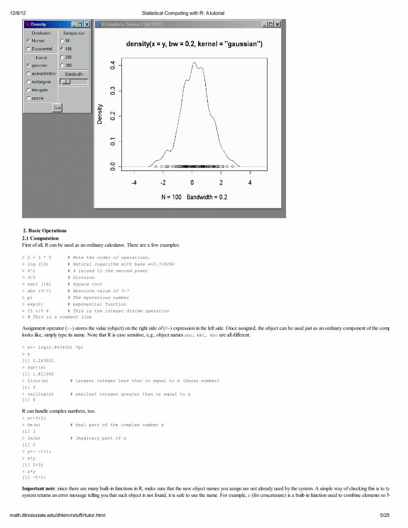
Effect of kernel choice, sample size and bandwidth can be conveniently illustrated by the following demonstration:
> library(tcltk)
> demo(tkdensity)
12/8/12 Statistical Computing with R: A tutorial
5/25math.illinoisstate.edu/dhkim/rstuff/rtutor.html
2. Basic Operations
2.1 Computation First of all, R can be used as an ordinary calculator. There are a few examples:
> 2 + 3 * 5 # Note the order of operations.
> log (10) # Natural logarithm with base e=2.718282
> 42 # 4 raised to the second power > 3/2 # Division
> sqrt (16) # Square root
> abs (3-7) # Absolute value of 3-7
> pi # The mysterious number > exp(2) # exponential function
> 15 %/% 4 # This is the integer divide operation > # This is a comment line
Assignment operator (<-) stores the value (object) on the right side of (<-) expression in the left side. Once assigned, the object can be used just as an ordinary component of the computation. To find out what the object
looks like, simply type its name. Note that R is case sensitive, e.g., object names abc, ABC, Abc are all different.
> x<- log(2.843432) *pi > x
[1] 3.283001
> sqrt(x)
[1] 1.811905 > floor(x) # largest integer less than or equal to x (Gauss number)
[1] 3
> ceiling(x) # smallest integer greater than or equal to x [1] 4
R can handle complex numbers, too. > x<-3+2i
> Re(x) # Real part of the complex number x
[1] 3 > Im(x) # Imaginary part of x
[1] 2
> y<- -1+1i
> x+y [1] 2+3i
> x*y [1] -5+1i
Important note: since there are many built-in functions in R, make sure that the new object names you assign are not already used by the system. A simple way of checking this is to type in the name you want to use. If thesystem returns an error message telling you that such object is not found, it is safe to use the name. For example, c (for concatenate) is a built-in function used to combine elements so NEVER assign an object to c!
12/8/12 Statistical Computing with R: A tutorial
6/25math.illinoisstate.edu/dhkim/rstuff/rtutor.html
2.2 Vector
R handles vector objects quite easily and intuitively.
> x<-c(1,3,2,10,5) #create a vector x with 5 components > x
[1] 1 3 2 10 5
> y<-1:5 #create a vector of consecutive integers > y
[1] 1 2 3 4 5
> y+2 #scalar addition
[1] 3 4 5 6 7 > 2*y #scalar multiplication
[1] 2 4 6 8 10
> y2 #raise each component to the second power
[1] 1 4 9 16 25 > 2y #raise 2 to the first through fifth power
[1] 2 4 8 16 32
> y #y itself has not been unchanged [1] 1 2 3 4 5
> y<-y*2
> y #it is now changed [1] 2 4 6 8 10
More examples of vector arithmetic: > x<-c(1,3,2,10,5); y<-1:5 #two or more statements are separated by semicolons
> x+y
[1] 2 5 5 14 10
> x*y [1] 1 6 6 40 25
> x/y
[1] 1.0000000 1.5000000 0.6666667 2.5000000 1.0000000 > xy [1] 1 9 8 10000 3125
> sum(x) #sum of elements in x
[1] 21
> cumsum(x) #cumulative sum vector [1] 1 4 6 16 21
> diff(x) # first difference
[1] 2 -1 8 -5 > diff(x,2) #second difference
[1] 1 7 3
> max(x) #maximum [1] 10
> min(x) #minimum [1] 1
Sorting can be done using sort() command:
> x
[1] 1 3 2 10 5
> sort(x) # increasing order [1] 1 2 3 5 10
> sort(x, decreasing=T) # decreasing order [1] 10 5 3 2 1
Component extraction is a very important part of vector calculation.
> x
[1] 1 3 2 10 5
> length(x) # number of elements in x
[1] 5 > x[3] # the third element of x
[1] 2
> x[3:5] # the third to fifth element of x, inclusive
[1] 2 10 5
> x[-2] # all except the second element
[1] 1 2 10 5
> x[x>3] # list of elements in x greater than 3 [1] 10 5
Logical vector can be handy: > x>3
[1] FALSE FALSE FALSE TRUE TRUE
> as.numeric(x>3) # as.numeric() function coerces logical components to numeric
[1] 0 0 0 1 1
> sum(x>3) # number of elements in x greater than 3
12/8/12 Statistical Computing with R: A tutorial
7/25math.illinoisstate.edu/dhkim/rstuff/rtutor.html
[1] 2
> (1:length(x))[x<=2] # indices of x whose components are less than or equal to 2
[1] 1 3
> z<-as.logical(c(1,0,0,1)) # numeric to logical vector conversion > z [1] TRUE FALSE FALSE TRUE
Character vector:
> colors<-c("green", "blue", "orange", "yellow", "red")
> colors [1] "green" "blue" "orange" "yellow" "red"
Individual components can be named and referenced by their names.
> names(x) # check if any names are attached to x
NULL > names(x)<-colors # assign the names using the character vector colors
> names(x)
[1] "green" "blue" "orange" "yellow" "red"
> x
green blue orange yellow red
1 3 2 10 5
> x["green"] # component reference by its name green
1
> names(x)<-NULL # names can be removed by assigning NULL
> x [1] 1 3 2 10 5
seq() and rep() provide convenient ways to a construct vectors with a certain pattern.
> seq(10)
[1] 1 2 3 4 5 6 7 8 9 10 > seq(0,1,length=10)
[1] 0.0000000 0.1111111 0.2222222 0.3333333 0.4444444 0.5555556 0.6666667
[8] 0.7777778 0.8888889 1.0000000
> seq(0,1,by=0.1)
[1] 0.0 0.1 0.2 0.3 0.4 0.5 0.6 0.7 0.8 0.9 1.0
> rep(1,3)
[1] 1 1 1
> c(rep(1,3),rep(2,2),rep(-1,4)) [1] 1 1 1 2 2 -1 -1 -1 -1
> rep("Small",3)
[1] "Small" "Small" "Small"
> c(rep("Small",3),rep("Medium",4))
[1] "Small" "Small" "Small" "Medium" "Medium" "Medium" "Medium"
> rep(c("Low","High"),3) [1] "Low" "High" "Low" "High" "Low" "High"
2.3 Matrices A matrix refers to a numeric array of rows and columns. One of the easiest ways to create a matrix is to combine vectors of equal length using cbind(), meaning "column bind":
> x
[1] 1 3 2 10 5
> y
[1] 1 2 3 4 5
> m1<-cbind(x,y);m1
x y [1,] 1 1
[2,] 3 2
[3,] 2 3
[4,] 10 4
[5,] 5 5
> t(m1) # transpose of m1
[,1] [,2] [,3] [,4] [,5] x 1 3 2 10 5 y 1 2 3 4 5
> m1<-t(cbind(x,y)) # Or you can combine them and assign in one step
> dim(m1) # 2 by 5 matrix
[1] 2 5 > m1<-rbind(x,y) # rbind() is for row bind and equivalent to t(cbind()).
Of course you can directly list the elements and specify the matrix:
> m2<-matrix(c(1,3,2,5,-1,2,2,3,9),nrow=3);m2
[,1] [,2] [,3] [1,] 1 5 2
[2,] 3 -1 3

12/8/12 Statistical Computing with R: A tutorial
8/25math.illinoisstate.edu/dhkim/rstuff/rtutor.html
[3,] 2 2 9
Note that the elements are used to fill the first column, then the second column and so on. To fill row-wise, we specify byrow=T option:
> m2<-matrix(c(1,3,2,5,-1,2,2,3,9),ncol=3,byrow=T);m2
[,1] [,2] [,3] [1,] 1 3 2
[2,] 5 -1 2 [3,] 2 3 9
Extracting the component of a matrix involves one or two indices.
> m2
[,1] [,2] [,3]
[1,] 1 3 2
[2,] 5 -1 2 [3,] 2 3 9
> m2[2,3] #element of m2 at the second row, third column
[1] 2
> m2[2,] #second row
[1] 5 -1 2
> m2[,3] #third column
[1] 2 2 9 > m2[-1,] #submatrix of m2 without the first row
[,1] [,2] [,3]
[1,] 5 -1 2
[2,] 2 3 9
> m2[,-1] #ditto, sans the first column
[,1] [,2]
[1,] 3 2
[2,] -1 2 [3,] 3 9
> m2[-1,-1] #submatrix of m2 with the first row and column removed
[,1] [,2]
[1,] -1 2 [2,] 3 9
Matrix computation is usually done component-wise.
> m1<-matrix(1:4, ncol=2); m2<-matrix(c(10,20,30,40),ncol=2)
> 2*m1 # scalar multiplication [,1] [,2]
[1,] 2 6
[2,] 4 8
> m1+m2 # matrix addition
[,1] [,2]
[1,] 11 33
[2,] 22 44 > m1*m2 # component-wise multiplication
[,1] [,2]
[1,] 10 90 [2,] 40 160
Note that m1*m2 is NOT the usual matrix multiplication. To do the matrix multiplication, you should use %*% operator instead.
> m1 %*% m2
[,1] [,2]
[1,] 70 150 [2,] 100 220
> solve(m1) #inverse matrix of m1
[,1] [,2]
[1,] -2 1.5
[2,] 1 -0.5 > solve(m1)%*%m1 #check if it is so
[,1] [,2]
[1,] 1 0
[2,] 0 1
> diag(3) #diag() is used to construct a k by k identity matrix
[,1] [,2] [,3]
[1,] 1 0 0 [2,] 0 1 0
[3,] 0 0 1
> diag(c(2,3,3)) #as well as other diagonal matrices
[,1] [,2] [,3]
[1,] 2 0 0
[2,] 0 3 0 [3,] 0 0 3
12/8/12 Statistical Computing with R: A tutorial
9/25math.illinoisstate.edu/dhkim/rstuff/rtutor.html
Eigenvalues and eigenvectors of a matrix is handled by eigen() function:
> eigen(m2) $values [1] 53.722813 -3.722813
$vectors
[,1] [,2]
[1,] -0.5657675 -0.9093767 [2,] -0.8245648 0.4159736
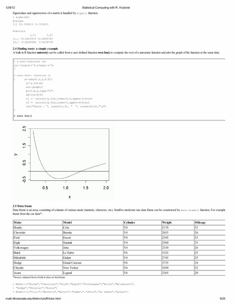
2.4 Finding roots: a simple example
A built-in R function uniroot() can be called from a user defined function root.fun() to compute the root of a univariate function and plot the graph of the function at the same time.
> y.fun<-function (x)
{y<-(log(x))2-x*exp(-x3) }
> root.fun<- function ()
{ x<-seq(0.2,2,0.01)
y<-y.fun(x)
win.graph()
plot(x,y,type="l")
abline(h=0)
r1 <- uniroot(y.fun,lower=0.2,upper=1)$root r2 <- uniroot(y.fun,lower=1,upper=2)$root
cat("Roots : ", round(r1,4), " ", round(r2,4),"\n") }
> root.fun()
2.5 Data frame
Data frame is an array consisting of columns of various mode (numeric, character, etc). Small to moderate size data frame can be constructed by data.frame() function. For example, we illustrate how to construct a data
frame from the car data*:
Make Model Cylinder Weight Mileage
Honda Civic V4 2170 33
Chevrolet Beretta V4 2655 26
Ford Escort V4 2345 33
Eagle Summit V4 2560 33
Volkswagen Jetta V4 2330 26
Buick Le Sabre V6 3325 23
Mitsubishi Galant V4 2745 25
Dodge Grand Caravan V6 3735 18
Chrysler New Yorker V6 3450 22
Acura Legend V6 3265 20
*Source: adapted from a built-in data set fuel.frame.
> Make<-c("Honda","Chevrolet","Ford","Eagle","Volkswagen","Buick","Mitsbusihi",
+ "Dodge","Chrysler","Acura")
> Model<-c("Civic","Beretta","Escort","Summit","Jetta","Le Sabre","Galant",

12/8/12 Statistical Computing with R: A tutorial
10/25math.illinoisstate.edu/dhkim/rstuff/rtutor.html
+ "Grand Caravan","New Yorker","Legend")
Note that the plus sign (+) in the above commands are automatically inserted when the carriage return is pressed without completing the list. Save some typing by using rep() command. For example, instructs R to repeat V4 five times.
> Cylinder<-c(rep("V4",5),"V6","V4",rep("V6",3))
> Cylinder
[1] "V4" "V4" "V4" "V4" "V4" "V6" "V4" "V6" "V6" "V6" > Weight<-c(2170,2655,2345,2560,2330,3325,2745,3735,3450,3265)
> Mileage<-c(33,26,33,33,26,23,25,18,22,20) > Type<-c("Sporty","Compact",rep("Small",3),"Large","Compact","Van",rep("Medium",2))
Now data.frame() function combines the six vectors into a single data frame.
> Car<-data.frame(Make,Model,Cylinder,Weight,Mileage,Type)
> Car
Make Model Cylinder Weight Mileage Type
1 Honda Civic V4 2170 33 Sporty 2 Chevrolet Beretta V4 2655 26 Compact
3 Ford Escort V4 2345 33 Small
4 Eagle Summit V4 2560 33 Small
5 Volkswagen Jetta V4 2330 26 Small
6 Buick Le Sabre V6 3325 23 Large
7 Mitsbusihi Galant V4 2745 25 Compact
8 Dodge Grand Caravan V6 3735 18 Van 9 Chrysler New Yorker V6 3450 22 Medium 10 Acura Legend V6 3265 20 Medium
> names(Car) [1] "Make" "Model" "Cylinder" "Weight" "Mileage" "Type"
Just as in matrix objects, partial information can be easily extracted from the data frame:
> Car[1,]
Make Model Cylinder Weight Mileage Type 1 Honda Civic V4 2170 33 Sporty
In addition, individual columns can be referenced by their labels:
> Car$Mileage [1] 33 26 33 33 26 23 25 18 22 20
> Car[,5] #equivalent expression, less informative
> mean(Car$Mileage) #average mileage of the 10 vehicles
[1] 25.9
> min(Car$Weight) [1] 2170
table() command gives a frequency table: > table(Car$Type)
Compact Large Medium Small Sporty Van 2 1 2 3 1 1
If the proportion is desired, type the following command instead: > table(Car$Type)/10
Compact Large Medium Small Sporty Van 0.2 0.1 0.2 0.3 0.1 0.1
Note that the values were divided by 10 because there are that many vehicles in total. If you don't want to count them each time, the following does the trick: > table(Car$Type)/length(Car$Type)
Cross tabulation is very easy, too: > table(Car$Make, Car$Type)
Compact Large Medium Small Sporty Van
Acura 0 0 1 0 0 0
Buick 0 1 0 0 0 0 Chevrolet 1 0 0 0 0 0
Chrysler 0 0 1 0 0 0
Dodge 0 0 0 0 0 1
Eagle 0 0 0 1 0 0
Ford 0 0 0 1 0 0
Honda 0 0 0 0 1 0
Mitsbusihi 1 0 0 0 0 0 Volkswagen 0 0 0 1 0 0
What if you want to arrange the data set by vehicle weight? order() gets the job done.
> i<-order(Car$Weight);i
[1] 1 5 3 4 2 7 10 6 9 8
> Car[i,]

12/8/12 Statistical Computing with R: A tutorial
11/25math.illinoisstate.edu/dhkim/rstuff/rtutor.html
Make Model Cylinder Weight Mileage Type 1 Honda Civic V4 2170 33 Sporty
5 Volkswagen Jetta V4 2330 26 Small
3 Ford Escort V4 2345 33 Small
4 Eagle Summit V4 2560 33 Small
2 Chevrolet Beretta V4 2655 26 Compact
7 Mitsbusihi Galant V4 2745 25 Compact
10 Acura Legend V6 3265 20 Medium 6 Buick Le Sabre V6 3325 23 Large
9 Chrysler New Yorker V6 3450 22 Medium 8 Dodge Grand Caravan V6 3735 18 Van
2.6 Creating/editing data objects
> y [1] 1 2 3 4 5
If you want to modify the data object, use edit() function and assign it to an object. For example, the following command opens notepad for editing. After editing is done, choose File | Save and Exit from Notepad. > y<-edit(y)
If you prefer entering the data.frame in a spreadsheet style data editor, the following command invokes the built-in editor with an empty spreadsheet.
> data1<-edit(data.frame()) After entering a few data points, it looks like this:
You can also change the variable name by clicking once on the cell containing it. Doing so opens a dialog box:
When finished, click in the upper right corner of the dialog box to return to the Data Editor window. Close the Data Editor to return to the R command window (R Console). Check the result by typing:
> data1
3. More on R Graphics
Not only R has fancy graphical tools, but also it has all sorts of useful commands that allow users to control almost every aspect of their graphical output to the finest details.
3.1 Histogram
We will use a data set fuel.frame which is based on makes of cars taken from the April 1990 issue of Consumer Reports.
> fuel.frame<-read.table("c:/fuel-frame.txt", header=T, sep=",")
> names(fuel.frame) [1] "row.names" "Weight" "Disp." "Mileage" "Fuel" "Type"
> attach(fuel.frame)
attach() allows to reference variables in fuel.frame without the cumbersome fuel.frame$ prefix.
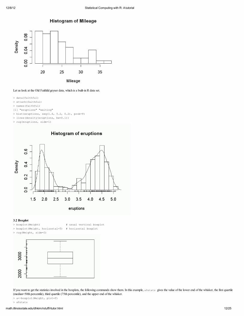
In general, graphic functions are very flexible and intuitive to use. For example, hist() produces a histogram, boxplot() does a boxplot, etc. > hist(Mileage)
> hist(Mileage, freq=F) # if probability instead of frequency is desired
12/8/12 Statistical Computing with R: A tutorial
12/25math.illinoisstate.edu/dhkim/rstuff/rtutor.html
Let us look at the Old Faithful geyser data, which is a built-in R data set.
> data(faithful)
> attach(faithful) > names(faithful) [1] "eruptions" "waiting"
> hist(eruptions, seq(1.6, 5.2, 0.2), prob=T) > lines(density(eruptions, bw=0.1))
> rug(eruptions, side=1)
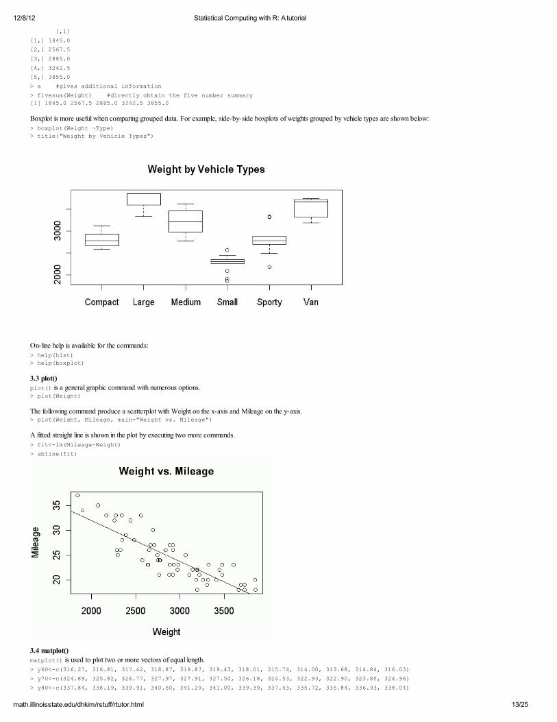
3.2 Boxplot > boxplot(Weight) # usual vertical boxplot
> boxplot(Weight, horizontal=T) # horizontal boxplot > rug(Weight, side=2)
If you want to get the statistics involved in the boxplots, the following commands show them. In this example, a$stats gives the value of the lower end of the whisker, the first quartile (25th percentile), second quartile(median=50th percentile), third quartile (75th percentile), and the upper end of the whisker.
> a<-boxplot(Weight, plot=F) > a$stats
12/8/12 Statistical Computing with R: A tutorial
13/25math.illinoisstate.edu/dhkim/rstuff/rtutor.html
[,1]
[1,] 1845.0 [2,] 2567.5 [3,] 2885.0
[4,] 3242.5 [5,] 3855.0
> a #gives additional information > fivenum(Weight) #directly obtain the five number summary [1] 1845.0 2567.5 2885.0 3242.5 3855.0
Boxplot is more useful when comparing grouped data. For example, side-by-side boxplots of weights grouped by vehicle types are shown below:
> boxplot(Weight ~Type) > title("Weight by Vehicle Types")
On-line help is available for the commands:
> help(hist) > help(boxplot)
3.3 plot()
plot() is a general graphic command with numerous options. > plot(Weight)
The following command produce a scatterplot with Weight on the x-axis and Mileage on the y-axis. > plot(Weight, Mileage, main="Weight vs. Mileage")
A fitted straight line is shown in the plot by executing two more commands. > fit<-lm(Mileage~Weight)
> abline(fit)
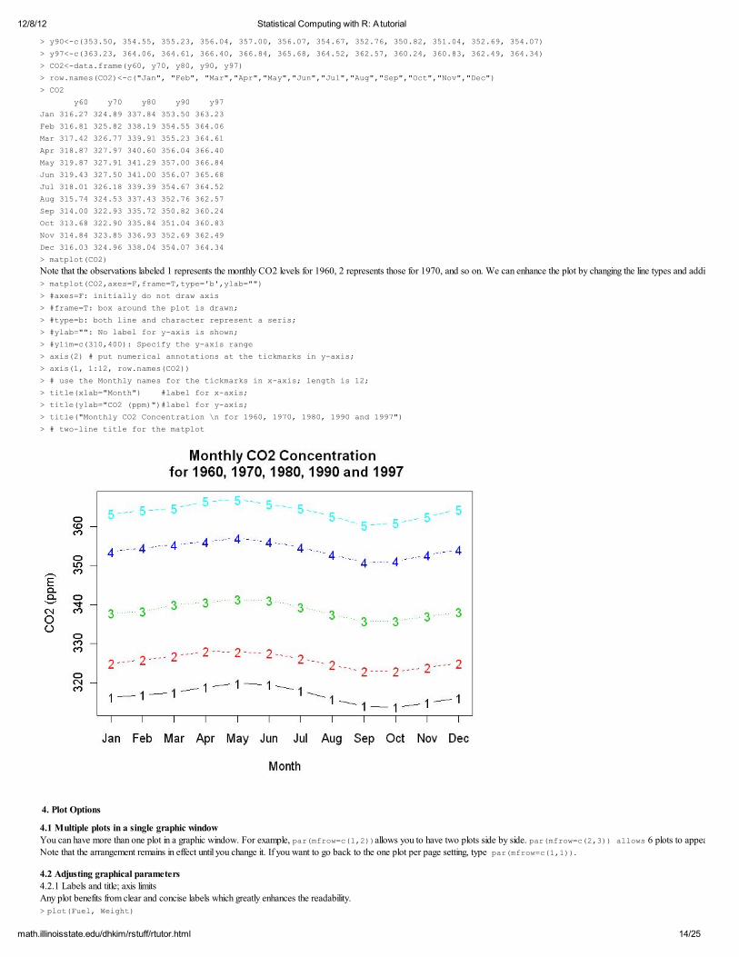
3.4 matplot() matplot() is used to plot two or more vectors of equal length.
> y60<-c(316.27, 316.81, 317.42, 318.87, 319.87, 319.43, 318.01, 315.74, 314.00, 313.68, 314.84, 316.03) > y70<-c(324.89, 325.82, 326.77, 327.97, 327.91, 327.50, 326.18, 324.53, 322.93, 322.90, 323.85, 324.96) > y80<-c(337.84, 338.19, 339.91, 340.60, 341.29, 341.00, 339.39, 337.43, 335.72, 335.84, 336.93, 338.04)
12/8/12 Statistical Computing with R: A tutorial
14/25math.illinoisstate.edu/dhkim/rstuff/rtutor.html
> y90<-c(353.50, 354.55, 355.23, 356.04, 357.00, 356.07, 354.67, 352.76, 350.82, 351.04, 352.69, 354.07)
> y97<-c(363.23, 364.06, 364.61, 366.40, 366.84, 365.68, 364.52, 362.57, 360.24, 360.83, 362.49, 364.34) > CO2<-data.frame(y60, y70, y80, y90, y97) > row.names(CO2)<-c("Jan", "Feb", "Mar","Apr","May","Jun","Jul","Aug","Sep","Oct","Nov","Dec")
> CO2 y60 y70 y80 y90 y97
Jan 316.27 324.89 337.84 353.50 363.23 Feb 316.81 325.82 338.19 354.55 364.06
Mar 317.42 326.77 339.91 355.23 364.61 Apr 318.87 327.97 340.60 356.04 366.40 May 319.87 327.91 341.29 357.00 366.84
Jun 319.43 327.50 341.00 356.07 365.68 Jul 318.01 326.18 339.39 354.67 364.52
Aug 315.74 324.53 337.43 352.76 362.57 Sep 314.00 322.93 335.72 350.82 360.24
Oct 313.68 322.90 335.84 351.04 360.83 Nov 314.84 323.85 336.93 352.69 362.49 Dec 316.03 324.96 338.04 354.07 364.34
> matplot(CO2) Note that the observations labeled 1 represents the monthly CO2 levels for 1960, 2 represents those for 1970, and so on. We can enhance the plot by changing the line types and adding axis labels and titles:
> matplot(CO2,axes=F,frame=T,type='b',ylab="") > #axes=F: initially do not draw axis
> #frame=T: box around the plot is drawn; > #type=b: both line and character represent a seris; > #ylab="": No label for y-axis is shown;
> #ylim=c(310,400): Specify the y-axis range > axis(2) # put numerical annotations at the tickmarks in y-axis;
> axis(1, 1:12, row.names(CO2)) > # use the Monthly names for the tickmarks in x-axis; length is 12;
> title(xlab="Month") #label for x-axis; > title(ylab="CO2 (ppm)")#label for y-axis; > title("Monthly CO2 Concentration \n for 1960, 1970, 1980, 1990 and 1997")
> # two-line title for the matplot
4. Plot Options
4.1 Multiple plots in a single graphic window
You can have more than one plot in a graphic window. For example, par(mfrow=c(1,2))allows you to have two plots side by side. par(mfrow=c(2,3)) allows 6 plots to appear on a page (2 rows of 3 plots each).Note that the arrangement remains in effect until you change it. If you want to go back to the one plot per page setting, type par(mfrow=c(1,1)).
4.2 Adjusting graphical parameters
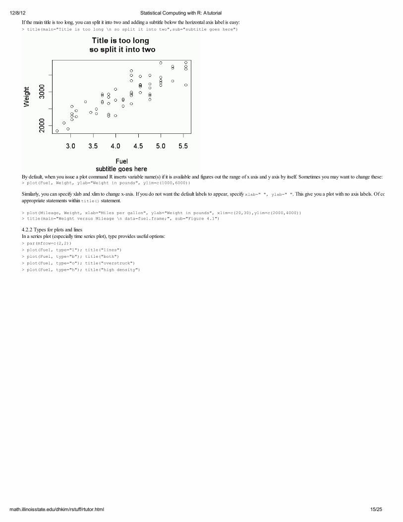
4.2.1 Labels and title; axis limits Any plot benefits from clear and concise labels which greatly enhances the readability. > plot(Fuel, Weight)
12/8/12 Statistical Computing with R: A tutorial
15/25math.illinoisstate.edu/dhkim/rstuff/rtutor.html
If the main title is too long, you can split it into two and adding a subtitle below the horizontal axis label is easy: > title(main="Title is too long \n so split it into two",sub="subtitle goes here")
By default, when you issue a plot command R inserts variable name(s) if it is available and figures out the range of x axis and y axis by itself. Sometimes you may want to change these: > plot(Fuel, Weight, ylab="Weight in pounds", ylim=c(1000,6000))
Similarly, you can specify xlab and xlim to change x-axis. If you do not want the default labels to appear, specify xlab=" ", ylab=" ". This give you a plot with no axis labels. Of course you can add the labels after using
appropriate statements within title() statement.
> plot(Mileage, Weight, xlab="Miles per gallon", ylab="Weight in pounds", xlim=c(20,30),ylim=c(2000,4000)) > title(main="Weight versus Mileage \n data=fuel.frame;", sub="Figure 4.1")
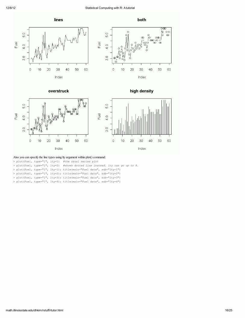
4.2.2 Types for plots and lines In a series plot (especially time series plot), type provides useful options:
> par(mfrow=c(2,2)) > plot(Fuel, type="l"); title("lines") > plot(Fuel, type="b"); title("both")
> plot(Fuel, type="o"); title("overstruck") > plot(Fuel, type="h"); title("high density")
12/8/12 Statistical Computing with R: A tutorial
16/25math.illinoisstate.edu/dhkim/rstuff/rtutor.html
Also you can specify the line types using lty argument within plot() command: > plot(Fuel, type="l", lty=1) #the usual series plot
> plot(Fuel, type="l", lty=2) #shows dotted line instead. lty can go up to 8. > plot(Fuel, type="l", lty=1); title(main="Fuel data", sub="lty=1")
> plot(Fuel, type="l", lty=2); title(main="Fuel data", sub="lty=2") > plot(Fuel, type="l", lty=3); title(main="Fuel data", sub="lty=3")
> plot(Fuel, type="l", lty=4); title(main="Fuel data", sub="lty=4")

12/8/12 Statistical Computing with R: A tutorial
17/25math.illinoisstate.edu/dhkim/rstuff/rtutor.html
Note that we can control the thickness of the lines by lwd=1 (default) through lwd=5 (thickest).
4.3 Colors and characters
You can change the color by specifying
> plot(Fuel, col=2) which shows a plot with different color. The default is col=1. The actual color assignment depends on the system you are using. You may want to experiment with different numbers. Of course you can specify the
together with other options such as type or lty. pch option allows you to choose alternative plotting characters when making a points-type plot. For example, the command > plot(Fuel, pch="*") # plots with * characters > plot(Fuel, pch="M") # plots with M.
4.4 Controlling axis line
bty ="n"; No box is drawn around the plot, although the x and y axes are still drawn.
bty="o"; The default box type; draws a four-sided box around the plot. bty="c"; Draws a three-sided box around the plot in the shape of an uppercase "C." bty="l"; Draws a two-sided box around the plot in the shape of an uppercase "L."
bty="7"; Draws a two-sided box around the plot in the shape of a square numeral "7." > par(mfrow = c(2,2))
> plot(Fuel) > plot(Fuel, bty="l")
> plot(Fuel, bty="7") > plot(Fuel, bty="c")
4.5 Controlling tick marks
tck parameter is used to control the length of tick marks. tck=1 draws grid lines. Any positive value between 0 and 1 draws inward tick marks for each axis. Also with some more work you can have tick marks of differentlengths, as the following example shows.
> plot(Fuel, main="Default") > plot(Fuel, tck=0.05, main="tck=0.05") > plot(Fuel, tck=1, main="tck=1")
> plot(Fuel, axes=F, main="Different tick marks for each axis") > #axes=F suppresses the drawing of axis
> axis(1)# draws x-axis. > axis(2, tck=1, lty=2) # draws y-axis with horizontal grid of dotted line > box()# draws box around the remaining sides.
4.6 Legend legend() is useful when adding more information to the existing plot.
12/8/12 Statistical Computing with R: A tutorial
18/25math.illinoisstate.edu/dhkim/rstuff/rtutor.html
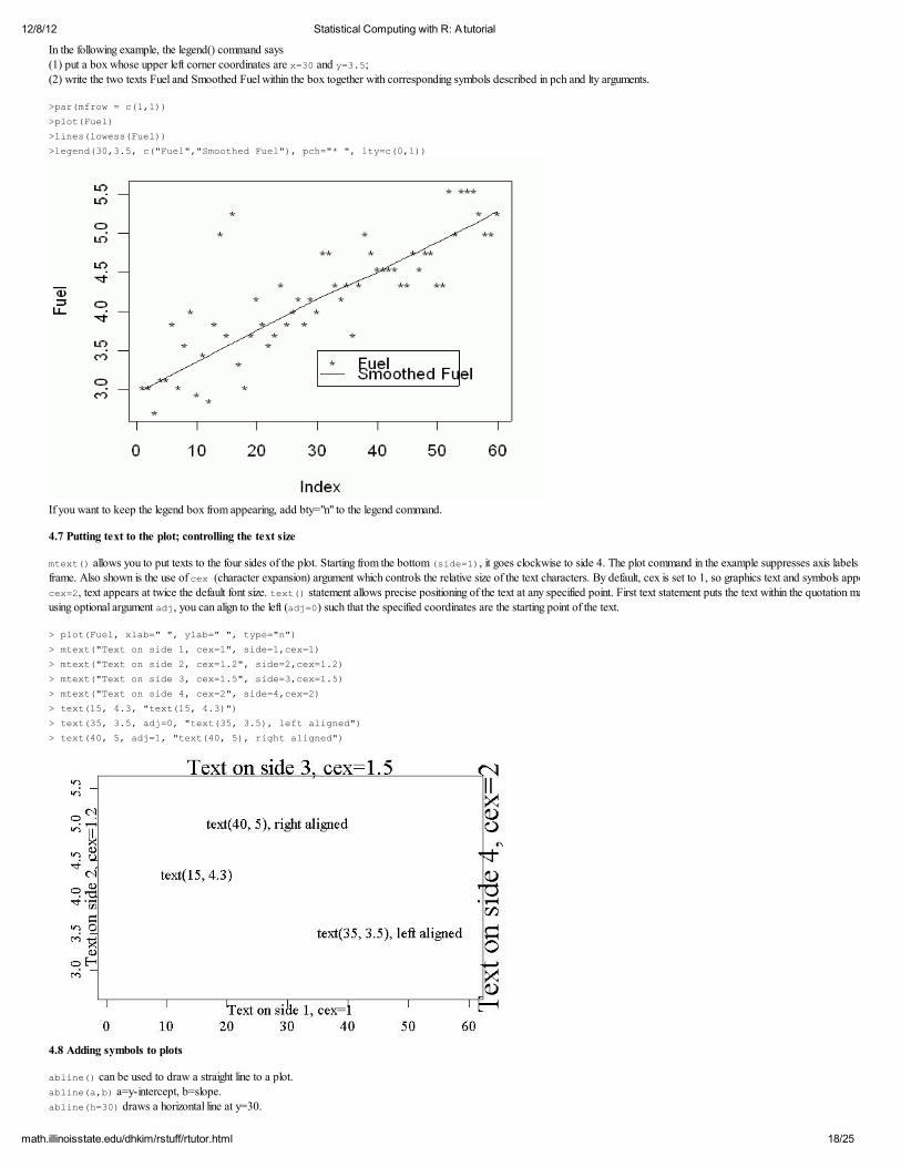
In the following example, the legend() command says (1) put a box whose upper left corner coordinates are x=30 and y=3.5;
(2) write the two texts Fuel and Smoothed Fuel within the box together with corresponding symbols described in pch and lty arguments.
>par(mfrow = c(1,1)) >plot(Fuel)
>lines(lowess(Fuel)) >legend(30,3.5, c("Fuel","Smoothed Fuel"), pch="* ", lty=c(0,1))
If you want to keep the legend box from appearing, add bty="n" to the legend command.
4.7 Putting text to the plot; controlling the text size
mtext() allows you to put texts to the four sides of the plot. Starting from the bottom (side=1), it goes clockwise to side 4. The plot command in the example suppresses axis labels and the plot itself. It just gives the
frame. Also shown is the use of cex (character expansion) argument which controls the relative size of the text characters. By default, cex is set to 1, so graphics text and symbols appear in the default font size. Withcex=2, text appears at twice the default font size. text() statement allows precise positioning of the text at any specified point. First text statement puts the text within the quotation marks centered at
using optional argument adj, you can align to the left (adj=0) such that the specified coordinates are the starting point of the text.
> plot(Fuel, xlab=" ", ylab=" ", type="n") > mtext("Text on side 1, cex=1", side=1,cex=1)
> mtext("Text on side 2, cex=1.2", side=2,cex=1.2) > mtext("Text on side 3, cex=1.5", side=3,cex=1.5)
> mtext("Text on side 4, cex=2", side=4,cex=2) > text(15, 4.3, "text(15, 4.3)") > text(35, 3.5, adj=0, "text(35, 3.5), left aligned")
> text(40, 5, adj=1, "text(40, 5), right aligned")
4.8 Adding symbols to plots
abline() can be used to draw a straight line to a plot. abline(a,b) a=y-intercept, b=slope.
abline(h=30) draws a horizontal line at y=30.
12/8/12 Statistical Computing with R: A tutorial
19/25math.illinoisstate.edu/dhkim/rstuff/rtutor.html
abline(v=12) draws a vertical line at x=12.
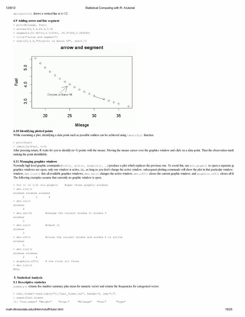
4.9 Adding arrow and line segment > plot(Mileage, Fuel)
> arrows(23,3.5,24.5,3.9) > segments(31.96713,3.115541, 29.97309,3.309592)
> title("arrow and segment") > text(23,3.4,"Chrysler Le Baron V6", cex=0.7)
4.10 Identifying plotted points While examining a plot, identifying a data point such as possible outliers can be achieved using identify() function.
> plot(Fuel)
> identify(Fuel, n=3) After pressing return, R waits for you to identify (n=3) points with the mouse. Moving the mouse cursor over the graphics window and click on a data point. Then the observation number appears next to the point, thus
making the point identifiable.
4.11 Managing graphics windows Normally high level graphic commands (hist(), plot(), boxplot(), ...) produce a plot which replaces the previous one. To avoid this, use win.graph() to open a separate graphic window. Even if more than one
graphics windows are open, only one window is active, i.e., as long as you don't change the active window, subsequent plotting commands will show the plot in that particular window. window, dev.list() lists all available graphics windows, dev.set() changes the active window, dev.off() closes the current graphic window, and graphics.off() closes all the open graphics windows at once.
The following examples assume that currently no graphic window is open.
> for (i in 1:3) win.graph() #open three graphic windows > dev.list()
windows windows windows 2 3 4
> dev.cur() windows 4
> dev.set(3) #change the current window to window 3 windows
3 > dev.cur() #check it
windows 3 > dev.off() #close the current window and window 4 is active
windows 4
> dev.list() windows windows
2 4 > graphics.off() # now close all three > dev.list()
NULL
5. Statistical Analysis
5.1 Descriptive statistics summary() returns five number summary plus mean for numeric vector and returns the frequencies for categorical vector.
> fuel.frame<-read.table("c:/fuel_frame.txt", header=T, sep=",")
> names(fuel.frame) [1] "row.names" "Weight" "Disp." "Mileage" "Fuel" "Type"
12/8/12 Statistical Computing with R: A tutorial
20/25math.illinoisstate.edu/dhkim/rstuff/rtutor.html
> attach(fuel.frame) > summary(Mileage)
Min. 1st Qu. Median Mean 3rd Qu. Max. 18.00 21.00 23.00 24.58 27.00 37.00 > summary(fuel.frame)
row.names Weight Disp. Acura.Legend.V6 : 1 Min. :1845 Min. : 0.73
Audi.80.4 : 1 1st Qu.:2571 1st Qu.:113.75 Buick.Century.4 : 1 Median :2885 Median :144.50
Buick.Le.Sabre.V6 : 1 Mean :2901 Mean :136.92 Buick.Skylark.4 : 1 3rd Qu.:3231 3rd Qu.:180.00 Chevrolet.Beretta.4: 1 Max. :3855 Max. :305.00
(Other) :54 Mileage Fuel Type
Min. :18.00 Min. :2.703 Compact:15 1st Qu.:21.00 1st Qu.:3.704 Large : 3
Median :23.00 Median :4.348 Medium :13 Mean :24.58 Mean :4.210 Small :13
3rd Qu.:27.00 3rd Qu.:4.762 Sporty : 9 Max. :37.00 Max. :5.556 Van : 7
var() returns the sample variance, sd() the sample standard deviation, and cor() the sample correlation coefficient between two vectors:
> var(Mileage) [1] 22.95904
> sd(Mileage) [1] 4.791559
> cor(Mileage,Weight) [1] -0.8478541
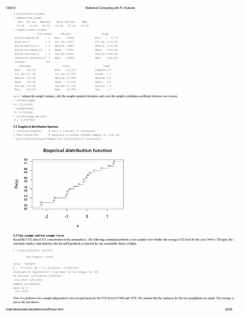
5.2 Empirical distribution function > library(stepfun) # call a library of functions > F20<-rnorm(20) # generate a normal random sample of size 20
> plot.ecdf(F20,main="Empirical distribution function")
5.3 One sample and two sample t tests Recall the CO2 data (CO2 concentration in the atmosphere). The following command performs a one-sample t-test whether the average CO2 level for the year 1960 is 320 ppm. By default, it does a two-sided test and
extremely small p-value indicates that the null hypothesis is rejected for any reasonable choice of alpha.
> t.test(CO2$y60, mu=320)
One Sample t-test
data: CO2$y60 t = -5.5183, df = 11, p-value = 0.0001812
alternative hypothesis: true mean is not equal to 320 95 percent confidence interval:
315.4502 318.0448 sample estimates:
mean of x 316.7475
Now we perform a two-sample independent t-test of equal mean for the CO2 level of 1960 and 1970. We assume that the variances for the two populations are equal. The average concentrations are significantly different,
just as the test shows.

12/8/12 Statistical Computing with R: A tutorial
21/25math.illinoisstate.edu/dhkim/rstuff/rtutor.html
> t.test(CO2$y60, CO2$y70,var.equal=T)
Two Sample t-test
data: CO2$y60 and CO2$y70 t = -11.1522, df = 22, p-value = 1.602e-10
alternative hypothesis: true difference in means is not equal to 0 95 percent confidence interval: -10.40088 -7.13912
sample estimates: mean of x mean of y 316.7475 325.5175
Paired t-test is also available. All you have to do is to include paired=T within t.test() argument.
5.4 Checking normality
Quite a few statistical tests are based on the normality of the underlying population. Here we illustrate normal plot and Kolmogorov-Smirnov test to check the normality assumption.
> #generate 500 observations from uniform (0,1) distribution > F500<-runif(500);a<-c(mean(F500),sd(F500))
> qqnorm(F500) #normal probability plot > qqline(F500) #ideal sample will fall near the straight line
Obviously the curve is far from the straight line so we strongly suspect the normality (if we didn't know that the generated data came from uniform). We formally test the normality by performing Kolmogorov-Smirnov test,
comparing the empirical distribution of F500 to a comparable normal distribution with the mean and standard deviation same as that of F500. > ks.test(F500, "pnorm", mean=a[1], sd=a[2])
One-sample Kolmogorov-Smirnov test
data: F500
D = 0.0655, p-value = 0.02742 alternative hypothesis: two.sided
5.5 Analysis of variance
ANOVA is an extension of a two-sample t test, testing the equality of means of more than two groups. In the example below, we use aov() function to test the equality of average weight per vehicle type. > a<-aov(Weight~Type)
> summary(a) Df Sum Sq Mean Sq F value Pr(>F)
Type 5 11161777 2232355 36.035 4.855e-16 *** Residuals 54 3345331 61951 ---
Signif. codes: 0 ***' 0.001 **' 0.01 *' 0.05 .' 0.1 ' 1 > boxplot(Weight~Type) #side-by-side boxplot
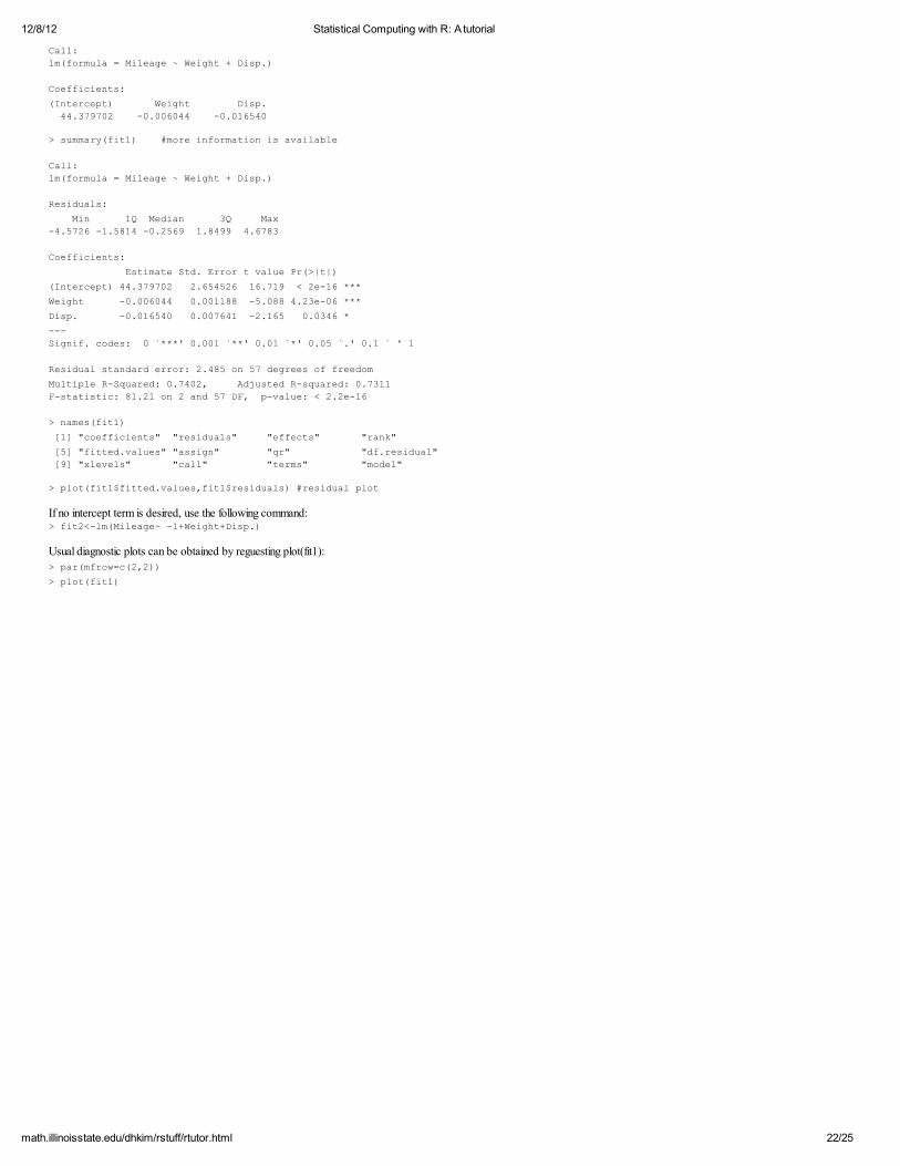
5.6 Linear regression model lm() fits a linear regression model. summary() returns rich information for the fit.
> attach(fuel.frame)
> names(fuel.frame) [1] "row.names" "Weight" "Disp." "Mileage" "Fuel" "Type"
> fit1<-lm(Mileage~Weight+Disp.) > fit1 #gives model specification and regression coefficients
12/8/12 Statistical Computing with R: A tutorial
22/25math.illinoisstate.edu/dhkim/rstuff/rtutor.html
Call: lm(formula = Mileage ~ Weight + Disp.)
Coefficients: (Intercept) Weight Disp. 44.379702 -0.006044 -0.016540
> summary(fit1) #more information is available
Call: lm(formula = Mileage ~ Weight + Disp.)
Residuals:
Min 1Q Median 3Q Max -4.5726 -1.5814 -0.2569 1.8499 4.6783
Coefficients: Estimate Std. Error t value Pr(>|t|)
(Intercept) 44.379702 2.654526 16.719 < 2e-16 *** Weight -0.006044 0.001188 -5.088 4.23e-06 *** Disp. -0.016540 0.007641 -2.165 0.0346 *
--- Signif. codes: 0 ***' 0.001 **' 0.01 *' 0.05 .' 0.1 ' 1
Residual standard error: 2.485 on 57 degrees of freedom Multiple R-Squared: 0.7402, Adjusted R-squared: 0.7311 F-statistic: 81.21 on 2 and 57 DF, p-value: < 2.2e-16
> names(fit1)
[1] "coefficients" "residuals" "effects" "rank" [5] "fitted.values" "assign" "qr" "df.residual" [9] "xlevels" "call" "terms" "model"
> plot(fit1$fitted.values,fit1$residuals) #residual plot
If no intercept term is desired, use the following command: > fit2<-lm(Mileage~ -1+Weight+Disp.)
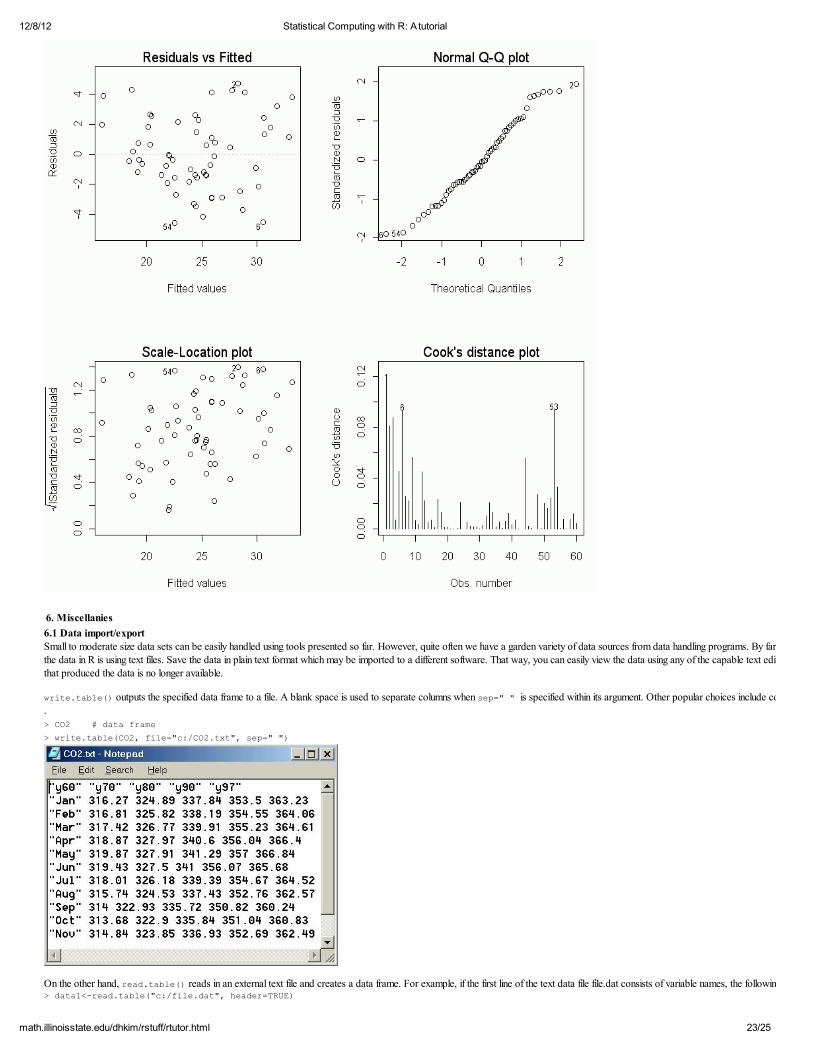
Usual diagnostic plots can be obtained by reguesting plot(fit1):
> par(mfrow=c(2,2)) > plot(fit1)
12/8/12 Statistical Computing with R: A tutorial
23/25math.illinoisstate.edu/dhkim/rstuff/rtutor.html
6. Miscellanies
6.1 Data import/export Small to moderate size data sets can be easily handled using tools presented so far. However, quite often we have a garden variety of data sources from data handling programs. By far the easiest way to import and export
the data in R is using text files. Save the data in plain text format which may be imported to a different software. That way, you can easily view the data using any of the capable text editor even when the original softwarethat produced the data is no longer available.
write.table() outputs the specified data frame to a file. A blank space is used to separate columns when sep=" " is specified within its argument. Other popular choices include comma (
. > CO2 # data frame > write.table(CO2, file="c:/CO2.txt", sep=" ")
On the other hand, read.table() reads in an external text file and creates a data frame. For example, if the first line of the text data file file.dat consists of variable names, the following command will do the job: > data1<-read.table("c:/file.dat", header=TRUE)
12/8/12 Statistical Computing with R: A tutorial
24/25math.illinoisstate.edu/dhkim/rstuff/rtutor.html
getwd() returns the current working directory and setwd() changes it. > getwd()
[1] "C:\\Program Files\\R\\rw1070" > setwd("c:/") # set the root directory as the working directory > getwd() [1] "c:\\"
> read.table(file="CO2.txt") > # now pathname is not required to read data files in the root directory
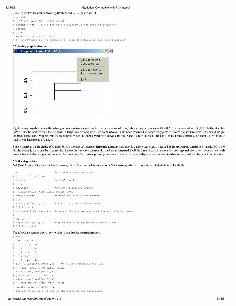
6.2 Saving graphical output
Right clicking anywhere inside the active graphics window shows a context sensitive menu, allowing either saving the plot as metafile (EMF) or postscript format (PS). On the other hand, Copy as metafile or Copy as bitmap(BMP) puts the information in the clipboard, a temporary memory area used by Windows. In the latter, you need to immediately paste it in some applications which understand the graphics format, e.g., MS Word. Moregraphical formats are available from the main menu. While the graphic window is active, click File| Save As from the menu and it lists six file formats (metafile, postscript, PDF, PNG, BMP, and JPG at three quality levels) in
total so you have plenty of choices.
Some comments on the choice of graphic formats are in order. In general metafile format retains graphic quality even when it is resized in the application. On the other hand, JPG is a very popular choice on the Internet andfile size is usually much smaller than metafile. Except for rare circumstances, I would not recommend BMP file format because it is usually very large and shows very poor picture quality when resized. Postscript file format is
useful when including the graphic file in another postscript file or when postscript printer is available. Picture quality does not deteriorate when resized, and it is the default file format to be included in TeX documents.
6.3 Missing values NA (Not Applicable) is used to denote missing values. Since many functions returns NA if missing values are present, we illustrate how to handle them.
> x #contains a missing value [1] 1 2 3 4 5 NA > mean(x) #doesn't work
[1] NA > is.na(x) #returns a logical vector [1] FALSE FALSE FALSE FALSE FALSE TRUE > sum(is.na(x)) #number of NA's in the vector
[1] 1 > x1<-x[!is.na(x)];x1 #retain only non-missing cases [1] 1 2 3 4 5 > a<-mean(x[!is.na(x)]);a #compute the average value of the non-missing cases [1] 3
> x2<-x > x2[is.na(x)]<-a;x2 #impute the missing by the average value [1] 1 2 3 4 5 3
The following example shows how to select those listwise nonmissing cases. > data2 var1 var2 var3 1 1 2.3 aa
2 4 3.2 <NA> 3 3 5.4 bc 4 NA 2.7 ed 5 3 4.1 dd
> a1<-!is.na(data2$var1);a1 #TRUE if nonmissing for var1 [1] TRUE TRUE TRUE FALSE TRUE > a2<-!is.na(data2$var2);a2 [1] TRUE TRUE TRUE TRUE TRUE > a3<-!is.na(data2$var3);a3
[1] TRUE FALSE TRUE TRUE TRUE > data3<-data2[a1*a2*a3==1,] > #select those rows if all of the elements are nonmissing.

12/8/12 Statistical Computing with R: A tutorial
25/25math.illinoisstate.edu/dhkim/rstuff/rtutor.html
> data3 var1 var2 var3
1 1 2.3 aa 3 3 5.4 bc 5 3 4.1 dd
6.4 Getting help By default, R has a couple of excellent manuals in PDF format. "An Introduction to R" is almost a required reading to begin using R. To access the manual, click Help | Manuals and the list of available documents will beshown. Also use help() to get command-specific information. > help(read.table)
Dong-Yun Kim, [email protected] location: http://math.illinoisstate.edu/dhk im/rstuff/rtutor.html
Related Documents