Statistical challenges in analyzing 16S microbiome data 0 ...

Statistical challenges in analyzing 16S microbiome data

An application to the identification of microbe-regulated pathways in allergy and

auto-immunity

Marine JeanmouginInstitut Curie, U932 - Immunity and cancer

Journées MAS, August 28th, 2014

1

Outline

1 IntroductionThe MAARS projectMicrobiome data production and features

2 Normalisation of 16S dataMotivationsState of the artEvaluation of current methods

3 Preliminary resultsExploratory analysisIntegration of microbiome and transcriptome data

2

Outline




3

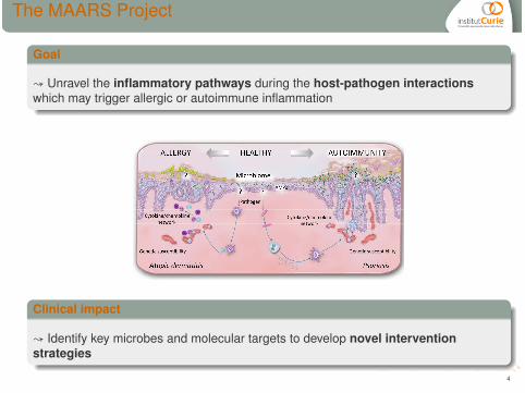
The MAARS Project

Goal

↝ Unravel the inflammatory pathways during the host-pathogen interactionswhich may trigger allergic or autoimmune inflammation

Clinical impact

↝ Identify key microbes and molecular targets to develop novel interventionstrategies

4

WP4: data management and analysis

WP4Data

Analysis

clinical

WP3WP2WP1

clinicaldb

BIRDlab

Processed data: BIRDomics

Raw data: KDS²

Raw data: KDS²

Animal model

WP6

Molecular and cellular network

WP5

Knowledge and Data Sharing SystemClinical DataBaseBIological Result Database

Data Management

microbiome transcriptome

King’s college - Sophia Tsoka - Gareth Muirhead

FIOH

- Dario Greco

Karolinska - Juha Kere - Shintaro Katayama

Fios Genomics- Varrie Ogilvie- Sarah Lynagh- Max Bylesjo

Institut Curie- Vassili Soumelis- Philippe Hupé- Gerome Jules-Clément- Marine Jeanmougin

5

16S data production

The skin microbiome

Ecosystem of microbes that live on the skin

Culture independent microbiome research:

▸ total microbiome DNA sequencing

▸ 16S rRNA sequencing

6

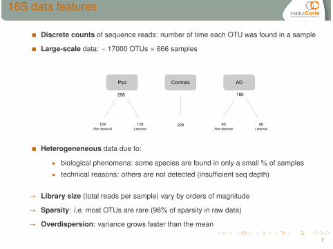
16S data features

Discrete counts of sequence reads: number of time each OTU was found in a sample

Large-scale data: ∼ 17000 OTUs × 666 samples

Pso Controls AD

228

180258

129Non-lesional

129Lesional

90Non-lesional

90Lesional

Heterogeneneous data due to:

▸ biological phenomena: some species are found in only a small % of samples

▸ technical reasons: others are not detected (insufficient seq depth)

→ Library size (total reads per sample) vary by orders of magnitude

→ Sparsity: i.e. most OTUs are rare (98% of sparsity in raw data)

→ Overdispersion: variance grows faster than the mean

7

Outline




8

Normalisation: motivations

Comparison across samples with different library sizes may induce biases in the downstreamanalysis

Differential analysis: the higher sequencing depth, the higher counts

Diversity/richness estimation: rarefaction phenomenon"The number of taxonomic features detected in a sample depends on the amount ofsequencing performed"

●

●

●

●

●

●

● ●

●

●

●

●

●

●

●

●

● ●

●

●

●

●

●

●

●

●

●

●

●

●

●

●

●

●

●

●

●

●

●

●

●

●

●

●

●

●

●

●

●

●

●

●

●

●

●

●

●

●

●

●

●

●

●

●

●

●

● ●

●●

●

●

●

●

●

●

●

●

●

●

●

●

●

●

●

●

●●

●

●

●

●

●

●

●

●●

●

●

●

●

●

●

●

●

●

●

●

●

●

●

●

●

●

●

●

●

●

●

●

●

●

●

●

●

●

●

●

●

●

●

●

●

●

●

●

●

●

●

●

●

●

●

●

●

● ●

●

●

●

●

●

●

●

●

●

●

●

●

●●

●

●

●

●

●

●

●

●

●

●

●

●

●

●●

●

●

●

●

●

●●

●

● ●

●

●

●

●

●

●

●

●

●

●

●

●

●

●

●

●

●

●

●

●

●

●

●

●

●

●

●

●●

●

●●

●

●●

●

●

●

●

●

●

●

●

●

●

●

●

●

●

●

●

●

●

●

●

●

●

●

●

●

●

●

●

●

●

●

●

●●

●

●

●

●

●

●

●

●

●

●

●

●

●●

●

●●

●●

●

●

●

0 5000 10000 15000

5010

015

020

025

030

0

Library size

Num

ber

of d

etec

ted

feat

ures

Figure: Illustration of the rarefaction phenomenon on MAARS data

9

Normalisation: current practices

Rarefying

Random subsampling of each sample to a common depth:

Omission of available data: add artificial uncertainty

Inflate the variance and induce a loss of power in differential analysis

Total-sum scaling (TSS): proportional abundance of species

Divide read counts by the total number of reads in each sample:

cij =cij

sj

where:

cij is the number of times taxonomic feature i was observed in sample j

sj = ∑i cij , sum of counts for sample i

In practice...

Does not account for heteroscedasticity

Dillies et al. demonstrated biais in RNA-seq data: undue influence of high-count genes onnormalized counts

▸ ↗ FPR when differences in library composition

10

Normalisation: alternative approaches

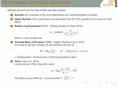
Methods derived from the field of RNA-seq data analysis:

1 Quantile (Q): Quantiles of the count distributions are matched between samples

2 Upper-Quartile (UQ): scale factors are calculated from the 75% quantile of the counts for eachlibrary

3 Relative Log Expression (RLE) - DESeq (Anders & Huber 2010):

sj = mediani(cij

(πnv=1civ)1/n

)

where n is the sample size.

4 Trimmed Mean of M-values (TMM) - EdgeR (Robinson et al. 2010)Trim data by log-fold-changes Mi and absolute intensity Ai :

Mi = log2cij /sj

cij′ /sj′; Ai = 1

2 log2(cij/sj × cij ′ /sj ′);

▷ Scaling factor: trimmed mean of the log-abundance ratios

5 Voom (Law et al. 2014)Log-counts per million (log-cpm) value:

yij = log2(cij + 0.5sj + 1

× 106)

The library size is offset by 1 to ensure that 0 < cij+0.5sj+1 < 1

11






sj = mediani(cij

(πnv=1civ)1/n

)



Mi = log2cij /sj






× 106)


11






sj = mediani(cij

(πnv=1civ)1/n

)



Mi = log2cij /sj






× 106)


11






sj = mediani(cij

(πnv=1civ)1/n

)



Mi = log2cij /sj






× 106)


11






sj = mediani(cij

(πnv=1civ)1/n

)



Mi = log2cij /sj






× 106)


11

Normalisation : Cumulative-Sum Scaling (CSS)

CSS strategy

Paulson, J. et al. (2013), Nature Methods

q lj : l th quantile of sample j

slj = ∑i ∣cij≤q l

jcij

N: normalization constant (ex: the medj (slj ))

cij =cij

slj

N

▸ avoid placing undue influence on high-count features

Selection of the appropriate quantile

q l = medj(q lj ), median l th quantile across samples

dl = medj ∣q lj − q l ∣, median absolute deviation of sample-specific quantiles

l : smallest value for which high instability is detected

12

Except for voom, all approaches decrease the range of library sizes

raw

Fre

quen

cy

0 4000 8000

050

100

150

200

prop

Fre

quen

cy

0 4000 8000

010

020

030

040

050

060

0

raref

Fre

quen

cy

0 4000 8000

010

020

030

040

050

0

rarefnoT

Fre

quen

cy

0 4000 8000

010

020

030

040

050

060

0

Q

Fre

quen

cy

0 4000 8000

050

100

150

TMM

Fre

quen

cy

0 4000 8000

050

100

150

200

RLE

Fre

quen

cy

0 4000 8000

050

100

150

200

UQ

Fre

quen

cy

0 4000 8000

050

100

150

200

TMMprop

Fre

quen

cy

0 4000 8000

010

020

030

040

050

060

0css

Fre

quen

cy

0 4000 8000

010

020

030

040

050

060

0

voom

Fre

quen

cy

100000 115000 130000

050

100

150

Figure: Distribution of library sizes across normalisation approaches

13

All the normalisation methods improve the homogeneity betweentechnical replicates

raw

prop

raref

rarefnoT

Q

TMM

RLE

UQ

TMMprop

css

voom

raw

prop

raref

rarefnoT

Q

TMM

RLE

UQ

TMMprop

css

voom

raw

prop

raref

rarefnoT

Q

TMM

RLE

UQ

TMMprop

css

voom

raw

prop

raref

rarefnoT

Q

TMM

RLE

UQ

TMMprop

css

voom

raw

prop

raref

rarefnoT

Q

TMM

RLE

UQ

TMMprop

css

voom

raw

prop

raref

rarefnoT

Q

TMM

RLE

UQ

TMMprop

css

voom

raw

prop

raref

rarefnoT

Q

TMM

RLE

UQ

TMMprop

css

voom

raw

prop

raref

rarefnoT

Q

TMM

RLE

UQ

TMMprop

css

voom

raw

prop

raref

rarefnoT

Q

TMM

RLE

UQ

TMMprop

css

voom

raw

prop

raref

rarefnoT

Q

TMM

RLE

UQ

TMMprop

css

voom

raw

prop

raref

rarefnoT

Q

TMM

RLE

UQ

TMMprop

css

voom

raw

prop

raref

rarefnoT

Q

TMM

RLE

UQ

TMMprop

css

voom

0.0 0.1 0.2 0.3 0.4 0.5 0.6 0.7

Homogeneity between library sizes of technical replicates

Coefficient of variation of library sizes

MAARS_ 3_122_02MAARS_ 3_122_01MAARS_ 3_121_12MAARS_ 3_120_01MAARS_ 3_119_12MAARS_ 3_118_02MAARS_ 3_118_01MAARS_ 3_115_12MAARS_ 3_114_02MAARS_ 3_114_01MAARS_ 3_113_02MAARS_ 3_113_01

Figure: Homogeneity of library sizes between technical replicates

14

Voom increases the distance between technical replicates

raw prop raref rarefnoT Q TMM RLE UQ TMMprop css voom

Distances between technical replicates

Dis

tanc

es in

the

spac

e of

the

1st a

nd 2

nd p

rinci

pal c

ompo

nent

s

05

1015

20

MAARS_ 3_122_02MAARS_ 3_122_01MAARS_ 3_121_12MAARS_ 3_120_01MAARS_ 3_119_12MAARS_ 3_118_02MAARS_ 3_118_01MAARS_ 3_115_12MAARS_ 3_114_02MAARS_ 3_114_01MAARS_ 3_113_02MAARS_ 3_113_01

Figure: Distances between technical replicates15

Rarefying decreases the biological signal

raw prop raref rarefnoT Q TMM RLE UQ TMMprop css voom

Distances between clinical group baryc. / Distances between technical replicates

01

23

45

6

Figure: Ratio of distances between clinical groups and technical replicates

16

Proportion and rarefying approaches show high FPR

McMurdie, P.J. and Holmes, S. (2014), PLOS Comp. Biol.

Effect size

Figure: Performance of differential abundance detection on simulated data

Preliminary results on permuted data show that proportions and rarefying exhibit a FPR of 30%17

Conclusions on normalisation approaches

● TMM and RLE are the best compromises :

show good results on simulated data (McMurdie 2014)

reduce the heterogeneity in library sizes

lower the distances between technical replicates

do not degrade the biological signal

● UQ performs well but need to be tested on simulated data

● Voom, Q and CSS normalisation approaches to be proscribed

● Perspectives for differential abundance testing: zero-inflated negative binomialmodel

18

Outline




19

Microbiome data enable to discriminate AD samples from controls

Non-metric MultiDimensional Scaling

Atopic DermatitisPsoriasis

20

Integration of microbiome and transcriptome data

▷ Unravel the interdependencies between skin microbiome and transcriptome

Univariate analysis

Associate the presence of a given microbe with different transcriptome profiles

Multivariate exploratory analysis

Canonical Correlation Analysis:↝ identify largest correlations between linear combinations of transcriptome and OTU profiles

Let us consider two matrices X and Y of order n × p and n × q respectively, with p ≤ q.

For S = 1, ...,p, find ρ1 ≥ ρ2 ≥ ... ≥ ρp such as:

ρs = maxaS,bS

cor(XaS,YbS) (1)

= cor(US,V S) (2)

with cor(US ,UK ) = cor(V S ,V K ) = 0 for S ≠ K .

US and V S : canonical variates

ρS : canonical correlations

21

Univariate approach: preliminary results

Abundance of given bacteria in AD is associated with different transcriptome profiles

Heatmap of the 400 « most significant » genes in bact 2. low/high patients

Heatmap of differentially expressed genes in bact. 1 low/high patients

Bact. 1 Bact. 2Bact. 1 low

Bact. 1 highBact. 2 low

Bact. 2 high

22

High abundance of bact. 1 is related to a dysregulated T-helpercell differentiation pathway

Down-regulation in « bact 1 high »

Up-regulation in « bact 1 high » IL13RA2 (FC = 0,74)

23

Conclusions and perspectives

16S data: large-scale count data

● similar features than RNA-seq data● BUT with a higher level of sparsity

Normalization methods used in RNA-seq analysis

● perform well on 16S data● should be transferred to microbiome research (instead of rarefying)

No consensus for differential analysis

Investigate co-occurences/co-exclusions of microbes

bact 1.

bact 2.

bact 3.

24

The MAARS consortium

25

Thanks !

Alix, Mahé, Paula, Sol, Caro, Max, Gérôme, Maude, Phil, Lucia, Irit, Vassili, Salvo,Sofia, Anto, Colline, Aurore.

26

Thank you !

27

Statistical challenges in analyzing 16S microbiome data 0 ...

Documents