Statistical Applications in Genetics and Molecular Biologykvansteen/GeneticEpi-Engineering/ac1415... · Statistical Applications in Genetics ... ology of many complex disorders, ...

Volume 11, Issue 2 2012 Article 4

Statistical Applications in Geneticsand Molecular Biology

COMPUTATIONAL STATISTICAL METHODS FOR GENOMICS ANDSYSTEMS BIOLOGY

Principal Components of Heritability for HighDimension Quantitative Traits and General

Pedigrees

Karim Oualkacha, University McGillAurelie Labbe, University McGill

Antonio Ciampi, University McGillMarc-Andre Roy, Centre de recherche Université Laval

Robert-GiffardMichel Maziade, Centre de recherche Université Laval

Robert-Giffard

Recommended Citation:Oualkacha, Karim; Labbe, Aurelie; Ciampi, Antonio; Roy, Marc-Andre; and Maziade, Michel(2012) "Principal Components of Heritability for High Dimension Quantitative Traits andGeneral Pedigrees," Statistical Applications in Genetics and Molecular Biology: Vol. 11: Iss. 2,Article 4.DOI: 10.2202/1544-6115.1711

©2012 De Gruyter. All rights reserved.Brought to you by | University of GhentAuthenticated

Download Date | 4/20/15 10:52 AM

Principal Components of Heritability for HighDimension Quantitative Traits and General

PedigreesKarim Oualkacha, Aurelie Labbe, Antonio Ciampi, Marc-Andre Roy, and Michel

Maziade

AbstractFor many complex disorders, genetically relevant disease definition is still unclear. For this

reason, researchers tend to collect large numbers of items related directly or indirectly to the diseasediagnostic. Since the measured traits may not be all influenced by genetic factors, researchersare faced with the problem of choosing which traits or combinations of traits to consider inlinkage analysis. To combine items, one can subject the data to a principal component analysis.However, when family date are collected, principal component analysis does not take familystructure into account. In order to deal with these issues, Ott & Rabinowitz (1999) introducedthe principal components of heritability (PCH), which capture the familial information acrosstraits by calculating linear combinations of traits that maximize heritability. The calculation of thePCHs is based on the estimation of the genetic and the environmental components of variance.In the genetic context, the standard estimators of the variance components are Lange's maximumlikelihood estimators, which require complex numerical calculations. The objectives of this paperare the following: i) to review some standard strategies available in the literature to estimatevariance components for unbalanced data in mixed models; ii) to propose an ANOVA methodfor a genetic random effect model to estimate the variance components, which can be applied togeneral pedigrees and high dimensional family data within the PCH framework; iii) to elucidate theconnection between PCH analysis and Linear Discriminant Analysis. We use computer simulationsto show that the proposed method has similar asymptotic properties as Lange's method when thenumber of traits is small, and we study the efficiency of our method when the number of traits islarge. A data analysis involving schizophrenia and bipolar quantitative traits is finally presented toillustrate the PCH methodology.

KEYWORDS: complex trait, heritability, linear discriminant analysis, principal componentanalysis, quantitative trait loci, variance components

Brought to you by | University of GhentAuthenticated


1 IntroductionThere is strong evidence that genetic mechanisms account for a large part of the eti-ology of many complex disorders, such as cardiovascular diseases, cancers, schizophre-nia, autism and many others. Although genome scans have identified a number ofcandidate regions of interest for several complex diseases, replication of the re-sults is often questionable. Foremost among the possible explanations for this isphenotype definition, a necessary prerequisite for establishing reliable genotype-phenotype relationships (Calum and Ramachandran, 2011). Since genetically rel-evant disease definition is still unclear for many complex disorders (Funalot et al.,2004), researchers tend to collect more and more items related directly or indirectlyto the disease diagnosis. The number of items can range from a handful to a couplethousand, as in expression quantitative trait loci (eQTL) studies where gene ex-pression measured on thousands of genes are used as quantitative traits in linkageanalysis.

Multivariate variance-components linkage analysis using several correlatedtraits provides greater statistical power than single trait analysis to detect suscep-tibility genes in loci, as shown in Amos et al. (2001) and Almasy et al. (1998).However, since not all measured traits are necessarily influenced by genetic factors,researchers are faced with the problem of choosing which traits or combinationsof traits to consider in linkage analysis. Typically, principal-component analysis(PCA) is used to combine traits into principal components and linkage analysis isbased only on the first few of these. For example, Arya et al. (2003) used PCAto identify loci influencing the factors of insulin resistance syndrome (IRS)-relatedphenotypes using eight IRS-related phenotypes. When family data are collected,it is relevant to give larger weights to traits that have a larger degree of familialheritability in the combined traits, since they are more likely to be linked to ge-netic factors. Nevertheless, the data reduction achieved by principal-componentsanalysis does not take into account family structure and heritability of traits.

In order to deal with the issues mentioned above, Ott & Rabinowitz (1999)introduced a new form of data reduction approach, which aims to capture the famil-ial information carried by traits. They sought to calculate at a linear combination oftraits that maximizes heritability, defined as the ratio of the family-specific (genetic)variation and the subject-specific (environmental) variation. Assuming that a trait isinfluenced by genetic factors, the idea is to give more weight to a trait showing sim-ilar values for subjects within the same family (smaller subject-specific variation).This linear combination was termed Principal Component of Heritability (PCH).Ott & Rabinowitz showed that using the first PCH as a quantitative trait in linkageanalysis provided a substantial gain in power as compared to the use of first princi-pal component from a standard PCA. However, when the number of traits is large,

1

Oualkacha et al.: Principal Components of Heritability for General Pedigrees

Published by De Gruyter, 2012



the PCH approach is not directly applicable and the components are unidentifiableand unstable. Wang et al. (2007a) proposed a penalized principal-components ap-proach based on heritability (PCHλ ) that can be applied to high dimensional familydata. By simulation studies, Wang et al. (2007a) showed that the traits combinedby the PCHλ approach have significant power gain in linkage analysis compared tothe usual PCA and PCH.

To calculate the PCH and PCHλ components, one needs to estimate the vari-ance covariance matrices of the quantitative trait model, which can be decomposedas the subject-specific component of variance Σe and the family-specific compo-nent of variance Σg. Ott & Rabinowitz proposed the usual sample within-familyvariance-covariance matrix as estimate of Σe and a new estimate for Σg. Wang etal. (2007a) used the same estimate of Σe and the sample between-family variance-covariance matrix to estimate Σg. When dealing with family-members of the sametype (e.g.: all the family members are siblings of each other), both approaches giveefficient estimates of the variance components, and they validly take into accountthe family structure. However, this is not the case when more complex families aresampled in the study, since the correlation between two individuals is assumed tobe the same for each pair in the family.

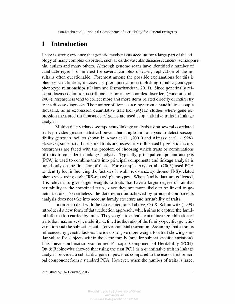
Wang et al. (2007a) stated without giving details that it is possible to extendthe PCH approach to general pedigrees with more complex structures (see Figure 1for an example of more complex structure). However, the estimation of the variancecomponents in the general case (pedigrees of unequal sizes and describing complexfamily relationships) is by no means an easy task. While in the case considered byOtt & Rabinowitz, the data was balanced, making the estimation of variance com-ponents relatively straightforward, in the general case we deal with multivariate un-balanced data (unequal subclass numbers). The estimation of variance componentsfrom multivariate unbalanced data has received little attention in the literature. TheANOVA, the maximum likelihood (ML) and the Restricted Maximum Likelihood(REML, Calvin, 1993) estimators of variance components are three standard ap-proaches for the estimation of the components Σg and Σe. The maximum likelihoodapproach in standard linear mixed models is discussed by Searle et al. (1992) andMcCulloch & Searle (2002). The ML and REML estimators can be negative withpositive probability in the unbalanced case. Similarly, the ANOVA estimators inthe unbalanced case are limited since they can also lead to negative values and losesome of their properties, as illustrated in McCulloch & Searle (2002).

In multivariate genetic linkage analysis, the state-of-the art estimators ofvariance components are Lange’s ML estimators implemented in Mendel software(Lange et al., 2001; 2006). These estimators are computed in most of the widelyused computer programs performing quantitative trait genetic analyses based onvariance components (eg: Solar (Almasy & Blangero, 1998)). In animal genetic

2

Statistical Applications in Genetics and Molecular Biology, Vol. 11 [2012], Iss. 2, Art. 4

DOI: 10.2202/1544-6115.1711



studies, the REML estimators of the variance components for multivariate unbal-anced genetic mixed linear models are usually computed using the specialized AS-REML software (Gilmour et al., 1999); this approach can easily be adapted to theestimation of human genetic models as well. The desirable features of Lange’s MLand ASREML’s estimators are their excellent theoretical properties with respect tobias and mean squared error, provided that multivariate normality can be assumed.However, the equations defining these estimators do not have in general a closedform solution, but have to be solved by heavy numerical computations. Further-more, both methods have problems dealing with a large number of traits.

The objectives of this paper are the following: i) to review some standardstrategies available in the literature to estimate variance components for unbalanceddata in mixed models; ii) to propose an efficient ANOVA method for a genetic ran-dom effect model to estimate the variance components, which can be applied togeneral pedigrees and high dimensional family data within the PCH framework; iii)to elucidate the connection between PCH analysis and Linear Discriminant Analy-sis.

The paper is organized as follows: Section 2 reviews the genetic variancecomponents model. Section 3 presents the principal component of heritability andstudies the relationship between the linear discriminant analysis and the PCH ap-proach. Section 4 proposes some ANOVA estimators of the variance componentsaccounting for the family correlation structure and also reviews current maximumlikelihood estimation strategies. In Section 5, we perform a simulation study tocompare the properties of the estimators discussed here and to assess their perfor-mance in linkage analysis. Finally, our proposed method will be applied to a dataseton schizophrenia and bipolar disorder.

2 Variance component modelThe variance component model for genetic quantitative traits aims to partition thephenotype variation into components attributable to shared genes and shared envi-ronment. As in Ott & Rabinowitz, these effects can be viewed as a family-specificcomponent G and a subject-specific component E respectively. Let Yi j be the vectorof r traits for an individual j ( j = 1, . . . ,ni) of family i (i = 1, . . . ,m). We representthe model as

Yi j = µ +Gi j +Ei j, (1)

where µ is a vector of dimension r representing the overall mean of all traits, withthe random effects G and E assumed to be mutually independent and normally

3





1

4

7

12

2

3

8

13

6

9

14

5

10 11

Figure 1: Example of a graphical representation of a general pedigree. Squaresrepresent males, circles represent females.

distributed. We write this as follows:

Gi j ∼N (0r,Σg), Ei j ∼N (0r,Σe),

where 0r represents a vector of zeros of dimension r, Σg is an r× r nonnegativedefinite matrix and Σe is an r× r positive definite matrix. Thus, the variance of Yi jis given by

Var(Yi j) = Σg +Σe.

The contribution of the alleles shared identical by descent (IBD) in the covariancebetween individuals of the same family can be written as

Cov(Yi j,Yik) =Cov(Gi j,Gik) = 2Φ(i)jk Σg, j,k = 1, . . . ,ni, j 6= k,

where Φ(i) is the ni×ni matrix of kinship coefficients of family i (see Lange, 2002,Chap 5). The coefficient of kinship between two individuals j and k, Φ jk, is theprobability that two alleles sampled at random from each individual are identicalby descent. For instance, Φ j j = 1/2 for all subjects j, Φ jk = 1/4 if j and k aresiblings or if one of them is a parent of the other, Φ jk = 1/8 if one of them is a

4


DOI: 10.2202/1544-6115.1711



grand-parent of the other and Φ jk = 1/16 if j and k are cousins. Thus, the furtherapart individuals are in the family, the smaller the contribution of their alleles IBDin the covariance matrix. Note that the matrix Φ(i) is known if the pedigree structureis known and can be directly computed using existing R libraries.

Assuming that families are independently sampled, the model (1) can berewritten as

Yi ∼ MN(

11ni⊗µ,2Φ(i)⊗Σg + Ini⊗Σe

),

Y ∼ MN (11n⊗µ,2Ψ⊗Σg + In⊗Σe) , (2)

where

Yi = (Y Ti1 , . . . ,Y

Tini)T , Y = (YT

1 , . . . ,YTm)

T , Ψ = diagΦ(i), i = 1, . . . ,m, n = ∑i

ni, (3)

Yi is the vector of the nir measures for the individuals of family i and Y is thevector of the nr measures for all the individuals. The notations 11ni , Ini and ⊗ referto the vector of 1’s of dimension ni, the ni× ni identity matrix and the Kroneckerproduct respectively. Note that the model of equation (1) is a general version ofthe Quantitative Trait Locus (QTL) model. To detect linkage between QTLs andmarkers of the human genome, equation (1) can be specified so as to decomposethe genetic effect G into an effect of a major locus or several loci, an effect of aresidual polygenic, and possibly additional terms specifying interactions betweengenetic and environmental effects, see Almasy & Blangero (1998).

3 Principal components of heritability

3.1 General approach

Let Ω be a r× r matrix and f (Ω, .) defined by

f (Ω,β ) = βT

Ωβ , β ∈ℜr, ||β ||= 1.

The range of the function f (Ω, .), is the segment [a,b] ∈ ℜ, where a and b are thesmallest and largest eigenvalue of Ω, respectively. In what follows, we will discussa number of data reduction approaches that are particular cases of the optimizationproblem of the function f (Ω, .) for various choices of Ω.

Suppose now we want to reduce the number of traits r. If we were notinterested in the within-family correlations, we could apply Principal Component

5





Analysis (PCA) to the data matrix Y. We recall that the first Principal Compo-nent (PC) is the linear combination of traits that maximizes the total variation, it istherefore the solution of a classic optimization problem:

PCA = arg maxβ

f (Ω,β ), Ω = Σg +Σe,

where β represents the weights associated to the r traits. Similarly, one would ex-tract the second PC by repeating the maximization on the orthogonal complementof the first PC, and so on, until one obtains an orthogonal basis in ℜr. PrincipalComponents were used in the literature to build composite phenotypes for linkageanalysis, in spite of the fact that their definition ignores an essential aspect of ge-netic data: the within family correlation structure. In an attempt to correct thisproblem, Ott & Rabinowitz introduced the notion of Principal Component of Heri-tability (PCH). Instead of looking at the linear combination of traits with maximumvariance, the authors suggested to look for the linear combination of traits whichmaximizes its heritability, a quantity which explicitly accounts for intra family cor-relations. The heritability of a linear combination of traits is defined as

h(β ) =β T Σgβ

β T (Σg +Σe)β. (4)

One can verify that the maximization of h(β ) is equivalent to the maximization off (Ω, .), with Ω = Σ−1

e Σg, hence we can write

PCH = arg maxβ

f (Σ−1e Σg,β ). (5)

Thus, the β which maximizes equation (4) is the first eigenvector of the matrixΣ−1

e Σg (Mardia et al, 1979). As in PCA, one can extract from Ω a sequence ofmutually orthogonal linear combinations, and retain only those corresponding tonon-negligible eigenvalues.

For high dimensional data, PCH analysis encounters the so-called smallsample size problem. This problem arises, in familial data, whenever the num-ber of families is smaller than the number of traits. For instance, in the microarraygene expression phenotypes used in genome-wide linkage analysis in Morley etal. (2004) to find evidence of linkage to specific chromosomal regions, there werer = 3554 phenotypes (traits) measured on only 14 families. Under these circum-stances, many eigenvalues of Σe may be estimated erroneously as zero. Indeed,f (Σ−1

e Σg,β ) is maximal for any β satisfying Σeβ = 0r, and so the maximum is notidentifiable unless β T Σgβ is also maximized. Due to this difficulty, Wang et al.

6


DOI: 10.2202/1544-6115.1711



(2007a) proposed a ridge regularization of the PCH approach and defined the PCHas

PCHλ = arg maxβ

f (Ωλ ,β ) , Ωλ = (Σe +λ Ir)−1

Σg,

where λ is the regularization parameter. Note that when λ is equal to zero, one hasPCHλ =PCH, and when λ tends to infinity, the PCHλ approaches the linear combi-nation that maximizes the between-family variation. The regularization parametercan be determined by the data through cross-validation (Wang et al., 2007a).

3.2 Linear discriminant analysis (LDA) and relationship withthe PCH analysis

In this section we will show that in the special case of siblings data, PCH analysis isequivalent to performing Fisher’s Linear Discriminant Analysis (LDA). Discrimi-nant analysis is used when subjects with multivariate measurements are partitionedinto known classes and it is believed that the distribution of the multivariate mea-surements depends on class memberships. LDA was introduced by Fisher (1936)as an exploratory technique. The objective of LDA is to identify directions in vari-able space that best separate classes. In our context, variables are traits and classesare families. Specifically, LDA seeks a projection β that maximizes the ratio ofbetween-class scatter Sb against within-class scatter Sw (Fisher’s criterion):

arg max||β ||=1

β T Sbβ

β T Swβ, (6)

where the r× r matrices Sw and Sb are defined as

Sw =m

∑i=1

ni

∑j=1

(Yi j− Yi)(Yi j− Yi)T , Sb =

m

∑i=1

ni(Yi− Y )(Yi− Y )T , (7)

with Yi = ∑ j Yi j/ni, Y = ∑i, j Yi j/n, and n = ∑i ni. As is well known, LDA alsoreduces to a generalized eigenvalue-eigenvector problem, and it produces eigenvec-tors known as Canonical Discriminant Components (CANDISC) or discriminantaxes. It is not difficult to see that in the genetic context one can explain LDA as fol-lows: assume we consider traits that are influenced by familial (e.g. genetic) factors,then a trait which varies little within the same family (trait with small within-classscatter) should receive greater weight in a CANDISC than a trait with large withinfamily scatter. Note that one can easily verify that the maximization in (6) is equiv-alent to maximizing f (S−1

w Sb, .). Moreover, if we let Σb and Σw be the population

7





between and within variance-covariance matrices of the data’ population respec-tively, then one can write

CANDISC = arg maxβ

f (Σ−1w Σb,β ). (8)

Therefore, the principal components of heritability are exactly the CANDISC whenwe assume that Σg = Σb and Σe = Σw.

When working with multiple siblings data, the correlation between any twosiblings of the same family is the same. In this case, the variance-covariance matrixof Y given in (3) can be written as

Var(Y) = 11n11Tn ⊗

Σg

2+ In⊗ (Σe +

Σg

2).

˜

Thus, the model given in (1) can be reduced to a standard one way random effectANOVA model with Σb = Σg/2 and Σw = Σe +Σg/2. And so, one can easily ver-ify that maximizing h(β ) given in (4) is equivalent to maximizing f (Σ−1

w Σb,β ).To see how the PCHs can be used to discriminate families, one can notice that bymaximizing heritability, the PCH framework also gives larger weights to heritabletraits. Such traits are expected to be similar within families and therefore shouldhave small within-class scatter. Thus, unless the total scatter matrix (sum of within-and between-class scatter) is negligible, the between-class scatter is large for thesetraits. Therefore, the PCH can be implicitly viewed as a search algorithm for pro-jections discriminating classes (families).

4 Estimation of the variance componentsWhen the data come from families with more complex structures than multiplesiblings (as it is the case in most human genetic studies), the estimation of thevariance components under a multivariate traits model is not an easy task. In thissection, we see how ANOVA estimators can be obtained, by looking at the geneticmodel (1) as a multivariate unbalanced one way random effect model. Maximumlikelihood methods are also reviewed.

4.1 ANOVA estimators of V.C. accounting for familial depen-dence

The ANOVA estimators of the VC under an unbalanced one way random effectANOVA model are given in Searle (1971), Swallow & Monahan (1984) and Searle

8


DOI: 10.2202/1544-6115.1711



(1992). However, these estimators do not take into account the familial structurein the data. When quantitative traits data are collected from general pedigrees, theexpectations of the statistics Sb and Sw given in (7) are summarized in Proposition1, which is proved in the Appendix.

Proposition 1 Under the model (1), if we let Sb and Sw be defined as in (7) thenone has

IE(Sw) = (n−m)Σe +(τa− τc)Σg, IE(Sb) = (m−1)Σe +(τc−τb

n)Σg, (9)

where

τa =m

∑i=1

τ(i)a , τb =

m

∑i=1

τ(i)b , τc =

m

∑i=1

1ni

τ(i)b , τ

(i)a = 2Trace

[Φ

(i)], τ

(i)b = 2

ni

∑j=1

ni

∑k=1

Φ(i)jk .

with Φ(i) being the kinship matrix of the i th family.

Equating the two statistics Sb and Sw to their expectations given in Proposition 1gives the following ANOVA estimates:

ΣAg =

Sb/(m−1)−Sw/(n−m)

(τc− τbn )/(m−1)− (τa− τc)/(n−m)

, ΣAe =

1(n−m)

Sw−(τa− τc)

(n−m)Σg, (10)

where τa, τb and τc are given in Proposition 1. Note that for the unbalanced one-way random effect ANOVA model the total variance’s decomposition is orthogonal,(i.e. St = Sb+Sw), where St is the total scatter Sum of Squares matrix. This leads toindependent sums of squares and competent and unique ANOVA estimators (see forinstance Swallow & Monahan, 1984, for more details). Note also that the ANOVAestimators we obtained from Proposition 1 are linear combination of Sb and Sw.Similarly, in the case of siblings data, Ott & Rabinowiz (1999) proposed to use:

Σ(O)g = St/(n−1)−Sw/(n−m), Σ

(O)e = Sw/(n−m). (11)

In fact, the next proposition shows that the principal components of heritabilityobtained from the ANOVA estimators and Ott’s estimators are identical; moreover,they coincide with the LDA discriminant axes.

Proposition 2 Let the principal components of heritability be defined by (5). If theestimators of Σg and Σe are linear combinations of Sb and Sw then the correspondingPCH are exactly the discriminant axes.

9





ˆ

Proof: To prove Proposition 2, let Σg and Σe be defined as

Σg = αgSb +δgSw, Σe = αeSb +δeSw.

ˆ

Let β be a discriminant axis obtained from (6) and let η be the eigenvalueof S−1

w Sb associated to β , i.e. S−1w Sbβ = ηβ . It follows that:

Σ−1e Σgβ = (αeSb +δeSw)

−1(αgSb +δgSw)β

= (αeS−1w Sb +δeIr)

−1S−1w Sw(αgS−1

w Sb +δgIr)β

= (αgη +δg)(αeS−1

w Sb +δeIr)−1

β

=αgη +δg

αeη +δeβ .

Hence Σ−1e Σg has β as an eigenvector. Note that the PCH are obtained as the eigen-

vectors of Σ−1e Σg, and so, the PCH obtained from their estimators of Proposition 2

are exactly the discriminant axes.As we mentioned, both our ANOVA estimators and Ott’s estimators are

linear combinations of Sb and Sw. In view of Proposition 2, this implies that theirassociated PCH are equal to the discriminant axes. However, the order of thesePCH is not necessarily the same since their associated eigenvalues are not equal tothose associated with the discriminant axes. Note that the order of the PCH’s leadsto important consequences when using only the first ones in linkage analysis.

4.2 ML and REML estimators of V.C. under the quantitativegenetic model

Consider now the multivariate variance component genetic model given by Lange(2002, Chap 8). If Y is defined as in (3) and µ = 11n⊗µ , then the ML and REMLestimates of µ , Σg and Σe can be obtained using the scoring algorithms, whichare implemented in the Mendel and ASREML software respectively, (Lange et al.,2001; 2006, Gilmour et al., 1999). As for the ANOVA method, the REML algo-rithm searches for translation invariant maximum likelihood VC estimators (i.e. es-timators which don’t involve µ). By default, ASREML estimators are calculated forunbalanced animal genetic mixed linear models. However, we could adapt this ap-proach to human genetic models as well. Although REML estimators are arguablypreferable on a theoretical basis to ML estimators, the Lange’s ML estimators arestill considered state-of-the art in multivariate human linkage analysis . Both MLand REML estimators share two highly desirable asymptotic properties : under the

10


DOI: 10.2202/1544-6115.1711



assumption of multivariate normality, they are consistent and asymptotically effi-cient. However, they have the disadvantage of requiring heavy computer resources.For example, when r is large (r > 30), Mendel software runs into severe memoryproblems and fails to complete the calculations of the ML estimators. SimilarlyASREML has a limitation of r ≤ 20.

5 SimulationsIn this section we describe and report the results of some simulation studies wehave carried out with the aim to evaluate and compare several estimators of thevariance components. In practice, ANOVA’s, MLE, REML’s and Ott’s estimatorsmay be negative with non-zero probability. In view of this, we have adopted theprocedure used by Amemiya (1985) to make these estimators nonnegative definite(n.n.d). This is achieved by replacing in the corresponding spectral decompositionany negative eigenvalue by zero. This approach was also used by Mathew et al.(1994) and Srivastava & Kubokawa (1999) to make their V.C. estimators n.n.d.Furthermore, to compute the PCHλ , the regularization parameter λ was chosen bythe cross-validation optimal criterion given in Wang et al. (2007a).

In all simulations, the basic genetic model has a single disease susceptibilitylocus with two alleles denoted by d and D with frequencies p and q respectively (dis the susceptible allele). The following model, which is used to generate traitsfor general pedigrees, was also used by Ott & Rabinowitz (1999) and Wang et al.(2007a) to simulate quantitative traits data under a PCH framework. It is given by

Yi j = Xi jµ +Ei j, (12)

where Xi j is the number of the disease susceptible alleles carried by the j−th subjectin the i−th family, µ ∈ℜr is the effect of the susceptible allele and Ei j represents theenvironmental component which is normal with mean zero and variance-covarianceΣ. Thus, the effect of allele d on the traits is assumed to be additive (i.e. carryingone copy of d adds µ to the mean of the traits). The effect µ is the same for eachfamily, but is different across traits.

5.1 Efficiency of the proposed ANOVA estimator for variancecomponents

We relied on the simulation setting used by Ott & Rabinowitz (1999) and Wang etal. (2007a) with r = 5 traits. This setting assumes that the genetic effect on the first

11





two traits is smaller than the last three, but the subject-specific (i.e. non genetic)effect on the first two traits is larger. Specifically, this leads to:

µ =

11222

, Σe =

3.0 0.5 0 0 00.5 3.0 0 0 00 0 1 0.5 0.50 0 0.5 1 0.50 0 0.5 0.5 1

.

To simulate data with an increasing number of traits (r = 10,15,50,100),we increased the size of the variance-covariance matrix Σe and the genetic ef-fect µ . The expanded effect vector of the genetic effect for r traits (r > 5) isµ = (1,1,2,2,2,0, . . . ,0)T

r , which implies that the first five traits are influencedby a single genetic locus and the other components are random noise with no ge-netic effect. Similarly, the expanded variance-covariance matrix of the multivariategaussian random vector is Σe 0 0

0 Σs 00 0 I(r−10)

,

ˆ

where Σs is a 5× 5 matrix with 1 in diagonal and 0.1 out of diagonal. Thus, itmeans that the first five non-genetic traits are correlated and the remaining (r−10)non-genetic traits are independent. We generated 100 families: 55 families withtwo parents and one child, 35 families with two parents and two children and 10families with two generations (8 subjects per family). The number of replicationsfor the simulation was B = 200.

In order to evaluate the efficiency of our proposed ANOVA estimator, weused risks and squared bias as evaluation criteria. Following Sun et al. (2003), therisk and the squared bias of an estimator Σ are defined respectively as

R(Σ,Σ) = tr

IE[(Σ−Σ)2] , ˆsb(Σ,Σ) = tr

[ ˆIE(Σ)−Σ]2

. (13)

The true values of the VC component can be computed under the model (12) (seesupplementary material, web appendix A): the family-specific component Σg andthe subject-specific component Σe are given by

Σg = 2pqµµT , Σe = Σ. (14)

Furthermore, in order to compute the risk and bias of the PCH using the differentVC estimators, one needs to know the true value of the PCH. In fact, assuming a

12


DOI: 10.2202/1544-6115.1711



frequency of the susceptible allele p = 0.5 and using the true values of the vari-ance components given in (14), one can calculate the first true PCH (PCH1) and itsassociated heritability (h1). These are given, respectively, by

PCH1 = (0.161,0.161,0.562,0.562,0.562,0, . . . ,0)Tr , h1 = 0.380.

The risk and the squared bias of each VC and PCH are calculated from (13). Thebias and the mean square error of heritability for the first PCH were respectively:

Bias(h) =1B

B

∑b=1

(hb−h1), and MSE(h) =1B

B

∑b=1

(hb−h1)2,

where h1 is the true heritability and hb was the estimate of h0 in the b th replication.

Table 1: Rows 1-4 represent the squared bias (sb) of the estimators of Σg, Σe, PCH1λ andall PCHλ (mean squared bias of each PCHs) respectively. Row 5 represents the bias of theheritability of the first PCH. Rows 6-9 represent the risk (R) of the estimators of Σg, Σe,PCH1λ and all PCHλ (mean risk of each PCHs) respectively. Row 10 represents the meansquared error of the heritability of the first PCH.

5 traits 10 traits 15 traitsMLE Anov REML Ott MLE Anov REML Ott MLE Anov REML Ott

sb(Σg+) 0.76 0.11 0.07 22.1 0.45 0.18 0.31 14.93 0.95 0.56 0.36 22.6sb(Σe+) 0.67 0.02 0.01 21.3 0.67 0.05 0.05 21.8 1.13 0.09 0.03 22.0

sb(PCH1) 0.02 0.02 0.02 0.02 0.06 0.06 0.08 0.06 0.95 0.35 0.19 0.96sball(PCH) 1.32 1.99 2.18 1.96 1.64 1.87 1.54 1.90 2.15 1.93 1.89 1.95

Bias(h) -0.08 -0.00 0.02 -0.50 -0.06 0.01 0.04 -0.50 -0.04 0.01 0.08 -0.50

R(Σg+) 2.69 4.43 1.96 22.6 5.75 7.03 4.90 15.8 8.68 7.67 4.46 23.4R(Σe+) 1.96 3.45 1.51 22.2 2.91 5.60 2.99 23.1 5.70 8.10 4.94 24.2

R(PCH1) 0.03 0.04 0.03 0.04 0.30 0.34 0.40 0.36 1.95 1.96 1.85 1.96Rall(PCH) 3.17 3.51 3.57 3.6 2.74 2.94 2.53 2.94 2.90 2.78 2.87 3.15MSE(h) 0.01 0.02 0.01 0.26 0.01 0.02 0.01 0.25 0.01 0.01 0.01 0.25

We compared our estimating approach (noted Anov in this section) with theMLE and REML estimators as well as with the variance components proposed inthe original PCH paper from Ott & Rabinowitz (1999) (noted Ott in this section).The squared bias and the empirical mean of the risk of Σg, Σe are presented in Table1 for r = 5,10,15 traits. This table also presents the risk and squared bias of the

13





matrix that has all PCH as columns as well as of the first PCH and its associatedheritability. We can see that our proposed estimators and the REML estimators pro-vide substantial reduction in squared bias over the MLE VC estimators (rows 1-4).When comparing the risks (rows 6-9), we see that ANOVA’s, MLE and REML’smethods are similar in terms of the efficiency except for the risk of Σg and Σe. Thisis consistent with the Monte Carlo simulation study conducted by Swallow andMonahan (1984). The significance of the difference between ANOVA’s and MLE’srisks decreases when the number of traits, r, increases, while REML’s risks main-tain good performance even as r increases. Furthermore, as proven in Proposition2, Table 5.1 shows that the estimation method of Ott gives the same PCH as theANOVA method. However, as one can see, Ott’s estimators do not lead to goodestimators of variance components and heritability.

Table 2: Empirical mean and mean-squared-error of the first ten components ofPCH1λ calculated from the ANOVA method for 50 and 100 traits respectively:

PCH1 ˆPCH1λ (50 traits) ˆPCH1λ (100 traits)ANOVA MLE ANOVA MLE

mean MSE mean MSE mean MSE mean MSE0.161 0.230 0.015 —– —– 0.231 0.012 —– —–0.161 0.208 0.012 —– —– 0.221 0.011 —– —–0.562 0.507 0.008 —– —– 0.524 0.006 —– —–0.562 0.489 0.010 —– —– 0.512 0.008 —– —–0.562 0.541 0.003 —– —– 0.470 0.011 —– —–

0 0.001 0.003 —– —– 0.003 0.002 —– —–0 0.001 0.004 —– —– 0.0004 0.002 —– —–0 0.001 0.003 —– —– 0.004 0.002 —– —–0 0.001 0.004 —– —– 0.003 0.002 —– —–0 0.001 0.004 —– —– 0.0003 0.002 —– —–

Table 2 summarizes the performance of the ANOVA estimator for r = 50and 100 traits while keeping the same simulation design as in Table 5.1. Notethat Mendel and ASREML Softwares could not provide estimates for such a highnumber of traits. Using Mendel, the extreme demands on working memory led to acrash in the machine system; also, ASREML gives automatically an error messagementioning its incapability to deal with more than 20 traits. Table 2 provides theweights of the first PCH for the first 10 traits (5 genetic trait components and 5non-genetic trait components). The other weights are not shown here. For r = 50,the minimal value of these weights was 0.0001 and the maximal was 0.001. For

14


DOI: 10.2202/1544-6115.1711



the augmented case r = 100 traits, PCHλ has a similar behavior compared to thecase r = 50. Note that the minimal value of the last 90 weights was 0.0001 and themaximal was 0.005. A summary of the above analyses is presented in Table 3.

Table 3: Conclusion of the ANOVA’s, MLE and REML’s method comparison. + de-notes significant difference, ++ denotes higher significant difference and 0 denotesno evidence for difference:

Method R(Σ+) R(PCH1λ ) square MSE(h) Bias(h) risk of high CPUbias all PCH dimension time

MLE + 0 0 0 0ANOVA 0 ++ 0 0 0 ++ ++REML ++ 0 ++ 0 0 0 +

5.2 Comparing the use of PCH versus PCA in linkage analysis

The previous set of simulation compared the efficiency of our proposed VC estima-tors with respect to the MLE and REML estimators. We also conducted two othersets of simulations to investigate linkage analysis using the first PCA (PCA1) andfirst PCH (PCH1) as phenotypes. This was done by performing a univariate mul-tipoint variance-component linkage analysis and test for linkage using the Mendelsoftware (Lange et al., 1976, 1983, 2001, 2006 and Bauman et al., 2005). Thetwo settings we used for linkage analysis were identical to Wang et al. (2007a).Specifically, parameters for the simulation were:

µ =

1.55

05

040

, Σe =

diag(0.255×1) 05×5 05×40

05×5 diag(2.55×1)+0.55×5 05×40

040×5 040×5 diag(0.540×1)

(15)

µ =

15

25

040

, Σe =

diag(2.95×1)+0.15×5 0.15×5 05×40

0.15×5 diag(0.95×1)+0.15×5 05×40

040×5 040×5 diag(240×1)

(16)

We generated the same 100 families scenario as before. For each subject,five markers were simulated 20cM appart from each other, with two alleles eachusing the SIMULATE program (Terwilliger & Ott, 1993). Except marker 2, whichhad allele frequencies of 0.8 and 0.2, all markers had equal allele frequencies of

15





0.5. We used the model given in (12) to generate traits for general pedigrees whereX represents the number of minor allele at marker 2. So, marker 2 is the QTL inthis case.

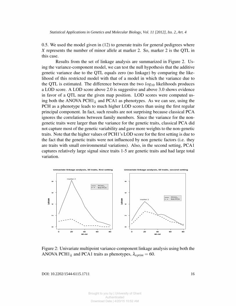
Results from the set of linkage analysis are summarized in Figure 2. Us-ing the variance-component model, we can test the null hypothesis that the additivegenetic variance due to the QTL equals zero (no linkage) by comparing the like-lihood of this restricted model with that of a model in which the variance due tothe QTL is estimated. The difference between the two log10 likelihoods producesa LOD score. A LOD score above 2.0 is suggestive and above 3.0 shows evidencein favor of a QTL near the given map position. LOD scores were computed us-ing both the ANOVA PCH1λ and PCA1 as phenotypes. As we can see, using thePCH as a phenotype leads to much higher LOD scores than using the first regularprincipal component. In fact, such results are not surprising because classical PCAignores the correlations between family members. Since the variance for the non-genetic traits were larger than the variance for the genetic traits, classical PCA didnot capture most of the genetic variability and gave more weights to the non-genetictraits. Note that the higher values of PCH1’s LOD score for the first setting is due tothe fact that the genetic traits were not influenced by non genetic factors (i.e. theyare traits with small environmental variations). Also, in the second setting, PCA1captures relatively large signal since traits 1-5 are genetic traits and had large totalvariation.

0 20 40 60 80

02

46

8

Univariate linkage analysis, 50 traits, first setting

80 cM

Lod s

core

0 20 40 60 80

02

46

8

80 cM

Lod s

core

marker 2

PCH1λ

first PCA

0 20 40 60 80

02

46

8

Univariate linkage analysis, 50 traits, second setting

80 cM

Lod s

core

0 20 40 60 80

02

46

8

80 cM

Lod s

core marker 2

PCH1λ

first PCA

Figure 2: Univariate multipoint variance-component linkage analysis using both theANOVA PCH1λ and PCA1 traits as phenotypes, λoptim = 60.

16


DOI: 10.2202/1544-6115.1711



In both settings we assumed no correlation between the last (r− 10) non-genetic traits. In microarray data, most gene-expression levels are highly correlatedwith each other; this is due on the one hand to underlying environmental factors,and on the other to some common genetic regulation. To reflect real situations,we added to both settings above a few scenarios corresponding to varying environ-mental correlations between the last r−10 traits (ρ = 0.2,0.5,0.7) for any pair oftraits. Figure 3 shows results for LOD scores computed using the ANOVA PCH1λ

as phenotype. One can notice that the performance of the ANOVA PCH1 estimatorsremained good as the correlation increased. Note that the same analysis using thefirst ANOVA PCA1 is not reported here as it did not detect linkage in any of thesettings (LOD scores equal to zero).

0 20 40 60 80

02

46

8

80 cM

Lod s

core

0 20 40 60 80

02

46

8

80 cM

Lod s

core

0 20 40 60 80

02

46

8

First PCH in linkage analysis, 50 traits, first setting

80 cM

Lod s

core

marker 2

ρ = 0.2ρ = 0.5ρ = 0.7

0 20 40 60 80

02

46

8

80 cM

Lod s

core

0 20 40 60 80

02

46

8

80 cM

Lod s

core

0 20 40 60 80

02

46

8

First PCH in linkage analysis, 50 traits, second setting

80 cM

Lod s

core

marker 2 ρ = 0.2ρ = 0.5ρ = 0.7

Figure 3: Univariate multipoint variance-component linkage analysis using theANOVA PCH1λ trait as phenotype, λoptim = 60.

6 Data analysisWe applied the PCH framework using our proposed ANOVA estimators to a uniqueschizophrenia (SZ) and bipolar disorder (BP) sample from the Eastern Quebec pop-ulation. This sample of 48 multigenerational families comprises a total of 1,278individuals, 365 of whom are affected by SZ or BP spectrum disorder. The life-time presence of symptoms of psychosis, manic and depressive symptoms in a total

17





of 439 subjects were evaluated on a six-point rating scale on each of the 82 itemsof the Comprehensive Assessment of Symptoms and History (CASH) instrument(Andreasen et al., 1992). These 439 subjects contained the 365 subjects affectedby SZ or BP spectrum disorder plus another set of 74 subjects unaffected by thesedisorders but showing the presence of some of these symptoms. The procedureof assessment is described in detail in Maziade et al. (1995). The 82 items cov-ered the following 11 dimensions: Delusion (15 items), Hallucination (6 items),Bizarre behavior (5 items), Catatonia (6 items), Thought disorder (7 items), Alo-gia (4 items), Anhedonia (5 items), Apathy (4 items), Affective blunting (8 items),Mania (8 items) and Depression (14 items). In the current paper, these 11 -acuteepisode- dimensions scores, computed as the average of their items, were used forsubsequent analyses.

First, we estimated the variance components of the genetic model (1) us-ing both ANOVA and maximum likelihood methods. Using these estimates, wecomputed the corresponding principal components of heritability. The estimates ofPCH1λ from these two methods and their associate heritabilities are given in Table4. As we can see in this Table (first two columns), the estimates of the first PCH

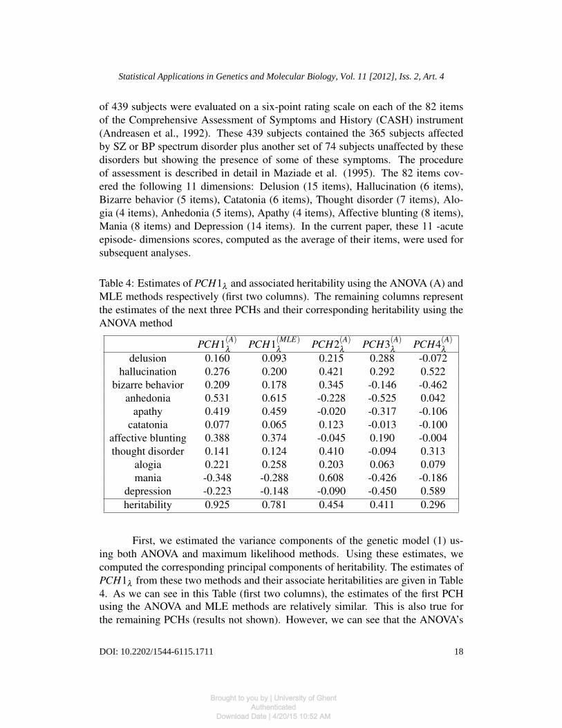
Table 4: Estimates of PCH1λ and associated heritability using the ANOVA (A) andMLE methods respectively (first two columns). The remaining columns representthe estimates of the next three PCHs and their corresponding heritability using theANOVA method

PCH1(A)λ

PCH1(MLE)λ

PCH2(A)λ

PCH3(A)λ

PCH4(A)λ

delusion 0.160 0.093 0.215 0.288 -0.072hallucination 0.276 0.200 0.421 0.292 0.522

bizarre behavior 0.209 0.178 0.345 -0.146 -0.462anhedonia 0.531 0.615 -0.228 -0.525 0.042

apathy 0.419 0.459 -0.020 -0.317 -0.106catatonia 0.077 0.065 0.123 -0.013 -0.100

affective blunting 0.388 0.374 -0.045 0.190 -0.004thought disorder 0.141 0.124 0.410 -0.094 0.313

alogia 0.221 0.258 0.203 0.063 0.079mania -0.348 -0.288 0.608 -0.426 -0.186

depression -0.223 -0.148 -0.090 -0.450 0.589heritability 0.925 0.781 0.454 0.411 0.296

using the ANOVA and MLE methods are relatively similar. This is also true forthe remaining PCHs (results not shown). However, we can see that the ANOVA’s

18


DOI: 10.2202/1544-6115.1711



estimate produces a larger heritability, and therefore can be more informative fora future genetic linkage analysis. The principal components of heritability can beinterpreted by looking at the weights for each trait component. Traits with largeweights (in absolute value) tend to have larger genetic effects. As we can see inTable 4 (first column), the first principal component of heritability discriminatessubjects with mania and depression symptoms from other subjects. This is inter-esting, as mania and depression symptoms characterize bipolar disorder. In otherwords, the first PCH discriminates BP subjects from other subjects. This was some-how expected, as it is known that the disease diagnostic is a heritable trait. However,using several PCHs may enable us to refine the diagnostic criterion. For example,by looking at the largest weights, the second PCH can be seen as a contrast betweensubjects showing an agitated and disorganized psychotic state (mania, hallucination,thought disorder, bizarre behavior) and other subjects.

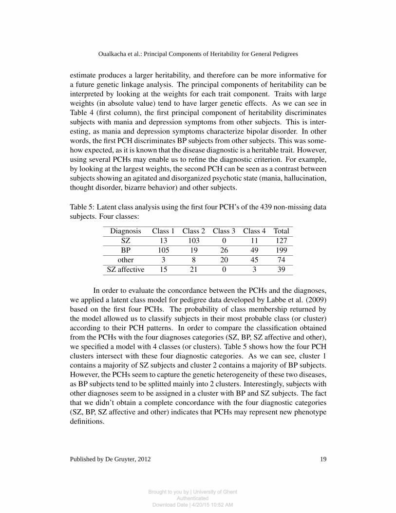
In order to evaluate the concordance between the PCHs and the diagnoses,we applied a latent class model for pedigree data developed by Labbe et al. (2009)based on the first four PCHs. The probability of class membership returned bythe model allowed us to classify subjects in their most probable class (or cluster)according to their PCH patterns. In order to compare the classification obtainedfrom the PCHs with the four diagnoses categories (SZ, BP, SZ affective and other),we specified a model with 4 classes (or clusters). Table 5 shows how the four PCHclusters intersect with these four diagnostic categories. As we can see, cluster 1

Table 5: Latent class analysis using the first four PCH’s of the 439 non-missing datasubjects. Four classes:

Diagnosis Class 1 Class 2 Class 3 Class 4 TotalSZ 13 103 0 11 127BP 105 19 26 49 199

other 3 8 20 45 74SZ affective 15 21 0 3 39

contains a majority of SZ subjects and cluster 2 contains a majority of BP subjects.However, the PCHs seem to capture the genetic heterogeneity of these two diseases,as BP subjects tend to be splitted mainly into 2 clusters. Interestingly, subjects withother diagnoses seem to be assigned in a cluster with BP and SZ subjects. The factthat we didn’t obtain a complete concordance with the four diagnostic categories(SZ, BP, SZ affective and other) indicates that PCHs may represent new phenotypedefinitions.

19





7 DiscussionWe proposed some modified ANOVA estimators of the variance components of aone way multivariate genetic random effect ANOVA model for general pedigreesand applied them to the PCH context. The main contribution of our work is thatthese ANOVA estimators allow to estimate PCH in families of any structure (andnot only siblings) as well as in situations where the number of traits is large. Inhuman studies, family data are typically collected over at least two generations.Furthermore, in fields such as mental health where phenotype definition is a chal-lenge, researchers collect more and more traits in order to better characterize thephenotype-genotype relationships. An extreme case of large number of phenotypesis also illustrated in eQTL (expression-QTL) studies where thousands of gene ex-pressions are used as phenotypes to better characterize the genetic contribution tothe variation of gene expressions.

As illustrated in our simulation study, our proposed ANOVA VC estimatorssignificantly reduce the bias over the corresponding maximum likelihood estima-tors, at the price of a slight increase in risk. Since it is beneficial to have estimatorsclose to the true value (small bias) with modest risk than the opposite, we wouldrecommend in practice the use of ANOVA’s estimators if the risk is not a seriousconcern. Otherwise, we recommend the REML estimators when applicable (i.e.small number of traits). Furthermore, these estimators are extremely fast to com-pute and are based on explicit formulas. They can also handle a large number oftraits, which is not the case for the maximum likelihood estimator. In fact, whatcould be seen first as an outdated approach is actually a fast and powerful wayto estimate variance components. As shown in Swallow & Monahan (1984), theANOVA VC estimators we propose are unique and efficient, as it is the case withone-way random effect models. Note that one can also include covariates in themodel. In this case, a mixed-effects regression model could be used to estimatethe regression coefficients and the variance components simultaneously (see for ex-ample Baltagi & Chang, 1994, for a discussion of the ANOVA estimates in such amodel).

Principal component of heritability is a great tool that allows the selection ofthe most heritable linear combination of phenotypes, measured in families. In thispaper, we established a link between PCHs and discriminant axes from a traditionallinear discriminant analysis. In particular, we showed that the PCHs computedusing the variance components of Ott & Rabinowitz and Wang et al. (2007a) forsimple pedigrees are exactly equal to the discriminant axes. As in standard principalcomponent analysis, selection of the PCH is an issue. In PCA, PCs are chosenaccording to the percentage of the variance explained. In a similar spirit, one maychoose the PCHs that have a higher heritability than each of the traits separately.

20


DOI: 10.2202/1544-6115.1711



Note that in order to obtain a better interpretation of the PCHs, it would also bepossible to apply a rotation R to the matrix A of genetic correlations between thetraits and the PCHs, as well as to the matrix of PCHs. The rotation would be chosensuch that the genetic correlations obtained in the matrix AR are either close to 0 or1.

Using the first PCH as a quantitative phenotype, or several PCH’s as multi-variate quantitative phenotypes in linkage analysis provides greater power to detectdisease susceptibility genes. Our simulations show that using PCH1λ as a pheno-type in linkage analysis leads to higher LOD score, while using the standard PCAresults in lower of LOD scores. This is coherent with the simulation studies con-ducted by Ott & Rabinowitz and Wang et al. (2007a). Wang et al. (2009) alsocompared PCA and Factor Analysis (FA) to uncover genetic factors that contributeto complex disease phenotypes. They found that FA generally produced factorsthat had stronger correlations with the genetic traits. Faced with high dimensionaltraits as in Morley et al. (2004), where 3,354 gene expression traits were measured,one could construct clusters that combine similar traits among family members andthen used the ML estimates of the PCH to combine the phenotypes in each cluster.However, the trait clusters can still be relatively large as it is the case with microar-ray gene expression data. Wang et al. (2007b) proposed a clustering approach thattakes into account the family structure information. They applied this approachto the gene expression data used in Morley et al. (2004) and then used the PCHapproach to combine the phenotypes in each cluster. Nevertheless, they used thesample between-family sum-of-squares to estimate Σg, and used the sample within-family sum-of-squares to estimate Σe for the 14 large families used in this data.Using the proposed ANOVA estimates of VC could greatly improve the estimationof the PCHs for these data.

Finally, we point out some limitations of the ANOVA approach: first, therisk of the VC estimators deteriorates when one deals with extremely large pedi-grees (results not shown). In practice, this is not of great importance since the sizeof a pedigree rarely exceeds 30 subjects. Second,we focused on simple variance-covariance structure of the genetic model. With a more general variance structure,the model will be more complex. For instance, one can assume that the phenotypeis influenced by l loci. However, if we are focusing on the analysis of one locusspecifically, we can absorb the effects of all the remaining QTLs in a residual ge-netic component and the variance-covariance between relatives will be decomposedinto three components: the major locus component (specific QTL), the polygeniccomponent (residual genetic) and the environmental component. Thus, a systemof three equations, rather than the two independent equations in (9), can solve thisestimation problem. It would be then interesting to compute the heritability basedon the major locus. This is the object of a future work. Finally, an R package

21





computing the estimators of Σg, Σe and PCHλ is available from the authors uponrequest.

Supplementary MaterialsWeb Appendix A, referenced in Section 5.1, is available under the Paper Informa-tion link at the Berkeley electronic press website

A Appendix

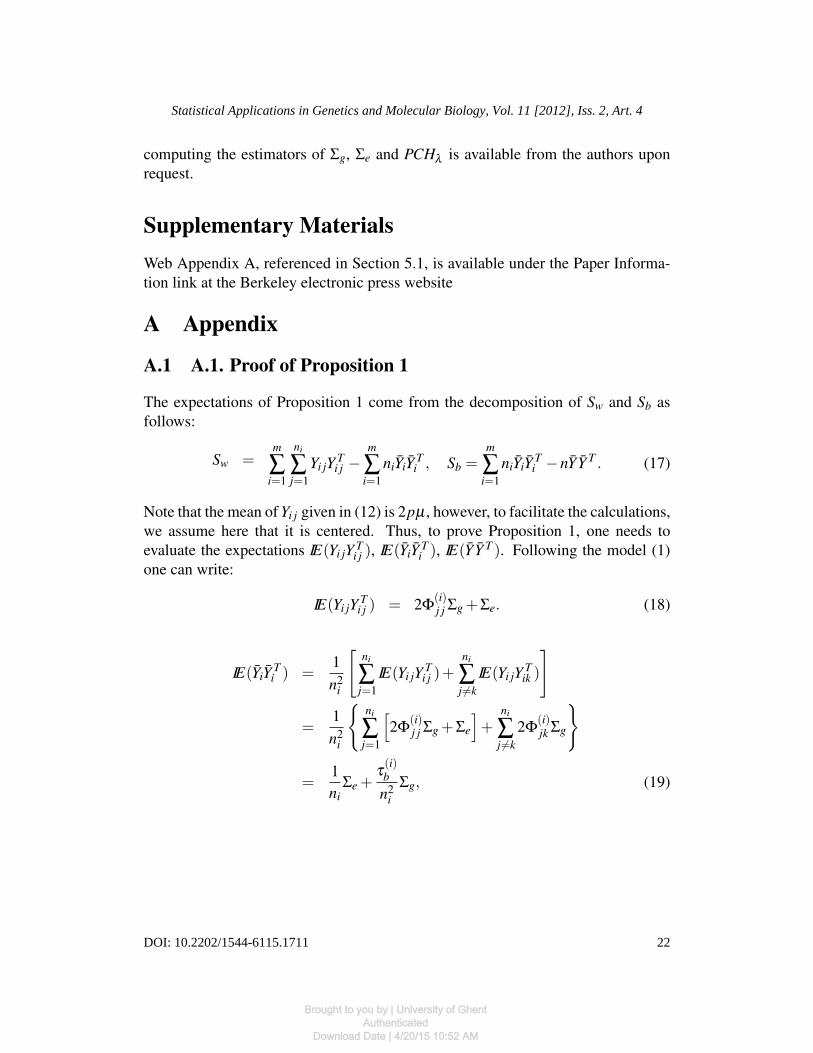
A.1 A.1. Proof of Proposition 1

The expectations of Proposition 1 come from the decomposition of Sw and Sb asfollows:

Sw =m

∑i=1

ni

∑j=1

Yi jY Ti j −

m

∑i=1

niYiY Ti , Sb =

m

∑i=1

niYiY Ti −nYY T . (17)

Note that the mean of Yi j given in (12) is 2pµ , however, to facilitate the calculations,we assume here that it is centered. Thus, to prove Proposition 1, one needs toevaluate the expectations IE(Yi jY T

i j ), IE(YiY Ti ), IE(YY T ). Following the model (1)

one can write:

IE(Yi jY Ti j ) = 2Φ

(i)j j Σg +Σe. (18)

IE(YiY Ti ) =

1n2

i

[ni

∑j=1

IE(Yi jY Ti j )+

ni

∑j 6=k

IE(Yi jY Tik )

]

=1n2

i

ni

∑j=1

[2Φ

(i)j j Σg +Σe

]+

ni

∑j 6=k

2Φ(i)jk Σg

=1ni

Σe +τ(i)b

n2i

Σg, (19)

22


DOI: 10.2202/1544-6115.1711



where τ(i)b is defined in Proposition 1. The expectation of YY T can be written as

IE(YY T ) =1n2 IE

(m

∑i=1

niYi

m

∑l=1

nlY Tl

)

=1n2

[m

∑i=1

n2i IE(YiY T

i )+m

∑i6=l

ninlIE(YiY Tl )

]

=1n2

[m

∑i=1

n2i

(1ni

Σe +τ(i)b Σg

n2i

)]=

1n

Σe +τb

n2 Σg, (20)

where τb is defined in Proposition 1. Using (17), (18) and (19), one has

IE(Sw) =m

∑i=1

ni

∑j=1

(2Φ

(i)j j Σg +Σe

)−

m

∑i=1

ni

(1ni

Σe +τ(i)b

n2i

Σg

),

= (n−m)Σe +(τa− τc)Σg.

The expectation of Sb is deduced in a similar way.

References[1] Almasy L, Dyer TH, Blangero J (1998). Bivariate quantitative trait linkage anal-

ysis: pleiotropy versus co-incident linkages. Genet. Epidemiol., 14: 953-958.[2] Almasy L, Blangero J (1998). Multipoint quantitative trait linkage analysis in

general pedigrees. American Journal of Human Genetics, 62:1198-1211.[3] Amemiya Y (1985). What should be done when an estimated between-group

covariance matrix is not nonnegative definit? Amer. Stat., 39, 112-117.[4] Amos CI, de Andrade M, Zhu DK (2001). Comparison of multivariate tests for

genetic linkage. Hum Hered, 51, 133-144.[5] Andreasen NC, Flaum M, Arndt S (1992). The Comprehensive Assessment

of Symptoms and History (CASH) an instrument for assessing diagnosis andpsychopathology. Arch Gen Psychiatry, 49(8), 615-623.

[6] Arya R, Blangero J, Williams K, Almasy L, Dyer TD, Leach RJ, O’Connell P,Stern MP, Duggirala R (2003). Factors of insulin resistance syndrome- relatedphenotypes are linked to genetic locations on chromosomes 6 and 7 in nondia-betic Mexican-Americans. Diabetes, 51, 841-847.

23





[7] Baltagi BH, Chang YJ (1994). Incomplete panels: A comparative study of alter-native estimators for the unbalanced one-way error component regression model.Journal of Econometrics, 62: 67–89.

[8] Bauman L, Almasy L, Blangero J, Duggirala R, Sinsheimer JS, Lange K(2005). Fishing for pleiotropic QTLs in a polygenic sea. Ann Hum Genet, 69:590-611.

[9] Calum AM, Ramachandran SV (2011). Next-generation genome-wide associa-tion studies: Time to focus on phenotype? Circ Cardiovasc Genet., 4: 334-336.

[10] Fisher RA (1936). The use of multiple measures in taxonomic problems. An-nals of Eugenics, 7, 179-188.

[11] Funalot B, Varenne O, Mas JL (2004). A call for accurate phenotype definitionin the study of complex disorders.. Nature Genetics, 36:3.

[12] Gilmour AR, Cullis BR, Welham SJ, Thompson R (1999). ASREML, refer-ence manual. Biometric bulletin, no 3, NSW Agriculture, Orange AgriculturalInstitute, Forest Road, Orange 2800 NSW Australia.

[13] Labbe A, Bureau A, Merette C (2009). Integration of genetic familial struc-turein latent class models. The International journal of Biostatistics, 5(1).

[14] Lange K, Westlake J, Spence MA (1976). Extensions to pedigree analysis. III.Variance components by the scoring method. Ann Hum Genet, 39, 485-491.

[15] Lange K, Boehnke M (l983). Extensions to pedigree analysis. IV. Covariancecomponents models for multivariate traits. Amer J Med Genet, 14, 513-524.

[16] Lange K, Cantor R, Horvath S, Perola M, Sabatti C, Sinsheimer J, Sobel E(2001). MENDEL version 4.0: A complete package for the exact genetic analy-sis of discrete traits in pedigree and population data sets. Amer J Hum Genet, 69(Suppl):504.

[17] Lange K (2002). Mathematical and Statistical Methods for Genetic Analysis.Springer Verlag, New York.

[18] Lange K, Sobel E (2006). Variance component models for X-linked QTLs.Genet Epidemiology, 30, 380-383.

[19] Mardia KV, Kent JT, Bibby JM (1979). Multivariate Analysis. AcademicPress, London.

[20] Mathew T, Niyogi A, Sinha BK (1994). Improved nonnegative estimationof variance components in balanced multivariate mixed models. J MultivariateAnal, 51, 83-101.

[21] Maziade M, Roy MA, Martinez M, Cliche D, Fournier JP, Garneau Y, et al.(1995). Negative, psychoticism, and disorganized dimensions in patients withfamilial schizophrenia or bipolar disorder: continuity and discontinuity betweenthe major psychoses. Am J Psychiatry, 152(10), 1458-63.

[22] McCulloch CE, Searle SR (2002). Generalized, Linear, and Mixed Models.John Wiley & Sons, New York.

24


DOI: 10.2202/1544-6115.1711



[23] Morley M, Molony CM, Weber TM, Devlin JL, Ewens KG, Spielman RS,Cheung BG (2004). Genetic analysis of genome-wide variation in human geneexpression. Nature, 430 (7001), 743-747.

[24] Ott J, Rabinowitz D (1999). A principal-components approach based on heri-tability for combining phenotype information. Hum Hered, 49, 106-111.

[25] Searle SR, Casella G, McCulloch CE (1992). Variance Components. John Wi-ley & Sons, New York.

[26] Srivastava MS, Kubokawa T (1999). Improved nonnegative estimation of mul-tivariate components of variance. The Annals of Statistics, 27, No. 6, 2008-2032.

[27] Sun YJ, Sinha BK, von Rosen D, Meng QY (2003). Nonnegative estimation ofvariance components in multivariate unbalanced mixed linear models with twovariance components. J Stat Plann and Inf, 115, 215234.

[28] Swallow WH ,Monahan JF (1984). Monte carlo comparison of ANOVA,MIVQUE, REML, and ML estimators of variance components. Technometrics,26, 47-57.

[29] Terwilliger JD, Speer M, Ott J (1993). Chromosome-based method for rapidcomputer simulation in human genetic linkage analysis. Genet Epidemiol, 10,217-224.

[30] Wang Y, Fang Y, Wang S (2007). Clustering and principal component analysisfor mapping co-regulated genome-wide variation using family data. BMC Genet,1(Suppl 1):S121.

[31] Wang Y, Fang Y, Jin M (2007). A ridge penalized principal-components ap-proach based on heritability for high-dimensional data. Hum Hered, 64, 182-191.

[32] Wang X, Kammerer CM, Anderson S, Lu J, Feingold E (2009). A comparisonof principal component analysis and factor analysis strategies for uncoveringpleiotropic factors. Genet Epidemiol, 33(4), 325-331.

25





Statistical Applications in Genetics and Molecular Biologykvansteen/GeneticEpi-Engineering/ac1415... · Statistical Applications in Genetics ... ology of many complex disorders, ...

Documents