Statistical Analysis of Text in Survey Records

1

Statistical Analysis of Text in Survey Records

Wendy Martinez Alex Measure

Bureau of Labor Statistics 2 Massachusetts Ave., N.E.

Washington, DC 20212

Proceedings of the 2013 Federal Committee on Statistical Methodology (FCSM) Research Conference

Introduction

The goal of this work is to provide the reader with some background information on the analysis of semi-structured and unstructured text fields that are often available in survey records. The hope is that some readers will then be able to apply these ideas to their own data. This first section introduces some concepts of text analysis, such as the types of tasks we might be interested in accomplishing. The next section briefly describes the typical steps we take in analyzing text, which is followed by a motivating example using the narratives from accident reports to illustrate the concepts.

There are many goals that one might want to accomplish when analyzing text or documents. We use the term document to refer to any section of text, which could be a phrase, sentence, paragraph, chapter, email, etc. The two main applications of text analysis described in this paper are the supervised and unsupervised classification of documents. Of course, these techniques can be applied to many different types of data – not just to documents.

In supervised document classification, we start with a set of documents (or a corpus), where each document has a label attached to it. This label could be many things; examples include the topic assigned to a news story, the occupation title attached to a job description, or the type of event in an accident report. We want to use the existing labeled corpus of documents to build a classifier, which can then be used to assign labels to unlabeled documents. Some potential applications of classification in survey data include the computer assisted coding of records in the Survey of Occupational Injuries and Illnesses (SOII) [Measure, 2013] and the determination of employee benefits from compensation plans for the National Compensation Survey (NCS).

In unsupervised document classification, we typically do not have labels attached to our documents, as we have with supervised learning. Instead, we are interested in grouping documents in such a way that documents in the same cluster or group are more similar to each other than they are to those in other groups. One way to gauge similarity with text-based data is by examining the individual words in the documents and their meaning. The hope is that together the documents in a cluster belong to a common topic of discourse. A potential application of unsupervised classification in survey data is to identify new relationships and commonalities among survey records.

Steps for Text Analysis

The basic steps in the analysis of text are given here, and we include some of the more common approaches for each of the steps. There are many variations and other possible methods for text analysis, but what is given below should provide the reader with an introduction to the topic.

Step 1 – Preprocess the Text

The first step in analyzing text data is to preprocess it. Typically, this part of the process is focused more on data cleaning. A common procedure is to convert all words to lower case and remove any special

2

characters, such as %, $, #, @, colons, semi-colons, etc. There are applications and approaches where word case and special characters are considered informative, but we focus here on the more widely-used methods.

It is also often useful to remove stop words. These are words that have low informational content and are typically common words. However, this is not necessarily the case, as we will see later in the paper. The appropriate choice of stop words is highly task specific. Examples of commonly-used stop words include the, of, her, it, etc.

Stemming is another preprocessing step that is sometimes used. Stemming is concerned with reducing the number of unique words in the lexicon by removing suffixes and prefixes of words. Thus, we are left with the stem (or root) of the word. For example, the words protecting, protected, protects would be reduced to the word protect [Solka, 2008; Porter, 1980]. Stemming saves storage space and other computational resources, but it also has the potential to remove useful information. For example, in some applications, we may want to distinguish between a singular noun and its plural, such as in “the worker broke his leg” or “the worker broke his legs.”

Step 2 – Encode the Text

We have to convert the text to numbers, so we can apply statistical methods to the data. A common method is to represent the text as a term-document matrix (TDM). This matrix has dimensions p n , where p is the number of unique words (or terms) in the lexicon (or the number of variables) and n is the number of documents (or the number of observations). The entries in the TDM typically contain some indicator of the occurrence of each term in the document, such as a 1 if it occurs and a 0, if it does not. Alternatively, the elements of the TDM could correspond to the number of times the i-th word appears in the j-th document.

The use of a term-document matrix is sometimes called a bag-of-words approach, since the relative positions of the terms in the text are lost when converted to the TDM. For most analyses, this results in a very high dimensional data set, and it is also an example of a small n, large p problem [Berry, et al., 1995; Berry, et al., 1999].

Some in the information retrieval community have developed weights to incorporate information beyond the occurrence of a word in a document. This is known as term weighting. One of the motivations for weighting words is that some words are more informative or discriminating than others. For example, the word employee occurs with high frequency in the accident records used in our example, so it is probably not very useful for distinguishing between incident reports.

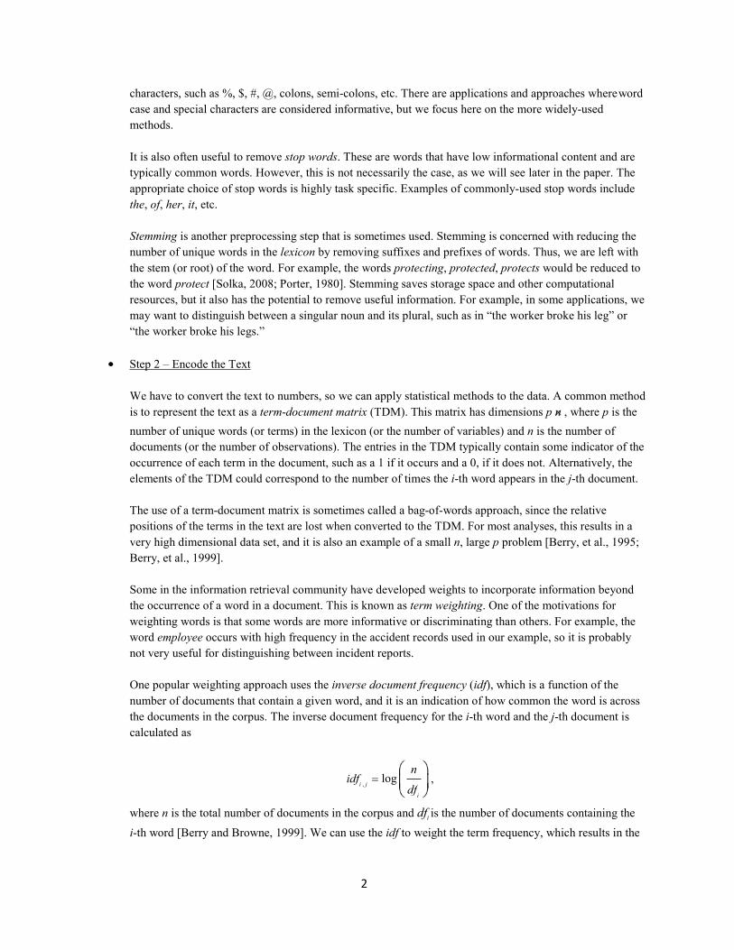
One popular weighting approach uses the inverse document frequency (idf), which is a function of the number of documents that contain a given word, and it is an indication of how common the word is across the documents in the corpus. The inverse document frequency for the i-th word and the j-th document is calculated as

idf

i , j

where n is the total number of documents in the corpus and dfi is the number of documents containing the i-th word [Berry and Browne, 1999]. We can use the idf to weight the term frequency, which results in the

log n

, df i

3

term frequency–inverse document frequency (tf-idf). To calculate the tf-idf, we multiply the raw frequency (denoted as tf ) by the inverse document frequency, as shown here

tf -idf

The tf-idf will be large if a word appears with high frequency in the document, but occurs rarely across the documents in the corpus. In text analysis applications, we could use the tf idfi, j as the elements in the TDM [Berry, 2001].

Step 3 – Reduce the Dimensionality

We saw in the previous step that we usually end up with a set of very high-dimensional data when we encode a set of documents as a term-document matrix. For some applications, it is necessary to first reduce the dimensionality in some manner before we can analyze the documents. We briefly describe three approaches for reducing the dimensionality in text analysis applications.

Perhaps, the most common approach is called latent semantic indexing (or analysis), which is based on the singular value decomposition of the term-document matrix [Deerwester, et al., 1990]. It involves finding the singular vectors and singular values of the term-document matrix, and thus, is somewhat similar to principal component analysis [Jackson, 1991].

Another approach to reduce the dimensionality of the term-document matrix is nonnegative matrix factorization [Lee and Seung, 1999]. This works in a similar manner to latent semantic analysis and principal component analysis, in that it seeks a factorization of the term-document matrix, where the elements of the factorization can be used to reduce the number of features. However, nonnegative matrix factorization applies constraints to keep the features nonnegative. This makes more sense with a term- document matrix, where all entries are nonnegative. One of the nice aspects of nonnegative matrix factorization is that one of the matrix factors provides a grouping or clustering of the documents, without any further processing.

A nonlinear approach for dimensionality reduction that works well in practice is isometric feature mapping (ISOMAP). ISOMAP was developed by Tenenbaum, et al. [2000] as an enhancement to multi-dimensional scaling (MDS). MDS requires all distances between observations as inputs to the algorithms, and Euclidean distance is used quite often. If we are trying to recover features on a nonlinear manifold (or surface) that is embedded in a higher-dimensional space, then the Euclidean distance is not the best measure to use. Thus, ISOMAP first estimates the geodesic distance between observations from the nearest-neighbors and uses those as inputs to classical MDS. This is the approach we employ in our example.

Step 4 – Analyze the Documents

Our text-based data have now been cleaned up and converted to numbers we can use. So, the next step is to analyze them in accordance with our application of interest. As stated previously, this analysis could take on many forms and might require a different encoding or representation of the text (Step 2). A brief list of options includes (1) assigning a label to a document, such as the topic or event type, (2) sentiment analysis to determine the emotion conveyed in text, (3) exploratory data analysis through clustering, or (4) author attribution.

tf i , j i , j idf .

i , j

i , j

4

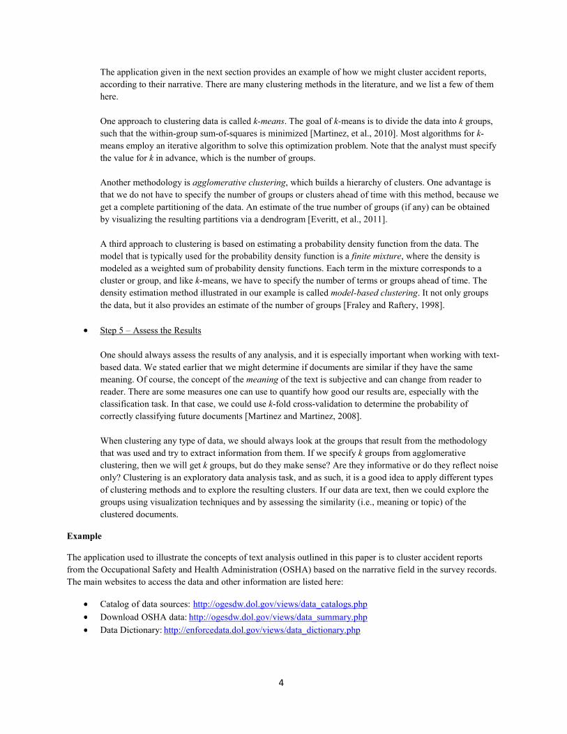
The application given in the next section provides an example of how we might cluster accident reports, according to their narrative. There are many clustering methods in the literature, and we list a few of them here.

One approach to clustering data is called k-means. The goal of k-means is to divide the data into k groups, such that the within-group sum-of-squares is minimized [Martinez, et al., 2010]. Most algorithms for k- means employ an iterative algorithm to solve this optimization problem. Note that the analyst must specify the value for k in advance, which is the number of groups.

Another methodology is agglomerative clustering, which builds a hierarchy of clusters. One advantage is that we do not have to specify the number of groups or clusters ahead of time with this method, because we get a complete partitioning of the data. An estimate of the true number of groups (if any) can be obtained by visualizing the resulting partitions via a dendrogram [Everitt, et al., 2011].

A third approach to clustering is based on estimating a probability density function from the data. The model that is typically used for the probability density function is a finite mixture, where the density is modeled as a weighted sum of probability density functions. Each term in the mixture corresponds to a cluster or group, and like k-means, we have to specify the number of terms or groups ahead of time. The density estimation method illustrated in our example is called model-based clustering. It not only groups the data, but it also provides an estimate of the number of groups [Fraley and Raftery, 1998].

Step 5 – Assess the Results

One should always assess the results of any analysis, and it is especially important when working with text- based data. We stated earlier that we might determine if documents are similar if they have the same meaning. Of course, the concept of the meaning of the text is subjective and can change from reader to reader. There are some measures one can use to quantify how good our results are, especially with the classification task. In that case, we could use k-fold cross-validation to determine the probability of correctly classifying future documents [Martinez and Martinez, 2008].

When clustering any type of data, we should always look at the groups that result from the methodology that was used and try to extract information from them. If we specify k groups from agglomerative clustering, then we will get k groups, but do they make sense? Are they informative or do they reflect noise only? Clustering is an exploratory data analysis task, and as such, it is a good idea to apply different types of clustering methods and to explore the resulting clusters. If our data are text, then we could explore the groups using visualization techniques and by assessing the similarity (i.e., meaning or topic) of the clustered documents.

Example

The application used to illustrate the concepts of text analysis outlined in this paper is to cluster accident reports from the Occupational Safety and Health Administration (OSHA) based on the narrative field in the survey records. The main websites to access the data and other information are listed here:

Catalog of data sources: http://ogesdw.dol.gov/views/data_catalogs.php Download OSHA data: http://ogesdw.dol.gov/views/data_summary.php Data Dictionary: http://enforcedata.dol.gov/views/data_dictionary.php

5

We downloaded OSHA accident reports for November and December 2011. The records have many variables, and several of them are semi-structured free-form text. A partial list of the text fields is given below:

Event description – short text phrase Event keywords – Nature, Body Part, Source, etc. Event type – label indicating the type of accident event Abstract – free-form text describing the accident

The goal is to cluster the records based on the narrative in the abstract field. We processed the text by removing all special characters and converting words to lower case as described in Step 1. We also removed stop words using a general list that was not adjusted to fit this particular data set or domain, and we did not apply stemming to these data. Our final data set was comprised of 358 abstracts or documents, and the lexicon had 3,841 words. Thus, we have n 358 and p 3841.

Using these data, we created a term-document matrix, where the ij-th element is the number of times the i-th word appears in the j-th document (Step 2). Note that we used the raw frequencies for this example, and our term- document matrix had 3,841 rows and 358 columns. In this example, we wanted to try an approach called model- based clustering, because it has some nice properties that we describe later. However, it requires the estimation of covariance matrices. Therefore, we first needed to reduce the dimensionality to a point where the computations become possible, and we used ISOMAP to do this.

We used MATLAB for all of the preprocessing, encoding, and analysis of the documents used in this application. The authors of ISOMAP published a MATLAB M-file that will return the coordinates of the observations in lower- dimensional spaces (specified by the user) and a scree plot that can be used to choose the number of final dimensions to use. The scree plot from ISOMAP is shown in Figure 1. We look for an elbow in the curve to help us choose the number of dimensions. There appears to be two elbows–one at 4 and another at 6. It is usually best to be parsimonious, so we chose 4 dimensions for this analysis.

We used the model-based clustering (MBC) approach to group the accident reports (Step 4). Model-based clustering is a methodology that estimates a finite mixture probability density function using the data [Fraley and Raftery, 1998]. The finite mixture is a weighted sum of probability densities, which for MBC are multivariate normal. The Expectation-Maximization (EM) algorithm is used to estimate the parameters of the finite mixture (i.e., the means, covariance matrices, and weights for each term).

The EM algorithm is an iterative method and requires a starting point (i.e., value of the parameters), as well as the number of terms in the mixture. The MBC method addresses these issues. It provides a sequence of starting points for the EM algorithm that are based on different constraints imposed on the covariance matrices and different values for the number of terms (or clusters). The finite mixture is estimated for each of these starting points, and the Bayesian Information Criterion (BIC) is calculated for each estimated mixture model. The final model we choose– number of terms and the shape of the groups–is determined by the one that produces the highest BIC.

It is perhaps easier to understand what is going on with model-based clustering by looking at the graph in Figure 2, which is an output from the MATLAB code for MBC. Here, we have nine curves, each one corresponding to one of the models that constrain the covariance matrices. The horizontal axis shows the number of terms we specify in the model, and the vertical axis reflects the BIC value. Each point on the curve is one of the starting points (or finite mixture model) to the EM algorithm. So, one can see that we loop through different values for the number of terms and covariance constraints (models), estimate the finite mixture, and calculate the BIC.

6

Scree Plot - ISOMAP 1

0.9

0.8

0.7

0.6

0.5

0.4

1 2 3 4 5 6 7 8 9 10 Isomap dimensionality

Figure 1 This shows the scree plot from ISOMAP. We can use the elbow in the curve as an indication of the number of dimensions to use in the lower-dimensional space. It looks like there are elbows at 4 and 6. It is usually best to be parsimonius, so we chose 4 dimensions for our analysis.

It appears from Figure 2 that the best model is one that has five terms or clusters. At this point, we do not concern ourselves with what constraints on the covariance matrices produced the best model. However, it is helpful to know that model-based clustering can produce a rather rich set of cluster configurations, unlike other clustering methods. For example, k-means clustering tends to produce all spherical clusters, while model-based clustering can produce clusters of different shapes. This aspect of MBC, coupled with the estimation of the number of groups (or terms in the mixture) that is also obtained, makes MBC an appealing approach to clustering.

Now that our documents are divided into groups, we need to assess the resulting clusters (Step 5). Do they indicate some cohesive structure or common meaning in the groups? Or, did we get just a meaningless result? We can examine the clusters in several ways. First, it is always a good idea to visualize the clusters in scatter plots, where we plot the documents with colors and/or symbols corresponding to the cluster. We can also try to determine topic labels by finding important words in each group.

Figure 3 shows a scatter plot matrix, which is a matrix of all pair-wise scatter plots of the data. The coordinates of the data correspond to the four ISOMAP dimensions, so we have a 4 4 matrix of plots. The diagonal elements of the plot matrix contain histograms of each of the four ISOMAP dimensions (or features). The colors and symbols of the points in the scatter plots indicate the cluster. We see from the scatter plots that the grouping seems reasonable from their spatial configurations over these four dimensions.

Res

idua

l var

ianc

e

7

2. C □IJo D oJ 0

D od\ o i D D

1 -

0 .

:

, cgor0 l:b

( c:i C C

[§JD O dJO 8rl 0

... -2.

2 . C

1- C cC

C C O OD OD · - Dr;Jl Doo

c'

.2 l,_ -- _ _., - - - -" '- -' ·'..c··· - --- - - -'-'L.- - - --- -- - >u - -

1: ; = ), I

2: 21._ = )k, I

--:· 3:; = /, B

4: 21._ = ), Bk

5: 21._ = )k, Bk 6:; = ), DAD'

* 7: ; = ), Dk A Dk' 8: ; = ), Dk Ak Dk'

9:; =;

·

I

')'

Model 2, 5 clusters is optima! - 30 50-- ·-------

-3100

1·

-3150 *

-3200

-3250

-3300

-3350

-3400 +

.3450 L 0

Number of clusters

Figure 2 These are the BIC curves from model-based clustering. The highest BIC value corresponds to 5 terms or clusters.

ISOMAP-40, 5 Clusters (MBC)

.2 -1 -2 -1 -2 -1 -2 -1

Figure 3 This is a scatter plot matrix of the four ISOMAP dimensions, where the colors and symbols indicate cluster membership. We see that the groupings seems reasonable.

8

We can find high frequency words in each cluster to help us assign a topic to them, or we can use the tf-idf instead of the raw word frequency as a measure of word importance. Table 1 shows the 10 highest frequency words in each of the five clusters. We highlighted the words in red that we feel can be used to indicate topics. For example, the first cluster seems to be accidents involving vehicles, and cluster 2 appears to consist of accidents from body parts being cut with sharp objects.

We can also see some potential non-informative words in Table 1. The word occurring with the highest frequency in all clusters is the word employee. That is not surprising given that these are accidents experienced by workers, but it does not provide any discrimination among the groups. Another example is the appearance of the words November and December across most of the clusters. We might consider adding these words to our stop list and repeating our analysis.

Table 1 Highest Frequency Words in Clusters

Cluster 1

31 Docs

Cluster 2

37 Docs

Cluster 3

102 Docs

Cluster 4

51 Docs

Cluster 5

137 Docs

employee employee employee employee employee

truck machine december ladder november

trailer finger approximately approximately december

approximately saw feet roof forklift

november left working fell approximately

driver hand fell working hospital

cable approximately november employees back

pole blade employer november right

december december tree december left

struck cutting accident ft working

Summary

In this paper, we provided an overview of text analysis in the context of a motivating example that applied the concepts to the clustering of narratives in accident reports. The goal was to motivate and encourage the reader to apply the methodologies to other survey data and to take advantage of this information-rich data source.

We conclude this paper by giving some additional references and computational resources for analyzing text. As stated previously, we used MATLAB for the example presented in this paper. MATLAB has extensive capabilities for handling text or strings. We used the MATLAB ISOMAP function that was written by the authors. This can be downloaded from their website http://isomap.stanford.edu/. It is also part of the Exploratory Data Analysis (EDA) Toolbox [Martinez, et al., 2010] for MATLAB, which can be downloaded here http://pi-sigma.info/. Additionally, the EDA Toolbox has several clustering options, including model-based clustering.

9

There is a website with resources for model-based clustering. This site has links to papers and software (MATLAB and R): http://www.stat.washington.edu/raftery/Research/mbc.html.

The open-source computing environment R can be downloaded at the Comprehensive R Archive Network at this website: http://cran.us.r-project.org/. There is a Task View that contains information about R packages for text analysis and natural language processing: http://cran.us.r-project.org/web/views/NaturalLanguageProcessing.html . Feinerer, et al. [2008] give a good overview of text mining, and they describe their R package that provides a framework for text mining in R. Finally, we mention the book by Baayen [2008] that provides an introduction to analyzing text and uses the R environment to demonstrate the concepts.

References

Baayen, R. H. 2008. Analyzing Linguistic Data: A Practical Introduction to Statistics Using R, Cambridge University Press.

Berry, M. W. (ed). 2001. Computational Information Retrieval, SIAM.

Berry, M. and M. Browne. 1999. Understanding Search Engines: Mathematical Modeling and Text Retrieval (Software, Environments, Tools), SIAM.

Berry, M., S. T. Dumais, and G. O’Brien. 1995. Using linear algebra for intelligent information retrieval, SIAM Review, 37:573 – 595.

Berry, M., Z. Drmac, and E. Jessup. 1999. Matrices, vector spaces, and information retrieval, SIAM Review, 41:335– 362.

Deerwester, S. S. Dumais, G. Furnas, T. Landauer, and R. Harshman. 1990. Indexing by latent semantic analysis, Journal of the American Society for Information Science, 41:391–407.

Everitt, B., S. Landau, M. Leese, and D. Stahl. 2011. Cluster Analysis, John Wiley.

Feinerer, I., K. Hornik, and D. Meyer. 2008. Text mining infrastructure in R, Journal of Statistical Software, March 2008, Volume 5, Issue 5, http://www.jstatsoft.org/v25/i05/paper, (accessed February 2014).

Fraley, C. and A. E. Raftery. 1998. How many clusters? Which clustering method? Answers via model-based cluster analysis, The Computer Journal, 41:578 – 588.

Jackson, J. E. 1991. A User’s Guide to Principal Components, Wiley and Sons.

Lee, D. D. and H. S. Seung. 1999. Learning the parts of objects by non-negative matrix factorization, Nature, 40:788–791.

Martinez, W. L. and A. R. Martinez. 2008. Computational Statistics Handbook with MATLAB, 2nd Edition, CRC Press.

Martinez, W. L., A. R. Martinez, and J. L. Solka. 2010. Exploratory Data Analysis with MATLAB, 2nd Edition, CRC Press.

Measure, A. 2013. Artificial Intelligence in Data Processing. Presentation at the 2013 FedCASIC. https://fedcasic.dsd.census.gov/fc2013/ppt/DM%20Fedcasic%202013%20Alex%20Measure%20AI%20in%20Data %20Processing%20FedCASIC%20version%202.pdf (accessed February 2014).

10

Porter, M. F. 1980. Algorithm for suffix stripping, Program, 130–137.

Solka, J. L. 2008. Text data mining: Theory and methods, Statistics Surveys, 2:94–112. http://projecteuclid.org/euclid.ssu/1216238228 (accessed February 2014).

Tenenbaum, J. B., V. de Silva, and J. C. Langford. 2000. A global geometric framework for nonlinear dimensionality reduction, Science, 22:2319–2323.