Statistical Analysis of Consumer Perceptions

Statistical Analysis of Consumer Perceptions

Helmut Strasser

January 26, 2000

Contents

1 Introduction 3

1.1 Problem description . . . . . . . . . . . . . . . . . . . . . . . . . . . 3

1.2 Overview . . . . . . . . . . . . . . . . . . . . . . . . . . . . . . . . 4

1.3 Notation . . . . . . . . . . . . . . . . . . . . . . . . . . . . . . . . . 6

1.4 Reduction of complexity . . . . . . . . . . . . . . . . . . . . . . . . 7

2 Statistical problems 8

2.1 Introductory example . . . . . . . . . . . . . . . . . . . . . . . . . . 8

2.2 The independence problem . . . . . . . . . . . . . . . . . . . . . . . 11

2.3 The symmetry problem . . . . . . . . . . . . . . . . . . . . . . . . . 13

2.4 Competition . . . . . . . . . . . . . . . . . . . . . . . . . . . . . . 14

2.5 The role of mixture models . . . . . . . . . . . . . . . . . . . . . . . 15

3 Explorative statistical analysis 17

3.1 Analysis of independence . . . . . . . . . . . . . . . . . . . . . . . . 17

3.2 The identification of homogeneous strata . . . . . . . . . . . . . . . . 20

3.3 Mixture models . . . . . . . . . . . . . . . . . . . . . . . . . . . . . 22

3.4 Analysis of symmetry . . . . . . . . . . . . . . . . . . . . . . . . . . 24

3.5 Analysis of competition . . . . . . . . . . . . . . . . . . . . . . . . . 27

1

Helmut Strasser 2

4 Test statistics 32

4.1 Univariate testing problems . . . . . . . . . . . . . . . . . . . . . . . 32

4.2 Multivariate testing problems . . . . . . . . . . . . . . . . . . . . . . 34

4.3 Tests of independence . . . . . . . . . . . . . . . . . . . . . . . . . . 34

4.4 Tests of symmetry . . . . . . . . . . . . . . . . . . . . . . . . . . . . 37

4.5 Adaptive partitions . . . . . . . . . . . . . . . . . . . . . . . . . . . 38

5 Critical values 40

5.1 The usual method . . . . . . . . . . . . . . . . . . . . . . . . . . . . 40

5.2 Exact critical values . . . . . . . . . . . . . . . . . . . . . . . . . . . 41

5.3 Practical evaluation . . . . . . . . . . . . . . . . . . . . . . . . . . . 43

6 Appendix 44

Helmut Strasser 3

1 Introduction

The approach which is the starting point of this paper is based on methods used byMazanec, 1995, 1999 and 2000. For further applications of this methodology we referto S. Dolnicar, K. Grabler and J. A. Mazanec, 1999).

We deal with statistical methods for marketing data which have been compressed by re-duction algorithms like those discussed by Strasser, 2000a. In conjunction with 2000a,the present paper aims at presenting some theoretical aspects of the approach usingonly little mathematical sophistication. A survey paper concerning the same subject isStrasser, 1999.

1.1 Problem description

Let us start with a brief description of the experimental design and some basic mar-keting problems which have inspired this paper. We do not claim to give a generalstatement on statistics in marketing. We are rather dealing with a very special andnarrow problem which can be extended into many directions.

The basic concepts are consumers and brands. We are interested to see how consumersperceive brands. Thus we are not dealing with choice preferences and not with con-suming decisions.

In this paper we restrict our attention to a situation where two brands are at disposal.The data arise from a consumer survey. It is an essential point for our considerationsthat the same questions about attributes are asked for both brands. We will denote byEthe set of possible answers to the series of questions. Typically, this setE is a subset ofa multidimensional space, i.e. a multivariate set in statistical terminology. In general,we haveE ⊆ Rd if there ared questions to be answered by the consumers. E.g., ifwe haved questions to be answered by ”yes” and ”no”, then the setE is the set ofall vectors of dimensiond with components equal to0 or 1. In mathematical notationthis meansE = {0, 1}d. In general, the components of vectors inE may be eithermetrically scaled variables or numerically coded but only nominally scaled variables.

Each consumer answers the same questions for both variables. Let us denote byX thevariable containing the answers for the first brand and byY the respective answers forthe second brand. These variables take values inE, thus being multivariate variableswith d components if we are askingd questions.

Dealing with data of this kind we observe that even for nominally scaled variablesmost data vectors in the sample have frequency one. This is not a surprise since for atypical dimensiond = 20 andE = {0, 1}d there are220 = 1 048 576 possible answers.Therefore it is a natural idea to look for interesting configurations, i.e. interestingsubsets ofE, rather than for single vectorsx ∈ E.

Helmut Strasser 4

Considering a single brand for its own sake, we may look at the distribution of theanswer vectors in the sample. A natural goal for the data analysis could be searchingfor subsetsA ⊆ E, where a considerable amount of data is concentrated around arelatively small area. Such subsets are called density clusters, and looking for suchdensity clusters is the traditional goal of statistical cluster analysis.

However, if we are interested in the relative positions of two brands in the mind ofconsumers, then it is not sufficient to look for clusters in the data set, but we have tothink about other problems. The basic issues from the applications point of view aredefined in Section 2. The topics are the heterogeneity of the consumer population,the exchangeability of the brands and the implications for the competition between thebrands. Using statistical terminology we are facing the independence problem and thesymmetry problem.

1.2 Overview

The subject of this paper are statistical methods for the analysis of the independenceproblem and the symmetry problem with particular emphasis on applications in mar-keting.

With the applications we have in mind the sample spaceE is of such a complex naturethat it is not possible to take all subsetsA ⊆ E into consideration. For a statisticalanalysis it is the proposal of Mazanec, 1995, 1999 and 2000, to apply a hybrid pro-cedure consisting of two steps. The first step is a data compression step resulting at areduction of complexity. The second step is devoted to the statistical analysis of thereduced data.

This chapter deals only with the second step, i.e. with the statistical analysis after thereduction of complexity.

An introduction to some basic ideas of the first step, i.e. the data compression, can befound in Strasser, 2000a. The methods which are described in that paper carry out thedata compression by reducing the original scale of the variablesX andY to a lower,namely a nominal level. This is done in an adaptive way, i.e. the construction of thenew nominal scale is based on the observed data. The algorithms are optimized aimingat little loss of information during the data compression. The mathematical foundationsof the reduction step are treated by Pötzelberger und Strasser, 1999, and by Strasser,2000b. Numerical simulation experiments related to those data compression methodsare contained in Steiner, 1999.

In the present paper we explain how the reduced data may be analyzed statistically.To begin with in Sections 3 and 3.4 we do not consider the problem of inferentialinduction. Later, in Sections 4 and 5 we show how to distinguish among observedpatterns by statistical inference.

Helmut Strasser 5

The methodology used by Mazanec applies the reduction step as an adaptive proce-dure. This fact leads to the fundamental question whether statistical inference is pos-sible in such circumstances at all. In Sections 4.5 and 5 we explain how to applystatistical tests with a controlled significance level for the independence and the sym-metry problems even if an adaptive data compression has been carried out before. It isa particularly attractive feature of Mazanec’s methodology that after an adaptive datacompression statistical inference is still available.

The tests we are proposing are distribution free and multivariate. If the reduction stepwas not carried out in an adaptive way then our tests could be considered as simple testsfor nominally scaled variables. But in view of the adaptive nature of the compressionstep the new nominal scales are data dependent. Therefore, it must be questionedwhether classical statistical tests can be applied in such situations.

The situation is similar to that of rank tests for univariate data. The methods which wepropose can be considered as multivariate extensions of rank tests. This point of viewis supported by the fact that our test procedures are constructed as permutation testswhich allow the definition of distribution free exact critical values. As is well-known,rank tests belong to the family of permutation tests, too.

Theoretical research on permutation tests by means of modern concepts of mathemati-cal statistics is in its infancy. The target is a general theory of multivariate permutationtests, quite parallel to that of univariate rank tests by Hajek und Sidak, 1967. Impor-tant steps into that direction are papers by Neuhaus, 1993 and 1998, and by Janssenand Neuhaus, 1997. As to multivariate problems, only thek-sample problem has beenconsidered by Strasser and Weber, 1999, up to now.

The complete two-step procedure can be carried out only with the help of computers.An essential point for the power of the inferential methods is the choice of the reduc-tion algorithm which has to be tailored to the particular testing problem. The gain inpower obtained by the right choice has been demonstrated in an impressive way byRahnenführer, 1999, by means of computer simulation experiments and thek-sampleproblem. Similar experiments, however, related to the independence problem and thesymmetry problem are still lacking.

The methods we are discussing are seemingly in contrast to methods labeled as statis-tical modeling, which nowadays dominate the majority of statistical data analysis inmarketing science and elsewhere. In Sections 2.5 and 3.3 we compare our approachto some concepts of statistical modeling as far as they are related to the problem underconsideration.

Helmut Strasser 6

1.3 Notation

If A ⊆ E is a subset of the sample space, then we denote by{X ∈ A} the set of allconsumers who observe brand 1 as belonging toA, or in other words, whose answerxis in A. Relative frequencies in the sample are denoted byf . Thus,f(X ∈ A) denotesthe relative frequency (the percentage) of consumers in the sample who observe brand1 in A. On the other hand, portions of the consumer population are denoted byP , i.e.the usual symbol for probabilities. This is justified, since for random samples portionsof the population coincide with sampling probabilities. Thus,P (X ∈ A) denotes theportion (the percentage) of consumers in the population, who observe brand 1 inA.

Let A andB be subsets ofE. The portions of consumers who observe the brandsin these subsets can be plotted as crosstabulations. Such a crosstabulation looks asfollows:

Y ∈ B Y /∈ BX ∈ A P (X ∈ A, Y ∈ B) P (X ∈ A, Y /∈ B) P (X ∈ A)X /∈ A P (X /∈ A, Y ∈ B) P (X /∈ A, Y /∈ B) P (X /∈ A)

P (Y ∈ B) P (Y /∈ B)

(1)

The central part of the table contains the portions of combinationsP (X ∈ A, Y ∈ B),etc. The collection of these numbers, whereA andB vary through all possible subsetsof E, is called the common distribution of the variablesX andY . Those portions,which are related only to a single variable, i.e.P (X ∈ A) oderP (Y /∈ B), are writtenat the margins of the table. The collection of those portions is thus called the margindistribution of the respective single variable. The margin distributions are the sums ofthe rows or columns in the central part of the table.

Similar notations are used for the relative frequencies, and the pertaining distributionsare then named frequency distributions.

It is a characteristic feature of crosstabulations like (1) that any portions or relativefrequencies are based on the whole population or the whole sample. A different type oftabulation occurs when for one variable the subset is fixed and we study the distributionof the other variable conditioned under that fixation. E.g., if we study the portions of{Y ∈ B} or {Y /∈ B} among those consumers who observe brand 1 inA, then we areconsidering the so-called conditional portions

P (Y ∈ B|X ∈ A) =P (X ∈ A, Y ∈ B)

P (X ∈ A), P (Y /∈ B|X ∈ A) =

P (X ∈ A, Y /∈ B)P (X ∈ A)

.

These numbers can be plotted in a tabular form, too, e.g. as

Y ∈ B Y /∈ BX ∈ A P (Y ∈ B|X ∈ A) P (Y /∈ B|X ∈ A) 1X /∈ A P (Y ∈ B|X /∈ A) P (Y /∈ B|X /∈ A) 1

Helmut Strasser 7

However, this is not a crosstabulation. The rows add to one and it makes no sense tocompute column sums. It is simply a table of distributions conditioned underX ∈ AandX 6∈ A, respectively. The transition from the common distribution to the condi-tional distributions is called conditioning.

1.4 Reduction of complexity

This subsection is devoted to a brief description of the result of the data compressionstep which is the starting point of the subsequent data analysis. We do not go into thedetails of the compression step but refer to the papers quoted earlier.

The information set of a reduced experiment is given by a partition of the samplespaceE into pairwise disjoint subsetsC1, C2, . . . , Cm. This partition will be namedthe basic partition throughout the following. The reduced experiment contains lessinformation than the original experiment. For the reduced experiment it is not knownwhich valuesx, y of the variablesX,Y have been observed, but only to which of thesubsetsC1, C2, . . . , Cm the observed values belong. Thus, the multivariate variablesX, Y are replaced by nominal variables.

The complexity of an experiment can be measured by the number of subsetsA ⊆ Ewhich have to be taken into account. Thus, the complexity of the original experiment is2|E| and is to be compared to the complexity2m of the reduced experiment. We see thatthe complexity of the reduced experiment is closely related to the numberm of subsetsin the basic partition. For convenience, let us usem as measure of the complexity ofthe reduced experiment.

It is clear that any reduction of complexity leads to a loss of information. Hence,given an upper bound for the complexity, it is important to find a basic partitionC1, C2, . . . , Cm such that it contains as much information as possible on the statis-tical problems to be analyzed. The way to achieve this goal is the topic of Strasser,2000a.

It is an essential point for the kind of statistical analysis we have in mind that for bothvariablesX andY we apply the same basic partition. In other words, both variables arecompressed to the same nominal scale. In fact, for the mere analysis of independenceand symmetry (see Section 2) we could use different scales for the two variables. Butthen it would not be possible to analyze the competitive situation between the brands.This is the reason why we impose the condition of identical nominal scales for the twovariables.

After the data compression the statistical model consists of the portions (probabilities)

pkl := P (X ∈ Ck, Y ∈ Cl),

Helmut Strasser 8

which can be written as a crosstabulation:

Y ∈ C1 Y ∈ C2 . . . Y ∈ Cm

X ∈ C1 p11 p12 . . . p1m

X ∈ C2 p21 p22 . . . p2m...

......

......

X ∈ Cm pm1 pm2 . . . pmm

The sample data observed by the reduced experiment are the relative frequencies

fkl := f(X ∈ Ck, Y ∈ Cl),

which also can be written as anm×m crosstabulation:

Y ∈ C1 Y ∈ C2 . . . Y ∈ Cm

X ∈ C1 f11 f12 . . . f1m

X ∈ C2 f21 f22 . . . f2m...

......

......

X ∈ Cm fm1 fm2 . . . fmm

This is the starting point of the statistical analysis which we discuss in the subsequentsections.

2 Statistical problems

To begin with let us explain the basic statistical questions at hand of an extremelysimplified example. Afterwards we will isolate the statistical problems and give aformal definition.

2.1 Introductory example

We are interested in the opinion of consumers concerning two brands. The samplespaceE consists of two alternativesA andA′. Let X denote the opinion of the con-sumers on brand 1 und letY denote the opinion on brand 2.

(2.1) EXAMPLE Suppose that the brands are the cities of Vienna and Budapest. An-swerA means „The city is attractive for its cultural supply ”, andB = A′ means „Thecity is attractive for its night clubs”. Thus, e.g. we have the interpretations

X ∈ A: „Vienna is attractive for its cultural supply”Y /∈ A: „Budapest is attractive for its night clubs”, etc. 2

Helmut Strasser 9

In principle, two experimental designs are conceivable. Using a two-sample design weexamine two independent consumer samples; the first sample for brand 1, the secondfor brand 2. As a result we obtain two independent data lists

Cases Brand 11 x1

2 x2...

...n1 xn1

Cases Brand 21 y1

2 y2...

...n2 yn2

and frequency distributions

Value FrequencyX ∈ A f (X ∈ A)X /∈ A f (X /∈ A)

Value FrequencyY ∈ A f (Y ∈ A)Y /∈ A f (Y /∈ A)

(2.2) EXAMPLE Suppose that in the situation of Example 2.1 we examine 100 con-sumers for each brand and observe the frequency distributions

Value FrequencyX ∈ A 0, 75X /∈ A 0, 25

Value FrequencyY ∈ A 0, 25Y /∈ A 0, 75

The interpetation is that Vienna is more attractive for its cultural supply whereas inBudapest the night clubs are dominating the image. Thus, the situation is a noncom-petitive one. But if the observed frequencies were

Value FrequencyX ∈ A 0, 75X /∈ A 0, 25

Value FrequencyY ∈ A 0, 75Y /∈ A 0, 25

,

then the two cities would be in competition since both are attractive for their culturalsupply. 2

If we analyze consumer perceptions on the basis of a two-sample design then we arriveat aggregated results which cannot distinguish between different interaction structuresof brand perceptions.

There is another possibility to organize the consumer survey, namely as a paired com-parison design with dependent obervations. Each consumer is asked about both brands.In this case we obtain a single data list with two variables

Cases Brand 1 Brand 21 x1 y1

2 x2 y2...

......

n xn yn

Helmut Strasser 10

and the frequency table can be written as a crosstabulation

Y ∈ A Y /∈ AX ∈ A P (X ∈ A, Y ∈ A) P (X ∈ A, Y /∈ A) P (X ∈ A)X /∈ A P (X /∈ A, Y ∈ A) P (X /∈ A, Y /∈ A) P (X /∈ A)

P (Y ∈ A) P (Y /∈ A)

Such a crosstabulation contains information both on the marginal distributions for eachbrand and the common distribution, thus showing any interactions if they exist. Thiskind of information is not available through a two-sample design. The answer to thequestion whether there is any additional information in the common distribution goingbeyond the marginals, depends on the existence of interactions. Let us consider someillustrative examples.

(2.3) EXAMPLE Suppose that we are working with a paired comparison design andhave observed as marginal distributions

Value FrequencyX ∈ A 0, 75X /∈ A 0, 25

Value FrequencyY ∈ A 0, 75Y /∈ A 0, 25

These marginal distributions indicate a competitive situation. However, the underlyingcommon distributions can be of a very different nature:

Damped competition Forced competitionY ∈ A Y /∈ A

X ∈ A 50 25 75X /∈ A 25 0 25

75 25

Y ∈ A Y /∈ AX ∈ A 75 0 75X /∈ A 0 25 25

75 25

IndependenceY ∈ A Y /∈ A

X ∈ A 56 19 75X /∈ A 19 6 25

75 25

The main diagonal of the crosstabulation contains the numbers of those consumers whoobserve the two brands in similar positions. The remaining cells show the numbers ofconsumers who observe the two brands in different positions.

This gives a first interpretation of our three tables. In the first table the brands are incompetition only for one half of the consumers. In the second table all consumers ob-serve the brands in competition. The third table shows a situation which is somewherein between. These examples show us that it is not possible to analyze competition bylooking only at the marginal distributions.

Helmut Strasser 11

The interpretation can be made even more explicit. Let us illustrate a more subtleinterpretation of our example 2.1.

In the whole sample of consumers there are 75% who estimate the cultural supplyof Vienna. We divide the sample into two parts with respect to the answer given forBudapest (i.e. we separate visitors of theatres and of night clubs in Budapest). Thuswe arrive at the following results for our three crosstabulations:

• In the first case 2/3 of theatre visitors in Budapest appreciate the cultural supplyof Vienna. This is a smaller portion than in the whole sample. Among night clubvisitors in Budapest the situation is similar since also a smaller portion (namely0%) than in the whole sample (25%) estimate the night clubs of Vienna. Asa result we obtain that there is less competition between the cities than it isindicated by the marginal distributions. We call this a situation of dampenedcompetition.

• In the second case all theatre visitors in Budapest appreciate Vienna’s cultureand all night club visitors in Budapest appreciate Vienna’s night clubs. Theseportions are considerably greater than in the whole sample and therefore this isa situation of strengthened competition.

• In the third example the observed positions of the two cities do not differ, and itdoes not matter whether we are looking at the whole sample or at theatre visitorsand night club visitors separately. The position of Budapest in the mind of aconsumer does not influence the position of Vienna. This situation is calledindependence. In this case we may analyze competition by looking only at themarginal distributions.

2

For analyzing the position of two brands in the mind of consumers it is an essentialpoint to consider not only the frequency distributions of each individual brand but alsothe frequencies of answer combinations for the two brands together. Any interaction inthe distribution of these combinations can dampen or strenghten the competitive threatbetween the brands.

The discussion of competition analysis will be continued in Sections 2.4 and 3.5. How-ever, we have to cover a systematic discussion of the concepts of independence andsymmetry first.

2.2 The independence problem

Let A andB be subsets of the sample space such that

P (X ∈ A, Y ∈ B) 6= P (X ∈ A)P (Y ∈ B). (2)

Helmut Strasser 12

This inequality has an interesting interpretation. It means that consumers with{X ∈ A} observe brand 2 in a different way than consumers with{X /∈ A}. Thisbecomes even more apparent if we look at the conditional portions instead of the un-conditional portions. In fact, the inequality

P (X ∈ A, Y ∈ B) > P (X ∈ A)P (Y ∈ B)

implies

P (Y ∈ B|X ∈ A) =P (X ∈ A, Y ∈ B)

P (X ∈ A)> P (Y ∈ B). (3)

This means that consumers with{X ∈ A} tend to observe brand 2 in subsetB moreoften than arbitrary consumers in the population. For consumers with{X /∈ A} theopposite is true. In a similar way we may interpret the reversed inequality.

If there are subsetsA andB such that (2) is valid then a separation of the populationinto the parts{X ∈ A} and{X /∈ A} uncovers strata with different perceptions ofbrand 2. Hence, the population is heterogeneous.

The problem of distinguishing between homogeneity and heterogeneity of the con-sumer population (with respect to perceptionsX andY ) is equivalent to the indepen-dence problem of statistics. Applying statistical terminology the independence prob-lem is concerned with the stochastic dependence of the random variablesX und Y .Stochastic dependence means that for predicting the answerY of a random consumerit is favorable to know his answerX. It is intuitively clear that the knowledge ofX isfavorable if and only if the population is heterogeneous.

(2.4) DEFINITION The variables X and Y are dependent if there are subsets A and Bsuch that the inequality (2) is valid. Otherwise the variables are called independent.

The independence problem is concerned with the following questions:

U1: Are there any subsetsA ⊆ E, B ⊆ E, such that the inequaltiy (2) is valid ?

U2: For which subsetsA ⊆ E, B ⊆ E is the inequality (2) valid ?

Question U1 is only concerned with existence. If the answer is negative then thepopulation is homogeneous and any interpretation can be based on the marginal distri-butions ofX andY . For practical applications this means we may consider the brands1 and 2 separately. The portionsP (X ∈ A, Y ∈ B) of perceptual combinations canbe obtained from the marginal portionsP (X ∈ A) andP (Y ∈ B) by the productformula

P (X ∈ A, Y ∈ B) = P (X ∈ A)P (Y ∈ B). (4)

In this case it makes no sense to consider question U2.

On the other hand, if the answer to question U1 is positive, then it is an interestingpoint to consider question U2.

Helmut Strasser 13

Details of the analysis of the independence problem and its implication for the hetero-geneity of the consumer population are considered in Sections 3 and 4.3.

It is a popular goal to look for homogeneous strata in the population. Very oftenthe starting point is the idea that the population is a mixture of homogeneous strata.We will discuss this kind of ideas in Section 2.5, and we will explain in Section 3.2,how the answer to question U2 is related to the search for homogeneous strata of thepopulation.

There is an interesting and technically important extension of questions U1 and U2which will play a role subsequently. This extension is based on recoding the vari-ablesX andY . By recoding we mean any data transformationsf andg, which viacomposition lead to numerical variablesf (X) andg (Y ). To begin with we recall awell-known fact from statistics.

(2.5) THEOREM The variables X and Y are dependent (i.e. the population is hetero-geneous) if and only if there are data transformations f and g such that the recodedvariables f (X) and g (Y ) are correlated.

Thus, analyzing the independence problem we may consider data transformations in-stead of subsets of the sample space. This does not simplify the existence problem U1,but it leads to considerable advantages with the analysis of question U2.

Our concept of heterogeneity looks completely different from usual concepts of het-erogeneity of consumer populations. In Section 2.5 we will explain why familiar mix-ture models, i.e. the popular idea for modeling heterogeneity, are a very special andsimplified case of our concept of heterogeneity.

2.3 The symmetry problem

Considering the exchangeability of brands we deal with the simple question whetherthe brands are observed by the consumer as equal or different. A first idea could be toconsider and to compare the portionsP (X ∈ B) andP (Y ∈ B) for fixed subsetsB.However, this idea is not the right way to cope with the problem.

We have to take into account the following phenomenon: The portionsP (X ∈ B)andP (Y ∈ B) may be equal in the whole population, but the individual consumersthemselves may observe the brands differently. It may happen that the consumers with{X ∈ A} and{Y ∈ A} are equal in number but disjoint subsets of the population, andare observing the second brand differently, e.g.

P (Y ∈ B|X ∈ A) 6= P (X ∈ B|Y ∈ A) . (5)

This inequality (5) is equivalent to

P (X ∈ A, Y ∈ B) 6= P (X ∈ B, Y ∈ A). (6)

Helmut Strasser 14

If there are subsetsA andB satisfying (6) then the brands are not exchangeable.

(2.6) DEFINITION The variables X and Y are said to be not exchangeable if there aresubsets A and B such that the inequality (6) is valid.

There is only one case where exchangeability can be analyzed by simply comparing themarginal portionsP (X ∈ B) andP (Y ∈ B), namely the case of independence. Inthis case the portions of the combinationsP (X ∈ A, Y ∈ B) andP (X ∈ B, Y ∈ A)can be obtained from the product formula (4).

The problem of exchangeability of the variablesX andY is equivalent to the symmetryproblem of statistics. The following questions have to be answered:

S1: Are there any subsetsA ⊆ E, B ⊆ E, such that the inequality (6) is valid ?

S2: For which subsetsA ⊆ E, B ⊆ E, is the inequality (6) valid ?

Again, question S1 only asks for existence. If the answer is negative then the variablesX andY are exchangeable. In this case question S2 need not be considered. However,if the answer to question S1 is affirmative then we have to consider question S2, too.

Questions S1 and S2 may be formulated in terms of recodings.

(2.7) THEOREM The variables X and Y are exchangeable if and only if thereare data transformations f and g such that the expectations E(f (X) g (Y )) andE(f (Y ) g (X)) differ from each other.

It follows that for the analysis of the symmetry problem we may look at data transfor-mations instead of subsets. This does not affect question S1 but is a favorable view fordealing with question S2.

The statistical analysis of the symmetry problem is considered in Sections 3.4 and 4.4.

2.4 Competition

In this subsection we make a few remarks on how we are going to use the labelscompetitive and complementary. These concepts are the really interesting points whenwe are analyzing marketing data in a framework as described in Section 1.1.

The following definitions should give a first idea of how we use the labels competitiveand complementary:

• The brands 1 and 2 are in a competitve situation for a consumer if this consumerobserves the brands at the same position or at similiar positions.

• The brands 1 and 2 are in a complementary situation for a consumer if thisconsumer observes the brands at different or at distant positions.

Helmut Strasser 15

We have to admit that our usage of the label ”complementary” is not completely correctfrom the economic point of view. Clearly, brands are complementary in a strict senseif they are supplements when they are consumed simultaneously. For this it is notsufficient that the brands are observed in different positions. But for convenience wewould like to use the label ”complementary” in the less strict sense we have definedbefore.

After having started with these preliminary definitions let us proceed to some addi-tional differentiations.

First, let us discuss how to compare positions of brands in the mind of consumers. Thedefinition of competition obviously depends on the scale of the variables. For nominalvariables we may only compare brands by the equality relation. But if the scale is atopological one, then we may use concepts like similarity, neighborhood and distance.

A second differentiation is concerned with the level of aggregation. Obviously, brandsmay be competitive in the view of one consumer and complementary in the view of an-other. Thus, competition is a local concept, i.e. it depends on the individual consumer.If we want to analyse competition for the whole population then the problem cannotbe whether there is competition or not. We rather have to look how the competitiveand complementary views are distributed among all consumers in the population.

The analysis of competition is discussed in Section 2.4.

2.5 The role of mixture models

The purpose of statistical models is to explain how statistical data come about. Somecomplex patterns in the observed data should be explained by simple reasons. Thus,first we have to answer the question which patterns should be explained and what wemean by a simple reason.

For the present marketing framework a population structure is simple if the populationis homogeneous and if the brands are exchangeable. In this case we have

P (X ∈ A, Y ∈ B) = Q (A) Q (B) ,

whereQ is a fixed probability model on the sample spaceE.

Any data structure can differ from this simple structure in two respects. Firstly, thepopulation can be heterogeneous, and secondly, it may happen that the brands are notexchangeable. If we want to build a model for such a more complex data structure thenit is a natural idea to conceive the population as a mixture of homogeneous subpopu-lations.

Let G1, G2, . . . , Gk be a partition of the original population intok subsets in such away that each subsetGi is homogeneous with respect to the perception of brands 1

Helmut Strasser 16

and 2, i.e. that for everyi = 1, 2, . . . , k the product formula

P (X ∈ A, Y ∈ B|Gi) = Qi,1 (A) Qi,2 (B)

is valid. Denoting byw (i) := P (Gi) the portion of consumers inGi, then the statisti-cal model is of the form

P (X ∈ A, Y ∈ B) =k∑

i=1

w (i) Qi,1 (A) Qi,2 (B) , (7)

which is a mixture model.

Such mixture models are interesting for several resaons. E.g., if it turns out that allweightsw (i) are near to zero except one which then has to be near to one, then thepopulation is more or less homogeneous. If it turns out that the probabilitiesQi,1

und Qi,2 are almost identical for most subsetsGi then the brands are more or lessexchangeable. Thus, if we have a completely defined and valid mixture model, we arein a position to give some answers to our central questions.

However, it is not at all true that every population can be conceived as a mixture model.A population can be heterogeneous and/or not symmetric without being a mixture ofhomogeneous populations. This is a very important point which we like to illustrateby further arguments.

(2.8) EXAMPLE Suppose that we are dealing with nominal variables each of whichhaving 10 values. Then the manifold of all possible models has(10 × 10) − 1 = 99degrees of freedom.

Now, let us consider all possible mixture models for these variables. To specify amixture model we have to fix the number of homogeneous strata. This number isdenoted byk. Then we havek − 1 degrees of freedom for the weights of the mixturemodel and(10 − 1) + (10 − 1) = 18 degrees of freedom for each model of a singlehomogeneous stratum. In total, we arrive at(k − 1) + 18k = 19k − 1 degrees offreedom for the choice of a mixture model withk homogeneous strata.

If k ≤ 5 then we have19k − 1 ≤ 94, and therefore we cannot construct all models asmixture models withk strata. On the other hand, ifk > 5, then we have19k−1 ≥ 113,and in such a case one mixture model can be equivalently represented by infinitelymany different mixture models. In the latter case there is no hope to obtain reasonableestimates for the parameters of the model. 2

If we want to assume the existence of a valid and uniquely defined mixture modelwe require more substantial reasons for such an assumption than mere modeling con-venience. We are convinced that for the majority of applications in the social andeconomic sciences such reasons do not exist.

Helmut Strasser 17

Another justification for assuming mixture models could be the superstition that suchmodels can be estimated efficiently. However, it should be clear that efficient estima-tion of wrongly specified models is useless.

In the present paper, however, we present statistical methods which admit a semipara-metric analysis of the independence and of the symmetry problem. These methods arenot restricted to the assumption of a valid mixture model.

3 Explorative statistical analysis

In this section it is shown how the questions of Section 2 can be answered in termsof portions and probabilities. At this point we omit any significance considerationswhich are implied by the fact that we are dealing with samples. Thus, let us assumefor the moment that our data originate from a very large sample and frequencies maybe identified with portions of the population. Significance problems are considered inlater sections.

3.1 Analysis of independence

The independence problem is concerned with questions U1 and U2, see page 12.

The basis of any data analysis is the crosstabulation

Y ∈ C1 Y ∈ C2 . . . Y ∈ Cm

X ∈ C1 p11 p12 . . . p1m r1

X ∈ C2 p21 p22 . . . p2m r2...

......

......

...X ∈ Cm pm1 pm2 . . . pmm rm

c1 c2 . . . cm

, (8)

wherepkl := P (X ∈ Ck, Y ∈ Cl) denote the portions of the value combinations, i.e.the common distribution, and whererk := P (X ∈ Ck), andcl := P (Y ∈ Cl) denoterow- and column sums, i.e. the marginal distributions.

The answer to the existence question U1 is very easy to obtain. We simply have tocheck whether there is any combination where the inequality (2) is valid. The cells oftable (8) are to be compared with the products of the respective cells at the margins. Ifthere is any difference then we have dependence, i.e. the population is heterogeneous.

Clearly, we have to ask whether any observed difference is large enough to be of prac-tical importance. This has nothing to do with significance, but rather with practical

Helmut Strasser 18

relevance. However, practical relevance can only be determined on the level of inter-pretation and not by formal methods.

Much more interesting than the existence problem is the analysis of question U2 whichhas to be considered if the answer to question U1 is positive.

If we have a dependent situation which means that the consumer population is hetero-geneous then, in general, there are many configurationsA ⊆ E, B ⊆ E, such thatinequality (2) is valid. Our goal is then to find configurations such that both the dif-ference in inequality (2) is large and there is a substantively interesting interpretation.The second claim cannot be fulfilled by a formal methods. Therefore our formal anal-ysis is restricted to the goal of finding a lot of configurations which fulfil the first ofthe two claims, i.e. for which the difference in inequality (2) is large.

A first idea could be to enumerate all configurationsA ⊆ E, B ⊆ E, and to checkinequality (2). After the data compression any configuration consists of subsets whichare unions of sets in the basic partitionC1, C2, . . . , Cm. Hence, there are2m × 2m

different configurationsA, B, which are enumerable as long asm is not too large.

This procedure ignores the fact that for small subsetsA ⊆ E or B ⊆ E the absolutedifference in inequality (2) is unavoidable small even if the structural difference isimportant, e.g. if the relative difference is large. If we are interested in importantstructural differences which are not covered by small portions in the population, thenwe should have a look at the relative differences

P (X ∈ A, Y ∈ B)− P (X ∈ A) P (Y ∈ B)

P (X ∈ A) P (Y ∈ B)=

P (X ∈ A, Y ∈ B)

P (X ∈ A) P (Y ∈ B)− 1

and we should try to obtain configurations such that those relative differences are large.

The procedures described so far can be carried out in principle and even practicallyif m is not too large. Next we are going to propose a method which can be carriedout even for larger values ofm, i.e. for cases where the complexity of the reducedexperiment is not small.

As we have mentioned previously question U2 can be generalized by replacing sub-sets by data transformations. Such a recoding is particularly simple if it is applied toreduced data. The reduction of complexity transforms the original variablesX andYinto nominal variables whose realizations may be identified with the subsets of the ba-sic partitionC1, C2, . . . , Cm. Any recoding of these nominal variables can be definedas

X :=

a1, if X ∈ C1,a2, if X ∈ C2,...

am, if X ∈ Cm,

andY :=

b1, if Y ∈ C1,b2, if Y ∈ C2,...

bm, if Y ∈ Cm.

(9)

Then the new question which extends question U2 reads:

Helmut Strasser 19

U3: Which recodingsX andY are correlated, i.e. for which data transformations isthe inequality

E((X − EX)(Y − EY )

)6= 0 (10)

valid ?

Although question U3 is much more general than question U2, it is easier to answersince there is a familiar statistical method, namely the analysis of correspondence.

Question U3 cannot be answered by enumerating all data transformations and checkinginequality (10). However, it is feasible to compute those data transformations wherethe covariance

E((X − EX)(Y − EY )

)is maximal.

For this we proceed as follows. We want to maximize the covariance

E((X − EX)(Y − EY )

)=

m∑k,l=1

akbl (pkl − pk.p.l)

where for reasons of standardization the side conditionsE(X) = E(Y ) = 0, andV (X) = V (Y ) = 1 have to be satisfied. Denotingxk := ak

√pk., yl := bl

√p.l, and

zkl :=pkl − pk.p.l√

pk.p.l

,

we obtainV (X) =∑

k x2k, V (X) =

∑l y

2l , and

E((X − EX)(Y − EY )

)=

m∑k,l=1

xkylzkl.

The computational analysis (i.e. the analysis of correspondence) starts with the matrixZ = (zkl) and computes the singular value decomposition. The singular value decom-position of the matrixZ provides the complete solution of the problem. The maximalsingular value of the matrixZ gives the maximal covariance and the basis vectorsxandy corresponding to this singular value lead us to the data transformations via

ak :=xk√pk.

, bl :=yl√p.l

.

The data transformations of the singular value decomposition are automatically cen-tered, i.e.E(X) = E(Y ) = 0.

Having obtained suitable data transformations it is not difficult to find subsets wherethe inequality (2) is valid. We simply have to combine those subsetsCk where thevaluesak are beyond a fixed levelc, thus leading to a subsetA to be applied forvariableX. In a similar way we find a subsetB for variableY . Enumerating allsubsets of this type we certainly find some where inequality (2) is fulfilled.

Helmut Strasser 20

3.2 The identification of homogeneous strata

Having obtained subsetsA andB such that inequality (2) is fulfilled means that con-sumers withX ∈ A andX ∈ A′ or Y ∈ B andY ∈ B′ form strata with differences inbrand perception. The question arises whether these strata are homogeneous subsets.In other words: Does a further splitting of those subsets lead to further differences inbrand perception, or are the perceptions of the brands within those subsets independentof each other ?

This is the problem of identification of homogeneous strata. In this subsection we aregoing to explain some basic facts related to this identification problem. The followingsubsection is then devoted to the question whether the assumption and calibration ofmixture models might faciliate the identification problem.

Any crosstabulation can be written as a superposition of subtables. In this way wearrive at different levels of consideration. The view at the level of the macro structurerefrains from looking at the structure within the subtables. Looking at the micro struc-ture, however, is concerned with the structure within the subtables. Both on the macrolevel and on the micro level we may observe dependencies being responsible for anyheterogeneity of the population.

Take a detailed look at the situation. For notational simplicity we define for arbitrarysubsetsA ⊆ E, B ⊆ E

A×B := {X ∈ A, Y ∈ B} ,

P (A×B) := P (X ∈ A, Y ∈ B).

Let A′ be the complement ofA, i.e. X 6∈ A meansX ∈ A′.

Suppose that there is a basic partitionC1, C2, . . . , Cm and that the macro structure isdefined by the subsetsA andB. This leads to the table

Y ∈ B Y ∈ B′

X ∈ A A×B A×B′

X ∈ A′ A′ ×B A′ ×B′

which shows the macro structure. For simplicity we assume that the subsetsA, A′, B, B′ can be represented by the basic partition in the following way:

A : C1, C2, . . . , Ck

A′ : Ck+1, Ck+2, . . . , Cm

B : C1, C2, . . . , Cl

B′ : Cl+1, Cl+2, . . . , Cm

In this way the big picture may be viewed as a two-by-two table whose cells contain

Helmut Strasser 21

crosstabulations of a finer partition. These crosstabulations show the micro structure.

Y ∈ B Y ∈ B′

C1 × C1 C1 × C2 . . . C1 × Cl C1 × Cl+1 C1 × Cl+2 . . . C1 × CmC2 × C1 C2 × C2 . . . C2 × Cl C2 × Cl+1 C2 × Cl+2 . . . C2 × Cm

X ∈ A ...

.

.

.. . .

.

.

....

.

.

.. . .

.

.

.Ck × C1 Ck × C2 . . . Ck × Cl Ck × Cl+1 Ck × Cl+2 . . . Ck × Cm

Ck+1 × C1 Ck+1 × C2 . . . Ck+1 × Cl Ck+1 × Cl+1 Ck+1 × Cl+2 . . . Ck+1 × CmCk+2 × C1 Ck+2 × C2 . . . Ck+2 × Cl Ck+2 × Cl+1 Ck+2 × Cl+2 . . . Ck+2 × Cm

X ∈ A′ ...

.

.

.. . .

.

.

....

.

.

.. . .

.

.

.Cm × C1 Cm × C2 . . . Cm × Cl Cm × Cl+1 Cm × Cl+2 . . . Cm × Cm

Let us study the independence problem for this superposition of tables.

The analysis of the macro structure is an easy matter.We compare the contingencytable with the indifference table, i.e.

Y ∈ B Y ∈ B′

X ∈ A P (A×B) P (A×B′)X ∈ A′ P (A′ ×B) P (A′ ×B′)

−Y ∈ B Y ∈ B′

X ∈ A P (A)P (B) P (A)P (B′)X ∈ A′ P (A′)P (B) P (A′)P (B′)

=Y ∈ B Y ∈ B′

X ∈ A a −aX ∈ A′ −a a

,

and the sign and absolute value ofa = P (A×B)− P (X ∈ A)P (Y ∈ B) shows thedirection and amount of dependence.

Next we are going to study the dependence within the cells of the two-by-two table.We illustrate the procedure only for the first cellA × B, since for the remaining cellsit is carried out in a similar way.

Let Ci ⊆ A andCj ⊆ B. The portions of consumers withinA × B areP (Ci × Cj),if the portions are based on the whole population. But if we want to study the microstructure withinA × B, we have to base any portions on this part of the population,i.e. we have to compute the conditional portions

P (Ci × Cj|A×B) :=P (Ci × Cj)

P (A×B)for i = 1, 2, . . . , k andj = 1, 2, . . . , l.

The dependence withinA×B is then visible through the differences

P (Ci × Cj|A×B)− P (X ∈ Ci|A×B) P (Y ∈ Cj|A×B)

=P (Ci × Cj)

P (A×B)− P (Ci ×B)

P (A×B)

P (A× Cj)

P (A×B)

If all these differences are zero then the subsetA × B of consumers is homogeneous.If this is not the case then the differences indicate some heterogeneity ofA×B.

As a result we see that starting with some coarse splitting and iterative refining we mayfind some homogeneous subsets of the consumer population if there are any at all.

Helmut Strasser 22

3.3 Mixture models

A particularly simple case happens if all cells of a macro structure, e.g. all cells of thestarting two-by-two table, are homogeneous. Such a situation is a rare event but it isinformative to study its consequences.

Let us denote the four homogeneous strata of the two-by-two table as

G1 = {X ∈ A, Y ∈ B}G2 = {X ∈ A′, Y ∈ B}G3 = {X ∈ A, Y ∈ B′}G4 = {X ∈ A′, Y ∈ B′}

For the first stratumG1 we have

P (Ci × Cj)

P (A×B)− P (Ci ×B)

P (A×B)

P (A× Cj)

P (A×B)= 0,

which implies

P (Ci × Cj) = P (A×B)P (Ci ×B)

P (A×B)

P (A× Cj)

P (A×B). (11)

Thus, the portion P (Ci × Cj) consists of the productP (X ∈ Ci|A×B) P (Y ∈ Cj|A×B) and the weightP (A×B). Similar as-sertions are true for the remaining strata.

For notational simplicity we define

w(i) := P (Gi),

Qi,1(M) := P (X ∈ M |Gi),

Qi,2(M) := P (Y ∈ M |Gi).

Then equation (11) reads

P (Ci × Cj) = w(1)Q1,1(Ci)Q1,2(Cj), if Ci × Cj ∈ G1.

Similarly we have

P (Ci × Cj) =

w(1)Q1,1(Ci)Q1,2(Cj), if Ci × Cj ∈ G1,w(2)Q2,1(Ci)Q2,2(Cj), if Ci × Cj ∈ G2,w(3)Q3,1(Ci)Q3,2(Cj), if Ci × Cj ∈ G3,w(4)Q4,1(Ci)Q4,2(Cj), if Ci × Cj ∈ G4,

Helmut Strasser 23

Thus we obtain for arbitrary subsetsM1 andM2

P (X ∈ M1, Y ∈ M2) =4∑

i=1

w(i)Qi,1(M1)Qi,2(M2).

This is exactly the structure of a mixture model.

(3.9) THEOREM Suppose, that in a crosstabulation which is a superposition of subta-bles there is no dependence in any subtable, then the model is a mixture model.

However, a mixture model of this form is a very special type of a mixture model.This is due to the fact that the homogeneous strataG1 to G4 can be separated byobservations. This means: ObservingX andY we may decide unambiguously thestratum where our observation comes from. Or still in other words: The images of thestrata under the variablesX andY are pairwise disjoint sets.

For a general mixture model this special property need not be fulfilled. The compo-nents of a general mixture model need not be observable. Some people think that suchgeneral mixture models with non-observable mixture components might be a usefulclass of statistical models. This is not our opinion as we have already indicated inSection (2.5). Now we would like to explain this point of view in a more explicit way.We will argue that mixture models do not bring about any further simplification foridentifying homogeneous subsets which goes beyond what is already possible withoutthe assumption of mixture models.

For this we assume for the following that a mixture model is actually valid for our data.But we do not assume that the mixture components can be separated by observables.If we are able to estimate the parameters of the mixture model, i.e. the numbersw (i),Qi,1 andQi,2, then we have a completely defined statistical model which allows toexplain the data generating process.

The statistical estimation of the parameters of a mixture model is a hard problem. Afirst difficulty is to fix the numberk of mixture components. A further difficulty isthe choice of the modelsQi,1 andQi,2 for the mixture components. The estimationproblem is very sensitive to misspecification. If we try to avoid misspecification byadmitting many degrees of freedom then we run into identification problems.

This is not the place to discuss whether it is realistic to hope that a mixture modelcan be estimated. Let us assume that estimation is possible and we were successfulin doing that. Let us even assume that our estimates are so good that we need notdistinguish between estimates and true parameter values.

Let us see which assertions can then be made concerning the population. It will turn outthat even under a couple of unrealistic assumptions we have made, the identificationof homogeneous strata does not become easier than without those assumptions.

Helmut Strasser 24

Given a completely known mixture model the observations are classified by the so-called Bayes factor. The decision rule

L (X, Y ) = argmax1≤i≤k

(w (i) qi,1 (X) qi,2 (Y ))

assigns to each pair of observations(X, Y ) a particular mixture component. Thisdecision rule is the optimal rule under the specified model assumptions.

It is possible to compute the posterior probability that a consumer with perceptionsX = x, Y = y belongs to stratumGi:

P (Gi|X = x, Y = y) =w (i) qi,1 (x) qi,2 (y)∑k

j=1 w (j) qj,1 (x) qj,2 (y). (12)

These posterior probabilities are measures for the separability of the mixture compo-nents by observations.

The validity of the decision rule depends on the separability of the model. The mix-ture model faciliates the identification of the homogeneous subsets, i.e. the mixturecomponents, only when all posterior probabilities favor only one singleGi. This is thecase if all posterior probabilities are either near to zero or near to one. If this is notthe case then the assignment defined by the decision rule is ambiguous and does notlead to an identification of the homogeneous subsets. Thus, a mixture model with lowseparability is practically useless.

How can it happen that the separability of a mixture model is good ? In this casethe posterior distributions must distinguish more or less one single setGi, which isonly possible if the setsGi are (more or less) pairwise disjoint. But this is exactly theeasy case which we have considered at the beginning of this section, and which can behandled by the statistical method of Section 3.2.

Thus, we have seen:

• The calibration of a mixture model leads to practically useful results only if themixture model is separable.

• If the data come from a separable mixture model then homogeneous strata canbe identified by statistical methods that can be applied also in more general sit-uations.

3.4 Analysis of symmetry

The analysis of symmetry is concerned with questions S1 and S2, (see page 14). Herewe discuss the problem without dealing with significance considerations which aretreated later in Section 4.4. The data analysis again starts with the crosstabulation (8).

Helmut Strasser 25

Answering the existence question S1 is a straightforward task. We simply have tocheck the existence of subsets such that inequality (6) is valid. If comparing table(8) with its transpose, i.e. the result of interchanging rows and columns, shows anydifferences then the brands are not exchangeable. One has to discuss the practicalrelevance of these differences which can only be assessed on the level of substantiveinterpretation.

A more challenging problem is question S2 which has to be considered if the answerto question S1 is positive.

If the brands are not exchangeable then, in general, there are many subsetsA ⊆ E,B ⊆ E, such that inequality (6) is valid. We want to find subsets for which thedifference in (6) is large and which have an interesting interpretation. Since the latterclaim cannot be satisfied by formal methods we have to concentrate our efforts on thefirst claim.

The first idea that comes to mind is to enumerate all configurationsA ⊆ E, B ⊆ E,and to check the inequality (6). After the data compression there are2m×2m differentconfigurationsA, B, which can be assessed as long asm is not too large.

This procedure does not regard the fact that small subsetsA ⊆ E oder B ⊆ E,necessarily lead to small differences in (6). If we are interested in structural differ-ences then we should look at relative differences. E.g. instead of the differencesP (X ∈ A, Y ∈ B)− P (Y ∈ A, X ∈ B) we could use the coefficient of skewness.The intuitive background of this measure is as follows: The difference between twonumbers relative to their average value is

(x− y)/

(x + y

2) = 2

x− y

x + y.

Thus the coefficient of skewness is given by

σ (A, B) = 2P (X ∈ A, Y ∈ B)− P (Y ∈ A, X ∈ B)

P (X ∈ A, Y ∈ B) + P (Y ∈ A, X ∈ B).

The goal is then to find configurations such that this coefficient is large in absolutevalue.

These procedures can be carried out if the numberm of the sets in the basic partitionis not too large. Next we propose a method which is practically available even ifm isnot small.

Question S2 can be generalized by replacing subsets by data transformations. Thesituation is similar to that of the independence problem. We apply two sets of recodings

Helmut Strasser 26

a1, a2, . . . , am andb1, b2, . . . , bm, and define at first

X1 :=

a1, falls X ∈ C1,a2, falls X ∈ C2,...

am, falls X ∈ Cm,

undY1 :=

b1, falls Y ∈ C1,b2, falls Y ∈ C2,...

bm, falls Y ∈ Cm.

, (13)

and then interchanging the code values

X2 :=

b1, falls X ∈ C1,b2, falls X ∈ C2,...

bm, falls X ∈ Cm,

undY2 :=

a1, falls Y ∈ C1,a2, falls Y ∈ C2,...

am, falls Y ∈ Cm.

. (14)

The question which extends question S2 reads as follows:

S3: For which data transformations is the inequality

E(X1Y1

)6= E

(X2Y2

)(15)

valid ?

Although question S3 is much more general than question S2 it is easier to handlesince there is a method, which is analogous to the analysis of correspondence. It is notpossible to enumerate all data transformations and to check the validity of inequality(15). But it is possible to find data transformations such that the differenceE(X1Y1)−E(X2Y2) is maximal.

The computational analysis runs as follows. We want to maximize

E(X1Y1)− E(X2Y2) =m∑

k,l=1

akbl (pkl − plk) (16)

where for reasons of standardization the side conditionsE(X1 + X2) = E(Y1 + Y2) =0, and

1

2(V (X1) + V (X2)) = 1 and

1

2(V (Y1) + V (Y2)) = 1

should be satisfied. Denoting

xk := ak

√pk. + p.k

2und yl := bl

√pl. + p.l

2

andzkl :=

pkl − plk√pk. + p.k

2

√pl. + p.l

2

,

Helmut Strasser 27

we have

1

2(V (X1) + V (X2))) =

∑k

x2k,

1

2(V (Y1) + V (Y2)) =

∑l

y2l ,

E(X1Y1)− E(X2Y2) =m∑

k,l=1

xkylzkl.

We start the computation with the matrixZ = (zkl) and we apply the singular valuedecomposition. This gives us already the complete solution. The largest singularvalue of the matrixZ is the maximal value of (16), and the basis vectorsx and ycorresponding to this singular value lead us to the data transformations via

ak :=xk√

pk. + p.k

2

, bl :=yl√

pl. + p.l

2

.

These data transformations are automatically centered, i.e.E(X1 + X2) = E(Y1 +Y2) = 0.

Having obtained the suitable data transformations it is not difficult to find subsetswhere the inequality (6) is valid. We simply have to combine those subsetsCk wherethe valuesak are beyond a fixed levelc, thus leading to a subsetA to be applied forvariableX. In a similar way we find a subsetB for variableY . Enumerating allsubsets of this type we certainly find some where the inequality (6) is fulfilled.

3.5 Analysis of competition

In the following we discuss the analysis of competition for variables measured on anominal scale. The reason is that our approach is preceded by a reduction of complex-ity as described in Section 1.4. If the sample space has a rich topological structure thenthe setsC1, C2, . . . , Cm of the basic partition are such that every setCi consists of sim-ilar and neighboring data points. Thus, equality in the reduced scale means similarityin the original scale.

The first step in rating the competitive situation is to compare the portions of con-sumers who observe the brands in competition with the portion of consumers whoobserve the brands as complementary.

PortionsCompetitive

∑i P (X ∈ Ci, Y ∈ Ci)

Complementary∑

i6=j P (X ∈ Ci, Y ∈ Cj)

Helmut Strasser 28

Since these portions add to one we need only remember the first of them:∑i

P (X ∈ Ci, Y ∈ Ci) =∑

i

pii

(3.10) DEFINITION The number κ =∑

i pii is the competition coefficient of thepopulation.

The competition coefficient takes values between zero and one. The larger the valuethe more consumers observe the brands in competition.

Next we would like to look for the reasons, which influence the competition coefficient.From the example in Section 2.1 it is clear that several reasons may be of importance.The marginal distributions play a role. If the marginal distributions are very differentthen the brands are observed in a very different way which indicates weak competition.Moreover, dependence in the crosstabulation is an influence factor. Dependence maydampen or enforce competition. We will show how the influence of these two factors,the marginals and the dependence, may be measured quantitatively.

Before going into details let us simplify the notation. Let

pkl := P (X ∈ Ck, Y ∈ Cl), rk := P (X ∈ Ck), cl := P (Y ∈ Cl),

which leads to the crosstabulation

Y ∈ C1 Y ∈ C2 . . . Y ∈ Cm

X ∈ C1 p11 p12 . . . p1m r1

X ∈ C2 p21 p22 . . . p2m r2...

......

......

...X ∈ Cm pm1 pm2 . . . pmm rm

c1 c2 . . . cm

.

Now we are in a position to analyze the structure of the competition coefficient. Thecoefficient can be decomposed into three parts each of which has a particular inter-pretation. We begin with a formal statement of the decomposition and present theinterpretation later on.

(3.11) THEOREM The competition coefficient κ =∑

i pii is decomposed as

κ =∑

i

pii

=m∑

i=1

(ri + ci

2

)2

−m∑

i=1

(ri − ci

2

)2

+m∑

i=1

(pii − rici) .

Helmut Strasser 29

The formula is easy to verify. Obviously, we have

κ =∑

i

pii =m∑

i=1

rici +m∑

i=1

(pii − rici) ,

and, moreover, it is clear that

rici =

(ri + ci

2

)2

−(

ri − ci

2

)2

für jedesi = 1, 2, . . . ,m.

Thus, let us turn to the interpretation of the decomposition formula. We will explainthe interpretation within three steps, increasing the complexity of the situation.

Case 1

Suppose that the population is homogeneous and that the brands are exchangeable.Homogeneity implies thatpii = rici and exchangeability givesri = ci. Thus, underthe present assumptions the second and third terms of the formula vanish and we have

κ =m∑

i=1

(ri + ci

2

)2

=m∑

i=1

g2i .

The numbersgi =

ri + ci

2denote the common values of the identical marginal distributions.

Which are the possible values of the competition coefficient in this case ? The answeris: The value ofκ is always between1

mand1, thus

1

m≤ κ ≤ 1.

The maximum1 is attained if and only if all numbersgi are zero except one, whichthen must be equal to one. This is the case of maximal competition since all consumersobserve the brands at the same position. Clearly, this extreme case is of little practicalimportance and it happens if by data compression we lost too much of information.The other extreme case, where the coefficient is minimal, can only occur when allportionsgi are equal, i.e.

gi =1

mfor all i = 1, 2, . . . ,m.

This is a consequence of a well-known fact for the mean value, namely

m∑i=1

g2i =

m∑i=1

(gi −

1

m

)2

+1

m

Helmut Strasser 30

How shall we interpret the value of the competition coefficientκ in the case of a ho-mogeneous population with exchangeable brands ? We have two possibilities. If thesets of the basic partitionC1, C2, . . . , Cm, viewed as values of a nominal variable,have a meaning in a sense of the substantive interpretation, then the numberκ mayalso be given an meaningful interpretation. But, if the basic partition is the result of apurely formal procedure aiming at a reduction of complexity then basically any value1m≤ κ ≤ 1 can be achieved by modifying the partition.

Case 2

Next, let us assume that the population is still homogeneous but that the brands neednot be exchangeable. In this case we have

κ =m∑

i=1

rici =m∑

i=1

(ri + ci

2

)2

−m∑

i=1

(ri − ci

2

)2

.

Now, the marignal distribution may be different from each other and the first term ofthe decomposition has a new meaning. The numbers

gi =ri + ci

2

are now the average portions of consumers who observe any brand at positioni, irre-spectively of the observation of the other brand. Thus, the first term of the decomposi-tion

m∑i=1

(ri + ci

2

)2

=m∑

i=1

g2i

says how large competition would be if we neglected the differences between themarginal distributions. The second term

m∑i=1

(ri − ci

2

)2

shows the decrease of competition, which is due to the differences between themarginal distributions. The negative sign of this term is implied by the obvious factthat any difference in observing the brands reduces the amount of competition.

In this case the competition coefficient can attain all values between0 and1. It reachesthe value1 if and only if

gi = ri = ci =

{1 for exactly onei,0 elsewhere.

The valueκ = 0 is attained ifrici = 0 for everyi, i.e. if for everyi we have eitherri = 0 or ci = 0.

Helmut Strasser 31

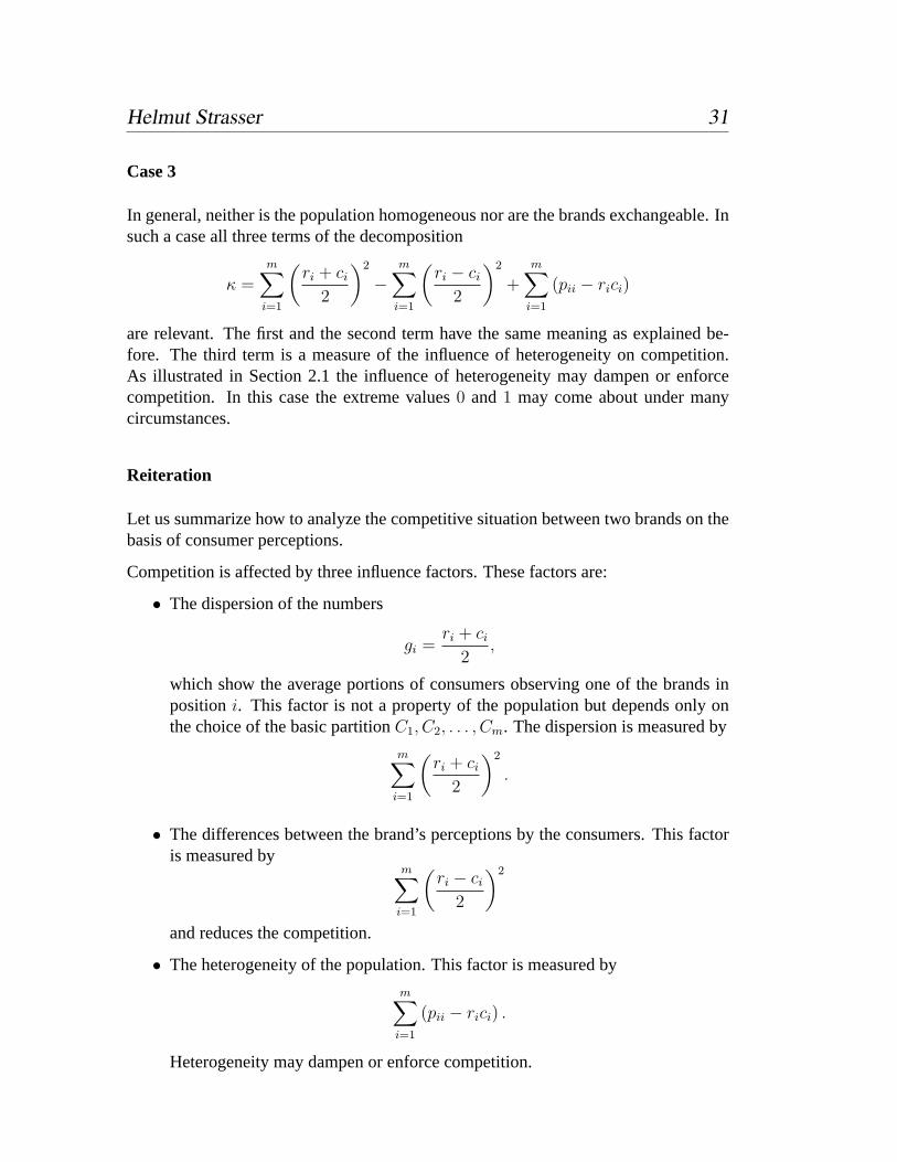
Case 3

In general, neither is the population homogeneous nor are the brands exchangeable. Insuch a case all three terms of the decomposition

κ =m∑

i=1

(ri + ci

2

)2

−m∑

i=1

(ri − ci

2

)2

+m∑

i=1

(pii − rici)

are relevant. The first and the second term have the same meaning as explained be-fore. The third term is a measure of the influence of heterogeneity on competition.As illustrated in Section 2.1 the influence of heterogeneity may dampen or enforcecompetition. In this case the extreme values0 and1 may come about under manycircumstances.

Reiteration

Let us summarize how to analyze the competitive situation between two brands on thebasis of consumer perceptions.

Competition is affected by three influence factors. These factors are:

• The dispersion of the numbers

gi =ri + ci

2,

which show the average portions of consumers observing one of the brands inpositioni. This factor is not a property of the population but depends only onthe choice of the basic partitionC1, C2, . . . , Cm. The dispersion is measured by

m∑i=1

(ri + ci

2

)2

.

• The differences between the brand’s perceptions by the consumers. This factoris measured by

m∑i=1

(ri − ci

2

)2

and reduces the competition.

• The heterogeneity of the population. This factor is measured by

m∑i=1

(pii − rici) .

Heterogeneity may dampen or enforce competition.

Helmut Strasser 32

Clearly, the choice of the basic partition is of importance for the measured amount ofcompetition. The influence of the basic partition should be as small as possible since,in general, there is no conceptual meaning of the basic partition. One aspect of thebasic partition is its concentration. The concentration of the basic partition determinesthe value of the first part of the decomposition formula which is nothing else than afamiliar measure of concentration. If the concentration of the basic partition is largethen this increases the value of the competition coefficient, too. If such an effect shouldbe avoided the basic partition should be chosen such that its concentration is low. Asis well-known the concentration is least if the subsets are of equal size.

4 Test statistics

Now, we turn to statistical inference. We assume that our data are obtained from asample survey. The exact portionsP (X ∈ A, Y ∈ B) and pkl in the populationare not available and we are dealing only with relative frequenciesf(X ∈ A, Y ∈B) andfkl in a relatively small sample. The questions posed in connection with theindependence and the symmetry problem have now to be answered on the basis ofincomplete empirical data.

We do not assume that the sample size is large enough to identify relative frequencieswith portions of the population. We face the problem that random fluctuations maygenerate patterns in the data that do not exist in the population.

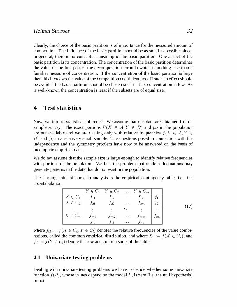
The starting point of our data analysis is the empirical contingency table, i.e. thecrosstabulation

Y ∈ C1 Y ∈ C2 . . . Y ∈ Cm

X ∈ C1 f11 f12 . . . f1m f1.

X ∈ C2 f21 f22 . . . f2m f2....

......

......

...X ∈ Cm fm1 fm2 . . . fmm fm.

f.1 f.2 . . . f.m

, (17)

wherefkl := f(X ∈ Ck, Y ∈ Cl) denotes the relative frequencies of the value combi-nations, called the common empirical distribution, and wherefk. := f(X ∈ Ck), andf.l := f(Y ∈ Cl) denote the row and column sums of the table.

4.1 Univariate testing problems

Dealing with univariate testing problems we have to decide whether some univariatefunctionf(P ), whose values depend on the modelP , is zero (i.e. the null hypothesis)or not.

Helmut Strasser 33

Considering e.g. the independence problem, the functions

f(P ) = pkl − rkrl,

f(P ) = P (X ∈ A, Y ∈ B)− P (X ∈ A)P (Y ∈ B),

f(P ) = E((X − EX)(Y − EY )

),

play an important role. Promising functions in connection with the symmetry problemare

f(P ) = pkl − plk,

f(P ) = P (X ∈ A, Y ∈ B)− P (X ∈ B, Y ∈ A),

f(P ) = E(X1Y1 − X2Y2).

Testing problems of this type can be treated by taking an estimatorT of the univariatefunction and choosing a critical valuec in such a way that under the null hypothesis

P (|T | ≤ c) ≥ α,

which implies that the so defined test has significance levelα. In order to maximizethe power of the test one should take an efficient estimatorT , which is no problemwith the examples considered before.

For the independence problem efficient estimators are

fkl − fk.f.l for pkl − rkrl,

f(X ∈ A, Y ∈ B)− f(X ∈ A)f(Y ∈ B)

for P (X ∈ A, Y ∈ B)− P (X ∈ A)P (Y ∈ B),

1

n

n∑i=1

xiyi −

(1

n

n∑i=1

xi

)(1

n

n∑i=1

yi

)for E

((X − EX)(Y − EY )

).

For the symmetry problem efficient estimators are

fkl − flk for pkl − plk,

f(X ∈ A, Y ∈ B)− f(X ∈ B, Y ∈ A)

for P (X ∈ A, Y ∈ B)− P (X ∈ B, Y ∈ A),

1

n

n∑i=1

(x1iy1i − x2iy2i) for E(X1Y1 − X2Y2).

We will discuss the computation of critical values later (see Section 5). In general,the critical valuec is not a constant number but data dependent. However, it is oftenpossible to transform the formula forT in such a way that for the transformed versiona constant critical value is available (standardization). But this is only a matter ofconvenience and does not concern the statistical properties of the test.

Helmut Strasser 34

4.2 Multivariate testing problems

If we are dealing with multivariate testing problems then it is not only a single univari-ate function, which is to be tested, but we are considering several functions which arecombined to a vector-valued, i.e. multivariate function.

Let us illustrate the simplest case of the independence problem.

If we want to decide whether the variablesX andY are independent or dependent thenit is not sufficient to check the equationpkl − rkcl = 0 for a particular pairk, l but wehave to do this for all pairsk, l simultaneously. Since for each functionpkl − rkcl wehave an efficient estimator it is a natural idea for constructing a test statistic for themultivariate testing problem to combine these estimators.

At first sight one could think that there is one particular optimal method to carry outthis combination of univariate estimators to get a multivariate test statistic. But this isnot true. And the reason for this lack of an optimal method is not a lack of theoreticalinsight or knowledge. The reason is that there is a vast number of possibilities for sucha combination each of which has specific advantages and specific drawbacks. In termsof statistical decision theory this fact reads: The family of all centrally symmetric andconvex acceptance regions defines a complete class of admissible tests (Theorem ofBirnbaum, 1955, see e.g. Strasser, 1985).

Thus, if we want to build a multivariate test statistic from univariate components de-fined by efficient estimators then, to some extent, we are allowed to accept conveniencearguments.

4.3 Tests of independence

Let us return to the independence problem. All familiar methods operate on thecrosstabulation of standardized deviations

zkl :=√

nfkl − fk.f.l√

fk.f.l

.

The best-known and most popular method of testing independence is the Chisquaretest based on the test statistic

T 21 :=

m∑k=1

m∑l=1

z2kl.

The Chisquare test statistic is a global measure for the amount of deviation of theempirical data from the ideal case of independence. A reason for the popularity ofthis test statistic is the time-honored fact that there are good approximations of its

Helmut Strasser 35

critical values. The Chisquare test is a useful choice if we want to answer the existencequestion U1. However, a drawback is the fact that using the Chisquare test it is not easyto decide, which of the inequalitiespkl − pk.p.l 6= 0 are actually valid.

If the Chisquare test yields a significant result then we know that the population isheterogeneous. In this case we want to get additional information concerning questionsU2 and U3.

Concerning question U2 we want to know for which subsetsA, B the inequality (2)

P (X ∈ A, Y ∈ B) 6= P (X ∈ A)P (Y ∈ B)

is valid. Before dealing with this problem let us consider the slightly simpler questionwhich pairsk, l are such that the inequality

P (X ∈ Ck, Y ∈ Cl) 6= P (X ∈ Ck)P (Y ∈ Cl)

holds, or in other words such thatpkl − pk.p.l 6= 0 is valid.

If we want to check the inequalitiespkl − pk.p.l 6= 0 for all pairsk, l simultaneously,then it would be completely wrong to carry out the respective univariate level-α-tests,each at a time. The significance level of such a procedure would be much worse thanα, and it would be impossible to get an idea what it really is. This kind of difficulty isdicussed in detail in the appendix, Section 6.

For a simultaneous testing of all inequalities we have to compute critical values of thetest statistic

T2 := max {|zkl| : 1 ≤ k, l ≤ m} = max

{√n

∣∣∣∣fkl − fk.f.l√fk.f.l

∣∣∣∣ : 1 ≤ k, l ≤ m

}.

If c is a critical value of levelα = 0.99 for this test statistic then we may consider allthose inequalitiespkl − pk.p.l 6= 0 as violated where|zkl| ≥ c. This kind of reasoningavoids the error of first kind with probability0.99. The theoretical background of sucha procedure is explained in the appendix, Section 6.

Unfortunately, there are no easy approximations for the critical values of the test statis-tic T2, which could be collected and looked up in tables. By contrast, we have to de-termine critical values in each individual case by extensive numerical computations.This will be the topic of Section 5.

Let us continue the discussion of test statistics, which can be applied for the treatmentof questions U2 und U3.

If dependence is proved then there are many configurationsA ⊆ E, B ⊆ E such thatthe inequality (2) is valid. If this inequality should be checked for all configurationssimultaneously then we define

z (A, B) :=√

nf (X ∈ A, Y ∈ B)− f (X ∈ A) f (Y ∈ B)√

f (X ∈ A) f (Y ∈ B),

Helmut Strasser 36

and build the test statistics

T3 := max {|z (A, B)|} ,

where the maximum is taken over all subsetsA, B which are unions of sets of the basicpartitionC1, C2, . . . , Cm. If we are able to find critical valuesc for that test statisticthen looking for|z (A, B)| > c allows to identify significant pairsA, B.

However, it is a cumbersome procedure to find critical values for the test statisticT3.Problems arise from the coincidence of two complications. First the maximum in thedefinition ofT3 can be determined only in a combinatoric way (i.e. by enumeration ofall possibilities). This means that we have to evaluate2m × 2m cases. Moreover, thenumerical computation of critical values forT3 requires, as we shall see in Section 5,the repetitive evaluation ofT3 for a large number of simulated data sets. Therefore, thewhole procedure soon reaches practical limits of computability.

A way out of this dilemma is to consider question U3 instead of question U2. At firstsight this problem again seems to be even more intricate as data transformations are amore complex object than pairs of subsets. But we will see that the test statistic for U3can be computed in a quick and relatively simple way.

Question U3 asks for recodings X und Y whose covariance

E((X − EX)(Y − EY )

)is different from zero. Starting with a fixed and

known data transformation it is clear which test statistic should be applied, namely

n∑i=1

xiyi −

(1

n

n∑i=1

xi

)(1

n

n∑i=1

yi

)=

m∑k,l=1

akbl (fkl − fk.f.l) .

But if the inequality (10) is to be checked for all possible data transformations simul-taneously then we have to define as test statistic

T4 := max

{√

n

∣∣∣∣∣m∑

k,l=1

akbl (fkl − fk.f.l)

∣∣∣∣∣}

,

where the maximum is to be taken over all normed recodings, i.e. all recodings suchthat

∑mk=1 a2

kfk. = 1 and∑m

l=1 b2l f.l = 1. The advantage of this test statistic is that it

can computed easily. As already explained in Section 3 the value of this test statisticis simply the maximal singular value of the matrixZ = (zkl). Moreover, we haveT4 ≥ T3, which implies that every critical value ofT4 may be used as critical value ofT3.

The discussion of how to find significant data transformations and deriving significantconfigurations goes beyond the scope of this paper. We conclude this Section with theremark that the same mathematical methods which yield the singular value decompo-sition of the matrixZ = (zkl) also offer means for getting a systematic overview oversignificant data transformations.

Helmut Strasser 37

4.4 Tests of symmetry

Let us turn to the symmetry problem. All popular methods have in common to departfrom

zkl :=

√n

2

fkl − flk√fkl + flk

. (18)

The simplest way for testing symmetry is to compute the Chisquare statistic

T 21 :=

m∑k=1

m∑l=1

z2kl.

The Chisquare statistic is a global measure for the deviation of the empirical data fromideal symmetry. For this test statistic there are good approximations of its critical val-ues. The asymptotic distribution of this Chisquare statistic is a Chisquare distributionwith m(m − 1)/2 degrees of freedom. The Chisquare statistic is well-suited for an-swering question S1. But it is a serious weakness that in case of significance we cannoteasily decide which inequalitiespkl − plk 6= 0 are valid.

If there is a significant deviation from symmetry then the brands are not exchangeableand we want to consider questions S2 and S3. Question S2 asks for configurationsA,B where inequality (6)

P (X ∈ A, Y ∈ B) 6= P (Y ∈ A, X ∈ B)

is fulfilled. Before we consider that problem let us discuss the slightly simpler ques-tion, which pairsk, l are such that

P (X ∈ Ck, Y ∈ Cl) 6= P (Y ∈ Ck, X ∈ Cl),

or in other words, such thatpkl − plk 6= 0, is true.

If we want to check the inequalitiespkl − plk 6= 0 simultaneously for all pairsk, l thenit would be wrong to apply univariate level-α-tests, each at a time. For a simultaneouscheck we have to apply the test statistic

T2 := max {|zkl| : 1 ≤ k, l ≤ m} = max

{√n

2

∣∣∣∣ fkl − flk√fkl + flk

∣∣∣∣ : 1 ≤ k, l ≤ m

}.

If c is a critical value of levelα = 0.99 for this test statistic then we may consider allthose inequalitiespkl − plk 6= 0 as true where|zkl| ≥ c. Such a procedure avoids theerror of first kind with probability0, 99. The theoretical foundations of this argumentare explained in the appendix, Section 6.

Unfortunately, there are no easy approximations for the critical values of the test statis-tic T2. We have to carry out extensive numerical computations. This will be discussedin Section 5.

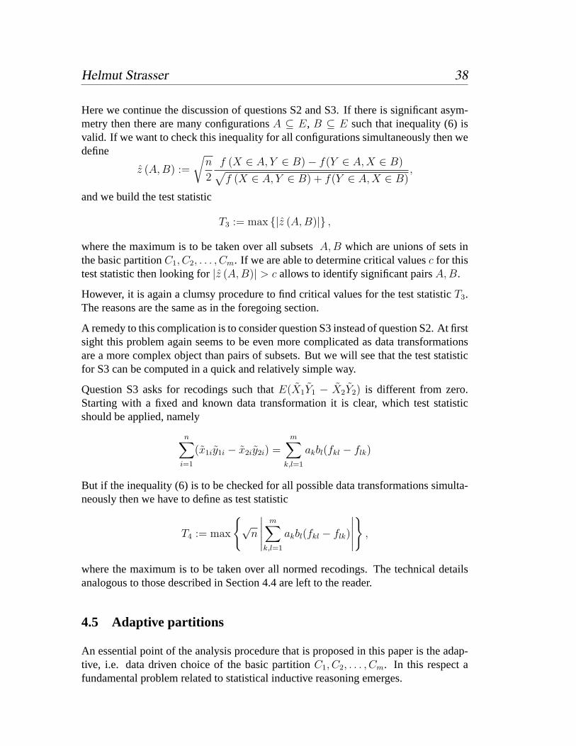
Helmut Strasser 38

Here we continue the discussion of questions S2 and S3. If there is significant asym-metry then there are many configurationsA ⊆ E, B ⊆ E such that inequality (6) isvalid. If we want to check this inequality for all configurations simultaneously then wedefine

z (A, B) :=

√n

2

f (X ∈ A, Y ∈ B)− f(Y ∈ A, X ∈ B)√f (X ∈ A, Y ∈ B) + f(Y ∈ A, X ∈ B)

,

and we build the test statistic

T3 := max {|z (A, B)|} ,

where the maximum is to be taken over all subsetsA, B which are unions of sets inthe basic partitionC1, C2, . . . , Cm. If we are able to determine critical valuesc for thistest statistic then looking for|z (A, B)| > c allows to identify significant pairsA, B.

However, it is again a clumsy procedure to find critical values for the test statisticT3.The reasons are the same as in the foregoing section.

A remedy to this complication is to consider question S3 instead of question S2. At firstsight this problem again seems to be even more complicated as data transformationsare a more complex object than pairs of subsets. But we will see that the test statisticfor S3 can be computed in a quick and relatively simple way.

Question S3 asks for recodings such thatE(X1Y1 − X2Y2) is different from zero.Starting with a fixed and known data transformation it is clear, which test statisticshould be applied, namely

n∑i=1

(x1iy1i − x2iy2i) =m∑

k,l=1

akbl(fkl − flk)

But if the inequality (6) is to be checked for all possible data transformations simulta-neously then we have to define as test statistic

T4 := max

{√

n

∣∣∣∣∣m∑

k,l=1

akbl(fkl − flk)

∣∣∣∣∣}

,

where the maximum is to be taken over all normed recodings. The technical detailsanalogous to those described in Section 4.4 are left to the reader.

4.5 Adaptive partitions

An essential point of the analysis procedure that is proposed in this paper is the adap-tive, i.e. data driven choice of the basic partitionC1, C2, . . . , Cm. In this respect afundamental problem related to statistical inductive reasoning emerges.

Helmut Strasser 39

If the data originate from a random sample where random fluctuations may supersedethe structural patterns of the population then there may arise additional patterns whichseemingly correspond to patterns in the population, although they are only caused byrandom effects.

E.g. in coping with the independence problem we may encounter associations in thecrosstabulation, which do not correspond to any dependence of probabilities in thepopulation. Dealing with the symmetry problem we may face random skewness, al-though the exact probabilities are symmetric.

The test statistics we are proposing are indicators for patterns in the data, which canbe caused by patterns in the population. Applying critical values, as is explained in thenext section, we are able to distinguish, which of the empirical patterns correspond tounderlying structures and which are only random fluctuations.

Now, if the computation of the test statistic is preceded by an adaptive data transforma-tion like a data driven basic partition, then it may happen that the indicative propertiesof the test statistics are deteriorated or even lost at all. E.g. it may happen that theadaptive partition obscures relevant patterns of the data or hides them at all. On theother hand the adaptive partition may emphasize randomly generated patterns.

If this happens then the test statistic which relies on the transformed data is flawed. Inany case the effect is that structural patterns in the data are no more significant. This ef-fect is obvious if the adaptive procedure obscures the structural patterns. But the sameeffect is incited if the adaptive procedure emphasizes randomly generated patterns,since for compensation the correct critical values automatically increase implying thatsignificant results come about much more rarely.

In terms of theoretical statistics this means: Any test statistics which are efficient for abasic partition fixed a priori may become inefficient, if the adaptive choice of the basicpartition is biased in favor or against the patterns of interest.

For these reasons it is imperative that any adaptive method which is applied to obtainthe basic partition is completely unbiased with respect to the patterns under discussion.We must avoid happen that relevant pattern are obscured or emphasized.

If this requirement is added to the independence problem or to the symmetry problemthen we arrive at a condition which is very easy to met. The unbiasedness of a methodis certainly satisfied if the method does not know which of the data belong to theX-sample and which belong to theY -sample. In fact, any pattern which is relevant forthe independence or the symmetry problem is concerned with a relation between dataof theX-sample and data of theY -sample. If a partioning method does not use theinformation which data belong to which sample then the method cannot be in favor ordisfavor of relevant patterns.

A sufficient condition for the realization of this unbiasedness condition is permutationinvariance. This means that in computing the adaptive partition the sequential order of

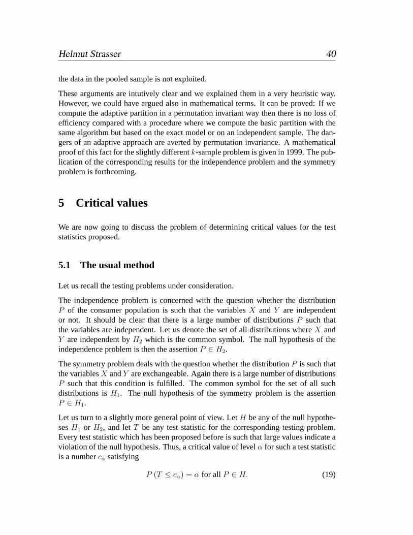
Helmut Strasser 40

the data in the pooled sample is not exploited.

These arguments are intutively clear and we explained them in a very heuristic way.However, we could have argued also in mathematical terms. It can be proved: If wecompute the adaptive partition in a permutation invariant way then there is no loss ofefficiency compared with a procedure where we compute the basic partition with thesame algorithm but based on the exact model or on an independent sample. The dan-gers of an adaptive approach are averted by permutation invariance. A mathematicalproof of this fact for the slightly differentk-sample problem is given in 1999. The pub-lication of the corresponding results for the independence problem and the symmetryproblem is forthcoming.

5 Critical values

We are now going to discuss the problem of determining critical values for the teststatistics proposed.

5.1 The usual method

Let us recall the testing problems under consideration.

The independence problem is concerned with the question whether the distributionP of the consumer population is such that the variablesX and Y are independentor not. It should be clear that there is a large number of distributionsP such thatthe variables are independent. Let us denote the set of all distributions whereX andY are independent byH2 which is the common symbol. The null hypothesis of theindependence problem is then the assertionP ∈ H2.

The symmetry problem deals with the question whether the distributionP is such thatthe variablesX andY are exchangeable. Again there is a large number of distributionsP such that this condition is fulfilled. The common symbol for the set of all suchdistributions isH1. The null hypothesis of the symmetry problem is the assertionP ∈ H1.

Let us turn to a slightly more general point of view. LetH be any of the null hypothe-sesH1 or H2, and letT be any test statistic for the corresponding testing problem.Every test statistic which has been proposed before is such that large values indicate aviolation of the null hypothesis. Thus, a critical value of levelα for such a test statisticis a numbercα satisfying

P (T ≤ cα) = α for all P ∈ H. (19)

Helmut Strasser 41

If the significance levelα is near to one then the eventT > cα allows the inductiveconclusion that the null hypothesis is violated.

Unfortunately, critical valuescα satisfying (19) do not exist. The reason is that condi-tion (19) is actually a series of conditions consisting of as many equations as there aredistributionsP ∈ H. In general, these equations canot be fulfilled simultaneously bya single numbercα. A realistic claim could be

P (T ≤ cα (P )) = α for all P ∈ H, (20)

i.e. we have to admit that the critical values may depend onP ∈ H. However,we do not know the distributionP . In order to carry out the significance test wehave to estimate the valuecα (P ) from the empirical data. For this estimation stepstatisticians have developed several ingenious methods which share the common ideathat the distributionP is replaced by some estimateP :

P (T ≤ cα(P )) ≈ α for all P ∈ H, (21)

As a result the critical valuecα(P ) is data dependent.

Admittedly, with many testing receipts in statistical textbooks this data dependenceof the critical values is not visible. This is due to the fact that usually the inequalityT ≤ cα(P ) is transformed into an equivalent formS ≤ dα wheredα is a constantwhich may be looked up in prefabricated statistical tables. The transition fromTto S very often obscures the intuitive interpretation of the test statistic and is one ofthe reasons for the deplorable alienation between statistical intuition and statisticaltechnology.

The plan to compute the critical valuescα(P ) is fine as long as it is feasible. How-ever, it is feasible only in a few special cases. These special cases which are chosenfor reasons of technical opportunity dominate the toolkits presented in statistical text-books. As a rule these special cases are justified afterwards as optimal solutions ofsome far-fetched optimization problems.

E.g. in case of the independence problem it is only possible for the Chisquare statisticT 2

1 to give analytic formulas approximating the critical values. For the remaining teststatisticsT2, T3, andT4, which are at least of equal interest this is not possible. Thesituation is similar for the symmetry problem.

5.2 Exact critical values

It is a remarkable feature of the testing problems we are considering, namely both ofthe independence problem and of the symmetry problem, that, if we agree to considerdata dependent critical values as in (21), then it is even possible to compute exact crit-ical values and not only approximations like the Chisquare quantiles for the Chisquarestatistic.

Helmut Strasser 42

In the following we will describe the procedure of how to compute exact critical valuesfor arbitrary test statisticsT .

We want to determine data dependent critical values

cα = cα (x1, x2, . . . , xn, y1, y2, . . . , yn) ,

such that the equations

P (T ≤ cα) = α for all P ∈ H, (22)

are satisfied. The idea of the following approach is based on the fact that for each ofthe two testing problems there are transformations of the data set

X Yx1 y1

x2 y2...

...xn yn

, (23)

which do not affect the validity of the null hypothesis.

For the independence problem with null hypothesisH2 these transformations are thepermutations of the columns in table (23). If the null hypothesisH2 is valid, i.e. if thevariablesX andY are independent, then all tables which are obtained from table (23)by permuting each column at a time are equally compatible with the null hypothesis asthe original table.

For the symmetry problem with null hypothesisH1 the admissible transformationsare the row permutations in table (23), i.e. the exchanges of numbers for each of thepairs at a time. If the null hypothesisH1 is valid, i.e. if the variablesX andY areexchangeable then all tables which are obtained from table (23) by permuting eachrow at a time are equally compatible with the null hypothesis as the original table.

Tests whose critical values are determined according to the procedure below are calledpermutation tests (see Lehmann, 1987, and Lehmann and Stein, 1949). In a veryvisionary way Pfanzagl, 1974, already emphasized the enormous potential of permu-tation tests (randomization tests in his terminology) as soon as computing facilitieswould admit their practical implementation.

We proceed as follows.

We compute all values which our test statistic attains if we apply all admissible per-mutations to table (23). These values are sorted in increasing order:

t1 < t2 < . . . < tN .

Helmut Strasser 43

Obviously,N can be a very large number. For the independence problem the numberis N = (n!)2 and for the symmetry problem it isN = 2n.

Then we definecα to be anα-quantile of this list, i.e.

f (i : ti < cα) < α ≤ f (i : ti ≤ cα) , for examplecα := t[αN ]+1.

This is the desired critical value and, apparently, it depends on the data.

The procedure can slightly be abbreviated by computing so-calledp-values. Signif-icance testing requires comparing the observed value of the test statisticT with thecritical valuecα. The observed value of the test statistic is one of the numbersti, sayti0. Then we have

ti0 ≤ cα ⇐⇒ f (i : ti < ti0) < α ⇐⇒ f (i : ti ≥ ti0) > 1− α,

ti0 ≥ cα ⇐⇒ f (i : ti ≤ ti0) ≥ α ⇐⇒ f (i : ti > ti0) ≤ 1− α.

Thus, comparingT with cα is equivalent to comparingf (i : ti > ti0) with 1− α. Thenumberf (i : ti > ti0) is called thep-value of the realizationti0 of T . Computing thep-value is sometimes quicker than computing the critical value since we may consideronly a small portion of the list of valuesti. Moreover, based on thep-value we mayperform tests of any levelα.

5.3 Practical evaluation

We have seen how to determine exact critical values for permutation tests. In any caseextensive combinatorial computations are required. The only exceptions are the mosttrivial cases dealing with two-by-two tables like the exact test by Fisher (independenceproblem) or the test by McNemar (symmetry problem) where explicit formulas for theexact critical values can be obtained. This computational burden is the reason whypermutation tests have not been applied at a large scale.

Thanks to the power of modern computing machines we are in a better position nowa-days. It is possible to compute exact critical values for larger crosstabulations thantwo-by-two tables. Some statistical software offers sophisticated algorithms to achievethis goal. However, each particular test statistic needs a special treatment and thereforea specific algorithm, and in this way the attractive universality of the permutation testapproach is lost.

An alternative which is completely sufficient for practical purposes is to get the criticalvalues by Monte Carlo simulation.

We refrain from applying all admissible permutation to table (23), but let us draw arandom sample of sizeK from the set of admissible permutations. Here the numberK may be large, say105 to 106, if we use fast computing machines. ThenK is still

Helmut Strasser 44

considerably smaller thanN but sufficiently large to obtain good estimates of the exactcritical value.

We collect all values which our test statistic attains if the permutations of the sampleare applied to table (23). These values are sorted in increasing order:

t1 < t2 < . . . < tK .

Theα-quantilecα of this sequence is an estimate of the exact critical valuecα. By well-known statistical methods we may obtain statistical error bounds for such estimates.

This Monte Carlo approach is the same for all test statistics and any preference fora particular test statistic implied by technical convenience is no longer necessary. Ifa test statistic is interesting for statistical reasons we can use it since we are able tocompute critical values. This is particularly true of the test statisticsT4.

6 Appendix: On the interpretation of maxima of uni-variate test statistics

It seems not to be common knowledge how to combine several univariate statisticaltests to obtain a multivariate test procedure. Therefore let us give some hints on thisissue. The arguments we are explaining in this section are applied several times in thisChapter.

Let us consider a particularly simple example. We want to explain the basic ideawithout being annoyed by technical complications. Afterwards we will indicate whywe may apply similar arguments in the more complex situations considered in thisvolume.

Let (Zi), i = 1, 2, . . . , n, be normally distributed random variables. We assume thecovariance to be known. LetE(Zi) = µi and consider the problem of deciding whichof these expectations is different from zero.

If this test is carried out for each random variable at a time then we have to choosecritical valuesci such that

P (|Zi| ≤ ci | µi = 0) ≥ α.

The significance levelα is a number near to one. We apply the decision rule

|Zi| ≤ ci ⇒ µi = 0,|Zi| > ci ⇒ µi 6= 0.

Since we haveP (|Zi| > ci | µi = 0) ≤ 1− α,

Helmut Strasser 45

the probability to rule in favor ofµi 6= 0 although it is wrong, is small.

But it is not our plan to make decisions only for one single random variableZi. Insteadfor all random variablesZ1, Z2, . . . , Zn we want to know whetherµi = 0 or not. Todiscuss this decision problem we have to make some prior remarks.

We are interested in the setJµ := {i : µi 6= 0},

where we denote byµ = (µ1, µ2, . . . , µn) the list of all parameters. From the empiricaldata we want to get a subsetJ(Z) ⊆ {1, 2, . . . , n} which we may use as basis for thedecision

i ∈ J(Z) ⇒ µi 6= 0, dh. J(Z) ⊆ Jµ,.

The error probability should be small, i.e.

P (J(Z) ⊆ Jµ | µ1, µ2, . . . , µn) ≥ α für alleµ = (µ1, µ2, . . . , µn). (24)

Thus, we would like to estimate the setJµ and we want to avoid overestimation. Thatmeans, we want to be sure that those parameter valuesµi, which are decided to be6= 0actually have this property. The error probability is controlled by inequality (24). Ifthis is true then we state that our setJ(Z) is of levelα.

Needless to say that we are also interested in discovering many of those parameterswhich satisfyµi 6= 0. In other words the difference setJµ \ J(Z) should be small.This claim is concerned with the power of the decision rule defined byJ(Z).

Now, how can we construct a data dependent setJ(Z) such that it is of levelα and haslarge power ?

The wrong way is to use the critical values of the univariate tests and to define:

J(Z) := {i : |Zi| > ci}.

Such a constructionJ(Z) is not of levelα. If the random variablesZi were indepen-dent then we could compute the actual significance level. E.g. if the error probabilitiesof the univariate tests are 1%, then forn = 10 the error probability ofJ(Z) wouldbe 9,6%. Forn = 20 it would increase to 18,2%. If the random variables are notindependent but correlated then the determination of the actual level is more difficultbut the principle remains the same.

The right way for constructing the setJ(Z) is to determine a common critical valuecfor all random variables. Let us choosec in such a way that

P (maxi|Zi| ≤ c | µ1 = 0, . . . , µn = 0) ≥ α. (25)

Based on this common critical valuec which is obviously larger than each of the num-bersci, we define

J(Z) := {i : |Zi| > c}.

Helmut Strasser 46

Now we are going to show that this setJ(Z) is actually of levelα in the sense of (24).

First we observe that

|Zi − µi| ≤ c ⇒ |Zi| − c ≤ |µi|

which implies|Zi − µi| ≤ c, |Zi| > c ⇒ µi 6= 0.

Thus we obtainmax

i|Zi − µi| ≤ c ⇒ J(Z) ⊆ Jµ.

Hence, in order to verify (24) it is sufficient to show that

P (maxi|Zi − µi| ≤ c | µ1, . . . , µn) ≥ α for all µ1, . . . , µn. (26)

This can be shown by applying special properties of our probability model. We assumethat the random variables are normally distributed and that the parameters under con-sideration are the expectationsµi. In this special situation we have for allµ1, . . . , µn

P (maxi|Zi| ≤ c | µ1 = 0, . . . , µn = 0) = P (max

i|Zi − µi| ≤ c | µ1, . . . , µn). (27)

Hence, equation (26) follows immediately from the choice of the critical valuec ac-cording to (25).

We have thus explained how to construct a setJ(Z) which is of levelα. The questionof power has been neglected so far. Clearly, there are many ways of constructing setsJ(Z) of levelα. However, a discussion of the problem of power is beyond the scope ofthis paper. Let us mention only one point: The procedure we are proposing is derivedfrom efficient confidence sets. Therefore, it should not be too difficult to prove someoptimality properties of this approach.

After having explained the basic idea for the construction of multivariate tests by asimple example let us turn to that situation which is considered in this volume. Theopen question is whether the invariance property (27), which is the essential technicalpoint for our construction, is valid also in situations lacking the simple structure of ourintroductory example.

Let us consider the independence problem and the test statistic

T2 := maxk,l

∣∣∣∣√n(fkl − fk.f.l)√fk.f.l

∣∣∣∣ .Let c be a critical value of levelα for this test statistic. This means: IfP0 is a distribu-tion such that the variablesX andY are independent, then we have

P0 (T2 ≤ c) = P0

(max

k,l

∣∣∣∣√n (fkl − fk.f.l)√fk.f.l

∣∣∣∣ ≤ c

)≥ α. (28)

Helmut Strasser 47

DefineJp := {(k, l) : pkl 6= pk.p.l}

and

J(Z) :=

{(k, l) :

∣∣∣∣√n(fkl − fk.f.l)√fk.f.l

∣∣∣∣ ≥ c

}.

The problem is whether for all possible values ofp = (pkl) the relation

Pp(J(Z) ⊆ Jp) ≥ α (29)

is valid. If this is the case then we may useJ(Z) for constructing a decision rule forchecking all differencespkl 6= pk.p.l.

This question cannot be answered at present. The reason is that the invariance property(27) of the introductory example cannot be extended exactly to the independence prob-lem. Admittedly, the relation (29) could be valid for allp = (pkl) in spite of lackingthe invariance property. But this has to be proved by other arguments.

So far the bad news.

The good news is that for small deviations from the null hypothesis the ardently desiredinvariance property is fulfilled approximately. This is an important consequence of themain theorem of the so-called local-asymptotic statistical theory. (We are talking aboutthe LAN-property. Confer Strasser, 1985.)

It follows that for thosep = (pk,l) which deviate only slightly from the null hypothesisof independence the equation (29) is fulfilled approximately. Therefore, the conditionsrequired for the interpretation ofJ(Z) in the sense ofJ(Z) ⊆ Jp are approximatelyfulfilled, too.

Befor we go into some details of this assertion let us explain what we mean by smalldeviations from the null hypothesis, and why such small deviations are all we need.This is due to the formal definition of small deviations given by the statistical theory.So-called small deviations are such that the deviation from the null hypothesis is notobvious from empirical data of the given size. (In case any critical expert of mathe-matical statistics is reading this paper until this point let me translate the concept ofa small deviation into mathspeech: The deviation between two distributions is smallfor the sample sizen if the variational distance between theirn-th powers is boundedaway from one.) Since we perform statistical tests only if the deviation from the nullhypothesis is not obvious, we need only consider small deviations from the null hy-pothesis. This type of argument goes back to A. Wald and is the basic argument onwhich the so-called local asymptotic theory of statistics was founded in the last fortyyears.

For the interested reader we conclude this section giving some details.

Helmut Strasser 48

Let t = (tkl) be a matrix and letp = (pk,l) be such that

pkl − pk.p.l =tkl√n

.

If t is not the null matrix then underPp the null hypothesis of independence is violated.By the local asymptotic statistical theory we may prove that for all matricest = (tkl)we have the relation

Pp

(max

k,l

∣∣∣∣√n (fkl − fk.f.l)− tkl√fk.f.l

∣∣∣∣ ≤ c

)≈ P0

(max

k,l

∣∣∣∣√n (fkl − fk.f.l)√fk.f.l

∣∣∣∣ ≤ c

),

(30)where the approximation becomes exact asn → ∞. The convergence is uniform onbounded sets oft = (tkl). This is exactly the invariance condition which we werelooking for.

Indeed, from the implication∣∣∣∣√n (fkl − fk.f.l)− tkl√fk.f.l

∣∣∣∣ ≤ c,

∣∣∣∣√n (fkl − fk.f.l)√fk.f.l

∣∣∣∣ > c ⇒ tkl 6= 0

it follows that

maxk,l

∣∣∣∣√n (fkl − fk.f.l)− tkl√fk.f.l

∣∣∣∣ ≤ c ⇒ J(Z) ⊆ Jp.

This implies

Pp

(max

k,l

∣∣∣∣√n (fkl − fk.f.l)− tkl√fk.f.l

∣∣∣∣ ≤ c

)≤ Pp(J(Z) ⊆ Jp)

for all possible values ofp = (pk,l). Up to now there are no approximations. Now wecombine the definition of the critical valuec in (28) with the approximate relation in(30) and thus obtain the announced assertion

Pp(J(Z) ⊆ Jp) ' α

for suchp = (pkl), which do not deviate much from the null hypothesis of indepen-dence.

References

Dolnicar, S., Grabler, K. and Mazanec, J.A.. A Tale of Three Cities: Perceptual Chart-ing for Analyzing Destination Images. In A. Woodside, editor,Consumer Psychologyof Tourism, Hospitality, and Leisure, London, CAB International, 1999.

Helmut Strasser 49

Hájek, J. and Sidák, Z.Theory of rank tests. Academic Press, 1967.

Janssen, A. and Neuhaus, G. Two sample rank tests for censored data with non-predictable weights.J. Statist. Planning and Inference, 1:45–59, 1997.

Lehmann, E. L. Testing Statistical Hypotheses. John Wiley and Sons, New York,1986.

Lehmann, E. L. and Stein, C. On the theory of some non-parametric hypotheses.Annals of Mathematical Statistics, 20:28–45, 1949.

Mazanec, J. A. Positioning Analysis with Self-Organizing Maps: An ExploratoryStudy on Luxury Hotels.Cornell Hotel and Restaurant Administration Quarterly,36:80-95, 1995.

Mazanec, J. A. Simultaneous Positioning and Segmentation Analysis with Topolog-ically Ordered Feature Maps: A Tour Operator Example.Journal of Retailing andConsumer Services, Special Issue on Marketing Applications of Neural Networks,6:219–235, 1999.

Mazanec, J. A. Neural Market Structure Analysis: Novel Topology-SensitiveMethodology.European Journal of Marketing, Special Issue on Computer Modellingin Marketing Management. To appear.

Neuhaus, G. Conditional rank tests for the two-sample problem under random cen-sorship.Annals of Statistics, 21:1760–1779, 1993.

Neuhaus, G. Conditional and unconditional two-sample rank tests for truncated data.Statistics and Decisions, 16:307–331, 1998.

Pfanzagl, J.Allgemeine Methodenlehre der Statistik 2. Walter de Gruyter, Berlin,1974.

Pfanzagl, J. and Wefelmeyer, W.Contributions to a general asymptotic statisticaltheory. Lecture Notes in Statistics 13, Springer, 1982.

Pötzelberger, K. and Strasser, H. Clustering and quantization by MSP-Partitions.1999, To appear in:Statistics and Decisions.

Rahnenführer, J. Multivariate permutation tests for clustered data. Technical report,1999.

Steiner, G.Quantization and clustering with maximal information: Algorithms andnumerical experiments. PhD thesis, Vienna University of Economics and BusinessAdministration, 1999.

Strasser, H.Mathematical theory of statistics: Statistical experiments and asymptoticdecision theory, volume 7 ofDe Gruyter Studies in Mathematics. de Gruyter, 1985.

Helmut Strasser 50

Strasser, H. Tangent vectors for models with independent but non-identically dis-tributed observations.Statistics and Decisions, 7:127–152, 1989.

Strasser, H. Data compression and statistical inference. Submitted for the Proceed-ings of the 6th Tartu Conference on Multivariate Statistics (Satellite meeting of ISI52nd session), 1999.

Strasser, H. Reduction of complexity. Technical report, Department of Statistics,Vienna University of Economics and Business Administration, 2000.

Strasser, H. Towards a statistical theory of optimal quantization. Technical report,Department of Statistics, Vienna University of Economics and Business Administra-tion, 2000.

Strasser, H. and Weber, C. On the asymptotic theory of permutation statistics.Math-ematical Methods of Statistics, 2:220–250, 1999.

Strasser, H. and Weber, C. Invariance principles for exchangeable random vectors.Technical report, Department of Statistics, Vienna University of Economics and Busi-ness Administration, 2000.