Statistical analysis of a dynamic model for dietary contaminant exposure

Statistical analysis of a dynamic model for dietary

contaminant exposure

Patrice Bertail, Stephan Clemencon, Jessica Tressou

To cite this version:

Patrice Bertail, Stephan Clemencon, Jessica Tressou. Statistical analysis of a dynamic modelfor dietary contaminant exposure. Journal of Biological Dynamics, Taylor & Francis Open,2010, 4 (2), pp.212-234. <10.1080/17513750903222960>. <hal-00308881v2>

HAL Id: hal-00308881

https://hal.archives-ouvertes.fr/hal-00308881v2

Submitted on 3 Feb 2009

HAL is a multi-disciplinary open accessarchive for the deposit and dissemination of sci-entific research documents, whether they are pub-lished or not. The documents may come fromteaching and research institutions in France orabroad, or from public or private research centers.

L’archive ouverte pluridisciplinaire HAL, estdestinee au depot et a la diffusion de documentsscientifiques de niveau recherche, publies ou non,emanant des etablissements d’enseignement et derecherche francais ou etrangers, des laboratoirespublics ou prives.

Statistical analysis of a dynamic model

for dietary contaminant exposure

Patrice Bertail∗

MODAL’X - Universite Paris X, 200 av. de la Republique, 92100 Nanterre cedex, France

Stephan Clemencon†

Telecom ParisTech - UMR541, 46 rue Barrault, 75634 Paris cedex 13, France

Jessica Tressou ‡

Unite INRA Met@risk - UR1204, 16 rue Claude Bernard, 75234 Paris cedex 05, France

February 3, 2009

Abstract

This paper is devoted to the statistical analysis of a stochastic model introduced inBertail, Clemencon & Tressou (2008) for describing the phenomenon of exposure to a certainfood contaminant. In this modeling, the temporal evolution of the contamination exposureis entirely determined by the accumulation phenomenon due to successive dietary intakesand the pharmacokinetics governing the elimination process in between intakes, in sucha way that the exposure dynamic through time is described as a piecewise deterministicMarkov process. Paths of the contamination exposure process are scarcely observable inpractice, therefore intensive computer simulation methods are crucial for estimating the time-dependent or steady-state features of the process. Here we consider simulation estimatorsbased on consumption and contamination data and investigate how to construct accuratebootstrap confidence intervals for certain quantities of considerable importance from theepidemiology viewpoint. Special attention is also paid to the problem of computing theprobability of certain rare events related to the exposure process path arising in dietaryrisk analysis using multilevel splitting or importance sampling techniques. Applicationsof these statistical methods to a collection of datasets related to dietary methyl mercurycontamination are discussed thoroughly.

Keywords:Food safety risk analysis; Linear pharmacokinetics model; Piecewise deter-ministic Markov process; Monte-Carlo techniques; Bootstrap; Rare event analysis.Classcode: Primary 92D30; Secondary 62D05, 62E20.

1 Introduction

Food safety is now receiving increasing attention both in the public health community and inscientific literature. For example, it was the second thematic priority of the 7th European Re-search Framework Program (refer to http://ec.europa.eu/research/fp7/) and advances in thisfield are starting to be reported in international conferences, as attested by the session statisticsin environmental and food sciences in the 25th European Meeting of Statisticians held in Osloin 2005, or in the 38emes journees de Statistique held in Clamart, France, in 2006. Addition-ally, several pluridisciplinary research units dedicated entirely to dietary risk analysis, such asMet@risk (INRA, http://www.paris.inra.fr/metarisk) in France, Biometris (www.biometris.nl)in the Netherlands or the Joint Institute for Food Safety and Applied Nutrition in the United∗The first author is also affiliated to CREST-LS, Malakoff, France†Corresponding author. Email: [email protected].‡The third author is a visiting scholar at the Hong Kong University of Science and Technology, her research is

partly supported by Hong Kong RGC Grant #601906.

1

States (www.foodrisk.org) have recently been created. This rapidly developing field involvesvarious disciplines across the medical, biological, social and mathematical sciences. The role ofStatistics in this field is becoming more and more widely recognized; see the seminal discus-sion in Renwick et al. [2003], and consists particularly of developing probabilistic methods forquantitative risk assessment, refer to Boon et al. [2003], Edler et al. [2002], Gibney and van derVoet [2003], van der Voet et al. [2007]. Hence, information related to the contamination levelsof an increasing number of food products for a wide range of chemicals on the one hand and tothe dietary behavior of large population samples on the other hand is progressively collected inmassive databases. The study of dietary exposure to food contaminants has raised many stim-ulating questions and motivated the use and/or development of appropriate statistical methodsfor analyzing the data, see Bertail and Tressou [2006], Tressou [2006] for instance. Recent workfocuses on static approaches for modeling the quantity X of a specific food contaminant ingestedover a short period of time and computing the probability that X exceeds a maximum tolerabledose, eventually causing adverse effects on human health; see Tressou [2005] and the referencestherein. One may refer to Bertail et al. [2006], Renwick et al. [2003] for a detailed accountof dose level thresholds such as the Provisional Tolerable Weekly Intake, meant to representthe maximum contaminant dose one may ingest per week without significant risk. However, asemphasized in Bertail et al. [2008], it is essential for successful modeling to take account of thehuman kinetics of the chemical of interest when considering contaminants such as methyl mer-cury (MeHg), our running example in this paper, that is not eliminated quickly, with a biologicalhalf-life measured in weeks rather than days, as detailed in section 2. In Bertail et al. [2008], adynamic stochastic model for dietary contamination exposure has been proposed, which is drivenby two key components: the accumulation phenomenon through successive dietary intakes andthe kinetics in man of the contaminant of interest that governs the elimination process. While adetailed study of the structural properties of the exposure process, such as communication andstochastic stability, has been carried out in Bertail et al. [2008], the aim of the present paperis to investigate the relation of the model to available data so as to propose suitable statisticalmethods.The rest of the article is organized as follows. In section 2, the dynamic model proposed inBertail et al. [2008] and its structural properties are briefly reviewed, with the aim of giving aninsight into how it is ruled by a few key components. In section 3, the relation of the dynamicexposure model previously described to available data is thoroughly investigated. In particu-lar, we show how computationally-intensive methods permit the analysis of the data in a validasymptotic theoretical framework. Special emphasis is placed on the problem of bootstrap confi-dence interval construction from simulation estimates of certain features of the exposure process,which are relevant from the epidemiology viewpoint. Statistical estimation of the probability ofcertain rare events, such as those related to the time required for the exposure process to exceedsome high and potentially critical contamination level, for which naive Monte-Carlo methodsobviously fail, is also considered. Multilevel splitting genetic algorithms or importance samplingtechniques are adapted to tackle this crucially important issue in the field of dietary risk assess-ment. This is followed by a section devoted to the application of the latter methodologies foranalyzing a collection of datasets related to dietary MeHg contamination, in which the eventualuse of the model for prediction and disease control from a public health guidance perspective isalso discussed. Technicalities are deferred to the Appendix.

2 Stochastic Modeling of Dietary Contaminant Exposure

In Bertail et al. [2008] an attempt was made to model the temporal evolution of the total bodyburden of a certain chemical present in a variety of foods involved in the diet, when contaminationsources other than dietary, such as environmental contamination for instance, are neglected. Asrecalled below, the dynamic of the general model proposed is governed by two key components,a marked point process (MPP) and a linear differential equation, in order to appropriatelyaccount for the accumulation of the chemical in the human body and its physiological elimination

2

respectively.

Dietary behavior. The accumulation phenomenon of the food contaminant in the body occursaccording to the successive dietary intakes, which may be mathematically described by a markedpoint process. Assume that the chemical is present in a collection of P types of food, indexedby p = 1, · · · , P . A meal is then modeled as a random vector Q = (Q(1), · · · , Q(P )), the p-th component Q(p) indicating the quantity of food of type p consumed during the meal, with1 ≤ p ≤ P . Suppose that also, for 1 ≤ p ≤ P , food type p eaten during a meal is contaminatedin random ratio C(p) in regards to the chemical of interest. For this meal the total contaminantintake is then

U =P∑p=1

C(p)Q(p) = 〈C,Q〉, (1)

of which distribution FU is the image of the joint distribution FQ ⊗ FC by the standard innerproduct 〈., .〉 on RP , denoting by FQ the distribution of the consumption vector Q and by FC thatof the contamination vector C = (C(1), · · · , C(P )), as soon as the r.v.’s Q and C are assumedto be independent of each other. Although solely the distribution FU is of interest from theperspective of dietary contamination analysis, the random vectors Q and C play an importantrole in the description of the model insofar as intakes are not observable in practice and theirdistribution is actually estimated from observed consumption and contamination vectors, seesection 3.

Equipped with this notation, a stochastic process model that carries information aboutthe times of the successive dietary intakes of an individual of the population of interest andthe quantities of contaminant ingested, at the same time, may be naturally constructed byconsidering the marked point process {(Tn, Qn, Cn)}n∈N, where the Tn’s denote the successivetimes when a food of type p ∈ {1, · · · , P} is consumed by the individual and the second andthird components of the MPP, Qn and Cn, are respectively the consumption vector and thecontamination vector related to the meal eaten at time Tn. One may naturally suppose that thesequence of quantities consumed (Qn)n∈N is independent from the sequence (Cn)n∈N of chemicalconcentrations.

A given dietary behavior may now be characterized by stipulating specific dependence re-lations for the (Tn, Qn)’s. When the chemical of interest is present in several types of food ofwhich consumption is typically alternated or combined for reasons related to taste or nutritionalaspects, assuming an autoregressive structure for the (∆Tn, Qn)’s, with ∆Tn = Tn − Tn−1 forall n ≥ 1, seems appropriate. In addition, different portions of the same food may be consumedon more than one occasion, which suggests that, for a given food type p, assuming depen-dency among their contamination levels C(p)

n ’s may also be pertinent in some cases. However,in many important situations, it is reasonable to consider a very simple model in which themarks {(Qn, Cn)}n∈N form an i.i.d. sequence independent from the point process (Tn)n∈N, thelatter being a pure renewal process, i.e. durations ∆Tn in between intakes are i.i.d. randomvariables. This modeling is particularly pertinent for chemicals largely present in one type offood. Examples include methyl mercury quasi-solely found in seafood products, certain myco-toxins such as Patulin exclusively present in apple products, see §3.3.2 in FAO/WHO [1995],or Chloropropanols, see §5.1 in FAO/WHO [2002]. Beyond its relevancy for such crucial casesin practice, though simple, this framework raises very challenging probabilistic and statisticalquestions, as shown in Bertail et al. [2008]. So that the theoretical results proved in this latterpaper may be used for establishing a valid asymptotic framework, we also set ourselves underthis set of assumptions in the present statistical study and leave for further investigation theissue of modeling more complex situations. Hence, throughout the article the accumulation ofa chemical in the body through time is described thoroughly by the MPP {(Tn, Un)}n∈N withi.i.d. marks Un = 〈Qn, Cn〉 drawn from FU (dx) = fU (x)dx, the common (absolutely continuous)distribution of the intakes, independent from the renewal process (Tn)n∈N. Let G(dt) = g(t)dtdenote the common distribution of the inter-intake durations ∆Tn, n ∈ N. Then, taking by con-

3

vention T0 = 0 for the first intake time, the total quantity of chemical ingested by the individualup to time t ≥ 0 is

B(t) =N(t)∑k=1

Uk, (2)

where N(t) =∑

k∈N I{Tk≤t} is the number of contaminant intakes up to time t, denoting by IAthe indicator function of any event A.

Pharmacokinetics. Given the metabolic rate of a given organism, physiological elimina-tion/excretion of the chemical in between intakes is classically described by an ordinary dif-ferential equation (ODE), the whole human body being viewed as a single compartment phar-macokinetic model, see Gibaldi and Perrier [1982], Rowland and Tozer [1995] for an account ofpharmacokinetic models. Supported by considerable empirical evidence, one may reasonablyassume the elimination rate to be proportional to the total body burden of the chemical innumerous situations, including the case of methyl mercury:

dx(t) = −θx(t) · dt, (3)

denoting by x(t) the total body burden of chemical at time t. The acceleration parameterθ > 0 describes the metabolism with respect to the chemical elimination. However in pharma-cology/toxicology, the elimination rate is classically measured by the biological half-life of thechemical in the body, log(2)/θ, that is the time required for the total body burden x to decreaseby half in the absence of a new intake. One may refer to Brett et al. [1999] for basics on linearpharmacokinetics systems theory, pharmacokinetics parameters, and standard methodologiesfor designing experiments and inferring numerical values for such parameters.

Remark 1 (Modelling variability in the metabolic rate) In order to account for vari-ability in the metabolic rate while preserving monotonicity of the solution x(t), various exten-sions of the model above may be considered. A natural way consists of incorporating a ‘biologicalnoise’ and randomizing the ODE (3), replacing θdt by dN (t), where {N (t)}t≥0 denotes a time-homogeneous (increasing) Poisson process with intensity θ (and compensator θt):

dx(t) = −x(t) · dN (t).

The results recalled below may be easily extended to this more general framework. However,as raw data related to physiological elimination of dietary contaminants are very seldom inpractice, this prevents us from fitting a sophisticated model in a reliable fashion, therefore werestrict ourselves to the simple model described by Eq. (3) on the grounds of parsimony.

Let X(t) denote the total body burden of a given chemical at time t ≥ 0. Under theassumptions listed above, the exposure process X = {X(t)}t≥0 moves deterministically accordingto the first order differential equation (3) in between intakes and has the same jumps as (B(t))t≥0.A typical cad-lag1 sample path of the exposure process is displayed below in Figure 1. Let A(t) =t− TN(t) denote the backward recurrence time at t ≥ 0 (i.e. the time since the last intake at t).The process {(X(t), A(t))}t≥0 belongs to the class of so-termed piecewise deterministic Markov(PDM) processes. Since the seminal contribution of Davis [1984], such stochastic processesare widely used in a large variety of applications in operations research, ranging from queuingsystems to storage models. Refer to Davis [1991] for an excellent account of PDM processesand their applications. In most cases, the ∆Tn’s are assumed to be exponentially distributed,making X itself a Markov process and its study much easier to carry out, see Chapter XIV inAsmussen [2003]. However, this assumption is clearly inappropriate in the dietary context andPDM models with increasing hazard rates are more realistic in many situations.

1Recall that a mapping x :]0,∞[→ R is said to be cad-lag if for all t > 0, lims→t, s>t x(s) = x(t) andlims→t, s<t x(s) = x(t−) <∞

4

Figure 1: Sample path of the exposure process X(t).

In Bertail et al. [2008], the structural properties of the exposure process X have been thor-oughly investigated using an embedded Markov chain analysis, namely by studying the behav-ior of the chain X = (Xn)n∈N describing the exposure process immediately after each intake:Xn = X(Tn) for all n ∈ N. As a matter of fact, the analysis of such a chain is facilitatedconsiderably by its autoregressive structure:{

Xn+1 = Xne−θ∆Tn+1 + Un+1, n ∈ N

X0 = x0.(4)

Such autoregressive models with random coefficients have been widely studied in the litera-ture, refer to Rachev and Samorodnitsky [1995] for a recent survey of available results on thistopic. The continuous-time process X may be easily related to the embedded chain X: solving(3) gives for all t ≥ 0

X(t) = XTN(t)e−θA(t). (5)

Long-term behavior. Under the conditions (i)-(iii) listed below, the behavior of the exposureprocess X in the long run can be determined. In addition, a (geometric) ergodicity rate can beestablished when condition (iv) is fulfilled.

(i) The inter-intake time distribution G has an infinite tail and either infx∈]0,ε] g(x) > 0 forsome ε > 0 or the intake distribution FU has infinite tail.

(ii) There exists some γ ≥ 1 such that E[Uγ1 ] <∞.

(iii) The inter-intake time distribution has first and second order finite momentsmG = E[∆T1] <∞ and σ2

G = var[∆T1] <∞.

(iv) There exists some δ > 0 such that E[eδ∆T2 ] <∞.

These mild hypotheses can easily be checked in practice as we do in section 4 for MeHg: as-sumption (i) stipulates that inter-intake times may be arbitrarily long with positive probabilityand they may also either be arbitrarily short with positive probability, which may then also sat-isfy the exponential moment condition (iv), or intakes may otherwise be arbitrarily large withpositive probability, but also ’relatively small’ in the case when (ii) is fulfilled. In the detailedergodicity study carried out in Bertail et al. [2008], Theorems 2 and 3 establish in particularthat under conditions (i)-(iv), respectively conditions (i)-(ii), the continuous-time exposure pro-cess X(t), respectively the embedded chain Xn corresponding to successive exposure levels at

5

intake times, settles to an equilibrium/steady state as t→∞, respectively as n→∞), describedby a governing, absolutely continuous, probability distribution µ(dx) = f(x)dx, respectivelyµ(dx) = f(x)dx for the embedded discrete chain. The limiting distributions µ and µ are relatedto one another by the following equation, see (15) in Bertail et al. [2008]:

µ([u,∞[) = m−1G

∫ ∞x=u

∫ ∞t=0

t ∧ log(x/u)θ

µ(dx)G(dt). (6)

These stationary distributions are of vital interest to quantify steady-state or long term quan-tities, pertinent to the epidemiology viewpoint, such as

• the steady-state mean exposure

mµ =∫ ∞x=0

xµ(dx) = limt→∞

E[X(t) | X(0) = x0], for any x0 ≥ 0, (7)

• the limiting average time the exposure process spent above some (possibly critical) thresh-old value u > 0,

µ([u,∞[) = limT→∞

1T

∫ T

t=0I{X(t)≥u}dt. (8)

In Bertail et al. [2008], a simulation study was carried out to evaluate the time to steady-state for women of chilbearing age in the situation of dietary MeHg exposure, that is the timeneeded for the exposure process to behave in a stationary fashion, which is also termed burn-inperiod in the MCMC method context. It was empirically shown that after 5 to 6 half lives, orabout 30 weeks, the values taken by the exposure process can be considered as drawn from thestationary distribution, which is a reasonable horizon on the human scale.

3 Statistical Inference via Computer Simulation

We now investigate the relation of the exposure model described in section 2 to existing data.In the first place, it should be noticed that information related to the contamination exposureprocess is scarcely available at the individual level. It seems pointless to try to collect datafor reconstructing individual trajectories: an experimental design measuring the contaminationlevels of all food ingested by a given individual over a long period of time would not actuallybe feasible. Inference procedures are instead based on data for the contamination ratio relatedto any given food and chemical stored in massive data repositories, as well as collected surveydata reporting the dietary behavior of large samples over short periods of time. In the following,we show how computer-based methods may be used practically for statistical inference of theexposure process X(t) from this kind of data. A valid asymptotic framework for these proceduresis also established from the stability analysis of the probabilistic model carried out in Bertailet al. [2008].

3.1 Naive Simulation Estimators

Suppose we are in the situation described above and have at our disposal three sets of i.i.d. dataG, C and Q drawn from G, FC and FQ respectively, as well as noisy half-life data H such asthose described in FAO/WHO [2003]. From these data samples, various estimation proceduresmay be used for producing estimators θ, G and FU of θ, G and FU , also fulfilling conditions(i)-(iii), see Remark 6 in the Appendix. One may refer in particular to Bertail and Tressou [2006]for an account of the problem of estimating the intake distribution FU from contamination andconsumption data sets C and Q, see also section 4 below. Although the law of the exposureprocess X(t) given the initial value X(0) = x0, which is assumed to be fixed throughout thissection, is entirely determined by the pharmacokinetic parameter θ and the distributions Gand FU , quantities related to the behavior that are of interest from the toxicology viewpoint

6

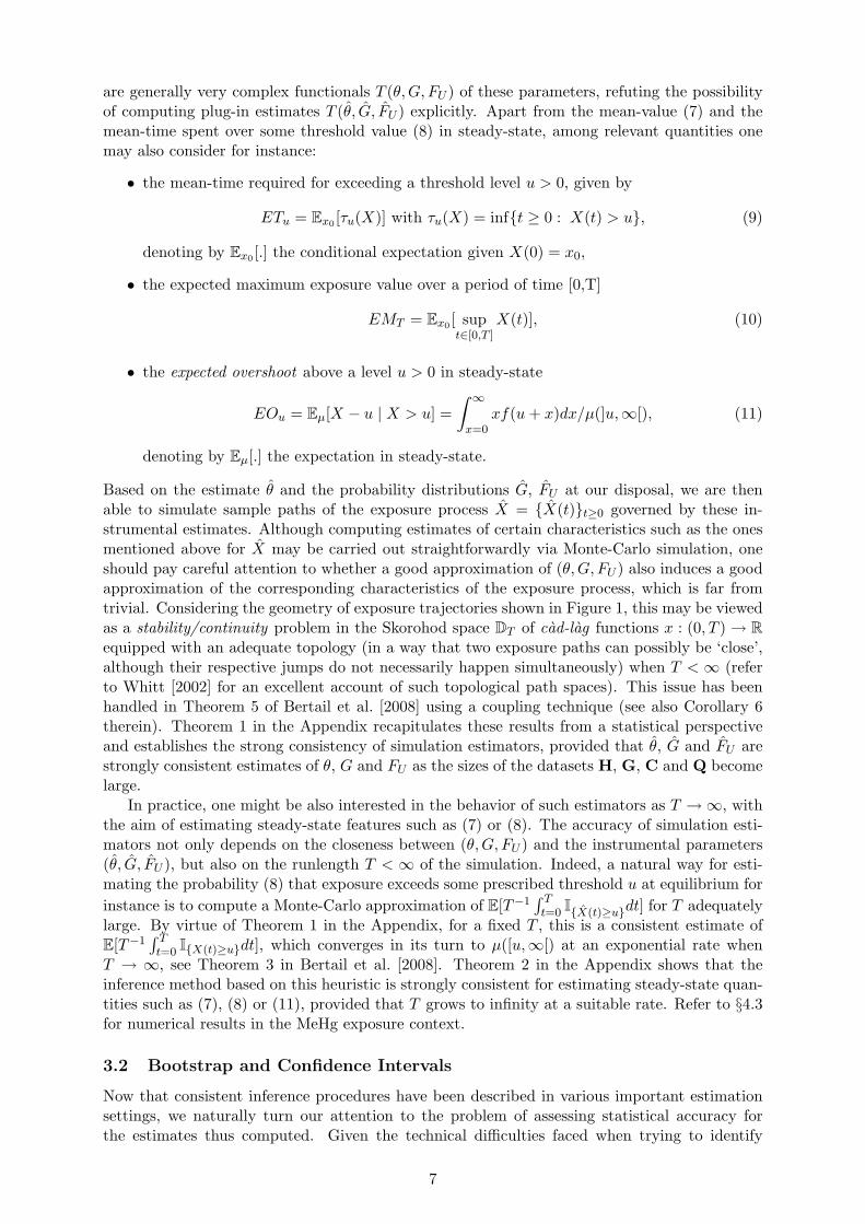
are generally very complex functionals T (θ,G, FU ) of these parameters, refuting the possibilityof computing plug-in estimates T (θ, G, FU ) explicitly. Apart from the mean-value (7) and themean-time spent over some threshold value (8) in steady-state, among relevant quantities onemay also consider for instance:

• the mean-time required for exceeding a threshold level u > 0, given by

ETu = Ex0 [τu(X)] with τu(X) = inf{t ≥ 0 : X(t) > u}, (9)

denoting by Ex0 [.] the conditional expectation given X(0) = x0,

• the expected maximum exposure value over a period of time [0,T]

EMT = Ex0 [ supt∈[0,T ]

X(t)], (10)

• the expected overshoot above a level u > 0 in steady-state

EOu = Eµ[X − u | X > u] =∫ ∞x=0

xf(u+ x)dx/µ(]u,∞[), (11)

denoting by Eµ[.] the expectation in steady-state.

Based on the estimate θ and the probability distributions G, FU at our disposal, we are thenable to simulate sample paths of the exposure process X = {X(t)}t≥0 governed by these in-strumental estimates. Although computing estimates of certain characteristics such as the onesmentioned above for X may be carried out straightforwardly via Monte-Carlo simulation, oneshould pay careful attention to whether a good approximation of (θ,G, FU ) also induces a goodapproximation of the corresponding characteristics of the exposure process, which is far fromtrivial. Considering the geometry of exposure trajectories shown in Figure 1, this may be viewedas a stability/continuity problem in the Skorohod space DT of cad-lag functions x : (0, T )→ Requipped with an adequate topology (in a way that two exposure paths can possibly be ‘close’,although their respective jumps do not necessarily happen simultaneously) when T <∞ (referto Whitt [2002] for an excellent account of such topological path spaces). This issue has beenhandled in Theorem 5 of Bertail et al. [2008] using a coupling technique (see also Corollary 6therein). Theorem 1 in the Appendix recapitulates these results from a statistical perspectiveand establishes the strong consistency of simulation estimators, provided that θ, G and FU arestrongly consistent estimates of θ, G and FU as the sizes of the datasets H, G, C and Q becomelarge.

In practice, one might be also interested in the behavior of such estimators as T →∞, withthe aim of estimating steady-state features such as (7) or (8). The accuracy of simulation esti-mators not only depends on the closeness between (θ,G, FU ) and the instrumental parameters(θ, G, FU ), but also on the runlength T < ∞ of the simulation. Indeed, a natural way for esti-mating the probability (8) that exposure exceeds some prescribed threshold u at equilibrium forinstance is to compute a Monte-Carlo approximation of E[T−1

∫ Tt=0 I{X(t)≥u}dt] for T adequately

large. By virtue of Theorem 1 in the Appendix, for a fixed T , this is a consistent estimate ofE[T−1

∫ Tt=0 I{X(t)≥u}dt], which converges in its turn to µ([u,∞[) at an exponential rate when

T → ∞, see Theorem 3 in Bertail et al. [2008]. Theorem 2 in the Appendix shows that theinference method based on this heuristic is strongly consistent for estimating steady-state quan-tities such as (7), (8) or (11), provided that T grows to infinity at a suitable rate. Refer to §4.3for numerical results in the MeHg exposure context.

3.2 Bootstrap and Confidence Intervals

Now that consistent inference procedures have been described in various important estimationsettings, we naturally turn our attention to the problem of assessing statistical accuracy forthe estimates thus computed. Given the technical difficulties faced when trying to identify

7

asymptotic distributions of the simulation estimators described in §3.1, we take advantage ofbootstrap confidence intervals, which are built directly from the data, via the implementation of asimplistic computer algorithm; see Hall [1997] for an account of the bootstrap theory, and Efronand Tibshirani [2004] for a more practice-oriented overview. Here we discuss the application ofthe bootstrap-percentile method to our specific setting for automatically producing confidenceintervals from simulation estimators.

Let us suppose that the parameter of interest is in the form of F (Φ) = E[Φ(X(t)}t∈[0,T ])],where T < ∞ and Φ : DT → R is a given function defined in the exposure path space. Aspreviously noted, typical choices are x 7→

∫ T0 I{x(t)≥u}dt and x 7→

∫ T0 (x(t) − u)I{x(t)≥u}dt for

u ≥ 0. We consider the problem of estimating the sampling distribution of a simulation estimatorF (Φ) = E[Φ({X(t)}t∈[0,T ])] of F (Φ) computed using instrumental parameter estimates θ, G andFU fitted from data samples H, G, C and Q: FΦ(x) = P(F (Φ)−F (Φ) ≤ x). Note that here theprobability refers to the randomness in the samples H, G, C and Q. The ’simulated bootstrap’algorithm is performed in five steps as follows.

Algorithm 1 - ‘Simulated Bootstrap’

1. Make i.i.d. draws with replacement in each of the four datasets H, G, C and Q, yieldingthe bootstrap samples H∗, G∗, C∗ and Q∗, with the same sizes as the original samples,respectively.

2. From data samples generated in step 1, compute bootstrap versions θ∗, G∗ and F ∗U of theinstrumental estimates θ, G and FU .

3. From the bootstrap parameters θ∗, G∗ and F ∗U , simulate the bootstrap exposure process:{X∗(t)}t∈[0,T ].

4. Compute the bootstrap estimate of the sampling distribution of F (Φ)

FBOOTΦ (x) = P∗(F ∗(Φ)− F (Φ) ≤ x), (12)

where P∗ denotes the conditional probability given the original datasets.

5. A bootstrap confidence interval at level 1−α ∈ (1/2, 1) for the parameter F (Φ) is obtainedusing the bootstrap root’s quantiles q∗α/2 and q∗1−α/2, of orders α/2 and 1−α/2 respectively:

I∗1−α = [F (Φ) + q∗α/2, F (Φ) + q∗1−α/2]. (13)

Here the redundant designation ’simulated bootstrap’ simply emphasizes the fact that a pathsimulation stage follows the data resampling and parameter recomputing steps. Asymptoticvalidity of this bootstrap procedure may be established at length by refining the proof of Theorem1, based on the Frechet differentiability notion. Owing to space limitations, technicalities hereare omitted.

Remark 2 (Monte-Carlo approximations) The bootstrap distribution estimate (12) maybe practically approximated by iterating B times the resampling step and averaging then overthe B resulting bootstrap trajectory replicates: {X∗b (t)}t∈[0,T ] with b ∈ {1, . . . , B}.

3.3 Rare Event Analysis

The statistical study of the extremal behavior of the exposure process is also of crucial impor-tance in practice. Indeed, accurately estimating the probability of reaching a certain possiblycritical level u within a lifetime is an essential concern from the public health perspective (seethe discussion in section 4). When the toxicological threshold level u of interest is ‘very high’,when compared to the mean behavior of the exposure process X, crude Monte-Carlo (CMC)

8

Figure 2: Examples of trajectories in the French adult female population compared to a referenceexposure process (Unit: µg/kg bw). The solid red curves are different trajectories with the sameinitial state x0 = 0. The dashed green curve stabilizes at a critical threshold of reference u, seesection 4 for details on its construction.

methods, as those proposed in §3.1, completely fail; see Figure 3.3 for an illustration of this phe-nomenon. We are then faced with computational difficulties inherent to the issue of estimatingthe probability of a rare event related to X’s law. In this paper, we leave aside the questionof fully describing the extremal behavior of the exposure process X in an analytical fashionand infering values for related theoretical parameters such as the extremal index, measuringto what extent extreme values tend to come in ‘small clusters’. Attention is rather focusedon practical simulation-based procedures for estimating probabilities of rare events of the formEu,T = {τu(X) ≤ T}, where T is a reasonable horizon on the human scale, and level u is verylarge in comparison with the long term mean exposure mµ for instance. Here, two methodsare proposed for carrying out such a rare event analysis in our setting, each having its ownadvantages and drawbacks, see Glasserman et al. [1999] for a review of available methods forestimating the entrance probability into a rare set. In the first approach, a classical importancesampling procedure is implemented, while our second strategy, based on an adequate factor-ization of the rare event probability Px0(Eu,T ) relying on the Markov structure of the process(X(t), A(t)) (i.e. a Feynman-Kac representation), consists of using a multilevel splitting algo-rithm, see Cerou et al. [2006]. In the latter, simulated exposure trajectories getting close to thetarget level u are ‘multiplied’, while we let the others die, in the spirit of the popular ReSTART(Repetitive Simulated Trials After Reaching Thresholds) method; refer to Villen-Altamirano andVillen-Altamirano [1991] for an overview. In section 4, both methodologies are applied in orderto evaluate the risk related to dietary MeHg exposure, namely the probability that the totalbody burden rises above a specific dose of reference.

3.3.1 Importance Sampling

Importance sampling (IS ) is a standard tool in rare event simulation. It relies on simulatingexposure paths from a different probability, P say, equivalent to the original along a suitablefiltration, chosen in a way that the event of interest Eu,T is much less rare, or even frequent, underthe latter distribution, refer to Bucklew [2004] for a recent account of IS techniques and theirapplications. The rare event probability estimate is then computed by multiplying the empiricalquantity output by the simulation algorithm using the new distribution by the correspondinglikelihood ratio (importance function).

9

In our setting, a natural way of speeding up the exceedance of level u by process X is toconsider an intake distribution FU (dx) = fU (x)dx equivalent to FU though much larger inthe stochastic ordering sense (i.e. FU (x) << FU (x) for all x > 0), so that large intakes mayoccur more frequently, and, simultaneously, an inter-intake time distribution G(dt) = g(t)dtwith same support as G(dt) but stochastically much smaller (namely, G(t) << G(t) for allt > 0), in order that the intake frequency is increased (see section 4 for specific choices in theMeHg case). In contrast, the elimination process cannot be slowed down, i.e. the biologicalhalf-life log 2/θ cannot be increased, at the risk of no longer preserving equivalence betweenP and P. To be more specific, let Px0 be the probability measure on the same underlyingmeasurable space as the one on which the original probability Px0 has been defined, makingX the process described in section 2. Under Px0 , the intakes {Uk}k≥1, respectively the inter-intake times {∆Tk}k≥1, are i.i.d. r.v.’s drawn from FU , respectively from G, and X0 = x0 ≥ 0.The distribution Px0 is absolutely continuous with respect to the IS distribution Px0 along thefiltration Ft = σ((Uk,∆Tk); 1 ≤ k ≤ N(t)), t ≥ 0, that is the collection of σ-fields generated bythe intakes and inter-intake times until time t. In addition, on FT , the likelihood ratio is givenby

LT =1−G(T − TN(T ))

1− G(T − TN(T ))×N(T )∏k=1

fU (Uk)fU (Uk)

· g(∆Tk)g(∆Tk)

. (14)

Hence, denoting by Ex0 [.] the Px0-expectation, we have the relationship

Px0(Eu,T ) = Ex0 [LT · IEu,T]. (15)

From a practical angle, the expectation on the right hand side of (15) is estimated by simulatinga large number of exposure trajectories of length T under the IS probability measure Px0 andthen applying a CMC approximation, which yields an unbiased estimate of the target Px0(Eu,T ).

3.3.2 Multilevel Splitting

The approach described above involves specifying an appropriate change of measure (adequatedf’s FU and G), so as to simulate a random variable LT · IEu,T

with reduced variance under thenew distribution P, see Chapter 14 in Bucklew [2004]. This delicate tuning step is generallybased on large-deviations techniques when tractable. Although encouraging results have beenobtained for estimating the probability of exceedance of large thresholds (in long time asymp-totics) for random walks through IS techniques (for instance refer to Chapter VI in Asmussenand Glynn [2000], where both the light-tailed and heavy-tailed cases are considered), no methodfor choosing a nearly optimal change of measure is currently available in our setup, where timeT is fixed. For this reason, the so-termed multilevel splitting technique has recently emergedas a serious competitor to the IS methodology, see Glasserman et al. [1999]. This approach isindeed termed non-intrusive, insofar as it does not require any modification of the instrumen-tal simulation distributions. Here, it boils down to represent the distribution of the exposureprocess exceeding the critical threshold u in terms of a Feynman-Kac branching particle model,see Moral [2004] for an account of Feynman-Kac formulae and their genealogical and interactingparticle interpretations. Precisely, the interval [0, u] in which the exposure process X evolvesbefore crossing the level x = u is split into sub-intervals corresponding to intermediary sublevels0 < u1 < . . . < um < u the exposure path must pass before reaching the rare set [u,∞[ and parti-cles, in this case exposure paths, branch out as soon as they pass the next sublevel. Connectionsbetween such a physical approach of rare event simulation and approximations of Feynman-Kacdistributions based on interacting particle systems are developed at length in Cerou et al. [2006].We now recall the principle of the multilevel splitting algorithm used in section 4. Suppose thatm intermediary sub-levels 0 < u1 < . . . < um < um+1 = u, are specified by the user (see Remark3), as well as instrumental simulation parameters (FU , G, θ) and x0 > 0. Let N ≥ 1 be fixedand denote the cardinal of any finite set X by | X |. The algorithm is then performed in m+ 1steps as follows.

10

Algorithm 2 - ‘Multi-level Splitting’

1. Simulate N exposure paths from x0 < u1 of runlength T , indexed by k ∈ {1, . . . , N} anddenoted by X [k] = {X [k]

t }t∈[0,T ], 1 ≤ k ≤ N .

2. For j = 1, . . . , m:

(a) Let I1,j be the index subset corresponding to the exposure trajectories having reachedlevel uj before endtime T , i.e. such that τ [k]

uj = inf{t ≥ 0; X [k]t ≥ uj} < T . Define

I0,j as the index subset corresponding to the other sample paths.(b) For each path indexed by k′ in I0,j , randomly draw k in I1,j and redefine X [k′] as

the trajectory confounded with X [k] until time τ [k]uj , and prolongated until time T by

simulation from the state X [k](τ [k]uj ). Note that hitting times τ [k]

uj necessarily occur atintake times.

(c) Compute Pj =| I1,j | /N and pass onto the next level uj+1.

3. Output the estimate of the probability Px0,u,T = Px0(Eu,T ):

Px0,u,T = P1 × . . .× Pm+1, (16)

where Pm+1 is defined as the proportion of particles that have reached the final level uamong those which have reached the previous sublevel um, that is | I1,m+1|/N .

Before illustrating how the procedure works on a toy example, below are two relevant re-marks.

Remark 3 (On practical choice of the tuning parameters) Although a rigorous asymp-totic validity framework has been established in Cerou et al. [2006] for Algorithm 2 when thenumber N of particles gets arbitrarily large, the intermediary sublevels u1, . . . , um must be se-lected by the user in practice. As noticed in Lagnoux [2006], an optimal choice would consistof choosing the sublevels so that the probability to pass from [uj ,∞[ to [uj+1,∞[ should be thesame, whatever the sublevel j. Here we mention the fact that, in the numerical experimentscarried out in section 4, the sublevels have been determined by using the adaptive variant ofAlgorithm 2 proposed in Cerou and Guyader [2007], where the latter are picked in such a waythat all probabilities involved in the factorization (16) are approximately of the same order ofmagnitude.

Remark 4 (‘Validation’) Stating the truth, estimating the probability of rare events such asEu,T is a difficult task in practice and, when feasible, the numerical results provided by differentpossible methods should be compared for assessing the order of magnitude of the rare eventprobability of interest. It should also be mentioned that, in a very specific case, namely whenFU and G are both exponential distributions, the distribution of the hitting time τu may beexplicitly computed through its Laplace transform using Dynkin’s formula, see Kella and Stadje[2001]. As an initial attempt, the latter may be thus used for computing a preliminary roughestimate of Px0,u,T .

A toy example. Figure 3 illustrates the way Algorithm 2 works in the case of N = 5trajectories starting from x0 = 3 with m = 2 intermediary levels (u = (4, 5, 6)) and a horizonT equal to one year in the model with exponential intake and inter-intake times distributions.Initially, all curves have reached the first intermediary level (u = 4) except the blue curve asshown in Figure 3(a). It is then restarted from the red curve at the exact point where it firstreached u = 4 in Figure 3(b). Now, only the blue and black curves have reached the secondintermediary level (u = 5). In Figure 3(c), all the other curves are thus restarted from one ofthese at the exact point where they first reached u = 5. Eventually, only the blue curve reachedthe level of interest u = 6. The probability of reaching 6 in less than one year is estimated by4/5× 2/5× 1/5 = 6.4%.

11

(a) Initialization: N = 5

(b) Iteration 1: u = 4 (c) Iteration 2: u = 5

Figure 3: Multilevel Splitting: an illustration for N = 5 particles starting from x0 = 3 withm = 2 intermediary levels (u ∈ {4, 5, 6}) and a horizon T equal to 1 year.

12

4 Numerical results for MeHg exposure

In this section, we apply the statistical techniques presented in the preceding section for analyzinghow a population of women of childbearing age (who are female between 15 and 45, for thepurpose of this study) are exposed to dietary MeHg, based on the dynamic model described insection 2. The group suffering the highest risk from this exposure is actually the unborn childas mentioned in the hazard characterization step described in FAO/WHO [2003]: the MeHgpresent in the seafood of the mother’s diet will certainly pass onto the developing foetus andmay cause irreversible brain damage.

From the available datasets related to MeHg contamination and fish consumption, essentialfeatures of the exposure process are inferred using the simulation-based estimation tools previ-ously described. Special attention is now paid to the probability of exceeding a specific dosederived from a toxicological level of reference in the static setup, namely the Provisional Tol-erable Weekly Intake (PTWI), which represents the contaminant dose an individual can ingestweekly over an entire lifetime without appreciable risk, as defined by the international expertcommittee of FAO/WHO, see FAO/WHO [2003]. This means it is crucial to implement the rareevent analysis methods reviewed in §3.3.

Eventually, the impact of the choice of the statistical methods used for fitting the instrumen-tal distributions is empirically quantified and discussed from the perspective of public healthguidelines.

4.1 Description of the datasets

We start off with a brief description of the datasets used in the present quantitative risk assess-ment. Note that fish and other seafood are the only source of MeHg.

Contamination data C. Here we use the contamination data related to fish and other seafoodsavailable on the French market that have been collected by accredited laboratories from officialnational surveys performed between 1994 and 2003 by the French Ministry of Agriculture andFisheries MAAPAR [1998-2002] and the French Research Institute for Exploitation of the SeaIFREMER [1994-1998]. This dataset comprises 2832 observations.Consumption data G, Q. The national individual consumption survey INCA CREDOC-AFSSA-DGAL [1999] provides the quantity consumed of an extensive list of foods over a week,among which fish and other seafoods, as well as the time consumption occurred with at leastthe information about the nature of the meal, whether it be breakfast, lunch, dinner or ‘snacks’.It is surveys 1985 adults aged 15 years or over, including 639 adult females between 15 and 45.From these observations, the dataset G consists of the actual durations between consecutiveintakes, when properly observed, together with right censored inter-intake times, when only theinformation that the duration between successive intakes is larger than a certain time can beextracted from the observations. Inter-intake times are expressed in hours.

As in Bertail et al. [2008], Verger et al. [2007], MeHg intakes are computed at each observedmeal through a so-termed deterministic procedure currently used in national and internationalrisk assessments. From the INCA food list, 92 different fish or seafood species are determinedand a mean level of contamination is computed from the contamination data, as in Crepet et al.[2005], Tressou et al. [2004]. Intakes are then obtained through Eq. (1) based on these meancontamination levels: this is a simplifying approach that bears the advantage that fish speciescan be taken into account as extensively explained in Tressou et al. [2004]. For comparisonsake, all consumptions are divided by the associated individual body weight, also provided inthe INCA survey, so that intakes are expressed in micrograms per kilogram of body weight permeal (µg/kgbw/meal).

As previously mentioned, raw data related to the biological half-life of contaminants such asMeHg are scarcely available. Refering to the scientific literature devoted to the pharmacokineticsof MeHg in the human body (see Rahola et al. [1972], Smith et al. [1994], Smith and Farris[1996], IPCS [1987]), the biological half-life fluctuates at around 44 days. This numerical value,

13

converted in hours, is thus retained for performing simulations, leading to pick log 2/(44 × 24)for the acceleration parameter estimate θ.

4.2 Estimation of the instrumental distributions FU and G

In order to estimate the cumulative distribution functions (cdf) of the intakes and inter-intaketimes, various statistical techniques have been considered, namely parametric and semi-parametricapproaches.

Estimating the intake distribution. By generating intake data as explained in §4.1, wedispose of a sample U of nFU

= 1088 intakes representative of the subpopulation consisting ofwomen of childbearing age, on which the following cdf estimates are based.

Parametric modeling. We first considered two simple parametric models for the intake dis-tribution: the first one stipulates that FU takes the form of an exponential distribution withparameter λFU

= 1/mFU, while the other assumes it is a heavy-tailed Burr type distribution

(with cdf (1− (1 +xc)−k) for c > 0 and k > 0) in order to avoid underestimating the probabilitythat very large intakes have occured. For both statistical models, related parameters have beenset by the maximum likelihood estimation (MLE ). It can be easily established that ML esti-mates are consistent and asymptotically normal in such regular models and, furthermore, thatthe cdf corresponding to the MLE parameter is also consistent in the L1- sense, see Remark6 in the Appendix. Numerically, based on U we found that λFU

= 4.06 by simply invertingthe sample mean in the exponential model, whereas in the Burr distribution based model, MLEyields c = 0.95 and k = 4.93. Recall that, in the Burr case, E[Uγ1 ] = Γ(k−γ/c)×Γ(1+γ/c)/Γ(k)is finite as soon as ck > γ. One may thus check that the intake distribution estimate fulfillscondition (ii) with γ = 4; see section 2.

Semi-parametric approach. In order to allow for more flexibility and accuracy on the one handand to obtain a resulting instrumental cdf well-suited for worst case risk analysis on the otherhand, a semi-parametric estimator has also been fitted the following way: the piecewise linear leftpart of the cdf corresponds to a histogram-based density estimator, while the tail is modelled bya Pareto distribution, with a continuity constraint at the change point xK . Precisely, a numberK of extreme intakes is used to determine the tail parameter α of the Pareto cdf 1 − (τx)−α,τ > 0 and α > 0, τ being chosen to ensure the continuity constraint. The value of K is fixedthrough a bias-variance trade-off, following exactly the methodology proposed in Tressou et al.[2004]. Numerically, we have α = 2.099, τ = 5.92, and xK = 0.355.

Probability plots are displayed in Figure 4(a). The semi-parametric estimator clearly pro-vides the best fit to the data. The Burr distribution is nevertheless a good parametric choice. Itis preferred to the Exponential distribution based on the AIC criteria, whereas the BIC criteriaadvocates for the Exponential distribution.

Estimating the inter-intake time distribution. We dispose of a sample G of nG = 1214right censored inter-intake times.

Parametric models. In this censored data setup, MLE boils down to maximizing the log likeli-hood given by

l(x, δ, ν) =nG∑i=1

(1− δi) log [fν (xi)] + δi ln [1− Fν (xi)] ,

where the (xi, δi)’s are the observations, δi denotes the censorship indicator, fν is the densitycandidate, and Fν the corresponding cdf. Four parametric distributions, widely used in sur-vival analysis, have been considered here: Exponential, Gamma, Weibull and Log Normal. It isnoteworthy that conditions (i)-(iii) listed in section 2 are satisfied for such distributions. Onemay also find that the cdf corresponding to the MLE parameter is L1- strongly consistent foreach of these regular statistical models. The resulting MLE estimators are: λG = 0.0078 for

14

the Exponential distribution Exp(λG), α = 1.06 and β = 117.2 for the Gamma distributionsuch that 1−G(t) ∝ tα−1 exp(−t/β), a = 128.7 and c = 0.999 for the Weibull distribution suchthat 1−G(t) = exp(−(t/a)c), and a = 4.41 and b = 1.31 for the Log Normal distribution, withparametrization such that log[(∆T2 − a)/b)] follows a standard normal.

Semi-parametric modeling. Using a semi-parametric approach, a cdf estimate is built from asmoothed Kaplan-Meier estimator FKM for the left part of the distribution and an exponentialdistribution for the tail behavior, with a continuity constraint at the change point. To be exact,the change point corresponds to the largest uncensored observation xK and the parameter of theexponential distribution to − log[1−FKM(xK)]/xK , in a way that continuity at xK is guaranteed.The resulting parameter of the exponential distribution is 0.0073, and xK = 146 hours.

Figure 4(b) displays the corresponding probability plots. Again, the semi-parametric esti-mator provides the best fit, except naturally for the tail part because of the right censorship.Based on AIC or BIC criteria, the Exponential distributions is chosen among the proposed para-metric distributions. However, the fitted Gamma distribution is marginally more accurate thanthe Weibull and Exponential distributions, since it offers the advantage of having an increasinghazard rate (here, α > 1), which is a realistic feature in the dietary context.

(a) FU : Intake distribution (b) G : Inter-intake time distribution

Figure 4: Probability plots (empirical cdf versus fitted cdf), comparison of the different adjust-ments.

4.3 Estimation of the main features of the exposure process

From the perspective of food safety, we now compute several important summary statisticsrelated to the dietary MeHg exposure process of French females of childbearing age using thesimulation estimators proposed in section 3. In chemical risk assessment, once a hazard has beenidentified, meaning that the potential adverse effects of the compound have been described, itis then characterized, using the notion of threshold of toxicological concern. This pragmaticapproach for chemical risk assessment consists of specifying a threshold value, below whichthere is a very low probability of observing adverse effects on human health. In practice, oneexperimentally determines the lowest dose that may be ingested by animals or humans, daily orweekly, without appreciable effects. The Tolerable Intake is then established by multiplying thisexperimental value, known as the Non Observed Adverse Effect Level (NOAEL) by a relevantsafety factor, taking into account both inter-species and inter-individual variabilities. Thisapproach dates from the early sixties, see Truhaut [1991], and is internationally recognized inFood Safety, see IPCS. The third and fourth steps of risk assessment consists of assessing theexposure to the chemical of interest for the studied population, and comparing it to the daily

15

Table 1: Estimation of the steady state mean and median for the 15 models with 95% confidenceintervals (unit: µg/kgbw, M = 1000, B = 200).

FU : Exponential FU : Burr FU : Semi-ParametricG :Exponential 3.01 ∈ [2.68, 3.32] 2.96 ∈ [2.67, 3.23] 2.98 ∈ [2.67, 3.39]

2.92 ∈ [2.53, 3.38] 2.97 ∈ [2.67, 3.24] 2.89 ∈ [2.53, 3.31]G :Gamma 3.07 ∈ [2.69, 3.42] 3.03 ∈ [2.73, 3.34] 3.05 ∈ [2.69, 3.40]

2.99 ∈ [2.57, 3.34] 3.04 ∈ [2.70, 3.31] 2.96 ∈ [2.57, 3.53]G :Weibull 2.98 ∈ [2.63, 3.33] 2.97 ∈ [2.60, 3.29] 2.99 ∈ [2.67, 3.29]

2.94 ∈ [2.54, 3.38] 2.96 ∈ [2.67, 3.23] 2.92 ∈ [2.47, 3.49]G :Log-Normal 2.28 ∈ [2.02, 2.57] 2.25 ∈ [1.99, 2.54] 2.26 ∈ [1.95, 2.61]

1.95 ∈ [1.63, 2.36] 2.45 ∈ [2.23, 2.70] 1.92 ∈ [1.56, 2.34]G : Semi-Parametric 2.95 ∈ [2.67, 3.23] 2.90 ∈ [2.62, 3.25] 2.93 ∈ [2.58, 3.26]

3.03 ∈ [2.71, 3.37] 2.83 ∈ [2.48, 3.16] 2.82 ∈ [2.42, 3.29]

or weekly tolerable intake. The first two steps are known as hazard identification and hazardcharacterization, while the last two are called exposure assessment and risk characterization. Ina static setup, when considering chemicals that are not accumulated in the human body anddescribing exposure by the supposedly i.i.d. sequence of intakes, this boils down to evaluating theprobability that weekly intakes exceed the reference dose d, termed the Provisionary TolerableWeekly Intake (PTWI), see Tressou [2005]. Considering compounds with longer biological half-lives, we propose comparing the stochastic exposure process to the limit of a deterministic processof reference {xn}n∈N. Mimicking the experiment carried out in the hazard characterization step,the latter is built up by considering intakes exactly equal to the PTWI d occuring every week(FU is a point mass at d, and G is a point mass at one week, that is 7 × 24). The referencelevel is thus given by the affine recurrence relationship xn = exp(− log(2)/HL × 1)xn−1 + d,yielding a reference level Xref,d = limn→∞ xn = d/(1 − 2−1/HL), where the half-life HL isexpressed in weeks. For MeHg, the value d = 0.7 µg/kgbw/w corresponds to the reference doseestablished by the U.S. National Research Council currently in use in the United States, seeNRC [National Research Council], whereas the PTWI has been set to d = 1.6 µg/kgbw/wby the international expert committee of FAO/WHO, see FAO/WHO [2003]. Numerically, thisyields Xref,0.7 = 6.42 µg/kgbw and Xref,1.6 = 14.67 µg/kgbw when MeHg’s biological half-life isfixed to HL = 6 weeks, as estimated in Smith and Farris [1996]. We termed this reference doseas ‘Tolerable Body Burden’ (TBB), which is more relevant than the previous ’Kinetic TolerableIntake’ (KTI) determined in Verger et al. [2007].

In the dynamic setup, several summarizing quantities can be considered for comparisonpurposes. We first estimated two important features of the process of exposure to MeHg, forall combinations of input distributions: the long-term mean exposure mµ, the median exposurevalue in the stationary regime, and the probability of exceeding the threshold Xref,0.7 in steady-state µ([Xref,0.7,∞[); see Table 1 and Figure 5. Computation is conducted as follows: M = 1000trajectories are simulated over a run length of 1 year after a burn-in period of 5 years, quantitiesof interest are then averaged over the M trajectories and this is repeated B = 200 times to buildthe bootstrap CI’s, as described in section 3.2. The major differences among the 15 modelsfor the stationary mean arise when using the Log Normal distribution for the inter-intake timeswith a lower estimation for this model presenting a heavy tail (longer inter-intake times are morefrequent). All the other models for G lead to similar results in terms of confidence intervals forthe mean and median exposures in the long run, whatever the choice for FU , refer to Table 1.When estimating a tail feature such as the probability of exceeding u = Xref,0.7 in steady-state,the choice of FU becomes of prime importance, since its tail behavior is the same as that ofthe stationary distribution µ, see Theorem 3.2 in Bertail et al. [2008]. As illustrated by thenotion of PTWI, risk management in food safety is generally treated in the framework of worst-

16

0 0.5 1 1.5 2 2.5 3

Exponential-Exponential

Exponential-Gamma

Exponential-Weibull

Exponential-LogNormal

Exponential-KMexp

Burr-Exponential

Burr-Gamma

Burr-Weibull

Burr-LogNormal

Burr-KMexp

EmpPareto-Exponential

EmpPareto-Gamma

EmpPareto-Weibull

EmpPareto-LogNormal

EmpPareto-KMexp

Figure 5: Estimation of the steady state probability of exceeding u = 6.42 for the 15 modelswith 95% confidence intervals (unit: %, M = 1000, B = 200)

case design. In the subsequent analysis, we thus focus on the Burr-Gamma model. Due to its‘conservative’ characteristics, it is unlikely that it leads to an underestimation of the risk. Itindeed stipulates heavy tail behavior for the intakes and light tail behavior for the inter-intaketimes.

Another interesting statistic is the expected overshoot over a safe level u. In the case of the‘Burr-Gamma’ model and for u = Xref,0.7, the estimated expected overshoot is 0.101 µg/kgbwwith 95% bootstrap confidence interval [0.033, 0.217], which corresponds to barely less than oneaverage intake. Before turning to the case of level u = Xref,1.6, Figure 6 illustrates the fact thatthe exposure process very seldomly reaches such high thresholds displaying the estimation ofthe expected maximum over [0, T ] for different values of T .

Let us now turn to the main risk evaluation, that is, inference of the probability of reachingu = Xref,1.6 = 14.67 within a reasonable time horizon. This estimation problem is consideredfor several time horizons, T = 5, 10, 15, and 20 years, in the ”heavy-tailed” Burr-Gammamodel. Close numerical results, obtained through crude Monte-Carlo and Multi-level Splitting,are shown in Figure 7.

In order to implement the Multilevel Splitting methodology, a first simulation has beenconducted according to the adaptive version proposed by Cerou and Guyader [2007] usingN = 1000 particles, so as to determine the intermediary levels u1, . . . , um such that half theparticles reach the next sublevel. When T = 20 years for instance, the resulting levels are7.85, 8.65, 9.47, 10.16, 11.07, 11.97, and 13.08 for an estimated probability of 0.52%.

Because they turned out to be inconsistent, empirical results based on the IS methodology arenot presented here. This illustrates well the difficulty of choosing the IS distribution properly,as previously discussed.

Eventually, we considered the case of the ”light-tailed” Exponential-Gamma model, withExponential intakes and Gamma inter-intake times. In this situation, the crude Monte-carloprocedure is totally inefficient and yields estimates of the probability of reaching the thresholdwithin any of the four time horizons all equal to zero (even if we increase the size of the simulation

17

0

2

4

6

8

10

12

0 5 10 15 20 25 30 35 40 45

T: Time in years

Max

imum

 of t

he e

xpos

ure 

proc

ess 

over

 [0,T

]

Figure 6: Estimation of the expected maximum of the exposure process over [0, T ] as a functionof the horizon T (M = 1000, and B = 200).

0.0%

0.5%

1.0%

1.5%

2.0%

2.5%

5 10 15 20

Multilevel Splitting Crude MC

Figure 7: Estimation of the probability of reaching u = Xref,1.6 = 14.67 within a reasonable timehorizon (Burr-Gamma model, M = 1000 is the size of the crude Monte carlo simulation, and95% simulation intervals are computed over B = 100 iterations and shown as error bars in thegraphic).

18

0

2E­11

4E­11

6E­11

8E­11

1E­10

1.2E­10

1.4E­10

1.6E­10

5 10 15 20

Multilevel Splitting

Figure 8: Estimation of the probability of reaching u = Xref,1.6 = 14.67 within a reasonabletime horizon (Exponential-Gamma model, 95% simulation intervals are computed over B = 100iterations and shown as error bars in the graphic).

to M = 10, 000 or 100, 000), whereas, in contrast, the Multilevel Splitting methodology allowsto quantify the probability of occurence of these rare events, as shown in Figure 8.

4.4 Some concluding remarks

Here we have endeavoured to explain how to exploit the data at our disposal, using a simplemathematical model, in order to compute a variety of statistical dietary risk indicators at thepopulation level, as well as their degree of uncertainty. This premier work can be improved inseveral directions. If more consumption data were available for instance, the inference procedureshould take into account the possible heterogeneity of the population of interest in regards todietary habits: a preliminary task would then consist of adequately stratifying the population inhomogeneous classes using clustering or mixture estimation techniques. Considering long termexposure, it could also be pertinent to account for possible temporal heterogeneities and modelthe evolution of the diet of an individual through time.

Although we showed how to evaluate the fit of various statistical models to the data bymeans of visual tools or model selection techniques, our present contribution solely aims atproviding a general framework and guiding principles for constructing a quantitative dietaryrisk model. Indeed, certain modelling issues must be left to the risk assessor’s choice, like usingextreme value theory for possibly modeling the intake’s tail out beyond the sample (refer to thediscussion in Tressou et al. [2004]) or incorporating features accounting for the metabolic rate’svariability to the model for instance, according to the availability and quality of the data theyrequire.

A Technical details

Though formulated in a fairly abstract manner at first glance, the conver-gence-preservationresults stated in Theorem 1 below are essential from a practical perspective. They automaticallyensure, under mild conditions, consistency of simulation-based estimators associated to variousfunctions of statistical interest. Recall that a sequence of estimators (Fn)n∈N of a cumulativedistribution function (cdf) F on R is said to be ’strongly consistent in the L1-sense’ whenM1(Fn, F ) =

∫t∈R |Fn(t)− F (t)|dt→ 0 almost surely, as n→∞. Convergence in distribution is

denoted by ‘⇒′ in the sequel and we suppose that the Skorohod space DT = D([0, T ]) is equipped

19

with the Hausdorff metric dT , the euclidean distance between cad-lag curves (completed withline segments at possible discontinuity points), and with the related M2 topology.

Theorem 1 (Consistency of simulation estimators, Bertail et al. [2008]) Let 0 ≤T ≤ ∞ and for all n ∈ N, consider a triplet of (random) parameters (θn, Gn, FU,n) that almostsurely fulfills conditions (i)-(iv) and defines a stochastic exposure process X(n). Assume furtherthat {(Gn, FU,n)}n∈N forms an L1-strongly consistent sequence of estimators of (G,FU ) and thatθn is a strongly consistent estimator of the pharmacokinetics parameter θ.

(i) Let Ψ : (DT , dT )→ R be any measurable function with a set of discontinuity points Disc(Ψ)such that P({X(t)}t∈(0,T ) ∈ Disc(Ψ)) = 0. Then, we almost surely have the convergencein distribution:

Ψ({X(n)(t)}t∈(0,T ))⇒ Ψ({X(t)}t∈(0,T )), as n→∞. (17)

(ii) Let Φ : (DT , dT )→ R be a Lipschitz mapping. Then, the expectations F (Φ) = E[Φ({X(t)}t∈(0,T ))]and Fn(Φ) = E[Φ({X(n)}t∈(0,T ))] are both finite. Besides, if supn∈N E[θn] < ∞ andsupn∈N σ

2Gn

<∞, then the following convergence in mean holds almost surely:

Fn(Φ)→ F (Φ), as n→∞. (18)

Before showing that this result applies to all functionals considered in this paper, a few remarksare in order.

Remark 5 (Monte-Carlo approximation) When T <∞, estimates of the mean F (Φ) maybe obtained in practice by replicating trajectories {X(n),m}t∈(0,T ), m = 1, . . . , M independentlyfrom the distribution parameters (θn, Gn, FU,n) and computing the Monte-Carlo approximationto the expectation Fn(Φ), that is

F (M)n (Φ) =

1M

M∑m=1

Φ({X(n),m}t∈[0,T ])). (19)

Remark 6 (Conditions fulfilled by the distribution estimates) Practical implemen-tation of the simulation-based estimation procedure proposed above involve computing estimatesof the unknown df’s, G and FU , according to a L1-strongly consistent method. These also haveto be instrumental probability distributions on R+, preferably convenient for simulation by cdfinversion. This may be easily carried out in most situations. In the simple case when the con-tinuous cdf on R, Fγ0 , to estimate belongs to some parametric class {Fγ}γ∈Γ with parameterset Γ ⊂ Rd such that γ 7→

∫|x|dFγ(x) and γ 7→ Fγ(t) for all t ≥ 0 are continuous mappings,

a natural choice is to consider the cdf Fγ corresponding to a strongly consistent estimator γ ofγ0 (computed by MLE for instance). In a nonparametric setup, adequate cdf estimators maybe obtained using various regularization-based statistical procedures. For instance, under mildhypotheses, the cdf Fn associated to a simple histogram density estimator based on an i.i.d.data sample of size n may be shown to classically satisfy, as n → ∞, Fn(x) → F (x) for all xand

∫|x|Fn(dx)→

∫|x|F (dx) almost surely by straightforward SLLN arguments.

Remark 7 (Rates of convergence) If the estimator Gn converges to G (resp. FU,n con-verges to FU , resp. θn converges to θ) at the rate vGn (resp. vFU

n , resp. vθn) in probability asn → ∞, careful examination of Theorem 2’s proof in Bertail et al. [2008] actually shows thatconvergence (18) takes place in probability at the rate vn = min{vGn , vFU

n , vθn}.

For all T < ∞, the mapping x ∈ DT 7→ sup0≤t≤T x(t) is Lipschitz with respect to theHausdorff distance, strong consistency of simulation estimators of (10) is thus guaranteed underthe assumptions of Theorem 1.

20

Besides, τu : x ∈ D∞ 7→ inf{t > 0 : x(t) > u} is a continuous mapping in the M2 topology.Thus, we almost surely have τu(X(n)) ⇒ τu(X) as n → ∞ in the situation of Theorem 1.Furthermore, it may be easily shown that {τu(X(n))}n∈N is uniformly integrable under mildadditional assumptions, so that convergence in mean also holds almost surely.

Similarly, for fixed T > 0, the mapping on (DT , dT ) that assigns to each trajectory x thetemporal mean T−1

∫ Tt=0 x(t)dt (respectively, the ratio T−1

∫ Tt=0 I{x(t)≥u}dt of time spent beyond

some threshold u) is continuous. Hence, we almost surely have the convergence in distribu-tion (respectively, in mean by uniform integrability arguments) of the corresponding simulationestimators as n→∞.

The next result guarantees consistency for simulation estimators of steady-state parameters,provided that the runlength T increases to infinity at a suitable rate, compared to the accuracyof the instrumental distributions.

Theorem 2 (Consistency for Steady-State Parameters, Bertail et al. [2008]) Let φ :R → R be any of the three functions y 7→ y, y 7→ I{y≥u} or y 7→ (y − u)I{y≥u}, with u > 0. SetΦT (x) = T−1

∫ Tt=0 φ(x(t))dt for any x ∈ DT . Assume that Theorem 1’s conditions are fulfilled.

When T → ∞ and n → ∞ so that both T 2 × (M1(G(n), G) + |θn − θ|) and T ×M1(F (n)U , FU )

almost surely tend to zero, then the following convergences take place almost surely:

ΦT (X(n))⇒ Lµ(φ) and Fn(ΦT )→ Eµ[φ(X)], (20)

denoting by Lµ(φ) the distribution of φ(X) when X is drawn from µ.

References

S. Asmussen. Applied Probability and Queues. Springer-Verlag, New York, 2003.

S. Asmussen and Peter W. Glynn. Stochastic Simulation. Springer-Verlag, New York, 2000.

P. Bertail and J. Tressou. Incomplete generalized U-Statistics for food risk assessment. Biomet-rics, 62(1):66–74, 2006.

P. Bertail, M. Feinberg, J. Tressou, and P. Verger (Coordinateurs). Analyse des Risques Ali-mentaires. TEC&DOC, Lavoisier, Paris, 2006.

P. Bertail, S. Clemencon, and J. Tressou. A storage model with random release rate for modelingexposure to food contaminants. Math. Biosc. Eng., 35(1):35–60, 2008.

P.E. Boon, H. van der Voet, and J.D. van Klaveren. Validation of a probabilistic model ofdietary exposure to selected pesticides in Dutch infants. Food Addit. Contam., 20(Suppl. 1):S36–S39, 2003.

M. Brett, H.J. Weimann, W. Cawello, H. Zimmermann, G. Pabst, B. Sierakowski, R. Giesche,and A. Baumann. Parameters for Compartment-free Pharmacokinetics: Standardisation ofStudy Design, Data Analysis and Reporting. Shaker Verlag, Aachen, Germany, 1999.

J.A. Bucklew. An Introduction to Rare Event Simulation. Springer Series In Statistics. Springer,2004.

F. Cerou and A. Guyader. Adaptative splitting for rare event analysis. Stoch. Anal. Proc., 25(2):417–443, 2007.

F. Cerou, P. Del Moral, F. LeGland, and P. Lezaud. Genetic genealogical models in rare eventanalysis. Alea, 1:183–196, 2006.

CREDOC-AFSSA-DGAL. Enquete INCA (individuelle et nationale sur les consommations ali-mentaires). TEC&DOC, Lavoisier, Paris, 1999. (Coordinateur : J.L. Volatier).

21

A. Crepet, J. Tressou, P. Verger, and J.Ch Leblanc. Management options to reduce expo-sure to methyl mercury through the consumption of fish and fishery products by the Frenchpopulation. Regul. Toxicol. Pharmacol., 42:179–189, 2005.

M.H.A. Davis. Applied Stochastic Analysis. Stochastics Monographs. Taylor & Francis, 1991.

M.H.A. Davis. Piecewise-deterministic Markov processes: A general class of non-diffusionstochastic models. J. R. Statist. Soc., 46(3):353–388, 1984.

L. Edler, K. Poirier, M. Dourson, J. Kleiner, B. Mileson, H. Nordmann, A. Renwick, W. Slob,K. Walton, and G. Wurtzen. Mathematical modelling and quantitative methods. Food Chem.Toxicol., 40:283–326, 2002.

B. Efron and R. J. Tibshirani. An Introduction to the Bootstrap. Monographs on Statistics andApplied Probability. Chapman & Hall, 2004.

FAO/WHO. Evaluation of certain food additives and contaminants for methylmercury. Sixtyfirst report of the Joint FAO/WHO Expert Committee on Food Additives, Technical ReportSeries, WHO, Geneva, Switzerland, 2003.

FAO/WHO. Evaluation of certain food additives and contaminants. Forty-fourth report of theJoint FAO/WHO Expert Committee on Food Additives 859, 1995.

FAO/WHO. Evaluation of certain food additives and contaminants. Fifty-seventh report of theJoint FAO/WHO Expert Committee on Food Additives 909, 2002.

M. Gibaldi and D. Perrier. Pharmacokinetics. Drugs and the Pharmaceutical Sciences: a Seriesof Textbooks and Monographs. Marcel Dekker, New York, 1982. second edition.

M.J. Gibney and H. van der Voet. Introduction to the Monte Carlo project and the approachto the validation of probabilistic models of dietary exposure to selected food chemicals. FoodAddit. Contam., 20(Suppl. 1):S1–S7, 2003.

P. Glasserman, P. Heidelberger, P. Shahabuddin, and T. Zajic. Multilevel splitting for estimatingrare event probabilities. Oper. Research, 47(4):585–600, 1999.

P. Hall. The Bootstrap and Edgeworth Expansion. Springer Series In Statistics. Springer, 1997.

IFREMER. Resultat du reseau national d’observation de la qualite du milieu marin pour lesmollusques (RNO), 1994-1998.

IPCS. Environmental health criteria 70: Principles for the safety assessment of food. Technicalreport, WHO, Geneva, 1987. International Programme on Chemical Safety, available at www.who.int/pcs/.

IPCS. Environmental health criteria 70: Principles for the safety assessment of food additivesand contaminants in food. Technical report, Geneva, World Health Organisation, InternationalProgramme on Chemical Safety. Available from: www.who.int/pcs/.

O. Kella and W. Stadje. On hitting times for compound Poisson dams with exponential jumpsand linear release. J. Appl. Probab., 38(3):781–786, 2001.

A. Lagnoux. Rare event simulation. Probability in the Engineering and Informational Sciences,20(1):45–66, 2006.

MAAPAR. Resultats des plans de surveillance pour les produits de la mer. Ministere del’Agriculture, de l’Alimentation, de la Peche et des Affaires Rurales, 1998-2002.

P. Del Moral. Feynman-Kac Formulae: Genealogical and Interacting Particle Systems WithApplications. Probability and its applications. Springer, New York, 2004.

22

S.T. Rachev and G. Samorodnitsky. Limit laws for a stochastic process and random recursionarising in probabilistic modelling. Adv. Appl. Probab., 27(1):185–202, 1995.

T. Rahola, R.K. Aaron, and J. K. Miettienen. Half time studies of mercury and cadmium bywhole body counting. In Assessment of Radioactive Contamination in Man, pages 553–562.Proceedings IAEA-SM-150-13, 1972.

A. G. Renwick, S. M. Barlow, I. Hertz-Picciotto, A. R. Boobis, E. Dybing, L. Edler, G. Eisen-brand, J. B. Greig, J. Kleiner, J. Lambe, D.J.G. Mueller, S. Tuijtelaarsand P.A. Van denBrandt, R. Walker, and R. Kroes. Risk characterisation of chemicals in food and diet. FoodChem. Toxicol., 41(9):1211–1271, 2003.

M. Rowland and T.N. Tozer. Clinical Pharmacokinetics: Concepts and Applications. 1995.

J.C. Smith and F.F. Farris. Methyl mercury pharmacokinetics in man: A reevaluation. Toxicol.Appl. Pharmacol., 137:245–252, 1996.

J.C. Smith, P.V. Allen, M.D. Turner, B. Most, H.L. Fisher, and L.L. Hall. The kinetics ofintravenously administered methyl mercury in man. Toxicol. Appl. Pharmacol., 128:251–256,1994.

J. Tressou. Methodes statistiques pour l’evaluation du risque alimentaire. PhD thesis, UniversiteParis X, 2005.

J. Tressou. Non parametric modelling of the left censorship of analytical data in food riskexposure assessment. J. Amer. Stat. Assoc., 101(476):1377–1386, 2006.

J. Tressou, A. Crepet, P. Bertail, M. H. Feinberg, and J. C. Leblanc. Probabilistic exposureassessment to food chemicals based on extreme value theory. Application to heavy metalsfrom fish and sea products. Food Chem. Toxicol., 42(8):1349–1358, 2004.

T. Truhaut. The concept of acceptable daily intake: an historical review. Food Addit. Contam.,8:151–162, 1991.

NRC (National Research Council). Committee on the toxicological effects of methylmercury.Technical report, Washington DC, 2000.

H. van der Voet, A. de Mul, and J. D. van Klaveren. A probabilistic model for simultaneousexposure to multiple compounds from food and its use for risk-benefit assessment. Food Chem.Toxicol., 45(8):1496–1506, 2007.

P. Verger, J. Tressou, and S. Clemencon. Integration of time as a description parameter inrisk characterisation: application to methylmercury. Regul. Toxicol. Pharmacol., 49(1):25–30,2007.

M. Villen-Altamirano and J. Villen-Altamirano. RESTART: A method for accelerating rareevent simulations. In 13th Int. Teletraffic Conference, ITC 13 (Queueing, Performance andControl in ATM), pages 71–76, Copenhagen, Denmark, 1991.

W. Whitt. Stochastic-Process Limits. An Introduction to Stochastic-Process Limits and theirApplication to Queues. Springer, 2002.

23