Statistical Analyses of Call Center Data - Technionie.technion.ac.il/serveng/References/Polina_thesis.pdfStatistical Analyses of Call Center Data ... We also present a statistical

Statistical Analyses of Call Center Data

Research Thesis

In Partial Fulfillment of the Requirements for theDegree of Doctor of Philosophy

Polyna Khudyakov

Submitted to the Senate of the Technion - IsraelInstitute of Technology

Tammuz, 5770 Haifa July, 2010

1

This Research Thesis Was Done Under the Supervision ofProfessor Malka Gorfine and Professor Paul D. Feigin

in the Faculty of Industrial Engineering.

The Generous Financial Help of the Technionis Gratefully Acknowledged.

2

Abstract

This study looks into management problems of call centers and the opportu-

nity to analyze a large quantity of data collected over a long time period. The

aim is to develop and apply methods of statistical analysis to call center data in

order to identify basic problems, to find the sources of such problems, to develop

ways for their solution and to estimate their possible impact.

We consider Markovian models for a call center with and without an Interac-

tive Voice Response (IVR) system and approximate performance in the Quality

and Efficiency Driven (QED) asymptotic regime, which is suitable for moder-

ate to large call centers. In contrast to exact calculations, the approximations

are both insightful and easy to implement (for up to thousands of agents). We

validate our models against data from a US Bank Call Center, and our results

demonstrate that simple models still provide very useful descriptions of much

more complex realities.

We also present a statistical analysis of customers patience. This work is the

first attempt to apply frailty models to an analysis of customers’ patience while

taking into account the possible dependency between calls of the same customer,

and estimating this dependency.

We extended the estimation technique of Gorfine et al. [37] to address the

case of different unspecified baseline hazard functions for each call, to address

the case in which customer’s behavior changes as s/he becomes more experienced

with the call center services. Then, we provided a new class of test statistics for

hypothesis testing of the equality of the baseline hazard functions. The asymp-

totic distribution of the test statistics was investigated theoretically under the

null hypothesis and certain local alternatives. We also provided variance estima-

tor. The properties of the test statistics, under finite sample size, were studied

by an extensive simulation study and verified the control of Type I error and

our proposed sample size formula. The utility of our proposed estimating tech-

nique is illustrated by the analysis of the call center data of an Israeli commercial

company that processes up to 100,000 calls per day. According to this analysis,

customers are more patient in their first call. The differences between customers’

patience in the second, third and fourth calls are not significant.

Key words: Queues, Closed Queueing Networks; Call or Contact Centers, Im-

patience, Busy Signals; IVR, VRU; QED or Halfin-Whitt regime; Asymptotic

Analysis; Multivariate Survival Analysis, Frailty Model, Customer Patience, Hy-

pothesis Testing, Nonparametric Baseline Hazard Function.

2

Contents

List of Acronyms . . . . . . . . . . . . . . . . . . . . . . . . . . . . . . 4

1 INTRODUCTION 8

1.1 Our Goals . . . . . . . . . . . . . . . . . . . . . . . . . . . . . . . 8

1.2 An Analysis of Call Center Performance . . . . . . . . . . . . . . 9

1.3 Customer Patience Analysis . . . . . . . . . . . . . . . . . . . . . 9

1.4 The Structure of the Work . . . . . . . . . . . . . . . . . . . . . . 10

2 LITERATURE REVIEW 12

2.1 Descriptive Statistical Analysis . . . . . . . . . . . . . . . . . . . 12

2.2 An Analysis of a Call Center Performance . . . . . . . . . . . . . 13

2.2.1 The QED Regime . . . . . . . . . . . . . . . . . . . . . . . 13

2.2.2 The Square-Root Staffing Principle . . . . . . . . . . . . . 13

2.2.3 Analytical Models of Call Center Performance . . . . . . . 14

2.3 Customer Patience Analysis . . . . . . . . . . . . . . . . . . . . . 16

2.3.1 Survival Analysis . . . . . . . . . . . . . . . . . . . . . . . 17

2.3.2 Frailty Models . . . . . . . . . . . . . . . . . . . . . . . . . 17

2.3.3 Testing for Equality of Hazard Functions . . . . . . . . . . 19

2.3.4 Sample Size Formula . . . . . . . . . . . . . . . . . . . . . 20

3 DESIGN AND INFERENCE FOR A TYPICAL CALL CEN-

TER 21

3.1 Notation and Formulation of Our Models . . . . . . . . . . . . . . 21

3.1.1 Call Center without an IVR . . . . . . . . . . . . . . . . . 21

3.1.2 Call Center with an IVR . . . . . . . . . . . . . . . . . . . 23

3.2 Asymptotic Analysis in the QED Regime . . . . . . . . . . . . . . 27

3.2.1 The Domain for Asymptotic Analysis . . . . . . . . . . . . 27

3.2.2 The M/M/S/N+M Queue . . . . . . . . . . . . . . . . . . 27

3.2.3 Call Center with an IVR . . . . . . . . . . . . . . . . . . . 29

1

3.3 Accuracy of the Approximations . . . . . . . . . . . . . . . . . . . 30

3.3.1 Approximations for the M/M/S/N+M Queue . . . . . . . 30

3.3.2 Approximations of the Model with an IVR . . . . . . . . 32

3.4 Rules-of-Thumb . . . . . . . . . . . . . . . . . . . . . . . . . . . . 34

3.4.1 Operational Regimes . . . . . . . . . . . . . . . . . . . . . 35

3.4.2 System Parameters . . . . . . . . . . . . . . . . . . . . . . 35

3.4.3 QED Regime in the M/M/S/N and M/M/S/N+M Queues 36

3.4.4 QED Regime for a Call Center with an IVR with and with-

out Abandonment . . . . . . . . . . . . . . . . . . . . . . . 37

3.4.5 QD and ED Regimes . . . . . . . . . . . . . . . . . . . . 38

3.4.6 Conclusions . . . . . . . . . . . . . . . . . . . . . . . . . . 39

3.5 Model Validation with Real Data . . . . . . . . . . . . . . . . . . 39

3.5.1 Data Description . . . . . . . . . . . . . . . . . . . . . . . 39

3.5.2 Fitting the Theoretical Model to a Real System . . . . . . 40

3.5.3 Comparison of Real and Approximated Performance Mea-

sures . . . . . . . . . . . . . . . . . . . . . . . . . . . . . . 42

3.6 Proofs . . . . . . . . . . . . . . . . . . . . . . . . . . . . . . . . . 47

3.6.1 Proof of Theorem 3.2.1 . . . . . . . . . . . . . . . . . . . . 47

3.6.2 Proof of Theorem 3.2.2 . . . . . . . . . . . . . . . . . . . . 50

3.7 Summary and Future Work . . . . . . . . . . . . . . . . . . . . . 56

4 CUSTOMER PATIENCE ANALYSIS 58

4.1 Description of the Data . . . . . . . . . . . . . . . . . . . . . . . . 58

4.2 Model Selection . . . . . . . . . . . . . . . . . . . . . . . . . . . . 60

4.3 Notation and Formulation of the Model . . . . . . . . . . . . . . . 60

4.4 Estimation . . . . . . . . . . . . . . . . . . . . . . . . . . . . . . . 61

4.4.1 The Proposed Estimation Procedure . . . . . . . . . . . . 62

4.4.2 Asymptotic Properties . . . . . . . . . . . . . . . . . . . . 64

4.5 Family of Weighted Tests for Correlated Samples . . . . . . . . . 65

4.5.1 Introduction and preliminaries . . . . . . . . . . . . . . . . 65

4.5.2 Test for Equality of Two Hazard Functions . . . . . . . . . 66

4.5.3 Test for Equality of m Hazard Functions . . . . . . . . . . 69

4.6 Sample Size Formula for Equality of Two Hazard Functions . . . . 72

4.7 Proofs . . . . . . . . . . . . . . . . . . . . . . . . . . . . . . . . . 75

4.7.1 Proof of Theorem 4.5.1 . . . . . . . . . . . . . . . . . . . . 75

4.7.2 Proof of Theorem 4.5.2 . . . . . . . . . . . . . . . . . . . . 76

2

4.7.3 An Estimator of the Variance of Sn(t, γ) . . . . . . . . . . 79

4.7.4 Proof of Theorem 4.5.3 . . . . . . . . . . . . . . . . . . . . 80

4.7.5 The estimation of V(t) . . . . . . . . . . . . . . . . . . . . 83

4.7.6 Proof of Theorem 4.6.1 . . . . . . . . . . . . . . . . . . . . 83

4.8 Simulation . . . . . . . . . . . . . . . . . . . . . . . . . . . . . . . 84

4.9 Data Analysis . . . . . . . . . . . . . . . . . . . . . . . . . . . . . 89

4.10 Summary and Future Directions . . . . . . . . . . . . . . . . . . . 94

4.10.1 Application of the Proposed Approach in Health Care Data 94

4.10.2 Future directions . . . . . . . . . . . . . . . . . . . . . . . 96

5 DISCUSSION AND CONCLUSIONS 99

3

List of Acronyms

IVR Interactive Voice Response

ACD Automatic Call Distributor

IEEE Institute of Electrical and Electronics Engineers

MCMC Markov Chain Monte Carlo

PASTA Poisson Arrivals See Time Averages

QED Quality and Efficiency Driven

4

List of Tables

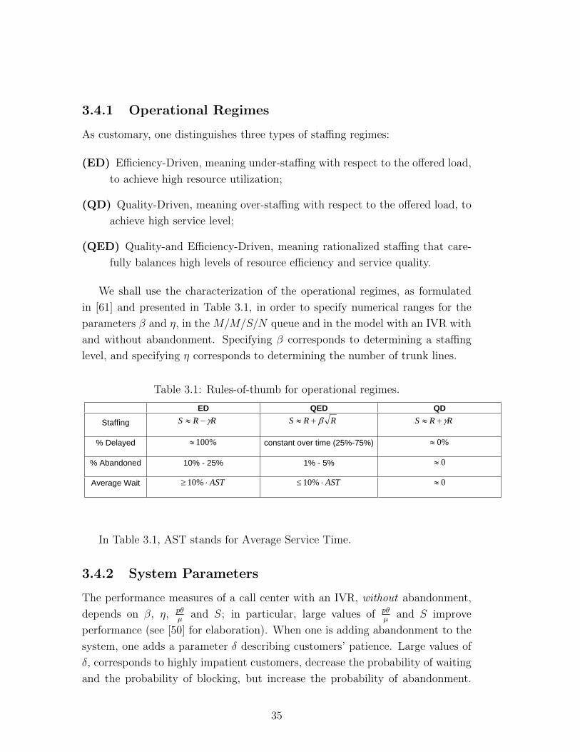
3.1 Rules-of-thumb for operational regimes. . . . . . . . . . . . . . . . 35

3.2 Rules-of-thumb for the QED regime in M/M/S/N

and M/M/S/N +M . . . . . . . . . . . . . . . . . . . . . . . . . . 37

3.3 Rules-of-thumb for the QED regime in a call center with an IVR

with and without abandonment. . . . . . . . . . . . . . . . . . . . 38

4.1 Summary of parameter estimates {θ, β, Λ(t)} based on 1000 simu-

lated random datasets with n = 250 and 500. . . . . . . . . . . . . 86

4.2 Comparison of σ2I (t) and σ2

II(t) for n = 250 and 500. . . . . . . . 87

4.3 Comparison of our proposed variance estimators with naive esti-

mators . . . . . . . . . . . . . . . . . . . . . . . . . . . . . . . . 88

4.4 Empirical power of a two-sided test with α = 0.05 and π = 0.80. . 89

4.5 Summary of the call center data set. . . . . . . . . . . . . . . . . . 90

4.6 The call center data set: parameters’ estimates and bootstrap stan-

dard errors. . . . . . . . . . . . . . . . . . . . . . . . . . . . . . . 90

4.7 The call center data set: Estimates of the cumulative baseline haz-

ard functions. . . . . . . . . . . . . . . . . . . . . . . . . . . . . . 91

4.8 The call center data set: results of the paired tests. . . . . . . . . . 92

5

List of Figures

2.1 Schematic model of a call center with one class of impatient cus-

tomers, busy signals, retrials and identical agents. . . . . . . . . . 14

3.1 M/M/S/N+M queue model. . . . . . . . . . . . . . . . . . . . . . 22

3.2 Schematic model of a call center with an IVR, S agents, N trunk

lines and customers’ abandonment. . . . . . . . . . . . . . . . . . 24

3.3 Schematic model of a call center with an interactive voice response,

S agents and N trunk lines. . . . . . . . . . . . . . . . . . . . . . 24

3.4 Schematic model of a call center with an interactive voice response,

S agents and N trunk lines. . . . . . . . . . . . . . . . . . . . . . 25

3.5 Comparison of the exact probability of waiting and its approxima-

tion, for a mid-sized call center with arrival rate 100 and 150 trunk

lines. . . . . . . . . . . . . . . . . . . . . . . . . . . . . . . . . . . 30

3.6 Comparison of the exact probability of abandonment, given wait-

ing, and its approximation, for a mid-sized call center with arrival

rate 100 and 150 trunk lines. . . . . . . . . . . . . . . . . . . . . . 31

3.7 Comparison of the exact probability of finding the system busy

and its approximation, for a mid-sized call center with arrival rate

100 and 120 trunk lines. . . . . . . . . . . . . . . . . . . . . . . . 31

3.8 Comparison of the exact probability of waiting and its approxima-

tion (3.22) for a small-sized call center with arrival rate 30 and 80

trunk lines. . . . . . . . . . . . . . . . . . . . . . . . . . . . . . . 33

3.9 Comparison of the exact probability of abandonment, given wait-

ing, and its approximation (3.23), for a small-sized call center with

arrival rate 30 and 80 trunk lines. . . . . . . . . . . . . . . . . . . 33

3.10 Comparison of the exact calculated probability to find all trunks

busy and its approximation (3.25), for a mid-sized call center with

arrival rate 30 and 80 trunk lines. . . . . . . . . . . . . . . . . . . 34

6

3.11 Schematic diagram of the call of a “Retail” customer in our US

Bank call center. . . . . . . . . . . . . . . . . . . . . . . . . . . . 40

3.12 Histogram of the IVR service time for “Retail” customers . . . . . 41

3.13 Histogram of Agents’ service time for “Retail” customers . . . . . 42

3.14 Relationship between the average waiting time given waiting, E[W |W >

0], and the proportion of abandoned calls given waiting, P (Ab|W >

0), for 30-minute intervals over 20 days. . . . . . . . . . . . . . . . 44

3.15 Comparison of approximate and observed probability of waiting. . 46

3.16 Comparison of the approximate and observed conditional proba-

bility to abandon P (ab|W > 0). . . . . . . . . . . . . . . . . . . . 46

3.17 Comparison of the approximate and observed conditional average

waiting time E(W |W > 0), in seconds. . . . . . . . . . . . . . . . 47

3.18 Area of the summation of the variable A1(λ). . . . . . . . . . . . 51

4.1 An illustration of two possible alternatives satisfying definition (4.29). 73

4.2 Estimates of the cumulative baseline hazard functions. . . . . . . 91

4.3 Naive 95% confidence intervals of the first and the second calls

(left plot) and the second and the third calls (right plot). . . . . . 93

4.4 Naive 95% confidence intervals of the first and the fifth calls. . . . 93

4.5 Estimates of the cumulative baseline hazard functions for the WAS

data by birth year. . . . . . . . . . . . . . . . . . . . . . . . . . . 95

4.6 Estimates of the baseline hazard functions for the call center data. 97

7

Chapter 1

INTRODUCTION

1.1 Our Goals

In our increasingly industrialized and globalized world, a large number of com-

panies include call centers in their structures and more than $300 billion is spent

annually on call centers around the world [34]. For a customer, addressing the

call center actually means addressing the company itself, and any negative expe-

rience on the part of the customer can lead to the rejection of company products

and services. Hence, for the company, it is very important to ensure that a call

center functions effectively and provides high quality service to its customers.

Call centers collect a huge amount of data, and this provides a great oppor-

tunity for companies to use this information for the analysis of customer needs,

desires, and intentions. Such data analysis can help improve the quality of cus-

tomer service and lower the costs. A typical call center spends about two-thirds

of its operational costs on salaries. However, it would be a false economy to re-

duce costs by decreasing the number of agents, because a small change in staffing

level can have a dramatic impact upon the level of service. Thus, a major goal of

a call center manager is to establish an appropriate tradeoff between its expenses

and its service level. We propose queueing models that can help reach sound

decisions by yielding performance-analysis tools that support this tradeoff. We

also supplement our theory with statistical analysis of our model’s primitive -

customer patience.

8

1.2 An Analysis of Call Center Performance

In order to achieve high-quality customer service and effective management of

operating costs, many leading companies are deploying new technologies, such as

enhanced Interactive Voice Response (IVR) devices, natural speech self-service

options and others. IVR systems are specialized technologies designed to enable

self-service of callers, without the assistance of human agents. The IVR technol-

ogy helps call centers to keep costs from rising (and sometimes to reduce costs),

while hopefully improving service levels, revenue and hence profits.

Our work develops and analyzes models, for a call center with and without an

IVR. We find analytical formulae which describe typical call center performance

measures, such as the probability of a busy signal, the probability of abandonment

and the average waiting time for an agent. The use of these formulae helps us to

analyze the impact of different parameters on the operational system performance

and to find the relationship between the number of agents and other system

parameters depending on the desired level of service.We also provide an empirical

study in order to evaluate the value of adding an IVR, which is based on analyzing

real data from a large call center.

1.3 Customer Patience Analysis

One of our models’ primitives is a customer patience, which we define as the

ability to endure waiting for service. This human trait plays an important role

in the call center mechanism. As mentioned above, every call can be considered

as a possibility to keep or to lose a customer, and the outcome depends on

the customer’s satisfaction. Moreover, customers are likely to remember one

disappointing service experience more clearly than twenty good ones. From this

point of view, an abandoned call is a negative experience which affects the future

customer’s choice.

There are different factors affecting the customer’s waiting behavior. Only

some of them are observable and available to us, and these are included in

the model as covariates. Unobservable factors that are likely to influence the

customer’s patience are different customer’s characteristics and customer’s tem-

perament. In this work, we use a model that takes into account observed and

unobserved personal customer’s features; and this provides a great advance in cus-

tomer patience analysis. In addition, we investigate the effect of the customers’

9

experiences on their waiting behavior.

1.4 The Structure of the Work

Chapter 2 contains a survey of the literature dealing with related works. In

Section 2.2 we review the literature concerning mathematical models of a call

center and analysis of operational performance measures. Literature related to

customer patience analysis is considered in Section 2.3.

Chapter 3 deals with the design and analysis of theoretical models describ-

ing a typical call center. In Section 3.1 we consider the extension of the model

proposed by Srinivasan et al. [80] by assuming finite customer patience and the

M/M/S/N+M queue model. Then, in Section 3.2 we find approximations for

frequently used performance measures, which support decision-making for call

center managers and help in the analysis of the staffing problem. An analysis of

the accuracy of the approximations is presented in Section 3.3. A detailed com-

parison between exact and approximated performance shows that the approxima-

tions often work perfectly, even outside the Quality and Efficiency Driven (QED)

regime. Section 3.4 summarizes our findings through practical rules-of-thumb

(expressed via the offered load) and we chart the boundary of this “outside”. In

Section 3.5, we validate our approximations against data from a real call cen-

ter, thus establishing their applicability. For the convenience of the reader, the

proofs of theorems from Section 3.2 are presented in Section 3.6. In Section 3.7

we summarize our findings and propose future directions for research.

Customer patience is analyzed in Chapter 4. In Section 4.1 we start with

a description of the data that motivated the study. In Section 4.2 we briefly ex-

plain the choice of our model. Section 4.3 presents the notation and formulation

of the model. The estimating procedure and the asymptotic properties of the

estimators are presented in Section 4.4. A new test for comparing of two or more

baseline hazard functions in the case of dependent observations is provided in

Section 4.5. In Section 4.6 we propose a sample size formula for given signifi-

cance level and power. The proofs and technical details are presented in separate

section, namely in Section 4.7. The utility of our proposed estimating technique,

a test for comparison and a sample size formula are illustrated in Section 4.8

by extensive simulation study. Then, in Section 4.9, we apply the results of our

approach to the real call center data. Our conclusions and future work are set

out in Section 4.10. Although our research was motivated by call center data, the

10

proposed methods can also be of practical importance in different research fields.

Thus, in Section 4.10.1, we apply our approach for analyzing breast cancer data

of family study.

In Chapter 5 we summarize the results of our work and discuss the innovation

proposed in our study, the methodology used and possible scientific and practical

contributions.

11

Chapter 2

LITERATURE REVIEW

2.1 Descriptive Statistical Analysis

Statistical analysis of call center data started with the creation of call centers.

The work of Roberts [75], Duffy and Mercer [23], Liu [59] and Kort [55] written

in the 1970s are dedicated mostly to the description and analysis of models with

customer abandonments and retrials that took place as a result of telephone net-

work impairments. The underlying research was initiated by companies providing

telephone services and telephone equipment.

The study by Liu [59] can be considered as a continuation of the survey con-

ducted in [23]. Liu’s main goal was to provide a comprehensive characterization

of network performance and customer behavior in setting up a customer’s de-

sired telephone connection. Using the collected data, Liu summarized various

statistical characteristics, i.e. initial attempts at disposition probabilities, retrial

probabilities, the number of additional attempts, ultimate success probabilities

and distribution functions for retrial intervals following different types of uncom-

pleted initial attempts.

Kort [55] described models and methods developed at Bell Laboratories to

evaluate customer acceptance of telephone connections in the Bell System Public

Switched Telephone Network. The models that were developed and used in this

study provided a basis for IEEE standards for telephone network performance

specifications in a multi-vendor environment. The detailed description of data

analyzed in our work can be found in Donin et al. [22] and Trofimov et al. [83].

12

2.2 An Analysis of a Call Center Performance

A detailed survey of literature on queuing models for call center design are pro-

vided by Gans et al. [30].

2.2.1 The QED Regime

The mathematical framework considered here is a multi-server heavy-traffic asymp-

totic regime, which is referred to as the QED (Quality and Efficiency Driven)

regime. Systems that operate in the QED regime enjoy a combination of very

high efficiency together with very high quality of service, as surveyed by Gans

et al. [30]. A mathematical characterization of the QED regime for the GI/M/S

queue was established by Halfin and Whitt [38] as having a non-trivial limit

(within (0,1)) of the fraction of delayed customers, with S increasing indefi-

nitely. The latter characterization was also established for GI/D/S (Jelenkovic

et al. [47]), M/M/S with exponential patience (Garnett et al. [31]) and with

general patience (Mandelbaum and Zeltyn [63]).

The QED regime was explicitly recognized as early as 1923 in Erlang’s paper

(that appeared in [27]), which addresses both Erlang-B (M/M/S/S) and Erlang-

C (M/M/S) models. Later extensive related work took place in various telecom

companies but little has been publicly documented. A precise characterization of

the asymptotic expansion of the blocking probability, for Erlang-B in the QED

regime, was given by Jagerman [46], Whitt [86], and then Massey and Wallace [65]

for the analysis of finite buffers. The phenomenon of abandonment in a call

center with multiple servers was analyzed by Garnett et al. [31] (Erlang-A model

(M/M/S+M)) and Mandelbaum and Zeltyn [63] (M/M/S+G).

2.2.2 The Square-Root Staffing Principle

Erlang’s characterization of the QED regime was in terms of the square-root

staffing principle (sometimes called the “safety-staffing principle”). The square-

root principle has two parts to it: first, the conceptual observation that the

safety staffing level is proportional to the square-root of the offered load; and

second, the explicit calculation of the proportionality coefficient. Borst et al. [12]

developed a framework that accommodates both of these needs. More impor-

tant, however, is the fact that their approach and framework allow an arbitrary

cost structure, having the potential to generalize beyond Erlang-C. The square-

13

root staffing principle arises also in [65] for the M/M/S/N queue, in [31] for

M/M/S+M, and others, as surveyed in Gans et al. [30].

2.2.3 Analytical Models of Call Center Performance

In the detailed introduction to call centers by Gans et al. [30], it is explained

how call centers can be modeled by queueing systems of various characteristics.

Many results and models with references are surveyed in that paper. The authors

examine models of single type customers and single skill agents; models with busy

signals and abandonment; skills-based routing; call blending and multi-media;

and geographically dispersed call centers.

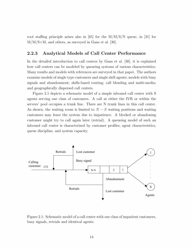
Figure 2.1 depicts a schematic model of a simple inbound call center with S

agents serving one class of customers. A call at either the IVR or within the

servers’ pool occupies a trunk line. There are N trunk lines in this call center.

As shown, the waiting room is limited to N − S waiting positions and waiting

customers may leave the system due to impatience. A blocked or abandoning

customer might try to call again later (retrial). A queueing model of such an

inbound call center is characterized by customer profiles, agent characteristics,

queue discipline, and system capacity.

Calling

customer )(

1

S

1N-S 2…

.

.

.

.

.

Lost customer

Busy signal

RetrialsLost customer

Abandonment

Agents

Retrials

Figure 2.1: Schematic model of a call center with one class of impatient customers,

busy signals, retrials and identical agents.

14

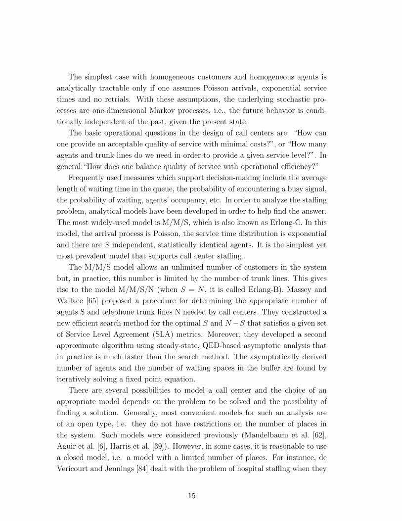
The simplest case with homogeneous customers and homogeneous agents is

analytically tractable only if one assumes Poisson arrivals, exponential service

times and no retrials. With these assumptions, the underlying stochastic pro-

cesses are one-dimensional Markov processes, i.e., the future behavior is condi-

tionally independent of the past, given the present state.

The basic operational questions in the design of call centers are: “How can

one provide an acceptable quality of service with minimal costs?”, or “How many

agents and trunk lines do we need in order to provide a given service level?”. In

general:“How does one balance quality of service with operational efficiency?”

Frequently used measures which support decision-making include the average

length of waiting time in the queue, the probability of encountering a busy signal,

the probability of waiting, agents’ occupancy, etc. In order to analyze the staffing

problem, analytical models have been developed in order to help find the answer.

The most widely-used model is M/M/S, which is also known as Erlang-C. In this

model, the arrival process is Poisson, the service time distribution is exponential

and there are S independent, statistically identical agents. It is the simplest yet

most prevalent model that supports call center staffing.

The M/M/S model allows an unlimited number of customers in the system

but, in practice, this number is limited by the number of trunk lines. This gives

rise to the model M/M/S/N (when S = N , it is called Erlang-B). Massey and

Wallace [65] proposed a procedure for determining the appropriate number of

agents S and telephone trunk lines N needed by call centers. They constructed a

new efficient search method for the optimal S and N−S that satisfies a given set

of Service Level Agreement (SLA) metrics. Moreover, they developed a second

approximate algorithm using steady-state, QED-based asymptotic analysis that

in practice is much faster than the search method. The asymptotically derived

number of agents and the number of waiting spaces in the buffer are found by

iteratively solving a fixed point equation.

There are several possibilities to model a call center and the choice of an

appropriate model depends on the problem to be solved and the possibility of

finding a solution. Generally, most convenient models for such an analysis are

of an open type, i.e. they do not have restrictions on the number of places in

the system. Such models were considered previously (Mandelbaum et al. [62],

Aguir et al. [6], Harris et al. [39]). However, in some cases, it is reasonable to use

a closed model, i.e. a model with a limited number of places. For instance, de

Vericourt and Jennings [84] dealt with the problem of hospital staffing when they

15

had to take into consideration the number of places in the system, namely, an

always finite number of beds in a given hospital. Another type of closed model

was considered by Randhawa and Kumar [73]. Their system was limited to a

number of subscribers. As mentioned above, such a model is appropriate for

communication systems.

Analytical models of a Call Center with an IVR were developed by Brandt

et al. [13]. They showed, and we shall use this fact later on, that it is possible

to replace the semi-open network of their model with a closed Jackson network.

Such a network has the well-known product form solution for its stationary dis-

tribution. This product-form distribution was used by Srinivasan et al. [80] in

order to calculate expressions for the probability to find all lines busy and the

conditional distribution function of the waiting time before service. However, due

to the complex nature of these expressions and the numerical instability associ-

ated with the computation process, the whole procedure may be time-consuming

and ultimately produce inaccurate values. On the other hand, it is possible to

use approximations for the system characteristics as was shown in my M.Sc. the-

sis [50]. These approximations are convenient for the investigation of the effect of

changes in the system parameters on the system performance. At the same time,

in [50] approximations of a real call center by models with and without an IVR

are analyzed, though it did not support possible customer abandonments. In the

current work we extend the model presented in [50] by equipping customers with

finite patience.

2.3 Customer Patience Analysis

The first model for customer patience was constructed by Palm [68] in 1943. He

introduced a so-called time-dependent inconvenience function that is actually a

proportional hazard rate function. An important result, postulated by Palm,

is the presence of a correlation between a hazard rate of the customer patience

time and his/her irritation caused by waiting. Palm also suggested that patience

was characterized by a Weibull distribution, a specific case of this distribution

being an exponential distribution widely used in queuing theory (Erlang-A queue

model). We also use the assumption of exponentially distributed patience time

to create a theoretical model of a typical call center (Sections 3.1.1 and 3.1.2).

The assumption of Weibull distributed patience also was proposed by Kort [55]

who studied customer acceptance of telephone connections. A detailed survey of

16

the above and other literature on models and methods used for the analysis of

customer patience was provided by Gans et al. [30].

A descriptive model of customer patience with the use of real call center

data was presented by Brown et al. [16]. They estimated the distribution of

customer patience using the standard Kaplan-Meier product limit estimator. The

survival functions were created for different types of service. The authors found

that customers performing stock trading are willing to wait more than customers

calling for regular services. This unexpected result was explained by the fact that

these customers need the service more urgently, and have more trust in the system

to provide it. In addition, Brown et al. [16] constructed nonparametric hazard

rate estimates. Namely, for each interval of length δ, the estimate of the hazard

rate was calculated as[] of events during (t, t + δ]

]/[(] at risk at t) × δ

]. The

resulting function had two peaks and these peaks occurred after a “Please wait”

message played by the system with 60 seconds difference. This example illustrates

that sometimes ostensibly correct management solutions have the opposite effect.

2.3.1 Survival Analysis

The complication of customer patience analysis is that in most cases customers

receive the required service before they lose their patience and we do not ob-

serve the values of customer patience. We call such incomplete data as censored

observations. To analyze the data with censored observations we need tools of

survival analysis. Generally, survival analysis involves the modeling of time to

event data. The occurrences of these events are often referred to as failures.

Failure time data occur in numerous fields including medicine, economics and

industry. The basic models of survival analysis are described in Kalbfleisch and

Prentice [48], Hougaard [42] and references therein, among others.

2.3.2 Frailty Models

The Cox proportional hazard model is one of the most widely used event history

models. It was proposed by Cox [21] and assumes that event times are indepen-

dent. Thus, for the analysis of correlated (clustered) failure times an extended

Cox model was proposed (Ripatti and Palmgren [74], Murphy [66], Parner [70]),

in which a random effect, for each cluster, is included in the model. This ran-

dom effect model is known as frailty model. Frailty model provides a natural

approach to account for risk heterogeneity. The cluster-specific random variate

17

acts multiplicatively on the hazard function. Under a frailty model, the regres-

sion coefficients are cluster-specific log-hazard ratios. It is clear that the frailty

model is modeling the conditional hazard function given the latent frailty (Hsu

et al. [43], Hsu et al. [45], Duffy et al. [24]). This is in contrast with the marginal

modeling (Hsu and Gorfine [44], Shih and Chatterjee [78], Lin [58]), where the

correlation is modeled through a multivariate distribution which often involves

a copula function, with a specified model for the marginal hazard function. The

regression coefficients in the marginal model represent the log-hazard ratios at

the population level, regardless of which cluster an individual comes from. In our

context, when the objective is to make inference about calls of the same customer,

a customer-specific risk estimate is more relevant than a population-averaged risk

estimate. Zeger et al. [88] provides a comprehensive comparison of cluster-level

modelling versus the marginal population-average approach.

Many frailty models have been considered, including Gamma (Klein [51],

Nielsen et al. [67]), Positive stable (Hougaard [41]), Inverse Gaussian (Aalen

and Gjessing [3]), compound Poisson (Henderson et al. [40], Aalen [2]), and Log-

normal (Ripatti and Palmgren [74]). Hougaard [42] provided a broad review

of models consists of different frailty distributions. The most commonly used

frailty distribution is the Gamma frailty distribution, because of mathematical

convenience. However, it is of concern that misspecification of Gamma frailty

distribution may invalidate the inference. Different frailty distributions induce

different dependence structure, then, it is important to examine the adequacy of

the Gamma frailty model for describing the intracluster dependence. Model diag-

nostic procedures have been developed for that purpose (Shih [77], Glidden [35],

Chen et al. [19]). There are also some works dealing with the misspesification

of frailty distribution (Glidden and Vittinghoff [36], Kosorok et al. [53]). Hsu et

al. [45] studied how the misspecification affects the estimation of the marginal

parameters. They analyzed the simulated data under the assumption of Gamma

distributed frailty, while the true distributions were Inverse Gaussian, Positive

Stable and a specific case of Discrete distribution. This analysis showed that the

Gamma distribution appears to be robust to frailty distribution misspecification

in cohort and case-control family studies.

A detailed review of methods for estimation and the model testing were pro-

vided by Hougaard [42]. Nielsen et al. [67] and Klein [51] considered the NPMLE

estimate of the proportional hazard model with gamma frailty. Murphy [66]

showed the consistency and asymptotic normality for this model without covari-

18

ates. Later, Parner [70] extended these results to the model with covariates. Zeng

and Lin [90] presented an estimation technique for the class of semiparametric

regression models for censored data, which also include the random effects for

dependent time failures. They provided a semi-parametric maximum likelihood

estimator, based on the EM algorithm, together with their asymptotic properties.

A noniterative estimation procedure for estimating the parameters of the frailty

model with any frailty distribution with finite moments was proposed by Gorfine

et al. [45]. The detailed proof of the asymptotic properties of the proposed esti-

mators was provided by Zucker et al. [91].

2.3.3 Testing for Equality of Hazard Functions

The most popular test statistic for testing the equatlity of two hazard functions

is the weighted log-rank test. It was first proposed by Mantel [64] and later Peto

and Peto [71] named it log-rank. An adaptation of this test to censored data

was suggested by Prentice [72]. Different extensions of the Wilcoxon rank-sum

statistic to censored failure time data were also considered (Gehan [32], Peto and

Peto [71], and Tarone and Ware [82]). These proposed models together with

the log-rank statistic can be incorporated into the class of weighted log-rank

statistics. The asymptotic properties of the weighted log-rank statistics were

derived via martingale theory (Gill [33], Fleming and Harrington [28], Andersen et

al. [8]). The family of log-rank statistics presented by Harrington and Fleming [28]

describes a large variety of weighted log-rank statistics such as the log-rank,

Prentice-Wilcoxon, Gehan-Wilcoxon and Tarone-Ware statistics.

Often weighted log-rank statistics considered data generated from indepen-

dent samples (Lawless and Nadeau [56], Cook et al. [20], Eng and Kosorok [26]).

Comparison of two treatments based on clustered data with no covariates is pre-

sented by Gangnon and Kosorok [29]. They used the weighted log-rank test

statistic and presented a simple sample size formula. Song et al. [79] studied

a covariate-adjusted weighted log-rank statistic for recurrent events data while

comparing between two independent treatment groups. For the best of our knowl-

edge, so far there is no published work that deals with correlated samples test

applied to a covariate adjusted frailty model.

19

2.3.4 Sample Size Formula

One of the most widely used sample size formula for the log-rank test under

the setting of two independent samples is that of Schoenfeld [76]. This formula

was developed under the assumption that the hazard functions are not time

varying. Combining the idea of Schoenfeld and extending the class of alternatives

presented by Fleming and Harrington [28], Kosorok and Lin [54] proposed a class

of contiguous alternatives for power and sample size calculations. This class was

used for sample size calculations for clustered survival data, with no covariates,

using the log-rank statistic (Gangnon and Kosorok [29]), for the supremum log-

rank statistic (Eng and Kosorok [26]) and for covariate adjusted log-rank statistic

for independent samples (Song et al. [79]). In all the above works, the sample

size formula was done under simplifying assumptions, such as assuming identical

censoring distributions, consistent difference between the two hazard functions,

and continuous hazard functions.

20

Chapter 3

DESIGN AND INFERENCE

FOR A TYPICAL CALL

CENTER

3.1 Notation and Formulation of Our Models

As mentioned earlier, a call center typically consists of telephone trunk lines, a

switching machine known as the Automatic Call Distributor (ACD), an interac-

tive voice response (IV R) unit, and agents to handle the incoming calls. In this

chapter we provide theoretical analyses of two models of a typical call center. The

first model does not take into account IVR processes and describes only agents’

service and waiting before this service. The second model is more complicated

and considers a pool of agents together with the service process in the IVR unit.

3.1.1 Call Center without an IVR

We assume that the arrival process is a Poisson process with rate λ. There are N

trunk lines in the system, i.e. arriving customers enter the system only if there

is an idle trunk line. We assume that customers have finite patience. Under

our assumptions, if a call waits in the queue, it may leave the system after an

exponentially distributed time, or is answered by an agent, whichever happens

first. The rate of abandonments equals δ. Agents’ service times are taken to be

independent identically distributed exponential random variables with the rate

of µ.

In queueing theory the described model is called the M/M/S/N+M queueing

21

model and schematically can be described as follows:

0 1 2 S-1 S S+1 N-1 N

μ μ2 μS δμ +S δμ )( SNS −+

λ λ λ λ λ

… …

Figure 3.1: M/M/S/N+M queue model.

The M/M/S/N+M queue has the following stationary distribution:

πi =

π01

i!

(λ

µ

)i, 0 ≤ i ≤ S;

π01

S!

(λµ

)Si−S∏j=1

λ

Sµ+ jδ, S < i ≤ N ;

0, otherwise

(3.1)

where

π0 =[ S∑i=0

1

i!

(λµ

)i+

N∑i=S+1

1

S!

(λµ

)S i−S∏j=1

λ

Sµ+ jδ

]−1

. (3.2)

According to the PASTA theorem [87] we can easily formulate the expressions

for operational performance measures. Let W be the waiting time - the time spent

by customers, who opt for service, from just after they leave the IVR until being

served by an agent. Thus,

• the probability P (W > 0) that a customer waits after the IVR:

P (W > 0) =N−1∑i=S

πi, (3.3)

• the probability of abandonment, given waiting:

P (Ab|W > 0) =

N∑i=S+1

πi(Sµ+ (i− S)δ)(i− S)δ

Sµ+ (i− S)δ

N∑i=S+1

πi(Sµ+ (i− S))

, (3.4)

• the expectation of the waiting time, given waiting can be calculated using

the following relationship:

E[W |W > 0] =P (Ab|W > 0)

δ, (3.5)

22

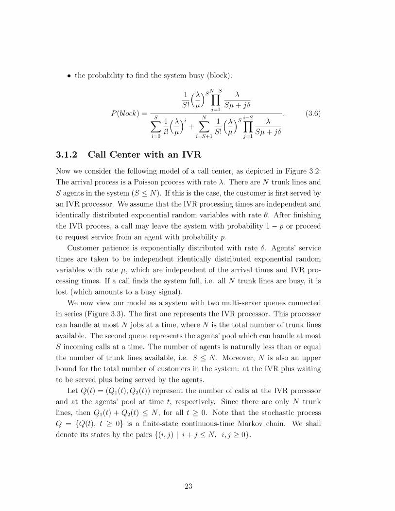
• the probability to find the system busy (block):

P (block) =

1

S!

(λµ

)SN−S∏j=1

λ

Sµ+ jδ

S∑i=0

1

i!

(λµ

)i+

N∑i=S+1

1

S!

(λµ

)S i−S∏j=1

λ

Sµ+ jδ

. (3.6)

3.1.2 Call Center with an IVR

Now we consider the following model of a call center, as depicted in Figure 3.2:

The arrival process is a Poisson process with rate λ. There are N trunk lines and

S agents in the system (S ≤ N). If this is the case, the customer is first served by

an IVR processor. We assume that the IVR processing times are independent and

identically distributed exponential random variables with rate θ. After finishing

the IVR process, a call may leave the system with probability 1 − p or proceed

to request service from an agent with probability p.

Customer patience is exponentially distributed with rate δ. Agents’ service

times are taken to be independent identically distributed exponential random

variables with rate µ, which are independent of the arrival times and IVR pro-

cessing times. If a call finds the system full, i.e. all N trunk lines are busy, it is

lost (which amounts to a busy signal).

We now view our model as a system with two multi-server queues connected

in series (Figure 3.3). The first one represents the IVR processor. This processor

can handle at most N jobs at a time, where N is the total number of trunk lines

available. The second queue represents the agents’ pool which can handle at most

S incoming calls at a time. The number of agents is naturally less than or equal

the number of trunk lines available, i.e. S ≤ N . Moreover, N is also an upper

bound for the total number of customers in the system: at the IVR plus waiting

to be served plus being served by the agents.

Let Q(t) = (Q1(t), Q2(t)) represent the number of calls at the IVR processor

and at the agents’ pool at time t, respectively. Since there are only N trunk

lines, then Q1(t) + Q2(t) ≤ N , for all t ≥ 0. Note that the stochastic process

Q = {Q(t), t ≥ 0} is a finite-state continuous-time Markov chain. We shall

denote its states by the pairs {(i, j) | i+ j ≤ N, i, j ≥ 0}.

23

4

N

3

2

1

.

.

....

.

.

.

S

3

2

1

Interactive Voice Response (IVR)

Automatic Call Distributor (ACD) Pool of Agents

N trunk lines

N-S

Customers leaving the system

Customersleavingthe system

Customers enteringthe system

Figure 3.2: Schematic model of a call center with an IVR, S agents, N trunk

lines and customers’ abandonment.

μ

1

2

3

N

.

.

. 1-p

1

2

S

.

.

.

…

“Queue” N-S

p θ λ

“IVR” N servers

“Agents” S servers

P(Ab)

Figure 3.3: Schematic model of a call center with an interactive voice response,

S agents and N trunk lines.

24

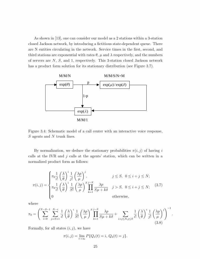
As shown in [13], one can consider our model as a 2 stations within a 3-station

closed Jackson network, by introducing a fictitious state-dependent queue. There

are N entities circulating in the network. Service times in the first, second, and

third stations are exponential with rates θ, µ and λ respectively, and the numbers

of servers are N , S, and 1, respectively. This 3-station closed Jackson network

has a product form solution for its stationary distribution (see Figure 3.7).

)exp(

M/M/S/N+M

)exp(/)exp(

M/M/1

)exp(

p

M/M/N

1-p

Figure 3.4: Schematic model of a call center with an interactive voice response,

S agents and N trunk lines.

By normalization, we deduce the stationary probabilities π(i, j) of having i

calls at the IVR and j calls at the agents’ station, which can be written in a

normalized product form as follows:

π(i, j) =

π01

i!

(λ

θ

)i1

j!

(λp

µ

)j, j ≤ S, 0 ≤ i+ j ≤ N ;

π01

i!

(λ

θ

)i1

S!

(λp

µ

)S j−S∏k=1

λp

Sµ+ kδj > S, 0 ≤ i+ j ≤ N ;

0 otherwise,

(3.7)

where

π0 =

(N−S−1∑i=0

N−i∑j=S+1

1

i!

(λ

θ

)i1

S!

(λp

µ

)S j−S∏k=1

λp

Sµ+ kδ+

∑i+j≤N,j≤S

1

i!

(λ

θ

)i1

j!

(λp

µ

)j)−1

.

(3.8)

Formally, for all states (i, j), we have

π(i, j) = limt→∞

P{Q1(t) = i, Q2(t) = j}.

25

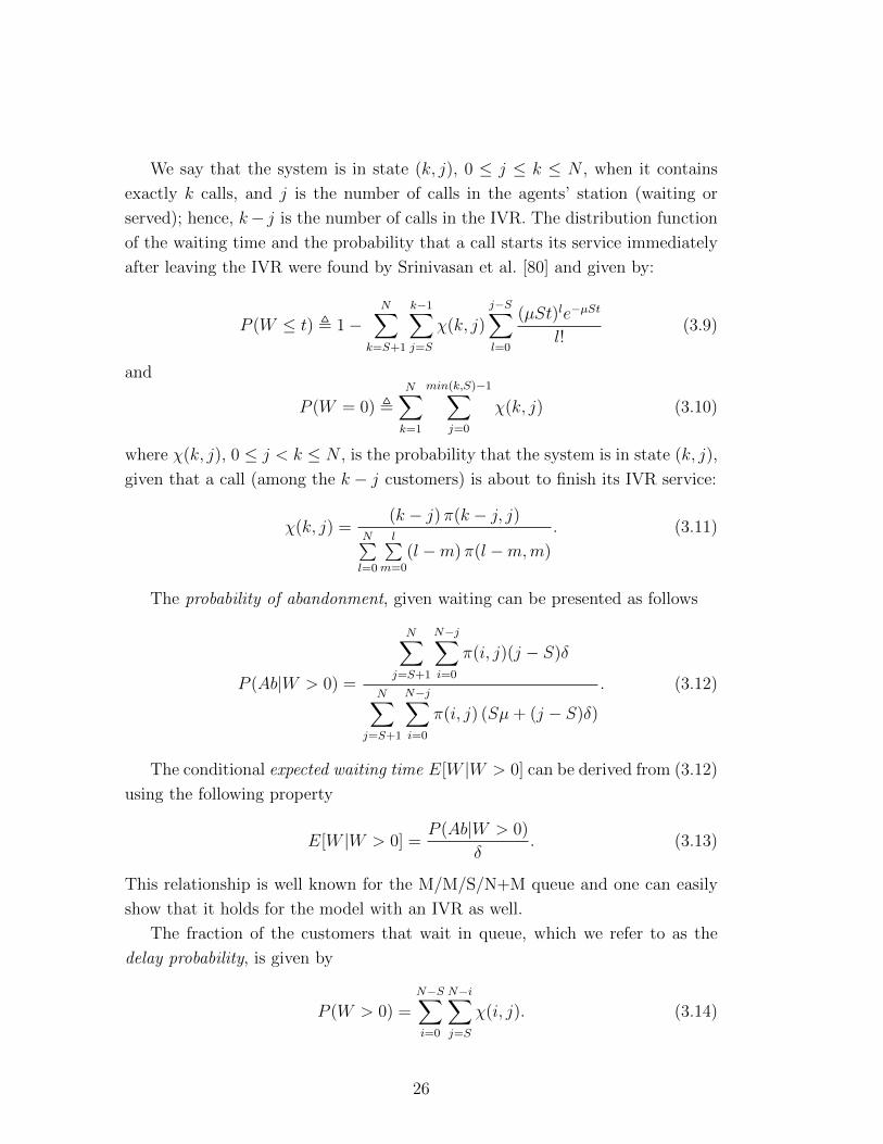
We say that the system is in state (k, j), 0 ≤ j ≤ k ≤ N , when it contains

exactly k calls, and j is the number of calls in the agents’ station (waiting or

served); hence, k− j is the number of calls in the IVR. The distribution function

of the waiting time and the probability that a call starts its service immediately

after leaving the IVR were found by Srinivasan et al. [80] and given by:

P (W ≤ t) , 1−N∑

k=S+1

k−1∑j=S

χ(k, j)

j−S∑l=0

(µSt)le−µSt

l!(3.9)

and

P (W = 0) ,N∑k=1

min(k,S)−1∑j=0

χ(k, j) (3.10)

where χ(k, j), 0 ≤ j < k ≤ N , is the probability that the system is in state (k, j),

given that a call (among the k − j customers) is about to finish its IVR service:

χ(k, j) =(k − j) π(k − j, j)

N∑l=0

l∑m=0

(l −m) π(l −m,m)

. (3.11)

The probability of abandonment, given waiting can be presented as follows

P (Ab|W > 0) =

N∑j=S+1

N−j∑i=0

π(i, j)(j − S)δ

N∑j=S+1

N−j∑i=0

π(i, j) (Sµ+ (j − S)δ)

. (3.12)

The conditional expected waiting time E[W |W > 0] can be derived from (3.12)

using the following property

E[W |W > 0] =P (Ab|W > 0)

δ. (3.13)

This relationship is well known for the M/M/S/N+M queue and one can easily

show that it holds for the model with an IVR as well.

The fraction of the customers that wait in queue, which we refer to as the

delay probability, is given by

P (W > 0) =N−S∑i=0

N−i∑j=S

χ(i, j). (3.14)

26

Equation (3.14) gives the conditional probability that a calling customer does

not immediately reach an agent, given that the calling customer is not blocked,

i.e., P (W > 0) is the delay probability for served customers. This conditional

probability can be reduced to an unconditional probability via the “Arrival The-

orem” [18]. Specifically, for the system with N trunk lines and S agents, the

fraction of customers that are required to wait after their IVR service, coincides

with the probability that a system with N − 1 trunk lines and S agents has all

its agents busy, namely

PN(W > 0) = PN−1(Q2(∞) ≥ S). (3.15)

3.2 Asymptotic Analysis in the QED Regime

3.2.1 The Domain for Asymptotic Analysis

All the following approximations will be derived when the arrival rate λ tends to

infinity. In order for the system to not be overloaded, we assume that the number

of agents S and the number of trunk lines N tend to infinity as well.

Our approximations for performance measures calculated according to the

M/M/S/N+M queue model are the same as were formulated in [65]:

(i) limλ→∞

N − S√S

= η, η ≥ 0,

(ii) limλ→∞

√S

(1− λ

µS

)= β, −∞ < β <∞.

(3.16)

The asymptotic domain for the model with an IVR were presented first in [50]

and has the following form:

(i) limλ→∞

N − S − λθ√

λθ

= η, −∞ < η <∞;

(ii) limλ→∞

√S

(1− λp

µS

)= β, −∞ < β <∞.

(3.17)

3.2.2 The M/M/S/N+M Queue

We start with approximations for performance characteristics of the M/M/S/N+M

queue. The results are formalized in the following theorem.

27

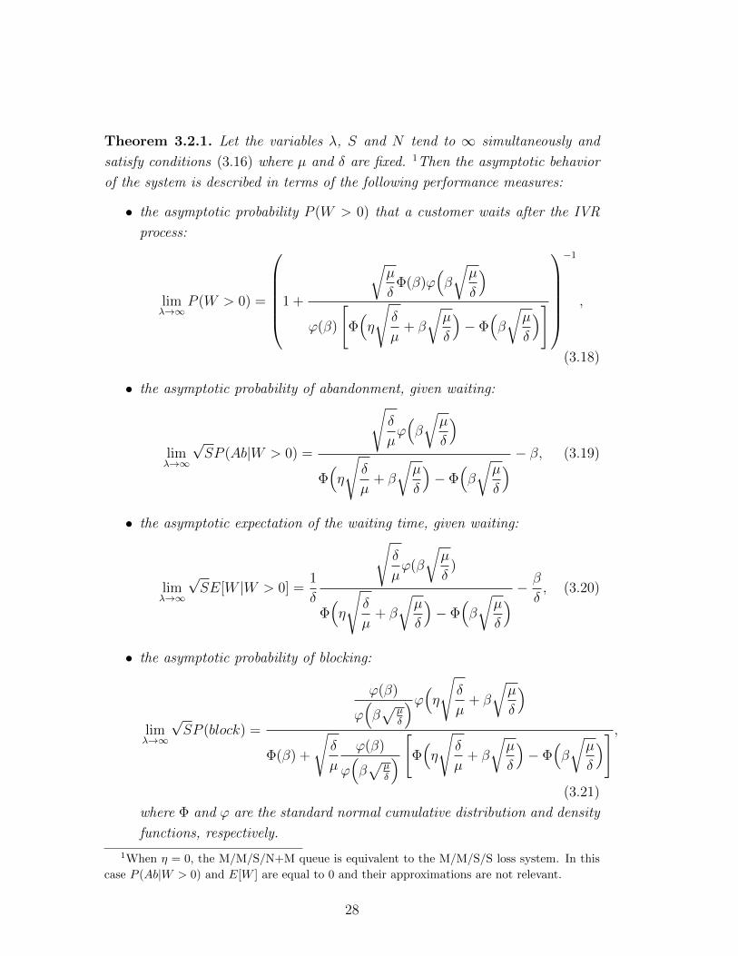
Theorem 3.2.1. Let the variables λ, S and N tend to ∞ simultaneously and

satisfy conditions (3.16) where µ and δ are fixed. 1Then the asymptotic behavior

of the system is described in terms of the following performance measures:

• the asymptotic probability P (W > 0) that a customer waits after the IVR

process:

limλ→∞

P (W > 0) =

1 +

õ

δΦ(β)ϕ

(β

õ

δ

)ϕ(β)

[Φ(η

√δ

µ+ β

õ

δ

)− Φ

(β

õ

δ

)]−1

,

(3.18)

• the asymptotic probability of abandonment, given waiting:

limλ→∞

√SP (Ab|W > 0) =

√δ

µϕ(β

õ

δ

)Φ(η

√δ

µ+ β

õ

δ

)− Φ

(β

õ

δ

) − β, (3.19)

• the asymptotic expectation of the waiting time, given waiting:

limλ→∞

√SE[W |W > 0] =

1

δ

√δ

µϕ(β

õ

δ)

Φ(η

√δ

µ+ β

õ

δ

)− Φ

(β

õ

δ

) − β

δ, (3.20)

• the asymptotic probability of blocking:

limλ→∞

√SP (block) =

ϕ(β)

ϕ(β√

µδ

)ϕ(η√ δ

µ+ β

õ

δ

)

Φ(β) +

√δ

µ

ϕ(β)

ϕ(β√

µδ

) [Φ(η

√δ

µ+ β

õ

δ

)− Φ

(β

õ

δ

)] ,(3.21)

where Φ and ϕ are the standard normal cumulative distribution and density

functions, respectively.

1When η = 0, the M/M/S/N+M queue is equivalent to the M/M/S/S loss system. In this

case P (Ab|W > 0) and E[W ] are equal to 0 and their approximations are not relevant.

28

The proof of Theorem 3.2.1 is presented in Section 3.6.1 and it is carried out

by using formulas (3.3) - (3.6), where the stationary probabilities are defined by

(3.1) and (3.2).

3.2.3 Call Center with an IVR

In the following theorem we formulate approximations of the operational perfor-

mance measures for a call center with an IVR, which were defined previously in

Section 3.1.2. Proof of Theorem 3.2.2 is presented in Section 3.6.2.

Theorem 3.2.2. Let the variables λ, S and N tend to ∞ simultaneously and

satisfy the QED conditions (3.17), where µ, p, θ and δ are fixed. Then the asymp-

totic behavior of the system is described in terms of the following performance

measures:

• the asymptotic probability P (W > 0) that a customer waits after the IVR

process:

limλ→∞

P (W > 0) =

(1 +

γ

ξ1 − ξ2

)−1

, (3.22)

• the asymptotic probability of abandonment, given waiting:

limλ→∞

√SP (Ab|W > 0) =

õ

δϕ(β

õ

δ)Φ(η)

∞∫β√

µδ

Φ(η + (β

õ

δ− t)

√pθ

µ)ϕ(t)dt

− β, (3.23)

• the asymptotic expectation of waiting time, given waiting:

limλ→∞

√SE[W |W > 0] =

1

δ

õ

δϕ(β

õ

δ)Φ(η)

∞∫β√

µδ

Φ(η + (β

õ

δ− t)

√pθ

µ)ϕ(t)dt

− β

δ, (3.24)

• the asymptotic probability of a busy signal:

limλ→∞

√SP (block) =

ν + ξ2ϕ[(η + β

√pµθ

δ

)/(√

1 +pθ

δ

)]/[1− Φ(β

õ

δ)]

γ + ξ1 − ξ2

;

(3.25)

29

in the above,

ξ1 =

õ

δ

ϕ(β)

ϕ(β√

µδ)

η∫−∞

Φ

((η − t)

√δ

pθ+ β

õ

δ

)ϕ(t)dt,

ξ2 =

õ

δ

ϕ(β)

ϕ(β√

µδ)Φ(β

õ

δ)Φ(η),

γ =

β∫−∞

Φ

(η + (β − t)

√pθ

µ

)ϕ(t)dt, and ν =

1√1 +

√µpθ

ϕ

η√

µpθ

+ β√1 + µ

pθ

Φ

β√

µpθ− η√

1 + µpθ

.

3.3 Accuracy of the Approximations

3.3.1 Approximations for the M/M/S/N+M Queue

Examining the approximations for performance measures of the M/M/S/N+M

queue, we model a mid-sized call center, in which the arrival rate λ is 100 cus-

tomers per minute. The number of agents S is in the domain where the traffic

intensity ρ = λpµS

is about 1 (namely, the number of agents is between 80 and

120).

P(W>0) and its approximation

0

0.2

0.4

0.6

0.8

1

1.2

80 82 84 86 88 90 92 94 96 98 100102104106108110112114116118120

S, agents

pro

ba

bil

ity

approx

exact

Figure 3.5: Comparison of the exact probability of waiting and its approximation,

for a mid-sized call center with arrival rate 100 and 150 trunk lines.

We let p = µ = θ = δ = 1. The number of trunk lines is mostly 150, but

when we check the probability of blocking, we take the number of trunk lines to

30

be 120 (this in order to avoid very small values).

P(Ab|W>0) and its approximation

0

0.02

0.04

0.06

0.08

0.1

0.12

0.14

0.16

93 95 97 99 101

103

105

107

109

111

113

115

117

119

S, agents

approx

exact

Figure 3.6: Comparison of the exact probability of abandonment, given waiting,

and its approximation, for a mid-sized call center with arrival rate 100 and 150

trunk lines.

P(Block) and its approximation

0

0.01

0.02

0.03

0.04

0.05

93 94 95 96 97 98 99 100 101 102 103 104 105 106 107 108 109 110

S, agents

approx

exact

Figure 3.7: Comparison of the exact probability of finding the system busy and

its approximation, for a mid-sized call center with arrival rate 100 and 120 trunk

lines.

One of the conclusions which can be derived from Figures 3.5-3.7 is the fact

that the approximations which were founded are close to the exact value although

31

in the small-sized call center. In addition, we have to emphasize that the calcu-

lation of the exact value is very difficult practically in the case of a bigger call

center, for example, when the arrival rate λ is 500, the number of trunk lines N is

1500, and the number of agents S is between 450 and 550 agents. Using the fact

that the approximation is very close to the exact value we can easily calculate

the performance measures in such call centers.

3.3.2 Approximations of the Model with an IVR

The accuracy of approximations for a model without abandonment was provided

in [50]. These approximations turn out to be extremely accurate, over a very wide

range of parameters (S already from 10 and above, N ≥ 50). Here, we present

approximations that accommodate abandonments. The numerical analysis is

heavier due to the increased number of integral-approximations. For example,

the approximation of P (W > 0) involves an integral in both γ and ξ (as opposed

to only γ, in the model without abandonment). In addition, for calculations

of the exact values we are restricted to relatively small N ’s (N ≤ 80 here, as

opposed to N ≤ 170).

To investigate the performance of our approximations, we compare the perfor-

mance measures of a model with an IVR and abandonment that corresponds to a

small-sized call center that has the arrival rate λ of 30 customers per minute. The

number of agents S is in the domain where the traffic intensity ρ = λpµS

is about 1

(namely, the number of agents is between 20 and 40, i.e. S ≈ 30± 2 ·√

30). For

simplicity, we let p = µ = θ = δ = 1. The number of trunk lines is 80. For each

value of the number of agents S, we calculate the parameters η and β by using

(3.17).

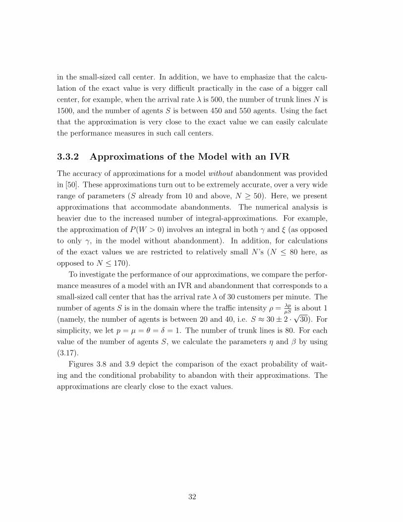
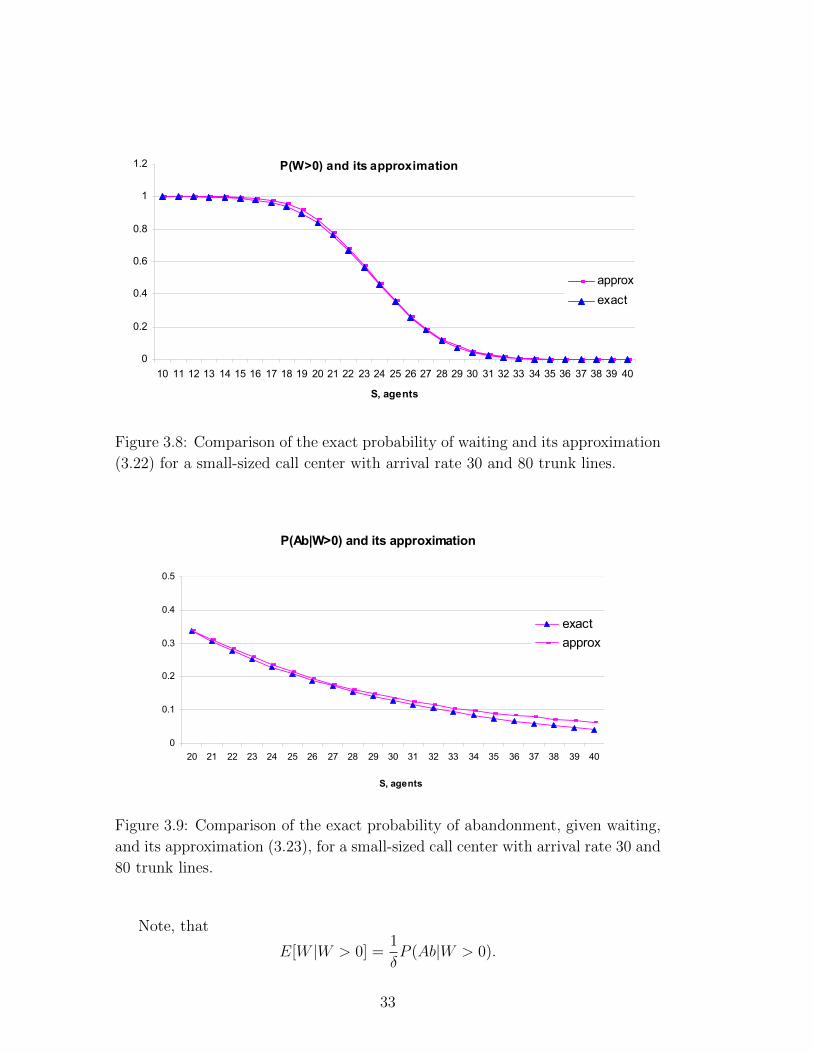
Figures 3.8 and 3.9 depict the comparison of the exact probability of wait-

ing and the conditional probability to abandon with their approximations. The

approximations are clearly close to the exact values.

32

P(W>0) and its approximation

0

0.2

0.4

0.6

0.8

1

1.2

10 11 12 13 14 15 16 17 18 19 20 21 22 23 24 25 26 27 28 29 30 31 32 33 34 35 36 37 38 39 40

S, agents

pro

ba

bil

ity

approx

exact

Figure 3.8: Comparison of the exact probability of waiting and its approximation

(3.22) for a small-sized call center with arrival rate 30 and 80 trunk lines.

P(Ab|W>0) and its approximation

0

0.1

0.2

0.3

0.4

0.5

20 21 22 23 24 25 26 27 28 29 30 31 32 33 34 35 36 37 38 39 40

S, agents

exact

approx

Figure 3.9: Comparison of the exact probability of abandonment, given waiting,

and its approximation (3.23), for a small-sized call center with arrival rate 30 and

80 trunk lines.

Note, that

E[W |W > 0] =1

δP (Ab|W > 0).

33

Thus, it is expected that the approximation of E[W ] will also be close to the

exact expectation.

P(Block) and its approximation

0

0.005

0.01

0.015

0.02

0.025

0.03

20 21 22 23 24 25 26 27 28 29 30 31 32 33 34 35 36 37 38 39 40

S, agents

approx

exact

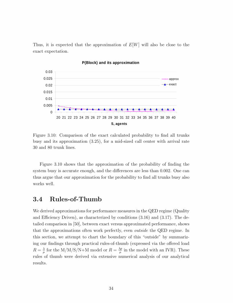
Figure 3.10: Comparison of the exact calculated probability to find all trunks

busy and its approximation (3.25), for a mid-sized call center with arrival rate

30 and 80 trunk lines.

Figure 3.10 shows that the approximation of the probability of finding the

system busy is accurate enough, and the differences are less than 0.002. One can

thus argue that our approximation for the probability to find all trunks busy also

works well.

3.4 Rules-of-Thumb

We derived approximations for performance measures in the QED regime (Quality

and Efficiency Driven), as characterized by conditions (3.16) and (3.17). The de-

tailed comparison in [50], between exact versus approximated performance, shows

that the approximations often work perfectly, even outside the QED regime. In

this section, we attempt to chart the boundary of this “outside” by summariz-

ing our findings through practical rules-of-thumb (expressed via the offered load

R = λµ

for the M/M/S/N+M model or R = λpµ

in the model with an IVR). These

rules of thumb were derived via extensive numerical analysis of our analytical

results.

34

3.4.1 Operational Regimes

As customary, one distinguishes three types of staffing regimes:

(ED) Efficiency-Driven, meaning under-staffing with respect to the offered load,

to achieve high resource utilization;

(QD) Quality-Driven, meaning over-staffing with respect to the offered load, to

achieve high service level;

(QED) Quality-and Efficiency-Driven, meaning rationalized staffing that care-

fully balances high levels of resource efficiency and service quality.

We shall use the characterization of the operational regimes, as formulated

in [61] and presented in Table 3.1, in order to specify numerical ranges for the

parameters β and η, in the M/M/S/N queue and in the model with an IVR with

and without abandonment. Specifying β corresponds to determining a staffing

level, and specifying η corresponds to determining the number of trunk lines.

Table 3.1: Rules-of-thumb for operational regimes.

ED QED QD

Staffing RRS RRS RRS

% Delayed %100 constant over time (25%-75%) %0

% Abandoned 10% - 25% 1% - 5% 0

Average Wait AST%10 AST%10 0

In Table 3.1, AST stands for Average Service Time.

3.4.2 System Parameters

The performance measures of a call center with an IVR, without abandonment,

depends on β, η, pθµ

and S; in particular, large values of pθµ

and S improve

performance (see [50] for elaboration). When one is adding abandonment to the

system, one adds a parameter δ describing customers’ patience. Large values of

δ, corresponds to highly impatient customers, decrease the probability of waiting

and the probability of blocking, but increase the probability of abandonment.

35

Small values of δ have the opposite influence. One must thus take into account

5 system’s parameters. In order to reduce the dimension of this problem, we fix

some parameters, at values that correspond to a realistic call center, based on

our experience (see [83]):

IVR service time equals, on average, 1 minute;

Agents’ service time equals, on average, 3 minutes;

Customers’ patience, on average, takes values between 3 and 10 minutes;

Fraction of customers requesting agents’ service, in addition to the IVR,

equals 30%;

Offered load equals 200 Erlangs (200 minutes per minute).

Our goal is to identify the parameter values for η (determines the number of

trunk lines) and β (determines the number of agents) that ensure QED perfor-

mance as described in Table 3.1, while simultaneously estimating the value of the

probability of blocking in each case (which does not appear in Table 3.1).

3.4.3 QED Regime in the M/M/S/N and M/M/S/N+M

Queues

From the definition of the QED regime for the M/M/S/N queue, η must be

strictly positive (η > 0), because otherwise there would be hardly any queue and,

thus, no reason to be concerned with the probability to wait or to abandon the

system. Table 3.2 provides our rules-of-thumb for call centers without IVR and

shows that when η > 3 the M/M/S/N queue behaves as the M/M/S queue

(negligible blocking).

The rules-of-thumb presented in Table 3.2 were calculated under the assump-

tion that the average customer patience equals 3 minutes (same as the average

service time). As already noted, in practice this value can become much larger,

but the performances are rather insensitive to the average patience time as long

as the average ≤ 15 minutes. For higher average values the performances are

similar to the corresponding model without abandonment.

36

Table 3.2: Rules-of-thumb for the QED regime in M/M/S/N

and M/M/S/N +M .

RRSSSN

M/M/S/N M/M/S/N+M

5.15.0 5.05.1 4.06.1

P(block) ;0,02.0

,0,S

;0,05.0

,0,S

35.1 8.05.0 6.08.0

P(block) ;0,01.0

,0,S

;0,0

0,02.0

3 0 8.05.0P(block) 0 0

3.4.4 QED Regime for a Call Center with an IVR with

and without Abandonment

As in the previous subsection, the rules-of-thumb for the system with an IVR

were calculated under the assumption that the average customer patience equals

3 minutes (same as the average service time). In the case where the system is

with an IVR, there is no restrictions for η to be non negative, but we propose

η ≥ 0 because otherwise (η < 0), the probability of blocking is higher than 0.1.

We believe that a call center cannot afford that 10% of its customers encounter

a busy signal. Going the other way, a call center can extend the number of trunk

lines to avoid the busy-line phenomenon altogether: as noted in Table 3.2, η > 3

suffices.

Table 3.3 shows that sometimes, one can reduce the number of trunk lines in

order to improve service level. For instance, starting with η > 3 and the number

of agents corresponding to β = −0.8 (ED performance), we can achieve QED

performance by reducing the number of trunk lines via η = 2; in that way, we

lose on waiting time and abandonment while the probability of blocking is still

less than 0.01. Moreover, modern technology enables a message that replaces a

busy-signal, with a suggestion to leave one’s telephone number in order to be

called back later; alternatively, a blocked call can be routed to an outsoursing al-

ternative. Thus, we are not necessarily losing these “blocked” customers. See [52]

37

and [85] for an analysis where the asymptotically optimal number of trunk lines

is determined.

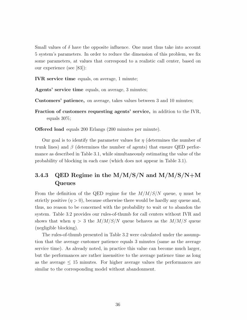
Table 3.3: Rules-of-thumb for the QED regime in a call center with an IVR with

and without abandonment.

RRS

SNIVR

without abandonment

IVRwith

abandonment10 2.02.1 06.1

P(block) ;0,04.0

,0,S08.0

21 5.07.0 4.02.1

P(block) ;0,03.0

,0,S04.0

32 7.03.0 6.08.0

P(block) ;0,02.0

,0,S01.0

3 0 8.06.0P(block) 0 0

According to Table 3.3, when η > 3, the system with an IVR behaves as one

with an infinite number of trunk lines.

3.4.5 QD and ED Regimes

For the QD and ED regimes (see Table 3.1), the number of agents can be specified

via 0.1 ≤ γ ≤ 0.25. In the case of QD, the number of agents is over-staffed; lim-

iting the number of trunk lines will cause unreasonable levels of agents’ idleness,

hence η ≥ 3 makes sense. In the case of ED, the number of agents is under-

staffed, and we are interested in reducing the system’s offered load. Therefore,

we propose to take η = 2. This choice yields a probability of blocking to be

approximately γ/2 (based on numerical experience).

38

3.4.6 Conclusions

Our rules-of-thumb demonstrate that for providing services in the QED regimes

(in both cases: with and without an IVR) one requires the number of agents to

be close to the system’s offered load; the probability of blocking in the system

with an IVR is always less than in the system without an IVR. One also observes

that the existence of the abandonment phenomena considerably helps provide the

same level of service as without abandonment, but with less agents. Moreover,

as discussed in Section 3.4.4, it is possible to maintain operational service quality

while reducing the number of agents by reducing access to the system. The cost

is an increased busy signal. Hence, such a solution must result from a tradeoff

between the probability of blocking and the probability to abandon.

3.5 Model Validation with Real Data

The approximations that have been developed can be of use in the operations

management of a call center, for example when trying to maintain a pre-determined

level of service quality. We analyze approximations of a real call center by mod-

els with and without an IVR. This evaluation is the goal of our empirical study,

which is based on analyzing real data from a large call center. (The size of our call

center, around 600-700 agents, forces one to use our approximations, as opposed

to exact calculations which are numerically prohibitive.)

3.5.1 Data Description

The data for the current analysis come from a call center of a large U.S. bank -

it will be referred to as the US Bank Call Center in the sequel. The full database

archives all the calls handled by the call center over the period of 30 months

from March 2001 until September 20032. The call center consists of four different

contact centers (nodes), which are connected using high technology switches so

that, in effect, they can be considered as a single system. The call path can be

described as follows. Customers, who make a call to the company, are first of

all served in the IVR. After that, they either complete the call or choose to be

served by an agent. In the latter case, customers typically listen to a message,

after which they are routed, as will be now described, to one of the four call

centers and join the agents’ queue.

2The data is available at http://seeserver.iem.technion.ac.il/see-terminal/.

39

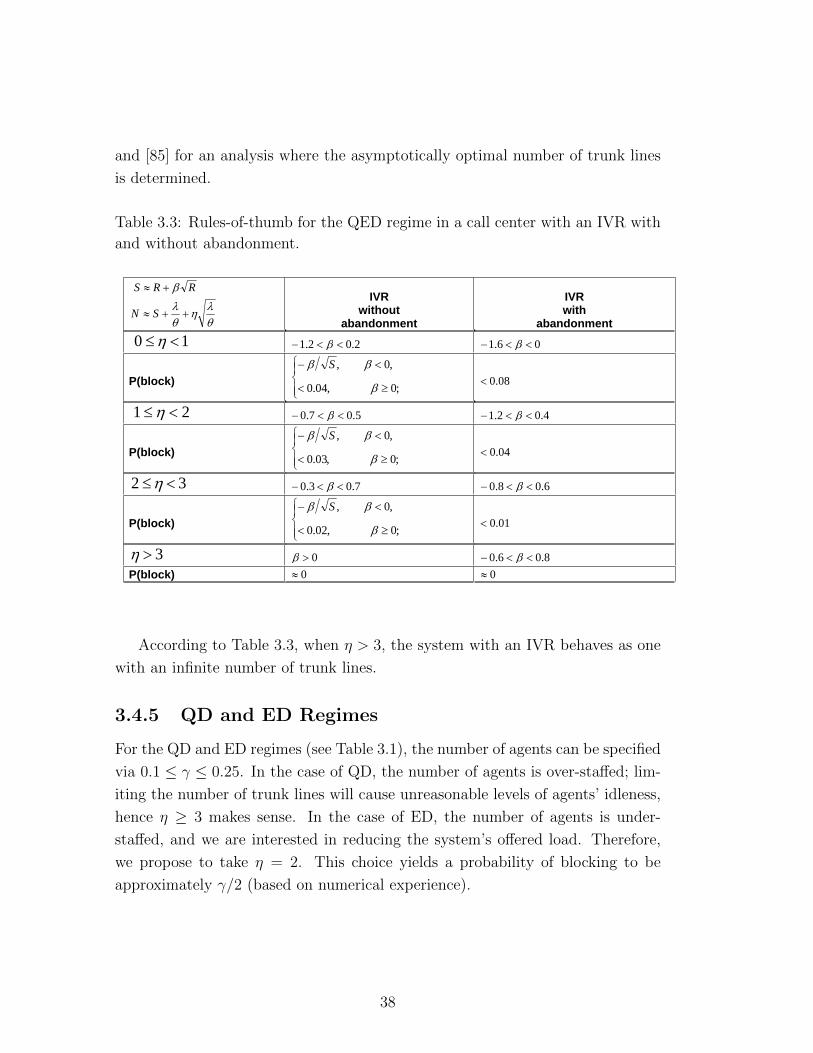
A schematic model of our US Bank Call Center is presented in Figure 3.11

Schematic Diagram of a Call

Back to IVR

Busy signal

Queue Service

No waiting

End of call

Abandonment

IVR/VRU

Figure 3.11: Schematic diagram of the call of a “Retail” customer in our US Bank

call center.

The choice of routing is usually performed according to the customer’s class,

which is determined in the IVR. If all the agents are busy, the customer waits

in the queue; otherwise, s/he is served immediately. Customers may abandon

the queue before receiving service. If they wait in the queue of a specific node

(one of the four connected) for more than 10 seconds, the call is transferred to a

common queue - so-called “inter queue”. This means that now the customer will

be answered by an agent with an appropriate skill from any of the four nodes.

After service by an agent, customers may either leave the system or return to the

IVR, from which point a new sub-call ensues. The call center is relatively large

with about 600 agents per shift, and is staffed 7 days a week, 24 hours a day.

3.5.2 Fitting the Theoretical Model to a Real System

Figure 3.11 describes the flow of a call through our call center. It differs somewhat

from the models described in Section 3.1. The main difference is that it is possible

for the customer to return to the IVR after being served by an agent. This is less

common for so-called Retail customers who, almost as a rule, complete the call

either after receiving service in the IVR or immediately after being served by an

agent. We therefore neglect those few calls that return to the IVR and compare

the models from Section 3.1 with the real system.

40

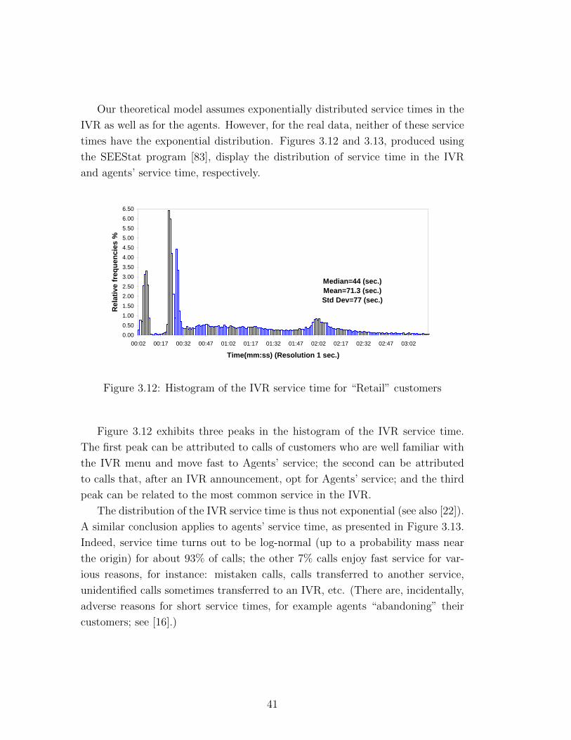
Our theoretical model assumes exponentially distributed service times in the

IVR as well as for the agents. However, for the real data, neither of these service

times have the exponential distribution. Figures 3.12 and 3.13, produced using

the SEEStat program [83], display the distribution of service time in the IVR

and agents’ service time, respectively.

Median=44 (sec.)Mean=71.3 (sec.)Std Dev=77 (sec.)

0.000.501.001.502.002.503.003.504.004.505.005.506.006.50

00:02 00:17 00:32 00:47 01:02 01:17 01:32 01:47 02:02 02:17 02:32 02:47 03:02

Time(mm:ss) (Resolution 1 sec.)

Rel

ativ

e fr

eque

ncie

s %

Figure 3.12: Histogram of the IVR service time for “Retail” customers

Figure 3.12 exhibits three peaks in the histogram of the IVR service time.

The first peak can be attributed to calls of customers who are well familiar with

the IVR menu and move fast to Agents’ service; the second can be attributed

to calls that, after an IVR announcement, opt for Agents’ service; and the third

peak can be related to the most common service in the IVR.

The distribution of the IVR service time is thus not exponential (see also [22]).

A similar conclusion applies to agents’ service time, as presented in Figure 3.13.

Indeed, service time turns out to be log-normal (up to a probability mass near

the origin) for about 93% of calls; the other 7% calls enjoy fast service for var-

ious reasons, for instance: mistaken calls, calls transferred to another service,

unidentified calls sometimes transferred to an IVR, etc. (There are, incidentally,

adverse reasons for short service times, for example agents “abandoning” their

customers; see [16].)

41

Median=163 (sec.)Mean=242.9 (sec.)Std Dev=271 (sec.)

0.00

0.25

0.50

0.75

1.00

1.25

1.50

1.75

2.00

2.25

2.50

00:00 01:00 02:00 03:00 04:00 05:00 06:00 07:00 08:00 09:00 10:00 11:00 12:00

Time(mm:ss) (Resolution 5 sec.)

Rel

ativ

e fr

eque

ncie

s %

Figure 3.13: Histogram of Agents’ service time for “Retail” customers

Similarly to non-Markovian (non-exponentially distributed) service times, the

assumption that the arrival process is a homogeneous Poisson is also over sim-

plistic. A more natural model for arrivals is an inhomogeneous Poisson process,

as shown by Brown et al. [16], in fact modified to account for overdispersion

(see [60]). However, and as done commonly in practice, if one divides the day

into half-hour intervals, we get that within each interval the arrival rate is more or

less constant and thus, within such intervals, we treat the arrivals as conforming

to a Poisson process.

Even though most of the model assumptions do not prevail in practice, notably

Markovian assumptions, experience has shown that Markovian models still pro-

vide very useful descriptions of non-Markovian systems (for example, the Erlang-

A model in [16]). We thus proceed to validate our models against the US Bank

Call Center, and our results will indeed demonstrate that this is a worthwhile

insightful undertaking.

3.5.3 Comparison of Real and Approximated Performance

Measures

For our calculations, the following variables must be estimated:

• λ - average arrival rate;

• θ - average rate of service in the IVR;

• µ - average rate of service by an agent;

42

• p - probability that a customer requests service by an agent;

• δ - average rate of customers’ (im)patience;

• S - number of agents;

• N - number of trunk lines.

We consider the Retail service time distribution for April 12, 2001, which

is an example of an ordinary week day. The analysis was carried out for data

from calls arriving between 07:00 and 18:00. This choice was made since we

were interested in investigating the system during periods of a meaningful load.

We consider 30 minutes time intervals, since approximately 8000 calls are made

during such intervals, we may expect that approximations for large λ would be

appropriate. Moreover, system parameters seem to be reasonably constant over

these intervals.

The following estimators will be calculated for each 30-minute interval as

follows:

λ = number of calls arriving to the system (30 min)

θ =30× 60

average IVR service time (sec)

µ =30× 60

average agent service time (sec)

p =number of calls seeking agent service

λ

It should be noted that, strictly speaking, we are not calculating the actual

average arrival rate because we see only the calls which did not find all trunks

busy; practically, the fraction of customers that found all trunks busy is very

small and hence the difference between the real and approximated (calculated

our way) arrival rate is not significant.

43

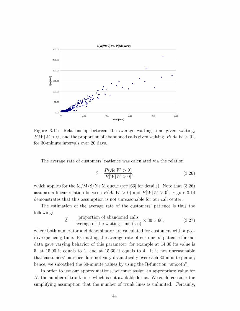
E[W|W>0] vs. P(Ab|W>0)

0.00

50.00

100.00

150.00

200.00

250.00

300.00

0 0.05 0.1 0.15 0.2 0.25

P(Ab|W>0)

E[W

|W>0

]

Figure 3.14: Relationship between the average waiting time given waiting,

E[W |W > 0], and the proportion of abandoned calls given waiting, P (Ab|W > 0),

for 30-minute intervals over 20 days.

The average rate of customers’ patience was calculated via the relation

δ =P (Ab|W > 0)

E[W |W > 0], (3.26)

which applies for the M/M/S/N+M queue (see [63] for details). Note that (3.26)

assumes a linear relation between P (Ab|W > 0) and E[W |W > 0]. Figure 3.14

demonstrates that this assumption is not unreasonable for our call center.

The estimation of the average rate of the customers’ patience is thus the

following:

δ =proportion of abandoned calls

average of the waiting time (sec)× 30× 60, (3.27)

where both numerator and denominator are calculated for customers with a pos-

itive queueing time. Estimating the average rate of customers’ patience for our

data gave varying behavior of this parameter, for example at 14:30 its value is

5, at 15:00 it equals to 1, and at 15:30 it equals to 4. It is not unreasonable

that customers’ patience does not vary dramatically over each 30-minute period;

hence, we smoothed the 30-minute values by using the R-function “smooth”.

In order to use our approximations, we must assign an appropriate value for

N , the number of trunk lines which is not available for us. We could consider the

simplifying assumption that the number of trunk lines is unlimited. Certainly,

44

call centers are typically designed so that the probability of finding the system

busy is very small, but nevertheless it is positive. One approach is to assume that,

because the system is heavily loaded, there must be calls that are blocked since

there are no explosions. In such circumstances, a naive way of underestimating

N for each 30-minute period is as follows3:

N =total duration of all calls that arrived to the system

30 · 60.

The calculation of the number of agents is also problematic, because the

agents who serve retail customers may also serve other types of customers, and

vice versa: if all Retail agents are busy, the other agent types may serve Retail

customers (see [57] for details). Thus, it is practically impossible to determine

their exact number and that is why we use an averaged value, as follows:

S =total agent service time

30 · 60

Figure 3.15 compares the approximated theoretical probabilities of waiting based

on the above estimators with the observed proportion of waiting customers, as

estimated directly from the data. The dark blue curve (with diamonds) shows

the proportion of customers that are waiting in the queue before agent service.

This proportion is calculated for each half-hour period. The lilac curve (squares)

shows the approximation based on the model with an IVR, calculated for each

half-hour period. The blue curve (triangles) corresponds to the approximation

based on the M/M/S/N+M queue model. We conclude that our approxima-

tions are performing reasonably well, especially based on the model with IVR.

The approximate values for this model, in many intervals, are very close to the

exact proportion. In some intervals the difference is about 10%, which can be

attributed to the non-perfect correspondence between the model and the real call

center. An additional explanation is in the estimation of the parameters, such

as N and S, which we estimate in a very crude way. The approximation from

the M/M/S/N+M queue works less well and sometimes it does not even reflect

the trends seen for the real values: namely, where the real values decrease the

approximation increases and vice versa. The reasons for these discrepancies can

be the same as previously stated, as well as due to ignoring the IVR influence.

3Note that for the system with an IVR, N depends on the total duration of calls in the IVR,

agents’ queue and service. For the system without IVR, it depends only on the total duration

of calls in the agents’ queue and service.

45

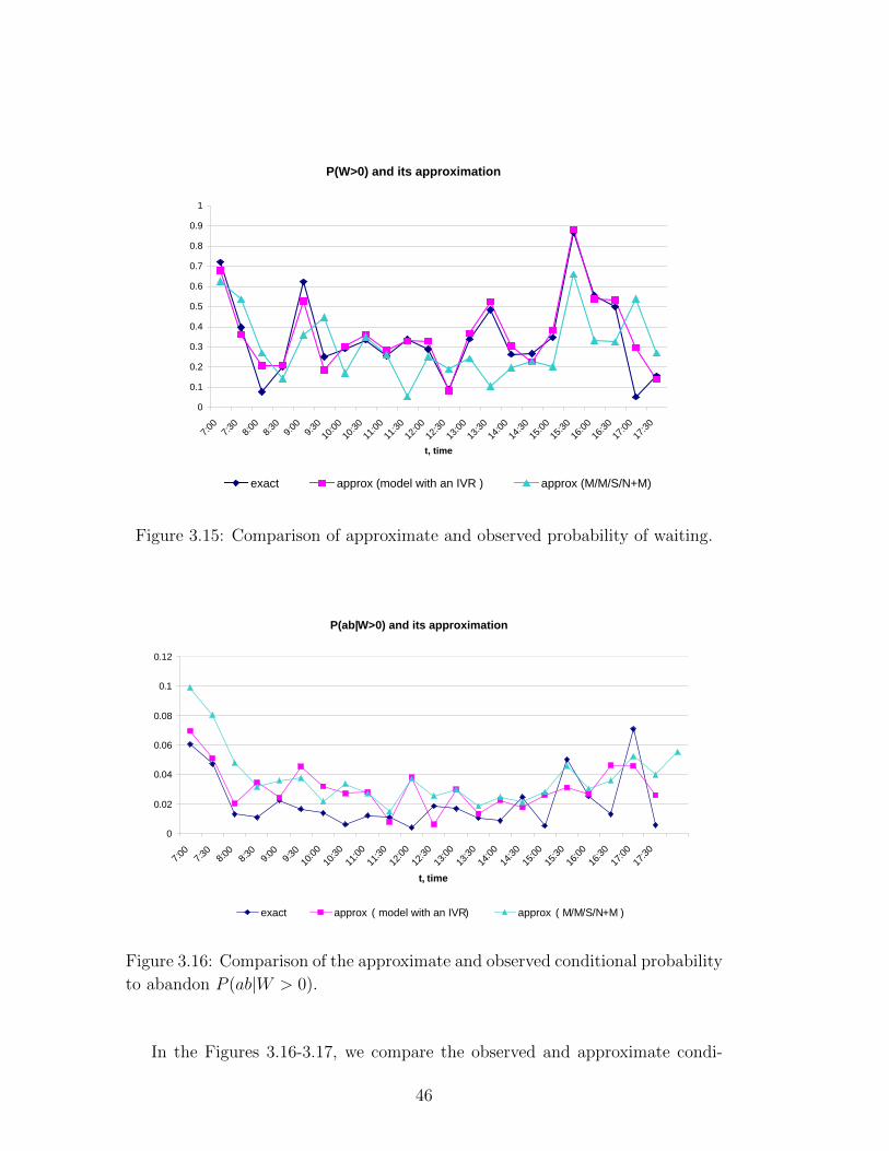
P(W>0) and its approximation

0

0.1

0.2

0.3

0.4

0.5

0.6

0.7

0.8

0.9

1

7:00

7:30

8:00

8:30

9:00

9:30

10:00

10:30

11:00

11:30

12:00

12:30

13:00

13:30

14:00

14:30

15:00

15:30

16:00

16:30

17:00

17:30

t, time

exact approx (model with an IVR ) approx (M/M/S/N+M)

Figure 3.15: Comparison of approximate and observed probability of waiting.

P(ab|W>0) and its approximation

0

0.02

0.04

0.06

0.08

0.1

0.12

7:00

7:30

8:00

8:30

9:00

9:30

10:00

10:30

11:00

11:30

12:00

12:30

13:00

13:30

14:00

14:30

15:00

15:30

16:00

16:30

17:00

17:30

t, time

exact approx ( model with an IVR ) approx ( M/M/S/N+M )

Figure 3.16: Comparison of the approximate and observed conditional probability

to abandon P (ab|W > 0).

In the Figures 3.16-3.17, we compare the observed and approximate condi-

46

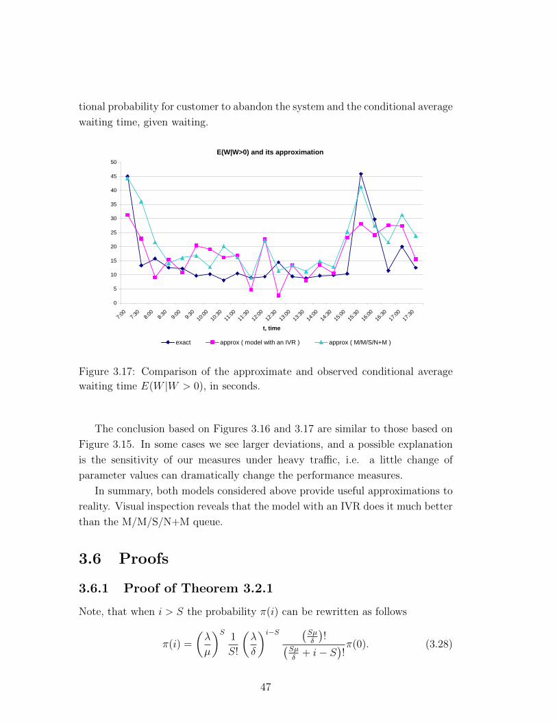
tional probability for customer to abandon the system and the conditional average

waiting time, given waiting.

E(W|W>0) and its approximation

0

5

10

15

20

25

30

35

40

45

50

7:00

7:30

8:00

8:30

9:00

9:30

10:00

10:30

11:00

11:30

12:00

12:30

13:00

13:30

14:00

14:30

15:00

15:30

16:00

16:30

17:00

17:30

t, time

exact approx ( model with an IVR ) approx ( M/M/S/N+M )

Figure 3.17: Comparison of the approximate and observed conditional average

waiting time E(W |W > 0), in seconds.

The conclusion based on Figures 3.16 and 3.17 are similar to those based on

Figure 3.15. In some cases we see larger deviations, and a possible explanation

is the sensitivity of our measures under heavy traffic, i.e. a little change of

parameter values can dramatically change the performance measures.

In summary, both models considered above provide useful approximations to

reality. Visual inspection reveals that the model with an IVR does it much better

than the M/M/S/N+M queue.

3.6 Proofs

3.6.1 Proof of Theorem 3.2.1

Note, that when i > S the probability π(i) can be rewritten as follows

π(i) =

(λ

µ

)S1

S!

(λ

δ

)i−S (Sµδ

)!(

Sµδ

+ i− S)!π(0). (3.28)

47

Let us find the probability to wait. By using PASTA

P (W > 0) =N−1∑i=S

π(i) =

N−1∑i=S

(λ

µ

)S1

S!

(λ

δ

)i−S (Sµδ

)!(

Sµδ

+ i− S)!

S−1∑i=0

1

i!

(λ

µ

)i+

N∑i=S

(λ

µ

)S1

S!

(λ

δ

)i−S (Sµδ

)!(

Sµδ

+ i− S)!

=B1(λ)

A(λ) +B2(λ).

Let us define ξ1(λ) = B1(λ)e−λµ , ξ2(λ) = B2(λ)e−

λµ and γ(λ) = A(λ)e−

λµ . Then,

P (W > 0) =ξ1(λ)

γ(λ) + ξ2(λ).

Let us suppose that Sµ/δ is integer. This assumption is relaxed later.

ξ1(λ) =

1

S!

(λ

µ

)Se−

λµ

e−λδ(

Sµδ

)!

(λ

δ

)Sµδ

N−S−1∑k=0

(λδ

)Sµδ

+ke−

λµ(

Sµδ

+ k)!

=P (Y = S)

P (X =Sµ

δ)P (X <

Sµ

δ+N − S),

where Xd= Pois(λ

δ) and Y

d= Pois(λ

µ). Using the Central Limit theorem, one

can write that

P (X =Sµ

δ) ∼ P

Sµ

δ− λ

δ√λ

δ

− 1√λ

δ

< Y ≤

Sµ

δ− λ

δ√λ

δ

∼ Φ

(β

õ

δ

)− Φ

(β

õ

δ−√δ

λ

)∼√δ

λϕ

(β

õ

δ

),

P (Y = S) ∼ P

S − λ

µ√λ

µ

−

√λ

µ< Y ≤

S − λ

µ√λ

µ

∼ Φ (β)− Φ

(β −

õ

λ

)∼√µ

λϕ(β)

P

(X ≤ Sµ

δ+N − S

)∼ Φ

((Sµ

δ+ η

√λ

µ− λ

δ

)/

√λ

δ

)∼ Φ

(η

√δ

µ+ β

õ

δ

).

48

Thus,

limλ→∞

ξ1(λ) =

õ

δ

ϕ(β)

ϕ(β√

µδ

)Φ

(η

√δ

µ+ β

õ

δ

).

Let us note that

limλ→∞

ξ1(λ) = limλ→∞

ξ2(λ),

and

limλ→∞

γ(λ) = limλ→∞

S−1∑i=0

1

i!

(λ

µ

)ie−

λµ = lim

λ→∞Φ

S − 1− λµ√

λµ

= Φ (β) .

So,

limλ→∞

P (W > 0) =

1 +Φ (β)ϕ

(β√

µδ

)√µδϕ(β)Φ

(η√

δµ

+ β√

µδ

)−1

. (3.29)

Now, consider an approximation for P (block). It can also be written as follows:

P (block) =τ(λ)

γ(λ) + ξ2(λ),

where

τ(λ) =1

S!

(λ

µ

)S (λ

δ

)N−S (Sµδ

)!(

Sµδ

+N − S)!

=P (Y = S)

P(X = Sµ

δ

)P (X =Sµ

δ+N − S

).

Note, that

P

(X =

Sµ

δ+N − S

)= P

Sµδ

+N − S − λδ√

λδ

− 1√λδ

< X ≤Sµδ

+N − S − λδ√

λδ

=

1√λδ

ϕ

(η

√δ

µ+ β

õ

δ

).

Then,

limλ→∞

√Sτ(λ) = lim

λ→∞

1√λµ

ϕ (β)

√λδ

ϕ(β√

µδ

)√λ

µϕ

(η

√δ

µ+ β

õ

δ

)

=ϕ (β)ϕ

(η√

δµ

+ β√

µδ

)ϕ(β√

µδ

) .

49

Therefore,

limλ→∞

√SP (block) =

ϕ (β)ϕ(η√

δµ

+ β√

µδ

)/ϕ(β√

µδ

)Φ (β) +

√µδ

ϕ(β)

ϕ(β√

µδ )

Φ(η√

δµ

+ β√

µδ

) . (3.30)

The conditional probability of abandonment can be written as follows

P (Ab|W > 0) = 1−

(Sµ/δ

)ζ1(λ)

ξ2(λ),

where ξ2(λ) as previously, and

ζ1(λ) = ξ2(λ)− P(X =

Sµ

δ

)≈ δ

µ

ϕ(β)

ϕ(β√µ/δ)

[Φ

(η

√δ

µ+ β

õ

δ

)− Φ

(β

õ

δ

)− ϕ

(β

õ

δ

)√δ

λ

].

Thus, we get

limλ→∞

√SP (Ab|W > 0) =

√µδϕ(β√

µδ

)− β

[Φ(η√

δµ

+ β√

µδ

)− Φ

(β√

µδ

)]Φ(η√

δµ

+ β√

µδ

)− Φ

(β√

µδ

) .

3.6.2 Proof of Theorem 3.2.2

Approximation for P (W > 0).

According to (3.7), (3.8), (3.11) and (3.14), the operational characteristic

P (W > 0) can be represented as follows:

P (W > 0) =

(1 +

A(λ)

B(λ)

)−1

, (3.31)

where

A(λ) = e−λ( 1θ

+ pµ

)∑

i+j≤N−1, j≤S−1

1

i!

(λ

θ

)i1

j!

(pλ

µ

)j(3.32)

and

B (λ) = e−λ( 1θ

+ pµ

)N−S−1∑i=0

N−i−1∑j=S

1

i!

(λ

θ

)i1

S!

(pλ

µ

)S (pλ

δ

)j−S(Sµ/δ)!

(Sµ/δ + j − S)!.

(3.33)

50

We now derive QED approximations for A(λ) and B(λ), as λ, S and N tend to

∞, according to (3.17).

Approximation for A(λ):

Consider a partition {Sj}lj=0 of the interval [0, S]:

Sj = S − j∆, j = 0, 1, ..., l; Sl+1 = 0, (3.34)

where ∆ = [ε√

λpµ

], ε is an arbitrary non negative real and l is a positive integer.

If λ and S tend to infinity and satisfy the assumption (3.17)(ii), then l is less

than S/∆ for λ large enough and all the Sj belong to [0, S], j = 0, 1, ..., l.

We emphasize that the length ∆ of every interval [Sj−1, Sj] depends on λ. The

variable A(λ) is given by formula (3.32), where the summation is taken over the

trapezoid: {(i, j) | i ∈ [0, N − j] and j ∈ [0, S − 1]}, presented in Figure 3.18.

Consider the lower estimate for A(λ), given by the following sum:

A(λ) ≥ A1(λ) =l∑

k=0

Sk−1∑j=Sk+1

1

j!

(λp

µ

)je−

λpµ

N−Sk∑i=0

1

i!

(λ

θ

)ie−

λθ

=l∑

k=0

P (Sk+1 ≤ Zλ < Sk)P (Xλ ≤ N − Sk),

(3.35)

where

Zλd=Pois

(λp

µ

)and Xλ

d=Pois

(λ

θ

). (3.36)

i

N-1

… …

N-10 lSkS1kS S j

Figure 3.18: Area of the summation of the variable A1(λ).

51

Applying the Central Limit Theorem and making use of the relations

limλ→∞

Sk − λpµ√

λpµ

= β−kε, limλ→∞

N − Sk − λθ√

λθ

= η+kε

√pθ

µ, k = 0, 1, ..., l, (3.37)

one obtains

limλ→∞

P (Sk+1 ≤ Zλ < Sk) = Φ(β−kε)−Φ(β−(k+1)ε), k = 0, 1, ...l−1, (3.38)

limλ→∞

P (0 ≤ Zλ < Sl) = Φ(β − lε), (3.39)

limλ→∞

P (Xλ < N − Sk) = Φ(η + kε

√pθ

µ), k = 0, 1, ...l. (3.40)

It follows from (3.35) and (3.38), (3.39), (3.40) that

lim infλ→∞

A(λ) ≥l−1∑k=0

Φ(η + kε√pθ/µ)[Φ(β − kε)− Φ(β − (k + 1)ε)]

+ Φ(β − lε)Φ(η + lε√pθ/µ).

(3.41)

It is easy to see that (3.41) is the lower Riemann-Stieltjes sum for the integral

−∞∫

0

Φ

(η + s

√pθ

µ

)dΦ(β − s) =

β∫−∞

Φ

(η + (β − t)

√pθ

µ

)ϕ(t)dt, (3.42)

corresponding to the partition {β − kε}lk=0 of the semi-axis (−∞, β).

Similarly, we obtain the upper Riemann-Stieltjes sum for the integral (3.42):

lim supλ→∞

A(λ) ≤l−1∑k=0

Φ

(η + (k + 1)ε

√pθ

µ

)[Φ(β−kε)−Φ(β−(k+1)ε)]+Φ(β−lε).

(3.43)

When ε→ 0, the estimates (3.41), (3.43) lead to the following equality

limλ→∞

A(λ) =

β∫−∞

Φ

(η + (β − t)

√pθ

µ

)ϕ(t)dt. (3.44)

Approximation for B(λ):

B (λ) =

e−pλµ

S!

(pλ

µ

)Se−

pλδ(

Sµδ

)!

(pλ

δ

)Sµδ

N−S−1∑i=0

1

i!

(λ

θ

)i N−S−i−1∑k=0

(pλδ

)Sµ/δ+ke−

pλδ

(Sµ/δ + k)!

=P (Yλ = S)

P(Xλ = Sµ

δ

) N−S−1∑i=0

P (Zλ = i)P

(Sµ

δ≤ Xλ ≤ N − S − i− 1 +

Sµ

δ

),

52

where

Xλd=Pois

(pλ

δ

), Yλ

d=Pois

(pλ

µ

)and Zλ

d=Pois

(λ

θ

). (3.45)

Analogously to calculations in approximation for A(λ), with the use of the Central

Limit Theorem we get

limλ→∞

N−S−1∑i=0

P (Zλ = i)P

(Sµ

δ≤ Xλ ≤ N − S − i− 1 +

Sµ

δ

)

= limλ→∞

N−S−1∑i=0

P (Zλ = i)[Φ

(Sµδ

+N − S − i− 1− pλδ√

pλ/δ

)− Φ

Sµδ− pλ

δ√pλδ

]

= limλ→∞

N−S−1∑i=0

[P (Zλ ≤ i)− P (Zλ ≤ i− 1)

]Φ

((N − S − i)

√δ

pλ+ β

õ

δ

)

− limλ→∞

Φ

(β

õ

δ

)N−S−1∑i=0

P (Zλ = i)

= limλ→∞

N−S−1∑i=0

[Φ

(i− λ/θ√

λ/θ

)− Φ

(i− λ/θ − 1√

λ/θ

)]Φ

((N − S − i)

√δ

pλ+ β

õ

δ

)

− limλ→∞

Φ

(β

õ

δ

)P (Zλ < N − S) .

From condition (i) of (3.17) one can see that

limλ→∞

Φ

(β

õ

δ

)P (Zλ < N − S) = Φ

(β

õ

δ

)Φ (η) . (3.46)

For the first term we get

limλ→∞

N−S−1∑l=0

[Φ

(N − S − l − λ/θ√

λ/θ

)− Φ

(N − S − λ/θ − (l + 1)√

λ/θ

)]Φ

(l

√δ

pλ+ β

õ

δ

)

= limλ→∞−

N−S−1∑l=0

∆Φ

(η − l√

λ

√θ

)Φ

(l√λ

√δ

p+ β

õ

δ

)

= −∫ ∞

0

Φ

(t

√δ

p+ β

õ

δ

)dΦ(η − t

√θ)

=

∫ η

−∞Φ

((η − s)

√δ

pθ+ β

õ

δ

)dΦ (s) .

(3.47)

53

It is easy to see that

P (Y = S) ∼ P

S − pλ

µ√pλ

µ

− 1√pλ

µ

< Y ≤S − pλ

µ√pλ

µ

∼ 1√

pλ

µ

ϕ(β)

(3.48)

and

P

(X =

Sµ

δ

)∼ P

Sµ

δ− pλ

δ√pλ

δ

− 1√pλ

δ

< Y ≤

Sµ

δ− pλ

δ√pλ

δ

∼ 1√

pλ

δ

ϕ

(β

õ

δ

) (3.49)

Combining (3.46)-(3.49) we get

limλ→∞

B(λ) =

õ

δ

ϕ(β)

ϕ(β√

µδ

)[ ∫ η

−∞Φ

((η − t)

√δ

pθ+ β

õ

δ

)dΦ (t)−Φ

(β

õ

δ

)Φ (η)

].

Approximation for P (Ab|W > 0).

Note that the probability of abandonment, given waiting can be presented as

follows

P (Ab|W > 0) = 1− Sµ

pλ

C(λ)

D(λ),

where

C(λ) = e−λ(1θ

+ pδ )

N∑j=S+1

N−j∑i=0

1

i!

(λ

θ

)i(pλ

δ

)j−S+Sµ/δ1

(Sµ/δ + j − S)!

= e−λ(1θ

+ pδ )

N−S∑k=1

N−S−k−1∑i=0

1

i!

(λ

θ

)i(pλ

δ

)k+Sµ/δ1

(Sµ/δ + k)!

=N−S∑k=1

(pλ

δ

)k+Sµ/δe−

pλδ

(Sµ/δ + k)!

N−S−k−1∑i=0

e−λθ

i!

(λ

θ

)i=

N−S∑k=1

P

(X =

Sµ

δ+ k

)P (Y ≤ N − S − k)

54

and

D(λ) =N∑

j=S+1

N−j∑i=0

1

i!

(λ

θ

)i(pλ

δ

)j−S−1+Sµ/δe−λ(

1θ

+ pδ )

(Sµ/δ + j − S − 1)!

=N−S∑k=1

N−S−k−1∑i=0

1

i!

(λ

θ

)i(pλ

δ

)k+Sµ/δe−λ(

1θ

+ pδ )

(Sµ/δ + k)!+

e−pλδ

(Sµ/δ)!

N−S∑i=0

e−λθ

i!

(λ

θ

)i=

N−S−1∑k=1

P

(X =

Sµ

δ+ k

)P (Y ≤ N − S − k − 1)

+ P

(X =

Sµ

δ

)P (Y ≤ N − S − 1) .

In both expressions for C(λ) and D(λ) we assume that Xd= Pois(pλ

δ) and Y

d=

Pois(λθ). Using conditions (3.1), the Central Limit Theorem, we obtain

N − S − k − λ/θ√λ/θ

∼ η − k√λ

√θ,

Sµ/δ + k − pλ/δ√pλ/δ

∼ β

õ

δ+

k√λ

√δ

p,

P (Y ≤ N − S − k) ∼ Φ

(η − k

√θ

λ

)and

P

(X =

Sµ

δ+ k

)∼ Φ

(β

õ

δ− k

√θ

pλ

)− Φ

(β

õ

δ− (k − 1)

√θ

pλ

).

Then,

N−S∑k=1

P

(X =

Sµ

δ+ k

)P (Y ≤ N − S − k)

∼N−S−1∑k=1

Φ(η − kε

√θ) [

Φ

(β

õ

δ+ kε

√δ

p

)− Φ

(β

õ

δ+ (k − 1)ε

√δ

p

)]∼∫ ∞

0

Φ(η − t

√θ)dΦ

(β

õ

δ+ t

√δ

p

)

∼∫ ∞

0

Φ

(η − s

√pθ

δ

)dΦ

(β

õ

δ+ s

)

∼ −β∫ ∞β√

µδ

Φ

(η − (t− β

õ

δ)

√pθ

δ

)dΦ (t) .

55

In addition, using

P

(X =

Sµ

δ

)∼ 1√

pλ/θϕ

(β

õ

δ

)and

Sµ

pλ∼(

1− β√S

)−1

we get an approximation for the probability of abandonment given waiting, which

is presented in Theorem 3.2.2.

3.7 Summary and Future Work

In this chapter we introduced appropriate models for the design of a typical call

center. These models enable one to quantify the operational performance of a

call center and to define staffing given a particular service level. Our proposed

approximations of performance measures demonstrate a high level of accuracy

and can be easily implemented for moderate-to-large call centers, where exact

calculations are unsuccessful due to numerical instability.

The evaluation of approximations for the real call center data shows that

even though most of the model assumptions do not prevail in practice, notably

our Markovian assumptions, experience has shown that Markovian models still

provide very useful descriptions of non-Markovian systems. The robustness of

the M/M/S+M queue with respect to its characteristics were considered by Zel-

tyn [89] in his Ph.D. thesis. In particular, Zeltyn found that the relationships

between the probability to abandon the system and the expectation of waiting

time in M/M/S+G is the following: P (Ab)/E[W ] = f(0), where f(0) is a value of

customer patience density function at time 0. In the case of the M/M/S+M queue

f(0) = θ and this is exactly the relationship that we used in our calculations.

In the future, we should like to improve our call center model by adding

retrials, where by retrials we understand the customer’s repeated attempts to

receive the desired service after the initial failure to obtain it. This will make our

model more realistic. Such an analysis can be extremely important, because the

negative impact of customer retrials is the increase in system load and, hence, the

deterioration of system performance and the corresponding increase in expenses.

In whole, we should note that analysis of abandonment and retrial processes is

very important for the management of call centers, because these phenomenons

describe customers’ satisfaction and the successfulness of the provided services.

One more realistic problem is the issue of different service requirements for

different classes of customers. Such problems are called Skills-Based Routing and

56

they have already been investigated by Armony et al. [9] and Atar et al. [10].

It would be interesting to investigate the models of Skills-Based Routing for call

centers with an IVR.

57

Chapter 4

CUSTOMER PATIENCE

ANALYSIS

In many cases when a customer rings a call center s/he needs to wait in a queue

before receiving someone to serve him/her. We can assume that each customer

has a finite amount of time that s/he is ready to spend in the queue. If this time

comes to an end and the customer has not been answered, s/he hangs up. In this

chapter we provide an analysis of customer patience, which we define as his/her

willingness to endure waiting in a queue before receiving service. The assessment

of customer patience is a complicated issue because, in most cases, customers

receive the required service before they lose their patience. The data with non-

zero service time are called censored data, and these data require analysis of a

special kind, known as survival analysis.

4.1 Description of the Data

We start with a short description of the data, which gives us the motivation for

a model of customer patience considered in this chapter. The data we analyze

are provided by a call center belonging to a financial company. From its call

center, we have the data covering a period of almost three years, i.e. October

2006 - June 2009. The call center works twenty-four hours a day on weekdays

(Sundays - Thursdays). It closes at 13:00 on Fridays, and reopens at about

17:00 on Saturdays. A customer making a call receives the service through an

IVR or directly from an agent. After receiving the service provided by an IVR,

the customer leaves the system or requests service from an agent. The customer

requesting service from an agent is redirected to a pool of agents. If all the agents

58

are busy, the customer waits in a queue. Otherwise, s/he is served immediately.

The customer is not always ready to wait in a queue, and he/she can choose to

abandon the system at any point during the waiting period. After being served

by an agent, the customer either finishes the call or proceeds to another service

(another agent), and so on.

The call center in question provides various services. Some of them are similar

in design and in their average service time. Others, on the contrary, are concep-

tually different. In our analysis, we will combine services of a similar kind into

one group.

The data do not contain any personal information about customers, such as

their age, social status, family status or education. Therefore, our analysis will

be carried out only on the basis of the technical characteristics of the call. For

each call, we have the following data:

• the individual number of a customer initiating this call (customer identification

number),

• the type of customer (a type of priority given to the customer by the system),

• the beginning of each “call segment”,

• the duration of each stage of a “call segment” (the service time, the waiting

time in a queue or the post-call agent service time),

• the type of the service (an IVR service or an agent service that can include

about fifteen different subtypes),

• the classification of call termination (after a received service, after call aban-

donment or due to a system error).

We identify each customer by his/her identification number which is retained

in the field named “customer id” and provides a unique number. However, some-

times “customer id” can be unidentified or invalid. To avoid fake identification

numbers we consider the data only for customers with fewer than thirty calls a

month.

For the analysis of customer behavior, we use a notion of a “series” which

we define as a sequence of consecutive calls from one customer happening in

chronological order. If the time that elapses between two consecutive calls is less

than three days we assume that these calls belong to the same “series”, otherwise,

59

we assume that these calls belong to two different series. This separation is based

on the assumption that a customer who has not called for a long time loses his/her

experience with the system.

4.2 Model Selection

We propose a statistical model that can be used in the analysis of customer

patience, under the setting of survival analysis. In our context, an event is the

customer abandonment of the system before being served. For a customer who

receives service, his/her patience time is not fully observed and is considered as

censored. Hence, for each customer, at each call, the observed time is the time

until abandonment (patience time) or time until being served, whichever comes

first. The data to be used in the current research consists of customer calls with

possibly multiple calls for a customer. We believe that the observed times of

the same customer are not independent. Therefore, the Cox proportional hazard

model [21] cannot be used directly, and we use a well-known and popular approach

that deals with clustered data - the frailty model approach (Hougaard [42],

Duchateau and Janssen [25], Aalen [1]).

The shared frailty model takes into account observed and unobserved personal

factors of a customer. However, it is also reasonable to assume that the customer

calls history influences his/her current waiting behavior. One of the models

dedicated to such an analysis is the well studied recurrent events model and its

extension to the shared frailty model [42]. However, these types of models cannot

be applied directly in our case, since for typical recurrent event data, a subject

can be censored at most once, and no information is available after this censoring

time. In our data, a customer can call more than one time, and the response

time in each call can be censored. So, we consider an extended shared frailty

model assuming that customer patience changes with the number of the call,

consistently for all customers.

4.3 Notation and Formulation of the Model

We consider n customers, where customer i has mi calls in a series (mi ≤ m for

all i = 1, ..., n). Later, we consider a real data set analysis with a maximum of

5 calls for each customer (m = 5). We assume that the waiting behavior of each

customer does not depend on the waiting behavior of other customers. Let T 0ij

60

and Cij denote the failure and censoring times, respectively, for call j of individual

i (i = 1, ..., n, j = 1, ...,mi). The observed follow-up time is Tij = min(T 0ij, Cij

),

and the failure indicator is δij = I(T 0ij ≤ Cij

). For call j of customer i we observe

a vector of covariates Zij and assume that the waiting behavior of customer i

(i = 1, ..., n) is influenced by some additional unobservable subject-dependent

properties which are represented by the frailty variate wi.

The conditional hazard function of the patience of customer i at the j-th call

given the frailty wi, is assumed to take the form

λij(t) = λ0j(t)wieβTZij i = 1, ..., n j = 1, ...,mi, (4.1)

where λ0j(t) is an unspecified baseline hazard function of call j and β is a p-

dimensional vector of unknown regression coefficients. In this model, the baseline

hazard functions are assumed to be different at each call, since it could be that

customer behavior changes as he/she becomes more experienced with the system.

It is also possible to consider a model with different regression coefficient vectors

βj, but for simplicity of presentation we suppose that βj = β, for all j. We also

assume the following assumptions:

(a) The frailty variate wi is independent of mi and Zij {j = 1, ...,mi}.

(b) The frailty variates wi i = 1, ..., n are independent and identically dis-

tributed random variables with a density of known parametric form: f(w) ≡f(w; θ), where θ is an unknown vector of parameters.

(c) The vector of covariates Zij is bounded.

(d) The random vectors (mi, T0i1, ..., T

0imi, Ci1, ..., Cimi , Zi1, ..., Zimi , wi), i = 1, ..., n,

are independent and identically distributed, and the model will be build

conditional on mi i = 1, ..., n.

(e) Given Zij {j = 1, ...,mi} and wi, calls of customer i are independent.

(f) Given Zij {j = 1, ...,mi} and wi, the censoring is independent and nonin-

formative for wi and (β,Λ0j).

4.4 Estimation

The main goal of this work is to provide a test for comparing two or more baseline

hazard functions. However, our proposed test requires estimators of the unknown

61

parameters: β, θ as well as {λ0j(t)}mj=1. A simple estimation procedure that

provides consistent estimators is given in the next section.

4.4.1 The Proposed Estimation Procedure

Our estimation procedure is based on the approach proposed by Gorfine et al. [37]

which handles any frailty distribution with finite moments. We extend this

method to the case of different baseline hazard functions λ0j(t). We describe

in short the estimation procedure so that this work may be self-contained.

According to our model (4.1), the full likelihood can be written as

L =n∏i=1

∫ ∞0

mi∏j=1

{λij (Tij)}δijSij (Tij) f(w)dw

=n∏i=1

mi∏j=1

{λ0j (Tij) eβTZij}δij

n∏i=1

∫ ∞0

wNi·(τ)e−wHi·(τ)f(w)dw,

(4.2)

where τ is the end of the observation period, Nij(t) = δijI (Tij ≤ t), Ni·(t) =∑mij=1 Nij(t), Hij(t) = Λ0j (Tij ∧ t) eβ

TZij , a∧ b = min(a, b), Hi·(t) =∑mi

j=1 Hij(t),

Λ0j(t) =∫ t

0λij(s)ds is the cumulative baseline hazard function and Sij(·) is the

conditional survival function for call j of subject i, namely,

Sij(t) = exp[−wieβ

TZijΛ0j(t)].

The log-likelihood is given by

lnL =n∑i=1

mi∑j=1

δij ln{λ0j (Tij) eβTZij}+

n∑i=1

ln{∫ ∞

0

wNi·(τ)e−wHi·(τ)f(w)dw}.

(4.3)

As in [37], let γ =(βT , θ

)T, and for simplicity assume that θ is a scalar. If

θ is a vector, the calculation can be derived in a similar way. The score vector,

namely the vector of the log-likelihood derivatives with respect to γ, denoted by

U(γ,{

Λ0j

}mj=1

) = (U1, ..., Up, Up+1), is determined as follows

Ur =1

n

n∑i=1

mi∑j=1

[Zijr

{δij −Hij(Tij)

}∫∞0wNi·(τ)+1 exp{−wHi·(τ)}f(w)dw∫∞

0wNi·(τ) exp{−wHi·(τ)}f(w)dw

]

for r = 1, ..., p, and

Up+1 =1

n

n∑i=1

∫∞0wNi·(τ) exp{−wHi·(τ)}f ′(w)dw∫∞

0wNi·(τ) exp{−wHi·(τ)}f(w)dw

,

62

where f ′(w) = df(w)/dθ. The estimation procedure consist of two steps. One is

to estimate γ by substituting estimators of{

Λ0j

}mj=1

into the equations

U(γ,{

Λ0j

}mj=1

) = 0.

The other is to estimate{

Λ0j

}mj=1

given the estimated value of γ.

To this end, we provide here the estimators of{

Λ0j

}mj=1

. Define Yij(t) =

I(Tij ≥ t) and the entire observed history Ft up to time t as

Ft = σ{Nij(u), Yij(u), Zij, i = 1, ..., n; j = 1, ...,mi; 0 ≤ u ≤ t

}.

To simplify notation, we define Zij = 0 and Nij(t) = Yij(t) = 0 for all t ∈ [0, τ ]

for each mi < j ≤ m and i = 1, ..., n. As shown in Parner [70], applying

the innovation theorem [14] to the observed history Ft, the stochastic intensity

process of Nij(t) with respect to Ft is given by

λ0j(t) exp(βTZij)Yij(t)ψi(t), (4.4)

where

ψi(t) = E(wi∣∣ Ft−). (4.5)

Using Bayes formula, we have

f(wi∣∣ Ft−) =

wNi·(t−)i exp{−wiHi·(t−)}f(wi)∫∞

0wNi·(t−)i exp{−wiHi·(t−)}f(wi)dwi

.

Therefore, the conditional expectation of wi given the observed history at [0, t)

is as follows

ψi(t) =

∫∞0wNi·(t−)+1e−wHi·(t−)f(w)dw∫∞

0wNi·(t−)e−wHi·(t−)f(w)dw

. (4.6)

It should be noted that ψi(t) is a function of the unknown parameter γ and{Λ0j

}mj=1

. Now, let

hij(t) = ψi(t) exp(βTZij) (4.7)

and note that given the intensity model (4.4), hij(t) can be considered as a time-

dependent covariate effect. Hence, the estimator of each Λ0j is provided by using

a Breslow-type [15] estimator as follows. Let Λ0j be a step function with jumps

at the observed failure times τjk (k = 1, ..., Kj and j = 1, ...,m). Then, the jump

size of Λ0j at τjk given the value of γ is defined by

∆Λ0j(τjk) =

n∑i=1

dNij(τjk)

n∑i=1

hij(τjk)Yij(τjk)

, (4.8)

63

where hij(t) = ψi(t) exp(βTZij) and in ψi(t) we substitute γ and{

Λ0j(t)}mj=1

into ψi(t). It is important to note that each value ∆Λ0j(τjk) is a function of{Λ0j(t)

}mj=1

, where t < τjk. Therefore, the estimation procedure is based on or-

dering the observed failure times of all the calls in increasing order and estimating{Λ0j

}mj=1

sequentially, according to the order of the observed failure times.

To summarize, the following is our proposed estimation procedure. Provide

initial value of γ, and proceed as follows:

Step 1 : Given the value of γ estimate{

Λ0j

}mj=1

by using (4.8).

Step 2 : Given the value of{

Λ0j

}mj=1

, estimate γ by solving

U(γ,{

Λ0j

}mj=1

) = 0.

Step 3 : Repeat Steps 1 and 2 until convergence is reached with respect to{Λ0j

}mj=1

and γ.

For the choice of initial values for β we propose to use the naive Cox regression

model, and for θ take 0. In case the integrals involved in (4.6) are not of closed

analytical form, one can use numerical integration. As was already shown by

Gorfine et al. [37], such an approach avoids the use of iterative processes in

estimating the cumulative baseline hazard functions as required in other proposed

procedures that are based on the EM-algorithm ([90], among others).

4.4.2 Asymptotic Properties

In this section, we formulate and summarize the asymptotic results of our pro-

posed estimators. We denote by γo =(βoT , θo

)Tand Λo

0(t) ={

Λo0j(t)

}mj=1

the

true values of β, θ and Λ0(t) ={

Λ0j(t)}mj=1

, respectively.

Claim 4.4.1. The estimator Λ0(t) converges almost surely to a limit Λ0(t, γ)

uniformly in t and γ, with Λ0(t, γ) = Λo0(t), and n1/2[Λ0(t) − Λo

0(t)] converges

weakly to a Gaussian process.

Claim 4.4.2. The function U [γ, Λ0(·)] converges almost surely in t and γ to a

limit u[γ,Λ0(·)].

Claim 4.4.3. There exists a unique consistent root to U [γ, Λ0(·)] = 0.

64

Claim 4.4.4. The asymptotic distribution of n1/2 (γ − γo) is normal with mean

zero and with a covariance matrix that can be consistently estimated by a sandwich

estimator.

The proofs of Claims 4.4.1 - 4.4.4 along with all the required conditions are

almost identical to those presented in Gorfine et al. [37] and Zucker et al. [91],

since the only minor difference is the use of {Λ0j(t)}mj=1 instead of a global esti-

mator based on all the calls together. Hence, the proofs and a detailed list of the

additional required assumptions are omitted.

It should be noted that although a consistent variance estimator of γ and{Λ0j(t)

}mj=1

can be provided, its form is very complicated. Hence, we recommend

using the bootstrap approach.

4.5 Family of Weighted Tests for Correlated Sam-

ples

4.5.1 Introduction and preliminaries

Our main objective is to provide a test statistic for comparing the cumulative

baseline hazard functions corresponding to different calls. Namely, we are inter-

ested in testing the hypothesis

H0 : Λ01 = Λ02 = ... = Λ0m = Λ0, (4.9)

where Λ0 is some unspecified cumulative hazard with Λ0(t) <∞. As noted earlier,

the intensity processes of the counting processes Nij(t) i = 1, ..., n, j = 1, ...,mi,

with respect to Ft has the form

hij(t)Yij(t)λ0j(t). (4.10)

However, given the frailty variate wi, the intensity processes of Nij(t) i = 1, ..., n,

j = 1, ...,mi take the form

hij(t)Yij(t)λ0j(t) (4.11)

with

hij(t) = wi exp(βTZij). (4.12)

Let Yj(t, γ) =∑n

i=1 hij(t)Yij(t) and Yj(t, γ) =∑n

i=1 hij(t)Yij(t), and note that

E[∑n

i=1wiYij(t)eβTZij

]= E

[∑ni=1 E

(wi∣∣ Ft−)Yij(t)eβTZij]. Then, by the uni-

form strong law of large numbers [7] the functions n−1Yj(t, γ) and n−1Yj(t, γ)

converge to the same function, if one of them converges.

65

For deriving the asymptotic properties of our proposed test statistic, we make

the following assumptions:

1. Wn(s) is nonnegative, cadlag or caglad, with bounded total variation, and

converges in probability to some uniformly bounded integrable function

W (s), that is sups∈[0,τ ]

∣∣ Wn(s)−W (s)∣∣ → 0.

2. There exist positive deterministic functions yj(s), j = 1, ...,m, such that

sups∈[0,τ ]

∣∣ n−1Yj(s, γo)− yj(s)

∣∣ → 0 sups∈[0,τ ]

∣∣ n−1Yj(s, γo)− yj(s)

∣∣ → 0,

j = 1, ...,m almost surely, as n→∞.

3. Qlj(s, γo) = ∂

∂γl

[Yj(s, γ)/Y·(s, γ)

]γ=γo

l = 1, ..., p+ 1 j = 1, ...,m are bounded

over [0, τ ] where Y.(s, γo) =

∑mj=1 Yj(s, γ

o).

4. There exist deterministic functions glj(s), l = 1, ..., p + 1 j = 1, ...,m, such

that

sups∈[0,τ ]

∣∣ Qlj(s, γo)− glj(s)

∣∣ → 0

almost surely, as n→∞.

4.5.2 Test for Equality of Two Hazard Functions

We start by comparing the cumulative baseline hazard functions of two calls. In

this subsection we use indexes 1 and 2 for comparing any two baseline hazard

functions out of the m possible functions. The extension to more than two calls

will follow. Assume we are interested in testing the hypothesis

H0 : Λ01 = Λ02 = Λ0. (4.13)

We propose to use the weighted log-rank statistic (Fleming and Harring-

ton [28]) that takes the form

Sn(t, γ) =1√n

∫ t

0

Wn(s)Y1(s, γ)Y2(s, γ)

Y1(s, γ) + Y2(s, γ)

{dΛ01(s)− dΛ02(s)

}=

1√n

∫ t

0

Wn(s)Y1(s, γ)Y2(s, γ)

Y1(s, γ) + Y2(s, γ)

{ dN1(s)

Y1(s, γ)− dN2(s)

Y2(s, γ)

},

(4.14)

for t ∈ [0, τ ] where dNj(s) =∑n

i=1 dNij(s) and the estimators γ and {Λ0j}mj=1 are

given in Section 4.4.

66

Given wi and the intensity process (4.11), the process

Mij(t) = Nij(t)− wi∫ t

0

λ0j(u)eβTZijYij(u)du

is a mean-zero martingale with respect to Ft, namely

E[dMij(t)

∣∣ wi, Ft−] = E[dNij(t)

∣∣ wi, Ft−]− E

[λ0j(t)e

βTZijYij(t)widt∣∣ wi, Ft−] = 0.

Then, given w· ={wi}ni=1

, the sum of these martingales Mj(t) =∑n

i=1 Mij(t)

is also a mean-zero martingale with respect to Ft−. Since Ni1(t) and Ni2(t) are

conditionally independent given wi for all i = 1, ..., n, then, given w·, M1(t) and

M2(t) are uncorrelated martingales.

To simplify notation we define Y·(s, γ) = Y1(s, γ) + Y2(s, γ) and

G(s, γ) =Y1(s, γ)Y2(s, γ)

Y·(s, γ), Dn(s, γ) =

Wn(s)√nG(s, γ), Dn

j (s, γ) =Wn(s)√

n

G(s, γ)

Yj(s, γ)

for j = 1, 2. For the asymptotic distribution of our test statistic Sn(t, γ) and its

variance estimator, we start with the following theorem.

Theorem 4.5.1. Given Assumptions 3-4 the test statistic Sn(t, γ) presented

in (4.14) has the same asymptotic distribution as

Sn(t, γo) + S∗∗n (t), (4.15)

where

Sn(t, γo) =1√n

∫ t

0

Wn(s)G(s, γo){ dM1(s)

Y1(s, γo)− dM2(s)

Y2(s, γo)

}, (4.16)

S∗∗n (t) =1√n

∫ t

0

Wn(s)G(s, γ){ Y1(s, γo)dΛ01(s)

Y1(s, γ)− Y2(s, γo)dΛ02(s)

Y2(s, γ)

}. (4.17)

The proof of Theorem 4.5.1 is presented in Section 4.7.1.

Now, consider the random variable S∗∗n (t). By the first order Taylor expansion

about γo we get

S∗∗n (t) =1√n

∫ t

0

Wn(s)[ Y2(s, γ)Y1(s, γo)

Y·(s, γ)dΛ01(s)− Y1(s, γ)Y2(s, γo)

Y·(s, γ)dΛ02(s)

]≈ 1√

n

∫ t

0

Wn(s)[ Y2(s, γo)Y1(s, γo)

Y·(s, γo)dΛ01(s)− Y1(s, γo)Y2(s, γo)

Y·(s, γo)dΛ02(s)

]+

1√n

∫ t

0

Wn(s){Y1(s, γo)Q2

T (s, γo)dΛ01(s)

− Y2(s, γo)Q1T (s, γo)dΛ02(s)

}(γ − γo).

(4.18)

67

where

QTj (s, γo) = (Q1j, ..., Q(p+1)j)

T and Qlj =∂

∂γl

[ Yj(s, γ)

Y·(s, γ)

]γ=γo

for l = 1, .., p+ 1 and j = 1, 2.

The second term of the right-hand side of (4.18) represents the additional

variability of Sn(t, γ) due to the estimation of γ and, based on Claim 4.4.4 it is

easy to see that it is asymptotically normal with mean zero. However, this term

is expected to be of a negligible contribution to the total variance, since, γ is

being estimated parametrically (Acar et al. [5], Section 2.3). It should be noted

that our extensive simulation study presented in Section 4.8 also supports this

argument. To summarize, we formulate the following conclusion.

Conclusion 4.5.1. An approximation of the asymptotic distribution of Sn(t, γ)

is the asymptotic distribution of

S∗n(t, γo) = Sn(t, γo) + S∗n(t, γo), (4.19)

where

S∗n(t, γo) =1√n

∫ t

0

Wn(s)G(s, γo)[ Y1(s, γo)

Y1(s, γo)dΛ01(s)− Y2(s, γo)

Y2(s, γo)dΛ02(s)

].

We deduce the asymptotic distribution of S∗n(t, γo) by considering the asymp-

totic distribution of each term in (4.19). For this end, consider the following

theorem.

Theorem 4.5.2. Given Assumptions 1-2 and under the null hypothesis,

(1) Sn(t, γo) converges to a zero-mean normally distributed random variable with

finite variance σ2S(t), as n diverges to infinity, where

σ2S(t) =

∫ t

0

W 2(s)y1(s)y2(s)

y1(s) + y2(s)dΛ0(s). (4.20)

(2) S∗n(t, γo) converges to a zero-mean random variable with finite variance σ2S∗(t)

as n diverges to infinity.

(3) The two random variables Sn(t, γo) and S∗n(t, γo) are uncorrelated.

68

The proof of Theorem 4.5.2 is presented in Section 4.7.2. Summarizing the

results of Conclusion 4.5.1 and Theorem 4.5.2, one can say that under the null

hypothesis, our test statistic Sn(t, γ) is asymptotically zero-mean normally dis-

tributed random variable, and its asymptotic variance can be approximated by

V ar{Sn(t, γo)}+ V ar{S∗n(t, γo)}. Thus, based on direct calculations of the vari-

ances, as presented in Section 4.7.3, we present the following variance estimator

of Sn(t, γ)

σ2I (t) =

∫ t

0

W 2n(s)

2∑j=1

{Dnj (s, γ)

}2 dNj(s)

Yj(s, γ)

n∑i=1

eβTZijYij(s)E(wi)

+

∫ t

0

∫ t

0

Dn1 (s, γ)Dn

1 (u, γ)n∑i=1

Yi1(s ∨ u)e2βTZi1V ar(wi∣∣ Fs∨u−)dΛ01(s)dΛ01(u)

+

∫ t

0

∫ t

0

Dn2 (s, γ)Dn

2 (u, γ)n∑i=1

Yi2(s ∨ u)e2βTZi2V ar(wi∣∣ Fs∨u−)dΛ02(s)dΛ02(u)

− 2

∫ t

0

∫ t

0

Dn1 (s, γ)Dn

2 (u, γ)n∑i=1

Yi1(s)Yi2(u)eβT (Zi1+Zi2)V ar(wi

∣∣ Fs∨u−)dΛ01(s)dΛ02(u).

(4.21)

For E(wi) and V ar(wi∣∣ Ft) one can use γ. Also, it should be noted that often

E(wi) is set to be 1 for the model (4.1) to be identifiable. In these cases E(wi) = 1

i = 1, ..., n. However, as we show by extensive simulation study (Section 4.8),

V ar{S∗n(t, γo)} is of a negligible contribution to the total variance (less than 10%).

Hence, we recommend to estimate the variance of the test statistic Sn(t, γ) by

the estimator of V ar{Sn(t, γo)}. Specifically,

σ2II(t) =

∫ t

0

W 2n(s)

2∑j=1

{Dnj (s, γ)

}2

dΛ0j(s)n∑i=1

eβTZijYij(s)E(wi). (4.22)

In conclusion, our proposed test statistic is defined by Sn(t, γ)/σn(t) and the

rejection region corresponding to the null hypothesis (4.13) should be defined by

the standard normal distribution.

4.5.3 Test for Equality of m Hazard Functions

Now we extend the test proposed in the previous section to test the null hypoth-

esis (4.9) with m > 2 baseline hazard functions. Namely, we compare each of

the m estimators of the cumulative baseline hazard functions{

Λ0j

}mj=1

with an

69

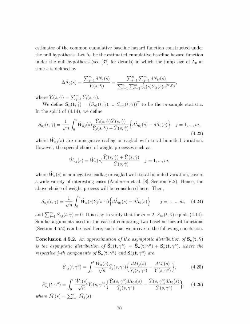
estimator of the common cumulative baseline hazard function constructed under

the null hypothesis. Let Λ0 be the estimated cumulative baseline hazard function

under the null hypothesis (see [37] for details) in which the jump size of Λ0 at

time s is defined by

∆Λ0(s) =

∑mj=1 dNj(s)

Y·(s, γ)=

∑ni=1

∑mj=1 dNij(s)∑n

i=1

∑mj=1 ψi(s)Yij(s)e

βTZij,

where Y·(s, γ) =∑m

j=1 Yj(s, γ).

We define Sn(t, γ) = (Sn1(t, γ), ..., Snm(t, γ))T to be the m-sample statistic.

In the spirit of (4.14), we define

Snj(t, γ) =1√n

∫ t

0

Wnj(s)Yj(s, γ)Y·(s, γ)

Yj(s, γ) + Y·(s, γ)

{dΛ0j(s)− dΛ0(s)

}j = 1, ...,m,

(4.23)

where Wnj(s) are nonnegative cadlag or caglad with total bounded variation.

However, the special choice of weight processes such as

Wnj(s) = Wn(s)Yj(s, γ) + Y·(s, γ)

Y·(s, γ)j = 1, ...,m,

where Wn(s) is nonnegative cadlag or caglad with total bounded variation, covers

a wide variety of interesting cases (Andersen et al. [8], Section V.2). Hence, the

above choice of weight process will be considered here. Then,

Snj(t, γ) =1√n

∫ t

0

Wn(s)Yj(s, γ){dΛ0j(s)− dΛ0(s)

}j = 1, ...,m, (4.24)

and∑m

j=1 Snj(t, γ) = 0. It is easy to verify that for m = 2, Sn1(t, γ) equals (4.14).

Similar arguments used in the case of comparing two baseline hazard functions

(Section 4.5.2) can be used here, such that we arrive to the following conclusion.

Conclusion 4.5.2. An approximation of the asymptotic distribution of Sn(t, γ)

is the asymptotic distribution of S∗n(t, γo) = Sn(t, γo) + S∗n(t, γo), where the

respective j-th components of Sn(t, γo) and S∗n(t, γo) are

Snj(t, γo) =

∫ t

0

Wn(s)√n

Yj(s, γo){ dMj(s)

Yj(s, γo)− dM·(s)

Y·(s, γo)

}, (4.25)

S∗nj(t, γo) =

∫ t

0

Wn(s)√n

Yj(s, γo){ Yj(s, γo)dΛ0j(s)

Yj(s, γo)− Y·(s, γ

o)dΛ0(s)

Y·(s, γo)

}, (4.26)

where M·(s) =∑n

i=1 Mj(s).

70

Note that given w·, M·(s) is a mean zero martingale with respect to Fs−.

For the asymptotic distribution of S∗n(t, γo) we present the following theorem

and its proof can be found in Section 4.7.4.

Theorem 4.5.3. Given Assumptions 1-2 and under the null hypothesis,

(1) Sn(t, γo) converges to a zero-mean multivariate normally distributed random

variable with variance matrix V(t) and its jk-th component is defined by

Vjk(t) =

∫ t

0

W 2(s)yj(s)

∑mr 6=j,r=1yr(s)

y·(s)λ0(s)ds k = j

−∫ t

0

W 2(s)yj(s)yk(s)

y·(s)λ0(s)ds k 6= j.

(2) S∗n(t, γo) converges to a zero-mean multivariate normal random variable with

covariance matrix having finite diagonal entries and zero valued non-diagonal

entries.

(3) The two random variables Sn(t, γo) and S∗n(t, γo) are uncorrelated.

Summarizing our results so far, we conclude that Sn(t, γ) is asymptotically

normal. Using similar arguments as for the case of testing equality of two hazard

functions, motivates us to estimate the variance of Sn(t, γ) based on the variance

estimator of Sn(t, γo). Hence our proposed estimator, denoted by V(t) is given

by

Vjj(t) =1

n

∫ t

0

W 2n(s)

n∑i=1

[{1− Yj(s, γ)

Y·(s, γ)

}2

E(wi)Yij(s)eβTZijdΛ0j(s)

+{ Yj(s, γ)

Y·(s, γ)

}2m∑l 6=j

E(wi)Yil(s)eβTZildΛ0l(s)

]j = 1, ...,m.

(4.27)

and for k 6= j

Vkj(t) =1

n

∫ t

0

W 2n(s)

[∑l 6=j,k

Yj(s, γ)Yk(s, γ)

Y 2· (s, γ)

E(wi)Yil(s)eβTZildΛ0l(s)

− Yj(s, γ)

Y·(s, γ)

n∑i=1

E(wi)Yik(s)eβTZikdΛ0k(s)

− Yk(s, γ)

Y·(s, γ)

n∑i=1

E(wi)Yij(s)eβTZijdΛ0j(s)

].

(4.28)

71

The details for the derivation of V(t) are presented in Section 4.7.5. It is clear

that V(t) has rank of (m−1). Hence, we define Vo(t) as a (m−1)× (m−1) ma-

trix obtained by deleting the last row and column of V(t). Also, let Son(t) =(

Sn1(t, γ), ..., Sn(m−1)(t, γ))T

. Then, our proposed test statistic is defined by

Son(t, γ)T

[Vo(t)

]−1

Son(t, γ) and the rejection region should be defined by the

χ2(m− 1) distribution.

It is clear that the above theory can be used directly for testing contrasts on

the baseline hazard functions.

4.6 Sample Size Formula for Equality of Two

Hazard Functions

In this section, we present a sample size formula under proportional means local

alternative and certain simplifying assumptions for testing the equality of two

baseline hazard functions. Specifically, let

H1 : Λn0j(s) =

∫ s

0

exp{(−1)j−1ϕ(u)/(2√n)}dΛ0(u) j = 1, 2 for all s ∈ [0, τ ],

(4.29)

where Λ0 is some unspecified cumulative hazard function with Λ0(s) < ∞ and

ϕ(s) 6= 0 for all s ∈ [0, τ ]. The above local alternative formulation was originally

proposed by Kosorok and Lin [54] and also these alternatives can be found in the

work of Gangnon and Kosorok [29].

It is easy to verify that the above Λn0j(s) j = 1, 2 satisfies the following as-

sumptions:

5. For j = 1, 2

sups∈[0,τ ]

∣∣ dΛn0j(s)/dΛ0(s)− 1

∣∣ → 0, as n→∞.

6. As n→∞,

sups∈[0,τ ]

∣∣ √n{dΛn01(s)

dΛn02(s)

− 1}− ϕ(s)

∣∣ → 0

where ϕ is either cadlag or caglad with bounded total variation.

Figure 4.1 presents two examples of the cumulative baseline hazard functions

under the above local alternatives defined by (4.29).

72

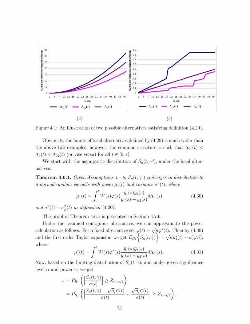
0

5

10

15

20

25

30

35

1 4 7 10 13 16 19 22 25 28 31 34 37 40 43 46 49

t, sec.

Cum

ulat

ive

base

line

haza

rd fu

nctio

n

Series1 Series2 Series3

02 ( )tΛ 01( )tΛ 0 ( )tΛ

(a)

0

0.1

0.2

0.3

0.4

0.5

0.6

0.7

0.8

0.9

1 4 7 10 13 16 19 22 25 28 31 34 37 40 43 46 49

t, sec.

Cum

ulat

ive

base

line

haza

rd fu

nctio

n

Series1 Series2 Series3

02 ( )tΛ 01( )tΛ 0 ( )tΛ

(b)

Figure 4.1: An illustration of two possible alternatives satisfying definition (4.29).

Obviously, the family of local alternatives defined by (4.29) is much wider than

the above two examples, however, the common structure is such that Λ01(t) <

Λ0(t) < Λ02(t) (or vise versa) for all t ∈ [0, τ ].

We start with the asymptotic distribution of Sn(t, γo), under the local alter-

natives.

Theorem 4.6.1. Given Assumptions 1 - 6, Sn(t, γo) converges in distribution to

a normal random variable with mean µ1(t) and variance σ2(t), where

µ1(t) =

∫ t

0

W (s)ϕ(s)y1(s)y2(s)

y1(s) + y2(s)dΛ0 (s) (4.30)

and σ2(t) = σ2S(t) as defined in (4.20).

The proof of Theorem 4.6.1 is presented in Section 4.7.6.

Under the assumed contiguous alternative, we can approximate the power

calculation as follows. For a fixed alternative set ϕ(t) =√nϕ∗(t). Then by (4.30)

and the first order Taylor expansion we get EH1

{Sn(t, γ)

}=√nµ∗1(t) + o(

√n),

where

µ∗1(t) =

∫ t

0

W (s)ϕ∗(s)y1(s)y2(s)

y1(s) + y2(s)dΛ0 (s) . (4.31)

Now, based on the limiting distribution of Sn(t, γ), and under given significance

level α and power π, we get

π = PH1

(∣∣∣Sn(t, γ)

σ(t)

∣∣∣ ≥ Z1−α/2

)= PH1

(∣∣∣Sn(t, γ)−√nµ∗1(t)

σ(t)+

√nµ∗1(t)

σ(t)

∣∣∣ ≥ Z1−α/2

),

73

where Zp is the p-th quantile of the standard normal distribution. Then,

Z1−α/2 −√nµ∗1(t)

σ(t)≈ −Zπ.

This gives us the following sample size formula

n =

(Z1−α/2 + Zπ

)2

σ2(t)

{µ∗1(t)}2. (4.32)

However, in order to calculate the required sample size based on (4.32) one should

estimate σ2(t) and µ∗1(t) based on a pilot study or existing relevant datasets.

In what follows, we propose simple estimators under simplifying assumptions,

similar to those of [79]. These simple estimators provide a practical sample size

formula.

Assume that the baseline hazard functions are continuous and the local alter-

natives satisfy ϕ∗(s) = ε for all s ∈ [0, τ ], when ε ∈ R and the weight function

is constant Wn(s) ≡ 1. We also assume that the limiting values of Yj(s, γ)/nj

are πj(s), j = 1, 2 and the proportion of customers making the j-th call, nj/n,

converges to pj ∈ (0, 1], j = 1, 2. Then, based on Assumption 2, we replace yj(s)

by pjπj(s). In addition, we assume that π1(s) = π2(s) = π(s). Hence, (4.31)

becomes

µ∗1(t) =

∫ t

0

εp1p2π

2(s)

p1π(s) + p2π(s)dΛ0 (s)

= εp1p2

p1 + p2

R(t),

(4.33)

where R(t) =∫ t

0π(s)dΛ0(s). A simple estimator of R(t) can be obtained as

follows

R(t) =

∫ t

0

{p1π1(s)dΛ01(s) + p2(s)π2dΛ02(s)}

=

∫ t

0

{n1

n

Y1(s, γ)

n1

dN1(s)

Y1(s, γ)+n2

n

Y2(s, γ)

n2

dN2(s)

Y2(s, γ)

}=

1

n

2∑j=1

Nj(t).

(4.34)

Thus, a simplified sample size formula is given by

n =

(Z1−α/2 + Zπ

)2

σ2II(t)

{εp1p2R(t)/(p1 + p2)}2, (4.35)

74

where σ2II(t) is given by (4.22).

Remark I. The widely used sample size formula proposed by Schoenfeld [76]

is for the case of independent samples. By simulation study we show (Section 4.8)

that Schoenfeld’s formula underestimates the required sample size under depen-

dent samples.

Remark II. Based on (4.20) and (4.30), and by the usual Cauchy-Schwartz

argument, it can be shown that under the local alternative (4.29) the optimal

weight function equals W (s) = ϕ(s) for all s ∈ [0, τ ].

4.7 Proofs

4.7.1 Proof of Theorem 4.5.1

Let

An(t, γ) =1√n

∫ t

0

Wn(s)

{Y2(s, γ)

Y.(s, γ)dM1(s)− Y1(s, γ)

Y.(s, γ)dM2(s)

}and write Sn(t, γ) = An(t, γ)+S∗∗n (t). The first order Taylor expansion of An(t, γ)

about γo gives

An(t, γ) ≈ Sn(t, γo)+1√n

∫ t

0

Wn(s){QT

2 (s, γo)dM1(s)−QT1 (s, γo)dM2(s)

}(γ−γo).

(4.36)

Since Mj(t)/√n converges in distribution as n→∞ (it is asymptotically normal

given w.) and using Assumptions 1 and 3-4 stating the existence of deterministic

functions W (s) and glj(s), l = 1, ..., p+ 1 j = 1, ...,m, such that

sups∈[0,τ ]

∣∣ Qlj(s, γo)− glj(s)

∣∣ → 0 sups∈[0,τ ]

{Wn(s)−W (s)

}−→ 0,

we get that the conditional distribution of

Bn(t, γo) =1√n

∫ t

0

Wn(s){QT

2 (s, γo)dM1(s)−QT1 (s, γo)dM2(s)

},

conditioning on w·, convergence to zero-mean multivariate normally distributed

random variable with finite entries of the covariance matrix that are free of the

frailties. Hence, this is also the unconditional asymptotic distribution of Bn(t, γo).

Then, given Claim 3.3, the second term of (4.36) goes to zero as n → ∞, by

Slutsky’s theorem.

75

4.7.2 Proof of Theorem 4.5.2

We present the proofs of each theorem’s statements in the sequence.

Proof of statement (1). Given w·, Sn(t, γo) is a mean-zero martingale.

Hence, to show that given w· it converges to a normally distributed random

variable, one needs to show that the conditions of the martingale central limit

theorem (see [1], Section 2.3.3, for details) hold. Namely,

(i)2∑j=1

{Dnj (s, γo)

}2λnj (s, γo) −→p v(s) for all s ∈ [0, τ ], as n→∞,

where λnj (s, γo) =∑n

i=1 Yij(s)hij(s, βo)λ0j(s) is a sum of intensity processes

of n independent customers, hij(s, βo) = wie

βoTZij and V (t) =∫ t

0v(s)ds is

the variance of the limiting process.

(ii) Dnj (s, γo) −→p 0 for all j = 1, 2 and s ∈ [0, τ ], as n→∞.

In our case, under the null hypothesis λ0j(s) = λ0(s), j = 1, 2 for all s ∈ [0, τ ].

Therefore, under the null hypothesis and Assumptions 1 - 2, we obtain

2∑j=1

{Dnj (s, γo)

}2λnj (s, γo) =

=2∑j=1

{Wn(s)√n

Y3−j(s, γo)

Y1(s, γo) + Y2(s, γo)

}2n∑i=1

Yij(s)hij(s, γo)λ0(s)

=W 2n(s)

n

Y 22 (s, γo)Y1(s, γo) + Y 2

1 (s, γo)Y2(s, γo)

{Y1(s, γo) + Y2(s, γo)}2λ0(s)

−→p W2(s)

y1(s)y2(s)

y1(s) + y2(s)λ0(s), as n→∞,

(4.37)

and

Dnj (s, γo) =

1√nWn(s)

Y3−j(s, γo)/n

{Y1(s, γo) + Y2(s, γo)}/n−→p 0, as n→∞.

Hence, we conclude that Sn(t, γo), given w·, converges to a normally distributed

random variable with moments that are free of the frailties w·. Therefore, Sn(t, γo)

also converges to a normally distributed random variable with the same param-

eters.

76

Proof of statement (2). Note that S∗n(t, γo) can be rewritten in the follow-

ing form

S∗n(t, γo) =1√n

∫ t

0

Wn(s)Y1(s, γo)Y2(s, γo)

Y·(s, γo)

{ Y1(s, γo)

Y1(s, γo)− Y2(s, γo)

Y2(s, γo)

}dΛ0(s)

=

∫ t

0

Wn(s)( Y2(s, γo)

Y·(s, γo)

{M1(s)− M∗

1 (s)}

− Y1(s, γo)

Y·(s, γo)

{M1(s)− M∗

1 (s)})dΛ0(s),

where M∗j =

∑ni=1M

∗ij(s) is a mean-zero martingale of the process Nj(s). Then,

applying the martingale central limit theorem in a way analogous to the proof of

statement (1), we obtain that S∗n(t, γo) is asymptotically normally distributed.

Obviously, that S∗n(t, γo) has mean zero and for the simplicity of its variance

calculation we let

gj(s) = Wn(s)λ0(s)Yj(s, γ

o)

Y·(s, γo)and X∗j (s) =

1√n

n∑i=1

Yij(s)eβTZij

{wi−E(wi

∣∣ Fs−)}

for j = 1, 2. Then,

V ar{S∗n(t, γo)} = V ar{∫ t

0

g1(s)X∗1 (s)ds}

+ V ar{∫ t

0

g2(s)X∗2 (s)ds}

− 2Cov{∫ t

0

g1(s)X∗1 (s)ds,

∫ t

0

g2(s)X∗2 (s)ds}.

(4.38)

Since X∗j (s) j = 1, 2 have mean zero, by using the law of total expectation we get

V ar{∫ t

0

gj(s)X∗j (s)ds

}=

= E

(E{∫ t

0

gj(s)X∗j (s)ds

∫ t

0

gj(u)X∗j (u)du∣∣ Fs∨u−})

=1

nE{∫ t

0

∫ t

0

gj(s)gj(u)n∑i=1

Yij(s ∨ u)e2βTZijV ar(wi∣∣ Fs∨u−)

}dsdu,

(4.39)

and

Cov{∫ t

0

g1(s)X∗1 (s)ds,

∫ t

0

g2(s)X∗2 (s)ds}

=

=1

nE{∫ t

0

∫ t

0

g1(s)g2(u)n∑i=1

Yi1(s)Yi2(u)eβT (Zi1+Zi2)V ar(wi

∣∣ Fs∨u−)}dsdu.

(4.40)

77

Combining (4.38)-(4.40) we get

V ar{S∗n(t, γo)} =

=1

n

( m∑j=1

E{∫ t

0

∫ t

0

gj(s)gj(u)n∑i=1

Yij(s ∨ u)e2βTZijV ar(wi∣∣ Fs∨u−)

}dsdu

− 2E{∫ t

0

∫ t

0

g1(s)g2(u)n∑i=1

Yi1(s)Yi2(u)eβT (Zi1+Zi2)V ar(wi

∣∣ Fs∨u−)}dsdu

).

(4.41)

Hence, it is easy to see that V ar{S∗n(t, γo)

}<∞.

Proof of statement (3). Note that under the null hypothesis, the covariance

between Sn(t, γo) and S∗n(t, γo) can be written as follows

Cov(Sn(t, γo), S∗n(t, γo)

)= E

[ ∫ t

0

Dn(s, γo){ dM1(s)

Y1(s, γo)− dM2(s)

Y2(s, γo)

}∫ t

0

Dn(s, γo){ Y1(s, γo)dΛ01(s)

Y1(s, γo)− Y2(s, γo)dΛ02(s)

Y2(s, γo)

}]=

∫ t

0

∫ t

0

E[Dn(s, γo)Dn(u, γo)

{ dM1(s)

Y1(s, γo)− dM2(s)

Y2(s, γo)

}{ Y1(u, γo)

Y1(u, γo)− Y2(u, γo)

Y2(u, γo)

}dΛ0(u)

].

(4.42)

Now we show that Cov{Sn(t, γo), S∗n(t, γo)} = 0 by showing that given w·

E

[Dn(s, γo)Dn(u, γo)

{ dM1(s)

Y1(s, γo)− dM2(s)

Y2(s, γo)

}{ Y1(u, γo)

Y1(u, γo)− Y2(u, γo)

Y2(u, γo)

}dΛ0(u)

]= 0,

for all s, u ∈ [0, τ ]. Indeed, for s ≥ u we get

E[E(Dn(s, γo)Dn(u, γo)

{ dM1(s)

Y1(s, γo)− dM2(s)

Y2(s, γo)

}{ Y1(u, γo)

Y1(u, γo)− Y2(u, γo)

Y2(u, γo)

}dΛ0(u)

∣∣ Fs−)]= E

[Dn(s, γo)Dn(u, γo)

{ Y1(u, γo)

Y1(u, γo)− Y2(u, γo)

Y2(u, γo)

}E({ dM1(s)

Y1(s, γo)− dM2(s)

Y2(s, γo)

} ∣∣ Fs−)dΛ0(u)]

= 0,

78

because E

(dM1(s)

Y1(s, γo)− dM2(s)

Y2(s, γo)

∣∣ Fs−) = 0 given w·, as an expectation of zero

mean martingales. For u > s, we get

E[E(Dn(s, γo)Dn(u, γo)

{ dM1(s)

Y1(s, γo)− dM2(s)

Y2(s, γo)

}{ Y1(u, γo)

Y1(u, γo)− Y2(u, γo)

Y2(u, γo)

}dΛ0(u)

∣∣ Fu−)]= E

[Dn(s, γo)Dn(u, γo)

{ dM1(s)

Y1(s, γo)− dM2(s)

Y2(s, γo)

}E({ Y1(u, γo)

Y1(u, γo)− Y2(u, γo)

Y2(u, γo)

} ∣∣ Fu−)dΛ0(u)]

= 0.

4.7.3 An Estimator of the Variance of Sn(t, γ)

In the following, we generate our variance estimators of V ar{Sn(t, γo)} and

V ar{S∗n(t, γo)}. Let us start with an estimator of V ar{Sn(t, γo)}. By using

the law of total variance we get

V ar{Sn(t, γo)} = E[V ar{Sn(t, γo)

∣∣ w·}]+ V ar[E{Sn(t, γo)

∣∣ w·}] .It is clear that Sn(t, γo) given w· is a mean-zero martingale under the null hy-

pothesis, as a difference between two mean zero martingales. Hence,

V ar{Sn(t, γo)} = E

(V ar

[∫ t

0

Dn(s, γo){ dM1(s)

Y1(s, γo)− dM2(s)

Y2(s, γo)

} ∣∣ w·]) .Since calls of customer i are conditionally independent given wi, the predictable

variation process of Sn(t, γo), given w·, is given by

< Sn∣∣ w· > (t, γo) =

∫ t

0

D2n(s, γo)V ar

{ dM1(s)

Y1(s, γo)− dM2(s)

Y2(s, γo)

∣∣ w·, Fs−}=

∫ t

0

D2n(s, γo)

(V ar

{ dM1(s)

Y1(s, γo)

∣∣ w·, Fs−}+ V ar{ dM2(s)

Y2(s, γo)

∣∣ w·, Fs−}) .Since V ar

{dMij(s)

∣∣ w·,Fs−} = Yij(s)eβTZijwiλ0j(s)ds we get

< Sn∣∣ w· > (t, γo) =

n∑i=1

wi

∫ t

0

D2n(s, γo)

{eβTZi1Yi1(s)

Y 21 (s, γo)

dΛ01(s) +eβ

TZi2Yi2(s)

Y 22 (s, γo)

dΛ02(s)}.

Then, the expectation with respect to the unknown frailties gives

n∑i=1

E(wi)

∫ t

0

D2n(s, γo)

{eβTZi1Yi1(s)

Y 21 (s, γo)

dΛ01(s) +eβ

TZi2Yi2(s)

Y 22 (s, γo)

dΛ02(s)}. (4.43)

79

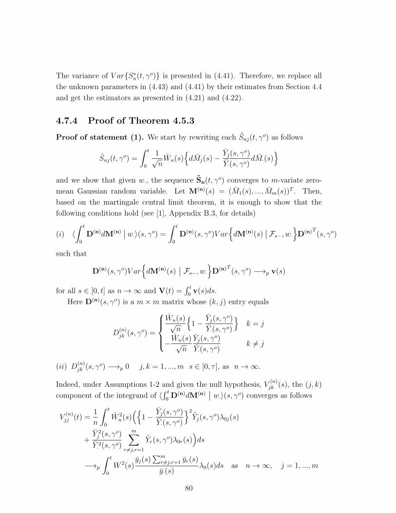
The variance of V ar{S∗n(t, γo)} is presented in (4.41). Therefore, we replace all

the unknown parameters in (4.43) and (4.41) by their estimates from Section 4.4

and get the estimators as presented in (4.21) and (4.22).

4.7.4 Proof of Theorem 4.5.3

Proof of statement (1). We start by rewriting each Snj(t, γo) as follows

Snj(t, γo) =

∫ t

0

1√nWn(s)

{dMj(s)−

Yj(s, γo)

Y·(s, γo)dM·(s)

}and we show that given w·, the sequence Sn(t, γo) converges to m-variate zero-

mean Gaussian random variable. Let M(n)(s) = (M1(s), ..., Mm(s))T . Then,

based on the martingale central limit theorem, it is enough to show that the

following conditions hold (see [1], Appendix B.3, for details)

(i) 〈∫ t

0

D(n)dM(n)∣∣ w·〉(s, γo) =

∫ t

0

D(n)(s, γo)V ar{dM(n)(s)

∣∣ Fs−, w·}D(n)T (s, γo)

such that

D(n)(s, γo)V ar{dM(n)(s)

∣∣ Fs−, w·}D(n)T (s, γo) −→p v(s)

for all s ∈ [0, t] as n→∞ and V(t) =∫ t

0v(s)ds.

Here D(n)(s, γo) is a m×m matrix whose (k, j) entry equals

D(n)jk (s, γo) =

Wn(s)√

n

{1− Yj(s, γ

o)

Y·(s, γo)

}k = j

−Wn(s)√n

Yj(s, γo)

Y·(s, γo)k 6= j

(ii) D(n)jk (s, γo) −→p 0 j, k = 1, ...,m s ∈ [0, τ ], as n→∞.

Indeed, under Assumptions 1-2 and given the null hypothesis, V(n)jk (s), the (j, k)

component of the integrand of 〈∫ t

0D(n)dM(n)

∣∣ w·〉(s, γo) converges as follows

V(n)jj (t) =

1

n

∫ t

0

W 2n(s)

({1− Yj(s, γ

o)

Y·(s, γo)

}2

Yj(s, γo)λ0j(s)

+Y 2j (s, γo)

Y 2· (s, γo)

m∑r 6=j,r=1

Yr(s, γo)λ0r(s)

)ds

−→p

∫ t

0

W 2(s)yj(s)

∑mr 6=j,r=1 yr(s)

y·(s)λ0(s)ds as n→∞, j = 1, ...,m

80

and for j 6= k, j, k = 1, ...,m

V(n)jk (t) =

1

n

∫ t

0

W 2n(s)

{ Yj(s, γo)Yk(s, γo)Y 2· (s, γo)

m∑r=1

Yr(s, γo)λ0r(s)

− Yj(s, γo)

Y·(s, γo)Yk(s, γ

o)λ0k(s)−Yk(s, γ

o)

Y·(s, γo)Yj(s, γ

o)λ0j(s)}ds

−→p −∫ t

0

W 2(s)yj(s)yk(s)

y·(s)λ0(s)ds as n→∞.

For Condition (ii), it is easy to see that under Assumptions 1-2, for j =

1, ...,m, sinceYj(s, γ

0)

Y·(s, γ0)−→ yj(s, γ

0)

y·(s, γ0), as n→∞,

D(n)jj (s, γo) =

Wn(s)√n

{1− Yj(s, γ

o)

Y·(s, γo)

}−→p 0, as n→∞

and

D(n)jk (s, γo) =

Wn(s)√n

Yj(s, γo)/n

Y·(s, γo)/n−→p 0, as n→∞.

As before, since the conditional asymptotic distribution of Sn(t, γo) given the

frailty variates is free of the frailties w· we conclude that this is also the asymptotic

distribution of Sn(t, γo).

Proof of statement (2). Since for j = 1, ...,m

E{ Yj(s, γo)Yj(s, γo)

− Y·(s, γo)

Y·(s, γo)

∣∣ Fs−} =

=

∑ni=1 Yij(s)e

βZijE[wi∣∣ Fs−]

Yj(s, γo)−∑m

k=1

∑ni=1 Yik(s)e

βZikE[wi∣∣ Fs−]

Y2(s, γo)

=Yj(s, γ

o)

Yj(s, γo)− Y·(s, γ

o)

Y·(s, γo)= 0

(4.44)

it is easy to show that under the null hypothesis

E[S∗nj(t, γ

o)]

= E[ ∫ t

0

Wn(s)√n

Yj(s, γo){ Yj(s, γo)Yj(s, γo)

− Y·(s, γo)

Y·(s, γo)

}dΛ0(s)

]= 0,

(4.45)

for j = 1, ...,m. Also, using again the law of total expectation by conditioning

81

on Fu∨s− we obtain that under the null hypothesis

Cov[S∗nj(t, γ

o), S∗nk(t, γo)]

=

=

∫ τ

0

∫ t

0

E[Wn(s)√

nYj(s, γ

o)Wn(u)√

nYk(u, γ

o){ Yj(s, γo)Yj(s, γo)

− Y·(s, γo)

Y·(s, γo)

}dΛ0(s){ Yk(u, γo)

Yk(u, γo)− Y·(u, γ

o)

Y·(u, γo)

}dΛ0(u)

]= 0.

Using similar arguments as in the proof of Theorem 4.5.2, one can show that each

of the j-th components of S∗nj(t, γo) is asymptotically normally distributed with

a finite variance.

Proof of statement (3). Note that under the null hypothesis, the covariance

between Snj(t, γo) and S∗nk(t, γ

o) for all j, k = 1, ...,m can be written as follows

Cov{Snj(t, γ

o), S∗nk(t, γo)}

= E[ ∫ t

0

Wn(s)√n

Yj(s, γo){ dMj(s)

Yj(s, γo)− dM·(s)

Y·(s, γo)

}∫ t

0

Wn(s)√n

Yk(s, γo){ Yk(s, γo)Yk(s, γo)

− Y·(s, γo)

Y·(s, γo)

}dΛ0(s)

]=

∫ τ

0

∫ t

0

E[Wn(s)√

nYj(s, γ

o)Wn(u)√

nYk(u, γ

o){ dMj(s)

Yj(s, γo)− dM·(s)

Y·(s, γo)

}{ Yk(u, γo)Yk(u, γo)

− Y·(u, γo)

Y·(u, γo)

}]dΛ0(u).

(4.46)

Now, let us show that Cov{Snj(t, γ

o), S∗nk(t, γo)}

= 0 by showing that

E

[Wn(s)Wn(u)

nYj(s, γ

o)Yk(u, γo){ dMj(s)

Yj(s, γo)− dM·(s)

Y·(s, γo)

}{ Yk(u, γo)Yk(u, γo)

− Y·(u, γo)

Y·(u, γo)

}]= 0,

for all u, s ∈ [0, τ ]. Indeed, for s ≥ u we have

E[Wn(s)Wn(u)

nYj(s, γ

o)Yk(u, γo){ Yk(u, γo)Yk(u, γo)

− Y·(u, γo)

Y·(u, γo)

}E({ dMj(s)

Yj(s, γo)− dM·(s)

Y·(s, γo)

} ∣∣ Fs−)] = 0,

because E

({ dMj(s)

Yj(s, γo)− dM·(s)

Y·(s, γo)

} ∣∣ Fs−) = 0, as an expectation of zero mean

82

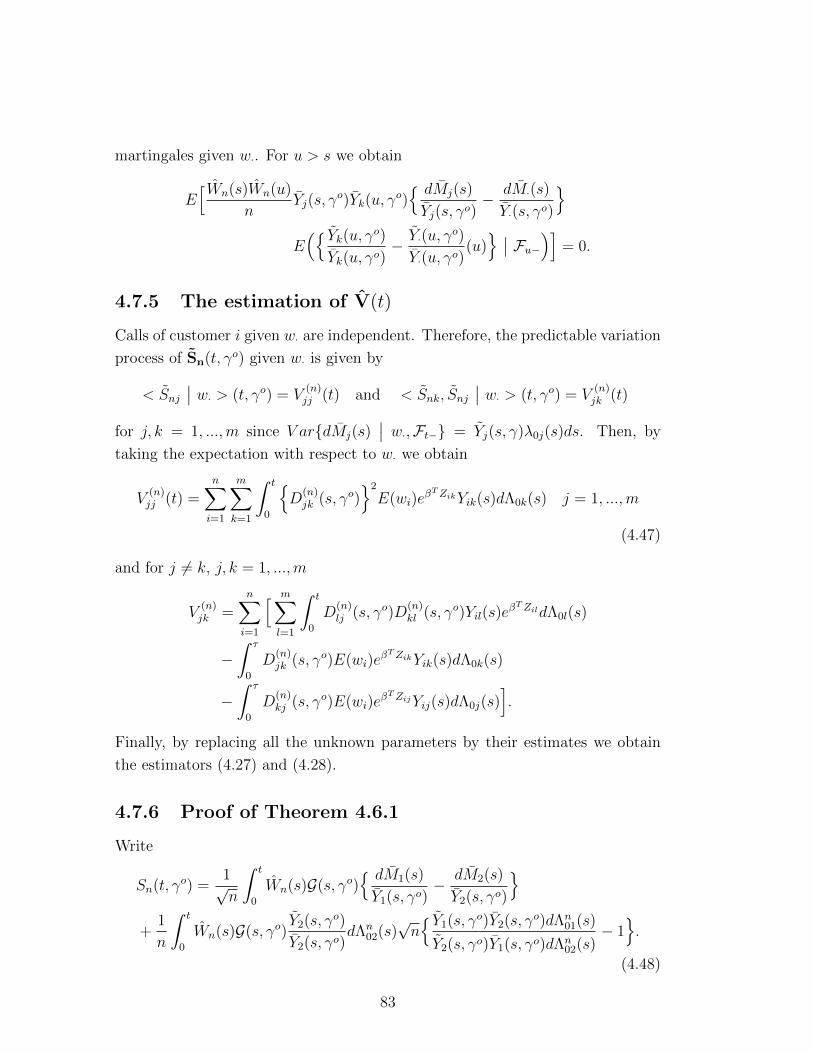
martingales given w·. For u > s we obtain

E[Wn(s)Wn(u)

nYj(s, γ

o)Yk(u, γo){ dMj(s)

Yj(s, γo)− dM·(s)

Y·(s, γo)

}E({ Yk(u, γo)

Yk(u, γo)− Y·(u, γ

o)

Y·(u, γo)(u)} ∣∣ Fu−)] = 0.

4.7.5 The estimation of V(t)

Calls of customer i given w· are independent. Therefore, the predictable variation

process of Sn(t, γo) given w· is given by

< Snj∣∣ w· > (t, γo) = V

(n)jj (t) and < Snk, Snj

∣∣ w· > (t, γo) = V(n)jk (t)

for j, k = 1, ...,m since V ar{dMj(s)∣∣ w·,Ft−} = Yj(s, γ)λ0j(s)ds. Then, by

taking the expectation with respect to w· we obtain

V(n)jj (t) =

n∑i=1

m∑k=1

∫ t

0

{D

(n)jk (s, γo)

}2

E(wi)eβTZikYik(s)dΛ0k(s) j = 1, ...,m

(4.47)

and for j 6= k, j, k = 1, ...,m

V(n)jk =

n∑i=1

[ m∑l=1

∫ t

0

D(n)lj (s, γo)D

(n)kl (s, γo)Yil(s)e

βTZildΛ0l(s)

−∫ τ

0

D(n)jk (s, γo)E(wi)e

βTZikYik(s)dΛ0k(s)

−∫ τ

0

D(n)kj (s, γo)E(wi)e

βTZijYij(s)dΛ0j(s)].

Finally, by replacing all the unknown parameters by their estimates we obtain

the estimators (4.27) and (4.28).

4.7.6 Proof of Theorem 4.6.1

Write

Sn(t, γo) =1√n

∫ t

0

Wn(s)G(s, γo){ dM1(s)

Y1(s, γo)− dM2(s)

Y2(s, γo)

}+

1

n

∫ t

0

Wn(s)G(s, γo)Y2(s, γo)

Y2(s, γo)dΛn

02(s)√n{ Y1(s, γo)Y2(s, γo)dΛn

01(s)

Y2(s, γo)Y1(s, γo)dΛn02(s)

− 1}.

(4.48)

83

First, we show that the first term of the right-hand side of (4.48) converges to a

normal random variable with mean zero. The proof is similar to that of Theorem

4.5.2. Hence, we need to show that Conditions (i) and (ii) of Section 4.7.2 hold.

Proof of Condition (ii) is exactly the same as in the proof of Theorem 4.5.2 and

the proof of Condition (i) is slightly different, as follows. Using Assumptions 1,

2 and 5, we have

2∑j=1

{Dnj (s, γo)

}2λnj (s) =

2∑j=1

n∑i=1

{Wn(s)√n

Y3−j(s, γo)

Y·(s, γo))

}2

Yij(s)hij(s, βo)d

dsΛ

(n)0j (s).

By writing dds

Λ(n)0j (s) = dΛ0(s)

ds

dΛ(n)0j (s)

dΛ0(s)and using Assumption 5 we get

2∑j=1

{Dnj (s, γo)

}2λnj (s) −→p W

2(s)y1(s)y2(s)

y1(s) + y2(s)λ0(s), as n→∞.

Now, by Assumptions 2, 5 and 6 we obtain that

sups∈[0,τ ]

∣∣∣√n{ Y1(s, γo)Y2(s, γo)dΛn01(s)

Y2(s, γo)Y1(s, γo)dΛn02(s)

− 1}− ϕ(s)

∣∣∣→ 0.

Therefore, the second term of the right-hand side of (4.48) converges to µ1(t) in

probability, as n→∞.

4.8 Simulation

In this section we present our simulation study aimed to investigate the finite

sample properties of our proposed procedures. The simulations were carried out

under the popular Gamma frailty model. Therefore, we start by presenting the

above procedures under the Gamma distribution with mean 1 and variance θ.

The log-likelihood function (4.3), under the frailty model with Gamma(1θ, 1θ),

becomes

lnL(γ) ∝n∑i=1

mi∑j=1

δijβTZij −

n∑i=1

{ln (θ)

θ+

(Ni·(τ) +

1

θ

)ln

(Hi·(τ) +

1

θ

)}

+n∑i=1

ln

Ni·(τ)−1∏j=0

(j +1

θ)

I{Ni·(τ)≥1},

(4.49)

84

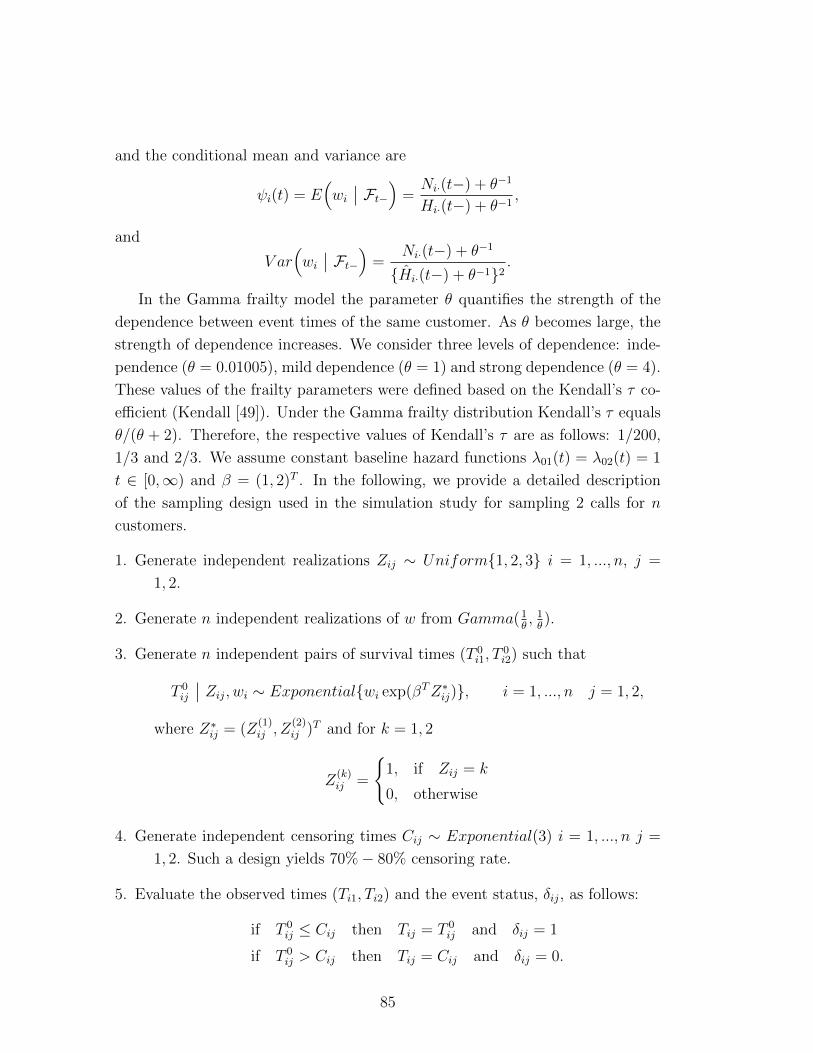
and the conditional mean and variance are

ψi(t) = E(wi∣∣ Ft−) =

Ni·(t−) + θ−1

Hi·(t−) + θ−1,

and

V ar(wi∣∣ Ft−) =

Ni·(t−) + θ−1

{Hi·(t−) + θ−1}2.

In the Gamma frailty model the parameter θ quantifies the strength of the

dependence between event times of the same customer. As θ becomes large, the

strength of dependence increases. We consider three levels of dependence: inde-

pendence (θ = 0.01005), mild dependence (θ = 1) and strong dependence (θ = 4).

These values of the frailty parameters were defined based on the Kendall’s τ co-

efficient (Kendall [49]). Under the Gamma frailty distribution Kendall’s τ equals

θ/(θ + 2). Therefore, the respective values of Kendall’s τ are as follows: 1/200,

1/3 and 2/3. We assume constant baseline hazard functions λ01(t) = λ02(t) = 1

t ∈ [0,∞) and β = (1, 2)T . In the following, we provide a detailed description

of the sampling design used in the simulation study for sampling 2 calls for n

customers.

1. Generate independent realizations Zij ∼ Uniform{1, 2, 3} i = 1, ..., n, j =

1, 2.

2. Generate n independent realizations of w from Gamma(1θ, 1θ).

3. Generate n independent pairs of survival times (T 0i1, T

0i2) such that

T 0ij

∣∣ Zij, wi ∼ Exponential{wi exp(βTZ∗ij)}, i = 1, ..., n j = 1, 2,

where Z∗ij = (Z(1)ij , Z

(2)ij )T and for k = 1, 2

Z(k)ij =

{1, if Zij = k

0, otherwise

4. Generate independent censoring times Cij ∼ Exponential(3) i = 1, ..., n j =

1, 2. Such a design yields 70%− 80% censoring rate.

5. Evaluate the observed times (Ti1, Ti2) and the event status, δij, as follows:

if T 0ij ≤ Cij then Tij = T 0

ij and δij = 1

if T 0ij > Cij then Tij = Cij and δij = 0.

85

Table 4.1: Summary of parameter estimates {θ, β, Λ(t)} based on 1000 simulated

random datasets with n = 250 and 500.

independence mild dependence strong dependence

true true true

value mean SD value mean SD value mean SD

n=250

θ 0.01005 0.084 0.150 1 0.929 0.240 4 3.806 0.812

β1 1 1.023 0.328 1 0.969 0.249 1 1.009 0.355

β2 2 2.059 0.318 2 1.935 0.264 2 1.986 0.368

Λ01(t1) 0.005 0.005 0.003 0.005 0.005 0.003 0.005 0.005 0.003

Λ01(t2) 0.01 0.010 0.004 0.01 0.011 0.004 0.01 0.010 0.005

Λ01(t3) 0.05 0.049 0.016 0.05 0.053 0.015 0.05 0.050 0.018

Λ01(t4) 0.1 0.096 0.031 0.1 0.104 0.029 0.1 0.098 0.034

Λ01(t1) 0.005 0.005 0.003 0.005 0.006 0.003 0.005 0.005 0.003

Λ01(t2) 0.01 0.010 0.005 0.01 0.011 0.005 0.01 0.010 0.005

Λ01(t3) 0.05 0.049 0.017 0.05 0.054 0.015 0.05 0.051 0.017

Λ01(t4) 0.1 0.097 0.033 0.1 0.108 0.029 0.1 0.101 0.031

n=500

θ 0.01005 0.064 0.098 1 1.025 0.175 4 3.925 0.596

β1 1 1.013 0.219 1 1.008 0.198 1 1.007 0.242

β2 2 2.021 0.211 2 2.003 0.201 2 1.999 0.262

Λ01(t1) 0.005 0.005 0.002 0.005 0.005 0.002 0.005 0.005 0.002

Λ01(t2) 0.01 0.010 0.003 0.01 0.010 0.003 0.01 0.010 0.004

Λ01(t3) 0.05 0.049 0.011 0.05 0.050 0.010 0.05 0.050 0.013

Λ01(t4) 0.1 0.098 0.021 0.1 0.101 0.019 0.1 0.100 0.025

Λ01(t1) 0.005 0.005 0.002 0.005 0.005 0.002 0.005 0.005 0.002

Λ01(t2) 0.01 0.010 0.003 0.01 0.010 0.003 0.01 0.010 0.004

Λ01(t3) 0.05 0.049 0.011 0.05 0.050 0.010 0.05 0.051 0.014

Λ01(t4) 0.1 0.098 0.021 0.1 0.101 0.019 0.1 0.100 0.025

86

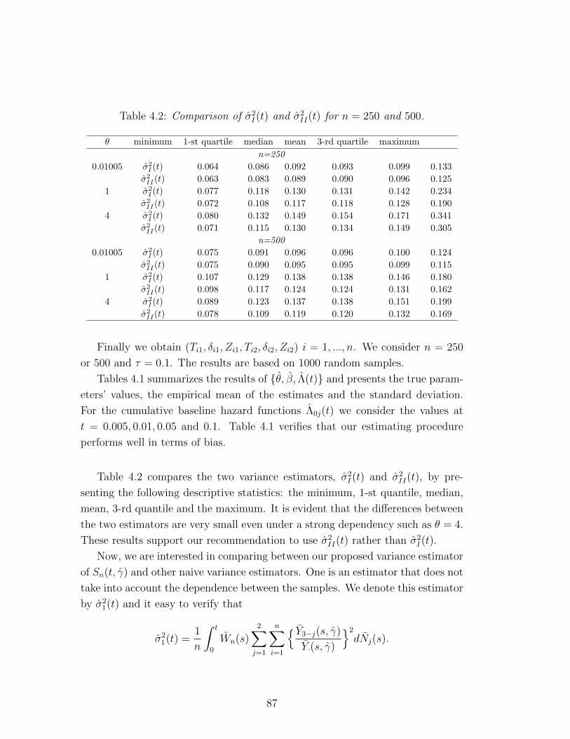
Table 4.2: Comparison of σ2I (t) and σ2

II(t) for n = 250 and 500.

θ minimum 1-st quartile median mean 3-rd quartile maximum

n=250

0.01005 σ2I (t) 0.064 0.086 0.092 0.093 0.099 0.133

σ2II(t) 0.063 0.083 0.089 0.090 0.096 0.125

1 σ2I (t) 0.077 0.118 0.130 0.131 0.142 0.234

σ2II(t) 0.072 0.108 0.117 0.118 0.128 0.190

4 σ2I (t) 0.080 0.132 0.149 0.154 0.171 0.341

σ2II(t) 0.071 0.115 0.130 0.134 0.149 0.305

n=500

0.01005 σ2I (t) 0.075 0.091 0.096 0.096 0.100 0.124

σ2II(t) 0.075 0.090 0.095 0.095 0.099 0.115

1 σ2I (t) 0.107 0.129 0.138 0.138 0.146 0.180

σ2II(t) 0.098 0.117 0.124 0.124 0.131 0.162

4 σ2I (t) 0.089 0.123 0.137 0.138 0.151 0.199

σ2II(t) 0.078 0.109 0.119 0.120 0.132 0.169

Finally we obtain (Ti1, δi1, Zi1, Ti2, δi2, Zi2) i = 1, ..., n. We consider n = 250

or 500 and τ = 0.1. The results are based on 1000 random samples.

Tables 4.1 summarizes the results of {θ, β, Λ(t)} and presents the true param-

eters’ values, the empirical mean of the estimates and the standard deviation.

For the cumulative baseline hazard functions Λ0j(t) we consider the values at

t = 0.005, 0.01, 0.05 and 0.1. Table 4.1 verifies that our estimating procedure

performs well in terms of bias.

Table 4.2 compares the two variance estimators, σ2I (t) and σ2

II(t), by pre-

senting the following descriptive statistics: the minimum, 1-st quantile, median,

mean, 3-rd quantile and the maximum. It is evident that the differences between

the two estimators are very small even under a strong dependency such as θ = 4.

These results support our recommendation to use σ2II(t) rather than σ2

I (t).

Now, we are interested in comparing between our proposed variance estimator

of Sn(t, γ) and other naive variance estimators. One is an estimator that does not

take into account the dependence between the samples. We denote this estimator

by σ21(t) and it easy to verify that

σ21(t) =

1

n

∫ t

0

Wn(s)2∑j=1

n∑i=1

{ Y3−j(s, γ)

Y·(s, γ)

}2

dNj(s).

87

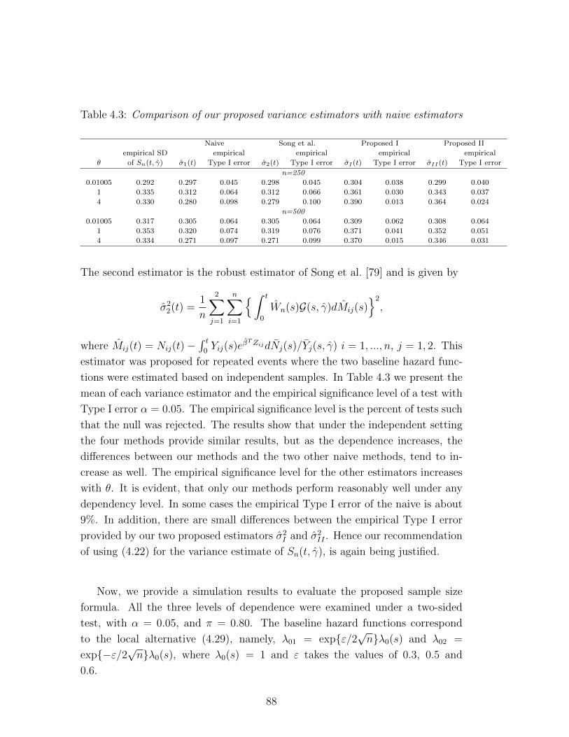
Table 4.3: Comparison of our proposed variance estimators with naive estimators

Naive Song et al. Proposed I Proposed II

empirical SD empirical empirical empirical empirical

θ of Sn(t, γ) σ1(t) Type I error σ2(t) Type I error σI(t) Type I error σII(t) Type I error

n=250

0.01005 0.292 0.297 0.045 0.298 0.045 0.304 0.038 0.299 0.040

1 0.335 0.312 0.064 0.312 0.066 0.361 0.030 0.343 0.037

4 0.330 0.280 0.098 0.279 0.100 0.390 0.013 0.364 0.024

n=500

0.01005 0.317 0.305 0.064 0.305 0.064 0.309 0.062 0.308 0.064

1 0.353 0.320 0.074 0.319 0.076 0.371 0.041 0.352 0.051

4 0.334 0.271 0.097 0.271 0.099 0.370 0.015 0.346 0.031

The second estimator is the robust estimator of Song et al. [79] and is given by

σ22(t) =

1

n

2∑j=1

n∑i=1

{∫ t

0

Wn(s)G(s, γ)dMij(s)}2

,

where Mij(t) = Nij(t)−∫ t

0Yij(s)e

βTZijdNj(s)/Yj(s, γ) i = 1, ..., n, j = 1, 2. This

estimator was proposed for repeated events where the two baseline hazard func-

tions were estimated based on independent samples. In Table 4.3 we present the

mean of each variance estimator and the empirical significance level of a test with

Type I error α = 0.05. The empirical significance level is the percent of tests such

that the null was rejected. The results show that under the independent setting

the four methods provide similar results, but as the dependence increases, the

differences between our methods and the two other naive methods, tend to in-

crease as well. The empirical significance level for the other estimators increases

with θ. It is evident, that only our methods perform reasonably well under any

dependency level. In some cases the empirical Type I error of the naive is about

9%. In addition, there are small differences between the empirical Type I error

provided by our two proposed estimators σ2I and σ2

II . Hence our recommendation

of using (4.22) for the variance estimate of Sn(t, γ), is again being justified.

Now, we provide a simulation results to evaluate the proposed sample size

formula. All the three levels of dependence were examined under a two-sided

test, with α = 0.05, and π = 0.80. The baseline hazard functions correspond

to the local alternative (4.29), namely, λ01 = exp{ε/2√n}λ0(s) and λ02 =

exp{−ε/2√n}λ0(s), where λ0(s) = 1 and ε takes the values of 0.3, 0.5 and

0.6.

88

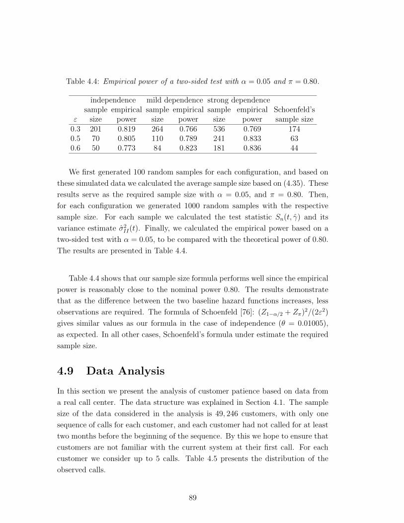
Table 4.4: Empirical power of a two-sided test with α = 0.05 and π = 0.80.

independence mild dependence strong dependencesample empirical sample empirical sample empirical Schoenfeld’s

ε size power size power size power sample size0.3 201 0.819 264 0.766 536 0.769 1740.5 70 0.805 110 0.789 241 0.833 630.6 50 0.773 84 0.823 181 0.836 44

We first generated 100 random samples for each configuration, and based on

these simulated data we calculated the average sample size based on (4.35). These

results serve as the required sample size with α = 0.05, and π = 0.80. Then,

for each configuration we generated 1000 random samples with the respective

sample size. For each sample we calculated the test statistic Sn(t, γ) and its

variance estimate σ2II(t). Finally, we calculated the empirical power based on a

two-sided test with α = 0.05, to be compared with the theoretical power of 0.80.

The results are presented in Table 4.4.

Table 4.4 shows that our sample size formula performs well since the empirical

power is reasonably close to the nominal power 0.80. The results demonstrate

that as the difference between the two baseline hazard functions increases, less

observations are required. The formula of Schoenfeld [76]: (Z1−α/2 + Zπ)2/(2ε2)

gives similar values as our formula in the case of independence (θ = 0.01005),

as expected. In all other cases, Schoenfeld’s formula under estimate the required

sample size.

4.9 Data Analysis

In this section we present the analysis of customer patience based on data from

a real call center. The data structure was explained in Section 4.1. The sample

size of the data considered in the analysis is 49, 246 customers, with only one

sequence of calls for each customer, and each customer had not called for at least

two months before the beginning of the sequence. By this we hope to ensure that

customers are not familiar with the current system at their first call. For each

customer we consider up to 5 calls. Table 4.5 presents the distribution of the

observed calls.

89

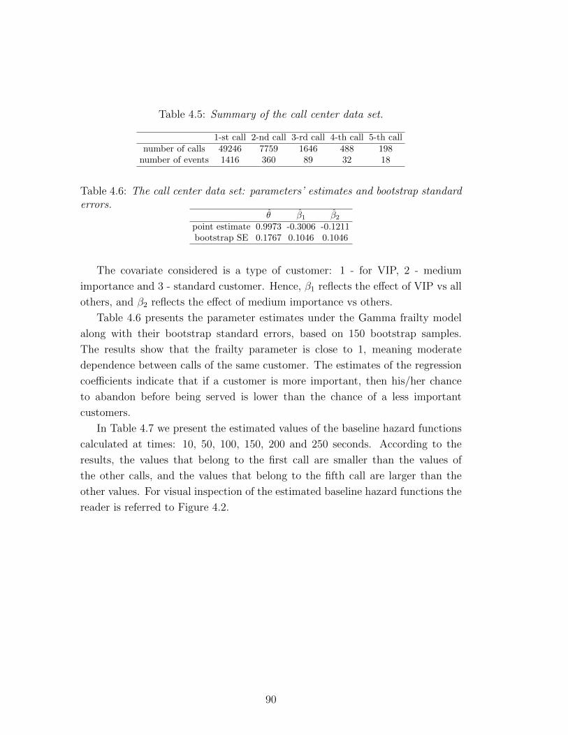
Table 4.5: Summary of the call center data set.

1-st call 2-nd call 3-rd call 4-th call 5-th callnumber of calls 49246 7759 1646 488 198

number of events 1416 360 89 32 18

Table 4.6: The call center data set: parameters’ estimates and bootstrap standarderrors.

θ β1 β2point estimate 0.9973 -0.3006 -0.1211bootstrap SE 0.1767 0.1046 0.1046

The covariate considered is a type of customer: 1 - for VIP, 2 - medium

importance and 3 - standard customer. Hence, β1 reflects the effect of VIP vs all

others, and β2 reflects the effect of medium importance vs others.

Table 4.6 presents the parameter estimates under the Gamma frailty model

along with their bootstrap standard errors, based on 150 bootstrap samples.

The results show that the frailty parameter is close to 1, meaning moderate

dependence between calls of the same customer. The estimates of the regression

coefficients indicate that if a customer is more important, then his/her chance

to abandon before being served is lower than the chance of a less important

customers.

In Table 4.7 we present the estimated values of the baseline hazard functions

calculated at times: 10, 50, 100, 150, 200 and 250 seconds. According to the

results, the values that belong to the first call are smaller than the values of

the other calls, and the values that belong to the fifth call are larger than the

other values. For visual inspection of the estimated baseline hazard functions the

reader is referred to Figure 4.2.

90

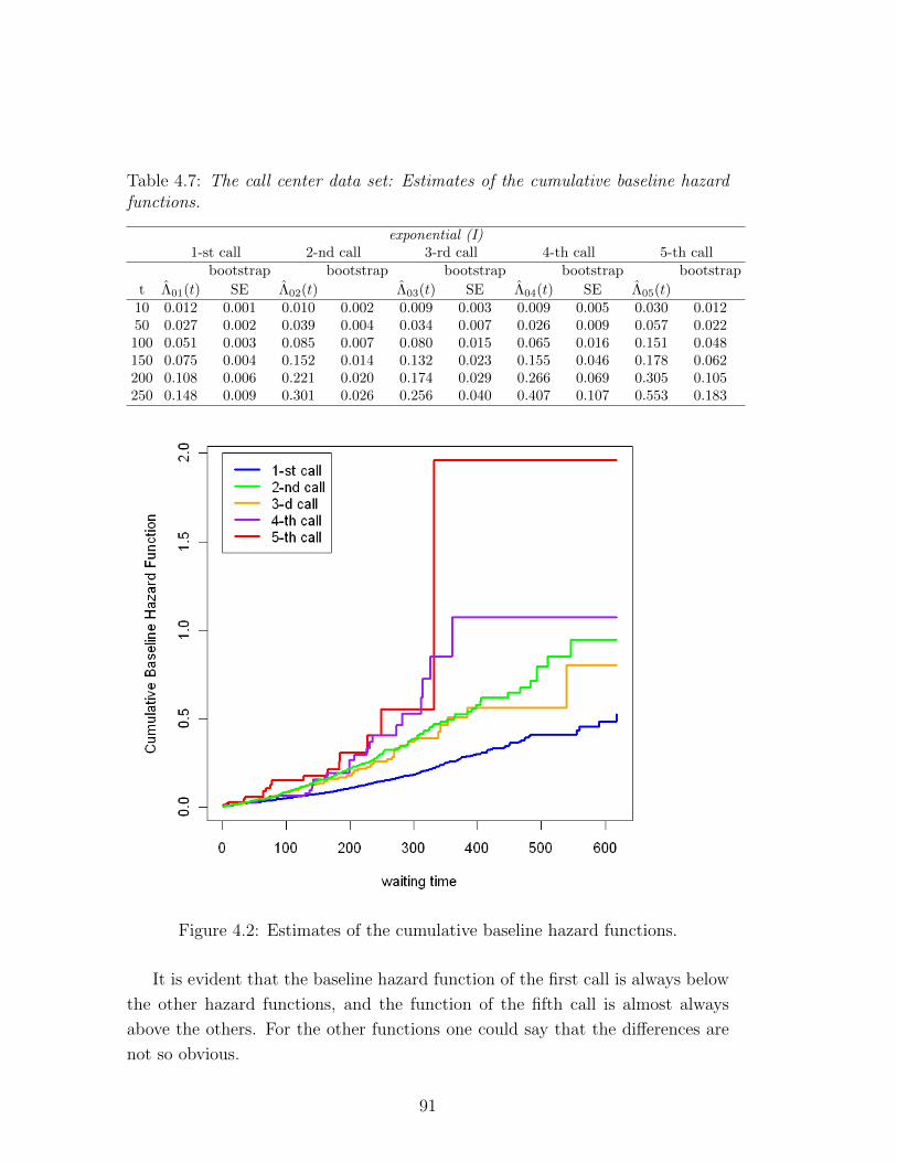
Table 4.7: The call center data set: Estimates of the cumulative baseline hazardfunctions.

exponential (I)1-st call 2-nd call 3-rd call 4-th call 5-th call

bootstrap bootstrap bootstrap bootstrap bootstrap

t Λ01(t) SE Λ02(t) Λ03(t) SE Λ04(t) SE Λ05(t)10 0.012 0.001 0.010 0.002 0.009 0.003 0.009 0.005 0.030 0.01250 0.027 0.002 0.039 0.004 0.034 0.007 0.026 0.009 0.057 0.022100 0.051 0.003 0.085 0.007 0.080 0.015 0.065 0.016 0.151 0.048150 0.075 0.004 0.152 0.014 0.132 0.023 0.155 0.046 0.178 0.062200 0.108 0.006 0.221 0.020 0.174 0.029 0.266 0.069 0.305 0.105250 0.148 0.009 0.301 0.026 0.256 0.040 0.407 0.107 0.553 0.183

Figure 4.2: Estimates of the cumulative baseline hazard functions.

It is evident that the baseline hazard function of the first call is always below

the other hazard functions, and the function of the fifth call is almost always

above the others. For the other functions one could say that the differences are

not so obvious.

91

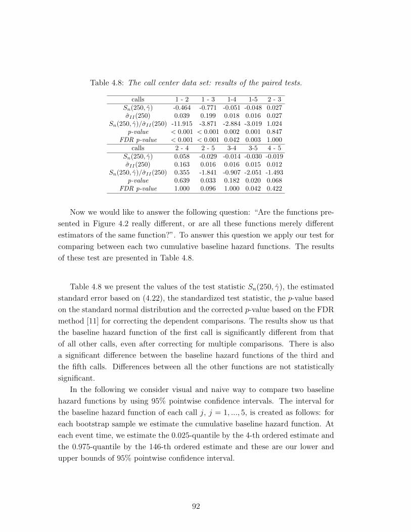
Table 4.8: The call center data set: results of the paired tests.

calls 1 - 2 1 - 3 1-4 1-5 2 - 3Sn(250, γ) -0.464 -0.771 -0.051 -0.048 0.027σII(250) 0.039 0.199 0.018 0.016 0.027

Sn(250, γ)/σII(250) -11.915 -3.871 -2.884 -3.019 1.024p-value < 0.001 < 0.001 0.002 0.001 0.847

FDR p-value < 0.001 < 0.001 0.042 0.003 1.000calls 2 - 4 2 - 5 3-4 3-5 4 - 5

Sn(250, γ) 0.058 -0.029 -0.014 -0.030 -0.019σII(250) 0.163 0.016 0.016 0.015 0.012

Sn(250, γ)/σII(250) 0.355 -1.841 -0.907 -2.051 -1.493p-value 0.639 0.033 0.182 0.020 0.068

FDR p-value 1.000 0.096 1.000 0.042 0.422

Now we would like to answer the following question: “Are the functions pre-

sented in Figure 4.2 really different, or are all these functions merely different

estimators of the same function?”. To answer this question we apply our test for

comparing between each two cumulative baseline hazard functions. The results

of these test are presented in Table 4.8.

Table 4.8 we present the values of the test statistic Sn(250, γ), the estimated

standard error based on (4.22), the standardized test statistic, the p-value based

on the standard normal distribution and the corrected p-value based on the FDR

method [11] for correcting the dependent comparisons. The results show us that

the baseline hazard function of the first call is significantly different from that

of all other calls, even after correcting for multiple comparisons. There is also

a significant difference between the baseline hazard functions of the third and

the fifth calls. Differences between all the other functions are not statistically

significant.

In the following we consider visual and naive way to compare two baseline

hazard functions by using 95% pointwise confidence intervals. The interval for

the baseline hazard function of each call j, j = 1, ..., 5, is created as follows: for

each bootstrap sample we estimate the cumulative baseline hazard function. At

each event time, we estimate the 0.025-quantile by the 4-th ordered estimate and

the 0.975-quantile by the 146-th ordered estimate and these are our lower and

upper bounds of 95% pointwise confidence interval.

92

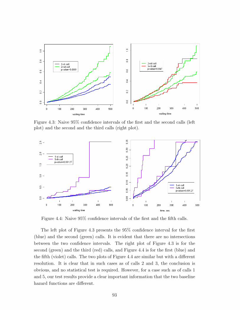
Figure 4.3: Naive 95% confidence intervals of the first and the second calls (leftplot) and the second and the third calls (right plot).

Figure 4.4: Naive 95% confidence intervals of the first and the fifth calls.

The left plot of Figure 4.3 presents the 95% confidence interval for the first

(blue) and the second (green) calls. It is evident that there are no intersections

between the two confidence intervals. The right plot of Figure 4.3 is for the

second (green) and the third (red) calls, and Figure 4.4 is for the first (blue) and

the fifth (violet) calls. The two plots of Figure 4.4 are similar but with a different

resolution. It is clear that in such cases as of calls 2 and 3, the conclusion is

obvious, and no statistical test is required. However, for a case such as of calls 1

and 5, our test results provide a clear important information that the two baseline

hazard functions are different.

93

4.10 Summary and Future Directions

In this chapter, we considered a model for customer patience. The proposed

model is an extended Cox model with frailty variate, reflecting the heterogeneity

of customers, and different baseline hazard functions, reflecting the customer’s

familiarity with the system. For estimation of parameters, the method proposed

by Gorfine et al. [37] was extended to the case of different baseline hazard func-

tions. The simulation study indicated that our method works well in terms of

bias for finite samples with any level of dependency within customer calls.

We provided a test for comparing two or more baseline hazard functions.

The asymptotic distribution of the proposed test statistic was presented and a

simulation study was conducted. The results of the simulation study show that

our proposed method works well and as expected, gives better results in compare

to the naive approaches that ignores within-subject dependence.

A sample-size formula was derived based on the limiting distribution of our

test statistic under local alternatives. Our simulation study shows that according

to the proposed formula the empirical power is reasonably close to the nominal

value.

The proposed approach was applied to a real call center dataset and it was

found that customers are significantly more patient in their first call. Moreover,

customers that are defined as more important to the system, are willing to wait

longer than the less important customers. In addition, there is a moderate level

of dependence in the waiting behavior of a customer.

4.10.1 Application of the Proposed Approach in HealthCare Data

This research project was motivated by the analysis of call center data, but

our test can also be useful in other research areas. For example, consider the

Washington Ashkenazi Kin-Cohort Study (WAS) (Struewing et al. [81]). In this

study, blood samples and questionnaire were collected from Ashkenazi Jewish

men and women volunteers living in the Washington DC area. Based on blood

samples, volunteers were tested for specific mutations in BRCA1 and BRCA2

genes. The questionnaire included information on cancer and mortality history

of the first-degree relatives of the volunteers.

For the current analysis we consider a subset of the data consist of female

first-degree relatives of volunteers (mother, sisters and daughters). The event is

94

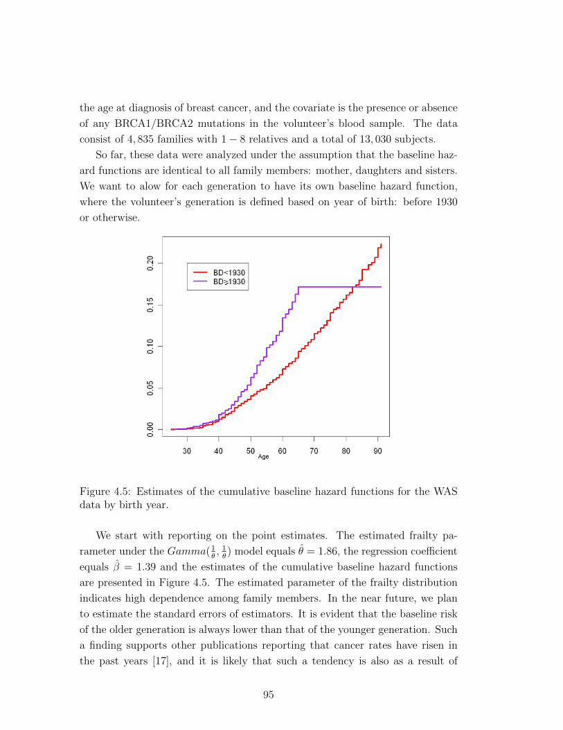
the age at diagnosis of breast cancer, and the covariate is the presence or absence

of any BRCA1/BRCA2 mutations in the volunteer’s blood sample. The data

consist of 4, 835 families with 1− 8 relatives and a total of 13, 030 subjects.

So far, these data were analyzed under the assumption that the baseline haz-

ard functions are identical to all family members: mother, daughters and sisters.

We want to alow for each generation to have its own baseline hazard function,

where the volunteer’s generation is defined based on year of birth: before 1930

or otherwise.

Figure 4.5: Estimates of the cumulative baseline hazard functions for the WASdata by birth year.

We start with reporting on the point estimates. The estimated frailty pa-

rameter under the Gamma(1θ, 1θ) model equals θ = 1.86, the regression coefficient

equals β = 1.39 and the estimates of the cumulative baseline hazard functions

are presented in Figure 4.5. The estimated parameter of the frailty distribution

indicates high dependence among family members. In the near future, we plan

to estimate the standard errors of estimators. It is evident that the baseline risk

of the older generation is always lower than that of the younger generation. Such

a finding supports other publications reporting that cancer rates have risen in

the past years [17], and it is likely that such a tendency is also as a result of

95

the increase in screening programs which detect the cancer in earlier stages [69].

As the continuation of this study we also plan to apply our statistical test for

comparing the two hazard functions. We expect to verify our visual inspection

and observe a significant difference between the two functions.

Another possible example of our model in a medical context is the scenario

where patients suffer a series of events that require hospitalization, and we are

interested in whether the distribution of the length of the k-th hospital stay

depends on k. In this example, though, time probably will be discrete.

4.10.2 Future directions

Our estimation method and statistical test are not limited to a particular frailty

distribution. The simulations and the data analysis were done under the Gamma

frailty model distribution. It could be of importance to see how the results of

the data analysis will vary, if at all, with other choices of frailty distribution.

Also, it is important to check the effect of using a wrong frailty distribution. For

example, the frailty is log-normally distributed, but the analysis is done under

the Gamma distribution.

An important extension of our approach is the prediction of customer pa-

tience. An implementation of the prediction of customer patience in the modern

Customer Relationship Management (CRM) software tools could be a huge ad-

vance in management of call centers. Such an option can significantly improve

customers’ satisfaction without additional financial costs. However, the right

implementation of this feature is not a simple task and it could rise additional

questions related to management science and queuing theory. Another possible

extension of our proposed model could be including of time dependent covariates.

Another future direction in customer patience analysis is to analyze the changes

in customer patience with the help of the hazard function. Adjusting the defini-

tion in [42] to our case, at any time point t, the hazard function is defined as the

probability of abandonment within a short interval, given that the customer was

in a queue at the beginning of the interval.

96

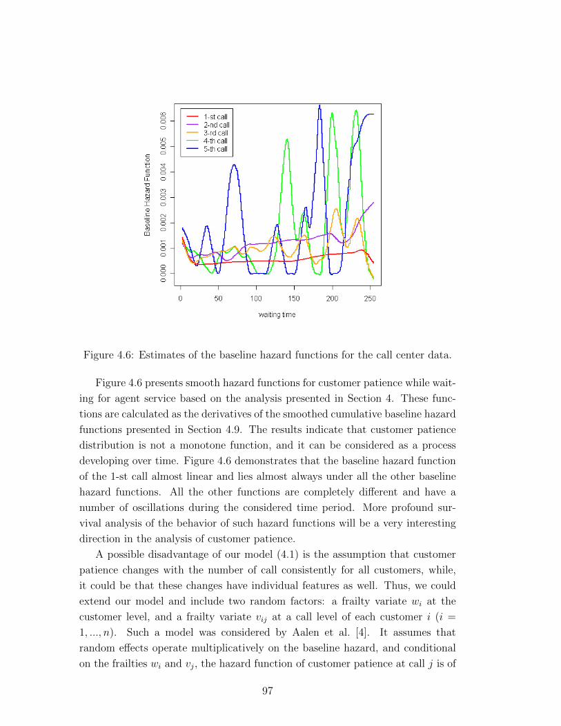
Figure 4.6: Estimates of the baseline hazard functions for the call center data.

Figure 4.6 presents smooth hazard functions for customer patience while wait-

ing for agent service based on the analysis presented in Section 4. These func-

tions are calculated as the derivatives of the smoothed cumulative baseline hazard

functions presented in Section 4.9. The results indicate that customer patience

distribution is not a monotone function, and it can be considered as a process

developing over time. Figure 4.6 demonstrates that the baseline hazard function

of the 1-st call almost linear and lies almost always under all the other baseline

hazard functions. All the other functions are completely different and have a

number of oscillations during the considered time period. More profound sur-

vival analysis of the behavior of such hazard functions will be a very interesting

direction in the analysis of customer patience.

A possible disadvantage of our model (4.1) is the assumption that customer

patience changes with the number of call consistently for all customers, while,

it could be that these changes have individual features as well. Thus, we could

extend our model and include two random factors: a frailty variate wi at the

customer level, and a frailty variate vij at a call level of each customer i (i =

1, ..., n). Such a model was considered by Aalen et al. [4]. It assumes that

random effects operate multiplicatively on the baseline hazard, and conditional

on the frailties wi and vj, the hazard function of customer patience at call j is of

97

the form

λij(t|wi, vij) = wivijλ0j(t)eβTZij , j = 1, ...,mi, i = 1, ..., n, (4.50)

where, for each customer, vij j = 1, ...,mi are i.i.d. random variables with density

function g(v) ≡ g(v;µ) where µ is an unknown vector of parameters. The frailty

vij can also be regarded as the set of covariates of call j that are not included

in Zij because they are not measured. This is a hierarchical frailty model with

two-levels of frailty: shared frailty at the customer level and unshared frailty at

the call level of each customer.

We grouped the customer’s calls in “series of retrials”. Hence, for studying

the effect of “series of retrials” we can consider the following model

λijk(t|wi, yk) = wiykhj0(t)eβTZijk , k = 1, ..., li, j = 1, ...,mki , i = 1, ..., n,

(4.51)

where yk is the frailty variate of the k-th series of a specific customer, li is the

total number of series of the customer, and mk is the total number of calls of

series k. This is also a hierarchical frailty model with two-levels of frailty: shared

frailty at the customer level and shared frailty at the “series of retrials” level of

each customer.

The hierarchial frailty model (4.51) is also considered by Aalen et al. [4] under

frailty distributions determined by non-negative Levy processes, which includes

Power Variance Function (PVF) distributions. The PVF distributions include the

gamma, positive stable, inverse Gaussian and compound Poisson distributions as

special cases (see [1] and [42] for details). The implementation of such models

can be a possible direction for further analysis.

The process of waiting on line before being served can be affected by factors

developing with the time. For example, at the beginning a customer is expecting

to wait a specific period of time, after this period s/he is astonished and after a

while even angry of having to wait. Our frailty model is constant in time, but

there may be a more realistic model which assumes a frailty that develops with

time. This can be modeled by considering frailty as a stochastic process. Con-

ditional on the unobserved frailty variate W (t), the hazard function of customer

patience would be of the form

h0(t)W (t)eβTWj , j = 1, ...,mi. (4.52)

Here, W (t) is a stochastic process.

98

Chapter 5

DISCUSSION ANDCONCLUSIONS

Call centers are intended to provide and improve customer service, marketing,

technical support, etc. Therefore, the right management of a call center is a very

important and crucial issue, that has to take into account many aspects. In our

work we constructed and analyze an analytical model of a typical call center.

Operational performance measures, such as the probability for a busy signal,

the probability of abandonment and average wait for an agent were calculated

in this work. The calculations of these measures are cumbersome and they lack

of insight. We thus approximated the measures in the QED asymptotic regime,

which is suitable for moderate to large call centers. The approximations are easy

to calculate for any number of agents.

A detailed comparison between exact and approximated performance shows

that the approximations often work perfectly well, even outside the QED regime.

Summarizing our findings through practical rules-of-thumb (expressed via the

offered load). These rules were derived via extensive numerical analysis of our

analytical results.

The approximations that have been developed can support the operations

management of a call center, for example when trying to maintain a pre-determined

level of service quality. We analyzed approximations of a real call center by mod-

els with and without an IVR, in order to evaluate the value of adding an IVR.

Using real call center data we provided an analysis which was intended to connect

theoretical investigations to real management problem solving and to allow the

evaluation of the quality and robustness of the analytical results.

Our data analysis showed that the assumptions of exponentially distributed

99

service times does not take place, neither for IVR service nor for agent service.

Similarly, the assumption that the arrival process is homogeneous Poisson is

also overly simplistic. This problem was solved by division of the day into half-

hour intervals. In this way, we find that within each interval the arrival rate

is more or less constant and thus, within such intervals, we treated the arrivals

as conforming to a Poisson process. The validation of our models against the

US Bank Call Center demonstrated that the accuracy of the approximations is

satisfactory. The approximated values in many intervals are very close to actual

performance measures.

An extensive analysis of real call center data shows that a little change of

parameters can dramatically change performance. Thus, the second part of our

work is devoted to analysis of our model primitive, namely, customers patience,

which is treated as a process. The provided study is a first attempt to apply

frailty models to customer patience analysis. We suggested a novel statistical

model and estimation procedure that was investigated theoretically and by ex-

tensive simulation studies. This model, together with the evident characteristics,

allows taking into account personal customer features and customer experience

with the system. This model provides an advance in customer patience analysis.

We provided a computer program which enables convenient application and the

possibility of processing large data samples by using our method of analysis.

We proposed a new test for comparison of two or more nonparametric baseline

hazard functions considering dependent observations. Our test helps to analyze

the influence of customer experience on his/her waiting behavior. The possible

extension of our results may allow call center managers to define appropriate rout-

ing and priority rules for arriving calls on two different levels: for all customers

and for each customer personally.

This thesis combines developing novel statistical models and tests, and anal-

ysis of real data sets. We expect that our research will contribute to a better

understanding of customer habits, needs and expectations and this will have an

impact on the improvement of call center operations, providing high quality ser-

vice with lower costs. Therefore, we expect our work to be of both practical and

theoretical importance.

We believe that some of the statistical models and procedures that were de-

veloped in this work, in particular the ones for customer patience analysis, can

be applied in many other areas such us medicine, economics and industry where

survival analysis is a very popular tool.

100

APPENDIX

A.1 The Estimation Procedure

####################################################################### # Name: estimation.R # # Purpose: To find estimates of the our proposed model # # Arguments: # n: number of customers; # J: number of calls; # m: number of observed times; # theta: frailty parameter; # beta: vector of regression’s coefficients; # lam: matrix of cumulative baseline hazard functions estimates # with dimension (mx(J+1)); # T: matrix of observed times (nxJ); # z: matrix (nxJ); # D: matrix (mx(J+1)); # delta: matrix of indicators of events (nxJ). ####################################################################### source("functions.R") x=c(theta,beta) T<-T.data(data) z<-Z.data(data) D<-D.data(T,data) delta<-delta.data(data) lam<-lam.est(data,T,theta,delta,z,D,beta) J=dim(T)[2] a<-lam[,1]

101

est.lam<-matrix(rep(0,(length(a))*(J+1)),length(a),(J+1)) x=c(0.5,1,1) # initialization of estimated parameters theta.est <- x[1] beta.est <- x[2:length(x)] repeat{ est.theta.old<-x[1] repeat{ beta.est.old<-x[2:length(x)] est.lam.old<-est.lam est.lam<-lam.est(y.data,T,theta.est,delta,z,D,beta.est)

estb<-nlminb(x[2:length(x)],obj=lnLb,dat=data0,theta=x[1], z,lam=est.lam,delta,T=T)

beta.est<-estb$par #result of optimization procedure diff1<-max(abs(est.lam-est.lam.old)) # calculation of differences diff2<-max(abs(beta.est-beta.est.old)) x[2:length(x)]<-beta.est if ((diff1 < 10^(-3)) & (diff2 < 10^(-5))) break } estt<-nlminb(x[1],obj=lnLt,dat=data0,beta=x[2:length(x)],z,lam=est.lam,delta,T) theta.est<-estt$par # result of optimization procedure diff3=abs(theta.est-est.theta.old) x[1]<-theta.est if (diff3<(10^(-5))) break } est.lam<-lam.est(y.data,T,x[1],delta,z,D,x[2]) }

102

A.2 The Cumulative Baseline HazardFunctions

########################################################################### # Name: functions.R # # Purpose: Main functions used in estimation procedure. # # New arguments: # tt: vector of observed times; # lampred: matrix of estimated values of cumulative baseline hazard functions, # calculated at observed times, using as values at the previous step; # lampred_f: matrix of estimated values of cumulative baseline hazard functions, # calculated at observed times, using as values at the current step; # e: matrix of exponents with power of product of regression’s coefficients and # covariets; # H: matrix of values of function H defined in Section 4.4; # N: matrix of number of events over each call of each customer; # psi: vector of estimations of the frailty values; # lam: matrix of cumulative baseline hazard functions estimates; # dlam: matrix of jump values of cumulative baseline hazard functions; # L: loglikelihood function; ############################################################################ ###################################################################### #Calculation of the estimation for cumulative baseline hazard function ###################################################################### lam.est<-function(y.data,T,theta,delta,z,d,beta){ ##vector of event times J=max(y.data[,5]) a<-y.data[y.data[,3]==1,] a<-a[!duplicated(a[,2]),2] a<-a[order(a)] ############# ##vector of all times tt=T[,1] for(j in 2:J){ tt<-c(tt,T[,j]) }

103

tt<-tt[!duplicated(tt)] tt<-sort(tt) if(tt[1]>0){tt=c(0,tt)} last_t=tt[length(tt)] n=dim(T)[1] if(tt[1]>0){tt=c(0,tt)} lampred<-matrix(rep(0,(length(tt))*(J+1)),length(tt),(J+1)) lampred_final<-matrix(rep(0,(n)*J),n,J) lampred[1:length(tt),1]<-tt q=1 qq=c(1,1) if(a[1]>0){a=c(0,a)} dlam<-vector() lam<-matrix(rep(0,(length(a))*(J+1)),length(a),(J+1)) lam[,1]<-a e<-e.data(z,beta,J) N<-matrix(rep(0,n*J),n,J) H<-matrix(rep(0,n*J),n,J) b<-vector() f<-vector() y=NA da1=matrix(rep(0,(J+1)*n),(J+1),n) da2=matrix(rep(0,(J+1)*n),(J+1),n) up<-vector() down<-vector() down1<-vector() dlam1<-vector() ###### Update of values of the baseline hazard functions ####### for(i in 2:(length(a))){ repeat{ lampred[qq[1],2]=lam[i-1,2] qq[1]=qq[1]+1 if(lampred[qq[1],1]>=a[i] | lampred[qq[1],1]>a[length(a)] |lampred[qq[1],1]==max(T[,1])) break }

104

###### Update of values of the baseline hazard functions ####### for(i in 2:(length(a))){

repeat{ lampred[qq[1],2]=lam[i-1,2] qq[1]=qq[1]+1 if(lampred[qq[1],1]>=a[i] | lampred[qq[1],1]>a[length(a)] |lampred[qq[1],1]==max(T[,1])) break } repeat{ lampred[qq[2],3]=lam[i-1,3] qq[2]=qq[2]+1 if(lampred[qq[2],1]>=a[i] | lampred[qq[2],1]>a[length(a)] |lampred[qq[2],1]==max(T[,2])) break }

da1=lampred[match(T[,1],lampred[,1]),] w1=da1[,1][!da1[,1] %in% y] w2=da1[,2][!da1[,2] %in% y] lampred_final[,1]=ifelse(w1<a[i-1],w2,lampred[lampred[,1]==a[i-1],2]) da2=lampred[match(T[,2],lampred[,1]),] ww1=da2[,1][!da2[,1] %in% y] ww2=da2[,3][!da2[,3] %in% y] lampred_final[,2]=ifelse(ww1<a[i-1],ww2,lampred[lampred[,1]==a[i-1],3]) taub=rep(a[i-1],J) down<-rep(0,J) dlam<-rep(0,J) ############ calculation of denominator ############# N<-delta[,]*ifelse(T[,]<=taub,1,0) H[,]=lampred_final[,]*e[,] psi<-(rowSums(N)+(1/theta))/(rowSums(H)+(1/theta))

for(j in 1:J) {

up[j]<-(D[i-1,j+1]) down[j]<-sum(psi*(ifelse(T[,j]>=a[i],1,0)*e[,j])) if(down[j]>0)dlam[j]=up[j]/down[j] else dlam[j]=0

} b=lam[i-1,2:(J+1)] lam[i,2:(J+1)]<-b+dlam } return(lam) } ####################################################################### #Calculation of the estimation for loglikelihood function #######################################################################

105

####################################################################### #Calculation of the estimation for loglikelihood function ####################################################################### lnLb<-function(beta,theta,z,lam,delta,T){ n=dim(T)[1] J=dim(T)[2] nnn=dim(lam)[1] lnl=1 lam0=LM(lam[2:nnn,],T,J) lam0=lam0[!lam0[,1]==0,] e<-e.data(z,beta,J) bt<-b.data(z,beta,J) L<-0 H=0 LL<-vector() LL=c(0) a<-lam0[,1] b<-a[length(a)] #N<-N.c(delta,T,b) N<-vector() N<-rowSums(delta[,]*ifelse(T[,]<=b,1,0)) for(i in 1:n){ H<-0 for (j in 1:J){

if(T[i,j]>0){ if(delta[i,j]>0){ L<-L+delta[i,j]*bt[i,j] }

H<-H+lam0[lam0[,1]==T[i,j],(j+1)]*e[i,j] }

} lnl=1 for(m in 0:(N[i]-1))

{ lnl=lnl*(m+1/theta) }

L<-L-(log(theta))/(theta)-(N[i]+1/theta)*log(H+1/theta)+ ifelse(N[i]>0,log(lnl),0)

LL=c(LL,L) } return(-L) }

106

A.3 Estimation for the Variance of Sn{τ, γ}

########################################################################### # Name: functions.R # # Purpose: Main functions used in estimation procedure. # # New arguments: # S: value of statitic; # V: value of estimator of variance (naïve); # V1: value of estimator of variance (Song et al.); # V2: value of estimator of variance ( )250(ˆ 2

IIσ ); # V3: value of estimator of variance ( )250(ˆ 2

Iσ ); # varw: matrix of estimations of frailty calculated at each observable time; # dlam: matrix of jump values of cumulative baseline hazard functions;

# plam: matrix of )()(ˆˆ

tYet ijZ

iijβψ ;

# blam: matrix of )(ˆ

tYe ijZijβ ;

############################################################################ source("functions.R") a=D[,1] a1=D[D[,2]==1,1] a2=D[D[,3]==1,1] DD=vector() b=0 kkk=length(a[a[]<0.1]) k1=length(a1[a1[]<0.1]) k2=length(a2[a2[]<0.1]) item=matrix(rep(0,250*8),250,8) dlam0<-ylam.data(data,T,theta,delta,z,D,beta) dlam=dlam0 S0=sum((dlam[2:(kkk+1),3]*D[1:kkk,2]-dlam[2:(kkk+1),2]*D[1:kkk,3])/(dlam[2:(kkk+1),3]+dlam[2:(kkk+1),2])) for(k in 1:k1){ Y1=dlam[dlam[,1]==a1[k],2] Y2=dlam[dlam[,1]==a1[k],3] YY1=vector()

107

plam=plam.data(data,T,theta,delta,z,D,beta,a1[k]) blam=blam.data(data,T,theta,delta,z,D,beta,a1[k]) X1=ifelse(T[,1]<a1[k],0,Y2/(Y1+Y2)*(-plam[,1]/Y1)) X7=ifelse(T[,1]<=a1[k],0,((Y2/(Y1+Y2))^2)*plam[,1]/Y1) X3=(Y2/(Y1+Y2))*(delta[,1]*ifelse(T[,1]==a1[k],1,0))*(1-plam[,1]/Y1) item[,1]=item[,1]+ifelse(X3>0,X3,X1) item[,3]=item[,3]+(Y2*Y1/(Y1+Y2))^2*ifelse(T[,1]<a1[k],0, (blam[,1]/(Y1^3))) item[,5]=item[,5]+X7 } for(k in 1:k2){ Y1=dlam[dlam[,1]==a2[k],2] Y2=dlam[dlam[,1]==a2[k],3] plam=plam.data(data,T,theta,delta,z,D,beta,a2[k]) blam=blam.data(data,T,theta,delta,z,D,beta,a2[k]) X2=ifelse(T[,2]<a2[k],0,Y1/(Y1+Y2)*(-plam[,2]/Y2)) X8=ifelse(T[,2]<=a2[k],0,((Y1/(Y1+Y2))^2)*plam[,2]/Y2) X4=(Y1/(Y1+Y2))*(delta[,2]*ifelse(T[,2]==a2[k],1,0))*(1-plam[,2]/Y2) item[,2]=item[,2]+ifelse(X4>0,X4,X2) item[,4]=item[,4]+(Y2*Y1/(Y1+Y2))^2*ifelse(T[,2]<a2[k],0, (blam[,2]/(Y2^3))) item[,6]=item[,6]+X8 } x1=0 x2=0 x3=0 e<-e.data(z,beta,2) a=D[,1] b=0 varw=varw.data(data,T,theta,delta,z,d,beta,a[kkk]) varw1=varw varw2=varw

108

for(s in 1:k){ for(u in 1:k){

varw=varw1[,max(u,s)] Y1=dlam[dlam[,1]==a[s],3]/((dlam[dlam[,1]==a[s],2] +dlam[dlam[,1]==a1[s],3])^2) Y2=dlam[dlam[,1]==a[u],3]/((dlam[dlam[,1]==a[u],2] +dlam[dlam[,1]==a1[u],3])^2)

item[,7]=ifelse(T[,1]>=max(a1[s],a1[u]),e[,1]*e[,1]*varw,0) x1=x1+Y1*Y2*sum(item[,7]) }

} for(s in 1:k){ for(u in 1:k){

varw=varw2[,max(s,u)] Y1=dlam[dlam[,1]==a [s],2]/((dlam[dlam[,1]==a2[s],2] +dlam[dlam[,1]==a2[s],3])^2) Y2=dlam[dlam[,1]==a2[u],2]/((dlam[dlam[,1]==a2[u],2] +dlam[dlam[,1]==a2[u],3])^2)

item[,7]=ifelse(T[,2]>=max(a2[s],a2[u]),e[,2]*e[,2]*varw,0) x2=x2+Y1*Y2*sum(item[,7]) } } for(s in 1:k){ for(u in 1:k){

if(u<s){varw=varw1[,s]}else{varw=varw2[,u]} Y11=dlam[dlam[,1]==a[s],3]/((dlam[dlam[,1]==a[s],2] +dlam[dlam[,1]==a[s],3])^2) Y21=dlam[dlam[,1]==a[u],2]/((dlam[dlam[,1]==a[u],2] +dlam[dlam[,1]==a[u],3])^2)

item[,8]=ifelse(T[,1]>=a1[s]&T[,2]>=a2[u],e[,1]*e[,1]*varw,0) x3=x3+Y11*Y21*sum(item[,8]) } }

109

## # Naive ## V=sum(item[,5])+sum(item[,6]) ## # Song et al. ## V1=sum(item[,1:2]^2) ## # Our ## V2=sum(item[,3])+sum(item[,4]) ## # Our full variance estimator ## V3 =sum(item[,3])+sum(item[,4])+x1+x2-2*x3

110

A.4 Sample Size Calculation

########################################################################### # Name: sample_size.R # # Purpose: Sample size calculation. # # New arguments: # T0: expected value of statistic calculated according to the formula proposed in # Section 4.6; # epsilon: power of exponent reflecting the difference between the two baseline hazard # functions; # Sigma2: value of estimator of variance ( )250(ˆ 2

IIσ ). ############################################################################ data <-read.table(dat[i],sep="",header=FALSE) delta<-delta.data(data) NN=100 lam0<-read.table(res[i],sep="",header=FALSE) n=(dim(lam0)[1])/3 lam_0=cbind(lam0[1:n,1],lam0[(n+1):(2*n),1],lam0[(2*n+1):(3*n),1]) lam=lam_0[2:n,] x=lam_0[1,] theta<-x[1] beta<-x[2:3] T<-T.data(data) z<-Z.data(data) D<-D.data(T,dataw) a=D[D[,1]<0.2,1] kkk=length(a) data=data_new dlam0<-ylam.data(data,T,theta,delta,z,D,beta) dlam=dlam0 T0=epsilon^2*((sum(delta[,1])+sum(delta[,2]))/NN)^2/4 TT=c(TT,T0) a1=D[D[,1]<0.2&D[,2]==1,1] a2=D[D[,1]<0.2&D[,3]==1,1] k1=length(a1) k2=length(a2) 111

item=matrix(rep(0,NN*8),NN,8) for(k in 1:k1){ Y1=dlam[dlam[,1]==a1[k],2] Y2=dlam[dlam[,1]==a1[k],3] plam=plam.data(data,T,theta,delta,z,D,beta,a1[k]) blam=blam.data(data,T,theta,delta,z,D,beta,a1[k]) item[,3]=item[,3]+(Y2*Y1/(Y1+Y2))^2*ifelse(T[,1]<a1[k],0, (blam[,1]/(Y1^3))) } for(k in 1:k2){ Y1=dlam[dlam[,1]==a2[k],2] Y2=dlam[dlam[,1]==a2[k],3] plam=plam.data(data,T,theta,delta,z,D,beta,a2[k]) blam=blam.data(data,T,theta,delta,z,D,beta,a2[k]) X4=(Y1/(Y1+Y2))*(delta[,2]*ifelse(T[,2]==a2[k],1,0))*(1-plam[,2]/Y2) item[,4]=item[,4]+(Y2*Y1/(Y1+Y2))^2*ifelse(T[,2]<a2[k],0,(blam[,2]/(Y2^3))) } V2=c(V2,(sum(item[,3])+sum(item[,4]))/(NN)) Sigma2=(sum(item[,3])+sum(item[,4]))/(NN) n_sample=c(n_sample,(1.9644854+0.84162)^2*sigma2/TT[i])

112

Bibliography

[1] Aalen, O.O., Borgan, O. and Gjessing, H.K. (2008). Survival and Event

History Analysis. New York: Springer. 60, 76, 80, 98

[2] Aalen, O.O. (1994). Effects of Frailty in Survival Analysis. Statistical Meth-

ods in Medical Research, 3, 227-243. 18

[3] Aalen, O.O. and Gjessing, H.K. (2001). Understanding the Shape of the

Hazard Rate: A Process Point of View. Statistical Science, 16(1), 1-22. 18

[4] Aalen, O.O. and Moger, T.A. (2006). Hierarchical Levy Frailty Models and

a Frailty Analysis of Data on Infant Mortality in Norwegian Siblings. UW

Biostatistics Working Paper Series, available at

www.bepress.com/cgi/viewcontent.cgi?article=1124&context=

uwbiostat 97, 98

[5] Acar, Crain and Yao (2010). Dependence Calibration in Conditional Copu-

las: A Nonparametric Approach. To appear in Biometrics, available at

http://www.utstat.utoronto.ca/craiu/Papers/R_DCCC_2.pdf 68

[6] Aguir, M.S., Karaesmen, F., Aksin, O.Z., and Chauvet. F. (2004). The Im-

pact of Retrials on Call Center Performance. OR Spectrum, Special Issue on

Call Center Management, 26(3), 353-376. 15

[7] Andersen, P.K. and Gill, D.R. (1982). Cox’s Regression Model for Counting

Processes: a Large Sample Study. Ann. Statist., 10, 1100-1120. 65

[8] Andersen, P.K., Borgan, O., Gill, D.R. and Keiding, N. (1993). Statistical

Models Based on Counting Processes. New York: Springer. 19, 70

[9] Armony, M., Gurvich, I. and Mandelbaum, A. (2008). Service Level Differ-

entiation in Call Centers with Ffully Flexible Servers. Management Science,

Special Issue on Call Center Management, 54(2), 279-294. available at

113

http://iew3.technion.ac.il/serveng/References/references.html

57

[10] Atar, R., Mandelbaum, A. and Shaikhet, G. (2006). Queueing Systems

with Many Servers: Null Controllability in Heavy Traffic. Annals of Applied

Probability, 16, 1764-1804, available at

http://iew3.technion.ac.il/serveng/References/references.html

57

[11] Benjamini Y. and Yekutieli D. (2001). The Control of the False Discovery

Rate in Multiple Testing Under Dependency. The Annals of Statistics, 29,

1165-1188. 92

[12] Borst, S., Mandelbaum, A. and Reiman, M. (2004). Dimensioning Large Call

Centers. Operations Research, 52(1), 17-34. 13

[13] Brandt, A., Brandt, M., Spahl, G. and Weber, D. (1997). Modelling and

Optimization of Call Distribution Systems. Proc. 15th Int. Teletraffic Cong.,

15, 133-144. 16, 25

[14] Bremaund, P. (1981). Point Processes and Queues. New York: Springer. 63

[15] Breslow, N. (1974). Covariance Analysis of Censored Survival Data. Biomet-

rics, 53, 1475-1484. 63

[16] Brown, L., Gans, N., Mandelbaum, A., Sakov, A., Zeltyn, S., Zhao, L.

and Haipeng, S. (2005). Statistical Analysis of a Telephone Call Center: A

Queueing-Science Perspective. Journal of the American Statistical Associa-

tion, 100, 36-50. 17, 41, 42

[17] Center, M.,M., Jemal, A. and Ward, E. (2009). International Trends in Col-

orectal Cancer Incidence Rates. Cancer Epidemiol. Biomarker Prev., 18(6),

1688-1694. 95

[18] Chen, H. and Yao, D.D. (2001). Fundamentals of Queueing Networks. New.

York: Springer-Verlag. 27

[19] Chen, M. and Bandeen-Roche, K. (2005). A Diagnostic for Association in

Bivariate Survival Models. Lifetime Data Analysis, 11, 245-264. 18

114

[20] Cook, R.J., Lawless, J.F. and Nadeau, C. (1996). Robust Tests for Treatment

Comparisons Based on Recurrent Event Responses. Biometrics, 52, 557-571.

19

[21] Cox, D.R. (1972). Regression Models and Life Tables (with discussion). J.R.

Statist. Soc., 34, 187-220, . 17, 60

[22] Donin, O., Trofimov, V., Feigin, P., Mandelbaum, A., Zeltyn, S., Ishay, E.,

Nadjarov, E. and Khudyakov, P. (2006). DATA-MOCCA: Data MOdel for

Call Center Analysis. Volume 4.1: The Call Center of “US Bank. Available

at

http://iew3.technion.ac.il/serveng/References/references.html

12, 41

[23] Duffy, F.P. and Mercer R.A. (1978). A Study of Network Performance and

Customer Behavior During Direct-Distance-Dialing Call Attempts in the

U.S.A. The BELL System Technical Journal, 57, 1-33, January 1978. 12

[24] Duffy, D.L., Martin, N.G. and Mathews, J.D. (1991). A Comparison of

Clustered-Specific and Population Avareged Approaches for Analyzing Cor-

related Binary Data. International Statistical Review, 59, 25-35. 18

[25] Duchateau, L. and Janssen, P. (2008). The Frailty Model. New York:

Springer. 60

[26] Eng, K.H. and Kosorok, M.R. (2005). Sample size formula for the supremum

log rank statistic. Biometrics, 61(1), 86-91. 19, 20

[27] Erlang, A.K. (1948). On the rational determination of the number of circuits.

The life and works of A.K.Erlang. Copenhagen: The Copenhagen Telephone

Company. 13

[28] Fleming, T.R. and Harrington, D.P. (1991). Counting Processes and Survival

Analysis. New York: Wiley. 19, 20, 66

[29] Gangnon, R.E. and Kosorok, M.R. (2004). Sample-size formula for clustered

survival data using weighted log-rank statistics. Biometrika, 91, 2, 263-275.

19, 20, 72

115

[30] Gans, N., Koole, G. and Mandelbaum, A. (2003). Telephone Call Centers:

Tutorial, Review, and Research Prospects. Manufacturing and Service Op-

erations Management (MSOM), 5(2), 79-141. 13, 14, 17

[31] Garnett, O., Mandelbaum, A. and Reiman, M. (2002). Designing a Call

Center with Impatient Customers. Manufacturing and Service Operations

Management (MSOM), 4(3), 208-227. 13, 14

[32] Gehan, E.A. (1965). A Generalized Wilcoxon Test for Comparing Arbitrary

Singly Censored Samples. Biometrika, 52, 203-223. 19

[33] Gill, R.D. (1980). Censoring and Stochastic Integrals. Tract 124, Amster-

dam: The Mathematical Center. 19

[34] Gilson, K.A. and Khandelwal, D.K. (2005). Getting more from call centers.

The McKinsey Quarterly, Web exclusive, available at

http://www.mckinseyquarterly.com/article_page.aspx 8

[35] Glidden, D.V. (1999). Checking the Adequacy of the Gamma Frailty Model

for Multivariate Failure Times. Biometrika, 86, 381-393. 18

[36] Glidden, D.V. and Vittinghoff, E. (2004). Modeling Clustered Survival Data

form Multicenter Clinical trials. Statistics in Medicine, 23, 369-388. 18

[37] Gorfine, M., Zucker, D.M. and Hsu, L. (2006). Prospective survival analysis

with a general semiparametric shared frailty model: A pseudo full likelihood

approach. Biometrika, 93, 3, 735-741. 1, 62, 64, 65, 70, 94

[38] Halfin, S. and Whitt, W. (1981). Heavy-Traffic Limits for Queues with Many

Exponential Servers. Operations Research, 29, 567-587. 13

[39] Harris, C.M., Karla, L.H. and Saunders, P.B. (1987). Modeling the IRS

Telephone Taxpayer Information System. Operations Research, 35(4), 504-

523. 15

[40] Henderson, R. and Oman, P. (1999). Effect of frailty on marginal regression

estimates in survival analysis. J.R. Statist. SOC. B, 61, 367-379. 18

[41] Hougaard, P. (1986). Survival models for heterogeneous populations derived

from stable distributions. Biometrika, 73, 387-396. 18

116

[42] Hougaard, P. (2000). Analysis of Multivariate Survival Data. Springer-Verlag

New York. 17, 18, 60, 96, 98

[43] Hsu, L., Chen, L., Gorfine, M. and Malone, K. (2004). Semiparametric Esti-

mation of Marginal Hazard Function From the Case-Control Family Studies.

Biometrics, 60, 936-944. 18

[44] Hsu, L. and Gorfine, M. (2006). Multivariate Survival Analysis for Case-

Control Family Data. Biostatistics, 7, 387-398. 18

[45] Hsu, L., Gorfine, M. and Malone, K. (2007). On Robustness of Marginal

Regression Coefficient Estimates and Hazard Functions in Multivariate Sur-

vival Analysis of Family Data when the Frailty Distribution is Misspecified.

Statistics in Medicine, 26, 4657-4678. 18, 19

[46] Jagerman, D.L. (1974). Some properties of the Erlang loss function. Bell

Systems Technical Journal, 53(3), 525-551. 13

[47] Jelenkovic, P., Mandelbaum A. and Momcilovic P. (2004). Heavy Traffic

Limits for Queues with Many Deterministic Servers. QUESTA, 47, 53-69.

13

[48] Kalbfleisch, J.D. and Prentice, R.L. (1980). The Statistical Analysis of Fail-

ure Time Data. Wiley New York. 17

[49] Kendall, M.G. (1938). A new measure of rank correlation. Biometrika, 30,

81-93. 85

[50] Khudyakov, P. (2006). Designing a Call Center with an IVR (Interactive

Voice Response). M.Sc. Thesis, Technion, available at

http://iew3.technion.ac.il/serveng/References/references.html

16, 27, 32, 34, 35

[51] Klein, J.P. (1992). Semiparametric estimation of random effects using the

Cox model based on the EM algoritm. Biometrics, 48, 795-806. 18

[52] Kocaga Y.L. and Ward A.R. (2009). Dynamic Outsourcing for Call Centers.

First Submitted January, available at

http://www-rcf.usc.edu/~amyward/KW_Dynamic_Outsourcing.pdf 37

117

[53] Kosorok, M.R., Lee, B.L. and Fine, J.P. (2004). Robust Inference for Univari-

ate Proportional Hazards Frailty Regression Models. The Annals of Statis-

tics, 32(4), 1448-1491. 18

[54] Kosorok, M.R. and Lin, C.Y. (1999). The Versality of Function-Indexed

Weighted Log-Rank Statistics. Jornal of the American Statistical Assosiation

94, 320-332. 20, 72

[55] Kort, B.W. (1983). Models and Methods for Evaluating Customer Accep-

tance of Telephone Connections. IEEE, 706-714. 12, 16

[56] Lawless, J.F. and Nadeau, C. (1995). Some Simple Robust Methods for the

Analysis of Recurrect Events. Technometrics, 37, 158-168. 19

[57] Liberman, P., Trofimov, V. and Mandelbaum, A. (2008). DATA-MOCCA:

Data MOdel for Call Center Analysis. Volume 5.1: Skills-Based-Routing-

USBank. Available at

http://iew3.technion.ac.il/serveng/References/references.html

45

[58] Lin, D.Y. (1994). Cox Regression Analysis of Multivariate Failure Time Data

- the Marginal Approach. (1994). Statistics in Medicine, 13, 2233-2247. 18

[59] Liu, K.S. (1980). Direct Distance Dialing: Call Completion and Customer

Retrial Behavior”, The BELL System Technical Journal, Vol.59, pp.295-311,

March . 12

[60] Maman, S. (2009) Uncertainty in the Demand for Service: The Case of Call

Centers and Emergency Departments. M.Sc. Thesis, Technion, available at

http://iew3.technion.ac.il/serveng/References/references.html

42

[61] Mandelbaum, A. (2008). Lecture Notes on QED Queues. Available at

http://iew3.technion.ac.il/serveng/Lectures/QED_lecture_

Introduction_2008S.pdf 35

[62] Mandelbaum, A., Massey, W.A., Reiman, M.I., Rider, B. and Stolyar,

A.L. (2000). Queue Lengths and Waiting Times for Multiserver Queues

with Abandonment and Retrials. Proceedings of the Fifth INFORMS

Telecommunications Conference, available at: http://iew3.technion.ac.

il/serveng/References/references.html 15

118

[63] Mandelbaum, A. and Zeltyn, S. Call centers with impatient customers:

many-server asymptotics of the M/M/n+G queue. Queueing Systems, 51,

361-402, available at

http://iew3.technion.ac.il/serveng/References/references.html

13, 44

[64] Mantel, N. (1966). Evaluation of survival data and two new rank order statis-

tics arising in its consideration. Cancer Chemother. Rep., 50, 163-170. 19

[65] Massey, A.W. and Wallace, B.R. (2006). An Optimal Design of the

M/M/C/K Queue for Call Centers. To appear in Queueing Systems. 13,

14, 15, 27

[66] Murphy, S.A. (1994). Consistency in a Proportional Hazards Model Incor-

porating a Random Effect. Ann. Statist., 23, 182-98. 17, 18

[67] Nielsen, G.G., Gill, R.D., Andersen, P.K. and Sorensen, T.I. (1992). A count-

ing process approach to maximum lekilihood estimation of frailty models.

Scand. J. Statist., 19, 25-43. 18

[68] Palm, C. (1953). Methods of Judging the Annoyance Caused by Congestion.

Tele, 2, available at:

http://iew3.technion.ac.il/serveng/Lectures/OptionalReading$_

$8.html 16

[69] Paltiel, O., Friedlander, Y., Deutsch, L., Yanetz, R., Calderon-Margalit, R.,

Tiram, E., Hochner, H., Barchana, M., Harlap, S. and Manor, O. (2007).

The interval between cancer diagnosis among mothers and offspring in a

population-based cohort. Familiar Cancer, 6, 121-129. 96

[70] Parner, E. (1998). Asymptotic theory for the correlated gamma-frailty

model. Ann. Statist., 26, 183-214. 17, 19, 63

[71] Peto, R. and Peto, J. (1972). Asymptotically Efficient Rank Invariant Test

Procedures. Journal of the Royal Statistical Society, 135 (2), 185207. 19

[72] Prentice, R.L. (1978). Linear rank tests with right censored data. Biometrika,

65, 167-179. 19

[73] Randhawa, R.S. and Kumar, S. (2009). Multi-Server Loss Systems with Sub-

scribers. Mathematics of Operations Research, 34(1), 142-179. 16

119

[74] Ripatti, S. and Palmgren, J. (1978). Estimation of multivariate frailty models

using penalized partial likelihood. Biometrics, 65, 153-158. 17, 18

[75] Roberts, J.W. (1979). Recent observations of subscriber behaviour. 9-th In-

ternational Teletraffic Conference. 12

[76] Schoenfeld, D.A. (1983). Sample-size formula for the proportional-hazards

regression model. Biometrics 39, 499-503. 20, 75, 89

[77] Shih, J.H. (1998). A Goodness-of-Fit Test for Association in a Bivariate

Survival Model. Biometrics, 85, 189-200. 18

[78] Shih, J.H. and Chatterjee, N. (2002). Analysis of Survival Data from Case-

Control Family Studies. Biometrics, 58, 502-509. 18

[79] Song, R., Kosorok, M.R. and Jianwen, C. (2008). Robust Covariate-Adjusted

Log-Rank Statistics and Corresponding Sample Size Formula for Recurrent

Events Data. Biometrics, 64, 741-750. 19, 20, 74, 88

[80] Srinivasan, R., Talim, J. and Wang, J. (2004). Performance Analysis of a

Call Center with Interacting Voice Response Units. TOP, 12, 91-110. 10,

16, 26

[81] Struewing, J.P., Hartge, P., Wacholder, S., Baker, S.M., Berlin, M.,

McAdams, M, Timmerman, M.M., Brody, L.C. and Tucker, M.A.

(1997).“The Risk of Cancer Associated with Specific Mutations of BRCA1

and BRCA2 among Ashkenazi Jews”. N Engl J Med, 336, 1401-1408. 94

[82] Tarone, R.E. and Ware, J. (1977). On distribution-free tests for equality of

survival distribution. Biometrika, 64, 156-160. 19

[83] Trofimov, V., Feigin, P., Mandelbaum, A., Ishay, E. and Nadjarov, E.

(2006). DATA-MOCCA: Data MOdel for Call Center Analysis. Volume 1:

Model Description and Introduction to User Interface. Available at

http://iew3.technion.ac.il/serveng/References/references.html

12, 36, 41

[84] de Vericourt, F. and Jennings, O.B. (2008). Large-Scale Membership Ser-

vices. Operations Research, 56, 174-187. 15

120

[85] Weerasinghe, A. and Mandelbaum, A. (2009). Abandonment vs. Blocking in

Many-Server Queues: Asymptotic Optimality in the QED Regime. Preprint.

38

[86] Whitt, W. (1992). Understanding the efficiency of multi-server service sys-

tems. Mgmt. Sc., 38, 708-723. 13

[87] Wolff, R.L. (1982). Poisson Arrivals See Time Averages. Oper. Res., 30,

223-231. 22

[88] Zeger, S., Liang, K.Y. and Albert, P.,S. (1998). Models for Longitudinal

Data: A generalized Estimation Equation Approach. Biometrics, 44, 1049-

1060. 18

[89] Zeltyn, S. (2006). Call Centers with Impatient Customers: Exact Analysis

and Many-Server Asymptotics of the M/M/n+G. Ph.D. thesis, Technion,

available at

http://iew3.technion.ac.il/serveng/References/references.html

56

[90] Zeng, D. and Lin, D. Y. (2007). Maximum Likelihood Estimation in Semi-

parametric Regression Models with Censored Data (with discussion). J.R.

Statist. Soc. B, 69(4), 507-564. 19, 64

[91] Zucker, D.M., Gorfine M. and Hsu L. (2007). Pseudo-full likelihood es-

timation for prospective survival analysis with a general semiparametric

shared frailty model: Asymptotic theory. J. Statist. Plann. Inference, doi:

10.1016/j.jspi.2007.08.005.

19, 65

121