STATIONARY MULTIVARIATE TIME SERIES ANALYSIS by KARIEN MALAN Submitted in partial fulfilment of the requirements for the degree MSc (Course Work) Mathematical Statistics in the Faculty of Natural & Agricultural Science University of Pretoria Pretoria July 2007

Welcome message from author
This document is posted to help you gain knowledge. Please leave a comment to let me know what you think about it! Share it to your friends and learn new things together.
Transcript

STATIONARY MULTIVARIATE TIME SERIES ANALYSIS
by
KARIEN MALAN
Submitted in partial fulfilment of the requirements for the degree
MSc (Course Work) Mathematical Statistics
in the Faculty of Natural & Agricultural Science
University of Pretoria
Pretoria
July 2007

ii
ACKNOWLEDGEMENT
I wish to express my appreciation to the following persons who made this thesis possible:
1 Dr H Boraine, my supervisor, for her guidance and support.
2 My mother, Katrien Malan, for all her encouragement and for being a phone call away
when I needed some help in finding articles and books.
3 Zbigi Adamski for all his encouragement, support and advise during the writing of the
thesis, as well as for reading my thesis to improve the grammar.
4 My grandmother, Liesbeth Janse van Rensburg, for her encouragement and all the
cups of tea to keep me motivated.

iii
DEDICATION
I would like to dedicate this thesis to my mother, Katrien Malan.
iv
CONTENTS
LIST OF SYMBOLS viii
LIST OF ABBREVIATIONS xiii
1. INTRODUCTION
1.1 Introduction and background 1
1.2 Layout of the study 2
2. INTRODUCTION TO STATIONARY MULTIVARIATE TIME SERIES
2.1 Introduction 3
2.2 Notation and definitions 3
2.3 Vector autoregressive processes 6
2.3.1 Vector autoregressive model of order 1 7
2.3.2 Vector autoregressive model of order p 16
2.4 Vector moving average processes 22
2.5 Vector autoregressive moving average processes 29
2.6 Conclusion 35
3. ESTIMATION OF VECTOR AUTOREGRESSIVE PROCESSES
3.1 Introduction 37
3.2 Multivariate least squares estimation 38
3.2.1 Notation 38
3.2.2 Least squares estimation 39
3.2.3 Asymptotic properties of the least squares estimator 42
3.3 Maximum likelihood estimation 47
3.3.1 The likelihood function 47
3.3.2 The maximum likelihood estimators 50
3.3.3 Asymptotic properties of the maximum likelihood estimator 52
3.4 Conclusion 55
v
4. ESTIMATION OF VARMA PROCESSES
4.1 Introduction 56
4.2 The likelihood function of a VMA(1) process 57
4.3 The likelihood function of a VMA(q) process 60
4.4 The likelihood function of a VARMA(1,1) process 62
4.5 The identification problem 65
4.6 Conclusion 67
5. ORDER SELECTION
5.1 Introduction 69
5.2 Sample autocovariance and autocorrelation matrices 70
5.3 Partial autoregression matrices 75
5.4 The minimum information criterion method 79
5.5 Conclusion 83
6. MODEL DIAGNOSTICS
6.1 Introduction 84
6.2 Multivariate diagnostic checks 85
6.2.1 Residual autocorrelation matrices 85
6.2.2 The Portmanteau statistic 87
6.3 Univariate diagnostic checks 88
6.3.1 The multiple coefficient of determination and the F-test for overall
significance
89
6.3.2 Durbin-Watson test 90
6.3.3 Jarque-Bera normality test 91
6.3.4 Autoregressive conditional heteroscedasticity (ARCH) model 92
6.3.5 F-test for AR disturbances 93
6.4 Examples 93
6.4.1 Simulated data 94
6.4.2 Temperature data 99
6.4.3 Electricity data 105
6.5 Conclusion 109

vi
7. CONCLUSION 110
APPENDIX A
Contents 112
A1 Properties of the vec operator 113
A2 Properties of the Kronecker product 114
A3 Rules for vector and matrix differentiation 115
A4 Definition of modulus 116
A5 Multivariate results 117
APPENDIX B: SAS
Contents 118
Description of some of the functions and procedures used in the SAS programs 119
PROC IML: Statements, functions, and subroutines 119
PROC IML: Operators 121
The VARMAX procedure 122
The ARIMA procedure 124
SAS programs 125
Example 2.1 125
Example 2.3 125
Example 2.5 126
Example 2.6 126
Example 3.1 127
Example 3.1 (Alternative way of generating data) 127
Example 3.2 129
Example 4.1 130
Example 4.2 131
Examples 5.1, 5.2, 5.3 132
Hosking simulation 134
Example 6.4.1 (Simulated data) 136
Example 6.4.2 (Temperature data) 140
Example 6.4.3 (Electricity data) 143
SAS output for the electricity data 144
vii
APPENDIX C: MATHEMATICA CALCULATIONS
Contents 161
Explicit expression for ( )0Γ for a bivariate VAR(1) model 162
Example 2.1 163
Example 2.3 165
Explicit expression for ( )lΓ for a bivariate VMA(1) model 168
Example 2.5 169
Example 2.6 170
REFERENCES 172
SUMMARY 175
viii
LIST OF SYMBOLS
1: ×kta vector white noise process
1:ˆ ×kta residuals of the estimated model
=×
0
0
a
A
t
M1: kpt
or ( )
=×+
0
0
a
0
0
a
M
M
t
t
qpk 1
( )T21Tk aaaA L=×:
( )pkpk ΦΦΦcB L21)1(: =+×
B : least squares estimator of B
( )pkpk ΦΦΦB L21
* : =×
*~B : maximum likelihood estimator of *B
1: ×kc vector of constant terms
kki ×:C sample autocovariance matrix of { }ta
kki ×:C residual autocovariance matrix
tε : residuals of the estimated univariate model
=×
−
0I00
00I0
000I
ΦΦΦΦ
F
k
k
k
pp
kpkp
K
MMOMM
K
K
K 121
:
ix
( ) kkl ×:Γ matrix of autocovariances at lag l
( ) kkl ×:Γ sample autocovariance matrix at lag l
:k dimension of the multivariate time series
:l lag
L: lag operator
−
−
−
=×
+−
−
µy
µy
µy
ξ
1
11:
pt
t
t
t kpM
µ : 1×k vector of means
( )′′′′=× µµµµ L1:*kT
µ~ : maximum likelihood estimator of µ
µ : sample estimate of the process mean
:p autoregressive order
P : multivariate Portmanteau test statistic
P′ modified multivariate Portmanteau test statistic
:q moving average order
kki ×:Φ autoregressive coefficient matrix, pi ,...2,1=
( ) ( )
=+×+
2221
1211:
ΦΦ
ΦΦΦ qpkqpk with
=×
−
0I0
00I
ΦΦΦ
Φ
k
k
pp
kpkp
L
MMOM
L
L 11
11 :
=×
−
000
000
ΘΘΘ
Φ
L
MMMM
L
L qq
kqkp
11
12 :
0Φ =× kpkq:21
=×
0I0
00I
000
Φ
k
kkqkq
L
MMOM
L
L
:22
x
kkpp ×:Φ partial autoregression matrix of lag p
imnr , : sample autocorrelation in row m, column n at lag i
2R : multiple coefficient of determination
kka ×:R white noise correlation matrix
kki ×:R sample autocorrelation matrix of { }ta
kki ×:R residual autocorrelation matrix
( )hh RRR K1
* =
( )hh RRR ˆˆˆ
1
*K=
( ) kkl ×:ρ matrix of autocorrelations at lag l
kkl ×:)(ρ sample autocorrelation matrix at lag l
imn,ρ : autocorrelation in row m, column n at lag i
kka ×:Σ white noise covariance matrix
aΣ : unbiased estimator of aΣ
aΣ~
maximum likelihood estimator of aΣ
=×
000
000
00Σ
Σ
L
MMMM
L
La
A kpkp: or ( ) ( )
=+×+
0000
0Σ0Σ
0000
0Σ0Σ
LL
MMMMMM
LL
MMMMMM
LL
LL
aa
aa
qpkqpk
:T sample size
kki ×:Θ moving average coefficient matrix, qi ,...2,1=
( )
=+×
k
k
k
TkkT
IΘ000
00IΘ0
000IΘ
Θ
1
1
1
1 1:
L
MOOMM
MOOMM
L
L
xi
=×
k
k
k
kTkT
IΘ00
00IΘ
000I
Θ
1
1
1 :~
L
MOOM
MOOM
L
L
( )
=+×
−
kq
kq
kqq
q qTkkT
IΘΘ00
0IΘΘΘ0
00IΘΘΘ
Θ
1
12
11
:
LLLL
MOOOOOMM
MOOOOOMM
LLO
LLL
=× −
kq
q
k
k
q kTkT
IΘΘ00
Θ0
ΘΘ
000IΘ
0000I
Θ
1
1
1
:~
OOOM
MOO
MMOO
MMOOM
LL
LL
−
−
=×
k
k
k
kTkT
IΦ00
00IΦ
000I
U
1
1
1 :
L
MOOM
MOOM
L
L
kk ×:2
1
V standard deviation matrix
kk ×:ˆ 2
1
V sample standard deviation matrix
kka ×:2
1
V diagonal matrix with the square root of the diagonal elements of 0C
−−−
−−−
−−−
=×
+−+−+−
−−
−
µyµyµy
µyµyµy
µyµyµy
X
Tppp
T
T
Tkp
L
MMMM
L
L
21
201
110
:
xii
=×
kt
t
t
t
y
y
y
kM
2
1
1:y
( )
==×
kTkk
T
T
T
yyy
yyy
yyy
Tk
K
MMMM
K
K
L
21
22221
11211
21: yyyY
( )
=×+
+−
−
+−
−
1
1
1
1
1:
qt
t
t
pt
t
t
t qpk
a
a
a
y
y
y
Y
M
M
or ( )
=×+
−
−
pt
t
t
pk
y
y
y
M
111
( )µyµyµyY −−−=× TTk K21
0 :
=×+
+− 1
1
1)1(:
pt
t
t kp
y
yZ
M
( )1)1(: −=×+ T10Tkp ZZZZ L

xiii
LIST OF ABBREVIATIONS
AAIC Corrected Akaike information criterion
AIC Akaike information criterion
AR Autoregressive
ARCH Autoregressive conditional heteroscedasticity
FPE Final prediction error
GLP General linear process
GLS Generalised least squares
HQC / HQ Hannan-Quinn criterion
IML Interactive matrix language
JB Jarque-Bera
LS Least squares
MINIC Minimum information criteria
ML Maximum likelihood
MSE Mean square error
SBC / SC Schwarz Bayesian criterion
VAR Vector autoregressive
VARMA Vector autoregressive moving average
VARMAX Vector autoregressive moving average processes with exogenous regressors
VMA Vector moving average
SSE Sum of squared differences of the observed and estimated values
SSR Sum of squared differences of the estimated value and the mean
SST Sum of squared differences of the observed value and the mean

1
CHAPTER 1
INTRODUCTION
1.1 INTRODUCTION AND BACKGROUND
In modern times the collection of data became such an easy process that we are able to gather
data as frequently as we want, as well as on any number of variables. Since the availability of
information is not a big concern nowadays, it only makes sense to analyse all related variables
simultaneously to gain more insight on a specific variable. Thus, instead of observing a
single time series, we rather observe several related time series. From this the need arises for
multivariate time series analysis techniques.
During the early 1950s, the field of economics expressed the need to analyse more than one
time series simultaneously. This sparked the beginning of multivariate time series analysis.
Whittle (1953) derived the least square estimation equations for a nondeterministic stationary
multiple process, while Bartlett & Rajalakshman (1953) were concerned with the goodness of
fit of simultaneous autoregressive series. In 1957 Quenouille summarised the work up to that
point, identified some gaps an addressed a few. Akaike (1969), Hannan (1970), Anderson
(1984), up to the more recent Lütkepohl (1991), Hamilton (1994), Reinsel (1997), Lütkepohl
(2005), are just some of the many that have studied and made contributions to the field of
multivariate time series analysis.
Multivariate time series analysis introduced a way to observe the relationship of variables
over time, thus making use of all possible information. In the case of univariate time series
one investigated the influence of the past values of a single time series on the future values of
that specific time series. Now we can expand this to also look at the influence of other
variables across time periods. This will ultimately improve the accuracy of the forecasts of an
individual time series.
2
1.2 LAYOUT OF THE STUDY
This dissertation is intended to provide an overview of all the aspects involved in the model
building process. This includes the identification of a possible model, the estimation thereof
and establishing the goodness of fit of the selected model. The study is restricted to the class
of stationary vector autoregressive moving average (VARMA) models.
Chapter 2 introduces the concept of stationarity and defines the different multivariate time
series models, namely the vector autoregressive model (VAR), the vector moving average
model (VMA) and the vector autoregressive moving average model (VARMA). The
moments of these models are also derived under the assumption of stationarity. Chapter 3 is
concerned with the estimation of VAR models. The least squares and maximum likelihood
estimators are derived, and the importance of their asymptotic distributions is discussed.
Deriving the likelihood function of VMA and VARMA models is the topic of Chapter 4. For
the estimation of the coefficient matrices it is assumed that the order of the model is known,
therefore Chapter 5 summarises some methods to determine the order of a possible model
based on the observed multivariate time series. Once the order is identified and an
appropriate model is estimated, the adequacy of the fitted model must be established. Chapter
6 deals with both multivariate and univariate diagnostic checks that can be utilised to assess
the goodness of fit of the selected model. This chapter is concluded with some real data
examples that illustrate the whole model building process.
3
CHAPTER 2
INTRODUCTION TO STATIONARY MULTIVARIATE TIME SERIES
2.1 INTRODUCTION
Multivariate time series analysis is a powerful tool for the analysis of data. The application is
wide-spread from, for example, the medical field where the relationship between exercise and
blood glucose can be modeled (Crabtree et al, 1990) to the engineering field where the
process control effectiveness can be evaluated (De Vries & Wu, 1978).
This chapter serves as an introduction to some of the concepts, namely stationarity,
invertibility, autocovariance and autocorrelation; and notation used in multivariate time series
analysis. The notation is a generalisation of that introduced by Box & Jenkins (1970) for the
univariate autoregressive moving average model. Jenkins & Alavi (1981), Newbold (1981)
and Tiao & Box (1981) provide a thorough overview of the early developments in the field of
multivariate time series analysis. In sections 2.3 to 2.5 the vector autoregressive, vector
moving average and vector autoregressive moving average time series models are defined and
their moments derived. Throughout the chapter examples will be used to illustrate some of
the findings. The SAS programs as well as the Mathematica®
calculations for these examples
are available in appendices B and C, respectively.
2.2 NOTATION AND DEFINITIONS
Let the components of vector ty represent k time series observed at time t,
=
kt
t
t
t
y
y
y
M
2
1
y where ∞<<∞− t
If k time series is observed for a specific time period, say t = 1 to T, then the notation can be
extended by using a Tk × matrix:

4
( )
==×
kTkk
T
T
T
yyy
yyy
yyy
Tk
K
MMMM
K
K
L
21
22221
11211
21: yyyY (2.1)
where each row represents a univariate time series, and each column represents the observed
measurements made on k variables at a specific point in time.
The process { ty } is strictly or strongly stationary if the probability distribution of the random
vectors ( )nttt yyy ,,,
21K and ( )ltltlt n +++ yyy ,,,
21K are the same for all
nttt ,,, 21 K , n and l.
Therefore the probability distribution of a stationary vector process is independent of time.
(Reinsel, 1997)
A weaker form of a stationary process, namely a covariance stationary process, can be defined
as a process { ty } that satisfies the following conditions:
(a) ( ) µy =tE , constant for all values of t where ( )′= kµµµ K21µ .
(b) The autocovariances, ( ) ( ) ( )( )
′
−−== −− µyµyΓyy lttltt El,cov , do not depend on
time t but just on the time period l that separates the two vectors.
Therefore, a process is weakly stationary if its first and second moments are time invariant.
(Reinsel, 1997; Lütkepohl, 2005) In this text the term stationary will refer to covariance or
weak stationarity.
The covariance and correlation between the i-th and the j-th components of the vector ty , at a
specific lag, l, is denoted by
( ) ( )( )jltjiitltjitij µyµyE,yyl −−== −− ,,cov)(γ (2.2)
and
( )( )2
1
)0()0(
)()( ,
jjii
ij
ltjitij
l,yycorrl
γγ
γρ == − where ( )itii yvar)0( =γ
respectively.
In the univariate case we observed a single time series over a period of time and calculated the
value of the covariance between observations at different lags, this resulted in a single value
5
for each lag. In the multivariate case we need to calculate the covariance between the k
different variables at varying lags, which results in a kk × matrix of cross-covariances
(autocovariances) at lag l, which we denote by
( ) ( )( )
=
′
−−= −
)()()(
)()()(
)()()(
21
22221
11211
lll
lll
lll
El
kkkk
k
k
ltt
γγγ
γγγ
γγγ
K
MMMM
K
K
µyµyΓ for ∞<<∞− l (2.3)
The corresponding cross-correlation (autocorrelation) matrix at lag l is
( )
( ) ( ) ( )
( ) ( ) ( )
( ) ( ) ( )
=
2
1
2
1
2
1
2
1
2
1
2
1
2
1
2
1
2
1
)0()0(
)(
)0()0(
)(
)0()0(
)(
)0()0(
)(
)0()0(
)(
)0()0(
)(
)0()0(
)(
)0()0(
)(
)0()0(
)(
22
2
11
1
22
2
2222
22
2211
21
11
1
2211
12
1111
11
kkkk
kk
kk
k
kk
k
kk
k
kk
k
lll
lll
lll
l
γγ
γ
γγ
γ
γγ
γ
γγ
γ
γγ
γ
γγ
γγγ
γ
γγ
γ
γγ
γ
K
MMMM
K
K
ρ
Let 2
1
V be the kk × standard deviation matrix defined as:
=
)0(00
0)0(0
00)0(
22
11
2
1
kkγ
γ
γ
K
MOMM
K
K
V
then
( )
==−−
)()()(
)()()(
)()()(
)(
21
22221
11211
2
1
2
1
lll
lll
lll
ll
kkkk
k
k
ρρρ
ρρρ
ρρρ
K
MMMM
K
K
VΓVρ (2.4)
In the scalar case )()( ll −= γγ for K,2,1,0=l for a stationary time series. When generalising
to more dimensions, it can be shown that ( ) ( )′=− ll ΓΓ for K,,l 21= . The covariance
between the i-th variable at time t and the j-th variable at time t - l, ),cov()( , ltjitij yyl −=γ , is
clearly not the same as the covariance between the j-th variable at time t and the i-th variable
at time t - l, ),cov()( , ltijtji yyl −=γ . The autocovariances, )(lijγ , only depend on the
difference in time, therefore we can replace t with t + l in (2.2), then

6
( )( )( )( )( )( )
)(
)(
,
,
,
l
µyµyE
µyµyE
µyµyEl
ji
iltijjt
jjtilti
jltjiitij
−=
−−=
−−=
−−=
+
+
−
γ
γ
therefore
( )
( ) (2.5)
)()()(
)()()(
)()()(
)()()(
)()()(
)()()(
21
22212
12111
21
22221
11211
′=
=
−−−
−−−
−−−
=−
l
lll
lll
lll
lll
lll
lll
l
kkkk
k
k
kkkk
k
k
Γ
Γ
γγγ
γγγ
γγγ
γγγ
γγγ
γγγ
K
MMMM
K
K
K
MMMM
K
K
and similarly
( ) ( )′=− ll ρρ (2.6)
2.3 VECTOR AUTOREGRESSIVE PROCESSES
The equation for modeling a univariate time series with an autoregressive model of order p
(AR(p)) is tptpttt ayyycy +++++= −−− φφφ ...2211 with { }ta a white noise time series. In the
multivariate case this formula can be expanded to model the f-th time series by including the
information provided by the k related time series processes. Thus
,k,,fayyy
yyy
yyycy
ftptkpfkptpfptpf
tkfktftf
tkfktftffft
K21for ...
...
...
...
,,,2,2,1,1
2,2,2,22,22,12,1
1,1,1,21,21,11,1
=+++++
++
+++++
+++++=
−−−
−−−
−−−
φφφ
φφφ
φφφ
Take note that the first subscript of φ denotes the time series we model, the second denotes
the related variable and the last indicates the lag. Thus, in matrix notation, the vector
autoregressive model of order p (VAR(p)) is

7
+
++
+
=
=
−
−
−
−
−
−
kt
t
t
ptk
pt
pt
pkkpkpk
pkpp
pkpp
tk
t
t
kkkk
k
k
kkt
t
t
t
a
a
a
y
y
y
y
y
y
c
c
c
y
y
y
MM
K
MMMM
K
K
KM
K
MMMM
K
K
MM
2
1
,
,2
,1
,,2,1
,2,22,21
,1,12,11
1,
1,2
1,1
1,1,21,1
1,21,221,21
1,11,121,11
2
1
2
1
φφφ
φφφ
φφφ
φφφ
φφφ
φφφ
y
or
tptpttt ayΦyΦyΦcy +++++= −−− K2211
where
1: ×kty random vector
kki ×:Φ autoregressive coefficient matrix, pi ,...2,1=
1: ×kc vector of constant terms
1: ×kta vector white noise process, which is defined as follows:
( ) 0a =tE
( )
( ) ( ) ( )( ) ( ) ( )
( ) ( ) ( )
==′
2
21
2
2
221
121
2
1
ktkttktt
kttttt
kttttt
att
aEaaEaaE
aaEaEaaE
aaEaaEaE
E
L
MMMM
L
L
Σaa , (2.7)
a kk × symmetric, positive definite matrix, called the white noise covariance
matrix, and
( ) 0aa =′stE for st ≠ , therefore uncorrelated across time.
This model will be discussed in more detail in section 2.3.2. Let us consider the vector
autoregressive model of order one, VAR(1).
2.3.1 Vector autoregressive model of order 1
In this section the vector autoregressive model of order 1 is considered. The stationarity
condition is provided, the model is expressed in terms of a general linear model and the
moments are derived. An explicit formula for establishing stationarity and determining the
autocovariance matrix at lag 0 for a bivariate VAR(1) model is determined using computer
algebra. The section is concluded with two numerical examples.
8
Definition
The vector autoregressive model of order 1, VAR(1), is given by
ttt ayΦcy ++= −11 (2.8)
or in lag operator form
( ) ttk L acyΦI +=− 1
where L is the lag operator, which operates on all the components of a vector, in this case
jtt
jL −= yy , KK ,2,1,0,1,−=j
Stationarity
If the eigenvalues of the autoregressive coefficient matrix of a VAR(1) process have modulus
(see Appendix A4) less than one, it implies that { }ty is a well-defined stochastic process. If
this is the case we will say that the VAR(1) process is stable. This is not limited to VAR(1)
processes, since VAR(p) and VARMA(p,q) processes also have a VAR(1) representation.
The stability condition is also sometimes referred to as the stationarity condition, because
stability implies stationarity. Time series with trends or seasonal patterns are examples of
unstable processes. In what follows we will assume that the process is stable. (Lütkepohl,
2005)
General Linear Process (GLP)
The VAR(1) model can be rewritten by means of back substitution, thus
( )
( )
( )K=
++++++=
++++++=
++++++=
++++=
++++=
++=
−−−
−−−
−−−
−−
−−
−
tttt
tttt
tttt
ttt
ttt
ttt
aaΦaΦyΦcΦΦI
aaΦaΦyΦcΦcΦc
aaΦayΦcΦcΦc
aaΦyΦcΦc
aayΦcΦc
ayΦcy
112
2
13
3
1
2
11
112
2
13
3
1
2
11
11231
2
11
112
2
11
1211
11
after n substitutions this expands to
( ) ttnt
n
nt
nn
t aaΦaΦyΦcΦΦΦIy +++++++++= −−−−
+
1111
1
11
2
11 KK (2.9)
9
For this series to be stationary the effect of 1+−nty on ty must be negligible for large n, in
other words 0Φ →m
1 as ∞→m . Suppose that kk ×:1Φ has ks ≤ linearly independent
eigenvectors. According to the Jordan decomposition a non-singular ( )kk × matrix P exists
such that
1
1
−= PJPΦ
with
=×
s
kk
Λ
Λ
Λ
JO
2
1
:
where iΛ has the eigenvalue iλ repeated on the main diagonal and unity repeated just above
the main diagonal. Then
( ) 11
1
−− == PPJPJPΦ mmm
If the modulus of the eigenvalues of 1Φ are less than one, then 0PPJΦ →= −1
1
mm as
∞→m . Therefore, for the VAR(1) model to be stationary, the modulus of the eigenvalues
of 1Φ need to be all less than one. (Hamilton, 1994; Lütkepohl, 2005) This is equivalent to
the modulus of the roots of ( ) 0det 1 =− zΦI being greater than one. (Lütkepohl, 2005)
If 0Φ →+1
1
n, it follows that (2.9) can be written as a pure vector moving average (V ( )∞MA )
process,
( ) KK +++++++= −− 2
2
111
2
11 tttt aΦaΦacΦΦIy (2.10)
Moments
In the remainder of this section the moments of the VAR(1) model are derived. If a VAR(1)
process is stationary, the mean ( µ ) is given by
( ) ( )( ) ( )
( ) cµΦI
µΦcµ
ayΦc
ayΦcy
=−
+=
++=
++=
−
−
1
1
11
11
tt
ttt
EE
EE
( ) cΦIµ1
1
−−= (2.11)
10
In general, if the modulus of the eigenvalues of a matrix A are less than one, then
( ) 0det ≠− zAI for 1≤z . The converse also holds. (Lütkepohl, 2005) From this property it
follows that the inverse of ( )1ΦI − exists, since the assumption of stationarity implies that
the modulus of the eigenvalues of 1Φ are all less than one.
Another way of determining the mean of a VAR(1) process follows by taking expected values
of the V ( )∞MA representation in (2.10) ,
( )cΦΦIµ K+++=2
11 (2.12)
Suppose that { }ty is a stationary VAR(1) process. The process { }ty can be written in terms
of the deviation from the mean,
( ) ( ) ttt aµyΦµy +−=− −11 (2.13)
where ( ) ( ) µyy == −1tt EE .
The matrix of autocovariances is determined by postmultiplying (2.13) by ( )′−− µy lt and
taking the expected value,
( )( ) ( ){ }{ }
′
−+−=
′
−− −−− µyaµyΦµyµy ltttltt EE 11
( ){ }{ } { }
′
−+
′
−−= −−− µyaµyµyΦ lttltt EE 11 (2.14)
Thus for l = 0, the second term of (2.14) becomes
{ } { }
( ){ }
( ) [ ]
[ ] [ ]matrix covariance noise whitethe,
since 1
11
11
a
tttt
tttt
ttt
ttltt
EE
EE
E
EE
Σ
0yaaa
aaΦµya
aµyΦa
µyaµya
=
=′′=
′+
′′
−=
′
+−=
′
−=
′
−
−
−
−
−
and for l > 0
{ } 0µya =
′
−−lttE
11
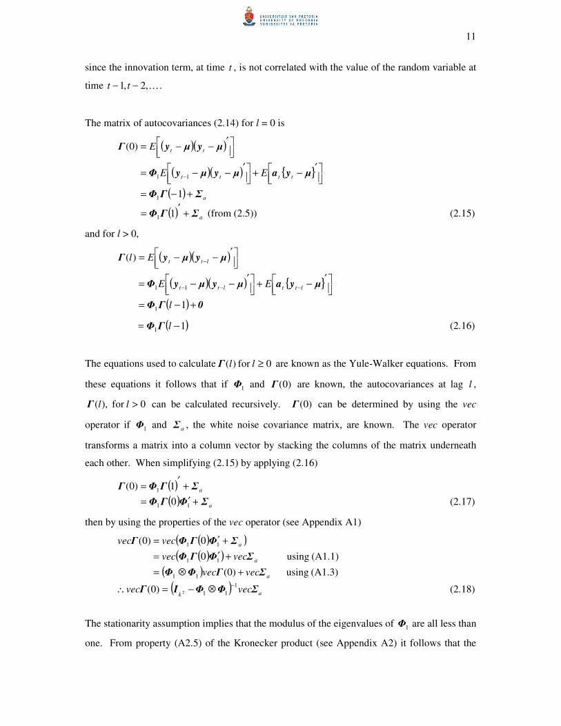
since the innovation term, at time t , is not correlated with the value of the random variable at
time K,2,1 −− tt .
The matrix of autocovariances (2.14) for l = 0 is
( )( )
( )( ) { }
( ) a
tttt
tt
EE
E
ΣΓΦ
µyaµyµyΦ
µyµyΓ
+−=
′
−+
′
−−=
′
−−=
−
1
)0(
1
11
( ) aΣΓΦ +′
= 11 (from (2.5)) (2.15)
and for l > 0,
( )( )
( )( ) { }
( ) 0ΓΦ
µyaµyµyΦ
µyµyΓ
+−=
′
−+
′
−−=
′
−−=
−−−
−
1
)(
1
11
l
EE
El
lttltt
ltt
( )11 −= lΓΦ (2.16)
The equations used to calculate 0for )( ≥llΓ are known as the Yule-Walker equations. From
these equations it follows that if 1Φ and )0(Γ are known, the autocovariances at lag l ,
0for ),( >llΓ can be calculated recursively. )0(Γ can be determined by using the vec
operator if 1Φ and aΣ , the white noise covariance matrix, are known. The vec operator
transforms a matrix into a column vector by stacking the columns of the matrix underneath
each other. When simplifying (2.15) by applying (2.16)
( ) aΣΓΦΓ +′
= 1)0( 1
( ) aΣΦΓΦ +′= 11 0 (2.17)
then by using the properties of the vec operator (see Appendix A1)
( )( )( )( )
( ) (A1.3) using )0(
(A1.1) using 0
0)0(
11
11
11
a
a
a
vecvec
vecvec
vecvec
ΣΓΦΦ
ΣΦΓΦ
ΣΦΓΦΓ
+⊗=
+′=
+′=
( ) akvecvec ΣΦΦIΓ
1
112)0(−
⊗−=∴ (2.18)
The stationarity assumption implies that the modulus of the eigenvalues of 1Φ are all less than
one. From property (A2.5) of the Kronecker product (see Appendix A2) it follows that the
12
eigenvalues of 11 ΦΦ ⊗ are just the product of the eigenvalues of 1Φ , therefore the modulus
of the eigenvalues of 11 ΦΦ ⊗ are also less than one. This implies that the inverse,
( ) 1
112
−⊗− ΦΦI
k, exists.
Explicit expression for )0(Γ
Consider the bivariate VAR(1) model ttt ayy +
= −1
2221
1211
φφ
φφ with
=
2212
1211
σσ
σσaΣ .
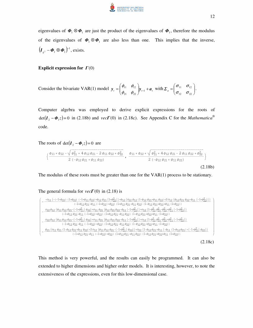
Computer algebra was employed to derive explicit expressions for the roots of
( ) 0det 12 =− zΦI in (2.18b) and )0(Γvec in (2.18c). See Appendix C for the Mathematica®
code.
The roots of ( ) 0det 12 =− zΦI are
: φ11+ φ22 −"##################### #### #### #### #### #### #### #####
φ112 + 4φ12φ21− 2 φ11 φ22+ φ22
2
2H−φ12φ21 +φ11 φ22L,
φ11+ φ22+"#################### #### #### #### #### #### #### #### ##
φ112 + 4φ12 φ21− 2 φ11φ22 +φ22
2
2H−φ12 φ21+ φ11φ22L>
(2.18b)
The modulus of these roots must be greater than one for the VAR(1) process to be stationary.
The general formula for )0(Γvec in (2.18) is
i
k
jjjjjjjjjjjjjjjjjjjjjjjjjjj
−−σ11I−H−1+φ22LH1+φ22L H−1+φ11φ22L+φ12φ21I1+φ222 MM+φ12Iσ22φ12H1−φ12φ21+φ11φ22L+2σ12 Iφ12φ21φ22−φ11 I−1+φ
222 MMM
H−1+φ12φ21−φ11H−1+φ22L+φ22LH1+φ12φ21−φ11φ22L H1−φ12φ21+φ22+φ11H1+φ22LL
−σ22φ12Iφ11φ12φ21−I−1+φ112 Mφ22M+σ11φ21Iφ12φ21φ22−φ11I−1+φ222 MM+σ12I1−φ122 φ
212 −φ
222 +φ
112 I−1+φ
222 MM
H−1+φ12φ21−φ11H−1+φ22L+φ22L H1+φ12φ21−φ11φ22L H1−φ12φ21+φ22+φ11H1+φ22LL
−σ22φ12Iφ11φ12φ21−I−1+φ112 Mφ22M+σ11φ21Iφ12φ21φ22−φ11I−1+φ222 MM+σ12I1−φ122 φ
212 −φ
222 +φ
112 I−1+φ
222 MM
H−1+φ12φ21−φ11H−1+φ22L+φ22L H1+φ12φ21−φ11φ22L H1−φ12φ21+φ22+φ11H1+φ22LL
−φ21Iσ11φ21H1−φ12φ21+φ11φ22L+2σ12Iφ11φ12φ21−I−1+φ112 Mφ22MM+σ22I1−φ12φ21+φ11I−φ11H1+φ12φ21L+I−1+φ112 Mφ22MM
H−1+φ12φ21−φ11H−1+φ22L+φ22LH1+φ12φ21−φ11φ22LH1−φ12φ21+φ22+φ11 H1+φ22LL
y
{
zzzzzzzzzzzzzzzzzzzzzzzzzzz
(2.18c)
This method is very powerful, and the results can easily be programmed. It can also be
extended to higher dimensions and higher order models. It is interesting, however, to note the
extensiveness of the expressions, even for this low-dimensional case.
13
Two examples for illustrating the calculation of the autocovariance matrices of a VAR(1)
model are given. The first one is numerical in nature, and illustrates the stationarity test, the
calculation of )0(Γ in terms of the vec operator and the use of the Yule-Walker equations for
the calculation of )1(Γ and )2(Γ for a two dimensional vector time series.
Example 2.2 provides an application of the explicit expressions derived in equations (2.18b)
and (2.18c). A spreadsheet is constructed where one just has to enter the coefficient matrix
and the white noise covariance matrix. Based on this information it will determine whether
the model is stationary and then calculate )0(Γ , )1(Γ and )2(Γ .
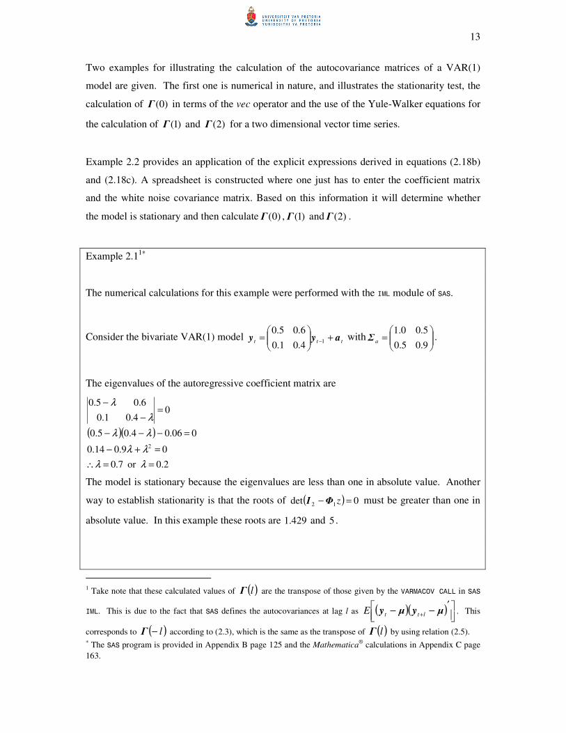
Example 2.11∗
The numerical calculations for this example were performed with the IML module of SAS.
Consider the bivariate VAR(1) model ttt ayy +
= −1
4.01.0
6.05.0 with
=
9.05.0
5.00.1aΣ .
The eigenvalues of the autoregressive coefficient matrix are
( )( )
2.0or 7.0
09.014.0
006.04.05.0
04.01.0
6.05.0
2
==∴
=+−
=−−−
=−
−
λλ
λλ
λλ
λ
λ
The model is stationary because the eigenvalues are less than one in absolute value. Another
way to establish stationarity is that the roots of ( ) 0det 12 =− zΦI must be greater than one in
absolute value. In this example these roots are 429.1 and 5 .
1 Take note that these calculated values of ( )lΓ are the transpose of those given by the VARMACOV CALL in SAS
IML. This is due to the fact that SAS defines the autocovariances at lag l as ( )( )
′
−− + µyµy lttE . This
corresponds to ( )l−Γ according to (2.3), which is the same as the transpose of ( )lΓ by using relation (2.5). ∗ The SAS program is provided in Appendix B page 125 and the Mathematica
® calculations in Appendix C page
163.
14
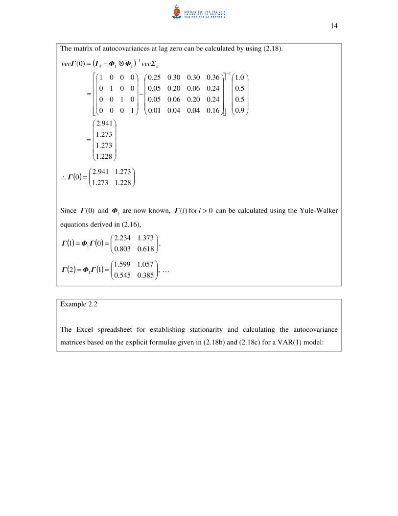
The matrix of autocovariances at lag zero can be calculated by using (2.18).
( )
=
−
=
⊗−=
−
−
228.1
273.1
273.1
941.2
9.0
5.0
5.0
0.1
16.004.004.001.0
24.020.006.005.0
24.006.020.005.0
36.030.030.025.0
1000
0100
0010
0001
)0(
1
1
114 avecvec ΣΦΦIΓ
( )
=∴
228.1273.1
273.1941.20Γ
Since )0(Γ and 1Φ are now known, 0for )( >llΓ can be calculated using the Yule-Walker
equations derived in (2.16),
( ) ( )
==
618.0803.0
373.1234.201 1ΓΦΓ ,
( ) ( )
==
385.0545.0
057.1599.112 1ΓΦΓ , K
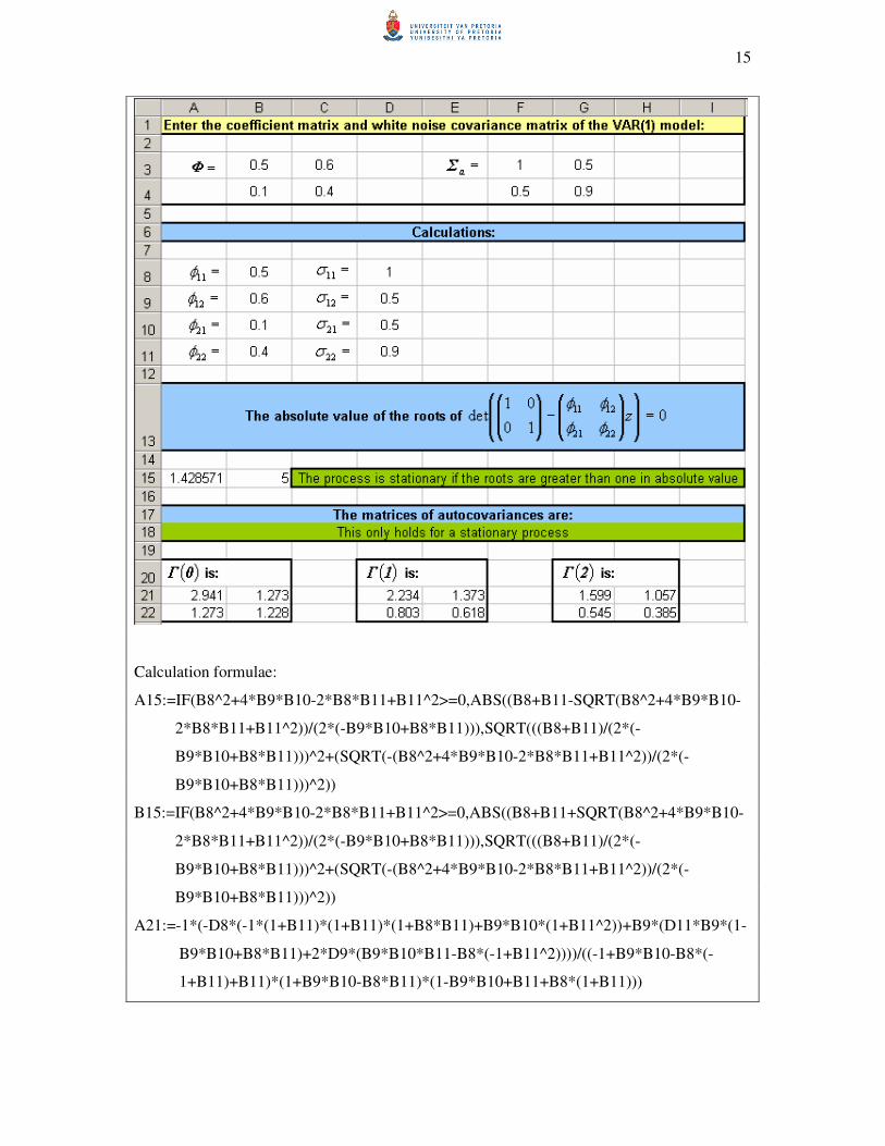
Example 2.2
The Excel spreadsheet for establishing stationarity and calculating the autocovariance
matrices based on the explicit formulae given in (2.18b) and (2.18c) for a VAR(1) model:
15
Calculation formulae:
A15:=IF(B8^2+4*B9*B10-2*B8*B11+B11^2>=0,ABS((B8+B11-SQRT(B8^2+4*B9*B10-
2*B8*B11+B11^2))/(2*(-B9*B10+B8*B11))),SQRT(((B8+B11)/(2*(-
B9*B10+B8*B11)))^2+(SQRT(-(B8^2+4*B9*B10-2*B8*B11+B11^2))/(2*(-
B9*B10+B8*B11)))^2))
B15:=IF(B8^2+4*B9*B10-2*B8*B11+B11^2>=0,ABS((B8+B11+SQRT(B8^2+4*B9*B10-
2*B8*B11+B11^2))/(2*(-B9*B10+B8*B11))),SQRT(((B8+B11)/(2*(-
B9*B10+B8*B11)))^2+(SQRT(-(B8^2+4*B9*B10-2*B8*B11+B11^2))/(2*(-
B9*B10+B8*B11)))^2))
A21:=-1*(-D8*(-1*(1+B11)*(1+B11)*(1+B8*B11)+B9*B10*(1+B11^2))+B9*(D11*B9*(1-
B9*B10+B8*B11)+2*D9*(B9*B10*B11-B8*(-1+B11^2))))/((-1+B9*B10-B8*(-
1+B11)+B11)*(1+B9*B10-B8*B11)*(1-B9*B10+B11+B8*(1+B11)))
16
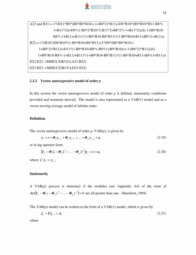
A22 and B21:=-1*(D11*B9*(B8*B9*B10-(-1+B8^2)*B11)+D8*B10*(B9*B10*B11-B8*(-
1+B11^2))+D9*(1-B9^2*B10^2-B11^2+B8^2*(-1+B11^2)))/((-1+B9*B10-
B8*(-1+B11)+B11)*(1+B9*B10-B8*B11)*(1-B9*B10+B11+B8*(1+B11)))
B22:=-1*(B10*(D8*B10*(1-B9*B10+B8*B11)+2*D9*(B8*B9*B10-(-
1+B8^2)*B11))+D11*(1-B9*B10+B8*(-B8*(1+B9*B10)+(-1+B8^2)*B11)))/((-
1+B9*B10-B8*(-1+B11)+B11)*(1+B9*B10-B8*B11)*(1-B9*B10+B11+B8*(1+B11)))
D21:E22: =MMULT(B3:C4,A21:B22)
G21:H22 :=MMULT(B3:C4,D21:E22)
2.3.2 Vector autoregressive model of order p
In this section the vector autoregressive model of order p is defined, stationarity conditions
provided and moments derived. The model is also represented as a VAR(1) model and as a
vector moving average model of infinite order.
Definition
The vector autoregressive model of order p, VAR(p), is given by
tptpttt ayΦyΦyΦcy +++++= −−− K2211 (2.19)
or in lag operator form
( ) tacyΦΦΦI +=−−−− t
p
pk LLL K2
21 (2.20)
where jtt
jL −= yy
Stationarity
A VAR(p) process is stationary if the modulus (see Appendix A4) of the roots of
( ) 0det 2
21 =−−−− p
pk zzz ΦΦΦI K are all greater than one. (Hamilton, 1994)
The VAR(p) model can be written in the form of a VAR(1) model, which is given by
ttt AFξξ += −1 (2.21)
where

17
−
−
−
=×
+−
−
µy
µy
µy
ξ
1
11:
pt
t
t
t kpM
=×
−
0I00
00I0
000I
ΦΦΦΦ
F
k
k
k
pp
kpkp
K
MMOMM
K
K
K 121
:
=×
0
0
a
A
t
M1: kpt
with ( ) A
a
tt kpkpE Σ
000
000
00Σ
AA =
=×′
L
MMMM
L
L
: and
( ) 0AA =′stE for st ≠ .
In the previous section we mentioned that a VAR(1) process is stationary if the eigenvalues of
the coefficient matrix, 1Φ , have modulus less than one. Since the VAR(p) model can be
represented as a VAR(1) model it follows that in order for the process to be stationary all the
eigenvalues of F must have modulus less than one.
Moments
Assume that { }ty is a stationary VAR(p) process. The VAR(p) model can be written in terms
of the deviations from the mean
( ) ( ) ( ) ( ) tptpttt aµyΦµyΦµyΦµy +−++−+−=− −−− K2211 (2.22)
To determine the Yule-Walker equations for )0(Γ and 0 ),( >llΓ we need to postmultiply
(2.22) with ( )′−− µy lt and take the expected value thereof, thus
18
( )( ) ( )( ) ( )( )
′
−−++
′
−−=
′
−− −−−−− µyµyΦµyµyΦµyµy ltptplttltt EEE K11
( )
′
−+ − µya lttE (2.23)
The matrix of autocovariances (2.23) for 0=l is
( )( )
( )( ) ( )( ) ( )
ap
tttptptt
tt
p
EEE
E
ΣΓΦΓΦ
µyaµyµyΦµyµyΦ
µyµyΓ
+−++−=
′
−+
′
−−++
′
−−=
′
−−=
−−
)()1(
)0(
1
11
K
K
ap p ΣΓΦΓΦ +′++′= )()1(1 K (from (2.5)) (2.24)
and for 0>l ,
)()1()( 1 plll p −++−= ΓΦΓΦΓ K (2.25)
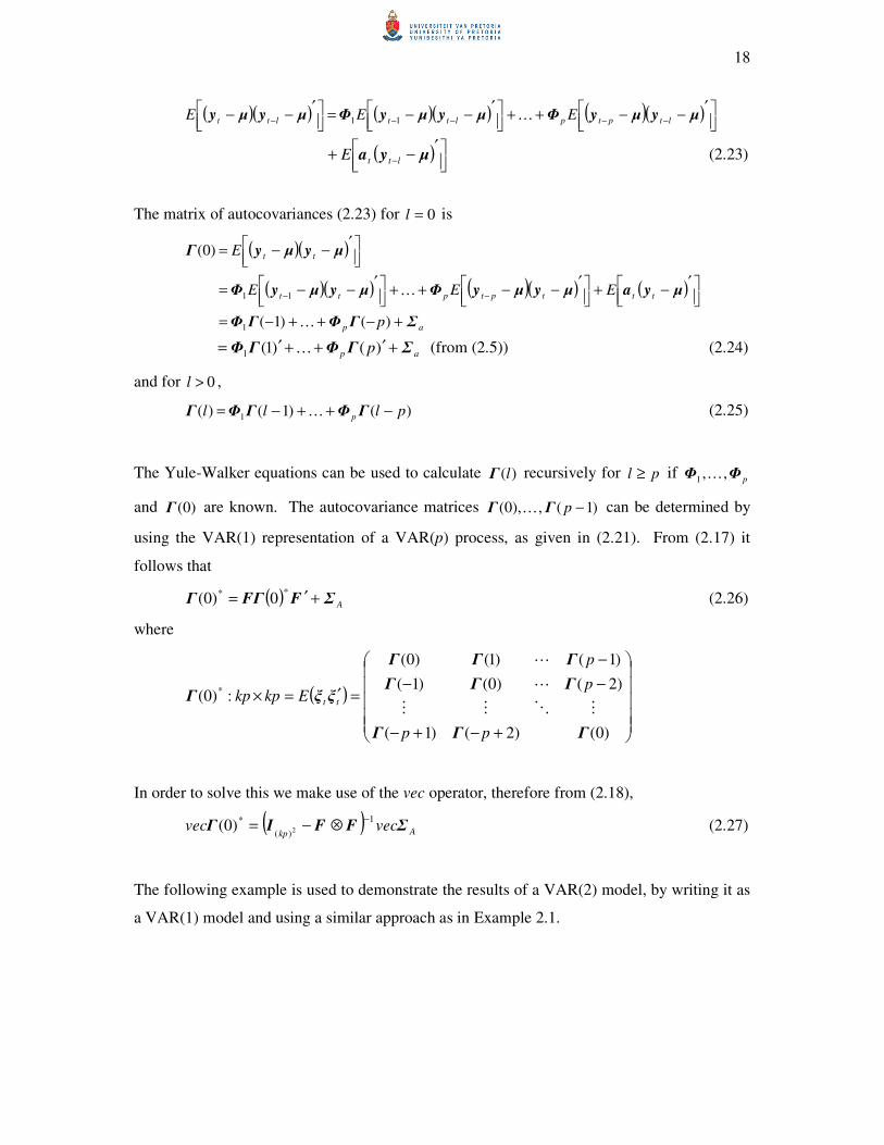
The Yule-Walker equations can be used to calculate )(lΓ recursively for pl ≥ if pΦΦ ,,1 K
and )0(Γ are known. The autocovariance matrices )1(,),0( −pΓΓ K can be determined by
using the VAR(1) representation of a VAR(p) process, as given in (2.21). From (2.17) it
follows that
( ) AΣFFΓΓ +′=** 0)0( (2.26)
where
( )
+−+−
−−
−
=′=×
)0()2()1(
)2()0()1(
)1()1()0(
:)0(*
ΓΓΓ
ΓΓΓ
ΓΓΓ
ξξΓ
pp
p
p
Ekpkp ttMOMM
L
L
In order to solve this we make use of the vec operator, therefore from (2.18),
( ) Akpvecvec ΣFFIΓ
1
)(
*2)0(
−⊗−= (2.27)
The following example is used to demonstrate the results of a VAR(2) model, by writing it as
a VAR(1) model and using a similar approach as in Example 2.1.
19
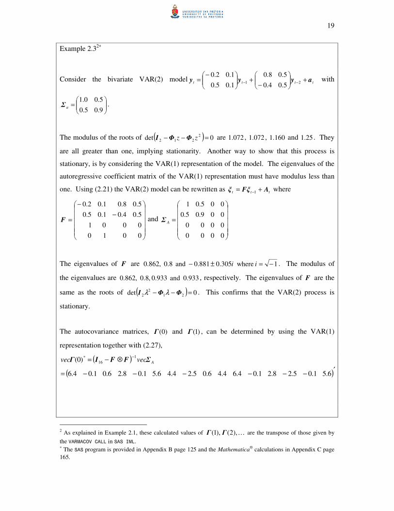
Example 2.32∗
Consider the bivariate VAR(2) modeltttt ayyy +
−+
−= −− 21
5.04.0
5.08.0
1.05.0
1.02.0 with
=
9.05.0
5.00.1aΣ .
The modulus of the roots of ( ) 0det2
212 =−− zz ΦΦI are 072.1 , 072.1 , 160.1 and 25.1 . They
are all greater than one, implying stationarity. Another way to show that this process is
stationary, is by considering the VAR(1) representation of the model. The eigenvalues of the
autoregressive coefficient matrix of the VAR(1) representation must have modulus less than
one. Using (2.21) the VAR(2) model can be rewritten as ttt AFξξ += −1 where
−
−
=
0010
0001
5.04.01.05.0
5.08.01.02.0
F and
=
0000
0000
009.05.0
005.01
AΣ
The eigenvalues of F are 1 where305.0881.0 and 8.0 ,862.0 −=±− ii . The modulus of
the eigenvalues are 933.0 and 933.0 ,8.0 ,862.0 , respectively. The eigenvalues of F are the
same as the roots of ( ) 0det 21
2
2 =−− ΦΦI λλ . This confirms that the VAR(2) process is
stationary.
The autocovariance matrices, )0(Γ and )1(Γ , can be determined by using the VAR(1)
representation together with (2.27),
( )
( )′−−−−−−=
⊗−=−
6.51.05.28.21.04.64.46.05.24.46.51.08.26.01.04.6
)0(1
16
*
Avecvec ΣFFIΓ
2 As explained in Example 2.1, these calculated values of K ),2( ),1( ΓΓ are the transpose of those given by
the VARMACOV CALL in SAS IML. ∗ The SAS program is provided in Appendix B page 125 and the Mathematica
® calculations in Appendix C page
165.
20
−−
−
−−
−
=
−=∴
6.51.05.28.2
1.04.64.46.0
5.24.46.51.0
8.26.01.04.6
)0()1(
)1()0()0(
*
ΓΓ
ΓΓΓ
5.24.4
8.26.0)1( and
6.51.0
1.04.6)0(
−=
−
−=∴ ΓΓ
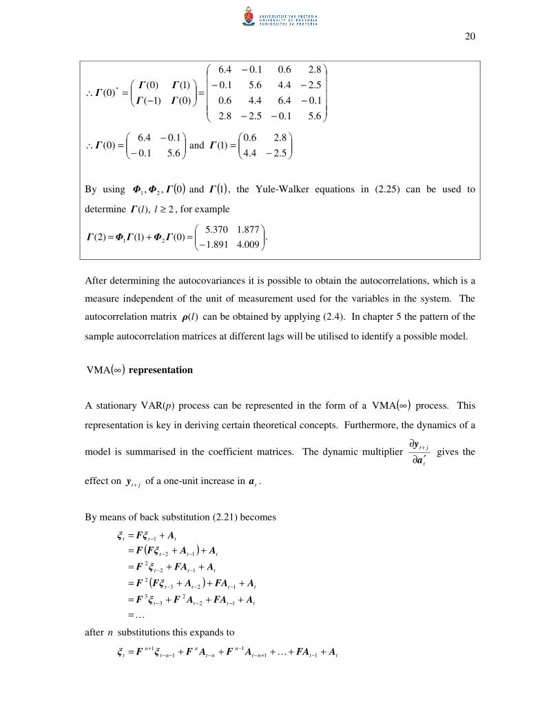
By using ( ) ( )1 and 0 , , 21 ΓΓΦΦ , the Yule-Walker equations in (2.25) can be used to
determine 2 ),( ≥llΓ , for example
−=+=
009.4891.1
877.1370.5)0()1()2( 21 ΓΦΓΦΓ .
After determining the autocovariances it is possible to obtain the autocorrelations, which is a
measure independent of the unit of measurement used for the variables in the system. The
autocorrelation matrix )(lρ can be obtained by applying (2.4). In chapter 5 the pattern of the
sample autocorrelation matrices at different lags will be utilised to identify a possible model.
( )∞VMA representation
A stationary VAR(p) process can be represented in the form of a ( )∞VMA process. This
representation is key in deriving certain theoretical concepts. Furthermore, the dynamics of a
model is summarised in the coefficient matrices. The dynamic multiplier t
jt
a
y
′∂
∂ + gives the
effect on jt +y of a one-unit increase in ta .
By means of back substitution (2.21) becomes
( )
( )
K=
+++=
+++=
++=
++=
+=
−−−
−−−
−−
−−
−
tttt
tttt
ttt
ttt
ttt
AFAAFξF
AFAAFξF
AFAξF
AAFξF
AFξξ
12
2
3
3
123
2
12
2
12
1
after n substitutions this expands to
ttnt
n
nt
n
nt
n
t AFAAFAFξFξ +++++= −+−
−
−−−
+
11
1
1
1K

21
The first k rows of tξ are
( ) ( ) ( ) 1
1
11211
2
111
1
−−
+
−−− +++++=− nt
n
nt
n
tttt ξFaFaFaFaµy K
where ( )11
1F is the row 1 column 1 submatrix of 1
F . From the stationarity assumption it
follows that 0F →+1n as ∞→n , therefore
K++++= −− 2211 tttt aΨaΨaµy
tL aΨµ )(+= (2.28)
where K+++= 2
21)( LLL ΨΨIΨ with ( ) ( ) K , , 11
2
211
1
1 FΨFΨ ==
The moving average coefficient matrices, jΨ , can be calculated by writing (2.20) in terms of
deviations from the mean form,
( )( ) taµyΦΦΦI =−−−−− t
p
pk LLL K2
21
( ) taµyΦ =−tL)( (2.29)
where ( )p
pk LLLL ΦΦΦIΦ −−−−= K2
21)( .
Then, by operating both sides of (2.29) with )(LΨ ,
( ) taΨµyΦΨ )()()( LLL t =−
but from (2.28),
( ) taΨµy )(Lt =−
therefore
)()()()( 1LLLL k ΦΦIΦΨ −== (2.30)
[ ] 1)()(
−=∴ LL ΦΨ
To obtain the coefficient matrices of the ( )∞VMA representation we make use of (2.30),
( )( ) kk
p
pk LLLLL IΨΨIΦΦΦI =+++−−−− KK2
21
2
21
Grouping the coefficients of jL and setting them equal to zero,
02211
312213122133
21121122
1111
ΨΦΨΦΨΦΨ
ΦΨΦΨΦΨ0ΨΦΨΦΦΨ
ΦΨΦΨ0ΨΦΦΨ
ΦΨ0ΦΨ
jjjj +++=
++=∴=−−−
+=∴=−−
=∴=−
−− K
M
where kIΨ =0 .
22
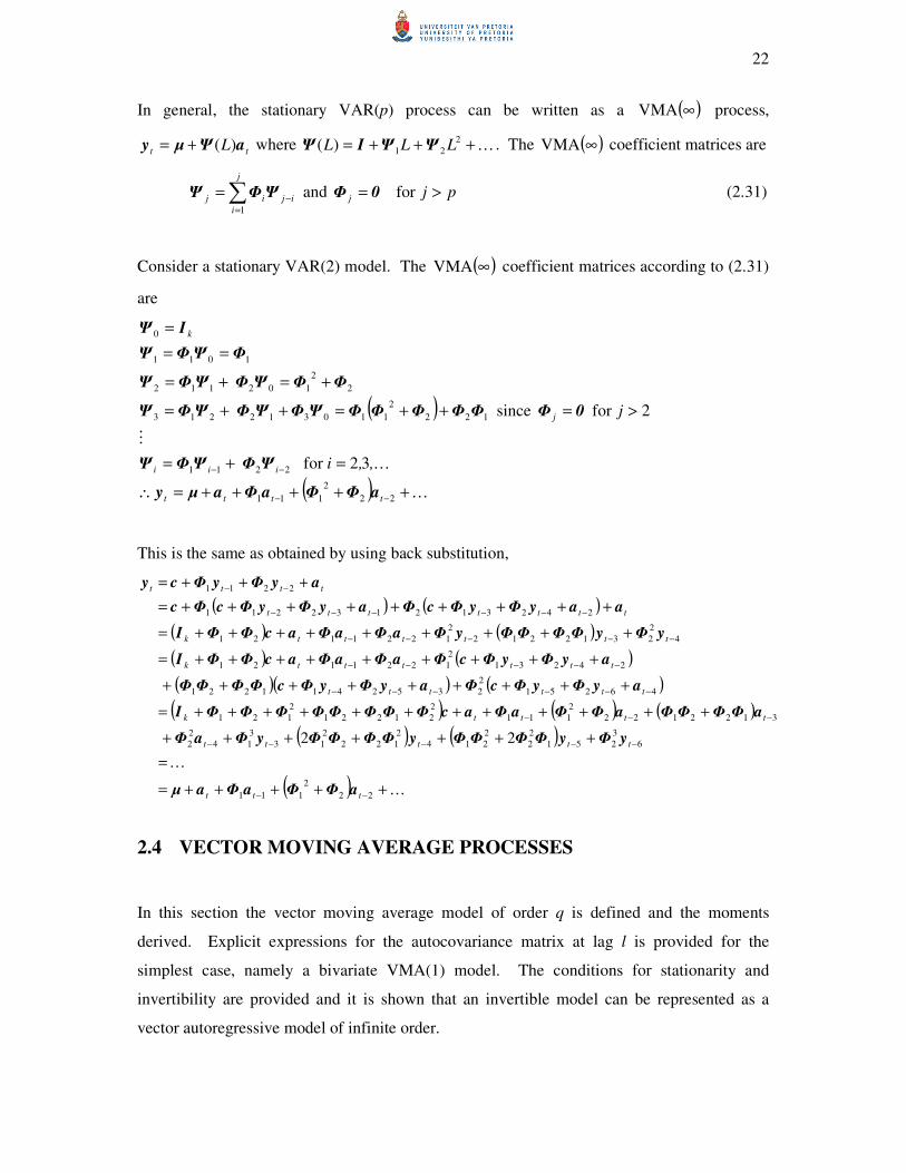
In general, the stationary VAR(p) process can be written as a ( )∞VMA process,
tt L aΨµy )(+= where K+++= 2
21)( LLL ΨΨIΨ . The ( )∞VMA coefficient matrices are
∑=
−=j
i
ijij
1
ΨΦΨ and pjj >= for 0Φ (2.31)
Consider a stationary VAR(2) model. The ( )∞VMA coefficient matrices according to (2.31)
are
( )
( ) K
K
M
+++++=∴
=+=
>=++=++=
+=+=
==
=
−−
−−
22
2
111
2211
122
2
110312213
2
2
102112
1011
0
32for
2for since
tttt
iii
j
k
,, i
j
aΦΦaΦaµy
ΨΦΨΦΨ
0ΦΦΦΦΦΦΨΦΨΦΨΦΨ
ΦΦΨΦΨΦΨ
ΦΨΦΨ
IΨ
This is the same as obtained by using back substitution,
( ) ( )
( ) ( )
( ) ( )
( )( ) ( )
( ) ( ) ( )
( ) ( )
( ) K
K
+++++=
=
+++++++
++++++++++++=
+++++++++
+++++++++=
+++++++++=
+++++++++=
+++=
−−
−−−−−
−−−
−−−−−−
−−−−−
−−−−−
−−−−−−
−−
22
2
111
6
3
251
2
2
2
214
2
122
2
13
3
14
2
2
3122122
2
111
2
21221
2
121
46251
2
2352411221
24231
2
1221121
4
2
2312212
2
1221121
242312132211
2211
22
ttt
ttttt
ttttk
tttttt
ttttttk
ttttttk
ttttttt
tttt
aΦΦaΦaµ
yΦyΦΦΦΦyΦΦΦΦyΦaΦ
aΦΦΦΦaΦΦaΦacΦΦΦΦΦΦΦΦI
ayΦyΦcΦayΦyΦcΦΦΦΦ
ayΦyΦcΦaΦaΦacΦΦI
yΦyΦΦΦΦyΦaΦaΦacΦΦI
aayΦyΦcΦayΦyΦcΦc
ayΦyΦcy
2.4 VECTOR MOVING AVERAGE PROCESSES
In this section the vector moving average model of order q is defined and the moments
derived. Explicit expressions for the autocovariance matrix at lag l is provided for the
simplest case, namely a bivariate VMA(1) model. The conditions for stationarity and
invertibility are provided and it is shown that an invertible model can be represented as a
vector autoregressive model of infinite order.
23
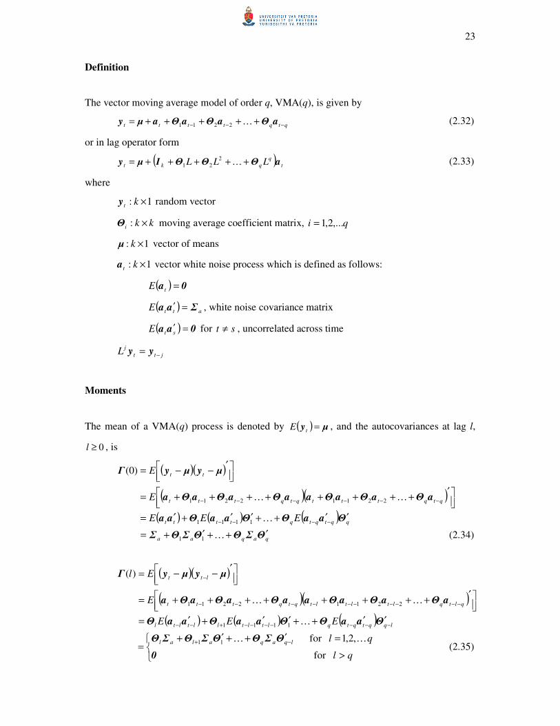
Definition
The vector moving average model of order q, VMA(q), is given by
qtqtttt −−− +++++= aΘaΘaΘaµy K2211 (2.32)
or in lag operator form
( ) t
q
qkt LLL aΘΘΘIµy +++++= K2
21 (2.33)
where
1: ×kty random vector
kki ×:Θ moving average coefficient matrix, qi ,...2,1=
1: ×kµ vector of means
1: ×kta vector white noise process which is defined as follows:
( ) 0a =tE
( ) attE Σaa =′ , white noise covariance matrix
( ) 0aa =′stE for st ≠ , uncorrelated across time
jtt
jL −= yy
Moments
The mean of a VMA(q) process is denoted by ( ) µy =tE , and the autocovariances at lag l,
0≥l , is
( )( )
( )( )
( ) ( ) ( )qqtqtqtttt
qtqtttqtqttt
tt
EEE
E
E
ΘaaΘΘaaΘaa
aΘaΘaΘaaΘaΘaΘa
µyµyΓ
′′++′′+′=
′
++++++++=
′
−−=
−−−−
−−−−−−
K
KK
1111
22112211
)0(
qaqaa ΘΣΘΘΣΘΣ ′++′+= K11 (2.34)
( )( )
( )( )
( ) ( ) ( )lqqtqtqltltlltltl
qltqltltltqtqttt
ltt
EEE
E
El
−−−−−−−+−−
−−−−−−−−−−
−
′′++′′+′=
′
++++++++=
′
−−=
ΘaaΘΘaaΘaaΘ
aΘaΘaΘaaΘaΘaΘa
µyµyΓ
K
KK
1111
22112211
)(
>
=′++′+=
−+
for
,2,1 for 11
q l
qllqaqalal
0
ΘΣΘΘΣΘΣΘ KK (2.35)
24
The autocovariances, ( )lΓ , for 0<l can be determined by making use of the relationship
derived in (2.5), namely that ( ) ( )′=− ll ΓΓ .
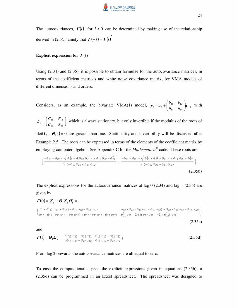
Explicit expression for )(lΓ
Using (2.34) and (2.35), it is possible to obtain formulae for the autocovariance matrices, in
terms of the coefficient matrices and white noise covariance matrix, for VMA models of
different dimensions and orders.
Considers, as an example, the bivariate VMA(1) model, 1
2221
1211
−
+= ttt aay
θθ
θθ with
=
2212
1211
σσ
σσaΣ , which is always stationary, but only invertible if the modulus of the roots of
( ) 0det 12 =+ zΘI are greater than one. Stationarity and invertibility will be discussed after
Example 2.5. The roots can be expressed in terms of the elements of the coefficient matrix by
employing computer algebra. See Appendix C for the Mathematica®
code. These roots are
: −θ11− θ22−"########## #### #### #### #### #### #### #### ############
θ112 + 4θ12 θ21− 2θ11θ22 +θ22
2
2H−θ12θ21+ θ11 θ22L,
−θ11− θ22 +"########### #### #### #### #### #### #### #### ###########
θ112 +4θ12 θ21− 2θ11 θ22+ θ22
2
2H−θ12θ21 +θ11 θ22L>
(2.35b)
The explicit expressions for the autocovariance matrices at lag 0 (2.34) and lag 1 (2.35) are
given by
( ) =′+= 110 ΘΣΘΣΓ aa
ikjjH1+ θ11
2 L σ11 + θ12H2θ11 σ12+ θ12σ22L σ12 +θ21 Hθ11σ11 + θ12σ12L+ θ22 Hθ11σ12 +θ12 σ22Lσ12 +θ11 Hθ21σ11 + θ22σ12L+ θ12 Hθ21σ12 +θ22 σ22L θ21
2 σ11+ 2θ21θ22 σ12+ H1+ θ222 L σ22
y{zz
(2.35c)
and
( ) == aΣΘΓ 11 (2.35d)
From lag 2 onwards the autocovariance matrices are all equal to zero.
To ease the computational aspect, the explicit expressions given in equations (2.35b) to
(2.35d) can be programmed in an Excel spreadsheet. The spreadsheet was designed to
Jθ11 σ11+ θ12σ12 θ11 σ12+ θ12σ22
θ21 σ11+ θ22σ12 θ21 σ12+ θ22σ22N

25
calculate the autocovariances once the coefficient matrix and the white noise covariance
matrix have been entered. This is illustrated in Example 2.4.
Example 2.4
The Excel spreadsheet for establishing invertibility and calculating the autocovariance
matrices based on the explicit formulae given in (2.35b) to (2.35d) for a VMA(1) model:
Calculation formulae:
A15:=IF(B8^2+4*B9*B10-2*B8*B11+B11^2>=0,ABS((-B8-B11-SQRT(B8^2+4*B9*B10-
2*B8*B11+B11^2))/(2*(-B9*B10+B8*B11))),SQRT(((-B8-B11)/(2*(-
B9*B10+B8*B11)))^2+(SQRT(-(B8^2+4*B9*B10-2*B8*B11+B11^2))/(2*(-
B9*B10+B8*B11)))^2))
26
B15:=IF(B8^2+4*B9*B10-2*B8*B11+B11^2>=0,ABS((-B8-B11+SQRT(B8^2+4*B9*B10-
2*B8*B11+B11^2))/(2*(-B9*B10+B8*B11))),SQRT(((-B8-B11)/(2*(-
B9*B10+B8*B11)))^2+(SQRT(-(B8^2+4*B9*B10-2*B8*B11+B11^2))/(2*(-
B9*B10+B8*B11)))^2))
A20:=(1+B8^2)*D8+B9*(2*B8*D9+B9*D11)
A21 and B20:=D9+B10*(B8*D8+B9*D9)+B11*(B8*D9+B9*D11)
B21:=B10^2*D8+2*B10*B11*D9+(1+B11^2)*D11
D20:=B8*D8+B9*D9
D21:=B10*D8+B11*D9
E20:=B8*D9+B9*D11
E21:=B10*D9+B11*D11
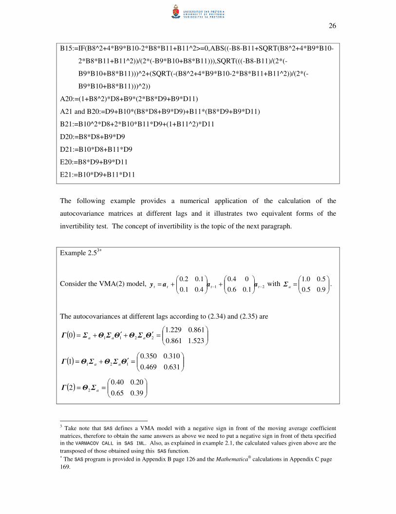
The following example provides a numerical application of the calculation of the
autocovariance matrices at different lags and it illustrates two equivalent forms of the
invertibility test. The concept of invertibility is the topic of the next paragraph.
Example 2.53∗
Consider the VMA(2) model, 21
1.06.0
04.0
4.01.0
1.02.0−−
+
+= tttt aaay with
=
9.05.0
5.00.1aΣ .
The autocovariances at different lags according to (2.34) and (2.35) are
( )
=′+′+=
523.1861.0
861.0229.10 2211 ΘΣΘΘΣΘΣΓ aaa
( )
=′+=
631.0469.0
310.0350.01 121 ΘΣΘΣΘΓ aa
( )
==
39.065.0
20.040.02 2 aΣΘΓ
3 Take note that SAS defines a VMA model with a negative sign in front of the moving average coefficient
matrices, therefore to obtain the same answers as above we need to put a negative sign in front of theta specified
in the VARMACOV CALL in SAS IML. Also, as explained in example 2.1, the calculated values given above are the
transposed of those obtained using this SAS function. ∗ The SAS program is provided in Appendix B page 126 and the Mathematica
® calculations in Appendix C page
169.

27
( )
=>
00
002for llΓ
The roots of ( ) 0det 2
212 =++ zz ΘΘI are i942.2987.0 ±− and i528.1513.0 ±− with
modulus 103.3 , 103.3 , 611.1 and 611.1 , respectively. These are greater than one, which
implies that the model is invertible. The condition that the modulus of the roots of
( ) 0det 2
212 =++ zz ΘΘI must be greater than one is equivalent to the modulus of the roots of
( ) 0det 21
2
2 =−− ΘΘI λλ being less than one. The latter are 0.875 and 425.0 ,229.0 ,471.0 .
Stationarity and Invertibility
Neither the vector of means nor the autocovariance matrices depend on time, implying that all
VMA(q) processes are stationary. In Section 2.3.2 it was shown that a VAR(p) process can
be expressed as a ( )∞VMA process, only if the stationariaty condition was met, in other
words when the modulus of the roots of ( ) 0det 2
21 =−−−− p
pk zzz ΦΦΦI K were all
greater than one. The next paragraph represents a VMA(q) process in the form of a ( )∞VAR
process. This is only possible when the modulus of the roots of
( ) 0det 2
21 =++++ q
qk zzz ΘΘΘI K are all greater than one. A VMA(q) process that
satisfies this condition is called invertible.
An invertible VMA(q) process can be written as a ( )∞VAR process, namely
( ) ttL aµyΠ =−)( , since
( ) t
q
qkt LLL aΘΘΘIµy ++++=− ...2
21
tt L aΘµy )(=− (2.36)
where ( )q
qk LLLL ΘΘΘIΘ ++++= ...)( 2
21 .
Then, by operating on both sides of (2.36) with )(LΠ ,
( ) tt LLL aΘΠµyΠ )()()( =−
but the ( )∞VAR representation is given by ( ) )( ttL aµyΠ =− , therefore
)()()()( 1LLLL k ΘΘIΘΠ −== (2.37)
[ ] 1)()(
−=∴ LL ΘΠ
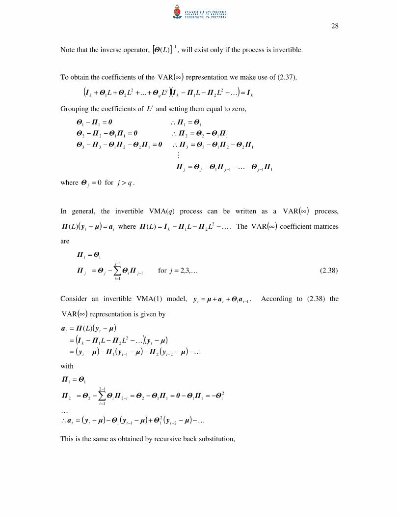
28
Note that the inverse operator, [ ] 1)(
−LΘ , will exist only if the process is invertible.
To obtain the coefficients of the ( )∞VAR representation we make use of (2.37),
( )( ) kk
q
qk LLLLL IΠΠIΘΘΘI =−−−++++ K2
21
2
21 ...
Grouping the coefficients of jL and setting them equal to zero,
1111
122133122133
11221122
1111
ΠΘΠΘΘΠ
ΠΘΠΘΘΠ0ΠΘΠΘΠΘ
ΠΘΘΠ0ΠΘΠΘ
ΘΠ0ΠΘ
−− −−−=
−−=∴=−−−
−=∴=−−
=∴=−
jjjj K
M
where 0=jΘ for qj > .
In general, the invertible VMA(q) process can be written as a ( )∞VAR process,
( ) ttL aµyΠ =−)( where K−−−= 2
21)( LLL k ΠΠIΠ . The ( )∞VAR coefficient matrices
are
11 ΘΠ =
K,, jj
i
ijijj 32for 1
1
=−= ∑−
=
−ΠΘΘΠ (2.38)
Consider an invertible VMA(1) model, 11 −++= ttt aΘaµy . According to (2.38) the
( )∞VAR representation is given by
( )
( )( )( ) ( ) ( ) K
K
−−−−−−=
−−−−=
−=
−− µyΠµyΠµy
µyΠΠI
µyΠa
2211
2
21
)(
ttt
tk
tt
LL
L
with
L
2
111112
12
1
222
11
ΘΠΘ0ΠΘΘΠΘΘΠ
ΘΠ
−=−=−=−=
=
∑−
=
−
i
ii
( ) ( ) ( ) K−−+−−−=∴ −− µyΘµyΘµya 2
2
111 tttt
This is the same as obtained by recursive back substitution,
29
( )( ) ( )[ ]
( ) ( )
( ) ( ) ( )[ ]
( ) ( ) ( )
( ) ( ) ( ) ( ) K
L
+−−−+−−−=
=
−−+−−−=
−−+−−−=
+−−−=
−−−−=
−−=
−−−
−−−
−−−
−−
−−
−
µyΘµyΘµyΘµy
aΘµyΘµyΘµy
aΘµyΘµyΘµy
aΘµyΘµy
aΘµyΘµy
aΘµya
3
3
12
2
111
3
3
12
2
111
312
2
111
2
2
111
2111
11
tttt
tttt
tttt
ttt
ttt
ttt
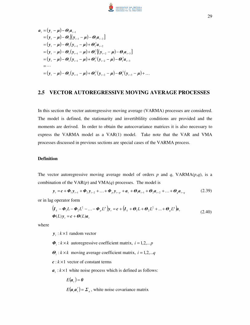
2.5 VECTOR AUTOREGRESSIVE MOVING AVERAGE PROCESSES
In this section the vector autoregressive moving average (VARMA) processes are considered.
The model is defined, the stationarity and invertiblility conditions are provided and the
moments are derived. In order to obtain the autocovariance matrices it is also necessary to
express the VARMA model as a VAR(1) model. Take note that the VAR and VMA
processes discussed in previous sections are special cases of the VARMA process.
Definition
The vector autoregressive moving average model of orders p and q, VARMA(p,q), is a
combination of the VAR(p) and VMA(q) processes. The model is
qtqtttptpttt −−−−−− +++++++++= aΘaΘaΘayΦyΦyΦcy KK 22112211 (2.39)
or in lag operator form
( ) ( )
tt
t
q
qkt
p
pk
LL
LLLLLL
aΘcyΦ
aΘΘΘIcyΦΦΦI
)()(
...2
21
2
21
+=
+++++=−−−− K (2.40)
where
1: ×kty random vector
kki ×:Φ autoregressive coefficient matrix, pi ,...2,1=
kki ×:Θ moving average coefficient matrix, qi ,...2,1=
1: ×kc vector of constant terms
1: ×kta white noise process which is defined as follows:
( ) 0a =tE
( ) attE Σaa =′ , white noise covariance matrix
30
( ) 0aa =′stE for st ≠ , uncorrelated across time.
jtt
jL −= yy
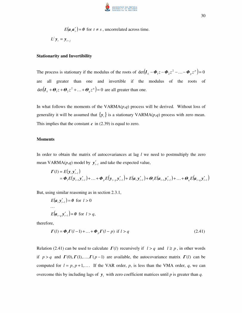
Stationarity and Invertibility
The process is stationary if the modulus of the roots of ( ) 0det 2
21 =−−−− p
pk zzz ΦΦΦI K
are all greater than one and invertible if the modulus of the roots of
( ) 0det 2
21 =++++ q
qk zzz ΘΘΘI K are all greater than one.
In what follows the moments of the VARMA(p,q) process will be derived. Without loss of
generality it will be assumed that { }ty is a stationary VARMA(p,q) process with zero mean.
This implies that the constant c in (2.39) is equal to zero.
Moments
In order to obtain the matrix of autocovariances at lag l we need to postmultiply the zero
mean VARMA(p,q) model by lt−
′y and take the expected value,
( )( ) ( ) ( ) ( ) ( )
ltqtqlttlttltptpltt
ltt
EEEEE
El
−−−−−−−−−
−
′++′+′+′++′=
′=
yaΘyaΘyayyΦyyΦ
yyΓ
KK 1111
)(
But, using similar reasoning as in section 2.3.1,
( )
( ) ,for
0for
qlE
lE
ltqt
ltt
>=′
>=′
−−
−
0ya
0ya
L
therefore,
qlplll p >−++−= if )()1()( 1 ΓΦΓΦΓ K (2.41)
Relation (2.41) can be used to calculate )(lΓ recursively if ql > and pl ≥ , in other words
if qp > and )1(,),1(),0( −pΓΓΓ K are available, the autocovariance matrix )(lΓ can be
computed for K,1, += ppl . If the VAR order, p, is less than the VMA order, q, we can
overcome this by including lags of ty with zero coefficient matrices until p is greater than q.
31
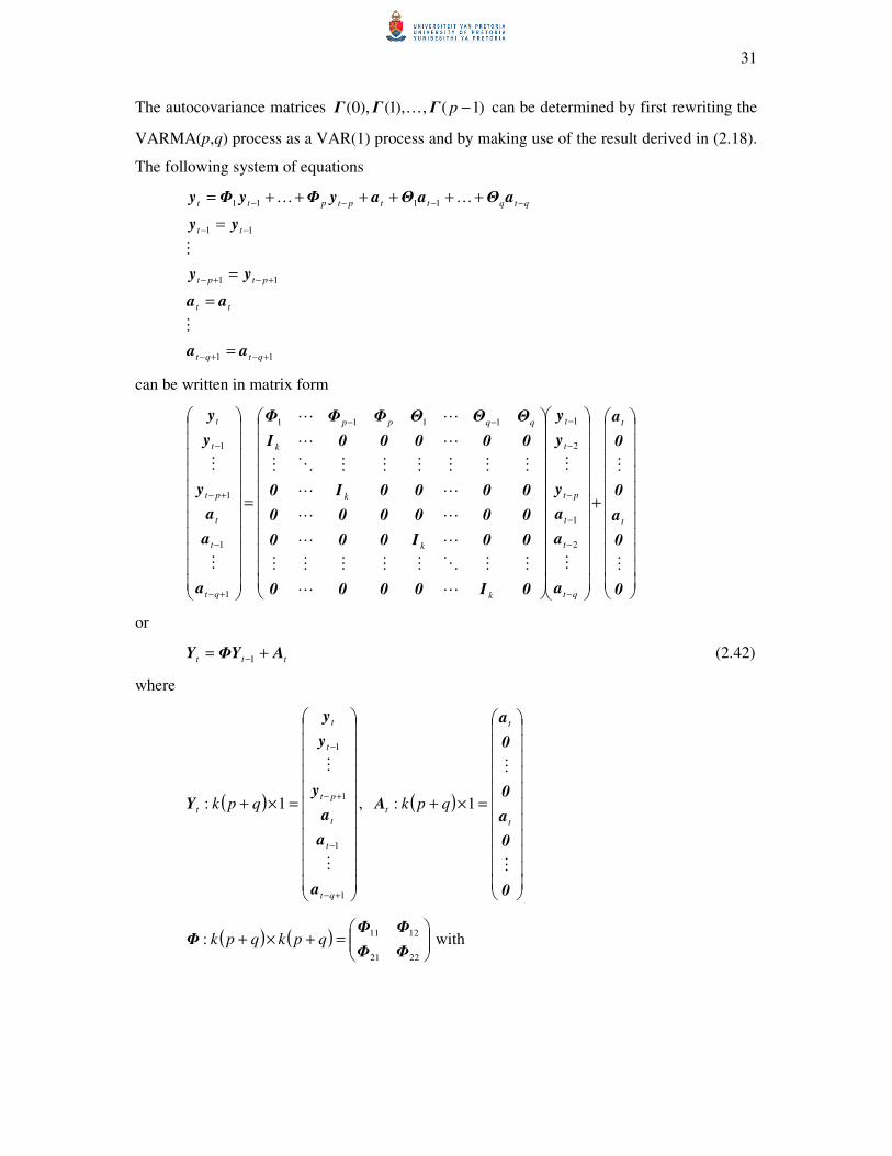
The autocovariance matrices )1(,),1(),0( −pΓΓΓ K can be determined by first rewriting the
VARMA(p,q) process as a VAR(1) process and by making use of the result derived in (2.18).
The following system of equations
11
11
11
1111
+−+−
+−+−
−−
−−−−
=
=
=
=
++++++=
qtqt
tt
ptpt
tt
qtqttptptt
aa
aa
yy
yy
aΘaΘayΦyΦy
M
M
KK
can be written in matrix form
+
=
−
−
−
−
−
−−−
+−
−
+−
−
0
0
a
0
0
a
a
a
a
y
y
y
0I0000
00I000
000000
0000I0
00000I
ΘΘΘΦΦΦ
a
a
a
y
y
y
M
M
M
M
LL
MMOMMMMM
LL
LL
LL
MMMMMMOM
LL
LL
M
M
t
t
qt
t
t
pt
t
t
k
k
k
k
qqpp
qt
t
t
pt
t
t
2
1
2
11111
1
1
1
1
or
ttt AΦYY += −1 (2.42)
where
( )
=×+
+−
−
+−
−
1
1
1
1
1:
qt
t
t
pt
t
t
t qpk
a
a
a
y
y
y
Y
M
M
, ( )
=×+
0
0
a
0
0
a
A
M
M
t
t
t qpk 1:
( ) ( )
=+×+
2221
1211:
ΦΦ
ΦΦΦ qpkqpk with
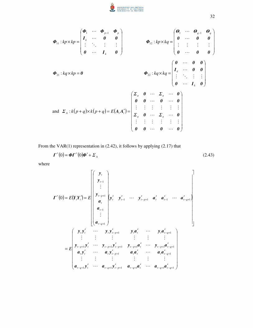
32
=×
−
0I0
00I
ΦΦΦ
Φ
k
k
pp
kpkp
L
MMOM
L
L 11
11 :
=×
−
000
000
ΘΘΘ
Φ
L
MMMM
L
L qq
kqkp
11
12 :
0Φ =× kpkq:21
=×
0I0
00I
000
Φ
k
kkqkq
L
MMOM
L
L
:22
and ( ) ( ) ( )
=′=+×+
0000
0Σ0Σ
0000
0Σ0Σ
AAΣ
LL
MMMMMM
LL
MMMMMM
LL
LL
aa
aa
ttA Eqpkqpk:
From the VAR(1) representation in (2.42), it follows by applying (2.17) that
( ) ( ) AΣΦΦΓΓ +′= 00 ** (2.43)
where
( ) ( ) ( )
′′′′
′′′′
′′′′
′′′′
=
′′′′′′
=′=
+−+−+−+−+−+−
+−+−
+−+−+−+−+−+−
+−+−
+−−+−−
+−
−
+−
−
111111
11
111111
11
1111
1
1
1
1
* 0
qtqttqtptqttqt
qttttptttt
qtpttptptpttpt
qttttptttt
qtttpttt
qt
t
t
pt
t
t
tt
E
EE
aaaayaya
aaaayaya
ayayyyyy
ayayyyyy
aaayyy
a
a
a
y
y
y
YYΓ
LL
MMMMMM
LL
LL
MMMMMM
LL
LL
M
M
33
( )
( ) ( ) ( ) ( )
( ) ( ) ( )( )
( ) ( )
( ) ( )
( ) ( )
00
00
01
10
0
*
22
*
12
*
12
*
11
111
11
1
*
′=
′′
′
′+−
′′−
=
+−+−+−
+−+−
+−
ΓΓ
ΓΓ
Σ0yaya
0Σ0ya
ay0ΓΓ
ayayΓΓ
Γ
aptqttqt
att
qtpt
qtttt
EE
E
Ep
EEp
LL
MOMMMM
LL
LL
MMMMOM
LL
( )
( ) ( ) ( )( ) ( ) ( )
( ) ( ) ( )
+−+−
−−
−
=×
021
201
110
:0*
11
ΓΓΓ
ΓΓΓ
ΓΓΓ
Γ
L
MOMM
L
L
pp
p
p
kpkp
( )
( ) ( ) ( )( ) ( )
( )
′
′′
′′′
=×
+−+−
+−−−−
+−−
11
1111
11
*
12 :0
qtpt
qtttt
qtttttt
E
EE
EEE
kqkp
ay00
ayay0
ayayay
Γ
L
MMMM
L
L
( )
=×
a
a
a
kqkq
Σ00
0Σ0
00Σ
Γ
L
MOMM
L
L
:0*
22
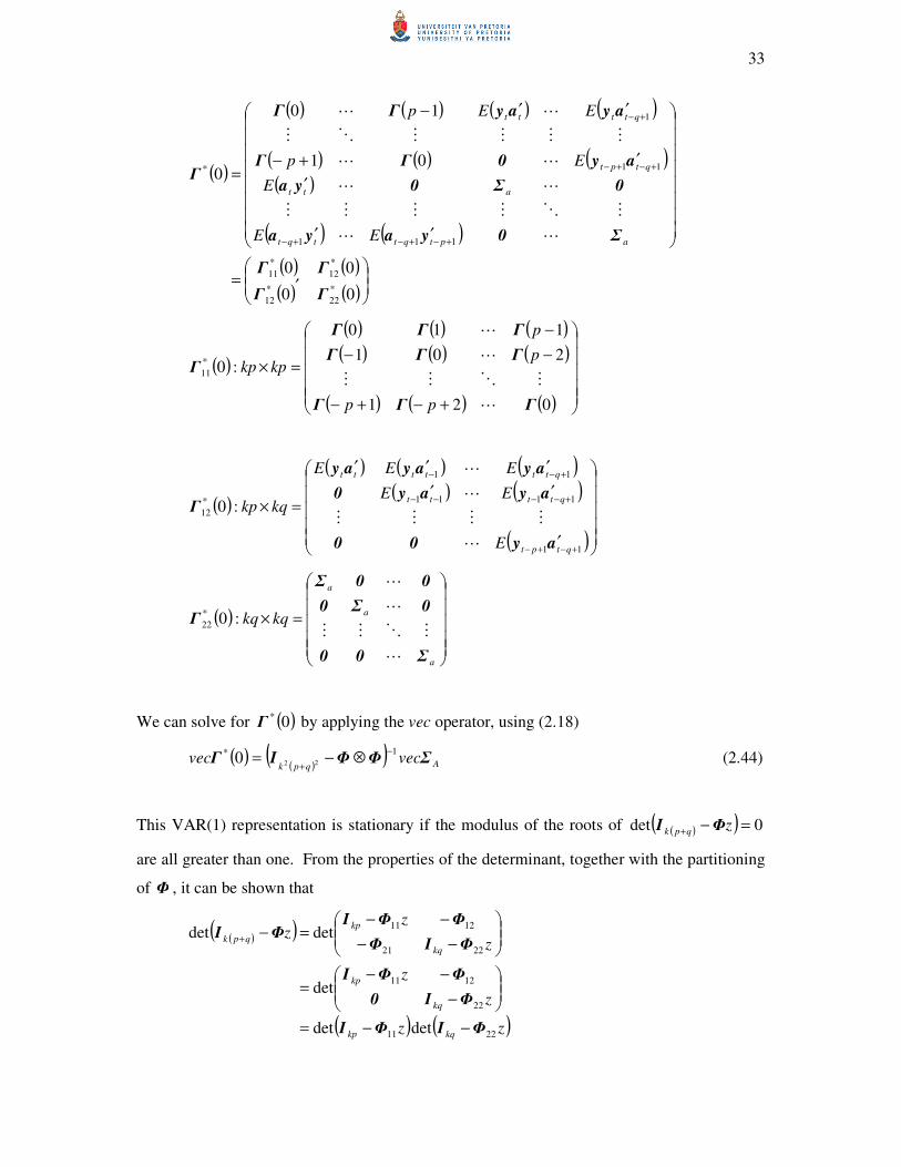
We can solve for ( )0*Γ by applying the vec operator, using (2.18)
( )( )
( ) Aqpkvecvec ΣΦΦIΓ
1*220
−
+⊗−= (2.44)
This VAR(1) representation is stationary if the modulus of the roots of ( )( ) 0det =−+ zqpk ΦI
are all greater than one. From the properties of the determinant, together with the partitioning
of Φ , it can be shown that
( )( )
( ) ( )zz
z
z
z
zz
kqkp
kq
kp
kq
kp
qpk
2211
22
1211
2221
1211
detdet
det
detdet
ΦIΦI
ΦI0
ΦΦI
ΦIΦ
ΦΦIΦI
−−=
−
−−=
−−
−−=−+
34
The matrix ( )zkq 22ΦI − is a lower triangular matrix with ones on the main diagonal, therefore
( ) ( ) ( )zzz kpkqkp 112211 detdetdet ΦIΦIΦI −=−−
It can be shown that ( ) ( )p
pkkp zzzz ΦΦΦIΦI −−−−=− K2
2111 detdet . The modulus of the
roots of ( ) 0det 2
21 =−−−− p
pk zzz ΦΦΦI K are greater than one if the VARMA(p,q)
process, { }ty , is stationary. If this is the case, the VAR(1) representation is also stationary.
Since the VAR(1) process is stationary the existence of the inverse of ( )
( )ΦΦI ⊗−+
22qpk
used
in (2.44) follows from similar reasoning as in section 2.3.1.
Once )(lΓ has been determined it is easy to obtain the autocorrelation matrices of the
VARMA(p,q) model by applying relation (2.4).
The following example considers a VARMA(2,1) model. The tests for stationarity and
invertibility are illustrated. The model is expressed in the form of a VAR(1) model in order to
calculate the matrices of autocovariances at lag 0 and 1. For lags greater than one, the
calculated )0(Γ and )1(Γ are used together with the Yule-Walker equations.
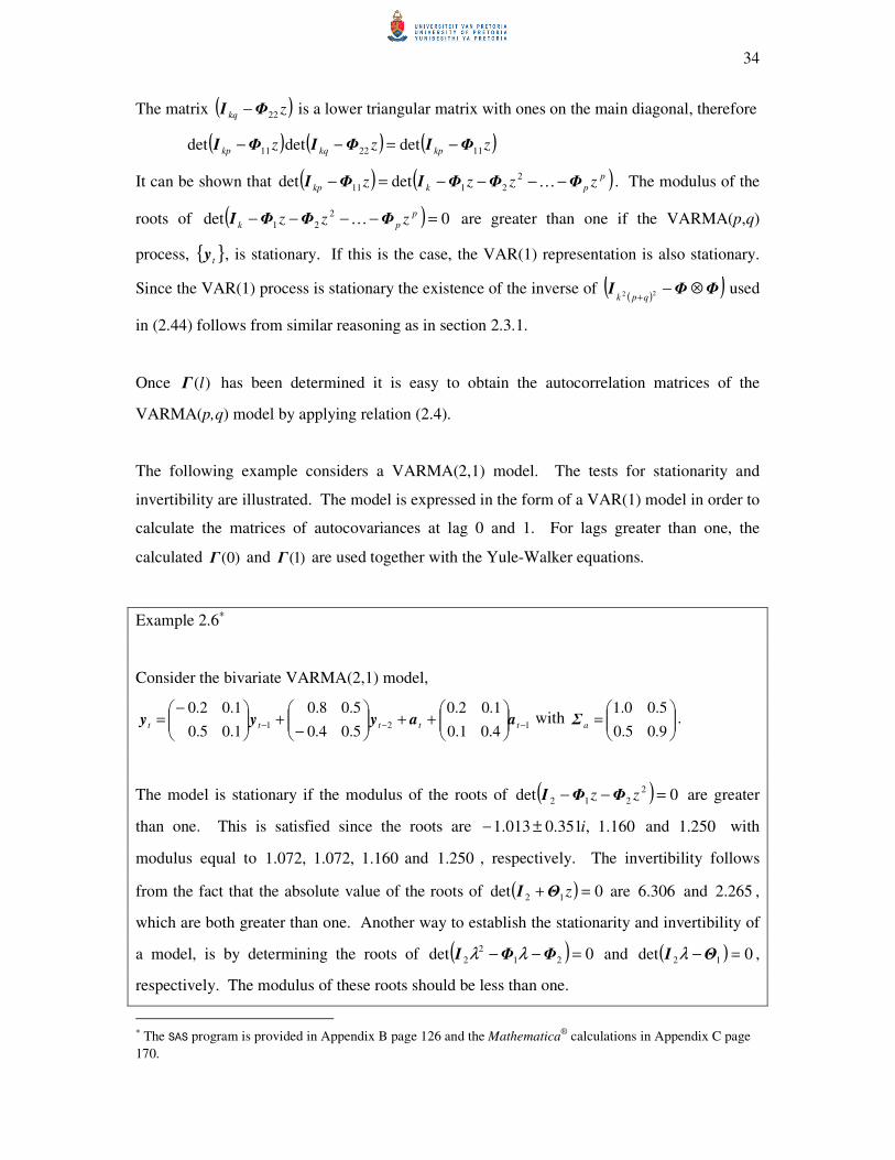
Example 2.6∗
Consider the bivariate VARMA(2,1) model,
1214.01.0
1.02.0
5.04.0
5.08.0
1.05.0
1.02.0−−−
++
−+
−= ttttt aayyy with
=
9.05.0
5.00.1aΣ .
The model is stationary if the modulus of the roots of ( ) 0det 2
212 =−− zz ΦΦI are greater
than one. This is satisfied since the roots are ,351.0013.1 i±− 160.1 and 250.1 with
modulus equal to ,072.1 ,072.1 160.1 and 250.1 , respectively. The invertibility follows
from the fact that the absolute value of the roots of ( ) 0det 12 =+ zΘI are 6.306 and 2.265 ,
which are both greater than one. Another way to establish the stationarity and invertibility of
a model, is by determining the roots of ( ) 0det 21
2
2 =−− ΦΦI λλ and ( ) 0det 12 =−ΘI λ ,
respectively. The modulus of these roots should be less than one.
∗ The SAS program is provided in Appendix B page 126 and the Mathematica
® calculations in Appendix C page
170.
35
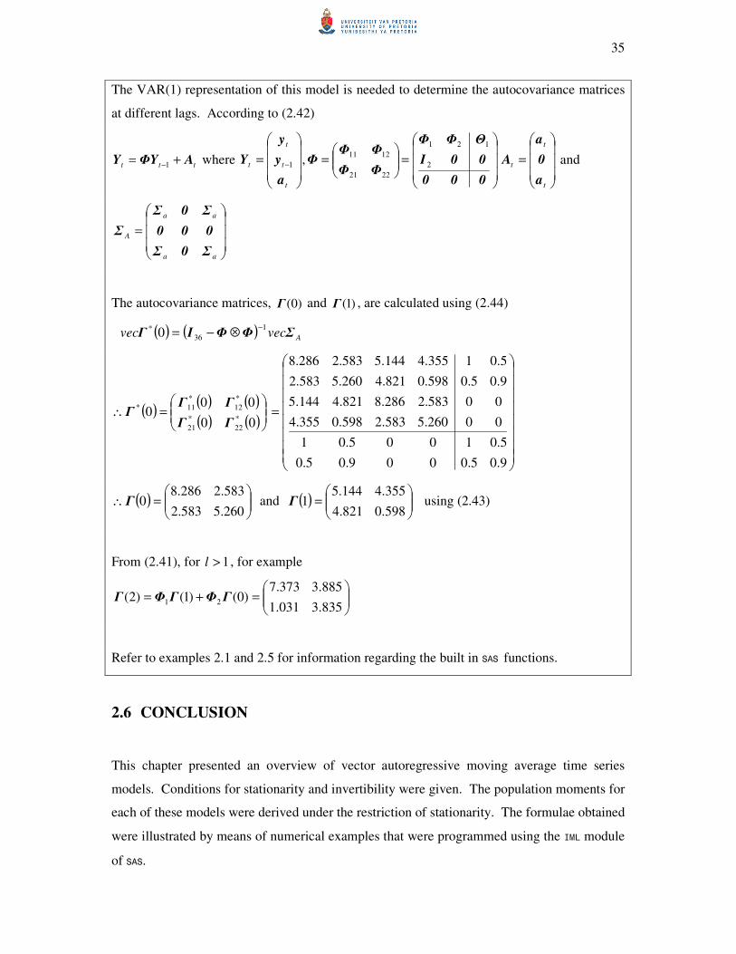
The VAR(1) representation of this model is needed to determine the autocovariance matrices
at different lags. According to (2.42)
ttt AΦYY += −1 where
= −
t
t
t
t
a
y
y
Y 1 ,
=
=
000
00I
ΘΦΦ
ΦΦ
ΦΦΦ 2
121
2221
1211
=
t
t
t
a
0
a
A and
=
aa
aa
A
Σ0Σ
000
Σ0Σ
Σ
The autocovariance matrices, )0(Γ and )1(Γ , are calculated using (2.44)
( ) ( ) Avecvec ΣΦΦIΓ1
36
* 0−
⊗−=
( )( ) ( )( ) ( )
=
=∴
9.05.0009.05.0
5.01005.01
00260.5583.2598.0355.4
00583.2286.8821.4144.5
9.05.0598.0821.4260.5583.2
5.01355.4144.5583.2286.8
00
000
*
22
*
21
*
12
*
11*
ΓΓ
ΓΓΓ
( ) 260.5583.2
583.2286.80
=∴Γ and ( )
598.0821.4
355.4144.51
=Γ using (2.43)
From (2.41), for 1>l , for example
835.3031.1
885.3373.7)0()1()2( 21
=+= ΓΦΓΦΓ
Refer to examples 2.1 and 2.5 for information regarding the built in SAS functions.
2.6 CONCLUSION
This chapter presented an overview of vector autoregressive moving average time series
models. Conditions for stationarity and invertibility were given. The population moments for
each of these models were derived under the restriction of stationarity. The formulae obtained
were illustrated by means of numerical examples that were programmed using the IML module
of SAS.

36
The properties of the population moments will later on be used to identify a possible model
for an observed time series vector. The next two chapters will focus on the estimation of the
parameters of these multivariate time series models.

37
CHAPTER 3
ESTIMATION OF VECTOR AUTOREGRESSIVE PROCESSES
3.1 INTRODUCTION
Vector autoregressive models are often used in practice due to the simplicity of the estimation
thereof. The VAR(p) model can be written in the form of a multivariate linear model. The
results of such a model can then be used to obtain least squares estimators. When the
assumption of a Gaussian error distribution is added, it is possible to obtain the likelihood
function and subsequently the maximum likelihood estimators of the unknown parameters.
These procedures are described by both Reinsel (1997) and Lütkepohl (2005) while Draper &
Smith (1998) provides a detailed discussion of generalised least squares estimation.
Estimation of VAR models was also considered by Hannan (1970) in the spectral domain,
who also derived the asymptotic distribution of the estimators.
Estimation is presented in two chapters. This chapter is used to describe the autoregressive
case. Closed form expressions are available. If a moving average component is added to the
model, estimation becomes much more complex, since the normal equations are nonlinear.
That will be the topic of the next chapter.
This chapter describes two methods used for estimating the parameters of a VAR(p) model,
namely least squares estimation and the method of maximum likelihood. The asymptotic
properties of these estimators are also briefly discussed. Both methods are illustrated with an
example; the SAS programs for these examples are available in Appendix B. In the derivations
of the estimators properties of the Kronecker product and vec operator are used, as well as
rules of vector and matrix differentiation. These properties and rules are given in Appendix
A.
Suppose we have k time series processes that were generated by a stationary VAR(p) process
as defined in (2.19). For each time series a sample of size T is observed. Assume that p
presample values for each of the k variables are available, namely 0121 ,,, yyyy −+−+− Kpp .

38
In what follows it is assumed that the vector of constant terms and the autoregressive
coefficient matrices are unknown, hence the aim is to estimate them.
3.2 MULTIVARIATE LEAST SQUARES ESTIMATION
In this section some basic notation is introduced, the least squares estimator is derived and its
asymptotic properties given. An example is provided to illustrate this method of estimation.
3.2.1 Notation
In this paragraph, the notation that will be used in the derivation of the least squares estimator
is defined.
( )
( )
( )( )T21
T10
pt
t
t
p
kTkk
T
T
T
Tk
Tkp
kp
kpk
yyy
yyy
yyy
Tk
aaaA
ZZZZ
y
yZ
ΦΦΦcB
yyyY
L
L
M
L
L
MMMM
L
L
L
=×
=×+
=×+
=+×
==×
−
+−
:
)1(:
1
1)1(:
)1(:
:
1
1
21
21
22221
11211
21
Furthermore, the dimensions of these matrices after applying the vec operator become
1:)( ×kTvec Y
1)(:)( 2 ×+ kpkvec B
1:)( ×kTvec A
Using notation (3.1), the VAR(p) model in (2.19) can be written as
tptpttt ayΦyΦyΦcy +++++= −−− K2211
tt aBZ += −1 (3.2)
(3.1)
39
Equation (3.2) can be expanded to model Tyyy ,,, 21 K simultaneously,
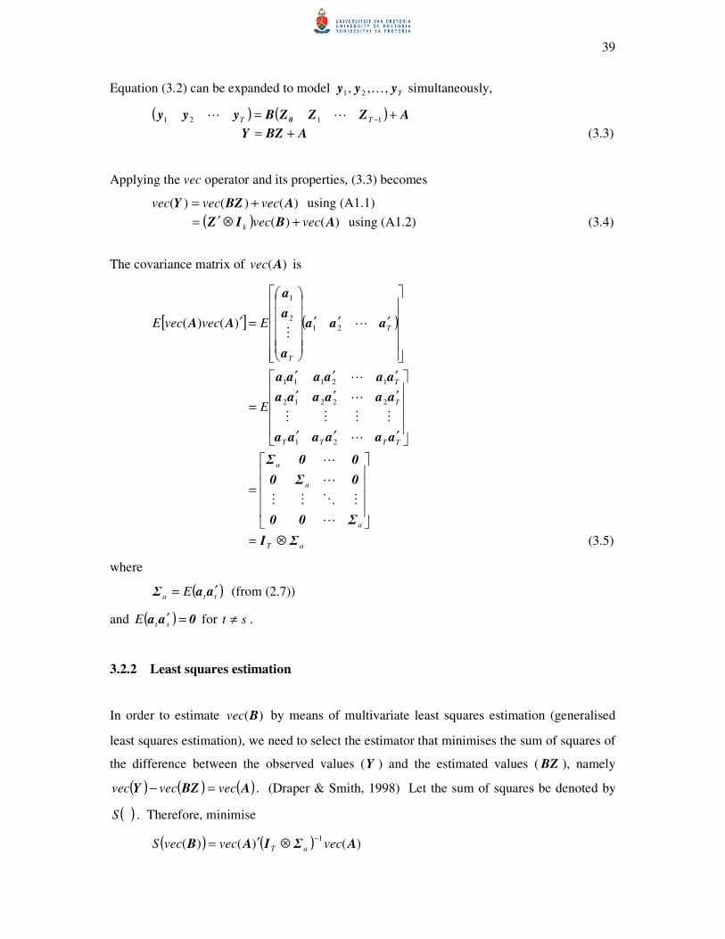
( ) ( ) AZZZByyy 0 += −1121 TT LL
ABZY += (3.3)
Applying the vec operator and its properties, (3.3) becomes
)()()( ABZY vecvecvec += using (A1.1)
( ) )()( ABIZ vecveck +⊗′= using (A1.2) (3.4)
The covariance matrix of )(Avec is
[ ] ( )
=
′′′
′′′
′′′
=
′′′
=′
a
a
a
TTTT
T
T
T
T
E
EvecvecE
Σ00
0Σ0
00Σ
aaaaaa
aaaaaa
aaaaaa
aaa
a
a
a
AA
L
MOMM
L
L
L
MMMM
L
L
LM
21
22212
12111
21
2
1
)()(
aT ΣI ⊗= (3.5)
where
( )tta E aaΣ ′= (from (2.7))
and ( ) 0aa =′stE for st ≠ .
3.2.2 Least squares estimation
In order to estimate )(Bvec by means of multivariate least squares estimation (generalised
least squares estimation), we need to select the estimator that minimises the sum of squares of
the difference between the observed values (Y ) and the estimated values ( BZ ), namely
( ) ( ) ( )ABZY vecvecvec =− . (Draper & Smith, 1998) Let the sum of squares be denoted by
( )S . Therefore, minimise
( ) ( ) )()()(1
AΣIAB vecvecvecS aT
−⊗′=
40
( ) )()(1
AΣIA vecvec aT
−⊗′= using (A2.1)
( ) )()(1
BZYΣIBZY −⊗′−=−
vecvec aT
( )[ ] ( ) ( )[ ]BZYΣIBZY vecvecvecvec aT −⊗′
−=−
)()(1
using (A1.1)
( )[ ] ( ) ( )[ ])()()()(1
BIZYΣIBIZY vecvecvecvec kaTk ⊗′−⊗′
⊗′−=−
using (A1.2) (3.6)
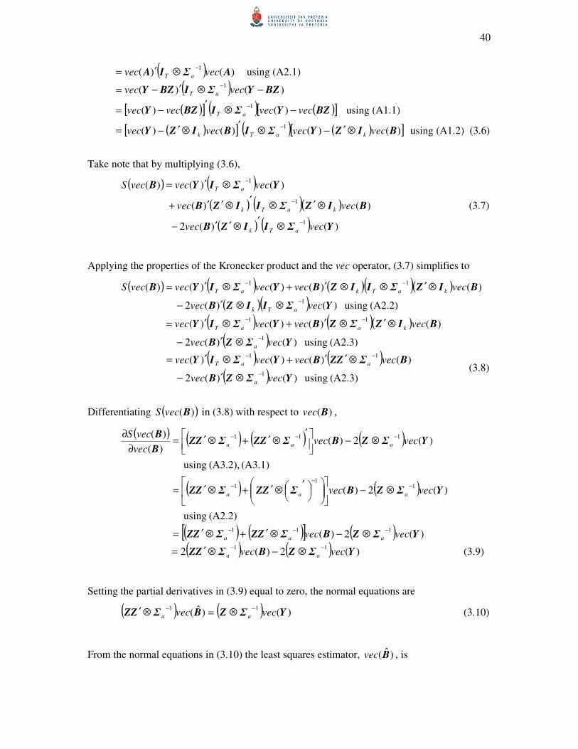
Take note that by multiplying (3.6),
( ) ( )( ) ( )( )
( ) ( ) )()(2
)()(
)()()(
1
1
1
YΣIIZB
BIZΣIIZB
YΣIYB
vecvec
vecvec
vecvecvecS
aTk
kaTk
aT
−
−
−
⊗′
⊗′′−
⊗′⊗′
⊗′′+
⊗′=
(3.7)
Applying the properties of the Kronecker product and the vec operator, (3.7) simplifies to
( ) ( ) ( )( )( )
( )( )( ) ( )( )
( ) (A2.3) using )()(2
)()()()(
(A2.2) using )()(2
)()()()()(
1
11
1
11
YΣZB
BIZΣZBYΣIY
YΣIIZB
BIZΣIIZBYΣIYB
vecvec
vecvecvecvec
vecvec
vecvecvecvecvecS
a
kaaT
aTk
kaTkaT
−
−−
−
−−
⊗′−
⊗′⊗′+⊗′=
⊗⊗′−
⊗′⊗⊗′+⊗′=
( ) ( )
( ) (A2.3) using )()(2
)()()()(
1
11
YΣZB
BΣZZBYΣIY
vecvec
vecvecvecvec
a
aaT
−
−−
⊗′−
⊗′′+⊗′= (3.8)
Differentiating ( ))(BvecS in (3.8) with respect to )(Bvec ,
( ) ( ) ( ) ( )
( ) ( )
( ) ( )[ ] ( ) )(2)(
(A2.2) using
)(2)(
(A3.1) (A3.2), using
)(2)()(
)(
111
11
1
111
YΣZBΣZZΣZZ
YΣZBΣZZΣZZ
YΣZBΣZZΣZZB
B
vecvec
vecvec
vecvecvec
vecS
aaa
aaa
aaa
−−−
−−
−
−−−
⊗−⊗′+⊗′=
⊗−
′
⊗′+⊗′=
⊗−
′⊗′+⊗′=
∂
∂
( ) ( ) )(2)(211
YΣZBΣZZ vecvec aa
−−⊗−⊗′= (3.9)
Setting the partial derivatives in (3.9) equal to zero, the normal equations are
( ) ( ) )()ˆ(11
YΣZBΣZZ vecvec aa
−−⊗=⊗′ (3.10)
From the normal equations in (3.10) the least squares estimator, )ˆ(Bvec , is
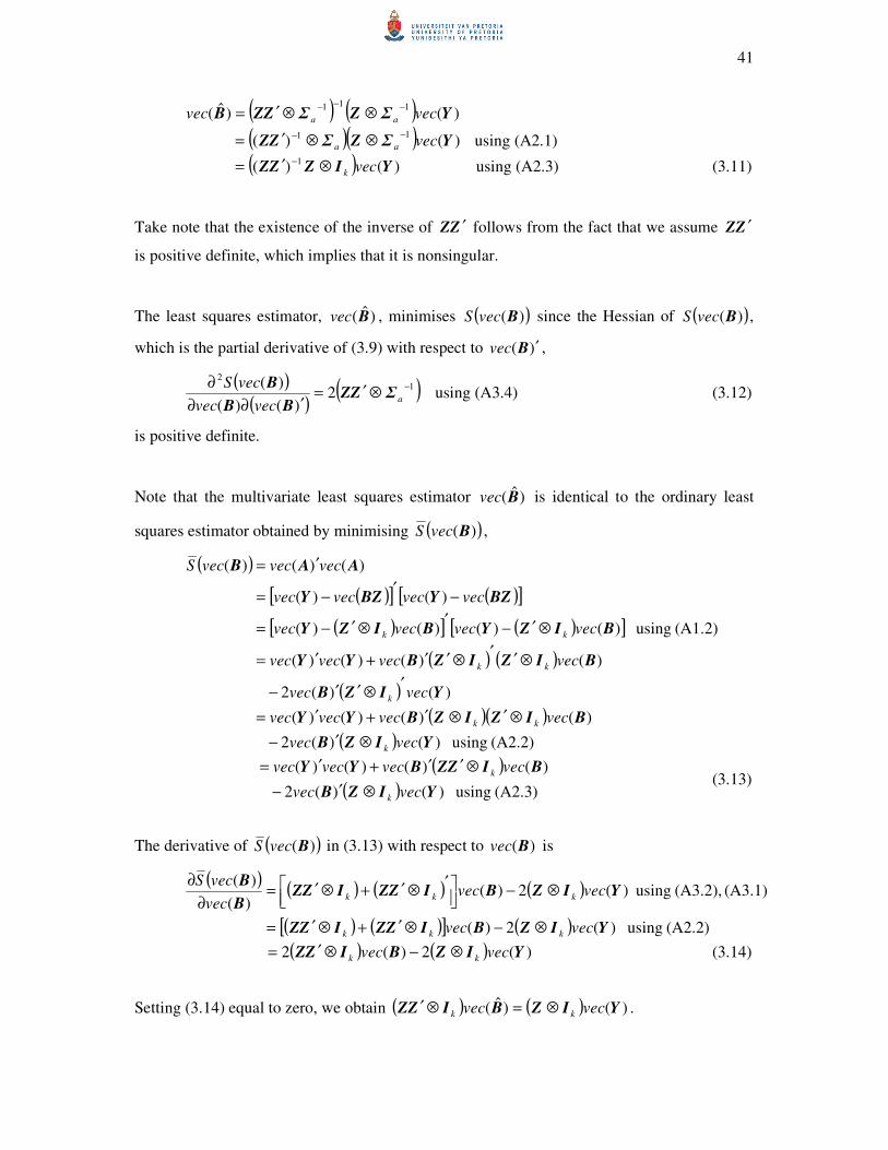
41
( ) ( ) )()ˆ(111
YΣZΣZZB vecvec aa
−−−⊗⊗′=
( )( ) )()(11
YΣZΣZZ vecaa
−− ⊗⊗′= using (A2.1)
( ) )()( 1YIZZZ veck⊗′= − using (A2.3) (3.11)
Take note that the existence of the inverse of ZZ ′ follows from the fact that we assume ZZ ′
is positive definite, which implies that it is nonsingular.
The least squares estimator, )ˆ(Bvec , minimises ( ))(BvecS since the Hessian of ( ))(BvecS ,
which is the partial derivative of (3.9) with respect to )( ′Bvec ,
( )( )
( )12
2)()(
)( −⊗′=
′∂∂
∂a
vecvec
vecSΣZZ
BB
B using (A3.4) (3.12)
is positive definite.
Note that the multivariate least squares estimator )ˆ(Bvec is identical to the ordinary least
squares estimator obtained by minimising ( ))(BvecS ,
( )
( )[ ] ( )[ ]
( )[ ] ( )[ ]
( ) ( )
( )( )( )
( ) (A2.2) using )()(2
)()()()(
)()(2
)()()()(
(A1.2) using )()()()(
)()(
)()()(
YIZB
BIZIZBYY
YIZB
BIZIZBYY
BIZYBIZY
BZYBZY
AAB
vecvec
vecvecvecvec
vecvec
vecvecvecvec
vecvecvecvec
vecvecvecvec
vecvecvecS
k
kk
k
kk
kk
⊗′−
⊗′⊗′+′=
′⊗′′−
⊗′′⊗′′+′=
⊗′−′
⊗′−=
−′
−=
′=
( )
( ) (A2.3) using )()(2
)()()()(
YIZB
BIZZBYY
vecvec
vecvecvecvec
k
k
⊗′−
⊗′′+′= (3.13)
The derivative of ( ))(BvecS in (3.13) with respect to )(Bvec is
( ) ( ) ( ) ( )
( ) ( )[ ] ( ) (A2.2) using )(2)(
(A3.1) (A3.2), using )(2)()(
)(
YIZBIZZIZZ
YIZBIZZIZZB
B
vecvec
vecvecvec
vecS
kkk
kkk
⊗−⊗′+⊗′=
⊗−
′
⊗′+⊗′=∂
∂
( ) ( ) )(2)(2 YIZBIZZ vecvec kk ⊗−⊗′= (3.14)
Setting (3.14) equal to zero, we obtain ( ) ( ) )()ˆ( YIZBIZZ vecvec kk ⊗=⊗′ .
42
Then the ordinary least squares estimator, )ˆ(Bvec , is
( ) ( )
( )( ) (A2.1) using )()(
)()ˆ(
1
1
YIZIZZ
YIZIZZB
vec
vecvec
kk
kk
⊗⊗′=
⊗⊗′=
−
−
( ) )()( 1YIZZZ veck⊗′= − using (A2.3)
which is the same as the multivariate least squares estimator obtained in (3.11).
The Hessian, ( )
( )( )k
vecvec
vecSIZZ
BB
B⊗′=
′∂∂
∂2
)()(
)(2
(using (A3.4)) is positive definite, therefore
)ˆ(Bvec minimises ( ))(BvecS .
The least squares estimator )ˆ(Bvec in (3.11) can also be written in an alternative form,
( ) )()()ˆ( 1YIZZZB vecvec k⊗′= −
( )1)( −′′= ZZZYvec using (A1.2) (3.15)
implying that
1)(ˆ −′′= ZZZYB (3.16)
3.2.3 Asymptotic properties of the least squares estimator
Now that the least squares estimator is determined, a way is needed to establish the
significance of the individual estimates. Usually the estimate is divided with its standard
error to obtain a t-ratio that can be compared with a critical value. In order to do this, the
distribution of the estimator is needed.
Proposition 3.1 of Lütkepohl (2005) addresses the consistency and the asymptotic normality
of the least squares estimator, namely
“Let { }ty be a stable, k-dimensional VAR(p) process with standard white noise residuals,
1)(ˆ −′′= ZZZYB is the LS estimator of the VAR coefficients B . Then
BB =ˆplim
and
( ) ( )a
dNvecT ΣΓ0BB ⊗→− −1,ˆ (3.17)
where T
ZZΓ
′= plim .”
43
A standard white noise process is a white noise process as described in section 2.3, with the
additional property that all the fourth moments must exist and be bounded.
Consistent estimators of the unknown parameters Γ and aΣ in (3.17) are given by Lütkepohl
(2005),
T
ZZΓ
′=ˆ (3.18)
t
T
t
taT
aaΣ ′= ∑=
ˆˆ1~
1
(3.19)
where ta is the vector of estimated residuals. The estimate of aΣ in (3.19) can be written in
terms of the notation defined in (3.1),
( )( )
( )( )
( )( )
( )( )YZZZZIZZZZIY
YZZZZYZZZZYY
ZZZZYYZZZZYY
ZBYZBY
AAΣ
′′′−′′−=
′′′−′′′−=
′′′−′′−=
′−−=
′=
−−
−−
−−
11
11
11
)()(1
)()(1
)()(1
(3.3)) (from ˆˆ1
ˆˆ1~
TT
a
T
T
T
T
T
( )YZZZZIY ′′′−= −1)(1
TT
(3.20)
aΣ~
is a biased estimator which can be adjusted to obtain an unbiased estimator aΣ ,
( )YZZZZIYΣΣ ′′′−−−
=−−
= −1)(1
1~
1ˆ
TaakpTkpT
T (3.21)
Lütkepohl (2005) showed that (3.18), (3.19) and (3.20) are consistent under certain
constraints.
Substituting Γ and aΣ into (3.17), it follows that
( )
⊗
′→−
−
a
d
TTNvec Σ
ZZ0BB ˆ1
,ˆ1
( ) ( )( )a
dNvec ΣZZ0BB ˆ,ˆ 1
⊗′→−−
(3.22)
44
The square root of the diagonal elements of ( ) aΣZZ ˆ1⊗′ −
, denoted by is , is the estimated
standard deviation of the corresponding ii ββ −ˆ , the i-th element of ( )BB −ˆvec . Equation
(3.22) implies that i
ii
s
ˆ ββ − has an approximate t-distribution which is asymptotically
standard normal. This can be used for hypothesis testing regarding the significance of the
least squares estimator.
The following example illustrates the calculation, using the expressions derived in this
section, of the least squares estimates of a generated VAR(1) model. The asymptotic results
are used to obtain t-ratios that can be used in testing for the significance of the parameter
values. The results are compared to the output of the VARMAX procedure in the SAS/ETS module.
Example 3.1∗
Consider the bivariate VAR(1) model ttt ayy +
= −1
4.01.0
6.05.0 with
=
9.05.0
5.00.1aΣ .
A sample of size 500 is generated. The method used to generate data from a multivariate normal
distribution is discussed after the example. The least squares estimate of )(Bvec in (3.11), is
−
=
320.0
503.0
115.0
516.0
028.0
055.0
)ˆ(Bvec
( )
−==∴
320.0115.0028.0
503.0516.0055.0ˆˆˆ
1ΦcB
The estimates for Γ and aΣ according to (3.18) and (3.21) are
−
−
=
211.1131.1033.0
131.1598.2070.0
033.0070.0000.1
Γ
∗ The SAS program is provided in Appendix B page 127.
45
=
974.0532.0
532.0005.1ˆ
aΣ
and
( )
−−−−
−−−−
−−
−−
−−
−−
=⊗′ −
0027251.00014892.0001191.0000651.0000173.0000095.0
0014892.00028115.0000651.0001228.0000095.0000179.0
001191.0000651.00012717.0000695.00001286.00000703.0
000651.0001228.0000695.0001312.00000703.00001326.0
000173.0000095.00001286.00000703.00019633.00010729.0
000095.0000179.00000703.00001326.00010729.00020256.0
ˆ1
aΣZZ
Using these estimates together with (3.22) makes it possible to determine the standard errors and
t-ratios of the least squares estimate. The results are summarised in the table below.
)ˆ(Bvec Standard error ( )is t-ratio
1c -0.055 0.045 -1.229
2c 0.028 0.044 0.628
11φ 0.516 0.036 14.244
21φ 0.115 0.036 3.222
12φ 0.503 0.053 9.491
22φ 0.320 0.052 6.137
This is comparable to the SAS output that is provided below. The slight differences are due to the
assumption that the presample values are known when calculating )ˆ(Bvec in (3.11), and in this
example 0y was generated the same way as the process was generated.
The VARMAX Procedure
Model Parameter Estimates
Standard
Equation Parameter Estimate Error t Value Pr > |t|
Variable
y1 CONST1 -0.05856 0.04500 -1.30 0.1938 1
AR1_1_1 0.51289 0.03623 14.15 0.0001 y1(t-1)
AR1_1_2 0.50467 0.05297 9.53 0.0001 y2(t-1)
y2 CONST2 0.02543 0.04435 0.57 0.5666 1
AR1_2_1 0.11264 0.03571 3.15 0.0017 y1(t-1)
AR1_2_2 0.32141 0.05220 6.16 0.0001 y2(t-1)
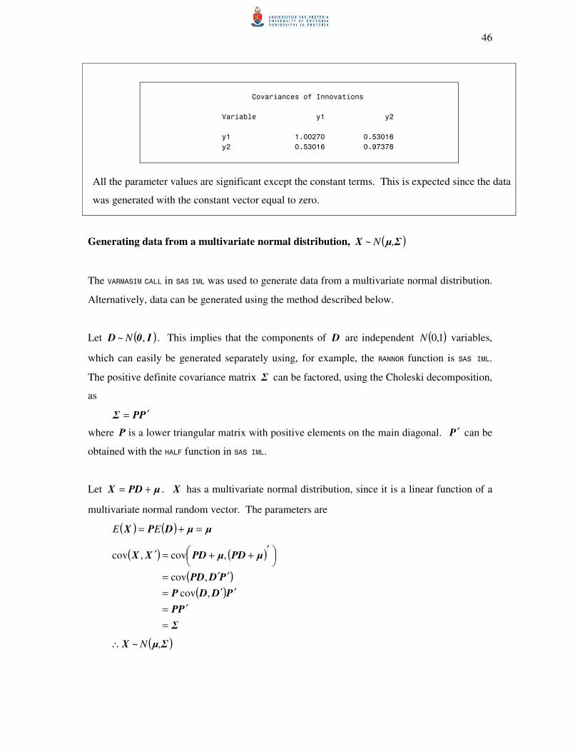
46
Covariances of Innovations
Variable y1 y2
y1 1.00270 0.53016
y2 0.53016 0.97378
All the parameter values are significant except the constant terms. This is expected since the data
was generated with the constant vector equal to zero.
Generating data from a multivariate normal distribution, X ~ ( )Σµ,N
The VARMASIM CALL in SAS IML was used to generate data from a multivariate normal distribution.
Alternatively, data can be generated using the method described below.
Let D ~ ( )I0,N . This implies that the components of D are independent ( )1,0N variables,
which can easily be generated separately using, for example, the RANNOR function is SAS IML.
The positive definite covariance matrix Σ can be factored, using the Choleski decomposition,
as
PPΣ ′=
where P is a lower triangular matrix with positive elements on the main diagonal. P ′ can be
obtained with the HALF function in SAS IML.
Let µPDX += . X has a multivariate normal distribution, since it is a linear function of a
multivariate normal random vector. The parameters are
( ) ( ) µµDPX =+= EE
( ) ( )
( )( )
Σ
PP
PDDP
PDPD
µPDµPDXX
=
′=
′′=
′′=
′
++=′
,cov
,cov
,cov,cov
X∴ ~ ( )Σµ,N
47
The method described above can be employed to generate the multivariate white noise series
{ }ta with mean zero and covariance matrix aΣ . The white noise series can then be used to
generate observations from any specified model. As an illustration the data from the bivariate
VAR(1) model, stated in Example 3.1, was also generated using this method. The SAS
program is given in Appendix B.
3.3 MAXIMUM LIKELIHOOD ESTIMATION
In this section the maximum likelihood estimator of the mean, the coefficient matrices and the
white noise covariance matrix are derived by obtaining the likelihood functions and
maximising them with respect to each of the unknown parameters. The asymptotic properties
of the maximum likelihood estimators are provided. The section is concluded with a
numerical example using the matrix expressions derived.
3.3.1 The likelihood function
When the distribution of a process is known, the maximum likelihood estimator can be
determined. Assume that we have a Gaussian VAR(p) process, this means that the white
noise process { }ta is normally distributed with mean zero and covariance matrix aΣ . This,
together with (3.5) implies that )(Avec has a ( )aTN ΣI0 ⊗, distribution, with probability
density function given by
( )( )
( )
⊗′−⊗=
−−
)()(2
1exp
2
1)(
121
2
AΣIAΣIA vecvecvecf aTaTkT
π (3.23)
The aim is to utilise (3.23) to determine the probability density function of )(Yvec using the
transformation theorem (A5.1). Rewriting the deviation from the mean form in (2.22) yields
( ) ( ) ( ) ( )µyΦµyΦµyΦµya −−−−−−−−= −−− ptptttt K2211
then
( ) ( ) ( ) ( )( ) ( ) ( ) ( )
( ) ( ) ( ) ( )µyΦµyΦµyΦµya
µyΦµyΦµyΦµya
µyΦµyΦµyΦµya
−−−−−−−−=
−−−−−−−−=
−−−−−−−−=
+−−−
+−
+−−
TppTTTT
pp
pp
K
M
K
K
2211
2021122
1120111
(3.24)
48
Let ( )tt g Ya = where
=
−
−
p
t
t
t
t
y
y
y
YM
1.
Using matrix notation, (3.24) becomes
−
−
−
−
−−−
−−−−
+
−
−
−
−
−−
−
=
+−
−
−
−
µy
µy
µy
0000
000Φ
0ΦΦΦ
ΦΦΦΦ
µy
µy
µy
IΦ00
0IΦΦ
00IΦ
000I
a
a
a
1
1
032
121
2
1
1
1
2
1
p
p
p
pp
T
kp
kpp
k
k
T
M
L
MMMMM
L
MMMMM
L
L
M
LL
MOMMMM
LL
MMMOMM
LL
LK
M
The partial derivative of )(Avec with respect to )( ′Yvec is
−
−−
−
=′∂
∂
−
kp
kpp
k
k
vec
vec
IΦ00
0IΦΦ
00IΦ
000I
Y
A
LL
MOMMMM
LL
MMMOMM
LL
LK
1
1
)(
)( (3.25)
therefore the Jacobian of the transformation from )(Avec to )(Yvec is
1)(
)(=
′∂
∂
Y
A
vec
vec (3.26)
since the derivative in (3.25) is a lower triangular matrix with ones on the main diagonal.
The next step is to rewrite )(Avec as a function of )(Yvec . From the deviation of the mean
form (3.24),
( )
−−−
−−−
−−−
−
−
−
−
=
+−+−+−
−−
−
µyµyµy
µyµyµy
µyµyµy
ΦΦΦ
µy
µy
µy
a
a
a
Tppp
T
T
p
TT
vec
L
MMMM
L
L
LMM
21
201
110
21
2
1
2
1
or
( )XBµYA**)()( vecvecvec −−=
( ) )()( **BIXµY vecvec k⊗′−−= using (A1.2) (3.27)
49
where
( )pkpk ΦΦΦB L21
* : =× (3.28)
( )′′′′=× µµµµ L1:*kT
−−−
−−−
−−−
=×
+−+−+−
−−
−
µyµyµy
µyµyµy
µyµyµy
X
Tppp
T
T
Tkp
L
MMMM
L
L
21
201
110
: (3.29)
According to the transformation theorem (A5.1) together with (3.23), (3.26) and (3.27) the
probability density function of )(Yvec is
( ) ( )
( ) ( )
( ))(
)()(
)(
)()()(
)(
)())()()(()(
2
22
′∂
∂=
′∂
∂=
′∂
∂=
Y
AA
Y
AaaaY
Y
AYYYyyy
1
11
vec
vecvecf
vec
vecvecfvech
vec
vecgggvecfvech
T
TT
K
KK
( )( )[ ]
( ) ( )[ ]})()(
)()(2
1exp
2
1
**1
**21
2
BIXµYΣI
BIXµYΣI
vecvec
vecvec
kaT
kaTkT
⊗′−−⊗
×′
⊗′−−−⊗=
−
−
π (3.30)
The log-likelihood function is obtained by taking the natural logarithm of (3.30),
( )
( ) ( )[ ]
( ) ( )[ ])()(
)()(2
1ln
2
12ln
2
,,ln
**1
**
*
BIXµYΣI
BIXµYΣI
ΣBµ
vecvec
vecveckT
L
kaT
kaT
a
⊗′−−⊗
×′
⊗′−−−⊗−−=
−
π (3.31)
( ) ( )[ ]
( ) ( )[ ] (A2.4) using )()(
)()(2
1ln
2
12ln
2**1
**
BIXµYΣI
BIXµYΣI
vecvec
vecveckT
kaT
k
T
a
k
T
⊗′−−⊗
×′
⊗′−−−−−=
−
π
( ) ( )[ ]
( ) ( )[ ])()(
)()(2
1ln
22ln
2**1
**
BIXµYΣI
BIXµYΣ
vecvec
vecvecTkT
kaT
ka
⊗′−−⊗
×′
⊗′−−−−−=
−
π
50
( ) ( ) ( )
( ) ( )
−−−
×
′
−−−−−−=
−
=
−
=
−
=
∑
∑ ∑
µyΦµy
ΣµyΦµyΣ
it
p
i
it
a
T
t
it
p
i
ita
TkT
1
1
1 1
2
1ln
22ln
2π
(3.32)
( )
∑ ∑∑
∑ ∑∑
∑ ∑∑
= =
−
=
= =
−
−
=
= =
−
−
=
−
+−
′
+−−
−
′
+−−
−
′
−−−−=
T
t
p
i
ia
p
i
i
T
t
p
i
itita
p
i
i
T
t
p
i
itita
p
i
itita
TkT
1 1
1
1
1 1
1
1
1 1
1
1
2
1
2
1ln
22ln
2
µΦµΣµΦµ
yΦyΣµΦµ
yΦyΣyΦyΣπ
( )
µΦIΣΦIµ
yΦyΣΦIµ
yΦyΣyΦyΣ
−
′
−′−
−
′
−′+
−
′
−−−−=
∑∑
∑ ∑∑
∑ ∑∑
=
−
=
= =
−
−
=
= =
−
−
=
−
p
i
ika
p
i
ik
T
t
p
i
itita
p
i
ik
T
t
p
i
itita
p
i
itita
T
TkT
1
1
1
1 1
1
1
1 1
1
1
2
2
1ln
22ln
2π
(3.33)
A different expression for the log-likelihood function, in terms of the deviation from the
mean, follows from (3.32)
( )
( ) ( ) ( )
−
′−−−−=
−XBYΣXBYΣ
ΣBµ
*01*0
*
2
1ln
22ln
2
,,ln
aa
a
trTkT
L
π (3.34)
where
( )µyµyµyY −−−=× TTk K21
0 :
*B and X are defined as in (3.28) and (3.29), respectively.
3.3.2 The maximum likelihood estimators
To find the maximum likelihood estimators of µ , )( *Bvec and aΣ we need to determine the
partial derivative of the log-likelihood function with respect to each of these unknown
parameters.
51
From (3.33) it follows that
µ∂
∂ Lln µΦIΣΦIyΦyΣΦI
−
′
−−
−
′
−= ∑∑∑ ∑∑
=
−
== =
−
−
=
p
i
ika
p
i
ik
T
t
p
i
itita
p
i
ik T1
1
11 1
1
1
using (A3.1), (A3.2)
−−
−
′
−= ∑∑ ∑∑
== =
−
−
=
µΦIyΦyΣΦIp
i
ik
T
t
p
i
itita
p
i
ik T11 1
1
1
(3.35)
Setting µ∂
∂ Lln in (3.35) equal to zero, the maximum likelihood estimator of µ , namely µ~ ,
is:
µΦIyΦy ~~~
11 1
−=
− ∑∑ ∑
== =
−
p
i
ik
T
t
p
i
itit T
∑ ∑∑= =
−
−
=
−
−=∴
T
t
p
i
itit
p
i
ikT 1 1
1
1
~~1~ yΦyΦIµ (3.36)
where iΦ~
is the maximum likelihood estimator of iΦ .
From (3.31) the terms involving )( *Bvec are
( ) ( ) ( ) ( )
( ) ( ) ( ) ( ) ( )
( ) ( ) ( ) ( )*1*
*1*
*1*
)(2
1
2
1
)(2
1
BIXΣIµY
BIXΣIIXB
µYΣIIXB
vecvec
vecvec
vecvec
kaT
kaTk
aTk
⊗′⊗′
−+
⊗′⊗′
⊗′′
−
−⊗′
⊗′′
−
−
−
( ) ( )( ) ( )
( ) ( )( ) ( ) ( ) (A2.2) using 2
1
)(
*1*
*1*
BIXΣIIXB
µYΣIIXB
vecvec
vecvec
kaTk
aTk
⊗′⊗⊗′
−
−⊗⊗′
=
−
−
(3.37)
Therefore, from (3.37) it follows that
)(
ln*
Bvec
L
∂
∂
( )( ) ( )
( )( ) ( ) ( )( ) ( )( ) ( )*11
*1
2
1
)(
BIXΣIIXIXΣIIX
µYΣIIX
vec
vec
kaTkkaTk
aTk
′⊗′⊗⊗+⊗′⊗⊗−
−⊗⊗=
−−
−
using (A3.1), (A3.2)
52
( )( ) ( ) ( )( ) ( ) ( )( )( )( ) ( )( )( ) ( )*1*1
*1*1
)(
)(
BIXΣIIXµYΣIIX
BIXΣIIXµYΣIIX
vecvec
vecvec
kaTkaTk
kaTkaTk
⊗′⊗⊗−−⊗⊗=
⊗′⊗⊗−−⊗⊗=
−−
−−
using (A2.1)
( )( ) ( ) ( )*1*1)( BΣXXµYΣX vecvec aa
−−⊗′−−⊗= using (A2.3) (3.38)
Setting )(
ln*
Bvec
L
∂
∂ in (3.38) equal to zero, the maximum likelihood estimator of ( )*
Bvec ,
namely ( )*~Bvec , is:
( )( ) ( ) ( )*1*1 ~~~~~)(~~
BΣXXµYΣX vecvec aa
−−⊗′=−⊗
( ) ( ) ( )( )( )( )( )( ) (A2.1) using ~)(
~~~~~
~)(~~~~~~
*11
*111*
µYΣXΣXX
µYΣXΣXXB
−⊗⊗′=
−⊗⊗′=∴
−−
−−−
vec
vecvec
aa
aa
( )( )( )*1 ~)(~~~
µYIXXX −⊗′=−
veck using (A2.3) (3.39)
From (3.34) it follows that
( )( )
′−−−−−=
∂
∂ −−− 1*0*011
2
1
2
lnaaa
a
TLΣXBYXBYΣΣ
Σ using (A3.5), (A3.6)
( )( ) 1*0*011
2
1
2
−−− ′−−+−= aaa
TΣXBYXBYΣΣ (3.40)
Setting a
L
Σ∂
∂ ln in (3.40) equal to zero, the maximum likelihood estimator of aΣ , namely aΣ
~,
is:
( )( ) 1*0*011 ~~~~~~~~
2
1~
2
−−− ′−−= aaa
TΣXBYXBYΣΣ
( )( )′−−=∴ XBYXBYΣ~~~~~~1~ *0*0
Ta (3.41)
Take note that X~
and 0~Y are obtained by replacing µ with the estimated value, µ~ .
3.3.3 Asymptotic properties of the maximum likelihood estimator
As explained in section 3.2.3 it is useful to know the asymptotic distribution of the estimator.
Proposition 3.4 of Lütkepohl (2005) states:

53
“Let { }ty be a stationary, stable Gaussian VAR(p) process. Then the ML estimator of
( ) ( )( )( ) ~)(~~~
~ *1*
µYIXXXB −⊗′=−
vecvec k is consistent and
( ) ( )( )aY
dNvecT ΣΓ0BB ⊗→−
−1** 0,~
(3.42)
where ( )
′=
TEY
XXΓ 0 .”
Rewriting (3.42) and substituting aΣ with the maximum likelihood estimator obtained in
(3.41) and estimating ( )0YΓ with ( )T
Y
XXΓ
~~
0ˆ ′= ,
( )
⊗
′→−
−
a
d
TTNvec Σ
XX0BB
~~~
1,
~1
**
( ) ( )( )a
dNvec ΣXX0BB
~~~,
~ 1** ⊗′→−−
(3.43)
Dividing the individual elements of ( )**~BB −vec with the square root of the diagonal
elements of ( ) aΣXX~~~ 1
⊗′−
, yields an approximate asymptotic standard normal distribution.
This can be used for hypothesis testing regarding the significance of the maximum likelihood
estimators.
Due to the complex nature of the iterative process of maximisation, Example 3.2 only
considers a simple case where it is assumed that it is known that the mean of the process is
equal to zero.
In the following example the maximum likelihood estimates of a VAR(1) model are
calculated using matrix operations. Approximate standard errors of the coefficient matrices
are determined. All the results are compared to the output produced by the VARMAX procedure
on the same sample.
54
Example 3.2∗
Consider the bivariate VAR(1) model ttt ayy +
= −1
4.01.0
6.05.0 with
=
9.05.0
5.00.1aΣ .
For simplicity it is assumed that it is know that 0µ = . A sample of size 500 is generated.
The maximum likelihood estimates of *B in (3.39) and aΣ in (3.40) are
( )
==
323.0113.0
498.0520.0ˆ~
1
*ΦB
=
969.0528.0
528.0002.1~aΣ
The standard errors and t-ratios of the maximum likelihood estimates of the autoregressive
coefficients can be obtained using (3.43). The results are summarised in the table below.
)~
( *Bvec Standard error t-ratio
11φ 0.520 0.036 14.413
21φ 0.113 0.035 3.190
12φ 0.498 0.053 9.440
22φ 0.323 0.052 6.218
This compares well with the SAS output that is provided below. As mentioned in Example
3.1, the slight differences are due to the presample values. All the parameter values are
significant.
The VARMAX Procedure
Model Parameter Estimates
Standard
Equation Parameter Estimate Error t Value Pr > |t|
Variable
y1 AR1_1_1 0.51822 0.03620 14.31 0.0001 y1(t-1)
AR1_1_2 0.50127 0.05285 9.48 0.0001 y2(t-1)
y2 AR1_2_1 0.11255 0.03557 3.16 0.0017 y1(t-1)
AR1_2_2 0.32529 0.05200 6.26 0.0001 y2(t-1)
∗ The SAS program is provided in Appendix B page 129.
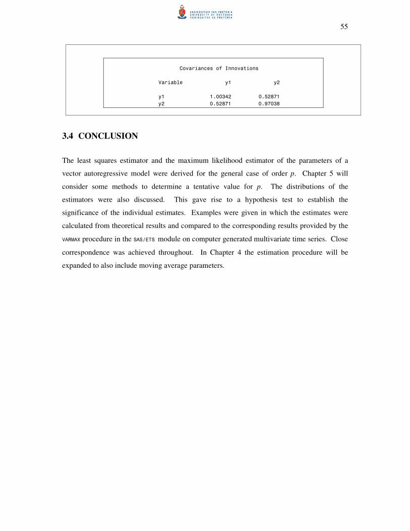
55
Covariances of Innovations
Variable y1 y2
y1 1.00342 0.52871
y2 0.52871 0.97038
.
3.4 CONCLUSION
The least squares estimator and the maximum likelihood estimator of the parameters of a
vector autoregressive model were derived for the general case of order p. Chapter 5 will
consider some methods to determine a tentative value for p. The distributions of the
estimators were also discussed. This gave rise to a hypothesis test to establish the
significance of the individual estimates. Examples were given in which the estimates were
calculated from theoretical results and compared to the corresponding results provided by the
VARMAX procedure in the SAS/ETS module on computer generated multivariate time series. Close
correspondence was achieved throughout. In Chapter 4 the estimation procedure will be
expanded to also include moving average parameters.
56
CHAPTER 4
ESTIMATION OF VARMA PROCESSES
4.1 INTRODUCTION
The simplicity of the estimation of VAR models makes them very attractive in practice. The
opposite is however true for VARMA models, because for VARMA models it is complicated
to obtain a unique representation. Hannan (1969) derived conditions for a VARMA model to
be uniquely identified, while Lütkepohl and Poskitt (1996) proposed the echelon form that
leads to a parsimonious and unique structure.
Hannan (1970) considered the estimation of a VMA model in the spectral domain, Osborn
(1977) derived an exact likelihood function for a VMA model and Phadke & Kedem (1978)
were concerned about the computation and maximisation of the exact likelihood function of a
VMA model. The problem of estimating the parameters of VARMA models has been
considered by Wilson (1973), Nicholls & Hall (1979), Hillmer & Tiao (1979) and more
recently by Mauricio (1995) and Ma (1997). De Frutos & Serrano (2002) proposed a
generalised least squares procedure for estimating VARMA models. This chapter will
however only focus on maximum likelihood estimation because it is the most common
procedure the moment moving average parameters are included. The primary source used for
this chapter is Lütkepohl (2005).
In sections 4.2, 4.3 and 4.4 we will only derive the likelihood function for the VMA(1),
VMA(q) and VARMA(1,1) processes, respectively. The VARMA(p,q) process will not be
presented since the VARMA representation is not unique. In order to overcome this
identification problem, the VARMA representation must be in final equations or echelon
form. This problem is briefly discussed in section 4.5.
The maximum likelihood estimates can be obtained by setting the normal equations equal to
zero and solving for the parameters. Since this is nonlinear in the parameters, numerical
optimisation methods are employed to obtain maximum likelihood estimates.
57
4.2 THE LIKELIHOOD FUNCTION OF A VMA(1) PROCESS
Suppose we have k time series processes each comprising of T equally spaced observations
that were generated by a Gaussian, invertible, zero mean with covariance matrix aΣ , VMA(1)
process, 11 −+= ttt aΘay . The constant term is set equal to zero for convenience. It can be
shown in a similar way as (3.5) that
( )aT
T
N ΣI0
a
a
a
⊗
+1
1
0
,~M
(4.1)
The matrix of time series observations is denoted by Tk ×:Y as in (2.1), where each column
represents the k observations at a specific point in time, while each row represents all the
observations of one of the k time series processes. ( )Yvec is a linear function of the white
noise vectors (4.1), therefore the multivariate normal distribution can be used to determine the
likelihood function.
( )
+
+
+
=
=×
−11
112
011
2
1
1:
TTT
kTvec
aΘa
aΘa
aΘa
y
y
y
YMM
=
=
TT
k
k
k
a
a
a
Θ
a
a
a
IΘ000
00IΘ0
000IΘ
MM
L
MOOMM
MOOMM
L
L
1
0
1
1
0
1
1
1
(4.2)
where ( )1:1 +× TkkTΘ .
By applying result (A5.2) to (4.2) and taking into account the distribution in (4.1) it follows
that ( ) ( )
′
⊗+ 111,~ ΘΣIΘ0Y aTNvec . Therefore, the likelihood function is proportional to
( ) ( ) ( ) ( ) ( )
′
⊗′
−′
⊗∝−
+
−
+ YΘΣIΘYΘΣIΘΣΘ vecvecL aTaTa
1
11111112
1exp,
2
1
(4.3)
58
To simplify (4.3) it can be assumed that the starting residuals are equal to zero ( 0a =0 ), then
(4.2) becomes
( )
=
T
k
k
k
vec
a
a
a
IΘ00
00IΘ
000I
YM
L
MOOM
MOOM
L
L
2
1
1
1
= ( )AΘ vec1
~ (4.4)
where .:~
1 kTkT ×Θ
The covariance matrix of ( )Avec , as derived in (3.5), is ( )aT ΣI ⊗ . By applying result
(A5.2) to (4.4) we have that ( ) ( )
′
⊗ 11
~~,~ ΘΣIΘ0Y aTNvec and therefore the conditional
likelihood function is proportional to
( ) ( ) ( ) ( ) ( )
′
⊗′
−′
⊗∝−−
YΘΣIΘYΘΣIΘΣΘ vecvecL aTaTa
1
11111
~~
2
1exp
~~,ˆ
2
1
(4.5)
Take note that according to the properties of the determinant
( ) aTaTaT ΣIΘΣIΘΘΣIΘ ⊗=′
⊗=′
⊗ 1111
~~~~ since 1
~Θ is a lower triangular matrix with
ones on the main diagonal and therefore 1~
1 =Θ . Furthermore, from property (A2.4) of the
Kronecker product, T
a
T
a
k
TaT ΣΣIΣI ==⊗ . The conditional likelihood function in
(4.5) simplifies to
( ) ( ) ( ) ( )
⊗
′′
−∝−−
−−
YΘΣIΘYΣΣΘ vecvecL aTaa
T1
1
11
11
~~
2
1exp,ˆ 2
( )( ) ( ) ( )( )
⊗′
−=−−− −
YΘΣIYΘΣ vecvec aTa
T1
1
1
1
~~
2
1exp
12 using (A2.1) (4.6)
Rewriting (4.4) in terms of ( )Avec , we have that
( ) ( )AYΘ vecvec =−1
1
~ (4.7)
Take note that the existence of the inverse of 1
~Θ follows from the fact that the determinant of
1
~Θ is unequal to zero.
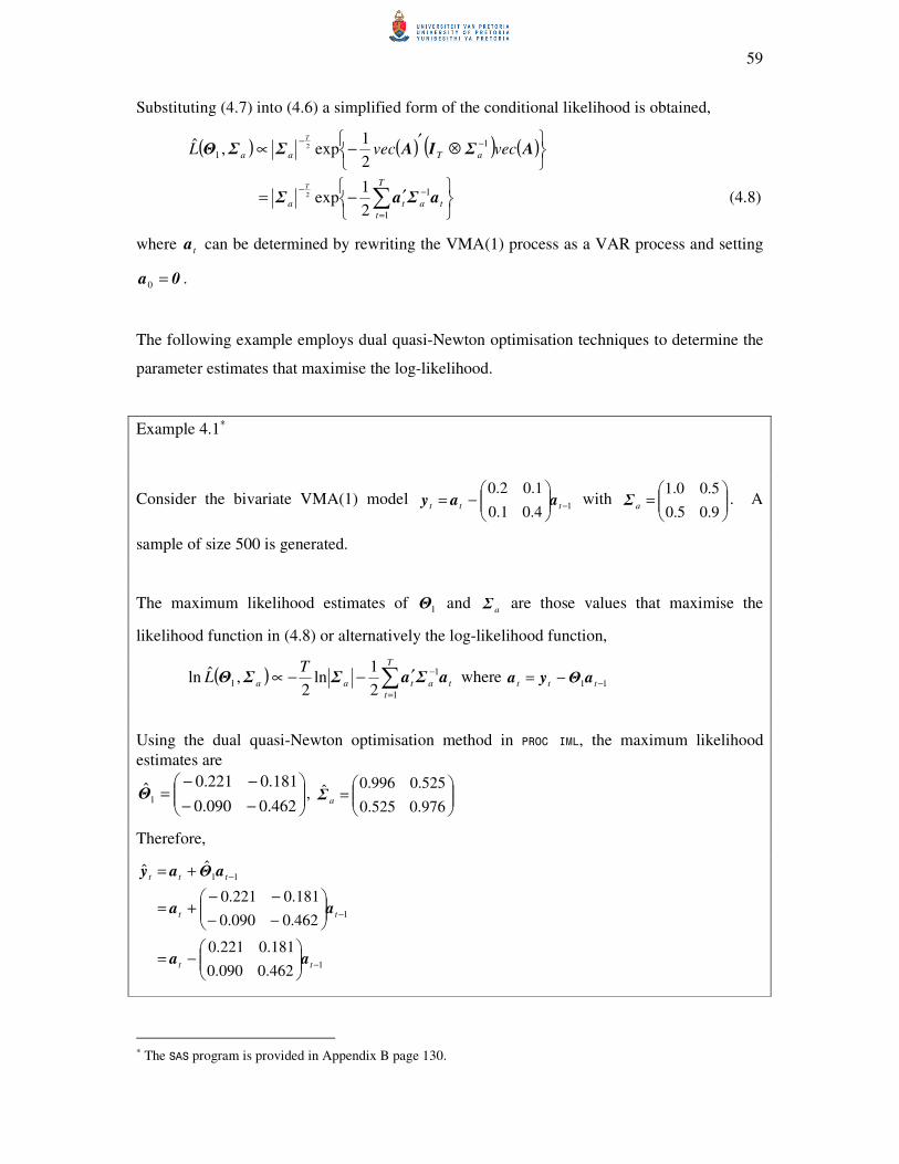
59
Substituting (4.7) into (4.6) a simplified form of the conditional likelihood is obtained,
( ) ( ) ( ) ( )
⊗′
−∝ −−AΣIAΣΣΘ vecvecL aTaa
T1
12
1exp,ˆ 2
′−= ∑=
−−T
t
tata
T
1
1
2
1exp2 aΣaΣ (4.8)
where ta can be determined by rewriting the VMA(1) process as a VAR process and setting
0a =0.
The following example employs dual quasi-Newton optimisation techniques to determine the
parameter estimates that maximise the log-likelihood.
Example 4.1∗
Consider the bivariate VMA(1) model 1
4.01.0
1.02.0−
−= ttt aay with
=
9.05.0
5.00.1aΣ . A
sample of size 500 is generated.
The maximum likelihood estimates of 1Θ and aΣ are those values that maximise the
likelihood function in (4.8) or alternatively the log-likelihood function,
( ) ∑=
−′−−∝T
t
tataa
TL
1
1
12
1ln
2,ˆln aΣaΣΣΘ where
11 −−= ttt aΘya
Using the dual quasi-Newton optimisation method in PROC IML, the maximum likelihood
estimates are
−−
−−=
462.0090.0
181.0221.0ˆ1Θ ,
=
976.0525.0
525.0996.0ˆ
aΣ
Therefore,
1
1
11
462.0090.0
181.0221.0
462.0090.0
181.0221.0
ˆˆ
−
−
−
−=
−−
−−+=
+=
tt
tt
ttt
aa
aa
aΘay
∗ The SAS program is provided in Appendix B page 130.
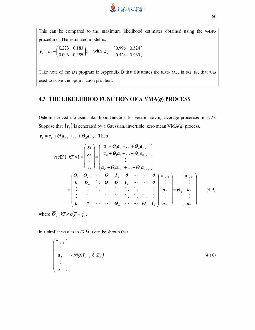
60
This can be compared to the maximum likelihood estimates obtained using the VARMAX
procedure. The estimated model is,
1459.0096.0
183.0223.0ˆ
−
−= ttt aay with
=
969.0524.0
524.0996.0ˆ
aΣ
Take note of the SAS program in Appendix B that illustrates the NLPQN CALL in SAS IML that was
used to solve the optimisation problem.
4.3 THE LIKELIHOOD FUNCTION OF A VMA(q) PROCESS
Osborn derived the exact likelihood function for vector moving average processes in 1977.
Suppose that { }ty is generated by a Gaussian, invertible, zero mean VMA(q) process,
qtqttt −− +++= aΘaΘay K11 . Then
( )
+++
+++
+++
=
=×
−−
−
−
qTqTT
T
kTvec
aΘaΘa
aΘaΘa
aΘaΘa
y
y
y
Y
K
M
K
K
M
11
2112
1011
2
1
1:
=
=
+−+−−
T
q
q
T
q
kq
kq
kqq
a
a
a
Θ
a
a
a
IΘΘ00
0IΘΘΘ0
00IΘΘΘ
M
M
M
M
LLLL
MOOOOOMM
MOOOOOMM
LLO
LLL
0
1
0
1
1
12
11
(4.9)
where ( )qTkkTq +×:Θ .
In a similar way as in (3.5) it can be shown that
+−
T
q
a
a
a
M
M
0
1
( )aqTN ΣI0 ⊗+,~ (4.10)
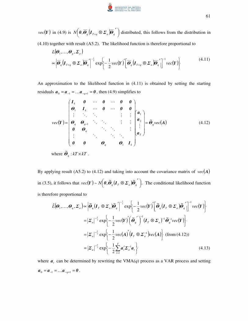
61
( )Yvec in (4.9) is ( )
′
⊗+ qaqTqN ΘΣIΘ0, distributed, this follows from the distribution in
(4.10) together with result (A5.2). The likelihood function is therefore proportional to
( )
( ) ( ) ( ) ( )
′
⊗′
−′
⊗∝−
+
−
+ YΘΣIΘYΘΣIΘ
ΣΘΘ
vecvec
L
qaqTqqaqTq
aq
1
1
2
1exp
,,,
2
1
K
(4.11)
An approximation to the likelihood function in (4.11) is obtained by setting the starting
residuals 0aaa === +−− 110 qK , then (4.9) simplifies to
( ) ( )AΘ
a
a
a
IΘΘ00
Θ0
ΘΘ
000IΘ
0000I
Y vecvec q
T
kq
q
k
k
~2
1
1
1
1
=
= −M
OOOM
MOO
MMOO
MMOOM
LL
LL
(4.12)
where kTkTq ×:~Θ .
By applying result (A5.2) to (4.12) and taking into account the covariance matrix of ( )Avec
in (3.5), it follows that ( ) ( )
′
⊗ qaTqNvec ΘΣIΘ0Y~~
,~ . The conditional likelihood function
is therefore proportional to
( ) ( ) ( ) ( ) ( )
( ) ( ) ( )
( ) ( ) ( ) (4.12)) (from 2
1exp
~~
2
1exp
~~
2
1exp
~~,,,ˆ
1
111
1
1
2
2
2
1
⊗′
−=
⊗
′′
−=
′
⊗′
−′
⊗∝
−−
−−−
−
−−
AΣIAΣ
YΘΣIΘYΣ
YΘΣIΘYΘΣIΘΣΘΘ
vecvec
vecvec
vecvecL
aTa
qaTqa
qaTqqaTqaq
T
T
K
′−= ∑=
−−T
t
tata
T
1
1
2
1exp2 aΣaΣ (4.13)
where ta can be determined by rewriting the VMA(q) process as a VAR process and setting
0aaa === +−− 110 qK .
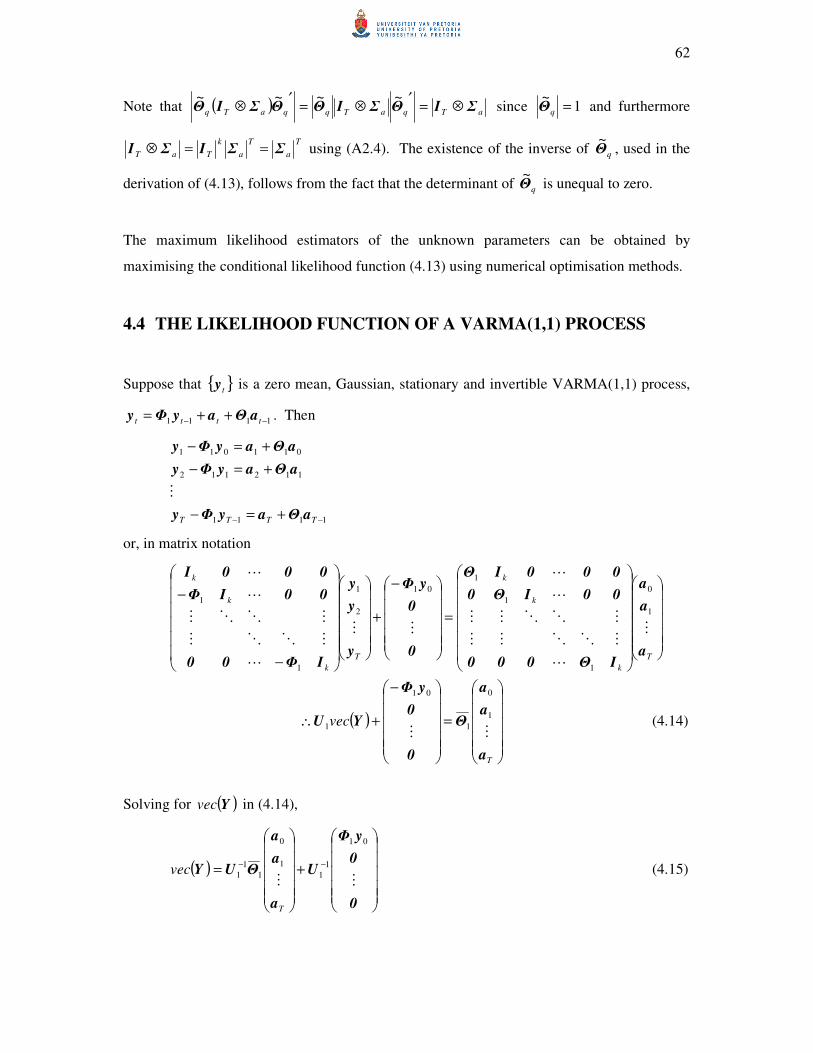
62
Note that ( ) aTqaTqqaTq ΣIΘΣIΘΘΣIΘ ⊗=′
⊗=′
⊗~~~~
since 1~
=qΘ and furthermore
T
a
T
a
k
TaT ΣΣIΣI ==⊗ using (A2.4). The existence of the inverse of qΘ~
, used in the
derivation of (4.13), follows from the fact that the determinant of qΘ~
is unequal to zero.
The maximum likelihood estimators of the unknown parameters can be obtained by
maximising the conditional likelihood function (4.13) using numerical optimisation methods.
4.4 THE LIKELIHOOD FUNCTION OF A VARMA(1,1) PROCESS
Suppose that { }ty is a zero mean, Gaussian, stationary and invertible VARMA(1,1) process,
1111 −− ++= tttt aΘayΦy . Then
1111
112112
011011
−− +=−
+=−
+=−
TTTT aΘayΦy
aΘayΦy
aΘayΦy
M
or, in matrix notation
=
−
+
−
−
T
k
k
k
T
k
k
k
a
a
a
IΘ000
00IΘ0
000IΘ
0
0
yΦ
y
y
y
IΦ00
00IΦ
000I
M
L
MOOMM
MOOMM
L
L
MM
L
MOOM
MOOM
L
L
1
0
1
1
1
01
2
1
1
1
( )
=
−
+∴
T
vec
a
a
a
Θ
0
0
yΦ
YUMM
1
0
1
01
1 (4.14)
Solving for ( )Yvec in (4.14),
( )
+
= −−
0
0
yΦ
U
a
a
a
ΘUYMM
01
1
1
1
0
1
1
1
T
vec (4.15)
63
By utilising (4.1) and result (A5.2), assuming fixed presample values 0y , the distribution of
( )Yvec is,
( ) ( )
′′⊗
−
+
−− 1
1111
1
1
01
1
1 ,~ UΘΣIΘU
0
0
yΦ
UY aTNvecM
The likelihood function is proportional to
( ) ( ) ×′′
⊗∝−
−
+
−2
1
1
1111
1
111 ,, UΘΣIΘUΣΘΦ aTaL
( ) ( ) ( )
−
′
⊗′
′
−− −−
+
−
0
0
yΦ
UYUΘΣIΘU
0
0
yΦ
UYMM
01
1
11
1
1111
01
1
12
1exp vecvec aT
( )
( ) ( ) ( )
−
′
⊗
′
−−
×′
⊗=
−
+
−
+
0
0
yΦ
YUΘΣIΘ
0
0
yΦ
YU
ΘΣIΘ
MM
01
1
1
111
01
1
111
2
1exp
2
1
vecvec aT
aT
(4.16)
Take note that the determinant, 11 =U since it is a lower diagonal matrix with ones on the
main diagonal.
An approximation of the likelihood function in (4.16) can be obtained by assuming that
0ay == 00 , then (4.14) simplifies to
( ) ( ) ( )AΘA
IΘ00
00IΘ
000I
YU vecvecvec
k
k
k
1
1
1
1
~=
=
L
MOOM
MOOM
L
L
and solving for ( )Yvec ,
( ) ( )AΘUY vecvec 1
1
1
~−= (4.17)
64
By applying result (A5.2) and (3.5) to (4.17), ( )Yvec is ( )
′′⊗ −− 1
111
1
1
~~, UΘΣIΘU0 aTN
distributed. Thus, the conditional likelihood function is proportional to
( )
( ) ( ) ( ) ( )
′′⊗
′−
′′⊗∝
−
−−
−
−− YUΘΣIΘUYUΘΣIΘU
ΣΘΦ
vecvec
L
aTaT
a
1
1
111
1
1
1
111
1
1
11
~~
2
1exp
~~
,,ˆ
2
1 (4.18)
Utilising the properties of the determinant and Kronecker product,
( ) aTaTaT ΣIUΘΣIΘUUΘΣIΘU ⊗=′′
⊗=′′
⊗ −−−− 1
111
1
1
1
111
1
1
~~~~ since 1U and 1
~Θ are lower
triangular matrices with ones on the main diagonal, therefore their determinants are equal to
one; and T
a
T
a
k
TaT ΣΣIΣI ==⊗ using (A2.4). Taking this into account, the
conditional likelihood function in (4.18) simplifies to
( ) ( ) ( ) ( )
( )( ) ( ) ( )
( ) ( ) ( ) (4.17)) (from 2
1exp
~~
2
1exp
~~
2
1exp,,ˆ
1
1
1
1
1
1
1
1
1
1
1
11
1111
2
2
2
⊗′
−=
⊗′
−=
⊗
′′′
−∝
−−
−−−−
−−−
−
AΣIAΣ
YUΘΣIYUΘΣ
YUΘΣIΘUYΣΣΘΦ
vecvec
vecvec
vecvecL
aTa
aTa
aTaa
T
T
T
′−= ∑=
−−T
t
tata
T
1
1
2
1exp2 aΣaΣ (4.19)
where ta can be determined by rewriting the VARMA(1,1) process as a VAR process and
setting 0ay == 00 .
The maximum likelihood estimators of the unknown parameters can be obtained by
maximising the likelihood function (4.19) using numerical optimisation techniques. The dual
quasi-Newton optimisation technique is used to illustrate maximum likelihood estimation of a
VARMA(1,1) model in the following example.
65
Example 4.2∗
Consider the bivariate VARMA(1,1) model 11
4.01.0
1.02.0
1.05.0
1.02.0−−
−+
−= tttt aayy with
=
9.05.0
5.00.1aΣ . A sample of size 500 is generated.
The NLPQN CALL in SAS IML was used to maximise the log-likelihood function,
( ) ∑=
−′−−=T
t
tataa
TL
1
1
112
1ln
2,,ˆln aΣaΣΣΘΦ where
1111 −− −−= tttt aΘyΦya
The maximum likelihood estimates are
−=
053.0467.0
150.0215.0ˆ
1Φ ,
−−
−−=
428.0050.0
235.0206.0ˆ1Θ ,
=
975.0525.0
525.0995.0ˆ
aΣ
Therefore, the estimated model is
11
11
1111
428.0050.0
235.0206.0
053.0467.0
150.0215.0
428.0050.0
235.0206.0
053.0467.0
150.0215.0
ˆˆˆ
−−
−−
−−
−+
−=
−−
−−++
−=
++=
ttt
ttt
tttt
aay
aay
aΘayΦy
These estimates are very similar to the maximum likelihood estimates obtained using the
VARMAX procedure, the estimated model using this procedure is
11434.0062.0
238.0213.0
065.0470.0
157.0209.0ˆ
−−
−+
−= tttt aayy with
=
969.0530.0
530.0003.1ˆ
aΣ
4.5 THE IDENTIFICATION PROBLEM
Let { }ty be a stationary, invertible VARMA(p,q) process, as defined in (2.39), with zero
mean. In terms of the lag operator this process can be represented as
∗ The SAS program is provided in Appendix B page 131.
66
( ) ( ) tt LL aΘyΦ = (4.20)
where the operators ( )LΦ and ( )LΘ are defined in (2.40).
It is possible that two VARMA(p,q) representations are observationally equivalent, that is,
two VARMA(p,q) models with different coefficient matrices will have the same ( )∞VMA
representation. This will be the case when the two sets of operators, say ( )L*
Φ and ( )L*
Θ
are related to ( )LΦ and ( )LΘ by premultiplying with a non-singular matrix ( )LU , for
example ( ) ( ) ( )LLL ΦUΦ =* and ( ) ( ) ( )LLL ΘUΘ =* . (Reinsel, 1997)
In order to specify a unique set of parameters we need to put certain restrictions on the VAR
and VMA operators. The representation must be such that there are no common factors in the
( )LΦ and ( )LΘ operators, except for unimodular operators. A unimodular operator is an
operator with its determinant equal to a non zero constant, which implies that the determinant
is not a function of L, the lag operator. If this is the case, the operators ( )LΦ and ( )LΘ are
called left-coprime. The only unimodular operator that will ensure uniqueness of the left-
coprime operators is the one equal to the identity matrix. (Lütkepohl, 2005)
The final equations form and the echelon form result in a unique representation of the
VARMA(p,q) process. Before defining these forms we need to consider a more general
representation of the standard VARMA representation in (2.39) by including coefficient
matrices for ty and ta , namely
qtqtttptpttt −−−−−− +++++++++= aΘaΘaΘaΘyΦyΦyΦcyΦ KK 2211022110 (4.21)
or in terms of the lag operator
( ) ( )tt
t
q
qt
p
p
LL
LLLLLL
aΘcyΦ
aΘΘΘΘcyΦΦΦΦ
)()(
...2
210
2
210
+=
+++++=−−−− K (4.22)
where
q
q
p
p
LLLL
LLLL
ΘΘΘΘΘ
ΦΦΦΦΦ
++++=
−−−−=
...)(
)(
2
210
2
210 K
with )(LΦ and )(LΘ left-coprime.

67
Definitions 12.1 and 12.2 of Lütkepohl (2005) define the final equations form and the echelon
form respectively, namely:
“The VARMA representation (4.22) is said to be in final equations form if kIΘ =0 and
( ) kLL IΦ φ=)( , where ( ) p
p LLL φφφ K−−= 11 is a scalar operator with .0≠pφ ”
“The VARMA representation (4.22) is said to be in echelon form or EARMA form if the
VAR and VMA operators ( )[ ]kimmi LL
,,1,)(
K== φΦ and ( )[ ]LL miθ=)(Θ are left-coprime and
satisfy the following conditions: the operators ( )Lmiφ ( )ki ,,1 K= and ( )Lmjθ ( )kj ,,1 K= in
the m-th row of ( )LΦ and ( )LΘ have degree mp and they have the form
( ) ∑=
−=mp
j
j
jmmmm LL1
,1 φφ , for km ,,1K=
( ) ∑+−=
−=m
mim
p
ppj
j
jmimi LL1
,φφ , for im ≠
and
( ) ∑=
=mp
j
j
jmimi LL0
,θθ , for kim ,,1, K= with 00 ΘΦ =
In the VAR operators ( )Lmiφ
( )( )
<
=≥+=
for ,min
,,1, for ,1min
impp
kimimppp
im
im
mi
K
That is, mip specifies the number of free coefficients in the operator ( )Lmiφ for mi ≠ . The
row degrees ( )kpp ,,1 K are called the Kronecker indices and their sum ∑=
k
i
ip1
is the McMillan
degree”
For more detail and examples we refer to chapter 12 of Lütkepohl (2005).
4.6 CONCLUSION
This chapter focused on maximum likelihood estimation of VARMA processes. Due to the
nonlinear nature of the normal equations with respect to the parameters, only the likelihood

68
functions were derived. The examples employed numerical optimisation techniques to
maximise the likelihood function in order to determine the parameter estimates. An overview
was given of the identification problem regarding the uniqueness of the VARMA
representation. Before a model can be estimated, one has to determine the values of p and q.
Chapter 5 will discuss some guidelines to select the appropriate order.
69
CHAPTER 5
ORDER SELECTION
5.1 INTRODUCTION
The order of the model is not known in most applications; therefore order selection forms part
of the model building process. We are looking for a parsimonious model, a model with as
little as possible parameters that explains most of the variation in the data.
Before the vector autoregressive coefficients, pii K,2,1 , =Φ and the vector moving average
coefficients qii K,2,1 , =Θ can be estimated, the order of the VARMA process need to be
determined. Thus we are searching for unique numbers p and q such that 0≠pΦ and
pii >= for 0Φ while 0≠qΘ and .for 0 qjj >=Θ
The problem of finding appropriate values for p and q was tackled by, amongst others, Tiao &
Box (1981). They considered methods based on the sample autocorrelations and the sample
partial autoregression matrices to select the order of pure VMA and VAR models,
respectively. They introduced a way of visualising the sample autocorrelation and sample
partial autoregression matrices by replacing the values with symbols. The challenge of
determining the order for mixed models was addressed by, for example, Quinn (1980) who
extended the Hannan-Quinn information criterion to the multivariate environment. This
method entails fitting different models and then selecting the model that minimises the
information criterion. This can be a time consuming exercise. Spliid (1983) was one of the
people who proposed an algorithm for the MINIC (minimum information criterion) method,
which is another way of tentatively identifying the order.
In section 5.2 the use of the sample autocovariance and autocorrelation matrices, to identify
the order of a pure VMA process, is considered. Section 5.3 focuses on identifying the order
of a pure VAR process by determining the partial autoregression matrices. Finally in section
5.4 a method to determine the order of a VARMA process, based on the information criteria,
is discussed.
70
The following bivariate models will be used in the examples to illustrate the different
techniques of determining the order of a VARMA process:
VAR(1) model: ttt ayy +
= −1
4.01.0
6.05.0
VMA(2) model: 21
1.06.0
04.0
4.01.0
1.02.0−−
−
−= tttt aaay
VARMA(2,1) model: 121
4.01.0
1.02.0
5.04.0
5.08.0
1.05.0
1.02.0−−−
−+
−+
−= ttttt aayyy
with
=
9.05.0
5.00.1aΣ for all the models.
5.2 SAMPLE AUTOCOVARIANCE AND AUTOCORRELATION
MATRICES
In this section, expression for sample autocovariance and sample autocorrelation matrices are
given, a large sample test for the significance of the elements of the autocorrelation matrix is
provided and illustrated by means of a numerical example.
Suppose we have k time series processes each comprising of T equally spaced observations
denoted by Tk ×:Y .
The sample estimate of the process mean is
( ) ∑=
=′
==T
t
tkT
yyy1
21
1ˆ yyµ L (5.1)
This estimate, y , is an unbiased estimator for the process mean since,
( ) ( ) µµyyy ===
= ∑∑∑
===
T
t
T
t
t
T
t
tT
ETT
EE111
111
The autocovariance matrix at lag l, ( ) ( )( )
′
−−= − µyµyΓ lttEl can be estimated from the
sample values to determine the sample autocovariance matrix,
( ) ( )( )∑+=
−
′−−=
T
lt
lttT
l1
1ˆ yyyyΓ K,1,0for =l (5.2)
71
The (i,j)-th element of ( )lΓ is given by ( ) ( )( )∑+=
− −−=T
lt
jltjiitij yyyyT
l1
,
1γ .
The formula for the sample autocovariance matrix in (5.2) only adds T-l observations and
then divides this by T, not by T-l. This means that as l increases the estimate decreases and
eventually will be zero. This is in line with the population autocovariance matrix because for
a stationary process ( ) 0Γ →l as ∞→l . (Hamilton, 1994)
From the sample autocovariance matrices in (5.2) the sample autocorrelations can be
calculated by
( )( )
( ) ( )0ˆ0ˆ
ˆˆ
jjii
ij
ij
ll
γγ
γρ = (5.3)
or in matrix form at lag l,
( ) 2
1
2
1
ˆˆˆ)(ˆ−−
= VΓVρ ll (5.4)
where 2
1
V is the kk × diagonal matrix with the sample standard deviations.
In Chapter 2 the autocovariance matrices, ( )lΓ , for a VMA(q) process were derived. It was
shown in (2.35) that ( ) .for qll >= 0Γ Since the autocorrelation matrices ( )lρ are a function
of the autocovariance matrices, it can be shown that ( ) .for qll >= 0ρ This property can be
used to determine the order of a pure VMA process. We will calculate the sample
autocorrelation matrices at different lags and determine whether they differ significantly from
zero. If they do not differ significantly from zero at lag ,1+j it can be concluded that the
data was generated by a VMA( j ) model.
This ‘significance test’ is more of an informal guideline developed by Tiao & Box (1981). It
has to be determined whether the autocorrelation matrices differ significantly from zero. In
other words one can test whether the autocorrelation matrix at different lags corresponds to
that of a white noise process. It is known that for large T, the individual elements of a sample
autocorrelation matrix of a white noise process are normally distributed with zero mean and
variance equal to T
1. This will be considered in more detail in Section 6.2.1. Based on this
distribution, Tiao & Box constructed a confidence interval with the following symbols:
72
“ – “
<
T
2- errors standard estimated 2- than less :
“ . “
T
2,
T
2- errors standard estimated wo within t:
“ + “
>
T
2 errors standard estimated 2an greater th :
In the following example PROC IML was used to determine the sample autocovariance and
sample autocorrelation matrices up to lag 3 using formulae (5.1), (5.2) and (5.4). The
individual elements of the sample autocorrelation matrices are tested for significance using
the guideline developed by Tiao & Box. The results were compared with the results produced
by the VARMAX procedure.
Example 5.1∗
The sample autocovariances and sample autocorrelations, for the three generated time series
processes with 500=T and a Gaussian error distribution, were calculated using (5.2) and
(5.4), respectively and are tabulated below.
Process 1 Process 2 Process 3
Generated by VAR(1) VMA(2) VARMA(2,1)
Autocovariances
( )0Γ
210.1131.1
131.1584.2
640.1925.0
925.0251.1
−
−
543.8173.3
173.3771.6
( )1Γ
516.0654.0
190.1896.1
−−
−−
279.0121.0
171.0202.0
−
−
005.7668.5
247.2355.4
( )2Γ
297.0425.0
882.0358.1
−−
−−
392.0613.0
185.0342.0
− 915.5979.5
567.0262.5
( )3Γ
207.0239.0
616.0916.0
082.0015.0
040.0013.0
−
−−
413.3615.6
189.1303.2
∗ The SAS program is provided in Appendix B page 132.
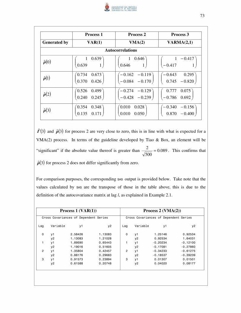
73
Process 1 Process 2 Process 3
Generated by VAR(1) VMA(2) VARMA(2,1)
Autocorrelations
( )0ρ
1639.0
639.01
1646.0
646.01
−
−
1417.0
417.01
( )1ρ
426.0370.0
673.0734.0
−−
−−
170.0084.0
119.0162.0
−
−
820.0745.0
295.0643.0
( )2ρ
245.0240.0
499.0526.0
−−
−−
239.0428.0
129.0274.0
− 692.0786.0
075.0777.0
( )3ρ
171.0135.0
348.0354.0
050.0010.0
028.0010.0
−
−−
400.0870.0
156.0340.0
( )3Γ and ( )3ρ for process 2 are very close to zero, this is in line with what is expected for a
VMA(2) process. In terms of the guideline developed by Tiao & Box, an element will be
“significant” if the absolute value thereof is greater than 089.0500
2= . This confirms that
( )3ρ for process 2 does not differ significantly from zero.
For comparison purposes, the corresponding SAS output is provided below. Take note that the
values calculated by SAS are the transpose of those in the table above, this is due to the
definition of the autocovariance matrix at lag l, as explained in Example 2.1.
Process 1 (VAR(1)) Process 2 (VMA(2))
Cross Covariances of Dependent Series
Lag Variable y1 y2
0 y1 2.58426 1.13083
y2 1.13083 1.21028
1 y1 1.89590 0.65443
y2 1.19016 0.51605
2 y1 1.35804 0.42457
y2 0.88176 0.29683
3 y1 0.91573 0.23894
y2 0.61588 0.20748
Cross Covariances of Dependent Series
Lag Variable y1 y2
0 y1 1.25146 0.92534
y2 0.92534 1.64031
1 y1 -0.20234 -0.12100
y2 -0.17081 -0.27860
2 y1 -0.34233 -0.61275
y2 -0.18537 -0.39239
3 y1 0.01307 0.01501
y2 0.04020 0.08177
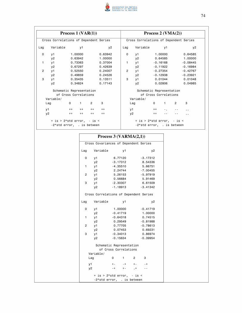
74
Process 1 (VAR(1)) Process 2 (VMA(2))
Cross Correlations of Dependent Series
Lag Variable y1 y2
0 y1 1.00000 0.63942
y2 0.63942 1.00000
1 y1 0.73363 0.37004
y2 0.67297 0.42639
2 y1 0.52550 0.24007
y2 0.49859 0.24526
3 y1 0.35435 0.13511
y2 0.34824 0.17143
Schematic Representation
of Cross Correlations
Variable/
Lag 0 1 2 3
y1 ++ ++ ++ ++
y2 ++ ++ ++ ++
+ is > 2*std error, - is <
-2*std error, . is between
Cross Correlations of Dependent Series
Lag Variable y1 y2
0 y1 1.00000 0.64585
y2 0.64585 1.00000
1 y1 -0.16168 -0.08445
y2 -0.11922 -0.16984
2 y1 -0.27354 -0.42767
y2 -0.12938 -0.23921
3 y1 0.01044 0.01048
y2 0.02806 0.04985
Schematic Representation
of Cross Correlations
Variable/
Lag 0 1 2 3
y1 ++ -. -- ..
y2 ++ -- -- ..
+ is > 2*std error, - is <
-2*std error, . is between
Process 3 (VARMA(2,1))
Cross Covariances of Dependent Series
Lag Variable y1 y2
0 y1 6.77120 -3.17312
y2 -3.17312 8.54336
1 y1 -4.35510 5.66751
y2 2.24744 -7.00455
2 y1 5.26153 -5.97919
y2 0.56684 5.91469
3 y1 -2.30307 6.61509
y2 -1.18913 -3.41342
Cross Correlations of Dependent Series
Lag Variable y1 y2
0 y1 1.00000 -0.41719
y2 -0.41719 1.00000
1 y1 -0.64318 0.74515
y2 0.29549 -0.81988
2 y1 0.77705 -0.78613
y2 0.07453 0.69231
3 y1 -0.34013 0.86974
y2 -0.15634 -0.39954
Schematic Representation
of Cross Correlations
Variable/
Lag 0 1 2 3
y1 +- -+ +- -+
y2 -+ +- .+ --
+ is > 2*std error, - is <
-2*std error, . is between
75
The schematic representation of the autocorrelations summarises the significance of the
individual elements. Each lag is represented by four symbols corresponding to the elements
of the autocorrelation matrix. A “+” or “-“ indicates significance, while a “.” means that the
hypothesis 0: ,0 =imnH ρ cannot be rejected. In this example no autocorrelation from lag 3
onwards for process 2 is significant, implying that this process is generated by a VMA(2)
model. The other two processes both have significant autocorrelations at lag 3, implying
either higher order VMA or mixed models. The partial autoregression matrices may shed
more light on the autoregressive order.
5.3 PARTIAL AUTOREGRESSION MATRICES
In this section the Yule-Walker equations of a VAR model are utilised to derive formulae for
the partial autoregression matrices up to lag 2. Another method of obtaining partial
autoregression matrices and a test for the significance of individual elements is given. The
section is concluded with a numerical example.
The partial autoregression matrix is a measure of the autocovariance between the observed
values at two time points after the effect of the terms in between the two time points has been
removed. These matrices can be used to identify the order of a VAR process, since the partial
autoregression matrices of a VAR(p) process are equal to zero from lag 1+p onwards. The
Yule-Walker equations in (2.25) that calculate the autocovariance matrix recursively, can be
used to determine the partial autoregression matrices. Consider as an example the VAR(1)
and VAR(2) processes.
For a VAR(1) process the Yule-Walker equation for the autocovariance matrix is,
( ) ( )11 −= ll ΓΦΓ , and therefore
( ) ( )01 11ΓΦΓ =
where 11Φ is called the partial autoregression matrix of lag 1. Solving for 11Φ we have that
( ) ( ) 1
11 01−
= ΓΓΦ (5.5)
In case of a VAR(1) process 111 ΦΦ = and .3322 0ΦΦ === K
76
Consider a VAR(2) process. The autocovariance matrix at lag l,
( ) ( ) ( )21 21 −+−= lll ΓΦΓΦΓ , and therefore
( ) ( ) ( ) ( ) ( )′+=−+= 10101 22122212 ΓΦΓΦΓΦΓΦΓ (5.6)
( ) ( ) ( )012 2212 ΓΦΓΦΓ += (5.7)
By solving these two equations simultaneously, the partial autoregression matrix of lag 2,
22Φ , can be determined,
( ) ( ) ( )′−= 110 2212 ΓΦΓΓΦ (from (5.6))
( ) ( ) ( ) ( ) 1
22
1
12 0101−− ′
−=∴ ΓΓΦΓΓΦ (5.8)
Substituting (5.8) into (5.7),
( ) ( ) ( ) ( ) ( ) ( ) ( ) ( )
( ) ( ) ( ) ( ) ( ) ( ) ( ) ( )
′
−=−
+′
−=
−−
−−
10101012
01011012
1
22
1
22
1
22
1
ΓΓΓΓΦΓΓΓΓ
ΓΦΓΓΓΦΓΓΓΓ
( ) ( ) ( ) ( )[ ] ( ) ( ) ( ) ( )1
11
22 10101012−
−−
′
−−=∴ ΓΓΓΓΓΓΓΓΦ (5.9)
For a VAR(2) process 222 ΦΦ = and .4433 0ΦΦ === K
In general, for a VAR(p) process, K,2,1=p , the partial autoregression matrices of lag p,
ppΦ , can be determined by solving the p Yule-Walker equations,
( ) ( )∑=
−=p
i
ip ill1
ΓΦΓ where pl ,,2,1 K= (5.10)
The partial autoregression matrix of order p, ppΦ is equal to pΦ and 0Φ =mm for .pm >
(Reinsel, 1997)
Note that the Yule-Walker equation system is used to derive expressions for the partial
autoregression matrices in terms of autocovariance matrices. The expressions are general,
they hold for all VARMA models.
This characteristic can be used to determine the order of a pure VAR process by determining
whether the matrix of partial autoregressions at lag ,1+j 1,1 ++ jjΦ , differs significantly from
zero. If 1,1 ++ jjΦ does not differ significantly from zero it can be concluded that the data was
generated by a VAR( j ) model.

77
The partial autoregression matrices are estimated by replacing the autocovariance matrices in
(5.5) and (5.9) with their sample estimates. The sample estimates of 11Φ and 22Φ are given
by,
( ) ( ) 1
11 0ˆ1ˆˆ −= ΓΓΦ (5.11)
( ) ( ) ( ) ( )[ ] ( ) ( ) ( ) ( )1
11
22 1ˆ0ˆ1ˆ0ˆ1ˆ0ˆ1ˆ2ˆˆ−
−−
′
−−= ΓΓΓΓΓΓΓΓΦ (5.12)
Another way of obtaining estimates for the partial autoregression matrices and their standard
errors are by fitting VAR models of increasing order. Tiao & Box (1981) also suggested a
guideline to tentatively determine the order of the VAR model by constructing a confidence
interval of errors standard estimated 2± . Each element of the partial autoregression matrix is
classified as a “ – “, “ . “ or “ + “ depending on whether it is below the confidence limit,
between the confidence limits or above the confidence limit.
In Example 5.2 PROC IML was used to calculate the estimated partial autoregression matrices
using the formulae derived in (5.5) and (5.9), respectively. It is shown that the estimates
obtained are the same as the results of the VARMAX procedure.
Example 5.2∗
The sample partial autoregression matrices, 11Φ and 22Φ , can be calculated using (5.11) and
(5.12), respectively. The sample partial autoregression matrices for the three generated time
series are tabulated below.
Process 1 Process 2 Process 3
Generated by VAR(1) VMA(2) VARMA(2,1)
Partial Autoregression Matrices
11Φ
321.0113.0
504.0513.0
−
−−
198.0050.0
022.0145.0
−
−
616.0548.0
029.0629.0
22Φ
−
−
005.0002.0
002.0049.0
−
−
027.0535.0
066.0356.0
− 221.0187.0
361.0890.0
∗ The SAS program is provided in Appendix B page 132.

78
22Φ for process 1 is very close to zero, this is in line with what is expected for a VAR(1)
process. The partial autoregression matrices for the other two processes are not close to zero
implying they are either VAR models of a higher order, VMA models or mixed model.
The SAS output of the partial autoregression matrices for the processes is provided below. The
schematic representations can be interpreted as in Example 5.1.
Process 1 (VAR(1)) Process 2 (VMA(2))
Partial Autoregression
Lag Variable y1 y2
1 y1 0.51311 0.50395
y2 0.11276 0.32103
2 y1 0.04868 -0.00223
y2 0.00179 -0.00529
3 y1 -0.03094 -0.00512
y2 -0.05409 0.03963
Schematic Representation
of Partial Autoregression
Variable/
Lag 1 2 3
y1 ++ .. ..
y2 ++ .. ..
+ is > 2*std error, - is <
-2*std error, . is between
Partial Autoregression
Lag Variable y1 y2
1 y1 -0.14529 -0.02217
y2 0.04958 -0.19781
2 y1 -0.35634 0.06602
y2 -0.53476 0.02730
3 y1 -0.16908 0.05576
y2 -0.28812 0.08834
Schematic Representation
of Partial Autoregression
Variable/
Lag 1 2 3
y1 -. -. -.
y2 .- -. -.
+ is > 2*std error, - is <
-2*std error, . is between
Process 3 (VARMA(2,1))
Partial Autoregression
Lag Variable y1 y2
1 y1 -0.62946 0.02927
y2 0.54820 -0.61627
2 y1 0.88979 0.36075
y2 -0.18681 0.22123
3 y1 0.17631 0.12897
y2 -0.03528 0.16250
Schematic Representation
of Partial Autoregression
Variable/
Lag 1 2 3
y1 -. ++ ++
y2 +- -+ .+
+ is > 2*std error, - is <
-2*std error, . is between
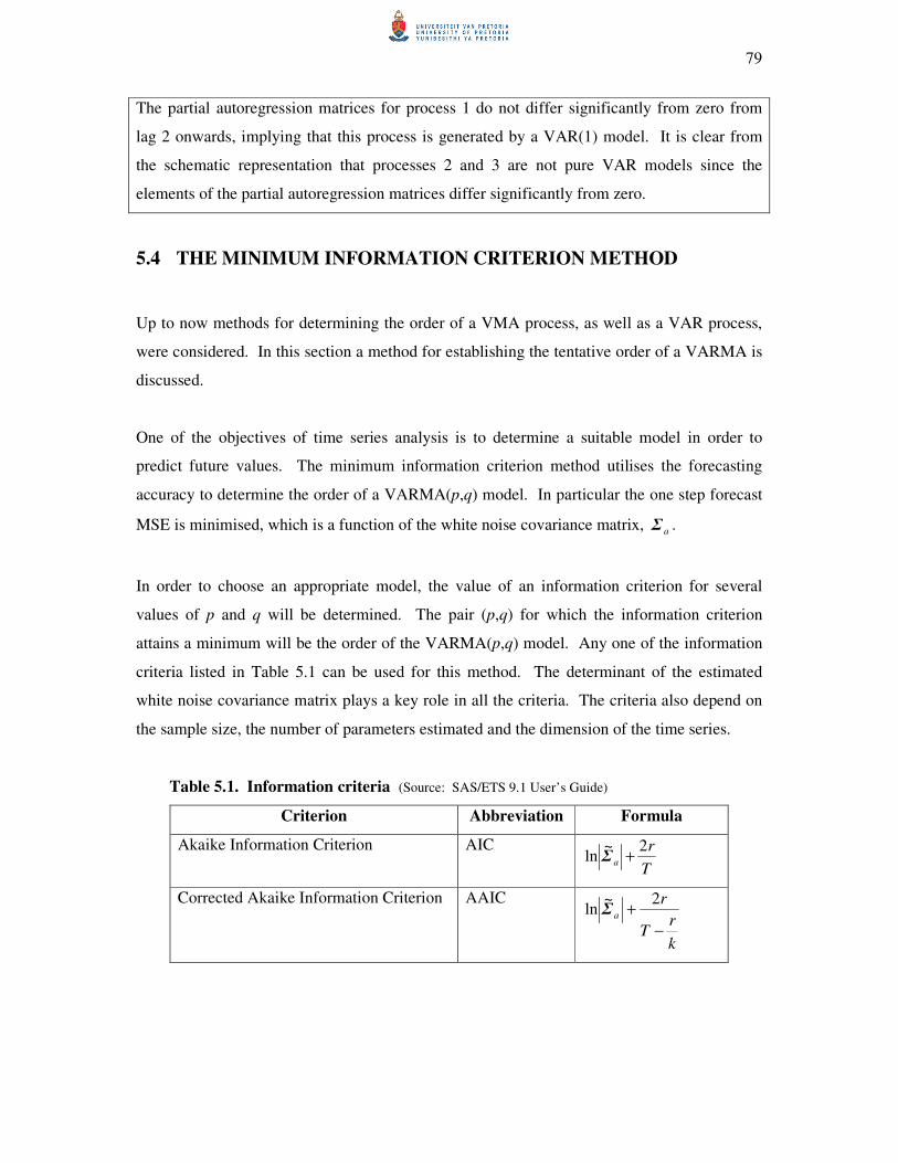
79
The partial autoregression matrices for process 1 do not differ significantly from zero from
lag 2 onwards, implying that this process is generated by a VAR(1) model. It is clear from
the schematic representation that processes 2 and 3 are not pure VAR models since the
elements of the partial autoregression matrices differ significantly from zero.
5.4 THE MINIMUM INFORMATION CRITERION METHOD
Up to now methods for determining the order of a VMA process, as well as a VAR process,
were considered. In this section a method for establishing the tentative order of a VARMA is
discussed.
One of the objectives of time series analysis is to determine a suitable model in order to
predict future values. The minimum information criterion method utilises the forecasting
accuracy to determine the order of a VARMA(p,q) model. In particular the one step forecast
MSE is minimised, which is a function of the white noise covariance matrix, aΣ .
In order to choose an appropriate model, the value of an information criterion for several
values of p and q will be determined. The pair (p,q) for which the information criterion
attains a minimum will be the order of the VARMA(p,q) model. Any one of the information
criteria listed in Table 5.1 can be used for this method. The determinant of the estimated
white noise covariance matrix plays a key role in all the criteria. The criteria also depend on
the sample size, the number of parameters estimated and the dimension of the time series.
Table 5.1. Information criteria (Source: SAS/ETS 9.1 User’s Guide)
Criterion Abbreviation Formula
Akaike Information Criterion AIC
T
ra
2~ln +Σ
Corrected Akaike Information Criterion AAIC
k
rT
ra
−
+2~
ln Σ
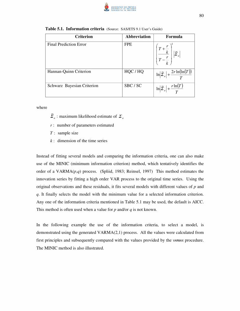
80
Table 5.1. Information criteria (Source: SAS/ETS 9.1 User’s Guide)
Criterion Abbreviation Formula
Final Prediction Error FPE
a
k
k
rT
k
rT
Σ~
−
+
Hannan-Quinn Criterion HQC / HQ ( )( )T
Tra
lnln2~ln +Σ
Schwarz Bayesian Criterion SBC / SC ( )T
Tra
ln~ln +Σ
where
:~
aΣ maximum likelihood estimate of aΣ
:r number of parameters estimated
:T sample size
:k dimension of the time series
Instead of fitting several models and comparing the information criteria, one can also make
use of the MINIC (minimum information criterion) method, which tentatively identifies the
order of a VARMA(p,q) process. (Spliid, 1983; Reinsel, 1997) This method estimates the
innovation series by fitting a high order VAR process to the original time series. Using the
original observations and these residuals, it fits several models with different values of p and
q. It finally selects the model with the minimum value for a selected information criterion.
Any one of the information criteria mentioned in Table 5.1 may be used, the default is AICC.
This method is often used when a value for p and/or q is not known.
In the following example the use of the information criteria, to select a model, is
demonstrated using the generated VARMA(2,1) process. All the values were calculated from
first principles and subsequently compared with the values provided by the VARMAX procedure.
The MINIC method is also illustrated.
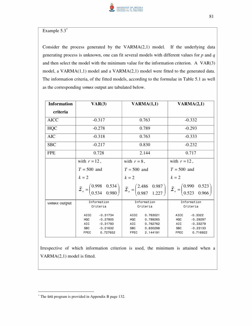
81
Example 5.3∗
Consider the process generated by the VARMA(2,1) model. If the underlying data
generating process is unknown, one can fit several models with different values for p and q
and then select the model with the minimum value for the information criterion. A VAR(3)
model, a VARMA(1,1) model and a VARMA(2,1) model were fitted to the generated data.
The information criteria, of the fitted models, according to the formulae in Table 5.1 as well
as the corresponding VARMAX output are tabulated below.
Information
criteria
VAR(3) VARMA(1,1) VARMA(2,1)
AICC -0.317 0.763 -0.332
HQC -0.278 0.789 -0.293
AIC -0.318 0.763 -0.333
SBC -0.217 0.830 -0.232
FPE 0.728 2.144 0.717
with 12=r ,
500=T and
2=k
=
980.0534.0
534.0998.0~aΣ
with 8=r ,
500=T and
2=k
=
227.1987.0
987.0486.2~aΣ
with 12=r ,
500=T and
2=k
=
966.0523.0
523.0990.0~aΣ
VARMAX output Information
Criteria
AICC -0.31734
HQC -0.27805
AIC -0.31793
SBC -0.21632
FPEC 0.727652
Information
Criteria
AICC 0.763021
HQC 0.789265
AIC 0.762762
SBC 0.830298
FPEC 2.144191
Information
Criteria
AICC -0.3322
HQC -0.29297
AIC -0.33279
SBC -0.23133
FPEC 0.716922
Irrespective of which information criterion is used, the minimum is attained when a
VARMA(2,1) model is fitted.
∗ The SAS program is provided in Appendix B page 132.

82
Instead of fitting several models with different values of p and q, the MINIC method can be
used. The SAS output regarding the MINIC method as well as the information criteria for the
fitted VAR(3) model is given below.
Minimum Information Criterion
Lag MA 0 MA 1 MA 2 MA 3 MA 4
AR 0 3.8514402 3.8350536 3.5061428 3.4004058 3.0793454
AR 1 1.4133135 1.3859316 1.0870527 1.052723 0.8185272
AR 2 -0.277616 -0.322909 -0.310653 -0.300108 -0.29529
AR 3 -0.324909 -0.312945 -0.301504 -0.291147 -0.279252
AR 4 -0.318086 -0.301794 -0.293259 -0.278826 -0.263467
Covariances of Innovations
Variable y1 y2
y1 1.01016 0.54044
y2 0.54044 0.99239
Information
Criteria
AICC -0.31734
HQC -0.27805
AIC -0.31793
SBC -0.21632
FPEC 0.727652
According to the MINIC method, the smallest value of the criterion ( 325.0− ) implies that a
VAR(3) model was selected. Take note that this minimum value is very close to the
criterion value for the VARMA(2,1) model ( 323.0− ).
Since a VAR(3) model was estimated using the method of least squares, the matrix of
autocovariances for the innovations must be mulitplied with T
kpT − to obtain the estimate
aΣ~
used in the formulae in Table 5.1. This is due to the fact that SAS adjusts the estimate of
the white noise covariance matrix to be unbiased. Since there is not an intercept included in
the model, this adjustment differs slightly from (3.21).
According to the information criteria for the two models, the VARMA(2,1) model performs
better than the VAR(3) model. One must keep in mind that the MINIC method only
tentatively selects the order, Chapter 6 will still look at the model diagnostics in order to
determine whether a selected model is an adequate representation of the underlying data
generating process.
83
5.5 CONCLUSION
This chapter was concerned with tentatively determining the order of a VARMA model. It is
relatively easy to determine the order of a pure VMA and a pure VAR model simply by
examining the sample autocorrelation matrices and the sample partial autoregression matrices,
respectively. However, the moment there is a combination of these models (VARMA
models), the above mentioned methods do not contribute in finding the order. For the more
complex models, the MINIC method was introduced. The MINIC method proved to be
successful, also for mixed (VARMA) models.
84
CHAPTER 6
MODEL DIAGNOSTICS
6.1 INTRODUCTION
In this chapter the goodness of fit of a selected model is assessed. The significance of the
estimated parameters (as determined in Sections 3.2.3 and 3.3.3) is a good starting point since
it is not desirable to have extra parameters that do not contribute to the model. On the other
side it may also be misleading, because the parameter estimates of a poor model may also be
significant. Thus, we can not solely rely on the significance of the parameters to assess the
model. As in most modeling situations the fit is assessed through the behaviour of the
residuals. If a model is an adequate representation of the process that generated the time
series, the residuals should have no significant trend or pattern. One way to establish this is to
look at the individual elements of the autocorrelation matrices of the residual vectors, this is
done in Section 6.2.1. In Section 6.2.2 the Portmanteau test statistic will be discussed, which
determines the overall significance of the residual autocorrelations.
Testing the adequacy of a fitted model based on the multivariate residual autocorrelation
matrices became popular since Chitturi (1974) derived the asymptotic distribution of residual
autocorrelations and proposed a Chi-squared statistic to test the fit of pure autoregressive
models. This was generalised to VARMA models by Hosking (1980) and Li & McLeod
(1981) who proposed the multivariate Portmanteau test statistic.
The estimated multivariate time series model can also be decomposed into univariate time
series models. These univariate models can be evaluated separately by means of a 2R value,
the Durbin-Watson test for serial correlation and the Jarque-Bera test for normality of the
residuals, to name only a few. These tests will be discussed in more detail in Section 6.3.
The multivariate and univariate diagnostic checks described in this chapter will be used in an
example in Section 6.4.1 to distinguish between a good and a poor model. The rest of Section
6.4 is devoted to examples of the whole model building process, based on two multivariate
time series datasets, namely temperatures and electricity demand.
85
6.2 MULTIVARIATE DIAGNOSTIC CHECKS
In this section the residual autocorrelation matrices of the fitted model are analysed, using two
methods. The first method tests the individual elements of the residual autocorrelation matrix
at different lags for significance, while the second method considers the autocorrelation
matrices up to a certain lag as a whole and tests that for significance.
6.2.1 Residual autocorrelation matrices
This section starts off by determining the distribution of the autocorrelation matrices of a
white noise process. The reason being that the residuals of a fitted model should behave the
same as a white noise process if the model fits well.
Let { }ta be a k-dimensional white noise process with covariance matrix aΣ and
corresponding correlation matrix aR . The sample autocovariance matrix and the sample
autocorrelation matrix of { }ta at lag i are given by
it
T
it
tiT
−
+=
′= ∑ aaC1
1 Thi <= ,,1,0 K (6.1)
2
1
2
1 −−= aiai VCVR Thi <= ,,1,0 K (6.2)
where T is the length of the time series and 2
1
aV is a kk × diagonal matrix with the square
root of the diagonal elements of 0C on the main diagonal. Let ( )
hh RRR K1
* = .
Proposition 4.4 of Lütkepohl (2005) states:
“Let { }ta be a k-dimensional identically distributed standard white noise process, that is, ta
and sa have the same multivariate distribution with nonsingular covariance matrix aΣ and
corresponding correlation matrix aR . Then, for 1≥h ,
( ) ( )aah
d
h NvecT RRI0R ⊗⊗→ ,* ” (6.3)
From (6.3) it follows that ( ) ( ) ( )aa
d
ji NvecTvecT RR0RR ⊗→ , and and that if ji ≠
they are asymptotically independent. (Lütkepohl, 2005)
86
The elements on the main diagonal of the correlation matrix, aR , are equal to one. This is
then also true for the elements on the main diagonal of aa RR ⊗ . Consequently, the
asymptotic distributions of the elements of ( ) *
hvecT R are approximate standard normal
distributions. This follows from the property of the multivariate normal distribution that all
subsets also have a (multivariate) normal distribution. (Johnson & Wichern, 2002) Consider
as an example a bivariate white noise process with the sample autocorrelation matrix at lag i,
=
ii
ii
irr
rr
,22,21
,12,11R and
=
1*
*1aR , then
( )
→
=
1***
*1**
**1*
***1
,
0
0
0
0
,22
,12
,21
,11
N
r
r
r
r
TvecTd
i
i
i
i
iR where * is an arbitrary number,
therefore ( )1,0, NrTd
imn → .
This property can be used to test whether the elements of the sample autocorrelation matrices
at different lags of a white noise process differ significantly from zero. Let imn,ρ be the true
correlation in row m, column n at lag i. The hypothesis tested is:
0: ,0 =imnH ρ against 0: , ≠imnaH ρ (6.4)
The null hypothesis will be rejected on an approximate 5% level of significance if
2, >imnrT or T
r imn
2, > (6.5)
This hypothesis test can be used as a guideline to determine whether the residuals of a fitted
model are correlated. If the null hypothesis cannot be rejected, it can be concluded that the
residuals behave like a white noise process and therefore the model fitted is adequate. This
test is performed on the non-duplicated elements of the autocorrelation matrices individually.
87
6.2.2 The Portmanteau statistic
The Box & Pierce (1970) goodness-of-fit test, the Portmanteau test, was extended to
multivariate VARMA models by Hosking (1980) and Li & McLeod (1981). This test
determines whether the residual autocorrelations, up to a specific lag, are zero.
Let it
T
it
tiT
−
+=
′= ∑ aaC ˆˆ1ˆ
1
be the i-th residual autocovariance matrix, where ta contains the
residuals of the estimated model at time t , and let iR be the corresponding residual
autocorrelation matrix. The hypothesis tested is:
( ) 0RRR ==hhH K1
*
0 : against ( ) 0RRR ≠=hhaH K1
*: (6.6)
An inability to reject the null hypothesis will indicate that the residuals behave like a white
noise process, and hence adequacy of the fitted model.
The multivariate Portmanteau test proposed by Hosking (1980) is
( )∑=
−−′=h
i
iitrTP1
1
0
1
0ˆˆˆˆ CCCC (6.7)
and it has an approximate Chi-squared distribution with ( )qphk −−2 degrees of freedom
under the null hypothesis, where p and q are the orders of the estimated VARMA(p,q) model
and h is the number of lags included in the test for overall significance. Ljung & Box (1978)
proposed a modification that leads to better small sample properties in the univariate case.
Hosking considered a similar modification for the multivariate case. The modified
Portmanteau test statistic is given by
( ) ( )∑=
−−− ′−=′h
i
iitriTTP1
1
0
1
0
12 ˆˆˆˆ CCCC (6.8)
Hosking (1980) used a simulation study to illustrate the effectiveness of this modification for
a sample of size 200. We expanded this simulation by also including other sample sizes.
Samples of size 1000, 200, 100 and 30 from a bivariate normal VAR(1) process,
ttt aΦyy += −1 , with
−=
4.06.0
1.09.0Φ and
=
14.0
4.01aΣ were generated. The residuals
of the estimated VAR(1) model were used to calculate P and P′ with .20=h The results
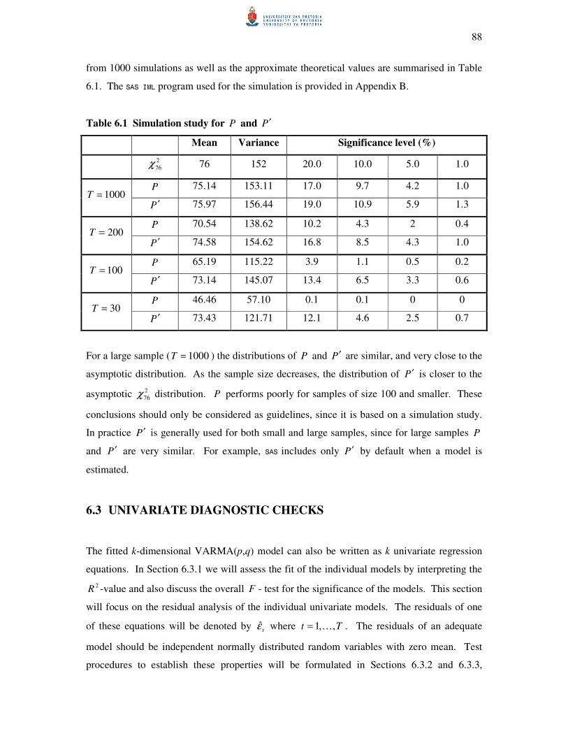
88
from 1000 simulations as well as the approximate theoretical values are summarised in Table
6.1. The SAS IML program used for the simulation is provided in Appendix B.
Table 6.1 Simulation study for P and P′
Mean Variance Significance level (%)
2
76χ 76 152 20.0 10.0 5.0 1.0
P 75.14 153.11 17.0 9.7 4.2 1.0 1000=T
P′ 75.97 156.44 19.0 10.9 5.9 1.3
P 70.54 138.62 10.2 4.3 2 0.4 200=T
P′ 74.58 154.62 16.8 8.5 4.3 1.0
P 65.19 115.22 3.9 1.1 0.5 0.2 100=T
P′ 73.14 145.07 13.4 6.5 3.3 0.6
P 46.46 57.10 0.1 0.1 0 0 30=T
P′ 73.43 121.71 12.1 4.6 2.5 0.7
For a large sample ( 1000=T ) the distributions of P and P′ are similar, and very close to the
asymptotic distribution. As the sample size decreases, the distribution of P′ is closer to the
asymptotic 2
76χ distribution. P performs poorly for samples of size 100 and smaller. These
conclusions should only be considered as guidelines, since it is based on a simulation study.
In practice P′ is generally used for both small and large samples, since for large samples P
and P′ are very similar. For example, SAS includes only P′ by default when a model is
estimated.
6.3 UNIVARIATE DIAGNOSTIC CHECKS
The fitted k-dimensional VARMA(p,q) model can also be written as k univariate regression
equations. In Section 6.3.1 we will assess the fit of the individual models by interpreting the
2R -value and also discuss the overall F - test for the significance of the models. This section
will focus on the residual analysis of the individual univariate models. The residuals of one
of these equations will be denoted by tε where Tt ,,1 K= . The residuals of an adequate
model should be independent normally distributed random variables with zero mean. Test
procedures to establish these properties will be formulated in Sections 6.3.2 and 6.3.3,
89
respectively. Section 6.3.4 deals with a test for heteroscedasticity of the residuals. A test for
higher order autocorrelation in the residuals is the subject of Section 6.3.5.
6.3.1 The multiple coefficient of determination and the F -.test for overall significance
In a regression context the multiple regression model is given by
εββββ ++++= pp xxxy L22110 (6.9)
where
y : dependent variable
s'β : parameters
sx' : explanatory variables
ε : error term
For our purpose, the explanatory variables may include lagged values of the dependent
variable.
The multiple coefficient of determination, 2R , is a measure of the portion of the variability in
the dependent variable (a single time series) that can be explained by the estimated regression
equation (lagged observations of the single time series, together with observations from the
( k -1) other time series processes). The calculation formula for 2R is
SST
SSRR =2 (6.10)
where
SSR : sum of squared differences of the estimated value and the mean
SST : sum of squared differences of the observed value and the mean
The F - test is used to establish whether a significant relationship exists between the
dependent and explanatory variables. The hypothesis,
zero toequal are parameters theallNot :
0: 210
a
p
H
H ==== βββ K (6.11)
can be tested using an F - statistic,
90
1−−
=
pT
SSE
p
SSR
F (6.12)
where
SSE : sum of squared differences of the observed and estimated values
p : number of explanatory variables
T : sample size
Under the null hypothesis, the F - statistic follows an F distribution with p and 1−− pT
degrees of freedom. The null hypothesis will be rejected when the F - statistic exceeds an
appropriate critical value. (Williams, Sweeney, Anderson, 2006)
6.3.2 Durbin-Watson test
The Durbin-Watson d statistic for detecting serial correlation of the error term originates from
regression analysis. Some of the assumptions underlying this statistic, summarised by
Gujarati (1995), include that the regression model has an intercept term and that the
regression model should not include lagged values of the dependent variable as explanatory
variables. The nature of time series analysis violates the last mentioned assumption. Durbin
(1970) proposed the h statistic for testing serial correlation in regression when some of the
regressors are lagged dependent variables. Nonetheless statistical packages still calculate the
Durbin-Watson d statistic.
The d statistic is derived in a paper by Durbin & Watson (1950), while the critical values of
this statistic are tabulated in a paper by the same authors (1951). Using the notation specified
in section 6.3, the d statistic is
( )
∑
∑
=
=
−−
=T
t
t
T
t
tt
d
2
2
2
2
1
ˆ
ˆˆ
ε
εε
(6.13)
The Durbin-Watson d statistic tests the null hypothesis of independence of the error terms
against an alternative that the error terms are generated by an AR(1) process. This is an
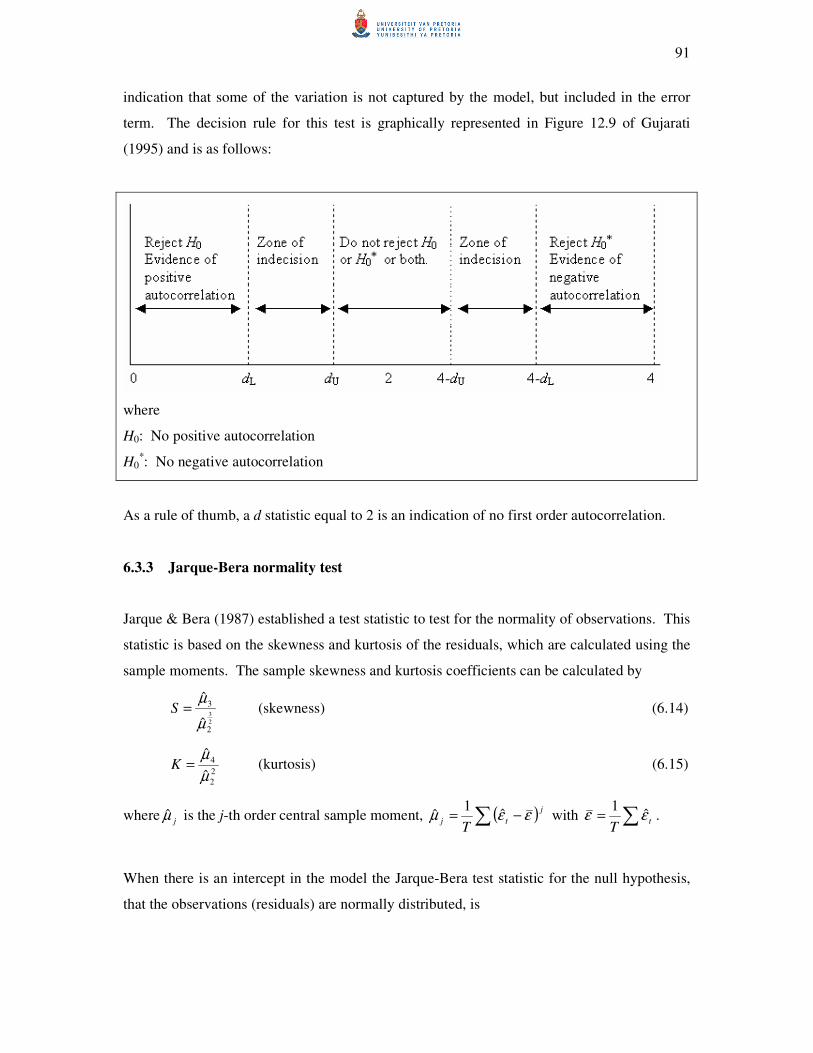
91
indication that some of the variation is not captured by the model, but included in the error
term. The decision rule for this test is graphically represented in Figure 12.9 of Gujarati
(1995) and is as follows:
where
H0: No positive autocorrelation
H0*: No negative autocorrelation
As a rule of thumb, a d statistic equal to 2 is an indication of no first order autocorrelation.
6.3.3 Jarque-Bera normality test
Jarque & Bera (1987) established a test statistic to test for the normality of observations. This
statistic is based on the skewness and kurtosis of the residuals, which are calculated using the
sample moments. The sample skewness and kurtosis coefficients can be calculated by
2
3
2
3
ˆ
ˆ
µ
µ=S (skewness) (6.14)
2
2
4
ˆ
ˆ
µ
µ=K (kurtosis) (6.15)
where jµ is the j-th order central sample moment, ( )∑ −=j
tjT
εεµ ˆ1
ˆ with ∑= tT
εε ˆ1
.
When there is an intercept in the model the Jarque-Bera test statistic for the null hypothesis,
that the observations (residuals) are normally distributed, is

92
( )
−+=
24
3
6
22KS
TJB (6.16)
The Jaque-Bera test has a Chi-squared distribution with 2 degrees of freedom asymptotically,
and the null hypothesis is rejected if the computed value exceeds a Chi-squared critical value.
6.3.4 Autoregressive conditional heteroscedasticity (ARCH) model
Consider the univariate AR(p) model
tptpttt ayyycy +++++= −−− φφφ K2211 (6.17)
where ta is a white noise process with zero mean and ( )
=
==
τ
τστ
t
taaE t
if 0
if 2
Engle (1982) proposed a class of models with nonconstant variances conditional on the past,
called ARCH models. The idea behind the ARCH model is that the conditional variance of
ta changes over time. For example, 2
ta may also follow an AR(m) process,
tmtmttt waaaa +++++= −−−
22
22
2
110
2 αααα K (6.18)
where tw is a white noise process. The conditional variance of
ta is then given by
( ) 22
22
2
110
22
1
2 ,, mtmttmttt aaaaaaE −−−−− ++++= αααα KK (6.19)
If this is the case then ta can be described by an ARCH(m) model. Based on this, the null
hypothesis to test for ARCH disturbances is
0: 210 ==== mH ααα K (6.20)
In practice we are usually interested in ARCH(1) disturbances. The hypothesis in (6.20) can
be tested by means of the F - test of overall significance of the regression
2
110
2 ˆˆˆˆ−+= tt εααε (6.21)
where tε denotes the residuals of the estimated model. (Hamilton, 1994; Gujarati, 1995)
Statistical packages usually report this F - statistic.
93
An alternative test procedure derived by Engle (1982) is to compare 2TR ( 2R is the
coefficient of determination for the regression in (6.21)) to a Chi-squared critical value with
one degree of freedom.
6.3.5 F - test for AR disturbances
The Durbin-Watson d statistic tests for independence of the error terms against an alternative
that they are generated by an AR(1) process. Another approach to test for autocorrelation in
the residuals is to fit an AR(1) model to the residuals,
11ˆˆ
−+= t
res
t c εφε (6.22)
and test the hypothesis
0ˆ: 10 =resH φ against the alternative 0ˆ: 1 ≠res
aH φ (6.23)
This is called the F - test for AR(1) disturbances.
The significance of higher order models can also be tested, for example the F - test for AR(4)
disturbances. This is done by fitting an AR(4) model to the residuals,
44332211ˆˆˆˆˆ
−−−− ++++= t
res
t
res
t
res
t
res
t c εφεφεφεφε (6.24)
and testing for overall significance of the model by means of the F - test for the hypothesis
zero toequal are tscoefficien theallnot :
0ˆˆˆˆ: 43210
a
resresresres
H
H ==== φφφφ (6.25)
(Williams, Sweeney, Anderson, 2006)
6.4 EXAMPLES
This section consists out of three examples. The first example is based on a generated
VAR(2) process. The purpose of this example is twofold, firstly the diagnostic tests described
in this chapter are calculated using the formulae provided to show that it is comparable to the
results obtained using the VARMAX procedure; and secondly to establish whether the diagnostic
checks can be used to distinguish between a poor and a good fitted model. The other two
examples illustrate the model building process, including a test for stationarity, order
selection, estimation and diagnostic checks, using observed multivariate time series datasets.
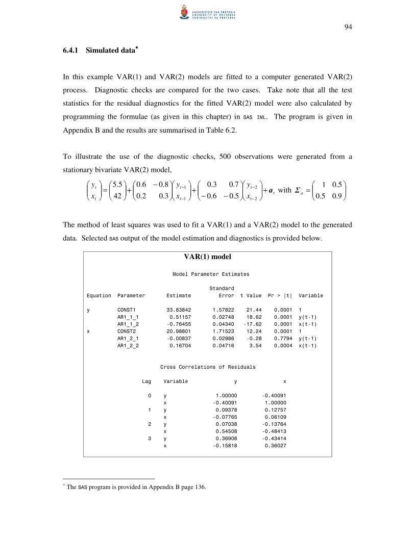
94
6.4.1 Simulated data∗∗∗∗
In this example VAR(1) and VAR(2) models are fitted to a computer generated VAR(2)
process. Diagnostic checks are compared for the two cases. Take note that all the test
statistics for the residual diagnostics for the fitted VAR(2) model were also calculated by
programming the formulae (as given in this chapter) in SAS IML. The program is given in
Appendix B and the results are summarised in Table 6.2.
To illustrate the use of the diagnostic checks, 500 observations were generated from a
stationary bivariate VAR(2) model,
t
t
t
t
t
t
t
x
y
x
y
x
ya+
−−+
−+
=
−
−
−
−
2
2
1
1
5.06.0
7.03.0
3.02.0
8.06.0
42
5.5 with
=
9.05.0
5.01aΣ
The method of least squares was used to fit a VAR(1) and a VAR(2) model to the generated
data. Selected SAS output of the model estimation and diagnostics is provided below.
VAR(1) model
Model Parameter Estimates
Standard
Equation Parameter Estimate Error t Value Pr > |t| Variable
y CONST1 33.83842 1.57822 21.44 0.0001 1
AR1_1_1 0.51157 0.02748 18.62 0.0001 y(t-1)
AR1_1_2 -0.76455 0.04340 -17.62 0.0001 x(t-1)
x CONST2 20.98801 1.71523 12.24 0.0001 1
AR1_2_1 -0.00837 0.02986 -0.28 0.7794 y(t-1)
AR1_2_2 0.16704 0.04716 3.54 0.0004 x(t-1)
Cross Correlations of Residuals
Lag Variable y x
0 y 1.00000 -0.40091
x -0.40091 1.00000
1 y 0.09378 0.12757
x -0.07765 0.06109
2 y 0.07038 -0.13764
x 0.54508 -0.48413
3 y 0.36908 -0.43414
x -0.15818 0.36027
∗ The SAS program is provided in Appendix B page 136.
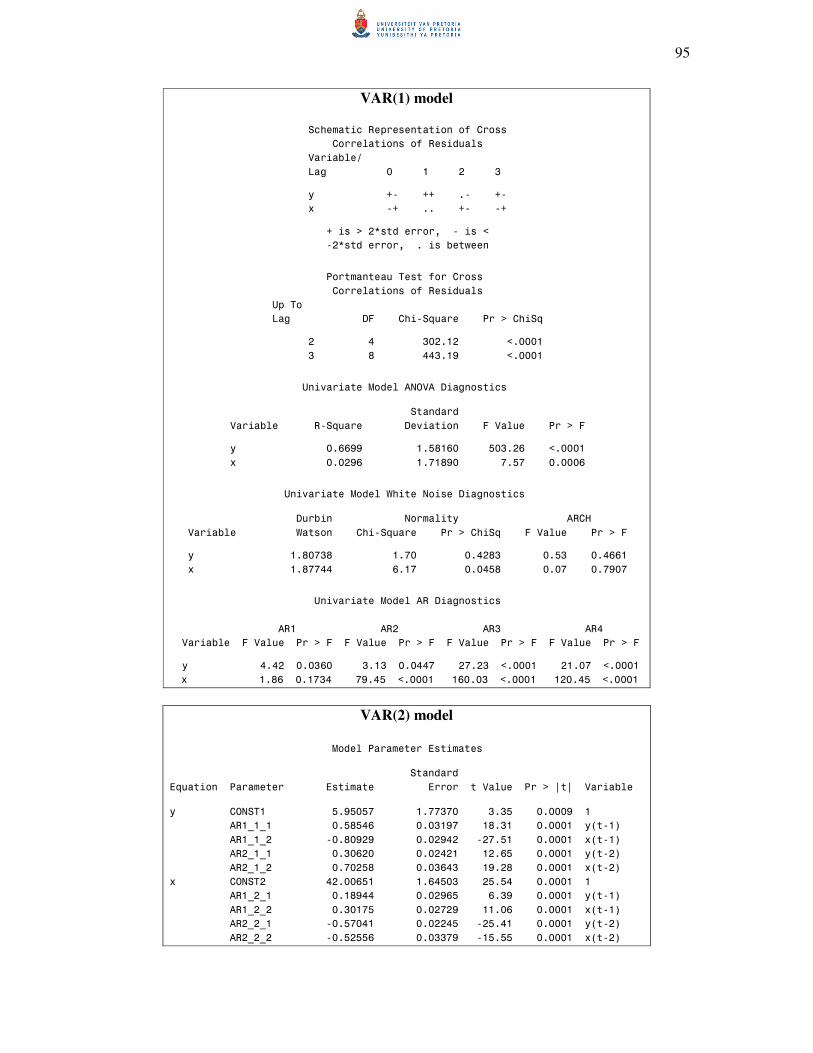
95
VAR(1) model
Schematic Representation of Cross
Correlations of Residuals
Variable/
Lag 0 1 2 3
y +- ++ .- +-
x -+ .. +- -+
+ is > 2*std error, - is <
-2*std error, . is between
Portmanteau Test for Cross
Correlations of Residuals
Up To
Lag DF Chi-Square Pr > ChiSq
2 4 302.12 <.0001
3 8 443.19 <.0001
Univariate Model ANOVA Diagnostics
Standard
Variable R-Square Deviation F Value Pr > F
y 0.6699 1.58160 503.26 <.0001
x 0.0296 1.71890 7.57 0.0006
Univariate Model White Noise Diagnostics
Durbin Normality ARCH
Variable Watson Chi-Square Pr > ChiSq F Value Pr > F
y 1.80738 1.70 0.4283 0.53 0.4661
x 1.87744 6.17 0.0458 0.07 0.7907
Univariate Model AR Diagnostics
AR1 AR2 AR3 AR4
Variable F Value Pr > F F Value Pr > F F Value Pr > F F Value Pr > F
y 4.42 0.0360 3.13 0.0447 27.23 <.0001 21.07 <.0001
x 1.86 0.1734 79.45 <.0001 160.03 <.0001 120.45 <.0001
VAR(2) model
Model Parameter Estimates
Standard
Equation Parameter Estimate Error t Value Pr > |t| Variable
y CONST1 5.95057 1.77370 3.35 0.0009 1
AR1_1_1 0.58546 0.03197 18.31 0.0001 y(t-1)
AR1_1_2 -0.80929 0.02942 -27.51 0.0001 x(t-1)
AR2_1_1 0.30620 0.02421 12.65 0.0001 y(t-2)
AR2_1_2 0.70258 0.03643 19.28 0.0001 x(t-2)
x CONST2 42.00651 1.64503 25.54 0.0001 1
AR1_2_1 0.18944 0.02965 6.39 0.0001 y(t-1)
AR1_2_2 0.30175 0.02729 11.06 0.0001 x(t-1)
AR2_2_1 -0.57041 0.02245 -25.41 0.0001 y(t-2)
AR2_2_2 -0.52556 0.03379 -15.55 0.0001 x(t-2)
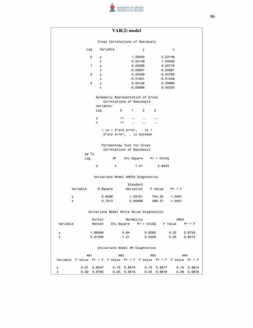
96
VAR(2) model
Cross Correlations of Residuals
Lag Variable y x
0 y 1.00000 0.52148
x 0.52148 1.00000
1 y 0.00368 0.00779
x -0.00691 -0.00681
2 y 0.02469 -0.00763
x -0.01631 -0.01248
3 y 0.00126 0.00668
x -0.00666 0.00230
Schematic Representation of Cross
Correlations of Residuals
Variable/
Lag 0 1 2 3
y ++ .. .. ..
x ++ .. .. ..
+ is > 2*std error, - is <
-2*std error, . is between
Portmanteau Test for Cross
Correlations of Residuals
Up To
Lag DF Chi-Square Pr > ChiSq
3 4 1.41 0.8423
Univariate Model ANOVA Diagnostics
Standard
Variable R-Square Deviation F Value Pr > F
y 0.8596 1.03151 754.32 <.0001
x 0.7012 0.95668 289.27 <.0001
Univariate Model White Noise Diagnostics
Durbin Normality ARCH
Variable Watson Chi-Square Pr > ChiSq F Value Pr > F
y 1.99066 0.84 0.6580 0.02 0.8753
x 2.01359 1.21 0.5459 0.20 0.6512
Univariate Model AR Diagnostics
AR1 AR2 AR3 AR4
Variable F Value Pr > F F Value Pr > F F Value Pr > F F Value Pr > F
y 0.01 0.9347 0.15 0.8574 0.10 0.9577 0.10 0.9814
x 0.02 0.8795 0.05 0.9515 0.03 0.9916 0.08 0.9875

97
Table 6.2 Summary of the diagnostic checks of the fitted VAR(2) model using explicit
formulae
Diagnostic Check Formula Result
Residual autocorrelation
matrices (6.2)
−=
−−
−=
−
−=
=
002.0007.0
007.0001.0ˆ
012.0008.0
016.0025.0ˆ
007.0008.0
007.0004.0ˆ
1521.0
521.01ˆ
32
10
RR
RR
Portmanteau statistic (6.7)
(6.8)
405.1=P
411.1=′P and 842.0=− valuep
Multiple coefficient of
determination (6.10)
:y 8596.02 =R
:x 7012.02 =R
F - statistic (6.12)
:y 354.754=F and 0=− valuep
:x 266.289=F and 0=− valuep
Durbin-Watson test (6.13)
:y 991.1=d
:x 014.2=d
Jarque-Bera normality test
(6.16)
:y 837.0=JB and 658.0=− valuep
:x 211.1=JB and 546.0=− valuep
ARCH model (6.21)
:y 02.0=F and 875.0=− valuep
:x 20.0=F and 651.0=− valuep
AR disturbances: AR(1) (6.22)
:y 01.0=F and 935.0=− valuep
:x 02.0=F and 880.0=− valuep
AR(2)
:y 15.0=F and 857.0=− valuep
:x 05.0=F and 952.0=− valuep
AR(3)
:y 10.0=F and 958.0=− valuep
:x 03.0=F and 992.0=− valuep
AR(4) (6.24)
:y 10.0=F and 981.0=− valuep
:x 08.0=F and 988.0=− valuep
The estimated models are
VAR(1): t
t
t
t
t
x
y
x
ya+
−
−+
=
−
−
1
1
167.0008.0
765.0512.0
988.20
838.33
ˆ
ˆ
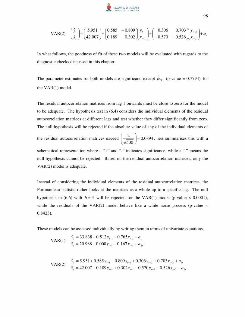
98
VAR(2): t
t
t
t
t
t
t
x
y
x
y
x
ya+
−−+
−+
=
−
−
−
−
2
2
1
1
526.0570.0
703.0306.0
302.0189.0
809.0585.0
007.42
951.5
ˆ
ˆ
In what follows, the goodness of fit of these two models will be evaluated with regards to the
diagnostic checks discussed in this chapter.
The parameter estimates for both models are significant, except 1,21φ (p-value = 0.7794) for
the VAR(1) model.
The residual autocorrelation matrices from lag 1 onwards must be close to zero for the model
to be adequate. The hypothesis test in (6.4) considers the individual elements of the residual
autocorrelation matrices at different lags and test whether they differ significantly from zero.
The null hypothesis will be rejected if the absolute value of any of the individual elements of
the residual autocorrelation matrices exceed 0894.0500
2=
. SAS summarises this with a
schematical representation where a “+” and “-” indicates significance, while a “.” means the
null hypothesis cannot be rejected. Based on the residual autocorrelation matrices, only the
VAR(2) model is adequate.
Instead of considering the individual elements of the residual autocorrelation matrices, the
Portmanteau statistic rather looks at the matrices as a whole up to a specific lag. The null
hypothesis in (6.6) with 3=h will be rejected for the VAR(1) model (p-value < 0.0001),
while the residuals of the VAR(2) model behave like a white noise process (p-value =
0.8423).
These models can be assessed individually by writing them in terms of univariate equations,
VAR(1): tttt
tttt
axyx
axyy
211
111
167.0008.0988.20ˆ
765.0512.0838.33ˆ
++−=
+−+=
−−
−−
VAR(2): tttttt
tttttt
axyxyx
axyxyy
22211
12211
526.0570.0302.0189.0007.42ˆ
703.0306.0809.0585.0951.5ˆ
+−−++=
+++−+=
−−−−
−−−−
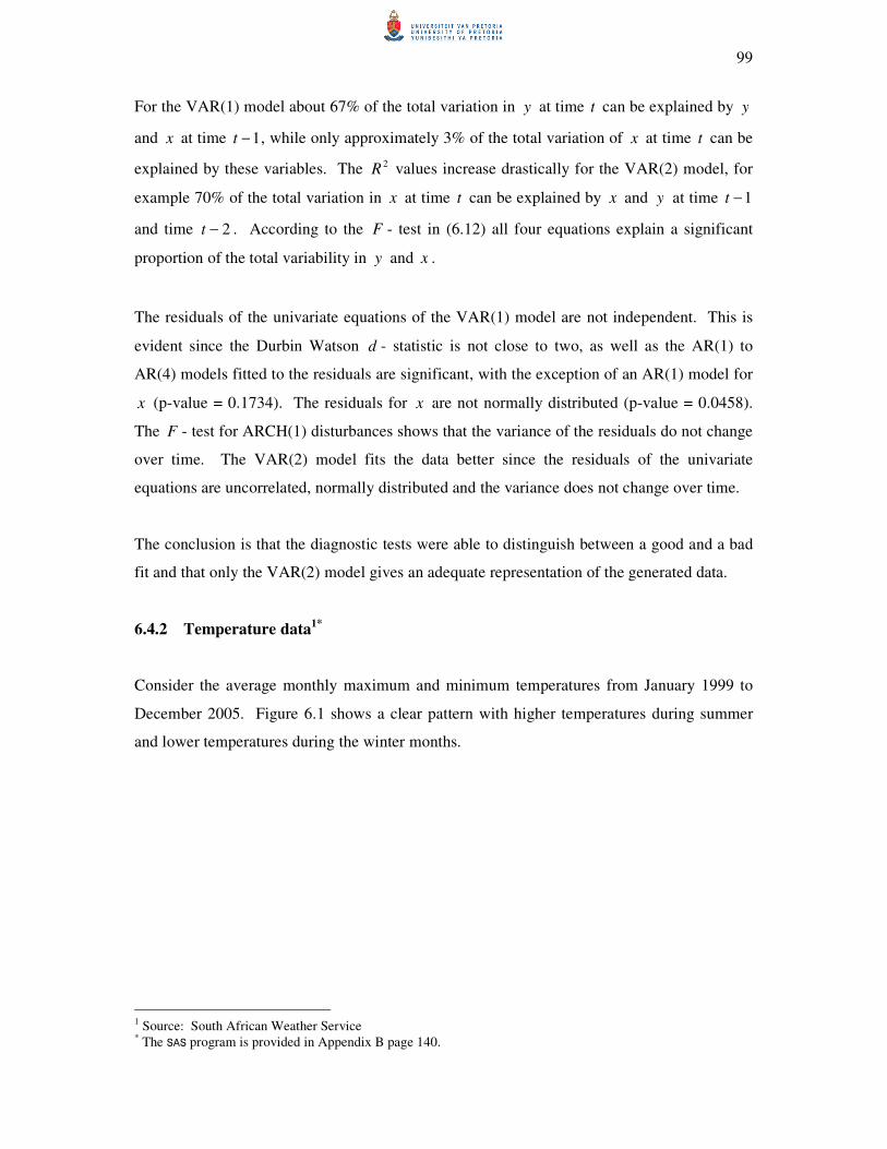
99
For the VAR(1) model about 67% of the total variation in y at time t can be explained by y
and x at time 1−t , while only approximately 3% of the total variation of x at time t can be
explained by these variables. The 2R values increase drastically for the VAR(2) model, for
example 70% of the total variation in x at time t can be explained by x and y at time 1−t
and time 2−t . According to the F - test in (6.12) all four equations explain a significant
proportion of the total variability in y and x .
The residuals of the univariate equations of the VAR(1) model are not independent. This is
evident since the Durbin Watson d - statistic is not close to two, as well as the AR(1) to
AR(4) models fitted to the residuals are significant, with the exception of an AR(1) model for
x (p-value = 0.1734). The residuals for x are not normally distributed (p-value = 0.0458).
The F - test for ARCH(1) disturbances shows that the variance of the residuals do not change
over time. The VAR(2) model fits the data better since the residuals of the univariate
equations are uncorrelated, normally distributed and the variance does not change over time.
The conclusion is that the diagnostic tests were able to distinguish between a good and a bad
fit and that only the VAR(2) model gives an adequate representation of the generated data.
6.4.2 Temperature data1*
Consider the average monthly maximum and minimum temperatures from January 1999 to
December 2005. Figure 6.1 shows a clear pattern with higher temperatures during summer
and lower temperatures during the winter months.
1 Source: South African Weather Service * The SAS program is provided in Appendix B page 140.
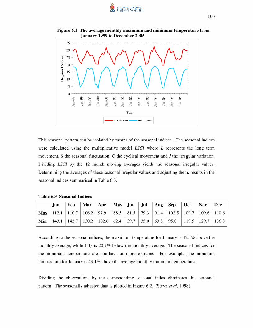
100
Figure 6.1 The average monthly maximum and minimum temperature from
January 1999 to December 2005
0
5
10
15
20
25
30
35
Jan-9
9
Jul-
99
Jan-0
0
Jul-
00
Jan-0
1
Jul-
01
Jan-0
2
Jul-
02
Jan-0
3
Jul-
03
Jan-0
4
Jul-
04
Jan-0
5
Jul-
05
Year
Deg
rees
Cel
ciu
s
maximum minimum
This seasonal pattern can be isolated by means of the seasonal indices. The seasonal indices
were calculated using the multiplicative model LSCI where L represents the long term
movement, S the seasonal fluctuation, C the cyclical movement and I the irregular variation.
Dividing LSCI by the 12 month moving averages yields the seasonal irregular values.
Determining the averages of these seasonal irregular values and adjusting them, results in the
seasonal indices summarised in Table 6.3.
Table 6.3 Seasonal Indices
Jan Feb Mar Apr May Jun Jul Aug Sep Oct Nov Dec
Max 112.1 110.7 106.2 97.9 88.5 81.5 79.3 91.4 102.5 109.7 109.6 110.6
Min 143.1 142.7 130.2 102.6 62.4 39.7 35.0 63.8 95.0 119.5 129.7 136.3
According to the seasonal indices, the maximum temperature for January is 12.1% above the
monthly average, while July is 20.7% below the monthly average. The seasonal indices for
the minimum temperature are similar, but more extreme. For example, the minimum
temperature for January is 43.1% above the average monthly minimum temperature.
Dividing the observations by the corresponding seasonal index eliminates this seasonal
pattern. The seasonally adjusted data is plotted in Figure 6.2. (Steyn et al, 1998)
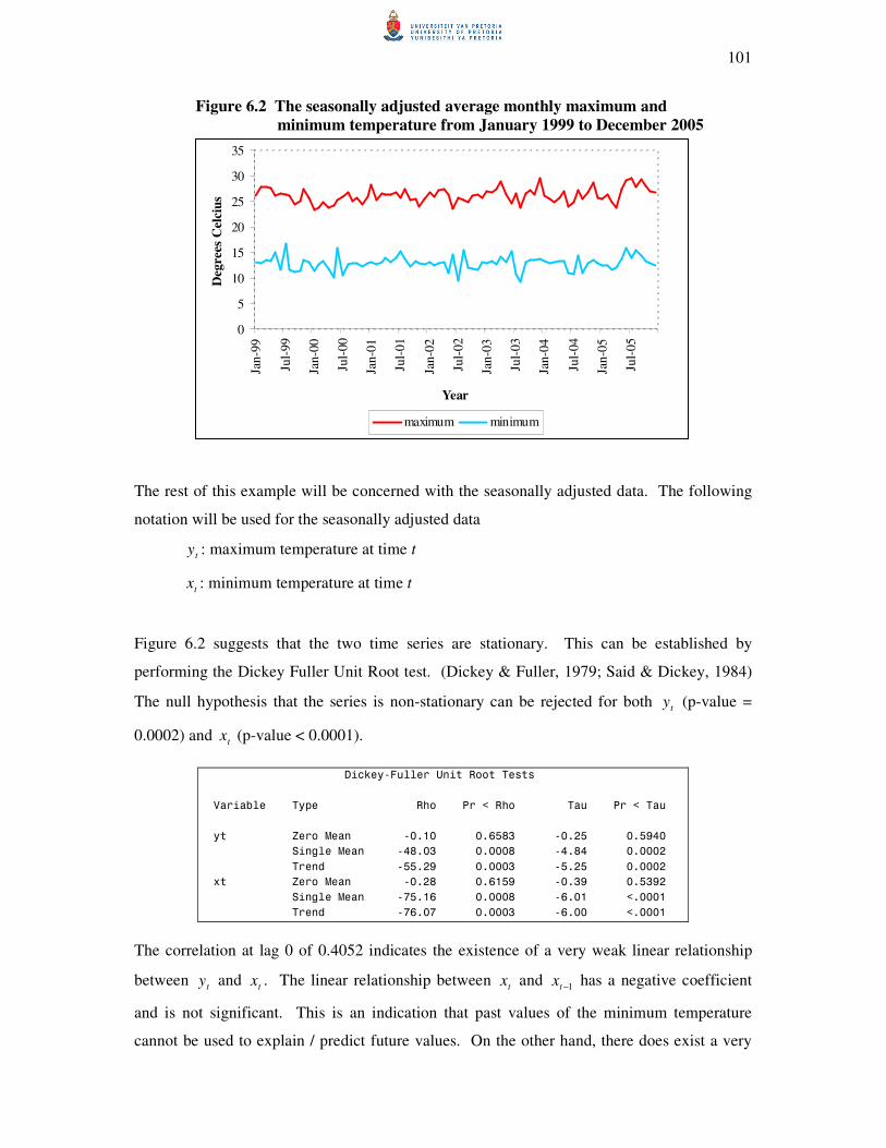
101
Figure 6.2 The seasonally adjusted average monthly maximum and
minimum temperature from January 1999 to December 2005
0
5
10
15
20
25
30
35
Jan-9
9
Jul-
99
Jan-0
0
Jul-
00
Jan-0
1
Jul-
01
Jan-0
2
Jul-
02
Jan-0
3
Jul-
03
Jan-0
4
Jul-
04
Jan-0
5
Jul-
05
Year
Deg
rees
Cel
ciu
s
maximum minimum
The rest of this example will be concerned with the seasonally adjusted data. The following
notation will be used for the seasonally adjusted data
ty : maximum temperature at time t
tx : minimum temperature at time t
Figure 6.2 suggests that the two time series are stationary. This can be established by
performing the Dickey Fuller Unit Root test. (Dickey & Fuller, 1979; Said & Dickey, 1984)
The null hypothesis that the series is non-stationary can be rejected for both ty (p-value =
0.0002) and tx (p-value < 0.0001).
Dickey-Fuller Unit Root Tests
Variable Type Rho Pr < Rho Tau Pr < Tau
yt Zero Mean -0.10 0.6583 -0.25 0.5940
Single Mean -48.03 0.0008 -4.84 0.0002
Trend -55.29 0.0003 -5.25 0.0002
xt Zero Mean -0.28 0.6159 -0.39 0.5392
Single Mean -75.16 0.0008 -6.01 <.0001
Trend -76.07 0.0003 -6.00 <.0001
The correlation at lag 0 of 0.4052 indicates the existence of a very weak linear relationship
between ty and
tx . The linear relationship between tx and
1−tx has a negative coefficient
and is not significant. This is an indication that past values of the minimum temperature
cannot be used to explain / predict future values. On the other hand, there does exist a very

102
weak relationship between tx and 1−ty and between ty and 1−tx . The autocorrelation
matrices from lag 2 onwards do not differ significantly from zero, implying that the
underlying data generating process could be a VMA(1) model.
Cross Correlations of Dependent Series
Lag Variable yt xt
0 yt 1.00000 0.40520
xt 0.40520 1.00000
1 yt 0.38973 0.26589
xt 0.26655 -0.12035
2 yt 0.16721 0.08074
xt 0.00946 0.11299
3 yt 0.16865 0.19466
xt 0.05809 -0.01309
4 yt -0.06268 -0.05705
xt -0.05808 0.02797
5 yt -0.07644 -0.04729
xt -0.11339 -0.14811
6 yt -0.10172 -0.09873
xt 0.00434 -0.01098
Schematic Representation of Cross Correlations
Variable/
Lag 0 1 2 3 4 5 6
yt ++ ++ .. .. .. .. ..
xt ++ +. .. .. .. .. ..
+ is > 2*std error, - is <
-2*std error, . is between
The minimum information criterion as well as the partial autoregression matrices suggest that
a VAR(1) model might be appropriate.
Minimum Information Criterion
Lag MA 0 MA 1 MA 2 MA 3 MA 4
AR 0 1.0795714 1.026612 0.99467 0.9895747 1.0708531
AR 1 0.8968038 1.1023662 1.0502803 1.0964425 1.1727411
AR 2 0.9083807 1.0464227 1.1152725 1.2130536 1.3059295
AR 3 1.0060682 1.1375668 1.1960255 1.3256859 1.4010507
AR 4 1.0668047 1.2196028 1.3064426 1.3848342 1.5053257
Partial Autoregression
Lag Variable yt xt
1 yt 0.33707 0.13449
xt 0.36381 -0.27290
2 yt 0.03673 -0.09182
xt 0.01952 -0.03103
3 yt 0.14303 -0.02943
xt 0.20747 -0.07518
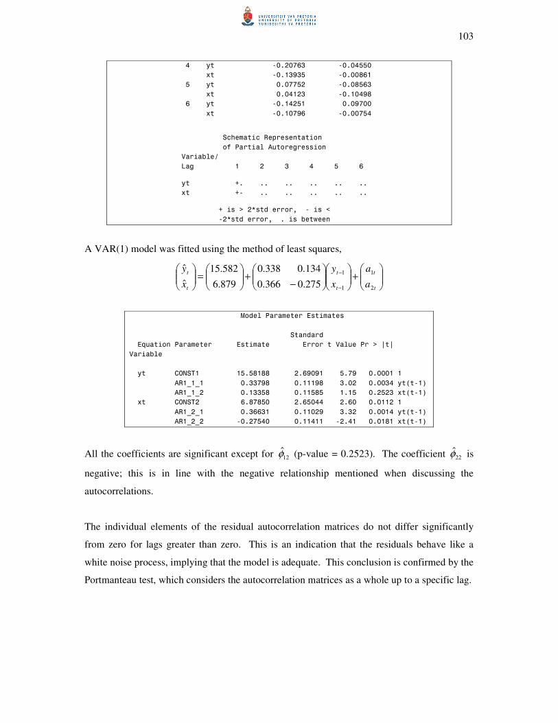
103
4 yt -0.20763 -0.04550
xt -0.13935 -0.00861
5 yt 0.07752 -0.08563
xt 0.04123 -0.10498
6 yt -0.14251 0.09700
xt -0.10796 -0.00754
Schematic Representation
of Partial Autoregression
Variable/
Lag 1 2 3 4 5 6
yt +. .. .. .. .. ..
xt +- .. .. .. .. ..
+ is > 2*std error, - is <
-2*std error, . is between
A VAR(1) model was fitted using the method of least squares,
+
−+
=
−
−
t
t
t
t
t
t
a
a
x
y
x
y
2
1
1
1
275.0366.0
134.0338.0
879.6
582.15
ˆ
ˆ
Model Parameter Estimates
Standard
Equation Parameter Estimate Error t Value Pr > |t|
Variable
yt CONST1 15.58188 2.69091 5.79 0.0001 1
AR1_1_1 0.33798 0.11198 3.02 0.0034 yt(t-1)
AR1_1_2 0.13358 0.11585 1.15 0.2523 xt(t-1)
xt CONST2 6.87850 2.65044 2.60 0.0112 1
AR1_2_1 0.36631 0.11029 3.32 0.0014 yt(t-1)
AR1_2_2 -0.27540 0.11411 -2.41 0.0181 xt(t-1)
All the coefficients are significant except for 12φ (p-value = 0.2523). The coefficient 22φ is
negative; this is in line with the negative relationship mentioned when discussing the
autocorrelations.
The individual elements of the residual autocorrelation matrices do not differ significantly
from zero for lags greater than zero. This is an indication that the residuals behave like a
white noise process, implying that the model is adequate. This conclusion is confirmed by the
Portmanteau test, which considers the autocorrelation matrices as a whole up to a specific lag.

104
Cross Correlations of Residuals
Lag Variable yt xt
0 yt 1.00000 0.38944
xt 0.38944 1.00000
1 yt 0.01169 0.00001
xt -0.02227 -0.01040
2 yt -0.04435 -0.05570
xt -0.10986 -0.08921
3 yt 0.19436 0.20926
xt 0.08690 0.04573
4 yt -0.13768 -0.03699
xt -0.09781 -0.01346
5 yt -0.03784 -0.01155
xt -0.06174 -0.09844
6 yt -0.13645 -0.11150
xt 0.07417 -0.03165
Schematic Representation of Cross
Correlations of Residuals
Variable/
Lag 0 1 2 3 4 5 6
yt ++ .. .. .. .. .. ..
xt ++ .. .. .. .. .. ..
+ is > 2*std error, - is <
-2*std error, . is between
Portmanteau Test for Cross
Correlations of Residuals
Up To
Lag DF Chi-Square Pr > ChiSq
2 4 1.38 0.8483
3 8 6.65 0.5753
4 12 8.57 0.7393
5 16 9.63 0.8853
6 20 13.54 0.8530
The VAR(1) model can be regarded in terms of two univariate equations,
tttt
tttt
axyx
axyy
211
111
275.0366.0879.6ˆ
134.0338.0582.15ˆ
+−+=
+++=
−−
−−
The portion of the variability explained by each of these univariate models only amounts to
16.62% and 13.39%, respectively. Even though this does not seem to be a lot, it is a vast
improvement from the result obtained when analysing these time series on their own. For
comparison purposes an AR(1) model was also fitted to both ty and tx . 15.23% of the
variation in ty can be explained by 1−ty , while only 1% of the variation in tx can be
explained by 1−tx . It turned out that when looking at tx alone, it is a white noise process.
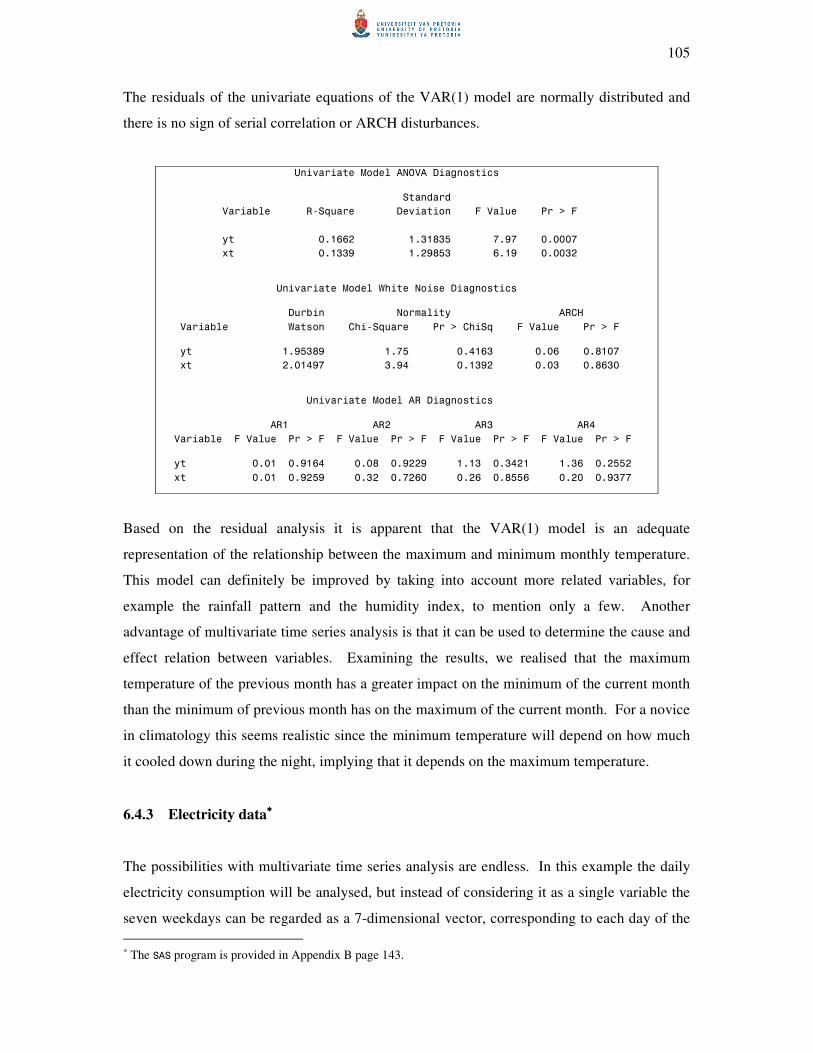
105
The residuals of the univariate equations of the VAR(1) model are normally distributed and
there is no sign of serial correlation or ARCH disturbances.
Univariate Model ANOVA Diagnostics
Standard
Variable R-Square Deviation F Value Pr > F
yt 0.1662 1.31835 7.97 0.0007
xt 0.1339 1.29853 6.19 0.0032
Univariate Model White Noise Diagnostics
Durbin Normality ARCH
Variable Watson Chi-Square Pr > ChiSq F Value Pr > F
yt 1.95389 1.75 0.4163 0.06 0.8107
xt 2.01497 3.94 0.1392 0.03 0.8630
Univariate Model AR Diagnostics
AR1 AR2 AR3 AR4
Variable F Value Pr > F F Value Pr > F F Value Pr > F F Value Pr > F
yt 0.01 0.9164 0.08 0.9229 1.13 0.3421 1.36 0.2552
xt 0.01 0.9259 0.32 0.7260 0.26 0.8556 0.20 0.9377
Based on the residual analysis it is apparent that the VAR(1) model is an adequate
representation of the relationship between the maximum and minimum monthly temperature.
This model can definitely be improved by taking into account more related variables, for
example the rainfall pattern and the humidity index, to mention only a few. Another
advantage of multivariate time series analysis is that it can be used to determine the cause and
effect relation between variables. Examining the results, we realised that the maximum
temperature of the previous month has a greater impact on the minimum of the current month
than the minimum of previous month has on the maximum of the current month. For a novice
in climatology this seems realistic since the minimum temperature will depend on how much
it cooled down during the night, implying that it depends on the maximum temperature.
6.4.3 Electricity data∗∗∗∗
The possibilities with multivariate time series analysis are endless. In this example the daily
electricity consumption will be analysed, but instead of considering it as a single variable the
seven weekdays can be regarded as a 7-dimensional vector, corresponding to each day of the
∗ The SAS program is provided in Appendix B page 143.
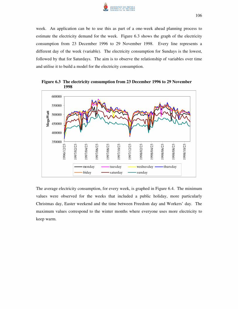
106
week. An application can be to use this as part of a one-week ahead planning process to
estimate the electricity demand for the week. Figure 6.3 shows the graph of the electricity
consumption from 23 December 1996 to 29 November 1998. Every line represents a
different day of the week (variable). The electricity consumption for Sundays is the lowest,
followed by that for Saturdays. The aim is to observe the relationship of variables over time
and utilise it to build a model for the electricity consumption.
Figure 6.3 The electricity consumption from 23 December 1996 to 29 November
1998
350000
400000
450000
500000
550000
600000
1996/1
2/2
3
1997/0
2/2
3
1997/0
4/2
3
1997/0
6/2
3
1997/0
8/2
3
1997/1
0/2
3
1997/1
2/2
3
1998/0
2/2
3
1998/0
4/2
3
1998/0
6/2
3
1998/0
8/2
3
1998/1
0/2
3
Meg
aW
att
monday tuesday wednesday thursday
friday saturday sunday
The average electricity consumption, for every week, is graphed in Figure 6.4. The minimum
values were observed for the weeks that included a public holiday, more particularly
Christmas day, Easter weekend and the time between Freedom day and Workers’ day. The
maximum values correspond to the winter months where everyone uses more electricity to
keep warm.
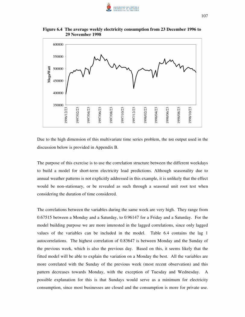
107
Figure 6.4 The average weekly electricity consumption from 23 December 1996 to
29 November 1998
350000
400000
450000
500000
550000
600000
1996/1
2/2
3
1997/0
2/2
3
1997/0
4/2
3
1997/0
6/2
3
1997/0
8/2
3
1997/1
0/2
3
1997/1
2/2
3
1998/0
2/2
3
1998/0
4/2
3
1998/0
6/2
3
1998/0
8/2
3
1998/1
0/2
3
Meg
aW
att
Due to the high dimension of this multivariate time series problem, the SAS output used in the
discussion below is provided in Appendix B.
The purpose of this exercise is to use the correlation structure between the different weekdays
to build a model for short-term electricity load predictions. Although seasonality due to
annual weather patterns is not explicitly addressed in this example, it is unlikely that the effect
would be non-stationary, or be revealed as such through a seasonal unit root test when
considering the duration of time considered.
The correlations between the variables during the same week are very high. They range from
0.67515 between a Monday and a Saturday, to 0.96147 for a Friday and a Saturday. For the
model building purpose we are more interested in the lagged correlations, since only lagged
values of the variables can be included in the model. Table 6.4 contains the lag 1
autocorrelations. The highest correlation of 0.83647 is between Monday and the Sunday of
the previous week, which is also the previous day. Based on this, it seems likely that the
fitted model will be able to explain the variation on a Monday the best. All the variables are
more correlated with the Sunday of the previous week (most recent observation) and this
pattern decreases towards Monday, with the exception of Tuesday and Wednesday. A
possible explanation for this is that Sundays would serve as a minimum for electricity
consumption, since most businesses are closed and the consumption is more for private use.
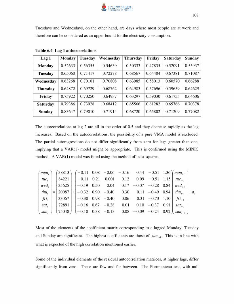
108
Tuesdays and Wednesdays, on the other hand, are days where most people are at work and
therefore can be considered as an upper bound for the electricity consumption.
Table 6.4 Lag 1 autocorrelations
Lag 1 Monday Tuesday Wednesday Thursday Friday Saturday Sunday
Monday 0.52633 0.56355 0.54639 0.50333 0.47835 0.52091 0.55937
Tuesday 0.65060 0.71417 0.72278 0.68567 0.64404 0.67381 0.71087
Wednesday 0.63268 0.70101 0.70808 0.63985 0.58013 0.60570 0.66288
Thursday 0.64872 0.69729 0.68762 0.64983 0.57696 0.59659 0.64629
Friday 0.75922 0.70250 0.64937 0.63297 0.59030 0.61755 0.64606
Saturday 0.79386 0.73928 0.68412 0.65566 0.61282 0.65766 0.70378
Sunday 0.83647 0.79010 0.71914 0.68720 0.65802 0.71209 0.77082
The autocorrelations at lag 2 are all in the order of 0.5 and they decrease rapidly as the lag
increases. Based on the autocorrelations, the possibility of a pure VMA model is excluded.
The partial autoregressions do not differ significantly from zero for lags greater than one,
implying that a VAR(1) model might be appropriate. This is confirmed using the MINIC
method. A VAR(1) model was fitted using the method of least squares,
t
t
t
t
t
t
t
t
t
t
t
t
t
t
t
sun
sat
fri
thu
wed
tue
mon
sun
sat
fri
thu
wed
tue
mon
a+
−−−−
−−−
−−−
−−−
−−−
−−
−−−−
+
=
−
−
−
−
−
−
−
1
1
1
1
1
1
1
92.024.009.008.013.038.010.0
91.037.010.001.028.067.016.0
10.173.031.006.040.098.030.0
94.049.011.030.040.090.032.0
84.028.007.017.004.050.019.0
15.151.009.012.0001.021.011.0
36.151.044.016.006.008.011.0
75048
72891
33067
20087
35625
84221
38813
Most of the elements of the coefficient matrix corresponding to a lagged Monday, Tuesday
and Sunday are significant. The highest coefficients are those of 1−tsun . This is in line with
what is expected of the high correlation mentioned earlier.
Some of the individual elements of the residual autocorrelation matrices, at higher lags, differ
significantly from zero. These are few and far between. The Portmanteau test, with null
109
hypothesis of no autocorrelaion in the residuals, cannot be rejected. This implies that the
residuals behave like a white noise process.
The multivariate VAR(1) model can also be considered as univariate equations. According to
the F - test all the univariate equations explain a significant portion of the total variability.
80% of the variability of the electricity consumption on a Wednesday can be explained by the
consumption of the previous week, while only 64% of the variation for a Saturday can be
explained by the same variables.
Based on the Durbin-Watson test and the AR(1) to AR(4) disturbances, the residuals of the
univariate models seem to be independent. According to the ARCH disturbances, the
variance of the residuals is also constant. The major concern is the normality. The null
hypothesis of normally distributed residuals is rejected for all the univariate equations. This
could be due to the extreme values for the holiday periods and possibly a seasonal pattern in
the data that was not accounted for in the model.
6.5 CONCLUSION
This chapter discussed procedures to determine whether the fitted model was an adequate
representation of the underlying data generating process. These procedures were grouped into
multivariate and univariate diagnostic checks. The multivariate checks were based on the
residual autocorrelation matrices. The aim was to show that the residuals behave like a
multivariate white noise process. This was achieved by testing whether the individual
elements of the autocorrelation matrices at different lags, as well as the whole matrix up to a
certain lag, differ significantly from zero. The univariate checks included several testing
procedures to establish whether the residuals of the univariate equations are independent,
normally distributed random variables with zero mean. The chapter was concluded with some
examples to illustrate the diagnostic checks and the model building process.

110
CHAPTER 7
CONCLUSION
The ultimate aim of this study was to explore the field of multivariate time series analysis,
and more particularly stationary processes. After defining the different multivariate time
series models, an overview was given of all the techniques used in finding a suitable model
for an observed multivariate time series. The model building process comprised of
investigating the sample autocorrelations and sample partial autoregressions to tentatively
select the order of a model; fitting a model using the method of least squares or the method of
maximum likelihood; and assessing the adequacy of the fitted model through analysing the
residuals.
Throughout the study examples were used to illustrate the different techniques. Most
formulae were programmed using the IML procedure in SAS. The results obtained were
compared to the output of the built-in SAS functions. Mathematica®
was used to do some
algebraic calculations and to show that it is possible to derive formulae for specific models in
terms of their coefficient matrices and the white noise covariance matrix. Since the last
mentioned formulae were computationally intense an Excel spreadsheet was developed where
one can just enter some information and Excel will calculate the answer.
Finally, fitting a model to observed data provided a practical overview of the model building
process. In the one example, the challenge was to estimate a model for the average monthly
minimum and maximum temperature. Using related variables to improve the model was
evident from this example. When the minimum temperature was analysed separately, it could
not be modeled because it was just a white noise process. When the extra information of the
maximum temperature was utilised, the model improved substantially. The other example
was concerned with the daily electricity consumption. Instead of considering the
consumption as a univariate time series, it was decomposed into a 7-dimensional multivariate
time series, where each day of the week was considered individually. This way, the weekly
pattern was taken into account. These two examples highlighted some of the advantages of
multivariate time series analysis.

111
In the future, statistical software packages especially open source packages (for example R)
can be explored to determine what other procedures are available and how to utilise them to
improve the model building process. Using the SAS code developed for this dissertation as a
basis it will be relatively simple to develop a module in open source for multivariate time
series analysis that would be available to a much wider user group than those who have access
to high-cost commercial software products. On a more theoretical note, forecasting of
multivariate time series models as well as the field of nonstationary processes could be
addressed.
112
APPENDIX A
CONTENTS
A1 Properties of the vec operator 113
A2 Properties of the Kronecker product 114
A3 Rules for vector and matrix differentiation 115
A4 Definition of modulus 116
A5 Multivariate results 117
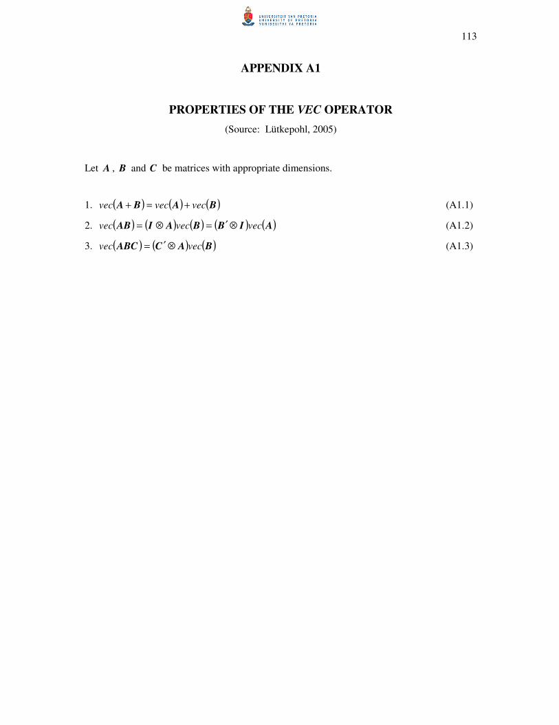
113
APPENDIX A1
PROPERTIES OF THE VEC OPERATOR
(Source: Lütkepohl, 2005)
Let A , B and C be matrices with appropriate dimensions.
1. ( ) ( ) ( )BABA vecvecvec +=+ (A1.1)
2. ( ) ( ) ( ) ( ) ( )AIBBAIAB vecvecvec ⊗′=⊗= (A1.2)
3. ( ) ( ) ( )BACABC vecvec ⊗′= (A1.3)
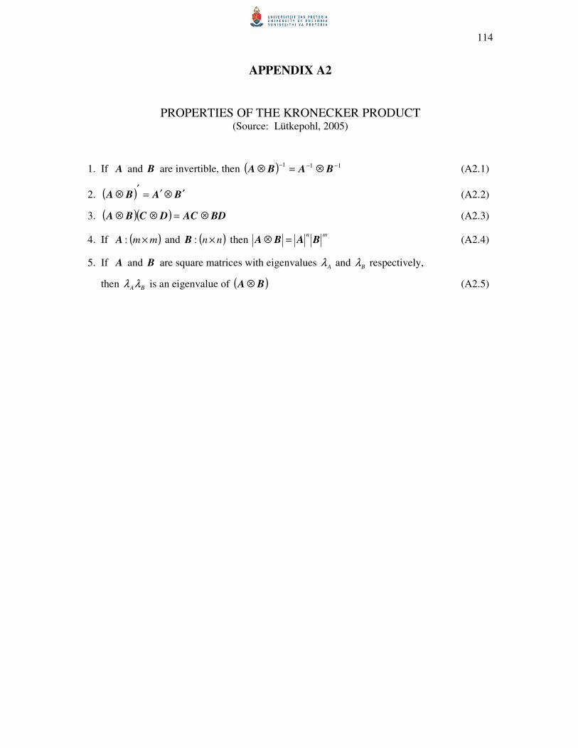
114
APPENDIX A2
PROPERTIES OF THE KRONECKER PRODUCT (Source: Lütkepohl, 2005)
1. If A and B are invertible, then ( ) 111 −−−⊗=⊗ BABA (A2.1)
2. ( ) BABA ′⊗′=′
⊗ (A2.2)
3. ( )( ) BDACDCBA ⊗=⊗⊗ (A2.3)
4. If ( )mm ×:A and ( )nn ×:B then mn
BABA =⊗ (A2.4)
5. If A and B are square matrices with eigenvalues Aλ and Bλ respectively,
then BAλλ is an eigenvalue of ( )BA ⊗ (A2.5)
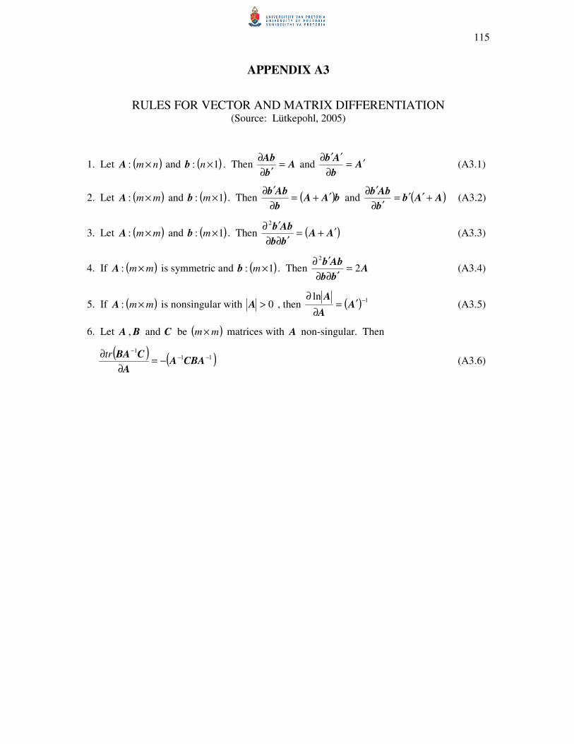
115
APPENDIX A3
RULES FOR VECTOR AND MATRIX DIFFERENTIATION (Source: Lütkepohl, 2005)
1. Let ( )nm ×:A and ( )1: ×nb . Then Ab
Ab=
′∂
∂ and A
b
Ab′=
∂
′′∂ (A3.1)
2. Let ( )mm ×:A and ( )1: ×mb . Then ( )bAAb
Abb′+=
∂
′∂ and ( )AAb
b
Abb+′′=
′∂
′∂ (A3.2)
3. Let ( )mm ×:A and ( )1: ×mb . Then ( )AAbb
Abb′+=
′∂∂
′∂ 2
(A3.3)
4. If ( )mm ×:A is symmetric and ( )1: ×mb . Then Abb
Abb2
2
=′∂∂
′∂ (A3.4)
5. If ( )mm ×:A is nonsingular with 0>A , then ( ) 1ln −′=∂
∂A
A
A (A3.5)
6. Let A , B and C be ( )mm × matrices with A non-singular. Then
( ) ( )11
1−−
−
−=∂
∂CBAA
A
CBAtr (A3.6)

116
APPENDIX A4
DEFINITION OF MODULUS (Source: Hamilton, 1994)
The modulus of a complex number ( )bia + is
22 babia +=+
The modulus of a real number ( 0=b ) is the absolute value of that number.
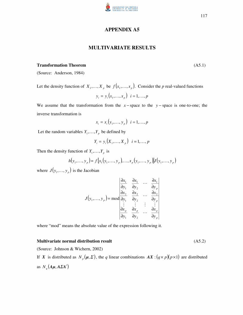
117
APPENDIX A5
MULTIVARIATE RESULTS
Transformation Theorem (A5.1)
(Source: Anderson, 1984)
Let the density function of pXX ,,1 K be ( )pxxf ,,1 K . Consider the p real-valued functions
( )pii xxyy ,,1 K= pi ,,1K=
We assume that the transformation from the −x space to the −y space is one-to-one; the
inverse transformation is
( )pii yyxx ,,1 K= pi ,,1K=
Let the random variables pYY ,,1 K be defined by
( )pii XXyY ,,1 K= pi ,,1K=
Then the density function of pYY ,,1 K is
( ) ( ) ( )[ ] ( )ppppp yyJyyxyyxfyyh ,,,,,,,,,, 11111 KKKKK =
where ( )pyyJ ,,1 K is the Jacobian
( )
p
ppp
p
p
p
y
x
y
x
y
x
y
x
y
x
y
x
y
x
y
x
y
x
yyJ
∂
∂
∂
∂
∂
∂
∂
∂
∂
∂
∂
∂
∂
∂
∂
∂
∂
∂
=
L
MMMM
L
L
K
21
2
2
2
1
2
1
2
1
1
1
1 mod,,
where “mod” means the absolute value of the expression following it.
Multivariate normal distribution result (A5.2)
(Source: Johnson & Wichern, 2002)
If X is distributed as ( )Σµ,pN , the q linear combinations ( )( )1: ×× ppqAX are distributed
as ( )AAΣAµ ′,qN
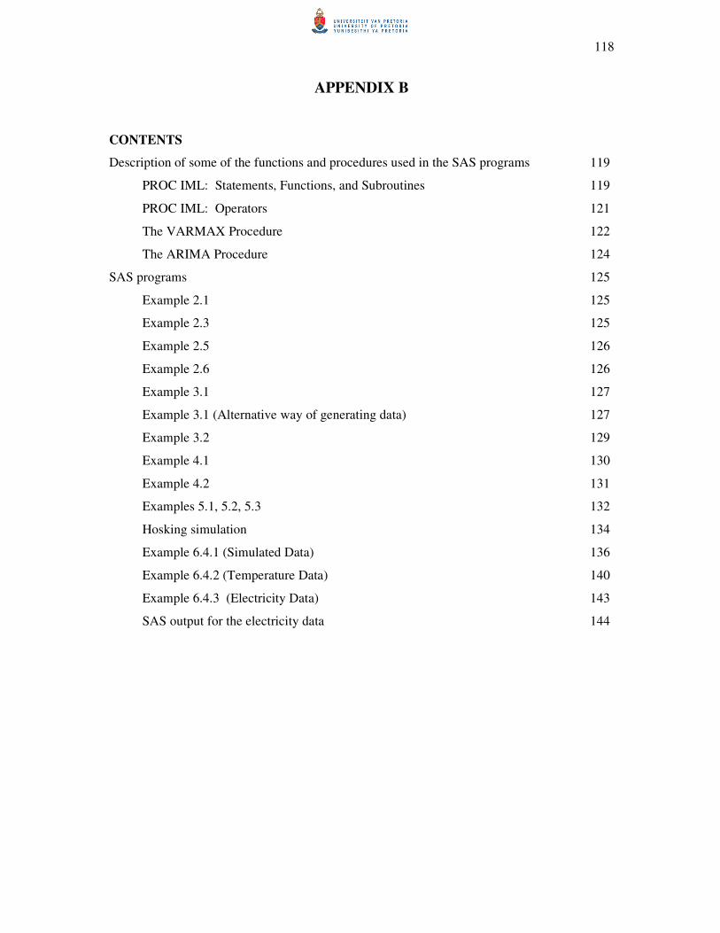
118
APPENDIX B
CONTENTS
Description of some of the functions and procedures used in the SAS programs 119
PROC IML: Statements, Functions, and Subroutines 119
PROC IML: Operators 121
The VARMAX Procedure 122
The ARIMA Procedure 124
SAS programs 125
Example 2.1 125
Example 2.3 125
Example 2.5 126
Example 2.6 126
Example 3.1 127
Example 3.1 (Alternative way of generating data) 127
Example 3.2 129
Example 4.1 130
Example 4.2 131
Examples 5.1, 5.2, 5.3 132
Hosking simulation 134
Example 6.4.1 (Simulated Data) 136
Example 6.4.2 (Temperature Data) 140
Example 6.4.3 (Electricity Data) 143
SAS output for the electricity data 144

119
DESCRIPTION OF SOME OF THE FUNCTIONS AND PROCEDURES
USED IN THE SAS PROGRMAS
(Quoted from: SAS/ETS 9.1 User’s Guide, 2004)
PROC IML: Statements, Functions, and Subroutines
APPEND Statement: adds observations to the end of a SAS data set
APPEND FROM from-name;
from-name is the name of a matrix containing data to append
CREATE Statement: creates a new SAS data set
CREATE SAS-data-set FROM matrix-name[COLNAME=column-];
SAS-data-set is the name of the new data set
matrix-name names a matrix containing the data
column-name is a character matrix containing descriptive names to associate with data
set variables
EIGVAL Function: computes the eigenvalues of a square matrix
EIGVAL(square-matrix)
DET Function: computes the determinant of a square matrix
DET( square-matrix)
DIAG Function: creates a diagonal matrix from a square matrix or a vector
DIAG(square-matrix / vector)
I Function: creates an identity matrix
I( dimension)
dimension specifies the size of the identity matrix
INV Function: computes the inverse of a square nonsingular matrix
INV(square-matrix)
J Function: creates a matrix of identical values
J( nrow, ncol, value)
nrow is the number of rows
ncol is a the number of columns.
value is the value used to fill the rows and columns of the matrix
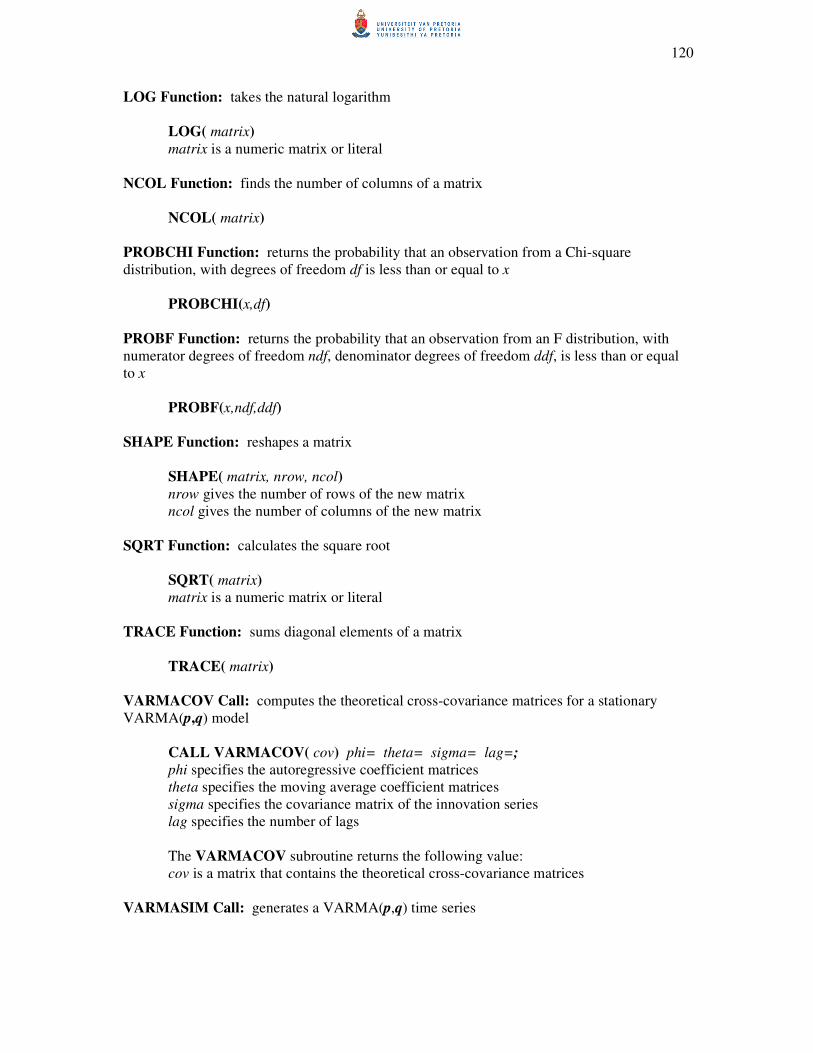
120
LOG Function: takes the natural logarithm
LOG( matrix)
matrix is a numeric matrix or literal
NCOL Function: finds the number of columns of a matrix
NCOL( matrix)
PROBCHI Function: returns the probability that an observation from a Chi-square
distribution, with degrees of freedom df is less than or equal to x
PROBCHI(x,df)
PROBF Function: returns the probability that an observation from an F distribution, with
numerator degrees of freedom ndf, denominator degrees of freedom ddf, is less than or equal
to x
PROBF(x,ndf,ddf)
SHAPE Function: reshapes a matrix
SHAPE( matrix, nrow, ncol)
nrow gives the number of rows of the new matrix
ncol gives the number of columns of the new matrix
SQRT Function: calculates the square root
SQRT( matrix)
matrix is a numeric matrix or literal
TRACE Function: sums diagonal elements of a matrix
TRACE( matrix)
VARMACOV Call: computes the theoretical cross-covariance matrices for a stationary
VARMA(p,q) model
CALL VARMACOV( cov) phi= theta= sigma= lag=;
phi specifies the autoregressive coefficient matrices
theta specifies the moving average coefficient matrices
sigma specifies the covariance matrix of the innovation series
lag specifies the number of lags
The VARMACOV subroutine returns the following value:
cov is a matrix that contains the theoretical cross-covariance matrices
VARMASIM Call: generates a VARMA(p,q) time series

121
CALL VARMASIM( series) phi= theta= mu= sigma= n= seed=;
phi specifies the autoregressive coefficient matrices
theta specifies the moving average coefficient matrices
mu specifies the mean vector of the series
sigma specifies the covariance matrix of the innovation series
n specifies the length of the series
seed specifies the random number seed
The VARMASIM subroutine returns the following value:
series is a matrix containing the generated time series.
VECDIAG Function: creates a vector from the diagonal elements of a square matrix
VECDIAG( square-matrix) VTSROOT Call: calculates the characteristic roots of the model from AR and MA
characteristic functions
CALL VTSROOT( root, phi, theta);
phi specifies the autoregressive coefficient matrices
theta specifies the moving average coefficient matrices
The VTSROOT subroutine returns the following value:
root is a matrix, where
the first column contains the real parts, x, of eigenvalues
the second column contains the imaginary parts, y, of the eigenvalues
the third column contains the modulus of the eigenvalues
PROC IML: Operators
Addition Operator + adds corresponding matrix elements
Concatenation Operator, Horizontal || concatenates matrices horizontally
Concatenation Operator, Vertical // concatenates matrices vertically
Kronecker Product Operator @ takes the Kronecker product of two matrices
Division Operator / performs elementwise division
Multiplication Operator, Elementwise # performs elementwise multiplication
Multiplication Operator, Matrix * performs matrix multiplication
Power Operator, Elementwise ## raises each element to a power
Power Operator, Matrix ** raises a matrix to a power
Subscripts [ ] select submatrices
matrix[rows,columns]
Subtraction Operator - subtracts corresponding matrix elements
Transpose Operator ` transposes a matrix

122
The VARMAX Procedure
Syntax
PROC VARMAX options ;
MODEL dependent variables </ options > ;
OUTPUT < options > ;
PROC VARMAX Statement
PROC VARMAX options ;
Options
DATA= SAS-data-set specifies the input SAS data set
MODEL Statement
MODEL dependents </ options > ;
The MODEL statement specifies dependent variables for the VARMAX model.
General Options
METHOD= value requests the type of estimates to be computed, the possible values are:
LS: specifies least-squares estimates
ML: specifies maximum likelihood estimates
NOINT
suppresses the intercept parameter
Printing Control Options
LAGMAX= number specifies the number of lags to display in the output
Printing Options
PRINT=(options) The following options can be used in the PRINT=( ) option:
CORRY(number) prints the cross-correlation matrices of dependent variables
COVY(number)
prints the cross-covariance matrices of dependent variables
PARCOEF(number) prints the partial autoregression coefficient matrices
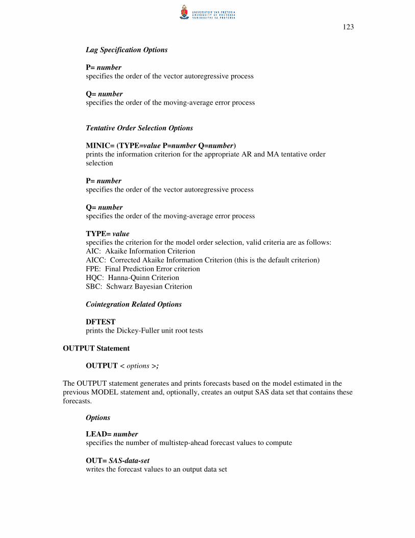
123
Lag Specification Options
P= number
specifies the order of the vector autoregressive process
Q= number specifies the order of the moving-average error process
Tentative Order Selection Options
MINIC= (TYPE=value P=number Q=number) prints the information criterion for the appropriate AR and MA tentative order
selection
P= number
specifies the order of the vector autoregressive process
Q= number specifies the order of the moving-average error process
TYPE= value specifies the criterion for the model order selection, valid criteria are as follows:
AIC: Akaike Information Criterion
AICC: Corrected Akaike Information Criterion (this is the default criterion)
FPE: Final Prediction Error criterion
HQC: Hanna-Quinn Criterion
SBC: Schwarz Bayesian Criterion
Cointegration Related Options
DFTEST prints the Dickey-Fuller unit root tests
OUTPUT Statement
OUTPUT < options >;
The OUTPUT statement generates and prints forecasts based on the model estimated in the
previous MODEL statement and, optionally, creates an output SAS data set that contains these
forecasts.
Options
LEAD= number specifies the number of multistep-ahead forecast values to compute
OUT= SAS-data-set writes the forecast values to an output data set

124
The ARIMA Procedure
Syntax
PROC ARIMA options;
IDENTIFY VAR=variable options;
ESTIMATE options;
FORECAST options;
PROC ARIMA Statement
PROC ARIMA options;
Options
DATA= SAS-data-set specifies the name of the SAS data set containing the time series
OUT= SAS-data-set
specifies a SAS data set to which the forecasts are output
IDENTIFY Statement
IDENTIFY VAR=variable;
The IDENTIFY statement specifies the time series to be modeled.
ESTIMATE Statement
ESTIMATE options;
The ESTIMATE statement specifies an ARMA model for the response variable specified in
the previous IDENTIFY statement, and produces estimates of its parameters. The ESTIMATE
statement also prints diagnostic information by which to check the model.
Options
P= order specifies the autoregressive part of the model
FORECAST Statement
FORECAST options;
The FORECAST statement generates forecast values for a time series using the parameter
estimates produced by the previous ESTIMATE statement
Options
LEAD= n specifies the number of multistep forecast values to compute
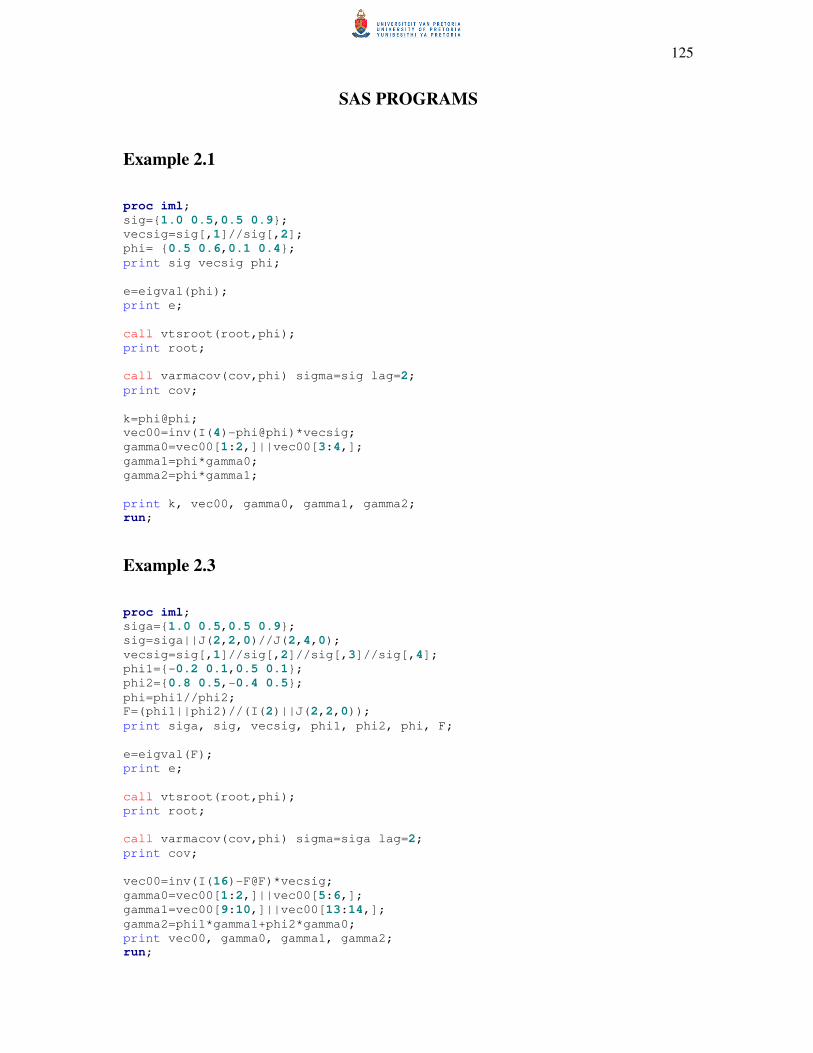
125
SAS PROGRAMS
Example 2.1
proc iml;
sig={1.0 0.5,0.5 0.9};
vecsig=sig[,1]//sig[,2];
phi= {0.5 0.6,0.1 0.4};
print sig vecsig phi;
e=eigval(phi);
print e;
call vtsroot(root,phi);
print root;
call varmacov(cov,phi) sigma=sig lag=2;
print cov;
k=phi@phi;
vec00=inv(I(4)-phi@phi)*vecsig;
gamma0=vec00[1:2,]||vec00[3:4,];
gamma1=phi*gamma0;
gamma2=phi*gamma1;
print k, vec00, gamma0, gamma1, gamma2;
run;
Example 2.3
proc iml;
siga={1.0 0.5,0.5 0.9};
sig=siga||J(2,2,0)//J(2,4,0);
vecsig=sig[,1]//sig[,2]//sig[,3]//sig[,4];
phi1={-0.2 0.1,0.5 0.1};
phi2={0.8 0.5,-0.4 0.5};
phi=phi1//phi2;
F=(phi1||phi2)//(I(2)||J(2,2,0));
print siga, sig, vecsig, phi1, phi2, phi, F;
e=eigval(F);
print e;
call vtsroot(root,phi);
print root;
call varmacov(cov,phi) sigma=siga lag=2;
print cov;
vec00=inv(I(16)-F@F)*vecsig;
gamma0=vec00[1:2,]||vec00[5:6,];
gamma1=vec00[9:10,]||vec00[13:14,];
gamma2=phi1*gamma1+phi2*gamma0;
print vec00, gamma0, gamma1, gamma2;
run;
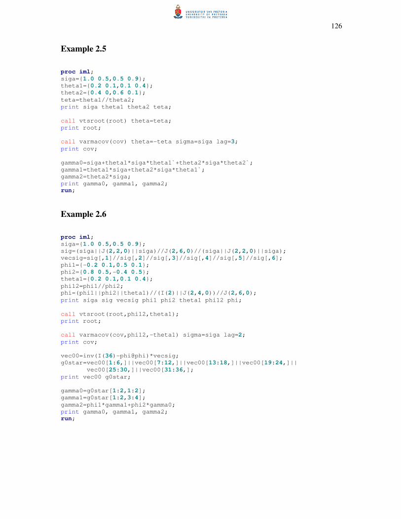
126
Example 2.5
proc iml;
siga={1.0 0.5,0.5 0.9};
theta1={0.2 0.1,0.1 0.4};
theta2={0.4 0,0.6 0.1};
teta=theta1//theta2;
print siga theta1 theta2 teta;
call vtsroot(root) theta=teta;
print root;
call varmacov(cov) theta=-teta sigma=siga lag=3;
print cov;
gamma0=siga+theta1*siga*theta1`+theta2*siga*theta2`;
gamma1=theta1*siga+theta2*siga*theta1`;
gamma2=theta2*siga;
print gamma0, gamma1, gamma2;
run;
Example 2.6
proc iml;
siga={1.0 0.5,0.5 0.9};
sig=(siga||J(2,2,0)||siga)//J(2,6,0)//(siga||J(2,2,0)||siga);
vecsig=sig[,1]//sig[,2]//sig[,3]//sig[,4]//sig[,5]//sig[,6];
phi1={-0.2 0.1,0.5 0.1};
phi2={0.8 0.5,-0.4 0.5};
theta1={0.2 0.1,0.1 0.4};
phi12=phi1//phi2;
phi=(phi1||phi2||theta1)//(I(2)||J(2,4,0))//J(2,6,0);
print siga sig vecsig phi1 phi2 theta1 phi12 phi;
call vtsroot(root,phi12,theta1);
print root;
call varmacov(cov,phi12,-theta1) sigma=siga lag=2;
print cov;
vec00=inv(I(36)-phi@phi)*vecsig;
g0star=vec00[1:6,]||vec00[7:12,]||vec00[13:18,]||vec00[19:24,]||
vec00[25:30,]||vec00[31:36,];
print vec00 g0star;
gamma0=g0star[1:2,1:2];
gamma1=g0star[1:2,3:4];
gamma2=phi1*gamma1+phi2*gamma0;
print gamma0, gamma1, gamma2;
run;

127
Example 3.1
proc iml;
T=500;
k=2;
p=1;
sig={1.0 0.5,0.5 0.9};
phi={0.5 0.6,0.1 0.4};
call varmasim(yy,phi) sigma=sig n=T seed=1;
cn={'y1' 'y2'};
create simul1 from yy[colname=cn];
append from yy;
y=yy`;
*print y;
vecy=y[,1];
do i= 2 to T;
vecy=vecy//y[,i];
end;
*print vecy;
call varmasim(yyy,phi) sigma=sig n=1 seed=2;
z=J(1,T,1)//(yyy`||y[,1:T-1]);
vecb=((inv(z*z`)*z)@I(k))*vecy;
print vecb;
b=vecb[1:2,]||vecb[3:4,]||vecb[5:6,];
print b;
gamhat=(1/T)#z*z`;
print gamhat;
sighat=1/(T-k*p-1)*(y*(I(T)-z`*inv(z*z`)*z)*y`);
print sighat;
var=inv(z*z`)@sighat;
print var;
stderr=sqrt(vecdiag(inv(z*z`)@sighat));
print stderr;
t=vecb/stderr;
print t;
proc varmax data=simul1;
model y1 y2 / p=1 lagmax=3;
run;
Example 3.1 (Alternative way of generating data)
proc iml;
T=500;
k=2;
porder=1;
128
siga={1.0 0.5,0.5 0.9};
phi={0.5 0.6,0.1 0.4};
p=half(siga)`;
print p;
*generate random starting point y0;
yp=J(2,1,0);
do j=1 to 50;
d=J(2,1,0);
d[1,1]=rannor(0);
d[2,1]=rannor(0);
aa=p*d;
yy=phi*yp+aa;
yp=yy;
end;
*print yp;
a=J(2,T,0);
y=J(2,T,0);
a[,1]=p*J(2,1,rannor(0));
y[,1]=phi*yp+a[,1];
do i=2 to T;
d=J(2,1,0);
d[1,1]=rannor(0);
d[2,1]=rannor(0);
a[,i]=p*d;
y[,i]=phi*y[,i-1]+a[,i];
end;
*print a y;
vecy=y[,1];
do m= 2 to T;
vecy=vecy//y[,m];
end;
z=J(1,T,1)//(yp||y[,1:T-1]);
vecb=((inv(z*z`)*z)@I(k))*vecy;
print vecb;
b=vecb[1:2,]||vecb[3:4,]||vecb[5:6,];
print b;
gamhat=(1/T)#z*z`;
print gamhat;
sighat=1/(T-k*porder-1)*(y*(I(T)-z`*inv(z*z`)*z)*y`);
print sighat;
stderr=sqrt(vecdiag(inv(z*z`)@sighat));
print stderr;
tstat=vecb/stderr;
print tstat;
yy=y`;
cn={'y1' 'y2'};
create simul1 from yy[colname=cn];
append from yy;
quit;
129
proc varmax data=simul1;
model y1 y2 / p=1 lagmax=3;
run;
Example 3.2
*assume mean is zero;
proc iml;
T=500;
k=2;
p=1;
sig={1.0 0.5,0.5 0.9};
phi={0.5 0.6,0.1 0.4};
call varmasim(yy,phi) sigma=sig n=T seed=1;
cn={'y1' 'y2'};
create simul1 from yy[colname=cn];
append from yy;
y=yy`;
*print y;
mean=1/T#y[,+];
print mean;
mu=J(2,1,0);
vecy=y[,1];
do i= 2 to T;
vecy=vecy//y[,i];
end;
*print vecy;
vecmu=mu;
do j=2 to T;
vecmu=vecmu//mu;
end;
call varmasim(yyy,phi) sigma=sig n=1 seed=2;
x=(yyy`-mu)||(y[,1:T-1]-mu*j(1,T-1,1));
vecb=((inv(x*x`)*x)@I(k))*(vecy-vecmu);
print vecb;
b=vecb[1:2,]||vecb[3:4,];
print b;
ynul=(y[,1:T]-mu*j(1,T,1));
sighat=1/T#(ynul-b*x)*(ynul-b*x)`;
print sighat;
stderr=sqrt(vecdiag(inv(x*x`)@sighat));
print stderr;
t=vecb/stderr;
print t;
130
proc varmax data=simul1;
model y1 y2 / p=1 method=ml noint lagmax=3;
run;
Example 4.1 *IML Program to optimise likelihood function of VMA(1) by means of dual
quasi Newton optimisation algorithm;
proc iml;
*simulate VMA(1) time series;
sig={1.0 0.5, 0.5 0.9 };
T=500;
theta1={0.2 0.1, 0.1 0.4};
call varmasim(yy) theta=theta1 sigma=sig n=T seed=1;
cn={'y1' 'y2'};
create vma1 from yy[colname=cn];
append from yy;
*Calculate -2*logL for VMA(1);
start loglike(x) global(yy);
theta=(x[1]||x[2])//(x[3]||x[4]);
siga=(x[5]||x[6])//(x[6]||x[7]);
*invertibility test;
e=eigval(theta);
norme=sqrt(e##2);
testi=(norme>=1)[+,];
*determinant sigma_a test;
detsiga=det(siga);
testd=(detsiga<=0);
test=testi+testd;
if test=0 then do;
a=j(nrow(yy),2,0);
do i=2 to nrow(a);
a[i,]=yy[i,]-a[i-1,]*theta`;
end;
aa=a[11:nrow(a),];
capt=nrow(aa);
sum=0;
isiga=inv(siga);
do j=1 to capt;
sum=sum+aa[j,]*isiga*aa[j,]`;
end;
logl=capt#log(det(siga))+sum;
end;
return(logl);
finish loglike;
x={-0.1 0.1 -0.1 0.1 1.01 0.01 1.01}; *Starting values for parameters;
optn = {0 2 . 2}; *Options for optimisation procedure;
call nlpqn(rc,xr,"loglike",x,optn);
run;

131
proc varmax data=vma1;
model y1 y2 / q=1 method=ml noint lagmax=3;
run;
quit;
Example 4.2 *IML Program to optimise likelihood function of VARMA(1,1) by means of dual
quasi Newton optimisation algorithm;
proc iml;
*simulate VARMA(1,1) time series;
sig={1.0 0.5, 0.5 0.9 };
T=500;
phi1={-0.2 0.1,0.5 0.1};
theta1={0.2 0.1,0.1 0.4};
call varmasim(yy) phi=phi1 theta=theta1 sigma=sig n=T seed=1;
cn={'y1' 'y2'};
create varma11 from yy[colname=cn];
append from yy;
*Calculate -2*logL for VMA(1);
start loglike(x) global(yy);
phi=(x[1]||x[2])//(x[3]||x[4]);
theta=(x[5]||x[6])//(x[7]||x[8]);
siga=(x[9]||x[10])//(x[10]||x[11]);
*stationarity test;
ep=eigval(phi);
normep=sqrt(ep##2);
tests=(normep>=1)[+,];
*invertibility test;
et=eigval(theta);
normet=sqrt(et##2);
testi=(normet>=1)[+,];
*determinant sigma_a test;
detsiga=det(siga);
testd=(detsiga<=0);
test=tests+testi+testd;
if test=0 then do;
a=j(nrow(yy),2,0);
do i=2 to nrow(a);
a[i,]=yy[i,]-yy[i-1,]*phi`-a[i-1,]*theta`;
end;
aa=a[11:nrow(a),];
capt=nrow(aa);
sum=0;
isiga=inv(siga);
do j=1 to capt;
sum=sum+aa[j,]*isiga*aa[j,]`;
end;
logl=capt#log(det(siga))+sum;
132
end;
return(logl);
finish loglike;
x={-0.1 0.1 -0.1 0.1 -0.1 0.1 -0.1 0.1 1.01 0.01 1.01}; *Starting values for
parameters;
optn = {0 2 . 2}; *Options for optimisation procedure;
call nlpqn(rc,xr,"loglike",x,optn);
run;
proc varmax data=varma11;
model y1 y2 /p=1 q=1 method=ml noint lagmax=3;
run;
quit;
Examples 5.1, 5.2, 5.3
proc iml;
start
autocovcor(T,y,gamma0,gamma1,gamma2,gamma3,rho0,rho1,rho2,rho3,phi11,phi22);
y=y`;
mean=(1/T)#y[,+]*J(1,500,1);
gamma0=(1/T)#(y-mean)*(y-mean)`;
gamma1=(1/T)#(y[,2:T]-mean[,2:T])*(y[,1:T-1]-mean[,1:T-1])`;
gamma2=(1/T)#(y[,3:T]-mean[,3:T])*(y[,1:T-2]-mean[,1:T-2])`;
gamma3=(1/T)#(y[,4:T]-mean[,4:T])*(y[,1:T-3]-mean[,1:T-3])`;
print gamma0,gamma1,gamma2,gamma3;
vhalf=sqrt(diag(gamma0));
rho0=inv(vhalf)*gamma0*inv(vhalf);
rho1=inv(vhalf)*gamma1*inv(vhalf);
rho2=inv(vhalf)*gamma2*inv(vhalf);
rho3=inv(vhalf)*gamma3*inv(vhalf);
print rho0,rho1,rho2,rho3;
phi11=gamma1*inv(gamma0);
phi22=(gamma2-gamma1*inv(gamma0)*gamma1)*inv(gamma0-
gamma1`*inv(gamma0)*gamma1);
print phi11, phi22;
finish autocovcor;
sig={1.0 0.5,0.5 0.9};
T=500;
phi={0.5 0.6,0.1 0.4};
call varmasim(y,phi) sigma=sig n=T seed=1;
cn={'y1' 'y2'};
create var1 from y[colname=cn];
append from y;
call
autocovcor(T,y,gamma0,gamma1,gamma2,gamma3,rho0,rho1,rho2,rho3,phi11,phi22);
133
theta1={0.2 0.1,0.1 0.4};
theta2={0.4 0,0.6 0.1};
theta12=theta1//theta2;
call varmasim(yy) theta=theta12 sigma=sig n=T seed=1;
cn={'y1' 'y2'};
create vma2 from yy[colname=cn];
append from yy;
call
autocovcor(T,yy,gamma0,gamma1,gamma2,gamma3,rho0,rho1,rho2,rho3,phi11,phi22)
;
phi1={-0.2 0.1,0.5 0.1};
phi2={0.8 0.5,-0.4 0.5};
theta1={0.2 0.1,0.1 0.4};
phi12=phi1//phi2;
call varmasim(yyy) phi=phi12 theta=theta1 sigma=sig n=T seed=1;
cn={'y1' 'y2'};
create varma21 from yyy[colname=cn];
append from yyy;
call
autocovcor(T,yyy,gamma0,gamma1,gamma2,gamma3,rho0,rho1,rho2,rho3,phi11,phi22
);
proc varmax data=var1;
model y1 y2 / noint lagmax=3 print=(covy(3)) print=(corry(3))
print=(parcoef);
run;
proc varmax data=vma2;
model y1 y2 / noint lagmax=3 print=(covy(3)) print=(corry(3))
print=(parcoef);
run;
proc varmax data=varma21 outstat=out21;
model y1 y2 /p=2 q=1 noint lagmax=3 method=ml print=(covy(3))
print=(corry(3)) print=(parcoef);
run;
proc iml;
use out21;
read all into out21;
T=500;
r21=12;
k=2;
siga21=out21[,1:2];
print siga21;
aic21=log(det(siga21))+2*r21/T;
aaic21=log(det(siga21))+(2*r21)/(T-r21/k);
fpe21=(((T+r21/k)/(T-r21/k))**k)*det(siga21);
hqc21=log(det(siga21))+2*r21*log(log(T))/T;
sbc21=log(det(siga21))+r21*log(T)/T;
print aic21 aaic21 fpe21 hqc21 sbc21;
run;
proc varmax data=varma21 outstat=out3;
model y1 y2 /p=3 noint lagmax=3;
run;

134
proc iml;
use out3;
read all into out3;
T=500;
r3=12;
k=2;
p=3;
siga3=out3[,1:2];
siga3=((t-k#p)/T)#siga3;
print siga3;
aic3=log(det(siga3))+2*r3/T;
aaic3=log(det(siga3))+(2*r3)/(T-r3/k);
fpe3=(((T+r3/k)/(T-r3/k))**k)*det(siga3);
hqc3=log(det(siga3))+2*r3*log(log(T))/T;
sbc3=log(det(siga3))+r3*log(T)/T;
print aic3 aaic3 fpe3 hqc3 sbc3;
run;
proc varmax data=varma21 outstat=out11;
model y1 y2 /p=1 q=1 noint lagmax=3;
run;
proc iml;
use out11;
read all into out11;
T=500;
r11=8;
k=2;
siga11=out11[,1:2];
print siga11;
aic11=log(det(siga11))+2*r11/T;
aaic11=log(det(siga11))+(2*r11)/(T-r11/k);
fpe11=(((T+r11/k)/(T-r11/k))**k)*det(siga11);
hqc11=log(det(siga11))+2*r11*log(log(T))/T;
sbc11=log(det(siga11))+r11*log(T)/T;
print aic11 aaic11 fpe11 hqc11 sbc11;
run;
proc varmax data=varma21;
model y1 y2 /noint minic=(p=4 q=4) lagmax=3;
run;
Hosking simulation
proc iml;
pp=J(1000,2,0);
do i=1 to 1000;
*******************************************;
* Generating the VAR(1) process *;
*******************************************;
135
k=2;
t=1000;
sig={1.0 0.4,0.4 1};
phi1={0.9 0.1,-0.6 0.4};
call varmasim(yy) phi=phi1 sigma=sig n=t seed=0;
****************************************************;
* Fit a VAR(1) model using method of least squares *;
****************************************************;
y=yy`;
call varmasim(yyy,phi1) sigma=sig n=1 seed=0;
z=J(1,T,1)//(yyy`||y[,1:T-1]);
b=y*z`*inv(z*z`);
*print bb;
bz=b*z;
*print bz;
resid=y-bz;
*print resid;
***********************************************;
* Portmanteau Statistic *;
***********************************************;
ncolr=ncol(resid);
c0=(1/ncolr)#resid*resid`;
c1=(1/ncolr)#resid[,2:ncolr]*(resid[,1:ncolr-1])`;
c2=(1/ncolr)#resid[,3:ncolr]*(resid[,1:ncolr-2])`;
c3=(1/ncolr)#resid[,4:ncolr]*(resid[,1:ncolr-3])`;
c4=(1/ncolr)#resid[,5:ncolr]*(resid[,1:ncolr-4])`;
c5=(1/ncolr)#resid[,6:ncolr]*(resid[,1:ncolr-5])`;
c6=(1/ncolr)#resid[,7:ncolr]*(resid[,1:ncolr-6])`;
c7=(1/ncolr)#resid[,8:ncolr]*(resid[,1:ncolr-7])`;
c8=(1/ncolr)#resid[,9:ncolr]*(resid[,1:ncolr-8])`;
c9=(1/ncolr)#resid[,10:ncolr]*(resid[,1:ncolr-9])`;
c10=(1/ncolr)#resid[,11:ncolr]*(resid[,1:ncolr-10])`;
c11=(1/ncolr)#resid[,12:ncolr]*(resid[,1:ncolr-11])`;
c12=(1/ncolr)#resid[,13:ncolr]*(resid[,1:ncolr-12])`;
c13=(1/ncolr)#resid[,14:ncolr]*(resid[,1:ncolr-13])`;
c14=(1/ncolr)#resid[,15:ncolr]*(resid[,1:ncolr-14])`;
c15=(1/ncolr)#resid[,16:ncolr]*(resid[,1:ncolr-15])`;
c16=(1/ncolr)#resid[,17:ncolr]*(resid[,1:ncolr-16])`;
c17=(1/ncolr)#resid[,18:ncolr]*(resid[,1:ncolr-17])`;
c18=(1/ncolr)#resid[,19:ncolr]*(resid[,1:ncolr-18])`;
c19=(1/ncolr)#resid[,20:ncolr]*(resid[,1:ncolr-19])`;
c20=(1/ncolr)#resid[,21:ncolr]*(resid[,1:ncolr-20])`;
port=ncolr#(trace(c1`*inv(c0)*c1*inv(c0))+
trace(c2`*inv(c0)*c2*inv(c0))+
trace(c3`*inv(c0)*c3*inv(c0))+
trace(c4`*inv(c0)*c4*inv(c0))+
trace(c5`*inv(c0)*c5*inv(c0))+
trace(c6`*inv(c0)*c6*inv(c0))+
trace(c7`*inv(c0)*c7*inv(c0))+
trace(c8`*inv(c0)*c8*inv(c0))+
136
trace(c9`*inv(c0)*c9*inv(c0))+
trace(c10`*inv(c0)*c10*inv(c0))+
trace(c11`*inv(c0)*c11*inv(c0))+
trace(c12`*inv(c0)*c12*inv(c0))+
trace(c13`*inv(c0)*c13*inv(c0))+
trace(c14`*inv(c0)*c14*inv(c0))+
trace(c15`*inv(c0)*c15*inv(c0))+
trace(c16`*inv(c0)*c16*inv(c0))+
trace(c17`*inv(c0)*c17*inv(c0))+
trace(c18`*inv(c0)*c18*inv(c0))+
trace(c19`*inv(c0)*c19*inv(c0))+
trace(c20`*inv(c0)*c20*inv(c0)));
portprime=(ncolr##2)#(1/(ncolr-1)#trace(c1`*inv(c0)*c1*inv(c0))+
1/(ncolr-2)#trace(c2`*inv(c0)*c2*inv(c0))+
1/(ncolr-3)#trace(c3`*inv(c0)*c3*inv(c0))+
1/(ncolr-4)#trace(c4`*inv(c0)*c4*inv(c0))+
1/(ncolr-5)#trace(c5`*inv(c0)*c5*inv(c0))+
1/(ncolr-6)#trace(c6`*inv(c0)*c6*inv(c0))+
1/(ncolr-7)#trace(c7`*inv(c0)*c7*inv(c0))+
1/(ncolr-8)#trace(c8`*inv(c0)*c8*inv(c0))+
1/(ncolr-9)#trace(c9`*inv(c0)*c9*inv(c0))+
1/(ncolr-10)#trace(c10`*inv(c0)*c10*inv(c0))+
1/(ncolr-11)#trace(c11`*inv(c0)*c11*inv(c0))+
1/(ncolr-12)#trace(c12`*inv(c0)*c12*inv(c0))+
1/(ncolr-13)#trace(c13`*inv(c0)*c13*inv(c0))+
1/(ncolr-14)#trace(c14`*inv(c0)*c14*inv(c0))+
1/(ncolr-15)#trace(c15`*inv(c0)*c15*inv(c0))+
1/(ncolr-16)#trace(c16`*inv(c0)*c16*inv(c0))+
1/(ncolr-17)#trace(c17`*inv(c0)*c17*inv(c0))+
1/(ncolr-18)#trace(c18`*inv(c0)*c18*inv(c0))+
1/(ncolr-19)#trace(c19`*inv(c0)*c19*inv(c0))+
1/(ncolr-20)#trace(c20`*inv(c0)*c20*inv(c0)));
*print port portprime;
pp[i,]=port||portprime;
end;
*print pp;
col={'p' 'pprime'};
create hosking from pp[colname=col];
append from pp;
run;
proc univariate data=hosking;
var p pprime;
run;
Example 6.4.1 (Simulated Data)
proc iml;
*******************************************;
* Generating the VAR(2) process *;
*******************************************;
t=500;
sig={1.0 0.5,0.5 0.9};
mean={30,25};

137
phi1={0.6 -0.8,0.2 0.3};
phi2={0.3 0.7,-0.6 -0.5};
phi12=phi1//phi2;
call varmasim(y) phi=phi12 mu=mean sigma=sig n=t seed=12;
cn={'y' 'x'};
create var2 from y[colname=cn];
append from y;
call vtsroot(root,phi12);
print root;
run;
******************************************;
* Fit a VAR(1) model using proc varmax *;
******************************************;
proc varmax data=var2;
model y x / p=1 method=ls lagmax=3;
run;
******************************************;
* Fit a VAR(2) model using proc varmax *;
******************************************;
proc varmax data=var2;
model y x / p=2 method=ls lagmax=3;
output out=forecast lead=0;
run;
***********************************************;
* Multivariate Model Diagnostics *;
***********************************************;
**********************************************;
* Residual Autocorrelation Matrices *;
**********************************************;
proc iml;
t=500;
p=2; *var order;
q=0; *vma order;
use forecast;
read all into forecast;
resid=(forecast[p+1:t,3]||forecast[p+1:t,9]);
*print resid;
rmean=(J(nrow(resid),1,1)*((1/nrow(resid))#resid[+,]))`;
resid=resid`;
ncolr=ncol(resid);
*print rmean;
gamma0=(resid-rmean)*(resid-rmean)`;
gamma1=(resid[,2:ncolr]-rmean[,2:ncolr])*(resid[,1:ncolr-1]-
rmean[,1:ncolr-1])`;
gamma2=(resid[,3:ncolr]-rmean[,3:ncolr])*(resid[,1:ncolr-2]-
rmean[,1:ncolr-2])`;
gamma3=(resid[,4:ncolr]-rmean[,4:ncolr])*(resid[,1:ncolr-3]-
rmean[,1:ncolr-3])`;

138
vhalf=sqrt(diag(gamma0));
rho0=inv(vhalf)*gamma0*inv(vhalf);
rho1=inv(vhalf)*gamma1*inv(vhalf);
rho2=inv(vhalf)*gamma2*inv(vhalf);
rho3=inv(vhalf)*gamma3*inv(vhalf);
print rho0,rho1,rho2,rho3;
***********************************************;
* Portmanteau Statistic *;
***********************************************;
k=2; *dimension;
h=3; *number of lags;
c0=(1/ncolr)#resid*resid`;
c1=(1/ncolr)#resid[,2:ncolr]*(resid[,1:ncolr-1])`;
c2=(1/ncolr)#resid[,3:ncolr]*(resid[,1:ncolr-2])`;
c3=(1/ncolr)#resid[,4:ncolr]*(resid[,1:ncolr-3])`;
*print c0 c1 c2 c3;
port=ncolr#(trace(c1`*inv(c0)*c1*inv(c0))+trace(c2`*inv(c0)*c2*inv(c0))+
trace(c3`*inv(c0)*c3*inv(c0)));
portprime=(ncolr##2)#(1/(ncolr-1)#trace(c1`*inv(c0)*c1*inv(c0))+
1/(ncolr-2)#trace(c2`*inv(c0)*c2*inv(c0))+
1/(ncolr-3)#trace(c3`*inv(c0)*c3*inv(c0)));
critpp=1-probchi(portprime,(k##2)#(h-p-q));
print port portprime critpp;
run;
***********************************************;
* Univariate Model Diagnostics ;
***********************************************;
***********************************************;
* R Square and F *;
***********************************************;
parm=2*p; *parameters of individual equation;
average=(1/t#forecast[+,1]*J(t-p,1,1))||(1/t#forecast[+,7]*J(t-p,1,1));
*print average;
ssr1=((forecast[p+1:t,2]-average[,1])##2)||((forecast[p+1:t,8]-
average[,2])##2);
ssr=ssr1[+,];
*print ssr;
sst1=((forecast[p+1:t,1]-average[,1])##2)||((forecast[p+1:t,7]-
average[,2])##2);
sst=sst1[+,];
*print sst;
sse1=((forecast[p+1:t,3])##2)||((forecast[p+1:t,9])##2);
sse=sse1[+,];
*print sse;
rsquare=ssr/sst;
print rsquare;
f=(ssr/parm)/(sse/(t-p-parm-1));
critf=1-probf(f,parm,t-p-parm-1);
print f critf;
139
***********************************************;
* Durbin Watson *;
***********************************************;
residual=(forecast[,3]||forecast[,9]);
d1=(residual[2:t,]-residual[1:t-1,])##2;
dbo=d1[+,];
d2=residual[2:t,]##2;
dond=d2[+,];
d=dbo/dond;
print d;
***********************************************;
* Jarqu-Bera *;
***********************************************;
m22=(resid-rmean)##2;
m2=(1/ncolr)#m22[,+];
m33=(resid-rmean)##3;
m3=(1/ncolr)#m33[,+];
m44=(resid-rmean)##4;
m4=(1/ncolr)#m44[,+];
s=m3/(m2##(3/2));
k=m4/(m2##2)-3;
jb=ncolr#((s##2)/6+(k##2)/24);
critjb=1-probchi(jb,2);
*print s k;
print jb critjb;
***********************************************;
* ARCH *;
***********************************************;
at=residual;
at1=J(1,2,.)//residual[1:t-1,];
atat=at##2;
at1at1=at1##2;
archreg=atat||at1at1;
*print atat at1at1 archreg;
col={'yat' 'xat' 'yat1' 'xat1'};
create archreg from archreg[colname=col];
append from archreg;
***********************************************;
* AR(1) - AR(4) *;
***********************************************;
a=residual;
a1=J(1,2,.)//a[1:t-1,];
a2=J(2,2,.)//a[1:t-2,];
a3=J(3,2,.)//a[1:t-3,];
a4=J(4,2,.)//a[1:t-4,];
ardist=a||a1||a2||a3||a4;
*print ar14;
col={'ya' 'xa' 'ya1' 'xa1' 'ya2' 'xa2' 'ya3' 'xa3' 'ya4' 'xa4'};
create ardist from ardist[colname=col];
append from ardist;

140
proc reg data=ardist;
model ya=ya1;
proc reg data=ardist;
model ya=ya1 ya2;
proc reg data=ardist;
model ya=ya1 ya2 ya3;
proc reg data=ardist;
model ya=ya1 ya2 ya3 ya4;
run;
proc reg data=ardist;
model xa=xa1;
proc reg data=ardist;
model xa=xa1 xa2;
proc reg data=ardist;
model xa=xa1 xa2 xa3;
proc reg data=ardist;
model xa=xa1 xa2 xa3 xa4;
run;
***********************************************;
* ARCH *;
***********************************************;
proc reg data=archreg;
model yat=yat1;
run;
proc reg data=archreg;
model xat=xat1;
run;
Example 6.4.2 (Temperature Data)
data a; *jan1999-des2005;
input t yt xt;
cards;
1 25.94868712 12.92476356
2 27.81361957 12.82533716
3 27.8724688 13.51923671
4 27.59007817 13.45073375
5 26.08907616 15.05343873
6 26.62787737 11.57998624
7 26.37219889 16.87041318
8 26.04728595 11.60759142
9 24.49451792 11.26737696
10 25.06128845 11.37850999
11 27.36336071 13.57102939
12 25.50606834 12.91000835
13 23.36273548 11.45762824
14 23.74994139 12.61508573
15 24.76506518 13.21198133
16 23.80921561 11.89122839
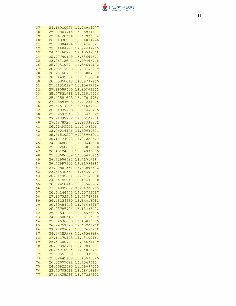
141
17 24.16910086 10.24914977
18 25.27807714 15.85954637
19 25.74128504 10.57975064
20 26.8133826 12.54874748
21 25.08004424 12.7416132
22 25.51694824 12.88448925
23 24.44460224 12.10597508
24 25.77740949 12.83665603
25 28.26712652 12.99462715
26 25.2851087 12.54500192
27 26.55417635 12.98153979
28 26.261667 13.93807917
29 26.31495561 12.97158018
30 26.75058649 14.09737455
31 25.61510227 15.15477794
32 27.36059449 13.80362223
33 25.27521968 12.21510026
34 25.42581628 13.47014786
35 23.98854623 12.72284005
36 25.32517424 12.61659907
37 26.84039458 12.99462715
38 25.82693246 12.33475049
39 27.21332258 12.75109826
40 27.4878927 12.96338832
41 26.31495561 11.0498646
42 23.56014956 14.60085221
43 25.61510227 9.435993811
44 25.17174693 15.37221567
45 24.8848688 12.00449508
46 25.97260803 11.88050308
47 26.45124869 11.64332635
48 25.50606834 13.05671299
49 26.92956532 12.7151728
50 26.72997205 13.31592383
51 27.49581381 12.52065672
52 28.81630387 14.13301734
53 26.31495561 12.97158018
54 24.54182246 15.10432988
55 26.62456443 10.86568984
56 23.74899602 9.254701269
57 26.64144778 13.05752097
58 27.15732348 13.63747888
59 26.45124869 13.64813751
60 29.30484448 13.71688387
61 26.03785786 13.13435432
62 25.37541266 12.75525335
63 24.76506518 12.98153979
64 25.54636868 13.45073375
65 26.99259395 13.45200908
66 23.9282769 11.07650858
67 24.73182288 10.86568984
68 27.14170973 14.43105961
69 25.3728074 11.05677179
70 26.88392761 12.80082374
71 28.54910634 13.64813751
72 25.59651539 12.76330371
73 25.32449189 12.43571845
74 26.36875622 12.4048343
75 24.85922893 11.59889059
76 23.70703013 12.08616656
77 27.44435285 13.77229501
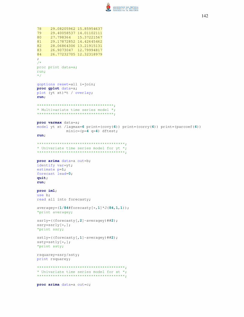
142
78 29.08205962 15.85954637
79 29.40058537 14.01102111
80 27.798364 15.37221567
81 29.17872852 14.42645462
82 28.06864306 13.21915131
83 26.9073047 12.79994817
84 26.77232705 12.32318979
;
/*
proc print data=a;
run;
*/
goptions reset=all i=join;
proc gplot data=a;
plot (yt xt)*t / overlay;
run;
**********************************;
* Multivariate time series model *;
**********************************;
proc varmax data=a;
model yt xt /lagmax=6 print=(covy(6)) print=(corry(6)) print=(parcoef(6))
minic=(p=4 q=4) dftest;
run;
***************************************;
* Univariate time series model for yt *;
***************************************;
proc arima data=a out=b;
identify var=yt;
estimate p=1;
forecast lead=0;
quit;
run;
proc iml;
use b;
read all into forecasty;
averagey=(1/84#forecasty[+,1]*J(84,1,1));
*print averagey;
ssr1y=((forecasty[,2]-averagey)##2);
ssry=ssr1y[+,];
*print ssry;
sst1y=((forecasty[,1]-averagey)##2);
ssty=sst1y[+,];
*print ssty;
rsquarey=ssry/ssty;
print rsquarey;
***************************************;
* Univariate time series model for xt *;
***************************************;
proc arima data=a out=c;
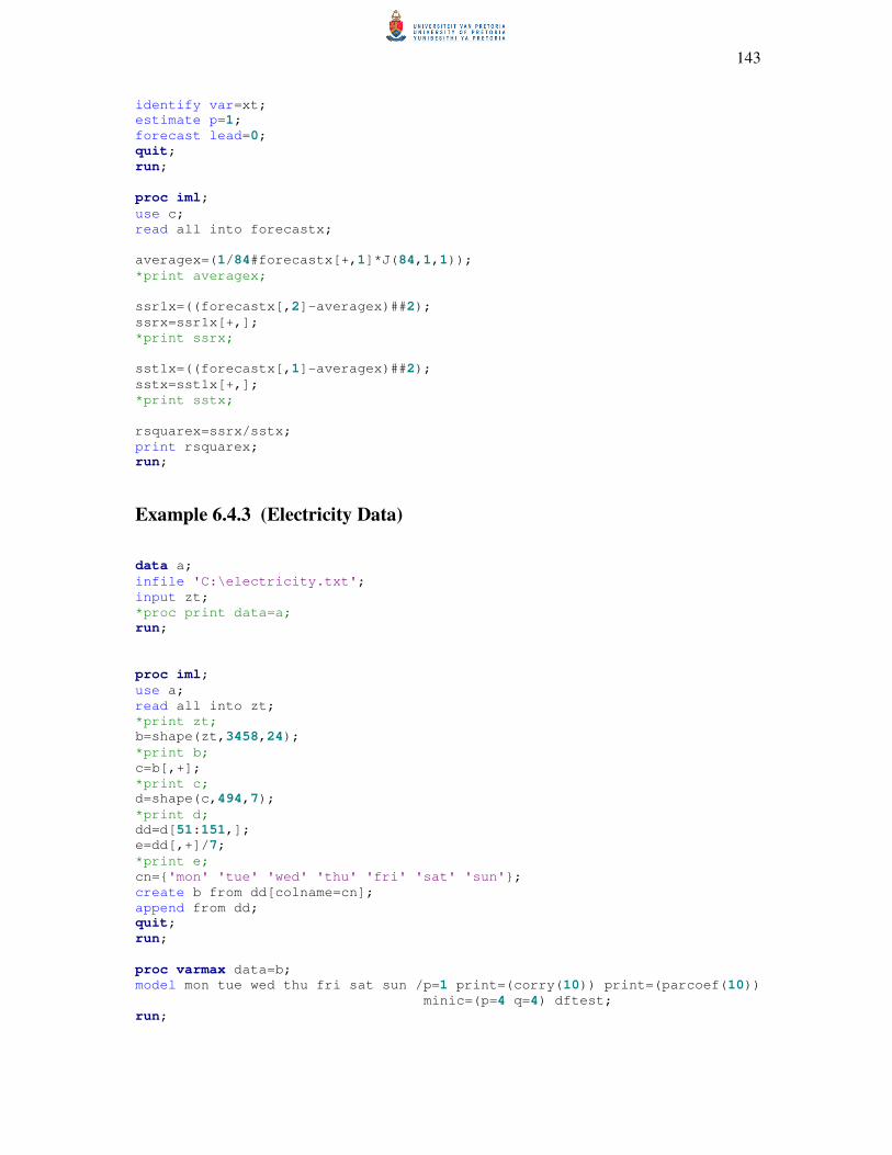
143
identify var=xt;
estimate p=1;
forecast lead=0;
quit;
run;
proc iml;
use c;
read all into forecastx;
averagex=(1/84#forecastx[+,1]*J(84,1,1));
*print averagex;
ssr1x=((forecastx[,2]-averagex)##2);
ssrx=ssr1x[+,];
*print ssrx;
sst1x=((forecastx[,1]-averagex)##2);
sstx=sst1x[+,];
*print sstx;
rsquarex=ssrx/sstx;
print rsquarex;
run;
Example 6.4.3 (Electricity Data)
data a;
infile 'C:\electricity.txt';
input zt;
*proc print data=a;
run;
proc iml;
use a;
read all into zt;
*print zt;
b=shape(zt,3458,24);
*print b;
c=b[,+];
*print c;
d=shape(c,494,7);
*print d;
dd=d[51:151,];
e=dd[,+]/7;
*print e;
cn={'mon' 'tue' 'wed' 'thu' 'fri' 'sat' 'sun'};
create b from dd[colname=cn];
append from dd;
quit;
run;
proc varmax data=b;
model mon tue wed thu fri sat sun /p=1 print=(corry(10)) print=(parcoef(10))
minic=(p=4 q=4) dftest;
run;
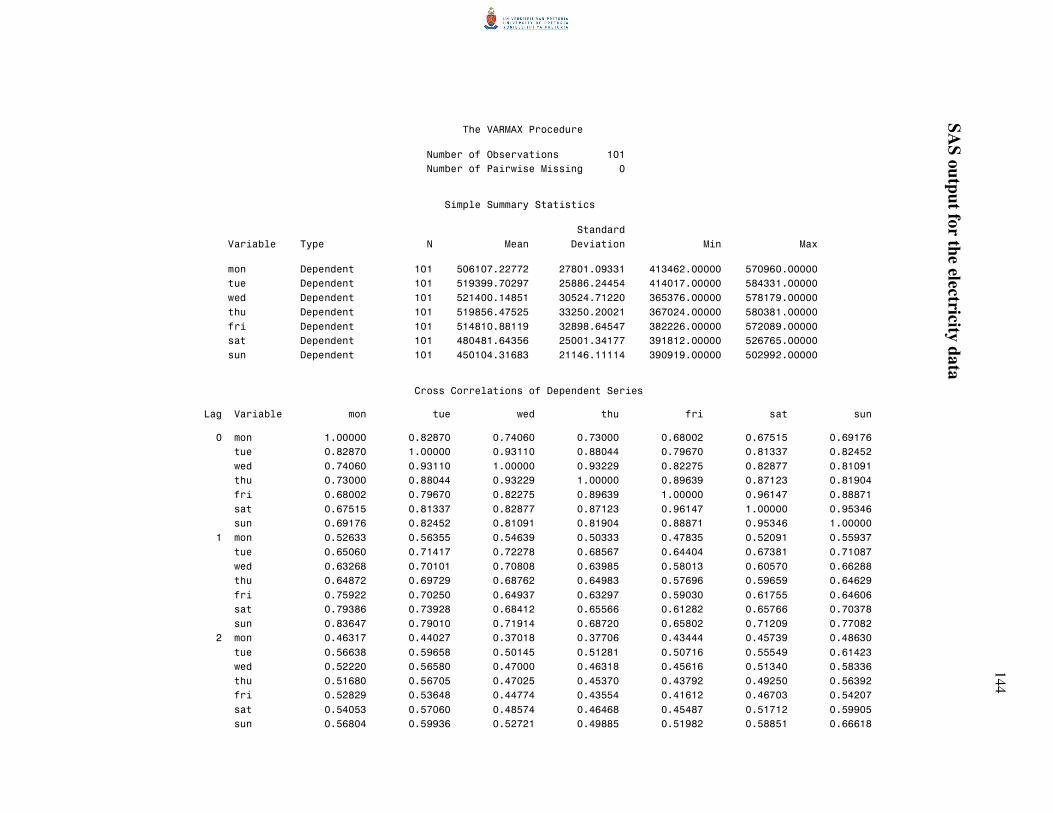
1
44
SA
S o
utp
ut fo
r the electricity
da
ta
The VARMAX Procedure
Number of Observations 101
Number of Pairwise Missing 0
Simple Summary Statistics
Standard
Variable Type N Mean Deviation Min Max
mon Dependent 101 506107.22772 27801.09331 413462.00000 570960.00000
tue Dependent 101 519399.70297 25886.24454 414017.00000 584331.00000
wed Dependent 101 521400.14851 30524.71220 365376.00000 578179.00000
thu Dependent 101 519856.47525 33250.20021 367024.00000 580381.00000
fri Dependent 101 514810.88119 32898.64547 382226.00000 572089.00000
sat Dependent 101 480481.64356 25001.34177 391812.00000 526765.00000
sun Dependent 101 450104.31683 21146.11114 390919.00000 502992.00000
Cross Correlations of Dependent Series
Lag Variable mon tue wed thu fri sat sun
0 mon 1.00000 0.82870 0.74060 0.73000 0.68002 0.67515 0.69176
tue 0.82870 1.00000 0.93110 0.88044 0.79670 0.81337 0.82452
wed 0.74060 0.93110 1.00000 0.93229 0.82275 0.82877 0.81091
thu 0.73000 0.88044 0.93229 1.00000 0.89639 0.87123 0.81904
fri 0.68002 0.79670 0.82275 0.89639 1.00000 0.96147 0.88871
sat 0.67515 0.81337 0.82877 0.87123 0.96147 1.00000 0.95346
sun 0.69176 0.82452 0.81091 0.81904 0.88871 0.95346 1.00000
1 mon 0.52633 0.56355 0.54639 0.50333 0.47835 0.52091 0.55937
tue 0.65060 0.71417 0.72278 0.68567 0.64404 0.67381 0.71087
wed 0.63268 0.70101 0.70808 0.63985 0.58013 0.60570 0.66288
thu 0.64872 0.69729 0.68762 0.64983 0.57696 0.59659 0.64629
fri 0.75922 0.70250 0.64937 0.63297 0.59030 0.61755 0.64606
sat 0.79386 0.73928 0.68412 0.65566 0.61282 0.65766 0.70378
sun 0.83647 0.79010 0.71914 0.68720 0.65802 0.71209 0.77082
2 mon 0.46317 0.44027 0.37018 0.37706 0.43444 0.45739 0.48630
tue 0.56638 0.59658 0.50145 0.51281 0.50716 0.55549 0.61423
wed 0.52220 0.56580 0.47000 0.46318 0.45616 0.51340 0.58336
thu 0.51680 0.56705 0.47025 0.45370 0.43792 0.49250 0.56392
fri 0.52829 0.53648 0.44774 0.43554 0.41612 0.46703 0.54207
sat 0.54053 0.57060 0.48574 0.46468 0.45487 0.51712 0.59905
sun 0.56804 0.59936 0.52721 0.49885 0.51982 0.58851 0.66618
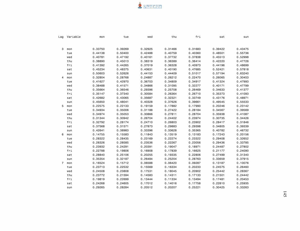
1
45
Lag Variable mon tue wed thu fri sat sun
3 mon 0.33750 0.39269 0.32925 0.31466 0.31683 0.39422 0.43475
tue 0.44138 0.50400 0.42488 0.40759 0.40360 0.48501 0.55736
wed 0.40781 0.47192 0.40161 0.37732 0.37838 0.45513 0.52998
thu 0.38890 0.45013 0.38319 0.36389 0.36414 0.42220 0.47726
fri 0.41392 0.44265 0.37019 0.36328 0.40973 0.44196 0.48699
sat 0.45234 0.48375 0.40631 0.40190 0.47685 0.52421 0.57818
sun 0.50603 0.52626 0.44153 0.44409 0.51017 0.57194 0.63240
4 mon 0.32804 0.28768 0.24887 0.26212 0.22470 0.26065 0.30453
tue 0.41627 0.42970 0.36703 0.34809 0.34917 0.41324 0.47993
wed 0.38488 0.41571 0.34866 0.31095 0.32277 0.40171 0.47799
thu 0.35664 0.36546 0.29396 0.25708 0.26469 0.34633 0.41377
fri 0.35147 0.37340 0.30584 0.26364 0.26710 0.35373 0.41093
sat 0.42682 0.43065 0.35687 0.32321 0.33749 0.43176 0.48971
sun 0.45650 0.48041 0.40328 0.37626 0.39661 0.49545 0.55533
5 mon 0.22575 0.22133 0.19159 0.17882 0.17990 0.20246 0.23142
tue 0.34934 0.35006 0.31188 0.27422 0.28184 0.34567 0.39569
wed 0.34974 0.35053 0.30866 0.27811 0.28704 0.35938 0.41087
thu 0.31344 0.30942 0.26704 0.24402 0.23974 0.30735 0.34426
fri 0.32792 0.28174 0.24710 0.26803 0.23902 0.28417 0.31846
sat 0.37568 0.31571 0.27873 0.29883 0.29398 0.34805 0.39339
sun 0.42641 0.38983 0.33396 0.33628 0.35365 0.40782 0.46732
6 mon 0.14755 0.15583 0.11843 0.13519 0.13183 0.17243 0.20156
tue 0.28322 0.28435 0.23169 0.22274 0.23322 0.29408 0.32652
wed 0.28326 0.28585 0.23536 0.22267 0.23056 0.29436 0.33785
thu 0.23932 0.24291 0.20391 0.19047 0.18971 0.24487 0.27802
fri 0.22788 0.19806 0.16908 0.17839 0.16625 0.21177 0.24090
sat 0.28840 0.25106 0.20255 0.19335 0.22806 0.27499 0.31340
sun 0.35354 0.32187 0.26484 0.25204 0.28763 0.33659 0.37915
7 mon 0.16524 0.15712 0.06588 0.06420 0.09287 0.13187 0.10076
tue 0.23713 0.22532 0.15569 0.16334 0.20233 0.24575 0.26460
wed 0.24508 0.23808 0.17531 0.18045 0.20902 0.25442 0.28367
thu 0.23772 0.21594 0.14583 0.14311 0.17133 0.21501 0.24442
fri 0.19819 0.22699 0.13444 0.11334 0.13494 0.17481 0.20453
sat 0.24268 0.24605 0.17012 0.14016 0.17758 0.22810 0.25935
sun 0.29265 0.28284 0.20512 0.20207 0.25221 0.30425 0.33263
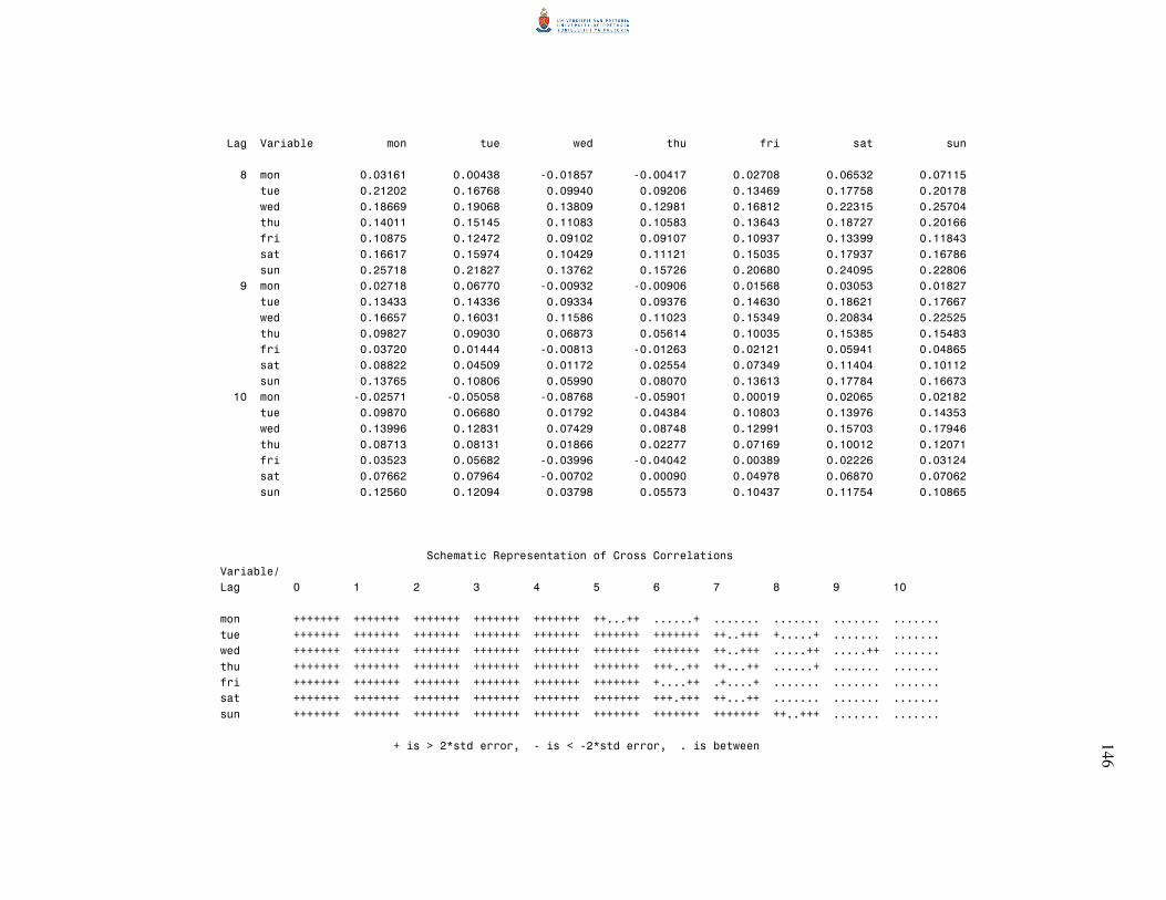
1
46
Lag Variable mon tue wed thu fri sat sun
8 mon 0.03161 0.00438 -0.01857 -0.00417 0.02708 0.06532 0.07115
tue 0.21202 0.16768 0.09940 0.09206 0.13469 0.17758 0.20178
wed 0.18669 0.19068 0.13809 0.12981 0.16812 0.22315 0.25704
thu 0.14011 0.15145 0.11083 0.10583 0.13643 0.18727 0.20166
fri 0.10875 0.12472 0.09102 0.09107 0.10937 0.13399 0.11843
sat 0.16617 0.15974 0.10429 0.11121 0.15035 0.17937 0.16786
sun 0.25718 0.21827 0.13762 0.15726 0.20680 0.24095 0.22806
9 mon 0.02718 0.06770 -0.00932 -0.00906 0.01568 0.03053 0.01827
tue 0.13433 0.14336 0.09334 0.09376 0.14630 0.18621 0.17667
wed 0.16657 0.16031 0.11586 0.11023 0.15349 0.20834 0.22525
thu 0.09827 0.09030 0.06873 0.05614 0.10035 0.15385 0.15483
fri 0.03720 0.01444 -0.00813 -0.01263 0.02121 0.05941 0.04865
sat 0.08822 0.04509 0.01172 0.02554 0.07349 0.11404 0.10112
sun 0.13765 0.10806 0.05990 0.08070 0.13613 0.17784 0.16673
10 mon -0.02571 -0.05058 -0.08768 -0.05901 0.00019 0.02065 0.02182
tue 0.09870 0.06680 0.01792 0.04384 0.10803 0.13976 0.14353
wed 0.13996 0.12831 0.07429 0.08748 0.12991 0.15703 0.17946
thu 0.08713 0.08131 0.01866 0.02277 0.07169 0.10012 0.12071
fri 0.03523 0.05682 -0.03996 -0.04042 0.00389 0.02226 0.03124
sat 0.07662 0.07964 -0.00702 0.00090 0.04978 0.06870 0.07062
sun 0.12560 0.12094 0.03798 0.05573 0.10437 0.11754 0.10865
Schematic Representation of Cross Correlations
Variable/
Lag 0 1 2 3 4 5 6 7 8 9 10
mon +++++++ +++++++ +++++++ +++++++ +++++++ ++...++ ......+ ....... ....... ....... .......
tue +++++++ +++++++ +++++++ +++++++ +++++++ +++++++ +++++++ ++..+++ +.....+ ....... .......
wed +++++++ +++++++ +++++++ +++++++ +++++++ +++++++ +++++++ ++..+++ .....++ .....++ .......
thu +++++++ +++++++ +++++++ +++++++ +++++++ +++++++ +++..++ ++...++ ......+ ....... .......
fri +++++++ +++++++ +++++++ +++++++ +++++++ +++++++ +....++ .+....+ ....... ....... .......
sat +++++++ +++++++ +++++++ +++++++ +++++++ +++++++ +++.+++ ++...++ ....... ....... .......
sun +++++++ +++++++ +++++++ +++++++ +++++++ +++++++ +++++++ +++++++ ++..+++ ....... .......
+ is > 2*std error, - is < -2*std error, . is between

1
47
Minimum Information Criterion
Lag MA 0 MA 1 MA 2 MA 3 MA 4
AR 0 129.79648 130.26498 130.92364 132.02659 133.24856
AR 1 128.1816 129.24413 130.16247 131.50464 133.17751
AR 2 128.79886 130.0952 131.28796 132.95227 134.95407
AR 3 129.83109 131.33926 132.87816 135.21806 137.65251
AR 4 131.10309 132.84838 134.71381 137.508 141.46216
Partial Autoregression
Lag Variable mon tue wed thu fri sat sun
1 mon -0.10753 0.08080 -0.05934 -0.16000 0.45173 -0.54001 1.37564
tue -0.11389 0.21218 0.00155 0.11995 0.10195 -0.53210 1.15920
wed -0.19207 0.50110 0.04507 0.16910 -0.05629 -0.30361 0.85653
thu -0.31894 0.90499 -0.40180 0.30207 0.12298 -0.51533 0.94936
fri -0.29639 0.98006 -0.39578 0.05358 0.31608 -0.75560 1.11308
sat -0.16408 0.67432 -0.28248 0.00872 0.10760 -0.39019 0.92102
sun -0.09849 0.38089 -0.12700 0.07419 -0.08001 -0.26029 0.93311
2 mon 0.05479 0.08251 -0.02623 -0.11404 0.35050 -0.01985 -0.67117
tue -0.08260 0.21581 -0.13648 0.09565 -0.01104 0.23372 -0.50699
wed -0.05670 0.14571 -0.20820 0.06684 -0.04960 0.19526 -0.51856
thu -0.09037 0.48166 -0.18845 -0.10186 0.01738 0.32495 -0.79887
fri 0.11873 0.21018 -0.12289 -0.08504 -0.04093 -0.06811 0.05445
sat 0.03223 0.13313 -0.04586 0.00396 -0.10499 -0.05986 0.18888
sun -0.02007 0.08020 -0.01430 -0.00442 -0.04071 -0.06360 0.29144
3 mon -0.04477 0.07579 -0.03870 -0.20730 0.16346 0.01153 -0.13257
tue 0.05116 0.01217 0.08504 -0.18405 0.03232 0.03058 0.12769
wed 0.09786 -0.07628 0.15653 -0.20074 0.02343 -0.04745 0.22477
thu 0.09393 -0.09418 -0.00570 -0.19112 0.01330 -0.14839 0.51227
fri 0.08571 -0.11893 -0.03639 -0.39235 -0.11844 0.64777 0.16452
sat 0.10965 -0.08202 0.04925 -0.30923 -0.22624 0.55183 0.22602
sun 0.07410 -0.04869 0.16159 -0.32722 -0.19005 0.47248 0.24553
4 mon -0.04533 0.16164 -0.23133 0.36552 -0.18083 0.11486 -0.30280
tue -0.13758 0.02836 0.02727 -0.00949 0.20779 -0.42978 0.19521
wed -0.12483 0.06871 0.01210 -0.12426 0.19435 -0.30296 0.07383
thu 0.00674 0.10279 -0.01796 -0.16578 0.02365 -0.11752 -0.12860
fri -0.14988 0.08864 0.11708 0.01981 -0.21326 -0.12762 -0.03367
sat -0.17459 -0.00329 0.10495 0.03653 -0.07727 -0.21189 0.20493
sun -0.18748 0.00768 0.12055 -0.01055 0.04020 -0.20461 0.12423

1
48
Lag Variable mon tue wed thu fri sat sun
5 mon 0.10721 -0.02117 -0.05178 -0.06550 0.11983 -0.12847 0.17597
tue -0.00293 -0.04184 -0.06846 0.06300 0.27266 -0.80512 0.58823
wed -0.01613 0.14084 -0.14557 0.12873 0.12642 -0.44738 0.15222
thu 0.02965 0.00554 -0.13020 -0.14154 0.23077 -0.00570 -0.17489
fri 0.00537 -0.04949 -0.19129 -0.09901 0.00308 0.09692 0.27832
sat -0.06038 -0.02404 -0.04140 -0.06304 -0.05189 0.15360 0.08876
sun -0.08118 -0.02514 0.05007 -0.12716 -0.00900 -0.01820 0.31045
6 mon -0.01384 0.04260 -0.17987 0.14698 0.12905 -0.26112 0.11032
tue -0.01777 0.18962 -0.21482 0.19184 -0.06256 -0.01139 -0.18662
wed -0.02230 0.20776 -0.26567 0.11663 -0.01165 0.06466 -0.33172
thu 0.06215 0.25412 -0.27552 0.24561 0.15206 -0.26576 -0.64238
fri -0.01420 0.26701 -0.24279 0.27360 -0.30776 0.52550 -0.77587
sat -0.05655 0.18603 -0.13783 0.12871 -0.08970 0.26138 -0.43535
sun -0.02874 0.01232 -0.05275 0.06785 -0.01856 0.14785 -0.21496
7 mon 0.03548 -0.02892 -0.18302 0.20178 0.22287 -0.34906 0.14331
tue 0.09912 -0.05539 -0.06851 -0.26773 0.62207 -0.51171 0.20338
wed 0.01896 -0.07679 -0.02456 -0.16488 0.09318 0.14910 -0.07187
thu -0.08513 0.06297 -0.10277 -0.17071 0.27247 -0.39171 0.29107
fri -0.10632 0.14604 -0.14334 -0.18573 0.40791 -0.78656 0.66632
sat -0.02742 0.04311 -0.11682 -0.04173 0.22054 -0.63129 0.59166
sun -0.17401 0.14229 -0.10883 0.03079 0.16739 -0.49094 0.38788
8 mon -0.14748 0.42232 0.02503 -0.19122 -0.15441 0.01812 0.07140
tue 0.00210 -0.04385 0.04079 0.18680 -0.38168 0.25976 -0.22087
wed -0.03166 -0.16601 0.10992 0.23095 -0.26537 0.13102 -0.39362
thu 0.12225 -0.37397 0.05117 0.28252 -0.60444 0.47977 -0.14368
fri 0.04778 -0.20065 -0.11406 0.40073 -0.94446 0.80901 -0.13886
sat 0.03537 -0.27587 0.00735 0.39532 -0.82827 0.69545 -0.18314
sun 0.05096 -0.22501 0.09367 0.32206 -0.58962 0.45178 -0.19822
9 mon -0.05485 0.21714 -0.08481 -0.41050 0.38555 -0.24030 0.06835
tue 0.00501 0.22327 -0.11244 -0.18069 0.18297 -0.26877 0.08115
wed -0.10969 0.44468 -0.26248 0.00967 0.15502 -0.34556 0.04348
thu -0.13920 0.51652 -0.16673 0.00007 -0.22492 0.02240 -0.07740
fri -0.11650 0.44993 -0.18906 0.00582 -0.25750 -0.12808 0.22466
sat -0.15749 0.26486 -0.11182 0.25444 -0.32662 -0.11506 0.18842
sun -0.08814 0.02199 0.00770 0.16319 -0.20552 -0.22333 0.24303
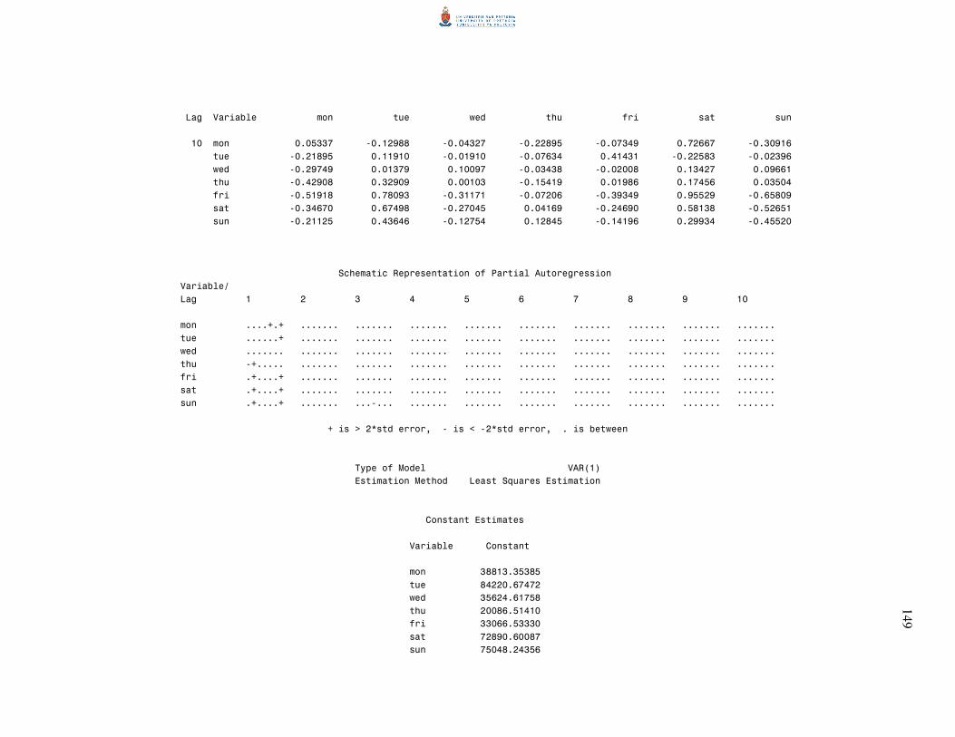
1
49
Lag Variable mon tue wed thu fri sat sun
10 mon 0.05337 -0.12988 -0.04327 -0.22895 -0.07349 0.72667 -0.30916
tue -0.21895 0.11910 -0.01910 -0.07634 0.41431 -0.22583 -0.02396
wed -0.29749 0.01379 0.10097 -0.03438 -0.02008 0.13427 0.09661
thu -0.42908 0.32909 0.00103 -0.15419 0.01986 0.17456 0.03504
fri -0.51918 0.78093 -0.31171 -0.07206 -0.39349 0.95529 -0.65809
sat -0.34670 0.67498 -0.27045 0.04169 -0.24690 0.58138 -0.52651
sun -0.21125 0.43646 -0.12754 0.12845 -0.14196 0.29934 -0.45520
Schematic Representation of Partial Autoregression
Variable/
Lag 1 2 3 4 5 6 7 8 9 10
mon ....+.+ ....... ....... ....... ....... ....... ....... ....... ....... .......
tue ......+ ....... ....... ....... ....... ....... ....... ....... ....... .......
wed ....... ....... ....... ....... ....... ....... ....... ....... ....... .......
thu -+..... ....... ....... ....... ....... ....... ....... ....... ....... .......
fri .+....+ ....... ....... ....... ....... ....... ....... ....... ....... .......
sat .+....+ ....... ....... ....... ....... ....... ....... ....... ....... .......
sun .+....+ ....... ...-... ....... ....... ....... ....... ....... ....... .......
+ is > 2*std error, - is < -2*std error, . is between
Type of Model VAR(1)
Estimation Method Least Squares Estimation
Constant Estimates
Variable Constant
mon 38813.35385
tue 84220.67472
wed 35624.61758
thu 20086.51410
fri 33066.53330
sat 72890.60087
sun 75048.24356
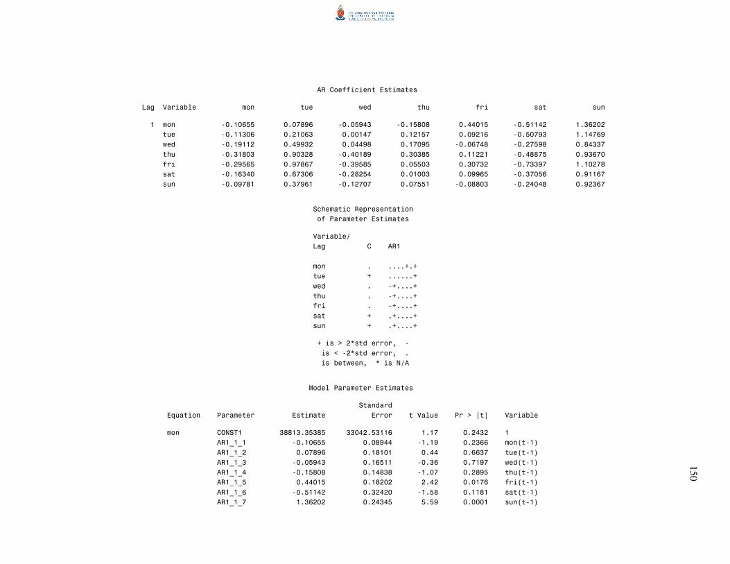
1
50
AR Coefficient Estimates
Lag Variable mon tue wed thu fri sat sun
1 mon -0.10655 0.07896 -0.05943 -0.15808 0.44015 -0.51142 1.36202
tue -0.11306 0.21063 0.00147 0.12157 0.09216 -0.50793 1.14769
wed -0.19112 0.49932 0.04498 0.17095 -0.06748 -0.27598 0.84337
thu -0.31803 0.90328 -0.40189 0.30385 0.11221 -0.48875 0.93670
fri -0.29565 0.97867 -0.39585 0.05503 0.30732 -0.73397 1.10278
sat -0.16340 0.67306 -0.28254 0.01003 0.09965 -0.37056 0.91167
sun -0.09781 0.37961 -0.12707 0.07551 -0.08803 -0.24048 0.92367
Schematic Representation
of Parameter Estimates
Variable/
Lag C AR1
mon . ....+.+
tue + ......+
wed . -+....+
thu . -+....+
fri . -+....+
sat + .+....+
sun + .+....+
+ is > 2*std error, -
is < -2*std error, .
is between, * is N/A
Model Parameter Estimates
Standard
Equation Parameter Estimate Error t Value Pr > |t| Variable
mon CONST1 38813.35385 33042.53116 1.17 0.2432 1
AR1_1_1 -0.10655 0.08944 -1.19 0.2366 mon(t-1)
AR1_1_2 0.07896 0.18101 0.44 0.6637 tue(t-1)
AR1_1_3 -0.05943 0.16511 -0.36 0.7197 wed(t-1)
AR1_1_4 -0.15808 0.14838 -1.07 0.2895 thu(t-1)
AR1_1_5 0.44015 0.18202 2.42 0.0176 fri(t-1)
AR1_1_6 -0.51142 0.32420 -1.58 0.1181 sat(t-1)
AR1_1_7 1.36202 0.24345 5.59 0.0001 sun(t-1)

1
51
Standard
Equation Parameter Estimate Error t Value Pr > |t| Variable
tue CONST2 84220.67472 28057.38223 3.00 0.0035 1
AR1_2_1 -0.11306 0.07595 -1.49 0.1400 mon(t-1)
AR1_2_2 0.21063 0.15370 1.37 0.1739 tue(t-1)
AR1_2_3 0.00147 0.14020 0.01 0.9917 wed(t-1)
AR1_2_4 0.12157 0.12599 0.96 0.3371 thu(t-1)
AR1_2_5 0.09216 0.15456 0.60 0.5525 fri(t-1)
AR1_2_6 -0.50793 0.27529 -1.85 0.0682 sat(t-1)
AR1_2_7 1.14769 0.20672 5.55 0.0001 sun(t-1)
wed CONST3 35624.61758 29893.70433 1.19 0.2364 1
AR1_3_1 -0.19112 0.08092 -2.36 0.0203 mon(t-1)
AR1_3_2 0.49932 0.16376 3.05 0.0030 tue(t-1)
AR1_3_3 0.04498 0.14937 0.30 0.7640 wed(t-1)
AR1_3_4 0.17095 0.13424 1.27 0.2061 thu(t-1)
AR1_3_5 -0.06748 0.16468 -0.41 0.6829 fri(t-1)
AR1_3_6 -0.27598 0.29331 -0.94 0.3492 sat(t-1)
AR1_3_7 0.84337 0.22025 3.83 0.0002 sun(t-1)
thu CONST4 20086.51410 41434.19250 0.48 0.6290 1
AR1_4_1 -0.31803 0.11216 -2.84 0.0056 mon(t-1)
AR1_4_2 0.90328 0.22698 3.98 0.0001 tue(t-1)
AR1_4_3 -0.40189 0.20704 -1.94 0.0553 wed(t-1)
AR1_4_4 0.30385 0.18606 1.63 0.1059 thu(t-1)
AR1_4_5 0.11221 0.22825 0.49 0.6242 fri(t-1)
AR1_4_6 -0.48875 0.40654 -1.20 0.2324 sat(t-1)
AR1_4_7 0.93670 0.30528 3.07 0.0028 sun(t-1)
fri CONST5 33066.53330 50914.32299 0.65 0.5177 1
AR1_5_1 -0.29565 0.13782 -2.15 0.0346 mon(t-1)
AR1_5_2 0.97867 0.27892 3.51 0.0007 tue(t-1)
AR1_5_3 -0.39585 0.25441 -1.56 0.1232 wed(t-1)
AR1_5_4 0.05503 0.22863 0.24 0.8103 thu(t-1)
AR1_5_5 0.30732 0.28048 1.10 0.2761 fri(t-1)
AR1_5_6 -0.73397 0.49956 -1.47 0.1452 sat(t-1)
AR1_5_7 1.10278 0.37513 2.94 0.0042 sun(t-1)
sat CONST6 72890.60087 35688.45966 2.04 0.0440 1
AR1_6_1 -0.16340 0.09661 -1.69 0.0941 mon(t-1)
AR1_6_2 0.67306 0.19551 3.44 0.0009 tue(t-1)
AR1_6_3 -0.28254 0.17833 -1.58 0.1165 wed(t-1)
AR1_6_4 0.01003 0.16026 0.06 0.9502 thu(t-1)
AR1_6_5 0.09965 0.19660 0.51 0.6135 fri(t-1)
AR1_6_6 -0.37056 0.35016 -1.06 0.2927 sat(t-1)
AR1_6_7 0.91167 0.26294 3.47 0.0008 sun(t-1)
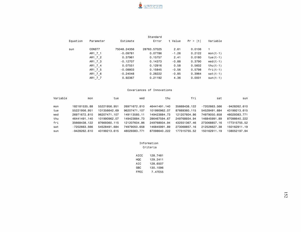
1
52
Standard
Equation Parameter Estimate Error t Value Pr > |t| Variable
sun CONST7 75048.24356 28763.57025 2.61 0.0106 1
AR1_7_1 -0.09781 0.07786 -1.26 0.2122 mon(t-1)
AR1_7_2 0.37961 0.15757 2.41 0.0180 tue(t-1)
AR1_7_3 -0.12707 0.14373 -0.88 0.3790 wed(t-1)
AR1_7_4 0.07551 0.12916 0.58 0.5602 thu(t-1)
AR1_7_5 -0.08803 0.15845 -0.56 0.5798 fri(t-1)
AR1_7_6 -0.24048 0.28222 -0.85 0.3964 sat(t-1)
AR1_7_7 0.92367 0.21192 4.36 0.0001 sun(t-1)
Covariances of Innovations
Variable mon tue wed thu fri sat sun
mon 182181535.88 55221956.951 26971672.810 46441491.140 35668438.122 -7202663.566 -9428262.610
tue 55221956.951 131356642.69 96207471.107 101990962.07 87669360.115 54528491.684 43199213.615
wed 26971672.810 96207471.107 149113585.11 149423884.73 121207604.86 74979050.658 48029383.771
thu 46441491.140 101990962.07 149423884.73 286467594.67 249768934.94 146845991.89 87098640.222
fri 35668438.122 87669360.115 121207604.86 249768934.94 432551367.46 273068857.16 177315755.52
sat -7202663.566 54528491.684 74979050.658 146845991.89 273068857.16 212526627.38 150162911.19
sun -9428262.610 43199213.615 48029383.771 87098640.222 177315755.52 150162911.19 138052197.94
Information
Criteria
AICC 128.7481
HQC 129.2411
AIC 128.6507
SBC 130.1096
FPEC 7.47E55
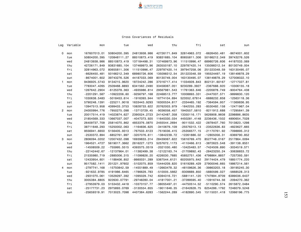
1
53
Cross Covariances of Residuals
Lag Variable mon tue wed thu fri sat sun
0 mon 167607013.01 50804200.395 24813938.986 42726171.849 32814963.072 -6626450.481 -8674001.602
tue 50804200.395 120848111.27 88510873.419 93831685.104 80655811.306 50166212.349 39743276.526
wed 24813938.986 88510873.419 137184498.31 137469973.96 111510996.47 68980726.606 44187033.069
thu 42726171.849 93831685.104 137469973.96 263550187.10 229787420.14 135098312.54 80130749.004
fri 32814963.072 80655811.306 111510996.47 229787420.14 397947258.06 251223348.59 163130495.07
sat -6626450.481 50166212.349 68980726.606 135098312.54 251223348.59 195524497.19 138149878.29
sun -8674001.602 39743276.526 44187033.069 80130749.004 163130495.07 138149878.29 127008022.10
1 mon 9436925.5743 9134215.9620 18724242.286 37016717.414 11034928.843 802131.60167 -12717027.81
tue 7783047.4265 2509468.8893 6341562.2490 33458067.051 9230289.3927 -2367688.920 -10306155.18
wed 1267642.2904 -6125378.363 -4935986.814 29567981.543 11761363.646 -2205878.749 -9004764.438
thu -2201291.587 -10922206.60 -9256797.168 22468513.777 10008893.331 -2447007.571 -9899830.120
fri 1030638.5483 -5018453.614 -1916393.944 16774104.694 523552.67814 -6888232.858 -12563118.36
sat 5790248.1391 -225211.9018 1633443.9293 16300534.817 -2334465.192 -7364594.957 -11369836.95
sun 13947513.958 4399433.3753 10828733.622 20762003.979 -1842255.283 -8530492.158 -12471967.04
2 mon 24000994.776 -7950275.098 -13713729.45 -9036058.457 1940557.5810 -8211912.688 -17295641.39
tue 20017514.419 14023874.627 2390024.2723 24142487.358 13350116.171 5626908.9608 2298886.8635
wed 21854569.333 13667037.007 -4047373.920 11640330.034 4450281.4148 2236436.1502 4890654.7028
thu 26409737.709 25814070.862 4853376.0870 2455544.2694 -9011532.422 -2878407.760 7013823.1298
fri 38711648.293 15250002.063 -1164836.625 -3410679.109 -25576313.13 -23522636.83 -4823627.665
sat 9556941.6650 5156405.9313 -767533.6123 -7519036.415 -25356577.15 -21170761.92 -7098895.312
sun -2530372.894 -6852761.997 -3207076.611 -13842239.72 -12261886.02 -12805056.31 -6369790.852
3 mon 2806094.0202 12007432.098 16939833.314 28439067.622 15616769.470 8527748.0167 2517864.0094
tue 1964521.4727 5619017.3662 2816227.1273 5257672.1173 -4110466.613 -3872623.548 -391138.8551
wed -14508509.22 -755995.5515 4393575.0519 -2021030.480 -10425483.57 -7424509.890 -3034519.571
thu -22142442.67 -12137964.01 -11382499.38 -12122163.74 -21709892.43 -28423250.24 -30638853.72
fri 21535980.719 -2885006.315 -11099826.20 4226030.7685 45852751.436 4798864.8857 -7257393.591
sat 12433954.601 -1188406.852 -8660031.289 5367544.6121 60205975.642 29174424.479 18851774.220
sun 9517582.1411 201221.97602 -5102075.859 15444209.820 51619289.429 27900046.665 19867214.561
4 mon -2797741.168 -15750842.59 -14551889.49 -12663478.32 -48109626.36 -39863203.18 -39195245.30
tue -921632.9785 4191986.6465 -1786629.783 -510005.5662 -8309889.850 -5880599.027 -5668528.313
wed -2931070.061 13529297.392 -1095029.742 -6394316.721 -5881141.120 1747894.8709 6389036.6437
thu 3005384.8805 922630.07791 -29748280.04 -41817001.21 -37289595.40 -10916744.56 -2094270.362
fri -27953979.03 5153432.4418 -10373157.77 -38055497.01 -44750514.52 -5110290.574 2615872.0484
sat -25177731.23 2975893.0769 -3130554.655 -19011646.35 -21642628.75 6254286.1792 7246079.5248
sun -25659319.91 7013023.7098 4407384.6283 -1562244.289 -4182890.545 15115031.418 12066196.775
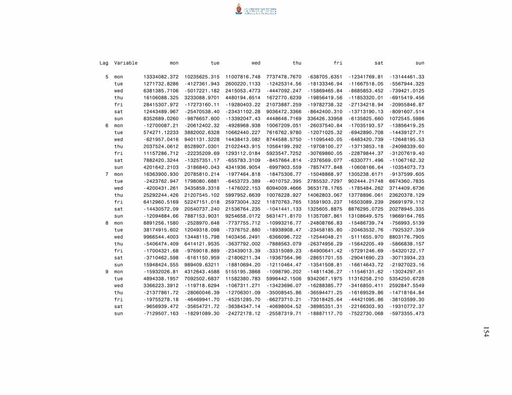
1
54
Lag Variable mon tue wed thu fri sat sun
5 mon 13334082.372 10235625.315 11007816.748 7737478.7670 -638705.6351 -12341769.81 -13144461.33
tue 1271732.8286 -4127361.943 2600220.1133 -12425314.56 -18133346.94 -11667518.05 -5567944.325
wed 6381385.7106 -5017221.182 2415053.4773 -4447092.247 -15869465.84 -8685853.452 -739421.0125
thu 16106088.325 3233088.9701 4480194.6514 1672770.6239 -19856419.56 -11853320.01 -6915419.456
fri 28415307.972 -17273160.11 -19280403.22 21073887.259 -19782738.32 -27134218.94 -20955846.87
sat 12443489.967 -25470538.40 -23431102.28 9036472.3366 -8642400.310 -13713190.13 -8091607.514
sun 8352689.0260 -9876657.600 -13392047.43 4448648.7169 336426.33958 -6135825.660 1072545.5986
6 mon -12700087.21 -20612402.32 -4928968.938 10067209.051 -26037540.84 -17035193.57 -13856419.25
tue 574271.12233 3882002.6328 10662440.227 7616762.9780 -12071025.32 -6942890.708 -14439127.71
wed -621957.0416 9401131.3228 14438413.082 8744588.5750 -11095440.05 -6483420.739 -12648195.53
thu 2037524.0612 8528907.0301 21022443.915 10564199.292 -19708100.27 -13713853.18 -24098339.60
fri 11157286.712 -22235209.69 1293112.0184 5923547.7252 -30769860.05 -22879844.37 -31207619.40
sat 7882420.3244 -13257351.17 -655783.3109 -8457664.814 -2376569.077 -6330771.496 -11067162.32
sun 4201642.2103 -3186840.043 4341936.9054 -6997903.559 -7857477.848 -10608166.64 -10354073.73
7 mon 16363900.930 20785810.214 -1977464.818 -18475306.77 -15048868.97 1305238.6171 -9137599.605
tue -2423762.947 1798080.6881 -6453723.389 -4010752.395 2785532.7297 902444.21748 6674360.7835
wed -4200431.261 3435859.3318 -1476022.153 6094009.4666 3653178.1765 -1785484.262 3714409.6736
thu 25292244.426 21207545.102 5997952.6639 10076228.927 14062803.067 13778896.061 23620378.129
fri 6412960.5169 52247151.018 25973004.322 11870763.765 13591903.237 16503089.239 26691979.112
sat -14430572.09 20540737.240 21536764.235 -1041441.133 1325605.8875 8876295.0725 20278945.335
sun -12094884.66 7887153.9031 9254658.0172 5631471.8170 11357087.861 13108649.575 19669164.765
8 mon 8891256.1580 -2528970.648 -7737755.712 -10993216.77 -24808766.83 -15486739.74 -756993.5139
tue 38174915.602 12049318.098 -7376752.880 -18938908.47 -23458185.80 -20463532.76 -7925327.359
wed 9966544.4003 13448115.798 1403456.2491 -6366096.722 -12544048.21 -5111655.970 8803176.7905
thu -5406474.409 6414121.9535 -3637792.002 -7888563.079 -26374956.29 -15642205.49 -5866838.157
fri -17004321.68 -9769018.889 -23439013.39 -33315089.23 -64900641.42 -57291246.69 -54320122.17
sat -3710462.598 -6161150.959 -21806211.34 -19367564.96 -28651701.55 -29041690.23 -30713934.23
sun 15948424.555 989409.63211 -18810694.20 -12110464.47 -13541508.81 -16614643.72 -21927023.16
9 mon -15932026.81 4312643.4588 5155195.3868 -1098790.202 -14811436.27 -11546131.62 -13024297.61
tue 4894338.1957 7092502.6837 11582380.783 5996442.1506 9342067.1975 11316258.210 5354250.6728
wed 3366223.3912 -119718.6294 -1067311.271 -13423696.07 -16288385.77 -3416850.411 2592847.5549
thu -21377861.72 -28060046.39 -12706301.09 -35008545.86 -36594471.25 -16169529.86 -14718164.84
fri -19755278.18 -46469941.70 -45251285.70 -66273710.21 -73018425.64 -44421095.86 -38103599.30
sat -9656939.472 -35654721.72 -36384347.14 -40698004.52 -38985351.31 -22166303.93 -19310772.37
sun -7129507.163 -18291089.30 -24272178.12 -25587319.71 -18887117.70 -7522730.068 -5973355.473
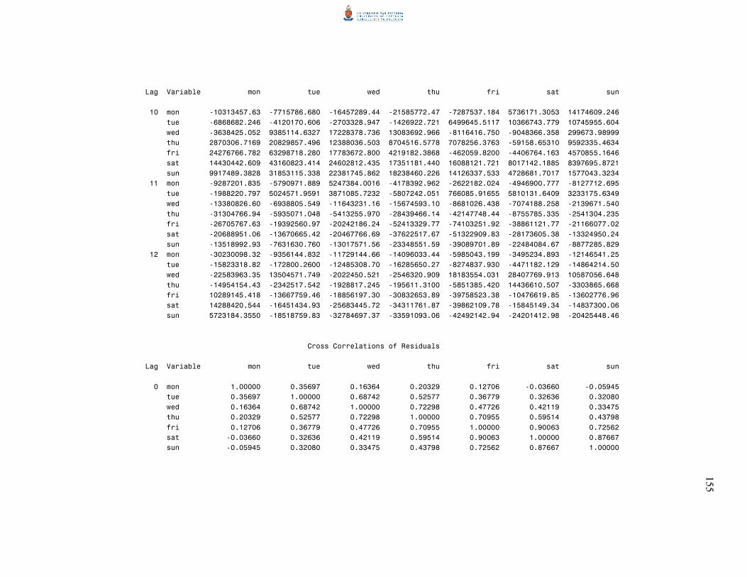
1
55
Lag Variable mon tue wed thu fri sat sun
10 mon -10313457.63 -7715786.680 -16457289.44 -21585772.47 -7287537.184 5736171.3053 14174609.246
tue -6868682.246 -4120170.606 -2703328.947 -1426922.721 6499645.5117 10366743.779 10745955.604
wed -3638425.052 9385114.6327 17228378.736 13083692.966 -8116416.750 -9048366.358 299673.98999
thu 2870306.7169 20829857.496 12388036.503 8704516.5778 7078256.3763 -59158.65310 9592335.4634
fri 24276766.782 63298718.280 17783672.800 4219182.3868 -462059.8200 -4406764.163 4570855.1646
sat 14430442.609 43160823.414 24602812.435 17351181.440 16088121.721 8017142.1885 8397695.8721
sun 9917489.3828 31853115.338 22381745.862 18238460.226 14126337.533 4728681.7017 1577043.3234
11 mon -9287201.835 -5790971.889 5247384.0016 -4178392.962 -2622182.024 -4946900.777 -8127712.695
tue -1988220.797 5024571.9591 3871085.7232 -5807242.051 766085.91655 5810131.6409 3233175.6349
wed -13380826.60 -6938805.549 -11643231.16 -15674593.10 -8681026.438 -7074188.258 -2139671.540
thu -31304766.94 -5935071.048 -5413255.970 -28439466.14 -42147748.44 -8755785.335 -2541304.235
fri -26705767.63 -19392560.97 -20242186.24 -52413329.77 -74103251.92 -38861121.77 -21166077.02
sat -20688951.06 -13670665.42 -20467766.69 -37622517.67 -51322909.83 -28173605.38 -13324950.24
sun -13518992.93 -7631630.760 -13017571.56 -23348551.59 -39089701.89 -22484084.67 -8877285.829
12 mon -30230098.32 -9356144.832 -11729144.66 -14096033.44 -5985043.199 -3495234.893 -12146541.25
tue -15823318.82 -172800.2600 -12485308.70 -16285650.27 -8274837.930 -4471182.129 -14864214.50
wed -22583963.35 13504571.749 -2022450.521 -2546320.909 18183554.031 28407769.913 10587056.648
thu -14954154.43 -2342517.542 -1928817.245 -195611.3100 -5851385.420 14436610.507 -3303865.668
fri 10289145.418 -13667759.46 -18856197.30 -30832653.89 -39758523.38 -10476619.85 -13602776.96
sat 14288420.544 -16451434.93 -25683445.72 -34311761.87 -39862109.78 -15845149.34 -14837300.06
sun 5723184.3550 -18518759.83 -32784697.37 -33591093.06 -42492142.94 -24201412.98 -20425448.46
Cross Correlations of Residuals
Lag Variable mon tue wed thu fri sat sun
0 mon 1.00000 0.35697 0.16364 0.20329 0.12706 -0.03660 -0.05945
tue 0.35697 1.00000 0.68742 0.52577 0.36779 0.32636 0.32080
wed 0.16364 0.68742 1.00000 0.72298 0.47726 0.42119 0.33475
thu 0.20329 0.52577 0.72298 1.00000 0.70955 0.59514 0.43798
fri 0.12706 0.36779 0.47726 0.70955 1.00000 0.90063 0.72562
sat -0.03660 0.32636 0.42119 0.59514 0.90063 1.00000 0.87667
sun -0.05945 0.32080 0.33475 0.43798 0.72562 0.87667 1.00000
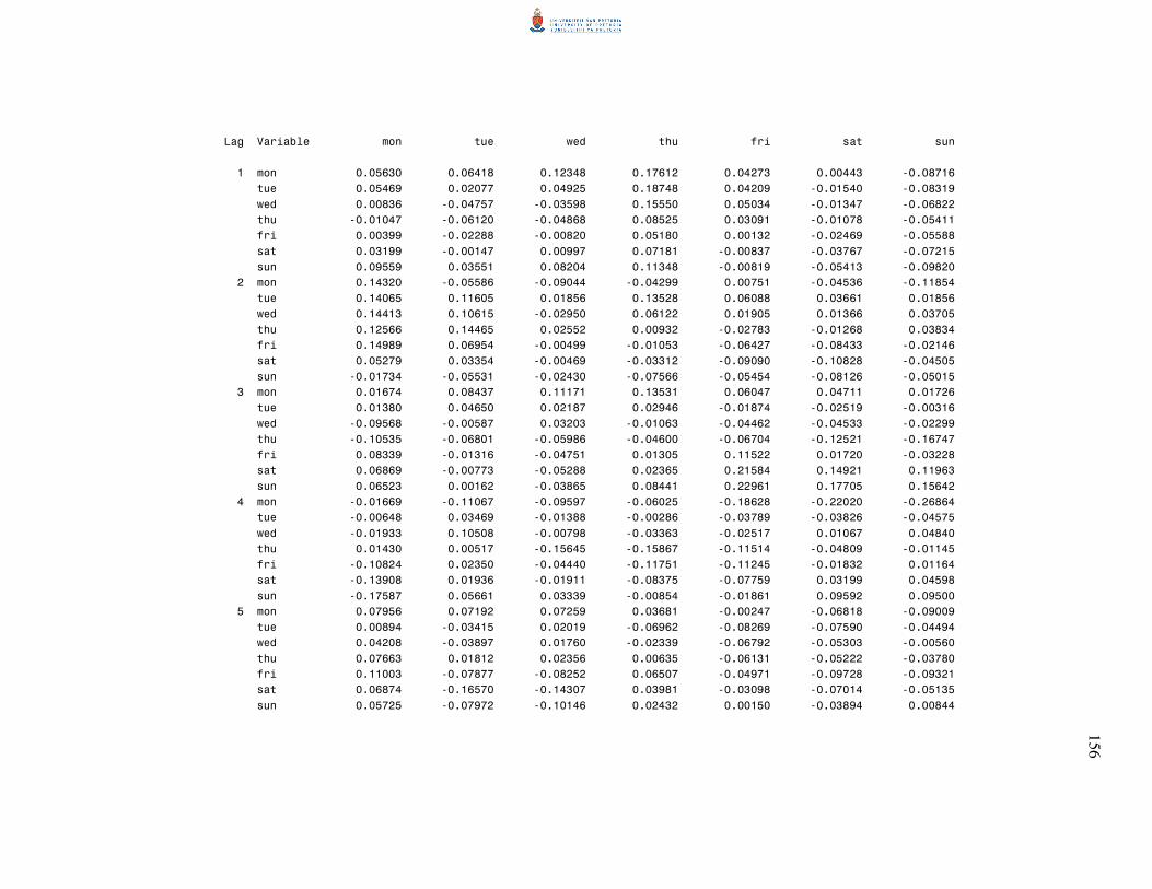
1
56
Lag Variable mon tue wed thu fri sat sun
1 mon 0.05630 0.06418 0.12348 0.17612 0.04273 0.00443 -0.08716
tue 0.05469 0.02077 0.04925 0.18748 0.04209 -0.01540 -0.08319
wed 0.00836 -0.04757 -0.03598 0.15550 0.05034 -0.01347 -0.06822
thu -0.01047 -0.06120 -0.04868 0.08525 0.03091 -0.01078 -0.05411
fri 0.00399 -0.02288 -0.00820 0.05180 0.00132 -0.02469 -0.05588
sat 0.03199 -0.00147 0.00997 0.07181 -0.00837 -0.03767 -0.07215
sun 0.09559 0.03551 0.08204 0.11348 -0.00819 -0.05413 -0.09820
2 mon 0.14320 -0.05586 -0.09044 -0.04299 0.00751 -0.04536 -0.11854
tue 0.14065 0.11605 0.01856 0.13528 0.06088 0.03661 0.01856
wed 0.14413 0.10615 -0.02950 0.06122 0.01905 0.01366 0.03705
thu 0.12566 0.14465 0.02552 0.00932 -0.02783 -0.01268 0.03834
fri 0.14989 0.06954 -0.00499 -0.01053 -0.06427 -0.08433 -0.02146
sat 0.05279 0.03354 -0.00469 -0.03312 -0.09090 -0.10828 -0.04505
sun -0.01734 -0.05531 -0.02430 -0.07566 -0.05454 -0.08126 -0.05015
3 mon 0.01674 0.08437 0.11171 0.13531 0.06047 0.04711 0.01726
tue 0.01380 0.04650 0.02187 0.02946 -0.01874 -0.02519 -0.00316
wed -0.09568 -0.00587 0.03203 -0.01063 -0.04462 -0.04533 -0.02299
thu -0.10535 -0.06801 -0.05986 -0.04600 -0.06704 -0.12521 -0.16747
fri 0.08339 -0.01316 -0.04751 0.01305 0.11522 0.01720 -0.03228
sat 0.06869 -0.00773 -0.05288 0.02365 0.21584 0.14921 0.11963
sun 0.06523 0.00162 -0.03865 0.08441 0.22961 0.17705 0.15642
4 mon -0.01669 -0.11067 -0.09597 -0.06025 -0.18628 -0.22020 -0.26864
tue -0.00648 0.03469 -0.01388 -0.00286 -0.03789 -0.03826 -0.04575
wed -0.01933 0.10508 -0.00798 -0.03363 -0.02517 0.01067 0.04840
thu 0.01430 0.00517 -0.15645 -0.15867 -0.11514 -0.04809 -0.01145
fri -0.10824 0.02350 -0.04440 -0.11751 -0.11245 -0.01832 0.01164
sat -0.13908 0.01936 -0.01911 -0.08375 -0.07759 0.03199 0.04598
sun -0.17587 0.05661 0.03339 -0.00854 -0.01861 0.09592 0.09500
5 mon 0.07956 0.07192 0.07259 0.03681 -0.00247 -0.06818 -0.09009
tue 0.00894 -0.03415 0.02019 -0.06962 -0.08269 -0.07590 -0.04494
wed 0.04208 -0.03897 0.01760 -0.02339 -0.06792 -0.05303 -0.00560
thu 0.07663 0.01812 0.02356 0.00635 -0.06131 -0.05222 -0.03780
fri 0.11003 -0.07877 -0.08252 0.06507 -0.04971 -0.09728 -0.09321
sat 0.06874 -0.16570 -0.14307 0.03981 -0.03098 -0.07014 -0.05135
sun 0.05725 -0.07972 -0.10146 0.02432 0.00150 -0.03894 0.00844

1
57
Lag Variable mon tue wed thu fri sat sun
6 mon -0.07577 -0.14483 -0.03251 0.04790 -0.10082 -0.09410 -0.09497
tue 0.00404 0.03212 0.08281 0.04268 -0.05504 -0.04517 -0.11655
wed -0.00410 0.07301 0.10525 0.04599 -0.04749 -0.03959 -0.09582
thu 0.00969 0.04779 0.11056 0.04008 -0.06086 -0.06041 -0.13172
fri 0.04320 -0.10139 0.00553 0.01829 -0.07732 -0.08202 -0.13881
sat 0.04354 -0.08625 -0.00400 -0.03726 -0.00852 -0.03238 -0.07023
sun 0.02880 -0.02572 0.03289 -0.03825 -0.03495 -0.06732 -0.08152
7 mon 0.09763 0.14605 -0.01304 -0.08791 -0.05827 0.00721 -0.06263
tue -0.01703 0.01488 -0.05012 -0.02247 0.01270 0.00587 0.05387
wed -0.02770 0.02668 -0.01076 0.03205 0.01564 -0.01090 0.02814
thu 0.12034 0.11883 0.03154 0.03823 0.04342 0.06070 0.12910
fri 0.02483 0.23825 0.11116 0.03666 0.03416 0.05916 0.11873
sat -0.07971 0.13363 0.13150 -0.00459 0.00475 0.04540 0.12869
sun -0.08290 0.06366 0.07011 0.03078 0.05052 0.08318 0.15487
8 mon 0.05305 -0.01777 -0.05103 -0.05231 -0.09606 -0.08555 -0.00519
tue 0.26823 0.09971 -0.05729 -0.10612 -0.10697 -0.13313 -0.06397
wed 0.06573 0.10445 0.01023 -0.03348 -0.05369 -0.03121 0.06669
thu -0.02572 0.03594 -0.01913 -0.02993 -0.08144 -0.06891 -0.03207
fri -0.06584 -0.04455 -0.10032 -0.10287 -0.16309 -0.20539 -0.24162
sat -0.02050 -0.04008 -0.13315 -0.08532 -0.10272 -0.14853 -0.19490
sun 0.10931 0.00799 -0.14251 -0.06619 -0.06023 -0.10543 -0.17264
9 mon -0.09506 0.03030 0.03400 -0.00523 -0.05735 -0.06378 -0.08927
tue 0.03439 0.05869 0.08996 0.03360 0.04260 0.07362 0.04322
wed 0.02220 -0.00093 -0.00778 -0.07060 -0.06971 -0.02086 0.01964
thu -0.10172 -0.15723 -0.06682 -0.13283 -0.11300 -0.07123 -0.08045
fri -0.07649 -0.21190 -0.19367 -0.20464 -0.18349 -0.15925 -0.16949
sat -0.05334 -0.23195 -0.22216 -0.17928 -0.13976 -0.11337 -0.12254
sun -0.04886 -0.14764 -0.18388 -0.13985 -0.08401 -0.04774 -0.04703
10 mon -0.06153 -0.05421 -0.10853 -0.10270 -0.02822 0.03169 0.09715
tue -0.04826 -0.03409 -0.02100 -0.00800 0.02964 0.06744 0.08674
wed -0.02399 0.07289 0.12559 0.06881 -0.03474 -0.05525 0.00227
thu 0.01366 0.11672 0.06515 0.03303 0.02186 -0.00026 0.05243
fri 0.09400 0.28864 0.07611 0.01303 -0.00116 -0.01580 0.02033
sat 0.07971 0.28078 0.15022 0.07644 0.05768 0.04100 0.05329
sun 0.06797 0.25711 0.16956 0.09969 0.06283 0.03001 0.01242
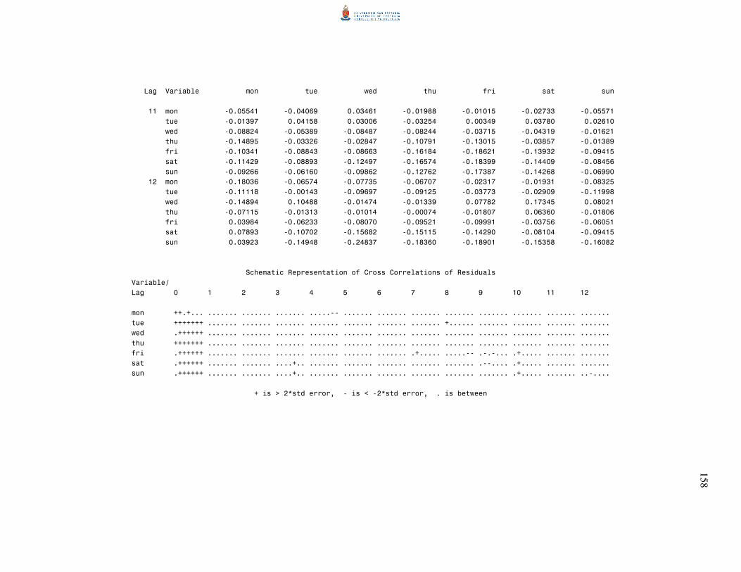
1
58
Lag Variable mon tue wed thu fri sat sun
11 mon -0.05541 -0.04069 0.03461 -0.01988 -0.01015 -0.02733 -0.05571
tue -0.01397 0.04158 0.03006 -0.03254 0.00349 0.03780 0.02610
wed -0.08824 -0.05389 -0.08487 -0.08244 -0.03715 -0.04319 -0.01621
thu -0.14895 -0.03326 -0.02847 -0.10791 -0.13015 -0.03857 -0.01389
fri -0.10341 -0.08843 -0.08663 -0.16184 -0.18621 -0.13932 -0.09415
sat -0.11429 -0.08893 -0.12497 -0.16574 -0.18399 -0.14409 -0.08456
sun -0.09266 -0.06160 -0.09862 -0.12762 -0.17387 -0.14268 -0.06990
12 mon -0.18036 -0.06574 -0.07735 -0.06707 -0.02317 -0.01931 -0.08325
tue -0.11118 -0.00143 -0.09697 -0.09125 -0.03773 -0.02909 -0.11998
wed -0.14894 0.10488 -0.01474 -0.01339 0.07782 0.17345 0.08021
thu -0.07115 -0.01313 -0.01014 -0.00074 -0.01807 0.06360 -0.01806
fri 0.03984 -0.06233 -0.08070 -0.09521 -0.09991 -0.03756 -0.06051
sat 0.07893 -0.10702 -0.15682 -0.15115 -0.14290 -0.08104 -0.09415
sun 0.03923 -0.14948 -0.24837 -0.18360 -0.18901 -0.15358 -0.16082
Schematic Representation of Cross Correlations of Residuals
Variable/
Lag 0 1 2 3 4 5 6 7 8 9 10 11 12
mon ++.+... ....... ....... ....... .....-- ....... ....... ....... ....... ....... ....... ....... .......
tue +++++++ ....... ....... ....... ....... ....... ....... ....... +...... ....... ....... ....... .......
wed .++++++ ....... ....... ....... ....... ....... ....... ....... ....... ....... ....... ....... .......
thu +++++++ ....... ....... ....... ....... ....... ....... ....... ....... ....... ....... ....... .......
fri .++++++ ....... ....... ....... ....... ....... ....... .+..... .....-- .-.-... .+..... ....... .......
sat .++++++ ....... ....... ....+.. ....... ....... ....... ....... ....... .--.... .+..... ....... .......
sun .++++++ ....... ....... ....+.. ....... ....... ....... ....... ....... ....... .+..... ....... ..-....
+ is > 2*std error, - is < -2*std error, . is between
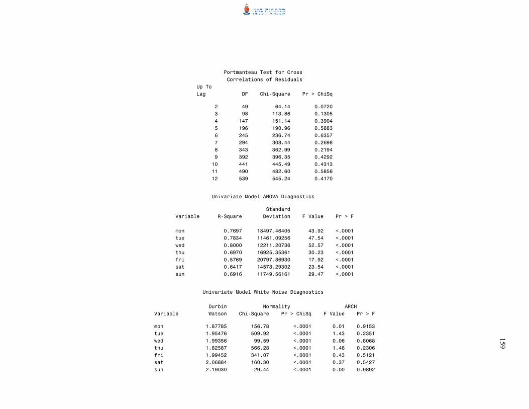
1
59
Portmanteau Test for Cross
Correlations of Residuals
Up To
Lag DF Chi-Square Pr > ChiSq
2 49 64.14 0.0720
3 98 113.86 0.1305
4 147 151.14 0.3904
5 196 190.96 0.5883
6 245 236.74 0.6357
7 294 308.44 0.2698
8 343 362.99 0.2194
9 392 396.35 0.4292
10 441 445.49 0.4313
11 490 482.60 0.5856
12 539 545.24 0.4170
Univariate Model ANOVA Diagnostics
Standard
Variable R-Square Deviation F Value Pr > F
mon 0.7697 13497.46405 43.92 <.0001
tue 0.7834 11461.09256 47.54 <.0001
wed 0.8000 12211.20736 52.57 <.0001
thu 0.6970 16925.35361 30.23 <.0001
fri 0.5769 20797.86930 17.92 <.0001
sat 0.6417 14578.29302 23.54 <.0001
sun 0.6916 11749.56161 29.47 <.0001
Univariate Model White Noise Diagnostics
Durbin Normality ARCH
Variable Watson Chi-Square Pr > ChiSq F Value Pr > F
mon 1.87785 156.78 <.0001 0.01 0.9153
tue 1.95476 509.92 <.0001 1.43 0.2351
wed 1.99356 99.59 <.0001 0.06 0.8068
thu 1.82587 566.28 <.0001 1.46 0.2306
fri 1.99452 341.07 <.0001 0.43 0.5121
sat 2.06884 160.30 <.0001 0.37 0.5427
sun 2.19030 29.44 <.0001 0.00 0.9892
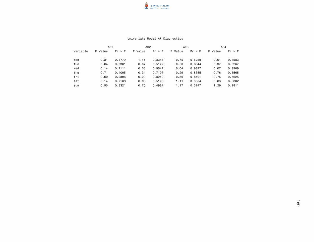
1
60
Univariate Model AR Diagnostics
AR1 AR2 AR3 AR4
Variable F Value Pr > F F Value Pr > F F Value Pr > F F Value Pr > F
mon 0.31 0.5779 1.11 0.3346 0.75 0.5259 0.61 0.6583
tue 0.04 0.8381 0.67 0.5122 0.50 0.6844 0.37 0.8267
wed 0.14 0.7111 0.05 0.9542 0.04 0.9897 0.07 0.9909
thu 0.71 0.4005 0.34 0.7107 0.29 0.8355 0.76 0.5565
fri 0.00 0.9896 0.20 0.8210 0.56 0.6401 0.75 0.5625
sat 0.14 0.7106 0.66 0.5195 1.11 0.3504 0.83 0.5082
sun 0.95 0.3321 0.70 0.4984 1.17 0.3247 1.29 0.2811
161
APPENDIX C
MATHEMATICA CALCULATIONS
CONTENTS
Explicit expression for ( )0Γ for a bivariate VAR(1) model 162
Example 2.1 163
Example 2.3 165
Explicit expression for ( )lΓ for a bivariate VMA(1) model 168
Example 2.5 169
Example 2.6 170
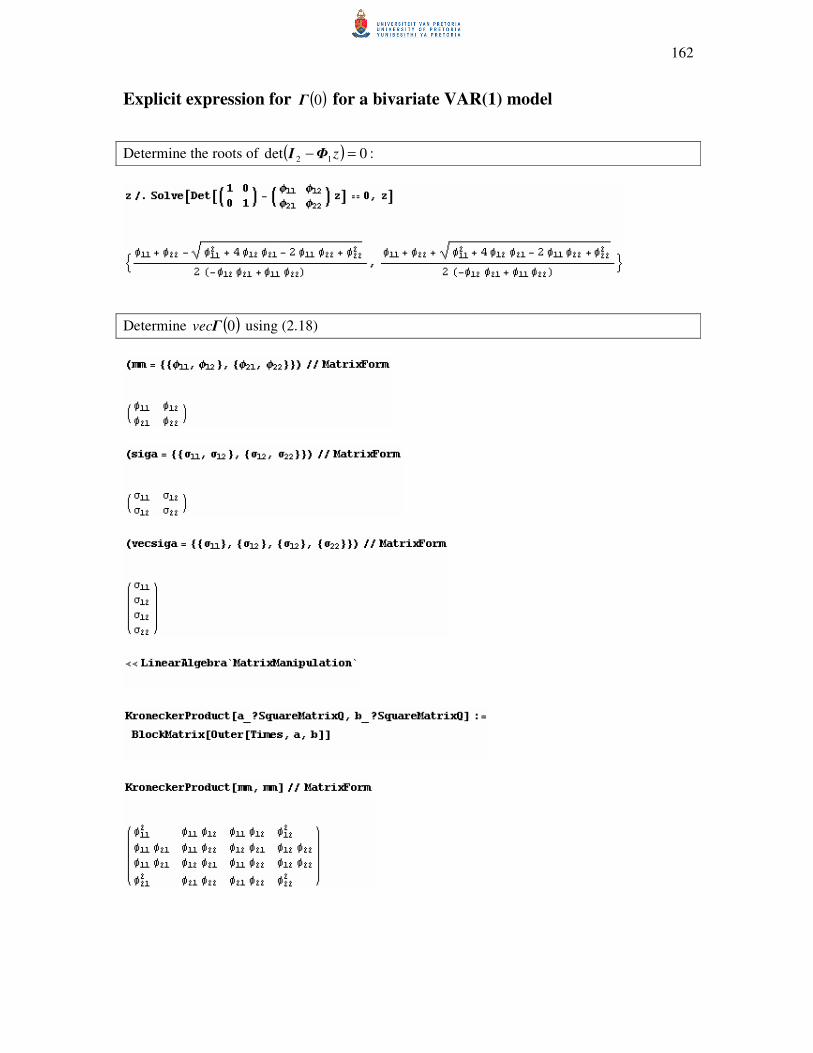
162
Explicit expression for ( )0Γ for a bivariate VAR(1) model
Determine the roots of ( ) 0det 12 =− zΦI :
Determine ( )0Γvec using (2.18)

163
( 44 × matrix)
Example 2.1
Determine the roots of ( ) 0det 12 =− zΦI :
Determine the roots of ( ) 0det 12 =−ΦI λ :

164
Determine ( )0Γvec using (2.18)
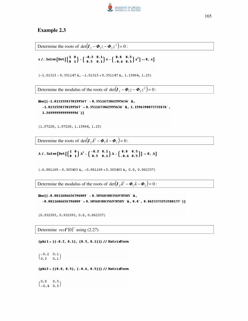
165
Example 2.3
Determine the roots of ( ) 0det 2
212 =−− zz ΦΦI :
Determine the modulus of the roots of ( ) 0det 2
212 =−− zz ΦΦI :
Determine the roots of ( ) 0det 21
2
2 =−− ΦΦI λλ :
Determine the modulus of the roots of ( ) 0det 21
2
2 =−− ΦΦI λλ :
Determine ( )*0Γvec using (2.27)
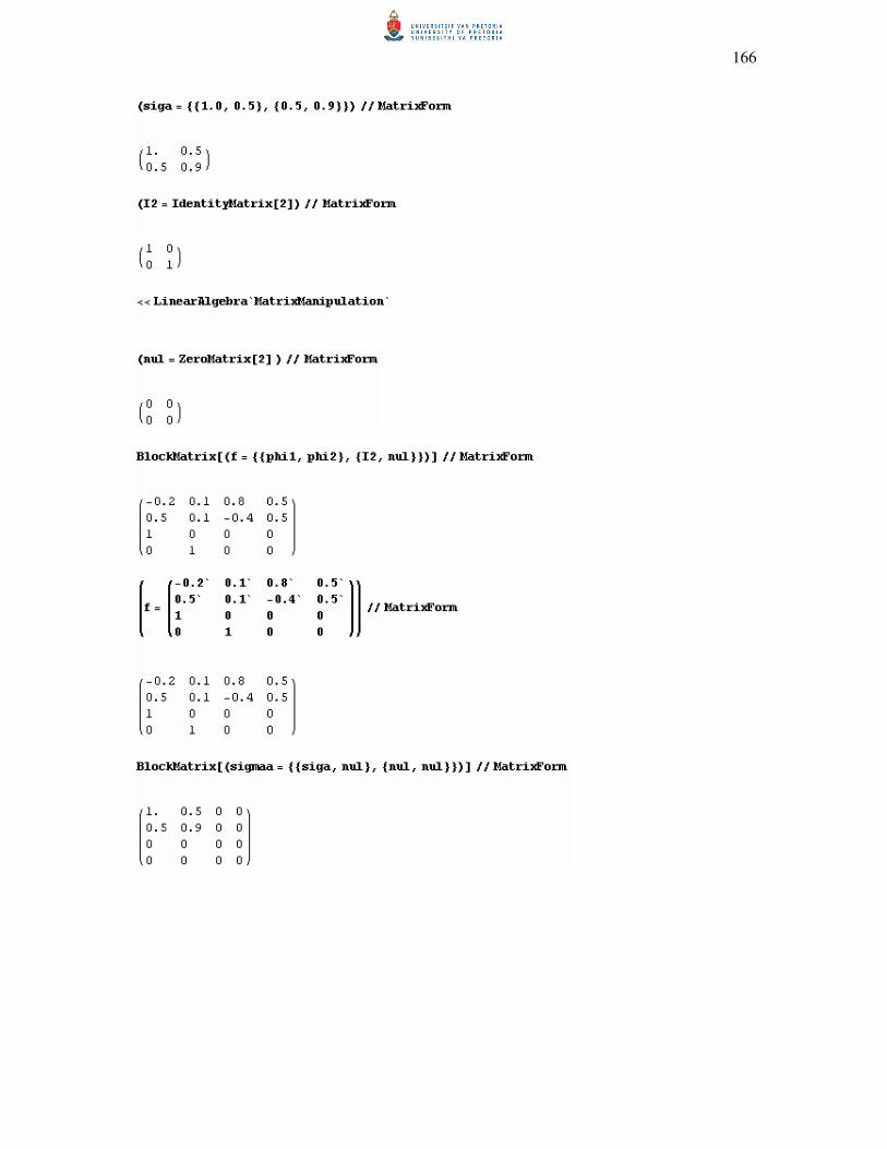
166
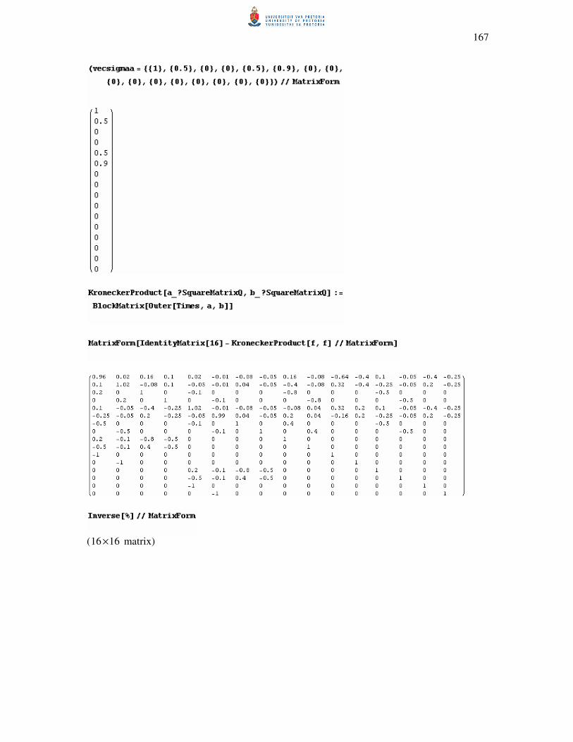
167
( 1616 × matrix)
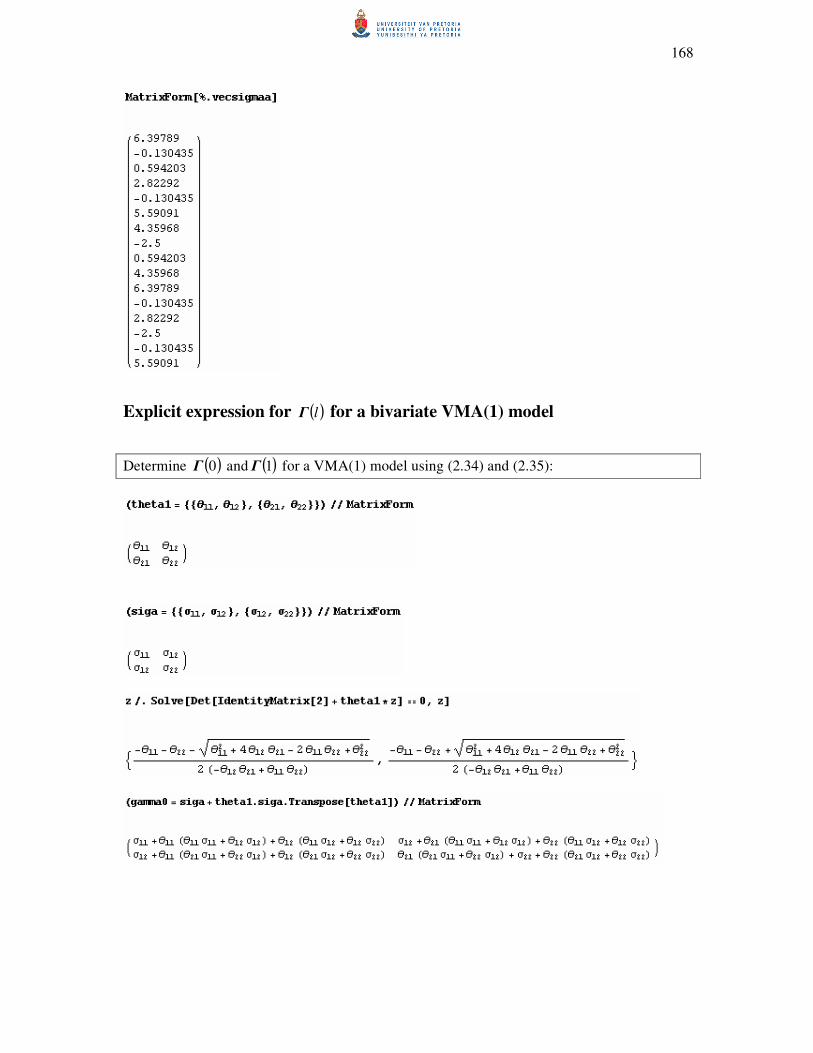
168
Explicit expression for ( )lΓ for a bivariate VMA(1) model
Determine ( )0Γ and ( )1Γ for a VMA(1) model using (2.34) and (2.35):
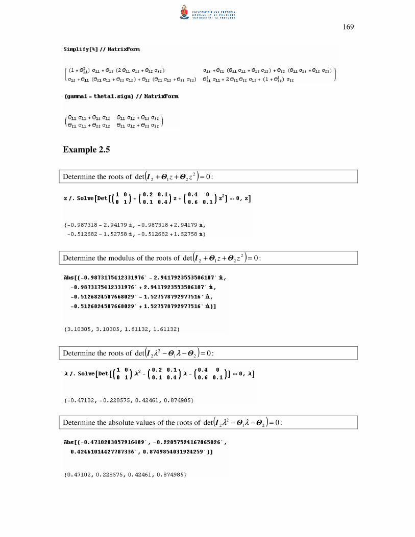
169
Example 2.5
Determine the roots of ( ) 0det 2
212 =++ zz ΘΘI :
Determine the modulus of the roots of ( ) 0det 2
212 =++ zz ΘΘI :
Determine the roots of ( ) 0det 21
2
2 =−− ΘΘI λλ :
Determine the absolute values of the roots of ( ) 0det 21
2
2 =−− ΘΘI λλ :
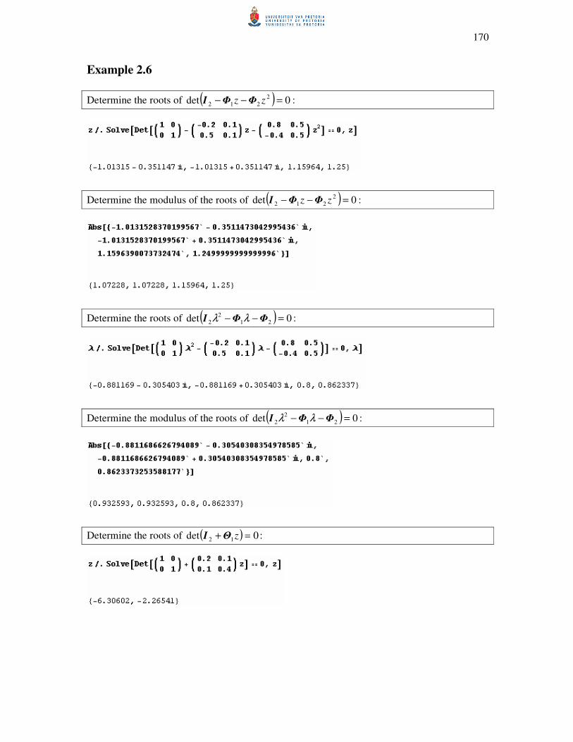
170
Example 2.6
Determine the roots of ( ) 0det 2
212 =−− zz ΦΦI :
Determine the modulus of the roots of ( ) 0det 2
212 =−− zz ΦΦI :
Determine the roots of ( ) 0det 21
2
2 =−− ΦΦI λλ :
Determine the modulus of the roots of ( ) 0det 21
2
2 =−− ΦΦI λλ :
Determine the roots of ( ) 0det 12 =+ zΘI :
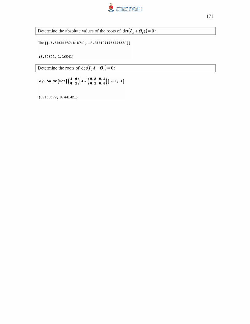
171
Determine the absolute values of the roots of ( ) 0det 12 =+ zΘI :
Determine the roots of ( ) 0det 12 =−ΘI λ :
172
REFERENCES
BOOKS
Anderson, T.W. 1984. An Introduction to Multivariate Statistical Analysis, 2nd
ed. New York:
John Wiley & Sons Inc.
Box, G.E.P. & Jenkins, G.M. 1970. Time Series Analysis: Forecasting and Control. San
Francisco: Holden-Day.
Draper, N.R. & Smith, H. 1998. Applied Regression Analysis, 3rd
ed. New York: John Wiley
& Sons Inc.
Gujarati, D.N. 1995. Basic Econometrics, 3rd
ed. New York: McGraw-Hill Inc.
Hamilton, J.D. 1994. Time Series Analysis. Princeton, N.J.: Princeton University Press
Hannan, E.J. 1970. Multiple Time Series. New York: John Wiley & Sons Inc.
Johnson, R.A. & Wichern, D.W. 2002. Applied Multivariate Statistical Analysis, 5th
ed. Upper
Saddle River, N.J.: Prentice Hall
Lütkepohl, H. 1991. Introduction to Multiple Time Series Analysis. Berlin: Springer.
Lütkepohl, H. 2005. New Introduction to Multiple Time Series Analysis. Berlin: Springer.
Quenouille, M.H. 1957. The Analysis of Multiple Time-Series. London: Griffin.
Reinsel, G.C. 1997. Elements of Multivariate Time Series Analysis, 2nd
ed. New York:
Springer.
SAS Institute Inc. 2004. SAS/ETS®
9.1 User’s Guide. Cary, NC: SAS Institute Inc.
Steyn, A.G.W., Smit, C.F., du Toit, S.H.C. & Strasheim, C. 1998. Moderne statistiek vir die
praktyk, 6de
uitg. Pretoria: Van Schaik
Williams, T.A., Sweeney, D.J. & Anderson, D.R. 2006. Contemporary Business Statistics
with Microsoft®
Excel. Mason, Ohio: Thomson
ARTICLES
Akaike, H. 1969. Fitting Autoregressive Models for Prediction. Annals of the Institute of
Statistical Mathematics, vol.21, no.1, p.243-247.
Bartlett, M.S. & Rajalakshman, D.V. 1953. Goodness of Fit Tests for Simultaneous
Autoregressive Series. Journal of the Royal Statistical Society. Series B (Methodological),
vol.15, no.1, p.107-124.
173
Box, G.E.P. & Pierce, D.A. 1970. Distribution of Residual Autocorrelations in
Autoregressive-Integrated Moving Average Time Series Models. Journal of the American
Statistical Association, vol.65, no.332, p.1509-1526.
Chitturi, R.V. 1974. Distribution of Residual Autocorrelations in Multiple Autoregressive
Schemes. Journal of the American Statistical Association, vol.69, no.348, p.928-934.
Crabtree, B.F., Ray, S.C., Schmidt, P.M., O’Connor, P.J. & Schmidt, D.D. 1990. The
individual over time: time series applications in health care research. Journal of Clinical
Epidemiology, vol.43, no.3, p.241-260.
De Frutos, R.F. & Serrano, G.R. 2002. A Generalized Least Squares Estimation Method for
VARMA Models. Statistics, vol.36, no.4, p.303-316.
De Vries, W.R. & Wu, S.M. 1978. Evaluation of Process Control Effectiveness and Diagnosis
of Variation in Paper Basis Weight via Multivariate Time-Series Analysis. IEEE Transactions
on Automatic Control, vol.23, no.4, p.702-708.
Dickey, D.A. & Fuller, W.A. 1979. Distribution of the Estimators for Autoregressive Time
Series With a Unit Root. Journal of the American Statistical Association, vol.74, no.366,
p.427-431.
Durbin, J. 1970. Testing for Serial Correlation in Least-Squares Regression When Some of
the Regressors are Lagged Dependent Variables. Econometrica, vol.38, no.3, p.410-421.
Durbin, J. & Watson, G.S. 1950. Testing for Serial Correlation in Least Squares Regression:
I. Biometrika, vol.37, no.3/4, p.409-428.
Durbin, J. & Watson, G.S. 1951. Testing for Serial Correlation in Least Squares Regression.
II. Biometrika, vol.38, no.1/2, p.159-177.
Engle, R.F. 1982. Autoregressive Conditional Heteroscedasticity with Estimates of the
Variance of United Kingdom Inflation. Econometrica, vol.50, no.4, p.987-1008.
Hannan, E.J. 1969. The Identification of Vector Mixed Autoregressive-Moving Average
Systems. Biometrika, vol.56, no.1, p.223-225.
Hillmer, S.C. & Tiao G.C. 1979. Likelihood Function of Stationary Multiple Autoregressive
Moving Average Models. Journal of the American Statistical Association, vol.74, no.367,
p.652-660.
Hosking, J.R.M. 1980. The Multivariate Portmanteau Statistic. Journal of the American
Statistical Association, vol.75, no.371, p.602-608.
Jarque, C.M. & Bera, A.K. 1987. A Test for Normality of Observations and Regression
Residuals. International Statistical Review / Revue Internationale de Statistique, vol.55, no.2,
p.163-172.
Jenkins, G.M. & Alavi, A.S. 1981. Some aspects of Modelling and Forecasting Multivariate
Time Series. Journal of Time Series Analysis, vol.2, no.1, p.1-47.
174
Li, W.K. & McLeod, A.I. 1981. Distribution of the Residual Autocorrelations in Multivariate
ARMA Time Series Models. Journal of the Royal Statistical Society. Series B
(Methodological), vol.43, no.2, p231-239.
Ljung, G.M. & Box, G.E.P. 1978. On a Measure of Lack of Fit in Time Series Models.
Biometrika, vol.65, no.2, p.297-303.
Lütkepohl, H. & Poskitt, D.S. 1996. Specification of Echelon-Form VARMA Models.
Journal of Business & Economic Statistics, vol.14, no.1, p.69-79.
Ma, C. 1997. On the Exact Likelihood Function of a Multivariate Autoregressive Moving
Average Model. Biometrika, vol.84, no.4, p.957-964.
Mauricio, J.A. 1995. Exact Maximum Likelihood Estimation of Stationary Vector ARMA
Models. Journal of the American Statistical Association, vol.90, no.429, p.282-291.
Newbold, P. 1981. Some Recent Developments in Time Series Analysis, Correspondent
Paper. International Statistical Review / Revue Internationale de Statistique, vol.49, no.1,
p53-66.
Nicholls, D.F. & Hall, A.D. 1979. The Exact Likelihood Function of Multivariate
Autoregressive-Moving Average Models. Biometrika, vol.66, no.2, p.259-264.
Osborn, D.R. 1977. Exact and Approximate Maximum Likelihood Estimators for Vector
Moving Average Processes. Journal of the Royal Statistical Society. Series B
(Methodological), vol.39, no.1, p.114-118.
Phadke, M.S. & Kedem, G. 1978. Computation of the Exact Likelihood Function of
Multivariate Moving Average Models. Biometrika, vol.65, no.3, p.511-519.
Quinn, B.G. 1980. Order Determination for a Multivariate Autoregression. Journal of the
Royal Statistical Society. Series B (Methodological), vol.42, no.2, p.182-185.
Said, S.E. & Dickey, D.A. 1984. Testing for Unit Roots in Autoregressive-Moving Average
Models of Unknown Order. Biometrika, vol.71, no.3 p.599-607.
Spliid, H. 1983. A Fast Estimation Method for the Vector Autoregressive Moving Average
Model With Exogenous Variables. Journal of the American Statistical Association, vol.78,
no.384, p.843-849.
Tiao, G.C. & Box, G.E.P. 1981. Modeling Multiple Time Series with Applications. Journal of
the American Statistical Association, vol.76, no.376, p.802-816.
Whittle, P. 1953. The Analysis of Multiple Stationary Time Series. Journal of the Royal
Statistical Society. Series B (Methodological), vol.15, no.1, p.125-139.
Wilson, G.T. 1973. The Estimation of Parameters in Multivariate Time Series Models.
Journal of the Royal Statistical Society. Series B (Methodological), vol.35, no.1, p.76-85.
175
SUMMARY
STATIONARY MULTIVARIATE TIME SERIES ANALYSIS
by
KARIEN MALAN
Supervisor: Dr. H. Boraine
Department: Statistics
Degree: MSc (Course Work) Mathematical Statistics
Multivariate time series analysis became popular in the early 1950s when the need to analyse
time series simultaneously arose in the field of economics. This study provides an overview
of some of the aspects of multivariate time series analysis in the case of stationarity.
The VARMA (vector autoregressive moving average) class of multivariate time series
models, including pure vector autoregressive (VAR) and vector moving average (VMA)
models is considered. Methods based on moments and information criteria for the
determination of the appropriate order of a model suitable for an observed multivariate time
series are discussed. Feasible methods of estimation based on the least squares and/or
maximum likelihood are provided for the different types of VARMA models. In some cases,
the estimation is more complicated due to the identification problem and the nonlinearity of
the normal equations. It is shown that the significance of individual estimates can be
established by using hypothesis tests based on the asymptotic properties of the estimators.
Diagnostic tests for the adequacy of the fitted model are discussed and illustrated. These
include methods based on both univariate and multivariate procedures. The complete model
building process is illustrated by means of case studies on multivariate electricity demand and
temperature time series.
Throughout the study numerical examples are used to illustrate concepts. Computer program
code (using basic built-in multivariate functions) is given for all the examples. The results are
benchmarked against those produced by a dedicated procedure for multivariate time series. It
is envisaged that the program code (given in SAS/IML) could be made available to a much
wider user community, without much difficulty, by translation into open source platforms.
Related Documents