Stationary distributions and mean first passage times of perturbed Markov chains

Res. Lett. Inf. Math. Sci., (2002), 3, 85-98Available online at http:/./.www.massey.ac.nz/~wwiims/research/letters/

Stationary Distributions and Mean First Passage Times of PerturbedMarkov Chains

Jeffrey J. HunterI.I.M.S. Massey University, Auckland, New [email protected]

AbstractStationary distributions of perturbed finite irreducible discrete time Markov chains are intimatelyconnected with the behaviour of associated mean first passage times. This interconnection is exploredthrough the use of generalized matrix inverses. Some interesting qualitative results regarding the natureof the relative and absolute changes to the stationary probabilities are obtained together with someimproved bounds.

AMS classification: 15A51; 60J10; 60J20; 65F20; 65F35

Keywords: Markov chains; Generalized inverses; Stationary distribution; Mean first passage times;Stochastic matrix; Perturbation theory

1. IntroductionMarkov chains subjected to perturbations have received attention in the literature over recent years. Themajor interest has focussed on the effects of perturbations of the transition probabilities on the stationarydistribution of the Markov chain with the derivation of bounds or changes, or relative changes, in themagnitude of the stationary probabilities. Recently sensitivity of the perturbation effects has beenconsidered in terms of the mean first passage times of the original irreducible Markov chain. In this paperwe provide further insights into this approach by giving some new derivations and examining somespecial cases in depth.

2. General perturbations and stationary distributionsLet P(1) = [pij

(1)] be the transition matrix of a finite irreducible, m-state Markov chain. Let P(2) = [pij(2)] =

P(1) + ΕΕΕΕ be the transition matrix of the perturbed Markov chain where ΕΕΕΕ = [εij] is the matrix ofperturbations. We assume that the perturbed Markov chain is also irreducible with the same state space S= {1, 2,…, m}. For i = 1, 2, let ππππ (i)' = (π1

(i), π2(i),…, πm

(i)) be the stationary probability vectors for therespective Markov chains.

There are a variety of techniques that we can use to obtain expressions for ππππ(1)' and ππππ(2)'. In particular, in[9], the author used some generalised matrix inverse techniques to obtain separate expressions for ππππ(1)'and ππππ(2)' in the rank one update case when ΕΕΕΕ = ab' with b'e = 0.

Since we are interested in the effect that the perturbations ΕΕΕΕ = [ε ij] have on changes to the stationaryprobabilities, we use an approach that leads directly to an expression for the difference ππππ(2)' – ππππ(1)'.

First observe that, since ππππ(1)'(I – P(1)) = 0' and ππππ(2)'(I – P(2)) = ππππ(2)'(I – P(1) – ΕΕΕΕ) = 0',

(ππππ(2)' – ππππ(1)')(I – P(1)) = ππππ(2)'ΕΕΕΕ. (2.1)

Equation (2.1) consists of a system of linear equations. Generalized matrix inverses (g-inverses) have animportant role in solving such equations. The relevant results (see e.g. [7] or [8]) that we shall make useof are the following:

86 R.L.I.M.S. Vol.3 April 2002

2.1 A ‘one condition’ g-inverse or an ‘equation solving’ g-inverse of a matrix A is any matrix A−−−− suchthat AA−−−−A = A.

2.2 Let P(1) be the transition matrix of a finite irreducible Markov chain with stationary probabilityvector ππππ(1)'. Let e' = (1, 1, …, 1) and t and u be any vectors.(a) I – P(1) + tu' is non-singular if and only if ππππ(1)'t ≠ 0 and u'e ≠ 0.(b) If ππππ(1)'t ≠ 0 and u'e ≠ 0 then [I – P(1) + tu']-1 is a g-inverse of I – P(1).

2.3 All one condition g-inverses of I – P(1) are of the form [I – P(1) + tu']-1 + ef ' + gππππ(1)' for arbitraryvectors f and g.

2.4 A necessary and sufficient condition for x'A = b' to have a solution is b'A−−−−A = b' . If thisconsistency condition is satisfied the general solution is given by x' = b'A−−−− + w'(I – AA−−−−) wherew' is an arbitrary vector.

2.5 The following results are easily established (see Section 3.3, [7])(a) u'[I – P(1) + tu']-1 = ππππ(1)'/(ππππ(1)'t). (2.2)(b) [I – P(1) + tu']-1t = e/(u'e). (2.3)(c) [I – P(1) + tu']-1(I – P(1)) = I – eu'/(u'e). (2.4)(d) (I – P(1))[I – P(1) + tu']-1 = I – tππππ(1)'/(ππππ(1)'t). (2.5)

2.6 Hunter, ([6]), established that Kemeny and Snell’s ‘fundamental matrix’, ([12]), Z( 1 ) ≡[I – P(1) + Π(1)]-1, where Π (1) = eππππ(1)', is a one condition g-inverse of I – P(1). Meyer, ([14]), showedthat the ‘group inverse’ A#(1) ≡ Z(1) – Π(1) is also a g-inverse of I – P(1).

Theorem 2.1: If G is any g-inverse of I – P(1) then, for any general perturbation E ,

ππππ(2)' – ππππ(1)' = ππππ(2)'ΕΕΕΕ G(I – Π(1)). (2.6)

Proof: By taking G as the general form [I – P(1) + tu']-1 + ef ' + gππππ(1)' and using results from §2.5, the facts

that Π(1)= eππππ(1)', ππππ(1)'e = 1 and P(1)e = e, it follows that

(I – P(1))G(I – Π(1)) = I – Π(1). (2.7)Thus, from (2.1) and (2.7),

(ππππ(2)' – ππππ(1)')(I – Π(1)) = (ππππ(2)' – ππππ(1)')(I – P(1))G(I – Π(1)) = ππππ(2)'ΕΕΕΕ G(I – Π(1)).

Further (ππππ(2)' – ππππ(1)')(I – Π(1)) = (ππππ(2)' – ππππ(1)')(I – eππππ(1)') = ππππ(2)' – ππππ(1)' and (2.6) follows.

An alternative approach to solving (2.1) is to use the results of §2.4 with x' = ππππ(2)' – ππππ(1)', A = I – P(1) , b'= ππππ(2)'ΕΕΕΕ and A−−−− = G, as above. The consistency condition is satisfied and the general solution has theform ππππ(2)' – ππππ(1)' = ππππ(2)'E G + w'{t/(ππππ(1)'t) – (I – P(1))g}ππππ(1)' with w' arbitrary. Since (ππππ(2)' – ππππ(1)')e = 0,the arbitrariness of w' is eliminated with w'{t/(ππππ(1)'t) – (I – P(1))g} = – ππππ (2)'ΕΕΕΕ G e and equation (2.6)follows.

Theorem 2.1 is a new result and all known results for the difference ππππ(2)' – ππππ(1)' can be obtained from thisresult. In particular we have the following special cases.

Corollary 2.1.1:(i) If G = [I – P(1) + tu']-1 + ef ' + gππππ(1)' with ππππ(1)'t ≠ 0, u'e ≠ 0, f ' and g arbitrary vectors,

then

ππππ(2)' – ππππ(1)' = ππππ(2)'ΕΕΕΕ [I – P(1) + tu']-1(I – Π(1)). (2.8)

J. J Hunter Stationary Distributions and Mean First Passage Times of Perturbed Markov Chains 87

(ii) If G = [I – P(1) + eu']-1 + ef ' + gππππ(1)' with ππππ(1)'t ≠ 0, u'e ≠ 0, f ' and g arbitrary vectors,then

ππππ(2)' – ππππ(1)' = ππππ(2)'ΕΕΕΕ [I – P(1) + eu']-1. (2.9)

(iii) If G = [I – P(1) + eu']-1 + ef ' with u'e ≠ 0, and f ' an arbitrary vector, then

ππππ(2)' – ππππ(1)' = ππππ(2)'ΕΕΕΕ G. (2.10)

(iv) If Z(1) is the‘fundamental matrix’ of I – P(1), then

ππππ(2)' – ππππ(1)' = ππππ(2)'ΕΕΕΕ Z(1). (2.11)

(v) If A#(1) is the ‘group inverse’ of I – P(1), then

ππππ(2)' –ππππ(1)' = ππππ(2)'ΕΕΕΕ A#(1). (2.12)

Proof: (i) For (2.8), substitution of G into (2.6) leads to the ef ' term vanishing since ΕΕΕΕ e = 0. Similarlythe gππππ(1)' term cancels since ππππ(1)'(I – eππππ(1)') = 0'.

(ii) Equation (2.9) follows from (2.8) upon substitution of t = e since, from (2.3),[I – P(1) + eu']-1e = e/(u'e) and ΕΕΕΕ e = 0.

(iii) Substitution of the form of G into (2.6) leads to the ππππ (2)'E G Π (1) term vanishingsince ΕΕΕΕ GΠ(1) = ΕΕΕΕ ([I – P(1) + eu']-1 + ef ')eππππ(1)' = ΕΕΕΕ e{1/ (u'e) + (f 'e)}ππππ(1)' = 0.

(iv) Equation (2.11) follows from (2.9) or (2.10) with u' = ππππ(1)'. (v) Equation (2.12) follows from (2.10) with u' = ππππ(1)' and f ' = ππππ(1)'.

The general result (2.8) is new. The other results, or special cases of them, appear in the literature butwith ad hoc derivations. Result (2.11) was initially derived by Schweitzer ([18]). Result (2.12) is due toMeyer ([15]). A special case of results (2.9) and (2.10), (with f ' = 0' and g = 0), appears in Seneta [19],while result (2.10) appears in Seneta [21].

The results obtained by the author in [9], in the case that ΕΕΕΕ = ab' where b'e = 0, can also be obtainedfrom Corollary 2.1.1.

Corollary 2.1.2:(i) If u'e ≠ 0, π (1)'t ≠ 0, αααα' = u'[I – P(1) + tu']-1 and ββββ' = b'[I – P(1) + tu']–1, then

=− ′ ′ ′ ′

− ′ ′ ′ ′

( )

( )( ( )( )

1

1

ββ αα αα ββββ αα αα ββ

aa e

+ (.

a)e) a+

(2.13)

(ii) If u'e ≠ 0, ππππ(1)'a ≠ 0, αααα' = u'[I – P(1) + au']–1 and ββββ' = b'[I – P(1) + au']–1, then

ππαααα

ππαα ββαα ββ

( ( .1 2) )

e′ =

′′

′ =′ ′′ ′e

+

e + (2.14)and

(iii) If u'e ≠ 0, αααα' = u'[I – P(1) + eu']–1 and ββββ' = b'[I – P(1) + eu']–1, then

ππ αα ππ ππααββ

ββ( ) ( ) ( ) .1 2 1

1′ = ′ ′ = ′ +

′− ′

′ (2.15)and

a

a

ππαααα

ππββ ππ ππ ββ

ββ ππ ββ

( ) ( )( ) ( )

( )

( ) ( )

( ) ( )( )

1 21 1

1

1

1′ =

′′

′ =− ′ ′ ′

− ′ + ′ ′

+

e

a

aand

a

a e

88 R.L.I.M.S. Vol.3 April 2002

(iv) If Z(1) = [I – P(1) + eππππ(1)']–1 is the fundamental matrix of I – P(1), then

= + . (2.16)ππ ππππ

ββππ ππ( ) ( )

( )( ) ( ) ( ) ( )2 1

11 1 1 1

1′ = ′ +

′

− ′

′ ′

′ ′a

ab ba

Z Z

Proof: (i) The expression for ππππ(1)' follows from (2.2) since αααα' = ππππ(1)'/(ππππ(1)'t) and αααα'e = 1/(ππππ(1)'t). Further,from (2.8),

ππππ(2)' – ππππ(1)' = (ππππ(2)'a)ββββ'(I – eππππ(1)') = (ππππ(2)'a)ββββ' – (ππππ(2)'a)(ββββ'e)ππππ(1)'. (2.17)

Post-multiplication of (2.17) by a and solving for ππππ(2)'a yields

ππππ

ββ ββ ππ

( )( )

( )

( ) ( )( )

.21

11′ =

′

− ′ + ′ ′a

a

a e a (2.18)

Substitution for ππππ(2)'a into (2.15) and solving for ππππ(2)' yields the expressions (2.13). (ii) Follows from (2.13) with t = a by noting that a'a = 0 and b'a = 1.

(iii) Follows from (2.13) with t = e by noting that a'e = 1 and b'e = 0. (iv) Follows from (2.15) with u' = ππππ(1)', since a' = ππππ(1)'Z(1) = ππππ(1)' and b' = b'Z(1).Note also from (2.18) that

For a summary on the current known results concerning absolute norm-wise error bounds on thedifferences between the two stationary probability vectors of the form

where (p,q) = (∞, ∞) or (1, ∞) depending on l, see Cho and Meyer [2]. They summarise and compareresults due to Schweitzer [18], Meyer [15], Haviv and Van der Heyden [5], Kirkland et al. [13], Funderlicand Meyer [4], Meyer [16], Seneta [20], Seneta [21], Seneta [22], Ipsen and Meyer [11], Cho and Meyer[3].

Results for component-wise bounds of the form

and relative error bounds of the form

are also discussed in Cho and Meyer [2]. For relative error bounds see also O’Cinneide [17] and Xue[23].

3. General perturbations and mean first passage timesIn Hunter [7], (see also [8]), a general technique for finding mean first passage times of a finiteirreducible discrete time Markov chains, using generalised inverses, was developed. The key result is asfollows:

Let M(1) = [mij(1)] be the mean first passage time matrix of a finite irreducible, Markov chain with

transition matrix P(1). If G is any generalised matrix inverse of I – P(1), then

( ) ( )1 2 ππ ππ ΕΕ − ≤

p

κ l q

j j

jl

( ) ( )

( )

1 2

1

ΕΕ π ππ

κ−

≤∞

j j l( ) ( )1 2π π κ− ≤

∞ ΕΕ

ππππ( )

( )

.

21

1′ =

′

− ′a

aab Z(1)

J. J Hunter Stationary Distributions and Mean First Passage Times of Perturbed Markov Chains 89

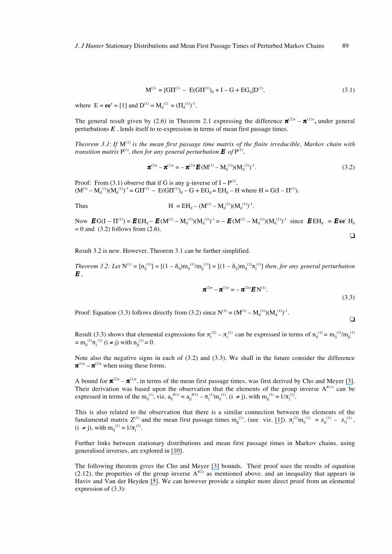
M(1) = [GΠ(1) – E(GΠ(1))d + I – G + EGd]D(1), (3.1)

where E = ee' = [1] and D(1) = Md(1) = (Πd

(1))-1.

The general result given by (2.6) in Theorem 2.1 expressing the difference ππππ(2)' – ππππ (1)', under generalperturbations E , lends itself to re-expression in terms of mean first passage times.

Theorem 3.1: If M(1) is the mean first passage time matrix of the finite irreducible, Markov chain withtransition matrix P(1), then for any general perturbation ΕΕΕΕ of P(1),

ππππ(2)' – ππππ(1)' = – ππππ(2)'ΕΕΕΕ (M(1) – Md(1))(Md

(1))-1. (3.2)

Proof: From (3.1) observe that if G is any g-inverse of I – P(1),(M(1) – Md

(1))(Md(1))-1 = GΠ(1) – E(GΠ(1))d – G + EGd = EHd – H where H = G(I – Π(1)).

Thus H = EHd – (M(1) – Md(1))(Md

(1))-1.

Now ΕΕΕΕ G(I – Π(1)) = ΕΕΕΕ EHd – ΕΕΕΕ (M(1) – Md(1))(Md

(1))-1 = – ΕΕΕΕ (M(1) – Md(1))(Md

(1))-1 since ΕΕΕΕ EHd = ΕΕΕΕ ee' Hd

= 0 and (3.2) follows from (2.6).

Result 3.2 is new. However, Theorem 3.1 can be further simplified.

Theorem 3.2: Let N(1) = [nij(1)] = [(1 – δij)mij

(1)/mjj(1)] = [(1 – δij)mij

(1)πj(1)] then, for any general perturbation

ΕΕΕΕ ,

ππππ(2)' – ππππ(1)' = – ππππ(2)'ΕΕΕΕ N(1). (3.3)

Proof: Equation (3.3) follows directly from (3.2) since N(1) = (M(1) – Md(1))(Md

(1))-1.

Result (3.3) shows that elemental expressions for πj(2) – πj

(1) can be expressed in terms of nij(1) = mij

(1)/mjj(1)

= mij(1)πj

(1) (i ≠ j) with njj(1) = 0.

Note also the negative signs in each of (3.2) and (3.3). We shall in the future consider the differenceππππ(1)' – ππππ(2)' when using these forms.

A bound for ππππ(2)' – ππππ(1)', in terms of the mean first passage times, was first derived by Cho and Meyer [3].Their derivation was based upon the observation that the elements of the group inverse A#(1) can beexpressed in terms of the mij

(1), viz. aij#(1) = ajj

#(1) – πj(1)mij

(1), (i ≠ j), with mjj(1) = 1/πj

(1).

This is also related to the observation that there is a similar connection between the elements of thefundamental matrix Z(1) and the mean first passage times mjj

(1), (see viz. [1]). πj(1)mij

(1) = zjj(1) – zij

(1) ,(i ≠ j), with mij

(1) = 1/πj(1).

Further links between stationary distributions and mean first passage times in Markov chains, usinggeneralised inverses, are explored in [10].

The following theorem gives the Cho and Meyer [3] bounds. Their proof uses the results of equation(2.12), the properties of the group inverse A#(1) as mentioned above, and an inequality that appears inHaviv and Van der Heyden [5]. We can however provide a simpler more direct proof from an elementalexpression of (3.3):

90 R.L.I.M.S. Vol.3 April 2002

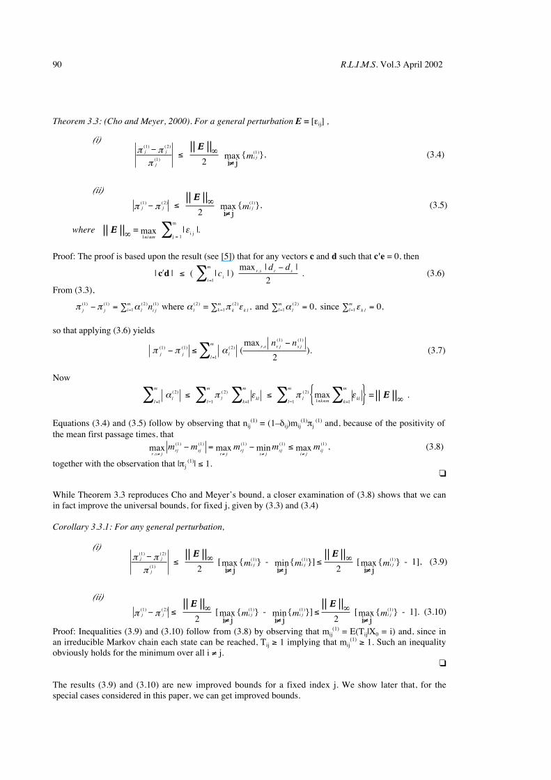
Theorem 3.3: (Cho and Meyer, 2000). For a general perturbation E = [εij] ,

Proof: The proof is based upon the result (see [5]) that for any vectors c and d such that c'e = 0, then

| | ( )max ,′ ≤

−=

∑c d | | | |

. (3.6)cd d

ii

mr s r s

1 2From (3.3),

so that applying (3.6) yields

Now

Equations (3.4) and (3.5) follow by observing that nij(1) = (1–δij)mij

(1)πj (1) and, because of the positivity of

the mean first passage times, that

r s jrj sj

r jrj

s jsj

i jijm m m m m

,

( ) ( ) ( ) ( ) ( )max max min max

≠ ≠ ≠ ≠− = − ≤1 1 1 1 1 , (3.8)

together with the observation that |πj (1)| ≤ 1.

While Theorem 3.3 reproduces Cho and Meyer’s bound, a closer examination of (3.8) shows that we canin fact improve the universal bounds, for fixed j, given by (3.3) and (3.4)

Corollary 3.3.1: For any general perturbation,

Proof: Inequalities (3.9) and (3.10) follow from (3.8) by observing that mij(1) = E(Tij|X0 = i) and, since in

an irreducible Markov chain each state can be reached, Tij ≥ 1 implying that mij(1) ≥ 1. Such an inequality

obviously holds for the minimum over all i ≠ j.

The results (3.9) and (3.10) are new improved bounds for a fixed index j. We show later that, for thespecial cases considered in this paper, we can get improved bounds.

(ii)

i j

max { } (3.5) j j i jm( ) ( ) ( ) ,1 2 1

2π π− ≤ ∞

≠

ΕΕ

(i)

i j

max { }, (3.4) j j

j

i jm( ) ( )

( )

( )1 2

1

1

2π π

π

−≤ ∞

≠

ΕΕ

π π α α π ε α εj j lim

i j l k k lkm

llm

k llmn( ) ( ) ( ) ( ) ( ) ( ) ( ) , ,1 1 2

11 2 2

12

1 10 0− = ∑ ∑ ∑ = ∑ == = = = where = , and since

). (3.7) π π αj j l

l

m r s r j s jn n( ) ( ) ( ) ,

( ) ( )

(max

1 1 2

1

1 1

2− ≤

−

=∑

max = .

= =α π ε π εl

l

m

ll

m

klk

m

ll

m

k m klk

m( ) ( ) ( )2

1

2

1 1

2

1 1 1= ≤ ≤∑ ∑ ∑ ∑ ∑≤ ≤ { } ∞= =

ΕΕ

(i)

[i j

max { } - i jmin{ }] [

i jmax { } - 1], (3.9)

j j

j

i j i j i jm m m( ) ( )

( )

( ) ( ) ( )1 2

1

1 1 1

2 2π π

π

−≤ ∞

≠ ≠≤ ∞

≠

ΕΕ ΕΕ

(ii)

[i j

max { } - i jmin{ }] [

i jmax { } - 1]. (3.10) j j i j i j i jm m m( ) ( ) ( ) ( ) ( )1 2 1 1 1

2 2π π− ≤ ∞

≠ ≠≤ ∞

≠

ΕΕ ΕΕ

= max | |i jj = 1

m

wherei m∞ ≤ ≤∑ ΕΕ

1ε .

J. J Hunter Stationary Distributions and Mean First Passage Times of Perturbed Markov Chains 91

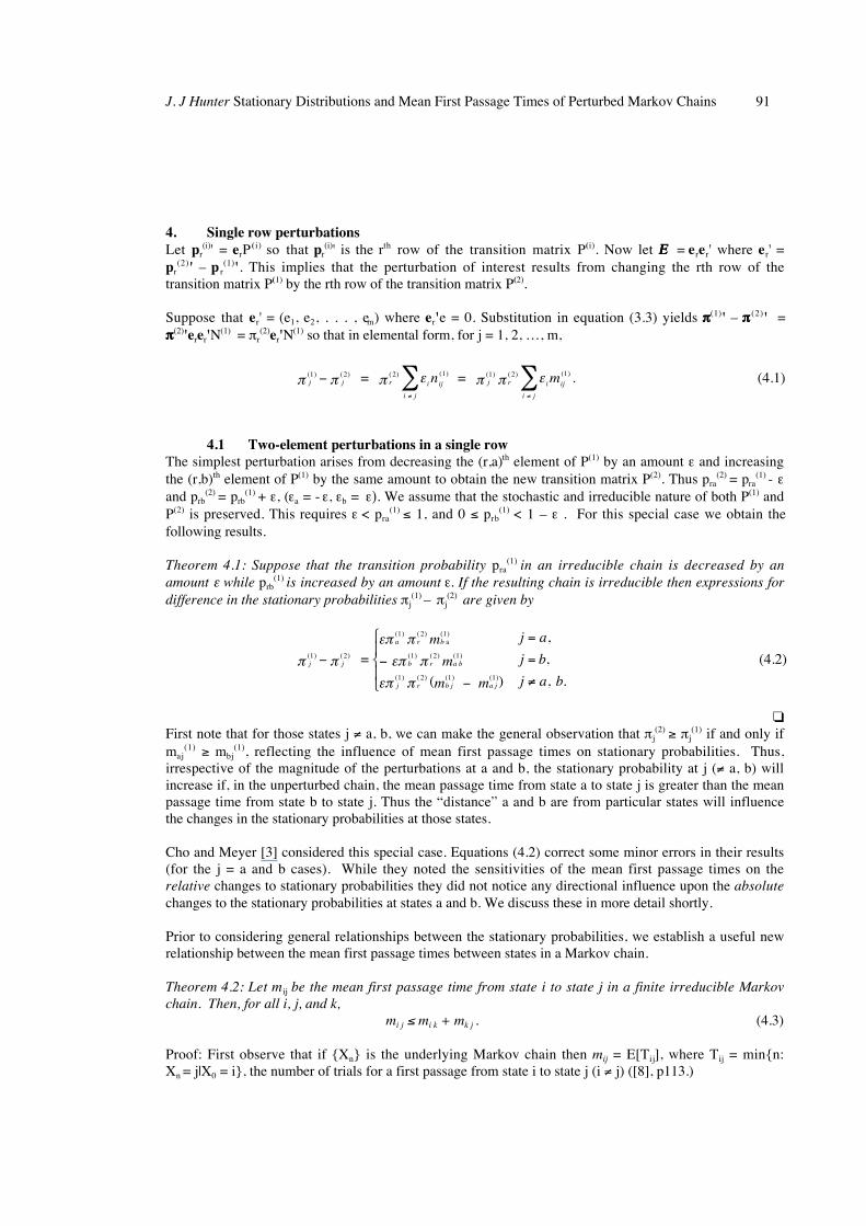
4. Single row perturbationsLet pr

(i)' = erP( i) so that pr

(i)' is the rth row of the transition matrix P(i). Now let ΕΕΕΕ = erer' where er' =pr

(2)' – p r(1)'. This implies that the perturbation of interest results from changing the rth row of the

transition matrix P(1) by the rth row of the transition matrix P(2).

Suppose that er' = (e1, e2, . . . , em) where er'e = 0. Substitution in equation (3.3) yields ππππ(1)' – ππππ (2)' =ππππ(2)'erer'N

(1) = πr(2)er'N

(1) so that in elemental form, for j = 1, 2, …, m,

4.1 Two-element perturbations in a single rowThe simplest perturbation arises from decreasing the (r,a)th element of P(1) by an amount ε and increasingthe (r,b)th element of P(1) by the same amount to obtain the new transition matrix P(2). Thus pra

(2) = pra(1) - ε

and prb(2) = prb

(1) + ε, (εa = - ε, εb = ε). We assume that the stochastic and irreducible nature of both P(1) andP(2) is preserved. This requires ε < pra

(1) ≤ 1, and 0 ≤ prb(1) < 1 – ε . For this special case we obtain the

following results.

Theorem 4.1: Suppose that the transition probability pra(1) in an irreducible chain is decreased by an

amount ε while prb(1) is increased by an amount ε. If the resulting chain is irreducible then expressions for

difference in the stationary probabilities πj(1) – πj

(2) are given by

First note that for those states j ≠ a, b, we can make the general observation that πj(2) ≥ πj

(1) if and only ifmaj

(1) ≥ mbj(1), reflecting the influence of mean first passage times on stationary probabilities. Thus,

irrespective of the magnitude of the perturbations at a and b, the stationary probability at j (≠ a, b) willincrease if, in the unperturbed chain, the mean passage time from state a to state j is greater than the meanpassage time from state b to state j. Thus the “distance” a and b are from particular states will influencethe changes in the stationary probabilities at those states.

Cho and Meyer [3] considered this special case. Equations (4.2) correct some minor errors in their results(for the j = a and b cases). While they noted the sensitivities of the mean first passage times on therelative changes to stationary probabilities they did not notice any directional influence upon the absolutechanges to the stationary probabilities at states a and b. We discuss these in more detail shortly.

Prior to considering general relationships between the stationary probabilities, we establish a useful newrelationship between the mean first passage times between states in a Markov chain.

Theorem 4.2: Let mij be the mean first passage time from state i to state j in a finite irreducible Markovchain. Then, for all i, j, and k,

mi j ≤ mi k + mk j . (4.3)

Proof: First observe that if {Xn} is the underlying Markov chain then mij = E[Tij], where Tij = min{n:Xn = j|X0 = i}, the number of trials for a first passage from state i to state j (i ≠ j) ([8], p113.)

j j r i ij j r i ij

i ji j

n m( ) ( ) ( ) ( ) ( ) ( ) ( )1 2 2 1 1 2 1π π π ε π π ε−≠≠

∑∑ = = . (4.1)

j j

a r b

b r a b

j r b j a j

m j a

m j b

m m j a b

( ) ( )

( ) ( ) ( )

( ) ( ) ( )

( ) ( ) ( ) ( )

,

,

( ) , .

1 2

1 2 1

1 2 1

1 2 1 1

π π

επ π

επ π

επ π

−

=

− =

− ≠

=

(4.2) a

92 R.L.I.M.S. Vol.3 April 2002

Now it is obvious, from the sample path of a typical chain, that Tij ≤ Tik + Tkj, since the chain will clearlytake at least as many transitions (steps) to move from state i to state j via a first passage through state kstarting at state i as it will without making such a forced first passage through state k. Equation (4.3)follows upon taking expectations of the respective random variables (which are all well-defined properrandom variables since the chain is irreducible.) While applications of the theorem are meaningful wheni ≠ j ≠ k the theorem obviously holds without such restrictions.

A consequence of equation (4.3) is that ma j ≤ ma b + mb j and that mb j ≤ mb a + ma j so that, for j ≠ a, b,

– ma b ≤ mb j – ma j ≤ mb a (4.4)

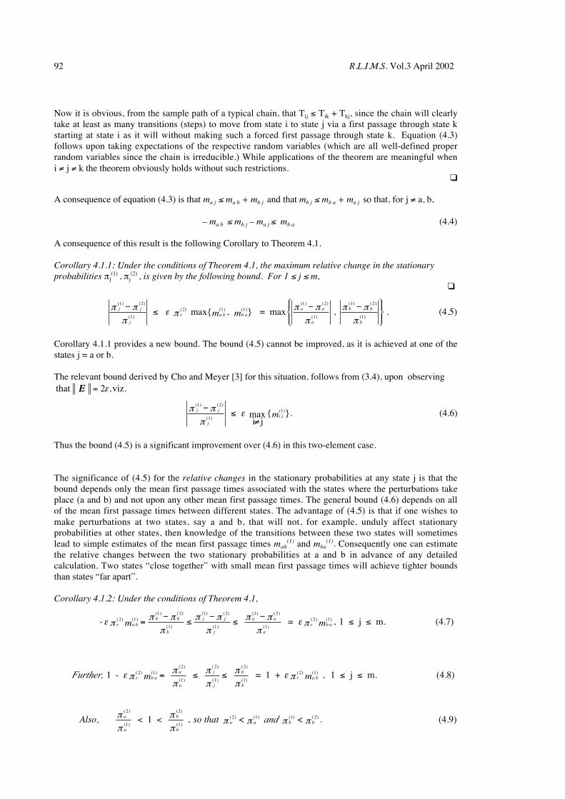
A consequence of this result is the following Corollary to Theorem 4.1.

Corollary 4.1.1: Under the conditions of Theorem 4.1, the maximum relative change in the stationaryprobabilities πj

(1) , πj(2) , is given by the following bound. For 1 ≤ j ≤ m,

Corollary 4.1.1 provides a new bound. The bound (4.5) cannot be improved, as it is achieved at one of thestates j = a or b.

The relevant bound derived by Cho and Meyer [3] for this situation, follows from (3.4), upon observing

Thus the bound (4.5) is a significant improvement over (4.6) in this two-element case.

The significance of (4.5) for the relative changes in the stationary probabilities at any state j is that thebound depends only the mean first passage times associated with the states where the perturbations takeplace (a and b) and not upon any other mean first passage times. The general bound (4.6) depends on allof the mean first passage times between different states. The advantage of (4.5) is that if one wishes tomake perturbations at two states, say a and b, that will not, for example, unduly affect stationaryprobabilities at other states, then knowledge of the transitions between these two states will sometimeslead to simple estimates of the mean first passage times mab

(1) and mba(1). Consequently one can estimate

the relative changes between the two stationary probabilities at a and b in advance of any detailedcalculation. Two states “close together” with small mean first passage times will achieve tighter boundsthan states “far apart”.

Corollary 4.1.2: Under the conditions of Theorem 4.1,

- = , 1 j m. (4.7) ε ππ π

ππ π

ππ π

πε πr a b

b b

b

j j

j

a a

a

r b am m( ) ( )( ) ( )

( )

( ) ( )

( )

( ) ( )

( )

( ) ( )2 11 2

1

1 2

1

1 2

1

2 1=−

≤−

≤−

≤ ≤

Further, 1 - = 1 + , 1 j m. (4.8) ε πππ

ππ

ππ

ε πr b aa

a

j

j

b

b

r a bm m( ) ( )( )

( )

( )

( )

( )

( )

( ) ( )2 12

1

2

1

2

1

2 1= ≤ ≤ ≤ ≤

max{ , } = max , . (4.5) j j

j

r a b b aa a

a

b b

b

m m( ) ( )

( )

( ) ( ) ( )( ) ( )

( )

( ) ( )

( )

1 2

1

2 1 11 2

1

1 2

1

π ππ

ε ππ π

ππ π

π

−≤

− −

, < < . (4.9) Also, anda

a

b

b

a a b bso that( )

( )

( )

( )

( ) ( ) ( ) ( )2

1

2

1

2 1 1 21ππ

ππ

π π π π< <

i j

max { }. (4.6) j j

j

i jm( ) ( )

( )

( )1 2

1

1π ππ

ε−

≤≠

that viz. ΕΕ = 2ε,

J. J Hunter Stationary Distributions and Mean First Passage Times of Perturbed Markov Chains 93

We can immediately make some interesting observations from Corollary 4.1.2.

First note, as a consequence of (4.7) and (4.8), that while the stationary probabilities at all other stateseither increase or decrease following a perturbation, the relative change in magnitude at any state neverexceeds the relative changes exhibited at the two states a and b. i.e. the minimal and maximal relativechanges occur at states a and b, respectively.

Secondly, as a consequence of (4.9), that when we decrease the transition probability at a single element,the a-th, in the rth row of the transition matrix of a finite irreducible Markov chain and make thecorresponding increase in the b-th element in the same row, then the absolute stationary probabilities forthe perturbed Markov chain at the a-th and b-th positions, correspondingly decrease and increase. i.e.

If pra(2) < pra

(1) and prb(2) > prb

(1) then πa(2) < πa

(1) and πb(2) > πb

(1).

This observation was also noted by Burnley, [1]. We cannot however make any statement regarding theabsolute changes in the stationary probabilities at a typical state j. The stationary probabilities at anygeneral state (apart from a and b) may increase or decrease.

Our interest now is to investigate whether the results of Theorem 4.1 or the inequalities given inCorollaries 4.1.1 and 4.1.2 also hold for other more general perturbations within a single row. In otherwords can we conclude that in a general single row perturbation with minimal and maximal perturbationsat states a and b, respectively, do inequalities (4.7) and (4.8) hold for the relative changes and (4.9) for theabsolute changes?

We consider first three-element perturbations before considering the more general setting.

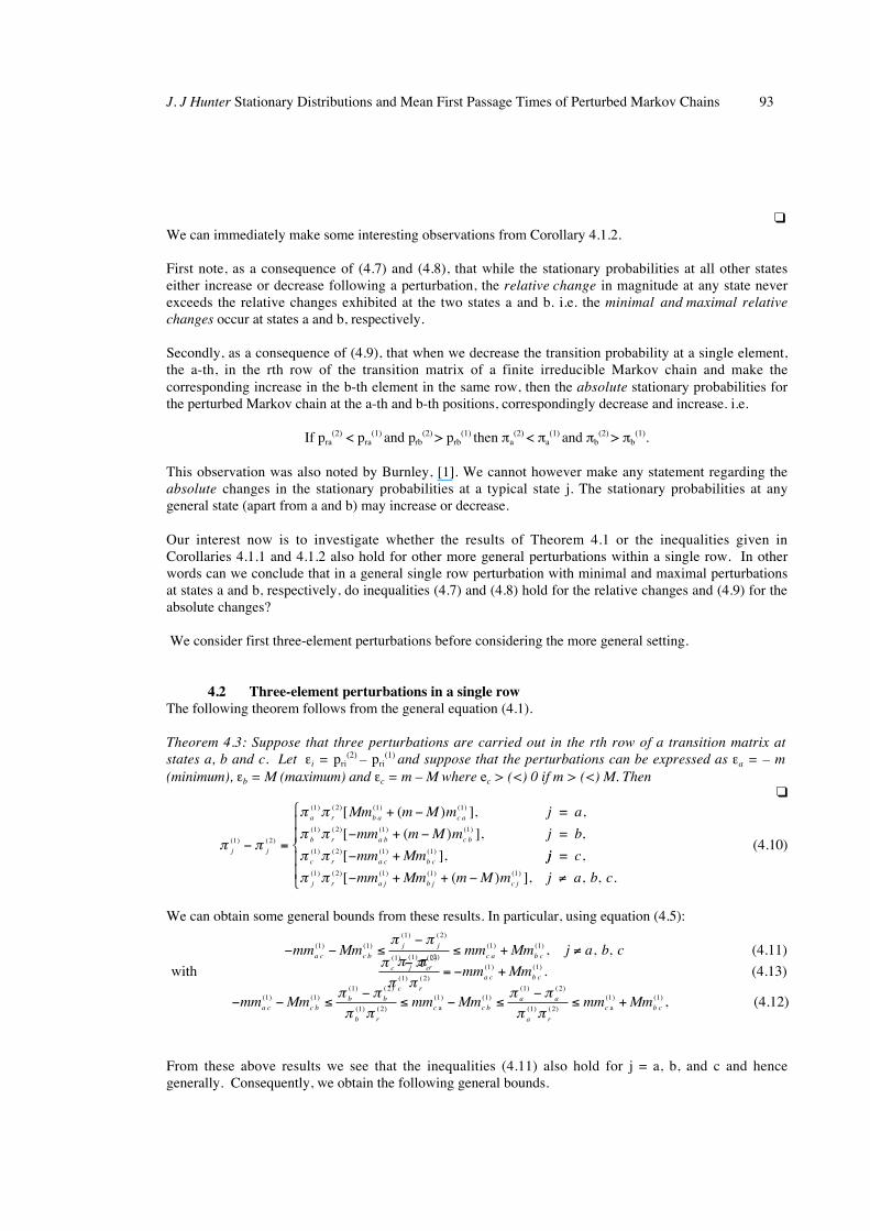
4.2 Three-element perturbations in a single rowThe following theorem follows from the general equation (4.1).

Theorem 4.3: Suppose that three perturbations are carried out in the rth row of a transition matrix atstates a, b and c. Let εi = pri

(2) – pri(1) and suppose that the perturbations can be expressed as εa = – m

(minimum), εb = M (maximum) and εc = m – M where ec > (<) 0 if m > (<) M. Then

We can obtain some general bounds from these results. In particular, using equation (4.5):

From these above results we see that the inequalities (4.11) also hold for j = a, b, and c and hencegenerally. Consequently, we obtain the following general bounds.

− − ≤−

≤ + ≠mm Mm mm Mm j a b ca c c b

j j

j r

c a b c (4.11)( ) ( )

( ) ( )

( ) ( )

( ) ( ) , , ,1 1

1 2

1 2

1 1π π

π π

− − ≤−

≤ − ≤−

≤ +mm Mm mm Mm mm Mma c c bb b

b r

c c ba a

a r

c b c a a (4.12)

( ) ( )( ) ( )

( ) ( )

( ) ( )( ) ( )

( ) ( )

( ) ( ) ,1 11 2

1 2

1 11 2

1 2

1 1π ππ π

π ππ π

with (4.13)

π ππ πc c

c r

a c b cmm Mm( ) ( )

( ) ( )

( ) ( ) .1 2

1 2

1 1−= − +

π π

π π

π π

π πj j

a r b a c a

b r a b c b

c r a c b c

Mm m M m j a

mm m M m j b

mm Mm( ) ( )

( ) ( ) ( ) ( )

( ) ( ) ( ) ( )

( ) ( ) ( ) ( )

[ ( ) ], ,

[ ( ) ], ,

[ ],1 2

1 2 1 1

1 2 1 1

1 2 1 1− =

+ −

− + −

− +

=

=

jj c

mm Mm m M m j a b cj r a j b j c j

= ,

π π( ) ( ) ( ) ( ) ( )[ ( ) ], , , .

( . )

1 2 1 1 1

4 10

− + + − ≠

94 R.L.I.M.S. Vol.3 April 2002

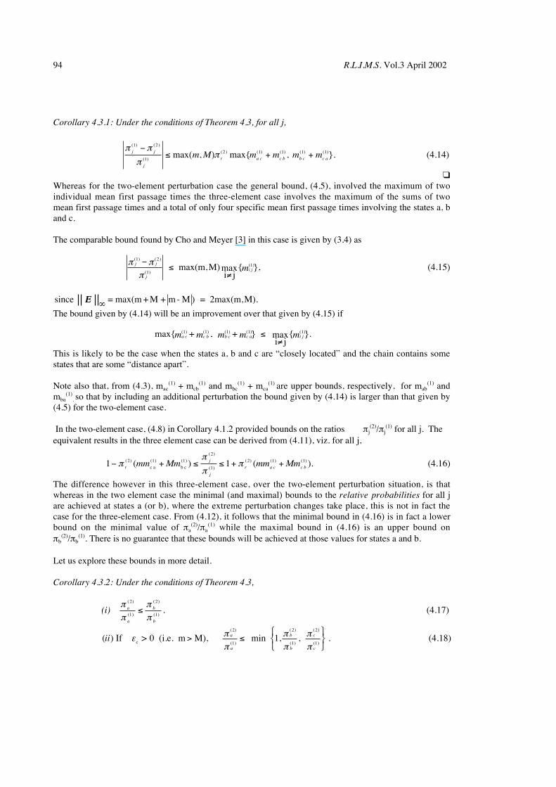
Corollary 4.3.1: Under the conditions of Theorem 4.3, for all j,

Whereas for the two-element perturbation case the general bound, (4.5), involved the maximum of twoindividual mean first passage times the three-element case involves the maximum of the sums of twomean first passage times and a total of only four specific mean first passage times involving the states a, band c.

The comparable bound found by Cho and Meyer [3] in this case is given by (3.4) as

The bound given by (4.14) will be an improvement over that given by (4.15) if

This is likely to be the case when the states a, b and c are “closely located” and the chain contains somestates that are some “distance apart”.

Note also that, from (4.3), mac(1) + mcb

(1) and mbc(1) + mca

(1) are upper bounds, respectively, for mab(1) and

mba(1)

. so that by including an additional perturbation the bound given by (4.14) is larger than that given by(4.5) for the two-element case.

In the two-element case, (4.8) in Corollary 4.1.2 provided bounds on the ratios πj(2)/πj

(1) for all j. Theequivalent results in the three element case can be derived from (4.11), viz. for all j,

The difference however in this three-element case, over the two-element perturbation situation, is thatwhereas in the two element case the minimal (and maximal) bounds to the relative probabilities for all jare achieved at states a (or b), where the extreme perturbation changes take place, this is not in fact thecase for the three-element case. From (4.12), it follows that the minimal bound in (4.16) is in fact a lowerbound on the minimal value of πa

(2)/πa(1) while the maximal bound in (4.16) is an upper bound on

πb(2)/πb

(1). There is no guarantee that these bounds will be achieved at those values for states a and b.

Let us explore these bounds in more detail.

Corollary 4.3.2: Under the conditions of Theorem 4.3,

π π

ππj j

j

r a c c b b c c am M m m m m( ) ( )

( )

( ) ( ) ( ) ( ) ( )max( , ) max{ ,1 2

1

2 1 1 1 1−

≤ + + }. (4.14)

( ) If > 0 (i.e. m M), 1, , . (4.18) cii a

a

b

b

c

c

ε ππ

ππ

ππ

> ≤

( )

( )

( )

( )

( )

( )min

2

1

2

1

2

1

(i) (4.17) ππ

ππ

a

a

b

b

( )

( )

( )

( ).

2

1

2

1≤

1 12 1 1

2

1

2 1 1− + ≤ ≤ + +ππ

ππr

j

j

r a c c bmm Mm mm Mm( ) ( ) ( )

( )

( )

( ) ( ) ( )( ) ( )c a b c . (4.16)

max(m,M)i j

max{ }, (4.15) j j

j

i jm( ) ( )

( )

( )1 2

1

1π ππ

−≤

≠

max{ + , + } i j

max{ }. a c c b b c c a i jm m m m m( ) ( ) ( ) ( ) ( )1 1 1 1 1≤≠

since = max(m + M + m- M ) = 2max(m,M).∞ ΕΕ

J. J Hunter Stationary Distributions and Mean First Passage Times of Perturbed Markov Chains 95

Proof:(i) Result (4.17) follows directly from equation (4.10) for the cases j = a and b together with

appropriate versions of equation (4.4).(ii) Results (4.18) follow from (4.10) using the results for j = a and j = c and (4.17).(iii) Results (4.19) follow from (4.10) using the results for j = b and j = c and (4.17).

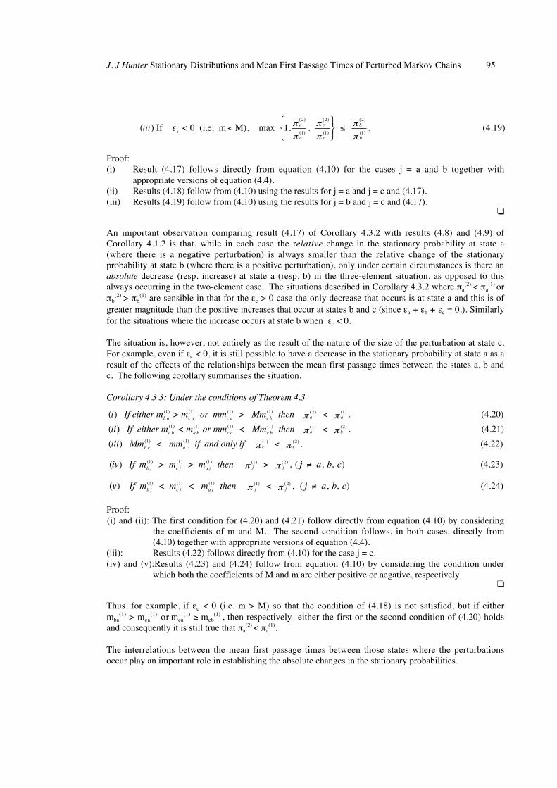
An important observation comparing result (4.17) of Corollary 4.3.2 with results (4.8) and (4.9) ofCorollary 4.1.2 is that, while in each case the relative change in the stationary probability at state a(where there is a negative perturbation) is always smaller than the relative change of the stationaryprobability at state b (where there is a positive perturbation), only under certain circumstances is there anabsolute decrease (resp. increase) at state a (resp. b) in the three-element situation, as opposed to thisalways occurring in the two-element case. The situations described in Corollary 4.3.2 where πa

(2) < πa(1) or

πb(2) > πb

(1) are sensible in that for the εc > 0 case the only decrease that occurs is at state a and this is ofgreater magnitude than the positive increases that occur at states b and c (since εa + εb + εc = 0.). Similarlyfor the situations where the increase occurs at state b when εc < 0.

The situation is, however, not entirely as the result of the nature of the size of the perturbation at state c.For example, even if εc < 0, it is still possible to have a decrease in the stationary probability at state a as aresult of the effects of the relationships between the mean first passage times between the states a, b andc. The following corollary summarises the situation.

Corollary 4.3.3: Under the conditions of Theorem 4.3

( ) > > . ( . )

( ) < <

i If either m m or mm Mm then

ii If either m m or mm Mm thenb a c a c a c b a a

c b a b c a c b b

( ) ( ) ( ) ( ) ( ) ( )

( ) ( ) ( ) ( )

1 1 1 1 2 1

1 1 1 1

4 20π π<(( ) ( )

( ) ( ) ( ) ( )

( ) ( ) ( ) ( ) ( )

1 2

1 1 1 2

1 1 1 1 2

π π

π π

π π

. (4.21)

( ) < . (4.22)

( ) > > , (

<

<

>

b

b c a c c c

b j c j a j j j

iii Mm mm if and only if

iv If m m m then jj a b c

v If m m m then j a b cb j c j a j j j

, , ) (4.23)

( ) < < , ( , , ) (4.24)

≠

< ≠( ) ( ) ( ) ( ) ( )1 1 1 1 2π π

Proof:(i) and (ii): The first condition for (4.20) and (4.21) follow directly from equation (4.10) by considering

the coefficients of m and M. The second condition follows, in both cases, directly from(4.10) together with appropriate versions of equation (4.4).

(iii): Results (4.22) follows directly from (4.10) for the case j = c.(iv) and (v):Results (4.23) and (4.24) follow from equation (4.10) by considering the condition under

which both the coefficients of M and m are either positive or negative, respectively.

Thus, for example, if εc < 0 (i.e. m > M) so that the condition of (4.18) is not satisfied, but if eithermba

(1) > mca(1) or mca

(1) ≥ mcb(1) , then respectively either the first or the second condition of (4.20) holds

and consequently it is still true that πa(2) < πa

(1).

The interrelations between the mean first passage times between those states where the perturbationsoccur play an important role in establishing the absolute changes in the stationary probabilities.

( ) If < 0 (i.e. m M), 1, , . (4.19) ciii a

a

c

c

b

b

ε ππ

ππ

ππ

<

≤max( )

( )

( )

( )

( )

( )

2

1

2

1

2

1

96 R.L.I.M.S. Vol.3 April 2002

We have not been able to establish simple general necessary and sufficient conditions under which eitherπj

(2) < πj(1) or πj

(2) > πj(1) apart from checking the right hand side of equations (4.10) for conditions of non-

negativity and negativity.

The observation that we made in the two-element case that the minimal (resp. maximal) absolute changesto the stationary probabilities occur at those states where the perturbations are the smallest (resp. largest)in magnitude need not hold in general in the three-element perturbation situation. This is substantiated bynumerical calculations for some specific chains.

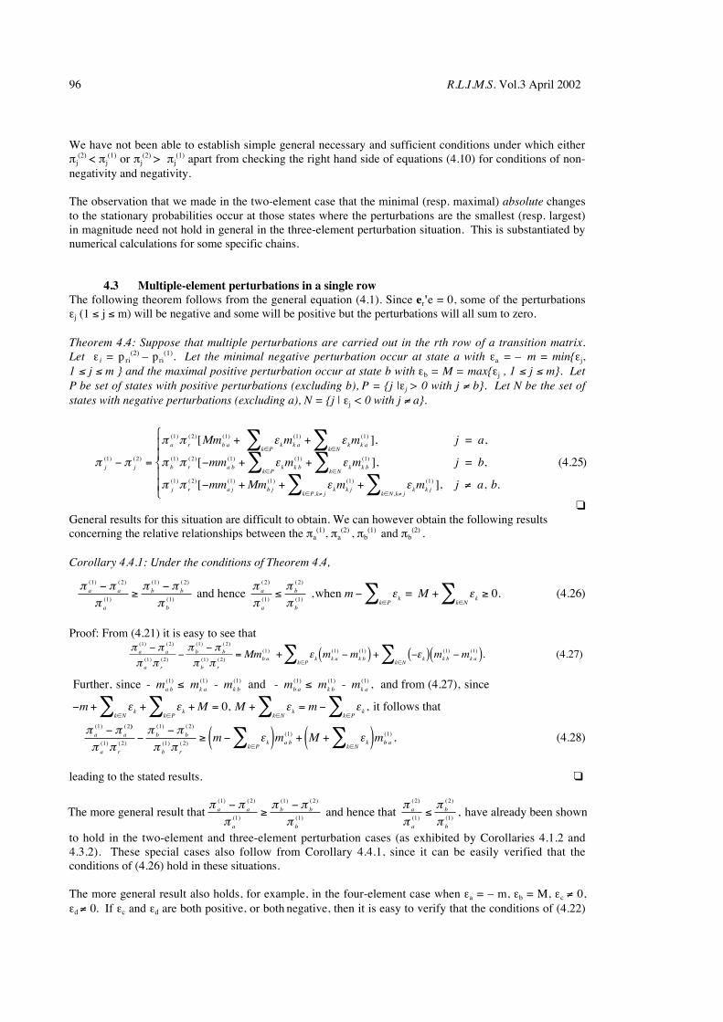
4.3 Multiple-element perturbations in a single rowThe following theorem follows from the general equation (4.1). Since er'e = 0, some of the perturbationsεj (1 ≤ j ≤ m) will be negative and some will be positive but the perturbations will all sum to zero.

Theorem 4.4: Suppose that multiple perturbations are carried out in the rth row of a transition matrix.Let ε i = pri

(2) – pri(1). Let the minimal negative perturbation occur at state a with εa = – m = min{εj,

1 ≤ j ≤ m } and the maximal positive perturbation occur at state b with εb = M = max{εj , 1 ≤ j ≤ m}. LetP be set of states with positive perturbations (excluding b), P = {j |εj > 0 with j ≠ b}. Let N be the set ofstates with negative perturbations (excluding a), N = {j | εj < 0 with j ≠ a}.

General results for this situation are difficult to obtain. We can however obtain the following resultsconcerning the relative relationships between the πa

(1), πa(2) , πb

(1) and πb(2) .

Corollary 4.4.1: Under the conditions of Theorem 4.4,

Proof: From (4.21) it is easy to see that

+ .

π ππ π

π ππ π

ε εa a

a r

b b

b r

b a kk P

k a k b k k b k ak N

Mm m m m m( ) ( )

( ) ( )

( ) ( )

( ) ( )

( ) ( ) ( ) ( ) ( ) ( . )1 2

1 2

1 2

1 2

1 1 1 1 1 4 27−

−−

= −( ) + −( ) −( )∈ ∈

∑ ∑

leading to the stated results.

to hold in the two-element and three-element perturbation cases (as exhibited by Corollaries 4.1.2 and4.3.2). These special cases also follow from Corollary 4.4.1, since it can be easily verified that theconditions of (4.26) hold in these situations.

The more general result also holds, for example, in the four-element case when εa = – m, εb = M, εc ≠ 0,εd ≠ 0. If εc and εd are both positive, or both negative, then it is easy to verify that the conditions of (4.22)

π π

π π ε ε

π π ε εj j

a r b a k k ak P

k k ak N

b r a b k k bk P

k k bk N

Mm m m j a

mm m m j( ) ( )

( ) ( ) ( ) ( ) ( )

( ) ( ) ( ) ( ) ( )

[ ], ,

[ ],1 2

1 2 1 1 1

1 2 1 1 1− =

+ +

− + +∈ ∈

∈ ∈

∑ ∑∑ ∑

=

=

b

mm Mm m m j a bj r a j b j k k jk P k j

k k jk N k j

,

[ ], , .

( . )( ) ( ) ( ) ( ) ( )

,

( )

,π π ε ε1 2 1 1 1 1

4 25

− + + + ≠

∈ ≠ ∈ ≠∑ ∑

and hence ,when = 0. π π

ππ π

πππ

ππ

ε εa a

a

b b

b

a

a

b

b

kk P

kk N

m M( ) ( )

( )

( ) ( )

( )

( )

( )

( )

( )( . )

1 2

1

1 2

1

2

1

2

14 26

−≥

−≤ − + ≥

∈ ∈∑ ∑

Further, since - - and - - , and from (4.27), since

it follows that

m m m m m m

m M M m

a b k a k b b a k b k a

kk N

kk P

kk N

kk P

a a

( ) ( ) ( ) ( ) ( ) ( )

( ) (

, ,

1 1 1 1 1 1

1 2

0

≤ ≤

− + + + = + = −

−∈ ∈ ∈ ∈

∑ ∑ ∑ ∑ε ε ε ε

π π ))

( ) ( )

( ) ( )

( ) ( )

( ) ( ) ( . )π π

π ππ π

ε εa r

b b

b r

kk P

a b kk N

b am m M m1 2

1 2

1 2

1 1 4 28−−

≥ −( ) + +( )∈ ∈

∑ ∑ ,

The more general result that and hence that , have already been shownπ π

ππ π

πππ

ππ

a a

a

b b

b

a

a

b

b

( ) ( )

( )

( ) ( )

( )

( )

( )

( )

( )

1 2

1

1 2

1

2

1

2

1

−≥

−≤

J. J Hunter Stationary Distributions and Mean First Passage Times of Perturbed Markov Chains 97

are satisfied. When εc < 0 and εd > 0 then, since – m ≤ εc < 0, it follows that M – m ≤ M + εc = m – εd

< M, implying that the conditions of Corollary 4.4.1 are satisfied when M – m ≥ 0. Further, since0 < εd ≤ M, it follows that m – N ≤ m – εd = M + εc < m and thus the conditions of Corollary 4.4.1 aresatisfied if m – M ≥ 0. Consequently, if either M – m ≥ or ≤ 0, i.e. generally, the results of (4.22) aresatisfied.

However the results of Corollary 4.4.1 do not necessarily hold in all situations. For example, it is easy toconstruct a multi-element example where the conditions of (4.22) are violated, (e.g. ε1 = – m = – 0.20, ε2

= – 0.15, ε3 = – 0.05, ε4 = 0.12, ε5 = 0.13, ε6 = M = 0.15).

We have been unable to obtain specific generalisations of the more general results concerning bounds on(πj

(1) – πj(2))/πj

(1) and πj(2)/πj

(1) or πj(1) – πj

(2) that we obtained in the two-element case (Corollaries 4.1.1 and4.1.2) and the three-element case (Corollaries 4.3.1, 4.3.2 and 4.3.3). In fact, examples can be constructedto show that some of the generalisations do not hold in more general settings. Further, general conditionsunder which πa

(2) < πa(1) and/or πb

(2) > πb(1) hold have not been found in this more general setting. What is

clear however is that both relative and absolute changes in the stationary probabilities can occur at statesother than a and b (where εa = – m, εb = M) of magnitude exceeding those at states a and b.

5. Concluding remarksThe results derived for the two-element case are elegant. The changes to the stationary probabilities thatoccur at any state in this situation can be easily determined from a knowledge of the mean first passagetimes, as exhibited by equations (4.2). If we can update the mean first passage times following a two-element perturbation then a useful procedure could be to consider a multiple-perturbation as a sequenceof two-element perturbations.

In a sequel to this paper we explore further procedures, using generalized matrix inverses, that will enableus to update the matrix of mean first passage times M(1), following a perturbation on the transition matrixP(1), to obtain M(2), the matrix of mean first passage times of the perturbed chain, without the necessity ofcalculating a further matrix inverse.

Acknowledgments:A major portion of this work was carried out within the Department of Statistics at the University ofNorth Carolina at Chapel Hill, N.C. while the author was a Visiting Professor in the Fall Semester of2001. The author also wishes to acknowledge the time and encouragement provided by Professor CarlMeyer of the Department of Mathematics, North Carolina State University, Raleigh, N.C. throughinsightful discussions on the material of this paper.

References:

1. Burnley C. 'Perturbation of Markov chains', Math Magazine, 60, 21-30, (1987).

2. Cho G.E. and Meyer C.D. 'Comparison of perturbation bounds for a stationary distribution of aMarkov chain, Linear Algebra Appl., 335, 137-150, (2001).

3. Cho G.E. and Meyer C.D. 'Markov chain sensitivity measured by mean first passage time',Linear Algebra Appl., 316, 21-28, (2000).

4. Funderlic R. and Meyer C.D. 'Sensitivity of the stationary distribution vector for an ergodicMarkov chain', Linear Algebra Appl., 76, 1-17, (1986).

5. Haviv M. and Van der Heyden L., 'Perturbation bounds for the stationary probabilities of a finiteMarkov chain', Adv. Appl. Prob., 16, 804-818, (1984).

98 R.L.I.M.S. Vol.3 April 2002

6. Hunter J.J. 'On the moments of Markov renewal processes', Adv. Appl. Probab., 1, 188-210,(1969).

7. Hunter J.J. 'Generalized inverses and their application to applied probability problems', LinearAlgebra Appl., 45, 157-198, (1982).

8. Hunter, J.J. Mathematical Techniques of Applied Probability, Volume 2, Discrete Time Models:Techniques and Applications, Academic, New York, 1983.

9. Hunter J.J. 'Stationary distributions of perturbed Markov chains', Linear Algebra Appl., 82, 201-214, (1986).

10. Hunter J.J. 'Stationary distributions and mean first passage times in Markov chains usinggeneralised inverses', Asia-Pacific Journal of Operational Research, 9, 145-153 (1992).

11. Ipsen I.C.F. and Meyer C.D. 'Uniform stability of Markov chains', SIAM J. Matrix Anal. Appl.,4, 1061-1074, (1994).

12. Kemeny J.G. and Snell, J.L. Finite Markov Chains, Van Nostrand, New York, 1960.

13. Kirkland S., Neumann M. and Shader B. L., 'Applications of Paz’s inequality to perturbationbounds for Markov chains', Linear Algebra Appl., 268, 183-196, (1998).

14. Meyer C.D. 'The role of the group generalized inverse in the theory of finite Markov chains',SIAM Rev., 17, 443-464, (1975).

15. Meyer C.D. 'The condition of a finite Markov chain and perturbation bounds for the limitingprobabilities', SIAM J. Algebraic Discrete Methods, 1, 273 – 283, (1980).

16. Meyer C.D. 'Sensitivity of the stationary distribution of a Markov chain', SIAM J. Matrix Appl.,15, 715-728, (1994).

17. O’Cinneide. 'Entrywise perturbation theory and error analysis for Markov chains', Numer. Math.,65, 190-120, (1993).

18. Schweitzer P. 'Perturbation theory and finite Markov chains’ J. Appl. Probab., 5, 410-413,(1968).

19. Seneta E. 'Sensitivity to perturbation of the stationary distribution: Some refinements', LinearAlgebra Appl., 108, 121-126, (1988).

20. Seneta E. 'Perturbation of the stationary distribution measured by the ergodicity coefficients',Adv Appl. Prob., 20, 228-230, (1988).

21. Seneta E. 'Sensitivity analysis, ergodicity coefficients, and rank-one updates for finite Markovchains', in 'Numerical Solution of Markov Chains' W.J. Stewart (Ed.), Probaility: Pure andApplied, Vol. 8, 121-129, Marcel-Dekker, New York, 1991.

22. Seneta E. 'Sensitivity of finite Markov chains under perturbation', Statist. Probab Lett., 17, 163-168, (1993).

23. Xue J. 'A note on entrywise perturbation theory for Markov chains', Linear Algebra Appl., 260,209-213, (1997).