Stationary BPS Solutions in N=2 Supergravity with R^2Interactions

arX

iv:h

ep-t

h/00

0923

4v2

22

Dec

200

0

Preprint typeset in JHEP style. - PAPER VERSION SPIN-00/21

ITP-UU-00/24

SU-ITP 00/19

hep-th/0009234

Stationary BPS Solutions in N = 2 Supergravity with

R2-Interactions

Gabriel Lopes Cardoso

Spinoza Institute, Utrecht University, Utrecht, The Netherlands, [email protected]

Bernard de Wit

Institute for Theoretical Physics and Spinoza Institute, Utrecht University, Utrecht, The

Netherlands, [email protected]

Jurg Kappeli

Institute for Theoretical Physics and Spinoza Institute, Utrecht University, Utrecht, The

Netherlands, [email protected]

Thomas Mohaupt

Physics Department, Stanford University, Stanford, CA 94305-4060, USA,

[email protected]

Abstract: We analyze a broad class of stationary solutions with residual N = 1 super-

symmetry of four-dimensional N = 2 supergravity theories with terms quadratic in the

Weyl tensor. These terms are encoded in a holomorphic function, which determines the

most relevant part of the action and which plays a central role in our analysis. The solu-

tions include extremal black holes and rotating field configurations, and may have multiple

centers. We prove that they are expressed in terms of harmonic functions associated with

the electric and magnetic charges carried by the solutions by a proper generalization of

the so-called stabilization equations. Electric/magnetic duality is manifest throughout the

analysis.

We also prove that spacetimes with unbroken supersymmetry are fully determined by

electric and magnetic charges. This result establishes the so-called fixed-point behavior

according to which the moduli fields must flow towards certain prescribed values on a fully

supersymmetric horizon, but now in a more general context with higher-order curvature

interactions. We briefly comment on the implications of our results for the metric on the

moduli space of extremal black hole solutions.

Contents

1. Introduction 1

2. Action and supersymmetry transformation rules 3

3. More supersymmetry variations 9

4. Fully supersymmetric field configurations 11

5. N = 1 supersymmetric field configurations 16

6. Discussion and conclusions 23

A. Notation and conventions 26

B. Superconformal calculus 27

1. Introduction

In this paper we determine a broad class of stationary solutions of four-dimensional N = 2

supergravity theories with R2-interactions. The supergravity theories that we consider

are based on vector multiplets and hypermultiplets coupled to the supergravity fields and

contain the standard Einstein-Hilbert action as well as terms quadratic in the Weyl tensor.

The most relevant part of the interactions is encoded in a holomorphic function, which plays

a central role in our analysis. The solutions that we consider are BPS solutions, because

they possess a residual N = 1 supersymmetry. Some of them describe extremal black holes

that carry electric and/or magnetic charges or superpositions thereof. We also describe

rotating solutions with one or several centers. The extremal black holes are solitonic

interpolations between two fully supersymmetric groundstates. Without R2-interactions

these are flat Minkowski spacetime at spatial infinity and a Bertotti-Robinson geometry

at the horizon. In that case, the moduli fields, which can take arbitrary values at infinity,

must flow to specific values at the horizon which are determined in terms of the charges.

This so-called fixed-point behavior explains why the black hole entropy depends only on

the charges and not on the asymptotic values of the moduli. This is in contradistinction

with the black hole mass which does depend on the values of the fields at spatial infinity.

Owing to this fixed-point behavior the resulting expressions for the entropy, based on the

effective low-energy action, can be compared successfully with microstate counting results

from string and brane theory, which also depend exclusively on the charges.

1

Solutions based on supergravity actions without R2-terms were analyzed some time ago

[1]-[4]. Important features of solutions with R2-interactions were presented more recently

in a number of papers [5]-[7] and reviewed in [8]. In [6] we showed that corrections to

the black hole entropy associated with R2-terms are in agreement with certain subleading

corrections to the entropy (in the limit of large charges) that follow from the counting of

microstates [9]. The main ingredients of the derivation in [6] are the behavior of the solution

at the horizon and the use of a definition of the black hole entropy that is appropriate when

R2-interactions are present. In order to ensure the validity of the first law of black hole

mechanics, we used the definition provided by the Noether method of [10]. This definition

leads to an entropy that deviates from the Bekenstein-Hawking area law.

The purpose of this work is to present the complete proof underlying the results of

[6] and to further extend our study of solutions in the presence of R2-interactions. In

particular we consider the full interpolating extremal black hole solution, multi-centered

solutions, as well as general stationary solutions. All solutions known so far (e.g. [1]-[3],

[11]) are contained as special cases. We begin our analysis by determining all spacetimes

with N = 2 supersymmetry. In doing so we systematize and complete the analysis pre-

sented in [6]. We prove that, in spite of the presence of R2-terms, there is still a unique

spacetime, which is of the Bertotti-Robinson type, whose radius as well as the values of the

various moduli fields are determined by the electric and magnetic charges carried by the

solution. Flat Minkowski spacetime can be viewed as a special case of such a solution, but

here the moduli are constant and arbitrary and there are no electric and magnetic fields.

Our analysis thus shows that the enhancement of supersymmetry at the horizon forces the

moduli fields to take prescribed values. Consequently the uniqueness of the horizon geom-

etry implies the existence of a fixed-point behavior even in the presence of R2-interactions.

Note that the fixed-point behavior is usually derived by invoking flow arguments based on

the interpolating solutions (see, e.g. [1, 4]), but these arguments are much more difficult

to derive in the presence of R2-interactions.

Subsequently we turn to the analysis of spacetimes with residual N = 1 supersym-

metry. A general analysis of the conditions for N = 1 supersymmetry turns out to be

extremely cumbersome. We therefore restrict ourselves to a well-defined class of embed-

dings of residual supersymmetry and derive the corresponding restrictions on the bosonic

background configurations. Our analysis is set up in such a way that the presence of the R2-

interactions hardly poses complications. This is so because the R2-terms are incorporated

into the Lagrangian by allowing the holomorphic function to depend on an extra holomor-

phic parameter. Furthermore, by stressing the underlying electric/magnetic duality of the

field equations throughout the calculations, the dependence on the R2-interactions remains

almost entirely implicit and does not require much extra attention.

Using the restrictions posed by residual supersymmetry and assuming stationary field

configurations we analyze the solutions. We prove that they are expressed in terms of har-

monic functions associated with the electric and magnetic charges carried by the solutions,

while the spatial dependence of the moduli is governed by so-called “generalized stabiliza-

tion equations”. The latter were first conjectured in [3] and in [5] for the case without and

with R2-interactions, respectively. The resulting stationary solutions include the case of

2

multi-centered solutions of extremal black holes.

Our analysis of the restrictions imposed by N = 2 and N = 1 supersymmetry on the

solutions is based on the existence of a full off-shell (superconformal) multiplet calculus

for N = 2 supergravity theories [12]. It turns out that the hypermultiplets play only a

rather passive role. It proves advantageous to perform most of the analysis before writing

the theory in its Poincare form (by imposing gauge conditions or reformulating it in terms

of fields that are invariant under the action of those superconformal symmetries that are

absent in Poincare supergravity). As a consequence we fix the stationary spacetime line

element only at a relatively late stage of the analysis. An unusual complication is that,

in order to determine the restrictions imposed by full or residual supersymmetry, it is not

sufficient to consider the supersymmetry variation of the fermions only. One also needs to

impose the vanishing of the supersymmetry variation of derivatives of the fermion fields.

We present an argument that shows which of these variations are needed.

The paper is organized as follows. In section 2 we review the relevant features of

the superconformal multiplet calculus which we use to construct N = 2 theories with

R2-interactions. We also briefly discuss electric/magnetic duality transformations in the

presence of R2-interactions. In section 3 we describe some of the technology needed for

performing the analysis. In particular, we construct various compensating fields for S-

supersymmetry (which are inert with respect to electric/magnetic duality) and we discuss

a number of additional transformation laws. In section 4 we perform a detailed analysis of

the restrictions imposed by N = 2 supersymmetry and make contact with previous results

[6]. Section 5 is devoted to the analysis of the restrictions imposed byN = 1 supersymmetry

for a particular class of embeddings of residual supersymmetry. We derive the “generalized

stabilization equations” that determine the spatial dependence of the moduli fields and

prove that the solutions are encoded in harmonic functions that are associated with the

electric and magnetic fields. Section 6 contains our conclusions as well as an outlook.

Appendices A and B explain some of the definitions and conventions used throughout this

paper.

2. Action and supersymmetry transformation rules

The N = 2 supergravity theories that we consider are based on abelian vector multiplets

and hypermultiplets coupled to the supergravity fields. The action contains the standard

Einstein-Hilbert action as well as terms quadratic in the Riemann tensor. To describe

such theories in a transparent way we make use of the superconformal multiplet calculus

[12], which incorporates the gauge symmetries of the N = 2 superconformal algebra. The

corresponding high degree of symmetry allows for the use of relatively small field represen-

tations. One is the Weyl multiplet, whose fields comprise the gauge fields corresponding

to the superconformal symmetries and a few auxiliary fields. The other ones are abelian

vector multiplets and hypermultiplets, as well as a general chiral supermultiplet, which will

be treated as independent in initial stages of the analysis but at the end will be expressed

in terms of the fields of the Weyl multiplet. Some of the additional (matter) multiplets will

provide compensating fields which are necessary in order that the action becomes gauge

3

equivalent to a Poincare supergravity theory. These compensating fields bridge the deficit

in degrees of freedom between the Weyl multiplet and the Poincare supergravity multi-

plet. For instance, the graviphoton, represented by an abelian vector field in the Poincare

supergravity multiplet, is provided by an N = 2 superconformal vector multiplet.

As we will demonstrate, it is possible to analyze the conditions for residual N = 1 or

full N = 2 supersymmetry directly in this superconformal setting, postponing a transition

to Poincare supergravity till the end. This implies in particular that our intermediate

results are subject to local scale transformations. Only towards the end we will convert to

expressions that are scale invariant.

The superconformal algebra contains general-coordinate, local Lorentz, dilatation, spe-

cial conformal, chiral SU(2) and U(1), supersymmetry (Q) and special supersymmetry (S)

transformations. The gauge fields associated with general-coordinate transformations (eaµ),

dilatations (bµ), chiral symmetry (V iµ j , Aµ) and Q-supersymmetry (ψi

µ) are realized by in-

dependent fields. The remaining gauge fields of Lorentz (ωabµ ), special conformal (fa

µ) and

S-supersymmetry transformations (φiµ) are dependent fields. They are composite objects,

which depend in a complicated way on the independent fields [12]. The corresponding

curvatures and covariant fields are contained in a tensor chiral multiplet, which comprises

24 + 24 off-shell degrees of freedom; in addition to the independent superconformal gauge

fields it contains three auxiliary fields: a Majorana spinor doublet χi, a scalar D and a self-

dual Lorentz tensor Tabij (where i, j, . . . are chiral SU(2) spinor indices)a. We summarize

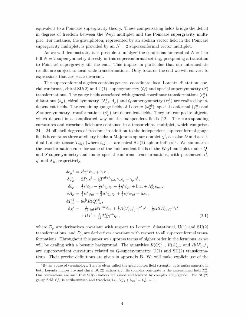
the transformation rules for some of the independent fields of the Weyl multiplet under Q-

and S-supersymmetry and under special conformal transformations, with parameters ǫi,

ηi and ΛaK, respectively,

δeµa = ǫiγaψµi + h.c. ,

δψiµ = 2Dµǫ

i − 18T

ab ijγab γµǫj − γµηi ,

δbµ = 12 ǫ

iφµi − 34 ǫ

iγµχi − 12 η

iψµi + h.c.+ ΛaK eµa ,

δAµ = 12 iǫ

iφµi + 34 iǫ

iγµχi + 12 iη

iψµi + h.c. ,

δT ijab = 8ǫ[iR(Q)

j]ab ,

δχi = − 112γabD/T

ab ijǫj + 16R(V)ab

ij γ

abǫj − 13 iR(A)abγ

abǫi

+D ǫi + 112T

ijabγ

abηj , (2.1)

where Dµ are derivatives covariant with respect to Lorentz, dilatational, U(1) and SU(2)

transformations, and Dµ are derivatives covariant with respect to all superconformal trans-

formations. Throughout this paper we suppress terms of higher order in the fermions, as we

will be dealing with a bosonic background. The quantities R(Q)iµν , R(A)µν and R(V)µνij

are supercovariant curvatures related to Q-supersymmetry, U(1) and SU(2) transforma-

tions. Their precise definitions are given in appendix B. We will make explicit use of the

aBy an abuse of terminology, Tabij is often called the graviphoton field strength. It is antisymmetric in

both Lorentz indices a, b and chiral SU(2) indices i, j. Its complex conjugate is the anti-selfdual field Tij

ab.

Our conventions are such that SU(2) indices are raised and lowered by complex conjugation. The SU(2)

gauge field Vi

µ j is antihermitian and traceless, i.e., V iµ j + Vµj

i = Vi

µ i = 0.

4

transformation of the S-supersymmetry gauge field,

δφiµ = −2 fa

µγaǫi + 1

4R(V)abijγ

abγµǫj + 1

2 iR(A)abγabγµǫ

i − 18D/T

ab ijγabγµǫj + 2Dµηi . (2.2)

Here f aµ is the gauge field of the conformal boosts, defined by (up to fermionic terms)

f aµ = 1

2R(ω, e)µa − 1

4(D + 13R(ω, e)) e a

µ − 12 iRµ

a(A) + 116T

ijµb T

abij , (2.3)

with R(ω, e)µa = R(ω)ab

µν eνb the (nonsymmetric) Ricci tensor and R(ω, e) the Ricci scalar.

Here R(ω)abµν is the curvature associated with the spin connection field ωab

µ . The spin

connection is not the usual torsion-free connection, but contains the dilatational gauge

field bµ. Because of that the curvature satisfies the Bianchi identity

R(ω)ab[µν eρ] b = 2∂[µbν e

aρ] . (2.4)

This leads to the modified pair-exchange property

R(ω)abcd −R(ω)cdab = 2

(

δ[c[aR(ω, e)b]

d] − δ[c[aR(ω, e)d]

b]

)

. (2.5)

It is important to mention that the covariant quantities of the Weyl multiplet constitute

a reduced chiral tensor multiplet, denoted byW abij , whose lowest-θ component is the tensor

T abij . In this multiplet the superconformal gauge fields appear only through covariant

derivatives and curvature tensors. From this multiplet one may form a scalar (unreduced)

chiral multiplet W 2 = [W abij εij ]2, which has Weyl and chiral weights w = 2 and c = −2,

respectively [13].

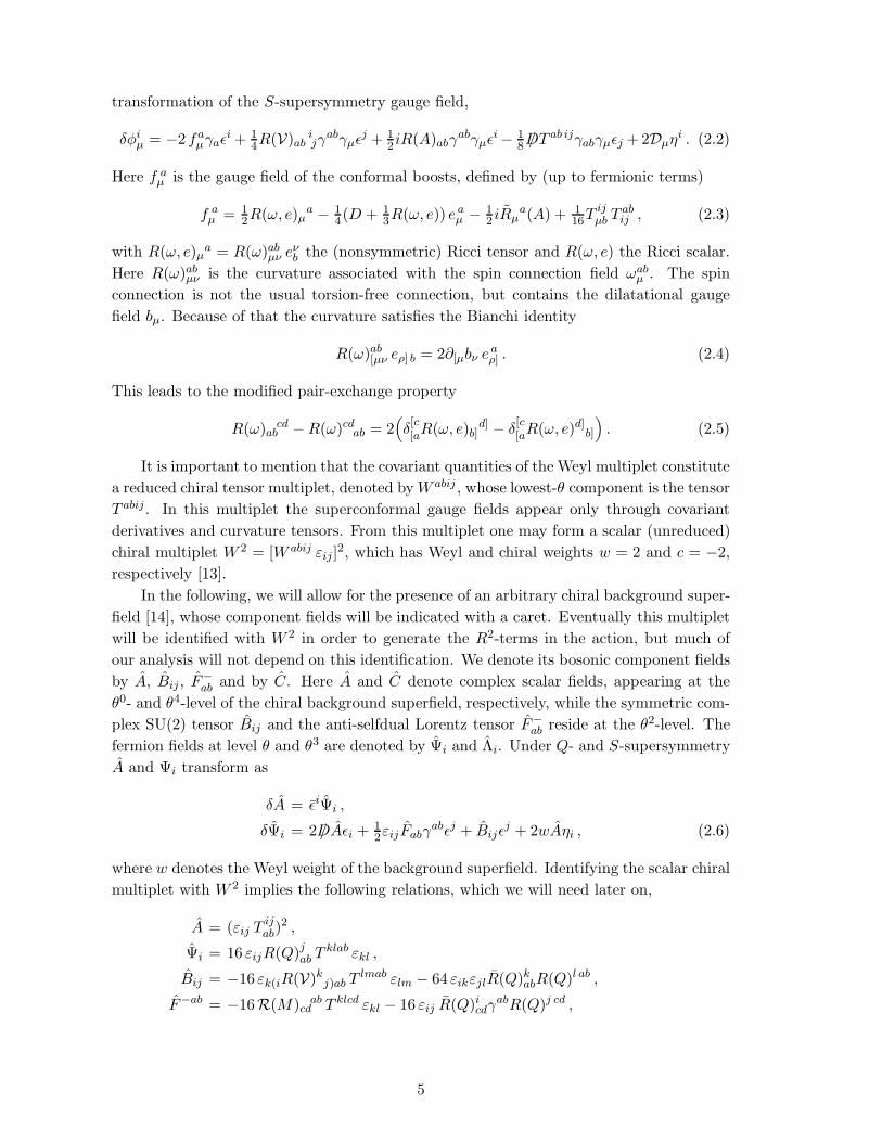
In the following, we will allow for the presence of an arbitrary chiral background super-

field [14], whose component fields will be indicated with a caret. Eventually this multiplet

will be identified with W 2 in order to generate the R2-terms in the action, but much of

our analysis will not depend on this identification. We denote its bosonic component fields

by A, Bij , F−ab and by C. Here A and C denote complex scalar fields, appearing at the

θ0- and θ4-level of the chiral background superfield, respectively, while the symmetric com-

plex SU(2) tensor Bij and the anti-selfdual Lorentz tensor F−ab reside at the θ2-level. The

fermion fields at level θ and θ3 are denoted by Ψi and Λi. Under Q- and S-supersymmetry

A and Ψi transform as

δA = ǫiΨi ,

δΨi = 2D/ Aǫi + 12εijFabγ

abǫj + Bijǫj + 2wAηi , (2.6)

where w denotes the Weyl weight of the background superfield. Identifying the scalar chiral

multiplet with W 2 implies the following relations, which we will need later on,

A = (εij Tijab)

2 ,

Ψi = 16 εijR(Q)jab Tklab εkl ,

Bij = −16 εk(iR(V)kj)ab Tlmab εlm − 64 εikεjlR(Q)kabR(Q)l ab ,

F−ab = −16R(M)cdab T klcd εkl − 16 εij R(Q)icdγ

abR(Q)j cd ,

5

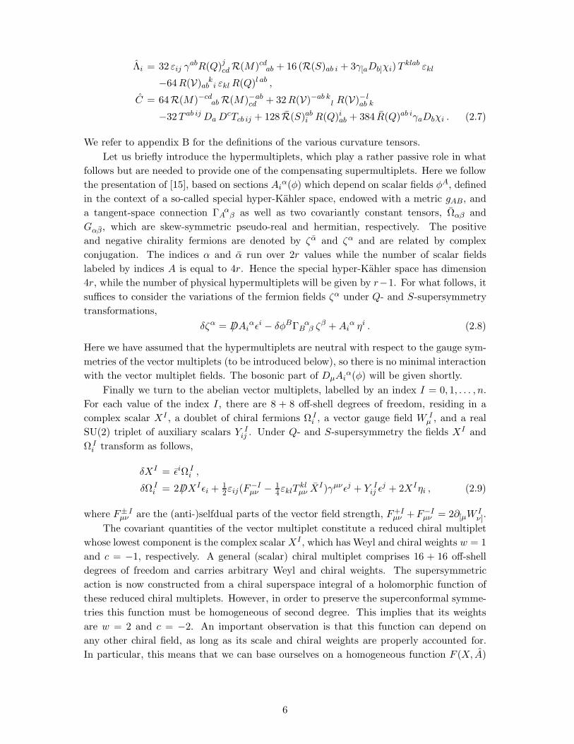
Λi = 32 εij γabR(Q)jcd R(M)cdab + 16 (R(S)ab i + 3γ[aDb]χi)T

klab εkl

−64R(V)abki εklR(Q)l ab ,

C = 64R(M)−cdab R(M)−cd

ab + 32R(V)−ab kl R(V)−ab

lk

−32T ab ij DaDcTcb ij + 128 R(S)ab

i R(Q)iab + 384 R(Q)ab iγaDbχi . (2.7)

We refer to appendix B for the definitions of the various curvature tensors.

Let us briefly introduce the hypermultiplets, which play a rather passive role in what

follows but are needed to provide one of the compensating supermultiplets. Here we follow

the presentation of [15], based on sections Aiα(φ) which depend on scalar fields φA, defined

in the context of a so-called special hyper-Kahler space, endowed with a metric gAB, and

a tangent-space connection ΓAα

β as well as two covariantly constant tensors, Ωαβ and

Gαβ , which are skew-symmetric pseudo-real and hermitian, respectively. The positive

and negative chirality fermions are denoted by ζ α and ζα and are related by complex

conjugation. The indices α and α run over 2r values while the number of scalar fields

labeled by indices A is equal to 4r. Hence the special hyper-Kahler space has dimension

4r, while the number of physical hypermultiplets will be given by r−1. For what follows, it

suffices to consider the variations of the fermion fields ζα under Q- and S-supersymmetry

transformations,

δζα = D/Aiαǫi − δφBΓB

αβ ζ

β +Aiα ηi . (2.8)

Here we have assumed that the hypermultiplets are neutral with respect to the gauge sym-

metries of the vector multiplets (to be introduced below), so there is no minimal interaction

with the vector multiplet fields. The bosonic part of DµAiα(φ) will be given shortly.

Finally we turn to the abelian vector multiplets, labelled by an index I = 0, 1, . . . , n.

For each value of the index I, there are 8 + 8 off-shell degrees of freedom, residing in a

complex scalar XI , a doublet of chiral fermions Ω Ii , a vector gauge field W I

µ , and a real

SU(2) triplet of auxiliary scalars Y Iij . Under Q- and S-supersymmetry the fields XI and

Ω Ii transform as follows,

δXI = ǫiΩ Ii ,

δΩ Ii = 2D/XIǫi + 1

2εij(F−Iµν − 1

4εklTklµν X

I)γµνǫj + Y Iij ǫ

j + 2XIηi , (2.9)

where F± Iµν are the (anti-)selfdual parts of the vector field strength, F+I

µν +F−Iµν = 2∂[µW

Iν].

The covariant quantities of the vector multiplet constitute a reduced chiral multiplet

whose lowest component is the complex scalar XI , which has Weyl and chiral weights w = 1

and c = −1, respectively. A general (scalar) chiral multiplet comprises 16 + 16 off-shell

degrees of freedom and carries arbitrary Weyl and chiral weights. The supersymmetric

action is now constructed from a chiral superspace integral of a holomorphic function of

these reduced chiral multiplets. However, in order to preserve the superconformal symme-

tries this function must be homogeneous of second degree. This implies that its weights

are w = 2 and c = −2. An important observation is that this function can depend on

any other chiral field, as long as its scale and chiral weights are properly accounted for.

In particular, this means that we can base ourselves on a homogeneous function F (X, A)

6

which is of degree two, that depends on the complex fields XI and on the scalar of the

background chiral multiplet, A. Therefore this function satisfies the relation,

XIFI +wAFA = 2F . (2.10)

Here FI and FA denote the derivatives of F (X, A) with respect to XI and A, respectively,

and w denotes the weight of the background field.

In the absence of a background it is known that there are representations of the theory

for which no function F (X) exists, although after a suitable electric/magnetic duality

transformation it can be rewritten in a form that exhibits the function F (X). In the

presence of a background, this feature does not seem to play a direct role, so we will simply

assume the existence of F (X, A). For some of the notations and background material,

see [14] and the third reference of [12], where a general chiral multiplet in supergravity is

discussed.

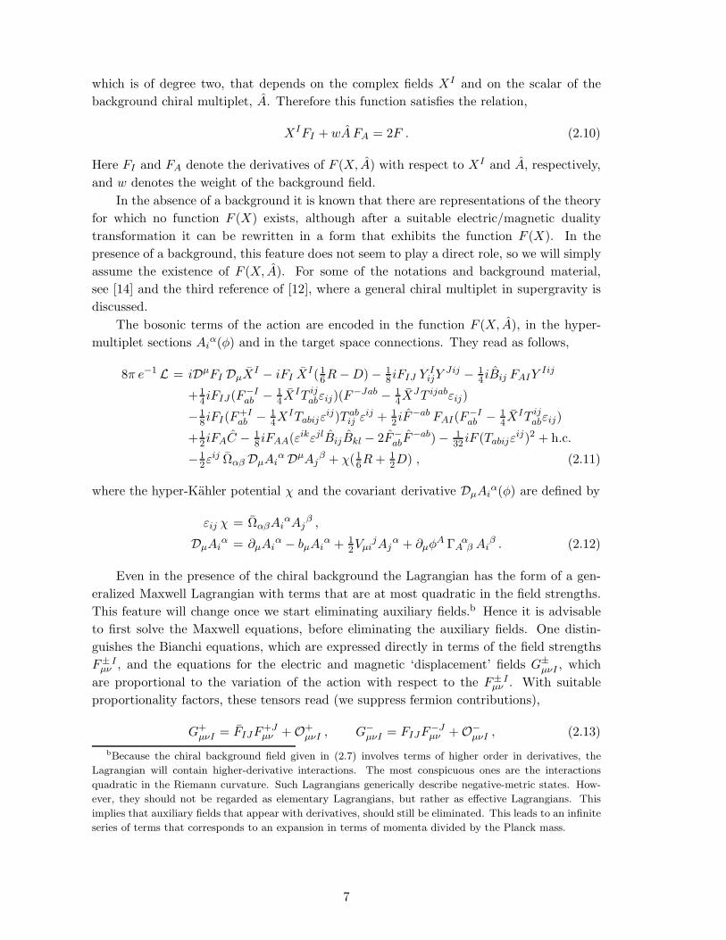
The bosonic terms of the action are encoded in the function F (X, A), in the hyper-

multiplet sections Aiα(φ) and in the target space connections. They read as follows,

8π e−1 L = iDµFI DµXI − iFI X

I(16R−D) − 1

8 iFIJ YIijY

Jij − 14 iBij FAIY

Iij

+14 iFIJ(F−I

ab − 14X

IT ijabεij)(F

−Jab − 14X

JT ijabεij)

−18 iFI(F

+Iab − 1

4XITabijε

ij)T abij ε

ij + 12 iF

−ab FAI(F−Iab − 1

4XIT ij

abεij)

+12 iFAC − 1

8 iFAA(εikεjlBijBkl − 2F−abF

−ab) − 132 iF (Tabijε

ij)2 + h.c.

−12ε

ij Ωαβ DµAiα DµAj

β + χ(16R+ 1

2D) , (2.11)

where the hyper-Kahler potential χ and the covariant derivative DµAiα(φ) are defined by

εij χ = ΩαβAiαAj

β ,

DµAiα = ∂µAi

α − bµAiα + 1

2VµijAj

α + ∂µφA ΓA

αβ Ai

β . (2.12)

Even in the presence of the chiral background the Lagrangian has the form of a gen-

eralized Maxwell Lagrangian with terms that are at most quadratic in the field strengths.

This feature will change once we start eliminating auxiliary fields.b Hence it is advisable

to first solve the Maxwell equations, before eliminating the auxiliary fields. One distin-

guishes the Bianchi equations, which are expressed directly in terms of the field strengths

F± Iµν , and the equations for the electric and magnetic ‘displacement’ fields G±

µνI , which

are proportional to the variation of the action with respect to the F± Iµν . With suitable

proportionality factors, these tensors read (we suppress fermion contributions),

G+µνI = FIJF

+Jµν + O+

µνI , G−µνI = FIJF

−Jµν + O−

µνI , (2.13)

bBecause the chiral background field given in (2.7) involves terms of higher order in derivatives, the

Lagrangian will contain higher-derivative interactions. The most conspicuous ones are the interactions

quadratic in the Riemann curvature. Such Lagrangians generically describe negative-metric states. How-

ever, they should not be regarded as elementary Lagrangians, but rather as effective Lagrangians. This

implies that auxiliary fields that appear with derivatives, should still be eliminated. This leads to an infinite

series of terms that corresponds to an expansion in terms of momenta divided by the Planck mass.

7

where

O+µνI = 1

4(FI − FIJXJ )Tµνijε

ij + F+µν FIA ,

O−µνI = 1

4(FI − FIJXJ )T ij

µν εij + F−µν FIA . (2.14)

In terms of these tensors the Maxwell equations in the absence of charges read (in the

presence of the background), Da(F− − F+)Iab = 0, and Da(G− −G+)ab I = 0. Eventually

we will solve these equations for a given configuration of electric and magnetic charges

in a stationary geometry. These charges will be denoted by (pI , qJ) and are normalized

such that for a stationary multi-centered solution with charges at centers ~xA, Maxwell’s

equations read

∂µ

(√g(F− − F+)I µt

√g(G− −G+)µt

I

)

= 4iπ∑

A

δ(~x − ~xA)

(

pIA

qAI

)

. (2.15)

Observe that√g (F− − F+)I µν and

√g (G− −G+)µν

I are Weyl invariant quantities.

The field equations of the vector multiplets are subject to equivalence transforma-

tions corresponding to electric/magnetic duality, which do not affect the fields of the Weyl

multiplet and of the chiral background. As is well-known, the following two complex

(2n + 2)-component vectors transform linearly under the SP(2n+ 2;R) duality group,(

XI

FI(X, A)

)

and

(

F± Iab

G±ab I

)

, (2.16)

but more such vectors can be constructed. The first vector has weights w = 1 and c = −1,

whereas the second one has zero Weyl and chiral weights. From (2.15) and (2.16) it follows

that also the charges (pI , qJ) comprise a symplectic vector. In the presence of these charges

the symplectic transformations are restricted to an integer-valued subgroup that keeps the

lattice of electric/magnetic charges invariant.

The electric/magnetic duality transformations cannot be performed at the level of the

action, but only at the level of the equations of motion. After applying the transformations

one can find the corresponding action. This is then characterized by a relation between

two different functions F (X, A). While the background field A is inert under the dualities,

it nevertheless enters in the explicit form of the transformations. For a discussion of this

phenomenon and its consequences, see [14].

The various transformation rules only take a symplectically invariant form when one

solves the field equations for the auxiliary fields Y Iij [14],

Y Iij = iN IJ

(

FJA Bij − FJA εikεjl Bkl)

. (2.17)

With this result we can cast δΩIi and δΨi in a symplectically covariant form (we suppress

fermionic bilinears),(

δΩIi

δ(FIJΩJi + FIAΨi)

)

= 2D/

(

XI

FI

)

ǫi + 12εijγ

abǫj[(

F−Iab

G−abI

)

− 14εklT

klab

(

XI

FI

)]

+iBij ǫj

(

N IJFJA

FIJNJKFKA

)

− iεikεjlBkl ǫj

(

N IJ FJA

FIJNJKFKA

)

+ 2ηi

(

XI

FI

)

. (2.18)

8

In the above formulae, N IJ is the inverse of

NIJ = −iFIJ + iFIJ . (2.19)

3. More supersymmetry variations

In the superconformal tensor calculus two of the matter supermultiplets are required in

order to provide the compensating degrees of freedom that are essential for making the sys-

tem equivalent to a Poincare supergravity theory. One of these multiplets is always a vector

multiplet and for the second one we choose a hypermultiplet. This implies that the number

of physical vector multiplets is equal to n and the number of physical hypermultiplets is

equal to r − 1.

In this section we will evaluate the supersymmetry variations of a number of spinors

that are needed in the analysis in subsequent sections. The results of this section follow

from those given in the previous one. Some of the spinors can act as suitable compensating

fields with regard to S-supersymmetry. We also evaluate the supersymmetry variations of

the supercovariant derivative of the spinors belonging to one of the matter multiplets as

well as the variation of the supersymmetry field strength R(Q)iab. This analysis naturally

leads us to the definition of a number of bosonic quantities that play a central role in what

follows.

The first spinor we consider is expressed in terms of hypermultiplet fermions and reads

ζH

i ≡ χ−1ΩαβAiα ζβ . (3.1)

Its supersymmetry variation reads

δζH

i = χ−1ΩαβAiαD/Aj

β ǫj + εijηj , (3.2)

where χ is the hyper-Kahler potential defined in (2.12) and where terms proportional to

the fermion fields are suppressed. It is important to realize that one has the decomposition

[15]

χ−1ΩαβAiαDµAj

β = 12kµ εij + kµ ij , (3.3)

where kµ is real and given by

kµ = χ−1(∂µ − 2 bµ)χ , (3.4)

and kµ ij is symmetric in i, j and pseudoreal so that it transforms as a vector under SU(2).

Its explicit form is not important for us. Hence we write

δζH

i = 12k/ εij ǫ

j + k/ ij ǫj + εij η

j . (3.5)

In the vector multiplet sector there are two spinors that can be constructed which

transform as scalars under electric/magnetic duality. One, denoted by ζV

i , transforms

inhomogeneously under S-supersymmetry. It can be conveniently introduced from the

variation of the symplectically invariant expression (with w = 2 and c = 0)

e−K = i[

XI FI(X, A) − FI(X,¯A)XI

]

. (3.6)

9

Here K resembles the Kahler potential in special geometry. Its supersymmetry variation

leads to the spinor

ζV

i ≡ −(

ΩIi

∂

∂XI+ Ψi

∂

∂A

)

K = −i eK[

(FI − XJFIJ)ΩIi − XIFIA Ψi

]

. (3.7)

It is obvious that ζVi transforms as a scalar under symplectic reparameterizations, because

it follows from a symplectic scalar. This can also been seen by noting that ζVi is generated

by the symplectic product FI δXI − XI δFI . This leads us to introduce yet another spinor

ζ0i generated by FI δX

I −XI δFI ,

ζ0

i ≡ (FI −XJFIJ)ΩIi −XIFIA Ψi . (3.8)

This spinor is invariant under S-supersymmetry and it vanishes in the absence of the chiral

scalar background field. However, it does not play a useful role in what follows.

Under Q- and S-supersymmetry ζVi transforms as

δζV

i = eKD/ e−Kǫi + 2iA/ ǫi − 12 iεij F

−ab γ

abǫj

+eKN IJ[

(FI − FIKXK)FJA Bij − (FI − FIKX

K)FJA εikεjlBkl]

ǫj + 2 ηi ,(3.9)

where we ignored higher-order fermionic terms. The quantity Aµ resembles a covariantized

(real) Kahler connection and F−ab is an anti-selfdual tensor,

Aµ = 12eK

(

XJ ↔

Dµ FJ − FJ

↔

Dµ XJ)

,

F−ab = eK

(

FI F−Iab − XI G−

ab I

)

. (3.10)

There is another symplectically invariant contraction of the field strengths,

eK(

FI F−Iab −XI G−

ab I

)

+ 14 iεijT

ijab = eK FIA

[

wA(F−Iab − 1

4XI εijT

ijab) −XI F−

ab

]

, (3.11)

which appears in the variation of ζ0i .

As it turns out we also need to consider the supersymmetry variations of derivatives of

the fermion fields. However, one can restrict oneself to the variation of the supercovariant

derivative of a single fermion field, as we will discuss in the next section. For this field we

choose ζHi , for which we present the variation under Q- and S-supersymmetry,

δ(DµζH

i ) = 12Dµ(χ−1Dνχ) εij γ

νǫj + Dµkνij γνǫj

− 132χ

−1/2(δjiDν − kνikε

kj)(χ1/2T lmab εlm) γνγabγµǫj

+εij[

fµaγaǫ

j − 18R(V)jkabγ

abγµǫk − 1

4 iR(A)abγabγµǫ

j]

+(14χ

−1D/χ εij + 12k/ ij) γµη

j . (3.12)

Finally we present the variation of the curvature tensor R(Q)iµν , defined by

R(Q)iµν = 2D[µψiν] − γ[µφ

iν] − 1

8Tijabγ

abγ[µψν]j , (3.13)

where φiµ is the dependent gauge field associated with S-supersymmetry, defined in ap-

pendix B. The variation of this tensor reads,

δR(Q)iab = −12D/T

ijab ǫj +R(V)−ab

ij ǫ

j

−12R(M)ab

cd γcdǫi + 1

8Tijcd γ

cdγab ηj , (3.14)

where R(M)abcd is defined in appendix B.

10

4. Fully supersymmetric field configurations

From the supersymmetry variations presented in the previous two sections one can de-

termine the conditions on the bosonic fields imposed by the requirement of full N = 2

supersymmetry. These conditions follow from setting all Q-supersymmetry variations

of the fermionic quantities to zero. However, these variations are determined up to an

S-supersymmetry transformation. Thus one can either impose the vanishing of all Q-

variations up to a uniform S-supersymmetry transformation, or one can restrict oneself

to linear combinations that are invariant under S-supersymmetry and require their Q-

supersymmetry variations to vanish. Examples of such S-invariant combinations are, for

instance, ΩIi −XIζV

i and Ψi − wA ζVi , while the spinor ζ0

i is S-invariant by itself. In this

section we will include an arbitrary number of hypermultiplets.

We start by considering the S-supersymmetric linear combination of ζVi and ζH

i . Re-

quiring its Q-supersymmetry variation to vanish for all supersymmetry parameters, we

establish immediately that

F−ab = Bij = kµ ij = Aµ = 0 , (4.1)

and

Dµ

(

eKχ)

= 0 . (4.2)

Comparing the supersymmetry variations of the vector multiplet fermions to those of ζVi

leads to

F−Iab = 1

4εklTklab X

I ,

G−abI = 1

4εklTklab FI ,

Dµ

(

eK/2XI)

= Dµ

(

eK/2FI

)

= 0 . (4.3)

These equations themselves again imply that F−ab and Aµ vanish. Furthermore, by using

the explicit expression of the tensors G−abI , one finds that F−

ab = 0. The last two equations

imply that we also have

Dµ

(

ewK/2A)

= 0 . (4.4)

From the supersymmetry variations of the hypermultiplets we find a similar result,

Dµ

(

χ−1/2Aiα)

= 0 . (4.5)

Observe that all the above equations are K-invariant.

Subsequently we compare the supersymmetry variations of the spinors χi and ζVi , which

leads to the relations,

D = R(V)abij = R(A)ab = Da

(

e−K/2T abij)

= 0 . (4.6)

With these results it follows that the vector field strengths satisfy the following equations,

DaF−Iab = DaG−

abI = 0 , (4.7)

11

which imply (but are stronger than) the equations of motion and the Bianchi identities for

the vector fields.

A similar calculation for the curvature R(Q)iab yields

DcTijab = −1

2DdK(

δdc T

ijab − 2δd

[a Tijb]c + 2ηc[a T

ij db]

)

,

R(M)abcd = 0 . (4.8)

The first equation is consistent with the result found earlier. Because D = 0, R(M)abcd is

just the traceless part of the curvature tensor R(ω)abcd associated with the spin connection

field ωabµ (which at this stage depends on the dilatational gauge field bµ). Upon suppressing

bµ, this tensor becomes equal to the Weyl tensor. Hence the above condition will eventually

lead to the conclusion that N = 2 supersymmetric solutions require a conformally flat

spacetime. We stress again that all of the above conditions are K-invariant.

Before continuing, let us make a few remarks. First of all, we note that at this stage all

equations are consistent with all the superconformal symmetries; in particular, we have not

yet fixed a scale. All the above results are also manifestly consistent with electric/magnetic

duality. Secondly we found a number of conditions on the chiral background field, namely

Bij = F−ab = 0 and the covariant constancy of exp(wK/2)A. So far no conditions have been

derived for its highest-θ component C, but by considering the supersymmetry variation of

the spinor Λi one can easily show that C = 0. It is illuminating to verify whether these

results hold for the chiral field starting with A = [T abijεij ]2. It turns out that they are

indeed satisfied on the basis of the above results, with the exception of the C component

which contains a term proportional to the second derivative of Tab ij. Also in view of later

applications we consider this term in more detail and note that the bosonic contribution

to the second derivative of T ijab takes the form

DµDcTijab = DµDcT

ijab + fµc T

ijab − 2fµ[a T

ijb]c + 2f d

µ ηc[a Tijb]d . (4.9)

Consequently

DµDaT ij

ab = DµDaT ijab − f a

µ T ijab . (4.10)

With this result we consider the relevant term in C,

T ab ij DaDcTcb ij = T ab ij DaDcTcb ij − f c

a Tab ij Tcb ij , (4.11)

where we note in passing that, in the first term on the right-hand side, we can symmetrize

the derivatives as the antisymmetric part vanishes due to the (anti-)selfduality of the T -

fields. By using the equations found above, we can work out the double derivative on the

T -field, and verify whether it vanishes against the second term proportional to f aµ .

Rather than determining f aµ in this way, we continue and consider the supersymmetry

variation of the supercovariant derivatives of fermion fields. First we make the observation

that the derivatives of S-invariant combinations of fields, whose Q-supersymmetric varia-

tions were already required to vanish in the bosonic background, will still vanish. But we

can also compare the variation of the supercovariant derivative of a fermion field to the

12

variation of a fermion field without derivatives. Consider for example the Q-variation of

the following S-invariant expression

DµζH

i + (−14χ

−1D/χ δji + 1

2k/ ikεkj) γµζ

H

j . (4.12)

The derivative of another fermion field can now be written as the derivative of an S-

invariant linear combination of that fermion field with a bosonic expression times ζHi , which

is one of the previously considered linear combinations whose vanishing variation in the

supersymmetric background has already been ensured, a term proportional to (4.12) and

terms proportional to ζHi without a derivative. Therefore, once we have imposed that the

variation of (4.12) vanishes, then the variation of the derivative of every other fermion field

is guaranteed to vanish against some bosonic term times the variation of ζHi . Consequently

variations of such linear combinations can be ignored and our only task is to require that the

variation of (4.12) vanishes. Note that the above argument can be extended to variations

of multiple derivatives as well, which therefore can also be ignored.

Imposing the condition that the Q-supersymmetry variation of (4.12) vanishes, we find

that most terms vanish already by virtue of previous results and we are left with just one

more equation,

Dµ

(

χ−1Daχ)

= 12

(

χ−1Dµχ)(

χ−1Daχ)

− 14e

aµ

(

χ−1Dcχ)2. (4.13)

Note that we have superconformal derivatives here which involve the gauge field fµa asso-

ciated with conformal boosts. Upon using the previous results (4.2), (4.3) and (4.5), all

equations coincide. Hence we are left with the following equation for f aµ ,

fµa = −1

2Dµ

(

eK Dae−K)

+ 14

(

eK Dµe−K)(

eK Dae−K)

− 18e

aµ

(

eK Dce−K)2, (4.14)

which is K-invariant. With this result we can verify that the term (4.11) vanishes as well,

so that we establish that the C component of the Weyl multiplet vanishes. The above

equation (4.14) can be rewritten as

R(ω, e)µa − 1

6R(ω, e) e aµ = −1

8Tijµb T

abij + DµDaK + 1

2DµKDaK − 14e

aµ (DcK)2 . (4.15)

So far the analysis is valid for any chiral background field. For the rest of this section

we assume that the chiral multiplet is given by (2.7) so that at this point we have identified

all supersymmetric configurations in the presence of R2-terms. The results obtained so far

are in a manifestly conformally covariant form. We can now impose gauge choices and set

bµ = 0 (because of the K-invariance the conditions found above are in fact independent of

bµ) and exp[K] equal to a constant. (Alternative we may use exp[K] as a compensator to

make all quantities invariant under scale transformations, at which point the field bµ will

drop out.) The values of exp[−K] and χ are related. With the choice that we made for the

action we find that χ = −2 exp[−K] as a result of the field equation for the field D. For

future reference, we give both the field equations for the field D and for the U(1) gauge

field Aµ,

3 e−K + 12χ = −192iD(FA − FA)

13

+4i

(εij Tijcd)

−2 εklTabkl (FI F

−Iab −XI G−

abI ) − h.c.

, (4.16)

e−KAa = 128iDb(

FAR(A)−ab − h.c.)

− 8Dc(FA + FA)Tijab Tijcb

+8(FA − FA)(

T ijabDcT

cbij − Tijab DcT

cbij)

−8Db

(εij Tijde)

−2 εklTkl c

[a (FI F−Ib]c −XI G−

b]cI) + h.c.

. (4.17)

Observe that these field equations can only be found from the action, and cannot be ob-

tained from requiring that the supersymmetry variations vanish, because the action consists

of a linear combination of two actions that are separately invariant, corresponding to the

vector multiplets and the hypermultiplets, respectively (we point out that the hypermul-

tiplets contribute only fermionic terms to (4.17), which have been suppressed above). The

coefficient of the Ricci scalar in the action is now equal to −(16π)−1 exp[−K], so that

Newton’s constant equals GN = exp[K], assuming a conventionally normalized flat metric.

Furthermore we can put the gauge fields Aµ and Vµij to zero, because their field strengths

vanish.

The most general N = 2 supersymmetric background can now be characterized as

follows. First of all the spacetime has zero Weyl tensor and is thus conformally flat. Its

Ricci tensor is given by

Rµν = −18T

ijµρ Tijν

ρ , (4.18)

where Tijµν (T ijµν) is a covariantly constant (anti-)selfdual tensor. Furthermore we have a

number of constants XI . The electric/magnetic field strengths are also covariantly constant

and given by

F−Iµν = 1

4εklTklµν X

I , G−µνI = 1

4εklTklµν FI . (4.19)

By using relations for products of (anti-)selfdual tensors one can verify that the in-

tegrability condition that follows from the covariant constancy of the tensor fields T ijµν , is

identically satisfied. In order to investigate explicit solutions one chooses coordinates such

that the metric reads

gµν = e2f(x)+K ηµν , (4.20)

with ηµν the flat Minkowski metric (normalized in the standard way). We included the

factor exp[K], which we adjusted to a constant, so that the function f is independent of

the scale. To have a vanishing Ricci scalar the function exp[f ] must be harmonic,

ηµν∂µ∂ν ef = 0 . (4.21)

The remaining conditions are (here we raise and lower indices with the flat metric)

Rµν = 2∂µ∂νf − 2∂µf ∂νf + ηµν (∂ρf)2 = −18T

ijµρ Tijν

ρ e−2f−K ,

∂µTijνρ = 2∂µf T

ijνρ − 2∂[νf T

ijρ]µ + 2ηµ[ν T

ijρ]σ ∂

σf . (4.22)

As a result of the second condition we derive

∂[µTijνρ] = ∂µT ij

µν = 0 , (4.23)

14

so that T ijµν is a harmonic tensor.

We are interested in time-independent solutions so that we assume that f is indepen-

dent of the time t. In that case we can express the tensor field in terms of a complex

potential Φ. Denoting spatial world indices by a, b, c, we may write

εijTij

ab= εabc ∂cΦ , εijT

ijta = i∂aΦ , (4.24)

where Φ is a complex harmonic function. The equations are now solved for by

Φ = 4 z ef+K/2 , (4.25)

with z a constant phase factor, and f satisfying

ef ∂a∂bef = 3 ∂ae

f ∂bef − δab (∂ce

f )2 . (4.26)

This system of differential equations can be integrated. Its solution is unique (up to

translations) and is given by exp[f(r)] = c/r, where c is a real constant. This leads to

a Bertotti-Robinson spacetime, the geometry of which describes the near-horizon limit of

an extremal black hole with horizon at r = 0. Thus there exist no fully supersymmetric

multi-centered solutions, which is not suprising in view of the fact that the differential

equations (4.26) are nonlinear in exp[f ]. The field A is now equal to

A = (εijTijab)

2 =64 e−K

z2 e2f(r)(∂af)2 . (4.27)

From evaluating (4.19) it follows that the electric and magnetic charges are equal to

pI = c eK/2 [z XI + z XI ] , qI = c eK/2 [z FI + z FI ] . (4.28)

With this result we consider the so-called BPS mass, which takes the form

Z = eK/2(pI FI − qI XI) = −iz c , (4.29)

so that we obtain the equations (sometimes called stabilization equations) [1, 2],

Z

(

XI

FI

)

− Z

(

XI

FI

)

= i e−K/2(

pI

qI

)

. (4.30)

Observe that this result is covariant with respect to electric/magnetic duality.

Finally we note that the area in Planck units equals

Area

GN= 4π c2 = 4π |Z|2 . (4.31)

This does not determine the black hole entropy, because the Bekenstein-Hawking area law

is not applicable for these black holes [10]. After including an appropriate correction one

obtains instead [6]

S = π[

|Z|2 − 256 Im[FA(XI , A)]]

, (4.32)

where A = −64 Z−2 e−K.

15

In section 5 we will be using another coordinate frame with line element given by

ds2 = −e2g dt2 + e−2g d~x2 . (4.33)

The conformal coordinates of this section are related to those of the above frame by

t −→ d

c2 eKt , ~x −→ d

~x

|~x|2 , (4.34)

where d is some real constant. The function e−2g in (4.33) corresponding to the line element

(4.20) is equal to

e−2g =c2 eK

|~x|2 . (4.35)

For later reference let us give the field strengths (4.19) in the frame (4.33),

F− Itm = izXI eg x

m

|~x|2 , G−tm I = izFI eg x

m

|~x|2 . (4.36)

Here (t,m) denote world indices in the frame (4.33). For these expressions Maxwell’s equa-

tions (2.15) are satisfied with the charges defined in (4.28). Observe that, when calculating

Maxwell’s equations directly from (4.19) in the frame (4.20), one encounters a different

sign as compared to (4.28). This is related to the fact that a charge located at the origin

in the frame (4.33) corresponds to a charge at infinity in the conformal coordinates used

in this section. When evaluating Maxwell’s equations in the latter coordinates one is con-

sidering the corresponding mirror charge placed at the origin. This explains the apparent

sign discrepancy.

5. N = 1 supersymmetric field configurations

A general analysis of the conditions for residual N = 1 supersymmetry is extremely cum-

bersome. Therefore we base ourselves on a given class of embeddings of the residual

supersymmetry by imposing the following condition on the supersymmetry parameters,

h ǫi = εij γ0 ǫj , (5.1)

where h is some unknown phase factor which is in general not constant, and which trans-

forms under U(1) with the same weight as the fields XI . At the moment we proceed

without imposing gauge choices. Therefore the choice of γ0 is somewhat arbitrary, because

it can be changed into any other gamma matrix by means of a local Lorentz transforma-

tion. However, we will eventually impose a gauge condition on the vierbein field, which

restricts the local Lorentz transformations to the three-dimensional rotationsc. It is clear

that (5.1) is then consistent with spatial rotations and SU(2) transformations, although

we will not require the solutions to be invariant under these symmetries. An embedding

cIn view of this, Lorentz covariant derivatives should be applied with caution, as the various equations

we are about to derive are not Lorentz covariant.

16

condition such as (5.1) was also used in the analysis presented in [3, 4] of N = 2 theories

without R2-interactions.

Subject to this embedding we can now evaluate the conditions for N = 1 supersym-

metry by following essentially the same steps as in the previous section. We start by

considering the variations of the vector multiplet fermions and of the spinors ζV

i and ζH

i .

They lead to the equations

Bij = ka ij = 0 , (5.2)

and

A0 = 0 , Ap = Re[hF−0p] ,

D0(χeK) = 0 , Dp(χeK) = 2χeK Im[hF−0p] , (5.3)

where the indices (0, p) with p = 1, 2, 3 refer to the tangent space. With this result we find

that the variation of ζVi simplifies considerably and reduces to

δζV

i = χ−1D/χ ǫi + 2 ηi . (5.4)

For the hypermultiplets we find the same condition as for full supersymmetry,

Da(χ−1/2Ai

α) = 0 . (5.5)

Returning to the vector multiplet spinors, we then establish the relations

D0(χ−1/2XI) = D0(χ

−1/2 FI) = 0 , (5.6)

and

Dp(χ−1/2 XI) = −hχ−1/2(F−I

0p − 14εklT

kl0p X

I) ,

Dp(χ−1/2 FI) = −hχ−1/2(G−

0pI − 14εklT

kl0p FI) . (5.7)

These last two equations transform covariantly with respect to electric/magnetic duality.

Taking their symplectically invariant product with (XI , FI) leads to the previous equations

(5.3).

Subsequently we consider the variations of the spinor χi, which lead to

R(V)abij = 0 ,

Dc(χ1/2 T ijc0 εij) = −6hχ1/2D ,

Dc(χ1/2 T ijcp εij) = 8ihχ1/2 R(A)−0p . (5.8)

Note that the first equation is consistent with the fact that Bij vanishes (c.f. (2.7)). In

view of the fact that the SU(2) field strengths vanish, we will set the SU(2) connections to

zero in what follows.

The variations for the field strength R(Q)iab lead to

D0Tijab − 1

2χ−1Ddχ

(

δd0 T

ijab − 2δd

[a Tijb]0 + 2η0[a T

ij db]

)

= 0 ,

DpTijab − 1

2χ−1Ddχ

(

δdp T

ijab − 2δd

[a Tijb]p + 2ηp[a T

ijb]

d)

= 4h εij R(M)−ab 0p . (5.9)

17

Finally we consider the variation of derivatives of fermion fields. The arguments pre-

sented below (4.12) about the fact that there is no need to consider more than one of these

variations, apply also to residual supersymmetry. Hence we consider the Q-supersymmetry

variation of (4.12), making use of the previously obtained results. This yields the following

equation,

Dµ(χ−1Daχ) + 14 (χ−1Dcχ)2 eµ

a − 12(χ−1Dµχ)(χ−1Daχ) =

−32D(eµ

a − 2eµ0 ηa0) − 2i[R(A)+ −R(A)−]µ

a − 4iR(A)−µ0 ηa0 . (5.10)

All terms in this equation are real, with the exception of the last term, from which it follows

that R(A)±a0 must be purely imaginary, so that

R(A)a0 = R(A)pq = 0 . (5.11)

Just as before, (5.10) fixes the value of the gauge field fµa, which takes the (K-invariant)

form

fµa = −1

2Dµ(χ−1Daχ) − 18(χ−1Dcχ)2 eµ

a + 14(χ−1Dµχ)(χ−1Daχ)

−34D(eµ

a − 2eµ0 ηa0) − i[R(A)+ −R(A)−]µ

a − 2iR(A)−µ0 ηa0 . (5.12)

Comparing with (2.3) yields

R(ω, e)µa − 1

6R(ω, e) e aµ =

−Dµ(χ−1Daχ) − 14(χ−1Dcχ)2 eµ

a + 12(χ−1Dµχ)(χ−1Daχ)

−18T

ijµb T

abij −D (eµ

a − 3eµ0 ηa0) + i[R(A)µ0 η

a0 − R(A)0a eµ

0] . (5.13)

Let us briefly return to (5.8) and (5.9) and explore the consequences of (5.11). The

first equation of (5.9) yields

D0Tij 0p − 1

2χ−1D0χT

ij 0p + 12χ

−1DqχTij qp = 0 . (5.14)

Making use of this, the last equation (5.8) leads to

DqTij qp + χ−1D0χT

ij 0p = −2ih εij R(A)0p , (5.15)

which can be rewritten as

D[pTijq]0 εij = 2iR(A)pqh− 1

2χ−1D0χT

ijpq εij . (5.16)

Observe that so far we have not imposed any gauge conditions. In order to proceed

we will now choose a gauge condition that eliminates the freedom of making (local) scale

transformations and conformal boosts. This gauge condition amounts to choosing bµ = 0

and χ constant. Therefore the covariant derivative Da contains only the spin connection

fields and the U(1) connection, when appropriate.

In this gauge, (5.16) and the second equation of (5.8) read,

hD[pTijq]0 εij = 2iR(A)pq , hDpT ij

p0 εij = 6D . (5.17)

18

Furthermore we establish from (5.13) that

R(ω, e) = −3D . (5.18)

Then, from the second equation of (5.9), one derives the following expressions for the

components of the curvature tensor R(M)ab cd,

R(M)pq 0r = 18 iεpq

s hDrTijs0 εij + h.c. ,

R(M)0r pq = 18 iεpq

s hDsTijr0 εij + h.c. ,

R(M)0p 0q = −18 hDqT

ijp0 εij + h.c. ,

R(M)pq rs = 18εrs

vεpqu hDvT

iju0 εij + h.c. . (5.19)

These expressions satisfy all the constraints (B.5) listed in appendix B, provided one makes

use of the relations for R(A) and D (cf. 5.17). Using (5.12) and the definition of R(M)

allows us to find expressions for the components of the Riemann tensor. Making use of

(5.17) we find

R(ω)pq 0r = R(ω)0r pq

= 18εpq

s[

i(hDrTijs0 εij − 1

2Tijr0 Tij s0) + h.c.

]

,

R(ω)0p 0q = R(ω)0q 0p

= −18

[

(hDqTijp0 εij + 1

2Tijq0 Tij p0) + h.c.

]

,

R(ω)pq rs = −12δ[r[p

[

hDq]Tijs]0 εij + h.c.

]

+14δ[r[p

[

T ijq]0 Tijs]0 + Tijq]0 T

ijs]0 − δq]s] T

ij v0 Tij v0

]

. (5.20)

Here we observe that, owing to (5.17), this result satisfies all the algebraic properties of

a Riemann tensor, such as cyclicity and pair exchange. We also note that, by virtue of

(5.17), (5.20) gives rise to (5.13) upon contraction.

At this point we adopt a gauge condition for local Lorentz invariance. We remind the

reader that the supersymmetry embedding condition (5.1) is obviously inconsistent with

local Lorentz invariance and presupposes that we would eventually impose such a gauge

condition. Therefore we bring the vierbein field in block-triangular form by imposing

etp = 0, thereby leaving the SO(3) tangent-space rotations unaffected. Denoting world

indices by (t,m), with m = 1, 2, 3, we parametrize the vierbein as follows,

eµ0dxµ = eg[ dt+ σm dxm ] , eµ

pdxµ = e−g emp dxm , (5.21)

where emp is the rescaled dreibein of the three-dimensional space. The corresponding

inverse vierbein components are then given by

e0t = e−g , e0

m = 0 , ept = −σp eg , ep

m = eg epm , (5.22)

where, on the right-hand side, spatial tangent-space and world indices are converted by

means of the dreibein fields emp and its inverse.

19

Now we concentrate on stationary spacetimes, so that we can adopt coordinates such

that the vierbein components are independent of the time coordinate t. In that case the

spin connection fields take the following form,

ωl pq = eg[ ωl pq + 2δl[p ∇q]g ] , ω0 pq = ωq p0 = −12e3g εpqlR(σ)l , ω0 0p = eg ∇pg , (5.23)

where ωmpq is the spin-connection field associated with the dreibein fields e in the standard

way. We used the definition

R(σ)l = εlpq ∇pσq . (5.24)

Observe that ∇pR(σ)p = 0. The covariant derivatives ∇m refer to the three-dimensional

space only. Hence they contain the three-dimensional spin connection ωmpq.

The corresponding curvature components take the following form (where we consis-

tently use three-dimensional notation on the right-hand side),

R(ω)pq 0r = 12εpq

s e4g[

∇rR(σ)s + 5R(σ)s ∇rg +R(σ)r ∇sg − 2δsr R(σ)u ∇ug]

,

R(ω)0p 0q = −e2g[

∇p∇qg + 3∇pg∇qg − δpq (∇rg)2]

+ 14e6g

[

R(σ)p R(σ)q − δpqR(σ)2]

,

R(ω)pq rs = e2g Rpq rs − 4 e2g δ[p[r

[

∇s]∇q]g + ∇s]g∇q]g − 12δs]q] (∇ug)

2]

+3e6g δ[p[r

[

R(σ)s]R(σ)q] − 12δs]q]R(σ)2

]

. (5.25)

However, for stationary solutions also other quantities than those that encode the

spacetime should be time-independent. Hence we infer that hXI , hFI , and hT ijp0 are time-

independent while (∂t + iAt)h = 0.

Until now we have restricted our attention to quantities that are supercovariant with

respect to full N = 2 supersymmetry. However, when considering residual supersymmetry,

certain linear combinations of the gravitini will still transform covariantly. To see how

this works, let us record the gravitini transformation rules in the restricted background.

Here we make use of (5.4) to argue that there is no need for including compensating S-

supersymmetry transformations. The result takes the form

δψit = 2∂tǫ

i + iAt ǫi + e2g

[

Tp −∇pg + 12 ie

2g R(σ)p]

γpγ0ǫi ,

δψim = 2∇mǫ

i − (Tm − iAm)ǫi

−ie pm εp

qr[

Tr −∇rg + 12 ie

2g R(σ)r]

γqγ0ǫi

+σm e2g[

Tp −∇pg + 12 ie

2g R(σ)p]

γpγ0ǫi , (5.26)

where we have introduced a three-dimensional world vector Tm,

Tm ≡ 14e−g em

p hT ijp0 εij . (5.27)

Now we observe that the combinations ψµi − h εijγ0ψjµ transform covariantly under the

residual supersymmetry. From the requirement that these covariant variations vanish we

deduce directly that

Tm = ∇mg − 12 ie

2g R(σ)m , h∇mh+ iAm = −12 ie

2g R(σ)m . (5.28)

20

This leads to the following expressions for the gravitini variations,

δψit = 2∂tǫ

i + iAtǫi , δψi

m = 2∇mǫi − (∇mg + h∇mh)ǫ

i . (5.29)

With these results we return to the previous identities and verify whether they are now

satisfied. It is straightforward to see that this is the case for (5.14). For the other identities

one needs the covariant derivative hDpTijq0, which, in three-dimensional notation, reads

hDpTijq0εij = 4e2g

[

∇pTq + 2TpTq − δpq (Tr)2]

. (5.30)

It is now straightforward to prove (5.17) with D given by

D = 23e2g

[

∇ 2p g − (∇pg)

2 + 14e4g (R(σ)p)

2]

. (5.31)

Furthermore, it turns out that (5.20) and (5.25) agree, provided that the curvature of the

three-space is zero,

Rmn pq = 0 , (5.32)

so that the three-dimensional space is flat. Observe that this result is consistent with the

integrability condition corresponding to the Killing spinor equations that one obtains when

setting the gravitino variations (5.29) to zero. The only remaining equations are now (5.7),

which express the abelian field strengths in terms of the other fields,

F−I0p = −eg

[

∇p(hXI) + (∇pg)hX

I − 12 ie

2gR(σ)p(hXI + hXI)

]

,

G−0pI = −eg

[

∇p(hFI) + (∇pg)hFI − 12 ie

2gR(σ)p(hFI + hFI)]

, (5.33)

where on the right-hand side, we consistently use three-dimensional tangent space indices.

With these results we derive the following expressions,

DaF−Iap = ieg εp

qr∇qF−I0r

= −12eg εp

qr∇q

[

e3gR(σ)r(hXI + hXI)

]

−ie2g εpqr ∇qg∇r(hX

I − hXI) ,

DaF−Ia0 = eg

[

∇qF−Iq0 − 2(∇qg − 1

2 ie2gR(σ)q)F−I

q0

]

= e2g[

∇ 2p (hXI) + (∇ 2

p g)hXI − (∇pg)

2 hXI + (∇pg)∇p(hXI − hXI)

−12 ie

3gR(σ)p ∇p[e−g(hXI − hXI)] + 1

2e4g(R(σ)p)2(hXI + hXI)

]

,(5.34)

and likewise for the electric/magnetic dual equations (i.e., replacing F−I by G−I , etcetera).

The imaginary parts of the above expressions correspond to Maxwell’s equations for the

abelian vector fields. Because the first expression is manifestly real, the corresponding

Maxwell equation (and its electric/magnetic dual) is satisfied. The imaginary part of the

second expression and its dual equation provide the remaining Maxwell equations, which

read

∇ 2p

[

e−g(hXI − hXI)]

= 0 ,

∇ 2p

[

e−g(hFI − hFI)]

= 0 , (5.35)

21

which shows that the functions in parentheses are harmonic. Furthermore we note the

equations

F−I0p + F+I

0p = −∇p

[

eg(hXI + hXI)]

,

G−0pI +G+

0pI = −∇p

[

eg(hFI + hFI)]

, (5.36)

so that the functions under the derivative can be regarded as electric and magnetic poten-

tials.

So far our analysis is valid for any chiral background. Now we identify this background

with (2.7) and note that the field A can be written as

A = −64e2g h2 (Tp)2 . (5.37)

With this choice for the background we now evaluate the field equations for the fields D

and Aµ, which were given in (4.16) and (4.17), respectively. Using (5.7), (5.31) and the

homogeneity properties of F (X, A), the first equation takes the form

e−K + 12χ = −128i e3g ∇p

[

e−g ∇pg (FA − FA)]

− 32i e6g (R(σ)p)2(FA − FA)

−64 e4gR(σ)p ∇p(FA + FA) . (5.38)

The second equation (4.17) comprises four equations. The one with a = 0 turns out to be

identically satisfied, by virtue of of an intricate interplay of all the results that we obtained

above. This constitutes a very subtle check upon the correctness of the results obtained so

far. Using similar manipulations the equation (4.17) with a = p can be written as

(hXI − hXI)↔

∇p (hFI − hFI) − 12χ e2g R(σ)p =

128 e2g ∇q[

2∇[pg∇q](FA + FA) + i∇[p

(

e2g R(σ)q] (FA − FA))]

. (5.39)

To arrive at this concise expression requires an extensive usage of many of the previously

obtained results, and in particular of (5.38).

This concludes our analysis. The solutions can now be expressed in terms of harmonic

functions according to (5.35). The two field equations (5.38) and (5.39) then determine the

function g and R(σ)p, from which all other quantities of interest follow. We should point

out that there are some equations of motion whose validity has not yet been verified. We

claim that those are implied by the residual supersymmetry of our solutions. For instance,

for the vector multiplets we have imposed the Maxwell equations. Therefore the N = 1

supersymmetry variation of the field equations of the vector multiplet fermions can only

lead to the field equations of the vector multiplet scalars, which must thus be satisfied

by supersymmetry. For the hypermultiplets a similar argument holds. Indeed, the result

(5.18), which is crucial for the validity of the field equation for the hypermultiplet scalars,

has already been established on the basis of the previous analysis. The field equations

for the fields of the Weyl multiplet have been imposed, with the exception of those for

the vierbein field and the tensor field Tijab (the field equations for the SU(2) gauge fields

are trivially satisfied because of the SU(2) symmetry of our solutions). However, the field

equations of the gravitino fields and of the fermion doublet χi transform into these two field

equations, from which one may conclude that they are also satisfied by supersymmetry.

22

6. Discussion and conclusions

In this paper we have characterized all stationary solutions with a residual N = 1 super-

symmetry embedded according to (5.1). In principle there may exist other solutions based

on inequivalent embeddings of N = 1 supersymmetry. It should be interesting to apply

our approach to more general embeddings of the residual supersymmetry.

By imposing the conditions for residual supersymmetry and a subset of the field equa-

tions we have obtained the full class of these solutions, albeit not explicitly because the

equations depend on the holomorphic function F (X, A) that characterizes both the vector

multiplets and the R2-interactions. A gratifying feature of our results is that the presence

of the R2-interactions gives rise to relatively minor complications, something that may

seem rather surprising in view of the complicated structure of the higher-derivative terms

in the action. There are two reasons for the fact that these complications can remain

so implicit in our analysis. The first is that the higher-derivative interactions are nicely

encoded in the holomorphic function F (X, A). The second reason is that we have consis-

tently used quantities that transform covariantly under electric/magnetic duality. Without

this guidance there would be a multitude of ways to express our results and perform the

analysis.

We have also shown that solutions with supersymmetry enhancement exhibit fixed-

point behavior of the moduli fields, simply because the solutions with full N = 2 super-

symmetry are unique. This result is relevant when calculating the horizon geometry of

extremal black holes since it explains why the black hole entropy depends only on the

electric and magnetic charges carried by the black hole.

Let us briefly summarize the solutions that we have found. Following [2] we introduce

the rescaled U(1) and Weyl invariant variables,

Y I = e−g hXI , Υ = e−2g h2 A , (6.1)

so that, using the homogeneity of F (X, A), we can write F (Y,Υ) = exp[−2g] h2F (X, A)

and(

Y I

FI(Y,Υ)

)

= e−g h

(

XI

FI(X, A)

)

. (6.2)

Observe that FA(X, A) = FΥ(Y,Υ). Henceforth we will always use the rescaled variables.

The rescaled background field Υ is given by

Υ = −64(

∇mg − 12 ie

2g R(σ)m)2. (6.3)

Furthermore from (3.6) and (6.1) we infer that

e−2g = i eK[

Y IFI(Y,Υ) − FI(Y , Υ)Y I]

. (6.4)

According to (5.35) we can express the imaginary part of (Y I , FJ ) in terms of a symplectic

array of 2(n + 1) harmonic functions (HI(~x),HJ(~x)),(

Y I − Y I

FI(Y,Υ) − FI(Y , Υ)

)

= i

(

HI

HI

)

. (6.5)

23

These are the “generalized stabilization equations” which were conjectured in [3] and [5]

for the case without and with R2-interactions respectively (a derivation for certain solu-

tions without R2-terms appeared in [11]). In principle these equations determine the full

spatial dependence of Y I in terms of the harmonic functions and the background field Υ.

However, explicit solutions of the stabilization equations can only be obtained in a small

number of cases and usually one has to solve the equations by iteration which is extremely

cumbersome. We will discuss a few examples of explicit solutions in a forthcoming paper

[18].

We write the harmonic functions as a linear combination of several harmonic functions

associated with multiple centers located at ~xA with electric charges qAI and magnetic

charges pIA,

HI(~x) = hI +∑

A

pIA

|~x− ~xA|, HI(~x) = hI +

∑

A

qAI

|~x− ~xA|, (6.6)

where the (hI , hJ ) are constants and the charges are normalized according to (2.15). Fur-

thermore, we recall

F−I0p = −e2g

[

∇pYI + (∇pg − 1

2 ie2gR(σ)p)(Y

I + Y I)]

,

G−0pI = −e2g

[

∇pFI + (∇pg − 12 ie

2gR(σ)p)(FI + FI)]

, (6.7)

and hence

F−I0p + F+I

0p = −∇p

[

e2g(Y I + Y I)]

,

G−0pI +G+

0pI = −∇p

[

e2g(FI + FI)]

. (6.8)

We also rewrite the expressions (5.38) and (5.39) in terms of the rescaled variables,

e−K + 12χ = −128i e3g ∇p

[

e−g ∇pg (FΥ − FΥ)]

− 32i e6g (R(σ)p)2(FΥ − FΥ)

−64 e4gR(σ)p ∇p(FΥ + FΥ) , (6.9)

HI ↔

∇p HI = −12χR(σ)p

−128∇q[

2∇[pg∇q](FΥ + FΥ) + i∇[p

(

e2g R(σ)q] (FΥ − FΥ))]

. (6.10)

We note that both sides of (6.10) are manifestly divergence free away from the centers.

Furthermore, in the one-center case where the solution has spherical symmetry and depends

only on the radial coordinate, the terms involving FΥ and its complex conjugate vanish in

(6.10).

Let us first briefly discuss the solutions in the absence of R2-interactions. Then (6.9)

and (6.10) imply that

e−K + 12χ = 0 , R(σ)m = −2χ−1HI ↔

∇m HI . (6.11)

Once we have solved the stabilization equations, we have thus constructed the full solution

in terms of the harmonic functions. For the static solutions, where R(σ)m = 0, this implies

that HI↔

∇m HI = 0, which leads to the following condition on the charges [3],

hI qAI − hI pIA = 0 , pI

A qBI − qAI pIB = 0 . (6.12)

24

The second condition implies that the charges are mutually local, i.e., the solution can

be related to one carrying electric charges only by electric/magnetic duality. Moreover it

implies that the total angular momentum of a dyon A in the field of a dyon B vanishes.

Asymptotically, at spatial infinity, the fields can be expanded in powers of 1/|~x|,

Y I(~x) = Y I(∞) +yI

|~x| + · · · , FI(~x) = FI(∞) +fI

|~x| + · · · . (6.13)

Inspection of (6.5) then shows that Y I(∞) − Y I(∞) = ihI , FI(∞) − FI(∞) = ihI as

well as yI − yI = ipI and fI − fI = iqI , where pI and qI denote the (total) magnetic

and electric charges, respectively. The homogeneity of the holomorphic function F implies

FI δYI − Y I δFI = 0, and therefore we conclude that yIFI(∞) − fIY

I(∞) = 0. The

following results can then be obtained by explicit calculation,

~R(σ)(~x) = eK[

hIpI − hIqI

] ~x

|~x|3 + · · · ,

e−K−2g =[

e−K−2g]

∞

1 +[

eK/2+g]

∞

2MADM

|~x| + · · ·

, (6.14)

where MADM denotes the ADM mass (in Planck units),

MADM = 12

[

eK/2+g]

∞

(

pIFI(∞) − qIYI(∞) + h.c.

)

. (6.15)

Note that the MADM can be written as MADM = 12 [hZ(∞)+hZ(∞)], where Z was defined

in (4.29). For static solutions hZ is real by virtue of the first condition in (6.12), so that

MADM = hZ(∞) [3]. With these results one easily shows that the electric and magnetic

fields (6.7) have the characteristic 1/r2 fall-off at spatial infinity.

We now discuss the solutions with R2-interactions. In the presence of these interactions

the equations (6.9) and (6.10) are more difficult to analyze. We note that, generically,

multi-centered solutions satisfying HI↔

∇p HI = 0 are not static, since (6.10) then reads

R(σ)p = −256χ−1 ∇q[

2∇[pg∇q](FΥ + FΥ) + i∇[p

(

e2g R(σ)q] (FΥ − FΥ))]

. (6.16)

Examples of black holes exhibiting this feature will be discussed in [18].

When a solution has a horizon with full supersymmetry, we can connect the results

of this section to those of section 4. In doing so, it is important to keep in mind that we

used a different parametrization of the metric in section 4 (c.f. 4.20). The results can be

connected through the following identifications, which are valid at the horizon (which we

take to be located at |~x| = 0, for convenience),

Y I ≈ [eK/2ZXI ]hor

|~x| , FI(Y ) ≈ [eK/2ZFI(X)]hor

|~x| ,

e−g ≈ [eK/2|Z|]hor

|~x| , h ≈ Z

|Z|∣

∣

∣

hor, Υ ≈ − 64

|~x|2 . (6.17)

In particular, when approaching the horizon, the expressions for the field strengths (6.7)

coincide with (4.36).

25

In the presence ofR2-interactions, the homogeneity of the holomorphic function F (Y,Υ)

implies FI δYI − Y I δFI = 2Υ δFΥ. If we assume that, at spatial infinity, the fields Y I , FI

and e−g have an asymptotic expansion of the type (6.13), and if we furthermore assume

that Υ δFΥ falls off to zero sufficiently rapidly so that we have yIFI(∞) − fIYI(∞) = 0,

then the ADM mass of the solution is still given by (6.15).

Finally, let us point out that the multi-centered solutions we have studied can now be

used as a starting point for computing the metric on the moduli space of four-dimensional

extremal black holes in the presence of R2-interactions. In the absence of R2-interactions,

it was found [16, 17] that the metric on the moduli space of electrically charged BPS

black holes is determined in terms of a moduli potential µ given by µ = −12χ∫

d3~x e−4g.

As shown above, when turning on R2-interactions, e−2g itself gets modified according to

(6.4) with eK given by (6.9). Thus, the moduli potential receives R2-corrections which are

encoded in e−4g (and possibly further corrections due to additional explicit modifications

of µ). Using (6.9) we can rewrite µ as follows,

µ = −12χ

∫

d3x e−4g

=

∫

d3x e−4g(

e−K + 256 e3g ∇m

[

ImFΥ ∇me−g]

− 64 e6g (R(σ)m)2 ImFΥ + 128 e4g R(σ)m ∇m ReFΥ

)

=

∫

d3x e−2g(

i[

Y IFI(Y,Υ) − FI(Y , Υ)Y I]

+ 4 |Υ| ImFΥ

)

, (6.18)

where we integrated by parts. Observe that the combination i[

Y IFI(Y,Υ)−FI(Y , Υ)Y I]

+

4 |Υ| ImFΥ, when evaluated at the horizon of a BPS black hole, is precisely equal to π−1r−2

times the expression for its macroscopic entropy (see (4.32) and (6.17))! This intriguing

feature of (6.18) may indicate that there are no additional explicit modifications of µ due

to R2-interactions. This is currently under investigation [18]. In establishing (6.18) we

dropped certain boundary terms when integrating by parts. Some of those are known to

be proportional to |~xA − ~xB |−1 (for two non-coincident centers A and B) and therefore do

not contribute to the metric on the moduli space [16].

Acknowledgments

During the course of this work various institutes contributed and offered us hospitality.

B.d.W. thanks the Aspen Center for Physics in the context of attending the workshop

“String Dualities and Their Applications”. J.K. is financially supported by the FOM

foundation. T.M. thanks the Erwin Schrodinger International Institute for Mathemat-

ical Physics in the context of attending the workshop “Duality, String Theory and M-

Theory”. This work was supported in part by the European Commission TMR programme

ERBFMRX-CT96-0045.

A. Notation and conventions

We denote spacetime indices by µ, ν, · · · , and Lorentz indices by a, b, · · · = 0, 1, 2, 3. Indices

26

i, j, k, . . . are usually reserved for SU(2)-indices. Our (anti)symmetrization conventions are

[ab] = 12(ab− ba) , (ab) = 1

2(ab+ ba) . (A.1)

We take

γaγb = ηab + γab , γ5 = iγ0γ1γ2γ3 , (A.2)

where ηab is of signature (− + ++). The complete antisymmetric tensor satisfies

εabcd = e−1εµνλσeaµebνe

cλe

dσ , ε0123 = i , (A.3)

which implies

γab = −12εabcdγ

cdγ5 . (A.4)

The dual of an antisymmetric tensor field Fab is given by

Fab = 12εabcdF

cd , (A.5)

and the (anti)selfdual part of Fab reads

F±ab = 1

2 (Fab ± Fab) . (A.6)

We note the following useful identities for (anti)selfdual tensors in 4 dimensions:

G±[a[cH

±d]b] = ±1

8G±ef H

±ef εabcd − 14(G±

ab H±cd +G±

cdH±ab) ,

G±ab H

∓cd +G±cdH∓ab = 4δ

[c[aG

±b]eH

∓d]e ,

12ε

abcd G±[c

eH±d]e = ±G±[a

eH±b]e ,

G±ac H±c

b +G±bc H±c

a = −12η

abG±cdH±cd ,

G±ac H∓c

b = G±bcH∓c

a , G±abH∓ab = 0 . (A.7)

Note that under hermitian conjugation (h.c.) selfdual becomes antiselfdual and vice-versa.

Any SU(2) index i or any quaternionic index α changes position under h.c., for instance

(Tab ij)∗ = T ij

ab , (Aαi )∗ = Ai

α . (A.8)

B. Superconformal calculus

The superconformal algebra consists of general coordinate, local Lorentz, dilatation, special

conformal, chiral U(1) and SU(2), and Q- and S-supersymmetry transformations. The fully

supercovariant derivatives are denoted by Da. We use Dµ to denote a covariant derivative

with respect to Lorentz, dilatation, chiral U(1), SU(2) and gauge transformations. The

component fields of the various superconformal multiplets carry certain Weyl and chiral

weights. Those of the Weyl multiplet and of the supersymmetry transformation parameters

are listed in table 1, whereas those of the vector and of hypermultiplets are given in table

2. These tables also list the fermion chirality of the various component fields. To exhibit

27

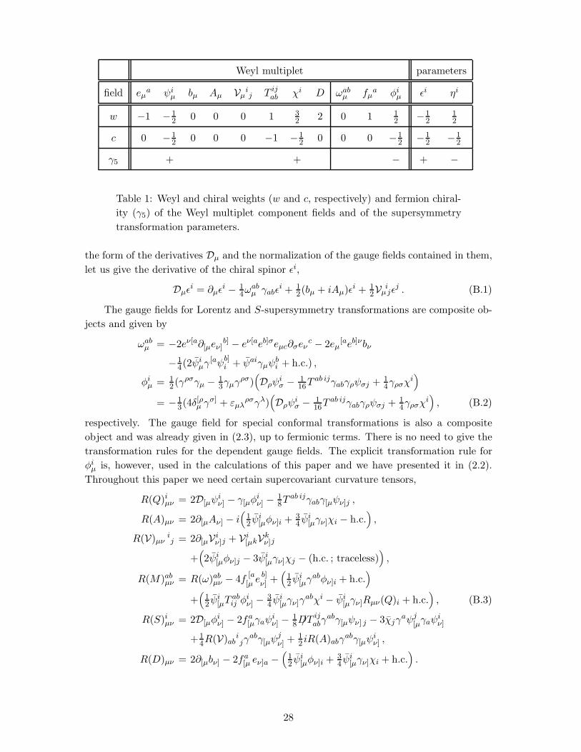
Weyl multiplet parameters

field eµa ψi

µ bµ Aµ Vµij T ij

ab χi D ωabµ fµ

a φiµ ǫi ηi

w −1 −12 0 0 0 1 3

2 2 0 1 12 −1

212

c 0 −12 0 0 0 −1 −1

2 0 0 0 −12 −1

2 −12

γ5 + + − + −

Table 1: Weyl and chiral weights (w and c, respectively) and fermion chiral-

ity (γ5) of the Weyl multiplet component fields and of the supersymmetry

transformation parameters.

the form of the derivatives Dµ and the normalization of the gauge fields contained in them,

let us give the derivative of the chiral spinor ǫi,

Dµǫi = ∂µǫ

i − 14ω

abµ γabǫ

i + 12(bµ + iAµ)ǫi + 1

2Vµijǫ

j . (B.1)

The gauge fields for Lorentz and S-supersymmetry transformations are composite ob-

jects and given by

ωabµ = −2eν[a∂[µeν]

b] − eν[aeb]σeµc∂σeνc − 2eµ

[aeb]νbν

−14(2ψi

µγ[aψ

b]i + ψaiγµψ

bi + h.c.) ,

φiµ = 1

2 (γρσγµ − 13γµγ

ρσ)(

Dρψiσ − 1

16Tab ijγabγρψσj + 1

4γρσχi)

= −13(4δ[ρµ γ

σ] + εµλρσγλ)

(

Dρψiσ − 1

16Tab ijγabγρψσj + 1

4γρσχi)

, (B.2)

respectively. The gauge field for special conformal transformations is also a composite

object and was already given in (2.3), up to fermionic terms. There is no need to give the

transformation rules for the dependent gauge fields. The explicit transformation rule for

φiµ is, however, used in the calculations of this paper and we have presented it in (2.2).

Throughout this paper we need certain supercovariant curvature tensors,

R(Q)iµν = 2D[µψiν] − γ[µφ

iν] − 1

8Tab ijγabγ[µψν]j ,

R(A)µν = 2∂[µAν] − i(

12 ψ

i[µφν]i + 3

4 ψi[µγν]χi − h.c.

)

,

R(V)µνij = 2∂[µV i

ν]j + V i[µkVk

ν]j

+(

2ψi[µφν]j − 3ψi

[µγν]χj − (h.c. ; traceless))

,

R(M)abµν = R(ω)ab

µν − 4f[a[µ e

b]ν] +

(

12 ψ

i[µγ

abφν]i + h.c.)

+(

12 ψ

i[µT

abij φ

iν] − 3

4 ψi[µγν]γ

abχi − ψi[µγν]Rµν(Q)i + h.c.

)

, (B.3)

R(S)iµν = 2D[µφiν] − 2fa

[µγaψiν] − 1

8D/Tijabγ

abγ[µψν] j − 3χjγaψj

[µγaψiν]

+14R(V)ab

ijγ

abγ[µψjν] + 1

2 iR(A)abγabγ[µψ

iν] ,

R(D)µν = 2∂[µbν] − 2fa[µ eν]a −

(

12 ψ

i[µφν]i + 3

4 ψi[µγν]χi + h.c.

)

.

28

The following modified curvature tensors appear in the component fields of the chiral

multiplet W 2 (c.f. 2.7),

R(M)abcd = R(M)ab

cd + 116

(

T ijcd Tijab + T ijab T

cdij

)

,

R(S)iab = R(S)iab + 34T

ijabχj . (B.4)

The T 2-modification cancels exactly the T 2-terms in the contribution to R(M) from f aµ .

The curvature R(M)abcd satisfies the following relations,

R(M)µνab eνb = iR(A)µ

a + 32D eµ

a ,

14εab

ef εcdgh R(M)efgh = R(M)ab

cd ,

εcdea R(M)cd eb = εbecd R(M)a

e cd = 2Rab(D) = 2iRab(A) . (B.5)

The first one is the constraint that determines the field fµa while the remaining equations

are Bianchi identities. Note that the modified curvature does not satisfy the pair exchange

property,

R(M)abcd = R(M)cdab + 4iδ

[c[a R(A)b]

d] . (B.6)

From these equations one determines for instance

R(M)±0[p0q] = ±1

2 iR(A)±pq . (B.7)

We note that R(Q)iab satisfies the constraint

γµR(Q)iµν + 32γνχ

i = 0 , (B.8)

which must therefore hold for its variation as well. This constraint implies that R(Q)iµν is

anti-selfdual, as follows from contracting it with γν γab.

The curvature R(S)iab satisfies

γaR(S)iab = 2DaR(Q)iab , (B.9)

as a result of the Bianchi identities and of the constraint (B.8). This identity (upon

contraction with γbγcd) leads to

R(S)iab − R(S)iab = 2/D(R(Q)iab + 34γabχ

i) . (B.10)

References

[1] S. Ferrara, R. Kallosh and A. Strominger, Phys. Rev. D52 (1995) 5412, hep-th/9508072; A.

Strominger, Phys. Lett. B383 (1996) 39, hep-th/9602111; S. Ferrara and R. Kallosh, Phys.

Rev. D54 (1996) 1514, hep-th/9602136; Phys. Rev. D54 (1996) 1525, hep-th/9603090.

[2] K. Behrndt, G. L. Cardoso, B. de Wit, R. Kallosh, D. Lust and T. Mohaupt, Nucl. Phys.

B488 (1997) 236, hep-th/9610105.

29

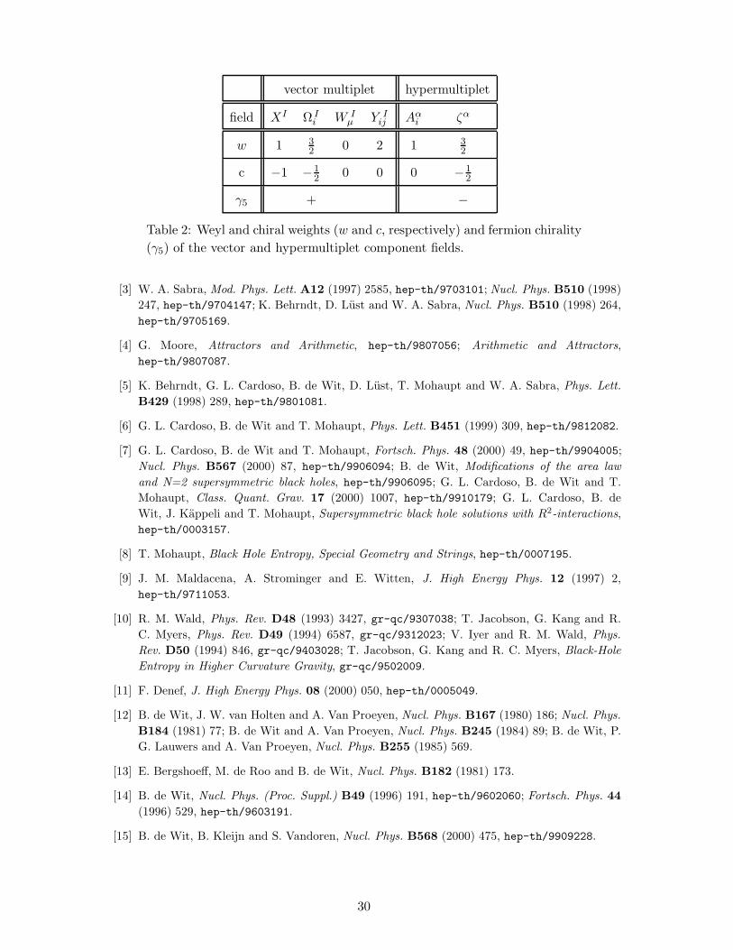
vector multiplet hypermultiplet

field XI Ω Ii W I

µ Y Iij Aα

i ζα

w 1 32 0 2 1 3

2

c −1 −12 0 0 0 −1

2

γ5 + −

Table 2: Weyl and chiral weights (w and c, respectively) and fermion chirality

(γ5) of the vector and hypermultiplet component fields.

[3] W. A. Sabra, Mod. Phys. Lett. A12 (1997) 2585, hep-th/9703101; Nucl. Phys. B510 (1998)

247, hep-th/9704147; K. Behrndt, D. Lust and W. A. Sabra, Nucl. Phys. B510 (1998) 264,

hep-th/9705169.

[4] G. Moore, Attractors and Arithmetic, hep-th/9807056; Arithmetic and Attractors,

hep-th/9807087.

[5] K. Behrndt, G. L. Cardoso, B. de Wit, D. Lust, T. Mohaupt and W. A. Sabra, Phys. Lett.

B429 (1998) 289, hep-th/9801081.

[6] G. L. Cardoso, B. de Wit and T. Mohaupt, Phys. Lett. B451 (1999) 309, hep-th/9812082.

[7] G. L. Cardoso, B. de Wit and T. Mohaupt, Fortsch. Phys. 48 (2000) 49, hep-th/9904005;

Nucl. Phys. B567 (2000) 87, hep-th/9906094; B. de Wit, Modifications of the area law

and N=2 supersymmetric black holes, hep-th/9906095; G. L. Cardoso, B. de Wit and T.

Mohaupt, Class. Quant. Grav. 17 (2000) 1007, hep-th/9910179; G. L. Cardoso, B. de

Wit, J. Kappeli and T. Mohaupt, Supersymmetric black hole solutions with R2-interactions,

hep-th/0003157.

[8] T. Mohaupt, Black Hole Entropy, Special Geometry and Strings, hep-th/0007195.

[9] J. M. Maldacena, A. Strominger and E. Witten, J. High Energy Phys. 12 (1997) 2,

hep-th/9711053.

[10] R. M. Wald, Phys. Rev. D48 (1993) 3427, gr-qc/9307038; T. Jacobson, G. Kang and R.

C. Myers, Phys. Rev. D49 (1994) 6587, gr-qc/9312023; V. Iyer and R. M. Wald, Phys.

Rev. D50 (1994) 846, gr-qc/9403028; T. Jacobson, G. Kang and R. C. Myers, Black-Hole

Entropy in Higher Curvature Gravity, gr-qc/9502009.

[11] F. Denef, J. High Energy Phys. 08 (2000) 050, hep-th/0005049.

[12] B. de Wit, J. W. van Holten and A. Van Proeyen, Nucl. Phys. B167 (1980) 186; Nucl. Phys.

B184 (1981) 77; B. de Wit and A. Van Proeyen, Nucl. Phys. B245 (1984) 89; B. de Wit, P.

G. Lauwers and A. Van Proeyen, Nucl. Phys. B255 (1985) 569.

[13] E. Bergshoeff, M. de Roo and B. de Wit, Nucl. Phys. B182 (1981) 173.

[14] B. de Wit, Nucl. Phys. (Proc. Suppl.) B49 (1996) 191, hep-th/9602060; Fortsch. Phys. 44

(1996) 529, hep-th/9603191.

[15] B. de Wit, B. Kleijn and S. Vandoren, Nucl. Phys. B568 (2000) 475, hep-th/9909228.

30

[16] A. Maloney, M. Spradlin and A. Strominger, Superconformal Multi-Black Hole Moduli Spaces

in Four Dimensions, hep-th/9911001.

[17] J. Gutowski and G. Papadopoulos, Phys. Rev. D62 (2000) 064023, hep-th/0002242.

[18] G. L. Cardoso, B. de Wit, J. Kappeli and T. Mohaupt, work in progress.

31