static-curis.ku.dkstatic-curis.ku.dk/portal/files/138468036/IFRO_WP_2015... ·  · 2015-06-02factory-operated and outgrower-operated sugarcane production in ... Factory-Operated

u n i ve r s i t y o f co pe n h ag e n

Københavns Universitet

Incentives and moral hazard

Wendimu, Mengistu Assefa; Henningsen, Arne; Czekaj, Tomasz Gerard

Publication date:2015

Document VersionPublisher's PDF, also known as Version of record

Citation for published version (APA):Wendimu, M. A., Henningsen, A., & Czekaj, T. G. (2015). Incentives and moral hazard: plot level productivity offactory-operated and outgrower-operated sugarcane production in Ethiopia. Frederiksberg: Department of Foodand Resource Economics, University of Copenhagen. IFRO Working Paper, No. 2015/02

Download date: 03. jul.. 2018

Incentives and Moral Hazard: Plot Level Productivity of Factory-Operated and Outgrower-Operated Sugarcane Production in Ethiopia

Mengistu Assefa Wendimu Arne Henningsen Tomasz Gerard Czekaj

2015 / 02

IFRO Working Paper 2015 / 02 Incentives and Moral Hazard: Plot Level Productivity of Factory-Operated and Outgrower-Operated Sugarcane Production in Ethiopia

Authors: Mengistu Assefa Wendimu, Arne Henningsen, Tomasz Gerard Czekaj

JEL-classification: D24, Q12, Q15

January 2015

See the full series IFRO Working Paper here: www.ifro.ku.dk/english/publications/foi_series/working_papers/

Department of Food and Resource Economics (IFRO) University of Copenhagen Rolighedsvej 25 DK 1958 Frederiksberg DENMARK www.ifro.ku.dk/english/

Incentives and Moral Hazard: Plot Level Productivity of

Factory-Operated and Outgrower-Operated Sugarcane Production in Ethiopia

Mengistu Assefa Wendimu1,2, Arne Henningsen1 and Tomasz Gerard Czekaj1

Abstract We investigate the unique contractual arrangement between a large Ethiopian sugar factory and its adjacent outgrower associations. The only significant difference between the sugarcane production on the factory-operated sugarcane plantation and on the outgrower-operated plots is the remuneration system and thus, the incentives to the workers. We compare the productivity of the factory-operated plantation with the outgrower-operated plots based on a new cross-sectional plot-level data set that includes all plots that are operated by the sugar factory and its adjacent outgrower associations. As sugar-cane production depends on various exogenous factors that are measured as categorical variables (e.g. soil type, cane variety, etc.), we estimate the production function by a nonparametric kernel regression method that takes into account both continuous and categorical explanatory variables without assuming a functional form and without imposing restrictions on interactions between the explanatory variables. In order to obtain meaningful productivity measures, we impose monotonicity in input quantities using the constrained weighted bootstrapping (CWB) method. Our results show that outgrower-operated plots have−ceteris paribus−a statistically and economically significantly higher productivity than factory-operated plots, which can be explained by outgrowers having stronger incentives to put more effort into their work than the employees of the sugar factory. Key Words Productivity, Outgrower schemes, large-scale plantation, agricultural workers, incentives, Nonparametric regression, Sugarcane, Ethiopia JEL codes: D24, Q12, Q15

1 University of Copenhagen, Department of Food and Resource Economics 2 Danish Institute for International Studies (DIIS)

1

1. Introduction

Agricultural productivity in Sub-Saharan Africa has received increasing attention from international donors, NGOs, and governments because it is much lower than in most other regions of the world and its enhancement is seen as an essential precondition for sustainable economic development (Collier and Dercon, 2014). An important instrument for enhancing productivity is the empirical analysis of productivity because it can help to improve managerial decisions and public policy formulation (Ferrantino et al., 1995). Increasing concerns regarding food security, natural resource management, and poverty reduction are additional reasons for a rapidly increasing interest in empirically analyzing productivity and efficiency in the agricultural sector (Hassine, 2009). This paper contributes to this literature, firstly, by providing a comprehensive analysis of the productivity of sugarcane production in Ethiopia and, secondly, by comparing the plot-level productivity of outgrowers and a large-scale plantation using a flexible nonparametric kernel regression method for both continuous and categorical explanatory variables.

In recent years, sugarcane production around the world has increased tremendously. The main driving forces behind this increase are increasing demand for sugar and sugar products and the use of sugarcane for biofuel (bioethanol) production. An increasing emphasis on sugarcane production and processing can also be observed in Ethiopia due to rising domestic demand for sugar, a desire for ethanol production from molasses to halt huge expenditures on oil imports, and the aspiration to earn foreign currency from sugar export (Lavers, 2012). Therefore, sugarcane production and processing is among the sub-sectors which have received the highest priority in the five-year Growth and Transformation Plan that the Ethiopian government has been implementing since 2010/2011 (MoFED, 2010).

An increase in sugarcane production can be achieved by increasing land use for sugarcane production and by improving the productivity of sugarcane production. Kostka et al. (2009) show that about 60% of the global increase in sugar production over the last 40 years has been achieved through land expansion rather than through productivity gains. Msuya and Ashimogo (2005) show that the high growth rate in sugarcane production achieved both by outgrowers and estate farms in Tanzania has been attained through the expansion of land under sugarcane production rather than through productivity improvements. However, further land expansion for sugarcane production is limited by declining land availability and low tolerance to further damage to the environment (Msuya and Ashimogo, 2005). Hence, significant increases in the productivity of sugarcane production are essential for the growth of the sugar industry. Furthermore, the increased productivity of sugarcane production is a key factor in improving the competitiveness of the sugar industry on the global market.

However, the intended increase in sugar production in Ethiopia is so large that it cannot solely be achieved by productivity enhancements. Thus, the land area used for sugarcane production is currently being rapidly increased and this has—together with other large-scale agricultural investments in food and non-food crop production—resulted in massive competition for land and water with local smallholder farmers. This situation can be observed not only in Ethiopia, but also in many other developing countries. Most land expansion for sugarcane production is through large-scale plantations, which often face strong resistance from local communities. Furthermore, the establishment of large-scale plantations has been highly criticized by many local and international NGOs for its perceived negative effects on the livelihoods of local communities. It has been suggested that the use of outgrower schemes can minimize the perceived negative effects. Abate and Teshome (2013) state that in developing countries like Ethiopia, where smallholder farmers take the largest share in agriculture, outgrower schemes

2

and contract farming are politically more acceptable than alternative forms of agricultural investments.

The literature on outgrower schemes and contract farming has so far focused to a great extent on examining the income effects of these schemes (e.g. Warning and Key, 2002; Bolwig et al., 2009; Bellemare, 2012) and the conditions under which these schemes benefit small-scale farmers (e.g. Glover, 1987; Nijhoff and Trienekens, 2010; Barret et al., 2012). Few studies, largely unpublished, analyze the effects of outgrower schemes on productivity and very few investigate sugarcane productivity. Msuya and Ashimogo (2005) compare the productivity of sugarcane outgrowers with rice producers in India and find that rice producers have a slightly higher productivity. Mahadevan (2007) examines the impact of land tenure and ethnicity on the productivity of sugarcane in Fiji and reports that Indo Fijians are more productive than their native counterparts. Khan (2006) estimates plot-level productivity of sugarcane production by the types of water ownership and reports that the average productivity is highest on plots where water is sourced from privately owned tube wells. Though outgrower schemes and nucleus estate (i.e. vertically integrated factory-operated) production are the dominant forms of sugarcane production in many African countries, the relative productivity of these two production models has not been sufficiently examined. Hence, the aim of this study is to fill this gap in the literature by comparing outgrowers’ sugarcane productivity with the productivity of a factory-operated plantation in Ethiopia. Our theoretical considerations are based on principal-agent theory and they suggest that outgrower plots should have a higher productivity than factory-operated plots. We test this hypothesis in our empirical analysis.

Our study is distinct from previous studies in three important aspects. First, in our study, the outgrowers and the factory have similar plot sizes, produce the same crop, have equal access to credit and input markets, and use the same inputs and the same technology so that the organizational form of the production (and hence the incentives to the workers) is the only significant difference between the production on the outgrower-operated plots and the factory-operated plots. Hence, identified differences in productivity between the outgrower-operated plots and the factory-operated plots can be attributed to the organizational form of production and hence the incentives to the workers. Second, our dataset contains a wide range of plot-level characteristics (e.g. soil type, cane variety, production cycle), which allows us to control for possible plot level differences. Third, we use a kernel regression method, which allows us to flexibly estimate the production function without imposing a priori assumptions regarding the functional form of the relationship between inputs and output, the influence of the categorical variables, and the interactions effects between all explanatory variables.

The structure of this paper is as follows. Section 2 reviews the literature on productivity and its relation with incentives and moral hazard, e.g. based on principal-agent theory. Section 3 briefly describes recent developments within the Ethiopian sugar industry and provides background information about the Wonji-Shoa Sugar Factory and the adjacent outgrower schemes. In sections 4 and 5, we describe our data set and present the econometric framework of our study, respectively. Our main findings are presented in section 6 while section 7 concludes the study.

2. Incentives, moral hazards and sources of variation in productivity

The relationship between farm size and productivity has been examined since the 1960s, but it is still one of the most debated topics in the development economics literature. Driven by the rapid increase in private large-scale land acquisitions, a revival in plantations and other forms

3

of large-scale commercial agriculture has been observed in Sub-Saharan Africa since the mid-2000s. Therefore, policy making for African agricultural development will continue to be driven by the small-scale versus large-scale farm productivity discourse (Smalley, 2013). Although this paper focusses on examining the effect of the organizational form of production3 on productivity, first we briefly review the literature on the relationship between farm size and productivity because the organizational form of production may be the most important argument for an inverse relationship.

2.1 Relationship between farm size and productivity

Most micro-level empirical studies that analyze the relationship between farm size and land productivity find an inverse relationship (e.g. Chayanov, 1926; Mazumdar, 1965; Berry and Cline, 1979; Collier, 1983; Cornia, 1985; Benjamin 1995; Barrett, 1996; Kimhi, 2006; and Barrett et al., 2010). The early explanations for the inverse relationship between farm size and land productivity were based on the theory of labor market segmentation or factor market imperfections (e.g. Sen, 1966; Mabro, 1971; Berry and Cline, 1979; Eswaran and Kotwal, 1986; Sen, 1996; Heltberg, 1998). In these early explanations, small-scale farming was identified as family farms, while large-scale farming was identified as plantation-type production (e.g. Mabro, 1971). Family farming is based on the use of underemployed household labor so that it faces a lower effective labor price (lower opportunity cost of labor) than plantations and thus, uses more labor per area unit to produce a higher output per area unit than plantation-type production (Mazumdar, 1965; Sen, 1966; Mabro, 1971).

A second group of studies (e.g. Feder, 1985; Eswaran and Kotwal, 1986; Ellis, 1993) uses the principal-agent framework to explain the inverse relationship between farm size and land productivity. The authors argue that household labor involves lower supervision costs and lower information asymmetries than hired labor because household laborers on small-scale farms have proper incentives to cultivate their land efficiently. We return to this in the next sub-section.

The third group of explanations is related to methodological issues such as omitted variable biases due to missing information on soil quality (e.g. Bhalla and Roy, 1988; Benjamin, 1995; Lamb, 2003); measurement errors (Lamb, 2003); misspecification of the functional form of the production function (Lipton, 2010); and unobserved heterogeneity between farmers (Assuncao and Ghatak, 2003). However, some recent studies reject the claims that the inverse relationship is related to methodological issues. Barrett et al. (2010) include plot-level soil quality—obtained by laboratory soil tests—as the additional explanatory variable and conclude that only a very limited share of the inverse relationship can be explained by the differences in soil quality. By using data from a Ugandan household survey in which the household´s self-reported land size was complemented by plot-size measurements collected using the Global Positioning System (GPS), Carletto et al. (2013) argue that the inverse relationship cannot be explained by measurement errors in land size. They conclude that when more precise measures of land size are used, the evidence for an inverse relationship is even strengthened. Verschelde et al. (2013) investigate the relationship between the farm size and farm productivity of small-scale farmers in Burundi using a nonparametric regression approach that avoids potential bias due to the choice of an unsuitable functional form (as suggested by Lipton, 2010). Their findings also support the existence of an inverse relationship. However, based on an extensive review of the experiences of large-scale farming

3 The organizational form of production here refers to the organizational arrangement of the sugarcane production, i.e. outgrower schemes and factory-operated production.

4

and plantation farming in Africa, Gibbon (2011) concludes that low productivity is not an inherent characteristic of large-scale farming and plantation farming. More recently, Collier and Dercon (2014) state that most of the literature that studies the inverse relationship compares very small farms with slightly larger farms, instead of comparing small-scale family farms with large-scale commercial plantations.

2.2 Organizational form of production and relative productivity

Ferrantino et al. (1995) point out that while productivity is determined by the underlying production technology and input quantities, other factors such as the organizational form of production may also influence the relative productivity of firms. The effect of the organizational form of production on relative productivity is most often investigated within the framework of principal-agent theory. The principal-agent literature mainly deals with a situation where the principal (the employer) contracts an agent (employee) to perform a job on his/her behalf (Eisenhardt, 1989). The principal-agent problem arises when: (i) there is disparity between the interest and objectives of the two parties; (ii) the principal does not have full information about the agent´s behavior, i.e. when it is technically or economically infeasible for the principal to precisely observe the quality of the job performed by the agent with regard to timing, effort exerted, and thoroughness, and; (iii) when the two parties have different risk strategies (i.e. risk averse, risk neutral or risk-taker) (e.g. Ross, 1973; Harris and Raw, 1979; Hölmstrom, 1979; Sanford and Oliver, 1983; Key and Runsten, 1999). When the incentives of the agent are not sufficiently aligned with the objectives of the principal to eliminate or mitigate the shirking of the agent, and it is too costly for the principal to monitor the agent´s behavior, the agent may not put his/her maximum effort into the production activity due to the presence of moral hazard, which results in the reduction of the principal´s outcome (Ross, 1973; Eisenhardt, 1989). Sharecropping, where the land owner and the farmer share both the output and the risk equally, is the most examined production arrangement in agriculture (Allen and Lueck, 1992). In the case of sharecropping, the farmer has a strong self-interest in a successful crop and no incentive to shirk, while the land owner can also assume that the farmer puts great effort into the production processes without needing to confirm it (Miller and Whitford, 2006).

The incentive structures both for farm managers and laborers play an important role in determining farm productivity. While outgrower production and other small-scale farming activities are mostly based on family laborers, large-scale production depends on hired labor, which may decrease its relative productivity due to principal-agent problems. Large-scale agricultural production usually has complex management hierarchies with many layers of principals and agents in the principal-agent ladder4, which may also affect productivity (Levačić, 2009). Since family laborers are the residual claimants, they have stronger incentives to adjust and work hard than wage laborers who receive a fixed wage. For this reason, family laborers usually exercise more care, effort and judgment than hired laborers who may have incentives to shirk (moral hazard) and thus, require costly supervision (Eisenhardt, 1989; Deininger, 2011). It is usually assumed that the amount of effort exerted by hired laborers—i.e. how hard or carefully they perform their work—depends on the level of supervision (e.g. Key and Runsten, 1999). Using plot-level data on Indian rice farms, Frisvold (1994) found that low effort exerted by wage laborers who were not sufficiently supervised by family laborers resulted in considerable output loss, which was greater than 10% of the output on more than 40% of the plots. One way to increase the productivity of hired laborers is through incentive payments, i.e. paying laborers based on type and

4 We illustrate this for our specific case in section 3.4 below.

5

magnitude of the task rather than a fixed wage (e.g. Paarsch and Shearer, 1999). However, especially in agriculture where the effect of low quality effort is not immediately observed, payments based on the type and magnitude of the task may not only increase the amount of tasks that the laborers complete per hour, but also reduce the quality of the work performed. Paarsch and Shearer (2000) found that although a payment system based on the magnitude of the task increased the productivity of tree-planting laborers by about 22.6%, only a small part of this could be attributed to valuable output because laborers reacted to the payment incentives by reducing the quality of their work. Thus, moral hazard due to principal-agent problems and the related labor supervision costs make the effective labor costs higher on large-scale farms than on smallholder plots (Feder, 1985; Smalley, 2013), which reduces the relative productivity of large-scale farms. Contract farming (outgrower schemes) provides an opportunity for smallholder farmers to take advantage of the relatively high productivity of family labor (Smalley, 2013).

3. Recent development within the Ethiopian sugar sub-sector

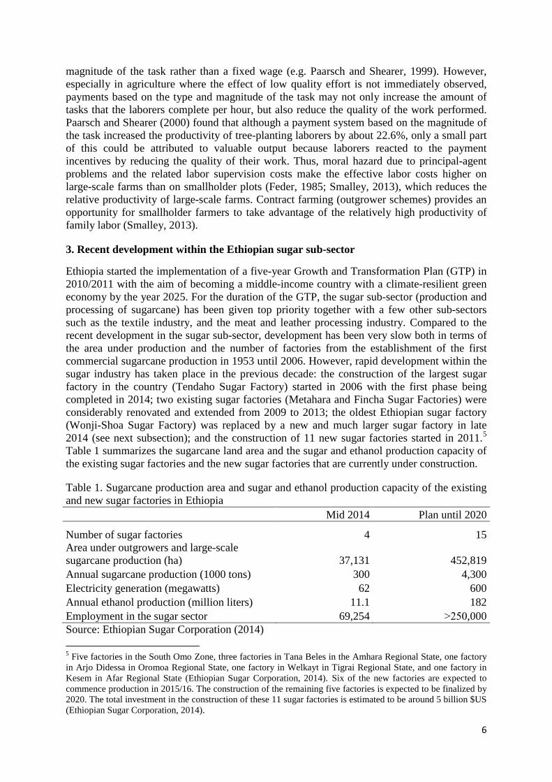
Ethiopia started the implementation of a five-year Growth and Transformation Plan (GTP) in 2010/2011 with the aim of becoming a middle-income country with a climate-resilient green economy by the year 2025. For the duration of the GTP, the sugar sub-sector (production and processing of sugarcane) has been given top priority together with a few other sub-sectors such as the textile industry, and the meat and leather processing industry. Compared to the recent development in the sugar sub-sector, development has been very slow both in terms of the area under production and the number of factories from the establishment of the first commercial sugarcane production in 1953 until 2006. However, rapid development within the sugar industry has taken place in the previous decade: the construction of the largest sugar factory in the country (Tendaho Sugar Factory) started in 2006 with the first phase being completed in 2014; two existing sugar factories (Metahara and Fincha Sugar Factories) were considerably renovated and extended from 2009 to 2013; the oldest Ethiopian sugar factory (Wonji-Shoa Sugar Factory) was replaced by a new and much larger sugar factory in late 2014 (see next subsection); and the construction of 11 new sugar factories started in 2011.5 Table 1 summarizes the sugarcane land area and the sugar and ethanol production capacity of the existing sugar factories and the new sugar factories that are currently under construction.

Table 1. Sugarcane production area and sugar and ethanol production capacity of the existing and new sugar factories in Ethiopia

Mid 2014 Plan until 2020

Number of sugar factories 4 15 Area under outgrowers and large-scale sugarcane production (ha) 37,131 452,819 Annual sugarcane production (1000 tons) 300 4,300 Electricity generation (megawatts) 62 600 Annual ethanol production (million liters) 11.1 182 Employment in the sugar sector 69,254 ˃250,000 Source: Ethiopian Sugar Corporation (2014)

5 Five factories in the South Omo Zone, three factories in Tana Beles in the Amhara Regional State, one factory in Arjo Didessa in Oromoa Regional State, one factory in Welkayt in Tigrai Regional State, and one factory in Kesem in Afar Regional State (Ethiopian Sugar Corporation, 2014). Six of the new factories are expected to commence production in 2015/16. The construction of the remaining five factories is expected to be finalized by 2020. The total investment in the construction of these 11 sugar factories is estimated to be around 5 billion $US (Ethiopian Sugar Corporation, 2014).

6

Ethiopia has one of the highest sugarcane yields (land productivity) in the world (see Figure 1). While Ethiopia exports a small part (about 7% in 2013) of its sugar production to the European Union (EU) to take advantage of the duty-free and quota-free access for sugar exports from developing countries, it imported more than half of its domestic sugar consumption in 2013. However, the Ethiopian sugar sub-sector aims to become self-sufficient and to start exporting sugar (in addition to the preferential exports to the EU) in 2015.

Source: FAOSTAT (2013)

Figure 1. Average sugarcane yield in the period 2008-2012 in tons per hectare for the five countries with highest sugarcane yield and the two largest sugarcane producers in the world (Brazil and India).

3.1. Wonji-Shoa Sugar Factory

When the Wonji Sugar Factory began production in 1954 it was the first sugar factory to be established in Ethiopia (Ethiopian Investment Agency, 2012). In order to meet the increasing demand for sugar in the country, the Shoa Sugar Factory was set up in 1962 under the same management about 7 km away from the Wonji Sugar Factory. The two factories (Wonji and Shoa) together cultivated about 5,900 ha of sugarcane on their own plantations and had a joint crushing capacity of 3,000 tons of cane per day. In late 2014, the two sugar factories were closed down and replaced by a new Wonji-Shoa sugar factory, which has a crushing capacity of 6,250 tons of cane per day; more than double the joint cane crushing capacity of the two previous sugar factories. In addition to its own production, the factory also sources sugarcane from outgrowers. The geographic location of the Wonji-Shoa sugar factories, their factory-operated plantation and the plots of the adjacent outgrowers are illustrated in Figure 2.

3.2. Sugarcane Outgrower Schemes in the Wonji-Shoa Area

The land area used by the factory for sugarcane production has remained the same since the 1960s due to a lack of unoccupied land in the vicinity of the factory that is suitable for sugarcane production. In order to increase the supply of sugarcane, seven sugarcane outgrower associations were established in 1975/76. Participation in the outgrower scheme was not on a voluntary basis. In the selected villages, all farmers who had suitable land for sugarcane production had to join the scheme or leave their land. The schemes were designed

0,0

20,0

40,0

60,0

80,0

100,0

120,0

140,0Y

ield

(ton

s/ha

)

7

in such a way that all farmers in a given outgrower association were allocated an equal amount of land regardless of the amount of land they originally contributed to the association. However, the amount of land owned by the outgrowers varies depending on the association and ranges between 0.2 and 6.0 ha. The sugarcane fields are jointly managed by the sugarcane outgrowers. Unless the outgrowers face a shortage of labor—which sometimes happens during peak planting and weeding seasons—the outgrowers undertake all the labor work on their plots except for harvesting, which is done by factory laborers. All sugarcane outgrowers are supposed to undertake the same amount of work, which can be on their own land or on other parts of the same plot that belong to other members of their outgrower association. The outgrowers receive a down-payment for their work on the sugarcane fields based on a fixed daily rate or according to the piece of work they have performed. After harvesting the sugarcane, the profit made on the plot (i.e. the revenue from selling the sugarcane minus all costs and the down-payment for the labor) is shared among all owners of the plot according to their share of land on the plot. Hence, this outgrower arrangement is a form of co-operative farming. The sugarcane productivity has a large effect on the outgrowers’ income because nearly 60% of the land that is cultivated by the outgrowers is used for sugarcane production and more than 50% of the outgrowers do not grow any crops other than sugarcane.

Source: provided by Beshir Kedi Lencha, Wonji-Shoa Sugar Factory

Figure 2. Map of Wonji-Shoa sugar factories, factory-operated plantation, and plots of outgrowers.

In order to further increase the supply of sugarcane, additional outgrower associations were established in 2008, 2011, and 2013 and this process is still going on. In the 2013/14 harvesting season, outgrowers supplied about 40% of the total cane that was crushed by the Wonji-Shoa Factory. Table 2 presents a summary of the outgrower associations that are attached to the Wonji-Shoa sugar factory.

8

Table 2. Overview of sugarcane outgrower schemes of the Wonji-Shoa sugar factory Year of establishment

Area Distance to factory

Number of associations

Area (in ha)

Number of outgrowers

1975 <10 km 7 1,124 1,516 2008 <10 km 5 1,690 1,172 2011 Dodota <25 km 4 1,726 1,034 2013- Welenchiti 42 km * 4,479 * Note: the year of establishment indicates the year when the outgrowers planted sugarcane for the first time; * = not known yet.

Source: Information from the Wonji Area Sugarcane Growers Union

3.3. Contractual Arrangement of the Outgrower Schemes in the Wonji-Shoa Area

The Wonji-Shoa sugar factory and the Wonji Area Sugarcane Growers Union6 have a formal contract that is renegotiated every three years. The sugar factory provides the outgrowers with all inputs used in sugarcane production such as cane seeds, fertilizers, pesticides, and machinery, where the contract specifies standard input quantities per hectare that outgrowers are supposed to apply. The contract also determines the prices of these inputs, the sugarcane price, the tasks that the outgrower associations have to perform, farm management plans, wage rates for harvesting and the down-payments for the outgrowers’ work , and payment rates for different overhead costs for the three-year contractual period. All input costs (including the down-payments for the outgrowers’ work) are initially disbursed by the factory. When the sugarcane of a plot has been harvested, the factory calculates the value of the sugarcane, deducts all corresponding advance payments, and transfers the remainder to the Wonji Area Sugarcane Growers Union, which then transfers the money to the outgrower associations.

Although the outgrower associations have their own supervisors, the Wonj-Shoa Factory assigns its own supervisors to monitor the outgrowers’ sugarcane production activities, e.g. the amount of labor and other inputs. All production activities from land preparation to harvesting are jointly planned and managed by the outgrower associations’ management committees, agronomists employed by the Wonji Area Sugarcane Growers Union, and the outgrowers department of the Wonji-Shoa factory. The outgrowers are required to sell all their output (sugarcane) to the factory. The sugarcane outgrower associations have the land-use rights (ownership) as a whole, but not the individual members so that the individual outgrowers do not have the decision power to renew or reject the contract when it expires. Since there is no exit option, in practice the farmers are locked into a lifelong contract to supply sugarcane to the factory.

3.4 Principal-Agent Relationships

We illustrate the principal-agent relationships in the Wonji-Shoa factory-operated plantation and in the outgrowers’ sugarcane production in Figure 3. The left-hand side of the figure demonstrates that factory-operated sugarcane production has many layers of principal-agent

6 In the year 2000, all outgrower associations that produced sugarcane for the Wonji-Shoa sugar factory formed the Wonji Area Sugarcane Growers Union. All newly established outgrower associations have joined the union which negotiates with the factory on behalf of all the outgrowers and also supports the associations with extension services.

9

relationships. In all these layers, there is information asymmetry as the principal does not have full information about how the agents at the lower level act. Thus, there is the potential for moral hazard at every level of the principal-agent relationships.

In contrast, the right side of the figure demonstrates that the outgrower schemes have far fewer layers of principal-agent relationships. Furthermore, information asymmetry between the principal and the agent is lower than in the factory-operated sugarcane production as the principals and agents live in the same village and know each other much better than the principals and agents in the factory-operated sugarcane production. Moreover, the members of the outgrower associations have high incentives to monitor the efforts of each other (i.e. there is peer pressure) and of the committee members because all outgrowers who jointly cultivate a sugarcane plot share the profit so that the income of each outgrower depends on the effort of the other outgrowers. Furthermore, the members of the outgrowers’ management committees are also outgrowers who receive a share of the profits and moreover, if the sugarcane production is highly profitable, it increases their chance of being re-elected by the outgrowers’ general assembly for the following three-year term.

The principal-agent relationship between the factory and the outgrower associations does not provide significant incentives for shirking because the information asymmetry between the factory (principal) and the outgrowers (agent) is very limited since the outgrowers are paid based on the weight of the cane that they supply to the factory, which means that the outgrowers bear all the risks of low effort. The only risk for the factory is a low supply of sugarcane, which may result in low capacity utilization and thus, lower profits for the sugar-factory. Factory Outgrowers

Council of Ministers General Assembly of Outgrowers

Director of Ethiopian Sugar Corporation Management Committee (Board)

Manager of Wonji-Shoa Sugar Factory Outgrowers

Heads of Agricultural Operation Departments

Field Supervisors

Foremen/Capos

Assistant foremen/Capos

Hired Laborers

Figure 3. Principal-agent relationships in factory-operated and outgrower-operated sugarcane production in Wonji-Shoa.

Based on the literature reviewed in section 2, the contractual arrangement described in section 3.3 and the principal-agent relationships presented in this section, we expect that the productivity will be—ceteris paribus—higher on outgrower-operated plots than on the factory-operated plantation.

10

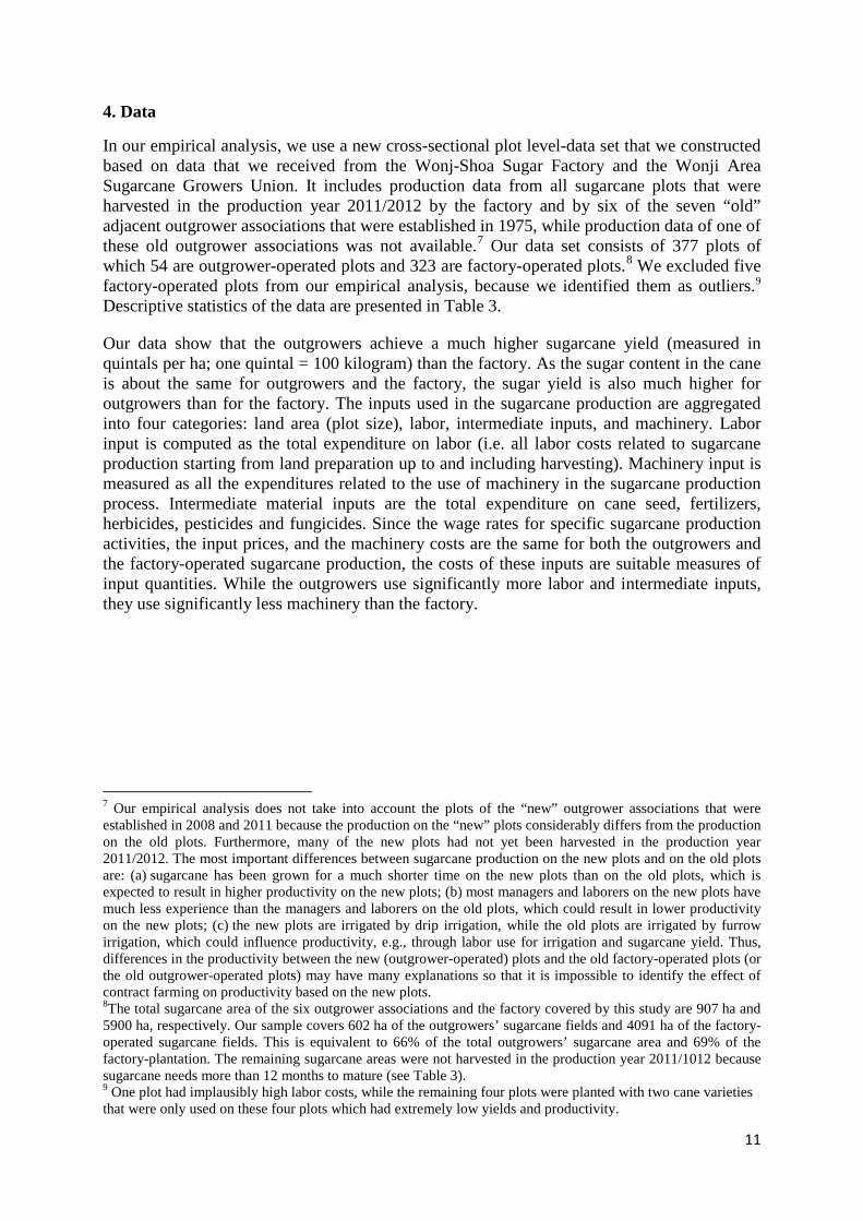
4. Data

In our empirical analysis, we use a new cross-sectional plot level-data set that we constructed based on data that we received from the Wonj-Shoa Sugar Factory and the Wonji Area Sugarcane Growers Union. It includes production data from all sugarcane plots that were harvested in the production year 2011/2012 by the factory and by six of the seven “old” adjacent outgrower associations that were established in 1975, while production data of one of these old outgrower associations was not available.7 Our data set consists of 377 plots of which 54 are outgrower-operated plots and 323 are factory-operated plots.8 We excluded five factory-operated plots from our empirical analysis, because we identified them as outliers.9 Descriptive statistics of the data are presented in Table 3.

Our data show that the outgrowers achieve a much higher sugarcane yield (measured in quintals per ha; one quintal = 100 kilogram) than the factory. As the sugar content in the cane is about the same for outgrowers and the factory, the sugar yield is also much higher for outgrowers than for the factory. The inputs used in the sugarcane production are aggregated into four categories: land area (plot size), labor, intermediate inputs, and machinery. Labor input is computed as the total expenditure on labor (i.e. all labor costs related to sugarcane production starting from land preparation up to and including harvesting). Machinery input is measured as all the expenditures related to the use of machinery in the sugarcane production process. Intermediate material inputs are the total expenditure on cane seed, fertilizers, herbicides, pesticides and fungicides. Since the wage rates for specific sugarcane production activities, the input prices, and the machinery costs are the same for both the outgrowers and the factory-operated sugarcane production, the costs of these inputs are suitable measures of input quantities. While the outgrowers use significantly more labor and intermediate inputs, they use significantly less machinery than the factory.

7 Our empirical analysis does not take into account the plots of the “new” outgrower associations that were established in 2008 and 2011 because the production on the “new” plots considerably differs from the production on the old plots. Furthermore, many of the new plots had not yet been harvested in the production year 2011/2012. The most important differences between sugarcane production on the new plots and on the old plots are: (a) sugarcane has been grown for a much shorter time on the new plots than on the old plots, which is expected to result in higher productivity on the new plots; (b) most managers and laborers on the new plots have much less experience than the managers and laborers on the old plots, which could result in lower productivity on the new plots; (c) the new plots are irrigated by drip irrigation, while the old plots are irrigated by furrow irrigation, which could influence productivity, e.g., through labor use for irrigation and sugarcane yield. Thus, differences in the productivity between the new (outgrower-operated) plots and the old factory-operated plots (or the old outgrower-operated plots) may have many explanations so that it is impossible to identify the effect of contract farming on productivity based on the new plots. 8The total sugarcane area of the six outgrower associations and the factory covered by this study are 907 ha and 5900 ha, respectively. Our sample covers 602 ha of the outgrowers’ sugarcane fields and 4091 ha of the factory-operated sugarcane fields. This is equivalent to 66% of the total outgrowers’ sugarcane area and 69% of the factory-plantation. The remaining sugarcane areas were not harvested in the production year 2011/1012 because sugarcane needs more than 12 months to mature (see Table 3). 9 One plot had implausibly high labor costs, while the remaining four plots were planted with two cane varieties that were only used on these four plots which had extremely low yields and productivity.

11

Table 3. Descriptive statistics of the data set Variable Outgrowers

(n=54) Plantation (n=318)

Total sample (N=372)

P-value

Cane yield (in quintals/ ha) 1451 (480) 1078 (357) 1132 (399) <0.001

Field sugar (in quintals/ha) 165.1 (58.3) 123.3 (43.5) 129.4 (48.2) <0.001

Plot size (in ha) 11.2 (4.2) 12.8 (6.6) 12.5 (6.3) 0.020

Labor (ETB/ha) 6796 (2106) 5269 (1492) 5490 (1681) <0.001

Intermediate inputs (ETB/ha) 5195 (1616) 3742 (1146) 3953 (1326) <0.001

Machinery (ETB/ha) 1039 (1595) 2147 (3077) 1987 (2934) <0.001

Duration of the growing period (months) 17.2 (3.7) 15.5 (2.8) 15.7 (3.1) 0.002

Plots harvested after two rainy seasons (%) 46.3 28.3 30.8 0.006

Soil types (%)

<0.001

A1 0.0 21.7 18.6

A2 57.4 25.5 30.0

B1.4 5.6 12.1 11.4

BA2 5.6 8.4 8.0

C1 31.5 32.3 32.1

Cane varieties (%) <0.001

B52-298 13.0 28.6 26.3

N-14 68.5 18.8 26.0

NCO-334 18.5 25.2 24.4

MV 0.0 11.2 9.6

B58-230 0.0 6.35 5.6

CO-421 0.0 2.8 2.4

Other varieties 0.0 6.8 5.8

Production cycle (%) 0.009

Plant cane 20.4 26.4 25.5

First ratoon 40.7 22.7 25.2

Second ratoon 27.8 24.2 24.9

Third ratoon 9.3 13.6 13.0

Fourth ratoon or later 1.9 13.2 11.4

Planting/ratooning month (%) <0.001

December 7.4 14.3 13.3

January 33.3 17.7 19.9

February 35.2 14.0 17.0

March 5.6 14.0 13.0

May 3.7 12.1 10.9

June 1.6 11.2 9.8

Other months 13.5 16.7 16.2 Gross margin (ETB/ha) 39,200 (16,246) 27,725 (11,239) 29,390 (12732) <0.001 Notes: The output quantities and the input values reported in the table are averages. The gross margin calculation only considers labor, machinery, and intermediate input costs. Costs such as overhead costs (e.g. supervision costs), utility costs (e.g. irrigation water and electricity bills for pumping irrigation water from river), and the cost of transporting cane to the factory gate are not included. Standard deviations are indicated in parentheses. The P-values of numeric variables are obtained from t-tests for the equal mean values of the two production types (allowing for different variances in the two subsets), and the P-values of the categorical variables are obtained from Fisher's exact test of independence between the respective variable and the production type. In the production year 2011/12, 100 Ethiopian Birr (ETB) = US$ 5.66.

12

In addition to input and output quantities, our data set contains information on a wide range of plot-level characteristics, which could potentially influence the sugarcane yield: soil type, cane variety, production cycle, planting or ratooning month, duration of the growing period, and the number of rainy seasons that the cane passed in the field. While the duration of the growing period (ranging between 10 months and 25 months) is a numeric variable, the remaining characteristics are expressed as (ordered or unordered) categorical variables. Compared to the factory-operated plantation, the growing period is, on average, longer for the outgrowers (17.2 months vs. 15.5 months), while a much higher percentage of their cane had been grown over two rainy seasons (46.3% vs. 28.3.%), which may in part explain the outgrowers’ higher labor use and higher yields. While the proportion of different subtypes of loamy soils (soil types “A1,” “A2,” “B1.4,” and “BA2”) differs significantly between factory-operated plots and outgrower-operated plots, the share of sandy soils (soil type “C1”) is around 32% for both factory-operated plots and outgrower-operated plots. As the first cane production cycle (the so-called plant crop) requires extensive land preparation with machinery, in contrast to the following production cycles (the so-called ratoon crops), the significantly higher proportion of plant cane at the factory-plantation (26.4%) compared to the outgrowers (20.4%) may, to a certain extent, explain the factory’s higher machinery costs. No planting or harvesting (and thus ratooning) takes place during the rainy season, which is July, August, and September.

5. Econometric Specification

In order to investigate the plot-level productivity of factory-operated and outgrower-operated sugarcane production for the Wonji-Shoa sugar factory, we estimate a plot-level production function with sugarcane production as output and land, labor, intermediate inputs, and machinery as inputs. The sugarcane production is not only affected by the level of input use, but may also depend on the production cycle, the planting/ratooning month, the duration of the growing period, the harvesting months, the soil type, and the cane variety. Therefore, our econometric model must take these plot-level characteristics into account. The most frequently used option is a parametric model specification that assumes a distinct functional form of the production function and includes a set of dummy variables to account for the categorical plot-level characteristics. This specification assumes that the plot-level characteristics can only affect the output level, but not the effects of the other explanatory variables on the output. As it is reasonable to assume that, for instance, the effect of fertilizers and the effect of the cane variety depend on the soil type and the production cycle, one could add interaction terms between the different sets of dummy variables as well as between the dummy variables and the continuous explanatory variables. This would correspond to partitioning the data set into all possible combinations of the categorical plot-level characteristics so that the number of observations would be insufficient to estimate the model in most of the combinations.

An alternative option is to use nonparametric regression methods that can account for the presence of both continuous and categorical explanatory variables (Li and Racine, 2004; Racine and Li, 2004). These nonparametric approximations—unlike the most frequently used parametric counterparts—are globally flexible and allow the estimation of a potentially complex relationship between the dependent variable and the continuous and categorical explanatory variables without imposing a specific functional form so that they avoid the problem of functional form misspecification. Another merit of this estimator is that it allows the effect of one explanatory variable on the dependent variable to depend on the values of this and all other explanatory variables. The nonparametric regression model for both continuous and (unordered and ordered) categorical explanatory variables that we use in our

13

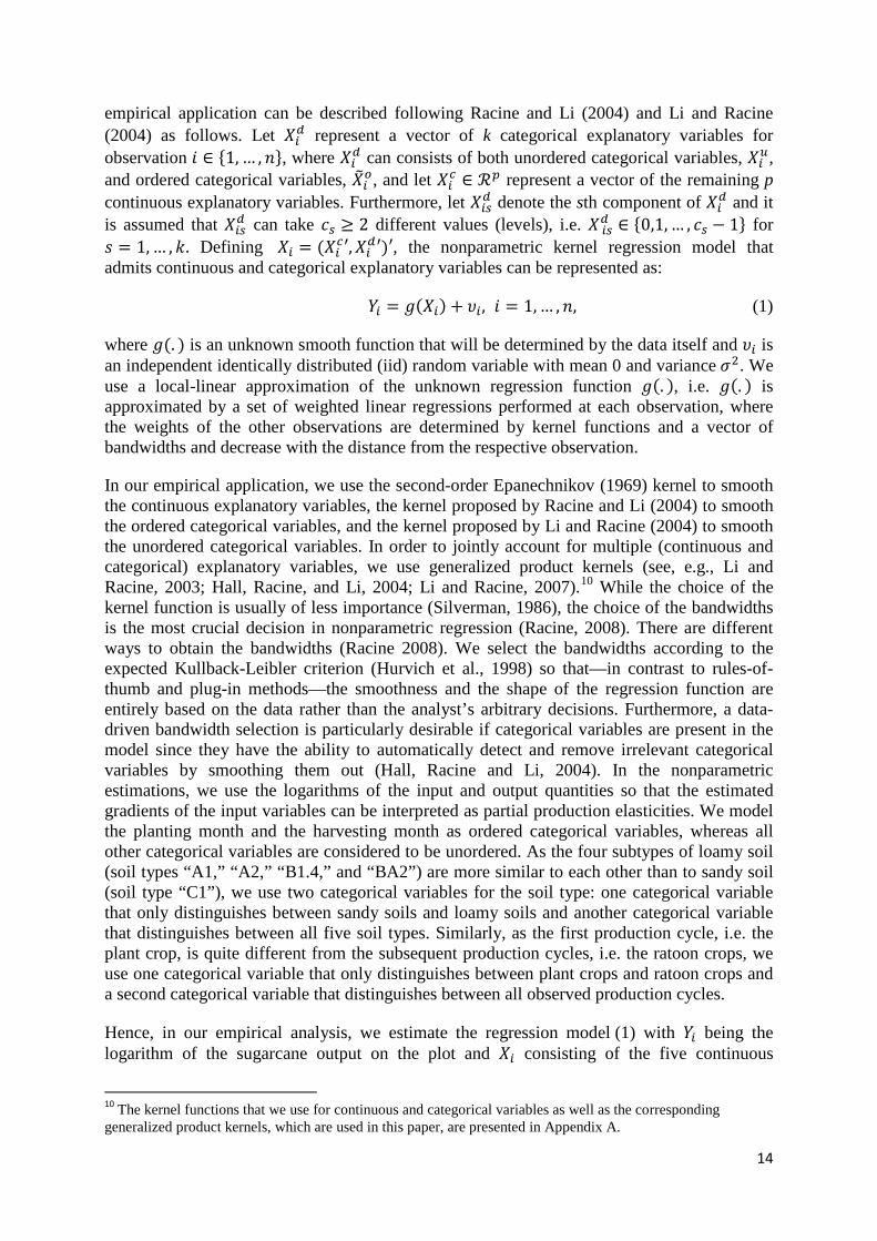
empirical application can be described following Racine and Li (2004) and Li and Racine (2004) as follows. Let 𝑋𝑋𝑖𝑖𝑑𝑑 represent a vector of k categorical explanatory variables for observation 𝑖𝑖 ∈ {1, … , 𝑛𝑛}, where 𝑋𝑋𝑖𝑖𝑑𝑑 can consists of both unordered categorical variables, 𝑋𝑋𝑖𝑖𝑢𝑢, and ordered categorical variables, 𝑋𝑋�𝑖𝑖𝑜𝑜, and let 𝑋𝑋𝑖𝑖𝑐𝑐 ∈ ℛ𝑝𝑝 represent a vector of the remaining p continuous explanatory variables. Furthermore, let 𝑋𝑋𝑖𝑖𝑖𝑖𝑑𝑑 denote the sth component of 𝑋𝑋𝑖𝑖𝑑𝑑 and it is assumed that 𝑋𝑋𝑖𝑖𝑖𝑖𝑑𝑑 can take 𝑐𝑐𝑖𝑖 ≥ 2 different values (levels), i.e. 𝑋𝑋 𝑖𝑖𝑖𝑖

𝑑𝑑 ∈ {0,1, … , 𝑐𝑐𝑖𝑖 − 1} for 𝑠𝑠 = 1, … ,𝑘𝑘. Defining 𝑋𝑋𝑖𝑖 = (𝑋𝑋𝑖𝑖𝑐𝑐′,𝑋𝑋𝑖𝑖𝑑𝑑′)′, the nonparametric kernel regression model that admits continuous and categorical explanatory variables can be represented as:

𝑌𝑌𝑖𝑖 = 𝑔𝑔(𝑋𝑋𝑖𝑖) + 𝜐𝜐𝑖𝑖, 𝑖𝑖 = 1, … ,𝑛𝑛, (1)

where 𝑔𝑔(. ) is an unknown smooth function that will be determined by the data itself and 𝜐𝜐𝑖𝑖 is an independent identically distributed (iid) random variable with mean 0 and variance 𝜎𝜎2. We use a local-linear approximation of the unknown regression function 𝑔𝑔(. ), i.e. 𝑔𝑔(. ) is approximated by a set of weighted linear regressions performed at each observation, where the weights of the other observations are determined by kernel functions and a vector of bandwidths and decrease with the distance from the respective observation.

In our empirical application, we use the second-order Epanechnikov (1969) kernel to smooth the continuous explanatory variables, the kernel proposed by Racine and Li (2004) to smooth the ordered categorical variables, and the kernel proposed by Li and Racine (2004) to smooth the unordered categorical variables. In order to jointly account for multiple (continuous and categorical) explanatory variables, we use generalized product kernels (see, e.g., Li and Racine, 2003; Hall, Racine, and Li, 2004; Li and Racine, 2007).10 While the choice of the kernel function is usually of less importance (Silverman, 1986), the choice of the bandwidths is the most crucial decision in nonparametric regression (Racine, 2008). There are different ways to obtain the bandwidths (Racine 2008). We select the bandwidths according to the expected Kullback-Leibler criterion (Hurvich et al., 1998) so that—in contrast to rules-of-thumb and plug-in methods—the smoothness and the shape of the regression function are entirely based on the data rather than the analyst’s arbitrary decisions. Furthermore, a data-driven bandwidth selection is particularly desirable if categorical variables are present in the model since they have the ability to automatically detect and remove irrelevant categorical variables by smoothing them out (Hall, Racine and Li, 2004). In the nonparametric estimations, we use the logarithms of the input and output quantities so that the estimated gradients of the input variables can be interpreted as partial production elasticities. We model the planting month and the harvesting month as ordered categorical variables, whereas all other categorical variables are considered to be unordered. As the four subtypes of loamy soil (soil types “A1,” “A2,” “B1.4,” and “BA2”) are more similar to each other than to sandy soil (soil type “C1”), we use two categorical variables for the soil type: one categorical variable that only distinguishes between sandy soils and loamy soils and another categorical variable that distinguishes between all five soil types. Similarly, as the first production cycle, i.e. the plant crop, is quite different from the subsequent production cycles, i.e. the ratoon crops, we use one categorical variable that only distinguishes between plant crops and ratoon crops and a second categorical variable that distinguishes between all observed production cycles.

Hence, in our empirical analysis, we estimate the regression model (1) with 𝑌𝑌𝑖𝑖 being the logarithm of the sugarcane output on the plot and 𝑋𝑋𝑖𝑖 consisting of the five continuous

10 The kernel functions that we use for continuous and categorical variables as well as the corresponding generalized product kernels, which are used in this paper, are presented in Appendix A.

14

explanatory variables (four logarithmic input quantities and the duration of the growing period), two ordered categorical explanatory variables (planting/ratooning month and harvesting month) and six unordered categorical explanatory variables (two variables for soil type, two variables for the production cycle, cane variety, production model).

The flexibility of the local-linear nonparametric regression comes at the cost of possible violations of the properties of production technologies derived from microeconomic theory (e.g. monotonicity). As non-monotone production technologies can result in misleading productivity measures (Henningsen and Henning, 2009), we impose monotonicity using the constrained weighted bootstrapping (CWB) method proposed by Hall and Huang (2001) and extended by Du et al. (2013).

Finally, we assess the statistical significance of each regressor with a nonparametric test for irrelevant regressors (Racine, 1997; Racine, Hart, and Li, 2006), where the bootstrap method based on independent identically distributed (iid) draws is used to obtain the distribution of the test statistic under the null hypothesis.

6. Results

The empirical analysis was performed within the statistical software environment “R” (R Development Core Team, 2013) using the add-on package “np” (Hayfield and Racine, 2008) for nonparametric estimations and specification tests.

The bandwidth selection for model (1) according to the expected Kullback-Leibler criterion and the test for irrelevant regressors (Racine, 1997; Racine, Hart, and Li, 2006) unanimously indicate that the harvesting month and the subtype of the loamy soil do not significantly affect the yield (given that we have controlled for other variables such as the planting/ratooning month, the duration of the growing period, and the soil type variable that distinguishes loamy soils and sandy soils). Thus we removed these two categorical variables from our model.

The optimal bandwidths that minimize the expected Kullback-Leibler criterion of the remaining explanatory variables are presented in Table 4.11 The bandwidths of continuous variables can range from zero to infinity. When the bandwidth of a continuous variable is more than two times the standard deviation, this variable is modeled approximately linearly (Parmeter et al., 2014). Therefore, we can conclude that all the continuous explanatory variables, except machinery, are modeled approximately linearly when holding all other continuous and categorical explanatory variables constant. However, in contrast to parametric linear regression, the slopes of the variables with large bandwidths can depend on the values of other explanatory variables. The bandwidths of the categorical explanatory variables can range from zero to one. If the bandwidth of a categorical variable is zero, the nonparametric regression basically splits the sample into sub-samples based on the values of this variable and separately estimates the model for each sub-sample. On the other hand, if the bandwidth of a categorical variable is one, the bandwidth selection indicates that this variable is irrelevant in predicting the value of the dependent variable and thus the nonparametric regression disregards this variable. Thus, the relatively large bandwidths of the soil type (loamy soil vs. sandy soil) and the planting/ratooning month indicate that the production functions are quite similar for the different soil types and planting/ratooning months. In

11 We also tried to select the bandwidths by least-squares leave-one-out cross-validation, but due to many local minima of the objective function, the bandwidth selection was very sensitive to the starting values and we were unable to ensure that we reached the global minimum. This problem did not occur in the bandwidth selection according to the expected Kullback-Leibler criterion.

15

contrast, the rather small bandwidth of the variable that distinguishes plant crops from ratoon crops indicates that the production function for plant crops is quite different from the production function for ratoon crops.

Table 4. Optimal bandwidths and statistical significance levels of the regressors Variable Bandwidth P-value Continuous variables log(plot size) ∞ 0.0902

log(machinery) 3.066 0.0025

log(intermediate inputs) ∞ ˂ 0.0001

log(labor) ∞ 0.4411 Duration of the growing period ∞ ˂ 0.0100

Categorical variables Number of rainy seasons 0.269 ˂ 0.0001 Planting/ratooning month 0.505 ˂ 0.0001 Production cycle (plant crop vs. ratoon crop) 0.063 0.0050 Production cycle 0.236 ˂ 0.0001 Soil type (loamy soil vs. sandy soil) 0.443 ˂ 0.0001 Production model (outgrower vs. plantation) 0.258 ˂ 0.0001 Note: an infinity symbol (∞) means that the bandwidth is greater than two times the standard deviation of the respective variable. The P-values are obtained by the test for irrelevant regressors suggested by Racine (1997) and extended by Racine, Hart, and Li (2006) applied to the monotonicity–constrained model.

The plot-level production function that we obtained by kernel regression with the bandwidths indicated in Table 4 violates the monotonicity conditions for three input variables (labor, machinery and intermediate inputs) at some of the observations.12 In order to make meaningful productivity comparisons, we impose monotonicity using the constrained weighted bootstrapping (CWB) method by constraining the gradients of all four input quantities so that they are non-negative.

We applied the test for irrelevant regressors suggested by Racine (1997) and extended by Racine, Hart, and Li (2006) to the monotonicity–constrained model (see Table 4). This test indicates that machinery inputs, intermediate inputs, and all plot-level characteristics have a statistically significant effect on sugarcane production. While the effect of the plot size is only significant at the 10% level, the effect of the labor input is clearly statistically insignificant. This is probably caused by a very high correlation between the (logarithmic) plot size and the (logarithmic) labor input (coefficient correlation = 0.904).

The mean values of the estimated derivatives/gradients obtained from the model with monotonicity imposed are given in Table 5.13 The plot size has the largest output elasticity, while machinery and intermediate inputs have rather low output elasticities. Although outgrowers use more labor and intermediate inputs than the plantation, they achieve considerably higher output elasticities of these two inputs, which indicates that outgrowers use labor and intermediate inputs more effectively than the plantation. The sums of the four output elasticities are mostly between 0.9 and 1.0, both for outgrower plots and for factory-

12 The distributions of the estimated gradients of the inputs and thus the prevalence of monotonicity violations are presented in Table B1 in appendix B. 13 We report the mean values of the gradients estimated by the unconstrained model in Table B2 in appendix B.

16

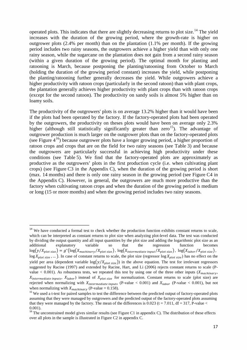
operated plots. This indicates that there are slightly decreasing returns to plot size.14 The yield increases with the duration of the growing period, where the growth-rate is higher on outgrower plots (2.4% per month) than on the plantation (1.1% per month). If the growing period includes two rainy seasons, the outgrowers achieve a higher yield than with only one rainy season, while the sugarcane on the plantation does not gain from a second rainy season (within a given duration of the growing period). The optimal month for planting and ratooning is March, because postponing the planting/ratooning from October to March (holding the duration of the growing period constant) increases the yield, while postponing the planting/ratooning further generally decreases the yield. While outgrowers achieve a higher productivity with ratoon crops (particularly in the second ratoon) than with plant crops, the plantation generally achieves higher productivity with plant crops than with ratoon crops (except for the second ratoon). The productivity on sandy soils is almost 5% higher than on loamy soils.

The productivity of the outgrowers' plots is on average 13.2% higher than it would have been if the plots had been operated by the factory. If the factory-operated plots had been operated by the outgrowers, the productivity on theses plots would have been on average only 2.3% higher (although still statistically significantly greater than zero15). The advantage of outgrower production is much larger on the outgrower plots than on the factory-operated plots (see Figure 416) because outgrower plots have a longer growing period, a higher proportion of ratoon crops and crops that are on the field for two rainy seasons (see Table 3) and because the outgrowers are particularly successful in achieving high productivity under these conditions (see Table 5). We find that the factory-operated plots are approximately as productive as the outgrowers’ plots in the first production cycle (i.e. when cultivating plant crops) (see Figure C3 in the Appendix C), when the duration of the growing period is short (max. 14 months) and there is only one rainy season in the growing period (see Figure C4 in the Appendix C). However, in general, the outgrowers are much more productive than the factory when cultivating ratoon crops and when the duration of the growing period is medium or long (15 or more months) and when the growing period includes two rainy seasons.

14 We have conducted a formal test to check whether the production function exhibits constant returns to scale, which can be interpreted as constant returns to plot size when analyzing plot-level data. The test was conducted by dividing the output quantity and all input quantities by the plot size and adding the logarithmic plot size as an additional explanatory variable so that the regression function becomes log�𝑦𝑦 𝑋𝑋𝑝𝑝𝑝𝑝𝑜𝑜𝑝𝑝 𝑖𝑖𝑖𝑖𝑠𝑠𝑠𝑠⁄ � = 𝑔𝑔∗�log�𝑋𝑋𝑚𝑚𝑚𝑚𝑐𝑐ℎ𝑖𝑖𝑖𝑖𝑠𝑠𝑖𝑖𝑖𝑖 𝑋𝑋𝑝𝑝𝑝𝑝𝑜𝑜𝑝𝑝 𝑖𝑖𝑖𝑖𝑠𝑠𝑠𝑠⁄ � , log�𝑋𝑋𝑖𝑖𝑖𝑖𝑝𝑝𝑠𝑠𝑖𝑖𝑚𝑚𝑠𝑠𝑑𝑑𝑖𝑖𝑚𝑚𝑝𝑝𝑠𝑠 𝑖𝑖𝑖𝑖𝑝𝑝𝑢𝑢𝑝𝑝 𝑋𝑋𝑝𝑝𝑝𝑝𝑜𝑜𝑝𝑝 𝑖𝑖𝑖𝑖𝑠𝑠𝑠𝑠⁄ � , log�𝑋𝑋𝑝𝑝𝑚𝑚𝑙𝑙𝑜𝑜𝑖𝑖 𝑋𝑋𝑝𝑝𝑝𝑝𝑜𝑜𝑝𝑝 𝑖𝑖𝑖𝑖𝑠𝑠𝑠𝑠⁄ � ,log𝑋𝑋𝑝𝑝𝑝𝑝𝑜𝑜𝑝𝑝 𝑖𝑖𝑖𝑖𝑠𝑠𝑠𝑠 , … �. In case of constant returns to scale, the plot size (regressor log𝑋𝑋𝑝𝑝𝑝𝑝𝑜𝑜𝑝𝑝 𝑖𝑖𝑖𝑖𝑠𝑠𝑠𝑠) has no effect on the yield per area (dependent variable log�𝑦𝑦 𝑋𝑋𝑝𝑝𝑝𝑝𝑜𝑜𝑝𝑝 𝑖𝑖𝑖𝑖𝑠𝑠𝑠𝑠⁄ �) in the above equation. The test for irrelevant regressors suggested by Racine (1997) and extended by Racine, Hart, and Li (2006) rejects constant returns to scale (P-value < 0.001). As robustness tests, we repeated this test by using one of the three other inputs (𝑋𝑋𝑚𝑚𝑚𝑚𝑐𝑐ℎ𝑖𝑖𝑖𝑖𝑚𝑚𝑖𝑖𝑖𝑖, 𝑋𝑋𝑖𝑖𝑖𝑖𝑝𝑝𝑠𝑠𝑖𝑖𝑚𝑚𝑠𝑠𝑑𝑑𝑖𝑖𝑚𝑚𝑝𝑝𝑠𝑠 𝑖𝑖𝑖𝑖𝑝𝑝𝑢𝑢𝑝𝑝𝑖𝑖, 𝑋𝑋𝑝𝑝𝑚𝑚𝑙𝑙𝑜𝑜𝑖𝑖) instead of 𝑋𝑋𝑝𝑝𝑝𝑝𝑜𝑜𝑝𝑝 𝑖𝑖𝑖𝑖𝑠𝑠𝑠𝑠 for normalization. Constant returns to scale (plot size) are rejected when normalizing with 𝑋𝑋𝑖𝑖𝑖𝑖𝑝𝑝𝑠𝑠𝑖𝑖𝑚𝑚𝑠𝑠𝑑𝑑𝑖𝑖𝑚𝑚𝑝𝑝𝑠𝑠 𝑖𝑖𝑖𝑖𝑝𝑝𝑢𝑢𝑝𝑝𝑖𝑖 (P-value < 0.001) and 𝑋𝑋𝑝𝑝𝑚𝑚𝑙𝑙𝑜𝑜𝑖𝑖 (P-value < 0.001), but not when normalizing with 𝑋𝑋𝑚𝑚𝑚𝑚𝑐𝑐ℎ𝑖𝑖𝑖𝑖𝑚𝑚𝑖𝑖𝑖𝑖 (P-value = 0.158). 15 We used a t-test for paired samples to test the difference between the predicted output of factory-operated plots assuming that they were managed by outgrowers and the predicted output of the factory-operated plots assuming that they were managed by the factory. The mean of the differences is 0.023 (t = 7.011, df = 317, P-value < 0.001). 16 The unconstrained model gives similar results (see Figure C1 in appendix C). The distribution of these effects over all plots in the sample is illustrated in Figure C2 in appendix C.

17

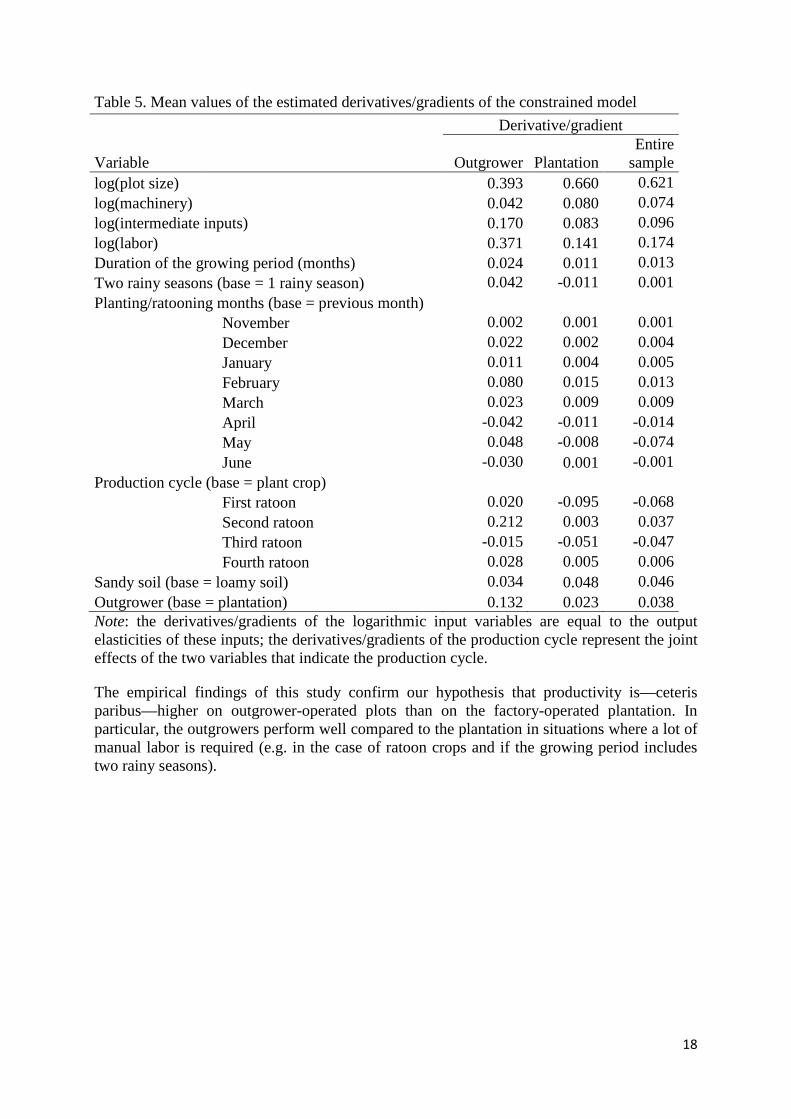
Table 5. Mean values of the estimated derivatives/gradients of the constrained model

Variable

Derivative/gradient

Outgrower Plantation Entire

sample log(plot size)

0.393 0.660 0.621

log(machinery) 0.042 0.080 0.074 log(intermediate inputs) 0.170 0.083 0.096 log(labor) 0.371 0.141 0.174 Duration of the growing period (months) 0.024 0.011 0.013 Two rainy seasons (base = 1 rainy season) 0.042 -0.011 0.001 Planting/ratooning months (base = previous month) November 0.002 0.001 0.001 December 0.022 0.002 0.004 January 0.011 0.004 0.005 February 0.080 0.015 0.013 March 0.023 0.009 0.009 April -0.042 -0.011 -0.014 May 0.048 -0.008 -0.074 June -0.030 0.001 -0.001 Production cycle (base = plant crop) First ratoon 0.020 -0.095 -0.068 Second ratoon 0.212 0.003 0.037 Third ratoon -0.015 -0.051 -0.047 Fourth ratoon 0.028 0.005 0.006 Sandy soil (base = loamy soil) 0.034 0.048 0.046 Outgrower (base = plantation) 0.132 0.023 0.038 Note: the derivatives/gradients of the logarithmic input variables are equal to the output elasticities of these inputs; the derivatives/gradients of the production cycle represent the joint effects of the two variables that indicate the production cycle.

The empirical findings of this study confirm our hypothesis that productivity is—ceteris paribus—higher on outgrower-operated plots than on the factory-operated plantation. In particular, the outgrowers perform well compared to the plantation in situations where a lot of manual labor is required (e.g. in the case of ratoon crops and if the growing period includes two rainy seasons).

18

Figure 4. Effects of outgrower management (compared to factory management) on productivity on plots that are operated by the factory and on plots that are operated by outgrowers.

Since higher productivity does not necessary mean higher profitability, we examine the gross margin (in ETB) of the two production models. For this analysis, we use the logarithm of the gross margin of the plot17 as the dependent variable and include the plot size, the number of rainy seasons, the soil type, the duration of the growing period, the planting/ratooning month, the production cycle, and the production model as explanatory variables. Except for the different dependent variable and the removal of the three variable input quantities (labor, machinery, intermediate inputs), we use the same nonparametric model specification as in our model for analyzing plot-level productivity. As the number of rainy seasons had an optimal bandwidth of one (which means that it is smoothed out) and was statistically insignificant, we removed it from the gross margin model. All other explanatory variables are statistically significant at least at the 5% significance level. The optimal bandwidths, the significance levels, and the mean values of the estimated derivatives/gradients for the gross margin model are given in Tables B3 and B4 in appendix B.

The estimated effects of outgrower management (compared to factory management) on plot-level gross margin are illustrated in Figure 5. Our analysis shows that outgrowers achieve a higher gross margin than the factory plantation. The effects of outgrower management on the gross margin are even greater than the effects on productivity. On plots that are operated by

17 Gross margin per plot was calculated as the total sugarcane yield per plot (in quintals) multiplied by the price of cane (ETB/quintal) minus the total input costs of labor, intermediate inputs and machinery per plot (in ETB).

19

the outgrowers, the outgrowers achieve on average a 21.4% higher gross margin than the factory would have achieved on these plots. On plots that are operated by the factory, the outgrowers would have achieved on average a 7.6% higher gross margin than the factory achieved on these plots.18

Figure 5. Effects of outgrower management (compared to factory management) on the gross margin on plots that are operated by the factory and on plots that are operated by outgrowers.

18 The difference in the gross-margin on the factory-operated plots is statistically significant only at the 10% level.

20

7. Conclusion

We applied a non-parametric kernel regression method to a new plot-level data set in order to compare the productivity of factory-operated and outgrower-operated sugarcane production in Ethiopia. Our study shows that the outgrowers achieve on average significantly higher productivity and a significantly higher gross-margin than the factory plantation. Our finding is consistent with the majority of previous studies, which suggest that small-scale farmers have higher productivity than large-scale production due to the high productivity of family labor compared to hired labor. While previous studies could only analyze the joint effect of incentives and access to credit and technologies, we can conclude that the identified productivity difference between the two production types in our study is solely caused by different incentive structures between the outgrowers and the laborers and managers at the plantation. The policy implication of this research is that the expansion of sugarcane production through establishing outgrower schemes may result in higher productivity than through extending factory-operated plantations.

21

Appendix A: kernel functions

The univariate second-order Epanechnikov (1969) kernel for a continuous regressor 𝑋𝑋𝑖𝑖𝑐𝑐 =(𝑋𝑋1𝑖𝑖𝑐𝑐 , . . . ,𝑋𝑋𝑖𝑖𝑖𝑖𝑐𝑐 )′, where the first subscript indicates the observation and n indicates the number of observations, is given by:

𝑤𝑤�𝑋𝑋𝑖𝑖𝑖𝑖𝑐𝑐 ,𝑋𝑋𝑗𝑗𝑖𝑖𝑐𝑐 , ℎ𝑖𝑖� = �3

�4√5��1 − 1

5�𝑋𝑋𝑖𝑖𝑖𝑖𝑐𝑐 −𝑋𝑋𝑗𝑗𝑖𝑖

𝑐𝑐

ℎ𝑖𝑖�2

�

0 if �

𝑋𝑋𝑖𝑖𝑖𝑖𝑐𝑐 − 𝑋𝑋𝑗𝑗𝑖𝑖𝑐𝑐

ℎ𝑖𝑖�2

< 5.0

otherwise,

where the kernel function (weighting function) 𝑤𝑤(∙) indicates the weight of observation j in the local linear kernel regression at observation i and ℎ𝑖𝑖 > 0 is the bandwidth for regressor 𝑋𝑋𝑖𝑖𝑐𝑐. In a multivariate case with 𝑝𝑝 continuous regressors, 𝑋𝑋𝑐𝑐 = (𝑋𝑋1𝑐𝑐, … ,𝑋𝑋𝑝𝑝𝑐𝑐), Li and Racine (2007) suggest using a generalized product kernel of univariate kernel functions defined as:

𝑊𝑊�𝑋𝑋𝑖𝑖𝑐𝑐 ,𝑋𝑋𝑗𝑗𝑐𝑐 ,ℎ� = �ℎ𝑖𝑖−1 𝑤𝑤�𝑋𝑋𝑖𝑖𝑖𝑖𝑐𝑐 ,𝑋𝑋𝑗𝑗𝑖𝑖𝑐𝑐 , ℎ𝑖𝑖�𝑝𝑝

𝑖𝑖=1

where 𝑤𝑤(∙) is a univariate kernel function for a continuous regressor 𝑋𝑋𝑖𝑖𝑐𝑐 and ℎ = �ℎ1, … ,ℎ𝑝𝑝�′ is a vector of bandwidths, where ℎ𝑖𝑖 denotes the bandwidth parameter associated with regressor 𝑋𝑋𝑖𝑖𝑐𝑐. For an unordered categorical regressor 𝑋𝑋𝑖𝑖𝑢𝑢 = (𝑋𝑋1𝑖𝑖𝑢𝑢 , . . . ,𝑋𝑋𝑖𝑖𝑖𝑖𝑢𝑢 )′, Racine and Li (2004) propose a kernel function, which is a variation on Aitchison and Aitken’s (1976) kernel function:

𝑙𝑙�𝑋𝑋𝑖𝑖𝑖𝑖𝑢𝑢 ,𝑋𝑋𝑗𝑗𝑖𝑖𝑢𝑢 , 𝜆𝜆𝑖𝑖� = � 1 if 𝑋𝑋𝑖𝑖𝑖𝑖𝑢𝑢 = 𝑋𝑋𝑗𝑗𝑖𝑖𝑢𝑢

𝜆𝜆𝑖𝑖 otherwise,

where the kernel function 𝑙𝑙(∙) indicates the weight of observation j in the local linear kernel regression at observation i and 𝜆𝜆s is the bandwidth parameter for the regressor 𝑋𝑋𝑖𝑖𝑢𝑢, which is in the range [0,1]. When λs = 0, the kernel function 𝑙𝑙(∙) becomes an indicator function, and when 𝜆𝜆𝑖𝑖 = 1, it becomes a uniform (constant) function, i.e. the regressor 𝑋𝑋𝑖𝑖𝑢𝑢 is smoothed out (removed). The product kernel function for 𝑞𝑞 unordered categorical regressors 𝑋𝑋𝑢𝑢 = (𝑋𝑋1𝑢𝑢, … ,𝑋𝑋𝑞𝑞𝑢𝑢) is given as:

𝐿𝐿�𝑋𝑋𝑖𝑖𝑢𝑢,𝑋𝑋𝑗𝑗𝑢𝑢, 𝜆𝜆� = �𝑙𝑙�𝑋𝑋𝑖𝑖𝑖𝑖𝑢𝑢 ,𝑋𝑋𝑗𝑗𝑖𝑖𝑢𝑢 , 𝜆𝜆𝑖𝑖�𝑞𝑞

𝑖𝑖=1

,

where 𝑙𝑙(∙) is a univariate kernel function for an unordered categorical regressor 𝑋𝑋𝑖𝑖𝑢𝑢 and 𝜆𝜆 = �𝜆𝜆1, … , 𝜆𝜆𝑞𝑞�′ is a vector of bandwidths, where 𝜆𝜆𝑖𝑖 denotes the bandwidth parameter associated with the regressor 𝑋𝑋𝑖𝑖𝑢𝑢. For an ordered categorical regressor 𝑋𝑋𝑖𝑖𝑜𝑜 = (𝑋𝑋1𝑖𝑖𝑜𝑜 , . . . ,𝑋𝑋𝑖𝑖𝑖𝑖𝑜𝑜 )′, Li and Racine (2004) propose the following kernel function:

𝑙𝑙�𝑋𝑋𝑖𝑖𝑖𝑖𝑜𝑜 ,𝑋𝑋𝑗𝑗𝑖𝑖𝑜𝑜 ,𝜓𝜓𝑖𝑖� = �1 if 𝑋𝑋𝑖𝑖𝑖𝑖𝑜𝑜 = 𝑋𝑋𝑗𝑗𝑖𝑖𝑜𝑜

𝜓𝜓𝑖𝑖|𝑋𝑋𝑖𝑖𝑖𝑖

𝑜𝑜−𝑋𝑋𝑗𝑗𝑖𝑖𝑜𝑜 |

if 𝑋𝑋𝑖𝑖𝑖𝑖𝑜𝑜 ≠ 𝑋𝑋𝑗𝑗𝑖𝑖𝑜𝑜 ,

where the kernel function 𝑙𝑙(∙) indicates the weight of observation j in the local linear kernel regression at observation i and 𝜓𝜓𝑖𝑖 is the bandwidth parameter for regressor 𝑋𝑋𝑖𝑖𝑜𝑜, which is in the range [0,1]. Similarly to the kernel function for unordered categorical regressors given above, when 𝜓𝜓𝑖𝑖 = 0, the kernel function 𝑙𝑙(∙) becomes an indicator function, and when 𝜓𝜓𝑖𝑖 = 1, it becomes a uniform (constant) weight function, i.e. the regressor 𝑋𝑋𝑖𝑖𝑜𝑜 is smoothed out (removed).

22

The product kernel function for 𝑟𝑟 ordered categorical regressors 𝑋𝑋𝑜𝑜 = (𝑋𝑋1𝑜𝑜 , … ,𝑋𝑋𝑖𝑖𝑜𝑜) is given as:

𝐿𝐿��𝑋𝑋𝑖𝑖𝑜𝑜 ,𝑋𝑋𝑗𝑗𝑜𝑜 ,𝜓𝜓� = �𝑙𝑙�𝑋𝑋𝑖𝑖𝑖𝑖𝑜𝑜 ,𝑋𝑋𝑗𝑗𝑖𝑖𝑜𝑜 ,𝜓𝜓𝑖𝑖�𝑖𝑖

𝑖𝑖=1

,

where 𝑙𝑙(∙) is a univariate kernel function for an ordered categorical regressor 𝑋𝑋𝑖𝑖𝑜𝑜 and 𝜓𝜓 =(𝜓𝜓1, … ,𝜓𝜓𝑖𝑖)′ is a vector of bandwidths, where 𝜓𝜓𝑖𝑖 denotes the bandwidth parameter associated with the regressor 𝑋𝑋𝑖𝑖𝑜𝑜. Finally, the kernel function for the vector of mixed continuous and (unordered and ordered) categorical regressors, 𝑥𝑥 = (𝑋𝑋𝑐𝑐,𝑋𝑋𝑢𝑢,𝑋𝑋𝑜𝑜), is the product of W(∙), L(∙) and 𝐿𝐿�(∙), given by:

𝐾𝐾�𝑋𝑋𝑖𝑖,𝑋𝑋𝑗𝑗 , 𝛾𝛾 � = 𝑊𝑊�𝑋𝑋𝑖𝑖𝑐𝑐,𝑋𝑋𝑗𝑗𝑐𝑐 ,ℎ� × 𝐿𝐿�𝑋𝑋𝑖𝑖𝑢𝑢,𝑋𝑋𝑗𝑗𝑢𝑢, 𝜆𝜆� × 𝐿𝐿��𝑋𝑋𝑖𝑖𝑜𝑜 ,𝑋𝑋𝑗𝑗𝑜𝑜 ,𝜓𝜓� , where 𝛾𝛾 = (ℎ, 𝜆𝜆,𝜓𝜓) is a vector of bandwidths for continuous and categorical regressors.

23

Appendix B: supplementary tables

Table B1. Distribution of gradients of the unconstrained model

Minimum 1st quartile Median Mean

3rd quartile Maximum

All plots

Plot size 0.305 0.710 0.828 0.809 0.897 1.465

Machinery -0.333 -0.008 0.032 0.034 0.084 0.277

Intermediate input -0.111 0.004 0.035 0.054 0.116 0.287

Labor -0.421 -0.079 -0.002 0.048 0.173 0.819

Outgrower plots

Plot size 0.305 0.387 0.487 0.507 0.593 0.793

Machinery -0.334 -0.047 -0.014 -0.022 0.050 0.098

Intermediate input -0.022 0.113 0.147 0.140 0.217 0.287

Labor 0.001 0.257 0.325 0.328 0.429 0.819

Factory-operated plots

Plot size 0.344 0.782 0.851 0.860 0.931 1.465

Machinery -0.154 0.0003 0.041 0.044 0.089 0.277

Intermediate input -0.111 -0.005 0.031 0.040 0.098 0.098

Labor -0.420 -0.087 -0.025 -0.001 0.092 0.448

24

Table B2. Mean values of the estimated derivatives/gradients of the unconstrained model

Variable

Derivative/gradient

Outgrower Plantation Entire

sample log(plot size)

0.507 0.860 0.809

log(machinery) -0.022 0.044 0.034 log(intermediate inputs) 0.140 0.040 0.054 log(labor) 0.329 -0.001 0.049 Duration of the growing period (months) 0.028 0.009 0.012 Two rainy seasons (base = 1 rainy season) 0.060 -0.010 0.005 Planting/ratooning months (base = previous month) November 0.003 0.001 0.001 December 0.023 0.003 0.004 January 0.011 0.003 0.005 February 0.006 0.011 0.010 March 0.080 0.005 0.010 April 0.013 -0.014 -0.011 May 0.027 -0.091 -0.085 June 0.004 0.001 0.001 Production cycle (base = plant crop) First ratoon 0.014 -0.115 -0.085 Second ratoon 0.309 -0.012 0.041 Third ratoon -0.036 -0.059 -0.057 Fourth ratoon 0.023 -0.011 -0.011 Sandy soil (base = loamy soil) 0.067 0.046 0.049 Outgrower (base = plantation) 0.175 Note: the derivatives/gradients of the logarithmic input variables are equal to the output elasticities of these inputs; the derivatives/gradients of the production cycle represent the joint effects of the two variables that indicate the production cycle.

25

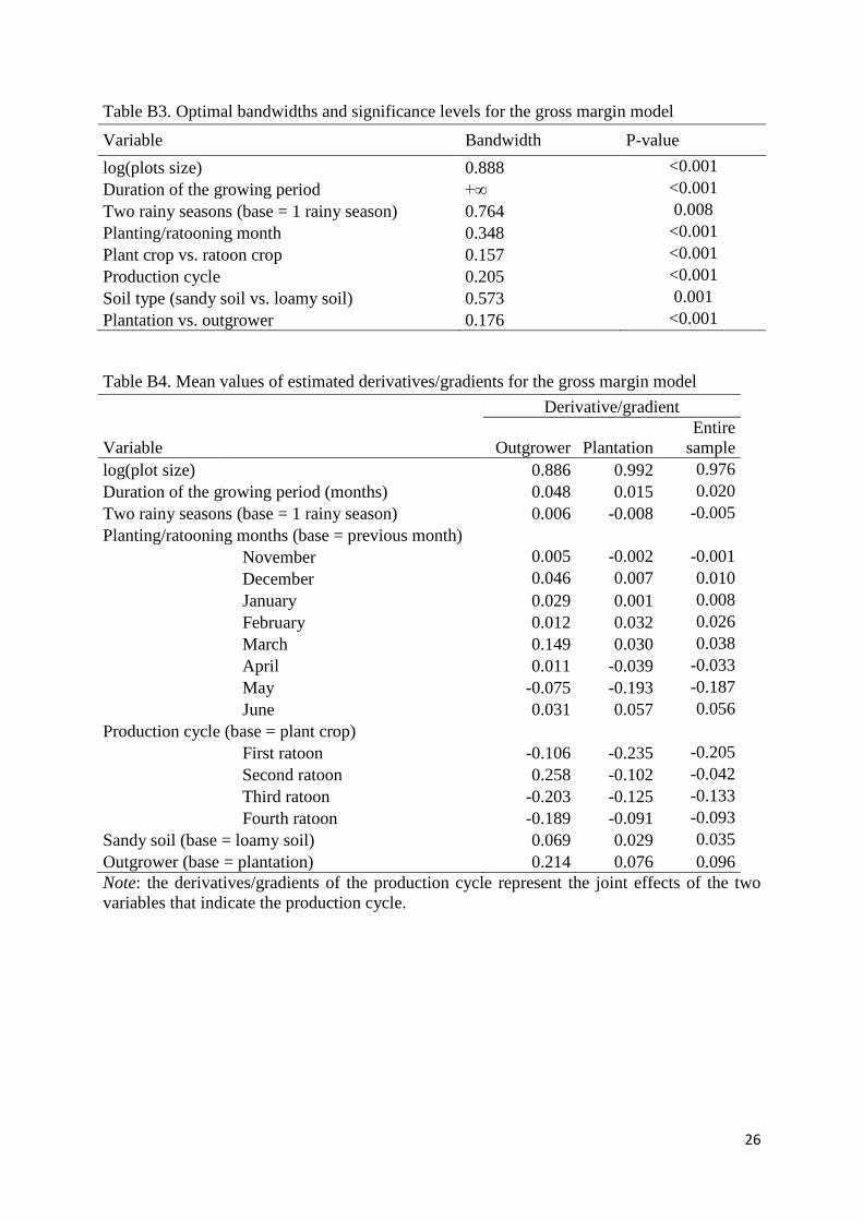
Table B3. Optimal bandwidths and significance levels for the gross margin model

Variable Bandwidth P-value log(plots size) 0.888 <0.001 Duration of the growing period +∞ <0.001

Two rainy seasons (base = 1 rainy season) 0.764 0.008 Planting/ratooning month 0.348 <0.001 Plant crop vs. ratoon crop 0.157 <0.001 Production cycle 0.205 <0.001 Soil type (sandy soil vs. loamy soil) 0.573 0.001 Plantation vs. outgrower 0.176 <0.001

Table B4. Mean values of estimated derivatives/gradients for the gross margin model

Variable

Derivative/gradient

Outgrower Plantation Entire

sample log(plot size)

0.886 0.992 0.976

Duration of the growing period (months) 0.048 0.015 0.020 Two rainy seasons (base = 1 rainy season) 0.006 -0.008 -0.005 Planting/ratooning months (base = previous month) November 0.005 -0.002 -0.001 December 0.046 0.007 0.010 January 0.029 0.001 0.008 February 0.012 0.032 0.026 March 0.149 0.030 0.038 April 0.011 -0.039 -0.033 May -0.075 -0.193 -0.187 June 0.031 0.057 0.056 Production cycle (base = plant crop) First ratoon -0.106 -0.235 -0.205 Second ratoon 0.258 -0.102 -0.042 Third ratoon -0.203 -0.125 -0.133 Fourth ratoon -0.189 -0.091 -0.093 Sandy soil (base = loamy soil) 0.069 0.029 0.035 Outgrower (base = plantation) 0.214 0.076 0.096 Note: the derivatives/gradients of the production cycle represent the joint effects of the two variables that indicate the production cycle.

26

Appendix C: supplementary figures

Figure C1. Effects of outgrower management (compared to factory management) on productivity on plots that are operated by the factory and on plots that are operated by outgrowers (unconstrained model).

27

Figure C2. Distribution of the effects of outgrower management (compared to factory management) on plot level productivity on all plots in the sample.

Figure C3. Effects of outgrower management (compared to factory management) on plot-level productivity under different production cycles.

Figure C4. Effects of outgrower management (compared to factory management) on plot-level productivity on plots with different numbers of rainy seasons in the growing period.

28

References

Abate, E., Teshome, A., 2013. Contract Farming: Theoretical Concepts, Opportunities and Challenges in Mid and High Altitude Areas of Northwestern Ethiopia. Proceedings of the First Regional Conference of the Amhara Regional State Economic Development. Bahirdar: Ethiopia.

Aitchison, J., Aitken, C. G. G., 1976. Multivariate binary discrimination by the kernel method. Biometrika 63, 413–420.

Allen, D., Lueck, D., 1992. Contract Choice in Modern Agriculture: Cash Rent versus Crop share. J. Law and Econ. 35, 397-426.

Assuncao, J., Ghatak, M., 2003. Can unobserved heterogeneity in farmer ability explain the inverse relationship between farm size and productivity? Econ. Letters 80: 189–194

Barrett, B., Bachke, M., Bellemare, M., Michelson, H., Narayanan, S., Walker, T., 2012. Smallholder participation in contract farming: Comparative evidence from five countries. World Dev. 40, 715-730.

Barrett, B., Bellemare, M., Hou, J., 2010. Reconsidering Conventional Explanations of the Inverse Productivity–Size Relationship. World Dev. 38, 88–97.

Barrett, B., 1996. On price risk and the inverse farm size-productivity relationship. J. Dev. Econ. 51, 193-215.

Bellemare, M., 2012. As You Sow, So Shall You Reap: The Welfare Impacts of Contract Farming. World Dev. 40, 1418–1434.

Benjamin, D., 1995. Can unobserved land quality explain the inverse productivity relationship? J. Dev. Econ. 46, 51-84.

Berry, R, Cline, W. 1979. Agrarian Structure and Production in Developing Countries. Johns Hopkins University Press, Baltimore, Maryland.

Bhalla, S., Roy, P., 1988. Misspecification in farm productivity analysis: the role of land quality. Oxf. Econ. Papers 40, 55–73

Bolwig, S., Gibbon, P., Jones, S., 2009. The Economics of Smallholder Organic Contract Farming in Tropical Africa. World Dev. 37, 1094–1104.

Carletto C., Savastano S., Zezza A., 2013. Fact or artifact: The impact of measurement errors on the farm size–productivity relationship. J. Dev. Econ. 103, 254-261.

Chayanov, A. V., 1926. The theory of peasant economy, In D. Thorner et al. (eds.), Irwin, Homewood, IL.

Collier, P., Dercon, S., 2014. African Agriculture in 50 Years: Smallholders in a Rapidly Changing World? World Dev. 63, 92-101.

29

Collier, P., 1983. Malfunctioning of African Rural Factor Markets: Theory and a Kenyan Example. Oxf. Bulletin of Econ. and Stat. 45, 141-72.

Cornia, G., 1985. Farm Size, Land Yields and the Agricultural Production function: an Analysis for fifteen Developing Countries. World Dev. 13, 513-34.

Czekaj T.G., Henningsen A., 2012. Comparing parametric and nonparametric regression methods for panel data: the optimal size of Polish crop farms. Institute of Food and Resource Economics, University of Copenhagen. FOI Working Paper; No. 2012/12.

Deininger, K., Byerlee, D., Lindsay,J., Norton, A., Selod, H., Stickler, M., 2011. Rising Global Interest in Farmland: can it yield sustainable and equitable benefits? The World Bank.

Du, P., Parmeter, C. F., Racine, J. S., 2013. Nonparametric kernel regression with multiple predictors and multiple shape constraints. Statistica Sinica 23, 1343–1372.

Eisenhardt, K., 1989. Agency Theory: An Assessment and Review. Academy of Management Review 14, 57-74.

Ellis, F, 1993. Peasant Economics: Farm Households and Agrarian Development. Cambridge University Press, Cambridge.

Epanechnikov, V. A., 1969. Non-parametric estimation of a multivariate probability density. Theory of Probability 14, 153-158.

Eswaran, M., Kotwal, A., 1986. Access to Capital and Agrarian Production Organization. Econ. J. 96, 482–498.

Ethiopian Investment Agency, 2013. An investment guide to Ethiopia: Opportunities and Conditions. Addis Ababa, Ethiopian.

Ethiopian Sugar Corporation, 2012. Tafach News Letter 1, 2012.

FAOSTAT, 2013. Country Level Production Statistics. Accessed from: http://faostat.fao.org/site/339/default.aspx.

Feder, G., 1985. The Relation between Farm Size and Farm Productivity: The Role of Family Labor, Supervision and Credit Constraints. J. Dev. Econ. 18, 297–313

Ferrantino, M., Ferrier, G., Linvill, C., 1995. Organisational Form of Efficiency: Evidence from Indian Sugar Manufacturing. J. Comparative Econ. 21, 29-53.

Frisvold, G., 1994. Does supervision matter? Some hypothesis tests using Indian farm-level data. J. Dev. Econ. 43, 217-238.

Gibbon, P., 2011. Experiences of Plantation and Large-Scale Farming in 20th Century Africa. DIIS working paper 2011: 20. Danish Institute for International Studies. Copenhagen.

Glover, D., 1987. Increasing the Benefits to Smallholders from Contract Farming: Problems for Farmers’ Organizations and Policy Makers. World Dev. 15, 441-448.

30

Hall, P., Huang, L.-S., 2001. Nonparametric kernel regression subject to monotonicity constraints. The Annals of Statistics 29, 624–647.

Hall, P., Racine, J., Li, Q., 2004. Cross-Validation and the Estimation of Conditional Probability Densities. J. Amer. Stat. Ass. 99, 1015-1026.

Harris, M., Raw, A. 1979. Optimal Incentive Contracts with Imperfect Information. J. Econ. Theory 20, 231-259.

Hassine, N., 2009. Trade liberalisation, agricultural productivity and poverty in the Mediterranean region. Eur. Rev. Agr. Econ. 36, 1–29.

Hayfeld, T., Racine, J., 2008. Nonparametric Econometrics: The np Package. J. Stat. Soft. 27, 1-32.

Heltberg, R., 1998. Rural Market Imperfections and the Farm Size–Productivity Relationship: Evidence from Pakistan. World Dev. 26, 1807–1826.

Henningsen, A., Henning, C.H.C.A., 2009: Imposing regional monotonicity on translog stochastic production frontiers with a simple three-step procedure. J. Prod. Ana. 32(3), 217–229.

Hölmstrom, B., 1979. Moral Hazard and Observability. The Bell J. Econ. 10, 74-91.

Hurvich, C., Simonoff, J., Tsai, Ch., 1998. Smoothing Parameter Selection in Nonparametric Regression Using an Improved Akaike Information Criterion. J. Royal Stat. Society 60, 271-293.

Key, N., Runsten, D., 1999. Contract Farming, Smallholders, and Rural Development in Latin America: The Organization of Agroprocessing Firms and the Scale of Outgrower Production. World Dev. 27, 381-401.

Khan, G., 2006. Technical Efficiency in Production and Resource Use in Sugar Cane: A Stochastic Production Function Analysis. Graduate Institute of International Studies: Geneva.

Kimhi, A., 2006. Plot size and maize productivity in Zambia: The inverse relationship re-examined. Agr. Econ. 35, 1–9.

Kostka, G., Polzin, Ch., Scharrer, J., 2009. The future of sugar cane in (the) People’s Republic of China and India: Supply constraints and expansion potential. Applied Energy 86, 100–107

Lamb, R., 2003. Inverse productivity: land quality, labor markets, and measurement error. J. Dev. Econ. 71, 71–95.

Lavers, T., 2012. Land grab’ as development strategy? The political economy of agricultural investment in Ethiopia. J. Peasant Studies 39,105-132.

Levačić, R., 2009. Teacher Incentives and Performance: An Application of Principal–Agent Theory. Oxf. Dev. Studies 37, 33-46.

31

Li, Q., Racine, J., 2007. Nonparametric Econometrics: Theory and Practice, Princeton University Press.

Li, Q., Racine, J., 2004. Cross-validated local linear nonparametric regression, Statistica Sinica 14, 485–512.

Li, Q., Racine, J., 2003. Nonparametric estimation of distributions with categorical and continuous data. J. Multivariate Analysis 86, 266-292.

Lipton, M., 2010. From Policy Aims and Small-farm Characteristics to Farm Science Needs. World Dev. 38, 1399-1412.

Mabro, R., 1971. Employment and Wages in Dual Agriculture. Oxf. Econ. Papers 23, 401-17.

Mahadevan, R., 2007. Fiji’s Sugar Woes: The Challenge of the Land Tenure System, Ethnicity and the Erosion of EU Sugar Preferences. Australian Agricultural and Resource Economics Society’s 51st Annual Conference, Queenstown, New Zealand.

Mazumdar, D., 1965. Size of Farm and Productivity: A Problem of Indian Peasant Agriculture. Economica 32, 161-173.

Miller, G., Whitford, A., 2006. The Principal’s Moral Hazard: Constraints on the Use of Incentives in Hierarchy. J. Public Adm. Research and Theory 17, 213–233.

Ministry of Finance and Economic Development (MoFED), 2010. The Federal Democratic Republic of Ethiopia Growth and Transformation Plan (GTP) 2010/11-2014/15, Draft document. Addis Ababa: Ethiopia.

Minot, N., 1986. Contract Farming and its Effect on Small Farmers in Less developed Countries. MSU International Development Papers, Working Paper Number 31.

Msuya, E., Ashimogo, G., 2005. Estimation of Technical Efficiency in Tanzanian Sugarcane Production: A Case Study of Mtibwa Sugar Estate Outgrower Scheme. Sokoine University of Agriculture. Morogoro: Tanzania

Nijhoff, H., Trienekens, J., 2010. Critical factors for contract farming arrangements: the case of Ethiopia. Wageningen University and Research Centre: The Netherlands.

Paarsch, H., Shearer, B., 2000. Piece Rates, Fixed Wages, and Incentive Effects: Statistical Evidence from Payroll Records. J. Int. Econ. Rev. 41, 59-92.

Paarsch, H., Shearer, B., 1999. The effects of Workers efforts to piece rates: Evidence from British Colombia Tree Planting. J. Human Res. 34, 643-667.

Parmeter, C. F., Sun, K., Henderson, D. J., Kumbhakar, S.C., 2014. Estimation and inference under economic restrictions. J. Prod. Ana. 41, 111–129.

Racine, J., 1997. Consistent significance testing for nonparametric regression. J. Business and Econ. Stat. 15, 369-379.

Racine, J., 2008. Nonparametric econometrics: A Primer. Foundation and Trends in Econometrics 3, 1-88.

32

Racine, J., Hart, J., Li, Q., 2006. Testing the significance of categorical predictor variables in nonparametric regression models. Econometric Rev. 25, 523-544.

Racine, J., Li, Q., 2004. Nonparametric estimation of regression functions with both categorical and continuous data. J. Econometrics 119, 99–130.

Ross, S., 1973. The Economic Theory of Agency: The Principal's Problem. The Am. Econ. Rev. 63, 134-139.

Sanford, G., Oliver H., 1983. An Analysis of the Principal-Agent Problem. Econometrica 51, 7-45.

Sen, K., 1966. Peasants and Dualism with or without Surplus Labour. J. Polit. Econ. 74, 425-450.

Sen, K., 1996. Economic reforms, employment, and poverty: Trends and options. Econ. and Polit. Weekly 31, 2459–2478.

Silverman, B., 1986. Density Estimation for Statistics and Data Analysis. London and New York: Chapman and Hall.

Smalley, R., 2013. Plantations, Contract Farming and Commercial Farming Areas in Africa: A Comparative Review. Future Agricultures Working Paper 55. Institute of Development Studies: University of Sussex.

Verschelde, M., D’Haese, M., Rayp, G., Vandamme, E., 2013. Challenging Small-Scale Farming, a Non-Parametric Analysis of the (Inverse) Relationship between Farm Productivity and Farm Size in Burundi. J. Agr. Econ. 64, 319-342.

Warning, M., Key, N., 2002. The Social Performance and Distributional Consequences of Contract Farming: An Equilibrium Analysis of the Arachide de Bouche Program in Senegal. World Dev. 30, 255–263.

33

Acknowledgments

This research was funded by the Danish Ministry of Foreign Affairs. The financial support from the Ministry is greatly appreciated. The authors are grateful to Peter Gibbon and participants of the North American Productivity Workshop (Ottawa, Canada, June 2014), the 14th Congress of the European Association of Agricultural Economists (Ljubljana, Slovenia, August 2014), and the International Conference on Contract Farming in Africa (Dar Es Salaam, Tanzania, October 2014) for their valuable comments on earlier drafts of this study. The authors would also like to thank the managers of the Wonji-Shoa Sugar Factory´s Agricultural Operation Department and the Wonji Area Sugarcane Growers Union for kindly providing the data used in this study. Finally, we thank Beshir Kedi Lencha for providing the map of the factory’s plantation and outgrower schemes. The authors take full responsibility for any remaining errors.

34