Static and dynamic efficiency of irreversible health care investments under alternative payment rules

Page 1

Sa

Ra

b

c

a

ARRAA

JID

KHDSR

1

tpbht

etomet

EsNtc

0d

Journal of Health Economics 31 (2012) 169– 179

Contents lists available at SciVerse ScienceDirect

Journal of Health Economics

j ourna l ho me page: www.elsev ier .com/ locate /econbase

tatic and dynamic efficiency of irreversible health care investments underlternative payment rules�

. Levaggia,∗, M. Morettob, P. Pertilec

Dip. di Scienze Economiche, University of Brescia, ItalyDip. di Scienze Economiche, University of Padova and FEEM, ItalyDip. di Scienze Economiche, University of Verona, Italy

r t i c l e i n f o

rticle history:eceived 2 August 2010eceived in revised form 25 August 2011ccepted 25 September 2011vailable online 1 October 2011

EL classification:18

a b s t r a c t

The paper studies the incentive for providers to invest in new health care technologies under alternativepayment systems, when the patients’ benefits are uncertain. If the reimbursement by the purchaserincludes both a variable (per patient) and a lump-sum component, efficiency can be ensured both in thetiming of adoption (dynamic) and the intensity of use of the technology (static). If the second instrument isunavailable, a trade-off may emerge between static and dynamic efficiency. In this context, we also discusshow the regulator could use control of the level of uncertainty faced by the provider as an instrument tomitigate the trade-off between static and dynamic efficiency. Finally, we calibrate the model to study a

92

eywords:ealth care technologiesynamic efficiencytatic efficiency

specific technology and estimate the cost of a regulatory failure.© 2011 Elsevier B.V. All rights reserved.

Ftist

itybtt

eal options

. Introduction

Since quasi-markets started to spread across health care sys-ems, health economists have focused on the characteristics of theayment schemes, as a crucial point in the contractual relationshipetween the purchaser and the provider. Several peculiarities of theealth care market have been highlighted and their implications forhe definition of (second-best) efficient contracts investigated.1

One characteristic of the treatment whose impact on thefficiency properties of alternative reimbursement schemes seemso have been largely neglected so far is that often the provisionf innovative treatments is the result of an irreversible invest-

ent decision. The most obvious example is the investment in

quipment whose cost is sunk, at least to some extent. However,here may be several other less obvious forms of irreversibility.

� R. Levaggi and P. Pertile acknowledge the support from the Italian Ministry ofducation (PRIN programme 2007/2008). Earlier versions of the paper were pre-ented at the 10th PET Conference in Istanbul, the 8th ECHE in Helsinki, the 2ndERI meeting in Padova and at the University of Augsburg. We would like to thank

he participants and in particular Mathias Kifmann and Robert Nuscheler for helpfulomments. The usual disclaimer applies.∗ Corresponding author. Tel.: +39 302988825.1 See, for example, Chalkley and Malcomson (1998, 2000).

pdiwca

mm

167-6296/$ – see front matter © 2011 Elsevier B.V. All rights reserved.oi:10.1016/j.jhealeco.2011.09.005

or example, Griffin et al. (2011) show that even when a decisiono admit a new technology to reimbursement is not formallyrreversible (e.g. pharmaceuticals, medical devices), it may involveome degree of irreversibility if the decision weakens the incentiveo accumulate new evidence on its actual (cost-) effectiveness.

Although some efforts have been made to interpret the empir-cal evidence concerning the diffusion of new technologies andhe effect on the outcome of hospital care,2 the literature has notet contributed to a full understanding of how regulation shoulde used to ensure that adoption and use decisions of new healthechnologies are “good value (health) for money” over time. A con-ribution to the static dimension of the problem has been recentlyrovided by Barros and Martinez-Giralt (2010), but the dynamicimension is still almost unexplored, despite the awareness of

ts importance.3 This rather scant interest is in sharp contrast

ith the concern that technological innovation is a major health

are cost driver (Weisbrod, 1988; Chandra and Skinner, 2011)nd that uncertainty on the performance of new technologies

2 See, among others, Farasat and Bokhari (2009), Baker and Phibss (2002).3 “. . ., I will contend that economists have been too preoccupied with a one-periododel of health care services that takes technology as given, and that we need to payore attention to technological change.”(Newhouse, 1992, p. 5).

Page 2

1 alth E

iMccFFt(

ismsutspcw

tppbttcampgtaiwfb

mctoc

2

2

rtf

b

witim

tsn

beptbc

anoictanuritdqpltpnrrtpsar

iw

d

witro

restricted to the period before the adoption. Once the investmentis made, the technology characteristics are fixed at the level corre-sponding to the time of adoption.8

5 See Levaggi et al. (2009) and references therein.6 This is referred to as “medical arms race” in the literature (Robinson and Luft,

1985). For a discussion of the impact of competition on the timing of investment innew health care technologies under uncertainty, see Pertile (2008).

7 Note that by the Markov property of Eq. (2) the quality of all subsequent resultsdoes not change for any non-zero trend in effectiveness. Positive drift parameterscould be either interpreted as reflecting the expectation that on average the tech-nology will go through a development process or it may represent a learning process

70 R. Levaggi et al. / Journal of He

s often substantial at the outset (Gelijns and Rosenberg, 1994;cClellan, 1995). A further motivation to investigate this issue

omes from the variety of solutions adopted in different healthare systems for the reimbursement of capital costs (HOPE, 2006).or instance, in a number of European countries (Austria, Finland,rance, Italy, Sweden, The Netherlands) tariffs tend to includehese costs, whereas in others they may be separately reimbursedDenmark, Germany, Portugal, Spain).

The adoption of a new technology with the characteristics of anrreversible investment is an intrinsically dynamic problem, whosetudy requires departure from the structure of the static modelsainly employed so far to study the purchaser-provider relation-

hip. Our approach is based on the literature on investment underncertainty (Dixit and Pindyck, 1994). This enables us to investigatewo dimensions of efficiency for alternative payment schemes: thetatic dimension concerning provision of the treatment to thoseatients for whom benefits exceed costs, and the dynamic effi-iency concerning the optimal adoption timing for a technologyhose benefits are still uncertain.

We show that both static and dynamic efficiency are attainable ifhe purchaser makes, on top of a fixed fee per patient, a lump-sumayment to cover part of the capital cost. If the payment is sim-ly based on the fixed price component, a trade-off may emergeetween static and dynamic efficiency: the price that ensures thathe efficient number of patients is treated provides a weak incentiveo invest, so that adoption of the new technology will be delayed inomparison with the social optimum. The reimbursement systemsdopted in several countries do not involve any lump-sum pay-ent at all. This may be due to either liability constraints for the

urchaser or inability to differentiate the pricing rules for technolo-ies with substantial capital costs. Whatever the reasons leading tohis choice, our model shows that this payment system produces

regulatory failure. Given the constraints that seem to character-ze the implementation of immediate capital cost reimbursements,

e lastly discuss use by the regulator of control of the uncertaintyaced by the provider as an instrument to mitigate the trade-offetween static and dynamic efficiency.

The paper is organized as follows. Section 2 introduces theodel, which is solved in the following section. Section 4 dis-

usses the policy implications. Section 5 presents a calibration ofhe model for a specific technology, which leads to the descriptionf a second-best efficient policy and to a tentative measure of theost of a regulatory failure for that case. Section 6 concludes.

. The model

.1. The environment

A new medical technology is available in the market and itequires an instantaneous sunk cost,4 I, to be adopted. Benefits tohe patients treated with the new technology are described by theunction,

(xt, �t) = a + �tx�t (1)

here xt is the number of patients treated in each period, and �t

s a measure of effectiveness. The parameter � (0 < � ≤ 1) defines

he shape of the benefit function, with marginal benefits decreas-ng in the number of patients treated. This reflects the fact that

ost new health care technologies are shown to provide most

4 The decision that we study may be indifferently seen as the one of adoptinghe technology to treat patients who were previously not treated, or to replace atandard technology with a new one. In this case, the net benefits of the former areormalized to zero.

oAif

swtntt

conomics 31 (2012) 169– 179

enefits to patients with specific characteristics and potential ben-fits decrease, or are at least more uncertain, as the treatment isrovided to patients who are lacking in some of those characteris-ics. Appropriateness, i.e. ensuring that only patients who can reallyenefit from the treatment receive it, is a major issue in most healthare systems.

The constant a represents the net benefit accruing to societys a consequence of the technology adoption, irrespective of theumber of patients treated. It can be interpreted as the net effectf informative spillovers, an impact on relational quality, and thempact on the efficiency of other providers which patients couldhoose. The first aspect relates to the impure public good aspect ofhe new technology. Health care technologies produce a benefit toll the individuals in terms of an option value to use it in case ofeed. A new treatment is available and this positively affects thetility of each individual as a potential patient. The second aspectelates to the positive effect that the new technology has on thentrinsic motivation of the medical staff. The benefit accruing tohe patients depends on the quality of the treatment which in turnepends on the technological content of the health care (medicaluality) and on the effort of the medical staff in motivating theatient to comply with the therapy (relational quality). A recent

iterature5 allows the physicians’ utility function to depend also onhe health outcome and the technology content of the productiverocess adopted by the hospital. In this case, introduction of theew technology increases the effort of the medical staff in terms ofelational quality, which in turn improves the benefit that patientseceive from the treatment. Unlike the first two factors affectinghe parameter a, the effect of a new adoption on the efficiency ofrovision of the treatment by other providers may be negative introngly competitive contexts. In this case, competition may cre-te an incentive to adoptions in excess of the efficient level, thuseducing the overall level of efficiency of provision.6

Since the technology is innovative, there is uncertainty concern-ng the benefits that it can actually provide to patients. In particular,

e assume that � follows a trendless Geometric Brownian motion:

�t = ��dwt (2)

here dwt are identically and independently distributed accord-ng to a normal distribution with mean zero and variance dt, andhe volatility parameter � is constant. The stochastic process rep-esents uncertainty concerning the evolution of the performancef the new technology.7

For the sake of simplicity, we assume that uncertainty is

n how to use the new technology that leads to improvement in its performance. generalization of the process in Eq. (2) allowing for Poisson jumps, is introduced

n Section 5. This may capture sudden technological shocks such as, for example, aurther innovation that replaces the current one.

8 This has no impact on the quality of results. The situation where uncertaintytops once the technology has been adopted is consistent, for example, with caseshere it is related to the characteristics of the technology. In this case, once a cer-

ain version of the technology is adopted, uncertainty disappears. Uncertainty mayot be resolved after the investment when it is due to limited evidence or evolu-ion of the cost of materials – consumables or pharmaceuticals – necessary for thereatment.

Page 3

alth E

c

w

hnc

2

T

˘

Itagcpntpvta

P

wtlmtf

p

Aswcpi

mocpbp

c

x

bt

aa

p

Womaca

pevataa

�

Tnt

2

t

˘

Ttttococat

3

3

tmoccing of adoption and the number of patients treated in each period.The solution to this problem requires maximization of total welfare(Eq. (4)) over time, also taking the investment cost I into account.

R. Levaggi et al. / Journal of He

The instantaneous cost function is:

(xt) = xıt (3)

ith ı > 1.Finally, for the sake of simplicity, we work with an infinite time

orizon. The annuity cost is �I, where � is the discount factor. Witho loss of generality we also assume that there are no other fixedosts.

.2. The purchaser

The purchaser is assumed to maximize total welfare over time.he corresponding instantaneous payoff function is,

t = b(xt, �t) − c(xt) (4)

n our model the purchaser has the same role as an external regula-or that has to define the payment rule for a number of purchasersnd providers, aiming to maximize total welfare. Without loss ofenerality we assume that the purchaser sets the rules and canommit to what is announced. The rules include the prospectiveayment and the level of effectiveness below which providers areot allowed to adopt the new technology. In particular, we assumehat there are two parameters which contribute to definition of theayment rule: the fixed-fee which is paid for each treatment pro-ided, and a lump-sum contribution to investment costs, i.e. a sumhat the purchaser pays to the provider at the time of adoption, as

contribution to capital costs:

t ={

ptxt + �I for t = tA

ptxt for t > tA

here tA denotes the time of adoption of the new technology byhe provider. In that period, the purchaser may decide to make aump-sum payment �I (0 ≤ � ≤ 1) that reduces the cost of invest-

ent actually faced by the provider. In each period in which theechnology is in operation (t > tA), the purchaser pays the same priceor each patient treated:

t = c′(xfbt ) + ��I

xfbt

(5)

ccording to Eq. (5), in setting the price level the purchaser con-iders two components. The first is the marginal cost for xt = xfb

t ,hich is the welfare maximizing number of treatments. The second

omponent refers to the possibility for the regulator to reimburseart of the fixed costs through the price. This decision is reflected

n the parameter � (0 ≤ � ≤ 1).9

In spite of the present debate (Claxton et al., 2008), reimburse-ent schemes designed in different health care systems are more

r less strictly cost based. Our reimbursement scheme, althoughost based, is also affected by the value, in terms of benefits toatients, of care produced, because it refers to the efficient num-er of treatments, which is in turn a function of the effectivenessarameter �.

The number of patients that ensures equality between marginalosts and marginal benefits is,

fbt =

(��t

)1/(ı−�)

(6)

ı

9 The nature of this component is such that its size is inversely related to the num-er of patients treated. With � = 1, the full investment cost is reimbursed throughhe price to the provider whose number of treatments equals the efficient level.

eE

pr

conomics 31 (2012) 169– 179 171

nd therefore the price function for any period subsequent to thedoption can be written as:

t = ı

(��t

ı

)((ı−1)/(ı−�))

+ ��I

(��t

ı

)−(1/(ı−�))

(7)

hen the technology is adopted, the purchaser observes the valuef � and sets the price according to the rule in Eq. (7). The paymentsade at the time of adoption (if any) and in subsequent periods

lso depend on � and � to which the purchaser had previouslyommitted. Given our assumption that uncertainty ceases after thedoption, the price is constant in the subsequent periods.

For very low values of �t this price formula could provideerverse incentives implying increasing reimbursement prices asffectiveness falls. In real life, the adoption of a technology withery low effectiveness will simply not be an issue because therere typically authorities that would prevent the admission of theseechnologies into the market.10 We assume that the purchaser fixes

minimum level of effectiveness below which adoptions are notllowed11:

≥[

��I

ı(ı − 1)

(�

ı

)−(ı/(ı−�))](ı−�)/ı

≡ � (8)

his is the minimum value of � such that the price in Eq. (7) is aon-decreasing function of �. In the rest of the paper we deal withhe case where � ≥ �.

.3. The provider

We assume that the provider’s instantaneous payoff function ishe difference between revenues and costs of provision:

t = ptxt − c(xt) (9)

he provider decides when to adopt the new technology, in ordero maximize its payoff function over time. Although we also studyhe case where the purchaser can enforce the desired number ofreatments per period, the most relevant case from a policy pointf view is the one where the provider is free to decide it. In thisase, the definition of the payment rule affects the provider’s pay-ff and hence the investment decision both directly, due to thehange in the price per patient and the actual cost of investment,nd indirectly, by changing the optimal number of treatments fromhe provider’s perspective.

. Optimal statics and dynamics

.1. The first-best

In order to set a benchmark, we study the solution that ensureshat the difference between the benefits for patients from treat-

ents provided and the costs of the technology (adoption andperation) are maximized. Given the characteristics of the pur-haser’s payoff function defined above, the first-best solution alsooincides with the case where the purchaser decides both the tim-

10 In some health care systems, this rule is more or less explicitly formalized. Forxample, the rule could take the form of a maximum value of the Incremental Cost-ffectiveness Ratio (ICER).11 We could alternatively assume that below that level of effectiveness therovider can adopt the technology, but the reimbursement per patient is p = 0. Theesult would be identical because in both cases the provider never invests.

Page 4

1 alth Economics 31 (2012) 169– 179

s

•

•

To

Po

�

w

ˇ

i

Pt

˘

TiTmdts

V

wtawto

go

˝

tbpiVtt

onopcc

V

F

Z

t

f

V

fttooiPtlpefi

˝

72 R. Levaggi et al. / Journal of He

To characterize such solution we define the following dimen-ions of efficiency:

Static: efficiency in provision of the treatment, once the technol-ogy is adopted. If the provision is efficient, only patients for whomthe marginal benefit is at least as large as the marginal cost aretreated. This requirement is satisfied when xt = xfb

t .Dynamic: efficiency in the timing of adoption of the new tech-nology. The benchmark for this efficiency dimension is given bya threshold value of the stochastic variable � that should triggerinvestment once hit, whereas waiting is the dynamically optimalstrategy for lower values.

he following proposition defines the optimal investment thresh-ld for the first-best.

roposition 1. Dynamic efficiency is characterized by the followingptimal threshold:

∗fb =

[�I − a

(1 − (ı/ˇ(ı − �)))(�/ı)�/(ı−�)(ı − �/ı)

]((ı−�)/ı)

(10)

here

= 12

+√

14

+ 2�

�2> 1

s inversely related to the level of uncertainty �.

roof. Substituting the efficient number of patients into Eq. (4),he following instantaneous payoff function is obtained:

fbt = a + �(ı/(ı−�))

t

(�

ı

)(�/(ı−�)) (ı − �

ı

)(11)

he type of problem to solve is referred to as “optimal stopping”n the real option literature (Dixit and Pindyck, 1994, Chapter 4).he idea is that at any point in time the value of immediate invest-ent (stopping) is compared with the expected value of waiting

t (continuation), given the information available at that point inime (the value of the stochastic variable) and the knowledge of thetochastic process. The value of the investment may be written as:

fb(�t) = max[

˝fb(�t),1

1 + �dtE[Vfb(�t + d�t)|�t

]]here ˝fb(�t) is the expected value of investing at time t, when

he stochastic variable is equal to �t. Vfb(�t) may be interpreteds the value of the opportunity to invest in the new technology,hich is the maximum between the expected values of “killing”

he option to invest immediately, and waiting dt, thus keeping theption alive.

The optimal threshold may be obtained using dynamic pro-ramming (Dixit and Pindyck, 1994). Let’s start from the definitionf the value function after the investment has been made:

fb(�t) = 1�

[a + �(ı/(ı−�))

t

(�

ı

)(�/(ı−�)) (ı − �

ı

)]− I

This is given by the expected present value of payoffs, usinghe exogenous discount rate �, minus the investment cost I. Sinceefore the investment is made the project yields no payoffs, theroject’s value corresponds only to the opportunity to make the

nvestment. It is shown in the Appendix that this value equalsfb(�t) = Z�ˇ

t . Since Z�ˇt represents the option value to invest in

he new technology, the constant Z must be positive and the solu-ion is valid over the range of � where it is optimal to keep the

wo

Fig. 1. First-best value functions.

ption alive (0 ≤ �t ≤ �∗fb

). The values of �∗fb

and Z are simulta-eously determined by imposing appropriate boundary conditionsn the value function. The typical boundary conditions for theseroblems are the so-called value matching and smooth pastingonditions, which ensure respectively that the value function isontinuous and differentiable in �∗

fb.

fb(�∗fb) = ˝fb(�∗

fb)

∂Vfb(�∗fb

)

∂�=

∂˝fb(�∗fb

)

∂�

rom the smooth pasting condition we obtain:

=(�∗

fb)1−ˇ

�ˇ

(�∗

fb�

ı

)(�/(ı−�))

> 0

Then, substituting Z into the value matching condition yields thehreshold in Eq. (10).

We can now write the purchaser’s value function in compactorm:

fb(�t ) =

⎧⎨⎩Z�ˇ

t for 0 ≤ �t < �∗fb

1�

[a + �∗(ı/(ı−�))

fb

(�

ı

)(�/(ı−�)) (ı − �

ı

)]− I for �t ≥ �∗

fb

(12)

The optimal trigger value �∗fb

indicates the level of effectivenessor which the purchaser will find it profitable to invest in the newechnology. In other words, the purchaser will decide to adopt theechnology the first time �, randomly fluctuating, hits the thresh-ld level �∗

fb. Fig. 1 illustrates the value functions incorporating the

ptimal decision. The dashed line is the value of the opportunity tonvest (first line in Eq. (12)), while the solid line represents the Netresent Value (NPV) (second line in Eq. (12)). Given our assump-ion that uncertainty resolves after the adoption, the NPV is a flatine in Fig. 1 for �t > �∗

fb. When the existence of an option to post-

one the investment is taken into account, the optimal thresholdxceeds the one corresponding to the NPV criterion (�npv

fbin the

gure). This can be seen by simply rewriting Eq. (10) as:

fb(�∗fb) ≡ 1

�

[a + �∗(ı/(ı−�))

fb

(�

ı

)(�/(ı−�)) (ı − �

ı

)]− I

(ı/(ı − �))[

a]

= =ˇ − (ı/(ı − �))

I −�

(13)

here the term ((ı/(ı − �)))/( − (ı/(ı − �)))[I − (a/�)] > 0 (i.e. theption value factor) indicates the difference between the expected

Page 5

alth Economics 31 (2012) 169– 179 173

pcutbs

teoti

3

otce

Pntt

�

Ps

˘

T

˝

TsbI

V

Tii

fga

c

oic

dp

etlc

b

Cd

�

3

ctivagimtrwcltde

Pai

R. Levaggi et al. / Journal of He

resent value of payoffs and the investment cost I that the pur-haser requires before making an irreversible investment providingncertain benefits. Moreover, as (∂ ˇ/∂ �) < 0, an increase in uncer-ainty over future realizations of � leads to an increase in the wedgeetween �∗

fband �npv

fbso that it is optimal from the societal per-

pective to delay the adoption of the technology.Finally, Eq. (10) shows that unless a is very big (a ≥ �I) a positive

hreshold exists only if > ı/(ı − �),12 meaning that if uncertaintyxceeds a certain level the technology should not be adopted. Obvi-usly, if a is very big, the level of benefits is so high that fromhe societal perspective it is optimal to adopt the new technologymmediately and independently of the value of �.

.2. Second-best: number of patients set by the purchaser

In this section we assume that the purchaser sets the numberf treatments to provide, whereas the investment decision is lefto the provider. Since in this case static efficiency is ensured, weoncentrate on the instruments available to the purchaser to ensurefficiency in the timing of investment.

roposition 2. When the provider is free to decide when to adopt theew technology, and the purchaser can set the number of treatments,he optimal timing of investment for the provider is characterized byhe following threshold:

∗sb = ı

�

[�I(1 − � − �)

(ı − 1)(

1 − (ı/ˇ(ı − �)))](ı−�)/ı

(14)

roof. The instantaneous payoff for the provider is obtained byubstituting the efficient number of patients (xt = xfb

t ) into Eq. (9):

sb = (ı − 1)

(�t�

ı

)ı/(ı−�)

+ ��I (15)

he corresponding stopping value is:

sb(�t) = ı − 1�

(�t�

ı

)ı/(ı−�)

− (1 − � − �)I

he shape of the value function in the waiting region (L�ˇt ) is the

ame as in the previous case (see Appendix). Only the constant wille different in general, since the optimal threshold will be different.n compact notation:

sb(�t ) =

⎧⎨⎩L�ˇ

t for � ≤ �t < �∗sb

ı − 1�

(�∗

sb�

ı

)ı/(ı−�)

− (1 − � − �)I for �t ≥ �∗sb

(16)

he usual boundary conditions (value matching and smooth past-ng) enable determination of the value of the constant L, and thenvestment threshold in Eq. (14) (Fig. 2).

There is nothing to prevent the threshold as defined by Eq. (14)rom lying below �. In this case the payment rule is sufficientlyenerous to induce the provider to invest at that level of �, but the

13

doption is prevented.Eq. (14) shows that when the number of patients treated can be

ontrolled by the purchaser, the parameters � and � have identical

12 This condition also implies that a positive threshold and the correspondingption value may exist with a linear benefit function, i.e. when the individual benefits the same for all patients, provided that the cost function is not too convex. For aomprehensive discussion of the linear model, see Levaggi et al. (2010).13 In this case although the provider is still able to claim the right to invest at a laterate, the stopping value equals zero over the whole range of values of �. Therefore,rovided that �∗

sb≥ �, we may drop the interval 0 ≤ � ≤ � from the analysis.

Pts

Fig. 2. Value functions.

ffects. In other words, the purchaser can make the investment byhe provider more (less) likely by increasing (reducing) either theump-sum payment � or the wedge between price and marginalost through �.

The comparison between the threshold in Eq. (14) and the first-est (Eq. (10)) shows that:

orollary 1. If the number of treatments is set by the purchaser,ynamic efficiency is attained by any payment scheme such that,

+ � = 1 −(

�I − a

�I

)(�(ı − 1)

ı − �

)(17)

.3. Third-best: number of patients set by the provider

Unlike in the previous section, here we assume that the provideran decide not only when to invest, but also the number of patientso treat. Technically speaking there is no particular difficulty inncluding the number of patients in a contract, nor, in most cases, inerifying it. However, the relevance of the international debate onppropriateness and necessity of treatments (Sistrom, 2009) sug-ests that the control of the number of treatments is difficult tomplement, and divergences from levels deemed ideal are asym-

etric, cases where patients in excess of the efficient level arereated being by far more frequent. Furthermore, thresholds oneimbursement are rarely treatment specific; they often include aider range of hospital activities. Since in this case the provider

an decide the mix of treatments, those with a comparativelyarge fixed cost component are likely to be the most conveniento expand. However, it can be shown that the quality of our resultsoes not change, even when a threshold on the number of patientsxists, as long as its level exceeds the efficient level.

roposition 3. When the provider can decide both the timing ofdoption and the number of treatments, the following equation implic-tly defines the optimal investment threshold:

�∗tb

�ˇ

(p

ı

)1/(ı−1)(

∂p(�∗tb

)

∂�

)

=(

ı − 1�

)(p(�∗

tb)

ı

)ı/(ı−1)

− (1 − �)I (18)

roof. In each period, the provider sets the number of patients toreat in order to maximize its instantaneous profit (Eq. 9), whilst, inetting the price, the purchaser still refers to the socially efficient

Page 6

174 R. Levaggi et al. / Journal of Health E

ni

˘

wo

˝

w

f

V

∗tb

Io

˝

wtimiit

Cmma

tCtpotwpi

imcpmttt�iiNoiCi

4

4

hmBcpp

Pa

Ptt(

�

tdapnotdlcg(t

4

oiri

Fig. 3. Value functions.

umber of patients xfbt . Under these assumptions, the provider’s

nstantaneous payoff function becomes:

tb = (ı − 1)(

p(�t)ı

)ı/(ı−1)

(19)

here p(�t) is given by Eq. (7). The corresponding expected valuef the investment (stopping value) is:

tb(�t) =(

ı − 1�

)(p(�t)

ı

)ı/(ı−1)

− (1 − �)I

hich is always increasing in �t for �t ≥ �.As before, we can write the provider’s value function in compact

orm:

tb(�t) =

⎧⎨⎩K�ˇ

t for � ≤ �t < �(ı − 1

�

)(p(�tb)

ı

)ı/(ı−1)

− (1 − �)I for �t ≥ �∗tb

mposing the standard boundary conditions at �∗tb

Eq. (18) isbtained as a solution to the problem.

As for the first-best, Eq. (18) can be rewritten as:

tb(�∗tb) ≡ ˘tb(�∗

tb)

�− (1 − �)I = ı

ı − 1p,�

ˇ(20)

here, p,� denotes the elasticity of price with respect to the effec-iveness parameter evaluated at �∗

tb. The term (ı/ı − 1)(p,�/ˇ) > 0,

ndicates the difference between expected payoffs and the invest-ent cost the provider requires before making an irreversible

nvestment. This is reflected in the distance between �∗tb

and �npvtb

n the figure, which, again, is greater the smaller the value of ˇ, i.e.he greater the uncertainty (see Fig. 3).

orollary 2. When the provider is free to set the number of treat-ents, an increase in � compensated by an identical reduction in � ,ay anticipate or delay the expected time of investment. The effect is

lways an anticipation if the degree of uncertainty is sufficiently small.

In the second-best, these two effects offset each other, so thathe optimal investment threshold is unaffected (Corollary 1). Theorollary states that this is no longer the case if the provider setshe number of treatments, because of the optimal response by therovider to the new payment rule. In addition to the contributionf an increase in � to pay the capital cost (which is the same as in

he second-best and is offset by the reduction in �), the providerill exploit its informative advantage to treat a larger number ofatients. In addition to this effect, which tends to anticipate the

nvestment as a result of the increase in the value of the NPV, there

ctnl

conomics 31 (2012) 169– 179

s also an impact on the value of the option to postpone the invest-ent, whose sign is ambiguous. On the one hand the weight of the

ertain revenue �I is reduced to increase the uncertain profit com-onent related to the payment of treatments provided. This impliesore uncertainty for the provider and hence a tendency to delay

he investment. On the other hand, the part of the price relatedo � provides a sort of insurance mechanism, since it increases ashe efficient number of treatments decreases (as a result of a lower). An increase in the weight of this component, as a result of the

ncrease in �, reduces the option value and hence anticipates thenvestment, thus reinforcing the effect related to the impact on thePV. Since the weight of the ambiguity related to the impact on theption value is directly related to the size of the option value, whichs in turn increasing in the level of uncertainty, the last part of theorollary follows. A formal discussion of the Corollary is presented

n Appendix.

. Policy implications

.1. Two instruments

The best possible scenario for the purchaser is one in whiche can control the price level through � and the lump-sum pay-ent through � . By setting � to zero, static efficiency is ensured.

y replacing this value into Eq. (18), the problem of dynamic effi-iency boils down to the one tackled in Section 3.2, because therovider treats the socially efficient number of patients when therice equals the marginal cost.

roposition 4. If the regulator can decide on both � and � , staticnd dynamic efficiency can be simultaneously ensured.

roof. It is sufficient to prove that for � = 0 a value of � exists suchhat the provider’s threshold equals the first-best threshold. Settinghe solution of Eq. (18) for � = 0 equal to the right hand side of Eq.10), the value of � that ensures dynamic efficiency is obtained:

∗ = 1 −(

1 − a

�I

)(�(ı − 1)

ı − �

)(21)

Proposition 4 states that even when both the decision onhe number of treatments and on the timing of investment areecentralized, static and dynamic efficiency can be simultaneouslychieved if the regulator can use both parameters defining theayment rule. In order to ensure this result, a two-part tariff isecessary: a variable component should cover the marginal costf provision; a lump-sum paid upfront should instead be grantedo cover a part of the capital cost. The optimal lump-sum paymentepends on the characteristics of the technology, but not on the

evel of uncertainty. In particular, the portion of the investmentost to be immediately reimbursed is greater for targeted technolo-ies (low �) and for those whose marginal cost is comparatively flatlow ı). Finally, large values of a obviously require a larger part ofhe investment cost to be immediately reimbursed.

.2. Limitations on the instruments set

The above section suggests an easy solution to the problemf static and dynamic efficiency when both the instrumentsntroduced in the model are available. The evidence on realeimbursement systems suggests that only some pricing schemesnvolve lump-sum payments. In actual health care systems there

an be different reasons why the purchaser is unable or unwillingo pay at least part of the capital cost of the investment. It isot our objective here to explore the stimulating issue of why

ump-sum contributions seem to be rather unpopular in the real

Page 7

alth E

wpo

Cp

Spn

�

wwSlemitba

Clt

apwtdhrletolbstscottctttiia

c

pe

trt

dsptbtta

eahfHmmasbHtrirecrptttcoittrf(t

5

iPise

c

Ws

R. Levaggi et al. / Journal of He

orld. Simply, having observed this, we try to investigate theolicy implications when the price per patient (through �) is thenly instrument available to the regulator (� = 0).

orollary 3. When the payment scheme involves no lump-sum com-onent, a trade-off may emerge between static and dynamic efficiency.

etting � = 0 in Eq. (18), the following threshold characterizes therovider’s optimal timing of investment when he is free to set theumber of treatments:

˜∗ = ı

�

[�I(1 − �)

(ı − 1)(1 − ı/(ˇ(ı − �)))

](ı−�)/ı

(22)

hich is greater than �∗fb

with � = 0. This implies an inefficientlyeak incentive for the provider to invest in the new technology.

ince the derivative of �∗tb

with respect to � is negative, at leastocally, starting from � = 0 it is always possible to anticipate thexpected time of investment by increasing the price above thearginal cost.14 The cost to pay for inducing the provider to antic-

pate the investment in this way is the provision of the treatmento some patients for whom the marginal cost exceeds the marginalenefit. The following corollary immediately follows from thepplication of the theory of the second-best15 to our problem:

orollary 4. When the regulator is constrained not to include anyump-sum component, it is second-best efficient to set � at a level suchhat the provider’s investment occurs later than in the first best.

An obvious implication of the Corollary above is that if � = 0 is constraint for the regulator, having technologies used to treatatients in excess of the efficient level and adopted later than itould be socially efficient may be second-best optimal. Besides

he rare use of capital cost contributions, the relevance of theebate concerning appropriateness is another fact common to mostealth care systems. Underlying is the idea that too many patientseceive some treatments once a technology is adopted, in particu-ar even patients with characteristics such that the evidence onffectiveness or cost-effectiveness is lacking. The coexistence ofhese two phenomena (no capital cost contribution and the issuef appropriateness) perfectly fits into our model when the use ofump-sum payments is ruled out. Prices above marginal costs cane interpreted as a way to improve dynamic efficiency sacrificingome static efficiency. As seen above, when the number of patientsreated cannot be controlled, the impact on the investment deci-ion is threefold. The first effect is the pure contribution to capitalosts embedded in the price (common to situations with and with-ut control over patients); the second is related to the fact thathe provider, at the time of deciding on the investment, anticipateshe opportunity to exploit the wedge between price and marginalost to increase the number of patients and therefore revenues; thehird is related to the impact on the value of the option to postponehe investment discussed at the end of Section 3.3. In this context,he debate on appropriateness may be interpreted as an attempt tomplement a control over the number of treatments, thus reduc-ng the size of the inefficiency due to the provider’s informative

dvantage.

The policy question that naturally arises is what factors mayontribute to mitigate the trade-off. From Eqs. (10) and (18), the

14 See Appendix. It should be noted that exploring the possibility that for somearameter values an increase in � increases the investment threshold is of no inter-st for us, because it would imply a loss both in static and dynamic efficiency.15 In what follows, the meaning of the expression second-best is consistent withhe standard economic theory. In particular it refers to the best response by theegulator to the impossibility of using � as a policy instrument in what is called thehird-best situation in the paper.

p

tpmbi

e

conomics 31 (2012) 169– 179 175

ifference between the first-best and the decentralized thresholdhrinks for comparatively low values of a. Therefore, competitiveressures towards technology adoption, or other factors reducinghe value of the fixed effect, contribute to make the trade-off lessinding when the possibility of making lump-sum payments byhe purchaser is limited. However, the possibility for the regulatoro influence the factors affecting the value of the fixed benefit ofdoption a may be very limited.

The characteristics of our model lead to some further consid-rations. It has been assumed throughout the paper that providernd purchaser face symmetric uncertainty. The discussion aboveas concentrated on two standard instruments typically available

or regulation: price and lump-sum contributions to capital costs.owever, in our setting, the control of uncertainty by the regulatoray be conceived as a further instrument when lump-sum pay-ents are not available. It is assumed in the paper that provider

nd purchaser face symmetric uncertainty and variations in thetochastic variable � are immediately and completely reflectedy the purchaser in variations in the level of price paid (Eq. (7)).owever, the regulator could also decide to transfer variations in

he stochastic variable only partially. As a standard result in theeal options literature, the value of the option to postpone thenvestment is greater the greater the level of uncertainty. Hence, aeduction in the level of uncertainty leads to an anticipation of thexpected time of adoption. Of course, in reality providers and pur-hasers face symmetric technological uncertainty. However, theegulator can reduce the level of uncertainty actually faced by therovider replacing the total and instantaneous adaptation of pricehat has been assumed so far, with a partial adaptation. Alterna-ively, lower and/or upper price boundaries could be set. Assuminghat � necessarily has to be set equal to zero, the extension of thisoncept to our framework suggests that a reduction in the levelf uncertainty the provider faces could be used as an incentive tonvest. This kind of incentive, unlike an increase in �, has no nega-ive implications for static efficiency. Of course, there is a price forhe use of this instrument, which is related to the fact that someisk is transferred from the provider to the purchaser. This trans-er could be efficient as long as the opportunities to diversify riskacross providers and technologies) are greater for the purchaserhan for the provider.

. The case of Positron Emission Tomography

In this section, we provide a numerical example by calibrat-ng the model developed in Section 3 to fit the characteristics ofositron Emission Tomography (PET), one of the main innovationsn diagnostic technologies in recent years. The decision that wetudy is the adoption of a PET scan, whose cost is about 3,800,000uros.16 In order to do this, we use the following cost function:

(xt) = 300xıt

e also assume that the net effect of the factors affecting a isuch that a = 10, 000 euros, and that the values of the technologicalarameters � and ı are respectively 0.8 and 1.2.

To simplify the analysis, we keep working on an infiniteime horizon, but we introduce a jump process describing the

robability that in each period a new technology arrives, whichakes PET obsolete. In other words, we assume that once PET has

een adopted, it will be in use until a sufficiently ground-breakingnnovation comes to replace it. In each period there is a given

16 For a description of the main characteristics of the investment in PET, see Pertilet al. (2009)

Page 8

176 R. Levaggi et al. / Journal of Health Economics 31 (2012) 169– 179

Table 1� = 0; � = 0.

� 0.01 0.08 0.15

First-best Threshold 6221 7614 11,482Patients 711 1178 3289Price 1339 1480 1818

Decentralized Threshold 8518 10,426 15,723Efficient no. of patients 1599 2584 7216Patients 1599 2584 7216Price 1566 1732 2128

Difference Threshold (euro) 2297 2812 4241Threshold (QALY) 0.077 0.094 0.141

poa�w

reitrygvyb

dtltiarott�

lb

e(

tiscTdoSldoai

Table 2� = 0:35; � = 0.

� 0.01 0.08 0.15

First-best Threshold 6221 7614 11,482Patients 711 1178 3289Price 1339 1480 1818

Decentralized Threshold 6944 8677 13,458Efficient no. of patients 935 1632 4891Patients 1510 2099 5238Price 1556 1662 1996

Difference Threshold (euro) 723 1063 1976

(d

eptenaeco�

tTcp4titdfiwclidmf

appt�vfirst-best, calculated for � = 0.08. This means that if the uncertaintyfaced by the provider could be substantially reduced, the dynamic

18 Since in our model static efficiency is only defined for a given level of effec-tiveness, the comparison between the first-best number of patients and thedecentralized number would be meaningless.

Patients 0 0 0

robability that PET becomes obsolete and therefore the numberf examinations falls to zero. It can be shown that formally thesessumptions simply imply that the relevant discount rate becomes

+ (Dixit and Pindyck, 1994, Chapter 4). We set � = 5% and = 5%,hich implies that the expected length of the project is 20 years.

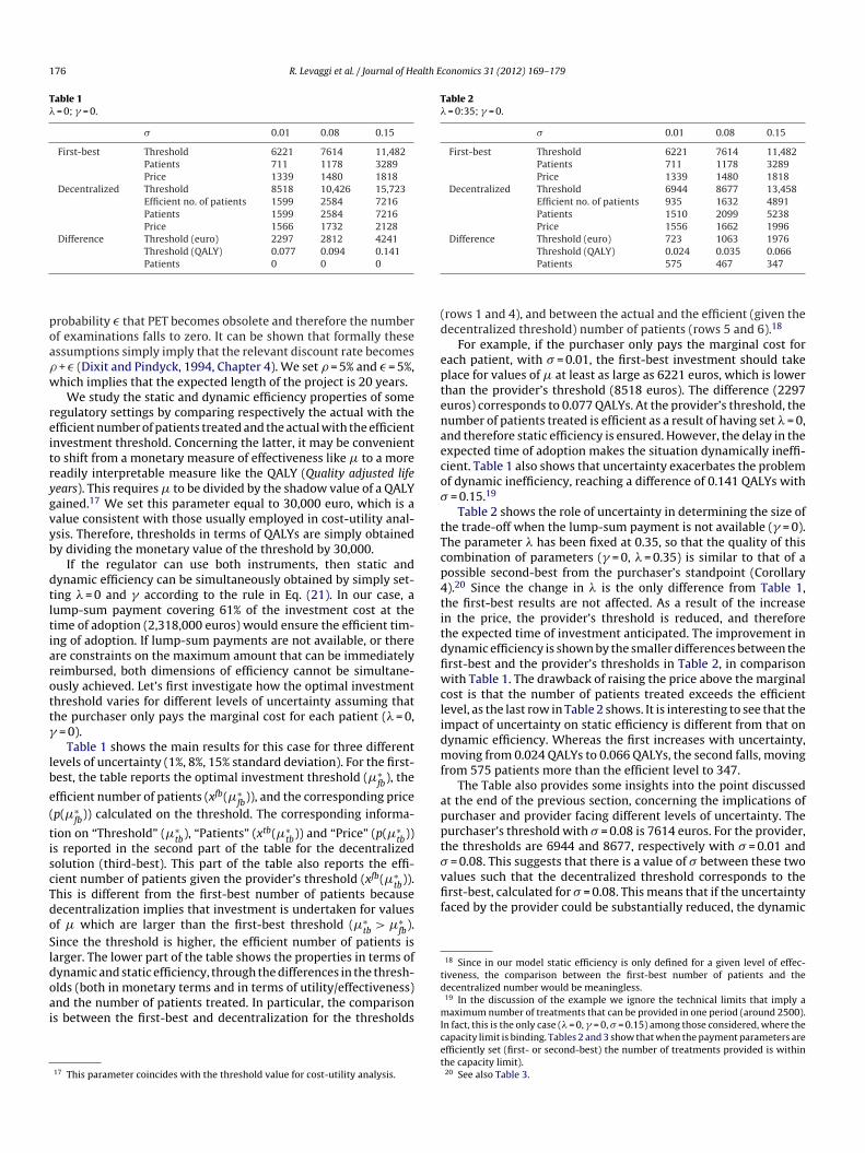
We study the static and dynamic efficiency properties of someegulatory settings by comparing respectively the actual with thefficient number of patients treated and the actual with the efficientnvestment threshold. Concerning the latter, it may be conveniento shift from a monetary measure of effectiveness like � to a moreeadily interpretable measure like the QALY (Quality adjusted lifeears). This requires � to be divided by the shadow value of a QALYained.17 We set this parameter equal to 30,000 euro, which is aalue consistent with those usually employed in cost-utility anal-sis. Therefore, thresholds in terms of QALYs are simply obtainedy dividing the monetary value of the threshold by 30,000.

If the regulator can use both instruments, then static andynamic efficiency can be simultaneously obtained by simply set-ing � = 0 and � according to the rule in Eq. (21). In our case, aump-sum payment covering 61% of the investment cost at theime of adoption (2,318,000 euros) would ensure the efficient tim-ng of adoption. If lump-sum payments are not available, or therere constraints on the maximum amount that can be immediatelyeimbursed, both dimensions of efficiency cannot be simultane-usly achieved. Let’s first investigate how the optimal investmenthreshold varies for different levels of uncertainty assuming thathe purchaser only pays the marginal cost for each patient (� = 0,

= 0).Table 1 shows the main results for this case for three different

evels of uncertainty (1%, 8%, 15% standard deviation). For the first-est, the table reports the optimal investment threshold (�∗

fb), the

fficient number of patients (xfb(�∗fb

)), and the corresponding pricep(�∗

fb)) calculated on the threshold. The corresponding informa-

ion on “Threshold” (�∗tb

), “Patients” (xtb(�∗tb

)) and “Price” (p(�∗tb

))s reported in the second part of the table for the decentralizedolution (third-best). This part of the table also reports the effi-ient number of patients given the provider’s threshold (xfb(�∗

tb)).

his is different from the first-best number of patients becauseecentralization implies that investment is undertaken for valuesf � which are larger than the first-best threshold (�∗

tb> �∗

fb).

ince the threshold is higher, the efficient number of patients isarger. The lower part of the table shows the properties in terms ofynamic and static efficiency, through the differences in the thresh-lds (both in monetary terms and in terms of utility/effectiveness)

nd the number of patients treated. In particular, the comparisons between the first-best and decentralization for the thresholds

17 This parameter coincides with the threshold value for cost-utility analysis.

mIcet

Threshold (QALY) 0.024 0.035 0.066Patients 575 467 347

rows 1 and 4), and between the actual and the efficient (given theecentralized threshold) number of patients (rows 5 and 6).18

For example, if the purchaser only pays the marginal cost forach patient, with � = 0.01, the first-best investment should takelace for values of � at least as large as 6221 euros, which is lowerhan the provider’s threshold (8518 euros). The difference (2297uros) corresponds to 0.077 QALYs. At the provider’s threshold, theumber of patients treated is efficient as a result of having set � = 0,nd therefore static efficiency is ensured. However, the delay in thexpected time of adoption makes the situation dynamically ineffi-ient. Table 1 also shows that uncertainty exacerbates the problemf dynamic inefficiency, reaching a difference of 0.141 QALYs with

= 0.15.19

Table 2 shows the role of uncertainty in determining the size ofhe trade-off when the lump-sum payment is not available (� = 0).he parameter � has been fixed at 0.35, so that the quality of thisombination of parameters (� = 0, � = 0.35) is similar to that of aossible second-best from the purchaser’s standpoint (Corollary).20 Since the change in � is the only difference from Table 1,he first-best results are not affected. As a result of the increasen the price, the provider’s threshold is reduced, and thereforehe expected time of investment anticipated. The improvement inynamic efficiency is shown by the smaller differences between therst-best and the provider’s thresholds in Table 2, in comparisonith Table 1. The drawback of raising the price above the marginal

ost is that the number of patients treated exceeds the efficientevel, as the last row in Table 2 shows. It is interesting to see that thempact of uncertainty on static efficiency is different from that onynamic efficiency. Whereas the first increases with uncertainty,oving from 0.024 QALYs to 0.066 QALYs, the second falls, moving

rom 575 patients more than the efficient level to 347.The Table also provides some insights into the point discussed

t the end of the previous section, concerning the implications ofurchaser and provider facing different levels of uncertainty. Theurchaser’s threshold with � = 0.08 is 7614 euros. For the provider,he thresholds are 6944 and 8677, respectively with � = 0.01 and

= 0.08. This suggests that there is a value of � between these twoalues such that the decentralized threshold corresponds to the

19 In the discussion of the example we ignore the technical limits that imply aaximum number of treatments that can be provided in one period (around 2500).

n fact, this is the only case (� = 0, � = 0, � = 0.15) among those considered, where theapacity limit is binding. Tables 2 and 3 show that when the payment parameters arefficiently set (first- or second-best) the number of treatments provided is withinhe capacity limit).20 See also Table 3.

Page 9

R. Levaggi et al. / Journal of Health E

Table 3Second-best efficient pricing rule.

� Dynamic eff. Static eff. Present value

FB thresh. Dec. thresh. Eff. patients Dec. patients

0 0.275 0.377 3160 3160 1,829,1700.1 0.275 0.363 2886 2995 1,923,4200.2 0.275 0.348 2585 2812 2,030,6500.3 0.275 0.328 2240 2599 2,148,0900.38 0.275 0.307 1899 2385 2,226,8900.39 0.275 0.304 1848 2353 2,231,310

ie

wtWff(p

I

E

w

7Ttrnefwbaeot(6co

6

oissor

t

fi

ambaaettiddnseaimce

lTismamhtmnfpodp

ocaetao

opviibspro

0.4 0.275 0.300 1795 2319 2,232,7500.41 0.275 0.297 1739 2283 2,220,6800.42 0.275 0.292 1677 2243 2,220,680

nefficiency of the situation described in Table 2 could be virtuallyliminated.

Finally, we want to study the optimal policy by the regulatorhen lump-sum payments are not available (� = 0) and therefore

he trade-off between static and dynamic efficiency arises (Table 3).e do this by studying how the present value of the investment

rom the purchaser’s standpoint changes as � is increased, startingrom � = 0, assuming that the provider sets the number of patientsTable 3). Given the purchaser’s objective function, the expectedresent value of the project is defined as:

= E0 [e−(�+)tA |� = �0]

(b(xtb) − c(xtb)

� + − I

)(23)

t is shown in Appendix that:

0 [e−(�+)tA |� = �0] =(

�0

�∗tb

)�

(24)

ith � > 1.The starting value of the stochastic parameter (�0) is set at

000 euros, with � = 0.1. The other parameter values are as above.able 3 shows the trade-off due to the increase in the price abovehe marginal cost. Increases in � anticipate the investment thuseducing the gap from the first-best threshold, but also increase theumber of patients above the efficient level.21 For the case underxamination a value of � = 0.4 yields the maximum present valueor the investment, and hence the optimal trade-off. Consistentlyith the statement in Corollary 4 this second-best solution implies

oth static and dynamic inefficiency. The former takes the form of larger threshold and hence a delay in investment, with a differ-nce of 0.025 QALYs. The latter leads to treat patients in excessf the efficient level (2319 vs. 1795). The comparison betweenhe second-best present value (2,232,750 euros) and the first-best2,437,640 euros), attainable with a lump-sum payment covering1% of the investment cost and a fixed fee equal to the marginalost, provides an estimate of the cost of the regulatory failure. Inur case this is 204,890 euros.

. Conclusion

The paper employs the typical instruments of the literaturen irreversible investments under uncertainty to investigate themplications of alternative reimbursement rules. Although deci-ions with these characteristics are frequent in the health care

ector (e.g. at the time of adopting innovative equipment) andften have substantial impacts on costs, specific regulation issueselated to these have been rarely addressed in the literature so

21 The number of patients in columns 4 and 5 are both calculated on the provider’shreshold.

pcf

conomics 31 (2012) 169– 179 177

ar. Moreover, there is a substantial variety among the solutionsmplemented in different health care systems.

A central issue investigated in the paper is the distinctionnd the interaction between static efficiency (providing the treat-ent to an efficient number of patients once the technology has

een adopted) and dynamic efficiency (efficiency in the timing ofdoption). If the purchaser is unable to set the level of patientst the efficient level, the choice of the payment scheme influ-nces both the timing of adoption and the number of patientshat receive the treatment. We have investigated the proper-ies of a number of instruments available to the regulator tomprove efficiency. If the purchaser can give the provider imme-iate reimbursement of a fraction of the capital cost (appropriatelyetermined) when the provider decides to invest in the new tech-ology, then both dynamic and static efficiency are obtained byimply paying the marginal cost for each patient treated. How-ver, if for some reasons lump-sum payments cannot be used,

trade-off emerges between static and dynamic efficiency: thencentive to adopt the new technology when the price equals

arginal cost, thus ensuring static efficiency, is too weak. In thisase, the adoption of the technology occurs later than would befficient.

The evidence from real world health care systems suggests thatump-sum reimbursements of capital costs are not frequently used.his may be due to either liability constraints for the purchaser ornability to differentiate the pricing rules for technologies with sub-tantial capital costs. Although the investigation of exactly why thisay be the case is beyond the scope of this work, our results provide

possible explanation of why appropriateness (provision of treat-ents only to those patients that really need it) is an issue in several

ealth care systems. It is also interesting to note that the regula-ors in health care systems that are more sensitive to this issue are

oving in the direction described in our model. In Switzerland theew DRG system that will come into force in 2012 foresees a model

or capital reimbursement that is very similar to the one we haveresented in this paper.22 The calibration of the model for the casef PET has provided a tentative estimate of the monetary cost ofeparting from the optimal payment rule, by relying only on theayment of a fixed price per patient.

For the health care systems that still use a pure DRG system,ur model set-up enables the identification of instruments thatould be used by the purchaser as a substitute for the immedi-te reimbursement of capital cost to foster dynamic efficiency. Forxample, setting boundaries to the variation of prices in responseo changes of the stochastic variable, would reduce the variancectually faced by the provider and hence reduce the value of theption to postpone the investment.

Hopefully, these results will contribute to the developmentf the theoretical analysis of the incentives underlying specificurchasing rules when the provision of the service requires an irre-ersible commitment of resources. Our model could be developedn a number of directions. For instance, competition is only implic-tly treated in our analysis through the impact on the fixed netenefit component. It would also be interesting to investigate theensitivity of the results to changes in the objective functions of theurchaser and the provider. Finally, the interaction of the paymentule with other policy tools (e.g. a direct control by the purchasern the timing of investment) could also provide useful insights. Inarticular, the reallocation of risk (uncertainty) between the pur-

haser and the provider as a policy tool could be a fruitful area foruture research.

22 See http://www.swissdrg.org.

Page 10

1 alth E

A

A

tkcta(

�

Aw

E

Te

−

T

V

wZpmo�ttt

A

Eaio

d

Tettt

oMcs

wrhetlioau

A

/�)[1

/�)[1

TftIto(Tss

A

dSifce

(

Be

78 R. Levaggi et al. / Journal of He

ppendix A.

.1. Derivation of the value function in the waiting region

As the investment opportunity yields no cash flow up to theime when the investment is undertaken, the only return fromeeping this opportunity alive is the option value’s capital appre-iation. By imposing the arbitrage condition (Bellman equation)hat the capital gain has to be equal to the natural return, overn infinitesimal period dt when it is optimal not to invest, we getDixit and Pindyck, 1994):

Vfb(�t) = limdt→0

1dt

E[dVfb(�t)] (25)

pplying Ito’s Lemma, the last term on the right hand side may beritten as:

[dVfb(�t)] = 12

�2�2t

∂2Vfb(�t)

∂�2t

(26)

he substitution of this into Eq. (25) yields the following differentialquation:

�Vfb(�t) + 12

�2�2t

∂2Vfb(�t)

∂�2t

= 0 (27)

he general solution of this equation is,

fb(�t) = Z1�ˇ1t + Z2�ˇ2

t

here, ˇ1 > 1 and ˇ2 < 0 are the roots of (ˇ) ≡ 1/2�2ˇ2 − 1/2�2

− � = 0. The value of the constants1 and Z2 are obtained by imposing appropriate restrictions. Inarticular, for values of �t that tend to zero, the term Z2�ˇ2

t wouldake the value jump to infinity. Of course, this is inconsistent with

ur problem, given that the provider is not allowed to invest for < �, and therefore the value of the corresponding opportunity

o invest is zero. Therefore, Z2 has to be set equal to zero. Setting,o simplify the notation, Z1 = Z and ˇ1 = the value Vfb(�t) reduceso Vfb(�t) = Z�ˇ

t as in the text.

.2. Formal discussion of Corollary 2

Eq. (18) can be written as,

˘tb(�∗tb

)

�− �∗

tb

�ˇ

[∂˘tb(�∗

tb)

∂�

]= I(1 − �) (28)

quating the total differential with respect to � and � to zero,nd after simplifying the expression accounting for the fact thatn xtb the marginal cost equals the price, the following expressionbtains:

∂�∗tb

∂�= −

(∂˘tb/∂�)(1

(∂˘tb/∂�∗tb

)(1

�

{xtb

�

(∂p

∂�

)− �∗

tb

�ˇ

[∂2

p

∂�∂�xtb + ∂p

∂�

∂xtb

∂�

]}= −Id� (29)

he first term in braces captures the impact of the change onxpected profits, whereas the second is related to the impact onhe value of the option to postpone the investment. The latter goeso zero when ˇ tends to infinity, which corresponds to no uncer-ainty. It is straightforward to check that this term would cancel

W

�

�

conomics 31 (2012) 169– 179

ut in the second-best where the number of patients treated is xfb.oreover, in this case the first term in braces would be equal to I,

onfirming that � and � are perfectly substitutable instruments, astated in Corollary 1.

In the third-best, the first term in braces is equal to I(xtb/xfb),hich is greater than I, implying that the direct effect on expected

evenues implies a tendency to reduce the optimal threshold andence anticipate investment. The two terms in brackets, whose rel-vance is increasing with uncertainty (which is inversely relatedo ˇ), capture the two effects that an increase in � and a paral-el reduction in � have on the value of the option to postpone thenvestment, respectively the strengthening of the insurance rolef the price component related to � (with an anticipatory effect)nd the effect of replacing a certain revenue component with anncertain one (with a delaying effect).

.3. The impact of increases in � on �∗tb

Applying the implicit function theorem to Eq. (20):

− (ı/(ı − 1))(1/ˇ)εp,�∗tb

] − (˘tb/�)(ı/(ı − 1))(1/ˇ)(∂ε/∂�)

− (ı/(ı − 1))(1/ˇ)εp,�∗tb

] − (˘tb/�)(ı/(ı − 1))(1/ˇ)(∂ε/∂�∗tb

)

he numerator is positive because the first term must be positiveor �∗

tbto exist, and (∂ε/∂�∗

tb) < 0. The general study of the sign of

he denominator is rather complicated. We study its limit for � → 0.n this case, ε = ı − 1/(ı − �) is independent of � so that the lasterm of the denominator cancels out and the following expressionbtains:

p

ı

)(ı/ı−1)−1 ∂p

∂�∗tb

1�

[1 − ı

ı − �

1ˇ

]his is positive whenever a value of � such that the investment isocially desirable exists (Eq. (10)). Therefore, we can draw conclu-ions on a local result:

d�∗tb

d�|�=0 < 0

.4. Proof of Eq. (24)

The solution to E0[e−(�+ε)tA |� = �0] can be obtained via the usualynamic programming decomposition (Dixit et al., 1999, p. 184).ince the process �t is continuous, the expected discount factor isncreasing in �0 and decreasing in �∗

tb; then it can be defined by a

unction D(�0; �∗tb

). Over the infinitesimal time interval dt, �t willhange by the small value d�t, hence we get the following Bellmanquation:

� + ε)D(�0; �∗tb)dt = E(dD(�0; �∗

tb))

y applying Itô’s Lemma to dD we obtain the following differentialquation:

12

�2�2 ∂2D

∂�2− (� + ε)D = 0

e solve it subject to the two boundary conditions:

lim D(�0; �∗tb) = 0

0→0

lim0→�∗

tb

D(�0; �∗tb) = 1

Page 11

alth E

a

D

w

R

B

B

F

C

C

C

C

D

D

G

G

H

L

L

M

N

P

P

Rvolume. J. Health Econ. 4, 333–356.

R. Levaggi et al. / Journal of He

nd we get

(�0; �∗tb) =

(�0

�∗tb

)�

,

here � > 1 is the positive root of the auxiliary quadratic equation (�) = 1

2 �2�(� − 1) − (� + ) = 0.

eferences

aker, L.C., Phibss, C.S., 2002. Managed care, technology adoption, and health care:the adoption of neonatal intensive care. RAND J. Econ. 33 (3), 524–548.

arros, P., Martinez-Giralt, X., 2010. Technological Adoption in Health Care. FEUNLWorking Paper Series. Universidade Nova de Lisboa, Faculdade de Economia.

arasat, A.S., Bokhari, 2009. Managed care competition and the adoption of hospi-tal technology: the case of cardiac catheterization. Int. J. Ind. Organizat. 27 (2),223–237.

halkley, M., Malcomson, J., 2000. Government purchasing of health services. In:Culyer, A.J., Newhouse, J.P. (Eds.), Handbook of Health Economics, vol. 1. , 1st ed.Elsevier, pp. 847–890, Chapter 15.

halkley, M., Malcomson, J.M., 1998. Contracting for health services with unmoni-tored quality. Econ. J. 108 (449), 1093–1110.

handra, A., Skinner, J., 2011. Technology Growth and Expenditure Growth in HealthCare. NBER Working Papers 16953, National Bureau of Economic Research, Inc.

laxton, K., Briggs, A., Buxton, M.J., Culyer, A.J., McCabe, C., Walker, S., Sculpher, M.J.,2008 FEB 2. Value based pricing for NHS drugs: an opportunity not to be missed?Br. Med. J. 336 (7638), 251–254.

ixit, A., Pindyck, R.S., 1994. Investment Under Uncertainty. Princeton UniversityPress, Princeton.

S

W

conomics 31 (2012) 169– 179 179

ixit, A., Pindyck, R.S., Sodal, S., 1999. A markup interpretation of optimal investmentrules. Econ. J. 109 (455), 179–189.

elijns, A.C., Rosenberg, N., 1994. The dynamics of technological change in medicine.Health Aff., 28–46 (Summer).

riffin, S.C., Claxton, K.P., Palmer, S.J., Sculpher, M.J., 2011. Dangerous omis-sions: the consequences of ignoring decision uncertainty. Health Econ. 20 (2),212–224.

OPE, 2006. DRGs as a Financial Tool. Technical Report, European Hospital andHealthcare Federation.

evaggi, R., Moretto, M., Rebba, V., 2009. Investment decisions in hospital technol-ogy when physicians are devoted workers. Econ. Innov. New Technol. 18 (5),487–512.

evaggi, R., Moretto, M., Pertile, P., 2010. Static and Dynamic Efficiency of Irre-versible Health Care Investments Under Alternative Payment Rules. WorkingPapers 2010.130, Fondazione Eni Enrico Mattei.

cClellan, M., 1995. Uncertainty, health care technologies, and health care choices.Am. Econ. Rev. 85 (2), 38–44.

ewhouse, J.P., 1992. Medical care costs: how much welfare loss? J. Econ. Perspect.6 (3), 3–21.

ertile, P., 2008. Investment in health technologies in a competitive model with realoptions. J. Public Econ. Theory 10 (5), 923–952.

ertile, P., Torri, E., Flor, L., Tardivo, S., 2009. The timing of adoption of PositronEmission Tomography: a real options approach. Health Care Manage. Sci. 12 (3),217–227.

obinson, J.C., Luft, H.S., 1985. The impact of hospital market structure on patient

istrom, C.L., 2009. The appropriateness of imaging: a comprehensive conceptualframework. Radiology 251 (3), 637–649.

eisbrod, B.A., 1988. The Non-Profit Economy. Harvard University Press, Cam-bridge, MA.