State Variables Estimation for a CounterFlow Double-Pipe Heat Exchanger Using Multi-linear Model

State Variables Estimation for a Counter-Flow Double-Pipe Heat Exchanger using Multi-linear Model

Betty López Zapata*, R.F. Escobar, Manuel Adam Medina, Carlos M. Astorga Zaragoza CENIDET, A.P. 5-164, C.P. 62050 Cuernavaca, Morelos, Mexico

Abstract This paper deals with the state variables (Temperatures) estimation for a counter-flow double-pipe heat exchanger using Multi-linear Models using a Kalman filter (FK) for the state variables approaching and using Bayes probability for the change of the model. The reliability of the proposed method was demonstrated via numerical simulation and laboratory experiments with a bench-scale pilot plant. 1. Introduction

The problem of observer design naturally arises in a system approach, as soon as one needs some internal information from external (directly available) measurements. In general indeed, it is clear that one cannot use as many sensors as signals of interest characterizing the system behavior (for cost reasons, technological constraints, etc), especially since such signals can come in a quite large number, and they can be of various types: they typically include time-varying signals characterizing the system (state variables), constant ones (parameters), and unmeasured external ones (disturbances) [1].

This need for internal information can be motivated by various purposes: modeling (identification), monitoring (fault detection), or driving (control) the system. All those purposes are actually jointly required when aiming at keeping a system under control[1]. Much of the work done to develop observers is based on Kalman filters [2, 3]. A different type of state estimators has been developed by other authors and implies the use of Luenberger observers or some extensions of them[4, 5].

In 1984 Blom present the approached Multi-Models interacting. However this approach was explained by Blom and Bar-Shalom until 1988 [6]. This approaching is called Multi-Models with fixed structure. This

algorithm was defined with a parallel bank of Kalman filter, in which each describes a model. In this context the approach Multi-linear Model (MLM) is used for estimation, identification, control and fault diagnosis [7-10]. To reach this approaching MLM, we need decomposition of the full operating range of the Nonlinear system (NLS) into a number of possible overlapping operating regimes [11, 12]. In each operation points, we will have a linear model

In chemical processes it is common to find a counter-flow double-pipe heat exchanger (cooler), generally its applications are required in exothermic processes or in processes where it is necessary to get down the temperature of a specific fluid. In this paper the aim is to estimate the state variables (Temperatures) for a counter-flow double-pipe heat exchanger using Multi-linear Models using a Kalman filter (KF) for the state variables approach and using Bayes probability for the change of the model.

This paper is organized as follows. In Section 2, a

heat exchanger simplified model is presented. In Section 3, MLM+ Kalman Filter is designed on the basis of the mathematical model described in Section 2 and subsequently, these models are experimentally evaluated and simulations on a bench-scale pilot plant. Both, experimental and simulation results are discussed in Section 4. Finally, conclusions are stated in Section 5. 2. The heat exchanger model

The heat exchanger model is based on the direct lumping of the process. The heat exchanger is split up into sections (in the axial direction of the exchanger), each section being a set of two cells, one per fluid. The temperature in each section is a model. It can be shown that two sections are sufficient [9].

2009 Electronics, Robotics and Automotive Mechanics Conference

978-0-7695-3799-3/09 $26.00 © 2009 IEEE

DOI 10.1109/CERMA.2009.39

309

2009 Electronics, Robotics and Automotive Mechanics Conference

978-0-7695-3799-3/09 $26.00 © 2009 IEEE

DOI 10.1109/CERMA.2009.39

349

2009 Electronics, Robotics and Automotive Mechanics Conference

978-0-7695-3799-3/09 $26.00 © 2009 IEEE

DOI 10.1109/CERMA.2009.39

349

2009 Electronics, Robotics and Automotive Mechanics Conference

978-0-7695-3799-3/09 $26.00 © 2009 IEEE

DOI 10.1109/CERMA.2009.39

349

The system dynamics is obtained through an energy balance rule applied to every element of a lumped model [13]:

⎥⎦

⎤⎢⎣

⎡=

⎥⎦

⎤⎢⎣

⎡+

⎥⎦

⎤⎢⎣

⎡−⎥

⎦

⎤⎢⎣

⎡

systeminsidecomponentgthofmolesofchangeofratetime

reactionschemicalfromcomponentgthofmolesofformationofrate

systemofoutcomponentgthofmolesofflow

systemtoicomponetgthofmolesofFlow

η

Thus, the application of the energy balance rule considering a single element per fluid (covering the whole tube length) to a counter flow heat exchanger gives rise to the following 2nd order dynamics: T TT T

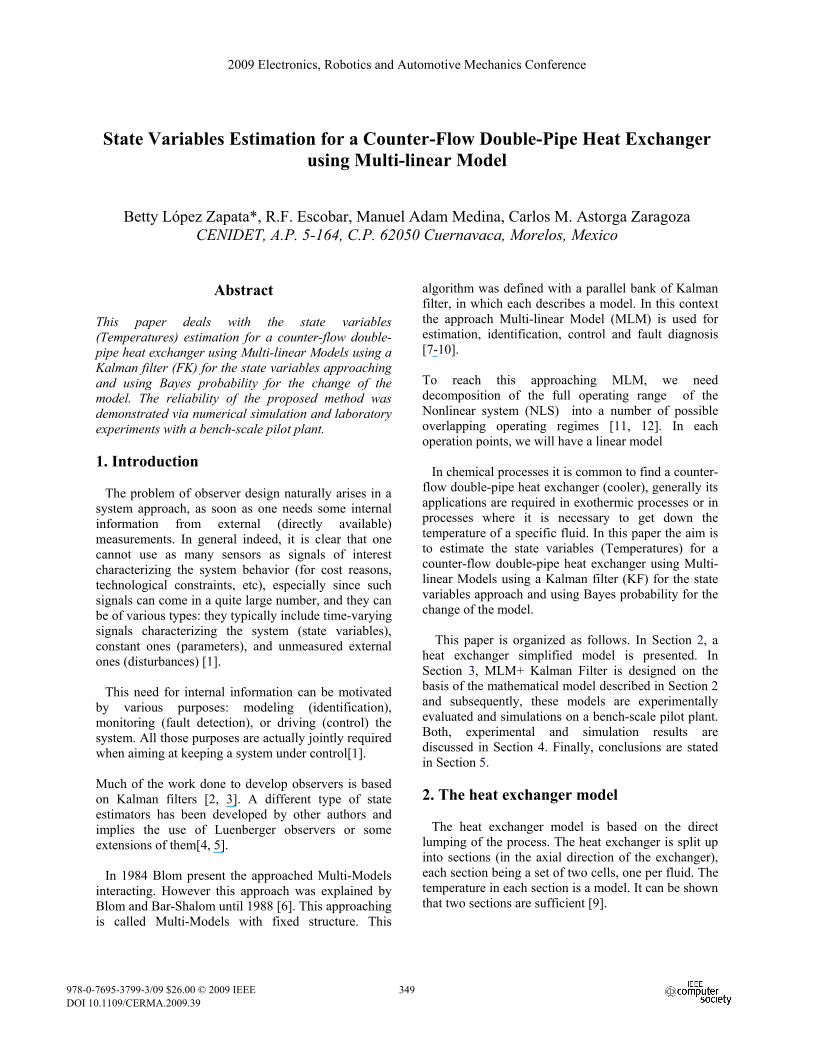
Where each of the terms are defined in table 1and the mathematical model presented here, takes into account the following assumptions: A1 equal inflows and outflows, implying constant volume in both tubes; A2 the heat transfer coefficient is related to the flow and the heat of the fluids; A3 there is no heat transfer between the external tube and the environment; A4 the thermophysical properties of the fluids are constant; A5 there is no energy storage in the walls; A6 the inlet temperatures are constant. Since the lumping procedure generally assumes that every element behaves like a perfectly stirred tank [14], the fluid temperature at each of such elements is considered to be uniformly distributed. This is why the outlet temperatures are taken to represent the bulk temperatures (at every considered element) to get the accumulation terms, and the driving force producing the heat conduction from the hot fluid to the cold one is modeled through the outlet temperatures difference. This model can be illustrated as a single cell which consists of two perfectly stirred tanks with inflows and outflows[15]. The two tanks are connected by a heat transfer area between them (Fig. 1). Despite its simplicity, the model in Eq. (1) keeps the main features of the qualitative behavior of heat exchangers under the state assumptions.

Fig. 1. One-cell representation of a counter flow heat exchanger.

A low-order model like (1) proves to be useful for (observer or control) synthesis purposes, while a higher-order dynamics is convenient for the implementation of numerical simulations oriented to test the (observer or control) designed algorithms [16]. Table 1. Nomenclature Nomenclature

Vc Volume in the cold side, m3

Vh Volume in the hot side, m3 Flow in the cold side, m3/seg

Flow in the hot side, m3/seg Cpc Specific heat in the cold side,

J/Kg°C Cph Specific heat in the hot side,

J/Kg°C ρc Density of the cold fluid, Kg/ m3 ρh Density of the hot fluid, Kg/ m3 A Heat transfer surface area, m2 U Heat transfer coefficient, W/ m2-

°C Tci, Thi, Inlet temperatures in the cold

and hot sides, respectively, °C Tco, Tho, Outlet temperatures in the cold

and hot sides, respectively, °C ts Simulation time

Sub-indices c cold h hot i inlet o outlet

3. Multi-linear models 3.1 MLM Statements Dynamic systems such as nonlinear, linear time invariant, linear time-variant, hybrid and piecewise can be represented by a decomposition of the full operating range into a number of possibly overlapping operating regimes [11, 12]. For each regime, a simple local linear system is defined. Let us assume the following general stochastic system considered by:

(1)

310350350350

( ) ( ) ( )( ) ( ) ( ) ( )kvkUDkXCkY

kwkUBkXAkX

jYjj

jXjj

j

j

+Δ++=

+Δ++=+ )1(

where X ∈ Rn represents the state vector, U ∈ Rp is the input vector, Y ∈ Rm is the measurement vector. Each linear model is defined around jth operating point, noted Pj ∀ j= [1,2,…M], where M is the total number of operating points. Each operating point is defined by a pair of input/output signals (YPj, UPj). Around the jth operating point it is assumed that ∀ j, rank (Cj) = m. The terms wj and vj are two independent zero mean white noises with variance-covariance matrices defined respectively by Qj y Rj. Aj, Bj, Cj and Dj are constant matrices with appropriate dimensions.

jXΔ and jYΔ

are vectors depending on the jth linear model. The linear system (1) can be specified by the set of system matrices:

[ ]MjvDCwBA

SjYjj

jXjjj

j

j ,...,2,1, =∀⎥⎥⎦

⎤

⎢⎢⎣

⎡ΔΔ

=

Let S(k) be a matrix sequence varying within a convex set [12], defined as:

( ) ( ) ( ) ( )⎭⎬⎫

⎩⎨⎧ =∑≥∑=

==1,0:

11kkSkkS j

M

jjj

M

jϕϕϕ

In the MLM framework, S(k) characterizes at each sample the non linear system (NLS). Consequently, the dynamic behavior of NLS can be defined by a convex combination of a LTI model set, noted ℑ

[ ]{ }( )MSSS ,...,: 21=ℑ . 3.2 MLM Design based on KF context In order to achieve the prediction of state a Kalman filter is designed. Under assumption that the NLS evolves around the ith [ ]Mi ...1∈∀ operating point, the Kalman filter is described by:

( ) ( ) ( ) ( ) ( )( )( ) ( ) ( )⎪⎩

⎪⎨⎧

Δ++=

−+Δ++=+

i

i

Yiiii

iiXiiii

kUDkXCkY

kYkYkKkUBkXAkX

ˆˆ

ˆˆ)1(ˆ

where ni RX ∈ˆ denotes the estimated state vector and

mi RY ∈ˆ is the output estimation obtained from the

linear filter based on the thi linear model. nxmi RK ∈ is

the Kalman filter gain matrix. Supposing that NLS is

represented by a linear model around the thi operating point equivalent to that used by the filter, i.e. j = i, the estimated error vector iε ( ) ( ) ( )( )kXkXk ii

ˆ−=ε and

the output residual vector ( ) ( ) ( )( )kYkYkrr iiiˆ−= are

calculated from equations (2) and (5):

( ) ( )( ) ( ) ( ) ( ) ( )kwkvkKkCkKAk jjiiiiii +−−=+ εε 1

( ) ( ) ( )kvkCkr jiii += ε The estimated error vector is written as ε i and the output residual vector is noted . Knowing that the system dynamics is specified in exactly M operating points on all the operating range, a bank of Kalman filters defined by the finite set ℑ of linear models is established. The use of a bank of Kalman filters results in a bank of residuals allowing the selection of the model that is more representative of the NLS dynamic. The residual, generated by the thi filter, is supposed to have Gaussian distribution properties with zero mean value (noted N). This residual allows one to evaluate the validity of each linear model. Indeed, [7] has considered the residual vector in order to determine the validity probabilities of each linear model, by taking into account the previous measurement according to Bayes probability theory. The valid model is the model that has the greatest probability. The residuals of the filter, considered around the corresponding operating point, follow a Gaussian distribution law. Then, assuming stationary of residuals, a probability distribution function, written as ( )ki℘ is defined by:

( ) ( ) ( )( ) ( ){ }( ) ( )( )[ ] 2

1

1

det2

5.0exp

kx

krxkxkxrk

im

Tiii

i

Θ

Θ−=℘

−

π where m

i ℜ∈Θ is the covariance matrix of the residuals( )kri . Based on the probability distribution function, a

mode probability, noted ( )( )kriϕ , can be computed by the Bayes theorem [ ]Mi ...1∈∀ as [10]:

( )( ) ( ) ( )( )( ) ( )( )∑ =

ℑ℘ℑ℘=+ M

h ih

iii

krxkkrxkkr

1

1ϕ

Therefore, the probability estimation algorithm can get locked onto one model so that the probability converges to one, while that associated to the other model converges to zero. The thi linear model validity is computed using (9).

(2)

(3)

(4)

(7)

(6)

(5)

(8)

(9)

311351351351

4. Results 4.1. Numerical simulation This method has been applied to real heat exchanger as described in section 2. In order to test the performance of the proposed filters, numerical simulations were carried out, they consist in estimating the state variables (Tco,Tho), from measurements of the inlet flow (vc), the inlet temperatures of a heat exchanger and only one of the outlet temperatures (Tco or Tho). Table 2. Physical data used in the simulations and real experiments

Constants Value Units νco

o 8.3300e-006 m3/s νh 1.667e-5 m3/s Vc 134.99e-6 m3 Vh 15.512e-6 m3 cρc 4180.9 J/Kg°C cρh 4196.5 J/Kg°C ρc 985 Kg/ m3 ρh 971.1535 Kg/ m3 A 0.01538752 m2 U 1400 W/ m2-°C

Tcoo 47 °C

Thoo 72 °C

The aim of this simulation is to prove the convergence of the estimated variable state with the state variable of the heat exchanger. Considering the process model given by (1). First step is the linearization of the model given by (1) used Taylor and use the operating points give in table 3. For filter design, we work with the linear models that we get previously. The initial conditions of the process model were the same for the filters used in simulation and with the experiment. Table 3.Operating points of Kalman filters

Tci Thi Tco Tho vc KF M1 29 81 47.4 72 7.5x10-6

KF M2 29 81.2 50.88 73 5.7x10-6 KF M3 30 81.4 61.5 76 2.6x10-6

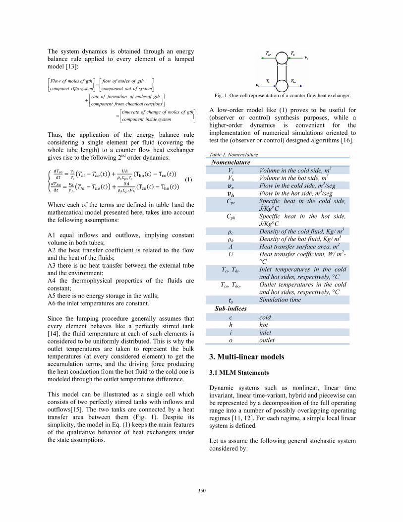
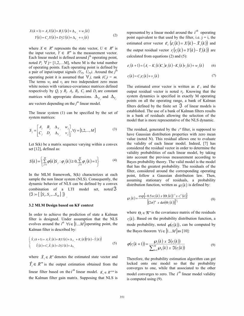
The bank of Kalman filters allows the generation of a bank of residuals (where M=3). Each residual correspond to each model. This residual allows one to evaluate the validity of each linear model. The passage (crossing) between models as shown fig. 3 to other depends of evolution of cold fluid flow (vc) as shown fig. 2.

Fig. 2. Inlet flow (vc).

Fig. 3. Probability to associate to each model The MM+FK was simulated using the values given in table 2 and use the operating points give in table 3. These values, were calculate depending of operating points. The inlet temperatures Tci and Thi were 29° C and 81°C respectively. The cold fluid flow was varied of 7.5x10-6 to 2.6x10-6 m3/s. These variations allow change the operating points. The sampling time of the filter was ts=0.25 s.

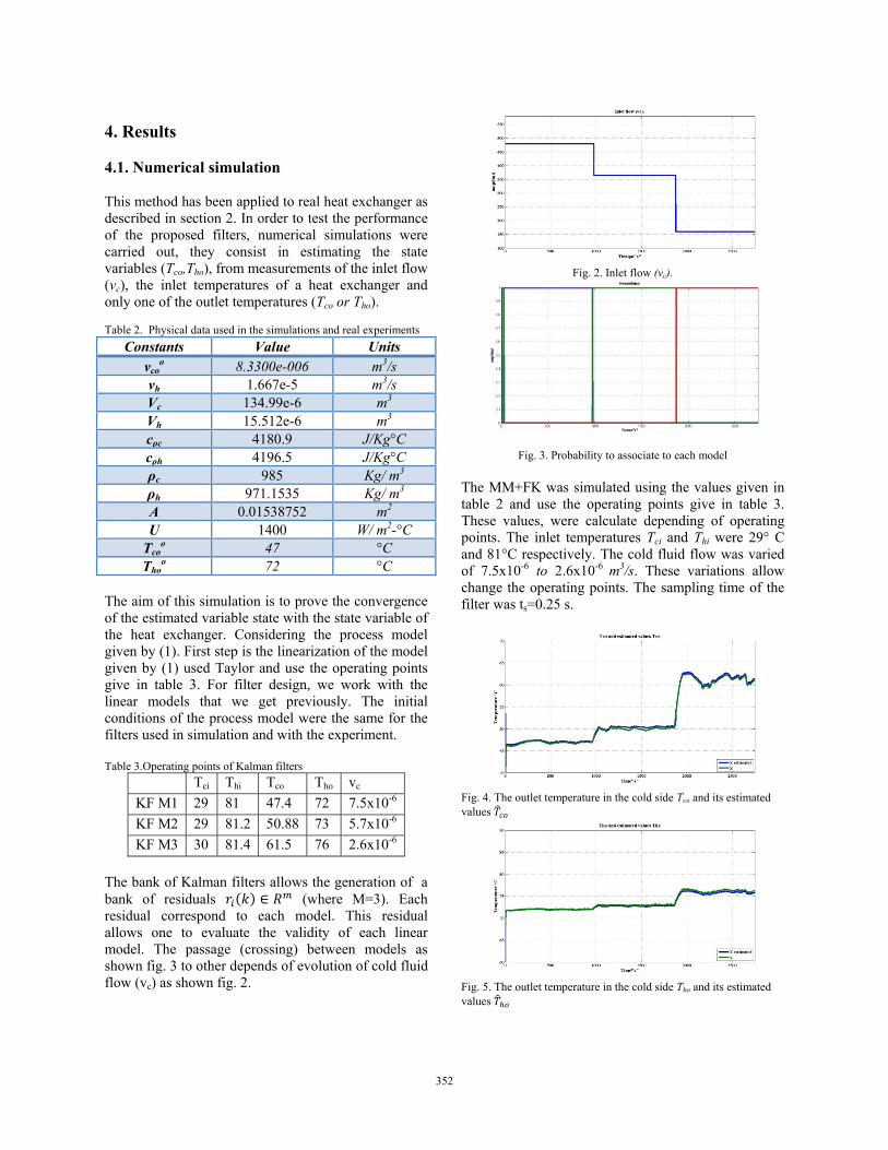
Fig. 4. The outlet temperature in the cold side Tco and its estimated values

Fig. 5. The outlet temperature in the cold side Tho and its estimated values

312352352352

The results of the estimation of temperatures Tco and Tho are reported in fig. 4 and fig. 5 respectively. It can be seen that the convergence of the estimates and

proves to be fast. 4.2. Experimental results The experimental pilot plant is a counter-flow double-pipe heat exchanger where the hot water flows through the inner tube and the cooling water flows through the external tube.

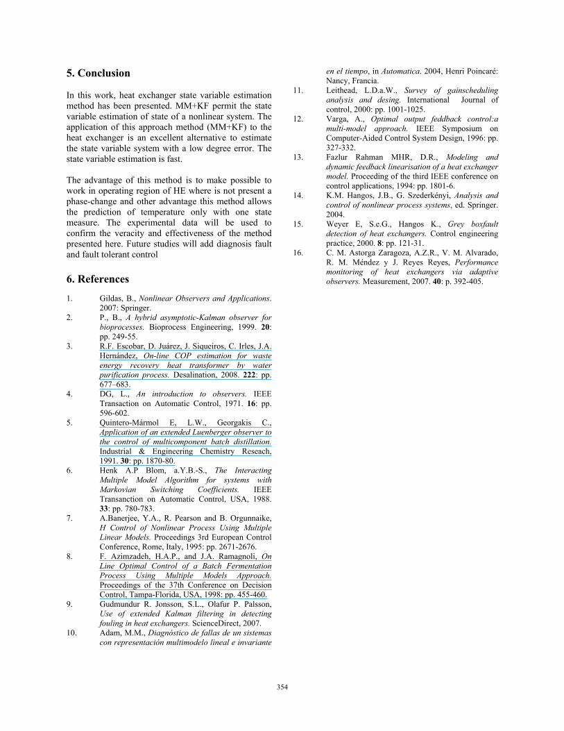
Fig. 6. Inlet flow (vc).

Fig. 7. Probability to associate to each model

Fig. 8. Transition of models

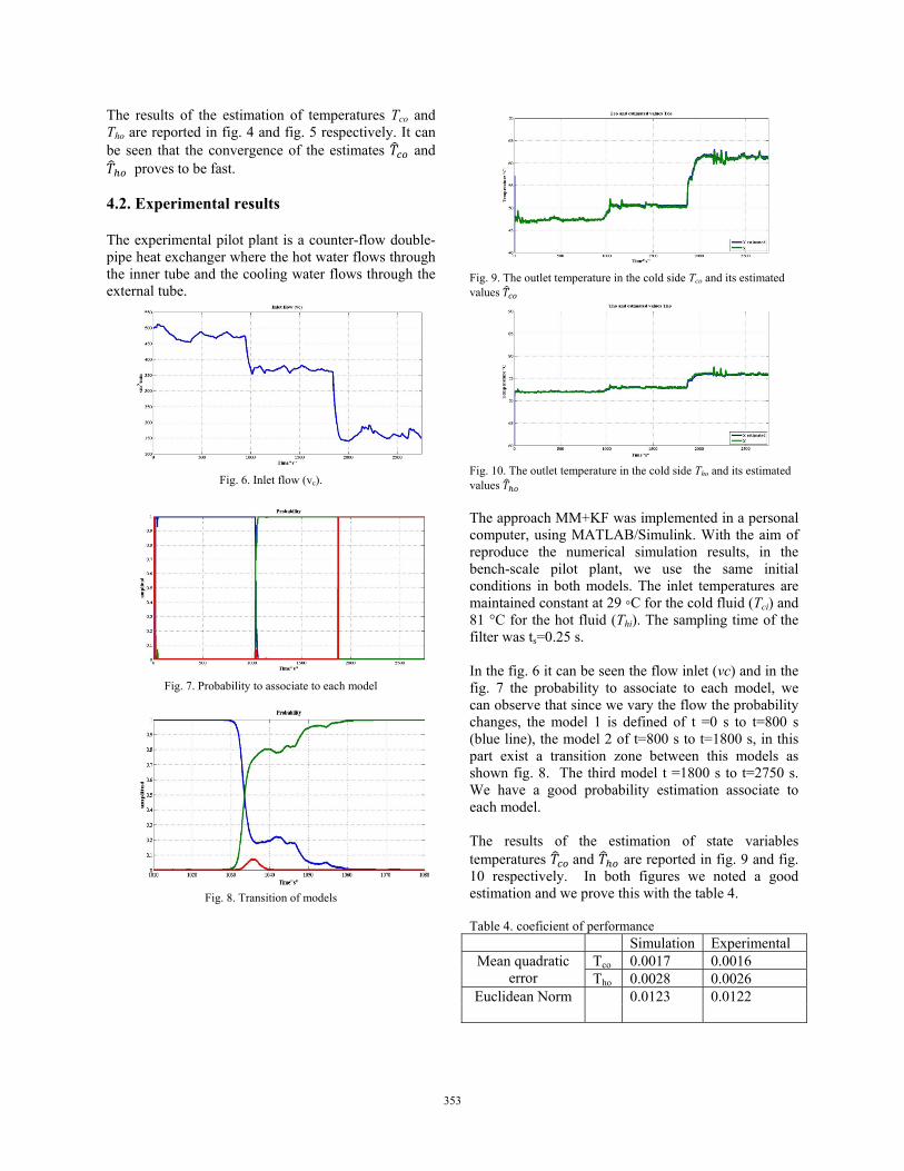
Fig. 9. The outlet temperature in the cold side Tco and its estimated values

Fig. 10. The outlet temperature in the cold side Tho and its estimated values The approach MM+KF was implemented in a personal computer, using MATLAB/Simulink. With the aim of reproduce the numerical simulation results, in the bench-scale pilot plant, we use the same initial conditions in both models. The inlet temperatures are maintained constant at 29 ◦C for the cold fluid (Tci) and 81 °C for the hot fluid (Thi). The sampling time of the filter was ts=0.25 s. In the fig. 6 it can be seen the flow inlet (vc) and in the fig. 7 the probability to associate to each model, we can observe that since we vary the flow the probability changes, the model 1 is defined of t =0 s to t=800 s (blue line), the model 2 of t=800 s to t=1800 s, in this part exist a transition zone between this models as shown fig. 8. The third model t =1800 s to t=2750 s. We have a good probability estimation associate to each model. The results of the estimation of state variables temperatures and are reported in fig. 9 and fig. 10 respectively. In both figures we noted a good estimation and we prove this with the table 4. Table 4. coeficient of performance Simulation Experimental

Mean quadratic error

Tco 0.0017 0.0016 Tho 0.0028 0.0026

Euclidean Norm 0.0123 0.0122

313353353353

5. Conclusion In this work, heat exchanger state variable estimation method has been presented. MM+KF permit the state variable estimation of state of a nonlinear system. The application of this approach method (MM+KF) to the heat exchanger is an excellent alternative to estimate the state variable system with a low degree error. The state variable estimation is fast. The advantage of this method is to make possible to work in operating region of HE where is not present a phase-change and other advantage this method allows the prediction of temperature only with one state measure. The experimental data will be used to confirm the veracity and effectiveness of the method presented here. Future studies will add diagnosis fault and fault tolerant control 6. References 1. Gildas, B., Nonlinear Observers and Applications.

2007: Springer. 2. P., B., A hybrid asymptotic-Kalman observer for

bioprocesses. Bioprocess Engineering, 1999. 20: pp. 249-55.

3. R.F. Escobar, D. Juárez, J. Siqueiros, C. Irles, J.A. Hernández, On-line COP estimation for waste energy recovery heat transformer by water purification process. Desalination, 2008. 222: pp. 677–683.

4. DG, L., An introduction to observers. IEEE Transaction on Automatic Control, 1971. 16: pp. 596-602.

5. Quintero-Mármol E, L.W., Georgakis C., Application of an extended Luenberger observer to the control of multicomponent batch distillation. Industrial & Engineering Chemistry Reseach, 1991. 30: pp. 1870-80.

6. Henk A.P Blom, a.Y.B.-S., The Interacting Multiple Model Algorithm for systems with Markovian Switching Coefficients. IEEE Transanction on Automatic Control, USA, 1988. 33: pp. 780-783.

7. A.Banerjee, Y.A., R. Pearson and B. Orgunnaike, H Control of Nonlinear Process Using Multiple Linear Models. Proceedings 3rd European Control Conference, Rome, Italy, 1995: pp. 2671-2676.

8. F. Azimzadeh, H.A.P., and J.A. Ramagnoli, On Line Optimal Control of a Batch Fermentation Process Using Multiple Models Approach. Proceedings of the 37th Conference on Decision Control, Tampa-Florida, USA, 1998: pp. 455-460.

9. Gudmundur R. Jonsson, S.L., Olafur P. Palsson, Use of extended Kalman filtering in detecting fouling in heat exchangers. ScienceDirect, 2007.

10. Adam, M.M., Diagnóstico de fallas de un sistemas con representación multimodelo lineal e invariante

en el tiempo, in Automatica. 2004, Henri Poincaré: Nancy, Francia.

11. Leithead, L.D.a.W., Survey of gainscheduling analysis and desing. International Journal of control, 2000: pp. 1001-1025.

12. Varga, A., Optimal output feddback control:a multi-model approach. IEEE Symposium on Computer-Aided Control System Design, 1996: pp. 327-332.

13. Fazlur Rahman MHR, D.R., Modeling and dynamic feedback linearisation of a heat exchanger model. Proceeding of the third IEEE conference on control applications, 1994: pp. 1801-6.

14. K.M. Hangos, J.B., G. Szederkényi, Analysis and control of nonlinear process systems, ed. Springer. 2004.

15. Weyer E, S.e.G., Hangos K., Grey boxfault detection of heat exchangers. Control engineering practice, 2000. 8: pp. 121-31.

16. C. M. Astorga Zaragoza, A.Z.R., V. M. Alvarado, R. M. Méndez y J. Reyes Reyes, Performance monitoring of heat exchangers via adaptive observers. Measurement, 2007. 40: p. 392-405.

314354354354