State Space Search and Planning

State Space Search and Planning

General Game Playing Lecture 4

Michael Genesereth Spring 2005

2

Outline

Cases: Single Player, Complete Information (today) Multiple Players, Partial Information (next time)

Search Direction: Search Strategy: Forward Search Depth First Backward Search Breadth First Bidirectional Search Iterative Deepening

Issues: State Collapse (Graph Search) Evaluation Functions

3

State Machine Model

c

b e

f

h

i

d g j

a k

4

Game Trees

a

c

hg

d

ji

b

fe

5

Search Direction

6

Forward Search

Even without variables, the number of models to be checked can be exceedingly large. There are, in general, infinitely many models to check.

As it turns out, Relational Logic has two nice properties that help to deal with this problem.

(1) Whenever a set of premises logically entails a conclusions, there is a finite proof of the conclusion from the premises.

(2) It is possible to enumerate all proofs in a systematic way.

7

Backward Search

Even without variables, the number of models to be checked can be exceedingly large. There are, in general, infinitely many models to check.

As it turns out, Relational Logic has two nice properties that help to deal with this problem.

(1) Whenever a set of premises logically entails a conclusions, there is a finite proof of the conclusion from the premises.

(2) It is possible to enumerate all proofs in a systematic way.

8

Bidirectional Search

Even without variables, the number of models to be checked can be exceedingly large. There are, in general, infinitely many models to check.

As it turns out, Relational Logic has two nice properties that help to deal with this problem.

(1) Whenever a set of premises logically entails a conclusions, there is a finite proof of the conclusion from the premises.

(2) It is possible to enumerate all proofs in a systematic way.

9

Nodes

function mguchkp (p,q,al) {cond(p=q, al; varp(p), mguchkp(p,cdr(assoc(q,al)),al); atom(q), nil; t, some(lambda(x).mguchkp(p,x,al),q))}

10

Node Expansion

function expand (node) (let (data al nl) {var player = player(node); var role = role(player) for action in legals(role,node) do old = data(node); data(node) == consaction(role,action,old); data = sort(simulate(node),#'minlessp); data(node) = old; if new = gethash(data,hasher(player)) then new else {new = makenode(player,data,theory, node); gethash(data,hasher(player)) = new; if termp(new) then score(new)= reward(role,new); (setf (score new) (reward (role player) new))) (setq nl (cons new nl)))) (setq al (acons (car l) new al)))))

11

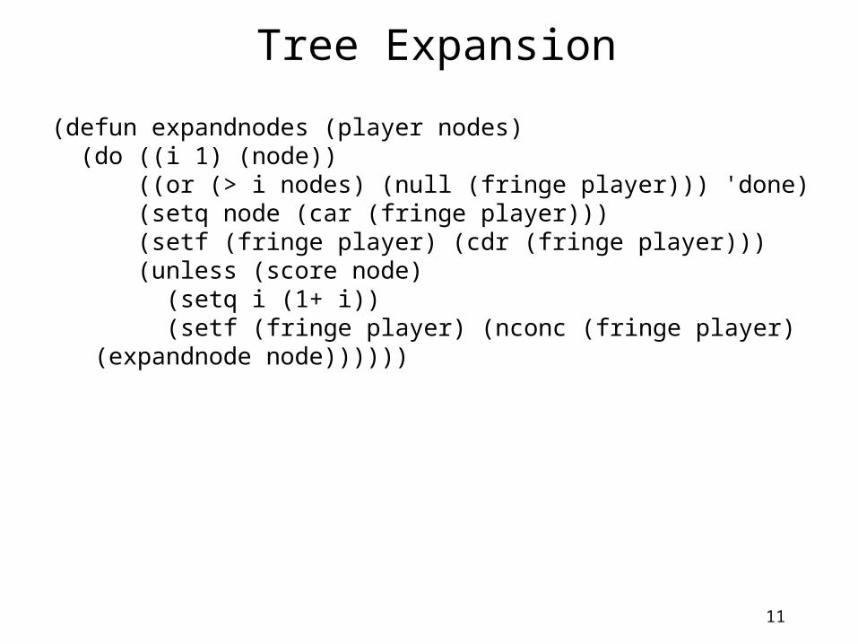
Tree Expansion

(defun expandnodes (player nodes) (do ((i 1) (node)) ((or (> i nodes) (null (fringe player))) 'done) (setq node (car (fringe player))) (setf (fringe player) (cdr (fringe player))) (unless (score node) (setq i (1+ i)) (setf (fringe player) (nconc (fringe player)

(expandnode node))))))

12

Search Strategy

13

Game Trees

a

c

hg

d

ji

b

fe

14

Breadth First Search

a b c d e f g h i j

a

c

hg

d

ji

b

fe

Advantage: Finds shortest pathDisadvantage: Consumes large amount of space

15

Depth First Search

a

c

hg

d

ji

b

fe

a b e f c g h d i j

Advantage: Small intermediate storageDisadvantage: Susceptible to garden pathsDisadvantage: Susceptible to infinite loops

16

Time Comparison

Analysis for branching 2 and depth d and solution at depth k

Time Best Worst

Depth k 2d −2d−k

Breadth 2k−1 2k−1

17

Time Comparison

Analysis for branching b and depth d and solution at depth k.

Time Best Worst

Depth kbd−bd−k

b−1

Breadthbk−1−1b−1

+1bk−1b−1

18

Space Comparison

Worst Case Space Analysis for search depth d and depth k.

Space Binary General

Depth d (b−1)×(d−1)+1

Breadth 2k−1 bk−1

19

Iterative Deepening

Run depth-limited search repeatedly,

starting with a small initial depth,

incrementing on each iteration,

until success or run out of alternatives.

20

Example

a

c

hg

d

ji

b

fe

aa b c da b e f c g h d i j

Advantage: Small intermediate storageAdvantage: Finds shortest pathAdvantage: Not susceptible to garden pathsAdvantage: Not susceptible to infinite loops

21

Time Comparison

Depth Iterative Depth

1 1 1

2 4 3

3 11 7

4 26 15

5 57 31

n 2n+1−n−2 2n−1

22

General Results

Theorem [Korf]: The cost of iterative deepening search is b/(b-1) times the cost of depth-first search (where b is the branching factor).

Theorem: The space cost of iterative deepening is no greater than the space cost for depth-first search.

23

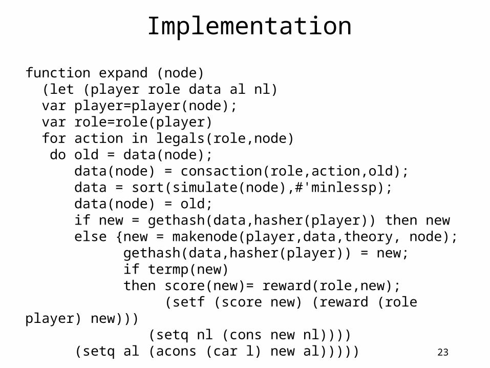
Implementation

function expand (node) (let (player role data al nl) var player=player(node); var role=role(player) for action in legals(role,node) do old = data(node); data(node) = consaction(role,action,old); data = sort(simulate(node),#'minlessp); data(node) = old; if new = gethash(data,hasher(player)) then new else {new = makenode(player,data,theory, node); gethash(data,hasher(player)) = new; if termp(new) then score(new)= reward(role,new); (setf (score new) (reward (role player) new))) (setq nl (cons new nl)))) (setq al (acons (car l) new al)))))

24

Graphs versus Trees

25

State Collapse

The game tree for Tic-Tac-Toe has approximately 900,000 nodes. There are approximately 5,000 distinct states. Searching the tree requires 180 times more work than searching the graph.

One small hitch: The graph is implicit in the state description and must be built in advance or incrementally. Recognizing a repeated state takes time that varies with the size of the graph thus far seen. Solution: Hashing.

26

Hashing

function mguchkp (p,q,al) {cond(p=q, al; varp(p), mguchkp(p,cdr(assoc(q,al)),al); atom(q), nil; t, some(lambda(x).mguchkp(p,x,al),q))}

27

Sorting

The game tree for Tic-Tac-Toe has approximately 900,000 nodes. There are approximately 5,000 distinct states. Searching the tree requires 180 times more work than searching the graph.

One small hitch: The graph is implicit in the state description and must be built in advance or incrementally. Recognizing a repeated state takes time that varies with the size of the graph thus far seen. Solution: Hashing.

28

Ordering Code

(defun minlessp (x y) (cond ((numberp x) (not (and (numberp y) (< y x)))) ((symbolp x) (cond ((numberp y) nil) ((symbolp y) (string< (symbol-name x) (symbol-name y)))) ((numberp y) nil) ((symbolp y) nil) (t (do ((l x (cdr l)) (m y (cdr m))) (nil) (cond ((null l) (return (not (null m)))) ((null m) (return nil)) ((minlessp (car l) (car m)) (return t)) ((equal (car l) (car m))) (t (return nil)))))))))

29

Node Expansion With State Collapse

function expand (node) (let (player role data al nl) var player=player(node); var role=role(player) for action in legals(role,node) do old = data(node); data(node) = consaction(role,action,old); data = sort(simulate(node),#'minlessp); data(node) = old; if new = gethash(data,hasher(player)) then new else {new = makenode(player,data,theory, node); gethash(data,hasher(player)) = new; if termp(new) then score(new)= reward(role,new); (setf (score new) (reward (role player) new))) (setq nl (cons new nl)))) (setq al (acons (car l) new al)))))

30

Early Termination

31

Heuristic Search

These are all techniques for blind search. In traditional approaches to game-playing, it is common to use evaluation functions to assess the quality of game state and, presumably, the likelihood of achieving the goal.

Example: piece count in chess.

In general game playing, the rules are not known in advance, and it is not possible to devise an evaluation function without such rules. We will discuss techniques for inventing evaluation functions in a later session.

32

Evaluation Functions

Even without variables, the number of models to be checked can be exceedingly large. There are, in general, infinitely many models to check.

As it turns out, Relational Logic has two nice properties that help to deal with this problem.

(1) Whenever a set of premises logically entails a conclusions, there is a finite proof of the conclusion from the premises.

(2) It is possible to enumerate all proofs in a systematic way.

33

Scores

function maxscore (node) {cond(score(node); null(alist(node),nil; t, for l = alist(node) with score = nil with max = 0 when null(l) return(max) do score <- maxscore(cdar(l)); cond(score = 100,return(100); ~numberp(score), max <- nil; ~max; score > max, max <- score))}

34

Best Move

function bestmove (node) {var best = nil; var score = nil; for pair in alist(node) do score = maxscore(cdr(pair)) cond(score = 100, return(car pair); score = 0, nil; null(best), best <- car(pair)) best or car(alist(node))}