STATE OF MAINE DEPARTMENT OF ENVIRONMENTAL PROTECTION BOARD OF ENVIRONMENTAL PROTECTION IN THE MATTER OF NORDIC AQUAFARMS, INC. :APPLICATIONS FOR AIR EMISSION, Belfast and Northport :SITE LOCATION OF DEVELOPMENT, Waldo County, Maine :NATURAL RESOURCES PROTECTION :ACT, and MAIN POLLUTANT :DISCHARGE ELIMINATION SYSTEM :(MEPDES)/WASTE DISCHARGE A-1146-71-A-N :LICENSE L-28319-26-A-N : L-28319-TG-B-N : L-28319-4E-C-N : L-28319-L6-D-N : L-28319-TW-E-N : W-009200-6F-A-N : ME0002771 Assessment of the Nordic Aquafarms Permit to Satisfy Clean Water Act Requirements TESTIMONY/EXHIBIT: TESTIMONY OF: DATE: NVC/UPSTREAM 7 George Aguiar James Merkel December 13, 2019 NVC/UPSTREAM 7 1

Welcome message from author
This document is posted to help you gain knowledge. Please leave a comment to let me know what you think about it! Share it to your friends and learn new things together.
Transcript

STATE OF MAINE
DEPARTMENT OF ENVIRONMENTAL PROTECTION
BOARD OF ENVIRONMENTAL PROTECTION
IN THE MATTER OF
NORDIC AQUAFARMS, INC. :APPLICATIONS FOR AIR EMISSION,
Belfast and Northport :SITE LOCATION OF DEVELOPMENT,
Waldo County, Maine :NATURAL RESOURCES PROTECTION
:ACT, and MAIN POLLUTANT
:DISCHARGE ELIMINATION SYSTEM
:(MEPDES)/WASTE DISCHARGE
A-1146-71-A-N :LICENSE
L-28319-26-A-N :
L-28319-TG-B-N :
L-28319-4E-C-N :
L-28319-L6-D-N :
L-28319-TW-E-N :
W-009200-6F-A-N :
ME0002771
Assessment of the Nordic Aquafarms Permit to Satisfy
Clean Water Act Requirements
TESTIMONY/EXHIBIT:
TESTIMONY OF:
DATE:
NVC/UPSTREAM 7
George Aguiar
James Merkel
December 13, 2019
NVC/UPSTREAM 7
1

PROFILE
Over 34 years of software development experience concentrating on working with state-of-the-art technologies to solve hard problems. Roles span complete product development life cycle from conception and design to implementation thru deployment and sustaining phases. Fully deployable from project lead to direct heavy lifting with a history of being a key player on teams which successfully met their goals.
Specializing in Rapid Application Development, Object Oriented design and development using WordPress, CiviCRM, JavaScript, PHP, React, VisualStudio.NET building .NET Enterprise and web based Service Oriented Solutions with Silverlight, .NET RIA Services, ADO.NET Entities, ASP.NET, Web Services, ADO.NET, Windows Forms, WPF, WCF, Mobile Internet Toolkit and the Compact Framework in C# and VB.NET with agile approaches to using Microsoft Patterns and Practices.
EXPERIENCE PRINCIPLE GEORGEAGUIAR.COM — 2011-PRESENT
Specialized version of CiviCrm, a CRM (Customer Relationship Management) system for nonprofits that focuses on Constituents, not Customers. Since 2011, have been providing CiviCrm on WordPress with custom options and training. Maintain websites for over 20 customers and nonprofits. Various long and short term engagements creating and maintaining websites and online web presence. Principle contractor for Promosis.Com: Design, build and maintain PHP websites and back end office tools for online marketing and incentive programs.
PRINCIPLE GLASSMENUS.COM, INC — 2009-2011 Designed and built backend website management tools using Silverlight 3.0, ADO.NET Entities, .NET RIA Services in C# using Visual Studio 8.0 and Blend 3.0 with service pack 1 employing TFS for source code control and project management. Designed and built Customer Relationship Management module which manages customer mailing list and integrates into Microsoft Word 2007 to compose and submit email content with integration into SmarterMail 5.5.
PRINCIPLE ENGINEER TJX COMPANIES — 2007-2009
Enhancements to TJX’s customized Buyer Worksheet application; a customized order worksheet written in VB.NET 2005 using Windows Forms and Component One’s C1FlexGrid and Excel C1XLBook components. Projects start with analyzing business
G E O R G E AG U I A R
NVC/UPSTREAM 7
2

George Aguiar
requirements, writing full UML design documentation and working to construction completion thru quality assurance and deployment all in a SOX compliant and security aware environment. Provided team mentoring delivering classes on Unit Testing, Debugging .Net using Advanced Tools, and Using Team Foundation Version Control.
PRINCIPLE GLASSMENUS.COM — 2005-2007
Headed up development for startup company: OdoClub.com using Flex 2.0, Flash, AJAX, Windows WebForms for Presentation Layer, .NET 3.0, WCF Web Services, Windows Workflow for Business Layer and SQL Server 2005 with Strongly Typed DataSets for the Data Layer. Conceived, designed and implemented a templatized, vertical market website solution using ASP.NET 3.0, C#, WCF, Windows Workflow, Flex 2.0 and AJAX. Solution provides a vertical market website in a box that can easily and economically be used to quickly implement custom websites for a niche market.
SOFTWARE ARCHITECT BCGI — 2003-2005
Primary responsibility for overall architecture for Mobile-Guardian: BCGI’s mobile phone access management solution. Duties include setting technical direction, recommending technologies and tools, designing, coding and testing. Analyzed business requirements and transformed marketing requirement documents into high level designs. Produced detailed designs including UML models and proof of concept prototypes. Provided team mentoring, validated code before check in and led technical aspect of interview process. Built and packaged software releases and provided installation and release documentation.
PRINCIPLE ENGINEER STRATUS COMPUTER — 2001-2003
Design and implementation of transition from heterogeneous Oracle 9i based high availability suite of tools to an n-tier .NET architecture based on Microsoft Best Practices and Architecture White Papers ASP.NET Web Forms, Business and Data Layers in C# passing Strongly Typed DataSets, Windows Management Instrumentation, Oracle SQL Mentoring of team members transitioning from ASP3.0/VB6.0 & VC++ 6.0 to .NET development environment including use of VS.NET 2003, Windows Server 2003, IIS 6.0, ASP.NET, ADO.NET and C#
VP PRODUCT ARCHITECTURE DASH.COM, INC. — 1999-2001
Responsible for next generation web site, data warehouse, and agent architecture built on top of IIS 5.0 and SQL Server 2000. Led initial development of IIS/ASP web site and browser based COM pluggin. Responsible for entire high volume web site and agent design, implementation and deployment on IIS web farm and SQL Server cluster. Brought initial concept from prototype to live in 7 months starting solo to build prototype for VC and then development lead. Led team of 17 developers on version 1 as VP of Development and 3 architects for subsequent releases as VP of Architecture.
38 Perkins Road Belfast ME 04915 508.341.3937 www.GeorgeAguiar.Com
NVC/UPSTREAM 7
3


George Aguiar
CTO ENGINEHOUSE MEDIA, INC — 1998-1999 Design and implementation of a first of a kind DNA-based Ad banner Management work flow product using Exchange/Outlook/IIS/ASP/SQL Server.
PRINCIPLE ENGINEER CENTRA SOFTWARE, INC — 1995-1998 Created Java/Swing client architecture and implemented framework. Designed and implemented Visual J++/Win32 client. Designed and implemented Java browser based client (applets).
SENIOR OPERATING SYSTEMS ENGINEER ALLIANT COMPUTER SYSTEM, INC — 1989-1995
Interactive performance enhancements to multi-processor OS. Device driver, computer resource and system accounting enhancements. Kernel base on UNIX – BSD 4.2.
SENIOR SOFTWARE ENGINEER NEC INFORMATION SYSTEMS INC — 1984-1989 Unix Engineering Workstation lead. PC UNIX (AT&T 5.1) work including internals, drivers, configuration, tuning and system management. Misc. projects: UUCP, Ethernet, NFS, RFS, graphics and X-Windows.
EDUCATION NORTHEASTERN UNIVERSITY BOSTON, MA — BSEE 1983
SKILLS Design and hands-on experience with PhpStorm, Microsoft Visual Studio.NET 2005/2008/2010, ASP.NET 1.1, 2.0 3.0, 3.5 & 4.0, Silverlight 3.0, .NET RIA Services, ADO.NET Entities, ADO.NET, Web Services, AJAX, Flex 2.0, Flash 8.0, ActionScript 3.0, WCF, Windows Workflow, Winforms, Mobile Controls, Microsoft Office, .NET Compact Framework, SQL Server 2000 & 2005, Oracle 9i, DHTML, JavaScript, XML, UML, ORM, ERD, Visio, Project, ASP, COM+ 1.5, MTS, MSMQ, C#, DNA, ASP, Visual C ++, Java, Visual Basic 6.0, C++, JSP, EJB, Swing.
38 Perkins Road Belfast ME 04915 508.341.3937 www.GeorgeAguiar.Com
NVC/UPSTREAM 7
5

James S. (Jim) Merkel: Resume 97 Patterson Hill Rd., Belfast, Maine 04915
(207) 323-1474, email: [email protected]
Jim is sustainability professional who authored Radical Simplicity, a hands-on guide to quantifying and monitoring sustainability. In 1989 he transitioned from the military engineering sector to moving institutions and individuals toward sustainability by: founding organizations, assisting campuses and organizations in measuring ecological footprints, working as Dartmouth College’s Sustainability Coordinator, creating city and regional transit and bike lanes and teaching sustainability at universities while experimenting in sustainable living.
Experience: 2014-Current Filmmaker, Independent, Belfast, Maine. 2005 – 2007 Sustainability Coordinator, Dartmouth College, Hanover, New Hampshire. Worked to integrate environmentally and socially sustainable practices into the College's operations, buildings, culture and strategic plan. Worked to reduce the carbon footprints of the campuses 110 buildings. His work helped Dartmouth College earn the highest grades on the Sustainability Report Card issued by the Sustainable Endowments Institute.
1994 – Present Founder and director of The Global Living Project (GLP) Conducted five multi-week GLP Summer Institutes where educators and students lived on an equitable portion of the biosphere. Researched and developed the 100 Year Plan, a societal approach to global sustainability.
1988 – 1994 Environment & Community Volunteer Work, San Luis Obispo, Ca. Elected to Vice-Chair, Executive Committee Chair, and Conservation Committee Chair of the Santa Lucia Chapter of the Sierra Club. State and federal lobbyist. Drafted legislation. Presented positions on transportation, land-use planning, open-space, peace, water, wilderness, Native American and oil spill issues at over 100 public hearings. Co-founded the Big Mountain Support Group. Delivered humanitarian aid to Navajo families resisting forced government relocation.
1985 - 5/89 TRW Electronic Products Inc., San Luis Obispo, California. Business Development, Foreign Military Sales, Senior Engineer.
1984 - 1985 ITT, Vandenberg AFB, California. Senior Electronic Engineer. Designed digital, R.F. and computer systems.
1977 - 1984 Photocircuits, Aquebogue, New York. Title: Electrical Engineer.
NVC/UPSTREAM 7
6

Teaching Experience: 2009-2014 Unity College, Adjunct Professor, Unity, Maine. Teaching
Environmental Issues and Insights, which includes student documentaries. 2009 Las Cañadas, Veracruz Mexico. Instructor for weeklong ecological
footprinting intensive. 2008 – 2009 Community College of Vermont, Adjunct Professor, Wilder, Vermont. 2008 – 2009 Longwood University, Farmville, Virginia. Radical Simplicity selected as
reading for First-year Experience 2008 & 2009. 2005 Antioch New England, Adjunct Professor, Keene, New Hampshire. 2003 University of British Columbia, Adjunct Professor, Vancouver, B.C.
Instructor for The Science and Practice of Sustainability. Publications:
• Radical Simplicity selected for edited book, Voluntary Simplicity – the poetic alternative to consumer culture, Stead & Daughters Ltd, New Zealand, 2009.
• Chapter in Less is more, New Society Publishers, Canada, 2009. • Author of Radical Simplicity – small footprints on a finite earth (in
third printing), New Society Publishers, Canada, 2003. Spanish Translation Simplicidad Radical, Fundación Tierra, Spain, 2005
Awards: 2016 Arthur Morgan Award, Yellow Springs, OH. 2008 Living Hero Award, New Hampshire Life Magazine, Concord, NH. 2006 Graduation Speaker, The Putney School, Vermont. 2006 Graduation Speaker, Vermont Law School, Vermont. 2000 Sustainable Living Award, Environmental Youth Alliance, Vancouver, B.C. 1999 The Bill Deneen Award for Outstanding Environmental Leadership, Nipomo, Ca. 1994 Gaia Fellowship, Earthwatch, research low resource use and high life quality in
Kerala, India. Researched light living in the Himalayas. 1992 Clean Air Award - American Lung Association, San Luis Obispo, Ca. 1991 Group of the Year Award for the Big Mountain Support Group - Economic
Opportunities Commission, San Luis Obispo, Ca. 1991 Citizen of the Year Nomination - Economic Opportunities Commission, San Luis
Obispo, Ca. 1990 Beyond War Award for work with the Earth Day Coalition, San Luis Obispo, Ca. Academic Background: • State University of New York at Stony Brook, B.S. in Electrical Engineering, May
1984. • Suffolk County Community College, New York, A.A.S. in Electrical Technology,
January 1981.
NVC/UPSTREAM 7
7


Authors: James Merkel
George Augiar
Nordic Aquafarms’ Total Carbon Footprint
Page 1
Summary
The findings of this study include:
1. That the proposed facility is greenhouse gas (GHG) intensive, and that lower carbon
solutions to feeding humanity are readily available. Our calculations have revealed that
the applicant’s annual GHG emissions represent approximately 5 to 6 percent of the 2030
total state GHG target.
2. If this facility were built and operated an unfair burden would be placed on existing
businesses and residents to meet Maine’s climate targets and the governor’s executive
orders.
3. The applicant should be required to amend their plan to:
a.) demonstrate carbon neutrality utilizing wind and solar power.
b.) find a Brownfield site that has stable soils to avoid releasing carbon stored in the
forest and soil, and to maintain the sequestration of a mature 35 acres of forests
and wetlands.
c.) find a location with access to deep ocean currents, or utilize a completely closed
system.
Our findings demonstrate that the construction (embodied CO2) and operations (CO2) of
Nordic Aquaculture farms (collectively, “the Project”) as proposed by the Applicant’s
Site Location and Development Permit Application (SLODA) to the Department of
Environmental Protection (DEP) on 5/16/2019 (the “Application”) adds significantly to
statewide greenhouse gas emissions. Our calculation estimates have revealed that the
applicant’s GHG contribution of between 0.55 and 0.76 MMTCO2e represents 4.6 – 6.4
percent of the 2030 total state GHG target, and between 12.8 and 17.6 percent of the
2050 target. To approve these new large sources of carbon emissions, while making
commitments to reduce GHG, violates the intent of PL 237, §576-A. This large-scale
aquaculture facility proposed by Nordic Aquafarms (NAF) in Belfast, Maine would also
NVC/UPSTREAM 7
9

Authors: James Merkel
George Augiar
Nordic Aquafarms’ Total Carbon Footprint
Page 2
make it difficult to “achieve carbon neutrality by 2045” as mandated by the Executive
Order No. 10FY 19/20, signed by Governor Mills on September 23, 2019.1
By conducting three separate life-cycle assessments of Nordic’s proposal, along with
surveying similar assessments of other recirculating aquaculture systems (RAS), an
estimate of both embedded and operational CO2e (Life-cycle CO2e = Embodied CO2 +
Operational CO2) was established. The results support what the literature has
determined: land-based aquaculture requires significant energy and feedstock, and
produces large amounts of greenhouse gases (GHG).2 3
Introduction
There is no shortage of warnings, reports and political statements concerning GHG
emissions, and the irreversible consequences of climate change. The United Nations
Emissions Gap Report Summary that was issued on November 26, 2019 states the
situation clearly: “[The] findings are bleak. Countries collectively failed to stop the
growth in global GHG emissions, meaning that deeper and faster cuts are now required.”4
Business-as-usual has accelerated the crisis which
“is more severe than anticipated, threatening natural ecosystems and the fate of humanity (IPCC 2019). Especially worrisome are potential irreversible climate tipping points and nature's reinforcing feedbacks (atmospheric, marine, and terrestrial) that could lead to a catastrophic “hothouse Earth,” well beyond the control of humans (Steffen et al. 2018). These climate chain reactions could cause significant
1https://www.maine.gov/governor/mills/sites/maine.gov.governor.mills/files/inline-files/Executive%20Order%209-23-2019_0.pdf
2Monterey Aquarium Seafood Watch https://www.seafoodwatch.org/-/m/sfw/pdf/standard%20revision%20reference/2015%20standard%20revision/public%20consultation%202/mba_seafoodwatch_criteria%20for%20greenhouse%20gas_msg_final.pdf?la=en 3Energy Use in Recirculating Aquaculture Systems https://www.researchgate.net/publication/323891940_Energy_use_in_Recirculating_Aquaculture_Systems_RAS_A_review 4 UN Environment Programme, Emissions Gap Report 2019 https://www.unenvironment.org/resources/emissions-gap-report-2019
NVC/UPSTREAM 7
10

Authors: James Merkel
George Augiar
Nordic Aquafarms’ Total Carbon Footprint
Page 3
disruptions to ecosystems, society, and economies, potentially making large areas of Earth uninhabitable.” 5
We are, as 11,000 scientists declared on November 5th in BioScience in a climate
emergency.6
Maine
In 2003 Maine enacted PL 237. This law required that the DEP develop and submit a
Climate Action Plan (CAP or Plan) for Maine, and mandates the reduction of GHG
emissions. Specifically, under §576-A of PL 237 the State's goals for the reduction of
emissions for 2020 are 10% below 1990 levels (21.65 MMTCO2e) by January 1, 2020,
(19.46 MMTCO2e) which Maine is, according to the 2019 Maine Interagency Climate
Adaptation work group (MICA) Update Report, on target to meet. However, §576-A
mandates that “by January 2030 the State shall reduce gross annual greenhouse gas
emissions to at least 45% below 1990 gross annual greenhouse gas emissions level”
putting the 2030 target at 11.91 (MMTCO2e). Furthermore, the law mandates that “by
January 1, 2050, the State shall reduce gross annual greenhouse gas emissions to at least
80% below the 1990 GHG emissions level,” or to 4.3 (MMTCO2e). By comparison, the
applicant’s greenhouse gas contribution of between 0.55 and 0.76 MMTCO2e represents
4.6 – 6.4 percent of the 2030 total state GHG target, and between 12.8 and 17.6 percent
of the 2045 target.
5 Ripple, William J, Wolf, Christopher, Newsome Thomas M., Barnard, Phoebe, and Moomaw, William R. World Scientists’ Warning of a Climate Emergency, BioScience, biz088, p. 3 https://doi.org/10.1093/biosci/biz088 6 Ripple, William J, Wolf, Christopher, Newsome Thomas M., Barnard, Phoebe, and Moomaw, William R., World Scientists’ Warning of a Climate Emergency, BioScience, biz088, https://doi.org/10.1093/biosci/biz088
NVC/UPSTREAM 7
11

Authors: James Merkel
George Augiar
Nordic Aquafarms’ Total Carbon Footprint
Page 4
Belfast
As stated in the Belfast’s Energy Committee’s mission statement, “[t]he committee's
objective is to recommend steps to the City Council and city residents that will reduce
both greenhouse and air pollution emissions throughout the city.” This facility will
significantly increase local GHG emissions, while eliminating vital sequestration
resources. The facility will also undermine the Belfast Climate Crisis committee’s
commitment to supporting and enhancing “Ecosystem-based Resilience.” Their report
states that “solutions [include] conserving and restoring smaller-scale natural ecosystems
within the watershed (wetlands, river mouths, beaches, dunes, intertidal and subtidal
habitats); designing containment areas; establishing appropriate vegetative cover along
shorelines; and mandating low-impact development practices.” The Nordic Aquaculture
facility is not a “low-impact development practice.”
Lifecycle Assessment (LCA) for CO2e
The intention of this research is to establish an estimate of the total carbon (TC) additions
to Maine’s annual CO2 emissions that can be expected, should the proposed Nordic
Aquafarms facility be built in Belfast. Three separate Life-Cycle Assessment (LCA)
tools/methodologies were used to establish a framework for accounting for many of the
impacts typically ignored when only considering operational flows of resources. Figure
1. illustrates a simplified diagram for a rather complicated analysis. The desired scope for
our purposes is to focus on CO2 equivalent emissions related to the entire facility from
turning a complex, mature forested site into an industrial facility (concrete, steel, pumps
and motors) and then summarizing the larger categories of operational inputs such as
feeds, electricity, diesel fuel, and chemicals.
NVC/UPSTREAM 7
12

Authors: James Merkel
George Augiar
Nordic Aquafarms’ Total Carbon Footprint
Page 5
Figure 1
The analysis is an underestimate as many real impacts are difficult to quantify at the
design stage, yet it provides a useful estimate for decision-making purposes. In the case
of Nordic’s proposal, extensive specialized buildings, fuel and chemical tanks, pipelines
into the bay, comprise unique and carbon intensive structures, with a broad range of
possible scenarios and risks should the project fail prematurely. LCA tools help plan for
worst-case outcomes. Maine industries have historically left behind “wicked problems”
such as mercury sediments covering miles of the Penobscot River7, and dioxin pollution
in several Maine Rivers.8 This analysis does not include decommissioning at the end of
the useful life of the facility, however, deconstruction at some point, will be carbon
intensive.
7 https://www.maine.gov/dep/spills/holtrachem/index.html 8https://www.nrcm.org/programs/waters/cleaning-up-the-androscoggin-river/maines-dioxin-problem/
NVC/UPSTREAM 7
13

Authors: James Merkel
George Augiar
Nordic Aquafarms’ Total Carbon Footprint
Page 6
Few LCA studies have been conducted on land-based aquaculture. In 2015 Seafood
Watch published research on energy use in a variety of aquaculture environments. Their
analysis determined land-based recirculating aquaculture systems (LB-RAS) to be the
most energy intensive of the studied methods.9
Figure 2: Energy and feed requirements of various aquaculture technologies.
In 2016, a study compared producing Atlantic salmon in open pens in seawater to a
hypothetical land-based closed containment recirculating aquaculture system (LBCC-
RAS) based upon the Conservation Fund’s Freshwater Institute grow out trials of Atlantic
salmon.10 This is the study that the applicant sites to argue that salmon grown in a LBCC-
9 Monterey Bay Aquarium Seafood Watch https://www.seafoodwatch.org/-/m/sfw/pdf/standard%20revision%20reference/2015%20standard%20revision/public%20consultation%202/mba_seafoodwatch_criteria%20for%20greenhouse%20gas_msg_final.pdf?la=en
NVC/UPSTREAM 7
14
Authors: James Merkel
George Augiar
Nordic Aquafarms’ Total Carbon Footprint
Page 7
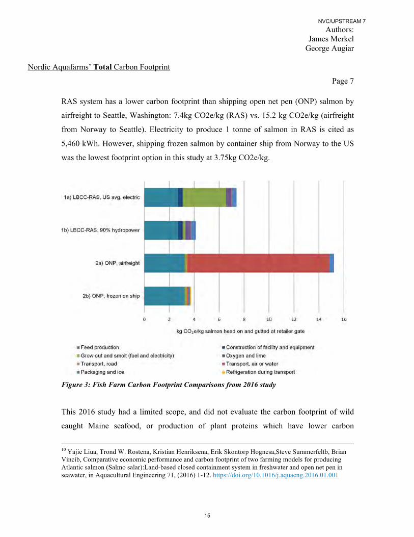
RAS system has a lower carbon footprint than shipping open net pen (ONP) salmon by
airfreight to Seattle, Washington: 7.4kg CO2e/kg (RAS) vs. 15.2 kg CO2e/kg (airfreight
from Norway to Seattle). Electricity to produce 1 tonne of salmon in RAS is cited as
5,460 kWh. However, shipping frozen salmon by container ship from Norway to the US
was the lowest footprint option in this study at 3.75kg CO2e/kg.
Figure 3: Fish Farm Carbon Footprint Comparisons from 2016 study
This 2016 study had a limited scope, and did not evaluate the carbon footprint of wild
caught Maine seafood, or production of plant proteins which have lower carbon
10 Yajie Liua, Trond W. Rostena, Kristian Henriksena, Erik Skontorp Hognesa,Steve Summerfeltb, Brian Vincib, Comparative economic performance and carbon footprint of two farming models for producing Atlantic salmon (Salmo salar):Land-based closed containment system in freshwater and open net pen in seawater, in Aquacultural Engineering 71, (2016) 1-12. https://doi.org/10.1016/j.aquaeng.2016.01.001
NVC/UPSTREAM 7
15

Authors: James Merkel
George Augiar
Nordic Aquafarms’ Total Carbon Footprint
Page 8
footprints than the options this study evaluated. For example, wild caught Demersal fish
(eg. Haddock) species have a life-cycle CO2e intensity of 2.4 kg CO2e/kg. Small Pelagic
fish (eg. Sardines) have a lifecycle CO2e of 0.2 kg CO2e/kg.11 Vegetarian diets including
legumes have CO2e in the range of 0.6 kg CO2e.12
A more recent LCA paper was published in 2019 which is the first analysis based upon
actual data from growing out 29,000 salmon in northern China from 100 g smolts to 4
KG fish.13 The results of this study were that to grow one tonne of live-weight salmon
required 7,509 KWh of electricity and generated 16.7 tonnes of Co2e, 106 kg of SO2 e,
2.4 kg of P e and 108kg of N e (cradle to farm gate). The study cited electricity and feed
as the larger components of the overall impact. This more recent study from an actual
operation reported roughly double the tonnes of CO2e/tonne of fish compared to the 2016
FreshWater Institute Study (7.4 vs. 16.7).14 The power per tonne of fish produced was
5,460 kWh in the 2016 study while the more recent China study was 7,509 kWh. Many
factors can account for the differences such as power grid composition, fish food sources
and makeup, different inventories and assumptions, however, the data are close enough to
offer some confidence in their similar methodologies and findings.
11Parker, Robert W.R., Blanchard, Julia, Gardener, Caleb et al., Fuel use and greenhouse gas emissions of world fisheries in Nature Climate Change, VOL 8, APRIL 2018 p. 333–337 http://www.ecomarres.com/downloads/GlobalFuel.pdf 12Clune, S. J., Crossin, E., & Verghese, K., Systematic review of greenhouse gas emissions for different fresh food categories. Journal of Cleaner Production, 140(Part 2), 766-783. http://www.research.lancs.ac.uk/portal/en/publications/systematic-review-of-greenhouse-gas-emissions-for-different-fresh-food-categories(153c618e-1b41-4cf4-b23e-7bc635cd2541).html 13 Song, Xingqiang, Liu, Ying, Brandão, Miguel et al. Life cycle assessment of recirculating aquaculture systems: A case of Atlantic salmon farming in China in Journal of Industrial Ecology, Vol 23, Issue 5, Oct 2019, pp. 1077-1086 https://doi.org/10.1111/jiec.12845 14 Yajie Liua, Trond W. Rostena, Kristian Henriksena, Erik Skontorp Hognesa,Steve Summerfeltb, Brian Vincib, Comparative economic performance and carbon footprint of two farming models for producing Atlantic salmon (Salmo salar):Land-based closed containment system in freshwater and open net pen in seawater, in Aquacultural Engineering 71, (2016) 1-12. https://doi.org/10.1016/j.aquaeng.2016.01.001
NVC/UPSTREAM 7
16

Authors: James Merkel
George Augiar
Nordic Aquafarms’ Total Carbon Footprint
Page 9
Figure 4: The boundary conditions for the 2019 China example
Figure 4 shows the system boundary and scope for the China example. Life-cycle
inventories used SimaPro 8.3 software to capture many of the cradle-to-farm-gate inputs.
To obtain a first order of magnitude estimation for the applicant’s proposed Belfast
operation, we used the resulting LCA CO2e per metric tonne of fish data from the 2019
China study. At buildout, the proposed Belfast facility anticipates producing 33,000
t/year output. The CO2e from NAF is calculated (16.7 tC/t X 33,000 t/year) to emit
551,100 tCO2e per year from both embodied and operational components. For
comparison, an average American car emits 4.6 t/yr, hence the NAF facility can be
estimated to be equivalent to adding 119,800 cars to the roads.
NVC/UPSTREAM 7
17

Authors: James Merkel
George Augiar
Nordic Aquafarms’ Total Carbon Footprint
Page 10
Generating specific LCA for the Belfast facility is difficult as the designs change
regularly as would be expected for a complex project. We have attempted to be as up to
date as possible while focusing on the larger footprint items. For example, earlier plans
were for an approximate 18 football fields of roof top solar panels. The panels have been
eliminated from the design and 8 diesel generators have been added. The generators use
has changed from not just supplying back up power during ice storms, but to shave
energy use on a daily basis to reduce the electricity billing rate. Additional changes
include, the outflow pipelines being shortened from a mile and a half into Belfast Bay to
⅔’s of a mile. Earlier, 1.5 million gallons/yr. of Methanol was listed and recently was
changed to 1 million gallons/yr. of a glycerin product MicroC 2000. Our calculations
have kept pace with most reported changes, but are not exhaustive, rather an attempt to
capture the larger construction details and design revisions.
In our second LCA analysis we used industry standard spreadsheet calculators looking at
as much of the project as possible aiming to include the embodied carbon (EC) specific to
this project. Traditionally, only steel and cement are calculated as they are commonly the
biggest contributors to a construction projects’ EC. Due to the nature of Land-Based
RAS (LB-RAS) we attempted to include as many of the significant embodied carbon
sources such as the Penobscot Bay pipeline (the design has changed from a trench to
buried to above the seabed), the site preparation, backup electrical generation, etc.
Figure 3 is the table from the Conservation Fund’s Freshwater Institute grow out trials of
Atlantic salmon.15 To this table, we have added the 2019 China analysis and the first
analysis we performed using industry standard spreadsheet (SS1) calculations, an
amended estimate of Nordic’s annual CO2e emissions based upon amortizing the
15 Conservation Fund’s Freshwater Institute https://doi.org/10.1016/j.aquaeng.2016.01.001
NVC/UPSTREAM 7
18
Authors: James Merkel
George Augiar
Nordic Aquafarms’ Total Carbon Footprint
Page 11
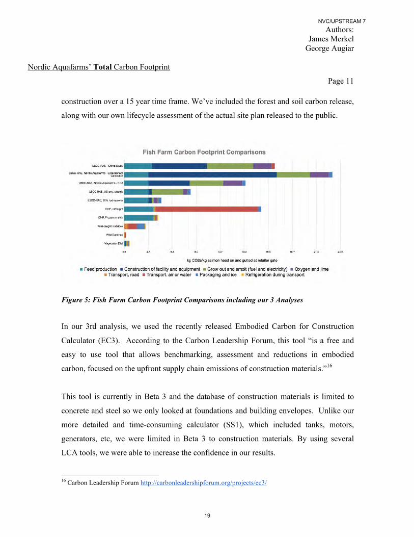
construction over a 15 year time frame. We’ve included the forest and soil carbon release,
along with our own lifecycle assessment of the actual site plan released to the public.
Figure 5: Fish Farm Carbon Footprint Comparisons including our 3 Analyses
In our 3rd analysis, we used the recently released Embodied Carbon for Construction
Calculator (EC3). According to the Carbon Leadership Forum, this tool “is a free and
easy to use tool that allows benchmarking, assessment and reductions in embodied
carbon, focused on the upfront supply chain emissions of construction materials.”16
This tool is currently in Beta 3 and the database of construction materials is limited to
concrete and steel so we only looked at foundations and building envelopes. Unlike our
more detailed and time-consuming calculator (SS1), which included tanks, motors,
generators, etc, we were limited in Beta 3 to construction materials. By using several
LCA tools, we were able to increase the confidence in our results.
16 Carbon Leadership Forum http://carbonleadershipforum.org/projects/ec3/
NVC/UPSTREAM 7
19

Authors: James Merkel
George Augiar
Nordic Aquafarms’ Total Carbon Footprint
Page 12
Our results from the spreadsheet calculator, listed in Figure 5 as “BBCC-RAS Nordic
Aquafarms - Spreadsheet Calculator” reported carbon intensity of approximately 23 kg
CO2e/kg salmon. At buildout, the proposed Belfast facility, producing 33,000 t/year
output would emit an estimated 759,000 tCO2e (23 tC/t X 33,000 t/year) from both
embodied and operational components. This is equivalent to 165,000 cars to the roads.
Results & Discussion
Life-cycle Assessment – embodied carbon discussion
The life-cycle assessment results of the applicant’s proposal support what the literature
has determined: land-based aquaculture requires significant energy and feedstock, and
produces large amounts of greenhouse gases (GHG).17 Most significant inputs include:
electricity for pumping water and operations; construction embodied energy for
buildings, pipes, tanks, wells, pumps, motors, filters, generators; fish foods; forest and
wetland elimination, and soil disturbances, are also important contributors.
The embodied carbon results are sensitive to the assumed lifespan of the infrastructure of
the project. The China study used 15 years, and conducted a sensitivity analysis to
include a 10 and 20-year option. For simplicity, our calculations used 15 years. The
lifespan of a new technology is very difficult to predict. Should the facility close in half
its expected life (due to falling salmon prices, disease outbreaks, technical issues, or
saltwater intrusion on wells) the embodied carbon footprint would double.
It is important to point out that there are many impacts that can and can’t be measured
using LCA, however, this paper focused upon CO2e emissions from construction and
17 Monterey Bay Aquarium Seafood Watch https://www.seafoodwatch.org/-/m/sfw/pdf/standard%20revision%20reference/2015%20standard%20revision/public%20consultation%202/mba_seafoodwatch_criteria%20for%20greenhouse%20gas_msg_final.pdf?la=en
NVC/UPSTREAM 7
20

Authors: James Merkel
George Augiar
Nordic Aquafarms’ Total Carbon Footprint
Page 13
operation. RAS facilities of the scale proposed are lacking a history of performance and
operating data, which would make for a more accurate LCA. However, the China LCA,
which has some actual operational data and a solid methodology, along with a team of
researchers, is a useful benchmark.
LCA methods can assist in identifying some of the potential unanticipated impacts of an
applicant’s project. In this case, a large-scale monoculture discharging into shallow and
recovering marine environments create risks that might require regular maintenance, and
replacements of filters, pumps and controllers and possibly additional heating and cooling
of discharge and intake water that could increase or decrease the estimates in our
analysis. Practical difficulties were not included in our analysis, such as construction
disputes or design flaws that could drive up embodied and operational emissions. The
real-world complexity of both ecosystems and human systems, dictate that these
estimates are likely conservative.
It is worth noting that only one of our analysis methods attempted to estimate the total
carbon of the eight 2MW generators and diesel engines, the smolt tanks, pumps, and
other equipment and machinery, the roadways, parking lots and walkways and the
pipeline into the bay. In this analysis, we made the best estimates working from the
drawings supplied to Belfast City Planning Office.
Life-cycle Assessment – operational carbon discussion
With electricity and feed among the primary operational footprint drivers of RAS carbon
footprint, several limitations in our analysis are noted below:
1) To complete a more accurate LCA would require specific fish feed composition,
including the breakdown of amounts of small fish in the feed, chicken and pig
slaughterhouse wastes, grains and pulses etc. Feed components derived from fish
are regularly shipped from South America. The applicant has not yet decided
NVC/UPSTREAM 7
21

Authors: James Merkel
George Augiar
Nordic Aquafarms’ Total Carbon Footprint
Page 14
exactly what they will feed their fish. It is also imperative to note that current fish
meal is impacting some of the poorest people on the planet, destroying wild food
sources for wild fish, and intensifying the impacts of the climate crisis.18 Many of
the small fish used as feed are eaten in other parts of the world and threatened by
largescale harvests as feedstocks.
2) The applicant has not been forthcoming with data such as design estimates of
annual electricity consumption, so our results have had to make estimates based
upon generator sizing checked against the data from other LCA assessments.
3) Maine’s electricity grid power source mix might seem favorable given the
considerable potentially “renewable” sources utilized. Some sources for CO2
emissions data make assumptions that biomass and hydroelectric are “carbon
neutral” and “renewable,” however, these terms are inaccurate in accounting for
the life-cycle impacts of these energy sources.19
Maine’s 2017 power-grid used biomass (26%) and hydro-electric (30%). Wood biomass
has a higher CO2 per BTU than coal.20 Hydroelectric dams, while considered to be
carbon neutral, are proving to release large amounts of Ch4 and CO2.21,22
18 Green, Matthew “Plundering Africa: Voracious Fishmeal Factories Intensify the Pressure of Climate Change”,ReutersOctober 13, 2018 https://www.reuters.com/investigates/special-report/ocean-shock-sardinella/ 19 Harvey, Chelsea, Heikkinen, Niina, Congress Says “Biomass Is Carbon-Neutral, but Scientists Disagree: Using wood as fuel source could actually increase CO2 emissions”, in Scientific AmericaE&E News, March 23, 2018 https://www.scientificamerican.com/article/congress-says-biomass-is-carbon-neutral-but-scientists-disagree/ 20 Carbon Emissions from Burning Biomass for Energy in Partnerships for Policy Integrity https://www.pfpi.net/wp-content/uploads/2011/04/PFPI-biomass-carbon-accounting-overview_April.pdf
21 Deemer, Bridget R. Harrison, John A. Li, Siyue et al. Greenhouse Gas Emissions from Reservoir Water Surfaces: A New Global Synthesis, in BioScience, Volume 66, Issue 11, 1 November 2016, Pages 949–964, https://doi.org/10.1093/biosci/biw117 22 Graham-Rowe, Duncan, Hydroelectric Power's Dirty Secret Revealed in New Scientist, 24 February 2005 https://www.newscientist.com/article/dn7046-hydroelectric-powers-dirty-secret-revealed/#ixzz67klj5iSG
NVC/UPSTREAM 7
22

Authors: James Merkel
George Augiar
Nordic Aquafarms’ Total Carbon Footprint
Page 15
Figure 6
The combustion of wood results in 213 lb CO2/mmbtu (bone dry) while Bituminous coal
comes in slightly lower at 205.3 lb CO2/mmbtu.23 Forests are very effective in
sequestering and storing carbon. It is argued that “trees grow back,” true, however the lag
time for the young forest to sequester carbon at rates that mature forests can is decades
long, while the release of carbon from biomass generators is instantaneous. It is the old
“slow in, fast out problem.”24 Biomass is only renewable if cut rates and forest practices
don’t diminish the ecosystem services while harvesting the biomass, (easy to state,
difficult to achieve). And while the cutting is taking place, the habitat is under stress,
soils and biodiversity are disturbed or eliminated, and forest resilience and long-term
health are diminished. All of which can result in additional C02 emissions.
23 Carbon emissions from burning biomass for energy https://www.pfpi.net/wp-content/uploads/2011/04/PFPI-biomass-carbon-accounting-overview_April.pdf 24 Moomaw, William R., Masino, Susan A., Faison, Edward K., Intact Forests in the United States: Proforestation Mitigates Climate Change and Serves the Greatest Good in Frontiers in Forests and Global Change, June 2019, Vol 2, pp 1-27. https://www.frontiersin.org/articles/10.3389/ffgc.2019.00027/full
NVC/UPSTREAM 7
23
Authors: James Merkel
George Augiar
Nordic Aquafarms’ Total Carbon Footprint
Page 16
Hydro-electric dams result in methane and CO2 release, and the elimination of large
tracks of forest lands that sequester and store carbon above and below the surface, and
provide critical habitat for biodiversity. A 2016 paper, found that GHG emissions from
reservoir water surfaces account for 0.8 (0.5–1.2) Pg CO2 equivalents per year, with the
majority of this forcing due to CH425. It can be viewed as ironic that the very dams that
have prevented untold millions of salmon from reproducing are now used to claim low
carbon footprints for contained salmon that never see the light of day. The point being
raised is that technologies such as large-scale hydroelectric plants solve one problem
(cheap electricity) while creating other problems (eg. Ch4 and CO2 release, habitat
destruction, loss of fishery).
The applicant plans to install 9 diesel generators, using 900,000 gallons of fuel resulting
in 9142 metric tons of CO2e annually. This is equal to adding an additional 1,988 cars to
Belfast’s roadways. In addition to CO2 emissions, the air quality impacts and noise need
to be considered, especially during periods of poor air quality and climate inversions.
Forest, wetlands, and soil removal
The facility requires the elimination of 34 acres of secondary growth mature pine and
hardwood trees, and the removal of between 15 and 48 feet of soil totaling an estimated
215,000 cubic yards. It also requires the complete elimination of ten wetlands, nine of
which are wetlands of special significance (WOSS). three significant streams will also be
eliminated.26 It is estimated that the forest, and the 17 wetlands of varying sizes, currently
25 Deemer, Bridget R. Harrison, John A. Li, Siyue et al. Greenhouse Gas Emissions from Reservoir Water Surfaces: A New Global Synthesis, in BioScience, Volume 66, Issue 11, 1 November 2016, Pages 949–964, https://doi.org/10.1093/biosci/biw117 26 While the GHG impact of this is not included in these findings, it is recommended that they be calculated and understood. As stated in the application: https://www.maine.gov/dep/ftp/projects/nordic/applications/NRPA/Attachment%2009%20-%20Site%20Condition/NRPA_A9_SiteConditions_text.pdf
NVC/UPSTREAM 7
24

Authors: James Merkel
George Augiar
Nordic Aquafarms’ Total Carbon Footprint
Page 17
store approximately 13,465 metric tons of carbon above and below ground. Left intact,
this forest’s current sequestration rate is approximately 42.9 metric tons of carbon each
year. Current research is showing that trees increase their carbon sequestration
significantly as they age27’28. In addition, forests and wetlands have a high value
providing multiple ecosystem services, and William R Moomaw’s recent work
establishes that proforestation, meaning enhancing older forests, is actually the most
viable way to achieve CO2 Targets29.
A large quantity of carbon is stored in forest soils, and is released upon deforestation and
disturbance.30 According to the application "[e]xcavation required to construct the
foundations and lower levels of the grow modules will be approximately 15 to 20 feet
below the existing grades. The water treatment building includes 2 stories below grade,
requiring a cut up to approximately 48 feet below the existing grades to accommodate
construction of the lower level and a seawater intake pipeline.”31 Because the soils will
have to be removed due to the fact that, “the native silt and clay soils that will be
“There will be a total of 1,325 linear feet (LF) of impacts to streams within the project area (Table 9-5). Streams S3, S5, S6, and S9 will be indirectly impacted by the project. Impacts to stream S9 will be limited to a permanent crossing located between wetlands W8 and W9, along with a temporary crossing during the installation of the force main sewer line. The permanent crossing will be constructed in such a manner to not impair flow during storm events. The upper reaches of streams S3, S5, and S6 will be filled as a result of this project. These filled streams will result in the loss of 1,180 LF of stream bed. Impacts to these streams will typically result in the loss of Groundwater Recharge/Discharge, Floodflow Alteration, and Wildlife Habitats in these locations.” 27 Anderson, Mark G., Wild Carbon: A Synthesis of Recent Findings in Wild Works, Volume 1 Northeast Wilderness Trust http://www.newildernesstrust.org/wp-content/uploads/2019/08/WildWorks_V1_WildCarbon-2.pdf 28 Moomaw, William R., Masino, Susan A., Faison, Edward K., Intact Forests in the United States: Proforestation Mitigates Climate Change and Serves the Greatest Good in Frontiers in Forests and Global Change, June 2019, Vol 2, pp 1-27. https://www.frontiersin.org/articles/10.3389/ffgc.2019.00027/full 29 Moomaw, William R., Masino, Susan A. et al. Intact Forests in the United States, in Frontiers https://www.frontiersin.org/articles/10.3389/ffgc.2019.00027/full 30Dartmouth College. "Clear-cutting destabilizes carbon in forest soils, study finds." ScienceDaily, 15 April 2016. www.sciencedaily.com/releases/2016/04/160415125925.htm 31 Ransom Project 171.05027.005 Executive Summary Page 1 of 2 Belfast Geotechnical Report\02-03 Report\February 2019 Report\Text Rev.2_final February 27, 2019
NVC/UPSTREAM 7
25

Authors: James Merkel
George Augiar
Nordic Aquafarms’ Total Carbon Footprint
Page 18
excavated are not suitable for reuse as structural fill at the site”32 a large portion of all the
carbon stored in the soils will be emitted into the atmosphere.
Recommendations:
1. The applicant be required to demonstrate carbon neutrality and not place
increased burden for CO2 reductions on Maine’s population. Solar and
wind generation have become economically viable for the applicant to utilize.
2. The applicant should not be permitted to clear a mature forest that currently
sequesters carbon or remove soils and wetlands that are currently storing
carbon. Rather, they should be required to find a Brownfield site that has
stable soils.
3. Our LCA studies show that other lower carbon footprint foods are available
in Maine.
4. The applicant should be required to find a location with access to deep ocean
currents, or utilize a completely closed system.
Conclusion
Our study concludes that proposed facility is CO2e intensive and that lower carbon
solutions to feeding humanity are readily available. Our calculations have revealed that
the applicant’s GHG emissions are between 0.55 and 0.76 MMTCO2e. This represents
4.6 – 6.4 percent of the 2030 total state GHG target, and between 12.8 and 17.6 percent
of the 2045 target. To approve these new large sources of carbon emissions, while
making commitments to reduce GHG, violates the intent of PL 237, §576-A.
32Nordic Aquaculture SLODA Application https://www.maine.gov/dep/ftp/projects/nordic/applications/SLODA/Section%2011%20-%20Soils/Appendix%2011-B.%20Geotechnical%20Engineering%20Report.pdf
NVC/UPSTREAM 7
26

Authors: James Merkel
George Augiar
Nordic Aquafarms’ Total Carbon Footprint
Page 19
A final consideration must include the unfair burden of further reductions that existing
businesses and residents will have to make to meet Maine’s targets and the governor’s
executive orders if this facility is approved. As stated in the Climate Action Plan for
Maine, (CAP) getting to Carbon Neutral by 2045 will not occur under “business-as-
usual” scenarios, rather it will require that any future large developments demonstrate
carbon neutrality, and preferably be carbon positive.33 There is a need for the DEP, and
the State of Maine, to avoid placing additional burdens on existing enterprises, and to
require that new businesses use strategies to achieve carbon neutrality with their
proposals.
This facility would use Maine’s “commons” including the clean aquatic sea water to
dilute effluent, clean ground water, and clean air to receive diesel emissions and capacity
on the power grid. The public suffers the loss, while the industry makes profits.
Extractive industries should not put the burden of proof on its citizens. With several
other RAS facilities proposing to come to Maine (Bucksport, Jonesport, Millinocket…)
the CO2 implications are significant.
Maine has made progress towards meeting its climate goals, however, the next set of
reductions will be more difficult, as Maine’s shifting to fracked natural gas, biomass and
hydroelectric each have serious impacts. More solar and wind energy will be helpful. As
society grapples with sustainability and climate change, the challenge of new
technologies is to solve past problems without creating new problems. The DEP should
therefore not approve the NAF project as submitted, for the long list of problems and
risks it creates as an untested, new technology. The DEP could require NAF to submit a
carbon neutral design utilizing solar and wind power on a brownfield site that connects to
33 Maine Climate Action Plan, https://www.maine.gov/dep/sustainability/climate/MaineClimateActionPlan2004.pdf
NVC/UPSTREAM 7
27
Authors: James Merkel
George Augiar
Nordic Aquafarms’ Total Carbon Footprint
Page 20
deep ocean currents, or is a closed system. Finally, much better options are available for
feeding humanity through local organic vegetable protein, and lower trophic level wild
local fish eaten sparingly, a movement known as “Slow Fish”34 while wild fisheries are
restored.
34 https://www.slowfood.com/slowfish/pagine/eng/pagina--id_pg=44.lasso.html
NVC/UPSTREAM 7
28
EXHIBIT A7


1 September14,2015
Seafood Watch® DRAFT Greenhouse Gas Emissions Criteria for Fisheries and Aquaculture
Multi Stakeholder Group Draft
Contents Introduction............................................................................................................................................................................2
Providingfeedback,commentsandsuggestion................................................................................................2
SeafoodWatchDRAFTEnergyCriteriaforFisheriesandAquaculture......................................................2
OverviewofGreenhouseGasEmissionsfromFisheries,AquacultureandLand‐basedFoodProduction...........................................................................................................................................................................3
RationaleforandSummaryoftheGreenhouseGasCriteriaforFisheriesandAquaculture.......4
WildCaptureFisheriesGreenhouseGasCriterion...............................................................................................5
Introduction.......................................................................................................................................................................5
Methods................................................................................................................................................................................6
Part1:DeterminingGreenhouseGasEmissionIntensityfromFuelUseIntensity..........................6
Part2:Qualityindicators.............................................................................................................................................7
DataCollection..................................................................................................................................................................8
CommunicatingGHGintensityvaluesforwildcapturefisheries..............................................................9
AquacultureGreenhouseGasEmissionCriterion..............................................................................................10
Introduction....................................................................................................................................................................10
Methods.............................................................................................................................................................................11
Part1:GHGEmissionsassociatedwithfeedingredients/EnergyReturnonInvestments......12
Part2:Farm‐LevelEnergyUse...............................................................................................................................13
DataCollection...............................................................................................................................................................15
CommunicatingGHGintensityvaluesforaquacultureoperations.......................................................15
SummaryofChangesMadeSincetheFirstandSecondPublicConsultation........................................16
References.............................................................................................................................................................................17
EXHIBIT B-7

2September14,2015
Introduction The Monterey Bay Aquarium is requesting and providing an opportunity to offer feedback on the Seafood Watch Greenhouse Gas (GHG) Emissions Assessment Criteria for Fisheries and Aquaculture during our current revision process. Before beginning this review, please familiarize yourself with all the documents available on our Standard review website.
Providingfeedback,commentsandsuggestionThis PDF document contains the second drafts of the GHG Emissions Criterion for Fisheries and the GHG Emissions Criterion for Aquaculture. A summary of the changes made to the first draft as a result of feedback during the first consultation process is provided at the end of the document, and individual changes are highlighted in the public comment guidance throughout. In their current form, these criteria are companions to the Fisheries and Aquaculture Assessment Criteria and are unscored due to data limitations. Seafood Watch will use these criteria to stimulate data collection and may score them in the future. “Guidance for public comment” sections have been inserted and highlighted, and various general and specific questions have been asked throughout. Seafood Watch welcomes feedback and particularly suggestions for improvement on any aspect of the Energy (GHG Emissions) Criteria. Please provide feedback, supported by references wherever possible in any sections of the criteria of relevance to your expertise. Please use the separate GHG Criteria Comment Form, which contains the excerpted “Guidance for public comment” sections from the PDF, to provide your comments. These criteria were developed in close consultation with Dr. Peter Tyedmers of Dalhousie University, and Seafood Watch is indebted to Dr. Tyedmers for his time and dedication to this effort.
Seafood Watch DRAFT Energy Criteria for Fisheries and Aquaculture MSG guidance ‐ This section contains the draft guiding principle for the Energy (GHG Emissions) Criteria, which has been edited since the first public consultation to acknowledge the contribution of GHGs to the acceleration of climate change and to acknowledge that GHG emissions from food production are a significant fraction of anthropogenic GHG emissions.
Guiding Principle The accumulation of greenhouse gases in the earth’s atmosphere and water drives ocean acidification, contributes to sea level rise, affects air and sea temperatures, and accelerates climate change. GHG emissions from food production are a significant fraction of anthropogenic GHG

3September14,2015
emissions1,2. Sustainable fisheries and aquaculture operations will have low greenhouse gas emissions compared to land‐based protein production methods.
MSG guidance ‐ This section contains an overview of GHGs associated with seafood (and other protein) production methods, the draft rationale and summary for the Energy (GHG Emissions) Criteria for fisheries and aquaculture. This section has been edited since the first public consultation to include the overview of GHG emissions from fisheries and aquaculture. It also contains information about the GHG emissions included in our approach comparing up to the farm gate/dock emissions from seafood to land‐based proteins (poultry and beef). In addition, we’ve clarified that we will be using the median values for comparative protein GHG intensities. Seafood Watch would like to be able to supplement or find replacement values for these comparative GHG intensities which factor soil CO2 emissions into total GHG emissions, and welcome suggestions for comprehensive, robust values calculated with a uniform methodology for at least poultry and beef.
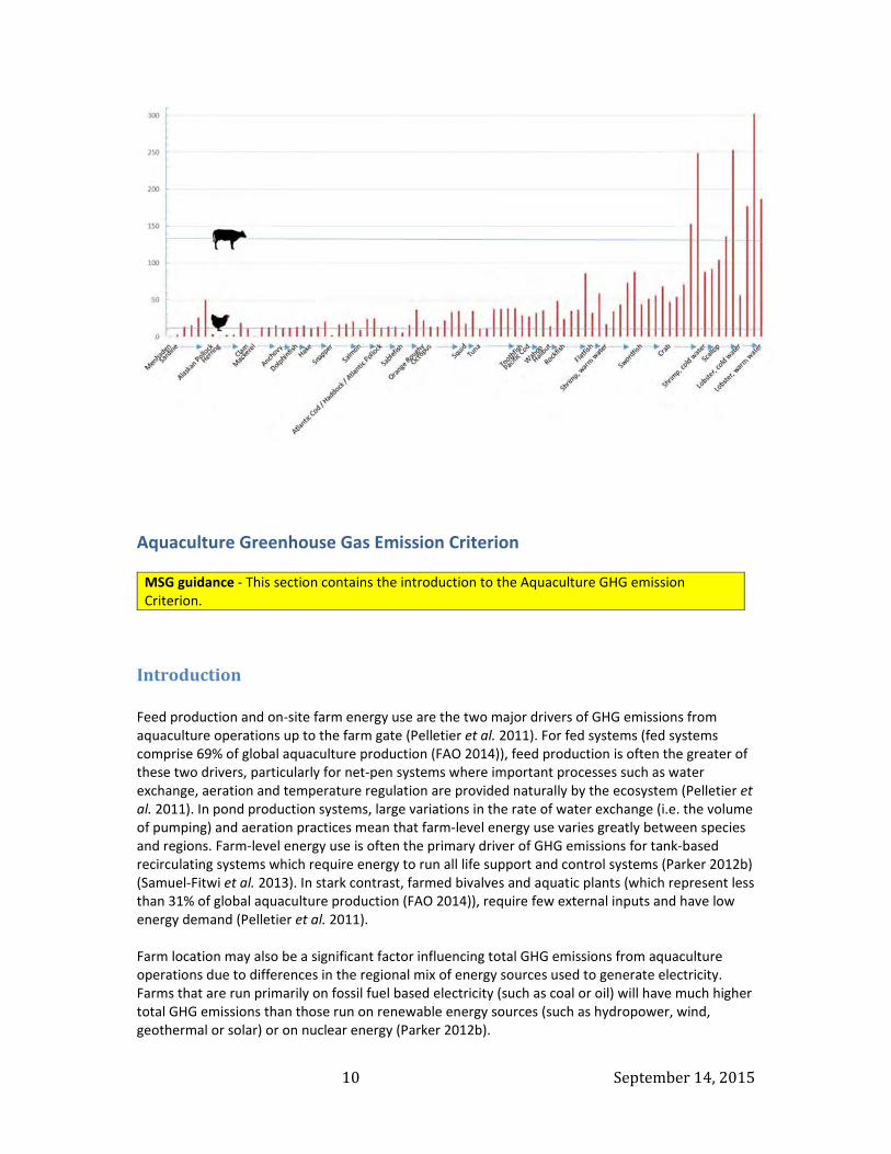
OverviewofGreenhouseGasEmissionsfromFisheries,AquacultureandLand‐basedFoodProduction The range of GHGs associated with food production are diverse, and not always well described or quantified in life cycle analysis studies about these emissions (Henriksson et al. 2012). Here we describe the main GHGs associated with food production up to the farm gate or dock. The primary GHG emissions associated with wild capture fisheries are from CO2 emitted via direct fossil fuel combustion. Fossil fuels are used for propulsion, deployment and retrieval of fishing gears, powering cooling systems and other activities (Parker 2015). Other potentially significant GHG emissions from fisheries are associated with refrigerant use (Ziegler et al. 2011) and while not GHGs, short‐lived, climate‐forcing agents, namely black carbon or soot (incompletely oxidized organic carbon), are produced from fuel combustion (McKuin & Campbell In Review). The GHGs associated with aquaculture production are more varied than those associated with wild capture fisheries and depend on the production method, species farmed and energy input regime (Pelletier et al 2011). These GHGs can include carbon dioxide (CO2), nitrous oxide (N2O) and methane (CH4). Aquaculture CO2 emissions are associated with farm level energy use and feed production. Feed production CO2 emissions include both energy use emissions as well as non‐energy emissions from soils. These soil CO2 emissions are associated with land conversion and land use and are not always well described or quantified (Nijdam et al. 2012). N2O emissions are associated with fertilizers used on feed crops (Pelletier & Tyedmers 2010) and from surface waters induced by microbial nitrification and denitrification (Hu et al. 2012). CH4 emissions are associated with feed production and organic material degradation (Nijdam et al. 2012). For fed systems, feed production can represent a significant proportion of emissions (Pelletier et al. 2011).
1 An overview of GHG emissions levels associated with food production (including fisheries and aquaculture) are available from the FAO (FAO 2011) 2 An overview GHG emissions associated with household energy use in the US, including from food are available in Jones et al. 2011 and the associated household emission calculator is available at: http://coolclimate.berkeley.edu/calculator

4September14,2015
The primary GHG emissions associated with land‐based food production systems (including crop and livestock) include CO2 from energy consumptive activities, CO2 resulting from land use and land conversion, N2O from fertilization of arable land and manure management and CH4 emissions from ruminant livestock (Nijdam et al. 2012).
RationaleforandSummaryoftheGreenhouseGasCriteriaforFisheriesandAquaculture Seafood Watch is proposing to incorporate GHG emission intensity into our science‐based methodology for assessing the sustainability of both wild caught and farmed seafood products. GHG accumulation in the Earth’s atmosphere and water drives ocean acidification, contributes to sea level rise, affects air and sea temperatures and accelerates climate change. The proposed criterion will evaluate greenhouse gas emissions per edible unit of protein from fisheries and aquaculture operations up to the dock or farm gate (i.e. the point of landing), consistent with the scope Seafood Watch assessments.3,4 Although a reliable index to define sustainable (or unsustainable) emissions of GHGs does not yet exist, as a baseline, we expect sustainable fisheries and aquaculture operations to have relatively low GHG emissions compared to the demonstrably high emission of some land‐based protein production methods. Therefore, in order to classify the GHG emission intensity of seafood products, Seafood Watch initially proposes to relate them to those of intensive poultry and beef production up to the farm gate; with products falling below the median value for poultry production considered as low emission sources, those between the median values for poultry and beef as moderate emission sources, and those above the median value for beef as high emission sources. The advantage of this method is that it provides consumers with information concerning relative impacts of food choices, beyond just seafood, enabling them to compare GHG intensity across edible protein sources Currently, Seafood Watch does not have a scalar metric (as we do for the scored criteria) to score the fisheries energy criterion. GHG emission intensity per edible unit of protein for both fishery and aquaculture products will be calculated using species‐specific edible protein estimates based on a literature review compiled by Peter Tyedmers (Dalhousie University, Nova Scotia, Canada). The edible protein estimate is based on the percent edible content and the percent protein content of muscle tissue for each species. Seafood Watch has discussed alternative standardization methods, such as excluding the percent protein content of muscle tissue (because invertebrates often have higher values), using wet weights or standardizing by product form, however, we are retaining the edible unit of protein standardization. We are basing the farm gate median values for poultry (13kg CO2/Kg protein) and beef (134 kg CO2/Kg protein) production on the supplementary information available from Nijdam et al. (2012), incorporating, if possible, a quantitative measure of uncertainty associated with these values, such as suggested in Henriksson et al (2015). The values from Nijdam et al. (2012) take into account both energy and non‐energy GHG emissions, and include N2O emissions from fertilization of arable land and manure, CH4 emissions from ruminant production and manure, and CO2 from fossil fuel energy. While this source acknowledges the importance of CO2 emissions from soil cultivation, these emissions are not factored in. This likely will underestimate total GHG emissions. Currently, Seafood
3 Seafood Watch assesses the ecological impacts on marine and freshwater ecosystems of fisheries and aquaculture operations up to the dock or farm gate. Seafood Watch assessments do not consider all ecological impacts (e.g. land use, air pollution), post‐harvest impacts such as processing or transportation, or non‐ecological impacts such as social issues, human health or animal welfare. 4 Seafood Watch will direct users of our recommendations to available post‐harvest greenhouse gas emissions calculators. Post‐harvest emission assessment is outside the scope of the current standards review.

5September14,2015
Watch is investigating comparative measures that incorporate soil CO2 emissions from land use and land conversion to supplement the values from Nijdam et al. (2012). For the wild‐capture fisheries criterion, Seafood Watch proposes using Fuel Use Intensity (FUI) to derive GHG emissions intensity for the target fishery plus an FUI derived GHG intensity factor for bait usage when available. For the aquaculture criterion, we propose a measure of direct farm‐level GHG emissions use plus an indirect measure of the GHG emissions associated with feed production.. Emissions associated with feed will be evaluated using a tiered approach, using specific ingredient information where available, and will be based on the dominant feed‐ingredient categories (aquatic, crop and land animal) when less information is available. An additional grouping for aquatic ingredients may be possible. Values will be sourced from existing data. Commercial fisheries and fish farms can achieve both environmental and financial benefits from reducing their energy use and non‐energy related GHG emissions. We recognize, however, that data collection related to energy use and non‐ energy GHG emissions are currently limited, so our aim with these criteria are to incentivize the collection and provision of energy use data and non‐energy GHG emission data from both fisheries and aquaculture operations to both track and improve the sustainability of seafood products. In this first iteration, the Seafood Watch Greenhouse Gas Criteria will be unscored additions to the Seafood Watch criteria, and will be used as companion criteria to our sustainable fisheries and aquaculture assessments.
Wild Capture Fisheries Greenhouse Gas Criterion MSG guidance ‐ This section contains the introduction to the Fisheries Energy (GHG Emissions) Criterion. This section is substantively unchanged from the first consultation draft. Feedback on the methodology is requested in the Methods section.
Introduction Fuel consumption is the primary driver of GHG emissions up to the point of landing for most wild capture fisheries, and is often the main source of emissions through the entire supply chain (Parker 2014, Parker & Tyedmers 2014). As such, measures of fuel consumption in fisheries provide an effective proxy for assessing the GHG emissions, or carbon footprint, of fishery‐derived seafood products. As mentioned earlier, Seafood Watch acknowledges that for some fisheries other GHG emissions and other climate forcing agent emissions may be significant, and will consider these additional emissions as information becomes available. Fuel consumption varies significantly between fisheries targeting different species, employing different gears, and operating in different locales. Fuel use also varies within fisheries over time: consumption increased in many fisheries throughout the 1990s and early 2000s, but has reversed in recent years as fisheries in Europe and Australia have both demonstrated consistent improvement in fuel consumption coinciding with increased fuel costs since 2004. As a result of this variation in fuel use, while it is difficult to estimate fuel consumption of individual fisheries without measuring it directly, generalizations can be made by analyzing previously reported rates in fisheries with similar characteristics. To this end, Robert Parker (PhD Candidate, Institute for Marine and Antarctic

6September14,2015
Studies, University of Tasmania, Australia) and Dr. Peter Tyedmers (Dalhousie University, Nova Scotia, Canada) manage a database of primary and secondary analyses of fuel use in fisheries (FEUD – Fisheries and Energy Use Database). Using this database, the draft Seafood Watch wild capture energy criterion is based on “Fuel Use Intensity “(FUI, as liters of fuel consumed per metric ton of round weight landings, L/MT) converted to Green‐House Gas Emission Intensity per edible unit of protein (KgCO2 equivalent/Kg edible protein).
MSG guidance ‐ This section contains the methodology for the Fisheries GHG Emissions Criterion and is substantively unchanged from the first consultation draft, except for the inclusion of example results in Figure 1 and the addition of a section on data collection.
MethodsThe sections below describe how GHG emission intensity will be calculated for wild capture fisheries and how data quality will be described.
Part1:DeterminingGreenhouseGasEmissionIntensityfromFuelUseIntensity Fisheries were categorized by species, ISSCAAP (International Standard Statistical Classification of Aquatic Animals and Plants) species class, gear type and FAO area. These codes were used to match each fishery to a subset of records in the FEUD database5 and each subset was analyzed using R to provide descriptive statistics and a weighted FUI estimate. The subset of database records used to estimate FUI of each fishery was selected using a ranked set of matching criteria. The best possible match in each case was used. The following ranking of matches were used to choose the subset most appropriate for each fishery’s estimate:
1) Records with matching individual species, gear type and FAO area 2) Records with matching individual species and gear type 3) Records with matching species class (ISSCAAP code), gear type and FAO area 4) Records with matching species class (ISSCAAP code) and gear type 5) Records with matching generalized species class (set of ISSCAAP codes), gear type and FAO
area 6) Records with matching generalized species class (set of ISSCAAP codes) and gear type
For each fishery, after selecting the most appropriate subset of records, the following information was calculated:
weighted mean (see below)
unweighted mean
standard deviation
standard error
median
5 FEUD currently includes 1,622 data points, covering a wide range of species, gears and regions. The best represented fisheries are those in Europe, those targeting cods and other coastal finfish, and those using bottom trawl gear. Coverage of fisheries from developing countries is limited but increasing. The database focuses on marine fisheries, and includes very few records related to freshwater fishes (except diadromous and catadromous species which are fished primarily in marine environments), marine mammals, or plants.
7September14,2015
minimum value
maximum value
number of data points
number of vessels or observations embedded in data points
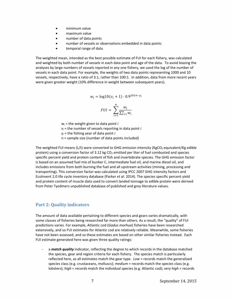
temporal range of data The weighted mean, intended as the best possible estimate of FUI for each fishery, was calculated and weighted by both number of vessels in each data point and age of the data. To avoid biasing the analyses by large numbers of vessels reported in any one fishery, we used the log of the number of vessels in each data point. For example, the weights of two data points representing 1000 and 10 vessels, respectively, have a ratio of 3:1, rather than 100:1. In addition, data from more recent years were given greater weight (10% difference in weight between subsequent years).
log10 1 ⋅ 0.9
∑
wi = the weight given to data point i vi = the number of vessels reporting in data point i yi = the fishing year of data point i n = sample size (number of data points included) The weighted FUI means (L/t) were converted to GHG emission intensity (KgCO2 equivalent/Kg edible protein) using a conversion factor of 3.12 kg CO2 emitted per liter of fuel combusted and species specific percent yield and protein content of fish and invertebrate species. The GHG emission factor is based on an assumed fuel mix of bunker C, intermediate fuel oil, and marine diesel oil, and includes emissions from both burning the fuel and all upstream activities (mining, processing and transporting). This conversion factor was calculated using IPCC 2007 GHG intensity factors and EcoInvent 2.0 life cycle inventory database (Parker et al. 2014). The species specific percent yield and protein content of muscle data used to convert landed tonnage to edible protein were derived from Peter Tyedmers unpublished database of published and grey literature values.
Part2:Qualityindicators The amount of data available pertaining to different species and gears varies dramatically, with some classes of fisheries being researched far more than others. As a result, the “quality” of FUI predictions varies. For example, Atlantic cod (Gadus morhua) fisheries have been researched extensively, and so FUI estimates for Atlantic cod are relatively reliable. Meanwhile, some fisheries have not been assessed, and so these estimates are based on other similar fisheries instead. Each FUI estimate generated here was given three quality ratings:
‐ a match quality indicator, reflecting the degree to which records in the database matched the species, gear and region criteria for each fishery. The species match is particularly reflected here, as all estimates match the gear type. Low = records match the generalized species class (e.g. crustaceans, molluscs); medium = records match the species class (e.g. lobsters); high = records match the individual species (e.g. Atlantic cod); very high = records

8September14,2015
match the individual species, gear type and region (e.g. Atlantic cod caught using longlines in FAO area 27). Table 2 shows a breakdown of assessed fisheries on the basis of the match quality.
Table 2. Criteria used to match Seafood Watch fisheries with FEUD records.
Matching factors Number of FUI estimates
Individual species, gear type and FAO area 21
Individual species and gear type 15
Species class (ISSCAAP code), gear type and FAO area
64
Species class (ISSCAAP code) and gear type 54
Generalized species class (set of ISSCAAP codes), gear type and FAO area
45
Generalized species class (set of ISSCAAP codes) and gear type
38
‐ a temporal quality indicator, reflecting the proportion of data points from years since 2000. Very low = all records are from before 2000; low = <25% of records are from 2000 on; medium = 25‐49% of records are from 2000 on; high = 50‐74% of records are from 2000 on; very high = 75% or more of records are from 2000 on.
‐ a subjective quality indicator reflects the confidence of the author in each estimate, based on the match criteria, temporal range, variability in the data, sample size, types of sources, and general understanding of typical patterns in FUI.
The subjective quality indicator is a good indication of the relative reliability of each estimate. It takes into account the range of data used, the method of weighting, and the degree to which the estimate reflects previous assessments of FUI in fisheries around the world. There are instances where the subjective quality indicator does not agree with the other quality rankings. For example, some estimates include a large number of older data points, and are therefore given a low temporal quality rating, but because the weighting method used gives more influence to more recent data points, the estimate closely reflects recent findings and is therefore given a high rating.
DataCollection As part of the assessment process, the analyst will search for and request additional information on Fuel Use for the fishery under assessment to supplement and add to data in the Fuel Use Intensity Database. The analyst will also research the potential for other GHG emissions and non‐GHG emissions of substances, like black carbon, which have high global warming potentials.

9September14,2015
CommunicatingGHGintensityvaluesforwildcapturefisheries As stated in the Rationale section, the proposed Seafood Watch GHG Criteria will be unscored additions to our sustainable seafood assessments. GHG intensity values for seafood will be compared to median GHG intensity values for land based protein production: poultry (considered a medium emission protein) and beef (considered a high emission protein). See the Rationale section for more information. Any method of communicating a GHG Intensity value for fisheries based on the FUI estimates generated here should take into account three things:
a) the estimates are based on fuel inputs to fisheries only, and, while fuel often accounts for the majority of life cycle carbon emissions, they need to be viewed in the context of the total supply chain. Most importantly, products that are associated with a high amount of product waste and loss during processing, or that are transported via air freight, are likely to have high sources of emissions beyond fuel consumption.
b) the quality of estimates varies, as is reflected in the quality indicators provided. Scoring fisheries with better quality estimates is easier than scoring predicted FUI of fisheries based on similar fisheries. For that reason, it may be justifiable to score only fisheries with a ‘high’ quality estimate, or to indicate that some scores are based on expected FUI rather than actual reported values.
c) the value should be expressed relative to some base value, reflecting relative performance of similar fisheries and/or alternative fishery products and/or alternative protein sources.
An example of how a subset of fisheries would fall relative to poultry and beef is shown in Figure 1 below. Figure 1: GHG Intensity Values for a subset of Seafood Watch recommendations, based on work performed by Robert Parker using the FEUD database. Fisheries represented by multiple gear types are shown by multiple red bars. Numerical value of median emission intensity for poultry production and beef production are shown as horizontal lines. Beef and poultry values were derived from Nijdam et al (2012).
10September14,2015
Aquaculture Greenhouse Gas Emission Criterion
MSG guidance ‐ This section contains the introduction to the Aquaculture GHG emission Criterion.
Introduction Feed production and on‐site farm energy use are the two major drivers of GHG emissions from aquaculture operations up to the farm gate (Pelletier et al. 2011). For fed systems (fed systems comprise 69% of global aquaculture production (FAO 2014)), feed production is often the greater of these two drivers, particularly for net‐pen systems where important processes such as water exchange, aeration and temperature regulation are provided naturally by the ecosystem (Pelletier et al. 2011). In pond production systems, large variations in the rate of water exchange (i.e. the volume of pumping) and aeration practices mean that farm‐level energy use varies greatly between species and regions. Farm‐level energy use is often the primary driver of GHG emissions for tank‐based recirculating systems which require energy to run all life support and control systems (Parker 2012b) (Samuel‐Fitwi et al. 2013). In stark contrast, farmed bivalves and aquatic plants (which represent less than 31% of global aquaculture production (FAO 2014)), require few external inputs and have low energy demand (Pelletier et al. 2011). Farm location may also be a significant factor influencing total GHG emissions from aquaculture operations due to differences in the regional mix of energy sources used to generate electricity. Farms that are run primarily on fossil fuel based electricity (such as coal or oil) will have much higher total GHG emissions than those run on renewable energy sources (such as hydropower, wind, geothermal or solar) or on nuclear energy (Parker 2012b).

11September14,2015
Additional GHG emissions may result from sources other than farm level energy use and feed production, such as from energy use associated with grow out infrastructure and smolt production and from non‐energy emissions of CH4 and N2O from ponds (as discussed in the above section “Overview of Greenhouse Gas Emissions from Fisheries, Aquaculture and Land‐based Food Production”). Seafood Watch recognizes that energy use varies greatly among different production systems and can be a major impact category for some aquaculture operations. It is noteworthy that improving practices for some of the Aquaculture Assessment Criteria may lead to more energy intensive production systems (e.g. where our recommendations are better for energy‐intensive closed recirculation systems than for open systems). Seafood Watch also recognizes (as mentioned in the above section “Overview of Greenhouse Gas Emissions from Fisheries, Aquaculture and Land‐based Food Production”), that non‐energy emissions associated with aquaculture production may be significant but are not always well described or quantified.
MSG guidance ‐ This section contains the methodology for the Aquaculture GHG Emissions Criterion. This criterion is less well developed than the fisheries criterion, primarily due the greater complexity of assessing the GHG emissions of aquaculture operations and the very limited data available. Changes made to this section since the first public consultation include 1) a tiered approach to evaluating GHG emissions associated with feed based on data availability 2) data from a literature review of farm level energy use and feed energy 3) factoring in non‐energy GHG emissions from both feed and farm level activities where this data is available 4) Separation out of sections on data collection and communicating GHG intensity values. Given the paucity of data, Seafood Watch will continue to collect and actively solicit information on GHG emissions associated with feed production and farm level activities. In particular, Seafood Watch will seek out information on the GHG emissions associated with specific feed ingredients.
Methods Seafood Watch is currently developing the methodology for assessing GHG emissions from aquaculture operations up to the farm gate. This methodology will include an assessment of the cumulative GHG emissions from feed use (primarily feed ingredient production, processing and potentially transport) as well as farm‐level emissions from energy use. We propose using a tiered approach to evaluating the feed contribution to GHG emissions. Where the specific origins of feed ingredients can be identified, it may be possible to determine the GHG emissions with high accuracy. When the specific ingredients are unknown, we propose basing the feed component on GHG emission estimates of dominant feed ingredient groups; i.e. aquatic (fishmeal and oil), crop and land animal (from Pelletier et al. 2009 and from additional sources) along with corresponding estimates of feed types and quantities fed by operations under assessment. We recognize that there may be significant differences in GHG emission values between the feeds in each of these groups, notably within the aquatic feed group (such as between a feed based primarily on fishmeal sourced from bycatch from a regional fishery on the low end of the spectrum and a feed sourced primarily from a distant reduction fishery), and we will break out the feeds in these groups where possible.

12September14,2015
For the farm‐level component, Seafood Watch proposes quantifying GHG emissions associated with pumping, aeration and other energy consumptive activities. Seafood Watch will draw data from existing studies and data gathered directly from aquaculture operations. As an initial step, Seafood Watch has compiled information from Life Cycle Analysis (LCA) studies and other sources on farm level energy use and energy use associated with feeds (carried out by Keegan McGrath). The results are summarized in Figure 2. When data are not available to finely estimate GHG emissions for each component (feed and farm‐level energy), Seafood Watch proposes defaulting to GHG estimates based on the most closely related species type, production type and the energy mix most commonly used in the region under assessment. As with the Fisheries criterion, all emissions estimates will be standardized to GHG Intensity per edible unit of protein (KgCO2 equivalent/Kg edible protein). The total GHG emissions will be obtained by summing the GHG emissions from feed ingredients (Part 1 below) and farm‐level energy use (Part 2 below). Figure 2: Energy use associated with aquaculture feeds (red bars) and farm level activities (blue bars) for a variety of species and production methods in units of megajoules/tonne of seafood, drawn from LCA studies and other information sources. Literature review carried out by Keegan McGrath. These data will be transformed into GHG Intensity per unit of edible protein (KgCO2 equivalent/Kg edible protein) when applied to this criterion.
Part1:GHGEmissionsassociatedwithfeedingredients/EnergyReturnonInvestments As mentioned above, Seafood Watch proposes using a tiered approach toquantify the GHG Intensity (KgCO2 equivalent/Kg edible protein) of feed ingredients. The tiers are based on the level of information available for the species and production system in the region or country under assessment. The first tier will be used when Seafood Watch can determine the specific feed ingredient mix and can determine associated GHG emission intensity values associated with the primary components (ideally taking into account the energy and non‐energy emissions associated with the feed). Data on the specific feed ingredient mix will be requested at the start of the assessment process with the goal of using this first tier. Seafood Watch will employ the second tier when we are unable to determine the specific feed ingredient mix, but can determine the
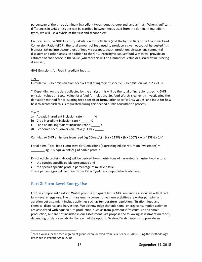
13September14,2015
percentage of the three dominant ingredient types (aquatic, crop and land animal). When significant differences in GHG emissions can be clarified between feeds used from the dominant ingredient types, we will use a hybrid of the first and second tiers. Factored into the GHG Intensity calculation for both tiers (and the hybrid tier) is the Economic Feed Conversion Ratio (eFCR), the total amount of feed used to produce a given output of harvested fish biomass, taking into account loss of feed via escapes, death, predation, disease, environmental disasters and other losses. In addition to the GHG Intensity value, Seafood Watch will provide an estimate of confidence in the value (whether this will be a numerical value or a scalar value is being discussed) GHG Emissions for Feed Ingredient Inputs: Tier 1 Cumulative GHG emission from feed = Total of ingredient specific GHG emission values* x eFCR * Depending on the data collected by the analyst, this will be the total of ingredient specific GHG emission values or a total value for a feed formulation. Seafood Watch is currently investigating the derivation method for calculating feed specific or formulation specific GHG values, and input for how best to accomplish this is requested during this second public consultation process. Tier 2 a) Aquatic ingredient inclusion rate = _____ % b) Crop ingredient inclusion rate = _____ % c) Land animal ingredient inclusion rate = _____ % d) Economic Feed Conversion Ratio (eFCR) = _____ Cumulative GHG emissions from feed (kg CO2‐eq/t) = [(a x 2158) + (b x 1007) + (c x 4138)] x (d)6 For all tiers: Total feed cumulative GHG emissions (expressing edible return on investment) = ________ Kg CO2 equivalents/Kg of edible protein Kgs of edible protein (above) will be derived from metric tons of harvested fish using two factors:
the species specific edible percentage and
the species specific protein percentage of muscle tissue. These percentages will be drawn from Peter Tyedmers’ unpublished database.
Part2:Farm‐LevelEnergyUse For this component Seafood Watch proposes to quantify the GHG emissions associated with direct farm‐level energy use. The primary energy consumptive farm activities are water pumping and aeration but also might include activities such as temperature regulation, filtration, feed and chemical dispersal and harvesting. We acknowledge that additional energy consumptive activities are associated with aquaculture production, such as from grow out infrastructure and smolt production, but are not included in our assessment. We propose the following assessment methods, depending on data availability. For each of the options, Seafood Watch intends to provide an
6 Mean values for the feed ingredient groups were derived from Pelletier et al. 2009, using the methodology described in Pelletier et al. 2010.

14September14,2015
estimate of confidence in the value (whether this will be a numerical value or a scalar value is under consideration) Farm‐level data As the most accurate measure, Seafood Watch aims to obtain farm‐level information on total energy use as well as the energy mix (e.g. diesel versus electricity, but also the regional mix of fuels used for electricity generation) specific to the aquaculture operations under assessment in order to estimate farm‐level GHG emissions. In addition to farm level energy, Seafood Watch aims to obtain information on non‐energy GHG emissions produced at the farm level. Such non‐energy emissions include N20 and CH4 from ponds (see the discussion in the section above: “Overview of Greenhouse Gas Emissions from Fisheries, Aquaculture and Land‐based Food Production”). As with the feed component, GHG emissions will be standardized to the Kgs of edible protein. Energy use values from scientific and grey Literature Where farm‐level information is not available, Seafood Watch proposes to model GHG emissions based on production method, species and farm‐level energy use data and non‐energy GHG emissions published in peer reviewed journals and available from grey literature. To estimate GHG emissions, this farm‐level energy use data will be synthesized with data on the most common mix of fuels used for electricity generation in the region of assessment. As with the feed component, GHG emissions will be standardized to the Kgs of edible protein. Relative energy use from water pumping and aeration When farm‐level or literature data are unavailable, Seafood Watch has developed the following tables to classify energy use from water pumping and aeration on a relative scale, which can be translated to relative GHG emission intensity. This method does not factor in non‐energy GHG emissions: Water Pumping A crude estimated measure of the energy used in pumping water Use pumping data or descriptions to select score value from the table below.
Water pumping characteristics7 Score
Zero No significant water pumping, e.g. cages, passive fill ponds, gravity fed tanks/ponds/raceways.
5
Low Static ponds 4
Low‐Moderate Harvest discharge or occasional exchange 3
Moderate Low daily exchange rate >0 to 3% 2
Moderate‐High Significant daily water exchanges 3‐10% 1
High Large daily water exchanges, recirculation systems >10% 0
Note ‐ low energy use is given a high score Energy use (pumping) score = ______ (range 0‐5) Record water pumping data here if available: Pumped volume per metric ton of product _______ m3 MT‐1] Average pumping head height _______ m Average pump power _______ KW or HP
7 As a guide, Low = <1000 m3/MT, Low‐Moderate = 1000 – 5,000 m3/MT, Moderate = 5,000 – 20,000 m3/MT, Moderate‐High = 20,000‐150,000 m3/MT, High = >150,000 m3/MT
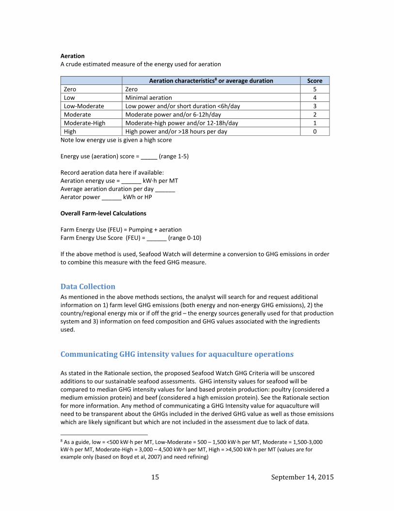
15September14,2015
Aeration A crude estimated measure of the energy used for aeration
Aeration characteristics8 or average duration Score
Zero Zero 5
Low Minimal aeration 4
Low‐Moderate Low power and/or short duration <6h/day 3
Moderate Moderate power and/or 6‐12h/day 2
Moderate‐High Moderate‐high power and/or 12‐18h/day 1
High High power and/or >18 hours per day 0
Note low energy use is given a high score Energy use (aeration) score = _____ (range 1‐5) Record aeration data here if available: Aeration energy use = ______ kW∙h per MT Average aeration duration per day ______ Aerator power ______ kWh or HP Overall Farm‐level Calculations Farm Energy Use (FEU) = Pumping + aeration Farm Energy Use Score (FEU) = ______ (range 0‐10) If the above method is used, Seafood Watch will determine a conversion to GHG emissions in order to combine this measure with the feed GHG measure.
DataCollectionAs mentioned in the above methods sections, the analyst will search for and request additional information on 1) farm level GHG emissions (both energy and non‐energy GHG emissions), 2) the country/regional energy mix or if off the grid – the energy sources generally used for that production system and 3) information on feed composition and GHG values associated with the ingredients used.
CommunicatingGHGintensityvaluesforaquacultureoperationsAs stated in the Rationale section, the proposed Seafood Watch GHG Criteria will be unscored additions to our sustainable seafood assessments. GHG intensity values for seafood will be compared to median GHG intensity values for land based protein production: poultry (considered a medium emission protein) and beef (considered a high emission protein). See the Rationale section for more information. Any method of communicating a GHG Intensity value for aquaculture will need to be transparent about the GHGs included in the derived GHG value as well as those emissions which are likely significant but which are not included in the assessment due to lack of data.
8 As a guide, low = <500 kW∙h per MT, Low‐Moderate = 500 – 1,500 kW∙h per MT, Moderate = 1,500‐3,000 kW∙h per MT, Moderate‐High = 3,000 – 4,500 kW∙h per MT, High = >4,500 kW∙h per MT (values are for example only (based on Boyd et al, 2007) and need refining)

16September14,2015
Summary of Changes Made Since the First and Second Public Consultation Several changes were made to the Criteria for Fisheries and Aquaculture as a result of the first consultation process feedback from the Seafood Watch Technical Advisory Committees, feedback solicited during an expert webinar and from collaborative work with Peter Tyedmers, who is both on the Seafood Watch Technical Advisory Committee for Aquaculture and was involved in the expert webinar. No substantive changes were made as a result of the second consultation process. Seafood Watch would like to thank and acknowledge everyone who provided feedback. These revisions are briefly described in bulleted format here:
Revised the Guiding Principle to acknowledge the contribution of GHGs to the acceleration of climate change and to acknowledge that GHG emissions from food production are a significant fraction of anthropogenic GHG emissions.
Included an overview of the range of GHG emissions associated with fisheries and aquaculture in the introductory information. The purpose of this is to acknowledge the range of potential GHGs associated with seafood production and provide for the assessment of the full range of emissions as information becomes available.
Provided additional information about the GHG emissions included in our approach comparing up to the farm gate/dock emissions from seafood to land‐based proteins. In addition we’ve clarified that we will be using the median values for comparative protein GHG intensities.
Included example results for the Fisheries Criterion Created a tiered approach to evaluate GHG emissions associated with feed, based on data
availability Included data obtained from a literature review of farm level energy use and feed energy Factored in non‐energy GHG emissions from both feed and farm level activities when these
data are available. Added separate sections on data collection both the fisheries and aquaculture criteria Added separate section on communicating GHG intensity values for aquaculture.

17September14,2015
References BSI. (2012). PAS 2050‐2: Assessment of Life Cycle Greenhouse Gas Emissions – Supplementary Requirements for the Application of PAS 2050:2011 to Seafood and Other Aquatic Food Products. British Standards Institution. FAO (2011). “Energy‐smart” Food for People and Climate. Rome: FAO. FAO. (2014). The State of World Fisheries and Aquaculture: Opportunities and Challenges. Rome: FAO. Henriksson, P.J.G, Guinee, J.B., Kleijn, R & G.R. de Snoo. (2012) Life cycle assessment of aquaculture systems – a review of methodologies. International Journal of Life Cycle Assessment 17:304‐313. Henriksson, PJ.G., Heijungs R., Dao H.M., Phan L.T., de Snoo GR & J.B. Guinée. (2015). Product carbon footprints and their uncertainties in comparative decision contexts. PLoS ONE 10(3): e0121221. doi:10.1371/journal.pone.0121221 Hu, Z., Lee, J.W., Chandran K, Kim S & S.K. Khanal. (2012). Nitrous oxide (N2O) emission from aquaculture: a review.Environmental Science and Technology 46 (12): 6470‐80. Jones, C.M., & D.M. Kammen. (2011). Quantifying Carbon Footprint Reduction Opportunities for U.S. Households and Communities. Environmental Science and Technology 45 (9): 4088–4095. McKuin, B. & J.E. Campbell. In Review. Emissions and climate forcing from global and Arctic fishing vessels. Journal of Geophysical Research: Atmospheres. Nijdam, D., Rood, T. & H. Westhoek. (2012). The price of protein: Review of land use and carbon footprints from life cycle assessments of animal food products and their substitutes. Food Policy 37, 760‐770. Parker, R. (2012). Energy use and wild‐caught commercial fisheries: Reasoning, feasibility and options for including energy use as an indicator in fisheries assessments by Seafood Watch. Report for Seafood Watch, Monterey, California. Parker, R. (2012b). Review of life cycle assessment research on products derived from fisheries and aquaculture. Report for the Sea Fish Industry Authority, Edinburgh, UK. Parker, R. (2014). Estimating the fuel consumption of fisheries assessed by Seafood Watch. Report for Seafood Watch, Monterey, California. Parker, R., Hartmann, K., Green, B., Gardner, C. & R.A. Watson. (2015). Environmental and economic dimensions of fuel use in Australian fisheries. Journal of Cleaner Production 87: 78‐86. Parker, R., & P. Tyedmers. (2014). Fuel consumption of global fishing fleets: Current understanding and knowledge gaps. Fish and Fisheries. Parker, R, Vázquez‐Rowe, I. & P. Tyedmers. (2015). Fuel performance and carbon footprint of the global purse seine tuna fleet. Journal of Cleaner Production 103:517‐524.

18September14,2015
Pelletier, N., Tyedmers, P., Sonesson, U., Scholz, A., Ziegler, F., Flysjo, A., Kruse, A. Cancino, B. & H. Silverman. (2009). Not All Salmon Are Created Equal: Life Cycle Assessment (LCA) of Global Salmon Farming Systems. Environmental Science and Technology 43: 8730–8736. Pelletier N., & P. Tyedmers. (2010). Life cycle assessment of frozen tilapia fillets from Indonesian lake‐based and pond‐based intensive aquaculture systems. Journal of Industrial Ecology 14: 467–481. Pelletier, N., Audsley, E., Brodt, S., Garnett, T., Henriksson, P., Kendall, A. & M. Troell, 2011. Energy intensity of agriculture and food systems. Annual Review of Environment and Resources. 36:223‐246. Samuel‐Fitwia,B., Nagela F., Meyera S., Schroedera,J.P. & C. Schulz. 2013. Comparative life cycle assessment (LCA) of raising rainbow trout(Oncorhynchus mykiss) in different production systems. Aquacultural Engineering 54: 84‐92. Tyedmers, P., Watson, R., & Pauly, D. (2005). Fueling global fishing fleets. Ambio, 34(8), 635‐638. Ziegler, F., Emanuelsson, A., Eichelsheim, J.L.,Flysjo, A., Ndiaye, V., & M. Thrane (2011). Extended life cycle assessment of southern pink shrimp products originating in Senegalese artisanal and industrial fisheries for export to Europe. Journal of Industrial Ecology 15(4): 527‐538.

Get rights and content
•
•
•
•
Aquacultural EngineeringVolume 81, May 2018, Pages 57-70
Review
Energy use in Recirculating Aquaculture Systems (RAS): AreviewM. Badiola , O.C. Basurko , R. Piedrahita , P. Hundley , D. Mendiola
Show more
https://doi.org/10.1016/j.aquaeng.2018.03.003
HighlightsRAS energy use is a drawback, increasing operational costs and environmentalimpact.
RAS design should comprehend water and energy use, waste discharge andproductivity.
Economic and environmental sustainable RAS is achieved quantifying all energyflows.
Fossil based fuels are less cost-effective and renewable energies of potential use.
Abstract
a a b c a
Get Access Share Export
EXHIBIT C7

Previous Next
Recirculating aquaculture systems (RASs) are intensive fish production systems, with reduceduse of water and land. However, their high energy requirement is a drawback, which increasesboth operational costs and the potential impacts created by the use of fossil fuels. Energy usein RAS has been studied indirectly and/or mentioned in several publications. Nevertheless, itsimportance and impacts have not been studied. In aiming to achieve economic andenvironmentally sustainable production a compromise has to be found between water use,waste discharge, energy consumption and productivity. The current review discussespublished studies about energy use and RAS designs efficiencies. Moreover, with the aim ofmaking an industry baseline study a survey about the energy use in commercial scale RAS wasconducted. The design of more efficient and less energy dependent RAS is presented,including optimized unit processes, system integration and equipment selection. The mainconclusions are: fossil based fuels are less cost-effective than renewable energies; energy is oflittle concern for the majority of the industry, and renewable energies are of potential use inRAS.
Keywords
Energy use; Recirculating aquaculture systems; Environment; Optimized-designs;
Cost-effectiveness; Sustainability
Recommended articles Citing articles (0)
© 2018 Elsevier B.V. All rights reserved.

About ScienceDirect Remote access Shopping cart Advertise Contact and support Terms and conditionsPrivacy policy
We use cookies to help provide and enhance our service and tailor content and ads. By continuing you agree to theuse of cookies.Copyright © 2019 Elsevier B.V. or its licensors or contributors. ScienceDirect ® is a registered trademark of Elsevier B.V.ScienceDirect ® is a registered trademark of Elsevier B.V.

Emissions Gap Report 2019
I
Emissions GapReport 2019Executive Summary
EXHIBIT D-7

Emissions Gap Report 2019
© 2019 United Nations Environment Programme
ISBN: 978-92-807-3766-0Job number: DEW/2263/NA
This publication may be reproduced in whole or in part and in any form for educational or non-profit services without special permission from the copyright holder, provided acknowledgement of the source is made. United Nations Environment Programme would appreciate receiving a copy of any publication that uses this publication as a source.
No use of this publication may be made for resale or any other commercial purpose whatsoever without prior permission in writing from the United Nations Environment Programme. Applications for such permission, with a statement of the purpose and extent of the reproduction, should be addressed to the Director, Communication Division, United Nations Environment Programme, P. O. Box 30552, Nairobi 00100, Kenya.
Disclaimers
The designations employed and the presentation of the material in this publication do not imply the expression of any opinion whatsoever on the part of United Nations Environment Programme concerning the legal status of any country, territory or city or its authorities, or concerning the delimitation of its frontiers or boundaries. For general guidance on matters relating to the use of maps in publications please go to http://www.un.org/Depts/Cartographic/english/htmain.htm
Mention of a commercial company or product in this document does not imply endorsement by the United Nations Environment Programme or the authors. The use of information from this document for publicity or advertising is not permitted. Trademark names and symbols are used in an editorial fashion with no intention on infringement of trademark or copyright laws.
The views expressed in this publication are those of the authors and do not necessarily reflect the views of the United Nations Environment Programme. We regret any errors or omissions that may have been unwittingly made.
© Maps, photos, and illustrations as specified
Suggested citationUNEP (2019). Emissions Gap Report 2019. Executive summary. United Nations Environment Programme, Nairobi.
http://www.unenvironment.org/emissionsgap
Supported by:

Emissions Gap Report 2019
Emissions Gap Report 2019Executive summary

Emissions Gap Report 2019
IV
Executive summary –Emissions Gap Report 2019
Introduction
This is the tenth edition of the United Nations Environment Programme (UNEP) Emissions Gap Report. It provides the latest assessment of scientific studies on current and estimated future greenhouse gas (GHG) emissions and compares these with the emission levels permissible for the world to progress on a least-cost pathway to achieve the goals of the Paris Agreement. This difference between “where we are likely to be and where we need to be” has become known as the ‘emissions gap’.
Reflecting on the ten-year anniversary, a summary report, entitled Lessons from a decade of emissions gap assessments, was published in September for the Secretary-General’s Climate Action Summit.
The summary findings are bleak. Countries collectively failed to stop the growth in global GHG emissions, meaning that deeper and faster cuts are now required. However, behind the grim headlines, a more differentiated message emerges from the ten-year summary. A number of encouraging developments have taken place and the political focus on the climate crisis is growing in several countries, with voters and protestors, particularly youth, making it clear that it is their number one issue. In addition, the technologies for rapid and cost-effective emission reductions have improved significantly.
As in previous years, this report explores some of the most promising and applicable options available for countries to bridge the gap, with a focus on how to create transformational change and just transitions. Reflecting on the report’s overall conclusions, it is evident that incremental changes will not be enough and there is a need for rapid and transformational action.
The political context in 2019 has been dominated by the United Nations Secretary-General’s Global Climate Action Summit, which was held in September and brought together governments, the private sector, civil society, local authorities and international organizations.
The aim of the Summit was to stimulate action and in particular to secure countries’ commitment to enhance their nationally determined contributions (NDCs) by 2020 and aim for net zero emissions by 2050.
According to the press release at the end of the Summit, around 70 countries announced their intention to submit
enhanced NDCs in 2020, with 65 countries and major subnational economies committing to work towards achieving net zero emissions by 2050. In addition, several private companies, finance institutions and major cities announced concrete steps to reduce emissions and shift investments into low-carbon technologies. A key aim of the Summit was to secure commitment from countries to enhance their NDCs, which was met to some extent, but largely by smaller economies. With most of the G20 members visibly absent, the likely impact on the emissions gap will be limited.
As regards the scientific perspective, the Intergovernmental Panel on Climate Change (IPCC) issued two special reports in 2019: the Climate Change and Land report on climate change, desertification, land degradation, sustainable land management, food security and greenhouse gas fluxes in terrestrial ecosystems, and the Ocean and Cryosphere in a Changing Climate report. Both reports voice strong concerns about observed and predicted changes resulting from climate change and provide an even stronger scientific foundation that supports the importance of the temperature goals of the Paris Agreement and the need to ensure emissions are on track to achieve these goals.
This Emissions Gap Report has been prepared by an international team of leading scientists, assessing all available information, including that published in the context of the IPCC special reports, as well as in other recent scientific studies. The assessment production process has been transparent and participatory. The assessment methodology and preliminary findings were made available to the governments of the countries specifically mentioned in the report to provide them with the opportunity to comment on the findings.
1. GHG emissions continue to rise, despite scientific warnings and political commitments.
▶ GHG emissions have risen at a rate of 1.5 per cent per year in the last decade, stabilizing only briefly between 2014 and 2016. Total GHG emissions, including from land-use change, reached a record high of 55.3 GtCO2e in 2018.
▶ Fossil CO 2 emissions from energy use and industry, which dominate total GHG emissions, grew 2.0 per cent in 2018, reaching a record 37.5 GtCO2 per year.

Emissions Gap Report 2019
V
▶ There is no sign of GHG emissions peaking in the next few years; every year of postponed peaking means that deeper and faster cuts will be required. By 2030, emissions would need to be 25 per cent and 55 per cent lower than in 2018 to put the world on the least-cost pathway to limiting global warming to below 2˚C and 1.5°C respectively.
▶ Figure ES.1 shows a decomposition of the average annual growth rates of economic activity (gross domestic product – GDP), primary energy use, energy use per unit of GDP, CO2 emissions per unit of energy and GHG emissions from all sources for Organisation for Economic Co-operation and Development (OECD) and non-OECD members.
▶ Economic growth has been much stronger in non-OECD members, growing at over 4.5 per cent per year in the last decade compared with 2 per cent per year in OECD members. Since OECD and non-OECD members have had similar declines in the amount of energy used per unit of economic activity, stronger economic growth means that primary energy use has increased much faster in non-OECD members (2.8 per cent per year) than in OECD members (0.3 per cent per year).
▶ OECD members already use less energy per unit of economic activity, which suggests that non-OECD members have the potential to accelerate improvements even as they grow, industrialize
and urbanize their economies in order to meet development objectives.
▶ While the global data provide valuable insight for understanding the continued growth in emissions, it is necessary to examine the trends of major emitters to gain a clearer picture of the underlying trends (figure ES.2). Country rankings change dramatically when comparing total and per capita emissions: for example, it is evident that China now has per capita emissions in the same range as the European Union (EU) and is almost at a similar level to Japan.
▶ Consumption-based emission estimates, also known as a carbon footprint, that adjust the standard territorial emissions for imports and exports, provide policymakers with a deeper insight into the role of consumption, trade and the interconnectedness of countries. Figure ES.3 shows that the net flow of embodied carbon is from developing to developed countries, even as developed countries reduce their territorial emissions this effect is being partially offset by importing embodied carbon, implying for example that EU per capita emissions are higher than Chinese when consumption-based emissions are included. It should be noted that consumption-based emissions are not used within the context of the United Nations Framework Convention on Climate Change (UNFCCC).
13
Emissions G
ap Report 2019
Chapter 4 – Trends And Bridging the gap: Strengthening NDCs and domestic policies
0
10
20
30
40
50
60
20182015201020051990 1995 2000
Glo
bal g
reen
hous
e ga
s em
issi
ons
(GtC
O�e
)
Land-use change (LUC)Fluorinated gases (F-gas)N�OCH�Fossil CO�
Aver
age
annu
al g
row
th ra
te(%
per
yea
r)
-2
-1
0
1
2
3
4
5
6
GHG
Fluorinated gase
sN�OCH�
CO� w/o
LUC
Carbon intensit
y
Energy intensit
y
Primary
energy
GDP (PPP)
Growth rate non-OECD: 2009–2018Growth rate OECD: 2009–2018
Figure 2.1 — Global greenhouse gas emissions from all sources.
Figure 2.2 — Average annual growth rates of key drivers of CO2 emissions (left of dotted line) and components of greenhouse gas emissions (right of dotted line) for the OECD and the non-OECD.
Figure ES.1. Average annual growth rates of key drivers of global CO2 emissions (left of dotted line) and components of greenhouse gas emissions (right of dotted line) for OECD and non-OECD members

Emissions Gap Report 2019
VI
2. G20 members account for 78 per cent of global GHG emissions. Collectively, they are on track to meet their limited 2020 Cancun Pledges, but seven countries are currently not on track to meet 2030 NDC commitments, and for a further three, it is not possible to say.
▶ As G20 members account for around 78 per cent of global GHG emissions (including land use), they largely determine global emission trends and the extent to which the 2030 emissions gap will be closed. This report therefore pays close attention to G20 members.
▶ G20 members with 2020 Cancun Pledges are collectively projected to overachieve these by about 1 GtCO2e per year. However, several individual G20 members (Canada, Indonesia, Mexico, the Republic of Korea, South Africa, the United States of America) are currently projected to miss their Cancun Pledges or will not achieve them with great certainty. Argentina, Saudi Arabia and Turkey have not made 2020 pledges and pledges from several countries that meet their targets are rather unambitious.
▶ Australia is carrying forward their overachievement from the Kyoto period to meet their 2020 Cancun
23 Em
issions Gap Report 2019
Chapter 4 – Trends And Bridging the gap: Strengthening NDCs and domestic policies
20181990 2000 20100
3
6
9
12
15
GtC
O�e
20181990 2000 20100
5
10
15
20
25
tCO
�e p
er c
apita
ChinaChina
RussiaRussia
USAUSA
Int. transportInt. transportJapanJapan
IndiaIndiaEU-28EU-28
GlobalGlobal
Figure 2.3 a+b — The top emitters of greenhouse gases, excluding land-use change emissions due to lack of reliable country-level data, on an absolute basis (left) and per capita basis (left).
Figure ES.2. Top greenhouse gas emitters, excluding land-use change emissions due to lack of reliable country-level data, on an absolute basis (left) and per capita basis (right)
Pledge and counts cumulative emissions between 2013 and 2020. With this method, the Australian Government projects that the country will overachieve its 2020 pledge. However, if this ‘carry-forward’ approach is not taken, Australia will not achieve its 2020 pledge.
▶ On the progress of G20 economies towards their NDC targets, six members (China, the EU28, India, Mexico, Russia and Turkey) are projected to meet their unconditional NDC targets with current policies. Among them, three countries (India, Russia and Turkey) are projected to be more than 15 per cent lower than their NDC target emission levels. These results suggest that the three countries have room to raise their NDC ambition significantly. The EU28 has introduced climate legislation that achieves at least a 40 per cent reduction in GHG emissions, which the European Commission projects could be overachieved if domestic legislation is fully implemented in member states.
▶ In contrast, seven G20 members require further action of varying degree to achieve their NDC: Australia, Brazil, Canada, Japan, the Republic of Korea, South Africa and the United States of

Emissions Gap Report 2019
VII
Figure ES.3. CO2 emissions allocated to the point of emissions (territorial) and the point of consumption, for absolute emissions (left) and per capita (right)
33 Em
issions Gap Report 2019
Chapter 4 – Trends And Bridging the gap: Strengthening NDCs and domestic policies
20171992 20021997 20122007 20171992 20021997 201220070
2
4
6
8
10
GtC
O�
0
5
10
15
20
25
tCO
� per
cap
ita
ChinaChina
consumptionconsumption
USAUSA
IndiaIndiaEU-28EU-28
territorialterritorial
territorialterritorial
consumptionconsumption
Figure 2.4 a+b — CO2 emissions allocated to the point of emissions (territorial) and the point of consumption, for absolute emissions (left) and per capita (right).
America. For Brazil, the emissions projections from three annually updated publications were all revised upward, reflecting the recent trend towards increased deforestation, among others. In Japan, however, current policy projections have been close to achieving its NDC target for the last few years.
▶ Studies do not agree on whether Argentina, Indonesia and Saudi Arabia are on track to meet their unconditional NDCs. For Argentina, recent domestic analysis that reflects the most recent GHG inventory data up to 2016 projects that the country will achieve its unconditional NDC target, while two international studies project that it will fall short of its target. For Indonesia, this is mainly due to uncertainty concerning the country’s land use, land-use change and forestry (LULUCF) emissions. For Saudi Arabia, the limited amount of information on the country’s climate policies has not allowed for further assessments beyond the two studies reviewed.
▶ S ome G20 members are cont inuously strengthening their mitigation policy packages, leading to a downward revision of current policy scenario projections for total emissions over time. One example is the EU, where a noticeable
downward shift has been observed in current policy scenario projections for 2030 since the 2015 edition of the Emissions Gap Report.
3. Although the number of countries announcing net zero GHG emission targets for 2050 is increasing, only a few countries have so far formally submitted long-term strategies to the UNFCCC.
▶ An increasing number of countries have set net zero emission targets domestically and 65 countries and major subnational economies, such as the region of California and major cities worldwide, have committed to net zero emissions by 2050. However, only a few long-term strategies submitted to the UNFCCC have so far committed to a timeline for net zero emissions, none of which are from a G20 member.
▶ Five G20 members (the EU and four individual members) have committed to long-term zero emission targets, of which three are currently in the process of passing legislation and two have recently passed legislation. The remaining 15 G20 members have not yet committed to zero emission targets.

Emissions Gap Report 2019
VIII
Table ES.1. Global total GHG emissions by 2030 under different scenarios (median and 10th to 90th percentile range), temperature implications and the resulting emissions gap
Scenario(rounded to the nearest gigaton)
Number of scenarios in set
Global total emissions in 2030 [GtCO2e]
Estimated temperature outcomes Closest correspondingIPCC SR1.5 scenario class
Emissions Gap in 2030 [GtCO2e]
50% probability
66% probability
90% probability
Below 2.0°C
Below 1.8°C
Below 1.5°C in 2100
2005-policies 664 (60–68)
Current policy
860 (58–64)
18 (17–23)
24 (23–29)
35 (34–39)
Unconditional NDCs
1156 (54–60)
15 (12–18)
21 (18–24)
32 (29–35)
Conditional NDCs
1254 (51–56)
12 (9–14)
18 (15–21)
29 (26–31)
Below 2.0°C(66% probability)
2941 (39–46)
Peak: 1.7-1.8°C In 2100:1.6-1.7°C
Peak: 1.9-2.0°C In 2100:1.8-1.9°C
Peak: 2.4-2.6°C In 2100:2.3-2.5°C
Higher-2°C pathways
Below 1.8°C(66% probability)
4335 (31–41)
Peak: 1.6-1.7°C In 2100:1.3-1.6°C
Peak: 1.7-1.8°C In 2100:1.5-1.7°C
Peak: 2.1-2.3°C In 2100:1.9-2.2°C
Lower-2°C pathways
Below 1.5°C in 2100and peak below 1.7°C (both with 66% probability)
1325 (22–31)
Peak: 1.5-1.6°CIn 2100:1.2-1-3°C
Peak: 1.6-1.7°CIn 2100:1.4-1.5°C
Peak: 2.0-2.1°CIn 2100:1.8-1.9°C
1.5°C with no or limited overshoot
4. The emissions gap is large. In 2030, annual emissions need to be 15 GtCO2e lower than current unconditional NDCs imply for the 2°C goal, and 32 GtCO2e lower for the 1.5°C goal.
▶ Estimates of where GHG emissions should be in 2030 in order to be consistent with a least-cost pathway towards limiting global warming to the specific temperature goals have been calculated from the scenarios that were compiled as part of the mitigation pathway assessment of the IPCC Special Report on Global Warming of 1.5°C report.
▶ This report presents an assessment of global emissions pathways relative to those consistent with limiting warming to 2°C, 1.8°C and 1.5°C, in order to provide a clear picture of the pathways that will keep warming in
the range of 2°C to 1.5°C. The report also includes an overview of the peak and 2100 temperature outcomes associated with different likelihoods. The inclusion of the 1.8°C level allows for a more nuanced interpretation and discussion of the implication of the Paris Agreement’s temperature targets for near-term emissions.
▶ The NDC scenarios of this year’s report are based on updated data from the same sources used for the current policies scenario and is provided by 12 modelling groups. Projected NDC levels for some countries, in particular China and India, depend on recent emission trends or GDP growth projections that are easily outdated in older studies. Thus, studies that were published in 2015, before the adoption of the Paris Agreement, have been excluded in this year’s update. Excluding such studies has had little impact

Emissions Gap Report 2019
IX
pathways limiting warming to below 2°C and 1.5°C is large (see Figure ES.4). Full implementation of the unconditional NDCs is estimated to result in a gap of 15 GtCO2e (range: 12–18 GtCO2e) by 2030, compared with the 2°C scenario. The emissions gap between implementing the unconditional NDCs and the 1.5°C pathway is about 32 GtCO2e (range: 29–35 GtCO2e).
▶ The full implementation of both unconditional and conditional NDCs would reduce this gap by around 2–3 GtCO2e.
▶ If current unconditional NDCs are fully implemented, there is a 66 per cent chance that warming will be limited to 3.2°C by the end of the century. If conditional NDCs are also effectively implemented, warming will likely reduce by about 0.2°C.
on the projected global emission levels of the NDC scenarios, which are very similar to those presented in the UNEP Emissions Gap Report 2018.
▶ With only current policies, GHG emissions are estimated to be 60 GtCO2e in 2030. On a least-cost pathway towards the Paris Agreement goals in 2030, median estimates are 41 GtCO2e for 2°C, 35 GtCO2e for 1.8°C, and 25 GtCO2e for 1.5°C.
▶ If unconditional and conditional NDCs are fully implemented, global emissions are estimated to reduce by around 4 GtCO2e and 6 GtCO2e respectively by 2030, compared with the current policy scenario.
▶ The emissions gap between estimated total global emissions by 2030 under the NDC scenarios and under
Figure ES.4. Global GHG emissions under different scenarios and the emissions gap by 2030
63 Em
issions Gap Report 2019
Chapter 4 – Trends And Bridging the gap: Strengthening NDCs and domestic policies
2°Crange
1.8°Crange
1.5°Crange
Turquoise area shows pathways limiting global temperature increase to
below 2°C withabout 66% chance
Green area shows pathwayslimiting global temperature
increase to below 1.5°C by 2100 and peak below
1.7°C (both with 66% chance)
Current policy scenario
Cond
. NDC
cas
e
Unco
nd. N
DC c
ase
Cond
. NDC
cas
e
Unco
nd. N
DC c
ase
Remaining gapto stay within
2°C limit
Remaining gapto stay within
2°C limit
Remaining gapto stay within 1.5°C limit
ConditionalNDC scenario
Unconditional NDC scenario
15GtCO2e 32
GtCO2e29GtCO2e
Median estimate of level consistent with 2°C:41 GtCO�e(range 39-46)
Median estimate of level consistent with 1.5°C:25 GtCO�e(range 22-31)
2005-Policies scenario
Current policy scenario
Conditional NDC scenarioUnconditional NDC scenario
2005-Policies scenario
2°Crange
1.8°Crange1.5°C
range
GtCO2e12
20
30
40
50
60
70
2015 2020 2025 2030
0
10
20
30
40
50
60
70
2010 2020 2030 2040 2050
GtC
O�e
Figure 3.1 — Global greenhouse gas emissions under different scenarios and the emissions gap in 2030 (median estimate and 10th to 90th percentile range).

Emissions Gap Report 2019
X
5. Dramatic strengthening of the NDCs is needed in 2020. Countries must increase their NDC ambitions threefold to achieve the well below 2°C goal and more than fivefold to achieve the 1.5°C goal.
▶ The ratchet mechanism of the Paris Agreement foresees strengthening of NDCs every five years. Parties to the Paris Agreement identified 2020 as a critical next step in this process, inviting countries to communicate or update their NDCs by this time. Given the time lag between policy decisions and associated emission reductions, waiting until 2025 to strengthen NDCs will be too late to close the large 2030 emissions gap.
▶ The challenge is clear. The recent IPCC special reports clearly describe the dire consequences of inaction and are backed by record temperatures worldwide along with enhanced extreme events.
▶ Had serious climate action begun in 2010, the cuts required per year to meet the projected emissions levels for 2°C and 1.5°C would only have been 0.7 per cent and 3.3 per cent per year on average. However, since this did not happen, the required cuts in emissions are now 2.7 per cent per year from 2020 for the 2°C goal and 7.6 per cent per year on average for the 1.5°C goal. Evidently, greater cuts will be required the longer that action is delayed.
▶ Further delaying the reductions needed to meet the goals would imply future emission reductions and removal of CO2 from the atmosphere at such a magnitude that it would result in a serious deviation from current available pathways. This, together with necessary adaptation actions, risks seriously damaging the global economy and undermining food security and biodiversity.
6. Enhanced action by G20 members will be essential for the global mitigation effort.
▶ This report has a particular focus on the G20 members, reflecting on their importance for global mitigation efforts. Chapter 4 in particular focuses on progress and opportunities for enhancing mitigation ambition of seven selected G20 members – Argentina, Brazil, China, the EU, India, Japan and the United States of America – which represented around 56 per cent of global GHG emissions in 2017. The chapter, which was pre-released for the Climate Action Summit, presents a detailed assessment of action or inaction in key sectors, demonstrating that even though there are a few frontrunners, the general picture is rather bleak.
▶ In 2009, the G20 members adopted a decision to gradually phase out fossil-fuel subsidies, though no country has committed to fully phasing these out by a specific year as yet.
▶ Although many countries, including most G20 members, have committed to net zero deforestation targets in the last few decades, these commitments are often not supported by action on the ground.
▶ Based on the assessment of mitigation potential in the seven previously mentioned countries, a number of areas have been identified for urgent and impactful action (see table ES.2). The purpose of the recommendations is to show potential, stimulate engagement and facilitate political discussion of what is required to implement the necessary action. Each country will be responsible for designing their own policies and actions.
7. Decarbonizing the global economy will require fundamental structural changes, which should be designed to bring multiple co-benefits for humanity and planetary support systems.
▶ If the multiple co-benefits associated with closing the emissions gap are fully realized, the required transition will contribute in an essential way to achieving the United Nations 2030 Agenda with its 17 Sustainable Development Goals (SDGs).
▶ Climate protection and adaptation investments will become a precondition for peace and stability, and will require unprecedented efforts to transform societies, economies, infrastructures and governance institutions. At the same time, deep and rapid decarbonization processes imply fundamental structural changes are needed within economic sectors, firms, labour markets and trade patterns.
▶ By necessity, this will see profound change in how energy, food and other material-intensive services are demanded and provided by governments, businesses and markets. These systems of provision are entwined with the preferences, actions and demands of people as consumers, citizens and communities. Deep-rooted shifts in values, norms, consumer culture and world views are inescapably part of the great sustainability transformation.
▶ Legitimacy for decarbonization therefore requires massive social mobilization and investments in social cohesion to avoid exclusion and resistance to change. Just and timely transitions towards sustainability need to be developed, taking into account the interests and rights of people vulnerable to the impacts of climate change, of people and regions where decarbonization requires structural adjustments, and of future generations.
▶ Fortunately, deep transformation to close the emissions gap between trends based on current
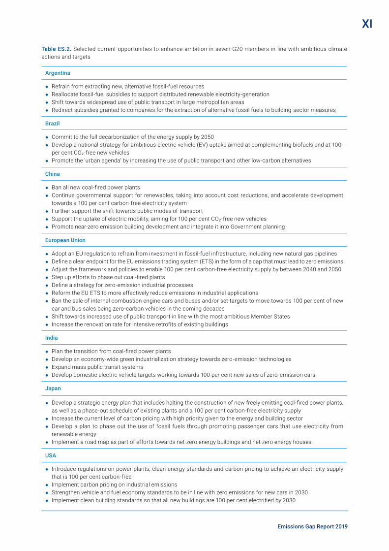
Emissions Gap Report 2019
XI
Argentina
● Refrain from extracting new, alternative fossil-fuel resources ● Reallocate fossil-fuel subsidies to support distributed renewable electricity-generation ● Shift towards widespread use of public transport in large metropolitan areas ● Redirect subsidies granted to companies for the extraction of alternative fossil fuels to building-sector measures
Brazil
● Commit to the full decarbonization of the energy supply by 2050 ● Develop a national strategy for ambitious electric vehicle (EV) uptake aimed at complementing biofuels and at 100-
per cent CO2-free new vehicles ● Promote the ‘urban agenda’ by increasing the use of public transport and other low-carbon alternatives
China
● Ban all new coal-fired power plants ● Continue governmental support for renewables, taking into account cost reductions, and accelerate development
towards a 100 per cent carbon-free electricity system ● Further support the shift towards public modes of transport ● Support the uptake of electric mobility, aiming for 100 per cent CO2-free new vehicles ● Promote near-zero emission building development and integrate it into Government planning
European Union
● Adopt an EU regulation to refrain from investment in fossil-fuel infrastructure, including new natural gas pipelines ● Define a clear endpoint for the EU emissions trading system (ETS) in the form of a cap that must lead to zero emissions ● Adjust the framework and policies to enable 100 per cent carbon-free electricity supply by between 2040 and 2050 ● Step up efforts to phase out coal-fired plants ● Define a strategy for zero-emission industrial processes ● Reform the EU ETS to more effectively reduce emissions in industrial applications ● Ban the sale of internal combustion engine cars and buses and/or set targets to move towards 100 per cent of new
car and bus sales being zero-carbon vehicles in the coming decades ● Shift towards increased use of public transport in line with the most ambitious Member States ● Increase the renovation rate for intensive retrofits of existing buildings
India
● Plan the transition from coal-fired power plants ● Develop an economy-wide green industrialization strategy towards zero-emission technologies ● Expand mass public transit systems ● Develop domestic electric vehicle targets working towards 100 per cent new sales of zero-emission cars
Japan
● Develop a strategic energy plan that includes halting the construction of new freely emitting coal-fired power plants, as well as a phase-out schedule of existing plants and a 100 per cent carbon-free electricity supply
● Increase the current level of carbon pricing with high priority given to the energy and building sector ● Develop a plan to phase out the use of fossil fuels through promoting passenger cars that use electricity from
renewable energy ● Implement a road map as part of efforts towards net-zero energy buildings and net-zero energy houses
USA
● Introduce regulations on power plants, clean energy standards and carbon pricing to achieve an electricity supply that is 100 per cent carbon-free
● Implement carbon pricing on industrial emissions ● Strengthen vehicle and fuel economy standards to be in line with zero emissions for new cars in 2030 ● Implement clean building standards so that all new buildings are 100 per cent electrified by 2030
Table ES.2. Selected current opportunities to enhance ambition in seven G20 members in line with ambitious climate actions and targets

Emissions Gap Report 2019
XII
policies and achieving the Paris Agreement can be designed to bring multiple co-benefits for humanity and planetary support systems. These range, for example, from reducing air pollution, improving human health, establishing sustainable energy systems and industrial production processes, making consumption and services more efficient and sufficient, employing less-intensive agricultural practices and mitigating biodiversity loss to liveable cities.
▶ This year’s report explores six entry points for progressing towards closing the emissions gap through transformational change in the following areas: (a) air pollution, air quality, health; (b) urbanization; (c) governance, education, employment; (d) digitalization; (e) energy- and material-efficient services for raising living standards; and (f) land use, food security, bioenergy. Building on this overview, a more detailed discussion of transitions in the energy sector is presented in chapter 6.
8. Renewables and energy efficiency, in combination with electrification of end uses, are key to a successful energy transition and to driving down energy-related CO2 emissions.
▶ The necessary transition of the global energy sector will require significant investments compared with a business-as-usual scenario. Climate policies that are consistent with the 1.5°C goal will require upscaling energy system supply-side investments to between US$1.6 trillion and US$3.8 trillion per year globally on average over the 2020–2050 time frame, depending on how rapid energy efficiency and conservation efforts can be ramped up.
▶ Given the important role that energy and especially the electricity sector will have to play in any low-carbon transformation, chapter 6 examines five transition options, taking into account their relevance for a wide range of countries, clear co-benefit opportunities and potential to deliver significant emissions reductions. Each of the following transitions correspond to a particular policy rationale or motivation, which is discussed in more detail in the chapter:
● Expanding Renewable Energy for electrification.
● Phasing out coal for rapid decarbonization of the energy system.
● Decarbonizing transport with a focus on electric mobility.
● Decarbonizing energy-intensive industry.
● Avoiding future emissions while improving energy access.
▶ Implementing such major transitions in a number of areas will require increased interdependency between energy and other infrastructure sectors, where changes in one sector can impact another. Similarly, there will be a strong need to connect demand and supply-side policies and include wider synergies and co-benefits, such as job losses and creation, rehabilitation of ecosystem ser vices, avoidance of reset tlements and reduced health and environmental costs as a result of reduced emissions. The same applies for decarbonizing transport, where there will be a need for complementarity and coordination of policies, driven by technological, environmental and land-use pressures. Policies will need to be harmonized wherever possible to take advantage of interdependencies and prevent undesirable outcomes such as CO2 leakage from one sector to another.
▶ Any transition at this scale is likely to be extremely challenging and will meet a number of economic, political and technical barriers and challenges. However, many drivers of climate action have changed in the last years, with several options for ambitious climate action becoming less costly, more numerous and better understood. First, technological and economic developments present oppor tunit ies to decarbonize the economy, especially the energy sector, at a cost that is lower than ever. Second, the synergies between climate action and economic growth and development objectives, including options for addressing distributional impacts, are better understood. Finally, policy momentum across various levels of government, as well as a surge in climate action commitments by non-state actors, are creating opportunities for countries to engage in real transitions.
▶ A key example of technological and economic trends is the cost of renewable energy, which is declining more rapidly than was predicted just a few years ago (see figure ES.5). Renewables are currently the cheapest source of new power generation in most of the world, with the global weighted average purchase or auction price for new utility-scale solar power photovoltaic systems and utility-scale onshore wind turbines projected to compete with the marginal operating cost of existing coal plants by 2020. These trends are increasingly manifesting in a decline in new coal plant construction, including the cancellation of planned plants, as well as the early retirement of existing plants. Moreover, real-life cost declines are outpacing projections.

Emissions Gap Report 2019
XIII
Option Major components Instruments Co-benefits Annual GHG emissions reduction potential of renewables, electrification, energy efficiency and other measures by 2050
Renewable energy electricity expansion
● Plan for large shares of variable renewable energy
● Electricity becomes the main energy source by 2050, supplying at least 50 per cent of total final energy consumption (TFEC)
● Share of renewable energy in electricity up to 85 per cent by 2050
● Transition
● Flexibility measures to take on larger shares of variable renewable energy
● Support for deployment of distributed energy
● Innovative measures: cost reflective tariff structures, targeted subsidies, reverse auctions, net metering
● Greater efficiency in end-use energy demand
● Health benefits ● Energy access and
security ● Employment
● Power sector: 8.1 GtCO2
● Building sector: 2.1 GtCO2
● District heat and others: 1.9 GtCO2
Coal phase-out
● Plan and implement phase-out of coal
● Coal to renewable energy transition
● Expand carbon capture usage and storage systems
● Improve system-wide efficiency
● Regional support programmes
● Tax breaks, subsidies
● Carbon pricing ● Moratorium policies ● De-risking of clean
energy investments ● Relocation of coal
workers (mines and power plants)
● Lower health hazards (air, water, land pollution)
● Future skills and job creation
Share of the power emissions reduction from a coal phase-out: 4 GtCO2 (range: 3.6– 4.4 GtCO2), with 1 GtCO2 from the OECD and 3 GtCO2 from the rest of the world
Decarbonize transport
● Reduce energy for transport
● Electrify transport ● Fuels substitution
(bioenergy, hydrogen) ● Modal shift
● Pathways for non-motorized transport
● Standards for vehicle emissions
● Establishing of charging stations
● Eliminating of fossil-fuel subsidies
● Investments in public transport
● Increased public health from more physical activity, less air pollution
● Energy security ● Reduced fuel
spending ● Less congestion
Electrification of transport: 6.1 GtCO2
Decarbonize industry
● Demand reduction (circular economy, modal shifts and logistics)
● Electrify heat processes
● Improve energy efficiency
● Direct use of biomass/biofuels
● Carbon pricing ● Standards and
regulations, especially on materials demand reduction
● Energy security ● Savings and
competitiveness
● Industry: 4.8 GtCO2
Avoid future emissions and energy access
● Link energy access with emission reductions for 3.5 billion energy-poor people
● Fit and auctions ● Standards and
regulations ● Targeted subsidies ● Support for
entrepreneurs
● Better access ● Meet basic needs
and SDGs
● N/A
Table ES.3. Summary of five energy transition options
A short summary of the main aspects of each transition is presented in table ES.3.

Emissions Gap Report 2019
XIV 73
Emissions G
ap Report 2019
Chapter 4 – Trends And Bridging the gap: Strengthening NDCs and domestic policies
Figure 6.1 — Here we're missing the headline and description of the figureFigure ES.5. Changes in global levelized cost of energy for key renewable energy technologies, 2010-2018
9. Demand-side material efficiency offers substantial GHG mitigation opportunities that are complementary to those obtained through an energy system transformation.
▶ While demand-side material efficiency widens the spectrum of emission mitigation strategies, it has largely been overlooked in climate policymaking until now and will be important for the cross-sectoral transitions.
▶ In 2015, the production of materials caused GHG emissions of approximately 11.5 GtCO2e, up from 5 GtCO2e in 1995. The largest contribution stems from bulk materials production, such as iron and steel, cement, lime and plaster, other minerals mostly used as construction products, as well as plastics and rubber. Two thirds of the materials are used to make capital goods, with buildings and vehicles among the most important. While the production of materials consumed in industrialized countries remained within the range of 2–3 GtCO2e, in the 1995–2015 period, those of developing and emerging economies have largely been behind the growth. In this context, it is important to keep in mind the discussion about the point of production and points of consumption (see figure ES.6).
▶ Material efficiency and substitution strategies affect not only energy demand and emissions during material production, but also potentially the operational energy
use of the material products. Analysis of such strategies therefore requires a systems or life cycle perspective. Several investigations of material efficiency have focused on strategies that have little impact on operations, meaning that trade-offs and synergies have been ignored. Many energy efficiency strategies have implications for the materials used, such as increased insulation demand for buildings or a shift to more energy-intensive materials in the lightweighting of vehicles. While these additional, material-related emissions are well understood from technology studies, they are often not fully captured in the integrated assessment models that produce scenario results, such as those discussed in this report.
▶ In chapter 7, the mitigation potential from demand-side material efficiency improvements is discussed in the context of the following categories of action:
● Product lightweighting and substitution of high-carbon materials with low-carbon materials to reduce material-related GHG emissions associated with product production, as well as operational energy consumption of vehicles.
● Improvements in the yield of material production and product manufacture.
● More intensive use, longer life, component reuse, remanufacturing and repair as strategies to obtain more service from material-based products.

Emissions Gap Report 2019
XV83
Emissions G
ap Report 2019
Chapter 4 – Trends And Bridging the gap: Strengthening NDCs and domestic policies
Figure 7.1 — Here we're missing the headline and description of the figure
0
5
10
GtC
O�e
11.5GtCO�e
11.5 GtCO�e
Construction5.0
Machinery2.0
Metal products0.9
Transportequipment
0.9
Electronics0.3
Other products1.0
Services0.6
Final use0.81.4 Plastic and rubber
0.9 Wood products
1.1 Other minerals
0.4 Glass
2.9 Cement
0.5 Other metals
0.6 Aluminium
3.7 Iron and steel
Figure ES.6. GHG emissions in GtCO2e associated with materials production by material (left) and by the first use of materials in subsequent production processes or final consumption (right)
● Enhanced recycling so that secondary materials reduce the need to produce more emission-intensive primary materials.
▶ These categories are elaborated for housing and cars, showing that increased material efficiency can reduce annual emissions from the construction and operations of buildings and the manufacturing and use of passenger vehicles, thus contributing a couple of gigatons of carbon dioxide equivalent in emission reductions to the global mitigation effort by 2030.

Emissions Gap Report 2019
16
United Nations Avenue, GigiriP O Box 30552, 00100 Nairobi, KenyaTel +254 20 76 1234 | [email protected]

Article Navigation
Issue Section: Viewpoint
World Scientists’ Warning of a Climate Emergency �William J Ripple 4 4 , Christopher Wolf 4 4 , Thomas M Newsome, Phoebe Barnard,William R Moomaw Author Notes
BioScience, biz088, https://doi.org/10.1093/biosci/biz088Published: 05 November 2019
A correction has been published: BioScience, biz152, https://doi.org/10.1093/biosci/biz152
Issue Section: Viewpoint
PDF Split View Cite Permissions Share -
< 5 9
EXHIBIT E-7

Scientists have a moral obligation to clearly warn humanity of any catastrophic threat and to
“tell it like it is.” On the basis of this obligation and the graphical indicators presented below,
we declare, with more than 11,000 scientist signatories from around the world, clearly and
unequivocally that planet Earth is facing a climate emergency.
Exactly 40 years ago, scientists from 50 nations met at the First World Climate Conference (in
Geneva 1979) and agreed that alarming trends for climate change made it urgently necessary
to act. Since then, similar alarms have been made through the 1992 Rio Summit, the 1997
Kyoto Protocol, and the 2015 Paris Agreement, as well as scores of other global assemblies and
scientists’ explicit warnings of insufficient progress (Ripple et al. 2017). Yet greenhouse gas
(GHG) emissions are still rapidly rising, with increasingly damaging effects on the Earth's
climate. An immense increase of scale in endeavors to conserve our biosphere is needed to
avoid untold suffering due to the climate crisis (IPCC 2018).
Most public discussions on climate change are based on global surface temperature only, an
inadequate measure to capture the breadth of human activities and the real dangers stemming
from a warming planet (Briggs et al. 2015). Policymakers and the public now urgently need
access to a set of indicators that convey the effects of human activities on GHG emissions and
the consequent impacts on climate, our environment, and society. Building on prior work (see
supplemental file S2), we present a suite of graphical vital signs of climate change over the last
40 years for human activities that can affect GHG emissions and change the climate (figure 1),
as well as actual climatic impacts (figure 2). We use only relevant data sets that are clear,
understandable, systematically collected for at least the last 5 years, and updated at least
annually.
Figure 1.
Open in new tab Download slide
Change in global human activities from 1979 to the present. These indicators are linked at least in part toclimate change. In panel (f), annual tree cover loss may be for any reason (e.g., wildfire, harvest within treeplantations, or conversion of forests to agricultural land). Forest gain is not involved in the calculation of treecover loss. In panel (h), hydroelectricity and nuclear energy are shown in figure S2. The rates shown in panels arethe percentage changes per decade across the entire range of the time series. The annual data are shown usinggray points. The black lines are local regression smooth trend lines. Abbreviation: Gt oe per year, gigatonnes ofoil equivalent per year. Sources and additional details about each variable are provided in supplemental file S2,including table S2.
Figure 2.

The climate crisis is closely linked to excessive consumption of the wealthy lifestyle. The most
affluent countries are mainly responsible for the historical GHG emissions and generally have
the greatest per capita emissions (table S1). In the present article, we show general patterns,
mostly at the global scale, because there are many climate efforts that involve individual
regions and countries. Our vital signs are designed to be useful to the public, policymakers, the
business community, and those working to implement the Paris climate agreement, the
Open in new tab Download slide
Climatic response time series from 1979 to the present. The rates shown in the panels are the decadal changerates for the entire ranges of the time series. These rates are in percentage terms, except for the intervalvariables (d, f, g, h, i, k), where additive changes are reported instead. For ocean acidity (pH), the percentage rateis based on the change in hydrogen ion activity, aH+ (where lower pH values represent greater acidity). The
annual data are shown using gray points. The black lines are local regression smooth trend lines. Sources andadditional details about each variable are provided in supplemental file S2, including table S3.

United Nations’ Sustainable Development Goals, and the Aichi Biodiversity Targets.
Profoundly troubling signs from human activities include sustained increases in both human
and ruminant livestock populations, per capita meat production, world gross domestic
product, global tree cover loss, fossil fuel consumption, the number of air passengers carried,
carbon dioxide (CO2) emissions, and per capita CO2 emissions since 2000 (figure 1, supple-
mental file S2). Encouraging signs include decreases in global fertility (birth) rates (figure 1b),
decelerated forest loss in the Brazilian Amazon (figure 1g), increases in the consumption of
solar and wind power (figure 1h), institutional fossil fuel divestment of more than US$7
trillion (figure 1j), and the proportion of GHG emissions covered by carbon pricing (figure 1m).
However, the decline in human fertility rates has substantially slowed during the last 20 years
(figure 1b), and the pace of forest loss in Brazil's Amazon has now started to increase again
(figure 1g). Consumption of solar and wind energy has increased 373% per decade, but in 2018,
it was still 28 times smaller than fossil fuel consumption (combined gas, coal, oil; figure 1h).
As of 2018, approximately 14.0% of global GHG emissions were covered by carbon pricing
(figure 1m), but the global emissions-weighted average price per tonne of carbon dioxide was
only around US$15.25 (figure 1n). A much higher carbon fee price is needed (IPCC 2018, section
2.5.2.1). Annual fossil fuel subsidies to energy companies have been fluctuating, and because of
a recent spike, they were greater than US$400 billion in 2018 (figure 1o).
Especially disturbing are concurrent trends in the vital signs of climatic impacts (figure 2,
supplemental file S2). Three abundant atmospheric GHGs (CO2, methane, and nitrous oxide)
continue to increase (see figure S1 for ominous 2019 spike in CO2), as does global surface
temperature (figure 2a–2d). Globally, ice has been rapidly disappearing, evidenced by
declining trends in minimum summer Arctic sea ice, Greenland and Antarctic ice sheets, and
glacier thickness worldwide (figure 2e–2h). Ocean heat content, ocean acidity, sea level, area
burned in the United States, and extreme weather and associated damage costs have all been
trending upward (figure 2i–2n). Climate change is predicted to greatly affect marine,
freshwater, and terrestrial life, from plankton and corals to fishes and forests (IPCC 2018,
2019). These issues highlight the urgent need for action.
Despite 40 years of global climate negotiations, with few exceptions, we have generally
conducted business as usual and have largely failed to address this predicament (figure 1). The
climate crisis has arrived and is accelerating faster than most scientists expected (figure 2,
IPCC 2018). It is more severe than anticipated, threatening natural ecosystems and the fate of
humanity (IPCC 2019). Especially worrisome are potential irreversible climate tipping points
and nature's reinforcing feedbacks (atmospheric, marine, and terrestrial) that could lead to a

catastrophic “hothouse Earth,” well beyond the control of humans (Steffen et al. 2018). These
climate chain reactions could cause significant disruptions to ecosystems, society, and
economies, potentially making large areas of Earth uninhabitable.
To secure a sustainable future, we must change how we live, in ways that improve the vital
signs summarized by our graphs. Economic and population growth are among the most
important drivers of increases in CO2 emissions from fossil fuel combustion (Pachauri et al.
2014, Bongaarts and O’Neill 2018); therefore, we need bold and drastic transformations
regarding economic and population policies. We suggest six critical and interrelated steps (in
no particular order) that governments, businesses, and the rest of humanity can take to lessen
the worst effects of climate change. These are important steps but are not the only actions
needed or possible (Pachauri et al. 2014, IPCC 2018, 2019).
Energy
The world must quickly implement massive energy efficiency and conservation practices and
must replace fossil fuels with low-carbon renewables (figure 1h) and other cleaner sources of
energy if safe for people and the environment (figure S2). We should leave remaining stocks of
fossil fuels in the ground (see the timelines in IPCC 2018) and should carefully pursue effective
negative emissions using technology such as carbon extraction from the source and capture
from the air and especially by enhancing natural systems (see “Nature” section). Wealthier
countries need to support poorer nations in transitioning away from fossil fuels. We must
swiftly eliminate subsidies for fossil fuels (figure 1o) and use effective and fair policies for
steadily escalating carbon prices to restrain their use.
Short-lived pollutants
We need to promptly reduce the emissions of short-lived climate pollutants, including
methane (figure 2b), black carbon (soot), and hydrofluorocarbons (HFCs). Doing this could
slow climate feedback loops and potentially reduce the short-term warming trend by more
than 50% over the next few decades while saving millions of lives and increasing crop yields
due to reduced air pollution (Shindell et al. 2017). The 2016 Kigali amendment to phase down
HFCs is welcomed.

Nature
We must protect and restore Earth's ecosystems. Phytoplankton, coral reefs, forests,
savannas, grasslands, wetlands, peatlands, soils, mangroves, and sea grasses contribute
greatly to sequestration of atmospheric CO2. Marine and terrestrial plants, animals, and
microorganisms play significant roles in carbon and nutrient cycling and storage. We need to
quickly curtail habitat and biodiversity loss (figure 1f–1g), protecting the remaining primary
and intact forests, especially those with high carbon stores and other forests with the capacity
to rapidly sequester carbon (proforestation), while increasing reforestation and afforestation
where appropriate at enormous scales. Although available land may be limiting in places, up to
a third of emissions reductions needed by 2030 for the Paris agreement (less than 2°C) could
be obtained with these natural climate solutions (Griscom et al. 2017).
Food
Eating mostly plant-based foods while reducing the global consumption of animal products
(figure 1c–d), especially ruminant livestock (Ripple et al. 2014), can improve human health
and significantly lower GHG emissions (including methane in the “Short-lived pollutants”
step). Moreover, this will free up croplands for growing much-needed human plant food
instead of livestock feed, while releasing some grazing land to support natural climate
solutions (see “Nature” section). Cropping practices such as minimum tillage that increase
soil carbon are vitally important. We need to drastically reduce the enormous amount of food
waste around the world.
Economy
Excessive extraction of materials and overexploitation of ecosystems, driven by economic
growth, must be quickly curtailed to maintain long-term sustainability of the biosphere. We
need a carbon-free economy that explicitly addresses human dependence on the biosphere
and policies that guide economic decisions accordingly. Our goals need to shift from GDP
growth and the pursuit of affluence toward sustaining ecosystems and improving human
well-being by prioritizing basic needs and reducing inequality.

Population
Still increasing by roughly 80 million people per year, or more than 200,000 per day (figure
1a–b), the world population must be stabilized—and, ideally, gradually reduced—within a
framework that ensures social integrity. There are proven and effective policies that
strengthen human rights while lowering fertility rates and lessening the impacts of population
growth on GHG emissions and biodiversity loss. These policies make family-planning services
available to all people, remove barriers to their access and achieve full gender equity, including
primary and secondary education as a global norm for all, especially girls and young women
(Bongaarts and O’Neill 2018).
Conclusions
Mitigating and adapting to climate change while honoring the diversity of humans entails
major transformations in the ways our global society functions and interacts with natural
ecosystems. We are encouraged by a recent surge of concern. Governmental bodies are making
climate emergency declarations. Schoolchildren are striking. Ecocide lawsuits are proceeding
in the courts. Grassroots citizen movements are demanding change, and many countries,
states and provinces, cities, and businesses are responding.
As the Alliance of World Scientists, we stand ready to assist decision-makers in a just
transition to a sustainable and equitable future. We urge widespread use of vital signs, which
will better allow policymakers, the private sector, and the public to understand the magnitude
of this crisis, track progress, and realign priorities for alleviating climate change. The good
news is that such transformative change, with social and economic justice for all, promises far
greater human well-being than does business as usual. We believe that the prospects will be
greatest if decision-makers and all of humanity promptly respond to this warning and
declaration of a climate emergency and act to sustain life on planet Earth, our only home.
Contributing reviewers
Franz Baumann, Ferdinando Boero, Doug Boucher, Stephen Briggs, Peter Carter, Rick
Cavicchioli, Milton Cole, Eileen Crist, Dominick A. DellaSala, Paul Ehrlich, Iñaki Garcia-De-
Cortazar, Daniel Gilfillan, Alison Green, Tom Green, Jillian Gregg, Paul Grogan, John
Guillebaud, John Harte, Nick Houtman, Charles Kennel, Christopher Martius, Frederico
Mestre, Jennie Miller, David Pengelley, Chris Rapley, Klaus Rohde, Phil Sollins, Sabrina Speich,
David Victor, Henrik Wahren, and Roger Worthington.
Funding
The Worthy Garden Club furnished partial funding for this project.
Project website
To view the Alliance of World Scientists website or to sign this article, go to https://scien-
tistswarning.forestry.oregonstate.edu.
Supplemental material
A list of the signatories appears in supplemental file S1.
Author Biographical
William J. Ripple ([email protected]) and Christopher Wolf (christopher.wolf@ore-
gonstate.edu) are affiliated with the Department of Forest Ecosystems and Society at Oregon
State University, in Corvallis and contributed equally to the work. Thomas M. Newsome is
affiliated with the School of Life and Environmental Sciences at The University of Sydney, in
Sydney, New South Wales, Australia. Phoebe Barnard is affiliated with the Conservation
Biology Institute, in Corvallis, Oregon, and with the African Climate and Development
Initiative, at the University of Cape Town, in Cape Town, South Africa. William R. Moomaw is
affiliated with The Fletcher School and the Global Development and Environment Institute, at
Tufts University, in Medford, Massachusetts
11,258 scientist signatories from 153 countries (list in supplemental file S1)
References cited
Briggs S, Kennel CF, Victor DG. 2015. Planetary vital signs. Nature Climate Change 5: 969.
Google Scholar Crossref
Bongaarts J, O’Neill BC 2018. Global warming policy: Is population left out in the cold? Science 361:650–652.
Google Scholar Crossref PubMed
Griscom BW et al. . 2017. Natural climate solutions. Proceedings of the National Academy of Sciences 114: 11645–11650.
Google Scholar Crossref
[IPCC] Intergovernmental Panel on Climate Change. 2018. Global Warming of 1.5°C: An IPCC SpecialReport . IPCC.
[IPCC] Intergovernmental Panel on Climate Change. 2019. Climate Change and Land . IPCC.
Pachauri RK et al. . 2014. Climate Change 2014: Synthesis Report. Intergovernmental Panel onClimate Change.
Ripple WJ, Smith P, Haberl H, Montzka SA, McAlpine C, Boucher DH. 2014. Ruminants, climate change,and climate policy. Nature Climate Change 4: 2–5.
Google Scholar Crossref
Ripple WJ, Wolf C, Newsome TM, Galetti M, Alamgir M, Crist E, Mahmoud MI, Laurance WF. 2017. Worldscientists’ warning to humanity: A second notice. BioScience 67: 1026–1028.
Google Scholar Crossref
Shindell D, Borgford-Parnell N, Brauer M, Haines A, Kuylenstierna J, Leonard S, Ramanathan V,Ravishankara A, Amann M, Srivastava L. 2017. A climate policy pathway for near- and long-termbenefits. Science 356: 493–494.
Google Scholar Crossref PubMed

View Metrics
Steffen W et al. . 2018. Trajectories of the Earth System in the Anthropocene. Proceedings of theNational Academy of Sciences 115: 8252–8259.
Google Scholar Crossref
Author notes
William J. Ripple and Christopher Wolf contributed equally to the work.
© The Author(s) 2019. Published by Oxford University Press on behalf of the American Institute of BiologicalSciences.
This article is published and distributed under the terms of the Oxford University Press, Standard JournalsPublication Model (https://academic.oup.com/journals/pages/open_access/funder_policies/chorus/standard-_publication_model)
Supplementary data
biz088_Supplemental_file_S1 - pdf filebiz088_Supplemental_file_S2 - pdf file

Email alerts
Article activity alert
Advance article alerts
New issue alert
Receive exclusive offers and updates
from Oxford Academic
Related articles in
Google Scholar
Citing articles via
Google Scholar
Crossref
Latest Most Read Most Cited

Chronicling Biology: Building an Oral History
The Community Ecology of HerbivoreRegulation in an Agroecosystem: Lessons fromComplex Systems
In Their Own Words: Rita Colwell
Planning for Change: Conservation-RelatedImpacts of Climate Overshoot
Into the Den: Investigating Hibernation
About BioScience
Editorial Board
Author Guidelines
Purchase
Recommend to your Library
Advertising and Corporate Services
Journals Career Network
Online ISSN 1525-3244
Print ISSN 0006-3568
Copyright © 2019 American Institute of Biological Sciences
https://academic.oup.com/bioscience/advance-article/doi/10.1093/biosci/biz141/5670753?searchresult=1

About Us
Contact Us
Careers
Help
Access & Purchase
Rights & Permissions
Open Access
Connect
Join Our Mailing List
OUPblog
YouTube
Tumblr
Resources
Authors
Librarians
Societies
Sponsors & Advertisers
Press & Media
Agents
Explore
Shop OUP Academic
Oxford Dictionaries
Oxford Index
Epigeum
OUP Worldwide
University of Oxford
Oxford University Press is a department of the University of
Oxford. It furthers the University's objective of excellence in
research, scholarship, and education by publishing worldwide
Copyright © 2019 Oxford University Press Cookie Policy Privacy Policy Legal Notice
Site Map Accessibility Get Adobe Reader

Maine Department of Environmental ProtectionHome → Spills & Site Cleanup → Mercury contamination in and along the Penobscot River
Mercury contamination in and along the PenobscotRiver
Map of entiresite(documents/site_map_for_webpage_8_8_2016.pdf)(pdf)
Mallinckrodt (Former Holtrachem Site)The Mallinckrodt facility, formerly known as the HoltraChem Manufacturing Company, sits on 235 acres onthe banks of the Penobscot River in Orrington, Maine. The plant operated under several owners from 1967through 2000. The facility manufactured chlorine, sodium hydroxide (caustic soda), sodium hypochlorite(chlorine bleach), hydrochloric acid and chloropicrin (a pesticide).
(images/2017-8-31.png)click to enlarge
DEP is currently overseeing cleanup activity at the site to ensure that the requirements of the 2010 BEP Orderare met. It is anticipated that the cleanup activities will be complete some time in 2019. For more up to dateand detailed information about the site cleanup and expected timelines, visit www.beyondholtrachem.com(http://www.beyondholtrachem.com)
For more information on the history or current status of this site, please contact Chris Swain
EXHIBIT F-7

(mailto:[email protected]) (207) 485-3852
Mallinckrodt data in Google Earth (../../gis/datamaps/brwm_holtrachem/brwm_holtrachem.kmz)
The Penobscot RiverIn 2000 the Natural Resources Defense Council (NRDC) and the Maine People’s Alliance (MPA) filed suitagainst Holtrachem and Mallinckrodt (Mallinckrodt) in Federal district court alleging that under RCRA42U.S.C. § 6972(a)(1)(B) Mallinckrodt caused an "imminent and substantial endangerment to health and theenvironment" as a result of discharging mercury into the Penobscot River. A 2002 judicial opinion and order(http://www.maine.gov/dep/spills/holtrachem/penobriver/orders/GC_07292002_1-00cv069_MePeople_v_Holtrache.pdf) were issued against Mallinckrodt.Subsequent court orders required the following activities to take place:
Phase I & II Mercury StudyPhase III Engineering Study
More detailed information including all court orders, the Phase I and II Mercury Study, and progress on thePhase III Engineering Study are all available at http://www.penobscotmercurystudy.com/(http://www.penobscotmercurystudy.com/) Please note: The State of Maine is not a party to this lawsuit or its subsequent court ordered studies. Thislawsuit is also separate from the 2010 BEP order currently undergoing implementation (see above).
For further information please contact Susanne Miller (mailto:[email protected]) , (207) 941-4190
Credits
Copyright © 2019All rights reserved.
Popular Pages
What Do My Recyclables BecomeTankSmartBeverage Container RedemptionStaff DirectoryNRPAGIS Maps and Data FilesStormwater BMPs

Connect with Us
Email UsTwitterReceive UpdatesRSS FeedsMeeting CalendarComment OpportunitiesOffice LocationsStaff Directory
Other Links
Board of Environmental ProtectionJobs @ DEPNatural Resources Service CenterNotice of NondiscriminationRequest for ProposalsSite PoliciesSubject Index A-ZTraining OpportunitiesDEP Intranet
Contact Information
17 State House Station28 Tyson DriveAugusta, Maine 04333-0017Tel: 207-287-7688Fax: 207-287-7826

NaturalResourcesCouncil of
Maine
Maine’s Dioxin Problem
What is Dioxin?The term “dioxin” describes a group of highly toxic chemicals that are produced by several industrial processesthat use or burn products containing chlorine, including incinerators and “kraft” paper mills. Dioxins are among themost potent toxic chemicals known.
What are the effects of dioxins on human health?
There is compelling scientiBc evidence that dioxins can cause cancer and disrupt hormonal, reproductive, andimmune systems in people. The developing fetus and breastfeeding infants are particularly sensitive to theharmful effects of dioxins. Studies suggest that dioxins are also an “endocrine disrupter” – one of a number oftoxic chemicals that interfere with our hormone systems by mimicking natural hormones and blocking or
EXHIBIT G-7

disrupting their normal action.
Human Health Hazards Linked to Dioxins
Cancer
Birth and Developmental Defects
Learning Disabilities
Increased Risk of Diabetes
Tumor Promotion
Decreased Fertility
Reduced Sperm Counts
Endometriosis
Suppressed Immune Systems
The U.S. Environmental Protection Agency has found increasing evidence that levels of dioxins in our bodies are ator near the levels at which many, if not all, of these effects may occur. Therefore, the levels at which many, if notall, of these effects may occur. Therefore, any additional dioxins in the environment are a signiBcant concern andmust be eliminated wherever possible.
Are certain people at greater risk?While dioxins are a general public health hazard, they pose even greater dangers to certain groups:
Developing fetuses and infants
Developing fetuses and nursing infants have a higher risk because dioxins are passed to them in utero andthrough their mother’s breast milk at the most sensitive stages of their development. Dioxins accumulateto greater amounts in fatty substances, such as breast milk, than in vegetables and fruits.
Fish consumers
Certain populations that consume large amounts of Bsh, such as recreational and avid anglers,subsistence Bsh consumers and Native Americans are at an increased risk due to their larger consumptionof Bsh contaminated with dioxins.

of Bsh contaminated with dioxins.
Are dioxins a hazard for wildlife?Yes. Animals on the top of the food chain, such as birds and mammals that eat contaminated Bsh, face thegreatest risks. Last summer, the U.S. Fish and Wildlife Service (USF&W) linked dioxin discharges from the bleachkraft mill in Lincoln with the reproductive failure among Penobscot River bald eagles. Reproduction among eaglesnesting within roughly two miles of the Lincoln mill has been as low as 40% below the statewide average. USF&Walso examined total dioxin contamination of bald eagle blood and eggs, and found levels in unhatched eggs nearthe Penobscot River exceeded “safe” levels by up to 85 times.
How does dioxin get into people and wildlife?Dioxin get into the bodies of people and wildlife primarily through food.
AirDioxins generated by burning of certain plastics and other chlorine-containing materials from incinerators andother sources travel through the air and can fall out on our farmland and food crops. Cows and other animals eatthe grasses and plants on which the dioxins have fallen, which contaminates their milk and meat.
WaterDioxins enter the water food chain – aquatic insects, Bsh, andshellBsh – indirectly from “fall-out” from air and directly from thewastewater discharge pollution from certain industries. In Maine, thedischarge of dioxins by “bleach kraft” paper mills contaminates Bshin papermaking rivers and the tomalley of lobsters in the bays ofthese rivers to levels that make them unsafe to eat.
Although there are a number of sources of dioxins in our environment, bleach kraft paper mills are the mostsigniBcant source of dioxin contamination in Maine’s waters. Therefore, elimination of dioxin discharges fromthese mills is not only a priority but also essential to allow people to enjoy the full economic, recreational, and
environmental beneBts of our largest waterbodies.
What is the extent of Maine’s paper mill dioxin problem?In 1985, more than 30 years ago, dioxins were Brst found in Bsh below Maine’s seven “bleach kraft” paper mills

In 1985, more than 30 years ago, dioxins were Brst found in Bsh below Maine’s seven “bleach kraft” paper millsthat use chlorine compounds to bleach their paper. These seven mills discharge more than 100 million gallons ofwastewater a day to the Penobscot, Kennebec, Androscoggin, Presumpscot and St. Croix Rivers. Although thelevels of dioxins in mill wastewaters are sometimes undetectable by conventional methods, they are nonethelessenough to contaminate the Bsh and shellBsh because Bsh act like sponges for dioxins, accumulating them at25,000-50,000 times the concentrations present in their environment.
Today, women of childbearing age are still warned strictly limit their intake of Bsh caught from 250 miles ofMaine’s rivers below paper mills and NO tomalley from lobsters caught along the entire coast. And the generalpublic is advised to severely restrict their consumption of dioxin-contaminated Bsh and tomalley.
Can Maine’s paper mill dioxin problem be solved?Yes! Papermaking technologies are available and in use today in the United States and worldwide that wouldeliminate dioxin discharges by using non-chlorine bleaching processes. These processes pave the way to “closedloop” mills that will not discharge any bleaching wastewaters, thereby drastically reducing the discharge of othertoxics, turbidity, color, odor, foam, and oxygen-depleting materials. Totally chlorine-free (TCF) papermakingprocess produces products that are of a brightness and quality comparable to products bleached with chlorine.
Didn’t Maine paper mills already commit to eliminate their dioxin discharges?On April 8, 1996, Governor Angus King announced that the state’s seven bleach kraft pulp and paper mills hadsigned on to the goal of eliminating the discharge of dioxins. Since then, the paper industry has consistentlyargued that their pledge to “eliminate” dioxins does not mean that their contribution of dioxins to Maine’s waterswill be zero.
Will conversion to 100% chlorine dioxide (ECF) technologies eliminate the dioxin problem?No. Maine mills are claiming that a switch from elemental chlorine to chlorine dioxide will “solve” the dioxinproblem. However, the chemistry of the ECF process clearly shows that the main bleaching agent, chlorine dioxide,is still capable of producing dioxins. Research by both the pulp industry and the EPA demonstrates that chlorinedioxide bleaching does not ensure total elimination of dioxins. Totally chlorine free bleaching processes will dothe job.

(https://www.facebook.com/NRCMenvironment)
(http://www.instagram.com/nrcmenvironment)
(https://www.linkedin.com/company/120019)
(https://www.nrcm.org/contact/rss-
feeds/)
(https://twitter.com/NRCMenvironment)
(https://www.youtube.com/nrcmenvironment)
Natural Resources Council of Maine
3 Wade Street, Augusta, Maine 04330(https://www.nrcm.org/about-nrcm/contact/)Phone: (207) 622-3101 Toll Free: (800) 287-2345Fax: (207) 622-4343
Privacy Policy (https://www.nrcm.org/about-nrcm/privacy-policy/)
NRCM Careers & Internships (https://www.nrcm.org/about-nrcm/employment-opportunities/)
Stay Informed
Sign up for our monthly enews(https://www.nrcm.org/take-action#signup)
Our Organization

© 2019 Copyright · Natural Resources Council of Maine (https://www.nrcm.org) · All Rights Reserved · Website Design by Seaside Web Design, LLC(http://www.seasidewebdesignme.com) ·
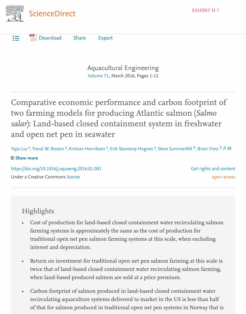
Get rights and content
open access
•
•
•
Aquacultural EngineeringVolume 71, March 2016, Pages 1-12
Comparative economic performance and carbon footprint oftwo farming models for producing Atlantic salmon (Salmosalar): Land-based closed containment system in freshwaterand open net pen in seawaterYajie Liu , Trond W. Rosten , Kristian Henriksen , Erik Skontorp Hognes , Steve Summerfelt , Brian Vinci
Show more
https://doi.org/10.1016/j.aquaeng.2016.01.001
Under a Creative Commons license
HighlightsCost of production for land-based closed containment water recirculating salmonfarming systems is approximately the same as the cost of production fortraditional open net pen salmon farming systems at this scale, when excludinginterest and depreciation.
Return on investment for traditional open net pen salmon farming at this scale istwice that of land-based closed containment water recirculating salmon farming,when land-based produced salmon are sold at a price premium.
Carbon footprint of salmon produced in land-based closed containment waterrecirculating aquaculture systems delivered to market in the US is less than halfof that for salmon produced in traditional open net pen systems in Norway that is
a a a a b b
Download Share Export
EXHIBIT H-7

delivered to the US by air freight.
AbstractOcean net pen production of Atlantic salmon is approaching 2 million metric tons (MT)annually and has proven to be cost- and energy-efficient. Recently, with technologyimprovements, freshwater aquaculture of Atlantic salmon from eggs to harvestable size of 4–5 kg in land-based closed containment (LBCC) water recirculating aquaculture systems (RAS)has been demonstrated as a viable production technology. Land-based, closed containmentwater recirculating aquaculture systems technology offers the ability to fully control therearing environment and provides flexibility in locating a production facility close to themarket and on sites where cost of land and power are competitive. This flexibility offersdistinct advantages over Atlantic salmon produced in open net pen systems, which isdependent on access to suitable coastal waters and a relatively long transport distance tosupply the US market. Consequently, in this paper we present an analysis of the investmentneeded, the production cost, the profitability and the carbon footprint of producing 3300 MTof head-on gutted (HOG) Atlantic salmon from eggs to US market (wholesale) using twodifferent production systems—LBCC-RAS technology and open net pen (ONP) technologyusing enterprise budget analysis and carbon footprint with the LCA method. In our analysiswe compare the traditional open net pen production system in Norway and a modelfreshwater LBCC-RAS facility in the US. The model ONP is small compared to the most ONPsystems in Norway, but the LBCC-RAS is large compared to any existing LBCC-RAS forAtlantic salmon. The results need to be interpreted with this in mind. Results of the financialanalysis indicate that the total production costs for two systems are relatively similar, withLBCC-RAS only 10% higher than the ONP system on a head-on gutted basis (5.60 US$/kgversus 5.08 US$/kg, respectively). Without interest and depreciation, the two productionsystems have an almost equal operating cost (4.30 US$/kg for ONP versus 4.37 US$/kg forLBCC-RAS). Capital costs of the two systems are not similar for the same 3300 MT of head-ongutted salmon. The capital cost of the LBCC-RAS model system is approximately 54,000,000US$ and the capital cost of the ONP system is approximately 30,000,000 US$, a difference of80%. However, the LBCC-RAS model system selling salmon at a 30% price premium iscomparatively as profitable as the ONP model system (profit margin of 18% versus 24%,respectively), even though its 15-year net present value is negative and its return on investmentis lower than ONP system (9% versus 18%, respectively). The results of the carbon footprintanalysis confirmed that production of feed is the dominating climate aspect for bothproduction methods, but also showed that energy source and transport methods are

Previous Next
important. It was shown that fresh salmon produced in LBCC-RAS systems close to a USmarket that use an average US electricity mix have a much lower carbon footprint than freshsalmon produced in Norway in ONP systems shipped to the same market by airfreight, 7.41versus 15.22 kg CO eq/kg salmon HOG, respectively. When comparing the carbon footprint ofproduction-only, the LBCC-RAS-produced salmon has a carbon footprint that is double that ofthe ONP-produced salmon, 7.01 versus 3.39 kg CO eq/kg salmon live-weight, respectively.
Abbreviations
CO , carbon dioxide; CO eq, carbon dioxide equivalents; EBIT, earnings beforeinterest and taxes; FCR, feed conversion ratio; HOG, head-on gutted; IRR, internalrate of return; LBCC, land-based closed containment; LCA, life cycle assessment; NPV,
net present value; ONP, open net pen; RAS, water recirculating aquaculture system;
ROR, required rate of return; S0, 1/2-year old smolt; S1, 1-year old smolt; TGC,
thermal growth coefficent; tkm, ton × kilometers; WFE, whole fish equivalent
Keywords
Salmon; Economics; Carbon footprint; Recirculating aquaculture systems; Net penaquaculture
1. IntroductionFarmed Atlantic salmon (Salmo salar) is sold globally in various forms and markets. The US isan important market for farmed Atlantic salmon, estimated to be more than 350,000 MT in2014 (Marine Harvest ASA, 2014), and has shown steady growth since the late 1980s (USDAERS, 2015). In 2014 the US market was primarily supplied by salmon produced in Chile(126,820 MT), Canada (47,454 MT) and Norway (26,208 MT) (USDA ERS, 2015). The USproduction of Atlantic salmon (18,000 MT [2012]) is relatively small in comparison to theamount consumed in the US (NOAA, 2013). Limited access to suitable coastal water areas andrigorous regulations in the US (NOAA, 2013) curtail the opportunity to produce Atlanticsalmon in open net pen systems, the industry’s preferred and established technology for the
2
2
2 2

on-growing phase of salmon farming in Norway, Canada, and Chile. An alternative technologyto open net pen systems for salmon production is land-based, closed containment (LBCC)water recirculating aquaculture systems (RAS) technology (LBCC-RAS). LBCC-RAS technologyhad been used for production of a limited number of species, like eel, beginning in the 1980s(Heinsbroek and Kamstra, 1990). Developments in LBCC-RAS technology since the 1980s haveled to the ability to culture a wide variety of fish species including cold-water salmonids (e.g.,Arctic char, rainbow trout, and Atlantic salmon to smolt size) (Summerfelt et al., 2004,Bergheim et al., 2009, Dalsgaard et al., 2013, Kolarevic et al., 2014). Most recently, freshwateraquaculture of Atlantic salmon from eggs to harvestable size of 4–5 kg in a LBCC-RAS facilityhas been demonstrated as a viable production technology (Summerfelt et al., 2013). Land-based, closed containment water recirculating aquaculture systems technology offers theability to fully control the rearing environment, exclude parasites and obligate pathogens, andprovide flexibility in locating a production facility close to the market and on sites where thecost of land and power are competitive. This control and flexibility offers advantages overAtlantic salmon produced in open net pen systems (ONP), which is negatively impacted by sealice and dependent on access to suitable coastal waters and a relatively long transport distanceto supply the US market. Interest in production of Atlantic salmon using LBCC-RAStechnology has led to construction of a number of commercial LBCC-RAS farms (Summerfeltand Christianson, 2014). Although their current supply to the US Atlantic salmon market isjust beginning, plans for a number of US-based LBCC-RAS farms for Atlantic salmon havebeen reported in the trade press. It is therefore of particular interest to compare such differentapproaches for production of the same seafood to the same market.
The aquaculture production of Atlantic salmon has been estimated to exceed 1,900,000 MT in2014; global production has increased 428% since 1994 (Marine Harvest ASA, 2014). Open netpen farming in the ocean has been the major technology for the on-growing portion of theproduction cycle. The technology for ONP farming with large net pen volumes, exceeding60,000 m in one pen, has proven to be cost- and energy-efficient (Ziegler et al., 2013), leadingto commercial success and founding a large global business. However, the growth of theindustry has not been without environmental conflicts, especially towards wild Atlanticsalmon and Sea Trout (Salmo Trutta) where negative impacts on wild populations due toescapees have been suggested (Naylor et al., 2005). Alternative methods for growing salmon inclosed containment systems for the whole production cycle have been attempted since thebeginning of the 1990s, with no commercial success, either land-based or in floating bags (Liuand Sumaila, 2007). Recently, a new interest for producing Atlantic salmon in closedcontainment systems has arisen (Summerfelt and Christiansen, 2014). A variety of closedcontainment systems are being suggested (Rosten et al., 2013), but LBCC-RAS technologyseems to have found a particular global interest, with LBCC-RAS farms being planned, built
3

and put into production in Europe, North America, China, and Norway (Summerfelt andChristianson, 2014).
Norwegian-farmed Atlantic salmon is sold as fresh, frozen, filleted, smoked and cured product.Fresh whole salmon is the primary product and accounts for approximately three quarters ofthe total value of exports (Statistics Norway, 2015). Fresh salmon has the highest export price.Denmark, France and Japan are the biggest export countries, making up of one-third of totalNorwegian salmon exports (Statistics Norway, 2015). Norwegian salmon made upapproximately 8% of the US salmon market in 2014 (USDA ERS, 2015).
The production cost of Atlantic salmon farming in Norway has been charted annually since1986. From 2008–2012 the production cost has varied between 21.04 and 22.98 NOK per kiloWFE (Directorate of Fisheries, 2014). It has recently increased due to the high cost of sea licetreatment (Liu and Bjelland, 2014). The relatively low investment cost for open net penproduction sites compared to the investment cost for proposed LBCC-RAS farms hashistorically favored open net pen production. Norway has the lowest production cost per kiloof salmon compared to Canada, Great Britain and Chile due to economies of scale (MarineHarvest ASA, 2014).
The economic viability of intensive LBCC-RAS has been evaluated (Muir, 1981, Gempesaw etal., 1993, Losordo and Westerman, 1994, De Ionno et al., 2006, Timmons and Ebeling, 2010),though these studies have largely focused on specific system designs for a single level ofoutput, and have not identified the capital and operating cost savings which may exist as watertreatment processes are optimized and as technologies are scaled appropriately. De Ionno et al.(2006) reported that increasing LBCC-RAS facility capacity, increasing sale price, anddecreasing facility capital cost were the most important factors affecting economic viability.These savings can be significant and can contribute to the success or failure of an aquaculturebusiness employing this type of technology.
Environmental assessments of ONP salmon production and distribution have identified feedproduction as a dominating climate aspect of salmon aquaculture production, closely followedby transportation of the salmon to retailer (Ziegler et al., 2013). A shift into more closedsystems includes changes such as: replacing ocean current energy with electricity; morealternative materials in the production facilities; controlling interactions with the surroundingenvironment; collecting and utilizing nutrients in the biosolids produced by the fish; andplacing the production close to the market or independent of oceans. There are severalpotential environmental tradeoffs in this shift. Feed efficiency is especially important, but alsothe balance between an increase in energy use in the growout phase versus a reduction intransport distance.
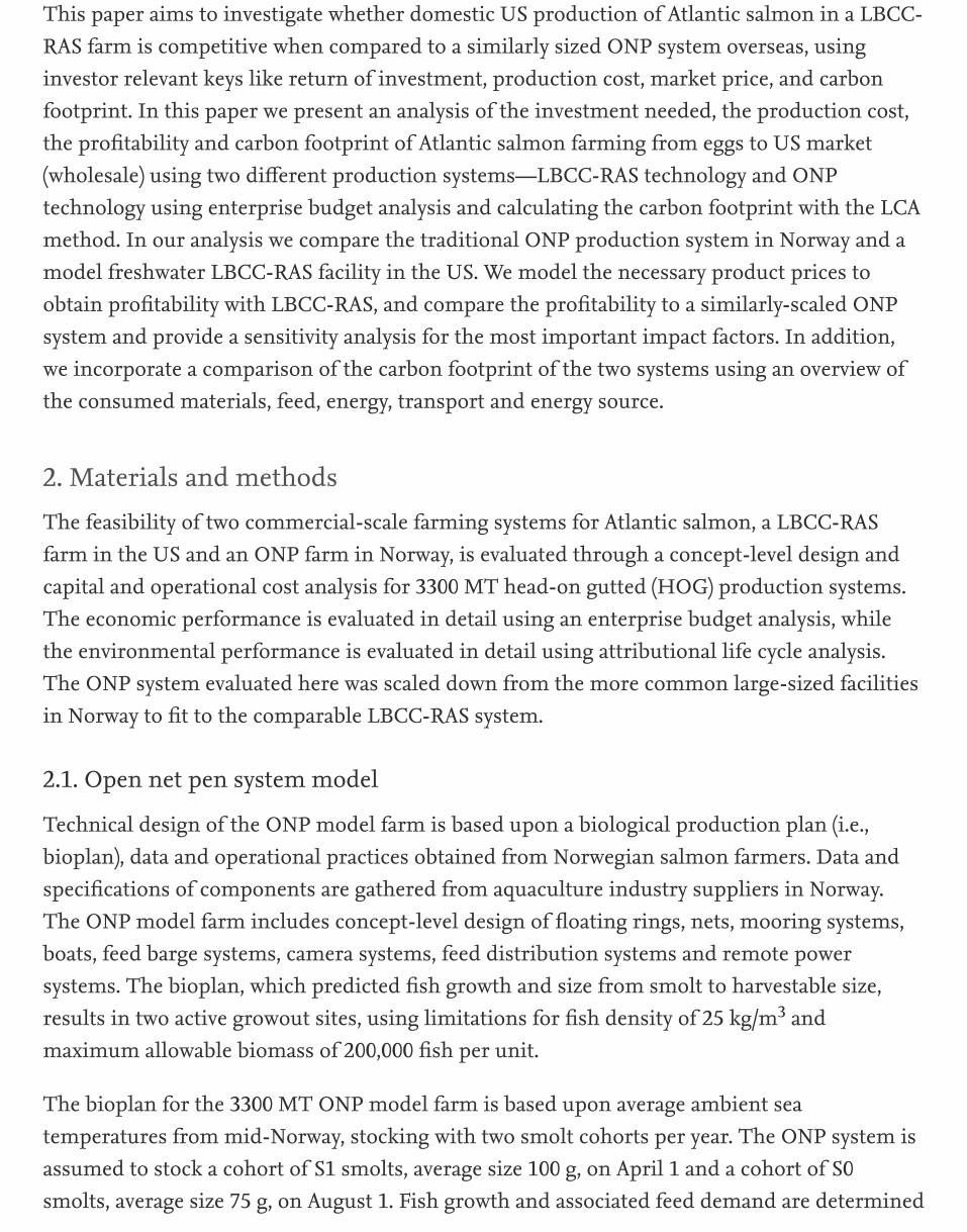
This paper aims to investigate whether domestic US production of Atlantic salmon in a LBCC-RAS farm is competitive when compared to a similarly sized ONP system overseas, usinginvestor relevant keys like return of investment, production cost, market price, and carbonfootprint. In this paper we present an analysis of the investment needed, the production cost,the profitability and carbon footprint of Atlantic salmon farming from eggs to US market(wholesale) using two different production systems—LBCC-RAS technology and ONPtechnology using enterprise budget analysis and calculating the carbon footprint with the LCAmethod. In our analysis we compare the traditional ONP production system in Norway and amodel freshwater LBCC-RAS facility in the US. We model the necessary product prices toobtain profitability with LBCC-RAS, and compare the profitability to a similarly-scaled ONPsystem and provide a sensitivity analysis for the most important impact factors. In addition,we incorporate a comparison of the carbon footprint of the two systems using an overview ofthe consumed materials, feed, energy, transport and energy source.
2. Materials and methodsThe feasibility of two commercial-scale farming systems for Atlantic salmon, a LBCC-RASfarm in the US and an ONP farm in Norway, is evaluated through a concept-level design andcapital and operational cost analysis for 3300 MT head-on gutted (HOG) production systems.The economic performance is evaluated in detail using an enterprise budget analysis, whilethe environmental performance is evaluated in detail using attributional life cycle analysis.The ONP system evaluated here was scaled down from the more common large-sized facilitiesin Norway to fit to the comparable LBCC-RAS system.
2.1. Open net pen system model
Technical design of the ONP model farm is based upon a biological production plan (i.e.,bioplan), data and operational practices obtained from Norwegian salmon farmers. Data andspecifications of components are gathered from aquaculture industry suppliers in Norway.The ONP model farm includes concept-level design of floating rings, nets, mooring systems,boats, feed barge systems, camera systems, feed distribution systems and remote powersystems. The bioplan, which predicted fish growth and size from smolt to harvestable size,results in two active growout sites, using limitations for fish density of 25 kg/m andmaximum allowable biomass of 200,000 fish per unit.
The bioplan for the 3300 MT ONP model farm is based upon average ambient seatemperatures from mid-Norway, stocking with two smolt cohorts per year. The ONP system isassumed to stock a cohort of S1 smolts, average size 100 g, on April 1 and a cohort of S0smolts, average size 75 g, on August 1. Fish growth and associated feed demand are determined
3

by using specific growth rates (SGR) and feed conversion ratios (FCR) given in feed supplierfeeding tables for various fish sizes. Fish growth estimates are reduced by 12% to compensatefor handling and treatment of the fish during the production cycle. The overall FCR was set to1.27 to obtain the average FCR from the last 10 years in Norway (Directorate of Fisheries, 2014).Mortalities for smolt to harvest are set to obtain 16% per generation mortality to comply witha dataset available from mid-Norway (Mattilsynet, 2011).
2.2. Land-based closed containment recirculating aquaculture system model
Technical design of the LBCC-RAS model farm is based on data developed by TheConservation Fund’s Freshwater Institute growout trials of Atlantic salmon, some of which hasbeen reported (Summerfelt et al., 2013). This includes concept-level water recirculation systemdesigns for each fish grouping developed in the bioplan. Each water recirculation systemdesign includes multiple recirculation modules to allow for staging and movement of fishthroughout the facility. Concept designs for incubation, fry, smolt, pre-growout, and growoutrearing areas, as well as a final purging system, are completed using steady-state mass balanceanalyses. Design water quality criteria used in the mass balance analyses are based on TheConservation Fund’s Freshwater Institute growout trials. Thermal growth coefficients (TGC)are used to predict fish growth for the bioplan for the 3300 MT LBCC-RAS model farm.Thermal growth coefficient values are based on data collected in growout trial data from TheConservation Fund’s Freshwater Institute. Additionally FCR, mortality, head-on gutted yield,and other performance indicators, which are used to develop a biological plan are taken frompast growout trials (Summerfelt et al., 2013). The FCR (kg/kg) and TGC (1000 g / °C days) areset to vary according to these growout trial data at different life stages; FCR: Fry, 0.75; smolt,0.90; pre-growout, 1.0; growout 1.1; and TGC: Fry, 1.25; smolt, 1.40; pre-growout, 2.00;growout, 2.30. The overall average FCR based on the individual values is 1.09. A maximumbiomass density of 80 kg/m is used for the biological plan of the LBCC-RAS model farm.
The steady-state feed requirement for the LBCC-RAS model farm is 11,815 kg/day. Watersupply required for the entire 3300 MT LBCC-RAS model farm is based on allowing no morethan 75 mg/L nitrate-nitrogen at maximum loading in each recirculation system, assuming nopassive denitrification within the systems. The amount of water supply needed to maintainthis nitrate-nitrogen level in the recirculation systems is calculated to be 7.7 m /min,including 1.1 m /min for finishing/purging the harvested salmon before slaughter. Theresulting water required per feed fed is 803 L/kg feed for the systems that have feeding fish,i.e., all RAS except the purge system. The power requirement for the model farm is 2458 kW,comprised primarily of power required for the water recirculation pumps (2079 kW); the totalpower required per unit of live weight salmon produced is 5.4 kWh/kg (4.6 kWh/kg forpumping only).
1/3
3
3
3

Concept-level design characteristics for each rearing area in both production systems aresummarized in Table 1; the inputs required for the two systems are summarized in Table 2;illustrative renderings are shown in Fig. 1. The technical design for each model farm allowedthe progression of capital and operating costs for comparison of the two production systems.Cost data used in the development of the concept-level estimates provided here is acombination of industry standard published cost data (Directorate of Fisheries, 2014, MarineHarvest ASA, 2014, RS Means, 2010) and project specific vendor quotations obtained in 2010–2011.
Table 1. Concept-level design characteristics for each rearing system in a 3,300 MT HOGAtlantic salmon land-based closed containment farm (LBCC-RAS) and a 3300 MT HOG opennet pen farm (ONP).
1 18 2 by 1.0 57 1.5 1.5 0.08 22.9
2 4 9 by 2.0 1,018 11.4 22.7 0.19 248.0
3 4 10 by 3.0 2,827 22 66 0.57 549.5
8 5 16 by 4.25 34,180 95 757 5.75 2063.5
1 2 16 by 4.25 1,709 38 38 1.1 –
Fish
Rearing
Area
Modules Units
per
module
Unit
diameter
by depth
(m × m)
Total
Rearing
Volume
(m )3
Module
Flow Rate
(m /min)3
Total
Flow
Rate
(m /min)3
Total
Makeup
Flow Rate
(m /min)3
Maximum
Module Feed
Rate (kg/day)
LBCC-
RAS—fry
LBCC-
RAS—
smolt
LBCC-
RAS—
pre-
growout
LBCC-
RAS—
growout
LBCC-
RAS—
final
purging
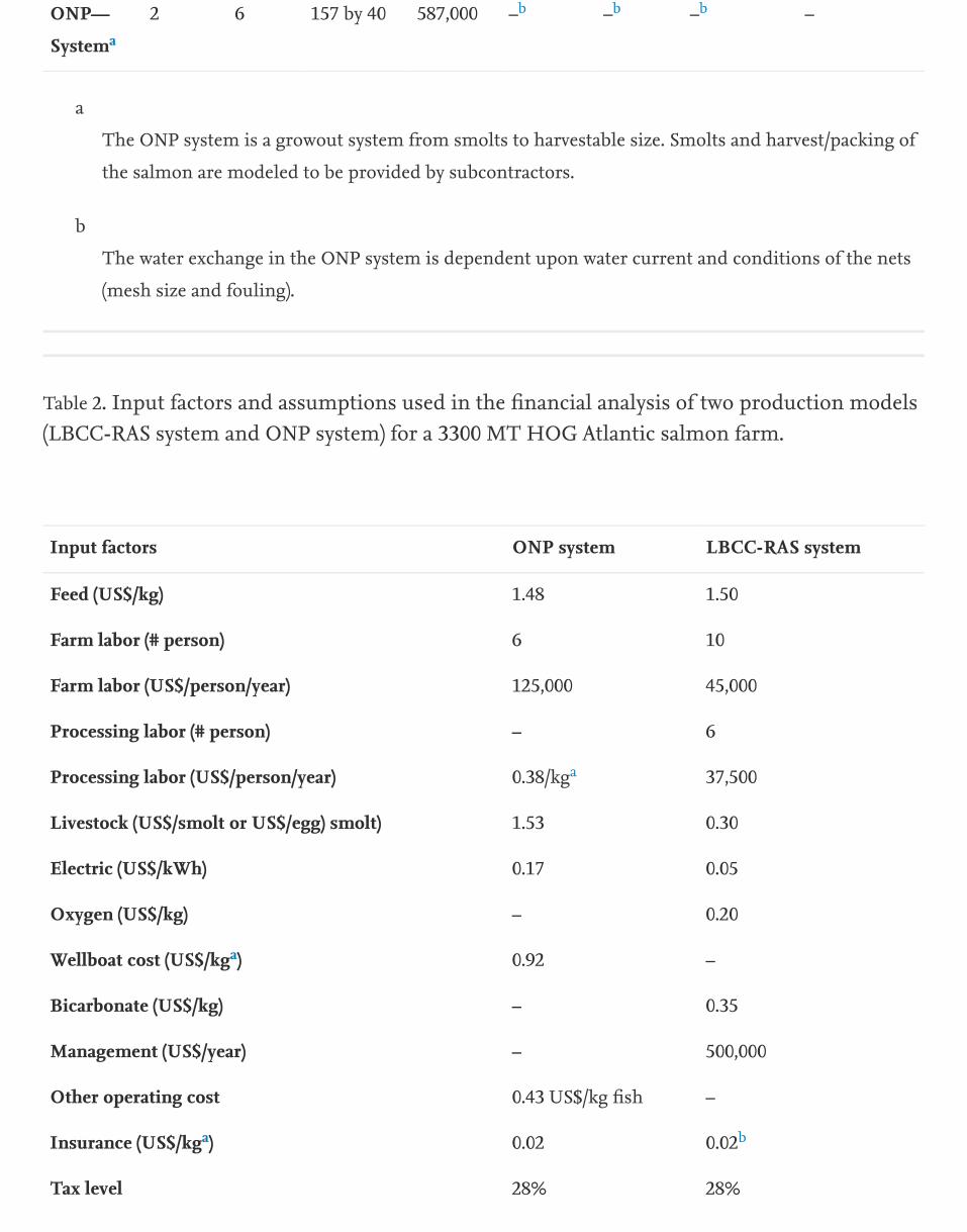
2 6 157 by 40 587,000 – – – –
a
The ONP system is a growout system from smolts to harvestable size. Smolts and harvest/packing of
the salmon are modeled to be provided by subcontractors.
b
The water exchange in the ONP system is dependent upon water current and conditions of the nets
(mesh size and fouling).
Table 2. Input factors and assumptions used in the financial analysis of two production models(LBCC-RAS system and ONP system) for a 3300 MT HOG Atlantic salmon farm.
1.48 1.50
6 10
125,000 45,000
– 6
0.38/kg 37,500
1.53 0.30
0.17 0.05
– 0.20
0.92 –
– 0.35
– 500,000
0.43 US$/kg fish –
0.02 0.02
28% 28%
ONP—
Systema
b b b
Input factors ONP system LBCC-RAS system
Feed (US$/kg)
Farm labor (# person)
Farm labor (US$/person/year)
Processing labor (# person)
Processing labor (US$/person/year) a
Livestock (US$/smolt or US$/egg) smolt)
Electric (US$/kWh)
Oxygen (US$/kg)
Wellboat cost (US$/kg )a
Bicarbonate (US$/kg)
Management (US$/year)
Other operating cost
Insurance (US$/kg )a b
Tax level

30% 40%
3.0% 6.0%
a
Whole fish weight.
b
First year is 0.04 US$/kg.
Equity ratio
Interest loans

Download : Download full-size image
Fig. 1. Concept-level renderings of the growout rearing area in a 3300 MT HOG Atlanticsalmon LBCC-RAS farm (A) and ONP farm (B).
2.3. Economics

Salmon aquaculture is a commercial operation whose purpose to be profitable. Theprerequisite for a business to be sustainable is to be profitable in both the short- and long-term and over the investment horizon. The financial performance of these two aquacultureproduction systems is investigated using an enterprise budget analysis; this allows anassessment of the feasibility and profitability of the two systems. Enterprise budgets, alsocalled production budgets, provide a framework within which all the components of costs andrevenues associated with the production of farm products are itemized. The budget isconstructed on a production basis, and the assessment is built upon a cash flow analysis. Theprofitability is calculated based on financial statements such as income statement and balancesheets.
There are a number of well-developed analytical techniques for analyzing profitability (Liu andSumaila, 2007, Kumar and Engle, 2011). Net present value (NPV) is a commonly usedparameter to provide an objective decision of an investment and project. Net present valuetakes into account the time value of money, and is the difference between the present value oftotal costs and total revenue over an operational horizon. Positive NPV indicates that aninvestment is worthwhile. In addition to NPV, other indicators are also used as assessmentcriteria; these include gross margin, return on investment (ROI), internal rate of return (IRR),payback period, and break-even production and price. Gross margin is expressed as revenueminus variable costs; net income or profit is revenue minus all costs. Return on investment isthe rate of return on the initial capital investment and is estimated by profit before taxesdivided by the capital investment. Internal rate of return is the discount rate at which netpresent value of profit is set equal to zero. Breakeven production/price represents the expectedproduction level and market price at which total sale revenue covers total production costs.Breakeven analysis can inform the conditions necessary for the business to become profitableor to remain in business.
2.3.1. Enterprise budget
The enterprise budget is estimated based on a total production of 4000 MT wet weight, whichis equivalent to 3300 MT of head-on gutted weight. Head-on gutted yield is estimated to be88% after a 5% loss of weight during final purging for both the ONP and the LBCC-RASproduction systems. The estimates of total investment cost and operating cost of each costitem are based on the production system design models and their associated bioplans. Thecosts include two parts: capital cost and operating cost.
2.3.2. Capital cost—ONP model
Capital costs incur at the beginning of the operation, and most of these costs are one-time

costs. The capital cost for the 3300 MT ONP model farm is based on information gatheredfrom the Norwegian aquaculture industry, and is thereby considered representative for anONP farm constructed and operated according to Norwegian laws and regulations (Norway,2008). The ONP model farm includes 3 licenses and 12 pens, and their associated physicalcomponents consisting of floating rings, nets, mooring systems, boats, feed barge systems,camera systems, feed distribution systems and remote power systems. The cost of each item isestimated based on current market price suppliers’ command. Compared to estimatesreported by Marine Harvest (Marine Harvest ASA, 2014), the capital cost for the ONP modelfarm is considered representative for a two site ONP farm. We assume that the lifespan of netsand feeding system is 5 years, floating rings is 8 years, camera and power systems is 10 years,and the remainder of the equipment is 20 years. These lifespans are used for calculation ofdepreciation and replacement cost.
The cost for an ONP farming license in Norway is included in the capital cost estimate for theONP model farm. The current cost of ONP farming licenses is much higher when comparedto license costs of the 1990s (Färe et al., 2005); cost for a license in the current open market isapproximately 55 million Norwegian kroners, which is equivalent to 8 million US dollars(Aardal, 2014). The total capital cost of the ONP model farm including licenses at currentprices is estimated to be 29.7 million US dollars for a total production of 3300 MT head-ongutted salmon (Table 3).
Table 3. Capital expenses for a 3,300 MT HOG LBCC-RAS and ONP Atlantic salmon farm.
23,571,429
1,834,286
857,143
342,857
1,285,714
1,371,429
214,286
34,114
1
ONP system cost components Cost (US$)
Licences
Floating rings
Nets
Moorings
Boats
Feed barges
Camera systems
Feed distributors

188,571
29,699,829
26,640,557
3,487,500
675,000
2,112,030
9,426,413
5,080,980
1,058,538
254,049
4,848,102
53,583,169
2.3.3. Capital cost—LBCC-RAS model
The capital cost of the LBCC-RAS model farm includes all RAS systems, water supply, effluenttreatment systems, buildings, engineering services, construction management services, aprimary processing facility and general contractor bonding requirements. These componentsare itemized based on material, equipment, labor and subcontractor services, upon which thecosts are estimated. Ten percent contingency is applied to capture uncertainty associated withthis level of cost estimation. We assume that the lifespan of materials and equipment is 10years and the lifespan for buildings and tanks is 20 years. These lifespans are used forcalculation of depreciation and replacement cost. The cost of bonding is included as insurancemay be required by owners that builders must have for large projects and is typically passedback to the owner. There are currently no comparable license costs for a LBCC-RAS farm inthe US. The total capital cost including contingency of the LBCC-RAS model farm is estimatedto be 53.6 million US dollars for a total production of 3300 MT head-on gutted salmon (Table3).
2.3.4. Operating cost—ONP model
The operating cost for the ONP model farm is estimated based on data collected by the
Power systems
Total
LBCC-RAS system cost components Cost (US$)
RAS Systems
Effluent treatment
Water supply
Processing
Building
Engineering
Construction management
Bond
Contingency (10%)
Total

Norwegian Directorate of Fisheries (2014) and also Marine Harvest ASA (2014), and are theaverage costs of the last five years, 2009–2013. Since there are uncertainties associated withthese items and the overall cost has increased gradually in the last several years, we applied a2% increase for the first five year’s estimates, and a 3% increase for the remaining year’sestimate to account for uncertainties for each cost item. In other words, it is assumed that eachcost item will increase 2% for the first five years and 3% for the rest. The operating costs arethe average estimates over 15 years. The breakdown of costs is presented in Table 4.
Table 4. Operating expenses for a 3,300 MT HOG LBCC-RAS and ONP Atlantic salmon farm.
2.05 14.34 1.90 13.33
0.47 3.30 – –
– – 0.12 0.86
0.31 2.15 0.52 3.65
0.18 1.23 – –
0.03 0.18 – –
– – 0.33 2.32
– – 0.15 1.07
– – 0.09 0.62
0.02 0.16 0.18 1.27
0.43 3.03 0.12 0.83
0.25 1.58 – –
0.09 0.60 – –
0.14 0.99 0.47 3.26
0.60 4.21 0.65 4.52
0.18 1.28 0.58 4.09
Cost item ONP system LBCC-RAS system
Cost (US$) Cost (NOK) Cost (US$) Cost (NOK)
Feed
Smolt
Egg
Labor
Well boat
Health
Electricity
Oxygen
Water treatment
Insurance
Primary processing
Transportation
Sales & marketing
Maintenance
Interest
Depreciations

0.33 2.32 0.49 3.45
5.08 35.37 5.60 39.27
2.3.5. Operating cost—LBCC-RAS model
The operating cost for the LBCC-RAS model farm is estimated based on the bioplan designedfor an annual production of 3300 MT after primary processing. Cost items include feed,oxygen, bicarbonate, electricity, eggs, labor, stock insurance, interest and depreciation. Feedamount and thus cost, is calculated based on the feed required for growth multiplied by feedconversion ratio at different life stages. The amounts, and thus costs, of oxygen andbicarbonate are dependent on the feed required. Oxygen required is estimated to be 0.60 kgoxygen per kg feed, which includes an oxygen transfer efficiency of 75%. Bicarbonate requiredis estimated to be 0.20 kg bicarbonate per kg feed, which includes a base chemical availabilityof 75%. The cost of the electricity is determined by the RAS design, which identified all pumpsand motors required for operation. The number, and thus cost, of eggs required is estimatedby the assumed mortality rates at different life stages. Labor costs for the LBCC-RAS modelfarm include management (biological and maintenance), fish culture technicians, laboratorytechnicians, maintenance mechanics, and primary processing staff. It is assumed thatinsurance cost for the first year of operation is 4% of standing biomass, and then that declinesto 2% of standing biomass in the following years. The ratio between interest and cash forcapital cost and first year operating cost was 60/40, and an interest rate of 6% was used.Depreciation of each item was estimated using a straight line approach, meaning depreciationcost was charged evenly throughout the useful life of each capital item. Maintenance cost wasestimated to be 10% of the total variable cost. To capture unknown costs, a contingency cost isalso included which was assumed to be 10% of the total cost. The increase with 2% for the first5 years and 3% for the rest are also applied for each cost item due to unforeseen futurechanges, same as the ONP system.
2.3.6. Sales and income
It takes approximately one year for salmon to grow to market size, therefore, there is noharvest for Year 1 and a proportionally smaller harvest for Year 2. In Year 3 and onwards, aconstant harvest of 3300 MT is assumed for the ONP and LBCC-RAS systems. The price usedhere is the export market price of fresh gutted salmon in the US market, which isapproximately 5.97 US$/kg or 41.8 NOK/kg averaged weekly price for the year 2014 (StatisticsNorway, 2015). It is also assumed that the price for salmon in the future would increase in asimilar way as the cost items, i.e., increased by 2% for the first five years and 3% for the rest.However, preliminary sales of Atlantic salmon produced by a LBCC-RAS farm have
Others
Total

commanded a significant price premium (Guy Dean, Albion Fisheries (Vancouver, BC),personal communication, September 4, 2014), here a 30% price premium is assumed which isapproximately 7.76 US$/kg. The total sales revenue is calculated based on export price andannual harvest.
2.4. Carbon footprint
The carbon footprint is the sum of potential climate impacts that a product causes from adefined part of its life cycle. The carbon footprint was calculated using life cycle assessment(LCA) methodology that is a tool for environmental assessment (ISO, 2006a, ISO, 2006b). Itassesses the inputs of energy and material to the system and from that calculates potentialenvironmental impacts caused by the resource use and outputs to nature in the form ofemissions, waste and products. This LCA includes both direct emissions from the feed andsalmon production and indirect emissions caused by production and distribution of thecommodities and infrastructure that underpin the salmon life cycle.
The potential climate impact, the global warming potential, is calculated by characterizing allemission and impacts into CO equivalents (CO eq) according to their radiative propertiesbased on IPCC guidelines (IPCC, 2007).
The goal of the carbon footprint was to compare the potential climate impacts from differentways of providing a retailer in Seattle, WA (US) with Atlantic salmon:
1a) Salmon from a LBCC-RAS system in the US running on electricity generated from a sourcethat uses a typical mix of coal, gas, nuclear, wind and hydropower. Salmon is assumed to betransported fresh to the retailer 250 km by truck.
1b) Salmon from a LBCC-RAS System in the US running on electricity generated from asource that uses 90% hydropower and 10% coal. Salmon is assumed to be transported fresh tothe retailer 250 km by truck.
2a) Salmon from a Norwegian ONP system. Salmon is assumed to be transported fresh, firstwith truck in Norway to Oslo, 520 km, and then with airfreight to Seattle, 7328 km.
2b) Salmon from a Norwegian ONP system. Salmon is assumed to be transported frozen, firstwith truck in Norway to Oslo, 520 km, and then with ship from Ålesund, Norway, to Seattlethrough the Panama Canal, 16,473 km.
The functional unit for the assessment, the basis for comparison, was 1 kg of gutted salmonwith head on, at the retailer gate. For each case, the assessment included the completeproduction system, from production of feed ingredients, smolt production and construction
2 2

of facilities, equipment and transports.
It was assumed that the salmon was gutted close to the production facility and that allbyproducts, such as guts, skin and trimmings were utilized mainly for feed production. Massallocation was applied meaning that the carbon footprint up to slaughter was allocatedbetween the head-on-and-gutted salmon and the byproducts based on their mass. Thus, perunit of mass live salmon and head on and gutted salmon have the same carbon footprint.Important cut offs, processes that are not included in the assessment include: slaughteringprocess, treatment of the biosolids from the LBCC-RAS system, and transport infrastructure.
2.4.1. Carbon footprint data
Table 5 presents important activity data for the carbon footprint of the two systems. Data forthe LBCC-RAS system was derived from the concept-level design. Data for the Norwegian ONPsystem is gathered from industry actors and industry statistics (Winther et al., 2009, Hognes etal., 2011, Hognes et al., 2014). Data on the climate impacts from capital and operational inputswere modeled with data from the LCA inventory database Ecoinvent v3.1 (2013). Since many ofthe operations performed at the ONP farm are performed by sub-contractors, and the extentof the activities, e.g., cleaning and priming of nets, are dependent of exact location, these dataare based on the assumption of a representative production model.
Table 5. Inventory data for carbon footprint for two production models (LBCC-RAS system andONP system) for a 3300 MT HOG Atlantic salmon farm. All numbers are per ton of salmonproduced or transported.
ton 1.09 1.27
kg 82.5 –
kg 14.40 0.63
kg – 0.70
kg 8.93 –
kg – 1.01
kg – 1.79
Unit LBCC-RAS System ONP system
Feed, economic FCR
Concrete
Steel, reinforcing
Steel, chromium 18/8 steel
Glass fiber
Nylon
Polypropylene

kg – 0.28
l – 10.50
kWh 5460 –
kg 656 –
kg 219 –
kg 25 25
kg 300 300
Both the LBCC-RAS and ONP systems are modeled using the same feed. Based on LCAs of theaverage Norwegian salmon feed in 2012, the feed is associated with a carbon footprint of 2.5 kgCO eq/kg feed at the feed factory gate. This is a feed with the following composition: 12%marine oil; 19% marine protein; 19% oil from crops; 39% protein from crops; 8% starch fromcrops and 3% micro ingredients (minerals, vitamins, pigments and other). This carbonfootprint reflects a feed where 50% of the soy in the feed is equal to the average Brazilian soy,as modeled by the Agrifootprint database (Centre for Design and Society of the RMITUniversity, 2014), and the remaining coming from old farms where climate impacts from landuse change is not included (Hognes et al., 2014).
Electricity for the LBCC-RAS system in case 1b is modeled as being generated from 90%hydropower and 10% coal power with data from Ecoinvent v3.1 (2013). This case is included asan illustrative case for what is possible if this type of electricity is available. Electricity loss of3.5% was included for the transmission of the power and transformation from high tomedium voltage. This associated the electricity with a carbon footprint of 0.04 kg CO eq/kWh.For comparison, the Ecoinvent v3.1 database also provides a dataset that describes theelectricity available in the regional entity of the North American Electric ReliabilityCorporation (NERC), that gives a carbon footprint of 0.64 kg CO eq/kWh. This was theelectricity data used for the LBCC-RAS system in case 1a.
Road transport was modeled with a truck carrying 20 tons of fish, consuming 3.7 L of dieselper 10 km and has a carbon footprint of 0.09 kg CO eq/tkm; this also includes fuel used for therefrigeration system and emission of refrigerants (Winther et al., 2009). The fuel consumptionreflects a modern truck. For the ONP system in case 2a, airfreight was modeled using data for aBoeing 747–400 from the Agrifootprint database, with an emission factor of 1.18 kg CO eq/tkm(Centre for Design and Society of the RMIT University, 2014). This plane is assumed to use100% of its load capacity (3600 tons) and the emissions include landing and takeoff for a flight
Polyethylene
Fuel
Electricity
Oxygen (liquid)
Lime (calcium carbonate)
EPS for transport packaging
Ice
2
2
2
2
2

of approximately 10,000 km. For the ONP system in case 2b, ship transport was modeled withdata for a ship of 120,000 tons (dry weight) utilizing 80% of its capacity, with an emission factorof 0.004 kg CO eq/tkm. Emissions from preparing for the return of the ship and re-loading isincluded in this data. Fuel for running refrigeration systems and emissions of refrigerantswere also included with an emission factor of 0.1 kg CO eq/h (Winther et al., 2009).
3. Results
3.1. Financial analysis
3.1.1. Capital cost
Tables 3 reports the capital cost of ONP and LBCC-RAS systems. In the ONP system, thelargest cost is license fees, which are almost 80% of the total capital cost, while the physicalstructure cost only accounts for 20%. For LBCC-RAS, the largest cost is the RAS system whichis half of the total cost; 18% of the LBCC-RAS capital cost is for building structures. Thecapital cost of LBCC-RAS is 80% higher than that of the ONP system given the sameproduction capacity. It is important to note that the replacement costs of some cost items arenot included in this table, but incorporated into the cash flow analysis.
3.1.2. Operating cost
The operating cost breakdowns for the two systems are presented in Table 4 and Fig. 2. Thetotal operating costs for the two systems are relatively similar, with LBCC-RAS only 10%higher than the ONP system. Without interest and depreciation, the two production systemshave an almost equal operating cost, 4.30 US$/kg for ONP and 4.37 US$/kg for LBCC-RAS.Feed is the single biggest cost item accounting for 41% and 34% of the total operating cost forthe ONP and the LBCC-RAS systems, respectively. It is worthwhile to note that these operatingcosts are subject to change with site selection due to differences in power costs, feed shippingcosts and other factors. For example, operating costs presented here do not include the cost ofheating or cooling that may or may not be required based on the geographic location of theLBCC-RAS facility.
2
2

Download : Download full-size image
Fig. 2. Estimated production costs (US$/kg HOG) according to the investments, product priceestimates and the biological production plans for a model 3300 MT HOG Atlantic salmonLBCC-RAS farm (A) and ONP farm (B).
3.1.3. Financial indicators
The financial analysis is conducted for a period of 15 years; the discount rate is set to sevenpercent. The summary of the financial analysis is presented in Table 6. Overall, the ONPmodel system is financially better than the LBCC-RAS model system, even when the LBCC-RAS is selling product with a price premium. All three cases generate positive operatingmargins, indicating that from a production operating perspective, all are financially viable.The LBCC-RAS system selling salmon at a price premium is comparatively as profitable as theONP system, even though its NPV is negative (−20,340,000 US$) and its return on investment(9.01%) is lower than the ONP system’s ROI (17.77%). However, when selling salmon at thesame price as the ONP system, the LBCC-RAS system is barely financially profitable and notan attractive investment. To be comparable with an ONP system, the LBCC-RAS system mustcommand higher market price to breakeven or be profitable.
Table 6. Economic indicators for a 3,300 MT HOG LBCC-RAS and ONP Atlantic salmon farm.Also presented are indicators for the LBCC-RAS farm selling salmon with a 30% pricepremium.
Economic indicator ONP system LBCC-RAS system LBCC-RAS system premium price

38.39% 17.56% 40.64%
23.62% (–) 18.18%
3.54 −120.20 −20.34
15.96% (–) 13.28%
7.94% (–) 2.67%
17.77% (–) 9.01%
1251 3307 2387
5.63 (–) 11.10
5.33 (–) 6.44
The IRR can be considered as the true expected yield from an investment. The IRR beforeEBIT for the LBCC-RAS with price premium is calculated to be 13.28%. The real IRR for theLBCC-RAS with price premium is 2.67%. The discount rate of 7% used here is below the IRRbefore EBIT and thus the LBCC-RAS would be an investment that results in a positive NPV.However, the discount rate of 7% used here is also above real IRR, and that investment inLBCC-RAS results in a negative NPV. Investors must make investment decisions based on herexpectation(s) on return, whether using the IRR of 13.28% or 2.67%.
3.1.4. Sensitivity analysis
The financial results are very sensitive to some factors. For instance, prices have substantialinfluence on the results, and are subject to short- and long-term fluctuations due to dynamicsin supply and demand. Feed is the largest cost item, so any changes in feed price and feedutilization have large impacts on the economic performance of the operations. Recent figureshave suggested the cost of feed has increased gradually. The assumption for feed conversionratio during growout is one of the most critical values in the estimation because it drives thelargest component of the cost of production—feed cost during growout. Performance datafrom repeated Freshwater Institute trials indicate a feed conversion ratio less than 1.1 duringthe final growout phase (Summerfelt et al., 2013); utilizing lower FCR values during finalgrowout instead of 1.1 would reduce the cost of production, by potentially up to 6%. Feed isalso the major factor influencing the carbon footprint. Other factors such as mortality rates,power cost and mortality also have impacts on financial performance.
3.2. Carbon footprint results
Operating (gross) margin
Profit margin
NPV (million US$)
IRR before EBIT
IRR
ROI
Break-even production (MT)
Pay-back period (year)
Break-even price (US$)

If the alternative is intercontinental export of fresh salmon by air, then a modern and efficientLBCC-RAS system close to the market can be a more climate friendly alternative, even whenrunning on electric power that mainly originates from fossil fuels (7.4 versus 15.2 kg CO eqper kg HOG salmon at retailer gate in Seattle). If the LBCC-RAS system is running on 90%hydropower the carbon footprint of the LBCC-RAS salmon is further reduced to 4.1 kg CO eqper kg HOG salmon at the retailer gate. The most climate friendly alternative of all is to shipfrozen salmon from Norway with a modern container ship, 3.8 kg CO eq per kg HOG salmonat the retailer gate. A frozen product is not directly comparable with a fresh, but with modernfreezing technologies, the quality of frozen products is not necessarily inferior to fresh.
At the producer gate, before transport to the retailer in Seattle, the production systems haveclimate impacts per unit produced of 3.4 versus 3.7 and 7.0 kg CO eq/kg salmon live-weightfor the ONP and the LBCC-RAS using hydropower or average fossil fuel based electricity,respectively (Table 7 and Fig. 3).
Table 7. Estimated carbon footprint with component contributions at the producer gate and theretailer gate for the following scenarios: (1a) Salmon from a LBCC-RAS system in the USrunning on a typical electricity mix; (1b) Salmon from a LBCC-RAS system in the US runningon electricity generated predominantly from hydropower; (2a) Salmon from a Norwegian ONPsystem transported by airfreight to Seattle; (2b) Salmon from a Norwegian ONP systemtransported by ship to Seattle.
2.69 2.69 3.21 3.21
0.39 0.39 0.02 0.02
3.48 0.21 0.16 0.16
0.44 0.44 – –
7.01 3.73 3.39 3.39
0.03 0.03 0.06 0.062
– – 11.40 0.09
0.37 0.37 0.37 0.11
0.00 0.00 0.00 0.10
2
2
2
2
1a) 1b) 2a) 2b)
Feed production
Construction of facility and equipment
Grow out and smolt (fuel and electricity)
Oxygen and lime
At producer gate (live weight)
Transport, road
Transport, air or water
Packaging and ice
Refrigeration during transport

7.41 4.14 15.22 3.75
Download : Download full-size image
Fig. 3. Estimated carbon footprint with component contributions at the producer gate and theretailer gate for the following scenarios: (1a) Salmon from a LBCC-RAS system in the USrunning on a typical electricity mix; (1b) Salmon from a LBCC-RAS system in the US runningon electricity generated predominantly from hydropower; (2a) Salmon from a Norwegian ONPsystem transported by airfreight to Seattle; (2b) Salmon from a Norwegian ONP systemtransported by ship to Seattle.
The more general findings confirmed what previous LCAs have found that fish feed is thedominant climate aspect for the selected salmon products, but that energy used in growoutand emissions from transports are also important. Production and maintenance of equipmentand production facilities are not important climate aspects compared to feed production,transport and water treatment.
At retailer gate (HOG)

4. DiscussionGiven current technology development and possible increases in market price for salmon andproduction input factors, the ONP system still remains the most profitable, even at thisrelatively small scale. To achieve comparative financial performance, the LBCC-RAS systemrequires a price premium, at least 25% higher than current market prices. This is mainly dueto considerably higher capital cost for the LBCC-RAS system. However, the difference inoperating costs between both systems is relatively small. If the feed conversion ratio can befurther improved from 1.1 to 1.0 for LBCC-RAS systems, the gap will be even smaller sincefeed is the most important cost item. However, improvements in feed conversion ratio are alsolikely to happen in ONP systems, so the difference in the future for optimized systems is hardto predict. It is important to note that ONP systems are just for the growout phase in Norway,and that salmon now spend more of their lifecycle in LBCC-RAS smolt production facilities(Dalsgaard et al., 2013). Additionally, other costs such as managing sea lice and loss due todisease could further increase the operating cost of ONP systems significantly (Liu andBjelland, 2014). The largest limiting factor for using LBCC-RAS system appears to be thecapital cost. Thus, there are economic incentives for advancing technological innovations ofLBCC-RAS systems that can reduce capital cost to become more competitive with ONPsystems.
LBCC-RAS systems are not a new technology, and have been used for the last twenty years forgrowing out both freshwater species, such as eel and catfish, and marine species like trout andsea bass (Martins et al., 2010, Badiola et al., 2012). There is increasing interest in applyingLBCC-RAS for the salmon smolt stage in Nordic countries and Europe (Dalsgaard et al., 2013).However, due to low returns on investment and and a history of failures when the technologywas not well advanced, LBCC-RAS have not been used widely.
Economic incentives have been proven to be more effective than traditional command andcontrol policy (Bailly and Willmann, 2001, Liu et al., 2013). Market-based economicinstruments such as taxes, subsidies, fees/charges and eco-labeling can create incentives forthe industry to foster cost-effective technology innovation and adaptation such as LBCC-RASsystems or other closed containment systems (Rosten et al., 2013). However, such incentive-based approaches have to be executed with the vectors of market and social forces such asenvironmental policy and consumers. Eco-labeling farmed products would be a market-driving power to change consumers’ purchasing behavior. Concerned consumers are likelywilling to pay more for the products which are produced in an environmental sustainable way.Subsidies and taxes can be used to stimulate cost-effective technology innovation andadaptation, e.g., rewarding improved environmental performance from capturing andcontrolling waste streams in closed-containment systems or eliminating sea lice infestation.

While environmental policies may also have a role, in Norway, “green” concessions for salmonfarming require the aquaculture industry to employ technological and operational innovationsand solutions to reduce the incidence of salmon lice and escapes. These technologies requireupfront investment which can be significant, but over the long run, such technologicalinnovation would increase social license to operate through improved environmentalperformance and reduced conflict with other resource users, perceived market payoffs throughreduced costs to obtain and maintain a license to operate, and monitor and mitigate negativeimpacts, e.g., costs of recapturing escapes. Captured nutrient laden waste streams associatedwith LBCC-RAS may also result in ancillary revenue streams, e.g., aquaponics.
The carbon footprint analysis showed that, with respect to climate impact, producing close tothe market is preferable by a good margin, especially when the LBCC-RAS system utilizedelectricity generated from 90% hydropower and the alternative is to export fish fresh, fast anda long distance. Even if salmon is LBCC-RAS produced with electricity based on fossil fuels,intercontinental export of fresh fish on airplanes is not a preferable option. However,environmental considerations involving high inputs of electricity should be followed up with adiscussion of what is the environmentally optimum way of using available electricity.Electricity is of the highest energy quality available, and many industrial and infrastructureprocesses do not have an alternative to electricity. Export of frozen salmon was the best optionof all, but cannot be directly compared with fresh salmon. Still, this result points to a futureoption, with product development, improvement of logistic chain management, to maintainquality through the transport, and market acceptance, frozen intercontinental export has thepotential to compete with local LBCC-RAS products. Another important assumptionregarding transport is that most intercontinental export of fresh Norwegian salmon is donewith flights that also carry passengers. Thus a more precise comparison should include detailsand insight into how it is reasonable to allocate the fuel used and corresponding emissionsbetween goods and passengers. In addition to this, the LCA data that is available on flighttransport is highly variable. This indicates that more precision on the exact age/technologyand size of the aircrafts being used should be included.
The carbon footprint contained several cut-offs and assumptions that limits the conclusionsthat can be drawn, e.g., the same data on feed was used for salmon production in the US andNorway. There are likely to be differences in the carbon footprint of the feeds that wouldactually be used. A potentially important cut off is that treatment of the biosolids was notincluded. Biosolids could be seen as both waste and a resource, but either way handling it willinvolve the use of both energy and transports together with emissions from the biosolidsitself. Still, this aspect was left out because it would be difficult to compare to the ONP system,where there is no biosolids capture and waste feed and feces is discharged directly in the

ocean.
Most often, the concentrated effluent of LBCC-RAS systems now in operation in NorthAmerica and Europe are treated in order to meet stringent wastewater discharge permits. Thusa flow-through system will have a higher eutrophication potential. However, if theconcentrated effluent of a LBCC-RAS is not treated there is no such advantage to be obtained.Rosten et al. (2013) suggests a classification system for closed containment systems from 1 to 4,where category 4 is the most closed system towards the external environment applyingtreatment of both inlet and outlet of a LBCC-RAS system. Acidification and toxic potentials arestrongly connected to energy consumption and thus similar to climate impacts with regards towhere and why they occur.
Aquaculture technologies have been compared with LCA previously; our assessment wascompared with a selection of peer reviewed literature (Table 8). This selection of literaturepoints to the same main conclusions: feed production is a dominating factor for carbonfootprint in salmon aquaculture, and for LBCC-RAS, the use of energy for water treatment canbe equally important and equipment and infrastructure is of minor importance. Theimportance of energy used for water treatment depends on how this energy is produced. Theliterature also shows that important parameters for the LCA, such as the FCR and energy usedfor water treatment varies considerably. This study has not gone into the details to explainthese differences, but important reasons are probably that the studies rely on differentassumptions, experimental data and site specific properties. These differences make it difficultto compare the final carbon footprint among studies. In addition to differences in theaquaculture systems that are compared, it is also not possible to be sure that the data on feedthat are used are comparable. Finally, there are also methodical differences, e.g., Ayer andTyedmers (2009) used allocation based on the energy content in the different outputs ratherthan their mass and Samuel-Fitwi et al. (2013) used system expansion.
Table 8. Data from published studies on LCAs of LBCC-RAS for rearing salmonids.
Net-pen: 1.49 Net-pen: 1.30 Net-pen: 2.07 Ayer and
Tyedmers
System analyzed and method Electricity
consumption
(kWh/kg)
Feed
efficiency
Carbon
footprint of
product (kg
CO eq/kg)2
Reference
Salmon production with marine net-pen,
marine floating bag, land-based saltwater flow

(2009)
Land, flow
through: 13.4
Land, flow
through: 1.17
Bag: 1.90
Land,
recirculating:
22.6
Land,
recirculating:
1.45
Land, flow
through: 2.77
Electricity
mix 80%
fossil fuels
Land,
recirculating:
28.20
Flow through
low pumping:
2.36
Flow
through: 1.10
Flow
through: 2.02
d’Orbcast
el et al.
(2009)
Recirculation:
10.7
Recirculation:
0.80
Recirculation:
1.60–2.04
86.6% nuclear
energy
Intensive
flow through:
2.55
Flow
through:
0.91–1.2
Flow through
extensive:
2.24
Samuel-
Fitwi et
al. (2013)
Recirculating:
19.6
Recirculating:
0.86
Flow through
intensive:
3.56
Electricity
based on
fossil fuels
Recirculating:
13.60
Flow-
through: 0.65
Flow
through: 1.15
Flow
through: 1.16
Dekamin
et al.
(2015)
Recirculating: Recirculating: Recirculating:
through and a land-based freshwater RAS.
Assessment from feed and smolt production to
farm gate
Trout production with a flow through system
and a hypothetical recirculating system. From
feed production to fish ready for slaughter
Rainbow trout production in flow through
systems (extensive and intensive) and
recirculating system. From feed production to
fish ready for slaughter
Rainbow trout production with flow-through,
recirculating and semi-closed system. From
feed production to fish ready for slaughter
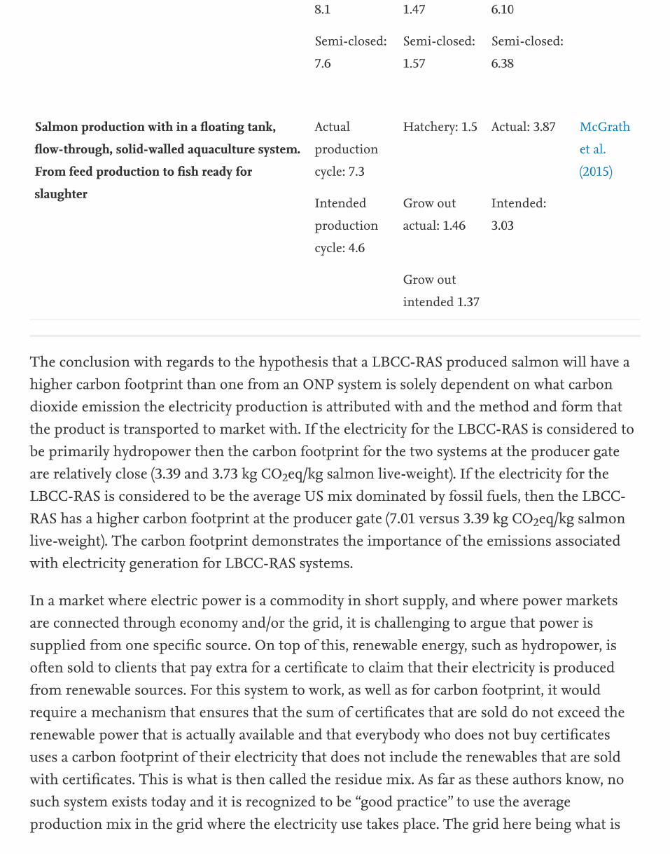
8.1 1.47 6.10
Semi-closed:
7.6
Semi-closed:
1.57
Semi-closed:
6.38
Actual
production
cycle: 7.3
Hatchery: 1.5 Actual: 3.87 McGrath
et al.
(2015)
Intended
production
cycle: 4.6
Grow out
actual: 1.46
Intended:
3.03
Grow out
intended 1.37
The conclusion with regards to the hypothesis that a LBCC-RAS produced salmon will have ahigher carbon footprint than one from an ONP system is solely dependent on what carbondioxide emission the electricity production is attributed with and the method and form thatthe product is transported to market with. If the electricity for the LBCC-RAS is considered tobe primarily hydropower then the carbon footprint for the two systems at the producer gateare relatively close (3.39 and 3.73 kg CO eq/kg salmon live-weight). If the electricity for theLBCC-RAS is considered to be the average US mix dominated by fossil fuels, then the LBCC-RAS has a higher carbon footprint at the producer gate (7.01 versus 3.39 kg CO eq/kg salmonlive-weight). The carbon footprint demonstrates the importance of the emissions associatedwith electricity generation for LBCC-RAS systems.
In a market where electric power is a commodity in short supply, and where power marketsare connected through economy and/or the grid, it is challenging to argue that power issupplied from one specific source. On top of this, renewable energy, such as hydropower, isoften sold to clients that pay extra for a certificate to claim that their electricity is producedfrom renewable sources. For this system to work, as well as for carbon footprint, it wouldrequire a mechanism that ensures that the sum of certificates that are sold do not exceed therenewable power that is actually available and that everybody who does not buy certificatesuses a carbon footprint of their electricity that does not include the renewables that are soldwith certificates. This is what is then called the residue mix. As far as these authors know, nosuch system exists today and it is recognized to be “good practice” to use the averageproduction mix in the grid where the electricity use takes place. The grid here being what is
Salmon production with in a floating tank,
flow-through, solid-walled aquaculture system.
From feed production to fish ready for
slaughter
2
2
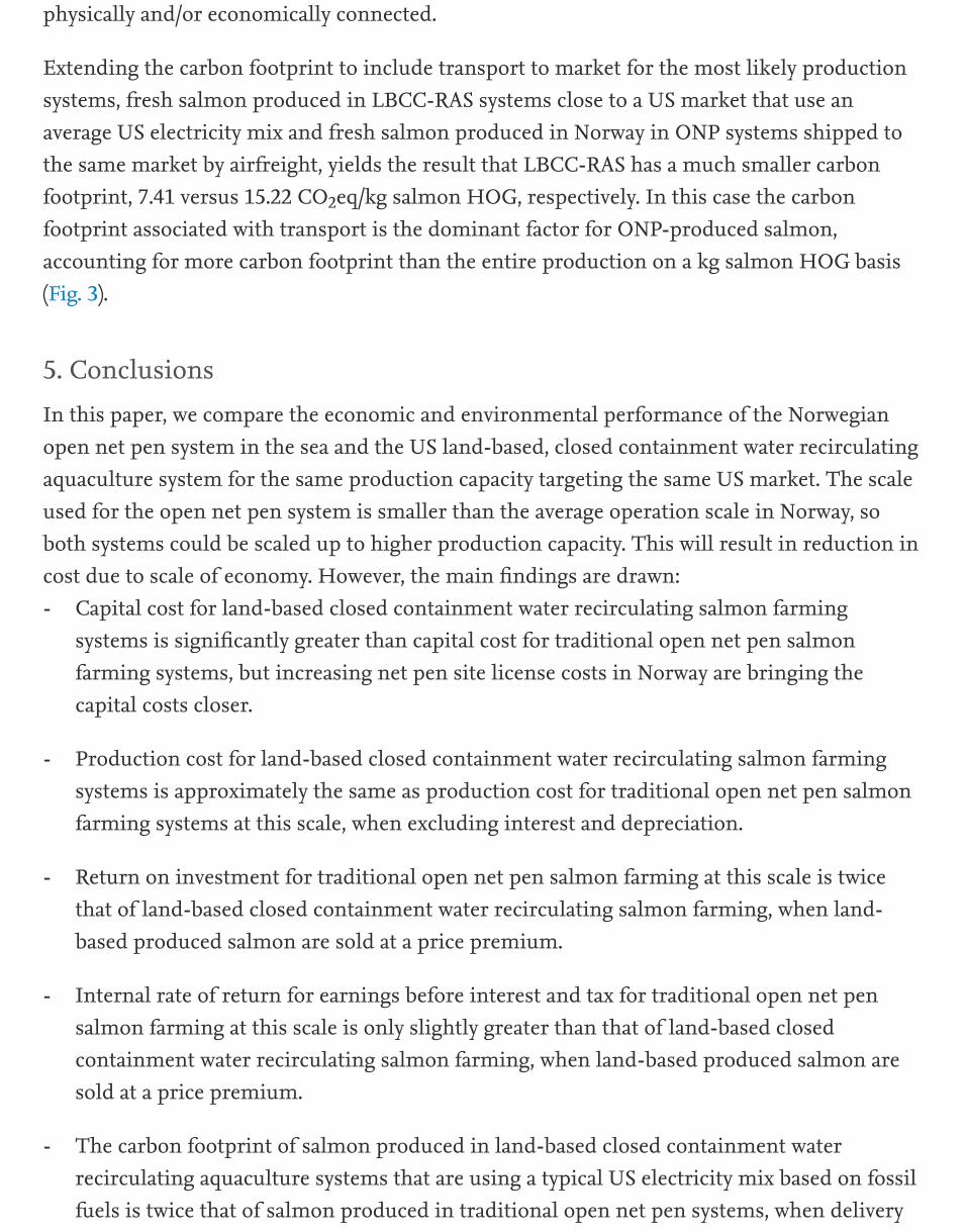
-
-
-
-
-
physically and/or economically connected.
Extending the carbon footprint to include transport to market for the most likely productionsystems, fresh salmon produced in LBCC-RAS systems close to a US market that use anaverage US electricity mix and fresh salmon produced in Norway in ONP systems shipped tothe same market by airfreight, yields the result that LBCC-RAS has a much smaller carbonfootprint, 7.41 versus 15.22 CO eq/kg salmon HOG, respectively. In this case the carbonfootprint associated with transport is the dominant factor for ONP-produced salmon,accounting for more carbon footprint than the entire production on a kg salmon HOG basis(Fig. 3).
5. ConclusionsIn this paper, we compare the economic and environmental performance of the Norwegianopen net pen system in the sea and the US land-based, closed containment water recirculatingaquaculture system for the same production capacity targeting the same US market. The scaleused for the open net pen system is smaller than the average operation scale in Norway, soboth systems could be scaled up to higher production capacity. This will result in reduction incost due to scale of economy. However, the main findings are drawn:
Capital cost for land-based closed containment water recirculating salmon farmingsystems is significantly greater than capital cost for traditional open net pen salmonfarming systems, but increasing net pen site license costs in Norway are bringing thecapital costs closer.
Production cost for land-based closed containment water recirculating salmon farmingsystems is approximately the same as production cost for traditional open net pen salmonfarming systems at this scale, when excluding interest and depreciation.
Return on investment for traditional open net pen salmon farming at this scale is twicethat of land-based closed containment water recirculating salmon farming, when land-based produced salmon are sold at a price premium.
Internal rate of return for earnings before interest and tax for traditional open net pensalmon farming at this scale is only slightly greater than that of land-based closedcontainment water recirculating salmon farming, when land-based produced salmon aresold at a price premium.
The carbon footprint of salmon produced in land-based closed containment waterrecirculating aquaculture systems that are using a typical US electricity mix based on fossilfuels is twice that of salmon produced in traditional open net pen systems, when delivery
2

-
Aardal, 2014
Ayer and Tyedmers, 2009
Badiola et al., 2012
Bailly and Willmann, 2001
to the market is not included.
The carbon footprint of salmon produced in land-based closed containment waterrecirculating aquaculture systems delivered to market in the US is less than half of that forsalmon produced in traditional open net pen systems in Norway that is delivered to the USby air freight.
AcknowledgementsThe authors thank the Agriculture Research Service of the United States Department ofAgriculture (Agreement No. 59-1930-1-130) and the Norwegian Research Council for fundingthis work.
Recommended articles Citing articles (0)
ReferencesJ. Aardal
Grønn Konsesion til Bjørøya: Bjørøya Fiskeoppdrett er tildelt grønn konsesjon foroppdrett av laksNamdalsavisa (2014)Available at: http://www.namdalsavisa.no/Nyhet/article7264369.eceGoogle Scholar
N.W. Ayer, P.H. TyedmersAssessing alternative aquaculture technologies: life cycle assessment of salmonidculture systems in CanadaJ. Clean. Prod., 17 (2009), pp. 362-373View Record in Scopus Google Scholar
M. Badiola, D. Mendiola, J. BostockRecirculating aquaculture systems (RAS) analysis: main issues on management andfuture challengesAquacult. Eng., 51 (2012), pp. 26-35View Record in Scopus Google Scholar
D. Bailly, R. WillmannPromoting sustainable aquaculture through economic and other incentivesR.P. Subasinghe, M.J. Phillips, P. Bueno, C. Hough, S.E. McGladdery, J.R. Arthur (Eds.),

Bergheim et al., 2009
Centre for Design and Society of the RMIT University,2014
Dalsgaard et al., 2013
Dekamin et al., 2015
d’Orbcastel et al., 2009
De Ionno et al., 2006
Aquaculture in the Third Millennium, FAO, Rome (2001), pp. 95-101View Record in Scopus Google Scholar
A. Bergheim, A. Drengstig, Y. Ulgenes, S. FivelstadProduction of Atlantic salmon smolts in Europe—current characteristics and futuretrendsAquacult. Eng., 41 (2009), pp. 46-52View Record in Scopus Google Scholar
Centre for Design and Society ofthe RMIT University
Agrifootprint [Data File]PRé Consultants, Amersfoort, The Netherlands (2014)Google Scholar
J. Dalsgaard, I. Lund, R. Thorarinsdottir, A. Drengstig, K. Arvonen, P.B.PedersenFarming different species in RAS in Nordic countries: current status and futureperspectivesAquacult. Eng., 53 (2013), pp. 2-13View Record in Scopus Google Scholar
M. Dekamin, H. Veisi, E. Safari, H. Liaghati, K. Khoshbakht, M.G.DekaminLife cycle assessment for rainbow trout (Oncorhynchus mykiss) production systems: acase study for IranJ. Clean. Prod., 91 (2015), pp. 43-55View Record in Scopus Google Scholar
E.R. d’Orbcastel, J.-P. Blancheton, J. AubinTowards environmentally sustainable aquaculture: comparison between two troutfarming systems using life cycle assessmentAquacult. Eng., 40 (2009), pp. 113-119View Record in Scopus Google Scholar
P.N. De Ionno, G.L. Wines, P.L. Jones, R.O. CollinsA bioeconomic evaluation of a commercial scale recirculating finfish growout system—an Australian perspectiveAquaculture, 259 (2006), pp. 315-327View Record in Scopus Google Scholar

Directorate of Fisheries,2014
Ecoinvent, 2013
Färe et al., 2005
Gempesaw et al., 1993
Heinsbroek and Kamstra, 1990
Hognes et al., 2011
Hognes et al., 2014
Directorate of FisheriesProfitability Survey on the Production of Atlantic Salmon andRainbow Trout
Statistics–Norwegian Aquaculture (2014)Available from Directorate of Fisheries website,http://www.fiskeridir.no/english/statisticsGoogle Scholar
Ecoinvent v3.1., 2013. LCA background database. Access can be purchased athttp://www.ecoinvent.org/database/ecoinvent-version-3/ecoinvent-v30/.Google Scholar
R. Färe, S. Grosskopf, B.-E. Roland, W.L. WeberLicense fees: the case of Norwegian salmon farmingWorking Paper Series in Economics and Management No.07/05 October 2005,University of Tromsø (2005)Google Scholar
C.M. Gempesaw, I. Supitaningsih, J.R. Bacon, J. Heinen, J. Hankins, J.WangEconomic analysis of an intensive aquaculture recirculating system for troutproductionJ. Wang (Ed.), Techniques for Modern Aquaculture, American Society of AgriculturalEngineers, St. Joseph, MI (1993), pp. 263-277View Record in Scopus Google Scholar
L.T.N. Heinsbroek, A. KamstraDesign and performance of water recirculation systems for eel cultureAquacult. Eng., 9 (1990), pp. 187-207View Record in Scopus Google Scholar
E.S. Hognes, F. Ziegler, V. SundCarbon Footprint and Area Use of Farmed Norwegian Salmon (SINTEF Fisheries andAquaculture Report: A22673)SINTEF Fisheries and Aquaculture, Trondheim, Norway (2011)Google Scholar
E.S. Hognes, G. Angus, F. ZieglerHandbook for Greenhouse Gas Assessment of Seafood Products (SINTEF Fisheriesand Aquaculture Report: A26745)

ISO, 2006a
ISO, 2006b
IPCC, 2007
Kolarevic et al., 2014
Kumar and Engle, 2011
Liu and Bjelland, 2014
SINTEF Fisheries and Aquaculture, Trondheim, Norway (2014)Google Scholar
International Organization for Standardization [ISO]ISO 14040:2006(E). Environmental Management–Life Cycle Assessment–Principles andFrameworkISO, Geneva, Switzerland (2006)Google Scholar
International Organization for Standardization [ISO]ISO 14044:2006(E). Environmental Management–Life Cycle Assessment–Requirementsand GuidelinesISO, Geneva, Switzerland (2006)Google Scholar
Intergovernmental Panel on Climate Change [IPCC]Contribution of Working Group IS. Solomon, D. Qin, M. Manning, Z. Chen, M. Marquis, K.B. Averyt, M. Tignor, H.L.Miller (Eds.), Fourth Assessment Report of the Intergovernmental Panel on ClimateChange, Cambridge University Press, Cambridge, UK (2007)Google Scholar
J. Kolarevic, G. Baeverfjord, H. Takle, E. Ytteborg, B.K.M. Reiten, S.Nergård, B.F. TerjesenPerformance and welfare of Atlantic salmon smolt reared in recirculating or flowthrough aquaculture systemsAquaculture, 432 (2014), pp. 15-25View Record in Scopus Google Scholar
G. Kumar, C. EngleThe effect of hybrid catfish fingerling prices on the relative profitability of hybridchannel catfishJ. World Aquacult. Soc., 42 (2011), pp. 469-483CrossRef View Record in Scopus Google Scholar
Y. Liu, H.V. BjellandEstimating costs of sea lice control strategy in NorwayPrev. Vet. Med., 117 (2014), pp. 469-477CrossRef View Record in Scopus Google Scholar

Liu et al., 2013
Liu and Sumaila, 2007
Losordo and Westerman, 1994
Marine Harvest ASA, 2014
Martins et al., 2010
Mattilsynet, 2011
McGrath et al., 2015
Muir, 1981
Y. Liu, R. Chuenpagdee, R. SumailaHow governable is salmon aquaculture?M. Bavinck, R. Chuenpagdee, S. Jentoft, J. Kooiman (Eds.), Governability of Fisheriesand Aquaculture: Theory and Applications, Springer, New York (2013), pp. 201-218CrossRef View Record in Scopus Google Scholar
Y. Liu, U.R. SumailaEconomic analysis of netcage versus sea-bag production systems for salmonaquaculture in British ColumbiaAquacult. Econ. Manag., 11 (2007), pp. 371-395CrossRef View Record in Scopus Google Scholar
T.M. Losordo, P.W. WestermanAn analysis of biological, economic, and engineering factors affecting the cost of fishproduction in recirculating aquaculture systemsJ. World Aquacult. Soc., 25 (2) (1994), pp. 193-203CrossRef View Record in Scopus Google Scholar
Marine Harvest ASA., 2014. Salmon Farming Industry Handbook2014. Available from Marine Harvest web site, (June)http://www.marineharvest.com/globalassets/investors/handbook/handbook-2014.pdf.Google Scholar
C.I.M. Martins, E.H. Eding, M.C. Verdegem, L.T. Heinsbroek, O.Schneider, J.-P. Blancheton, J.A.J. VerrethNew developments in recirculating aquaculture systems in Europe: a perspective onenvironmental sustainabilityAquacult. Eng., 43 (2010), pp. 83-93View Record in Scopus Google Scholar
Mattilsynet, 2011. Per Generation Mortality for Atlantic salmon. Availablefrom Mattilsynet website, http://www.mattilsynet.no/fisk_og_akvakultur/.Google Scholar
K.P. McGrath, N.L. Pelletier, P.H. TyedmersLife cycle assessment of a novel closed-containment salmon aquaculture technologyEnviron. Sci. Technol., 49 (2015), pp. 5628-5636CrossRef View Record in Scopus Google Scholar
J. Muir

Naylor et al., 2005
Norway, 2008
Rosten et al., 2013
RS Means, 2010
Samuel-Fitwi et al., 2013
Statistics Norway, 2015
Summerfelt and Christianson, 2014
Management and cost implications in recirculating water systemsL.J. Allen, E.C. Kinney (Eds.), Proceedings of the Bio-Engineering Symposium for FishCulture (FCS Publ. 1), American Fisheries Society, Bethesda, MD (1981), pp. 116-127View Record in Scopus Google Scholar
R. Naylor, K. Hindar, I. Fleming, R. Goldburg, S. Williams, J. Volpe, F.Whoriskey, J. Eagle, D. Kelso, M. MangelFugitive salmon: assessing the risks of escaped fish from net-pen aquacultureBioscience, 55 (2005), pp. 427-437View Record in Scopus Google Scholar
Norway, 2008. Regulations on the Operation of Aquaculture Facilities (FOR2008-06-17 No. 822). Available from LOVDATA website,https://lovdata.no/dokument/SF/forskrift/2008-06-17-822?q=akvakulturloven.Google Scholar
T. Rosten, B.F. Terjesen, Y. Ulgenes, K. Henriksen, E. Biering, U. Wintherlukkede oppdrettsanlegg i sjø–økt kunnskap er nødvendigVANN 01 2013 (2013), pp. 5-13View Record in Scopus Google Scholar
RS Means, 2010. Facilities construction cost data, 2010. Access can bepurchased at http://www.rsmeans.com/65205.aspx.Google Scholar
B. Samuel-Fitwi, F. Nagel, S. Meyer, J.P. Schroeder, C. SchulzComparative life cycle assessment (LCA) of raising rainbow trout (Oncorhynchus mykiss)in different production systemsAquacult. Eng., 54 (2013), pp. 85-92View Record in Scopus Google Scholar
Statistics Norway, 2015. Export of Salmon. Available from StatisticsNorway website, https://www.ssb.no/en/utenriksokonomi/statistikker/laks.Google Scholar
S. Summerfelt, L. ChristiansonFish farming in land-based closed-containment systemsWorld Aquacult. (March) (2014), pp. 18-22View Record in Scopus Google Scholar
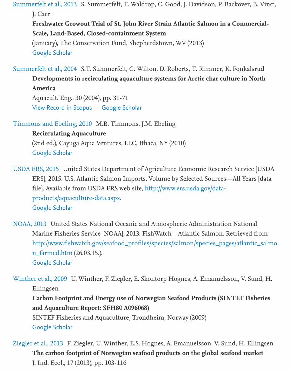
Summerfelt et al., 2013
Summerfelt et al., 2004
Timmons and Ebeling, 2010
USDA ERS, 2015
NOAA, 2013
Winther et al., 2009
Ziegler et al., 2013
S. Summerfelt, T. Waldrop, C. Good, J. Davidson, P. Backover, B. Vinci,J. CarrFreshwater Growout Trial of St. John River Strain Atlantic Salmon in a Commercial-Scale, Land-Based, Closed-containment System(January), The Conservation Fund, Shepherdstown, WV (2013)Google Scholar
S.T. Summerfelt, G. Wilton, D. Roberts, T. Rimmer, K. FonkalsrudDevelopments in recirculating aquaculture systems for Arctic char culture in NorthAmericaAquacult. Eng., 30 (2004), pp. 31-71View Record in Scopus Google Scholar
M.B. Timmons, J.M. EbelingRecirculating Aquaculture(2nd ed.), Cayuga Aqua Ventures, LLC, Ithaca, NY (2010)Google Scholar
United States Department of Agriculture Economic Research Service [USDAERS], 2015. U.S. Atlantic Salmon Imports, Volume by Selected Sources—All Years [datafile]. Available from USDA ERS web site, http://www.ers.usda.gov/data-products/aquaculture-data.aspx.Google Scholar
United States National Oceanic and Atmospheric Administration NationalMarine Fisheries Service [NOAA], 2013. FishWatch—Atlantic Salmon. Retrieved fromhttp://www.fishwatch.gov/seafood_profiles/species/salmon/species_pages/atlantic_salmon_farmed.htm (26.03.15.).Google Scholar
U. Winther, F. Ziegler, E. Skontorp Hognes, A. Emanuelsson, V. Sund, H.EllingsenCarbon Footprint and Energy use of Norwegian Seafood Products (SINTEF Fisheriesand Aquaculture Report: SFH80 A096068)SINTEF Fisheries and Aquaculture, Trondheim, Norway (2009)Google Scholar
F. Ziegler, U. Winther, E.S. Hognes, A. Emanuelsson, V. Sund, H. EllingsenThe carbon footprint of Norwegian seafood products on the global seafood marketJ. Ind. Ecol., 17 (2013), pp. 103-116

CrossRef View Record in Scopus Google Scholar
1 US dollar = 7 Norwegian kroners.
Copyright © 2016 The Authors. Published by Elsevier B.V.
1
About ScienceDirect Remote access Shopping cart Advertise Contact and support Terms and conditionsPrivacy policy
We use cookies to help provide and enhance our service and tailor content and ads. By continuing you agree to theuse of cookies.Copyright © 2019 Elsevier B.V. or its licensors or contributors. ScienceDirect ® is a registered trademark of Elsevier B.V.ScienceDirect ® is a registered trademark of Elsevier B.V.
Related Documents