TR0003 (REV 10/98) TECHNICAL REPORT DOCUMENTATION PAGE STATE OF CALIFORNIA • DEPARTMENT OF TRANSPORTATION Reproduction of completed page authorized. 1. REPORT NUMBER CA15-2107 2. GOVERNMENT ASSOCIATION NUMBER 3. RECIPIENT'S CATALOG NUMBER 4. TITLE AND SUBTITLE Non-destructive Damage Evaluation Based on Power Method with Time Collocation 5. REPORT DATE March 2016 6. PERFORMING ORGANIZATION CODE 7. AUTHOR Li, R., Keating, P. B., and Stubbs, N. 8. PERFORMING ORGANIZATION REPORT NO. 9. PERFORMING ORGANIZATION NAME AND ADDRESS Texas A&M Transportation Institute Texas A&M University College Station, TX 77843-3135 10. WORK UNIT NUMBER 11. CONTRACT OR GRANT NUMBER 65A0401 12. SPONSORING AGENCY AND ADDRESS California Department of Transportation Division of Engineering Services 1801 30th Street, MS #9-2/5I Sacramento, CA 95815 13. TYPE OF REPORT AND PERIOD COVERED Final 14. SPONSORING AGENCY CODE 15. SUPPLEMENTARY NOTES 16. ABSTRACT The objective of this dissertation is to develop a nondestructive evaluation (NDE) method that could accurately locate and evaluate damage in mass, stiffness and damping properties of structural members. The method is based on the power (Refer to the definition in Section 2.2) equilibrium between the undamaged and damaged structural systems. The method is applicable to a variety of structures and has high tolerance capacity to noise. To demonstrate the above characteristics of the proposed method, the following several tasks will be addressed: (1) the application of the proposed method to different discrete systems with exact deformation data; (2) the application of the proposed method to different continuous systems with exact deformation data; (3) the application of the proposed method to discrete and continuous systems with noise-polluted inputs; (4) the validation of the proposed method using field data. The damage detection results from Task #1 and Task #2 indicated that the proposed method can accurately locate and evaluate damage in mass, stiffness and damping of the structure if exact deformation data were given. The results from Task #3 indicated that the proposed method is proved to be effective in locating and evaluating damage at least fewer than 5% white noise. The damage evaluation results from the field experiment showed that the proposed method is applicable to real-world damage detection by providing damage locations and estimations of damage severities. 17. KEY WORDS non-destructive damage evaluation (NDE); time domain; damage severity 18. DISTRIBUTION STATEMENT No restrictions. This document is available to the public through the National Technical Information Center, Springfield, Virginia 22161 19. SECURITY CLASSIFICATION (of this report) Unclassified 20. NUMBER OF PAGES 447 21. COST OF REPORT CHARGED For individuals with sensory disabilities, this document is available in alternate formats. For information call (916) 654-6410 or TDD (916) 654-3880 or write Records and Forms Management, 1120 N Street, MS-89, Sacramento, CA 95814. ADA Notice

Welcome message from author
This document is posted to help you gain knowledge. Please leave a comment to let me know what you think about it! Share it to your friends and learn new things together.
Transcript

TR0003 (REV 10/98)TECHNICAL REPORT DOCUMENTATION PAGESTATE OF CALIFORNIA • DEPARTMENT OF TRANSPORTATION
Reproduction of completed page authorized.
1. REPORT NUMBER
CA15-2107
2. GOVERNMENT ASSOCIATION NUMBER 3. RECIPIENT'S CATALOG NUMBER
4. TITLE AND SUBTITLE
Non-destructive Damage Evaluation Based on Power Method with Time Collocation5. REPORT DATE
March 20166. PERFORMING ORGANIZATION CODE
7. AUTHOR
Li, R., Keating, P. B., and Stubbs, N.
8. PERFORMING ORGANIZATION REPORT NO.
9. PERFORMING ORGANIZATION NAME AND ADDRESS
Texas A&M Transportation Institute Texas A&M University College Station, TX 77843-3135
10. WORK UNIT NUMBER
11. CONTRACT OR GRANT NUMBER
65A040112. SPONSORING AGENCY AND ADDRESS
California Department of Transportation Division of Engineering Services 1801 30th Street, MS #9-2/5I Sacramento, CA 95815
13. TYPE OF REPORT AND PERIOD COVERED
Final
14. SPONSORING AGENCY CODE
15. SUPPLEMENTARY NOTES
16. ABSTRACT
The objective of this dissertation is to develop a nondestructive evaluation (NDE) method that could accurately locate and evaluate damage in mass, stiffness and damping properties of structural members. The method is based on the power (Refer to the definition in Section 2.2) equilibrium between the undamaged and damaged structural systems. The method is applicable to a variety of structures and has high tolerance capacity to noise. To demonstrate the above characteristics of the proposed method, the following several tasks will be addressed: (1) the application of the proposed method to different discrete systems with exact deformation data; (2) the application of the proposed method to different continuous systems with exact deformation data; (3) the application of the proposed method to discrete and continuous systems with noise-polluted inputs; (4) the validation of the proposed method using field data. The damage detection results from Task #1 and Task #2 indicated that the proposed method can accurately locate and evaluate damage in mass, stiffness and damping of the structure if exact deformation data were given. The results from Task #3 indicated that the proposed method is proved to be effective in locating and evaluating damage at least fewer than 5% white noise. The damage evaluation results from the field experiment showed that the proposed method is applicable to real-world damage detection by providing damage locations and estimations of damage severities.
17. KEY WORDS
non-destructive damage evaluation (NDE); time domain; damage severity
18. DISTRIBUTION STATEMENT
No restrictions. This document is available to the public through the National Technical Information Center, Springfield, Virginia 22161
19. SECURITY CLASSIFICATION (of this report)
Unclassified
20. NUMBER OF PAGES
447
21. COST OF REPORT CHARGED
For individuals with sensory disabilities, this document is available in alternate formats. For information call (916) 654-6410 or TDD (916) 654-3880 or write Records and Forms Management, 1120 N Street, MS-89, Sacramento, CA 95814.
ADA Notice

ii
DISCLAIMER STATEMENT
This document is disseminated in the interest of information exchange. The contents of
this report reflect the views of the authors who are responsible for the facts and accuracy
of the data presented herein. The contents do not necessarily reflect the official views or
policies of the State of California or the Federal Highway Administration. This
publication does not constitute a standard, specification or regulation. This report does
not constitute an endorsement by the Department of any product described herein.
For individuals with sensory disabilities, this document is available in alternate formats.
For information, call (916) 654-8899, TTY 711, or write to California Department of
Transportation, Division of Research, Innovation and System Information, MS-83, P.O.
Box 942873, Sacramento, CA 94273-0001.

Report No. CA15-2107
NON-DESTRUCTIVE DAMAGE EVALUATION BASED ON POWER METHOD WITH TIME COLLOCATION
Final Report
Submitted to California Department of Transportation
Division of Engineering Services Sacramento, California 95815
by
Ran Li Graduate Research Assistant
Peter B. Keating, Ph.D., P.E. Associate Research Engineer
Norris Stubbs, Ph.D., P. E.
Research Engineer
Texas A&M Transportation Institute Texas A&M University
College Station, Texas 77843-3135
March 2016

iii
ABSTRACT
The objective of this dissertation is to develop a nondestructive evaluation (NDE)
method that could accurately locate and evaluate damage in mass, stiffness and damping
properties of structural members. The method is based on the power (Refer to the
definition in Section 2.2) equilibrium between the undamaged and damaged structural
systems. The method is applicable to a variety of structures and has high tolerance
capacity to noise. To demonstrate the above characteristics of the proposed method, the
following several tasks will be addressed: (1) the application of the proposed method to
different discrete systems with exact deformation data; (2) the application of the
proposed method to different continuous systems with exact deformation data; (3) the
application of the proposed method to discrete and continuous systems with
noise-polluted inputs; (4) the validation of the proposed method using field data. The
damage detection results from Task #1 and Task #2 indicated that the proposed method
can accurately locate and evaluate damage in mass, stiffness and damping of the
structure if exact deformation data were given. The results from Task #3 indicated that
the proposed method is proved to be effective in locating and evaluating damage at least
fewer than 5% white noise. The damage evaluation results from the field experiment
showed that the proposed method is applicable to real-world damage detection by
providing damage locations and estimations of damage severities.

iv
TABLE OF CONTENTS
Page
DISCLAIMER STATEMENT ......................................................................................... ii
ABSTRACT .................................................................................................................... iii
TABLE OF CONTENTS ................................................................................................ iv
LIST OF FIGURES ....................................................................................................... viii
LIST OF TABLES ........................................................................................................ xxv
1 INTRODUCTION ......................................................................................................... 1
1.1 Problem Statement ......................................................................................... 1
1.2 Background on Non-Destructive Evaluation Method .................................... 2
1.3 Limitations of Current Non-Destructive Evaluation Techniques ................. 15
1.4 Research Objectives ..................................................................................... 18
1.5 Significance of This Work ............................................................................ 20
2 THEORY OF DAMAGE EVALUATION ON MASS, STIFFNESS, AND
DAMPING FOR DISCRETE SYSTEMS ................................................................. 22
2.1 Introduction .................................................................................................. 22
2.2 Development of the General Power Method ................................................ 22
2.3 Theory for 1-DOF Spring-Mass-Damper Systems ...................................... 25
2.4 Theory for 2-DOF Spring-Mass-Damper Systems ...................................... 29
2.5 Theory for N-DOF Spring-Mass-Damper Systems ...................................... 37
2.6 Theory for Isolated Spring-Mass-Damper Systems ..................................... 51
2.7 Overall Solution Procedure .......................................................................... 57
2.8 Summary ...................................................................................................... 57
3 CASE STUDIES OF DAMAGE EVALUATION FOR DISCRETE SYSTEMS ....... 59
3.1 Introduction .................................................................................................. 59

v
Page
3.2 Damage Evaluation for a 1-DOF Spring-Mass-Damper System ................. 60
3.3 Damage Evaluation for a 2-DOF Spring-Mass-Damper System ................. 65
3.4 Damage Evaluation for an N-DOF Spring-Mass-Damper System .............. 71
3.5 Damage Evaluation for Isolated Spring-Mass-Damper Systems ................. 78
3.6 Summary ...................................................................................................... 83
4 THEORY OF DAMAGE EVALUATION ON MASS AND STIFFNESS FOR
CONTINUOUS SYSTEMS ....................................................................................... 84
4.1 Introduction .................................................................................................. 84
4.2 Theory for Rods ............................................................................................ 84
4.3 Theory for Euler-Bernoulli Beams ............................................................. 109
4.4 Theory for Plane Frames ............................................................................ 118
4.5 Theory for Space Trusses ........................................................................... 127
4.6 Overall Solution Procedure ........................................................................ 138
4.7 Summary .................................................................................................... 139
5 CASE STUDIES OF DAMAGE EVALUATION FOR CONTINUOUS
SYSTEMS ................................................................................................................ 141
5.1 Introduction ................................................................................................ 141
5.2 Damage Evaluation for a Rod .................................................................... 142
5.3 Damage Evaluation for a Rod as a Whole System ..................................... 150
5.4 Damage Evaluation for an Euler-Bernoulli Beam ..................................... 157
5.5 Damage Evaluation for a Plain Frame ....................................................... 165
5.6 Damage Evaluation for a Space Truss ........................................................ 178
5.7 Summary .................................................................................................... 186
6 STUDIES OF NOISE INFLUENCE TO THE PERFORMANCE OF THE POWER
METHOD ................................................................................................................. 187
6.1 Introduction ................................................................................................ 187
6.2 Studies of Noise Influence to a Discrete System Using Integral
Method ..................................................................................................... 191
6.3 Studies of Noise Influence to a Discrete System Using Isolation
Method ..................................................................................................... 210

vi
Page
6.4 Studies of Noise Influence to a Continuous System Using Integral
Method ..................................................................................................... 232
6.5 Studies of Noise Influence to a Continuous System Using Isolation
Method ..................................................................................................... 249
6.6 Evaluation of Results ................................................................................. 271
7 REANALYSIS .......................................................................................................... 284
7.1 Introduction ................................................................................................ 284
7.2 Study of Nodes without External Loads (Case #7.1) ................................. 284
7.3 Study of Efficiency of Noise-Influence Reduction by Repeating the
Experiment (Case #7.2) ............................................................................ 299
7.4 Study of Damage Detection in Continuous Structures with Proportional
Damping (Case #7.3) ................................................................................ 308
8 APPLICATION OF THE METHOD TO SHAKE TABLE TESTS .......................... 336
8.1 Introduction ................................................................................................ 336
8.2 Description of the Structure and Test Setup ............................................... 336
8.3 Theory of Approach .................................................................................... 343
8.4 Experimental Data Processing.................................................................... 354
8.5 Damage Evaluation of the Shake Table Tests ............................................ 363
8.6 Evaluation of Designed Damage Extent .................................................... 371
8.7 Results Discussion ...................................................................................... 377
8.8 Damage Evaluation with Element Damping Effect ................................... 379
8.9 Conclusion .................................................................................................. 387
9 SUMMARY AND CONCLUSIONS ........................................................................ 388
9.1 Summary .................................................................................................... 388
9.2 Findings ...................................................................................................... 389
9.3 Originality of This Work ............................................................................ 392
9.4 Contribution of This Work ......................................................................... 393
9.5 Conclusion .................................................................................................. 394
9.6 Future Work ................................................................................................ 394

vii
Page
REFERENCES ............................................................................................................. 397
APPENDIX .................................................................................................................. 403

viii
LIST OF FIGURES
Page
Figure 2.1. 1-DOF Spring-Mass-Damper System .......................................................... 26
Figure 2.2. 2-DOF Spring-Mass-Damper System .......................................................... 30
Figure 2.3. 5-DOF Spring-Mass-Damper System .......................................................... 38
Figure 2.4. Isolated Spring-Mass-Damper System ........................................................ 51
Figure 3.1. Property Definition and Load Case of the 1-DOF
Spring-Mass-Damper System .................................................................... 61
Figure 3.2. Applied External Load for Both the Undamaged and Damaged Cases ....... 62
Figure 3.3. Displacements of the Mass Block under the Given External Load ............. 62
Figure 3.4. Velocities of the Mass Block under the Given External Load ..................... 63
Figure 3.5. Accelerations of the Mass Block under the Given External Load ............... 63
Figure 3.6. Element Damage Indices (βi) for 1-DOF Spring-Mass-Damper
System ........................................................................................................ 64
Figure 3.7. Element Damage Severities (аi) for 1-DOF Spring-Mass-Damper
System ........................................................................................................ 65
Figure 3.8. Property Definition and Load Case of the 2-DOF
Spring-Mass-Damper System .................................................................... 66
Figure 3.9. Applied External Load for Both the Undamaged and Damaged Cases ....... 67
Figure 3.10. Displacements of the Mass Block 1 under the Given External Load ........ 68
Figure 3.11. Velocities of the Mass Block 1 under the Given External Load ................ 68

ix
Page
Figure 3.12. Accelerations of the Mass Block 1 under the Given External Load .......... 69
Figure 3.13. Element Damage Indices (βi) for 2-DOF Spring-Mass-Damper
System ........................................................................................................ 70
Figure 3.14. Element Damage Severities (аi) for 2-DOF Spring-Mass-Damper
System ........................................................................................................ 70
Figure 3.15. Property Definition and Load Case of the 5-DOF
Spring-Mass-Damper System .................................................................... 72
Figure 3.16. Applied External Load for Both the Undamaged and Damaged Cases ..... 74
Figure 3.17. Displacements of the Mass Block 1 under the Given External Load ........ 74
Figure 3.18. Velocities of the Mass Block 1 under the Given External Load ................ 75
Figure 3.19. Accelerations of the Mass Block 1 under the Given External Load .......... 75
Figure 3.20. Element Damage Indices (βi) for 5-DOF Spring-Mass-Damper
System ........................................................................................................ 77
Figure 3.21. Element Damage Severities (аi) for 5-DOF Spring-Mass-Damper
System ........................................................................................................ 77
Figure 3.22. Property Definition and Load Case of the Isolated
Spring-Mass-Damper System .................................................................... 79
Figure 3.23. Element Damage Indices (βi) for Isolated Spring-Mass-Damper
System ........................................................................................................ 81
Figure 3.24. Element Damage Severities (аi) for Isolated Spring-Mass-Damper
System ........................................................................................................ 82
Figure 4.1. Two nearby Rod Elements ........................................................................... 85
Figure 4.2. Free Body Diagram of Node i under Axial and Torsional Effects ............... 86

x
Page
Figure 4.3. Two nearby Rod Elements ........................................................................... 96
Figure 4.4. Free Body Diagram of Node i under Axial Effects ...................................... 96
Figure 4.5. Two nearby Euler–Bernoulli Beam Elements Considering Shear
Force and Bending Moment ..................................................................... 110
Figure 4.6. Free Body Diagram of Node i Considering Shear Force and Bending
Moment .................................................................................................... 110
Figure 4.7. Two nearby Plane Frame Elements ............................................................ 119
Figure 4.8. Free Body Diagram of Node i Considering Axial, Shear Forces, and
Bending Moment ...................................................................................... 119
Figure 4.9. One Joint from a Space Truss with All Bars Joined to the Joint γ ............. 128
Figure 4.10. Free Body Diagram of Joint γ in Space ................................................... 129
Figure 5.1. Geometry, Damage Scenario, and Finite Element Discretization of
the Rod ..................................................................................................... 144
Figure 5.2. Geometry of the Cross-Section of the Rod ................................................ 145
Figure 5.3. Displacements in Axial Direction of the Node 13 of the Undamaged
and Damaged Rods under the Given External Load ................................ 145
Figure 5.4. Velocities of the Node 13 in Axial Direction of the Undamaged and
Damaged Rods under the Given External Load ....................................... 146
Figure 5.5. Accelerations of the Node 13 in Axial Direction of the Undamaged
and Damaged Rods under the Given External Load ................................ 146
Figure 5.6. Damage Indices of Nodal Mass (βmi) for the Rod under Axial and
Torsional Vibrations ................................................................................. 148

xi
Page
Figure 5.7. Damage Severities of Nodal Mass (аmi) for the Rod under Axial and
Torsional Vibrations ................................................................................. 148
Figure 5.8. Damage Indices of Element Stiffness (βki) for the Rod under Axial
and Torsional Vibrations ........................................................................... 149
Figure 5.9. Damage Severities of Element Stiffness (аki) for the Rod under Axial
and Torsional Vibrations ........................................................................... 149
Figure 5.10. Geometry, Damage Scenario, and Finite Element Discretization of
the Rod ..................................................................................................... 152
Figure 5.11. Displacements in Axial Direction of Node 13 of the Undamaged
and Damaged Rods under the Given External Load ................................ 152
Figure 5.12. Velocities of Node 13 in Axial Direction of the Undamaged and
Damaged Rods under the Given External Load ....................................... 153
Figure 5.13. Accelerations of Node 13 in Axial Direction of the Undamaged
and Damaged Rods under the Given External Load ................................ 153
Figure 5.14. Damage Indices of Nodal Mass (βmi) for the Rod under Axial and
Torsional Vibrations ................................................................................. 155
Figure 5.15. Damage Severities of Nodal Mass (аmi) for the Rod under Axial
and Torsional Vibrations ........................................................................... 155
Figure 5.16. Damage Indices of Element Stiffness (βki) for the Rod under Axial
and Torsional Vibrations ........................................................................... 156
Figure 5.17. Damage Severities of Element Stiffness (аki) for the Rod under
Axial and Torsional Vibrations ................................................................. 156
Figure 5.18. Geometry, Damage Scenario, and Load Case for the Propped
Cantilever ................................................................................................. 159
Figure 5.19. Geometry of the Cross-Section of the I Beam ......................................... 159

xii
Page
Figure 5.20. Deflection of the Node 7 of the Undamaged and Damaged Cases
under the Given External Load ................................................................ 160
Figure 5.21. Velocities in Transverse Direction of the Node 7 of the Undamaged
and Damaged Cases under the Given External Load ............................... 160
Figure 5.22. Accelerations in Transverse Direction of the Node 7 of the
Undamaged and Damaged Cases under the Given External Load ........... 161
Figure 5.23. Damage Indices of Nodal Mass (βmi) for the Propped Cantilever ........... 163
Figure 5.24. Damage Severities of Nodal Mass (аmi) for the Propped Cantilever ....... 163
Figure 5.25. Damage Indices of Element Stiffness (βki) for the Propped
Cantilever ................................................................................................. 164
Figure 5.26. Damage Severities of Element Stiffness (аki) for the Propped
Cantilever ................................................................................................. 164
Figure 5.27. Geometry, Damage Scenario, and Finite Element Discretization for
the Two-Bay Frame .................................................................................. 168
Figure 5.28. Cross Sectional Geometries of the Three Elastic Isolators ...................... 168
Figure 5.29. Displacements of the Node 61 on the Continuous Beam for Both
the Undamaged and Damaged Cases under the Given External
Load .......................................................................................................... 169
Figure 5.30. Velocities of the Node 61 on the Continuous Beam for Both the
Undamaged and Damaged Cases under the Given External Load ........... 169
Figure 5.31. Accelerations of the Node 61 on the Continuous Beam for Both
the Undamaged and Damaged Cases under the Given External
Load .......................................................................................................... 170
Figure 5.32. Damage Indices of Nodal Mass (βmi) for the Continuous Beam from
the Two-Bay Frame .................................................................................. 170
xiii
Page
Figure 5.33. Damage Severities of Nodal Mass (аmi) for the Continuous Beam
from the Two-Bay Frame ......................................................................... 171
Figure 5.34. Damage Indices of Element Stiffness (βki) for the Continuous
Beam from the Two-Bay Frame ............................................................... 171
Figure 5.35. Damage Severities of Element Stiffness (аki) for the Continuous
Beam from the Two-Bay Frame ............................................................... 172
Figure 5.36. Damage Indices of Nodal Mass (βmi) for the Isolator and Column A
from the Two-Bay Frame ......................................................................... 172
Figure 5.37. Damage Severities of Nodal Mass (аmi) for the Isolator and
Column A from the Two-Bay Frame ........................................................ 173
Figure 5.38. Damage Indices of Element Stiffness (βki) for the Isolator and
Column A from the Two-Bay Frame ........................................................ 173
Figure 5.39. Damage Severities of Element Stiffness (аki) for the Isolator and
Column A from the Two-Bay Frame ........................................................ 174
Figure 5.40. Damage Indices of Nodal Mass (βmi) for the Isolator and
Column B from the Two-Bay Frame ........................................................ 174
Figure 5.41. Damage Severities of Nodal Mass (аmi) for the Isolator and
Column B from the Two-Bay Frame ........................................................ 175
Figure 5.42. Damage Indices of Element Stiffness (βki) for the Isolator and
Column B from the Two-Bay Frame ........................................................ 175
Figure 5.43. Damage Severities of Element Stiffness (аki) for the Isolator and
Column B from the Two-Bay Frame ........................................................ 176
Figure 5.44. Damage Indices of Nodal Mass (βmi) for the Isolator and
Column C from the Two-Bay Frame ........................................................ 176

xiv
Page
Figure 5.45. Damage Severities of Nodal Mass (аmi) for the Isolator and
Column C from the Two-Bay Frame ........................................................ 177
Figure 5.46. Damage Indices of Element Stiffness (βki) for the Isolator and
Column C from the Two-Bay Frame ........................................................ 177
Figure 5.47. Damage Severities of Element Stiffness (аki) for the Isolator and
Column C from the Two-Bay Frame ...................................................... 178
Figure 5.48. Geometry, Damage Scenario, and Finite Element Discretization for
the Space Truss ......................................................................................... 180
Figure 5.49. Displacements of the Joint 6 in Global X Direction for Both the
Undamaged and Damaged Systems under the Given External
Load .......................................................................................................... 181
Figure 5.50. Velocities of the Joint 6 in Global X Direction for Both the
Undamaged and Damaged Systems under the Given External
Load .......................................................................................................... 181
Figure 5.51. Accelerations of the Joint 6 in Global X Direction for Both the
Undamaged and Damaged Systems under the Given External
Load .......................................................................................................... 182
Figure 5.52. Damage Indices of Joint Mass (βmi) for the Space Truss ......................... 184
Figure 5.53. Damage Severities of Joint Mass (аmi) for the Space Truss ..................... 184
Figure 5.54. Damage Indices of Member Stiffness (βki) for the Space Truss .............. 185
Figure 5.55. Damage Severities of Member Stiffness (аki) for the Space Truss .......... 185
Figure 6.1. Property Definition and Load Case of the 5-DOF
Spring-Mass-Damper System .................................................................. 192
Figure 6.2. Applied External Excitation Forces at Each Mass Block .......................... 194

xv
Page
Figure 6.3. Noise-Polluted Accelerations of Mass Block 2 for the Undamaged
and Damaged Models of Case #6.1 (1% Noise): (a) Full Plot and
(b) Zoomed in Plot ................................................................................... 195
Figure 6.4. Filtered Noise-Polluted Accelerations of Mass Block 2 for the
Undamaged and Damaged Models of Case #6.1 (1% Noise):
(a) Full Plot and (b) Zoomed in Plot ........................................................ 196
Figure 6.5. Estimated Velocities of Mass Block 2 for the Undamaged and
Damaged Models of Case #6.1 (1% Noise): (a) Full Plot and
(b) Zoomed in Plot ................................................................................... 197
Figure 6.6. Estimated Displacements of Mass Block 2 for the Undamaged and
Damaged Models of Case #6.1 (1% Noise): (a) Full Plot
and (b) Zoomed in Plot ............................................................................. 198
Figure 6.7. Damage Indices (βi) for 5-DOF Spring-Mass-Damper System with
Noise-Polluted Accelerations (1% Noise) ................................................ 200
Figure 6.8. Damage Severities (аi) for 5-DOF Spring-Mass-Damper System
with Noise-Polluted Accelerations (1% Noise) ........................................ 200
Figure 6.9. Normalized Damage Indices (βn,i) for 5-DOF Spring-Mass-Damper
System with Noise-Polluted Accelerations (1% Noise) ........................... 201
Figure 6.10. Probability Damage Indices (βp,i) for 5-DOF Spring-Mass-Damper
System with Noise-Polluted Accelerations (1% Noise) ........................... 201
Figure 6.11. Noise-Polluted Accelerations of Mass Block 2 for the Undamaged
and Damaged Models of Case #6.2 (5% Noise): (a) Full Plot
and (b) Zoomed in Plot ............................................................................. 203
Figure 6.12. Filtered Noise-Polluted Accelerations of Mass Block 2 for the
Undamaged and Damaged Models of Case #6.2 (5% Noise):
(a) Full Plot and (b) Zoomed in Plot ........................................................ 204
xvi
Page
Figure 6.13. Estimated Velocities of Mass Block 2 for the Undamaged and
Damaged Models of Case #6.2 (5% Noise): (a) Full Plot
and (b) Zoomed in Plot ............................................................................. 205
Figure 6.14. Estimated Displacements of Mass Block 2 for the Undamaged
and Damaged Models of Case #6.2 (5% Noise): (a) Full Plot
and (b) Zoomed in Plot ............................................................................. 206
Figure 6.15. Damage Indices (βi) for 5-DOF Spring-Mass-Damper System with
Noise-Polluted Accelerations (5% Noise) ................................................ 208
Figure 6.16. Damage Severities (аi) for 5-DOF Spring-Mass-Damper System
with Noise-Polluted Accelerations (5% Noise) ........................................ 208
Figure 6.17. Normalized Damage Indices (βn,i) for 5-DOF Spring-Mass-Damper
System with Noise-Polluted Accelerations (5% Noise) ........................... 209
Figure 6.18. Probability Damage Indices (βp,i) for 5-DOF Spring-Mass-Damper
System with Noise-Polluted Accelerations (5% Noise) ........................... 209
Figure 6.19. Noise-Polluted Accelerations of Mass Block 2 for the Undamaged
and Damaged Models of Case #6.3 (1% Noise): (a) Full Plot
and (b) Zoomed in Plot ............................................................................. 213
Figure 6.20. Filtered Noise-Polluted Accelerations of Mass Block 2 for the
Undamaged and Damaged Models of Case #6.3 (1% Noise):
(a) Full Plot and (b) Zoomed in Plot ........................................................ 214
Figure 6.21. Estimated Velocities of Mass Block 2 for the Undamaged and
Damaged Models of Case #6.3 (1% Noise): (a) Full Plot
and (b) Zoomed in Plot ............................................................................. 215
Figure 6.22. Estimated Displacements of Mass Block 2 for the Undamaged and
Damaged Models of Case #6.3 (1% Noise): (a) Full Plot
and (b) Zoomed in Plot ............................................................................. 216

xvii
Page
Figure 6.23. Damage Indices (βi) for the 5 Isolated Spring-Mass-Damper System
with Noise-Polluted Accelerations (1% Noise) ........................................ 218
Figure 6.24. Damage Severities (аi) for 5-DOF Spring-Mass-Damper System
with Noise-Polluted Accelerations (1% Noise) ........................................ 219
Figure 6.25. Normalized Damage Indices (βn,i) for 5-DOF Spring-Mass-Damper
System with Noise-Polluted Accelerations (1% Noise) ........................... 220
Figure 6.26. Damage Possibility Indices (βp,i) for 5-DOF Spring-Mass-Damper
System with Noise-Polluted Accelerations (1% Noise) ........................... 221
Figure 6.27. Noise-Polluted Accelerations of Mass Block 2 for the Undamaged
and Damaged Models of Case #6.4 (5% Noise): (a) Full Plot and
(b) Zoomed in Plot ................................................................................... 223
Figure 6.28. Filtered Noise-Polluted Accelerations of Mass Block 2 for the
Undamaged and Damaged Models of Case #6.4 (5% Noise):
(a) Full Plot and (b) Zoomed in Plot ........................................................ 224
Figure 6.29. Estimated Velocities of Mass Block 2 for the Undamaged and
Damaged Models of Case #6.4 (5% Noise): (a) Full Plot
and (b) Zoomed in Plot ............................................................................. 225
Figure 6.30. Estimated Displacements of Mass Block 2 for the Undamaged and
Damaged Models of Case #6.4 (5% Noise): (a) Full Plot
and (b) Zoomed in Plot ............................................................................. 226
Figure 6.31. Damage Indices (βi) for the 5 Isolated Spring-Mass-Damper System
with Noise-Polluted Accelerations (5% Noise) ........................................ 228
Figure 6.32. Damage Severities (аi) for 5-DOF Spring-Mass-Damper System
with Noise-Polluted Accelerations (5% Noise) ........................................ 229
Figure 6.33. Normalized Damage Indices (βn,i) for 5-DOF Spring-Mass-Damper
System with Noise-Polluted Accelerations (5% Noise) ........................... 230

xviii
Page
Figure 6.34. Damage Possibility Indices (βp,i) for 5-DOF Spring-Mass-Damper
System with Noise-Polluted Accelerations (5% Noise) ........................... 231
Figure 6.35. Geometry and Damage Scenario for the Fixed-Fixed Beam ................... 234
Figure 6.36. Noise-Polluted Accelerations of Node 2 for the Undamaged and
Damaged Models of Case #6.5 (1% Noise): (a) Full Plot and
(b) Zoomed in Plot ................................................................................... 235
Figure 6.37. Filtered Noise-Polluted Accelerations of Node 2 for the
Undamaged and Damaged Models of Case #6.5 (1% Noise):
(a) Full Plot and (b) Zoomed in Plot ........................................................ 236
Figure 6.38. Estimated Velocities of Node 2 for the Undamaged and Damaged
Models of Case #6.5 (1% Noise): (a) Full Plot and
(b) Zoomed in Plot ................................................................................... 237
Figure 6.39. Estimated Displacements of Node 2 for the Undamaged and
Damaged Models of Case #6.5 (1% Noise): (a) Full Plot and
(b) Zoomed in Plot ................................................................................... 238
Figure 6.40. Damage Indices (βi) for the Fixed-Fixed Beam with Noise-Polluted
Accelerations (1% Noise) ......................................................................... 239
Figure 6.41. Damage Severities (аi) for the Fixed-Fixed Beam with
Noise-Polluted Accelerations (1% Noise) ................................................ 240
Figure 6.42. Normalized Damage Indices (βn,i) for the Fixed-Fixed Beam with
Noise-Polluted Accelerations (1% Noise) ................................................ 240
Figure 6.43. Probability Damage Indices (βp,i) for the Fixed-Fixed Beam with
Noise-Polluted Accelerations (1% Noise) ................................................ 241
Figure 6.44. Noise-Polluted Accelerations of Node 2 for the Undamaged and
Damaged Models of Case #6.6 (5% Noise): (a) Full Plot and
(b) Zoomed in Plot ................................................................................... 242

xix
Page
Figure 6.45. Filtered Noise-Polluted Accelerations of Node 2 for the
Undamaged and Damaged Models of Case #6.6 (5% Noise):
(a) Full Plot and (b) Zoomed in Plot ........................................................ 244
Figure 6.46. Estimated Velocities of Node 2 for the Undamaged and Damaged
Models of Case #6.6 (5% Noise): (a) Full Plot and
(b) Zoomed in Plot ................................................................................... 245
Figure 6.47. Estimated Displacements of Node 2 for the Undamaged and
Damaged Models of Case #6.6 (5% Noise): (a) Full Plot and
(b) Zoomed in Plot ................................................................................... 246
Figure 6.48. Damage Indices (βi) for the Fixed-Fixed Beam with Noise-Polluted
Accelerations (5% Noise) ......................................................................... 247
Figure 6.49. Damage Severities (аi) for the Fixed-Fixed Beam with
Noise-Polluted Accelerations (5% Noise) ................................................ 248
Figure 6.50. Normalized Damage Indices (βn,i) for the Fixed-Fixed Beam with
Noise-Polluted Accelerations (5% Noise) ................................................ 248
Figure 6.51. Probability Damage Indices (βp,i) for the Fixed-Fixed Beam with
Noise-Polluted Accelerations (5% Noise) ................................................ 249
Figure 6.52. Noise-Polluted Accelerations of Node 2 for the Undamaged and
Damaged Models of Case #6.7 (5% Noise): (a) Full Plot
and (b) Zoomed in Plot ............................................................................. 252
Figure 6.53. Filtered Noise-Polluted Accelerations of Node 2 for the
Undamaged and Damaged Models of Case #6.7 (5% Noise):
(a) Full Plot and (b) Zoomed in Plot ........................................................ 253
Figure 6.54. Estimated Velocities of Node 2 for the Undamaged and Damaged
Models of Case #6.7 (5% Noise): (a) Full Plot and
(b) Zoomed in Plot ................................................................................... 254

xx
Page
Figure 6.55. Estimated Displacements of Node 2 for the Undamaged and
Damaged Models of Case #6.7 (5% Noise): (a) Full Plot and
(b) Zoomed in Plot ................................................................................... 255
Figure 6.56. Damage Indices (βi) for the Fixed-Fixed Beam with Noise-Polluted
Accelerations Using Isolated Beam Element Analysis Method
(1% Noise) ................................................................................................ 257
Figure 6.57. Damage Severities (аi) for the Fixed-Fixed Beam with
Noise-Polluted Accelerations Using Isolated Beam Element
Analysis Method (1% Noise) ................................................................... 258
Figure 6.58. Normalized Damage Indices (βn,i) for the Fixed-Fixed Beam with
Noise-Polluted Accelerations Using Isolated Beam Element
Analysis Method (1% Noise) ................................................................... 259
Figure 6.59. Probability Damage Indices (βp,i) for the Fixed-Fixed Beam with
Noise-Polluted Accelerations Using Isolated Beam Element
Analysis Method (1% Noise) ................................................................... 260
Figure 6.60. Noise-Polluted Accelerations of Node 2 for the Undamaged and
Damaged Models of Case #6.8 (5% Noise): (a) Full Plot and
(b) Zoomed in Plot ................................................................................... 262
Figure 6.61. Filtered Noise-Polluted Accelerations of Node 2 for the
Undamaged and Damaged Models of Case #6.8 (5% Noise):
(a) Full Plot and (b) Zoomed in Plot ........................................................ 263
Figure 6.62. Estimated Velocities of Node 2 for the Undamaged and Damaged
Models of Case #6.8 (5% Noise): (a) Full Plot and
(b) Zoomed in Plot ................................................................................... 264
Figure 6.63. Estimated Displacements of Node 2 for the Undamaged and
Damaged Models of Case #6.8 (5% Noise): (a) Full Plot and
(b) Zoomed in Plot ................................................................................... 265

xxi
Page
Figure 6.64. Damage Indices (βi) for the Fixed-Fixed Beam with
Noise-Polluted Accelerations Using Isolated Beam Element
Analysis Method (5% Noise) ................................................................... 267
Figure 6.65. Damage Severities (аi) for the Fixed-Fixed Beam with
Noise-Polluted Accelerations Using Isolated Beam Element
Analysis Method (5% Noise) ................................................................... 268
Figure 6.66. Normalized Damage Indices (βn,i) for the Fixed-Fixed Beam with
Noise-Polluted Accelerations Using Isolated Beam Element
Analysis Method (5% Noise) ................................................................... 269
Figure 6.67. Damage Possibility Indices (βp,i) for the Fixed-Fixed Beam with
Noise-Polluted Accelerations Using Isolated Beam Element
Analysis Method (5% Noise) ................................................................... 270
Figure 7.1. Two nearby Plane Frame Elements ............................................................ 286
Figure 7.2. Free Body Diagram of Node i Considering Axial, Shear Forces,
and Bending Moment ............................................................................... 286
Figure 7.3. Geometry and Damage Scenario for the Cantilever Beam ........................ 292
Figure 7.4. Applied External Load at the Free End of the Cantilever .......................... 293
Figure 7.5. Displacements in Axial Direction of Node 7 of the Cantilever under
the Given External Load: (a) Full Plot and (b) Zoomed in Plot ............... 294
Figure 7.6. Velocities in Axial Direction of the Node 7 of the Cantilever under
the Given External Load: (a) Full Plot and (b) Zoomed in Plot ............... 295
Figure 7.7. Accelerations in Axial Direction of Node 7 of the Cantilever under
the Given External Load: (a) Full Plot and (b) Zoomed in Plot ............... 296
Figure 7.8. Damage Indices (βi) for the Fixed-Fixed Beam with Proportional
Damping Using Isolated Beam Element Analysis Method ...................... 297
xxii
Page
Figure 7.9. Damage Severities (аi) for the Fixed-Fixed Beam with Proportional
Damping Using Isolated Beam Element Analysis Method ...................... 298
Figure 7.10. Averaged Damage Indices (βi) for 5-DOF Spring-Mass-Damper
System with Noise-Polluted Accelerations (5% Noise, Ten Tests) .......... 302
Figure 7.11. Averaged Damage Severities (аi) for 5-DOF Spring-Mass-Damper
System with Noise-Polluted Accelerations (5% Noise, Ten Tests) .......... 302
Figure 7.12. Normalized Averaged Damage Indices (βn,i) for 5-DOF
Spring-Mass-Damper System with Noise-Polluted Accelerations
(5% Noise, Ten Tests) ............................................................................... 303
Figure 7.13. Probability Damage Indices (βp,i) for 5-DOF Spring-Mass-Damper
System with Noise-Polluted Accelerations (5% Noise, Ten Tests) .......... 303
Figure 7.14. Damage Indices (βi) for 5-DOF Spring-Mass-Damper System with
Averaged Noise-Polluted Accelerations (5% Noise, Ten Tests) ............... 306
Figure 7.15. Damage Severities (аi) for 5-DOF Spring-Mass-Damper System
with Averaged Noise-Polluted Accelerations (5% Noise, Ten Tests) ....... 306
Figure 7.16. Normalized Damage Indices (βn,i) for 5-DOF Spring-Mass-Damper
System with Averaged Noise-Polluted Accelerations
(5% Noise, Ten Tests) ............................................................................... 307
Figure 7.17. Probability Damage Indices (βp,i) for 5-DOF Spring-Mass-Damper
System with Averaged Noise-Polluted Accelerations
(5% Noise, Ten Tests) ............................................................................... 307
Figure 7.18. Free Body Diagram of Node i Considering Axial, Shear Forces,
and Bending Moment ............................................................................... 309
Figure 7.19. Geometry of the Fixed-Fixed Beam with Proportional Damping ........... 328

xxiii
Page
Figure 7.20. Displacements in Transverse Direction of Node 4 of the
Fixed-Fixed Beam under the Given External Load: (a) Full Plot
and (b) Zoomed in Plot ............................................................................. 329
Figure 7.21. Velocities in Transverse Direction of the Node 4 of the
Fixed-Fixed Beam under the Given External Load: (a) Full Plot
and (b) Zoomed in Plot ............................................................................. 330
Figure 7.22. Accelerations in Transverse Direction of Node 4 of the
Fixed-Fixed Beam under the Given External Load: (a) Full Plot
and (b) Zoomed in Plot ............................................................................. 331
Figure 7.23. Damage Indices (βi) for the Fixed-Fixed Beam with Proportional
Damping Using Isolated Beam Element Analysis Method ...................... 333
Figure 7.24. Damage Severities (аi) for the Fixed-Fixed Beam with Proportional
Damping Using Isolated Beam Element Analysis Method ...................... 334
Figure 8.1. Test Setup and Global Coordinate System (Benzoni et al. 2012) .............. 339
Figure 8.2. Geometry of the Structure under Testing: (a) Geometry of Columns
and (b) Geometry of Deck (Benzoni et al. 2012) ..................................... 340
Figure 8.3. Locations of Accelerometers and Damage Scenarios ................................ 342
Figure 8.4. Locations of String Pots (Benzoni et al. 2012) .......................................... 342
Figure 8.5. Comparison of the Measured Accelerations from Tri-Axis and
Single-Axis Accelerometers (Test #11) .................................................... 344
Figure 8.6. Simplified Numerical Model for the Bridge Model .................................. 345
Figure 8.7. Free Body Diagram Analysis of the Deck (Element #2) ........................... 345
Figure 8.8. Measured Displacement Time Histories by String Pots from Test #01:
(a) Full Plot and (b) Zoomed in Plot ........................................................ 355

xxiv
Page
Figure 8.9. Measured Displacement Time Histories by String Pots from
Test #03: (a) Full Plot and (b) Zoomed in Plot......................................... 357
Figure 8.10. Measured Displacement Time Histories by String Pots from
Test #11: (a) Full Plot and (b) Zoomed in Plot ......................................... 358
Figure 8.11. Measured Displacement Time Histories by String Pots from
Test #16: (a) Full Plot and (b) Zoomed in Plot......................................... 359
Figure 8.12. Power Spectrum Density Analysis of Displacements from String
Pots from Test#11: (a) Full Plot and (b) Zoomed in Plot ......................... 366
Figure 8.13. Filtered Displacement Time Histories Recorded By String Pots
from Test#11: (a) Full Plot and (b) Zoomed in Plot ................................. 368
Figure 8.14. Filtered Velocity Time Histories at the Locations of the String Pots
from Test#11: (a) Full Plot and (b) Zoomed in Plot ................................. 369
Figure 8.15. Filtered Acceleration Time Histories at the Locations of the String
Pots from Test#11: (a) Full Plot and (b) Zoomed in Plot ......................... 370
Figure 8.16. Layout of the Cross Section of the Column of the Bridge Model ........... 372

xxv
LIST OF TABLES
Page
Table 3.1. Physical Properties of the 1-DOF Spring-Mass-Damper System ................. 61
Table 3.2. Damage Detection Results for the 1-DOF Spring-Mass-Damper
System ........................................................................................................ 64
Table 3.3. Physical Properties of the 2-DOF System ..................................................... 67
Table 3.4. Damage Detection Results for the 2-DOF Spring-Mass-Damper
System ........................................................................................................ 69
Table 3.5. Physical Properties of the 5-DOF System ..................................................... 73
Table 3.6. Damage Detection Results for the 5-DOF Spring-Mass-Damper
System ........................................................................................................ 76
Table 3.7. Physical Properties of the Isolated Spring-Mass-Damper System ................ 79
Table 3.8. Damage Detection Results for the Isolated Spring-Mass-Damper
System ........................................................................................................ 80
Table 5.1. Damage Detection Results for the Rod under Axial and Torsional
Vibrations ................................................................................................. 147
Table 5.2. Damage Detection Results for the Analysis of Rod under Axial As a
Whole ....................................................................................................... 154
Table 5.3. Damage Detection Results for the Propped Cantilever ............................... 162
Table 5.4. Damage Detection Results for the Space Truss ........................................... 183
Table 6.1. Physical Properties of the 5-DOF System for Noise Study ......................... 193

xxvi
Page
Table 6.2. Damage Detection Results for the 5-DOF Spring-Mass-Damper
System (1% Noise Pollution) ................................................................... 199
Table 6.3. Damage Detection Results for the 5-DOF Spring-Mass-Damper
System (5% Noise Pollution) ................................................................... 207
Table 6.4. Physical Properties of the 5 Isolated Spring-Mass-Damper Systems
for Noise Study ......................................................................................... 212
Table 6.5. Damage Detection Results for the 5 Isolated Spring-Mass-Damper
System (1% Noise Pollution) ................................................................... 217
Table 6.6. Damage Detection Results for the 5 Isolated Spring-Mass-Damper
System (5% Noise Pollution) ................................................................... 227
Table 6.7. Damage Detection Results for the Fixed-Fixed Beam (1% Noise
Pollution) .................................................................................................. 239
Table 6.8. Damage Detection Results for the Fixed-Fixed Beam (5% Noise
Pollution) .................................................................................................. 247
Table 6.9. Damage Detection Results for the Fixed-Fixed Beam Using Isolated
Method (1% Noise Pollution) .................................................................. 256
Table 6.10. Damage Detection Results for the Fixed-Fixed Beam Using Isolated
Method (1% Noise Pollution) .................................................................. 266
Table 6.11. Results Evaluation for Discrete System with 1% Noise Pollution
Using Integral Method ............................................................................. 272
Table 6.12. Results Evaluation for Discrete System with 5% Noise Pollution
Using Integral Method ............................................................................. 273
Table 6.13. Results Evaluation for Discrete System with 1% Noise Pollution
Using Isolated Method ............................................................................. 275

xxvii
Page
Table 6.14. Results Evaluation for Discrete System with 5% Noise Pollution
Using Isolated Method ............................................................................. 277
Table 6.15. Results Evaluation for Continuous System with 1% Noise Pollution
Using Integral Method ............................................................................. 279
Table 6.16. Results Evaluation for Continuous System with 5% Noise Pollution
Using Integral Method ............................................................................. 280
Table 6.17. Results Evaluation for Continuous System with 1% Noise Pollution
Using Isolated Method ............................................................................. 282
Table 6.18. Results Evaluation for Continuous System with 5% Noise Pollution
Using Isolated Method ............................................................................. 283
Table 7.1. Damage Detection Results for the Cantilever under Axial Vibrations ........ 297
Table 7.2. Summary of Damage Detection Results for the 5-DOF
Spring-Mass-Damper System (5% Noise Pollution, Ten Tests)............... 301
Table 7.3. Damage Detection Results for the 5-DOF Spring-Mass-Damper
System Based on Averaged Inputs (5% Noise Pollution, Ten Tests) ....... 305
Table 7.4. Designed Damage Scenario for the Fixed-Fixed Beam .............................. 328
Table 7.5. Damage Detection Results for the Fixed-Fixed Beam with
Proportional Damping .............................................................................. 332
Table 8.1. Locations of Bending Mode and Selected Pass Band of Digital Filters ...... 371
Table 8.2. Damage Indices and Damage Severities for the Bridge Model .................. 371
Table 8.3. Cross-Sectional Properties of the Tube and Channel Sections .................... 373
Table 8.4. Moment of Inertia of the Cross Section of Column .................................... 377
Table 8.5. Evaluation of Damage Indices and Damage Severities ............................... 377

xxviii
Page
Table 8.6. Damage Indices and Damage Severities for the Bridge Model with
Element Damping Effects ........................................................................ 385
1
1 INTRODUCTION
Damage in civil infrastructure can be caused by either aging from daily use or extreme
loads from natural or man-made disasters. It's important to be able to measure damage in
structures as well as protect life and property from the potential losses due to the existing
damage in the structure. Thus, it's necessary to have an efficient non-destructive
evaluation method which can locate and evaluate damage accurately. When compared to
the local damage detection techniques, such as visual and ultrasonic inspection, global
damage detection techniques are more efficient for use on civil infrastructures.
Frequency-domain damage detection and time-domain damage detection techniques are
two major categories of global damage detection techniques. Compared to the
frequency-domain global damage detection techniques, the time-domain global damage
detection techniques can be used to detect not only stiffness damage, but also damping
and mass damage. Also, it's more convenient to apply the time-domain global damage
detection techniques, since this type of global damage detection techniques is based on
response time history, which can be measured directly from field experiments.
1.1 PROBLEM STATEMENT
Since the failure of the civil infrastructures may result in serious life and property loss,
the prediction and evaluation of existing damage in civil structures is critical.
Non-destructive damage evaluation (NDE) techniques can play a key role.
Efficient non-destructive damage detection technique can save human lives, protect
property and reduce maintenance costs and time. Because of this, non-destructive

2
damage detection techniques have been very well focused over the past few decades.
Non-destructive damage detection method can be categorized as either local methods or
global methods. Local methods are generally based on ultrasonic, visual, or radiograph
inspection. Global methods include damage detection methods based on modal
information or the vibration time history of structures. Local NDE methods have two
critical limitations: (i) the general damage locations need to be known beforehand; (ii)
the general damage locations are accessible. Compared to local NDE methods, the
global NDE methods are more economical and applicable to some specific purposes,
such as life-cycle automated health monitoring.
The global method can also be classified into two sub-categories: (1) global method in
time domain; (2) global method in frequency domain. Compared to the global NDE
method in frequency domain, the global NDE method in time domain is able to directly
use the measured time histories to detect damage in mass, stiffness, and damping without
going through modal analysis.
This study presents a global NDE method in time domain which can be used to detect,
locate, and evaluate the damage in the structure. Further, the structural damage may be
defined as the changes of mass, stiffness, and damping.
1.2 BACKGROUND ON NON-DESTRUCTIVE EVALUATION METHOD
1.2.1 Review of Frequency-Domain Methods
In the past two decades, much research work focusing on damage detection in existed
structures has been carried out. The following discussion briefly reviews significant

3
research findings.
Adams et al. (1975) proposed a method using the changes of natural frequencies and
damping ratios as indications of damage. The theory is based on the assumption that any
damage in the material could result in shifts of natural frequencies and damping ratios.
The proposed theory has been demonstrated by its application to complex composite
structures.
Loland and Dodds (1976) tried to detect the existences of damage by observing the
changes of frequencies. Since the natural frequencies of a structure are determined by
the geometry, stiffness, and mass of the structure, the natural frequencies may change if
stiffness of members is changed. The proposed method was also validated using the
acceleration records from three different offshore platforms in the southern sector of the
North Sea. The advantages of this method are: (1) the instruments required by the
method is only accelerometers; (2) the post analysis after the data collection is simple
and can be performed automatically by computer. One of the limitations of this method
is that it is hard to locate damaged area only by observing the changes of the frequencies.
Also, the changes of the natural frequencies are controlled by the mass of the structure as
well. If both mass and stiffness of a structure are changed, detect and locate damage may
even harder. Moreover, the sensitivity of this method to the initial stage of members'
damage is unknown. This method cannot provide evaluations to the damage severities.
Cawley and Adams (1979) presented a further study of the NDE method by investigating
the changes of frequencies. Based on the idea that the ratio of the frequency changes in
two modes is only a function of the damage location, the locations of damage can be
4
found by matching the experimentally measured ratio of frequency changes with the
theoretically determined ratio, which is corresponded to a specified damage location.
The major advantage of this method is that natural frequencies and damping of a
structure need only be measured at any one location of the structure. However, since the
method uses a passive procedure to locate and evaluate the damage by matching the
measured values with the computer simulated values, the amount of computation time
can be significant.
Allemang and Brown (1982) proposed a criterion to detect the existence of damage in
structures by checking the consistency of mode shapes between the damaged and
undamaged structures. The proposed criterion is known as the Modal Assurance
Criterion (MAC). The MAC varies from zero to one, which is determined by the
expression of the MAC. When the MAC is equal to zero, it means no linearly dependent
relationship existed in the mode shapes from the undamaged and damaged structures,
which means the structure may suffer severe damage. On the other hand, when the MAC
is equal to one, it means the mode shapes from the damaged structure is linearly
dependent to the mode shapes from the undamaged structure, which may indicates no
damage or insignificant damage in the structure. This method can be easily performed if
the mode shapes from the damaged and undamaged structures are given. However, the
MAC criterion can only be an approximate primary check, because (1) the differences
between the mode shapes from the undamaged and damaged structures can be so small
that the computed MAC will still be closed to one; (2) this criterion cannot be used to
locate and evaluate damage.
Lieven and Ewins (1988) proposed a similar criterion to detect damage, the Co-ordinate

5
Modal Assurance Criterion, known as COMAC. The COMAC showed the correlation
between the mode shapes at a selected measurement point of the structure instead of the
overall difference of the two groups of mode shapes. Unlike MAC, COMAC is said to
be able to not only detect the existences of damage but also be able to locate damage.
However, as stated previously, the sensitivity of the mode shapes to small physical
property changes is questionable. With the uncertainty caused by the existence of noise
in the measured data, the COMAC can be impractical to the detections of small physical
property changes in in-service structures.
Rizos et al. (1990) proposed a NDE method based on the flexural vibration. At one of
the natural mode of the structure, based on the recorded vibration amplitudes at two
separated locations, the vibration frequency and an analytical solution of the dynamic
response, the crack can be located and the depth of the crack can be closely estimated.
The theory was validated using a cantilever beam which is 300 mm long and is clamped
to a vibrating table. The damage was simulated as a thin saw cut. Five specimens with
different damage locations and cut depths were tested. The difference between the
measured and the computed values of the crack locations and depth were not larger than
8% for all tests.
Pandey et al. (1991) proposed a damage detection method based on changes of mode
shape curvatures. The method could detect and locate damage according to the
indication from the absolute difference of the mode shape curvatures between the
damaged and undamaged structures. According to this study, the mode shape curvatures
possessed higher sensitivity to damage than the mode shapes. The method was validated
using a finite element cantilever beam model.

6
Raghavendrachar and Aktan (1992) applied the NDE method based on modal flexibility
to a three-span reinforced concrete bridge. According to the study, the flexibility
coefficients were found to be more sensitive to local damage than natural frequencies
and mode shapes.
Stubbs et al. (1992) proposed a NDE method, known as the Damage Index Method
(DIM), to detect and locate damage in the given structure. The proposed method was
based on equality of the energy fractions between the undamaged and damaged
structures. Mode shape curvatures were used to estimate the element strain energy for
each element. The proposed method required no baseline model and was applicable to
multi-damage locations. The method was validated using a numerical model of an
offshore jacket platform.
Peterson et al. (1993) presented a damage detection method to locate both mass and
stiffness damage. The method worked in modal domain and is based on changes in
measured stiffness and mass matrix which was constructed using Eigen-system
Realization Algorithm and the Common Basis Structural Identification Algorithm. The
method was validated using numerical examples and experimental data.
Pandey and Biswas (1994) presented a NDE method based on the modal flexibility
matrix. The flexibility matrix for the given structure was estimated using a few
low-frequency modes and related frequencies. The damage was indicated by the plot of
the maximum absolute value of the difference flexibility matrix between the damaged
and undamaged structures. Numerical cantilever, simply supported, and free-free ends

7
beam models were employed to validate the method.
Ko et al. (1994) reported an application of the sensitivity study and MAC/COMAC
analysis to a steel portal frame. The reports stated that the COMAC analysis can be used
as a reliable indicator of the location of damage if the most sensitive correlated mode
shape pairs were used.
Choy et al. (1995) proposed a fault-identification procedure to identify the defect in the
stiffness of beam and the defect in the stiffness and damping characteristics in damping
of the supporting foundation under the beam. The proposed methodology was based on
the measurement of natural frequencies of the system and was limited to detecting the
existences of damage.
Zhang and Aktan (1995) suggested using the changes of uniform flexibility shape
curvatures to detect damage. Instead of computing the curvatures of the mode shapes,
the proposed method computes the flexibility matrices for both the damaged and
undamaged structures and used the difference of curvatures of each column vector from
the flexibility matrices as the damage indicators.
Sheinman (1996) proposed a new damage detection algorithm based on updating the
stiffness and mass matrices using mode data. By comparing the difference between the
undamaged and damaged ones, the damage can be located, and then subsequent
algorithm was required to evaluate the damage. The method was validated using several
numerical examples.
8
Hjelmstad and Shin (1996) proposed a damage detection method based on system
identification and measured modal response of a structure. The parameters of the
damaged structure were estimated from the modal data by using modal displacement
error method. A data perturbation scheme, based on Monte Carlo method, was used to
assess the damage. The method was validated using a cantilever beam model and a plane
stress model.
Stubbs and Kim (1996) presented a damage detection method to locate and estimate the
severities of damage in structures. The method required only a few modal parameters
from damaged structures and a finite element model. The modal parameters of the
undamaged structure would be provided by the system identification technique by
combining the post-damage modal parameters and modal parameters from the finite
element model. The method was validated using a continuous beam model with only
post-damage modal parameters available.
Cornwell et al. (1999) presented a damage detection method for plate-like structures.
The proposed damage detection was an extension of the Damage Index Method (Stubbs
et al. 1992). The method uses only mode shapes of the undamaged and damaged
plate-like structures and requires no mass-normalization process. The method was
validated using numerical and experimental 2-D plates.
Catbas et al. (2006) proposed a NDE method based on modal flexibility. The method
detected the damage by comparing the displacement profiles of the undamaged and
damaged structure. The displacement profiles were estimated from the frequency
response function measurements of the structure. The method was demonstrated

9
experimentally on two in-service bridges.
Just et al. (2006) detected the damage in a sandwich composite aluminum beams by
comparing the damping matrix in the damaged case with the one in the undamaged case,
by acknowledging that damping characteristics were more sensitive to the changes in
structures compared with stiffness changes. The damping matrix for the undamaged and
the damaged cases were identified using an updated damping matrix identification
iterative algorithm which was based on analytical mass and stiffness matrices and
experimentally obtained natural frequencies, mode shapes, and damping ratios.
Zhong et al. (2008) proposed a damage detection method based on auxiliary mass spatial
probing using the spectral center correction method. The method used the response time
history of beam-like structures to get modal frequencies. Since this method requires
accurate frequencies and the modal frequencies from the fast Fourier transform method
are not accurate enough due to the leakage effect, the spectral center correction method
is adopted and is able to provide more accurate frequencies. The auxiliary mass was used
to enhance the effects of a crack and the changes of the modal parameters of a damaged
beam. The method was validated using numerical examples.
Curadelli et al. (2008) presented a new damage detection scheme based on instantaneous
damping coefficient identification using wavelet transform. Given the damage in the
structure would cause more obvious changes in damping than in modal frequencies or
mode shapes, the proposed method treated damping changes as damage indicators. The
proposed method was validated by the application to a numerical simulation of 2D
reinforced concrete frame, an experimental reinforced concrete beam, and an

10
experimental 3D frame model.
Gandomi et al. (2011) presented a new approach to detect and locate damage in plates
based on mode shapes of the damaged and undamaged plates. This new approach used
the governing differential equation on transverse deformation, the transverse shear force
equation, and the invariant expression for the sum of transverse loading of an orthotropic
plate. From the numerical study, it is concluded that the method is especially capable of
detecting and locating damage in orthotropic plates.
Shinozuka et al. (2011) proposed a pipeline rupture detection method based on the
measurement of pipe vibration. In this study, the acceleration data at the surface of the
pipe were measured and analyzed in both time domain and frequency domain. In time
domain, the sudden narrow increase of acceleration amplitude was treated as indication
of damage. In the frequency domain, the damage were indicated by the frequency shifts
which would be traced using a correlation function and the short time Fourier Transform
technique.
1.2.2 Review of Time-Domain Methods
Cattarius and Inman (1997) presented a time domain approach to detect both the mass
and stiffness damage in the unknown structure. The proposed procedure relied on the
comparison of the measured time responses from both the undamaged and damaged
structures. By subtracting the two time responses from one another, the resulting beating
phenomena could be acquired and used as an indication of the existence and extent of
damage reflected in local mass and/or stiffness changes.

11
Lopez III and Zimmerman (2002) presented a damage detection method in time domain.
The method used the modal minimum rank perturbation theory to compute the
perturbation matrices estimating structural changes from a linear state to another linear
state caused by damage. The method was validated using numerical examples. Although
the method provides good indications of the locations of damage, the evaluation of
damage severities in noise-polluted situation may need further studies.
Majumder and Manohar (2003) provided a time-domain method to detect changes in
structural stiffness. The proposed method used acceleration, velocity, and displacements
data from the vibration response of the detected structure. The source of excitation was
induced by a moving vehicle. A finite element model was built to validate the proposed
method.
Choi and Park (2003) presented a method to locate and evaluate damage in a truss
structure. Based on the response data, the algorithm could size the damage by comparing
the mean strain energy of an element from both undamaged and damaged case at a
specified time period. Data from one complex numerical truss was used to validate the
algorithm.
Ma et al. (2004) proposed a time domain structural health monitoring method. The
method is mainly based on the proposed monitors that designed based on the residual
generator technique. The main characteristic of these monitors is that they are only
sensitive to the damage in the structural components that they are attached to. When
there is damage in the structural component that the monitor is attached, the output will
become nonzero. When there is no damage in the structural component, the output of the

12
monitor be closed to zero. In this way, the occurrence of the damage of one structural
component can be detected. And because monitor will be attached to each key member
of the structure, thus the damage will be located within the whole structure. With the
input excitation signals and output structural reaction signals, the damage severities of
the members can be computed using traditional time-domain system identification
techniques.
The method required each structural component to be monitored by a structural health
monitor designed using the residual generator technique. Each structural health monitor
was only sensitive to the damage of the structural component connected to it. An obvious
nonzero output from the monitor indicates the damage in the structural component under
monitored. In this way, the proposed method could detect, locate and quantify structural
damage.
Kang et al. (2005) presented a system identification method in time domain. The
proposed method could be used to estimate the stiffness and damping parameters of
structure using acceleration time history. The method required a priori knowledge of the
mass and dealt with only linear structural behavior. The method was demonstrated on a
numerical two-span truss bridge and an experimental three-story shear building model.
Frizzarin et al. (2010) presented a vibration based damage detection method in time
domain. The proposed method used damping changes as an indication of damage. The
method was validated using a large-scale concrete bridge model subjected to different
levels of seismic damage simulated by shake table tests.

13
Gul and Catbas (2011) proposed a time-domain approach to detect, locate, and evaluate
damage in given structure. The approach used statistic techniques to analyze the free
response of the structure. An Auto-Regressive Model with exogenous input model
(known as ARX model) was created for different sensor clusters by using the free
response of the structure. Two different approaches are used for extracting damage
features: 1. the coefficients of the ARX models were directly used as the damage
features; 2. the ARX model fits ratios were used as the damage features.
Zhang et al. (2013) proposed a damage detection method in time domain. The method
was generated based on the statistical moment-based damage detection in frequency
domain. The method required the measurement of displacement responses and external
excitations for both undamaged and damaged structures. The proposed method was
validated using both numerical shear buildings models and shake table tests.
1.2.3 Review of Techniques That Simultaneously Evaluate Mass, Stiffness and
Damping Damage
Lindner and Kirby (1994) proposed a method to detect damage in a beam. The method
assumed to know the model of the undamaged beam. The damaged beam model was
updated from the undamaged model using the dynamic response data by an
identification algorithm. By comparing the parameters in the undamaged and damaged
beam models, the damage could be detected, located, and evaluated. The damage in
stiffness and mass of an Euler-Bernoulli beam were detected.
Kiddy and Pines (1998) provide an approach to simultaneously update the stiffness and
mass matrices. In the approach, the stiffness and mass matrix were updated

14
simultaneously by modal data after adding constrain in the damage detection problem. A
numerical example was used to validate the approach.
Lin et al. (2005) applied the Hilbert-Huang transform (HHT) technique for damage
identification to the phase I IASC-ASCE benchmark problem (Johnson et al 2004) for
structural health monitoring. The approach can be used to identify the natural
frequencies, damping ratios, mode shapes stiffness matrix, and damping matrix of a
structure based on the measured noisy acceleration responses caused by ambient
vibration.
Shin and Oh (2007) proposed a nonlinear time-domain system identification algorithm.
The algorithm used the acceleration time history to synchronously evaluate the stiffness
and damping parameters of the structure. The algorithm was validated using both
numerical simulation and laboratory experiments.
Bighamian and Mirdamadi (2013) presented a new approach to simultaneously detect
damage in mass and stiffness in aerospace structures. The presented procedure was only
related to signals and was not related to modal parameters. The system digital pulse
response data related to a selected number of collocated sensor-actuator DOFs to assess
the extent of damage that occurred in the structure.
To find the current research background about the techniques which can simultaneously
evaluate mass, stiffness, and damping damage, the author has searched several major
journals, which are related to non-destructive damage detection techniques, during
2009-2013 period by using “damage” as the keyword in the title. Limited number of

15
papers was found. Although there are two or three techniques that may be able to
provide information in mass, stiffness, and damping damage simultaneously but there
wasn’t one NDE technique that will provide detailed damage information in mass,
stiffness, and damping as the one proposed in this proposal.
1.3 LIMITATIONS OF CURRENT NON-DESTRUCTIVE EVALUATION
TECHNIQUES
Vibration-Based Global nondestructive methods could be classified into two major
categories: 1. Frequency-domain methods; 2. Time-domain methods.
The NDE methods in frequency domain are normally based on the modal parameters,
such as modal frequencies, mode shapes or mode-shape curvatures. During the past two
decades, a large number of NDE methods in frequency domain have been created and
developed (e.g. Pandy et al. 1991, Stubbs et al. 1992, Pandy and Biswas 1994 and Zhang
and Aktan 1995). However, the NDE methods in frequency domain have their own
limitations:
(1) Damage detection algorithm based on changes of frequency
This type of algorithms has three major limitations: (i) the changes of the natural
frequencies due to damage are not obvious (Farrar, et al., 1994, Doebling et al. 1996).
Change of the environmental conditions, such as change of humidity and temperature,
will cause the change of the material properties of the structural material such as mass,
stiffness, and damping properties and finally result in the change of natural frequency.
Thus it will be hard to decide whether the changes of natural frequencies are caused by
damage in the structure or the change of environmental conditions. (ii) Different type
16
damage may result in same level changes of natural frequencies. That is same amount of
damage at symmetric locations could cause the same change of frequencies and different
amount of damage at different locations could cause the same changes of frequencies.
Moreover, different combinations of damage in mass and stiffness could also result in
same changes of frequencies.
(2) Damage detection algorithm based on changes of mode shapes
This type of damage detection algorithms is also not ideal. Mainly because mode shapes
of a structure are not sensitive to damage (Huth et al. 2005). This could be demonstrated
by the MAC and COMAC computation shown by Pandey et al. (1991), the nearly
identical results can hardly be used as an indication of damage existence. Moreover,
most of the algorithms based on changes of mode shapes are limited by locating damage
and will not be able to provide detail damage information about each property of the
material (Pandey et al. 1991, Lee et al. 2005).
(3) Damage detection algorithm based on the changes of mode shape curvatures
This type of algorithms might provide the false indications of damage locations when
dealing with higher modes (Pandey et al. 1991), which might cause misjudge of damage
locations. Since there is not a reasonable way to combine all the results from different
mode shape curvatures, the damage detection algorithm will not be able to provide
accurate damage severities estimations. Most of the algorithms in this group are limited
by locating and evaluating general damage and will not be able to detect damage in mass,
stiffness, and damping separately.
(4) Damage detection algorithm based on the changes of modal flexibility

17
That the modal flexibility provides a reasonable way to combine the damage information
contained in the natural frequencies and the mode shapes of a structure. This type of
methods may provide indication of damage existences and damage locations. However,
since it's hard to relate the modal flexibility matrix to local stiffness, the accurate
stiffness damage severities are hard to obtain (Pandey and Biswas 1994, Zhang and
Aktan 1995). And obtaining the mass normalized modes could be an issue when the
modes were obtained from ambient data (Farrar and Jauregui 1996). Moreover, the
existing NDE techniques based on modal flexibility are mainly designed for static state,
it is also difficult for this type of method to detect damage in mass and damping
parameters.
(5) Damage detection algorithm based on the changes of modal strain energy
Since the modal strain energy is directly related to the mode shape curvatures. The
algorithms based on modal strain energy may share the same drawbacks as the
algorithms based on mode shape curvatures, such as the false indication of damage
locations. Since there is currently not a reasonable way to combine all the damage
information in each modes, the damage severities from each mode won't be exact
(Stubbs et al. 1992). Also, because the existing NDE techniques based on modal strain
energy are mainly designed for static state, it is difficult for this type of method to detect
damage in mass and damping parameter.
In conclusion, one major drawback of the NDE methods in frequency domain is that
most of the techniques, based on the literature review, are designed to detect stiffness
damage only. Although some of the methods may be able to detect the damage resulting
from mass changes, it is difficult for these methods to locate the mass damage, let alone

18
evaluate the mass damage accurately. This is because most of the current NDE methods
in frequency domain are designed to work on static situation. Compared to the mass
damage detection, it may be even harder for the NDE methods in frequency domain to
detect damping damage. The reluctant of the modal parameters (i.e. modal frequencies,
mode shapes and mode shape curvatures) towards damping changes (Hyung 2007)
makes it even harder for the NDE methods in frequency domain to detect the damping
damage. Thus, it is necessary to develop an NDE method in time domain which could
evaluate the damage not only in stiffness but also in mass and damping.
On the other hand, the current existing NDE methods in time domain are not ideal either.
Most of the existing techniques are limited by detecting the existence of damage
(Cattarius and Inman 1997, Frizzarin et al. 2010, Shinozuka et al. 2011, Zimin and
Zimmerman 2009) and locate damage (Trickey et al. 2002, Qu and Peng 2007, Gul and
Catbas 2011,). Just a few methods could detect, locate and evaluate damage (Lopez III
and Zimmerman 2002, Majumder and Manohar 2003, Ma et al. 2004,). It became even
rarer that the NDE methods in time domain could detect and locate damage in mass and
stiffness or in damping and stiffness at the same time (Kiddy and Pines 1998, Shin and
Oh 2007, Bighamian and Mirdamadi 2013). Moreover, according to the current literature
review, just a few methods (Lin et al. 2005), currently, can detect damage in mass,
stiffness, and damping simultaneously.
1.4 RESEARCH OBJECTIVES
According to Rytter (1993), damage evaluation methods can be classified into four levels
and the criterion for each level is defined as following:
Level I (Detection of Damage): A quantitative indication regarding the existence

19
of damage in a structure;
Level II (Localization of Damage): A quantitative indication specifying the
location of damage;
Level III (Assessment of the Severity of Damage): A quantitative indication
regarding the severity of damage that was previously located; and
Level IV (Performance Evaluation after Damage): A quantitative analysis
regarding the impact of damage on the performance of structure. (Li
2013)
The objective of the present study is to develop a Level III non-destructive damage
evaluation method in the time domain which can simultaneously detect damage in
stiffness, mass, and damping. To achieve the goal of this study the following tasks are
anticipated:
Task 1 - Theoretical derivation of the nondestructive evaluation algorithm for
discrete systems;
Task 2 - Theoretical derivation of the nondestructive evaluation algorithm for
continuous systems;
Task 3 - Validation of the accuracy of the developed algorithm for discrete
systems using structural deformational data generated from the
dynamic analysis of the finite element models in SAP2000;
Task 4 - Validation of the accuracy of the developed algorithm for continuous
system using structural deformational data generated from the dynamic
analysis of the finite element models in SAP2000; and
Task 5 – Application of the methodology to an existing structure using real-world
data.

20
In the current study, the state of damage will be evaluated by two parameters: namely,
the Damage Index (DI) and the Damage Severity (DS). The damage is defined as the
change of mass, stiffness, and/or damping.
1.5 SIGNIFICANCE OF THIS WORK
Most NDE methods proposed to date are only classified as Level I or Level II methods,
which means only the presences of the damage or at most, the locations of the damage
can be detected. From the other side, most of these methods are limited in the detection
of stiffness damage only and are not able to locate or evaluate mass damage and
damping damage. The damage detection algorithm proposed here is a Level III method
that has the following features:
(1) It may detect damage in local stiffness, mass and damping;
(2) It may provide a clear indicator to locate damage;
(3) It may locate tiny and obscure damage;
(4) It may provide accurate damage severities that are quantitative in value;
(5) An analytical model of the structure is not required;
(6) The data from the field experiment can be directly used to complete the
analyses;
(7) The method is applicable to many types of structures and as well as cases
with multiple damage locations; and
(8) The computation process is rather straight-forward.
According to the features listed above, this algorithm has the potential to be an excellent
Level III non-destructive evaluation method. When fully developed, the method should

21
contribute to reduce property losses and maintenance cost of critical structures.

22
2 THEORY OF DAMAGE EVALUATION ON MASS, STIFFNESS,
AND DAMPING FOR DISCRETE SYSTEMS
2.1 INTRODUCTION
In this section, five major sub tasks are addressed. In Section 2.2, the general form of the
Power Method will be developed. In Section 2.3, the specific form of the Power Method
for 1-DOF spring-mass-damper system will be developed; In Section 2.4, the specific
form of the Power Method for 2-DOF spring-mass-damper system will be developed; In
Section 2.5, the specific form of the Power Method for N-DOF (5-DOF)
spring-mass-damper system will be developed; In Section 2.6, the specific form of the
Power Method for an isolated spring-mass-damper system will be developed; In Section
2.7, the overall solution procedure will be provided.
2.2 DEVELOPMENT OF THE GENERAL POWER METHOD
One of the most important concept used in this dissertation is concept of “power”. The
power mentioned in this dissertation is different from the traditional definition of power
in the classical mechanics. The word ”power” mentioned in this dissertation represents
the dot product of an external force vector with any given combination velocity vector.
Namely, since the pre-multiplied velocity vector can be arbitrarily selected and is not
necessarily composed by the actual velocities at the force application locations, the
computed power is different from the power defined in the more traditional physical
senses.
For the undamaged and damaged discrete system, the equation of motion under the

23
external force can be written as,
)}({}]{[}]{[}]{[ tpxkxcxm (2.1)
)}({}]{[}]{[}]{[ ******* tpxkxcxm (2.2)
Given any velocity vector, }{ , the power done by the external forces can be computed
by pre-multiplying each term in Eq. 2.1 and Eq. 2.2. The resulting equations can be
expressed as follows,
)}({}{}]{[}{}]{[}{}]{[}{ tpxkxcxm TTTT (2.3)
)}({}{}]{[}{}]{[}{}]{[}{ *********** tpxkxcxm TTTT (2.4)
Where for discrete system, the external load vector can be expressed as,
)(
)(
)(
)}({
1
tp
tp
tp
tp
n
i
(2.5)
)(
)(
)(
)}({
*
*
1*
*
tp
tp
tp
tp
n
i
(2.6)
Note, the superscripts, in this dissertation, denote the properties of nodes/joints/lumped
mass points and the subscripts denote the properties of elements/links (i.e. springs and
dash pots). Thus, in the above expression, the superscript, ‘i’, denotes the ith degree of

24
freedom (i.e. the ith mass block) and )(tpi represents the external force applied to the
ith degree of freedom.
Assume the applied external loads and velocities are the same for both the undamaged
and damaged system,
)}({)}({ * tptp (2.7)
}{}{ * (2.8)
Substituting Eq. 2.7 and Eq. 2.8 into Eq. 2.4 yields,
)}({}{}]{[}{}]{[}{}]{[}{ ****** tpxkxcxm TTTT (2.9)
Noticing the power done by the external load is the same for both the undamaged and
damaged system. Substituting Eq. 2.9 into Eq. 2.3, yields,
}]{[}{}]{[}{}]{[}{}]{[}{}]{[}{}]{[}{ ****** xkxcxmxkxcxm TTTTTT
(2.10)
The above equation is the connection between the undamaged and damaged system. The
damage severities of mass, stiffness and damping can be estimated from the above
equation using least square method.
To better indicate the location and extent of a damage, the damage index (β) and damage
severity (α) are used. The damage index (β) is defined as the ratio of the property from the
undamaged system and the counterpart property in the damaged system,

25
*
(2.11)
Where is any physical property from the undamaged system; * is any physical
property from the damaged system; and the asterisk (*) indicates the parameters for
damaged cases.
And the damage severity (α) is defined as the ratio of the difference between the stiffness
of the damaged and undamaged structures and the stiffness of the undamaged structure,
*
(2.12)
Where is any physical property from the undamaged system; * is any physical
property from the damaged system; and the asterisk (*) indicates the parameters for
damaged cases.
From the expression of Eq. 2.11 and Eq. 2.12, the relationship between damage index (β)
and damage severity (α) is found and is given as following
* * 11 1
(2.13)
2.3 THEORY FOR 1-DOF SPRING-MASS-DAMPER SYSTEMS
For a typical 1-DOF spring-mass-damper system, as shown in Figure 2.1, the system is
composed of one lumped mass, one linear spring, and one linear dash pot. )(tp is the
external dynamic force acting on the lumped mass at time point t. )(tx is the
displacement of the lumped mass relative to the ground at time point t. )(tx is the
velocity of the lumped mass relative to the ground at time point t. )(tx is the acceleration
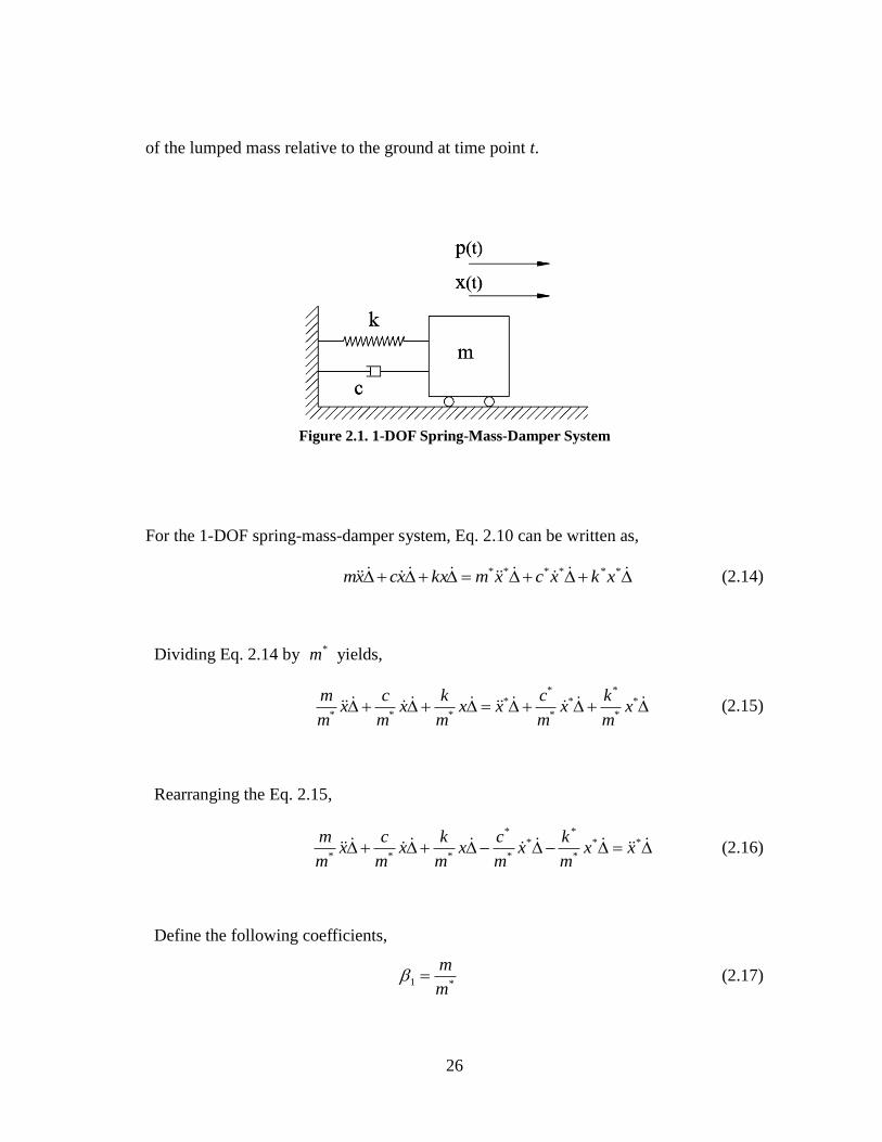
26
of the lumped mass relative to the ground at time point t.
Figure 2.1. 1-DOF Spring-Mass-Damper System
For the 1-DOF spring-mass-damper system, Eq. 2.10 can be written as,
****** xkxcxmkxxcxm (2.14)
Dividing Eq. 2.14 by *m yields,
*
*
**
*
**
***x
m
kx
m
cxx
m
kx
m
cx
m
m (2.15)
Rearranging the Eq. 2.15,
**
*
**
*
*
***xx
m
kx
m
cx
m
kx
m
cx
m
m (2.16)
Define the following coefficients,
*1m
m (2.17)

27
*2m
c (2.18)
*3m
k (2.19)
*
*
4m
c (2.20)
*
*
5m
k (2.21)
Substituting Eq. 2.17 through Eq. 2.21 to Eq. 2.16 yields,
**
5
*
4321 xxxxxx (2.22)
Writing the Eq. 2.22 at different time point, yields the following groups of equations,
For 0tt ,
000000|)(|)(|)(|)(|)(|)( **
5
*
4321 tttttt xxxxxx (2.23)
For itt ,
iiiiii tttttt xxxxxx |)(|)(|)(|)(|)(|)( **
5
*
4321 (2.24)
For Ntt ,
NiNNNNN tttttt xxxxxx |)(|)(|)(|)(|)(|)( **
5
*
4321 (2.25)
Arrange the above Equation group into matrix form,

28
1
*
*
*
155
4
3
2
1
5
**
**
**
|)(
|)(
|)(
|)(|)(|)(|)(|)(
|)(|)(|)(|)(|)(
|)(|)(|)(|)(|)(000000
Nt
t
t
Nttttt
ttttt
ttttt
N
i
NNNNN
iiiii
x
x
x
xxxxx
xxxxx
xxxxx
(2.26)
Define
NNNNN
iiiii
ttttt
ttttt
ttttt
xxxxx
xxxxx
xxxxx
|)(|)(|)(|)(|)(
|)(|)(|)(|)(|)(
|)(|)(|)(|)(|)(
**
**
**
00000
Χ (2.27)
5
4
3
2
1
β (2.28)
N
i
t
t
t
x
x
x
|)(
|)(
|)(
*
*
*
0
Y (2.29)
The above equation may be expressed as,
YβΧ (2.30)
Based on the Least Square Method, the β can be computed from the following equation,

29
)()( 1YΧΧΧβ
TT (2.31)
According to the definition of the damage index in Eq. 2.11, the damage indices for
stiffness, mass and damping can be computed as follows,
1*
m
mm (2.32)
4
2
*
*
*
*
m
c
m
c
c
cc (2.33)
5
3
*
*
*
*
m
k
m
k
k
kk (2.34)
According to the relationship between the damage severity and damage index of one
element, shown in Eq. 2.13, the damage severities for stiffness, mass and damping can be
computed as follows,
1
1 11 1m
m
(2.35)
4
2
11 1c
c
(2.36)
5
3
11 1k
k
(2.37)
2.4 THEORY FOR 2-DOF SPRING-MASS-DAMPER SYSTEMS
For a typical 2-DOF spring-mass-damper system, as shown in Figure 2.2, the system is
composed of two lumped masses, three linear springs, and three linear dash pots. )(1 tp

30
and )(2 tp are the external dynamic forces acting on lumped mass 1 and lumped mass 2
respectively. )(1 tx and )(2 tx are the displacements of mass block 1 and mass block 2
relative to the ground at time point t. )(1 tx and )(2 tx are the velocities of mass block 1
and mass block 2 relative to the ground at time point t. )(1 tx and )(2 tx are the
accelerations of mass block 1 and mass block 2 relative to the ground at time point t.
Figure 2.2. 2-DOF Spring-Mass-Damper System
For the 2-DOF spring-mass-damper system, Eq. 2.10 can be written as,
2*
1*
*
3
*
2
*
2
*
2
*
2
*
1
2
1
2*
1*
*
3
*
2
*
2
*
2
*
2
*
1
2
1
2*
1*
2*
1*
2
1
2
1
322
221
2
1
2
1
322
221
2
1
2
1
2
1
2
1
0
0
0
0
x
x
kkk
kkk
x
x
ccc
ccc
x
x
m
m
x
x
kkk
kkk
x
x
ccc
ccc
x
x
m
m
TTT
TTT
(2.38)
Eq. 2.38 can be rewritten as,

31
22**
3
212*1**
2
11**
1
22**
3
212*1**
2
11**
1
22*2*11*1*
22
3
2121
2
11
1
22
3
2121
2
11
1
222111
))((
))((
))((
))((
xkxxk
xkxcxxcxcxmxm
xkxxk
xkxcxxcxcxmxm
(2.39)
Dividing Eq. 2.39 by 1*m yields,
22*
1*
*
3212*1*
1*
*
2
11*
1*
*
122*
1*
*
3212*1*
1*
*
211*
1*
*
122*
1*
2*11*
22
1*
32121
1*
2
11
1*
122
1*
32121
1*
211
1*
122
1*
211
1*
1
))((
))((
))((
))((
xm
kxx
m
k
xm
kx
m
cxx
m
cx
m
cx
m
mx
xm
kxx
m
k
xm
kx
m
cxx
m
cx
m
cx
m
mx
m
m
(2.40)
Rearranging Eq. 2.40 yields
11*22*
1*
*
3212*1*
1*
*
211*
1*
*
122*
1*
*
3
212*1*
1*
*
211*
1*
*
122*
1*
2*22
1*
32121
1*
2
11
1*
122
1*
32121
1*
211
1*
122
1*
211
1*
1
))((
))(())((
))((
xxm
kxx
m
kx
m
kx
m
c
xxm
cx
m
cx
m
mx
m
kxx
m
k
xm
kx
m
cxx
m
cx
m
cx
m
mx
m
m
(2.41)
Define,
1*
1
1m
m (2.42)

32
1*
2
2m
m (2.43)
1*
13
m
c (2.44)
1*
24
m
c (2.45)
1*
35
m
c (2.46)
1*
16
m
k (2.47)
1*
27
m
k (2.48)
1*
38
m
k (2.49)
1*
2*
9m
m (2.50)
1*
*
110
m
c (2.51)
1*
*
211
m
c (2.52)
1*
*
312
m
c (2.53)
1*
*
113
m
k (2.54)
1*
*
214
m
k (2.55)
1*
*
315
m
k (2.56)
Substitute Eqs. 2.42 through 2.56 into Eq. 2.41, yields,

33
11*22*
15
212*1*
14
11*
13
22*
12
212*1*
11
11*
10
22*
9
22
8
2121
7
11
6
22
5
2121
4
11
3
22
2
11
1
))((
))(())((
))((
xxxxxx
xxxxxxx
xxxxxxx
(2.57)
Apply Eq. 2.57 at different time point,
For 0tt ,
00
0000
00000
00000
|)(|)(
|)))(((|)(|)(|)))(((
|)(|)(|)(|)))(((|)(
|)(|)))(((|)(|)(|)(
11*22*
15
212*1*
14
11*
13
22*
12
212*1*
11
11*
10
22*
9
22
8
2121
7
11
6
22
5
2121
4
11
3
22
2
11
1
tt
tttt
ttttt
ttttt
xx
xxxxxx
xxxxxx
xxxxxx
(2.58)
For itt ,
ii
iiii
iiiii
iiiii
tt
tttt
ttttt
ttttt
xx
xxxxxx
xxxxxx
xxxxxx
|)(|)(
|)))(((|)(|)(|)))(((
|)(|)(|)(|)))(((|)(
|)(|)))(((|)(|)(|)(
11*22*
15
212*1*
14
11*
13
22*
12
212*1*
11
11*
10
22*
9
22
8
2121
7
11
6
22
5
2121
4
11
3
22
2
11
1
(2.59)
For Ntt ,
NN
NNNN
NNNNN
NNNNN
tt
tttt
ttttt
ttttt
xx
xxxxxx
xxxxxx
xxxxxx
|)(|)(
|)))(((|)(|)(|)))(((
|)(|)(|)(|)))(((|)(
|)(|)))(((|)(|)(|)(
11*22*
15
212*1*
14
11*
13
22*
12
212*1*
11
11*
10
22*
9
22
8
2121
7
11
6
22
5
2121
4
11
3
22
2
11
1
(2.60)

34
Put the above equation into matrix form, the coefficient matrix can be defined as,
Ni
Ni
Ni
Ni
Ni
Ni
Ni
Ni
Ni
Ni
Ni
Ni
Ni
Ni
Ni
ttt
ttt
ttt
ttt
ttt
ttt
ttt
ttt
ttt
ttt
ttt
ttt
ttt
ttt
ttt
T
xxx
xxxxxx
xxx
xxx
xxxxxx
xxx
xxx
xxx
xxxxxx
xxx
xxx
xxxxxx
xxx
xxx
xxx
|)(...|)(...|)(
|)))(((...|)))(((...|)))(((
|)(...|)(...|)(
|)(...|)(...|)(
|)))(((...|)))(((...|)))(((
|)(...|)(...|)(
|)(...|)(...|)(
|)(...|)(...|)(
|)))(((...|)))(((...|)))(((
|)(...|)(...|)(
|)(...|)(...|)(
|))((...|))((...|))((
|)(...|)(...|)(
|)(...|)(...|)(
|)(...|)(...|)(
22*22*22*
212*1*212*1*212*1*
11*11*11*
22*22*22*
212*1*212*1*212*1*
11*11*11*
22*22*22*
222222
212121212121
111111
222222
212121212121
111111
222222
111111
0
0
0
0
0
0
0
0
0
0
0
0
0
0
0
X
(2.61)
The vector of unknowns and the vector of known can be defined as,

35
15
14
13
12
11
10
9
8
7
6
5
4
3
2
1
β (2.62)
N
i
t
t
t
x
x
x
|)(
|)(
|)(
11*
11*
11*
0
Y (2.63)
The above equation may be expressed as,
YβΧ (2.64)
Based on the Least Square Method, the β can be computed from the following equation,
)()( 1YΧΧΧβ
TT (2.65)
According to the definition of the damage index in Eq. 2.11, the damage indices for
stiffness, mass and damping can be computed as follows,

36
11*
1
1 m
mm
(2.66)
9
2
1*
2*
1*
2
2*
2
2
m
m
m
m
m
mm
(2.67)
10
3
1*
*
1
1*
1
*
1
1
1
m
c
m
c
c
cc (2.68)
11
4
1*
*
2
1*
2
*
2
2
2
m
c
m
c
c
cc (2.69)
12
5
1*
*
3
1*
3
*
3
3
3
m
c
m
c
c
cc (2.70)
13
6
1*
*
1
1*
1
*
1
1
1
m
k
m
k
k
kk (2.71)
14
7
1*
*
2
1*
2
*
2
2
2
m
k
m
k
k
kk (2.72)
15
8
1*
*
3
1*
3
*
3
3
3
m
k
m
k
k
kk (2.73)
According to the relationship between the damage severity and damage index of one
element, shown in Eq. 2.13, the damage severities for stiffness, mass and damping can be

37
computed as follows,
11
11
11
1
m
m (2.74)
111
2
9
2
2
m
m (2.75)
1
1
10
3
11 1c
c
(2.76)
2
2
11
4
11 1c
c
(2.77)
3
3
12
5
11 1c
c
(2.78)
1
1
13
6
11 1k
k
(2.79)
2
2
14
7
11 1k
k
(2.80)
3
3
15
8
11 1k
k
(2.81)
2.5 THEORY FOR N-DOF SPRING-MASS-DAMPER SYSTEMS
For a typical 5-DOF spring-mass-damper system, as shown in Figure 2.3, the system is
composed of five lumped masses, six linear springs, and six linear dash pots. The terms
)(1 tp through )(5 tp are the external dynamic forces acting on lumped masses 1 through
5 separately at time point t. The terms )(1 tx through )(5 tx are the displacements of the
five mass blocks relative to the ground at time point t. The terms )(1 tx through )(5 tx

38
are the velocities of the five mass blocks relative to the ground at time point t. The terms
)(1 tx through )(5 tx are the accelerations of the five mass blocks relative to the ground
at time point t.
Figure 2.3. 5-DOF Spring-Mass-Damper System
For the 5-DOF spring-mass-damper system, Eq. 2.10 can be written as,

39
5*
4*
3*
2*
1*
*
6
*
5
*
5
*
5
*
5
*
4
*
4
*
4
*
4
*
3
*
3
*
3
*
3
*
2
*
2
*
2
*
2
*
1
5
4
3
2
1
5*
4*
3*
2*
1*
*
6
*
5
*
5
*
5
*
5
*
4
*
4
*
4
*
4
*
3
*
3
*
3
*
3
*
2
*
2
*
2
*
2
*
1
5
4
3
2
1
5*
4*
3*
2*
1*
5*
4*
3*
2*
1*
5
4
3
2
1
5
4
3
2
1
655
5544
4433
3322
221
5
4
3
2
1
5
4
3
2
1
655
5544
4433
3322
221
5
4
3
2
1
5
4
3
2
1
5
4
3
2
1
5
4
3
2
1
000
00
00
00
000
000
00
00
00
000
0000
0000
0000
0000
0000
000
00
00
00
000
000
00
00
00
000
0000
0000
0000
0000
0000
x
x
x
x
x
kkk
kkkk
kkkk
kkkk
kkk
x
x
x
x
x
ccc
cccc
cccc
cccc
ccc
x
x
x
x
x
m
m
m
m
m
x
x
x
x
x
kkk
kkkk
kkkk
kkkk
kkk
x
x
x
x
x
ccc
cccc
cccc
cccc
ccc
x
x
x
x
x
m
m
m
m
m
T
T
T
T
T
T
(2.82)

40
Eq. 2.82 can be rewritten as,
55**
6
545*4**
5
434*3**
4
323*2**
3
212*1**
2
11**
1
55**
6
545*4**
5
434*3**
4
323*2**
3
212*1**
2
11**
1
55*5*44*4*33*3*22*2*11*1*
55
6
5454
5
4343
4
3232
3
2121
2
11
1
55
6
5454
5
4343
4
3232
3
2121
2
11
1
555444333222111
))((
))(())(())((
))((
))(())(())((
))((
))(())(())((
))((
))(())(())((
xkxxk
xxkxxkxxkxk
xcxxc
xxcxxcxxcxc
xmxmxmxmxm
xkxxk
xxkxxkxxkxk
xcxxc
xxcxxcxxcxc
xmxmxmxmxm
(2.83)
Rearranging Eq. 2.83 yields,
11*1*
55**
6
545*4**
5
434*3**
4
323*2**
3
212*1**
2
11**
1
55**
6
545*4**
5
434*3**
4
323*2**
3
212*1**
2
11**
1
55*5*44*4*33*3*22*2*
55
6
5454
5
4343
4
3232
3
2121
2
11
1
55
6
5454
5
4343
4
3232
3
2121
2
11
1
555444333222111
))((
))(())(())((
))((
))(())(())((
))((
))(())(())((
))((
))(())(())((
xm
xkxxk
xxkxxkxxkxk
xcxxc
xxcxxcxxcxc
xmxmxmxm
xkxxk
xxkxxkxxkxk
xcxxc
xxcxxcxxcxc
xmxmxmxmxm
(2.84)
Dividing each term in Eq. 2.84 by 1*m yields,
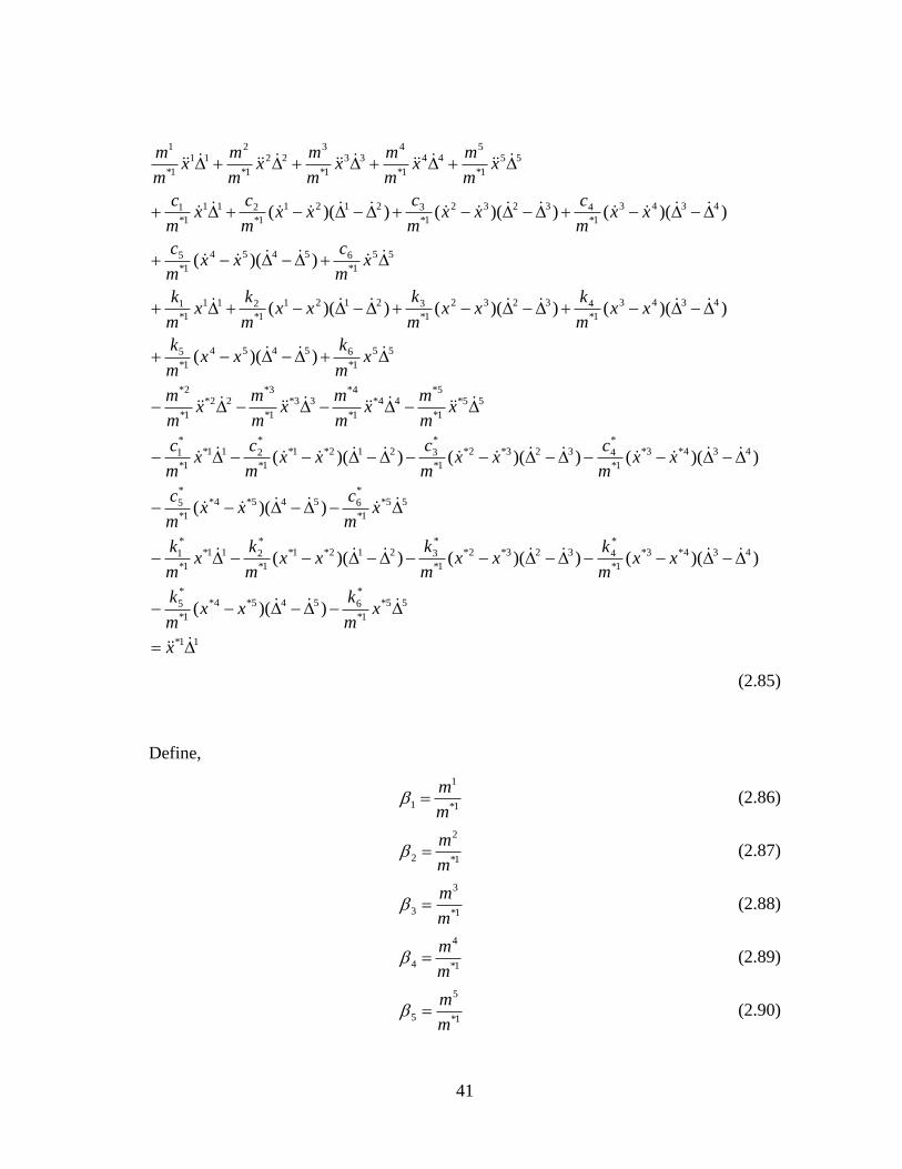
41
11*
55*
1*
*
6545*4*
1*
*
5
434*3*
1*
*
4323*2*
1*
*
3212*1*
1*
*
211*
1*
*
1
55*
1*
*
6545*4*
1*
*
5
434*3*
1*
*
4323*2*
1*
*
3212*1*
1*
*
211*
1*
*
1
55*
1*
5*44*
1*
4*33*
1*
3*22*
1*
2*
55
1*
65454
1*
5
4343
1*
43232
1*
32121
1*
211
1*
1
55
1*
65454
1*
5
4343
1*
43232
1*
32121
1*
211
1*
1
55
1*
544
1*
433
1*
322
1*
211
1*
1
))((
))(())(())((
))((
))(())(())((
))((
))(())(())((
))((
))(())(())((
x
xm
kxx
m
k
xxm
kxx
m
kxx
m
kx
m
k
xm
cxx
m
c
xxm
cxx
m
cxx
m
cx
m
c
xm
mx
m
mx
m
mx
m
m
xm
kxx
m
k
xxm
kxx
m
kxx
m
kx
m
k
xm
cxx
m
c
xxm
cxx
m
cxx
m
cx
m
c
xm
mx
m
mx
m
mx
m
mx
m
m
(2.85)
Define,
1*
1
1m
m (2.86)
1*
2
2m
m (2.87)
1*
3
3m
m (2.88)
1*
4
4m
m (2.89)
1*
5
5m
m (2.90)

42
1*
16
m
c (2.91)
1*
27
m
c (2.92)
1*
38
m
c (2.93)
1*
49
m
c (2.94)
1*
510
m
c (2.95)
*1
611
m
c (2.96)
1*
112
m
k (2.97)
1*
213
m
k (2.98)
1*
314
m
k (2.99)
1*
415
m
k (2.100)
1*
516
m
k (2.101)
1*
617
m
k (2.102)
1*
2*
18m
m (2.103)
1*
3*
19m
m (2.104)
1*
4*
20m
m (2.105)
1*
5*
21m
m (2.106)
1*
*
122
m
c (2.107)

43
1*
*
223
m
c (2.108)
1*
*
324
m
c (2.109)
1*
*
425
m
c (2.110)
1*
*
526
m
c (2.111)
1*
*
627
m
c (2.112)
1*
*
128
m
k (2.113)
1*
*
229
m
k (2.114)
1*
*
330
m
k (2.115)
1*
*
431
m
k (2.116)
1*
*
532
m
k (2.117)
1*
*
633
m
k (2.118)
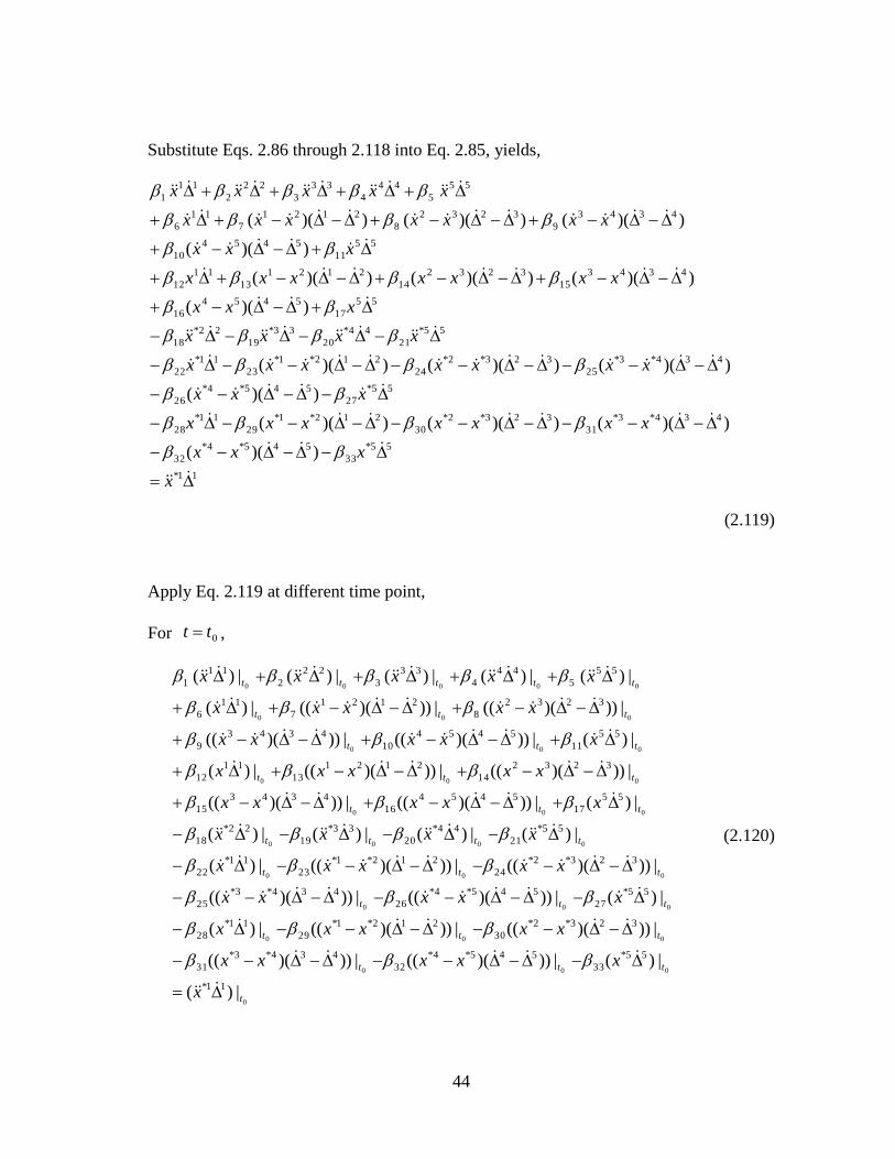
44
Substitute Eqs. 2.86 through 2.118 into Eq. 2.85, yields,
11*
55*
33
545*4*
32
434*3*
31
323*2*
30
212*1*
29
11*
28
55*
27
545*4*
26
434*3*
25
323*2*
24
212*1*
23
11*
22
55*
21
44*
20
33*
19
22*
18
55
17
5454
16
4343
15
3232
14
2121
13
11
12
55
11
5454
10
4343
9
3232
8
2121
7
11
6
55
5
44
4
33
3
22
2
11
1
))((
))(())(())((
))((
))(())(())((
))((
))(())(())((
))((
))(())(())((
x
xxx
xxxxxxx
xxx
xxxxxxx
xxxx
xxx
xxxxxxx
xxx
xxxxxxx
xxxxx
(2.119)
Apply Eq. 2.119 at different time point,
For 0tt ,
0
000
000
000
000
0000
000
000
000
000
00000
|)(
|)(|)))(((|)))(((
|)))(((|)))(((|)(
|)(|)))(((|)))(((
|)))(((|)))(((|)(
|)(|)(|)(|)(
|)(|)))(((|)))(((
|)))(((|)))(((|)(
|)(|)))(((|)))(((
|)))(((|)))(((|)(
|)(|)(|)(|)(|)(
11*
55*
33
545*4*
32
434*3*
31
323*2*
30
212*1*
29
11*
28
55*
27
545*4*
26
434*3*
25
323*2*
24
212*1*
23
11*
22
55*
21
44*
20
33*
19
22*
18
55
17
5454
16
4343
15
3232
14
2121
13
11
12
55
11
5454
10
4343
9
3232
8
2121
7
11
6
55
5
44
4
33
3
22
2
11
1
t
ttt
ttt
ttt
ttt
tttt
ttt
ttt
ttt
ttt
ttttt
x
xxxxx
xxxxx
xxxxx
xxxxx
xxxx
xxxxx
xxxxx
xxxxx
xxxxx
xxxxx
(2.120)
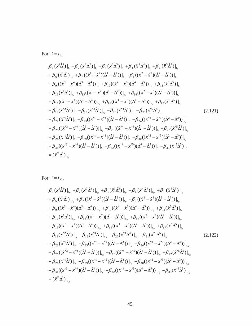
45
For itt ,
i
iii
iii
iii
iii
iiii
iii
iii
iii
iii
iiiii
t
ttt
ttt
ttt
ttt
tttt
ttt
ttt
ttt
ttt
ttttt
x
xxxxx
xxxxx
xxxxx
xxxxx
xxxx
xxxxx
xxxxx
xxxxx
xxxxx
xxxxx
|)(
|)(|)))(((|)))(((
|)))(((|)))(((|)(
|)(|)))(((|)))(((
|)))(((|)))(((|)(
|)(|)(|)(|)(
|)(|)))(((|)))(((
|)))(((|)))(((|)(
|)(|)))(((|)))(((
|)))(((|)))(((|)(
|)(|)(|)(|)(|)(
11*
55*
33
545*4*
32
434*3*
31
323*2*
30
212*1*
29
11*
28
55*
27
545*4*
26
434*3*
25
323*2*
24
212*1*
23
11*
22
55*
21
44*
20
33*
19
22*
18
55
17
5454
16
4343
15
3232
14
2121
13
11
12
55
11
5454
10
4343
9
3232
8
2121
7
11
6
55
5
44
4
33
3
22
2
11
1
(2.121)
For Ntt ,
N
NNN
NNN
NNN
NNN
NNNN
NNN
NNN
NNN
NNN
NNNNN
t
ttt
ttt
ttt
ttt
tttt
ttt
ttt
ttt
ttt
ttttt
x
xxxxx
xxxxx
xxxxx
xxxxx
xxxx
xxxxx
xxxxx
xxxxx
xxxxx
xxxxx
|)(
|)(|)))(((|)))(((
|)))(((|)))(((|)(
|)(|)))(((|)))(((
|)))(((|)))(((|)(
|)(|)(|)(|)(
|)(|)))(((|)))(((
|)))(((|)))(((|)(
|)(|)))(((|)))(((
|)))(((|)))(((|)(
|)(|)(|)(|)(|)(
11*
55*
33
545*4*
32
434*3*
31
323*2*
30
212*1*
29
11*
28
55*
27
545*4*
26
434*3*
25
323*2*
24
212*1*
23
11*
22
55*
21
44*
20
33*
19
22*
18
55
17
5454
16
4343
15
3232
14
2121
13
11
12
55
11
5454
10
4343
9
3232
8
2121
7
11
6
55
5
44
4
33
3
22
2
11
1
(2.122)
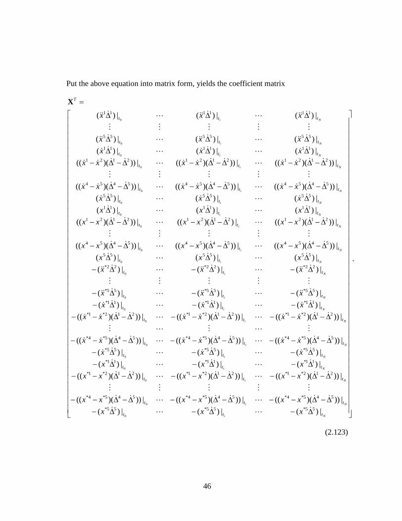
46
Put the above equation into matrix form, yields the coefficient matrix
`
|)(|)(|)(
|)))(((|)))(((|)))(((
|)))(((|)))(((|)))(((
|)(|)(|)(
|)(|)(|)(
|)))(((|)))(((|)))(((
|)))(((|)))(((|)))(((
|)(|)(|)(
|)(|)(|)(
|)(|)(|)(
|)(|)(|)(
|)))(((|)))(((|)))(((
|)))(((|))(((|)))(((
|)(|)(|)(
|)(|)(|)(
|)))(((|)))(((|)))(((
|)))(((|)))(((|)))(((
|)(|)(|)(
|)(|)(|)(
|)(|)(|)(
55*55*55*
545*4*545*4*545*4*
212*1*212*1*212*1*
11*11*11*
55*55*55*
545*4*545*4*545*4*
212*1*212*1*212*1*
11*11*11*
55*55*55*
22*22*22*
555555
545454545454
212121212121
111111
555555
545454545454
212121212121
111111
555555
111111
0
0
0
0
0
0
0
0
0
0
0
0
0
0
0
0
0
0
0
0
Ni
Ni
Ni
Ni
Ni
Ni
Ni
Ni
Ni
Ni
Ni
Ni
Ni
Ni
Ni
Ni
Ni
Ni
Ni
Ni
ttt
ttt
ttt
ttt
ttt
ttt
ttt
ttt
ttt
ttt
ttt
ttt
ttt
ttt
ttt
ttt
ttt
ttt
ttt
ttt
T
xxx
xxxxxx
xxxxxx
xxx
xxx
xxxxxx
xxxxxx
xxx
xxx
xxx
xxx
xxxxxx
xxxxxx
xxx
xxx
xxxxxx
xxxxxx
xxx
xxx
xxx
X
(2.123)

47
Define
33
1
iβ (2.124)
N
i
t
t
t
x
x
x
|)(
|)(
|)(
11*
11*
11*
1
Y (2.125)
The above equation may be expressed as,
YβΧ (2.126)
Based on the Least Square Method, the β can be computed from the following equation,
)()( 1YΧΧΧβ
TT (2.127)
According to the definition of the damage index in Eq. 2.11, the damage indices for
stiffness, mass and damping can be computed as follows,
11*
1
1 m
mm
(2.128)
18
2
1*
2*
1*
2
2
m
m
m
m
m (2.129)
19
3
1*
3*
1*
3
3
m
m
m
m
m (2.130)

48
20
4
1*
4*
1*
4
4
m
m
m
m
m (2.131)
21
5
1*
5*
1*
5
5
m
m
m
m
m (2.132)
22
6
1*
*
1
1*
1
1
m
c
m
c
c (2.133)
23
7
1*
*
2
1*
2
2
m
c
m
c
c (2.134)
24
8
1*
*
3
1*
3
3
m
c
m
c
c (2.135)
25
9
1*
*
4
1*
4
4
m
c
m
c
c (2.136)
26
10
1*
*
5
1*
5
5
m
c
m
c
c (2.137)
27
11
1*
*
6
1*
6
6
m
c
m
c
c (2.138)
28
12
1*
*
1
1*
1
1
m
k
m
k
k (2.139)

49
29
13
1*
*
2
1*
2
2
m
k
m
k
k (2.140)
30
14
1*
*
3
1*
3
3
m
k
m
k
k (2.141)
31
15
1*
*
4
1*
4
4
m
k
m
k
k (2.142)
32
16
1*
*
5
1*
5
5
m
k
m
k
k (2.143)
33
17
1*
*
6
1*
6
6
m
k
m
k
k (2.144)
According to the relationship between the damage severity and damage index of one
element, shown in Eq. 2.13, the damage severities for stiffness, mass and damping can be
computed as follows,
11
11
11
1
m
m (2.145)
111
2
18
2
2
m
m (2.146)
111
3
19
3
3
m
m (2.147)

50
111
4
20
4
4
m
m (2.148)
111
5
21
5
5
m
m (2.149)
1
1
22
6
11 1c
c
(2.150)
2
2
23
7
11 1c
c
(2.151)
3
3
24
8
11 1c
c
(2.152)
4
4
25
9
11 1c
c
(2.153)
5
5
26
10
11 1c
c
(2.154)
6
6
27
11
11 1c
c
(2.155)
1
1
28
12
11 1k
k
(2.156)
2
2
29
13
11 1k
k
(2.157)
3
3
30
14
11 1k
k
(2.158)
4
4
31
15
11 1k
k
(2.159)

51
111
16
32
5
5
k
k (2.160)
111
17
33
6
6
k
k (2.161)
2.6 THEORY FOR ISOLATED SPRING-MASS-DAMPER SYSTEMS
An isolated spring-mass-damper system means a mass block along with the springs and
dash pots attached to it are taken out from a discrete system and considered separately. A
typical isolated spring-mass-damper system is shown schematically in Figure 2.4. The
isolated spring-mass-damper system is composed of one lumped mass, two linear springs,
and two linear dash pots. )(tpi is the external dynamic force acting on lumped masses at
time point t. )(txi is the displacement of the mass block relative to the ground at time
point t. )(txi is the velocity of the mass block relative to the ground at time point t.
)(txi is the acceleration of the mass block relative to the ground at time point t.
Figure 2.4. Isolated Spring-Mass-Damper System

52
For the isolated spring-mass-damper system, Eq. 2.10 can be written as,
1*
*
1*
*
1
*
1
**
1*
*
1*
*
1
*
1
****
1
1
11
1
1
11
i
i
i
iiii
i
i
i
i
iiii
iiii
i
i
i
iiii
i
i
i
i
iiii
i
i
ii
x
x
x
kkkk
x
x
x
ccccxm
x
x
x
kkkk
x
x
x
ccccxm
(2.162)
Eq. 2.162 can written as,
iii
i
iii
i
iii
i
iii
i
iii
iii
i
iii
i
iii
i
iii
i
iii
xxkxxkxxcxxcxm
xxkxxkxxcxxcxm
)()()()(
)()()()(
1***
1
1***1***
1
1*****
1
1
11
1
1
(2.163)
Dividing Eq. 2.163 by *
im yields,
iii
i
iiii
i
iiii
i
iiii
i
iii
iii
i
iiii
i
iiii
i
iiii
i
iii
i
i
xxm
kxx
m
kxx
m
cxx
m
cx
xxm
kxx
m
kxx
m
cxx
m
cx
m
m
)()()()(
)()()()(
1**
*
*
11**
*
*1**
*
*
11**
*
**
1
*
11
*
1
*
11
**
(2.164)
Rearranging Eq. 2.164, yields,
iiiii
i
iiii
i
iiii
i
iiii
i
i
iii
i
iiii
i
iiii
i
iiii
i
iii
i
i
xxxm
kxx
m
kxx
m
cxx
m
c
xxm
kxx
m
kxx
m
cxx
m
cx
m
m
*1**
*
*
11**
*
*1**
*
*
11**
*
*
1
*
11
*
1
*
11
**
)()()()(
)()()()(
(2.165)

53
Define the following coefficients,
i
i
m
m*1 (2.166)
i
i
m
c*2 (2.167)
i
i
m
c*
13
(2.168)
i
i
m
k*4 (2.169)
i
i
m
k*
15
(2.170)
i
i
m
c*
*
6 (2.171)
i
i
m
c*
*
17
(2.172)
i
i
m
k*
*
8 (2.173)
i
i
m
k*
*
19
(2.174)
Substituting Eq. 2.166 through Eq. 2.174 to Eq. 2.165 yields,
iiiiiiiiiiiiii
iiiiiiiiiiiiii
xxxxxxxxx
xxxxxxxxx
*1**
9
1**
8
1**
7
1**
6
1
5
1
4
1
3
1
21
)()()()(
)()()()(
(2.175)
Writing the Eq. 2.175 at different time point, yields the following groups of equations,

54
For 0tt ,
00
0000
0000
|)(|))((
|))((|))((|))((|))((
|))((|))((|))((|)(
*1**
9
1**
8
1**
7
1**
6
1
5
1
4
1
3
1
21
t
ii
t
iii
t
iii
t
iii
t
iii
t
iii
t
iii
t
iii
t
iii
t
ii
xxx
xxxxxxxx
xxxxxxx
(2.176)
For itt ,
ii
iiii
iiii
t
ii
t
iii
t
iii
t
iii
t
iii
t
iii
t
iii
t
iii
t
iii
t
ii
xxx
xxxxxxxx
xxxxxxx
|)(|))((
|))((|))((|))((|))((
|))((|))((|))((|)(
*1**
9
1**
8
1**
7
1**
6
1
5
1
4
1
3
1
21
(2.177)
For Ntt ,
NN
NNNN
NNNN
t
ii
t
iii
t
iii
t
iii
t
iii
t
iii
t
iii
t
iii
t
iii
t
ii
xxx
xxxxxxxx
xxxxxxx
|)(|))((
|))((|))((|))((|))((
|))((|))((|))((|)(
*1**
9
1**
8
1**
7
1**
6
1
5
1
4
1
3
1
21
(2.178)
Arrange the above Equation group into matrix form,
Ni
Ni
Ni
Ni
Ni
Ni
Ni
Ni
Ni
t
iii
t
iii
t
iii
t
iii
t
iii
t
iii
t
iii
t
iii
t
iii
t
iii
t
iii
t
iii
t
iii
t
iii
t
iii
t
iii
t
iii
t
iii
t
iii
t
iii
t
iii
t
iii
t
iii
t
iii
t
ii
t
ii
t
ii
T
xxxxxx
xxxxxx
xxxxxx
xxxxxx
xxxxxx
xxxxxx
xxxxxx
xxxxxx
xxx
|))((...|))((...|))((
|))((...|))((...|))((
|))((...|))((...|))((
|))((...|))((...|))((
|))((...|))((...|))((
|))((...|))((...|))((
|))((...|))((...|))((
|))((...|))((...|))((
|)(...|)(...|)(
1**1**1**
1**1**1**
1**1**1**
1**1**1**
111
111
111
111
0
0
0
0
0
0
0
0
0
Χ

55
(2.179)
Define
9
8
7
6
5
4
3
2
1
β (2.180)
N
i
t
ii
t
ii
t
ii
x
x
x
|)(
|)(
|)(
*
*
*
0
Y (2.181)
The above equation may be expressed as,
YβΧ (2.182)
Based on the Least Square Method, the β can be computed from the following equation,
)()( 1YΧΧΧβ
TT (2.183)
According to the definition of the damage index in Eq. 2.11, the damage indices for
stiffness, mass and damping can be computed as follows,

56
1*
i
i
m m
mi (2.184)
6
2
*
*
*
*
i
i
i
i
i
i
c
m
c
m
c
c
c
i (2.185)
7
3
*
*
1
*
1
*
1
1
1
i
i
i
i
i
i
c
m
c
m
c
c
c
i
(2.186)
8
4
*
*
*
*
i
i
i
i
i
i
k
m
k
m
k
k
k
i (2.187)
9
5
*
*
1
*
1
*
1
1
1
i
i
i
i
i
i
k
m
k
m
k
k
k
i
(2.188)
According to the relationship between the damage severity and damage index of one
element, shown in Eq. 2.13, the damage severities for stiffness, mass, and damping can
be computed as follows,
11
11
1
i
i
m
m (2.189)
6
2
11 1
i
i
c
c
(2.190)
1
1
7
3
11 1
i
i
c
c
(2.191)
8
4
11 1
i
i
k
k
(2.192)

57
1
1
9
5
11 1
i
i
k
k
(2.193)
2.7 OVERALL SOLUTION PROCEDURE
To perform the proposed damage detection method to discrete system, the following
steps should be followed:
(1) Derive the linear equation group for the specific discrete system;
(2) Collect the displacement, velocity, and acceleration records required by the
coefficient matrix and the known vector of the linear equation group defined
by step 1;
(3) Use the least square method to solve for the unknown vector; and
(4) Compute for the Damage Indices and Damage severities for each physical
property in the discrete system.
The general process will be clearly demonstrated in Section 3.
2.8 SUMMARY
In this Section, the algorithms of Power Method for 1-DOF, 2-DOF, N-DOF, and
isolated spring-mass-damper system were derived. The damage index for each physical
property in each discrete system was also provided. The derivation processes were
demonstrated in Section 2.2 to Section 2.7. The general application process of the Power
Method on one specific discrete system was provided in Section 2.8. Based on the
analysis in Section 2, the Power Method can be applied to both simple and complex
discrete systems. Moreover, the Power Method can be applied to the whole discrete
system. When the Power Method is applied to the whole system, damage indices for all

58
physical properties related to the system can be computed by one group of linear
equations. The Power Method can also be applied to one isolated system, which is a part
of the whole system. In this way, the damage indices of the physical properties related to
the isolated system can be computed separately.

59
3 CASE STUDIES OF DAMAGE EVALUATION FOR DISCRETE
SYSTEMS
3.1 INTRODUCTION
The objective of this section is to validate the accuracy of the theory. To achieve this
goal, the theory was validated using exact displacements, velocities, and accelerations of
the undamaged and damaged discrete systems modeled within SAP2000 (version 15).
The exact displacements, velocities, and accelerations are the linear direct integration
results from SAP2000. The Hilber-Hughes-Taylor time integration method was used by
SAP2000. The three parameters of the Hilber-Hughes-Taylor method: Gamma, Beta and
Alpha were set to be 0.5, 0.25, and 0, respectively. Four numerical cases were studied in
this section,
Case #1: the accuracy of the theory will be studied on a 1-DOF spring-mass-damper
system. The algorithm of the Power Method for a 1-DOF spring-mass-damper system is
provided in Section 2.3. The damage is simulated by the changes of mass, stiffness, and
damping coefficient.
Case #2: the accuracy of the theory will be studied on a 2-DOF spring-mass-damper
system. The algorithm of the Power Method for a 2-DOF spring-mass-damper system is
provided in Section 2.4. The damage is simulated by the changes of masses, stiffness,
and damping coefficients at multiple locations.
Case #3: the accuracy of the theory will be studied on a 5-DOF spring-mass-damper

60
system. The algorithm of the Power Method for a 5-DOF spring-mass-damper system is
provided in Section 2.5. The damage is simulated by the changes of masses, stiffness,
and damping coefficients at multiple locations.
Case #4: the accuracy of the theory will be studied on an isolated spring-mass-damper
system. The algorithm of the Power Method for an isolated spring-mass-damper system
is provided in Section 2.6. The damage is simulated by the changes of masses, stiffness,
and damping coefficients at multiple locations.
3.2 DAMAGE EVALUATION FOR A 1-DOF SPRING-MASS-DAMPER SYSTEM
In this section, a typical 1-DOF spring-mass-damper system will be developed and used
to validate the accuracy of the Power Method. The numerical models for the damaged
and undamaged 1-DOF mass-spring-damper system were generated using SAP2000. The
1-DOF spring-mass-damper system used in this case study is plotted in Figure 3.1. The
physical properties in the undamaged and damaged systems are listed in Table 3.1. Both
the undamaged and damaged systems are excited by the same external force. The applied
external force is given at each 1E-4 seconds for 0.2 seconds and is plotted in Figure 3.2.
In SAP2000, displacements, velocities, and accelerations of the mass block were
computed every 1E-4 seconds (10,000 Hz) for 0.2 seconds. The displacements,
velocities, and accelerations of the mass blocks in both the undamaged and damaged
systems were plotted in Figure 3.3, Figure 3.4, and Figure 3.5, respectively.
In this case, the computed velocity ( )(tx ) of the mass block in the undamaged case was
used as the velocity used to compute power ( ) for both undamaged and damaged cases.
The coefficient matrices and known vector, X and Y, were constructed by substituting

61
the acceleration ( )(tx ), velocity ( )(tx ), displacement ( )(tx ), and velocity used to
compute power ( ) into Eq. 2.27 and Eq. 2.29. The coefficient damage index vector, β,
was computed using Eq. 2.31. Then the damage indices for mass, spring, and damper are
computed using Eqs. 2.32 through 2.34. The damage severities for mass, spring and
damper are computed using Eqs. 2.35 through 2.37. The estimated damage indices and
the designed damage indices for each physical property are listed in Table 3.2 and are
plotted in Figure 3.6. The estimated damage severities and the designed damage
severities for each physical property are plotted in Figure 3.7. Comparing the estimated
damage indices with the designed damage indices, the proposed method can accurately
locate and size multiple damage in a typical 1-DOF spring-mass-damper system.
Figure 3.1. Property Definition and Load Case of the 1-DOF Spring-Mass-Damper System
Table 3.1. Physical Properties of the 1-DOF Spring-Mass-Damper System
Property Undamaged System Damaged System
m (kip-s2/in.) 2 1.7
c (kip-s/in.) 0.8 0.7
k (kip/in.) 10 8

62
Figure 3.2. Applied External Load for Both the Undamaged and Damaged Cases
Figure 3.3. Displacements of the Mass Block under the Given External Load

63
Figure 3.4. Velocities of the Mass Block under the Given External Load
Figure 3.5. Accelerations of the Mass Block under the Given External Load

64
Table 3.2. Damage Detection Results for the 1-DOF Spring-Mass-Damper System
Figure 3.6. Element Damage Indices (βi) for 1-DOF Spring-Mass-Damper System
Property Damage Index (βi) Damage Severity (αi, %)
m 1.18 -15.00
k 1.25 -20.00
c 1.14 -12.50

65
Figure 3.7. Element Damage Severities (аi) for 1-DOF Spring-Mass-Damper System
3.3 DAMAGE EVALUATION FOR A 2-DOF SPRING-MASS-DAMPER SYSTEM
In this section, a typical 2-DOF spring-mass-damper system will be built and used to
validate the accuracy of the Power Method. The numerical models for the damaged and
undamaged 2-DOF mass-spring-damper systems were generated using SAP2000. The
2-DOF spring-mass-damper system used in this case study is plotted in Figure 3.8. The
physical properties in the undamaged and damaged systems are listed in Table 3.3. Both
the undamaged and damaged systems are excited by the same external force. The applied
external force is given at each 1E-4 seconds for 0.2 seconds and is plotted in Figure 3.9.
In SAP2000, displacements, velocities and accelerations of the mass blocks were
computed every 1E-4 seconds (10,000 Hz) for 0.2 seconds. The displacements,
velocities, and accelerations of the mass block 1 in both the undamaged and damaged

66
systems were plotted in Figure 3.10, Figure 3.11, and Figure 3.12, respectively.
In this case, the computed velocity ( )(tx ) of the mass block in the undamaged case was
used as the velocity used to compute power ( ) for both undamaged and damaged cases.
The coefficient matrices and known vector, X and Y, were constructed by substituting
the acceleration ( )(tx ), velocity ( )(tx ), displacement ( )(tx ), and velocity used to
compute power ( ) into Eq. 2.61 and Eq. 2.63. The coefficient damage index vector, β,
was computed using Eq. 2.65. Then the damage indices for mass, spring and damper are
computed using Eqs. 2.66 through 2.73. The damage severities for mass, spring and
damper are computed using Eqs. 2.74 through 2.81. The estimated damage indices and
the designed damage indices for each physical property are listed in Table 3.4 and are
plotted in Figure 3.13. The estimated damage severities and the designed damage
severities for each physical property are plotted in Figure 3.14. Comparing the estimated
damage indices with the designed damage indices, the proposed method can accurately
locate and size multiple damage in a typical 2-DOF spring-mass-damper system.
Figure 3.8. Property Definition and Load Case of the 2-DOF Spring-Mass-Damper System

67
Table 3.3. Physical Properties of the 2-DOF System
Figure 3.9. Applied External Load for Both the Undamaged and Damaged Cases
Property Undamaged System Damaged System
m1 (kip-s2/in.) 2 1.7
m2 (kip-s2/in.) 3 2.9
c1 (kip-s/in.) 0.8 0.7
c2 (kip-s/in.) 0.4 0.23
c3 (kip-s/in.) 0.3 0.33
k1 (kip/in.) 10 8
k2 (kip/in.) 20 21
k3 (kip/in.) 15 15.3

68
Figure 3.10. Displacements of the Mass Block 1 under the Given External Load
Figure 3.11. Velocities of the Mass Block 1 under the Given External Load

69
Figure 3.12. Accelerations of the Mass Block 1 under the Given External Load
Table 3.4. Damage Detection Results for the 2-DOF Spring-Mass-Damper System
PropertyDamage Index (βi,
Esimated)
Damage Severity (αi,
Esimated)
Damage Index (βi,
Designed)
m1 1.18 -0.15 1.18
m2 1.03 -0.03 1.03
c1 1.14 -0.12 1.14
c2 1.74 -0.43 1.74
c3 0.91 0.10 0.91
k1 1.25 -0.20 1.25
k2 0.95 0.05 0.95
k3 0.98 0.02 0.98

70
Figure 3.13. Element Damage Indices (βi) for 2-DOF Spring-Mass-Damper System
Figure 3.14. Element Damage Severities (аi) for 2-DOF Spring-Mass-Damper System

71
3.4 DAMAGE EVALUATION FOR AN N-DOF SPRING-MASS-DAMPER
SYSTEM
In this section, a typical 5-DOF spring-mass-damper system is used to simulate an
N-DOF spring-mass-damper system and will be used to validate the accuracy of the
Power Method. The numerical models for the damaged and undamaged 5-DOF
mass-spring-damper systems were generated using SAP2000. The 5-DOF
spring-mass-damper system used in this case study is plotted in Figure 3.15. The
physical properties in the undamaged and damaged systems are listed in Table 3.5. Both
the undamaged and damaged systems are excited by the same external force. The applied
external force is given at each 1E-4 seconds for 0.2 seconds and is plotted in Figure 3.16.
In SAP2000, displacements, velocities and accelerations of the mass blocks were
computed every 1E-4 seconds (10,000 Hz) for 0.2 seconds. The displacements,
velocities, and accelerations of the mass block 1 in both the undamaged and damaged
systems were plotted in Figure 3.17, Figure 3.18, and Figure 3.19, respectively.
In this case, the computed velocity ( )(tx ) of the mass block in the undamaged case was
used as the velocity used to compute power ( ) for both undamaged and damaged cases.
The coefficient matrices and known vector, X and Y, were constructed by substituting
the acceleration ( )(tx ), velocity ( )(tx ), displacement ( )(tx ), and velocity used to
compute power ( ) into Eq. 2.123 and Eq. 2.125. The coefficient damage index vector,
β, was computed using Eq. 2.127. Then the damage indices for mass, spring and damper
are computed using Eqs. 2.128 through 2.144. The damage severities for mass, spring
and damper are computed using Eqs. 2.145 through 2.161. The estimated damage indices
and the designed damage indices for each physical property are listed in Table 3.6 and
are plotted in Figure 3.20. The estimated damage severities and the designed damage

72
severities for each physical property are plotted in Figure 3.21. Comparing the estimated
damage indices with the designed damage indices, the proposed method can accurately
locate and size multiple damage in a typical 5-DOF spring-mass-damper system.
Figure 3.15. Property Definition and Load Case of the 5-DOF Spring-Mass-Damper System

73
Table 3.5. Physical Properties of the 5-DOF System
Property Undamaged System Damaged System
m1 (kip-s2/in.) 2 1.7
m2 (kip-s2/in.) 3 2.9
m3 (kip-s2/in.) 5 4.7
m4 (kip-s2/in.) 4 3.8
m5 (kip-s2/in.) 1 0.6
c1 (kip-s/in.) 0.8 0.7
c2 (kip-s/in.) 0.4 0.23
c3 (kip-s/in.) 0.3 0.33
c4 (kip-s/in.) 0.7 0.66
c5 (kip-s/in.) 0.55 0.5
c6 (kip-s/in.) 0.6 0.4
k1 (kip/in.) 10 8
k2 (kip/in.) 20 21
k3 (kip/in.) 15 15.3
k4 (kip/in.) 30 26
k5 (kip/in.) 18 16.8
k6 (kip/in.) 13 12.3

74
Figure 3.16. Applied External Load for Both the Undamaged and Damaged Cases
Figure 3.17. Displacements of the Mass Block 1 under the Given External Load

75
Figure 3.18. Velocities of the Mass Block 1 under the Given External Load
Figure 3.19. Accelerations of the Mass Block 1 under the Given External Load

76
Table 3.6. Damage Detection Results for the 5-DOF Spring-Mass-Damper System
PropertyDamage Index (βi,
Esimated)
Damage Severity (αi,
Esimated)
Damage Index (βi,
Designed)
m1 1.18 -0.15 1.18
m2 1.03 -0.03 1.03
m3 1.06 -0.06 1.06
m4 1.05 -0.05 1.05
m5 1.67 -0.40 1.67
c1 1.14 -0.12 1.14
c2 1.74 -0.43 1.74
c3 0.91 0.10 0.91
c4 1.06 -0.06 1.06
c5 1.10 -0.09 1.10
c6 1.50 -0.33 1.50
k1 1.25 -0.20 1.25
k2 0.95 0.05 0.95
k3 0.98 0.02 0.98
k4 1.15 -0.13 1.15
k5 1.07 -0.07 1.07
k6 1.06 -0.05 1.06

77
Figure 3.20. Element Damage Indices (βi) for 5-DOF Spring-Mass-Damper System
Figure 3.21. Element Damage Severities (аi) for 5-DOF Spring-Mass-Damper System
78
3.5 DAMAGE EVALUATION FOR ISOLATED SPRING-MASS-DAMPER
SYSTEMS
In this section, an isolated spring-mass-damper system is isolated from a 5-DOF system
and is used to validate the accuracy of the Power Method. The numerical models for the
damaged and undamaged 5-DOF mass-spring-damper systems were generated using
SAP2000. The 5-DOF spring-mass-damper system used in this case study is plotted in
Figure 3.15. The physical properties in the undamaged and damaged systems are listed in
Table 3.7. Both the undamaged and damaged systems are excited by the same external
force. The applied external force is given at each 1E-4 seconds for 0.2 seconds and is
plotted in Figure 3.16. In SAP2000, displacements, velocities and accelerations of the
mass blocks were computed every 1E-4 seconds (10,000 Hz) for 0.2 seconds. The
displacements, velocities and accelerations of the mass block 1 in both the undamaged
and damaged systems were plotted in Figure 3.17, Figure 3.18 and Figure 3.19,
respectively.
In this case, the computed velocity ( )(tx ) of the mass block in the undamaged case was
used as the velocity used to compute power ( ) for both undamaged and damaged cases.
The coefficient matrices and known vector, X and Y, were constructed by substituting
the acceleration ( )(tx ), velocity ( )(tx ), displacement ( )(tx ), and velocity used to
compute power ( ) into Eq. 2.179 and Eq. 2.181. The coefficient damage index vector,
β, was computed using Eq. 2.183. Then the damage indices for mass, spring and damper
are computed using Eqs. 2.184 through 2.188. The damage severities for mass, spring
and damper are computed using Eqs. 2.189 through 2.193. The estimated damage indices
and the designed damage indices for each physical property are listed in Table 3.8 and
are plotted in Figure 3.23. The estimated damage severities and the designed damage

79
severities for each physical property are plotted in Figure 3.24. Comparing the estimated
damage indices with the designed damage indices, the proposed method can accurately
locate and size multiple damage in an isolated spring-mass-damper system.
Figure 3.22. Property Definition and Load Case of the Isolated Spring-Mass-Damper System
Table 3.7. Physical Properties of the Isolated Spring-Mass-Damper System
Property System #1 System #2 System #3 System #4 System #5
mi (kip-s2/in.) 2.00 3.00 5.00 4.00 1.00
ci (kip-s/in.) 0.80 0.40 0.30 0.70 0.55
ci+1 (kip-s/in.) 0.40 0.30 0.70 0.55 0.60
ki (kip/in.) 10.00 20.00 15.00 30.00 18.00
ki+1 (kip/in.) 20.00 15.00 30.00 18.00 13.00
Property System #1 System #2 System #3 System #4 System #5
mi (kip-s2/in.) 1.70 2.90 4.70 3.80 0.60
ci (kip-s/in.) 0.70 0.23 0.33 0.66 0.50
ci+1 (kip-s/in.) 0.23 0.33 0.66 0.50 0.40
ki (kip/in.) 8.00 21.00 15.40 26.00 16.80
ki+1 (kip/in.) 21.00 15.30 26.00 16.80 12.30
Undamage Systems
Damaged Systems

80
Table 3.8. Damage Detection Results for the Isolated Spring-Mass-Damper System
Property System #1 System #2 System #3 System #4 System #5
mi 1.18 1.03 1.06 1.05 1.67
ci 1.14 1.74 0.91 1.06 1.10
ci+1 1.74 0.91 1.06 1.10 1.50
ki 1.25 0.95 0.98 1.15 1.07
ki+1 0.95 0.98 1.15 1.07 1.06
Property System #1 System #2 System #3 System #4 System #5
mi 1.18 1.03 1.06 1.05 1.67
ci 1.14 1.74 0.91 1.06 1.10
ci+1 1.74 0.91 1.06 1.10 1.50
ki 1.25 0.95 0.98 1.15 1.07
ki+1 0.95 0.98 1.15 1.07 1.06
Designed Damage Indices
Estimated Damage Indices

81
Figure 3.23. Element Damage Indices (βi) for Isolated Spring-Mass-Damper System
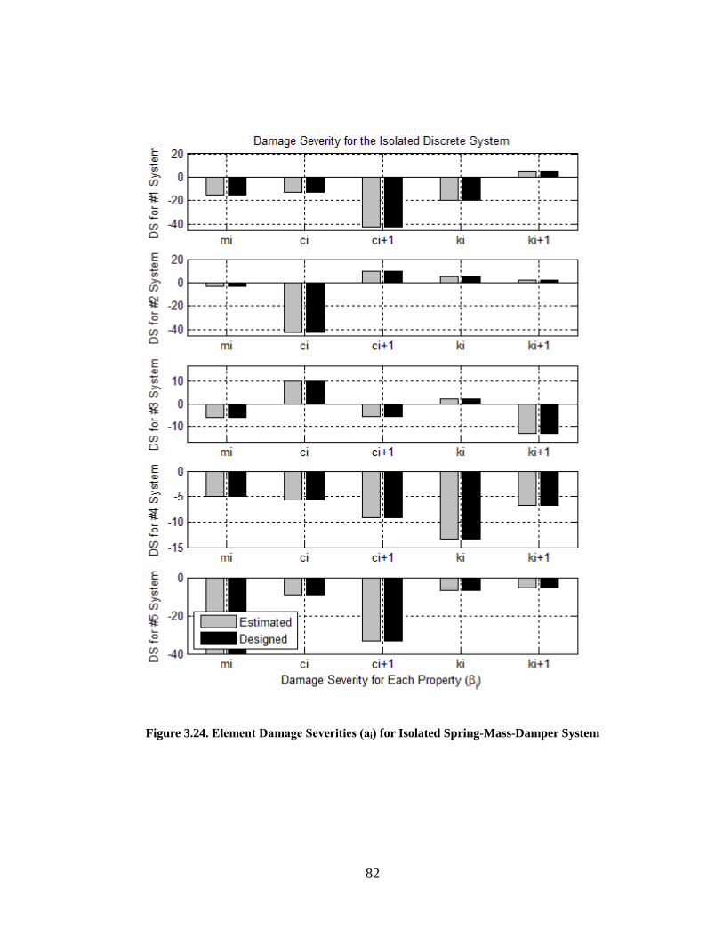
82
Figure 3.24. Element Damage Severities (аi) for Isolated Spring-Mass-Damper System

83
3.6 SUMMARY
In this section, 1-DOF, 2-DOF, 5-DOF and isolated spring-mass-damper systems were
studied. In each numerical damage detection experiment, different levels of damage in
mass, stiffness, and damping were simultaneously simulated in the related damaged
system. For both the damaged and undamaged systems, the displacements, velocities and
accelerations were exact values (i.e. free from signal noise pollution) and were computed
using linear direct integration method in SAP2000. The algorithms given in the Section 2
were used to compute the damage indices and damage severities in each numerical
experiment.
According to Table 3.2, Table 3.4, Table 3.6 and Table 3.8, all the designed damage in
masses, springs, and dampers were located and evaluated accurately in each numerical
experiment. Moreover, for all numerical experiments, neither false-positive damage
index nor false-negative damage index was found. Namely, for the proposed damage
detection method, if accurate displacement, velocity, and acceleration data are given, all
type of damage will be located and evaluated without any error. In addition, the results
from Section 3.4 and 3.5 indicate that the proposed method is applicable to both integral
discrete system and isolated discrete system.

84
4 THEORY OF DAMAGE EVALUATION ON MASS AND
STIFFNESS FOR CONTINUOUS SYSTEMS
4.1 INTRODUCTION
In this section, seven major subtasks are addressed. In Section 4.2, the specific form of
the Power Method for rods is developed; In Section 4.3, the specific form of the Power
Method for Euler-Bernoulli beams is developed; In Section 4.4, the specific form of the
Power Method for plane frames is developed; In Section 4.5, the specific form of the
Power Method for space trusses is developed; In Section 4.6, the overall solution
procedures is provided. In Section 4.7, the summary for Section 4 is made.
4.2 THEORY FOR RODS
4.2.1 Theory for Rods at Isolated Element Nodes
In this subsection, the proposed non-destructive evaluation theory is applied to the axial
and torsional vibration of rods at a single node.
According to finite element method, one rod can be meshed into several elements.
Isolating two nearby rod elements, as shown in Figure 4.1, the modulus of elasticity of the
material for the Element i is denoted as iE . The modulus of elasticity in shear of the
material for the Element i is denoted as iG . The length of the Element i is
iL . The area
and the moment of inertia of the cross section of the Element i are denoted as iA and iI ,
respectively. The torsional constant of the cross section of the Element i is denoted iJ .
Let }{ iP be the force vector at Node i, where iP1 denotes the axial force at Node i, iP4

85
denotes the torsional moment at Node i. As shown in the free body diagram of Node i in
Figure 4.2, the external loads ( }{ iP ), internal forces ( }{ iF and }{ 1iF ) and inertial forces
}{ iI form a dynamic equilibrium condition for Node i. The dynamic equilibrium
condition can be written as,
}{}{}{}{ 1
i
ii
i PFFI (4.1)
For this subsection, only axial force and torsional moment will be considered. Thus, each
force vector in Eq. 4.1 is composed by two force components: (1) axial force, (2)
torsional moment. Namely, Eq. 4.1 can be developed into,
i
i
i
i
i
i
i
i
P
P
F
F
F
F
I
I
4
1
4,1
1,1
4,
1,
4
1 (4.2)
Where subscript one (“1”) indicates the force in axial direction of the rod and subscript
four (“4”) indicates the force in torsional direction.
Figure 4.1. Two nearby Rod Elements

86
Figure 4.2. Free Body Diagram of Node i under Axial and Torsional Effects
Similarly, for the damaged case, the dynamic equilibrium condition can be expressed as,
}{}{}{}{ **
1
** i
ii
i PFFI (4.3)
Where the asterisk (“*”) denotes the quantities from the damaged case.
Given any velocity vectors, }{ i and }{ *i , for the undamaged and damaged systems.
The power done by the external forces in the undamaged and damaged systems can be
expressed as follows,
}{}{}{}{}{}{}{}{ 1
iTi
i
Ti
i
TiiTi PFFI (4.4)
}{}{}{}{}{}{}{}{ ***
1
***** iTi
i
Ti
i
TiiTi PFFI (4.5)
Assume that the applied external loads and velocities used to compute power at Node i
are the same for both the undamaged and damaged systems,
}{}{ *ii (4.6)
}{}{ *ii PP (4.7)

87
Substituting Eq. 4.6 and Eq. 4.7 into Eq. 4.5 yields,
}{}{}{}{}{}{}{}{ *
1
** iTi
i
Ti
i
TiiTi PFFI (4.8)
Noticing the power performed by the external load is the same for both the undamaged
and damaged systems, substituting Eq. 4.8 into Eq. 4.4 yields,
}{}{}{}{}{}{}{}{}{}{}{}{ *
1
**
1 i
Ti
i
TiiTi
i
Ti
i
TiiTi FFIFFI (4.9)
Note Eq. 4.9 is equivalent to Eq. 2.10.
For the axial and torsional vibration, the inertial force, }{ iI , can be considered using
lumped mass method. Namely,
For the axial vibration,
ii
A
iiiiii
A mLmLm
I 1111
22}{
(4.10)
For the torsional vibration,
ii
T
i
i
iii
i
iiii
T mA
LIm
A
LImI 44
1
11,01,0
22}{
(4.11)
Where im is the linear mass for Element i; iI ,0 is polar moment of inertia of the cross
section of Element i.
In SAP2000, however, the torsional inertia force is equal to zero due to the zero mass in

88
the torsional direction. To make the theory application better match the later numerical
example (i.e. in SAP2000, the inertial force of a bar element in torsional direction is
neglected), the torsional inertia force will also be neglected. Namely, set
}0{)0(}{ 4 ii
TI (4.12)
Writing Eq. 4.12 and Eq. 4.10 into the matrix form, yields,
i
iiiii
i
T
i
Ai
LmLm
I
II
4
111
00
022}{
(4.13)
Extracting the physical properties from the above equation, yields,
}]{[00
01
22}{
4
111 ii
o
i
i
i
iiii
i
T
i
Ai MmLmLm
I
II
(4.14)
Where im is the lumped mass of the Node i; ][ i
oM is commonly called the configuration
matrix of the mass matrix.
Similarly, for the damaged system,
}]{[00
01
22}{ ***
*
4
*
1
**
11
*
*
* ii
o
i
i
i
iiii
i
T
i
Ai MmLmLm
I
II
(4.15)
The force vectors (i.e. }{ iF , }{ 1iF , }{ *
iF , and }{ *
1iF ) in Eq. 4.19 can also be computed
using stiffness matrices and node displacement vectors,
For axial motion,

89
i
i
i
iL
EA
L
EAF
1
1
1
1, }{
(4.16)
1
1
1
1
1,1 }{i
i
i
iL
EA
L
EAF
(4.17)
For torsional load,
i
i
i
iL
JG
L
JGF
4
1
4
4, }{
(4.18)
1
4
4
1
4,1 }{i
i
i
iL
JG
L
JGF
(4.19)
Similarly, for the damaged case, the force vectors can be computed as,
i
i
i
iL
EA
L
EAF
*
1
1*
1
*
*
1, }{
(4.20)
1*
1
*
1
*
1
*
1,1 }{i
i
i
iL
EA
L
EAF
(4.21)
And
i
i
i
iL
JG
L
JGF
*
4
1*
4
*
*
4, }{
(4.22)
1*
4
*
4
*
1
*
4,1 }{i
i
i
iL
JG
L
JGF
(4.23)
Combining Eq. 4.16 and Eq. 4.18 yields,

90
i
i
i
i
i
i
L
JG
L
JGL
EA
L
EA
F
4
1
1
4
1
1
00
00}{
(4.24)
Given the relationship between Young’s modulus and shear modulus, the shear modulus
can be expressed as,
)1(2
EG (4.25)
Substituting Eq. 4.25 into Eq. 4.24, yields,
i
i
i
i
i
i
L
JE
L
JEL
EA
L
EA
F
4
1
1
4
1
1
)1(20
)1(20
00
}{
(4.26)
Extracting the common factor out, yields,
}]{[
)1(20
)1(20
00
}{ ,
4
1
1
4
1
1
iioi
i
i
i
i
ii
i KkJJAA
L
EF
(4.27)
Similarly, other force vectors, }{ 1iF , }{ *
iF , and }{ *
1iF , can be computed as,
}]{[
)1(20
)1(20
00
}{ 11,1
1
4
1
1
4
1
11
1
iioi
i
i
i
i
ii
i KkJJAA
L
EF
(4.28)

91
For damaged system,
}]{[
)1(20
)1(20
00
}{ **
,
*
*
4
*
1
1*
4
1*
1**
*
iioi
i
i
i
i
ii
i KkJJAA
L
EF
(4.29)
}]{[
)1(20
)1(20
00
}{ *
1
*
1,
*
1
1*
4
1*
1
*
4
*
1*
1
*
1
*
1
iioi
i
i
i
i
ii
i KkJJAA
L
EF
(4.30)
Note as shown in the above equations (i.e. Eq. 4.14, Eq. 4.15, and Eqs. 4.27 through
4.30), the force vectors (i.e. }{ iI , }{ iF , }{ 1iF , }{ *iI , }{ *
iF , and }{ *
1iF ) can be
summarized as a combination of a property coefficient, a configuration matrix and a
nodal deformation vector. Because the designed damage are simulated by the changes of
Young’s modulus ( E ) and linear mass ( m ), other parameters, such as the length of the
element ( L ), the cross sectional area ( A ), the torsional constant of element ( J ) and the
Poisson’s ratio are not influenced by damage and remain the same for the undamaged
and damaged elements. Consequently, the configuration matrices for the element stiffness
and element mass are the same for both the damaged and undamaged elements, namely,
][][ ,
*
, ioio KK (4.31)
][][ 1,
*
1, ioio KK (4.32)
][][ * i
o
i
o MM (4.33)
Substitute Eqs. 4.31 through 4.33 into Eq. 4.15, Eq. 4.29 and Eq. 4.30, yields,

92
}]{[}{ *** ii
o
i MmI (4.34)
}]{[}{ *
,
**
iioii KkF (4.35)
}]{[}{ *
11,
*
1
*
1 iioii KkF (4.36)
Substitute Eq. 4.14, Eq. 4.27, Eq. 4.28 and Eqs. 4.34 through 4.36 into Eq. 4.9, yields,
}]{[}{}]{[}{}]{[}{
}]{[}{}]{[}{}]{[}{
*
11,
*
1
*
,
***
11,1,
iioi
Ti
iioi
Tiii
o
iTi
iioi
Ti
iioi
Tiii
o
iTi
KkKkMm
KkKkMm
(4.37)
Rearranging Eq. 4.37,
}]{[}{}]{[}{}]{[}{
}]{[}{}]{[}{}]{[}{
***
11,
*
1
*
,
*
11,1,
ii
o
Tii
iio
Ti
iiio
Ti
i
iio
Ti
iiio
Ti
i
ii
o
Tii
MmKkKk
KkKkMm
(4.38)
Dividing Eq. 4.38 by im* ,
}]{[}{}]{[}{}]{[}{
}]{[}{}]{[}{}]{[}{
**
11,*
*
1*
,*
*
11,*
1,**
ii
o
Ti
iio
Ti
i
iiio
Ti
i
i
iio
Ti
i
iiio
Ti
i
iii
o
Ti
i
i
MKm
kK
m
k
Km
kK
m
kM
m
m
(4.39)
Define the following coefficients,
i
i
m
m*1 (4.40)
i
i
m
k*2 (4.41)

93
i
i
m
k*
13
(4.42)
i
i
m
k*
*
4 (4.43)
i
i
m
k*
*
15
(4.44)
Substituting Eq. 4.40 through Eq. 4.44 into Eq. 4.39, yields,
}]{[}{}]{[}{}]{[}{
}]{[}{}]{[}{}]{[}{
**
11,5
*
,4
11,3,21
ii
o
Ti
iio
Ti
iio
Ti
iio
Ti
iio
Tiii
o
Ti
MKK
KKM
(4.45)
Writing the Eq. 4.45 at different time point, yields the following groups of equations,
For 0tt ,
000
000
|})]{[}({|})]{[}({|})]{[}({
|})]{[}({|})]{[}({|})]{[}({
**
11,5
*
,4
11,3,21
t
ii
o
Ti
tiio
Ti
tiio
Ti
tiio
Ti
tiio
Ti
t
ii
o
Ti
MKK
KKM
(4.46)
For jtt ,
jjj
jjj
t
ii
o
Ti
tiio
Ti
tiio
Ti
tiio
Ti
tiio
Ti
t
ii
o
Ti
MKK
KKM
|})]{[}({|})]{[}({|})]{[}({
|})]{[}({|})]{[}({|})]{[}({
**
11,5
*
,4
11,3,21
(4.47)
For Ntt ,
NNN
NNN
t
ii
o
Ti
tiio
Ti
tiio
Ti
tiio
Ti
tiio
Ti
t
ii
o
Ti
MKK
KKM
|})]{[}({|})]{[}({|})]{[}({
|})]{[}({|})]{[}({|})]{[}({
**
11,5
*
,4
11,3,21
(4.48)

94
Arrange the above Equation group into matrix form, yields,
YβΧ (4.49)
Where the coefficient matrix of the linear equation group is given as following (note, due to
the limitation of the page size, the transposed form of the matrix is provided),
Nj
Nj
Nj
Nj
Nj
tiio
Ti
tiio
Ti
tiio
Ti
tiio
Ti
tiio
Ti
tiio
Ti
tiio
Ti
tiio
Ti
tiio
Ti
tiio
Ti
tiio
Ti
tiio
Ti
t
i
io
Ti
t
i
io
Ti
t
i
io
Ti
T
KKK
KKK
KKK
KKK
MMM
|})]{[}({...|})]{[}({...|})]{[}({
|})]{[}({...|})]{[}({...|})]{[}({
|})]{[}({...|})]{[}({...|})]{[}({
|})]{[}({...|})]{[}({...|})]{[}({
|})]{[}({...|})]{[}({...|})]{[}({
*
11,
*
11,
*
11,
*
,
*
,
*
,
11,11,11,
,,,
,,,
0
0
0
0
0
Χ
(4.50)
The vector of unknowns and the vector of known are given as,
5
4
3
2
1
β (4.51)
N
j
t
ii
o
Ti
t
ii
o
Ti
t
ii
o
Ti
M
M
M
|})]{[}({
|})]{[}({
|})]{[}({
*
*
*
0
Y (4.52)
Based on the Least Square Method, the β can be computed from the following equation,
)()( 1YΧΧΧβ
TT (4.53)

95
The damage indices for stiffness, mass and damping can be computed as follows,
1
1
*
1
*
11
*
22
22
iiii
iiii
i
i
mLmLm
LmLm
m
mi (4.54)
4
2
*
*
*
*
i
i
i
i
i
i
k
m
k
m
k
k
k
i
(4.55)
5
3
*
*
1
*
1
*
1
1
1
i
i
i
i
i
i
k
m
k
m
k
k
k
i
(4.56)
4.2.2 Theory for Rods among Multiple Nodes
In this subsection, the proposed non-destructive evaluation theory will be applied to
multiple nodes on a rod. The damage detection to the physical properties (i.e. mass,
stiffness, damping, etc.) related to these nodes will be completed simultaneously. Since
the idea of combining the axial and torsional vibrations has already been demonstrated in
the above sub-section, for simplicity purposes, the torsional vibration will not be
considered in this subsection.
Given two nearby rod elements, as shown in Figure 4.3, the modulus of elasticity of the
material for Element i is denoted as iE . The length of Element i is iL . The cross sectional
area of Element i is denoted as iA . Let iP1 denotes the external axial force applied at

96
Node i. As shown in the free body diagram of Node i in Figure 4.4, the external axial load
(iP1 ), internal axial forces ( 1,iF and 1,1iF ) and inertial axial forces
iI1 form a dynamic
equilibrium condition for Node i. The dynamic equilibrium condition can be written as,
i
ii
i PFFI 11,11,1 (4.57)
Where the subscript ‘i’ denotes Node i and the ‘1’ denotes the component in axial
direction.
Figure 4.3. Two nearby Rod Elements
Figure 4.4. Free Body Diagram of Node i under Axial Effects

97
For the damaged case, the dynamic equilibrium condition is,
i
ii
i PFFI *
1
*
1,1
*
1,
*
1 (4.58)
Where the asterisk (“*”) denotes the quantities from the damaged case.
Given any node axial velocity, i
1 , the power done by the external axial loads in the
undamaged and damaged system can be computed as follows,
ii
i
i
i
iii PFFI 111,111,111 (4.59)
ii
i
i
i
iii PFFI *
1
*
1
*
1,1
*
1
*
1,
*
1
*
1
*
1 (4.60)
For N nodes in the structure, the axial force vector can be written as,
N
i
P
P
P
P
1
1
1
1
1 }{
(4.61)
Given any node axial velocity vector, }{ 1 , the power done by the external axial loads in
the undamaged system can be computed as following,
1,11,1
1,11,1
1,21,1
1
1
1
1
1
1
1
1
1
1
1
1
1
1
11 }}{{
NN
N
ii
i
T
N
i
N
i
T
N
i
FFI
FFI
FFI
P
P
P
P
(4.62)
Similarly, for the damaged system, the power done by the external axial loads can be

98
computed as follows,
*
1,1
*
1,
*
1
*
1,1
*
1,
*
1
*
1,2
*
1,1
1*
1
*
1
*
1
1*
1
*
1
*
1
1*
1
*
1
*
1
1*
1
*
1
*
1 }}{{
NN
N
ii
i
T
N
i
N
i
T
N
i
FFI
FFI
FFI
P
P
P
P
(4.63)
Assuming the applied external loads and velocities used to compute power are the same
for both the undamaged and damaged system. Namely
}{}{ *
11 (4.64)
}{}{ *
11 PP (4.65)
Substituting Eq. 4.64 and Eq. 4.65 into Eq. 4.63 yields,
*
1,1
*
1,
*
1
*
1,1
*
1,
*
1
*
1,2
*
1,1
1*
1
1
1
1
1
1
1
1
1
1
1
1
1
11
*
1
*
1 }}{{}}{{
NN
N
ii
i
T
N
i
N
i
T
N
i
FFI
FFI
FFI
P
P
P
PP
(4.66)
Noticing the power performed by the external load is the same for both the undamaged
and damaged system. Substituting Eq. 4.66 into Eq. 4.62, yields,
*
1,1
*
1,
*
1
*
1,1
*
1,
*
1
*
1,2
*
1,1
1*
1
1
1
1
1
1,11,1
1,11,1
1,21,1
1
1
1
1
1
1
NN
N
ii
i
T
N
i
NN
N
ii
i
T
N
i
FFI
FFI
FFI
FFI
FFI
FFI
(4.67)

99
Note, Eq. 4.67 is equivalent to Eq. 2.10.
Eq. 4.67 can be developed into the following equation,
)()()(
)()()(
*
1,1
*
1,
*
11
*
1,1
*
1,
*
11
*
1,2
*
1,1
1*
1
1
1
1,11,111,11,11
2
1
1
1
1
1
1
1
NN
NN
ii
ii
NN
NN
ii
ii
FFIFFIFFI
FFIFFIFFI
(4.68)
Rearranging Eq. 4.68 yields,
NN
N
N
N
N
ii
ii
NN
NN
ii
ii
IFFFFIFFI
FFIFFIFFI
*
11
*
1,11
*
1,1
*
1,1
*
1,
*
11
*
1,2
*
1,1
1*
1
1
1
1,11,111,11,11
2
1
1
1
1
1
1
1
)()(
)()()(
(4.69)
However, since two nearby nodes will share the same rod element, the same force vector
will appear twice in the above equation, which means rows in the coefficient matrix are
linearly depend. This will create singularity problem in the later least square analysis. To
avoid the singularity problem, the common terms in the above equation will be extracted
and merged together. This is process is demonstrated by the following derivations,
A more detailed expression for Eq. 4.69 is given as,
NN
N
N
N
N
NN
NN
ii
ii
ii
ii
NN
NN
NN
NN
ii
ii
ii
ii
I
FFFFIFFI
FFIFFIFFI
FFIFFIFFI
FFIFFIFFI
*
11
*
1,11
*
1,1
*
1,
*
1,1
1*
1
1*
1
*
1,2
*
1,1
1*
1
1
1
*
1,1
*
1,
*
11
*
1,3
*
1,2
2*
1
2
1
*
1,2
*
1,1
1*
1
1
1
1,11,111,1,1
1
1
1
11,21,1
1
1
1
1
1,11,111,31,2
2
1
2
11,21,1
1
1
1
1
)()(
)()()(
)()()(
)()()(
(4.70)
According to Eq. 4.10, Eq. 4.16, Eq. 4.17, Eq. 4.20, and Eq. 4.21,

100
iiiiiiii
A mLmLm
I 1111
22}{
(4.10)
iiiiiiii
A mLmLm
I *
1
**
1
*
1
*
1
***
22}{
(4.71)
)()(}{ 1
1
11
1
11,
ii
i
ii
i
i kL
EAF
(4.72)
)()(}{ 1
111
1
11
1
1,1
ii
i
ii
i
i kL
EAF (4.73)
)()(}{ *
1
1*
1
**
1
1*
1
*
*
1,
ii
i
ii
i
i kL
EAF
(4.74)
)()(}{ 1*
1
*
1
*
1
1*
1
*
1
*
1
*
1,1
ii
i
ii
i
i kL
EAF (4.75)
Substituting Eq. 4.10 and Eqs. 4.71 through 4.75 into the Eq. 4.70, yields,
NNNNN
N
NNN
N
N
ii
i
ii
i
iii
ii
i
ii
i
iii
NN
N
NN
N
NNN
ii
i
ii
i
iii
ii
i
ii
i
iii
mkk
kkm
kkm
kkm
kkm
kkm
kkm
kkm
kkm
kkm
*
1
*
1
1*
1
*
1
*
11
*
1
1*
1
*
1
2*
1
1*
1
*
2
1*
1
*
1
*
1
1*
1
1*1
1
1*
1
*
1
*
1
*
1
1*
1
**
1
*
1
3*
1
2*
1
*
3
2*
1
1*
1
*
2
2*
1
2*2
1
2*
1
1*
1
*
2
1*
1
0*
1
*
1
1*
1
1*
1
1
1
1
1111
1
111
2
1
1
12
1
111
1
1
11
1
1
1111
1
111
3
1
2
13
2
1
1
12
2
1
22
1
2
1
1
12
1
1
0
11
1
1
11
1
)()(
))()((
))()((
))()((
))()((
))()((
))()((
))()((
))()((
))()((
(4.76)
Extracting and merging the common term in the above equation, yields,
101
NNN
NN
N
NNN
N
NN
ii
i
ii
NNNiii
NN
N
NNN
N
NN
ii
i
ii
NNNiii
m
kk
kkk
mmm
kk
kkk
mmm
*
1
*
1
1*
1
*
1
*
11
*
1
1*
1
*
1
1
1
*
1
1*
1
*
1
1
1
2*
1
1*
1
*
2
2
1
1
1
1*
1
0*
1
*
1
1
1
1*
1
1*1
1
*
1
*
1
1*
1
1*1
1
1
11111
1
11
1
1
1
1
11
1
1
2
1
1
12
2
1
1
1
1
1
0
11
1
1
1111
1
1
11
1
)()()(
)()()()()(
)()()(
)()()()()(
(4.77)
Moving the physical property to the front of each term yields,
NNN
NNN
N
NNNN
N
iiii
i
NNNiii
NNN
N
NNNN
N
iiii
i
NNNiii
m
kk
kkk
mmm
kk
kkk
mmm
*
11
*
1*
1
*
11
*
1
*
1
1*
11
1
1
*
*
1
1*
11
1
1
*2*
1
1*
1
2
1
1
1
*
2
1*
1
0*
1
1
1
*
1
1*
1
1
1
1**
11
*1*
1
1
1
1*
1
11111
1
11
1
1
1
1
11
1
1
2
1
1
1
2
1
1
12
1
1
0
1
1
11
1111
1
1
1
1
1
)())((
))(())(()(
)())((
))(())(()(
(4.78)
Dividing Eq. 4.78 by Nm*
yields,
102
NN
NNN
N
NNNNN
N
N
iiii
N
i
NN
NN
N
N
ii
N
i
N
NNN
N
NNNNN
N
N
iiii
N
i
NN
NN
N
N
ii
N
i
N
m
k
m
k
m
k
m
k
m
k
m
m
m
m
m
m
m
k
m
k
m
k
m
k
m
k
m
m
m
m
m
m
*
11
1*
1
*
11*
*
1*
1
1*
11
1
1*
*
*
1
1*
11
1
1*
*2*
1
1*
1
2
1
1
1*
*
21*
1
0*
1
1
1*
*
1
1*
1
1
1*
1*
*
11*
*
1*
1
1
1*
1*
1
111*
11
1
11
1
1*
1
1
11
1
1*
2
1
1
1
2
1
1
1*
21
1
0
1
1
1*
1
11*11*
1
1
1
1*
1
)())((
))(())(()(
)())((
))(())(()(
(4.79)
Define the following (4N+1) coefficients,
Nm
m*
1
1 (4.80)
…
N
i
im
m*
(4.81)
…
N
N
Nm
m*
(4.82)
*
11
N
Nm
k (4.83)
…
103
N
iiN
m
k*
(4.84)
…
N
NN
m
k*
112
(4.85)
NNm
m*
1*
22 (4.86)
…
N
i
iNm
m*
*
12 (4.87)
…
N
N
Nm
m*
1*
3
(4.88)
NNm
k*
*
113 (4.89)
…
N
NN
m
k*
*
114
(4.90)
Substituting Eq. 4.80 through Eq. 4.90 to Eq. 4.79 yields,

104
NN
NNN
N
NNNN
N
iiii
iNNN
NN
N
ii
iNN
NNN
N
NNNN
N
iiii
iNNN
NN
N
ii
i
*
11
1*
1
*
1114
*
1
1*
11
1
14
*
1
1*
11
1
13
2*
1
1*
1
2
1
1
123
1*
1
0*
1
1
113
1*
1
1
13
*
1112
1*
1
1
122
1
111121
1
11
1
12
1
1
11
1
1
2
1
1
1
2
1
1
12
1
1
0
1
1
11
1111
1
1
1
11
)())((
))(())(()(
)())((
))(())(()(
(4.91)
Writing the Eq. 4.91 at different time point, yields the following groups of equations,
For 0tt ,
0
00
00
000
000
00
0000
|)(
|))((|)))(((
|)))(((|)))(((
|))((|)(|)(
|)(|))((|)))(((
|)))(((|)))(((
|))((|)(|)(|)(
*
11
1*
1
*
1114
*
1
1*
11
1
14
*
1
1*
11
1
13
2*
1
1*
1
2
1
1
123
1*
1
0*
1
1
113
1*
1
1
13
*
1112
1*
1
1
122
1
111121
1
11
1
12
1
1
11
1
1
2
1
1
1
2
1
1
12
1
1
0
1
1
111111
1
1
1
11
t
NN
t
NNN
Nt
NNNN
N
t
iiii
iNtN
tNt
NN
Nt
ii
iN
tNt
NNN
Nt
NNNN
N
t
iiii
iNtN
tNt
NN
Nt
ii
it
(4.92)
105
For jtt ,
j
jj
jj
jjj
jjj
jj
jjjj
t
NN
t
NNN
Nt
NNNN
N
t
iiii
iNtN
tNt
NN
Nt
ii
iN
tNt
NNN
Nt
NNNN
N
t
iiii
iNtN
tNt
NN
Nt
ii
it
|)(
|))((|)))(((
|)))(((|)))(((
|))((|)(|)(
|)(|))((|)))(((
|)))(((|)))(((
|))((|)(|)(|)(
*
11
1*
1
*
1114
*
1
1*
11
1
14
*
1
1*
11
1
13
2*
1
1*
1
2
1
1
123
1*
1
0*
1
1
113
1*
1
1
13
*
1112
1*
1
1
122
1
111121
1
11
1
12
1
1
11
1
1
2
1
1
1
2
1
1
12
1
1
0
1
1
111111
1
1
1
11
(4.93)
For Ntt ,
N
NN
NN
NNN
NNN
NN
NNNN
t
NN
t
NNN
Nt
NNNN
N
t
iiii
iNtN
tNt
NN
Nt
ii
iN
tNt
NNN
Nt
NNNN
N
t
iiii
iNtN
tNt
NN
Nt
ii
it
|)(
|))((|)))(((
|)))(((|)))(((
|))((|)(|)(
|)(|))((|)))(((
|)))(((|)))(((
|))((|)(|)(|)(
*
11
1*
1
*
1114
*
1
1*
11
1
14
*
1
1*
11
1
13
2*
1
1*
1
2
1
1
123
1*
1
0*
1
1
113
1*
1
1
13
*
1112
1*
1
1
122
1
111121
1
11
1
12
1
1
11
1
1
2
1
1
1
2
1
1
12
1
1
0
1
1
111111
1
1
1
11
(4.94)
Arrange the above Equation group into matrix form, yields,
YβΧ (4.95)
Where the coefficient matrix of the linear equation group is given as following (note, due to
the limitation of the page size, the transposed form of the matrix is provided),

106
Nj
Nj
Nj
Nj
Nj
Nj
Nj
Nj
Nj
Nj
Nj
Nj
Nj
Nj
Nj
Nj
t
NNN
t
NNN
t
NNN
t
NNNN
t
NNNN
t
NNNN
t
iiii
t
iiii
t
iiii
ttt
ttt
t
NN
t
NN
t
NN
t
ii
t
ii
t
ii
ttt
t
NNN
t
NNN
t
NNN
t
NNNN
t
NNNN
t
NNNN
t
iiii
t
iiii
t
iiii
ttt
ttt
t
NN
t
NN
t
NN
t
ii
t
ii
t
ii
ttt
T
|))((|))((|))((
|)))(((|)))(((|)))(((
|)))(((|)))(((|)))(((
|)))(((|)))(((|)))(((
|))((|))((|))((
|)(|)(|)(
|)(|)(|)(
|)(|)(|)(
|))((|))((|))((
|)))(((|)))(((|)))(((
|)))(((|)))(((|)))(((
|)))(((|)))(((|)))(((
|))((|))((|))((
|)(|)(|)(
|)(|)(|)(
|)(|)(|)(
1*
1
*
11
1*
1
*
11
1*
1
*
11
*
1
1*
11
1
1
*
1
1*
11
1
1
*
1
1*
11
1
1
*
1
1*
11
1
1
*
1
1*
11
1
1
*
1
1*
11
1
1
2*
1
1*
1
2
1
1
1
2*
1
1*
1
2
1
1
1
2*
1
1*
1
2
1
1
1
1*
1
0*
1
1
1
1*
1
0*
1
1
1
1*
1
0*
1
1
1
1*
1
1
1
1*
1
1
1
1*
1
1
1
*
11
*
11
*
11
1*
1
1
1
1*
1
1
1
1*
1
1
1
1
111
1
111
1
111
1
1
11
1
11
1
11
1
11
1
11
1
1
1
1
11
1
11
1
11
1
11
1
11
1
1
2
1
1
1
2
1
1
1
2
1
1
1
2
1
1
1
2
1
1
1
2
1
1
1
1
1
0
1
1
1
1
1
0
1
1
1
1
1
0
1
1
1
111111
111111
1
1
1
1
1
1
1
1
1
1
1
1
0
0
0
0
0
0
0
0
0
0
0
0
0
0
0
0
Χ
(4.96)

107
The vector of unknown and the vector of known are given as,
14
13
3
12
22
12
1
1
N
N
N
iN
N
N
iN
N
N
i
β (4.97)
N
j
t
NN
t
NN
t
NN
|)(
|)(
|)(
*
11
*
11
*
11 0
Y (4.98)
Based on the Least Square Method, the β can be computed from the following equation,
)()( 1YΧΧΧβ
TT (4.99)
Then the damage indices for stiffness, mass and damping can be computed as follows,

108
22
1
*
1*
*
1
1*
1
2
*
21
*
1
2211
22
221
N
N
N
m
m
m
m
m
m
m
LmLm
LmLm
(4.100)
…
iN
i
N
i
N
i
i
i
iiii
iiii
m
m
m
m
m
m
m
LmLm
LmLm
i
12
*
*
*
*
1
*
1
*
11
22
22
(4.101)
…
N
N
N
N
N
N
N
N
NNNN
NNNN
m
m
m
m
m
m
m
LmLm
LmLm
N
3
1
*
1*
*
1
1*
1
*
1
*
1
11
22
221
(4.102)
NN
N
NNNN
NNNN
m m
m
LmLm
LmLm
N
*
1
*
1
*
11
22
22 (4.103)
…
13
1
*
*
1
*
1
*
1
1
*
1
1
1
N
N
N
N
k
m
k
m
k
k
k
L
EA
L
EA
(4.104)
…
iN
iN
N
i
N
i
i
i
i
i
k
m
k
m
k
k
k
L
EA
L
EA
i
3
*
*
*
**
(4.105)
…

109
14
12
*
*
1
*
1
*
1
1
*
1
1
1
N
N
N
N
N
N
N
N
N
N
k
m
k
m
k
k
k
L
EA
L
EA
N
(4.106)
4.3 THEORY FOR EULER-BERNOULLI BEAMS
In this subsection, the proposed non-destructive evaluation theory will be applied to the
bending vibration of Euler-Bernoulli beam.
According to the finite element method, one beam can be meshed into several elements.
Isolating two nearby beam elements, as shown in Figure 4.5, the modulus of elasticity of
the material for Element i is denoted as iE . The length of Element i is iL . The area and
the moment of inertia of the cross section of Element i are denoted as iA and iI ,
respectively. Let }{ iP be the force vector at Node i, where iP2 denotes the shear force at
Node i, iP3 denotes the bending moment at Node i. As shown in the free body diagram of
Node i in Figure 4.6, the external loads ( }{ iP ), internal forces ( }{ iF and }{ 1iF ) and
inertial forces }{ iI form a dynamic equilibrium condition for Node i. The dynamic
equilibrium condition can be written as,
}{}{}{}{ 1
i
ii
i PFFI (4.107)
The beam element will only consider shear and moment in two directions. Each force
vector in Eq. 4.107 is composed by two force components: (1) shear force, (2) bending
moment. Namely, Eq. 4.107 can be developed into,

110
i
i
i
i
i
i
i
i
P
P
F
F
F
F
I
I
3
2
3,1
2,1
3,
2,
3
2 (4.108)
Where subscript two (“2”) indicates shear force and subscript three (“3”) indicates
bending moment.
Figure 4.5. Two nearby Euler–Bernoulli Beam Elements Considering Shear Force and Bending
Moment
Figure 4.6. Free Body Diagram of Node i Considering Shear Force and Bending Moment

111
Similarly, for the damaged case, the dynamic equilibrium condition is,
}{}{}{}{ **
1
** i
ii
i PFFI (4.109)
Where the asterisk (“*”) denotes the quantities from the damaged case.
Given any velocity vectors, }{ i and }{ *i , for the undamaged and damaged systems.
The power done by the external forces in the undamaged and damaged systems can be
expressed as follows,
}{}{}{}{}{}{}{}{ 1
iTi
i
Ti
i
TiiTi PFFI (4.110)
}{}{}{}{}{}{}{}{ ***
1
***** iTi
i
Ti
i
TiiTi PFFI (4.111)
Assume that the applied external loads and velocities used to compute power at Node i
are the same for both the undamaged and damaged systems,
}{}{ *ii (4.112)
}{}{ *ii PP (4.113)
Substituting Eq. 4.112 and Eq. 4.113 into Eq. 4.111 yields,
}{}{}{}{}{}{}{}{ *
1
** iTi
i
Ti
i
TiiTi PFFI (4.114)
Noticing the power done by the external load are the same for both the undamaged and
damaged system. Substituting Eq. 4.114 into Eq. 4.110 yields,

112
}{}{}{}{}{}{}{}{}{}{}{}{ *
1
**
1 i
Ti
i
TiiTi
i
Ti
i
TiiTi FFIFFI
(4.115)
Note, Eq. 4.115 is equivalent to Eq. 2.10.
The inertia force vectors in this case can be written as following, (note that the inertial
effect associated with any rotational degree of freedom is neglected)
}]{[00
01
22}{
3
211 ii
o
i
i
i
iiiii MmLmLm
I
(4.116)
Where im is the linear mass of Element i; i
2 is the acceleration in transverse direction at
Node i and i
3 is acceleration in bending rotation direction at Node i within the plain.
im is the lumped mass at Node i; ][ i
oM is the configuration matrix for the nodal mass.
Similarly, for the damaged system, the inertia force vector can be computed as,
}]{[00
01
22}{ ***
*
3
*
2
*
1
*
1
*** ii
o
i
i
i
iiiii MmLmLm
I
(4.117)
According to the finite element method, the force vectors (i.e. }{ iF , }{ 1iF , }{ *
iF , and
}{ *
1iF ) in Eq. 4.115 can be computed using stiffness matrices and nodal deformation
vectors,
113
}]{[4626
612612}{ ,
3
2
1
3
1
2
223 iioi
i
i
i
i
ii
i KkLLLL
LL
L
EIF
(4.118)
}]{[2646
612612}{ 11,1
1
3
1
2
3
2
1
22
1
31
iioi
i
i
i
i
ii
i KkLLLL
LL
L
EIF
(4.119)
Similarly, for the damaged case,
}]{[4626
612612}{ **
,
*
*
3
*
2
1*
3
1*
2*
22
*
3
*
iioi
i
i
i
i
ii
i KkLLLL
LL
L
EIF
(4.119)
}]{[2646
612612}{ *
1
*
1,
*
1
1*
3
1*
2
*
3
*
2*
1
22
*
1
3
*
1
iioi
i
i
i
i
ii
i KkLLLL
LL
L
EIF
(4.120)
Where i
2 is the displacement in vertical direction at Node i; i
3 is the nodal rotation
within the plain at Node i.
Substitute Eqs. 4.116 through 4.120 into Eq. 4.115 yields,
}]{[}{}]{[}{}]{[}{
}]{[}{}]{[}{}]{[}{
*
1
*
1,
*
1
**
,
****
11,1,
iioi
Ti
iioi
Tiii
o
iTi
iioi
Ti
iioi
Tiii
o
iTi
KkKkMm
KkKkMm
(4.121)
Note the force vectors (i.e. }{ iI , }{ iF , }{ 1iF , }{ *iI , }{ *
iF and }{ *
1iF ) can be

114
summarized as the multiplication of a property coefficient, a configuration matrix and a
node displacement vector. Because the designed damage are simulated by the changes of
Young’s modulus ( E ) and linear mass ( m ), the length of element ( L ) is not influenced
by damage and remain the same for the undamaged and damaged elements.
Consequently, the configuration matrices for the element stiffness and element mass are
the same for both the damaged and undamaged elements. Namely,
][][ ,
*
, ioio KK (4.122)
][][ 1,
*
1, ioio KK (4.123)
][][ * i
o
i
o MM (4.124)
Substituting Eqs. 4.122 through 4.124 into Eq. 4.121 yields,
}]{[}{}]{[}{}]{[}{
}]{[}{}]{[}{}]{[}{
*
11,
*
1
*
,
***
11,1,
iioi
Ti
iioi
Tiii
o
iTi
iioi
Ti
iioi
Tiii
o
iTi
KkKkMm
KkKkMm
(4.125)
Moving forward the property constant from each term in Eq. 16 yields,
}]{[}{}]{[}{}]{[}{
}]{[}{}]{[}{}]{[}{
***
11,
*
1
*
,
*
11,1,
ii
o
Tii
iio
Ti
iiio
Ti
i
iio
Ti
iiio
Ti
i
ii
o
Tii
MmKkKk
KkKkMm
(4.126)
Dividing Eq. 4.126 by im* yields,
}]{[}{}]{[}{}]{[}{
}]{[}{}]{[}{}]{[}{
**
11,*
*
1*
,*
*
11,*
1,**
ii
o
Ti
iio
Ti
i
iiio
Ti
i
i
iio
Ti
i
iiio
Ti
i
iii
o
Ti
i
i
MKm
kK
m
k
Km
kK
m
kM
m
m
(4.127)

115
Define the following coefficients,
i
i
m
m*1 (4.128)
i
i
m
k*2 (4.129)
i
i
m
k*
13
(4.130)
i
i
m
k*
*
4 (4.131)
i
i
m
k*
*
15
(4.132)
Substituting Eq. 4.128 through Eq. 4.132 into Eq. 4.127 yields,
}]{[}{}]{[}{}]{[}{
}]{[}{}]{[}{}]{[}{
**
11,5
*
,4
11,3,21
ii
o
Ti
iio
Ti
iio
Ti
iio
Ti
iio
Tiii
o
Ti
MKK
KKM
(4.133)
Writing the Eq. 4.133 at different time point, yields the following groups of equations,
For 0tt ,
000
000
|})]{[}({|})]{[}({|})]{[}({
|})]{[}({|})]{[}({|})]{[}({
**
11,5
*
,4
11,3,21
t
ii
o
Ti
tiio
Ti
tiio
Ti
tiio
Ti
tiio
Ti
t
ii
o
Ti
MKK
KKM
(4.134)
For jtt ,
jjj
jjj
t
ii
o
Ti
tiio
Ti
tiio
Ti
tiio
Ti
tiio
Ti
t
ii
o
Ti
MKK
KKM
|})]{[}({|})]{[}({|})]{[}({
|})]{[}({|})]{[}({|})]{[}({
**
11,5
*
,4
11,3,21
(4.135)

116
For Ntt ,
NNN
NNN
t
ii
o
Ti
tiio
Ti
tiio
Ti
tiio
Ti
tiio
Ti
t
ii
o
Ti
MKK
KKM
|})]{[}({|})]{[}({|})]{[}({
|})]{[}({|})]{[}({|})]{[}({
**
11,5
*
,4
11,3,21
(4.136)
Arranging the above linear equation group into matrix form, yields,
YβΧ (4.137)
Where the coefficient matrix of the linear equation group is given as following (note,
due to the limitation of the page size, the transposed form of the matrix is provided),
Nj
Nj
Nj
Nj
Nj
tiio
Ti
tiio
Ti
tiio
Ti
tiio
Ti
tiio
Ti
tiio
Ti
tiio
Ti
tiio
Ti
tiio
Ti
tiio
Ti
tiio
Ti
tiio
Ti
t
ii
o
Ti
t
ii
o
Ti
t
ii
o
Ti
T
KKK
KKK
KKK
KKK
MMM
|})]{[}({...|})]{[}({...|})]{[}({
|})]{[}({...|})]{[}({...|})]{[}({
|})]{[}({...|})]{[}({...|})]{[}({
|})]{[}({...|})]{[}({...|})]{[}({
|})]{[}({...|})]{[}({...|})]{[}({
*
11,
*
11,
*
11,
*
,
*
,
*
,
11,11,11,
,,,
0
0
0
0
0
Χ
(4.138)
The vector of unknown and the vector of known are given as,
5
4
3
2
1
β (4.139)
117
N
j
t
ii
o
Ti
t
ii
o
Ti
t
ii
o
Ti
M
M
M
|})]{[}({
|})]{[}({
|})]{[}({
*
*
*
0
Y (4.140)
Using the Least Square Method, the vector of unknown, ‘β’, can be computed from the
following equation,
)()( 1YΧΧΧβ
TT (4.141)
With the vector of unknown computed, the damage indices for stiffness, mass, and
damping can be computed as follows,
1
1
*
1
*
11
*
22
22
iiii
iiii
i
i
mLmLm
LmLm
m
mi (4.142)
4
2
*
3
3
*
*
*
*
i
i
i
i
i
i
i
i
k
L
EI
L
EI
k
k
m
k
m
k
i
(4.143)
5
3
*
1
3
1
3
*
1
1
*
*
1
*
1
1
i
i
i
i
i
i
i
i
k
L
EI
L
EI
k
k
m
k
m
k
i
(4.144)
Note, because the proposed damage detection algorithm used no information on the

118
boundary conditions of the beam, the damage detection algorithm can be applied to
beams with any support conditions.
4.4 THEORY FOR PLANE FRAMES
In this subsection, the proposed non-destructive evaluation theory will be applied to the
axial and bending vibration of plane frame.
According to the finite element method, one frame structure can be meshed into several
elements. Isolating two nearby plain frame elements, as shown in Figure 4.7, the modulus
of elasticity of the material for Element i is denoted as iE . The length of Element i is iL .
The area and the moment of inertia of the cross section of Element i are denoted as iA
and iI , respectively. Let }{ iP be the force vector at Node i, in which iP1 denotes the
axial force at Node i, iP2 denotes the shear force at Node i, iP3 denotes the nodal
moment at Node i. As shown in the free body diagram of Node i in Figure 4.8, the external
loads ( }{ iP ), internal forces ( }{ iF and }{ 1iF ) and inertial forces }{ iI form a dynamic
equilibrium condition for Node i. The dynamic equilibrium condition can be written as,
}{}{}{}{ 1
i
ii
i PFFI (4.145)
In this case, degrees of freedom in axial, transversal, and rotational directions will be
taken into consideration. Thus each force vector in Eq. 4.145 is composed by three force
components: (1) Axial force; (2) shear force; (3) bending moment.
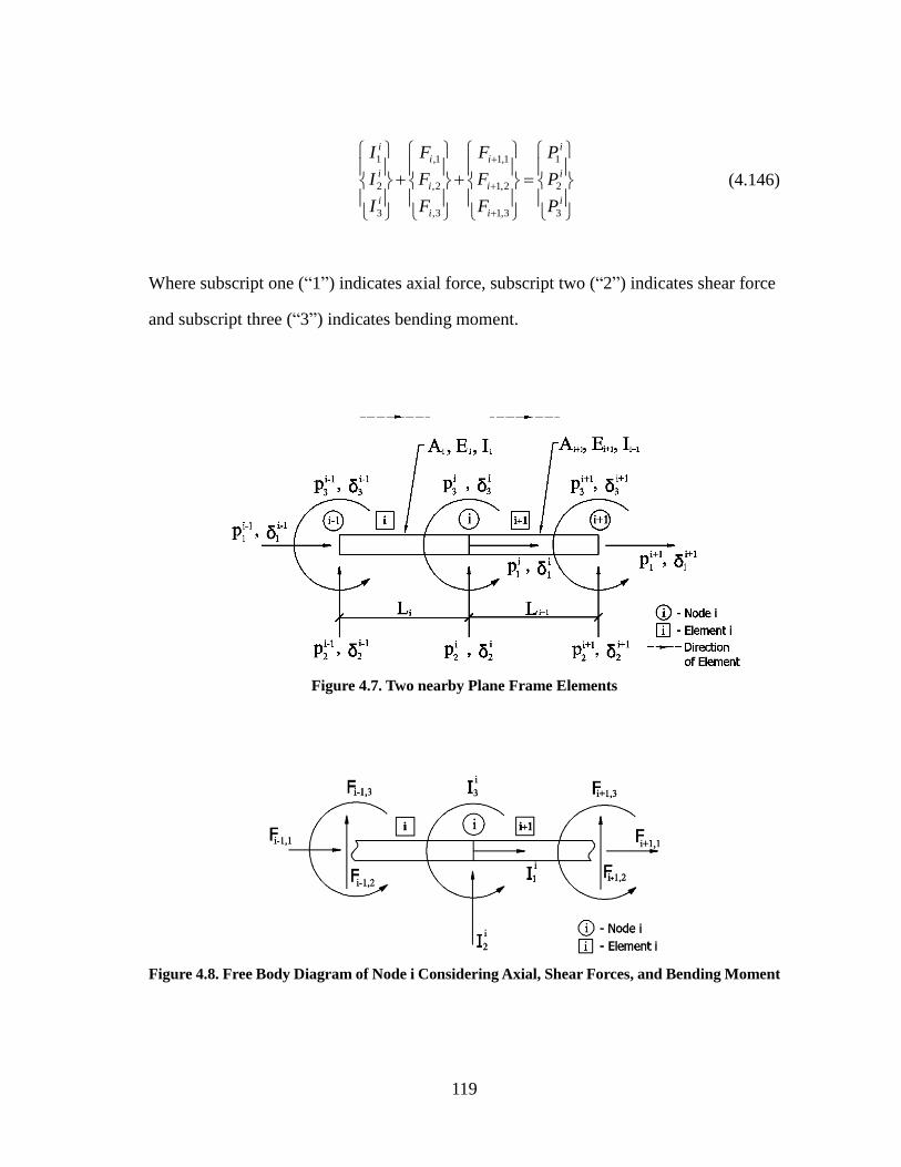
119
i
i
i
i
i
i
i
i
i
i
i
i
P
P
P
F
F
F
F
F
F
I
I
I
3
2
1
3,1
2,1
1,1
3,
2,
1,
3
2
1
(4.146)
Where subscript one (“1”) indicates axial force, subscript two (“2”) indicates shear force
and subscript three (“3”) indicates bending moment.
Figure 4.7. Two nearby Plane Frame Elements
Figure 4.8. Free Body Diagram of Node i Considering Axial, Shear Forces, and Bending Moment

120
Similarly, for the damaged case, the dynamic equilibrium condition is,
}{}{}{}{ **
1
** i
ii
i PFFI (4.147)
Where the asterisk (“*”) denotes the quantities from the damaged case.
Given any velocity vectors, }{ i and }{ *i , for the undamaged and damaged systems,
the power performed by the external forces in the undamaged and damaged systems can
be expressed as follows,
}{}{}{}{}{}{}{}{ 1
iTi
i
Ti
i
TiiTi PFFI (4.148)
}{}{}{}{}{}{}{}{ ***
1
***** iTi
i
Ti
i
TiiTi PFFI (4.149)
Assume that the applied external loads and velocities used to compute power at Node i
are the same for both the undamaged and damaged systems,
}{}{ *ii (4.150)
}{}{ *ii PP (4.151)
Substituting Eq. 4.150 and Eq. 4.151 into Eq. 4.149 yields,
}{}{}{}{}{}{}{}{ *
1
** iTi
i
Ti
i
TiiTi PFFI (4.152)
Noticing the power performed by the external load is the same for both the undamaged
and damaged system. Substituting Eq. 4.152 into Eq. 4.148 yields,
}{}{}{}{}{}{}{}{}{}{}{}{ *
1
**
1 i
Ti
i
TiiTi
i
Ti
i
TiiTi FFIFFI (4.153)
Note, Eq. 153 is equivalent to Eq. 10.

121
In this case, the inertial forces for the undamaged system can be expressed using the
following lumped mass matrix. Note that the inertial effect associated with any rotational
degree of freedom is neglected.
}]{[
0
1
1
22}{
3
2
1
11 ii
o
i
i
i
i
i
iiiii MmLmLm
I
(4.154)
where im is the linear mass of Element i; i
1 is the acceleration in axial direction at
Node i; i
2 is the acceleration in transverse direction at Node i and i
3 is the rotational
acceleration in bending direction within the plain at Node i.
Similarly, for the damaged system,
}]{[
0
1
1
22}{ ***
3
2
*
1*
1
*
1
*** ii
o
i
i
i
i
i
iiiii MmLmLm
I
(4.155)
The force vectors (i.e. }{ iF , }{ 1iF , }{ *
iF , and }{ *
1iF ) in Eq. 4.153 can be computed
using stiffness matrices and node displacement vectors,

122
}]{[
460260
61206120
0000
}{ ,
3
2
1
1
3
1
2
1
1
22
22
3 iioi
i
i
i
i
i
i
i
i
i Kk
LLLL
LLI
AL
I
AL
L
EIF
(4.156)
}]{[
260460
61206120
0000
}{ 11,1
1
3
1
2
1
1
3
2
1
1
22
22
1
31
iioi
i
i
i
i
i
i
i
i
i Kk
LLLL
LLI
AL
I
AL
L
EIF
(4.157)
For the damaged case,
}]{[
460260
61206120
0000
}{ **
,
*
*
3
*
2
*
1
1*
3
1*
2
1*
1*
22
22
*
3
*
iioi
i
i
i
i
i
i
i
i
i Kk
LLLL
LLI
AL
I
AL
L
EIF
(4.158)
}]{[
260460
61206120
0000
}{ *
1
*
1,
*
1
1*
3
1*
2
1*
1
*
3
*
2
*
1*
1
22
22
*
1
3
*
1
iioi
i
i
i
i
i
i
i
i
i Kk
LLLL
LLI
AL
I
AL
L
EIF
(4.159)

123
Where i
1 is the displacement in axial direction at Node i; i
2 is displacement in
transverse direction at Node i; i
3 is the nodal rotation in bending rotation direction
within the plain at Node i.
Substitute Eqs. 4.154 through 4.159 into Eq. 4.153 yields,
}]{[}{}]{[}{}]{[}{
}]{[}{}]{[}{}]{[}{
*
1
*
1,
*
1
**
,
****
11,1,
iioi
Ti
iioi
Tiii
o
iTi
iioi
Ti
iioi
Tiii
o
iTi
KkKkMm
KkKkMm
(4.160)
Note that the force vectors (i.e. }{ iI , }{ iF , }{ 1iF , }{ *iI , }{ *
iF , and }{ *
1iF ) can be
summarized as the multiplication of a property coefficient, a configuration matrix and a
node displacement vector. Because the designed damage are simulated by the changes of
Young’s modulus ( E ) and linear mass ( m ), other parameters, the length of element ( L ),
the cross sectional area ( A ) and the moment inertia of the cross section ( I ), are not
influenced by damage and remain the same for the undamaged and damaged elements.
Consequently, the configuration matrices for the element stiffness and element mass are
the same for both the damaged and undamaged elements. Namely,
][][ ,
*
, ioio KK (4.161)
][][ 1,
*
1, ioio KK (4.162)
][][ * i
o
i
o MM (4.163)
Substituting Eqs. 4.161 through 4.163 into Eq. 4.160 yields,

124
}]{[}{}]{[}{}]{[}{
}]{[}{}]{[}{}]{[}{
*
1
*
1,
*
1
**
,
****
11,1,
iioi
Ti
iioi
Tiii
o
iTi
iioi
Ti
iioi
Tiii
o
iTi
KkKkMm
KkKkMm
(4.164)
Moving forward the property constant from each term in Eq. 4.164 yields,
}]{[}{}]{[}{}]{[}{
}]{[}{}]{[}{}]{[}{
****
1
*
1,
*
1
**
,
*
11,1,
ii
o
Tii
iio
Ti
iiio
Ti
i
iio
Ti
iiio
Ti
i
ii
o
Tii
MmKkKk
KkKkMm
(4.165)
Dividing Eq. 4.165 by im* yields,
}]{[}{}]{[}{}]{[}{
}]{[}{}]{[}{}]{[}{
***
1
*
1,*
*
1**
,*
*
11,*
1,**
ii
o
Ti
iio
Ti
i
iiio
Ti
i
i
iio
Ti
i
iiio
Ti
i
iii
o
Ti
i
i
MKm
kK
m
k
Km
kK
m
kM
m
m
(4.166)
Define the following coefficients,
i
i
m
m*1 (4.167)
i
i
m
k*2 (4.168)
i
i
m
k*
13
(4.169)
i
i
m
k*
*
4 (4.170)
i
i
m
k*
*
15
(4.171)

125
Substituting Eq. 4.167 through Eq. 4.171 to Eq. 4.166 yields,
}]{[}{}]{[}{}]{[}{
}]{[}{}]{[}{}]{[}{
***
1
*
1,5
**
,4
11,3,21
ii
o
Ti
iio
Ti
iio
Ti
iio
Ti
iio
Tiii
o
Ti
MKK
KKM
(4.172)
Writing the Eq. 4.172 at different time point, yields the following groups of equations,
For 0tt ,
000
000
|})]{[}({|})]{[}({|})]{[}({
|})]{[}({|})]{[}({|})]{[}({
***
1
*
1,5
**
,4
11,3,21
t
ii
o
Ti
tiio
Ti
tiio
Ti
tiio
Ti
tiio
Ti
t
ii
o
Ti
MKK
KKM
(4.173)
For jtt ,
jjj
jjj
t
ii
o
Ti
tiio
Ti
tiio
Ti
tiio
Ti
tiio
Ti
t
ii
o
Ti
MKK
KKM
|})]{[}({|})]{[}({|})]{[}({
|})]{[}({|})]{[}({|})]{[}({
***
1
*
1,5
**
,4
11,3,21
(4.174)
For Ntt ,
NNN
NNN
t
ii
o
Ti
tiio
Ti
tiio
Ti
tiio
Ti
tiio
Ti
t
ii
o
Ti
MKK
KKM
|})]{[}({|})]{[}({|})]{[}({
|})]{[}({|})]{[}({|})]{[}({
***
1
*
1,5
**
,4
11,3,21
(4.175)
Arranging the above linear equation group into matrix form, yields,
YβΧ (4.176)
Where the coefficient matrix of the linear equation group is given as following, (note,
due to the limitation of the page size, the transposed form of the matrix is provided)

126
Nj
Nj
Nj
Nj
Nj
tiio
Ti
tiio
Ti
tiio
Ti
tiio
Ti
tiio
Ti
tiio
Ti
tiio
Ti
tiio
Ti
tiio
Ti
tiio
Ti
tiio
Ti
tiio
Ti
t
ii
o
Ti
t
ii
o
Ti
t
ii
o
Ti
T
KKK
KKK
KKK
KKK
MMM
|})]{[}({...|})]{[}({...|})]{[}({
|})]{[}({...|})]{[}({...|})]{[}({
|})]{[}({...|})]{[}({...|})]{[}({
|})]{[}({...|})]{[}({...|})]{[}({
|})]{[}({...|})]{[}({...|})]{[}({
*
11,
*
11,
*
11,
*
,
*
,
*
,
11,11,11,
,,,
0
0
0
0
0
Χ
(4.177)
The vector of unknown and the vector of known are given as,
5
4
3
2
1
β (4.178)
N
j
t
ii
o
Ti
t
ii
o
Ti
t
ii
o
Ti
M
M
M
|})]{[}({
|})]{[}({
|})]{[}({
*
*
*
0
Y (4.179)
Using the Least Square Method, the vector of unknown, ‘β’, can be computed from the
following equation,
)()( 1YΧΧΧβ
TT (4.180)
With the vector of unknown computed, the damage indices for stiffness, mass, and
damping can be computed as follows,
127
1
1
*
1
*
11
*
22
22
iiii
iiii
i
i
mLmLm
LmLm
m
mi (4.181)
4
2
*
3
3
*
*
*
*
i
i
i
i
i
i
i
i
k
L
EI
L
EI
k
k
m
k
m
k
i
(4.182)
5
3
*
1
3
1
3
*
1
1
*
*
1
*
1
1
i
i
i
i
i
i
i
i
k
L
EI
L
EI
k
k
m
k
m
k
i
(4.183)
4.5 THEORY FOR SPACE TRUSSES
In this subsection, the proposed non-destructive evaluation theory will be applied to
space truss at each joint considering vibrations in the global X, Y, and Z directions
simultaneously.
For a joint in space, as shown in Figure 4.9, assume that there are n bars jointed to the
Joint γ and each bar has a defined direction from negative end towards positive end. The
modulus of elasticity of the material for Bar i is denoted as iE . The length of Bar i is iL .
The cross sectional area of Bar i is denoted as Ai. The axial force of Bar i is denoted as
1,iF . The unit vector in the direction of Bar i is denoted as in . According to the free
body diagram at Joint γ shown in Figure 4.10, the dynamic equilibrium condition for the
undamaged system at Joint γ can be expressed as,

128
}{}{...}{...}{}{ 1,1,11,1
PnFnFnFI nnii (4.184)
Similarly, for the damaged case, the dynamic equilibrium condition at Joint i can be
expressed as,
}{}{...}{...}{}{ ***
1,
**
1,
*
1
*
1,1
* PnFnFnFI nnii (4.185)
Where the asterisk (“*”) denotes the quantities from the damaged case.
Figure 4.9. One Joint from a Space Truss with All Bars Joined to the Joint γ
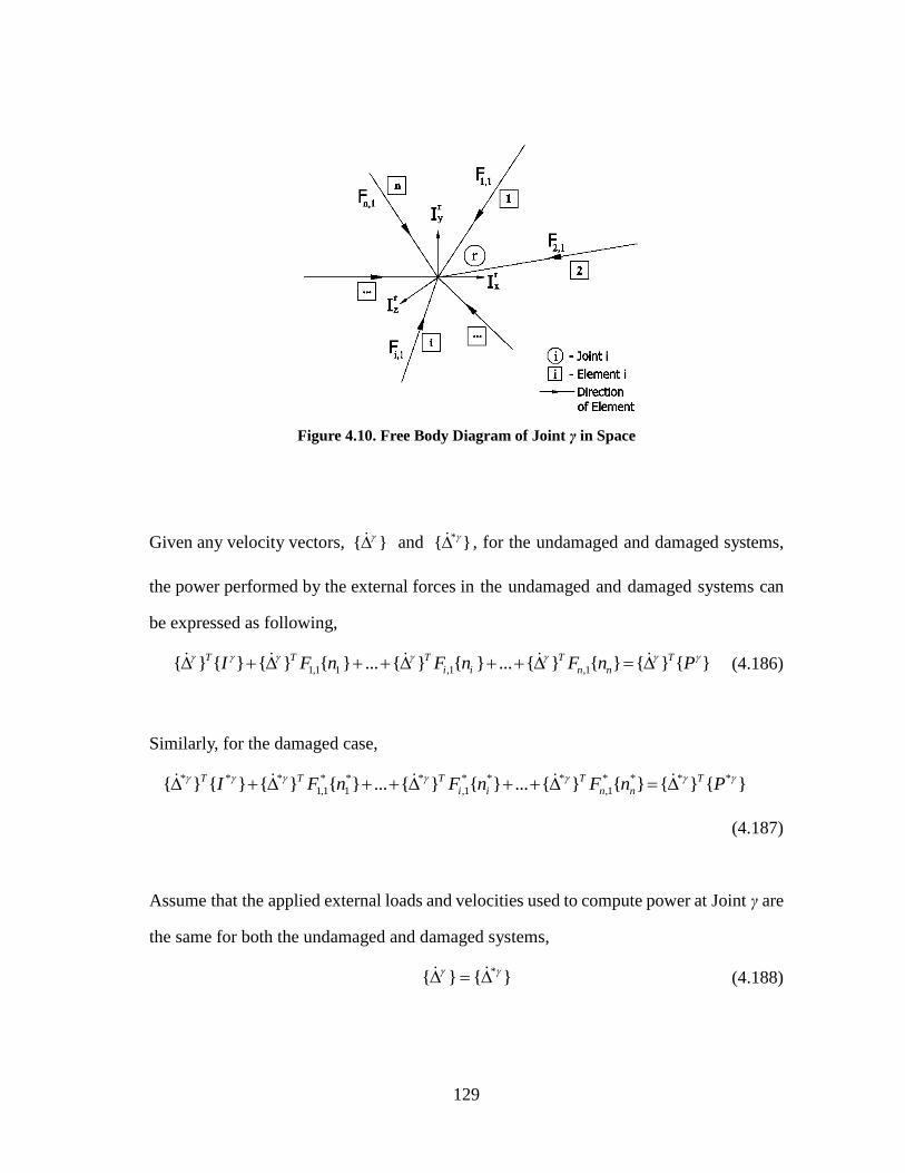
129
Figure 4.10. Free Body Diagram of Joint γ in Space
Given any velocity vectors, }{ and }{ * , for the undamaged and damaged systems,
the power performed by the external forces in the undamaged and damaged systems can
be expressed as following,
}{}{}{}{...}{}{...}{}{}{}{ 1,1,11,1
PnFnFnFI T
nn
T
ii
TTT (4.186)
Similarly, for the damaged case,
}{}{}{}{...}{}{...}{}{}{}{ ****
1,
***
1,
**
1
*
1,1
*** PnFnFnFI T
nn
T
ii
TTT
(4.187)
Assume that the applied external loads and velocities used to compute power at Joint γ are
the same for both the undamaged and damaged systems,
}{}{ * (4.188)

130
}{}{ * PP (4.189)
Substituting Eq. 4.188 and Eq. 4.189 into Eq. 4.187 yields,
}{}{}{}{...}{}{...}{}{}{}{ **
1,
**
1,
*
1
*
1,1
* PnFnFnFI T
nn
T
ii
TTT
(4.190)
Noticing the power performed by the external load are the same for both the undamaged
and damaged system. Substituting Eq. 4.190 into Eq. 4.186 yields,
}{}{...}{}{...}{}{}{}{
}{}{...}{}{...}{}{}{}{
**
1,
**
1,
*
1
*
1,1
*
1,1,11,1
nn
T
ii
TTT
nn
T
ii
TTT
nFnFnFI
nFnFnFI
(4.191)
Note, Eq. 4.191 is equivalent to Eq. 2.10.
In this case, the inertial forces can be expressed using the following lumped mass matrix.
Namely,
}]{[
1
1
1
222}{ 11
o
z
y
x
nnii MmLmLmLm
I
(4.192)
Where im is the linear mass of Bar i; x is the acceleration of Joint γ in x-direction in
the global coordinate system; y is the acceleration of Joint γ in y-direction in the
global coordinate system and z is the acceleration of Joint γ in z-direction in the global
coordinate system; m is the lumped mass of the Joint γ; and ][
oM is the

131
configuration matrix of the mass matrix.
Similarly, for the damaged system,
}]{[
1
1
1
222}{ ***
*
*
*
*****
1
*
1*
o
z
y
x
nnii MmLmLmLm
I
(4.193)
Note, in this case, the ][ oM and ][ *
oM are both 3×3 identity matrices, thus,
][][ * oo MM (4.194)
Substituting Eq. 4.194 into Eq. 4.193 yields,
}]{[}{ *** oMmI (4.195)
The axial force of the ith bar connected the Joint γ can be computed as,
)ˆˆ(ˆ
ˆ11 1,1,
1,
1,
1,
ii
ii
i
i
i
iL
EA
L
EAF
(4.196)
where,
1,ˆi is the axial direction movement of the positive end of the Bar i connected to
Joint γ in local coordinate system;
1,ˆi is the axial direction movement of the negative
end of Bar i connected with Joint γ in the local coordinate system. The upward arrow (‘^’)
means the value in the local coordinate.
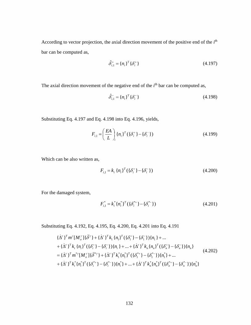
132
According to vector projection, the axial direction movement of the positive end of the ith
bar can be computed as,
}{}{ˆ1,
i
T
ii n (4.197)
The axial direction movement of the negative end of the ith bar can be computed as,
}{}{ˆ1,
i
T
ii n (4.198)
Substituting Eq. 4.197 and Eq. 4.198 into Eq. 4.196, yields,
}){}({}{1,
ii
T
i
i
i nL
EAF (4.199)
Which can be also written as,
}){}({}{1,
ii
T
iii nkF (4.200)
For the damaged system,
}){}({}{ *****
1,
ii
T
iii nkF (4.201)
Substituting Eq. 4.192, Eq. 4.195, Eq. 4.200, Eq. 4.201 into Eq. 4.191
}}){{}({}{}{...}}){{}({}{}{
...}}){{}({}{}{}]{[}{
}}){{}({}{}{...}}){{}({}{}{
...}}){{}({}{}{}]{[}{
**********
*
1
*
1
*
1
*
1
*
1
**
11111
nnn
T
nn
T
iii
T
ii
T
TT
o
T
nnn
T
nn
T
iii
T
ii
T
TT
o
T
nnknnk
nnkMm
nnknnk
nnkMm
(4.202)
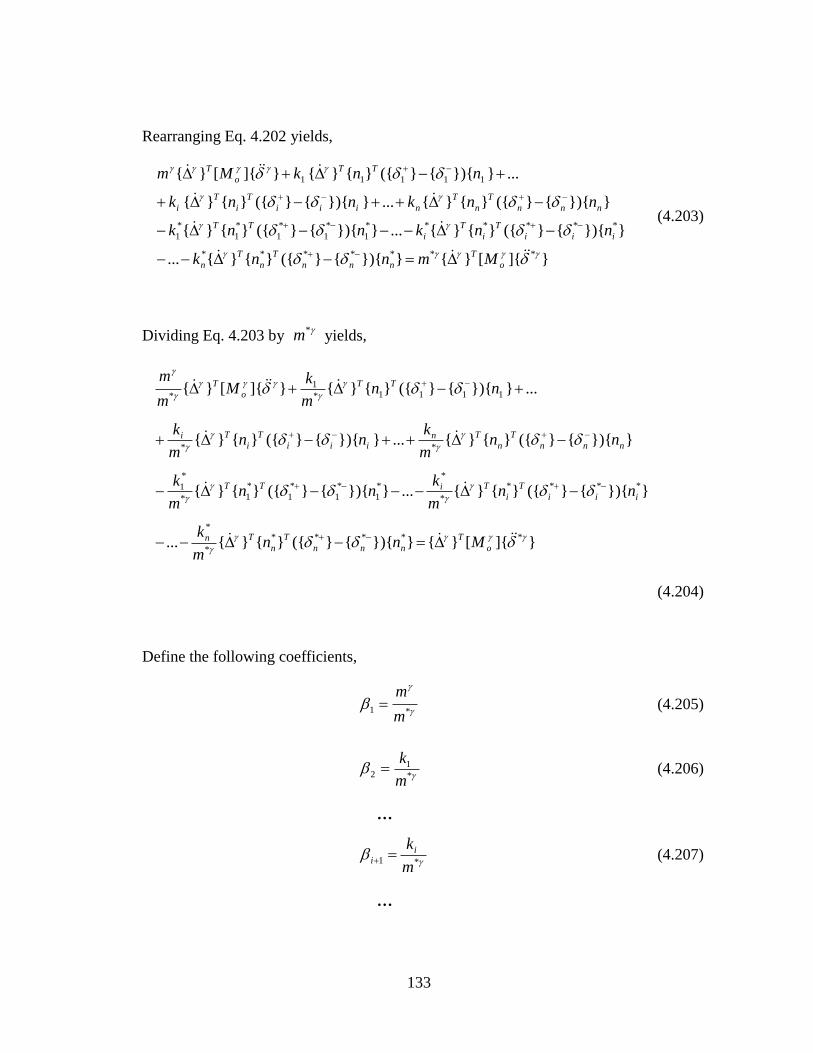
133
Rearranging Eq. 4.202 yields,
}]{[}{}}){{}({}{}{...
}}){{}({}{}{...}}){{}({}{}{
}}){{}({}{}{...}}){{}({}{}{
...}}){{}({}{}{}]{[}{
*******
******
1
*
1
*
1
*
1
*
1
11111
o
T
nnn
T
n
T
n
iii
T
i
T
i
TT
nnn
T
n
T
niii
T
i
T
i
TT
o
T
Mmnnk
nnknnk
nnknnk
nnkMm
(4.203)
Dividing Eq. 4.203 by *m yields,
}]{[}{}}){{}({}{}{...
}}){{}({}{}{...}}){{}({}{}{
}}){{}({}{}{...}}){{}({}{}{
...}}){{}({}{}{}]{[}{
*****
*
*
****
*
**
1
*
1
*
1
*
1*
*
1
**
1111*
1
*
o
T
nnn
T
n
Tn
iii
T
i
TiTT
nnn
T
n
Tniii
T
i
Ti
TT
o
T
Mnnm
k
nnm
knn
m
k
nnm
knn
m
k
nnm
kM
m
m
(4.204)
Define the following coefficients,
*1
m
m (4.205)
*
12
m
k (4.206)
…
*1m
kii (4.207)
…
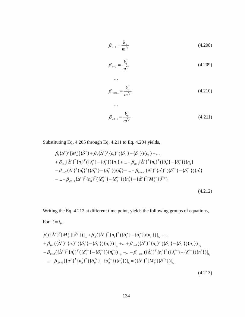
134
*1m
knn
(4.208)
*
*
12
m
kn
(4.209)
…
*
*
1m
kini
(4.210)
…
*
*
12m
knn
(4.211)
Substituting Eq. 4.205 through Eq. 4.211 to Eq. 4.204 yields,
}]{[}{}}){{}({}{}{...
}}){{}({}{}{...}}){{}({}{}{
}}){{}({}{}{...}}){{}({}{}{
...}}){{}({}{}{}]{[}{
*****
12
****
1
*
1
*
1
*
1
*
12
11
111121
o
T
nnn
T
n
T
n
iii
T
i
T
ni
TT
n
nnn
T
n
T
niii
T
i
T
i
TT
o
T
Mnn
nnnn
nnnn
nnM
(4.212)
Writing the Eq. 4.212 at different time point, yields the following groups of equations,
For 0tt ,
00
00
00
00
|})]{[}({|})}){{}({}{}({...
|})}){{}({}{}({...|})}){{}({}{}({
|})}){{}({}{}({...|})}){{}({}{}({
...|})}){{}({}{}({|})]{[}({
*****
12
****
1
*
1
*
1
*
1
*
12
11
111121
to
T
tnnn
T
n
T
n
tiii
T
i
T
nit
TT
n
tnnn
T
n
T
ntiii
T
i
T
i
t
TT
to
T
Mnn
nnnn
nnnn
nnM
(4.213)

135
For jtt ,
jj
jj
jj
jj
to
T
tnnn
T
n
T
n
tiii
T
i
T
nit
TT
n
tnnn
T
n
T
ntiii
T
i
T
i
t
TT
to
T
Mnn
nnnn
nnnn
nnM
|})]{[}({|})}){{}({}{}({...
|})}){{}({}{}({...|})}){{}({}{}({
|})}){{}({}{}({...|})}){{}({}{}({
...|})}){{}({}{}({|})]{[}({
*****
12
****
1
*
1
*
1
*
1
*
12
11
111121
(4.214)
For Ntt ,
NN
NN
NN
NN
to
T
tnnn
T
n
T
n
tiii
T
i
T
nit
TT
n
tnnn
T
n
T
ntiii
T
i
T
i
t
TT
to
T
Mnn
nnnn
nnnn
nnM
|})]{[}({|})}){{}({}{}({...
|})}){{}({}{}({...|})}){{}({}{}({
|})}){{}({}{}({...|})}){{}({}{}({
...|})}){{}({}{}({|})]{[}({
*****
12
****
1
*
1
*
1
*
1
*
12
11
111121
(4.215)
Arranging the above linear equation group into matrix form, yields,
YβΧ (4.216)
Where the coefficient matrix of the linear equation group is given as following, (note,
due to the limitation of the page size, the transposed form of the matrix is provided),

136
Nj
Nj
Nj
Nj
Nj
Nj
Nj
tnnn
T
n
T
tnnn
T
n
T
tnnn
T
n
T
tiii
T
i
T
tiii
T
i
T
tiii
T
i
T
t
TT
t
TT
t
TT
tnnn
T
n
T
tnnn
T
n
T
tnnn
T
n
T
tiii
T
i
T
tiii
T
i
T
tiii
T
i
T
t
TT
t
TT
t
TT
to
T
to
T
to
T
T
nnnnnn
nnnnnn
nnnnnn
nnnnnn
nnnnnn
nnnnnn
MMM
|})}){{}({}{}({|})}){{}({}{}({|})}){{}({}{}({
|})}){{}({}{}({|})}){{}({}{}({|})}){{}({}{}({
|})}){{}({}{}({|})}){{}({}{}({|})}){{}({}{}({
|})}){{}({}{}({|})}){{}({}{}({|})}){{}({}{}({
|})}){{}({}{}({|})}){{}({}{}({|})}){{}({}{}({
|})}){{}({}{}({|})}){{}({}{}({|})}){{}({}{}({
|})]{[}({|})]{[}({|})]{[}({
************
************
*
1
*
1
*
1
*
1
*
1
*
1
*
1
*
1
*
1
*
1
*
1
*
1
111111111111
0
0
0
0
0
0
0
Χ
(4.217)

137
The vector of unknown and the vector of known are given as,
12
1
2
1
1
2
1
n
ni
n
n
i
β (4.218)
N
j
to
T
to
T
to
T
M
M
M
|})]{[}({
|})]{[}({
|})]{[}({
*
*
*
0
Y (4.219)
Using the Least Square Method, the vector of unknown, ‘β’, can be computed from the
following equation,
)()( 1YΧΧΧβ
TT (4.220)
With the vector of unknown computed, the damage indices for stiffness, mass and
damping can be computed as follows,
1*****
1
*
1
11
*
222
222
nnii
nnii
mLmLmLm
LmLmLm
m
m
(4.221)

138
2
2
*
*
1
*
1
*
1
1
*
1
1
1
n
k
m
k
m
k
k
k
L
EA
L
EA
(4.222)
…
1
1
*
*
*
**
ni
i
i
i
i
i
i
i
k
m
k
m
k
k
k
L
EA
L
EA
i
(4.223)
…
12
1
*
*
*
**
n
n
n
n
n
n
n
n
k
m
k
m
k
k
k
L
EA
L
EA
n
(4.224)
4.6 OVERALL SOLUTION PROCEDURE
To perform the proposed damage detection method to continuous system, the following
steps should be followed:
(1) Derive the linear equation group for the specific continuous system based on
the power equilibrium at a single joint or among multiple joints;
(2) Collect the displacement, velocity, and acceleration records required by the
coefficient matrix and the vector of knowns of the linear equation group
defined by step 1;
(3) Use the least square method to solve the linear equation group for the vector
of unknown; and
(4) Compute for the Damage Indices and Damage severities for each physical
property based on the vector of unknown computed from Step 3.

139
The general process will be clearly demonstrated in Section 5.
4.7 SUMMARY
In this Section, the Power Method for a rod, Euler-Bernoulli beam, plane frame, and
space truss were studied. The derivation processes were provided in Section 4.2 to
Section 4.5 and the overall solution procedure was provided in Section 4.6. In section
4.2.1, the specific form of the proposed method was derived to detect and evaluate
damage in rod elements based on the power equilibrium at each joint. In Section 4.2.2,
the specific form of the proposed method was derived to detect and evaluate damage in
rod elements based on the power equilibrium at multiple joints. In Section 4.3, the
specific form of the proposed method was derived to detect and evaluate damage in
beam elements based on the power equilibrium at each joint. In Section 4.4, the specific
form of the proposed method was derived to detect and evaluate damage in plane frame
elements based on the power equilibrium at each joint. In Section 4.5, the specific form
of the proposed method was derived to detect and evaluate damage in space truss
elements (bars) based on the power equilibrium at each joint.
The advantage of the Power Method is that the method was able to simultaneously detect
damage in physical properties of multiple structural members related to multiple types of
vibrations. In other words,
(1) In real experiment, the vibration is not limited in one direction and one type.
By using the dynamic data from vibration of all related directions, the Power
Method will provide more reliable damage evaluation results; and
(2) The Power Method provides the option of detecting damage in the whole

140
structure or at multiple locations of the structure, besides at single location.
This advantage can be used to increase the computation efficiency.

141
5 CASE STUDIES OF DAMAGE EVALUATION FOR CONTINUOUS
SYSTEMS
5.1 INTRODUCTION
The objective of this section is to validate the proposed theory for continuous systems
using numerical examples. To achieve this goal, the theory is validated using exact
displacements, velocities, and accelerations of the undamaged and damaged continuous
systems modeled within SAP2000 (Version 15). The exact displacements, velocities, and
accelerations are computed from the linear direct integration in SAP2000. The
Hilber-Hughes-Taylor time integration method was used by SAP2000. The three
parameters of the Hilber-Hughes-Taylor method: Gamma, Beta and Alpha were set to be
0.5, 0.25 and 0, respectively. Five linearly elastic numerical cases are studied in this
section,
Case #1: the accuracy of the theory will be studied on a rod under axial and torsional
vibrations. The rod is fixed at its left end. The damage detection algorithm of the Power
Method for a rod under axial and torsional vibration is derived and is provided in Section
4.2.1. The damage is simulated by the changes of masses and stiffness of specific rod
elements.
Case #2: the accuracy of the theory will be studied on the same rod under axial vibration.
The algorithm of the Power Method for the whole rod under axial vibration is derived
and is provided in Section 4.2.2. The damage is simulated by the changes of masses and
stiffness of specific rod elements.

142
Case #3: the accuracy of the theory will be studied on a propped cantilever beam under
bending vibration. The algorithm of the Power Method for an Euler-Bernoulli beam
under bending vibration is derived and is provided in Section 4.3. The damage is
simulated by the changes of masses and stiffness of specific beam elements.
Case #4: the accuracy of the theory will be studied on a two-bay frame. The algorithm of
the Power Method for a plane frame under axial and bending vibration is derived and is
provided in Section 4.4. The damage is simulated by the changes of masses and stiffness
of specific frame elements.
Case #5: the accuracy of the theory will be studied on a simple space truss. The
algorithm of the Power Method for a space truss is derived and is provided in Section 4.5.
The damage is simulated by the changes of masses and stiffness of specific truss
elements.
5.2 DAMAGE EVALUATION FOR A ROD
In Case #1, a rod fixed at its left end is used to evaluate the proposed theory. Figure 5.1
indicates the geometry, and damage scenario under consideration. The geometry of the
cross-section of the rod is shown in Figure 5.2. The modulus of elasticity (E) of the
material is 29,000 ksi. The modulus of elasticity in shear (G) of the material is 11,154 ksi.
The Poisson’s ratio of the material (υ) is 0.3. The torsional constant of the cross section
of (J) is 7.9522. The mass density of the material is 7.345×10⁻⁷ kipsec2/in4. In this case,
four elements with damaged mass and stiffness are studied.

143
The rod is meshed into 12 elements and has 13 equally spaced nodes. The length of each
element is 1.0 inches. For illustrative purposes, typical elements are indicated in Figure
5.1. The damage is simulated by a ten percent (10%) reduction of the modulus of
elasticity and twenty percent (20%) reduction of the mass of Elements 5, 6, 9, and 10.
For each node in the rod model, a dynamic force, 100cos(2πt), is applied in both axial (x1)
and torsional (θ1) direction. Given the applied load case, the displacement, velocity, and
acceleration time histories in both axial and torsional direction are directly generated
from SAP2000 using linear direct integration method. The computation step is 1E-4
seconds (10,000 Hz) for total 0.2 seconds. For both the undamaged and damaged Rods,
the displacements, velocities and accelerations of the Node 13 in axial direction were
plotted in Figure 5.3, Figure 5.4, and Figure 5.5.
In this case, the computed velocity ( )(tx ) of each node in the undamaged case was used
as the velocity used to compute power ( ) for both the undamaged and damaged cases.
For every two nearby elements, the coefficient matrices (‘X’) and known vector (‘Y’)
were constructed by substituting the acceleration ( )(tx ), velocity ( )(tx ), displacement
( )(tx ), and velocity used to compute power ( ) into Eq. 4.50 and Eq. 4.52. The
coefficient damage index vector, β, related to the two nearby elements, is computed
using Eq. 4.53. Then the damage indices for mass and stiffness are computed using Eqs.
4.54 through 4.56. The damage severities for mass and stiffness are computed using Eq.
2.13. For each two nearby elements, the above process is performed. For simplicity
purposes, no overlap element is used. Thus, the proposed theory is only applied to six
pairs of elements. The estimated damage indices and the designed damage indices for

144
each physical property are listed in Table 5.1 and are plotted in Figure 5.6 for nodal mass
and Figure 5.8 for element stiffness. The estimated damage severities and the designed
damage severities for each physical property are plotted in Figure 5.7 for nodal mass and
Figure 5.9 for element stiffness. Because the proposed method is applied at the center
node of two nearby elements, only six nodes were taken into consideration (i.e. Nodes 2,
4, 6, 8, 10, and 12). Comparing the estimated damage indices with the designed damage
indices, the proposed method can accurately locate and size multiple damage in a rod
with axial and torsional vibrations.
Figure 5.1. Geometry, Damage Scenario, and Finite Element Discretization of the Rod

145
Figure 5.2. Geometry of the Cross-Section of the Rod
Figure 5.3. Displacements in Axial Direction of the Node 13 of the Undamaged and Damaged
Rods under the Given External Load

146
Figure 5.4. Velocities of the Node 13 in Axial Direction of the Undamaged and Damaged Rods
under the Given External Load
Figure 5.5. Accelerations of the Node 13 in Axial Direction of the Undamaged and Damaged
Rods under the Given External Load
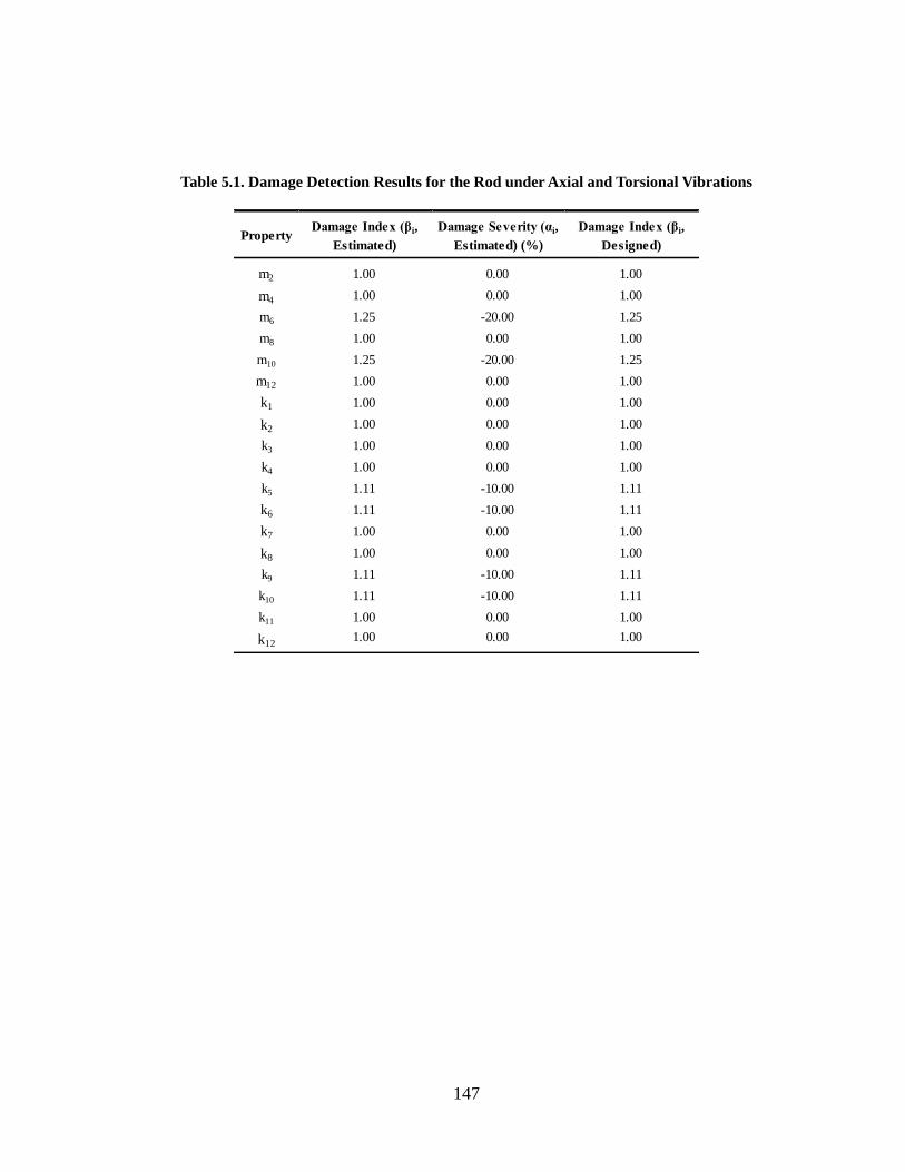
147
Table 5.1. Damage Detection Results for the Rod under Axial and Torsional Vibrations
PropertyDamage Index (βi,
Estimated)
Damage Severity (αi,
Estimated) (%)
Damage Index (βi,
Designed)
m2 1.00 0.00 1.00
m4 1.00 0.00 1.00
m6 1.25 -20.00 1.25
m8 1.00 0.00 1.00
m10 1.25 -20.00 1.25
m12 1.00 0.00 1.00
k1 1.00 0.00 1.00
k2 1.00 0.00 1.00
k3 1.00 0.00 1.00
k4 1.00 0.00 1.00
k5 1.11 -10.00 1.11
k6 1.11 -10.00 1.11
k7 1.00 0.00 1.00
k8 1.00 0.00 1.00
k9 1.11 -10.00 1.11
k10 1.11 -10.00 1.11
k11 1.00 0.00 1.00
k121.00 0.00 1.00

148
Figure 5.6. Damage Indices of Nodal Mass (βmi) for the Rod under Axial and Torsional
Vibrations
Figure 5.7. Damage Severities of Nodal Mass (аmi) for the Rod under Axial and Torsional
Vibrations

149
Figure 5.8. Damage Indices of Element Stiffness (βki) for the Rod under Axial and Torsional
Vibrations
Figure 5.9. Damage Severities of Element Stiffness (аki) for the Rod under Axial and Torsional
Vibrations

150
5.3 DAMAGE EVALUATION FOR A ROD AS A WHOLE SYSTEM
In Case #2, the same rod is used to evaluate the proposed theory. The geometry, damage
scenario and finite element discretization under consideration are indicated in Figure
5.10. The geometry of the cross-section of the rod is shown in Figure 5.2. The modulus
of elasticity (E) of the material is 29,000 ksi. The modulus of elasticity in shear (G) of the
material is 11154 ksi. The Poisson’s ratio of the material (υ) is 0.3. The torsional constant
of the cross section of (J) is 7.9522. The mass density of the material is 7.345×10⁻⁷
kipsec2/in4. In this case, four elements with damaged mass and stiffness are studied.
The rod is meshed into 12 elements and has 13 equally spaced nodes. The length of each
element is 1.0 inches. For illustrative purposes, typical elements are indicated in Figure
5.10. The damage is simulated by a ten percent (10%) reduction of the modulus of
elasticity and twenty percent (20%) reduction of the mass of Elements 5, 6, 9, and 10.
For each node in the rod model, a dynamic force, 100cos(2πt), is applied in only axial (x1)
direction. Given the external load case, the displacement, velocity, and acceleration time
histories are directly generated from SAP2000 using linear direct integration method.
The computation step is 1E-4 seconds (10,000Hz) for total 0.2 seconds. The
displacements, velocities and accelerations of Node 13 in both the undamaged and
damaged rods were plotted in Figure 5.11, Figure 5.12, and Figure 5.13.
In this case, the computed velocity ( )(tx ) of each node in the undamaged case was used
as the velocity used to compute power ( ) for both the undamaged and damaged cases.
For all the nodes in the rod, the coefficient matrices (‘X’) and known vector (‘Y’) were
constructed at one time by substituting the acceleration ( )(tx ), velocity ( )(tx ),

151
displacement ( )(tx ), and velocity used to compute power ( ) into Eq. 4.96 and Eq. 4.98.
The coefficient damage index vector, β, related to the each element in the rod was
computed using Eq. 4.99. Then the damage indices for mass and stiffness are computed
using Eqs. 4.100 through 4.106. The damage severities for mass and stiffness are
computed using Eq. 2.13. For the whole rod, the above process is performed only once.
The estimated damage indices and the designed damage indices for each physical
property are listed in Table 5.2 and are plotted in Figure 5.14 for nodal mass and Figure
5.16 for element stiffness. The estimated damage severities and the designed damage
severities for each physical property are plotted in Figure 5.15 for nodal mass and Figure
5.17 for element stiffness. Because the proposed method is applied at the each node of
the whole rod, thus all nodes, except for the fixed node, were taken into consideration
(i.e. Nodes 1 through 12). Comparing the estimated damage indices with the designed
damage indices, the proposed method can accurately locate and size multiple damage in
a rod with axial and torsional vibrations.
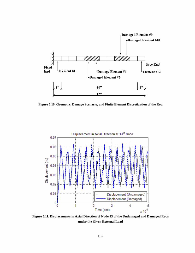
152
Figure 5.10. Geometry, Damage Scenario, and Finite Element Discretization of the Rod
Figure 5.11. Displacements in Axial Direction of Node 13 of the Undamaged and Damaged Rods
under the Given External Load

153
Figure 5.12. Velocities of Node 13 in Axial Direction of the Undamaged and Damaged Rods
under the Given External Load
Figure 5.13. Accelerations of Node 13 in Axial Direction of the Undamaged and Damaged Rods
under the Given External Load

154
Table 5.2. Damage Detection Results for the Analysis of Rod under Axial As a Whole
PropertyDamage Index (βi,
Estimated)
Damage Severity (αi,
Estimated) (%)
Damage Index (βi,
Designed)
m1 1.00 0.00 1.00
m2 1.00 0.00 1.00
m3 1.00 0.00 1.00
m4 1.11 -10.00 1.11
m5 1.25 -20.00 1.25
m6 1.11 -10.00 1.11
m7 1.00 0.00 1.00
m8 1.11 -10.00 1.11
m9 1.25 -20.00 1.25
m10 1.11 -10.00 1.11
m11 1.00 0.00 1.00
m12 1.00 0.00 1.00
k1 1.00 0.00 1.00
k2 1.00 0.00 1.00
k3 1.00 0.00 1.00
k4 1.00 0.00 1.00
k5 1.11 -10.00 1.11
k6 1.11 -10.00 1.11
k7 1.00 0.00 1.00
k8 1.00 0.00 1.00
k9 1.11 -10.00 1.11
k10 1.11 -10.00 1.11
k11 1.00 0.00 1.00
k121.00 0.00 1.00

155
Figure 5.14. Damage Indices of Nodal Mass (βmi) for the Rod under Axial and Torsional
Vibrations
Figure 5.15. Damage Severities of Nodal Mass (аmi) for the Rod under Axial and Torsional
Vibrations

156
Figure 5.16. Damage Indices of Element Stiffness (βki) for the Rod under Axial and Torsional
Vibrations
Figure 5.17. Damage Severities of Element Stiffness (аki) for the Rod under Axial and Torsional
Vibrations

157
5.4 DAMAGE EVALUATION FOR AN EULER-BERNOULLI BEAM
In Case #3, a propped cantilever is used to evaluate the proposed theory. The geometry,
damage scenario, and load case under consideration are indicated in Figure 5.18. The
geometry of the cross-section of the cantilever is shown in Figure 5.19. The modulus of
elasticity (E) of the material is 29,000 ksi. The mass density of the material is 7.345×10⁻⁷
kipsec2/in4.
The propped cantilever is meshed into 12 elements and has 13 equally spaced nodes. The
length of each element is 1.0 inches. For illustrative purposes, typical elements are
indicated in Figure 5.18. Four elements with damaged mass and stiffness are studied.
The damage is simulated by a ten percent (10%) reduction of the modulus of elasticity
and twenty percent (20%) reduction of the mass of Element 5 and Element 6 and a five
percent (5%) reduction of the modulus of elasticity and ten percent (10%) reduction of
the mass of Element 11 and Element 12 of the beam.
For each node of the propped cantilever beam, a dynamic point load, 10cos(2πt), is
applied in transverse direction at each node. Given the external load case, the
displacement, velocity, and acceleration time histories are directly generated from
SAP2000 using linear direct integration method. The computation step is 1E-4 seconds
(10,000 Hz) for total 0.2 seconds. The deflections, velocities in transverse direction and
accelerations in transverse direction of Node 7 in both the undamaged and damaged
propped cantilever were plotted in Figure 5.20, Figure 5.21, and Figure 5.22.
In this case, the computed velocity ( )(tx ) of each node in the undamaged case was used
as the velocity used to compute power ( ) for both the undamaged and damaged cases.

158
For every two nearby elements, the coefficient matrices (‘X’) and known vector (‘Y’)
were constructed by substituting the acceleration ( )(tx ), velocity ( )(tx ), displacement
( )(tx ), and velocity used to compute power ( ) into Eq. 4.138 and Eq. 4.140. The
coefficient damage index vector, β, related to the two nearby elements was computed
using Eq. 4.141. Then the damage indices for mass and stiffness are computed using Eqs.
4.142 through 4.144. The damage severities for mass and stiffness are computed using
Eq. 2.13. For each two nearby elements, the above process is performed. For simplicity
purposes, no overlap element is used. Thus, the proposed theory is only applied to six
pairs of elements. The estimated damage indices and the designed damage indices for
each physical property are listed in Table 5.3 and are plotted in Figure 5.23 for nodal
mass and Figure 5.25 for element stiffness. The estimated damage severities and the
designed damage severities for each physical property are plotted in Figure 5.24 for
nodal mass and Figure 5.26 for element stiffness. Comparing the estimated damage
indices with the designed damage indices, the proposed method can accurately locate
and size multiple damage in a beam with bending vibrations.

159
Figure 5.18. Geometry, Damage Scenario, and Load Case for the Propped Cantilever
Figure 5.19. Geometry of the Cross-Section of the I Beam

160
Figure 5.20. Deflection of the Node 7 of the Undamaged and Damaged Cases under the Given
External Load
Figure 5.21. Velocities in Transverse Direction of the Node 7 of the Undamaged and Damaged
Cases under the Given External Load

161
Figure 5.22. Accelerations in Transverse Direction of the Node 7 of the Undamaged and
Damaged Cases under the Given External Load

162
Table 5.3. Damage Detection Results for the Propped Cantilever
PropertyDamage Index (βi,
Estimated)
Damage Severity (αi,
Estimated) (%)
Damage Index (βi,
Designed)
m2 1.000 0.000 1.000
m4 1.000 0.000 1.000
m6 1.250 -20.000 1.250
m8 1.000 0.000 1.000
m10 1.000 0.000 1.000
m12 1.111 -10.000 1.111
k1 1.000 0.000 1.000
k2 1.000 0.000 1.000
k3 1.000 0.000 1.000
k4 1.000 0.000 1.000
k5 1.111 -10.000 1.111
k6 1.111 -10.000 1.111
k7 1.000 0.000 1.000
k8 1.000 0.000 1.000
k9 1.000 0.000 1.000
k10 1.000 0.000 1.000
k11 1.053 -5.000 1.053
k12 1.053 -5.000 1.053

163
Figure 5.23. Damage Indices of Nodal Mass (βmi) for the Propped Cantilever
Figure 5.24. Damage Severities of Nodal Mass (аmi) for the Propped Cantilever
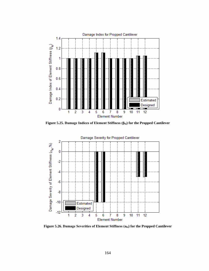
164
Figure 5.25. Damage Indices of Element Stiffness (βki) for the Propped Cantilever
Figure 5.26. Damage Severities of Element Stiffness (аki) for the Propped Cantilever

165
5.5 DAMAGE EVALUATION FOR A PLAIN FRAME
In Case #4, a two-bay frame is used to evaluate the proposed theory. The structure
includes three types of members: a continuous beam, three columns, and elastic isolators
in between. Three elastic isolators are fixed to the beam and each column is fixed to the
end of each isolator. The elastic isolators are simulated by beam elements with smaller
cross section, shown in Figure 5.28. The cross sections for the continuous beam and the
columns are the same and the geometry of the cross section is shown in Figure 5.19. The
material properties for the all three types of members are the same. The modulus of
elasticity (E) of the material is 29,000 ksi. The mass density of the material is 7.345×10⁻⁷
kipsec2/in4. A cosine external point load, 10cos(2πt) kips, is applied on each node of the
frame. The geometry of the structure and the damage scenario are shown in Figure 5.27.
The damage scenario for this case is as follows: (1) both of the two spans of the
continuous beam are damaged; (2) the two left isolators are damaged; and (3) the two
left columns are damaged. The right isolator and right column are intact. The damage are
simulated by a ten percent (10%) reduction of the modulus of elasticity and twenty
percent (20%) reduction of the mass of the damaged elements. The damaged elements in
the damaged two-bay frame include: (1) Element 43, Element 44, Element 103 and
Element 104 on the continuous beam; (2) all elements in the left and middle isolators (i.e.
six elements for each isolator); (3) Element 43 and Element 44 in each of the left two
columns. The damaged isolators are denoted by “Damaged Isolator A” and “Damaged
Isolator B” and the damaged elements on both the beam (43rd, 44th, 103rd and 104th) and
the two columns (43rd and 44th) are indicated as a solid black in Figure 5.27.
The beam is meshed into 120 elements and has 121 equally spaced nodes. Each of the

166
elastic isolators is meshed into 6 elements and has 7 equally spaced nodes. Each column
is meshed into 60 elements and has 61 equally spaced nodes. The length of each element
in the three types of members is 2.0 inches. For illustrative purposes, several typical
elements are indicated in Figure 5.27.
Given the external load case, the displacement, velocity, and acceleration time histories
are directly generated from SAP2000 using linear direct integration method. The
computation step is 1E-4 seconds (10,000 Hz) for total 0.01 seconds. The deflections,
velocities in transverse direction and accelerations in transverse direction of Node 61 in
both the undamaged and damaged propped cantilever were plotted in Figure 5.29, Figure
5.30, and Figure 5.31. (Note, the two-bay frame is a linearly elastic frame)
In this case, the computed velocity ( )(tx ) of each node in the undamaged case was used
as the velocity used to compute power ( ) for both the undamaged and damaged cases.
For every two nearby elements, the coefficient matrices (‘X’) and known vector (‘Y’)
were constructed by substituting the acceleration ( )(tx ), velocity ( )(tx ), displacement
( )(tx ), and velocity used to compute power ( ) into Eq. 4.177 and Eq. 4.179. The
coefficient damage index vector, β, related to the two nearby elements was computed
using Eq. 4.180. Then the damage indices for mass and stiffness are computed using Eqs.
4.181 through 4.183. The damage severities for mass and stiffness are computed using
Eq. 2.13. For each two nearby elements, the above process is performed. The estimated
damage indices for nodal mass and element stiffness for the continuous beam are plotted
in Figure 5.32 and Figure 5.34, respectively. The estimated damage severities for nodal
mass and element stiffness for the continuous beam are plotted in Figure 5.33 and Figure

167
5.35, respectively.
The estimated damage indices for nodal mass and element stiffness for the Isolator and
Column A are plotted in Figure 5.36 and Figure 5.38, respectively. The estimated damage
severities for nodal mass and element stiffness for the Isolator and Column A are plotted
in Figure 5.37 and Figure 5.39, respectively.
The estimated damage indices for nodal mass and element stiffness for the Isolator and
Column B are plotted in Figure 5.40 and Figure 5.42, respectively. The estimated
damage severities for nodal mass and element stiffness for the Isolator and Column B are
plotted in Figure 5.41 and Figure 5.43, respectively.
The estimated damage indices for nodal mass and element stiffness for the Isolator and
Column C are plotted in Figure 5.44 and Figure 5.46, respectively. The estimated
damage severities for nodal mass and element stiffness for the Isolator and Column C are
plotted in Figure 5.45 and Figure 5.47, respectively.
Comparing the estimated damage indices with the designed damage indices, the
proposed method can accurately locate and size multiple damage in a two-bay frame.

168
Figure 5.27. Geometry, Damage Scenario, and Finite Element Discretization for the Two-Bay
Frame
Figure 5.28. Cross Sectional Geometries of the Three Elastic Isolators
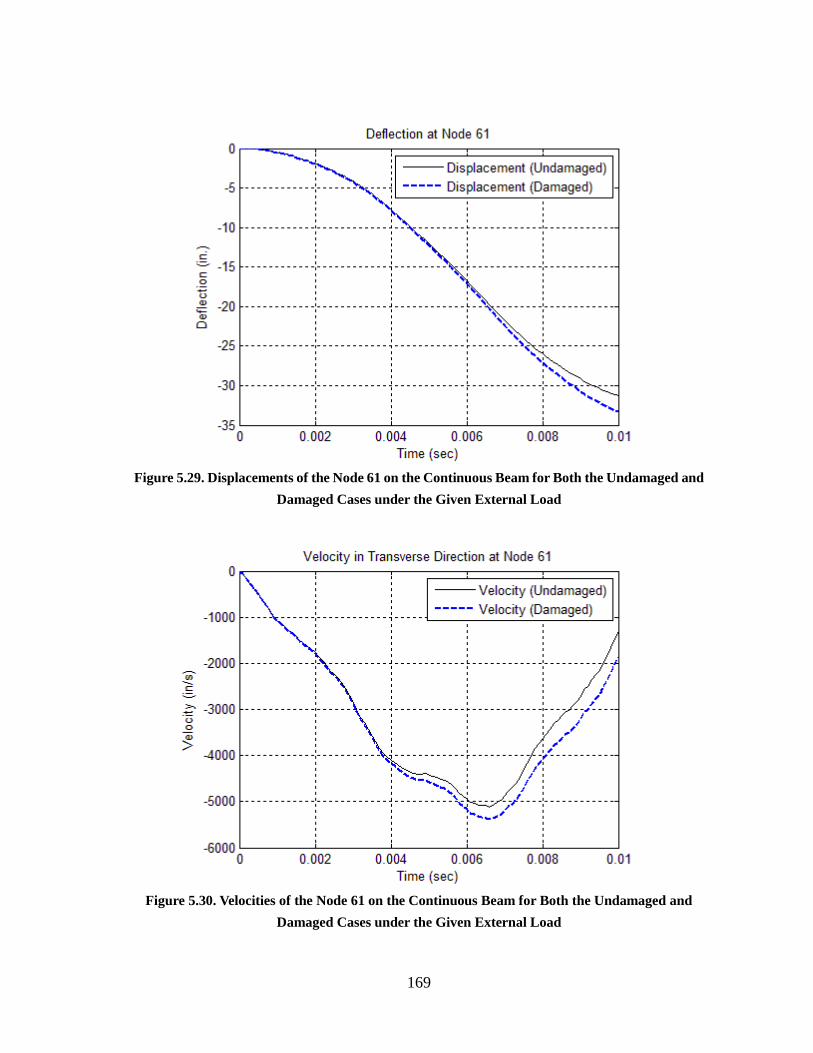
169
Figure 5.29. Displacements of the Node 61 on the Continuous Beam for Both the Undamaged and
Damaged Cases under the Given External Load
Figure 5.30. Velocities of the Node 61 on the Continuous Beam for Both the Undamaged and
Damaged Cases under the Given External Load

170
Figure 5.31. Accelerations of the Node 61 on the Continuous Beam for Both the Undamaged and
Damaged Cases under the Given External Load
Figure 5.32. Damage Indices of Nodal Mass (βmi) for the Continuous Beam from the Two-Bay
Frame

171
Figure 5.33. Damage Severities of Nodal Mass (аmi) for the Continuous Beam from the Two-Bay
Frame
Figure 5.34. Damage Indices of Element Stiffness (βki) for the Continuous Beam from the
Two-Bay Frame

172
Figure 5.35. Damage Severities of Element Stiffness (аki) for the Continuous Beam from the
Two-Bay Frame
Figure 5.36. Damage Indices of Nodal Mass (βmi) for the Isolator and Column A from the
Two-Bay Frame

173
Figure 5.37. Damage Severities of Nodal Mass (аmi) for the Isolator and Column A from the
Two-Bay Frame
Figure 5.38. Damage Indices of Element Stiffness (βki) for the Isolator and Column A from the
Two-Bay Frame
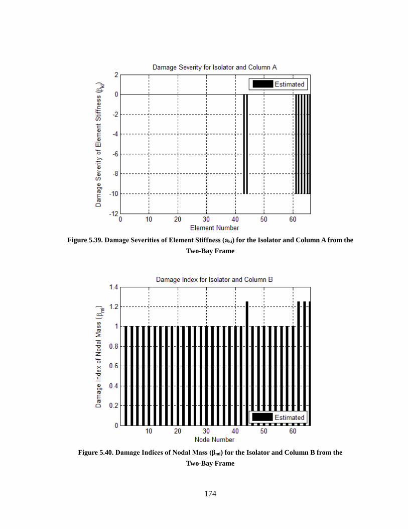
174
Figure 5.39. Damage Severities of Element Stiffness (аki) for the Isolator and Column A from the
Two-Bay Frame
Figure 5.40. Damage Indices of Nodal Mass (βmi) for the Isolator and Column B from the
Two-Bay Frame

175
Figure 5.41. Damage Severities of Nodal Mass (аmi) for the Isolator and Column B from the
Two-Bay Frame
Figure 5.42. Damage Indices of Element Stiffness (βki) for the Isolator and Column B from the
Two-Bay Frame

176
Figure 5.43. Damage Severities of Element Stiffness (аki) for the Isolator and Column B from the
Two-Bay Frame
Figure 5.44. Damage Indices of Nodal Mass (βmi) for the Isolator and Column C from the
Two-Bay Frame

177
Figure 5.45. Damage Severities of Nodal Mass (аmi) for the Isolator and Column C from the
Two-Bay Frame (note: all values are close to zeros, no damage)
Figure 5.46. Damage Indices of Element Stiffness (βki) for the Isolator and Column C from the
Two-Bay Frame

178
Figure 5.47. Damage Severities of Element Stiffness (аki) for the Isolator and Column C from the
Two-Bay Frame (note: all values are close to zeros, no damage)
5.6 DAMAGE EVALUATION FOR A SPACE TRUSS
In Case #5, a space truss is used to validate the proposed theory. The geometry, damage
scenario, and finite element discretization under consideration are indicated in Figure
5.48. There are 18 truss members and eight (8) joints in the space truss. The lower four
(4) joints are pin connected to the ground. Each of the above four (4) joints has three (3)
transitional degrees of freedom (i.e. global X, Y, Z directions). The numbering systems
of joints and of truss members are given in Figure 5.48. To better describe the geometry
of the space truss, the coordinate of each joint in the space truss is also given in Figure
5.48.
The geometry of the cross-section of the truss member is shown in Figure 5.19. The

179
modulus of elasticity (E) of the material is 29,000 ksi. The mass density of the material
is 7.345×10⁻⁷ kipsec2/in4. In this case, four elements with damaged mass and stiffness
are studied. The damage is simulated by a ten percent (10%) reduction of the modulus of
elasticity and twenty percent (20%) reduction of the mass of both Member 26 and
Member 25, and fifteen percent (15%) reduction of the modulus of elasticity and thirty
percent (30%) reduction of the mass of Member 68.
The load case is simulated by applying four cosine forces in the global X direction at
each of the free joints. For Joint 5, a cosine force, 400cos(2πt), in the global X direction
is applied. For Joint 6, a cosine force, 100cos(2πt), in the global X direction is applied.
For Joint 7, a cosine force, 200cos(2πt), in the global X direction is applied. For Joint 8,
a cosine force, 300cos(2πt), in the global X direction is applied. Given the external load
case, the displacement, velocity, and acceleration time histories of the movable joints are
directly generated from SAP2000 using linear direct integration method. The
computation step is 1E-4 seconds (10,000 Hz) for total 0.2 seconds. The displacement,
velocity, and acceleration of Joint 6 in global x direction for both the undamaged and
damaged systems were plotted in Figure 5.49, Figure 5.50, and Figure 5.51.
In this case, the computed velocity ( )(tx ) of each joint in the undamaged case was used
as the velocity used to compute power ( ) for both the undamaged and damaged cases.
For each joint, the coefficient matrices (‘X’) and known vector (‘Y’) were constructed
by substituting the acceleration ( )(tx ), velocity ( )(tx ), displacement ( )(tx ), and
velocity used to compute power ( ) into Eq. 4.217 and Eq. 4.219. The coefficient
damage index vector, β, related to the two nearby elements was computed using Eq.
4.220. Then the damage indices for mass and stiffness are computed using Eqs. 4.221
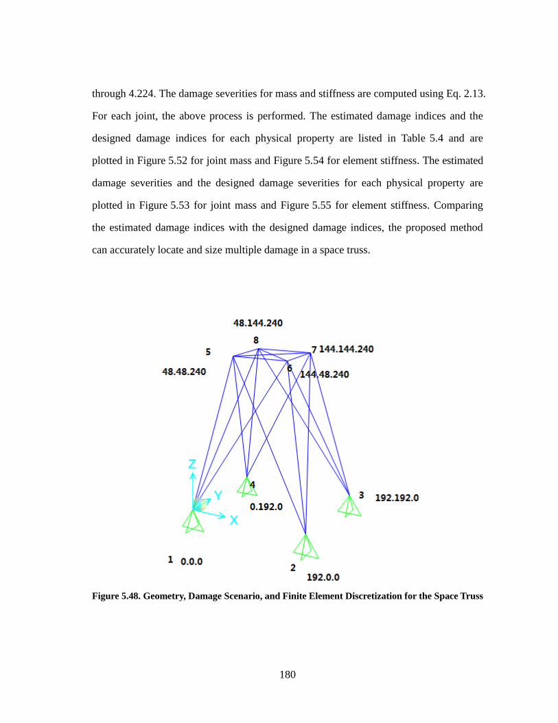
180
through 4.224. The damage severities for mass and stiffness are computed using Eq. 2.13.
For each joint, the above process is performed. The estimated damage indices and the
designed damage indices for each physical property are listed in Table 5.4 and are
plotted in Figure 5.52 for joint mass and Figure 5.54 for element stiffness. The estimated
damage severities and the designed damage severities for each physical property are
plotted in Figure 5.53 for joint mass and Figure 5.55 for element stiffness. Comparing
the estimated damage indices with the designed damage indices, the proposed method
can accurately locate and size multiple damage in a space truss.
Figure 5.48. Geometry, Damage Scenario, and Finite Element Discretization for the Space Truss

181
Figure 5.49. Displacements of the Joint 6 in Global X Direction for Both the Undamaged and
Damaged Systems under the Given External Load
Figure 5.50. Velocities of the Joint 6 in Global X Direction for Both the Undamaged and
Damaged Systems under the Given External Load

182
Figure 5.51. Accelerations of the Joint 6 in Global X Direction for Both the Undamaged and
Damaged Systems under the Given External Load

183
Table 5.4. Damage Detection Results for the Space Truss
PropertyDamage Index (βi,
Estimated)
Damage Severity (αi,
Estimated) (%)
Damage Index (βi,
Designed)
m5 1.052 -4.960 1.052
m6 1.086 -7.919 1.086
m7 1.000 -0.003 1.000
m8 1.037 -3.553 1.037
k15 1.000 -0.018 1.000
k16 1.000 -0.012 1.000
k18 0.999 0.081 1.000
k25 1.111 -9.980 1.111
k26 1.111 -10.001 1.111
k27 0.997 0.256 1.000
k36 1.000 -0.007 1.000
k37 1.001 -0.127 1.000
k38 1.000 -0.006 1.000
k45 1.000 0.003 1.000
k47 1.000 -0.005 1.000
k48 1.001 -0.052 1.000
k56 1.000 -0.002 1.000
k57 0.999 0.097 1.000
k58 1.000 0.039 1.000
k67 0.999 0.084 1.000
k68 1.175 -14.907 1.176
k78 1.002 -0.151 1.000
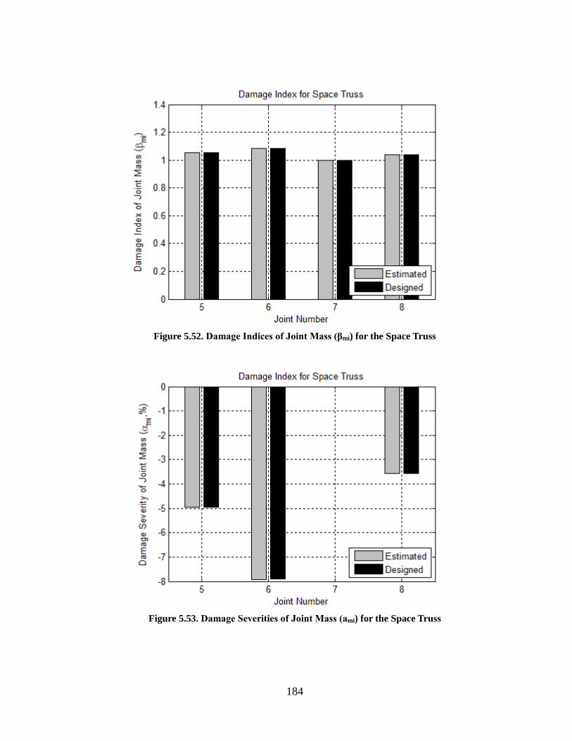
184
Figure 5.52. Damage Indices of Joint Mass (βmi) for the Space Truss
Figure 5.53. Damage Severities of Joint Mass (аmi) for the Space Truss

185
Figure 5.54. Damage Indices of Member Stiffness (βki) for the Space Truss
Figure 5.55. Damage Severities of Member Stiffness (аki) for the Space Truss

186
5.7 SUMMARY
In this section, numerical models of rod under axial and torsional vibration, rod under
axial vibration only, beam under bending vibration, plane frame under axial and bending
vibration, and space truss under axial vibration were simulated and studied. In each
numerical damage detection experiment, damage in mass, stiffness were simultaneously
simulated in each damaged system. For both the damaged and undamaged systems, the
displacements, velocities and accelerations were computed using linear direct integration
method in SAP2000. The displacements, velocities and accelerations used in the Section
5 are exact data without noise. The algorithms given in the Section 4 were used to
compute the damage indices and damage severities in each numerical case.
For each numerical case, all the designed damage in masses and stiffness were located
and evaluated accurately. Moreover, for all numerical experiments, neither false-positive
damage index nor false-negative damage index was found. Namely, for the proposed
damage detection method, if accurate displacement, velocity, and acceleration data are
given, all type of damage will be accurately located and evaluated. In addition,
according to the results from Section 5.2 and Section 5.3, the proposed method was
proved to be applicable to both the integral continuous system and isolated continuous
system. The proposed method was also proved to be able to detect and evaluation
damage by using measured data from different types of vibrations
187
6 STUDIES OF NOISE INFLUENCE TO THE PERFORMANCE OF
THE POWER METHOD
6.1 INTRODUCTION
The objective of this section is to evaluate the accuracy of the theory when the inputs are
noise-polluted. To simulate the noise-polluted inputs, exact accelerations contaminated
by white noise are used as the input acceleration; the input velocities and input
displacements are estimated based on the noise-polluted accelerations. Eight numerical
cases including two noise levels are taken into consideration and general description of
each numerical cases are given as follows,
Case #6.1: The Power Method for n-DOF discrete system was applied on a 5-DOF
spring-mass-damper system. The noise-polluted accelerations were simulated by the
superposition of 1% of white noise and the exact accelerations outputted from the
discrete system. The algorithm of the Power Method for a 5-DOF spring-mass-damper
system is provided in Section 2.5.
Case #6.2: The Power Method for n-DOF discrete system was applied on a 5-DOF
spring-mass-damper system. The noise-polluted accelerations were simulated by the
superposition of 5% of white noise and the exact accelerations outputted from the
discrete system. The algorithm of the Power Method for a 5-DOF spring-mass-damper
system is provided in Section 2.5.
Case #6.3: The Power Method for Isolated discrete system was applied on a 5-DOF

188
spring-mass-damper system. The noise-polluted accelerations were simulated by the
superposition of 1% of white noise and the exact accelerations outputted from the
discrete system. The algorithm of the Power Method for a 5-DOF spring-mass-damper
system is provided in Section 2.6.
Case #6.4: The Power Method for Isolated discrete system was applied on a 5-DOF
spring-mass-damper system. The noise-polluted accelerations were simulated by the
superposition of 5% of white noise and the exact accelerations outputted from the
discrete system. The algorithm of the Power Method for a 5-DOF spring-mass-damper
system is provided in Section 2.6.
Case #6.5: The Power Method for whole rod analysis was applied on a fixed-fixed beam.
The noise-polluted accelerations were simulated by the superposition of 1% of white
noise and the exact accelerations outputted from the discrete system. The algorithm of
the Power Method for whole rod analysis is provided in Section 4.2.2.
Case #6.6: The Power Method for whole rod analysis was applied on a fixed-fixed beam.
The noise-polluted accelerations were simulated by the superposition of 5% of white
noise and the exact accelerations outputted from the discrete system. The algorithm of
the Power Method for whole rod analysis is provided in Section 4.2.2.
Case #6.7: The Power Method for isolated rod element analysis was applied on a
fixed-fixed beam. The noise-polluted accelerations were simulated by the superposition
of 1% of white noise and the exact accelerations outputted from the discrete system. The
algorithm of the Power Method for whole rod analysis is provided in Section 4.2.1.

189
Case #6.8: The Power Method for isolated rod element analysis was applied on a
fixed-fixed beam. The noise-polluted accelerations were simulated by the superposition
of 5% of white noise and the exact accelerations outputted from the discrete system. The
algorithm of the Power Method for whole rod analysis is provided in Section 4.2.1.
6.1.1 Generation of Noise-Polluted Accelerations
The noise-polluted accelerations are computed using the following equation,
)(
)()()()(
wstd
astdtwtata
pure
iipureinoise (6.1)
Where )( inoise ta is the noise-polluted acceleration at time it ; )( ipure ta is the exact
acceleration at time it ; )( itw is the random white noise at time it ; is the percent of
noise selected to add into the pure acceleration data; std(x) indicates the standard
deviation of Vector x.
6.1.2 Estimation of Velocity and Displacement
The velocity time histories are estimated based on the filtered noise-polluted acceleration
time histories, using,
)(2
)()()()( 01
01
01 tttata
tvtv
(6.2)
Where, the initial velocity and initial acceleration are zeros. Namely, 0)0( v , 0)0( a ,
0001.0)( 01 dttt seconds.
The displacement time histories are estimated based on the velocity time histories from Eq.

190
6.2, using,
)(2
)()()()( 01
01
01 tttvtv
tsts
(6.3)
Where, the initial displacement and initial velocity are zeros for the shake table test.
Namely, 0)0( s , 0)0( v , 0001.0)( 01 dttt seconds.
6.1.3 Normalized Damage Index and Damage Possibility Index
According to the later study, the damage indices for undamaged and damaged elements
can be less than the expected values due to the noise and applied digital band-pass filter.
For these cases, the normalized damage indices might be more illustrative. Given the
normalized damage index, the damage possibility index can be computed based on
standard normal distribution.
The expression of the normalized damage index,
i
in, (6.4)
Where μ is the average value of the βi series, and σ is the standard deviation of the βi
series.
The standard normal probability density function used to generate damage possibility
index is given as following,
2
2,
2
)(
,2
1)1,0|(
in
ef in (6.5)
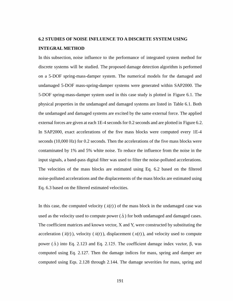
191
6.2 STUDIES OF NOISE INFLUENCE TO A DISCRETE SYSTEM USING
INTEGRAL METHOD
In this subsection, noise influence to the performance of integrated system method for
discrete systems will be studied. The proposed damage detection algorithm is performed
on a 5-DOF spring-mass-damper system. The numerical models for the damaged and
undamaged 5-DOF mass-spring-damper systems were generated within SAP2000. The
5-DOF spring-mass-damper system used in this case study is plotted in Figure 6.1. The
physical properties in the undamaged and damaged systems are listed in Table 6.1. Both
the undamaged and damaged systems are excited by the same external force. The applied
external forces are given at each 1E-4 seconds for 0.2 seconds and are plotted in Figure 6.2.
In SAP2000, exact accelerations of the five mass blocks were computed every 1E-4
seconds (10,000 Hz) for 0.2 seconds. Then the accelerations of the five mass blocks were
contaminated by 1% and 5% white noise. To reduce the influence from the noise in the
input signals, a band-pass digital filter was used to filter the noise-polluted accelerations.
The velocities of the mass blocks are estimated using Eq. 6.2 based on the filtered
noise-polluted accelerations and the displacements of the mass blocks are estimated using
Eq. 6.3 based on the filtered estimated velocities.
In this case, the computed velocity ( )(tx ) of the mass block in the undamaged case was
used as the velocity used to compute power ( ) for both undamaged and damaged cases.
The coefficient matrices and known vector, X and Y, were constructed by substituting the
acceleration ( )(tx ), velocity ( )(tx ), displacement ( )(tx ), and velocity used to compute
power ( ) into Eq. 2.123 and Eq. 2.125. The coefficient damage index vector, β, was
computed using Eq. 2.127. Then the damage indices for mass, spring and damper are
computed using Eqs. 2.128 through 2.144. The damage severities for mass, spring and

192
damper are computed using Eqs. 2.145 through 2.161.
6.2.1 Case #6.1: Discrete System with 1% Noise Pollution Using Integral Method
In this case, the exact accelerations of the mass blocks outputted directly from SAP2000
were contaminated by 1% of white noise. The noise-polluted accelerations of Mass Block
#2 in both the undamaged and damaged cases are plotted in Figure 6.3. The filtered
accelerations, estimated velocities, and estimated displacements of mass Block #2 are
plotted in Figure 6.4, Figure 6.5, and Figure 6.6, respectively.
The estimated damage indices and the designed damage indices for each physical property
are listed in Table 6.2 and are plotted in Figure 6.7. The estimated damage severities and
the designed damage severities for each physical property are also listed in Table 6.2 and
are plotted in Figure 6.8. The normalized damage indices are computed using Eq. 6.4 and
are plotted in Figure 6.9. The damage possibility indices are plotted in Figure 6.10.
Comparing the estimated damage indices with the designed damage indices, the integrated
system analysis method can accurately locate and size multiple damage with 1%
noise-polluted input data from a typical 5-DOF spring-mass-damper system.
Figure 6.1. Property Definition and Load Case of the 5-DOF Spring-Mass-Damper System
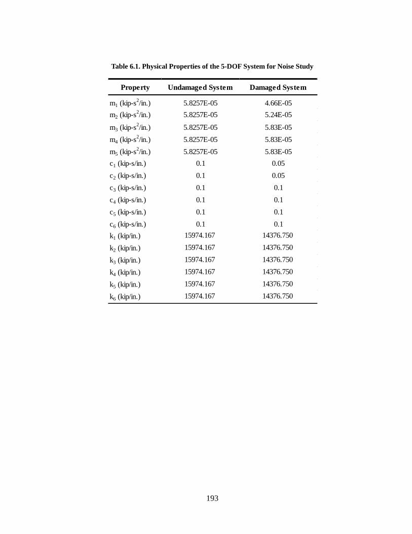
193
Table 6.1. Physical Properties of the 5-DOF System for Noise Study
Property Undamaged System Damaged System
m1 (kip-s2/in.) 5.8257E-05 4.66E-05
m2 (kip-s2/in.) 5.8257E-05 5.24E-05
m3 (kip-s2/in.) 5.8257E-05 5.83E-05
m4 (kip-s2/in.) 5.8257E-05 5.83E-05
m5 (kip-s2/in.) 5.8257E-05 5.83E-05
c1 (kip-s/in.) 0.1 0.05
c2 (kip-s/in.) 0.1 0.05
c3 (kip-s/in.) 0.1 0.1
c4 (kip-s/in.) 0.1 0.1
c5 (kip-s/in.) 0.1 0.1
c6 (kip-s/in.) 0.1 0.1
k1 (kip/in.) 15974.167 14376.750
k2 (kip/in.) 15974.167 14376.750
k3 (kip/in.) 15974.167 14376.750
k4 (kip/in.) 15974.167 14376.750
k5 (kip/in.) 15974.167 14376.750
k6 (kip/in.) 15974.167 14376.750
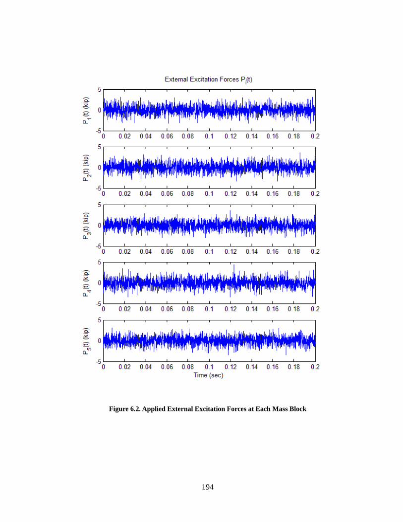
194
Figure 6.2. Applied External Excitation Forces at Each Mass Block
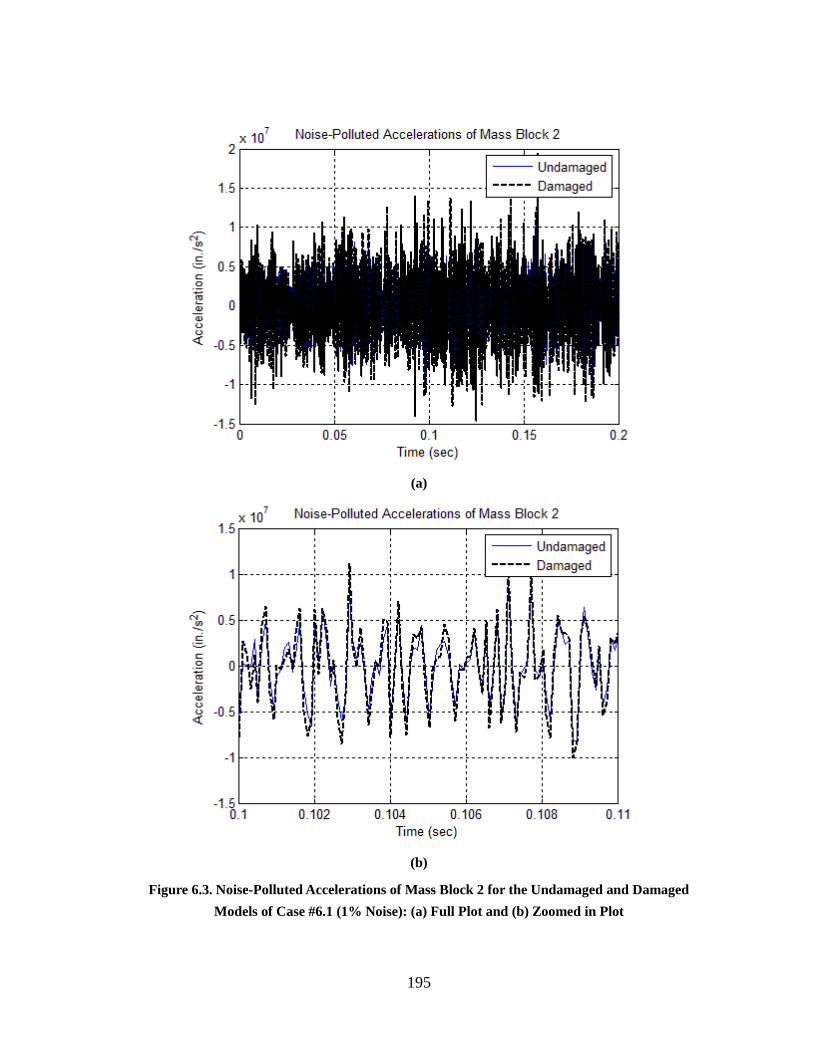
195
(a)
(b)
Figure 6.3. Noise-Polluted Accelerations of Mass Block 2 for the Undamaged and Damaged
Models of Case #6.1 (1% Noise): (a) Full Plot and (b) Zoomed in Plot

196
(a)
(b)
Figure 6.4. Filtered Noise-Polluted Accelerations of Mass Block 2 for the Undamaged and
Damaged Models of Case #6.1 (1% Noise): (a) Full Plot and (b) Zoomed in Plot
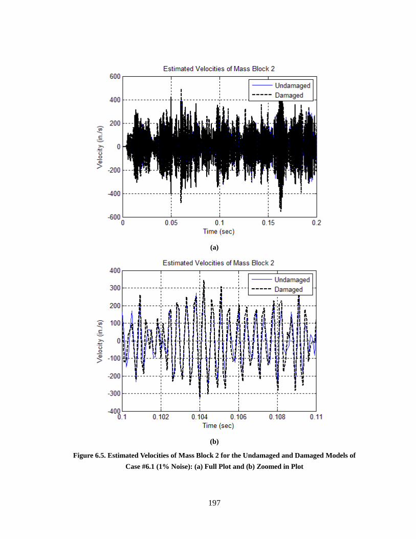
197
(a)
(b)
Figure 6.5. Estimated Velocities of Mass Block 2 for the Undamaged and Damaged Models of
Case #6.1 (1% Noise): (a) Full Plot and (b) Zoomed in Plot

198
(a)
(b)
Figure 6.6. Estimated Displacements of Mass Block 2 for the Undamaged and Damaged Models
of Case #6.1 (1% Noise): (a) Full Plot and (b) Zoomed in Plot
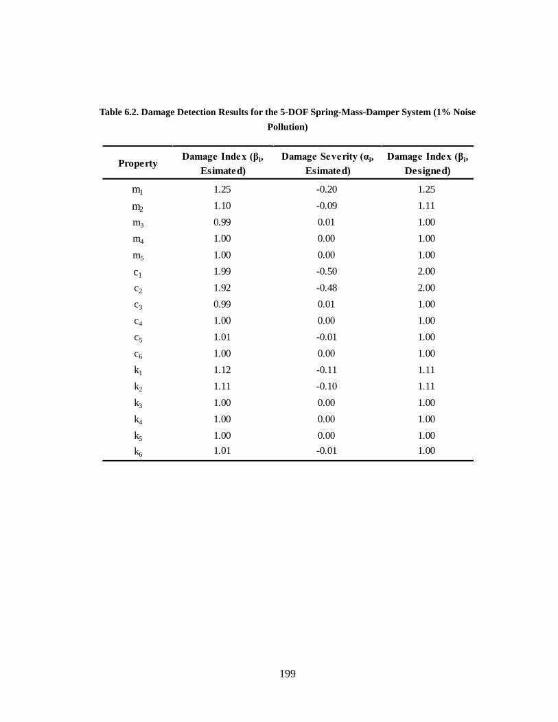
199
Table 6.2. Damage Detection Results for the 5-DOF Spring-Mass-Damper System (1% Noise
Pollution)
PropertyDamage Index (βi,
Esimated)
Damage Severity (αi,
Esimated)
Damage Index (βi,
Designed)
m1 1.25 -0.20 1.25
m2 1.10 -0.09 1.11
m3 0.99 0.01 1.00
m4 1.00 0.00 1.00
m5 1.00 0.00 1.00
c1 1.99 -0.50 2.00
c2 1.92 -0.48 2.00
c3 0.99 0.01 1.00
c4 1.00 0.00 1.00
c5 1.01 -0.01 1.00
c6 1.00 0.00 1.00
k1 1.12 -0.11 1.11
k2 1.11 -0.10 1.11
k3 1.00 0.00 1.00
k4 1.00 0.00 1.00
k5 1.00 0.00 1.00
k6 1.01 -0.01 1.00

200
Figure 6.7. Damage Indices (βi) for 5-DOF Spring-Mass-Damper System with Noise-Polluted
Accelerations (1% Noise)
Figure 6.8. Damage Severities (аi) for 5-DOF Spring-Mass-Damper System with Noise-Polluted
Accelerations (1% Noise)

201
Figure 6.9. Normalized Damage Indices (βn,i) for 5-DOF Spring-Mass-Damper System with
Noise-Polluted Accelerations (1% Noise)
Figure 6.10. Probability Damage Indices (βp,i) for 5-DOF Spring-Mass-Damper System with
Noise-Polluted Accelerations (1% Noise)

202
6.2.2 Case #6.2: Discrete System with 5% Noise Pollution Using Integral Method
In this case, the exact accelerations of the mass blocks outputted directly from SAP2000
were contaminated by 5% of white noise. The noise-polluted accelerations of Mass Block
#2 in both the undamaged and damaged cases are plotted in Figure 6.11. The filtered
accelerations, estimated velocities and estimated displacements of Mass Block #2 are
plotted in Figure 6.12, Figure 6.13, and Figure 6.14, respectively.
The estimated damage indices and the designed damage indices for each physical property
are listed in Table 6.3 and are plotted in Figure 6.15. The estimated damage severities and
the designed damage severities for each physical property are also listed in Table 6.3 and
are plotted in Figure 6.16. The normalized damage indices are computed using Eq. 6.4
and are plotted in Figure 6.17. The damage possibility indices are plotted in Figure 6.18.
Comparing the estimated damage indices with the designed damage indices, the integrated
system analysis method can accurately locate and size multiple damage with 5%
noise-polluted input data from a typical 5-DOF spring-mass-damper system.

203
(a)
(b)
Figure 6.11. Noise-Polluted Accelerations of Mass Block 2 for the Undamaged and Damaged
Models of Case #6.2 (5% Noise): (a) Full Plot and (b) Zoomed in Plot

204
(a)
(b)
Figure 6.12. Filtered Noise-Polluted Accelerations of Mass Block 2 for the Undamaged and
Damaged Models of Case #6.2 (5% Noise): (a) Full Plot and (b) Zoomed in Plot

205
(a)
(b)
Figure 6.13. Estimated Velocities of Mass Block 2 for the Undamaged and Damaged Models of
Case #6.2 (5% Noise): (a) Full Plot and (b) Zoomed in Plot

206
(a)
(b)
Figure 6.14. Estimated Displacements of Mass Block 2 for the Undamaged and Damaged Models
of Case #6.2 (5% Noise): (a) Full Plot and (b) Zoomed in Plot

207
Table 6.3. Damage Detection Results for the 5-DOF Spring-Mass-Damper System (5% Noise
Pollution)
PropertyDamage Index (βi,
Esimated)
Damage Severity (αi,
Esimated)
Damage Index (βi,
Designed)
m1 1.28 -0.22 1.25
m2 1.08 -0.07 1.11
m3 1.00 0.00 1.00
m4 1.02 -0.02 1.00
m5 1.00 0.00 1.00
c1 1.37 -0.27 2.00
c2 1.64 -0.39 2.00
c3 0.88 0.14 1.00
c4 0.89 0.12 1.00
c5 0.86 0.17 1.00
c6 1.19 -0.16 1.00
k1 1.14 -0.13 1.11
k2 1.09 -0.09 1.11
k3 1.01 -0.01 1.00
k4 1.01 -0.01 1.00
k5 0.99 0.01 1.00
k6 1.00 0.00 1.00

208
Figure 6.15. Damage Indices (βi) for 5-DOF Spring-Mass-Damper System with Noise-Polluted
Accelerations (5% Noise)
Figure 6.16. Damage Severities (аi) for 5-DOF Spring-Mass-Damper System with Noise-Polluted
Accelerations (5% Noise)

209
Figure 6.17. Normalized Damage Indices (βn,i) for 5-DOF Spring-Mass-Damper System with
Noise-Polluted Accelerations (5% Noise)
Figure 6.18. Probability Damage Indices (βp,i) for 5-DOF Spring-Mass-Damper System with
Noise-Polluted Accelerations (5% Noise)

210
6.3 STUDIES OF NOISE INFLUENCE TO A DISCRETE SYSTEM USING
ISOLATION METHOD
In this subsection, noise influence to the performance of isolated system method for
discrete systems will be studied. Isolated spring-mass-damper systems from a 5-DOF
system were used to study the accuracy of the Power Method. The numerical models for
the damaged and undamaged 5-DOF mass-spring-damper systems were generated using
SAP2000. The 5-DOF spring-mass-damper system used in this case study is plotted in
Figure 6.1. The physical properties in the undamaged and damaged systems are listed in
Table 6.4. Both the undamaged and damaged systems are excited by the same external
force. The applied external forces are given at each 1E-4 seconds for 0.2 seconds and are
plotted in Figure 6.2. In SAP2000, exact accelerations of the five mass blocks were
computed every 1E-4 seconds (10,000 Hz) for 0.2 seconds. Then the accelerations of the
five mass blocks were contaminated by 1% and 5% white noise. To reduce the influence
from the noise in the input signals, a bandpass digital filter was used to filter the
noise-polluted accelerations. The velocities of the mass blocks are estimated using Eq. 6.2
based on the filtered noise-polluted accelerations and the displacements of the mass
blocks are estimated using Eq. 6.3 based on the filtered estimated velocities.
In this case, the computed velocity ( )(tx ) of the mass block in the undamaged case was
used as the velocity used to compute power ( ) for both undamaged and damaged cases.
The coefficient matrices and known vector, X and Y, were constructed by substituting the
acceleration ( )(tx ), velocity ( )(tx ), displacement ( )(tx ), and velocity used to compute
power ( ) into Eq. 2.179 and Eq. 2.181. The coefficient damage index vector, β, was
computed using Eq. 2.183. Then the damage indices for mass, spring and damper are
computed using Eqs. 2.184 through 2.188. The damage severities for mass, spring and

211
damper are computed using Eqs. 2.189 through 2.193.
6.3.1 Case #6.3: Discrete System with 1% Noise Pollution Using Isolation Method
In this case, the exact accelerations of the mass blocks outputted directly from SAP2000
were contaminated by 1% of white noise. The noise-polluted accelerations of Mass Block
#2 in both the undamaged and damaged cases are plotted in Figure 6.19. The filtered
accelerations, estimated velocities and estimated displacements of Mass Block #2 are
plotted in Figure 6.20, Figure 6.21, and Figure 6.22, respectively.
The estimated damage indices and the designed damage indices for each physical property
are listed in Table 6.5 and are plotted in Figure 6.23. The estimated damage severities and
the designed damage severities for each physical property are also listed in Table 6.5 and
are plotted in Figure 6.24. The normalized damage indices are computed using Eq. 6.4
and are plotted in Figure 6.25. The damage possibility indices are plotted in Figure 6.26.
Comparing the estimated damage indices with the designed damage indices, the isolated
system analysis method can accurately locate and size multiple damage with 1%
noise-polluted input data from a typical 5-DOF spring-mass-damper system.

212
Table 6.4. Physical Properties of the 5 Isolated Spring-Mass-Damper Systems for Noise Study
Property System #1 System #2 System #3 System #4 System #5
mi (kip-s2/in.) 5.826E-05 5.826E-05 5.826E-05 5.826E-05 5.826E-05
ci (kip-s/in.) 0.10 0.10 0.10 0.10 0.10
ci+1 (kip-s/in.) 0.10 0.10 0.10 0.10 0.10
ki (kip/in.) 15974.17 15974.17 15974.17 15974.17 15974.17
ki+1 (kip/in.) 15974.17 15974.17 15974.17 15974.17 15974.17
Property System #1 System #2 System #3 System #4 System #5
mi (kip-s2/in.) 4.661E-05 5.243E-05 5.826E-05 5.826E-05 5.826E-05
ci (kip-s/in.) 0.05 0.05 0.10 0.10 0.10
ci+1 (kip-s/in.) 0.05 0.10 0.10 0.10 0.10
ki (kip/in.) 14376.75 14376.75 15974.17 15974.17 15974.17
ki+1 (kip/in.) 14376.75 15974.17 15974.17 15974.17 15974.17
Undamage Systems
Damaged Systems

213
(a)
(b)
Figure 6.19. Noise-Polluted Accelerations of Mass Block 2 for the Undamaged and Damaged
Models of Case #6.3 (1% Noise): (a) Full Plot and (b) Zoomed in Plot

214
(a)
(b)
Figure 6.20. Filtered Noise-Polluted Accelerations of Mass Block 2 for the Undamaged and
Damaged Models of Case #6.3 (1% Noise): (a) Full Plot and (b) Zoomed in Plot
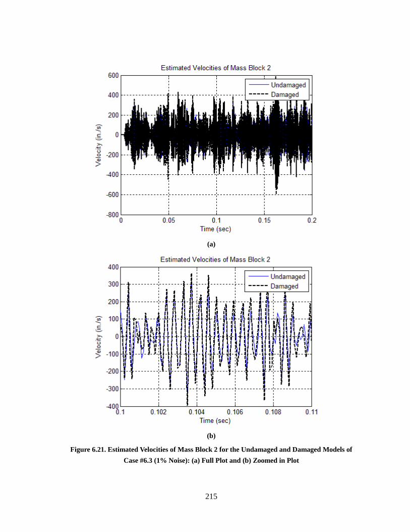
215
(a)
(b)
Figure 6.21. Estimated Velocities of Mass Block 2 for the Undamaged and Damaged Models of
Case #6.3 (1% Noise): (a) Full Plot and (b) Zoomed in Plot

216
(a)
(b)
Figure 6.22. Estimated Displacements of Mass Block 2 for the Undamaged and Damaged Models
of Case #6.3 (1% Noise): (a) Full Plot and (b) Zoomed in Plot
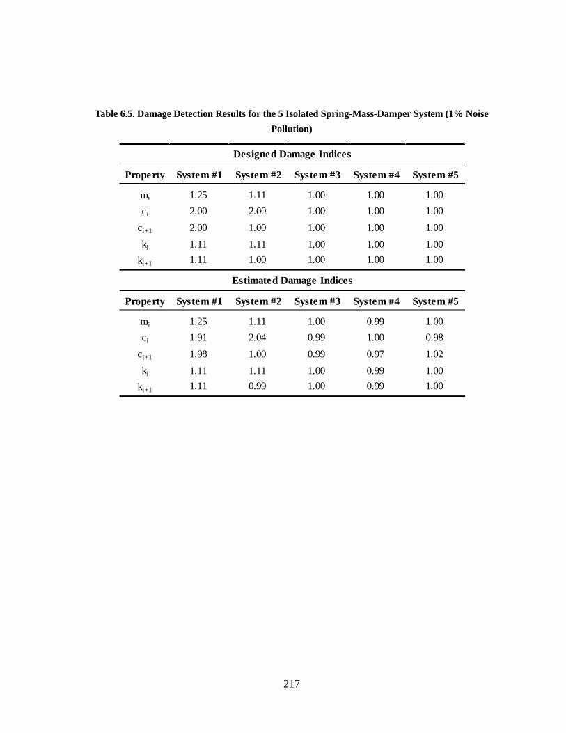
217
Table 6.5. Damage Detection Results for the 5 Isolated Spring-Mass-Damper System (1% Noise
Pollution)
Property System #1 System #2 System #3 System #4 System #5
mi 1.25 1.11 1.00 1.00 1.00
ci 2.00 2.00 1.00 1.00 1.00
ci+1 2.00 1.00 1.00 1.00 1.00
ki 1.11 1.11 1.00 1.00 1.00
ki+1 1.11 1.00 1.00 1.00 1.00
Property System #1 System #2 System #3 System #4 System #5
mi 1.25 1.11 1.00 0.99 1.00
ci 1.91 2.04 0.99 1.00 0.98
ci+1 1.98 1.00 0.99 0.97 1.02
ki 1.11 1.11 1.00 0.99 1.00
ki+1 1.11 0.99 1.00 0.99 1.00
Designed Damage Indices
Estimated Damage Indices

218
Figure 6.23. Damage Indices (βi) for the 5 Isolated Spring-Mass-Damper System with
Noise-Polluted Accelerations (1% Noise)

219
Figure 6.24. Damage Severities (аi) for 5-DOF Spring-Mass-Damper System with Noise-Polluted
Accelerations (1% Noise)

220
Figure 6.25. Normalized Damage Indices (βn,i) for 5-DOF Spring-Mass-Damper System with
Noise-Polluted Accelerations (1% Noise)

221
Figure 6.26. Damage Possibility Indices (βp,i) for 5-DOF Spring-Mass-Damper System with
Noise-Polluted Accelerations (1% Noise)

222
6.3.2 Case #6.4: Discrete System with 5% Noise Pollution Using Isolation Method
In this case, the exact accelerations of the mass blocks outputted directly from SAP2000
were contaminated by 5% of white noise. The noise-polluted accelerations of Mass Block
#2 in both the undamaged and damaged cases are plotted in Figure 6.27. The filtered
accelerations, estimated velocities and estimated displacements of Mass Block #2 are
plotted in Figure 6.28, Figure 6.29, and Figure 6.30, respectively.
The estimated damage indices and the designed damage indices for each physical property
are listed in Table 6.6 and are plotted in Figure 6.31. The estimated damage severities and
the designed damage severities for each physical property are also listed in Table 6.6 and
are plotted in Figure 6.32. The normalized damage indices are computed using Eq. 6.4
and are plotted in Figure 6.33. The damage possibility indices are plotted in Figure 6.34.
Comparing the estimated damage indices with the designed damage indices, the integrated
system analysis method can accurately locate and size multiple damage with 5%
noise-polluted input data from a typical 5-DOF spring-mass-damper system.
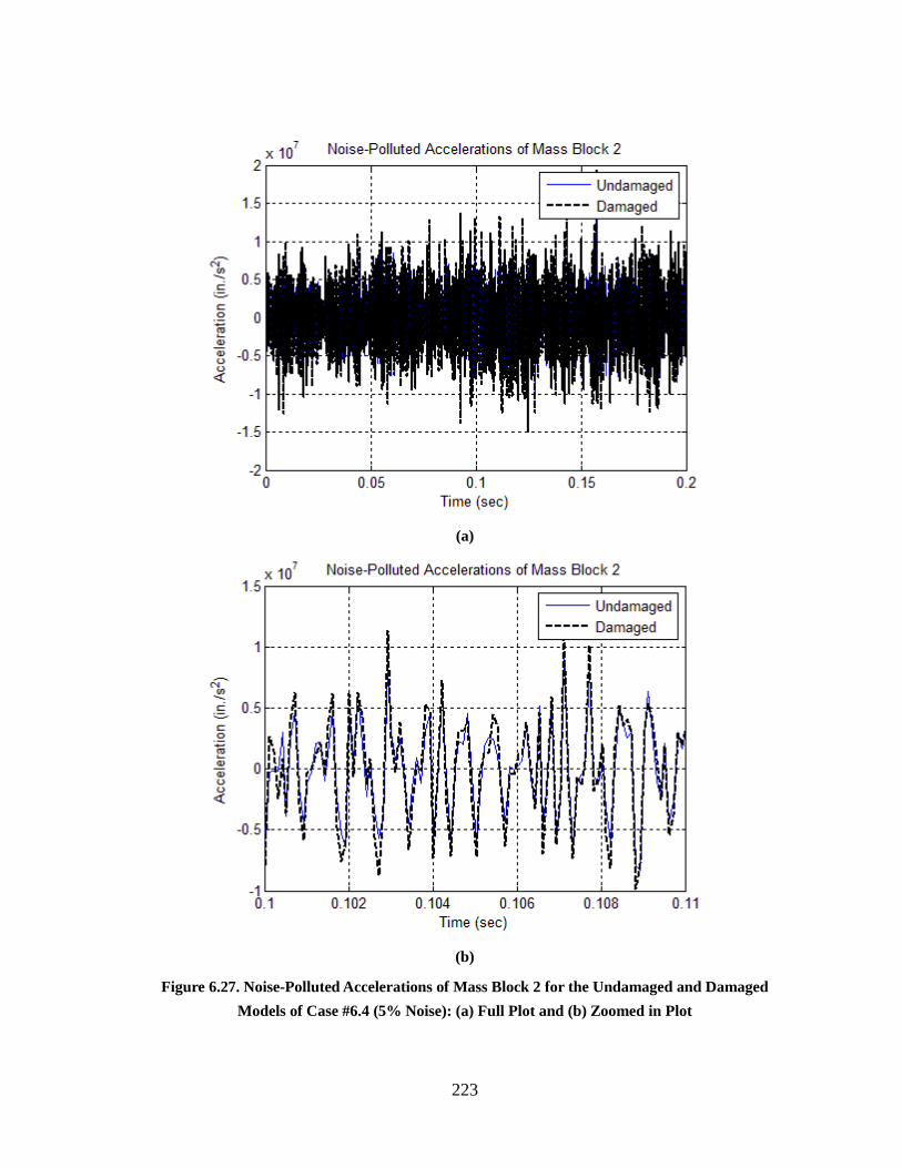
223
(a)
(b)
Figure 6.27. Noise-Polluted Accelerations of Mass Block 2 for the Undamaged and Damaged
Models of Case #6.4 (5% Noise): (a) Full Plot and (b) Zoomed in Plot

224
(a)
(b)
Figure 6.28. Filtered Noise-Polluted Accelerations of Mass Block 2 for the Undamaged and
Damaged Models of Case #6.4 (5% Noise): (a) Full Plot and (b) Zoomed in Plot
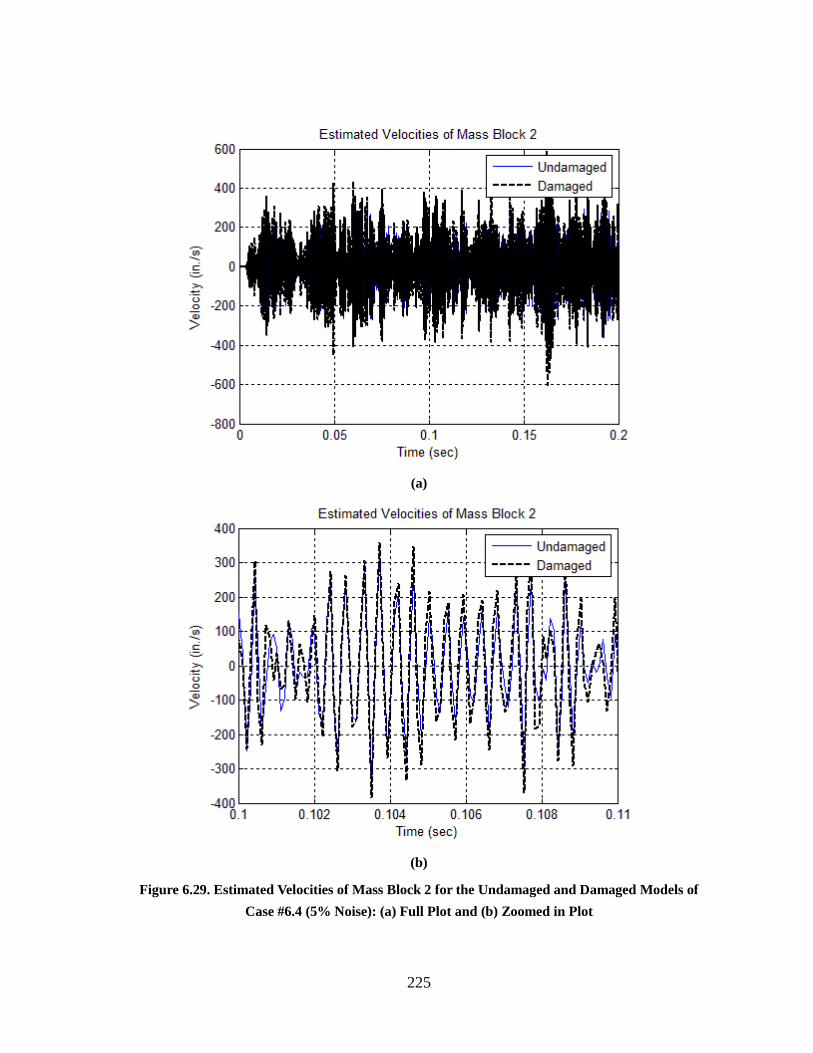
225
(a)
(b)
Figure 6.29. Estimated Velocities of Mass Block 2 for the Undamaged and Damaged Models of
Case #6.4 (5% Noise): (a) Full Plot and (b) Zoomed in Plot

226
(a)
(b)
Figure 6.30. Estimated Displacements of Mass Block 2 for the Undamaged and Damaged Models
of Case #6.4 (5% Noise): (a) Full Plot and (b) Zoomed in Plot

227
Table 6.6. Damage Detection Results for the 5 Isolated Spring-Mass-Damper System (5% Noise
Pollution)
Property System #1 System #2 System #3 System #4 System #5
mi 1.25 1.11 1.00 1.00 1.00
ci 2.00 2.00 1.00 1.00 1.00
ci+1 2.00 1.00 1.00 1.00 1.00
ki 1.11 1.11 1.00 1.00 1.00
ki+1 1.11 1.00 1.00 1.00 1.00
Property System #1 System #2 System #3 System #4 System #5
mi 1.25 1.10 1.01 0.97 0.99
ci 1.96 1.60 0.87 1.01 0.58
ci+1 1.68 0.95 0.95 0.52 0.99
ki 1.13 1.09 1.00 0.97 1.00
ki+1 1.10 0.99 1.01 0.93 0.97
Designed Damage Indices
Estimated Damage Indices

228
Figure 6.31. Damage Indices (βi) for the 5 Isolated Spring-Mass-Damper System with
Noise-Polluted Accelerations (5% Noise)

229
Figure 6.32. Damage Severities (аi) for 5-DOF Spring-Mass-Damper System with Noise-Polluted
Accelerations (5% Noise)

230
Figure 6.33. Normalized Damage Indices (βn,i) for 5-DOF Spring-Mass-Damper System with
Noise-Polluted Accelerations (5% Noise)

231
Figure 6.34. Damage Possibility Indices (βp,i) for 5-DOF Spring-Mass-Damper System with
Noise-Polluted Accelerations (5% Noise)

232
6.4 STUDIES OF NOISE INFLUENCE TO A CONTINUOUS SYSTEM USING
INTEGRAL METHOD
In this subsection, a fixed-fixed beam is used to evaluate the performance of the proposed
theory in dealing with noise-polluted data. The geometry and damage scenario under
consideration are indicated in Figure 6.35. The geometry of the cross-section of the beam
is shown in Figure 5.19. The modulus of elasticity (E) of the material is 29,000 ksi. The
mass density of the material is 7.345×10⁻⁷ kipsec2/in4.
The fixed-fixed beam is meshed into 6 elements and has 7 equally spaced nodes. The
length of each element is 12.0 inches. For illustrative purposes, typical elements are
indicated in Figure 6.35. Two elements with damaged mass and stiffness are studied. The
damage is simulated by a ten percent (10%) reduction of the modulus of elasticity and
twenty percent (20%) reduction of the mass of the first (1st) and second (2nd) elements on
the beam.
For each node on the beam, a white noise, 100×random(-1,1), is used as node force and is
applied in axial direction. The five white-noise forces are the same as the one applied in
the above four cases and are plotted in Figure 6.2. Given the external load case, exact
accelerations of the five nodes were computed at every 1E-4 seconds (10,000 Hz) for 0.2
seconds. Then the accelerations of the five nodes were contaminated by 1% and 5% white
noise. To reduce the influence from the noise in the input signals, a bandpass digital filter
was used to filter the noise-polluted accelerations. The velocities of the mass blocks are
estimated using Eq. 6.2 based on the filtered noise-polluted accelerations and the
displacements of the mass blocks are estimated using Eq. 6.3 based on the filtered
estimated velocities.

233
In this case, the computed velocity ( )(tx ) of each node in the undamaged case was used as
the velocity used to compute power ( ) for both the undamaged and damaged cases. For
every two nearby elements, the coefficient matrices (‘X’) and known vector (‘Y’) were
constructed by substituting the acceleration ( )(tx ), velocity ( )(tx ), displacement ( )(tx ),
and velocity used to compute power ( ) into Eq. 4.96 and Eq. 4.98. The coefficient
damage index vector, β, related to the two nearby elements was computed using Eq. 4.95.
Then the damage indices for mass and stiffness are computed using Eqs. 4.100 through
4.106. The damage severities for mass and stiffness are computed using Eq. 2.13.
6.4.1 Case #6.5: Continuous System with 1% Noise Pollution Using Integral
Method
In this case, the exact accelerations of the mass blocks outputted directly from SAP2000
were contaminated by 1% of white noise. The noise-polluted accelerations of Node 2 in
both the undamaged and damaged cases are plotted in Figure 6.36. The filtered
accelerations, estimated velocities and estimated displacements of Node 2 are plotted in
Figure 6.37, Figure 6.38, and Figure 6.39, respectively.
The estimated damage indices and the designed damage indices for each physical property
are listed in Table 6.7 and are plotted in Figure 6.40. The estimated damage severities and
the designed damage severities for each physical property are also listed in Table 6.7 and
are plotted in Figure 6.41. The normalized damage indices are computed using Eq. 6.4
and are plotted in Figure 6.42. The damage possibility indices are plotted in Figure 6.43.
Comparing the estimated damage indices with the designed damage indices, the integrated
system analysis method can accurately locate and size multiple damage with 1%

234
noise-polluted input data from a typical fixed-fixed beam.
Figure 6.35. Geometry and Damage Scenario for the Fixed-Fixed Beam

235
(a)
(b)
Figure 6.36. Noise-Polluted Accelerations of Node 2 for the Undamaged and Damaged Models of
Case #6.5 (1% Noise): (a) Full Plot and (b) Zoomed in Plot

236
(a)
(b)
Figure 6.37. Filtered Noise-Polluted Accelerations of Node 2 for the Undamaged and Damaged
Models of Case #6.5 (1% Noise): (a) Full Plot and (b) Zoomed in Plot

237
(a)
(b)
Figure 6.38. Estimated Velocities of Node 2 for the Undamaged and Damaged Models of Case
#6.5 (1% Noise): (a) Full Plot and (b) Zoomed in Plot

238
(a)
(b)
Figure 6.39. Estimated Displacements of Node 2 for the Undamaged and Damaged Models of
Case #6.5 (1% Noise): (a) Full Plot and (b) Zoomed in Plot

239
Table 6.7. Damage Detection Results for the Fixed-Fixed Beam (1% Noise Pollution)
Figure 6.40. Damage Indices (βi) for the Fixed-Fixed Beam with Noise-Polluted Accelerations (1%
Noise)
PropertyDamage Index (βi,
Esimated)
Damage Severity (αi,
Esimated)
Damage Index (βi,
Designed)
m1 1.15 -0.13 1.25
m2 1.03 -0.03 1.11
m3 0.93 0.08 1.00
m4 0.93 0.08 1.00
m5 0.93 0.08 1.00
k1 1.02 -0.02 1.11
k2 1.02 -0.02 1.11
k3 0.93 0.07 1.00
k4 0.93 0.08 1.00
k5 0.92 0.08 1.00
k6 0.94 0.07 1.00

240
Figure 6.41. Damage Severities (аi) for the Fixed-Fixed Beam with Noise-Polluted Accelerations
(1% Noise)
Figure 6.42. Normalized Damage Indices (βn,i) for the Fixed-Fixed Beam with Noise-Polluted
Accelerations (1% Noise)

241
Figure 6.43. Probability Damage Indices (βp,i) for the Fixed-Fixed Beam with Noise-Polluted
Accelerations (1% Noise)
6.4.2 Case #6.6: Continuous System with 5% Noise Pollution Using Integral
Method
In this case, the exact accelerations of the mass blocks outputted directly from SAP2000
were contaminated by 5% of white noise. The noise-polluted accelerations of Node 2 in
both the undamaged and damaged cases are plotted in Figure 6.44. The filtered
accelerations, estimated velocities and estimated displacements of Node 2 are plotted in
Figure 6.45, Figure 6.46, and Figure 6.47, respectively.
The estimated damage indices and the designed damage indices for each physical property
are listed in Table 6.7 and are plotted in Figure 6.48. The estimated damage severities and
the designed damage severities for each physical property are also listed in Table 6.7 and

242
are plotted in Figure 6.49. The normalized damage indices are computed using Eq. 6.4
and are plotted in Figure 6.50. The damage possibility indices are plotted in Figure 6.51.
Comparing the estimated damage indices with the designed damage indices, the integrated
system analysis method can accurately locate and size multiple damage with 5%
noise-polluted input data from a typical fixed-fixed beam.
(a)
Figure 6.44. Noise-Polluted Accelerations of Node 2 for the Undamaged and Damaged Models of
Case #6.6 (5% Noise): (a) Full Plot and (b) Zoomed in Plot

243
(b)
Figure 6.44. Continued

244
(a)
(b)
Figure 6.45. Filtered Noise-Polluted Accelerations of Node 2 for the Undamaged and Damaged
Models of Case #6.6 (5% Noise): (a) Full Plot and (b) Zoomed in Plot
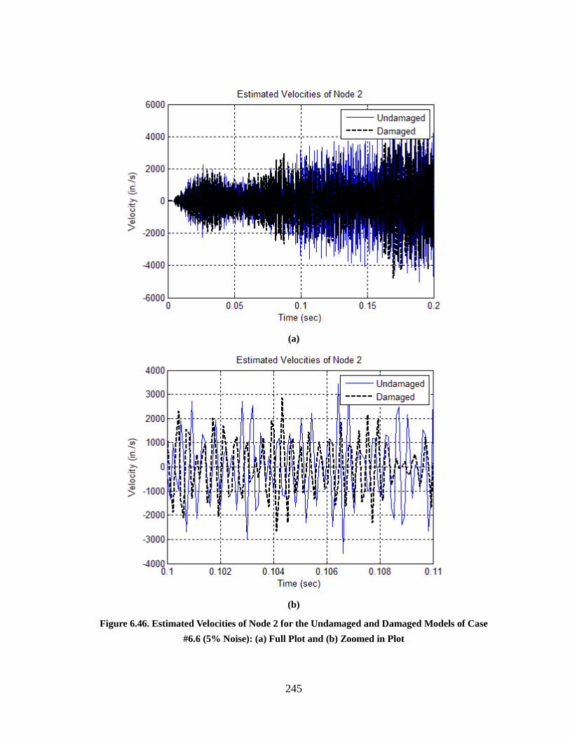
245
(a)
(b)
Figure 6.46. Estimated Velocities of Node 2 for the Undamaged and Damaged Models of Case
#6.6 (5% Noise): (a) Full Plot and (b) Zoomed in Plot
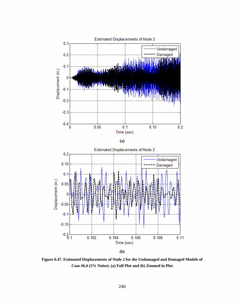
246
(a)
(b)
Figure 6.47. Estimated Displacements of Node 2 for the Undamaged and Damaged Models of
Case #6.6 (5% Noise): (a) Full Plot and (b) Zoomed in Plot

247
Table 6.8. Damage Detection Results for the Fixed-Fixed Beam (5% Noise Pollution)
Figure 6.48. Damage Indices (βi) for the Fixed-Fixed Beam with Noise-Polluted Accelerations (5%
Noise)
PropertyDamage Index (βi,
Esimated)
Damage Severity (αi,
Esimated)
Damage Index (βi,
Designed)
m1 0.76 0.31 1.25
m2 0.69 0.45 1.11
m3 0.63 0.59 1.00
m4 0.61 0.63 1.00
m5 0.62 0.61 1.00
k1 0.68 0.48 1.11
k2 0.68 0.46 1.11
k3 0.62 0.60 1.00
k4 0.62 0.61 1.00
k5 0.61 0.64 1.00
k6 0.63 0.58 1.00

248
Figure 6.49. Damage Severities (аi) for the Fixed-Fixed Beam with Noise-Polluted Accelerations
(5% Noise)
Figure 6.50. Normalized Damage Indices (βn,i) for the Fixed-Fixed Beam with Noise-Polluted
Accelerations (5% Noise)

249
Figure 6.51. Probability Damage Indices (βp,i) for the Fixed-Fixed Beam with Noise-Polluted
Accelerations (5% Noise)
6.5 STUDIES OF NOISE INFLUENCE TO A CONTINUOUS SYSTEM USING
ISOLATION METHOD
In this subsection, noise influence to the performance of isolated system method for
continuous systems will be studied. The proposed damage detection algorithm is
performed on the same fixed-fixed beam as used in the above subsection. The geometry
and damage scenario under consideration are indicated in Figure 6.35. The geometry of
the cross-section of the beam is shown in Figure 5.19. The modulus of elasticity (E) of the
material is 29,000 ksi. The mass density of the material is 7.345×10⁻⁷ kipsec2/in4.
The fixed-fixed beam is meshed into 6 elements and has 7 equally spaced nodes. The
length of each element is 12.0 inches. For illustrative purposes, typical elements are

250
indicated in Figure 6.35. Two elements with damaged mass and stiffness are studied. The
damage is simulated by a ten percent (10%) reduction of the modulus of elasticity and
twenty percent (20%) reduction of the mass of the first (1st) and second (2nd) elements on
the beam.
For each node on the beam, a white noise, 100×random(-1,1), is used as node force and is
applied in axial direction. The five white-noise forces are the same as the one applied in
the above four cases and are plotted in Figure 6.2. Given the external load case, exact
accelerations of the five nodes were computed at every 1E-4 seconds (10,000 Hz) for 0.2
seconds. Then the accelerations of the five nodes were contaminated by 1% and 5% white
noise. To reduce the influence from the noise in the input signals, a bandpass digital filter
was used to filter the noise-polluted accelerations. The velocities of the mass blocks are
estimated using Eq. 6.2 based on the filtered noise-polluted accelerations and the
displacements of the mass blocks are estimated using Eq. 6.3 based on the filtered
estimated velocities.
In this case, the computed velocity ( )(tx ) of each node in the undamaged case was used as
the velocity used to compute power ( ) for both the undamaged and damaged cases. For
every two nearby elements, the coefficient matrices (‘X’) and known vector (‘Y’) were
constructed by substituting the acceleration ( )(tx ), velocity ( )(tx ), displacement ( )(tx ),
and velocity used to compute power ( ) into Eq. 4.50 and Eq. 4.52. The coefficient
damage index vector, β, related to the two nearby elements was computed using Eq. 4.49.
Then the damage indices for mass and stiffness are computed using Eqs. 4.54 through 4.56.
The damage severities for mass and stiffness are computed using Eq. 2.13. For each two
nearby elements, the above process is performed. Thus, the proposed theory is applied to

251
five pairs of elements.
6.5.1 Case #6.7: Continuous System with 1% Noise Pollution Using Isolation
Method
In this case, the exact accelerations of the mass blocks outputted directly from SAP2000
were contaminated by 1% of white noise. The noise-polluted accelerations of Node 2 in
both the undamaged and damaged cases are plotted in Figure 6.52. The filtered
accelerations, estimated velocities, and estimated displacements of Node 2 are plotted in
Figure 6.53, Figure 6.54, and Figure 6.55, respectively.
The estimated damage indices and the designed damage indices for each physical property
are listed in Table 6.9 and are plotted in Figure 6.56. The estimated damage severities and
the designed damage severities for each physical property are also listed in Table 6.9 and
are plotted in Figure 6.57. The normalized damage indices are computed using Eq. 6.4
and are plotted in Figure 6.58. The damage possibility indices are plotted in Figure 6.59.
Comparing the estimated damage indices with the designed damage indices, the isolated
system analysis method can accurately locate and size multiple damage with 1%
noise-polluted input data from a typical fixed-fixed beam.

252
(a)
(b)
Figure 6.52. Noise-Polluted Accelerations of Node 2 for the Undamaged and Damaged Models of
Case #6.7 (5% Noise): (a) Full Plot and (b) Zoomed in Plot
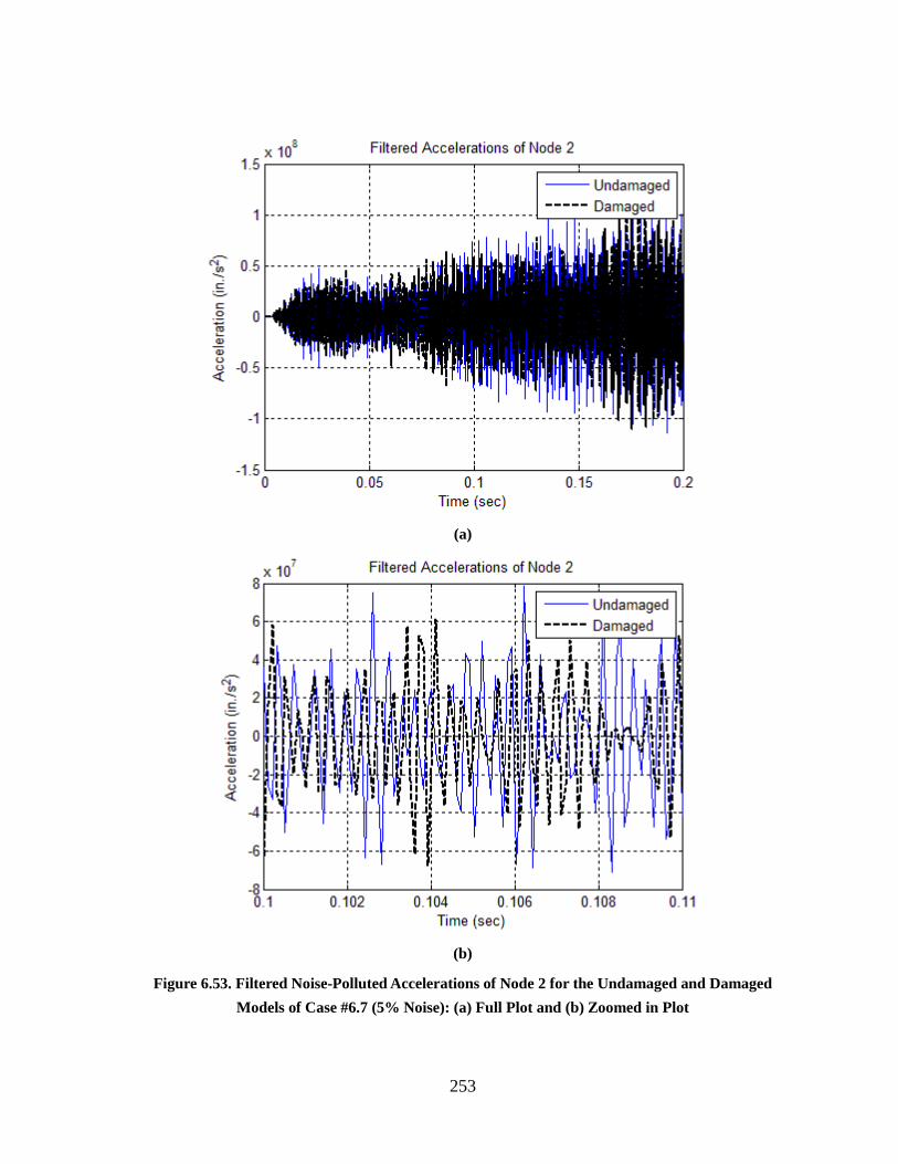
253
(a)
(b)
Figure 6.53. Filtered Noise-Polluted Accelerations of Node 2 for the Undamaged and Damaged
Models of Case #6.7 (5% Noise): (a) Full Plot and (b) Zoomed in Plot

254
(a)
(b)
Figure 6.54. Estimated Velocities of Node 2 for the Undamaged and Damaged Models of Case
#6.7 (5% Noise): (a) Full Plot and (b) Zoomed in Plot

255
(a)
(b)
Figure 6.55. Estimated Displacements of Node 2 for the Undamaged and Damaged Models of
Case #6.7 (5% Noise): (a) Full Plot and (b) Zoomed in Plot

256
Table 6.9. Damage Detection Results for the Fixed-Fixed Beam Using Isolated Method (1% Noise
Pollution)
Property System #1 System #2 System #3 System #4 System #5
mi 1.25 1.11 1.00 1.00 1.00
ki 1.11 1.11 1.00 1.00 1.00
ki+1 1.11 1.00 1.00 1.00 1.00
Property System #1 System #2 System #3 System #4 System #5
mi 1.13 1.00 0.95 0.98 0.89
ki 1.00 1.00 0.95 0.98 0.88
ki+1 1.00 0.91 0.95 0.98 0.89
Designed Damage Indices
Estimated Damage Indices

257
Figure 6.56. Damage Indices (βi) for the Fixed-Fixed Beam with Noise-Polluted Accelerations
Using Isolated Beam Element Analysis Method (1% Noise)

258
Figure 6.57. Damage Severities (аi) for the Fixed-Fixed Beam with Noise-Polluted Accelerations
Using Isolated Beam Element Analysis Method (1% Noise)

259
Figure 6.58. Normalized Damage Indices (βn,i) for the Fixed-Fixed Beam with Noise-Polluted
Accelerations Using Isolated Beam Element Analysis Method (1% Noise)

260
Figure 6.59. Probability Damage Indices (βp,i) for the Fixed-Fixed Beam with Noise-Polluted
Accelerations Using Isolated Beam Element Analysis Method (1% Noise)

261
6.5.2 Case #6.8: Continuous System with 5% Noise Pollution Using Isolation
Method
In this case, the exact accelerations of the mass blocks outputted directly from SAP2000
were contaminated by 5% of white noise. The noise-polluted accelerations of Node 2 in
both the undamaged and damaged cases are plotted in Figure 6.60. The filtered
accelerations, estimated velocities, and estimated displacements of Node 2 are plotted in
Figure 6.61, Figure 6.62, and Figure 6.63, respectively.
The estimated damage indices and the designed damage indices for each physical property
are listed in Table 6.10 and are plotted in Figure 6.64. The estimated damage severities
and the designed damage severities for each physical property are also listed in Table 6.10
and are plotted in Figure 6.65. The normalized damage indices are computed using Eq.
6.4 and are plotted in Figure 6.66. The damage possibility indices are plotted in Figure
6.67. Comparing the estimated damage indices with the designed damage indices, the
integrated system analysis method can accurately locate and size multiple damage with 5%
noise-polluted input data from a typical fixed-fixed beam.

262
(a)
(b)
Figure 6.60. Noise-Polluted Accelerations of Node 2 for the Undamaged and Damaged Models of
Case #6.8 (5% Noise): (a) Full Plot and (b) Zoomed in Plot
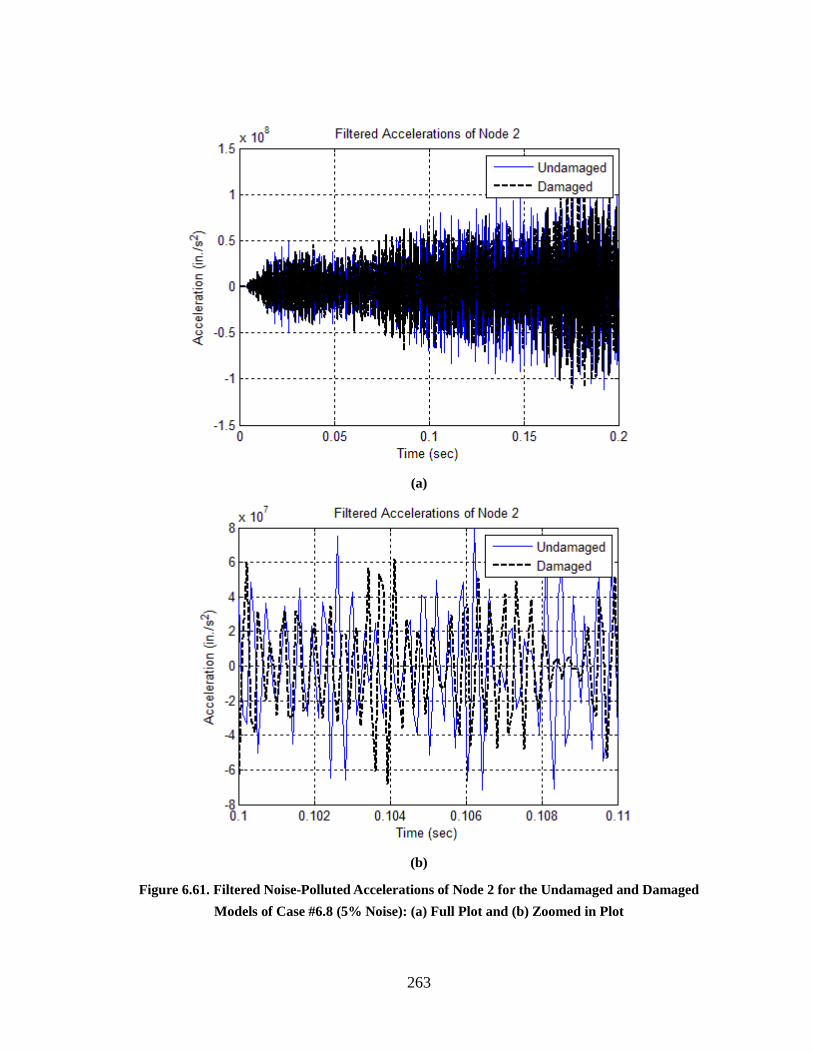
263
(a)
(b)
Figure 6.61. Filtered Noise-Polluted Accelerations of Node 2 for the Undamaged and Damaged
Models of Case #6.8 (5% Noise): (a) Full Plot and (b) Zoomed in Plot
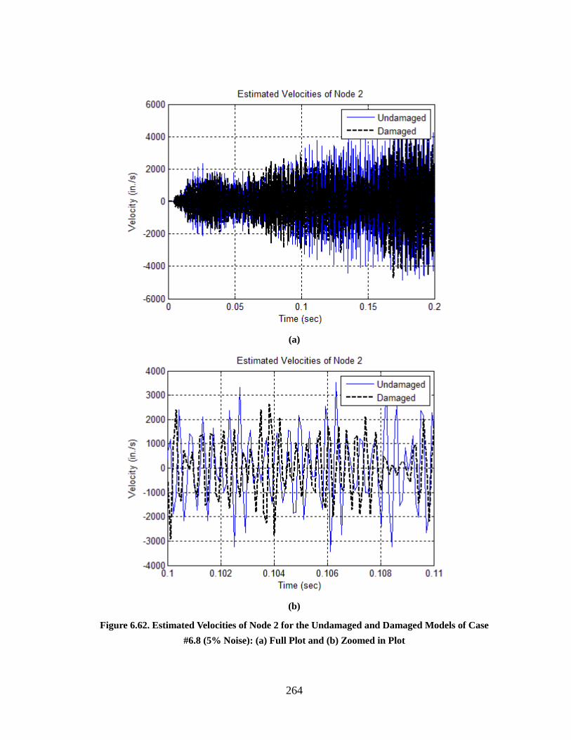
264
(a)
(b)
Figure 6.62. Estimated Velocities of Node 2 for the Undamaged and Damaged Models of Case
#6.8 (5% Noise): (a) Full Plot and (b) Zoomed in Plot

265
(a)
(b)
Figure 6.63. Estimated Displacements of Node 2 for the Undamaged and Damaged Models of
Case #6.8 (5% Noise): (a) Full Plot and (b) Zoomed in Plot
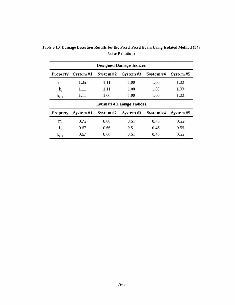
266
Table 6.10. Damage Detection Results for the Fixed-Fixed Beam Using Isolated Method (1%
Noise Pollution)
Property System #1 System #2 System #3 System #4 System #5
mi 1.25 1.11 1.00 1.00 1.00
ki 1.11 1.11 1.00 1.00 1.00
ki+1 1.11 1.00 1.00 1.00 1.00
Property System #1 System #2 System #3 System #4 System #5
mi 0.75 0.66 0.51 0.46 0.55
ki 0.67 0.66 0.51 0.46 0.56
ki+1 0.67 0.60 0.51 0.46 0.55
Designed Damage Indices
Estimated Damage Indices

267
Figure 6.64. Damage Indices (βi) for the Fixed-Fixed Beam with Noise-Polluted Accelerations
Using Isolated Beam Element Analysis Method (5% Noise)

268
Figure 6.65. Damage Severities (аi) for the Fixed-Fixed Beam with Noise-Polluted Accelerations
Using Isolated Beam Element Analysis Method (5% Noise)

269
Figure 6.66. Normalized Damage Indices (βn,i) for the Fixed-Fixed Beam with Noise-Polluted
Accelerations Using Isolated Beam Element Analysis Method (5% Noise)
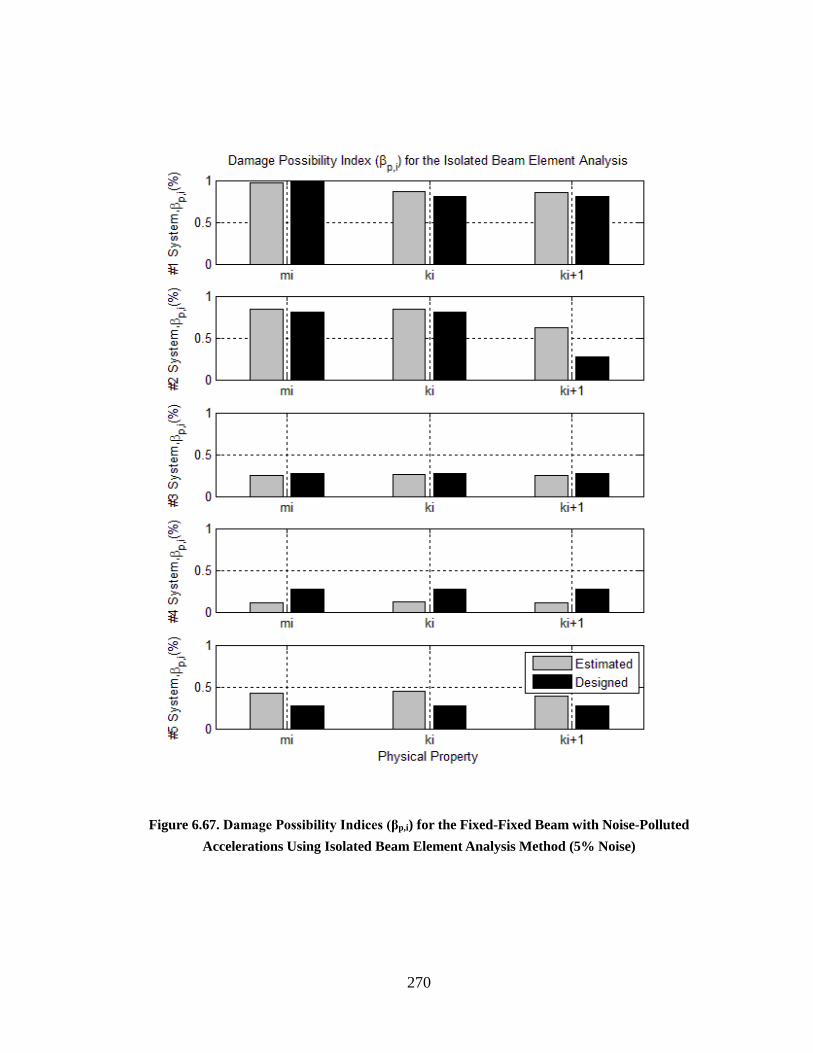
270
Figure 6.67. Damage Possibility Indices (βp,i) for the Fixed-Fixed Beam with Noise-Polluted
Accelerations Using Isolated Beam Element Analysis Method (5% Noise)

271
6.6 EVALUATION OF RESULTS
In this subsection, all the results from the previous subsection of Section 6 will be
summarized and evaluated. Because for some cases, the traditional damage index will be
influenced severely by the existence of noise and the application of band-pass filters, the
results evaluations will be mainly based on the damage possibility indices.
To distinguish the damaged elements from the undamaged elements, the damage
judgement criterion for the Damage Possibility Index is subjectively set as 50%. Namely,
if the Damage Possibility Index is greater than 50%, the element property is considered
to be damaged.
6.6.1 Evaluation of Results for Case #6.1
From Figure 6.7 through Figure 6.10, the damage detection results using the data
contaminated by 1% noise are very close to the designed damage detection results. Only
small discrepancies can be found. The percentage error between the Designed Damage
Possibility Indices and Estimated Damage Possibility Indices are displayed in Table 6.11.
The false negatives reported in Table 6.11 are due to the damage criteria set in the
beginning of the section, not due to noise influence. For this case, since the Damage
Indices and Damage Severities, shown in Figure 6.7 and Figure 6.8 are not severely
influenced by the noise, the damage locations and damage extents can still be well
estimated by using Damage Indices and Damage Severities.

272
Table 6.11. Results Evaluation for Discrete System with 1% Noise Pollution Using Integral
Method
6.6.2 Evaluation of Results for Case #6.2
From Figure 6.15 and Figure 6.16, the Damage Indices and Damage Severities are
influenced by the noise. However, the damage designed in m1, m2, c1, c2, k1, and k2 can
still be detected and well estimated and only one false positive is found at c6. The
percentage error between the Designed Damage Possibility Indices and Estimated
Physical
Properties
Measured
Damage
Possibility
Indices, βp,i
Designed
Damage
Possibility
Indices, βp,i
Percentage
Error (%)
False
Positive
False
Negative
m1 0.6331 0.6217 1.83 0 0
m2 0.4443 0.4522 1.75 0 1
m3 0.3156 0.3228 2.21 0 0
m4 0.3192 0.3228 1.11 0 0
m5 0.3264 0.3228 1.11 0 0
c1 0.9966 0.9953 0.13 0 0
c2 0.9934 0.9953 0.19 0 0
c3 0.3121 0.3228 3.31 0 0
c4 0.3228 0.3228 0.00 0 0
c5 0.3300 0.3228 2.23 0 0
c6 0.3192 0.3228 1.11 0 0
k1 0.4681 0.4522 3.51 0 1
k2 0.4562 0.4522 0.88 0 1
k3 0.3192 0.3228 1.11 0 0
k4 0.3156 0.3228 2.21 0 0
k5 0.3192 0.3228 1.11 0 0
k6 0.3336 0.3228 3.36 0 0
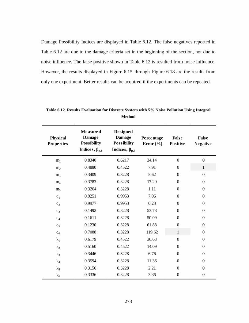
273
Damage Possibility Indices are displayed in Table 6.12. The false negatives reported in
Table 6.12 are due to the damage criteria set in the beginning of the section, not due to
noise influence. The false positive shown in Table 6.12 is resulted from noise influence.
However, the results displayed in Figure 6.15 through Figure 6.18 are the results from
only one experiment. Better results can be acquired if the experiments can be repeated.
Table 6.12. Results Evaluation for Discrete System with 5% Noise Pollution Using Integral
Method
Physical
Properties
Measured
Damage
Possibility
Indices, βp,i
Designed
Damage
Possibility
Indices, βp,i
Percentage
Error (%)
False
Positive
False
Negative
m1 0.8340 0.6217 34.14 0 0
m2 0.4880 0.4522 7.91 0 1
m3 0.3409 0.3228 5.62 0 0
m4 0.3783 0.3228 17.20 0 0
m5 0.3264 0.3228 1.11 0 0
c1 0.9251 0.9953 7.06 0 0
c2 0.9977 0.9953 0.23 0 0
c3 0.1492 0.3228 53.78 0 0
c4 0.1611 0.3228 50.09 0 0
c5 0.1230 0.3228 61.88 0 0
c6 0.7088 0.3228 119.62 1 0
k1 0.6179 0.4522 36.63 0 0
k2 0.5160 0.4522 14.09 0 0
k3 0.3446 0.3228 6.76 0 0
k4 0.3594 0.3228 11.36 0 0
k5 0.3156 0.3228 2.21 0 0
k6 0.3336 0.3228 3.36 0 0

274
6.6.3 Evaluation of Results for Case #6.3
From Figure 6.23 through Figure 6.26, the damage detection results using the data
contaminated by 1% noise are very close to the designed damage detection results. Only
small discrepancies can be found. The percentage error between the Designed Damage
Possibility Indices and Estimated Damage Possibility Indices are displayed in Table 6.13.
The false negatives reported in Table 6.13 are due to the damage criteria set in the
beginning of the section, not due to noise influence. For this case, since the Damage
Indices and Damage Severities, shown in Figure 6.23 and Figure 6.24 are not severely
influenced by the noise, the damage locations and damage extents can still be well
estimated by using Damage Indices and Damage Severities.
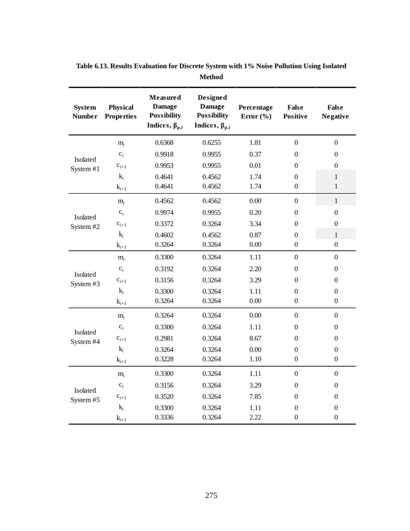
275
Table 6.13. Results Evaluation for Discrete System with 1% Noise Pollution Using Isolated
Method
System
Number
Physical
Properties
Measured
Damage
Possibility
Indices, βp,i
Designed
Damage
Possibility
Indices, βp,i
Percentage
Error (%)
False
Positive
False
Negative
mi 0.6368 0.6255 1.81 0 0
ci 0.9918 0.9955 0.37 0 0
ci+1 0.9953 0.9955 0.01 0 0
ki 0.4641 0.4562 1.74 0 1
ki+1 0.4641 0.4562 1.74 0 1
mi 0.4562 0.4562 0.00 0 1
ci 0.9974 0.9955 0.20 0 0
ci+1 0.3372 0.3264 3.34 0 0
ki 0.4602 0.4562 0.87 0 1
ki+1 0.3264 0.3264 0.00 0 0
mi 0.3300 0.3264 1.11 0 0
ci 0.3192 0.3264 2.20 0 0
ci+1 0.3156 0.3264 3.29 0 0
ki 0.3300 0.3264 1.11 0 0
ki+1 0.3264 0.3264 0.00 0 0
mi 0.3264 0.3264 0.00 0 0
ci 0.3300 0.3264 1.11 0 0
ci+1 0.2981 0.3264 8.67 0 0
ki 0.3264 0.3264 0.00 0 0
ki+1 0.3228 0.3264 1.10 0 0
mi 0.3300 0.3264 1.11 0 0
ci 0.3156 0.3264 3.29 0 0
ci+1 0.3520 0.3264 7.85 0 0
ki 0.3300 0.3264 1.11 0 0
ki+1 0.3336 0.3264 2.22 0 0
Isolated
System #1
Isolated
System #2
Isolated
System #3
Isolated
System #4
Isolated
System #5

276
6.6.4 Evaluation of Results for Case #6.4
From Figure 6.31 and Figure 6.32, the Damage Indices and Damage Severities are
influenced by the noise. However, the damage designed in mi, ci, ci+1, ki, and ki+1 in
System #1 and mi, ci, and ki in System #2 can still be detected and well estimated. Neither
obvious false positives nor false negative was reported in Figure 6.31 and Figure 6.32.
The percentage error between the Designed Damage Possibility Indices and Estimated
Damage Possibility Indices are displayed in Table 6.14. Moreover, neither false negative
no false negative was reported in Table 6.14, either. The current results displayed in Figure
6.31 through Figure 6.34 are the results from only one experiment. Better results can be
acquired if the experiments can be repeated.

277
Table 6.14. Results Evaluation for Discrete System with 5% Noise Pollution Using Isolated
Method
System
Number
Physical
Properties
Measured
Damage
Possibility
Indices, βp,i
Designed
Damage
Possibility
Indices, βp,i
Percentage
Error (%)
False
Positive
False
Negative
mi 0.7357 0.6255 17.61 0 0
ci 0.9985 0.9955 0.31 0 0
ci+1 0.9798 0.9955 1.57 0 0
ki 0.5910 0.4562 29.54 0 0
ki+1 0.5478 0.4562 20.07 0 0
mi 0.5438 0.4562 19.20 0 0
ci 0.9616 0.9955 3.40 0 0
ci+1 0.3594 0.3264 10.13 0 0
ki 0.5398 0.4562 18.33 0 0
ki+1 0.4013 0.3264 22.96 0 0
mi 0.4325 0.3264 32.53 0 0
ci 0.2611 0.3264 20.00 0 0
ci+1 0.3520 0.3264 7.85 0 0
ki 0.4168 0.3264 27.72 0 0
ki+1 0.4286 0.3264 31.32 0 0
mi 0.3745 0.3264 14.75 0 0
ci 0.4286 0.3264 31.32 0 0
ci+1 0.0359 0.3264 88.99 0 0
ki 0.3821 0.3264 17.08 0 0
ki+1 0.3228 0.3264 1.10 0 0
mi 0.4090 0.3264 25.34 0 0
ci 0.0548 0.3264 83.21 0 0
ci+1 0.4052 0.3264 24.15 0 0
ki 0.4129 0.3264 26.53 0 0
ki+1 0.3821 0.3264 17.08 0 0
Isolated
System #1
Isolated
System #2
Isolated
System #3
Isolated
System #4
Isolated
System #5

278
6.6.5 Evaluation of Results for Case #6.5
From Figure 6.40 and Figure 6.41, all the Damage Indices are reduced by certain levels
and all Damage Severities are shifted upward to the positive side. This is resulted from the
application of band-pass filter and the noise influence. Although the damage in m1, m2, k1,
and k2 can still be located, the differences between the estimated damage severities and
designed damage severities are obvious. However, this problem can be solved by using the
Normalized Damage Index and Damage Possibility Index. From Figure 6.42 and Figure
6.43, the estimated results matches well with the designed results. Because the designed
Damage Indices for the damage properties are closed to each other, all the damage
possibility indices for the damaged properties are greater than 50%. Consequently, no
false negative is reported in Table 6.15. In addition, no false positive is found using the
Damage Possibility Index.
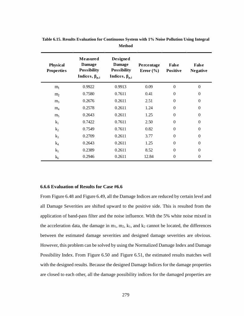
279
Table 6.15. Results Evaluation for Continuous System with 1% Noise Pollution Using Integral
Method
6.6.6 Evaluation of Results for Case #6.6
From Figure 6.48 and Figure 6.49, all the Damage Indices are reduced by certain level and
all Damage Severities are shifted upward to the positive side. This is resulted from the
application of band-pass filter and the noise influence. With the 5% white noise mixed in
the acceleration data, the damage in m1, m2, k1, and k2 cannot be located, the differences
between the estimated damage severities and designed damage severities are obvious.
However, this problem can be solved by using the Normalized Damage Index and Damage
Possibility Index. From Figure 6.50 and Figure 6.51, the estimated results matches well
with the designed results. Because the designed Damage Indices for the damage properties
are closed to each other, all the damage possibility indices for the damaged properties are
Physical
Properties
Measured
Damage
Possibility
Indices, βp,i
Designed
Damage
Possibility
Indices, βp,i
Percentage
Error (%)
False
Positive
False
Negative
m1 0.9922 0.9913 0.09 0 0
m2 0.7580 0.7611 0.41 0 0
m3 0.2676 0.2611 2.51 0 0
m4 0.2578 0.2611 1.24 0 0
m5 0.2643 0.2611 1.25 0 0
k1 0.7422 0.7611 2.50 0 0
k2 0.7549 0.7611 0.82 0 0
k3 0.2709 0.2611 3.77 0 0
k4 0.2643 0.2611 1.25 0 0
k5 0.2389 0.2611 8.52 0 0
k6 0.2946 0.2611 12.84 0 0
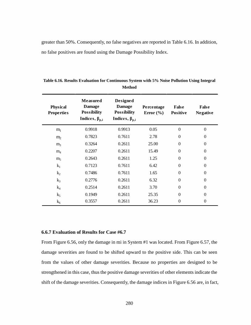
280
greater than 50%. Consequently, no false negatives are reported in Table 6.16. In addition,
no false positives are found using the Damage Possibility Index.
Table 6.16. Results Evaluation for Continuous System with 5% Noise Pollution Using Integral
Method
6.6.7 Evaluation of Results for Case #6.7
From Figure 6.56, only the damage in mi in System #1 was located. From Figure 6.57, the
damage severities are found to be shifted upward to the positive side. This can be seen
from the values of other damage severities. Because no properties are designed to be
strengthened in this case, thus the positive damage severities of other elements indicate the
shift of the damage severities. Consequently, the damage indices in Figure 6.56 are, in fact,
Physical
Properties
Measured
Damage
Possibility
Indices, βp,i
Designed
Damage
Possibility
Indices, βp,i
Percentage
Error (%)
False
Positive
False
Negative
m1 0.9918 0.9913 0.05 0 0
m2 0.7823 0.7611 2.78 0 0
m3 0.3264 0.2611 25.00 0 0
m4 0.2207 0.2611 15.49 0 0
m5 0.2643 0.2611 1.25 0 0
k1 0.7123 0.7611 6.42 0 0
k2 0.7486 0.7611 1.65 0 0
k3 0.2776 0.2611 6.32 0 0
k4 0.2514 0.2611 3.70 0 0
k5 0.1949 0.2611 25.35 0 0
k6 0.3557 0.2611 36.23 0 0

281
shifted downward and thus, not all damage were detected. However, this problem can be
solved by using the Normalized Damage Index and Damage Possibility Index. From
Figure 6.58 and Figure 6.59, the designed damage in mi, ki, and ki+1 in System #1 and mi
and ki in System #2 were successfully detected. However, according to Table 6.17, false
positives were found in System #4. The false positives in System #4 are due to the
differences of amplitudes of shift for each isolated system. This can be seen from Table
6.9: for System #3, the average value is 0.95; for System #4, the average value is 0.98; for
System #5, the average value is 0.89. Consequently, after normalization, the average value
for System #4 will be bigger than the average values of System #3 and System #5 after
normalization. The differences of amplitudes of shift for each isolated system are natural
because each isolated system is analyzed separately.

282
Table 6.17. Results Evaluation for Continuous System with 1% Noise Pollution Using Isolated
Method
6.6.8 Evaluation of Results for Case #6.8
From Figure 6.64 and Figure 6.65, all the Damage Indices are reduced by certain level and
all Damage Severities are shifted upward to the positive side. This is resulted from the
application of band-pass filter and the noise influence. However, this problem can be
solved by using the Normalized Damage Index and Damage Possibility Index. According
to Table 6.18, the designed damage in mi, ki and ki+1 in System #1 and mi and ki in System
#2 were successfully detected. One false positive was found in Table 6.18 in ki+1 in System
#2. This false positive is resulted from the noise influence. Comparing to the previous case,
System
Number
Physical
Properties
Measured
Damage
Possibility
Indices, βp,i
Designed
Damage
Possibility
Indices, βp,i
Percentage
Error (%)
False
Positive
False
Negative
mi 0.9946 0.9965 0.19 0 0
ki 0.7088 0.8051 11.96 0 0
ki+1 0.7157 0.8051 11.11 0 0
mi 0.7324 0.8051 9.03 0 0
ki 0.7324 0.8051 9.03 0 0
ki+1 0.1685 0.2709 37.80 0 0
mi 0.3897 0.2709 43.85 0 0
ki 0.3974 0.2709 46.69 0 0
ki+1 0.3859 0.2709 42.44 0 0
mi 0.6026 0.2709 122.40 1 0
ki 0.5987 0.2709 120.98 1 0
ki+1 0.5910 0.2709 118.12 1 0
mi 0.1057 0.2709 61.00 0 0
ki 0.0968 0.2709 64.27 0 0
ki+1 0.1112 0.2709 58.94 0 0
Isolated
System #1
Isolated
System #2
Isolated
System #3
Isolated
System #4
Isolated
System #5
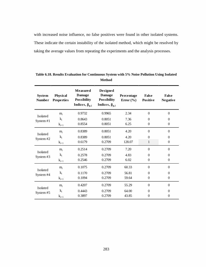
283
with increased noise influence, no false positives were found in other isolated systems.
These indicate the certain instability of the isolated method, which might be resolved by
taking the average values from repeating the experiments and the analysis processes.
Table 6.18. Results Evaluation for Continuous System with 5% Noise Pollution Using Isolated
Method
System
Number
Physical
Properties
Measured
Damage
Possibility
Indices, βp,i
Designed
Damage
Possibility
Indices, βp,i
Percentage
Error (%)
False
Positive
False
Negative
mi 0.9732 0.9965 2.34 0 0
ki 0.8643 0.8051 7.36 0 0
ki+1 0.8554 0.8051 6.25 0 0
mi 0.8389 0.8051 4.20 0 0
ki 0.8389 0.8051 4.20 0 0
ki+1 0.6179 0.2709 128.07 1 0
mi 0.2514 0.2709 7.20 0 0
ki 0.2578 0.2709 4.83 0 0
ki+1 0.2546 0.2709 6.02 0 0
mi 0.1075 0.2709 60.33 0 0
ki 0.1170 0.2709 56.81 0 0
ki+1 0.1094 0.2709 59.64 0 0
mi 0.4207 0.2709 55.29 0 0
ki 0.4443 0.2709 64.00 0 0
ki+1 0.3897 0.2709 43.85 0 0
Isolated
System #1
Isolated
System #2
Isolated
System #3
Isolated
System #4
Isolated
System #5

284
7 REANALYSIS
7.1 INTRODUCTION
In this section, three problems that are either arose in the previous numerical examples or
anticipated in the further applications will be demonstrated and the solutions are provided.
The problems will be analyzed in the following subsections are,
(1) Case #7.1: Nodes without external loads;
(2) Case #7.2: Efficiency of noise-influence reduction by repeating experiment;
(3) Case #7.3: Damage detection in Continuous structure with proportional damping;
7.2 STUDY OF NODES WITHOUT EXTERNAL LOADS (CASE #7.1)
7.2.1 Introduction
In this subsection, the problem caused by nodes without external loads will be studied and
solved. For all the numerical cases that are studied in the previous sections, external loads
had been applied at each node that was analyzed. This is not a problem for the integral
system method of the Power Method, because the power equilibrium of the integral
method can be applied if there is one node with external loads. However, for the isolated
system method, the algorithm given in the previous section will only be applicable to the
node with external load. For the node without external load, the previous algorithm for
isolated system won’t work due to the rank deficiency of the coefficient matrix for the
final linear equation groups. Under this situation, a new algorithm is proposed in
Subsection 7.2.2.

285
7.2.2 Theory for Node without External Loads
In this subsection, the theory for node without external load will be provided. For
simplicity purposes, only the theory for node without external loads for plain frame will be
provided and the theory for node without external loads for other structural components
can be easily completed following the same idea and process.
According to the finite element method, one plain frame can be meshed into several
elements. Isolating two nearby plain frame elements, as shown in Figure 7.1, the modulus
of elasticity of the material for Element i is denoted as iE . The length of Element i is iL .
The area and the moment of inertia of the cross section of Element i are denoted as iA
and iI , respectively. Let }{ iP be the force vector at Node i, where iP1 denotes the axial
force at Node i, iP2 denotes the shear force at Node i, iP3 denotes the bending moment at
Node i. As shown in the free body diagram of Node i in Figure 7.2, the external loads
( }{ iP ), internal forces ( }{ iF and }{ 1iF ), and inertial forces }{ iI form a dynamic
equilibrium condition at Node i. The dynamic equilibrium condition can be written as,
}{}{}{}{ 1
i
ii
i PFFI (7.1)
In this case, degrees of freedom in axial, transversal and rotational directions will be taken
into consideration. Thus each force vector in Eq. 7.1 is composed by three force
components: (1) Axial force; (2) shear force; (3) bending moment.
i
i
i
i
i
i
i
i
i
i
i
i
P
P
P
F
F
F
F
F
F
I
I
I
3
2
1
3,1
2,1
1,1
3,
2,
1,
3
2
1
(7.2)
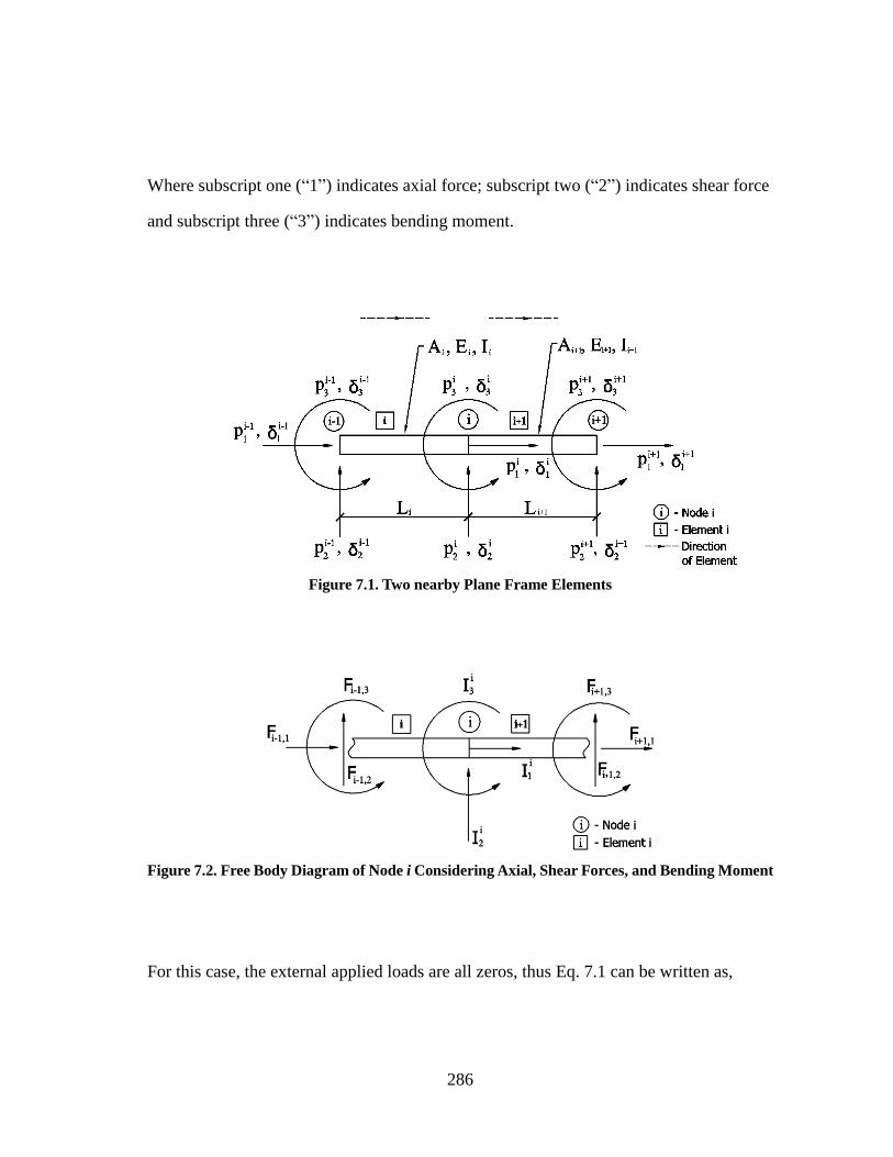
286
Where subscript one (“1”) indicates axial force; subscript two (“2”) indicates shear force
and subscript three (“3”) indicates bending moment.
Figure 7.1. Two nearby Plane Frame Elements
Figure 7.2. Free Body Diagram of Node i Considering Axial, Shear Forces, and Bending Moment
For this case, the external applied loads are all zeros, thus Eq. 7.1 can be written as,

287
}0{}{}{}{ 1 ii
i FFI (7.3)
Given any velocity vectors, }{ i , the power done by the external forces can be expressed
as following,
}0{}{}{}{}{}{}{}{}{ 1
iTi
i
Ti
i
TiiTi PFFI (7.4)
Rearrange Eq. 7.4 yields,
}{}{}{}{}{}{ 1
iTi
i
Ti
i
Ti IFF (7.5)
In this case, the inertial forces for the undamaged system can be expressed using the
following lumped mass matrix, (note that the inertial effect associated with any rotational
degree of freedom is neglected)
}]{[
0
1
1
22}{
3
2
1
11 ii
o
i
i
i
i
i
iiiii MmLmLm
I
(7.6)
Where im is the linear mass of Element i; i
1 is the acceleration in axial direction at
Node i; i
2 is the acceleration in transverse direction at Node i and i
3 is the acceleration
in bending rotation direction within the plain at Node i.
The force vectors (i.e. }{ iF and }{ 1iF ) in Eq. 7.5 can be computed using stiffness
matrices and node deformation vectors,

288
}]{[
460260
61206120
0000
}]{[}{
,
3,
2,
1,
3,
2,
1,
22
22
3
iioi
i
i
i
i
i
i
i
i
iii
Kk
LLLL
LLI
AL
I
AL
L
EIKF
(7.7)
}]{[
260460
61206120
0000
}]{[}{
11,1
3,1
2,1
1,1
3,1
2,1
1,1
1
22
22
1
3111
iioi
i
i
i
i
i
i
i
i
iii
Kk
LLLL
LLI
AL
I
AL
L
EIKF
(7.8)
Where
1,i and
1,i are the displacement in axial direction at the positive and negative
ends of Element i, respectively;
2,i and
2,i are the displacement in transverse
direction at the positive and negative ends of Element i, respectively;
3,i and
3,i are
the node rotations in bending rotation direction at the positive and negative ends of
Element i, respectively.
Substitute Eqs. 7.6 through 7.8 into Eq. 7.5 yields,
}]{[}{}]{[}{}]{[}{ 11,1,
ii
o
iTi
iioi
Ti
iioi
Ti MmKkKk (7.9)
Moving forward the property constant from each term in Eq. 7.9 yields,

289
}]{[}{}]{[}{}]{[}{ 11,1,
ii
o
Tii
iio
Ti
iiio
Ti
i MmKkKk (7.10)
Dividing each term in Eq. 7.10 by im yields,
}]{[}{}]{[}{}]{[}{ 11,1
,
ii
o
Ti
iio
Ti
i
iiio
Ti
i
i MKm
kK
m
k
(7.11)
Define the following coefficients,
i
i
m
k1 (7.12)
i
i
m
k 12
(7.13)
Substituting Eq. 7.12 and Eq. 7.13 to Eq. 7.11 yields,
}]{[}{}]{[}{}]{[}{ 11,2,1
ii
o
Ti
iio
Ti
iio
Ti MKK (7.14)
Writing the Eq. 7.14 at different time point, yields the following groups of equations,
For 0tt ,
000|})]{[}({|})]{[}({|})]{[}({ 11,2,1 t
ii
o
Ti
tiio
Ti
tiio
Ti MKK (7.15)
For jtt ,
jjj t
ii
o
Ti
tiio
Ti
tiio
Ti MKK |})]{[}({|})]{[}({|})]{[}({ 11,2,1 (7.16)
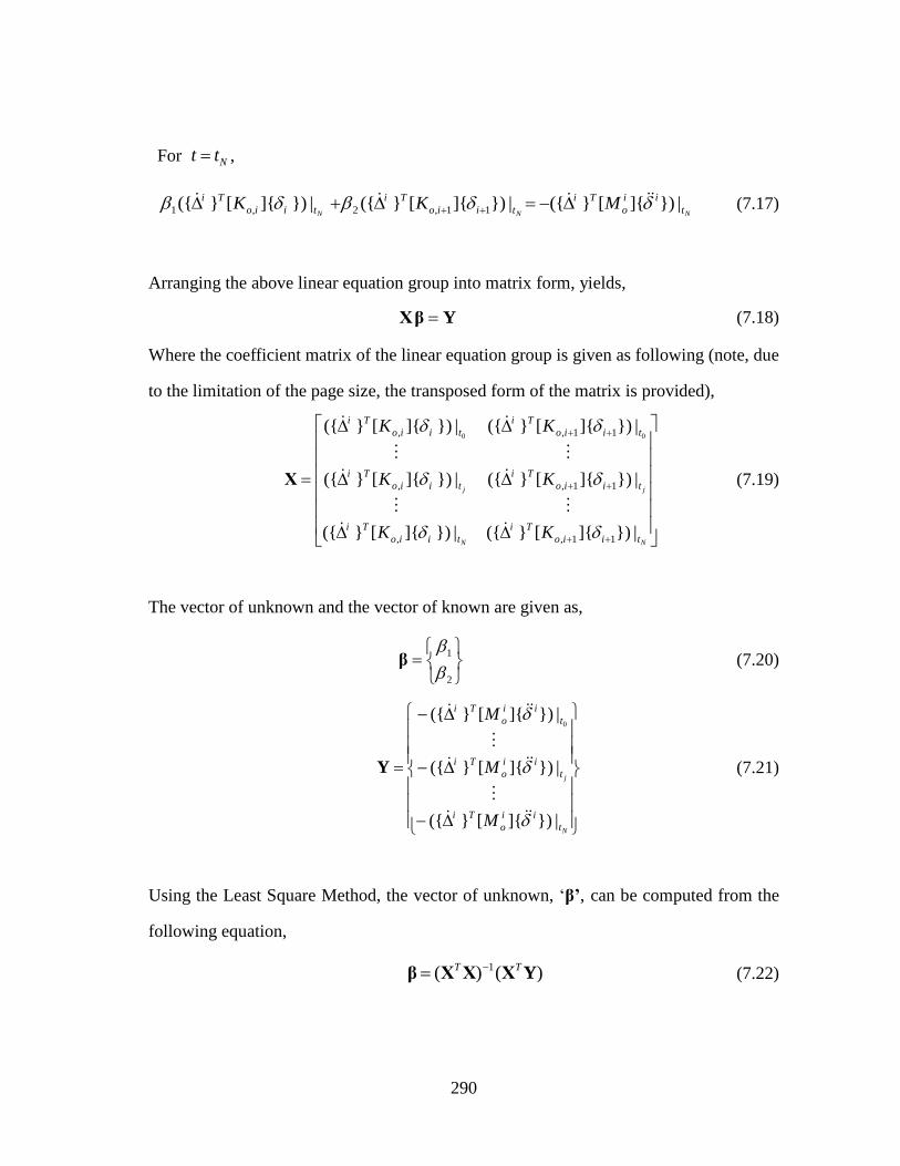
290
For Ntt ,
NNN t
ii
o
Ti
tiio
Ti
tiio
Ti MKK |})]{[}({|})]{[}({|})]{[}({ 11,2,1 (7.17)
Arranging the above linear equation group into matrix form, yields,
YβΧ (7.18)
Where the coefficient matrix of the linear equation group is given as following (note, due
to the limitation of the page size, the transposed form of the matrix is provided),
NN
jj
tiio
Ti
tiio
Ti
tiio
Ti
tiio
Ti
tiio
Ti
tiio
Ti
KK
KK
KK
|})]{[}({|})]{[}({
|})]{[}({|})]{[}({
|})]{[}({|})]{[}({
11,,
11,,
11,, 00
Χ (7.19)
The vector of unknown and the vector of known are given as,
2
1
β (7.20)
N
j
t
ii
o
Ti
t
ii
o
Ti
t
ii
o
Ti
M
M
M
|})]{[}({
|})]{[}({
|})]{[}({0
Y (7.21)
Using the Least Square Method, the vector of unknown, ‘β’, can be computed from the
following equation,
)()( 1YΧΧΧβ
TT (7.22)

291
With the vector of unknown computed, the damage indices for stiffness can be computed
as follows,
isystem
isystem
i
i
i
i
i
i
i
i
k
L
EI
L
EI
k
k
m
k
m
k
,2
,1
1
3
3
11
(7.23)
isystem
isystem
i
i
i
i
i
i
m
m
k
m
k
m
m
,2
1,1
1
1
1
1
(7.24)
7.2.3 Damage Evaluation for Cantilever with External Load at Free End Only
In this subsection, a cantilever beam is used to evaluate the performance of the proposed
theory in dealing with nodes without external loads. The geometry of the cantilever and
damage scenario under consideration are indicated Figure 7.3. The geometry of the
cross-section of the beam is shown in Figure 5.19. The modulus of elasticity (E) of the
material is 29,000 ksi. The mass density of the material is 7.345×10⁻⁷ kipsec2/in4.
The cantilever beam is meshed into 6 elements and has 7 equally spaced nodes. The length
of each element is 12.0 inches. For illustrative purposes, typical elements are indicated in
Figure 7.3. Two elements with damaged mass and stiffness are studied. The damage is
simulated by a ten percent (10%) reduction of the modulus of elasticity and twenty percent
(20%) reduction of the mass of the second (2nd) and fifth (5th) elements on the beam.
Only the node at the free end of the cantilever is excited by external nodal load, which is

292
simulated using a white noise, 100×random(-1,1) and is applied in axial direction. This
external nodal load is plotted in Figure 7.4. Given the external load case, exact
accelerations, velocities and displacements of the six nodes were computed at every 1E-4
seconds (10,000 Hz) for 0.2 seconds.
In this case, the computed velocity ( )(tx ) of each node in the undamaged case was used as
the velocity used to compute power ( ) for both the undamaged and damaged cases. For
every two nearby elements, the coefficient matrices (‘X’) and known vector (‘Y’) were
constructed by substituting the acceleration ( )(tx ), velocity ( )(tx ), displacement ( )(tx ),
and velocity used to compute power ( ) into Eq. 7.19 and Eq. 7.21. The coefficient
damage index vector, β, related to the two nearby elements was computed using Eq. 7.22.
Then the damage indices for Element stiffness and Nodal mass are computed using Eq.
7.23 and Eq. 7.24, respectively. The damage severities for stiffness are computed using
Eq. 2.13.
Figure 7.3. Geometry and Damage Scenario for the Cantilever Beam

293
Figure 7.4. Applied External Load at the Free End of the Cantilever

294
(a)
(b)
Figure 7.5. Displacements in Axial Direction of Node 7 of the Cantilever under the Given
External Load: (a) Full Plot and (b) Zoomed in Plot

295
(a)
(b)
Figure 7.6. Velocities in Axial Direction of the Node 7 of the Cantilever under the Given External
Load: (a) Full Plot and (b) Zoomed in Plot

296
(a)
(b)
Figure 7.7. Accelerations in Axial Direction of Node 7 of the Cantilever under the Given External
Load: (a) Full Plot and (b) Zoomed in Plot

297
Table 7.1. Damage Detection Results for the Cantilever under Axial Vibrations
Figure 7.8. Damage Indices (βi) for the Fixed-Fixed Beam with Proportional Damping Using
Isolated Beam Element Analysis Method
Property
Comparison
Damage Index
(βi, Esimated)
Damage Severity
(αi, Esimated)
Damage Index
(βi, Designed)
k1\k2 1.11 -0.10 1.11
k2\k3 0.90 0.11 0.90
k3\k4 1.00 0.00 1.00
k4\k5 1.11 -0.10 1.11
k5\k6 0.90 0.11 0.90
m1\m2 1.00 0.00 1.00
m2\m3 0.90 0.11 0.90
m3\m4 1.11 -0.10 1.11
m4\m5 1.00 0.00 1.00
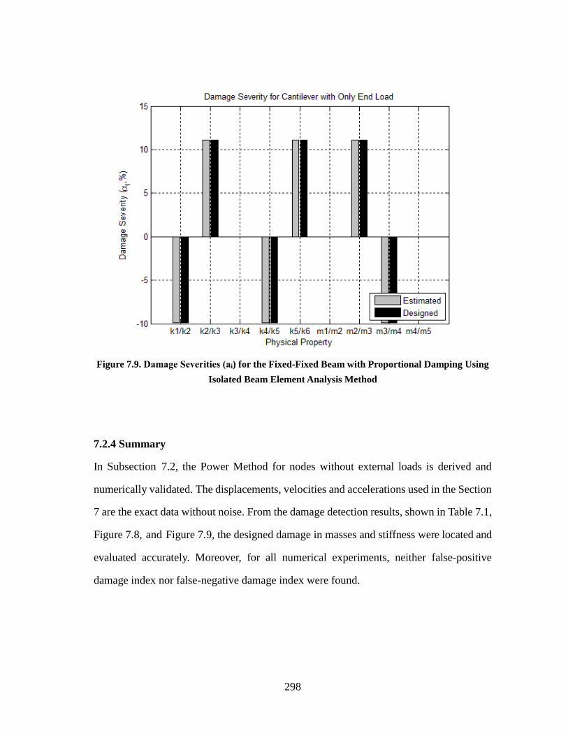
298
Figure 7.9. Damage Severities (аi) for the Fixed-Fixed Beam with Proportional Damping Using
Isolated Beam Element Analysis Method
7.2.4 Summary
In Subsection 7.2, the Power Method for nodes without external loads is derived and
numerically validated. The displacements, velocities and accelerations used in the Section
7 are the exact data without noise. From the damage detection results, shown in Table 7.1,
Figure 7.8, and Figure 7.9, the designed damage in masses and stiffness were located and
evaluated accurately. Moreover, for all numerical experiments, neither false-positive
damage index nor false-negative damage index were found.

299
7.3 STUDY OF EFFICIENCY OF NOISE-INFLUENCE REDUCTION BY
REPEATING THE EXPERIMENT (CASE #7.2)
7.3.1 Introduction
In this subsection, the efficiency of noise-influence reduction will be studied. According
to the damage detection results in Section 6, when the acceleration inputs are
contaminated by noise signals, the estimations of the damage severities will become less
reliable, which, for example, can be seen in Figure 6.15 and Figure 6.18. For repeatable
experiments, the noise influence can be reduced by repeating experiments and the white
noise signals can be reduced by averaging white noises.
There are mainly two ways to reduce white noise influence:
(1) Compute damage indices based on each experimental measurement and then compute
the average of the damage indices; and
(2) Compute the average inputs from the combination of all the measurements and
compute the damage indices based on the average inputs.
7.3.2 Efficiency Study of Noise-Influence Reduction Based on Averaged Damage
Detection Results
In this subsection, the efficiency of noise-influence reduction based on averaged damage
detection results will be studied using the 5-DOF spring-mass-damper system introduced
in Case #6.2 in Section 6.2.2.
The inputs will be simulated by the exact accelerations of the mass blocks directly
outputted from SAP2000 were contaminated by 5% of white noise. For illustration
purposes, the noise-polluted accelerations of Mass Block #2 in both the undamaged and

300
damaged cases can be seen in Figure 6.11. The filtered accelerations, estimated velocities
and estimated displacements of Mass Block #2 are can be seen from Figure 6.12, Figure
6.13, and Figure 6.14, respectively.
For illustration purposes, the vibration test for the 5-DOF spring-mass-damper system was
assumed to be conducted ten times. The computed damage indices based on each vibration
test, the averaged damage indices and the designed damage indices are listed in Table 7.2.
The averaged damage indices and the designed damage indices are plotted in Figure 7.10.
The related damage severities are plotted in Figure 7.11. The normalized damage indices
are computed using Eq. 6.4 and are plotted in Figure 7.12. The damage possibility indices
are plotted in Figure 7.13. Comparing the averaged damage indices with the designed
damage indices, the accuracy of the damage indices are not obviously improved.
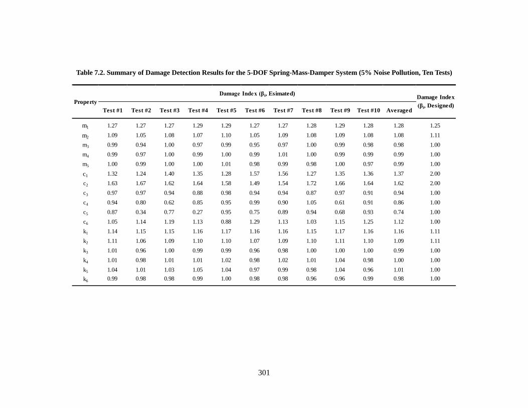
301
Table 7.2. Summary of Damage Detection Results for the 5-DOF Spring-Mass-Damper System (5% Noise Pollution, Ten Tests)
Test #1 Test #2 Test #3 Test #4 Test #5 Test #6 Test #7 Test #8 Test #9 Test #10 Averaged
m1 1.27 1.27 1.27 1.29 1.29 1.27 1.27 1.28 1.29 1.28 1.28 1.25
m2 1.09 1.05 1.08 1.07 1.10 1.05 1.09 1.08 1.09 1.08 1.08 1.11
m3 0.99 0.94 1.00 0.97 0.99 0.95 0.97 1.00 0.99 0.98 0.98 1.00
m4 0.99 0.97 1.00 0.99 1.00 0.99 1.01 1.00 0.99 0.99 0.99 1.00
m5 1.00 0.99 1.00 1.00 1.01 0.98 0.99 0.98 1.00 0.97 0.99 1.00
c1 1.32 1.24 1.40 1.35 1.28 1.57 1.56 1.27 1.35 1.36 1.37 2.00
c2 1.63 1.67 1.62 1.64 1.58 1.49 1.54 1.72 1.66 1.64 1.62 2.00
c3 0.97 0.97 0.94 0.88 0.98 0.94 0.94 0.87 0.97 0.91 0.94 1.00
c4 0.94 0.80 0.62 0.85 0.95 0.99 0.90 1.05 0.61 0.91 0.86 1.00
c5 0.87 0.34 0.77 0.27 0.95 0.75 0.89 0.94 0.68 0.93 0.74 1.00
c6 1.05 1.14 1.19 1.13 0.88 1.29 1.13 1.03 1.15 1.25 1.12 1.00
k1 1.14 1.15 1.15 1.16 1.17 1.16 1.16 1.15 1.17 1.16 1.16 1.11
k2 1.11 1.06 1.09 1.10 1.10 1.07 1.09 1.10 1.11 1.10 1.09 1.11
k3 1.01 0.96 1.00 0.99 0.99 0.96 0.98 1.00 1.00 1.00 0.99 1.00
k4 1.01 0.98 1.01 1.01 1.02 0.98 1.02 1.01 1.04 0.98 1.00 1.00
k5 1.04 1.01 1.03 1.05 1.04 0.97 0.99 0.98 1.04 0.96 1.01 1.00
k6 0.99 0.98 0.98 0.99 1.00 0.98 0.98 0.96 0.96 0.99 0.98 1.00
Property
Damage Index (βi, Esimated)Damage Index
(βi, Designed)

302
Figure 7.10. Averaged Damage Indices (βi) for 5-DOF Spring-Mass-Damper System with
Noise-Polluted Accelerations (5% Noise, Ten Tests)
Figure 7.11. Averaged Damage Severities (аi) for 5-DOF Spring-Mass-Damper System with
Noise-Polluted Accelerations (5% Noise, Ten Tests)
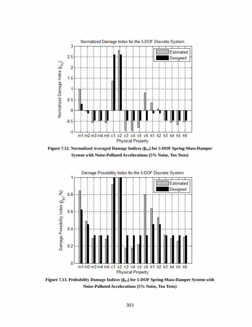
303
Figure 7.12. Normalized Averaged Damage Indices (βn,i) for 5-DOF Spring-Mass-Damper
System with Noise-Polluted Accelerations (5% Noise, Ten Tests)
Figure 7.13. Probability Damage Indices (βp,i) for 5-DOF Spring-Mass-Damper System with
Noise-Polluted Accelerations (5% Noise, Ten Tests)

304
7.3.3 Efficiency Study of Noise-Influence Reduction Based on Averaged Inputs
In this subsection, the efficiency of noise-influence reduction based on averaged damage
detection results will be studied using the 5-DOF spring-mass-damper system introduced
in Case #6.2 in Section 6.2.2.
As introduced in the previous subsection, the numerical experiment will be simulated ten
times. Before input each noise-polluted signals into the program, the ten groups of
noise-polluted signals will be combined and averaged. The inputs for the program will be
the averaged noise-polluted signals from the ten numerical experiments.
The estimated damage indices based on the averaged inputting signals and the designed
damage indices for each physical property are listed in Table 7.3 and are plotted in Figure
7.14 and the related damage severities are plotted in Figure 7.15. The normalized damage
indices are computed using Eq. 6.4 and are plotted in Figure 7.16. The damage possibility
indices are plotted in Figure 7.17. Comparing the estimated damage indices with the
designed damage indices, the accuracy of the damage indices has been obviously
improved.

305
Table 7.3. Damage Detection Results for the 5-DOF Spring-Mass-Damper System Based on
Averaged Inputs (5% Noise Pollution, Ten Tests)
PropertyDamage Index
(βi, Esimated)
Damage Severity
(αi, Esimated)
Damage Index
(βi, Designed)
m1 1.25 -0.20 1.25
m2 1.11 -0.10 1.11
m3 1.00 0.00 1.00
m4 1.00 0.00 1.00
m5 1.00 0.00 1.00
c1 2.20 -0.54 2.00
c2 1.88 -0.47 2.00
c3 0.98 0.02 1.00
c4 1.00 0.00 1.00
c5 1.04 -0.04 1.00
c6 0.99 0.01 1.00
k1 1.12 -0.11 1.11
k2 1.11 -0.10 1.11
k3 0.99 0.01 1.00
k4 1.00 0.00 1.00
k5 1.01 -0.01 1.00
k6 1.00 0.00 1.00

306
Figure 7.14. Damage Indices (βi) for 5-DOF Spring-Mass-Damper System with Averaged
Noise-Polluted Accelerations (5% Noise, Ten Tests)
Figure 7.15. Damage Severities (аi) for 5-DOF Spring-Mass-Damper System with Averaged
Noise-Polluted Accelerations (5% Noise, Ten Tests)

307
Figure 7.16. Normalized Damage Indices (βn,i) for 5-DOF Spring-Mass-Damper System with
Averaged Noise-Polluted Accelerations (5% Noise, Ten Tests)
Figure 7.17. Probability Damage Indices (βp,i) for 5-DOF Spring-Mass-Damper System with
Averaged Noise-Polluted Accelerations (5% Noise, Ten Tests)
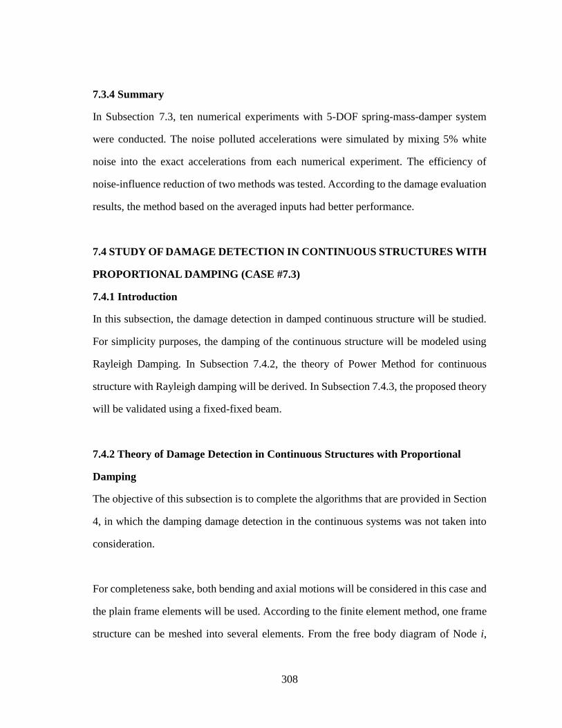
308
7.3.4 Summary
In Subsection 7.3, ten numerical experiments with 5-DOF spring-mass-damper system
were conducted. The noise polluted accelerations were simulated by mixing 5% white
noise into the exact accelerations from each numerical experiment. The efficiency of
noise-influence reduction of two methods was tested. According to the damage evaluation
results, the method based on the averaged inputs had better performance.
7.4 STUDY OF DAMAGE DETECTION IN CONTINUOUS STRUCTURES WITH
PROPORTIONAL DAMPING (CASE #7.3)
7.4.1 Introduction
In this subsection, the damage detection in damped continuous structure will be studied.
For simplicity purposes, the damping of the continuous structure will be modeled using
Rayleigh Damping. In Subsection 7.4.2, the theory of Power Method for continuous
structure with Rayleigh damping will be derived. In Subsection 7.4.3, the proposed theory
will be validated using a fixed-fixed beam.
7.4.2 Theory of Damage Detection in Continuous Structures with Proportional
Damping
The objective of this subsection is to complete the algorithms that are provided in Section
4, in which the damping damage detection in the continuous systems was not taken into
consideration.
For completeness sake, both bending and axial motions will be considered in this case and
the plain frame elements will be used. According to the finite element method, one frame
structure can be meshed into several elements. From the free body diagram of Node i,

309
shown in Figure 7.18, the dynamic equilibrium condition for Node i can be written as,
}{}{}{}{}{}{ 1,,1,,
i
icicisis
i PFFFFI (7.25)
Where }{ iI is the inertial force vector at Node i, }{ ,isF is the internal force from the
positive end of Element i due to element stiffness; }{ ,icF is the internal force from the
positive end of Element i due to element damping; }{ iP is the applied external load at
Node i. Note that the positive end of Element i and the negative end of Element i+1 share
the same node.
Figure 7.18. Free Body Diagram of Node i Considering Axial, Shear Forces, and Bending
Moment
Similarly, for the damaged case, the dynamic equilibrium condition is,
}{}{}{}{}{}{ **
1,
*
,
*
1,
*
,
* i
icicisis
i PFFFFI (7.26)
Where the asterisk (“*”) denotes the quantities from the damaged case.

310
Given any velocity vectors, }{ i and }{ *i , for the undamaged and damaged systems,
the power performed by the external forces in the undamaged and damaged systems can
be expressed as follows,
}{}{}{}{}{}{}{}{}{}{}{}{ 1,,1,,
iTi
ic
Ti
ic
Ti
is
Ti
is
TiiTi PFFFFI
(7.27)
}{}{}{}{}{}{}{}{}{}{}{}{ ***
1,
**
,
**
1,
**
,
*** iTi
ic
Ti
ic
Ti
is
Ti
is
TiiTi PFFFFI
(7.28)
Assume that the applied external loads and the applied velocities used to compute power
at Node i are the same for both the undamaged and damaged systems,
}{}{ *ii (7.29)
}{}{ *ii PP (7.30)
Substituting Eq. 7.29 and Eq. 7.30 into Eq. 7.28 yields,
}{}{}{}{}{}{}{}{}{}{}{}{ *
1,
**
,
**
1,
**
,
*** iTi
ic
Ti
ic
Ti
is
Ti
is
TiiTi PFFFFI
(7.31)
Noticing the power done by the external load are the same for both the undamaged and
damaged system. Substituting Eq.7.31 into Eq. 7.27 yields,
}{}{}{}{}{}{}{}{}{}{
}{}{}{}{}{}{}{}{}{}{
*
1,
*
,
*
1,
*
,
*
1,,1,,
ic
Ti
ic
Ti
is
Ti
is
TiiTi
ic
Ti
ic
Ti
is
Ti
is
TiiTi
FFFFI
FFFFI
(7.32)
Note, Eq. 7.32 is equivalent to Eq. 2.10.

311
In this case, the inertial forces for the undamaged system can be expressed using the
following lumped mass matrix, (note that the inertial effect associated with any rotational
degree of freedom is assumed can be neglected)
}]{[
0
1
1
22}{
3
2
1
11 ii
o
i
i
i
i
i
iiiii MmLmLm
I
(7.33)
Where im is the linear mass of Element i; i
1 is the acceleration in axial direction at
Node i; i
2 is the acceleration in transverse direction at Node i and i
3 is the acceleration
in bending rotation direction within the plain at Node i.
Similarly, for the damaged system,
}]{[
0
1
1
22}{ ***
*
3
*
2
*
1*
1
*
1
*** ii
o
i
i
i
i
i
iiiii MmLmLm
I
(7.34)
The internal force vectors (i.e. }{ ,isF , }{ 1, isF , }{ ,icF , }{ 1, icF , }{ *
,isF , }{ *
1, isF , }{ *
,icF ,
and }{ *
1, icF ) in Eq. 7.32 can be computed as followings,

312
}]{[
460260
61206120
0000
}]{[}{
,
3,
2,
1,
3,
2,
1,
22
22
3,
iioi
i
i
i
i
i
i
i
i
iiis
Kk
LLLL
LLI
AL
I
AL
L
EIKF
(7.35)
}]{[
260460
61206120
0000
}]{[}{
11,1
3,1
2,1
1,1
3,1
2,1
1,1
1
22
22
1
3111,
iioi
i
i
i
i
i
i
i
i
iiis
Kk
LLLL
LLI
AL
I
AL
L
EIKF
(7.36)

313
}]{[}]{[2
460260
61206120
0000
000
010
001
2
460260
61206120
0000
000000
010000
001000
2
}]{[}]{[}]){[][(}]{[}{
,1,0,
3,
2,
1,
3,
2,
1,
22
22
31,
3,
2,
1,
0,
3,
2,
1,
3,
2,
1,
22
22
31,
3,
2,
1,
3,
2,
1,
0,
1,0,1,0,,
iioiii
i
oi
i
i
i
i
i
i
i
i
i
i
i
i
i
i
i
i
i
i
i
i
i
i
i
i
i
i
i
i
i
i
i
i
i
i
iiiiiiiiiiiiiic
KkaMm
a
LLLL
LLI
AL
I
AL
L
EIa
Lma
LLLL
LLI
AL
I
AL
L
EIa
Lma
KaMaKaMaCF
(7.37)
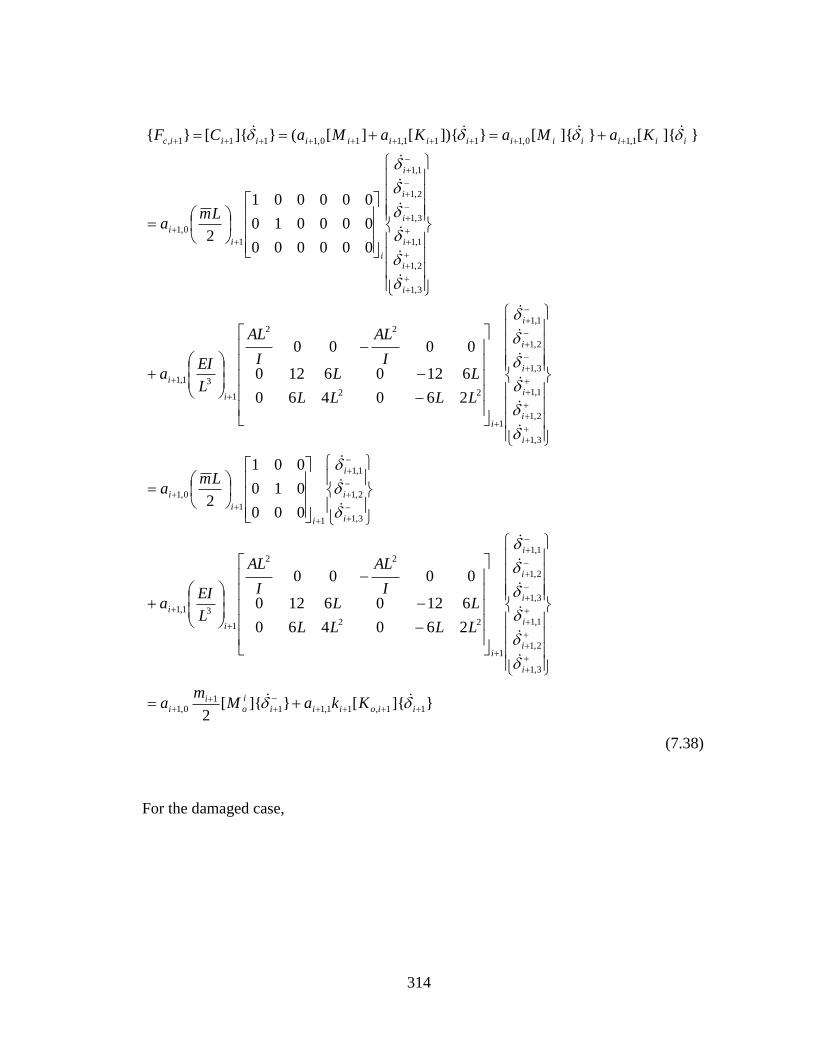
314
}]{[}]{[2
260460
61206120
0000
000
010
001
2
260460
61206120
0000
000000
000010
000001
2
}]{[}]{[}]){[][(}]{[}{
11,11,111
0,1
3,1
2,1
1,1
3,1
2,1
1,1
1
22
22
1
31,1
3,1
2,1
1,1
1
1
0,1
3,1
2,1
1,1
3,1
2,1
1,1
1
22
22
1
31,1
3,1
2,1
1,1
3,1
2,1
1,1
1
0,1
1,10,1111,110,1111,
iioiii
i
oi
i
i
i
i
i
i
i
i
i
i
i
i
i
i
i
i
i
i
i
i
i
i
i
i
i
i
i
i
i
i
i
i
i
i
iiiiiiiiiiiiiic
KkaMm
a
LLLL
LLI
AL
I
AL
L
EIa
Lma
LLLL
LLI
AL
I
AL
L
EIa
Lma
KaMaKaMaCF
(7.38)
For the damaged case,

315
}]{[
460260
61206120
0000
}{ **
,
*
*
3,
*
2,
*
1,
*
3,
*
2,
*
1,*
22
22
*
3
*
, iioi
i
i
i
i
i
i
i
i
is Kk
LLLL
LLI
AL
I
AL
L
EIF
(7.39)
}]{[
260460
61206120
0000
}{ *
1
*
1,
*
1
*
3,1
*
2,1
*
1,1
*
3,1
*
2,1
*
1,1*
1
22
22
*
1
3
*
1,
iioi
i
i
i
i
i
i
i
i
is Kk
LLLL
LLI
AL
I
AL
L
EIF
(7.40)

316
}]{[}]{[2
460260
61206120
0000
000
010
001
2
460260
61206120
0000
000000
010000
001000
2
}]{[}]{[}]){[][(}]{[}{
**
,
**
1,
***
*
0,
*
3,
*
2,
*
1,
*
3,
*
2,
*
1,
22
22
*
3
*
1,
*
3,
*
2,
*
1,*
*
0,
*
3,
*
2,
*
1,
*
3,
*
2,
*
1,
22
22
*
3
*
1,
*
3,
*
2,
*
1,
*
3,
*
2,
*
1,
*
*
0,
***
1,
***
0,
***
1,
**
0,
***
,
iioiii
i
oi
i
i
i
i
i
i
i
i
i
i
i
i
i
i
i
i
i
i
i
i
i
i
i
i
i
i
i
i
i
i
i
i
i
i
iiiiiiiiiiiiiic
KkaMm
a
LLLL
LLI
AL
I
AL
L
EIa
Lma
LLLL
LLI
AL
I
AL
L
EIa
Lma
KaMaKaMaCF
(7.41)

317
}]{[}]{[2
260460
61206120
0000
000
010
001
2
260460
61206120
0000
000000
000010
000001
2
}]{[}]{[}]){[][(}]{[}{
*
1
*
1,
*
1
*
1,1
*
1
**
1*
0,1
*
3,1
*
2,1
*
1,1
*
3,1
*
2,1
*
1,1
1
22
22
*
1
3
*
1,1
*
3,1
*
2,1
*
1,1*
1
*
0,1
*
3,1
*
2,1
*
1,1
*
3,1
*
2,1
*
1,1
1
22
22
*
1
3
*
1,1
*
3,1
*
2,1
*
1,1
*
3,1
*
2,1
*
1,1
*
1
*
0,1
***
1,1
***
0,1
*
1
*
1
*
1,1
*
1
*
0,1
*
1
*
1
*
1,
iioiii
i
oi
i
i
i
i
i
i
i
i
i
i
i
i
i
i
i
i
i
i
i
i
i
i
i
i
i
i
i
i
i
i
i
i
i
iiiiiiiiiiiiiic
KkaMm
a
LLLL
LLI
AL
I
AL
L
EIa
Lma
LLLL
LLI
AL
I
AL
L
EIa
Lma
KaMaKaMaCF
(7.42)
Where i
1 is the velocity in axial direction at Node i;
i
2 is the velocity in transverse
direction at Node i and i
3 is the angular velocity within the plain at Node i. 0,ia and
1,ia are the damping coefficients for the proportional damping.
318
Substitute Eqs. 7.33 through 7.42 into Eq. 7.32 yields,
}]{[}{
}]{[2
}{}]{[}{}]{[2
}{
}]{[}{}]{[}{}]{[}{
}]{[}{
}]{[2
}{}]{[}{}]{[2
}{
}]{[}{}]{[}{}]{[}{
*
1
*
1,
*
1
*
1,1
*
1
**
1*
0,1
**
,
**
1,
***
*
0,
*
1
*
1,
*
1
**
,
****
11,11,1
11
0,1,1,0,
11,1,
iioii
Ti
i
i
oi
i
Ti
iioii
Ti
i
i
oi
i
Ti
iioi
Ti
iioi
Tiii
o
iTi
iioii
Ti
i
i
oi
i
Ti
iioii
Ti
i
i
oi
i
Ti
iioi
Ti
iioi
Tiii
o
iTi
Kka
Mm
aKkaMm
a
KkKkMm
Kka
Mm
aKkaMm
a
KkKkMm
(7.43)
Note that the positive end of Element i, the negative end of Element i+1 and Node i shares
the same node in the structure, thus,
}{}{}{ 1
i
ii
(7.44)
}{}{}{ **
1
* i
ii
(7.45)
Substitute Eq. 7.44 and Eq. 7.45 into Eq. 7.43, yields,
}]{[}{
}]{[2
}{}]{[}{}]{[2
}{
}]{[}{}]{[}{}]{[}{
}]{[}{
}]{[2
}{}]{[}{}]{[2
}{
}]{[}{}]{[}{}]{[}{
*
1
*
1,
*
1
*
1,1
***
1*
0,1
**
,
**
1,
***
*
0,
*
1
*
1,
*
1
**
,
****
11,11,1
10,1,1,0,
11,1,
iioii
Ti
ii
oi
i
Ti
iioii
Tiii
oi
i
Ti
iioi
Ti
iioi
Tiii
o
iTi
iioii
Ti
ii
oi
i
Ti
iioii
Tiii
oi
i
Ti
iioi
Ti
iioi
Tiii
o
iTi
Kka
Mm
aKkaMm
a
KkKkMm
Kka
Mm
aKkaMm
a
KkKkMm
(7.46)
Rearranging the above equation yields,

319
}]{[}{}]{[}{}]{[2
}{
}]{[}{}]{[}{}]{[}{
}]{[}{}]{[}{}]{[2
}{
}]{[}{}]{[}{}]{[}{
*
1
*
1,
*
1
*
1,1
**
,
**
1,
**
*
1
*
0,1
**
0,
*
1
*
1,
*
1
**
,
****
11,11,1,1,
10,10,
11,1,
iioii
Ti
iioii
Tiii
o
iiiiTi
iioi
Ti
iioi
Tiii
o
iTi
iioii
Ti
iioii
Tiii
o
iiiiTi
iioi
Ti
iioi
Tiii
o
iTi
KkaKkaMmama
KkKkMm
KkaKkaMmama
KkKkMm
(7.47)
Note that the force vectors (i.e. }{ iI , }{ ,isF , }{ 1, isF , }{ ,icF , }{ 1, icF , }{ *
iI , }{ *
,isF ,
}{ *
1, isF , }{ *
,icF , }{ *
1, icF ) can be summarized as the multiplication of property coefficients,
configuration matrices and node displacement vectors. Because the designed damage are
simulated by the changes of Young’s modulus ( E ), linear mass ( m ) and proportional
damping coefficients 0,ia and 1,ia , other parameters, for example, the length of element
( L ), the cross sectional area ( A ) and the moment inertia of the cross section ( I ), are not
influenced by damage and remain the same for the undamaged and damaged elements.
Consequently, the configuration matrices for the element stiffness and element mass are
the same for both the damaged and undamaged elements. Namely,
][][ ,
*
, ioio KK (7.48)
][][ 1,
*
1, ioio KK (7.49)
][][ * i
o
i
o MM (7.50)
Substituting Eqs. 7.48 through 7.50 into Eq. 7.47 yields,

320
}]{[}{}]{[}{}]{[2
}{
}]{[}{}]{[}{}]{[}{
}]{[}{}]{[}{}]{[2
}{
}]{[}{}]{[}{}]{[}{
*
11,
*
1
*
1,1
*
,
**
1,
*
*
1
*
0,1
**
0,
*
11,
*
1
*
,
***
11,11,1,1,
10,10,
11,1,
iioii
Ti
iioii
Tiii
o
iiiiTi
iioi
Ti
iioi
Tiii
o
iTi
iioii
Ti
iioii
Tiii
o
iiiiTi
iioi
Ti
iioi
Tiii
o
iTi
KkaKkaMmama
KkKkMm
KkaKkaMmama
KkKkMm
(7.51)
Moving forward the property constant from each term into Eq. 7.51 and rearrange the
equation yields,
}]{[}{
}]{[}{}]{[}{
}]{[}{2
}]{[}{}]{[}{
}]{[}{}]{[}{}]{[}{2
}]{[}{}]{[}{}]{[}{
**
*
11,
*
1
*
1,1
*
,
**
1,
*
*
1
*
0,1
**
0,*
11,
*
1
*
,
*
11,11,1,1,
10,10,
11,1,
ii
o
Tii
iio
Ti
iiiio
Ti
ii
ii
o
Tiiiii
iio
Ti
iiio
Ti
i
iio
Ti
iiiio
Ti
ii
ii
o
Tiiiii
iio
Ti
iiio
Ti
i
ii
o
Tii
Mm
KkaKka
Mmama
KkKk
KkaKkaMmama
KkKkMm
(7.52)
Dividing Eq. 7.52 by im* yields,

321
}]{[}{
}]{[}{}]{[}{
}]{[}{2
}]{[}{}]{[}{
}]{[}{}]{[}{}]{[}{2
}]{[}{}]{[}{}]{[}{
*
*
11,*
*
1
*
1,1*
,*
**
1,
*
*
*
1
*
0,1
**
0,*
11,*
*
1*
,*
*
11,*
11,1
,*
1,
*
10,10,
11,*
1,**
ii
o
Ti
iio
Ti
i
ii
iio
Ti
i
ii
ii
o
Ti
i
iiii
iio
Ti
i
iiio
Ti
i
i
iio
Ti
i
ii
iio
Ti
i
iiii
o
Ti
i
iiii
iio
Ti
i
iiio
Ti
i
iii
o
Ti
i
i
M
Km
kaK
m
ka
Mm
mamaK
m
kK
m
k
Km
kaK
m
kaM
m
mama
Km
kK
m
kM
m
m
(7.53)
Define the following coefficients,
i
i
m
m*1 (7.54)
i
i
m
k*2 (7.55)
i
i
m
k*
13
(7.56)
i
iiii
m
mama*
10,10,
42
(7.57)
i
ii
m
ka*
1,
5 (7.58)
i
ii
m
ka*
11,1
6
(7.59)
i
i
m
k*
*
7 (7.60)

322
i
i
m
k*
*
18
(7.61)
i
iiii
m
mama*
*
1
*
0,1
**
0,
92
(7.62)
i
ii
m
ka*
**
1,
10 (7.63)
i
ii
m
ka*
*
1
*
1,1
11
(7.64)
Substituting Eq. 7.54 through Eq. 7.64 to Eq. 7.53 yields,
}]{[}{}]{[}{
}]{[}{}]{[}{}]{[}{
}]{[}{}]{[}{}]{[}{
}]{[}{}]{[}{}]{[}{}]{[}{
**
11,11
*
,10
*
9
*
11,8
*
,711,6,5
411,3,21
ii
o
Ti
iio
Ti
iio
Tiii
o
Ti
iio
Ti
iio
Ti
iio
Ti
iio
Ti
ii
o
Ti
iio
Ti
iio
Tiii
o
Ti
MK
KMK
KKK
MKKM
(7.65)
Writing the Eq. 7.65 at different time point, yields the following groups of equations,
For 0tt ,
000
000
000
000
|})]{[}({|})]{[}({|})]{[}({
|})]{[}({|})]{[}({|})]{[}({
|})]{[}({|})]{[}({|})]{[}({
|})]{[}({|})]{[}({|})]{[}({
**
11,11
*
,10
*
9
*
11,8
*
,7
11,6,54
11,3,21
t
ii
o
Ti
tiio
Ti
tiio
Ti
t
ii
o
Ti
tiio
Ti
tiio
Ti
tiio
Ti
tiio
Ti
t
ii
o
Ti
tiio
Ti
tiio
Ti
t
ii
o
Ti
MKK
MKK
KKM
KKM
(7.66)

323
For jtt ,
jjj
jjj
jjj
jjj
t
ii
o
Ti
tiio
Ti
tiio
Ti
t
ii
o
Ti
tiio
Ti
tiio
Ti
tiio
Ti
tiio
Ti
t
ii
o
Ti
tiio
Ti
tiio
Ti
t
ii
o
Ti
MKK
MKK
KKM
KKM
|})]{[}({|})]{[}({|})]{[}({
|})]{[}({|})]{[}({|})]{[}({
|})]{[}({|})]{[}({|})]{[}({
|})]{[}({|})]{[}({|})]{[}({
**
11,11
*
,10
*
9
*
11,8
*
,7
11,6,54
11,3,21
(7.67)
For Ntt ,
NNN
NNN
NNN
NNN
t
ii
o
Ti
tiio
Ti
tiio
Ti
t
ii
o
Ti
tiio
Ti
tiio
Ti
tiio
Ti
tiio
Ti
t
ii
o
Ti
tiio
Ti
tiio
Ti
t
ii
o
Ti
MKK
MKK
KKM
KKM
|})]{[}({|})]{[}({|})]{[}({
|})]{[}({|})]{[}({|})]{[}({
|})]{[}({|})]{[}({|})]{[}({
|})]{[}({|})]{[}({|})]{[}({
**
11,11
*
,10
*
9
*
11,8
*
,7
11,6,54
11,3,21
(7.68)
Arranging the above linear equation group into matrix form, yields,
YβΧ (7.69)
Where the coefficient matrix of the linear equation group is given as following, (note, due
to the limitation of the page size, the transposed form of the matrix is provided)

324
Nj
Nj
Nj
Nj
Nj
Nj
Nj
Nj
Nj
Nj
Nj
tiio
Ti
tiio
Ti
tiio
Ti
tiio
Ti
tiio
Ti
tiio
Ti
t
ii
o
Ti
t
ii
o
Ti
t
ii
o
Ti
tiio
Ti
tiio
Ti
tiio
Ti
tiio
Ti
tiio
Ti
tiio
Ti
tiio
Ti
tiio
Ti
tiio
Ti
tiio
Ti
tiio
Ti
tiio
Ti
t
ii
o
Ti
t
ii
o
Ti
t
ii
o
Ti
tiio
Ti
tiio
Ti
tiio
Ti
tiio
Ti
tiio
Ti
tiio
Ti
t
ii
o
Ti
t
ii
o
Ti
t
ii
o
Ti
T
KKK
KKK
MMM
KKK
KKK
KKK
KKK
MMM
KKK
KKK
MMM
|})]{[}({...|})]{[}({...|})]{[}({
|})]{[}({...|})]{[}({...|})]{[}({
|})]{[}({...|})]{[}({...|})]{[}({
|})]{[}({...|})]{[}({...|})]{[}({
|})]{[}({...|})]{[}({...|})]{[}({
|})]{[}({...|})]{[}({...|})]{[}({
|})]{[}({...|})]{[}({...|})]{[}({
|})]{[}({...|})]{[}({...|})]{[}({
|})]{[}({...|})]{[}({...|})]{[}({
|})]{[}({...|})]{[}({...|})]{[}({
|})]{[}({...|})]{[}({...|})]{[}({
*
11,
*
11,
*
11,
*
,
*
,
*
,
***
*
11,
*
11,
*
11,
*
,
*
,
*
,
11,11,11,
,,,
11,11,11,
,,,
0
0
0
0
0
0
0
0
0
0
0
Χ
(7.70)
The vector of unknown and the vector of known are given as,
11
10
9
8
7
6
5
4
3
2
1
β (7.71)

325
N
j
t
ii
o
Ti
t
ii
o
Ti
t
ii
o
Ti
M
M
M
|})]{[}({
|})]{[}({
|})]{[}({
*
*
*
0
Y (7.72)
Using the Least Square Method, the vector of unknown, ‘β’, can be computed from the
following equation,
)()( 1YΧΧΧβ
TT (7.73)
With the vector of unknown computed, the damage indices for stiffness, mass and
damping can be computed as follows,
i
i
m m
mi * (7.74)
7
2
*
*
*
*
i
i
i
i
i
i
k
m
k
m
k
k
k
i
(7.75)
8
3
*
*
1
*
1
*
1
1
1
i
i
i
i
i
ik
m
k
m
k
k
ki
(7.76)
i
i
ki
i
i
ii
i
ii
i
i
ak
k
m
ka
m
ka
a
a
1
10
5
*
*
**
1,
*
1,
*
1,
1,
1, (7.77)
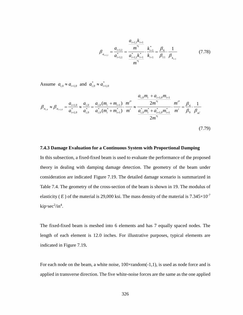
326
1
1,1
1
11
6
1
*
1
*
*
1
*
1,1
*
11,1
*
1,1
1,1
i
i
ki
i
i
ii
i
ii
i
i
a k
k
m
ka
m
ka
a
a
(7.78)
Assume 0,10, ii aa and *
0,1
*
0, ii aa
i
ii
m
i
i
i
iiii
i
iiii
i
i
iii
iii
i
i
i
i
aam
m
m
mama
m
mama
m
m
mma
mma
a
a
a
a
1
2
2
)(
)(
9
4
*
*
*
1
*
0,1
**
0,
*
10,10,
*
*
1
**
0,
10,
*
0,
0,
*
0,1
0,1
0,10,
(7.79)
7.4.3 Damage Evaluation for a Continuous System with Proportional Damping
In this subsection, a fixed-fixed beam is used to evaluate the performance of the proposed
theory in dealing with damping damage detection. The geometry of the beam under
consideration are indicated Figure 7.19. The detailed damage scenario is summarized in
Table 7.4. The geometry of the cross-section of the beam is shown in 19. The modulus of
elasticity ( E ) of the material is 29,000 ksi. The mass density of the material is 7.345×10⁻⁷
kipsec2/in4.
The fixed-fixed beam is meshed into 6 elements and has 7 equally spaced nodes. The
length of each element is 12.0 inches. For illustrative purposes, typical elements are
indicated in Figure 7.19.
For each node on the beam, a white noise, 100×random(-1,1), is used as node force and is
applied in transverse direction. The five white-noise forces are the same as the one applied

327
in the above four cases and are plotted in Figure 6.2. Given the external load case, exact
accelerations, velocities and displacements of the five nodes were computed at every 1E-4
seconds (10,000 Hz) for 0.2 seconds.
In this case, the velocity ( )(tx ) of each node in the undamaged case was used as the
velocity used to compute power ( ) for both the undamaged and damaged cases. For
every two nearby elements, the coefficient matrices (‘X’) and known vector (‘Y’) were
constructed by substituting the acceleration ( )(tx ), velocity ( )(tx ), displacement ( )(tx ),
and velocity used to compute power ( ) into Eq. 7.70 and Eq. 7.72. The coefficient
damage index vector, β, related to the two nearby elements was computed using Eq. 7.73.
Then the damage indices for nodal mass, element stiffness and element damping
coefficients are computed using Eq. 7.74 through Eq. 7.79. The damage severities for
stiffness are computed using Eq. 2.13. The damage indices for each property are shown
in Table 7.5 and are plotted in Figure 7.23. The related damage severities are plotted in
Figure 7.24

328
Figure 7.19. Geometry of the Fixed-Fixed Beam with Proportional Damping
Table 7.4. Designed Damage Scenario for the Fixed-Fixed Beam
a0 a1
#1 0 0 0 0
#2 0 0 0 0
#3 10 20 20 10
#4 10 20 20 10
#5 0 0 10 10
#6 0 0 10 10
Element
Number
Element
Stiffness
Element
Mass
Element Damping
Designed Damage Severity (%)

329
(a)
(b)
Figure 7.20. Displacements in Transverse Direction of Node 4 of the Fixed-Fixed Beam under the
Given External Load: (a) Full Plot and (b) Zoomed in Plot

330
(a)
(b)
Figure 7.21. Velocities in Transverse Direction of the Node 4 of the Fixed-Fixed Beam under the
Given External Load: (a) Full Plot and (b) Zoomed in Plot

331
(a)
(b)
Figure 7.22. Accelerations in Transverse Direction of Node 4 of the Fixed-Fixed Beam under the
Given External Load: (a) Full Plot and (b) Zoomed in Plot

332
Table 7.5. Damage Detection Results for the Fixed-Fixed Beam with Proportional Damping
Property System #1 System #2 System #3
mi
1.00 1.25 1.00
ki 1.00 1.11 1.00
ki+1 1.00 1.11 1.00
ai,11.00 1.11 1.11
ai+1,11.00 1.11 1.11
ai,0 1.00 1.25 1.11
ai+1,0 1.00 1.25 1.11
Property System #1 System #2 System #3
mi
1.00 1.25 1.00
ki 1.00 1.11 1.00
ki+1 1.00 1.11 1.00
ai,11.00 1.11 1.11
ai+1,11.00 1.11 1.11
ai,0 1.00 1.25 1.11
ai+1,0 1.00 1.25 1.11
Designed Damage Indices
Estimated Damage Indices

333
Figure 7.23. Damage Indices (βi) for the Fixed-Fixed Beam with Proportional Damping Using
Isolated Beam Element Analysis Method

334
Figure 7.24. Damage Severities (аi) for the Fixed-Fixed Beam with Proportional Damping Using
Isolated Beam Element Analysis Method
335
7.4.4 Summary
In Subsection 7.4, the Power Method was developed to be able to detect damage in
continuous system with damping, which was simulated by the proportional damping and a
fixed-fixed beam is provided to validate the proposed theory. In the numerical case,
damage in mass, stiffness, and damping were simulated and exact displacements,
velocities, and accelerations were computed. According to the damage detection results,
all the designed damage in masses, stiffness, and damping were located and evaluated
accurately and neither false-positive damage index nor false-negative damage index was
found.

336
8 APPLICATION OF THE METHOD TO SHAKE TABLE TESTS
8.1 INTRODUCTION
In this section, the performance of the proposed method in the real world will be studied
using experimental data sets. The data sets were collected from a series of shake table
tests of a bridge model conducted at the Caltrans Seismic Response Modification
Devises facility at the University of California San Diego by Dr. Gianmario Benzoni, Dr.
Noemi Bonessio, and Dr. Giuseppe Lomiento (Benzoni et al. 2012).
8.2 DESCRIPTION OF THE STRUCTURE AND TEST SETUP
The bridge model tested on the shake table is a one-span steel frame composed by two
columns, one deck and additional mass. The two columns of the bridge model are
identical. The column is composed by four column portions and one cap beam which is
prepared for the later installation of the viscous dampers between column and deck.
Each of the four column portions is composed by one hollow rectangular section
(HSS8×4×1/4) with four channel section (C4×7.25) on each side. The cap beam is
composed by two 51 inches long plates with small plates in between. The height of each
column portion is 17.5 inches and the height of the cap beam is 10 inches. The
connections between two column portions and the connection between column portion
and cap beam are both bolted connections. The deck of the bridge model is composed by
two steel boxes and two longitudinal wide flange beams (W6×15) with six wide flange
beams (W4×13) in between. Each of the steel boxes is seated on the top of each cap
beam. The width of the deck is 64 inches and the length of the deck is 126 inches. Steel
plates were put on the top of the deck as the additional mass to the bridge model to

337
reduce the natural frequencies of the bridge model. The total weight of the additional
mass is 3,600 lbs. The bridge model and the global coordinate system are given in the
photograph of Figure 8.1. The detailed dimensions of the structure are given in Figure
8.2. At different locations, tri-axial, single-axial accelerometers and string pots were
installed to collect accelerations, and displacements in different directions. The locations
of the accelerometers are indicated in the photograph of Figure 8.3. The locations of the
string pots are indicated in the photograph of Figure 8.4. The acceleration and
displacement data from the bridge model were collected at 0.002 second intervals.
Three types of white noise signals were used as inputs to excite the structure in global X,
Y and Z directions. Input Type A is the reference input for X direction with frequency
band 1-10 Hz. Input Type B is the reference input for Y direction with frequency band
1-10 Hz. Input Type C is the reference input for Z direction with frequency band 5-20
Hz. If the input intensity of the base vibration is risen up to 100%, the structure will be
forced to reach its nominal capacity in the corresponding input direction of the base
vibration. In case of any damage caused by extensive base vibration, the input intensity
of the base vibration is limited up to 50%.
In the given data file, seventeen data sets were provided: Test #01, Test #03, and Test
#05 through Test #19. Since Test#05, Test#06, Test#08, Test#09, Test#12, Test#13,
Test#14, andTest#19 were not excited in the global X direction, these eight tests will not
be taken into consideration in the following damage detection process. The remaining
nine shake table tests were either excited solely in the global X direction or excited in
the global X, Y, Z directions at the same time. Among these nine tests, the first five tests
are undamaged cases and the remaining four tests are damaged cases:

338
(1) Test #01 is an undamaged case and the structure is excited by 10% input Type
A in global X direction only;
(2) Test #03 is an undamaged case and the structure is excited by 25% input Type
A in global X direction;
(3) Test #07 is an undamaged case and the structure is excited by 50% input Type
A in global X direction only;
(4) Test #10 is an undamaged case and the structure is excited by 25% input Type
A in global X direction, 25% input Type B in global Y direction, 25% input
Type C in global Z direction;
(5) Test #11 is an undamaged case and the structure is excited by 25% input Type
A in global X direction only;
(6) Test #15 is a damaged case and the structure is excited by 25% input Type A
in global X direction, 25% input Type B in global Y direction, 25% input
Type C in global Z direction. The damage is simulated by removing the south
channel section from the lowest section of the north column;
(7) Test #16 is a damaged case and the structure is excited by 25% input Type A
in global X direction, 25% input Type B in global Y direction, 25% input
Type C in global Z direction. The damage is simulated by (1) removing the
south channel section from the lowest section of the north column and (2)
removing the west channel section from the lowest section of the south
column;
(8) Test #17 is a damaged case and the structure is excited by 25% input Type A
in global X direction, 25% input Type B in global Y direction, 25% input
Type C in global Z direction. The damage in the model is simulated by (1)
removing the south channel section from the lowest section of the north

339
column, (2) removing the west channel section from the lowest section of the
south column and (3) removing the bottom beam component from central
section of the west beam.
(9) Test #18 is a damaged case and the structure is excited by 25% input Type A
in global X direction. The damage is simulated by (1) removing the west
channel section from the lowest section of the south column and (2)
removing the bottom beam component from central section of the west beam.
To better illustrate the location of the damage, all the simulated damage in the structure
are indicated in Figure 8.3.
Figure 8.1. Test Setup and Global Coordinate System (Benzoni et al. 2012)

340
(a)
Figure 8.2. Geometry of the Structure under Testing: (a) Geometry of Columns and (b) Geometry of Deck (Benzoni et al. 2012)

341
(b)
Figure 8.2. Continued

342
Figure 8.3. Locations of Accelerometers and Damage Scenarios
(Note, the original figure was copied from the report written by Dr. Benzoni et al. (2012).)
Figure 8.4. Locations of String Pots (Benzoni et al. 2012)

343
8.3 THEORY OF APPROACH
From Figure 8.3, the Power Method can be applied using the data collected from tri-axial
accelerometers. However, the noise level of the acceleration records from tri-axial
accelerometers is much higher comparing with the noise level of the acceleration records
from mono-axial accelerometers, which can be seen from Figure 8.5. The noise level of
the acceleration records from tri-axial accelerometers is even higher than the acceptable
noise level of the proposed method (5% to 10%). Thus, the damage detection results
using the proposed method based on the data collected from the tri-axial accelerometers
will be unstable and inaccurate.
From Figure 8.3, the Power Method can also be applied based on the data collected from
mono-axial accelerometers. The noise level of the data collected from the mono-axial
accelerometers is around 2% to 3%, which is acceptable and can be roughly seen from
Figure 8.5. However, since the author has some doubt on the locations of the mono-axial
accelerometers, the data collected from the mono-axial accelerometers will not be
considered in the following damage detection process.
From Figure 8.4, the Power Method can also be applied based on the data collected from
string pots. The noise level of the displacement records from the string pots are
acceptable, which can be seen from Figure 8.10(a) and Figure 8.11(a).
Because only the data collected from the string pots at top ends of the two columns will
be used to detect damage in the bridge model, the bridge model is simplified into the
one-bay frame shown in Figure 8.6. The element number, joint number and element
directions are also shown in Figure 8.6. Given the simplified model, the damage
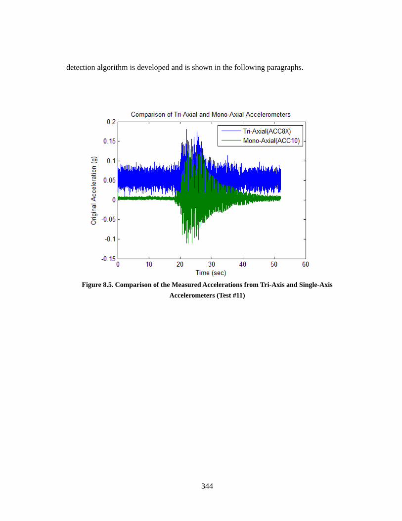
344
detection algorithm is developed and is shown in the following paragraphs.
Figure 8.5. Comparison of the Measured Accelerations from Tri-Axis and Single-Axis
Accelerometers (Test #11)

345
Figure 8.6. Simplified Numerical Model for the Bridge Model
Figure 8.7. Free Body Diagram Analysis of the Deck (Element #2)
Since only the measurements of displacements in the global X direction at both ends of
the columns in the bridge model satisfied the noise tolerance of the proposed method,

346
only the translational force and torsional moment of the deck can be estimated accurately.
As shown in Figure 8.7, considering the translational force and torsional moment
balance of the deck, gives
01,31,31,21,11,1 FIIFI (8.1)
05,35,35,25,15,1 FIIFI (8.2)
Where, the first subscript is the element number; the second subscript is the force
direction: ‘1’ represents the shear force in the global X direction and ‘5’ represents the
bending moment in the global Y direction. The superscript ‘+’ indicates the positive end
of the element and ‘-’ indicates the negative end of the element. For example,
1,1I
indicates the inertia force at the positive end of element #1 (north column) in shear force
in the global X direction.
To avoid using the highly noise polluted acceleration data from the tri-axis accelerometer
installed at the center of the deck, the inertia force for the deck is computed as the
combination of the inertia force at the positive end of the deck and the inertia force at the
negative end of the deck. Namely,
1,21,21,2 III (8.3)
5,25,25,2 III (8.4)
Note the above negative sign in Eq. 8.4 is due to the different positive direction defined
for Joint 2 and Joint 3 around the global Y direction.
Substituting Eq. 8.3 and Eq. 8.4 into Eq. 8.1 and Eq. 8.2, respectively, yield,
01,31,31,21,21,11,1 FIIIFI (8.5)

347
05,35,35,25,25,15,1 FIIIFI (8.6)
The above two equations can be combined as following,
0
0
10
01
5,3
1,3
5,3
1,3
5,2
1,2
5,2
1,2
5,1
1,1
5,1
1,1
F
F
I
I
I
I
I
I
F
F
I
I (8.7)
The force components in the above expression can be computed as follows,
5,1
1,1
5,1
1,1
5,1
1,1
0
0
m
m
I
I (8.8)
5,2
1,2
5,2
1,2
5,2
1,2
0
0
m
m
I
I (8.9)
5,2
1,2
5,2
1,2
5,2
1,2
0
0
m
m
I
I (8.10)
5,3
1,3
5,3
1,3
5,3
1,3
0
0
m
m
I
I (8.11)
5,1
1,1
5,1
1,1
2
11
2
11
11
3
1
11
5,1
1,1
4626
612612
LLLL
LL
L
IE
F
F (8.12)
5,3
1,3
5,3
1,3
2
33
2
33
33
3
3
33
5,3
1,3
2646
612612
LLLL
LL
L
IE
F
F (8.13)
Where
1,im and
1,im represent the mass at the positive and negative ends of Element i
along the global X axis direction, respectively;
5,im and
5,im represents the mass
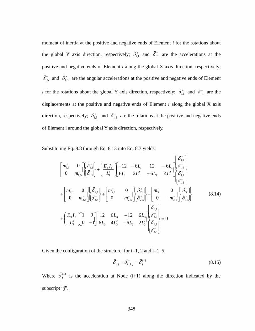
348
moment of inertia at the positive and negative ends of Element i for the rotations about
the global Y axis direction, respectively;
1,i and
1,i are the accelerations at the
positive and negative ends of Element i along the global X axis direction, respectively;
5,1 and
5,1 are the angular accelerations at the positive and negative ends of Element
i for the rotations about the global Y axis direction, respectively;
1,i and
1,i are the
displacements at the positive and negative ends of Element i along the global X axis
direction, respectively;
5,1 and
5,1 are the rotations at the positive and negative ends
of Element i around the global Y axis direction, respectively.
Substituting Eq. 8.8 through Eq. 8.13 into Eq. 8.7 yields,
02646
612612
10
01
0
0
0
0
0
0
4626
612612
0
0
5,3
1,3
5,3
1,3
2
33
2
33
33
3
3
33
5,3
1,3
5,3
1,3
5,2
1,2
5,2
1,2
5,2
1,2
5,2
1,2
5,1
1,1
5,1
1,1
2
11
2
11
11
3
1
11
5,1
1,1
5,1
1,1
LLLL
LL
L
IE
m
m
m
m
m
m
LLLL
LL
L
IE
m
m
(8.14)
Given the configuration of the structure, for i=1, 2 and j=1, 5,
1
,1,
i
jjiji (8.15)
Where 1i
j is the acceleration at Node (i+1) along the direction indicated by the
subscript “j”.

349
Substituting Eq. 8.15 into Eq. 8.14, yields,
02646
612612
10
01
0
0
10
01
4626
612612
0
0
5,3
1,3
5,3
1,3
2
33
2
33
33
3
3
33
3
5
3
1
5,35,2
1,31,2
5,1
1,1
5,1
1,1
2
11
2
11
11
3
1
11
2
5
2
1
5,25,1
1,21,1
LLLL
LL
L
IE
mm
mm
LLLL
LL
L
IE
mm
mm
(8.16)
Define,
2
11,21,1 mmm (8.17)
2
55,25,1 mmm (8.18)
3
11,31,2 mmm (8.19)
3
55,35,2 mmm (8.20)
3
i
iii
L
IEk (8.21)
2
11
2
11
11
1,4626
612612][
LLLL
LLKo (8.22)
2
33
2
33
33
2,2646
612612][
LLLL
LLKo (8.23)

350
5,
1,
5,
1,
}{
i
i
i
i
i
(8.24)
10
01][ 3R (8.25)
Substituting Eq. 8.17 through Eq. 8.25 into Eq. 8.16, yields,
0}]{][[0
0][}]{[
0
032,333
5
3
1
3
5
3
1
311,12
5
2
1
2
5
2
1
oo KRk
m
mRKk
m
m
(8.26)
Ignore the mass moment of inertia in Eq. 8.26, yields,
0}]{][[00
0][}]{[
00
032,333
5
3
1
3
1
311,12
5
2
1
2
1
oo KRk
mRKk
m
(8.27)
Define
00
01][ oM (8.28)
Then Eq. 8.27 can be rewritten as,
0}]{][[}]{][[}]{[}]{[ 32,33
3
3
3
111,1
22
1 oooo KRkMRmKkMm (8.29)
Consider the following vector as the velocity vector used to compute power that will be
used in the Power Method analysis.

351
3
1
2
1}{
(8.30)
Multiplying Eq. 8.29 by the velocity vector used to compute power (i.e. Eq. 8.30) yields,
0}]{][}[{
}]{][}[{}]{}[{}]{}[{
32,33
3
3
3
111,1
22
1
o
ooo
KRk
MRmKkMm
(8.31)
Rearrange the Eq. 8.31 yields,
}]{][}[{
}]{][}[{}]{}[{}]{}[{
3
3
3
1
32,3311,1
22
1
o
ooo
MRm
KRkKkMm
(8.32)
Dividing Eq. 8.32 by 3
1m yields,
}]{][}[{
}]{][}[{}]{}[{}]{}[{
3
3
32,33
1
311,3
1
12
3
1
2
1
o
ooo
MR
KRm
kK
m
kM
m
m
(8.33)
Define the following coefficients,
3
1
2
11
m
m (8.34)
3
1
12
m
k (8.35)
3
1
33
m
k (8.36)
Substituting Eq. 8.34 through Eq. 8.36 into Eq. 8.33 yields,

352
}]{][}[{
}]{][}[{}]{}[{}]{}[{
3
3
32,3311,2
2
1
o
ooo
MR
KRKM
(8.37)
Writing the Eq. 8.37 at different time points yields the following groups of equations,
For 0tt ,
0
000
|})]{][}[({
|})]{][}[({|})]{}[({|})]{}[({
3
3
32,3311,2
2
1
to
tototo
MR
KRKM
(8.38)
For jtt ,
j
jjj
to
tototo
MR
KRKM
|})]{][}[({
|})]{][}[({|})]{}[({|})]{}[({
3
3
32,3311,2
2
1
(8.39)
For Ntt ,
N
NNN
to
tototo
MR
KRKM
|})]{][}[({
|})]{][}[({|})]{}[({|})]{}[({
3
3
32,3311,2
2
1
(8.40)
Arranging the above linear equation group into matrix form, yields,
YβΧ (8.41)
Where the coefficient matrix of the linear equation group is given as followings,

353
NNN
jjj
tototo
tototo
tototo
KRKM
KRKM
KRKM
|})]{][}[({|})]{}[({|})]{}[({
|})]{][}[({|})]{}[({|})]{}[({
|})]{][}[({|})]{}[({|})]{}[({
32,311,
2
32,311,
2
32,311,
2
000
Χ
(8.42)
The vector of unknown and the vector of known are given as followings,
3
2
1
β (8.43)
N
j
to
to
to
MR
MR
MR
|})]{][}[({
|})]{][}[({
|})]{][}[({
3
3
3
3
3
3 0
Y (8.44)
Using the Least Square Method, the vector of unknown, ‘β’, can be computed from the
following equation,
)()( 1YΧΧΧβ
TT (8.45)
With the vector of unknown computed, the damage indices for stiffness, mass and
damping can be computed as followings,
13
1
2
1
1
m
mm
(8.46)

354
3
2
3
1
3
3
1
1
3
1
m
k
m
k
k
kk
(8.47)
8.4 EXPERIMENTAL DATA PROCESSING
8.4.1 Introduction
As stated previously, the data that will be used in the damage detection process is the
date collected from the string pots at the top ends of the two columns. The displacement
feedback from the shake table will be used as the base displacements of the two columns.
For illustration purposes, the recorded displacement time histories from Test #01, Test
#03, Test #07, and Test #16 are plotted in Figure 8.8 through Figure 8.11. From the
Figure 8.8 and Figure 8.9, it’s obvious that the displacement time histories from Test #01
and Test #03 are greatly influenced by noise. Consequently, Test #01 and Test #03 won’t
be taken into consideration for the later damage detection process. In the plotted
displacement time histories, the noise level of one record can be seen from the beginning
and ending of the plotted data, when the structure was in static situation. For example,
the noise level of the displacements measured from Test #01 can be seen from the first
fifteen seconds and the last 5 seconds in Figure 8.8(a). However, there might be other
type of noise in the measured displacement records, which can be seen from the sudden
changes of the measured displacement curve at the southeast corner of the desk in Figure
8.8(b) and Figure 8.9(b). Also from the plotted displacement time histories, the recorded
time histories are observed to be shifted up or down by a small constant, which can be
observed from Figure 8.8 (a). The constant mixed in the displacement records are
considered to be initial zero setting problems. To reduce the noise levels and eliminate

355
the constant components from the measured displacement time histories, digital
bandpass filters were used to process the data. To achieve better results, the average
value will be deducted from each displacement record before the digital bandpass filter
is applied.
(a)
Figure 8.8. Measured Displacement Time Histories by String Pots from Test #01: (a) Full Plot
and (b) Zoomed in Plot

356
(b)
Figure 8.8. Continued

357
(a)
(b)
Figure 8.9. Measured Displacement Time Histories by String Pots from Test #03: (a) Full Plot
and (b) Zoomed in Plot

358
(a)
(b)
Figure 8.10. Measured Displacement Time Histories by String Pots from Test #11: (a) Full Plot
and (b) Zoomed in Plot

359
(a)
(b)
Figure 8.11. Measured Displacement Time Histories by String Pots from Test #16: (a) Full Plot
and (b) Zoomed in Plot

360
8.4.2 Joint Motion Estimation
To compute the shear forces and moments at the ends of the two columns, the following
dynamic data at the top ends of the two columns are required: the joint rotations, joint
angular velocities, joint angular accelerations around the global Y direction and joint
translational displacements, joint translational velocities and joint translational
accelerations in global X direction. However, only the joint translational displacements
can be measured by the string pots at the northeast and southeast corners of the deck.
The other joint motions will be estimated based on the measured displacement data at
the two ends of the columns. Besides the author’s doubt on the locations of the
mono-axis accelerometers, the other reasons why the measured acceleration records are
not used here are:
(1) The locations of the accelerometers and string pots are not sufficiently close
to each other; and
(2) The noise within the measured accelerations and measured displacements are
not the same due to the difference of the measuring instruments.
Due to the above two reasons, the damage indices based on the measured displacements
and measured accelerations are not as stable as the damage indices based solely on
measured displacements.
In order to compute joint angular velocities and joint angular accelerations, the joint
translational velocities and joint translational accelerations should be estimated from
measured displacement data. The joint translational velocity time histories are estimated
based on the measured displacement time histories, using,

361
)(
)()(2)()(
01
0101
tt
tttt
(8.48)
Where, the initial displacement and initial velocity are zeros for the shake table test.
Namely, 0)0( , 0)0( , 002.0)( 01 dttt sec.
The joint translational acceleration time histories are estimated based on the joint
translational velocity time histories using,
)(
)()(2)()(
01
0101
tt
tttt
(8.49)
Where, the initial velocity and initial acceleration are zeros for the shake table test.
Namely, 0)0( , 0)0( , 002.0)( 01 dttt sec.
Given the joint translational motions, the joint rotational motions can be estimated. In
the current study, the joint rotational motions (i.e. joint rotations, joint angular velocities
and joint angular accelerations) at the ends of the two columns are estimated using cubic
interpolation and finite difference methods. To simulate the fixed bottom joints of the
two columns, a pseudo joint, which shares the same motion (i.e. displacements,
velocities and accelerations) as the base joint, is used and is assumed two inches beneath
the base joint of each column. Given the joint translational motions at the pseudo joint,
base joint and top end joint of each column, the deflection curve of each column at each
time point is described using the cubic interpolation at each 0.05 inches. The joint
rotations, joint angular velocities and joint angular accelerations at the top of the
columns are estimated using the following finite difference equations based on the
interpolated displacements , velocities and accelerations,

362
2
5
1,11,1
5,111
1
dz
dzLzLz
Lz (8.50)
3
5
1,31,3
5,311
1
dz
dzLzLz
Lz (8.51)
2
5
1,11,1
5,111
1
dz
dzLzLz
Lz (8.52)
3
5
1,31,3
5,311
1
dz
dzLzLz
Lz (8.53)
2
5
1,11,1
5,111
1
dz
dzLzLz
Lz (8.54)
3
5
1,31,3
5,311
1
dz
dzLzLz
Lz (8.55)
Where dz is the interpolation spacing for the cubic interpolation and is set to be 0.05
inches in this case; 1L is the length of the column; z
i 5, , z
i 5, , and z
i 5, are the
joint rotation, joint angular velocity, and joint angular acceleration around the global Y
direction (indicated by subscript ‘5’) of Element #i at the height of z; zi 1, ,
zi 1, , and
zi 1, are the translational displacement, velocity, and acceleration along the global X
direction (indicated by subscript ‘1’) of Element #i at the height of z.
8.4.3 General Data Processing Procedures
In order to apply the proposed method to detect damage in the bridge model using only
the measured displacement records at both ends of the columns, the measured
displacement records need to be filtered and other joint motions, such as joint

363
translational acceleration and joint rotations, need to be estimated. The general data
processing procedures, used in the current study, are summarized as follows,
(1) Plot the power spectrum densities of the measured joint translational
displacement time histories at both ends of each column and design the
digital bandpass filter to filter out the first bending mode, which is indicated
by the highest peak in the power spectrum densities plot;
(2) Compute the filtered displacements by applying the designed filter from Step
(1) to the measured displacement time histories;
(3) Compute joint translational velocities using Eq. 8.48 and compute joint
translational accelerations using Eq. 8.49;
(4) Compute the filtered translational velocities and filtered translational
acceleration using digital bandpass filters;
(5) Compute joint rotations, joint angular velocities and joint angular
accelerations using Eq. 8.50 to Eq. 8.55;
(6) Input the computed filtered joint translational displacements, accelerations,
joint rotations and joint angular accelerations into Eq. 8.42 and Eq. 8.44 and
compute the coefficients of the linear equation group by using Eq. 8.45; and
(7) Compute the damage indices for mass and stiffness using Eq. 8.46 and Eq.
8.47.
8.5 DAMAGE EVALUATION OF THE SHAKE TABLE TESTS
According to the general data processing procedures introduced in Section 8.4.3, the
power spectrum density for the original measured displacement time histories were
plotted and passband of the digital filter were selected. For illustration purposes, the
power spectrum densities of the measured displacement records from Test #11 are

364
plotted in Figure 8.12. If the displacement time histories are filtered at the highest peak
shown in Figure 8.12, the filtered displacements at the tops of the north and south
columns will be vibrating in the same direction with similar amplitudes. Based on the
above observation, the highest peak is relative to the lateral bending mode in global X
direction. The locations of the first bending mode in global X direction based on the
displacement records for all the tests are reported in Table 8.1. The width of the pass
band of the digital filters for all the tests are also provided in Table 8.1. Based on the
observation of the frequency change of the bending modes from all tests, the frequency
of bending mode will decrease for the damaged cases. However, based solely on the
changes of the frequencies, the damage locations and damage severities cannot be
detected and evaluated. As described in Steps (2) to (4) in Section 8.4.3, the filtered joint
displacements, filtered joint velocities, filtered joint accelerations are computed. The
filtered joint rotations, filtered joint angular velocities and filtered joint angular
accelerations are computed as described in Step (5) in Section 8.4.3. For illustration
purposes, the filtered joint displacement time histories at the top ends of the two columns
for Test #11 are plotted in Figure 8.13. The filtered joint velocity time histories at the top
ends of the two columns for Test #11 are plotted in Figure 8.14. The filtered joint
acceleration time histories at the top ends of the two columns for Test #11 are plotted in
Figure 8.15.
Due to the existence of noise in the measured displacement time histories, digital
bandpass filters were adopted in: (1) filtering measured displacement time histories; (2)
filtering estimated velocities; (3) filtering estimated accelerations. However, both the
existence of noise and the filtering technique will cause a certain amount of loss of the
damage information contained in the perfect displacement time histories. According to

365
experience acquired from detecting damage in noise-contained numerical models, two
key points will assure the stable performance of the proposed method to the bridge
model:
(1) Use narrow bandpass filter. The main objective of using a digital bandpass
filter is to increase the signal-to-noise ratio in the filtered displacement time
histories. By applying a narrow bandpass filter right at the peak will enable
most of the useful information to pass while most of useless noise to be
filtered. The numerical error caused by an inappropriate narrow bandpass
filter is obvious and can be modified by increase the width of the pass band
appropriately.
(2) Use relative displacements for the computation of member forces. Because
the amplitude of base vibration is smaller than the vibration amplitude at
each column top and the amplitude of noise in the base displacement time
histories is the same, the signal-to-noise ratios of base displacement records
are lower than the ones of the displacement records from column tops. By
using the relative displacements, the base displacement records will become
all zeros without any noise while the signal-to-noise ratios of the
displacement records from column tops remain the same.
The coefficient matrix and known vector can be computed by substituting the computed
joint absolute acceleration time histories and joint relative displacement time histories
into Eq. 8.42 and Eq. 8.44. Then unknown coefficient vector shown in Eq. 8.43 can be
computed using Eq. 8.45. The damage index of the joint translational masses and the
damage index of the lateral stiffness of the columns can be computed using Eq. 8.46 and
Eq. 8.47. The computed damage indices and damage severities for all the tests are listed

366
in Table 8.2.
(a)
Figure 8.12. Power Spectrum Density Analysis of Displacements from String Pots from Test#11:
(a) Full Plot and (b) Zoomed in Plot

367
(b)
Figure 8.12. Continued

368
(a)
(b)
Figure 8.13. Filtered Displacement Time Histories Recorded By String Pots from Test#11: (a)
Full Plot and (b) Zoomed in Plot

369
(a)
(b)
Figure 8.14. Filtered Velocity Time Histories at the Locations of the String Pots from Test#11: (a)
Full Plot and (b) Zoomed in Plot

370
(a)
(b)
Figure 8.15. Filtered Acceleration Time Histories at the Locations of the String Pots from
Test#11: (a) Full Plot and (b) Zoomed in Plot

371
Table 8.1. Locations of Bending Mode and Selected Pass Band of Digital Filters
Table 8.2. Damage Indices and Damage Severities for the Bridge Model
8.6 EVALUATION OF DESIGNED DAMAGE EXTENT
In this subsection, the designed damage extent regarding to the whole columns will be
evaluated. The designed damage indices for the damaged portion of the column are easy
to compute. However, as stated in the above analysis, each column will be treated as one
Test Num.Location of Bending Mode
Peak (Hz)
Designed Pass Bands for
Digital Filters (Hz)
Test #07 3.8 ~ 4.3 3.83 ~ 3.93
Test #10 3.8 ~ 4.05 3.84 ~ 3.95
Test #11 3.8 ~ 4.2 3.83 ~ 4.00
Test #15 3.8 ~ 4.0 3.85 ~ 3.98
Test #16 3.45 ~ 3.75 3.53 ~ 3.68
Test #17 3.4 ~ 3.8 3.56 ~ 3.66
Test #18 3.3 ~ 3.8 3.61 ~ 3.7
βm βk αm αk
Test #07 0.981 0.974 0.02 0.03
Test #10 1.000 0.994 0.00 0.01
Test #11 1.021 0.992 -0.02 0.01
Test #15 1.025 0.982 -0.02 0.02
Test #16 1.154 1.095 -0.13 -0.09
Test #17 1.195 1.109 -0.16 -0.10
Test #18 1.200 1.167 -0.17 -0.14
Test Num.Damage Index Damage Severity

372
single element, thus the damage index for the whole column need to be computed. The
computed designed damage index for the whole column will be used as a reference to
check the accuracies of the damage detection results of the damaged column using the
proposed method.
In order to compute the damage extent for the whole column, the damage extent for
lowest section of the column needs to be evaluated. The layout of the cross section of the
column is shown in Figure 8.16. The cross-sectional properties of the tube section and
channel section are provided in Table 8.3. According to the given cross-sectional
properties in Table 8.3, the moment of inertia of the undamaged column cross section
can be computed as following,
Figure 8.16. Layout of the Cross Section of the Column of the Bridge Model

373
Table 8.3. Cross-Sectional Properties of the Tube and Channel Sections
(Note, x, y in the above table indicate the direction of local axes.)
The moment of inertia for bending around the global Y direction (note, the global
directions are given in Figure 8.16),
)(22 2
,,, yCCyCxHSSxy dAIIII (8.56)
The moment of inertia for bending around the global X direction,
Cross-Sectional Area, AHss (in2.) 5.24
Moment of Inertia about Y axis, Iy,HSS (in
4.) 14.4
Moment of Inertia about X axis, Ix,HSS (in
4.) 42.5
Cross-Sectional Area, AC (in2.) 2.13
Moment of Inertia about Y axis, Iy,C (in
4.) 0.425
Moment of Inertia about X axis, Ix,C (in4.) 4.58
C4x7.25
Distance of the Paralleled Axes in Global X
Direction, dx (in.)
Distance of the Paralleled Axes in Global Y
Direction, dy (in.)
5.439
3.439
HSS8x4x0.25
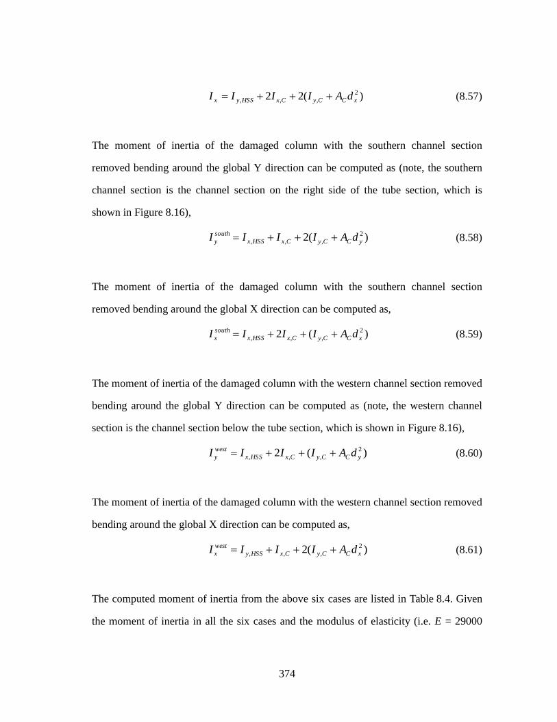
374
)(22 2
,,, xCCyCxHSSyx dAIIII (8.57)
The moment of inertia of the damaged column with the southern channel section
removed bending around the global Y direction can be computed as (note, the southern
channel section is the channel section on the right side of the tube section, which is
shown in Figure 8.16),
)(2 2
,,, yCCyCxHSSx
south
y dAIIII (8.58)
The moment of inertia of the damaged column with the southern channel section
removed bending around the global X direction can be computed as,
)(2 2
,,, xCCyCxHSSx
south
x dAIIII (8.59)
The moment of inertia of the damaged column with the western channel section removed
bending around the global Y direction can be computed as (note, the western channel
section is the channel section below the tube section, which is shown in Figure 8.16),
)(2 2
,,, yCCyCxHSSx
west
y dAIIII (8.60)
The moment of inertia of the damaged column with the western channel section removed
bending around the global X direction can be computed as,
)(2 2
,,, xCCyCxHSSy
west
x dAIIII (8.61)
The computed moment of inertia from the above six cases are listed in Table 8.4. Given
the moment of inertia in all the six cases and the modulus of elasticity (i.e. E = 29000

375
ksi), six numerical cantilever models were built in SAP2000,
(1) Undamaged column bending in global Y direction;
(2) Undamaged column bending in global X direction;
(3) Damaged column with southern channel section removed bending in global Y
direction;
(4) Damaged column with southern channel section removed bending in global X
direction;
(5) Damaged column with western channel section removed bending in global Y
direction; and
(6) Damaged column with western channel section removed bending in global X
direction.
In SAP2000, one unit transverse load was added at the top ends of the cantilever beams
and the static displacements at the top ends of the cantilever beam were outputted for the
above six cases. The stiffness for each of the six cantilevers can be computed. Then the
damage indices and damage severities are computed. The static displacements (‘S’ and
‘S*’), stiffness (‘k’ and ‘k*’), damage indices (‘βk’) and damage severities (‘αk’) for the
undamaged and damaged cases are listed in Table 8.5.
In Table 8.5,
(1) Case #1 compares the Y-direction bending stiffness between the damaged
column with the southern channel section removed (‘south
yI ’) and the
undamaged column (‘ yI ’). Note that this case is relative to damage scenario
in Test #15;

376
(2) Case #2 compares the Y-direction bending stiffness between damaged
column with the southern channel section removed (‘south
yI ’) and damaged
column with the western channel section removed (‘west
yI ’). Note that this
case is relative to damage scenario in Test #16 and Test #17;
(3) Case #3 compares the Y-direction bending stiffness between the undamaged
column (‘ yI ’) and damaged column with the western channel section
removed (‘west
yI ’). Note that this case is relative to damage scenario in Test
#18;
(4) Case #4 compares the X-direction bending stiffness between undamaged
column (‘ xI ’) and damaged column with southern channel section removed
(‘ south
xI ’); and
(5) Case #5 compares the X-direction bending stiffness between the undamaged
column (‘ xI ’) and damaged column with western channel section removed
(‘ west
xI ’).
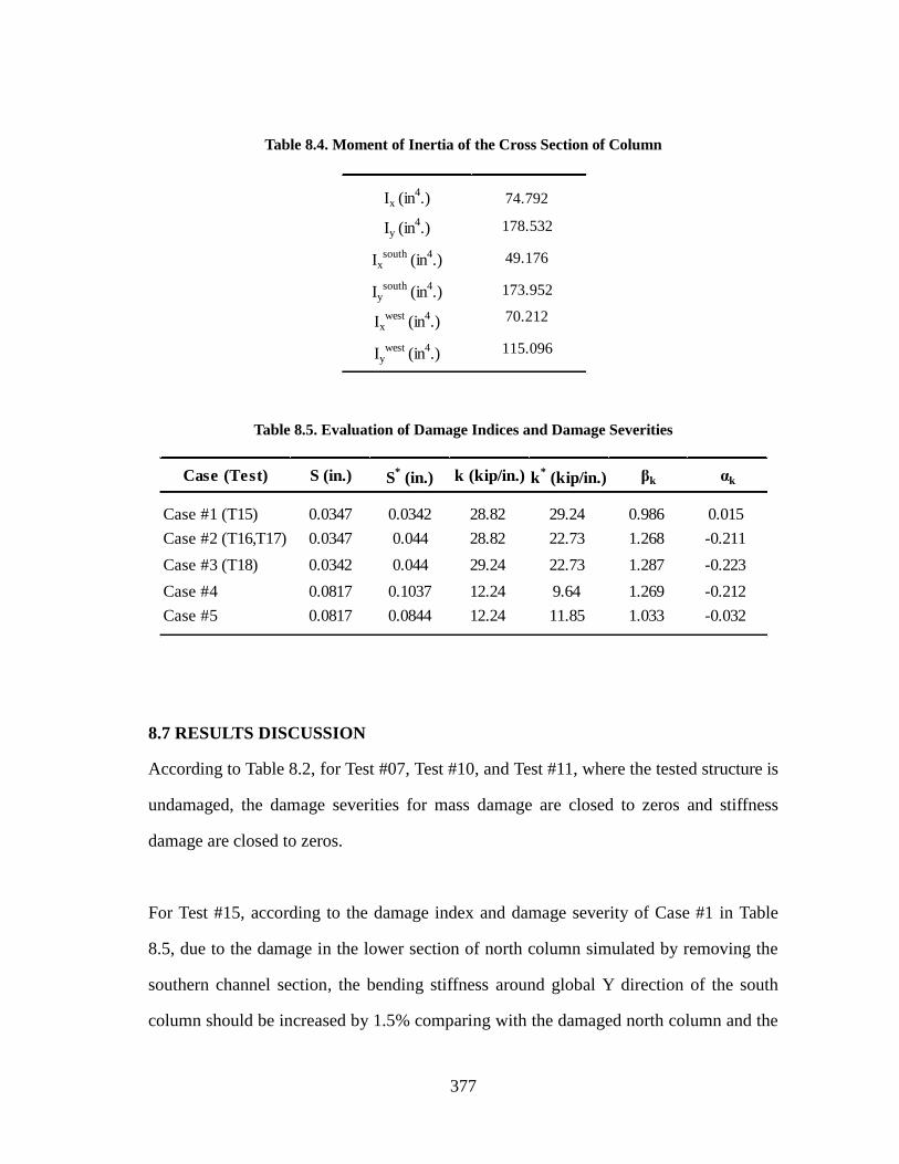
377
Table 8.4. Moment of Inertia of the Cross Section of Column
Table 8.5. Evaluation of Damage Indices and Damage Severities
8.7 RESULTS DISCUSSION
According to Table 8.2, for Test #07, Test #10, and Test #11, where the tested structure is
undamaged, the damage severities for mass damage are closed to zeros and stiffness
damage are closed to zeros.
For Test #15, according to the damage index and damage severity of Case #1 in Table
8.5, due to the damage in the lower section of north column simulated by removing the
southern channel section, the bending stiffness around global Y direction of the south
column should be increased by 1.5% comparing with the damaged north column and the
Ix (in4.) 74.792
Iy (in4.) 178.532
Ixsouth
(in4.) 49.176
Iysouth
(in4.) 173.952
Ixwest
(in4.) 70.212
Iywest
(in4.) 115.096
Case (Test) S (in.) S* (in.) k (kip/in.) k
* (kip/in.) βk αk
Case #1 (T15) 0.0347 0.0342 28.82 29.24 0.986 0.015
Case #2 (T16,T17) 0.0347 0.044 28.82 22.73 1.268 -0.211
Case #3 (T18) 0.0342 0.044 29.24 22.73 1.287 -0.223
Case #4 0.0817 0.1037 12.24 9.64 1.269 -0.212
Case #5 0.0817 0.0844 12.24 11.85 1.033 -0.032

378
translational mass should remain approximately the same. Comparing to the damaged
north column, the computed damage severities for the stiffness is 2% increase and 2%
decrease for the mass damage.
For Test #16 and Test #17, according to Case #2 in Table 8.5, the bending stiffness of the
south column around the global Y direction is 21.1% decrease and the lumped mass of
the south column should remain approximately the same with the one of the north
column. Comparing to the north column, the computed damage severities for lumped
mass of the south column are 13% for Test #16 and 16% for Test #17. The computed
damage severities of the column bending stiffness are 9% decrease for Test #16 and 10%
decrease for Test #17.
For Test #18, according to Case #3 in Table 8.5, the bending stiffness of the south
column around the global Y direction is 22.3% decrease and the translational mass and
mass moment of inertia of the south column should remain approximately the same with
the ones of the north column. Comparing to the north column, the computed damage
severities for lumped mass of the south column is 17% decrease. The computed damage
severities of the column bending stiffness are 14% decrease.
The main reasons caused the errors in the damage detection results are,
(1) Estimation of joint rotation at the top of the two columns. According to the
analysis experience to the numerical models, the error in the estimation of
joint rotations will underestimate the damage in column bending stiffness;
(2) Estimation of joint translational accelerations. The estimation of the joint
translational accelerations will cause inaccuracy in the mass damage

379
detection;
(3) Noise in the measured displacement records. The noise in the measured
displacements will cause the overall inaccuracy of the damage detection
process; and
(4) The application of digital bandpass filter. Although the application of the
digital bandpass filter will reduce the noise influence, it will also cause the
incompatibility among displacement, velocity, and acceleration time histories,
which will cause the inaccuracy of damage detection results.
8.8 DAMAGE EVALUATION WITH ELEMENT DAMPING EFFECT
For the steel members in the bridge model, it is inappropriate to consider damping in the
level of individual structural members and it is impractical to determine the damping
matrix in the same manner as the stiffness matrix is determined. Because the damping
properties of materials are not well established and the significant amount of energy
dissipation caused by effects other than material damping properties, such as the friction
at the joint connections. The damping matrix for the structure should be determined from
its modal damping ratios.
However, for experimental purposes, the damping properties of individual structural
members will be considered in this subsection. For simplicity purposes, the Rayleigh
damping model is used.
8.8.1 Theory of Approach
According to Subsection 7.4.2, the damping forces can be computed as the Eq. 7.37. And
the power done by the damping forces can be computed as Eq. 8.62. However, since the

380
displacement time histories were filtered by a narrow bandpass filter and the joint
angular velocities were computed based on the filtered displacement time histories, the
‘ }]{}[{ i
i
oM ’ and ‘ }]{}[{ , iioK ’ parts become linearly dependent to each other,
which will impact the performance of the least square method and force the damage
detection results of 0,ia and 1,ia to be ones (i.e. “1” means undamaged). To overcome
this dilemma, only the stiffness-proportional damping model will be used to simulate the
element damping, which is given in Eq. 8.63.
}]{[}]{[2
460260
61206120
0000
000000
010010
001001
2
}]{[}]{[}]){[][(}]{[}{
,1,0,
3,
2,
1,
3,
2,
1,
22
22
31,
3,
2,
1,
3,
2,
1,
0,
1,0,1,0,,
iioiii
i
oi
i
i
i
i
i
i
i
i
i
i
i
i
i
i
i
i
i
i
i
iiiiiiiiiiiiiic
KkaMm
a
LLLL
LLI
AL
I
AL
L
EIa
Lma
KaMaKaMaCF
(7.37)
}]{}[{}]{}[{2
}]{}[{}}{{}{ ,1,0,,, iioiii
i
oi
iiiicic KkaMm
aCFP (8.62)
}]{[}]{[}{ ,1,, iioiiiiic KkaCF (8.63)

381
Substituting Eq. 8.63 into Eq. 8.29 yields,
0}]{][[}]{][[
}]{][[}]{[}]{[}]{[
32,331,332,33
3
3
3
111,11,111,1
22
1
oo
oooo
KRkaKRk
MRmKkaKkMm (8.64)
Multiplying Eq. 8.64 by the velocity vector used to compute power (i.e. Eq. 8.30) yields,
0}]{][}[{}]{][}[{}]{][}[{
}]{}[{}]{}[{}]{}[{
32,331,332,33
3
3
3
1
11,11,111,1
22
1
ooo
ooo
KRkaKRkMRm
KkaKkMm (8.65)
Rearranging Eq. 8.65 yields,
}]{][}[{}]{][}[{}]{][}[{
}]{}[{}]{}[{}]{}[{
3
3
3
132,331,332,33
11,11,111,1
22
1
ooo
ooo
MRmKRkaKRk
KkaKkMm
(8.66)
Dividing Eq. 8.66 by 3
1m yields,
}]{][}[{}]{][}[{}]{][}[{
}]{}[{}]{}[{}]{}[{
3
332,33
1
31,3
32,33
1
3
11,3
1
11,1
11,3
1
12
3
1
2
1
ooo
ooo
MRKRm
kaKR
m
k
Km
kaK
m
kM
m
m
(8.67)
Define the following coefficients,
3
1
2
11
m
m (8.68)
3
1
12
m
k (8.69)
3
1
33
m
k (8.70)

382
3
1
11,1
4m
ka (8.71)
3
1
31,3
5m
ka (8.72)
Substituting Eq. 8.68 through Eq. 8.72 into Eq. 8.67 yields,
}]{][}[{}]{][}[{}]{][}[{
}]{}[{}]{}[{}]{}[{
3
332,3532,33
11,411,2
2
1
ooo
ooo
MRKRKR
KKM
(8.73)
Writing the Eq. 8.73 at different time point, yields the following groups of equations,
For 0tt ,
000
000
|})]{][}[({|})]{][}[({|})]{][}[({
|})]{}[({|})]{}[({|})]{}[({
3
332,3532,33
11,411,2
2
1
tototo
tototo
MRKRKR
KKM
(8.74)
For jtt ,
jjj
jjj
tototo
tototo
MRKRKR
KKM
|})]{][}[({|})]{][}[({|})]{][}[({
|})]{}[({|})]{}[({|})]{}[({
3
332,3532,33
11,411,2
2
1
(8.75)
For Ntt ,
NNN
NNN
tototo
tototo
MRKRKR
KKM
|})]{][}[({|})]{][}[({|})]{][}[({
|})]{}[({|})]{}[({|})]{}[({
3
332,3532,33
11,411,2
2
1
(8.76)

383
Arranging the above linear equation group into matrix form, yields,
YβΧ (8.77)
Where the coefficient matrix of the linear equation group is given as following
Nj
Nj
Nj
Nj
Nj
tototo
tototo
tototo
tototo
tototo
T
KRKRKR
KKK
KRKRKR
KKK
MMM
|})]{][}[({|})]{][}[({|})]{][}[({
|})]{}[({|})]{}[({|})]{}[({
|})]{][}[({|})]{][}[({|})]{][}[({
|})]{}[({|})]{}[({|})]{}[({
|})]{}[({|})]{}[({|})]{}[({
32,332,332,3
11,11,11,
32,332,332,3
11,11,11,
222
0
0
0
0
0
Χ
(8.78)
The vector of unknown and the vector of known are given as follows,
5
4
3
2
1
β (8.79)
N
j
to
to
to
MR
MR
MR
|})]{][}[({
|})]{][}[({
|})]{][}[({
3
3
3
3
3
3 0
Y (8.80)
Using the Least Square Method, the vector of unknown, ‘β’, can be computed from the
following equation,
)()( 1YΧΧΧβ
TT (8.81)

384
With the vector of unknown computed, the damage indices for stiffness, mass and
damping can be computed as follows,
13
1
2
1
1
m
mm
(8.82)
3
2
3
1
3
3
1
1
3
1
m
k
m
k
k
kk
(8.83)
ka k
k
m
ka
m
ka
a
a
1
5
4
1
3
3
1
31,3
3
1
11,1
1,3
1,1
1
(8.84)
8.8.2 Damage Evaluation Results
According to Section 8.4.3, the filtered joint translational displacements, velocities,
accelerations and the filtered joint rotations, angular velocities, angular accelerations are
computed. Then the coefficient matrix is computed using Eq. 8.78 and the known vector
is computed using Eq. 8.80. As stated in Section 8.5, the damping forces of columns are
also computed using relative velocities. The unknown coefficient vector shown in Eq.
8.79 can be computed using Eq. 8.81. The damage indices of the joint translational
masses, lateral stiffness of the columns and damping coefficients of the columns can be
computed using Eq. 8.82 through Eq. 8.84. The computed damage indices and damage
severities for all the tests are listed in Table 8.6.

385
Table 8.6. Damage Indices and Damage Severities for the Bridge Model with Element Damping
Effects
8.8.3 Results Discussion
According to Table 8.6, for Test #07, Test #10 and Test #11, where the tested structure is
undamaged, the damage severities for mass and stiffness damage are closed to zeros.
The damage severities for damping damage are not as stable as the ones for stiffness and
mass damage.
For Test #15, according to Table 8.5, the designed damage severity for stiffness damage
is +1.5%. From Table 8.6, the detected stiffness damage is +5%, which is higher than the
ones from the undamaged cases (i.e. Test #07, Test #10 and Test #11). As expected, the
damage severity for damping damage is around zero. This is because, as stated in
Section 8.6, the damage in the north column has very small impact on the bending
stiffness. Thus, the amplitudes of vibration velocities of the north and south columns are
very similar.
βm,shear βk βa1 αm,shear αk αa1
Test #07 0.980 0.979 1.064 0.02 0.02 -0.06
Test #10 0.966 0.976 0.975 0.04 0.02 0.03
Test #11 0.958 0.960 1.165 0.04 0.04 -0.14
Test #15 0.937 0.952 0.972 0.07 0.05 0.03
Test #16 1.091 1.095 0.902 -0.08 -0.09 0.11
Test #17 1.163 1.204 0.829 -0.14 -0.17 0.21
Test #18 1.256 1.209 0.937 -0.20 -0.17 0.07
Damage SeverityTest Num.
Damage Index

386
For Test #16, Test #17 and Test #18, the designed damage severities for stiffness,
according to Table 8.5, are around 20%. From Table 8.6, the detected damage severities
for stiffness damage are 9% for Test #16 and 17% for both Test #17 and Test #18. The
error in the estimation of the joint rotations, joint angular velocities, and joint angular
accelerations contributed to the underestimation of the stiffness damage for Test #16,
Test #17, and Test #18. According to Table 8.6, the damping effects for the south column
are increased after damage for Test #16, Test #17 and Test #18. The increase of the
damping effect can be explained by the increase of vibration amplitude of the damaged
column.
The main reasons caused the errors in the damage detection results are,
(1) Estimation of joint rotation at the top of the two columns. According to the
analysis experience to the numerical models, the error in the estimation of
joint rotations will underestimate the damage in column bending stiffness;
(2) Estimation of joint translational accelerations. The estimation of the joint
translational accelerations will cause inaccuracy in the mass damage
detection;
(3) Noise in the measured displacement records. The noise in the measured
displacements will cause the overall inaccuracy of the damage detection
process;
(4) The application of digital bandpass filter. Although the application of the
digital bandpass filter will reduce the noise influence, it will also cause the
incompatibility among displacement, velocity, and acceleration time histories,
which will cause the inaccuracy of damage detection results;
(5) The application of the Rayleigh Damping as the element damping model. The

387
method in computing damping force in this section may cause the inaccuracy
and instability in the damping damage detection; and
(6) Estimation of the joint translational velocities and joint angular velocities.
These two factors will also contribute to the inaccuracy of the damping
damage detection and will cause a certain influence to the damage detection
results to mass and stiffness.
8.9 CONCLUSION
According to the above analysis, the proposed theory could locate the damaged column
and provide a close estimation the damage severities regarding to the whole column. And
the accuracy of the estimation of the damage severities can be improved by providing
more useful and less noise-polluted structural vibration measurements.
Note, the proposed method could locate and estimate the original designed damage in
the lower portion of the column if less noise-polluted data could have been collected
from the tri-axial accelerometers distributed on the north and south columns. Namely,
more dense distribution of sensors is required in order to locate damage more accurately.

388
9 SUMMARY AND CONCLUSIONS
9.1 SUMMARY
In this dissertation, a new non-destructive evaluation method, named as the Power Method,
was developed. The Power Method can be used to detect damage in both isolated
structural components and the integral structures. To validate the proposed method, the
method has been applied to different types of structures and the following sections were
introduced,
In Section 2, the general form of the Power Method was developed. And also, the specific
form of the proposed method for the 1-DOF, 2-DOF, N-DOF, and isolated
spring-mass-damper systems were developed.
In Section 3, numerical examples for 1-DOF, 2-DOF, N-DOF, and isolated
spring-mass-damper systems were developed and were used to validate the theories
developed in Section 2. All the designed damage in masses, springs and dampers were
located and evaluated accurately in each numerical model.
In Section 4, the specific form of the Power Method for rod, Euler-Bernoulli beam, plane
frame, and space truss were developed.
In Section 5, numerical models of rod under axial and torsional vibrations, rod under axial
vibration only, beam under bending vibration, plane frame under axial and bending
vibrations, and space truss under axial vibration were simulated. All the designed damage
389
in masses and stiffness were located and evaluated accurately in each numerical
experiment.
In Section 6, the performance of the proposed method to noise polluted inputs were
evaluated for both the discrete and continuous systems. Two noise levels were considered
for each numerical case. The proposed method was found to be able to accurately locate
and evaluate multiple damage under the lower noise level (1% noise) and to be able to
accurately locate damage and roughly evaluate damage under higher noise level (5%
noise).
In Section 7, three possible technical issues were studied and solved. The three possible
issues studied in this section are, (1) no external loads were applied within the structural
components that were under damage detection; (2) the efficiency study of the two methods
to reduce noise influence for the repeatable damage detection process; (3) the damping
damage detection in continuous structures.
In Section 8, the proposed method was validated using experimental data from a shake
table test made in University of California, San Diego. By using the displacement records
at the top ends of the two columns, the designed damage in south column was detected and
evaluated.
9.2 FINDINGS
After finishing all the studies related to the Power Method, the followings were found,
From Section 2 and 3, the new findings are,

390
(1) The Power Method can be applied to all kinds of linear discrete systems. For
example, 1-DOF, 2DOF, and 5-DOF spring-mass-damper systems;
(2) The Power Method can be applied to the whole discrete system and evaluate
multiple structural components at one time, which makes the Power Method
very efficient and economical;
(3) The Power Method can be applied to isolated discrete systems and detect
damage in the structural components that are within the isolated system; and
(4) The advantages of the isolated system method is that it requires less motion
information since fewer structural needs to be evaluated. Also, by using the
isolated system method, the possibility of encountering a singularity problem
during the application stage of least square method will become smaller. This
is because less unknowns will be considered and solved.
From Section 4 and 5, the new findings are,
(1) The Power Method can be applied to all kinds of linear continuous structural
components. For example, rod, beam, frame and truss;
(2) The Power Method can be applied to the whole continuous system and
evaluate multiple structural components at one time;
(3) The Power Method can be applied to isolated continuous systems and
evaluate only the structural components within the isolated system;
(4) When the Power Method is applied to the isolated system, dynamic
information from different type of vibrations can be combined; and
(5) Comparing to the static damage evaluation method based on structural
curvatures, such as, Element Strain Energy method, the Power Method won’t
be influenced by the singularity problem caused by zero bending curvature

391
and force redistribution (secondary effect) of the statically indeterminate
structures. This advantage makes the Power Method become superior to the
damage detection methods based on static structural deformation.
From Section 6, the new findings are,
(1) With 1% white noise, accurate damage evaluation can still be achieved by
applying the proposed method;
(2) With 5% white noise, the Power Method can accurately locate multiple
damage. But the computed damage severities will become less reliable;
(3) The Power Method requires only acceleration data. The velocity and
displacement data can be computed based the given acceleration data; and
(4) Comparing to the isolated system method, the integral system method will
provide less false positives. This is because the integral system method will
take all the dynamic inputs into consideration, the damage indices for all the
undamaged elements will share similar values. Consequently, less damage
indices for the undamaged elements will become false positives after the
normalization process (i.e. defined in Eq. 6.4).
From Section 7, the new findings are,
(1) The Power Method remains effective even no external loads are applied in the
structural components that are under consideration;
(2) For repeatable experiments, the proposed method based on the averaged
inputs will yield better damage detection results; and
(3) The Power Method can be used to detect damping damage in the continuous
structural components.

392
From Section 8, the new findings are,
(1) The Power Method can be used to detect damage in real structures; and
(2) Because the Power Method requires only the structural vibration data, the
damage detection process won’t be restricted by the time and location of the
engineers. After the recorded structural vibration data is uploaded online,
with limited programming effort, the computer will be able to download the
data and run the damage detection program automatically.
9.3 ORIGINALITY OF THIS WORK
The originalities of the proposed method includes, but is not limited to,
(1) The proposed method can be used to evaluate damage in mass, stiffness and
damping simultaneously, while most of existing non-destructive evaluation
methods will only be able to detect damage in stiffness, and a handful of
non-destructive evaluation methods can be used to detect either damage in
stiffness and mass or damage in stiffness and damping;
(2) The proposed method can be used to evaluate damage in single structural
component, multiple structural components, and the integral structure at one
time;
(3) The proposed method allows measurements from different types of vibration
to be inputted in, the structural properties related to different vibrations will
be analyzed at the same time;
(4) The proposed method uses only the dynamic measurement directly from the
structure. Thus, the proposed method can be easily applied to the real-world
damage detection;

393
(5) Because the proposed method is based on dynamic measurements not the
modal or physical curvatures of the structure, singularity problems caused by
zero bending curvatures will be out of concern;
(6) This work introduced the procedures to detect damage in different discrete
and continuous systems;
(7) This work introduced the procedures to deal with the noise pollution within
the real-world measurements and along with other approaches to handle
some of the unfavorable situations; and
(8) The damage detection process introduced in Section 8 set an example in the
application of the proposed method and other similar methods to real-world
data.
9.4 CONTRIBUTION OF THIS WORK
The dissertation will contribute to the following areas. Firstly, a new and powerful level III
damage detection method is established and validated. As mentioned in the previous
section, the Power Method is able to detect and evaluate damage in mass, stiffness and
damping simultaneously. Moreover, the proposed method can not only detect damage in
the whole system at one time but also evaluate damage using information from multiple
types of vibrations. Secondly, the work recorded in this dissertation will be a good
guidance for further studies and applications to help to reduce property losses and the
maintenance cost of critical structures. The theories of the proposed method for various
types of discrete and continuous systems were developed and validated using numerical
examples and solutions for several unfavorable situations were provided as well. Finally,
the idea of the Power Method which introduces new approaches to establish relationships
between the undamaged and damaged structures will contribute to the developments of

394
other static and dynamic non-destructive evaluation methods.
9.5 CONCLUSION
Most NDE methods proposed to date are only classified as Level I or Level II
methods, which means only the presences of the damage, or at most, the locations of the
damage can be detected. Moreover, most of these methods are limited in the detection of
stiffness damage only and are not able to locate or evaluate mass damage and damping
damage. The damage detection algorithm proposed in this work is a Level III method that
has the following features:
(1) It detects damage in local stiffness, mass and damping;
(2) It provides clear indications to locate damage;
(3) It locates tiny and obscure damage;
(4) It provides accurate quantitative values of damage severities;
(5) No analytical model of the structure is required;
(6) The data from the field experiment can be directly used to complete the
analyses;
(7) The proposed method will still be able to accurately locate damage and
provide referable estimations of damage severities with 5% noise;
(8) The method is applicable to nearly all types of structures and cases with
multiple damage locations; and
(9) The computation process is straight-forward.
9.6 FUTURE WORK
Although the Power Method is well developed and validated in this dissertation, the
following issues are remain to be unsolved,
395
(1) How to choose the velocity vector used to compute power to achieve better
results. During the research process, the author found that, for the pure
numerical cases, using the computed nodal velocity as the velocity vector
used to compute power will yield better results than the results from using a
constant vector as the velocity vector used to compute power. However, for
the noise-polluted cases, the results from using a constant vector as the
velocity vector used to compute power will be more stable and generally more
accurate than the results from using the computed nodal velocity as the
velocity vector used to compute power;
(2) Extend the Power Method to solve for the structural components with
unknown stiffness and mass matrices. For the current study cases, the
stiffness, mass, and damping properties of one element can be expressed with
well-known matrices. However, for the complex structural components and
with limited number of sensors, the element matrices of the stiffness, mass,
and damping might be unknown;
(3) Development of the specific form of the Power Method for Timoshenko
Beams. The proposed method can be easily applied to the damage detection in
Timoshenko beams if the stiffness matrix of the Timoshenko beam is given.
The detailed expression of the stiffness matrix of the Timoshenko beam can be
found in relevant chapter in books related to finite element analysis. If only
the differential equations were given, good ways to compute the partial
differentiations of nodal displacements and nodal rotations should be found;
(4) Development of the specific form of the Power Method for Kirchhoff-Love
plates. Similarly, the proposed method can be applied to the damage detection
in Kirchhoff-Love plates, if the stiffness matrix of the plate member is ready at

396
hand; and
(5) Improve the noise tolerance capacity of the Power Method. Currently, the
noise tolerance capacity of the proposed method is less than 10% of white
noise. Although the noise in the input data is reduced using digital filters and
the application of the least square method is also helpful in finding a good
estimation of the real damage severities, the applications of the digital filters
will introduce errors into the input data and the least square method is
sensitive to input errors. Thus, more advanced techniques are needed to make
the proposed method more robust to noise in the inputs.

397
REFERENCES
Adams, R. D., Walton, D., Flitcroft, J. E., and Short, D. (1975). "Vibration Testing as a
Nondestructive Test Tool for Composite Materials." Composite Reliability, ASTM
STP 580, Philadelphia, 159-175.
Allemang, R. J. and Brown, D. L. (1982). "A Correlation Coefficient for Modal Vector
Analysis." In Proceedings of the 1st International Modal Analysis Conference,
Orlando, Florida, 110-116.
Bighamian, R. and Mirdamadi, H. R. (2013). "Input/Output System Identification of
Simultaneous Mass/Stiffness Damage Assessment Using Discrete‐Time Pulse
Responses, Differential Evolution Algorithm, and Equivalent Virtual Damped
SDOF." Structural Control and Health Monitoring, 20(4), 576-592.
Benzoni, G., Bonessio, N., and Lomiento, G. (2012). "Preliminary Shake Table Tests on
the Bridge Model." Unpublished Manuscript, University of California San Diego,
California, United States of America.
Catbas, F. N., Brown, D. L., and Aktan, A. E. (2006). "Use of Modal Flexibility for
Damage Detection and Condition Assessment: Case Studies and Demonstrations on
Large Structures." Journal of Structural Engineering, 132(11), 1699-1712.
Cawley, P. and Adams, R. D. (1979). "The Location of Defects in Structures from
Measurements of Natural Frequencies." Journal of Strain Analysis, 14(2), 49-57.
Cattarius, J. and Inman, D. J. (1997). "Time Domain Analysis for Damage Detection in
Smart Structures." Mechanical Systems and Signal Processing, 11(3), 409-423.
Choi, S. H. and Park, S. Y. (2003). "Nondestructive Damage Identification in a Truss
Structure Using Time Domain Responses." Journal of the Earthquake Engineering
Society of Korea, 7(4), 89-95.
Choy, F. K., Liang, R., and Xu, P. (1995). "Fault Identification of Beams on Elastic
Foundation." Computers and Geotechnics. 17(2), 157-176.

398
Cornwell, P., Doebling, S. W., and Farrar, C. R. (1999). "Application of the Strain
Energy Damage Detection Method to Plate-Like Structures." Journal of Sound and
Vibration, 224(2), 359-374.
Curadelli, R. O., Riera, J. D., Ambrosini, D., and Amani, M. G. (2008). "Damage
Detection by Means of Structural Damping Identification." Engineering Structures,
30(12), 3497-3504.
Doebling, S. W., Farrar, C. R., Prime, M. B., and Shevitz, D. W. (1996). "Damage
Identification and Health Monitoring of Structural and Mechanical Systems from
Changes in Their Vibration Characteristics: a Literature Review." Report No.
LA-13070-MS, Los Alamos National Laboratory, New Mexico, United States of
America.
Farrar, C. R., Baker, W. E., Bell, T. M., Cone, K. M., Darling, T. W., Duffey, T. A., Eklund,
A., and Migliori, A. (1994). "Dynamic Characterization and Damage Detection in the
I-40 Bridge over the Rio Grande." Report No. LA-12767-MS, Los Alamos National
Laboratory, New Mexico, United States of America.
Farrar, C. and Jauregui, D. (1996). "Damage Detection Algorithms Applied to
Experimental and Numerical Modal Data from the 1-40 Bridge." Report No.
LA-13074-MS, Los Alamos National Laboratory, New Mexico, United States of
America.
Frizzarin, M., Feng, M. Q., Franchetti, P., Soyoz, S., and Modena, C. (2010). "Damage
Detection Based on Damping Analysis of Ambient Vibration Data." Structural
Control and Health Monitoring, 17(4), 368-385.
Gandomi, A. H., Sahab, M. G., and Rahai, A. (2011) "A Dynamic Nondestructive
Damage Detection Methodology for Orthotropic Plate Structures." Structural
Engineering and Mechanics, 39(2), 223-239.
Gul, M. and Catbas, F. N. (2011). "Structural Health Monitoring and Damage
Assessment Using a Novel Time Series Analysis Methodology with Sensor
Clustering." Journal of Sound and Vibration, 330(6), 1196-1210.
Hjelmstad, K. D. and Shin, S. (1996). "Crack Identification in a Cantilever Beam from
Modal Response." Journal of Sound and Vibration, 198(5), 527-545.
399
Huth, O., Feltrin, G., Maeck, J., Kilic, N., and Motavalli, M. (2005). "Damage
Identification Using Modal Data: Experiences on a Prestressed Concrete Bridge."
Journal of Structural Engineering-ASCE, 131(12), 1898-1910.
Hyung, S. S. (2007). "Nondestructive Damage Detection by Simultaneous Identification
of Stiffness and Damping." Doctoral Dissertation, Texas A&M University, College
Station, Texas, United States of America.
Johnson, E. A., Lam, H. F., Katafygiotis, L. S., and Beck, J. L. (2004). "Phase I
IASC-ASCE Structural Health Monitoring Benchmark Problem Using Simulated
Data." Journal of Engineering Mechanics, 130(1), 3-15.
Just, F., Shafiq, B., Serrano, D., and Ortiz, M. (2006). "Damage Detection in Sandwich
Composites Using Damping Matrix Identification." Journal of the Mechanical
Behavior of Materials, 17(1), 17-30.
Kang, J. S., Park, S. K., Shin, S., and Lee, H. S. (2005). "Structural System Identification
in Time Domain Using Measured Acceleration." Journal of Sound and Vibration,
288(1), 215-234.
Kiddy, J. and Pines, D. (1998). "Eigenstructure Assignment Technique for Damage
Detection in Rotating Structures." American Institute of Aeronautics and
Astronautics Journal, 36(9), 1680-1685.
Ko, J. M., Wong, C. W., and Lam, H. F. (1994). "Damage Detection in Steel Framed
Structures by Vibration Measurement Approach." In Proceedings of the 12th
International Modal Analysis, 2251, 280-286.
Lee, J. J., Lee, J. W., Yi, J. H., Yun, C. B., and Jung, H. Y. (2005). "Neural
Networks-Based Damage Detection for Bridges Considering Errors in Baseline
Finite Element Models." Journal of Sound and Vibration, 280(3), 555-578.
Li, R. (2013). "Non-Destructive Damage Evaluation Based on Element Strain Energies."
Master Thesis, Texas A&M University, College Station, Texas, United States of
America.
Lieven, N. A. J. and Ewins, D. J. (1988). "Spatial Correlation of Mode Shapes, the
Co-Ordinate Modal Assurance Criterion (COMAC)." In Proceedings of the 6th
International Modal Analysis Conference, 1, 690-695.

400
Lin, S., Yang, J. N., and Zhou, L. (2005). "Damage Identification of a Benchmark
Building For Structural Health Monitoring." Smart Materials and Structures, 14(3),
S162.
Lindner, D. K. and Kirby, G. (1994). "Location and Estimation of Damage in a Beam
Using Identification Algorithms." In Proceedings of 35th
AIAA/ASME/ASCE/AHS/ASC Structures, Structural Dynamics and Materials
Conference, 192-198.
Loland, O. and Dodds, C. J. (1976). "Experiences in Developing and Operating Integrity
Monitoring System in North Sea." In Proceedings of the 8th Annual Offshore
Technology Conference 2, OTC Paper No.2551, 313-319.
Lopez, F. and Zimmerman, D. C. (2002). "Nonlinear Damage Detection Using a
Time-Domain Minimum Rank Perturbation Theory." In Proceedings SPIE, The
International Society for Optical Engineering, 4702, 179-190.
Ma, T. W., Yang, H. T., and Chang, C. C. (2004). "Direct Damage Diagnosis of
Structural Component Using Vibration Response." NDE for Health Monitoring and
Diagnostics, 192-200.
Majumder, L. and Manohar, C. S. (2003). "A Time-Domain Approach for Damage
Detection in Beam Structures Using Vibration Data with a Moving Oscillator as an
Excitation Source." Journal of Sound and Vibration, 268(4), 699-716.
Pandey, A. K., Biswas, M., and Samman, M. M. (1991). "Damage Detection from
Changes in Curvature Mode Shapes." Journal of Sound and Vibration, 145(2),
321-332.
Pandey, A. K. and Biswas, M. (1994). "Damage Detection in Structures Using Changes in
Flexibility." Journal of Sound and Vibration, 169(1), 3-17.
Peterson, L. D., Alvin, K. F., Doebling, S. W., and Park, K. C. (1993). "Damage
Detection Using Experimentally Measured Mass and Stiffness Matrices." In
Proceedings of 34th AIAA/ASME/ASCE/AHS/ASC Structures, Structural
Dynamics, and Materials Conference, 1, 1518-1528.

401
Qu, W. and Peng, Q. (2007). "Damage Detection Method for Vertical Bars of Mast
Structure in Time Domain." Earthquake Engineering and Engineering
Vibration-Chinese Edition-, 27(5), 110.
Raghavendrachar, M. and Aktan, A. E. (1992). "Flexibility by Multi-reference Impact
Testing for Bridge Diagnostics." ASCE Journal of Structural Engineering, 118(8),
2186-2203.
Rizos, P. F., Aspragathos, N., and Dimarogona, A. D. S. (1990). "Identification of Crack
Location and Magnitude in a Cantilever Beam from the Vibration Modes." Journal of
Sound and Vibration, 138(3), 381-388.
Rytter, A. (1993). "Vibration Based Inspection of Civil Engineering Structures." Doctoral
Dissertation, University of Aalborg, Aalborg, Denmark.
Sheinman, I. (1996). "Damage Detection and Updating of Stiffness and Mass Matrices
Using Mode Data." Computers and Structures, 59(1), 149-156.
Shin, S. and Oh, S. H. (2007). "Damage Assessment of Shear Buildings By Synchronous
Estimation Of Stiffness and Damping Using Measured Acceleration." Smart
Structures and Systems, 3(3), 245-261.
Shinozuka, M., Lee, S., Kim, S., and Chou, P. H. (2011). "Lessons from Two Field Tests
on Pipeline Damage Detection Using Acceleration Measurement." Smart Structures
and Materials, Nondestructive Evaluation and Health Monitoring, 7983,
798328-798328.
Stubbs, N., Kim, J. T., and Topole, N. G. (1992). "An Efficient and Robust Algorithm for
Damage Localization in Offshore Platforms." 10th Structures Congress, San Antonio,
Texas, 543-546.
Stubbs, N. and Kim, J. T. (1996). "Damage Localization in Structures without Baseline
Modal Parameters." American Institute of Aeronautics and Astronautics Journal,
34(8), 1644-1649.
Trickey, S., Todd, M. D., Seaver, M. E., and Nichols, J. M. (2002). "Geometric
Time-Domain Methods of Vibration-Based Damage Detection." NDE for Health
Monitoring and Diagnostics, 113-121.

402
Zhang, Z. and Aktan, A. E. (1995). "The Damage Indices for the Constructed Facilities."
In Proceedings of the 13th International Modal Analysis Conference, 2, 1520-1529.
Zhang, J., Xu, Y. L., Li, J., Xia, Y., and Li, J. C. (2013). "Statistical Moment-Based
Structural Damage Detection Method in Time Domain." Earthquake Engineering
and Engineering Vibration, 12(1), 13-23.
Zhong, S., Oyadiji, S. O., and Ding, K. (2008). "Response-Only Method for Damage
Detection of Beam-Like Structures Using High Accuracy Frequencies with
Auxiliary Mass Spatial Probing." Journal of Sound and Vibration, 311(3),
1075-1099.
Zimin, V. D. and Zimmerman, D. C. (2009). "Structural Damage Detection Using Time
Domain Periodogram Analysis." Structural Health Monitoring, 8(2), 125-135.
403
APPENDIX
NUMERICAL VALIDATION OF THE PROPOSED THEORY
A.1 INTRODUCTION
The objective of the Appendix A is to verify the proposed process that was used to detect
damage in the UCSD shake table tests. To verify this proposed process, a group of data
was generated from the finite element model of the bridge model.
A.2 DESCRIPTION OF THE FINITE ELEMENT MODEL
In SAP2000, a one-bay frame was built and the properties of the cross sections of the
frame were adjusted to simulate the real structure. The one-bay frame is plotted in Figure
8.6. The height of each column is 81 inches. The beam of the one-bay frame is designed
to simulate the steel deck in the real structure and the length of the beam is 108 inches.
In the finite element model, the moment of inertia of the cross section of the undamaged
column is 178.532 in4 in X-direction and 74.792 in4 in Y-direction. The moment of inertia
of cross section of the damaged portion in the south column is simulated as 115.096 in4
(around 35.5% reduction for the damaged section) in X-direction bending and 70.212 in4
(around 6.1% reduction for the damaged section) in Y-direction bending. The
cross-sectional area of the undamaged column is 13.76 in2. The cross-sectional area of
the damaged portion of the south column is 11.63 in2 (around 15.5% reduction for the
damaged section). The mass per unit length of the undamaged column is adjusted so that
the total weight for the undamaged north column is around 0.891 kips. The total weight
of the damaged south column is around 0.88 kips. The mass difference between the north
column and the south column is caused by the removal of the lower west channel section
404
from the south column. The damping coefficients in the finite element model are
assumed. The damping coefficients for the undamaged column portion are 0.025 for ‘Cm’
and 0.015 for ‘Ck’. The damping coefficients for the damaged column portion are 0.03
for ‘Cm’ and 0.02 for ‘Ck’.
The moment of inertia of the beam element in X direction bending is 116. 64 in4 and the
moment of inertia of the beam element in Z direction bending is 12533.9 in4. The moment
of inertia of the beam element is set according to the equivalent moment of inertia of the
steel deck in the real bridge model. The cross-sectional area of the beam is 8.86 in2. The
total weight of the beam element is 5.835 kips (2.24 kips from the self-weight of the steel
deck and 3.6 kips from the steel plates on the top of the steel deck).
Because the designed damage scenario is similar to the damage scenario of Test #18
from the shake table tests, the finite element model is excited using the base
accelerations from Test #18 (i.e. Accelerations in the global X direction). Using the
linear direction integration method within SAP2000, the displacement records at the top
ends of the two columns can be outputted.
According to the modal analysis using the SAP2000, the first mode of the finite element
model is the bending mode in the global X direction at 8.40 Hz; the second mode of the
finite element model is the torsional mode around the global Z direction at 9.47 Hz; the
third mode is the bending mode in the global Y direction at 10.26 Hz. The natural
frequencies detected for the finite element model are larger than the real bridge model.
The natural frequencies detected for the real bridge model by researchers in UCSD are:
(1) around 3.5 Hz for the bending mode in the global X direction; (2) around 3.9 Hz for

405
the bending mode in the global Y direction; (3) around 7.5 Hz for the torsional mode
around the global Z direction. The differences between the natural frequencies from the
finite element model and the natural frequencies from the real bridge model might be
caused by the following factors:
(1) The finite element model built within SAP2000 is a simplified equivalent
bar-joint model instead of a detailed 3D model with shell elements.
(2) The parts in real bridge model are connected with bolts. However, it is hard to
simulate these bolted connections even in the very detailed finite element
model.
A.3 NOISE SIMULATION
One of the main objectives of the Appendix A is to test the noise-tolerant capacity of the
proposed process. According to the computation in Section 8, the noise levels in the
displacement records from shake table tests are around 3%. To simulate the noise in the
displacement records, 6% of white noise was superimposed into the exact displacement
records which are directly outputted from SAP2000.
The noise-polluted displacements are computed using the following equation,
)(
)()()()(
wstd
SstdtwtStS
pure
iipureinoise (A.1)
Where )( inoise tS is the noise-polluted displacement at time it ; )( ipure tS is the exact
displacement at time it ; )( itw is the random white noise at time it ; is the percent of
noise selected to add into the pure acceleration data; std(x) indicates the standard
deviation of vector x.

406
However, due to the limitation of the capacity of the personal computer, only the
behavior of the model within the first 8.58 seconds was computed. The displacements at
the top ends of the two columns are closed to parabolas and are quite close to each other,
which are given in Figure A.1. If the 6% white noise is directly superimposed onto the
absolute displacement records, the noise level will be too big comparing to the real case,
which is shown in Figure A.2. However, if we add the 6% white noise into the relative
displacement records, which is shown in Figure A.3, then numerical case will match the
real case better. Thus two groups of 6% white noise were superimposed onto the relative
displacement records at the two top ends of the north and south columns. For
comparison purposes, the relative displacement records from the real bridge model
measured from Test #18 are plotted in Figure A.4.

407
(a)
(b)
Figure A.1. The Absolute Displacements at the Top Ends of the North and South Columns with 6%
White Noise from Finite Element Model: (a) Full Plot and (b) Zoomed in Plot

408
(a)
(b)
Figure A.2. The Absolute Displacements at the Top Ends of the North and South Columns from
Test #18 of the Shake Table Tests: (a) Full Plot and (b) Zoomed in Plot
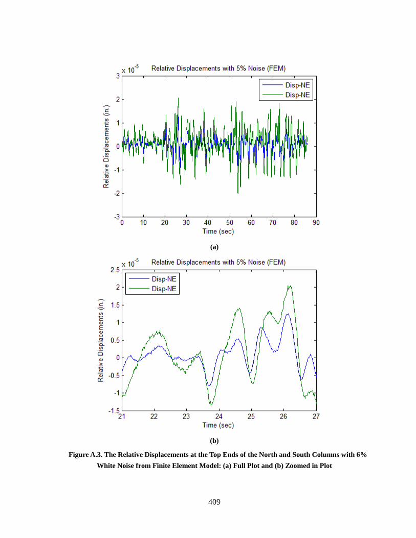
409
(a)
(b)
Figure A.3. The Relative Displacements at the Top Ends of the North and South Columns with 6%
White Noise from Finite Element Model: (a) Full Plot and (b) Zoomed in Plot

410
(a)
(b)
Figure A.4. The Relative Displacements at the Top Ends of the North and South Columns from
Test #18 of the Shake Table Tests: (a) Full Plot and (b) Zoomed in Plot

411
Note that the sudden changes shown in Figure A.4(b) will only appears at limited peaks
of the displacement records, thus, the influence of these sudden changes can be reduced
by the application of the digital bandpass filters.
A.4 DAMAGE EVALUATION RESULTS
Firstly, the theory of approach introduced in Section 8.3 and data processing techniques
introduced in Section 8.4 were used to detect damage in the finite element model
described in Section A.2. When the white noise level is 6%, ten groups of results are
computed and are shown in Table A.1.
Secondly, the theory of approach introduced in Section 8.8.1 and data processing
techniques introduced in Section 8.4 were used to detect damage in the finite element
model described in Section A.2. When the white noise level is 6%, ten groups of results
are computed and are shown in Table A.2.
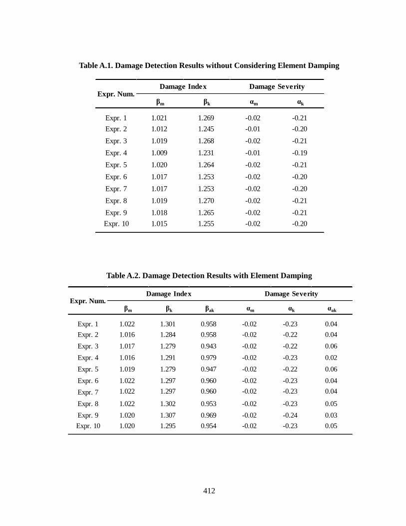
412
Table A.1. Damage Detection Results without Considering Element Damping
Table A.2. Damage Detection Results with Element Damping
βm βk αm αk
Expr. 1 1.021 1.269 -0.02 -0.21
Expr. 2 1.012 1.245 -0.01 -0.20
Expr. 3 1.019 1.268 -0.02 -0.21
Expr. 4 1.009 1.231 -0.01 -0.19
Expr. 5 1.020 1.264 -0.02 -0.21
Expr. 6 1.017 1.253 -0.02 -0.20
Expr. 7 1.017 1.253 -0.02 -0.20
Expr. 8 1.019 1.270 -0.02 -0.21
Expr. 9 1.018 1.265 -0.02 -0.21
Expr. 10 1.015 1.255 -0.02 -0.20
Expr. Num.Damage Index Damage Severity
βm βk βak αm αk αak
Expr. 1 1.022 1.301 0.958 -0.02 -0.23 0.04
Expr. 2 1.016 1.284 0.958 -0.02 -0.22 0.04
Expr. 3 1.017 1.279 0.943 -0.02 -0.22 0.06
Expr. 4 1.016 1.291 0.979 -0.02 -0.23 0.02
Expr. 5 1.019 1.279 0.947 -0.02 -0.22 0.06
Expr. 6 1.022 1.297 0.960 -0.02 -0.23 0.04
Expr. 7 1.022 1.297 0.960 -0.02 -0.23 0.04
Expr. 8 1.022 1.302 0.953 -0.02 -0.23 0.05
Expr. 9 1.020 1.307 0.969 -0.02 -0.24 0.03
Expr. 10 1.020 1.295 0.954 -0.02 -0.23 0.05
Expr. Num.Damage Index Damage Severity

413
A.5 RESULTS DISCUSSION
According to Table A.1, the damage severity of the stiffness of the right column is stable
at 20% to 21% decrease and the damage severity of the mass of the right column is
stable at 1% to 2% decrease. According to the third row in Table 8.5, the designed
damage severity of the stiffness of the right column is 22.3% decrease. The results from
Table A.1 provide an accurate estimation to the designed damage.
According to Table A.2, the damage severity of the stiffness of the right column is stable
at 22% to 23% decrease, the damage severity of the mass of the right column is stable at
2% decrease and the damage severity of the damping of the right column is stable at 4%
to 6% increase. According to the third row in Table 8.5, the designed damage severity of
the stiffness of the right column is 22.3%. The influence of the designed damage to the
mass of right column can be ignored. According to the settings of the physical properties
of the frame in Section A.2, the damping coefficient related to column stiffness (Ck) is
increased from 0.15 to 0.2 after damage. Thus the designed damage severity for the
damaged portion of the column is a 33.3% increase. However, since the theory
introduced in Section 8.8.1 considers the damping damage for the whole south column,
the designed damping damage severity of the whole column should be smaller than
33.3%. Also the noise superimposed into the displacement data may also contribute to
the reduction of the damage severity of damping coefficient. Thus, the detected damping
damage, which is 4% to 6%, can be reasonable. Thus, the results from Table A.2 provide
an accurate estimation to the designed damage.
A.6 SENSITIVITY ANALYSIS
In this subsection, the sensitivity of the proposed method to white noise will be studied.

414
For the given numerical model, the exact displacement time histories will be computed
from SAP2000. By mixing with different white noise, the noise-polluted displacement
data is generated. The white noise level varies from 2% to 20% with 2% increment.
Then the theory of approach introduced in Section 8.3 and data processing techniques
introduced in Section 8.4 were used to detect damage using the noise-polluted
displacement data. For each noise level, damage detection results from ten numerical
experiments were collected. Under the designed different noise level, the damage
detection results using a constant combination velocity vector (i.e. [1,1,1] in this case)
are reported in Table A.3. Under the designed different noise level, the damage detection
results using a variable combination velocity vector (i.e. [1, transverse velocity at the top
of the north column, transverse velocity at the top of the south column] in this case) are
reported in Table A.4. According to the summary of the damage detection results from
Table A.5 and Table A.6, the following noise sensitivity figure is plotted.

415
Figure A.5. Study of the Noise Sensitivity of the Power Method

416
Table A.7. Damage Detection Results with Different Noise Level Using Constant Velocity Vector
Noise Level
Expr. Num. βm βk βm βk βm βk βm βk βm βk
Expr. 1 0.9698 1.3112 0.9747 1.3020 0.9717 1.3063 0.9920 1.2344 1.0048 1.1813
Expr. 2 0.9723 1.3035 0.9749 1.2966 0.9733 1.3061 0.9948 1.2356 1.0073 1.1683
Expr. 3 0.9759 1.2959 0.9721 1.3064 0.9730 1.3047 0.9951 1.2291 0.9997 1.2069
Expr. 4 0.9725 1.3061 0.9706 1.3100 0.9743 1.3027 0.9984 1.2179 1.0114 1.1769
Expr. 5 0.9727 1.3063 0.9699 1.3115 0.9711 1.3076 0.9915 1.2425 1.0125 1.1352
Expr. 6 0.9744 1.2986 0.9721 1.3075 0.9710 1.3075 0.9740 1.3021 0.9717 1.3067
Expr. 7 0.9706 1.3087 0.9733 1.3059 0.9721 1.3077 0.9703 1.3104 0.9709 1.3103
Expr. 8 0.9697 1.3132 0.9729 1.3045 0.9715 1.3099 0.9699 1.3103 0.9707 1.3077
Expr. 9 0.9727 1.3059 0.9727 1.3067 0.9735 1.3052 0.9746 1.3007 0.9699 1.3107
Expr. 10 0.9720 1.3054 0.9704 1.3090 0.9744 1.3028 0.9720 1.3070 0.9758 1.2992
Damage Detectable Rate 10/10 10/10 10/10 10/10 10/10
Noise Level
Expr. Num. βm βk βm βk βm βk βm βk βm βk
Expr. 1 1.0237 1.0138 1.0336 0.8608 1.0338 0.9644 1.0593 0.2975 1.0718 0.4899
Expr. 2 1.0187 1.0845 1.0285 1.0036 1.0365 0.8249 1.0398 0.9928 1.0557 0.7335
Expr. 3 1.0253 0.9845 1.0218 1.0836 1.0346 0.9450 1.0674 1.7576 1.0786 4.3967
Expr. 4 1.0238 0.9452 1.0228 1.0615 1.0386 0.7957 1.0534 0.4363 1.0515 0.8548
Expr. 5 1.0122 1.1569 1.0295 0.9228 1.0376 0.9708 1.0553 0.4099 1.0519 0.7644
Expr. 6 1.0184 1.0874 1.0243 1.1019 1.0258 1.0788 1.0489 0.6487 1.0508 0.8908
Expr. 7 1.0196 1.0681 1.0351 0.8412 1.0327 1.0690 1.0448 0.8948 1.0607 0.2352
Expr. 8 1.0207 1.0712 1.0267 1.0046 1.0260 1.0630 1.0647 0.3579 1.0586 0.5737
Expr. 9 1.0090 1.1619 1.0249 1.0346 1.0392 0.8565 1.0517 0.7059 1.0623 0.6329
Expr. 10 1.0138 1.1150 1.0252 1.0104 1.0402 0.7298 1.0511 0.7313 1.0542 0.6612
Damage Detectable Rate 8/10 7/10 3/10 1/10 1/10
12% 14% 16% 18% 20%
2% 4% 6% 8% 10%
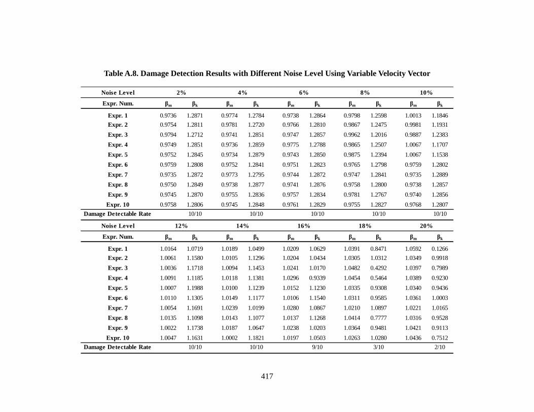
417
Table A.8. Damage Detection Results with Different Noise Level Using Variable Velocity Vector
Noise Level
Expr. Num. βm βk βm βk βm βk βm βk βm βk
Expr. 1 0.9736 1.2871 0.9774 1.2784 0.9738 1.2864 0.9798 1.2598 1.0013 1.1846
Expr. 2 0.9754 1.2811 0.9781 1.2720 0.9766 1.2810 0.9867 1.2475 0.9981 1.1931
Expr. 3 0.9794 1.2712 0.9741 1.2851 0.9747 1.2857 0.9962 1.2016 0.9887 1.2383
Expr. 4 0.9749 1.2851 0.9736 1.2859 0.9775 1.2788 0.9865 1.2507 1.0067 1.1707
Expr. 5 0.9752 1.2845 0.9734 1.2879 0.9743 1.2850 0.9875 1.2394 1.0067 1.1538
Expr. 6 0.9759 1.2808 0.9752 1.2841 0.9751 1.2823 0.9765 1.2798 0.9759 1.2802
Expr. 7 0.9735 1.2872 0.9773 1.2795 0.9744 1.2872 0.9747 1.2841 0.9735 1.2889
Expr. 8 0.9750 1.2849 0.9738 1.2877 0.9741 1.2876 0.9758 1.2800 0.9738 1.2857
Expr. 9 0.9745 1.2870 0.9755 1.2836 0.9757 1.2834 0.9781 1.2767 0.9740 1.2856
Expr. 10 0.9758 1.2806 0.9745 1.2848 0.9761 1.2829 0.9755 1.2827 0.9768 1.2807
Damage Detectable Rate 10/10 10/10 10/10 10/10 10/10
Noise Level
Expr. Num. βm βk βm βk βm βk βm βk βm βk
Expr. 1 1.0164 1.0719 1.0189 1.0499 1.0209 1.0629 1.0391 0.8471 1.0592 0.1266
Expr. 2 1.0061 1.1580 1.0105 1.1296 1.0204 1.0434 1.0305 1.0312 1.0349 0.9918
Expr. 3 1.0036 1.1718 1.0094 1.1453 1.0241 1.0170 1.0482 0.4292 1.0397 0.7989
Expr. 4 1.0091 1.1185 1.0118 1.1381 1.0296 0.9339 1.0454 0.5464 1.0389 0.9230
Expr. 5 1.0007 1.1988 1.0100 1.1239 1.0152 1.1230 1.0335 0.9308 1.0340 0.9436
Expr. 6 1.0110 1.1305 1.0149 1.1177 1.0106 1.1540 1.0311 0.9585 1.0361 1.0003
Expr. 7 1.0054 1.1691 1.0239 1.0199 1.0280 1.0867 1.0210 1.0897 1.0221 1.0165
Expr. 8 1.0135 1.1098 1.0143 1.1077 1.0137 1.1268 1.0414 0.7777 1.0316 0.9528
Expr. 9 1.0022 1.1738 1.0187 1.0647 1.0238 1.0203 1.0364 0.9481 1.0421 0.9113
Expr. 10 1.0047 1.1631 1.0002 1.1821 1.0197 1.0503 1.0263 1.0280 1.0436 0.7512
Damage Detectable Rate 10/10 10/10 9/10 3/10 2/10
12% 14% 16% 18% 20%
2% 4% 6% 8% 10%

418
A.7 CONCLUSION
According to the analysis in Subsection A.4 and Subsection A.5, the proposed theory in
Section 8 can be used to locate the damaged column and provide a close estimation the
damage severities regarding to the whole column in the finite element model of the
bridge model with 6% noise.
According to the analysis in Subsection A.6, the proposed theory will be able to locate
damages under the given conditions up to 10% to 14% white noise depending the
selected combination velocity vector, which is used to compute power. However, the
sensitivity plot in Figure A.6 may not be generally ture for each situation. The sensitivity
of the proposed method may vary from case to case. To find the general sensitivity of the
proposed method, futher study is needed.
Related Documents