The Indiana Enterprise Zone Program: Fiscal Impact of a Job Creation Tax Credit Sarah A. Low Center for the Study of Rural America, Federal Reserve Bank of Kansas City 925 Grand Boulevard Kansas City, MO 64198 816-881-6758 816-881-2199 [email protected] Kevin T. McNamara Department of Agricultural Economics, Purdue University 403 W. State St. West Lafayette, IN 47907 765-494-2936 765-494-9176 [email protected] Presented at the Annual Meeting of the American Agricultural Economics Association in Denver, CO; August 2004 Copyright 2004 by Sarah A. Low & Kevin T. McNamara. All rights reserved. Readers may make verbatim copies of this document for non-commercial purposes by any means, provided that this copyright notice appears on all such copies.

Welcome message from author
This document is posted to help you gain knowledge. Please leave a comment to let me know what you think about it! Share it to your friends and learn new things together.
Transcript

The Indiana Enterprise Zone Program: Fiscal Impact of a Job Creation Tax Credit
Sarah A. Low Center for the Study of Rural America, Federal Reserve Bank of Kansas City
925 Grand Boulevard Kansas City, MO 64198
816-881-6758 816-881-2199
Kevin T. McNamara Department of Agricultural Economics,
Purdue University 403 W. State St.
West Lafayette, IN 47907 765-494-2936 765-494-9176
[email protected] Presented at the Annual Meeting of the American Agricultural Economics Association in Denver, CO; August 2004 Copyright 2004 by Sarah A. Low & Kevin T. McNamara. All rights reserved. Readers may make verbatim copies of this document for non-commercial purposes by any means, provided that this copyright notice appears on all such copies.

The Indiana Enterprise Zone Program: Fiscal Impact of a Job Creation Tax Credit
Abstract
This paper estimated the fiscal impact of a job creation tax credit, a proposed incentive
for establishments participating in the Indiana enterprise zone program. State unemployment
insurance files were utilized with GIS to obtain enterprise zone data. Labor demand and labor
supply were estimated. Job creation due to the credit was calculated from empirical results.
Keywords: Wage elasticity of labor demand, job creation credit, regional tax incentives
JEL Codes: R100, R580
2

The Indiana Enterprise Zone Program
During the early 1980s the Indiana economy was in decline. Restructuring of the
economy occurred after experiencing a 24 percent decline in jobs and unemployment rate of 14
percent (Wilder and Rubin 1988). These conditions and the failure of federal enterprise zone
legislation sparked the evolution of Indiana’s enterprise zone program in 1981 (Papke 1993).
Today there are 29 urban enterprise zones in Indiana; these zones maintain a business recruitment
focus, work to retain and expand existing enterprise zone businesses and strive to improve the
economic well being of zone residents. Municipalities may apply to the State Enterprise Zone
Board for enterprise zone designation if the proposed enterprise zone meets poverty or
unemployment, population and size requirements. Figure 1 shows the counties which contain
enterprise zones. Municipalities or military installations which contain an enterprise zone are
labeled. Most enterprise zones are located in decaying urban areas in need of redevelopment.
Enterprise zones are required to have a household poverty level of 25% or unemployment 1.5
times the state average; the state poverty level is 6.7%.
Most incentives provided to enterprise zones to encourage business investment and job
creation are tax credits; in Indiana enterprise zones the inventory tax credit is most widely used.
Indiana is one of nine states taxing inventory; all inventory held is taxed as personal property.
Ninety percent, or $32.9 million, of tax savings to enterprise zone establishments in 1999 was
from the inventory tax abatement. Enterprise zone establishments which hold inventory are
exempted from paying property tax on inventory each year as a tax incentive for locating and
operating within a designated enterprise zone. The inventory tax abatement encourages
manufacturing investment; the credit is not as useful in the service or trade sector. During the
2003 legislative session tax re-structuring process, a plan to phase-out the inventory tax by 2007
was promulgated. Although there are a handful of other incentives available for enterprise zone
businesses, none has proven as useful in retaining and attracting business as the inventory tax
credit (Crowe Chizek 2001).
3

Figure 1. Indiana Counties and Municipalities Containing an Enterprise Zone
Indiana House Bill 1716-2003 attempted to replace the inventory tax credit with a $1500
job creation tax credit. However, the legislature was unable to calculate the fiscal impact of the
bill because no wage, employment, or business data for enterprise zones were available. The lack
of enterprise zone business data plagues enterprise zone program analysis and as a result,
empirical work on cost and effectiveness of enterprise zone programs has been hindered. Due to a
lack of information about enterprise zone businesses, House Bill 1716-2003 was not voted upon
and a replacement tax incentive for enterprise zone businesses was not approved during the 2003
legislative session.
The purpose of this study was to estimate the fiscal impact of a $1500 one-time job
creation tax credit which was proposed by the state legislature. A labor supply and demand model
4

was estimated and results were used to estimate a wage elasticity of labor demand. This was used
to estimate the job creation response of a job creation tax credit within enterprise zones.
Theoretical Model
The theoretical labor model developed the method for estimating the wage elasticity of
labor demand. Labor demand and supply will be simultaneously solved using two-stage least
squares regression technique (Hamermesh 1976).
Labor demand is the quantity of labor establishments desire to employ at any given wage.
Firm employment depends upon wage, output of the firm, and firm type (Hamermesh 1976;
1992). The labor demand equation is presented below where L is employment, W is wage, q is
output, and f is firm sector.
L=F(W,q,f) (1)
Wage, W, is a determinant of labor demand because at high wages, firms will demand
less labor. Wage is an endogenous variable in this model, as wages have a two-way relationship
with employment (Tokle and Huffman 1991). Wage affects labor supply because as wages rise,
more workers are willing to enter the labor force. The coefficient on wage will be used to
estimate the wage elasticity of labor demand.
Output, q, is a determinant of labor demand, as higher output creates a larger need for
labor. Firm industry sector, f, can influence the amount of labor demanded because certain
industries are more labor intensive than others. In a region, labor demand could be affected by the
number of labor intensive firms located within commuting distance (Clark and Freeman 1991).
Labor supply is the quantity of labor which would be supplied for any given wage. The
labor supply curve depends upon factors such as wage, unemployment, labor force size and
education of the workforce (Tokle and Huffman 1991). Tokle and Huffman developed a labor
supply equation to be used simultaneously with a labor demand model. Equation 2 shows factors
5

of labor supply in the form of a wage-participation equation where wage, W, is the dependent
variable. Employment, L, unemployment, u, and education level, e, are independent variables.
W=F(L,u,e) (2)
Employment is the number of people in the workforce currently employed. In this
equation employment is an independent variable used in the estimation of wage. Unemployment
is the number of people in the workforce, but currently unemployed. Unemployment is an
important determinant of labor supply in several studies (Tokle and Huffman 1991; Blanchflower
and Oswald 1994; Renkow, 2003). Education of the workforce also influences labor supply.
Employment and wages are the two endogenous variables in the system of simultaneous
equations; both influence labor demand and labor supply. Predicted wage and employment, from
the supply and demand equations, were used in estimation of the model. Instrumental variables
influencing labor supply were unemployment and education. Results were used to estimate the
wage elasticity of labor demand. If a job credit is offered to employers, then employment will
increase (Faulk 2002). Wage elasticity of labor demand is the responsiveness of labor demand to
a change in wage rates or the amount of labor demanded when labor costs are decreased by a job
creation tax credit. The slope of the demand curve will give the relationship between change in
wage and change in employment.
Figure 2 shows how the slope of the demand curve and a job creation credit/wage subsidy
will affect demand for labor. Initial equilibrium wage is paid at level P0 and the equilibrium
quantity of labor is L0. Firms demand more labor, QLd, at the lower wage, Psubsidy, but labor is
supplied at equilibrium, L0, as labor supplied is relative to wage received by workers. The labor
demand curve shifts outwards. Where the new labor demand curve, D1, and the labor supply
curve, S0, meet is where the new equilibrium between wage and labor occurs. P1 is the wage
received by workers after the subsidy. Employers are paying Psubsidy, and the job creation subsidy
is shared. Establishments receive P0 minus Psubsidy of the government subsidy and employees
6
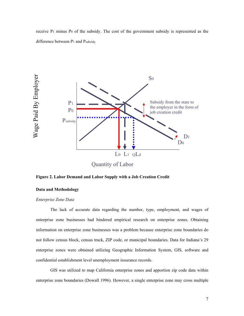
receive P1 minus P0 of the subsidy. The cost of the government subsidy is represented as the
difference between P1 and Psubsidy.
Wag
e Pa
id B
y Em
ploy
er
Figure 2. Labor Demand and Labor Supply with a Job Creation Credit
Data and Methodology
Enterprise Zone Data
The lack of accurate data regarding the number, type, employment, and wages of
enterprise zone businesses had hindered empirical research on enterprise zones. Obtaining
information on enterprise zone businesses was a problem because enterprise zone boundaries do
not follow census block, census track, ZIP code, or municipal boundaries. Data for Indiana’s 29
enterprise zones were obtained utilizing Geographic Information System, GIS, software and
confidential establishment level unemployment insurance records.
GIS was utilized to map California enterprise zones and apportion zip code data within
enterprise zone boundaries (Dowall 1996). However, a single enterprise zone may cross multiple
S0W
age Paid by Employer
D0
QLd
Quantity of Labor
Subsidy from the state to the employer in the form of job creation credit P0
P1
Psubsidy
D1
L0 L1
7

zip code boundaries, or may be a small portion of a zip code. Data aggregated at the zip code
level yielded an estimation of businesses within the enterprise zone. Methodology used in this
study built upon Dowall’s by geographically placing individual businesses on a street map, rather
than within a zip code region, and using a digital enterprise zone map to select businesses which
were physically located within each enterprise zone.
State unemployment insurance records, composed of Federal ES202 data, were obtained
from the Indiana Department of Commerce. Physical location address, establishment industry
code, wage and employment data for each firm were in this database. These data were a good
measure of variables needed.
Each of Indiana’s 29 enterprise zones were digitally mapped using ArcView GIS©
software. Indiana 2002 TIGER© address data were obtained from the U.S. Census Bureau, and
legal descriptions of each enterprise zone, obtained from the Indiana Department of Commerce,
were used to map enterprise zone boundaries. Once digitized maps of each zone were created,
they were checked by local enterprise zone administrators for accuracy.
Third quarter 2002 Indiana unemployment insurance records contained 153,889
establishments. Physical location addresses for these establishments were geocoded, or
geographically pinpointed on the street file. Geocoding reads physical location addresses from the
unemployment insurance records, and attempts to match them to street addresses in the TIGER©
address data, creating a point on the map at each match, or cluster of matches. Once the
geocoding had been completed the enterprise zone maps were layered over the address data and
businesses physically located within boundaries, or on the boundary, of each enterprise zone map
were highlighted. Geocoding involved address cleaning, setting minimum geocoding match
scores, and choosing a buffer zone around each enterprise zone. The end result is a list of
businesses which were physically located within Indiana enterprise zones during third quarter,
2002, and employment, wage and sector information for each establishment. Figure 3 shows the
8

TIGER© address data, the Indianapolis enterprise zone map, and map results of geocoding in
Indianapolis.
Figure 3. View of Street File, Enterprise Zone, and Geocoding
The geocoding process resulted in a list of 6,432 establishments located within all 29
Indiana enterprise zones, 4.2% of all Indiana establishments. Manufacturing and mining
establishments accounted for 10.4 percent of establishments, 23.5 percent were wholesale and
retail trade and 66.1 percent were service establishments. Annual employment was estimated to
be 145,096, 4.6% of total Indiana employment. The average enterprise zone wage was estimated
to be $34,736, while median Indiana income was is $41,567. Enterprise zone establishment totals
are shown in Table 1.
9

TABLE 1. Estimated Indiana Enterprise Zone Establishment Totals Enterprise Zone Businesses Totals Percentage Manufacturing 670 10.4%Service 4,251 66.1%Trade 1,511 23.5%Total businesses 6,432 Annual Employment 145,096 Annual Wages $ 5,039,995,476 Average Wage $ 34,736 Empirical Model Data
Units of observation were all 92 counties and 14 labor market areas (LMAs) in Indiana as
counties and LMAs represent the economy an enterprise zone operates within. Labor market
areas are multicounty areas with a minimum population of 100,000 and are aggregated by
counties according to commuting patterns (McNamara, 1991). Figure 4 outlines the fourteen
LMAs used in this analysis.
Figure 4. Indiana Labor Market Areas
10

Data at the county level were obtained from the Bureau of Economic Analysis, Bureau of
Labor Statistics, County Business Patterns, and the 2000 U.S. Decennial Census. Table 2 shows
data used, what it measured and the source; summary statistics are given in Table 3. 2001 data
were used for all variables, except where noted, as it was the most recent data available. Bureau
of Economic Analysis employment data showed a decline in employment in 2001 after ten years
of steady growth. To capture what appeared to be normal employment growth, the change in
employment variable, LMAchange, was calculated from 1996 to 2000, using data showing five
years of continuous growth in aggregate employment.
TABLE 2. List of Independent Variables and Sources
Measuring Source Demand: Employ00=f(LMAwage, LMAchange, Population, Manufacturer)
LMAwage Average annual wage in LMA County Business Patterns, 2001
LMAchange Employment growth rate from 1996-2000 in LMA
Bureau of Economic Analysis, 2001
Population Population in county U.S. Census, 2000
Manufacturer Manufacturing firm rate in county County Business Patterns, 2001
Supply: Wage=f(Employ00, LMAunemp, HSeducation, WorkShare)
LMAunemp Unemployment rate within LMA Bureau of Labor Statistics, 2001
HSeducation Rate of those age 25+ who are high school educated U.S. Census, 2000
WorkShare Percent of population in workforce in county
Bureau of Labor Statistics, 2001
Employ00 Number employed in county Bureau of Labor Statistics, 2001
11
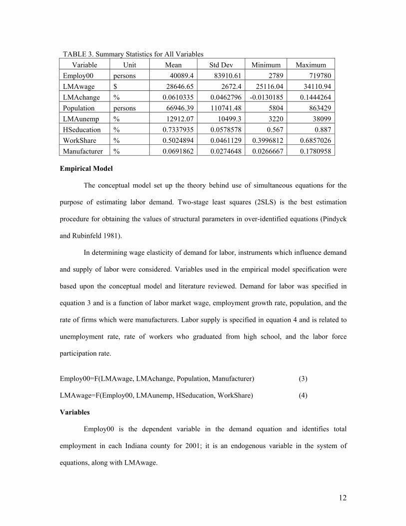
TABLE 3. Summary Statistics for All Variables Variable Unit Mean Std Dev Minimum Maximum
Employ00 persons 40089.4 83910.61 2789 719780LMAwage $ 28646.65 2672.4 25116.04 34110.94LMAchange % 0.0610335 0.0462796 -0.0130185 0.1444264Population persons 66946.39 110741.48 5804 863429LMAunemp % 12912.07 10499.3 3220 38099HSeducation % 0.7337935 0.0578578 0.567 0.887WorkShare % 0.5024894 0.0461129 0.3996812 0.6857026Manufacturer % 0.0691862 0.0274648 0.0266667 0.1780958
Empirical Model
The conceptual model set up the theory behind use of simultaneous equations for the
purpose of estimating labor demand. Two-stage least squares (2SLS) is the best estimation
procedure for obtaining the values of structural parameters in over-identified equations (Pindyck
and Rubinfeld 1981).
In determining wage elasticity of demand for labor, instruments which influence demand
and supply of labor were considered. Variables used in the empirical model specification were
based upon the conceptual model and literature reviewed. Demand for labor was specified in
equation 3 and is a function of labor market wage, employment growth rate, population, and the
rate of firms which were manufacturers. Labor supply is specified in equation 4 and is related to
unemployment rate, rate of workers who graduated from high school, and the labor force
participation rate.
Employ00=F(LMAwage, LMAchange, Population, Manufacturer) (3)
LMAwage=F(Employ00, LMAunemp, HSeducation, WorkShare) (4)
Variables
Employ00 is the dependent variable in the demand equation and identifies total
employment in each Indiana county for 2001; it is an endogenous variable in the system of
equations, along with LMAwage.
12
LMAwage is the average annual payroll in 2001 for workers in each Indiana LMA. Labor
market area wage was chosen rather than county wage because the LMA represents the area in
which residents commute to work, thus wage throughout the LMA will be similar. The resulting
coefficient on LMAwage was used to determine the wage elasticity of demand for labor. This
elasticity provided an estimate of fiscal impact for the job creation credit.
LMAchange is change in total employment over the 1996 through 2000 period as a
growth rate within each labor market area. LMAchange was included in the labor demand
equation because LMAs with high job growth will have higher employment; additionally this
variable was used by Tokle and Huffman (1991).
Population is county population in 2001. This variable was chosen to be a proxy for
market size for a firm as aggregated county average market and price data were not available.
Manufacturer is the percent of firms within a county which were manufacturers in 2001.
This is a measure of the structure of the economy; counties with high rates of manufacturing
firms are expected to have more employment. Other industry sectors were not significant and
were not included in the final empirical model.
Other variables affect labor supply rather than demand. LMAunemp is the unemployment
rate in a labor market area. HSeducation is the rate of those over age 25 with at least a high
school education. Education is an important component in estimating labor supply as educated
workers are more desirable (Blanchflower and Oswald 1994). WorkShare is the share of the
county population in the workforce. A higher share of the population in the workforce will lead to
higher labor supply.
The demand for labor was estimated using measures for wage, output, firm sector and
labor supply. Wage data were obtained, population was used as a proxy for output and firm sector
was measured by the percentage of manufacturers. Labor supply was estimated using
unemployment rate, share of population in the workforce and education of the workforce.
13

Equations 3 and 4 were simultaneously estimated using two-stage least squares regression
technique.
Results
Regression results are show in Table 4 along with the significance of each variable, R-
square, adjusted R-square, the F statistic.
TABLE 4. Two-State Least Squares Regression Results
Independent Variable Coefficient Standard Error T Statistic
Employ00=F(LMAwage, LMAchange, Population, Manufacturer)
R-Square .95838 Adjusted R-Square .95646 F Statistic 500.80
Constant 41810.05 26879.66 (1.56)
LMAwage -2.34831 0.982732 (-2.39)
LMAchange 55020.33 41536.59 (1.32)
Population 0.761405 0.018128 (42.00)
Manufacturer 162160.8 68705.75 (2.36)
LMAWage=F(Employ00, LMAunemploy, HSeducation, WorkShare)
R-Square .61540 Adjusted R-Square .59772 F Statistic 34.80
Constant 19298.14 2721.009 (7.09)
LMAunemp 0.183489 0.018867 (9.73)
HSeducation 4676.216 3465.843 (1.35)
WorkShare 7154.912 4114.216 (1.74)
Employ00 -0.00118 0.002325 (-0.51)
Expected and resulting signs of coefficients are shown in Table 5 along with respective
levels of significance for the coefficients. The coefficient on LMAwage was negative and
significant at the 0.05 level, indicating the wage elasticity of labor demand was negative as
expected. Blanchflower and Oswald (1994) wrote that in a labor demand model the wage
elasticity of aggregate labor demand for a locality is negative. Population and Manufacturer both
had positive signs and were significant at the 0.01 and 0.05 level, respectively. The coefficient on
LMAchange was not significant, indicating that this variable was not a determinant of labor
14

demand as suggested by Tokle and Huffman (1991) in this model. Employment growth is likely a
consequence of labor demand, rather than a determinant.
The labor supply equation had expected signs on all significant coefficients. A coefficient
sign of interest was the positive coefficient on LMAunemp. Renkow (2003) wrote that the
coefficient between wage and unemployment should be positive; results of the empirical model
support this conclusion, at a 0.01 level of significance. WorkShare was significant at the 0.1 level
with the expected sign. Employ00 and HSeducation were not significant.
TABLE 5. Expected Signs and Significance Independent Variable Expected Sign Resulting Sign Significance
Demand Employ00=f(LMAwage, LMAchange, Population, Manufacturer)
Constant +/- +
LMAwage - - **
LMAchange + +
Population + + *
Manufacturer + + **
Supply Wage=f(Employ00, LMAunemp, HSeducation, WorkShare)
Constant +/- + *
LMAunemp + + *
HSeducation + +
WorkShare + + ***
Employ00 - -
* Significant at =.01 level ** Significant at =.05 level *** Significant at =.1 level
The coefficient on wage in the labor demand equation was -2.34. The elasticity of the
labor demand curve was estimated by taking the natural log of each coefficient and re-estimating
the equation. The wage elasticity of labor demand was estimated to be -0.55, and assumed to be
constant. Hamermesh (1976) found wage elasticity of labor demand to be between -0.04 and
-0.16 in a literature review. Hamermesh noted that the elasticities found in his literature review
15

were smaller than expected. Bureau of Labor Statistics data were employed with OLS to estimate
the wage elasticity of labor demand to be -0.24 (Clark and Freeman 1980).
Fiscal Impact Estimation
The fiscal impact of a one-time job creation tax credit was estimated by first estimating
the number of jobs created solely due to the job creation tax credit, without normal job growth.
This is job growth due to employers’ decreased cost of labor, the $1500 tax credit, which enabled
them to employ more labor. The wage elasticity of labor demand was applied to the average wage
and total employment in each enterprise zone to estimate the number of jobs which would be
created due to the decreased cost of labor. The fiscal impact of incentives for jobs created due to
the job creation tax credit is the number of jobs created due to the credit multiplied by the $1500
tax credit. Table 6 shows the fiscal impact of the job creation tax credit due to jobs created as a
result of the credit, not normal job growth. In enterprise zones statewide an estimated 122.5 jobs
would be created as a result of a one-time $1500 job creation tax credit.
TABLE 6. Jobs Created and Fiscal Impact due to $1500 Job Creation Tax Credit
Enterprise Zone
2002 EZ Employment
Ave. EZ
wage ($)
% change in wage
with credit
Jobs created due
to tax credit
Cost of Jobs Created ($)
Anderson 4294 41774 -0.036 2.78 4172 Bedford 4391 28961 -0.052 4.10 6154 Bloomington 6518 28771 -0.052 6.13 9195 Clark County 518 27926 -0.054 0.50 753 Connersville 1748 25630 -0.059 1.85 2768 East Chicago 15340 46385 -0.032 8.95 13422 Elkhart 6814 34420 -0.044 5.36 8035 Evansville 7522 30543 -0.049 6.66 9995 Fort Harrison 919 33933 -0.044 0.73 1099 Fort Wayne 9787 29832 -0.050 8.88 13315 Frankfort 2361 21591 -0.069 2.96 4438 Gary 9789 55721 -0.027 4.75 7130 Grissom 505 27225 -0.055 0.50 753 Hammond 7121 31256 -0.048 6.16 9247 Indianapolis 4929 34119 -0.044 3.91 5863
16

Jeffersonville 5984 28070 -0.053 5.77 8652 Kokomo 4355 23673 -0.063 4.98 7467 Lafayette 6352 23673 -0.063 7.26 10890 LaPorte 6608 30667 -0.049 5.83 8745 Marion 6285 44765 -0.034 3.80 5698 Michigan City 4922 32026 -0.047 4.16 6238 Mitchell 1018 25153 -0.060 1.10 1643 New Albany 3726 26668 -0.056 3.78 5671 Portage 2566 29245 -0.051 2.37 3561 Richmond 3498 28448 -0.053 3.33 4991 Salem 3067 21911 -0.068 3.79 5681 South Bend 6898 41687 -0.036 4.48 6716 Terre Haute 4191 28313 -0.053 4.01 6008 Vincennes 3070 23005 -0.065 3.61 5416
TOTAL 145096 $31,220 -0.051 122.48 $183,717
The job creation tax credit can be claimed by all enterprise zone establishments which
create a job, regardless of whether the job was created as a result of the tax credit. The fiscal
impact of the $1500 job creation tax credit must also include the cost of the credit for jobs which
would have been created regardless of the credit; jobs which can be attributed to trend growth in
the economy. The second step in estimating fiscal impact of the job creation tax credit was to
estimate normal job growth in the economy. Job creation data were not available at the county
level, so county job growth data, during a period of economic growth, were used as a proxy.
Three estimates for trend job growth were obtained: annual average job growth, the highest level
of a 95 percent confidence interval for county job growth, and the lowest level of a 95 percent
confidence interval for county job growth, all over the 1996 through 2000 period. Annual average
job growth was estimated to be the average of annual county job growth rates over the 1996
through 2000 period for enterprise zone counties. The 95 percent confidence interval was
estimated using the same annual county job growth rates, their standard deviation, and average.
Maximum job growth was estimated to be the high end of the 95 percent confidence interval.
17

Minimum county job growth was estimated to be the low end of the 95 percent confidence
interval.
County job growth rates were calculated from Bureau of Economic Analysis employment
data over the 1996 through 2000 period, as this was the most recent period of consistent job
growth. If 2001 had been included, the average annual job growth rate would have been negative
for more counties and thus not a good measure of what can happen during a growth cycle. Table
7 shows normal job growth and associated credit cost due to normal job growth. When job
growth was estimated to be negative, it was omitted from the table; this occurs as job growth data
were used as a proxy for job creation data and job creation could not be negative. Table 7 does
not include jobs created as a result of the job creation tax credit; this was reported in Table 6.
Average annual job growth in Indiana enterprise zones was estimated to be 1,466 jobs.
TABLE 7. Expected Job Growth and Credit Cost associated with Local Job Creation
Enterprise Zone
2002 Enter. Zone
Employ.
Average Annual
Job Growth
Maximum annual job
growth, 95% C.I.
Minimum annual
job growth,
95% C.I.
Average one-time
Credit Cost ($)
Maximum (95% C.I.) one-time
credit cost ($)
Minimum (95% C.I.) one-time
credit cost ($)
Anderson 4294 -50.07 15.90 - - 23,849 -
Bedford 4391 5.36 75.63 - 8,045 113,438 -
Bloomington 6518 86.12 124.07 48.16 129,175
186,111 72,240
INAAP 518 16.36 24.94 7.79 24,545
37,404 11,686
Connersville 1748 -11 2.72 - - 4,078 -
East Chicago 15340 137.04 370.56 - 205,561 555,846 -
Elkhart 6814 177.87 317.34 38.40 266,801
476,005 57,597
Evansville 7522 71.87 123.83 19.91 107,806
185,746 29,865
Fort Harrison 919 18.17 22.60 13.74 27,259
33,905 20,612
Fort Wayne 9787 141.69 223.76 59.61 212,532
335,646 89,419
Frankfort 2361 -28.36 7.02 - - 10,523 -
18

Gary 9789 87.45 236.47 - 131,176 354,705 -
Grissom 505 11.59 16.16 7.03 17,388
24,236 10,541
Hammond 7121 63.62 172.02 - 95,424 258,030 -
Indianapolis 4929 97.47 121.23 73.70 146,200
181,850 110,551
Jeffersonville 5984 189.03 288.06 90.00 283,546
432,096 134,995
Kokomo 4355 12.58 59.01 - 18,877 88,519 -
Lafayette 6352 137.59 173.37 101.81 206,388
260,057 152,720
LaPorte 6608 96.31 112.16 80.45 144,458
168,244 120,672
Marion 6285 -36.53 - - - - - Michigan City 4922 71.73 83.54
59.92 107,600
125,317 89,883
Mitchell 1018 1.24 17.53 - 1,865 26,299 -
New Albany 3726 89.02 142.74 35.29 133,523
214,113 52,933
Portage 2566 20.65 31.18 10.12 30,972
46,769 15,174
Richmond 3498 -8.39 23.59 - - 35,390 -
Salem 3067 44.29 134.25 - 66,434 201,373 -
South Bend 6898 68.19 155.75 - 102,279 233,632 -
Terre Haute 4191 -16.25 77.29 - - 115,939 -
Vincennes 3070 -29.11 31.16 - - 46,742 -
TOTAL 145,096 1,466 3,184
646 $2,467,854
$4,775,863 $ 968,885
The third step in estimating fiscal impact was to estimate the total cost of the job creation
credit by adding the fiscal impact associated with trend job growth (Table 7) to the fiscal impact
associated with job growth as a result of the job creation tax credit (Table 6). The total estimated
fiscal impact was $5.0 million, $1.1 million, and $2.7 million for the estimated maximum,
minimum, and average annual job growth rates respectively (Table 8).
19

TABLE 8. Estimated Maximum, Minimum, and Average Fiscal Cost
Enterprise Zone
Maximum (95% C.I)
Credit Cost ($)
Minimum (95% C.I.)
Credit Cost ($) Average Credit Cost
($) Anderson 28,021 4,172 4,172Bedford 119,592 6,154 14,199Bloomington 195,306 81,435 138,370Clark County 38,157 12,439 25,298Connersville 6,846 2,768 2,768East Chicago 569,268 13,422 218,983Elkhart 484,039 67,593 274,836Evansville 195,742 30,964 117,801Fort Harrison 35,005 33,927 28,358Fort Wayne 348,961 93,857 225,847Frankfort 14,962 4,438 4,438Gary 361,835 7,130 138,306Grissom 24,988 19,787 18,141Hammond 267,277 9,247 104,671Indianapolis 187,713 119,203 152,063Jeffersonville 440,748 142,462 292,198Kokomo 95,985 7,467 26,344Lafayette 270,948 161,465 217,278LaPorte 176,989 126,370 153,203Marion 5,698 5,698 5,698Michigan City 131,555 91,525 113,838Mitchell 27,942 1,643 3,508New Albany 219,783 56,494 139,194Portage 50,331 20,164 34,533Richmond 40,380 4,991 4,991Salem 207,054 5,681 72,115South Bend 240,348 6,716 108,995Terre Haute 121,947 6,008 6,008Vincennes 52,159 5,416 5,416
TOTAL $4,959,579 $1,146,734 $2,651,571 Conclusion
A $1500 one-time job creation tax credit for establishments located within Indiana
enterprise zones was estimated to create 122.5 jobs. This is small compared to total enterprise
zone employment; enterprise zone employment would increase by 0.0008 percent with the
20

creation of 122.5 jobs. Of annual enterprise zone job growth, 7.7% would be attributed to the job
creation tax credit. Employment will be impacted by the tax credit, but this impact would be
small. The fiscal impact of the job creation tax credit will be 3 to 15 percent of the inventory tax
abatement.
In other states, job creation incentives range from a one-time credit of $500 in Illinois, to
$8000 in Wisconsin. If the proposed $1500 job creation tax credit was raised, it would increase
employment in enterprise zones, but the same credit would be given to employers who created a
job irregardless of the incentive, increasing the fiscal impact. A solution may be to implement a
credit similar to Wisconsin’s. Wisconsin’s community development zone program offers a one-
time job creation credit of up to $8000 for enterprise zone establishments which fill newly created
jobs with dislocated and disadvantaged workers. A one-time job creation credit of $6000 is
offered to community development zone establishments which create a job not filled by a
member of a target group of disadvantaged workers. Wisconsin’s program creates an incentive to
hire disadvantaged workers and also limits the number of credits which can be claimed, thus
decreasing the fiscal impact.
A job creation tax credit with restrictions similar to Wisconsin’s could be implemented in
Indiana. The proposed $1500 job creation tax credit could be restricted to certain establishments
or certain employees. Targeting establishments by industry sector would limit the number of
credits claimed, reducing fiscal impact, and targeting the benefits to a specific sector. Offering a
targeted credit to manufacturing firms could entice a manufacturing plant to locate within an
Indiana enterprise zone. A job creation tax credit targeted to specific employees, such as zone
residents, welfare recipients or displaced workers would benefit specific groups. Targeting of the
job creation tax credit would reduce the fiscal impact, as fewer credits would be claimed.
Additional incentives could be coupled with the job creation tax credit to increase the
total incentive package. These may not increase employment directly but could increase
investment, save establishments money, and thus indirectly increase firm employment. Some
21

22
states exempt sales tax for machinery, equipment and building supplies. Some states have a 5 to
10 percent investment credit. The fiscal impact of these additional incentives would need to be
estimated for Indiana enterprise zones. These incentives may be a better alternative to the job
creation tax credit for promoting redevelopment, investment, and job creation in Indiana
enterprise zones.
The fiscal impact estimate was based on the static one-year impact of a $1500 job
creation tax credit; this met the immediate research needs of the Indiana state legislature. Further
analysis is needed to determine long term implication of both fiscal impact and employment
growth. The actual incentive would need to be capitalized into the wage rate; it would actually be
less effective as an incentive, as discussed in figure 2. Future research area should examine the
effect of the tax credit in a dynamic manner and in conjunction with other incentives. Future
research should be conducted using a comparable control group for enterprise zones as the data
used was taken while enterprise zone establishments were receiving inventory tax abatement.
New incentives and no inventory tax anywhere in the state will draw establishments of different
industry sectors to Indiana’s urban enterprise zones.
Summary
The inventory tax abatement, the centerpiece financial incentive for enterprise zone
establishments, is being phased-out. A $1500 job creation tax credit was proposed to replace the
inventory tax abatement. Before the state legislature could consider such legislation, the fiscal
impact of the proposed policy had to be estimated. The wage elasticity of labor demand was
applied to enterprise zone wage and employment data to determine the number of jobs which
would be created due to the proposed policy. The number of jobs which would be created in a
normal growth cycle was also estimated. The fiscal impact of the policy was the cost of providing
the tax incentive to establishments which created a job due to the credit and establishments which
created a job due to trend economic growth. Results suggested that a $1500 job creation tax credit
would have a small impact on enterprise zone employment and a fiscal impact to the state of an

23
estimated $1.1 million to $5.0 million. The application of these results is limited as they are
estimated for a static one-year job creation tax credit and there was no control group.
24
References
Blanchflower, David and Andrew Oswald. 1994. The Wage Curve. Massachusetts Institute of Technology.
Clark, Kim and Richard Freeman. 1980. “How Elastic Is the Demand for Labor?” The Review of Economics and Statistics. pp. 509-520.
Crowe Chizek. 2001. Indiana Department of Commerce: Enterprise Zone Program Evaluation Phase I-Program Description. March 22.
Dowall, David E. 1996. “An Evaluation of California Enterprise Zone Programs” Economic Development Quarterly, Vol. 10, #4, Nov. pp. 352-368.
Faulk, Dagney. 2002. “Do State Economic Development Incentives Create Jobs? An Analysis of State Employment Tax Credit” National Tax Journal. June.
Hammermesh, Daniel S. 1976. “Econometric Studies of Labor Demand and Their Applications to Policy Analysis” Journal of Human Resources. Fall. pp. 507-525.
Hammermesh, Daniel S. 1992. “A General Model of Dynamic Labor Demand” The Review of Economics and Statistics. Vol. 71, #4, Nov. pp. 733-737.
Legislative Services Agency. 2003. LSA Enterprise Zone Fiscal Impact Project, Presented to the Commission on State Tax and Financing Policy. November.
McNamara, Kevin T. 1991. “Employment Growth in Indiana: A State and Regional Analysis” Purdue University Cooperative Extension Service. June.
Papke, Leslie E. 1993. “What Do We Know About Enterprise Zones?” NBER Working Paper Series #4251. National Bureau of Economic Research. Jan.
Pindyck, Robert S. and David L. Rubinfeld. 1981. Econometric Models and Economic Forecasts. McGraw-Hill. Renkow, Mitch. 2003. “Employment Growth, Worker Mobility, and Rural Economic Development” American Journal of Agricultural Economics. May. pp. 503-513. Tokle, J. G. and Wallace E. Huffman. 1991. “Local Economic Conditions and Wage Labor Decisions of Farm and Rural Nonfarm Couples” American Journal of Agricultural Economics. August. Wilder, Margaret G. and Barry M. Rubin. 1988. “Targeted Redevelopment Through Urban Enterprise Zones” Journal of Urban Affairs. Vol. 10, #1. pp.1-17.
Related Documents