Stata Introduction - Studenten · Stata Stata Introduction Bachelor thesis Dr. Anna Salomons Utrecht School of Economics (USE) 1 May 2013 1/86

Stata

Stata IntroductionBachelor thesis

Dr. Anna Salomons

Utrecht School of Economics (USE)

1 May 2013

1 / 86

Stata

This class

This class

This class will cover basic Stata skills:

I Entering data & saving your work

I Summarizing data

I Modifying data

I Analyzing data

2 / 86

Stata

A research example

A research question inspired by Biggie Smalls

3 / 86

Stata

A research example

Research question: does money make people happy?

I In answering this question, we need to control forconfounding variables which the economic literature tells usalso impact happiness (and may be correlated to income):

I healthI educationI genderI ageI social life

I I will use micro-data from the European Social Survey from2012.

4 / 86

Stata

A research example

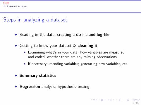
Steps in analyzing a dataset

I Reading in the data; creating a do-�le and log-�le

I Getting to know your dataset & cleaning itI Examining what�s in your data: how variables are measuredand coded; whether there are any missing observations

I If necessary: recoding variables; generating new variables, etc.

I Summary statistics

I Regression analysis; hypothesis testing.

5 / 86

Stata

Getting started and saving your work

Do- and log-�les

Opening a do�le: command doedit

6 / 86

Stata


Do- and log-�les

First lines in your do�le

I Change the directory where Stata saves your data, log�les,etcetera:

I cd "directory"

I Clear any open dataset from memoryI clear

I Close any open log-�le ("capture" tells Stata to only do this ifrelevant- so if no log was open the command is ignored)

I capture log close

I Tell Stata not to pause if output does not �t the screenI set more o¤

7 / 86

Stata


Do- and log-�les

First lines in your do�le (cont�d)

I Open a log-�leI log using "logname.log", replace

I If necessary, change the memory allocated to Stata (makesure it is more than the size of your dataset).

I set mem 2000M

I Any text which are not Stata commands should be written inbetween /* */

8 / 86

Stata


Do- and log-�les

First lines in your do�le: example

cd "E:/mythesis/stata_�les"

clear

capture log close

set more o¤

log using "myresults.log", replace

use "ESS.dta", clear

/* This is European Social Survey data */

9 / 86

Stata


Do- and log-�les

Do�le: example

10 / 86

Stata


Opening datasets

Loading data into Stata

I Stata directly reads �les with a .dta extensionI use "dataset.dta", clear

I Data from Excel can be pasted into Stata after using thecommand edit

I Afterwards, save as a Stata dataset:save "dataset.dta", replace

I Other extensions (.txt, .raw, .sps, .sas, ..) can eitherimported into Stata via File>>Import; or transferred to the.dta extension by using another program such as StatTransfer

11 / 86

Stata


Inspecting the data

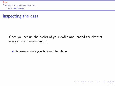
Inspecting the data

Once you set up the basics of your do�le and loaded the dataset,you can start examining it.

I browse allows you to see the data

12 / 86

Stata


Inspecting the data

Browse

13 / 86

Stata


Inspecting the data

Inspecting the data

Once you set up the basics of your do�le and loaded the dataset,you can start examining it.

I browse allows you to see the data

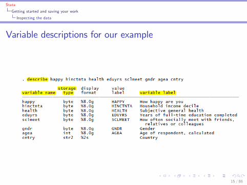
I describe gives a summary of all variables

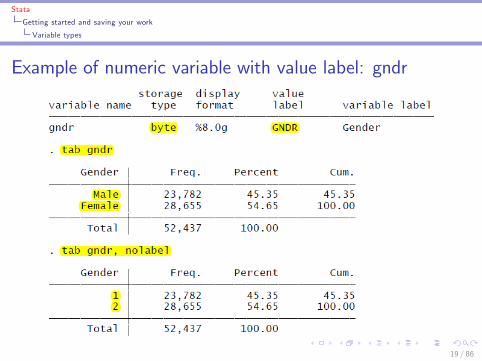
I variable name: the names of the variablesI storage type: whether variables are numeric or alphanumericI value label: meaning of the outcomes of numeric variablesI variable label: description of the variables

14 / 86

Stata


Inspecting the data

Variable descriptions for our example

15 / 86

Stata


Variable types

Di¤erent variable types

In the table produced by describe you see di¤erent "storage types"-these re�ect two main variable types:

I A string variable (e.g. str2, str9) is alphanumericI values should be referred to in quotation marks " ".

I All other variable types (byte, int, long, �oat, or double) arenumeric.

I Note: numeric variables may have value labels (this does notmake them string variables!)

16 / 86

Stata


Variable types

Example of string variable: cntry

17 / 86

Stata


Variable types

Example of numeric variable: agea

18 / 86

Stata


Variable types

Example of numeric variable with value label: gndr

19 / 86

Stata


Variable types

Summary: getting started

I Always work with a do�le and log�le

I use command

I describe command

I Di¤erent variable types: string, numeric, numeric with valuelabel

20 / 86

Stata

Summary statistics for the raw data

Sum and tab

Summary statistics

To get to know our data better, we compile some summarystatistics

I sum: numerical summary of all variables (add a list ofvariable names to only summarize a subset)

I More detailed summary by adding the suboption , detail

I tab varname: tabulates all possible values of one variable(varname = the name of that particular variable)

I tab varname, nolabel suppresses any value labels

21 / 86

Stata


Sum and tab

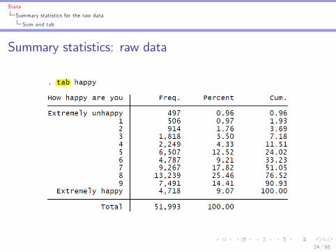
Summary statistics: raw data

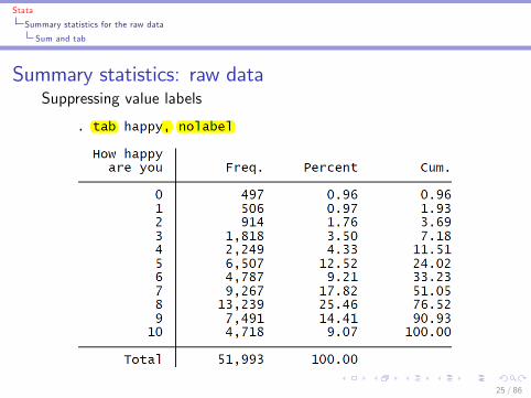
Summary statistics for the raw data (note di¤erent numbers ofobservations for di¤erent variables):

22 / 86

Stata


Sum and tab


23 / 86

Stata


Sum and tab


24 / 86

Stata


Sum and tab

Summary statistics: raw dataSuppressing value labels

25 / 86

Stata


Sum and tab


26 / 86

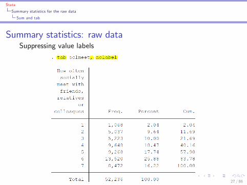
Stata


Sum and tab

Summary statistics: raw dataSuppressing value labels

27 / 86

Stata


If

The if command

I The if command can be added after many other commands,including sum, gen, and reg

I It tells Stata to execute that particular command under thecondition you specify in the if command

I The command combines withI == equal toI != not equal toI > larger thanI >= larger than or equal toI < smaller thanI <= smaller than or equal to

28 / 86

Stata


If

Examples of if commands (combined with sum)

29 / 86

Stata


If

Examples of if commands (combined with tab)

30 / 86

Stata


Bysort

The bysort command

I The bysort command can be pre�xed to many othercommands, including sum, gen, and reg.

I The command is bysort varlist:I e.g. bysort cntry: sum happyI e.g. bysort cntry gndr: sum happyI e.g. bysort cntry: reg happy hinctnta

I It tells Stata to execute that particular command separatelyfor each category of the variable(s) speci�ed in the variable(s)listed after bysort

31 / 86

Stata


Bysort

Example of a bysort command

32 / 86

Stata


Bysort

Summary: exploring the raw data

I sum and tab commands

I if and bysort commands

I These give you an idea of what�s in your raw data, andwhether any modi�cations are necessary

33 / 86

Stata

Cleaning the dataset

Data cleaning

The main components of data cleaning:

I Examine the amount of missing values in your variables ofinterest

I If necessary, recode missings and/or drop them

I Generating new variables needed for the analysis

I In your thesis�data section:I Describe any data cleaning you have doneI Show summary statistics for the cleaned data

34 / 86

Stata


Dealing with missing values

Missing values

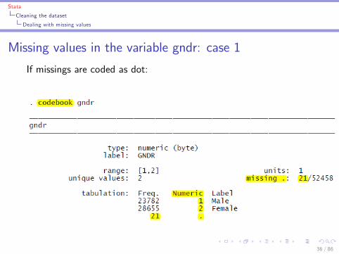
I Missing values from numerical variables are denoted by adot.

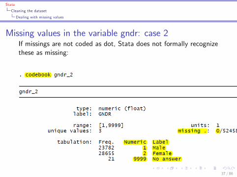
I Missing values from string variables are denoted by no textat all (i.e. no dot either).

I codebook varlist provides the number of missing observationsin the list of variables you specify in varlist

I If missings are coded di¤erently, you need to convert them tothe dot before beginning analysis: this can be done withreplace or recode

35 / 86

Stata



Missing values in the variable gndr: case 1

If missings are coded as dot:

36 / 86

Stata



Missing values in the variable gndr: case 2If missings are not coded as dot, Stata does not formally recognizethese as missing:

37 / 86

Stata



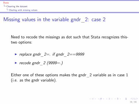
Missing values in the variable gndr_2: case 2

Need to recode the missings as dot such that Stata recognizes this-two options:

I replace gndr_2=. if gndr_2==9999

I recode gndr_2 (9999=.)

Either one of these options makes the gndr_2 variable as in case 1(i.e. as the gndr variable).

38 / 86

Stata


Dropping (or keeping) values or variables

Dropping values

I When running a regression, Stata automatically ignoresmissing values1

I In a regression, the nr of observations equals the number ofdata points which are available for all variables in theregression.

I However, sometimes you may want to drop missings, or dropspeci�c values

1As long as they�re signi�ed by a dot in the case of numerical variables, andby an empty cell in the case of string variables. If that is not the case, �rstrecode them!

39 / 86

Stata



Dropping observations with speci�c valuesI To drop missings:

I drop if there is no information on the variable happy:drop if happy==.

I To drop speci�c valuesI remove any extremely unhappy or extremely happy people:drop if happy==0 j happy==10

I remove any data from non-EU countries (i.e. dropping Israel,Russia and the Ukraine):drop if cntry=="IL" j cntry=="RU" j cntry=="UA"

I remove extremely unhappy Russians:drop if happy==0 & cntry=="RU"

I Note thatI j orI & and

40 / 86

Stata



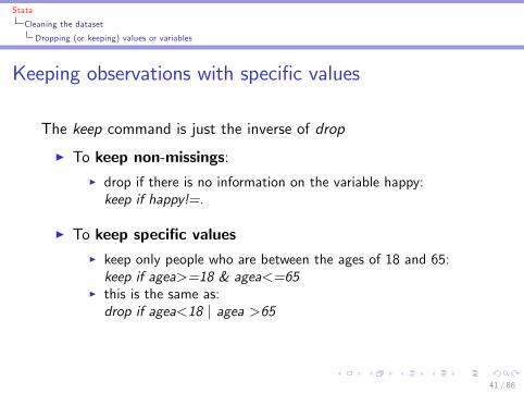
Keeping observations with speci�c values

The keep command is just the inverse of drop

I To keep non-missings:I drop if there is no information on the variable happy:keep if happy!=.

I To keep speci�c valuesI keep only people who are between the ages of 18 and 65:keep if agea>=18 & agea<=65

I this is the same as:drop if agea<18 j agea >65

41 / 86

Stata



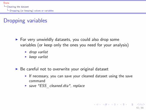
Dropping variables

I For very unwieldly datasets, you could also drop somevariables (or keep only the ones you need for your analysis)

I drop varlistI keep varlist

I Be careful not to overwrite your original datasetI If necessary, you can save your cleaned dataset using the savecommand

I save "ESS_cleaned.dta", replace

42 / 86

Stata


Example

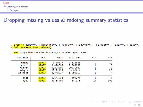
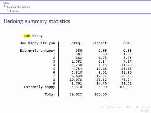
Dropping missing values & redoing summary statistics

43 / 86

Stata


Example

Redoing summary statistics

44 / 86

Stata


Generating new variables

Generating new variables: operators

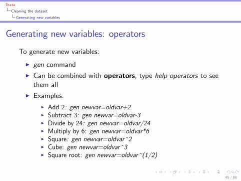
To generate new variables:

I gen commandI Can be combined with operators, type help operators to seethem all

I Examples:I Add 2: gen newvar=oldvar+2I Subtract 3: gen newvar=oldvar-3I Divide by 24: gen newvar=oldvar/24I Multiply by 6: gen newvar=oldvar*6I Square: gen newvar=oldvar^2I Cube: gen newvar=oldvar^3I Square root: gen newvar=oldvar^(1/2)

45 / 86

Stata



Generating new variables: functions

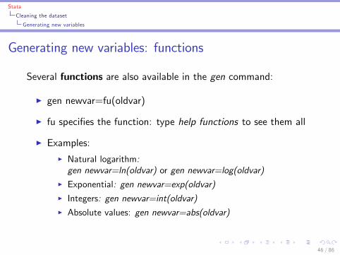
Several functions are also available in the gen command:

I gen newvar=fu(oldvar)

I fu speci�es the function: type help functions to see them all

I Examples:I Natural logarithm:gen newvar=ln(oldvar) or gen newvar=log(oldvar)

I Exponential: gen newvar=exp(oldvar)I Integers: gen newvar=int(oldvar)I Absolute values: gen newvar=abs(oldvar)

46 / 86

Stata



Other variable modi�cations

I Renaming variables: rename oldname newnameI rename gndr gender

I Labeling variables: label variable varname "text"I label variable gender "Gender of the respondent"

47 / 86

Stata


More advanced data manipulations

Generating new variables with egen

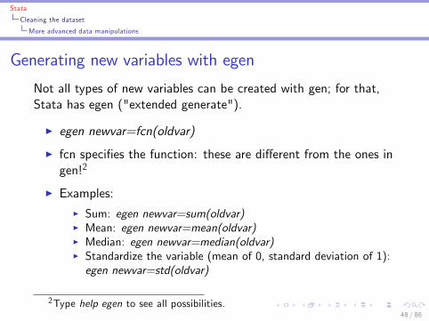
Not all types of new variables can be created with gen; for that,Stata has egen ("extended generate").

I egen newvar=fcn(oldvar)

I fcn speci�es the function: these are di¤erent from the ones ingen!2

I Examples:I Sum: egen newvar=sum(oldvar)I Mean: egen newvar=mean(oldvar)I Median: egen newvar=median(oldvar)I Standardize the variable (mean of 0, standard deviation of 1):egen newvar=std(oldvar)

2Type help egen to see all possibilities.48 / 86

Stata



Reshaping the data

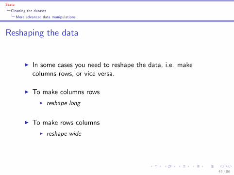
I In some cases you need to reshape the data, i.e. makecolumns rows, or vice versa.

I To make columns rowsI reshape long

I To make rows columnsI reshape wide

49 / 86

Stata



Reshaping the data: example

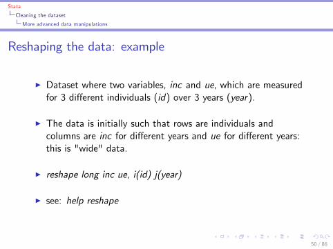
I Dataset where two variables, inc and ue, which are measuredfor 3 di¤erent individuals (id) over 3 years (year).

I The data is initially such that rows are individuals andcolumns are inc for di¤erent years and ue for di¤erent years:this is "wide" data.

I reshape long inc ue, i(id) j(year)

I see: help reshape

50 / 86

Stata



Initial format: wide

51 / 86

Stata



Result after reshaping: long

52 / 86

Stata



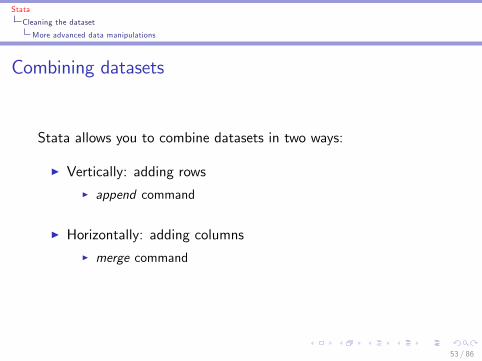
Combining datasets

Stata allows you to combine datasets in two ways:

I Vertically: adding rowsI append command

I Horizontally: adding columnsI merge command

53 / 86

Stata



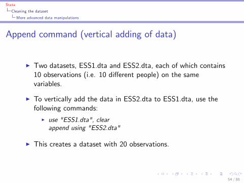
Append command (vertical adding of data)

I Two datasets, ESS1.dta and ESS2.dta, each of which contains10 observations (i.e. 10 di¤erent people) on the samevariables.

I To vertically add the data in ESS2.dta to ESS1.dta, use thefollowing commands:

I use "ESS1.dta", clearappend using "ESS2.dta"

I This creates a dataset with 20 observations.

54 / 86

Stata



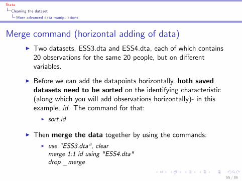
Merge command (horizontal adding of data)I Two datasets, ESS3.dta and ESS4.dta, each of which contains20 observations for the same 20 people, but on di¤erentvariables.

I Before we can add the datapoints horizontally, both saveddatasets need to be sorted on the identifying characteristic(along which you will add observations horizontally)- in thisexample, id. The command for that:

I sort id

I Then merge the data together by using the commands:I use "ESS3.dta", clearmerge 1:1 id using "ESS4.dta"drop _merge

55 / 86

Stata



Merge command (horizontal adding of data)

I merge automatically prints information on how manydatapoints were matched.

I If your datasets should not be added 1-to-1, you shouldchange the command to re�ect that:

I Many-to-one: merge m:1 id using "data.dta"I One-to-many: merge 1:m id using "data.dta"I Many-to-many: merge m:m id using "data.dta"

I See help merge for more explanation.

56 / 86

Stata



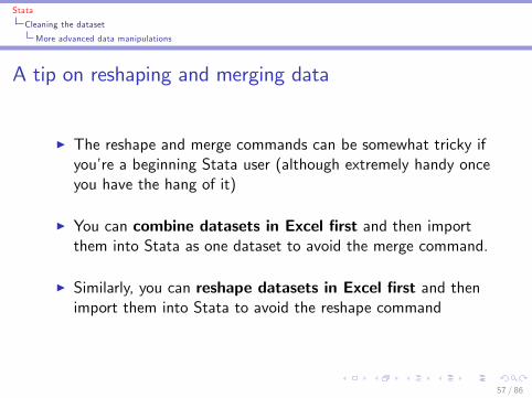
A tip on reshaping and merging data

I The reshape and merge commands can be somewhat tricky ifyou�re a beginning Stata user (although extremely handy onceyou have the hang of it)

I You can combine datasets in Excel �rst and then importthem into Stata as one dataset to avoid the merge command.

I Similarly, you can reshape datasets in Excel �rst and thenimport them into Stata to avoid the reshape command

57 / 86

Stata



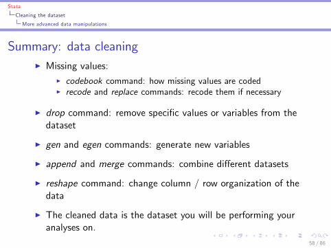
Summary: data cleaningI Missing values:

I codebook command: how missing values are codedI recode and replace commands: recode them if necessary

I drop command: remove speci�c values or variables from thedataset

I gen and egen commands: generate new variables

I append and merge commands: combine di¤erent datasets

I reshape command: change column / row organization of thedata

I The cleaned data is the dataset you will be performing youranalyses on.

58 / 86

Stata

Analyzing data

Correlation analysis


I Calculate correlations between variables:I corr varlist

I Also obtain p-values for the (pairwise) correlations:I pwcorr varlist, sig

59 / 86

Stata

Analyzing data


corr

60 / 86

Stata

Analyzing data


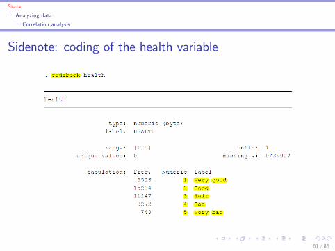
Sidenote: coding of the health variable

61 / 86

Stata

Analyzing data


pwcorr

62 / 86

Stata

Analyzing data

Regression analysis

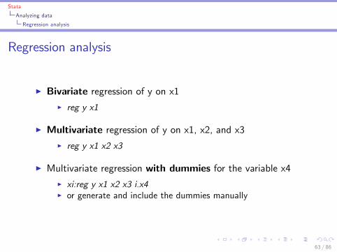
Regression analysis

I Bivariate regression of y on x1I reg y x1

I Multivariate regression of y on x1, x2, and x3I reg y x1 x2 x3

I Multivariate regression with dummies for the variable x4I xi:reg y x1 x2 x3 i.x4I or generate and include the dummies manually

63 / 86

Stata

Analyzing data

Regression analysis

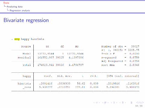
Bivariate regression

64 / 86

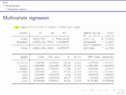
Stata

Analyzing data

Regression analysis

Multivariate regression

65 / 86

Stata

Analyzing data

Regression analysis

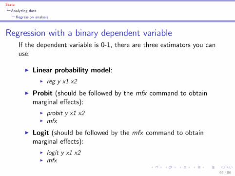
Regression with a binary dependent variableIf the dependent variable is 0-1, there are three estimators you canuse:

I Linear probability model:I reg y x1 x2

I Probit (should be followed by the mfx command to obtainmarginal e¤ects):

I probit y x1 x2I mfx

I Logit (should be followed by the mfx command to obtainmarginal e¤ects):

I logit y x1 x2I mfx

66 / 86

Stata

Analyzing data

Regression analysis

Including dummies for an independent variable

2 options:

I Manually generate & include dummiesI creating dummies for each category of a variable:tab varname, gen(dvarname)

I then manually include them

I The xi: pre�xI Add xi: before reg, and put i. in front of the independentvariable(s) you want to include dummies for

67 / 86

Stata

Analyzing data

Regression analysis

Manually generating dummies

68 / 86

Stata

Analyzing data

Regression analysis

Manually including dummies

69 / 86

Stata

Analyzing data

Regression analysis

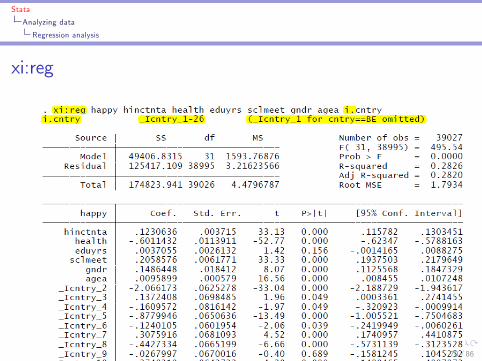
xi:reg

70 / 86

Stata

Analyzing data

Regression analysis

Dummy variables generated from xi:reg

71 / 86

Stata

Analyzing data

Regression analysis

Including a quadratic term

72 / 86

Stata

Analyzing data

Regression analysis

Quadratic term: a reminder on interpretation

I Estimated partial e¤ect of income on happiness:

∂happy∂hinctnta

= b1 + 2b2hinctnta

= 0.286� 2(0.015)hinctnta

I Find & classify stationary point:

0.286� 0.030hinctnta = 0

hinctnta � 9.5

Maximum since ∂2happy∂hinctnta2 = �0.030 < 0

I Hence: all else equal, happiness increases with income up tothe 95th income percentile, and decreases thereafter.

73 / 86

Stata

Analyzing data

Hypothesis testing

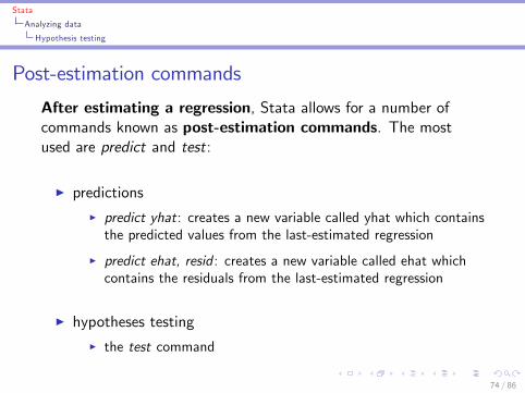
Post-estimation commands

After estimating a regression, Stata allows for a number ofcommands known as post-estimation commands. The mostused are predict and test:

I predictionsI predict yhat: creates a new variable called yhat which containsthe predicted values from the last-estimated regression

I predict ehat, resid : creates a new variable called ehat whichcontains the residuals from the last-estimated regression

I hypotheses testingI the test command

74 / 86

Stata

Analyzing data

Hypothesis testing

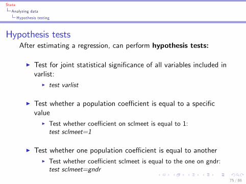
Hypothesis testsAfter estimating a regression, can perform hypothesis tests:

I Test for joint statistical signi�cance of all variables included invarlist:

I test varlist

I Test whether a population coe¢ cient is equal to a speci�cvalue

I Test whether coe¢ cient on sclmeet is equal to 1:test sclmeet=1

I Test whether one population coe¢ cient is equal to anotherI Test whether coe¢ cient sclmeet is equal to the one on gndr:test sclmeet=gndr

75 / 86

Stata

Analyzing data

Hypothesis testing

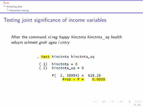
Testing joint signi�cance of income variables

After the command xi:reg happy hinctnta hinctnta_sq healtheduyrs sclmeet gndr agea i.cntry

76 / 86

Stata

Analyzing data

Hypothesis testing

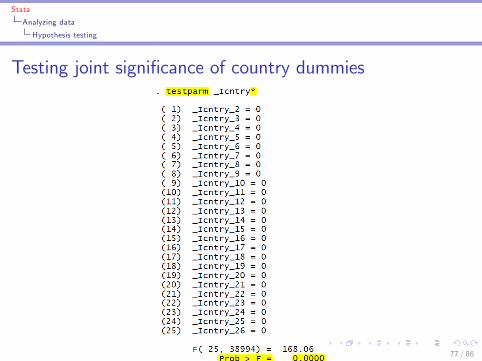
Testing joint signi�cance of country dummies

77 / 86

Stata

Analyzing data

Time series commands

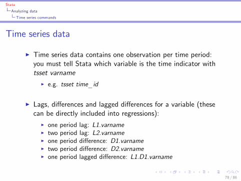
Time series data

I Time series data contains one observation per time period:you must tell Stata which variable is the time indicator withtsset varname

I e.g. tsset time_id

I Lags, di¤erences and lagged di¤erences for a variable (thesecan be directly included into regressions):

I one period lag: L1.varnameI two period lag: L2.varnameI one period di¤erence: D1.varnameI two period di¤erence: D2.varnameI one period lagged di¤erence: L1.D1.varname

78 / 86

Stata

Analyzing data

Time series commands

Summary: data analysisI corr and pwcorr commands: correlation analysis

I reg command: regression analysis

I xi: pre�x: regression analysis with dummy independentvariables

I logit, probit and mfx commands: regression analysisspeci�cally for binary dependent variables (in extended slides)

I tsset command and lag (L.) and di¤erence (D.)operators fortime-series datasets (in extended slides)

I test command: hypothesis testing

79 / 86

Stata

Outputting results

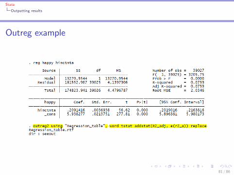
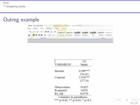
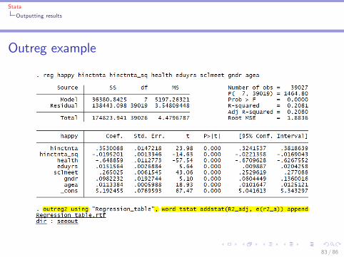
Outputting results from Stata: outreg2 commandI Can make tables in another program (e.g. Excel) and �ll themin by hand

I Or: can have Stata produce ready-made tables with theoutreg2 command

I reg y x1 x2I outreg2 using "�le_name", word tstat addstat(R2_adj,e(r2_a)) replace

I Perform another regression, add the results to the previoustable:

I reg y x1 x2 x3 x4I outreg2 using "�le_name", word tstat addstat(R2_adj,e(r2_a)) append

80 / 86

Stata

Outputting results

Outreg example

81 / 86

Stata

Outputting results

Outreg example

82 / 86

Stata

Outputting results

Outreg example

83 / 86

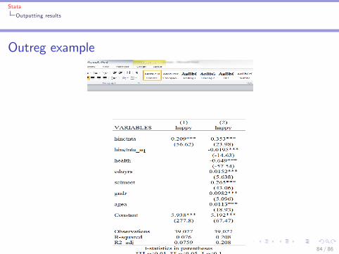
Stata

Outputting results

Outreg example

84 / 86

Stata

Getting help within Stata


I The help command can be used from the command line orfrom the Help window.

I To use help the command must be spelled correctly and thefull name of the command must be used.

I e.g. help reshape

85 / 86

Stata


Stata particularsAs in all programming, you have to be precise:

I commands and variable names need to be typed in withouttypos (also, Stata is case-senstitive)

I right: sum happyI wrong: sum Happy ; Sum happy ; sum hippy

I commands and variable names must be followed by a spacebefore entering another command or variable name

I right: sum happy ageaI wrong: sumhappyagea; sumhappy agea; sum happyagea

I you cannot:I create a variable with a name that already exists in the dataset;I put spaces in variable names;I have variable names that start with a number.

86 / 86

Stata Introduction - Studenten · Stata Stata Introduction Bachelor thesis Dr. Anna Salomons Utrecht School of Economics (USE) 1 May 2013 1/86

Documents