Stasis or kinesis? Hidden dynamics of a rocky intertidal macrophyte mosaic revealed by a spatially explicit approach

Page 1

www.elsevier.com/locate/jembe

Journal of Experimental Marine Biolo

Stasis or kinesis? Hidden dynamics of a rocky intertidal

macrophyte mosaic revealed by a spatially explicit approach

Bruce A. Mengea,*, Gary W. Allisonb, Carol A. Blanchettec, Terry M. Farrelld,

Annette M. Olsona, Teresa A. Turnere, Peter van Tamelenf

aDepartment of Zoology, Oregon State University, Corvallis, Oregon 97331-2914, USAbDepartment of Evolution, Ecology and Organismal Biology, The Ohio State University, Columbus, OH 43212-1156, United States

cDepartment of Ecology, Evolution and Marine Biology, University of California, Santa Barbara, CA 93106, United StatesdBiology Department, Box 8270, Stetson University, 421 North Woodland Blvd, DeLand, FL 32720, United StateseDivision of Science and Mathematics, University of the Virgin Islands, St. Thomas, USVI, 00802, United States

f14320 Otter Way, Juneau, AK 99801, United States

Received 8 August 2004; received in revised form 28 August 2004; accepted 5 September 2004

Abstract

Macrophyte mosaics, or tile-like assemblages of turfy marine macroalgae and surfgrass (Phyllospadix scouleri), are

persistent and highly diverse along the central Oregon coast. To test the hypothesis that spatial pattern and species abundances

are relatively invariant in this system, we studied community structure, disturbance, and species interactions from 1985 to 1990.

Abundances and disturbance in permanently marked plots at each of five sites spanning wave-exposed to wave-protected areas

were monitored photographically each year. The analysis was spatially explicit, incorporated position effects, and allowed

determination of species displacements. To interpret the potential influence of substratum on disturbance, we quantified rock

hardness and sediment depth at each site. Field experiments tested the role of grazers and spatial interactions on maintenance of

between-patch boundaries.

Mosaic dynamics varied with wave exposure. At wave-exposed and wave-protected sites, average patterns of abundance and

assemblage structure were relatively constant through time, but analysis of transition probabilities showed high rates of change

among mosaic elements at wave-exposed sites and low rates of change at wave-protected sites. At wave-exposed sites, most

changes involved Phyllospadix displacing neighboring macroalgal turfs but rarely the reverse. At all wave-exposures, surfgrass

was the most frequently disturbed mosaic element. Disturbed areas were quickly colonized by macroalgae. At wave-exposed

sites, disturbances were closed by regrowth of surfgrass. Disturbance rates were similar across wave-exposures, with wave

forces causing most loss at wave-exposed sites and a combination of substratum failure and sediment burial causing most loss at

wave-protected sites. At wave-exposed sites, disturbances tended to be larger (436.7 vs. 278.6 cm2) but less numerous (228 vs.

484 total disturbances) than at wave-protected sites.

At wave-exposed sites, surfgrass overgrew all other species except the kelp Lessoniopsis littoralis, which was competitively

equivalent to surfgrass. Grazing had no effect on spatial interactions. Disturbance prevented surfgrass monocultures, and with

0022-0981/$ - s

doi:10.1016/j.jem

* Correspon

E-mail addr

gy and Ecology 314 (2005) 3–39

ee front matter D 2004 Elsevier B.V. All rights reserved.

be.2004.09.015

ding author. Tel.: +1 541 737 5358; fax: +1 541 737 3360.

ess: [email protected] (B.A. Menge).

Page 2

B.A. Menge et al. / J. Exp. Mar. Biol. Ecol. 314 (2005) 3–394

variable dispersal and patchy recruitment, maintained mosaic structure. At wave-protected sites, standoffs were the usual

outcome of interactions, and patchiness resulted primarily from colonization of disturbances and subsequent succession. Like

mussels, Phyllospadix are simultaneously dominant competitors, the most disturbance-susceptible species, and poor colonizers.

These features are shared by theoretical models exploring the processes underlying spatially structured assemblages, and may

characterize spatially structured systems in general.

D 2004 Elsevier B.V. All rights reserved.

Keywords: Competition; Disturbance; Grazing; Macrophyte mosaics; Oregon; Phyllospadix scouleri

1. Introduction

In his final contribution to science, MacArthur

(1972) commented that bto do science is to search for

repeated patterns, not simply to accumulate facts, and

to do the science of geographical ecology is to search

for patterns of plant and animal life that can be put on

a map.Q Plants in particular but also sessile marine

animals often show repeated patterns bthat can be put

on a mapQ such as zonation and patchiness, and

ecologists have dealt with such patterns using two

general approaches. One uses a bmean field

approach,Q meaning that averaged abundances are

used to represent the pattern, while the other uses a

bspatially explicit approach,Q meaning that the actual

pattern of space occupancy across two-dimensional

space represents the pattern (e.g., Tilman and Kareiva,

1997). This latter intellectual descendant of MacAr-

thur’s (1972) vision, i.e., a focus on the generation of

spatial pattern, or structure (defined as the arrangement

of organisms in space) and the community consequen-

ces of position in a system has become known as

bspatial ecologyQ (Tilman and Kareiva, 1997).

Why is a spatially explicit approach a useful

method of addressing spatial pattern? Perhaps most

importantly, one of the most universal modes of

species interactions involves space. For example,

neighbors are more likely to influence each other

directly than are individuals separated in space, and

thus the clearest understanding of local-scale change

in abundance is likely to involve how interactions are

mediated by their spatial position relative to one

another. Mean-field approaches, in contrast, bblurQ outthese local-scale dynamics by representing change as

an average across some unit of space. A second

important reason for using spatially explicit ap-

proaches is that averages can actually produce a very

misleading view of the dynamics that underlie pattern.

For example, in a system where the overall abundan-

ces and diversity of organisms change little through

time, but within which neighbors are overgrowing one

another, invading each other’s space, and recruiting or

dying, a spatially explicit approach would reveal a

highly dynamic scenario while the mean-field

approach would suggest that the system changes little

through time.

This is the exact scenario addressed in this paper.

We present a study of a macrophyte-dominated

community in the low rocky intertidal region on the

Oregon coast. Our focus is on macrophyte mosaics, or

tile-like patchy assemblages of marine seaweeds.

Such patterns are arguably the most complex spatial

pattern in natural communities.

1.1. Spatial ecology and mosaic pattern

What factors generate and maintain mosaics?

Answering this question will contribute to under-

standing spatial pattern in ecology, and has been the

focus of both theorists and empiricists (Turkington

and Harper, 1979; Dethier, 1984; Sousa, 1984a;

Menge et al., 1993; Lavorel et al., 1994; Levin and

Pacala, 1997; Pacala and Levin, 1997; Burrows and

Hawkins, 1998; Johnson et al., 1998; Wootton, 2001;

Guichard et al., 2003). The history of ecology

demonstrates that spatial considerations are critical

to the understanding of, among other things, popula-

tion and community stability, species diversity,

species coexistence, and invasions (Armstrong,

1976; Horn and MacArthur, 1972; Huffaker, 1958).

Considering the spatially explicit aspects of species in

assemblages has led to surprising results. For exam-

ple, in spatial models, patchiness or clumping arise

unavoidably even in homogeneous environments

Page 3

B.A. Menge et al. / J. Exp. Mar. Biol. Ecol. 314 (2005) 3–39 5

(Durrett and Levin, 1994a,b; Steinberg and Kareiva,

1997; Tilman et al., 1997). All environments are

heterogeneous, however, further complicating efforts

to understand the basis of pattern genesis, mainte-

nance and diversity. Spatial structure can thus vary as

a function of factors both intrinsic and extrinsic to a

system, including species interactions, dispersal,

physical disturbance, and environmental stress (Dur-

rett and Levin, 1994a,b; Burrows and Hawkins, 1998;

Wootton, 2001; Robles and Desharnais, 2002; Gui-

chard et al., 2003). Spatial pattern is also strongly

dependent on scaling (Levin, 1992; Levin and Pacala,

1997). Taken together, these details expose the

downside of spatial ecology: combining even a few

factors, scales and structural elements in a study of

community structure can yield an investigation of

great complexity and difficulty, and constraints on

replication can undermine efforts to empirically test

model predictions (Steinberg and Kareiva, 1997).

Despite such impediments, considerable progress has

been made (see above references).

The work presented here addresses the mean-field

vs. spatially explicit paradox that lies at the heart of

studies of spatial structure and dynamics. When

viewed using a bmean-fieldQ approach, the macro-

phyte mosaic appears to be relatively static through

time. For example, the sites investigated in the present

study have looked qualitatively and quantitatively the

same since ~1980 when we first began work at these

sites (Menge, personal observations, unpublished

data). However, when viewed using a spatially

explicit approach, spatial patterns that seemingly have

changed little at larger scales are revealed as highly

kinetic, and actually undergo striking change at

smaller scales (e.g., between neighboring individuals

or clones). In addition to revealing insight into how

such systems are structured, such dynamism is likely

to be an important determinant of the resilience of a

system, or its ability to absorb perturbations without a

major shift in system state (e.g., Beisner et al., 2003).

1.2. Rocky intertidal mosaics

Rocky intertidal communities are especially useful

in spatially explicit approaches to the study of

community pattern and dynamics (Burrows and

Hawkins, 1998; Wootton, 2001; Robles and Deshar-

nais, 2002; Guichard et al., 2003). The combination of

sessile or sedentary and relatively small organisms

laid out on a mostly two-dimensional surface, rapid

temporal responses to perturbations and compact

habitat space enhances the ease and feasibility of the

mechanistic study of the determinants of spatio-

temporal pattern. In a spatially explicit study of the

determinants of a fucoid alga–limpet herbivore–

barnacle-bare space mosaic on the Isle of Man, for

example, the system has gone through at least two

cycles of five different states since the beginning of

the study in the late 1970s (Hawkins and Hartnoll,

1983; Hartnoll and Hawkins, 1985; Hawkins et al.,

1992; Johnson et al., 1997; Burrows and Hawkins,

1998). Key mechanisms underlying these cycles

appear to be physical disturbance, dispersal and larval

supply (of barnacles), and species interactions

(between limpets, barnacles and the fucoid canopy).

On rocky shores of the northeastern Pacific, low

intertidal shorescapes are often nearly completely

covered by a multispecific assemblage of macro-

phytes. Macrophyte assemblages are patchy at two

spatial scales, the among shorescape-element scale

whose elements include kelps, surfgrass and turfs, and

the within shorescape-element scale. Patches within

the turf and surfgrass elements commonly occur in the

mosaic pattern, defined explicitly as an arrangement

of contiguous, irregularly shaped, intermingled poly-

gons (Dethier, 1984; Menge et al., 1993; Allison,

2004). Patches in such mosaics are often monospe-

cific and mosaics can include up to 20 species, so

pattern diversity is high. Macrophyte mosaics occur

on shores ranging from high to low wave-exposure. In

wave-exposed areas, elements can include intertidal

kelps (Laminariales; Hedophyllum sessile, Lessoniop-

sis littoralis), surfgrasses (Angiospermae: Phyllospa-

dix spp.), and a variety of turf-forming red algae

(Rhodophyta). In wave-protected areas, kelps are

sparse to absent, leaving surfgrass and red algal turfs

as dominant space occupiers.

1.2.1. Succession in surfgrass-dominated mosaics

In wave-protected areas along the Oregon coast,

succession following removal of surfgrass (Phyllo-

spadix scouleri) can follow different trajectories

(Turner, 1983a). In Turner’s (1983a) study, disturbed

areas were colonized by either the green alga Ulva sp.

(winter/spring) or by the brown alga Phaeostrophion

irregulare (late summer/fall). Early colonists persisted

Page 4

B.A. Menge et al. / J. Exp. Mar. Biol. Ecol. 314 (2005) 3–396

in some plots, but in others were replaced by mid-

successional species such as the red algae Cryptosi-

phonia woodii, Odonthalia floccosa, and Neorhodo-

mela larix. Recovery by surfgrass was slow and

mostly vegetative (as opposed to recovery derived

from new recruits), reaching ~15% cover after three

years, with an annual rate of reinvasion into 0.25 m2

plots of about 6 cm/year (Turner, 1985). Recruitment

of surfgrass seedlings was infrequent and depended on

facilitation by certain mid-successional species

(Turner, 1983b). Such recruitment facilitation by

existing host plants appears general in surfgrasses;

similar results were obtained in studies of Phyllospa-

dix torreyi recruitment in southern California (Blanch-

ette et al., 1999) as well as with P. torreyi and P.

serrulatus in Oregon (Turner and Lucas, 1985).

Transitions between successional stages depended

on several mechanisms, including inhibition, grazing,

facilitation and overgrowth. Surfgrass dominance was

maintained by its ability to preempt space and prevent

invasion. Disturbance rates were low (0.13% and

0.04% of the area per year at two sites), but in

combination with slow recovery rates were deemed

sufficient to maintain a diverse mosaic (Turner, 1985).

Tidepool communities in Washington state also

demonstrated relatively slow recovery by surfgrass

from disturbance (Dethier, 1984). At a wave-protected

site in the San Juan Islands (Cattle Point), 0%

recovery occurred after 4 years. At a somewhat more

wave-exposed site (Pile Point), recovery ranged from

10% to 18% after 2 years, while at a wave-exposed

outer coast site (Shi-Shi), recovery ranged from 0% to

50% after 3 years. The wide variation in recovery

rates was attributed to a lack of appropriate facilitators

for seed recruitment, limpet grazing, and invasion by a

preemptive alternative dominant, anemones (Dethier,

1984). Dethier (1984) estimated that for many tide-

pools, recovery after disturbance would take at least a

decade. The variable rates of recovery, possible effects

of grazers and variable mechanisms of spatial

interactions in these studies suggested that wave-

exposure, position in the mosaic and the identity of

the occupant of the neighboring patch were important

aspects of the dynamics of these mosaics.

Here we combine quantitative observation of

spatial patterns occurring at sites along a wave-

exposure gradient with field experiments to evaluate

the roles of both physical and biotic factors. The spatial

scope of the study thus ranged from tens of centimeters

(within-quadrat scales) to hundreds of meters (among-

locations within a site). We focused on three stages of

space occupation (clearance, colonization, and succes-

sion), and on the ecological processes affecting each

one (Connell and Slatyer, 1977; Sousa, 1979a,b,

1984b). We addressed the following questions:

1. How dynamic is mosaic structure? Is patch

position static, or constantly shifting?

2. What are the patterns and rates of disturbance,

and how do they vary with wave-exposure and

substratum?

3. What are the rates of recovery from disturbance,

and how do they vary with wave-exposure?

4. What are the patterns, rates and outcomes of

interactions among the most common mosaic

elements, and how do these vary with wave-

exposure?

5. What are the effects of grazers on interactions

among mosaic elements at wave-exposed sites?

6. How comparable are the dynamics of this algal

mosaic to those of similar systems?

2. Methods

2.1. Study sites

Our study was done from 1985 to 1991 in the low

zone of rocky intertidal shores at two well-studied

closely adjacent areas, Boiler Bay and Fogarty Creek

(44850VN, 124803VW) (see descriptions in Turner,

1983a,b, 1985; Farrell, 1991; Menge et al., 1993;

Blanchette, 1996; Allison, 2004) (see Fig. 1). We

selected five sites within these areas spread across a

wave-exposed (two sites) to wave-intermediate (one

site) to wave-protected (two sites) gradient of wave

force. The site at Fogarty Creek (E-FC for Exposed-

Fogarty Creek) was an exposed, basaltic headland

c0.8 km to the north of Boiler Bay (Fig. 1, Appendix

1). Each of three Boiler Bay sites (E-BB, I-BB, and P-

BBC, or Exposed-Boiler Bay, Intermediate-Boiler

Bay, and Protected-Boiler Bay Cove, respectively)

was on a separate, gently inclined bench of similar

substratum (basalt overlying mudstone) but differing

wave exposure. A fourth site at Boiler Bay (P-BBM or

Protected-Boiler Bay Mudstone; Fig. 1, Appendix 1)

Page 5

Fig. 1. Map of the Boiler Bay–Fogarty Creek intertidal reef complex (44850VN, 124803VW) showing the location of the five study sites: E-FC or

Exposed Fogarty Creek; E-BB, or Exposed Boiler Bay; I-BB or Intermediate Boiler Bay; P-BBM or Protected Boiler Bay Mudstone; and

P-BBC or Protected Boiler Bay Cove. Thick wiggly line is low tide mark and thin wiggly line is high tide mark. Highway 101 is shown for

reference. Drawn from an aerial photograph of the area. Scale: 1.5 km from top to bottom of frame.

B.A. Menge et al. / J. Exp. Mar. Biol. Ecol. 314 (2005) 3–39 7

was located on a mudstone bench sheltered from

waves by the intermediate and exposed benches.

2.2. Sources of natural disturbance

2.2.1. Wave exposure

The gradient of wave-exposure was confirmed by

estimates of wave exposure that employed maximum

wave-force dynamometers (Menge et al., 1996).

Under most circumstances, physical disturbance

caused by dislodgement by large waves increases

with increasing wave exposure (Dayton, 1971;

Menge, 1976; Denny, 1995; Sousa, 2001).

2.2.2. Rock hardness

The hardness of the substratum can influence

disturbance rates because softer rock might be more

prone to failure under wave-generated and other forces

(Sousa, 2001). Quantitative estimates of rock hardness

at each site (Appendix 1) demonstrated that the

substratum was substantially harder at E-BB, E-FC,

and I-BB than at P-BBC and P-BBM (Appendix 1; one-

way ANOVA on log10-transformed seconds to reach a

fixed depth in the rock, F=384; pb0.0001; 4, 95 df).

2.2.3. Sediment depth

Physical disturbance (i.e. loss of macrophytes)

could also result from sediment burial, which is

inversely correlated with wave exposure (Sousa,

2001). Although none of our sites was subject to

seasonal sand burial, we observed accumulations of

finer sediments in the macrophyte mosaics at our

more wave-protected (P-BBM, P-BBC) and inter-

mediate (I-BB) sites, but not at our exposed sites

(E-BB, FC; Appendix 1, Table 1). Sediments were

consistently deeper at P-BBM than at P-BBC

(Appendix 1), and tended to be deeper in summer

(August 1987, September 1988) than in other months.

August 1987 was the only month in which measurable

sedimentation occurred at I-BB; no measurable sedi-

ments occurred at the wave-exposed sites throughout

the study (1985–1990).

2.3. Elements of the macrophyte mosaic

Dominant elements of the mosaic at each of the five

study sites are listed in Appendix 1; a comprehensive

list of the component macrophytes with taxonomic

authorities is available elsewhere (Table 1 in Menge et

Page 6

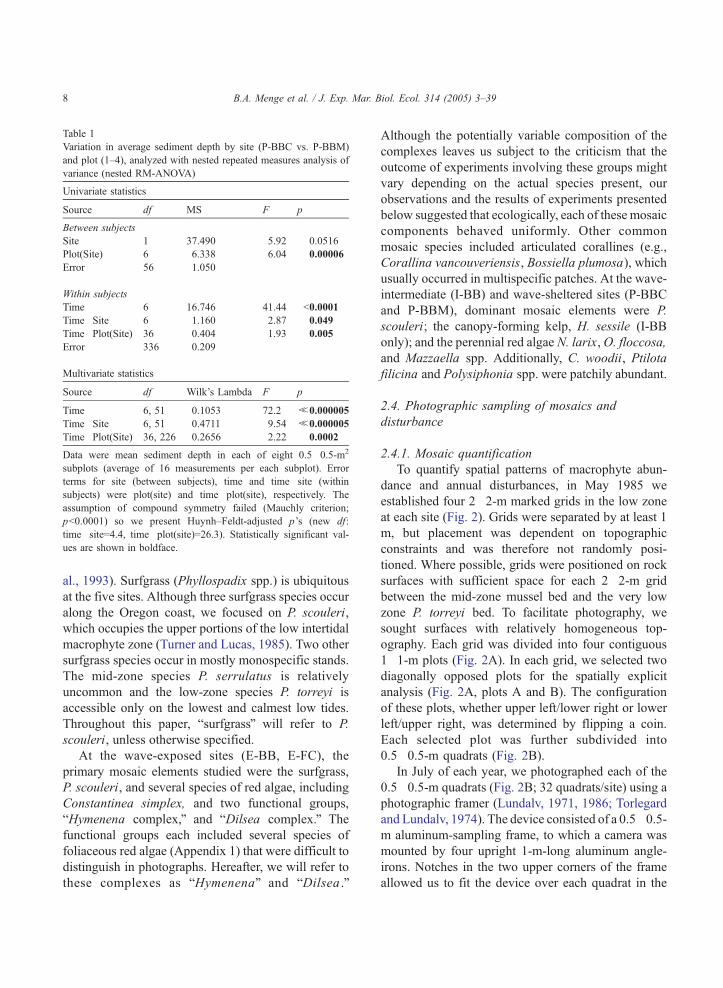
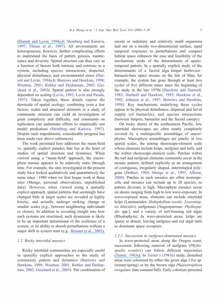
Table 1

Variation in average sediment depth by site (P-BBC vs. P-BBM)

and plot (1–4), analyzed with nested repeated measures analysis of

variance (nested RM-ANOVA)

Univariate statistics

Source df MS F p

Between subjects

Site 1 37.490 5.92 0.0516

Plot(Site) 6 6.338 6.04 0.00006

Error 56 1.050

Within subjects

Time 6 16.746 41.44 b0.0001

Time�Site 6 1.160 2.87 0.049

Time�Plot(Site) 36 0.404 1.93 0.005

Error 336 0.209

Multivariate statistics

Source df Wilk’s Lambda F p

Time 6, 51 0.1053 72.2 b0.000005

Time�Site 6, 51 0.4711 9.54 b0.000005

Time�Plot(Site) 36, 226 0.2656 2.22 0.0002

Data were mean sediment depth in each of eight 0.5�0.5-m2

subplots (average of 16 measurements per each subplot). Error

terms for site (between subjects), time and time�site (within

subjects) were plot(site) and time�plot(site), respectively. The

assumption of compound symmetry failed (Mauchly criterion;

pb0.0001) so we present Huynh–Feldt-adjusted p’s (new df:

time�site=4.4, time�plot(site)=26.3). Statistically significant val-

ues are shown in boldface.

B.A. Menge et al. / J. Exp. Mar. Biol. Ecol. 314 (2005) 3–398

al., 1993). Surfgrass (Phyllospadix spp.) is ubiquitous

at the five sites. Although three surfgrass species occur

along the Oregon coast, we focused on P. scouleri,

which occupies the upper portions of the low intertidal

macrophyte zone (Turner and Lucas, 1985). Two other

surfgrass species occur in mostly monospecific stands.

The mid-zone species P. serrulatus is relatively

uncommon and the low-zone species P. torreyi is

accessible only on the lowest and calmest low tides.

Throughout this paper, bsurfgrassQ will refer to P.

scouleri, unless otherwise specified.

At the wave-exposed sites (E-BB, E-FC), the

primary mosaic elements studied were the surfgrass,

P. scouleri, and several species of red algae, including

Constantinea simplex, and two functional groups,

bHymenena complex,Q and bDilsea complex.Q The

functional groups each included several species of

foliaceous red algae (Appendix 1) that were difficult to

distinguish in photographs. Hereafter, we will refer to

these complexes as bHymenenaQ and bDilsea .Q

Although the potentially variable composition of the

complexes leaves us subject to the criticism that the

outcome of experiments involving these groups might

vary depending on the actual species present, our

observations and the results of experiments presented

below suggested that ecologically, each of these mosaic

components behaved uniformly. Other common

mosaic species included articulated corallines (e.g.,

Corallina vancouveriensis, Bossiella plumosa), which

usually occurred in multispecific patches. At the wave-

intermediate (I-BB) and wave-sheltered sites (P-BBC

and P-BBM), dominant mosaic elements were P.

scouleri; the canopy-forming kelp, H. sessile (I-BB

only); and the perennial red algae N. larix,O. floccosa,

and Mazzaella spp. Additionally, C. woodii, Ptilota

filicina and Polysiphonia spp. were patchily abundant.

2.4. Photographic sampling of mosaics and

disturbance

2.4.1. Mosaic quantification

To quantify spatial patterns of macrophyte abun-

dance and annual disturbances, in May 1985 we

established four 2�2-m marked grids in the low zone

at each site (Fig. 2). Grids were separated by at least 1

m, but placement was dependent on topographic

constraints and was therefore not randomly posi-

tioned. Where possible, grids were positioned on rock

surfaces with sufficient space for each 2�2-m grid

between the mid-zone mussel bed and the very low

zone P. torreyi bed. To facilitate photography, we

sought surfaces with relatively homogeneous top-

ography. Each grid was divided into four contiguous

1�1-m plots (Fig. 2A). In each grid, we selected two

diagonally opposed plots for the spatially explicit

analysis (Fig. 2A, plots A and B). The configuration

of these plots, whether upper left/lower right or lower

left/upper right, was determined by flipping a coin.

Each selected plot was further subdivided into

0.5�0.5-m quadrats (Fig. 2B).

In July of each year, we photographed each of the

0.5�0.5-m quadrats (Fig. 2B; 32 quadrats/site) using a

photographic framer (Lundalv, 1971, 1986; Torlegard

and Lundalv, 1974). The device consisted of a 0.5�0.5-

m aluminum-sampling frame, to which a camera was

mounted by four upright 1-m-long aluminum angle-

irons. Notches in the two upper corners of the frame

allowed us to fit the device over each quadrat in the

Page 7

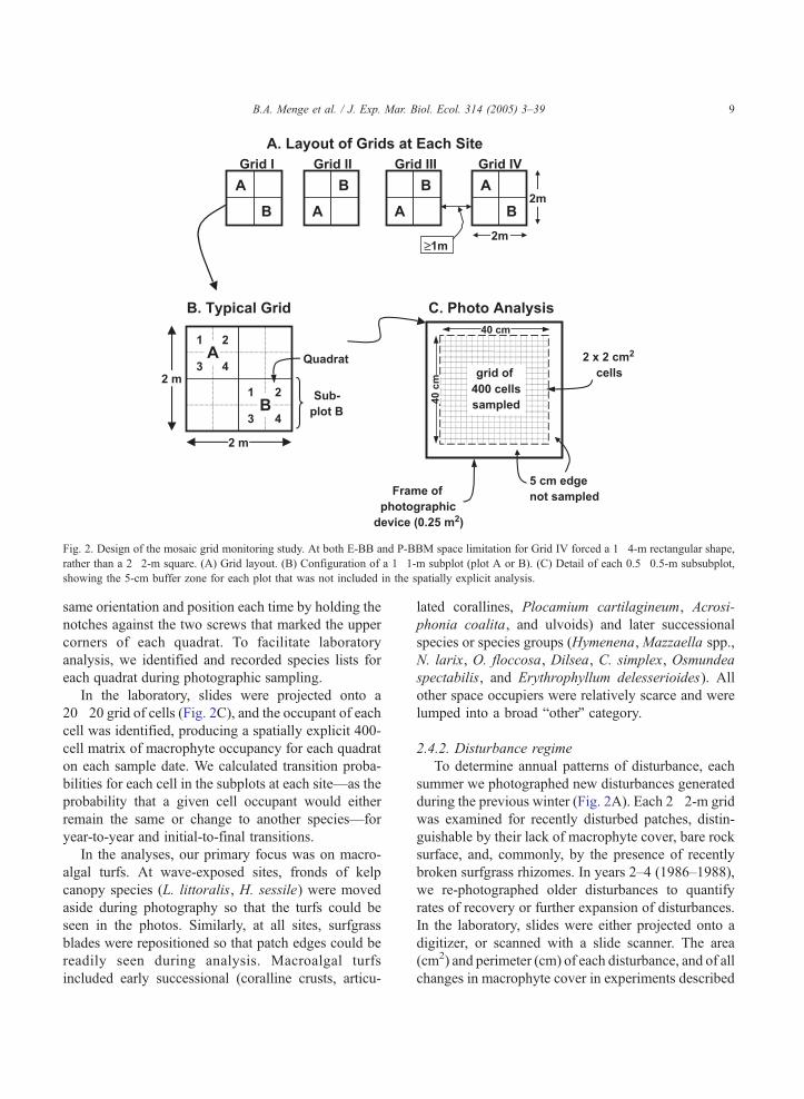
Fig. 2. Design of the mosaic grid monitoring study. At both E-BB and P-BBM space limitation for Grid IV forced a 1�4-m rectangular shape,

rather than a 2�2-m square. (A) Grid layout. (B) Configuration of a 1�1-m subplot (plot A or B). (C) Detail of each 0.5�0.5-m subsubplot,

showing the 5-cm buffer zone for each plot that was not included in the spatially explicit analysis.

B.A. Menge et al. / J. Exp. Mar. Biol. Ecol. 314 (2005) 3–39 9

same orientation and position each time by holding the

notches against the two screws that marked the upper

corners of each quadrat. To facilitate laboratory

analysis, we identified and recorded species lists for

each quadrat during photographic sampling.

In the laboratory, slides were projected onto a

20�20 grid of cells (Fig. 2C), and the occupant of each

cell was identified, producing a spatially explicit 400-

cell matrix of macrophyte occupancy for each quadrat

on each sample date. We calculated transition proba-

bilities for each cell in the subplots at each site—as the

probability that a given cell occupant would either

remain the same or change to another species—for

year-to-year and initial-to-final transitions.

In the analyses, our primary focus was on macro-

algal turfs. At wave-exposed sites, fronds of kelp

canopy species (L. littoralis, H. sessile) were moved

aside during photography so that the turfs could be

seen in the photos. Similarly, at all sites, surfgrass

blades were repositioned so that patch edges could be

readily seen during analysis. Macroalgal turfs

included early successional (coralline crusts, articu-

lated corallines, Plocamium cartilagineum, Acrosi-

phonia coalita, and ulvoids) and later successional

species or species groups (Hymenena,Mazzaella spp.,

N. larix, O. floccosa, Dilsea, C. simplex, Osmundea

spectabilis, and Erythrophyllum delesserioides). All

other space occupiers were relatively scarce and were

lumped into a broad botherQ category.

2.4.2. Disturbance regime

To determine annual patterns of disturbance, each

summer we photographed new disturbances generated

during the previous winter (Fig. 2A). Each 2�2-m grid

was examined for recently disturbed patches, distin-

guishable by their lack of macrophyte cover, bare rock

surface, and, commonly, by the presence of recently

broken surfgrass rhizomes. In years 2–4 (1986–1988),

we re-photographed older disturbances to quantify

rates of recovery or further expansion of disturbances.

In the laboratory, slides were either projected onto a

digitizer, or scanned with a slide scanner. The area

(cm2) and perimeter (cm) of each disturbance, and of all

changes in macrophyte cover in experiments described

Page 8

B.A. Menge et al. / J. Exp. Mar. Biol. Ecol. 314 (2005) 3–3910

below, was estimated using computer software (either

SigmaScanR, or NIH ImageR). Disturbances were

classified relative to their original size as expanding

(larger area) or recovering (smaller area).

2.5. Effect of biotic interactions on between-patch

boundaries

Experiments were run to understand how themosaic

pattern was maintained, with a focus on factors

affecting changes at the edges of mosaic patches (Fig.

3). For example, competition for space or facilitation or

selective grazing by macro-herbivores (limpets, chi-

tons, sea urchins) could control changes in between-

patch boundaries. Unfortunately, limited numbers of

appropriate boundaries prevented simultaneous tests of

the effects of neighbors and grazers.

2.5.1. Grazing effect

Macro-herbivore fence-exclosure experiments at

E-BB tested the hypothesis that grazing influences

Fig. 3. Design of the competition and grazing experiments. In the competit

competitors present; +A +B) and twomanual removals of either competitor (

on either side of the patch boundary. At E-BB, spatial interactions between t

Phyllospadix vs. Constantinea, Phyllospadix vs. bDilsea,Q Constantine

bHymenena.QAt P-BBM, spatial interactions between three pairs were tested

Odonthalia (five replicates), and Neorhodomela vs. Odonthalia (five replic

plots: a reference (both competitors present and grazers present with no fen

grazers present with a partial fence; +A +B/+G+fence), and a grazer exclusio

+A +B/�G+fence). Two pairs were tested: Phyllospadix vs. bDilseaQ and Phfrom the wave-sheltered surfgrass beds and working time was limited at w

between-patch boundaries at wave-exposed sites

(similar tests at wave-protected sites were precluded

by the near-absence of herbivores within the mosaic at

these sites; Fig. 3). Two species pairs were inves-

tigated: P. scouleri vs. C. simplex and P. scouleri vs.

Dilsea. Plots (15�30 cm) were centered on between-

patch boundaries and subjected to three treatments:

the bnormalQ situation (+Grazers �Fence), a partial

fence control for inadvertent effects of exclosures

(+Grazers +Fence), and an exclusion fence (�Grazers

+Fence). Screws marked a 15-cm border along the

boundary, and the four corners of the plot, forming

adjacent contiguous marked squares extending 15 cm

into each patch. Stainless steel fences were seven cm

high and fastened to the rock using stainless steel

screws. During biweekly to monthly monitoring

visits, the few herbivores invading the exclosures

were removed. The experiments were monitored

photographically in July, November, and December

1985, March and July 1986, June 1987 and July

1988. The response variable was the change in the

ion experiment, each replicate included three plots: a reference (both

�A+B and +A�B). Dots indicate position of marking screws on, and

he following five pairs, all with four replicates each, were established:

a vs. bDilsea,Q Constantinea vs. bHymenena,Q and bDilseaQ vs.

: Phyllospadix vs. Neorhodomela (eight replicates), Phyllospadix vs.

ates). In the grazing experiment, each of four replicates included three

ce; +A +B/+G�fence), a fence control (both competitors present and

n (both competitors present and grazers absent with a complete fence;

yllospadix vs. Constantinea. Because grazers were essentially absent

ave-exposed sites, the grazing experiment was done only at E-BB.

Page 9

B.A. Menge et al. / J. Exp. Mar. Biol. Ecol. 314 (2005) 3–39 11

distance moved towards the neighbor in centimeter

(average of three evenly spaced measurements) along

the boundary between patches.

2.5.2. Spatial interactions among established patches

We established spatial interaction experiments at

E-BB and P-BBM to test the effects of interactions

between neighbors (Fig. 3). At E-BB, we investigated

five sets of pairwise spatial interactions, each repli-

cated four times; P. scouleri vs. C. simplex, P. scouleri

vs. Dilsea, C. simplex vs. Dilsea, C. simplex vs.

Hymenena, and Dilsea vs. Hymenena. Three sets of

pairwise interactions were studied at P-BBM; P.

scouleri vs. N. larix (eight replicates), P. scouleri vs.

O. floccosa (five replicates), and N. larix vs. O.

floccosa (five replicates). Insufficient numbers of other

species pairings were available for experimentation.

As in the macrograzer experiments, replicates

were three rectangular plots (15�30 cm) centered

over the boundary between two adjacent patches

(Fig. 3). For patch species bAQ and bB,Q the three

treatments were both species present (+A +B),

species A present/species B absent (removed with

scrapers; +A �B), and species A absent/species B

present (�A +B). Cleared space not covered by the

advancing neighbor was periodically re-scraped,

approximately seasonally in fall and winter, and

somewhat more often in spring and summer. The E-

BB experiment was monitored on the same dates as

the herbivore-effect experiments. P-BBM experi-

ments were photographed in July and December

1985, March and July 1986, May 1987 and May

1988.

2.5.3. Recruit–adult interactions: Phyllospadix vs.

Neorhodomela

Space at all wave-intermediate and wave-protected

locations was dominated by surfgrass and the red alga

N. larix. Since the spatial interaction experiments

suggested that both competition and facilitation could

be important in mediating interactions among estab-

lished mosaic elements, we tested the impact of these

factors on the establishment of these two dominants.

Prior studies (Turner, 1983b) had shown that

recruitment of P. scouleri is facilitated by certain

macroalgae (such as N. larix) having a central axis ~1

mm in diameter to which the hooked surfgrass seeds

can attach. N. larix should thus positively influence

surfgrass recruits. The reciprocal effect, of resident

surfgrass on colonization of N. larix was unstudied,

although a prior investigation showed that N. larix

recruitment rates were very low (Menge et al., 1993).

Hence, the high abundance of N. larix seemed most

likely maintained by lateral vegetative spread of the

basal holdfast system of this alga.

We established reciprocal recruit–adult experi-

ments to determine either if N. larix recruits could

increase in abundance in the presence of resident

surfgrass, or if surfgrass recruits could increase in the

presence of resident N. larix. We defined N. larix

recruits as clumps of 1–5 thalli (~2–10 cm2 in area)

surrounded by (bresidentQ) P. scouleri, and defined P.

scouleri recruits as plants of one or few blades

growing out of seeds attached to the surrounding

(bresidentQ) N. larix. Nine replicate pairs of N. larix

recruits and ten replicate pairs of P. scouleri recruits

(five each at the upper and lower edges of the low

zone) were marked with three stainless steel screws

arranged in a triangle around each recruit. Treatment

pairs were +recruit +resident, and +recruit �resident,

assigned using a coin flip. Encroaching residents were

removed periodically to maintain the �resident treat-

ment. Experiments were established at I-BB in August

1987, and were monitored photographically in

August, September and November 1987 and January,

May and August 1988.

2.6. Data analysis

Data were analyzed using SYSTAT statistical

software (version 10; SPSS) and JMP (SAS) on an

IBM-compatible PC. Linear regression was used to

determine the relationship between abundance of

species in the marked plots in successive years.

Calculation of transition probabilities was determined

using a program written in Pascal. The effects of

wave exposure and year on the disturbance regime,

including disturbance density, mean disturbance area,

total proportion of each plot disturbed, perimeter/area

ratio, and departure from circularity, was analyzed

using two-way analysis of variance (ANOVA) for

each component. We used linear contrasts to make

pairwise comparisons, and for calculation of estimates

for use in determining effect sizes. In this and all

other analyses, we examined probability plots of

studentized residuals and plots of studentized resid-

Page 10

B.A. Menge et al. / J. Exp. Mar. Biol. Ecol. 314 (2005) 3–3912

uals against estimated values, respectively, to deter-

mine if residuals were normally distributed and if

errors were independent (Wilkinson, 1998). These

assumptions were met in most cases after trans-

formation (log10 or ln(x+1) for areas, densities or

ratios and arcsin[square root] for percent cover and

proportional data). Where assumptions were not met

even after transformation, probabilities were highly

significant indicating that the analysis was probably

reliable (Underwood, 1981). Cochran’s C test was

used to test the assumption of equality of variances

(Winer et al., 1991).

Because the residuals in regression analysis

between initial disturbance area and percent recovery

in the first year were not normal or independent, even

with transformation, we analyzed recovery rates of

disturbed patches using log-linear model analysis

(Ramsey and Schafer, 1997; Quinn and Keough,

2002). The analysis was performed on counts of

disturbances categorized by their rates of recovery

(b50%, 51–90% and N90% recovery in the year

following disturbance), initial area (b500 and N500

cm2) and wave exposure (exposed, intermediate,

protected). In contrast, analysis of rates of expansion

of disturbed patches satisfied assumptions of normal-

ity and independence, so we employed analysis of

covariance, with initial area as the covariate. Linear

regression was used to establish the relationship

between initial disturbance area and percent recovery

or percent expansion after 1 year.

Variation in sediment depth by plot nested within

the wave-protected sites was analyzed using nested

repeated measures analysis of variance (nested RM-

ANOVA), because measurements were taken repeat-

edly on the same grid of points in each plot. The

effects of height on the shore and presence of

competition on recruit growth for surfgrass, and the

effect of competition on recruit growth for N. larix

were tested using two-way or one-way RM-ANOVA,

respectively. We used the Mauchly Criterion to

evaluate the multivariate assumption of compound

symmetry in RM-ANOVA (Crowder and Hand,

1990), and adjusted the critical value by reducing

the degrees of freedom by multiplying by the

Huynh–Feldt E (b1.0). Finally, the effects of macro-

grazers on between-patch boundaries and of com-

petitors on growth of surfgrass and its competitors

were all tested using one-way ANOVA.

3. Results

3.1. Mosaic structure: diversity and abundance

The taxon richness and abundance of mosaic

elements (defined as P. scouleri, bare rock, and the

different bearlyQ and blateQ successional algal groups)remained remarkably constant through time, but

varied among sites. P. scouleri dominated at all sites

(Fig. 4A–C), but diversity (richness) of other mosaic

elements declined across the wave-exposure gradient

from 13 to 10 elements/site (an average of 6.3 to 4.3

elements/plot, Appendix 1), reflecting an almost

complete turnover of algal groups. Within sites,

however, total macrophyte abundance and composi-

tion were comparatively constant through time and

similar at a given wave-exposure.

Surfgrass was the dominant space occupant at all

five sites over the entire study period (Fig. 4A–C).

Mean surface area covered by P. scouleri ranged from

~34% (E-BB, 1989) to ~62% (P-BBM, 1989).

Surfgrass cover varied little through time, with annual

means differing by only 10% to 20% (39–49% at P-

BBC; ~37–57% at I-BB, respectively). These inter-

annual fluctuations exhibited no obvious synchrony

among sites. Years of minimum and maximum mean

cover by site were 1989 and 1986 (E-BB), 1987 and

1990 (E-FC), 1985 and 1990 (I-BB), 1985 and 1989 (P-

BBC), and 1990 and 1989 (P-BBM).

Among the other elements of the mosaic, early

successional elements were relatively minor compo-

nents of the mosaic, with average total abundances

varying from 0% to 8.1%. Early elements are those

that typically regrow rapidly upon release from

shading (crustose and articulated coralline algae) or

rapidly re-colonize (P. cartilagineum, P. filicina, A.

coalita, ulvoids) following disturbance. Their cover

and that of bare rock was low, but relatively constant

through time, suggesting a low rate of disturbance

(also see direct measures of disturbance in Section

3.3). Coralline algae were abundant only at wave-

exposed sites, while cover of P. cartilagineum was

intermediate at wave-exposed sites (E-BB, E-FC) and

highest at the most wave-protected site (P-BBM).

Later successional elements were frequently co-

dominant with P. scouleri, maintaining relatively

constant cover within a given site over time. Their

composition, however, varied markedly among sites.

Page 11

Fig. 4. Abundance (percent cover) of the most common macrophyte mosaic elements at (A) two wave exposed sites, Exposed Boiler Bay (E-BB,

A) and Exposed Fogarty Creek (E-FC, B), (B) the site of intermediate wave exposure, Intermediate Boiler Bay (I-BB), and (C) two wave-

protected sites, Protected Boiler Bay Cove (P-BBC and Protected Boiler Bay Mudstone (P-BBM), from 1985 to 1990. Data are mean cover per

m2+1 S.E. Because each 1�1-m plot is separated from the others by a 10-cm buffer that was not included in the analysis (see Fig. 1C), we consider

each subplot an independent replicate with n=8. Late successional species are grouped on the right in the shaded portion.

B.A. Menge et al. / J. Exp. Mar. Biol. Ecol. 314 (2005) 3–39 13

Page 12

B.A. Menge et al. / J. Exp. Mar. Biol. Ecol. 314 (2005) 3–3914

For example, the turf-forming elements (Hymenena,

Dilsea, C. simplex, O. spectabilis) were important

only at the more wave-exposed sites. In contrast, the

branched red algae N. larix and O. floccosa were

absent from wave-exposed sites, but were strong co-

dominants at intermediate and protected sites. The red

blade macroalga Mazzaella spp., occurred at all sites,

but reached its highest abundance at the intermediate

(I-BB) and one protected (P-BBC) site. The canopy-

forming kelps, L. littoralis and H. sessile, were

common subdominants at only one site each (E-BB

and I-BB, respectively).

These data confirmed our impression, gained

over the previous 5 years that patterns of relative

abundance of the different components of the

macrophyte mosaic are relatively static through

time, but vary with wave-exposure. At each site,

comparison of the abundances (proportional cover)

of each component in year t to that in year t+1

Fig. 5. Scatterplots of the proportion of cover of each mosaic element in

comparisons are shown in the left five columns (e.g., 1985 vs. 1986, 1986 v

and final cover. Site code is as indicated in Fig. 3 captions. Coefficients

suggests only modest inter-annual shifts in abun-

dance in successive years (Fig. 5; 21 of 25

coefficients of determination, r2’s, were N0.85).

Longer-term (1985–1990) comparisons reveal larger

proportionate changes than do year-to-year compar-

isons (all five r2’s were b0.78), although final

abundances were still quite similar to initial

abundances.

Examination of time-series photos dispels the

notion of a relatively static or unchanging commun-

ity. For example, at E-BB and P-BBM, both annual

and longer-term (6 years) changes were generally

substantial (Figs. 6 and 7). Surfgrass patches in

particular tended to shift positions in the plots, both

advancing over neighboring turfs, and retreating

from or abandoning space previously occupied.

Species also came and went over time. Thus,

spatially explicit observations suggested a level of

dynamism that would have been missed had we

year x (abscissa) vs. its cover in year x+1 (ordinate). Year-by-year

s. 1987, etc.); the right column shows the comparison between initial

of determination (r2) are shown for each comparison.

Page 13

B.A. Menge et al. / J. Exp. Mar. Biol. Ecol. 314 (2005) 3–39 15

analyzed temporal changes in mosaic structure using

average percent cover.

3.2. Mosaic structure: spatially explicit analysis

Analysis of transition probabilities was consistent

with the high degree of constancy in composition

over time at all five sites (Fig. 8A–C). P. scouleri was

the most abundant single species, and total abun-

dance of late-successional macroalgae also

approached that of P. scouleri at some sites. Surfgrass

and other late-successional elements retained most of

the space from 1 year to the next, and P. scouleri was

as likely to be replaced by one of the late elements

Fig. 6. Time series of annual photos (taken in July) of the same plot at a w

(green) in the upper left in 1985 moves toward the lower right corner in 198

1987, moves rightward (right half of clump) or remains stationary (left hal

the upper left (right half) in 1989 and moves toward the lower right corner a

(upper right), Constantinea, Dilsea, and Plocamium. The kelp Lessoniopsis

to 1990. Another Lessoniopsis expands into the plot from below starting in

presumably has grazed down to the underlying coralline crust in the upper

visible in the lower center in 1988.

(primarily Lessoniopsis; see following paragraph), as

it was to replace them. Spatial extent of disturbance

as coarsely indicated by change from any mosaic

category to early-successional elements (second

column in all panels) appeared to be low but nearly

constant at all sites. By this measure, late succes-

sional algae were as likely as surfgrass to be replaced

by early elements. Recovery from disturbance,

coarsely indicated by change from early successional

elements to surfgrass or later successional elements

(second row in all panels), was higher at exposed

than at intermediate or protected sites (but see

Section 3.3 for a more detailed analysis). In sum, at

the scale of functional groups, the successional

ave-exposed site (E-BB) from 1985 to 1990. The clump of surfgrass

6, moves further toward the lower right corner and splits into two in

f) in 1988, moves largely out of the frame (left half) or back toward

gain in 1990. Other species showing shifts in position are Hymenena

invades from the top in 1987 and expands downward and rightward

1985. A chiton, Katharina tunicata appears in a small gap, which it

right corner in 1990. An anemone Anthopleura xanthogrammica is

Page 14

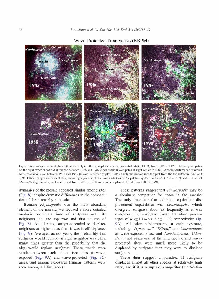
Fig. 7. Time series of annual photos (taken in July) of the same plot at a wave-protected site (P-BBM) from 1985 to 1990. The surfgrass patch

on the right experienced a disturbance between 1986 and 1987 (seen as the ulvoid patch at right center in 1987). Another disturbance removed

some Neorhodomela between 1988 and 1989 (ulvoid in center of plot, 1989). Surfgrass moved into the plot from the top between 1988 and

1990. Other changes are evident also, including replacement of ulvoid and Odonthalia patches by Neorhodomela (1985–1987), and invasion of

Mazzaella (right center; replaced ulvoid from 1987 to 1988 and center, replaced ulvoid from 1989 to 1990).

B.A. Menge et al. / J. Exp. Mar. Biol. Ecol. 314 (2005) 3–3916

dynamics of the mosaic appeared similar among sites

(Fig. 8), despite dramatic differences in the composi-

tion of the macrophyte mosaic.

Because Phyllospadix was the most abundant

element of the mosaic, we focused a more detailed

analysis on interactions of surfgrass with its

neighbors (i.e. the top row and first column of

Fig. 8). At all sites, surfgrass tended to displace

neighbors at higher rates than it was itself displaced

(Fig. 9). Averaged across years, the probability that

surfgrass would replace an algal neighbor was often

many times greater than the probability that the

alga would replace surfgrass. These trends were

similar between each of the two sites at wave-

exposed (Fig. 9A) and wave-protected (Fig. 9C)

areas, and among exposures (similar patterns were

seen among all five sites).

These patterns suggest that Phyllospadix may be

a dominant competitor for space in the mosaic.

The only interactor that exhibited equivalent dis-

placement capabilities was Lessoniopsis, which

overgrew surfgrass about as frequently as it was

overgrown by surfgrass (mean transition percen-

tages of 8.3F1.1% vs. 8.8F1.1%, respectively; Fig.

9A). All other subdominants at each exposure,

including bHymenena,Q bDilsea,Q and Constantinea

at wave-exposed sites, and Neorhodomela, Odon-

thalia and Mazzaella at the intermediate and wave-

protected sites, were much more likely to be

displaced by surfgrass than they were to displace

surfgrass.

These data suggest a paradox. If surfgrass

displaces almost all other species at relatively high

rates, and if it is a superior competitor (see Section

Page 15

Fig. 8. Annual transition probabilities among functional groups, including surfgrass (bPhyllospadixQ), early and late successional species, and allother space occupants aggregated (botherQ). Categories from which the change occurs are listed on the ordinate, categories to which the change

occurs are listed on the abscissa. All probabilities total to 1.0 in each year at each site. Persistence (i.e., no change) is the most frequent

btransitionQ at all sites. The focus of our analysis was on the transitions involving change.

B.A. Menge et al. / J. Exp. Mar. Biol. Ecol. 314 (2005) 3–39 17

3.4.1) why does not it eliminate them? As detailed

below, the answer lies in changes in susceptibility to

disturbance and competitive ability of surfgrass along

the wave-exposure gradient: both are high at wave-

exposed sites and low at wave-protected sites.

3.3. Disturbance regime

Physical disturbance is evidently the primary

deterrent to the potential dominance of Phyllospadix,

especially at wave-exposed sites. Examination of the

Page 16

Fig. 9. Annual transition probabilities (mean+1 S.E. of per-plot means, averaged across years) for the main components of the macrophyte

matrix, focusing on transitions involving Phyllospadix (i.e., surfgrass overgrowing other species and other species overgrowing surfgrass). Most

change involves surfgrass overgrowing its neighbors.

B.A. Menge et al. / J. Exp. Mar. Biol. Ecol. 314 (2005) 3–3918

Page 17

Fig. 10. Size frequency of disturbances by site, totalled over 1985–

1990 (n is the total number of disturbances for each site). The

majority of disturbances at wave-protected sites were small (0–99.9

cm2); those at wave-exposed sites were larger on average, with the

most frequent size in the next-to-smallest category (100–199.9 cm2).

Fig. 11. Components of the disturbance regime, including per year (A) den

4m2 plot disturbed, (D) variation in shape as indicated by perimeter/area rat

perimeter/perimeter of a circle. All data are mean+1 S.E.

B.A. Menge et al. / J. Exp. Mar. Biol. Ecol. 314 (2005) 3–39 19

edges of surfgrass patches frequently revealed

rhizomes that had been broken along segments of

the edge. Further, surfaces next to these areas of

broken rhizomes were often bare, covered with

encrusting coralline algae, or occupied by algal

species that are known to be rapid colonizers of

vacated space. Rapid colonizers include ulvoids,

diatoms, and various species of red and brown algae

(see description of botherQ category under Section

3.1). These clear markers of disturbance allowed us

to quantify the disturbance regime as described in

Methods. This analysis also aimed at understanding

another seeming paradox. What was the cause of

disturbances in wave-protected areas where the

magnitude of wave turbulence is very much less than

at wave-exposed areas?

Most disturbances were small (b200 cm2) in area

(Fig. 10), although they occasionally reached much

larger sizes (maximum sizes: E-BB, 1876 cm2; E-FC,

3310 cm2; I-BB, 1598 cm2; P-BBC, 26,418 cm2; P-

BBM 6169 cm2). Disturbance size frequencies varied

sity (number/4 m2), (B) area (cm2), (C) percent of total area of each

ios, and (E) departure from circularity as indicated by ratios of actual

Page 18

B.A. Menge et al. / J. Exp. Mar. Biol. Ecol. 314 (2005) 3–3920

with wave-exposure (Fig. 10). At wave-exposed sites,

disturbances 100–200 cm2 were most numerous,

while at the intermediate and wave-protected sites,

disturbances 0–100 cm2 were most common. Further,

wave-exposed sites tended to have more disturbances

at intermediate size ranges (200–1000 cm2) while

wave-protected sites tended to have more very large

disturbances (N4000 cm2).

Disturbance regimes varied substantially in space

and time (Fig. 11). The number of disturbances per

year/plot, or rate of disturbance, varied with wave

exposure and year (Table 2A, wave exposure�year

interaction term; p=0.048). Overall, the rate of

Table 2

Effect of year and wave-exposure on disturbance regime

Disturbance metric Source of variation df MS F P

(A) Disturbance

density (no./plot)

Wave exposure 2 1.473 16.0 b0.00

Year 4 1.240 13.5 b0.00

Wave exposure�year 8 0.192 2.08 0.04

Error 78 0.092

(B) Mean disturbance

area

Wave exposure 2 0.866 9.23 0.00

Year 4 0.877 9.34 b0.00

Wave exposure�year 8 0.179 1.91 0.07

Error 78 0.094

(C) Proportion of plot

disturbed

Wave exposure 2 0.060 2.64 0.08

Year 4 0.149 6.54 0.00

Wave exposure�year 8 0.027 1.20 0.31

Error 85 0.023

(D) Shape variation

(perimeter/area)

Wave exposure 2 0.191 14.3 b0.00

Year 4 0.223 16.8 b0.00

Wave exposure�year 8 0.144 10.8 b0.00

Error 78 0.013

(E) Departure from

circularity

Wave exposure 2 0.004 1.70 0.2

Year 4 0.095 40.3 b0.00

Wave exposure�year 8 0.003 1.16 0.34

Error 78 0.002

Pairwise comparisons on main effects (by wave exposure with years com

contrasts. E=exposed; I=intermediate; P=protected. Lines in pairwise co

magnitude with largest values listed first. When a factor was statistically sig

wave exposure comparisons and for comparisons between the largest

Disturbance density, mean area, shape variation, and departure from circula

and CVof disturbance area were arcsin-transformed. Cochran’s C test (Win

transformation except for the proportion of the plots disturbed. Significa

analysis because no data were available from P-BBC and P-BBM.

generation of disturbances at wave-protected sites

was 2.5� (95% confidence interval: 1.8� to 3.3�) the

rate at wave-exposed sites, and 1.8� (1.2� to 2.5�)

the rate at the intermediate site (Table 2A, effect size).

Disturbance rate varied among years (rank order:

86N87N88N90N85). Rates in 1986 (highest rate) were

4.6� (2.9� to 7.2�) those in 1985 (lowest rate).

Disturbance size (mean area in cm2) also varied

with wave exposure and year (Table 2B, main effects;

wave exposure p=0.0003, year pb0.0001). As sug-

gested by the size frequency patterns (Fig. 10), mean

disturbance size at wave-exposed sites was 2.3�(1.6� to 3.3�) larger than at the intermediate site and

R2 Pairwise comparisons Effect size (95% CI)

01 0.58 PNI=E PNE: 2.5� (1.8� to 3.3�)

PNI: 1.8� (1.2� to 2.5�)

01 86N85: 4.6� (2.9� to 7.2�)

8

03 0.50 ENI=P ENI: 2.3� (1.6� to 3.3�)

ENP: 1.6� (1.2� to 2.2�)

01 88N90: 4.0� (2.5� to 6.2�)

0.36

01 87N85: 12.2� (5.2� to 22.2�)

01 0.71 P=INE PNE: 1.36� (1.22 to 1.52)

INE: 1.34� (1.17� to 1.54�)

01 87N88: 2.0� (1.69� to 2.36�)

01

0.71

01 88N90: 1.49� (1.39� to 1.6�)

bined, by year with exposures combined) were made using linear

mparisons overlap levels that do not differ; levels are ordered by

nificant, effect size and 95% confidence intervals were calculated for

and smallest annual values using estimates from linear contrasts.

rity were log10-transformed, and the proportion of the plots disturbed

er et al., 1991) indicated that all variances were homoscedastic after

nt values are shown in boldface. 1989 data were dropped from the

Page 19

B.A. Menge et al. / J. Exp. Mar. Biol. Ecol. 314 (2005) 3–39 21

1.6� (1.2� to 2.2�) larger than at the wave-protected

sites (Table 2B, effect size). The largest average

disturbance sizes occurred at E-BB in 1987 and 1988

and at E-FC in 1988 (Fig. 11B). Disturbance size

variation across years, by rank, was 88N86N87N

85N90, and 1988 disturbances (the largest) were

4.0� (2.5� to 6.2�) larger than 1990 disturbance

(the smallest) (Table 2B, linear contrasts and effect

sizes). Note that in 1987 at P-BBM, the site�year

combination with the highest observed rate of

disturbance, average disturbance size was relatively

small, around 200 cm2. In contrast, in 1988 at E-FC,

the site�year combination with the largest disturban-

ces, the rate of disturbance was relatively small, about

seven per plot (Fig. 11A,B).

The percent of the total area of the plot disturbed

can serve as an indication of the relative extensiveness

of the damage from disturbance. The extensiveness of

disturbance damage varied strikingly among years,

but not among wave-exposures (Fig. 11C, Table 2C).

As suggested by the patterns of disturbance rate and

size, the most extensive loss was in 1987 and 1988

(rank order: 87N88N86N90N85). Percent damage in

1987 (highest level) was 12.2� (2.2� to 22.2�)

greater than in 1985 (lowest level).

Disturbed patches were typically ovoid in shape,

but in some years shape varied dramatically, including

Fig. 12. Recovery from disturbance (i.e., rate of return to surfgrass) during

reference, approximate actual area (non-transformed) of initial disturba

approximate percent (non-transformed) recovery is shown on the right ord

extensive lobes with corridor-like attachments. We

examined this pattern by calculating the ratio of

perimeter to area (P/A ratio) and an index of the extent

to which the disturbances departed from a circular

shape independent of area (the ratio of the actual

perimeter to the perimeter of a circle of the same area)

(Fig. 11D,E). Shape variation varied greatly with

wave exposure and year (Table 2D, wave exposure�year interaction). Thus, shape varied little through

time at the wave-exposed sites but at sites of low

turbulence, large P/A ratios occurred in 1987 and

1990 (Fig. 11D), suggesting that at low turbulence

sites (intermediate and wave-protected) disturbances

tended to be more irregular in shape. This comparison

is confounded, however, by the fact that mean

disturbance size was greater at wave-exposed sites

than at the intermediate and wave-protected sites

(Table 2B). If disturbance size is factored out by

examining the actual to circle perimeter ratio, shape

varied primarily through time (Table 2E, year as a

main effect: rank order, 88N87N86N85N90). Distur-

bances were more irregular during years of high

frequency, size, and proportion disturbed (1986–1988)

and more circular in years of low overall disturbance

(1985, 1990) (Fig. 11E, Table 2E; linear contrasts).

Disturbance shape ratios in 1988 were 1.5� (1.4� to

1.6�) larger (more irregular) than those in 1990.

the first post-disturbance year by wave-exposure, 1986–1988. For

nce is shown at intervals in parentheses along the abscissa and

inate. Each symbol represents one disturbance.

Page 20

B.A. Menge et al. / J. Exp. Mar. Biol. Ecol. 314 (2005) 3–3922

3.3.1. Recovery from disturbance

As suggested by a plot of initial area vs. percent

recovery in the first year (Fig. 12), disturbances

recovered differentially by exposure and initial size

(Table 3; log-linear model analysis; likelihood-ratio

v2=31.0, 8 df , pb0.0001). Large (N500 cm2)

disturbances recovered at a disproportionately higher

rate at wave-exposed sites than did those at wave-

protected sites. Of the 44 wave-exposed disturban-

Table 3

Recovery and expansion of disturbances to surfgrass

(A) Recovery analysis

I. Regressions of initial disturbance area (cm2) vs. percent recovery in the

Exposure Linear regression

Wave-exposed (two sites) % recovery=1.89–0.093 (area)

Intermediate (one site) % recovery=2.34–0.197 (area)

Wave-protected (two sites) % recovery=2.50–0.275 (area)

II. Loglinear model analysis (best fit model: exposure+initial size+rate of

Observed (expected) Frequencies (number of disturbances falling in each

Exposure Initial size (cm2)

Exposed b500

N500

Intermediate b500

N500

Protected b500

N500

Statistic Value

Pearson v2 28.2

Likelihood-ratio v2 31.0

(B) Expansion analysis

I. Regressions of initial disturbance area (cm2) vs. percent expansion in t

Exposure Linear regression

Wave-exposed (two sites) % increase=9.22–0.838 (area

Intermediate (one site) % increase=9.13–0.969 (area

Wave-protected (two sites) % increase=7.86–0.796 (area

II. Analysis of covariance

Source df MS F

Exposure 2 8.620 4.58

Initial area 1 33.483 17.8

Error 69 1.881

Percent recovery data were arcsin-transformed, and initial area was ln-tra

(parallelism) was met; interactions between initial area and exposure we

p=0.96, 2, 67 df). Linear contrasts indicated that for the expansion analysi

wave-protected site, but that the intermediate site did not differ from eith

ces undergoing N90% recovery, 11 (25%) were

large, while of the 22 wave-protected disturbances

undergoing N90% recovery, 0 were large. Small

disturbances tended to recover more quickly at

wave-exposed sites as well. Of the 38 small

disturbances at wave-exposed sites, 33 (86.8%)

underwent N90% recovery while of the 53 small

disturbances at wave-protected sites, only 22

(41.5%) recovered nearly fully. The largest disturb-

following year

n p r2

58 0.025 0.087

29 0.09 0.102

57 0.0009 0.182

closure+exposure�initial size+initial size�rate)

exposure�size�rate category)

Rate of closure (% recovered/year)

b50 51–90 N90

2 (7.8) 3 (6.6) 33 (23.6)

5 (4.8) 3 (5.4) 11 (8.8)

6 (5.2) 2 (4.3) 17 (15.5)

1 (1.3) 2 (1.4) 2 (2.3)

16 (11.0) 15 (9.1) 22 (32.9)

1 (1.0) 3 (1.1) 0 (1.9)

df p

8 0.00046

8 0.00014

he following year

n p r2

) 32 0.01 0.20

) 14 0.01 0.41

) 27 0.047 0.15

p r2 Effect size

0.01 0.22 ENP: 3.3�b0.0001 (1.6� to 5.2�)

nsformed. In A and B II, the assumption of homogeneity of slopes

re not significant (A II: F=1.73, p=0.18, 2, 138 df; B II: F=0.04,

s, the regression for the wave-exposed site differed from that for the

er.

Page 21

B.A. Menge et al. / J. Exp. Mar. Biol. Ecol. 314 (2005) 3–39 23

ance to recover fully in the first year at wave-

exposed sites was 1880 cm2 in area, almost four

times larger than the largest disturbances to recover

fully at wave-protected sites (476 cm2). As

expected, disturbance recovery at the intermediate

site tended to be intermediate between recovery

rates at more and less wave-exposed sites.

3.3.2. Expansion of disturbances

When disturbances increased in size during the

second year, smaller clearances expanded proportion-

ately more than did larger ones (Fig. 13), and wave-

exposed clearances expanded at a rate 3.3� (1.6� to

5.2�) greater than wave-protected clearances (Table

3B). Thus, expansion in size of disturbances seemed

primarily to be a function of the wave-exposure

regime.

3.4. Effect of biotic interactions on patch boundaries

3.4.1. Grazer effect

In general, macrograzers are sparse in low zone

turf mosaics (Turner, 1985; Menge, personal obser-

vations), and at wave-exposed areas the main macro-

grazers in surfgrass-dominated areas were limpets

(Lottia spp.), chitons (Katharina tunicata, Tonicella

lineata), and isopods (Idotea wosnesenskii). The

most obvious evidence of a herbivore effect were

the rare occasions where a Katharina or Tonicella

could be observed residing in, and presumably

Fig. 13. Rate of further expansion of disturbances that continued to

enlarge, by wave exposure, from 1986 to 1988. Wave-exposed

disturbances (EXP, solid line) enlarged faster than did wave-

protected disturbances (PROT, dashed line).

maintaining a small clearing in the turf (see, e.g.,

the 1990 photo in Fig. 6). Nonetheless, because

abundance does not necessarily reflect impact, we

tested the effects of limpets and chitons on bounda-

ries between Phyllospadix and both Constantinea

and bDilseaQ (Fig. 14). Results after 38 months

showed that as expected, herbivores did not influence

the boundaries between these species pairings (Fig.

14; one-way ANOVA; p=0.74 and 0.45, respectively,

2, 9 df). Surfgrass overgrew its neighbors at about

the same rate in both +Grazer and �Grazer treat-

ments. Further, the presence of a stainless-steel fence

did not seem to influence this pattern. Surfgrass

growth in +Grazer +Fence and +Grazer �Fence plots

did not differ for either pairing.

3.4.2. Spatial interactions among established patches

Experiments at the wave-exposed sites yielded

results consistent with those in the spatially explicit

analyses. Surfgrass appeared to be the dominant

competitor for space among the turf species in the

mosaic. As indicated earlier, mosaic co-dominants at

the wave-exposed sites included C. simplex, bDilseaQcomplex, and bHymenenaQ complex. Thus, with

Phyllospadix, six species pairings among these taxa

were possible in pairwise border competition experi-

ments. Of these, only Phyllospadix vs. bHymenenaQwas not done due to lack of sufficient border space in

the experimental area between patches of these

species for at least four replicates.

Surfgrass grew into neighboring patches of both

bDilseaQ and Constantinea regardless of whether or

not the algal neighbor was removed (Fig. 15A,B).

During the 38-month run of the experiment, surf-

grass grew on average 20 cm (0.53 cm/month�38)

into the neighboring +bDilseaQ plot and 13 cm into

the �bDilseaQ plot, rates sufficient to fully displace

(or nearly so) all the algae in the 15�15-cm

neighboring plot. Similarly, surfgrass nearly com-

pletely displaced Constantinea as well (14.4 cm in

+Constantinea plots, 10.7 cm in �Constantinea

plots). Note that there was a trend towards slower

growth by surfgrass when its competitor was

absent, suggesting that neighbors facilitate surfgrass

overgrowth. Finally, although we were unable to

carry out experiments with the Phyllospadix–

bHymenenaQ pairing, bHymenenaQ was displaced

by surfgrass at a very high rate in the overgrowth

Page 22

Fig. 14. Results of grazing experiments at E-BB. (A) Outcome of

interaction at boundary between Phyllospadix and Constantinea

and (B) outcome of interaction at boundary between Phyllospadix

and bDilsea.Q See text and Fig. 3 for explanation of treatments.

Surfgrass overgrew its neighbors regardless of the presence or

absence of grazers or an exclosure fence.

B.A. Menge et al. / J. Exp. Mar. Biol. Ecol. 314 (2005) 3–3924

analysis using transition matrices (Fig. 9), suggest-

ing that this species was also a subordinate

competitor to Phyllospadix.

Interactions among the other wave-exposed mosaic

turf species were slower. Growth patterns in bDilseaQ–bHymenena,Q and Constantinea–bHymenenaQ inter-

actions suggested that when a neighbor is absent, the

remaining species moves into the vacated space

(Fig. 15C,D). In these two pairings, bHymenenaQtended to overgrow its neighbor when both neigh-

bors were present as well as when both neighbors

were absent, suggesting that bHymenenaQ may

dominate in competition amongst red algal turfs. In

Constantinea–bDilseaQ pairings, the interaction

appeared to be a virtual standoff (Fig. 15E). After

38 months, Constantinea had grown towards its

neighbor in both its presence and absence, but only

3 to 4 cm.

In the wave-protected experiments at P-BBM, little

change occurred at the pairwise species boundaries

regardless of the presence or absence of neighbors

(Fig. 16). Neither surfgrass nor its main co-occupants

of space, Neorhodomela and Odonthalia, grew much

in any treatment, and although surfgrass and Odon-

thalia tend to move into vacated space, the changes

were not significant. For example, in the absence of

Neorhodomela, surfgrass grew only 2.2 cm into the

vacated space in 38 months. Similarly, Odonthalia

grew only 3.7 cm into �Phyllospadix space and

surfgrass grew only 1.1 cm into �Odonthalia space.

Thus, in contrast to the wave-exposed results, where

surfgrass almost completely displaced neighbors or

fully occupied vacated space within 3+ years, macro-

phytes barely grew at the wave-protected site over the

same time interval.

3.4.3. Recruit–adult interactions: Phyllospadix vs.

Neorhodomela

The growth of surfgrass recruits (seedlings) was

affected by Neorhodomela, but the effect varied

through time (Fig. 17, Table 4, month�Neorhodomela

interaction, univariate p=0.016). At both upper and

lower levels of the low zone, Phyllospadix grew more

slowly in the presence of Neorhodomela from August

through November 1987, and then grew more rapidly

in the presence of Neorhodomela from January

through May 1988. The drop in percent cover that

occurred in August 1988, plus the slower growth in

the presence of Neorhodomela during the previous

summer to early autumn, suggests that growth of

surfgrass recruits may vary with seasonal changes in

environmental stress. Air temperatures reach a peak

during July and August, and each year since 1985 we

have observed that surfgrass bleaches and desiccates

during this time. The slower growth observed in the

upper low zone experiments (Fig. 17A, Table 4,

Height effect, p=0.04) is consistent with this possible

affect of thermal stress on surfgrass. These fluctua-

tions suggest the hypothesis that growth of surfgrass

recruits is inhibited by its co-dominant during more

stressful times of the year and is facilitated during less

stressful times of the year (late autumn through

spring).

Page 23

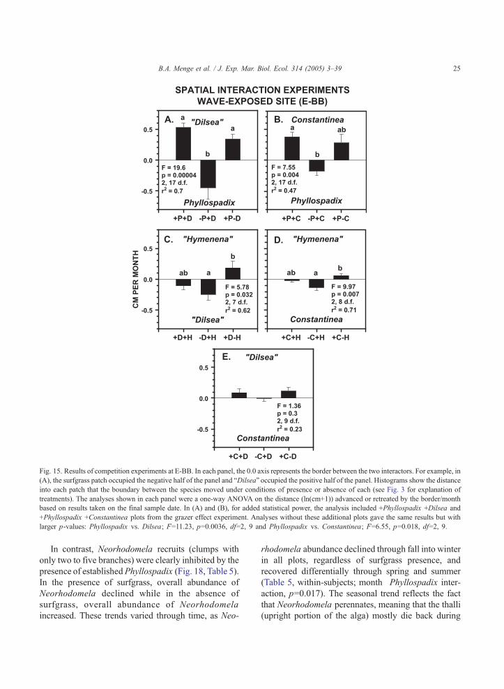
Fig. 15. Results of competition experiments at E-BB. In each panel, the 0.0 axis represents the border between the two interactors. For example, in

(A), the surfgrass patch occupied the negative half of the panel and bDilseaQ occupied the positive half of the panel. Histograms show the distance

into each patch that the boundary between the species moved under conditions of presence or absence of each (see Fig. 3 for explanation of

treatments). The analyses shown in each panel were a one-way ANOVA on the distance (ln(cm+1)) advanced or retreated by the border/month

based on results taken on the final sample date. In (A) and (B), for added statistical power, the analysis included +Phyllospadix +Dilsea and

+Phyllospadix +Constantinea plots from the grazer effect experiment. Analyses without these additional plots gave the same results but with

larger p-values: Phyllospadix vs. Dilsea; F=11.23, p=0.0036, df=2, 9 and Phyllospadix vs. Constantinea; F=6.55, p=0.018, df=2, 9.

B.A. Menge et al. / J. Exp. Mar. Biol. Ecol. 314 (2005) 3–39 25

In contrast, Neorhodomela recruits (clumps with

only two to five branches) were clearly inhibited by the

presence of establishedPhyllospadix (Fig. 18, Table 5).

In the presence of surfgrass, overall abundance of

Neorhodomela declined while in the absence of

surfgrass, overall abundance of Neorhodomela

increased. These trends varied through time, as Neo-

rhodomela abundance declined through fall into winter

in all plots, regardless of surfgrass presence, and

recovered differentially through spring and summer

(Table 5, within-subjects; month�Phyllospadix inter-

action, p=0.017). The seasonal trend reflects the fact

that Neorhodomela perennates, meaning that the thalli

(upright portion of the alga) mostly die back during

Page 24

Fig. 17. Results of experiments testing change in abundance of

Phyllospadix recruits in the presence and absence of Neorhodomela

in the upper low zone (A) and lower low zone (B). From August to

November 1987, surfgrass recruits tended to expand in size faster in

the absence of Neorhodomela, suggesting release from competition.

From January to May 1988, Phyllospadix expanded faster in the

presence of Neorhodomela, suggesting facilitation.

Fig. 16. Results of competition experiments at P-BBM. See Fig. 15

caption for interpretation of results.

B.A. Menge et al. / J. Exp. Mar. Biol. Ecol. 314 (2005) 3–3926

winter leaving the basal crust holdfast to regrow new

thalli in spring. Together, these results suggest that in

adult–recruit interactions, surfgrass recruits are capable

of gradual expansion while surrounded by Neorhodo-

mela, but that Neorhodomela recruits will gradually be

overwhelmed and displaced when surrounded by

surfgrass. These patterns suggest that surfgrass is the

dominant competitor at the I-BB site, although com-

petition is likely to proceed slowly as at the more

protected site in which the pairwise experiments were

done.

4. Discussion

This study demonstrates that, in contrast to the

bmean-fieldQ impression of relatively unchanging

macrophyte abundances, when viewed in a spatially

explicit manner, the picture is one of constant change.

In addition to generating new understanding of the

dynamics of macrophyte-dominated low rocky inter-

tidal assemblages along the eastern Pacific coast, we

suggest that our results make several additional

Page 25

Fig. 18. Results of experiments testing change in abundance of

Neorhodomela brecruitsQ (small clumps) in the presence and absence

of Phyllospadix. Neorhodomela expanded in area in the absence of

surfgrass and shrank in area in its presence, suggesting competition.

Table 4

Test of effect of height on the low shore and established

Neorhodomela larix on growth (ln of percent cover) of Phyllospa-

dix scouleri recruits

Univariate analysis

Source of variation df Mean

square

F p

Between subjects

Height on the shore 1 0.9802 5.17 0.04

Neorhodomela 1 0.0617 0.33 0.58

Height�Neorhodomela 1 0.1226 0.65 0.44

Error 13 0.1896

Within subjects

Month 5 0.1287 12.6 b0.000001

Month�Height 5 0.0134 1.31 0.27

Month�Neorhodomela 5 0.0311 3.04 0.016

Month�Height�Neorhodomela

5 0.0097 0.95 0.45

Error 65 0.0102

Multivariate analysis

Source Wilk’s

Lambda

df F p

Month 0.1392 5, 9 11.13 0.0012

Month�Height 0.5153 5, 9 1.69 0.23

Month�Neorhodomela 0.3183 5, 9 3.86 0.038

Month�Height�Neorhodomela

0.5958 5, 9 1.22 0.37

Analysis employed repeated measures analysis of variance (RM-

ANOVA) because the same plots were sampled repeatedly through

time. The assumption of compound symmetry was met (Mauchly

criterion=0.133, v2=22.4, 14 df, p=0.07) so we present unadjusted

probabilities. Statistically significant probabilities are shown in

boldface.

Table 5

Test of effect of established Phyllospadix scouleri on growth (ln per

cent cover per plot) of Neorhodomela larix recruits

Univariate analysis

Source of variation df Mean

Square

F p

Between subjects

Phyllospadix scouleri 1 3.6426 15.13 0.0013

Error 16 0.2407

Within subjects

Month 6 0.2738 9.02 b0.000001

Month�Phyllospadix 6 0.1777 5.85 0.00003

Error 96 0.0304

Multivariate analysis

Source of variation Wilk’s

Lambda

df F p

Month 0.1764 6, 11 8.56 0.0013

Month�Phyllospadix 0.2966 6, 11 4.35 0.017

Analysis employed RM-ANOVA. The assumption of compound

symmetry was met (Mauchly criterion=0.2624, v2=18.4, 20 df,

p=0.56) so unadjusted probabilities are presented. Statistically

significant probabilities are shown in boldface.

B.A. Menge et al. / J. Exp. Mar. Biol. Ecol. 314 (2005) 3–39 27

advances. First, our work offers insight into the

dynamics of a common but relatively unstudied

pattern, plant-dominated mosaics, whether marine or

non-marine. Second, this study expands our under-

standing of the factors structuring low zone commun-

ities in general, and of the dynamics of rocky intertidal

communities as a whole. Third, this study provides a

case study that is relevant to the theory of spatial

dynamics. We address each of these issues in turn

below.

4.1. Macrophyte mosaic dynamics along a wave-

exposure gradient

The dynamics of these macrophyte mosaics are

primarily a function of processes focused on the

surfgrass P. scouleri. At wave-exposed sites in partic-

ular, this angiosperm is affected by forces that disturb

the spatial pattern of the mosaic, and disturbance

combined with patterns of growth of surfgrass dictates

the structure of the mosaic. The composition of the

mosaic varies with wave exposure, presumably

because dispersal ranges or the tolerance ranges to

Page 26

B.A. Menge et al. / J. Exp. Mar. Biol. Ecol. 314 (2005) 3–3928

wave exposure-related factors of the mostly red algal

co-occupants of the mosaic are narrower than the range

of conditions present. Surfgrass, in contrast, spans the

entire range of conditions, although our results suggest

that optimal growth conditions exist toward the wave-

exposed end of the environmental gradient. In the

following, we organize our comments following the

three stages of the dynamics of the mosaic, clearance,

colonization, and succession, and on the processes

involved in each.

4.1.1. Clearance

Disturbance regimes clearly varied through time,

with several disturbance metrics suggesting that the

highest rates of loss occurred in 1986–1988 while

lower rates occurred in 1985 and 1989–1990 (Fig. 11,

Table 2). To our surprise, disturbance regimes were

roughly similar across the wave exposure gradient. For

example, the average number of disturbances per 4 m2

plot was similar at wave-exposed, intermediate, and

wave-protected sites in 1985, 1986, 1989 and 1990

(Table 6). Average disturbance size differed with

exposure only in 1988, and the total proportion of

each plot disturbed did not vary with exposure in any

year of the 6-year study. Proportional losses/year

averaged over years were (meanF95% confidence

interval) 6.5F2.3% (wave-exposed), 3.3F4.7% (inter-

Table 6

Analysis of variation (one-way ANOVA) in disturbance regime (numbe

disturbed) across the wave exposure gradient by year from 1985 to 1990

Characteristic Year MS MSE

Number per year 1985 3.15

1986 7.93

1987 1121.1 1

1988 244.5

1989 7.04

1990 40.09

Mean area 1985 2758.7 65

1986 21,219 42,4

1987 169,442 132,2

1988 829,319 131,8

1989 30,146 35,7

1990 26,312 33,2

Proportion disturbed 1985 0.00013

1986 0.0034

1987 0.071

1988 0.0065

1989 0.00057

1990 0.00093

mediate) and 9.4F2.3%. Thus, contrary to expectation,

mosaics in wave-protected areas appear to be disturbed

about as much as do mosaics in wave-exposed areas.

Further, in those few cases where disturbance did vary

with wave-exposure, patterns were still not entirely as

expected. Some measures indicated that in some years

disturbance was greater at wave-exposed sites (e.g.,

average disturbance size in 1988; Fig. 11B) but for

others disturbance was greater in wave-protected areas

(e.g., average number of disturbances per plot, pro-

portion of plot disturbed; Fig. 11A,C).

4.1.2. Role of substratum

What was the basis of these patterns, particularly the

unexpectedly high disturbance in wave-protected

areas? Our estimates of rock hardness and of sediment

depth suggest that disturbance in these mosaics is an

integrated result of the combination of wave impact,

which diminishes from wave-exposed to wave-pro-

tected areas (e.g., Menge et al., 1996), variable

substratum strength, and variable sedimentation

(Appendix 1). Wave-exposed sites, with basaltic rock

composition, presumably have substrata that are less

prone to failure than substrata at wave-protected sites,

which are mudstone or mudstone under a thin layer of

basalt. Thus, although wave impact is less in wave-

sheltered sites, plants attached to the weaker substra-

r per year, average disturbance area and proportion of total area

df F p r2

6.6176 2, 17 0.48 0.63 0.053

18.3456 2, 17 0.43 0.66 0.048

24.32 2, 17 9.02 0.002 0.51

34.65 2, 17 7.06 0.006 0.45

8.588 1, 10 0.82 0.39 0.076

11.79 2, 17 3.40 0.057 0.29

01.0 2, 17 0.42 0.66 0.048

17 2, 17 0.50 0.62 0.056

07 2, 17 1.28 0.30 0.13

28 2, 17 6.29 0.009 0.425

37 1, 10 0.84 0.38 0.078

36 2, 17 0.79 0.47 0.085

0.00016 2, 17 0.82 0.46 0.088

0.0055 2, 17 0.61 0.55 0.067

0.044 2, 17 1.60 0.23 0.159

0.0060 2, 17 1.09 0.36 0.113

0.00067 1, 10 0.85 0.38 0.079

0.00061 2, 17 1.53 0.24 0.153

Page 27

B.A. Menge et al. / J. Exp. Mar. Biol. Ecol. 314 (2005) 3–39 29

tum in these areas presumably are more susceptible to

wave forces. By weakening surfgrass rhizomes, burial

by sediment may exacerbate plant detachment during

even modest wave action. We suspect that both softer

substratum and sedimentation underlie the unexpect-

edly high disturbance rates in wave-protected areas, but

have no information with which to evaluate this

expectation or its alternatives (i.e., that one or the other

factor is the more important one).

4.1.3. Annual variation

Why did disturbance vary so dramatically among

years? The most obvious possibility is that the winters

preceding summer measurements of low disturbance

had less severe wave action than did winters preceding

summer measurements of high disturbance. Unfortu-

nately, the technology to quantify wave forces directly

at each of these sites during the study period was

unavailable at the time. A less direct measure is to

examine patterns of significant wave height (hs)

recorded by NOAA’s array of offshore data buoys

which measure hs, defined as the highest one-third of

all of the wave heights during each hourly 20-min

sampling period (see http://www.ndbc.noaa.gov).

Using buoy data and disturbance rates in Paine and

Levin (1981), Denny’s (1995) analysis successfully

used hs to predict the range of rates of mussel dislodge-

ment. Denny (Table 4 in Denny, 1995) provided annual

estimates for hs for Coquille River, OR, about 200 km

south of our sites. Comparing these estimates of yearly

average hs (in meters) to estimates of the percentage of

our 2�2-m plots that was disturbed (meanF95%

confidence interval) from 1985 to 1990 yields:

1985—hs=2.202, % disturbed=0.97F0.4%;

1986—hs=2.272, % disturbed=10.8F0.4%;

1987—hs=2.090, % disturbed=11.9F0.4%;

1988—hs=2.410, % disturbed=10.9F0.4;

1989—hs=2.061, no data for % disturbed; and

1990—hs=2.359, % disturbed=1.8F0.4.

Although high hs and high disturbance occurred in

1986 and 1988, no such relationships are evident in

1985, 1987 and 1990. We conclude that the evidence

is insufficient to attribute the annual variation in the

macrophyte mosaic disturbance regime to annual

variation in storminess. Similar non-correspondence

between disturbance loss and storminess has more

recently been observed in our studies of mid-zone

mussel bed disturbance at this and other sites along

the Oregon coast (G. Allison, P. Halpin, B. Menge

unpublished data). Other alternatives, such as varia-

tion in susceptibility to disturbance due to annual

differences in wintertime surfgrass physiological

condition (e.g., due to periods of exceptional thermal

stress) cannot be discounted on the basis of present

information.

4.1.4. Colonization

Although the patterns of disturbance help explain

why surfgrass monocultures do not replace the mosaic,

the explanation of why the turf is composed of many

algal species rather than few is less clear. One

hypothesis, that propagules of algal turf species have

dispersal limited to the immediate vicinity of repro-

ductive plants (e.g., (Sousa, 1984a), may help explain

variation in recolonization of clearances at wave-

exposed sites, but not at wave-protected sites. Specif-

ically, while the red alga C. simplex exhibited variation

in density of recruitment at different distances from

propagule sources at a wave-exposed site, no variation

in recruit density with distance from propagule source

was observed for O. floccosa or N. larix (Menge et al.,

1993). Large differences in average recruit density

were observed, however, with Neorhodomela settling

at much lower densities than Odonthalia.

Nonetheless, our observations during this research

and the studies of Turner (1983a, 1985) make it clear

that recolonization of disturbed areas was not predict-

able. Turner’s (1983a) studies of succession in wave-

protected mosaics suggested that colonization and

successional pathways varied with the season of

clearance. Spring clearances were colonized and

initially dominated by different species than were

observed in autumn clearances.

Studies of algal phenology suggest that life history

differences are likely to also play a key role in

maintaining the mosaic structure (Menge et al., 1993),

at least at wave-exposed areas. The red algae C.

simplex and Hymenena flabelligera were reproductive

for relatively brief periods in spring and summer, for

example, meaning spores for colonization of distur-

bances would be available only during this time

period. At wave-protected areas, phenological obser-

vations indicated that the two most common mosaic

algae, Odonthalia and Neorhodomela were reproduc-

Page 28

B.A. Menge et al. / J. Exp. Mar. Biol. Ecol. 314 (2005) 3–3930

tive during all months but January and February and

thus were likely to be able to colonize disturbances

almost year-round. With respect to Odonthalia and

Neorhodomela, we suspect that Odonthalia’s advant-

age in colonization ability is offset by a persistence-

competitive advantage by Neorhodomela, but this

possibility has not been investigated.

These differences in phenology and in apparent

dispersal distance with wave exposure are consistent

with the differences in mosaic diversity along the

environmental stress gradient. Higher diversity at

wave-exposed sites, for instance, may be a function

of high variation in the identity of invaders of

disturbed patches due to brief periods of spore

dispersal and localized dispersal. Lower diversity at

wave-protected sites may result from more predictable

patch colonization due to lengthy periods of repro-

duction (by Odonthalia and Neorhodomela) and

wider-ranging dispersal of spores (by Odonthalia).

4.1.5. Succession

The structure of the macrophyte mosaic was

remarkably stable at each site over the 6 years of this

study (Fig. 4). Based on these quantitative results, and

qualitative observations begun in 1980, this pattern of

seeming constancy has persisted for N20 years.

Intensive research involving at least monthly visits

continues to the present (summer 2004) at Boiler Bay

and Fogarty Creek, and, with the exception of a sharp

reduction in the abundance of laminarians (e.g.,

Lessoniopsis, Hedophyllum) during the El Nino of

1997–1998 (Menge et al., personal observations;

Freidenburg et al., unpublished data), algal mosaic

structure has remained unchanged.

4.1.6. Overgrowth interactions

The study of spatially explicit changes in the

permanently marked plots, however, demonstrated that

this apparent constancy is illusory (e.g., Figs. 6–9).

Large shifts occurred within the mosaic on an annual

basis at wave-exposed, intermediate and wave-pro-

tected areas. With field observations of overgrowth of

algal neighbors by surfgrass, the competition and

grazer-effect experiments indicate that in the absence

of disturbance, all sites would eventually become

surfgrass monocultures. With the exception of Lesso-

niopsis–Phyllospadix interactions, all surfgrass–algal

interactions were strictly hierarchical: surfgrass was

never overgrown by any algal turf species. Although

we did not quantify epiphytic algae, field observa-

tions indicated that epiphytic cover of Phyllospadix

blades was minimal. The Lessoniopsis–Phyllospadix

interaction appears to have been a standoff, at least

under normal conditions. Although each exchanged

space at the expense of the other, at least at Exposed

Boiler Bay (Fig. 9A), these changes appeared to

balance out, at least during 1985–1990. Expansion of

the temporal scale of these studies to include severe

El Ninos, such as that in 1997–1998, would have

been interesting because during this time Lessoniop-

sis virtually disappeared from E-BB while surfgrass

appeared unaffected (Menge et al., personal observa-

tions). By summer 2000, however, this kelp had

recovered to abundances that qualitatively appeared

comparable to those observed previously. The mech-

anisms underlying the reduction of the kelp appeared

to include nutrient depletion and thermal stress

(Freidenburg et al., unpublished data) while the

mechanisms underlying its rapid recovery are

unknown.

4.1.7. Experimental evidence

The experimental and marked plot results suggest

that P. scouleri is a dominant competitor for space in

this mosaic, but that the rate of displacement of

competitors by surfgrass varies with wave exposure.

In the wave-exposed competition experiments, surf-

grass almost completely overgrew its neighbors in

adjacent plots, meaning that in 3 years the edge of the

surfgrass patch grew ~15 cm (in terms of mean area or

percent area covered F95% confidence interval:

4.91F1.0 cm2/month or 3.7F1.6%/month) (Fig. 15).

In terms of % area overgrown annually in the 2�2-m

plots at wave-exposed sites, this growth rate translates

into about 19.6% of a plot being overgrown by

surfgrass in a year. At this rate, in the absence of

disturbance it would take about 5 years for surfgrass

to occupy 100% of the space in an initially clear plot.

Note that this rate is about 3� higher than the rate of

disturbance in the marked plots (range of area lost to

disturbance across wave exposures was 3.3 to 9.4/

year; see above). We believe that this difference is

related in part to the disturbance plots being somewhat

higher (by about 0.3 to 0.6 m) on the shore than were

the experimental plots. Surfgrass higher on the shore

is likely to grow slower due to lesser immersion time,

Page 29

B.A. Menge et al. / J. Exp. Mar. Biol. Ecol. 314 (2005) 3–39 31

and thus shorter exposure to nutrients and longer

exposure to thermal and desiccation stress.

Growth in experiments at wave-protected sites was

far less than at wave-exposed sites (Fig. 16). Monthly

growth rate (area covered) was 0.32F1.0 cm2 or

0.75F0.8% (and thus statistically undetectable from

zero growth), or about 1.4% of a plot being over-

grown by surfgrass in a year. At this rate, in the

absence of disturbance, it would take about 70 years

for surfgrass to occupy 100% of the space in an

initially clear plot. This rate of growth is substantially

lower than the rate of disturbance at wave-protected

sites (9.4F1.3%), suggesting that recovery from

disturbance is more a reflection of processes influenc-

ing colonization and growth of the macroalgae than of

processes influencing surfgrass growth. These

between-exposure differences in growth also seem

most likely due to thermal and desiccation stress, both

of which increase towards more wave-sheltered parts

of the shore. Stress effects were often observed in the

field; during late spring and summer the distal

portions of blades of surfgrass commonly die, turn

brown or white and eventually slough off at wave-

protected areas while such effects are seen far less

often at wave-exposed areas. It seems likely that the

energy devoted to replacing such losses in surfgrass is

likely to come at the cost of slower rhizome growth.

Macroalgae such as Neorhodomela and Odonthalia in

contrast seem less affected by stress.

We thus postulate that the processes underlying

mosaic structure at wave-exposed sites are disturb-

ance, surfgrass overgrowth and competition for space,

and variable algal life histories. Disturbance focused

primarily on Phyllospadix clearly prevents surfgrass,

the dominant competitor for space in this system,

from eliminating its turf-forming algal neighbors. As

suggested by our experiments and observations,

grazing appears of minimal importance in either

causing gaps in the mosaic or in maintaining patches.

This result was expected: limpets and chitons, the

most likely macrograzers to have a potential effect on

surfgrass or turfy algae, are sparse in the algal mosaic

(e.g., Turner, 1985; Menge, personal observations),

probably because of the almost total lack of open

space (Fig. 4). At wave-protected sites, in contrast,

disturbance, persistence and standoff competition, and

differential colonization among the macroalgae seem

to be the primary processes. Disturbance seems less

focused on any particular species, and overgrowth

competition for space seems of minimal importance.

New disturbances are occupied rapidly by ephemeral

algae such as ulvoids, which are soon replaced by

Odonthalia, also a rapid colonist. Surfgrass appears to

be a co-dominant with Neorhodomela, and both are

slow colonists.

4.2. Dynamics of macrophyte-dominated intertidal

zones

Macrophyte-dominated mosaic dynamics have

been studied in a number of locations globally (e.g.,

Lubchenco and Menge, 1978; Sousa, 1979a; Under-

wood and Jernakoff, 1981; Dethier, 1984; Hartnoll

and Hawkins, 1985; Stewart, 1989; Hawkins et al.,

1992; Williams, 1993; Airoldi et al., 1995; Johnson et

al., 1997; Burrows and Hawkins, 1998; Dudgeon et

al., 1999; Airoldi, 2000; Benedetti-Cecchi, 2000;

Benedetti-Cecchi et al., 2000), but with the exception

of the Isle of Man studies (Hartnoll and Hawkins,

1985; Hawkins et al., 1992; Johnson et al., 1997;

Burrows and Hawkins, 1998), incorporation of

spatially explicit approaches remains rare. Below,

we examine similarities and differences between the

present study and several other investigations of the

dynamics of macrophyte-dominated assemblages in

rocky intertidal regions.

In Washington State, the intertidal kelp H. sessile

dominated space at moderate wave exposures due to

competitive exclusion of other potential canopy-

forming macroalgae (Dayton, 1975). Combining all

wave exposures, the shade provided by Hedophyllum

facilitated the persistence of an assemblage of

bobligateQ understory species (20 species, some of

which are components of the algal mosaic studied

here). Hedophyllum inhibited the abundance of

another assemblage of bfugitiveQ species (33 species).

The dominance of Hedophyllum was diminished

towards more wave-sheltered areas by thermal and

desiccation stress, and towards more wave-exposed

areas by competition with Lessoniopsis and Lami-

naria setchellii. Thus, as with Phyllospadix, growth

and competitive ability of Hedophyllum varied along

a wave-exposure gradient, with diminished abundance

being associated with heightened stress. Interestingly,

surfgrass was not abundant at Dayton’s (1975) sites,

even though wave-exposures and other physical

Page 30

B.A. Menge et al. / J. Exp. Mar. Biol. Ecol. 314 (2005) 3–3932

environmental characteristics at outer coast Washing-

ton and central Oregon coast sites are similar (Menge,

personal observations).

In the San Juan Islands of Washington State, a more

wave-sheltered region, surfgrass was an abundant

component of low zone macrophyte assemblages

(Dethier, 1984). Studies focused in tidepool assemb-

lages showed that surfgrass was a dominant competitor.

As we have observed in the present study, when

surfgrass dominated a tidepool it was invulnerable to

competitive displacement, and surfgrass seemed to be a

primary target of wave-caused disturbance (Dethier,

1984).

A study of surfgrass (P. torreyi)–macroalgal turf

interactions in Southern California also suggested that

surfgrass was competitively dominant on the lower

shore and a primary target of disturbance (Stewart,

1989). Further, Stewart (1989) indicated that temporal

variation in the border between P. torreyi and the turf

was a dynamic response of growth to variable

disturbance intensity from wave forces, environmental

stress, and substratum strength.

In New England, algal turf, consisting primarily of

Chondrus crispus and Mastocarpus stellatus, domi-

nates space in the low intertidal zone of moderately

wave-exposed to wave-sheltered areas (Lubchenco

and Menge, 1978; Dudgeon et al., 1999). Mussels

(Mytilus edulis), which can overgrow and smother

these red algae under natural conditions at wave-

exposed areas or in the experimental absence of

predators at more sheltered areas, are the only species

capable of displacing Chondrus (Lubchenco and

Menge, 1978). Recently, Dudgeon et al. (1999)

investigated the interaction between Chondrus and

Mastocarpus and demonstrated that the nature of the

interaction varies with increasing height on the shore.

At lower elevations, Chondrus was fast-growing and

dominated in competition with Mastocarpus. The

latter had low recruitment on the lower shore, and

persisted at this level primarily as a prostrate encrust-

ing holdfast. Disturbance from waves during winter

storms was the only deterrent to the development of

Chondrus monocultures. Higher on the shore, Chond-

rus grew slower and was differentially more suscep-

tible to loss of tissue from thermal and desiccation

stress in spring, summer and fall. Dudgeon et al.

(1999) suggest that this differential tissue loss

prevented competitive exclusion by Chondrus and is

therefore the most likely mechanism allowing these

species to coexist in the upper low zone. Hence, as in

our study, the competitive ability of the dominant

varied along a gradient of environmental stress.

Coexistence was maintained by a combination of

disturbance, environmental stress, life history charac-

teristics and competition.

The Isle of Man studies (Hartnoll and Hawkins,

1985; Hawkins et al., 1992; Johnson et al., 1997;

Burrows and Hawkins, 1998) provide the clearest

contrast with the disturbance-competition dominated

dynamics summarized for the above studies. Dynam-

ics of the mid-intertidal fucoid–barnacle–limpet

mosaic are driven by the limpet–fucoid interaction.

Bare rock surface is most likely to be colonized by

barnacles, especially if limpets are sparse. A barnacle

substratum inhibits limpet grazing and thus enhances

fucoid settlement (juveniles of which settle on both

barnacles and bare rock). Through time denser stands

of juvenile fucoids coalesce into adult fucoid-domi-

nated patches due to losses of fucoid plants attached to

barnacles (from wave disturbance and barnacle

mortality caused by whelks aggregating to the

fucoid–barnacle patches) and to bare rock (from

limpet grazers attracted by the fucoid canopy).

Eventually, fucoid adults are lost to wave disturbance,

partly as a consequence of thalli weakened by grazing,

and bare rock is again exposed. Limpets, whose

grazing inhibits barnacle settlement, gradually move

away after the canopy is gone, starting the cycle anew.

Such cycles last about 5 to 6 years (Burrows and

Hawkins, 1998). Thus, although disturbance plays a

role, the primary forces driving this system appear to

revolve around limpets, their grazing effects on

fucoids, and the facilitation of limpets by fucoid

canopies. Competition for space also appears to play a

relatively minor role.

4.3. Rocky intertidal community dynamics

How do the patterns we have documented in this

macrophyte mosaic compare to other rocky intertidal

systems? With a few exceptions, the number of rocky

intertidal investigations that have characterized dis-

turbance regimes is surprisingly small. All of the

examples known to us that quantified at least some

aspects of the disturbance regime in comparable units

are listed in Table 7. These include three studies of

Page 31

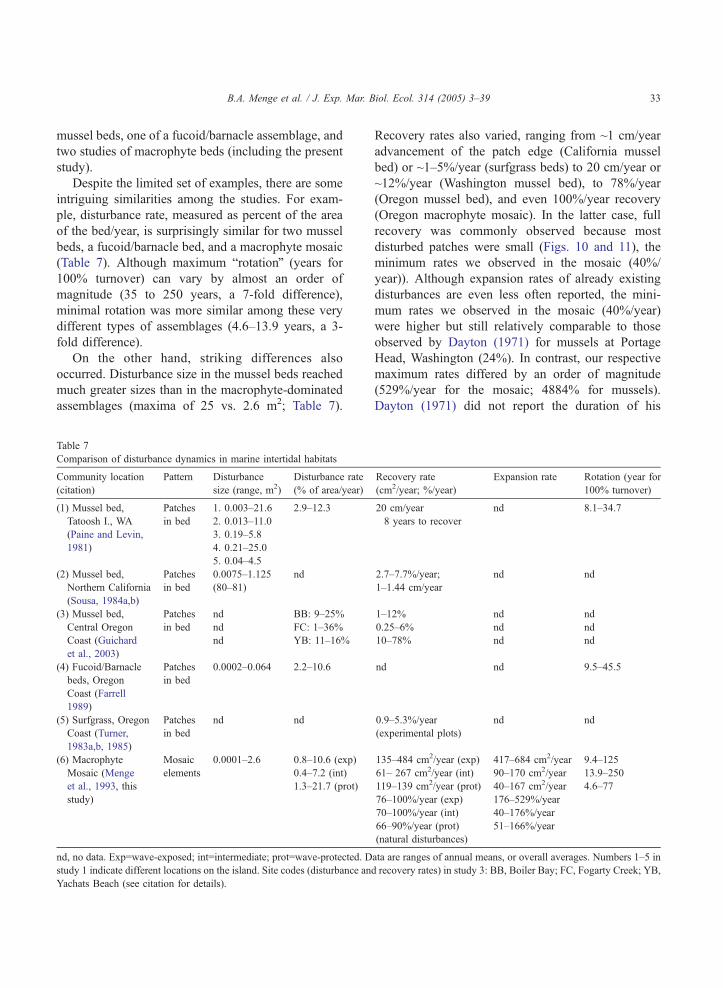
B.A. Menge et al. / J. Exp. Mar. Biol. Ecol. 314 (2005) 3–39 33

mussel beds, one of a fucoid/barnacle assemblage, and

two studies of macrophyte beds (including the present

study).

Despite the limited set of examples, there are some

intriguing similarities among the studies. For exam-

ple, disturbance rate, measured as percent of the area

of the bed/year, is surprisingly similar for two mussel

beds, a fucoid/barnacle bed, and a macrophyte mosaic

(Table 7). Although maximum brotationQ (years for

100% turnover) can vary by almost an order of

magnitude (35 to 250 years, a 7-fold difference),

minimal rotation was more similar among these very

different types of assemblages (4.6–13.9 years, a 3-

fold difference).

On the other hand, striking differences also

occurred. Disturbance size in the mussel beds reached

much greater sizes than in the macrophyte-dominated

assemblages (maxima of 25 vs. 2.6 m2; Table 7).

Table 7

Comparison of disturbance dynamics in marine intertidal habitats

Community location

(citation)

Pattern Disturbance

size (range, m2)

Disturbance rate

(% of area/year)

(1) Mussel bed,

Tatoosh I., WA

(Paine and Levin,

1981)

Patches

in bed

1. 0.003–21.6 2.9–12.3

2. 0.013–11.0

3. 0.19–5.8

4. 0.21–25.0

5. 0.04–4.5

(2) Mussel bed,

Northern California

(Sousa, 1984a,b)

Patches

in bed

0.0075–1.125

(80–81)

nd

(3) Mussel bed,

Central Oregon

Coast (Guichard

et al., 2003)

Patches

in bed

nd BB: 9–25%

nd FC: 1–36%

nd YB: 11–16%

(4) Fucoid/Barnacle

beds, Oregon

Coast (Farrell

1989)

Patches

in bed

0.0002–0.064 2.2–10.6

(5) Surfgrass, Oregon

Coast (Turner,

1983a,b, 1985)

Patches

in bed

nd nd

(6) Macrophyte

Mosaic (Menge

et al., 1993, this

study)

Mosaic

elements

0.0001–2.6 0.8–10.6 (exp)

0.4–7.2 (int)

1.3–21.7 (prot)

nd, no data. Exp=wave-exposed; int=intermediate; prot=wave-protected. D

study 1 indicate different locations on the island. Site codes (disturbance an

Yachats Beach (see citation for details).

Recovery rates also varied, ranging from ~1 cm/year

advancement of the patch edge (California mussel

bed) or ~1–5%/year (surfgrass beds) to 20 cm/year or

~12%/year (Washington mussel bed), to 78%/year

(Oregon mussel bed), and even 100%/year recovery

(Oregon macrophyte mosaic). In the latter case, full

recovery was commonly observed because most

disturbed patches were small (Figs. 10 and 11), the

minimum rates we observed in the mosaic (40%/

year)). Although expansion rates of already existing

disturbances are even less often reported, the mini-

mum rates we observed in the mosaic (40%/year)

were higher but still relatively comparable to those

observed by Dayton (1971) for mussels at Portage

Head, Washington (24%). In contrast, our respective

maximum rates differed by an order of magnitude

(529%/year for the mosaic; 4884% for mussels).

Dayton (1971) did not report the duration of his

Recovery rate

(cm2/year; %/year)

Expansion rate Rotation (year for

100% turnover)

20 cm/year

�8 years to recover

nd 8.1–34.7

2.7–7.7%/year;

1–1.44 cm/year

nd nd

1–12% nd nd

0.25–6% nd nd

10–78% nd nd

nd nd 9.5–45.5

0.9–5.3%/year

(experimental plots)

nd nd

135–484 cm2/year (exp) 417–684 cm2/year 9.4–125

61– 267 cm2/year (int) 90–170 cm2/year 13.9–250

119–139 cm2/year (prot) 40–167 cm2/year 4.6–77

76–100%/year (exp) 176–529%/year

70–100%/year (int) 40–176%/year

66–90%/year (prot)

(natural disturbances)

51–166%/year

ata are ranges of annual means, or overall averages. Numbers 1–5 in

d recovery rates) in study 3: BB, Boiler Bay; FC, Fogarty Creek; YB,

Page 32

B.A. Menge et al. / J. Exp. Mar. Biol. Ecol. 314 (2005) 3–3934

observation period for these data (probably b3 years).

Nonetheless, these comparisons, and our field obser-

vations at both Washington and Oregon sites, indicate

that disturbed patches in mussel beds can reach far

greater sizes, and are likely to expand at higher rates

than in macrophyte mosaics.

Because of the small sample size, little more can be

made of these comparisons. It does seem clear,

however, that the dynamics of mussel beds and

macrophyte mosaics share a common feature that is

independent of phyletic considerations. Both mussels

and surfgrass were dominant competitors, and both

were the most susceptible species to disturbance in

their respective systems. A similar set of tradeoffs has

been documented for kelp bed mosaics (Dayton et al.,

1984). The kelp beds off central and southern

California consist of a diverse assemblage of species

of differing morphologies, ranging from tall canopy-

forming perennials to mid-level understory kelps to

substratum-hugging prostrate canopy species to algal

turfs. Field observations and experiments demonstra-

ted that the dominant kelp Macrocystis pyrifera was

both the dominant competitor for light and was the

most susceptible member of the mosaic to disturbance

from storm-generated waves.

4.4. Comparison to non-marine communities

Mosaics are common in terrestrial habitats, partic-

ularly in grasslands, prairies, meadows, pastures and

old fields (e.g., Turkington et al., 1979; Turkington

and Harper, 1979; Grubb, 1986; Turkington and

Mehrhoff, 1990; Lavorel et al., 1994). Disturbance

is an important process in these environments, and the

disturbance regime has been quantified in a variety of

studies (e.g., Goldberg and Gross, 1988). Interest-

ingly, in many of these the annual disturbance rate is

similar to the rates observed in mussel beds, fucoid/

barnacle beds, and macrophyte turfs (Table 7). In

examples of prairie, coastal dunes, and old fields,

average % area disturbed/year was commonly in the

range of 0.1–10% (Table 8 in Goldberg and Gross,

1988), which is similar to the ranges listed in Table 7.

Most disturbances in terrestrial environments were

due to biotic sources (pocket gophers, moles, ants,

mice, ground squirrels, badgers) rather than physical

disturbance. These similarities are intriguing and may

suggest that the ecological principles underlying

regimes of disturbance share commonalities regard-

less of the habitat.

4.5. Community theory

The influence of spatial structure on species

coexistence has a long history in ecology (Skellam,

1951; Huffaker, 1958; Levins and Culver, 1971; Horn

and MacArthur, 1972; Armstrong, 1976). The dra-

matic increase of computing power during the past

few decades has facilitated a major expansion of

theory in this area, and helped to foster a variety of

approaches including patch models, reaction diffusion

equations, interacting particle systems, and cellular

automata (Lavorel et al., 1993; Durrett and Levin,

1994a,b; Tilman and Kareiva, 1997; Wilson and

Nisbet, 1997).

At the community level, incorporation of spatial

structure has offered new insight into the question of

species coexistence (Tilman, 1994). As indicated by

Tilman (1994), the incorporation of spatial structure

frees models from the unrealistic restriction that the

number of coexisting species is limited by the number

of discrete limiting resources. Hismodels indicated that

under certain conditions, there is no limit to the number

of species that can coexist on a single limiting resource.

His basic model assumed a spatially subdivided,

infinitely large and physically homogeneous habitat

with random colonization and no dispersal from

outside the habitat, and that species differed system-

atically in competitive ability, colonization ability, and

mortality rate. In addition, the model also assumes a

trade-off between competitive ability and colonization

ability and possibly between competitive ability and

longevity. In this case, limitation of species number

would result from the imposition of finite boundaries

on the habitat, demographic stochasticity, or evolu-

tionary limits to dispersal or longevity. Other factors

that presumably could enhance diversity are a physi-

cally heterogeneous environment and disturbance.

The appropriateness of surfgrass communities for

testing such a model appears mixed. We can quantify

competitive ability, colonization ability and rate,

mortality and change in occupancy of space in a

spatially explicit manner, but the surfgrass system is

open to dispersal, not closed, so this aspect of the model

would need modification. For example, although some

algae have very limited dispersal distances (Sousa,

Page 33

B.A. Menge et al. / J. Exp. Mar. Biol. Ecol. 314 (2005) 3–39 35

1984a), others disperse tens to hundreds of kilometers

(Reed et al., 1988; Kinlan and Gaines, 2003). Surfgrass

seeds seem likely to disperse distances of at least

kilometers, and thus also to have open populations. In

bmean fieldQ-type models (e.g., Lotka-Volterra com-

petition and predation models), the outcomes of open

vs. closed models are dramatically different (Gaines

and Lafferty, 1995), so it is likely that similar changes

would occur in open vs. closed spatially explicit

models.

In marine rocky intertidal systems, cellular auto-

toma approaches have begun to provide valuable

insights. In a study of mussel beds on Tatoosh Island,

Washington, Wootton (2001) showed that the natural

pattern of patchiness and diversity in a mussel bed

mosaic was well mimicked by a cellular autotoma

model, predicting 92.5% of the variance in composi-

tion. He concluded that such accuracy required con-

siderable detail, including specifics of interactions

among species, size structure of the mussels, neigh-

bor–neighbor interactions, and the disturbance regime.

In a second mussel bed study at Bamfield, British

Columbia, the cellular autotoma model of Robles and

Desharnais (2002) accurately reproduced the two-

dimensional layout of a mussel bed across vertical

tidal and horizontal wave exposure gradients. Their

model included mussel size, mussel recruitment rate,

predation rate and mussel growth rate and how these

varied across the two environmental gradients. Finally,

in a mussel bed study on the Oregon coast, Guichard et

al. (2003) demonstrated that processes acting locally,

such as neighbor–neighbor interactions and disturb-

ance, and globally acting forces such as phytoplankton

productivity interacted to produce pattern in the bed,

and that locally generated pattern scaled to large-scale

pattern in a scale-invariant manner.

The macrophyte mosaic study reported here is

highly amenable to cellular autotoma and similar

spatially explicit analysis. In fact, Keymer (2003) has

begun modeling efforts base on the algal mosaic

system presented here. His efforts embed the algal

mosaic dynamic in a broader array of theoretical

possibilities, ranging in complexity from a mono-

specific dominant (such as surfgrass or mussels), to

algal metapopulations within a surfgrass matrix, to a

mosaic. Such efforts, combining the greater detail of

an empirical study with the broader generality of a

theoretical study warrant further attention.

5. Conclusions

We conclude that the structure of this mosaic is

primarily a consequence of disturbance, competition

for space among neighboring mosaic elements, life

history differences, colonization ability, and how these

vary with wave exposure. Surfgrass is the dominant

competitor but appears to be a poor colonizer, at least

to surfgrass beds, and is the most susceptible to

disturbance from storm-generated waves. Coexisting

algal species are inferior competitors, and include

species with a range of dispersal capabilities, includ-

ing fast-colonizing bfugitiveQ species such as Ulva

spp., Enteromorpha spp., Corallina officinalis, P.

irregulare, and O. floccosa, as well as slower

colonizers. Disturbance, from waves (wave-exposed

areas) and sedimentation and substratum weakness

(wave-protected areas), varies primarily through time

but surprisingly little across the wave-exposure

gradient. Differences in species composition with

wave-exposure regime undoubtedly reflect differences

in physiological tolerances and for some species,

probably dispersal limitation. Life history differences,

including morphological characteristics such as

whether or not a species has an encrusting, spreading

holdfast system, also seem to play a role in determin-

ing whether or not an alga is a common component of

the algal mosaic. Many of these characteristics seem

to characterize other systems, both marine and non-

marine.

Many aspects of this system would seem to make it

useful for interactive tests of spatial theory. Recent

advances in understanding of dispersal patterns of

macrophytes and invertebrates in relation to coastal

oceanography (Sponaugle et al., 2002; Kinlan and

Gaines, 2003; Siegel et al., 2003) raise the expectation

that a more inclusive set of models can be developed

that would be appropriate for open as well as closed

systems.

Acknowledgements

We thank M. Bracken, J. Burnaford, T. Freiden-

burg, B. Grantham, P. Halpin, C. Krenz, H. Leslie, J.

Lubchenco, K. Nielsen, and C. Reimer for comments

and critiques on this research. Constructive comments

by S. Shumway and R. Osman improved the final

Page 34

B.A. Menge et al. / J. Exp. Mar. Biol. Ecol. 314 (2005) 3–3936

version of the manuscript. We thank Betsy Abbott and

the late Alice Abbott King for access to the Fogarty

Creek site. Thanks also to D. Schiel and B. Davison of

the University of Canterbury, Christchurch, New

Zealand, for providing space and facilities for the

first author to write and analyze while on sabbatical.

The research was funded by NSF grants OCE84-

15609 and OCE88-11369. Analysis and writing were

supported by grants from the A.W. Mellon Founda-

tion, the David and Lucile Packard Foundation,

Robert and Betty Lundeen, and an endowment from

the Wayne and Gladys Valley Foundation. This is

contribution number 159 from PISCO, the Partnership

for Interdisciplinary Studies of Coastal Oceans: A

Long-Term Ecological Consortium funded by the

David and Lucile Packard Foundation. [SS]

Appendix 1. Characterization of study sites

Substratum

Macrophytes

Site location

(site code)

Slope

(aspect)

Rock type

Rock hardness

index1

(meanFS.E.M.)

Sediment

deposition

Sediment

depth2

(range, cm)

Taxon

richness3

mean (range)

Dominant elements of

macrophyte mosaic

Wave-exposed sites

Fogarty Creek (E-FC)

b158(~SW)

basalt

9.8F0.3a none 0 5.7 (2–10) Phyllospadix spp.,

Lessoniopsis littoralis,

bHymenenaQ complex 4,

articulated coralline algae

Boiler Bay (E-BB)

118(~SW)

basalt

9.6F0.2a none 0 6.8 (3–11) Phyllospadix spp.,

bHymenenaQ complex,

Constantinea simplex,

Plocamium cartilagineum,

bDilseaQ complex

Wave-intermediate site

Boiler Bay (I-BB)

108(~SW)

basalt

11.2F0.4b infrequent 0–0.62 5.6 (2–9) Phyllospadix spp.,

Mazzaella spp. 6,

Odonthalia floccosa,

Neorhodomela larix,

Hedophyllum sessile

Wave-protected sites

Boiler Bay Neorhodomela

Cove (P-BBC)

108(~SW)

mudstone

overlain by

basalt

3.3F0.1c

common 0.38–1.46 4.8 (2–9) Phyllospadix scouleri,

larix, Mazzaella spp.,

Odonthalia floccosa

Boiler Bay Neorhodomela

Mudstone (P-BBM)

08(undef.)

mudstone

3.7F0.1c common 0.93–2.62 4.3 (1–9) Phyllospadix scouleri,

larix, Odonthalia floccosa

1 An index of rock hardness was estimated by using a stopwatch to record the time required to drill a hole of 6.35–mm diameter to a

standard depth of 76 mm, under the weight of our gasoline-powered rotohammer. Twenty holes were drilled at haphazardly located places at

each of the five sites. Values with different superscripts (a–c) are significantly different at the a=0.05 level (Bonferroni-corrected post hoc test of

differences among means). Measurable sediment at I-BB occurred only once, in August 1987.2 Sediment depth was sampled in eight 0.5�0.5 m quadrats in each grid (see Methods) at each site from 1986 to 1988 by placing a quadrat

frame, subdivided by nylon cord into 25 squares (each 10�10 cm), over each mosaic quadrat. Sediment depth was measured at each of the 4�4

(16) cord intersections, in November 1986, January, May, August, and November 1987, and January and September 1988. Data shown are the

maximum and minimum monthly means for each site.3 Number of macrophyte taxa per 0.25–m2 quadrat, n=32 quadrats per year per site.a H. flabelligera, H. multiloba, Polyneura latissima, and Cryptopleura spp.b Dilsea californica, Schizymenia pacifica, and Halymenia schizymenioides.c Mostly M. splendens, but occasionally M. flaccida and M. heterocarpa.

Page 35

B.A. Menge et al. / J. Exp. Mar. Biol. Ecol. 314 (2005) 3–39 37

References

Airoldi, L., Rindi, F., Cinelli, F., 1995. Structure, seasonal

dynamics and reproductive phenology of a filamentous turf

assemblage on a sediment influenced, rocky subtidal shore.

Botanica Marina 38, 227–237.

Airoldi, L., 2000. Effects of disturbance, life histories, and

overgrowth on coexistence of algal crusts and turfs. Ecology

81, 798–814.

Allison, G.W., 2004. The influence of species diversity and stress

intensity on community resistance and resilience. Ecological

Monographs 74, 117–134.

Armstrong, R.A., 1976. Fugitive species: experiments with

fungi and some theoretical considerations. Ecology 57,

953–963.

Beisner, B.E., Haydon, D.T., Cuddington, K., 2003. Alternative

stable states in ecology. Frontiers in Ecology and Evolution 1,

376–382.

Benedetti-Cecchi, L., 2000. Predicting direct and indirect inter-

actions during succession in a mid-littoral rocky shore assem-

blage. Ecological Monographs 70, 45–72.

Benedetti-Cecchi, L., Bulleri, F., Cinelli, F., 2000. The interplay of

physical and biological factors in maintaining mid-shore and

low-shore assemblages on rocky coasts in the northwest

Mediterranean. Oecologia 123, 406–417.

Blanchette, C.A., 1996. Seasonal patterns of disturbance influence

recruitment of the sea palm, Postelsia palmaeformis. Journal of

Experimental Marine Biology and Ecology 197, 1–14.

Blanchette, C.A., Worcester, S.E., Reed, D.C., Holbrook, S.J.,

1999. Algal morphology, flow, and spatially variable recruit-

ment of surfgrass Phyllospadix torreyi . Marine Ecology.

Progress Series 184, 119–128.

Burrows, M.T., Hawkins, S.J., 1998. Modelling patch dynamics on

rocky shores using deterministic cellular automata. Marine

Ecology. Progress Series 167, 1–13.

Connell, J.H., Slatyer, R.O., 1977. Mechanisms of succession in

natural communities and their role in community stability and

organization. American Naturalist 111, 1119–1144.

Crowder, M.J., Hand, D.J., 1990. Analysis of Repeated Measures.

Chapman and Hall, London, UK.

Dayton, P.K., 1971. Competition, disturbance, and community

organization: the provision and subsequent utilization of space

in a rocky intertidal community. Ecological Monographs 41,

351–389.

Dayton, P.K., 1975. Experimental evaluation of ecological

dominance in a rocky intertidal algal community. Ecological

Monographs 45, 137–159.

Dayton, P.K., Currie, V., Gerrodette, T., Keller, B.D., Rosenthal,

R., Ven Tresca, D., 1984. Patch dynamics and stability of some

California kelp communities. Ecological Monographs 54,

253–289.

Denny, M.W., 1995. Predicting physical disturbance: mechanistic

approaches to the study of survivorship on wave-swept shores.

Ecological Monographs 65, 371–418.

Dethier, M.N., 1984. Disturbance and recovery in intertidal pools:

maintenance of mosaic patterns. Ecological Monographs 54,

99–118.

Dudgeon, S.R., Steneck, R.S., Davison, I.R., Vadas, R.L., 1999.

Coexistence of similar species in a space-limited intertidal zone.

Ecological Monographs 69, 331–352.

Durrett, R., Levin, S.A., 1994a. The importance of being discrete

(and spatial). Theoretical Population Biology 46, 363–394.

Durrett, R., Levin, S.A., 1994b. Stochastic spatial models: a user’s

guide to ecological applications. Philosophical Transactions of

the Royal Society of London. B 343, 329–350.

Farrell, T.M., 1989. Succession in a rocky intertidal community:

the importance of disturbance size and position within a

disturbed patch. Journal of Experimental Marine Biology and

Ecology 128, 57–73.

Farrell, T.M., 1991. Models and mechanisms of succession: an

example from a rocky intertidal community. Ecological Mono-

graphs 61, 95–113.

Gaines, S.D., Lafferty, K.D., 1995. Modeling the dynamics of

marine species: the importance of incorporating larval dispersal.

In: McEdwards, L. (Ed.), Ecology of Marine Invertebrate

Larvae. CRC Press, Boca Raton, FL, pp. 389–412.

Goldberg, D.E., Gross, K.L., 1988. Disturbance regimes of

midsuccessional old fields. Ecology 69, 1677–1688.

Grubb, P.J., 1986. Problems posed by sparse and patchily

distributed species in species-rich plant communities. In:

Diamond, J., Case, T.J. (Eds.), Community Ecology. Harper

and Row, New York, NY, pp. 207–225.

Guichard, F., Halpin, P., Allison, G.W., Lubchenco, J., Menge,

B.A., 2003. Mussel disturbance dynamics: signatures of

oceanographic forcing from local interactions. American Natu-

ralist 161, 889–904.

Hawkins, S.J., Hartnoll, R.G., 1983. Grazing of intertidal algae by

marine invertebrates. Oceanography and Marine Biology

Annual Reviews 21, 195–282.

Hartnoll, R.G., Hawkins, S.J., 1985. Patchiness and fluctuations on

moderately exposed rocky shores. Ophelia 24, 53–63.

Hawkins, S.J., Hartnoll, R.G., Kain, J.M., Norton, T.A., 1992.

Plant–animals interactions on hard substrata in the north-east

Atlantic. In: John, D.M., Hawkins, S.J., Price, J.H. (Eds.),

Plant–Animals Interactions in the Marine Benthos. Oxford

University Press, Oxford, England, pp. 1–32.

Horn, H.S., MacArthur, R.H., 1972. Competition among fugitive

species in a harlequin environment. Ecology 53, 749–752.

Huffaker, C.B., 1958. Experimental studies on predation:

dispersion factors and predator–prey oscillations. Hilgardia,

343–383.

Johnson, M.P., Burrows, M.T., Hawkins, S.J., Hartnoll, R.G.,

1997. Spatial structure on moderately exposed rocky shores:

patch scales and the interactions between limpets and algae.

Marine Ecology. Progress Series 160, 209–215.

Johnson, M.P., Burrows, M.T., Hawkins, S.J., 1998. Individual

based simulations of the direct and indirect effects of limpets on

a rocky shore Fucus mosaic. Marine Ecology. Progress Series

169, 179–188.

Keymer, J.E. 2003. Competition for space and intertidal commun-

ity structure. PhD Princeton University, Princeton, NJ.

Kinlan, B.P., Gaines, S.D., 2003. Propagule dispersal in marine

and terrestrial environments: a community perspective. Ecology

84, 2007–2020.

Page 36

B.A. Menge et al. / J. Exp. Mar. Biol. Ecol. 314 (2005) 3–3938

Lavorel, S., Gardner, R.H., O’Neill, R.V., 1993. Analysis of patterns

in hierarchically structure landscapes. Oikos 67, 521–528.

Lavorel, S., Lepart, J., Debussche, M., Lebreton, J.-D., Beffy,

J.-L., 1994. Small scale disturbances and the maintenance

of species diversity in Mediterranean old fields. Oikos 70,

455–473.

Levin, S.A., 1992. The problem of pattern and scale in ecology.

Ecology 73, 1943–1967.

Levin, S.A., Pacala, S.W., 1997. Theories of simplification and

scaling of spatially distributed processes. In: Tilman, D.,

Kareiva, P. (Eds.), Spatial Ecology: The Role of Space in

Population Dynamics and Interspecific Interactions. Princeton

University Press, Princeton, New Jersey, pp. 271–295.

Levins, R., Culver, D., 1971. Regional coexistence of species and

competition between rare species. Proceedings of the National

Academy of Sciences of the United States of America 68,

1246–1248.

Lubchenco, J., Menge, B.A., 1978. Community development and

persistence in a low rocky intertidal zone. Ecological Mono-

graphs 48, 67–94.

Lundalv, T., 1971. Quantitative studies on rocky-bottom biocoe-

noses by underwater photogrammetry. A methodological study.

Thalassia Jugoslavica 7, 201–208.

Lundalv, T., 1986. Detection of long-term trends in rocky

sublittoral communities: representatives of fixed sites. In:

Moore, P.G., Seed, R. (Eds.), The Ecology of Rocky Coasts.

Columbia University Press, New York, NY, pp. 329–345.

MacArthur, R.H., 1972. Geographical Ecology. Harper and Row,

Publishers, New York, NY.

Menge, B.A., 1976. Organization of the New England rocky

intertidal community: role of predation, competition and

environmental heterogeneity. Ecological Monographs 46,

355–393.

Menge, B.A., Farrell, T.M., Olson, A.M., van Tamelen, P.,

Turner, T., 1993. Algal recruitment and the maintenance of a

plant mosaic in the low intertidal region on the Oregon coast.

Journal of Experimental Marine Biology and Ecology 170,

91–116.

Menge, B.A., Daley, B.A., Wheeler, P.A., 1996. Control of

interaction strength in marine benthic communities. In: Polis,

G.A., Winemiller, K.O. (Eds.), Food Webs: Integration of

Pattern and Dynamics. Chapman and Hall, New York, NY,

pp. 258–274.

Pacala, S.W., Levin, S.A., 1997. Biologically generated spatial

pattern and the coexistence of competing species. In: Tilman,

D., Kareiva, P. (Eds.), Spatial Ecology: The Role of Space in

Population Dynamics and Interspecific Interactions. Princeton

University Press, Princeton, New Jersey, pp. 204–232.

Paine, R.T., Levin, S.A., 1981. Intertidal landscapes: disturbance

and the dynamics of pattern. Ecological Monographs 51,

145–178.

Quinn, G.P., Keough, M.J., 2002. Experimental Design and Data

Analysis for Biologists. Cambridge University Press, Cam-

bridge, UK.

Ramsey, F.L., Schafer, D.W. 1997. The statistical sleuth: a course

in methods of data analysis. Duxbury Press, Wadsworth

Publishing, Belmont, CA.

Reed, D.C., Laur, D.R., Ebeling, A.W., 1988. Variation in algal

dispersal and recruitment: the importance of episodic events.

Ecological Monographs 58, 321–335.

Robles, C., Desharnais, R., 2002. History and current development

of a paradigm of predation in rocky intertidal communities.

Ecology 83, 1521–1536.

Siegel, D.A., Kinlan, B.P., Gaylord, B., Gaines, S.D., 2003.

Lagrangian descriptions of marine larval dispersal. Marine

Ecology. Progress Series 260, 83–96.

Skellam, J.G., 1951. Random dispersal in theoretical populations.

Biometrika 38, 196–218.

Sousa, W.P., 1979a. Disturbance in marine intertidal boulder fields:

the nonequilibrium maintenance of species diversity. Ecology

60, 1225–1239.

Sousa, W.P., 1979b. Experimental investigations of disturbance

and ecological succession in a rocky intertidal algal community.

Ecological Monographs 49, 227–254.

Sousa, W.P., 1984a. Intertidal mosaics: patch size, propagule

availability, and spatially variable patterns of succession.

Ecology 65, 1918–1935.

Sousa, W.P., 1984b. The role of disturbance in natural commun-

ities. Annual Reviews of Ecology and Systematics 15, 353–

391.

Sousa, W.P., 2001. Natural disturbance and the dynamics of marine

benthic communities. In: Bertness, M.D., Gaines, S.D., Hay,

M.E. (Eds.), Marine Community Ecology. Sinauer Associates,

Sunderland, MA, pp. 85–130.

Sponaugle, S., Cowen, R.K., Shanks, A.L., Morgan, S.G., Leis,

J.M., Pineda, J., Boehlert, G.W., Kingsford, M.J., Lindeman,

K.C., Grimes, C., Munro, J.L., 2002. Predicting self-recruit-

ment in marine populations: biophysical correlates and

mechanisms. Bulletin of Marine Science 70, 341–375.

Supplement.

Steinberg, E.K., Kareiva, P., 1997. Challenges and opportunities

for empirical evaluation of bspatial theoryQ. In: Tilman, D.,

Kareiva, P. (Eds.), Spatial Ecology: The Role of Space in

Population Dynamics and Interspecific Interactions. Princeton

University Press, Princeton, New Jersey, pp. 319–332.

Stewart, J.G., 1989. Maintenance of a balanced, shifting boundary

between the seagrass Phyllospadix and algal turf. Aquatic

Botany 33, 223–241.

Tilman, D., 1994. Competition and biodiversity in spatially

structured habitats. Ecology 75, 2–16.

Tilman, D., Kareiva, P. (Eds.), Spatial Ecology: The Role of Space

in Population Dynamics and Interspecific Interactions. Princeton

University Press, Princeton, New Jersey.

Tilman, D., Lehman, C.L., Kareiva, P., 1997. Population dynamics

in spatial habitats. In: Tilman, D., Kareiva, P. (Eds.), Spatial

Ecology: The Role of Space in Population Dynamics and

Interspecific Interactions. Princeton University Press, Princeton,

New Jersey, pp. 1–20.

Torlegard, A.K.I., Lundalv, T., 1974. Under-water analytical

system. Photogrammetric Engineering 40, 287–293.

Turkington, R., Harper, J.L., 1979. The growth, distribution and

neighbor relationships of Trifolium repens in a permanent

pasture: I. Ordination, pattern and contact. Journal of Ecology

67, 201–218.

Page 37

B.A. Menge et al. / J. Exp. Mar. Biol. Ecol. 314 (2005) 3–39 39

Turkington, R., Mehrhoff, L.A., 1990. The role of competition in

structuring pasture communities. In: Grace, J.B., Tilman, D.

(Eds.), Perspectives on Plant Competition. Academic Press,

New York, NY, pp. 307–340.

Turkington, R., Cahn, M.A., Vardy, A., Harper, J.L., 1979. The

growth, distribution, and neighbor relationships of Trifolium

repens in a permanent pasture: III. The establishment and

growth of Trifolium repens in natural and perturbed sites.

Journal of Ecology 67, 231–243.

Turner, T., 1983a. Complexity of early and middle successional

stages in a rocky intertidal surfgrass community. Oecologia

(Berlin) 60, 56–65.

Turner, T., 1983b. Facilitation as a successional mechanism in a

rocky intertidal community. American Naturalist 121, 729–738.

Turner, T., 1985. Stability of rocky intertidal surfgrass beds:

persistence, preemption, and recovery. Ecology 66, 83–92.

Turner, T., Lucas, J., 1985. Differences and similarities in the

community roles of three rocky intertidal surfgrasses. Journal of

Experimental Marine Biology and Ecology 89, 175–189.

Underwood, A.J., 1981. Techniques of analysis of variance in

experimental marine biology and ecology. Annual Reviews of

Oceanography and Marine Biology 19, 513–605.

Underwood, A.J., Jernakoff, P., 1981. Effects of interactions

between algae and grazing gastropods on the structure of a

low-shore intertidal algal community. Oecologia (Berlin) 48,

221–233.

Wilkinson, L., 1998. SYSTAT 8.0 Statistics. SPSS, Chicago, IL.

Williams, G.A., 1993. Seasonal variation in algal species richness

and abundance in the presence of molluscan herbivores on a

tropical rocky shore. Journal of Experimental Marine Biology

and Ecology 167, 261–275.

Wilson, W.G., Nisbet, R.M., 1997. Cooperation and competi-

tion along smooth environmental gradients. Ecology 78,

2004–2017.

Winer, B.J., Brown, D.R., Michels, K.M., 1991. Statistical

Principles in Experimental Design. 3rd ed.

Wootton, J.T., 2001. Local interactions predict large-scale pattern

in empirically derived cellular automata. Nature 413, 841–844.