Randall Pruim Nicholas J. Horton Daniel T. Kaplan Start Teaching with R Project MOSAIC

Welcome message from author
This document is posted to help you gain knowledge. Please leave a comment to let me know what you think about it! Share it to your friends and learn new things together.
Transcript
Randall Pruim Nicholas J. Horton Daniel T. Kaplan
Start
Teaching with
R Project MOSAIC

2 pruim, horton kaplan
Copyright (c) 2015 by Randall Pruim, Nicholas Hor-ton, & Daniel Kaplan.
Edition 1.0, January 2015
This material is copyrighted by the authors under aCreative Commons Attribution 3.0 Unported License.You are free to Share (to copy, distribute and transmitthe work) and to Remix (to adapt the work) if youattribute our work. More detailed information aboutthe licensing is available at this web page: http://www.mosaic-web.org/go/teachingRlicense.html.
Cover Photo: Maya Hanna

Contents
1 Some Advice on Getting Started With R 11
2 Getting Started with RStudio 16
3 Using R Early in the Course 25
4 Less Volume, More Creativity 36
5 What Students Need to Know about R 68
6 What Instructors Need to Know about R 83
7 Getting Interactive: manipulate and shiny 133
8 Bibliography 140
9 Index 141

About These Notes
We present an approach to teaching introductory and in-termediate statistics courses that is tightly coupled withcomputing generally and with R and RStudio in particular.These activities and examples are intended to highlighta modern approach to statistical education that focuseson modeling, resampling based inference, and multivari-ate graphical techniques. A secondary goal is to facilitatecomputing with data through use of small simulationstudies and appropriate statistical analysis workflow. Thisfollows the philosophy outlined by Nolan and TempleLang1. The importance of modern computation in statis- 1 D. Nolan and D. Temple Lang.
Computing in the statisticscurriculum. The AmericanStatistician, 64(2):97–107, 2010
tics education is a principal component of the recentlyadopted American Statistical Association’s curriculumguidelines2.
2 Undergraduate GuidelinesWorkshop. 2014 curriculumguidelines for undergraduateprograms in statistical science.Technical report, American Sta-tistical Association, November2014
Throughout this book (and its companion volumes),we introduce multiple activities, some appropriate foran introductory course, others suitable for higher levels,that demonstrate key concepts in statistics and modelingwhile also supporting the core material of more tradi-tional courses.
A Work in ProgressCaution!
Despite our best efforts, youWILL find bugs both in thisdocument and in our code.Please let us know when youencounter them so we can callin the exterminators.
These materials were developed for a workshop entitledTeaching Statistics Using R prior to the 2011 United StatesConference on Teaching Statistics and revised for US-COTS 2011 and eCOTS 2014. We organized these work-shops to help instructors integrate R (as well as somerelated technologies) into statistics courses at all levels.We received great feedback and many wonderful ideasfrom the participants and those that we’ve shared thiswith since the workshops.
Consider these notes to be a work in progress. We ap-
start teaching with r 5
preciate any feedback you are willing to share as we con-tinue to work on these materials and the accompanyingmosaic package. Drop us an email at [email protected] any comments, suggestions, corrections, etc.
Updated versions will be posted at http://mosaic-web.org.
Two Audiences
The primary audience for these materials is instructors ofstatistics at the college or university level. A secondaryaudience is the students these instructors teach. Someof the sections, examples, and exercises are written withone or the other of these audiences more clearly at theforefront. This means that
1. Some of the materials can be used essentially as is withstudents.
2. Some of the materials aim to equip instructors to de-velop their own expertise in R and RStudio to developtheir own teaching materials.
Although the distinction can get blurry, and whatworks “as is" in one setting may not work “as is" in an-other, we’ll try to indicate which parts fit into each cate-gory as we go along.
R, RStudio and R Packages
R can be obtained from http://cran.r-project.org/.Download and installation are quite straightforward forMac, PC, or linux machines.
RStudio is an integrated development environment(IDE) that facilitates use of R for both novice and expertusers. We have adopted it as our standard teaching en-vironment because it dramatically simplifies the use of R
for instructors and for students. RStudio can be installed
More Info
Several things we use that canbe done only in RStudio, forinstance manipulate() or RStu-
dio’s support for reproducibleresearch).
as a desktop (laptop) application or as a server applica-tion that is accessible to users via the Internet.
Teaching Tip
RStudio server version workswell with starting students. Allthey need is a web browser,avoiding any potential prob-lems with oddities of students’individual computers.
In addition to R and RStudio, we will make use of sev-eral packages that need to be installed and loaded sep-arately. The mosaic package (and its dependencies) will
6 pruim, horton kaplan
be used throughout. Other packages appear from time totime as well.
Marginal Notes
Marginal notes appear here and there. Sometimes these Have a great suggestion for amarginal note? Pass it along.are side comments that we wanted to say, but we didn’t
want to interrupt the flow to mention them in the maintext. Others provide teaching tips or caution about traps,pitfalls and gotchas.
What’s Ours Is Yours – To a Point
This material is copyrighted by the authors under a Cre-ative Commons Attribution 3.0 Unported License. Youare free to Share (to copy, distribute and transmit thework) and to Remix (to adapt the work) if you attributeour work. More detailed information about the licensingis available at this web page: http://www.mosaic-web.org/go/teachingRlicense.html. Digging Deeper
If you know LATEX as well asR, then knitr provides a nicesolution for mixing the two. Weused this system to producethis book. We also use it forour own research and to intro-duce upper level students toreproducible analysis methods.For beginners, we introduceknitr with RMarkdown, whichproduces PDF, HTML, or Wordfiles using a simpler syntax.
This document was created on December 22, 2014, us-ing knitr and R version 3.1.0 Patched (2014-06-02 r65832).

Project MOSAIC
This book is a product of Project MOSAIC, a communityof educators working to develop new ways to introducemathematics, statistics, computation, and modeling tostudents in colleges and universities.
The goal of the MOSAIC project is to help share ideasand resources to improve teaching, and to develop a cur-ricular and assessment infrastructure to support the dis-semination and evaluation of these approaches. Our goalis to provide a broader approach to quantitative stud-ies that provides better support for work in science andtechnology. The project highlights and integrates diverseaspects of quantitative work that students in science, tech-nology, and engineering will need in their professionallives, but which are today usually taught in isolation, if atall.
In particular, we focus on:
Modeling The ability to create, manipulate and investigateuseful and informative mathematical representations ofa real-world situations.
Statistics The analysis of variability that draws on ourability to quantify uncertainty and to draw logical in-ferences from observations and experiment.
Computation The capacity to think algorithmically, tomanage data on large scales, to visualize and inter-act with models, and to automate tasks for efficiency,accuracy, and reproducibility.
Calculus The traditional mathematical entry point for col-lege and university students and a subject that still hasthe potential to provide important insights to today’sstudents.

8 pruim, horton kaplan
Drawing on support from the US National ScienceFoundation (NSF DUE-0920350), Project MOSAIC sup-ports a number of initiatives to help achieve these goals,including:
Faculty development and training opportunities, such as theUSCOTS 2011, USCOTS 2013, eCOTS 2014, and ICOTS9 workshops on Teaching Statistics Using R and RStu-
dio, our 2010 Project MOSAIC kickoff workshop at theInstitute for Mathematics and its Applications, andour Modeling: Early and Often in Undergraduate CalculusAMS PREP workshops offered in 2012, 2013, and 2015.
M-casts, a series of regularly scheduled webinars, de-livered via the Internet, that provide a forum for in-structors to share their insights and innovations andto develop collaborations to refine and develop them.Recordings of M-casts are available at the Project MO-SAIC web site, http://mosaic-web.org.
The construction of syllabi and materials for courses thatteach MOSAIC topics in a better integrated way. Suchcourses and materials might be wholly new construc-tions, or they might be incremental modifications ofexisting resources that draw on the connections be-tween the MOSAIC topics.
We welcome and encourage your participation in all ofthese initiatives.
Computational Statistics
There are at least two ways in which statistical softwarecan be introduced into a statistics course. In the first ap-proach, the course is taught essentially as it was beforethe introduction of statistical software, but using a com-puter to speed up some of the calculations and to preparehigher quality graphical displays. Perhaps the size ofthe data sets will also be increased. We will refer to thisapproach as statistical computation since the computerserves primarily as a computational tool to replace pencil-and-paper calculations and drawing plots manually.
In the second approach, more fundamental changes inthe course result from the introduction of the computer.Some new topics are covered, some old topics are omit-ted. Some old topics are treated in very different ways,and perhaps at different points in the course. We will re-fer to this approach as computational statistics becausethe availability of computation is shaping how statistics isdone and taught. Computational statistics is a key com-ponent of data science, defined as the ability to use datato answer questions and communicate those results.
Our students need to see as-pects of computation and datascience early and often to de-velop deeper skills. Establishingprecursors in introductorycourses will help them getstarted.
In practice, most courses will incorporate elements ofboth statistical computation and computational statistics,but the relative proportions may differ dramatically fromcourse to course. Where on the spectrum a course lieswill be depend on many factors including the goals of thecourse, the availability of technology for student use, theperspective of the text book used, and the comfort-level ofthe instructor with both statistics and computation.
Among the various statistical software packages avail-able, R is becoming increasingly popular. The recent addi-tion of RStudio has made R both more powerful and moreaccessible. Because R and RStudio are free, they have be-come widely used in research and industry. Training in R

10 pruim, horton kaplan
and RStudio is often seen as an important additional skillthat a statistics course can develop. Furthermore, an in-creasing number of instructors are using R for their ownstatistical work, so it is natural for them to use it in theirteaching as well. At the same time, the development of R
and of RStudio (an optional interface and integrated de-velopment environment for R) are making it easier andeasier to get started with R.
Nevertheless, those who are unfamiliar with R or whohave never used R for teaching are understandably cau-tious about using it with students. If you are in that cate-gory, then this book is for you. Our goal is to reveal someof what we have learned teaching with R and to maketeaching statistics with R as rewarding and easy as pos-sible – for both students and faculty. We will cover bothtechnical aspects of R and RStudio (e.g., how do I get R todo thus and such?) as well as some perspectives on howto use computation to teach statistics. The latter will be il-lustrated in R but would be equally applicable with otherstatistical software.
Others have used R in their courses, but have per-haps left the course feeling like there must have beenbetter ways to do this or that topic. If that sounds morelike you, then this book is for you, too. As we have beenworking on this book, we have also been developing themosaic R package (available on CRAN) to make certainaspects of statistical computation and computationalstatistics simpler for beginners. You will also find heresome of our favorite activities, examples, and data sets,as well as answers to questions that we have heard fre-quently from both students and faculty colleagues. Weinvite you to scavenge from our materials and ideas andmodify them to fit your courses and your students.

1
Some Advice on Getting Started With R
Learning R is a gradual process, and getting off to a goodstart goes a long way toward ensuring success. In thischapter we discuss some strategies and tactics for gettingstarted teaching statistics with R. In subsequent chap-ters we provide more details about the (relatively few) R
commands that students need to know and some addi- The mosaic package includesa vignette outlining a possibleminimalist set of R commandsfor teaching an introductorycourse.
tional information about R that is useful for instructorsto know. Along the way we present some of our favoriteexamples that highlight the use of R, including some thatcan be used very early in a course.
1.1 Strategies
Each instructor will choose to start his or her course dif-ferently, but we offer the following strategies (followedby some tactics and examples) that can serve as a guidefor starting the course in a way that prepares students forsuccess with R.
1. Start right away.
Do something with R on day 1. Do something else onday 2. Have students do something by the end of week1 at the latest.
2. Illustrate frequently.
Teaching Tip
RMarkdown provides a easyway to create handouts orslides for your students. SeeR Markdown: Integrating a Re-producible Analysis Tool intoIntroductory Statistics by BBaumer et al for more aboutintegrating RMarkdown intoyour course. For those alreadyfamiliar with LATEX, there isalso knitr/LATEXintegration inRStudio.
Have R running every class period and use it as neededthroughout the course so students can see what R
does. Preview topics by showing before asking stu-dents to do things.
3. Teach R as a language. (But don’t overdo it.)
12 pruim, horton kaplan
There is a bit of syntax to learn – so teach it explicitly.
• Emphasize that capitalization (and spelling) matter.
• Explain carefully (and repeatedly) the syntax offunctions.
Fortunately, the syntax is very straightforward. Itconsists of a function name followed by an openingparenthesis, followed by a comma-separated list ofarguments (which may be named), followed by aclosing parenthesis.
functionname ( name1=arg1, name2=arg2, ... )
Get students to think about what a function doesand what it needs to know to do its job. Generally,the function name indicates what the function does.The arguments provide the function with the neces-sary information to do the task at hand.
• Every object in R has a type (class). Ask frequently:What type of thing is this?
Students need to understand the difference betweena variable and a data frame and also that there aredifferent kinds of variables (factor for categoricaldata and numeric for numerical data, for example).Instructors and more advanced students will wantto know about vector and list objects.
Give more details in higher level courses.
Upper level students should learn more about user-defined functions and language control structures suchas loops and conditionals. Students in introductorycourses don’t need to know as much about the lan-guage.
4. “Less volume, more creativity." [Mike McCarthy, headcoach, Green Bay Packers]
This is one of the primary motivations behind ourmosaic package, which seeks to make more things sim-pler and more similar to each other so that studentscan more easily become independent, creative usersof R. But even if you don’t choose to do things exactlythe way we do, we recommend using “Less Volume,More Creativity" as a guideline. Use a few methods
start teaching with r 13
frequently and students will learn how to use themwell, flexibly, even creatively.
Focus on a small number of data types: numericalvectors, character strings, factors, and data frames.Choose functions that employ a similar frameworkand style to increase the ability of students to transferknowledge from one situation to another.
5. Find a way to have computers available for tests.
It makes the test match the rest of the course and is agreat motivator for students to learn R. It also changeswhat you can ask for and about on tests.
One of us first did this at the request of students in anintroductory statistics course who asked if there was away to use computers during the test “since that’s howwe do all the homework." He now has students bring lap-tops to class for tests. Another of us has both in-class(without computer) and out-of-class (with computer)components to his assessment.
6. Rethink your course.
If you have taught computer-free or computer-lightcourses in the past, you may need to rethink somethings. With ubiquitous computing, some things disap-pear from your course:
• Reading statistical tables.
One of the main uses of calculators on the AP Statis-tics exams is for the calculation of p-values and re-lated quantiles. Does anyone still consult a table forvalues of sin, or log? All three of us have sworn offthe use of tabulations of critical values of distribu-tions (since none of us use them in our professionalwork, why would we teach this to students?)
• “Computational formulas".
Replace them with computation. Teach only themost intuitive formulas. Focus on how they lead tointuition and understanding, not computation.
• (Almost all) hand calculations.
At the same time, other things become possible thatwere not before:

14 pruim, horton kaplan
• Large data sets
• Beautiful plots
• Simulations and methods based on randomizationand resampling
• Quick computations
• Increased focus on concepts rather than calculations
Get your students to think that using the computer isjust part of how statistics is done, rather than an add-on.
7. It is important not to get too complicated too quickly.Early on, we typically use default settings and focuson the main ideas. Later, we may introduce fancieroptions as students become comfortable with sim-pler things (and often demand more). Keep the mes-sage as simple as possible and keep the commandsaccordingly simple. Particularly when doing graph-ics, beware of distracting students with the sometimesintricate details of beautifying for publication. If thedefault behavior is good enough, go with it.
8. Anticipate computationally challenged students, butbe confident that you are leading them down the rightpath.
Some students pick up R very easily. In every coursethere will be a few students who struggle. To helpthem, focus on diagnosing what they don’t know andhow to help them “get it”.
In our experience, the computer is often a fall guy forother things the student does not understand. Becausethe computer gives immediate feedback, it revealsthese misunderstandings. For example, if students areconfused about the distinctions among variables, statis-tics, and observational units, they will have a difficulttime providing the correct information to a plottingfunction. The student may blame R, but that is not theprimary source of the difficulty. If you can diagnosethe true problem, you will improve their understand-ing of statistics and fix R difficulties simultaneously.
Teaching Tip
When introducing R code tostudents, we emphasize the fol-lowing questions: What do youwant R to do for you? and Whatinformation must you provide, ifR is going to do that? The firstquestion generally determinesthe function that will be used.The second determines theinputs to that function.
Even students with a solid understanding of the statis-tical concepts will encounter R errors that they cannot
start teaching with r 15
eliminate. Tell students to copy and paste R code Teaching Tip
Tell your students to copy andpaste error messages into emailrather than describe themvaguely. It’s a big time saverfor everyone
and error messages into email when they have trouble.When you reply, explain how the error message helpedyou diagnose their problem and help them general-ize your solution to other situations. See Chapter 6 forsome of the common error messages and what theymight indicate.
1.2 TacticsStudents must learn to see beforethey can see to learn.1. Introduce Graphics Early.
In keeping with this advice,most of the examples in thisbook fall in the area of ex-ploratory data analysis. The or-ganization is chosen to developgradually anunderstanding ofR. See the companion volumeACompendium of Commands toTeach Statistics with R for a tourof commands used in the pri-mary sorts analyses used in thefirst two undergraduate statis-tics courses. This companionvolume is organized by typesof data analyses and presumessome familiarity with the R
language.
Introduce graphics very early, so that students seethat they can get impressive output from simple com-mands. Try to break away from their prior expectationthat there is a “steep learning curve."
Accept the defaults – don’t worry about the niceties(good labels, nice breaks on histograms, colors) tooearly. Let them become comfortable with the basicgraphics commands and then play (make sure it feelslike play!) with fancying things up.
Keep in mind that just because the graphs are easy tomake on the computer doesn’t mean your studentsunderstand how to read the graphs. Use examples thatwill help students develop good habits for visualizingdata.
2. Introduce Sampling and Randomization Early.
Since sampling drives much of the logic of statistics,introduce the idea of a random sample very early, andhave students construct their own random samples.The phenomenon of a sampling distribution can beintroduced in an intuitive way, setting it up as a topicfor later discussion and analysis.

2
Getting Started with RStudio
RStudio is an integrated development environment (IDE)for R that provides an alternative interface to R that hasseveral advantages over other the default R interfaces:
• RStudio runs on Mac, PC, and Linux machines and pro-vides a simplified interface that looks and feels identicalon all of them.
The default interfaces for R are quite different on thevarious platforms. This is a distractor for students andadds an extra layer of support responsibility for theinstructor.
• RStudio can run in a web browser.
In addition to stand-alone desktop versions, RStudio
can be set up as a server application that is accessedvia the internet. Installation is straightforward foranyone with experience administering a Linux sys-tem. Once set up at your institution, students canstart using RStudio by simply opening a website from abrowser and logging in. No additional installation orconfiguration is required.
The web interface is nearly identical to the desktopversion. As with other web services, users login to Caution!
The desktop and server versionof RStudio are so similar thatif you run them both, you willhave to pay careful attentionto make sure you are workingin the one you intend to beworking in.
access their account. If students logout and login inagain later, even on a different machine, their sessionis restored and they can resume their analysis rightwhere they left off. With a little advanced set up, in-structors can save the history of their classroom R useand students can load those history files into their ownenvironment.Using RStudio in a browser is like Face-book for statistics. Each time the user returns, the pre-
start teaching with r 17
vious session is restored and they can resume workwhere they left off. Users can login from any devicewith internet access.
• RStudio provides support for reproducible research.
RStudio makes it easy to include text, statistical analysis(R code and R output), and graphical displays all inthe same document. The RMarkdown system providesa simple markup language and renders the results inHTML. The knitr/LATEX system allows users to com-bine R and LATEX in the same document. The rewardfor learning this more complicated system is muchfiner control over the output format. Depending on thelevel of the course, students can use either of these forhomework and projects. To use Markdown or
knitr/LATEX requires that theknitr package be installed onyour system. See Section 5.3for instructions on installingpackages.
We typically introduce students to RMarkdown veryearly, requiring students to use it for assignments andreports. Handouts, exams, and books like this oneare produced using knitr/LATEX, and it is relativelyeasy for interested students to migrate to knitr fromRMarkdown if they are interested.
• RStudio provides an integrated support for editing andexecuting R code and documents.
• RStudio provides some useful functionality via a graph-ical user interface.
RStudio is not a GUI for R, but it does provide a GUIthat simplifies things like installing and updatingpackages; monitoring, saving and loading environ-ments; importing and exporting data; browsing andexporting graphics; and browsing files and documenta-tion.
• RStudio provides access to the manipulate package.
The manipulate package provides a way to create sim-ple interactive graphical applications quickly and eas-ily.
While one can certainly use R without using RStudio,RStudio makes a number of things easier and we highlyrecommend using RStudio. Furthermore, since RStudio isin active development, we fully expect more useful fea-tures in the future.
18 pruim, horton kaplan
2.1 Setting up R and RStudio
R can be obtained from http://cran.r-project.org/.Download and installation are pretty straightforward forMac, PC, or Linux machines. RStudio is available fromhttp://www.rstudio.org/. RStudio can be installed as adesktop (laptop) application or as a server applicationthat is accessible to others via the Internet.
2.1.1 RStudio in the cloud
We primarily use an online version of RStudio. RStudio isa innovative and powerful interface to R that runs in aweb browser or on your local machine. Running in thebrowser has the advantage that you don’t have to installor configure anything. Just login and you are good togo. Futhermore, RStudio will “remember” what you weredoing so that each time you login (even on a differentmachine) you can pick up right where you left off. Thisis “R in the cloud" and works a bit like GoogleDocs orFacebook for R.
Your system administrator will likely need to set upyour own installation of RStudio for your institution,but we can attest that the process is straightforward andgreatly facilitates student and faculty use.
2.1.2 RStudio on your computer
There is also a stand-alone version of the RStudio envi-ronment that you can install on your desktop or laptopmachine. This can be downloaded from http://www.
rstudio.org/. This assumes that you have a version ofR installed on your computer (see below for instructionsto download this from CRAN). Even if your students areprimarily or exclusively using the server version of RStu-
dio in a browser, instructors may like to have the securityblanket of a version that does not require access to theinternet. But be warned, the two version look so similarthat you may occasionally find yourself working in one ofthem when you intend to be in the other.
start teaching with r 19
2.1.3 Getting R from CRAN
CRAN is the Comprehensive R Archive Network (http://cran.r-project.org/). You can download free versionsof R for PC, Mac, and Linux from CRAN. (If you use theRStudio stand-alone version, you also need to install R
this way first.) All the instructions for downloading andinstalling are on CRAN. Just follow the appropriate in-structions for your platform.
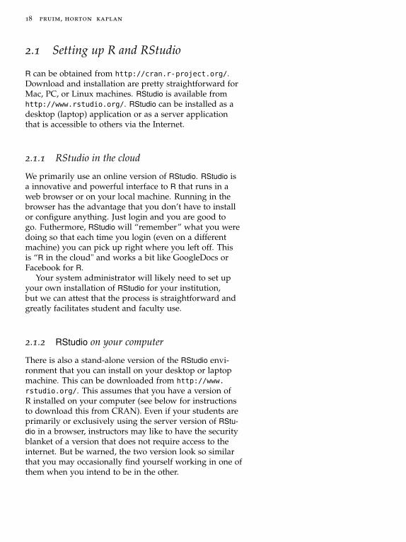
2.1.4 Running RStudio the first time
Once you have launched the desktop version of RStudio orlogged in to an RStudio server, you will see something likethe following.
Notice that RStudio divides its world into four panels.Several of the panels are further subdivided into multi-ple tabs. Which tabs appear in which panels can be cus-tomized by the user. We find it convenient to put the
console in the upper left ratherthan the default location (lowerright) so that students can seeit better when we project our R
session in class.
2.2 Using R as a Calculator in the Console
R can do much more than a simple calculator, and we willintroduce additional features in due time. But performingsimple calculations in R is a good way to begin learningthe features of RStudio.
Commands entered in the Console tab are immediatelyexecuted by R. A good way to familiarize yourself withthe console is to do some simple calculator-like compu-tations. Most of this will work just like you would expect
20 pruim, horton kaplan
from a typical calculator. Try typing the following com-mands in the console panel.
5 + 3
[1] 8
15.3 * 23.4
[1] 358.02
sqrt(16) # square root
[1] 4
This last example demonstrates how functions arecalled within R as well as the use of comments. Com-ments are prefaced with the # character. Comments canbe very helpful when writing scripts with multiple com-mands or to annotate example code for your students.
You can save values to named variables for later reuse.
product = 15.3 * 23.4 # save result
product # display the result
[1] 358.02
product <- 15.3 * 23.4 # <- can be used instead of =
product
[1] 358.02
Teaching Tip
It’s best to settle on using oneor the other of the right-to-leftassignment operators ratherthan to switch back and forth.The authors have differentpreferences: two of us find theequal sign to be simpler for stu-dents and more intuitive, whilethe other prefers the arrowoperator because it representsvisually what is happening inan assignment, because it canalso be used in a left to rightmanner, and because it makes aclear distinction between the as-signment operator, the use of =to provide values to argumentsof functions, and the use of ==to test for equality.
Once variables are defined, they can be referenced inother operations and functions.
0.5 * product # half of the product
[1] 179.01
log(product) # (natural) log of the product
[1] 5.880589
log10(product) # base 10 log of the product
[1] 2.553907

start teaching with r 21
log2(product) # base 2 log of the product
[1] 8.483896
log(product, base=2) # another way for base 2 log
[1] 8.483896
The semi-colon can be used to place multiple com-mands on one line. One frequent use of this is to save andprint a value all in one go:
product <- 15.3 * 23.4; product # store and show result
[1] 358.02
2.3 Working with Files
2.3.1 R Script Files
As an alternative, R commands can be stored in a file.RStudio provides an integrated editor for editing thesefiles and facilitates executing some or all of the com-mands. To create a file, select File, then New File, then R
Script from the RStudio menu. A file editor tab will openin the Source panel. R code can be entered here, and but-tons and menu items are provided to run all the code(called sourcing the file) or to run the code on a singleline or in a selected section of the file.
2.3.2 RMarkdown, and knitr/LATEX
A third alternative is to take advantage of RStudio’s sup-port for reproducible research. If you already know LATEX,you will want to investigate the knitr/LATEX capabili-ties. For those who do not already know LATEX, the sim-pler RMarkdown system provides an easy entry into theworld of reproducible research methods. It also providesa good facility for students to create homework and re-ports that include text, R code, R output, and graphics.

22 pruim, horton kaplan
To create a new RMarkdown file, select File, then New
File, then RMarkdown. The file will be opened with a shorttemplate document that illustrates the mark up language.Click on Compile HTML to convert this to an HTML file.There is a button the provides a brief description of themark commands supported, and the RStudio web siteincludes more extensive tutorials on using RMarkdown. Caution!
RMarkdown, and knitr/LATEXfiles do not have access to theconsole environment, so thecode in them must be self-contained.
It is important to remember that unlike R scripts,which are executed in the console and have access tothe console environment, RMarkdown and knitr/LATEXfiles do not have access to the console environment Thisis a good feature because it forces the files to be self-contained, which makes them transferable and respectsgood reproducible research practices. But beginners, es-pecially if they adopt a strategy of trying things out in theconsole and copying and pasting successful code from theconsole to their file, will often create files that are incom-plete and therefore do not compile correctly.
One good strategy for getting student to use RMark-down is to provide them with a template that includesthe boiler plate you want them to use, loads any R pack-ages that they will need, sets any knitr or R settings theyway you prefer them, and has placeholders for the workyou want them to do.
2.4 The Other Panels and Tabs
2.4.1 The History Tab
As commands are entered in the console, they appear inthe History tab. These histories can be saved and loaded,there is a search feature to locate previous commands,and individual lines or sections can be transfered backto the console. Keeping the History tab open will allowstudents to look back and see the previous several com-mands. This can be especially useful when commandsproduce a fair amount of output and so scroll off thescreen rapidly. History files can be saved and distributedto students so that they can rerun the code illustrated inclass. (Before saving the history, you can remove any linesthat you don’t want saved to spare your students repeat-ing all of your typing errors.)

start teaching with r 23
An alternative is to produce RMarkdown files in classand make those available. This provides a better mecha-nism for adding additional comments or instructions.
2.4.2 Communication between tabs
RStudio provides several ways to move R code betweentabs. Pressing the Run button in the editing panel for an R
script or RMarkdown or other file will copy lines of codeinto the Console and run them.
2.4.3 The Files Tab
The Files tab provides a simple file manager. It can benavigated in familiar ways and used to open, move, re-name, and delete files. In the browser version of RStudio,the Files tab also provides a file upload utility for movingfiles from the local machine to the server. In RMarkdownand knitr files one can also run the code in a particularchunk or in all of the chunks in a file. Each of these fea-tures makes it easy to try out code “live” while creating adocument that keeps a record of the code.
In the reverse direction, code from the history can becopied either back into the console to run them again(perhaps after editing) or into one of the file editing tabsfor inclusion in a file.
2.4.4 The Help Tab
The Help tab is where RStudio displays R help files. Thesecan be searched and navigated in the Help tab. You canalso open a help file using the ? operator in the console.For example
?log
Will provide the help file for the logarithm function.
2.4.5 The Environment Tab
The Environment tab shows the objects available to the con-sole. These are subdivided into data, values (non-dataframe, non-function objects) and functions. The broom

24 pruim, horton kaplan
icon can be used to remove all objects from the environ-ment, and it is good to do this from time to time, espe-cially when running in RStudio server or if you choose tosave the environment when shutting down RStudio sincein these cases objects can stay in the environment essen-tially indefinitely.
2.4.6 The Plots TabIf you haven’t been enteringthese example commands atyour console, go back and do it!
Plots created in the console are displayed in the Plots tab.For example,
# this will make lattice graphics available to the session
require(mosaic)
xyplot( births ~ dayofyear, data=Births78)
dayofyear
birt
hs
7000
8000
9000
10000
0 100 200 300
will display the number of births in the United States foreach day in 1978. From the Plots tab, you can navigate toprevious plots and also export plots in various formatsafter interactively resizing them.
2.4.7 The Packages Tab
Much of the functionality of R is located in packages,many of which can be obtained from a central clearinghouse called CRAN (Comprehensive R Archive Network).The Packages tab facilitates installing and loading pack-ages. It will also allow you to search for packages thathave been updated since you installed them.

3
Using R Early in the Course
This chapter includes some of our favorite activities forearly in the course. These activities simultaneously pro-vide the students with a first glimpse of R and an intro-duction to some major themes of the course. Used thisway, it is not necessary for students to understand the de-tails of the R code. Instead have them focus on the ques-tions being asked on how the results presented shed lighton the answers to these questions.
3.1 Coins and Cups: The Lady Tasting TeaThis section is a slightly mod-ified version of a handout oneof the authors has given IntroStats students on Day 1 aftergoing through the activity as aclass discussion.
There is a famous story about a lady who claimed thattea with milk tasted different depending on whether themilk was added to the tea or the tea added to the milk.The story is famous because of the setting in which shemade this claim. She was attending a party in Cambridge,England, in the 1920s. Also in attendance were a numberof university dons and their wives. The scientists in at-tendance scoffed at the woman and her claim. What, afterall, could be the difference?
All the scientists but one, that is. Rather than simplydismiss the woman’s claim, he proposed that they decidehow one should test the claim. The tenor of the conversa-tion changed at this suggestion, and the scientists beganto discuss how the claim should be tested. Within a fewminutes cups of tea with milk had been prepared andpresented to the woman for tasting.
At this point, you may be wondering who the innova-tive scientist was and what the results of the experimentwere. The scientist was R. A. Fisher, who first described

26 pruim, horton kaplan
this situation as a pedagogical example in his 1925 bookon statistical methodology 1. Fisher developed statistical 1 R. A. Fisher. Statistical Methods
for Research Workers. Oliver &Boyd, 1925
methods that are among the most important and widelyused methods to this day, and most of his applicationswere biological.
You might also be curious about how the experimentcame out. How many cups of tea were prepared? Howmany did the woman correctly identify? What was theconclusion?
Fisher never says. In his book he is interested in themethod, not the particular results. But we can use thissetting to introduce some key ideas in statistics.
Let’s suppose we decide to test the lady with ten cupsof tea. We’ll flip a coin to decide which way to preparethe cups. If we flip a head, we will pour the milk in first;if tails, we put the tea in first. Then we present the tencups to the lady and have her state which ones she thinkswere prepared each way.
It is easy to give her a score (9 out of 10, or 7 out of 10,or whatever it happens to be). It is trickier to figure Teaching Tip
The score is setting up the ideaof a test statistic for later, butthere is no need to introducethat terminology on day 1.
out what to do with her score. Even if she is just guessingand has no idea, she could get lucky and get quite a fewcorrect – maybe even all 10. But how likely is that?
Let’s try an experiment. I’ll flip 10 coins. You guesswhich are heads and which are tails, and we’ll see howyou do. Have each student make a
guess by writing down a se-quence of 10 H’s or T’s whileyou flip the coin behind a bar-rier so that the students cannotsee the results.
Comparing with your classmates, we will undoubtedlysee that some of you did better and others worse.
Now let’s suppose the lady gets 9 out of 10 correct.That’s not perfect, but it is better than we would expectfor someone who was just guessing. On the other hand,it is not impossible to get 9 out of 10 just by guessing. Sohere is Fisher’s great idea: Let’s figure out how hard itis to get 9 out of 10 by guessing. If it’s not so hard to do,then perhaps that’s just what happened, so we won’t betoo impressed with the lady’s tea tasting ability. On theother hand, if it is really unusual to get 9 out of 10 correctby guessing, then we will have some evidence that shemust be able to tell something.
But how do we figure out how unusual it is to get 9
out of 10 just by guessing? We’ll learn another method

start teaching with r 27
later, but for now, let’s just flip a bunch of coins and keeptrack. If the lady is just guessing, she might as well beflipping a coin.
So here’s the plan. We’ll flip 10 coins. We’ll call theheads correct guesses and the tails incorrect guesses.Then we’ll flip 10 more coins, and 10 more, and 10 more,and . . . . That would get pretty tedious. Fortunately, com-puters are good at tedious things, so we’ll let the com-puter do the flipping for us.
The rflip() function can flip one coin
There is a subtle switch here.Before we were asking howmany of the students H’s andT’s matched the flipped coin.Now we are using H to sim-ulate a correct guess and T tosimulate an incorrect guess.This makes simulating easier.
require(mosaic)
rflip()
Flipping 1 coin [ Prob(Heads) = 0.5 ] ...
T
Number of Heads: 0 [Proportion Heads: 0]
or a number of coins
rflip(10)
Flipping 10 coins [ Prob(Heads) = 0.5 ] ...
H T H H T H H H T H
Number of Heads: 7 [Proportion Heads: 0.7]
Typing rflip(10) a bunch of times is almost as te-dious as flipping all those coins. But it is not too hard totell R to do() this a bunch of times. Notice that do() is clever about
what information it records.Rather than recording all ofthe individual tosses, it is onlyrecording the number of flips,the number of heads, and thenumber of tails.
do(3) * rflip(10)
n heads tails prop
1 10 8 2 0.8
2 10 7 3 0.7
3 10 9 1 0.9

28 pruim, horton kaplan
Let’s get R to do() it for us 10,000 times and make a tableof the results.
Teaching Tip
There is always the questionof how many simulations toperform. This is a trade-offbetween speed and accuracy.For simple things, one caneasily perform 10,000 or moresimulations live in class. Formore complicated things (thatmight require fitting a modeland extracting informationfrom it at each iteration) youmight prefer a smaller numberfor live demonstrations.
When you cover inferencefor a proportion, it is a goodidea to use those methods torevisit the question of howmany replications are requiredin that context.
# store the results of 10000 simulated ladies
random.ladies <- do(10000) * rflip(10)
tally(~heads, data=random.ladies)
0 1 2 3 4 5 6 7 8 9 10
3 103 431 1183 2138 2497 1955 1136 464 78 12
# We can also display table using percentages
tally(~heads, data=random.ladies, format="prop")
0 1 2 3 4 5 6 7
0.0003 0.0103 0.0431 0.1183 0.2138 0.2497 0.1955 0.1136
8 9 10
0.0464 0.0078 0.0012
We can display this table graphically using a plotcalled a histogram with bins of width 1. The mosaic package adds
some additional features tohistogram(). In particular, thewidth and center arguments,which make it easier to controlthe bins, are only available ifyou are using the mosaic pack-age.
histogram(~ heads, data=random.ladies, width=1)
heads
Den
sity
0.000.050.100.150.200.25
0 2 4 6 8 10
You might be surprised to see that the number of cor-rect guesses is exactly 5 (half of the 10 tries) only 25%of the time. But most of the results are quite close to 5
correct. For example, 67% of the results are 4, 5, or 6, forexample. About 90% of the results are between 3 and 7
(inclusive). But getting 8 correct is a bit unusual, and get-ting 9 or 10 correct is even more unusual.

start teaching with r 29
So what do we conclude? It is possible that the ladycould get 9 or 10 correct just by guessing, but it is notvery likely (it only happened in about 0.9% of our simula-tions). So one of two things must be true:
• The lady got unusually “lucky", or
• The lady is not just guessing.
Although Fisher did not say how the experiment cameout, others have reported that the lady correctly identifiedall 10 cups! 2 2 D. Salsburg. The Lady Tasting
Tea: How statistics revolutionizedscience in the twentieth century.W.H. Freeman, New York, 2001
A different design
Suppose instead that we prepare five cups each way(and that the woman tasting knows this). We give her fivecards labeled “milk first”, and she must place them nextto the cups that had the milked poured first. How doesthis design change things?
We could simulate this by shuffling a deck of 10 cardsand dealing five of them.cards <- factor(c("M","M","M","M","M","T","T","T","T","T"))
tally(~deal(cards, 5))
M T
2 3
The use of factor() here lets R
know that the possible valuesare ‘M’ and ‘T’, even when onlyone or the other appears in agiven random sample.
results <- do(10000) * tally(~deal(cards, 5))
tally(~ M, data=results)
0 1 2 3 4 5
26 934 3957 3999 1047 37
tally(~ M, data=results, format="prop")
0 1 2 3 4 5
0.0026 0.0934 0.3957 0.3999 0.1047 0.0037
tally(~ M, data=results, format="perc")
0 1 2 3 4 5
0.26 9.34 39.57 39.99 10.47 0.37

30 pruim, horton kaplan
3.2 Births by Day
The Births78 data set contains the number of births inthe United States for each day of 1978. A scatter plot of The use of the phrase “depends
on” is intentional. Later we willemphasize how ˜ can often beinterpreted as “depends on”.
births by day of year reveals some interesting patterns.Let’s see how the number of births depends on the day ofthe year. Teaching Tip
The plot could also be made us-ing date. For general purposes,this is probably the better plotto make, but using dayofyear
forces students to think moreabout what the x-axis means.
xyplot(births ~ dayofyear, data=Births78)
dayofyear
birt
hs
7000
8000
9000
10000
0 100 200 300
When shown this image, students should readily beable to describe two patterns in the data; they shouldnotice both the rise and fall over the course of the yearand the two “parallel waves". Many students will be Teaching Tip
This can make a good “think-pair-share” activity. Have stu-dents come up with possibleexplanations, then discuss theseexplanations with a partner.Finally, have some of the pairsshare their explanations withthe entire class.
able to come up with conjectures about the peaks andvalleys, but they often struggle to correctly interpret theparallel waves. Having them make conjectures about thiswill quickly reveal whether they are correctly interpretingthe plot.
One conjecture about the parallel waves can be checkedusing the data at hand. If we display each day of theweek with a different symbol or color, we see that thereare fewer births on weekends – likely because scheduledbirths are less likely on weekends. There are a handful ofexceptions which are readily seen to be holidays.
start teaching with r 31
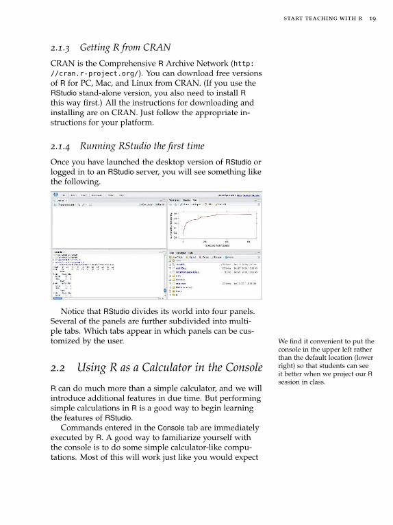
require(mosaicData) # load mosaic data sets
xyplot(births ~ dayofyear, data=Births78,
groups=dayofyear%%7,
auto.key=list(space="right"))
dayofyear
birt
hs
7000
8000
9000
10000
0 100 200 300
0123456
A discussion of this or some other data set that canbe explored through graphical displays is a good way todemonstrate “statistical curiosity", to illustrate the powerof R for creating graphs, and to introduce the importanceof covariates in statistical analysis.
Visualization has been calledthe “gateway drug” to statis-tics. It can be a great way tolure students into statistics –and away from their graphingcalculators.
3.3 SAT and Confounding
The SAT data set contains information about the link be-tween SAT scores and measures of educational expendi-tures. Students are often surprised to see that states thatspend more on education do worse on the SAT.

32 pruim, horton kaplan
xyplot(sat ~ expend, data=SAT)
expend
sat
850
900
950
1000
1050
1100
4 5 6 7 8 9 10
The implication, that spending less might give betterresults, is not justified. Expenditures are confounded withthe proportion of students who take the exam, and scoresare higher in states where fewer students take the exam.
xyplot(expend ~ frac, data=SAT)
xyplot(sat ~ frac, data=SAT)
frac
expe
nd
4
5
6
7
8
9
10
20 40 60 80
frac
sat
850
900
950
1000
1050
1100
20 40 60 80
It is interesting to look at the original plot if we placethe states into two groups depending on whether more orfewer than 40% of students take the SAT:
SAT <- mutate(SAT,
fracGroup = derivedFactor(
hi = (frac > 40),
lo = (frac <=40) ))
xyplot( sat ~ expend | fracGroup , data=SAT,
type=c("p","r") )
xyplot( sat ~ expend, groups = fracGroup , data=SAT,
type=c("p","r") )
start teaching with r 33
expend
sat
850900950
100010501100
4 5 6 7 8 9 10
hi
4 5 6 7 8 9 10
lo
expend
sat
850
900
950
1000
1050
1100
4 5 6 7 8 9 10
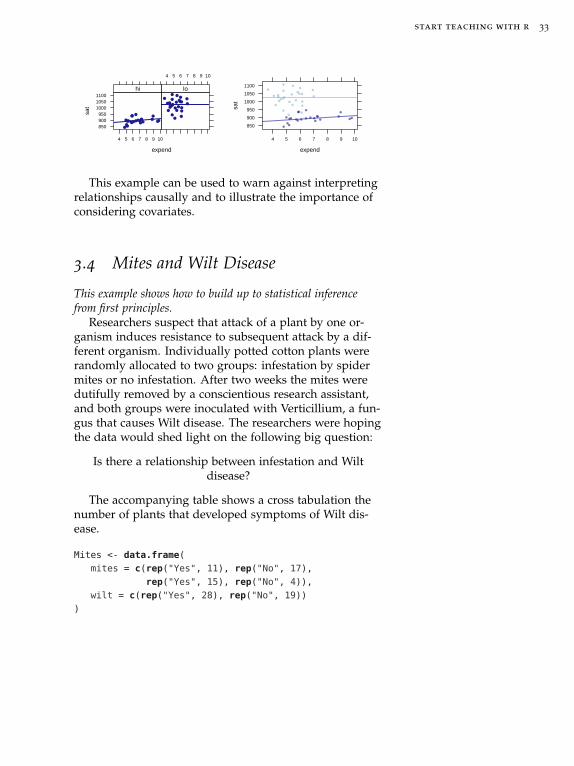
This example can be used to warn against interpretingrelationships causally and to illustrate the importance ofconsidering covariates.
3.4 Mites and Wilt Disease
This example shows how to build up to statistical inferencefrom first principles.
Researchers suspect that attack of a plant by one or-ganism induces resistance to subsequent attack by a dif-ferent organism. Individually potted cotton plants wererandomly allocated to two groups: infestation by spidermites or no infestation. After two weeks the mites weredutifully removed by a conscientious research assistant,and both groups were inoculated with Verticillium, a fun-gus that causes Wilt disease. The researchers were hopingthe data would shed light on the following big question:
Is there a relationship between infestation and Wiltdisease?
The accompanying table shows a cross tabulation thenumber of plants that developed symptoms of Wilt dis-ease.
Mites <- data.frame(
mites = c(rep("Yes", 11), rep("No", 17),
rep("Yes", 15), rep("No", 4)),
wilt = c(rep("Yes", 28), rep("No", 19))
)
34 pruim, horton kaplan
tally(~ wilt + mites, Mites)
mites
wilt No Yes
No 4 15
Yes 17 11
Some questions for students:
1. Here, what do you think is the explanatory variable?Response variable?
2. What proportion of the plants in the study with mitesdeveloped Wilt disease?
3. What proportion of the plants in the study with nomites developed Wilt disease?
4. Relative risk is the ratio of two risk proportions. Whatis the relative risk of developing Wilt disease, compar-ing mites to no mites?
5. If there were no association between mites and Wiltdisease, what would the relative risk be (in the popu-lation as a whole)? How close is the relative risk com-puted from the data to this value?
6. Let X be the number of plants in the no mites groupthat did not develop Wilt disease. What are the possi-ble values for X?
7. Assuming a population relative risk of 1, give two pos-sible values for X that would be more unusual than thevalue for these data?
Questions 6-7 can be addressed using cards:
Physical Simulation
1. Select 47 cards from your deck: 26 red (mites!) and 21 black
2. Shuffle the cards well
3. Deal out 19 cards, these represent the 19 plants without Wilt disease.
4. Count the number of black cards among those 19. What do these represent?
5. Repeat steps 2 –4, five times.
Students can pool their results by recording them ina table on the board at the front of the room. Then have
start teaching with r 35
students process the results by answering the followingquestions.
8. How many black cards would we expect (on average)?Why?
9. What did we observe?
10. How would we summarize these results? What is thebig idea?
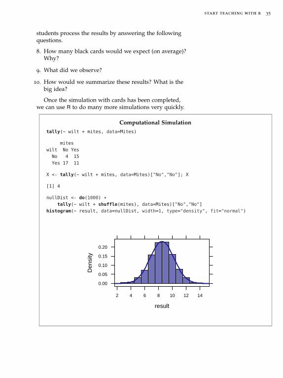
Once the simulation with cards has been completed,we can use R to do many more simulations very quickly.
Computational Simulation
tally(~ wilt + mites, data=Mites)
mites
wilt No Yes
No 4 15
Yes 17 11
X <- tally(~ wilt + mites, data=Mites)["No","No"]; X
[1] 4
nullDist <- do(1000) *tally(~ wilt + shuffle(mites), data=Mites)["No","No"]
histogram(~ result, data=nullDist, width=1, type="density", fit="normal")
result
Den
sity
0.00
0.05
0.10
0.15
0.20
2 4 6 8 10 12 14

4
Less Volume, More Creativity
A lot of times you end up putting in a lot more vol-ume, because you are teaching fundamentals and youare teaching concepts that you need to put in, but youmay not necessarily use because they are building blocksfor other concepts and variations that will come off ofthat ... In the offseason you have a chance to take a stepback and tailor it more specifically towards your teamand towards your players.
– Mike McCarthy, Head Coach, Green Bay Packers
Perfection is achieved, not when there is nothing more toadd, but when there is nothing left to take away.
– Antoine de Saint-Exupery, writer, poet, aviator
One key to successfully introducing R is finding a set ofcommands that is
• small,
• coherent, and
• powerful.
This chapter provides an extensive example of this“Less Volume, More Creativity" approach. The mosaic
package (combined with the lattice package and othercore R functionality) provides a simple yet powerfulframework that equips students to produce all of the
• numerical summaries,
• graphical summaries, and
• linear models

start teaching with r 37
needed in an introductory course. By presenting this asone master template with variations, we emphasize thesimilarity among these commands and reduce the cogni-tive load for students. In our experience, this has made R
much more approachable and enjoyable for students andtheir instructors.
4.1 The mosaic package and the formula tem-
plate
Much of the early work on the mosaic package centeredon producing a minimal set of R commands that couldprovide students with everything need for introductorystatistics without overwhelming students with too manycommands. One of the mosaic package vignettes includesa document describing just such a set of commands.
Much of this is built off the following template that isused repeatedly
(
∼ , data =
)
The template is used by filling in the boxes. It helps togive each box a name:
goal
(
y ∼ x , data = mydata
)
Teaching Tip
After introducing this template,you might quiz students tomake sure they have learnedit. This will also emphasize itsimportance.
The template has a bit more flexibility than we haveindicated. Sometimes the y is not needed:
goal ( ~ x, data=mydata )
The formula may also include a third part
goal ( y ~ x | z , data=mydata )
We can unify all of these into one form:
goal ( formula , data=mydata )
The template can be applied to create numerical sum-maries, graphical summaries, or model fits by answeringtwo questions and using the answers to fill in the slots ofthe template:
38 pruim, horton kaplan
1. What do you want R to do?
This is the goal.
2. What must R know to do that?
These are the inputs to the function. For numericalsummaries, graphical summaries, and model fits, wetypically need to specify the variables involved and thedata frame in which they are stored.
4.2 Graphical summaries of data
Teaching Tip
We recommend showing someplots on the first day and hav-ing student generate their owngraphs before the end of thefirst week.
Graphical summaries are an important and eye-catchingway to demonstrate the power and flexibility of our tem-plate. We like to introduce students to graphical sum-maries early in the course. This gives the students accessto functionality where R really shines (and is certainlymuch better than a hand-held calculator). It also beginsto develop their ability to interpret graphical represen-tations of data, to think about distributions, and to posestatistical questions.
More Info
We are often asked about theother graphics systems, espe-cially ggplot2 graphics. In ourexperience, lattice makes iteasier for beginners to createa wide variety of more or less“standard” plots – includingthe ability to represent multiplevariables at once. ggplot2, onthe other hand, makes it easierto generate custom plots or tocombine plot components. Eachhas their place, and we use bothsystems. But for beginners, wetypically emphasize lattice.
The new ggvis package, bythe same author as ggplot2
adds interactivity and speed tothe strengths of ggplot2.
There are several ways to make graphs in R. One ap-proach is a system called lattice graphics. Wheneverthe mosaic package is loaded, the lattice package is alsoloaded. One of the attractive aspects of lattice plots isthat they make use of the same template we will use fornumerical summaries and linear models.
4.2.1 Graphical summaries of two variables
A first example: Making a scatter plot
As an example, let’s create the following plot, whichshows the number of births in the United States for eachday in 1978.
start teaching with r 39
date
birt
hs
7000
8000
9000
10000
Jan Apr Jul Oct Jan
Teaching Tip
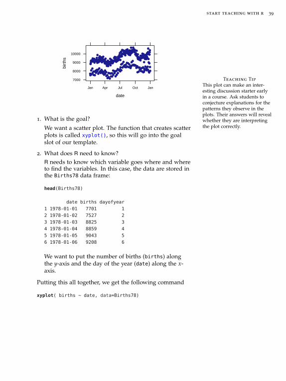
This plot can make an inter-esting discussion starter earlyin a course. Ask students toconjecture explanations for thepatterns they observe in theplots. Their answers will revealwhether they are interpretingthe plot correctly.
1. What is the goal?
We want a scatter plot. The function that creates scatterplots is called xyplot(), so this will go into the goalslot of our template.
2. What does R need to know?
R needs to know which variable goes where and whereto find the variables. In this case, the data are stored inthe Births78 data frame:
head(Births78)
date births dayofyear
1 1978-01-01 7701 1
2 1978-01-02 7527 2
3 1978-01-03 8825 3
4 1978-01-04 8859 4
5 1978-01-05 9043 5
6 1978-01-06 9208 6
We want to put the number of births (births) alongthe y-axis and the day of the year (date) along the x-axis.
Putting this all together, we get the following command
xyplot( births ~ date, data=Births78)

40 pruim, horton kaplan
Another Example: Boxplots
Now let’s create this plot, which shows boxplots of agefor each of three substances abused by participants in theHealth Evaluation and Linkage to Primary Care randomizedclinical trial. More Info
You can find out more aboutthe HELPrct data set using thehelp command: ?HELPrct.
age
20
30
40
50
60
alcohol cocaine heroin
The data we need are in the HELPrct data frame, fromwhich we want to display variables age and substance onthe y- and x-axes. According to our template, the com-mand to create this plot has the form
goal( age ~ substance, data=HELPrct )
The only additional information we need is the nameof the function that creates boxplots. That function isbwplot(). So we can create the plot with
bwplot( age ~ substance, data=HELPrct)
To make the boxplots horizontal instead of vertical,reverse the roles of age and substance:
bwplot( substance ~ age, data=HELPrct )
age
alcohol
cocaine
heroin
20 30 40 50 60

start teaching with r 41
More Info
You may be wondering aboutplots for two categorical vari-ables. A commonly used plotfor this is a segmented bargraph. We will treat this as aaugmented version of a simplebar graph, which is a graphicalsummary of one categoricalvariable.
Another plot that can beused to display two (or more)categorical variables is a mosaicplot. The lattice package doesnot include mosaic plots, butthe vcd package provides amosaic() function that createsmosaic plots.
4.2.2 Graphical summaries of one variable
If we want to make a plot that involves only one variable,we simply omit the y-part of the formula. For example, ahistogram like
age
Den
sity
0.00
0.01
0.02
0.03
0.04
0.05
0.06
20 30 40 50 60
can be made with Caution!It is important to note thatwhen there is only one variableit is on the right side of theformula.
Teaching Tip
Tell students that because R
is computing the y values, wedon’t need to provide them.This isn’t exactly the reasonwhy things are this way, but ithelps them remember.
histogram( ~ age, data=HELPrct)
Introducing width and center
here is perhaps a violation ofour usual policy of acceptingdefaults and saving options forlater. But it is important thathistogram bins be chosen ap-propriately, and no algorithmicdefault works well for all datasets. We encourage students tomake several histograms andto experiment with center andespecially width.
The mosaic package adds some extra functionality tohistogram() to make it easier to specify the bins used. Inparticular, the options width and center (default is 0) canbe used to define the width of the bins and the center ofone of the bins. For example, to create a histogram withbins that are 5 years wide we can use width=5, and wecan shift the bins left and right by providing a value forcenter. center need not be contained in the bins that aredisplayed. So to get bins with edges “on the 0’s and 5’s”,we can set the center to 2.5, regardless of the range of thedata.
histogram( ~ age, data=HELPrct, width=5)
histogram( ~ age, data=HELPrct, width=5, center=2.5)
age
Den
sity
0.00
0.01
0.02
0.03
0.04
0.05
20 30 40 50 60
age
Den
sity
0.00
0.01
0.02
0.03
0.04
0.05
20 30 40 50 60

42 pruim, horton kaplan
There is enough data here to use a bin for each integer ifwe like. Because the default value of center is 0, settingwidth to 1 centers the bins on the integers, avoiding po-tential confusion about which edge is included in the bin.
histogram( ~ age, data=HELPrct, width=1)
age
Den
sity
0.00
0.02
0.04
0.06
0.08
20 30 40 50 60
Additional plots of a single quantitative variable are illus-trated in Section sec:paletteOfPlots.
For a single categorical variable, we can make a bargraph for a categorical variable using bargraph() in placeof histogram(). Since formulas are required to have aright-hand side, horizontal bar graphs are produced us-ing horizontal = TRUE. More Info
The bargraph() function is notin the lattice package butin the mosaic package. Thelattice function barchart()
creates bar graphs from sum-marized data; bargraph() takescare of creating this summarydata and then uses barchart()
to create the plot.
bargraph( ~ substance, data=HELPrct )
bargraph( ~ substance, data=HELPrct, horizontal=TRUE )
Fre
quen
cy
0
50
100
150
alcohol cocaine heroin
Frequency
alcohol
cocaine
heroin
0 50 100 150
4.2.3 A palette of plots
The power of the template is that we can now make manydifferent kinds of plots by mimicking the examples abovebut replacing the goal.

start teaching with r 43
histogram( ~age, data=HELPrct )
densityplot( ~age, data=HELPrct )
freqpolygon( ~age, data=HELPrct )
dotPlot( ~age, data=HELPrct, width=1 )
bwplot( ~age, data=HELPrct )
qqmath( ~age, data=HELPrct )
age
Den
sity
0.00
0.01
0.02
0.03
0.04
0.05
0.06
20 30 40 50 60
age
Den
sity
0.00
0.01
0.02
0.03
0.04
0.05
20 30 40 50 60
age
Den
sity
0.00
0.01
0.02
0.03
0.04
0.05
0.06
20 30 40 50 60
age
Cou
nt
0
10
20
30
20 30 40 50 60
age
20 30 40 50 60
qnorm
age
20
30
40
50
60
−3 −2 −1 0 1 2 3
For one categorical variable, we can use a bar graph.The lattice package does not supply a function for cre-ating pie charts. This is no great loss since it is generallyharder to make comparisons using a pie chart.
bargraph( ~sex, data=HELPrct ) # categorical variable
Fre
quen
cy
0
100
200
300
female male

44 pruim, horton kaplan
xyplot( width ~ length, data=KidsFeet ) # 2 quantitative vars
plotPoints( width ~ length, data=KidsFeet ) # mosaic alternative
bwplot( length ~ sex, data=KidsFeet ) # 1 cat; 1 quant
bwplot( sex ~ length, data=KidsFeet ) # reverse roles
length
wid
th
8.0
8.5
9.0
9.5
22 23 24 25 26 27
length
wid
th8.0
8.5
9.0
9.5
22 23 24 25 26 27
leng
th
22
23
24
25
26
27
B G
length
B
G
22 23 24 25 26 27
Caution!There is also a functiondotPlot() (with a capital P).Note that dotplot() produces avery different kind of plot fromthat produced by dotPlot().
The lattice package also provides the stripplot()
and dotplot() functions which can be used for one-dimensional scatter plots. These work reasonably wellfor small data sets but are of limited utility for larger datasets.
stripplot( ~length, data=KidsFeet )
dotplot( ~length, data=KidsFeet )
length
22 23 24 25 26 27
length
22 23 24 25 26 27
These and xyplot() or plotPoints() can also be used Teaching Tip
We generally don’t introducedotplot() and stripplot()
to students but simply usexyplot() or plotPoints().
with one quantitative variable and one categorical vari-able.
xyplot( sex ~ length, data=KidsFeet )
plotPoints( sex ~ length, data=KidsFeet )
stripplot( sex ~ length, data=KidsFeet )
dotplot( sex ~ length, data=KidsFeet )

start teaching with r 45
length
sex
B
G
22 23 24 25 26 27
length
sex
B
G
22 23 24 25 26 27
length
B
G
22 23 24 25 26 27
length
B
G
22 23 24 25 26 27
4.2.4 Groups and sub-plots
We can add additional variables to our plots either byoverlaying multiple plots or by placing multiple plotsnext to each other in a grid. To overlay plots, we add anextra argument to our template using groups = , and tocreate sub-plots (called panels in lattice and facets inggplot2 graphics) using a formula of the form
y ~ x | z
For example, we can overlay density plots of age foreach substance group in separate panels for each sex:
densityplot( ~ age | sex, data=HELPrct,
groups=substance,
auto.key=TRUE)
age
Den
sity
0.000.020.040.06
10 20 30 40 50 60 70
female
10 20 30 40 50 60 70
male
alcoholcocaineheroin

46 pruim, horton kaplan
auto.key=TRUE adds a simple legend so we can tell whichof the overlaid curves is which.
4.3 Numerical Summaries
The important thing to notice in this section is how littlethere is to learn once you know how to make plots. Sim-ply change the plot name to a summary statistic nameand your done. Numerical summaries can be created inthe same way, we simply replace the plot name with thename of the numerical summary we desire. Nothing elsechanges; a mean and a histogram each summarise a sin-gle variable, so exchanging histogram() for mean() givesus the numerical summary we desire.
histogram( ~ age, data=HELPrct )
mean( ~ age, data=HELPrct )
[1] 35.65342
age
Den
sity
0.00
0.01
0.02
0.03
0.04
0.05
0.06
20 30 40 50 60
More Info
To see the full list of theseformula-aware numericalsummary functions, usehelp(favstats).
The mosaic package includes formula-aware versionsof several numerical summaries, including mean(), sd(),var(), min(), max(), sum(), IQR(). In addition, the favstats()
function computes many of our favorite statistics all atonce:
favstats( ~ age, data=HELPrct )
min Q1 median Q3 max mean sd n missing
19 30 35 40 60 35.65342 7.710266 453 0
The tally() function can be used to count cases.

start teaching with r 47
tally( ~ sex, data=HELPrct)
female male
107 346
tally( ~ substance, data=HELPrct)
alcohol cocaine heroin
177 152 124
Sometimes it is more convenient to display proportions orpercents.
tally( ~ substance, data=HELPrct, format="percent")
alcohol cocaine heroin
39.07285 33.55408 27.37307
tally( ~ substance, data=HELPrct, format="proportion")
alcohol cocaine heroin
0.3907285 0.3355408 0.2737307
Summary statistics can be computed separately formultiple subsets of a data set. This is analogous to plot-ting multiple variables and can be thought about in threeways. Each of these computes the same value.
# age dependant on substance
sd( age ~ substance, data=HELPrct )
alcohol cocaine heroin
7.652272 6.692881 7.986068
# age separately for each substance
sd( ~ age | substance, data=HELPrct )
alcohol cocaine heroin
7.652272 6.692881 7.986068
# age grouped by substance
sd( ~ age, groups=substance, data=HELPrct )
alcohol cocaine heroin
7.652272 6.692881 7.986068
48 pruim, horton kaplan
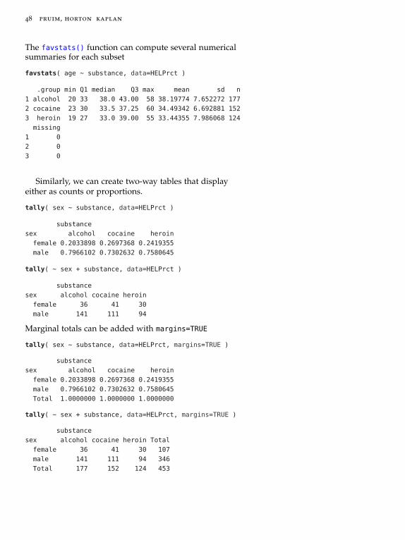
The favstats() function can compute several numericalsummaries for each subset
favstats( age ~ substance, data=HELPrct )
.group min Q1 median Q3 max mean sd n
1 alcohol 20 33 38.0 43.00 58 38.19774 7.652272 177
2 cocaine 23 30 33.5 37.25 60 34.49342 6.692881 152
3 heroin 19 27 33.0 39.00 55 33.44355 7.986068 124
missing
1 0
2 0
3 0
Similarly, we can create two-way tables that displayeither as counts or proportions.
tally( sex ~ substance, data=HELPrct )
substance
sex alcohol cocaine heroin
female 0.2033898 0.2697368 0.2419355
male 0.7966102 0.7302632 0.7580645
tally( ~ sex + substance, data=HELPrct )
substance
sex alcohol cocaine heroin
female 36 41 30
male 141 111 94
Marginal totals can be added with margins=TRUE
tally( sex ~ substance, data=HELPrct, margins=TRUE )
substance
sex alcohol cocaine heroin
female 0.2033898 0.2697368 0.2419355
male 0.7966102 0.7302632 0.7580645
Total 1.0000000 1.0000000 1.0000000
tally( ~ sex + substance, data=HELPrct, margins=TRUE )
substance
sex alcohol cocaine heroin Total
female 36 41 30 107
male 141 111 94 346
Total 177 152 124 453

start teaching with r 49
4.4 Linear models
Although we have not mentioned linear models yet, theyare an important motivation for the template approach tographical and numerical summaries. The lattice graph-ics system already makes use of the same template aslinear models, and the mosaic package makes it possibleto do numerical summaries with the same template. Byintroducing students to the template for graphical andnumerical summaries, there is very little new to learnwhen they are ready to fit a model.
Perhaps you are thinking thismeans that we don’t need towait so long to introduce mod-eling in the introductory statis-tics course. We think so too. Seethe companion volume, StartModeling in R.
For example, suppose we want to know how the widthof kids’ feet depends on the length of the their feet. Wecould make a scatter plot and we can construct a linearmodel using the same template
xyplot( width ~ length, data=KidsFeet )
lm( width ~ length, data=KidsFeet )
Call:
lm(formula = width ~ length, data = KidsFeet)
Coefficients:
(Intercept) length
2.8623 0.2479
length
wid
th
8.0
8.5
9.0
9.5
22 23 24 25 26 27
We’ll have more to say about modeling elsewhere. Fornow, the important point is that our use of the templatefor graphing and numerical summaries prepares studentsto ask how does y depend on x and to formalize modelsof two or more variables when the time comes.

50 pruim, horton kaplan
4.5 A few other tests
Many introductory statistics classes introduce studentsto one- and two-sample tests for means and proportions.The mosaic package brings these into the template aswell. More Info
For a more thorough treatmentof how to use R for the coretopics of a traditional intro-ductory statistics course, seeA Compendium of Commands toTeach Statistics with R.t.test( ~ length, data=KidsFeet )
One Sample t-test
data: data$length
t = 117.1807, df = 38, p-value < 2.2e-16
alternative hypothesis: true mean is not equal to 0
95 percent confidence interval:
24.29597 25.15019
sample estimates:
mean of x
24.72308
The output from these functions also includes more thanwe really need. The mosaic package provides pval() andconfint() for extracting p-values and confidence inter-vals: More Info
Chi-squared tests can be per-formed using chisq.test().This function is a little differentin that it operates on tabulateddata of the sort produced bytally() rather than on the dataitself. So the use of the templatehappens inside tally() ratherthan in chisq.test().
pval( t.test( ~ length, data=KidsFeet ) )
p.value
3.064229e-50
confint( t.test( ~ length, data=KidsFeet ) )
mean of x lower upper level
24.72308 24.29597 25.15019 0.95000

start teaching with r 51
confint(t.test( length ~ sex, data=KidsFeet ))
mean in group B mean in group G lower upper level
25.10500000 24.32105263 -0.04502067 1.61291541 0.95000000
# using Binomial distribution
confint(binom.test( ~ sex, data=HELPrct ))
probability of success lower upper level
0.2362031 0.1978173 0.2780728 0.9500000
# using normal approximation to the binomial distribution
confint(prop.test( ~ sex, data=HELPrct ))
p lower upper level
0.2362031 0.1983770 0.2785900 0.9500000
confint(prop.test( sex ~ homeless, data=HELPrct ))
prop 1 prop 2 lower upper level
0.191387560 0.274590164 -0.164977680 -0.001427528 0.950000000
4.6 lattice bells and whistles
In the plots we have shown so far, we have focused oncreating a variety of useful plots and (for the most part)accepted the default presentation of them. The lattice
graphics system provides many bells and whistles thatcan be introduced once the graphics template has beenmastered. Optional arguments to the graphics functionscan be used to add or modify
• the viewing window
• titles,
• axis labels,
• colors, shapes, sizes, and line types,
• transparency,
• fonts

52 pruim, horton kaplan
and many other features of a plot. Our advice is to holdoff on such bells and whistles until students ask or ananalysis demands them.
4.6.1 Example: Number of births per day
We have seen the Births78 data set in Section 3.2. Theplots below take advantage of additional arguments toimprove the plot. The first plot below illustrates one of More Info
%% performs modular arith-metic, in this case giving sevengroups, one for each day of theweek.
the important features of this data set – there are usuallyfewer births on two days of the week and more on theother five. From this we can be quite certain that 1978
More Info
Some of the arguments hereuse lists. Lists are one of thefundamental “container types”in R. Instructors will benefitfrom being able to recognizethem. We will have more to sayabout them in Chapter 6.
began on a Sunday.
More Info
We could also use the wday()
function in the lubridate pack-age to compute the weekdaydirectly from date.
xyplot( births ~ date, data=Births78,
groups=dayofyear %% 7,
auto.key=list(columns=4),
main="Number of US births each day in 1978",
xlab="day of year",
ylab="# of births",
par.settings=list(
superpose.symbol=list(pch=16, cex=.8, alpha=.8))
)
Number of US births each day in 1978
day of year
# of
bir
ths
7000
8000
9000
10000
Jan Apr Jul Oct Jan
01
23
45
6
Here we have used
• auto.key to control the layout of the legend (4 columnsinstead of 1)
• main to set the title for the plot
• xlab and ylab to set the axis labels
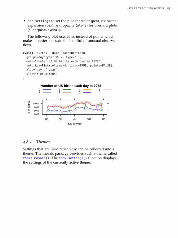
start teaching with r 53
• par.settings to set the plot character (pch), characterexpansion (cex), and opacity (alpha) for overlaid plots(superpose.symbol).
The following plot uses lines instead of points whichmakes it easier to locate the handful of unusual observa-tions.
xyplot( births ~ date, data=Births78,
groups=dayofyear %% 7, type='l',
main="Number of US births each day in 1978",
auto.key=list(columns=4, lines=TRUE, points=FALSE),
xlab="day of year",
ylab="# of births"
)
Number of US births each day in 1978
day of year
# of
bir
ths
7000
8000
9000
10000
Jan Apr Jul Oct Jan
01
23
45
6
4.6.2 Themes
Settings that are used repeatedly can be collected into atheme. The mosaic package provides such a theme calledtheme.mosaic(). The show.settings() function displaysthe settings of the currently active theme.
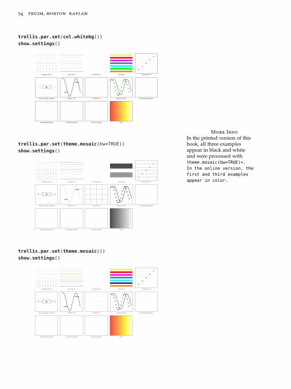
54 pruim, horton kaplan
trellis.par.set(col.whitebg())
show.settings()
superpose.symbol superpose.line strip.background strip.shingle dot.[symbol, line]
box.[dot, rectangle, umbrella] add.[line, text]
Hello
World
reference.line plot.[symbol, line] plot.shingle[plot.polygon]
histogram[plot.polygon] barchart[plot.polygon] superpose.polygon regions
More Info
In the printed version of thisbook, all three examplesappear in black and whiteand were processed withtheme.mosaic(bw=TRUE)+.
In the online version, the
first and third examples
appear in color.
trellis.par.set(theme.mosaic(bw=TRUE))
show.settings()
superpose.symbol superpose.line strip.background strip.shingle dot.[symbol, line]
box.[dot, rectangle, umbrella] add.[line, text]
Hello
World
reference.line plot.[symbol, line] plot.shingle[plot.polygon]
histogram[plot.polygon] barchart[plot.polygon] superpose.polygon regions
trellis.par.set(theme.mosaic())
show.settings()
superpose.symbol superpose.line strip.background strip.shingle dot.[symbol, line]
box.[dot, rectangle, umbrella] add.[line, text]
Hello
World
reference.line plot.[symbol, line] plot.shingle[plot.polygon]
histogram[plot.polygon] barchart[plot.polygon] superpose.polygon regions
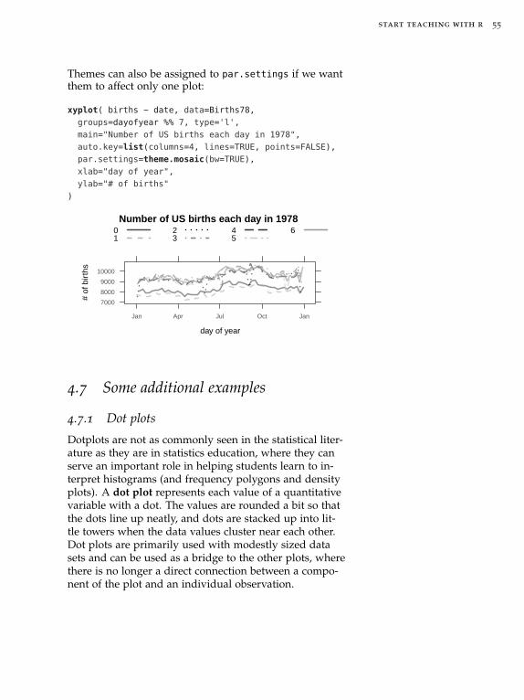
start teaching with r 55
Themes can also be assigned to par.settings if we wantthem to affect only one plot:
xyplot( births ~ date, data=Births78,
groups=dayofyear %% 7, type='l',
main="Number of US births each day in 1978",
auto.key=list(columns=4, lines=TRUE, points=FALSE),
par.settings=theme.mosaic(bw=TRUE),
xlab="day of year",
ylab="# of births"
)
Number of US births each day in 1978
day of year
# of
bir
ths
7000
8000
9000
10000
Jan Apr Jul Oct Jan
01
23
45
6
4.7 Some additional examples
4.7.1 Dot plots
Dotplots are not as commonly seen in the statistical liter-ature as they are in statistics education, where they canserve an important role in helping students learn to in-terpret histograms (and frequency polygons and densityplots). A dot plot represents each value of a quantitativevariable with a dot. The values are rounded a bit so thatthe dots line up neatly, and dots are stacked up into lit-tle towers when the data values cluster near each other.Dot plots are primarily used with modestly sized datasets and can be used as a bridge to the other plots, wherethere is no longer a direct connection between a compo-nent of the plot and an individual observation.

56 pruim, horton kaplan
Here is an example using the sepal lengths recorded inthe iris data set.
dotPlot(~ Sepal.Length, data=iris,
n=30, # approx. 30 bins/columns
alpha=.6) # partially transparent
Sepal.Length
Cou
nt
0
2
4
6
8
10
12
5 6 7 8
We can use a conditional variable to give us separate
Teaching Tip
Dot plots are useful for dis-playing sampling distributionsand bootstrap distributions,especially if the total numberof dots is chosen to be some-thing simple like 1000. In thatcase, probabilities can be easilyestimated by counting dots.
dot plots for each of the three species in this data set.
dotPlot(~ Sepal.Length | Species, data=iris, n=20,
layout=c(3,1)) # 3 columns (x) and 1 row (y)
Sepal.Length
Cou
nt
0
2
4
6
8
5 6 7 8
setosa
5 6 7 8
versicolor
5 6 7 8
virginica
The connection between histograms and dot plots canbe visualized by overlaying one on top of the other.
Sepal.Length
Cou
nt
0
5
10
15
5 6 7 8

start teaching with r 57
4.7.2 Frequency polygons: freqpolygon()
Frequency polygons and density plots provide alterna-tives to histograms that make it easier to overlay the rep-resentations of multiple subsets of the data. A frequencypolygon is created from the same data summary (binsand counts) as a histogram, but instead of representingeach bin with a bar, it is represented by a point (at thecenter of the where the top of the histogram bar wouldhave been).
These points are then connected with line segments.Here is an example that shows the distribution of OldFaithful eruptions times from a sequence of observations Caution!
The faithful data set containssimilar data, but the variablenames in that data frame arepoorly chosen. The geyser dataset in the MASS package hasbetter names and more data.
require(MASS)
freqpolygon( ~ duration, data=geyser, n=15)
duration
Den
sity
0.0
0.2
0.4
0.6
1 2 3 4 5 6
Numerically, the data are being summarized and rep-
Teaching Tip
Point out that an interestingfeature of this distribution is itsclear bimodality. In particular,the mean and median eruptiontime are not a good measuresof the duration of a “typical”eruption since almost none ofthe eruption durations are nearthe mean and median.
resented in exactly the same way as for histograms, butvisually the horizontal and vertical line segments of thehistogram are replaced by sloped line segments.
duration
Den
sity
0.0
0.2
0.4
0.6
1 2 3 4 5 6

58 pruim, horton kaplan
duration
Den
sity
0.0
0.2
0.4
0.6
1 2 3 4 5 6
This may give a more accurate visual representation insome situations (since the distribution can “taper off” bet-ter). More importantly, it makes it much easier to overlaymultiple distributions.
freqpolygon( ~ Sepal.Length, data=iris,
groups=Species,
ylim=c(0,1.5) # manually set y-axis range
)
Sepal.Length
Den
sity
0.5
1.0
4 5 6 7 8
4.7.3 Density plots: densityplot()
Density plots are similar to frequency polygons, but thepiecewise linear representation is replaced by a smoothcurve.
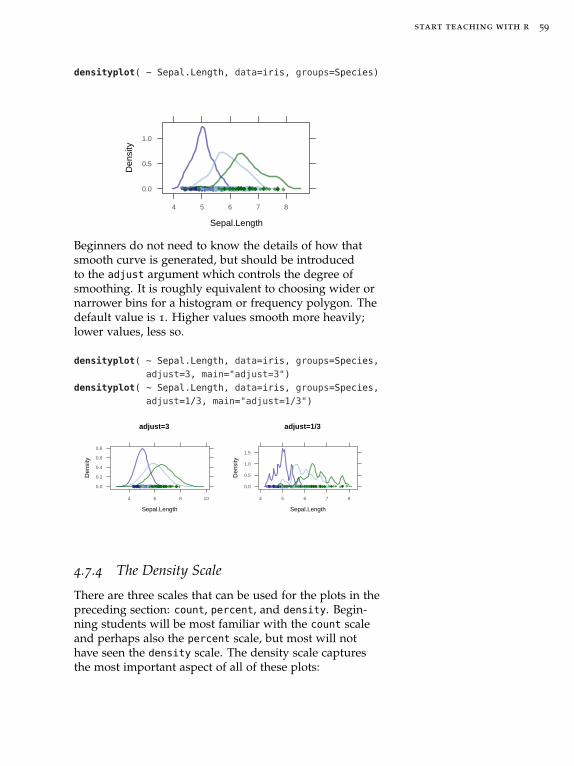
start teaching with r 59
densityplot( ~ Sepal.Length, data=iris, groups=Species)
Sepal.Length
Den
sity
0.0
0.5
1.0
4 5 6 7 8
Beginners do not need to know the details of how thatsmooth curve is generated, but should be introducedto the adjust argument which controls the degree ofsmoothing. It is roughly equivalent to choosing wider ornarrower bins for a histogram or frequency polygon. Thedefault value is 1. Higher values smooth more heavily;lower values, less so.
densityplot( ~ Sepal.Length, data=iris, groups=Species,
adjust=3, main="adjust=3")
densityplot( ~ Sepal.Length, data=iris, groups=Species,
adjust=1/3, main="adjust=1/3")
adjust=3
Sepal.Length
Den
sity
0.0
0.2
0.4
0.6
0.8
4 6 8 10
adjust=1/3
Sepal.Length
Den
sity
0.0
0.5
1.0
1.5
4 5 6 7 8
4.7.4 The Density Scale
There are three scales that can be used for the plots in thepreceding section: count, percent, and density. Begin-ning students will be most familiar with the count scaleand perhaps also the percent scale, but most will nothave seen the density scale. The density scale capturesthe most important aspect of all of these plots:

60 pruim, horton kaplan
Area is proportional to frequency.
The density scale is chosen so that the constant of propor-tionality is 1, in which case we have
Area equals proportion.Teaching Tip
Create some histograms or fre-quency polygons with a densityscale and see if your studentscan determine what the scaleis. Choosing convenient binwidths (but not 1) and com-paring plots with different binwidths and different scale typescan help them reach a goodconjecture about the densityscale.
This is the only scale available for densityplot() and isthe most suitable scale if one is primarily interested in theshape of the distribution. The vertical scale is affected verylittle by the choice of bin widths or adjust multipliers.It is also the appropriate scale to use when overlaying adensity function onto a histogram, something the mosaic
package makes easy to do.
histogram( ~ Sepal.Length | Species, data=iris, fit="normal" )
Sepal.Length
Den
sity
0.00.20.40.60.81.0
5 6 7 8
setosa
5 6 7 8
versicolor
5 6 7 8
virginica
The other scales are primarily of use when one wantsto be able to read off bin counts or percents from the plot.
4.7.5 Groups or panels?
The following examples using the iris data set providea comparison of using groups or panels to separate sub-sets of the data. First we put the three species into threeseparate panels.
xyplot(Sepal.Length ~ Sepal.Width | Species, data=iris,
layout=c(3,1)) # layout controls number of columns and rows
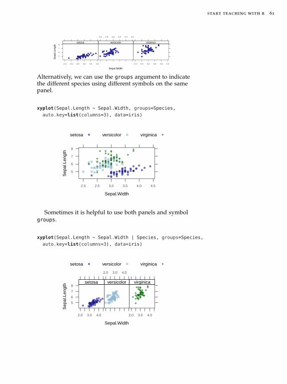
start teaching with r 61
Sepal.Width
Sep
al.L
engt
h5
6
7
8
2.0 2.5 3.0 3.5 4.0 4.5
setosa
2.0 2.5 3.0 3.5 4.0 4.5
versicolor
2.0 2.5 3.0 3.5 4.0 4.5
virginica
Alternatively, we can use the groups argument to indicatethe different species using different symbols on the samepanel.
xyplot(Sepal.Length ~ Sepal.Width, groups=Species,
auto.key=list(columns=3), data=iris)
Sepal.Width
Sep
al.L
engt
h
5
6
7
8
2.0 2.5 3.0 3.5 4.0 4.5
setosa versicolor virginica
Sometimes it is helpful to use both panels and symbolgroups.
xyplot(Sepal.Length ~ Sepal.Width | Species, groups=Species,
auto.key=list(columns=3), data=iris)
Sepal.Width
Sep
al.L
engt
h
5
6
7
8
2.0 3.0 4.0
setosa
2.0 3.0 4.0
versicolor
2.0 3.0 4.0
virginica
setosa versicolor virginica

62 pruim, horton kaplan
4.7.6 Dealing with long labels
Suppose we want to display the following table (based ondata from the 1985 Current Population Survey) using bargraph.
tally( ~sector, data=CPS85 )
clerical const manag manuf other prof
97 20 55 68 68 105
sales service
38 83
The mosaic function bargraph() can display these tablesas bar graphs, but there isn’t enough room for the labels.
bargraph(~ sector, data=CPS85)
Fre
quen
cy
0
20
40
60
80
100
clericalconstmanagmanufother prof salesservice
One solution would be to use horizontal bars
# horizontal bars
bargraph(~ sector, data=CPS85, horizontal=TRUE)
Frequency
clericalconst
managmanufotherprof
salesservice
0 20 40 60 80 100
Another is to rotate the labels.

start teaching with r 63
bargraph(~ sector, data=CPS85,
scales=list(x=list(rot=45)))
Fre
quen
cy
0
20
40
60
80
100
cleric
al
cons
t
man
ag
man
ufot
her
prof
sales
serv
ice
As with the other lattice plots, we can add grouping orconditioning to our plot.
bargraph(~ sector, data=CPS85, groups=race,
auto.key=list(space="right"),
scales=list(x=list(rot=45)))
bargraph(~ sector | race, data=CPS85,
scales=list(x=list(rot=45)))
Fre
quen
cy
0
20
40
60
80
100
cleric
al
cons
t
man
ag
man
ufot
herpr
of
sales
serv
ice
NWW
Fre
quen
cy
0
20
40
60
80
100
cleric
al
cons
t
man
ag
man
ufot
herpr
of
sales
serv
ice
NW
cleric
al
cons
t
man
ag
man
ufot
herpr
of
sales
serv
ice
W
4.8 Saving Your Plots
There are several ways to save plots in RStudio, but theeasiest is probably the following: You can save all of this export-
ing and copying and pastingif you use RMarkdown, orknitr/LATEX to prepare yourdocuments.
1. In the Plots tab, click the “Export” button.
2. Copy the image to the clipboard using right click.
3. Go to your document (e.g. Microsoft Word) and pastein the image.
4. Resize or reposition your image as needed.

64 pruim, horton kaplan
The pdf() function can be used to save plots as pdf files.See the documentation of this function for details andlinks to functions that can be used to save graphics inother file formats.
4.9 mplot()
The mplot() function does a number of different things,depending on what information it is provided. When More Info
mplot() is a generic function.R includes many generic func-tions (like print() and plot()
and summary()). These func-tions inspect the objects passedas arguments (at least the firstone) and decide what to dobased on the class of the argu-ment(s).
mplot() is given a data frame in RStudio, it opens up aninteractive plot with controls that allow the user to selectvariables and create plots of various sorts.
The plots can be made using lattice or ggplot2, andthere is a “Show expression” button that displays thecode used to create the plot. This can be used to learnhow to make the plot and can be copied and pasted intothe console or documents. Caution!
This feature of mplot() takesadvantage of the manipulate
package and so works onlywithin RStudio. See Chapter 7
for more about manipulate.
The use of mplot() makes it easy to explore a numberof plots quickly and can facilitate learning either latticeor ggplot2 by showing the code used to create the plots.
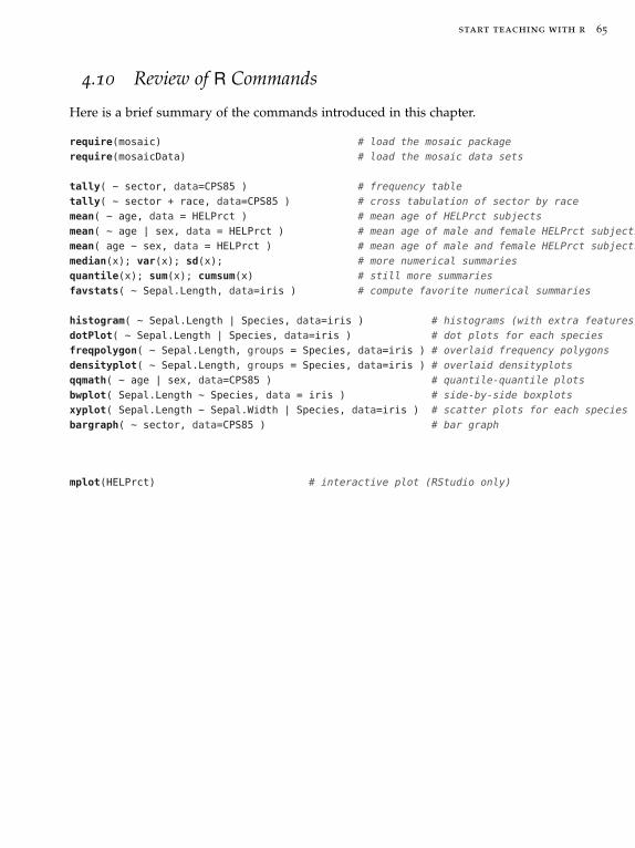
start teaching with r 65
4.10 Review of R Commands
Here is a brief summary of the commands introduced in this chapter.
require(mosaic) # load the mosaic package
require(mosaicData) # load the mosaic data sets
tally( ~ sector, data=CPS85 ) # frequency table
tally( ~ sector + race, data=CPS85 ) # cross tabulation of sector by race
mean( ~ age, data = HELPrct ) # mean age of HELPrct subjects
mean( ~ age | sex, data = HELPrct ) # mean age of male and female HELPrct subjects
mean( age ~ sex, data = HELPrct ) # mean age of male and female HELPrct subjects
median(x); var(x); sd(x); # more numerical summaries
quantile(x); sum(x); cumsum(x) # still more summaries
favstats( ~ Sepal.Length, data=iris ) # compute favorite numerical summaries
histogram( ~ Sepal.Length | Species, data=iris ) # histograms (with extra features)
dotPlot( ~ Sepal.Length | Species, data=iris ) # dot plots for each species
freqpolygon( ~ Sepal.Length, groups = Species, data=iris ) # overlaid frequency polygons
densityplot( ~ Sepal.Length, groups = Species, data=iris ) # overlaid densityplots
qqmath( ~ age | sex, data=CPS85 ) # quantile-quantile plots
bwplot( Sepal.Length ~ Species, data = iris ) # side-by-side boxplots
xyplot( Sepal.Length ~ Sepal.Width | Species, data=iris ) # scatter plots for each species
bargraph( ~ sector, data=CPS85 ) # bar graph
mplot(HELPrct) # interactive plot (RStudio only)

66 pruim, horton kaplan
4.11 Exercises
4.1 The Utilities2 data set in the mosaic package con-tains information about the bills for various utilities at aresidence in Minnesota collected over a number of years.Since the number of days in a billing cycle varies frommonth to month, variables like gasbillpday (elecbillpday,etc.) contain the gas bill (electric bill, etc.) divided by thenumber of days in the billing cycle.
a) Use the documentation to determine what the kwh vari-ables contains.
b) Make a scatter plot of gasbillpday vs. monthsSinceY2Kusing the command
xyplot(gasbillpday ~ monthsSinceY2K, data=Utilities2,
type='l') # the letter l
What pattern(s) do you see?
c) What does type=’l’ do? Make your plot with andwithout it. Which is easier to read in this situation?
d) What happens if we replace type=’l’ with type=’b’?
e) Make a scatter plot of gasbillpday by month. What doyou notice?
f) Make side-by-side boxplots of gasbillpday by month
using the Utilities2 data frame. What do you notice?
Your first try probably won’t give you what you ex-pect. The reason is that month is coded using num-bers, so R treats it as numerical data. We want to treatit as categorical data. To do this in R use factor(month)
in place of month. R calls categorical data a factor.
g) Make any other plot you like using this data. Includeboth a copy of your plot and a discussion of what youcan learn from it.
4.2 The table below is from a study of nighttime lightingin infancy and eyesight (later in life).
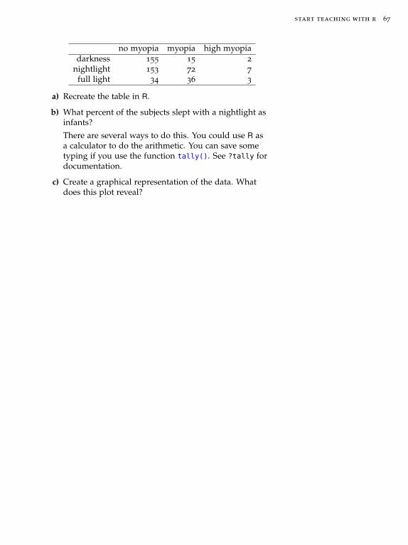
start teaching with r 67
no myopia myopia high myopiadarkness 155 15 2
nightlight 153 72 7
full light 34 36 3
a) Recreate the table in R.
b) What percent of the subjects slept with a nightlight asinfants?
There are several ways to do this. You could use R asa calculator to do the arithmetic. You can save sometyping if you use the function tally(). See ?tally fordocumentation.
c) Create a graphical representation of the data. Whatdoes this plot reveal?
5
What Students Need to Know About R& How to Teach It
In Chapter 2, we give a brief orientation to the RStudio
IDE and what happens in each of its tabs and panels.In Chapter 4, we show how to make use of a commontemplate for graphical summaries, numerical summaries,and modeling. In this chapter we cover some additionalthings that are important for students to know about theR language.
5.1 Two Questions
When we introduced the formula template in Chapter 4,we presented two important questions to ask before con-structing an R command. These questions are useful incontexts beyond the formula template, and indeed forcomputer systems beyond R, so we repeat them here.
Teaching Tip
When students have difficultyaccomplishing a task in R, makesure they can answer thesequestions before you showthem what to do. If they can-not answer these questions,then the primary problem isnot with R. If you do this con-sistently, eventually, you willfind your students presentingtheir R questions to you by an-swering these two questionsand then asking “So how do Iget R to do that?" More likely,once they have answered thesetwo questions, they will alreadyknow how to get R to do whatthey want – unless they are ask-ing about functionality that youhave not yet presented.
1. What do you want R to do?
This will generally determine which R function to use.
2. What must R know to do that?
This will determine the inputs to the function.
5.2 Four Things to Know About R
As is true for most computer languages, R has to be usedon its terms. R does not learn the personality and styleof its users. Getting along with R is much easier if you

start teaching with r 69
keep in mind (and remind your students about) a few keyfeatures of the R language.
1. R is case-sensitive
Teaching Tip
Some students will be slow tocatch on to the importance ofcapitalization. So you may haveto remind them several timesearly on.
If you mis-capitalize something in R it won’t do whatyou want. Unfortunately, there is not a consistent con-vention about how capitalization should be used, soyou just have to pay attention when encountering newfunctions and data sets.
2. Functions in R use the following syntax:
functionname( argument1, argument2, ... )
Teaching Tip
Introduce functions by em-phasizing the questions Whatdo we want the computer to do?and What information does thecomputer need to compute this?The answer to the first ques-tion determines the function touse. The answer to the secondquestion determines what thearguments must be.
• The arguments are always surrounded by (round)
parentheses and separated by commas.
Some functions (like data()) have no required argu-ments, but you still need the parentheses.
• If you type a function name without the parenthe-ses, you will see the code for that function (this gen-erally isn’t what you want unless you are curiousabout how something is implemented).
3. TAB completion and arrows can improve typing speedand accuracy.
If you begin a command and hit the TAB key, R andRStudio will show you a list of possible ways to com-plete the command. If you hit TAB after the openingparenthesis of a function, RStudio will display the listof arguments it expects.
The up and down arrows can be used to retrieve pastcommands when working in the console.
4. If you see a + prompt, it means R is waiting for moreinput. Caution!
Your students will sometimesfind themselves in a syntactichole from which they cannotdig out. Teach them about theESC key early.
Often this means that you have forgotten a closingparenthesis or made some other syntax error. If youhave messed up and just want to get back to the nor-mal prompt, press the escape key and start the com-mand fresh.
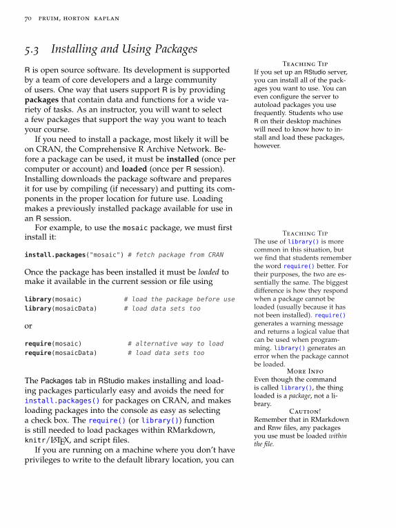
70 pruim, horton kaplan
5.3 Installing and Using PackagesTeaching Tip
If you set up an RStudio server,you can install all of the pack-ages you want to use. You caneven configure the server toautoload packages you usefrequently. Students who useR on their desktop machineswill need to know how to in-stall and load these packages,however.
R is open source software. Its development is supportedby a team of core developers and a large communityof users. One way that users support R is by providingpackages that contain data and functions for a wide va-riety of tasks. As an instructor, you will want to selecta few packages that support the way you want to teachyour course.
If you need to install a package, most likely it will beon CRAN, the Comprehensive R Archive Network. Be-fore a package can be used, it must be installed (once percomputer or account) and loaded (once per R session).Installing downloads the package software and preparesit for use by compiling (if necessary) and putting its com-ponents in the proper location for future use. Loadingmakes a previously installed package available for use inan R session.
For example, to use the mosaic package, we must firstinstall it:
install.packages("mosaic") # fetch package from CRAN
Once the package has been installed it must be loaded tomake it available in the current session or file using
Teaching Tip
The use of library() is morecommon in this situation, butwe find that students rememberthe word require() better. Fortheir purposes, the two are es-sentially the same. The biggestdifference is how they respondwhen a package cannot beloaded (usually because it hasnot been installed). require()generates a warning messageand returns a logical value thatcan be used when program-ming. library() generates anerror when the package cannotbe loaded.
library(mosaic) # load the package before use
library(mosaicData) # load data sets too
or
require(mosaic) # alternative way to load
require(mosaicData) # load data sets too
More Info
Even though the commandis called library(), the thingloaded is a package, not a li-brary.
Caution!Remember that in RMarkdownand Rnw files, any packagesyou use must be loaded withinthe file.
The Packages tab in RStudio makes installing and load-ing packages particularly easy and avoids the need forinstall.packages() for packages on CRAN, and makesloading packages into the console as easy as selectinga check box. The require() (or library()) functionis still needed to load packages within RMarkdown,knitr/LATEX, and script files.
If you are running on a machine where you don’t haveprivileges to write to the default library location, you can

start teaching with r 71
install a personal copy of a package. If the location ofyour personal library is first in R_LIBS, this will probablyhappen automatically. If not, you can specify the locationmanually:
install.packages("mosaic", lib="~/R/library")
CRAN is not the only repository of R packages. Bio-conductor is another large and popular repository, espe-cially for biological applications, and increasingly authorsare making packages available via github. For example,you can also install the mosaic package using
# if you haven't already installed this package
install.packages("devtools")
require(devtools)
install_github("mosaic", "rpruim")
Occasionally you might find a package of interest thatis not available via a repository like CRAN or Bioconduc-tor. Typically, if you find such a package, you will alsofind instructions on how to install it. If not, you can usu-ally install directly from the zipped up package file.
# repos = NULL indicates to use a file, not a repository
install.packages('some-package.tar.gz', repos=NULL)
From this point on, we will assume that the mosaic
package has been installed and loaded.
5.4 Getting Help
If something doesn’t go quite right, or if you can’t re-member something, it’s good to know where to turn forhelp. In addition to asking your friends and neighbors,you can use the R help system.
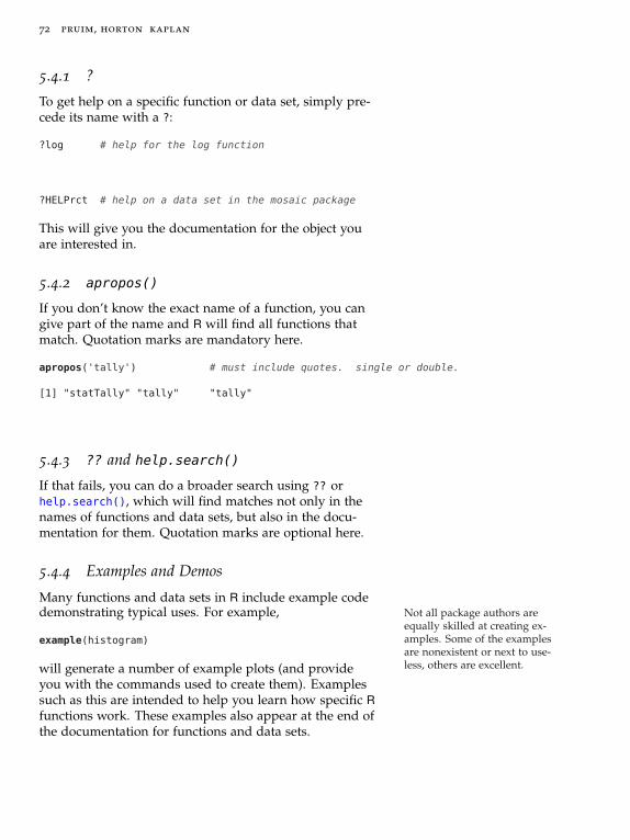
72 pruim, horton kaplan
5.4.1 ?
To get help on a specific function or data set, simply pre-cede its name with a ?:
?log # help for the log function
?HELPrct # help on a data set in the mosaic package
This will give you the documentation for the object youare interested in.
5.4.2 apropos()
If you don’t know the exact name of a function, you cangive part of the name and R will find all functions thatmatch. Quotation marks are mandatory here.
apropos('tally') # must include quotes. single or double.
[1] "statTally" "tally" "tally"
5.4.3 ?? and help.search()
If that fails, you can do a broader search using ?? orhelp.search(), which will find matches not only in thenames of functions and data sets, but also in the docu-mentation for them. Quotation marks are optional here.
5.4.4 Examples and Demos
Many functions and data sets in R include example codedemonstrating typical uses. For example, Not all package authors are
equally skilled at creating ex-amples. Some of the examplesare nonexistent or next to use-less, others are excellent.
example(histogram)
will generate a number of example plots (and provideyou with the commands used to create them). Examplessuch as this are intended to help you learn how specific R
functions work. These examples also appear at the end ofthe documentation for functions and data sets.

start teaching with r 73
The mosaic package (and some other packages as well)also includes demos. Demos are bits of R code that canbe executed using the demo() command with the name ofthe demo. To see how demos work, give this a try:
demo(lattice)
Demos are intended to illustrate a concept or a methodand are independent of any particular function or dataset.
You can get a list of available demos using
demo() # all demos
demo(package='mosaic') # just demos from mosaic package
5.5 Data
5.5.1 Data Frames
Data sets are usually stored in a special structure called adata frame. Teaching Tip
Students who collect their owndata, especially if they storeit in Excel, are unlikely to putdata into the correct formatunless explicitly taught to doso.
Data frames have a 2-dimensional structure.
• Rows correspond to observational units (people,animals, plants, or other objects we are collectingdata about).
• Columns correspond to variables (measurementscollected on each observational unit). Teaching Tip
To help students keep variablesand data frames straight, andto make it easier to rememberthe names, we have adopted theconvention that data frames inthe mosaic package are capi-talized and variables (usually)are not. This convention hasworked well, and you may wishto adopt it for your data sets aswell.
Births78 The Births78 data frame contains three vari-ables measured for each day in 1978. There are severalways we can get some idea about what is in the Births78
data frame.

74 pruim, horton kaplan
head(Births78) # show the first few rows
date births dayofyear
1 1978-01-01 7701 1
2 1978-01-02 7527 2
3 1978-01-03 8825 3
4 1978-01-04 8859 4
5 1978-01-05 9043 5
6 1978-01-06 9208 6
sample(Births78, 4) # show 4 randomly selected rows
date births dayofyear orig.ids
105 1978-04-15 7527 105 105
287 1978-10-14 8554 287 287
149 1978-05-29 7780 149 149
320 1978-11-16 9568 320 320
summary(Births78) # provide summary info about each variable
date births dayofyear
Min. :1978-01-01 Min. : 7135 Min. : 1
1st Qu.:1978-04-02 1st Qu.: 8554 1st Qu.: 92
Median :1978-07-02 Median : 9218 Median :183
Mean :1978-07-02 Mean : 9132 Mean :183
3rd Qu.:1978-10-01 3rd Qu.: 9705 3rd Qu.:274
Max. :1978-12-31 Max. :10711 Max. :365
str(Births78) # show the structure of the data frame
'data.frame': 365 obs. of 3 variables:
$ date : POSIXct, format: "1978-01-01" ...
$ births : int 7701 7527 8825 8859 9043 9208 8084 7611 9172 9089 ...
$ dayofyear: int 1 2 3 4 5 6 7 8 9 10 ...
The output from str() is also available in the Environment
tab.In interactive mode, you can also try
?Births78
to access the documentation for the data set. This is alsoavailable in the Help tab. Finally, the Environment tab pro-
start teaching with r 75
vides a list of data in the workspace. Clicking on one ofthe data sets brings up the same data viewer as
View(Births78)
We can gain access to a single variable in a data frameusing the $ operator or, alternatively, using the with()
function.
dataframe$variable
with(dataframe, variable)
For example, either of
Births78$births
with(Births78, births)
will show the contents of the births variable in Births78
data set. As we will see, there are rela-tively few instances where oneneeds to use the $ operator.
Listing the entire set of values for a particular variableisn’t very useful for a large data set. We would prefer tocompute numerical or graphical summaries. We’ll do thatshortly.
5.5.2 The Perils of attach()Caution!
Avoid the use of attach().The attach() function in R can be used to make objectswithin data frames accessible in R with fewer keystrokes,but we strongly discourage its use, as it often leads toname conflicts and other complications. The Google RStyle Guide1 echoes this advice, stating that 1 http://google-styleguide.
googlecode.com/svn/trunk/
google-r-style.htmlThe possibilities for creating errors when using attach() arenumerous. Avoid it.
It is far better to directly access variables using the $ syn-tax or to use functions that allow you to avoid the $ oper-ator.
5.5.3 Data in Packages
Data sets in R packages are the easiest to deal with. In
Teaching Tip
Start out using data in packagesand show students how toimport their own data oncethey understand how to workwith data.
section 5.5.4, we’ll describe how to load your own datainto R and RStudio, but we recommend starting with data

76 pruim, horton kaplan
in packages, and that is what we will do here, too. Oncestudents know how to work with data and what data in R
are supposed to look like, they will be better prepared toimport their own data sets.
Many packages contain data sets. You can see a list ofall data sets in all loaded packages using
data()
You can optionally choose to restrict the list to a singlepackage:
data(package="mosaic")
TypicallyThis depends on the package. Most packageauthors set up their packages with “lazy loading” of data.If they do not, then you need to use data() explicitly.youcan use data sets by simply typing their names. But if youhave already used that name for something or need torefresh the data after making some changes you no longerwant, you can explicitly load the data using the data()
function with the name of the data set you want.
data(Births78)
There is no visible effect of this command, but the Caution!If two packages include datasets with the same name, youmay need to specify whichpackage you want the datafrom with data(Births78,
package="mosaic")
Births78 data frame has now been reloaded from themosaic package and is ready for use. Anything you mayhave previously stored in a variable with this same nameis replaced by the version of the data set stored with inthe mosaic package.
5.5.4 Using Your Own DataTeaching Tip
Start out using data from pack-ages and focusing on what R
can do with the data. Later,once students are familiar withR and understand the formatrequired for data, teach stu-dents how to import their owndata.
Eventually, students will want to move from using ex-ample data sets in R packages to using data they find orcollect themselves. When this happens will depend on thetype of students you have and the type of course you areteaching.
R provides the functions read.csv() (for comma sep-arated values files), read.table() (for white space de-limited files) and load() (for loading data in R’s na-tive format). The mosaic package includes a function

start teaching with r 77
called read.file() that uses slightly different defaultsettings and infers whether it should use read.csv(),read.table(), or load() based on the file name.
Since most software packages can export to csv format,this has become a sort of lingua franca for moving databetween packages. Data in excel, for example, can be ex-ported as a csv file for subsequent reading in R. If you Caution!
There is a conflict between theresample() functions in gdata
and mosaic. If you want to usemosaic’s resample(), be sureto load mosaic after you loadgdata.
have python installed on your system, you can also useread.xls() from the gdata package to read read directlyfrom Excel files without this extra step.
Each of these functions accepts a URL as well as a filename, which provides an easy way to distribute data viathe Internet:
births <- read.file('http://www.calvin.edu/~rpruim/data/births.txt', header=TRUE)
head(births) # live births in the US each day of 1978.
date births datenum dayofyear
1 1/1/78 7701 6575 1
2 1/2/78 7527 6576 2
3 1/3/78 8825 6577 3
4 1/4/78 8859 6578 4
5 1/5/78 9043 6579 5
6 1/6/78 9208 6580 6
We can omit the header=TRUE if we use read.file()births <- read.file('http://www.calvin.edu/~rpruim/data/births.txt')
5.5.5 Importing Data in RStudioTeaching Tip
Remind students that the 2-stepprocess (upload, then import)works much like images inFacebook. First you uploadthem to Facebook, and oncethey are there you can includethem in posts, etc.
The RStudio interface provides some GUI tools for load-ing data. If you are using the RStudio server, you willfirst need to upload the data to the server (in the Files
tab), and then import the data into your R session (in theWorkspace tab).
If you are running the desktop version, the upload stepis not needed.
5.5.6 Working with Pretabulated Data Even if you use RStudio GUI forinteractive work, you will wantto know how to use functionslike read.csv() for working inRMarkdown, or knitr/LATEXfiles.
Because categorical data is so easy to summarize in a ta-ble, often the frequency or contingency tables are given

78 pruim, horton kaplan
instead. You can enter these tables manually using a com-bination of c(), rbind() and cbind():
Teaching Tip
This is an important techniqueif you use a text book thatpresents pre-tabulated cate-gorical data.
myrace <- c( NW=67, W=467 ) # c for combine or concatenate
myrace
NW W
67 467
mycrosstable <- rbind(
NW = c(clerical=15, const=3, manag=6, manuf=11,
other=5, prof=7, sales=3, service=17),
W = c(82,17,49,57,63,98,35,66)
)
mycrosstable
clerical const manag manuf other prof sales service
NW 15 3 6 11 5 7 3 17
W 82 17 49 57 63 98 35 66
Replacing rbind() with cbind() will allow you to givethe data column-wise instead.
Teaching Tip
If plotting pre-tabulated cat-egorical data is important,you probably want to provideyour students with a wrapperfunction to simplify all this.We generally avoid this situ-ation by provided the data inraw format or by presentingan analysing the data in ta-bles without using graphicalsummaries.
This arrangement of the data would be sufficient forapplying the Chi-squared test, but it is not in a formatsuitable for plotting with lattice. Our cross table is stillmissing a bit of information – the names of the variablesbeing stored. We can add this information if we convert itto a table:
class(mycrosstable)
[1] "matrix"
mycrosstable <- as.table(mycrosstable)

start teaching with r 79
# mycrosstable now has dimnames, but they are unnamed
dimnames(mycrosstable)
[[1]]
[1] "NW" "W"
[[2]]
[1] "clerical" "const" "manag" "manuf" "other"
[6] "prof" "sales" "service"
# let's add meaninful dimnames
names(dimnames(mycrosstable)) <- c('race', 'sector')
mycrosstable
sector
race clerical const manag manuf other prof sales service
NW 15 3 6 11 5 7 3 17
W 82 17 49 57 63 98 35 66
We can use barchart() instead of bargraph() to plotdata already tabulated in this way, but first we need yetone more transformation.
head(as.data.frame(mycrosstable))
race sector Freq
1 NW clerical 15
2 W clerical 82
3 NW const 3
4 W const 17
5 NW manag 6
6 W manag 49
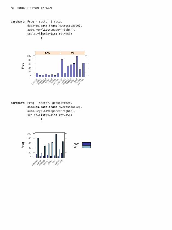
80 pruim, horton kaplan
barchart( Freq ~ sector | race,
data=as.data.frame(mycrosstable),
auto.key=list(space='right'),
scales=list(x=list(rot=45))
)
Fre
q
0
20
40
60
80
100
cleric
al
cons
t
man
ag
man
ufot
herpr
of
sales
serv
ice
NW
cleric
al
cons
t
man
ag
man
ufot
herpr
of
sales
serv
ice
W
barchart( Freq ~ sector, groups=race,
data=as.data.frame(mycrosstable),
auto.key=list(space='right'),
scales=list(x=list(rot=45))
)
Fre
q
0
20
40
60
80
100
cleric
al
cons
t
man
ag
man
ufot
herpr
of
sales
serv
ice
NWW
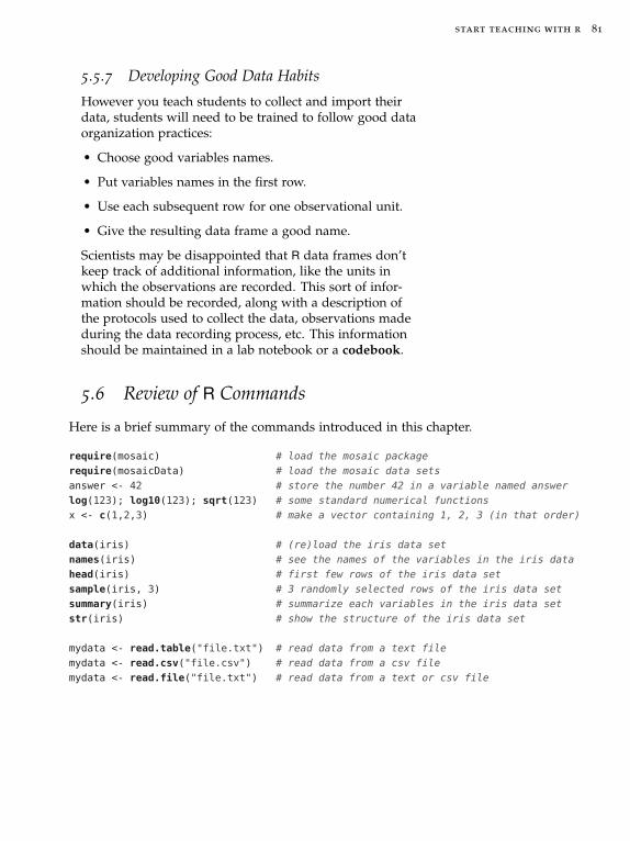
start teaching with r 81
5.5.7 Developing Good Data Habits
However you teach students to collect and import theirdata, students will need to be trained to follow good dataorganization practices:
• Choose good variables names.
• Put variables names in the first row.
• Use each subsequent row for one observational unit.
• Give the resulting data frame a good name.
Scientists may be disappointed that R data frames don’tkeep track of additional information, like the units inwhich the observations are recorded. This sort of infor-mation should be recorded, along with a description ofthe protocols used to collect the data, observations madeduring the data recording process, etc. This informationshould be maintained in a lab notebook or a codebook.
5.6 Review of R Commands
Here is a brief summary of the commands introduced in this chapter.
require(mosaic) # load the mosaic package
require(mosaicData) # load the mosaic data sets
answer <- 42 # store the number 42 in a variable named answer
log(123); log10(123); sqrt(123) # some standard numerical functions
x <- c(1,2,3) # make a vector containing 1, 2, 3 (in that order)
data(iris) # (re)load the iris data set
names(iris) # see the names of the variables in the iris data
head(iris) # first few rows of the iris data set
sample(iris, 3) # 3 randomly selected rows of the iris data set
summary(iris) # summarize each variables in the iris data set
str(iris) # show the structure of the iris data set
mydata <- read.table("file.txt") # read data from a text file
mydata <- read.csv("file.csv") # read data from a csv file
mydata <- read.file("file.txt") # read data from a text or csv file

82 pruim, horton kaplan
5.7 Exercises
5.1 Enter the following small data set in an Excel orGoogle spreadsheet and import the data into RStudio.
6
What Instructors Need to Know about R
You may find that some ofthese things are useful for yourstudents to know as well. Thatwill depend on the goals foryour course and the abilities ofyour students. In higher levelcourses, much of the material inthis chapter is also appropriatefor students.
We recommend keeping the amount of R that studentsneed to learn to a minimum, and choosing functions thatsupport a formula interface whenever possible to keepthe required functions syntactically similar. But thereare some additional things that instructors (and somestudents) should know about R. We outline some of thesethings in this chapter.
6.1 Some Workflow Suggestions
Our workflow advice can be summarized in one shortsentence:
Think like a programmer.
We don’t really think of our classroom use of R as pro-gramming since we use R in a mostly declarative ratherthan algorithmic way.It doesn’t take sophisticated pro-gramming skills to be good at using R. In fact, most usesof R for teaching statistics can be done working one stepat a time, where each line of code does one complete anduseful task. After inspecting the output (and perhaps sav-ing it for further computation later), one can proceed tothe next operation.
Nevertheless, we can borrow from the collective wis-dom of the programming community and adopt somepractices that will make our experience more pleasurable,more efficient, and less error-prone.
• Store your code in a file.

84 pruim, horton kaplan
It can be tempting to do everything in the console. Butthe console is ephemeral. It is better to get into thehabit of storing code in files. Get in the habit (and getyour students in the habit) of working with R scriptsand especially RMarkdown files.
You can execute all the code in an R script file using
More Info
R can be used to create exe-cutable scripts. Option parsingand handling is supported withthe optparse package.
source("file.R")
RStudio has additional options for executing some orall lines in a file. See the buttons in the tab for any R
script, RMarkdown or Rnw file. (You can create a newfile in the main File menu.)
If you work at the console’s interactive prompt andlater wish you had been putting your commands into afile, you can save your past commands with
savehistory("someRCommandsIalmostLost.R")
In RStudio, you can selectively copy portions of yourhistory to a script file (or the console) using the History
tab.
• Use meaningful names.
Rarely should objects be named with a single letter.
Adopt a personal convention regarding case of letters.This will mean you have one less thing to rememberwhen trying to recall the name of an object. For exam-ple, in the mosaic package, all data frames begin witha capital letter. Most variables begin with a lower caseletter (a few exceptions are made for some variableswith names that are well-known in their capitalizedform).
• Adopt reusable idioms.
Computer programmers refer to the little patterns thatrecur throughout their code as idioms. For example,here is a “compute, save, display” idiom.
# compute, save, display idiom
footModel <- lm( length ~ width, data=KidsFeet ); footModel

start teaching with r 85
Call:
lm(formula = length ~ width, data = KidsFeet)
Coefficients:
(Intercept) width
9.817 1.658
# alternative that reflects the order of operations
lm( length ~ width, data=KidsFeet ) -> footModel; footModel
Call:
lm(formula = length ~ width, data = KidsFeet)
Coefficients:
(Intercept) width
9.817 1.658
Often there are multiple ways to do the same thing inR, but if you adopt good programming idioms, it willbe clearer to both you and your students what you aredoing.
• Write reusable functions.
Learning to write your own functions (see Section 6.7)will greatly increase your efficiency and also help youunderstand better how R works. This, in turn, willhelp you debug your students error messages. (Moreon error messages in 6.10.) It also makes it possiblefor you to simplify tasks you want your students tobe able to do in R. That is how the mosaic packageoriginated – as a collection of tools we had assembledover time to make teaching and learning easier.
• Comment your code.
It’s amazing what you can forget. The comment char-acter in R is #. If you are working in RMarkdown orRnw files, you can also include nicely formatted text todescribe what you are doing and why.
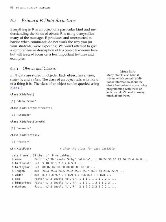
86 pruim, horton kaplan
6.2 Primary R Data Structures
Everything in R is an object of a particular kind and un-derstanding the kinds of objects R is using demystifiesmany of the messages R produces and unexpected be-havior when commands do not work the way you (oryour students) were expecting. We won’t attempt to givea comprehensive description of R’s object taxonomy here,but will instead focus on a few important features andexamples.
6.2.1 Objects and Classes
In R, data are stored in objects. Each object has a name,contents, and a class. The class of an object tells what kindof a thing it is. The class of an object can be queried usingclass()
More Info
Many objects also have at-tributes which contain addi-tional information about theobject, but unless you are doingprogramming with these ob-jects, you don’t need to worrymuch about them.class(KidsFeet)
[1] "data.frame"
class(KidsFeet$birthmonth)
[1] "integer"
class(KidsFeet$length)
[1] "numeric"
class(KidsFeet$sex)
[1] "factor"
str(KidsFeet) # show the class for each variable
'data.frame': 39 obs. of 8 variables:
$ name : Factor w/ 36 levels "Abby","Alisha",..: 10 24 36 20 23 34 13 4 14 8 ...
$ birthmonth: int 5 10 12 1 2 3 2 6 5 9 ...
$ birthyear : int 88 87 87 88 88 88 88 88 88 88 ...
$ length : num 24.4 25.4 24.5 25.2 25.1 25.7 26.1 23 23.6 22.9 ...
$ width : num 8.4 8.8 9.7 9.8 8.9 9.7 9.6 8.8 9.3 8.8 ...
$ sex : Factor w/ 2 levels "B","G": 1 1 1 1 1 1 1 2 2 1 ...
$ biggerfoot: Factor w/ 2 levels "L","R": 1 1 2 1 1 2 1 1 2 2 ...
$ domhand : Factor w/ 2 levels "L","R": 2 1 2 2 2 2 2 2 2 1 ...

start teaching with r 87
act, they must all be of the same atomic type. Atomictypes are are the basic building blocks for R. It is not pos-sible to store more complicated objects (like data frames)in a vector.!
From this we see that KidsFeet is a data frame andthat the variables are of different types (integer, numeric,and factor). These are the kinds of variables you are mostlikely to encounter, although you may also see variablesthat are logical (true or false) or character (text) as well.
Factors are the most common way for categorical datato be stored in R, but sometimes the character class isbetter. The class of an object determines what things More Info
One difference between a factorand a character is that a fac-tor knows the possible values,even if some them do not occur.Sometimes this is an advantage(tallying empty cells in a table)and sometimes it is a disadvan-tage (when factors are used asunique identifiers).
can be done with it and how it appears when printed,plotted, or displayed in the console.
6.2.2 Containers
The situation is actually a little bit more complicated.The birthmonth variable in KidsFeet is not a single in-teger but a collection of integers. So we can think ofbirthmonth as a kind of container holding a number ofintegers. There is more than one kind of container in More Info
Even when we only have asingle integer, R will treat itlike a container of integers withonly one integer in it.
R. The containers used for variables in a data frame arecalled vectors. The items in a vector are ordered (startingwith 1) and must all be of the same type.
bVectors can be created using the c() function:
c(2, 3, 5, 7)
[1] 2 3 5 7
c("Abe", "Betty", "Chan")
[1] "Abe" "Betty" "Chan"
c(1.2, 3.2, 4.5)
[1] 1.2 3.2 4.5
If you attempt to put different types of objects into a vec-tor, R will attempt to convert them all to the same type ofobject. If it is unable to do so, it will generate an error.
Caution!When reading data created inother software (like Excel) orstored in CSV files, it is impor-tant to know how missing datawere indicated, otherwise, thecode for missing data may beinterpreted as a character, caus-ing all the other items in thatcolumn to be converted to char-acter values as well, and losingthe important information thatsome of the data were missing.
x <- c(1, 1.1, 1.2); x # convert integer to numeric
[1] 1.0 1.1 1.2

88 pruim, horton kaplan
class(x)
[1] "numeric"
y <- c(TRUE, FALSE, 0, 1, 2); y # logicals converted to numeric
[1] 1 0 0 1 2
class(y)
[1] "numeric"
z <- c(1, TRUE, 1.2, "vector"); z # all converted to character
[1] "1" "TRUE" "1.2" "vector"
class(z)
[1] "character"
Digging Deeper
A factor can be ordered or un-ordered (which can affect howstatistics tests are performedbut otherwise does not mattermuch). The default is for fac-tors to be unordered. Whetherthe factors are ordered or un-ordered, thelevels will appearin a fixed order – alphabeticalby default. The distinction be-tween ordered and unorderedfactors has to do with whetherthis order is meaningful orarbitrary.
Factors can be created by wrapping a vector withfactor():
w <- factor(x); w
[1] 1 1.1 1.2
Levels: 1 1.1 1.2
class(w)
[1] "factor"
Notice how factors display the levels (possible values) aswell as the values themselves. When categorical data arecoded as integers, it is important to remember to convertthem to factors in this way for certain statistical proce-dures and some plots.
Patterned integer or numeric vectors can be createdusing the : operator or the seq() function.1:10
[1] 1 2 3 4 5 6 7 8 9 10
seq(1, 10, by=0.5)
[1] 1.0 1.5 2.0 2.5 3.0 3.5 4.0 4.5 5.0 5.5 6.0
[12] 6.5 7.0 7.5 8.0 8.5 9.0 9.5 10.0

start teaching with r 89
Individual items in a vector can be accessed or as-signed using the square bracket operator:
w[1]
[1] 1
Levels: 1 1.1 1.2
x[2]
[1] 1.1
y[3]
[1] 0
z[5] # this is not an error, but returns NA (missing)
[1] NA
Missing values are coded as NA (not available). Asking foran entry “off the end” of a vector returns NA. Assigning avalue “off the end” of a vector results in the vector beinglengthened so that the new value can be stored in theappropriate location.
q <- 1:5
q
[1] 1 2 3 4 5
q[10] <- 10
q
[1] 1 2 3 4 5 NA NA NA NA 10
R also provides some more unusual (but very useful)features for accessing elements in a vector.letters # alphabet
[1] "a" "b" "c" "d" "e" "f" "g" "h" "i" "j" "k" "l" "m" "n"
[15] "o" "p" "q" "r" "s" "t" "u" "v" "w" "x" "y" "z"More Info
letters is a built-in charactervector containing the lowercase letters. LETTERS containscapitals.
x <- letters[1:10]; x # first 10 letters
[1] "a" "b" "c" "d" "e" "f" "g" "h" "i" "j"

90 pruim, horton kaplan
x[2:4] # select items 2 through 4
[1] "b" "c" "d"
x[2:4] <- c("X","Y","Z"); x # change items 2 through 4
[1] "a" "X" "Y" "Z" "e" "f" "g" "h" "i" "j"
y <- (1:10)^2; y # first 10 squares
[1] 1 4 9 16 25 36 49 64 81 100
y [ y > 20 ] # select the items greater than 20
[1] 25 36 49 64 81 100
The last item deserves a bit of comment. The expressioninside the brackets evaluates to a vector of logical values.
y > 20
[1] FALSE FALSE FALSE FALSE TRUE TRUE TRUE TRUE TRUE
[10] TRUE
The logical values are then used to select (true) or dese-lect (false) the items in the vector, producing a new (andpotentially shorter) vector. If the number of logical sup-plied is less than the length of the vector, the values arerecycled (repeated).
y[ c(TRUE,FALSE) ] # every other
[1] 1 9 25 49 81
y[ c(TRUE,FALSE,FALSE) ] # every third
[1] 1 16 49 100
A matrix is a 2-dimensional table of values that allhave the same type. As with vectors, all of the items in amatrix must be of the same type. But matrices are two-dimensional – each item is located in a row and column.An array is a multi-dimensional version of a matrix. Ma-trices and arrays are important containers for statisticalwork, but less likely to be encountered by beginners.

start teaching with r 91
M <- matrix(1:15, nrow=3); M # a 3 x 5 matrix
[,1] [,2] [,3] [,4] [,5]
[1,] 1 4 7 10 13
[2,] 2 5 8 11 14
[3,] 3 6 9 12 15
The dimensions of an array, matrix or data frame can beobtained using dim() or nrow() and ncol().
dim(M)
[1] 3 5
dim(KidsFeet)
[1] 39 8
nrow(KidsFeet)
[1] 39
ncol(KidsFeet)
[1] 8
Another commonly used container in R is a list. Wehave already seen a few examples of lists used as argu-ments to lattice plotting functions. Lists are also or-dered, but the items in a list can be objects of any type(they need not all be the same type). Behind the scenes,a data frame is a list of vectors with the restriction thateach vector must have the same length (contain the samenumber of items).
Lists can be created using the list() function.
l <- list( 1, "two", 3.2, list(1, 2)); l
[[1]]
[1] 1
[[2]]
[1] "two"
[[3]]
[1] 3.2
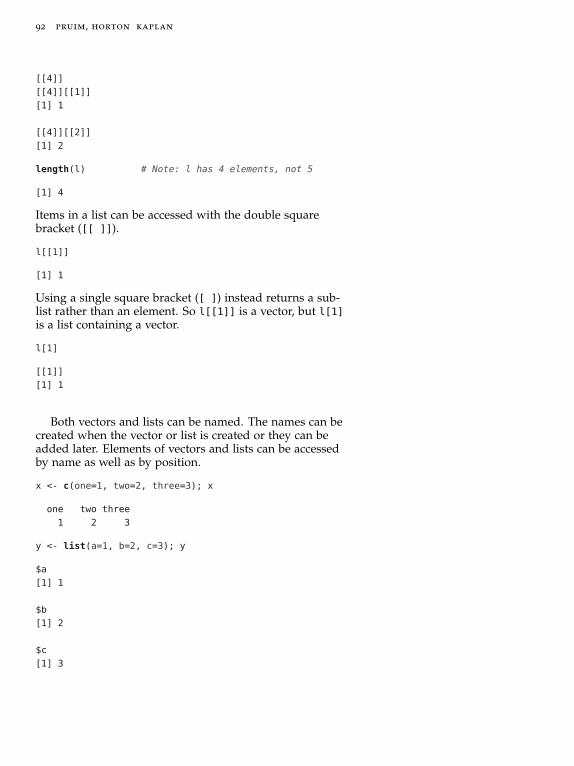
92 pruim, horton kaplan
[[4]]
[[4]][[1]]
[1] 1
[[4]][[2]]
[1] 2
length(l) # Note: l has 4 elements, not 5
[1] 4
Items in a list can be accessed with the double squarebracket ([[ ]]).
l[[1]]
[1] 1
Using a single square bracket ([ ]) instead returns a sub-list rather than an element. So l[[1]] is a vector, but l[1]is a list containing a vector.
l[1]
[[1]]
[1] 1
Both vectors and lists can be named. The names can becreated when the vector or list is created or they can beadded later. Elements of vectors and lists can be accessedby name as well as by position.
x <- c(one=1, two=2, three=3); x
one two three
1 2 3
y <- list(a=1, b=2, c=3); y
$a
[1] 1
$b
[1] 2
$c
[1] 3

start teaching with r 93
x["one"]
one
1
y["a"]
$a
[1] 1
names(x)
[1] "one" "two" "three"
names(x) <- c("A", "B", "C"); x
A B C
1 2 3
The access operators – [ ] and [[ ]] for lists – areactually functions in R. This has some important conse-quences:
• Accessing elements in a vector is slower than in a lan-guage like C/C++ where access is done by pointerarithmetic.
• These functions also have named arguments, so youcan see code like the following
M
[,1] [,2] [,3] [,4] [,5]
[1,] 1 4 7 10 13
[2,] 2 5 8 11 14
[3,] 3 6 9 12 15
M[5]
[1] 5
M[,2] # this is 1-d (a vector)
[1] 4 5 6
M[,2, drop=FALSE] # this is 2-d (still a matrix)
[,1]
[1,] 4
[2,] 5
[3,] 6

94 pruim, horton kaplan
Data frames can be constructed by supplying data.frame()
with the variables (as vectors):
ddd <- data.frame(number=1:5, letter=letters[1:5])
6.2.3 Vectorized functions
Vectors are so important in R that they deserve some ad-ditional discussion. Many R functions and operations are“vectorized” and can be applied not just to an individualvalue but to an entire vector, in which case they are ap-plied componentwise and return a vector of transformedvalues. Most of the commonly used functions from math-ematics are available and work this way.
x <- 1:5; y <- seq(10, 60, by=10)
x
[1] 1 2 3 4 5
y
[1] 10 20 30 40 50 60
y + 1 # add 1 to each element
[1] 11 21 31 41 51 61
x * 10 # multiply each element by 10
[1] 10 20 30 40 50
x < 3 # check whether each is less than 3
[1] TRUE TRUE FALSE FALSE FALSE
x^2 # square each element
[1] 1 4 9 16 25
sqrt(x) # square root of each element
[1] 1.000000 1.414214 1.732051 2.000000 2.236068
log(x) # natural log
[1] 0.0000000 0.6931472 1.0986123 1.3862944 1.6094379
log10(x) # base 10 log
[1] 0.0000000 0.3010300 0.4771213 0.6020600 0.6989700

start teaching with r 95
Vectors can be combined into a matrix using rbind() orcbind(). This can facilitate side-by-side comparisons.
# compare round() and signif() by binding row-wise into a matrix
z <- rnorm(5); z
[1] -0.56047565 -0.23017749 1.55870831 0.07050839
[5] 0.12928774
rbind(round(z, digits=3), signif(z, digits=3))
[,1] [,2] [,3] [,4] [,5]
[1,] -0.56 -0.23 1.559 0.0710 0.129
[2,] -0.56 -0.23 1.560 0.0705 0.129
6.2.4 Functions that act on vectors as vectors
Other functions, including many statistical functions,are designed to compute a single number (technically, avector of length 1) from an entire vector.
z <- rnorm(100)
# basic statistical functions; notice the use of names
c(mean=mean(z), sd=sd(z), var=var(z), median=median(z))
mean sd var median
0.06073364 0.90886782 0.82604071 -0.01139128
range(z) # range returns a vector of length 2
[1] -2.309169 2.187333
x <- 1:10
c(sum=sum(x), prod=prod(x)) # sums and products
sum prod
55 3628800
Still other functions return vectors that are derivedfrom the original vector, but not as a componentwisetransformation.
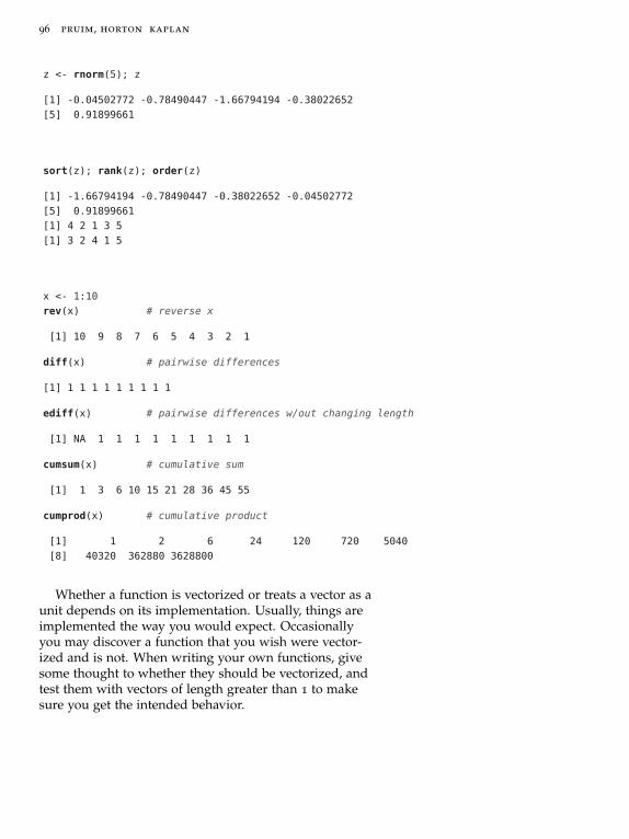
96 pruim, horton kaplan
z <- rnorm(5); z
[1] -0.04502772 -0.78490447 -1.66794194 -0.38022652
[5] 0.91899661
sort(z); rank(z); order(z)
[1] -1.66794194 -0.78490447 -0.38022652 -0.04502772
[5] 0.91899661
[1] 4 2 1 3 5
[1] 3 2 4 1 5
x <- 1:10
rev(x) # reverse x
[1] 10 9 8 7 6 5 4 3 2 1
diff(x) # pairwise differences
[1] 1 1 1 1 1 1 1 1 1
ediff(x) # pairwise differences w/out changing length
[1] NA 1 1 1 1 1 1 1 1 1
cumsum(x) # cumulative sum
[1] 1 3 6 10 15 21 28 36 45 55
cumprod(x) # cumulative product
[1] 1 2 6 24 120 720 5040
[8] 40320 362880 3628800
Whether a function is vectorized or treats a vector as aunit depends on its implementation. Usually, things areimplemented the way you would expect. Occasionallyyou may discover a function that you wish were vector-ized and is not. When writing your own functions, givesome thought to whether they should be vectorized, andtest them with vectors of length greater than 1 to makesure you get the intended behavior.

start teaching with r 97
The operations listed below can be helpful when writ-ing your own functions.
cumsum()
cumprod()
cummin()
cummax()
Returns vector of cumulative sums, products, min-ima, or maxima.
pmin(x,y,...)
pmax(x,y,...)
Returns vector of parallel minima or maxima whereith element is max or min of x[i], y[i], . . . .
which(x) Returns a vector of indices of elements of x that aretrue. Typical use: which(y > 5) returns the indiceswhere elements of y are larger than 5.
any(x) Returns a logical indicating whetherany elements of x are true. Typical use:if ( any(y > 5) ) { ...}.
na.omit(x) Returns a vector with missing values removed.unique(x) Returns a vector with repeated values removed.table(x) Returns a table of counts of the number of occur-
rences of each value in x. The table is similar to avector with names indicating the values, but it is nota vector.
paste(x,y,...,
sep=" ")
Pastes x and y together componentwise (as strings)with sep between elements. Recycling applies.
6.3 Working with Data
In Section 5.5 we discussed using data in R packages,and in Section 5.5.4 we discussed methods for bringingyour own data into R. In both of these scenarios, we haveassumed that the data had been entered and cleaned insome other software and focussed primarily on data im-port. In this section we discuss ways to create and ma-nipulate data within R. But first we discuss a few moredetails regarding importing data.
6.3.1 Finer control over data import
Even if you primarily use theRStudio interface to import data,it is good to know about thecommand line methods sincethese are required to importdata into scripts, RMarkdown,and knitr/LATEX files.
The na.strings argument can be used to specify codesfor missing values. Setting na.strings as in the following

98 pruim, horton kaplan
for reading csv files that might have been produced bysystems such as SAS.
someData <- read.csv('file.csv',
na.strings=c('NA','','.','-','na'))
SAS uses a period (.) to code missing data and some csvexporters use ‘-’. If the above definition for na.strings,or something like it, R will treat missing-data markers asstring data, instead of NA. This forces the entire variable tobe of character type even if it’s otherwise purely numeric.
By default, R will recode character data as a factor. If
More Info
The read.file() function inthe mosaic package uses this asits default for na.strings.
you prefer to leave such variables in character format, youcan use More Info
This works with read.csv()
and read.table() as well.someData <- read.file('file.csv',
stringsAsFactors=FALSE)
Even finer control can be obtained by manually set-ting the class (type) used for each column in the file. Inaddition, this speeds up the reading of the file. For a csvfile with four columns, we can declare them to be of classinteger, numeric, character, and factor with the followingcommand.
someData <- read.file('file.csv',
na.strings=c('NA','','.','-','na'),
colClasses=c('integer','numeric','character','factor'))
6.3.2 Manually entering data
We have already seen that the c() function can be used tocombine elements into a single vector.
x <- c(1, 1, 2, 3, 5, 8, 13); x
[1] 1 1 2 3 5 8 13
The scan() function can speed up data entry in theconsole by allowing you to avoid the commas. Individ-ual values are separated by white space or new lines. A

start teaching with r 99
blank line is used to signal the end of the data. By de-fault, scan() is expecting numeric data, but it is possibleto tell scan() to expect something else, like character data(i.e., text). There are other options for data types, but Caution!
When using scan() be sure toremember to save your datasomewhere. Otherwise you willhave to type it again.
numerical and text data handle the most important cases.See ?scan for more information and examples.
6.3.3 Simulating samples from distributions
R has functions that make it simple to sample from awide range of distributions. Each of these functions be-gins with the letter ‘r’ (for random) followed by the nameof the distribution (often abbreviated somewhat). Thearguments to the function specify the size of the sampledesired and any parameter values required for the dis-tribution. For example, to simulate selecting a sampleof size 12 from a normal population with mean 100 andstandard deviation 10, usernorm(12, mean=100, sd=10)
[1] 94.24653 106.07964 83.82117 99.44438 105.19407
[6] 103.01153 101.05676 93.59294 91.50296 89.75871
[11] 101.17647 90.52525
Functions for sampling from other distributions in-clude rbinom(), rchisq(), rt(), rf(), rhyper(), etc.
It is also easy to sample (with or without replacement)from existing data using sample() and resample().
x <- 1:10
# random sample of size 5 from x (no replacement)
sample(x, size=5)
[1] 4 7 10 9 6
# a different random sample of size 5 from x (no replacement)
sample(x, size=5)
[1] 8 3 2 5 10
# random sample of size 5 from x (with replacement)
resample(x, size=5)
[1] 6 8 2 5 5
Using resample() makes it easy to simulate small discrete

100 pruim, horton kaplan
distributions. For example, to simulate rolling 20 dice, wecould use
resample(1:6, size=20)
[1] 6 6 6 5 6 4 4 3 3 1 4 6 1 1 1 5 5 6 3 1
For working with cards, the mosaic package provides avector named Cards and deal() as an alternative namefor sample().
deal( Cards, 5 ) # poker hand
[1] "9H" "AH" "8C" "8D" "QC"
deal( Cards, 13 ) # bridge, anyone?
[1] "5C" "9D" "AS" "KC" "4C" "7H" "2D" "6C" "QS" "KH" "9S"
[12] "9H" "2S"
If you want to sort the hands nicely, you can create a fac-tor from Cards first:hand <- deal( factor(Cards, levels=Cards), 13 )
sort(hand) # sorted by suit, then by denomination
[1] 2C 7C 8C 7D 8D 10D 4H 9H QH AH 2S 10S AS
52 Levels: 2C 3C 4C 5C 6C 7C 8C 9C 10C JC QC KC AC ... AS
Example 6.1. For teaching purposes it is sometimesnice to create a histogram that has the approximate shapeof some distribution. One way to do this is to randomlysample from the desired distribution and make a his-togram of the resulting sample.
x1 <- rnorm(500, mean=10, sd=2)
histogram(~x1, width=.5)
x1
Den
sity
0.00
0.05
0.10
0.15
0.20
5 10 15

start teaching with r 101
This works, but the resulting plot has a fair amount ofnoise.
The ppoints() function returns evenly spaced proba-bilities and allows us to obtain theoretical quantiles of thenormal distribution instead. The resulting plot now illus-trates the idealized sample from a normal distribution.
x2 <- qnorm( ppoints(500), mean=10, sd=2 )
histogram(~x2, width=.5)
x2
Den
sity
0.00
0.05
0.10
0.15
0.20
5 10 15
This is not what real data will look like (even if it comesfrom a normal population), but it can be better for illus-trative purposes to remove the noise. ⋄
6.3.4 Saving Data
write.table() and write.csv() can be used to save datafrom R into delimited flat files.
ddd <- data.frame(number=1:5, letter=letters[1:5])
write.table(ddd, "ddd.txt")
write.csv(ddd, "ddd.csv")
Data can also be saved in native R format. Saving datasets (and other R objects) using save() has some advan-tages over other file formats:
More Info
If you want to save an R ob-ject but not its name, you canuse saveRDS() and choose itsname when you read it withreadRDS().
• Complete information about the objects is saved, in-cluding attributes.
• Data saved this way takes less space and loads muchmore quickly.

102 pruim, horton kaplan
• Multiple objects can be saved to and loaded from asingle file.
The downside is that these files are only readable in R.
abc <- "abc"
ddd <- data.frame(number=1:5, letter=letters[1:5])
# save both objects in a single file
save(ddd, abc, file="ddd.rda")
# load them both
load("ddd.rda")
For more on importing and exporting data, especiallyfrom other formats, see the R Data Import/Export manualavailable on CRAN.
6.4 Manipulating Data Frames with dplyr
There are several ways to manipulate data frames in R.The approach illustrated here relies heavily on the func-tions in the dplyr package. This package is loaded whenthe mosaic package is loaded. The dplyr package definesfive primary operations on a data frame
1. mutate() – add or change variables
2. select() – choose a subset of columns
3. filter() – choose a subset of rows
4. summarise() – reduce the entire data frame to a sum-mary row
5. arrange() – reorder the rows
These become especially powerful when combined with asixth command, group_by().
6. group_by() – split the data frame into multiple subsets
Additional functions (inner_join() and left_join() canbe used to combine data from multiple data frames.

start teaching with r 103
6.4.1 Adding new variables to a data frame
The mutate() function can be used to add or modify vari-ables in a data frame. mutate() is evaluated in such away that you have direct access to the other variables inthe data frame, including one created earlier in the samemutate() command.
Here we show how to modify the Births78 data frameso that it contains a new variable day that is an orderedfactor.
More Info
The lubridate package pro-vides a wday() function thatcan do this more simply anddirectly from the date variableas well as a number of utilitiesfor creating and manipulatingdate and time objects.
data(Births78)
weekdays <- c("Sun", "Mon", "Tue", "Wed", "Thr", "Fri", "Sat")
Births <- mutate( Births78,
day = factor(weekdays[1 + (dayofyear - 1) %% 7],
ordered=TRUE, levels = weekdays) )
head(Births,3)
date births dayofyear day
1 1978-01-01 7701 1 Sun
2 1978-01-02 7527 2 Mon
3 1978-01-03 8825 3 Tue
xyplot( births ~ date, Births, groups=day, auto.key=list(space='right') )
date
birt
hs
7000
8000
9000
10000
Jan Apr Jul Oct Jan
SunMonTueWedThrFriSat
Number of US births in 1978
colored by day of week.The CPS85 data frame contains data from a CurrentPopulation Survey (current in 1985, that is). Two of thevariables in this data frame are age and educ. We can esti-mate the number of years a worker has been in the work-force if we assume they have been in the workforce sincecompleting their education and that their age at grad-uation is 6 more than the number of years of educationobtained.
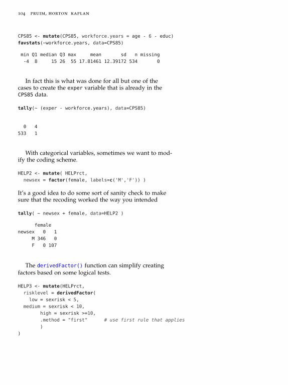
104 pruim, horton kaplan
CPS85 <- mutate(CPS85, workforce.years = age - 6 - educ)
favstats(~workforce.years, data=CPS85)
min Q1 median Q3 max mean sd n missing
-4 8 15 26 55 17.81461 12.39172 534 0
In fact this is what was done for all but one of thecases to create the exper variable that is already in theCPS85 data.
tally(~ (exper - workforce.years), data=CPS85)
0 4
533 1
With categorical variables, sometimes we want to mod-ify the coding scheme.
HELP2 <- mutate( HELPrct,
newsex = factor(female, labels=c('M','F')) )
It’s a good idea to do some sort of sanity check to makesure that the recoding worked the way you intended
tally( ~ newsex + female, data=HELP2 )
female
newsex 0 1
M 346 0
F 0 107
The derivedFactor() function can simplify creatingfactors based on some logical tests.
HELP3 <- mutate(HELPrct,
risklevel = derivedFactor(
low = sexrisk < 5,
medium = sexrisk < 10,
high = sexrisk >=10,
.method = "first" # use first rule that applies
)
)

start teaching with r 105
head(HELP3, 4)
age anysubstatus anysub cesd d1 daysanysub dayslink drugrisk e2b female sex g1b
1 37 1 yes 49 3 177 225 0 NA 0 male yes
2 37 1 yes 30 22 2 NA 0 NA 0 male yes
3 26 1 yes 39 0 3 365 20 NA 0 male no
4 39 1 yes 15 2 189 343 0 1 1 female no
homeless i1 i2 id indtot linkstatus link mcs pcs pss_fr racegrp satreat
1 housed 13 26 1 39 1 yes 25.111990 58.41369 0 black no
2 homeless 56 62 2 43 NA <NA> 26.670307 36.03694 1 white no
3 housed 0 0 3 41 0 no 6.762923 74.80633 13 black no
4 housed 5 5 4 28 0 no 43.967880 61.93168 11 white yes
sexrisk substance treat risklevel
1 4 cocaine yes low
2 7 alcohol yes medium
3 2 heroin no low
4 4 heroin no low
6.4.2 Dropping variables
Since we already have educ, there is no reason to keepour new variable workforce.years. Let’s drop it. Noticethe clever use of the minus sign.
CPS1 <- select(CPS85, -workforce.years)
head(CPS1, 1)
wage educ race sex hispanic south married exper union age
1 9 10 W M NH NS Married 27 Not 43
sector
1 const
Digging Deeper
Master programers in R suchas Hadley Wickham, the authorof the dplyr package, takeadvantage of special featuresof the language that allow suchnotation as minus to mean“exclude."
Any number of variables can be dropped or kept inthis manner by supplying a vector of variables names.
CPS1 <- select(CPS85, c(workforce.years,exper))
Columns can be specified by number as well as name (butthis can be dangerous if you are wrong about where thecolumns are):
CPSsmall <- select(CPS85, select=1:4)
head(CPSsmall,2)

106 pruim, horton kaplan
select1 select2 select3 select4
1 9.0 10 W M
2 5.5 12 W M
The functions matches(), contains(), starts_with(),ends_with(), and number_range() are special functionsthat only work in the context of select() but can be use-ful for describing sets of variables to keep or discard.
head( select(HELPrct, contains("risk")), 2 )
drugrisk sexrisk
1 0 4
2 0 7
The nested functions in the previous command makethe code a bit hard to read, and things would be worse ifwe were composing several more functions. The magrittr
package (which loads when dplyr is loaded, hence whenmosaic is loaded) provides an alternative syntax:
HELPrct %>% select(contains("risk")) %>% head(2)
drugrisk sexrisk
1 0 4
2 0 7
The %>% operator uses the output from the left-hand sideas the first input to the function on the right-hand side.This makes it easy to chain several data manipulationcommands together in the order in which they are ap-plied to the data without having to carefully nest paren-theses and explicitly pass along outputs of one functionas an argument to the next.
Here are a few more examples:
HELPrct %>% select( ends_with("e")) %>% head(2)
age female substance
1 37 0 cocaine
2 37 0 alcohol
HELPrct %>% select( starts_with("h")) %>% head(2)
homeless
1 housed
2 homeless

start teaching with r 107
HELPrct %>% select( matches("i[12]")) %>% head(2) # regex matching
i1 i2
1 13 26
2 56 62
6.4.3 Renaming variables
Both the column (variable) names and the row names of adata frames can be changed by simple assignment usingnames() or row.names().
ddd # small data frame we defined earlier
number letter
1 1 a
2 2 b
3 3 c
4 4 d
5 5 e
# changing the row.names affects how a data.frame prints
row.names(ddd) <- c("Abe","Betty","Claire","Don","Ethel")
ddd
number letter
Abe 1 a
Betty 2 b
Claire 3 c
Don 4 d
Ethel 5 e
It is also possible to reset just individual names with thefollowing syntax.
# misspelled a name, let's fix it
row.names(ddd)[2] <- "Bette"
row.names(ddd)
[1] "Abe" "Bette" "Claire" "Don" "Ethel"
The faithful data set (in the datasets package, whichis always available) has very unfortunate names.
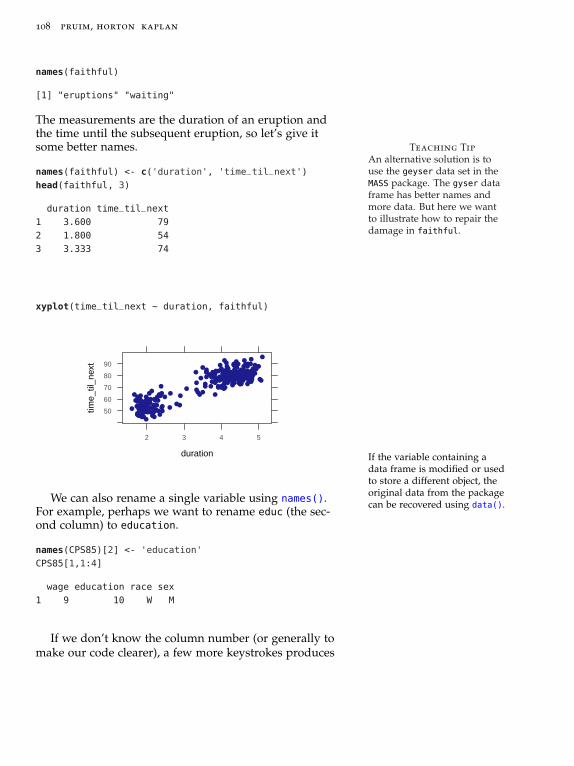
108 pruim, horton kaplan
names(faithful)
[1] "eruptions" "waiting"
The measurements are the duration of an eruption andthe time until the subsequent eruption, so let’s give itsome better names. Teaching Tip
An alternative solution is touse the geyser data set in theMASS package. The gyser dataframe has better names andmore data. But here we wantto illustrate how to repair thedamage in faithful.
names(faithful) <- c('duration', 'time_til_next')
head(faithful, 3)
duration time_til_next
1 3.600 79
2 1.800 54
3 3.333 74
xyplot(time_til_next ~ duration, faithful)
duration
time_
til_n
ext
50
60
70
80
90
2 3 4 5
If the variable containing adata frame is modified or usedto store a different object, theoriginal data from the packagecan be recovered using data().
We can also rename a single variable using names().For example, perhaps we want to rename educ (the sec-ond column) to education.
names(CPS85)[2] <- 'education'
CPS85[1,1:4]
wage education race sex
1 9 10 W M
If we don’t know the column number (or generally tomake our code clearer), a few more keystrokes produces

start teaching with r 109
names(CPS85)[names(CPS85) == 'education'] <- 'educ'
CPS85[1,1:4]
wage educ race sex
1 9 10 W M
See Section 6.4.2 for informa-tion that will make it clearerwhat is going on here.
The select() function can also be used to renamevariables.
data(faithful) # restore the original version
faithful2 <- faithful %>%
select(duration=eruptions, time_til_next = waiting)
head(faithful2, 2)
duration time_til_next
1 3.6 79
2 1.8 54
6.4.4 Creating subsets
We can use filter() to select only certain rows from adata frame.
# any logical can be used to create subsets
faithful2 %>% filter(duration > 3) -> faithfulLong
xyplot( time_til_next ~ duration, faithfulLong )
duration
time_
til_n
ext
70
80
90
3.0 3.5 4.0 4.5 5.0
If all we want to do is produce a graph and don’t needto save the subset, the plot above could also be made withone of the following

110 pruim, horton kaplan
xyplot( time_til_next ~ duration,
data = faithful2 %>% filter( duration > 3) )
xyplot( time_til_next ~ duration, data = faithful2,
subset=duration > 3 )
6.4.5 Summarising a data frame
The summarise() (or summarize()) function summarizes adata frame as a single row.
HELPrct %>% summarise(x.bar = mean(age), s=sd(age))
x.bar s
1 35.65342 7.710266
This is especially useful in combination with group_-
by(), which divides the data frame into subsets. The fol-lowing command will compute the mean and standarddeviation for each subgroup defined by a different combi-nation of sex and substance.
HELPrct %>% group_by(sex, substance) %>%
summarise(x.bar = mean(age), s=sd(age))
Source: local data frame [6 x 4]
Groups: sex
sex substance x.bar s
1 female alcohol 39.16667 7.980333
2 female cocaine 34.85366 6.195002
3 female heroin 34.66667 8.035839
4 male alcohol 37.95035 7.575644
5 male cocaine 34.36036 6.889772
6 male heroin 33.05319 7.973568
The formula-based numerical summary functions sup-plied by the mosaic package are probably easier for thisparticular task, but using dplyr is more general.
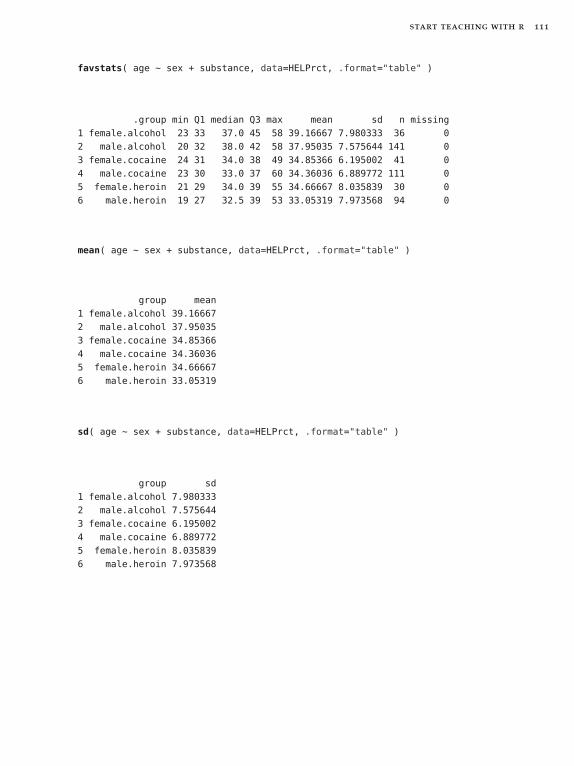
start teaching with r 111
favstats( age ~ sex + substance, data=HELPrct, .format="table" )
.group min Q1 median Q3 max mean sd n missing
1 female.alcohol 23 33 37.0 45 58 39.16667 7.980333 36 0
2 male.alcohol 20 32 38.0 42 58 37.95035 7.575644 141 0
3 female.cocaine 24 31 34.0 38 49 34.85366 6.195002 41 0
4 male.cocaine 23 30 33.0 37 60 34.36036 6.889772 111 0
5 female.heroin 21 29 34.0 39 55 34.66667 8.035839 30 0
6 male.heroin 19 27 32.5 39 53 33.05319 7.973568 94 0
mean( age ~ sex + substance, data=HELPrct, .format="table" )
group mean
1 female.alcohol 39.16667
2 male.alcohol 37.95035
3 female.cocaine 34.85366
4 male.cocaine 34.36036
5 female.heroin 34.66667
6 male.heroin 33.05319
sd( age ~ sex + substance, data=HELPrct, .format="table" )
group sd
1 female.alcohol 7.980333
2 male.alcohol 7.575644
3 female.cocaine 6.195002
4 male.cocaine 6.889772
5 female.heroin 8.035839
6 male.heroin 7.973568

112 pruim, horton kaplan
6.4.6 Arranging a data frame
Sometimes it is convenient to reorder a data frame. Wecan do this with the arrange() function by specifying thevariable(s) on which to do the sorting.
HELPrct %>%
group_by(sex, substance) %>%
summarise(x.bar = mean(age), s=sd(age)) %>%
arrange(x.bar)
Source: local data frame [6 x 4]
Groups: sex
sex substance x.bar s
1 female heroin 34.66667 8.035839
2 female cocaine 34.85366 6.195002
3 female alcohol 39.16667 7.980333
4 male heroin 33.05319 7.973568
5 male cocaine 34.36036 6.889772
6 male alcohol 37.95035 7.575644
6.4.7 Merging datasets
The fusion1 data frame in the fastR package containsgenotype information for a SNP (single nucleotide poly-morphism) in the gene TCF7L2. The pheno data framecontains phenotypes (including type 2 diabetes case/controlstatus) for an intersecting set of individuals. We canmerge these together to explore the association betweengenotypes and phenotypes using one of the join functionsin dplyr or using the merge() function.
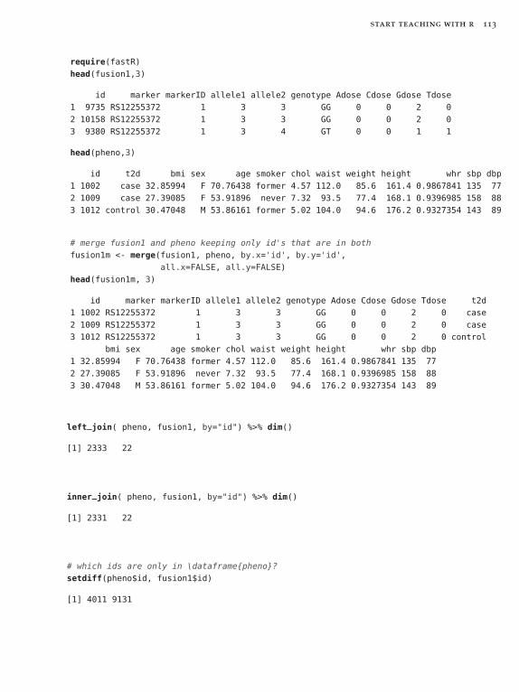
start teaching with r 113
require(fastR)
head(fusion1,3)
id marker markerID allele1 allele2 genotype Adose Cdose Gdose Tdose
1 9735 RS12255372 1 3 3 GG 0 0 2 0
2 10158 RS12255372 1 3 3 GG 0 0 2 0
3 9380 RS12255372 1 3 4 GT 0 0 1 1
head(pheno,3)
id t2d bmi sex age smoker chol waist weight height whr sbp dbp
1 1002 case 32.85994 F 70.76438 former 4.57 112.0 85.6 161.4 0.9867841 135 77
2 1009 case 27.39085 F 53.91896 never 7.32 93.5 77.4 168.1 0.9396985 158 88
3 1012 control 30.47048 M 53.86161 former 5.02 104.0 94.6 176.2 0.9327354 143 89
# merge fusion1 and pheno keeping only id's that are in both
fusion1m <- merge(fusion1, pheno, by.x='id', by.y='id',
all.x=FALSE, all.y=FALSE)
head(fusion1m, 3)
id marker markerID allele1 allele2 genotype Adose Cdose Gdose Tdose t2d
1 1002 RS12255372 1 3 3 GG 0 0 2 0 case
2 1009 RS12255372 1 3 3 GG 0 0 2 0 case
3 1012 RS12255372 1 3 3 GG 0 0 2 0 control
bmi sex age smoker chol waist weight height whr sbp dbp
1 32.85994 F 70.76438 former 4.57 112.0 85.6 161.4 0.9867841 135 77
2 27.39085 F 53.91896 never 7.32 93.5 77.4 168.1 0.9396985 158 88
3 30.47048 M 53.86161 former 5.02 104.0 94.6 176.2 0.9327354 143 89
left_join( pheno, fusion1, by="id") %>% dim()
[1] 2333 22
inner_join( pheno, fusion1, by="id") %>% dim()
[1] 2331 22
# which ids are only in \dataframe{pheno}?
setdiff(pheno$id, fusion1$id)
[1] 4011 9131

114 pruim, horton kaplan
The difference between an inner join and a left join isthat the inner join only includes rows from the first dataframe that have a match in the second but aleft join in-cludes all rows of the first data frame, even if they do nothave a match in the second. In the example above, thereare two subjects in pheno that do not appear in fusion1.
merge() handles these distinctions with the all.x
and all.y arguments. In this case, since the values arethe same for each data frame, we could collapse by.x
and by.y to by and collapse all.x and all.y to all. Thefirst of these specifies which column(s) to use to identifymatching cases. The second indicates whether cases inone data frame that do not appear in the other shouldbe kept (TRUE) or dropped (filling in NA as needed) ordropped from the merged data frame.
Now we are ready to begin our analysis.
tally(~t2d + genotype + marker, data=fusion1m)
, , marker = RS12255372
genotype
t2d GG GT TT
case 737 375 48
control 835 309 27
6.5 Getting data from mySQL data bases
The RMySQL package allows direct access to data in MySQLdata bases and the dplyr package facilitates processingthis data in the same way as for data in a data frame.This makes it easy to work with very large data setsstored in public databases. The example below queriesthe UCSCgenome browser to find all the known genes on UCSC — Univ. of California,
Santa Cruzchromosome 1.
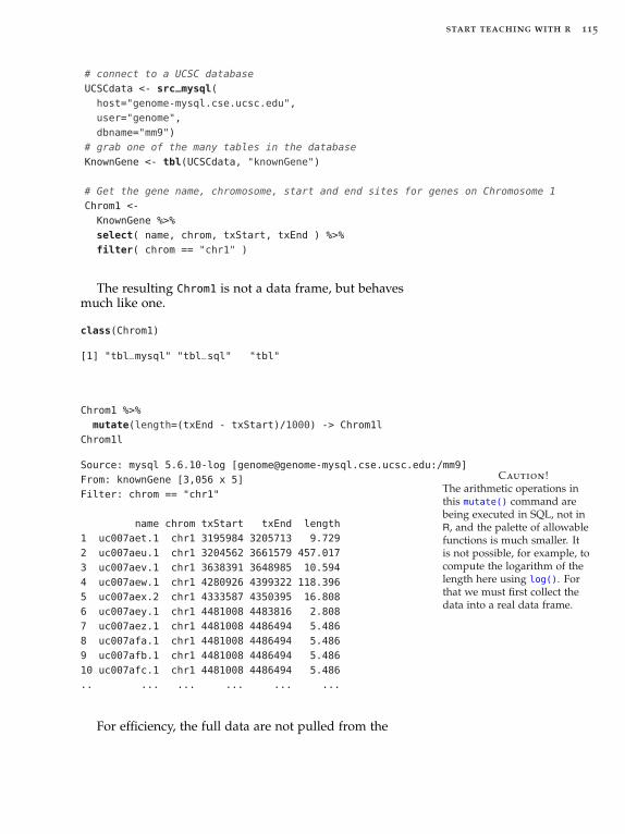
start teaching with r 115
# connect to a UCSC database
UCSCdata <- src_mysql(
host="genome-mysql.cse.ucsc.edu",
user="genome",
dbname="mm9")
# grab one of the many tables in the database
KnownGene <- tbl(UCSCdata, "knownGene")
# Get the gene name, chromosome, start and end sites for genes on Chromosome 1
Chrom1 <-
KnownGene %>%
select( name, chrom, txStart, txEnd ) %>%
filter( chrom == "chr1" )
The resulting Chrom1 is not a data frame, but behavesmuch like one.
class(Chrom1)
[1] "tbl_mysql" "tbl_sql" "tbl"
Caution!The arithmetic operations inthis mutate() command arebeing executed in SQL, not inR, and the palette of allowablefunctions is much smaller. Itis not possible, for example, tocompute the logarithm of thelength here using log(). Forthat we must first collect thedata into a real data frame.
Chrom1 %>%
mutate(length=(txEnd - txStart)/1000) -> Chrom1l
Chrom1l
Source: mysql 5.6.10-log [[email protected]:/mm9]
From: knownGene [3,056 x 5]
Filter: chrom == "chr1"
name chrom txStart txEnd length
1 uc007aet.1 chr1 3195984 3205713 9.729
2 uc007aeu.1 chr1 3204562 3661579 457.017
3 uc007aev.1 chr1 3638391 3648985 10.594
4 uc007aew.1 chr1 4280926 4399322 118.396
5 uc007aex.2 chr1 4333587 4350395 16.808
6 uc007aey.1 chr1 4481008 4483816 2.808
7 uc007aez.1 chr1 4481008 4486494 5.486
8 uc007afa.1 chr1 4481008 4486494 5.486
9 uc007afb.1 chr1 4481008 4486494 5.486
10 uc007afc.1 chr1 4481008 4486494 5.486
.. ... ... ... ... ...
For efficiency, the full data are not pulled from the

116 pruim, horton kaplan
database until needed (or until we request this usingcollect()). This allows us, for example, to inspect thefirstfew rows of a potentially large pull from the databasewithout actually having done all ofthe work required topull that data.
But certain things do not work unless we collect theresults from the data based into an actual data frame. Toplot the data using lattice or ggplot2, for example, wemust first collect() it into a data frame.
Chrom1df <- collect(Chrom1l) # collect into a data frame
histogram( ~length, data=Chrom1df, xlab="gene length (kb)" )
gene length (kb)
Den
sity
0.000
0.002
0.004
0.006
0.008
0 200 400 600 800 1000
6.6 Reshaping data
reshape() provides a flexible way to change the arrange-ment of data. It was designed for converting betweenlong and wide versions of time series data and its argu-ments are named with that in mind.
A common situation is when we want to convert froma wide form to a long form because of a change in per-spective about what a unit of observation is. For example,in the traffic data frame, each row is a year, and datafor multiple states are provided.
traffic
year cn.deaths ny cn ma ri
1 1951 265 13.9 13.0 10.2 8.0
2 1952 230 13.8 10.8 10.0 8.5
3 1953 275 14.4 12.8 11.0 8.5

start teaching with r 117
4 1954 240 13.0 10.8 10.5 7.5
5 1955 325 13.5 14.0 11.8 10.0
6 1956 280 13.4 12.1 11.0 8.2
7 1957 273 13.3 11.9 10.2 9.4
8 1958 248 13.0 10.1 11.8 8.6
9 1959 245 12.9 10.0 11.0 9.0
We can reformat this so that each row contains a mea-surement for a single state in one year.
longTraffic <-
reshape(traffic[,-2], idvar="year", ids=row.names(traffic),
times=names(traffic)[3:6], timevar="state",
varying=list(names(traffic)[3:6]), v.names="deathRate",
direction="long")
head(longTraffic)
year state deathRate
1951.ny 1951 ny 13.9
1952.ny 1952 ny 13.8
1953.ny 1953 ny 14.4
1954.ny 1954 ny 13.0
1955.ny 1955 ny 13.5
1956.ny 1956 ny 13.4
We can also reformat the other way, this time havingall data for a given state form a row in the data frame.stateTraffic <- reshape(longTraffic, direction='wide', v.names="deathRate",
idvar="state", timevar="year")
stateTraffic
state deathRate.1951 deathRate.1952 deathRate.1953 deathRate.1954 deathRate.1955
1951.ny ny 13.9 13.8 14.4 13.0 13.5
1951.cn cn 13.0 10.8 12.8 10.8 14.0
1951.ma ma 10.2 10.0 11.0 10.5 11.8
1951.ri ri 8.0 8.5 8.5 7.5 10.0
deathRate.1956 deathRate.1957 deathRate.1958 deathRate.1959
1951.ny 13.4 13.3 13.0 12.9
1951.cn 12.1 11.9 10.1 10.0
1951.ma 11.0 10.2 11.8 11.0
1951.ri 8.2 9.4 8.6 9.0
In simpler cases, stack() or unstack() may suffice.

118 pruim, horton kaplan
Hmisc also provides reShape() as an alternative to reshape().
6.7 Functions in R
Functions in R have several components:
• a name (like histogram)1 1 Actually, it is possible to de-fine functions without namingthem; and for short functionsthat are only needed once, thiscan actually be useful.
• an ordered list of named arguments that serve as in-puts to the function
These are matched first by name and then by order tothe values supplied by the call to the function. This iswhy we don’t always include the argument name inour function calls. On the other hand, the availabilityof names means that we don’t have to remember theorder in which arguments are listed.
Arguments often have default values which are used ifno value is supplied in the function call.
• a return value
This is the output of the function. It can be assigned toa variable using the assignment operator (=, <-, or ->).
• side effects
A function may do other things (like make a graph orset some preferences) that are not necessarily part ofthe return value.
When you read the help pages for an R function, you willsee that they are organized in sections related to thesecomponents. The list of arguments appears in the Usagesection along with any default values. Details about howthe arguments are used appear in the Arguments section.The return value is listed in the Value section. Any sideeffects are typically mentioned in the Details section. Even if you do not end up writ-
ing many functions yourself,writing a few functions willgive you a much better feel forhow information flows throughR code.
Now let’s try writing our own function. Suppose youfrequently wanted to compute the mean, median, andstandard deviation of a distribution. You could make afunction to do all three to save some typing.
Let’s name our function mystats(). The mystats()
will have one argument, which we are assuming will be avector of numeric values. Here is how we could define it:

start teaching with r 119
mystats <- function(x) {
mean(x)
median(x)
sd(x)
}
mystats((1:20)^2)
[1] 127.9023
There are ways to check theclass of an argument to seeif it is a data frame, a vector,numeric, etc. A really robustfunction should check to makesure that the values supplied tothe arguments are of appropri-ate types.
The first line says that we are defining a function calledmystats() with one argument, named x. The lines sur-rounded by curly braces give the code to be executedwhen the function is called. So our function computesthemean, then the median, then the standard deviation of itsargument.
But as you see, this doesn’t do exactly what we wanted.So what’s going on? The value returned by the last line ofa function is (by default) returned by the function to itscalling environment, where it is (by default) printed tothe screen so you can see it. In our case, we computedthe mean, median, and standard deviation, but only thestandard deviation is being returned by the function andhence displayed. So this function is just an inefficient ver-sion of sd(). That isn’t really what we wanted.
We can use print() to print out things along the wayif we like.
mystats <- function(x) {
print(mean(x))
print(median(x))
print(sd(x))
}
mystats((1:20)^2)
[1] 143.5
[1] 110.5
[1] 127.9023
Alternatively, we could use a combination of cat() andpaste(), which would give us more control over how the
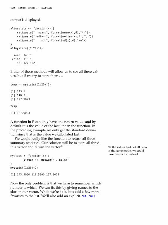
120 pruim, horton kaplan
output is displayed.
altmystats <- function(x) {
cat(paste(" mean:", format(mean(x),4),"\n"))
cat(paste(" edian:", format(median(x),4),"\n"))
cat(paste(" sd:", format(sd(x),4),"\n"))
}
altmystats((1:20)^2)
mean: 143.5
edian: 110.5
sd: 127.9023
Either of these methods will allow us to see all three val-ues, but if we try to store them . . .
temp <- mystats((1:20)^2)
[1] 143.5
[1] 110.5
[1] 127.9023
temp
[1] 127.9023
A function in R can only have one return value, and bydefault it is the value of the last line in the function. Inthe preceding example we only get the standard devia-tion since that is the value we calculated last.
We would really like the function to return all threesummary statistics. Our solution will be to store all threein a vector and return the vector.2 2 If the values had not all been
of the same mode, we couldhave used a list instead.
mystats <- function(x) {
c(mean(x), median(x), sd(x))
}
mystats((1:20)^2)
[1] 143.5000 110.5000 127.9023
Now the only problem is that we have to remember whichnumber is which. We can fix this by giving names to theslots in our vector. While we’re at it, let’s add a few morefavorites to the list. We’ll also add an explicit return().

start teaching with r 121
mystats <- function(x) {
result <- c(min(x), max(x), mean(x), median(x), sd(x))
names(result) <- c("min","max","mean","median","sd")
return(result)
}
mystats((1:20)^2)
min max mean median sd
1.0000 400.0000 143.5000 110.5000 127.9023
summary(Sepal.Length~Species, data=iris, fun=mystats)
Length Class Mode
3 formula call
aggregate(Sepal.Length~Species, data=iris, FUN=mystats)
Species Sepal.Length.min Sepal.Length.max
1 setosa 4.3000000 5.8000000
2 versicolor 4.9000000 7.0000000
3 virginica 4.9000000 7.9000000
Sepal.Length.mean Sepal.Length.median Sepal.Length.sd
1 5.0060000 5.0000000 0.3524897
2 5.9360000 5.9000000 0.5161711
3 6.5880000 6.5000000 0.6358796
Notice how nicely this works with aggregate() andwith the summary() function from the Hmisc package. Youcan, of course, define your own favorite function to usewith summary(). The favstats() function in the mosaic
package includes the quartiles, mean, standard, deviation,sample size and number of missing observations.favstats(Sepal.Length ~ Species, data=iris)
.group min Q1 median Q3 max mean sd n missing
1 setosa 4.3 4.800 5.0 5.2 5.8 5.006 0.3524897 50 0
2 versicolor 4.9 5.600 5.9 6.3 7.0 5.936 0.5161711 50 0
3 virginica 4.9 6.225 6.5 6.9 7.9 6.588 0.6358796 50 0
6.8 Sharing With and Among Your Students
Instructors often have their own data sets to illustratepoints of statistical interest or to make a particular con-

122 pruim, horton kaplan
nection with a class. Sometimes you may want your classas a whole to construct a data set, perhaps by filling in asurvey or by contributing their own small bit of data to aclass collection. Students may be working on projects insmall groups; it’s nice to have tools to support such workso that all members of the group have access to the dataand can contribute to a written report.
There are now many technologies that support suchsharing. For the sake of simplicity, we will emphasizethree that we have found particularly useful both inteaching statistics and in our professional collaborativework. These are:
• Within RStudio server.
• A web site with minimal overhead, such as providedby Dropbox.
• The services of Google Docs.
• A web-based RStudio server for R.
The first two are already widely used in university envi-ronments and are readily accessible simply by setting upaccounts. Setting up an RStudio web server requires someIT support, but is well within the range of skills found inIT offices and even among some individual faculty.
6.8.1 Using RStudio server to share files
Teaching Tip
When accounts are set up onthe RStudio server for a newclass at Calvin, each user isgiven a symbolic link to a di-rectory where the instructorcan write files and students canonly read files. This providesan easy way to make data, R
code, or history files availableto students from inside RStudio.
The RStudio server runs on a Linux machine. Users ofRStudio have accounts on the underlying Linux file systemand it is possible to set up shared directories with permis-sions that allow multiple users to read and/or write filesstored there. This has to be done outside of RStudio, but ifyou are familiar with the Linux operating system or havea system administrator who is willing to help you out,this is not difficult to do.
6.8.2 Your own web site
You may already have a web site. We have in mind aplace where you can place files and have them accesseddirectly from the Internet. For sharing data, it’s best ifthis site is public, that is, it does not require a login. In

start teaching with r 123
this case, read.file() can read the data into R directlyfrom the URL:
Fires <- read.csv("http://www.calvin.edu/~rpruim/data/Fires.csv")
head(Fires)
Year Fires Acres
1 2011 74126 8711367
2 2010 71971 3422724
3 2009 78792 5921786
4 2008 78979 5292468
5 2007 85705 9328045
6 2006 96385 9873745
xyplot( Acres/Fires ~ Year, data=Fires, ylab="acres per fire",
type=c("p","smooth"))
Year
acre
s pe
r fir
e
20
40
60
80
100
120
1960 1970 1980 1990 2000 2010
Unfortunately, most “course support” systems such asMoodle orBlackboard do not provide such easy access todata. The Dropbox service for storing files in the “cloud”provides a very convenient way to distribute files over theweb. (Go to dropbox.com for information and to sign upfor a free account.) Dropbox is routinely used to provideautomated backup and coordinated file access on multi-ple computers. But the Dropbox service also provides aPublic directory. Any files that you place in that direc-tory can be accessed directly by a URL.
Our discussion of Dropbox isprimarily for those who do notalready know how to do thisother ways.
To illustrate, suppose you wish to share some dataset with your students. You’ve constructed this data setin a spreadsheet and stored it as a csv file, let’s call itexample-A.csv. Move this file into the Public directoryunder Dropbox — on most computers Dropbox arrangesthings so that its directories appear exactly like ordinarydirectories and you’ll use the ordinary, familiar file man-agement techniques such as drag and drop.
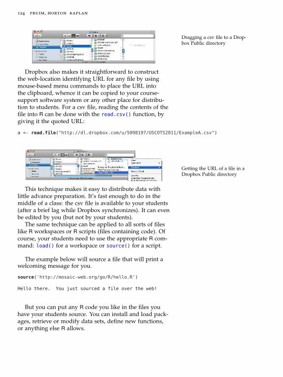
124 pruim, horton kaplan
Dragging a csv file to a Drop-box Public directory
Dropbox also makes it straightforward to constructthe web-location identifying URL for any file by usingmouse-based menu commands to place the URL intothe clipboard, whence it can be copied to your course-support software system or any other place for distribu-tion to students. For a csv file, reading the contents of thefile into R can be done with the read.csv() function, bygiving it the quoted URL:
a <- read.file("http://dl.dropbox.com/u/5098197/USCOTS2011/ExampleA.csv")
Getting the URL of a file in aDropbox Public directory
This technique makes it easy to distribute data withlittle advance preparation. It’s fast enough to do in themiddle of a class: the csv file is available to your students(after a brief lag while Dropbox synchronizes). It can evenbe edited by you (but not by your students).
The same technique can be applied to all sorts of fileslike R workspaces or R scripts (files containing code). Ofcourse, your students need to use the appropriate R com-mand: load() for a workspace or source() for a script.
The example below will source a file that will print awelcoming message for you.
source('http://mosaic-web.org/go/R/hello.R')
Hello there. You just sourced a file over the web!
But you can put any R code you like in the files youhave your students source. You can install and load pack-ages, retrieve or modify data sets, define new functions,or anything else R allows.

start teaching with r 125
Many instructors will find it useful to create a file withyour course-specific R scripts, adding on to it and modi-fying it as the course progresses. This allows you to dis-tribute all sorts of special-purpose functions, letting youdistribute new R material to your students. That brilliantnew idea you had at 2 AM can be programmed up andput in place for your students to use the next morning inclass. Then as you identify bugs and refine the program,you can make the updated software immediately avail-able to your students. Caution!
Security through Obscurity of thissort will not generally satisfyinstitutional data protectionregulations nor professionalethical requirements, so nothingtruly sensitive or confidentialshould be “protected" in thismanner.
If privacy is a concern, for instance if you want thedata available only to your students, you can effectivelyaccomplish this by giving files names known only to yourstudents, e.g., Example-A78r423.csv.
6.8.3 GoogleDocs
The Dropbox technique (or any other system of postingfiles to the Internet) is excellent for broadcasting: tak-ing files you create and distributing them in a read-onlyfashion to your students. But when you want two-way ormulti-way sharing of files, other techniques are called for,such as provided by the GoogleDocs service.
GoogleDocs allows students and instructors to createvarious forms of documents, including reports, presen-tations, and spreadsheets. (In addition to creating doc-uments de novo, Google will also convert existing docu-ments in a variety of formats.)
Once on the GoogleDocs system, the documents canbe edited simultaneously by multiple users in differentlocations. They can be shared with individuals or groupsand published for unrestricted viewing and even editing.
For teaching, this has a variety of uses:
• Students working on group projects can all simulta-neously have access to the report as it is being writtenand to data that is being assembled by the group.
• The entire class can be given access to a data set, bothfor reading and for writing.
• The Google Forms system can be used to constructsurveys, the responses to which can populate a spread-sheet that can be read back into RStudio by the survey

126 pruim, horton kaplan
creators.
• Students can “hand in” reports and data sets by copy-ing a link into a course support system such as Moodleor Blackboard, or emailing the link.
• The instructor can insert comments and/or correctionsdirectly into the document.
An effective technique for organizing student workand ensuring that the instructor (and other graders) haveaccess to it, is to create a separate Google directory foreach student in your class (Dropbox can also be usedin this manner). Set the permission on this directory toshare it with the student. Anything she or he drops intothe directory is automatically available to the instructor.The student can also share with specific other students(e.g., members of a project group).
We will illustrate the entire process in the context ofthe following example.
Example 6.2. One exercise for students starting out ina statistics course is to collect data to find out whether the“close door” button on an elevator has any effect. This isan opportunity to introduce simple ideas of experimentaldesign. But it’s also a chance to teach about the organiza-tion of data.
Have your students, as individuals or small groups,study a particular elevator, organize their data into aspreadsheet, and hand in their individual spreadsheet.Then review the spreadsheets in class. You will likely findthat many groups did not understand clearly the distinc-tion between cases and variables, or coded their data inambiguous or inconsistent ways.
Work with the class to establish a consistent schemefor the variables and their coding, e.g., a variable ButtonPress
with levels “Yes” and “No”, a variable Time with the timein seconds from a fiducial time (e.g. when the buttonwas pressed or would have been pressed) with time mea-sured in seconds, and variables ElevatorLocation andGroupName. Create a spreadsheet with these variables anda few cases filled in. Share it with the class.
Have each of your students add their own data to theclass data set. Although this is a trivial task, having totranslate their individual data into a common format
start teaching with r 127
strongly reinforces the importance of a consistent mea-surement and coding system for recording data.
Once you have a spreadsheet file in GoogleDocs, youwill want to open it in R. This can be exported as a csvfile, then open it using the csv tools in R, such as read.csv().
Direct communication with GoogleDocs requires fa-cilities that are not present in the base version of R, butare available through the RCurl package. In order to makethese readily available to students, the mosaic packagecontains a function that takes the quoted (and cumber-some) string with the Google-published URL and readsthe corresponding file into a data frame. RCurl neads tobe installed for this to work, and will be loaded if it is notalready loaded when fetchGoogle() is called.
elev <- fetchGoogle(
"https://spreadsheets.google.com/spreadsheet/pub?hl=en&hl=en&
key=0Am13enSalO74dEVzMGJSMU5TbTc2eWlWakppQlpjcGc&single=TRUE&gid=0&output=csv")
128 pruim, horton kaplan
head(elev)
StudentGroup Elevator CloseButton Time Enroute LagToPress
1 HA Campus Center N 8.230 N 0
2 HA Campus Center N 7.571 N 0
3 HA Campus Center N 7.798 N 0
4 HA Campus Center N 8.303 N 0
5 HA Campus Center Y 5.811 N 0
6 HA Campus Center Y 6.601 N 0
Teaching Tip
Another option is to get shorterURLs using a service liketinyurl.com or bitly.com.
Of course, you’d never want your students to type thatURL by hand; you should provide it in a copy-able formon a web site or within a course support system. ⋄
6.9 Additional Notes on R Syntax
6.9.1 Text and Quotation Marks
For the most part, text in R must be enclosed in eithersingle or double quotations. It usually doesn’t matterwhich you use, unless you want one or the other type ofquotation mark inside your text. Then you should use theother type of quotation mark to mark the beginning andthe end.
# apostrophe inside requires double quotes around text
text1 <- "Mary didn't come"
# this time we flip things around
text2 <- 'Do you use "scare quotes"?'
6.10 Common Error Messages and What Causes
Them
6.10.1 Error: Object not found
R reports that an object is not found when it cannot locatean object with the name you have used. One commonreason for this is a typing error. This is easily corrected byretyping the name with the correct spelling.

start teaching with r 129
histogram( ~ aeg, data=HELPrct )
Error in eval(expr, envir, enclos): object ’aeg’ not
found
Another reason for an object-not-found error is usingunquoted text where quotation marks were required.
text3 <- hello
Error in eval(expr, envir, enclos): object ’hello’ not
found
In this case, R is looking for some object named hello,but we meant to store a string:
text3 <- "hello"
6.10.2 Error: unexpected . . .
If while R is parsing a statement it encounters somethingthat does not make sense it reports that something is “un-expected”. Often this is the result of a typing error – likeomitting a comma.
c(1,2 3) # missing a commaError in c(): unexpected numeric constant in "c(1,2 3"
6.10.3 Error: object of type ‘closure’ is not subsettable
The following produces an error if time has not been de-fined.
time[3]
Error in time[3]: object of type ’closure’ is not
subsettable
There is a function called time() in R, so if you haven’tdefined a vector by that name, R will try to subset thetime() function, which doesn’t make sense.

130 pruim, horton kaplan
Typically when you see this error, you have a functionin a place you don’t mean to have a function. The mes-sage can be cryptic to new users because of the referenceto a closure.
6.10.4 Other Errors
If you encounter other errors and cannot decipher them,often pasting the error message into a google searchwill find a discussion of that error in a context where itstumped someone else.
6.11 Review of R Commands
Here is a brief summary of the commands introduced inthis chapter.source( "file.R" ) # execute commands in a file
x <- 1:10 # create vector with numbers 1 through 10
M <- matrix( 1:12, nrow=3 ) # create a 3 x 4 matrix
data.frame(number = 1:26, letter=letters[1:26] ) # create a data frame
mode(x) # returns mode of object x
length(x) # returns length of vector or list
dim(HELPrct) # dimension of a matrix, array, or data frame
nrow(HELPrct) # number of rows
ncol(HELPrct) # number of columns
names( HELPrct ) # variable names in data frame
row.names( HELPrct ) # row names in a data frame
attributes(x) # returns attributes of x
toupper(x) # capitalize
as.character(x) # convert to a character vector
as.logical(x) # convert to a logical (TRUE or FALSE)
as.numeric(x) # convert to numbers
as.integer(x) # convert to integers
factor(x) # convert to a factor [categorical data]
class(x) # returns class of x
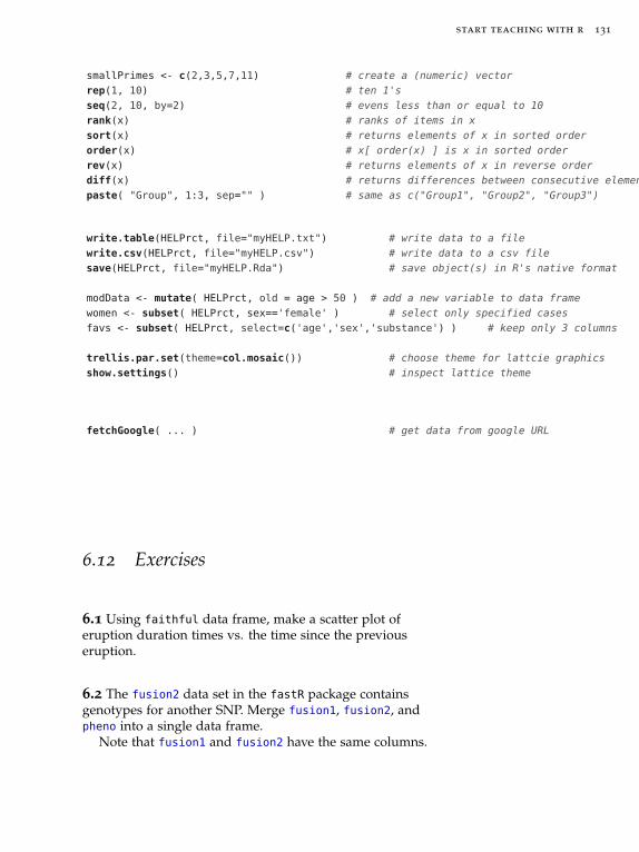
start teaching with r 131
smallPrimes <- c(2,3,5,7,11) # create a (numeric) vector
rep(1, 10) # ten 1's
seq(2, 10, by=2) # evens less than or equal to 10
rank(x) # ranks of items in x
sort(x) # returns elements of x in sorted order
order(x) # x[ order(x) ] is x in sorted order
rev(x) # returns elements of x in reverse order
diff(x) # returns differences between consecutive elements
paste( "Group", 1:3, sep="" ) # same as c("Group1", "Group2", "Group3")
write.table(HELPrct, file="myHELP.txt") # write data to a file
write.csv(HELPrct, file="myHELP.csv") # write data to a csv file
save(HELPrct, file="myHELP.Rda") # save object(s) in R's native format
modData <- mutate( HELPrct, old = age > 50 ) # add a new variable to data frame
women <- subset( HELPrct, sex=='female' ) # select only specified cases
favs <- subset( HELPrct, select=c('age','sex','substance') ) # keep only 3 columns
trellis.par.set(theme=col.mosaic()) # choose theme for lattcie graphics
show.settings() # inspect lattice theme
fetchGoogle( ... ) # get data from google URL
6.12 Exercises
6.1 Using faithful data frame, make a scatter plot oferuption duration times vs. the time since the previouseruption.
6.2 The fusion2 data set in the fastR package containsgenotypes for another SNP. Merge fusion1, fusion2, andpheno into a single data frame.
Note that fusion1 and fusion2 have the same columns.

132 pruim, horton kaplan
names(fusion1)
[1] "id" "marker" "markerID" "allele1" "allele2"
[6] "genotype" "Adose" "Cdose" "Gdose" "Tdose"
names(fusion2)
[1] "id" "marker" "markerID" "allele1" "allele2"
[6] "genotype" "Adose" "Cdose" "Gdose" "Tdose"
You may want to use the suffixes argument to merge()
or rename the variables after you are done merging tomake the resulting data frame easier to navigate.
Tidy up your data frame by dropping any columnsthat are redundant or that you just don’t want to have inyour final data frame.
7
Getting Interactive: manipulate and shiny
One very attractive feature of RStudio is the manipulate()
function (in the manipulate package, which is only avail-able within RStudio). This function makes it easy to createa set of controls (such as sliders, checkboxes, drop downselections, etc.) that can be used to dynamically changevalues within an expression. When a value is changedusing these controls, the expression is automatically re-executed and any plots created as a result are redrawn.This can be used to quickly prototype a number of activi-ties and demos as part of a statistics lecture.
shiny is a new web development system for R be-ing designed by the RStudio team. shiny uses a reactiveprogramming model to make it relatively easy for an R
programmer to create highly interactive, well designedweb applications using R without needing to know muchabout web programming. Programming in shiny is moreinvolved than using manipulate, but it offers the designermore flexibility. One of the goals in creating shiny was tosupport corporate environments, where a small numberof statisticians and programmers can create web appli-cations that can be used by others within the companywithout requiring them to know any R. This same frame-work offers many possibilities for educational purposesas well. Some have even suggested implementing fairlyextensive GUI interfaces to commonly used R functional-ity using shiny.

134 pruim, horton kaplan
7.1 Getting Started with manipulate
The manipulate() function and the various control func-tions that are used with it are only available after loadingthe manipulate package, which is only available in RStu-
dio.
require(manipulate)
7.1.1 Sliders
manipulate(
histogram( ~ eruptions, data=faithful, n=N),
N = slider(5,40)
)
This generates a plot along with a slider ranging from 5 We find it useful to capitalizethe inputs to the manipulatedexpression that are hooked upto manipulate controls. Thishelps avoid naming collisionsand signals how the main ma-nipulated expression is beingused.
bins to 40.
When the slider is changed, we see a clearer view ofthe eruptions of Old Faithful.

start teaching with r 135
7.1.2 Check Boxes
manipulate(
histogram( ~ age, data=HELPrct, n=N, density=DENSITY),
N = slider(5,40),
DENSITY = checkbox()
)
7.1.3 Drop-down Menus
Drop-down menus can be added using the picker()
function.
manipulate(
histogram( ~ age, data=HELPrct, n=N,
fit=DISTRIBUTION, dlwd=4),
N = slider(5,40),
DISTRIBUTION =
picker('normal', 'gamma', 'exponential', 'lognormal',
label="distribution")
)

136 pruim, horton kaplan
7.1.4 Visualizing Normal Distributions
In this section we will gradually build up a small manipulateexample that shows the added flexibility that comes fromwriting a function that returns a manipulate object. Suchfunctions can be distributed to students to allow them toexplore interactively in a more flexible way.
We begin by creating an illustration of tail probabilitiesin a normal distribution.
manipulate(
xpnorm( X, 500, 100, verbose=FALSE, invisible=TRUE ),
X = slider(200,800) )
The version below can be used to investigate central prob-abilities and tail probabilities.
manipulate(
xpnorm( c(-X,X), 500, 100, verbose=FALSE, invisible=TRUE ),
X = slider(200,800) )
These examples work with a fixed distribution. Here isa fancier version in which a function returns a manipulateobject. This allows us to easily create illustrations like theones above for any normal distribution.
mNorm <- function( mean=0, sd=1 ) {
lo <- mean - 5*sd
hi <- mean + 5*sd
manipulate(
xpnorm( c(A,B), mean, sd, verbose=FALSE, invisible=TRUE ),
A = slider(lo, hi, initial=mean-sd),
B = slider(lo, hi, initial=mean+sd)
)
}
mNorm( mean=100, sd=10 )
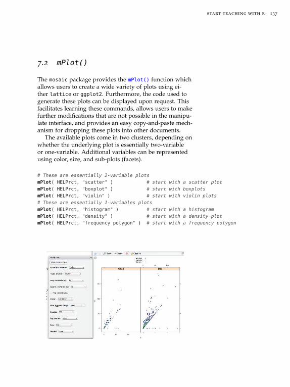
start teaching with r 137
7.2 mPlot()
The mosaic package provides the mPlot() function whichallows users to create a wide variety of plots using ei-ther lattice or ggplot2. Furthermore, the code used togenerate these plots can be displayed upon request. Thisfacilitates learning these commands, allows users to makefurther modifications that are not possible in the manipu-late interface, and provides an easy copy-and-paste mech-anism for dropping these plots into other documents.
The available plots come in two clusters, depending onwhether the underlying plot is essentially two-variableor one-variable. Additional variables can be representedusing color, size, and sub-plots (facets).
# These are essentially 2-variable plots
mPlot( HELPrct, "scatter" ) # start with a scatter plot
mPlot( HELPrct, "boxplot" ) # start with boxplots
mPlot( HELPrct, "violin" ) # start with violin plots
# These are essentially 1-variables plots
mPlot( HELPrct, "histogram" ) # start with a histogram
mPlot( HELPrct, "density" ) # start with a density plot
mPlot( HELPrct, "frequency polygon" ) # start with a frequency polygon

138 pruim, horton kaplan
7.3 Shiny
shiny is a package created by the RStudio team to, in theirwords,
[make] it incredibly easy to build interactive web appli-cations with R. Automatic “reactive" binding betweeninputs and outputs and extensive pre-built widgets makeit possible to build beautiful, responsive, and powerfulapplications with minimal effort.
These web applications can, of course, run R code to docomputations and produce graphics that appear in theweb page.
The level of coding skill required to create this is be-yond the scope of this book, but those with a little moreprogramming background can easily learn the necessarytoolkit to make beautiful interactive web pages. More in-formation about shiny and some example applicationsare available at http://www.rstudio.com/shiny/.
Exercises
7.1 The following code makes a scatterplot with separatesymbols for each sex.
xyplot(cesd ~ age, data=HELPrct, groups=sex)
Build a manipulate example that allows you to turn thegrouping on and off with a checkbox.
7.2 Build a manipulate example that uses a picker to se-lect from a number of variables to make a plot for. Here’san example with a histogram:

start teaching with r 139
7.3 Design your own interactive demonstration idea andimplement it using RStudio manipulate tools.

8
Bibliography
[Fis25] R. A. Fisher. Statistical Methods for Research Work-ers. Oliver & Boyd, 1925.
[Fis70] R. A. Fisher. Statistical Methods for Research Work-ers. Oliver & Boyd, 14th edition, 1970.
[NT10] D. Nolan and D. Temple Lang. Computing in thestatistics curriculum. The American Statistician,64(2):97–107, 2010.
[Sal01] D. Salsburg. The Lady Tasting Tea: How statisticsrevolutionized science in the twentieth century. W.H.Freeman, New York, 2001.
[Wor14] Undergraduate Guidelines Workshop. 2014 cur-riculum guidelines for undergraduate programsin statistical science. Technical report, AmericanStatistical Association, November 2014.

9
Index
->, 118
<-, 118
=, 118
?, 71
??, 72
[ ], 86, 88
[[ ]], 86, 92
#, 85
$, 75
lattice settings, 54
alpha, 52
any(), 96
apropos(), 72
argument of an R function, 118
array, 90
as.data.frame(), 79
attach()
avoid, 75
auto.key, 52, 61
barchart(), 42, 79
bargraph(), 42, 62, 65, 79
binom.test(), 51
Bioconductor, 71
Births78, 39, 76
boxplot, see bwplot()bwplot(), 40, 65
c(), 78, 81, 87, 98
Cards, 100
cat(), 120
cbind(), 78, 95
cex, 52
class, 86
class(), 86
collect(), 116
comment character in R (#), 85
conditional plots, 46, 56, 60
confint(), 50
contains(), 106
CPS85, 62
CRAN (Comprehensive RArchive Network, 70
cummax(), 96
cummin(), 96
cumprod(), 95, 96
cumsum(), 65, 95, 96
Current Population Survey, seeCPS85
dataimporting, 97
importing into RStudio, 77
pretabulated, 77
data frame, 73
data(), 76, 81
data.frame(), 94
deal(), 100
demo(), 73
density scale, 59
densityplot(), 42, 58, 65
devtools, 71
diff(), 95, 96
dim(), 91
dotPlot(), 42, 56, 65
dotplot(), 44
Dropbox, 123
ediff(), 95
ends_with(), 106
evironmentsR, 74
example(), 72
Excel, 77
facets, see conditional plotsfactor(), 88, 100
favstats(), 46, 65, 121
Fisher, R. A., 25
freqpolygon(), 42, 57, 65
frequency polygon, seefreqpolygon()
function(), 118
functions in R, 118
gdata, 77
generic functions, 64
geyser, 57
ggplot2, 64
ggvis, 38
github, 71
Google, 75
gplot2, 38
head(), 74, 77, 79, 81

142 pruim, horton kaplan
help.search(), 72
HELPrct, 40
histogram(), 41, 56, 65
install.packages(), 70
install_github(), 71
IQR(), 46
iris, 60
labelsaxis, 52
ladd(), 57
lattice, 38, 64
legends, 46
length(), 91
LETTERS[ ], 89
letters[ ], 89
library(), 70
linear models, see also lm()
list, 91
list(), 92
lm(), 49
load(), 76
log(), 81, 94
log10(), 81
main, 52
manipulate, 64
MASS, 57
matches(), 106
matrix, 90
matrix(), 91
max(), 46
mean(), 46, 65, 94
median(), 46, 65, 94
min(), 46
mosaic plot, 41
mplot(), 64, 65
mutate(), 115
mystats(), 118
na.omit(), 96
na.strings, 98
names(), 81, 92
ncol(), 91
nrow(), 91
number_range(), 106
object, 86
observational unit, 73
opacity, see alphaorder(), 95, 96
packageinstalling, see also
install.packages(), seealso install_github(),70
loading, see also library(),see also require(), 70
par.settings, 52
paste(), 96, 120
pch, 52
pdf(), 64
plot symbolshape, see pchsize, see cex
plot(), 64
plotPoints(), 43
pmax(), 96
pmin(), 96
print(), 64
prod(), 96
prop.test(), 51
pval(), 50
qqmath(), 42, 65
quantile(), 65
quantile-quantile plots, seeqqmath
questionstwo, 37, 68
rank(), 95, 96
rbind(), 78, 95
read.csv(), 76, 81, 98
read.file(), 76, 77, 81, 98
read.table(), 76, 77, 81, 98
read.xls(), 77
require(), 70, 81
resample(), 77, 99
reshape(), 116
return(), 120
rev(), 96
RMySQL, 114
rnorm(), 99
round(), 95
sample(), 74, 81
savehistory(), 84
scan(), 98
scatter plot, see xyplot()sd(), 46, 65, 94
select(), 105
seq(), 88
show.settings(), 54
signif(), 95
sort(), 95, 96, 100
source(), 84
SQL, 114
sqrt(), 81
src_mysql, 115
stack(), 118
starts_with(), 106
str, 74
str(), 81
stringsAsFactors, 98
stripplot(), 44
sum(), 46, 65, 96
summary(), 64, 74, 81
t.test(), 50
table(), 96
tally(), 46, 62, 65
tbl, 115
templatethe, 68
theme.mosaic(), 53
themeslattice, see
trellis.par.set()
titles (plots), 52
transparency, see alphatrellis.par.set(), 54

start teaching with r 143
unique(), 96
unstack(), 118
Utilities2, 66
var(), 46, 65, 94
variable, 73
vcd, 41
vector, 87
vectorized functions, 94
View(), 75
which(), 96
with(), 75
xlab, 52
xyplot, 60
xyplot(), 38, 65
ylab, 52
Related Documents