Stanford Exploration Project, Report 103, April 27, …sep · Stanford Exploration Project, Report 103, April 27, 2000, pages 205–231 204. Stanford Exploration Project, Report 103

Stanford Exploration Project, Report 103, April 27, 2000, pages 205–231

204

Stanford Exploration Project, Report 103, April 27, 2000, pages 205–231

Ground roll and the Radial Trace Transform – revisited

Morgan Brown and Jon Claerbout1

ABSTRACT

The Radial Trace Transform (RTT) is an attractive tool for wavefield separation becauseit lowers the apparent temporal frequency of radial events like ground roll, making it pos-sible to remove them from the data by simple bandpass filtering in the Radial Trace (RT)domain. We discuss two implementations of the RTT. In the first, and better known, the RTdomain is well-sampled, and thus suitable for post-filtering, but is prone to interpolationerrors. We present an alternate implementation, which is pseudo-unitary in the limit of aninfinitely densely sampled RT space, with the side effect that the RT domain has missingdata. Using a simple 2-D filter for regularization, we estimate the missing data in the RTdomain by least squares optimization, without affecting the invertibility of the RTT. Ourimplementation suppresses radial noise while preserving signal, including static shifts.Although it runs into trouble when noise is spatially aliased, we show that application ofa linear moveout correction prior to processing increases our scheme’s effectiveness.

INTRODUCTION

The Radial Trace Transform (RTT), is a simple coordinate transform of normal (t , x) domainseismic gathers; a horizontal deformation, accomplished by the following linear mapping

t t (1)

xx

t

The radial coordinate is termed “ ” because the RTT sorts the data by apparent velocity. Ne-glecting dispersion effects, ground roll maps to zero temporal frequency in the RT domain.The RTT is not a new concept. Nearly twenty years ago, this coordinate transform was anactive subject of research for use in multiple suppression (Taner, 1980), migration (Ottolini,1982), and even for the subject of this paper, ground roll removal (Claerbout, 1983). Henley’s(1999) recent paper reminded the world of the RTT’s usefulness in attacking ground roll. Savaand Fomel (2000) use the RTT to compute angle gathers, exploiting the fact that slant-stack inthe (t , x) domain is equivalent to computing the RTT in the Fourier domain.

Figure 1 shows 30 radial traces (thick lines) overlain on a rectangular (t , x) mesh. Pointsalong radial traces rarely fall exactly on (t , x) data locations, making the RTT an exercise in

1email: [email protected],[email protected]

205

206 Brown & Claerbout SEP–103

interpolation. In matrix notation, let us denote the RTT of data d as follows:

Rd r (2)

R is generally non-square, and even if square, is usually noninvertible. Often, however, suchinterpolation operators are nearly unitary: RT R I. We define the interpolation error asfollows

e I RTR d. (3)

Figure 1: 30 radial traces overlayinga (t , x) grid. morgan1-figure1 [NR]

0 0.5 1 1.5

0

0.02

0.04

0.06

0.08

0.1

0.12

0.14

0.16

0.18

0.2

offset

time

30 Radial traces on (t,x) grid

METHODOLOGY

In this paper, two implementations of the RTT are investigated. Each is illustrated schemati-cally in Figure 2.

1. -interpolation method: For fixed (t , x) bins, linearly interpolate between radial traces.

2. x-interpolation method: For fixed (t , ) bins, linearly interpolate between offsets.

Figure 2: Left: “ -interpolation”implementation. Right: “x-interpolation implementation.morgan1-schem [NR]

vi vi+1v

t

x

t

xi x xi+1

v

In the -interpolation approach, R “pushes” energy — weighted by linear interpolation coef-ficients — from fixed (t , x) bins into the two radial trace (t , ) bins that bracket them. Thisimplementation will cause interpolation error in regions where many (t , x) bins lie between

SEP–103 Radial Trace Transform 207

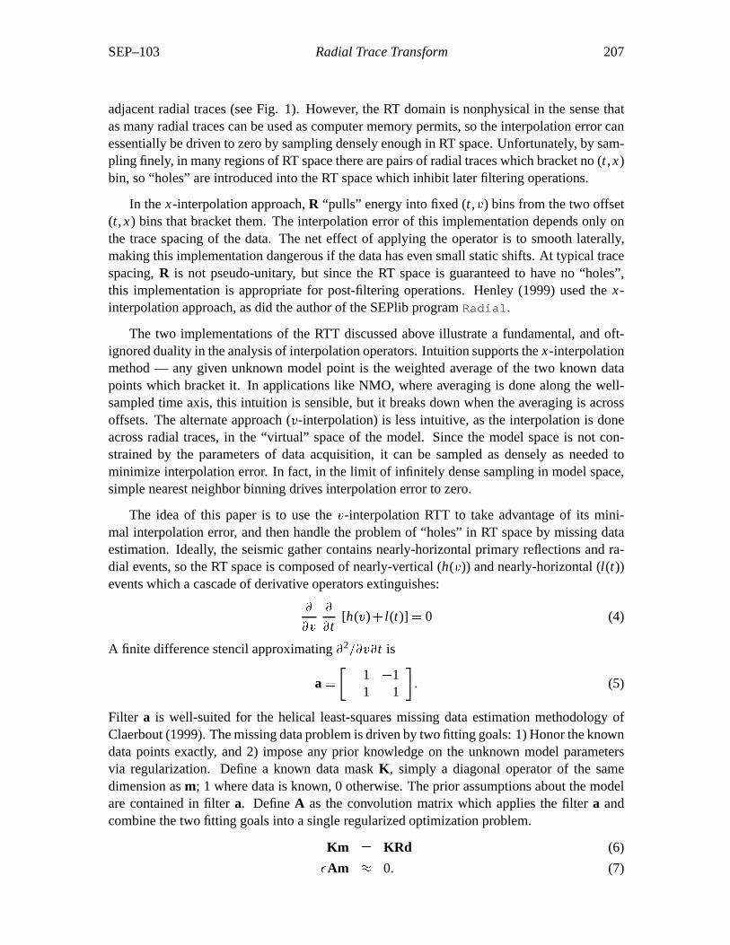
adjacent radial traces (see Fig. 1). However, the RT domain is nonphysical in the sense thatas many radial traces can be used as computer memory permits, so the interpolation error canessentially be driven to zero by sampling densely enough in RT space. Unfortunately, by sam-pling finely, in many regions of RT space there are pairs of radial traces which bracket no (t , x)bin, so “holes” are introduced into the RT space which inhibit later filtering operations.

In the x-interpolation approach, R “pulls” energy into fixed (t , ) bins from the two offset(t , x) bins that bracket them. The interpolation error of this implementation depends only onthe trace spacing of the data. The net effect of applying the operator is to smooth laterally,making this implementation dangerous if the data has even small static shifts. At typical tracespacing, R is not pseudo-unitary, but since the RT space is guaranteed to have no “holes”,this implementation is appropriate for post-filtering operations. Henley (1999) used the x-interpolation approach, as did the author of the SEPlib program Radial.

The two implementations of the RTT discussed above illustrate a fundamental, and oft-ignored duality in the analysis of interpolation operators. Intuition supports the x-interpolationmethod — any given unknown model point is the weighted average of the two known datapoints which bracket it. In applications like NMO, where averaging is done along the well-sampled time axis, this intuition is sensible, but it breaks down when the averaging is acrossoffsets. The alternate approach ( -interpolation) is less intuitive, as the interpolation is doneacross radial traces, in the “virtual” space of the model. Since the model space is not con-strained by the parameters of data acquisition, it can be sampled as densely as needed tominimize interpolation error. In fact, in the limit of infinitely dense sampling in model space,simple nearest neighbor binning drives interpolation error to zero.

The idea of this paper is to use the -interpolation RTT to take advantage of its mini-mal interpolation error, and then handle the problem of “holes” in RT space by missing dataestimation. Ideally, the seismic gather contains nearly-horizontal primary reflections and ra-dial events, so the RT space is composed of nearly-vertical (h( )) and nearly-horizontal (l(t))events which a cascade of derivative operators extinguishes:

t[h( ) l(t)] 0 (4)

A finite difference stencil approximating 2 t is

a1 11 1

. (5)

Filter a is well-suited for the helical least-squares missing data estimation methodology ofClaerbout (1999). The missing data problem is driven by two fitting goals: 1) Honor the knowndata points exactly, and 2) impose any prior knowledge on the unknown model parametersvia regularization. Define a known data mask K, simply a diagonal operator of the samedimension as m; 1 where data is known, 0 otherwise. The prior assumptions about the modelare contained in filter a. Define A as the convolution matrix which applies the filter a andcombine the two fitting goals into a single regularized optimization problem.

Km KRd (6)

Am 0. (7)

208 Brown & Claerbout SEP–103

Equation (6) forces the model to match the data where the latter is known. Equation (7)minimizes the power of the convolution of a with m, i.e., optimality is achieved when theunknown model is filled with horizontal and vertical events. is a user-chosen scale factor.

In this paper, we seek to use the RTT to do noise suppression. Specifically, we map a 2-Dseismic gather to RT space, then apply a conservative (6.5 Hz cutoff) highpass filter – call it B– to remove the noise, and finally transform back to (t , x) space. In symbols, we can write theestimated signal, s, as follows

s RT BRd. (8)

The corresponding estimate of the noise, n, is obtained simply by subtracting the estimatedsignal from the data:

n d s I RT BR d. (9)

RESULTS

Figure 3 shows a 2-D shot gather from a multicomponent survey in Venezuela, which exhibitsdispersive ground roll with an apparent velocity range of 200-500 m/s. A relatively fine tracespacing of 17 m partially mitigates spatial aliasing. Some weak backscattered energy may bepresent. Additionally, static shifts of one sample were introduced to the data randomly, inorder to emphasize the effect of the RTT on data whose lateral coherency may be degraded.Figure 4 shows the RTT of the data in Figure 3 for both implementations. Each panel contains300 radial traces. As mentioned by Henley (1999), the origin of the RTT can be placed any-where. Often in land surveys, the near-zero offset traces are not recorded, meaning that theapparent origin of radial events will lie off the section. The following results were obtainedwith the the origin of the RTT placed at 0.25 seconds. As expected, the raw -interpolationpanel has many “holes”, while the x-interpolation panel does not. The missing data estimationalgorithm described above has plausibly filled the missing data, insofar as visual similarity tothe x-interpolation panel is a valid measure.

Figure 5 compares the error arising from both implementations of the RTT (equation (3).In the RTT panels shown in Figure 4, each containing 300 radial traces, the error in bothof the -interpolation panels is negligible. This figure gives visual proof of the fact that themissing data infill process does not harm the original data, i.e., that the missing data pointsin RT space are in the nullspace of RT . As expected, the x-interpolation error is nonzero,particularly for high-wavenumber events like ground roll and likely backscatter. Additionally,and less obviously, the primary events between 1.75 and 2.5 seconds suffer energy loss and anoticeable lateral smoothing as a result of the transform.

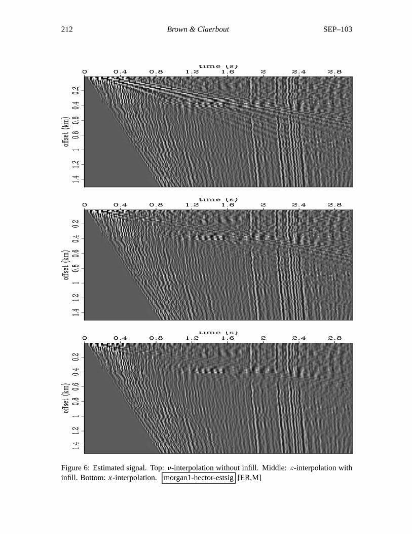
Figure 6 is the estimated signal (equation (8)). Notice that missing data infill has markedlyimproved the quality of noise suppression obtained by the -interpolation technique. Still, byvisual inspection, we must conclude that the x-interpolation result is the best of the three fornoise suppression.

SEP–103 Radial Trace Transform 209

Figure 3: 2-D shot gather.morgan1-hector-dat [ER]

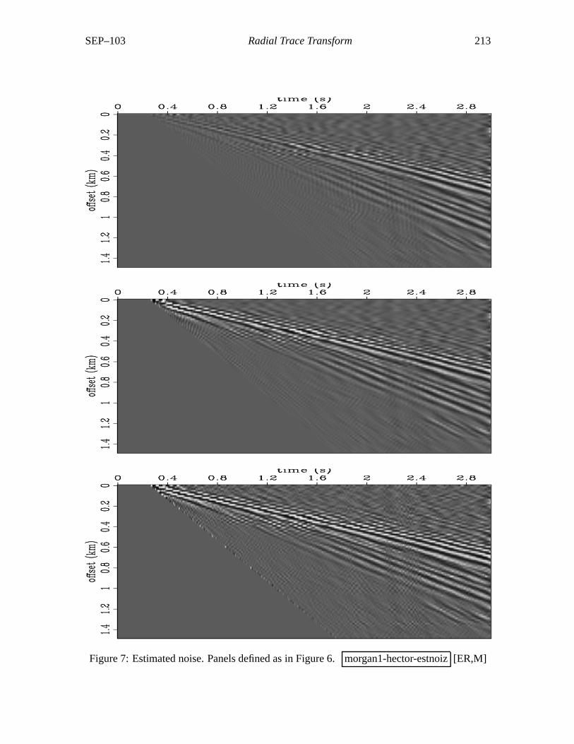
Figure 7 is the estimated noise (equation (9)). First notice that x-interpolation result con-tains more than just the radial ground roll that the simple physical model accounts for. FromFigure 5, we know that the presence of the primary energy between 1.75 and 2.5 seconds andbackscattered noise in the x-interpolation panel is due to interpolation errors, and not to thehighpass filtering. The non-infilled -interpolation result contains some energy (either artifactsor primary energy) around 1 second, while the infilled result does not. From the standpoint ofsignal preservation, the -interpolation result with missing data infill is the best of the three.Philosophically, by using a pseudo-unitary RTT operator and thus ensuring that the only thingmodifying the original data is the bandpass filter, the -interpolation implementation honorsthe physics which drives the problem in the first place.

Aliased Data

Ground roll is nearly always spatially aliased, so the relatively unaliased example of Figure 3is a somewhat unrealistic exception to the practical rule. To inject some realism, we decimatedthe original 2-D shot gather (Figure 3) by a factor of two in offset, as shown in Figure 8, so thatthe ground roll is quite aliased. Figure 9 compares the RTT of the decimated data. The resultsare disappointing. Looking at the -interpolation without infill panel (top), the human eye caneasily interpolate vertically to reconstruct the radial events in RT space. Unfortunately, the

210 Brown & Claerbout SEP–103

Figure 4: Radial Trace Transform. Top: -interpolation without infill. Middle: -interpolationwith infill. “A” points to an example of the “+”-shaped impulse response of the missing datafilter of equation (7). Bottom: x-interpolation. morgan1-hector-radial-comp [ER,M]

SEP–103 Radial Trace Transform 211

Figure 5: Interpolation error. Top: -interpolation error without infill. Middle: -interpolation error with infill. Bottom: x-interpolation error. “A” points to lost energyfrom the primary events around 2 seconds. “B” points to removed backscattered noise.morgan1-hector-raderr-comp [ER,M]

212 Brown & Claerbout SEP–103

Figure 6: Estimated signal. Top: -interpolation without infill. Middle: -interpolation withinfill. Bottom: x-interpolation. morgan1-hector-estsig [ER,M]

SEP–103 Radial Trace Transform 213

Figure 7: Estimated noise. Panels defined as in Figure 6. morgan1-hector-estnoiz [ER,M]

214 Brown & Claerbout SEP–103

-interpolation panel with infill does not have the desired vertical coherence. In fact, it wouldseem that the central premise motivating this paper — that the RTT maps ground roll to zerotemporal frequency — is violated. Figures 10 and 11 are analogous to Figures 6 and 7 — theyare the estimates of signal and noise, respectively. All implementations ( -interpolation withand without infill, and x-interpolation) do an relatively poor job of noise suppression.

A simple way to dealias linear ground roll is to apply a linear moveout (LMO) correction.Figure 12 shows the result of applying a 1.5 km/sec LMO correction to the decimated data ofFigure 8. The ground roll is no longer spatially aliased, but the primaries are also no longer“flat”, as they were originally. As a result, interpolation errors for the x-interpolation RTT willincrease. Figure 13 compares the RTT panels for the decimated/LMO’ed data. The groundroll now occupies a higher effective velocity band, and more importantly, is much closer tozero temporal frequency than in Figure 9. The noise suppression achieved (Figure 14) is betterthan the case in which LMO was not used (Figure 10). As expected, and mentioned above, thex-interpolation RTT leads to severe losses of signal energy, quite a bit more severe than eitherof the two -interpolation implementations, as can be seen in Figure 15. Unfortunately, both

-interpolation implementations seem to suffer some small signal losses, which suggests thatLMO may actually be “aliasing” the primaries by mapping them to low temporal frequency inthe RT domain.

Figure 8: Same 2-D shot gatheras Figure 3, only decimatedby a factor of two in offset.morgan1-hectoralias-dat [ER]

SEP–103 Radial Trace Transform 215

Figure 9: Top: -interpolation without infill. Middle: -interpolation with infill. Bottom:x-interpolation. morgan1-hectoralias-radial-comp [ER,M]

216 Brown & Claerbout SEP–103

Figure 10: Estimated signal. Top: -interpolation without infill. Middle: -interpolation withinfill. Bottom: x-interpolation. morgan1-hectoralias-estsig [ER,M]

SEP–103 Radial Trace Transform 217

Figure 11: Estimated noise. Panels defined as in Figure 10. morgan1-hectoralias-estnoiz[ER,M]

218 Brown & Claerbout SEP–103

Figure 12: Decimated 2-D shotgather (Figure 8), after 1.0km/sec linear moveout correc-tion. morgan1-hectorlmo-dat[ER]

CONCLUSIONS

Our implementation of the RTT effectively suppresses unaliased radial noise while preservingsignal, including static shifts. In its current form, our missing data interpolation technique dida relatively poor job of coherently interpolating spatially aliased radial noise events to verticalevents in the RT domain, although we have high hopes that success is only a small conceptualleap away. To combat aliasing, we applied an LMO correction to the data to dealias the noiseevents with an LMO correction, leading to improved noise suppression, at the cost of somelost signal.

REFERENCES

Claerbout, J. F., 1983, Ground roll and radial traces: SEP–35, 43–54.

Claerbout, J., 1999, Geophysical estimation by example: Environmental soundings imageenhancement: Stanford Exploration Project, http://sepwww.stanford.edu/sep/prof/.

Henley, D., 1999, The radial trace transform: an effective domain for coherent noise attenua-tion and wavefield separation: 69th Annual Internat. Mtg., Soc. Expl. Geophys., ExpandedAbstracts, pages 1204–1207.

Ottolini, R., 1982, Migration of reflection seismic data in angle midpoint coordinates: SEP–33.

SEP–103 Radial Trace Transform 219

Figure 13: Top: -interpolation without infill. Middle: -interpolation with infill. Bottom:x-interpolation. morgan1-hectorlmo-radial-comp [ER,M]

220 Brown & Claerbout SEP–103

Figure 14: Estimated signal. Top: -interpolation without infill. Middle: -interpolation withinfill. Bottom: x-interpolation. morgan1-hectorlmo-lmo-estsig [ER,M]

SEP–103 Radial Trace Transform 221

Figure 15: Estimated noise. Panels defined as in Figure 14. morgan1-hectorlmo-lmo-estnoiz[ER,M]

222 Brown & Claerbout SEP–103

Sava, P., and Fomel, S., 2000, Angle-gathers by Fourier Transform: SEP–103, 119–130.

Taner, M. T., 1980, Long-period sea-floor multiples and their suppression: Geophys. Prosp.,28, no. 01, 30–48.

372 SEP–103